arX

iv:1

203.

3309

v1 [

phys

ics.

com

p-ph

] 1

5 M

ar 2

012 The camera method, or how to track numerically a

deformable particle moving in a fluid network.

Baptiste Moreau1, Philippe Dantan1, Patrice Flaud1 and Benjamin Mauroy1,2,⋆

1 Laboratoire Matiere et Systemes Complexes,

UMR CNRS 7057, Universite Paris 7 Denis Diderot, Paris, France.

2 Laboratoire J.A. Dieudonne,

UMR CNRS 7351, Universite de Nice-Sophia Antipolis, Nice, France.

⋆ Corresponding author, email: benjamin.mauroy@unice.fr

Corresponding author :

Benjamin MauroyLaboratoire J.A. Dieudonne, Universite de Nice-Sophia Antipolis,Parc Valrose, 06108 Nice cedex 2,France.email: benjamin.mauroy@unice.frtel: +33 (0) 4 92 07 62 10fax: +33 (0) 4 93 51 79 74

1

Abstract

The goal of this work is to follow the displacement and possible deformation of a free particlein a fluid flow in 2D axi-symmetry, 2D or 3D using the classical finite elements method withoutthe usual drawbacks finite elements bring for fluid-structure interaction, i.e. huge numerical prob-lems and strong mesh distortions. Working with finite elements is a choice motivated by the factthat finite elements are well known by a large majority of researchers and are easy to manipulate.The method we describe in this paper, called the camera method, is well adapted to the study ofa single particle in a network and most particularly when the study focuses on the particle be-haviour. The camera method is based on two principles: 1/ the fluid structure interaction problemis restricted to a neighbourhood of the particle, thus reducing drastically the number of degreesof freedom of the problem; 2/ the neighbourhood mesh moves and rotates with the particle, thusavoiding most of the mesh distortions that occur in a standard ALE method. In this article, wepresent the camera method and the conditions under which it can be used. Then we apply it toseveral examples from the literature in 2D axi-symmetry, 2D and 3D.

Keywords : fluid structure interaction, particle, finite elements, camera method, penalization.

1 Introduction

Tracking a particle in a fluid has many applications in a wide range of up to date thematics:biofluidics and medicine (red blood cells, drugs delivery, etc.), electrophoresis, magnetic particledriving, aerosols, pollutants, etc. The particle can either be a solid, a deformable particle or afluid enclosed inside a membrane (vesicle or capsule). It can move in a fluid domain whose size iseither of the scale of the particle (a red blood cell in a capillary) or many scales larger than theparticle (a red blood cell in an artery, an aerosol in the lungs, a pollutant in a house, etc.).

A typical application is the study of an isolated vesicle in external flows. This subject is ex-tremely challenging, since vesicles exhibit complex behaviours depending on a small number ofphysical parameters (reduced volume, internal/external viscosity ratio, capillary number). Be-haviours of vesicles such as tank-threading, tumbling or vacillating-breathing appears when scan-ning the range of these parameters and all have been predicted by theory [35, 23, 17] and observedin experiments [14, 6]. To improve the understanding of these phenomena, numerical simula-tions are very useful. Different computational methods are used: the boundary integral method[16, 18, 32, 33, 34], particles-based methods [28] and hybrid methods [24, 36]. Each method modelsthe fluid and/or vesicle behaviour in a particular way and accuracy often goes with high compu-tational costs. Very few studies use the classical finite elements method, except for research ofstationary shapes [10, 20] or for studies limited in 2D axi-symmetry for non stationary regime [21].The major reason is that, although this method is well known and spread in laboratories, it is not,at first sight, well adapted to such problems, be it vesicles or more generally a particle in an ex-ternal flow. Actually, if one wants to use standard finite elements, an ALE (Arbitrary LagrangianEulerian) method will be generally used. The particle displacements are solutions of Lagrangianequations in the reference frame (mechanics equations) while fluid velocities and pressures aresolutions of Eulerian equations in the deformed frame (incompressible Navier-Stokes or Stokesequations). The deformed frame is determined thanks to a transformation of the reference frame.This coordinates change coincides with the particle displacement on the particle subdomain andis the results of a bearing (i.e. is extended) on the fluid subdomain. Such as, this method needsthe whole fluid region and particle to be meshed. The first difficulty appears when particle andfluid domain scales are different because the mesh elements will be inhomogeneous and in largenumbers in order to cover the range of scales. If this problem can anyway be handled, ALE methodwill work well as long as the solid displacements remain small comparatively to the domains size.Indeed, for large displacements (even in the case where particle deformations are small), the def-inition of the transformation from the reference frame to the deformed frame becomes less good

2

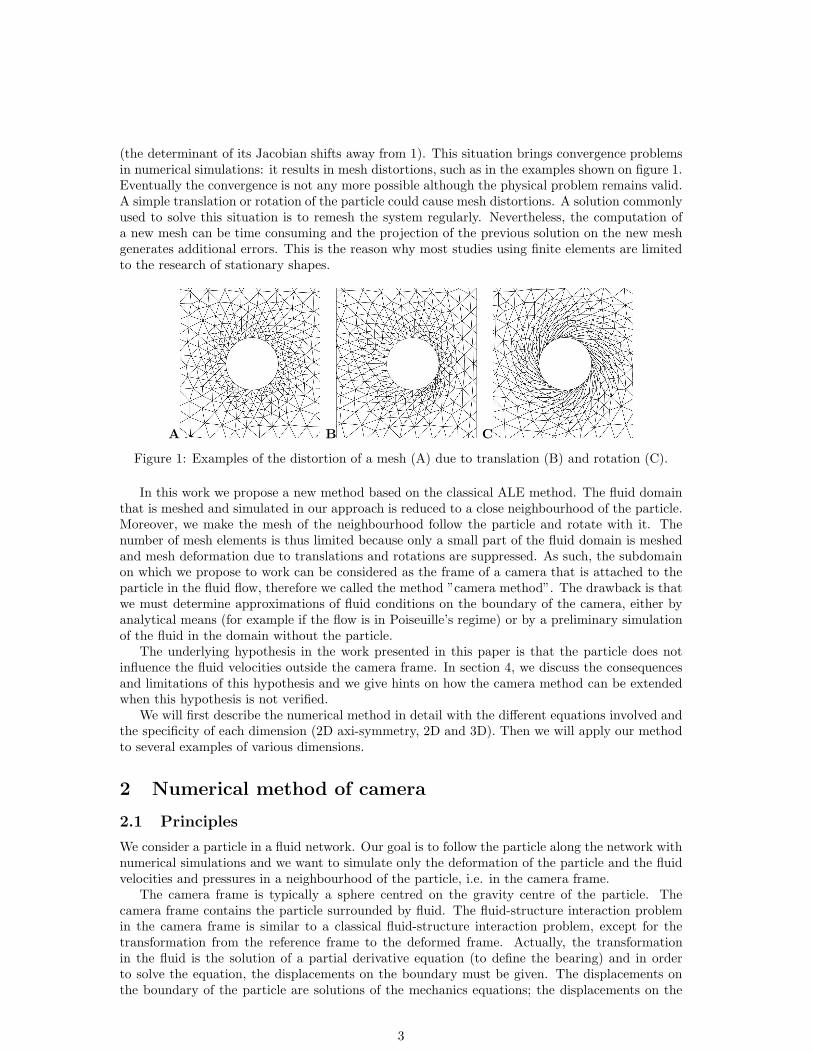
(the determinant of its Jacobian shifts away from 1). This situation brings convergence problemsin numerical simulations: it results in mesh distortions, such as in the examples shown on figure 1.Eventually the convergence is not any more possible although the physical problem remains valid.A simple translation or rotation of the particle could cause mesh distortions. A solution commonlyused to solve this situation is to remesh the system regularly. Nevertheless, the computation ofa new mesh can be time consuming and the projection of the previous solution on the new meshgenerates additional errors. This is the reason why most studies using finite elements are limitedto the research of stationary shapes.

A B C

Figure 1: Examples of the distortion of a mesh (A) due to translation (B) and rotation (C).

In this work we propose a new method based on the classical ALE method. The fluid domainthat is meshed and simulated in our approach is reduced to a close neighbourhood of the particle.Moreover, we make the mesh of the neighbourhood follow the particle and rotate with it. Thenumber of mesh elements is thus limited because only a small part of the fluid domain is meshedand mesh deformation due to translations and rotations are suppressed. As such, the subdomainon which we propose to work can be considered as the frame of a camera that is attached to theparticle in the fluid flow, therefore we called the method ”camera method”. The drawback is thatwe must determine approximations of fluid conditions on the boundary of the camera, either byanalytical means (for example if the flow is in Poiseuille’s regime) or by a preliminary simulationof the fluid in the domain without the particle.

The underlying hypothesis in the work presented in this paper is that the particle does notinfluence the fluid velocities outside the camera frame. In section 4, we discuss the consequencesand limitations of this hypothesis and we give hints on how the camera method can be extendedwhen this hypothesis is not verified.

We will first describe the numerical method in detail with the different equations involved andthe specificity of each dimension (2D axi-symmetry, 2D and 3D). Then we will apply our methodto several examples of various dimensions.

2 Numerical method of camera

2.1 Principles

We consider a particle in a fluid network. Our goal is to follow the particle along the network withnumerical simulations and we want to simulate only the deformation of the particle and the fluidvelocities and pressures in a neighbourhood of the particle, i.e. in the camera frame.

The camera frame is typically a sphere centred on the gravity centre of the particle. Thecamera frame contains the particle surrounded by fluid. The fluid-structure interaction problemin the camera frame is similar to a classical fluid-structure interaction problem, except for thetransformation from the reference frame to the deformed frame. Actually, the transformationin the fluid is the solution of a partial derivative equation (to define the bearing) and in orderto solve the equation, the displacements on the boundary must be given. The displacements onthe boundary of the particle are solutions of the mechanics equations; the displacements on the

3

boundary of the camera frame depend also on the solution of the mechanics equations since theyfollow the global displacement of the particle (translation and rotation(s)).

To have correct fluid velocities and pressures inside the camera, we must also define correctfluid conditions on the boundary of the camera. We choose to impose Dirichlet velocity conditionson the boundaries along with a pressure reference in some point in the camera frame. Sincewe assume that the particle does not influence the fluid velocities in the network outside thecamera, if we are able to determine the velocity profiles in the network, then the knowledge of thetranslations and rotation(s) of the camera gives the positions of the boundaries in the networkand the velocities to impose. To determine those velocity profiles (and pressures), we can eitheruse analytical calculation if possible (for example in the case of a long tube in Poiseuille’s regime)or a preliminary numerical simulation of the fluid in the network without any particle (purecomputational fluid dynamics simulations).

A part of the camera frame can get out of the fluid network when the particle comes too closeto the network walls. In the part outside the network, the fluid does not physically exist, butits velocity can be extended mathematically with a null velocity. This operation leads to fluidvelocities that are continuous in the whole camera frame and that are consistent with wall boundaryconditions in the network. This is integrated in the fluid equations thanks to a penalization method[25, 5]. Note that we assume that the camera frame does not get out of the network near an inletor an outlet. If this happens, then the extension of velocity is still feasible but more complex, allthe more if the camera gets simultaneously out of a wall boundary.

2.2 General equations

In this section we will describe the mathematical equations involved in the camera method. Sincethis method is inspired from the standard ALE method, we will recall first the equations used forthat method.

2.2.1 Standard ALE equations

As shown on figure 2, we will consider a fluid network Ω0 ⊂ RN (N = 2 or 3)) which has inlet(s)

Γin,0 ⊂ ∂Ω0, outlet(s) Γout,0 ⊂ ∂Ω0) and walls (Γw,0 ⊂ ∂Ω0) such that ∂Ω0 = Γin,0∪Γw,0∪Γout,0.In this network, a particle fills initially the subdomain S0 of Ω0. Consequently, the initial fluiddomain is F0 = Ω0\S0. This geometry corresponds to the reference frame where the equations ofthe particle mechanics are defined. We call (x) the coordinates in the reference frame.

The deformed frame at time t corresponds to the physical frame where the particle has movedand is deformed. The fluid domain in the deformed frame is the one in which the fluid physicallyspans at time t and thus where the Navier-Stokes equations are defined. The deformed frame isassumed to be the image by a smooth derivable and invertible (typically a C1 diffeomorphism)application φ of the reference frame, we call (y) the coordinates in the deformed frame and y =φ(x, t). For each subset X0 of RN defined in the reference frame, we define Xt its image by φ inthe deformed frame i.e. Xt = φ(X0, t), see figure 2.

The solid equations are written in the reference frame of the solid, i.e. on S0, (Lagrangianequations) while the fluid equations are written in the deformed frame where the solid has movedand is deformed (Eulerian equations). Consequently, we need to determine the transformation φthat transforms the coordinates of the reference frame (x) into the coordinates of the deformedframe (y = φ(x, t)).

From now on, the fluid velocity is represented by v(y, t), the fluid pressure p(y, t) and thestructure displacement u(x, t). The fluid and solid densities are respectively denoted ρf and ρsand the fluid viscosity is denoted ηf . The fluid constraints tensor is σf (v, p) = −pI+ηf (∇u+ t∇u)and the solid tensor constraint is σs(u). The transformation φ is known in the solid S0 since forx ∈ S0, φ(x, t) = x+u(x, t). It is however necessary to define the transformation φ on the referencefluid domain F0, in order to be able to write the fluid equations. A way to define φ on F0 is touse the Laplace equations:

4

Γin,0

Γout,0

Γw,0

Γw,0S0

F0

reference frame Ω0

coordinates (x)solid equations on S0

Γin,t

Γout,t

Γw,t

Γw,t

St

Ft

y = φ(x, t)

deformed frame Ωt

coordinates (y)fluid equations on Ft

Figure 2: 2D example of the initial domains of the physical problem (left) that corresponds to thereference frame and of the deformed frame (right). particle equations are written in the referenceframe while fluid equations are written in the deformed frame. The application x → y = φ(x, t)transforms the coordinates of the reference frame into the coordinates of the deformed frame.

φ = 0 on F0

φ(x, t) = x+ u(x, t) on ∂S0

φ(x, t) = x on ∂Ω0

(1)

Note that we assume that the boundary ∂Ω0 is unmoving, thus the transformation is theidentity on ∂Ω0.

Incompressible fluid-structure interaction is governed by the mechanics equations for the struc-ture in the reference frame (x) and the equations of Navier-Stokes for the fluid in the deformedframe (y = φ(x, t)).

The mechanics equations are:

ρS∂2u∂t2

− div (σs(u)) = 0 on S0

σs(u).ns = −σf (v, p).nf on ∂S0(2)

The constraints on the boundary of the solid are equal to the fluid constraints on the solidboundary brought back to the reference frame thanks to the application φ. The minus signis due to the orientation of the normals ns and nf which are defined as outwards normals in theirrespective subset.

The Navier-Stokes equations are:

ρf∂v∂t

+ ρf (v.∇) v − div (σf (v, p)) = 0 on Ft = φ(F0)div(v) = 0 on Ft = φ(F0)v(y) = ∂u

∂t

(

φ−1(y, t))

on ∂St = φ(∂S0)v(y) = 0 on Γw,t

+inlet and outlet boundary conditions on Γin,t and Γout,t

(3)

Due to fluid viscosity, the fluid is sticking on the particle and fluid velocity at particle boundaryis equal to the particle velocity (second to last equality).

In the next section, we use the equations of the standard ALE method to define the equationsof the camera method.

2.2.2 Camera method

We consider a neighbourhood C of S0, typically a sphere centred on the barycentre of S0. C isthe frame of the camera. We do now the hypothesis that the particle S0 does not influence thefluid outside of C. We will discuss the meaning of this hypothesis later in this paper. We will

5

assume that the barycentre of the particle S0 is initially at the origin of the coordinates frame(i.e.

∫

S0

xdx = 0), because it simplifies the writing of equations (see below). This is not restrictivebecause a simple translation of the domains makes this condition true.

On the contrary of the standard ALE method, the camera method works by solving only asubset of the full problem. The fluid-structure interaction problem is restricted to the neighbour-hood C of the particle. Moreover, the mesh of the neighbourhood C of the particle moves androtates with the particle in order to avoid most of the mesh deformation. Two points need to beaddressed to solve that new problem. First, fluid velocities (and fluid pressure) are not known onthe boundaries of C, so we will use an a priori estimation of these quantities in absence of theparticle. Secondly, in the general case, the neighbourhood C does not fit the network geometryand some parts of C can be outside the network where no fluid physically exists (see an exampleon figure 13 (right) or figure 14). This second point is solved by making the fluid virtually spanoutside Ωt and by setting its velocity there to zero with a penalization method (also called im-mersed boundary method) [25, 5].

Decomposition of the structure displacement. This method is based on the uniquedecomposition of the solid displacement u(x, t) under the hypothesis that the gravity center of thesolid S0 is at the origin of the reference frame (

∫

S0

xdx = 0) [30]:

x+ u(x, t) = τ(t) +Rθ(t) (x+ d(x, t)) (= φ(x, t) on S0) (4)

where :

• (x, t) → d(x, t) is an ”elementary” displacement without any translation or rotation, i.e.:

∫

S0

d(x, t)dx = 0 no translation∫

S0

x ∧ d(x, t)dx = 0 no rotation(5)

• t → τ(t) is a vector representing the global translation of S0 at time t.

• Rθ(t) is an invertible matrix that reflects the rotation(s) of S0 at time t. The definition ofRθ(t) depends on the dimension of the space, see the next sections for more details. We willdenote R

−θ(t) the inverse of the matrix Rθ(t).

Our goal is not to calculate the function d but to use its existence to determine the translationτ(t) and the rotations θ(t). Once these quantities are determined, they are used to make themesh translate and rotate with the solid, thus avoiding most of mesh deformations. Whatever thedimension of the space, the translation is given by

τ(t) =

∫

S0

u(x, t)dx∫

S0

dx(6)

Finally, the fluid structure interaction equations can be rewritten using these new information.The major changes will affect the transformation and the representation of the fluid.

The equations that determine the transformation φ become:

φ = 0 on F0

φ(x, t) = x+ u(x, t) on ∂S0

φ(x, t) = Rθ(t)x+ τ(t) on ∂C(7)

This defines the coordinate transformation we used in our work. It lets the mesh centered onthe particle S and makes it rotate with the particle. There is an alternative way to define thetransformation φ by taking for boundary conditions on ∂S0 and ∂C: φ(x, t) = x+u(x, t)− τ(t) on∂S0, and φ(x, t) = Rθ(t)x on ∂C. This alternative transformation makes the visualisation processeasier, since the mesh remains centered on the origin at each time step.

6

Fluid domain and boundary conditions. Since we limit the fluid domain to the frame ofthe camera that corresponds to a neighbourhood of the structure S, we need to be able to imposezero velocity to the fluid if a part of the camera frame gets out of Ωt. This is achieved thanks toa penalisation method. Using the function χ(y) that is equal to 0 in Ωt and to 1 in R

n\Ωt, thenthe fluid equations become

ρf∂v∂t

+ ρf (v.∇) v − div (σf (u, p)) + ρfχǫv = 0 on Ft = φ(F0)

div(v) = 0 on Ft = φ(F0)v = ∂u

∂ton ∂St = φ(∂S0)

v = v0 on ∂Cp = p0 on a point P (reference pressure)

(8)

The difficulty arises in the determination of the velocities v0 on the boundary of the camera(∂C). Since we hypothesized that the particle does not influence the fluid outside the camera, v0can be determined as the result of an analytical calculation or a preliminary numerical simulationof the fluid in the network without the particle. The reference pressure p = p0 on an arbitrary pointP in the camera frame is required for pressure uniqueness. The point P moves with the cameraand consequently, the pressure reference is time-dependent. However, this does not influence thepressure drops nor the fluid velocities which are correctly computed, since the time-dependentreference pressure disappears under the spatial gradient that operates on the pressure in the fluidequation.

3 Camera method set up and validation through examples

The set up of the camera method depends on the space dimension. The translation vector is easilycomputed whatever the number of dimensions. However the definition of rotations depends on thenumber of dimensions in the space. In this section, we describe how to set up the camera methodin a 2D axi-symmetric space, in a 2D space and in a 3D space. For each case, we explain how thenumber of dimensions affects the camera method and for each case, we validate with an examplefrom the literature. Furthermore, a 2D axi-symmetric space is well adapted to the tracking of aperiodic train of particles along a straight channel. Thus, we outline how the camera method canbe used in such a context with a model of red blood cells in a capillary.

The numerical simulations performed in this work were done with the commercial finite el-ements package Comsol Multiphysics, with the linear solver PARDISO. The computations areperformed on eight cores of a bi-processors workstation (two Xeon E5645) with 32 GBytes ofmemory. The most memory consuming computation (standard ALE method, see below) needsabout 4 GBytes to run.

3.1 2D axi-symmetry

The axis of axi-symmetry is referred to as the (z) axis while the coordinates along the radius isreferred to as the (r) axis. In the following sections, we assume that all quantities are independenton the phase, thus we write vector coordinates in the form v = (vr, vz).

3.1.1 Specificity of camera method in 2D-axi

Both the particle and the network are assumed axi-symmetric. The model is able to represent aparticle moving along the axis of a unidirectional channel whose section is circular. The radius ofthe channel is not necessarily constant and can depend on z coordinate. The camera is bound tomove along the axis of the channel, and no camera or particle rotation is possible, i.e. θ(t) = 0for each time t:

Rθ(t) = I

7

The movement of the barycentre of the particle is limited to a translation along the z-axis,consequently τ(t) has only one non zero component on the z coordinate: τ(t) = (0, τz(t)).

There are two possible ways to define the camera frame when working in 2D axi-symmetry.The first way is to work with a fixed frame and to use penalization to nullify the fluid velocitywhere the wall crosses the camera frame (see left part of figure 3). So the general equations of theprevious section apply. The other way is to use the specificity of the 2D axi-symmetry and to makethe “upper” border of the camera frame fit the wall geometry (see right part of figure 3). Thissecond method is well adapted to axi-symmetry. Although it reduces slightly the mesh quality, itavoids the use of penalization that can sometimes lead to convergence problems. The equationsof the transformation φ are slightly different than equations 7 and they need a parametrization ofthe channel radius along the axis: R : z −→ R(z). The transformation φ is then solution of theequations (x = (r, z)):

φ = 0 on F0

φ(x, t) = (r + ur(x, t), z + uz(x, t)) on ∂S0

φ(x, t) = (R(z + τz(t)), z + τz(t)) on W0

φ(x, t).n = 0 on I0 ∪Ot

(9)

fluid penalization (χ = 1 implies v ∼ 0)

C ∩ Ft

St

camera frame C

Ct ∩ Ft = Ct

St

ItOt

Wt

camera frames C0 and Ct

frame upper boundarysticks to channel wall

initial camera frame (C0)

camera frame at time t (Ct)

Figure 3: Two ways to define camera frames in 2D axi-symmetry. Left: “classic” camera frame,penalization is used to nullify fluid velocity in the intersection between channels walls and cameraframe. Right: the upper border of the camera frame moves such that it fits the wall geometry ofthe channel at any time, the frame of the camera never crosses the walls of the channel.

The fluid boundary conditions need also to be slightly adapted: on the “upper” boundary ofthe camera frame (Wt), we use no-slip boundary conditions. On inlet It and outlet Ot fluid velocityconditions (Dirichlet) are imposed from an a priori estimation as before (numeric or analytic). Ifthe Reynolds number is low enough and if the width of the camera is large enough, one can usePoiseuille profiles as approximations.

In the following, we will systematically use the alternative method (camera border fittingchannel wall) when dealing with 2D axi-symmetry problems. In particular this alternative methodcan be slightly adapted to model infinite trains of particles in straight channels, such as red bloodcells in capillaries. It is achieved by adding a periodicity condition on the boundary of the cameraframe and a Lagrange multiplier in the equations, see section 3.1.3.

3.1.2 2D-axi validation: deformation of a vesicle in a narrowing channel

A vesicle consists in a thin membrane enclosing an inner fluid [27], vesicles are deformable objectsable to undergo strong deformation. Red blood cells are natural vesicles that carry oxygen inblood [37], bio-artificial vesicles also exists and can be used to carry medicine to a precise location.When such an object is motioned by an outer fluid in a narrow channel, such as the capillariesfor red blood cells, then its stationary shape is a ”parachute” shape [11]. The characteristics ofthat shape depends on the different physical parameter involved in the outer and inner fluid andin the membrane. Experimental and numerical works [29, 3, 7, 27] have been made to study thebehaviour of a vesicle in a narrowing channel. The numerical simulations made in [29, 27] make a

8

good benchmark to validate the camera method in 2D axi-symmetry. In these works, the vesiclesare droplets of salt water surrounded by a thin polymeric membrane whose thickness is about30 µm. Their size is millimetric.

We assume that the vesicle is initially a sphere of radius a and that it is motioned througha narrow channel of radius R. The behaviour of the vesicle is determined by [29, 27]: 1/ thecapillary number Ca = ηextU

K, where ηext is the viscosity of the outer fluid, U the bulk velocity of

the fluid and K the membrane area dilatation modulus (N.m−1); 2/ the ratio a/R between thevesicle radius and the channel radius.

In our simulations, the membrane is a full 2D axi-symmetric material, whose thickness is thatof the experimental object, 30 µm. We assume the material to be elastic and that it undergoeslarge deformation. Its Young modulus is E and its Poisson’s ratio is ν. In the numerical worksproposed in [29, 3, 27, 7], the authors used a boundary integral method with an infinitely thinmembrane. The parameters E and ν used in our simulations were chosen such that the materialproperties fits the infinitely thin membrane models used in [29, 27]:

ν =K − µ

K + µand E =

4Kµ

h(K + µ)

The vesicle is injected into a wide channel whose radius decreases to reach a radius of R = 2mmclose to the radius of the vesicle which needs to deform to enter the constriction. We model thechannel with the geometry shown on figure 4. First the vesicle is accelerated in the wide sectionof the channel, then it enters the constriction.

1.58 mm

8 mm

2 mm

10 cm

Figure 4: Numerical model of experiments from [29]: 2D axi-symmetric geometry of the channel,vesicle and camera frame (grayed box). The arrow reflects the orientation of the fluid flow andthe direction in which the vesicle and the camera are moving.

The upper and lower boundary of the camera frame coincide respectively to the channel walland to the symmetry axis. The left and right borders are fluid filled sections of the channel, seefigure 4. The fluid boundary conditions on the left and right borders are assumed to be parabolicvelocity profiles. This last hypothesis is an approximation, however the Reynolds number value islow and the camera frame width is large relatively to the distance needed for the fluid to be fullydeveloped. Thus the fluid is fully developed far before it reaches the neighbourhood of the vesicle.

We computed the deformed shape of a vesicle whose a/R ratio is 0.78 and whose membranearea dilatation modulus is K = 1.30 N.m−1. Two cases were simulated: µ/K = 1, Ca = 0.02 andµ/K = 1/3, Ca = 0.027. Our results are compared with the experimental shapes and numericalsimulations from [29, 7] on figure 5. Volume variations of the vesicle during our computations areless than 0.02%, which is compatible with the incompressibility assumption for the inner fluid.The numerical simulations from [7] and our simulations give close results with a slight differenceat the rear of the vesicle, which is probably a consequence of the different models used for themembranes. As discussed in [29], the numerical shapes match well the front and intermediateparts of the experimental vesicle but not the rear.

9

Figure 5: Shapes of the vesicles computed with camera method (red thick lines) for a/R =0.78. Up: Ca = 0.02, mu/K ∼ 1; Down: Ca = 0.027, µ/K ∼ 1/3. The thick black linescorresponds to the experiments made by Risso et al [29], the thin black lines corresponds tothe results of simulations made by Diaz and Barthes-Biesel [7] with infinitely thin membranemodel. The coordinates are normalized with the radius of the constricted section of the channel(R = 2 mm).

3.1.3 2D axi extension: periodic train of red blood cells in a capillary

In this section, we show with an example how to use the camera method to model a train ofparticles in a straight channel. We model here a train of red blood cells going through an idealizedcapillary. The red blood cells are modeled as discoid vesicles. The vesicle diameter is 7.5 µm andthe vesicle thickness ranges from 1 µm on their center to 2 µm near their periphery [37]. Halfsections of the vesicle are plotted on figure 6. The frame of the camera contains one vesicle onwhich it is centered. The frame is rectangular and unchanging during the simulation since thecapillary is assumed to have a constant diameter of 8 µm. The upper boundary corresponds tothe wall of the capillary and the lower boundary to the axi-symmetry axis. The left and rightboundaries correspond to capillary sections that moves with the vesicles. As for the previousexample, it is not necessary to use fluid penalization since the top border of the camera alwayscoincides with the wall of the capillary. A scheme of the camera frame is plotted on figure 6.

St

I O

W

Ft

Ft

periodic camera frame

Figure 6: Frame of the camera for the axi-symmetric model of a periodic train of red blood cells.The dashed-dotted line represents the axis of axi-symmetry. Periodic boundary conditions areapplied on I and O boundaries: velocities and normal constraints are equal on I and O.

The capillary consists in successive copies of the camera frame that are connected by theirleft and right boundaries (I and O). The number of red blood cells volumetric fraction can beeasily modulated by changing the width of the camera frame. Mathematically, this succession of”cells” can be represented with periodic boundary conditions for the fluid on I and O. The fluidequations are (see for example [2]):

10

ρf∂v∂t

+ ρf (v.∇) v − div (σf (u, p)) = 0 on Ft

div(v) = 0 on Ft

v = ∂u∂t

on ∂St

v = 0 on Wp = 0 on an arbitrary point (reference pressure)v|I = v|O∇v.n|I = −∇v.n|O∫

Iv.nds = Q

(10)

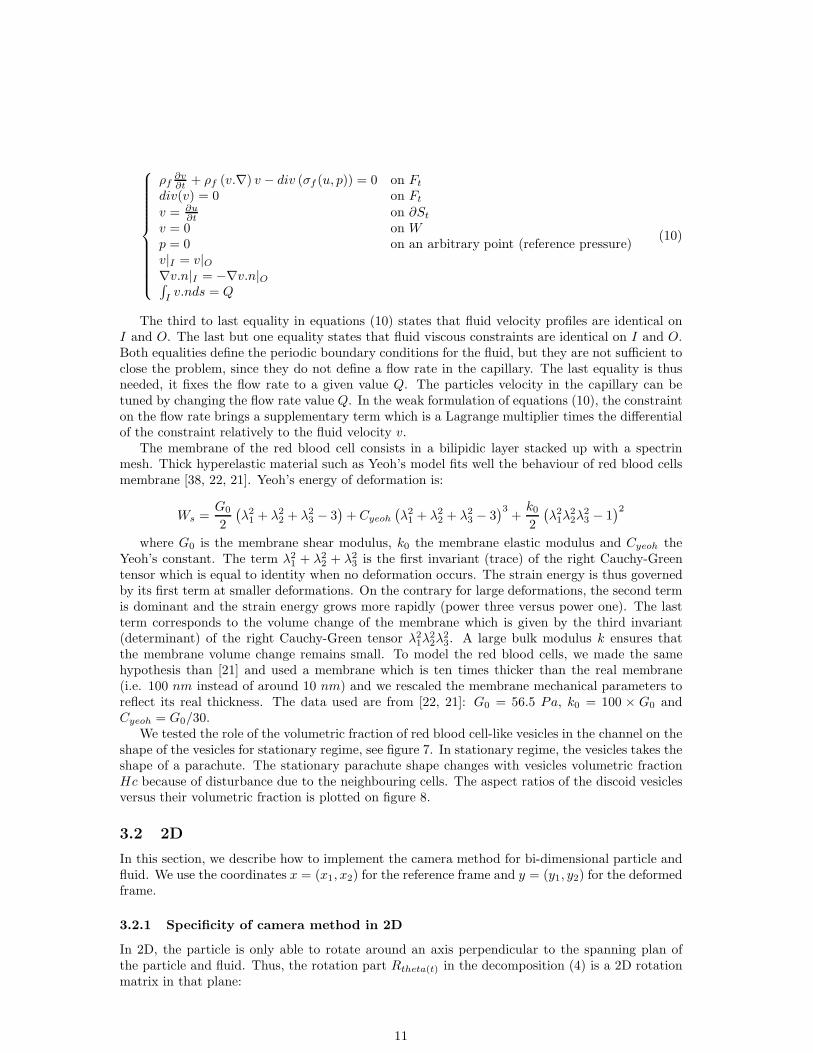
The third to last equality in equations (10) states that fluid velocity profiles are identical onI and O. The last but one equality states that fluid viscous constraints are identical on I and O.Both equalities define the periodic boundary conditions for the fluid, but they are not sufficient toclose the problem, since they do not define a flow rate in the capillary. The last equality is thusneeded, it fixes the flow rate to a given value Q. The particles velocity in the capillary can betuned by changing the flow rate value Q. In the weak formulation of equations (10), the constrainton the flow rate brings a supplementary term which is a Lagrange multiplier times the differentialof the constraint relatively to the fluid velocity v.

The membrane of the red blood cell consists in a bilipidic layer stacked up with a spectrinmesh. Thick hyperelastic material such as Yeoh’s model fits well the behaviour of red blood cellsmembrane [38, 22, 21]. Yeoh’s energy of deformation is:

Ws =G0

2

(

λ21 + λ2

2 + λ23 − 3

)

+ Cyeoh

(

λ21 + λ2

2 + λ23 − 3

)3+

k02

(

λ21λ

22λ

23 − 1

)2

where G0 is the membrane shear modulus, k0 the membrane elastic modulus and Cyeoh theYeoh’s constant. The term λ2

1 + λ22 + λ2

3 is the first invariant (trace) of the right Cauchy-Greentensor which is equal to identity when no deformation occurs. The strain energy is thus governedby its first term at smaller deformations. On the contrary for large deformations, the second termis dominant and the strain energy grows more rapidly (power three versus power one). The lastterm corresponds to the volume change of the membrane which is given by the third invariant(determinant) of the right Cauchy-Green tensor λ2

1λ22λ

23. A large bulk modulus k ensures that

the membrane volume change remains small. To model the red blood cells, we made the samehypothesis than [21] and used a membrane which is ten times thicker than the real membrane(i.e. 100 nm instead of around 10 nm) and we rescaled the membrane mechanical parameters toreflect its real thickness. The data used are from [22, 21]: G0 = 56.5 Pa, k0 = 100 × G0 andCyeoh = G0/30.

We tested the role of the volumetric fraction of red blood cell-like vesicles in the channel on theshape of the vesicles for stationary regime, see figure 7. In stationary regime, the vesicles takes theshape of a parachute. The stationary parachute shape changes with vesicles volumetric fractionHc because of disturbance due to the neighbouring cells. The aspect ratios of the discoid vesiclesversus their volumetric fraction is plotted on figure 8.

3.2 2D

In this section, we describe how to implement the camera method for bi-dimensional particle andfluid. We use the coordinates x = (x1, x2) for the reference frame and y = (y1, y2) for the deformedframe.

3.2.1 Specificity of camera method in 2D

In 2D, the particle is only able to rotate around an axis perpendicular to the spanning plan ofthe particle and fluid. Thus, the rotation part Rtheta(t) in the decomposition (4) is a 2D rotationmatrix in that plane:

11

Hc = 0.11

Hc = 0.18 Hc = 0.25

Figure 7: Results of 2D axi-symmetric camera simulations: stationary shapes of models of redblood cells for different value of their volumetric fraction Hc in the channel. The color representsthe amplitudes of fluid velocities (in plasma or vesicle cytosol, in m.s−1).

0.1 0.15 0.2 0.25

1.3

1.4

1.5

1.6

1.7

1.8

1.9

2

Volumic fraction

Asp

ect r

atio

0.5 mm/s1 mm/s1.5 mm/s2 mm/s

Figure 8: Discoid vesicle aspect ratio (length over diameter) versus volumetric fraction of vesiclesin the channel for different vesicle velocities.

Rθ(t) =

(

cos(θ(t)) − sin(θ(t))sin(θ(t)) cos(θ(t))

)

The number θ(t) is the rotation angle of the particle at time t. Generally, the rotation anglereference is chosen for t = 0, i.e. θ(0) = 0. The angle θ(t) is computed from the rotation constrainton the elementary displacement d(x, t), see equations (5). Thus, θ(t) is computed by solving theequation:

∫

S0

x ∧ d(x, t) dx =∫

S0

x ∧ R−θ(t) (x+ u(x, t)− τ(t)) dx = 0. The angle of rotation

θ(t) can then be computed explicitly as a function of the particle displacements u:

tan (θ(t)) =

∫

S0

x ∧ u(x, t)dx∫

S0

x. (x+ u(x, t))

In order to have a unique solution, θ(t) is computed from this last formula using a functionatan2.

Ideally, the 2D camera frame is a disk centered on the particle, such as the frame on figure 9.A disk-shaped frame remains still whatever the rotation, which makes post-processing easier to

12

interpret. However, the disk shape is not compulsory and any other shape is possible as soon asit encloses the particle and is wide enough to be able to neglect the particle influence outside ofthe camera frame.

3.2.2 2D validation: a deformable particle in shear flow

A circular elastic particle in a shear flow deforms in an ellipse which rotates around its gravitycenter. This phenomena is well known, see for example [13, 14], and is often used to validatenumerical work like in [1].

v(y) =

(

γy20

)

y1

y2

Figure 9: The elastic particle stands in a shear flow. The camera frame is represented by thedotted circle enclosing the particle. The particle deforms in an ellipsoid shape [13].

The particle at rest is a disk whose diameter is dp = 1 mm. The particle material is a Neo-Hookean material whose density is 1000 kg.m−3 and whose shear modulus is G = 1 Pa. The fluidenclosing the particle is water (viscosity ηext = 10−3 Pa.s, density ρext = 1000 kg.m−3) and itspans infinitely in all directions. The shear flow is defined from the shear rate γ which is constantin space. The fluid velocity in the absence of the particle is then known everywhere in space:

v(y) =

(

γy20

)

(11)

In the camera method, the particle and the fluid interact only inside the frame of the camera.The camera frame is a disk centered on the particle and has a radius of 10 dp. The boundaryconditions for the fluid on the camera frame boundaries are given by (11). A scheme of the modelis shown on figure 9.

The two parameters that drive the system physics are the Reynolds number Re =ρextγd

2

p

ηextand

the capillary number Ca = ηextγG

, as shown in [13]. We fixed the Reynolds number to Re = 0.05,typical for mimicking low flow regime [13]. We focused on the role of the capillary number and wemade it range from 0.02 to 0.7 by adjustments of the fluid shear rate γ.

The particle is known to deform into an ellipse and the deformation can be represented with adimensionless number built from the lengths of the two axises of the ellipses: a is the largest axisand b is the small axis [13]:

D =a− b

a+ b(12)

Figure 10 shows the results obtained with the camera method. The Reynolds number isRe = 0.05 in all simulations. The variations of D versus the capillary number Ca are plotted onthe left. As expected, the number D follows a linear regime D = Ca for values of Ca lower than0.3-0.4 and starts to shift downwards the curve D = Ca when Ca increases.

13

0 0.1 0.2 0.3 0.4 0.5 0.6 0.70

0.1

0.2

0.3

0.4

0.5

0.6

0.7

Ca

D Ca = 0.1 Ca = 0.3

Ca = 0.5 Ca = 0.7

Figure 10: Left: particle diameter relative difference D versus its capillary number Ca, Re = 0.05.Right: the circles represents the stationary particle shape and the dots the initial particle shape.

0 1 2 3 4 5 6−4

−3.5

−3

−2.5

−2

−1.5

−1

−0.5

0

0.5

time (s)

Rot

atio

n an

gle

(deg

rees

)

Figure 11: Angle (degrees) variation along time for a particle with Ca = 0.4 and Re = 0.05.The particle is rotating, with the camera method, the mesh quality remains very good and noremeshing was needed.

X

Y

θ

X Y

θ

Figure 12: Mesh details in the case Ca = 0.4 and Re = 0.05. Left: initial (t = 0). Right:stationary shape (t = 100). The mesh rotates with the particle.

Once in stationary regime, the particle rotates around its gravity center at a constant velocityspeed of θ = −1.42 degrees.s−1 which is independent of Ca, the camera method makes themesh rotate with the particle and avoid triangle elements to distort too much. Angle variation isplotted on figure 11 in the case Ca = 0.4. The minimal quality of the mesh elements during the

14

computation remains in that case always larger than 0.55. Figure 12 gives an example on how thecamera mesh rotates and deforms and shows clearly that remeshing is not necessary.

3.2.3 A particle in a bifurcation

In this section, we detail the use of the camera method for the case of a particle going through afluid network shaped as a bifurcation, the network geometry is shown on figure 13 (left). In thisexample, the wall of the network intersects the camera frame all along the computation, as shownon figure 13 (right). The topology of the network part inside the camera frame changes and thesolution that consists in sticking the camera boundary to the network boundary is not any morepossible. Thus we use penalization to force fluid velocity to be zero in the camera frame partoutside of the network. The diameters of the network channel is constant everywhere and equalto 20 µm.

The particle shape and size are those of a section of a red blood cell, its material is elastic(Young’s modulus 68 Pa and Poisson’s ratio 0.4995) and undergoes large deformations, its densityis that of water. The fluid is assumed to be water at low flow regime (Stokes equations). Weassume that two same parabolic velocity profiles are imposed at up and down outlets of thebifurcation. An open boundary condition (zero constraint) is applied at the inlet. The maximalvelocity reached on the horizontal channel center line is 0.001 m.s−1. The particle is initiallypositioned next to the inlet, one micron below the center line of the flow as shown on figure 13,and it is carried away in the network by the fluid.

Initial position

Position at time 0.04 s

Figure 13: The fluid domain is a bifurcation, the channels diameter is 20 microns. The fluidenters the network from the inlet on the left and gets out from the two outlets on the right (upand down). The particle is initially positioned near the inlet. The color represents the amplitudeof the fluid velocity (increasing from blue (0 mm.s−1) to red (1 mm.s−1)). The camera frame onthe right is a disk of diameter 80 µm centered on the particle, the image represents the particleat time 0.04 s.

We compared the results of two numerical methods to compute the particle displacements inthe bifurcation. In all our simulations, the mesh is made of triangular elements and the mesh sizerepresents the maximal length of triangles edges. The first method is a standard ALE methodand the computation is stopped when the mesh quality becomes too bad. The second method isthe camera method. We confronted results and computation times.

With the standard ALE method the simulation is not able to reach the time when the particleenters the bifurcation. On the contrary, the camera method is able to simulate the motion of theparticle all the way through the bifurcation, from the inlet to one of the outlets, with very fewloss in mesh quality, see figure 14. We compared the particle trajectories and rotations of thecamera method with the standard ALE method using the same mesh size 1 µm and a cameraframe diameter of 60 µm. The particle trajectory and rotation computed with the camera methodare shown on figure 14 and they are compared with the standard ALE method on figure 15.

15

Figure 14: Particle trajectory computed with the camera method (camera diameter 60 µm). Theparticle and the camera (circle centered on the particle) move from left to right and are plottedeach 0.03 s. The color represents the amplitude of the fluid or structure velocity (increasing fromblue (0 mm.s−1) to red (1 mm.s−1)). The computation stops a bit before the camera borderscross the bottom outlet.

0 1 2 3 4 5 6 7 8

x 10−5

−1.6

−1.4

−1.2

−1

−0.8

−0.6

−0.4

−0.2

0x 10

−5

x position (m)

y po

sitio

n (m

)

std ale methodcamera method

0 0.5 1 1.5 2 2.5 3 3.5 4 4.5

x 10−5

−1.2

−1.15

−1.1

−1.05

−1x 10

−6

x position (m)

y po

sitio

n (m

)

std ale methodcamera method

0 0.02 0.04 0.06 0.08 0.1 0.12

−60

−50

−40

−30

−20

−10

0

time (s)

thet

a (d

egre

es)

std ale methodcamera method

0 0.01 0.02 0.03 0.04 0.05 0.06−50

−45

−40

−35

−30

−25

−20

−15

−10

−5

0

time (s)

thet

a (d

egre

es)

std ale methodcamera method

Figure 15: Up: particle trajectory (meters), the right plot is a zoom. Down: particle rotation(degrees), the right plot is a zoom. The black lines correspond to the camera method and the redcrosses correspond to the standard ALE method. Note that the standard ALE method was notable to simulate the particle after the time 0.04 s.

We compared standard ALE method and camera method by measuring the difference in theparticle gravity center displacement (dx, dy) and particle rotation θ at time t = 0.04 s, the lasttime computed by the standard ALE method before it stops due to low elements quality. The

16

40 50 60 70 80

0.011

0.012

0.013

0.014

0.015

0.016

camera diameter (microns)

rela

tive

shift

0.5 1 1.5

0.005

0.01

0.015

0.02

0.025

0.03

mesh size (microns)

rela

tive

shift

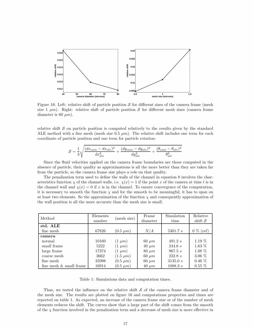
Figure 16: Left: relative shift of particle position S for different sizes of the camera frame (meshsize 1 µm). Right: relative shift of particle position S for different mesh sizes (camera framediameter is 60 µm).

relative shift S on particle position is computed relatively to the results given by the standardALE method with a fine mesh (mesh size 0.5 µm). The relative shift includes one term for eachcoordinate of particle position and one term for particle rotation:

S =1

3

√

(dxcam − dxale)2

dx2ale

+(dycam − dyale)2

dy2ale+

(θcam − θale)2

θ2ale

Since the fluid velocities applied on the camera frame boundaries are those computed in theabsence of particle, their quality as approximations is all the more better than they are taken farfrom the particle, so the camera frame size plays a role on that quality.

The penalization term used to define the walls of the channel in equation 8 involves the char-acteristics function χ of the channel walls, i.e. χ(x) = 1 if the point x of the camera at time t is inthe channel wall and χ(x) = 0 if x is in the channel. To ensure convergence of the computation,it is necessary to smooth the function χ and for the smooth to be meaningful, it has to span onat least two elements. So the approximation of the function χ and consequently approximation ofthe wall position is all the more accurate than the mesh size is small.

MethodElementsnumber

(mesh size)Frame

diameterSimulation

timeRelativeshift S

std. ALE

fine mesh 67826 (0.5 µm) N/A 5301.7 s 0 % (ref)camera

normal 10160 (1 µm) 60 µm 491.2 s 1.19 %small frame 5222 (1 µm) 40 µm 244.6 s 1.63 %large frame 17374 (1 µm) 80 µm 967.5 s 1.08 %coarse mesh 3662 (1.5 µm) 60 µm 232.8 s 3.06 %fine mesh 35998 (0.5 µm) 60 µm 3135.0 s 0.46 %fine mesh & small frame 16914 (0.5 µm) 40 µm 1088.3 s 0.55 %

Table 1: Simulations data and computation times.

Thus, we tested the influence on the relative shift S of the camera frame diameter and ofthe mesh size. The results are plotted on figure 16 and computations properties and times arereported on table 1. As expected, an increase of the camera frame size or of the number of meshelements reduces the shift. The curves show that a large part of the shift comes from the smoothof the χ function involved in the penalization term and a decrease of mesh size is more effective in

17

term of shift reduction than an increase of the camera frame size. Consequently, a small cameraframe is very efficient, computation time is small and quality remains good. Thus, reducing thecamera frame is a good strategy as long as the camera remains large enough to capture most ofthe effects of the particle on the fluid. To illustrate the previous points, a computation was madewith a small camera frame (diameter 40 µm) and a fine mesh (mesh size 0.5 µm), the relativeshift found was 0.55 % and the computation time was five times smaller than the standard ALEmethod.

3.3 3D

In this section, we describe how to implement the camera method for three-dimensional particleand fluid. We use the coordinates x = (x1, x2, x3) for the reference frame and y = (y1, y2, y3) forthe deformed frame.

3.3.1 Specificity of the camera method in 3D

In a three dimensional space, a rotation is defined with three angles. Different ways to define therotations are possible and we chose to use Euler angles [30]. We will write θ(t) = (θ1(t), θ2(t), θ3(t)).With this definition for rotations, the matrix Rθ(t) is the product of three 3D rotation matrices:

Rθ(t) = Rθ3(t)Rθ2(t)Rθ1(t)

Rθi represents the rotation around the axis i whose angle is θi. In 3D, it is not possibleto calculate an analytical expression for the three angles of rotations. Thus, the three anglesare computed numerically by solving the three non linear equations arising from the rotationconstraint on the elementary displacement

∫

S0

x ∧ d(x, t)dx = 0, which can be rewritten with the

full displacement u:∫

S0

x ∧R−θ(t) (x+ u(x, t)− τ(t)) dx = 0. These equations are coupled to the

fluid-structure interaction equations in the camera and solved together.Figure 17 shows a typical camera frame, a sphere centered on the particle. As for the bi-

dimensional case, the shape of the camera frame can be any shape enclosing the particle and wideenough to be able to neglect the effect of the particle on the fluid outside the camera frame.

capsule_

x1

x2

x3

camera frame

Figure 17: Example of a typical camera frame in 3D space. The camera is a sphere centered onthe particle and filled with fluid. The fluid boundary conditions on the boundary of the cameraframe are given either by analytical data or by a priori numerical simulations of the fluid in thewhole network without the particle. The camera moves and rotates with the particle.

3.3.2 3D validation: a vesicle in shear stress

In this section, we consider a 3D spherical vesicle laying on the center line of a shear flow. Moreprecisely, we assume that the fluid velocity without the vesicle (or far from the vesicle) is a pureshear flow. Thus, if γ is the shear rate of the fluid, its analytical expression is:

18

v(y) =

0γy30

(13)

A 3D spherical vesicle on the center line of a shear flow deforms into an ellipsoid in the directiondefined by the shear flow velocities [15, 9, 19]. The properties of the vesicle deformation dependon the capillary number Ca, which is computed from the shear rate of the fluid, the viscosity ofthe outer fluid ηout and the shear modulus of the membrane G:

Ca =ηoutγ

G

Then, the deformation of the vesicle can be represented with a dimensionless number Dyz builtwith the largest diameter a and the smallest diameter b of the ellipsoid in the plane defined bythe shear flow velocities, here (yz), see figure 18:

Dyz =a− b

a+ b

a

b

Figure 18: Diameters a and b used to compute the dimensionless number Dyz = a−ba+b

for the 3Dvesicle.

In linear regime, i.e. for small capillary number, the dependence of Dyz with the capillary isknown analytically, and Dyz varies linearly with Ca [26]:

Dyz =5

4

2 + ν

1 + νCa

In non linear regime, the dependence of Dyz with the capillary number has been studiednumerically in the literature using thin membrane models, see for example [3, 4, 19]. Thus,we simulated the deformation of a spherical vesicle in a shear flow with the 3D camera methodand we compared the Dxy’s computed with the camera method with the Dxy’s computed in theliterature [15, 9, 19]. We assume that the membrane of the vesicle is made of a thick Neo-Hookeanhyperelastic material and that the thickness of the membrane is 2.5% the vesicle diameter. Thecamera frame is a sphere centered on the vesicle, the diameter of the sphere is five times thediameter of the vesicle, see figure 17. As in the preceding section, we assume that the vesicle doesnot affect the fluid outside of the camera frame. The analytical expression of the velocity givesfluid boundary conditions on the camera boundaries.

Results are plotted on figure 19. The red continuous curve represents the aspect ratios com-puted with the camera method and the thick membrane; the black dotted curve represents theresults computed by [4] with a thin membrane model; the dashed line represents the linear case. Asexpected, for low capillary numbers (Ca < 0.05) the vesicle behaves linearly. For higher capillarynumbers, the aspect ratio is no more linear. Our results are very close to that of [4] except for aslight downward shift that should be expected because of the differences between the membranemodels. Indeed, bending forces are not accounted for in that particular thin membrane model,

19

0 0.1 0.2 0.3 0.4 0.5 0.60

0.1

0.2

0.3

0.4

0.5

Ca

Dyz

Camera − thick membraneAnalytical − thin membraneBoundary integral − thin membrane

Figure 19: Dyz versus capillary number. The dashed line represents the analytical expression ofDyz for small deformations, the dotted line represents the boundary integral simulations with aninfinitely thin membrane from [3], the continuous line represents the numerical simulations withthe camera method using a thick membrane model.

but they are accounted for in thick membrane models such as ours. Bending forces withstand tothe membrane displacements and models neglecting them slightly overestimate Dyz. Nevertheless,bending forces are often neglected because most of the time their effects remain small, and this isconfirmed by our results for this case.

4 Discussion

The camera method enables to compute the motion and deformation of a particle in a fluid domainof any size. The simulations are performed on a neighbourhood of the particle only, consequentlythe size of the numerical problem is drastically reduced. Moreover, the mesh moves and rotateswith the particle, which avoids most of the remeshings. This spares computation time and avoidsa potential loss of precision relative to the successive projections of the numerical solutions on newmeshes. Finally, the camera method can be easily implemented with any finite elements library andany non-linear solver, such as Comsol Multiphysics. The camera method is particularly adaptedto study the details of the behaviour of a single particle moving in a network.

Fluid-structure interaction problems are inherently non linear, and the camera method addsnon linearity to the system by adding in the equations the instantaneous rotation angles andtranslation vector. However, one can avoid this new non linearity in the numerical scheme byusing explicit rotation angles and translation vector. Using the rotation angles and translationvector of the preceding time step induces an approximation and a mesh distortion that dependson the time step chosen. The time step can be easily tuned however, for example using linear timeestimation of particle translation and rotations:

τ(tn+1) = τ(tn) + (tn+1 − tn)dτdt(tn)

θ(tn+1) = θ(tn) + (tn+1 − tn)dθdt(tn)

If the estimated translations and rotations for the time we want to compute (tn+1) remain ”close”to that of the preceding time (tn), then the mesh distortion induced by the use of explicit formu-lation remains reasonable. Consequently, the time step chosen will have to depend on the particlemean velocity and particle mean rotation velocity at the preceding time (tn).

Working with only a subpart of the fluid domain makes necessary to determine fluid boundaryconditions on the boundaries of the camera frame. Ideally, we would like to apply exact boundaryconditions. Uniqueness theorems for the solution of Stokes equations or for Navier-Stokes equations(at least at low Reynolds numbers) [31] would then ensure that the fluid structure interactionproblem is not altered by the domain restriction. Unfortunately we are not able to determineexact boundary conditions since it would require to solve the whole problem, which is exactlywhat we intend to avoid. Consequently, we need to find approximate boundary conditions. Fluidproperties near the particle are highly perturbed and too complex to be easily predicted, but far

20

from the particle, the particle is seen by the fluid as a simple extra pressure drop. In these regionsonly, we can hope to approximate correctly the behaviour of the fluid. The first consequence forthe camera frame is that it has to be wide enough so that its boundaries do not cross the perturbedfluid. Next, two types of boundary conditions for the fluid on the camera frame are possible: eitherfluid constraint conditions (Neumann, σf (v, p).n = g0) or velocity conditions (Dirichlet, v = v0).Fluid constraints are always strongly dependent on the particle behaviour and position since theparticle affects the pressure distributions globally in the network. On the contrary, velocities canbe only weakly dependent on the particle behaviour thanks to flow conservation (div(v) = 0) andin this case, its dependence is vanishing when going away from the particle [12]. This happenswhen two conditions on the network topology and on the fluid conditions at the inlets and outletsof the network meet:

1. if there are N inlets and outlets in the network, then fluid flow (Dirichlet) is imposed atleast on N − 1 of them.

2. there is no loop in the network.

With these two conditions, velocity profiles and amplitudes in the network are disturbed near theparticle but recover when going away from it, going eventually back to the state they have in theabsence of particle, fully developed again. The distance for the fluid to become fully developed [8]should be correlated to the size of the camera frame, typically the camera size should be at leasttwice the developed distance. With such size for the camera frame, velocity profiles in the absenceof particle become a very good approximation for Dirichlet fluid boundary conditions on thecamera boundary. This gives however few information on pressure distributions and consequentlyon fluid constraints, these information will however be a result of the numerical simulation.

For example, both conditions 1. and 2. are verified in any channel with Dirichlet (velocity)conditions at either or both extremities, or in any tree-like networks with flow conditions atleaflets. Boundary conditions can be computed either by an a priori numerical simulation, or bya theoretical calculation of the flow velocities in the network without the particle. For example,under Poiseuille’s regime, the velocity profile in a straight channel is parabolic.

Actually, if there are more than one pressure conditions (Neumann) at network inlets or outlets,and/or if there is any loop in the fluid domain, then the particle affects the fluid properties globally.The particle is seen by distant fluid regions as an added pressure drop somewhere in the networkand flow rates are re-distributed accordingly to the position and amount of that added pressuredrop. Both conditions 1. and 2. are however not compulsory when 1D approximations areavailable (such as linear regime with Stokes flow), because the fluid properties can be determinedby the coupling of the camera method equations with 1D equations that links pressure drops andflow rates in the network with the added pressure drop due to the particle. Since this present workis focused on the camera method itself and is the first to do so, we chose for the sake of clarity toavoid for now such aspects that increase greatly the complexity of the method description.

The shape of the camera frame for our 2D and 3D examples is spherical (sections 3.2 and 3.3),however any shape can be used and they can also change (smoothly) with time and/or particleposition. In our 2D axi-symmetric example, the shape of the camera frame depends on the particleposition, the camera boundaries coincide with the channel wall (section 3.1.2). Similarly, one canmake the camera shape deform to contain at any time the wake of the particle or the boundarylayer, if any. Moreover, camera frame shape and boundary conditions can be tuned to mimicphenomenon such as periodicity (section 3.1.3) or insulation.

Finally, if the particle has inertia (heavy particle, high Reynolds number, etc.), then contactwith walls are possible. This is not an issue when walls are defined with a penalization method,but convergence problems could occur if time steps are not finely tuned. Actually, if time stepsbecome too small and go to zero then the computation time may increase a lot, on the contraryif time steps are too large, then the particle can ”jump” into the wall and be partially ”trapped”inside and suffer non physical adhesion or deformation.

21

5 Conclusion

In this work, we propose an original numerical method to track a solid or deformable particle in afluid network whatever the dimension. The camera method is well adapted as soon as the studyneeds to focus on the particle behaviour, but not only. With this method, the fluid-structureinteraction problem is not solved in the whole fluid domain, and the mesh is limited to a domainwhose size is of the order of the size of the particle. The camera method makes also the meshrotate and translate with the particle to avoid most of the remeshing. In this paper, we focus onthe camera method and thus we used a simple fluid background: we make the hypothesis that thefluid velocity in the fluid parts far from the particle is not altered by it. However this hypothesisis not compulsory and can be bypassed by coupling the camera method with 1D fluid models.Consequently, the camera method is very flexible and can be used in a large number of situationsand we plan to develop it in future works.

References

[1] Ai Y., Mauroy B., Sharma A. and Qian S., Electrokinetic motion of a deformable particle:

Dielectrophoretic effect, Electrophoresis, vol. 32 (17), pp. 2282-2291, 2011.

[2] Amrouche C., Batchi M. and Batina J., Stokes and Navier-Stokes Equations with PeriodicBoundary Conditions and Pressure Loss, Monografas del Seminario Matematico Garca deGaldeano 33, 27-33, 2006.

[3] Barthes-Biesel D., Modeling the motion of capsules in flow, Current Opinion in Colloid &Interface Science 16, 3-12, 2011.

[4] Barthes-Biesel D., Diaz A., Dhenin E., Effect of constitutive laws for two-dimensional mem-

branes on flow-induced capsule deformation, J. Fluid Mech.,460, 211-222, 2002.

[5] Cottet G.-H., Maitre E., A level-set formulation of immersed boundary methods for fluid-

structure interaction problems, C. R. Math., 338 (7), 581-586, 2004.

[6] Deschamps J., Kantsler V., Steinberg V., Phase diagram of single vesicle dynamical states in

shear flow, Phys. Rev. Lett. 102 (11) 118105, 2009.

[7] Diaz A., Barthes-Biesel D., Entrance of a bioartificial vesicle in a pore, Comput. Mod. Engng.Sci. 3, 321-337, 2002.

[8] Durst F., Ray S., Unsal B., Bayoumi O. A., The Development Lengths of Laminar Pipe and

Channel Flows, J. Fluids Eng. 127 (6), pp. 1154-1160, 2005.

[9] Eggleton C., Popel A., Large deformation of red blood cell ghosts in a simple shear flow,Physics of Fluids, 10(8): 1834-1845, 1998.

[10] Feng F., Klug W.S, Finite element modeling of lipid bilayer membranes, J. Comp. Phys. 220,394-408, 2006.

[11] Fung Y.C., Biomechanics: Mechanical Properties of Living Tissues, Springer, 1993.

[12] Galdi G.P., An Introduction to the Mathematical Theory of the Navier-Stokes Equations,Springer Tracts in Natural Philosophy, vol 38 & 39, 1994.

[13] Gao T., Hu H.H., Deformation of elastic particles in viscous shear flow, Journal of Compu-tational Physics 228 2132-2151, 2009.

[14] Goldsmith H.L., Mason S.G., The microrheology of dispersions, in Rheology, theory and ap-

plications,Vol 4, F. R. Eirich Ed., Academic press, pp 85-250, 1967.

22

[15] Gong Z., Lu C., Research on the Spherical Capsule Motion in 3D Simple Shear Flows, J.Shanghai Jiaotong Univ. (Sci.), 15(6): 702-706, 2010.

[16] Kaoui B., Ristow G.H., Cantat I., Misbah C., Zimmermann W., Lateral migration of a two-

dimensional vesicle in unbounded Poiseuille flow, Phys. Rev. E 77, 021903, 2008.

[17] Keller S.R., Skalak R., Motion of a tank-reading ellipsoidal particle in shear flow, J. FluidMech. 120 (1982) 27-47.

[18] Kraus M., Wintz W., Seifert U., Lipowsky R., Fluid vesicle in shear flow, Phys. Rev. Lett.77, 3685-3688, 1996.

[19] Lac E., Barthes-Biesel D., Pelekasis N., Spherical capsules in three-dimensional unbounded

Stokes flows: Effect of the membrane constitutive law and onset of buckling, Journal of FluidMechanics, 516: 303-334, 2004.

[20] Ma L., Klug W., Viscous regularization and r-adaptive remeshing for finite element analysis

of lipid membrane mechanics, J. Comp. Phys. 227, 5816-5835, 2008.

[21] Mauroy B., Following red blood cells in a pulmonary capillary, ESAIM Proc, 23, 48-65, 2008.

[22] Mills J.P., Qie L., Dao M., Lim C.T. and Suresh S., Nonlinear Elastic and Viscoelastic

Deformation of the Human Red Blood Cell with Optical Tweezers, MCB, vol. 1, no. 3, pp.169-180, 2004.

[23] Misbah C., Vacillating breathing and tumbling of vesicles under shear flow, Phys. Rev. Lett.96 028104, 2006.

[24] Noguchi N., Gompper G., Dynamics of fluid vesicles in shear flow: Effect of membrane

viscosity and thermal fluctuations, Phys. Rev. E, 72, 011901, 2005.

[25] Peskin C.S., The immersed boundary method, Acta Numerica, 11, pp. 1-39, 2002.

[26] Pozrikidis C., Modelling and simulation of capsules and biological cells, London, UK: Chap-man & Hall, CRC Press, 2003.

[27] Queguiner C., Barthes-Biesel D., Axisymmetric motion of capsules through cylindrical chan-

nels, J. Fluid Mech. 348, 349-376, 1997.

[28] Richardson P.D., Pivkin I.V., Karniadakis G.E., Red cells in shear flow: Dissipative particle

dynamics modeling, Biorheology 45, 107-108, 2008.

[29] Risso F. , Colle-Paillot F. and Zagzoule M., Experimental investigation of a bioartificial cap-

sule flowing in a narrow tube, J. Fluid Mech. 547, 149-174, 2006.

[30] Salomon J., Weiss A., Wohlmuth B., Energy conserving algorithms for a co-rotational formu-

lation, SIAM J. Num. Anal. 46 (4), pp. 1842-1866, 2008.

[31] Simon J., Equations de Navier-Stokes, M2 course, Universite Blaise Pascal, Clermont-Ferrand,France, 1991.

[32] Veerapaneni S.K., Gueyffier D., Zorin D., Biros G., A boundary integral method for simulating

the dynamics of inextensible vesicles suspended in a viscous fluid in 2D, J. Comp. Phys. 228(7) 2334-2353, 2009.

[33] Veerapaneni S.K., Gueyffier D., Biros G. and Zorin D., A numerical method for simulating

the dynamics of 3D axisymmetric vesicles suspended in viscous flows, J. Comp. Phys, 228(19), pp. 7233-7249, 2009.

[34] Veerapaneni S.K., Rahimian A., Biros G., Zorin D., A fast algorithm for simulating vesicle

flows in three dimensions, J. Comp. Phys, 230 (14), 2011.

23

[35] Vlahovska P.M., Podgorski T., Misbah C., Vesicles and red blood cells in flow: From individual

dynamics to rheology, C. R. Physique 10, 775-789, 2009.

[36] Walter J., Salsac A.V., Barthes-Biesel D., Le Tallec P., Coupling of finite element and bound-

ary integral methods for a capsule in a Stokes flow, Int. J. Num. Meth. Eng., vol 83 (7),829-850, 2010.

[37] Weibel E.R., The Pathway for Oxygen, Harvard University Press, 1984.

[38] Yeoh O.H., Characterization of elastic properties of carbon-black-filled rubber vulcanizates,Rubber Chem. Technol., vol. 63, pp. 792-805, 1990.

[39] Zhou H, Pozrikidis C., Deformation of liquid capsules with incompressible interfaces in simple

shear flow, J. Fluid Mech., 283, pp. 175-200, 1995.

24