Visual tracking of deformable objects with RGB-D camera
162
HAL Id: tel-03210909 https://tel.archives-ouvertes.fr/tel-03210909v3 Submitted on 28 Apr 2021 HAL is a multi-disciplinary open access archive for the deposit and dissemination of sci- entific research documents, whether they are pub- lished or not. The documents may come from teaching and research institutions in France or abroad, or from public or private research centers. L’archive ouverte pluridisciplinaire HAL, est destinée au dépôt et à la diffusion de documents scientifiques de niveau recherche, publiés ou non, émanant des établissements d’enseignement et de recherche français ou étrangers, des laboratoires publics ou privés. Visual tracking of deformable objects with RGB-D camera Agniva Sengupta To cite this version: Agniva Sengupta. Visual tracking of deformable objects with RGB-D camera. Robotics [cs.RO]. Université Rennes 1, 2020. English. NNT : 2020REN1S069. tel-03210909v3
-
Upload
khangminh22 -
Category
Documents
-
view
0 -
download
0
Transcript of Visual tracking of deformable objects with RGB-D camera
HAL Id: tel-03210909https://tel.archives-ouvertes.fr/tel-03210909v3
Submitted on 28 Apr 2021
HAL is a multi-disciplinary open accessarchive for the deposit and dissemination of sci-entific research documents, whether they are pub-lished or not. The documents may come fromteaching and research institutions in France orabroad, or from public or private research centers.
L’archive ouverte pluridisciplinaire HAL, estdestinée au dépôt et à la diffusion de documentsscientifiques de niveau recherche, publiés ou non,émanant des établissements d’enseignement et derecherche français ou étrangers, des laboratoirespublics ou privés.
Visual tracking of deformable objects with RGB-Dcamera
Agniva Sengupta
To cite this version:Agniva Sengupta. Visual tracking of deformable objects with RGB-D camera. Robotics [cs.RO].Université Rennes 1, 2020. English. NNT : 2020REN1S069. tel-03210909v3

THÈSE DE DOCTORAT DE
L’UNIVERSITE DE RENNES 1
ÈCOLE DOCTORALE N° 601Mathèmatique et Sciences et Technologies de l’Information et de la CommunicationSpécialité : Informatique
Par
Agniva SENGUPTAVisual Tracking of Deformable Objects with RGB-D Camera
Thèse présentée et soutenue à l’IRISA, le 29 juin 2020Unité de recherche : INRIA - Rainbow
Rapporteurs avant soutenance :Andrea CHERUBINI Maitre de conférences HDR, Université de MontpellierGilles SIMON Maitre de conférences HDR, Université de Lorraine
Composition du jury :
Présidente : Luce MORIN Professeure des Universités, INSA de Rennes
Examinateurs : Stéphane COTIN Directeur de recherche Inria, StrasbourgAndrea CHERUBINI Maitre de conférences HDR, Université de MontpellierGilles SIMON Maitre de conférences HDR, Université de LorraineEric MARCHAND Professeur des Universités, Université de Rennes 1Alexandre KRUPA Chargé de recherche Inria, HDR, Rennes
Dir. de thèse : Alexandre KRUPA Chargé de recherche Inria, HDR, Rennes
Co-dir. de thèse : Eric MARCHAND Professeur des Universités, Université de Rennes 1

RÉSUMÉ DE LA THÈSE
Pour traiter de l’analyse d’objets déformables dans une séquence d’images, il estnécessaire de disposer d’une base mathématique préalable permettant de modéliserles déformations. Ce modèle de déformation régit un ensemble de règles permettantde prédire les déformations subies par l’objet. Toute approche de suivi et d’analyse desdéformations doit reposer sur un modèle de déformation pour expliquer le comporte-ment observé de l’objet qu’elle entend suivre. Dans la littérature, une combinaison demodèles géométriques, visuels et physiques a été utilisée en conjonction avec destechniques de vision par ordinateur standard pour suivre les déformations avec undegré de précision variable.
Au cours des dernières décennies, l’état de l’art sur le suivi d’objets non rigides aévolué rapidement. Toutefois, malgré ces progrès, il reste de nombreux défis à releveravant que le suivi des déformations puisse être considéré comme un problème "ré-solu". Dans cette thèse, nous examinons ces problèmes et proposons des méthodesnovatrices pour relever certains de ces défis.
Cette thèse aborde le problème du suivi temporelle de la surface d’un objet dé-formable en utilisant uniquement des informations visuelles capturées à l’aide d’unecaméra de profondeur (RGB-D). Les méthodes proposées dans cette thèse ont étédéveloppées en vue d’applications industrielles notamment la manipulation d’objetsmous par des préhenseurs et des actionneurs robotisés. Bien que la manipulation ro-botique utilisant le suivi des déformations reste le principal domaine d’application decette thèse, des approches similaires ou étroitement liées peuvent également être uti-lisées pour la robotique chirurgicale, la capture de mouvement, la réalité augmentée etle SLAM non rigide.
Au cours des dernières années, de nombreuses approches ont été proposées pourrésoudre ce problème de suivi d’objets non rigides. Dans notre cas, nous avons choisid’utiliser des approches basées sur la simulation physique pour la modélisation desdéformations. Cette approche confère une réalité physique aux méthodes de suivi desdéformations proposées, mais elle nous permet également d’étendre les algorithmesde suivi des déformations à des applications robotiques.
3

Motivations Dans la plupart des applications robotiques industrielles, une caméramonoculaire ou de profondeur est utilisée comme capteur principal. Pour manipulerdes objets complexes en temps réel, il est nécessaire de connaître la position de l’objet(six degrés de liberté) par rapport au robot. Si l’objet se déforme, il est nécessaire desuivre non seulement les 6 degrés de liberté de l’objet, mais aussi de caractériser sesdéformations. Cela peut être fait avec ou sans modèle CAO de l’objet. Cependant,sans modèle, le problème devient moins contraint. De plus, sans le modèle de l’objet,il est impossible d’avoir une idée des surfaces occultées ou cachées de l’objet. Dansun contexte industriel, un modèle approximatif de l’objet qui doit être manipulé estgénéralement disponible.
Cela nous amène à opter pour des solutions de suivi d’objets déformables baséessur des modèles. Cependant, nous nous assurons que toutes les approches propo-sées dans cette thèse sont efficientes avec un modèle grossier de l’objet. Le proces-sus de reconstruction d’un maillage fin d’un objet quelconque de forme complexe esten effet sensiblement plus complexe (et coûteux) que l’acquisition d’un modèle 3D ap-proximatif. De plus, la précision du suivi doit être suffisamment élevée et robuste pourgérer les occultations et le bruit de mesures.
Au cours de la seconde partie de la thèse, nous arrivons progressivement à abor-der un problème secondaire : l’estimation des paramètres d’élasticité d’un objet touten suivant visuellement ses déformations. Ceci a été rendu possible en grande par-tie grâce à la présence du modèle de suivi des déformations basé sur la simulationphysique.
Contributions
Cette thèse apporte les contributions suivantes dans le domaine du suivi des objetsnon rigides à partir de séquences d’images fournies par une caméra de profondeur(RGB-D) :
Une méthode permettant de suivre des objets rigides et de formes complexes àpartir d’un modèle approché de l’objet d’intérêt ;
Une méthode reposant sur la simulation physique pour suivre le mouvement non-rigide d’objets déformables. Cette approche repose sur la minimisation d’une erreur dedistance géométrique entre le modèle de l’objet et un nuage de points 3D fourni parune caméra de profondeur. Elle se base sur une estimation en ligne du gradient del’erreur à partir d’une simulation itérative de la déformation ;
Une méthode similaire qui se base sur les propriétés physiques de l’objet permet-
4
tant la minimisation de fonctions de coût géométriques et photométriques. Cette mé-thode permet de déterminer analytiquement le gradient de l’erreur, évitant ainsi d’ef-fectuer les simulations itératives de la déformation qui sont nécessaires à l’estimationdu gradient des fonctions de coût et qui sont coûteuses en temps de calcul ;
Une approche permettant d’estimer les paramètres d’élasticité d’un objet se défor-mant sous l’action d’un bras robotique. Cette approche utilise le résultat du suivi de ladéformation et permet également d’estimer les forces externes appliquées sur l’objetuniquement à partir des informations visuelles.
Structure de la thèse
Le manuscrit de cette thèse est organisé comme suit :
Le premier chapitre présente les concepts fondamentaux de la vision et de la géo-métrie par ordinateur. La première partie du chapitre rappelle les méthodes classiquesdédiées au suivi d’objets rigides. La deuxième partie présente une analyse des mé-thodes existantes dans la littérature pour le suivi d’objets non rigides. Nous y expli-quons en détail les concepts pertinents et analysons les résultats de l’état de l’art.
Dans le second chapitre, nous développons une méthode permettant de suivreavec précision des objets rigides de formes complexes. La méthode se base sur l’uti-lisation d’un modèle approché de l’objet d’intérêt et utilise en entrée les données four-nies par une caméra de profondeur de type RGB-D. Nous décrivons la méthodologieen détail et validons l’approche sur des données simulées et réelles. A l’aide de don-nées simulées, nous comparons notre approche à une approche similaire de l’état del’art et présentons les résultats permettant d’analyser les performances de l’approcheproposée.
Le troisième chapitre présente notre première approche permettant de suivre desobjets non rigides en utilisant les données RGB-D. Nous décrivons la méthodologie,les détails de la fonction de coût et la stratégie proposée pour sa minimisation. Nousvalidons notre approche sur des données simulées et réelles et démontrons expéri-mentalement que l’approche est invariante par rapport à la précision des paramètresphysiques de l’objet qui sont fournis en entrée du modèle de déformation.
Dans le quatrième chapitre, nous reformulons l’approche de suivi des déformationsafin de minimiser une combinaison d’erreurs photométriques et géométriques. Cettenouvelle méthode se base sur une formulation analytique du gradient des erreurs.Nous expliquons d’abord la méthode dans un cadre générique, de manière à four-nir une solution quel que soit le choix du critère visuel à minimiser. Nous présentons
5
ensuite son utilisation pour un exemple spécifique qui consiste à minimiser un termed’erreur combinant des informations géométriques et photométriques. Les résultats decette approche sont ensuite comparés aux approches de l’état de l’art et égalementà notre première contribution présentée dans le chapitre précédent. Nous validonségalement expérimentalement la méthode sur des objets réels et étendons l’approchepour permettre l’estimation des forces externes appliquées sur un objet déformable àpartir d’une estimation préalable de ses paramètres d’élasticité.
Le cinquième chapitre traite des applications robotiques du suivi des déformations.Nous abordons le problème de l’estimation des paramètres d’élasticité d’un objet parle développement d’une méthode qui combine le suivi des déformations et les me-sures de force provenant d’un actionneur robotique. Cette méthode permet d’estimerautomatiquement les paramètres d’élasticité lors d’une tâche de manipulation robo-tique. Dès que les paramètres d’élasticité sont disponibles, l’approche proposée dansle troisième chapitre rend alors possible l’estimation des forces externes de déforma-tion appliquées sur l’objet et ceci en utilisant uniquement les données fournies par lacaméra de profondeur.
Le sixième chapitre présente une conclusion générale du travail de thèse et met enavant des perspectives à court et moyen termes.
6
ACKNOWLEDGEMENT
This thesis would not have been possible without the guidance and supervision ofAlexandre Krupa and Eric Marchand. This thesis is a result of their efforts, suggestionsand timely encouragement. I would also remember them for being extremely nice, es-pecially Alexandre for his discernment and wit and Eric for his occasional words ofwisdom that were extremely helpful. I would also like to thank Maud Marchal for herinsightful comments and help during our brief interaction.
I would like to thank the members of the jury, Stéphane Cotin, Andrea Cherubini,Gilles Simon and Luce Morin for reading and reviewing my thesis as well as for theinvigorating discussion during the defense.
I have to thank François Chaumette and Paolo Robuffo Giordano for welcoming andsupporting me in Lagadic and Rainbow. Fabien Spindler had been wonderfully helpfulto me on multiple occasions and I thank him for his efforts. And a lot of thanks to Hélènede la Ruée for the numerous helps during the entirety of my PhD. I thank Ekrem Misimifor all the wonderful interactions over the years, as well as for hosting me in Trondheim.
A lot of thanks to the entire team of Rainbow for the wonderful memories throughoutthe years. I would fondly remember the co-workers in my office including Alexander,Fabrizio, Souriya and Aly, as well as Sunny, Daniel and Steven. I want to thank Pe-dro, Usman, Ide-flore, Firas, Hadrien, Marco & Marco, Bryan, Rahaf, Quentin, Wouter,Samuel, Javad, Ramana and Florian for all the good moments. A special thanks toRomain Lagneau for not only being an incredible collaborator but also a good friend.
I want to take this opportunity to thank my friends at the AGOS for some wonderfulexperiences, including Sebastien, Raphaël and everyone else. And a special thanksto Patrick and Pierre for putting up with me in Fontainbleau. I must also mention thatI will fondly remember the chats at the cafét with Vijay and Sudhanya, thanks for thewonderful time.
I thank Somdotta for supporting me throughout the thesis and bearing with methrough this often difficult journey of PhD. And I thank my parents for enabling me topursue my dreams in the first place. However, it is not nearly possible to thank myfamily sufficiently enough with a few words of acknowledgement.
7


TABLE OF CONTENTS
Introduction 13
1 Background 211.1 Preliminary Mathematical Definitions . . . . . . . . . . . . . . . . . . . . 21
1.1.1 Frame Transformation . . . . . . . . . . . . . . . . . . . . . . . . 221.1.2 Perspective Projection Model . . . . . . . . . . . . . . . . . . . . 231.1.3 Object Model and Pointcloud . . . . . . . . . . . . . . . . . . . . 261.1.4 Sensor Setup . . . . . . . . . . . . . . . . . . . . . . . . . . . . . 27
1.2 Rigid Object Tracking . . . . . . . . . . . . . . . . . . . . . . . . . . . . . 281.2.1 Classical Approaches . . . . . . . . . . . . . . . . . . . . . . . . 28
1.2.1.1 3D-3D Registration . . . . . . . . . . . . . . . . . . . . 281.2.1.2 Dense 2D-2D Registration . . . . . . . . . . . . . . . . 301.2.1.3 2D-3D Registration . . . . . . . . . . . . . . . . . . . . 33
1.2.2 State-of-the-art for Rigid Object Tracking . . . . . . . . . . . . . . 341.3 Non-rigid Object Tracking . . . . . . . . . . . . . . . . . . . . . . . . . . 35
1.3.1 Physically-based Models . . . . . . . . . . . . . . . . . . . . . . 371.3.1.1 Tracking using Physics-based Models . . . . . . . . . . 46
1.3.2 Geometric Models . . . . . . . . . . . . . . . . . . . . . . . . . . 491.3.2.1 Tracking using Geometric Models . . . . . . . . . . . . 53
1.3.3 Non-rigid Tracking and Reconstruction . . . . . . . . . . . . . . . 551.3.4 Non-Rigid Structure from Motion (NR-SfM) . . . . . . . . . . . . 60
1.4 Positioning this Thesis . . . . . . . . . . . . . . . . . . . . . . . . . . . . 611.5 Conclusion . . . . . . . . . . . . . . . . . . . . . . . . . . . . . . . . . . 63
2 Rigid Object Tracking 652.1 Background . . . . . . . . . . . . . . . . . . . . . . . . . . . . . . . . . . 652.2 Method . . . . . . . . . . . . . . . . . . . . . . . . . . . . . . . . . . . . 67
2.2.1 Tracking . . . . . . . . . . . . . . . . . . . . . . . . . . . . . . . . 682.2.1.1 Point-to-plane Distance Minimization . . . . . . . . . . 68
9

TABLE OF CONTENTS
2.2.1.2 Photometric Minimization . . . . . . . . . . . . . . . . . 682.2.1.3 Optimization . . . . . . . . . . . . . . . . . . . . . . . . 69
2.2.2 Point Correspondences . . . . . . . . . . . . . . . . . . . . . . . 712.2.3 Selection of Keyframe . . . . . . . . . . . . . . . . . . . . . . . . 71
2.3 Results . . . . . . . . . . . . . . . . . . . . . . . . . . . . . . . . . . . . 722.4 Conclusion . . . . . . . . . . . . . . . . . . . . . . . . . . . . . . . . . . 77
3 Depth based Non-rigid Object Tracking 793.1 Background . . . . . . . . . . . . . . . . . . . . . . . . . . . . . . . . . . 803.2 Method . . . . . . . . . . . . . . . . . . . . . . . . . . . . . . . . . . . . 81
3.2.1 Notations . . . . . . . . . . . . . . . . . . . . . . . . . . . . . . . 823.2.2 Deformation Modelling . . . . . . . . . . . . . . . . . . . . . . . . 843.2.3 Rigid Registration . . . . . . . . . . . . . . . . . . . . . . . . . . 85
3.2.3.1 Depth based geometric error . . . . . . . . . . . . . . . 853.2.3.2 Feature based minimization . . . . . . . . . . . . . . . 85
3.2.4 Non Rigid Tracking . . . . . . . . . . . . . . . . . . . . . . . . . . 863.2.4.1 Jacobian Computation . . . . . . . . . . . . . . . . . . 873.2.4.2 Minimization . . . . . . . . . . . . . . . . . . . . . . . . 89
3.3 Implementation . . . . . . . . . . . . . . . . . . . . . . . . . . . . . . . . 893.4 Results . . . . . . . . . . . . . . . . . . . . . . . . . . . . . . . . . . . . 90
3.4.1 Simulation . . . . . . . . . . . . . . . . . . . . . . . . . . . . . . . 913.4.1.1 Comparison . . . . . . . . . . . . . . . . . . . . . . . . 91
3.4.2 Real Data . . . . . . . . . . . . . . . . . . . . . . . . . . . . . . . 953.5 Conclusion . . . . . . . . . . . . . . . . . . . . . . . . . . . . . . . . . . 96
4 Non-rigid Object Tracking with Depth and Photometry 1034.1 Introduction . . . . . . . . . . . . . . . . . . . . . . . . . . . . . . . . . . 1034.2 Background . . . . . . . . . . . . . . . . . . . . . . . . . . . . . . . . . . 1044.3 Proposed Approach . . . . . . . . . . . . . . . . . . . . . . . . . . . . . 106
4.3.1 Non-rigid Tracking . . . . . . . . . . . . . . . . . . . . . . . . . . 1064.3.1.1 Motivation . . . . . . . . . . . . . . . . . . . . . . . . . 1064.3.1.2 Methodology . . . . . . . . . . . . . . . . . . . . . . . . 107
4.3.2 Determining the Control Handles . . . . . . . . . . . . . . . . . . 1144.3.3 Approximate Rigid Tracking . . . . . . . . . . . . . . . . . . . . . 1144.3.4 Non-rigid Error Terms . . . . . . . . . . . . . . . . . . . . . . . . 115
10

TABLE OF CONTENTS
4.3.4.1 Jacobian . . . . . . . . . . . . . . . . . . . . . . . . . . 1154.3.5 Implementing the Mechanical Model . . . . . . . . . . . . . . . . 1174.3.6 Force Tracking . . . . . . . . . . . . . . . . . . . . . . . . . . . . 117
4.4 Results . . . . . . . . . . . . . . . . . . . . . . . . . . . . . . . . . . . . 1184.4.1 Validation of Force Tracking . . . . . . . . . . . . . . . . . . . . . 1214.4.2 Runtime Evaluation . . . . . . . . . . . . . . . . . . . . . . . . . 123
4.5 Conclusion . . . . . . . . . . . . . . . . . . . . . . . . . . . . . . . . . . 124
5 Robotic Applications for Non-rigid Object Tracking 1255.1 Background . . . . . . . . . . . . . . . . . . . . . . . . . . . . . . . . . . 1265.2 Elasticity Estimation from Deformation . . . . . . . . . . . . . . . . . . . 128
5.2.1 Modeling . . . . . . . . . . . . . . . . . . . . . . . . . . . . . . . 1295.2.2 STEPE . . . . . . . . . . . . . . . . . . . . . . . . . . . . . . . . 129
5.2.2.1 External Force Measurements Module . . . . . . . . . 1305.2.2.2 Deformation Tracking Method . . . . . . . . . . . . . . . 1305.2.2.3 Estimation algorithm . . . . . . . . . . . . . . . . . . . . 131
5.2.3 Remote force estimation . . . . . . . . . . . . . . . . . . . . . . . 1335.3 Experiments . . . . . . . . . . . . . . . . . . . . . . . . . . . . . . . . . 134
5.3.1 Setup . . . . . . . . . . . . . . . . . . . . . . . . . . . . . . . . . 1345.3.2 Results . . . . . . . . . . . . . . . . . . . . . . . . . . . . . . . . 134
5.4 Discussion . . . . . . . . . . . . . . . . . . . . . . . . . . . . . . . . . . 1385.5 Conclusion . . . . . . . . . . . . . . . . . . . . . . . . . . . . . . . . . . 140
6 Conclusion and Perspectives 1416.1 Conclusion . . . . . . . . . . . . . . . . . . . . . . . . . . . . . . . . . . 141
6.1.1 Brief Summary of the Thesis . . . . . . . . . . . . . . . . . . . . 1416.2 Perspectives . . . . . . . . . . . . . . . . . . . . . . . . . . . . . . . . . 143
6.2.1 Short-term Perspectives . . . . . . . . . . . . . . . . . . . . . . . 1436.2.2 Long-term Perspectives . . . . . . . . . . . . . . . . . . . . . . . 143
11


INTRODUCTION
Salvador Dalí’s illustrious career of over six decades was well known for his fa-mous artworks that interpret common, rigid objects as flexible. However, little is said orknown about an obscure and unfinished project of his own, the hundred-meter horse.In 1980, Salvador Dalí conceptualized the model of a horse with its shoulder and rumpstretched apart over a distance of several meters while it appeared to be proportionallyappropriate when viewed from the right perspective [Banchoff et al., 2014]. Due to rea-sons which remains unclear, this project of designing the ‘hundred-meter horse’ neverreally took off. By 1982, Dalí had rechristened his original idea as Horse from the Earthto the Moon. In this renewed project, the shoulder of the horse was supposed to beon a mountaintop while the rump shall be on the moon. Evidently, none of these ideasever materialized. However, despite the obvious absurdity of the concept, it is likelythat Dalí’s model of the horse stretched from the earth to the moon, if constructed andviewed from the right place at the right time, would appear to be in perfect proportions.
This example is representative of the conundrum faced by all systems that involveviewing deformed objects from an arbitrary point in space. The visual perception ofa deformed shape is highly dependant on the perspective of the viewer. Any attemptmade towards geometrically explaining these shapes tend to become a highly uncons-trained problem. If the system used for observing the deformation involves a projectionoperation, we loose another dimension of space in the captured data. Projection makesit even more challenging to resolve the structure of the object that is being viewed.
The fundamental principles of computer vision were originally developed with rigidobjects and rigid scene as the only input. However, the actual physical world is madeup of a very large amount of non-rigid objects. To be of practical utility, computer visionand vision based control systems needed to evolve techniques for dealing with non-rigid objects as well. This is especially true when robotic devices attempt to interactwith soft objects.
To deal with the analysis of deforming objects in an observed visual data, it is ne-cessary to have a mathematical prior to explain the deformation. The mathematicalpriors form a deformation model, which is a set of rules that the deforming object can
13
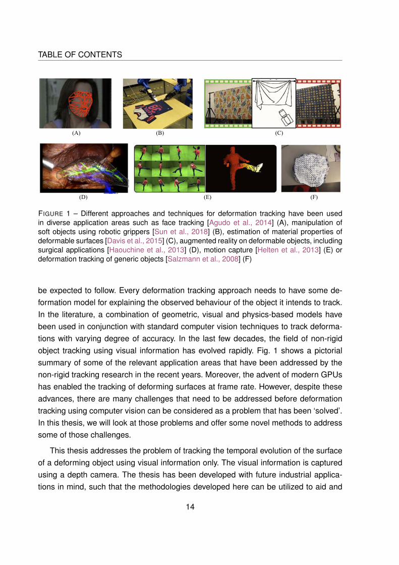
TABLE OF CONTENTS
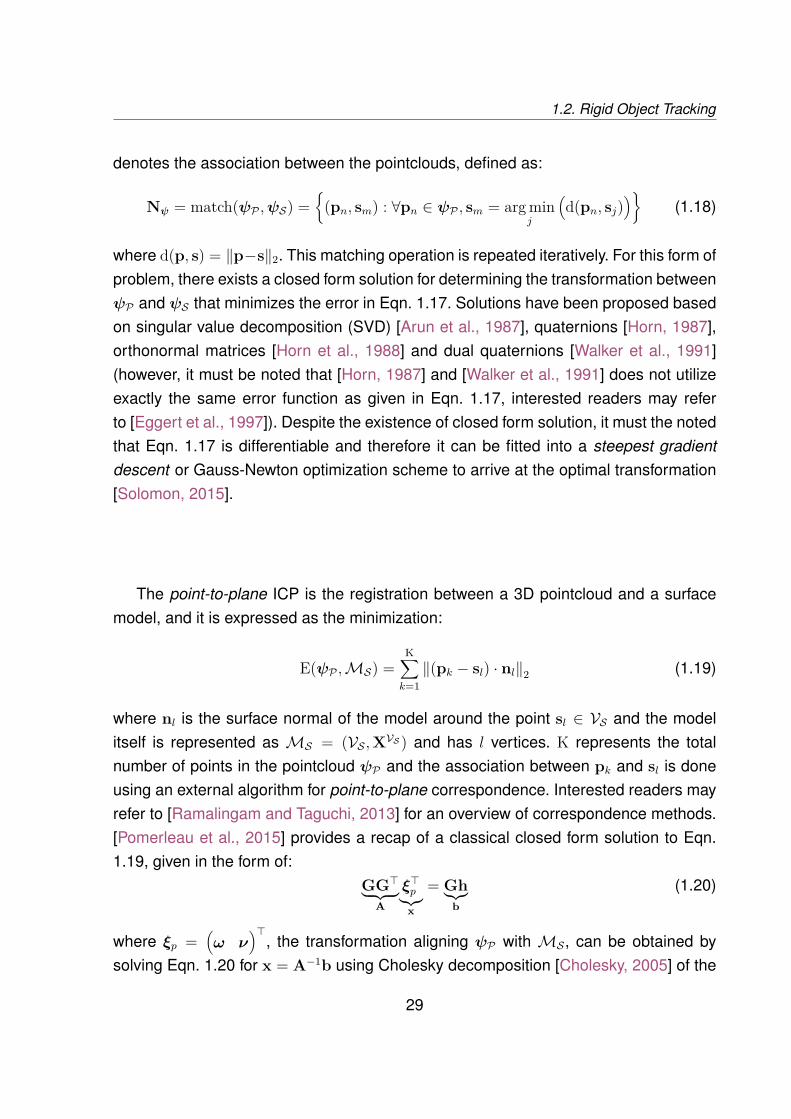
FIGURE 1 – Different approaches and techniques for deformation tracking have been usedin diverse application areas such as face tracking [Agudo et al., 2014] (A), manipulation ofsoft objects using robotic grippers [Sun et al., 2018] (B), estimation of material properties ofdeformable surfaces [Davis et al., 2015] (C), augmented reality on deformable objects, includingsurgical applications [Haouchine et al., 2013] (D), motion capture [Helten et al., 2013] (E) ordeformation tracking of generic objects [Salzmann et al., 2008] (F)
be expected to follow. Every deformation tracking approach needs to have some de-formation model for explaining the observed behaviour of the object it intends to track.In the literature, a combination of geometric, visual and physics-based models havebeen used in conjunction with standard computer vision techniques to track deforma-tions with varying degree of accuracy. In the last few decades, the field of non-rigidobject tracking using visual information has evolved rapidly. Fig. 1 shows a pictorialsummary of some of the relevant application areas that have been addressed by thenon-rigid tracking research in the recent years. Moreover, the advent of modern GPUshas enabled the tracking of deforming surfaces at frame rate. However, despite theseadvances, there are many challenges that need to be addressed before deformationtracking using computer vision can be considered as a problem that has been ‘solved’.In this thesis, we will look at those problems and offer some novel methods to addresssome of those challenges.
This thesis addresses the problem of tracking the temporal evolution of the surfaceof a deforming object using visual information only. The visual information is capturedusing a depth camera. The thesis has been developed with future industrial applica-tions in mind, such that the methodologies developed here can be utilized to aid and
14

TABLE OF CONTENTS
enable the manipulation of soft objects by robotic grippers and actuators.
Deformation tracking using depth cameras has many practical utilities. Althoughrobotic manipulation using deformation tracking remains the primary application areaof this thesis, similar or closely-related approaches can also be utilized for surgicalrobotics [Moerman et al., 2009], motion capture [Hughes, 2012], augmented reality[Huang et al., 2015] and non-rigid SLAM [Agudo et al., 2011].
In the recent years, many approaches have been proposed to address the problemof tracking non-rigid objects. However, due to reasons discussed in details throughoutthe dissertation, we chose to utilize physics based approaches for deformation model-ling. Not only does this approach impart physical reality to the deformation trackingmethods proposed in this thesis, this approach also enables us to extend the defor-mation tracking algorithms towards robotic applications. These applications could havesignificant industrial use-cases by themselves.
Motivation
In most industrial robotic applications, monocular or depth camera is used as theprimary sensor (apart from tactile sensing). To manipulate complex objects in real-time, it is necessary to know the position of the object along all 6 degrees-of-freedom(DoF) with respect to the robot. If the object happens to be deforming and changing itsshape, it is necessary to track not just the 6-DoF of the object, but to track the entiresurface. This can be done with or without a CAD model of the object. However, withouta model, the problem statement becomes more unconstrained. Moreover, without theobject model, it is not possible to have any idea about the occluded or hidden surfaceof the object. In an industrial setup, an approximate CAD model of the object thatneeds to be manipulated is usually readily available. There are many industrial roboticassemblies which deal only with known objects that have been identified beforehand.
This leads us to opt for model based tracking of deforming objects. However, weensure that all the approaches proposed in this thesis work accurately with a coarsemodel of the object, since the process of reconstructing a fine mesh of a random,complex shaped object is significantly more complex (and expensive) than acquiringan approximate 3D model. Moreover, the tracking accuracy has to be high enough androbust enough to handle occlusion and sensor noise.
Over the second half of the dissertation, we progressively arrive towards addressing
15

TABLE OF CONTENTS
a secondary problem statement. This involves estimating the elasticity parameters ofan object while we visually track its deformation. This has been made possible largelydue to the presence of the physics based model for deformation tracking.
Contributions
This dissertation makes the following contributions to the field of non-rigid objecttracking:
— A rigid object tracking methodology is developed to track complex shaped objectsusing a coarse object model ;
— A physics based model is utilized to track deforming objects by minimization ofdepth based error by estimating the gradient of error using repeated simulationof deformations ;
— A similar physics based model is used for minimization of geometric and pho-tometric cost functions using a novel approach to analytically approximate thegradient of error, thereby avoiding the expensive simulations for gradient estima-tion at every iteration ;
— Having developed a non-rigid object tracking methodology, we utilize this ap-proach to estimate the physical elasticity parameter of a deforming object usinga robotic actuator and also use the estimated parameter to track the forces beingapplied on the object using visual information only
Structure of the thesis
The manuscript of this dissertation is organized as follows:
Chapter 1 introduces some of the fundamental concepts of computer vision andgeometry. The first part of this chapter recalls some of the classical algorithms for rigidobject tracking. The second half devotes itself to analyzing the existing methods fornon-rigid object tracking, as available in the literature. We explain some of the relevantconcepts in details and analyze some of the important results and observations fromthe pertinent literature.
16
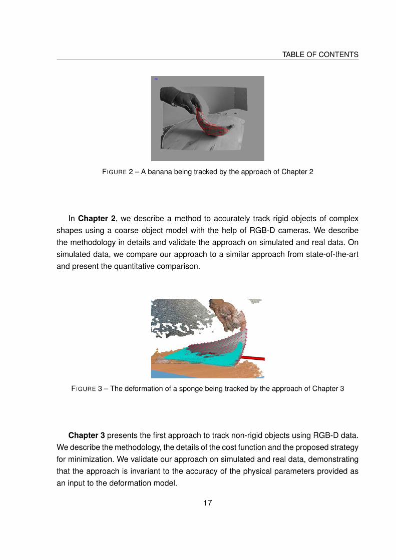
TABLE OF CONTENTS
FIGURE 2 – A banana being tracked by the approach of Chapter 2
In Chapter 2, we describe a method to accurately track rigid objects of complexshapes using a coarse object model with the help of RGB-D cameras. We describethe methodology in details and validate the approach on simulated and real data. Onsimulated data, we compare our approach to a similar approach from state-of-the-artand present the quantitative comparison.
FIGURE 3 – The deformation of a sponge being tracked by the approach of Chapter 3
Chapter 3 presents the first approach to track non-rigid objects using RGB-D data.We describe the methodology, the details of the cost function and the proposed strategyfor minimization. We validate our approach on simulated and real data, demonstratingthat the approach is invariant to the accuracy of the physical parameters provided asan input to the deformation model.
17
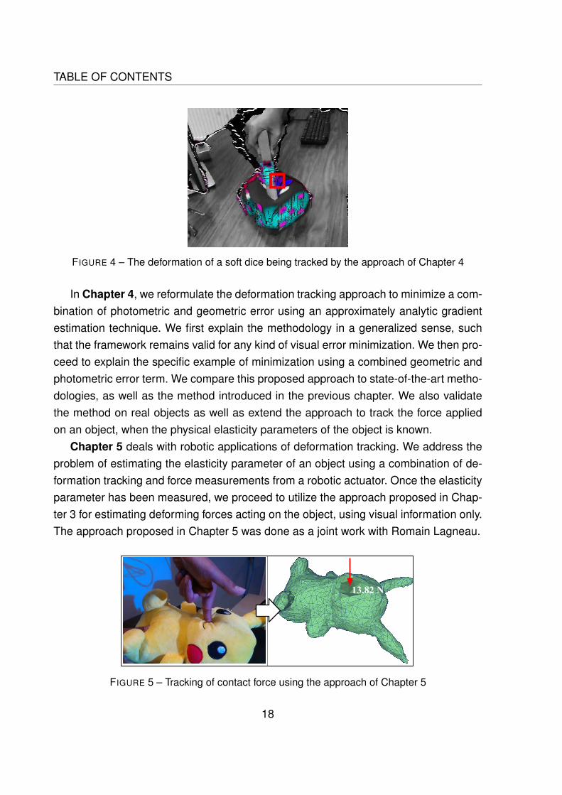
TABLE OF CONTENTS
FIGURE 4 – The deformation of a soft dice being tracked by the approach of Chapter 4
In Chapter 4, we reformulate the deformation tracking approach to minimize a com-bination of photometric and geometric error using an approximately analytic gradientestimation technique. We first explain the methodology in a generalized sense, suchthat the framework remains valid for any kind of visual error minimization. We then pro-ceed to explain the specific example of minimization using a combined geometric andphotometric error term. We compare this proposed approach to state-of-the-art metho-dologies, as well as the method introduced in the previous chapter. We also validatethe method on real objects as well as extend the approach to track the force appliedon an object, when the physical elasticity parameters of the object is known.
Chapter 5 deals with robotic applications of deformation tracking. We address theproblem of estimating the elasticity parameter of an object using a combination of de-formation tracking and force measurements from a robotic actuator. Once the elasticityparameter has been measured, we proceed to utilize the approach proposed in Chap-ter 3 for estimating deforming forces acting on the object, using visual information only.The approach proposed in Chapter 5 was done as a joint work with Romain Lagneau.
FIGURE 5 – Tracking of contact force using the approach of Chapter 5
18
TABLE OF CONTENTS
Contributions
We present a brief summary of the contributions that were disseminated during thisPh.D.
Publications
This thesis resulted in the following publications being accepted in internationalconferences :
— Sengupta, A., Krupa, A. and Marchand, E., 2019, September. RGB-D tracking ofcomplex shapes using coarse object models. In 2019 IEEE International Confe-rence on Image Processing (ICIP) (pp. 3980-3984)
— Sengupta, A., Krupa, A. and Marchand, E., 2019, October. Tracking of Non-RigidObjects using RGB-D Camera. In 2019 IEEE International Conference on Sys-tems, Man and Cybernetics (SMC) (pp. 3310-3317)
— Sengupta, A., Lagneau, R., Krupa, A., Marchand, E. and Marchal, M., 2020, June.Simultaneous Tracking and Elasticity Parameter Estimation of Deformable Ob-jects. In IEEE Int. Conf. on Robotics and Automation, (ICRA)
Dataset
The following dataset were created and made publicly available for aiding futureresearch and for enabling future comparison with our proposed approaches :
— github.com/lagadic/nr-dataset.git
— github.com/lagadic/VisualDeformationTracking.git
Videos
The following videos have been made publicly available for demonstrating our re-sults from the methods proposed throughout this thesis :
— Demonstration of rigid object tracking methodology : youtu.be/_TPJkleBu3w
— Demonstration of non-rigid object tracking using depth information only : youtu.be/RFd-Ix9hcdg
19

TABLE OF CONTENTS
— Demonstration of non-rigid object tracking using depth and photometric informa-tion : youtu.be/y4uuXpWFrvE
— : Robotic applications of deformation tracking : youtu.be/k1MPnmqmovQ
20
CHAPTER 1
BACKGROUND
Non-rigid object tracking is a complex problem to solve. It becomes even more chal-lenging when it is required to be done in real-time. This has only been made possibleby the recent developments over the last decade or so. Rigid object tracking, on theother hand, is a very well-developed research area. There are multiple alternative ap-proaches available in the state-of-the-art for handling the problem of tracking deformingobjects using visual sensors. However, a many existing non-rigid tracking methods uti-lize some format of rigid object tracking as an initial registration step. Given this context,we commence our study of non-rigid object tracking by first analyzing some fundamen-tal principles involving rigid object tracking. This is followed by a survey of the existingliterature of deformation tracking, as well as a brief explanation of some underlyingprinciples.
The first half of this chapter (Sec. 1.1) introduces some of the preliminary mathe-matical notations required for a detailed study of rigid object tracking (Sec. 1.2), whilethe second-half (Sec. 1.3) dives into the state-of-the-art for deformation tracking.
1.1 Preliminary Mathematical Definitions
Since the state-of-the-art is significantly diverse in terms of approaches used fortracking deformations, we confine ourselves to describing only those preliminary no-tations and fundamentals which are strongly relevant to the method proposed in thethesis. Some additional approaches are discussed in section 1.3, as required.
Since the overall approach for deformation tracking proposed in this paper broadlyinvolves visual tracking using mechanical object models, the Sec. 1.1 is splitted into twosub-parts, one which recalls the classical mathematical tools used in visual tracking ofrigid objects and the other describing the details of the mechanical models.
21

Chapter 1 – Background
1.1.1 Frame Transformation
In this thesis, the Euclidean transformation of points, lines and planes are almostalways restricted to the rotation group SO(3) and the special Euclidean group of trans-formation SE(3). An element R ∈ SO(3) ⊂ R3 is a matrix denoting the group of 3Drotation. An element of SE(3) is usually denoted by the homogeneous matrix:
T = R t
01×3 1
∈ SE(3)
∣∣∣∣∣∣R ∈ SO(3), t ∈ R3 (1.1)
where t ∈ R3. The tangent space of SO(3) and SE(3), denoted by so(3) and se(3)respectively, is obtained using the logarithmic map:
ω = θ
2 sin θ
r32 − r23
r13 − r31
r21 − r12
=
ω1
ω2
ω3
(1.2)
where
R =
r11 r12 r13
r21 r22 r23
r31 r32 r33
(1.3)
andθ = cos−1
(tr(R)− 12
)(1.4)
such that ω = (ω1, ω2, ω3) ∈ so(3) and the corresponding skew-symmetric matrix isgiven by
[ω]× =
0 −ω3 ω2
ω3 0 −ω1
−ω2 ω1 0
(1.5)
An element ξ =(ν> ω>
)∈ se(3) can be derived by:
ν =(I3×3 +
(1− cos θθ2
)[ω]× +
(θ − sin θθ3
)[ω]2×
)−1t (1.6)
The setup for visual tracking (in the context of this thesis) would always containat-least three cartesian reference frames, one centered at the camera (or the visualsensor) F c, another centered at the object being tracked Fo and the last one depic-
22

1.1. Preliminary Mathematical Definitions
ting the world reference frame Fw. The coordinate frames belong to the 3D Euclideanspace E3. An arbitrary 3D point P in real coordinate space R3 is represented in homoge-neous coordinates as a 4-vector P = (X,Y,Z, 1), while the point itself is represented asP = (X,Y,Z) ∈ R3 w.r.t F c. The same point, when expressed w.r.t the world or objectcoordinate, gets represented as wP and oP respectively. Using standard convention, atransformation from an arbitrary reference frame A to another arbitrary reference frameB is denoted by BTA. With this representation, a 3D point can be transformed from theframe A to B using:
BP = BTAAP (1.7)
If T is represented as q = (t, θu), where u is the axis of the rotation R and θ itsrelative angle, the time derivative q can be used to represent the same expression asa velocity twist ξ = q, provided θ and t are very small.
1.1.2 Perspective Projection Model
When a 3D point P is imaged using the pinhole camera model of the general pro-jective camera [Hartley and Zisserman, 2003], a 2D image point p = (u, v), with thecorresponding homogeneous coordinate p = (u, v, 1), is formed on the image plane I,where
u = fxXZ + cx
v = fyYZ + cy
(1.8)
(fx, fy) are the focal lengths of the camera, expressed in pixel units, whereas (cx, cy)denotes the 2D coordinates of the principal point on the image plane.
For a point p, the projective transformation Kp can be expressed as the mapping:
XYZ1
7→fxX + cxZfyY + cyZ
Z
= p = KpΠpP (1.9)
23
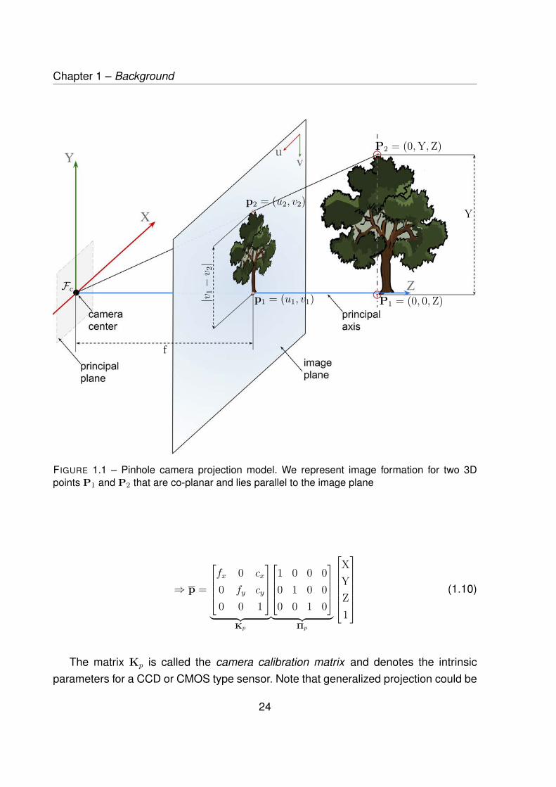
Chapter 1 – Background
P2 = (0,Y,Z)
P1 = (0, 0,Z)
p2 = (u2, v2)
p1 = (u1, v1)|v1−v 2|
Y
f
Fc
FIGURE 1.1 – Pinhole camera projection model. We represent image formation for two 3Dpoints P1 and P2 that are co-planar and lies parallel to the image plane
⇒ p =
fx 0 cx
0 fy cy
0 0 1
︸ ︷︷ ︸
Kp
1 0 0 00 1 0 00 0 1 0
︸ ︷︷ ︸
Πp
XYZ1
(1.10)
The matrix Kp is called the camera calibration matrix and denotes the intrinsicparameters for a CCD or CMOS type sensor. Note that generalized projection could be
24

1.1. Preliminary Mathematical Definitions
modelled with an additional skew parameter sp, such that:
Kp =
fx sp cx
0 fy cy
0 0 1
(1.11)
sp is an axial skew parameter which denotes the shear distortion in the projected image.However, it can be assumed that sp = 0 for most normal cameras. Moreover, to genera-lize the projection even further, if p is not maintained at the camera-centered referenceframe, an additional transformation can be utilized to orient the point oP from its object-centered reference frame to that of the camera, such that:
p = KpΠpcTo︸ ︷︷ ︸
camera projection matrix
oP (1.12)
The R3 7→ R2 operation corresponding to the perspective projection of 3D points to 2Dpixel on the image plane can be simplified by the projection operator Π
(·)
such that
p = Π(P)
can be expressed using the non-homogeneous coordinates of the 3D and2D points.
I(u, v) gives the grayscale intensity of the pixel at coordinates (u, v) of I. The pin-hole camera model used for this projection operation is shown in Fig. 1.1. This pers-pective projection ideally allows us to represent light rays by straight lines, but withmost cameras in real-life, certain radial distortions are observed in the pixel coordi-nates. These radial distortions can be modelled easily [Faugeras, 1993] [Hartley andZisserman, 2003], and is represented as:
u = ud(1 + k1s2 + k2s
4)
v = vd(1 + k1s2 + k2s
4)(1.13)
where (u, v) is a point in the image plane which can be obtained using perspectiveprojection only while (ud, vd) is the corresponding point with distortion. Here, s2 = u2
d+v2d
and k1 and k2 are the parameters of distortion coefficient, which can be estimated usingclassical calibration techniques, such as [Brown, 1971] [Stein, 1997].
25

Chapter 1 – Background
1.1.3 Object Model and Pointcloud
The 3D model depicting the surface of an object is expressed using the tuple M =(AV ,XV
), where:
AV =[P1 P2 · · · PN
]=
P1X P2X · · · PNX
P1Y P2Y · · · PNY
P1Z P2Z · · · PNZ
1 1 · · · 1
(1.14)
and AV =[P1 P2 · · · PN
]is a set of 3D points of a model with N vertices (Fig.
1.2a), maintained at an arbitrary reference frame A.
P1
P2
P3
P4
P5
P6
P1
P2
P3
P4
P5
P6
P1 P2 P3 P4 P5 P6
V =[P1 P2 P3 P4 P5 P6
]
= XV
(a) (b)
FIGURE 1.2 – Example of the mesh model setup used in this thesis, showing a mesh consistingof six vertices
A pointcloud comprising of multiple 3D points is denoted by ψ, which has the samematrix structure as AV, i.e., ψ =
[P1 P2 · · · PK
]and Aψ =
[P1 P2 · · · PK
],
where K denotes the number of points in the pointcloud.Note that V and ψ denotessimilar matrices that represent a set of 3D points. However, throughout this thesis, Vhas been used to denote the vertices of a mesh whereas ψ has been used to denotepointclouds. XV denotes the adjacency matrix of the simple, undirected mesh suchthat:
XVij =
1 if (Pi,Pj) is connected
0 else(1.15)
thereby depicting a model with N 3D points and M number of Q − hedral surfaces(denoting a polygon with Q edges), as shown in Fig. 1.2b.
26
1.1. Preliminary Mathematical Definitions
IR
Projector
IR
Imager
RGB
Module
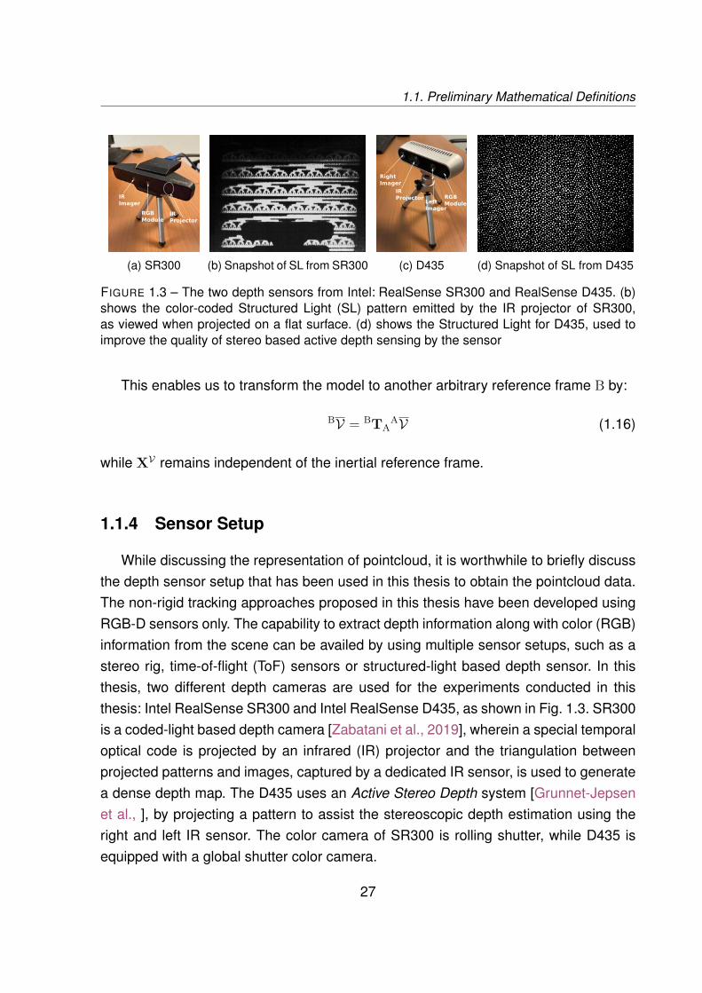
(a) SR300 (b) Snapshot of SL from SR300
Right
Imager
IR
ProjectorLeft
Imager
RGB
Module
(c) D435 (d) Snapshot of SL from D435
FIGURE 1.3 – The two depth sensors from Intel: RealSense SR300 and RealSense D435. (b)shows the color-coded Structured Light (SL) pattern emitted by the IR projector of SR300,as viewed when projected on a flat surface. (d) shows the Structured Light for D435, used toimprove the quality of stereo based active depth sensing by the sensor
This enables us to transform the model to another arbitrary reference frame B by:
BV = BTAAV (1.16)
while XV remains independent of the inertial reference frame.
1.1.4 Sensor Setup
While discussing the representation of pointcloud, it is worthwhile to briefly discussthe depth sensor setup that has been used in this thesis to obtain the pointcloud data.The non-rigid tracking approaches proposed in this thesis have been developed usingRGB-D sensors only. The capability to extract depth information along with color (RGB)information from the scene can be availed by using multiple sensor setups, such as astereo rig, time-of-flight (ToF) sensors or structured-light based depth sensor. In thisthesis, two different depth cameras are used for the experiments conducted in thisthesis: Intel RealSense SR300 and Intel RealSense D435, as shown in Fig. 1.3. SR300is a coded-light based depth camera [Zabatani et al., 2019], wherein a special temporaloptical code is projected by an infrared (IR) projector and the triangulation betweenprojected patterns and images, captured by a dedicated IR sensor, is used to generatea dense depth map. The D435 uses an Active Stereo Depth system [Grunnet-Jepsenet al., ], by projecting a pattern to assist the stereoscopic depth estimation using theright and left IR sensor. The color camera of SR300 is rolling shutter, while D435 isequipped with a global shutter color camera.
27

Chapter 1 – Background
1.2 Rigid Object Tracking
While tracking rigid objects using visual information, there are multiple approachesthat can be utilized for frame-to-frame registration. We first describe the classical ap-proaches for rigid object tracking and then take a look at some of the recent methodsfrom the state-of-the-art for rigid object and scene tracking.
1.2.1 Classical Approaches
Since we utilize a depth camera, we can choose to track objects in terms of 3D-3Dregistration only, we can restrict ourselves to just the image data and track objects in a2D-2D sense, we can switch back and forth between 2D-3D registration or we can usethe hybrid data consisting of depth and image information together in RGB-D format.We shall present the basic principles related to the different approaches for registrationof rigid objects:
1.2.1.1 3D-3D Registration
The first approach for rigid object tracking involves the registration of a pair of 3Ddata obtained from some suitable depth sensor. Given a stream of 3D points from thedepth sensor, one of the simplest approach to align the points is using an IterativeClosest Point (ICP) algorithm which was first proposed as a method for registration of3D shapes in [Besl and McKay, 1992]. It was later summarized by [Pomerleau et al.,2015], outlining more than two decades of refinement since it was first proposed.
In its basic form, ICP has two variants, one involving the registration of 3D pointswith another set of 3D points (point-to-point ICP), while the other variant involves theminimization of distance between a set of 3D points with planar surfaces (point-to-planeICP). The point-to-point ICP can be expressed as the minimization of the following costfunction w.r.t the transformation between two pointclouds:
E(ψP ,ψS) =∑
(p,s)∈Nψ
‖p− s‖2 (1.17)
where ψP and ψS are two pointclouds located close to each other, and the set Nψ
28
1.2. Rigid Object Tracking
denotes the association between the pointclouds, defined as:
Nψ = match(ψP ,ψS) =
(pn, sm) : ∀pn ∈ ψP , sm = arg minj
(d(pn, sj)
)(1.18)
where d(p, s) = ‖p−s‖2. This matching operation is repeated iteratively. For this form ofproblem, there exists a closed form solution for determining the transformation betweenψP and ψS that minimizes the error in Eqn. 1.17. Solutions have been proposed basedon singular value decomposition (SVD) [Arun et al., 1987], quaternions [Horn, 1987],orthonormal matrices [Horn et al., 1988] and dual quaternions [Walker et al., 1991](however, it must be noted that [Horn, 1987] and [Walker et al., 1991] does not utilizeexactly the same error function as given in Eqn. 1.17, interested readers may referto [Eggert et al., 1997]). Despite the existence of closed form solution, it must the notedthat Eqn. 1.17 is differentiable and therefore it can be fitted into a steepest gradientdescent or Gauss-Newton optimization scheme to arrive at the optimal transformation[Solomon, 2015].
The point-to-plane ICP is the registration between a 3D pointcloud and a surfacemodel, and it is expressed as the minimization:
E(ψP ,MS) =K∑k=1‖(pk − sl) · nl‖2 (1.19)
where nl is the surface normal of the model around the point sl ∈ VS and the modelitself is represented as MS = (VS ,XVS ) and has l vertices. K represents the totalnumber of points in the pointcloud ψP and the association between pk and sl is doneusing an external algorithm for point-to-plane correspondence. Interested readers mayrefer to [Ramalingam and Taguchi, 2013] for an overview of correspondence methods.[Pomerleau et al., 2015] provides a recap of a classical closed form solution to Eqn.1.19, given in the form of:
GG>︸ ︷︷ ︸A
ξ>p︸︷︷︸x
= Gh︸︷︷︸b
(1.20)
where ξp =(ω ν
)>, the transformation aligning ψP with MS , can be obtained by
solving Eqn. 1.20 for x = A−1b using Cholesky decomposition [Cholesky, 2005] of the
29
Chapter 1 – Background
matrix denoted by A. Here:
G = · · · pk × nk · · ·
nk
︸ ︷︷ ︸
[6×K]
(1.21)
and:
h =
...
(sk − pk) · nk...
︸ ︷︷ ︸
[K×1]
(1.22)
However, it is also possible to reach at a similar solution with non-linear least squaresoptimization, where the Jacobian relating the variation of ξp with the change of E(ψP ,MS)is given by:
Jicp = ∂E(ψP ,MS)∂ξp
=[pk × nk nk
](1.23)
while the update ∆ξp can be computed in the Gauss-Newton sense:
∆ξp = −(J>icpJicp)−1J>icpE(ψP ,MS) (1.24)
The update is combined with the initial estimate by (ξp)t = (ξp)t−1 + ∆ξp where(ξp)t is the estimate of ξp at t-th iteration of the minimization. This iterative gradientestimation and update of ξp is continued till a certain convergence criterion is reached.The exact convergence criterion is often determined empirically and depends on theapplication area. Interested readers are directed to [Salzo and Villa, 2012] for a detailedanalysis of convergence properties and criteria for Gauss-Newton method.
1.2.1.2 Dense 2D-2D Registration
Having summarized some of the traditional methods for 3D-3D registration, we nowtake a look into some of the 2D-2D registration techniques based on just the imagedata. This is a more classical problem statement, since monocular cameras were po-pularized much earlier than affordable depth sensors. Tracking with images can be
30
1.2. Rigid Object Tracking
usually expressed as the minimization of the sum of squared error term:
E(p) = arg minx
∑p
[I(W(p,x))− I∗(p)
]2(1.25)
With classical image based tracking using the Lucas-Kanade algorithm [Baker andMatthews, 2004], p is usually the image pixel coordinates, where I∗(·) is the tar-get/template image and I is the current image, W is an image warping function basedon the warp parameters x = (x1, x2, · · ·, xn), a vector of parameters defining the warp.Minimizing the expression in Eq. 1.25 is a non-linear optimization task, even if W islinear in x. To optimize Eq. 1.25, the current estimate of x is assumed to be known.The increment ∆x is iteratively solved by minimizing
E(p) =∑p
[I(W(p,x + ∆x)
)− I∗
(p)]2
(1.26)
and the parameters are updated by
x← x + ∆x (1.27)
The Lucas-Kanade algorithm is specifically a Gauss-Newton based gradient des-cent algorithm. However, steepest gradient descent, Newton-Raphson [Acton, 1990]or Levenberg-Marquadt [Marquardt, 1963] [Solomon, 2015] based minimization canbe equally applicable for a minimization of this nature. The expression for intensitydifference can be linearized using the Taylor expansion:
I(W(p,x + ∆x))− I∗(p) = I(W(p,x)) +∇I ∂W∂x
∆x− I∗(p) (1.28)
where∇I =(∂I∂u
∂I∂v
), the image gradients along x and y axis of the image plane. The
term ∂W∂x is the Jacobian of the warping function and is given by:
∂W∂x
=∂Wx
∂x1∂Wx
∂x2· · · ∂Wx
∂xn∂Wy
∂x1
∂Wy
∂x2· · · ∂Wy
∂xn
(1.29)
The formulation of eqn. 1.26 is termed the forward-additive formulation for direct imageintensity based visual tracking. Forward-compositional formulation [Shum and Sze-
31
Chapter 1 – Background
liski, 2001], inverse-additive formulation [Hager and Belhumeur, 1998] and inverse-compositional formulation [Baker and Matthews, 2001] are used as well. The compa-rative outline of these methods are summarized below:
1. Forward-additive method The error function is given as by Eqn. 1.26, while theupdate is given by Eqn. 1.2.1.2.
2. Forward-compositional method The error function is given by:
E(p) =∑p
[I(
W(W(p,∆x)
),x)− I∗
(p)]2
(1.30)
and the update is given by:
W(p,x)←W(p,x) W(p,∆x) (1.31)
where the operator denotes the composition of two warps, such that:
W(p,x) W(p,∆x) ≡W(W(p,∆x),x
)(1.32)
3. Inverse-compositional method The error function is given by:
E(p) =∑p
[I∗(W(p,∆x)
)− I
(W(p,x)
)]2(1.33)
while the update is given by:
W(p,x)←W(p,x) W(p,∆x)−1 (1.34)
4. Inverse-additive method The error function is the same as Eqn. 1.26, whilethe role of the template and the image is switched. This reformulates the Taylorexpansion of Eqn. 1.28 into:
E(p) =∑p
[I(W(p,x)
)+∇I∗
(∂W∂p
)−1∂W∂x ∆x− I∗(p)
]2(1.35)
and the parameter update is given by x← x−∆x
The Lucas-Kanade algorithm described above enables us to track an image basedon a template. We now focus on deriving a relationship between a small number of
32
1.2. Rigid Object Tracking
image points in two different images when a one-to-one correspondence between theimage positions are given. Given a set of four 2D to 2D point correspondences api ↔bpi, where api = (bui,
avi, 1) and bpi = (bui,bvi, 1) are two points on the image plane in
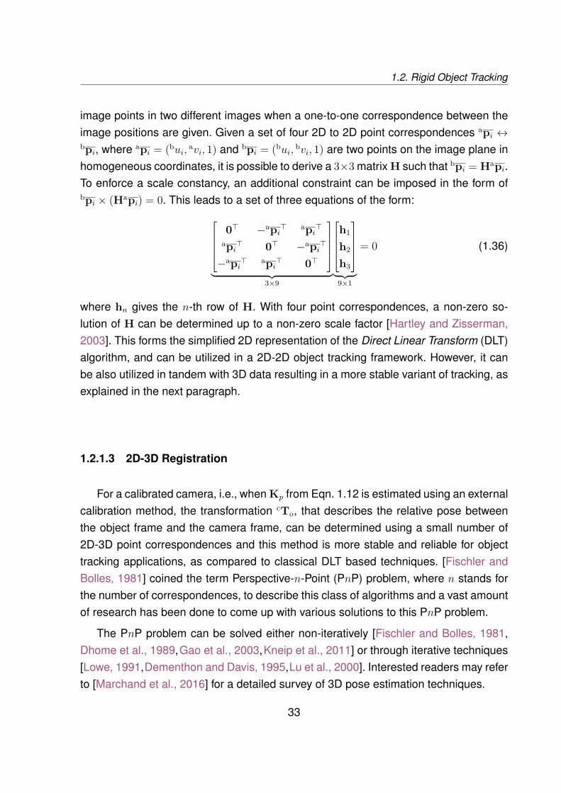
homogeneous coordinates, it is possible to derive a 3×3 matrix H such that bpi = Hapi.To enforce a scale constancy, an additional constraint can be imposed in the form ofbpi × (Hapi) = 0. This leads to a set of three equations of the form:
0> −api> api>
api> 0> −api>
−api> api> 0>
︸ ︷︷ ︸
3×9
h1
h2
h3
︸ ︷︷ ︸
9×1
= 0 (1.36)
where hn gives the n-th row of H. With four point correspondences, a non-zero so-lution of H can be determined up to a non-zero scale factor [Hartley and Zisserman,2003]. This forms the simplified 2D representation of the Direct Linear Transform (DLT)algorithm, and can be utilized in a 2D-2D object tracking framework. However, it canbe also utilized in tandem with 3D data resulting in a more stable variant of tracking, asexplained in the next paragraph.
1.2.1.3 2D-3D Registration
For a calibrated camera, i.e., when Kp from Eqn. 1.12 is estimated using an externalcalibration method, the transformation cTo, that describes the relative pose betweenthe object frame and the camera frame, can be determined using a small number of2D-3D point correspondences and this method is more stable and reliable for objecttracking applications, as compared to classical DLT based techniques. [Fischler andBolles, 1981] coined the term Perspective-n-Point (PnP) problem, where n stands forthe number of correspondences, to describe this class of algorithms and a vast amountof research has been done to come up with various solutions to this PnP problem.
The PnP problem can be solved either non-iteratively [Fischler and Bolles, 1981,Dhome et al., 1989,Gao et al., 2003,Kneip et al., 2011] or through iterative techniques[Lowe, 1991,Dementhon and Davis, 1995,Lu et al., 2000]. Interested readers may referto [Marchand et al., 2016] for a detailed survey of 3D pose estimation techniques.
33

Chapter 1 – Background
1.2.2 State-of-the-art for Rigid Object Tracking
The rigid object tracking literature is extensive and heterogeneous. An exhaustivesurvey of all such techniques is beyond the scope of this thesis. Therefore, we restrictthe discussion to a few of the more important and relevant object tracking methodo-logies that were proposed in the last three decades. A brief summary of some of thenotable research in the field of rigid object tracking is given below.
As mentioned in Sec. 1.2, [Besl and McKay, 1992] is one of the earliest paper toexplain the ICP in details. The approach involves calculating the closest distance froma point to either a parametric entity: viz., curves or surfaces, or implicit geometric en-tity: like a vector-valued, multivariate function. A Newtonian minimization approach isused for the former, while an augmented Lagrange multiplier system [Luenberger et al.,1984] is used for the later. The closest point calculation and registration is done iterati-vely till the mean square error falls below a preset threshold. This forms the basic ICPalgorithm described in [Wikipedia, 2016]. Alternate methods of point cloud registrationhas been proposed by [Pottmann et al., 2004] for point cloud registration without usingthe original ICP proposed by [Besl and McKay, 1992]. [Pottmann et al., 2004] proposesa kinematic model-based approach to 3D point cloud registration.
[Newcombe et al., 2011] and [Izadi et al., 2011] provided a major advance in real-time tracking and mapping. It allowed users to create very accurate map of the scenewhile tracking the camera reliably, leading to implementation in applications like 3Dmodelling, high quality, tracking of robots mounted with these depth cameras, etc. Thetechnique used for KinectFusion is broadly divided into four steps: A) measurement, B)pose estimation, C) Reconstruction and D) Surface Prediction. The measurement ofthe raw data coming in from the sensor is stored as a dense vertex map and a pyramidof normal map. The reconstruction of the scene, at every step, is stored as a TruncatedSigned Distance Function (TSDF). It eases the integration of new measurement intothe reconstructed model. If the transformation of the camera (or Kinect) with respectto the world is known, the appearance of the depth map at the next iteration can bepredicted by transforming the reconstruction using the camera’s rotation and transla-tion, and then projecting it into the image plane using ray-casting techniques. Poseestimation, on the other hand, is done using ICP.
Many subsequent papers have tried to improve upon the accuracy of KinectFu-sion. [Henry et al., 2013] is one of the primary research work dealing with improve-ment of tracking accuracy of KinectFusion by implementing global optimization on the
34
1.3. Non-rigid Object Tracking
pose frame graph. This was done using g2o [Kümmerle et al., 2011]. [Roth and Vona,2012], [Nießner et al., 2013], [Zeng et al., 2012] and [Whelan et al., 2013] improves themapping capabilities of KinectFusion. [Choi and Christensen, 2013] proposed a par-ticle filtering based approach to track the degrees of freedom of an object from RGB-Ddata, wherein the likelihood of each particle was evaluated using a combination of geo-metric and photometric information.
Extending this approach, [Ren et al., 2017] proposes to express the probability ofeach pixel as a joint distribution over a combined function of the camera pose, Si-gned Distance Function (SDF) [Chan and Zhu, 2005] of the object, RGB value of thepixel and a step function which determines if the object belongs to background or fo-reground. The pose is determined by a Levenberg - Marquardt minimization of theNegative Log-Likelihood (NLL) of this distribution. [Slavcheva et al., 2016] proposesa real-time SDF to SDF registration method using a combination of geometric andsurface normal based constraints to generate a colored pointcloud which is globallyregistered.
Among the recent approaches, [Kehl et al., 2016] uses a convolutional auto-encoderfor matching scene-patch descriptors with synthetic model patches to detect and loca-lize all 6 DoF of an object. [Garon and Lalonde, 2017] proposes a CNN based 6DoFobject tracker using Microsoft Kinect. In 2017, [Xiang et al., 2018] proposed PoseCNN,a CNN based semantic labelling and 6DoF object tracking framework. [Wu et al., 2018]proposes a realtime technique for 6DoF object localization using CNN based on RGBimages only.
1.3 Non-rigid Object Tracking
We shall now present a brief overview of the existing state-of-the-art on non-rigidobject tracking, as well as the summary of some of the relevant and notable methodo-logies used in the literature. However, we begin by defining the objective of this thesis.
Problem Statement
Given a 3D mesh model M (which can be a triangular or tetrahedral mesh) anda 3D point cloud ψ, we define a cost function d(M ,ψ) that provides a similarity mea-
35

Chapter 1 – Background
[Agudo et al., 2014]
[Agudo and M-Noguer, 2015]
[Agudo et al., 2017]
[Malti and Herzet, 2017]
[Schulman et al., 2013]
[Petit et al., 2015b]
[Petit et al., 2018]
[Salzmann et al., 2007]
[Salzmann et al., 2008]
[Pilet et al., 2008]
[Bartoli et al., 2015]
[Parashar et al., 2015]
[Collins and Bartoli, 2015]
[Newcombe et al., 2015]
[Innmann et al., 2016]
[Slavcheva et al., 2017a]
[Slavcheva et al., 2018]
[Gao and Tedrake, 2018]
[Gotardo and Martinez, 2011b]
[Gotardo and Martinez, 2011a]
[Kumar et al., 2016]
FIGURE 1.4 – Categorization of some of the selected literature about deformation tracking usingvisual and/or depth information. The highlighted region denotes the area of interest of this thesis
sure between the pointcloud and the model. We also define a deformational functionF which acts on the model M to produce a deformed model F (M ). F can be pa-rameterized using a deformation or force field. The objective of the non-rigid trackingmethod is to minimize the cost function:
E(ψ) = arg minF
d(F (M ),ψ
)(1.37)
With this objective, tracking of deforming objects can be handled using multiple ap-proaches, based on the application area and the practical constraints involved with thetargeted application. The available literature on this subject can be broadly classified
36

1.3. Non-rigid Object Tracking
into two categories: a) template/model based tracking, and b) model-free reconstruc-tion and tracking of deforming objects. Even though this thesis primarily deals withmodel based tracking, we also present the details of the research from the relevantreconstruction and tracking literature as well.
For the sake of completeness, we discuss the state-of-the-art for both these para-digms. An overview of some of the notable approaches that we plan to discuss aregiven in Fig. 1.4. The explanation and the relevant discussion about these researcharticles follow in the subsequent paragraphs. In this thesis, we use a physically baseddeformation model, the co-rotational FEM, for modelling the deformation of objects.The following paragraphs are an attempt to explain the rationale behind this choiceand to highlight the advantage of using physically based models for deformation tra-cking, over other alternative approaches.
1.3.1 Physically-based Models
Mechanical models for modelling bio-mechanical deformation of organic objectscan be done using various advanced mechanical models, such as Finite Element Me-thod (FEM), Smoothed-Particle Hydrodynamics (SPH) or porous media model [Weiet al., 2009] based fluid flow simulation. However, in this thesis, we confine our studyof physics based deformable model to FEM.
FEM aims to discretize a dynamic system involving elastic materials (in the contextof mechanical engineering), such that the temporal evolution of the state of the systemwhen subjected to external, unbalanced forces can be simulated across time steps. Todo so, multiple formats of mechanical models can be used, such as triangular, tetrahe-dral or hexahedral meshes. This mechanical model alone is sufficient to evaluate theevolution of the FEM. However, since we are interested in visual tracking, it is importantto map this mechanical model with a visual model of the surface of the object beingtracked.
The mapping between the vertices of the mechanical mesh Vm and the visual modelVs, as shown in Fig. 1.5, can be expressed by Vs = J (Vm) (the notation for the meshvertices is defined in Sec. 1.1.3) while the velocities are related by Us = JsmUm, whereU = V, the differentiation w.r.t time, and the Jacobian:
Jsm = ∂Vs∂Vm
(1.38)
37
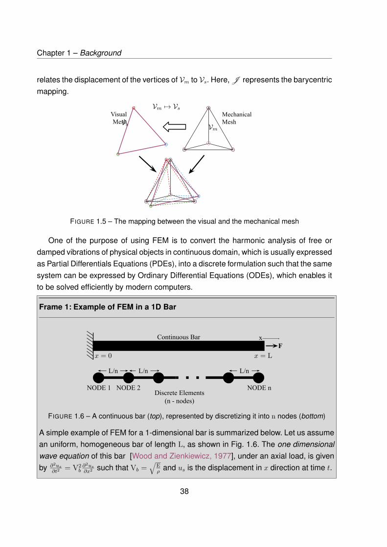
Chapter 1 – Background
relates the displacement of the vertices of Vm to Vs. Here, J represents the barycentricmapping.
VmVs
Vm 7→ Vs
FIGURE 1.5 – The mapping between the visual and the mechanical mesh
One of the purpose of using FEM is to convert the harmonic analysis of free ordamped vibrations of physical objects in continuous domain, which is usually expressedas Partial Differentials Equations (PDEs), into a discrete formulation such that the samesystem can be expressed by Ordinary Differential Equations (ODEs), which enables itto be solved efficiently by modern computers.
Frame 1: Example of FEM in a 1D Bar
x = Lx = 0
FIGURE 1.6 – A continuous bar (top), represented by discretizing it into n nodes (bottom)
A simple example of FEM for a 1-dimensional bar is summarized below. Let us assumean uniform, homogeneous bar of length L, as shown in Fig. 1.6. The one dimensionalwave equation of this bar [Wood and Zienkiewicz, 1977], under an axial load, is givenby ∂2us
∂t2= V2
b∂2us∂x2 such that Vb =
√Eρ
and us is the displacement in x direction at time t.
38
1.3. Non-rigid Object Tracking
E and ρ are the Young’s modulus and density of the bar respectively, while Vb gives thewave propagation velocity. For FEM based analysis, it is necessary to represent theforce-displacement relationship in a matrix representation of the format:
F = Kus (1.39)
where K is the stiffness matrix, us is the vector of displacements and F is the externalforce vector. It can be shown [Rao, 1995] that for the i-th node of the bar:
Ki = nCk
1 −1−1 1
(1.40)
and:F =
∫ l
0Fb(x, t)φdx (1.41)
Here, A is the cross-sectional area of the bar, Ck = EA, l is the length of the currentelement, Fb(x, t) is a time-varying distributed load and φ is the shape function [Logan,2011]. Representing the stiffness matrix for individual elements as:
Ki =K11
i K12i
K21i K22
i
(1.42)
we can assemble the global stiffness matrix as:
Kn×n
=
K111 K12
1
K211 K22
1 + K112 K12
2
K212 K22
2 + K113
···
K22n
(1.43)
Since the left end of the bar in Fig. 1.6 is fixed, the row and column corresponding tonode 0 will be set to zero, thereby enforcing the boundary condition. If the forces areknown, the nodal displacement vector can be obtained as:
us = K−1F (1.44)
39
Chapter 1 – Background
Tetrahedral MeshTriangular Mesh
Wireframe Representation Block Representation
FIGURE 1.7 – The triangular, surface model coupled with a tetrahedral, volumetric model
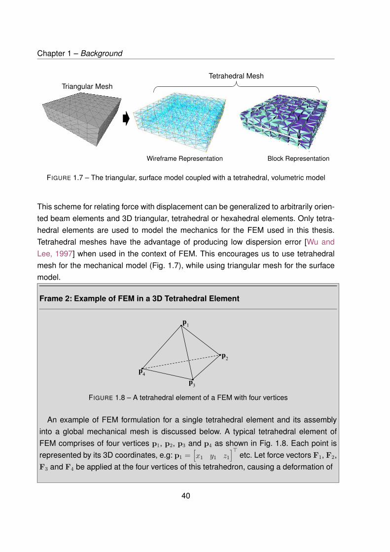
This scheme for relating force with displacement can be generalized to arbitrarily orien-ted beam elements and 3D triangular, tetrahedral or hexahedral elements. Only tetra-hedral elements are used to model the mechanics for the FEM used in this thesis.Tetrahedral meshes have the advantage of producing low dispersion error [Wu andLee, 1997] when used in the context of FEM. This encourages us to use tetrahedralmesh for the mechanical model (Fig. 1.7), while using triangular mesh for the surfacemodel.
Frame 2: Example of FEM in a 3D Tetrahedral Element
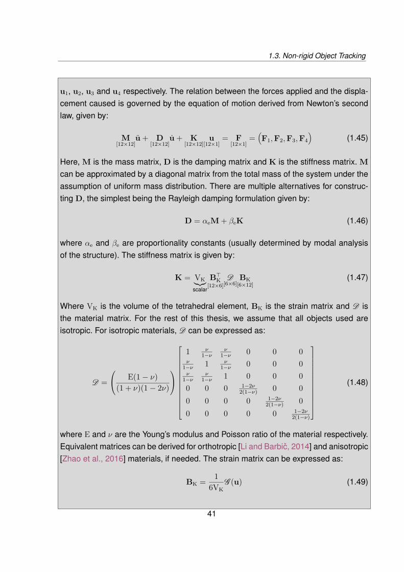
FIGURE 1.8 – A tetrahedral element of a FEM with four vertices
An example of FEM formulation for a single tetrahedral element and its assemblyinto a global mechanical mesh is discussed below. A typical tetrahedral element ofFEM comprises of four vertices p1, p2, p3 and p4 as shown in Fig. 1.8. Each point isrepresented by its 3D coordinates, e.g: p1 =
[x1 y1 z1
]>etc. Let force vectors F1, F2,
F3 and F4 be applied at the four vertices of this tetrahedron, causing a deformation of
40
1.3. Non-rigid Object Tracking
u1, u2, u3 and u4 respectively. The relation between the forces applied and the displa-cement caused is governed by the equation of motion derived from Newton’s secondlaw, given by:
M[12×12]
u + D[12×12]
u + K[12×12]
u[12×1]
= F[12×1]
=(F1,F2,F3,F4
)(1.45)
Here, M is the mass matrix, D is the damping matrix and K is the stiffness matrix. Mcan be approximated by a diagonal matrix from the total mass of the system under theassumption of uniform mass distribution. There are multiple alternatives for construc-ting D, the simplest being the Rayleigh damping formulation given by:
D = αeM + βeK (1.46)
where αe and βe are proportionality constants (usually determined by modal analysisof the structure). The stiffness matrix is given by:
K = VK︸︷︷︸scalar
B>K[12×6]
D[6×6]
BK[6×12]
(1.47)
Where VK is the volume of the tetrahedral element, BK is the strain matrix and D isthe material matrix. For the rest of this thesis, we assume that all objects used areisotropic. For isotropic materials, D can be expressed as:
D = E(1− ν)
(1 + ν)(1− 2ν)
1 ν1−ν
ν1−ν 0 0 0
ν1−ν 1 ν
1−ν 0 0 0ν
1−νν
1−ν 1 0 0 00 0 0 1−2ν
2(1−ν) 0 00 0 0 0 1−2ν
2(1−ν) 00 0 0 0 0 1−2ν
2(1−ν)
(1.48)
where E and ν are the Young’s modulus and Poisson ratio of the material respectively.Equivalent matrices can be derived for orthotropic [Li and Barbic, 2014] and anisotropic[Zhao et al., 2016] materials, if needed. The strain matrix can be expressed as:
BK = 16VK
G (u) (1.49)
41

Chapter 1 – Background
where G (u) can be expanded as:
G (u) =
a1 0 0 a2 0 0 a3 0 0 a4 0 00 b1 0 0 b2 0 0 b3 0 0 b4 00 0 c1 0 0 c2 0 0 c3 0 0 c4
b1 a1 0 b2 a2 0 b3 a3 0 b4 a4 00 c1 b1 0 c2 b2 0 c3 b3 0 c4 b4
c1 0 a1 c2 0 a2 c3 0 a3 c4 0 a4
(1.50)
where:a1 = −(y3z4 − z3y4) + (y2z4 − y4z2)− (y2z3 − y3z2)
b1 = (x3z4 − x4z3)− (x2z4 − x4z2) + (x2z3 − x3z2)
c1 = −(x3y4 − y3x4) + (x2y4 − x4y2)− (x2y3 − x3y2)
a2 = (y3z4 − y4z3)− (y1z4 − y4z1) + (y1z3 − y3z1)
b2 = −(x3z4 − x4z3) + (x1z4 − x4z1)− (x1z3 − x3z1)
c2 = (x3y4 − x4y3)− (x1y4 − x4y1) + (x1y3 − x3y1)
a3 = −(y2z4 − y4z2) + (y1z4 − y4z1)− (y1z2 − y2z1)
b3 = (x2z4 − x4z2)− (x1z4 − x4z1) + (x1z2 − x2z1)
c3 = −(x2y4 − x4y2) + (x1y4 − x4y1)− (x1y2 − x2y1)
a4 = (y2z3 − y3z2)− (y1z3 − y3z1) + (y1z2 − y2z1)
b4 = −(x2z3 − x3z2) + (x1z3 − x3z1)− (x1z2 − x2z1)
c4 = (x2y3 − x3y2)− (x1y3 − x3y1) + (x1y2 − x2y1)
(1.51)
The volume of the tetrahedron is available using elementary geometry, given by theexpression VK = 1
6
∣∣∣(p1 − p4)·((p2 − p4)× (p3 − p4)
)∣∣∣. Having summarized the FEMformulation for a single tetrahedral element, we now describe how to assemble theseelement-wise matrices into a global equation for the entire object.
Global Assembly
We denote the global assembled matrices with the suffix (·)g, thereby providing us withglobal stiffness matrix Kg, global force vector Fg and so on. Let us consider the caseof an object that has been modelled with N tetrahedral elements. Let Fd be the forcevectors of the N elements stacked column-wise, i.e., Fd
[12N×1]=(
F1[12×1]
,F2, . . . ,FN)
.
42
1.3. Non-rigid Object Tracking
It is possible to construct an assembly matrix A such that:
Fd[12N×1]
= A[12N×NV ]
Fg[NV ×1]
⇒ Fg[NV ×1]
= A >[NV ×12N]
Fd[12N×1]
(1.52)
where NV is the number of vertices in the global mechanical model of the object. It ispossible to use the assembly matrix to construct the global stiffness matrix, given by:
Kg[NV ×NV ]
= A >[NV ×12N]
Kd[12N×12N]
A[12N×NV ]
(1.53)
where:
Kd =
K1 0 0 . . .
0 K2 ...
0 . . .. . .
... KN
︸ ︷︷ ︸
[12N×12N]
(1.54)
Similarly, ug can be constructed using the approach of Eqn. 1.52 and Mg. Dg can beconstructed using the approach of Eqn. 1.53.
Co-rotational FEM
We utilize the co-rotational formulation [Müller and Gross, 2004] for modelling de-formation using FEM since the co-rotational model is more robust and computatio-nally efficient. The main idea of the co-rotational method is to introduce a local co-ordinate system that continuously rotates and translates with the system. From theliterature [Rankin, 1988, Felippa, 2000], some of the advantages of the co-rotationalmethod can be summarized as:
— Co-rotational FEM is better suited to handle problems with large rotational motionbut with small strains
— It decouples the non-linearity and possible anisotropic behavior of the materialfrom geometric non-linearities of motion
43
Chapter 1 – Background
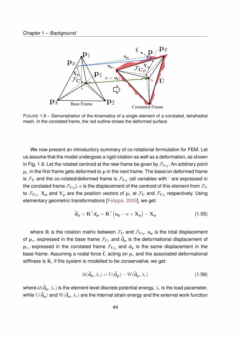
FIGURE 1.9 – Demonstration of the kinematics of a single element of a corotated, tetrahedralmesh. In the corotated frame, the red outline shows the deformed surface
fr
c = uC
upx
up
Xp
Yp
We now present an introductory summary of co-rotational formulation for FEM. Letus assume that the model undergoes a rigid rotation as well as a deformation, as shownin Fig. 1.9. Let the rotated centroid at the new frame be given by FCR
. An arbitrary pointpx in the first frame gets deformed to p in the next frame. The base/un-deformed frameis FC and the co-rotated/deformed frame is FCR
(all variables with · are expressed inthe corotated frame FCR
). c is the displacement of the centroid of this element from FC
to FCR. Xp and Yp are the position vectors of px at FC and FCR
respectively. Usingelementary geometric transformations [Felippa, 2000], we get:
dp = R>dp = R>(up − c + Xp
)−Xp (1.55)
where R is the rotation matrix between FC and FCR, up is the total displacement
of px, expressed in the base frame FC, and dp is the deformational displacement ofpx, expressed in the corotated frame FCR
and dp is the same displacement in thebase frame. Assuming a nodal force fr acting on px and the associated deformationalstiffness is K, if the system is modelled to be conservative, we get:
U(dp, λr) = U(dp)−W(dp, λr) (1.56)
where U(dp, λr) is the element-level discrete potential energy, λr is the load parameter,while U(dp) and W(dp, λr) are the internal strain energy and the external work function
44
1.3. Non-rigid Object Tracking
respectively. Differentiating Eqn. 1.56 w.r.t dp yields:
r = ∂U(dp, λr)∂dp
= ∂U∂dp
− ∂W∂dp
= f Ir − fr = 0 (1.57)
Clearly, f Ir is the vector of internal forces. This gives us the formulation for the residual
force vector r in the co-rotated frame. This leads to the formulation:
r = τ>r = f Ir − fr (1.58)
fr = τ>fr (1.59)
f Ir = τ>f I
r (1.60)
K = τ>Kτ + r ·Q (1.61)
where the matrix τ denotes the change of position of dp with up and the variationof the i-th vertex w.r.t the j-th vertex’s displacement is given by:
τij = ∂dpi∂upj
(1.62)
and:
Qijk = ∂2dpi∂upj∂upk
(1.63)
τ and Q forms the transformation array for this co-rotated configuration. When r = 0,we can write K = τ>Kτ .
Now, applying similar motion to the nodes of the tetrahedron, we can represent theinternal, elastic forces acting on the nodes by:
Fe = ReKeUR (1.64)
Here, UR = (p1, p2, p3, p4)12×1
, Ke12×12
is the stiffness matrix and Re12×12
is the block diago-
nal matrix of four R rotation matrices stacked diagonally. Fe12×1
is the elastic forces acting
on the nodes of this tetrahedral element.
To determine the interaction between forces and their resulting displacement usingthe FEM, we solve a second order differential equation, given by:
Mp + Dp + Kgp = Fext + Fe (1.65)
45
Chapter 1 – Background
where M and D are the model’s mass and damping matrices respectively. The ele-ments of M are given as :
Mij =∫
ΨφiφjdV (1.66)
where Mij denotes the element of M at the i-th row and j-th column, φi, φj is theshape function at the i-th and j-th vertex of VM respectively, V is the volume of thetetrahdron associated with i and j and Ψ is the domain of VM. In this thesis, we use aRayleigh style damping matrix D given by :
D = rMM + rKKg (1.67)
where rM and rK are the Rayleigh mass and Rayleigh stiffness respectively. Non-Rayleigh style damping matrices can be used as well [Pilkey, 1998]. Kg is the globalstiffness matrix. Fext are the external forces acting on the vertices.
Interested readers may refer to [Hughes, 2012] for a detailed treatment of standardFEM formulation.
1.3.1.1 Tracking using Physics-based Models
Using a triangular finite element method, [Agudo et al., 2017] proposes a methodto tackle deformation of planar objects using modal analysis using the shape basisof the modes of deformation. [Agudo et al., 2017] is based on the seminal work of[Bregler et al., 2000], which proposed a new method to recover 3D non-rigid shapemodels from image sequences by representing the 3D model as a combination of basisshapes. In [Agudo and M-Noguer, 2015] the elastic model of the object is estimated byapproximating the full force-field from a low-rank basis. This approach estimates theentire force field acting on all points of the considered object while estimating the elasticmodel of that object and the pose of the camera using an Expectation Maximization(EM) algorithm. [Agudo et al., 2014] uses modal analysis from continuum mechanicsto model the shape as discretized, linear elastic triangles and the solution to the forcebalance equations for an undamped free vibration model of the underlying FEM is usedto recover the shape of the deforming object. Using a slightly different approach, [Maltiand Herzet, 2017] proposes a new class of method, termed Sparse Linear Elastic -SfT (SLE-SfT), which replaces the `2-norm minimization of standard SfT approacheswith `0-norm for minimizing the cardinal of the non-zero components of the deforming
46
1.3. Non-rigid Object Tracking
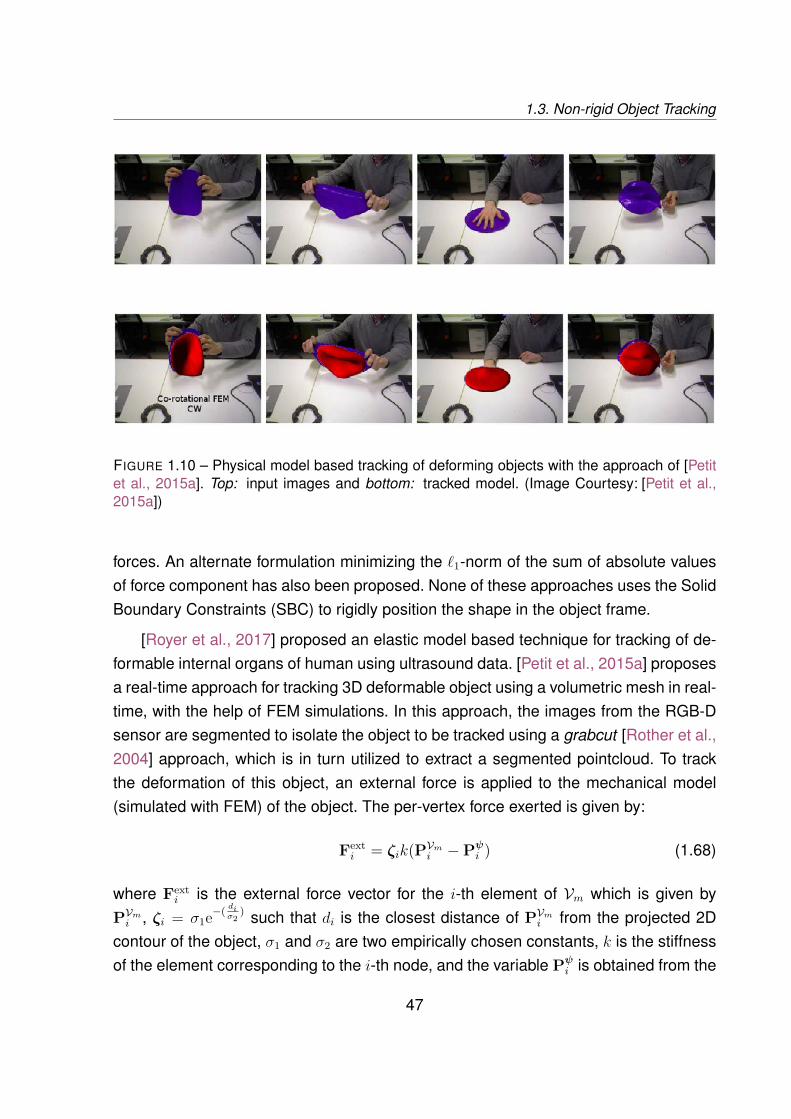
FIGURE 1.10 – Physical model based tracking of deforming objects with the approach of [Petitet al., 2015a]. Top: input images and bottom: tracked model. (Image Courtesy: [Petit et al.,2015a])
forces. An alternate formulation minimizing the `1-norm of the sum of absolute valuesof force component has also been proposed. None of these approaches uses the SolidBoundary Constraints (SBC) to rigidly position the shape in the object frame.
[Royer et al., 2017] proposed an elastic model based technique for tracking of de-formable internal organs of human using ultrasound data. [Petit et al., 2015a] proposesa real-time approach for tracking 3D deformable object using a volumetric mesh in real-time, with the help of FEM simulations. In this approach, the images from the RGB-Dsensor are segmented to isolate the object to be tracked using a grabcut [Rother et al.,2004] approach, which is in turn utilized to extract a segmented pointcloud. To trackthe deformation of this object, an external force is applied to the mechanical model(simulated with FEM) of the object. The per-vertex force exerted is given by:
Fexti = ζik(PVmi −Pψ
i ) (1.68)
where Fexti is the external force vector for the i-th element of Vm which is given by
PVmi , ζi = σ1e−( diσ2
) such that di is the closest distance of PVmi from the projected 2Dcontour of the object, σ1 and σ2 are two empirically chosen constants, k is the stiffnessof the element corresponding to the i-th node, and the variable Pψ
i is obtained from the
47

Chapter 1 – Background
segmented pointcloud ψ by the formulation:
Pψi =
αNNψ(PVmi ) + (1− α) 1
#ψi
∑Pj∈ψi
Pj if #ψi > 0
αNNψ(PVmi ) + (1− α)PVmi else(1.69)
where NNψ(PVmi ) denotes the nearest neighbor of PVmi in ψ, ψi is a subset of ψ suchthat ∀(ψi)j ∈ ψi there exists NNVm((ψi)j) = PVmi and α is a tunable parameter. Anexample of the tracking achieved by this approach is shown in Fig. 1.10. [Petit et al.,2015b] extends the same approach to track fractures in the deforming objects, whiletracking their deformation at the same time. Both these approaches use co-rotationalFEM as the mechanical model and simulates the full volumetric deformation of theobject to track deformation. [Petit et al., 2018] also extends this method to capturecollision among interacting objects while tracking their deformation simultaneously.
[Wang et al., 2015] proposes a method to capture deformation of soft objects usingco-rotational FEM, where the tracking is handled with a probabilistic approach. Givena set of points ψi ∈ ψ in a pointcloud, the problem statement is to fit a surface modelVs to the pointcloud to maximize the probability (represented by the function p(·)) ofvertex position, given the measurement of the pointcloud, such that:
Vs = arg maxVs
p(Vs|ψ) (1.70)
This maximum-aposteriori-estimation (MAP) problem is solved by regulating the ex-ternal force acting on the mechanical model Vm which is connected with the surfacemodel Vs in a scheme similar to [Petit et al., 2015a], as shown in Fig. 1.5. This external,virtual force is expressed as:
fj = η∑i
p(zji)σ−1j (Pψ
i −PVsj ) (1.71)
where η is a scaling factor, σj is the diagonalized co-variance matrix of Pψi and zji is a
latent variable that indicates if Pψi has any contribution towards PVsj or not. A graphical
outline of this approach is shown in Fig. 1.11.
It must be noted that [Wang et al., 2015] is an improved variant of the approachproposed in [Schulman et al., 2013] and most of the fundamental concepts of trackingpointclouds using virtual force is based on Schulman et. al. However, unlike [Schulman
48
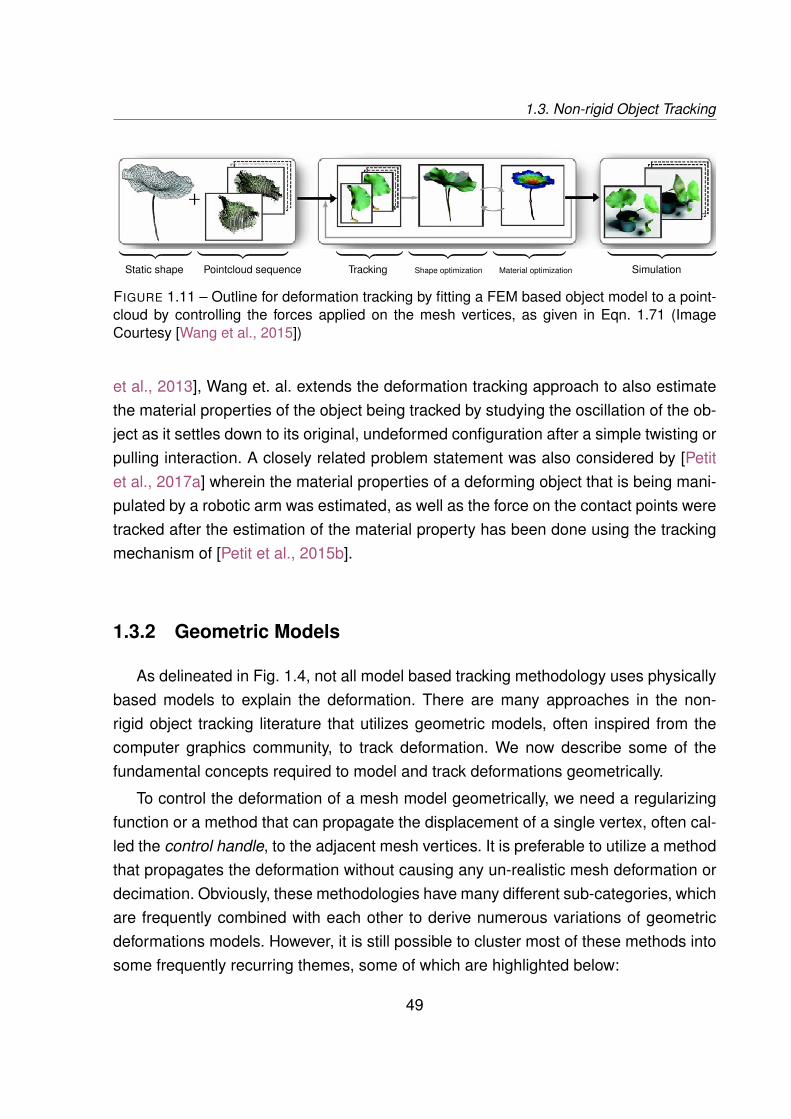
1.3. Non-rigid Object Tracking
︸ ︷︷ ︸Static shape
︸ ︷︷ ︸Pointcloud sequence
︸ ︷︷ ︸Tracking
︸ ︷︷ ︸Shape optimization
︸ ︷︷ ︸Material optimization
︸ ︷︷ ︸Simulation
FIGURE 1.11 – Outline for deformation tracking by fitting a FEM based object model to a point-cloud by controlling the forces applied on the mesh vertices, as given in Eqn. 1.71 (ImageCourtesy [Wang et al., 2015])
et al., 2013], Wang et. al. extends the deformation tracking approach to also estimatethe material properties of the object being tracked by studying the oscillation of the ob-ject as it settles down to its original, undeformed configuration after a simple twisting orpulling interaction. A closely related problem statement was also considered by [Petitet al., 2017a] wherein the material properties of a deforming object that is being mani-pulated by a robotic arm was estimated, as well as the force on the contact points weretracked after the estimation of the material property has been done using the trackingmechanism of [Petit et al., 2015b].
1.3.2 Geometric Models
As delineated in Fig. 1.4, not all model based tracking methodology uses physicallybased models to explain the deformation. There are many approaches in the non-rigid object tracking literature that utilizes geometric models, often inspired from thecomputer graphics community, to track deformation. We now describe some of thefundamental concepts required to model and track deformations geometrically.
To control the deformation of a mesh model geometrically, we need a regularizingfunction or a method that can propagate the displacement of a single vertex, often cal-led the control handle, to the adjacent mesh vertices. It is preferable to utilize a methodthat propagates the deformation without causing any un-realistic mesh deformation ordecimation. Obviously, these methodologies have many different sub-categories, whichare frequently combined with each other to derive numerous variations of geometricdeformations models. However, it is still possible to cluster most of these methods intosome frequently recurring themes, some of which are highlighted below:
49

Chapter 1 – Background
P1
P2P3P4
P′1
P′2
P′3
P′4
FIGURE 1.12 – Regularization of deformation using embedded deformation graphs
Embedded Deformation Graph
In this approach, the spatial deformation of an object is represented by a collectionof affine transformations organized in a graph structure. Each node of the graph hasa particular transformation associated with it and the deformation is propagated to thenearby space by a series of affine transforms, as explained below. Let a particular nodePi has the rotational matrix Ri and translation ti associated with it. This transformationis propagated to a node Pj (which is connected to Pi through a graph of undirectededges) to produce its deformed configuration P′j via the relationship:
P′j =n∑i=1
wi(Pj)(Ri(Pj −Pi) + Pi + ti
)(1.72)
where wi(Pj) is a weighting parameter. As shown in Fig. 1.12, with this deformationpropagation mechanism in place [Sumner et al., 2007], a set of rotational and regu-larizational constraints can be imposed on this graph structure to result in spatiallycoherent and smooth deformation when some controlled nodes are deformed arbitra-rily (either by user specified commands, or by minimization of some secondary errorterms).
Thin plate spline (TPS)
TPS warp presents an efficient shape interpolation and smoothing function forcontrolling or regularizing the deformation of non-rigid surfaces in 2D or 3D. In its sim-
50

1.3. Non-rigid Object Tracking
plest form, the 3D interpolation is given by:
P = a0 + a1XP + a2YP + a3ZP +N∑i=1
λiU(|| P−Pi ||
)(1.73)
where Pi = (XPi ,YPi ,ZPi) | i = 1, 2, · · · ,N
(1.74)
are the landmark points,a0, a1, a2, a3, λ1, · · ·, λN
are weighting coefficients and P =
(XP,YP,ZP) are the interpolated points. U(x) = x2 log(x2) is the radial basis function.
As-rigid-as-possible (ARAP) regularizer
Assuming that we have a triangular mesh V which gets deformed to a new configu-ration V ′, while two connected model vertices are denoted by Pi and Pj, ARAP [Bregleret al., 2000] proposes to regularize deformation by minimizing the energy term:
EARAP =n∑i=1
wi∑j∈XV
wij ||(P′i −P′j
)−R
(Pi −Pj
)||2 (1.75)
where wi and wij are suitable cell and edge weights, while R is the approximaterigid rotation matrix between V and V ′.
Coherent Point Drift (CPD)
In its simplest form, CPD [Myronenko and Song, 2010] offers a mechanism to aligntwo pointclouds with each other, irrespective of the nature of the transformation bet-ween them, i.e., it can be used to estimate both rigid and non-rigid transformations.Assuming that a set of target point cloud is denoted by
ψX = pxi | i = 1, · · ·,N
,
while ψ∗Y denotes the centroids of the Gaussian Mixture Model (GMM) of another setof source pointcloud
ψY = pyj | j = 1, · · ·,M
, CPD based alignment involves the
minimization of the following term:
ECPD = −N∑n=1
logM+1∑m=1
P(m)p(px | m) (1.76)
wherep(px | m) = 1
(2πσ2)e−||px−pym ||
2
2σ2 (1.77)
51
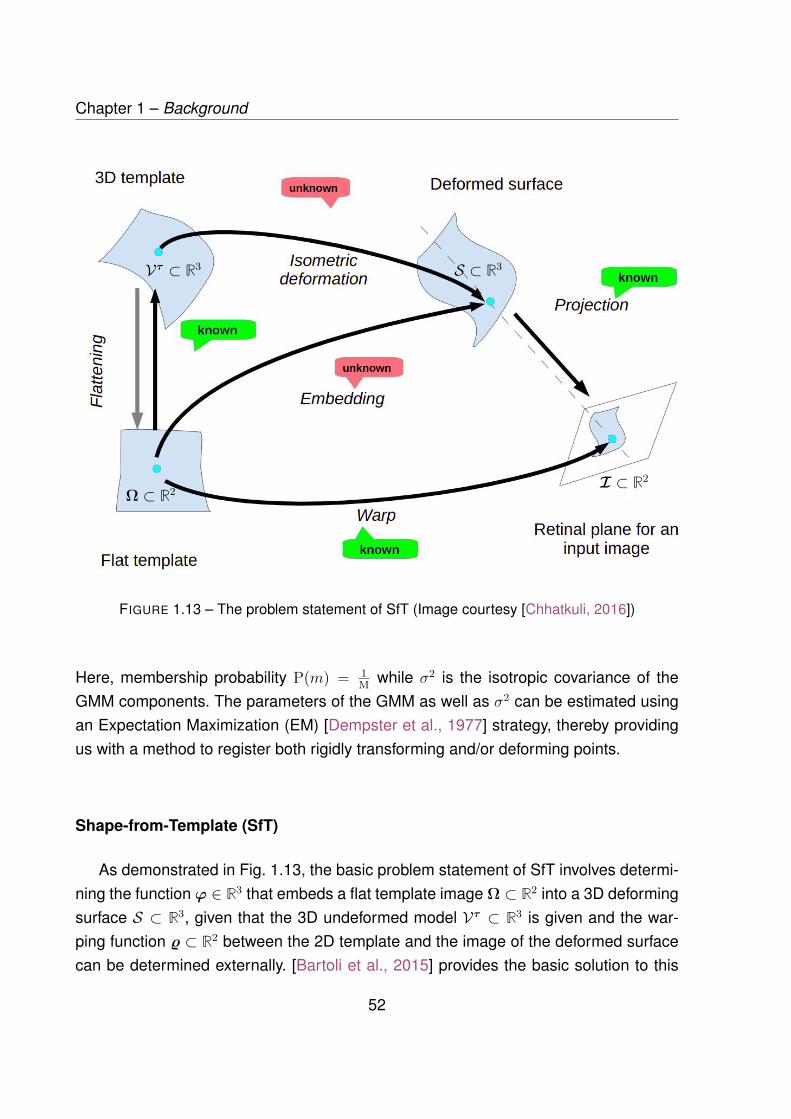
Chapter 1 – Background
FIGURE 1.13 – The problem statement of SfT (Image courtesy [Chhatkuli, 2016])
Vτ ⊂ R3
Ω ⊂ R2
S ⊂ R3
I ⊂ R2
Here, membership probability P(m) = 1M while σ2 is the isotropic covariance of the
GMM components. The parameters of the GMM as well as σ2 can be estimated usingan Expectation Maximization (EM) [Dempster et al., 1977] strategy, thereby providingus with a method to register both rigidly transforming and/or deforming points.
Shape-from-Template (SfT)
As demonstrated in Fig. 1.13, the basic problem statement of SfT involves determi-ning the function ϕ ∈ R3 that embeds a flat template image Ω ⊂ R2 into a 3D deformingsurface S ⊂ R3, given that the 3D undeformed model Vτ ⊂ R3 is given and the war-ping function % ⊂ R2 between the 2D template and the image of the deformed surfacecan be determined externally. [Bartoli et al., 2015] provides the basic solution to this
52
1.3. Non-rigid Object Tracking
problem. The embedding function can be represented as:
ϕ = χ ∆ (1.78)
where χ is the isometric deformation of Vτ and ∆ is the function that embeds Ω intoVτ . On such a system, two different constraints are imposed. The first constraint aimsto preserve the isometry, and is given by:
J>ϕJϕ = J>∆J∆ (1.79)
where Jϕ and J∆ are the Jacobians obtained by differentiating ϕ and ∆. The secondconstraint ensures the consistency between the warp and the projection of the embed-ding in the image Π, and is given by:
% = Π ϕ (1.80)
Eqn. 1.79 and eqn. 1.80 forms a system of partial differential equations and ananalytic solution for the unknown parameters has been established in [Bartoli et al.,2015]. Many variants of the standard SfT formulation exists in the literature and isbriefly reviewed in the following paragraph.
1.3.2.1 Tracking using Geometric Models
A method to detect and recover three dimensional shape from monocular videosequence was proposed in [Salzmann et al., 2007]. This approach creates a low di-mensional model of deformable, planar 3D surfaces and based on the assumption thatthe deformation is strictly isometric, a dimensionality reduction technique is used tothe deformation models needed for tracking and detection. [Pilet et al., 2008] provi-ded a method to detect and register non-rigid, planar surfaces based on wide-baselinepoint matches between the undeformed and deformed image of an object. [Salzmannet al., 2008] offers a closed form solution to the problem of recovering 3D shape fromnon-rigid, elastic 3D-to-2D correspondences. The set of 3D-to-2D correspondencesconstitutes a linear system, which can also be expressed as a weighted sum of ei-gen vectors, the solution of which accounts for the inextensibility constraints betweenneighboring mesh vertices.
[Bartoli et al., 2015] proposes a first-order method using both image point loca-
53
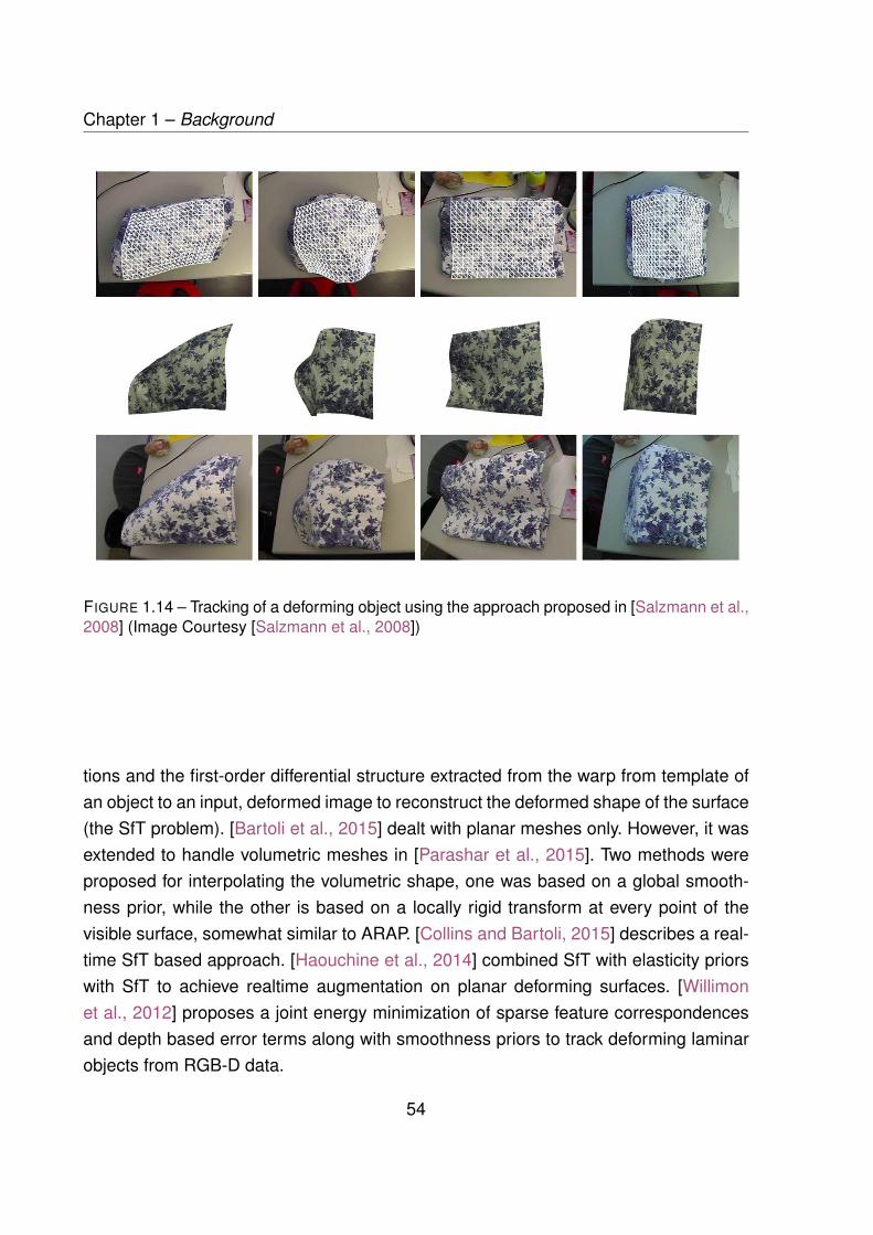
Chapter 1 – Background
FIGURE 1.14 – Tracking of a deforming object using the approach proposed in [Salzmann et al.,2008] (Image Courtesy [Salzmann et al., 2008])
tions and the first-order differential structure extracted from the warp from template ofan object to an input, deformed image to reconstruct the deformed shape of the surface(the SfT problem). [Bartoli et al., 2015] dealt with planar meshes only. However, it wasextended to handle volumetric meshes in [Parashar et al., 2015]. Two methods wereproposed for interpolating the volumetric shape, one was based on a global smooth-ness prior, while the other is based on a locally rigid transform at every point of thevisible surface, somewhat similar to ARAP. [Collins and Bartoli, 2015] describes a real-time SfT based approach. [Haouchine et al., 2014] combined SfT with elasticity priorswith SfT to achieve realtime augmentation on planar deforming surfaces. [Willimonet al., 2012] proposes a joint energy minimization of sparse feature correspondencesand depth based error terms along with smoothness priors to track deforming laminarobjects from RGB-D data.
54
1.3. Non-rigid Object Tracking
1.3.3 Non-rigid Tracking and Reconstruction
Model free tracking of deformation involves tracking the surface of the deformingobject as well as iteratively generative the mesh model of the entire surface of theobject or scene under consideration. Many of the fundamentals used for geometricmodel-based tracking are re-utilized for reconstruction and tracking as well. Trackingand reconstruction of non-rigid objects using RGB-D cameras have been developed inrecent years. [Zollhöfer et al., 2014] tracked a deformable template in real-time, withouthaving any limitations about apriori knowledge of the template. It must be noted thatthis research is entirely based on the output of a stereo rig and not from a depth ca-mera. The approach works by minimizing the global rigid transformation as well as theper-vertex displacement between consecutive frames. This is done by minimizing fourerror terms: a point-to-point distance, a point-to-plane distance, direct color intensitydifference and a geometric prior term acting as the ARAP regularizer.
Frame 3: Truncated Signed Distance Field (TSDF)
TSDF and Signed Distance Function (SDF) has been used extensively in rigid and non-rigid reconstruction from depth sensors in the recent years, including [Newcombe et al.,2011], [Izadi et al., 2011], [Newcombe et al., 2015], [Slavcheva et al., 2016], [Slavchevaet al., 2017a] and [Slavcheva et al., 2018], among many others. The TSDF algorithmprovides a simple method to reconstruct rigid scene from multiple depth scans (usingany depth sensor) and it is possible to modify the TSDF algorithm to effectively re-construct non-rigid scenes too. Given its efficacy and popularity, it can be useful totake a closer look at the TSDF methodology for the sake of completeness. TSDF wasintroduced for rigid object reconstruction by [Newcombe et al., 2011] and [Izadi et al.,2011]. However, the principle of TSDF is heavily based on SDF, introduced by [Curlessand Levoy, 1996]. SDF is a voxel based implicit representation of a scene, where eachvoxel is associated with a function measuring the distance of the voxel from the nearestsurface.
55
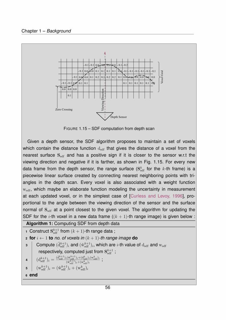
Chapter 1 – Background
FIGURE 1.15 – SDF computation from depth scan
Given a depth sensor, the SDF algorithm proposes to maintain a set of voxelswhich contain the distance function dsdf that gives the distance of a voxel from thenearest surface Ssdf and has a positive sign if it is closer to the sensor w.r.t theviewing direction and negative if it is farther, as shown in Fig. 1.15. For every newdata frame from the depth sensor, the range surface (Sksdf for the k-th frame) is apiecewise linear surface created by connecting nearest neighboring points with tri-angles in the depth scan. Every voxel is also associated with a weight functionwsdf , which maybe an elaborate function modeling the uncertainty in measurementat each updated voxel, or in the simplest case of [Curless and Levoy, 1996], pro-portional to the angle between the viewing direction of the sensor and the surfacenormal of Ssdf at a point closest to the given voxel. The algorithm for updating theSDF for the i-th voxel in a new data frame ((k + 1)-th range image) is given below :
Algorithm 1: Computing SDF from depth data
1 Construct Sk+1sdf from (k + 1)-th range data ;
2 for i← 1 to no. of voxels in (k + 1)-th range image do3 Compute (dk+1
sdf )i and (wk+1sdf )i, which are i-th value of dsdf and wsdf
respectively, computed just from Sk+1sdf ;
4 (dk+1sdf )i = (dk+1
sdf )i(wk+1sdf )i+(dksdf)i(w
ksdf)i
(wk+1sdf )i+(wksdf)i
;
5 (wk+1sdf )i = (wk+1
sdf )i + (wksdf)i
6 end
56

1.3. Non-rigid Object Tracking
[Izadi et al., 2011] modified the method of Algorithm 1 to store the SDF only for atruncated region around the actual surface, resulting in the TSDF value dtsdf , given by :
(dk+1tsdf )i =
min(1, (dk+1
sdf )iσmax
)If (dk+1
sdf )i > 0
max(− 1, (dk+1
sdf )iσmin
)else
(1.81)
where σmax and σmin are the maximum and minimum truncation depth required by thealgorithm. An example of surface reconstruction from 3 consecutive RGB-D frames(captured at 30 fps) using this TSDF methodology is demonstrated in Fig. 1.16.
FIGURE 1.16 – Example of rigid reconstruction using TSDF methodology (similar to [Izadi et al.,2011]) for 3 consecutive frames coming from a RGB-D camera, as shown in (a). The TSDF vo-lume is computed and the isosurface is extracted using the Marching Cubes method [Lorensenand Cline, 1987] with a truncation distance of 5mm, 1cm and 1m for (b), (c) and (d) respectively
σmin, σmax = ±5mm σmin, σmax = ±1cm σmin, σmax = ±1m
DynamicFusion [Newcombe et al., 2015] extended the premise of KinectFusion intonon-rigid objects. It enabled the tracking and modeling of deformable objects on the go,without using a previously known template. In DynamicFusion, the objective is split intothree steps, estimating the warping function of the current depth frame from the cano-nical model, fusion of the live depth frame into the canonical model once the warpingfunction has been determined and adaption of the warp field structure to track thecamera movement using ICP. The non-rigid warp field is represented as a 6D transfor-mation in SE3, but to avoid memory overhead, this 6D transformation is kept sparse,while all the dense points in between are interpolated using a weighted blending ofdual quaternion. The weight alters the radius of influence of each transformation node.Fusion between the current depth frame and the canonical model is done using theTSDF fusion technique. The warp field is estimated by minimizing an energy functioncomprising of a data term, which is the dense model-to-frame ICP cost, and a regula-
57
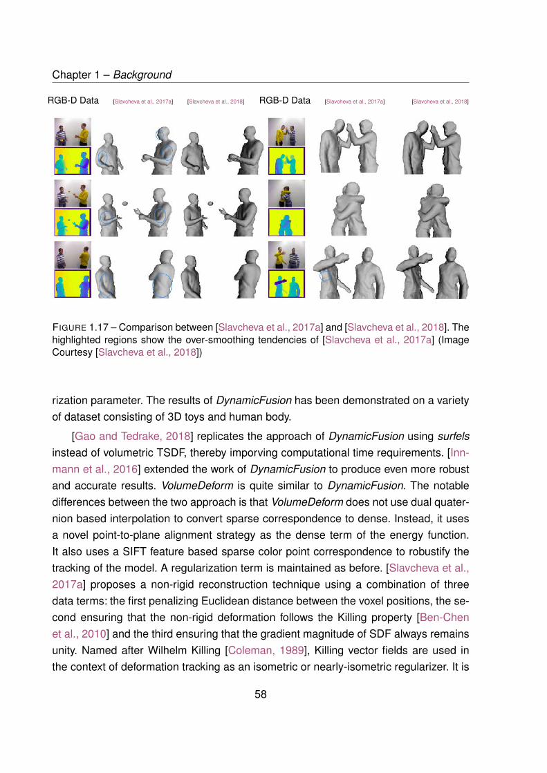
Chapter 1 – Background
FIGURE 1.17 – Comparison between [Slavcheva et al., 2017a] and [Slavcheva et al., 2018]. Thehighlighted regions show the over-smoothing tendencies of [Slavcheva et al., 2017a] (ImageCourtesy [Slavcheva et al., 2018])
RGB-D Data [Slavcheva et al., 2017a] [Slavcheva et al., 2018] RGB-D Data [Slavcheva et al., 2017a] [Slavcheva et al., 2018]
rization parameter. The results of DynamicFusion has been demonstrated on a varietyof dataset consisting of 3D toys and human body.
[Gao and Tedrake, 2018] replicates the approach of DynamicFusion using surfelsinstead of volumetric TSDF, thereby imporving computational time requirements. [Inn-mann et al., 2016] extended the work of DynamicFusion to produce even more robustand accurate results. VolumeDeform is quite similar to DynamicFusion. The notabledifferences between the two approach is that VolumeDeform does not use dual quater-nion based interpolation to convert sparse correspondence to dense. Instead, it usesa novel point-to-plane alignment strategy as the dense term of the energy function.It also uses a SIFT feature based sparse color point correspondence to robustify thetracking of the model. A regularization term is maintained as before. [Slavcheva et al.,2017a] proposes a non-rigid reconstruction technique using a combination of threedata terms: the first penalizing Euclidean distance between the voxel positions, the se-cond ensuring that the non-rigid deformation follows the Killing property [Ben-Chenet al., 2010] and the third ensuring that the gradient magnitude of SDF always remainsunity. Named after Wilhelm Killing [Coleman, 1989], Killing vector fields are used inthe context of deformation tracking as an isometric or nearly-isometric regularizer. It is
58
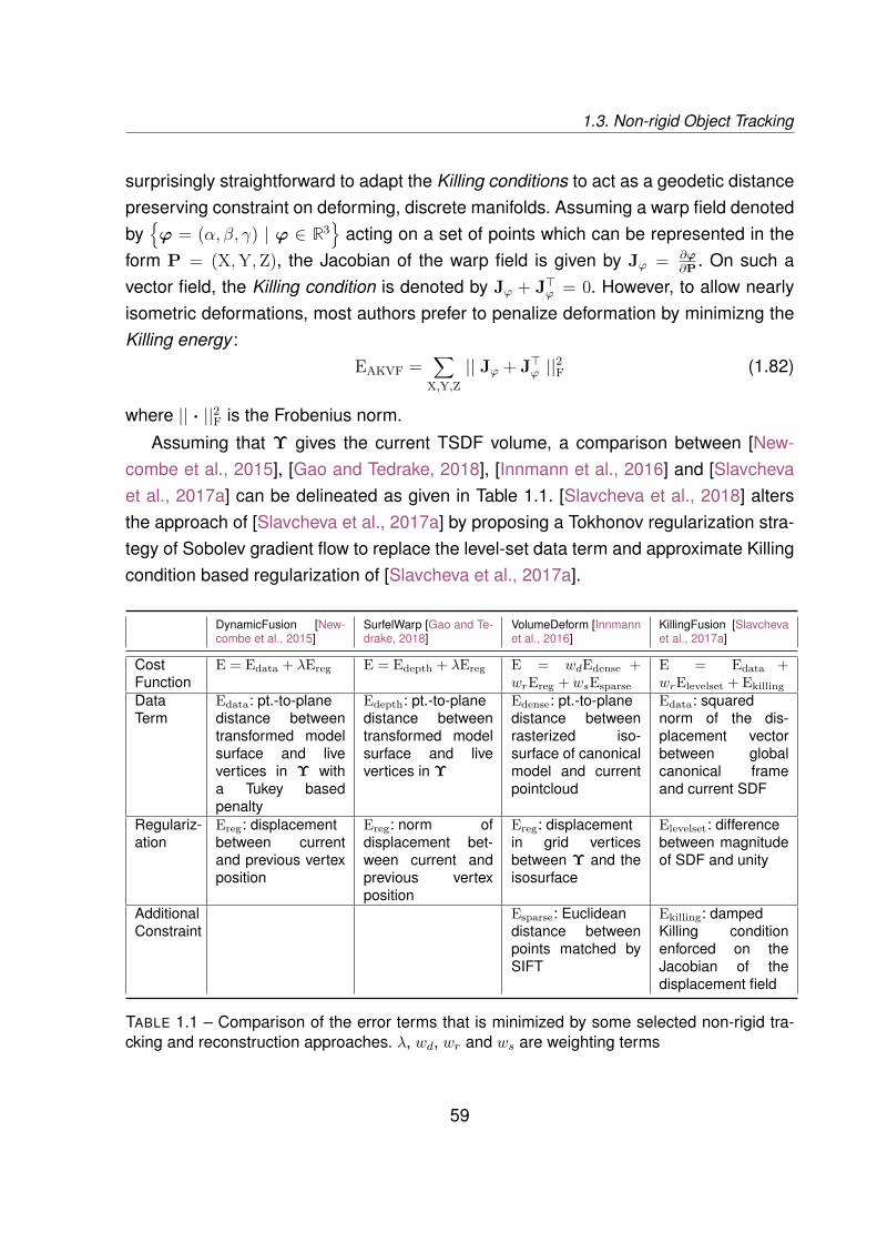
1.3. Non-rigid Object Tracking
surprisingly straightforward to adapt the Killing conditions to act as a geodetic distancepreserving constraint on deforming, discrete manifolds. Assuming a warp field denotedby
ϕ = (α, β, γ) | ϕ ∈ R3
acting on a set of points which can be represented in the
form P = (X,Y,Z), the Jacobian of the warp field is given by Jϕ = ∂ϕ∂P . On such a
vector field, the Killing condition is denoted by Jϕ + J>ϕ = 0. However, to allow nearlyisometric deformations, most authors prefer to penalize deformation by minimizng theKilling energy :
EAKVF =∑
X,Y,Z|| Jϕ + J>ϕ ||2F (1.82)
where || · ||2F is the Frobenius norm.
Assuming that Υ gives the current TSDF volume, a comparison between [New-combe et al., 2015], [Gao and Tedrake, 2018], [Innmann et al., 2016] and [Slavchevaet al., 2017a] can be delineated as given in Table 1.1. [Slavcheva et al., 2018] altersthe approach of [Slavcheva et al., 2017a] by proposing a Tokhonov regularization stra-tegy of Sobolev gradient flow to replace the level-set data term and approximate Killingcondition based regularization of [Slavcheva et al., 2017a].
DynamicFusion [New-combe et al., 2015]
SurfelWarp [Gao and Te-drake, 2018]
VolumeDeform [Innmannet al., 2016]
KillingFusion [Slavchevaet al., 2017a]
CostFunction
E = Edata + λEreg E = Edepth + λEreg E = wdEdense +wrEreg + wsEsparse
E = Edata +wrElevelset + Ekilling
DataTerm
Edata: pt.-to-planedistance betweentransformed modelsurface and livevertices in Υ witha Tukey basedpenalty
Edepth: pt.-to-planedistance betweentransformed modelsurface and livevertices in Υ
Edense: pt.-to-planedistance betweenrasterized iso-surface of canonicalmodel and currentpointcloud
Edata: squarednorm of the dis-placement vectorbetween globalcanonical frameand current SDF
Regulariz-ation
Ereg: displacementbetween currentand previous vertexposition
Ereg: norm ofdisplacement bet-ween current andprevious vertexposition
Ereg: displacementin grid verticesbetween Υ and theisosurface
Elevelset: differencebetween magnitudeof SDF and unity
AdditionalConstraint
Esparse: Euclideandistance betweenpoints matched bySIFT
Ekilling: dampedKilling conditionenforced on theJacobian of thedisplacement field
TABLE 1.1 – Comparison of the error terms that is minimized by some selected non-rigid tra-cking and reconstruction approaches. λ, wd, wr and ws are weighting terms
59

Chapter 1 – Background
1.3.4 Non-Rigid Structure from Motion (NR-SfM)
NR-SfM is an excellent technique to resolve the shape of a deforming object alongwith camera motion parameters. It is inherently a batch technique, requiring sequentialobservation of deforming keypoints on the object. This makes it somewhat unsuitablefor sequential, fast tracking of deforming surfaces. However, for the sake of comple-teness, we take a brief look at some of the notable approaches developed from thistechnique.
Let the shape of a non-rigid object be described by a set of K keyframe basis,denoted by Si
3×Pdenoting P points. The overall shape can be described using:
S =K∑i=1
li · Si | li ∈ R (1.83)
Under scaled orthographic projection, the basis set can be used to express theimage coordinates (ui, vi) of the keypoints as:
u1 · · · uP
v1 · · · vP
=[l1R[2] · · · lKR[2]
]
S1
···
SK
(1.84)
where R[2] gives the first two rows of the camera rotation matrix. Assuming we haveL data frames for the sequence, we can re-arrange Eqn. 1.3.4 as:
ς2L×P
=
u11 · · · u1
P
v11 · · · v1
P
· · · · ·uL
1 · · · uLP
vL1 · · · vL
P
=
l11R1[2] · · · l1KR1
[2]
· · · · ·· · · · ·· · · · ·
lL1 RL[2] · · · lLKRL
[2]
︸ ︷︷ ︸
Q2L×3K
S1
···
SK
︸ ︷︷ ︸
Sl3K×P
(1.85)
ς is termed as the tracking matrix and can be formed by observing a set of keypointsacross multiple frames (e.g: using a feature detector/matching technique). Applying a
60

1.4. Positioning this Thesis
FIGURE 1.18 – Results from applying NR-SfM using the approach of [Kumar et al., 2016]. Thetop row shows the input images, while the row at the bottom shows the extracted meshes.(Image Courtesy [Kumar et al., 2016])
SVD decomposition on ς, we get SVD: ς = UΣV> = QSl. Solving this equation, therotational pose of camera R and shape configuration S can be factored simultaneously.
[Gotardo and Martinez, 2011a] proposed a kernel trick to better constraint the wea-kened low rank constraint, without requiring additional basis shapes to model keypointsmoving along curved paths. [Gotardo and Martinez, 2011b] improved the standard NR-SfM representation by considering K complementary spaces of rank 3 as the 3D basisshapes for factorization. [Kumar et al., 2016] extends NR-SfM to multibody deformationtracking using a subspace clustering approach (Fig. 1.18).
1.4 Positioning this Thesis
Having provided an overview of the existing state-of-the-art for deformation tracking,we now discuss the aim of this thesis and compare our contribution with the availableliterature from an application perspective. Before we begin discussing the technical de-tails in the subsequent chapters, it is important to justify the approach that we utilize totrack deforming objects. It is important to weigh the relative advantages and disadvan-tages of the state-of-the-art approaches in the context of this thesis.
The prominent research approaches presented in Sec. 1.3.1 through Sec. 1.3.4can be grouped on the basis of the input data, as shown in Table 1.2. We discard the
61
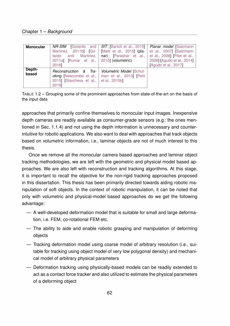
Chapter 1 – Background
Monocular NR-SfM [Gotardo andMartinez, 2011b] [Go-tardo and Martinez,2011a] [Kumar et al.,2016]
SfT : [Bartoli et al., 2015][Malti et al., 2015] (pla-nar) ; [Parashar et al.,2015] (volumetric)
Planar model [Salzmannet al., 2007] [Salzmannet al., 2008] [Pilet et al.,2008] [Agudo et al., 2014][Agudo et al., 2017]
Depth-based
Reconstruction & Tra-cking [Newcombe et al.,2015] [Slavcheva et al.,2018]
Volumetric Model [Schul-man et al., 2013] [Petitet al., 2015b]
TABLE 1.2 – Grouping some of the prominent approaches from state-of-the-art on the basis ofthe input data
approaches that primarily confine themselves to monocular input images. Inexpensivedepth cameras are readily available as consumer-grade sensors (e.g.: the ones men-tioned in Sec. 1.1.4) and not using the depth information is unnecessary and counter-intuitive for robotic applications. We also want to deal with approaches that track objectsbased on volumetric information, i.e., laminar objects are not of much interest to thisthesis.
Once we remove all the monocular camera based approaches and laminar objecttracking methodologies, we are left with the geometric and physical model based ap-proaches. We are also left with reconstruction and tracking algorithms. At this stage,it is important to recall the objective for the non-rigid tracking approaches proposedin this dissertation. This thesis has been primarily directed towards aiding robotic ma-nipulation of soft objects. In the context of robotic manipulation, it can be noted thatonly with volumetric and physical-model based approaches do we get the followingadvantage:
— A well-developed deformation model that is suitable for small and large deforma-tion, i.e. FEM, co-rotational FEM etc.
— The ability to aide and enable robotic grasping and manipulation of deformingobjects
— Tracking deformation model using coarse model of arbitrary resolution (i.e., sui-table for tracking using object model of very low polygonal density) and mechani-cal model of arbitrary physical parameters
— Deformation tracking using physically-based models can be readily extended toact as a contact force tracker and also utilized to estimate the physical parametersof a deforming object
62

1.5. Conclusion
Given these strong advantages, we dedicate the rest of this dissertation to the studyof deformation tracking using physically-based models.
1.5 Conclusion
In Sec. 1.1 of this chapter, we presented a summary of classical techniques invol-ving visual tracking of rigid objects and physical modelling of deforming objects usingstandard and co-rotational FEM. In this thesis, a combination of these two paradigmsare going to be used to design a set of methodologies that enable the tracking of de-forming objects.
In Sec. 1.3 of this chapter, we discuss the state-of-the-art for non-rigid object tra-cking using visual information. Only a small subset of these approaches involve phy-sical models for deformation tracking. We consider volumetric physical model baseddeformation tracking as the most relevant framework, since it enables us to achievethe following objectives (some of which has already been implemented while somewhich remains a future work [ marked with a * ]):
— Accurate and fast 3D tracking of deforming surface, with and without the know-ledge of the physical parameters (Young’s modulus, Poisson’s ratio etc.). Pre-sence of advanced physical model enables us to track large deformations
— Extending the 3D tracking framework to either track external, applied forces onthe object or to estimate the physical parameters of the object
— Tracking multi-object collision and non-isometric deformations (cutting, tearing,fracturing etc.) of the object *
— Providing a deformation model that can be used to predict the future state of adeforming object when force is applied on it - which can have significant utilitiesin the area of robotic manipulation of compliant objects
Chapter 2 provides a framework for tracking of rigid objects, which is an essentialinitial step for subsequent non-rigid tracking. Chapter 3 details the first methodologydeveloped to track deforming object using depth data only. This is followed by Chapter4, which improves the approach of Chapter 3 to utilize both depth and photometric datasimultaneously, while the tracking methodology evolves to become faster and morerobust. Chapter 5 describes a robotic application of the approach developed in Chapter3 involving estimation of physical parameters of objects and visual force tracking.
63

CHAPTER 2
RIGID OBJECT TRACKING
In the previous chapter, we introduced some of the existing literature on non-rigidobject tracking and discussed some of the fundamental concepts about deformationmodelling and tracking. Multiple real-time non-rigid tracking approaches, e.g., [Petitet al., 2018], uses two separate methods for non-rigid object tracking. One that approxi-mately tracks the object rigidly, and another that tracks the deformation independentlyfrom the rigid motion. This is especially useful for the physical model based deforma-tion tracking that we intend to do for this thesis. To this end, in this chapter we present amethod to track rigid motion in objects with complex shapes using approximate 3D mo-dels of those objects. This is entirely based on RGB-D sensors. The key contributionsof this chapter are:
— Combining point-to-plane distance minimization and photometry for tracking ofcomplex objects using coarse model ;
— Using the concept of ‘keyframe’ in object tracking for increased robustness ;
— Accurate tracking of objects with inaccurate and coarse object models.
In this thesis, a coarse model implies a 3D, surface based model of an object withouthigh density of vertices (approximately < 6800 vertices/m2 on the surface of the mesh)and with relatively higher registration error (∼ ±2cm in the worst cases) with the object.
2.1 Background
Although a brief summary of research about rigid object tracking was already pro-vided in Sec. 1.2.2, it is worthwhile to look into some more state-of-the-art researchrelated to rigid object tracking in the context of this chapter specifically. Research re-lated to localizing and/or tracking simple geometric shapes is extensive [Lepetit et al.,2005] and has been studied since a long time [Armstrong and Zisserman, 1995]. Someapproaches use probabilistic models for tracking shapes. [Prisacariu and Reid, 2012]
65
Chapter 2 – Rigid Object Tracking
aims to maximize the discrimination between background and foreground of a scenewhile simultaneously tracking the 6DoF pose of an object with known 3D model. Thismethod used only RGB images as input. [Teichman et al., 2013] extended this me-thod to depth cameras, adding more cues like local image appearance, depth dis-continuities, optical flow, and surface normal to inform the segmentation decision ina conditional random field model. Similar approaches have been used to track arti-culated objects [Cifuentes et al., 2017] with remarkable precision, but the tracking ofarticulated joints remain beyond the scope of our discussion. Particle filtering basedapproaches have been parallelized using GPU and implemented towards tracking rigidobjects [Choi and Christensen, 2013]. The second group of algorithms uses learning-based techniques to track objects. [Hinterstoisser et al., 2012] proposes a pose esti-mation technique for complex objects under heavy clutter, but the training model needscolor gradient information. In our method, however, we assume that the object’s ac-curate model and any model based on color / texture are not available. [Doumano-glou et al., 2016], [Michel et al., 2017] and [Xiang et al., 2018] propose increasinglyaccurate posing estimation techniques, but they can not be considered real-time. [Mc-Cormac et al., 2018] and [Runz et al., 2018] are both a dynamic SLAM algorithm thatuses R-CNN Mask for segmentation and performs object tracking as a by-product. Theaccuracy of the per frame object tracking has not been evaluated explicitly. The thirdgroup of algorithms use well known minimization techniques to track objects usinggeometric and photometric constraints. [Pomerleau et al., 2015] has already been in-troduced in Sec. 1.2 as an excellent summary of classical ICP. Many variants of ICPhave been proposed for probabilistic [Segal et al., 2009] implementation of point setregistration. In this context, SLAM and object tracking have been tackled interchangea-bly by some authors [Salas-Moreno et al., 2013]. CoFusion [Rünz and Agapito, 2017]is a dynamic SLAM system that uses a combination of dense ICP and photometricerror minimization between the model and the current frame to track objects. The ap-proach we propose, in terms of the framework for object tracking, is somewhat closerto CoFusion [Rünz and Agapito, 2017]. However, we do not undertake explicit motionsegmentation, we are not interested in reconstruction and we use the concept of key-frames. Moreover, the presence of coarse object model makes it a different problemstatement altogether.
In this chapter we focus on the high-accuracy tracking of rigid, complex shapeswith approximately known geometry using depth cameras. We consider the coarse
66

2.2. Method
model to be a highly decimated, minimal representation of the object model (insteadof a high-resolution and detailed CAD model), containing very few triangular facesat best. The model does not contain any color or textural information. This is easyto generate and can also be rendered without a depth scanner (e.g: using manualmeasurements), making it suitable for various industrial applications. Our approach issignificantly robust to measurement errors in the coarse model. We are interested intracking all the 6 degrees of freedom [Yilmaz et al., 2006] of the object. The proposedapproach is validated both quantitatively and qualitatively in the subsequent sections.
2.2 Method
The approach proposed here to track rigid objects is a combination of point-to-plane distance minimization and photometric error minimization between frames. Wework with two types of input data: 1) registered and calibrated depth and grayscaleimages from the depth camera, and 2) simulated data of 3D points along with theircorresponding grayscale values.
We denote the depth data (obtained from the sensor in the RGB-D format) as:
ψ =(
(P1, c1), · · · , (PN , cN))
(2.1)
where Pi = (Xi,Yi,Zi) and ci is the intensity value of the point Pi, expressed in thecamera centered coordinate frame. A function Π(·) acts upon a 3D point and projects itto an image plane using the pinhole camera model such that pi = Π(Pi). The functionci = I(pi) provides the image intensity of the point pi. ∇I i,x and ∇I i,y gives thegradient of the image along x and y axis.
The model of the object is also presumed to be known for the purpose of tracking.We represent it as a surface 3D mesh composed of a set of planes given by OV ,XV
and nj = (nXj , nYj , nZj ) is the normal to the j-th plane of the mesh which lies at a per-pendicular distance of dj from the origin of the camera-centered coordinate frame.
The n-th frame from the depth sensor (or from a simulated data) is denoted byCn, while certain frames get tagged as keyframes Cn ⇒ CK
n . Fo denotes the objectcentered coordinate frame. These keyframes serve as the reference for photometrictracking and is explained in details in Sec. 2.2.3.
67
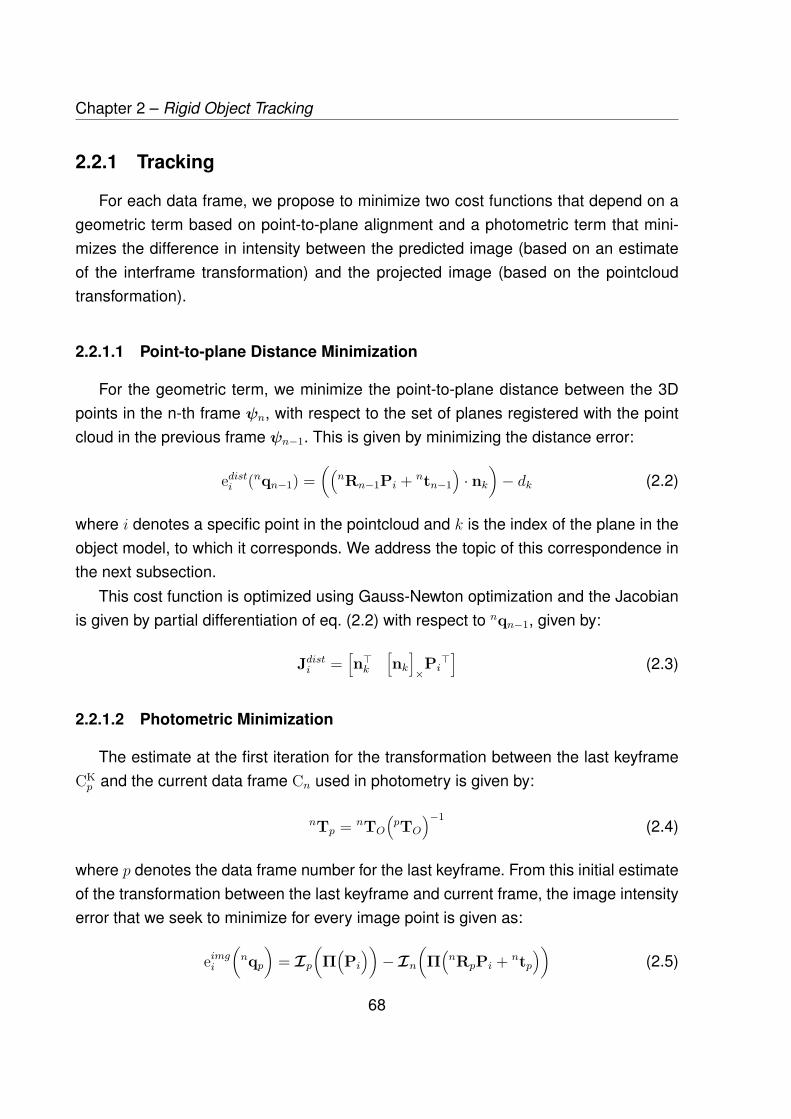
Chapter 2 – Rigid Object Tracking
2.2.1 Tracking
For each data frame, we propose to minimize two cost functions that depend on ageometric term based on point-to-plane alignment and a photometric term that mini-mizes the difference in intensity between the predicted image (based on an estimateof the interframe transformation) and the projected image (based on the pointcloudtransformation).
2.2.1.1 Point-to-plane Distance Minimization
For the geometric term, we minimize the point-to-plane distance between the 3Dpoints in the n-th frame ψn, with respect to the set of planes registered with the pointcloud in the previous frame ψn−1. This is given by minimizing the distance error:
edisti (nqn−1) =((
nRn−1Pi + ntn−1)· nk
)− dk (2.2)
where i denotes a specific point in the pointcloud and k is the index of the plane in theobject model, to which it corresponds. We address the topic of this correspondence inthe next subsection.
This cost function is optimized using Gauss-Newton optimization and the Jacobianis given by partial differentiation of eq. (2.2) with respect to nqn−1, given by:
Jdisti =[n>k
[nk]×Pi>]
(2.3)
2.2.1.2 Photometric Minimization
The estimate at the first iteration for the transformation between the last keyframeCKp and the current data frame Cn used in photometry is given by:
nTp = nTO
(pTO
)−1(2.4)
where p denotes the data frame number for the last keyframe. From this initial estimateof the transformation between the last keyframe and current frame, the image intensityerror that we seek to minimize for every image point is given as:
eimgi
(nqp
)= Ip
(Π(Pi
))− In
(Π(nRpPi + ntp
))(2.5)
68

2.2. Method
m-th frame m+ 1-th frame
Jdisttx Jdistty Jdisttz Jdistθux Jdistθuy Jdistθuz
Jimgtx Jimgty Jimgtz Jimgθux Jimgθuy Jimgθuz
FIGURE 2.1 – Jacobian of depth and photometric error between two data frames m and m+ 1.Jdist and Jimg are the gradient of the geometric and photometric error respectively, while thesuffix tx, ty, tz, θux, θuy, θuz represents the component of the gradient along the 6 dimensionsof the (t, θu) vector (the gradient intensities have been thresholded for visualization)
The Jacobian used for this minimization is:
Jimgi[1×6]
= ∇I i[1×2]
fx 00 fy
︸ ︷︷ ︸
[2×2]
− 1Z
0 XZ2
XYZ2 −(1 + X2
Z2 ) YZ
0 − 1Z
YZ2 −(1 + Y 2
Z2 ) −XYZ2 −X
Z
︸ ︷︷ ︸
[2×6]
(2.6)
where∇I i =
[∇I i,x ∇I i,y
](2.7)
and fx and fy are the focal lengths. The value of the Jacobians expressed in eq. 2.3and eq. 2.6 can be projected on the image plane and visualized, as shown in Fig. 2.1.
2.2.1.3 Optimization
Having computed the error and the Jacobian matrices for the two different types oferror function, we now describe the method used for computing the pose update that
69
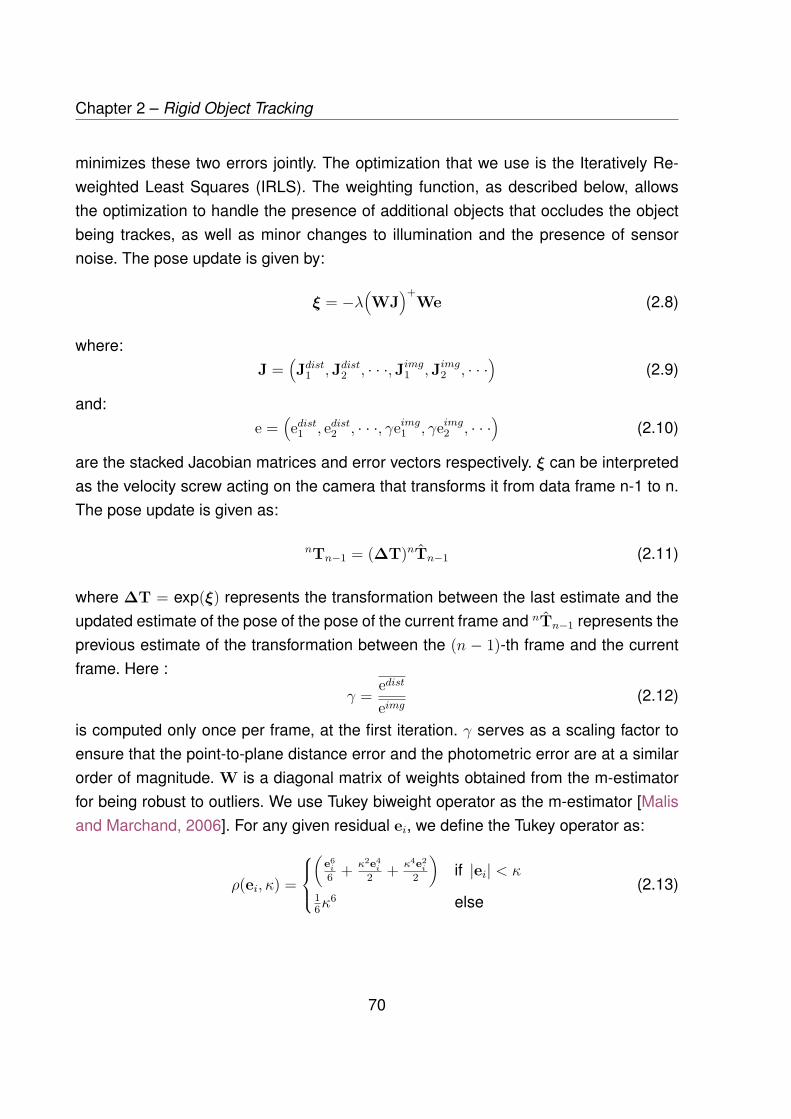
Chapter 2 – Rigid Object Tracking
minimizes these two errors jointly. The optimization that we use is the Iteratively Re-weighted Least Squares (IRLS). The weighting function, as described below, allowsthe optimization to handle the presence of additional objects that occludes the objectbeing trackes, as well as minor changes to illumination and the presence of sensornoise. The pose update is given by:
ξ = −λ(WJ
)+We (2.8)
where:J =
(Jdist1 ,Jdist2 , · · ·,Jimg1 ,Jimg2 , · · ·
)(2.9)
and:e =
(edist1 , edist2 , · · ·, γeimg1 , γeimg2 , · · ·
)(2.10)
are the stacked Jacobian matrices and error vectors respectively. ξ can be interpretedas the velocity screw acting on the camera that transforms it from data frame n-1 to n.The pose update is given as:
nTn−1 = (∆T)nTn−1 (2.11)
where ∆T = exp(ξ) represents the transformation between the last estimate and theupdated estimate of the pose of the pose of the current frame and nTn−1 represents theprevious estimate of the transformation between the (n − 1)-th frame and the currentframe. Here :
γ = edisteimg
(2.12)
is computed only once per frame, at the first iteration. γ serves as a scaling factor toensure that the point-to-plane distance error and the photometric error are at a similarorder of magnitude. W is a diagonal matrix of weights obtained from the m-estimatorfor being robust to outliers. We use Tukey biweight operator as the m-estimator [Malisand Marchand, 2006]. For any given residual ei, we define the Tukey operator as:
ρ(ei, κ) =
(
e6i
6 + κ2e4i
2 + κ4e2i
2
)if |ei| < κ
16κ
6 else(2.13)
70
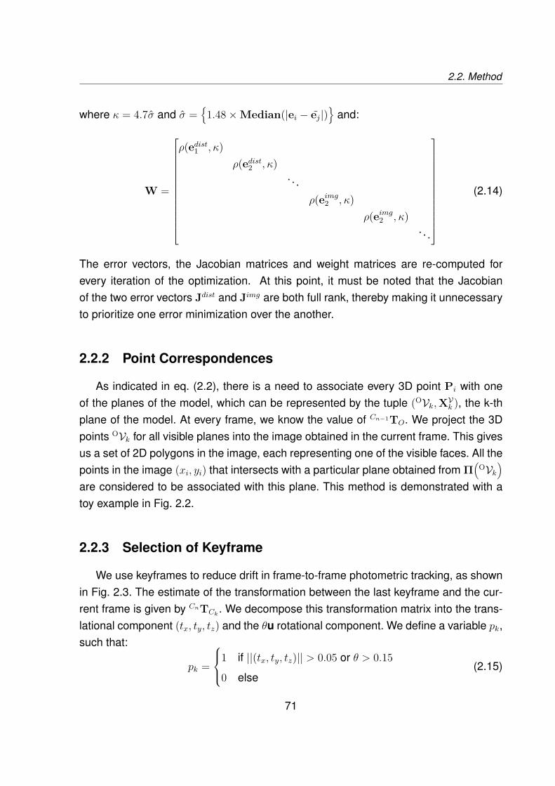
2.2. Method
where κ = 4.7σ and σ =
1.48×Median(|ei − ej|)
and:
W =
ρ(edist1 , κ)ρ(edist2 , κ)
. . .
ρ(eimg2 , κ)ρ(eimg2 , κ)
. . .
(2.14)
The error vectors, the Jacobian matrices and weight matrices are re-computed forevery iteration of the optimization. At this point, it must be noted that the Jacobianof the two error vectors Jdist and Jimg are both full rank, thereby making it unnecessaryto prioritize one error minimization over the another.
2.2.2 Point Correspondences
As indicated in eq. (2.2), there is a need to associate every 3D point Pi with oneof the planes of the model, which can be represented by the tuple (OVk,XVk ), the k-thplane of the model. At every frame, we know the value of Cn−1TO. We project the 3Dpoints OVk for all visible planes into the image obtained in the current frame. This givesus a set of 2D polygons in the image, each representing one of the visible faces. All thepoints in the image (xi, yi) that intersects with a particular plane obtained from Π
(OVk
)are considered to be associated with this plane. This method is demonstrated with atoy example in Fig. 2.2.
2.2.3 Selection of Keyframe
We use keyframes to reduce drift in frame-to-frame photometric tracking, as shownin Fig. 2.3. The estimate of the transformation between the last keyframe and the cur-rent frame is given by CnTCk . We decompose this transformation matrix into the trans-lational component (tx, ty, tz) and the θu rotational component. We define a variable pk,such that:
pk =
1 if ||(tx, ty, tz)|| > 0.05 or θ > 0.15
0 else(2.15)
71

Chapter 2 – Rigid Object Tracking
FIGURE 2.2 – A toy example demonstrating the point-plane correspondence methodology. Thecorrespondence is decided entirely on the image plane, with the green, blue and red dotscorresponding to the planes marked A, B and C
The distance threshold is expressed in millimetre while the angular threshold is givenin radian. At the very first frame, we set k = n = 0, thereby providing an initializationfor the keyframe.
2.3 Results
For benchmarking the performance of the tracker, we generated three short se-quences of simulated RGB-D data, comprising of three objects: a marmalade contai-ner, a coffee machine and a simulated car. A very simple model is used to track theseobjects. The model is not required to be continuous or topologically closed. We endup with a coarse approximation of the shape of the object, comprising of 24, 48 and62 faces for the three objects respectively. The tracker is initialized using the ViSP li-brary [Marchand et al., 2005], by matching some keypoints detected in the very firstimage with those extracted in the training images using an approach similar to [Choiand Christensen, 2010].
Very few model-free tracking and reconstruction algorithms are publicly availablealong with their open source code (e.g: [Izadi et al., 2011], [Rünz and Agapito, 2017]),but it is not trivial and requires significant modifications to compare reconstructionand tracking methods with model-based object tracking using RGB-D data. Hence,we compare the proposed method with two approaches: a) ‘edge + keypoint + depth
72

2.3. Results
CKi CK
i+5
FIGURE 2.3 – The photometric tracking is based on a keyframe-to-frame error minimization.This figure shows an example of keyframes being generated after every 5-th frame. The exactcriteria for generating a new keyframe is given in Eqn. 2.15
tracker’from [Trinh et al., 2018] (denoted in the figures as ViSP), and b) stacked errorminimization of point-to-plane distance with photometric error, without using keyframes(denoted as No KF ). The proposed approach is denoted as PA in the figures.
The quantitative comparison of the various tracking methods 1 with the ground-truthis summarized in Table 2.1. The marmalade container sequence (Fig. 2.4a) showsaccurate tracking with all the approaches. The proposed approach manages to out-perform the other two methods, although by a small margin. However, in the coffeemachine sequence, the proposed approach outperforms ViSP significantly. As shownin frame 275 of Fig. 2.4b, ViSP shows a noticeable drift while tracking a set of co-planar faces with not enough image features in it. This is the only instance among allthe sequences tested across all the available methods, where the tracking resulted ina visually noticeable drift. No KF alone, does not solve the issue of the drift comple-tely, but the proposed approach eliminates the visible drift and the positional trackingis 83.09% better than that of ViSP. Simulated car is a bit more challenging sequencedue to larger inter-frame motion towards the end. No KF shows very low accuracy inthis sequence. In the rotation, ViSP outperforms the proposed approach by averageof 0.51° over the entire sequence. This drift is not noticeable visually, and happensbecause a combination of a large number of robust feature points and edges makes iteasier for ViSP to track the overall orientation of the car, while larger inter-frame motiondisadvantages the photometric minimization. However, the proposed approach is moreaccurate than ViSP in terms of translation.
1. All results can be viewed at: youtu.be/_TPJkleBu3w
73

Chapter 2 – Rigid Object Tracking
TABLE 2.1 – Summary of RMSE values
Marmalade Container Coffee Machine Simulated CarTranslation Rotation Translation Rotation Translation Rotation
No KF 0.045 0.139 0.284 0.032 0.265 0.072[Trinh et al., 2018] 0.053 0.004 0.118 0.008 0.183 0.027
PA 0.043 0.003 0.048 0.006 0.179 0.036
Across the three sequences, it can be concluded that the proposed approach per-forms better than both No KF and ViSP. We show the tracking error plots of only ViSPand the proposed approach in Fig. 2.5a and Fig. 2.5b. Some additional results on real-world, complex shaped objects from the dataset of [Choi and Christensen, 2013] isshown in Fig. 2.7.
For the real objects, all the object models were constructed using manual mea-surements of the object. The data was captured using Intel RealSense SR300. Thebanana model is only a rough approximation of the shape of the real banana. Both thebox and the car got accurately tracked (for visual validation, refer to Fig. 2.6), despitethe obvious inaccuracies in the model. The proposed approach does not get affectedby moderate occlusion of the objects by the hand. There were some slippage of themodel from the actual object while tracking the banana. However, it never completelylooses tracking.
The proposed approach has been implemented on C++ with occasional utilizationof the PCL library [Rusu and Cousins, 2011] and the ViSP library for I/O and the IRLSimplementation respectively. The simulated data has been generated using the Blendersoftware [Blender, 2018].The proposed algorithm has been tested on an Intel Corei7-6600U CPU with 16 GB RAM. Running on a single core of the system, withoutSSE optimization and without using GPU in any format, the basic C++ code written forimplementing the proposed approach achieves a runtime of 100 - 160 ms per frame,including data capture, tracking and display on a simple GUI. It can be envisaged thatwith either SSE optimization or with the use of GPU, the overall algorithm can run muchfaster, if required.
74
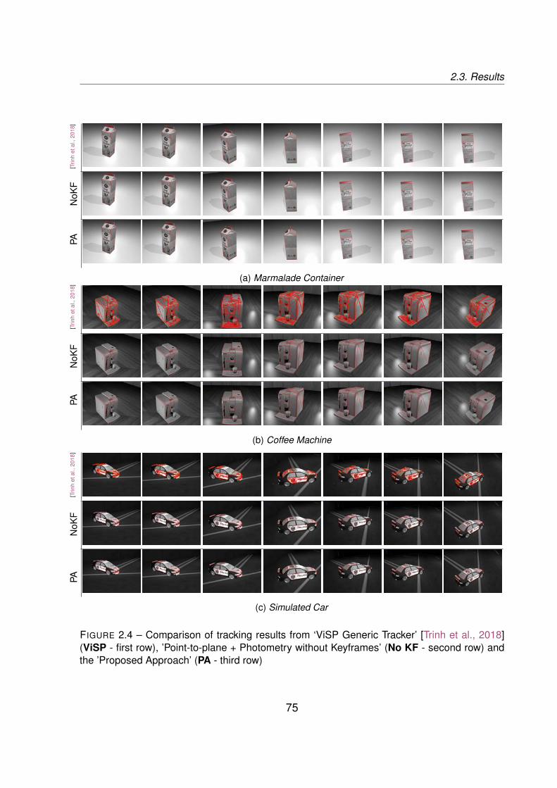
2.3. Results
(a) Marmalade Container
(b) Coffee Machine
(c) Simulated Car
[Trin
het
al.,
2018
]N
oKF
PA[ T
rinh
etal
.,20
18]
NoK
FP A
[Trin
het
al.,
2018
]N
oKF
P A
FIGURE 2.4 – Comparison of tracking results from ‘ViSP Generic Tracker’ [Trinh et al., 2018](ViSP - first row), ’Point-to-plane + Photometry without Keyframes’ (No KF - second row) andthe ’Proposed Approach’ (PA - third row)
75
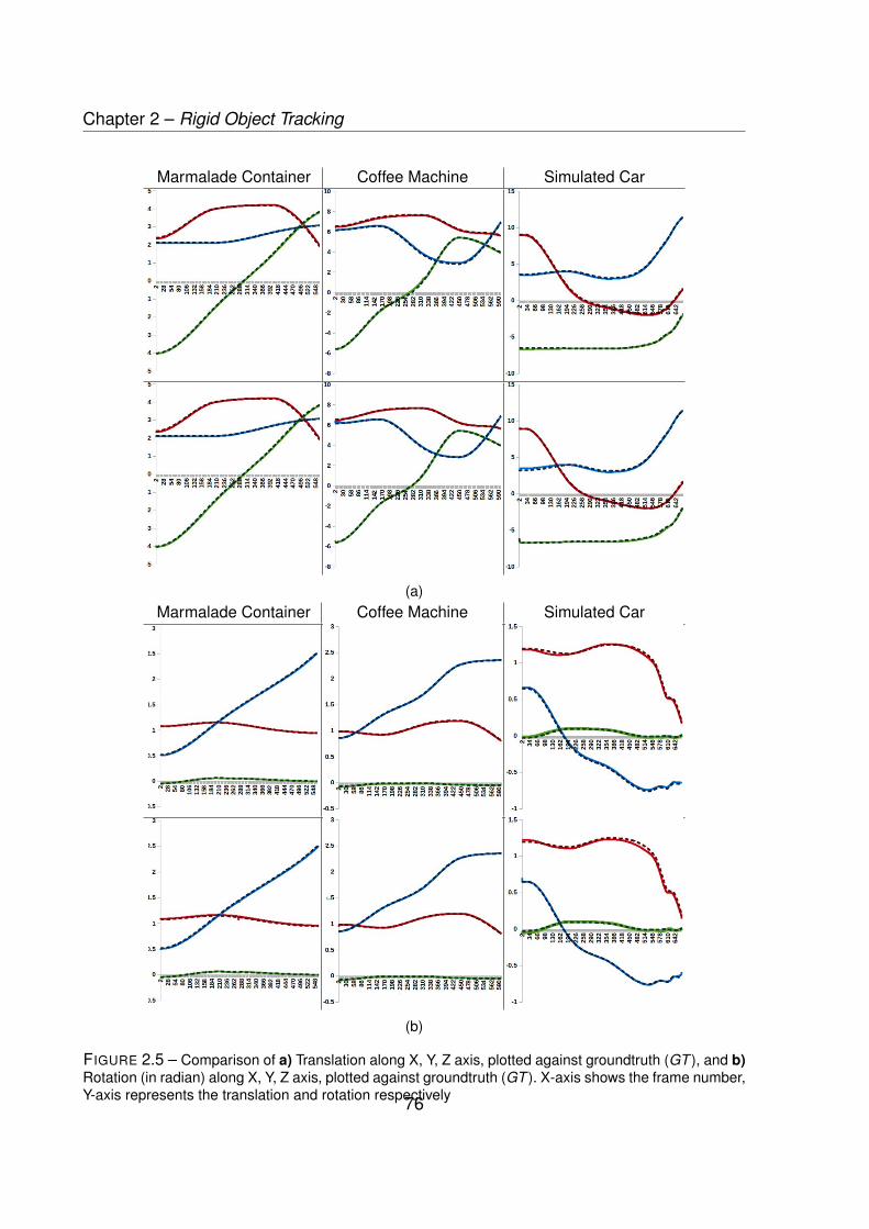
Chapter 2 – Rigid Object Tracking
Marmalade Container Coffee Machine Simulated Car
(a)Marmalade Container Coffee Machine Simulated Car
(b)
FIGURE 2.5 – Comparison of a) Translation along X, Y, Z axis, plotted against groundtruth (GT ), and b)Rotation (in radian) along X, Y, Z axis, plotted against groundtruth (GT ). X-axis shows the frame number,Y-axis represents the translation and rotation respectively76
2.4. Conclusion
FIGURE 2.6 – Tracking results from real data captured using Intel RealSense for a) a box, b) atoy car, c) a banana
2.4 Conclusion
In this chapter, we present an algorithm to accurately track the pose of rigid andcomplex-shaped objects. The tracking is robust to occlusion and partial specularityof the scene. We provide validation on both simulated and real data. The proposedapproach outperforms one of the best among the open-sourced, model-based, 6DoFobject tracking methods. It also outperforms a partial re-implementation of a state-of-the-art tracking method from recent advances in the field of tracking and reconstruction.The proposed approach is an efficient method to track complex objects that a) doesnot require detailed object model (reducing the setup time in practical applications), b)tracks objects with better accuracy than comparable state-of-the-art approaches.
77
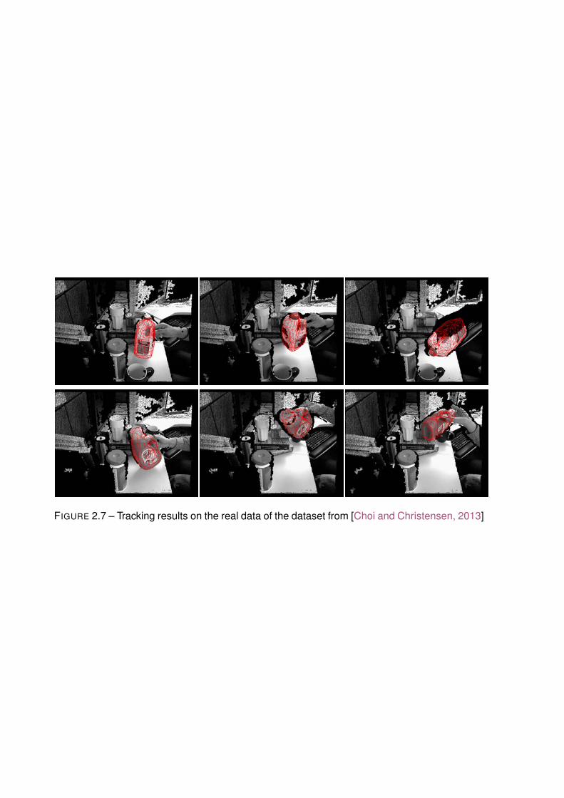
FIGURE 2.7 – Tracking results on the real data of the dataset from [Choi and Christensen, 2013]
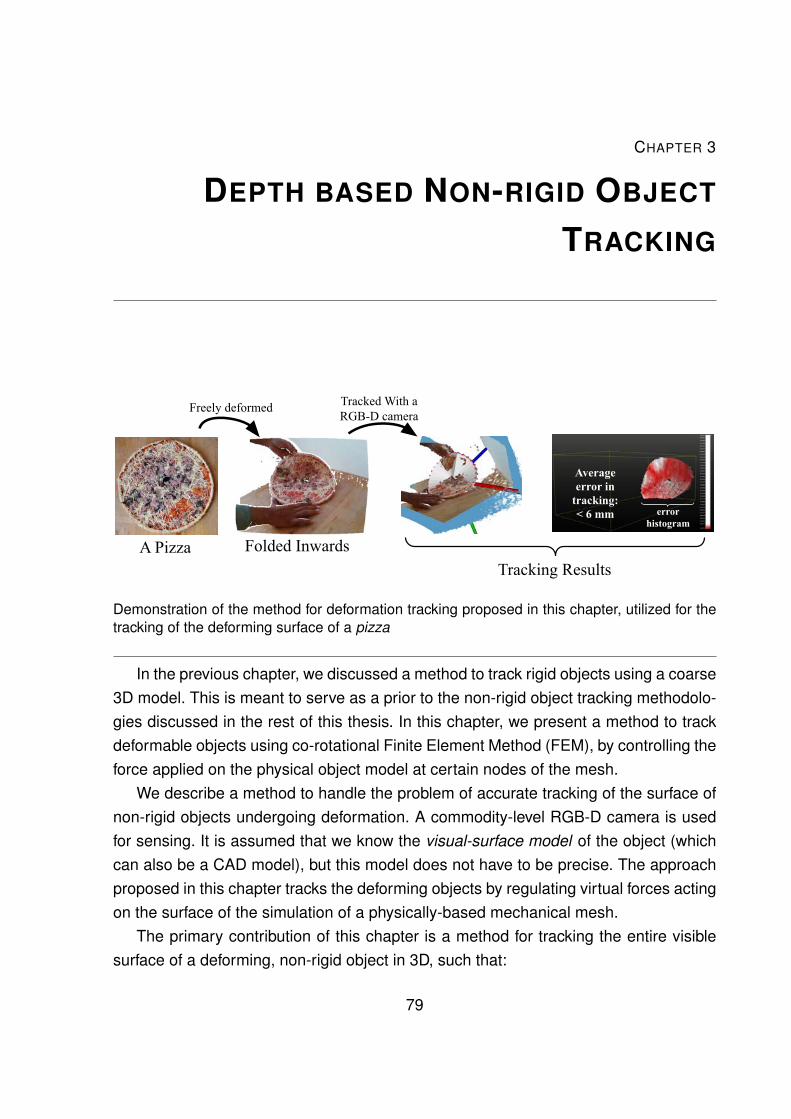
CHAPTER 3
DEPTH BASED NON-RIGID OBJECT
TRACKING
Demonstration of the method for deformation tracking proposed in this chapter, utilized for thetracking of the deforming surface of a pizza
In the previous chapter, we discussed a method to track rigid objects using a coarse3D model. This is meant to serve as a prior to the non-rigid object tracking methodolo-gies discussed in the rest of this thesis. In this chapter, we present a method to trackdeformable objects using co-rotational Finite Element Method (FEM), by controlling theforce applied on the physical object model at certain nodes of the mesh.
We describe a method to handle the problem of accurate tracking of the surface ofnon-rigid objects undergoing deformation. A commodity-level RGB-D camera is usedfor sensing. It is assumed that we know the visual-surface model of the object (whichcan also be a CAD model), but this model does not have to be precise. The approachproposed in this chapter tracks the deforming objects by regulating virtual forces actingon the surface of the simulation of a physically-based mechanical mesh.
The primary contribution of this chapter is a method for tracking the entire visiblesurface of a deforming, non-rigid object in 3D, such that:
79
Chapter 3 – Depth based Non-rigid Object Tracking
— it requires only a very coarse estimate of the physical properties (Young’s modu-lus and Poisson ratio) of the object ;
— it performs accurate frame-to-frame tracking of deformation of the non-rigid ob-ject ;
— it has been validated on simulated data with ground truth, as well as real data.
3.1 Background
We use the co-rotational FEM to simulate the physics behind the deformation ofnon-rigid objects. For simulating the FEM, we use a tetrahedral mesh as the physicalmodel of the object. But, unlike the state-of-the-art approaches in the literature, we ex-tend the method to minimize an error function with a closed-loop optimization basedon a point-to-plane geometric error. This additional step effectively reduces the depen-dency of the system on the accuracy of the physical properties of object matter used forthe finite element modelling. Moreover, we dissociate the rigid and non-rigid trackinginto two parallel processes. The rigid tracking is purely based on the surface model,while the FEM is used strictly for tracking the non-rigid deformations. This parallel sys-tem is capable of real-time performance. Our approach has been both quantitativelyand qualitatively evaluated using a combination of ground-truthed, simulated data andreal data.
Having decided to utilize physically based models for deformation tracking, in thischapter we begin the study of tracking approaches based on depth information only.Since depth data is an important information available from the RGB-D sensors andcan be conveniently utilized for tracking the temporal evolution of non-rigid objects, wedesign a methodology for tracking this depth data using the co-rotational FEM model.However, such approaches are not completely unprecedented.
As discussed in Sec. 1.3.1.1, physics based framework for deformation trackinghas been demonstrated using mass-spring-damper systems [Royer et al., 2017], fi-nite element model (FEM) [Petit et al., 2015a] and kinematic chains [Schmidt et al.,2014]. For model based tracking of non-rigid objects, the representation of the modelis usually done by a set of triangular faces representing the surface of the object. Ho-wever, tetrahedral, volumetric model is preferred [Paloc et al., 2002] for tracking usingmass-spring-damper systems, while the FEM based systems available in the literature
80
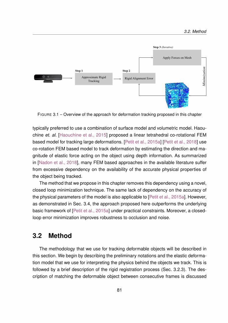
3.2. Method
FIGURE 3.1 – Overview of the approach for deformation tracking proposed in this chapter
typically preferred to use a combination of surface model and volumetric model. Haou-chine et. al. [Haouchine et al., 2015] proposed a linear tetrahedral co-rotational FEMbased model for tracking large deformations. [Petit et al., 2015a] [Petit et al., 2018] useco-rotation FEM based model to track deformation by estimating the direction and ma-gnitude of elastic force acting on the object using depth information. As summarizedin [Nadon et al., 2018], many FEM based approaches in the available literature sufferfrom excessive dependency on the availability of the accurate physical properties ofthe object being tracked.
The method that we propose in this chapter removes this dependency using a novel,closed loop minimization technique. The same lack of dependency on the accuracy ofthe physical parameters of the model is also applicable to [Petit et al., 2015a]. However,as demonstrated in Sec. 3.4, the approach proposed here outperforms the underlyingbasic framework of [Petit et al., 2015a] under practical constraints. Moreover, a closed-loop error minimization improves robustness to occlusion and noise.
3.2 Method
The methodology that we use for tracking deformable objects will be described inthis section. We begin by describing the preliminary notations and the elastic deforma-tion model that we use for interpreting the physics behind the objects we track. This isfollowed by a brief description of the rigid registration process (Sec. 3.2.3). The des-cription of matching the deformable object between consecutive frames is discussed
81
Chapter 3 – Depth based Non-rigid Object Tracking
next (Sec. 3.2.4). We follow this up with the mechanism for computing the Jacobianthat links the variation in the geometric error with the variation of force applied on aparticular vertex. We use this Jacobian for minimizing the error using an Iteratively Re-weighted Least Square (IRLS) formulation. We finish this section by summarizing thesteps for minimizing the non-rigid error.
In the approach proposed here, first the deforming object is tracked rigidly using its3D object model. After the rigid tracking, the remaining residual error occurs purely dueto the deformation of the model. In the second step, this non-rigid error is minimizedby applying a deforming force on the physical object model. The method for obtainingthis deforming force that minimizes the non-rigid error is the primary contribution of thischapter and is described in Sec. 3.2.4. The overview of this approach is described inFig. 3.1.
3.2.1 Notations
We use two types of 3D model for the non-rigid tracking. The first is a visual-surfacemodel, denoted by VS, and the other one is a tetrahedral, volumetric, internal model,denoted by VM. Continuing from the definition in Sec. 1.1.3, CVS and OVS denotes thevisual-surface model in the camera (Fc) and object frame (Fo) respectively while CVM
and OVM denotes the internal model in a similar manner. The visual-surface model isdescribed using a set of planes which are represented using the nodes defining theboundary of the surface (usually a triangle) and the connectivity between these nodes.We can represent this surface as
VS =[p1 p2 ... pM
](3.1)
where M is the number of vertices in VS and the i-th vertex is pi =(Xi, Yi, Zi
), the
3D coordinate of a point in the reference frame of the base model. As given in Sec.1.1.3, we have a corresponding, connectivity map, given by XVS. M is the number ofvertices and N is the number of triangular faces in VS. The 3D coordinates of the threevertices of the triangle representing a given face can be derived from XVS. Clearly, thenormal vector ni = (nXi , nYi , nZi ) and distance to origin di for any given face can bederived from VS and XVS using elementary geometry. We similarly define a tetrahedral,volumetric, internal model VM along with its connectivity map XVM, such that everyelement of XVM has four indices, instead of three. As shown in Fig. 3.2, VM represents
82
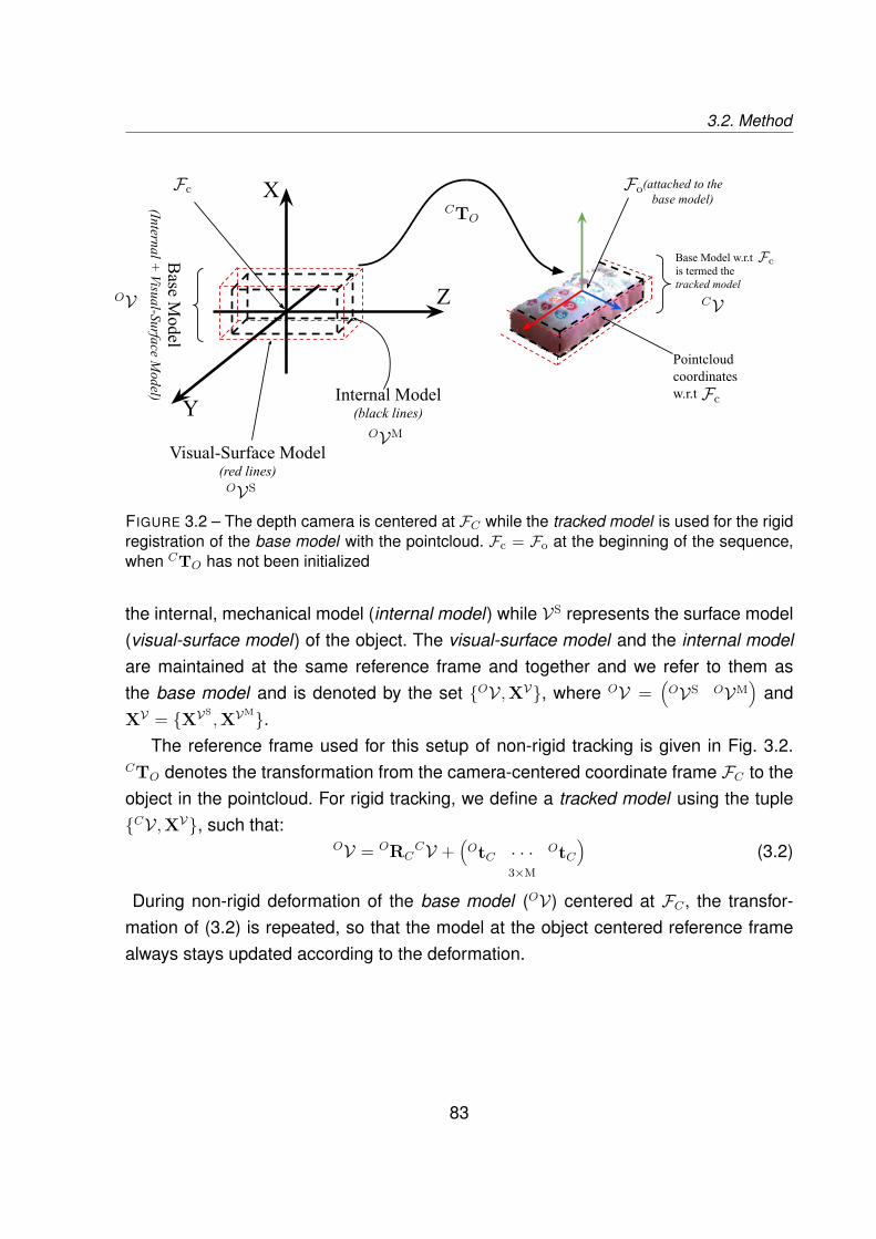
3.2. Method
Fc
OVM
OVS
OV CV
Fc
Fc
Fo
CTO
FIGURE 3.2 – The depth camera is centered at FC while the tracked model is used for the rigidregistration of the base model with the pointcloud. Fc = Fo at the beginning of the sequence,when CTO has not been initialized
the internal, mechanical model (internal model) while VS represents the surface model(visual-surface model) of the object. The visual-surface model and the internal modelare maintained at the same reference frame and together and we refer to them asthe base model and is denoted by the set OV ,XV, where OV =
(OVS OVM
)and
XV = XVS,XVM.
The reference frame used for this setup of non-rigid tracking is given in Fig. 3.2.CTO denotes the transformation from the camera-centered coordinate frame FC to theobject in the pointcloud. For rigid tracking, we define a tracked model using the tupleCV ,XV, such that:
OV = ORCCV +
(OtC · · · OtC
)3×M
(3.2)
During non-rigid deformation of the base model (OV) centered at FC , the transfor-mation of (3.2) is repeated, so that the model at the object centered reference framealways stays updated according to the deformation.
83
Chapter 3 – Depth based Non-rigid Object Tracking
3.2.2 Deformation Modelling
We use co-rotational FEM as the deformation model, for developing the deformationtracking method proposed in this chapter. As explained in Sec. 1.3.1, co-rotational FEMoffers us a method to model large deformations efficiently.
We can now briefly recall some of the relevant concepts used for simulating thedeformation using FEM. For a tetrahedral mesh, we can represent the internal elasticforces acting on the nodes by:
Fe = ReKeUR (3.3)
Here, UR = (p1, p2, p3, p4)12×1
is obtained using Eqn. 3.3, Ke12×12
is the stiffness matrix and
Re12×12
is the block diagonal matrix of four R rotation matrices stacked diagonally. Fe12×1
gives the elastic forces acting on the nodes of this tetrahedral element.To resolve the interaction between forces and their resulting displacement using the
FEM, we solve a second order differential equation, given by:
Mp + Dp + Kgp = Fext + Fe (3.4)
where M and D are the model’s mass and damping matrices respectively, derivedusing Eqn. 1.66 and Eqn. 1.67. Kg is the global stiffness matrix. Fext are the externalforces acting on the vertices. The method for determining Fext is discussed in the sub-sequent sections. To solve this differential equation, we use a linear solver based onconjugate gradient descent [Faure et al., 2012b]. To impose additional constraint, Eqn.(3.4) can be multiplied using a projection matrix that sets the values of certain indicesto zero. We use the projective constraint to eliminate the rigid motion of the object. Thisis discussed in the next section
It must be noted that the force Fext is just the deforming force acting on the model,and does not include the forces causing the rigid transformation of the body. In fact, thedeformation model proposed here is completely independent of rigid motion that resultsfrom the effects of gravity and interaction with other contact surfaces. As described inSec. 3.2.3, the rigid motion is tracked separately. This separation of rigid and non-rigidtracking method, along with the minimization described Sec. 3.2.4, makes the overallsystem independent from the inaccuracies of the physical parameters.
84
3.2. Method
3.2.3 Rigid Registration
The rigid registration is a joint minimization of two error terms: depth based geome-tric error and keypoint based feature tracking [Trinh et al., 2018]. The two error termsare explained below:
3.2.3.1 Depth based geometric error
Assuming that we know the accurate CTn−1O at the (n−1)-the frame and nTn−1 gives
the initial estimate of transformation between previous and current frame, the error isgiven as:
eD(nqn−1) =((
nRn−1P + ntn−1)· nk
)− dk (3.5)
where nk and dk are the normal and distance to origin respectively, for the k-th planarface that corresponds with the point P in the pointcloud. The Jacobian that links thevariation of the error eD(nqn−1) with the variation of nqn−1, is given by:
JDi =
[n>k
[nk]×Pi>]
(3.6)
3.2.3.2 Feature based minimization
The Harris corner features are used for tracking with keypoints. This is based onthe classical KLT algorithm [Baker and Matthews, 2004]. Let u = (x, y, 1) be the homo-geneous 2D coordinate of a feature point in the (n− 1)-th image and u∗ = (x∗, y∗, 1) bethe matched coordinate for the same point in the n-th frame. We define the error termas:
eK(nqn−1) =x(nqn−1)− x∗
y(nqn−1)− y∗
(3.7)
where(x(nqn−1), y(nqn−1), 1) = nHn−1u (3.8)
Here, u = (x, y, 1) and u∗ = (x∗, y∗, 1) are the homogeneous pixel coordinates of thetracked feature point in the (n− 1)-th and n-th data frame respectively. Moreover:
nHn−1 = nRn−1 +ntn−1
dn> (3.9)
85
Chapter 3 – Depth based Non-rigid Object Tracking
where n and d are interpreted in the same way as (3.5). The corresponding Jacobianthat relates the variation of eK(nqn−1) with the time variation of nqn−1 is given by:
JK =− 1
Z 0 xZ xy −(1 + x2) y
0 − 1Z
yZ (1 + y2) −xy −x
(3.10)
where (x, y) are the pixel coordinates and Z is in meters. Given these two errorsand their corresponding Jacobian, the combined error e(nqn−1) is obtained by sta-cking the vectors eD(nqn−1) and eK(nqn−1), while the combined Jacobian J is givenby J = (JD,JK). The combined error is minimized with the update given by:
ξ = −λ(WJ
)+We (3.11)
where W is the weight matrix for outlier removal using the Tukey m-estimator [Beatonand Tukey, 1974], and ξ ∈ se(3). This becomes an iteratively re-weighted least squaresproblem.
3.2.4 Non Rigid Tracking
Before starting the non-rigid tracking using a minimization technique, it is necessaryto determine the possible points of application of forces that needs to be tracked. It issufficient to track only a small subset of nodes, depending upon a set of criteria. Thesecriteria, as detailed below, is obtained by clustering the residual error from the rigidtracking step. Only regions surrounding the clusters with higher value of errors areconsidered to be relevant for non-rigid tracking. It must be noted that only the point-to-plane error based depth information is used for determining the point of application offorces.
At the end of the rigid registration process, we can construct a map that links thepoints in the 3D pointcloud to their corresponding geometric error from (3.5). Giventhat eD
i denotes the error for the i-th point Pi in the entire pointcloud P, it is possible toderive a new pointcloud P∗ using a linear thresholding operation, such that:
P∗ = Pi ∈ P∣∣∣|eD
i | ≥ θD (3.12)
where θD is a threshold that depends on the geometry of the object being tracked.We subject the pointcloud P∗ to a clustering step using Eucledian distances [Hartigan
86
3.2. Method
and Wong, 1979]. Very small clusters and clusters spanning more than half of thesize of the entire pointcloud are discarded. Let us assume that we obtain j clustersfrom this operation, denoted by K1,K2, · · ·,Kj, and their corresponding centroids arerepresented by k1,k2, · · ·,kj, where k = (X,Y,Z, 1) is the homogeneous 3D coordinateof the point w.r.t FC . These points are inverse transformed with the last estimate ofCTO obtained after minimization with (3.11), such that
k∗i =(CTO
)−1ki (3.13)
For all these j centroids, we determine their nearest neighbors in CVM using the k-nearest neighbor algorithm [Fukunage and Narendra, 1975]. Let the nearest neighborsof k∗1,k∗2, · · ·,k∗j in CVM be denoted by CVM
k1 ,CVM
k2 , · · ·,CVM
kj.
For the following discussion, let us consider an arbitrary ki-th cluster alone, whichwe refer to as CVM
i for the sake of simplicity. At this stage, we must modify (3.5) toaccommodate a slightly different variant of the same error function. We re-define it aseD(CVS
i
), assuming the r-th plane corresponds to the s-th point in the pointcloud, and
the normal nr and the distance to origin dr is derived from CVSi . This change in notation
is necessary because the error term eD is no longer a function of nqn−1 at this point ofnon-rigid tracking, it is rather a function of CVS
i , i.e., the position of the surface model ofthe object w.r.t the s-th point in the pointcloud. The correspondence between the pointand the plane is done using a strategy similar to Sec. 2.2.2. The propagation of thevertex displacement from CVM
i to CVSi happens through the barycentric mapping J
(defined in Sec. 1.3.1).
3.2.4.1 Jacobian Computation
The Jacobian that relates the variation of eD(CVS
i
)with the variation of the applied
force is computed numerically by perturbing the node OVMi by a very small, constant
force ∆FJ successively along the three axes, as shown in Fig. 3.3. After applying theforce on the node, a simulation based on FEM is done using the minimization describedin Sec. 3.2.2 - Eqn. 3.4. After the conjugate gradient solver optimizes (3.4), the systemwill attain a static condition. There will be six such configurations of the mesh, obtainedby the perturbation along the positive and the negative direction of the three axes. Wedenote these new six configurations of OVM
i by using the axis direction X+,X−, · · · ,Z−
87

Chapter 3 – Depth based Non-rigid Object Tracking
FIGURE 3.3 – The node closest to the centroid of a cluster is perturbed by a small force alongthe three axes in both positive and negative direction, producing six deformed configurationsper node
as a superscript, given as:
(OVMi )F =
[(OVM
i )X+ (OVMi )X− (OVM
i )Y+ (OVMi )Y− (OVM
i )Z+ (OVMi )Z−
](3.14)
Following the definition of Sec. 1.3.1, the deformed meshes from Eqn. 3.14 is propa-gated down to the visual-surface model via the barycentric map:
(OVSi )F = J
((OVM
i )F)
(3.15)
We take these modified, visual mesh and transform it back to the registered pointcloudusing:
(CVSi )F = CRO
((OVS
i )F)
+[CtO · · · CtO
]︸ ︷︷ ︸
3×6M
(3.16)
where M is the number of vertices of VS. The relation of the variation of the externalforce with the variation in error can be expressed as:
eD(CVS
i
)= JiFext (3.17)
88
3.3. Implementation
The term Ji is obtained numerically by finite difference computation using central diffe-rences. The final Jacobian used is:
Ji =(JXi JYi JZi
)(3.18)
⇒ Ji =[
(OVMi )X+−(OVM
i )X−2FJ
(OVMi )Y+−(OVM
i )Y−2FJ
(OVMi )Z+−(OVM
i )Z−2FJ
](3.19)
3.2.4.2 Minimization
So far, j nodes have been selected for application of external force to deform themodel. We have p points in the pointcloud, and their correspondence with the modelis known. If the iteration of minimization is denoted by n, the initial estimate of thevertically stacked force vector at the (n − 1)-th iteration is denoted by Fn−1
ext︸ ︷︷ ︸3j×1
and the
values are set to zero. The Jacobian matrices are stacked up horizontally, such that:
J︸︷︷︸p×3j
=(J1 J2 · · · Jj
)(3.20)
The update is computed as:
∆F = −λ(
W︸︷︷︸p×p
J)+
WeD(CVS
i
)︸ ︷︷ ︸
p×1
(3.21)
W is a weighting matrix obtained from the Tukey based m-estimator, similar to Sec.3.2.3. λ is a scaling factor. The force vector is updated by:
Fnext = Fn−1
ext + ∆F (3.22)
This force is applied on the base model and the final node displacements are determi-ned, once again, using (3.4).
3.3 Implementation
In order to compute the cost function, it is necessary to associate every 3D point Pi
with one of the planar surfaces of the visual-surface model OVS. Given that we know the
89
Chapter 3 – Depth based Non-rigid Object Tracking
value of CTO obtained at the previous frame, we project the 3D points OVS for all visibleplanes into the image obtained in the current frame. The visibility is checked usingthe classical ray-casting algorithm [Roth, 1982]. The ray-casting is also needed forimposing the projective constraints. The nodes invisible to the camera are consideredto be immobile under the influence of external force. Moreover, we do not consider thevolumetric, internal mesh to be an input to the system. The mesh is rather generatedapriori, using Dirichlet tessellation, followed by Delaunay tetrahedralization of the inputmesh using the Bowyer-Watson algorithm [Si, 2015].
In contrast to [Petit et al., 2015a] and [Petit et al., 2018], the approach proposedhere does not require a visual segmentation for separating the region of interest fromthe background. This is done by initializing the pose of the object at the first frame usingpre-trained markers on the object. It is done using the ViSP library [Marchand et al.,2005], by matching the keypoints detected in the very first image with those extractedin the training images using an approach similar to [Dementhon and Davis, 1995].
The algorithm is implemented using a parallel framework, where two different pro-cesses are involved for the rigid and non-rigid tracking of the object respectively, asshown in Figure 3.4. The rigid tracking process is capable of processing each frameat < 100 ms, thereby ensuring real-time interaction. The un-optimized, non-rigid tra-cking code runs at 800ms to 1.3s (approximately) per frame, depending on the size ofthe object and its proximity to the camera. The results reported here have been achie-ved using processes running on a single core of a i7-6600U CPU with 16GB of RAM.An Intel Skylake GT2 GPU has been utilized, but only for the ray-casting. The FEMsolvers are implemented using the SOFA library [Faure et al., 2012b], without usingCUDA. The rigid tracking process runs at > 10 fps, while the non-rigid tracking processhandles every 10-th/12-th frame coming from the sensor.
3.4 Results
The results are quantitatively validated on two sets of simulated data, as well as onmultiple real objects 1.
1. Please visit the following URL for all results on real data: https://youtu.be/RFd-Ix9hcdg
90

3.4. Results
FIGURE 3.4 – The parallel implementation of the rigid and non-rigid tracking processes enableus to track the deforming surface at frame rate
3.4.1 Simulation
For the simulated data, the deformation of the objects were generated using si-mulation of co-rotational FEM. Two objects are considered, a cube and a rectangularboard. They are made to undergo simple but large deformations, as shown in Fig. 3.5.We made the dataset available at: github.com/lagadic/nr-dataset. The visual modelsproduced as an output of the simulation were subjected to texturing, shading and ren-dering using the Blender software, followed by the generation of the pointcloud usinga RGB-D camera simulator. In the simulation, both the objects were modelled usingYoung’s modulus (YM) of 50000 Pa and Poisson’s ratio of 0.3. Rayleigh mass wasassumed to be 0.1 and Rayleigh stiffness to be 0.3.
3.4.1.1 Comparison
We utilize the simulated dataset not only to validate our approach, but also to com-pare the proposed method to existing paradigm for deformation tracking from the state-of-the-art literature. As a comparison, it must be noted that merely idea of applyingcontrolled forces to mesh vertices for deformation tracking is not entirely novel. As no-ted in Sec. 1.3.1.1, similar ideas have been proposed by [Schulman et al., 2013], [Wanget al., 2015] and [Petit et al., 2015a]. The novelty of the approach proposed by us lies in
91
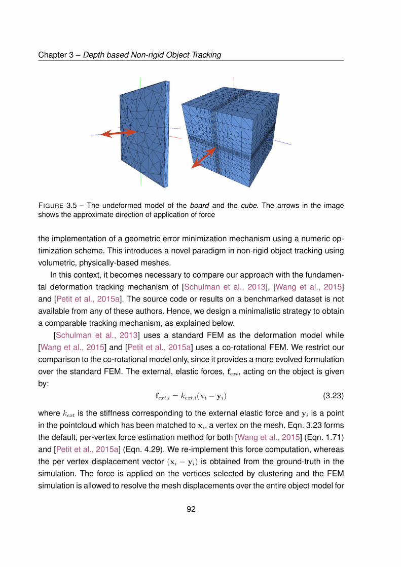
Chapter 3 – Depth based Non-rigid Object Tracking
FIGURE 3.5 – The undeformed model of the board and the cube. The arrows in the imageshows the approximate direction of application of force
the implementation of a geometric error minimization mechanism using a numeric op-timization scheme. This introduces a novel paradigm in non-rigid object tracking usingvolumetric, physically-based meshes.
In this context, it becomes necessary to compare our approach with the fundamen-tal deformation tracking mechanism of [Schulman et al., 2013], [Wang et al., 2015]and [Petit et al., 2015a]. The source code or results on a benchmarked dataset is notavailable from any of these authors. Hence, we design a minimalistic strategy to obtaina comparable tracking mechanism, as explained below.
[Schulman et al., 2013] uses a standard FEM as the deformation model while[Wang et al., 2015] and [Petit et al., 2015a] uses a co-rotational FEM. We restrict ourcomparison to the co-rotational model only, since it provides a more evolved formulationover the standard FEM. The external, elastic forces, fext, acting on the object is givenby:
fext,i = kext,i(xi − yi) (3.23)
where kext is the stiffness corresponding to the external elastic force and yi is a pointin the pointcloud which has been matched to xi, a vertex on the mesh. Eqn. 3.23 formsthe default, per-vertex force estimation method for both [Wang et al., 2015] (Eqn. 1.71)and [Petit et al., 2015a] (Eqn. 4.29). We re-implement this force computation, whereasthe per vertex displacement vector (xi − yi) is obtained from the ground-truth in thesimulation. The force is applied on the vertices selected by clustering and the FEMsimulation is allowed to resolve the mesh displacements over the entire object model for
92
3.4. Results
a fixed number of iterations. The number of iterations allowed to converge is constantfor both this re-implementation and the approach proposed by us. This implies thatin the re-implementation, the displacement vector associated with the deformation isprovided exactly from the groundtruth, providing it with a significant advantage over theapproach proposed by us. In general, the fundamental difference between the methodproposed in this chapter and the approach of [Petit et al., 2015a] lies in the fact thatwe propose an optimization based method for deformation tracking while [Petit et al.,2015a] relies on force-estimation from pointcloud matching using a modified k-nearestneighbor search.
In the subsequent text, the results obtained from the approach proposed in thischapter are denoted by Numeric-optimization, while the results from this partial re-implementation scheme (as discussed above) are denoted by Linear-force-estimate.
To analyze the robustness of the two approaches, experiments were repeated byvarying the Young’s modulus of the model for determining the variance in error withchange in physical parameters. The physical parameters used for simulation are consi-dered unknown in the implementation of the proposed approach. The tracking wasrepeated over the values of 5 Pa, 500 Pa, 50000 Pa, 5×10⁶ Pa and 5×10⁸ Pa respecti-vely. The results are summarized in Fig. 3.6 and Fig. 3.7. In the figure, the ground-truthof the model undergoing deformation is provided in the left-most column. The rest of theimages show the 3D model (the tracked model) obtained from the tracking algorithm,placed into the pointcloud with the latest estimate of CTO.
Since the ground-truth for the deformation is known, it is possible to compute theHausdorff distance metric [Henrikson, 1999] between the output of the tracking andthe ground-truth, to quantify the error between the ideal and the actual output. Fig. 3.8delineates the Hausdorff distance of the output for various values of Young’s modulus.
As given in Table 3.1, the mean error in terms of Hausdorff distance using Numeric-optimization and Linear-force-estimate are 0.305 and 1.622 units for the cube datasetand 0.834 and 1.100 units for the board dataset respectively. As a reference, the lengthof the largest diagonal is 69.28 and 55.19 units for the cube and the board models res-pectively (the data is simulated using geometrically defined values for the dimensionof the objects and the FEM is simulated without applying the gravity vector, hence theexact unit of length cannot be expressed in SI units directly). Hence, the tracking accu-racy of the proposed approach is 81.18% better than Linear-force-estimate in the cubedata and 24.20% better than Linear-force-estimate in the board data. The tracking
93
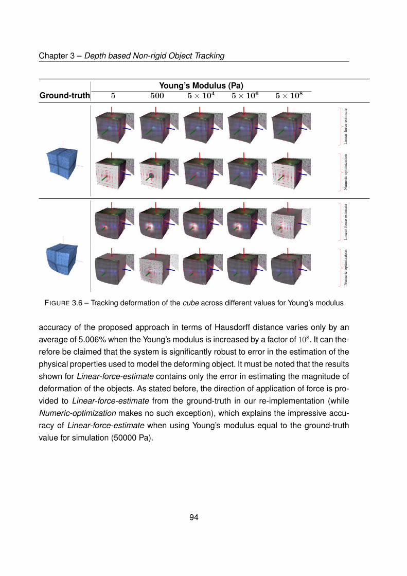
Chapter 3 – Depth based Non-rigid Object Tracking
Young’s Modulus (Pa)Ground-truth 5 500 5× 10⁴ 5× 10⁶ 5× 10⁸
FIGURE 3.6 – Tracking deformation of the cube across different values for Young’s modulus
accuracy of the proposed approach in terms of Hausdorff distance varies only by anaverage of 5.006% when the Young’s modulus is increased by a factor of 108. It can the-refore be claimed that the system is significantly robust to error in the estimation of thephysical properties used to model the deforming object. It must be noted that the resultsshown for Linear-force-estimate contains only the error in estimating the magnitude ofdeformation of the objects. As stated before, the direction of application of force is pro-vided to Linear-force-estimate from the ground-truth in our re-implementation (whileNumeric-optimization makes no such exception), which explains the impressive accu-racy of Linear-force-estimate when using Young’s modulus equal to the ground-truthvalue for simulation (50000 Pa).
94

3.4. Results
Young’s Modulus (Pa)Ground-truth 5 500 5× 10⁴ 5× 10⁶ 5× 10⁸
FIGURE 3.7 – Tracking deformation of the board across different values for Young’s modulus
3.4.2 Real Data
The real data has been captured using the Intel RealSense SR300 RGB-D camera.It is a commodity level depth sensor that produces RGB-D images of reasonably goodresolution between 20 to 150 cm depth. Three objects have been tracked for the va-lidation: a) a pizza, b) a cuboidal soft toy and c) a rectangular sponge. A Poisson’sratio of 0.3 was assigned to all the objects uniformly. All the objects were tracked usingmultiple values of Young’s modulus which were set coarsely and empirically. The pizzadata was tracked with an Young’s modulus of 5 × 10³ Pa, 5 × 10⁴ Pa and 5 × 10⁵ Pa,the toy was tracked using 5 × 10⁴ Pa, 5 × 10⁵ Pa and 5 × 10⁶ Pa, and the sponge wastracked using 8× 10⁵ Pa, 8× 10⁶ Pa and 8× 10⁷ Pa. The tracking results are shown inFig. 3.9, Fig. 3.10 and Fig. 3.11.
Given these results, the average, per pixel point-to-plane error across the entiresequence for multiple values of Young’s modulus are given in Fig. 3.12.
95
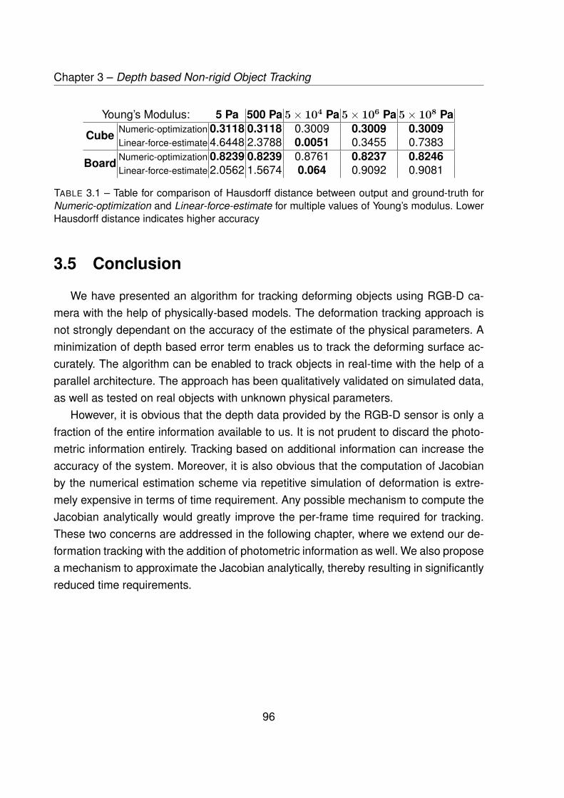
Chapter 3 – Depth based Non-rigid Object Tracking
Young’s Modulus: 5 Pa 500 Pa 5× 10⁴ Pa 5× 10⁶ Pa 5× 10⁸ Pa
Cube Numeric-optimization 0.3118 0.3118 0.3009 0.3009 0.3009Linear-force-estimate 4.6448 2.3788 0.0051 0.3455 0.7383
Board Numeric-optimization 0.8239 0.8239 0.8761 0.8237 0.8246Linear-force-estimate 2.0562 1.5674 0.064 0.9092 0.9081
TABLE 3.1 – Table for comparison of Hausdorff distance between output and ground-truth forNumeric-optimization and Linear-force-estimate for multiple values of Young’s modulus. LowerHausdorff distance indicates higher accuracy
3.5 Conclusion
We have presented an algorithm for tracking deforming objects using RGB-D ca-mera with the help of physically-based models. The deformation tracking approach isnot strongly dependant on the accuracy of the estimate of the physical parameters. Aminimization of depth based error term enables us to track the deforming surface ac-curately. The algorithm can be enabled to track objects in real-time with the help of aparallel architecture. The approach has been qualitatively validated on simulated data,as well as tested on real objects with unknown physical parameters.
However, it is obvious that the depth data provided by the RGB-D sensor is only afraction of the entire information available to us. It is not prudent to discard the photo-metric information entirely. Tracking based on additional information can increase theaccuracy of the system. Moreover, it is also obvious that the computation of Jacobianby the numerical estimation scheme via repetitive simulation of deformation is extre-mely expensive in terms of time requirement. Any possible mechanism to compute theJacobian analytically would greatly improve the per-frame time required for tracking.These two concerns are addressed in the following chapter, where we extend our de-formation tracking with the addition of photometric information as well. We also proposea mechanism to approximate the Jacobian analytically, thereby resulting in significantlyreduced time requirements.
96

FIGURE 3.8 – Comparison of Hausdorff distance between output and ground-truth for Numeric-optimization and Linear-force-estimate for multiple values of Young’s modulus
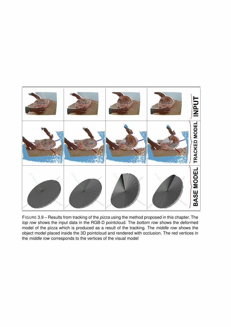
FIGURE 3.9 – Results from tracking of the pizza using the method proposed in this chapter. Thetop row shows the input data in the RGB-D pointcloud. The bottom row shows the deformedmodel of the pizza which is produced as a result of the tracking. The middle row shows theobject model placed inside the 3D pointcloud and rendered with occlusion. The red vertices inthe middle row corresponds to the vertices of the visual model
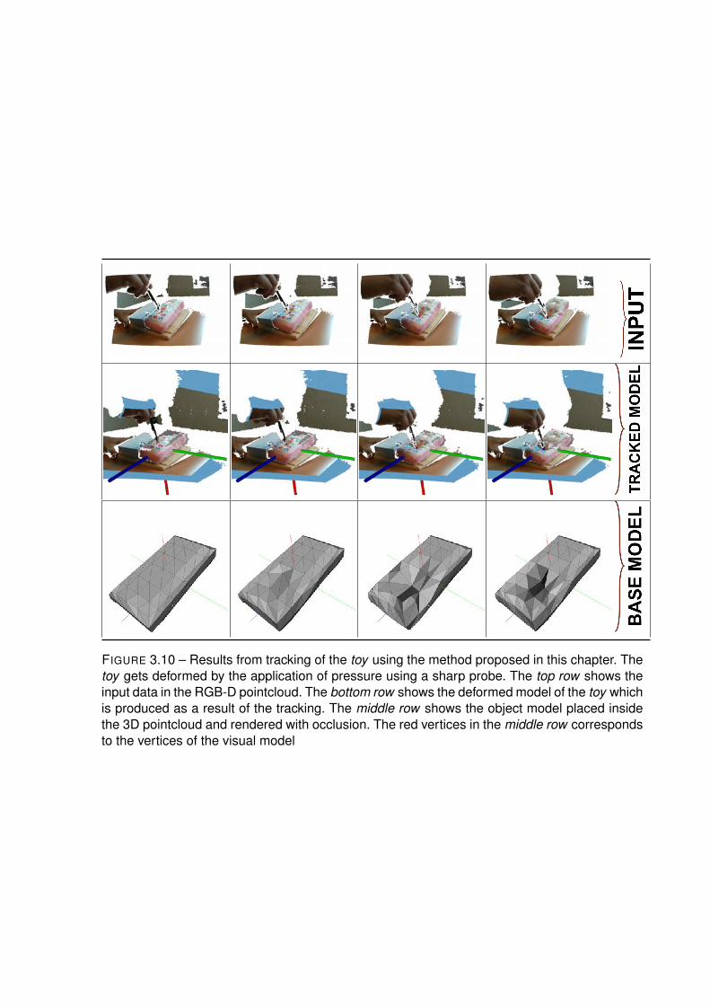
FIGURE 3.10 – Results from tracking of the toy using the method proposed in this chapter. Thetoy gets deformed by the application of pressure using a sharp probe. The top row shows theinput data in the RGB-D pointcloud. The bottom row shows the deformed model of the toy whichis produced as a result of the tracking. The middle row shows the object model placed insidethe 3D pointcloud and rendered with occlusion. The red vertices in the middle row correspondsto the vertices of the visual model

FIGURE 3.11 – Results from tracking of the sponge using the method proposed in this chapter.The sponge gets folded inwards by lifting one of its end while holding down the other end witha transparent ruler. The top row shows the input data in the RGB-D pointcloud. The bottomrow shows the deformed model of the sponge which is produced as a result of the tracking.The middle row shows the object model placed inside the 3D pointcloud and rendered withocclusion. The red vertices in the middle row corresponds to the vertices of the visual model

(a) Variation of mean point-to-plane error for multiple values of Young’s modulus, taken across consecu-tive frames
(b) The mean point-to-plane error across all the frames, plotted against the respective Young’s Modulus(shown inside the bars, the values are in Pascal)
FIGURE 3.12 – Summary of point-to-plane error obtained from experiments on real data

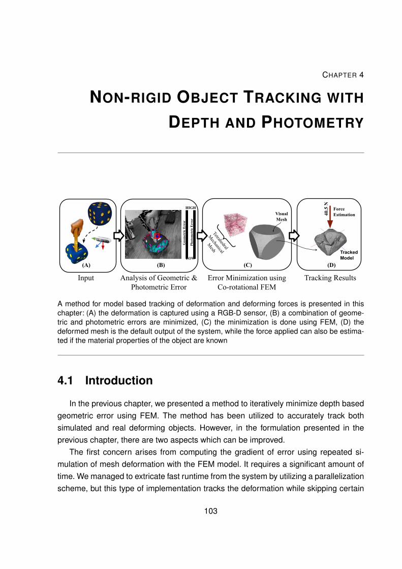
CHAPTER 4
NON-RIGID OBJECT TRACKING WITH
DEPTH AND PHOTOMETRY
A method for model based tracking of deformation and deforming forces is presented in thischapter: (A) the deformation is captured using a RGB-D sensor, (B) a combination of geome-tric and photometric errors are minimized, (C) the minimization is done using FEM, (D) thedeformed mesh is the default output of the system, while the force applied can also be estima-ted if the material properties of the object are known
4.1 Introduction
In the previous chapter, we presented a method to iteratively minimize depth basedgeometric error using FEM. The method has been utilized to accurately track bothsimulated and real deforming objects. However, in the formulation presented in theprevious chapter, there are two aspects which can be improved.
The first concern arises from computing the gradient of error using repeated si-mulation of mesh deformation with the FEM model. It requires a significant amount oftime. We managed to extricate fast runtime from the system by utilizing a parallelizationscheme, but this type of implementation tracks the deformation while skipping certain
103
Chapter 4 – Non-rigid Object Tracking with Depth and Photometry
frames, because the rigid tracking runs significantly faster than the non-rigid trackingmethod. It is not trivial to modify this algorithm into a sequentially real-time system.It is not possible to optimize ∼ 20 − 30 iterations of complete FEM simulation, eachcontaining ∼ 40− 60 iterations of the conjugate gradient solver into a real-time system.However, skipping intermediate frames is also not desirable.
The second aspect which merits closer inspection is the fact that purely depth ba-sed object tracking (especially using a point-to-plane distance based cost function) hasscope for improvement. In Chapter 2, we already noticed that combining photometricerror minimization with depth based error lead to better accuracy in the case of ri-gid tracking. It can be interpreted intuitively that addition of more error terms into theminimization loop of Chapter 3 should usually lead to better accuracy in the case ofnon-rigid object tracking too. The availability of images from the RGB sensor of thedepth camera leads us to conclude that a direct photometric intensity based error termis an obvious choice for this additional error.
In this chapter, we address these concerns arising out of Chapter 3. A frameworkis proposed to track non-rigid objects using RGB-D cameras by utilizing physically-based models. The physics of the model is similar to that proposed in Chapter 3, i.e.,co-rotational FEM. The methodology proposed here integrates classical computer vi-sion based error minimization using photometric and geometric cost functions with thedeformation simulation capabilities of co-rotational FEM.
The main contributions of the methodology proposed in this chapter are:
— Combined minimization of error terms based on depth and photometric informa-tion ;
— A new technique for approximating the gradient of these errors w.r.t displacementof vertices ;
— An improved methodology for determining the vertices which are to be controlledfor tracking ;
— Improved runtime
4.2 Background
This chapter combines classical computer vision with geometric analysis of de-forming manifolds and physics-based structural models from mechanical engineering.
104
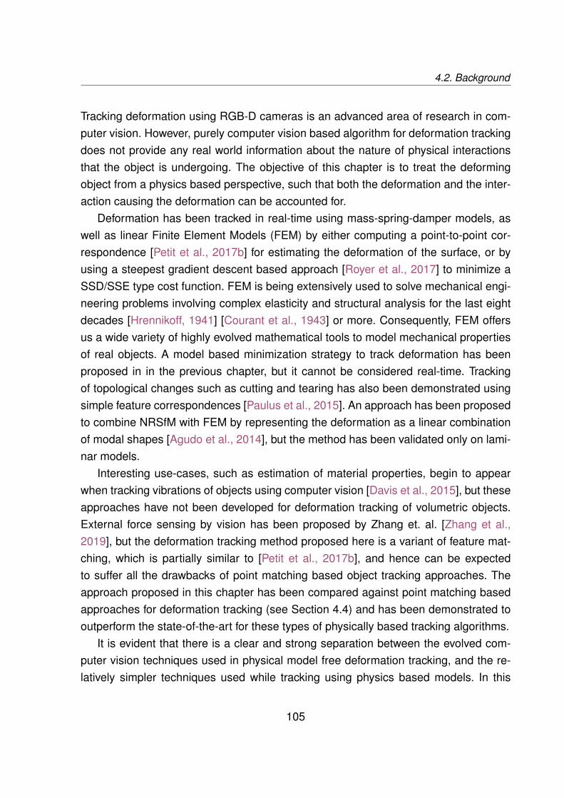
4.2. Background
Tracking deformation using RGB-D cameras is an advanced area of research in com-puter vision. However, purely computer vision based algorithm for deformation trackingdoes not provide any real world information about the nature of physical interactionsthat the object is undergoing. The objective of this chapter is to treat the deformingobject from a physics based perspective, such that both the deformation and the inter-action causing the deformation can be accounted for.
Deformation has been tracked in real-time using mass-spring-damper models, aswell as linear Finite Element Models (FEM) by either computing a point-to-point cor-respondence [Petit et al., 2017b] for estimating the deformation of the surface, or byusing a steepest gradient descent based approach [Royer et al., 2017] to minimize aSSD/SSE type cost function. FEM is being extensively used to solve mechanical engi-neering problems involving complex elasticity and structural analysis for the last eightdecades [Hrennikoff, 1941] [Courant et al., 1943] or more. Consequently, FEM offersus a wide variety of highly evolved mathematical tools to model mechanical propertiesof real objects. A model based minimization strategy to track deformation has beenproposed in in the previous chapter, but it cannot be considered real-time. Trackingof topological changes such as cutting and tearing has also been demonstrated usingsimple feature correspondences [Paulus et al., 2015]. An approach has been proposedto combine NRSfM with FEM by representing the deformation as a linear combinationof modal shapes [Agudo et al., 2014], but the method has been validated only on lami-nar models.
Interesting use-cases, such as estimation of material properties, begin to appearwhen tracking vibrations of objects using computer vision [Davis et al., 2015], but theseapproaches have not been developed for deformation tracking of volumetric objects.External force sensing by vision has been proposed by Zhang et. al. [Zhang et al.,2019], but the deformation tracking method proposed here is a variant of feature mat-ching, which is partially similar to [Petit et al., 2017b], and hence can be expectedto suffer all the drawbacks of point matching based object tracking approaches. Theapproach proposed in this chapter has been compared against point matching basedapproaches for deformation tracking (see Section 4.4) and has been demonstrated tooutperform the state-of-the-art for these types of physically based tracking algorithms.
It is evident that there is a clear and strong separation between the evolved com-puter vision techniques used in physical model free deformation tracking, and the re-latively simpler techniques used while tracking using physics based models. In this
105

Chapter 4 – Non-rigid Object Tracking with Depth and Photometry
chapter, we propose to bridge this divide between vision based tracking and mecha-nical models by enabling an iterative minimization strategy for generic, vision-basedcost functions using FEM. The method described here involves the minimization of acombination of a geometric and a photometric cost functions. A textureless, coarsemodel is required as the input of the system while the output consists of the tracked 3Dmodel. Moreover, the availability of an advanced physically based model enables us totrack the forces acting on the deformed object, whenever an approximate estimate ofthe material properties are available.
4.3 Proposed Approach
The input to the system consists of RGB-D data stream from a depth camera anda coarse 3D model of the surface of the object being tracked. Unlike similar methodsin the literature, we do not require the material properties of the object being trackedor the textured model of the object. For each frame, the first step is to approximatelytrack the rigid pose of the object w.r.t the camera (described in Section 4.3.3). This isfollowed by determining the approximate areas where the error in rigid registration hasa higher magnitude (see Section 4.3.2). The mesh vertices lying close to these areaswith high rigid registration error are termed as control handles. These control handlesare utilized to minimize a set of error terms (explained in Section 4.3.1), which aredefined w.r.t the surface model of the object.
4.3.1 Non-rigid Tracking
We briefly recap our motivation behind proposing the non-rigid object tracking me-thod of this chapter before explaining the technical details.
4.3.1.1 Motivation
The procedure for real-time, RGB-D based tracking of non-rigid objects withoutusing mechanical model usually involves the iterative minimization of one or multiplehighly non-linear objective function, such as point-to-point distance [Wang et al., 2017],point-to-plane distance [Newcombe et al., 2015], combination of point-to-plane dis-tance and sparse feature alignment error [Innmann et al., 2016], etc. However, in the
106

4.3. Proposed Approach
absence of a physics based framework for modelling the real-world properties of thedeforming object, a regularizing or smoothing data term is used to prevent unnaturaldeformations while tracking the object. For tracking using physics based models, theproblem statement becomes much more constrained due to the presence of a modelthat already mimics the physical properties of the actual object. The tracking methodo-logy changes from an iterative minimization to displacing one or multiple vertex/verticesto follow the object deformation, since estimating the gradient of the non-linear errorterm with respect to the vertex displacement involves time-consuming deformation si-mulation, which is not suitable for online tracking. However, we have demonstratedin Chapter 3 that iterative optimization of depth based error term is possible usingphysically-based model and results in accurate tracking. Through the mechanism pro-posed in this chapter for tracking non-rigid objects, we aim to bridge this divide betweenthe physical-model free and physical-model based approaches even further. This isdone by the minimization of photometric error term along with depth based error whilethe gradient of error in approximated analytically. We first describe the overall frame-work for generic objective functions. The specific error term is described thereafter.
4.3.1.2 Methodology
We now describe our proposed methodology for tracking non-rigid objects. Let usdenote the non-linear error term that we seek to minimize by E. We first discuss theprocedure that we follow to minimize this error using the physically based model, i.e.,co-rotational FEM. Throughout the rest of the chapter, the notation PM is used to de-note the vertices of the mechanical tetrahedral mesh VM, while P = (PX,PY,PZ) de-notes the vertices of the surface model VS w.r.t the object centered reference frame Fo.The surface model consists of triangular faces and the j-th face is denoted by:
Vj︸︷︷︸3×3
=(Pi Pi+1 Pi+2
)(4.1)
starting from the i-th vertex of VS. The mapping VS 7→ VM is done via a standardmaster-slave configuration using barycentric mapping. The RGB-D camera is assu-med to be at a reference frame Fc. For the sake of brevity, the baseline between thedepth and the color camera is not mentioned explicitly and all data presented here areassumed to be aligned with the color camera.
107

Chapter 4 – Non-rigid Object Tracking with Depth and Photometry
Let us assume that the method chosen for the deformation tracking involves a phy-sical model P that describes the interaction between the applied forces and displace-ment of the vertices of VM. Recall that VM is coupled with the surface geometry VS ofthe object. We propose to track the deformation of this object using the minimizationof one or multiple error term(s) defined strictly on the triangular elements of the facesof VS. This is done by defining a set of control handles C on VM, such that the entiredeformation becomes optimizable by regulating the displacement of C. Note that anydisplacement of C gets propagated to all vertices of VM using the properties of P. Withthese constraints in place, let us assume that we are trying to optimize for a set of Nobjective functions E1,E2, ...,EN, defined on VS. We are interested in minimizing
ES = (E1,E2, · · ·,EN) (4.2)
with the help of the displacement vector on C, given by uC. However, to opti-mize in a non-linear least squares fashion, we need to obtain the gradient of the sta-cked/combined cost function, which can be done numerically. But with any modernphysical model P, numeric estimation can be computationally expensive as determi-ning the node displacements typically involves multiple iteration of conjugate gradientdescent for solving an equation of the nature of (3.4). This is beyond the reasonablelimits of performance optimization and, to the best of our knowledge, online method fordeformation tracking using minimization of visual error term(s) w.r.t node displacementsof a mechanical model is unavailable in the literature. We propose an assumption tosolve this problem, as described below.
Let us analyze the case of an arbitrary point p of the RGB-D pointcloud, which lieson the triangle
(Pi Pi+1 Pi+2
)of VS. Let us assume that a small displacement:
∆uC =[∆uCX ∆uCY ∆uCZ
](4.3)
produces the displacement ∆x,∆y and ∆z on the j-th surface plane of VS comprisingof three vertices Pi,Pi+1 and Pi+2 respectively. This vector of vertex positions is givenby:
ϑj =[P>i P>i+1 P>i+2
](4.4)
108

4.3. Proposed Approach
Subsequently, the gradient of the error ES(p) w.r.t uC is given by the Jacobian:
JS(p) = ∂ES(p)∂uC
= ∂ES(p)∂ϑj1×9
∂ϑj∂uC9×3
(4.5)
Estimating ∂ES(p)∂ϑj
is usually a straightforward modification of a series of well establishedtechniques in computer vision [Hartley and Zisserman, 2003]. The details of how thiscan be done in our case is demonstrated in section 4.3.4. On the other hand, the term∂ϑj∂uC
is somewhat similar to the classical strain-displacement matrix, as expressed inconventional FEM literature. As stated before, determining the exact value of ∂ϑj
∂uCfor
any sufficiently advanced choice of P will require computationally expensive simulationof model deformation at every iteration of the non-linear least squares solver.
We propose that this additional complexity can be avoided by estimating the de-formation of the mechanical model VM, for every new control handle explored by ourproposed approach, only once. For the j-th control handle Cj, this is done by displacingthe vertex in VM corresponding to Cj by a small distance along the positive directionof X, Y and Z axis. The magnitude of this deformation ∆uC is empirically determinedsuch that it slightly exceeds the RMSE of the sensor noise (e.g: we use Intel RealSenseD435 for capturing the real data, and the magnitude of ∆uC was set to 2 mm, whichsuccessfully overwhelmed the sensor noise [Ahn et al., 2019]).
This estimation step produce three deformed meshes per control handle, which canbe directly utilized for determining ∂ϑj
∂uCusing forward finite differences. Assuming that
uC points to the c-th vertex of VM, the values of ∂Pi∂uC
can be mapped to a matrix ΓO bya mapping function C such that:
ΓO = C( ∂Pi
∂uC
)(4.6)
given that:∂ϑj∂uC
=(∂Pi∂uC
, ∂Pi+1∂uC
, ∂Pi+2∂uC
)(4.7)
Here, C represents the mapping ∂Pi∂uC7→ ΓO and it is a one-to-one, bijective map as
long as the number of vertices in VM and VS are equal. Assuming that M denotes the
109
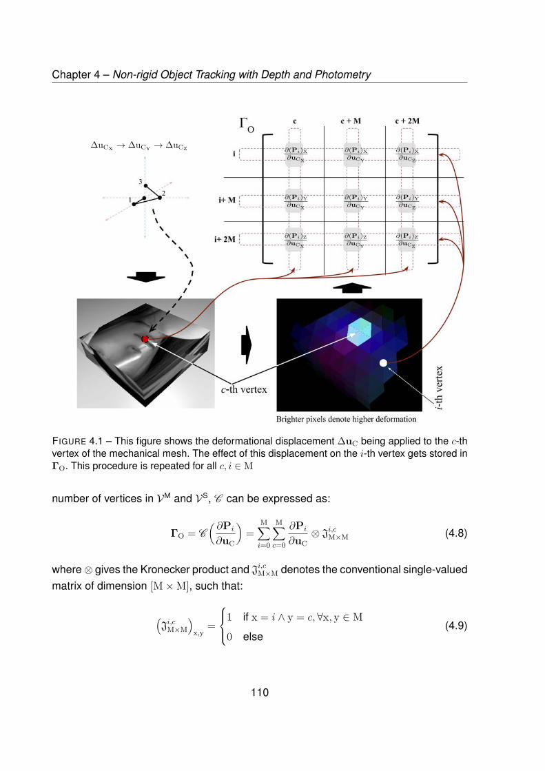
Chapter 4 – Non-rigid Object Tracking with Depth and Photometry
∆uCX → ∆uCY → ∆uCZ ∂(Pi)X∂uCX
∂(Pi)Y∂uCX
∂(Pi)Z∂uCX
∂(Pi)X∂uCY
∂(Pi)Y∂uCY
∂(Pi)Z∂uCY
∂(Pi)X∂uCZ
∂(Pi)Y∂uCZ
∂(Pi)Z∂uCZ
FIGURE 4.1 – This figure shows the deformational displacement ∆uC being applied to the c-thvertex of the mechanical mesh. The effect of this displacement on the i-th vertex gets stored inΓO. This procedure is repeated for all c, i ∈ M
number of vertices in VM and VS, C can be expressed as:
ΓO = C(∂Pi
∂uC
)=
M∑i=0
M∑c=0
∂Pi
∂uC⊗ Ji,cM×M (4.8)
where⊗ gives the Kronecker product and Ji,cM×M denotes the conventional single-valuedmatrix of dimension [M×M], such that:
(Ji,cM×M
)x,y
=
1 if x = i ∧ y = c,∀x, y ∈ M
0 else(4.9)
110
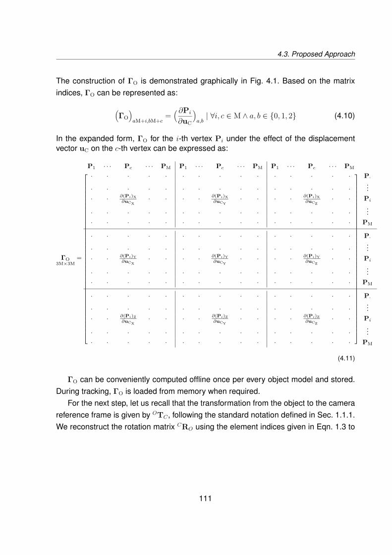
4.3. Proposed Approach
The construction of ΓO is demonstrated graphically in Fig. 4.1. Based on the matrixindices, ΓO can be represented as:
(ΓO)aM+i,bM+c
=( ∂Pi
∂uC
)a,b| ∀i, c ∈ M ∧ a, b ∈ 0, 1, 2 (4.10)
In the expanded form, ΓO for the i-th vertex Pi under the effect of the displacementvector uC on the c-th vertex can be expressed as:
ΓO3M×3M
=
P1 · · · Pc · · · PM P1 · · · Pc · · · PM P1 · · · Pc · · · PM
· · · · · · · · · · · · · · · P·
· · · · · · · · · · · · · · ·...
· · ∂(Pi)X∂uCX
· · · · ∂(Pi)X∂uCY
· · · · ∂(Pi)X∂uCZ
· · Pi
· · · · · · · · · · · · · · ·...
· · · · · · · · · · · · · · · PM
· · · · · · · · · · · · · · · P·
· · · · · · · · · · · · · · ·...
· · ∂(Pi)Y∂uCX
· · · · ∂(Pi)Y∂uCY
· · · · ∂(Pi)Y∂uCZ
· · Pi
· · · · · · · · · · · · · · ·...
· · · · · · · · · · · · · · · PM
· · · · · · · · · · · · · · · P·
· · · · · · · · · · · · · · ·...
· · ∂(Pi)Z∂uCX
· · · · ∂(Pi)Z∂uCY
· · · · ∂(Pi)Z∂uCZ
· · Pi
· · · · · · · · · · · · · · ·...
· · · · · · · · · · · · · · · PM
(4.11)
ΓO can be conveniently computed offline once per every object model and stored.During tracking, ΓO is loaded from memory when required.
For the next step, let us recall that the transformation from the object to the camerareference frame is given by OTC , following the standard notation defined in Sec. 1.1.1.We reconstruct the rotation matrix CRO using the element indices given in Eqn. 1.3 to
111
Chapter 4 – Non-rigid Object Tracking with Depth and Photometry
represent a modified matrix RΓ representing the rotation such that:
RΓ3M×3M
= CRO ⊗ 1M×M =
diag(r11)M
diag(r12)M
diag(r13)M
diag(r21)M
diag(r22)M
diag(r23)M
diag(r31)M
diag(r32)M
diag(r33)M
(4.12)
where:
diag(rx)M
=
rx
. . .
rx
︸ ︷︷ ︸
M×M
(4.13)
and 1M×M is an identity matrix of dimension [M×M]. This allows us to rotate ΓO (obtai-ned from offline computation) to the current camera reference frame. This transformedmatrix ΓC is given by:
ΓC = RΓΓO (4.14)
We then derive the matrix Γ by thresholding ΓC such that its value at an arbitraryindex m, n associated with the i-th vertex Pi is given by:
Γm,n =
1 if ε > 3α||∆uC ||2
0 else(4.15)
given that:
ε =2∑
a=0
2∑b=0
((ΓC)m+a,n+b
)2(4.16)
where ∆uC is the calibrating deformation (implying that ||∆uC || is a constant for aparticular ΓO). α is a tunable parameter which regulates the area for which the value ofΓ will be 1.
At this point, it is natural to question the necessity of thresholding the value of ΓC.using Eqn. (4.15). This thresholding is done purely because we intend to utilize thepoint-to-plane distance as an error term in the minimization, as explained in Sec. 4.3.4.Point-to-plane distance minimization using planar (or nearly planar) surface model re-
112
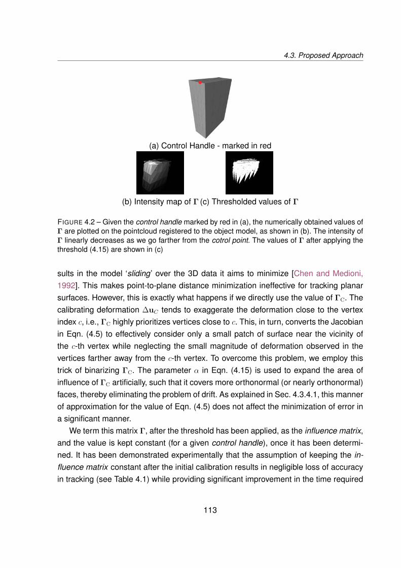
4.3. Proposed Approach
(a) Control Handle - marked in red
(b) Intensity map of Γ (c) Thresholded values of Γ
FIGURE 4.2 – Given the control handle marked by red in (a), the numerically obtained values ofΓ are plotted on the pointcloud registered to the object model, as shown in (b). The intensity ofΓ linearly decreases as we go farther from the cotrol point. The values of Γ after applying thethreshold (4.15) are shown in (c)
sults in the model ‘sliding’ over the 3D data it aims to minimize [Chen and Medioni,1992]. This makes point-to-plane distance minimization ineffective for tracking planarsurfaces. However, this is exactly what happens if we directly use the value of ΓC. Thecalibrating deformation ∆uC tends to exaggerate the deformation close to the vertexindex c, i.e., ΓC highly prioritizes vertices close to c. This, in turn, converts the Jacobianin Eqn. (4.5) to effectively consider only a small patch of surface near the vicinity ofthe c-th vertex while neglecting the small magnitude of deformation observed in thevertices farther away from the c-th vertex. To overcome this problem, we employ thistrick of binarizing ΓC. The parameter α in Eqn. (4.15) is used to expand the area ofinfluence of ΓC artificially, such that it covers more orthonormal (or nearly orthonormal)faces, thereby eliminating the problem of drift. As explained in Sec. 4.3.4.1, this mannerof approximation for the value of Eqn. (4.5) does not affect the minimization of error ina significant manner.
We term this matrix Γ, after the threshold has been applied, as the influence matrix,and the value is kept constant (for a given control handle), once it has been determi-ned. It has been demonstrated experimentally that the assumption of keeping the in-fluence matrix constant after the initial calibration results in negligible loss of accuracyin tracking (see Table 4.1) while providing significant improvement in the time required
113
Chapter 4 – Non-rigid Object Tracking with Depth and Photometry
to handle each data frame (see Table 4.2). Intuitively, these values after applying thethreshold in the influence matrix merely determines the faces of VS for which the errorterm ES will be minimized, as shown in figure 4.2. Replacing the matrix elements with1 turns M into a pseudo-rigid object around the vicinity of uC . As long as the inter-frame deformation remains small, this assumption remains valid and does not affectthe outcome of the minimization in a significant manner.
4.3.2 Determining the Control Handles
The determination of the control handles can also be handled in a generic way. Gi-ven the set of N objective functions of ES acting on L different points of the pointcloud,such that p =
(p1 p2 · · · pL
). We define a function IEn
(Π(pL)
)which represents
the error value using the n-th cost function En(pl) projected on the image. The combi-ned error matrix IES
(Π(p)
)on the image plane is obtained by:
IES
(Π(p)
)=⟨IE1
(Π(p)
)⟩ · · ·
⟨IEN
(Π(p)
)⟩(4.17)
where denotes the Hadamard product and 〈·〉 gives the normalized matrix. IES
(Π(p)
)is clustered into multiple clusters, and the centroid of each cluster is associated withthe nearest vertex Π(r), the projection of the visible vertices of VM on the image plane.These associated vertices of VM are identified as the control handles for that particu-lar frame. This approach of determining the point of interest is highly effective, since ittreats the determination of control handles as a function of the objective functions inuse.
4.3.3 Approximate Rigid Tracking
Before commencing the minimization of the objective function(s) used for deforma-tion tracking, the rigid pose of the object in the current frame needs to be determinedapproximately. This enables us to track the deforming motions acting on the surfaceof the object alone, without having to care about the interaction with the surroundingscene (forces causing rigid motion, friction, collision etc.). This is done in a mannerexactly similar to Sec. 3.2.3.
114

4.3. Proposed Approach
4.3.4 Non-rigid Error Terms
Once an approximate estimate of pTp−1 has been obtained, a combination of depthbased geometric error and direct photometric error is minimized to achieve the trackingof the deformation using the method described in Section 4.3.1. We now define theerror term that needs to be minimized for a single point p of the pointcloud at the p-thdata frame. The point-to-plane distance based geometric error is given by:
EN(pp) = nj · ppl − dj (4.18)
assuming that the j-th surface of VS has been associated with the l-th point of pointcloudpl. We propose a photometric error term defined on the (p-1)-th frame by:
EP(pp−1) = Ip(pp−1e )− Ip−1(pp−1) (4.19)
The updated point position pp−1e is determined by a barycentric map
pp−1e =
[P′i P′i+1 P′i+2
]B (4.20)
such that pp−1 corresponded with the triangle(Pi Pi+1 Pi+2
)and P′i gives the upda-
ted vertex position of Pi when subject to the update ϑ, given that B is a column vectordenoting the barycentric coordinates of pp−1 w.r.t Pi,Pi+1 and Pi+2.
The combined cost function is given by ES = (EN, µEP), where µ = ‖EN‖‖EP‖
is used forbringing the geometric and photometric error terms to the same scale. Following theoutline provided by (4.5), we can now develop the partial derivatives ∂EN(p)
∂ϑand ∂EP(p)
∂ϑ.
4.3.4.1 Jacobian
We describe the method to obtain the Jacobian for the geometric and photometricerror term described in Eqn. 4.18 and Eqn. 4.19. The combined cost function that weseek to minimize is given as:
ES = (EN, µEP) (4.21)
We aim to minimize (4.21) w.r.t uC , the displacement of the control handle. The
115

Chapter 4 – Non-rigid Object Tracking with Depth and Photometry
Jacobian relating the change of uC to the change of ES is given by:
J = ∂ES
∂uC= ∂EN
∂ξ
µ∂EP∂ξ
Γ (4.22)
where:
∂EN
∂ξ=
−n>j − n>l
(A[Pi+2 −Pi+1
]×
)−n>l (A
[Pi −Pi+2
]×
)−n>l
(A[Pi+1 −Pi
]×
)>
(4.23)
whereA = 1
‖nj‖(13×3 − njn>j ) (4.24)
given that:nj = (Pi+2 −Pi)× (Pi+1 −Pi) (4.25)
and nl = ppl −Pi.On the other hand:
∂EP
∂ξ=[∇Iup ∇Ivp
]
b1 00 b1
b2 00 b2
b3 00 b3
>
HPi
HPi+1
HPi+2
19×9 (4.26)
where:
HPq = fx
(Pq)Z 0 −fx (Pq)X(Pq)2
Z
0 fy(Pq)Z −fy (Pq)Y
(Pq)2Z
∀q ∈ i, (i+ 1), (i+ 2) (4.27)
and B =(b1, b2, b3
)are the barycentric coordinates.
The optimization method of our choice is Iteratively Re-weighted Least Squares(IRLS) solver, and the update is given by:
∆uC = −λ(WJ
)+WES (4.28)
where W is a weighting matrix using Tukey based M-estimator [Meer et al., 1991], andλ is a scaling factor. The new position uC+∆uC of Cj is to be applied on the mechanical
116
4.3. Proposed Approach
model such that it deforms to minimize the errors from (4.18) and (4.19).
4.3.5 Implementing the Mechanical Model
The goal of this chapter is to formalize a method for dissociating the cost functionES from the physical model P while using them together to solve a non-linear leastsquares problem. To this end, as indicated in Sec. 1.3.1, we intend to base our choiceof P on FEM. In practice, we validate our approach using two mechanical models: alinear FEM and a co-rotational FEM using a tetrahedral mesh.
As indicated in section 4.3.3, the rigid tracking of the object is handled withoutusing the mechanical model (i.e., only based on the surface model), thereby allowingthe deformation estimation to tackle a better posed problem. The object is assumedto be attached to a fixed base via projective constraints on the vertices of M that lieson the ground plane, thereby eliminating the necessity of modelling friction or contactforces.
4.3.6 Force Tracking
With the deformation tracking methodology in place, it is possible to utilize this ap-proach to online estimate the deforming forces acting on the object. To do this, twoadditional constraints are required: the material properties of the object being tracked,i.e., Young’s modulus, Poisson’s ratio, Rayleigh stiffness etc. and the approximate pointof contacts on the object. The control handles derived in Section 4.3.2 are virtual pointsthat may or may not have a physical meaning. However, to track forces, we need theactual points of application of force. All our force tracking examples have been perfor-med by tracking the tool applying the force using external, fiducial markers (classicalhand or finger tracking algorithms [Letessier and Bérard, 2004] [Hamer et al., 2009]can be used in unison with the approach proposed here to freely track applied forceson hand-manipulated objects).
Once a point PC has been identified as the point of contact, its nearest mechanicalmesh vertex PM
C is obtained using a nearest neighbor search. Thereafter, the forceapplied on PC is given as
∥∥∥∥∑i
FPMi
∥∥∥∥, for all indices i such that PMC is a neighbor of PM
i ,
wherein the force vectors FPMi
is derived using (3.3).
117
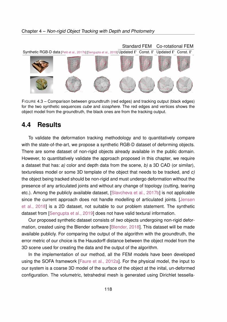
Chapter 4 – Non-rigid Object Tracking with Depth and Photometry
Standard FEM Co-rotational FEMSynthetic RGB-D data [Petit et al., 2017b] [Sengupta et al., 2019] Updated Γ Const. Γ Updated Γ Const. Γ
FIGURE 4.3 – Comparison between groundtruth (red edges) and tracking output (black edges)for the two synthetic sequences cube and icosphere. The red edges and vertices shows theobject model from the groundtruth, the black ones are from the tracking output.
4.4 Results
To validate the deformation tracking methodology and to quantitatively comparewith the state-of-the-art, we propose a synthetic RGB-D dataset of deforming objects.There are some dataset of non-rigid objects already available in the public domain.However, to quantitatively validate the approach proposed in this chapter, we requirea dataset that has: a) color and depth data from the scene, b) a 3D CAD (or similar),textureless model or some 3D template of the object that needs to be tracked, and c)the object being tracked should be non-rigid and must undergo deformation without thepresence of any articulated joints and without any change of topology (cutting, tearingetc.). Among the publicly available dataset, [Slavcheva et al., 2017b] is not applicablesince the current approach does not handle modelling of articulated joints. [Jensenet al., 2018] is a 2D dataset, not suitable to our problem statement. The syntheticdataset from [Sengupta et al., 2019] does not have valid textural information.
Our proposed synthetic dataset consists of two objects undergoing non-rigid defor-mation, created using the Blender software [Blender, 2018]. This dataset will be madeavailable publicly. For comparing the output of the algorithm with the groundtruth, theerror metric of our choice is the Hausdorff distance between the object model from the3D scene used for creating the data and the output of the algorithm.
In the implementation of our method, all the FEM models have been developedusing the SOFA framework [Faure et al., 2012a]. For the physical model, the input toour system is a coarse 3D model of the surface of the object at the inital, un-deformedconfiguration. The volumetric, tetrahedral mesh is generated using Dirichlet tessella-
118
4.4. Results
tion and by Delaunay tetrahedralization of the input mesh using the Bowyer-Watsonalgorithm [Si, 2015]. The initialization of CTO at the very first frame is done by mat-ching pre-trained markers with those extracted from the initial images, similar to theapproach of [Choi and Christensen, 2010]. Since we track the model frame-to-frame,no segmentation is required for this approach.
Frame 4: Re-implementation of [Petit et al., 2015a]
In [Petit et al., 2015a], the images from the RGB-D sensor are segmented to isolatethe object to be tracked using a grabcut approach, which is in turn utilized to extracta segmented pointcloud. To track the deformation of this object, an external force isapplied to the mechanical model (simulated with FEM) of the object. The per-vertexforce exerted is given by:
Fexti = ζik(PVmi −Pψ
i ) (4.29)
where Fexti is the external force vector for the i-th element of Vm which is given by
PVmi , ζi = σ1e−( diσ2
) such that di is the closest distance of PVmi from the projected 2Dcontour of the object, σ1 and σ2 are two empirically chosen constants, k is the stiffnessof the element corresponding to the i-th node, and the variable Pψ
i is obtained from thesegmented pointcloud ψ by the formulation:
Pψi =
αNNψ(PVmi ) + (1− α) 1
#ψi
∑Pj∈ψi
Pj if #ψi > 0
αNNψ(PVmi ) + (1− α)PVmi else(4.30)
where NNψ(PVmi ) denotes the nearest neighbor of PVmi in ψ, ψi is a subset of ψ suchthat ∀(ψi)j ∈ ψi there exists NNVm((ψi)j) = PVmi and α is a tunable parameter. Someadditional weights are assigned to the vertices based on the distance to the nearestcontour of the mesh, as visible from the projection of the model on the image plane. Were-implement this method from [Petit et al., 2015a], while implementing co-rotationalFEM using SOFA library and repeat the experiments while fine-tuning the empiricalparameters. We keep only the best results among all the experiments. Moreover, toavoid ambiguity, we restrict the comparison to dataset with small deformation only (de-formation confined inside the contour of the projected model).
119
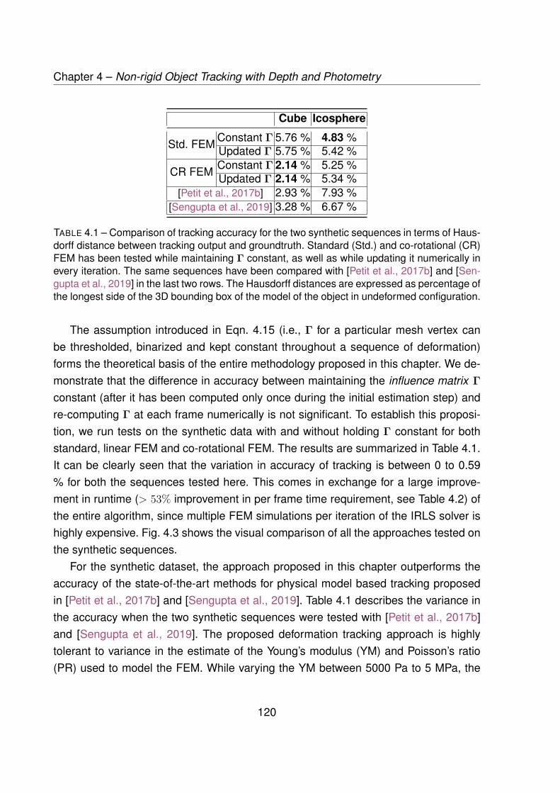
Chapter 4 – Non-rigid Object Tracking with Depth and Photometry
Cube Icosphere
Std. FEM Constant Γ 5.76 % 4.83 %Updated Γ 5.75 % 5.42 %
CR FEM Constant Γ 2.14 % 5.25 %Updated Γ 2.14 % 5.34 %
[Petit et al., 2017b] 2.93 % 7.93 %[Sengupta et al., 2019] 3.28 % 6.67 %
TABLE 4.1 – Comparison of tracking accuracy for the two synthetic sequences in terms of Haus-dorff distance between tracking output and groundtruth. Standard (Std.) and co-rotational (CR)FEM has been tested while maintaining Γ constant, as well as while updating it numerically inevery iteration. The same sequences have been compared with [Petit et al., 2017b] and [Sen-gupta et al., 2019] in the last two rows. The Hausdorff distances are expressed as percentage ofthe longest side of the 3D bounding box of the model of the object in undeformed configuration.
The assumption introduced in Eqn. 4.15 (i.e., Γ for a particular mesh vertex canbe thresholded, binarized and kept constant throughout a sequence of deformation)forms the theoretical basis of the entire methodology proposed in this chapter. We de-monstrate that the difference in accuracy between maintaining the influence matrix Γconstant (after it has been computed only once during the initial estimation step) andre-computing Γ at each frame numerically is not significant. To establish this proposi-tion, we run tests on the synthetic data with and without holding Γ constant for bothstandard, linear FEM and co-rotational FEM. The results are summarized in Table 4.1.It can be clearly seen that the variation in accuracy of tracking is between 0 to 0.59% for both the sequences tested here. This comes in exchange for a large improve-ment in runtime (> 53% improvement in per frame time requirement, see Table 4.2) ofthe entire algorithm, since multiple FEM simulations per iteration of the IRLS solver ishighly expensive. Fig. 4.3 shows the visual comparison of all the approaches tested onthe synthetic sequences.
For the synthetic dataset, the approach proposed in this chapter outperforms theaccuracy of the state-of-the-art methods for physical model based tracking proposedin [Petit et al., 2017b] and [Sengupta et al., 2019]. Table 4.1 describes the variance inthe accuracy when the two synthetic sequences were tested with [Petit et al., 2017b]and [Sengupta et al., 2019]. The proposed deformation tracking approach is highlytolerant to variance in the estimate of the Young’s modulus (YM) and Poisson’s ratio(PR) used to model the FEM. While varying the YM between 5000 Pa to 5 MPa, the
120
4.4. Results
accuracy varied by less than 0.001%, which is practically negligible. While varying thePoisson’s ratio between 0.2 and 0.5, the accuracy drifted by < 0.129%.
To validate our approach on real objects, we utilized two objects: a deformable dicemade of foam and a block of sponge in the shape of a cuboid. The results are visuallydemonstrated in Fig. 4.4. The tracking results are visually coherent while sufferingocclusions/outliers in the range of ±5 cm. The dice was compressed for more than14 cm (> 87% of its own height), but our approach still tracked the entire deformationaccurately.
4.4.1 Validation of Force Tracking
To validate the force tracking methodology, we use a 6-DOF anthropomorphic robotarm (a Viper 850 from ADEPT) fitted with a ATI Gamma IP65 force/torque sensor anda 3D-printed stylus as an end-effector distal tool. The robot is used only to utilize itsforce sensor to obtain a groundtruth of the force that is being applied on the object. Toget a proper estimate of the force using the proposed method, we need to know thematerial property (Young’s modulus, Poisson’s ratio, etc.) of the object, and the pointof contact needs to be measured separately. To demonstrate this feature, we use thesponge and a ball made of foam. First, the Young’s modulus of the sponge and the ballis determined by repeated indentation tests. It is determined that the sponge and theball has a Young’s modulus of 460 kPa and 160 kPa respectively. Next, these objectsare subjected to a strong deformation using the robot’s end-effector, while our proposedmethod is used to track the deformation and the force applied simultaneously. The 3Dprinted end-effector is tracked using pre-trained markers from the image data of theRGB-D camera. The mesh vertex nearest to the tip of the end-effector gives us thepoint of contact. The results of the force tracking approach are summarized in Fig. 4.5.
We observe a force tracking accuracy of ∼ 97% for the sponge and of ∼ 90% forthe ball, when the deformation is optimally observable. For very small deformations(< 1 cm), the sensor noise causes small variances in the force measurement whileat very large deformation, the tip of the end-effector occludes the deformed surfaceto a very large extent, causing the accuracy to decrease in the experiment with thesponge. However, with properly observable deformations (> 1 cm and free from largeocclusions), the approach is very accurate. The measured forces show a consistentPearson correlation coefficient of > 0.92 with the actually applied forces over a large
121
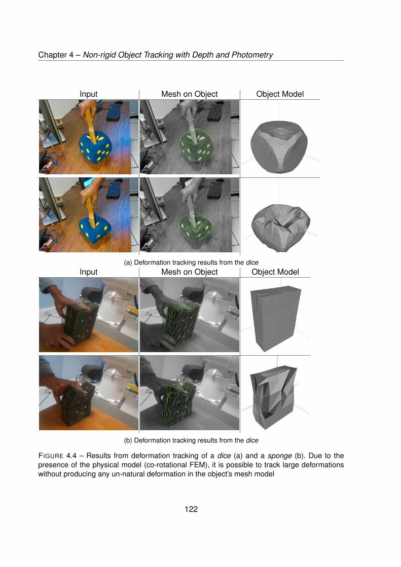
Chapter 4 – Non-rigid Object Tracking with Depth and Photometry
Input Mesh on Object Object Model
(a) Deformation tracking results from the diceInput Mesh on Object Object Model
(b) Deformation tracking results from the dice
FIGURE 4.4 – Results from deformation tracking of a dice (a) and a sponge (b). Due to thepresence of the physical model (co-rotational FEM), it is possible to track large deformationswithout producing any un-natural deformation in the object’s mesh model
122

4.4. Results
number of experiments.
(a) Sponge - deformation setup (b) Sponge - tracked mesh (d) Ball - deformation setup (e) Ball - tracked mesh
(c) Actual vs. Measured Force : sponge (f) Actual vs. Measured Force : ball
Forc
e (
N)
Forc
e (
N)
Iteration # Iteration #
4.93 N
17.74 N
36.93 N
62.78 N
2.10 N
6.31 N
12.11 N
18.85 N
26.08 N
35.13 N
highly accurate
(~ 96.9 %)accuracy > 90%
Actuator occludes
the deforming area
FIGURE 4.5 – Setup and results for force tracking on the sponge. The Viper 850 robot is beingused deform the object while being tracked. The red plot is the force measurement from therobot’s force sensor, the blue plot is the estimated force reported by the proposed approach
4.4.2 Runtime Evaluation
The experiments discussed in this chapter were performed on a Intel Xeon CPUworking at 3.70GHz. Utilizing only a single core of the computer, the un-optimised codewas able to achieve a runtime of 350 msec - 550 msec/frame while tracking deforma-tions using the constant value of Γ, showing that it can achieve real-time performanceat frame rate. The time taken to estimate the value of Γ for each node is approximately0.5 sec - 0.6 sec per frame, which is a one time cost that can be either done offlineor computed when needed, as per the requirements of the application. The runtime forthe real data used in this chapter is summarized in Table 4.2.
123

Chapter 4 – Non-rigid Object Tracking with Depth and Photometry
Constant Γ Updated Γ
Std. FEM Dice 0.505 sec 1.401 secSponge 0.492 sec 0.825 sec
CR FEM Dice 0.393 sec 1.007 secSponge 0.465 sec 0.734 sec
TABLE 4.2 – Comparison of the per frame time requirement for deformation tracking withconstant and updated values of Γ using Standard (Std.) and Co-rotational (CR) FEM
4.5 Conclusion
The chapter presented here describes a new method for combining visual errorminimization with FEM to create an accurate and fast deformation tracking method.The algorithm has been tested on synthetic and real data and has been shown tooutperform state-of-the-art methods in tracking accuracy for generic deforming objects.The algorithm proposed here can be extended to other, more complex physical modelswithout loss of generalization. The method proposed here has been demonstrated asa reliable visual force tracking system, when the material properties of the object beingtracked are available. We believe that there is a large potential for such applications inthe field of robotics and augmented/mixed reality.
In this dissertation, we have so far presented two different approaches for deforma-tion tracking. In the next chapter, we are going to present some applications of defor-mation tracking, especially highlighting the benefits of using a FEM based approach asthe primary deformation model. We will present a robotic application involving estima-tion of elasticity parameters of a deforming object while it is being tracked by a RGB-Dcamera.
124
CHAPTER 5
ROBOTIC APPLICATIONS FOR
NON-RIGID OBJECT TRACKING
The preceding chapters dealt with different mechanisms to track deforming objectusing mechanical model. As indicated in Chapter 1, the usage of mechanical modelsenable us to re-utilize these deformation tracking methodologies into some interes-ting use-cases, which would not have been straightforward using physical model-freedeformation tracking approaches. In this chapter, we take a look into some of the practi-cal applications that arises out of using physical models for deformation tracking. Morespecifically, we describe a method to estimate the physical properties of an object usingthe deformation tracking algorithm and an external force sensor mounted on a roboticarm. Later in this chapter, we extend that approach to track freely applied forces on theobject, once the physical properties have been determined.
Robotic manipulation of rigid objects is a well-studied and well-developed area ofresearch. However, non-rigid object manipulation using robotic end-effector is a moredifficult problem to address. Part of the problem arises from the fact that real-time tra-cking of non-rigid objects had been an unsolved problem until the last few years. Evenwith the recent development of non-rigid object tracking methods using computer vi-sion, there remains significant scope for improvement in tracking the entire surfacemodel of the object under challenging conditions. Another important question arisingwhile interacting with soft objects is the determination of the elasticity parameters ofthe object, especially the Young’s modulus. Simultaneous manipulation and trackingof deformable objects could improve different use-cases such as humanoid robots in-teracting with soft objects, compliance testing in product manufacturing or automated,preventive healthcare [Stults, 1984]. The aim of this approach is to simultaneouslytrack and estimate the elasticity parameters of a soft object that is being deformed bythe end-effector of a robot. In this chapter, we propose a closed-loop method consis-ting of: a) a deformation tracking method and b) an elasticity estimation algorithm. This
125
Chapter 5 – Robotic Applications for Non-rigid Object Tracking
closed-loop method allows to achieve two objectives: STEPE (Simultaneous Trackingand Estimation of Parameters of Elasticity) and remote force estimation. The requiredinputs of STEPE are a coarse 3D geometric model (mesh) of the object to track and theexternal measurements of the forces deforming the object. The deformation trackingmethod uses a depth sensor to capture the deformation and tracks it using a physics-based simulation of the object deformations. The elasticity estimation algorithm usesthe result of the deformation tracking method and measurements of the deformationforces, obtained from an external force sensor, in order to estimate the elasticity pa-rameters of the object. Once the elasticity estimation is achieved, the parameter canbe used by the deformation tracking method, thereby closing the loop. The methodwill iteratively converge towards a correct estimation of the elasticity parameters ofthe object. The elasticity parameters obtained at the convergence of the method arethereafter used for remote force estimation. From this stage, the deformation trackingmethod can be used to estimate the deformation forces acting on the object withoutany external force sensor.
The main contributions of this chapter are summarized below:
— We propose a novel method to simultaneously track the deformation of soft ob-jects and estimate their elasticity parameter. The tracking of the deformable objectis performed by combining the visual information acquired with a RGB-D sensorwith interactive simulation of the object deformation based on FEM;
— In parallel, the elasticity parameter estimation minimizes the error between thetracked object and a simulated object deformed by the forces that are measuredusing a force sensor ;
— Once the elasticity parameters are estimated, our tracking algorithm can thenalso be used to estimate the deformation forces applied on an object without theuse of a force sensor
5.1 Background
As discussed in Sec. 1.3, non-rigid object tracking can be done using either aphysics-based model, or a geometry-based model for computing the deformations.Both physics-based model such as [Newcombe et al., 2015, Innmann et al., 2016] orgeometric-based models such as [Bronte et al., 2017,Bronte et al., 2014] offer mecha-
126

5.1. Background
nism to track complex 3D shapes without utilizing any kind of machine-learning basedapproach. However, iteratively refining the physical parameters of the object being tra-cked is not possible using any of these techniques. Zhang et al. use a RGB-D camera totrack the external forces applied on an object, but they utilized very specific soft-robotsfor the purpose, instead of doing it for any arbitrary deformable objects [Zhang et al.,2019]. The approach of Petit et al. [Petit et al., 2018] is better suited for the purposeof deformation tracking using a physics-based model. However, since it relies solely ondepth data and a point-to-plane correspondence matching scheme to determine thedirection and magnitude of deformation, this approach is more susceptible to error in-duced from incorrect correspondences due to heavy occlusions. Among the machinelearning based approaches for deformation tracking, Varol et al. use a constrained la-tent variable model for learning the deformational behavior of an object from its latentstate to an output state [Varol et al., 2012]. The results from this approach has howe-ver only been demonstrated on planar objects. From the literature, the methodologyproposed by Frank et al. [Frank et al., 2010] has some resemblance to the methodproposed in this chapter for simultaneously tracking deformation and estimating para-meters. The approach utilizes a combined tracking and elasticity estimation modulesusing a point-to-point ICP [Besl and McKay, 1992] for pointcloud registration along witha linear, tetrahedral FEM as the deformation model. The use of linear FEM makes thisapproach not suitable when large rotational deformations occur. Additionally, point-to-point ICP is not tolerant towards occlusion adequately, which compels the authors toutilize a narrow wooden probe (attached to the end-effector) to avoid occlusion. To thebest of our knowledge, this approach has not been used as a force estimator.
Manipulation of soft objects becomes an easier problem statement when the elas-ticity parameters of the objects are known. Sedef et al. proposed a method using ahaptic device and a force sensor to compute the linear viscoelastic parameters of ahomogeneous soft biological tissue [Sedef et al., 2006]. Bickel et al. proposed a me-thod for handling elastic objects [Bickel et al., 2009] of heterogeneous composition. Asoft object, monitored by a marker-based stereovision system, is stimulated by a probeequipped with a force sensor to estimate the Lamé’s coefficients of heterogeneousdeformable objects. Data-driven methods are also available to determine elasticity pa-rameters of heterogeneous elastic objects. Wang et al. proposed an approach that ite-ratively performs deformation tracking and parameter estimation using a physics-basedmodel with the help of a two-step optimization method [Wang et al., 2015]. A method
127

Chapter 5 – Robotic Applications for Non-rigid Object Tracking
based on static Euler-Bernouilli deformation model along with a tracking methodologyusing multi-section parameterization, was developed for simultaneous tracking and es-timation of deformable objects in [Fugl et al., 2012]. This method has two assumptions:the first is that the object is homogeneous and linearly elastic, the second assumptionis that the bending of the object is subject to gravity. However, this method has onlybeen tested on planar object.
In this chapter, we propose the simultaneous tracking and elasticity parameter es-timation of arbitrary soft objects using the same physical model, which can be refinediteratively, as opposed to [Frank et al., 2010]. The deformation tracking methodologyused here is similar to Chapter 3. It does not use any fiducial markers on the deformingobject. An approximate model of the object is enough for both deformation tracking andelasticity parameter estimation. As opposed to [Zhang et al., 2019], the remote forceestimator does not require a prior knowledge of the elasticity parameters. The STEPEmethod can run on inexpensive hardware requiring only a consumer-grade RGB-Dsensor and force measurements.
This chapter is divided into three sections. The next section details the proposedmethodology. The results are presented next. The discussions and the concluding re-marks are conducted in the last two sections.
5.2 Elasticity Estimation from Deformation
The objective of the methodology proposed in this chapter is to track a deformableobject while estimating its elasticity parameters simultaneously. In this chapter, weachieve this objective using a method, that we named STEPE (Simultaneous Trackingand Estimation of Parameters of Elasticity), made of three different modules: one per-forming the deformation tracking, one estimating the elasticity parameters and onemeasuring the external deformation forces applied on the object. In STEPE, all themodules are involved. When doing remote force estimation, only the module using thedeformation tracking method is considered. The overview of the principle of the methodis depicted in Fig. 5.1.
128

5.2. Elasticity Estimation from Deformation
FIGURE 5.1 – Overview of the STEPE and Remote Force Estimation architecture.
5.2.1 Modeling
The deformation model proposed for this method is similar to Chapter 3. The co-rotational formulation of FEM [Müller and Gross, 2004] is used to avoid large defor-mational artifacts. The fundamental principle involves the Hooke’s law that relates thestress and the strain applied on an object using a linear equation that depends on theelastic parameters of the object, i.e., the Young’s modulus and the Poisson ratio.
Let the number of vertices of the mesh VM be n, M the mass matrix, D ∈ R3n×3n
the damping matrix and K ∈ R3n×3n the stiffness matrix which depends on the Young’smodulus and Poisson ratio of the entire object. Let p(t) ∈ R3n denote the position ofeach vertex of the mesh at time t, f ext ∈ R3n the external forces applied onto the objectand f int ∈ R3n the internal forces resulting from the deformation. The linear algebraicequation of motion of an object is given by Eqn. 3.4. This equation is used to estimatethe elasticity parameters from the deformation observations as well as to compute theexternal deformation forces from deformation observations when the elasticity parame-ters have converged.
5.2.2 STEPE
The STEPE methodology consists primarily of three sub-modules: the first onemeasures the external forces and controls the robotic end-effector to deform the object
129
Chapter 5 – Robotic Applications for Non-rigid Object Tracking
gradually by applying a pre-determined displacement along a direction which mini-mizes the geometric error defined on the surface model of the object. Second moduletracks the object using the deformation tracking methodology that will be describedhere. Third module estimates the elasticity parameters of the object using the output ofdeformation tracking and with the sensor data obtained from the measurement module.We now describe these modules in details.
5.2.2.1 External Force Measurements Module
The external measurements module is responsible for measuring the deformingforces that are applied on the tracked object. To ensure that the experiments are re-peatable, we decided to use a robotic arm equipped with a force sensor in order toboth manipulate the object and measure the resulting forces. The end-effector deformsthe object by sequential, compressive motions approximately along the direction ofthe normal to the surface of contact while recording the forces that are exerted. Theend-effector motion is stopped at a certain point in order to maintain a static defor-med state. This module stores the external force measurements and timestamps atwhich they were acquired in order to transmit them to the estimation algorithm when asteady-state has been reached in the deformation tracking.
5.2.2.2 Deformation Tracking Method
In this chapter, we implemented a deformation tracking method similar to the oneproposed in [Sengupta et al., 2019]. The initial pose of the object(O) w.r.t the camera(C) is obtained in the first image frame using pre-trained markers with an approachsimilar to [Marchand et al., 2016]. The pose of the camera w.r.t the object, denoted bythe homogeneous transformation matrix CTO and is updated at the beginning of eachframe, using an approximate rigid object tracking method with the assumption that theobject is rigid. The rigid tracking is done with the technique described in Section 3.2.3of Chapter 3.
The geometric residual error is computed according to Eqn. 3.5. As given in Sec.3.2.4, the minimization of this residual error by regulating the virtual forces acting onthe surface of the mechanical object model results in the deformation tracking. The Ja-cobian (J) is computed using the axial perturbation method, which is somewhat similarto the approach demonstrated in shown in Fig. 3.3. Every node is subjected to a small
130
5.2. Elasticity Estimation from Deformation
force given by ∆Fx, ∆Fy and ∆Fz, acting along the three axes. The displacement of allvertices of the mesh are computed by solving Eqn. 3.4 using an Euler-Implicit mecha-nism of a conjugate gradient based linear solver [Faure et al., 2012a]. The Jacobian Jis computed using finite differences in the value of eN obtained from the three deformedconfigurations. The only difference between the Jacobian computation in this chapterw.r.t the method described in Chapter 3.2.4 is the modification of the axial perturba-tion from central-differences to forward-finite differences, which results in performanceoptimization.
Once the Jacobian J relating the variation of eN w.r.t the variation of the force vectorF is obtained, the force update is given by:
∆F = −λ(WJ
)+WeN(k−1P) (5.1)
where W is a weighting matrix from Tukey based M-estimator [Meer et al., 1991], and
λ =(λX λY λZ
)(5.2)
is a scaling factor. The deformation caused in the mesh due to the Jacobian computa-tion is discarded and the update:
k−1F = k−1F + ∆F (5.3)
is applied on the node, where k−1F is the external force already existing on the nodeat the previous image frame. This Iteratively Re-weighted Least Squares scheme isallowed to repeat for a fixed number of iteration at every image frame.
These estimated forces using Eqn. 5.3 result in deformation of the mechanical meshusing the co-rotational FEM formulation, as described in Sec. 1.3.1. The vertices ofthe mesh VM obtained by the procedure given above, i.e., tracking of the observedRGB-D data, is denoted by p∗, and will be used for elasticity parameter estimation, asdescribed in the following section.
5.2.2.3 Estimation algorithm
In this chapter, we chose to use the Hooke’s law evoked in 5.2.1 to represent the de-formable objects. Consequently the elasticity parameters that can be estimated are theYoung’s modulus and the Poisson ratio. In order to estimate the elasticity parameters
131
Chapter 5 – Robotic Applications for Non-rigid Object Tracking
at a contact point of a deformable object, the algorithm relies on the tracking results p∗
and the external measurements of the deformation forces f∗ taken at the same point.Let VS
v (the visible mesh and vertices are denoted by the suffix (·)v) be the vertices thatthe camera can see at any given frame (determined by a raytracing algorithm) and pvdenotes every vertex of the visible mesh. A cost-function e(V) is minimized using theLevenberg-Marquardt algorithm [Moré, 1978] for updating the value of υ, the Young’smodulus of the object, and is given by:
e(V) =∑
pv∈VSv
ev(υ)2 (5.4)
In this expression, ev is the error function defined such as:
ev(υ) = ‖p∗v − psv(f∗,υ)‖ (5.5)
and is equal to the Euclidean distance between p∗v and psv, which are respectively thetracked and simulated 3D positions of VS
v .p∗v is taken in at the final deformed state at the end of tracking and psv at the end of
the simulation. The estimated parameters are the ones for which the cost-function e(V)is minimized.
The simulation applies forces on the simulated object, which replicate the ones thatwere recorded during the experiment. The Jacobian of the cost-function is needed tocompute the update of the elasticity parameters between two steps k and k + 1 ofthe minimization algorithm. This Jacobian is numerically estimated by running severalcorotational FEM simulations using different values of elasticity parameters and com-puting the error between the experimental data and the simulation result. Let ∆υ(k) bethe update of the elasticity parameters at the k-th iteration step,5e be the Jacobian atthis step of the function ps(f∗,υ) w.r.t. the elasticity parameters and µ be a dampingfactor that is adjusted at each Levenberg-Marquardt step. The update of the elasticityparameters can be computed by solving for ∆υ(k) the linear equation :
∆υ(k) =(5e>5e + µ diag
(5e>5e
))−1(5e>e
)(5.6)
υ(k + 1) = υ(k) + ∆υ(k) (5.7)
132
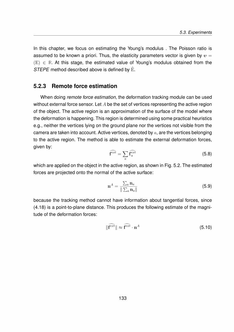
5.3. Experiments
In this chapter, we focus on estimating the Young’s modulus . The Poisson ratio isassumed to be known a priori. Thus, the elasticity parameters vector is given by υ =(E) ∈ R. At this stage, the estimated value of Young’s modulus obtained from theSTEPE method described above is defined by E.
5.2.3 Remote force estimation
When doing remote force estimation, the deformation tracking module can be usedwithout external force sensor. Let A be the set of vertices representing the active regionof the object. The active region is an approximation of the surface of the model wherethe deformation is happening. This region is determined using some practical heuristicse.g., neither the vertices lying on the ground plane nor the vertices not visible from thecamera are taken into account. Active vertices, denoted by a, are the vertices belongingto the active region. The method is able to estimate the external deformation forces,given by:
f ext =∑a
f exta (5.8)
which are applied on the object in the active region, as shown in Fig. 5.2. The estimatedforces are projected onto the normal of the active surface:
nA =∑a na
‖∑a na‖(5.9)
because the tracking method cannot have information about tangential forces, since(4.18) is a point-to-plane distance. This produces the following estimate of the magni-tude of the deformation forces:
‖f ext‖ ≈ f ext · nA (5.10)
133
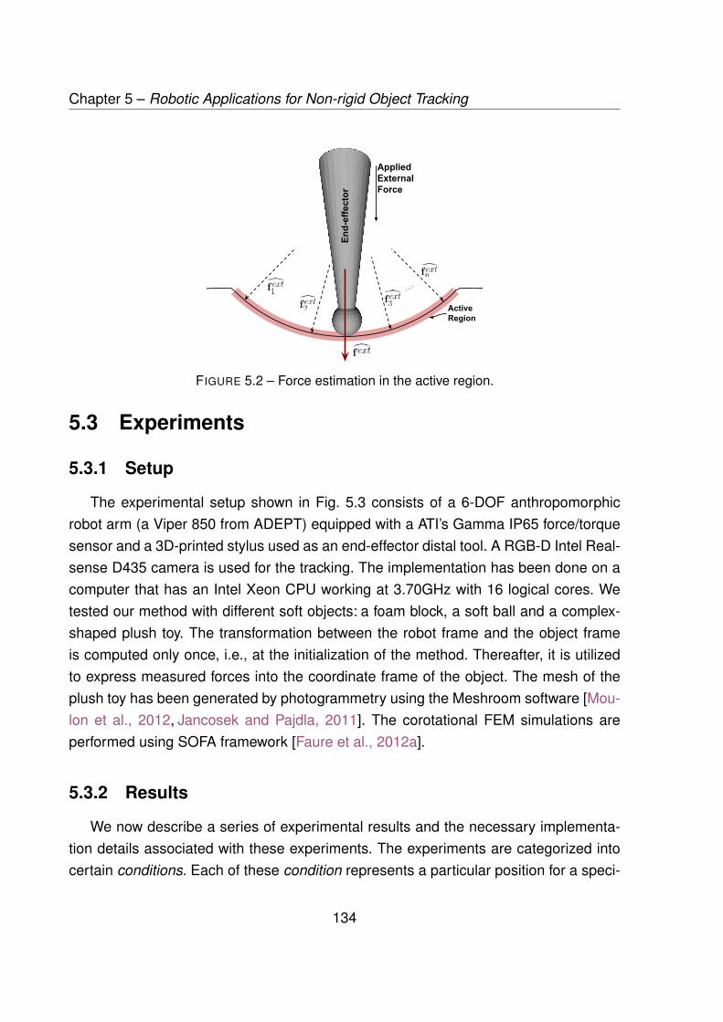
Chapter 5 – Robotic Applications for Non-rigid Object Tracking
FIGURE 5.2 – Force estimation in the active region.
5.3 Experiments
5.3.1 Setup
The experimental setup shown in Fig. 5.3 consists of a 6-DOF anthropomorphicrobot arm (a Viper 850 from ADEPT) equipped with a ATI’s Gamma IP65 force/torquesensor and a 3D-printed stylus used as an end-effector distal tool. A RGB-D Intel Real-sense D435 camera is used for the tracking. The implementation has been done on acomputer that has an Intel Xeon CPU working at 3.70GHz with 16 logical cores. Wetested our method with different soft objects: a foam block, a soft ball and a complex-shaped plush toy. The transformation between the robot frame and the object frameis computed only once, i.e., at the initialization of the method. Thereafter, it is utilizedto express measured forces into the coordinate frame of the object. The mesh of theplush toy has been generated by photogrammetry using the Meshroom software [Mou-lon et al., 2012, Jancosek and Pajdla, 2011]. The corotational FEM simulations areperformed using SOFA framework [Faure et al., 2012a].
5.3.2 Results
We now describe a series of experimental results and the necessary implementa-tion details associated with these experiments. The experiments are categorized intocertain conditions. Each of these condition represents a particular position for a speci-
134

5.3. Experiments
(a)
Fw
Fc
Fo
(b)
FIGURE 5.3 – The experimental setup shown with and without annotation in Fig. 5.3a and Fig.5.3b. The robot (at reference frame Fw) is deforming a plush toy (at reference frame Fo) whilethe data is being captured from an Intel RealSense D435 RGB-D Camera (at reference frameFc). The transformation between these reference frames are shown in Fig. 5.3a, following theconvention established in Sec. 1.1.1
fic object. E.g., the first condition described below denotes the rectangular foam beingdeformed at the center of its largest face, while being placed horizontally on a table.To evaluate the accuracy of the estimation process, the ground truth of Young’s mo-dulus EGT has been determined through indentation tests for each condition of experi-ments [McKee et al., 2011]. The indentation tests can be described as: repeated, slowand incremental vertical displacements applied on the objects using the robot whilemeasuring the forces and the displacements. Forces are measured from the force sen-sor fitted in the robot’s arm while displacements are obtained using the odometry of
TABLE 5.1 – Evaluation of tracking and estimation times and Young’s modulus (in kPa) estima-tion accuracy w.r.t. different quality of visual and mechanical meshes.
Objects No. of verticesin Visual Mesh
No. of verticesin MechanicalMesh
ttr(s) std(ttr)(s) tst(s) test(s) ¯EGT Eest Error(%)
foam 35 1049 1.94 0.14 62 310 454 431 5.08foam 415 1049 2.37 0.15 122 180 454 438 3.62foam 178 554 1.21 0.02 60 180 454 497 9.47ball 404 627 1.38 0.03 126 70 156 136 12.8ball 404 1060 1.61 0.02 118 96 156 148 5.0ball 404 1954 3.09 0.07 130 330 156 148 5.1
135

Chapter 5 – Robotic Applications for Non-rigid Object Tracking
FIGURE 5.4 – Visual results from the deformation tracking methodology. The first and the fourthcolumn shows the color image, the second and the fifth column shows the tracked object modeland the third and the sixth column shows the value of eN (the geometric error computed usingEqn. 3.5), color-coded and augmented on the object
the robot. For each condition of experiment, the average of several indentation tests isconsidered to be the ground truth. We denote that as: EGT .
Let E(i) be the estimation of the Young’s modulus obtained from the tracking resultsfor the ith deformation. The Young’s modulus that is thereafter used for the externalforce estimation, denoted by Eest, is the one for which the following convergence crite-rion is respected:
E(i)− E(i− 1)E(i− 1)
< 0.05 (5.11)
Some examples of the output of the deformation tracking method are shown in Fig.5.4. The mean of the norm of the error (‖eN‖) was found to be 1.53 mm, 0.51 mmand 0.21 mm for the foam block, soft ball and plush toy, while the standard deviationswere 7.2 mm, 0.7 mm and 1.4 mm respectively, across all the experiments reported inthis article. In the three example sequences shown in Fig. 5.4, the mean of the normof error varied between a maximum of 0.381 mm (for the plush toy, deformed by itsnose) to as low as 3 µm (for the undeformed sponge block), despite having outlyingcorrespondence or noise in the range of -5.5 cm to +9.0 cm (which gets rejected by
136

5.3. Experiments
the M-estimator). In the experiments shown in Table 5.1, the time required for trackingvaries between 1.21 to 3.1 sec/frame. However, it was possible to run the same algo-rithm on the foam block at ∼ 800 ms/frame without using any GPU based computation,with negligible loss of accuracy (< 10%).
Our method can be evaluated on different criteria. The first set of experimentswas conducted to evaluate the time-performance of the tracking and the quality ofthe Young’s modulus estimation w.r.t. the number of vertices of both the visual meshand the mechanical mesh. The results of this set of experiments are grouped in Table5.1. In this table, #Visual designates the number of vertices of the visual mesh while#Mechanical designates the number of vertices of the mechanical mesh. ttr is the ave-rage deformation tracking time, std(ttr) is its standard deviation, tst is the time that wasrequired to deform the object and reach a steady-state and test is the time to estimatethe Young’s modulus. All the times are expressed in seconds. EGT and Eest correspondto the average ground truth of Young’s modulus and estimated Young’s modulus res-pectively, both expressed in kilo Pascals. Finally, Error designates the percentage oferror of the estimation and is given by Error = 100 ∗ abs(EGT − Eest)/EGT where abs
designates the absolute value.
TABLE 5.2 – Evaluation of the estimation of the Young’s modulus (in kPa).
Objects E0 EGT Eest Error
foam middle200 454 480 5.7%1500 454 451 0.7%15000 454 488 7.5%
foam comer 200 247 224 9.3%ball 1000 156 154 1.3%
toy nose 200 51 53 3.790toy leg 50 42 43.1 2.6%
The second set of experiments was conducted to evaluate the consistency of theYoung’s modulus estimation w.r.t. the initial estimate E0. Low initial estimate are usuallyof the order of 0.1× EGT and high initial estimate of the order of 10× EGT . The resultsof this set of experiments are grouped in Table 5.2.
The last set of experiments was conducted to evaluate the estimation of the defor-
137
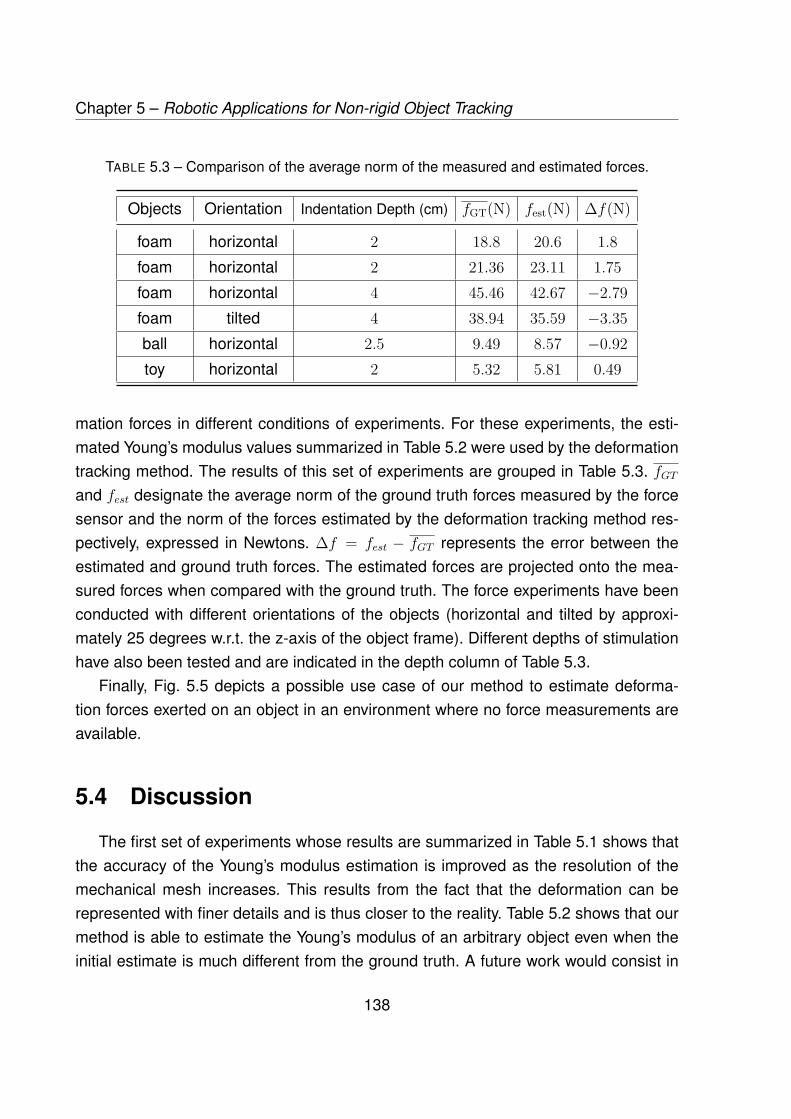
Chapter 5 – Robotic Applications for Non-rigid Object Tracking
TABLE 5.3 – Comparison of the average norm of the measured and estimated forces.
Objects Orientation Indentation Depth (cm) fGT(N) fest(N) ∆f(N)
foam horizontal 2 18.8 20.6 1.8foam horizontal 2 21.36 23.11 1.75foam horizontal 4 45.46 42.67 −2.79foam tilted 4 38.94 35.59 −3.35ball horizontal 2.5 9.49 8.57 −0.92toy horizontal 2 5.32 5.81 0.49
mation forces in different conditions of experiments. For these experiments, the esti-mated Young’s modulus values summarized in Table 5.2 were used by the deformationtracking method. The results of this set of experiments are grouped in Table 5.3. fGTand fest designate the average norm of the ground truth forces measured by the forcesensor and the norm of the forces estimated by the deformation tracking method res-pectively, expressed in Newtons. ∆f = fest − fGT represents the error between theestimated and ground truth forces. The estimated forces are projected onto the mea-sured forces when compared with the ground truth. The force experiments have beenconducted with different orientations of the objects (horizontal and tilted by approxi-mately 25 degrees w.r.t. the z-axis of the object frame). Different depths of stimulationhave also been tested and are indicated in the depth column of Table 5.3.
Finally, Fig. 5.5 depicts a possible use case of our method to estimate deforma-tion forces exerted on an object in an environment where no force measurements areavailable.
5.4 Discussion
The first set of experiments whose results are summarized in Table 5.1 shows thatthe accuracy of the Young’s modulus estimation is improved as the resolution of themechanical mesh increases. This results from the fact that the deformation can berepresented with finer details and is thus closer to the reality. Table 5.2 shows that ourmethod is able to estimate the Young’s modulus of an arbitrary object even when theinitial estimate is much different from the ground truth. A future work would consist in
138
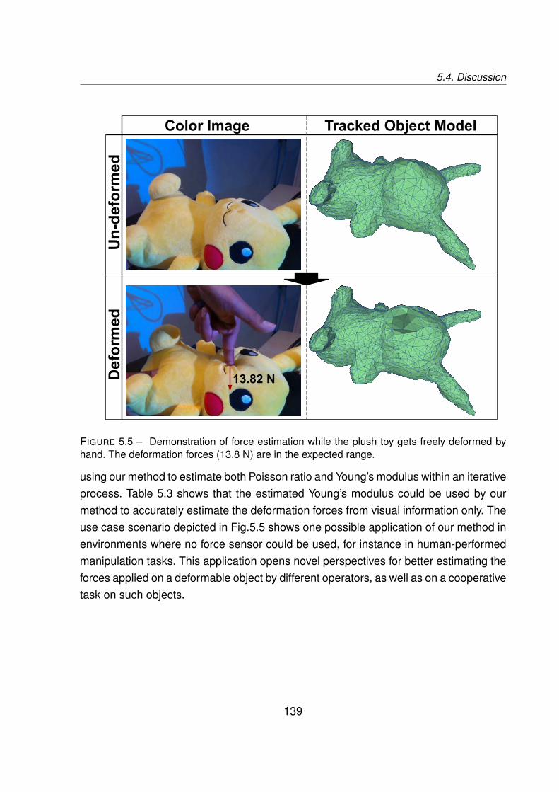
5.4. Discussion
FIGURE 5.5 – Demonstration of force estimation while the plush toy gets freely deformed byhand. The deformation forces (13.8 N) are in the expected range.
using our method to estimate both Poisson ratio and Young’s modulus within an iterativeprocess. Table 5.3 shows that the estimated Young’s modulus could be used by ourmethod to accurately estimate the deformation forces from visual information only. Theuse case scenario depicted in Fig.5.5 shows one possible application of our method inenvironments where no force sensor could be used, for instance in human-performedmanipulation tasks. This application opens novel perspectives for better estimating theforces applied on a deformable object by different operators, as well as on a cooperativetask on such objects.
139
Chapter 5 – Robotic Applications for Non-rigid Object Tracking
5.5 Conclusion
In this chapter, we described a method, that we named STEPE, to simultaneouslyestimate the elasticity parameters of a deforming object while tracking their surfaceusing a RGB-D camera. The fundamental technique for tracking the surface was al-ready developed in Chapter 3, while this chapter produced a more optimized method ofdeformation tracking, enabling the estimation of elasticity parameters simultaneously.Moreover, we utilize the estimated parameters to track the deforming forces acting onthe object remotely, without using any external force sensor. These results pave theway for better control of deformable objects manipulated by a robot.
140

CHAPTER 6
CONCLUSION AND PERSPECTIVES
6.1 Conclusion
Here, we first briefly recall the concepts presented throughout this thesis. This isfollowed by a concluding summary of the individual chapters. We then proceed to endthis thesis by discussing some of the short and long term perspective research workthat can be spawned by the approaches proposed in this thesis.
6.1.1 Brief Summary of the Thesis
In Chapter 2, we present a framework for precisely tracking objects of complexshapes with joint optimization of depth-based geometric and photometric error termsusing a low-accuracy 3D object model with the help of RGB-D cameras. Object trackingwith coarse 3D model is useful for industrial applications, where scanning and recons-tructing exact 3D model is often prohibitively difficult. In this chapter, a method is pro-posed that uses a combination of point-to-plane distance minimization and photometricerror minimization to track objects accurately. ‘Keyframes’ are used in this mechanismof object tracking for minimizing drift. The approach proposed in this chapter has beenvalidated on both simulated and real data. It has been shown that our approach ismore accurate than existing state-of-the-art approaches on benchmarked, simulateddataset, especially while dealing with low-textured objects with co-planar faces.
In Chapter 3, a method to track deformable objects with a RGB-D camera usinga coarse 3D model is presented. The model of deformation is based on corotationalFEM. The physical model of the deforming object does not need to be precise and wedo not require the precise physical properties of the object to track it accurately. Thevertex positions of the surface mesh of the tracked object is regulated using virtualforces which are obtained by minimizing a point-to-plane distance based geometricerror between the pointcloud and the mesh. The point of application of force is obtained
141

Chapter 6 – Conclusion and Perspectives
by thresholding and clustering of the error obtained from rigid tracking, which is run inparallel with the non-rigid tracking algorithm. This parallel implementation also enablesthe overall system nearly real-time at frame-rate. The proposed approach has beenevaluated on a synthetic dataset with ground-truth, as well as on real data.
In Chapter 4, we propose a methodology for tracking non-rigid objects with RGB-Dcameras by minimizing a combination of depth and photometric error. The approachproposed in this chapter does not depend on the accuracy of the material propertiesprovided as input for deformation tracking. However, if an accurate estimate of the ma-terial properties are known, it can be used to measure the external, deforming forcesacting on the object with just the visual data obtained from the RGB-D camera. The me-chanism proposed in this chapter combines computer-vision based methodologies withphysical model based deformation representation without computing expensive nume-rical optimization for minimizing the non-linear error terms. The method proposed herehas been validated on synthetic and real data and has been shown to outperform someof the state-of-the-art techniques in physical model based deformation tracking, whileopening up new applications, such as visual force estimation on deforming objects.
In Chapter 5, a new approach to simultaneously track the deformation of soft ob-jects and estimate their elasticity parameters has been suggested. This approach alsoallows the estimation of deforming forces applied on an object from the visual infor-mation only. This is done by combining corotational FEM simulations and minimizationalgorithms to track the deformation and estimate the elasticity parameters of a softobject jointly. A commercial RGB-D sensor is used for obtaining the visual informationneeded for tracking. This information is utilized to deform the object model accordingto the virtual forces computed using the deformation tracking algorithm. The moduleinvolved in the elasticity parameter estimation minimizes the error between the trackedobject and a simulated object deformed by the forces that are measured using a forcesensor mounted on a robotic arm. Once the elasticity parameter is estimated, the de-formation tracking can then estimate the deforming forces applied on the object withoutthe use of a force sensor. The accuracy of the elasticity parameter estimation and of theforce estimation has been validated on several soft objects with various complexities ofshape.
142

6.2. Perspectives
6.2 Perspectives
There are some important work which can be done to follow up the methodologiesproposed in this dissertation. We categorize them based on the expected duration itwould take to complete this perspective research work. The perspectives can also bedifferentiated from the possible application areas of deformation tracking, which can benumerous.
6.2.1 Short-term Perspectives
The approaches proposed here have been demonstrated to work with depth andphotometry based error minimization. However, in Chapter 4, we have already set thegroundwork for easily incorporating multiple new cost functions e.g., sparse-featurebased, edge-based or wavelet based error terms. This can be a relatively straightfor-ward extension of our approach in Chapter 4 that could lead to further improvement intracking accuracy.
All of the methods implemented in this thesis have been implemented on a singlecore of a CPU (OpenMP has been used sparingly for the STEPE method presented inChapter 5). Therefore, all run-time performances reported in this thesis can be subjec-ted to extensive performance optimization, thereby decreasing the runtime. There is astrong potential for improving the runtime significantly, given that some of the compu-tations involved are highly parallelizable.
This thesis makes the use of control handles for tracking deformation. In Chapter3 and Chapter 4, two different methods for determining these control handles from theinput data has been proposed. However, determining the exact sequence of controlhandles that maximizes the accuracy of the tracking requires some heuristics and canbe sensitive to noise and occlusion. Investigating a novel and robust mechanism forselecting these control handles to maximize the non-rigid tracking accuracy can bean interesting research area. This can possibly use the help of deep learning basedapproaches.
6.2.2 Long-term Perspectives
The approaches proposed in Chapter 3 and Chapter 4 can be extended to per-form deformation tracking using monocular data. Given that the initial object to camera
143
Chapter 6 – Conclusion and Perspectives
transformation at the first frame is known, a frame-to-frame tracking of the deformingsurface can be done using a similar method, but with suitably modified cost functionsto suit the monocular data.
Iterative mechanical mesh refinement using adaptive remeshing [Narain et al., 2013]could be combined with the approaches proposed in this thesis for tracking the tearingor fracturing of volumetric objects without the prior knowledge of the physical propertiesof the object being tracked. On the same note, adaptive remeshing can also be usedto reconstruct a physically-based model from RGB-D based voxel data. This onlinereconstructed physical mesh can be used to do the non-rigid object tracking.
A challenging direction for future research could possibly involve developing an uni-fied, physics-based framework that is capable of tracking multiple mutually-interactingrigid objects, non-rigid objects and fluid surfaces using visual information only.
144
BIBLIOGRAPHIE
[Acton, 1990] Acton, F. S. (1990). Numerical methods that work. The MathematicalAssociation of America (MAA).
[Agudo et al., 2014] Agudo, A., Agapito, L., Calvo, B., and Montiel, J. M. (2014). Goodvibrations : A modal analysis approach for sequential non-rigid structure from motion.In Proceedings of the IEEE Conference on Computer Vision and Pattern Recogni-tion, pages 1558–1565.
[Agudo et al., 2011] Agudo, A., Calvo, B., and Montiel, J. (2011). Fem models to codenon-rigid ekf monocular slam. In 2011 IEEE International Conference on ComputerVision Workshops (ICCV Workshops), pages 1586–1593.
[Agudo and M-Noguer, 2015] Agudo, A. and M-Noguer, F. (2015). Learning shape,motion and elastic models in force space. In Proceedings of the IEEE InternationalConference on Computer Vision, pages 756–764.
[Agudo et al., 2017] Agudo, A., Montiel, J. M. M., Agapito, L., and Calvo, B. (2017). Mo-dal space : A physics-based model for sequential estimation of time-varying shapefrom monocular video. Journal of mathematical imaging and vision, 57(1) :75–98.
[Ahn et al., 2019] Ahn, M. S., Chae, H., Noh, D., Nam, H., and Hong, D. (2019). Ana-lysis and noise modeling of the intel realsense d435 for mobile robots. In 2019 16thInternational Conference on Ubiquitous Robots (UR), pages 707–711.
[Armstrong and Zisserman, 1995] Armstrong, M. and Zisserman, A. (1995). Robustobject tracking. In Asian Conference on Computer Vision, volume 1, pages 58–61.
[Arun et al., 1987] Arun, K. S., Huang, T. S., and Blostein, S. D. (1987). Least-squaresfitting of two 3-d point sets. IEEE Transactions on pattern analysis and machineintelligence, (5) :698–700.
[Baker and Matthews, 2001] Baker, S. and Matthews, I. (2001). Equivalence and ef-ficiency of image alignment algorithms. In IEEE Computer Society Conference onComputer Vision and Pattern Recognition, volume 1, pages I–1090.
145
BIBLIOGRAPHIE
[Baker and Matthews, 2004] Baker, S. and Matthews, I. (2004). Lucas-kanade 20years on : A unifying framework. International journal of computer vision, 56(3) :221–255.
[Banchoff et al., 2014] Banchoff, T. et al. (2014). Salvador dalí and the fourth dimen-sion. Proceedings of the Bridges.
[Bartoli et al., 2015] Bartoli, A., Gerard, Y., Chadebecq, F., Collins, T., and Pizarro, D.(2015). Shape-from-template. IEEE transactions on pattern analysis and machineintelligence, 37(10) :2099–2118.
[Beaton and Tukey, 1974] Beaton, A. E. and Tukey, J. W. (1974). The fitting of powerseries, meaning polynomials, illustrated on band-spectroscopic data. Technometrics,16(2) :147–185.
[Ben-Chen et al., 2010] Ben-Chen, M., Butscher, A., Solomon, J., and Guibas, L.(2010). On discrete killing vector fields and patterns on surfaces. In ComputerGraphics Forum, volume 29, pages 1701–1711.
[Besl and McKay, 1992] Besl, P. J. and McKay, N. D. (1992). Method for registrationof 3-d shapes. In Robotics-DL tentative, pages 586–606. International Society forOptics and Photonics.
[Bickel et al., 2009] Bickel, B., Bächer, M., Otaduy, M. A., Matusik, W., Pfister, H., andGross, M. (2009). Capture and modeling of non-linear heterogeneous soft tissue. InACM Transactions on Graphics (TOG), volume 28, page 89.
[Blender, 2018] Blender, O. C. (2018). Blender - a 3D modelling and rendering pa-ckage. Blender Foundation, Stichting Blender Foundation, Amsterdam.
[Bregler et al., 2000] Bregler, C., Hertzmann, A., and Biermann, H. (2000). Recoveringnon-rigid 3d shape from image streams. In IEEE Conference on Computer Visionand Pattern Recognition (CVPR), volume 2, page 2690.
[Bronte et al., 2017] Bronte, S., Bergasa, L., Pizarro, D., and Barea, R. (2017). Model-based real-time non-rigid tracking. Sensors.
[Bronte et al., 2014] Bronte, S., Paladini, M., Bergasa, L. M., Agapito, L., and Arroyo,R. (2014). Real-time sequential model-based non-rigid sfm. In 2014 IEEE/RSJInternational Conference on Intelligent Robots and Systems, pages 1026–1031.
[Brown, 1971] Brown, D. C. (1971). Close-range camera calibration, photogrammetricengineering. Engineering and Remote Sensing, 37(8) :855–866.
146

BIBLIOGRAPHIE
[Chan and Zhu, 2005] Chan, T. and Zhu, W. (2005). Level set based shape prior seg-mentation. In 2005 IEEE Computer Society Conference on Computer Vision andPattern Recognition (CVPR), volume 2, pages 1164–1170.
[Chen and Medioni, 1992] Chen, Y. and Medioni, G. G. (1992). Object modeling byregistration of multiple range images. Image Vision Comput., 10(3) :145–155.
[Chhatkuli, 2016] Chhatkuli, A. (2016). Local Analytic and Global Convex Methods forthe 3D Reconstruction of Isometric Deformable Surfaces. PhD thesis.
[Choi and Christensen, 2010] Choi, C. and Christensen, H. I. (2010). Real-time 3dmodel-based tracking using edge and keypoint features for robotic manipulation. In2010 IEEE International Conference on Robotics and Automation (ICRA), pages4048–4055.
[Choi and Christensen, 2013] Choi, C. and Christensen, H. I. (2013). RGB-d objecttracking : A particle filter approach on GPU. In Intelligent Robots and Systems(IROS), 2013 IEEE/RSJ International Conference on, pages 1084–1091.
[Cholesky, 2005] Cholesky, A.-L. (2005). Sur la résolution numérique des systèmesd’équations linéaires. Bulletin de la Sabix. Société des amis de la Bibliothèque et del’Histoire de l’École polytechnique, (39) :81–95.
[Cifuentes et al., 2017] Cifuentes, C. G., Issac, J., Wüthrich, M., Schaal, S., and Bohg,J. (2017). Probabilistic articulated real-time tracking for robot manipulation. IEEERobotics and Automation Letters, 2(2) :577–584.
[Coleman, 1989] Coleman, A. (1989). The greatest mathematical paper of all time.The Mathematical Intelligencer, 11(3) :29–38.
[Collins and Bartoli, 2015] Collins, T. and Bartoli, A. (2015). Realtime shape-from-template : System and applications. In ISMAR, pages 116–119.
[Courant et al., 1943] Courant, R. et al. (1943). Variational methods for the solution ofproblems of equilibrium and vibrations. Verlag nicht ermittelbar.
[Curless and Levoy, 1996] Curless, B. and Levoy, M. (1996). A volumetric method forbuilding complex models from range images. In Proceedings of the 23rd annualconference on Computer graphics and interactive techniques, pages 303–312.
[Davis et al., 2015] Davis, A., Bouman, K. L., Chen, J. G., Rubinstein, M., Durand, F.,and Freeman, W. T. (2015). Visual vibrometry : Estimating material properties from
147
BIBLIOGRAPHIE
small motion in video. In Proceedings of the ieee conference on computer vision andpattern recognition, pages 5335–5343.
[Dementhon and Davis, 1995] Dementhon, D. F. and Davis, L. S. (1995). Model-basedobject pose in 25 lines of code. International journal of computer vision, 15(1-2) :123–141.
[Dempster et al., 1977] Dempster, A. P., Laird, N. M., and Rubin, D. B. (1977). Maxi-mum likelihood from incomplete data via the em algorithm. Journal of the RoyalStatistical Society : Series B (Methodological), 39(1) :1–22.
[Dhome et al., 1989] Dhome, M., Richetin, M., Lapreste, J.-T., and Rives, G. (1989).Determination of the attitude of 3d objects from a single perspective view. IEEEtransactions on pattern analysis and machine intelligence, 11(12) :1265–1278.
[Doumanoglou et al., 2016] Doumanoglou, A., Kouskouridas, R., Malassiotis, S., andKim, T.-K. (2016). Recovering 6d object pose and predicting next-best-view in thecrowd. In Proceedings of the IEEE Conference on Computer Vision and PatternRecognition, pages 3583–3592.
[Eggert et al., 1997] Eggert, D. W., Lorusso, A., and Fisher, R. B. (1997). Estimating3-d rigid body transformations : a comparison of four major algorithms. Machinevision and applications, 9(5-6) :272–290.
[Faugeras, 1993] Faugeras, O. (1993). Three-dimensional computer vision : a geome-tric viewpoint. MIT press.
[Faure et al., 2012a] Faure, F., Duriez, C., Delingette, H., Allard, J., Gilles, B., Mar-chesseau, S., Talbot, H., Courtecuisse, H., Bousquet, G., Peterlik, I., and Cotin, S.(2012a). SOFA : A Multi-Model Framework for Interactive Physical Simulation. InSoft Tissue Biomechanical Modeling for Computer Assisted Surgery, volume 11 ofStudies in Mechanobiology, Tissue Engineering and Biomaterials, pages 283–321.
[Faure et al., 2012b] Faure, F., Duriez, C., Delingette, H., Allard, J., Gilles, B., Mar-chesseau, S., Talbot, H., Courtecuisse, H., Bousquet, G., Peterlik, I., et al. (2012b).Sofa : A multi-model framework for interactive physical simulation. In Soft tissuebiomechanical modeling for computer assisted surgery, pages 283–321. Springer.
[Felippa, 2000] Felippa, C. A. (2000). A systematic approach to the element-independent corotational dynamics of finite elements. Technical report, TechnicalReport CU-CAS-00-03, Center for Aerospace Structures.
148

BIBLIOGRAPHIE
[Fischler and Bolles, 1981] Fischler, M. A. and Bolles, R. C. (1981). Random sampleconsensus : a paradigm for model fitting with applications to image analysis andautomated cartography. Communications of the ACM, 24(6) :381–395.
[Frank et al., 2010] Frank, B., Schmedding, R., Stachniss, C., Teschner, M., and Bur-gard, W. (2010). Learning the elasticity parameters of deformable objects with amanipulation robot. In Proceedings of the IEEE Conference on Intelligent Robotsand Systems, pages 1877–1883.
[Fugl et al., 2012] Fugl, A. R., Jordt, A., Petersen, H. G., Willatzen, M., and Koch, R.(2012). Simultaneous estimation of material properties and pose for deformableobjects from depth and color images. In Joint DAGM (German Association for PatternRecognition) and OAGM Symposium, pages 165–174.
[Fukunage and Narendra, 1975] Fukunage, K. and Narendra, P. M. (1975). A branchand bound algorithm for computing k-nearest neighbors. IEEE transactions on com-puters, (7) :750–753.
[Gao and Tedrake, 2018] Gao, W. and Tedrake, R. (2018). Surfelwarp : Efficient non-volumetric single view dynamic reconstruction. In Robotics : Science and System(RSS 2018).
[Gao et al., 2003] Gao, X.-S., Hou, X.-R., Tang, J., and Cheng, H.-F. (2003). Completesolution classification for the perspective-three-point problem. IEEE transactions onpattern analysis and machine intelligence, 25(8) :930–943.
[Garon and Lalonde, 2017] Garon, M. and Lalonde, J.-F. (2017). Deep 6-dof tracking.IEEE transactions on visualization and computer graphics, 23(11) :2410–2418.
[Gotardo and Martinez, 2011a] Gotardo, P. F. and Martinez, A. M. (2011a). Kernel non-rigid structure from motion. In 2011 International Conference on Computer Vision,pages 802–809.
[Gotardo and Martinez, 2011b] Gotardo, P. F. and Martinez, A. M. (2011b). Non-rigidstructure from motion with complementary rank-3 spaces. In CVPR 2011, pages3065–3072.
[Grunnet-Jepsen et al., ] Grunnet-Jepsen, A., Sweetser, J. N., Winer, P., Takagi, A.,and Woodfill, J. Projectors for intel® realsense™ depth cameras d4xx. Intel® Cor-poration.
149
BIBLIOGRAPHIE
[Hager and Belhumeur, 1998] Hager, G. D. and Belhumeur, P. N. (1998). Efficient re-gion tracking with parametric models of geometry and illumination. IEEE Transac-tions on Pattern Analysis & Machine Intelligence, (10) :1025–1039.
[Hamer et al., 2009] Hamer, H., Schindler, K., Koller-Meier, E., and Van Gool, L.(2009). Tracking a hand manipulating an object. In 2009 IEEE 12th InternationalConference on Computer Vision (ICCV), pages 1475–1482.
[Haouchine et al., 2015] Haouchine, N., Cotin, S., Peterlik, I., Dequidt, J., Lopez, M. S.,Kerrien, E., and Berger, M. (2015). Impact of soft tissue heterogeneity on augmentedreality for liver surgery. IEEE transactions on visualization and computer graphics,21(5) :584–597.
[Haouchine et al., 2014] Haouchine, N., Dequidt, J., Berger, M.-O., and Cotin, S.(2014). Single view augmentation of 3d elastic objects. In 2014 IEEE Internatio-nal Symposium on Mixed and Augmented Reality (ISMAR), pages 229–236.
[Haouchine et al., 2013] Haouchine, N., Dequidt, J., Peterlik, I., Kerrien, E., Berger,M.-O., and Cotin, S. (2013). Image-guided simulation of heterogeneous tissue de-formation for augmented reality during hepatic surgery. In 2013 IEEE internationalsymposium on mixed and augmented reality (ISMAR), pages 199–208.
[Hartigan and Wong, 1979] Hartigan, J. A. and Wong, M. A. (1979). Algorithm as 136 :A k-means clustering algorithm. Journal of the Royal Statistical Society. Series C(Applied Statistics), 28(1) :100–108.
[Hartley and Zisserman, 2003] Hartley, R. and Zisserman, A. (2003). Multiple viewgeometry in computer vision. Cambridge university press.
[Helten et al., 2013] Helten, T., Baak, A., Müller, M., and Theobalt, C. (2013). Full-bodyhuman motion capture from monocular depth images. In Time-of-Flight and DepthImaging. Sensors, Algorithms, and Applications, pages 188–206.
[Henrikson, 1999] Henrikson, J. (1999). Completeness and total boundedness of thehausdorff metric. MIT Undergraduate Journal of Mathematics, 1 :69–80.
[Henry et al., 2013] Henry, P., Fox, D., Bhowmik, A., and Mongia, R. (2013). Patchvolumes : Segmentation-based consistent mapping with rgb-d cameras. In 2013International Conference on 3D Vision-3DV 2013, pages 398–405.
[Hinterstoisser et al., 2012] Hinterstoisser, S., Lepetit, V., Ilic, S., Holzer, S., Bradski,G., Konolige, K., and Navab, N. (2012). Model based training, detection and pose
150
BIBLIOGRAPHIE
estimation of texture-less 3d objects in heavily cluttered scenes. In Asian Conf. oncomputer vision, pages 548–562.
[Horn, 1987] Horn, B. K. (1987). Closed-form solution of absolute orientation usingunit quaternions. Josa a, 4(4) :629–642.
[Horn et al., 1988] Horn, B. K., Hilden, H. M., and Negahdaripour, S. (1988). Closed-form solution of absolute orientation using orthonormal matrices. JOSA A,5(7) :1127–1135.
[Hrennikoff, 1941] Hrennikoff, A. (1941). Solution of problems of elasticity by the fra-mework method. Journal of applied mechanics, 8(4) :169–175.
[Huang et al., 2015] Huang, J., Ong, S.-K., and Nee, A. Y. (2015). Real-time finiteelement structural analysis in augmented reality. Advances in Engineering Software,87 :43–56.
[Hughes, 2012] Hughes, T. J. (2012). The finite element method : linear static anddynamic finite element analysis. Courier Corporation.
[Innmann et al., 2016] Innmann, M., Zollhöfer, M., Nießner, M., Theobalt, C., andStamminger, M. (2016). Volumedeform : Real-time volumetric non-rigid reconstruc-tion. arXiv preprint arXiv :1603.08161.
[Izadi et al., 2011] Izadi, S., Kim, D., Hilliges, O., Molyneaux, D., Newcombe, R., Kohli,P., Shotton, J., Hodges, S., Freeman, D., Davison, A., et al. (2011). Kinectfusion :real-time 3d reconstruction and interaction using a moving depth camera. In Pro-ceedings of the 24th annual ACM symposium on User interface software and tech-nology, pages 559–568.
[Jancosek and Pajdla, 2011] Jancosek, M. and Pajdla, T. (2011). Multi-view recons-truction preserving weakly-supported surfaces. In Proceedings of IEEE Conferenceon Computer Vision and Pattern Recognition (CVPR).
[Jensen et al., 2018] Jensen, S. H. N., Del Bue, A., Doest, M. E. B., and Aanæs, H.(2018). A benchmark and evaluation of non-rigid structure from motion. arXiv pre-print arXiv :1801.08388.
[Kehl et al., 2016] Kehl, W., Milletari, F., Tombari, F., Ilic, S., and Navab, N. (2016).Deep learning of local rgb-d patches for 3d object detection and 6d pose estimation.In European Conference on Computer Vision, pages 205–220.
151
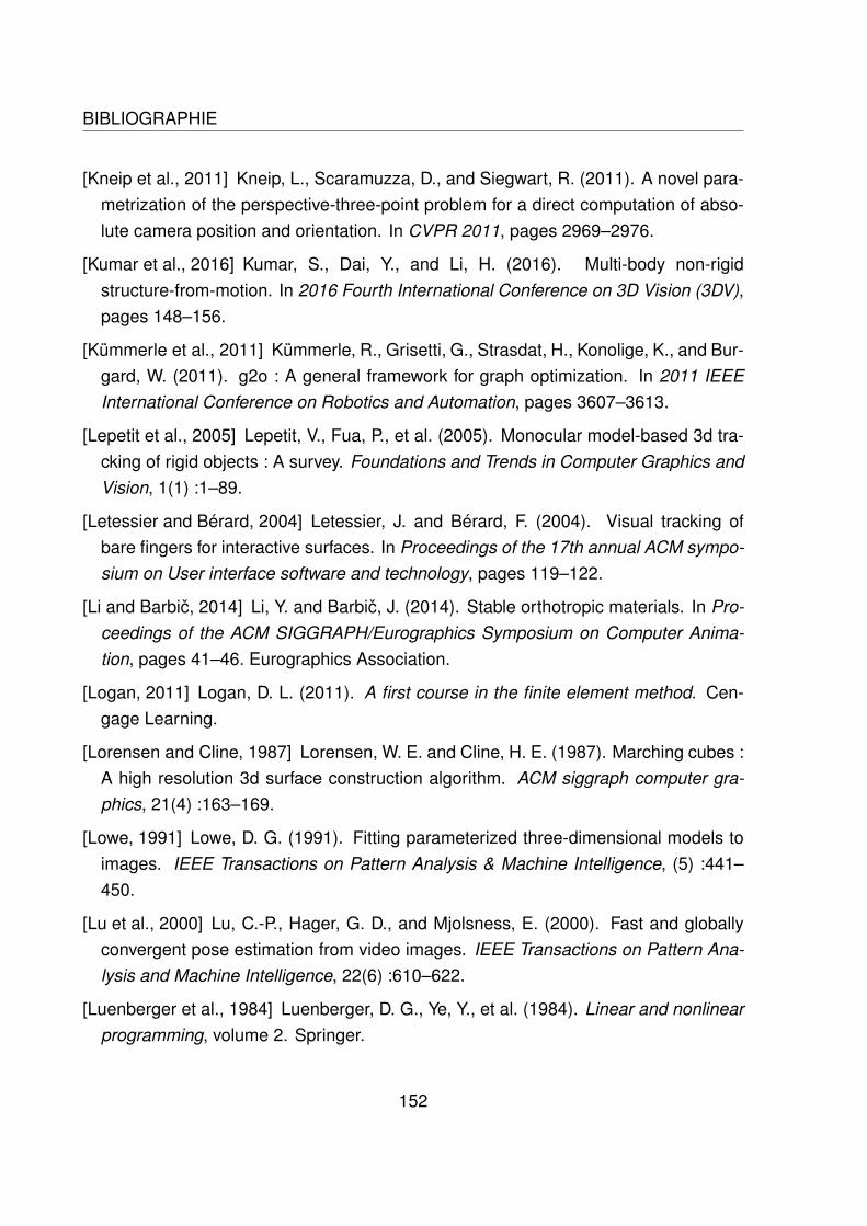
BIBLIOGRAPHIE
[Kneip et al., 2011] Kneip, L., Scaramuzza, D., and Siegwart, R. (2011). A novel para-metrization of the perspective-three-point problem for a direct computation of abso-lute camera position and orientation. In CVPR 2011, pages 2969–2976.
[Kumar et al., 2016] Kumar, S., Dai, Y., and Li, H. (2016). Multi-body non-rigidstructure-from-motion. In 2016 Fourth International Conference on 3D Vision (3DV),pages 148–156.
[Kümmerle et al., 2011] Kümmerle, R., Grisetti, G., Strasdat, H., Konolige, K., and Bur-gard, W. (2011). g2o : A general framework for graph optimization. In 2011 IEEEInternational Conference on Robotics and Automation, pages 3607–3613.
[Lepetit et al., 2005] Lepetit, V., Fua, P., et al. (2005). Monocular model-based 3d tra-cking of rigid objects : A survey. Foundations and Trends in Computer Graphics andVision, 1(1) :1–89.
[Letessier and Bérard, 2004] Letessier, J. and Bérard, F. (2004). Visual tracking ofbare fingers for interactive surfaces. In Proceedings of the 17th annual ACM sympo-sium on User interface software and technology, pages 119–122.
[Li and Barbic, 2014] Li, Y. and Barbic, J. (2014). Stable orthotropic materials. In Pro-ceedings of the ACM SIGGRAPH/Eurographics Symposium on Computer Anima-tion, pages 41–46. Eurographics Association.
[Logan, 2011] Logan, D. L. (2011). A first course in the finite element method. Cen-gage Learning.
[Lorensen and Cline, 1987] Lorensen, W. E. and Cline, H. E. (1987). Marching cubes :A high resolution 3d surface construction algorithm. ACM siggraph computer gra-phics, 21(4) :163–169.
[Lowe, 1991] Lowe, D. G. (1991). Fitting parameterized three-dimensional models toimages. IEEE Transactions on Pattern Analysis & Machine Intelligence, (5) :441–450.
[Lu et al., 2000] Lu, C.-P., Hager, G. D., and Mjolsness, E. (2000). Fast and globallyconvergent pose estimation from video images. IEEE Transactions on Pattern Ana-lysis and Machine Intelligence, 22(6) :610–622.
[Luenberger et al., 1984] Luenberger, D. G., Ye, Y., et al. (1984). Linear and nonlinearprogramming, volume 2. Springer.
152

BIBLIOGRAPHIE
[Malis and Marchand, 2006] Malis, E. and Marchand, E. (2006). Experiments with ro-bust estimation techniques in real-time robot vision. In 2006 IEEE/RSJ InternationalConference on Intelligent Robots and Systems, pages 223–228. IEEE.
[Malti et al., 2015] Malti, A., Bartoli, A., and Hartley, R. (2015). A linear least-squaressolution to elastic shape-from-template. In Proceedings of the IEEE Conference onComputer Vision and Pattern Recognition, pages 1629–1637.
[Malti and Herzet, 2017] Malti, A. and Herzet, C. (2017). Elastic shape-from-templatewith spatially sparse deforming forces. In Proceedings of the IEEE Conference onComputer Vision and Pattern Recognition, pages 3337–3345.
[Marchand et al., 2005] Marchand, E., Spindler, F., and Chaumette, F. (2005). Visp forvisual servoing : a generic software platform with a wide class of robot control skills.IEEE Robotics and Automation Magazine, 12(4) :40–52.
[Marchand et al., 2016] Marchand, E., Uchiyama, H., and Spindler, F. (2016). Poseestimation for augmented reality : a hands-on survey. IEEE transactions on visuali-zation and computer graphics, 22(12) :2633–2651.
[Marquardt, 1963] Marquardt, D. W. (1963). An algorithm for least-squares estimationof nonlinear parameters. Journal of the society for Industrial and Applied Mathema-tics, 11(2) :431–441.
[McCormac et al., 2018] McCormac, J., Clark, R., Bloesch, M., Davison, A., and Leu-tenegger, S. (2018). Fusion++ : Volumetric object-level slam. In 2018 InternationalConference on 3D Vision (3DV), pages 32–41.
[McKee et al., 2011] McKee, C. T., Last, J. A., Russell, P., and Murphy, C. J. (2011).Indentation versus tensile measurements of young’s modulus for soft biological tis-sues. Tissue Engineering Part B : Reviews, 17(3) :155–164.
[Meer et al., 1991] Meer, P., Mintz, D., Rosenfeld, A., and Kim, D. Y. (1991). Robustregression methods for computer vision : A review. International Journal of ComputerVision (IJCV), 6(1) :59–70.
[Michel et al., 2017] Michel, F., Kirillov, A., Brachmann, E., Krull, A., Gumhold, S., Sav-chynskyy, B., and Rother, C. (2017). Global hypothesis generation for 6d objectpose estimation. In IEEE Conference on Computer Vision and Pattern Recognition(CVPR).
153

BIBLIOGRAPHIE
[Moerman et al., 2009] Moerman, K. M., Holt, C. A., Evans, S. L., and Simms, C. K.(2009). Digital image correlation and finite element modelling as a method to deter-mine mechanical properties of human soft tissue in vivo. Journal of biomechanics,42(8) :1150–1153.
[Moré, 1978] Moré, J. J. (1978). The levenberg-marquardt algorithm : implementationand theory. In Numerical analysis, pages 105–116. Springer.
[Moulon et al., 2012] Moulon, P., Monasse, P., and Marlet, R. (2012). Adaptive struc-ture from motion with a contrario model estimation. In Proceedings of the AsianComputer Vision Conference (ACCV 2012), pages 257–270. Springer Berlin Heidel-berg.
[Müller and Gross, 2004] Müller, M. and Gross, M. (2004). Interactive virtual mate-rials. In Proceedings of Graphics Interface 2004, pages 239–246. Canadian Human-Computer Communications Society.
[Myronenko and Song, 2010] Myronenko, A. and Song, X. (2010). Point set registra-tion : Coherent point drift. IEEE transactions on pattern analysis and machine intel-ligence, 32(12) :2262–2275.
[Nadon et al., 2018] Nadon, F., Valencia, A., and Payeur, P. (2018). Multi-modal sen-sing and robotic manipulation of non-rigid objects : A survey. Robotics, 7(4) :74.
[Narain et al., 2013] Narain, R., Pfaff, T., and O’Brien, J. F. (2013). Folding and crum-pling adaptive sheets. ACM Transactions on Graphics (TOG), 32(4) :1–8.
[Newcombe et al., 2015] Newcombe, R. A., Fox, D., and Seitz, S. M. (2015). Dynamic-fusion : Reconstruction and tracking of non-rigid scenes in real-time. In Proceedingsof the IEEE conference on computer vision and pattern recognition, pages 343–352.
[Newcombe et al., 2011] Newcombe, R. A., Izadi, S., Hilliges, O., Molyneaux, D., Kim,D., Davison, A. J., Kohi, P., Shotton, J., Hodges, S., and Fitzgibbon, A. (2011). Ki-nectfusion : Real-time dense surface mapping and tracking. In Mixed and augmentedreality (ISMAR), 2011 10th IEEE international symposium on, pages 127–136.
[Nießner et al., 2013] Nießner, M., Zollhöfer, M., Izadi, S., and Stamminger, M. (2013).Real-time 3d reconstruction at scale using voxel hashing. ACM Transactions onGraphics (TOG), 32(6) :169.
[Paloc et al., 2002] Paloc, C., Bello, F., Kitney, R. I., and Darzi, A. (2002). Online mul-tiresolution volumetric mass spring model for real time soft tissue deformation. In
154
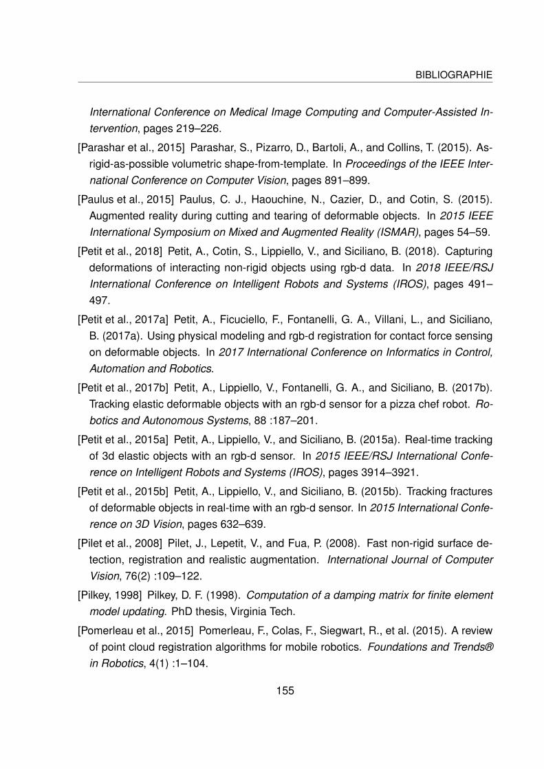
BIBLIOGRAPHIE
International Conference on Medical Image Computing and Computer-Assisted In-tervention, pages 219–226.
[Parashar et al., 2015] Parashar, S., Pizarro, D., Bartoli, A., and Collins, T. (2015). As-rigid-as-possible volumetric shape-from-template. In Proceedings of the IEEE Inter-national Conference on Computer Vision, pages 891–899.
[Paulus et al., 2015] Paulus, C. J., Haouchine, N., Cazier, D., and Cotin, S. (2015).Augmented reality during cutting and tearing of deformable objects. In 2015 IEEEInternational Symposium on Mixed and Augmented Reality (ISMAR), pages 54–59.
[Petit et al., 2018] Petit, A., Cotin, S., Lippiello, V., and Siciliano, B. (2018). Capturingdeformations of interacting non-rigid objects using rgb-d data. In 2018 IEEE/RSJInternational Conference on Intelligent Robots and Systems (IROS), pages 491–497.
[Petit et al., 2017a] Petit, A., Ficuciello, F., Fontanelli, G. A., Villani, L., and Siciliano,B. (2017a). Using physical modeling and rgb-d registration for contact force sensingon deformable objects. In 2017 International Conference on Informatics in Control,Automation and Robotics.
[Petit et al., 2017b] Petit, A., Lippiello, V., Fontanelli, G. A., and Siciliano, B. (2017b).Tracking elastic deformable objects with an rgb-d sensor for a pizza chef robot. Ro-botics and Autonomous Systems, 88 :187–201.
[Petit et al., 2015a] Petit, A., Lippiello, V., and Siciliano, B. (2015a). Real-time trackingof 3d elastic objects with an rgb-d sensor. In 2015 IEEE/RSJ International Confe-rence on Intelligent Robots and Systems (IROS), pages 3914–3921.
[Petit et al., 2015b] Petit, A., Lippiello, V., and Siciliano, B. (2015b). Tracking fracturesof deformable objects in real-time with an rgb-d sensor. In 2015 International Confe-rence on 3D Vision, pages 632–639.
[Pilet et al., 2008] Pilet, J., Lepetit, V., and Fua, P. (2008). Fast non-rigid surface de-tection, registration and realistic augmentation. International Journal of ComputerVision, 76(2) :109–122.
[Pilkey, 1998] Pilkey, D. F. (1998). Computation of a damping matrix for finite elementmodel updating. PhD thesis, Virginia Tech.
[Pomerleau et al., 2015] Pomerleau, F., Colas, F., Siegwart, R., et al. (2015). A reviewof point cloud registration algorithms for mobile robotics. Foundations and Trends®in Robotics, 4(1) :1–104.
155

BIBLIOGRAPHIE
[Pottmann et al., 2004] Pottmann, H., Leopoldseder, S., and Hofer, M. (2004). Regis-tration without icp. Computer Vision and Image Understanding, 95(1) :54–71.
[Prisacariu and Reid, 2012] Prisacariu, V. A. and Reid, I. D. (2012). Pwp3d : Real-timesegmentation and tracking of 3d objects. International journal of computer vision,98(3) :335–354.
[Ramalingam and Taguchi, 2013] Ramalingam, S. and Taguchi, Y. (2013). A theory ofminimal 3d point to 3d plane registration and its generalization. International journalof computer vision, 102(1-3) :73–90.
[Rankin, 1988] Rankin, C. (1988). Consistent linearization of the element-independentcorotational formulation for the structural analysis of general shells. NASA ContractorReport 278428, Lockheed Palo Alto Res. Lab., CA, 1988.
[Rao, 1995] Rao, S. S. (1995). Mechanical Vibrations Laboratory Manual. Year, EditionAddison-Wesley Publishing Company.
[Ren et al., 2017] Ren, C., Prisacariu, V., Kähler, O., Reid, I., and Murray, D. (2017).Real-time tracking of single and multiple objects from depth-colour imagery using 3dsigned distance functions. International Journal of Computer Vision, pages 1–16.
[Roth and Vona, 2012] Roth, H. and Vona, M. (2012). Moving volume kinectfusion. InBMVC, pages 1–11.
[Roth, 1982] Roth, S. D. (1982). Ray casting for modeling solids. Computer graphicsand image processing, 18(2) :109–144.
[Rother et al., 2004] Rother, C., Kolmogorov, V., and Blake, A. (2004). Grabcut : In-teractive foreground extraction using iterated graph cuts. In ACM transactions ongraphics (TOG), volume 23, pages 309–314. ACM.
[Royer et al., 2017] Royer, L., Krupa, A., Dardenne, G., Le Bras, A., Marchand, E., andMarchal, M. (2017). Real-time target tracking of soft tissues in 3d ultrasound imagesbased on robust visual information and mechanical simulation. Medical image ana-lysis, 35 :582–598.
[Rünz and Agapito, 2017] Rünz, M. and Agapito, L. (2017). Co-fusion : Real-timesegmentation, tracking and fusion of multiple objects. In Robotics and Automation(ICRA), 2017 IEEE International Conference on, pages 4471–4478.
[Runz et al., 2018] Runz, M., Buffier, M., and Agapito, L. (2018). Maskfusion : Real-time recognition, tracking and reconstruction of multiple moving objects. In 2018
156

BIBLIOGRAPHIE
IEEE International Symposium on Mixed and Augmented Reality (ISMAR), pages10–20.
[Rusu and Cousins, 2011] Rusu, R. B. and Cousins, S. (2011). 3D is here : PointCloud Library (PCL). In IEEE International Conference on Robotics and Automation(ICRA), Shanghai, China.
[Salas-Moreno et al., 2013] Salas-Moreno, R. F., Newcombe, R. A., Strasdat, H., Kelly,P. H., and Davison, A. J. (2013). Slam++ : Simultaneous localisation and mapping atthe level of objects. In Proceedings of the IEEE conference on computer vision andpattern recognition, pages 1352–1359.
[Salzmann et al., 2008] Salzmann, M., Moreno-Noguer, F., Lepetit, V., and Fua, P.(2008). Closed-form solution to non-rigid 3d surface registration. In European confe-rence on computer vision, pages 581–594.
[Salzmann et al., 2007] Salzmann, M., Pilet, J., Ilic, S., and Fua, P. (2007). Surfacedeformation models for nonrigid 3d shape recovery. IEEE Transactions on PatternAnalysis and Machine Intelligence, 29(8) :1481–1487.
[Salzo and Villa, 2012] Salzo, S. and Villa, S. (2012). Convergence analysis of aproximal gauss-newton method. Computational Optimization and Applications,53(2) :557–589.
[Schmidt et al., 2014] Schmidt, T., Newcombe, R. A., and Fox, D. (2014). Dart : Densearticulated real-time tracking. In Robotics : Science and Systems.
[Schulman et al., 2013] Schulman, J., Lee, A., Ho, J., and Abbeel, P. (2013). Trackingdeformable objects with point clouds. In 2013 IEEE International Conference onRobotics and Automation, pages 1130–1137.
[Sedef et al., 2006] Sedef, M., Samur, E., and Basdogan, C. (2006). Real-time finite-element simulation of linear viscoelastic tissue behavior based on experimental data.IEEE Computer Graphics and Applications, 26(6).
[Segal et al., 2009] Segal, A., Haehnel, D., and Thrun, S. (2009). Generalized-icp. InRobotics : science and systems, volume 2, page 435.
[Sengupta et al., 2019] Sengupta, A., Krupa, A., and Marchand, E. (2019). Trackingof non-rigid objects using rgb-d camera. In 2019 IEEE International Conference onSystems, Man, and Cybernetics (SMC), Bari, Italy.
157
BIBLIOGRAPHIE
[Shum and Szeliski, 2001] Shum, H.-Y. and Szeliski, R. (2001). Construction of pano-ramic image mosaics with global and local alignment. In Panoramic vision, pages227–268. Springer.
[Si, 2015] Si, H. (2015). Tetgen, a delaunay-based quality tetrahedral mesh generator.ACM Transactions on Mathematical Software (TOMS), 41(2) :11.
[Slavcheva et al., 2017a] Slavcheva, M., Baust, M., Cremers, D., and Ilic, S. (2017a).Killingfusion : Non-rigid 3d reconstruction without correspondences. In Proceedingsof the IEEE Conference on Computer Vision and Pattern Recognition, pages 1386–1395.
[Slavcheva et al., 2017b] Slavcheva, M., Baust, M., Cremers, D., and Ilic, S. (2017b).KillingFusion : Non-rigid 3D Reconstruction without Correspondences. In IEEEConference on Computer Vision and Pattern Recognition (CVPR).
[Slavcheva et al., 2018] Slavcheva, M., Baust, M., and Ilic, S. (2018). Sobolevfusion :3d reconstruction of scenes undergoing free non-rigid motion. In Proceedings of theIEEE Conference on Computer Vision and Pattern Recognition, pages 2646–2655.
[Slavcheva et al., 2016] Slavcheva, M., Kehl, W., Navab, N., and Ilic, S. (2016). Sdf-2-sdf : Highly accurate 3d object reconstruction. In European Conference on ComputerVision, pages 680–696.
[Solomon, 2015] Solomon, J. (2015). Numerical algorithms : methods for computervision, machine learning, and graphics. AK Peters/CRC Press.
[Stein, 1997] Stein, G. P. (1997). Lens distortion calibration using point correspon-dences. In Proceedings of IEEE Computer Society Conference on Computer Visionand Pattern Recognition, pages 602–608.
[Stults, 1984] Stults, B. M. (1984). Preventive health care for the elderly. WesternJournal of Medicine, 141(6) :832.
[Sumner et al., 2007] Sumner, R. W., Schmid, J., and Pauly, M. (2007). Embedded de-formation for shape manipulation. ACM Transactions on Graphics (TOG), 26(3) :80.
[Sun et al., 2018] Sun, L., Aragon-Camarasa, G., Rogers, S., and Siebert, J. P. (2018).Autonomous clothes manipulation using a hierarchical vision architecture. IEEE Ac-cess, 6 :76646–76662.
[Teichman et al., 2013] Teichman, A., Lussier, J. T., and Thrun, S. (2013). Learning tosegment and track in rgbd. IEEE Transactions on Automation Science and Enginee-ring, 10(4) :841–852.
158
BIBLIOGRAPHIE
[Trinh et al., 2018] Trinh, S., Spindler, F., Marchand, E., and Chaumette, F. (2018). Amodular framework for model-based visual tracking using edge, texture and depthfeatures. In 2018 IEEE/RSJ International Conference on Intelligent Robots and Sys-tems (IROS), pages 89–96.
[Varol et al., 2012] Varol, A., Salzmann, M., Fua, P., and Urtasun, R. (2012). Aconstrained latent variable model. In 2012 IEEE Conference on Computer Visionand Pattern Recognition, pages 2248–2255.
[Walker et al., 1991] Walker, M. W., Shao, L., and Volz, R. A. (1991). Estimating 3-dlocation parameters using dual number quaternions. CVGIP : image understanding,54(3) :358–367.
[Wang et al., 2015] Wang, B., Wu, L., Yin, K., Ascher, U., Liu, L., and Huang, H.(2015). Deformation Capture and Modeling of Soft Objects. ACM Trans. Graph.,34(4) :94 :1–94 :12.
[Wang et al., 2015] Wang, B., Wu, L., Yin, K., Ascher, U. M., Liu, L., and Huang, H.(2015). Deformation capture and modeling of soft objects. ACM Trans. Graph.,34(4) :94–1.
[Wang et al., 2017] Wang, K., Zhang, G., and Xia, S. (2017). Templateless non-rigidreconstruction and motion tracking with a single rgb-d camera. IEEE Transactionson Image Processing, 26(12) :5966–5979.
[Wei et al., 2009] Wei, Y., Cotin, S., Fang, L., Allard, J., Pan, C., and Ma, S. (2009).Toward real-time simulation of blood-coil interaction during aneurysm embolization.In International Conference on Medical Image Computing and Computer-AssistedIntervention, pages 198–205.
[Whelan et al., 2013] Whelan, T., Kaess, M., Leonard, J. J., and McDonald, J. (2013).Deformation-based loop closure for large scale dense rgb-d slam. In 2013 IEEE/RSJInternational Conference on Intelligent Robots and Systems, pages 548–555.
[Wikipedia, 2016] Wikipedia (2016). Iterative closest point. [Online ; accessed 04-January-2016].
[Willimon et al., 2012] Willimon, B., Hickson, S., Walker, I., and Birchfield, S. (2012).An energy minimization approach to 3d non-rigid deformable surface estimationusing rgbd data. In 2012 IEEE/RSJ International Conference on Intelligent Robotsand Systems, pages 2711–2717.
159
BIBLIOGRAPHIE
[Wood and Zienkiewicz, 1977] Wood, R. D. and Zienkiewicz, O. (1977). Geometricallynonlinear finite element analysis of beams, frames, arches and axisymmetric shells.Computers & Structures, 7(6) :725–735.
[Wu et al., 2018] Wu, J., Zhou, B., Russell, R., Kee, V., Wagner, S., Hebert, M., Tor-ralba, A., and Johnson, D. M. (2018). Real-time object pose estimation with poseinterpreter networks. In 2018 IEEE/RSJ International Conference on Intelligent Ro-bots and Systems (IROS), pages 6798–6805.
[Wu and Lee, 1997] Wu, J.-Y. and Lee, R. (1997). The advantages of triangular andtetrahedral edge elements for electromagnetic modeling with the finite-element me-thod. IEEE Transactions on Antennas and Propagation, 45(9) :1431–1437.
[Xiang et al., 2018] Xiang, Y., Schmidt, T., Narayanan, V., and Fox, D. (2018). Po-secnn : A convolutional neural network for 6d object pose estimation in clutteredscenes.
[Yilmaz et al., 2006] Yilmaz, A., Javed, O., and Shah, M. (2006). Object tracking : Asurvey. Acm computing surveys (CSUR), 38(4) :13.
[Zabatani et al., 2019] Zabatani, A., Surazhsky, V., Sperling, E., Moshe, S. B., Me-nashe, O., Silver, D. H., Karni, T., Bronstein, A. M., Bronstein, M. M., and Kimmel, R.(2019). Intel® realsense™ sr300 coded light depth camera. IEEE transactions onpattern analysis and machine intelligence.
[Zeng et al., 2012] Zeng, M., Zhao, F., Zheng, J., and Liu, X. (2012). A memory-efficient kinectfusion using octree. In Computational Visual Media, pages 234–241.Springer.
[Zhang et al., 2019] Zhang, Z., Petit, A., Dequidt, J., and Duriez, C. (2019). Calibrationand external force sensing for soft robots using an rgb-d camera. IEEE Robotics andAutomation Letters, 4(3) :2356–2363.
[Zhao et al., 2016] Zhao, J.-M., Song, X.-X., and Liu, B. (2016). Standardized com-pliance matrices for general anisotropic materials and a simple measure of aniso-tropy degree based on shear-extension coupling coefficient. International Journal ofApplied Mechanics, 8(06) :1650076.
[Zollhöfer et al., 2014] Zollhöfer, M., Nießner, M., Izadi, S., Rehmann, C., Zach, C.,Fisher, M., Wu, C., Fitzgibbon, A., Loop, C., Theobalt, C., et al. (2014). Real-timenon-rigid reconstruction using an rgb-d camera. ACM Transactions on Graphics(TOG), 33(4) :156.
160
Titre :Suivi visuel d’objets déformables avec une caméra
RGB-D
Mot clés : Suivi visuel, suivi des déformations, FEM
Resumé : Le suivi d’objets déformable à partir d’informa-tions visuelles à de nombreuses applications dans le domainede la robotique, de l’animation ou de la simulation. Dans cettethèse, nous proposons de nouvelles approches pour le suivid’objets rigides et non rigides à l’aide d’une caméra RGB-D.Cette thèse comporte quatre contributions principales. La pre-mière contribution est une nouvelle approche de suivi d’objetsdans des images RGB-D qui utilise des erreurs basées sur laprofondeur et la photométrie pour suivre et localiser des formescomplexes en utilisant leur modèle 3D grossier. La secondecontribution porte sur une méthode de suivi d’objets non rigides
reposant sur une approche par éléments finis (FEM) pour suivreet caractériser les déformations. La troisième contribution estune approche de suivi de la déformation qui minimise une com-binaison d’erreurs géométriques et photométriques tout en uti-lisant la FEM comme modèle de déformation. Finalement, laquatrième contribution consiste à estimer les propriétés d’élas-ticité d’un objet analysant ses déformations toujours à l’aided’une caméra RGB-D. Une fois les paramètres d’élasticité esti-més, la même méthodologie peut être réutilisée pour caractéri-ser les forces de contact.
Title : Visual Tracking of Deformable Objects with RGB-
D Camera
Keywords : Visual Tracking, Deformation Tracking, FEM
Abstract : Tracking soft objects using visual in-formation has immense applications in the fieldof robotics, computer graphics and automation. Inthis thesis, we propose multiple new approachesfor tracking both rigid and non-rigid objects usinga RGB-D camera. There are four main contribu-tions of this thesis. The first contribution is a ri-gid object tracking method which utilizes depthand photometry based errors for tracking complexshapes using their coarse, 3D template. The se-cond contribution is a non-rigid object tracking me-thod which uses co-rotational FEM to track defor-
ming objects by regulating the virtual forces actingon the surface of a physics based model of theobject. The third contribution is a deformation tra-cking approach which minimizes a combination ofgeometric and photometric error while utilizing co-rotation FEM as the deformation model. The fourthcontribution involves estimating the elasticity pro-perties of a deforming object while tracking theirdeformation using RGB-D camera. Once the elas-ticity parameters have been estimated, the samemethodology can be re-utilized for tracking contactforces on the surface of deforming objects.