Targetless camera calibration

TARGETLESS CAMERA CALIBRATION

L. Barazzetti a, L. Mussio

b, F. Remondino

c, M. Scaioni

a

a Politecnico di Milano, Dept. of Building Engineering Science and Technology, Milan, Italy

{luigi.barazzetti, marco.scaioni}@polimi.it, web: http://www.icet-rilevamento.lecco.polimi.it/ b Politecnico di Milano, Dept. of Environmental, Hydraulic, Infrastructures and Surveying Engineering, Milan, Italy

[email protected], web: http://www.diiar.polimi.it/diiar

c 3D Optical Metrology Unit, Bruno Kessler Foundation (FBK), Trento, Italy

[email protected], web: http://3dom.fbk.eu

KEY WORDS: Automation, Accuracy, Calibration, Matching, Orientation

ABSTRACT:

In photogrammetry a camera is considered calibrated if its interior orientation parameters are known. These encompass the principal

distance, the principal point position and some Additional Parameters used to model possible systematic errors. The current state of

the art for automated camera calibration relies on the use of coded targets to accurately determine the image correspondences. This

paper presents a new methodology for the efficient and rigorous photogrammetric calibration of digital cameras which does not

require any longer the use of targets. A set of images depicting a scene with a good texture are sufficient for the extraction of natural

corresponding image points. These are automatically matched with feature-based approaches and robust estimation techniques. The

successive photogrammetric bundle adjustment retrieves the unknown camera parameters and their theoretical accuracies. Examples,

considerations and comparisons with real data and different case studies are illustrated to show the potentialities of the proposed

methodology.

a) b)

Figure 1. A target-based calibration procedure (a) and the targetless approach (b).

1. INTRODUCTION

Accurate camera calibration and image orientation procedures

are a necessary prerequisite for the extraction of precise and

reliable 3D metric information from images (Gruen and Huang,

2001). A camera is considered calibrated if its principal

distance, principal point offset and lens distortion parameters

are known. Camera calibration has always been an essential

component of photogrammetric measurement. Self-calibration

is nowadays an integral and routinely applied operation within

photogrammetric image triangulation, especially in high-

accuracy close-range measurement. With the very rapid growth

in adoption of off-the-shelf (or consumer-grade) digital cameras

for 3D measurement applications, however, there are many

situations where the geometry of the image network cannot

support the robust recovery of camera interior parameters via

on-the-job calibration. For this reason, stand-alone and target-

based camera calibration has again emerged as an important

issue in close-range photogrammetry.

In many applications, especially in Computer Vision (CV), only

the focal length is generally recovered. In case of precise

photogrammetric measurements, the whole set of calibration

parameters is instead employed. Various algorithms for camera

calibration have been reported over the past years in the

photogrammetry and CV literature (Remondino and Fraser,

2006). The algorithms are usually based on perspective or

projective camera models, with the most popular approach

being the well-known self-calibrating bundle adjustment

(Brown, 1976; Fraser, 1997; Gruen and Beyer, 2001). It was

first introduced in close-range photogrammetry in the early

1970s by Brown (1971). Analytical camera calibration was a

major topic of research interest in photogrammetry over the

next decade and it reached its full maturity in the mid 1980s. In

the early days of digital cameras, self-calibration became again

a hot research topic and it reached its maturity in the late ‘90s

with the development of fully automated vision metrology

systems mainly based on targets (e.g. Ganci and Handley,

1998). In the last decade, with the tremendous use of consumer-

grade digital cameras for many measurement applications, there

was a renewed interest in stand-alone photogrammetric

calibration approaches, especially for fully automatic on-the-job

calibration procedures. Nowadays the state of the art basically

relies on the use of coded targets which are depicted in images

forming a block with a suitable geometry for estimating all the

calibration parameters (Cronk et al., 2006). Target measurement

and identification is performed in an automatic way. A bundle

International Archives of the Photogrammetry, Remote Sensing and Spatial Information Sciences, Volume XXXVIII-5/W16, 2011ISPRS Trento 2011 Workshop, 2-4 March 2011, Trento, Italy

335

adjustment allows then the estimation of all the unknown

parameters and their theoretical accuracies.

On the other hand, camera calibration continues to be a more

active area of research within the CV community, with a

perhaps unfortunate characteristic of much of the work being

that it pays too little heed to previous findings from

photogrammetry. Part of this might well be explained in terms

of a lack of emphasis on (and interest in) accuracy aspects and a

basic premise that nothing whatever needs to be known about

the camera which is to be calibrated within a linear projective

rather than Euclidean scene reconstruction.

2. CAMERA CALIBRATION IN PHOTOGRAMMETRY

AND COMPUTER VISION

In photogrammetry camera calibration is meant as the recovery

of the interior camera parameters. Camera calibration plays a

fundamental role in both photogrammetry and CV but there is

an important distinction between the approaches used in both

disciplines. Even the well-known term self-calibration has

different meanings.

Lens distortion generates a misalignment between the

perspective centre, the image point and the object point. It is

quite simple to understand that the collinearity principle, which

is the basis for image orientation, is no longer respected

(“departure from collinearity”). Modelling lens distortion

allows to strongly reduce this effect. A calibrated camera is a

powerful measuring tool, with a precision superior to 1:25,000

as reported in different vision metrology applications (Maas and

Niederöst, 1997; Albert et al., 2002; Amiri Parian et al., 2006;

Barazzetti and Scaioni, 2009; Barazzetti and Scaioni, 2010).

The importance of camera calibration is confirmed by the vast

number of papers in the technical literature: accuracy aspects,

low-cost and professional cameras, stability and behaviour of

the parameters, variations in the different colour channels as

well as algorithmic issues were reported in Fraser and Shortis

(1995), D’Apuzzo and Maas (1999), Läbe and Förstner (2004),

Fraser and Al-Ajlouni (2006), Peipe and Tecklenburg (2006)

and Remondino and Fraser (2006).

During a photogrammetric camera calibration procedure, the

systematic errors in digital CCD/CMOS sensor are universally

compensated with an 8-terms physical mathematical model

originally formulated by Brown (1971). This comprises terms

for the principal distance (c) and principal point offset (x0, y0)

correction, three coefficients for the radial distortion (k1, k2, k3),

and two coefficients for the decentring distortion (p1, p2). The

model can be extended by two further parameters to account for

affinity and shear within the image plane, but such terms are

rarely if ever significant in modern digital cameras, especially

for heritage and architectural applications. The corrections

terms are generally called Additional Parameters (APs).

The three APs used to model the radial distortion δr are

generally expressed with an odd-ordered polynomial series:

7

3

5

2

3

1rkrkrkr ++=δ (1)

where r is the radial distance of the generic image point (x, y)

from the principal point (x0, y0):

( ) ( )2

0

2

0yyxxr −+−= (2)

The components along x and y of δr may be estimated as

follows:

( ) ( )r

ryyy

r

rxxx

δδ

δδ

00, −=−= (3)

The coefficients ki are a function of the used principal distance

and are usually highly correlated, with most of the error signal

generally being accounted for by the cubic term k1r3. The k2 and

k3 terms are typically included for photogrammetric (low

distortion) and wide-angle lenses and in higher-accuracy vision

metrology applications. Recent research has demonstrated the

feasibility of empirically modelling radial distortion throughout

the magnification range of a zoom lens as a function of the focal

length written to the image EXIF header (Fraser and Al-

Ajlouni, 2006).

A misalignment of the lens elements along the optical axis

instead generates decentring distortion. The corrections terms

for the measured image coordinates are given by:

( )[ ] ( )( )

( )[ ] ( )( )001

2

0

2

2

002

2

0

2

1

22

22

yyxxpyyrpt

yyxxpxxrpt

y

x

−−+−+=

−−+−+=

δ

δ (4)

The decentering distortion parameters p1 and p2 are invariably

strongly projectively coupled with x0 and y0. Decentering

distortion is usually an order of magnitude or more less than the

radial distortion and it also varies with focus, but to a much less

extent.

Considering all the APs, the image coordinates correction terms

can be formulated as:

y

x

txcc

yyyy

txcc

xxxx

δδ

δδ

++∆−

+∆−=∆

++∆−

+∆−=∆

00

00 (5)

The simultaneous estimation of APs and camera parameters is

generally referred to as self-calibrating bundle adjustment. The

bundle adjustment with APs needs a favourable network

geometry to be correctly solved i.e. convergent and rotated

images of a preferably 3D object should be acquired, with well

distributed points throughout the image format (Figure 2a). If

the network is geometrically weak, high correlations between

the unknown parameters may lead to instabilities in the least-

squares estimation. The inappropriate use of the APs can also

weaken the bundle adjustment solution, leading to over-

parameterization, in particular in the case of minimally

constrained adjustments (Fraser, 1982).

The collinearity model and the related bundle adjustment

problem must be linearized to obtain a system of linear

observation equations. The linearized model can be solved with

the Gauss-Markov model of least squares (Mikhail et al., 2001)

and its solution is rigorous in a functional and stochastic sense.

Good initial values of the unknown parameters are needed for

the linearization process based on the Taylor series expansion.

External constraints (e.g. GNSS/INS data, GCPs) can also be

efficiently incorporated into the general model. The final system

is made up of observation equations (those written as functions

of both observations and parameters) and constraint equations

(those written in terms of the parameters). The second group of

equations is usually formulated as pseudo-observation

equations, where the unknown parameters are linked to their

measured values. All the variables in the adjustment become

weighted observations. By properly tuning each weight it is

possible to give more or less emphasis to the observed values of

each unknown parameter.


336

If the observations are image coordinates, the reconstruction is

affected by an overall ambiguity (i.e. a 3D similarity

transformation). This “datum problem” (or rank deficiency) can

be solved by introducing ground control points (GCPs) and/or

GNSS/INS information. The second solution is almost the

standard in aerial photogrammetry, while these data are not

generally available in close-range surveys. The rank deficiency

of the Least Squares problem can also be removed with an inner

constraint. This does not involve external observations and

leads to the so-called free-net solution (Granshaw, 1980;

Dermanis, 1994). The theoretical accuracy obtainable with a

free-net adjustment, coupled with precise image points and

good calibration parameters is superior to 1:100,000. In some

cases, a theoretical accuracy of about one part in a million was

reached (Fraser, 1992).

(a)

(b)

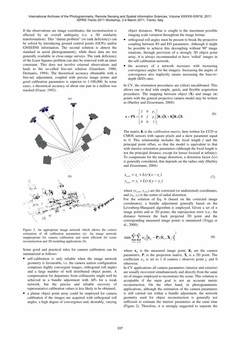
Figure 2. An appropriate image network which allows the correct

estimation of all calibration parameters (a). An image network

inappropriate for camera calibration and more efficient for scene

reconstruction and 3D modeling applications (b).

Some good and practical rules for camera calibration can be

summarized as follows:

• self-calibration is only reliable when the image network

geometry is favourable, i.e. the camera station configuration

comprises highly convergent images, orthogonal roll angles

and a large number of well distributed object points. A

compensation for departures from collinearity might well be

achieved in a bundle adjustment with APs for a weak

network, but the precise and reliable recovery of

representative calibration values is less likely to be obtained;

• a planar object point array could be employed for camera

calibration if the images are acquired with orthogonal roll

angles, a high degree of convergence and, desirably, varying

object distances. What is sought is the maximum possible

imaging scale variation throughout the image format.

• orthogonal roll angles must be present to break the projective

coupling between IO and EO parameters. Although it might

be possible to achieve this decoupling without 90o image

rotations, through provision of a strongly 3D object point

array, it is always recommended to have ‘rolled’ images in

the self-calibration network;

• the accuracy of a network increases with increasing

convergence angles for the imagery. Increasing the angles of

convergence also implicitly means increasing the base-to-

depth (B/D) ratio.

In CV, the orientation procedures are (often) uncalibrated. This

allows one to deal with simple, quick, and flexible acquisition

procedures. The mapping between object (X) and image (x)

points with the general projective camera model may be written

as (Hartley and Zissermann, 2004):

[ ] [ ]XtRKXtRPXx ,,

100

0

0

=

== y

x

pf

pf (6)

The matrix K is the calibration matrix, here written for CCD or

CMOS sensors with square pixels and a skew parameter equal

to 0. This relationship includes the focal length f and the

principal point offset, so that the model is equivalent to that

with interior orientation parameters (although the focal length is

not the principal distance, except for lenses focused at infinity).

To compensate for the image distortion, a distortion factor L(r)

is generally considered, that depends on the radius only (Hartley

and Zissermann, 2004):

))((

))((

cccorr

cccorr

yyrLyy

xxrLxx

−+=

−+=

(7)

where (xcorr, ycorr) are the corrected (or undistorted) coordinates,

and (xc, yc) is the centre of radial distortion.

For the solution of Eq. 6 (based on the corrected image

coordinates), a bundle adjustment generally based on the

Levenberg-Marquard algorithm is employed. Given a set of n

image points and m 3D points, the reprojection error (i.e., the

distance between the back projected 3D point and the

corresponding measured image point) is minimized (Triggs et

al., 2000):

2

1 1

),K(min∑∑= =

−n

i

jiiij

m

j

ijw XPx (8)

where xij is the measured image point, Ki are the camera

parameters, Pi is the projection matrix, Xj is a 3D point. The

coefficient wij is set to 1 if camera i observes point j, and 0

otherwise.

In CV applications all camera parameters (interior and exterior)

are usually recovered simultaneously and directly from the same

set of images employed to reconstruct the scene. This solution is

acceptable if the main goal is not an accurate metric

reconstruction. On the other hand, in photogrammetric

applications, although the estimation of the camera parameters

is still carried out within a bundle adjustment, the network

geometry used for object reconstruction is generally not

sufficient to estimate the interior parameters at the same time

(Figure 2). Therefore, it is strongly suggested to separate the


337

recovery of the interior and exterior orientation parameters by

means of two separate procedures with adequate networks.

3. TARGETLESS CAMERA CALIBRATION

Since many years commercial photogrammetric packages use

coded targets for the automated calibration and orientation

phase (Ganci and Handley, 1998; Cronk et al., 2006). Coded

targets can be automatically recognized, measured and labelled

to solve for the identification of the image correspondences and

the successive camera parameters within few minutes.

Figure 3. Examples of coded targets.

Commercial software (e.g., iWitness and PhotoModeler)

typically works with small coded targets (Figure 3) that can be

distributed in order to form a 3D calibration polygon. The main

advantage of this procedure is related to the possibility to have a

portable solution. This is useful in many photogrammetric

surveys and to assure a correct and automated identification of

the image correspondences.

This paper presents a new methodology to efficiently calibrate a

digital camera using the ATiPE system, widely described in

Barazzetti et al. (2010a) and Barazzetti (2011). ATiPE can

automatically and accurately identify homologues points from a

set of convergent images without any coded target or marker. A

set of natural features of an existing object are used to

determine the image correspondences. These image points are

automatically matched with the implemented feature-based

matching (FBM) approaches. The object should have a good

texture in order to provide a sufficient number of tie points well

distributed in the images. The operator has to acquire a set of

images (12-15) with a good spatial distribution around an object

(including 90o camera roll variations). Architectural objects

(e.g. arcades, building facades, colonnades and similar) should

be avoided because of their repetitive textures and symmetries.

Big rocks, bas-reliefs, decorations, ornaments or even a pile of

rubble are appropriate (Figure 4).

Figure 4. Examples of good calibration objects.

ATiPE uses SIFT (Lowe, 2004) and SURF (Bay et al., 2008) as

feature detectors and descriptors. A kd-tree search (Arya et al.,

1998) speeds up the comparison between the descriptors of the

adopted FBM algorithms. The experimental tests demonstrated

that points are rarely matched with convergence angles superior

to 30-40°. A normal exhaustive quadratic comparison of the

feature descriptors is a more robust approach in case of very

convergent images. This is the most important drawback of the

method, which leads to a long elaboration time. The global

processing time is often unpredictable. It ranges from few

minutes up to some hours for large datasets with very

convergent images.

4. EXAMPLES AND PERFORMANCE ANALYSES

4.1 Practical tests

Figure 5a shows a calibration testfield created with some coded

targets. 16 images are acquired using a Nikon D700

(4,256×2,832 pixels) equipped with a 35 mm Nikkor lens

(focused at ∞). The camera calibration solution was computed

within Australis, which can automatically detected all the coded

targets and compute the calibration parameters (Table 1)

according to the 8-term mathematical model described in

Section 2. The same images were then processed with ATiPE in

order to extract a set of natural points randomly distributed in

the scene (Figure 5b). The successive estimation of the bundle

solution (within Australis) provided all calibration parameters

with the camera poses and 3D points (Figure 5c and 5d). The

corresponding calibration parameters and their precisions are

equal and shown in Table 1. The project with targets

comprehends 55 3D points (5 circles × 11 targets). The

estimated theoretical accuracies along the x, y and z axis were

1:83,000, 1:40,900 and 1:64,500, respectively. The processing

with ATiPE provided for 2,531 3D natural points (at least 4

images for each point; 1,356 points were matched in 6 or more

images). The estimated theoretical accuracies along the x, y and

z axis were 1:22,100, 1:6,500; 1:9,400, respectively. This

disparity is motivated by the use of different matching strategies

leading to different accuracy in the image measurements. The

measurement of the centre of the targets is performed more

precisely than natural points extracted using FBM methods.

Indeed, as also stated by Fraser (1996), the accuracy of the

computed object coordinates depends on the image

measurement precision, image scale and geometry as well as the

number of exposure.

Targets

Value Std.dev

RMSE (µm) 0.89

c (mm) 35.8970 ±0.005

x0 (mm) -0.0973 ±0.004

y0 (mm) -0.1701 ±0.004

k1 6.97946e-005 ±6.0510e-007

k2 -5.40867e-008 ±3.2964e-009

k3 -1.21579e-011 ±5.4357e-012

p1 -1.4449e-006 ±1.074e-006

p2 -5.3279e-006 ±9.990e-007

ATiPE

Value Std.dev

RMSE (µm) 2.97

c (mm) 35.8891 ±0.003

x0 (mm) -0.0703 ±0.002

y0 (mm) -0.1716 ±0.002

k1 6.97850e-5 ±3.6472e-7

k2 -5.64321e-8 ±2.0338e-9

k3 -5.65025e-12 ±3.4521e-12

p1 -6.3586e-6 ±6.064e-7

p2 -5.2057e-6 ±6.068e-7

Table 1. Camera interior parameters estimated with the target-based

approach and using ATiPE (targetless) method for a Nikon D700

mounting a 35 mm lens.


338

a) b)

c) d)

Figure 5. The calibration polygon with iWitness/Australis targets (a). Tie points extracted by ATiPE using the natural texture of the scene (b). The

bundle adjustment results achieved in Australis using coded target image coordinates (c) and natural features image coordinates (d). The recovered

camera parameters of both approaches are reported in Table 1.

Figure 6 shows another example of the experiments. The

camera employed is a Nikon D200 with a 20 mm Nikkor lens. A

set of 30 images was acquired, including coded targets to

perform an automated camera calibration. The self-calibrating

bundle adjustment with and without coded targets achieved very

similar results for the interior parameters (Table 2).

Figure 6. The scene used for the automated camera calibration with and

without coded targets (top). The camera network of the targetless

solution with the recovered camera poses and sparse point cloud

(bottom).

Targets ATiPE

Value Std.dev Value Std.dev

RMSE (µm) 1.01 - 3.63 -

c (mm) 20.4367 0.003 20.4244 0.003

x0 0.0759 0.002 0.0760 0.002

y0 0.0505 0.003 0.0481 0.002

k1 2.8173e-4 2.605e-6 2.7331e-4 2.5102e-6

k2 -4.5538e-7 3.585e-8 -4.6780e-7 2.666e-8

k3 -2.7531e-10 1.452e-10 -5.8892e-11 9.2528e-11

p1 7.849e-6 2.113e-6 1.9942e-6 1.979e-6

p2 -1.6824e-5 2.247e-6 -1.4358e-5 1.858e-6

Table 2. Results for a Nikon D200 equipped with a 20 mm Nikkor lens,

with and without targets.

4.2 Accuracy analysis with independent check points

The consistence and accuracy of the first targetless calibration

experiement were verified using a special testfield composed of

21 circular targets which are used as Ground Control Points

(GCPs). Their 3D coordinates were measured with a theodolite

Leica TS30, using three stations and a triple intersection to

obtain high accuracy results. The standard deviation of the

measured coordinates was ±0.2 mm in x (depth) and ±0.1 mm in

y and z.

A photogrammetric block of 6 images was also acquired. All

target centres were measured via LSM to obtain sub-pixel

precisions. The photogrammetric bundle adjustment was carried

out with the two sets of calibration parameters. Both

photogrammetric projects were run in free-net and then

transformed into the Ground Reference System (GRS) using 5

GCPs. The remaining 16 points were used as independent check

points (ChkP) to evaluate the quality of the estimation

procedure. The following quantities were computed for each

ChkP:


339

∆x = xGRS - xPhoto, ∆y = yGRS - yPhoto, ∆z = zGRS - zPhoto (9)

The differences in both configurations are shown in Table 3. It

can be noted that the behaviour is quite similar and the standard

deviations of the differences along x, y and z are equivalent.

GRS – Targets

∆x ∆y ∆z

Mean (mm) 0.15 0.59 -0.32

Std.dev (mm) 0.43 0.75 1.45

Max (mm) 0.83 1.58 2.22

Min (mm) -0.55 -0.90 -2.43

GRS – ATiPE

∆x ∆y ∆z

Mean (mm) 0.16 0.61 -0.35

Std.dev (mm) 0.40 0.77 1.44

Max (mm) 0.81 1.62 2.12

Min (mm) -0.46 -0.95 -2.42

Table 3. Comparison between ChkP coordinates measured with a

theodolite (GRS) and photogrammetric measurements with and

without targets (ATiPE). The behaviour and the residuals are

similar for both photogrammetric approaches.

a)

GRS - Targets

-3

-2

-1

0

1

2

3

0 2 4 6 8 10 12 14 16

Dif

fere

nce

s (

mm

)

delta x

delta y

delta z

b)

GRS - ATiPE

-3

-2

-1

0

1

2

3

0 2 4 6 8 10 12 14 16

Dif

fere

nces

(m

m)

delta x

delta y

delta z

c)

Targets - ATiPE

-0.3

-0.2

-0.1

0

0.1

0.2

0.3

0 2 4 6 8 10 12 14 16

Dif

fere

nce

s (

mm

)

delta x

delta y

delta z

Figure 7. Graphical behaviour of the differences of the ChkP

coordinates in the solution obtained using coded targets (a) and natural

features extracted with ATiPE (b). The differences between the target

and targetless approach are shown in (c).

It is also interesting that the differences are superior to 2 mm for

some points. This is probably due to a residual movement of the

targets during the data acquisition phase. Indeed, both reference

data and images were acquired at different epochs. All targets

are made of paper and probably there was a small deformation

of this deformable material. This is also demonstrated by the

coherence of both photogrammetric projects (Figure 7).

The coordinates of both photogrammetric projects were then

compared. They confirm the consistence between these

calibration datasets. A graphical visualization of the differences

between the ATiPE procedure (targetless) and the estimation

based on targets is shown in Figure 7.

4.3 Analysis of covariance and correlation matrices

The use of a free-net bundle adjustment for the estimation of the

calibration parameters leads to a modification of the general

form of the least squares problem. In some cases, if the network

geometry is not sufficiently robust to incorporate all calibration

parameters (basic interior plus the APs), the adjustment can

provide highly correlated values. Therefore, a statistical

evaluation of the obtained APs is always recommended (Gruen,

1981; Jacobsen, 1982; Gruen, 1985). This can be carried out by

using the estimated covariance matrices and not only with the

independent analysis of the standard deviations of each single

unknown (Cox and Hinkley, 1976; Kendall, 1990; Sachs,

1984).

In the following, the dataset with targets is used as reference, as

it can be assumed as the current state of the art for traditional

photogrammetric calibrations. In particular, CT is the 8×8

covariance matrix of all calibration parameters estimated using

targets. The covariance matrix with the targetless procedure is

named CA (A = ATiPE). The aim is to demonstrate that CT and

CA are similar, in order to confirm the consistence of both

calibrations. There exist several criteria for comparing

covariance matrices, e.g. different distances d(CT, CA) which

depend on the choice of the model employed. However, it is

quite complicated to understand when d is small, especially if

the estimated values have different measurement units. A

possible solution could be to use the eigenvalues λi of the

covariance matrices, in order to obtain new diagonal matrices

that can be compared (Jolliffe, 2002). According to this

procedure, the directions of the principal axes of the confidence

ellipsoids are given by the eigenvectors.

To check the equality of the covariance matrices, the

Hotelling’s test could also be used:

( )2/

1

2

2/

2 detlog2

mn

j

xj

m

−=

∏=

σ

χC

(10)

where m is the number of data and n the number of calibration

parameters (8 in this case). For both matrices the ratio of the

values given by Eq. 10 was estimated, obtaining a large

disparity between CT and CA because of the different number of

observations used during the estimation of the photogrammetric

bundle solutions. To understand better the results achieved with

both calibration procedures it is possible to use the correlation

matrix R. It is well-known that some calibration parameters are

highly correlated, e.g. the coefficient ki modelling radial

distortion. In addition, there is a projective coupling between p1

and p2 with x0 and y0, respectively. The experimental results

provided two correlation matrices (RT, RA) very similar, where

the correlations between the listed parameter configurations are

quite strong (>0.8), although the targetless procedure seems

slightly better (Table 4).


340

RT c xp yp K1 K2 K3 P1 P2

C 1

xp 0.13 1

yp -0.01 -0.06 1

K1 0.22 0.05 -0.01 1

K2 -0.27 -0.04 -0.05 -0.97 1

K3 0.24 0.03 0.07 0.93 -0.99 1

P1 -0.21 -0.91 0.08 -0.11 0.1 -0.09 1

P2 -0.01 0.04 -0.93 0.01 0.03 -0.04 -0.06 1

RA c xp yp K1 K2 K3 P1 P2

c 1

xp 0.02 1

yp -0.04 -0.03 1

K1 0.02 0.02 0.05 1

K2 -0.09 -0.01 -0.04 -0.96 1

K3 0.09 0.01 0.03 0.9 -0.98 1

P1 -0.03 -0.86 0.05 -0.02 0.02 -0.02 1

P2 0 0.03 -0.87 -0.09 0.06 -0.05 -0.04 1

Table 4. The correlation matrices estimated with targets (top) and

ATiPE (bottom).

For the remaining parameters, the correlations are instead

correctly reduced. A consideration deserve to be mentioned: in

the case of uncorrelated parameters the relationship det(R) = 1

must be verified. Therefore, a simple general criterion to assess

the quality of these covariance matrices can be the simple

comparison of the determinants:

det(RT) = 1.3·106 < det(RA) = 7.1·105

This values are quite similar, because the matrices look quite

similar. Therefore test the equality of the correlation structures,

a multi-dimensional statistical analysis should be employed.

Lawley’s procedure (1963) requires the estimation of the

following statistic:

∑∑−

= +=

+−−=

1

1 1

22

6

521

n

i

n

ij

ijr

nmχ (11)

where m is the number of data and n the number of calibration

parameters (8 in this case). The application of this criterion

shows that CA and CT are not equal (the ratio between the χ2

values is superior to 40), but this is mainly due to the different

number of observations between the procedures (e.g. 55 3D

points with the target-based method, 7,593 with ATiPE). The

estimation of the ratio log(det(R(A))/log(det(RT)) ≈ 32 confirms

the previous results.

In summary, the statistical interpretation of the results is quite

difficult because of the different numbers of input data. The

comparison between different sets of calibration parameters

using total station measurements is probably a better factor to

check the final quality of the targetless calibration parameters.

5. CONCLUSION

This paper has presented a new procedure for camera

calibration based on the natural texture of an object which has

to be properly selected. The method can also be assumed as the

initial step for a complete 3D reconstruction pipeline of some

categories of objects. It is worth noting that different phases of

the “reconstruction problem” can be now carried out in a fully

automated way.

The proposed methodology for camera calibration is not based

on targets, but it is capable of providing the unknown camera

parameters values with the same theoretical accuracy of the

more familiar target-based procedure. It has also been proved

that the larger number of tie points extracted for computing self-

calibration gives rise to slightly smaller correlations among the

parameters. But further statistical analyses should be performed.

The key-point leading to a successful calibration is (i) the

selection of a proper object featuring a good shape and textures

and (ii) the acquisition of a set of images which results in a

suitable image block geometry.

For industrial and highly-precise photogrammetric projects, the

target-based camera calibration procedure will probably remain

the standard solution while for many other 3D modeling

applications, the presented method can be the ideal solution to

speed up the entire photogrammetric pipeline, avoid targets and

allow on-the-job self-calibration in a precise and reliable way.

REFERENCES

Albert, J., Maas, H.G., Schade, A. and Schwarz, W., 2002. Pilot

studies on photogrammetric bridge deformation measurement.

Proceedings of the 2nd IAG Symposium on Geodesy for

Geotechnical and Structural Engineering: 133-140.

Amiri Parian, J., Gruen, A. and Cozzani, A., 2006. Highly

accurate photogrammetric measurements of the Planck

Telescope reflectors. 23rd Aerospace Testing Seminar (ATS),

Manhattan Beach, California, USA, 10-12 October.

Arya, S., Mount, D.M., Netenyahu, N.S., Silverman, R. and

Wu, A.Y., 1998. An optimal algorithm for approximate nearest

neighbor searching fixed dimensions. Journal of the ACM,

45(6): 891-923.

Barazzetti, L. and Scaioni, M., 2009. Crack measurement:

development, testing and application of an image-based

algorithm. ISPRS Journal of Photogrammetry and Remote

Sensing, 64: 285-296.

Barazzetti, L. and Scaioni, M., 2010. Development and

implementation of image-based algorithms for measurement of

deformations in material testing. Sensors: 7469-7495.

Barazzetti, L., Remondino, F. and Scaioni, M., 2010a.

Extraction of accurate tie points for automated pose estimation

of close-range blocks. Int. Archives of Photogrammetry, Remote

Sensing and Spatial Information Sciences, Vol. 38(3A), 6

pages.

Barazzetti, L., Remondino, F. and Scaioni, M., 2010b.

Orientation and 3D modelling from markerless terrestrial

images: combining accuracy with automation. Photogrammetric

Record, 25(132), pp. 356-381.

Barazzetti, L., 2011. Automatic Tie Point Extraction from

Markerless Image Blocks in Close-range Photogrammetry. PhD

Thesis, Politecnico di Milano, Milan, 155 pages.

Bay, H., Ess, A., Tuytelaars, T. and van Gool, L., 2008.

Speeded-up robust features (SURF). Computer Vision and

Image Understanding, 110(3): 346-359.


341

Brown, D.C., 1971. Close-range camera calibration.

Photogrammetric Engineering and Remote Sensing, 37(8): 855-

866.

Brown, D.C., 1976. The bundle adjustment - progress and

prospects. Int. Arch. of Photogrammetry, Vol. 21, B3, Helsinki.

Cox, D.R. and Hinkley, D.V., 1979. Theoretical Statistics.

Chapman and Hall, London. 528 pages.

Cronk, S., Fraser, C. and Hanley, H., 2006. Automated metric

calibration of colour digital cameras. Photogrammetric Record,

21(116): 355-372.

D'Apuzzo, N. and Maas, H.-G., 1999. On the suitability of

digital camcorders for virtual reality image data capture. In: El-

Hakim, S,F., Gruen, A. (Eds.), Videometrics VI, Proc. of SPIE,

Vol. 3461, San Jose, USA, pp. 259-267.

Dermanis, A., 1994. The photogrammetric inner constraints.

ISPRS Journal of Photogrammetry and Remote Sensing, 49(1):

25-39.

Fraser, C.S., 1992. Photogrammetric measurement to one part

in a million. Photogrammetric Engineering & Remote Sensing,

58: 305-310.

Fraser, C. S. and Shortis, M. R., 1995. Metric exploitation of

still video imagery. Photogrammetric Record, 15: 107–122.

Fraser, C.S., 1996: Network design. In ‘Close-range

Photogrammetry and Machine Vision’, Atkinson (Ed.),

Whittles Publishing, UK, pp.256-282

Fraser, C.S., 1997. Digital camera self-calibration. ISPRS

Journal of Photogrammetry and Remote Sensing, 52: 149-159.

Fraser, C.S. and Al-Ajlouni, S., 2006. Zoom-dependent camera

calibration in close-range photogrammetry. Photogrammetric

Engineering & Remote Sensing, 72(9): 1017-1026.

Ganci, G. and Handley, H.B., 1998. Automation in

videogrammetry. International Archives of Photogrammetry

and Remote Sensing, 32(5): 53-58.

Granshaw, S.I., 1980. Bundle adjustment methods in

engineering photogrammetry. Photogrammetric Record,

10(56): 181-207.

Gruen, A., 1981. Precision and reliability aspects in close-range

photogrammetry. Photogrammetric Journal of Finland, 8(2):

117-132.

Gruen, A., 1985. Data processing methods for amateur

photographs. Photogrammetric Record, 11(65): 567-579.

Gruen, A. and Beyer, H.A., 2001. System calibration through

self-calibration. In ‘Calibration and Orientation of Cameras in

Computer Vision’ Gruen and Huang (Eds.), Springer Series in

Information Sciences 34, pp. 163-194.

Hartley, R.I. and Zisserman A., 2004. Multiple View Geometry

in Computer Vision. Second edition. Cambridge University

Press, Cambridge, 672 pages.

Gruen, A. and Huang, T., 2001. Calibration and orientation of

cameras in computer vision. Springer Series in Information

Sciences 34, Springer Berlin, Heidelberg, New York, 235

pages.

Jacobsen, K., 1982. Programmgesteuerte Auswahl zusaetzlicher

Parameter. Bildmessung und Luftbildwesen, 50, pp. 213-217.

Jolliffe, I. T., 2002. Principal Component Analysis, 2nd edition,

Springer, 2002.

Kendall, M., 1980. Multivariate Analysis. Charles Griffin &

Company LTD, London.

Läbe, T. and Förstner, W., 2004. Geometric stability of low-cost

digital consumer cameras. Int. Archives of Photogrammetry,

Remote Sensing and Spatial Information Sciences, 35(5): 528-

535.

Lawley, D.N., 1963. On Testing a Set of Correlation

Coefficients for Equality. The Annals of Mathematical

Statistics, 34(1): 149-151.

Lowe, D.G., 2004. Distinctive image features from scale-

invariant keypoints. International Journal of Computer Vision,

60(2): 91-110.

Maas, H.G. and Niederöst, M., 1997. The accuracy potential of

large format still video cameras. SPIE 3174: 145-152.

Mikhail, E.M., Bethel, J. and McGlone, J.C., 2001.

Introduction to Modern Photogrammetry. John Wiley & Sons.

479 pages.

Peipe, J. and Tecklenburg, W., 2006. Photogrammetric camera

calibration software - a comparison. International Archives of

Photogrammetry, Remote Sensing and Spatial Information

Sciences, 36(5), 4 pages

Remondino, F. and Fraser, C., 2006. Digital camera calibration

methods: considerations and comparisons. International

Archives of Photogrammetry, Remote Sensing and Spatial

Information Sciences, 36(5): 266-272.

Sachs, L., 1984. Applied Statistics. A handbook of Techniques.

Springer, New York.

Triggs, B., McLauchlan, P.F., Hartley, R. and Fitzgibbon, A.,

2000. Bundle adjustment - A modern synthesis. In Vision

Algorithm ‘99, Triggs/Zisserman/Szeliski (Eds), LNCS 1883,

pp. 298-372.

Australis – www.photometrix.com.au

CLORAMA – www.4dixplorer.com

Photomodeler – www.photomodeler.com


342

Targetless camera calibration

Documents

Transcript of Targetless camera calibration