Biologically Motivated Keypoint Detection for RGB-D Data
176
UNIVERSIDADE DA BEIRA INTERIOR Engineering Biologically Motivated Keypoint Detection for RGB-D Data Sílvio Brás Filipe Thesis for obtaining the degree of Doctor of Philosophy in Computer Science and Engineering (3 rd Cycle Studies) Covilhã, November 2016
-
Upload
khangminh22 -
Category
Documents
-
view
1 -
download
0
Transcript of Biologically Motivated Keypoint Detection for RGB-D Data
UNIVERSIDADE DA BEIRA INTERIOREngineering
Biologically Motivated Keypoint Detection forRGB-D Data
Sílvio Brás Filipe
Thesis for obtaining the degree of Doctor of Philosophy inComputer Science and Engineering
(3rd Cycle Studies)
Covilhã, November 2016

Biologically Motivated Keypoint Detection for RGB-D Data
ii

Thesis prepared at IT - Instituto de Telecomunicações, within Pattern and Image Analysis- Covilhã, and submitted to University of Beira Interior for defense in a public examinationsession.
Work is supported by `FCT - Fundação para a Ciência e Tecnologia' (Portugal) throughthe research grant `SFRH/BD/72575/2010', and the funding from `FEDER - QREN - Type 4.1 -Formação Avançada', co-founded by the European Social Fund and by national funds throughPortuguese `MEC - Ministério da Educação e Ciência'. It is also supported by the IT - Institutode Telecomunicações through `PEst-OE/EEI/LA0008/2013'.
iii

Biologically Motivated Keypoint Detection for RGB-D Data
iv

Dedicatory
Dedicated to the persons who love me.
v

Biologically Motivated Keypoint Detection for RGB-D Data
vi

Acknowledgments
This is an important part of this work, since I have the opportunity to thank the peoplewho in one way or another were essential for its development. It would not have been possibleto make this thesis without the help and support of many people.
First and foremost, I would like to express my gratitude to the University of Beira Interior,specially to Dr. Luís A. Alexandre and Dr. Hugo Proença by the knowledge, support, advice,motivation, guidance, knowledge, and encouragement they gave me during the eight years thatI worked with them. They have surely made my research a fulfilling and rewarding experience. Ialso appreciate the support, motivation and friendship given by Dr. Manuela Pereira, Dr. Simãode Sousa and Dr. Paulo Fiadeiro.
I am equally grateful to Dr. Laurent Itti, professor of computer science, psychology andneuroscience at University of Southern California (Los Angeles, USA) for providing a stimulatingenvironment and knowledge during my short visit as a PhD student.
I am grateful to the `FCT - Fundação para a Ciência e Tecnologia' through `SFRH/BD/72575/2010', Instituto de Telecomunicações (PEst-OE/EEI/LA0008/2013) and `FEDER - QREN - Type4.1 - Formação Avançada', co-founded by the European Social Fund and by the Portuguese `MEC- Ministério da Educação e Ciência', for their financial support, without which it would not havebeen possible to complete the present document.
I am also grateful to the anonymous reviewers who have read my work with professionalcare and attention and have offered valuable comments and suggestions. I would also like tothank my colleagues at the Soft Computing and Image Analysis Lab (SOCIA-LAB), with whom Ishared the good and bad times of doing research.
Finally, I would like to express my gratitude to my family, girlfriend and friends for theirunconditional support and encouragement. Especially my parents support and help me through-out the stages of my life.
Many thanks to all!
vii

Biologically Motivated Keypoint Detection for RGB-D Data
viii

"There is a real danger that computers
will develop intelligence and take over.
We urgently need to develop direct
connections to the brain so that
computers can add to human intelligence
rather than be in opposition."
Stephen Hawking
ix

Biologically Motivated Keypoint Detection for RGB-D Data
x
List of Publications
Journal Papers
1. BIK-BUS: Biologically Motivated 3D Keypoint based on Bottom-Up SaliencyFilipe, S., Itti, L., Alexandre, L.A., IEEE Transactions on Image Processing, vol. 24, pp.163-175, January 2015.
International Conference Papers
1. PFBIK-Tracking: Particle Filter with Bio-Inspired Keypoints TrackingFilipe, S., Alexandre, L.A., in IEEE Symposium on Computational Intelligence for Multime-dia, Signal and Vision Processing, 2014, December 9-12, Orlando, Florida, USA.
2. A Biological Motivated Multi-Scale Keypoint Detector for local 3D DescriptorsFilipe, S., Alexandre, L.A., in 10th International Symposium on Visual Computing, 2014,pp. 218-227, December 8-10, Las Vegas, Nevada, USA.
3. A Comparative Evaluation of 3D Keypoint Detectors in a RGB-D Object DatasetFilipe, S., Alexandre, L.A., in 9th International Conference on Computer Vision Theory andApplications, 2014, pp. 476-483, January 5-8, Lisbon, Portugal.
Portuguese Conference Papers
1. A 3D Keypoint Detector based on Biologically Motivated Bottom-Up Saliency MapFilipe, S., Alexandre, L.A., in 20th edition of the Portuguese Conference on Pattern Recog-nition, 2014, October 31, Covilhã, Portugal, 2014.
2. A Comparative Evaluation of 3D Keypoint DetectorsFilipe, S., Alexandre, L.A., in 9th Conference on Telecommunications, 2013, pp. 145-148,May 8-10, Castelo Branco, Portugal, 2013.
xi

Biologically Motivated Keypoint Detection for RGB-D Data
xii
Resumo
Com o interesse emergente na visão ativa, os investigadores de visão computacional têmestado cada vez mais preocupados com os mecanismos de atenção. Por isso, uma série demodelos computacionais de atenção visual, inspirado no sistema visual humano, têm sido de-senvolvidos. Esses modelos têm como objetivo detetar regiões de interesse nas imagens.
Esta tese está focada na atenção visual seletiva, que fornece um mecanismo para queo cérebro concentre os recursos computacionais num objeto de cada vez, guiado pelas pro-priedades de baixo nível da imagem (atenção Bottom-Up). A tarefa de reconhecimento deobjetos em diferentes locais é conseguida através da concentração em diferentes locais, umde cada vez. Dados os requisitos computacionais dos modelos propostos, a investigação nestaárea tem sido principalmente de interesse teórico. Mais recentemente, psicólogos, neurobiólo-gos e engenheiros desenvolveram cooperações e isso resultou em benefícios consideráveis. Noinício deste trabalho, o objetivo é reunir os conceitos e ideias a partir dessas diferentes áreasde investigação. Desta forma, é fornecido o estudo sobre a investigação da biologia do sistemavisual humano e uma discussão sobre o conhecimento interdisciplinar da matéria, bem comoum estado de arte dos modelos computacionais de atenção visual (bottom-up). Normalmente,a atenção visual é denominada pelos engenheiros como saliência, se as pessoas fixam o olharnuma determinada região da imagem é porque esta região é saliente. Neste trabalho de inves-tigação, os métodos saliência são apresentados em função da sua classificação (biologicamenteplausível, computacional ou híbrido) e numa ordem cronológica.
Algumas estruturas salientes podem ser usadas, em vez do objeto todo, em aplicaçõestais como registo de objetos, recuperação ou simplificação de dados. É possível considerarestas poucas estruturas salientes como pontos-chave, com o objetivo de executar o reconheci-mento de objetos. De um modo geral, os algoritmos de reconhecimento de objetos utilizam umgrande número de descritores extraídos num denso conjunto de pontos. Com isso, estes têm umcusto computacional muito elevado, impedindo que o processamento seja realizado em temporeal. A fim de evitar o problema da complexidade computacional requerido, as característicasdevem ser extraídas a partir de um pequeno conjunto de pontos, geralmente chamados pontos-chave. O uso de detetores de pontos-chave permite a redução do tempo de processamento e aquantidade de redundância dos dados. Os descritores locais extraídos a partir das imagens têmsido amplamente reportados na literatura de visão por computador. Uma vez que existe umgrande conjunto de detetores de pontos-chave, sugere a necessidade de uma avaliação compar-ativa entre eles. Desta forma, propomos a fazer uma descrição dos detetores de pontos-chave2D e 3D, dos descritores 3D e uma avaliação dos detetores de pontos-chave 3D existentes numabiblioteca de pública disponível e com objetos 3D reais. A invariância dos detetores de pontos-chave 3D foi avaliada de acordo com variações nas rotações, mudanças de escala e translações.Essa avaliação retrata a robustez de um determinado detetor no que diz respeito às mudançasde ponto-de-vista e os critérios utilizados são as taxas de repetibilidade absoluta e relativa. Nasexperiências realizadas, o método que apresentou melhor taxa de repetibilidade foi o métodoISS3D.
Com a análise do sistema visual humano e dos detetores de mapas de saliência com in-spiração biológica, surgiu a ideia de se fazer uma extensão para um detetor de ponto-chavecom base na informação de cor na retina. A proposta produziu um detetor de ponto-chave 2Dinspirado pelo comportamento do sistema visual. O nosso método é uma extensão com base
xiii
Biologically Motivated Keypoint Detection for RGB-D Data
na cor do detetor de ponto-chave BIMP, onde se incluem os canais de cor e de intensidade deuma imagem. A informação de cor é incluída de forma biológica plausível e as característi-cas multi-escala da imagem são combinadas num único mapas de pontos-chave. Este detetoré comparado com os detetores de estado-da-arte e é particularmente adequado para tarefascomo o reconhecimento de categorias e de objetos. O processo de reconhecimento é realizadocomparando os descritores 3D extraídos nos locais indicados pelos pontos-chave. Para isso, aslocalizações do pontos-chave 2D têm de ser convertido para o espaço 3D. Isto foi possível porqueo conjunto de dados usado contém a localização de cada ponto de no espaço 2D e 3D. A avaliaçãopermitiu-nos obter o melhor par detetor de ponto-chave/descritor num RGB-D object dataset.Usando o nosso detetor de ponto-chave e o descritor SHOTCOLOR, obtemos uma noa taxa dereconhecimento de categorias e para o reconhecimento de objetos é com o descritor PFHRGBque obtemos os melhores resultados.
Um sistema de reconhecimento 3D envolve a escolha de detetor de ponto-chave e de-scritor, por isso é apresentado um novo método para a deteção de pontos-chave em nuvens depontos 3D e uma análise comparativa é realizada entre cada par de detetor de ponto-chave3D e descritor 3D para avaliar o desempenho no reconhecimento de categorias e de objetos.Estas avaliações são feitas numa base de dados pública de objetos 3D reais. O nosso detetorde ponto-chave é inspirado no comportamento e na arquitetura neural do sistema visual dosprimatas. Os pontos-chave 3D são extraídas com base num mapa de saliências 3D bottom-up,ou seja, um mapa que codifica a saliência dos objetos no ambiente visual. O mapa de saliên-cia é determinada pelo cálculo dos mapas de conspicuidade (uma combinação entre diferentesmodalidades) da orientação, intensidade e informações de cor de forma bottom-up e puramenteorientada para o estímulo. Estes três mapas de conspicuidade são fundidos num mapa de saliên-cia 3D e, finalmente, o foco de atenção (ou "localização do ponto-chave") está sequencialmentedirecionado para os pontos mais salientes deste mapa. Inibir este local permite que o sistemaautomaticamente orientado para próximo local mais saliente. As principais conclusões são: comum número médio similar de pontos-chave, o nosso detetor de ponto-chave 3D supera os outrosoito detetores de pontos-chave 3D avaliados, obtendo o melhor resultado em 32 das métricasavaliadas nas experiências do reconhecimento das categorias e dos objetos, quando o segundomelhor detetor obteve apenas o melhor resultado em 8 dessas métricas. A única desvantagemé o tempo computacional, uma vez que BIK-BUS é mais lento do que os outros detetores. Dadoque existem grandes diferenças em termos de desempenho no reconhecimento, de tamanhoe de tempo, a seleção do detetor de ponto-chave e descritor tem de ser interligada com atarefa desejada e nós damos algumas orientações para facilitar esta escolha neste trabalho deinvestigação.
Depois de propor um detetor de ponto-chave 3D, a investigação incidiu sobre um métodorobusto de deteção e tracking de objetos 3D usando as informações dos pontos-chave num filtrode partículas. Este método consiste em três etapas distintas: Segmentação, Inicialização doTracking e Tracking. A segmentação é feita de modo a remover toda a informação de fundo,a fim de reduzir o número de pontos para processamento futuro. Na inicialização, usamos umdetetor de ponto-chave com inspiração biológica. A informação do objeto que queremos seguiré dada pelos pontos-chave extraídos. O filtro de partículas faz o acompanhamento dos pontos-chave, de modo a se poder prever onde os pontos-chave estarão no próximo frame. As experiên-cias com método PFBIK-Tracking são feitas no interior, num ambiente de escritório/casa, ondese espera que robôs pessoais possam operar. Também avaliado quantitativamente este métodoutilizando um "Tracking Error". A avaliação passa pelo cálculo das centróides dos pontos-chave edas partículas. Comparando o nosso sistema com o método de tracking que existe na biblioteca
xiv

usada no desenvolvimento, nós obtemos melhores resultados, com um número muito menor depontos e custo computacional. O nosso método é mais rápido e mais robusto em termos deoclusão, quando comparado com o OpenniTracker.
Palavras-chave
Atenção Visual; Sistema Visual Humano; Saliência; Região de Interesse; Visão ComputacionalBiologicamente Motivada; Detetores de Ponto-Chave; Pontos de Interesse; Reconhecimento deObjetos 3D; Extração de Características; Avaliação da Performance; Tracking; Filtro de Partic-ulas; Aprendizagem Automática.
xv

Biologically Motivated Keypoint Detection for RGB-D Data
xvi
Resumo Alargado
Este capítulo resume, de forma alargada e em Língua Portuguesa, o trabalho de investi-gação descrito na tese de doutoramento intitulada "Biologically Motivated Keypoint Detectionfor RGB-D Data". A parte inicial deste capítulo descreve o enquadramento da tese, o problemaabordado, os objetivos do doutoramento, o argumento da tese, e descreve as suas principaiscontribuições. De seguida, é abordado o tópico de investigação sobre a deteção de pontos-chavee são apresentados com maior detalhe os trabalhos de investigação e as principais contribuiçõesda tese. O capítulo termina com a discussão breve das principais conclusões e a apresentaçãode algumas linhas de investigação futura.
Introdução
Esta tese aborda o tema da deteção de ponto-chave, propondo novos métodos com in-spiração biológica e uma avaliação contra os métodos do estado-da-arte num sistema de re-conhecimento de objetos. O contexto e o foco da tese são ainda descritos neste capítulo, emconjunto com a definição do problema, motivação e objetivos, o estado da tese, as principaiscontribuições, bem como a organização de tese.
Motivação e Objetivos
Vivemos num mundo cheio de dados visuais. O fluxo contínuo de dados visuais está con-stantemente a bombardear as nossas retinas e precisa de ser processado de forma a extrairapenas a informação que é importante para as nossas ações. Para selecionar as informaçõesimportantes a partir da grande quantidade de dados recebidos, o cérebro deve filtrar as suasentradas. O mesmo problema é enfrentado por muitos sistemas técnicos modernos. Os sistemasde visão computacional precisam de lidar com um grande número de pixels em cada imagem,bem como com a elevada complexidade computacional das muitas abordagens relacionadas coma interpretação dos dados numa imagem [1]. A tarefa torna-se especialmente difícil, se um sis-tema tem de funcionar em tempo real.
A atenção visual seletiva fornece um mecanismo para que o cérebro seja capaz de con-centrar os recursos computacionais num único objeto de cada vez, guiados pelas propriedadesda imagem de baixo nível (atenção Bottom-Up) ou com base numa tarefa específica (atençãoTop-Down). O reconhecimento dos objetos em diferentes localizações é conseguido através daconcentração da atenção em diferentes locais, um de cada vez. Durante muitos anos, a investi-gação nesta área teve principalmente um interesse teórico, dadas as exigências computacionaisdos modelos apresentados. Por exemplo, Koch e Ullman [2] apresentaram o primeiro modeloteórico de atenção seletiva em macacos, mas foi só Itti et al. [3] que conseguiram reproduzireste modelo num computador. Desde então, o poder computacional aumentou substancial-mente, permitindo o aparecimento de mais implementações de sistemas computacionais deatenção, que são úteis em aplicações práticas.
No início, esta tese pretende apresentar ambas as faces dos sistemas de atenção visual,da neurociência aos sistemas computacionais. Para os investigadores interessados em sistemascomputacionais de atenção, o conhecimento da neurociência sobre a atenção visual humana é
xvii
Biologically Motivated Keypoint Detection for RGB-D Data
dada no capítulo 2. Enquanto que para os neurocientistas são apresentados os vários tipos deabordagens computacionais disponíveis para a simulação de atenção visual humana baseada naatenção Bottom-Up (capítulo 3). Este trabalho apresenta não só abordagens biologicamenteplausíveis, mas também discute as abordagens computacionais e híbridas (uma mistura de con-ceitos biológicos e computacionais). Heinke e Humphreys [4] realizaram uma revisão dos mode-los de atenção computacionais com um propósito psicológico. Por outro lado, um estudo sobremodelos computacionais inspirados na neurobiologia e psicofísica da atenção são apresentadospor Rothenstein e Tsotsos [1]. Finalmente, Bundesen e Habekost [5], e mais recentemente Borjie Itti [6], apresentam uma revisão abrangente dos modelos de atenção psicológica em geral.
Uma outra área que tem atraído muita atenção na comunidade de visão computacionaltem sido a deteção de ponto-chave, o desenvolvimento de uma série de métodos que são es-táveis a uma ampla gama de transformações [7]. Os pontos-chave são pontos de interesse epodem ser considerados pontos que ajudam os humanos a reconhecer os objetos de uma formacomputacional. Alguns deles são desenvolvidos com base em características gerais [8], maisespecíficas [7,9,10] ou uma mistura delas [11]. Dado o número de detetores de pontos-chave,é surpreendente como é que muitos dos melhores sistemas de reconhecimento não usam estesdetetores. Em vez disso, eles processam a imagem inteira, quer pelo pré-processamento deimagem inteira de forma obter vetores de características [12], por sub-amostragem dos de-scritores numa grelha [13] ou pelo processamento de imagens inteiras de forma hierárquicae detetando características salientes durante processo [14]. Estas abordagens fornecem umasérie de dados que ajudam a classificação, mas também introduzem uma grande quantidade deredundância [15] ou alto custo computacional [13]. Normalmente, o maior custo computacionaldestes sistemas está na fase de processar as características (ou descritores em 3D), por isso,faz sentido usar apenas um subconjunto não redundante de pontos obtidos a partir da imagemde entrada ou da nuvem de pontos. O custo computacional dos descritores é geralmente ele-vado, por isso não faz sentido extrair descritores em todos os pontos. Assim, os detetores depontos-chave são usados para selecionar pontos de interesse sobre os quais descritores serãoentão computados. A finalidade dos detetores de pontos-chave é a de determinar os pontos quesão diferentes, a fim de permitir que uma descrição eficiente do objeto e que continue a existiruma correspondência mesmo com variações no ponto-de-vista do objeto [16].
Motivado pela necessidade de comparar quantitativamente as diferentes abordagens dedeteção de ponto-chave, num processo experimentalmente comum e bem estabelecido, dado ogrande número de detetores de pontos-chave disponíveis e inspirado pelo trabalho apresentadopara 2D em [17,18] e para 3D em [19], uma comparação entre vários detetores de pontos-chave3D é feita neste trabalho. Em relação ao trabalho apresentado em [17,19], a novidade consisteno uso de um conjunto de dados real em vez de um artificial, maior número de nuvens de pontos3D e detetores de pontos-chave diferentes. A vantagem de usar nuvens de pontos 3D reais éque estas refletem o que acontece na vida real, como com a visão do robô. Estes nunca "vêem"um objeto perfeito ou completo, como os apresentados por objetos artificiais. Para avaliar ainvariância dos métodos de deteção de ponto-chave, os pontos-chave são extraídos diretamenteda nuvem inicial. Além disso, uma transformação é aplicada à nuvem de pontos 3D original antesde extrair um outro conjunto de pontos-chave. Uma vez obtidos os pontos-chave da nuvem depontos transformada, é possível aplicar uma transformação inversa, de modo que possam sercomparados com os pontos-chave extraídos a partir da nuvem inicial. Se um dado método forinvariante à transformação aplicada, os pontos-chave extraídos diretamente da nuvem originaldevem corresponder aos pontos-chave extraídos a partir da nuvem onde a transformação foiaplicada.
xviii
O interesse sobre o uso de informações da profundidade em aplicações de visão computa-cional vem crescendo recentemente, devido à diminuição dos preços das câmaras 3D, como aKinect ou a Asus Xtion. Com este tipo de câmaras, é possível fazer uma análise 2D e 3D dosobjetos capturados. As informações de profundidade melhora a perceção do objeto, uma vezque permite determinar de sua forma ou geometria. As câmaras podem retornar diretamentea imagem 2D e a nuvem de pontos correspondente, a qual é composta pela informação RGBe profundidade. Informações de profundidade melhoram a percepção do objeto, uma vez quepermite a determinação de sua forma ou geometria. Um recurso útil para os utilizadores destetipo de sensores é a biblioteca PCL [20] que contém muitos algoritmos que lidam com dados dasnuvens de pontos, desde a segmentação ao reconhecimento. Esta biblioteca é utilizada paralidar com dados reais em 3D e também para avaliar a robustez dos detetores com variações noponto-de-vista dos dados reais em 3D.
Nesta tese, é apresentado um novo detetor de ponto-chave em 2D. O método possuimotivação biológica e multi-escala, que usa os canais da cor e da intensidade de uma imagem.Este tem por base o método Biologically Inspired keyPoints (BIMP) [7], o qual é um detetor rápidode ponto-chave com base na biologia do córtex visual humano. A extensão deste método é feitaintroduzindo a análise da cor de forma similar ao que é feito na retina humana. A avaliaçãocomparativa é feita no conjunto de dados RGB-D Object Dataset [21], composto por 300 objetosreais e divididos em 51 categorias. A avaliação do método apresentado e dos detetores depontos-chave do estado-da-arte é feita com base no reconhecimento do próprio objeto e da suacategoria utilizando descritores 3D. Este conjunto de dados contém a localização de cada pontono espaço 2D, o que nos permite usar detetores de ponto-chave 2D nestas nuvens de pontos.
Aqui também é proposto um detetor de ponto-chave para 3D derivado de um modelo dedeteção de saliências baseado na atenção espacial numa arquitetura biologicamente plausívelproposta em [2, 3]. Este utiliza os três canais de características: a cor, a intensidade e aorientação. O algoritmo computacional deste modelo de saliência foi apresentado em [3] econtinua a ser a base de muitos modelos posteriores e o detetor de saliência padrão nas imagens2D. Neste trabalho é apresentado a versão 3D deste detetor de saliência e foi demonstradocomo podem ser extraídos os pontos-chave a partir de um mapa de saliência. Os detetores depontos-chave 3D e os descritores comparados podem ser encontrados na versão 1.7 da PCL [20].Com isso, é possível encontrar o qual é o melhor par de detetor ponto-chave/descritor paraobjetos em nuvem de pontos 3D. Isto é feito a fim de superar as dificuldades que surgem quandose pretende escolher o par mais adequado para uso numa determinada tarefa. Este trabalhopropõe-se a responder a esta pergunta com base no conjunto de dados RGB-D Object Dataset.
Em [22], o Alexandre foca-se nos descritores disponíveis na PCL, explicando como elesfuncionam e fez uma avaliação comparativa sobre o mesmo conjunto de dados. Ele comparadescritores com base em dois métodos de extração de ponto-chave: o primeiro é um detetor deponto-chave e a segunda abordagem consiste apenas numa sub-amostragem da nuvem de pontosde entrada com dois tamanhos diferentes, usando uma voxelgrid com 1 e 2 cm. Os pontos sub-amostradas são considerados pontos-chave. Uma das conclusões deste trabalho é que o aumentodo número de pontos-chave melhora os resultados de reconhecimento à custa do aumento dotamanho e custo computacional. O mesmo autor estuda a precisão das distâncias, tanto paraos reconhecimento dos objetos bem como das suas categorias [23].
As propostas desta tese terminam com um sistema de tracking de pontos-chave. O track-ing é o processo de seguir objetos em movimento ao longo do tempo usando uma câmara. Ex-iste uma vasta gama de aplicações para estes sistemas, tais como, aviso de colisão de veículos,robótica móvel, localização de um orador, seguimento de pessoas e de animais, o acompan-
xix
Biologically Motivated Keypoint Detection for RGB-D Data
hamento de um alvo militar e imagens médicas. Para realizar o seguimento, o algoritmo analisaas sequências de imagens de vídeo e emite a localização dos alvos em cada uma das imagens.
Existem duas componentes principais num sistema de seguimento visual: representaçãodo alvo e a sua filtragem. A representação do alvo é principalmente um processo bottom-up,ao passo que a filtragem é principalmente um processo top-down. Estes métodos fornecemuma variedade de ferramentas para identificar o objeto em movimento. Alguns algoritmos deseguimento mais comuns são: Blob tracking, Kernel-based ou mean-shift tracking e contourtracking. A filtragem envolve a incorporação de informação prévia sobre a cena ou sobre o ob-jeto, tem de lidar com a dinâmica de objetos e realizar uma avaliação das diferentes hipóteses.Estes métodos permitem o seguimento de objetos complexos juntamente com a interação objetomais complexo como seguir objetos em movimento atrás de obstáculos [24]. Nesta tese, a in-formação é fornecida diretamente por uma câmara Kinect. Com esta câmara, não é necessáriogastar recursos computacionais para produzir o mapa de profundidade, uma vez que este éfornecido diretamente pela câmara. Na visão estéreo tradicional, com duas câmaras, colocadashorizontalmente uma da outra são utilizadas para obter dois pontos de vista diferentes de umacena, de uma maneira semelhante à visão binocular humana.
Principais Contribuições
Esta secção descreve brevemente as quatro principais contribuições científicas resul-tantes do trabalho de investigação apresentado nesta tese.
A primeira contribuição é a descrição e a avaliação da invariância de detetores de pontos-chave 3D que estão disponíveis publicamente na biblioteca PCL. A invariância de detetores depontos-chave 3D é avaliada de acordo com várias rotações, mudanças de escala e translações.Os critérios de avaliação utilizados são a taxa de repetibilidade absoluta e a relativa. Usandoestes critérios, a robustez dos detetores é avaliada em relação às mudanças do ponto-de-vista.Este estudo é parte do capítulo 4, que consiste num artigo publicado na 9th Conference onTelecommunications (Conftele'13) [25] e estendido para a 9th International Joint Conferenceon Computer Vision, Imaging and Computer Graphics Theory and Applications (VISAPP'14) [26].
A segunda contribuição desta tese é a proposta de um detector de ponto-chave 2D, quecontém inspiração biológica. O método é uma extensão da colorimétrica do detetor de pontos-chave BIMP [7], onde a informação de cor está incluído em uma maneira plausível biológicae reproduz a informação como a cor é analisada na retina. Características da imagens emvárias escalas são combinadas num único mapa pontos-chave. O detetor é comparado com osdetetores do estado-da-arte e é particularmente adequado para tarefas como o reconhecimentode categorias e de objetos. Com base nesta comparação, foi obtido o melhor par de detetorde ponto-chave 2D/descritor 3D no conjunto de dados RGB-D Object Dataset. Este detetor deponto-chave 2D é apresentado no capítulo 5 e foi publicado na 10th International Symposium onVisual Computing (ISVC'14) [27].
A terceira contribuição desta tese consiste num detetor de ponto-chave 3D baseado nasaliência e inspirado pelo comportamento e arquitetura neural do sistema visual dos primatas.Os pontos-chave são extraídos com base num bottom-up mapa de saliências 3D, ou seja, ummapa que codifica a saliência dos objetos no ambiente visual. O mapa de saliência é determi-nado pelo cálculo de mapas conspicuidade (uma combinação entre diferentes modalidades) daorientação, intensidade e informações de cor num processo bottom-up e de uma maneira pu-ramente orientada para o estímulo. Estes três mapas de conspicuidade são fundidos num únicomapa de saliência 3D e, finalmente, o foco de atenção (ou "localização dos pontos-chave") é
xx
sequencialmente direcionado para os pontos mais salientes deste mapa. A inibição de este localpermite que o sistema seja capaz de automaticamente mudar o foco de atenção para o próximolocal mais saliente. A análise comparativa entre cada par de detetores de ponto-chave 3D edescritores 3D é realizada, a fim de avaliar o seu desempenho no reconhecimento de objetos ecategorias. Este detetor de ponto-chave 3D é descrito no capítulo 6, que consiste num artigopublicado na 20th Portuguese Conference on Pattern Recognition (RecPad'14) [28] e estendidopara a IEEE Transaction on Image Processing (IEEE TIP) [29].
A última contribuição desta tese é a proposta de um sistema robusto de deteção e de segui-mento (tracking) de objetos 3D usando informações dos pontos-chave num filtro de partículas.O método é composto por três etapas distintas: Segmentação, Inicialização do Tracking e Track-ing. Um passo da segmentação é realizado para remover toda a informação de fundo, a fim dereduzir o número de pontos para os processamentos posteriores. A informação inicial do objetoa ser seguido é dado pelos pontos-chave extraídos. O filtro de partículas faz o acompanhamentodos pontos-chave, de modo a que se possa prever onde é que este se encontrará na próximoimagem. Este tracker é apresentado no capítulo 7 e publicado na 10th IEEE Symposium Serieson Computational Intelligence (IEEE SSCI'14) [30].
Organização de Tese
Esta tese está organizada em oito capítulos principais. O primeiro capítulo descreve ocontexto, foco e o problema abordado no trabalho de investigação, bem como a motivaçãoda tese, objetivos, declaração e a abordagem adotada para resolver o problema. Também estáincluído um resumo das principais contribuições desta tese, seguido da descrição da organizaçãoe estrutura da tese. Os temas e a organização dos principais capítulos restantes desta tese sãoapresentados a seguir.
O capítulo 2 fornece uma visão geral sobre o sistema visual humano, descrevendo comoé feito o processamento dos sinais visuais captadas pelos nossos olhos. A descrição é baseadana opinião de neurocientistas e psicólogos, sendo mais focado numa área de atenção visualhumana. Este capítulo é adicionado nesta tese, a fim de dar suporte à análise das diferençasentre as aplicações com inspiração biológica e as computacionais apresentadas no capítulo 3.
No capítulo 3 é apresentado o estado-da-arte de métodos bottom-up de deteção de sal-iência. Estes são classificados com base na sua inspiração: biologicamente plausível, puramentecomputacional, ou híbrido. Quando um método é classificado como biologicamente plausível,significa que resulta do conhecimento sobre o sistema visual humano. Outros métodos são pu-ramente computacionais e não com base em qualquer dos princípios biológicos da visão. Osmétodos classificados como híbridos são aqueles que incorporam ideias parcialmente baseadosem modelos biológicos.
O capítulo 4 é composto por três partes: 1) descrição dos detetores de ponto-chave2D e 3D que serão usados em capítulos posteriores; 2) descrição de descritores 3D que serãousados para avaliar os detetores de ponto-chave e obter o melhor par de detetor de ponto-chave/descritor no reconhecimento de objetos; 3) por fim, uma avaliação da repetibilidade dosdetetores de ponto-chave 3D, a fim de medir a invariância dos métodos relativamente à rotação,mudança de escala e translação.
No capítulo 5 é apresentado um novo método de deteção de ponto-chave com inspiraçãobiológica e compara com os métodos do estado-da-arte numa perspetiva de reconhecimentode objetos. Uma extensão de cor com base na retina foi desenvolvido para um detetor deponto-chave existente na literatura e inspirado no sistema visual humano.
xxi
Biologically Motivated Keypoint Detection for RGB-D Data
Enquanto que no capítulo 6 é proposto um detetor de ponto-chave 3D baseado nummétodo bottom-up de deteção de saliência e avaliados da mesma forma como apresentadoanteriormente. Os mapas de conspicuidade obtidos a partir da intensidade e orientação sãoentão fundidas a fim de produzir o mapa de saliência. Com isso, a atenção pode ser direcionadapara o ponto mais saliente e considerá-lo um ponto-chave.
O capítulo 7 apresenta um método de tracking de pontos-chave 3D que usa um filtro departículas e é composto por três etapas principais: Segmentação, Inicialização do Tracking eTracking. Este método é comparado com um outr que está presente na biblioteca utilizada. Asexperiências são feitas no interior, num ambiente de escritório/casa, onde se espera que robôspessoais possam operar.
Por fim, o capítulo 8 apresenta as conclusões e contribuições desta tese e discute direçõespara um futuro trabalho de investigação.
Atenção Visual Humana
O capítulo 2 aborda o tema da atenção visual humana por parte dos neurocientistas epsicólogos, a fim de facilitar a compreensão de como é feito o processamento de informações nosistema visual humano. A maioria da informação vem de uma área normalmente referida comoComputational Neuroscience e definida por Trappenberg como: "o estudo teórico do cérebrousado para descobrir os princípios e mecanismos que orientam as capacidades de desenvolvi-mento, organização, processamento das informações mentais e do sistema nervoso" [31].
Sistema Visual
Nesta secção é apresentada uma introdução sobre a anatomia e fisiologia do sistemavisual. Informações mais detalhadas podem ser encontrados em, por exemplo, Hubel [32] eKolb et al. [33].
Retina
A retina é uma parte do cérebro responsável pela formação de imagens, isto é, o sentidoda visão [32]. Em cada retina há cerca de 120 milhões de fotoreceptores (cones e bastonetes)que libertam moléculas neurotransmissoras a uma taxa que é máxima na escuridão e diminui,de forma logarítmica, com o aumento da intensidade da luz. Este sinal é então transmitido parauma rede local de células bipolares e células ganglionares.
Há cerca de 1 milhão de células ganglionares na retina e nos seus axons que formam onervo ótico (ver figura 2.1). Há, portanto, cerca de 100 fotoreceptores por célula ganglionar;no entanto, cada uma das células do gânglio recebe sinais de um campo recetivo na retina, umaárea mais ou menos circular que cobre milhares de fotoreceptores.
Uma imagem é produzida pela excitação dos bastonetes e cones da retina. A excitaçãoé processada por várias partes do cérebro que funcionam em paralelo, para formar uma repre-sentação do ambiente externo no cérebro.
Os bastonetes, que são muito mais numerosos do que os cones e são responsáveis pelanossa visão com pouca luz, sendo que com luz do dia estes não contribuem para a formação daimagem [34,35]. Por outro lado, os cones não respondem à luz fraca, mas são responsáveis pelanossa capacidade de ver detalhes finos e para a nossa visão a cores [32].
xxii
A retina, ao contrário de uma câmara, não envia apenas uma imagem para o cérebro. Estacodifica espacial (comprime) a imagem para a ajustar à capacidade limitada do nervo ótico. Acompressão é necessária porque há 100 vezes mais células fotoreceptoras do que ganglionares.Na retina, a codificação espacial é realizada pelas estruturas center-surround implementadaspelas células bipolares e ganglionares. Existem dois tipos de estruturas center-surround naretina (ver figura 2.2): ON-Center e OFF-Center. As ON-Center utilizam um centro de compeso positivo e um peso negativo na vizinhança. As OFF-Center usam exatamente o oposto. Apesagem positiva é mais conhecida como excitadora e pela negativa o inibidora [32].
Estas estruturas center-surround não são físicas, no sentido em que podem ser vistasatravés da coloração de tecidos e a análise das amostras anatómicas da retina. As estruturascenter-surround são apenas lógicas (isto é, matematicamente abstratas) no sentido em queelas dependem da força da conexão entre as células bipolares e ganglionares. Acredita-se que aforça de ligação entre as células depende do número e tipos de canais de iões incorporados nassinapses entre as células bipolares e ganglionares. Kuffler, na década de 1950, foi o primeiro acomeçar a entender as estruturas center-surround na retina dos gatos
As estruturas center-surround são matematicamente equivalentes aos algoritmos de de-teção de arestas utilizados por programadores de computador para extrair ou reforçar os con-tornos de uma imagem. Assim, a retina realiza operações sobre as arestas dos objetos dentro docampo visual. Depois da imagem ser espacialmente codificada pelas estruturas center-surround,o sinal é enviado através do nervo ótico (isto é, dos axons das células do gânglio) para o quiasmaatravés do Lateral Geniculate Nucleus, como apresentado na figura 2.1.
Lateral Geniculate Nucleus
O Lateral Geniculate Nucleus é o centro de transmissão primária para informações visuaisrecebidas da retina e encontra-se no interior do tálamo. Este recebe informações diretamentedas células ganglionares da retina através do nervo ótico e do sistema de ativação reticular. Osistema de ativação reticular é uma área do cérebro responsável pela regulação da excitação(estado fisiológico e psicológico de estar acordado ou recetivo a estímulos). Os neurónios noLGN enviam seus axons através da radiação ótica, uma via direta para o córtex visual primário,como mostrado na figura 2.3. Nos mamíferos, os dois caminhos mais fortes que ligam o olho aocérebro são aqueles que são projetados para a parte dorsal do LGN no tálamo e para o superiorcolliculus [36].
Tanto o LGN do hemisfério direito e como o esquerdo recebem entradas de cada um dosolhos. No entanto, cada um recebe apenas informação de uma metade do campo visual. Isto édevido aos axons das células do gânglio da metade interna da retina (lado nasal), atravessandopara o outro lado do cérebro através do quiasma, como é apresentado na figura 2.1. Os axons dascélulas ganglionares da metade exterior dos lados da retina (temporais) permanecem no mesmolado do cérebro. Por isso, o hemisfério direito recebe informações visuais do campo visualesquerdo, e o hemisfério esquerdo recebe a informação visual do campo visual direito [37].
Córtex Visual
O córtex visual do cérebro é a parte responsável pelo processamento de informação visual.Ele está localizado no lobo occipital, na parte de trás do cérebro (ver figura 2.4). O termo córtexvisual refere-se ao córtex visual primário (também conhecida como córtex estriado ou V1) e asáreas do córtex extra-estriado compreende as áreas visuais V2, V3, V4 e V5.
xxiii
Biologically Motivated Keypoint Detection for RGB-D Data
Os neurónios no córtex visual permitem o desenvolvimento de uma ação quando os es-tímulos visuais aparecem dentro de seu campo recetivo. Por definição, o campo recetivo é aregião dentro de todo o campo visual que provoca uma "potencial de ação" (na fisiologia, umpotencial de ação é um evento de curta duração em que o potencial elétrico da membrana deuma célula rapidamente sobe e desce, seguindo uma trajetória consistente). Mas um deter-minado neurónio pode responder melhor a um subconjunto de estímulos dentro de seu camporecetivo. Por exemplo, um neurónio no V1 pode disparar a qualquer estímulo vertical no seucampo recetivo e ignorar outros tipos de estímulo. Nas áreas visuais anteriores, como no córtexinferotemporal (ver figura 2.3), um neurónio pode disparar apenas quando uma determinadaface aparece em seu campo recetivo.
Córtex Primário (V1) O córtex visual primário é a área mais bem estudados do sistema visual.Em todos os mamíferos estudados, está localizada no pólo posterior do córtex occipital (respon-sável por processar os estímulos visuais), como apresentado nas figuras 2.3 e 2.4. É altamenteespecializada no processamento de informações sobre objetos estáticos e em movimento, e éexcelente em reconhecimento de padrões.
O V1 tem um mapa bem definido de informação espacial visual. Por exemplo, nos sereshumanos todo o topo do calcarine sulcus responde fortemente para a metade inferior do campovisual, e a parte inferior para a metade superior do campo visual. Concetualmente, o mapea-mento retinotopic é uma transformação da imagem visual da retina para V1. A correspondênciaentre um determinado local em V1 no campo subjetivo da visão é muito precisa: até mesmo ospontos cegos são mapeados para o V1.
O consenso atual parece ser que as respostas iniciais de neurónios do V1 são compostaspor uns conjuntos de filtros espaço-temporais seletivos. No espaço, o funcionamento do V1pode ser pensado como sendo semelhante a muitas funções espaciais locais, transformadasde Fourier, ou mais precisamente filtros de Gabor. Teoricamente, esses filtros juntos podemrealizar o processamento neural das frequências espaciais, orientações, movimentos, direções,velocidades (frequência temporal), e muitas outras características espaço-temporais.
Os neurónios do V1 também são sensíveis à organização global de uma cena [38]. Estaspropriedades provavelmente resultam da repetição do processamento e conexões laterais naspirâmides dos neurónios [39]. As conexões feedforward são na sua maioria de condução, e asconexões de feedback são as que na sua maioria modulam em seus efeitos [40,41].
As teorias computacionais da atenção espacial no sistema visual propõem que a modu-lação da atenção aumenta as respostas dos neurónios em muitas áreas do córtex visual [42--44].O lugar natural onde é possível prever um aumento precoce deste tipo é no V1 e recente as ev-idências do functional Magnetic Resonance Imaging (fMRI) mostram que o córtex estriado podeser modulado pela atenção de uma maneira consistente com esta teoria [45].
Área Visual V2 A área visual V2, também denominada por córtex prestriate [46], é a segundamaior área do córtex visual e a primeira região dentro da área de associação visual. Esta recebefortes conexões feedforward do V1 e envia fortes ligações para o V3, V4 e V5. Ele tambémenvia forte conexões de feedback para o V1. Funcionalmente, o V2 tem muitas propriedadesem comum com V1. Investigações recentes têm mostrado que as células no V2 mostram umapequena quantidade de modulação à atenção (mais do que em V1, menos do que em V4), sendodefinidas como padrões moderadamente complexos, e pode ser acionado por várias orientaçõesem diferentes sub-regiões dentro de um único recetivo campo [47,48].
xxiv
Argumenta-se que todo o fluxo ventral (ver figura 2.4) é importante para a memória vi-sual [49]. Esta teoria prevê que a memória relacionada com o reconhecimento de objetos sofrealterações e que pode resultar na manipulação do V2. Um estudo recente revelou que cer-tas células do V2 desempenham um papel muito importante no armazenamento da informaçãorelacionada com o reconhecimento de objetos e na conversão de memórias de curto prazo emmemórias de longo prazo [50]. A maioria dos neurónios nesta área respondem a característi-cas visuais simples, como a orientação, frequência espacial, tamanho, cor e forma [51--53].As células do V2 também responder a várias características de formas complexas, tais comoa orientação dos contornos ilusórios [51] e se o estímulo provém do foreground ou do back-ground [54,55].
Área Visual V3 A região do córtex V3 está localizado imediatamente à frente do V2. Há aindauma certa controvérsia sobre a extensão exata da área V3, alguns investigadores propõem queo córtex está localizado à frente do V2 e podem incluir duas ou três subdivisões funcionais. Porexemplo, Felleman et al. [56] propõem a existência de um V3 dorsal no hemisfério superior,que é distinto do V3 ventral localizado na parte inferior do cérebro. A região dorsal e ventraldo V3 têm ligações distintas com outras partes do cérebro e possuem neurónios que respondema diferentes combinações de estímulos visuais.
Área Visual V4 A área visual V4 está localizada antes do V2 e depois da área Posterior Infer-otemporal, como se mostra na figura 2.3. V4 é a terceira área cortical no fluxo ventral e recebefortes entradas feedforward do V2 e envia fortes ligações para o Posterior Inferotemporal. V4é a primeira área ventral na corrente que tem uma forte modulação da atenção. A maioria dosestudos indicam que a atenção seletiva pode alterar as taxas de disparo dos neurónios do V4 emcerca de 20%. Moran e Desimone [57] caracterizaram estes efeitos, e este foi o primeiro estudoa encontrar efeitos de atenção em qualquer lugar no córtex visual [58]. Ao contrário do V1,o V4 é ajustado de forma a extrair características dos objetos de média complexidade, comoformas geométricas simples, embora ninguém consiga ainda apresentar uma descrição completados parâmetros do V4.
Área Visual V5 ou MT A área visual V5, também conhecida como área visual Middle Temporal(MT), é uma região do córtex visual que se pensa ter um papel importante na perceção domovimento e orientações globais de alguns movimentos oculares [59]. As suas entradas incluemdas áreas visuais V1, V2 e da parte dorsal do V3 [60, 61], regiões koniocellulare do LateralGeniculate Nucleus [62]. As projeções para o MT variam um pouco, dependendo do campovisual periférico [63]. DeAmgelis e Newsome [64] argumentam que os neurónios no MT estãoorganizados com base em seu ajustes na disparidade binocular.
De uma forma global, o V1 é a área que fornece a entrada mais importante para o MT [59](ver figura 2.3). No entanto, vários estudos têm demonstrado que os neurónios do MT sãocapazes de responder às informações visuais muitas vezes de forma seletiva [65]. Além disso,a investigação realizada por Zeki [66] sugere que certos tipos de informações visuais podemchegar MT antes mesmo de chegarem ao V1.
Atenção Visual
Nesta secção são discutidos vários conceitos sobre a atenção visual. Informações maisdetalhadas podem ser encontrados em, por exemplo, Pashler [67,68], Style [69], e Johnson and
xxv
Biologically Motivated Keypoint Detection for RGB-D Data
Proctor [70].
De um modo geral, embora parece que estamos a manter uma representação rica do nossomundo visual, apenas uma pequena região da cena é analisada em detalhe, em cada momento:foco da atenção. Esta é, geralmente, mas nem sempre, a mesma região que é capturada pe-los olhos [71, 72]. A ordem pela qual uma cena é analisada é determinada pelos mecanismosde atenção seletiva. Corbetta propôs a seguinte definição de atenção: "define a capacidademental para selecionar estímulos, respostas, memórias, ou pensamentos que são comporta-mentalmente relevantes entre muitos outros que são comportamentalmente irrelevantes" citeCorbetta1998.
Existem duas categorias de fatores que motivam a atenção: os fatores bottom-up e osfatores top-down [73]. Corbetta e Shulman [74] analisar as evidências em redes parcialmentesegregadas de áreas do cérebro que desempenham diferentes funções da atenção. A preparaçãoe aplicação de uma meta direcionada (top-down) de seleção de estímulos é realizada por umsistema que inclui partes do córtex intraparietal e do córtex frontal superior, o que tambémé modulado pela deteção de estímulos. Um outro sistema, onde a seleção top-down não estáincluída, é em grande parte lateralizado para o hemisfério direito, onde se inclui o córtex tem-poroparietal e o córtex frontal inferior. Este sistema é especializado na deteção de estímuloscomportamentalmente relevantes, particularmente quando eles são salientes ou inesperados.Assim, é possível indicar que existem duas áreas separadas do cérebro que estão envolvidosna atenção. De acordo com Theeuwes [75], a influência bottom-up não é voluntariamente su-pressivo: uma região altamente salientes captura o foco de atenção, independentemente datarefa.
Os fatores bottom-up derivam exclusivamente da cena visual [76]. As regiões de interesseque atraem a atenção de um modo bottom-up são denominadas por salientes e as caracterís-ticas responsáveis por estas reações devem ser suficientemente discriminantes em relação àscaracterísticas circundantes. Além da atenção bottom-up, este mecanismo é também chamadoa atenção exógena, automática, reflexiva, ou atenção periférica dirigida [77].
Em contraste, a atenção top-down é estimulada por fatores cognitivos como as expec-tativas de conhecimento e objetivos atuais [74]. Por exemplo, os condutores de automóveissão mais propensos a ver postos de gasolina numa rua e os ciclistas a notar a existência deciclovias [78].
Os mecanismos de atenção bottom-up foram mais cuidadosamente investigados do que osmecanismos de atenção top-down. Uma razão é que os dados que impulsionam os estímulos sãomais fáceis de controlar do que os fatores cognitivos, como o conhecimento e as expectativas,embora pouco se sabe sobre a interação entre os dois processos.
Os mecanismos de atenção seletiva no cérebro humano ainda permanecem em aberto nocampo da investigação da perceção. A inexistência de uma área do cérebro exclusivamente ori-entada para atenção visual [79--81] é uma das descobertas mais importantes da neurofisiologia,mas a seleção visual parece estar presente em quase todas as áreas do cérebro associadas como processamento visual [82]. Além disso, as novas descobertas indicam que muitas áreas docérebro partilham o processamento da informações através dos diferentes sentidos e há cadavez mais evidências de que grandes partes do córtex são multi-sensoriais [83]. A rede das áreasanatómicas executa os mecanismos de atenção [74]. As opiniões divergem sobre a questão:quais são as áreas que executam determinadas tarefas.
xxvi
Saliência, Modelos Computacionais para a Atenção Visual
A atenção visual seletiva, inicialmente proposta por Koch e Ullman [2], é usada por muitosmodelos computacionais de atenção visual. Mapa de saliência é o termo introduzido por Itti etal. [3] no seu trabalho sobre rapid scene analysis, e por Tsotsos et al. [84] e Olshausen et al. [85]nos seus trabalhos sobre "atenção visual". Em alguns estudos, como por exemplo em [84,86], otermo saliência aparece referido como "atenção visual" ou em [87,88] como "imprevisibilidade,raridade ou surpresa". Os mapas de saliência são utilizados como sendo um mapa escalar bidi-mensional que representam a localização da saliência visual, independentemente do estímuloparticular que faz com que a localização seja saliente [1].
Com o interesse emergente na "visão ativa", os investigadores da área da visão por com-putador têm-se preocupado cada vez mais com os mecanismos de atenção e propuseram nu-merosos modelos computacionais de atenção. Um sistema de visão ativo é um sistema que podemanipular o ponto de vista da(s) câmara(s), a fim de analisar o seu meio ambiente circundantee de forma obter uma melhor informação a partir dele.
Os métodos de deteção de saliências podem ser classificados em: biologicamente plausíveis,puramente computacionais, ou híbridos [89]. Outros tipos de categorias são descritas em [6].Em geral, todos os métodos utilizam uma abordagem de baixo nível para determinar o contrastedas regiões na imagem em relação ao seu ambiente, utilizando uma ou mais característicasde intensidade, cor ou orientação. Quando um método é dito biologicamente plausível quesignifica que este resulta do conhecimento do sistema visual humano. Geralmente, há uma ten-tativa de combinar elementos conhecidos, extraídos pela retina, Lateral Geniculate Nucleus,córtex visual primário (V1), ou por outros campos visuais (tais como V2, V3, V4 e V5). Itti etal. [3], por exemplo, a base de seu método é uma arquitetura biologicamente plausível pro-posta em [2], onde eles determinam o contraste center-surround com o abordagem Differenceof Gaussians (DoG). Frintrop et al. [90] apresentam um método inspirado no método do Itti etal., mas as diferenças no center-surround são obtidas recorrendo a filtros quadrados e imagensintegrais de forma a reduzir o tempo de processamento.
Os métodos são puramente computacionais e não possuem qualquer tipo de base nosprincípios biológicos da visão. Ma and Zhang [86] and Achanta et al. [91] estimam a saliênciausando as distâncias do center-surround. Enquanto Hu et al. [92] estimam a saliência através daaplicação de medidas heurísticas sobre medidas de saliência iniciais obtidas pelo thresholdingdo histograma dos mapas de características. A maximização da informação mútua entre asdistribuições das características do centro e da vizinhança de uma imagem é feita em [93]. Houe Zhang [94] executam o processamento no domínio das frequências.
Os métodos classificados como híbridos são aqueles que incorporam ideias que são par-cialmente baseadas nos modelos biológicos. Aqui, o método de Itti et al. [3] é usado por Harrelet al. [95] de forma a gerar os mapas de características e a normalização é feita através de umaabordagem em grafos. Outros métodos utilizam abordagens computacionais como a maximiza-ção da informação [96] que representam modelos plausíveis biológicos de deteção de saliências.
Exemplos da Deteção de Saliências
Nesta secção são apresentados alguns resultados obtidos por vários métodos de deteçãode saliência. A avaliação foi realizada em duas bases de dados, que vamos descrever.
A primeira base de dados, denominada por "Toronto", foi apresentado em [96]. Estacontém 120 imagens capturadas em ambientes fechados e ao ar livre com uma resolução de 681×
xxvii
Biologically Motivated Keypoint Detection for RGB-D Data
511 pixels. Para o eye tracking, as imagens foram apresentadas aleatoriamente a 20 pessoase entre cada imagem era apresentada uma tela cinzenta durante 2 segundos num monitor CRTde 21 polegadas e as pessoas estavam a uma distância de 0.75 metros do monitor. Os estímuloseram imagens a cores e a tarefa passava pela visualização da mesma, de forma a registaremquais eram as zonas para onde as pessoas olhavam mais.
A segunda base de dados é denominada por "MIT" e foi apresentada em [97]. As imagensforam coletadas a partir da "Flicker: creative commons" e do conjunto de dados "LabelMe".Nesta base de dados contém 1007 imagens, estas foram vistas livremente e a tela cinza apareciadurante 1 segundo entre cada imagem e o sistema de eye tracking era reajustado após cada 50imagens.
A tabela 3.1 apresenta os mapas de saliência produzidos por 13 métodos em três imagensde cada uma das base de dados, aqui também são apresentados os tempos médios que cada umdos métodos demorou a produzir o mapa.
Aplicações
Até agora, a atenção concentrou-se nos conceitos da atenção visual humana e apresen-tam teorias psicológicas e neurológicas sobre o que se sabe sobre o sistema visual humano quetem influenciado os modelos de atenção computacionais. Também foi feita uma descrição daestrutura geral e das características dos modelos computacionais de atenção, dando uma visãogeral do estado-da-arte nesta área. Há, no entanto, muitas aplicações tecnológicas destes mod-elos que foram desenvolvidos ao longo dos anos e que têm aumentado ainda mais o interessena modelação da atenção. As aplicações que modelam a atenção estão organizadas em quatrocategorias: imagem, objeto, robótica e vídeo, como mostra a tabela 3.2.
A categoria das imagens foi dividida em cinco sub-categorias: assembling, compressão,avaliação da qualidade, resolução e target. Há também algumas aplicações adaptadas parafuncionarem com vídeos. A diferença entre um método que só pode funciona com imagensestáticas e outro que funciona nos vídeos está ligado à sua complexidade computacional, porquese eles pretenderem analisar todo o vídeo, o método tem de ser extremamente rápido. Alémdisso, as operações realizadas num vídeo utilizando mapas de saliência são muito semelhantesàs usadas nas imagens.
A divisão feita para a categoria objeto é a seguinte: deteção, reconhecimento, segmen-tação e tracking. A deteção de objetos é um passo muito importante na visão de computadore isso pode ser feito através de mapas de saliência, como demonstrado por vários autores.Os métodos apresentados que se focam na segmentação utilizando os mapas de saliência sãométodos que dão mais importância para às arestas dos objetos.
Detetores de Ponto-Chave, Descritores e Avaliação
Aqui é feita uma descrição de alguns detetores de pontos-chave 2D e 3D (mais focado no3D), e também dos descritores 3D. Finalmente, uma avaliação de detetores de pontos-chave3D (disponíveis na biblioteca PCL) são feitos com objetos reais em nuvens de pontos 3D. Ainvariância dos detetores de pontos chave 3D é avaliada de acordo com a rotação, mudança deescala e translação. Os critérios de avaliação utilizados são a taxa de repetibilidade absoluta ea relativa. Usando estes critérios, a robustez dos detetores é avaliada em relação às mudançasde ponto-de-vista.
xxviii
Detetores de Ponto-Chave
Harris 3D, Lowe and Noble Methods O método de Harris [98] é baseado na deteção de arestase estes tipos de métodos são caracterizados pelas variações nas intensidades. Na biblioteca PCLestão disponíveis duas variantes do detetor de pontos-chave Harris3D: estes são denominadospor Lowe [99] e Noble [100]. A diferença entre eles é a função que define a resposta dospontos-chave.
Kanade-Lucas-Tomasi (KLT) Este detetor [98] foi proposto alguns anos após o detetor Harris epossui a mesma base que o detetor Harris3D. A principal diferença é que a matriz de covariânciaé calculada usando os valores das intensidades, em vez dos normais da superfície.
Curvature O método de curvatura calcula as curvaturas principais da superfície em cada pontousando os normais. A resposta dos pontos-chave utilizada para suprimir os pontos-chave maisfracos em torno dos mais fortes é o mesmo que no detetor Harris3D.
Smallest Univalue Segment Assimilating Nucleus (SUSAN) Este é um método genérico debaixo nível no processamento de imagem que, para além da deteção de cantos, também temsido utilizado para deteção e de supressão de ruído [101].
Scale Invariant Feature Transform (SIFT) Este foi proposto em [9] e a versão 3D em [102],sendo que partilha propriedades semelhantes às dos neurónios no córtex temporal inferior quesão usados no reconhecimento de objetos na visão dos primatas.
Speeded-Up Robust Features (SURF) Os autores deste método inspiraram-se no método SIFTpara o desenvolver [10]. Este é baseado na soma das respostas das 2D Haar wavelet e fizeramuma utilização eficiente das imagens integrais.
Intrinsic Shape Signatures 3D (ISS3D) O ISS3D [103] é um método relacionado com a mediçãoda qualidade das regiões. Este método utiliza a magnitude do menor valor próprio (para incluirapenas os pontos com grandes variações ao longo de cada direção principal) e a relação entredois valores próprios sucessivos (para excluir pontos similares ao longo de direções principais).
Biologically Inspired keyPoints (BIMP) O BIMP [7] é um detetor de ponto-chave com base nocórtex visual e visa resolver o do problema computacional do método apresentado em [104].
Descritores 3D
3D Shape Context O descritor 3DSC [105] é a versão 3D do descritor Shape Context [106] e ébaseado numa grelha esférica centrada em cada ponto-chave.
Point Feature Histograms Este descritor é representado pelas normais da superfície, as esti-mativas da curvatura e as distâncias entre os pares de pontos [107]. Este possui uma versão queusa a informação da cor denominado por PFHRGB.
xxix
Biologically Motivated Keypoint Detection for RGB-D Data
Fast Point Feature Histograms O descritor FPFH [108,109] é uma simplificação do PFH (definidomais à frente) e neste caso os ângulos das orientações das normais não são calculadas para todosos pares de pontos e seu vizinhos.
Viewpoint Feature Histogram Em [110], os autores propõem uma extensão do descritor FPFH,denominada por VFH (definido mais à frente). A principal diferença é que a superfície da normalé centrada na centróide e não num ponto.
Clustered Viewpoint Feature Histogram O descritor CVFH [111] é uma extensão do VFH e aideia por trás deste é que os objetos possuem regiões estáveis.
Oriented, Unique and Repeatable Clustered Viewpoint Feature Histogram O descritor OUR-CVFH [112] é um descritor semi-global baseado no Semi-Global Unique Reference Frames e noCVFH, sendo que este explora a orientação fornecida pelo reference frame para codificar aspropriedades geométricas da superfície do objeto.
Point Pair Feature O descritor PPF [113] assume que tanto a cena e como o modelo são rep-resentados como um conjunto finito de pontos orientados, onde uma normal é associada a cadaponto, este também possui uma versão que usa informação da cor denominada por PPFRGB.
Signature of Histograms of OrienTations O descritor SHOT [114] baseia-se numa assinaturade histogramas que representam características topológicas, de forma a torná-lo invariante àtranslação e à rotação. Em [115], eles propõem duas variantes: a primeira é uma versão queusa informação da cor, no espaço CIELab, (SHOTCOLOR); no segundo (SHOTLRF), eles codificamapenas a informação referencial local, descartando os bins do histograma provenientes da formae das informações esféricas.
Unique Shape Context Uma atualização do descritor 3DSC é proposto em [116], denominadopor USC. Os autores relataram que um dos problemas encontrados no 3DSC reside nas múltiplasdescrições para o mesmo ponto-chave, com base na necessidade de obter tantas versões dodescritor como o número de azimuth bins.
Ensemble of Shape Functions Em [117], eles introduziram o descritor ESF, que se baseia naforma para descrever as propriedades do objeto. Isto é feito recorrendo às três funções deforma apresentadas em [118]: o ângulo, a distância entre pontos e área.
Point Curvature Estimation O descritor PCE calcula as direções e magnitudes das principaiscurvaturas da superfície em cada ponto-chave.
Características dos Descritores Na tabela 4.1 são apresentadas algumas características dosdescritores apresentados e é baseada naquela que é apresentada em [22]. A segunda colunacontém o número de pontos gerados por cada descritor dado um ponto da nuvem de entrada comn pontos Neste trabalho, a nuvem de entrada serão apenas os pontos-chave. A terceira colunamostra o comprimento de cada ponto. A quarta coluna indica se o descritor requer o cálculodos normais de superfície em cada ponto. A coluna 5 mostra se o método é um descritor globalou apenas local. Descritores globais requerem a noção de objeto completo, enquanto que os
xxx
descritores locais são processados localmente em torno de cada ponto-chave e trabalham semesse pressuposto. A sexta coluna indica se o descritor é baseado na geometria ou da forma doobjeto, e se a análise de um ponto é feita usando uma esfera.
Conjunto de Dados
Neste trabalho de investigação foi utilizado o conjunto de dados RGB-D Object Dataset1
[21]. Este conjunto de dados foi coletado por meio de uma câmara RGB-D e contém um totalde 207621 nuvens segmentadas. O conjunto de dados contém 300 objetos distintos capturadosnuma plataforma giratória em 4 diferentes poses e os objetos são organizados em 51 categorias.Exemplos de alguns objetos são apresentados na figura 4.1. É possível ver que existem algunserros nas nuvens de pontos, isto deve-se a erros de segmentação ou ruído do sensor de profun-didade (alguns materiais não refletem o infravermelho usado para obter informações de pro-fundidade). Os objetos escolhidos são normalmente encontrados em residências e escritórios,onde se espera que robôs pessoais possam operar.
Avaliação dos Detetores de Ponto-Chave
Este trabalho é motivado pela necessidade de comparar quantitativamente diferentesabordagens para a deteção de pontos-chave numa framework experimental, dado o grandenúmero de detetores de pontos-chave disponíveis. Inspirado pelos trabalhos em 2D apresentadosem [17,18] e para 3D em [19] é feita uma comparação de vários detetores de pontos-chave 3D.Em relação aos trabalhos em [17,19], a novidade é que foi usado um conjunto de dados real emvez de um artificial, o grande número de nuvens de pontos 3D e diferentes detetores de pontos-chave. A vantagem de usar nuvens de pontos 3D riais é que estas refletem o que acontece navida real, como na visão do robô. Estes nunca "veem" um objeto perfeito ou completo, como osrepresentados por objetos artificiais.
O sistema de avaliação dos detetores de pontos-chave utilizado é apresentado na figura4.2. De forma a avaliar a invariância destes métodos, os pontos-chave são extraídos diretamenteda nuvem inicial. Além disso, a transformação é aplicada na nuvem 3D original antes de extrairum novo conjunto de pontos-chave. Obtendo estes pontos-chave da nuvem transformada, atransformação inversa é aplicada, de modo a compará-los com os pontos-chave extraídos a partirda nuvem inicial. Se um método particular é invariante para uma determinada transformaçãoaplicada, os pontos-chave extraídos diretamente da nuvem original devem corresponder aospontos-chave extraídos a partir da nuvem onde a transformação foi aplicada.
A característica mais importante de um detetor de ponto-chave é a sua repetibilidade.Esta característica leva em conta a capacidade do detetor conseguir encontrar o mesmo con-junto de pontos-chave em diferentes aparições do mesmo modelo. As diferenças no modelospodem ser devido ao ruído, mudança de ponto de vista, oclusão ou por uma combinação dosanteriores. A medida repetibilidade usada nesta neste trabalho é baseada na medida utilizadaem [17] para pontos chave 2D e em [19] para os pontos-chave em 3D, que são repetibilidadeabsoluta e relativa.
A invariância dos métodos é avaliada em relação à rotação, translação e mudança deescala. Para isto, a rotação é realizada de acordo com os três eixos (X, Y e Z). As rotaçõesaplicadas variaram entre os 5o e os 45o, com saltos de 10o. A translação é realizada simul-taneamente nos três eixos e o deslocamento da nuvem de pontos é aplicado em cada eixo e
1Conjunto de dados público e disponível em http://www.cs.washington.edu/rgbd-dataset.
xxxi
Biologically Motivated Keypoint Detection for RGB-D Data
obtido aleatoriamente. Por fim, as mudanças de escala são aplicadas de forma aleatória (entre]1×, 5×]).
Na tabela 4.2 são apresentados alguns resultados em relação a cada detetor de ponto-chave aplicado às nuvens originais. A percentagem de nuvens onde os detetores de pontos-chavesão extraídos com sucesso (mais do que um ponto-chave) é apresentado na coluna 2. A coluna 3representa o número médio de pontos-chave extraídos em cada nuvem. E finalmente, o tempomédio gasto na deteção dos pontos-chave (em segundos) por cada método.
Para fazer uma comparação justa entre os detetores, todas as etapas são iguais (verfigura 4.2). As figuras 4.4, 4.5 e 4.6 mostram os resultados da avaliação dos diferentes métodosaplicados com as várias transformações. O threshold das distâncias analisadas variam entre[0, 2] cm, com pequenas variações entre elas e foram calculadas para 33 distâncias identicamenteespaçadas. Conforme apresentado na secção 4.1, os métodos têm um conjunto relativamentegrande de parâmetros a serem ajustado: os valores utilizados foram os estabelecidos por padrãona biblioteca PCL.
Extensão Colorimétrica Inspirada na Retina para um Detetor de
Ponto-Chave 2D
O BMMSKD usa a informação da cor de forma a criar uma extensão do método BIMP.A maneira pela qual se adiciona a informação de cor é baseada numa arquitetura neural dosistema visual primata [3,119]. A figura 5.1 apresenta o diagrama de blocos deste novo detetorde ponto-chave.
Para uma dada imagem a cores, são criadas três novas imagens a partir dos canais RGB,que são: RG, BY e a imagem em escala de cinza I (apresentadas na coluna da esquerda da figura5.2). Os canais r, g e b são normalizados por I a fim de dissociar a tonalidade da intensidade. Noentanto, as variações de tonalidade não são percetíveis a muito baixa luminância (e, portanto,não são salientes), logo a normalização é aplicada somente nos locais onde I é maior do que 1/10de seu máximo ao longo de toda a imagem. Quatro canais de cores são criados: R para o canalvermelho, G para o verde, B para o azul e Y para amarelo. Em cada um dos canais de cor RG,BY e I, o detetor de ponto-chave BIMP é aplicado e são fundidos os locais dos pontos-chave.
Dada a aplicação do método BIMP em cada canal, são obtidos três conjuntos de pontos-chave kRG, kBY e kI e apresentados na coluna da direita entre a segunda e quarta linha dafigura 5.2. A localização é considerada um ponto-chave, se existe um outro canal de cor na suavizinhança que indica que existe um ponto-chave na região. Um exemplo do resultado da fusãoé apresentada no fundo da primeira coluna na figura 5.2.
Resultados e Discussão
O processo de captura das imagens/nuvens de pontos e a segmentação são simulados peloconjunto de dados RGB-D Object Dataset [21]. Foi selecionado de modo aleatório um conjuntode 5 imagens/nuvens de pontos de cada objeto distinto, num total de 1500 imagens. Desteconjunto de dados foram selecionadas 1500 imagens e com estas foi possível gerar mais de 2milhões de comparações para cada par detetor de ponto-chave/descritor. Neste trabalho deinvestigação foram avaliados 60 pares (4 detetores de ponto-chave × 15 descritores). Nestaparte da tese existe a particularidade que os detetores de ponto-chave funcionam com imagens
xxxii
2D e os descritores em 3D, sendo para isso necessário fazer uma projeção dos pontos-chave parao espaço 3D.
Uma das etapas no reconhecimento é a correspondência entre um descritor de entrada(objeto a ser reconhecido) e um descritor que esteja armazenado na base de dados. A corre-spondência é tipicamente feita recorrendo uma função de distância entre os dois conjuntos dedescritores. Em [23], são estudadas várias funções de distância, sendo que neste trabalho foiusada a medida D6.
A fim de realizar a avaliação do reconhecimento serão utilizados três medidas, que são ascurvas ROC, AUC e DEC. Os valores para a AUC e DEC obtidos no reconhecimento das categoriase dos objetos são apresentados nas tabelas 5.3 e 5.4, e as curvas ROCs são apresentadas nasfiguras 5.5 e 5.6.
Como mostra a tabela 5.3 e 5.4, o método aqui apresentado melhora os resultados doreconhecimento, tanto a nível da categoria do objeto como do próprio objeto. Comparandoesta com a abordagem com a original, é possível verificar que a informação de cor apresentouuma melhoria significativa em ambos os tipos de reconhecimento.
Para o reconhecimento da categoria (tabela 5.3), o método BMMSKD, aqui apresentado,mostra piores resultados em apenas três casos para a medida AUC e em seis casos para o DEC.Nos outros pares existem melhorias significativas em comparação com os outros três métodosde deteção de pontos-chave, que também são visíveis nos gráficos da figura 5.5. O melhorresultado para o reconhecimento da categoria foi obtido pelo par BMMSKD/PFHRGB, sendo oúnico em que o índice DEC ultrapassou o limiar de 1.000. Além disso, o BMMSKD só apresentauma menor AUC em comparação com o valor médio (no caso do descritor ESF), mas em termosdo valor médio do DEC este já é inferior em cinco casos.
Os resultados do reconhecimento de objetos são apresentados na tabela 5.4 e nos grá-ficos da figura 5.6. Comparando os resultados globais do detetor de pontos-chave SIFT para oreconhecimento de categorias com os do detetor de pontos-chave SURF no reconhecimento deobjetos, é possível verificar que existe uma inversão entre os resultados. Ou seja, enquanto ométodo SIFT apresentou melhores resultados em vários casos e o SURF não, aqui é o oposto. Deforma geral, existe uma melhoria nos resultados do reconhecimento de objetos para todos osmétodos, porque não existem tantas variações nos dados.
Detetor de Ponto-Chave 3D com Inspiração Biológica
O BIK-BUS é um detetor de pontos-chave baseado nos mapas de saliência. Os mapas desaliência são determinados pelo cálculo de mapas de conspicuidade da intensidade e orientaçãode forma bottom-up. Estes mapas de conspicuidade são fundidos num mapa de saliência e,por fim, o foco de atenção é sequencialmente direcionado para os pontos mais salientes nestemapa [120]. Usando esta teoria e seguindo os passos apresentados em [3, 119] é apresentadoeste novo detetor de pontos-chave (ver diagrama na figura 6.1).
Filtragem Linear
A parte inicial deste método é semelhante à extensão colorimétrica inspirada na retinaapresentada anteriormente. Aqui, os quatro canais de cor (R, G, B and Y ) e o canal da intensi-dade I também são usados. As pirâmides Gaussianas [121] são usadas nas escalas espaciais, queprogressivamente reduzem a nuvem de pontos. Cinco pirâmides Gaussianas R(σ ), G(σ ), B(σ ),
xxxiii
Biologically Motivated Keypoint Detection for RGB-D Data
Y (σ ) and I(σ ) são criadas a partir dos canais da cor e da intensidade, onde o σ representa odesvio padrão do kernel Gaussiano.
As pirâmides das orientações O(σ, θ) são obtidas recorrendo às normais extraídas a partirdo canal da intensidade I, onde θ ∈ {0o, 45o, 90o, 135o} são as orientações preferenciais [121].No córtex visual primário, a resposta aos impulsos nos neurónios da orientação seletiva é aprox-imada por filtros de Gabor [122]. As pirâmides de orientação são criadas de uma forma semel-hante aos canais de cor, mas aplicando filtros Gabor 3D com diferentes orientações θ.
Diferenças Center-Surround
Na retina, as células bipolares e ganglionares codificam a informação espacial, utilizandoestruturas center-surround. As estruturas center-surround na retina podem ser descritas comoon-center e off-center. O on-center usam um centro pesado positivamente e os vizinhos neg-ativamente, sendo que o off-center usam exatamente o oposto. A pesagem positiva é maisconhecida como excitadora e a negativa como inibidora [123].
O primeiro conjunto de mapas de características está preocupado com o contraste dasintensidades. Nos mamíferos, este é detetado pelos neurónios sensíveis aos centros escuros evizinhanças brilhantes (off-center) ou aos centros brilhantes e vizinhanças escuras (on-center)[3,122].
Para os canais de cor, o processo é semelhante e no córtex é normalmente denominado porum sistema "color double-opponent" [3]. No centro dos seus campos recetivos, os neurónios sãoexcitados por uma cor e inibida por outra, enquanto que o inverso é verdadeiro na vizinhança. Aexistência de um oponente espacial e cromático entre pares de cores no córtex visual primáriohumano é descrito em [124]. Dado um oponente cromático são criados os mapas RG(c, s) eBY (c, s) de forma a ter em conta o oponente cromático vermelho/verde e verde/vermelho, eazul/amarelo e amarelo/azul.
Normalização
Um passo de normalização é realizado visto que não podemos combinar diretamente osdiferentes mapas de características, isto porque representam diferentes dinâmicas e mecanis-mos de extração. Alguns objetos salientes aparecem apenas em alguns mapas, que podem sermascarados pelo ruído ou por outro objetos menos salientes presentes num maior número demapas. De forma a resolver este problema é utilizado um operador de normalização N (.). Istopromove os mapas que contêm um pequeno número de fortes atividades, e suprime os picos nomapas que possuem muitos [3].
Combinação Escalar
Os mapas de conspicuidade são a combinação dos mapas de características, para a inten-sidade, cor e orientação. Eles são obtidos através da redução de cada mapa para a escala quatroe uma adição ponto-a-ponto `
⊕'. O mapa de conspicuidade para a intensidade é definido por
I e para os canais de cor por C . Para orientação são criados inicialmente quatro mapas inter-mediários, que são uma combinação dos seis mapas de características para um determinado θ.Finalmente, eles são combinados num único mapa. Os três canais separados (I, C e O) têm umacontribuição independente no mapa de saliência e onde as características semelhantes entreeles terão um forte impacto no saliência.
xxxiv
Combinação Linear
O mapa final da saliência é obtido pela normalização e por uma combinação linear entreeles:
S = 13(N (I) + N (C ) + N (O)
). (1)
Inhibition-Of-Return
O Inhibition-Of-Return faz parte do método e é responsável pela seleção de pontos-chave.Ele deteta a localização mais saliente (máximo global) e dirige a atenção para ele, considerando-o a localização de um ponto-chave. Depois disso, o mecanismo Inhibition-Of-Return suprimeeste local no mapa de saliências e as suas vizinhanças num pequeno raio, de tal forma a que aatenção seja dirigida autonomamente para o próximo local mais saliente na imagem. A supressãoé conseguida substituindo valores mapa de saliência com zero. O seguinte iteração vai encontraro ponto mais saliente (novo máximo) num local diferente. Este processo iterativo é interrompidoquando o máximo do mapa de saliências atinge um determinado valor mínimo, o qual é definidopor um limiar. Computacionalmente, o Inhibition-Of-Return executa um processo semelhanteao de selecionar os máximos globais e locais.
Avaliação Experimental e Discussão
Porções desta avaliação, bem como as nuvens de pontos selecionadas, são as mesmasque as apresentadas no método anterior. As principais diferenças entre estas duas avaliaçõessão relativas ao número de pares de detetores de pontos-chave/descritores avaliados e ao fatode que estes detetores de pontos-chave funcionarem diretamente sobre as nuvens de pontos enão nas imagens 2D. Aqui, é avaliado um total de 135 pares (9 detetores de ponto-chave × 15descritores).
As medidas de AUC e DEC são apresentadas na tabela 6.3, enquanto os ROCs para o recon-hecimento das categorias e de objetos são apresentados nas figuras 6.4 e 6.5, respetivamente.A tabela 6.4 apresenta as informações sobre o número de vezes em que cada detetor de pontos-chave conseguiu obter o melhor resultado no reconhecimento de categorias e de objetos, e assomas dessas contagens (na coluna total).
Em termos de tempo computacional e espaço, os requisitos dos descritores variam muito.Se a aplicação desejada necessita de desempenho em tempo real ou de usar dispositivos embe-bidos com recursos limitados existem alguns descritores que não podem ser consideradas.
Considerando apenas a precisão, a melhor combinação para o reconhecimento das cat-egorias é o par BIK-BUS/PFHRGB, seguido de perto do BIK-BUS/SHOTCOLOR, ISS3D/PFHRGB eISS3D/SHOTCOLOR, tanto em termos de AUC e DEC. Os pares BIK-BUS/PFHRGB e BIK-BUS/SHOTCOLORtêm exatamente a mesma AUC, a diferença está no DEC onde é ligeiramente superior no casode PFHRGB. Em relação aos descritores 3DSC e SHOTLRF, o detetor de pontos-chave propostoobtém o melhor DEC, enquanto que a AUC é melhor quando se utiliza o detetor Curvature emambos os descritores.
Em termos de reconhecimento de objetos, o melhor par é o BIK-BUS/PFHRGB, mas sóbate a segunda melhor combinação, ISS3D/PFHRGB, porque apresenta um melhor DEC. Para osdescritores SHOT e SHOTCOLOR se compararmos o detetor de ponto-chave aqui apresentadocom o ISS3D obtemos melhorias de 1.5% no caso de reconhecimento de categorias, e de 1.1%
xxxv
Biologically Motivated Keypoint Detection for RGB-D Data
e 1.4% no reconhecimento de objetos, respetivamente. O único ponto contra é em relaçãoao tempo de processamento, uma vez que é de aproximadamente 6 vezes mais lento do queISS3D. O tempo de processamento pode ser reduzido através de uma paralelização ou por umaimplementação em GPGPU. A arquitetura do BIK-BUS, apresentada na figura 6.1, mostra que aparalelização seria uma boa estratégia para resolver este problema.
Aplicação de Pontos-Chave 3D no Tracking
Esta parte da tese foca-se numa aplicação dos detetores de pontos-chave no tracking. Ométodo PFBIK-Tracking é apresentado na figura 7.1. Este é composto por duas etapas principais:Segmentação e Tracking, que serão descritas em detalhe a seguir.
A segmentação começa com o Pass Through Filter. Este filtro remove regiões de pro-fundidade que não estão contidas nas distâncias de trabalho desejadas [dmin, dmax ], onde dmin
é a distância mínima em que o sistema deve funcionar e dmax a distância máxima. As regiõescom profundidades que não estejam incluídas entre essas distâncias são considerados de fundo(background) e são descartadas pelo nosso sistema de tracking. Ao retirar estas regiões (apre-sentado na figura 7.2(b)), que não tem informações interessantes para o sistema de tracking deobjetos, é obtida uma considerável redução no tempo de processamento.
A segunda etapa da segmentação é uma segmentação planar, que se baseia no algo-ritmo RANSAC [125]. Este é um método iterativo para estimar os parâmetros de um modelomatemático do conjunto de dados observados. A distribuição dos dados inliers pode ser expli-cada por um conjunto de parâmetros do modelo, mas podem estar sujeitos a ruído e outliersque são dados que não se encaixam no modelo. Os outliers podem vir de valores extremos doruído, de medições erradas ou hipóteses incorretas sobre a interpretação dos dados. Dada aregião plana estimada por algoritmo RANSAC, é possível remover as regiões planas a partir danuvem, mantendo apenas os restantes objetos (como apresentado na figura 7.2(c)).
Inicialização do Tracking
Na primeira nuvem de pontos capturada, de forma inicializar o tracking, é aplicado umaterceira etapa da segmentação que passa pela extração de um cluster. O objetivo é que ospontos do mesmo cluster tenham uma pequena distância entre eles, enquanto que os pontosem diferentes agrupamentos estejam a uma grande distância uns dos outros. Esta etapa iráretornar uma lista com os clusters (apresentado na figura 7.2(d)) e onde cada um contém asinformações de um objeto presente na cena da nuvem.
Como mencionado anteriormente, em [26], foi apresentada uma avaliação dos detetoresde pontos-chave disponíveis na biblioteca PCL. O detetor SIFT foi proposto em [9] e é represen-tado por vetores de medições locais nas nuvens de pontos. A implementação 3D d detetor depontos-chave SIFT (SIFT3D) foi apresentado em [102]. Ele usa uma versão 3D da Hessiana paraselecionar esses pontos de interesse.
Tracking
Como apresentado na figura 7.1, o tracking é realizado por um filtro de partículas adap-tativo apresentado em [126,127] . Eles apresentaram uma abordagem estatística para adaptaro tamanho do conjunto de amostras dos filtros de partículas on-the-fly. O número de partículas
xxxvi
adapta-se com base na distância Kullback-Leibler [128], onde é interligado o erro introduzidopela representação à base da amostra do filtro de partículas. Este método irá escolher difer-entes números de amostras, dependendo da densidade da nuvem de pontos 3D.
Resultados
Para avaliar o desempenho do método é calculada a distância euclidiana entre a centróidedos pontos-chave e a centróide da particulas do método. O objetivo de realizar esta comparaçãoé verificar se um sistema é capaz de seguir os pontos-chave de um objeto. Isto é feito, a fimde não ser necessário aplicar um detetor de ponto-chave em todas as frames. Num sistema detempo real, não é possível aplicar um detetor de ponto-chave em cada frame, devido ao custocomputacional do seu cálculo.
A fim de avaliar adequadamente o desempenho do método, este será comparado com ummétodo que realiza a sub-amostragem dos pontos na nuvem, denominado por OpenniTrackerdisponível na biblioteca PCL. É aplicado o processo de segmentação neste tracker, onde o re-sultado desta etapa é apresentado na figura 7.3. Assim, os dados de entrada são exatamenteos mesmos para ambos os métodos.
A diferença entre os dois métodos é a inicialização do filtro de partículas. Considerandoque um é inicializado com os resultados do detetor de ponto-chave e o OpenniTracker com umasub-amostragem. Isto é uma diferença muito importante no reconhecimento de objetos, porquea sub-amostragem só reduz o número de pontos de uma forma linear, enquanto o detetor deponto-chave faz uma redução do número de pontos com base nas características do objeto.
Os resultados são apresentados nas tabelas 7.1, 7.2 e 7.3, e foram obtidos com o conjuntode dados capturado por nós e apresentado na figura 7.3. Este conjunto de dados contém 10objetos diferentes em movimento num total de 3300 nuvens de pontos.
Principais Conclusões
Esta tese foi focada em sistemas baseados na atenção visual humana. Os sistemas desen-volvidos tem características que foram obtidas a partir de estudos no campo da neurociência e dapsicologia. Para entender essas características, uma visão geral do sistema visual humano (capí-tulo 2) e uma revisão dos métodos computacionais que tentam modelar atenção visual (capítulo3) foi fornecida. O foco foi principalmente nos modelos de atenção bottom-up, embora algunsmodelos top-down também foram discutidos em [129--133].
A atenção visual é um campo altamente interdisciplinar e os investigadores nesta áreaprovêm de diferentes origens. Para os psicólogos, as investigações realizadas na área do com-portamento humano é feita através do isolamento de determinadas funções específicas, a fimde compreender os processos internos do cérebro, muitas vezes resultando em teorias ou mod-elos psicofísicos [134]. Enquanto que os neurocientistas observam a resposta do cérebro emrelação a determinados estímulos [135], usando técnicas como o fMRI, tendo portanto, umavisão direta das áreas do cérebro que estão ativas sob certas condições [45, 136, 137]. Final-mente, os engenheiros utilizam as descobertas feitas nessas áreas, e tentam reproduzi-las emmodelos computacionais, de modo a que possam reduzir o tempo de processamento em algumasaplicações [42--44].
Nos últimos anos, estas diferentes áreas têm lucrado consideravelmente umas das outras.Os psicólogos usam pesquisa realizada por neurocientistas, a fim de melhorar os seus mode-
xxxvii
Biologically Motivated Keypoint Detection for RGB-D Data
los de atenção, enquanto os neurocientistas usam as experiências feitas pelos psicólogos parainterpretar seus dados [134]. Além disso, os psicólogos começaram a implementar modeloscomputacionais ou usam modelos computacionais desenvolvidos anteriormente, para verificarse eles têm um comportamento semelhante ao da perceção humana. Assim, os psicólogos ten-dem a melhorar a compreensão dos mecanismos e ajudam no desenvolvimento de melhoresmodelos computacionais.
A atenção computacional ganhou uma popularidade significativa na última década. Umdos fatores que contribuiu para o aumento na popularidade foi a melhoria dos recursos com-putacionais. Outra contribuição, foi os ganhos de desempenho obtidos a partir da inclusãode módulos de atenção visual (ou deteção saliência) em sistemas de reconhecimento de obje-tos [131,138,139].
A maioria das investigações apresentadas, centrou-se na componente bottom-up da atençãovisual. Enquanto os esforços anteriores são apreciados, o campo da atenção visual ainda carecede princípios computacionais para a atenção dirigida a uma determinada tarefa. A direçãopromissora para investigações futuras é o desenvolvimento de modelos que levem em conta ocusto computacional dependendo das exigências da tarefa, especialmente em ambientes in-terativos, complexos e dinâmicos. Além disso, ainda não há um entendimento nos princípioscomputacionais baseados na atenção visual. A solução está além do escopo de uma única área.A fim de se obter uma solução, é necessário que exista a cooperação entre as várias áreas, apartir da comunidade de aprendizagem automática, de visão por computador e também as áreasbiológicas, assim como neurologia e psicologia.
A tabela 3.2 mostra algumas áreas onde foram aplicados os mapas de saliência, mas nãohouve referências ao fato de estes serem usados para extrair diretamente de pontos-chave, osque mais se aproximaram foram o Rodrigues e du Buf [104]. O trabalho de Ardizzone et al. [140]compara se um determinado método extrai os pontos-chave nas regiões mais salientes. Comisso, foi feita uma análise dos detetores de pontos-chave mais populares e apresentados nocapítulo 4, especialmente para os que utilizam informações RGB-D. Além de uma descrição dosdescritores 3D e foi feita uma avaliação de detetores de pontos-chave 3D, em dados públicosdisponíveis com objetos 3D reais. A comparação experimental proposta neste trabalho delineouaspetos dos métodos do estado-da-arte para os detetores de pontos-chave 3D. Este trabalhopermitiu assim avaliar qual dos métodos apresenta o melhor desempenho em termos de váriastransformações (rotação, mudança de escala e de translação).
A novidade deste trabalho em comparação com os trabalhos apresentados em [17] e [19]são: é uso de um conjunto de dados real em vez de um artificial, um grande número de nuvensde pontos e diferentes detetores de pontos-chave. A vantagem de utilizar uma base de dadosreal é que os nossos objetos possuem "oclusões", obtidos por algum tipo de falha no sensor deinfravermelhos da câmara ou do método de segmentação. Nos objetos artificiais isso não acon-tece, desta forma os métodos de pontos-chave podem gerar resultados melhores, mas menosrealistas. Pelo contrário, as experiências realizadas refletem o que pode acontecer na vida real,como, com a visão de um robô. Em geral, SIFT3D e ISS3D produziram os melhores resultados emtermos de repetibilidade e o ISS3D demonstrou ser o mais invariante.
Uma outra parte deste trabalho de investigação é descrita no capítulo 5 e abrangeu oestudo de um detetor de ponto-chave 2D num sistema de reconhecimento. Aqui também éfeita a proposta de um novo método de deteção de ponto-chave que usa as informações de corda retina, chamado BMMSKD. A informação da cor da retina foi aplicada como uma extensão aométodo BIMP, a fim deste suportar a utilização das informações provenientes da cor. A avaliaçãoda abordagem proposta foi feita em dados públicos disponíveis com objetos 3D reais. Para esta
xxxviii
avaliação, os detetores de ponto-chave utilizados foram desenvolvidos recorrendo à bibliotecaOpenCV e os locais dos pontos em 2D foram projetados para o espaço 3D de forma a se poderusar os descritores 3D disponíveis na biblioteca PCL.
Com este trabalho, foi possível verificar que os locais de pontos chave podem ajudar ouprejudicar o processo de reconhecimento e os descritores que usam informações de cor devemser usados em vez de um similar que use apenas informações da forma. Uma vez que existemgrandes diferenças em termos de resultados no reconhecimento, de tamanho dos descritorese de custo computacional, o descritor a ser usado deve ser ajustado dependendo da tarefadesejada. Se pretender realizar o reconhecimento da categoria de um objeto ou um sistemaem tempo real, a recomendação passa por usar o método SHOTCOLOR, isto porque mesmoapresentando uma taxa de reconhecimento de 7% abaixo do PFHRGB o seu custo computacionalé muito menor. Por outro lado, para fazer o reconhecimento de objetos, a recomendação passapor usar PFHRGB porque apresenta uma taxa de reconhecimento de 12.9% superior ao descritorSHOTCOLOR.
Um novo detetor de ponto-chave 3D biologicamente motivado pelo comportamento e aarquitetura neuronal do sistema visual dos primatas foi apresentado no capítulo 6. Da mesmaforma que no capítulo 5, uma avaliação comparativa foi realizada entre vários detetores depontos-chave e descritores num conjunto de dados públicos disponíveis com objetos 3D reais.O BIK-BUS é um detetor de ponto-chave que usa uma técnica computacional para determinar aatenção visual, que também são conhecidos como mapas de saliência. Os mapas de saliênciasão determinados por um conjunto de características bottom-up. A fusão desses conjuntosproduziram o mapa de saliência e o foco de atenção é sequencialmente direcionado para ospontos mais salientes neste mapa, o que representa um ponto-chave.
Na avaliação, os detetores de pontos-chave 3D e os descritores 3D estão disponíveis nabiblioteca PCL. Com um número médio similar de pontos-chave, o detetor de ponto-chave 3Dproposto supera os outros oito detetores de pontos-chave 3D avaliados por obtendo o melhorresultado em 32 das métricas avaliadas nas experiências de reconhecimento por categoria eobjeto, quando o segundo melhor detetor só obteve o melhor resultado em 8 dessas métricas (vertabela 6.4), num total de 60 testes. A única desvantagem é o tempo computacional, uma vez queBIK-BUS é mais lento do que os outros detetores. Para um sistema em tempo real, os detetoresISS3D ou Curvatura são boas escolhas, uma vez que têm um desempenho que só é superado peloBIK-BUS e são mais rápidos. Finalmente, em termos dos descritores, a recomendação passapela utilização de PFHRGB ou SHOTCOLOR. PFHRGB deve ser usado se pretender um sistemade reconhecimento mais preciso e em tempo real uma boa escolha é o SHOTCOLOR porqueapresenta um bom equilíbrio entre as taxas de reconhecimento e complexidade temporal.
Neste trabalho de investigação, também foi apresentado uma aplicação os detetores depontos-chave 3D, denominado por PFBIK-Tracking, que era um sistema para realizar o segui-mento dos pontos-chave. O objetivo era eliminar a necessidade de aplicação de um detetorde ponto-chave em todas as sequências de imagens que queríamos analisar. Isso porque, seos detetores de pontos-chave fossem aplicados a todos as imagens, o sistema não seria capazde operar em tempo real. Para resolver este problema, um tracker de ponto-chave foi de-senvolvido a fim de simular a aplicação dos detetores de pontos-chave em todos as imagens dovídeo, uma vez que o principal objetivo seria para extrair os descritores de um objeto particularna cena, de modo a executar o reconhecimento. Para isso, várias etapas de segmentação foramapresentadas, de forma a remover todo o fundo e os objetos ficarem isolados. Com os objetossegmentados, um método de clustering e o detetor de ponto-chave SIFT3D são aplicados, o qualfoi utilizado para inicializar o filtro de partículas. O detetor de ponto-chave SIFT3D foi usada
xxxix
Biologically Motivated Keypoint Detection for RGB-D Data
porque tem características semelhantes às do IT [99]. Depois deste ser inicializado com o ob-jeto pretendido, só será necessário ter como entrada a saída da segmentação. Esta abordagemobteve melhores resultados do que usar o OpenniTracker disponível na biblioteca PCL, sendoum método mais rápido e robusto.
Os principais objetivos desta tese foram cumpridos mediante a apresentação dos trêsmétodos. Juntos, os métodos propostos permitem a incorporação de características com inspi-ração biológica em sistemas de reconhecimento. Neste caso, as experiências foram realizadasapenas num sistema de reconhecimento de objetos, mas pode ser aplicada a outros tipos, taiscomo sinais biométricos 3D (um exemplo seria o uso da face em 3D).
Direções Para Trabalho Futuro
Como trabalho futuro destacamos três direções principais. A primeira seria a reduçãodo custo computacional dos dois detetores ponto-chave apresentados. É possível considerar aparalelização do código ou uma implementação do GPGPU, a fim de reduzir o tempo computa-cional de BMMSKD e BIK-BUS. Esta paralelização é possível por causa da arquitetura dos métodos,mostrado nas figuras 5.1 e 6.1.
Em segundo lugar, seria uma boa ideia fornecer algumas dicas sobre o porquê de um de-tetor de ponto-chave ou uma combinação de um detetor de ponto-chave e descritor funcionammelhor do que os outros por um determinado teste específico. Isto pode ser feito selecionandoum pequeno número dos melhores detetores de pontos-chave e descritores (com base nos re-sultados apresentados neste trabalho de investigação), a fim de analisar quais são as melhorespares para fazerem o reconhecimento de um tipo particular de categoria ou um objeto. Nestetrabalho, uma análise foi feita a fim de abranger o conjunto de dados completo e não se con-centrou num casos específicos. Esta análise não foi realizada por dois motivos: 1) o conjunto dedados usado neste trabalho é muito grande, sendo composto por 300 objetos e estes estão divi-didos em 51 categorias; 2) também foram avaliar 135 pares de detetor de ponto-chave/descritore esta análise é inviável usando todos esses métodos.
Por fim, o trabalho futuro incidirá sobre o sistema de tracking de pontos-chave propostoe aqui há várias possibilidades ainda em aberto e que podem ser exploradas. A primeira possi-bilidade centra-se na a substituição do método de detetor de ponto-chave, a fim de utilizar oBIK-BUS em vez de SIFT3D. Isso deve ser feito visto que o BIK-BUS apresentou melhores resultadosdo que SIFT3D no framework de reconhecimento de objetos e categorias.
Outro ponto a explorar e melhorar neste trabalho de investigação será o conjunto dedados. Os dados a serem adicionados a este conjunto de dados passam pela adição de maisobjetos e a forma como os objetos se movem na cena. Este novo conjunto de dados já foicapturado, ele contém 46 objetos diferentes, que são organizados em 24 categorias e têm várioslongos períodos de oclusão (como por exemplo, fora do alcance da câmara ou atrás de caixas). Acaptura dos objetos foi feita usando uma câmara Kinect colocada em vários locais de uma sala eos objetos deslocavam-se sobre um carro telecomandado, a fim de ser capaz de se moverem aolongo da sala. Para utilizar este conjunto de dados ainda é necessário segmentar os objetos queestão em movimento na cena. A segmentação vai permitir a realização de várias experiência ecomparações neste conjunto de dados. As primeiras experiências incluem uma avaliação similarà que foi feita nos capítulos 5 e 6, isso irá permitir consolidar os resultados apresentados nessescapítulos. Com os objetos segmentados, é possível propor uma extensão para o CLEAR MOTMetric [141]. Esta medida só está disponível para métodos 2D e não considera a profundidade
xl

do objeto, desta forma a extensão para o 3D deverá incluir a informação da profundidade e nãoapenas a largura e altura dos objetos, como é feito no 2D. A diferença com a medida proposta nocapítulo 7 é que ela também faz a avaliação da sobreposição entre a posição do objeto real e oestimado pelo método de tracking. Por fim, deverá ser feito o reconhecimento das categorias edos objetos usando as partículas do método de tracking como pontos-chave, a fim de compararcom o processo de reconhecimento utilizando detetores de pontos-chave.
xli

Biologically Motivated Keypoint Detection for RGB-D Data
xlii
Abstract
With the emerging interest in active vision, computer vision researchers have been in-creasingly concerned with the mechanisms of attention. Therefore, several visual attentioncomputational models inspired by the human visual system, have been developed, aiming atthe detection of regions of interest in images.
This thesis is focused on selective visual attention, which provides a mechanism for thebrain to focus computational resources on an object at a time, guided by low-level image prop-erties (Bottom-Up attention). The task of recognizing objects in different locations is achievedby focusing on different locations, one at a time. Given the computational requirements of themodels proposed, the research in this area has been mainly of theoretical interest. More re-cently, psychologists, neurobiologists and engineers have developed cooperation's and this hasresulted in considerable benefits. The first objective of this doctoral work is to bring togetherconcepts and ideas from these different research areas, providing a study of the biological re-search on human visual system and a discussion of the interdisciplinary knowledge in this area, aswell as the state-of-art on computational models of visual attention (bottom-up). Normally, thevisual attention is referred by engineers as saliency: when people fix their look in a particularregion of the image, that's because that region is salient. In this research work, saliency meth-ods are presented based on their classification (biological plausible, computational or hybrid)and in a chronological order.
A few salient structures can be used for applications like object registration, retrieval ordata simplification, being possible to consider these few salient structures as keypoints whenaiming at performing object recognition. Generally, object recognition algorithms use a largenumber of descriptors extracted in a dense set of points, which comes along with very high com-putational cost, preventing real-time processing. To avoid the problem of the computationalcomplexity required, the features have to be extracted from a small set of points, usually calledkeypoints. The use of keypoint-based detectors allows the reduction of the processing time andthe redundancy in the data. Local descriptors extracted from images have been extensivelyreported in the computer vision literature. Since there is a large set of keypoint detectors, thissuggests the need of a comparative evaluation between them. In this way, we propose to do adescription of 2D and 3D keypoint detectors, 3D descriptors and an evaluation of existing 3D key-point detectors in a public available point cloud library with 3D real objects. The invariance ofthe 3D keypoint detectors was evaluated according to rotations, scale changes and translations.This evaluation reports the robustness of a particular detector for changes of point-of-view andthe criteria used are the absolute and the relative repeatability rate. In our experiments, themethod that achieved better repeatability rate was the ISS3D method.
The analysis of the human visual system and saliency maps detectors with biological in-spiration led to the idea of making an extension for a keypoint detector based on the colorinformation in the retina. Such proposal produced a 2D keypoint detector inspired by the be-havior of the early visual system. Our method is a color extension of the BIMP keypoint detector,where we include both color and intensity channels of an image: color information is includedin a biological plausible way and multi-scale image features are combined into a single key-points map. This detector is compared against state-of-art detectors and found particularlywell-suited for tasks such as category and object recognition. The recognition process is per-formed by comparing the extracted 3D descriptors in the locations indicated by the keypoints
xliii
Biologically Motivated Keypoint Detection for RGB-D Data
after mapping the 2D keypoints locations to the 3D space. The evaluation allowed us to obtainthe best pair keypoint detector/descriptor on a RGB-D object dataset. Using our keypoint de-tector and the SHOTCOLOR descriptor a good category recognition rate and object recognitionrate were obtained, and it is with the PFHRGB descriptor that we obtain the best results.
A 3D recognition system involves the choice of keypoint detector and descriptor. A newmethod for the detection of 3D keypoints on point clouds is presented and a benchmarking isperformed between each pair of 3D keypoint detector and 3D descriptor to evaluate their per-formance on object and category recognition. These evaluations are done in a public databaseof real 3D objects. Our keypoint detector is inspired by the behavior and neural architectureof the primate visual system: the 3D keypoints are extracted based on a bottom-up 3D saliencymap, which is a map that encodes the saliency of objects in the visual environment. The saliencymap is determined by computing conspicuity maps (a combination across different modalities)of the orientation, intensity and color information, in a bottom-up and in a purely stimulus-driven manner. These three conspicuity maps are fused into a 3D saliency map and, finally, thefocus of attention (or "keypoint location") is sequentially directed to the most salient points inthis map. Inhibiting this location automatically allows the system to attend to the next mostsalient location. The main conclusions are: with a similar average number of keypoints, our 3Dkeypoint detector outperforms the other eight 3D keypoint detectors evaluated by achiving thebest result in 32 of the evaluated metrics in the category and object recognition experiments,when the second best detector only obtained the best result in 8 of these metrics. The uniquedrawback is the computational time, since BIK-BUS is slower than the other detectors. Giventhat differences are big in terms of recognition performance, size and time requirements, theselection of the keypoint detector and descriptor has to be matched to the desired task and wegive some directions to facilitate this choice.
After proposing the 3D keypoint detector, the research focused on a robust detection andtracking method for 3D objects by using keypoint information in a particle filter. This methodconsists of three distinct steps: Segmentation, Tracking Initialization and Tracking. The seg-mentation is made to remove all the background information, reducing the number of points forfurther processing. In the initialization, we use a keypoint detector with biological inspiration.The information of the object that we want to follow is given by the extracted keypoints. Theparticle filter does the tracking of the keypoints, so with that we can predict where the keypointswill be in the next frame. In a recognition system, one of the problems is the computational costof keypoint detectors with this we intend to solve this problem. The experiments with PFBIK-Tracking method are done indoors in an office/home environment, where personal robots areexpected to operate. The Tracking Error evaluates the stability of the general tracking method.We also quantitatively evaluate this method using a "Tracking Error". Our evaluation is done bythe computation of the keypoint and particle centroid. Comparing our system that the trackingmethod which exists in the Point Cloud Library, we archive better results, with a much smallernumber of points and computational time. Our method is faster and more robust to occlusionwhen compared to the OpenniTracker.
xliv

Keywords
Visual Attention; Human Visual System; Saliency; Regions of Interest; Biologically MotivatedComputer Vision; Keypoints Detectors; Interest Points; 3D Object Recognition; Feature Extrac-tion; Descriptors; Performance Evaluation; Tracking; Particle Filter; Machine Learning.
xlv

Biologically Motivated Keypoint Detection for RGB-D Data
xlvi

Contents
Acknowledgments vii
List of Publications xi
Resumo xiii
Resumo Alargado xvii
Abstract xliii
Contents xlix
List of Figures lii
List of Tables liv
List of Acronyms lv
1 Introduction 11.1 Thesis Motivation and Objectives . . . . . . . . . . . . . . . . . . . . . . . . . 1
1.2 Main Contributions . . . . . . . . . . . . . . . . . . . . . . . . . . . . . . . . 4
1.3 Thesis Outline . . . . . . . . . . . . . . . . . . . . . . . . . . . . . . . . . . . 5
2 The Human Visual Attention: Neuroscientists and Psychologists Perspectives 72.1 Visual System . . . . . . . . . . . . . . . . . . . . . . . . . . . . . . . . . . . 7
2.1.1 Retina . . . . . . . . . . . . . . . . . . . . . . . . . . . . . . . . . . . 7
2.1.2 Lateral Geniculate Nucleus (LGN) . . . . . . . . . . . . . . . . . . . . . 10
2.1.3 Visual Cortex . . . . . . . . . . . . . . . . . . . . . . . . . . . . . . . . 11
2.2 Visual Attention . . . . . . . . . . . . . . . . . . . . . . . . . . . . . . . . . . 15
2.3 Summary . . . . . . . . . . . . . . . . . . . . . . . . . . . . . . . . . . . . . 17
3 Saliency, the Computational Models of Visual Attention 193.1 Biological Plausible Methods . . . . . . . . . . . . . . . . . . . . . . . . . . . . 20
3.2 Computational Methods . . . . . . . . . . . . . . . . . . . . . . . . . . . . . . 24
3.3 Hybrid Methods . . . . . . . . . . . . . . . . . . . . . . . . . . . . . . . . . . 30
3.4 Examples of Saliency Detection . . . . . . . . . . . . . . . . . . . . . . . . . . 35
3.5 Applications . . . . . . . . . . . . . . . . . . . . . . . . . . . . . . . . . . . . 37
3.6 Summary . . . . . . . . . . . . . . . . . . . . . . . . . . . . . . . . . . . . . 38
4 Keypoint Detectors, Descriptors and Evaluation 414.1 Keypoint Detectors . . . . . . . . . . . . . . . . . . . . . . . . . . . . . . . . 41
4.1.1 Harris 3D . . . . . . . . . . . . . . . . . . . . . . . . . . . . . . . . . . 41
4.1.2 Kanade-Lucas-Tomasi . . . . . . . . . . . . . . . . . . . . . . . . . . . 42
4.1.3 Curvature . . . . . . . . . . . . . . . . . . . . . . . . . . . . . . . . . 42
4.1.4 Smallest Univalue Segment Assimilating Nucleus . . . . . . . . . . . . . . 42
4.1.5 Scale Invariant Feature Transform . . . . . . . . . . . . . . . . . . . . . 42
4.1.6 Speeded-Up Robust Features . . . . . . . . . . . . . . . . . . . . . . . . 43
xlvii

Biologically Motivated Keypoint Detection for RGB-D Data
4.1.7 Intrinsic Shape Signatures 3D . . . . . . . . . . . . . . . . . . . . . . . . 43
4.1.8 Biologically Inspired keyPoints . . . . . . . . . . . . . . . . . . . . . . . 43
4.2 3D Descriptors . . . . . . . . . . . . . . . . . . . . . . . . . . . . . . . . . . . 44
4.2.1 3D Shape Context . . . . . . . . . . . . . . . . . . . . . . . . . . . . . 44
4.2.2 Point Feature Histograms . . . . . . . . . . . . . . . . . . . . . . . . . 44
4.2.3 Fast Point Feature Histograms . . . . . . . . . . . . . . . . . . . . . . . 45
4.2.4 Viewpoint Feature Histogram . . . . . . . . . . . . . . . . . . . . . . . 45
4.2.5 Clustered Viewpoint Feature Histogram . . . . . . . . . . . . . . . . . . 45
4.2.6 Oriented, Unique and Repeatable Clustered Viewpoint Feature Histogram 45
4.2.7 Point Pair Feature . . . . . . . . . . . . . . . . . . . . . . . . . . . . . 46
4.2.8 Signature of Histograms of OrienTations . . . . . . . . . . . . . . . . . . 46
4.2.9 Unique Shape Context . . . . . . . . . . . . . . . . . . . . . . . . . . . 47
4.2.10 Ensemble of Shape Functions . . . . . . . . . . . . . . . . . . . . . . . 47
4.2.11 Point Curvature Estimation . . . . . . . . . . . . . . . . . . . . . . . . 47
4.2.12 Descriptors Characteristics . . . . . . . . . . . . . . . . . . . . . . . . . 47
4.3 Dataset . . . . . . . . . . . . . . . . . . . . . . . . . . . . . . . . . . . . . . 48
4.4 Evaluation of 3D keypoint Detectors . . . . . . . . . . . . . . . . . . . . . . . . 49
4.4.1 Keypoints Correspondence . . . . . . . . . . . . . . . . . . . . . . . . . 49
4.4.2 Repeatability Measures . . . . . . . . . . . . . . . . . . . . . . . . . . 50
4.4.3 Results and Discussion . . . . . . . . . . . . . . . . . . . . . . . . . . . 51
4.5 Summary . . . . . . . . . . . . . . . . . . . . . . . . . . . . . . . . . . . . . 53
5 Retinal Color Extension for a 2D Keypoint Detector 55
5.1 Proposed 2D Keypoint Detector . . . . . . . . . . . . . . . . . . . . . . . . . . 55
5.2 Object Recognition Pipeline . . . . . . . . . . . . . . . . . . . . . . . . . . . . 57
5.2.1 Segmented Objects and Object Database . . . . . . . . . . . . . . . . . 57
5.2.2 2D Keypoint Detectors . . . . . . . . . . . . . . . . . . . . . . . . . . . 58
5.2.3 3D Descriptors . . . . . . . . . . . . . . . . . . . . . . . . . . . . . . . 58
5.2.4 Distance Measure and Matching . . . . . . . . . . . . . . . . . . . . . . 58
5.2.5 Recognition Measures . . . . . . . . . . . . . . . . . . . . . . . . . . . 59
5.3 Results and Discussion . . . . . . . . . . . . . . . . . . . . . . . . . . . . . . . 60
5.4 Summary . . . . . . . . . . . . . . . . . . . . . . . . . . . . . . . . . . . . . 61
6 Biologically Inspired 3D Keypoint Detector based on Bottom-Up Saliency 65
6.1 Proposed 3D Keypoint Detector . . . . . . . . . . . . . . . . . . . . . . . . . . 65
6.1.1 Linear Filtering . . . . . . . . . . . . . . . . . . . . . . . . . . . . . . . 65
6.1.2 Center-Surround Differences . . . . . . . . . . . . . . . . . . . . . . . . 66
6.1.3 Normalization . . . . . . . . . . . . . . . . . . . . . . . . . . . . . . . 67
6.1.4 Across-Scale Combination . . . . . . . . . . . . . . . . . . . . . . . . . 68
6.1.5 Linear Combination . . . . . . . . . . . . . . . . . . . . . . . . . . . . 68
6.1.6 Inhibition-Of-Return . . . . . . . . . . . . . . . . . . . . . . . . . . . . 68
6.2 3D Object Recognition Pipeline . . . . . . . . . . . . . . . . . . . . . . . . . . 69
6.2.1 Keypoint Extraction . . . . . . . . . . . . . . . . . . . . . . . . . . . . 69
6.2.2 Descriptor Extraction . . . . . . . . . . . . . . . . . . . . . . . . . . . 70
6.3 Experimental Evaluation and Discussion . . . . . . . . . . . . . . . . . . . . . . 70
6.4 Summary . . . . . . . . . . . . . . . . . . . . . . . . . . . . . . . . . . . . . 78
xlviii

7 A 3D Keypoint Application for Tracking 837.1 Particle Filter with Bio-Inspired Keypoints Tracking . . . . . . . . . . . . . . . . 83
7.1.1 Segmentation . . . . . . . . . . . . . . . . . . . . . . . . . . . . . . . 837.1.2 Tracking Initialization . . . . . . . . . . . . . . . . . . . . . . . . . . . 857.1.3 Tracking . . . . . . . . . . . . . . . . . . . . . . . . . . . . . . . . . . 86
7.2 Results . . . . . . . . . . . . . . . . . . . . . . . . . . . . . . . . . . . . . . 867.3 Summary . . . . . . . . . . . . . . . . . . . . . . . . . . . . . . . . . . . . . 88
8 Conclusions and Further Work 918.1 Main Conclusions . . . . . . . . . . . . . . . . . . . . . . . . . . . . . . . . . 918.2 Future Work . . . . . . . . . . . . . . . . . . . . . . . . . . . . . . . . . . . . 93
Bibliography 118
xlix

Biologically Motivated Keypoint Detection for RGB-D Data
l

List of Figures
2.1 The optic nervous system. The visual system includes the eyes, the connectingpathways through to the visual cortex and other parts of the brain in the mam-malian system (figure adapted from [142]). . . . . . . . . . . . . . . . . . . . . 8
2.2 Receptive field with center-surround organization. The upper photoreceptors arecomposed by OFF-Center and ON-Surround, and the bottom one is the inverse(figure adapted from [143]). . . . . . . . . . . . . . . . . . . . . . . . . . . . 9
2.3 Block diagram of the connections between the visual reception and the visualspecialized brain lobes of the HVS. . . . . . . . . . . . . . . . . . . . . . . . . 10
2.4 Specialized brain lobes (left hemisphere) and the ventral and dorsal streams (fig-ure adapted from [142]). . . . . . . . . . . . . . . . . . . . . . . . . . . . . . 11
4.1 Examples of some objects of the RGB-D Object Dataset. . . . . . . . . . . . . . 48
4.2 Keypoint detectors evaluation pipeline used in this section. . . . . . . . . . . . 49
4.3 Graphical representation of sets of keypoints. . . . . . . . . . . . . . . . . . . 51
4.4 Rotation results represented by the relative repeatability measure. . . . . . . . 52
4.5 Rotation results represented by the absolute repeatability measure. . . . . . . . 53
4.6 Relative and absolute repeatability measures for the scale change and translationclouds. . . . . . . . . . . . . . . . . . . . . . . . . . . . . . . . . . . . . . . 54
5.1 Block diagram of the proposed 2D keypoint detector method. Our method receivesan image directly from the camera and generates the three new images (RG, BYand I). In each of these images the BIMP keypoint detector is applied and theresult of the three detections is fused. See the text for details. . . . . . . . . . 55
5.2 Our keypoint detection method. The first column shows the original image on thetop and the keypoint fusion on the bottom. The second, third and fourth columnscontain the RG, BY and gray color channels (top) and the respective keypointdetection on the bottom. . . . . . . . . . . . . . . . . . . . . . . . . . . . . . 56
5.3 Block diagram of the 3D recognition pipeline. . . . . . . . . . . . . . . . . . . 57
5.4 Example of the keypoints extracted by the four methods in an image. . . . . . . 58
5.5 ROCs for the category recognition experiments using 2D keypoint detectors (bestviewed in color). . . . . . . . . . . . . . . . . . . . . . . . . . . . . . . . . . 62
5.6 ROCs for the object recognition experiments using 2D keypoint detectors (bestviewed in color). . . . . . . . . . . . . . . . . . . . . . . . . . . . . . . . . . 63
6.1 General architecture of our Biologically Inspired Keypoint Detector based on Bottom-Up Saliency. Our method receives as input a point cloud similar to those shownin figures 4.1 and 6.3 and a linear filter is applied to obtain the color, intensityand orientations information. The full process is described in the text. . . . . . 66
6.2 Block diagram of the 3D recognition pipeline. . . . . . . . . . . . . . . . . . . 69
6.3 Keypoint detectors applied on a "food_box" point cloud. The red points are thekeypoints extracted from each detector and the number of these is presented inthe legend of each sub-figure (best viewed in color). . . . . . . . . . . . . . . 71
6.4 ROCs for the category recognition experiments (best viewed in color). . . . . . . 79
6.5 ROCs for the object recognition experiments (best viewed in color). . . . . . . . 80
li

Biologically Motivated Keypoint Detection for RGB-D Data
7.1 Setup of the recognition system. The diagram presents a complete object recog-nition system in order to understand better how the communication between thedifferent stages is processed. . . . . . . . . . . . . . . . . . . . . . . . . . . . 84
7.2 Representation of the segmentation steps. Figure (a) represents a cloud capturedby the kinect camera. Figure (b) is the output of the pass through filter withdmin = 0.0 m and dmax = 1.6 m, and in (c) the result of the removal of planarregions. Figure (d) are the clusters of the objects, wherein each object is repre-sented by a different color. . . . . . . . . . . . . . . . . . . . . . . . . . . . . 84
7.3 Segmented point cloud sequences of the dataset. These point clouds are the in-puts of the presented tracking methods, and these have already been segmented.. . . . . . . . . . . . . . . . . . . . . . . . . . . . . . . . . . . . . . . . . . 87
lii

List of Tables
3.1 Comparing saliency maps and average execution time of some models in imagesfrom Toronto and MIT databases. . . . . . . . . . . . . . . . . . . . . . . . . . 35
3.1 Comparing saliency maps and average execution time of some models in imagesfrom Toronto and MIT databases. . . . . . . . . . . . . . . . . . . . . . . . . . 36
3.1 Comparing saliency maps and average execution time of some models in imagesfrom Toronto and MIT databases. . . . . . . . . . . . . . . . . . . . . . . . . . 37
3.2 Applications that use computational models of attention. . . . . . . . . . . . . 38
4.1 Features and statistics of the evaluated descriptors in this work. n = number ofpoints in input cloud; p = Number of Azimuth bins; m = Number of stable regions;Y = Yes; N = No. . . . . . . . . . . . . . . . . . . . . . . . . . . . . . . . . . 48
4.2 Statistics about each keypoint detector. These values come from processing theoriginal clouds. . . . . . . . . . . . . . . . . . . . . . . . . . . . . . . . . . . 51
5.1 Keypoints statistics for 2D keypoint detectors. The number of points, time inseconds (s) and size in kilobytes (KB) presented are related to each cloud in theprocessing of the test set. . . . . . . . . . . . . . . . . . . . . . . . . . . . . 58
5.2 Descriptors statistics (for more details see caption of table 5.1). . . . . . . . . 59
5.3 AUC and DEC values for the category recognition for each pair 2D keypoints/descriptor.The underline value is the best result for this descriptor and the best pair is thebold one. . . . . . . . . . . . . . . . . . . . . . . . . . . . . . . . . . . . . . 60
5.4 AUC and DEC values for the object recognition for each pair keypoints/descriptor.The underline value is the best result for this descriptor and the best pair is thebold one. . . . . . . . . . . . . . . . . . . . . . . . . . . . . . . . . . . . . . 61
6.1 Statistics of the 3D keypoint detectors. The parameters are the same as thosepresented in table 5.1. . . . . . . . . . . . . . . . . . . . . . . . . . . . . . . 70
6.2 Statistics of the evaluated descriptors in this work. The time in seconds (s) andsize in kilobytes (KB) presented are related to each cloud in the processing of thetest set. To know the total time or the total size spent by a database of one ofthis descriptor. To obtain the total size of the database, you need to multiply thesize presented by the number of clouds in the database. . . . . . . . . . . . . . 72
6.3 AUC and DEC values for the category and object recognition for each pair keypointdetector/descriptor. We also present the mean time (in seconds) required for thekeypoints and descriptors extraction. BOLD indicates the best (bigger) results interms of AUC and DEC for each pair. . . . . . . . . . . . . . . . . . . . . . . . 73
6.3 AUC and DEC values for the category and object recognition for each pair keypointdetector/descriptor. We also present the mean time (in seconds) required for thekeypoints and descriptors extraction. BOLD indicates the best (bigger) results interms of AUC and DEC for each pair. . . . . . . . . . . . . . . . . . . . . . . . 74
6.3 AUC and DEC values for the category and object recognition for each pair keypointdetector/descriptor. We also present the mean time (in seconds) required for thekeypoints and descriptors extraction. BOLD indicates the best (bigger) results interms of AUC and DEC for each pair. . . . . . . . . . . . . . . . . . . . . . . . 75
liii

Biologically Motivated Keypoint Detection for RGB-D Data
6.3 AUC and DEC values for the category and object recognition for each pair keypointdetector/descriptor. We also present the mean time (in seconds) required for thekeypoints and descriptors extraction. BOLD indicates the best (bigger) results interms of AUC and DEC for each pair. . . . . . . . . . . . . . . . . . . . . . . . 76
6.3 AUC and DEC values for the category and object recognition for each pair keypointdetector/descriptor. We also present the mean time (in seconds) required for thekeypoints and descriptors extraction. BOLD indicates the best (bigger) results interms of AUC and DEC for each pair. . . . . . . . . . . . . . . . . . . . . . . . 77
6.4 Counting the number of times a keypoint detector has the best result in table 6.3.In case of a tie both methods score. . . . . . . . . . . . . . . . . . . . . . . . 78
7.1 Mean and standard deviation number of keypoints and particles resulting fromthe tracker. In the OpenniTracker case, the column keypoints represents thesub-sampled cloud. . . . . . . . . . . . . . . . . . . . . . . . . . . . . . . . . 88
7.2 Euclidean distance between the output of the tracker and the expected result. . 887.3 Mean and standard deviation of the Computational time (in seconds) of the eval-
uated methods. Here, the time of the segmentation step is discarded, because itis the same in both methods. . . . . . . . . . . . . . . . . . . . . . . . . . . . 88
liv

3DSC 3D Shape Context
AIT Anterior Inferotemporal
AUC Area Under the ROC Curve
BIK-BUS Biologically Inspired 3D Keypoint based on Bottom-Up Saliency
BIMP Biologically Inspired keyPoints
BMMSKD Biological Motivated Multi-Scale Keypoint Detector
CE Cluster Extraction
CM Cognitive Mapping
CRF Conditional Random Field
CVFH Clustered Viewpoint Feature Histogram
CVS Computer Vision Systems
DEC Decidability
DoG Difference of Gaussians
ESF Ensemble of Shape Functions
FDN Frequency Domain Divisive Normalization
FEF Frontal Eye Field
fMRI functional Magnetic Resonance Imaging
FOA Focus of Attention
FPFH Fast Point Feature Histograms
GPGPU General-Purpose Computation on Graphics Processing Unit
I-POMDP Infomax - Partially Observable Markov Decision Processes
ICA Independent Component Analysis
ICL Incremental Coding Length
Infomax Information Maximization
IOR Inhibition-Of-Return
ISS3D Intrinsic Shape Signatures 3D
IT Inferotemporal
HC Histogram-based Contrast
HVS Human Visual System
KL Kullback-Leibler
KLT Kanade-Lucas-Tomasi
lv

Biologically Motivated Keypoint Detection for RGB-D Data
LGN Lateral Geniculate Nucleus
LIP Lateral Intraparietal
LOOCV Leave-One-Out Cross-Validation
LTM Long-Term Memory
MM Motor Mapping
MST Medial Superior Temporal
MT Middle Temporal
OMM Observable Markov Model
OpenCV Open Source Computer Vision
ORM Object-Recognition Memory
OUR-CVFH Oriented, Unique and Repeatable Clustered Viewpoint Feature Histogram
PCA Principal Component Analysis
PCE Principal Curvatures Estimation
PCL Point Cloud Library
PFBIK-Tracking Particle Filter with Bio-Inspired Keypoints Tracking
PFDN Piecewise Frequency Domain Divisive Normalization
PFH Point Feature Histograms
PIT Posterior Inferotemporal
PNN Probabilistic Neural Network
PO Parieto-Occipital
POMDP Partially Observable Markov Decision Processes
PP Posterior Parietal
PPF Point Pair Feature
PQFT Phase spectrum of Quaternion Fourier Transform
PS Planar Segmentation
PTF Pass Through Filter
RANSAC Random Sample Consensus
RAS Reticular Activating System
RC Region-based Contrast
RLVC Reinforcement Learning of Visual Classes
ROC Receiver Operator Characteristic
lvi

ROI Region of Interest
RPI Residual Perceptual Information
SC Superior Colliculus
SDC Shape Distribution Component
SEF Supplementary Eye Field
SGURF Semi-Global Unique Reference Frames
SHOT Signature of Histograms of OrienTations
SIFT Scale Invariant Feature Transform
SM Sensory Mapping
SPL Superior Parietal Lobe
SUN Saliency Using Natural statistics
SURF Speeded-Up Robust Features
SUSAN Smallest Univalue Segment Assimilating Nucleus
SVM Support Vector Machine
USAN Univalue Segment Assimilating Nucleus
USC Unique Shape Context
VFH Viewpoint Feature Histogram
VOCUS Visual Object Detection with a Computational Attention System
lvii

Biologically Motivated Keypoint Detection for RGB-D Data
lviii
Chapter 1
Introduction
This thesis addresses the subject of keypoint detection, proposing new methods with bio-logical inspiration and evaluating them against the state-of-art methods in an object recognitionframework. The context and focus of the thesis are further described in this chapter, with theproblem definition, motivation and objectives, the thesis statement, the main contributions,and the thesis organization.
1.1 Thesis Motivation and Objectives
We live in a world full of visual data. The continuous flow of visual data flowing towardsour retinas needs to be processed to extract the information important for our actions. Toselect the important information from the large amount of data received, the brain must filterits inputs. The same problem is faced by many modern technical systems. Computer VisionSystems (CVS) have to deal with a very large number of pixels in each frame, as well as withthe high computational complexity of many approaches related to the interpretation of imagedata [1], making the task specially difficult if the system has to function in real time.
Selective visual attention provides a mechanism for the brain to focus computationalresources on an object at a time, either guided by low-level image properties (Bottom-Up at-tention) or based on a specific task (Top-Down attention). Recognizing objects on different lo-cations is achieved by focusing the attention on one location at a time. For many years, researchin this area has been mainly of theoretical interest, given the computational requirements ofthe models presented. For example, Koch and Ullman [2] presented the first theoretical modelof selective attention in monkeys but only Itti et al. [3] that could reproduce this model on acomputer. Since then, the computing power has increased substantially, allowing the appear-ance of more implementations of computational attention systems that are useful in practicalapplications.
First, this thesis intends to present both faces of visual attention systems, from neuro-science to computational systems. For researchers interested in computer attention systems,the necessary neuroscience knowledge on human visual attention is given (in chapter 2). Whilefor neuroscientists, the various types of available computational approaches for the simulationof human visual attention based on Bottom-Up attention are presented (in chapter 3). Thiswork presents not only the biologically plausible approaches, but discusses also the computa-tional and hybrid approaches (a mixture of biological and computational concepts). Heinke andHumphreys [4] conducted a review of the computational attention models with a psychologicalpurpose. On the other hand, a study on computational models of attention inspired by neuro-biology and psychophysics is presented by Rothenstein and Tsotsos [1]. Finally, Bundesen andHabekost [5] presents a comprehensive review of psychological attention models in general.
An area that has attracted a lot of attention in the computer vision community is the areaof keypoint detection, with the development of a series of methods which are stable under awide range of transformations [7]. The keypoints are points of interest which can be consid-
1
Biologically Motivated Keypoint Detection for RGB-D Data
ered to help humans on the recognition of objects in a computational way. Some of them aredeveloped based on general features [8], specific [7,9,10] or a mixture of them [11]. Given thenumber of existing keypoint detectors, it is surprising that many of top recognition systems donot use these detectors. Instead, they process the entire image, either by pre-processing it toobtain feature vectors [12], by sampling descriptors on a dense grid [13] or by processing en-tire images hierarchically and detecting salient features in the process [14]. These approachesprovide a lot of data that helps classification, but also introduce much redundancy [15] or highcomputacional cost [13]. Typically, the largest computational cost of these systems is in thestage of feature computation (or descriptors in 3D). Therefor, it makes sense to use a non-redundant subset of points from the input image or point cloud: as the computational cost ofdescriptors is generally high, it does not make sense to extract descriptors from all points. Thus,keypoint detectors are used to select interesting points which descriptors are then computedin these locations. The purpose of the keypoint detectors is to determine the points that aredifferent in order to allow an efficient object description and correspondence with respect topoint-of-view variations [16].
Motivated by the need to quantitatively compare different keypoint detector approache,in a common and well established experimentally framework inspired by the work on 2D [17,18]and 3D features [19] a comparison of several 3D keypoint detectors is made. In relation to thework of Schmid et al. [17] and Salti et al. [19], the novelties are: it uses a real database insteadof an artificial one; the large number of 3D point clouds; and different keypoint detectors. Thebenefit of using real 3D point clouds is that it reflects what happens in real life (e.g. robotvision). Robots never "see" a perfect or complete object, like the ones simulated by artificialobjects. To evaluate the invariance of keypoint detection methods, the keypoints are extracteddirectly from the original cloud. Moreover, a transformation to the original 3D point cloud be-fore extracting a second set of keypoints is applied. Once we have those keypoints from thetransformed cloud, it is possible to apply an inverse transformation, so that they can be com-pared with the keypoints extracted from the original cloud. If a particular method is invariantto the applied transformation, the keypoints extracted directly from the original cloud shouldcorrespond to the keypoints extracted from the cloud where the transformation was applied.
The interest on using depth information in computer vision applications has been growingrecently due to the decreasing prices of 3D cameras such as Kinect and Asus Xtion. This type ofcameras renders, it is possible to make a 2D and 3D analysis of the captured objects, as depthinformation improves object perception, allowing the determination of its shape or geometry.The cameras can return directly the 2D image and the corresponding cloud point, which iscomposed by the RGB and depth information. Depth information improves object perception,as it allows the determination of its shape or geometry. A useful resource for users of this typeof sensors is the Point Cloud Library (PCL) [20] which contains many algorithms that deal withpoint cloud data, from segmentation to recognition, from search to input/output. This library isused in this work to deal with real 3D data and also to evaluate the robustness of the detectorswith variations of the point-of-view in real 3D data.
In this thesis, a new 2D keypoint detector is also presented. The method is a biologicallymotivated multi-scale keypoint detector, which uses color and intensity channels of an image.our approach is based on the Biologically Inspired keyPoints (BIMP) [7], which is a fast keypointdetector inspired by the biology of the human visual cortex, extended by introducing coloranalysis, similar to what is done in the human retina. A comparative evaluation is conductedon a large public RGB-D Object Dataset [21], which is composed by 300 real objects from 51categories. The evaluation of the proposed method and the state-of-art keypoint detectors
2
is based on category and object recognition using 3D descriptors. This dataset contains thelocation of each point in the 2D space, which allows us to use 2D keypoint detector methods onthe point clouds.
Furthermore, a 3D keypoint detector is also proposed, which consists on a saliency modelbased on spatial attention derived from the biologically plausible architecture proposed by Kochand Ullman [2] and Itty et al. [3]. It uses three feature channels: color, intensity and orientation.The computational algorithm of this saliency model has been presented in [3] and it remainsthe basis of later models and the standard saliency benchmark in 2D images. We present the 3Dversion of this saliency detector and demonstrate how keypoints can be extracted from a saliencymap. The 3D keypoint detectors and descriptors that are compared can be found in version 1.7of the PCL [20]. It is then possible to find what is the best pair of keypoint detector/descriptorfor 3D point cloud objects. This is done to overcome the difficulty that arises when choosingthe most suitable pair of keypoint detector and descriptor for use in a particular task, which isarchived with the public RGB-D Object Dataset.
In his work [22], Alexandre focuses on the descriptors available in PCL, explaining howthey work and making a comparative evaluation on the same dataset. It compares descriptorsbased on two methods for keypoint extraction: the first one is a keypoint detector; and thesecond approach consists on sub-sampling the input cloud with two different sizes, using avoxelgrid with 1 and 2 centimeter leaf size, being the sub-sampled points considered keypoints.One conclusion in his work is that the increased number of keypoints improves recognition resultsat the expense of size and computational time. In this study, we further explore that approachdemonstrating that the results also depend on the keypoint location. The same author studiesthe accuracy of the distances both for objects and category recognition and finds that simpledistances give competitive results [23].
This thesis ends by proposing a system for tracking keypoints, where the tracking is theprocess of following moving objects over time using a camera. There is a vast range of appli-cations for tracking, such as, vehicle collision warning and avoidance, mobile robotics, speakerlocalization, people and animal tracking, tracking a military target and medical imaging. To per-form tracking an algorithm analyzes sequential video frames and outputs the location of targetson each frame. There are two major components of a visual tracking system: target represen-tation and filtering. Target representation is mostly a bottom-up process, whereas filtering ismostly a top-down process. These methods give a variety of tools for identifying the movingobject. We identified the following as the most common target representation algorithms: Blobtracking, Kernel-based or mean-shift tracking and contour tracking. Filtering involves incorpo-rating prior information about the scene or object, dealing with object dynamics, and evaluatingdifferent hypotheses. These methods allow the tracking of complex objects along with morecomplex object interaction (e.g. tracking objects moving behind obstructions [24]).
In this thesis, we use the information given by a Kinect camera directly. With this camera,it is unnecessary to spend time producing the depth map, since it is given by the camera. Intraditional stereo vision systems, two cameras are placed horizontally from one another andused to obtain two differing views of the scene, in a similar manner to the human binocularvision.
3
Biologically Motivated Keypoint Detection for RGB-D Data
1.2 Main Contributions
This section briefly describes the four main scientific contributions resulting from theresearch work in this thesis.
The first contribution is an in-depth analysis of 3D keypoint detectors that are publiclyavailable in the PCL library, with their description and an evaluation of the invariance. Theinvariance of the 3D keypoint detectors is evaluated according to rotations, scale changes andtranslations. The evaluation criteria used are the absolute and the relative repeatability rate.Using these criteria, the robustness of the detectors is evaluated with for changes of point-of-view. This study is part of chapter 4, which consists of an article published in the 9th Con-ference on Telecommunications (Conftele'13) [25] and extended to the 9th International JointConference on Computer Vision, Imaging and Computer Graphics Theory and Applications (VIS-APP'14) [26].
The second contribution of this thesis is the proposal of a 2D keypoint detector containingbiological inspiration. The method can be regarded as a color extension of the BIMP keypointdetector [7], where the color information is included in a biological plausible way and repro-duces the color information in the retina. Multi-scale image features are combined into a singlekeypoints map. The detector is compared against state-of-art detectors and is particularlywell-suited for tasks such as category and object recognition. The evaluation gave the bestpair 2D keypoint detector/descriptor on a RGB-D object dataset. This 2D keypoint detector ispresented in chapter 5 and published in the 10th International Symposium on Visual Computing(ISVC'14) [27].
The third contribution of this thesis consists of a 3D keypoint detector based on saliencyand inspired by the behavior and neural architecture of the primate visual system. The keypointsare extracted based on a bottom-up 3D saliency map, which is a map that encodes the saliencyof objects in the visual environment. The saliency map is determined by computing conspicuitymaps (a combination across different modalities) of the orientation, intensity and color infor-mation in a bottom-up and in a purely stimulus-driven manner. These three conspicuity mapsare fused into a 3D saliency map and, finally, the focus of attention (or "keypoint location") issequentially directed to the most salient points in this map. Inhibiting this location automati-cally allows the system to attend to the next most salient location. A benchmarking betweeneach pair of 3D keypoint detector and 3D descriptor is performed, to evaluate their performanceon object and category recognition. These evaluations are done in a public database of real 3Dobjects. This 3D keypoint detector is described in chapter 6, which consists of an article pub-lished in the 20th Portuguese Conference on Pattern Recognition (RecPad'14) [28] and extendedto the IEEE Transactions on Image Processing (IEEE TIP) [29].
The last contribution of this thesis is the proposal of a robust detection and trackingmethod for 3D objects by using keypoint information in a particle filter. The method is composedby three distinct steps: Segmentation, Tracking Initialization and Tracking. The segmentationstep is performed to remove the background information, thus reducing the number of pointsfor further processing. The initial information of the tracked object is given by the extractedkeypoints. The particle filter does the tracking of the keypoints, so with that we can predictwhere the keypoints location will be in the next frame. This tracker is presented in chapter 7 andpublished in the 10th IEEE Symposium Series on Computational Intelligence (IEEE SSCI'14) [30].
4
1.3 Thesis Outline
This thesis is organized in eight chapters. The present chapter describes the context,focus and the problems addressed in the research work, as well as the thesis motivation, ob-jectives, statement and the adopted approach for solving the problem. A summary of the maincontributions of this doctoral program is also included, followed by a description of its organi-zation and structure. The remainder chapters of this thesis can are summarized as follows.
Chapter 2 provides an overview on the Human Visual System (HVS), describing how itprocess the visual signals captured by the eyes. That description is based on the opinion of neu-roscientists and psychologists, being focused on the area of human visual attention. This chapteris added in this thesis to give support to the analysis of the differences between applicationswith biological inspiration and computational ones, presented in chapter 3.
Chapter 3 presents the state-of-art of bottom-up saliency methods. The methods arecategorized based on whether they are biologically plausible, purely computational, or hybrid.When a method is classified as biologically plausible it means that it follows the knowledgeof the HVS. Other methods are purely computational and not based on any of the biologicalprinciples of vision. The methods classified as hybrid are those that incorporate ideas that arepartially based on biological models.
Chapter 4 is composed by three parts: 1) description of the 2D and 3D keypoint detectorsthat will be used in later chapters; 2) description of 3D descriptors that will be used to evaluatethe keypoint detectors and get the best pair of keypoint detector/descriptor in object recogni-tion; 3) a repeatability evaluation of the 3D keypoint detectors, to measure the invariance ofthe methods relatively to the rotation, scale change and translation.
Chapter 5 presents a new keypoint detection method with biological inspiration and com-pares it against state-of-the art methods in object recognition. A retinal color extension wasalso developed for an existing keypoint detector in the literature, inspired by the HVS.
Chapter 6 proposes a 3D keypoint detector based on a biological bottom-up saliencymethod, which is evaluated in the same way as presented earlier. The conspicuity maps ob-tained from the intensity and orientation are fused in order to produce the saliency map. Withthat, the attention can be directed to the most salient point, thus considering a keypoint.
Chapter 7 presents a particle filter framework for 3D keypoint tracking and it is composedby three main steps: segmentation, tracking initialization and tracking. This method is com-pared against the one presented in the used library. The experiments are done indoors in anoffice/home environment, where personal robots are expected to operate.
Chapter 8 presents the conclusions and contributions of this thesis and discusses directionsfor future research work.
5

Biologically Motivated Keypoint Detection for RGB-D Data
6
Chapter 2
The Human Visual Attention: Neuroscientists andPsychologists Perspectives
This chapter introduces the topic of human visual attention as seen by neuroscientistsand psychologists, in order to facilitate the understanding of how information processing in theHVS is done. Most of the information comes from an area commonly referred to as Compu-tational Neuroscience, defined by Trappenberg as: "the theoretical study of the brain used todiscover the principles and mechanisms that guide the development, organization, informationprocessing and mental abilities of the nervous system" [31].
2.1 Visual System
In this section, an introduction on the anatomy and physiology of the visual system ispresented. More detailed information can be found in, for example, Hubel [32] and Kolb etal. [33].
2.1.1 Retina
The retina is part of the brain, having been sequestered from it early in developmentbut having kept its connections with the brain proper through a bundle of the optic nerve. It isresponsible for the formation of images, i.e., the sense of sight [32].
In each retina there are about 120 million photoreceptors (rods and cones) that releaseneurotransmitter molecules at a rate that is maximal in darkness and decreases, logarithmically,with increasing light intensity. This signal is then transmitted to a local chain of bipolar cellsand ganglion cells.
There are about 1 million ganglion cells in the retina and their axons form the optic nerve(see figure 2.1). There are, therefore, about 100 photoreceptors per ganglion cell; however,each ganglion cell receives signals from a receptive field on the retina, a roughly circular areathat covers thousands of photoreceptors.
Between the photoreceptors and bipolar cells, there is a horizontal layer of cells (calledhorizontal cells) linked together so that the potential of each is a weighted average of its neigh-bors' potential. Each bipolar cell receives input from a photoreceptor and a horizontal cell,producing a signal that is proportional to the logarithm of the difference between the signalsproduced by the other two cells. As a result, large areas with uniform illumination producevery weak signals, and areas with illumination changes, such as object contours, result in strongsignals. That is, the retina detects essentially brightness variations.
As horizontal cells have a relatively slow response, when a photoreceptor detects a movingobject, they still have information about the previous object position. This way, the outputsignal of the bipolar cells (after passing through the layer of amacrine cell to the ganglion cells)contains useful information for motion detection.
7
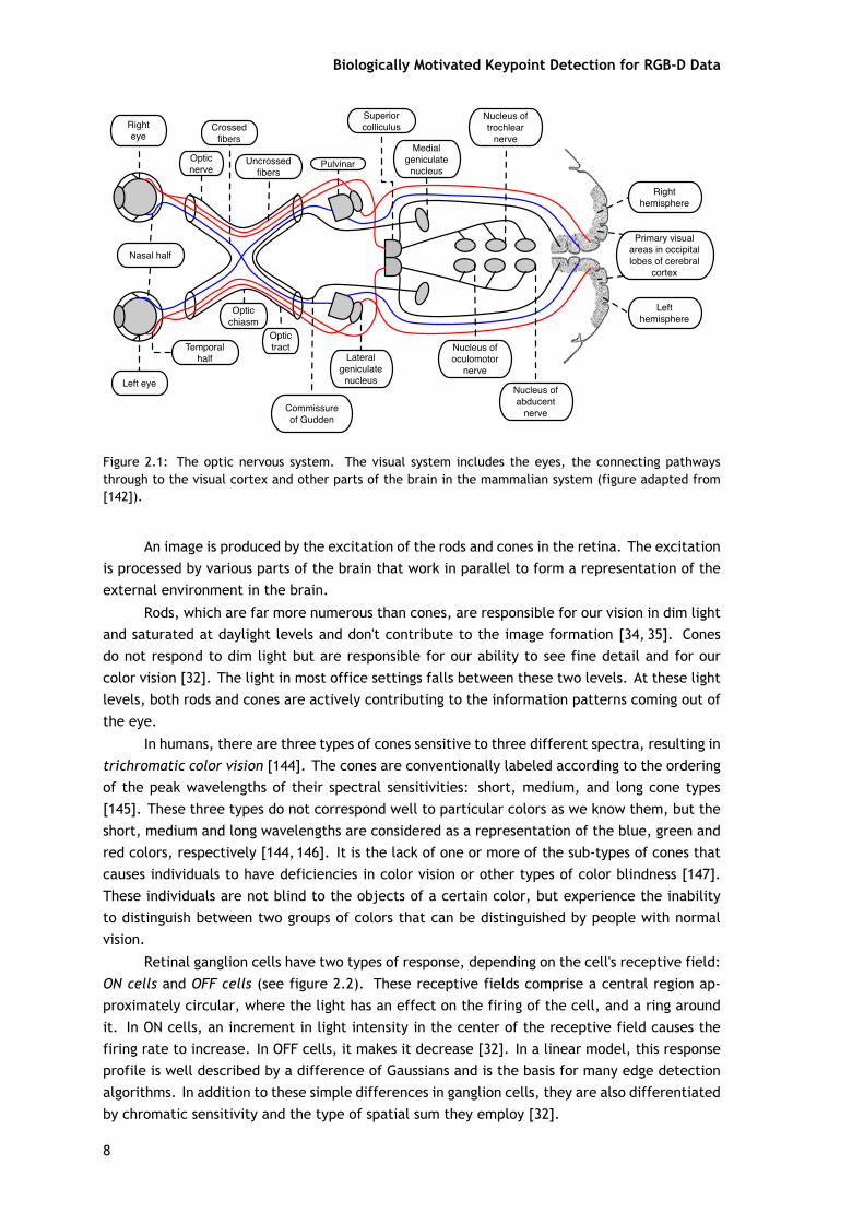
Biologically Motivated Keypoint Detection for RGB-D Data
Optic nerve
Crossed fibers
Uncrossed fibers
Optic chiasm
Optic tract
Pulvinar
Lateral geniculate
nucleus
Superior colliculus
Medial geniculate
nucleus
Nucleus of oculomotor
nerve
Nucleus of trochlear
nerve
Nucleus of abducent
nerve
Primary visual areas in occipital lobes of cerebral
cortex
Nasal half
Temporal half
Right eye
Left eye
Right hemisphere
Left hemisphere
Commissure of Gudden
Figure 2.1: The optic nervous system. The visual system includes the eyes, the connecting pathwaysthrough to the visual cortex and other parts of the brain in the mammalian system (figure adapted from[142]).
An image is produced by the excitation of the rods and cones in the retina. The excitationis processed by various parts of the brain that work in parallel to form a representation of theexternal environment in the brain.
Rods, which are far more numerous than cones, are responsible for our vision in dim lightand saturated at daylight levels and don't contribute to the image formation [34, 35]. Conesdo not respond to dim light but are responsible for our ability to see fine detail and for ourcolor vision [32]. The light in most office settings falls between these two levels. At these lightlevels, both rods and cones are actively contributing to the information patterns coming out ofthe eye.
In humans, there are three types of cones sensitive to three different spectra, resulting intrichromatic color vision [144]. The cones are conventionally labeled according to the orderingof the peak wavelengths of their spectral sensitivities: short, medium, and long cone types[145]. These three types do not correspond well to particular colors as we know them, but theshort, medium and long wavelengths are considered as a representation of the blue, green andred colors, respectively [144,146]. It is the lack of one or more of the sub-types of cones thatcauses individuals to have deficiencies in color vision or other types of color blindness [147].These individuals are not blind to the objects of a certain color, but experience the inabilityto distinguish between two groups of colors that can be distinguished by people with normalvision.
Retinal ganglion cells have two types of response, depending on the cell's receptive field:ON cells and OFF cells (see figure 2.2). These receptive fields comprise a central region ap-proximately circular, where the light has an effect on the firing of the cell, and a ring aroundit. In ON cells, an increment in light intensity in the center of the receptive field causes thefiring rate to increase. In OFF cells, it makes it decrease [32]. In a linear model, this responseprofile is well described by a difference of Gaussians and is the basis for many edge detectionalgorithms. In addition to these simple differences in ganglion cells, they are also differentiatedby chromatic sensitivity and the type of spatial sum they employ [32].
8
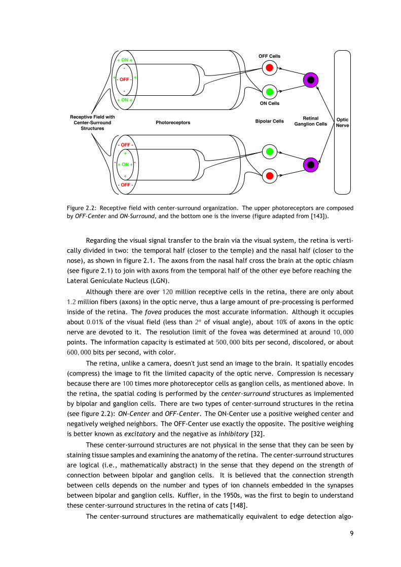
+ ON +
+ +
+ ON +
-
- OFF -
-
Receptive Field with Center-Surround
StructuresPhotoreceptors Bipolar Cells Retinal
Ganglion CellsOpticNerve
- OFF -
- -
- OFF -
+
+ ON +
+
OFF Cells
ON Cells
Figure 2.2: Receptive field with center-surround organization. The upper photoreceptors are composedby OFF-Center and ON-Surround, and the bottom one is the inverse (figure adapted from [143]).
Regarding the visual signal transfer to the brain via the visual system, the retina is verti-cally divided in two: the temporal half (closer to the temple) and the nasal half (closer to thenose), as shown in figure 2.1. The axons from the nasal half cross the brain at the optic chiasm(see figure 2.1) to join with axons from the temporal half of the other eye before reaching theLateral Geniculate Nucleus (LGN).
Although there are over 120 million receptive cells in the retina, there are only about1.2 million fibers (axons) in the optic nerve, thus a large amount of pre-processing is performedinside of the retina. The fovea produces the most accurate information. Although it occupiesabout 0.01% of the visual field (less than 2o of visual angle), about 10% of axons in the opticnerve are devoted to it. The resolution limit of the fovea was determined at around 10, 000points. The information capacity is estimated at 500, 000 bits per second, discolored, or about600, 000 bits per second, with color.
The retina, unlike a camera, doesn't just send an image to the brain. It spatially encodes(compress) the image to fit the limited capacity of the optic nerve. Compression is necessarybecause there are 100 times more photoreceptor cells as ganglion cells, as mentioned above. Inthe retina, the spatial coding is performed by the center-surround structures as implementedby bipolar and ganglion cells. There are two types of center-surround structures in the retina(see figure 2.2): ON-Center and OFF-Center. The ON-Center use a positive weighed center andnegatively weighed neighbors. The OFF-Center use exactly the opposite. The positive weighingis better known as excitatory and the negative as inhibitory [32].
These center-surround structures are not physical in the sense that they can be seen bystaining tissue samples and examining the anatomy of the retina. The center-surround structuresare logical (i.e., mathematically abstract) in the sense that they depend on the strength ofconnection between bipolar and ganglion cells. It is believed that the connection strengthbetween cells depends on the number and types of ion channels embedded in the synapsesbetween bipolar and ganglion cells. Kuffler, in the 1950s, was the first to begin to understandthese center-surround structures in the retina of cats [148].
The center-surround structures are mathematically equivalent to edge detection algo-
9
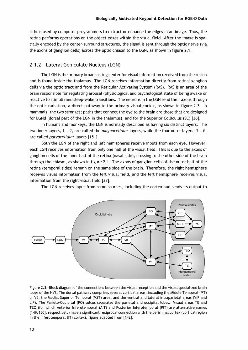
Biologically Motivated Keypoint Detection for RGB-D Data
rithms used by computer programmers to extract or enhance the edges in an image. Thus, theretina performs operations on the object edges within the visual field. After the image is spa-tially encoded by the center-surround structures, the signal is sent through the optic nerve (viathe axons of ganglion cells) across the optic chiasm to the LGN, as shown in figure 2.1.
2.1.2 Lateral Geniculate Nucleus (LGN)
The LGN is the primary broadcasting center for visual information received from the retinaand is found inside the thalamus. The LGN receives information directly from retinal ganglioncells via the optic tract and from the Reticular Activating System (RAS). RAS is an area of thebrain responsible for regulating arousal (physiological and psychological state of being awake orreactive to stimuli) and sleep-wake transitions. The neurons in the LGN send their axons throughthe optic radiation, a direct pathway to the primary visual cortex, as shown in figure 2.3. Inmammals, the two strongest paths that connect the eye to the brain are those that are designedfor LGNd (dorsal part of the LGN in the thalamus), and for the Superior Colliculus (SC) [36].
In humans and monkeys, the LGN is normally described as having six distinct layers. Thetwo inner layers, 1 − 2, are called the magnocellular layers, while the four outer layers, 3 − 6,are called parvocellular layers [151].
Both the LGN of the right and left hemispheres receive inputs from each eye. However,each LGN receives information from only one half of the visual field. This is due to the axons ofganglion cells of the inner half of the retina (nasal side), crossing to the other side of the brainthrough the chiasm, as shown in figure 2.1. The axons of ganglion cells of the outer half of theretina (temporal sides) remain on the same side of the brain. Therefore, the right hemispherereceives visual information from the left visual field, and the left hemisphere receives visualinformation from the right visual field [37].
The LGN receives input from some sources, including the cortex and sends its output to
Inferotemporal cortex
Retina LGN V1 V2 V3
MT
PO
V4
TEO
TE
Occipital lobe
Parietal cortex
VIP
MST
LIP
7a
Figure 2.3: Block diagram of the connections between the visual reception and the visual specialized brainlobes of the HVS. The dorsal pathway comprises several cortical areas, including the Middle Temporal (MT)or V5, the Medial Superior Temporal (MST) area, and the ventral and lateral intraparietal areas (VIP andLIP). The Parieto-Occipital (PO) sulcus separates the parietal and occipital lobes. Visual areas TE andTEO (for which Anterior Inferotemporal (AIT) and Posterior Inferotemporal (PIT) are alternative names[149,150], respectively) have a significant reciprocal connection with the perirhinal cortex (cortical regionin the Inferotemporal (IT) cortex), figure adapted from [142].
10
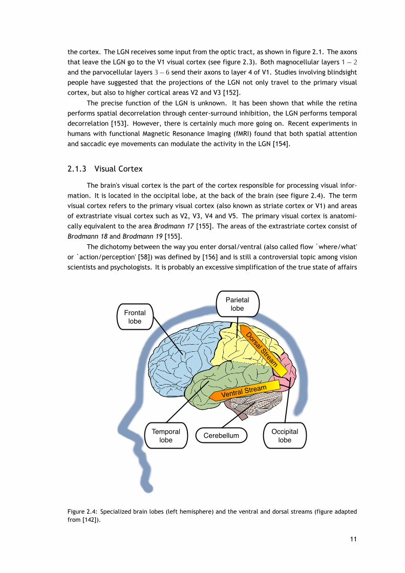
the cortex. The LGN receives some input from the optic tract, as shown in figure 2.1. The axonsthat leave the LGN go to the V1 visual cortex (see figure 2.3). Both magnocellular layers 1 − 2and the parvocellular layers 3 − 6 send their axons to layer 4 of V1. Studies involving blindsightpeople have suggested that the projections of the LGN not only travel to the primary visualcortex, but also to higher cortical areas V2 and V3 [152].
The precise function of the LGN is unknown. It has been shown that while the retinaperforms spatial decorrelation through center-surround inhibition, the LGN performs temporaldecorrelation [153]. However, there is certainly much more going on. Recent experiments inhumans with functional Magnetic Resonance Imaging (fMRI) found that both spatial attentionand saccadic eye movements can modulate the activity in the LGN [154].
2.1.3 Visual Cortex
The brain's visual cortex is the part of the cortex responsible for processing visual infor-mation. It is located in the occipital lobe, at the back of the brain (see figure 2.4). The termvisual cortex refers to the primary visual cortex (also known as striate cortex or V1) and areasof extrastriate visual cortex such as V2, V3, V4 and V5. The primary visual cortex is anatomi-cally equivalent to the area Brodmann 17 [155]. The areas of the extrastriate cortex consist ofBrodmann 18 and Brodmann 19 [155].
The dichotomy between the way you enter dorsal/ventral (also called flow `where/what'or `action/perception' [58]) was defined by [156] and is still a controversial topic among visionscientists and psychologists. It is probably an excessive simplification of the true state of affairs
Dorsal Stream
Frontal lobe
Temporal lobe
Parietal lobe
Occipital lobeCerebellum
Ventral Stream
Figure 2.4: Specialized brain lobes (left hemisphere) and the ventral and dorsal streams (figure adaptedfrom [142]).
11
Biologically Motivated Keypoint Detection for RGB-D Data
in the visual cortex. It is based on the study of visual illusions, such as the Ebbinghaus illusion,that may distort judgments of nature perception, but when the subject responds with an action,such as grasping, no distortion occurs. However, recent work, like in [157], suggests that bothsystems of action and perception are equally fooled by such illusions.
The neurons in the visual cortex allow the development of an action when visual stim-uli appear within their receptive field. By definition, the receptive field is the region withinthe entire visual field that causes an action potential (in physiology, an action potential is ashort-lasting event in which the electrical membrane potential of a cell rapidly rises and falls,following a consistent trajectory). But any given neuron can better respond to a subset of stim-uli within its receptive field. For example, a neuron in V1 may fire to any vertical stimulus inits receptive field and ignore other types of stimulus. In the earlier visual areas, like in the ITcortex (see figure 2.3), a neuron can only fire when a certain face appears in its receptive field.
2.1.3.1 Primary Visual Cortex (V1)
The primary visual cortex is the best-studied area of the visual system. In all studiedmammals, it is located in the posterior pole of the occipital cortex (the occipital cortex isresponsible for processing visual stimuli), as shown in figures 2.3 and 2.4. It is the simplest andoldest part of the visual cortical area. It is strongly specialized in processing information aboutstatic and moving objects, and is excellent in pattern recognition. The primary visual cortex isdivided into six distinct functional layers, labeled 1 to 6. The 4th layer is the one that receivesmore visual input from the LGN. The average number of neurons in the primary visual cortex ofan adult human being was estimated to be 280 million [158].
V1 has a well defined map of visual spatial information. For example, in humans the wholetop of the calcarine sulcus responds strongly to the lower half of the visual field, and the bottomof the calcarine to the upper half of the visual field. Conceptually, this retinotopic mapping isa transformation of the visual image of the retina to V1. The correspondence between a givenlocation in V1 in the subjective field of vision is very precise: even the blind spots are mappedin V1. In humans and animals with a fovea on the retina the proportion of the central visualfield, a phenomenon known as cortical magnification. Perhaps for the purpose of precise spatialencoding, neurons in V1 have the smallest receptive field size in all regions of the visual cortex.
The tuning properties of V1 neurons differ greatly. That is, the responses can discriminatesmall changes in visual orientations, spatial frequencies and colors. In addition, individual V1neurons in human and animals with binocular vision have ocular dominance (namely, there is apreference for one of the eyes). In V1, and in the primary sensory cortex in general, neurons withsimilar properties tend to cortical columns. Hubel and Wiesel [159] proposed a new organizationof classic ice cube cortical columns for two tuning properties: ocular dominance and orientation.However, this model can not accommodate color, spatial frequency and many other featuresto which neurons are tuned. The exact arrangement of all these cortical columns within V1remains a research topic.
The current consensus seems to be that the initial responses of V1 neurons are composedof sets of tiled selective spatio-temporal filters. In space, the operation of the V1 can be thoughtof as similar to many local spatial functions, complex Fourier transforms, or more preciselyGabor transforms. Theoretically, these filters together can carry out the neural processing ofspatial frequencies, orientations, movements, directions, speeds (thus temporal frequency),and many other spatio-temporal features.
V1 neurons are also sensitive to the global scene organization [38]. These response prop-
12
erties probably result from recurrent processing and lateral connections in the neuron pyra-mids [39]. Feedforward connections are mostly driving, and feedback connections are mostlymodulatory in their effects [40,41]. Evidence shows that the feedback connections originatingfrom higher-level areas such as V4, IT, MT, with larger and more complex receptive fields, canchange and shape responses in V1, representing contextual or extra-classical receptive fieldeffects [160--163].
Computational theories of spatial attention in the visual system propose that the attentionmodulation increases the responses of neurons in many areas of the visual cortex [42--44]. Thenatural place where it is possible predict an early increase of this type is V1 and recent fMRIevidence shows that the striate cortex can be modulated by attention in a manner consistentwith this theory [45].
Studies in macaque disagree as to the presence and amount of attention modulation in V1[164]. Experiments performed with human neuroimaging are less ambiguous and invariably findrobust changes of attention in primary visual cortex [45,165] and in subcortical structures [166,167]. Electrophysiological studies in humans often report an attention modulation in the visualcortex [136,137], but the spatial origins of these signals are normally only estimated by indirectmeans (for example, the response time of the signal or the relation of waveforms on stimuluslocation). Direct estimates of neural modulation from electrophysiological measurements withhigher spatial precision differ considerably [168]. Another recent study of attention modulationin human V1 using intracranial electrodes in a single subject could not find attention effects[169]. One possible explanation for this result is that this task was not demanding enough togenerate strong modulation of the neural response. Generally, it appears that attention canact at early places in the visual stream and modulate neural responses, but the effects may beweaker than those seen in higher areas or confined to a subset of the neural population [164].
2.1.3.2 Visual Area V2
The visual area V2, also called the prestriate cortex [46], is the second largest area ofthe visual cortex, and the first region within the visual association area. It receives strongfeedforward connections from V1 and sends strong connections to V3, V4 and V5. It also sendsstrong feedback connections to V1.
Anatomically, V2 is divided into four quadrants, a dorsal and ventral representation ineach hemisphere (left and right). Together, these four regions provide a complete map of thevisual world. Functionally, V2 has many properties in common with V1. Recent research hasshown that cells in V2 show a small amount of attention modulation (more than in V1, less thanin V4), are set to moderately complex patterns, and can be driven by multiple orientations indifferent sub-regions within a single receptive field [47,48].
It is argued that the entire ventral stream (see figure 2.4) is important for visual memory[49]. This theory predicts that the Object-Recognition Memory (ORM) undergoes changes thatmay result in the manipulation of V2. In a recent study it was revealed that certain V2 cellsplay a very important role in storage in the ORM, and the conversion of short-term memoriesinto long-term memories [50]. This area is highly interconnected within the ventral streamof the visual cortex. In the monkey brain, this area receives strong feedforward connectionsfrom the primary visual cortex and sends strong projections to the other secondary visual cortexareas (V3, V4 and V5) [170, 171] (see figure 2.3). Most neurons in this area respond to simplevisual features such as orientation, spatial frequency, size, color and shape [51--53]. V2 cellsalso respond to various characteristics of complex shapes, such as the orientation of illusory
13
Biologically Motivated Keypoint Detection for RGB-D Data
contours [51] and if the stimulus is part of the foreground or the background [54,55].
2.1.3.3 Visual Area V3
The V3 cortex region is located immediately in front of V2. There is still some controversyover the exact extent of area V3, with some researchers proposing that the cortex located infront of V2 may include two or three functional subdivisions. For example, Felleman et al. [56]proposed the existence of a dorsal V3 in the upper hemisphere, which is distinct from ventralV3 located at the bottom of the brain. The dorsal and ventral V3 have distinct connections withother parts of the brain, appear in different sections stained with a variety of methods, andcontain neurons that respond to different combinations of visual stimuli.
The dorsal V3 is usually considered part of the dorsal stream (shown in figure 2.4), re-ceiving inputs from V2 and the primary visual area and projecting to the Posterior Parietal (PP)cortex. Some studies with fMRI suggested that the V3 area may play a role in the processing ofglobal motion [172]. Other studies considered the dorsal V3 as part of a larger area called thedorsomedial area, which contains a representation of the entire visual field. The neurons in thedorsomedial area respond to the coherent motion of large patterns covering large portions ofthe visual field [173].
The ventral V3 has considerably weaker connections to the primary visual area, andstronger connections to the IT cortex. While previous studies suggested that the ventral V3had only a representation of the upper visual field, a more recent work indicates that this areais more extensive than previously appreciated, and like the other visual areas, may contain acomplete visual representation [174].
2.1.3.4 Visual Area V4
The visual area V4 is one of the visual areas of the extrastriate visual cortex. It is locatedbefore V2 and after the PIT area, as shown in figure 2.3. V4 is the third cortical area in theventral stream, receiving strong feedforward input from V2 and sending strong connections tothe PIT.
V4 is the first area in the ventral stream that has a strong attention modulation. Moststudies indicate that selective attention can change firing rates in V4 by about 20%. Moran andDesimone [57] characterize these effects, and this was the first study to find effects of attentionanywhere in the visual cortex [58].
Like the V1, V4 is tuned at the level of orientation, spatial frequency, and color. Butunlike V1, V4 is set to feature extraction of objects of intermediate complexity, like simplegeometric shapes, although no one develop a complete description of the V4 parameter space.The visual area V4 is not tuned for complex objects like faces, as the areas of the IT cortex.
The firing properties of V4 were first described, at the end of 1970, by Zeki [66], thatalso named the area. Originally, Zeki argued that the purpose of V4 was to be responsiblefor processing color information. At the beginning of 1980, it was proved that V4 was directlyinvolved in the shape recognition, as previous areas of the cortex. This research supported thehypothesis of the two streams first presented by Ungerleider and Mishkin [156].
2.1.3.5 Visual Area V5 or MT
The visual area V5, also known as Middle Temporal (MT) visual area, is a region of theextrastriate visual cortex, which is thought to play an important role in the perception of motion,
14
the integration of local motion signals into global perceptions and orientations of some eyemovements [59]. The MT is connected to a large variety of cerebral cortical and subcorticalareas. Its inputs include visual cortical areas V1, V2 and dorsal V3 [60,61], koniocellulare regionsof the LGN [62] and inferior pulvinar. The pattern of projections to MT changes somewhatbetween the representations of the foveal and peripheral visual fields [63]. The MT was shownto be organized in steering columns [175]. DeAmgelis and Newsome [64] argued that the neuronsin MT have also been organized based on its fit to the binocular disparity.
The standard view is that V1 provides the most important input to the MT [59] (see figure2.3). However, several studies have shown that neurons in MT are able to respond to visualinformation, often in a selective manner, even after V1 is destroyed or disabled [65]. In addition,research carried out by Zeki [66] suggests that certain types of visual information may reach MTbefore it even reaches V1.
The MT sends its outputs to areas located in the immediately surrounding cortex. Earlystudies of the electro-physiological properties of neurons in MT showed that a large proportionof cells were in tune with the speed and direction of visual stimuli on the move [176,177]. Theseresults suggest that MT plays a significant role in the processing of visual motion.
The study of lesions also supports the role of MT in motion perception and eye movement.Neuropsychological studies of a patient who could not see motion, seeing the world as a seriesof static frames instead, suggested that MT in the primates is homologous to V5 in humans[178,179]. There is still much controversy about the exact form of the calculations performedin MT [180] and some research suggests that movement perception is already available at lowerlevels of the visual system (such as on the V1 [181,182]). These results left open the question ofprecisely what MT could do that V1 could not. Much work has been performed in this region, sinceit seems to integrate the local signals of visual motion in the global movement of complex objects[183]. For example, an injury in V5 can cause a deficit in motion perception and processing ofcomplex stimuli. It contains many neurons tuned to the motion of complex visual features. Themicro-stimulation of a neuron located in the V5 affects the perception of motion. For example,if someone finds a neuron with a preference for upward motion, and then uses an electrode tostimulate it, the monkey becomes more sensitive to upward motion [184].
2.2 Visual Attention
In this section, several concepts regarding visual attention are discussed. More detailedinformation can be found in, for example, Pashler [67,68], Style [69], and Johnson and Proctor[70].
Generally, we seem to keep a rich representation of our visual world and major changesto our environment will attract our attention. Only a small region of the scene is analyzed indetail, in each moment: the attention focus region. This is usually, but not always, the sameregion which is fixed by the eyes [71, 72]. The order in which a scene is investigated is deter-mined by the mechanisms of selective attention. Corbetta proposed the following definition ofattention: "defines the mental ability to select stimuli, responses, memories, or thoughts thatare behaviorally relevant among many others that are behaviorally irrelevant" [134].
There are two categories of factors that motivate attention: the bottom-up factors andtop-down factors [73]. Corbetta and Shulman [74] review the evidence on partially segregatednetworks of brain areas that perform different attention functions. The preparation and appli-cation of goal directed (top-down) selection of stimuli is performed by a system that includes
15
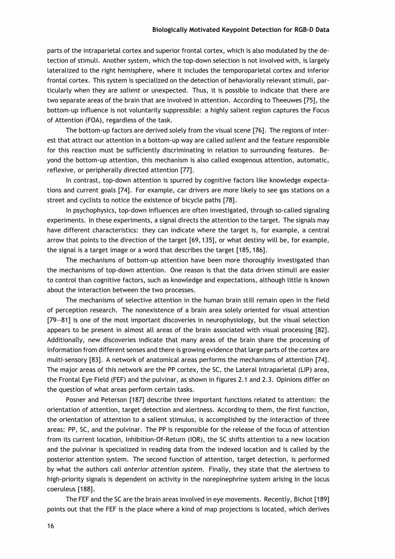
Biologically Motivated Keypoint Detection for RGB-D Data
parts of the intraparietal cortex and superior frontal cortex, which is also modulated by the de-tection of stimuli. Another system, which the top-down selection is not involved with, is largelylateralized to the right hemisphere, where it includes the temporoparietal cortex and inferiorfrontal cortex. This system is specialized on the detection of behaviorally relevant stimuli, par-ticularly when they are salient or unexpected. Thus, it is possible to indicate that there aretwo separate areas of the brain that are involved in attention. According to Theeuwes [75], thebottom-up influence is not voluntarily suppressible: a highly salient region captures the Focusof Attention (FOA), regardless of the task.
The bottom-up factors are derived solely from the visual scene [76]. The regions of inter-est that attract our attention in a bottom-up way are called salient and the feature responsiblefor this reaction must be sufficiently discriminating in relation to surrounding features. Be-yond the bottom-up attention, this mechanism is also called exogenous attention, automatic,reflexive, or peripherally directed attention [77].
In contrast, top-down attention is spurred by cognitive factors like knowledge expecta-tions and current goals [74]. For example, car drivers are more likely to see gas stations on astreet and cyclists to notice the existence of bicycle paths [78].
In psychophysics, top-down influences are often investigated, through so-called signalingexperiments. In these experiments, a signal directs the attention to the target. The signals mayhave different characteristics: they can indicate where the target is, for example, a centralarrow that points to the direction of the target [69,135], or what destiny will be, for example,the signal is a target image or a word that describes the target [185,186].
The mechanisms of bottom-up attention have been more thoroughly investigated thanthe mechanisms of top-down attention. One reason is that the data driven stimuli are easierto control than cognitive factors, such as knowledge and expectations, although little is knownabout the interaction between the two processes.
The mechanisms of selective attention in the human brain still remain open in the fieldof perception research. The nonexistence of a brain area solely oriented for visual attention[79--81] is one of the most important discoveries in neurophysiology, but the visual selectionappears to be present in almost all areas of the brain associated with visual processing [82].Additionally, new discoveries indicate that many areas of the brain share the processing ofinformation from different senses and there is growing evidence that large parts of the cortex aremulti-sensory [83]. A network of anatomical areas performs the mechanisms of attention [74].The major areas of this network are the PP cortex, the SC, the Lateral Intraparietal (LIP) area,the Frontal Eye Field (FEF) and the pulvinar, as shown in figures 2.1 and 2.3. Opinions differ onthe question of what areas perform certain tasks.
Posner and Peterson [187] describe three important functions related to attention: theorientation of attention, target detection and alertness. According to them, the first function,the orientation of attention to a salient stimulus, is accomplished by the interaction of threeareas: PP, SC, and the pulvinar. The PP is responsible for the release of the focus of attentionfrom its current location, Inhibition-Of-Return (IOR), the SC shifts attention to a new locationand the pulvinar is specialized in reading data from the indexed location and is called by theposterior attention system. The second function of attention, target detection, is performedby what the authors call anterior attention system. Finally, they state that the alertness tohigh-priority signals is dependent on activity in the norepinephrine system arising in the locuscoeruleus [188].
The FEF and the SC are the brain areas involved in eye movements. Recently, Bichot [189]points out that the FEF is the place where a kind of map projections is located, which derives
16
information from bottom-up, as well as top-down influences. The saliency maps, for otherresearchers, are located in different areas, for instance at LIP [190], at SC [191], at V1 [192] orat V4 [193].
The source of top-down signals may derive from a network of areas in the parietal andfrontal cortex. Based on [194], these areas include the Superior Parietal Lobe (SPL), the FEFand the Supplementary Eye Field (SEF). The transient response of the signal in the occipitallobe and more sustained responses in the dorsal PP cortex along the intraparietal sulcus (IPs)and frontal cortex in or near the putative human homologue of the FEFs were found by Corbettaand Shulman [74]. The interaction of bottom-up and top-down signals occurs in V4, in the viewof Ogawa and Komatsu [195].
2.3 Summary
With this chapter, an overview of the HVS was provided. Visual attention is a highly in-terdisciplinary field and researchers in this area come from different backgrounds [131]. Forpsychologists, research conducted in the area of human behavior is performed by isolating cer-tain specific tasks, in order to understand the internal processes of the brain, often resulting inpsychophysical theories or models [134]. While neurobiologists observe the brain's response tocertain stimuli [135], using techniques such as fMRI, having therefore a direct view of the brainareas that are active under certain conditions [45,136,137].
In recent years, these different areas have profited considerably from each other. Psy-chologists use research conducted by neurobiologists, in order to improve their attention mod-els, while neurobiologists consider psychological experiments to interpret their data [134]. Inaddition, psychologists began to implement computer models or use computer models previ-ously developed, to verify that they have a similar behavior to that of human perception. Thus,psychologists tend to improve the understanding of the mechanisms and help the developmentof better computational models.
17

Biologically Motivated Keypoint Detection for RGB-D Data
18

Chapter 3
Saliency, the Computational Models of VisualAttention
Selective visual attention, initially proposed by Koch and Ullman [2], is used by manycomputational models of visual attention. Saliency maps is a term which was introduced by Ittiet al. [3] in their work on the rapid scene analysis, and by Tsotsos et al. [84] and Olshausenet al. [85] in their work on visual attention. In some studies, for example in [84, 86], theterm saliency appears referred to as visual attention or in [87,88] as unpredictability, rarity orsurprise. The saliency maps are used as a two-dimensional scalar map of values representingthe visual saliency of the corresponding location, independently of the particular stimulus thatmakes the location salient [1].
With the emerging interest in active vision, the computer vision researchers have beenincreasingly concerned with the mechanisms of attention and have proposed a number of com-putational models of attention. An active vision system is one that can manipulate the pointof view of the camera(s) in order to analyze the surrounding environment and to obtain betterinformation from it.
The methods that will be presented can be categorized based on whether they are biolog-ically plausible, purely computational, or hybrid [89]. Other types of categories are describedin [6]. In general, all methods employ a low-level approach by determining the contrast ofthe image regions relative to their surroundings, using one or more features of intensity, colorand orientation. When a method is said to be biologically plausible it means that it follows theknowledge of the HVS. There is usually an attempt to combine known features, extracted bythe retina, LGN, primary visual cortex (V1), or by other visual fields (such as V2, V3, V4 and V5).Itti et al. [3], for example, base their method on a biologically plausible architecture proposedin [2]. They determine the center-surround contrast with the Difference of Gaussians (DoG) ap-proach. Frintrop et al. [90] present a method inspired by Itti's method, but the center-surrounddifferences are obtained using square filters and integral images to reduce the processing time.
Other methods are purely computational and not based on any of the biological principlesof vision. Ma and Zhang [86] and Achanta et al. [91] estimate the saliency using the distancesfrom the center-surround. While Hu et al. [92] estimate the saliency through the applicationof heuristic measures on the initial saliency measures obtained by histogram thresholding offeature maps. The maximization of mutual information between the distributions of features inthe center and surround of an image is made [93]. Hou and Zhang [94] perform the processingin the frequency domain.
The methods classified as hybrid are those that incorporate ideas that are partially basedon biological models. Here, the method of Itti et al. [3] is used by Harrel et al. [95] to generatethe characteristics maps; the normalization is performed by an approach based on graphs. Othermethods use computational approaches like maximization of information [96] that representbiological plausible models of saliency detection.
In the rest of this chapter, we focus only on those models which can process arbitrarydigital images and return corresponding saliency maps. In each of the following sections, themodels are introduced in chronological order.
19

Biologically Motivated Keypoint Detection for RGB-D Data
3.1 Biological Plausible Methods
Many plausible biological models that have strong links with the psychological or neu-rophysiological findings are described in this section. Almost all these attention models aredirectly or indirectly inspired by cognitive concepts.
A visual attention model is proposed by Ahmad [196]. It consists of a network propagationcorresponding to the pulvinar, whose outputs correspond to the areas V4, IT and MT. The mainnetwork corresponds to the SC, FEF and PP areas, while the control network corresponds to thePP areas and the working memory corresponds to the prefrontal cortex.
The attention model proposed by Niebur and Koch [197] scans the scene both in the formof a rapid, bottom-up, saliency-driven and task-independent manner and in a slower, top-down,volition-controlled and task-dependent manner, based on the work in [2,198,199].
Itti et al. [3,200] built a saliency model based on spatial attention derived from the bio-logically plausible architecture proposed by Koch and Ullman [2], using three feature channels:color, intensity, and orientation. This model has been the basis of later models and the stan-dard benchmark for comparison. It has been shown to correlate with human eye movementsin free-viewing tasks [201,202]. The features are calculated by a linear set of center-surroundoperations, similar to visual receptive fields. Typically visual neurons are more sensitive to asmall region of the visual space (the center), while stimuli presented in a broader concentricregion with the center (the surround) inhibit the neuronal response. This type of architecture,sensitive to local spatial discontinuities, is particularly well-suited to detect locations whichstand out from their surroundings and is a general computational principle in the retina, LGN,and primary visual cortex [122]. Based on retinal input, given the intensity, color, and orienta-tions, they create Gaussian pyramids. The center-surround contrast is determined using a DoGapproach from the Gaussian pyramids, creating "feature maps". An input image is subsampledinto a Gaussian pyramid and each pyramid level σ is decomposed into channels for Red (R),Green (G), Blue (B), Yellow (Y), Intensity (I), and local orientations (Oσ ). From these channels,center-surround feature maps fl for different features l are constructed and normalized (N (·)).In each channel, maps are summed across scale and normalized again:
fl = N( 4∑
c=2
c+4∑
s=c+3fl,c,s
), ∀ ∈ LI ∪ LC ∪ LO (3.1)
LI = {I}, LC = {RG, BY }, LO = {0o, 45o, 90o, 135o} (3.2)
The feature maps are combined into a single "conspicuity map" for each feature type:
CI = fI , CC = N(∑
l∈LC
fl
), CO = N
(∑
l∈LO
fl
)(3.3)
The three conspicuity maps then are summed into the unique bottom-up saliency map:
S = 13
∑
k∈{I,C ,O}
Ck . (3.4)
20
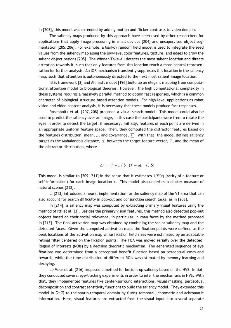
In [203], this model was extended by adding motion and flicker contrasts to video domain.
The saliency maps produced by this approach have been used by other researchers forapplications that apply image processing in small devices [204] and unsupervised object seg-mentation [205,206]. For example, a Markov random field model is used to integrate the seedvalues from the saliency map along the low-level color features, texture, and edges to grow thesalient object regions [205]. The Winner-Take-All detects the most salient location and directsattention towards it, such that only features from this location reach a more central represen-tation for further analysis. An IOR mechanism transiently suppresses this location in the saliencymap, such that attention is autonomously directed to the next most salient image location.
Itti's framework [3] and Ahmad's model [196] build up an elegant mapping from computa-tional attention model to biological theories. However, the high computational complexity inthese systems requires a massively parallel method to obtain fast responses, which is a commoncharacter of biological structure based attention models. For high-level applications as robotvision and video content analysis, it is necessary that these models produce fast responses.
Rosenholtz et al. [207, 208] proposed a visual search model. This model could also beused to predict the saliency over an image, in this case the participants were free to rotate theeyes in order to detect the target, if necessary. Initially, features of each point are derived inan appropriate uniform feature space. Then, they computed the distractor features based onthe features distribution, mean, µ, and covariance,
∑. With that, the model defines saliency
target as the Mahalanobis distance, ∆, between the target feature vector, T , and the mean ofthe distractor distribution, where
∆2 = (T − µ)′−1∑
(T − µ). (3.5)
This model is similar to [209--211] in the sense that it estimates 1/P(x) (rarity of a feature orself-information) for each image location x. This model also underlies a clutter measure ofnatural scenes [212].
Li [213] introduced a neural implementation for the saliency map of the V1 area that canalso account for search difficulty in pop-out and conjunction search tasks, as in [203].
In [214], a saliency map was computed by extracting primary visual features using themethod of Itti et al. [3]. Besides the primary visual features, this method also detected pop-outobjects based on their social relevance, in particular, human faces by the method proposedin [215]. The final activation map was obtained by combining the scalar saliency map and thedetected faces. Given the computed activation map, the fixation points were defined as thepeak locations of the activation map while fixation field sizes were estimated by an adaptableretinal filter centered on the fixation points. The FOA was moved serially over the detectedRegion of Interests (ROIs) by a decision theoretic mechanism. The generated sequence of eyefixations was determined from a perceptual benefit function based on perceptual costs andrewards, while the time distribution of different ROIs was estimated by memory learning anddecaying.
Le Meur et al. [216] proposed a method for bottom-up saliency based on the HVS. Initial,they conducted several eye-tracking experiments in order to infer the mechanisms in HVS. Withthat, they implemented features like center-surround interactions, visual masking, perceptualdecomposition and contrast sensitivity functions to build the saliency model. They extended thismodel in [217] to the spatio-temporal domain by fusing temporal, chromatic and achromaticinformation. Here, visual features are extracted from the visual input into several separate
21
Biologically Motivated Keypoint Detection for RGB-D Data
parallel channels. A feature map is obtained for each channel, then a unique saliency map isbuilt from the combination of those channels. The major novelty lies in the inclusion of thetemporal dimension as well as the addition of a coherent normalization scheme.
Navalpakkam and Itti [218, 219] proposed a computational model for the task-specificguidance of visual attention in real-world scenes. Their model emphasizes four aspects that areimportant in biological vision: determining task-relevance of an entity, biasing attention for thelow-level visual features of desired targets, recognizing these targets using the same low-levelfeatures, and incrementally building a visual map of task-relevance at every scene location.Given a task definition in the form of keywords, the model first determines and stores thetask-relevant entities in working memory, using prior knowledge stored in Long-Term Memory(LTM). It attempts to detect the most relevant entity by biasing its visual attention system withthe entity's learned low-level features. It attends to the most salient location in the scene,and attempts to recognize the attended object through hierarchical matching against objectrepresentations stored in LTM. It updates its working memory with the task-relevance of therecognized entity and updates a topographic task-relevance map with the location and relevanceof the recognized entity. The model's performance on search for single features and featureconjunctions is consistent with existing psychophysical data. These results of their biologically-motivated architecture suggest that the model may provide a reasonable approximation to manybrain processes involved in complex task-driven visual behaviors.
Frintrop [131] presented a biologically motivated computer model called Visual ObjectDetection with a Computational Attention System (VOCUS). The system is based on a mechanismof human perception called selective attention. To imitate the biological process the VOCUSsystem first analyses the provided audio and video data, considering different features likecontrast, color or intensity in parallel. Then, the saliency maps that indicate interest regions,are generated based on the analysis. If additional information is provided the maps are thenprocessed in search for matching attributes. In other words, the model can use both bottom-upattention cues, characteristics of the image and top-down cues and emotion related aspects ofthe image [220]. In the end, all the information is fused and a focus region is established formore detailed analysis.
VOCUS is based on psychological models like the feature integration theory presentedin [221] and on computational models as the Neuromorphic Vision Toolkit of Itti et al. [3]. It isalso one of the few systems able to perform goal-directed search, which means that it is able torecognize previously defined objects in provided data. The system is also able to process datain real time and thus it may be used in robotics or monitoring systems [222, 223]. The modelrepresents a major step forward on integration of data and model-driven mechanisms for studiesof visual attention [131] and has been referenced in many works on computer vision [224].Frintrop et al. [90,131] used images integrals [215,225] to accelerate the computation of center-surround differences to find regions salient using maps of separate features of color, intensityand orientation. Their proposal obtains a higher resolution in the saliency maps as compared tothe method of [3]. For this, they resize the filter on each scale, instead of the image and thusmaintain the same resolution as the original image on all scales.
Kootstra et al. [226] proposed a multi-scale extension for three symmetry-saliency op-erators and compared them with human eye-tracking data. This extension was applied on theisotropic symmetry and radial symmetry operators presented in [227] and the color symmetryof Heidemann [228]. The authors compared their model against the Itti et al. [3] method andshowed that their performance is significantly better on symmetric stimuli.
Marat et al. [229] developed a bottom-up model for spatio-temporal saliency prediction in
22

video. Based on the magnocellular and parvocellular cells of the retina, their approach extractsfrom the video. With this, they produce a static saliency map and a dynamic one, which is fusedin a single spatio-temporal map. Prediction results of this model were better for the first fewframes of each clip snippet.
Bian et al. [230, 231] propose a biologically plausible frequency domain saliency detec-tion method called Frequency Domain Divisive Normalization (FDN), which has the topology ofa biologically based spatial domain model, but is conducted in the frequency domain. This re-duces computational complexity because unlike all spatial domain methods, they don't needto decompose the input image into numerous feature maps separated in orientation and scale(like [3,95]), and then compute saliency at every spatial location of every feature map. Saliencyis normally defined as some measure of difference between center and surround. In orderto overcome this constraint, they propose a Piecewise Frequency Domain Divisive Normaliza-tion (PFDN) using Laplacian pyramids and overlapping local patches. While PFDN is slower thanFDN, it is more biologically plausible and performs better in eye fixation prediction.
The PFDN algorithm from input image to final saliency map is given by:
1. Convert the input image to CIELab color space;
2. Decompose the image into a number of scales using a Laplacian pyramid;
3. For each scale and every color channel, separate into overlapping local patches with ashift between patches;
4. Perform a Fourier transform for each patch using R [k ] = Fk{I}, where F denotes a Fouriertransform and R [k ] is the k-th Fourier coefficient;
5. Calculate normalization terms Ei =√
w∑
k∈i |R [k ]|2N+σ2 and to simplify set the constants w =
σ = 1;
6. Obtain the divisive normalized Fourier coefficients;
7. Obtain the saliency maps of each patch S = W |F−1{R}|2, where F−1 denotes the inverseFourier transform, W is a windowing function to remove edge effects, and S is the corre-sponding spatial domain saliency map;
8. For each scale and color channel, recombine the saliency maps of all patches by takingthe maximum value at each pixel location;
9. Resize all scales to be equal in size and take the spatial maximum across all scales andcolor channels to obtain the final saliency map;
10. Smooth the saliency map with a Gaussian filter.
Chikkerur et al. [232] proposed a model similar to the model of Rao [130]. The goal oftheir work is to infer the identity and the position of objects in visual scenes: spatial attentionemerges as a strategy to reduce the uncertainty in shape information while feature-based at-tention reduces the uncertainty in spatial information. In this model, attention emerges as theinference in a Bayesian graphical model which implements interactions between ventral anddorsal areas. This model is able to explain some physiological data (neural responses in ventralstream (V4 and PIT) and dorsal stream (LIP and FEF)) as well as psychophysical data (humanfixations in free viewing and search tasks).
23
Biologically Motivated Keypoint Detection for RGB-D Data
Murray et al. [233] proposed a model based on a low-level vision system. This modelcontains a principled selection of parameters as well as an innate spatial pooling mechanism,can be generalized to obtain a saliency model. They generalize a particular low-level modeldeveloped to predict color appearance [234] and has three main levels:
1. Visual stimuli are processed based on what is known about the early human visual pathway(color-opponent and luminance channels, followed by a multi-scale decomposition);
2. A simulation of the inhibition mechanisms present in cells of the visual cortex;
3. Information is integrated at multiple scales by performing an inverse wavelet transformdirectly on weights computed from the non-linearization of the cortical outputs.
Biologically plausible models have the advantage of expanding our view of biological un-derpinnings of visual attention. This further helps understanding computational principles orneural mechanisms of this process as well as other complex processes such as object recogni-tion.
3.2 Computational Methods
A serial model for visual pattern recognition based on the primate selective attentionmechanism and applied it to handwritten digit and face recognition was proposed by Salah etal. [138]. In an attentive level, they constructed a bottom-up saliency map using simple featuresin order to decrease the computational cost. In the intermediate level, the information isextracted by dividing the image space into uniform regions and training a single-layer perceptronat each region of the image. Finally, they used an associative level with a discrete ObservableMarkov Model (OMM) in order to combine the information. Regions visited by a fovea are treatedas states of the OMM. An IOR allows the fovea to focus on the other positions in the image.
The work of Ramström and Christensen [129] is focused on a discussion of saliency measureusing multiple cues based on game theory concepts. Feature maps are integrated using a scalepyramid, inspired by the attention mechanism of Tsotsos et al. [84]. The nodes of the pyramidare subject to trading on a market and the outcome of the trading represents the saliency. Theyuse the spotlight mechanism for finding the ROI.
In [130, 235], they proposed a template matching model by sliding a template of thedesired target to every location in the image. In each location, they compute saliency as asimilarity measure between the template and the local image patch.
Ma et al. [86,236] propose a method based on local contrast for generating saliency mapswhich operates on a scale only and is not based on any biological model. The input to thismap is resized and the image color in the space CIELuv is subdivided into blocks of pixels. Thesaliency map is obtained by summing the differences of blocks of pixels in small neighborhoods.This framework extracts the regions and points of attention. For object segmentation, a fuzzy-growing method is applied in the saliency map regions. In contrast with Itti's framework [3] andAhmad's model [196], they employ the theories on human attention mechanisms as high-levelguidance for computer algorithm design. For example, they proposed a motion attention modelfor video skimming [237], a static attention model for image content analysis [86], and a purecomputational algorithm for salient region extraction from video [238]. They have also proposeda user attention model for video summarization in [239], which integrated Itti's model as staticattention model.
24
The model of visual control presented in [240] is built around the concept of visual behav-iors. They borrow the usage of behavior from the robotics community to refer to a sensory-actioncontrol module that is responsible for handling a single narrowly defined goal [241]. The keyadvantage of the behavior based approach is compositionality: complex control problems canbe solved by sequencing and combining simple behaviors. For the purpose of modeling humanperformance it is assumed that each behavior has the ability to direct the eye, perform appro-priate visual processing to retrieve the information necessary for performance of the behavior'stask, and choose an appropriate course of action.
Hu et al. [92,242] estimate the saliency applying heuristic measures to the initial saliencyobtained by histogram thresholding the feature maps. The threshold was applied to the color,intensity and orientation maps through the analysis of histogram thresholding entropy insteadof an approach in different scales. Then, they use a spatial compactness measure, calculated asthe area of the convex hull covering the saliency region, and saliency density, which is a functionof the magnitude of saliency values in the saliency feature maps, to weigh the individual saliencymaps before their combination.
Gao and Vasconcelos [93] maximize the mutual information between feature distributionsof the center and surround regions of an image by proposing a specific goal for the saliency:classification. An object in the visual stimulus is classified as belonging to each class of interest(or not), and the saliency must be assigned to locations that are useful for this task. This wasinitially used for object detection [93], where a set of features are selected to improve thediscrimination of the class of interest from all other stimuli, and the saliency is defined as theweighted sum of the responses in the set of features which are salient to this class.
In [243, 244], Gao et al. extended their static image saliency to dynamic scenes. Thesaliency is measured as the Kullback-Leibler (KL) divergence between the histogram of featuresin a location and the surrounding region, with the features implemented as optic flow. They useDoG filters and Gabor filters, to measure the saliency of a point as the KL divergence between thehistogram of filter responses on the point and the histogram of filter responses in the surroundingregion. Thus, they solve the complexity problem commonly faced by this type of models, as wellas some models of ridge filters using linear responses as features. These models always assignhigh salience scores for highly textured areas. In [245], these authors used discriminant saliencymodel in recognition applications, which shows good performance.
Ko and Nam [206] used a Support Vector Machine (SVM) trained on the region featuresof the image to select the salient regions of interest from the input image, which are thenclustered to extract the salient objects.
Jodogne and Piater [246] proposed reinforcement learning algorithm that can be usedwhen the perceptual space contains images, called Reinforcement Learning of Visual Classes(RLVC). RLVC is an iterative algorithm that is suitable for learning direct image-to-action map-pings by taking advantage of the local-appearance paradigm. It consists of two interleavedlearning processes: Reinforcement learning of a mapping from visual classes to actions, andincremental building of a feature-based image classifier.
Hou and Zhang [94] presented a model that is independent of features, categories, orother forms of prior knowledge of the objects. Through analysis of the log-spectrum of an inputimage, they extract the spectral residual of an image. In this model, the spectral residual is theinnovation and serves as a compressed representation of a scene. Given an input image I(x),amplitude A(f ) and phase P(f ) are derived. Then, the log spectrum L(f ) is computed from thedown-sampled image. From L(f ), the spectral residual R(f ) can be obtained by multiplying L(f )with hn(f ) which is an n × n local average filter. Using Inverse Fast Fourier Transform, they
25
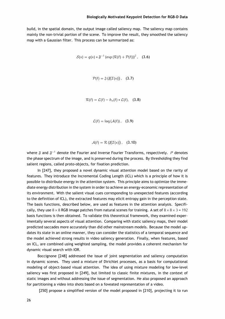
Biologically Motivated Keypoint Detection for RGB-D Data
build, in the spatial domain, the output image called saliency map. The saliency map containsmainly the non-trivial portion of the scene. To improve the result, they smoothed the saliencymap with a Gaussian filter. This process can be summarized as:
S(x) = g(x) ∗ F−1 (exp (R(f ) + P(f )))2 , (3.6)
P(f ) = J (F[I(x)]) , (3.7)
R(f ) = L(f ) − hn(f ) ∗ L(f ), (3.8)
L(f ) = log (A(f )) , (3.9)
A(f ) = R (F[I(x)]) , (3.10)
where F and F−1 denote the Fourier and Inverse Fourier Transforms, respectively. P denotesthe phase spectrum of the image, and is preserved during the process. By thresholding they findsalient regions, called proto-objects, for fixation prediction.
In [247], they proposed a novel dynamic visual attention model based on the rarity offeatures. They introduce the Incremental Coding Length (ICL) which is a principle of how it ispossible to distribute energy in the attention system. This principle aims to optimize the imme-diate energy distribution in the system in order to achieve an energy-economic representation ofits environment. With the salient visual cues corresponding to unexpected features (accordingto the definition of ICL), the extracted features may elicit entropy gain in the perception state.The basis functions, described below, are used as features in the attention analysis. Specifi-cally, they use 8×8 RGB image patches from natural scenes for training. A set of 8×8×3 = 192basis functions is then obtained. To validate this theoretical framework, they examined exper-imentally several aspects of visual attention. Comparing with static saliency maps, their modelpredicted saccades more accurately than did other mainstream models. Because the model up-dates its state in an online manner, they can consider the statistics of a temporal sequence andthe model achieved strong results in video saliency generation. Finally, when features, basedon ICL, are combined using weighted sampling, the model provides a coherent mechanism fordynamic visual search with IOR.
Boccignone [248] addressed the issue of joint segmentation and saliency computationin dynamic scenes. They used a mixture of Dirichlet processes, as a basis for computationalmodeling of object-based visual attention. The idea of using mixture modeling for low-levelsaliency was first proposed in [249], but limited to classic finite mixtures, in the context ofstatic images and without addressing the issue of segmentation. He also proposed an approachfor partitioning a video into shots based on a foveated representation of a video.
[250] propose a simplified version of the model proposed in [210], projecting it to run
26

in real time. They empirically evaluate the saliency model in saccades control of a camera insocial robotics situations.
More recently, in [251], Zhang et al. developed an algorithm in which the saliency isupdated online on each new frame. The performance of the model for predicting human fix-ation while watching videos is comparable to previous methods, with the advantage that it issubstantially simpler.
Butko and Movellan [252] extend Najemik and Geisler framework [253] by applying long-term Partially Observable Markov Decision Processes (POMDP) [254] planning methods, in whichthe primary goal is to gather information. Najemik and Geisler [253] developed an InformationMaximization (Infomax) model of eye movement and applied it to explain the visual searchof simple objects. They modeled the visual search as a control strategy designed to detectthe location of a visual target. According to these authors, the model successfully capturedsome aspects of human saccades, but has two important limitations: (1) Its fixation policy isglutton, maximizing the instantaneous information gain rather than the long-term gathering ofinformation; (2) It applies only to artificially constructed images.
Butko and Movellan [252] refer to their extension of the approach presented in [253] asInfomax - Partially Observable Markov Decision Processes (I-POMDP), where they showed thatlong-term Infomax reduces search time. The new formulation allows them to give answers toquestions about the temporal dynamics of optimal eye movement. Furthermore, the strategysearch varies depending on the characteristics of the optical device that is used to search [252].While this model is intended to solve the first limitation of the model in [253], the secondlimitation remained unsolved. The model was only suitable for a limited class of psychophysicalstimuli, in particular images that could be described as containing a field of Gaussian noise.In [255], they present a first attempt to extend the I-POMDP model to be useful for computervision applications. And in [132], they have a computational analysis of eye movement from thepoint of view of the theory of stochastic optimal control.
A model of attention with visual memory and online learning is proposed in [161], andit is composed of three parts: Sensory Mapping (SM), Cognitive Mapping (CM) and Motor Map-ping (MM). The novelty of this model lies in the CM, which incorporates into the visual memoryand online learning. To mimic visual memory, they present an Amnesic Incremental Hierachi-cal Discriminant Regression tree which is used to guide the amnesic elimination of redundantinformation from the tree. The Self-Supervised Competition Neural Network in CM has the char-acteristics of online learning since its connection weights can be updated in real time accordingto environment changes.
Guo et al. [256] present an approach named Phase spectrum of Quaternion Fourier Trans-form (PQFT) that produces a spatial-temporal saliency, thereby extending the Quaternion FourierTransform method [257]. More recently, in [258], these authors have applied the saliency de-tection method PQFT to perform the compression of images and video, taking advantage of themulti-resolution representation of wavelets.
Achanta et al. [91] present a method to determine saliency regions in images using theCIELab color space [259]. They use low level color and luminance features. An advantage of thismethod is that the saliency maps have the same size and resolution as the input image. Theyuse the difference-of-mean filter to estimate the center-surround contrast. The lower frequen-cies are retained depending of the size of the largest surround filter and higher frequenciesdepend on the size of the smallest central filter. In this way, this approach retains all of thefrequency range ]0, π] with a notch in the mean. They demonstrate the use of this algorithm inthe segmentation of semantically meaningful whole objects from digital images.
27
Biologically Motivated Keypoint Detection for RGB-D Data
More recently, in [89], Achanta et al. changed some concepts of their previous method[91] so that the objects' salient regions have more well defined limits. These limits are preservedthrough a substantial retention of the most frequent content from the original image. Thesaliency map is obtained by calculating the Euclidean distance between the mean vector Lab(obtained by converting the image to the CIELab color space) of an input image and each pixelvalue of a version of the image with Gaussian blur, before being converted to CIELab colorspace. They uniformly attribute saliency values to the entire salient regions, instead of onlyto the edges or texture regions. This is achieved by relying on the overall contrast of the pixelinstead of the local contrast measured in terms of both color and intensity features.
Unlike previous models presented by these authors, Achanta and Süsstraunck [260] presenta model where they are concerned with the computational efficiency, noise robust re-targetingscheme based on seam carving [261] by using saliency maps that assign higher importance tovisually prominent whole regions (and not just edges). The values of the stronger saliency arenot just assigned to the edge image, but to the whole region. This is accomplished by calculat-ing global pixel saliency using intensity as well as color features. The saliency maps easily avoidthe artifacts that conventional seam carving generates and are more robust in the presence ofnoise. In this method, the saliency maps are processed only once, independently of the numberof seams added or removed.
The most recent algorithm for saliency detection presented by Achanta and Süsstraunck[262] is based on the premise that you can make assumptions about the scale of the object tobe detected based on their position in the image. A pixel belonging to a salient object near theboundary will be less central than one inside the object. So, assuming that the salient objectis completely within the image, and not cut-off by the image borders, it is possible to varythe bandwidth of the center-surround filter by increasing the low frequency cut-off when theyapproach the image borders. Indeed, as they approach the image borders they use a more localsurround region. They choose to do this by making the surround symmetric around the centerwith respect to the edges of the image. When choosing a surrounding symmetrical to eachpixel, they implicitly address each pixel to be placed in the center of its own sub-image. Thismethod is different from the one in [89], where the entire image is used as the common globalsurround (abstracted as the average image CIELab color vector) to any given pixel, resulting inan asymmetric environment for pixels that are not in the center of the image.
Rosin [263] proposed an edge-based scheme for saliency detection over grayscale images,being composed in four steps:
A simple method for detecting salient regions in images was proposed by Rosin [263]. Thismethod only requires: a Sobel edge detection; a threshold decomposition at multiple levelsto produce a set of binary edge images; a the distance transformation on each of the binaryedge images to propagate the edge information; and sum it to obtain the overall saliency map.Moreover, it avoids the need for setting any parameter values.
Seo and Milanfar [264] proposed a framework for both static and space-time saliencydetection. Initially they used a local image structure at each pixel represented by a matrix oflocal regression kernels (equation 3.11), which are robust in the presence of noise and imagedistortions.
K (xl − xi) =√
det(Ci)h2 exp
{(xl − xi)T Cl(xl − xi)
−2h2
}, Cl ∈ R2×2, (3.11)
where l = 1, . . . , P , P is the number of the pixels in a local window, h is a global smoothing
28
parameter, and the matrix Cl is a covariance matrix estimated from a collection of spatial gra-dient vectors within the local analysis window around a sampling position xl = [x1, x2]Tl . Then,they use a nonparametric kernel density estimation for such features, which results in a saliencymap constructed from a local "self-resemblance" measure, indicating the likelihood of saliency.A "matrix cosine similarity" (a generalization of cosine similarity) is employed to measure theresemblance of each pixel to its surroundings. For each pixel, the resulting saliency map rep-resents the statistical likelihood of its feature matrix Fi given the feature matrices Fj of thesurrounding pixels:
si = 1∑N
j=1 exp(
−1+ρ(Fi,Fj )σ2
) , (3.12)
where ρ(Fi, Fj ) is the matrix cosine similarity between two feature maps Fi and Fj , and σ is alocal weighting parameter.
Yu et al. [265] attempt to simulate top-down influences. Five components of top-downinfluences are modeled: structure of object representation for LTM, learning of object represen-tations, deduction of task-relevant features, estimation of top-down biases, mediation betweenbottom-up and top-down models, and perceptual completion. This model builds a dual-codingobject representation for LTM. It consists of local and global codings, characterizing internalproperties and global attributes of an object. Probabilistic Neural Networks (PNNs) are usedfor object representation in that they can model probabilistic distribution of an object throughcombination of confident values. A dynamically constructive learning algorithm was developedto train PNNs when an object is attended. Given a task-specific object, this proposed modelrecalls the corresponding object representation from PNNs, deduces the task-relevant featuredimensions and evaluates top-down biases. Bottom-up and top-down biases are mediated toyield a primitive grouping based saliency map. The most salient primitive grouping is finally putinto the perceptual completion processing module to yield an accurate and complete objectrepresentation for attention.
Mahadevan and Vasconcelos [266] introduced a spatio-temporal saliency algorithm basedon a center-surround, which extends a discriminant formulation of center-surround saliency pre-viously proposed for static imagery in [93]. This method is inspired by the biological mechanismsof motion-based perceptual grouping. The combination of discriminant center-surround saliencywith dynamic textures produced spatio-temporal saliency algorithm, applicable to scenes withhighly dynamic backgrounds and moving cameras.
Li et al. [267] proposed a visual saliency model based on conditional entropy for bothimage and video. Saliency was defined as the minimum uncertainty of a local region givenits surrounding area (namely the minimum conditional entropy), when perceptional distortionis considered. They approximated the conditional entropy by the lossy coding length of mul-tivariate Gaussian data. The final saliency map was accumulated pixel-by-pixel and furthersegmented to detect the proto-objects. In [268], they proposed a newer version of this modelby adding a multi-resolution scheme to it.
Avraham and Lindenbaum [269] presented a bottom-up attention mechanism, based on avalidated stochastic model to estimate the probability that an image part is of interest. Theyrefer to the probability as saliency, and therefore specify the saliency mathematically. Themodel quantifies the various intuitive observations, such as increased correspondence likeli-hood between visually similar regions of the image. The algorithm starts with a pre-attentive
29
Biologically Motivated Keypoint Detection for RGB-D Data
segmentation and then uses a rough approximation to a graphical model to efficiently revealwhich segments are more likely to be of interest. They prefer the objects belonging to smallergroups than those which are relatively very different from the rest of the image. Their approachto the design of the saliency algorithm is to quantify the labels that are target and non-targetcandidates in a probabilistic model, which would eventually identify the salience of a candidatewith their likelihood of being a target.
Borji et al. [133] proposed a three-layered approach for interactive object-based atten-tion inspired by RLVC and U-Tree algorithms [270]. Each time the object that is most importantto disambiguate appears, a partially unknown state is attended by the biased bottom-up saliencymodel and recognized. Then the appropriate action for the scene is performed.
Based on the principle of the Infomax, Wang et al. [271] introduced a computationalmodel to simulate human saccadic scanpaths on natural images. The model integrates somefactors that drives human attention reflected by eye movements: reference sensory responses,fovea-periphery resolution discrepancy, and visual working memory. They compute three multi-band filter response maps for each eye movement which are then combined into multi-bandresidual filter response maps. Finally, they compute Residual Perceptual Information (RPI) ateach location, which is a dynamic saliency map varying along with eye movements. The nextfixation is selected as the location with the maximal RPI value.
3.3 Hybrid Methods
Lee and Yu [272] proposed that mutual information among the cortical representations ofthe retinal image, the priors constructed from our long-term visual experience, and a dynamicshort-term internal representation constructed from recent saccades, all provide a map forguiding eye navigations. By directing the eyes to locations of maximum complexity in neuronalensemble responses at each step, the automatic saccadic eye movement system greedily collectsinformation about the external world while modifying the neural representations in the process.This model is close to the work presented in [253].
Renninger et al. [273] built a model based on the idea that humans fixate at those infor-mative points in an image which reduce our overall uncertainty about the visual stimulus, andit is similar to the approach presented in [272]. This model is a sequential information maxi-mization approach whereby each fixation is aimed at the most informative image location giventhe knowledge acquired at each point. A foveated representation is incorporated by reducingresolution as distance increases from the center. Shape histogram edges are used as features.
Peters et al. [274--277] presented a model of spatial attention that can be applied toarbitrary static and dynamic image sequences with interactive tasks. The claimed novelty liesin the combination of these elements and in the fully computational nature of the model. Thebottom-up component computes a saliency map from 12 low-level multi-scale visual features.The top-down component computes a low-level signature of the entire image, and learns toassociate different classes of signatures with the different gaze patterns recorded from humansubjects performing a task of interest. They measured the ability of this model to predict theeye movements of people playing contemporary video games. They showed that a point-wisemultiplication of bottom-up saliency with the top-down map learned in this way results in highprediction performance.
Harelet al. [95] proposed a new visual saliency model, called Graph-Based Visual Saliency.It consists of two steps: first forming activation maps on certain feature channels, and then
30
normalizing them in a way which highlights conspicuity and admits combination with other map.
Oliva et al. [278] and Torralba et al. [249,279] proposed a Bayesian framework for visualsearch tasks, where they use biologically inspired linear filters for different orientations andscales. The filter responses are known to correlate with each other. For example, a verticalbar in the image will activate an adjusted filter to the vertical bars but will also activate (withless intensity) an adjusted filter for bars with an inclination of 45 degrees. The joint probabilityof a feature vector is estimated using multivariate Gaussian distributions [278] and posteriorlyby multivariate generalized Gaussian distributions [279]. Bottom-up saliency is derived fromtheir formulation as 1
p(f |fG ) where fG represents a global feature that summarizes the probabilitydensity of presence of the target object in the scene, based on analysis of the scene gist.
Torralba et al. [279] present their model of Contextual Guidance, which is a Bayesianformulation of visual salience. The Contextual Guidance model makes use of global features,forming a holistic representation of the scene to guide attention to locations in a scene thatmight contain the target. Global features are calculated by forming a low-dimensional repre-sentation of a scene, combining the low-level features in large parts of the image and usingPrincipal Component Analysis (PCA) to further reduce the dimensionality.
Bruce and Tsotsos [96] define bottom-up saliency based on maximum information sam-pling. The information in this model is computed based on Shannon's self-information. Thedistribution of the features is estimated from a neighborhood of a point, which can be as largeas the entire image. When the vicinity of each point is defined as the entire image of inter-est, as implemented in [96], the definition of projection becomes identical to the term of thebottom-up saliency from the work presented in [278,279]. It is noteworthy, however, that thefeature spaces used in the two models are different. They present a model for calculating thevisual saliency constructed on the basis of a theoretical formulation of information. The modelemploys features that were learned from natural images using Independent Component Analy-sis (ICA). These were shown to resemble the receptive fields of neurons in the primary visualcortex (V1), and their answers have the desirable property of dispersion. Moreover, the featureslearned are approximately independent, simplifying the likelihood estimation without makingindependence assumptions.
The Bayesian Surprise theory of Itti et al. [88, 280, 281] define saliency as a deviationfrom what is expected based on a set of internal models of the local visual world. According tothis theory, the organisms form models of their environment and assign probability distributionsover the possible models. With the arrival of new data, the distributions of the possible modelsare updated with the Bayes rule and the KL divergence between the prior distributions, wherethe posterior distributions is measured. The new data forces the distribution to be altered, thegreater the divergence. These KL scores of different distributions with respect to the modelsare combined to produce a saliency score. Their implementation of this theory leads to analgorithm that determines the saliency as a kind of deviation of the features present in theclosest neighbors, but extends the concept of neighborhood to the spatio-temporal realm.
Kienzle et al. [282, 283] addressed the bottom-up influence of local image informationon human eye movements. The model consists of a non-parametric bottom-up approach forlearning attention directly from human eye-tracking data. The saliency function is determinedby its maximization of prediction performance on the observed data. A SVM was trained todetermine the saliency using the local intensities. Also this method produces center-surroundoperators analogous to receptive fields of neurons in early visual areas (LGN and V1).
Liu et al. [284--286] formulate salient object detection as a problem of image segmen-tation, where they separate the salient object from the background. In [284], they propose a
31
Biologically Motivated Keypoint Detection for RGB-D Data
set of features including multi-scale contrast, center-surround histogram and color spatial dis-tribution to describe a salient object locally, regionally and globally. The Conditional RandomField (CRF) is learned to effectively combine these features to detect salient objects.
In [285,286], they extended the local, regional and global salient features to the field ofmotion, so as to be applied not only to images, but also to videos. They designed a dynamicprogramming algorithm to solve a global optimization problem, with a rectangle to representeach salient object. The salient object sequence detection is defined as an energy minimizationproblem (like a binary labeling) using a CRF framework, while static and dynamic salience,spatial and temporal coherence, and the global topic model are well defined and integrated toidentify a salient object sequence.
Zhang et al. [15, 210] proposed a model called Saliency Using Natural statistics (SUN),by considering what the visual system is trying to optimize when directing attention. The re-sulting model is a Bayesian framework in which bottom-up saliency emerges naturally as theself-information of visual features, and overall saliency (incorporating top-down informationwith bottom-up saliency) emerges as the point-wise mutual information between local imagefeatures and the search target's features when searching for a target. Self-information in thiscontext, learned from natural images statistics, corresponds to the findings of the new itemsthat attract attention in visual search [287]. The SUN formula for bottom-up saliency is similarto the ones in [96, 249, 278, 279], which are all based on the concept of self-information ora Bayesian formulation. The statistical differences between the current image statistics andnatural ones leads to radically different types of self-information. The motivation for usingself-information with the statistics of the current image is that a foreground object is likely tohave features that are distinct from the features of the background. Since targets are observedless frequently than background during an organism's lifetime, rare features are more likely toindicate targets.
The idea that the salience of an item depends on its deviation from the average statisticsof the image can find its roots in the model of visual search proposed in [207], which representeda number of motion pop-out phenomena, and can be seen as a generalization of the saliency ofthe center-surround-base found in [2].
In [210], the saliency is calculated locally, which means that the model is consistent withthe early visual system neuroanatomy and results in an efficient algorithm, with very few freeparameters. They extend the model in [15] to temporally dynamic scenes, and characterize thevideo statistics around each pixel using a bank of spatio-temporal filters with separable space-time components. The joint spatio-temporal impulse response of these filters is the productof a spatial and a temporal impulse response. In [210], the spatial impulse responses are DoG,which model the properties of neurons in the LGN.
To predict the likelihood of where humans typically focus on a video scene, Pang etal. [288] proposed a stochastic model of visual attention by introducing a dynamic Bayesiannetwork to predict where humans typically focus in a video scene.. Their model simulates andcombines the visual saliency response and the cognitive state of a person to estimate the mostprobable attended regions [289]. They reported that the HVS are not deterministic and peoplemay attend to different locations on the same visual input on different occasions.
Garcia-Diaz et al. [211, 290, 291] introduced an approach to visual saliency that relieson a contextually adapted representation produced through adaptive whitening of color andscale features. The proposed approach is based on the classic hierarchical decomposition ofimages which are initially separate chromatic components (CIELab color space). The luminancechannel is decomposed into various orientations and scale representation by means of Gabor
32
bank of filters. This approach is inspired by the image representation described in the earlystages of the visual pathway. Then, whitening is imposed to groups of oriented scales for eachwhitened chromatic component. This strategy keeps the number of components involved inwhitening limited, overcoming the problems of computational complexity. The decorrelation isachieved by applying PCA on the multi-scale responses, extracting from them a local measureof variability. Furthermore, a local mean is performed to obtain a unified and efficient measureof saliency. As a result, a specifically adapted image representation arises. The resulting imagecomponents have zero mean and unit variance. To obtain a saliency map, they simply computepoint distinctiveness by taking, for each pixel, the squared vector norm in this representationdivided by the sum of the representation across all pixels (Hotelling's T 2 statistic [292]).
we generalize our saliency framework to dynamic scenes and develop a simple, efficient,and online bottom-up saliency algorithm.
Zhang et al. [251] extended the SUN model to dynamic scenes and develop a simple,efficient, and online bottom-up saliency algorithm. The first step starts by applying a bank ofspatio-temporal filters to each video. These filters are designed to be both efficient and in linewith the HVS. The probability distributions of these spatio-temporal features were learned froma set of videos from natural environments. Finally, the model calculates features and estimatesthe bottom-up saliency for each point as − log p(F = fz).
Following the same direction as the one presented in [249, 278, 279, 293], they linearlyintegrated three components (bottom-up saliency, gist, and object features) for explaining eyemovements in looking for people in a database of about 900 natural scenes.
Judd et al. [97] use a learning approach and train a linear SVM classifier, similarly to onein [283], directly from human eye tracking data and they also present a new public database.The classifier trained by these authors uses low, mid and high level features extracted directlyfrom the images with a resolution of 200×200. The low-level biologically plausible features usedwere: local energy of the steerable pyramid filters [294], the simple saliency model describedin [207,209], based on subband pyramids, and intensity, orientation and color contrast featurescorresponding to the image features calculated in [3]. The mid-level features are due to thehorizon, where human beings naturally look more to the objects. At this feature level, theyintroduced the horizontal line detector from mid-level gist features [209]. Finally, the high-level features used are the Viola and Jones face detector [215,225] and the Felzenszwalb et al.person detector [295].
Using the database presented in [97, 296] measured the amount of visual informationthat is available from blurred images. Moreover, they separated the natural images in easy,medium and hard based on their complexity using the following informal criterion: each imagewas displayed at various resolutions and the authors estimated the lowest resolution in whichthe image could be understood. The images perceived as having low resolution were classifiedinitially and images understood as containing higher resolutions were classified at the end.Easy images are those which tend to contain a large object or a simple landscape and can beunderstood using squared images with only 16 or 32 pixels resolution. The medium images havemultiple objects or are more complex and can be understood using squared images with around32−64 pixels. The hard images have many small details or are often abstract and need 64−128pixels of resolution. To reduce the resolution of each image, they used the same method asin [297]. They applied a binomial low-pass filter to each color channel, and then the filteredimage was downsampled by a factor of two. As color is an important feature, they preservedthe color range of the blurred version of the images. To do this, they scaled the range of eachdownsampled image as large as possible within the range of 0 − 1, maintaining the same mean
33
Biologically Motivated Keypoint Detection for RGB-D Data
values of pixel luminance.
Li et al. [298] presented a probabilistic multi-task learning approach for visual saliencyestimation in video. Here, the problem of visual saliency estimation was modeled by simultane-ously considering the stimulus-driven and task-related factors in a probabilistic framework. Thestimulus-driven component simulates the low-level processes in HVS using multi-scale waveletdecomposition and unbiased feature competition, while a task-related component simulates thehigh-level processes to bias the competition of the input features. The algorithm learns variousfusion strategies, which are used to integrate the stimulus-driven and task-related componentsto obtain the visual saliency, similar to the one presented in [276]. Experiments on two eye-fixation datasets [299] and one regional saliency dataset [300] show that this model outperformsseven existing bottom-up approaches presented in [3,94,95,256,280,301,302].
Goferman et al. [303, 304] propose a context-aware saliency that detects regions of theimage representing the scene. The goal is to identify both fixation points and detect the dom-inant object. In conformity with this setting, they present a detection algorithm that is basedon four observations realized in the psychological literature [221,305--307]:
1. Local low-level considerations, such as contrast and color;
2. Global considerations, suppressing features which occur frequently, maintaining the fea-tures that deviate from the norm;
3. Visual organization rules, indicating that the visual forms may have one or more centersof gravity depending on how they are organized;
4. High-level factors, such as human faces.
In conformity with the first observation, the areas that have different colors or patterns mustobtain higher saliency values. Moreover, the homogeneous or blurred areas must obtain lowersaliency values. According to the second observation, the features that occur more often shouldbe removed. For the third observation, the salient pixels are grouped and not spread throughoutthe image. In this algorithm, they first define the saliency in a single local-global scale, basedon the principles 1 − 3. Then, they improve the saliency using multiple scales. In the next step,they modify the saliency to further accommodate the third principle. Finally, observation fouris implemented as post-processing.
Cheng et al. [308] focus on data-driven bottom-up saliency using the detection of theimage contrast, based on the work presented in [309], where they believe that cortical cellscan be hard wired to respond preferentially to stimuli of high contrast in their receptive fields.They propose a contrast analysis for extracting high-resolution, full-field saliency maps basedon the following observations:
1. A method based on global contrast, that separates a large-scale object from its surround-ings, is preferred to obtain the local contrast;
2. Global considerations enable the assignment of comparable saliency values to similar im-age regions, and can uniformly highlight entire objects;
3. The saliency of a region depends mainly on its contrast with neighboring regions;
4. Saliency maps should be rapid and easy to generate, in order to allow the processing oflarge collections of files, and facilitate efficient classification of the images.
34
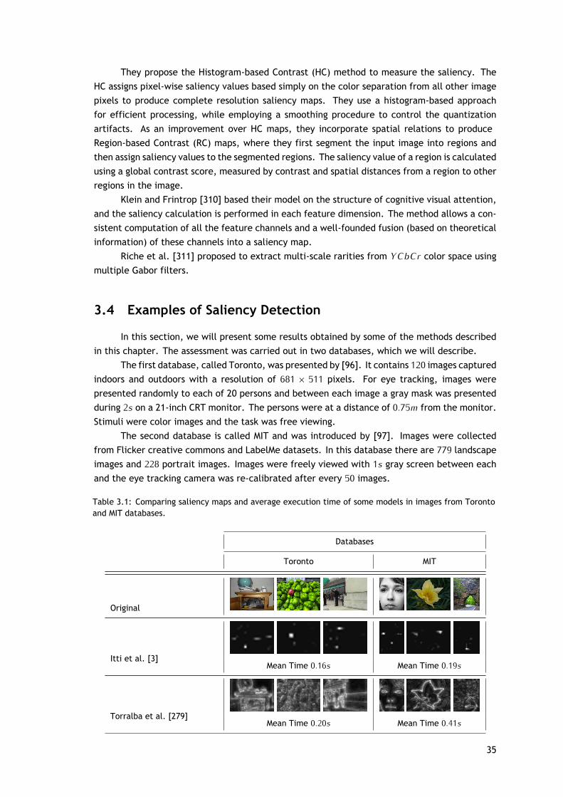
They propose the Histogram-based Contrast (HC) method to measure the saliency. TheHC assigns pixel-wise saliency values based simply on the color separation from all other imagepixels to produce complete resolution saliency maps. They use a histogram-based approachfor efficient processing, while employing a smoothing procedure to control the quantizationartifacts. As an improvement over HC maps, they incorporate spatial relations to produceRegion-based Contrast (RC) maps, where they first segment the input image into regions andthen assign saliency values to the segmented regions. The saliency value of a region is calculatedusing a global contrast score, measured by contrast and spatial distances from a region to otherregions in the image.
Klein and Frintrop [310] based their model on the structure of cognitive visual attention,and the saliency calculation is performed in each feature dimension. The method allows a con-sistent computation of all the feature channels and a well-founded fusion (based on theoreticalinformation) of these channels into a saliency map.
Riche et al. [311] proposed to extract multi-scale rarities from YCbCr color space usingmultiple Gabor filters.
3.4 Examples of Saliency Detection
In this section, we will present some results obtained by some of the methods describedin this chapter. The assessment was carried out in two databases, which we will describe.
The first database, called Toronto, was presented by [96]. It contains 120 images capturedindoors and outdoors with a resolution of 681 × 511 pixels. For eye tracking, images werepresented randomly to each of 20 persons and between each image a gray mask was presentedduring 2s on a 21-inch CRT monitor. The persons were at a distance of 0.75m from the monitor.Stimuli were color images and the task was free viewing.
The second database is called MIT and was introduced by [97]. Images were collectedfrom Flicker creative commons and LabelMe datasets. In this database there are 779 landscapeimages and 228 portrait images. Images were freely viewed with 1s gray screen between eachand the eye tracking camera was re-calibrated after every 50 images.
Table 3.1: Comparing saliency maps and average execution time of some models in images from Torontoand MIT databases.
Databases
Toronto MIT
Original
Itti et al. [3]Mean Time 0.16s Mean Time 0.19s
Torralba et al. [279]Mean Time 0.20s Mean Time 0.41s
35
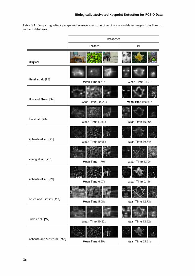
Biologically Motivated Keypoint Detection for RGB-D Data
Table 3.1: Comparing saliency maps and average execution time of some models in images from Torontoand MIT databases.
Databases
Toronto MIT
Original
Harel et al. [95]Mean Time 0.61s Mean Time 0.60s
Hou and Zhang [94]Mean Time 0.0029s Mean Time 0.0031s
Liu et al. [284]Mean Time 13.61s Mean Time 15.36s
Achanta et al. [91]Mean Time 10.98s Mean Time 69.74s
Zhang et al. [210]Mean Time 1.79s Mean Time 4.39s
Achanta et al. [89]Mean Time 0.07s Mean Time 0.12s
Bruce and Tsotsos [312]Mean Time 5.08s Mean Time 12.73s
Judd et al. [97]Mean Time 10.32s Mean Time 13.82s
Achanta and Süsstrunk [262]Mean Time 4.19s Mean Time 23.81s
36
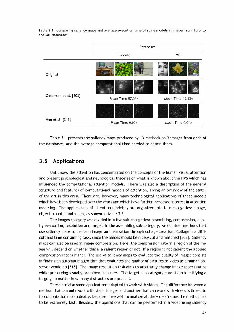
Table 3.1: Comparing saliency maps and average execution time of some models in images from Torontoand MIT databases.
Databases
Toronto MIT
Original
Goferman et al. [303]Mean Time 57.28s Mean Time 49.43s
Hou et al. [313]Mean Time 0.02s Mean Time 0.01s
Table 3.1 presents the saliency maps produced by 13 methods on 3 images from each ofthe databases, and the average computational time needed to obtain them.
3.5 Applications
Until now, the attention has concentrated on the concepts of the human visual attentionand present psychological and neurological theories on what is known about the HVS which hasinfluenced the computational attention models. There was also a description of the generalstructure and features of computational models of attention, giving an overview of the state-of-the art in this area. There are, however, many technological applications of these modelswhich have been developed over the years and which have further increased interest in attentionmodeling. The applications of attention modeling are organized into four categories: image,object, robotic and video, as shown in table 3.2.
The images category was divided into five sub-categories: assembling, compression, qual-ity evaluation, resolution and target. In the assembling sub-category, we consider methods thatuse saliency maps to perform image summarization through collage creation. Collage is a diffi-cult and time consuming task, since the pieces should be nicely cut and matched [303]. Saliencymaps can also be used in image compression. Here, the compression rate in a region of the im-age will depend on whether this is a salient region or not. If a region is not salient the appliedcompression rate is higher. The use of saliency maps to evaluate the quality of images consistsin finding an automatic algorithm that evaluates the quality of pictures or video as a human ob-server would do [318]. The image resolution task aims to arbitrarily change image aspect ratioswhile preserving visually prominent features. The target sub-category consists in identifying atarget, no matter how many distractors are present.
There are also some applications adapted to work with videos. The difference between amethod that can only work with static images and another that can work with videos is linked toits computational complexity, because if we wish to analyze all the video frames the method hasto be extremely fast. Besides, the operations that can be performed in a video using saliency
37
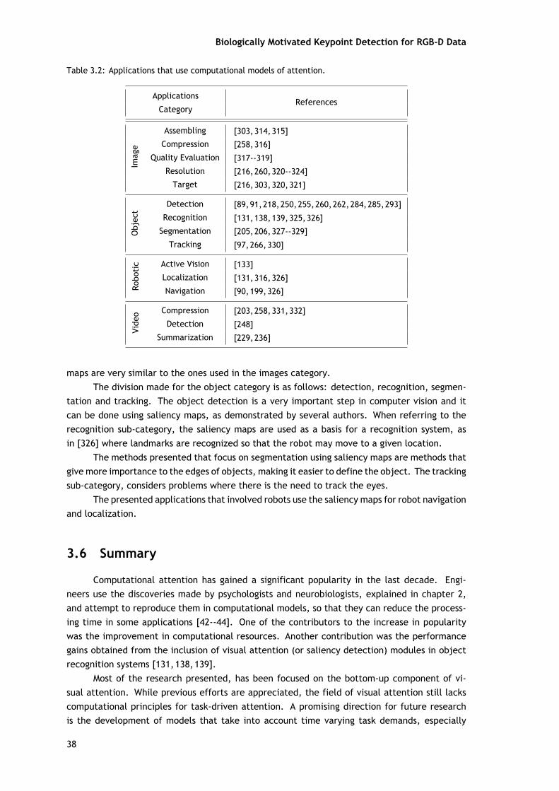
Biologically Motivated Keypoint Detection for RGB-D Data
Table 3.2: Applications that use computational models of attention.
ApplicationsReferences
Category
Image
Assembling [303,314,315]
Compression [258,316]
Quality Evaluation [317--319]
Resolution [216,260,320--324]
Target [216,303,320,321]
Object
Detection [89,91,218,250,255,260,262,284,285,293]
Recognition [131,138,139,325,326]
Segmentation [205,206,327--329]
Tracking [97,266,330]
Robo
tic Active Vision [133]
Localization [131,316,326]
Navigation [90,199,326]
Vide
o Compression [203,258,331,332]
Detection [248]
Summarization [229,236]
maps are very similar to the ones used in the images category.The division made for the object category is as follows: detection, recognition, segmen-
tation and tracking. The object detection is a very important step in computer vision and itcan be done using saliency maps, as demonstrated by several authors. When referring to therecognition sub-category, the saliency maps are used as a basis for a recognition system, asin [326] where landmarks are recognized so that the robot may move to a given location.
The methods presented that focus on segmentation using saliency maps are methods thatgive more importance to the edges of objects, making it easier to define the object. The trackingsub-category, considers problems where there is the need to track the eyes.
The presented applications that involved robots use the saliency maps for robot navigationand localization.
3.6 Summary
Computational attention has gained a significant popularity in the last decade. Engi-neers use the discoveries made by psychologists and neurobiologists, explained in chapter 2,and attempt to reproduce them in computational models, so that they can reduce the process-ing time in some applications [42--44]. One of the contributors to the increase in popularitywas the improvement in computational resources. Another contribution was the performancegains obtained from the inclusion of visual attention (or saliency detection) modules in objectrecognition systems [131,138,139].
Most of the research presented, has been focused on the bottom-up component of vi-sual attention. While previous efforts are appreciated, the field of visual attention still lackscomputational principles for task-driven attention. A promising direction for future researchis the development of models that take into account time varying task demands, especially
38

in interactive, complex, and dynamic environments. In addition, there is not yet a principledcomputational understanding of visual attention. The solution is beyond the scope of a singlearea. In order to obtain a solution it is necessary to have the cooperation of the several areas,from the machine learning community, computer vision and also the biological areas as well asneurology and psychology.
39

Biologically Motivated Keypoint Detection for RGB-D Data
40
Chapter 4
Keypoint Detectors, Descriptors and Evaluation
When processing image or 3D point cloud data, features must be extracted from a small setof points, usually called keypoints. This is done to avoid the computational complexity requiredto extract features from all points. There are many keypoint detectors and this suggests the needof a comparative evaluation. When the keypoint detectors are applied to objects, the aim is todetect a few salient structures which can be used, instead of the whole object, for applicationslike object registration, retrieval and data simplification. In this chapter, the description ofsome 2D and 3D keypoint detectors (focusing more on 3D), and also 3D descriptors is made.Finally, an evaluation of 3D keypoint detectors, available in PCL, is made with real objectson 3D point clouds. The invariance of the 3D keypoint detectors is evaluated according torotations, scale changes and translations. The evaluation criteria used are the absolute and therelative repeatability rate. Using these criteria, the robustness of the detectors is evaluatedwith respect to changes of point-of-view.
4.1 Keypoint Detectors
4.1.1 Harris 3D
The Harris method [333] is a corner and edge based method and these types of methodsare characterized by their high-intensity changes. These features can be used in shape andmotion analysis and they can be detected directly from the grayscale images. For the 3D case,the adjustment made in PCL for the Harris3D detector replaces the image gradients by surfacenormals, where the covariance matrix Cov will be calculated. The keypoints responsemeasuredat each pixel coordinate (x, y, z) is then defined by
r(x, y, z)=det(Cov (x, y, z))−k (trace(Cov (x, y, z)))2 , (4.1)
where k is a positive real valued parameter and a thresholding process is used to suppress weakkeypoints around the stronger ones. The keypoint responses are positive in the corner region,negative in the edge regions, and small in flat regions [333]. If the contrast of the point cloudincreases, the magnitude of the keypoint responses also increase. The flat region is specifiedby the trace falling below some selected threshold.
In the PCL are available two variants of the Harris3D keypoint detector: these are calledLowe [99] and Noble [100]. The differences between them are the functions that define thekeypoints response (equation 4.1). Thus, for the Lowe method the keypoints response is givenby:
r(x, y, z) = det(Cov (x, y, z))trace(Cov (x, y, z))2 . (4.2)
41

Biologically Motivated Keypoint Detection for RGB-D Data
The keypoints response for Noble method is given by:
r(x, y, z) = det(Cov (x, y, z))trace(Cov (x, y, z)) . (4.3)
In the case of the Lowe detector, the differences between the values of the keypointresponses in the corner regions, edge regions and planar regions tend to be closer to zero com-pared to those of the Noble detector. This means that there are more regions considered flat.
4.1.2 Kanade-Lucas-Tomasi
The Kanade-Lucas-Tomasi (KLT) detector [98] was proposed a few years after the Harrisdetector. In the 3D version presented in the PCL, this keypoint detector has the same basis asthe Harris3D detector. The main differences are: the covariance matrix is calculated using theintensity value instead of the surface normals; and for the keypoints response they used thefirst eigenvalue of the covariance matrix. Finally, the suppression process is similar to the oneused in the Harris3D method.
4.1.3 Curvature
The curvature method in the PCL calculates the principal surface curvatures on each pointusing the surface normals. The keypoints response used to suppress weak keypoints, around thestronger ones is the same as in the Harris3D.
4.1.4 Smallest Univalue Segment Assimilating Nucleus
The Smallest Univalue Segment Assimilating Nucleus (SUSAN) corner detector was intro-duced in [101]. SUSAN is a generic low-level image processing technique which, apart fromcorner detection, has also been used for edge detection and noise suppression. A geometricthreshold is applied, which is simply a precise restatement of the SUSAN principle: if the nu-cleus (center pixel of a circular region) lies on a corner then the Univalue Segment AssimilatingNucleus (USAN) area will be less than half of its possible value.
USAN is a measure of how similar a center pixel's intensity is to those in its neighborhood.A gray value similarity function s(g1, g2) measures the similarity between the gray values g1 andg2. Summing over this kind of function for a set of pixels is equivalent to counting the numberof similar pixels. It can be used to adjust the detector's sensitivity to the image's global contrastlevel. The smoothness plays of s(g1, g2) an important role in noise suppression [101], since itonly depends on the difference between g1 and g2. To make the method more robust, pointscloser in value to the nucleus receive a higher weighting. Moreover, a set of rules presentedin [334] are used to suppress qualitatively "bad'' keypoints. Local minima of the SUSANs are thenselected from the remaining candidates.
4.1.5 Scale Invariant Feature Transform
The Scale Invariant Feature Transform (SIFT) keypoint detector was proposed in [9]. Thismethod shares similar properties with neurons in inferior temporal cortex that are used forobject recognition in primate vision. In [102], the original algorithm for 3D data is presented,which uses a 3D version of the Hessian to select the interest points, which will be called SIFT3D.
42
The image I is convolved with a number of Gaussian filters whose standard deviationsdiffer by a fixed scale factor. That is, σj+1 = kσj where k is a constant scalar that should be setto
√2. The convolutions yield smoothed images, denoted by
G(x, y, σj ), i = 1, . . . , n. (4.4)
The adjacent smoothed images are then subtracted by
D(x, y, σj ) = G(x, y, σj+1) − G(x, y, σj ). (4.5)
These two steps are repeated, yielding a number of DoGs over the scale space. Once DoGs havebeen obtained, keypoints are identified as local minima/maxima of the DoGs across scales.This is done by comparing each point in the DoGs to its eight neighbors at the same scale andnine corresponding neighborhood points in each of the neighborhood scales. The dominantorientations are assigned to localized keypoints.
4.1.6 Speeded-Up Robust Features
Speeded-Up Robust Features (SURF) [10] is partly inspired by the SIFT descriptor. SURFis based on sums of 2D Haar wavelet responses and makes an efficient use of integral images.It uses an integer approximation to the determinant of Hessian blob detector, which can becomputed extremely quickly with an integral image. For features, it uses the sum of the Haarwavelet response around the point of interest.
4.1.7 Intrinsic Shape Signatures 3D
Intrinsic Shape Signatures 3D (ISS3D) [103] is a method relying on region-wise qualitymeasurements. This method uses the magnitude of the smallest eigenvalue (to include onlypoints with large variations along each principal direction) and the ratio between two successiveeigenvalues (to exclude points having similar spread along principal directions).
The ISS3D Si = {Fi, fi} at a point pi consists of two components: 1 -- The intrinsic ref-erence frame Fi = {pi, {ex
i , eyi , ez
i }} where pi is the origin, and {exi , ey
i , ezi } is the set of basis
vectors. The intrinsic frame is a characteristic of the local object shape and independent ofviewpoint. Therefore, the view independent shape features can be computed using the frameas a reference. However, its basis {ex
i , eyi , ez
i }, which specifies the vectors of its axes in thesensor coordinate system, are view dependent and directly encode the pose transform betweenthe sensor coordinate system and the local object-oriented intrinsic frame, thus enabling fastpose calculation and view registration. 2 -- The 3D shape feature vector fi = (fi0, fi1, . . . , fiK−1),which is a view independent representation of the local/semi-local 3D shape. These featurescan be compared directly to facilitate the matching of surface patches or local shapes fromdifferent objects.
4.1.8 Biologically Inspired keyPoints
Biologically Inspired keyPoints (BIMP) [7,335] is a cortical keypoint detector for extractingmeaningful points from images, solving the computational problem of [104]. The keypoints are
43

Biologically Motivated Keypoint Detection for RGB-D Data
extracted by a series of filtering operations: simple cells, complex cells, end-stopped cells andinhibition cells. Simple cells are modeled using complex Gabor filters with phases in quadratureare given by:
gλ,σ,θ,ϕ(x, y) = exp(
− x2 + γy2
2σ 2
)exp
(i2πx
λ
), (4.6)
where x = x cos(θ) + y sin(θ), y = y cos(θ) − x sin(θ), with σ the receptive field size, θ thefilter orientation, λ is the wavelength and γ = 0.5. Simple cell responses are obtained byconvolving the image with the complex Gabor filter: Rλ,θ = I ∗ gλ,θ. Complex cells are themodulus of simple cell responses Cλ,θ = |Rλ,θ |. Remaining kernels are sums of Dirac functions(δ). If ds = 0.6λ sin(θ) and dc = 0.6λ cos(θ), double-stopped cell kernels are defined by
kDλ,θ =δ(x, y)− δ(x−2ds, y+2dc)+δ(x+2ds, y−2dc)
2 (4.7)
and the final keypoints is given by
K Dλ =
π∑
θ=0|Cλ,θkD
λ,θ |+−2π∑
θ=0|Cλ,θkT I
λ,θ +Cλ,θ⊥kRIλ,θ −Cλ,θ |+, (4.8)
where θ⊥ is orthogonal to θ, |.|+ represents the suppression of negatives values. kT Iλ,θ is the
tangential inhibition kernel and kRIλ,θ the radial.
kT Iλ,θ =−2δ(x, y)+δ(x+dc, y+ds)+δ(x−dc, y−ds) (4.9)
kRIλ,θ =δ(x + dc/2, y + ds/2)+δ(x − dc/2, y − ds/2). (4.10)
4.2 3D Descriptors
4.2.1 3D Shape Context
The 3D Shape Context (3DSC) descriptor [105] is the 3D version of the Shape Contextdescriptor [106]. It is based on a spherical grid centered on each keypoint. The surface normalestimation is used to orient the grid to the north pole. The grid is defined by bins along theazimuth, elevation and radial dimensions. The bins along the azimuth and elevation dimensionsare equally spaced, on the other hand, the radial dimension is logarithmically spaced. The finalrepresentation of the descriptor is a 3D histogram, where in each bin contains a weighted sumof the number of points falling on the grid region. These weights are inversely proportional tothe bin volume and the local point density.
4.2.2 Point Feature Histograms
Descriptors such as Point Feature Histograms (PFH) [107], Fast Point Feature Histograms(FPFH) [108, 109], Viewpoint Feature Histogram (VFH) [110], Clustered Viewpoint Feature His-togram (CVFH) [111] and Oriented, Unique and Repeatable Clustered Viewpoint Feature His-
44
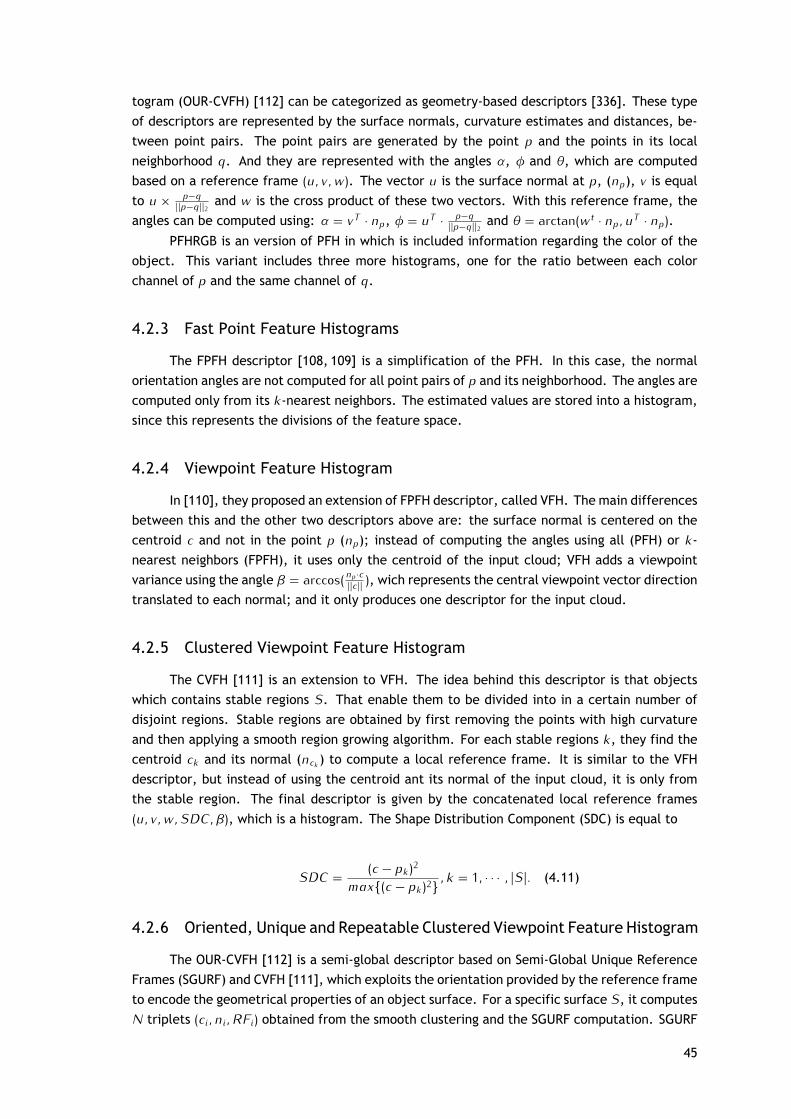
togram (OUR-CVFH) [112] can be categorized as geometry-based descriptors [336]. These typeof descriptors are represented by the surface normals, curvature estimates and distances, be-tween point pairs. The point pairs are generated by the point p and the points in its localneighborhood q. And they are represented with the angles α, ϕ and θ, which are computedbased on a reference frame (u, v, w). The vector u is the surface normal at p, (np), v is equalto u × p−q
||p−q||2 and w is the cross product of these two vectors. With this reference frame, theangles can be computed using: α = vT · np, ϕ = uT · p−q
||p−q||2 and θ = arctan(wt · np, uT · np).PFHRGB is an version of PFH in which is included information regarding the color of the
object. This variant includes three more histograms, one for the ratio between each colorchannel of p and the same channel of q.
4.2.3 Fast Point Feature Histograms
The FPFH descriptor [108, 109] is a simplification of the PFH. In this case, the normalorientation angles are not computed for all point pairs of p and its neighborhood. The angles arecomputed only from its k-nearest neighbors. The estimated values are stored into a histogram,since this represents the divisions of the feature space.
4.2.4 Viewpoint Feature Histogram
In [110], they proposed an extension of FPFH descriptor, called VFH. The main differencesbetween this and the other two descriptors above are: the surface normal is centered on thecentroid c and not in the point p (np); instead of computing the angles using all (PFH) or k-nearest neighbors (FPFH), it uses only the centroid of the input cloud; VFH adds a viewpointvariance using the angle β = arccos( np·c
||c|| ), wich represents the central viewpoint vector directiontranslated to each normal; and it only produces one descriptor for the input cloud.
4.2.5 Clustered Viewpoint Feature Histogram
The CVFH [111] is an extension to VFH. The idea behind this descriptor is that objectswhich contains stable regions S. That enable them to be divided into in a certain number ofdisjoint regions. Stable regions are obtained by first removing the points with high curvatureand then applying a smooth region growing algorithm. For each stable regions k, they find thecentroid ck and its normal (nck ) to compute a local reference frame. It is similar to the VFHdescriptor, but instead of using the centroid ant its normal of the input cloud, it is only fromthe stable region. The final descriptor is given by the concatenated local reference frames(u, v, w, SDC, β), which is a histogram. The Shape Distribution Component (SDC) is equal to
SDC = (c − pk )2max{(c − pk )2} , k = 1, · · · , |S|. (4.11)
4.2.6 Oriented, Unique and Repeatable Clustered Viewpoint Feature Histogram
The OUR-CVFH [112] is a semi-global descriptor based on Semi-Global Unique ReferenceFrames (SGURF) and CVFH [111], which exploits the orientation provided by the reference frameto encode the geometrical properties of an object surface. For a specific surface S, it computesN triplets (ci, ni, RFi) obtained from the smooth clustering and the SGURF computation. SGURF
45
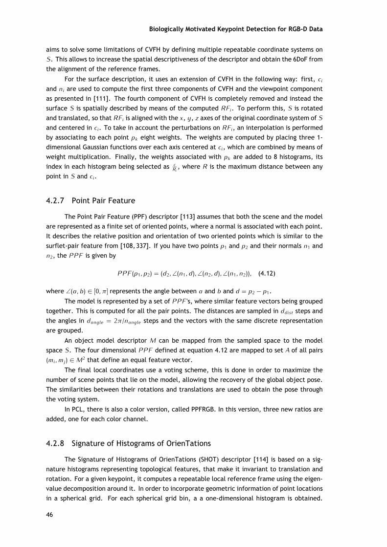
Biologically Motivated Keypoint Detection for RGB-D Data
aims to solve some limitations of CVFH by defining multiple repeatable coordinate systems onS. This allows to increase the spatial descriptiveness of the descriptor and obtain the 6DoF fromthe alignment of the reference frames.
For the surface description, it uses an extension of CVFH in the following way: first, ci
and ni are used to compute the first three components of CVFH and the viewpoint componentas presented in [111]. The fourth component of CVFH is completely removed and instead thesurface S is spatially described by means of the computed RFi. To perform this, S is rotatedand translated, so that RFi is aligned with the x, y, z axes of the original coordinate system of Sand centered in ci. To take in account the perturbations on RFi, an interpolation is performedby associating to each point pk eight weights. The weights are computed by placing three 1-dimensional Gaussian functions over each axis centered at ci, which are combined by means ofweight multiplication. Finally, the weights associated with pk are added to 8 histograms, itsindex in each histogram being selected as c
Ri, where R is the maximum distance between any
point in S and ci.
4.2.7 Point Pair Feature
The Point Pair Feature (PPF) descriptor [113] assumes that both the scene and the modelare represented as a finite set of oriented points, where a normal is associated with each point.It describes the relative position and orientation of two oriented points which is similar to thesurflet-pair feature from [108,337]. If you have two points p1 and p2 and their normals n1 andn2, the PPF is given by
PPF (p1, p2) = (d2,∠(n1, d),∠(n2, d),∠(n1, n2)), (4.12)
where ∠(a, b) ∈ [0, π] represents the angle between a and b and d = p2 − p1.
The model is represented by a set of PPF 's, where similar feature vectors being groupedtogether. This is computed for all the pair points. The distances are sampled in ddist steps andthe angles in dangle = 2π/nangle steps and the vectors with the same discrete representationare grouped.
An object model descriptor M can be mapped from the sampled space to the modelspace S. The four dimensional PPF defined at equation 4.12 are mapped to set A of all pairs(mi, mj ) ∈ M2 that define an equal feature vector.
The final local coordinates use a voting scheme, this is done in order to maximize thenumber of scene points that lie on the model, allowing the recovery of the global object pose.The similarities between their rotations and translations are used to obtain the pose throughthe voting system.
In PCL, there is also a color version, called PPFRGB. In this version, three new ratios areadded, one for each color channel.
4.2.8 Signature of Histograms of OrienTations
The Signature of Histograms of OrienTations (SHOT) descriptor [114] is based on a sig-nature histograms representing topological features, that make it invariant to translation androtation. For a given keypoint, it computes a repeatable local reference frame using the eigen-value decomposition around it. In order to incorporate geometric information of point locationsin a spherical grid. For each spherical grid bin, a a one-dimensional histogram is obtained.
46
This histogram is constructed by summing point counts of the angle between the normal of thekeypoint and the normal of each point belonging to the spherical grid. Finally, the descriptoroverride all these histograms according to the local reference frame. It uses 9 values to encodethe reference frame, and 11 shape bins and 32 divisions of the spherical grid, which gives anadditional 352 values.
In [115], they propose two variants: one is a color version (SHOTCOLOR), where use theCIELab color space as color information; the second one (SHOTLRF), they encode only the localreference frame information, discarding the shape bins and spherical information (resulting ina 9 values to describe the local reference frame).
4.2.9 Unique Shape Context
An upgrade of the 3DSC descriptor [105] is proposed in [116], called Unique Shape Con-text (USC). The authors reported that one of the problems found in 3DSC is to avoid multipledescriptions for the same keypoint, based on the need to obtain as many versions of the de-scriptor as the number of azimuth bins. It can cause a possible ambiguity during the successivematching and classification process. To resolve that, they proposed to define only a local ref-erence frame (as defined in [114]) for each keypoint, such that spherical grid associated to adescriptor be directed exclusively by the two main directions in relation to the normal plane.The remaining process for obtaining USC descriptor still the same as the 3DSC.
4.2.10 Ensemble of Shape Functions
In [117], they introduced the Ensemble of Shape Functions (ESF) which is a shape functiondescribing feature properties. This is done using the three shape functions presented in [118],that are the angle, the point distance, and the area. To compute this, they use three pointsrandomly selected, where: two of them are used to calculate the distance; the angle is definedby two lines created from all of them; and area of the triangle formed between them. Anapproximation (voxel grid) of the real surface is used to separate the shape functions into moredescriptive histograms. These histograms will represent the point distances, angles, areas and(on, off or both) surface
4.2.11 Point Curvature Estimation
The Principal Curvatures Estimation (PCE) descriptor calculates the directions and mag-nitudes of principal surface curvatures (obtained using the cloud normals.) on each keypoint,eigenvectors and eigenvalues respectively. For each keypoint, it will produce a descriptor with5 values. Three values are the principal curvature, which is the eigenvector with the largesteigenvalue and the other two values are the largest and smallest eigenvalues.
4.2.12 Descriptors Characteristics
Table 4.1 presents some features of the descriptors and is based on the one presentedin [22]. The second column contains the number of points generated by each descriptor givenan input point cloud with n points In this work the input cloud will be only the keypoints points.The third column shows the length of each point. The fourth column indicates if the descrip-tor requires the calculation of the surface normals at each point. The column 5 shows if themethod is a global or a local descriptor. Global descriptors require the notion of the complete
47
Biologically Motivated Keypoint Detection for RGB-D Data
Table 4.1: Features and statistics of the evaluated descriptors in this work. n = number of points in inputcloud; p = Number of Azimuth bins; m = Number of stable regions; Y = Yes; N = No.
Descriptor N. Points Point Size Normals Local/Global Category
3DSC n × p 1980 + 9 Y Local Spherical + Shape
CVFH m ⩽ n 308 Y Global Geometry + Shape
ESF 1 640 N Global Shape
FPFH n 33 Y Local Geometry
OUR-CVFH 1 308 Y Global Geometry + Shape
PCE n 5 Y Local Shape
PFH n 125 Y Local Geometry
PFHRGB n 250 Y Global Geometry
PPF n 5 Y Global Geometry
PPFRGB n 8 Y Global Geometry
SHOT n 352 + 9 Y Local Geometric + Spherical
SHOTCOLOR n 1344 + 9 Y Local Geometric + Spherical
SHOTLRF n 9 N Local Geometric + Spherical
USC n 1980 + 9 N Local Spherical + Shape
VFH 1 308 Y Global Geometry
object while local descriptors are computed locally around each keypoint and work without thatassumption. The sixth column indicates if the descriptor is based on the geometry or shape ofthe object, and if the analysis of a point is done using a sphere.
4.3 Dataset
The large RGB-D Object Dataset1 [21] will be used to evaluate the 2D and 3D keypointdetectors and 3D descriptors. This dataset is a hierarchical multi-view object dataset collected
1The dataset is publicly available at http://www.cs.washington.edu/rgbd-dataset.
Figure 4.1: Examples of some objects of the RGB-D Object Dataset.
48
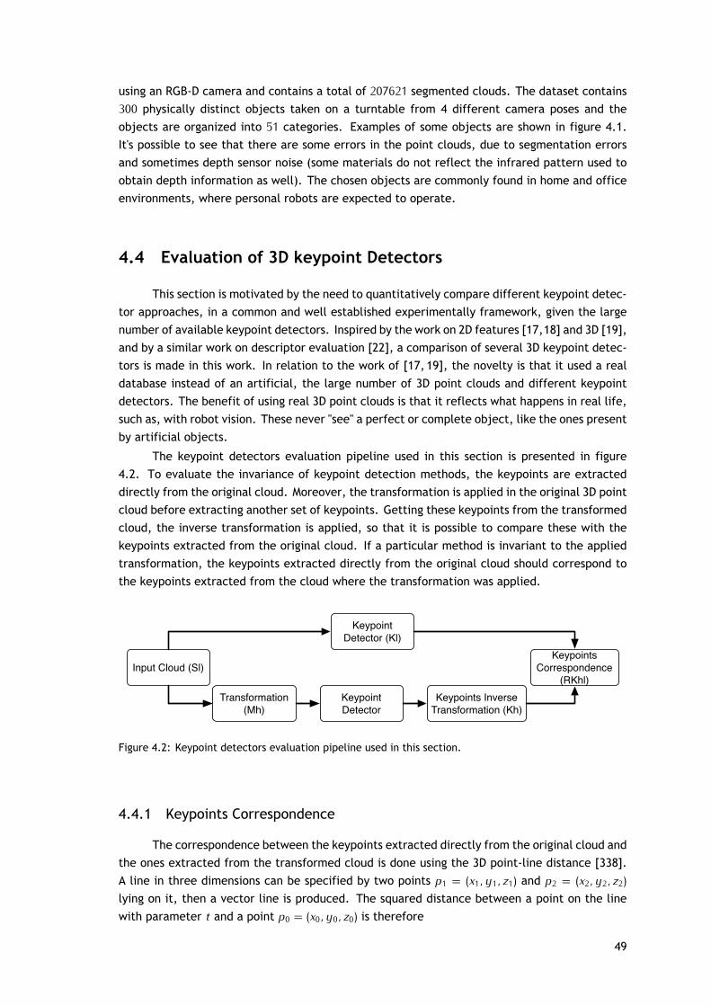
using an RGB-D camera and contains a total of 207621 segmented clouds. The dataset contains300 physically distinct objects taken on a turntable from 4 different camera poses and theobjects are organized into 51 categories. Examples of some objects are shown in figure 4.1.It's possible to see that there are some errors in the point clouds, due to segmentation errorsand sometimes depth sensor noise (some materials do not reflect the infrared pattern used toobtain depth information as well). The chosen objects are commonly found in home and officeenvironments, where personal robots are expected to operate.
4.4 Evaluation of 3D keypoint Detectors
This section is motivated by the need to quantitatively compare different keypoint detec-tor approaches, in a common and well established experimentally framework, given the largenumber of available keypoint detectors. Inspired by the work on 2D features [17,18] and 3D [19],and by a similar work on descriptor evaluation [22], a comparison of several 3D keypoint detec-tors is made in this work. In relation to the work of [17, 19], the novelty is that it used a realdatabase instead of an artificial, the large number of 3D point clouds and different keypointdetectors. The benefit of using real 3D point clouds is that it reflects what happens in real life,such as, with robot vision. These never "see" a perfect or complete object, like the ones presentby artificial objects.
The keypoint detectors evaluation pipeline used in this section is presented in figure4.2. To evaluate the invariance of keypoint detection methods, the keypoints are extracteddirectly from the original cloud. Moreover, the transformation is applied in the original 3D pointcloud before extracting another set of keypoints. Getting these keypoints from the transformedcloud, the inverse transformation is applied, so that it is possible to compare these with thekeypoints extracted from the original cloud. If a particular method is invariant to the appliedtransformation, the keypoints extracted directly from the original cloud should correspond tothe keypoints extracted from the cloud where the transformation was applied.
Input Cloud (Sl)
Transformation (Mh)
Keypoint Detector
Keypoints Inverse Transformation (Kh)
Keypoints Correspondence
(RKhl)
Keypoint Detector (Kl)
Figure 4.2: Keypoint detectors evaluation pipeline used in this section.
4.4.1 Keypoints Correspondence
The correspondence between the keypoints extracted directly from the original cloud andthe ones extracted from the transformed cloud is done using the 3D point-line distance [338].A line in three dimensions can be specified by two points p1 = (x1, y1, z1) and p2 = (x2, y2, z2)lying on it, then a vector line is produced. The squared distance between a point on the linewith parameter t and a point p0 = (x0, y0, z0) is therefore
49
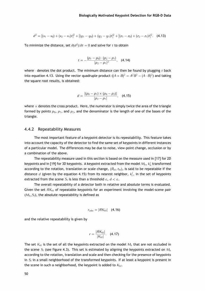
Biologically Motivated Keypoint Detection for RGB-D Data
d2 = [(x1 − x0) + (x2 − x1)t]2 + [(y1 − y0) + (y2 − y1)t]2 + [(z1 − z0) + (z2 − z1)t]2. (4.13)
To minimize the distance, set ∂(d2)/∂t = 0 and solve for t to obtain
t = − (p1 − p0) · (p2 − p1)|p2 − p1|2 , (4.14)
where · denotes the dot product. The minimum distance can then be found by plugging t backinto equation 4.13. Using the vector quadruple product ((A × B)2 = A2B2 − (A · B)2) and takingthe square root results, is obtained:
d = |(p0 − p1) × (p0 − p2)||p2 − p1| , (4.15)
where × denotes the cross product. Here, the numerator is simply twice the area of the triangleformed by points p0, p1, and p2, and the denominator is the length of one of the bases of thetriangle.
4.4.2 Repeatability Measures
The most important feature of a keypoint detector is its repeatability. This feature takesinto account the capacity of the detector to find the same set of keypoints in different instancesof a particular model. The differences may be due to noise, view-point change, occlusion or bya combination of the above.
The repeatability measure used in this section is based on the measure used in [17] for 2Dkeypoints and in [19] for 3D keypoints. A keypoint extracted from the model Mh, k i
h transformedaccording to the rotation, translation or scale change, (Rhl, thl), is said to be repeatable if thedistance d (given by the equation 4.15) from its nearest neighbor, k j
l , in the set of keypointsextracted from the scene Sl is less than a threshold ε, d < ε.
The overall repeatability of a detector both in relative and absolute terms is evaluated.Given the set RKhl of repeatable keypoints for an experiment involving the model-scene pair(Mh,Sl), the absolute repeatability is defined as
rabs = |RKhl| (4.16)
and the relative repeatability is given by
r = |RKhl||Khl|
. (4.17)
The set Khl is the set of all the keypoints extracted on the model Mh that are not occluded inthe scene Sl (see figure 4.3). This set is estimated by aligning the keypoints extracted on Mh
according to the rotation, translation and scale and then checking for the presence of keypointsin Sl in a small neighborhood of the transformed keypoints. If at least a keypoint is present inthe scene in such a neighborhood, the keypoint is added to Khl.
50
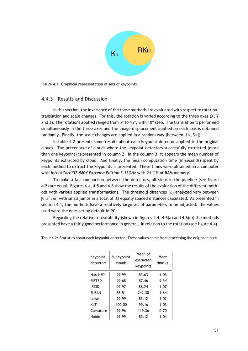
Kh RKhl
Figure 4.3: Graphical representation of sets of keypoints.
4.4.3 Results and Discussion
In this section, the invariance of the these methods are evaluated with respect to rotation,translation and scale changes. For this, the rotation is varied according to the three axes (X, Yand Z). The rotations applied ranged from 5o to 45o, with 10o step. The translation is performedsimultaneously in the three axes and the image displacement applied on each axis is obtainedrandomly. Finally, the scale changes are applied in a random way (between ]1×, 5×]).
In table 4.2 presents some results about each keypoint detector applied to the originalclouds. The percentage of clouds where the keypoint detectors successfully extracted (morethan one keypoint) is presented in column 2. In the column 3, it appears the mean number ofkeypoints extracted by cloud. And finally, the mean computation time (in seconds) spent byeach method to extract the keypoints is presented. These times were obtained on a computerwith Intel®Core™i7-980X Extreme Edition 3.33GHz with 24 GB of RAM memory.
To make a fair comparison between the detectors, all steps in the pipeline (see figure4.2) are equal. Figures 4.4, 4.5 and 4.6 show the results of the evaluation of the different meth-ods with various applied transformations. The threshold distances (ε) analyzed vary between[0, 2] cm, with small jumps in a total of 33 equally spaced distances calculated. As presented insection 4.1, the methods have a relatively large set of parameters to be adjusted: the valuesused were the ones set by default in PCL.
Regarding the relative repeatability (shown in figures 4.4, 4.6(a) and 4.6(c)) the methodspresented have a fairly good performance in general. In relation to the rotation (see figure 4.4),
Table 4.2: Statistics about each keypoint detector. These values come from processing the original clouds.
Keypoint % KeypointMean of
Mean
detectors cloudsextracted
time (s)keypoints
Harris3D 99.99 85.63 1.05
SIFT3D 99.68 87.46 9.54
ISS3D 97.97 86.24 1.07
SUSAN 86.51 242.38 1.64
Lowe 99.99 85.12 1.02
KLT 100.00 99.16 1.03
Curvature 99.96 119.36 0.70
Noble 99.99 85.12 1.04
51
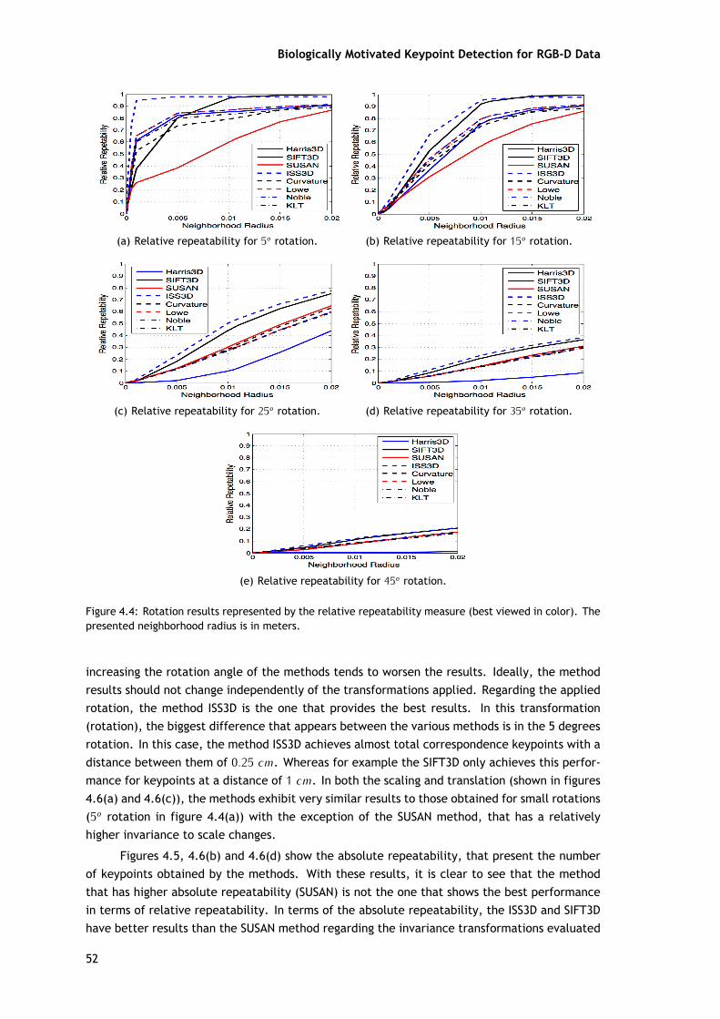
Biologically Motivated Keypoint Detection for RGB-D Data
(a) Relative repeatability for 5o rotation. (b) Relative repeatability for 15o rotation.
(c) Relative repeatability for 25o rotation. (d) Relative repeatability for 35o rotation.
(e) Relative repeatability for 45o rotation.
Figure 4.4: Rotation results represented by the relative repeatability measure (best viewed in color). Thepresented neighborhood radius is in meters.
increasing the rotation angle of the methods tends to worsen the results. Ideally, the methodresults should not change independently of the transformations applied. Regarding the appliedrotation, the method ISS3D is the one that provides the best results. In this transformation(rotation), the biggest difference that appears between the various methods is in the 5 degreesrotation. In this case, the method ISS3D achieves almost total correspondence keypoints with adistance between them of 0.25 cm. Whereas for example the SIFT3D only achieves this perfor-mance for keypoints at a distance of 1 cm. In both the scaling and translation (shown in figures4.6(a) and 4.6(c)), the methods exhibit very similar results to those obtained for small rotations(5o rotation in figure 4.4(a)) with the exception of the SUSAN method, that has a relativelyhigher invariance to scale changes.
Figures 4.5, 4.6(b) and 4.6(d) show the absolute repeatability, that present the numberof keypoints obtained by the methods. With these results, it is clear to see that the methodthat has higher absolute repeatability (SUSAN) is not the one that shows the best performancein terms of relative repeatability. In terms of the absolute repeatability, the ISS3D and SIFT3Dhave better results than the SUSAN method regarding the invariance transformations evaluated
52
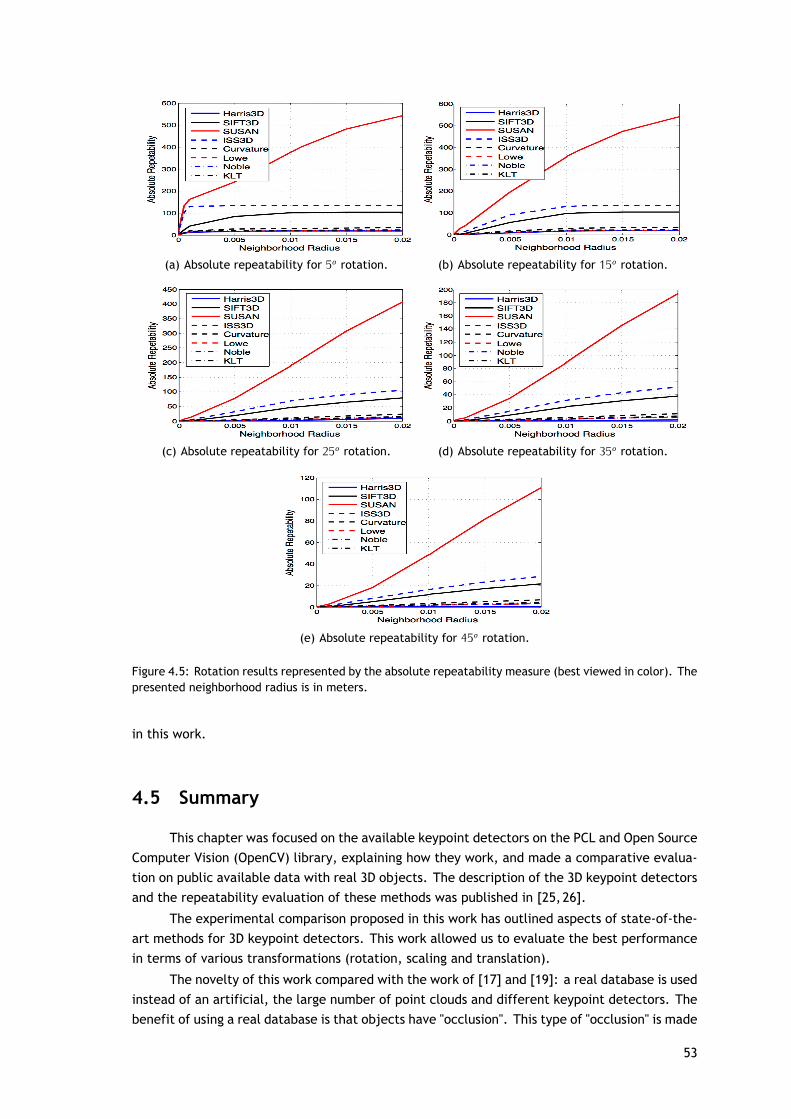
(a) Absolute repeatability for 5o rotation. (b) Absolute repeatability for 15o rotation.
(c) Absolute repeatability for 25o rotation. (d) Absolute repeatability for 35o rotation.
(e) Absolute repeatability for 45o rotation.
Figure 4.5: Rotation results represented by the absolute repeatability measure (best viewed in color). Thepresented neighborhood radius is in meters.
in this work.
4.5 Summary
This chapter was focused on the available keypoint detectors on the PCL and Open SourceComputer Vision (OpenCV) library, explaining how they work, and made a comparative evalua-tion on public available data with real 3D objects. The description of the 3D keypoint detectorsand the repeatability evaluation of these methods was published in [25,26].
The experimental comparison proposed in this work has outlined aspects of state-of-the-art methods for 3D keypoint detectors. This work allowed us to evaluate the best performancein terms of various transformations (rotation, scaling and translation).
The novelty of this work compared with the work of [17] and [19]: a real database is usedinstead of an artificial, the large number of point clouds and different keypoint detectors. Thebenefit of using a real database is that objects have "occlusion". This type of "occlusion'' is made
53
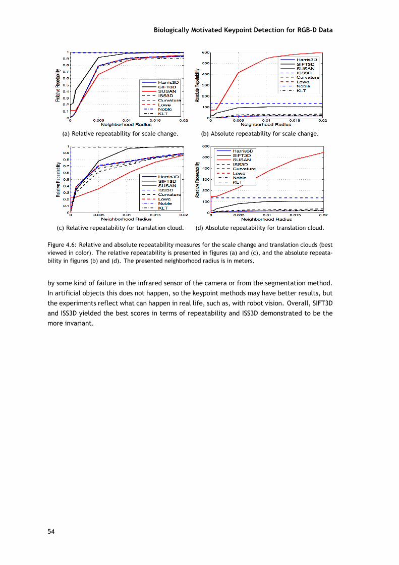
Biologically Motivated Keypoint Detection for RGB-D Data
(a) Relative repeatability for scale change. (b) Absolute repeatability for scale change.
(c) Relative repeatability for translation cloud. (d) Absolute repeatability for translation cloud.
Figure 4.6: Relative and absolute repeatability measures for the scale change and translation clouds (bestviewed in color). The relative repeatability is presented in figures (a) and (c), and the absolute repeata-bility in figures (b) and (d). The presented neighborhood radius is in meters.
by some kind of failure in the infrared sensor of the camera or from the segmentation method.In artificial objects this does not happen, so the keypoint methods may have better results, butthe experiments reflect what can happen in real life, such as, with robot vision. Overall, SIFT3Dand ISS3D yielded the best scores in terms of repeatability and ISS3D demonstrated to be themore invariant.
54
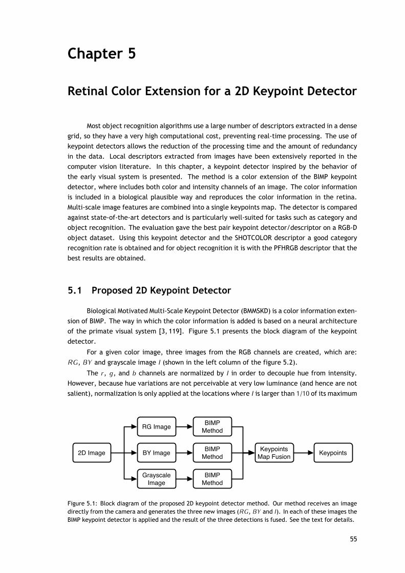
Chapter 5
Retinal Color Extension for a 2D Keypoint Detector
Most object recognition algorithms use a large number of descriptors extracted in a densegrid, so they have a very high computational cost, preventing real-time processing. The use ofkeypoint detectors allows the reduction of the processing time and the amount of redundancyin the data. Local descriptors extracted from images have been extensively reported in thecomputer vision literature. In this chapter, a keypoint detector inspired by the behavior ofthe early visual system is presented. The method is a color extension of the BIMP keypointdetector, where includes both color and intensity channels of an image. The color informationis included in a biological plausible way and reproduces the color information in the retina.Multi-scale image features are combined into a single keypoints map. The detector is comparedagainst state-of-the-art detectors and is particularly well-suited for tasks such as category andobject recognition. The evaluation gave the best pair keypoint detector/descriptor on a RGB-Dobject dataset. Using this keypoint detector and the SHOTCOLOR descriptor a good categoryrecognition rate is obtained and for object recognition it is with the PFHRGB descriptor that thebest results are obtained.
5.1 Proposed 2D Keypoint Detector
Biological Motivated Multi-Scale Keypoint Detector (BMMSKD) is a color information exten-sion of BIMP. The way in which the color information is added is based on a neural architectureof the primate visual system [3, 119]. Figure 5.1 presents the block diagram of the keypointdetector.
For a given color image, three images from the RGB channels are created, which are:RG, BY and grayscale image I (shown in the left column of the figure 5.2).
The r, g, and b channels are normalized by I in order to decouple hue from intensity.However, because hue variations are not perceivable at very low luminance (and hence are notsalient), normalization is only applied at the locations where I is larger than 1/10 of its maximum
2D Image
RG Image
BY Image
Grayscale Image
BIMP Method
BIMP Method
BIMP Method
Keypoints Map Fusion Keypoints
Figure 5.1: Block diagram of the proposed 2D keypoint detector method. Our method receives an imagedirectly from the camera and generates the three new images (RG, BY and I). In each of these images theBIMP keypoint detector is applied and the result of the three detections is fused. See the text for details.
55
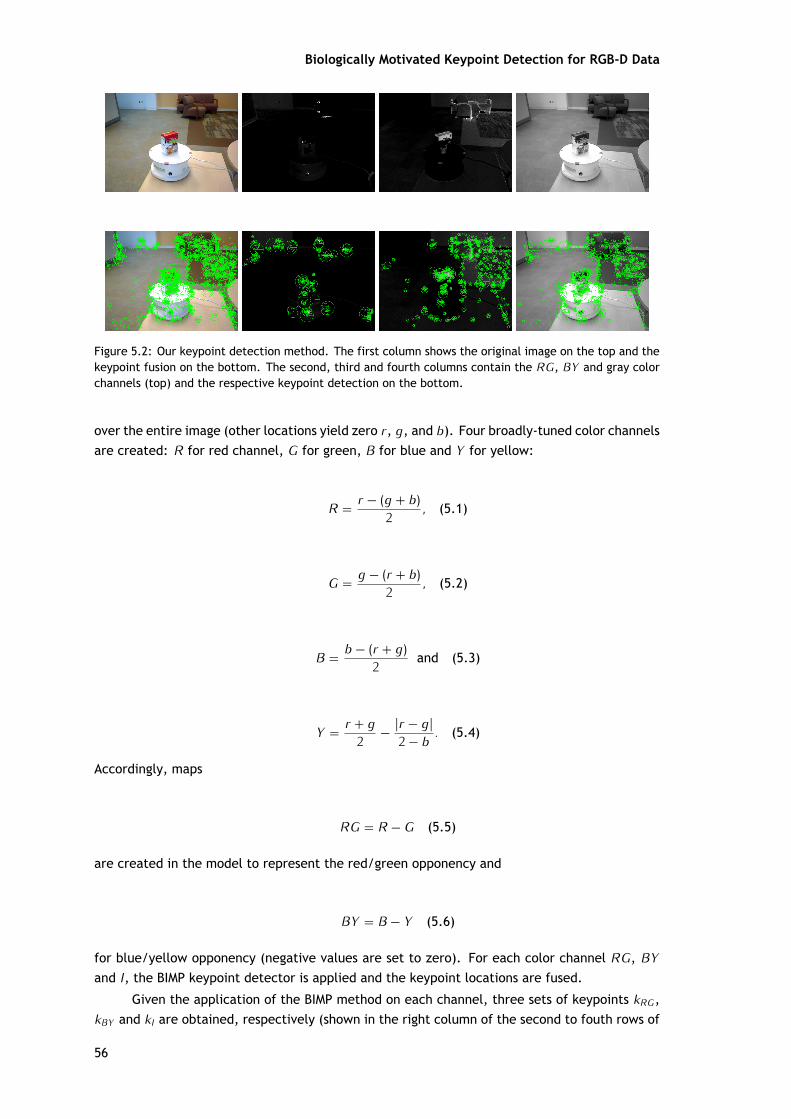
Biologically Motivated Keypoint Detection for RGB-D Data
Figure 5.2: Our keypoint detection method. The first column shows the original image on the top and thekeypoint fusion on the bottom. The second, third and fourth columns contain the RG, BY and gray colorchannels (top) and the respective keypoint detection on the bottom.
over the entire image (other locations yield zero r, g, and b). Four broadly-tuned color channelsare created: R for red channel, G for green, B for blue and Y for yellow:
R = r − (g + b)2 , (5.1)
G = g − (r + b)2 , (5.2)
B = b − (r + g)2 and (5.3)
Y = r + g2 − |r − g|
2 − b . (5.4)
Accordingly, maps
RG = R − G (5.5)
are created in the model to represent the red/green opponency and
BY = B − Y (5.6)
for blue/yellow opponency (negative values are set to zero). For each color channel RG, BYand I, the BIMP keypoint detector is applied and the keypoint locations are fused.
Given the application of the BIMP method on each channel, three sets of keypoints kRG,kBY and kI are obtained, respectively (shown in the right column of the second to fouth rows of
56
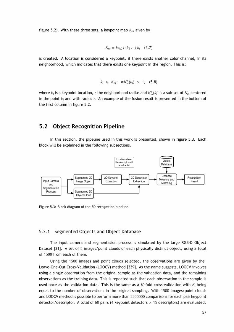
figure 5.2). With these three sets, a keypoint map Km given by
Km = kRG ∪ kBY ∪ kI (5.7)
is created. A location is considered a keypoint, if there exists another color channel, in itsneighborhood, which indicates that there exists one keypoint in the region. This is:
kl ∈ Km : #K rm(kl) > 1, (5.8)
where kl is a keypoint location, r the neighborhood radius and K rm(kl) is a sub-set of Km centered
in the point kl and with radius r. An example of the fusion result is presented in the bottom ofthe first column in figure 5.2.
5.2 Object Recognition Pipeline
In this section, the pipeline used in this work is presented, shown in figure 5.3. Eachblock will be explained in the following subsections.
Segmented 2D Image Object
2D Keypoint Extraction
3D Descriptor Extraction
Distance Measure and
Matching
Recognition Result
Object Database
Location where the descriptor will
be extracted
Segmented 3D Object Cloud
Input Camera and
Segmentation Process
Figure 5.3: Block diagram of the 3D recognition pipeline.
5.2.1 Segmented Objects and Object Database
The input camera and segmentation process is simulated by the large RGB-D ObjectDataset [21]. A set of 5 images/point clouds of each physically distinct object, using a totalof 1500 from each of them.
Using the 1500 images and point clouds selected, the observations are given by theLeave-One-Out Cross-Validation (LOOCV) method [339]. As the name suggests, LOOCV involvesusing a single observation from the original sample as the validation data, and the remainingobservations as the training data. This is repeated such that each observation in the sample isused once as the validation data. This is the same as a K -fold cross-validation with K beingequal to the number of observations in the original sampling. With 1500 images/point cloudsand LOOCV method is possible to perform more than 2200000 comparisons for each pair keypointdetector/descriptor. A total of 60 pairs (4 keypoint detectors × 15 descriptors) are evaluated.
57
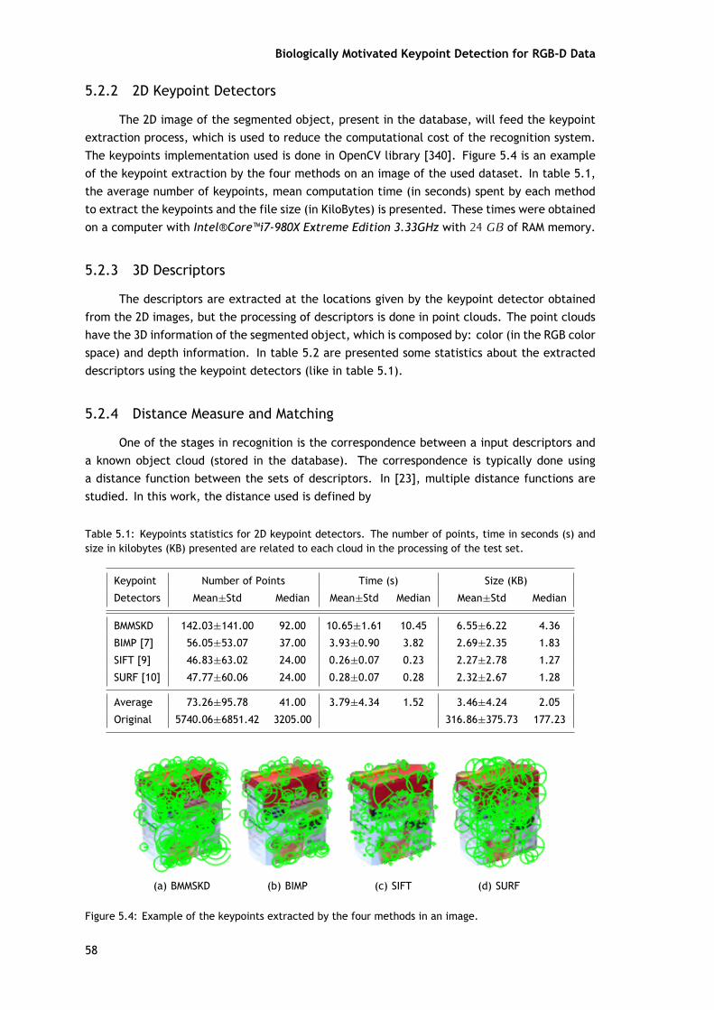
Biologically Motivated Keypoint Detection for RGB-D Data
5.2.2 2D Keypoint Detectors
The 2D image of the segmented object, present in the database, will feed the keypointextraction process, which is used to reduce the computational cost of the recognition system.The keypoints implementation used is done in OpenCV library [340]. Figure 5.4 is an exampleof the keypoint extraction by the four methods on an image of the used dataset. In table 5.1,the average number of keypoints, mean computation time (in seconds) spent by each methodto extract the keypoints and the file size (in KiloBytes) is presented. These times were obtainedon a computer with Intel®Core™i7-980X Extreme Edition 3.33GHz with 24 GB of RAM memory.
5.2.3 3D Descriptors
The descriptors are extracted at the locations given by the keypoint detector obtainedfrom the 2D images, but the processing of descriptors is done in point clouds. The point cloudshave the 3D information of the segmented object, which is composed by: color (in the RGB colorspace) and depth information. In table 5.2 are presented some statistics about the extracteddescriptors using the keypoint detectors (like in table 5.1).
5.2.4 Distance Measure and Matching
One of the stages in recognition is the correspondence between a input descriptors anda known object cloud (stored in the database). The correspondence is typically done usinga distance function between the sets of descriptors. In [23], multiple distance functions arestudied. In this work, the distance used is defined by
Table 5.1: Keypoints statistics for 2D keypoint detectors. The number of points, time in seconds (s) andsize in kilobytes (KB) presented are related to each cloud in the processing of the test set.
Keypoint Number of Points Time (s) Size (KB)
Detectors Mean±Std Median Mean±Std Median Mean±Std Median
BMMSKD 142.03±141.00 92.00 10.65±1.61 10.45 6.55±6.22 4.36
BIMP [7] 56.05±53.07 37.00 3.93±0.90 3.82 2.69±2.35 1.83
SIFT [9] 46.83±63.02 24.00 0.26±0.07 0.23 2.27±2.78 1.27
SURF [10] 47.77±60.06 24.00 0.28±0.07 0.28 2.32±2.67 1.28
Average 73.26±95.78 41.00 3.79±4.34 1.52 3.46±4.24 2.05
Original 5740.06±6851.42 3205.00 316.86±375.73 177.23
(a) BMMSKD (b) BIMP (c) SIFT (d) SURF
Figure 5.4: Example of the keypoints extracted by the four methods in an image.
58
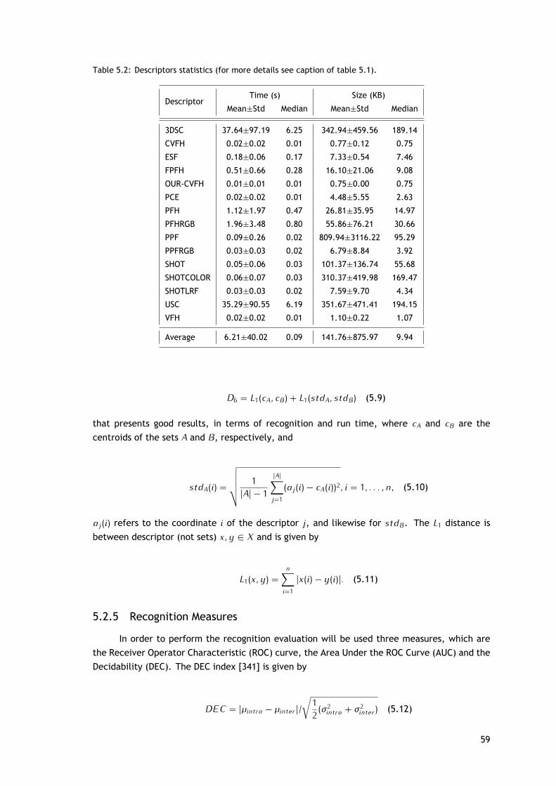
Table 5.2: Descriptors statistics (for more details see caption of table 5.1).
DescriptorTime (s) Size (KB)
Mean±Std Median Mean±Std Median
3DSC 37.64±97.19 6.25 342.94±459.56 189.14
CVFH 0.02±0.02 0.01 0.77±0.12 0.75
ESF 0.18±0.06 0.17 7.33±0.54 7.46
FPFH 0.51±0.66 0.28 16.10±21.06 9.08
OUR-CVFH 0.01±0.01 0.01 0.75±0.00 0.75
PCE 0.02±0.02 0.01 4.48±5.55 2.63
PFH 1.12±1.97 0.47 26.81±35.95 14.97
PFHRGB 1.96±3.48 0.80 55.86±76.21 30.66
PPF 0.09±0.26 0.02 809.94±3116.22 95.29
PPFRGB 0.03±0.03 0.02 6.79±8.84 3.92
SHOT 0.05±0.06 0.03 101.37±136.74 55.68
SHOTCOLOR 0.06±0.07 0.03 310.37±419.98 169.47
SHOTLRF 0.03±0.03 0.02 7.59±9.70 4.34
USC 35.29±90.55 6.19 351.67±471.41 194.15
VFH 0.02±0.02 0.01 1.10±0.22 1.07
Average 6.21±40.02 0.09 141.76±875.97 9.94
D6 = L1(cA, cB) + L1(stdA, stdB) (5.9)
that presents good results, in terms of recognition and run time, where cA and cB are thecentroids of the sets A and B, respectively, and
stdA(i) =
√√√√√ 1|A| − 1
|A|∑
j=1(aj (i) − cA(i))2, i = 1, . . . , n, (5.10)
aj (i) refers to the coordinate i of the descriptor j, and likewise for stdB. The L1 distance isbetween descriptor (not sets) x, y ∈ X and is given by
L1(x, y) =n∑
i=1|x(i) − y(i)|. (5.11)
5.2.5 Recognition Measures
In order to perform the recognition evaluation will be used three measures, which arethe Receiver Operator Characteristic (ROC) curve, the Area Under the ROC Curve (AUC) and theDecidability (DEC). The DEC index [341] is given by
DEC = |µintra − µinter |/√
12(σ 2
intra + σ 2inter) (5.12)
59
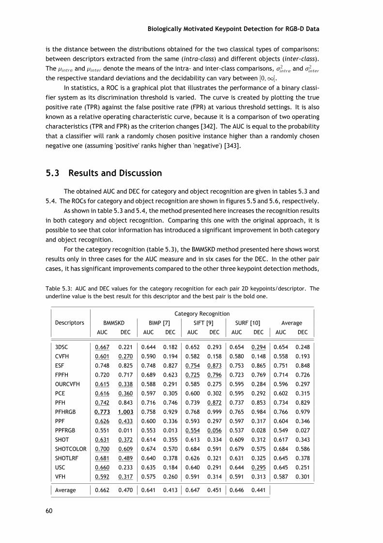
Biologically Motivated Keypoint Detection for RGB-D Data
is the distance between the distributions obtained for the two classical types of comparisons:between descriptors extracted from the same (intra-class) and different objects (inter-class).The µintra and µinter denote the means of the intra- and inter-class comparisons, σ 2
intra and σ 2inter
the respective standard deviations and the decidability can vary between [0, ∞[.In statistics, a ROC is a graphical plot that illustrates the performance of a binary classi-
fier system as its discrimination threshold is varied. The curve is created by plotting the truepositive rate (TPR) against the false positive rate (FPR) at various threshold settings. It is alsoknown as a relative operating characteristic curve, because it is a comparison of two operatingcharacteristics (TPR and FPR) as the criterion changes [342]. The AUC is equal to the probabilitythat a classifier will rank a randomly chosen positive instance higher than a randomly chosennegative one (assuming 'positive' ranks higher than 'negative') [343].
5.3 Results and Discussion
The obtained AUC and DEC for category and object recognition are given in tables 5.3 and5.4. The ROCs for category and object recognition are shown in figures 5.5 and 5.6, respectively.
As shown in table 5.3 and 5.4, the method presented here increases the recognition resultsin both category and object recognition. Comparing this one with the original approach, it ispossible to see that color information has introduced a significant improvement in both categoryand object recognition.
For the category recognition (table 5.3), the BMMSKD method presented here shows worstresults only in three cases for the AUC measure and in six cases for the DEC. In the other paircases, it has significant improvements compared to the other three keypoint detection methods,
Table 5.3: AUC and DEC values for the category recognition for each pair 2D keypoints/descriptor. Theunderline value is the best result for this descriptor and the best pair is the bold one.
Descriptors
Category Recognition
BMMSKD BIMP [7] SIFT [9] SURF [10] Average
AUC DEC AUC DEC AUC DEC AUC DEC AUC DEC
3DSC 0.667 0.221 0.644 0.182 0.652 0.293 0.654 0.294 0.654 0.248
CVFH 0.601 0.270 0.590 0.194 0.582 0.158 0.580 0.148 0.558 0.193
ESF 0.748 0.825 0.748 0.827 0.754 0.873 0.753 0.865 0.751 0.848
FPFH 0.720 0.717 0.689 0.623 0.725 0.796 0.723 0.769 0.714 0.726
OURCVFH 0.615 0.338 0.588 0.291 0.585 0.275 0.595 0.284 0.596 0.297
PCE 0.616 0.360 0.597 0.305 0.600 0.302 0.595 0.292 0.602 0.315
PFH 0.742 0.843 0.716 0.746 0.739 0.872 0.737 0.853 0.734 0.829
PFHRGB 0.773 1.003 0.758 0.929 0.768 0.999 0.765 0.984 0.766 0.979
PPF 0.626 0.433 0.600 0.336 0.593 0.297 0.597 0.317 0.604 0.346
PPFRGB 0.551 0.011 0.553 0.013 0.554 0.056 0.537 0.028 0.549 0.027
SHOT 0.631 0.372 0.614 0.355 0.613 0.334 0.609 0.312 0.617 0.343
SHOTCOLOR 0.700 0.609 0.674 0.570 0.684 0.591 0.679 0.575 0.684 0.586
SHOTLRF 0.681 0.489 0.640 0.378 0.626 0.321 0.631 0.325 0.645 0.378
USC 0.660 0.233 0.635 0.184 0.640 0.291 0.644 0.295 0.645 0.251
VFH 0.592 0.317 0.575 0.260 0.591 0.314 0.591 0.313 0.587 0.301
Average 0.662 0.470 0.641 0.413 0.647 0.451 0.646 0.441
60
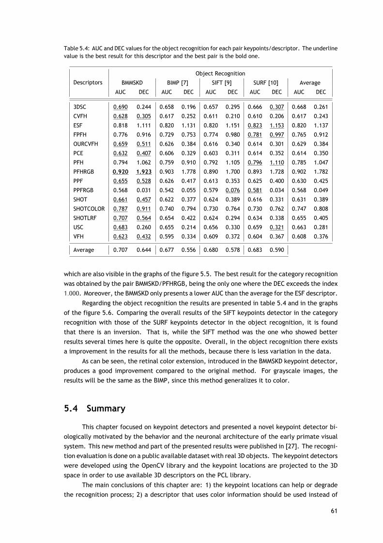
Table 5.4: AUC and DEC values for the object recognition for each pair keypoints/descriptor. The underlinevalue is the best result for this descriptor and the best pair is the bold one.
Descriptors
Object Recognition
BMMSKD BIMP [7] SIFT [9] SURF [10] Average
AUC DEC AUC DEC AUC DEC AUC DEC AUC DEC
3DSC 0.690 0.244 0.658 0.196 0.657 0.295 0.666 0.307 0.668 0.261
CVFH 0.628 0.305 0.617 0.252 0.611 0.210 0.610 0.206 0.617 0.243
ESF 0.818 1.111 0.820 1.131 0.820 1.151 0.823 1.153 0.820 1.137
FPFH 0.776 0.916 0.729 0.753 0.774 0.980 0.781 0.997 0.765 0.912
OURCVFH 0.659 0.511 0.626 0.384 0.616 0.340 0.614 0.301 0.629 0.384
PCE 0.632 0.407 0.606 0.329 0.603 0.311 0.614 0.352 0.614 0.350
PFH 0.794 1.062 0.759 0.910 0.792 1.105 0.796 1.110 0.785 1.047
PFHRGB 0.920 1.923 0.903 1.778 0.890 1.700 0.893 1.728 0.902 1.782
PPF 0.655 0.528 0.626 0.417 0.613 0.353 0.625 0.400 0.630 0.425
PPFRGB 0.568 0.031 0.542 0.055 0.579 0.076 0.581 0.034 0.568 0.049
SHOT 0.661 0.457 0.622 0.377 0.624 0.389 0.616 0.331 0.631 0.389
SHOTCOLOR 0.787 0.911 0.740 0.794 0.730 0.764 0.730 0.762 0.747 0.808
SHOTLRF 0.707 0.564 0.654 0.422 0.624 0.294 0.634 0.338 0.655 0.405
USC 0.683 0.260 0.655 0.214 0.656 0.330 0.659 0.321 0.663 0.281
VFH 0.623 0.432 0.595 0.334 0.609 0.372 0.604 0.367 0.608 0.376
Average 0.707 0.644 0.677 0.556 0.680 0.578 0.683 0.590
which are also visible in the graphs of the figure 5.5. The best result for the category recognitionwas obtained by the pair BMMSKD/PFHRGB, being the only one where the DEC exceeds the index1.000. Moreover, the BMMSKD only presents a lower AUC than the average for the ESF descriptor.
Regarding the object recognition the results are presented in table 5.4 and in the graphsof the figure 5.6. Comparing the overall results of the SIFT keypoints detector in the categoryrecognition with those of the SURF keypoints detector in the object recognition, it is foundthat there is an inversion. That is, while the SIFT method was the one who showed betterresults several times here is quite the opposite. Overall, in the object recognition there existsa improvement in the results for all the methods, because there is less variation in the data.
As can be seen, the retinal color extension, introduced in the BMMSKD keypoint detector,produces a good improvement compared to the original method. For grayscale images, theresults will be the same as the BIMP, since this method generalizes it to color.
5.4 Summary
This chapter focused on keypoint detectors and presented a novel keypoint detector bi-ologically motivated by the behavior and the neuronal architecture of the early primate visualsystem. This new method and part of the presented results were published in [27]. The recogni-tion evaluation is done on a public available dataset with real 3D objects. The keypoint detectorswere developed using the OpenCV library and the keypoint locations are projected to the 3Dspace in order to use available 3D descriptors on the PCL library.
The main conclusions of this chapter are: 1) the keypoint locations can help or degradethe recognition process; 2) a descriptor that uses color information should be used instead of
61
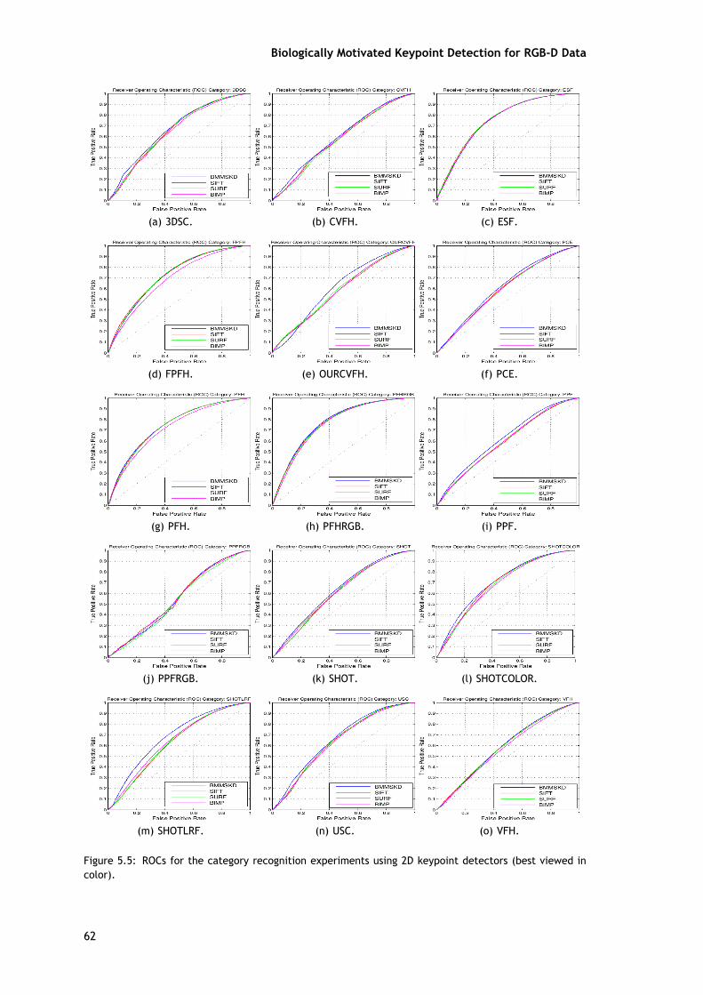
Biologically Motivated Keypoint Detection for RGB-D Data
(a) 3DSC. (b) CVFH. (c) ESF.
(d) FPFH. (e) OURCVFH. (f) PCE.
(g) PFH. (h) PFHRGB. (i) PPF.
(j) PPFRGB. (k) SHOT. (l) SHOTCOLOR.
(m) SHOTLRF. (n) USC. (o) VFH.
Figure 5.5: ROCs for the category recognition experiments using 2D keypoint detectors (best viewed incolor).
62
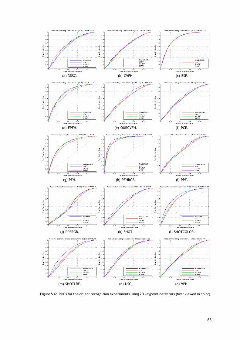
(a) 3DSC. (b) CVFH. (c) ESF.
(d) FPFH. (e) OURCVFH. (f) PCE.
(g) PFH. (h) PFHRGB. (i) PPF.
(j) PPFRGB. (k) SHOT. (l) SHOTCOLOR.
(m) SHOTLRF. (n) USC. (o) VFH.
Figure 5.6: ROCs for the object recognition experiments using 2D keypoint detectors (best viewed in color).
63

Biologically Motivated Keypoint Detection for RGB-D Data
a similar one that uses only shape information; 3) since there are big differences in terms ofrecognition performance, size and time requirements, the descriptor should be matched tothe desired task; 4) to recognize the category of an object or a real-time system, it is recom-mended the use the SHOTCOLOR method because it presents a recognition rate of 7% belowof the PFHRGB but with a much lower computational cost; and 5) to do the object recogni-tion, the recommendation is PFHRGB because it presents a recognition rate 12.9% higher thanSHOTCOLOR.
64
Chapter 6
Biologically Inspired 3D Keypoint Detector basedon Bottom-Up Saliency
A new method for the detection of 3D keypoints on point clouds is presented. A bench-marking between each pair of 3D keypoint detector and 3D descriptor is performed, in order toevaluate their performance on object and category recognition. These evaluations are done in apublic database of real 3D objects. The keypoint detector is inspired by the behavior and neuralarchitecture of the primate visual system. The 3D keypoints are extracted based on a bottom-up3D saliency map, that is, a map that encodes the saliency of objects in the visual environment.The saliency map is determined by computing conspicuity maps (a combination across differentmodalities) of the orientation, intensity and color information in a bottom-up and in a purelystimulus-driven manner. These three conspicuity maps are fused into a 3D saliency map and,finally, the focus of attention (or "keypoint location") is sequentially directed to the most salientpoints in this map. Inhibiting this location automatically allows the system to attend to the nextmost salient location.
6.1 Proposed 3D Keypoint Detector
The Biologically Inspired 3D Keypoint based on Bottom-Up Saliency (BIK-BUS) is a keypointdetector that is based on saliency maps. The saliency maps are determined by computing con-spicuity maps of the features intensity, color and orientation in a bottom-up and data-drivenmanner. These conspicuity maps are fused into a saliency map and, finally, the focus of atten-tion is sequentially directed to the most salient points in this map [120]. Using this theory andfollowing the steps presented in [3,119], a new keypoint detector is presented (shown in figure6.1).
6.1.1 Linear Filtering
The initial part of this step is similar to the retinal color extension presented in section5.1. Here, the four broadly-tuned color channels (R, G, B and Y ) and the intensity I channelare also used.
Gaussian pyramids [121] are used in the spatial scales, which progressively low-pass anddown-sample the input cloud, producing horizontal and vertical cloud-reduction factors. FiveGaussian pyramids R(σ ), G(σ ), B(σ ), Y (σ ) and I(σ ) are created from the color and intensitychannels, where σ represents the standard deviation used in the Gaussian kernel.
Each Gaussian pyramid is achieved by convolving the cloud with Gaussian kernels of in-creasing radius, resulting in a pyramid of clouds. We apply a similar concept to search thedensity map D over a range of scales, where D can be {R, G, B, Y , I}. We convolve D with aset of 3D Gaussian kernels to construct a pyramid of density maps, with each layer representingthe scale σ . A factor of 2 is used to down-sample the density map and the reduction of the
65

Biologically Motivated Keypoint Detection for RGB-D Data
Input Cloud
Color Information
RG(c, s)
R(�)G(�)
B(�)
BY(c, s)
Y(�)
Intensity
I(c, s)
I(�)
Orientations obtained from 3D objects normals
O(c, s, 0º)
O(c, s, 90º)
O(c, s, 45º)
O(�, 0º)O(�, 90º)
O(�, 45º)
O(c, s, 135º)
O(�, 135º)
Center-Surround Differences and Normalization
Saliency Map
6 Scales
8 Scales
Keypoints
Inhibition-of-Return
Across-Scale Combinations and Normalization
Conspicuity Maps
I OC
Linear Filtering
Linear Combination
Figure 6.1: General architecture of our Biologically Inspired Keypoint Detector based on Bottom-UpSaliency. Our method receives as input a point cloud similar to those shown in figures 4.1 and 6.3 anda linear filter is applied to obtain the color, intensity and orientations information. The full process isdescribed in the text.
standard deviation of the Gaussian kernel by√
2. The pyramid creation is a step similar to theDoG presented in the section 4.1.5.
Let L(·) (one of the five Gaussian pyramids) be a scale space for D:
L(x, y, z, σ ) = D ∗ g(x, y, z, σ ), (6.1)
where ∗ is the convolution operator and g(x, y, z, σ ) is a 3D Gaussian with standard deviation σgiven by:
g(x, y, z, σ ) = exp(
−x2 − y2 − z2
2σ 2
). (6.2)
The orientation pyramids O(σ, θ) are obtained using the normals extracted from the in-tensity cloud I, where θ ∈ {0o, 45o, 90o, 135o} is the preferred orientation [121]. In the primaryvisual cortex, the impulse response of orientation-selective neurons is approximated by Gaborfilters [122]. The orientation pyramids are created in a similar way to the color channels, butapplying 3D Gabor filters with different orientations θ.
6.1.2 Center-Surround Differences
In the retina, bipolar and ganglion cells encode the spatial information, using center-surround structures. The center-surround structures in the retina can be described as on-centerand off-center. The on-center use a positive weighed center and negatively weighed neighbors.
66

The off-center use exactly the opposite. The positive weighing is better known as excitatoryand the negative as inhibitory [123].
Similarly to the visual receptive fields, a set of linear center-surround operations is usedto compute each feature. Visual neurons are most sensitive in a small region of the visual space(the center), while stimuli in the surround inhibit neuronal response [3]. Center-surround iscomputed as the difference between the center pixel at scale c ∈ {2, 3, 4}, and the surround isthe corresponding pixel at scale
s = c + δ , (6.3)
with δ ∈ {3, 4}. The across-scale difference between twomaps (represented by `⊖') is obtainedby interpolation to the center scale c and point-by-point subtraction.
The first set of feature maps is concerned with intensity contrast. In mammals, thisis detected by neurons sensitive either to dark centers on bright surrounds (off-center) or tobright centers on dark surrounds (on-center) [3, 122]. Here, both types of sensitivities aresimultaneously computed in a set of six maps I(c, s):
I(c, s) = |I(c)⊖ I(s)|. (6.4)
For the color channels, the process is similar, which, in the cortex, is called `color double-opponent' system [3]. In the center of their receptive fields, neurons are excited by one colorand inhibited by an other, while the converse is true in the surround. The existence of a spatialand chromatic opponency between color pairs in human primary visual cortex is described in[124]. Given the chromatic opponency, the maps RG(c, s) and BY (c, s) are created to takein account the red/green and green/red, and blue/yellow and yellow/blue double opponency,respectively, as:
RG(c, s) = |(R(c) − G(c))⊖(G(s) − R(s))|, (6.5)
BY (c, s) = |(B(c) − Y (c))⊖(Y (s) − B(s))|. (6.6)
Orientation feature maps, O(c, s, θ), encode, as a group, local orientation contrast be-tween the center and surround scales:
O(c, s, θ) = |O(c, θ)⊖O(s, θ)|. (6.7)
6.1.3 Normalization
We cannot combine directly the different feature maps because they represent differentdynamic ranges and extraction mechanisms. Some salient objects appear only in a few maps,which can be masked by noise or by less salient objects present in a larger number of maps. Inorder to resolve that, a map normalization operator N (.) is used. This promotes the maps that
67

Biologically Motivated Keypoint Detection for RGB-D Data
contain a small number of strong activity, and suppresses the peaks in the maps that have manyof them [3]. N (.) consists of:
1. Large amplitude differences are eliminated by normalizing the map values to a fixed range[0..M ], where M is the global maximum of the map;
2. Multiply the map by (M − m)2, where m is the average of all its other local maxima.
The lateral cortical inhibition is the biological motivation for this normalization [344].
6.1.4 Across-Scale Combination
The conspicuity maps are the combination of the feature maps, for intensity, color andorientation. They are obtained through the reduction of each map to scale four and point-by-point addition `
⊕', called across-scale addition. The conspicuity maps for the intensity, I, and
color channels, C , are given by:
I =4⊕
c=2
c+4⊕
s=c+3N (I(c, s)) and (6.8)
C =4⊕
c=2
c+4⊕
s=c+3[N (RG(c, s)) + N (BY (c, s))] . (6.9)
For orientation, we first created four intermediary maps, which are a combination of thesix feature maps for a given θ. Finally, they are combined into a single orientation conspicuitymap:
O =∑
θ∈{0o,45o,90o,135o}
N[ 4⊕
c=2
c+4⊕
s=c+3N (O(c, s, θ))
]. (6.10)
The three separate channels (I, C and O) have an independent contribution in the saliencymap and where similar features will have a strong impact on the saliency.
6.1.5 Linear Combination
The final saliency map is obtained by the normalization and a linear combination betweenthem:
S = 13(N (I) + N (C ) + N (O)
). (6.11)
6.1.6 Inhibition-Of-Return
The IOR is part of the method that is responsible for the selection of keypoints. It detectsthe most salient location and directs attention towards it, considering that location a keypoint.After that, the IOR mechanism transiently suppresses this location in the saliency map and itsneighborhoods in a small radius, such that attention is autonomously directed to the next most
68
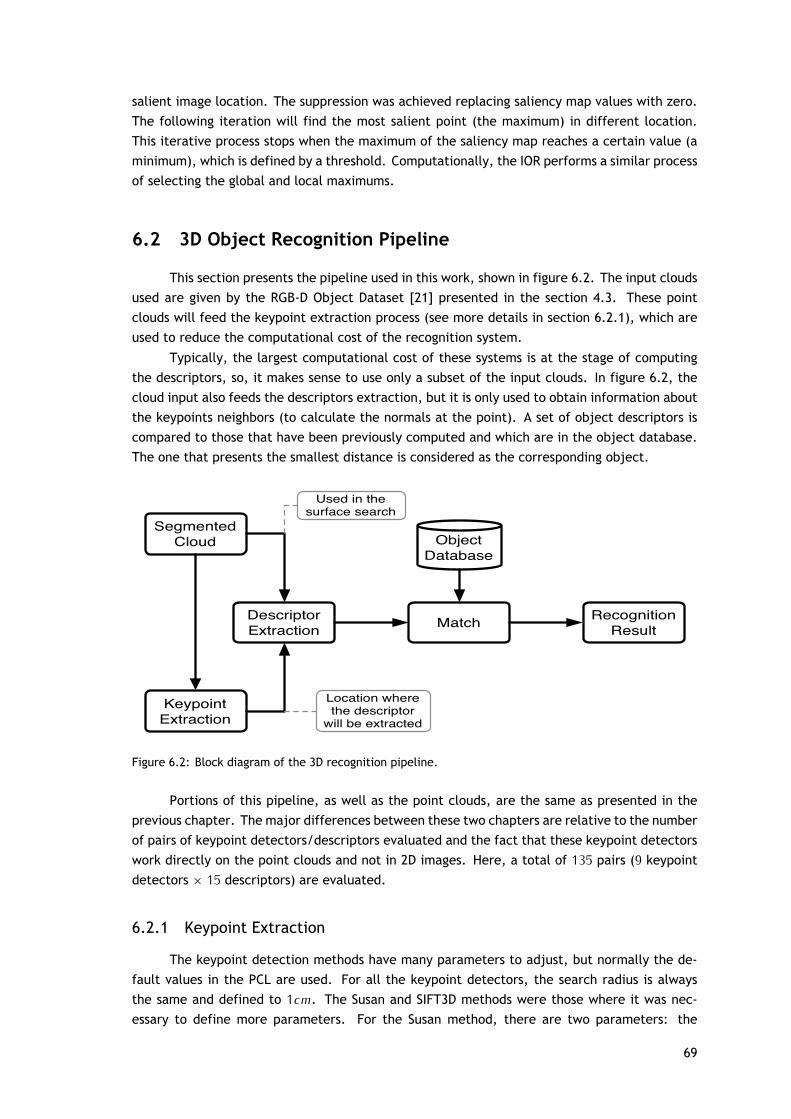
salient image location. The suppression was achieved replacing saliency map values with zero.The following iteration will find the most salient point (the maximum) in different location.This iterative process stops when the maximum of the saliency map reaches a certain value (aminimum), which is defined by a threshold. Computationally, the IOR performs a similar processof selecting the global and local maximums.
6.2 3D Object Recognition Pipeline
This section presents the pipeline used in this work, shown in figure 6.2. The input cloudsused are given by the RGB-D Object Dataset [21] presented in the section 4.3. These pointclouds will feed the keypoint extraction process (see more details in section 6.2.1), which areused to reduce the computational cost of the recognition system.
Typically, the largest computational cost of these systems is at the stage of computingthe descriptors, so, it makes sense to use only a subset of the input clouds. In figure 6.2, thecloud input also feeds the descriptors extraction, but it is only used to obtain information aboutthe keypoints neighbors (to calculate the normals at the point). A set of object descriptors iscompared to those that have been previously computed and which are in the object database.The one that presents the smallest distance is considered as the corresponding object.
Segmented Cloud
Keypoint Extraction
Descriptor Extraction Match Recognition
Result
Object Database
Location where the descriptor
will be extracted
Used in the surface search
Figure 6.2: Block diagram of the 3D recognition pipeline.
Portions of this pipeline, as well as the point clouds, are the same as presented in theprevious chapter. The major differences between these two chapters are relative to the numberof pairs of keypoint detectors/descriptors evaluated and the fact that these keypoint detectorswork directly on the point clouds and not in 2D images. Here, a total of 135 pairs (9 keypointdetectors × 15 descriptors) are evaluated.
6.2.1 Keypoint Extraction
The keypoint detection methods have many parameters to adjust, but normally the de-fault values in the PCL are used. For all the keypoint detectors, the search radius is alwaysthe same and defined to 1cm. The Susan and SIFT3D methods were those where it was nec-essary to define more parameters. For the Susan method, there are two parameters: the
69
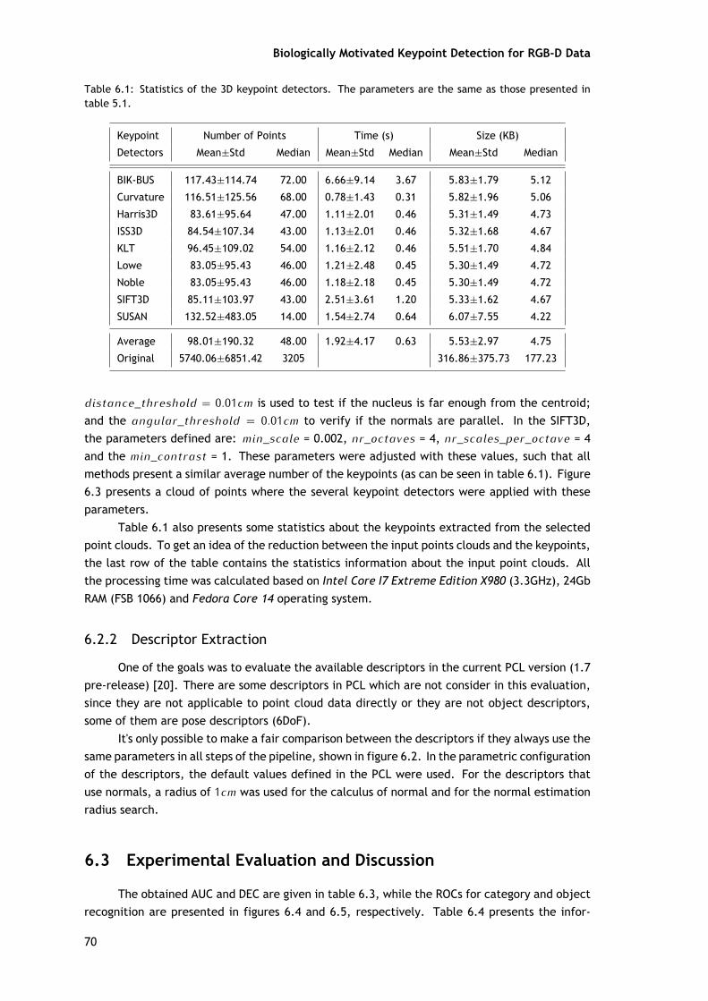
Biologically Motivated Keypoint Detection for RGB-D Data
Table 6.1: Statistics of the 3D keypoint detectors. The parameters are the same as those presented intable 5.1.
Keypoint Number of Points Time (s) Size (KB)
Detectors Mean±Std Median Mean±Std Median Mean±Std Median
BIK-BUS 117.43±114.74 72.00 6.66±9.14 3.67 5.83±1.79 5.12
Curvature 116.51±125.56 68.00 0.78±1.43 0.31 5.82±1.96 5.06
Harris3D 83.61±95.64 47.00 1.11±2.01 0.46 5.31±1.49 4.73
ISS3D 84.54±107.34 43.00 1.13±2.01 0.46 5.32±1.68 4.67
KLT 96.45±109.02 54.00 1.16±2.12 0.46 5.51±1.70 4.84
Lowe 83.05±95.43 46.00 1.21±2.48 0.45 5.30±1.49 4.72
Noble 83.05±95.43 46.00 1.18±2.18 0.45 5.30±1.49 4.72
SIFT3D 85.11±103.97 43.00 2.51±3.61 1.20 5.33±1.62 4.67
SUSAN 132.52±483.05 14.00 1.54±2.74 0.64 6.07±7.55 4.22
Average 98.01±190.32 48.00 1.92±4.17 0.63 5.53±2.97 4.75
Original 5740.06±6851.42 3205 316.86±375.73 177.23
distance_threshold = 0.01cm is used to test if the nucleus is far enough from the centroid;and the angular_threshold = 0.01cm to verify if the normals are parallel. In the SIFT3D,the parameters defined are: min_scale = 0.002, nr_octaves = 4, nr_scales_per_octave = 4and the min_contrast = 1. These parameters were adjusted with these values, such that allmethods present a similar average number of the keypoints (as can be seen in table 6.1). Figure6.3 presents a cloud of points where the several keypoint detectors were applied with theseparameters.
Table 6.1 also presents some statistics about the keypoints extracted from the selectedpoint clouds. To get an idea of the reduction between the input points clouds and the keypoints,the last row of the table contains the statistics information about the input point clouds. Allthe processing time was calculated based on Intel Core I7 Extreme Edition X980 (3.3GHz), 24GbRAM (FSB 1066) and Fedora Core 14 operating system.
6.2.2 Descriptor Extraction
One of the goals was to evaluate the available descriptors in the current PCL version (1.7pre-release) [20]. There are some descriptors in PCL which are not consider in this evaluation,since they are not applicable to point cloud data directly or they are not object descriptors,some of them are pose descriptors (6DoF).
It's only possible to make a fair comparison between the descriptors if they always use thesame parameters in all steps of the pipeline, shown in figure 6.2. In the parametric configurationof the descriptors, the default values defined in the PCL were used. For the descriptors thatuse normals, a radius of 1cm was used for the calculus of normal and for the normal estimationradius search.
6.3 Experimental Evaluation and Discussion
The obtained AUC and DEC are given in table 6.3, while the ROCs for category and objectrecognition are presented in figures 6.4 and 6.5, respectively. Table 6.4 presents the infor-
70
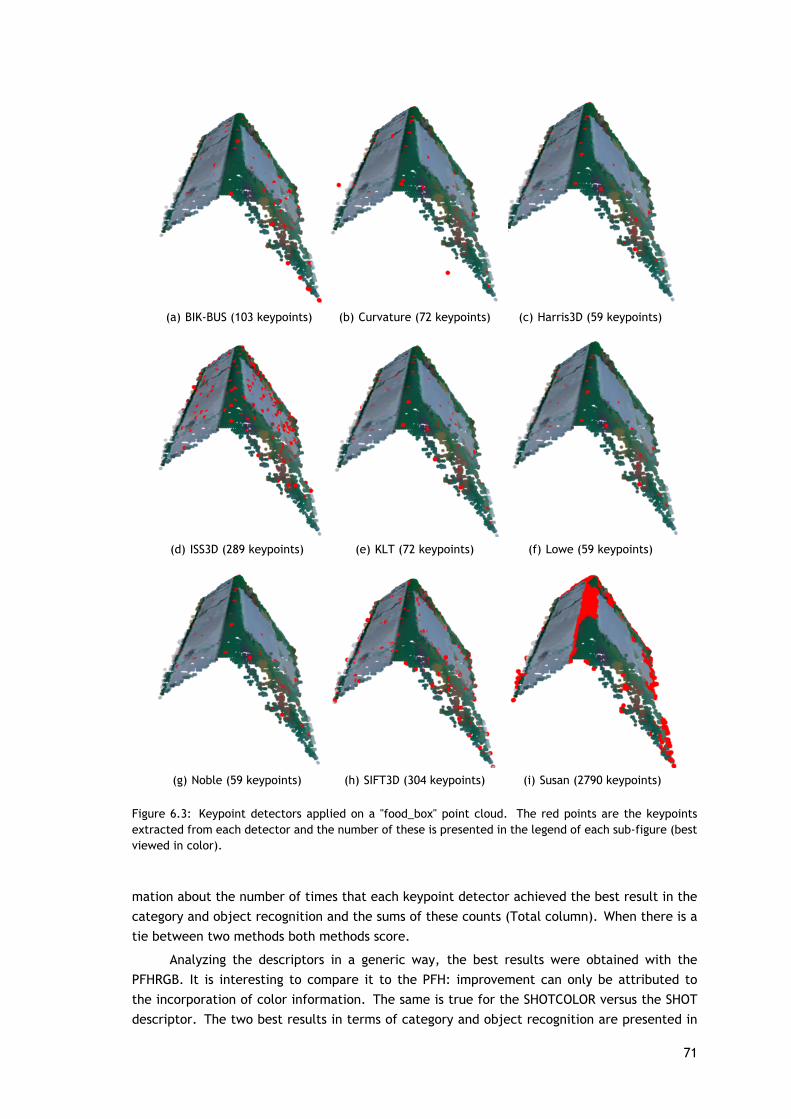
(a) BIK-BUS (103 keypoints) (b) Curvature (72 keypoints) (c) Harris3D (59 keypoints)
(d) ISS3D (289 keypoints) (e) KLT (72 keypoints) (f) Lowe (59 keypoints)
(g) Noble (59 keypoints) (h) SIFT3D (304 keypoints) (i) Susan (2790 keypoints)
Figure 6.3: Keypoint detectors applied on a "food_box" point cloud. The red points are the keypointsextracted from each detector and the number of these is presented in the legend of each sub-figure (bestviewed in color).
mation about the number of times that each keypoint detector achieved the best result in thecategory and object recognition and the sums of these counts (Total column). When there is atie between two methods both methods score.
Analyzing the descriptors in a generic way, the best results were obtained with thePFHRGB. It is interesting to compare it to the PFH: improvement can only be attributed tothe incorporation of color information. The same is true for the SHOTCOLOR versus the SHOTdescriptor. The two best results in terms of category and object recognition are presented in
71
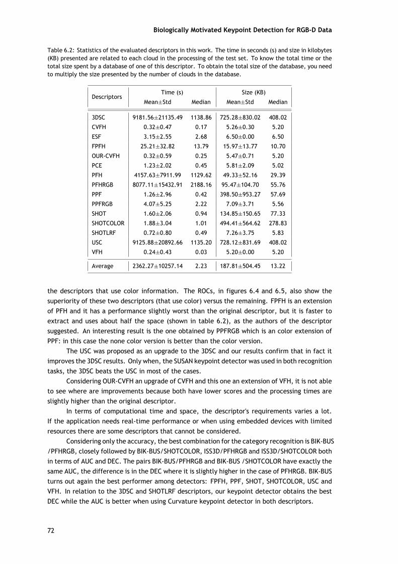
Biologically Motivated Keypoint Detection for RGB-D Data
Table 6.2: Statistics of the evaluated descriptors in this work. The time in seconds (s) and size in kilobytes(KB) presented are related to each cloud in the processing of the test set. To know the total time or thetotal size spent by a database of one of this descriptor. To obtain the total size of the database, you needto multiply the size presented by the number of clouds in the database.
DescriptorsTime (s) Size (KB)
Mean±Std Median Mean±Std Median
3DSC 9181.56±21135.49 1138.86 725.28±830.02 408.02
CVFH 0.32±0.47 0.17 5.26±0.30 5.20
ESF 3.15±2.55 2.68 6.50±0.00 6.50
FPFH 25.21±32.82 13.79 15.97±13.77 10.70
OUR-CVFH 0.32±0.59 0.25 5.47±0.71 5.20
PCE 1.23±2.02 0.45 5.81±2.09 5.02
PFH 4157.63±7911.99 1129.62 49.33±52.16 29.39
PFHRGB 8077.11±15432.91 2188.16 95.47±104.70 55.76
PPF 1.26±2.96 0.42 398.50±953.27 57.69
PPFRGB 4.07±5.25 2.22 7.09±3.71 5.56
SHOT 1.60±2.06 0.94 134.85±150.65 77.33
SHOTCOLOR 1.88±3.04 1.01 494.41±564.62 278.83
SHOTLRF 0.72±0.80 0.49 7.26±3.75 5.83
USC 9125.88±20892.66 1135.20 728.12±831.69 408.02
VFH 0.24±0.43 0.03 5.20±0.00 5.20
Average 2362.27±10257.14 2.23 187.81±504.45 13.22
the descriptors that use color information. The ROCs, in figures 6.4 and 6.5, also show thesuperiority of these two descriptors (that use color) versus the remaining. FPFH is an extensionof PFH and it has a performance slightly worst than the original descriptor, but it is faster toextract and uses about half the space (shown in table 6.2), as the authors of the descriptorsuggested. An interesting result is the one obtained by PPFRGB which is an color extension ofPPF: in this case the none color version is better than the color version.
The USC was proposed as an upgrade to the 3DSC and our results confirm that in fact itimproves the 3DSC results. Only when, the SUSAN keypoint detector was used in both recognitiontasks, the 3DSC beats the USC in most of the cases.
Considering OUR-CVFH an upgrade of CVFH and this one an extension of VFH, it is not ableto see where are improvements because both have lower scores and the processing times areslightly higher than the original descriptor.
In terms of computational time and space, the descriptor's requirements varies a lot.If the application needs real-time performance or when using embedded devices with limitedresources there are some descriptors that cannot be considered.
Considering only the accuracy, the best combination for the category recognition is BIK-BUS/PFHRGB, closely followed by BIK-BUS/SHOTCOLOR, ISS3D/PFHRGB and ISS3D/SHOTCOLOR bothin terms of AUC and DEC. The pairs BIK-BUS/PFHRGB and BIK-BUS /SHOTCOLOR have exactly thesame AUC, the difference is in the DEC where it is slightly higher in the case of PFHRGB. BIK-BUSturns out again the best performer among detectors: FPFH, PPF, SHOT, SHOTCOLOR, USC andVFH. In relation to the 3DSC and SHOTLRF descriptors, our keypoint detector obtains the bestDEC while the AUC is better when using Curvature keypoint detector in both descriptors.
72
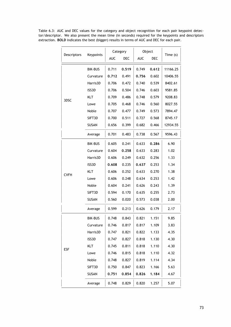
Table 6.3: AUC and DEC values for the category and object recognition for each pair keypoint detec-tor/descriptor. We also present the mean time (in seconds) required for the keypoints and descriptorsextraction. BOLD indicates the best (bigger) results in terms of AUC and DEC for each pair.
Descriptors KeypointsCategory Object
Time (s)AUC DEC AUC DEC
3DSC
BIK-BUS 0.711 0.519 0.749 0.612 11166.25
Curvature 0.712 0.491 0.756 0.602 10406.55
Harris3D 0.706 0.472 0.740 0.539 8402.61
ISS3D 0.706 0.504 0.746 0.603 9581.85
KLT 0.709 0.486 0.748 0.579 9208.83
Lowe 0.705 0.468 0.746 0.560 8027.55
Noble 0.707 0.477 0.749 0.573 7894.47
SIFT3D 0.700 0.511 0.727 0.568 8745.17
SUSAN 0.656 0.399 0.682 0.466 12934.55
Average 0.701 0.483 0.738 0.567 9596.43
CVFH
BIK-BUS 0.605 0.241 0.633 0.286 6.90
Curvature 0.604 0.258 0.633 0.283 1.02
Harris3D 0.606 0.249 0.632 0.256 1.33
ISS3D 0.608 0.235 0.637 0.253 1.34
KLT 0.606 0.252 0.633 0.270 1.38
Lowe 0.606 0.248 0.634 0.253 1.42
Noble 0.604 0.241 0.626 0.243 1.39
SIFT3D 0.594 0.170 0.635 0.255 2.73
SUSAN 0.560 0.020 0.573 0.038 2.00
Average 0.599 0.213 0.626 0.179 2.17
ESF
BIK-BUS 0.748 0.843 0.821 1.151 9.85
Curvature 0.746 0.817 0.817 1.109 3.83
Harris3D 0.747 0.821 0.822 1.133 4.35
ISS3D 0.747 0.827 0.818 1.130 4.30
KLT 0.745 0.811 0.818 1.110 4.30
Lowe 0.746 0.815 0.818 1.110 4.32
Noble 0.748 0.827 0.819 1.114 4.34
SIFT3D 0.750 0.847 0.823 1.166 5.63
SUSAN 0.751 0.854 0.826 1.184 4.67
Average 0.748 0.829 0.820 1.257 5.07
73
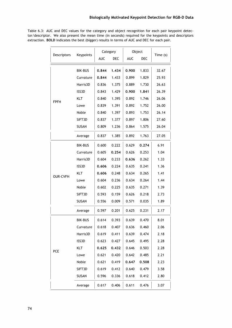
Biologically Motivated Keypoint Detection for RGB-D Data
Table 6.3: AUC and DEC values for the category and object recognition for each pair keypoint detec-tor/descriptor. We also present the mean time (in seconds) required for the keypoints and descriptorsextraction. BOLD indicates the best (bigger) results in terms of AUC and DEC for each pair.
Descriptors KeypointsCategory Object
Time (s)AUC DEC AUC DEC
FPFH
BIK-BUS 0.844 1.434 0.900 1.833 32.67
Curvature 0.844 1.433 0.899 1.829 25.93
Harris3D 0.836 1.375 0.889 1.730 26.63
ISS3D 0.843 1.429 0.900 1.841 26.39
KLT 0.840 1.395 0.892 1.746 26.06
Lowe 0.839 1.391 0.892 1.752 26.00
Noble 0.840 1.397 0.893 1.753 26.14
SIFT3D 0.837 1.377 0.897 1.806 27.60
SUSAN 0.809 1.236 0.864 1.575 26.04
Average 0.837 1.385 0.892 1.763 27.05
OUR-CVFH
BIK-BUS 0.600 0.222 0.629 0.274 6.91
Curvature 0.605 0.254 0.626 0.253 1.04
Harris3D 0.604 0.233 0.636 0.262 1.33
ISS3D 0.606 0.224 0.635 0.241 1.36
KLT 0.606 0.248 0.634 0.265 1.41
Lowe 0.604 0.236 0.634 0.264 1.44
Noble 0.602 0.225 0.635 0.271 1.39
SIFT3D 0.593 0.159 0.626 0.218 2.73
SUSAN 0.556 0.009 0.571 0.035 1.89
Average 0.597 0.201 0.625 0.231 2.17
PCE
BIK-BUS 0.614 0.393 0.639 0.470 8.01
Curvature 0.618 0.407 0.636 0.460 2.06
Harris3D 0.619 0.411 0.639 0.474 2.18
ISS3D 0.623 0.427 0.645 0.495 2.28
KLT 0.625 0.432 0.646 0.503 2.28
Lowe 0.621 0.420 0.642 0.485 2.21
Noble 0.621 0.419 0.647 0.508 2.23
SIFT3D 0.619 0.412 0.640 0.479 3.58
SUSAN 0.596 0.336 0.618 0.412 2.80
Average 0.617 0.406 0.611 0.476 3.07
74
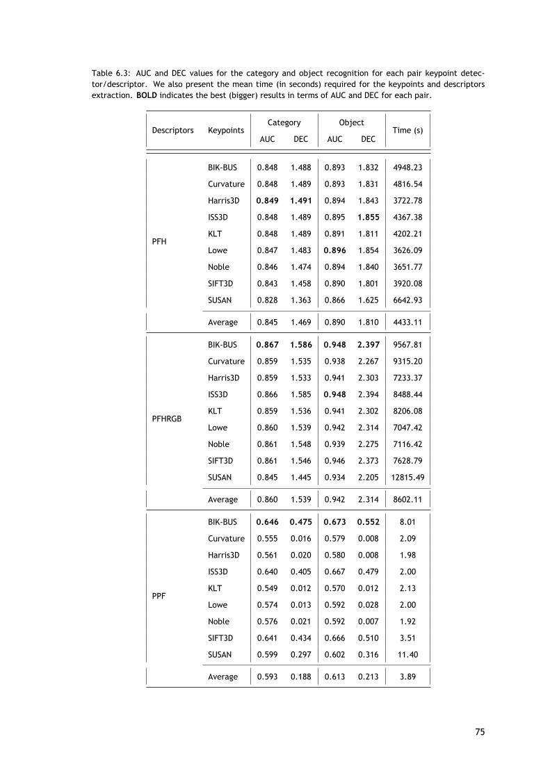
Table 6.3: AUC and DEC values for the category and object recognition for each pair keypoint detec-tor/descriptor. We also present the mean time (in seconds) required for the keypoints and descriptorsextraction. BOLD indicates the best (bigger) results in terms of AUC and DEC for each pair.
Descriptors KeypointsCategory Object
Time (s)AUC DEC AUC DEC
PFH
BIK-BUS 0.848 1.488 0.893 1.832 4948.23
Curvature 0.848 1.489 0.893 1.831 4816.54
Harris3D 0.849 1.491 0.894 1.843 3722.78
ISS3D 0.848 1.489 0.895 1.855 4367.38
KLT 0.848 1.489 0.891 1.811 4202.21
Lowe 0.847 1.483 0.896 1.854 3626.09
Noble 0.846 1.474 0.894 1.840 3651.77
SIFT3D 0.843 1.458 0.890 1.801 3920.08
SUSAN 0.828 1.363 0.866 1.625 6642.93
Average 0.845 1.469 0.890 1.810 4433.11
PFHRGB
BIK-BUS 0.867 1.586 0.948 2.397 9567.81
Curvature 0.859 1.535 0.938 2.267 9315.20
Harris3D 0.859 1.533 0.941 2.303 7233.37
ISS3D 0.866 1.585 0.948 2.394 8488.44
KLT 0.859 1.536 0.941 2.302 8206.08
Lowe 0.860 1.539 0.942 2.314 7047.42
Noble 0.861 1.548 0.939 2.275 7116.42
SIFT3D 0.861 1.546 0.946 2.373 7628.79
SUSAN 0.845 1.445 0.934 2.205 12815.49
Average 0.860 1.539 0.942 2.314 8602.11
PPF
BIK-BUS 0.646 0.475 0.673 0.552 8.01
Curvature 0.555 0.016 0.579 0.008 2.09
Harris3D 0.561 0.020 0.580 0.008 1.98
ISS3D 0.640 0.405 0.667 0.479 2.00
KLT 0.549 0.012 0.570 0.012 2.13
Lowe 0.574 0.013 0.592 0.028 2.00
Noble 0.576 0.021 0.592 0.007 1.92
SIFT3D 0.641 0.434 0.666 0.510 3.51
SUSAN 0.599 0.297 0.602 0.316 11.40
Average 0.593 0.188 0.613 0.213 3.89
75
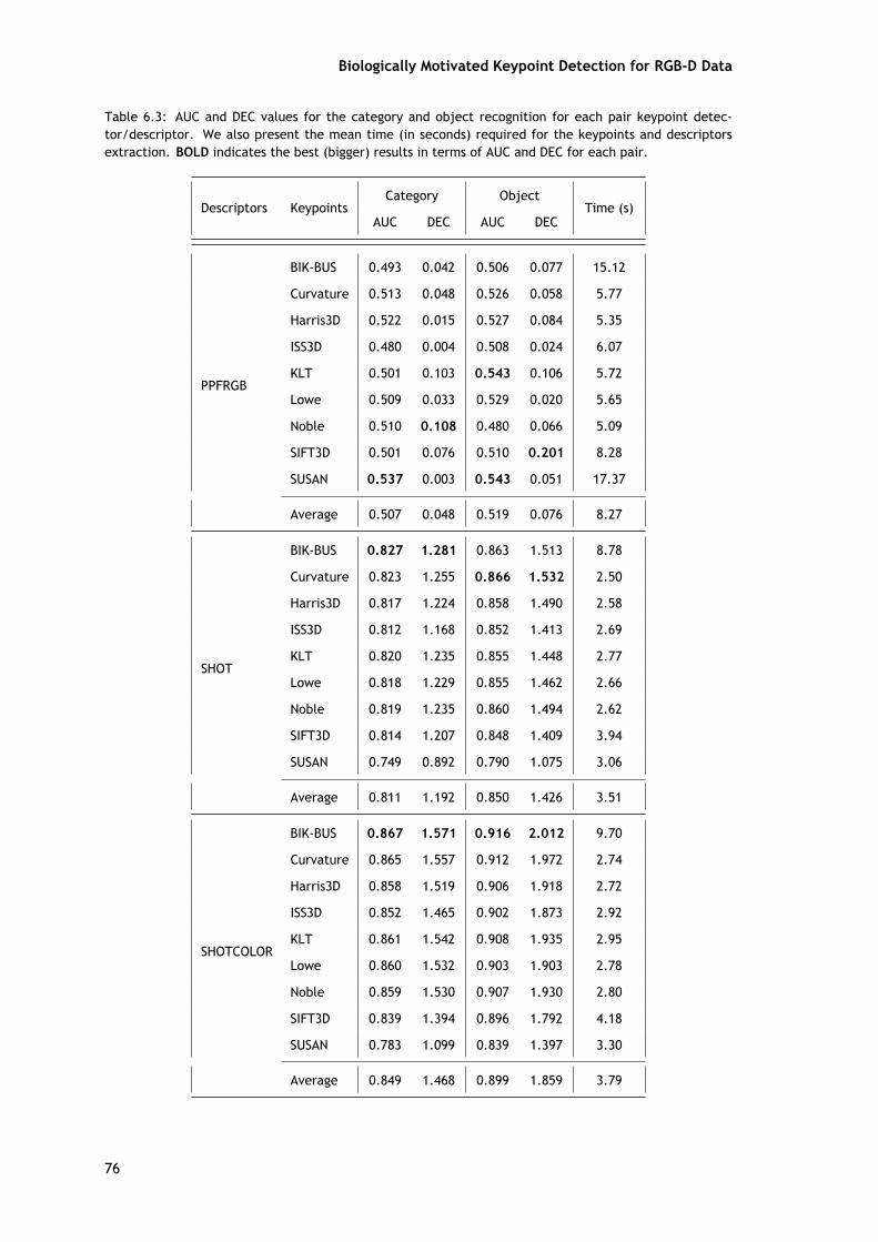
Biologically Motivated Keypoint Detection for RGB-D Data
Table 6.3: AUC and DEC values for the category and object recognition for each pair keypoint detec-tor/descriptor. We also present the mean time (in seconds) required for the keypoints and descriptorsextraction. BOLD indicates the best (bigger) results in terms of AUC and DEC for each pair.
Descriptors KeypointsCategory Object
Time (s)AUC DEC AUC DEC
PPFRGB
BIK-BUS 0.493 0.042 0.506 0.077 15.12
Curvature 0.513 0.048 0.526 0.058 5.77
Harris3D 0.522 0.015 0.527 0.084 5.35
ISS3D 0.480 0.004 0.508 0.024 6.07
KLT 0.501 0.103 0.543 0.106 5.72
Lowe 0.509 0.033 0.529 0.020 5.65
Noble 0.510 0.108 0.480 0.066 5.09
SIFT3D 0.501 0.076 0.510 0.201 8.28
SUSAN 0.537 0.003 0.543 0.051 17.37
Average 0.507 0.048 0.519 0.076 8.27
SHOT
BIK-BUS 0.827 1.281 0.863 1.513 8.78
Curvature 0.823 1.255 0.866 1.532 2.50
Harris3D 0.817 1.224 0.858 1.490 2.58
ISS3D 0.812 1.168 0.852 1.413 2.69
KLT 0.820 1.235 0.855 1.448 2.77
Lowe 0.818 1.229 0.855 1.462 2.66
Noble 0.819 1.235 0.860 1.494 2.62
SIFT3D 0.814 1.207 0.848 1.409 3.94
SUSAN 0.749 0.892 0.790 1.075 3.06
Average 0.811 1.192 0.850 1.426 3.51
SHOTCOLOR
BIK-BUS 0.867 1.571 0.916 2.012 9.70
Curvature 0.865 1.557 0.912 1.972 2.74
Harris3D 0.858 1.519 0.906 1.918 2.72
ISS3D 0.852 1.465 0.902 1.873 2.92
KLT 0.861 1.542 0.908 1.935 2.95
Lowe 0.860 1.532 0.903 1.903 2.78
Noble 0.859 1.530 0.907 1.930 2.80
SIFT3D 0.839 1.394 0.896 1.792 4.18
SUSAN 0.783 1.099 0.839 1.397 3.30
Average 0.849 1.468 0.899 1.859 3.79
76
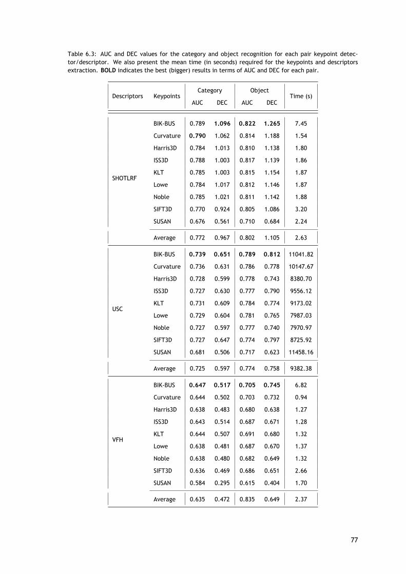
Table 6.3: AUC and DEC values for the category and object recognition for each pair keypoint detec-tor/descriptor. We also present the mean time (in seconds) required for the keypoints and descriptorsextraction. BOLD indicates the best (bigger) results in terms of AUC and DEC for each pair.
Descriptors KeypointsCategory Object
Time (s)AUC DEC AUC DEC
SHOTLRF
BIK-BUS 0.789 1.096 0.822 1.265 7.45
Curvature 0.790 1.062 0.814 1.188 1.54
Harris3D 0.784 1.013 0.810 1.138 1.80
ISS3D 0.788 1.003 0.817 1.139 1.86
KLT 0.785 1.003 0.815 1.154 1.87
Lowe 0.784 1.017 0.812 1.146 1.87
Noble 0.785 1.021 0.811 1.142 1.88
SIFT3D 0.770 0.924 0.805 1.086 3.20
SUSAN 0.676 0.561 0.710 0.684 2.24
Average 0.772 0.967 0.802 1.105 2.63
USC
BIK-BUS 0.739 0.651 0.789 0.812 11041.82
Curvature 0.736 0.631 0.786 0.778 10147.67
Harris3D 0.728 0.599 0.778 0.743 8380.70
ISS3D 0.727 0.630 0.777 0.790 9556.12
KLT 0.731 0.609 0.784 0.774 9173.02
Lowe 0.729 0.604 0.781 0.765 7987.03
Noble 0.727 0.597 0.777 0.740 7970.97
SIFT3D 0.727 0.647 0.774 0.797 8725.92
SUSAN 0.681 0.506 0.717 0.623 11458.16
Average 0.725 0.597 0.774 0.758 9382.38
VFH
BIK-BUS 0.647 0.517 0.705 0.745 6.82
Curvature 0.644 0.502 0.703 0.732 0.94
Harris3D 0.638 0.483 0.680 0.638 1.27
ISS3D 0.643 0.514 0.687 0.671 1.28
KLT 0.644 0.507 0.691 0.680 1.32
Lowe 0.638 0.481 0.687 0.670 1.37
Noble 0.638 0.480 0.682 0.649 1.32
SIFT3D 0.636 0.469 0.686 0.651 2.66
SUSAN 0.584 0.295 0.615 0.404 1.70
Average 0.635 0.472 0.835 0.649 2.37
77
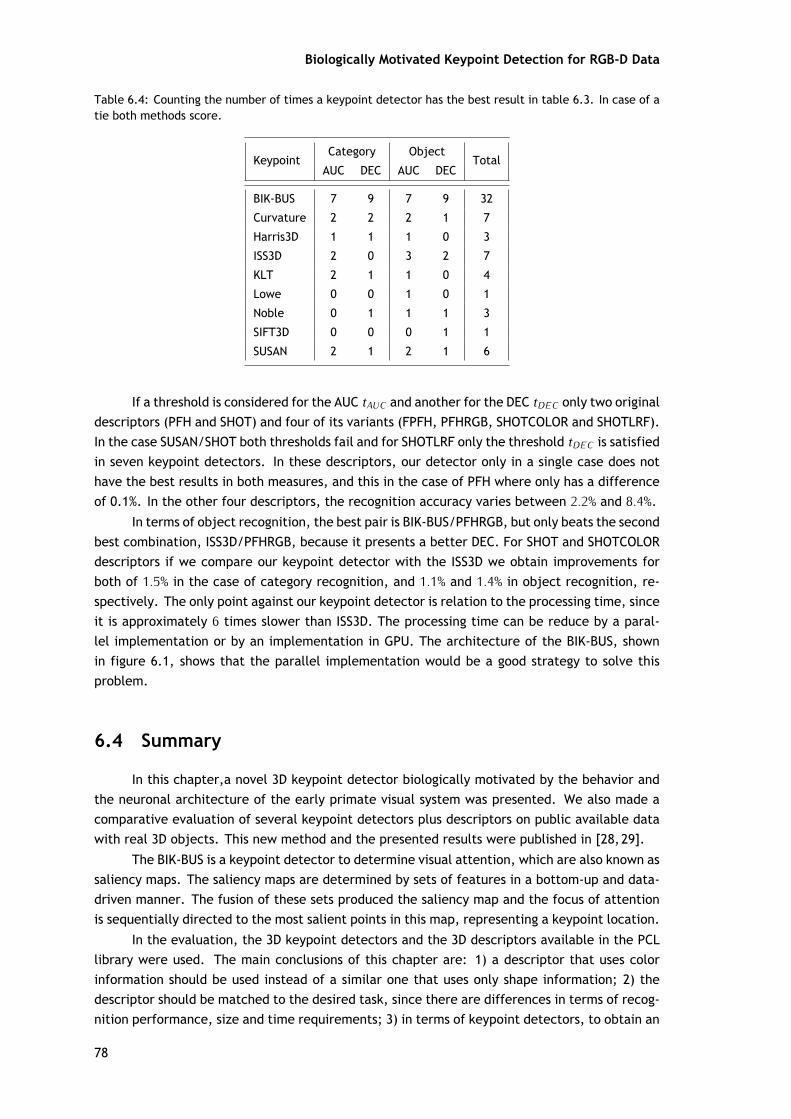
Biologically Motivated Keypoint Detection for RGB-D Data
Table 6.4: Counting the number of times a keypoint detector has the best result in table 6.3. In case of atie both methods score.
KeypointCategory Object
TotalAUC DEC AUC DEC
BIK-BUS 7 9 7 9 32
Curvature 2 2 2 1 7
Harris3D 1 1 1 0 3
ISS3D 2 0 3 2 7
KLT 2 1 1 0 4
Lowe 0 0 1 0 1
Noble 0 1 1 1 3
SIFT3D 0 0 0 1 1
SUSAN 2 1 2 1 6
If a threshold is considered for the AUC tAUC and another for the DEC tDEC only two originaldescriptors (PFH and SHOT) and four of its variants (FPFH, PFHRGB, SHOTCOLOR and SHOTLRF).In the case SUSAN/SHOT both thresholds fail and for SHOTLRF only the threshold tDEC is satisfiedin seven keypoint detectors. In these descriptors, our detector only in a single case does nothave the best results in both measures, and this in the case of PFH where only has a differenceof 0.1%. In the other four descriptors, the recognition accuracy varies between 2.2% and 8.4%.
In terms of object recognition, the best pair is BIK-BUS/PFHRGB, but only beats the secondbest combination, ISS3D/PFHRGB, because it presents a better DEC. For SHOT and SHOTCOLORdescriptors if we compare our keypoint detector with the ISS3D we obtain improvements forboth of 1.5% in the case of category recognition, and 1.1% and 1.4% in object recognition, re-spectively. The only point against our keypoint detector is relation to the processing time, sinceit is approximately 6 times slower than ISS3D. The processing time can be reduce by a paral-lel implementation or by an implementation in GPU. The architecture of the BIK-BUS, shownin figure 6.1, shows that the parallel implementation would be a good strategy to solve thisproblem.
6.4 Summary
In this chapter,a novel 3D keypoint detector biologically motivated by the behavior andthe neuronal architecture of the early primate visual system was presented. We also made acomparative evaluation of several keypoint detectors plus descriptors on public available datawith real 3D objects. This new method and the presented results were published in [28,29].
The BIK-BUS is a keypoint detector to determine visual attention, which are also known assaliency maps. The saliency maps are determined by sets of features in a bottom-up and data-driven manner. The fusion of these sets produced the saliency map and the focus of attentionis sequentially directed to the most salient points in this map, representing a keypoint location.
In the evaluation, the 3D keypoint detectors and the 3D descriptors available in the PCLlibrary were used. The main conclusions of this chapter are: 1) a descriptor that uses colorinformation should be used instead of a similar one that uses only shape information; 2) thedescriptor should be matched to the desired task, since there are differences in terms of recog-nition performance, size and time requirements; 3) in terms of keypoint detectors, to obtain an
78
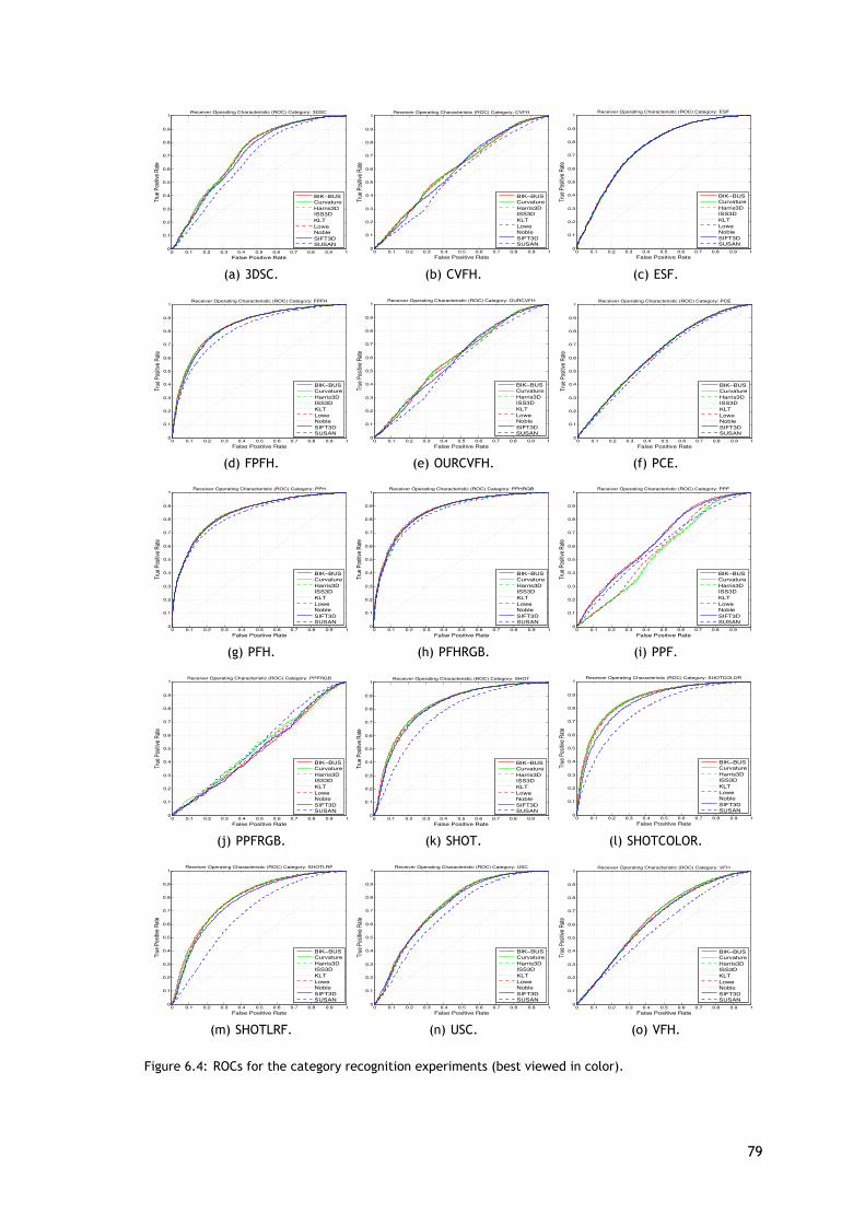
0 0.1 0.2 0.3 0.4 0.5 0.6 0.7 0.8 0.9 10
0.1
0.2
0.3
0.4
0.5
0.6
0.7
0.8
0.9
1
False Positive Rate
True P
ositiv
e Rate
Receiver Operating Characteristic (ROC) Category: 3DSC
BIK−BUSCurvatureHarris3DISS3DKLTLoweNobleSIFT3DSUSAN
(a) 3DSC.
0 0.1 0.2 0.3 0.4 0.5 0.6 0.7 0.8 0.9 10
0.1
0.2
0.3
0.4
0.5
0.6
0.7
0.8
0.9
1
False Positive Rate
True P
ositiv
e Rate
Receiver Operating Characteristic (ROC) Category: CVFH
BIK−BUSCurvatureHarris3DISS3DKLTLoweNobleSIFT3DSUSAN
(b) CVFH.
0 0.1 0.2 0.3 0.4 0.5 0.6 0.7 0.8 0.9 10
0.1
0.2
0.3
0.4
0.5
0.6
0.7
0.8
0.9
1
False Positive Rate
True P
ositiv
e Rate
Receiver Operating Characteristic (ROC) Category: ESF
BIK−BUSCurvatureHarris3DISS3DKLTLoweNobleSIFT3DSUSAN
(c) ESF.
0 0.1 0.2 0.3 0.4 0.5 0.6 0.7 0.8 0.9 10
0.1
0.2
0.3
0.4
0.5
0.6
0.7
0.8
0.9
1
False Positive Rate
True P
ositiv
e Rate
Receiver Operating Characteristic (ROC) Category: FPFH
BIK−BUSCurvatureHarris3DISS3DKLTLoweNobleSIFT3DSUSAN
(d) FPFH.
0 0.1 0.2 0.3 0.4 0.5 0.6 0.7 0.8 0.9 10
0.1
0.2
0.3
0.4
0.5
0.6
0.7
0.8
0.9
1
False Positive Rate
True P
ositiv
e Rate
Receiver Operating Characteristic (ROC) Category: OURCVFH
BIK−BUSCurvatureHarris3DISS3DKLTLoweNobleSIFT3DSUSAN
(e) OURCVFH.
0 0.1 0.2 0.3 0.4 0.5 0.6 0.7 0.8 0.9 10
0.1
0.2
0.3
0.4
0.5
0.6
0.7
0.8
0.9
1
False Positive Rate
True P
ositiv
e Rate
Receiver Operating Characteristic (ROC) Category: PCE
BIK−BUSCurvatureHarris3DISS3DKLTLoweNobleSIFT3DSUSAN
(f) PCE.
0 0.1 0.2 0.3 0.4 0.5 0.6 0.7 0.8 0.9 10
0.1
0.2
0.3
0.4
0.5
0.6
0.7
0.8
0.9
1
False Positive Rate
True P
ositiv
e Rate
Receiver Operating Characteristic (ROC) Category: PFH
BIK−BUSCurvatureHarris3DISS3DKLTLoweNobleSIFT3DSUSAN
(g) PFH.
0 0.1 0.2 0.3 0.4 0.5 0.6 0.7 0.8 0.9 10
0.1
0.2
0.3
0.4
0.5
0.6
0.7
0.8
0.9
1
False Positive Rate
True P
ositiv
e Rate
Receiver Operating Characteristic (ROC) Category: PFHRGB
BIK−BUSCurvatureHarris3DISS3DKLTLoweNobleSIFT3DSUSAN
(h) PFHRGB.
0 0.1 0.2 0.3 0.4 0.5 0.6 0.7 0.8 0.9 10
0.1
0.2
0.3
0.4
0.5
0.6
0.7
0.8
0.9
1
False Positive Rate
True P
ositiv
e Rate
Receiver Operating Characteristic (ROC) Category: PPF
BIK−BUSCurvatureHarris3DISS3DKLTLoweNobleSIFT3DSUSAN
(i) PPF.
0 0.1 0.2 0.3 0.4 0.5 0.6 0.7 0.8 0.9 10
0.1
0.2
0.3
0.4
0.5
0.6
0.7
0.8
0.9
1
False Positive Rate
True P
ositiv
e Rate
Receiver Operating Characteristic (ROC) Category: PPFRGB
BIK−BUSCurvatureHarris3DISS3DKLTLoweNobleSIFT3DSUSAN
(j) PPFRGB.
0 0.1 0.2 0.3 0.4 0.5 0.6 0.7 0.8 0.9 10
0.1
0.2
0.3
0.4
0.5
0.6
0.7
0.8
0.9
1
False Positive Rate
True P
ositiv
e Rate
Receiver Operating Characteristic (ROC) Category: SHOT
BIK−BUSCurvatureHarris3DISS3DKLTLoweNobleSIFT3DSUSAN
(k) SHOT.
0 0.1 0.2 0.3 0.4 0.5 0.6 0.7 0.8 0.9 10
0.1
0.2
0.3
0.4
0.5
0.6
0.7
0.8
0.9
1
False Positive Rate
True P
ositiv
e Rate
Receiver Operating Characteristic (ROC) Category: SHOTCOLOR
BIK−BUSCurvatureHarris3DISS3DKLTLoweNobleSIFT3DSUSAN
(l) SHOTCOLOR.
0 0.1 0.2 0.3 0.4 0.5 0.6 0.7 0.8 0.9 10
0.1
0.2
0.3
0.4
0.5
0.6
0.7
0.8
0.9
1
False Positive Rate
True P
ositiv
e Rate
Receiver Operating Characteristic (ROC) Category: SHOTLRF
BIK−BUSCurvatureHarris3DISS3DKLTLoweNobleSIFT3DSUSAN
(m) SHOTLRF.
0 0.1 0.2 0.3 0.4 0.5 0.6 0.7 0.8 0.9 10
0.1
0.2
0.3
0.4
0.5
0.6
0.7
0.8
0.9
1
False Positive Rate
True P
ositiv
e Rate
Receiver Operating Characteristic (ROC) Category: USC
BIK−BUSCurvatureHarris3DISS3DKLTLoweNobleSIFT3DSUSAN
(n) USC.
0 0.1 0.2 0.3 0.4 0.5 0.6 0.7 0.8 0.9 10
0.1
0.2
0.3
0.4
0.5
0.6
0.7
0.8
0.9
1
False Positive Rate
True P
ositiv
e Rate
Receiver Operating Characteristic (ROC) Category: VFH
BIK−BUSCurvatureHarris3DISS3DKLTLoweNobleSIFT3DSUSAN
(o) VFH.
Figure 6.4: ROCs for the category recognition experiments (best viewed in color).
79
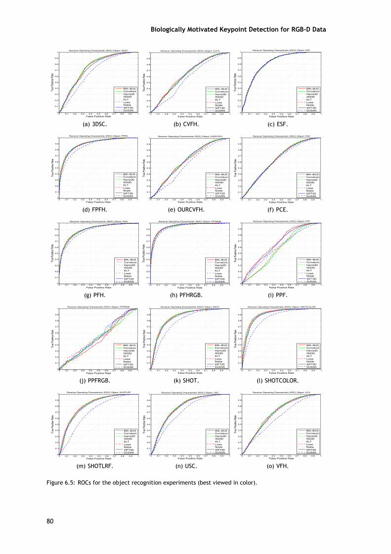
Biologically Motivated Keypoint Detection for RGB-D Data
0 0.1 0.2 0.3 0.4 0.5 0.6 0.7 0.8 0.9 10
0.1
0.2
0.3
0.4
0.5
0.6
0.7
0.8
0.9
1
False Positive Rate
True P
ositiv
e Rate
Receiver Operating Characteristic (ROC) Object: 3DSC
BIK−BUSCurvatureHarris3DISS3DKLTLoweNobleSIFT3DSUSAN
(a) 3DSC.
0 0.1 0.2 0.3 0.4 0.5 0.6 0.7 0.8 0.9 10
0.1
0.2
0.3
0.4
0.5
0.6
0.7
0.8
0.9
1
False Positive Rate
True P
ositiv
e Rate
Receiver Operating Characteristic (ROC) Object: CVFH
BIK−BUSCurvatureHarris3DISS3DKLTLoweNobleSIFT3DSUSAN
(b) CVFH.
0 0.1 0.2 0.3 0.4 0.5 0.6 0.7 0.8 0.9 10
0.1
0.2
0.3
0.4
0.5
0.6
0.7
0.8
0.9
1
False Positive Rate
True P
ositiv
e Rate
Receiver Operating Characteristic (ROC) Object: ESF
BIK−BUSCurvatureHarris3DISS3DKLTLoweNobleSIFT3DSUSAN
(c) ESF.
0 0.1 0.2 0.3 0.4 0.5 0.6 0.7 0.8 0.9 10
0.1
0.2
0.3
0.4
0.5
0.6
0.7
0.8
0.9
1
False Positive Rate
True P
ositiv
e Rate
Receiver Operating Characteristic (ROC) Object: FPFH
BIK−BUSCurvatureHarris3DISS3DKLTLoweNobleSIFT3DSUSAN
(d) FPFH.
0 0.1 0.2 0.3 0.4 0.5 0.6 0.7 0.8 0.9 10
0.1
0.2
0.3
0.4
0.5
0.6
0.7
0.8
0.9
1
False Positive Rate
True P
ositiv
e Rate
Receiver Operating Characteristic (ROC) Object: OURCVFH
BIK−BUSCurvatureHarris3DISS3DKLTLoweNobleSIFT3DSUSAN
(e) OURCVFH.
0 0.1 0.2 0.3 0.4 0.5 0.6 0.7 0.8 0.9 10
0.1
0.2
0.3
0.4
0.5
0.6
0.7
0.8
0.9
1
False Positive Rate
True P
ositiv
e Rate
Receiver Operating Characteristic (ROC) Object: PCE
BIK−BUSCurvatureHarris3DISS3DKLTLoweNobleSIFT3DSUSAN
(f) PCE.
0 0.1 0.2 0.3 0.4 0.5 0.6 0.7 0.8 0.9 10
0.1
0.2
0.3
0.4
0.5
0.6
0.7
0.8
0.9
1
False Positive Rate
True P
ositiv
e Rate
Receiver Operating Characteristic (ROC) Object: PFH
BIK−BUSCurvatureHarris3DISS3DKLTLoweNobleSIFT3DSUSAN
(g) PFH.
0 0.1 0.2 0.3 0.4 0.5 0.6 0.7 0.8 0.9 10
0.1
0.2
0.3
0.4
0.5
0.6
0.7
0.8
0.9
1
False Positive Rate
True P
ositiv
e Rate
Receiver Operating Characteristic (ROC) Object: PFHRGB
BIK−BUSCurvatureHarris3DISS3DKLTLoweNobleSIFT3DSUSAN
(h) PFHRGB.
0 0.1 0.2 0.3 0.4 0.5 0.6 0.7 0.8 0.9 10
0.1
0.2
0.3
0.4
0.5
0.6
0.7
0.8
0.9
1
False Positive Rate
True P
ositiv
e Rate
Receiver Operating Characteristic (ROC) Object: PPF
BIK−BUSCurvatureHarris3DISS3DKLTLoweNobleSIFT3DSUSAN
(i) PPF.
0 0.1 0.2 0.3 0.4 0.5 0.6 0.7 0.8 0.9 10
0.1
0.2
0.3
0.4
0.5
0.6
0.7
0.8
0.9
1
False Positive Rate
True P
ositiv
e Rate
Receiver Operating Characteristic (ROC) Object: PPFRGB
BIK−BUSCurvatureHarris3DISS3DKLTLoweNobleSIFT3DSUSAN
(j) PPFRGB.
0 0.1 0.2 0.3 0.4 0.5 0.6 0.7 0.8 0.9 10
0.1
0.2
0.3
0.4
0.5
0.6
0.7
0.8
0.9
1
False Positive Rate
True P
ositiv
e Rate
Receiver Operating Characteristic (ROC) Object: SHOT
BIK−BUSCurvatureHarris3DISS3DKLTLoweNobleSIFT3DSUSAN
(k) SHOT.
0 0.1 0.2 0.3 0.4 0.5 0.6 0.7 0.8 0.9 10
0.1
0.2
0.3
0.4
0.5
0.6
0.7
0.8
0.9
1
False Positive Rate
True P
ositiv
e Rate
Receiver Operating Characteristic (ROC) Object: SHOTCOLOR
BIK−BUSCurvatureHarris3DISS3DKLTLoweNobleSIFT3DSUSAN
(l) SHOTCOLOR.
0 0.1 0.2 0.3 0.4 0.5 0.6 0.7 0.8 0.9 10
0.1
0.2
0.3
0.4
0.5
0.6
0.7
0.8
0.9
1
False Positive Rate
True P
ositiv
e Rate
Receiver Operating Characteristic (ROC) Object: SHOTLRF
BIK−BUSCurvatureHarris3DISS3DKLTLoweNobleSIFT3DSUSAN
(m) SHOTLRF.
0 0.1 0.2 0.3 0.4 0.5 0.6 0.7 0.8 0.9 10
0.1
0.2
0.3
0.4
0.5
0.6
0.7
0.8
0.9
1
False Positive Rate
True P
ositiv
e Rate
Receiver Operating Characteristic (ROC) Object: USC
BIK−BUSCurvatureHarris3DISS3DKLTLoweNobleSIFT3DSUSAN
(n) USC.
0 0.1 0.2 0.3 0.4 0.5 0.6 0.7 0.8 0.9 10
0.1
0.2
0.3
0.4
0.5
0.6
0.7
0.8
0.9
1
False Positive Rate
True P
ositiv
e Rate
Receiver Operating Characteristic (ROC) Object: VFH
BIK−BUSCurvatureHarris3DISS3DKLTLoweNobleSIFT3DSUSAN
(o) VFH.
Figure 6.5: ROCs for the object recognition experiments (best viewed in color).
80

accurate recognition system is recommended the use of the BIK-BUS, since its performance wasbetter in 32 tests, in a total of 60 tests. When the second best detector only obtained the bestperformance 8 times (see table 6.4); 4) for a real-time system, the ISS3D or Curvature detec-tors are good choices, since they have a performance that is only surpassed by BIK-BUS and arefaster; 5) in terms of descriptors, if the focus is on accuracy the use of PFHRGB is recommendedand for real-time a good choice is the SHOTCOLOR because it presents a good balance betweenrecognition performance and time complexity.
81

Biologically Motivated Keypoint Detection for RGB-D Data
82
Chapter 7
A 3D Keypoint Application for Tracking
In this chapter, a robust detection and tracking method for 3D objects by using keypointinformation in a particle filter is proposed. Our method consists of three distinct steps: Seg-mentation, Tracking Initialization and Tracking. The segmentation is made in order to removeall the background information, in order to reduce the number of points for further processing.In the initialization, a keypoint detector with biological inspiration is used. The information ofthe followed object is given by the extracted keypoints. The particle filter does the tracking ofthe keypoints, so with that you can predict where the keypoints will be in the next frame. In arecognition system, one of the problems is the computational cost of keypoint detectors. Thisapproach aims to solve this problem.
The experiments with the proposed method are done indoors in an office/home environ-ment, where personal robots are expected to operate. The Tracking Error evaluate the stabilityof the general tracking method. We also evaluate quantitatively this method using a "TrackingError". Our evaluation is done by the computation of the keypoint and particle centroid.
7.1 Particle Filter with Bio-Inspired Keypoints Tracking
This section will focus on the Particle Filter with Bio-Inspired Keypoints Tracking (PFBIK-Tracking)block presented in the figure 7.1. This method is composed by two main steps: Segmentationand Tracking, which will be described in detail below.
The Recognition block is presented in this work only in a illustrative way and it will notbe discussed in this chapter. But in [22, 23, 27, 29] and the last two chapters (5 and 6) give usa good perspective on how to solve the issue of object recognition. In [22], the focus is on thedescriptors available in PCL (Feature Extraction step). We briefly explain how they work andmade a comparative evaluation on publicly available data.
7.1.1 Segmentation
The segmentation starts with the Pass Through Filter (PTF). This filter removes depthregions that are not contained on the desired working distances [dmin, dmax ], where dmin is theminimum distance at which the system should work and dmax the maximum distance. Depthregions that are not included between these distances are considered background and are dis-carded by the tracking system. By removing these regions (shown in figure 7.2(b)), which donot have interesting information for the object tracking system, a considerable reduction in theprocessing time is obtained.
The second step of the segmentation is the Planar Segmentation (PS), which is based onthe Random Sample Consensus (RANSAC) algorithm [125]. It is an iterative method to estimateparameters of a mathematical model from a set of observed data which contains outliers. Ba-sically, the data consists of "inliers" and "outliers". The distribution of the inlier's data can beexplained by some set of model parameters, but may be subject to noise and outliers, which
83
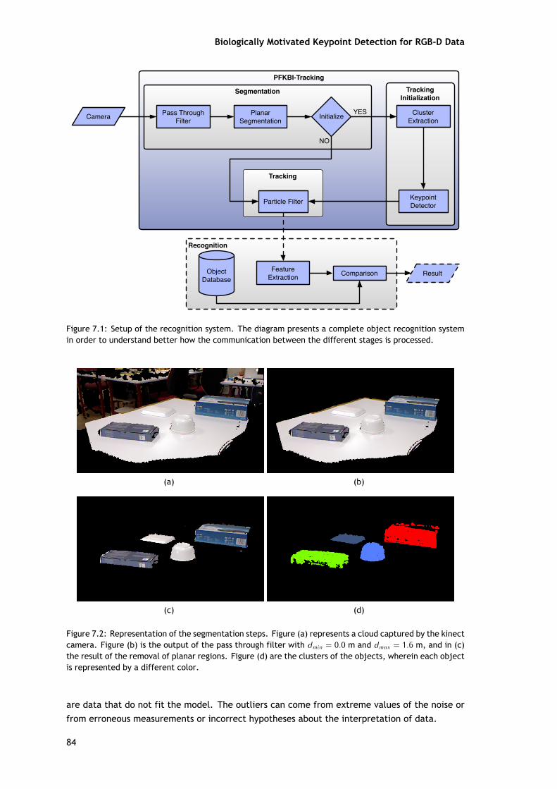
Biologically Motivated Keypoint Detection for RGB-D Data
Camera
Recognition
Feature Extraction ComparisonObject
DatabaseResult
PFKBI-Tracking
Segmentation
Planar Segmentation
Pass Through Filter Initialize YES
NO
Tracking Initialization
Cluster Extraction
Keypoint Detector
Tracking
Particle Filter
Figure 7.1: Setup of the recognition system. The diagram presents a complete object recognition systemin order to understand better how the communication between the different stages is processed.
(a) (b)
(c) (d)
Figure 7.2: Representation of the segmentation steps. Figure (a) represents a cloud captured by the kinectcamera. Figure (b) is the output of the pass through filter with dmin = 0.0 m and dmax = 1.6 m, and in (c)the result of the removal of planar regions. Figure (d) are the clusters of the objects, wherein each objectis represented by a different color.
are data that do not fit the model. The outliers can come from extreme values of the noise orfrom erroneous measurements or incorrect hypotheses about the interpretation of data.
84
Let w be the probability of choosing an inlier each time a single point is selected, thatis, w = #inliers
#points . Using n points, selected independently, for estimating the model, wn is theprobability that all n points are inlier's and 1 − wn is the probability that at least one of the npoints is an outlier. That probability to the power of k (number of iterations) is the probabilitythat the algorithm never selects a set of n points which all are inlier's and this must be the sameas 1 − p. Where p is the probability that the RANSAC algorithm in some iteration selects onlyinlier's from the input cloud set when it chooses the n points from which the model parametersare estimated. Consequently,
1 − p = (1 − wn)k (7.1)
which, after taking the logarithm of both sides, leads to
k = log(1 − p)log(1 − wn) . (7.2)
Given the planar region estimated by RANSAC algorithm, it is possible to remove theplanar regions from the cloud, keeping only the remaining objects (shown in figure 7.2(c)).
7.1.2 Tracking Initialization
In the first frame captured, to initialize the tracking, the third step of segmentation isperformed, the Cluster Extraction (CE). Clustering is the process of examining a collection of"points", and grouping the points into "clusters" according to some distance measure. That is,the goal is that points in the same cluster have a small distance from one another, while pointsin different clusters are at a large distance from one another. This step will return a list of theclusters (shown in figure 7.2(d)), where each one contains the information of an object presentin the cloud scene. In this work, Euclidean Clustering method is used. As the name implies, thedistance between two points p1, p2 is given by the Euclidean distance:
D(p1, p2) =√
(p1x − p2x )2 + (p1y − p2y )2 + (p1z − p2z )2. (7.3)
This PCL implementation is explained in [345].
As mentioned earlier, in [26], we presented an evaluation of the keypoint detectors avail-able on PCL. The SIFT keypoint detector was proposed in [9]. The SIFT features are vectors thatrepresent local cloud measurements. The 3D implementation of SIFT3D keypoint detector waspresented in [102]. It uses a 3D version of the Hessian to select such interest points.
The performance of human vision is obviously far superior to that of current computervision systems, so there is potentially much to be gained by emulating biological processes.Fortunately, there have been dramatic improvements within the past few years in understandinghow object recognition is accomplished in animals and humans [99]. Some features found in ITcortex are composed by neurons that respond to various moderately complex object features,and those that cluster in a columnar region that runs perpendicular to the cortical surfacerespond to similar features [346]. These neurons maintain highly specific responses to shapefeatures that appear anywhere within a large portion of the visual field and over a several octaverange of scales [347]. The complexity of many of these features appears to be roughly the same
85
Biologically Motivated Keypoint Detection for RGB-D Data
as for the SIFT. The DoG clouds are also similar to the "Place cells", which are pyramidal cellsin the hippo-campus which exhibit strongly increased firing in specific spatial locations [348].The feature responses have been shown to depend on previous visual learning from exposureto specific objects containing these features [349]. These features appear to be derived inthe brain by a highly computation-intensive parallel process, which is quite different from thestaged filtering given by this method. A retinotopic organization, parallel processing, feed-forward, feedback and lateral connection are a complex composition of the human visual system[350]. However, the results are much the same: an image is transformed into a large set oflocal features that each match a small fraction of potential objects yet are largely invariant tocommon viewing transformations.
7.1.3 Tracking
The Tracking block presented in figure 7.1 is the Particle Filter. For this, an adaptiveparticle filter presented in [126,127] is used. They presented a statistical approach to adaptingthe sample set size of particle filters on-the-fly. The number of the particles changes adaptivelybased on KL distance sampling [128], where they bind the error introduced by sample-basedrepresentation of the particle filter. The samples are generated iteratively until their numberis large enough to ensure that the KL distance between the maximum likelihood estimate and theunderlying posterior does not exceed a pre-specified bound. This method will choose differentnumbers of samples depending on the density of the 3D point cloud. If selects a small numberof samples, the density is focused in a small subspace and it selects a larger number of samples,the samples have to cover most of the state space.
7.2 Results
To evaluate the performance of the method, the Euclidean distance (equation 7.3) be-tween the centroid of the keypoints and result of the method will be used, which is the "TrackingError". The purpose of performing this comparison is to evaluate whether a system is able totrack the keypoints of an object. The tracking is done in order to remove the necessity of apply-ing a keypoint detector in all frames. In a real-time system is not feasible to apply a keypointdetector in each frame, due to the computational time spent on their calculation.
The centroid of a finite set of p points p1, p2, …, pk in Rn is given by
C =∑k
i=1 pi
k (7.4)
This point minimizes the sum of squared Euclidean distances between itself and each point inthe set.
In order to properly evaluate the performance of the method, it will be compared with thesample-based method OpenniTracker available in PCL 1.7 (from the trunk). The segmentationstep is applied in this tracker, where the output of this step is shown in figure 7.3. Thus, exactlythe same data is given as input to both methods.
The difference between the twomethods is the initialization of the particle filter. Whereasit is initialized with the results of the keypoint detector, the OpenniTracker only makes a sub-sampling. This is a very important difference in the object recognition frameworks, because the
86
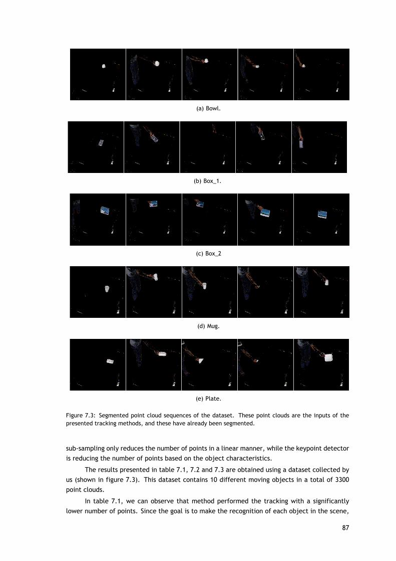
(a) Bowl.
(b) Box_1.
(c) Box_2
(d) Mug.
(e) Plate.
Figure 7.3: Segmented point cloud sequences of the dataset. These point clouds are the inputs of thepresented tracking methods, and these have already been segmented.
sub-sampling only reduces the number of points in a linear manner, while the keypoint detectoris reducing the number of points based on the object characteristics.
The results presented in table 7.1, 7.2 and 7.3 are obtained using a dataset collected byus (shown in figure 7.3). This dataset contains 10 different moving objects in a total of 3300point clouds.
In table 7.1, we can observe that method performed the tracking with a significantlylower number of points. Since the goal is to make the recognition of each object in the scene,
87

Biologically Motivated Keypoint Detection for RGB-D Data
Table 7.1: Mean and standard deviation number of keypoints and particles resulting from the tracker. Inthe OpenniTracker case, the column keypoints represents the sub-sampled cloud.
Number of Points
Keypoints Particles
PFBIK-Tracking 116.973 ± 76.251 102.107 ± 92.102
OpenniTracker 2502.536 ± 1325.807 2132.124 ± 1987.516
Table 7.2: Euclidean distance between the output of the tracker and the expected result.
Distance between Centroids
X axis Y axis Z axis All axis
PFBIK-Tracking 0.036 ± 0.032 0.013 ± 0.012 0.019 ± 0.019 0.045 ± 0.036
OpenniTracker 0.038 ± 0.023 0.013 ± 0.011 0.027 ± 0.015 0.052 ± 0.022
Table 7.3: Mean and standard deviation of the Computational time (in seconds) of the evaluated methods.Here, the time of the segmentation step is discarded, because it is the same in both methods.
TrackingTracking
Initialization
PFBIK-Tracking 0.203 ± 0.162 0.081 ± 0.057
OpenniTracker 0.173 ± 0.187 0.186 ± 0.170
the method has a stable performance with fewer points. With this number of points it is possibleto think of making recognition in real time. On the other hand, with the number of points shownby the OpenniTracker this is very difficult to archive.
In table 7.2, the distance between the cloud of keypoints ('what we expect') are presentedand the resulting cloud of points produced by the tracker ('what we estimate'). As alreadymentioned, the Euclidean distance is calculated based on the centroid of what was estimatedand what we really are looking. In this table, we can see that even with a large decline in thenumber of points (around 50 times), this method has better performance than OpenniTracker.
In table 7.3, the mean processing time of the two evaluated methods is presented. Thesetimes were obtained on a computer with Intel®Core™2 Quad Processor Q9300 2.5GHz with 4 GBof RAM memory. Our method takes longer to initialize the tracking, but then the trackingsystem becomes 2.3 times faster than the other method presented. The initialization time isnot a problem since this is only done once. The initialization is slower due to the fact thatthe keypoints are extracted, instead of the sub-sampling process used by the other method. Insummary, the presented method obtains better results in terms of tracking (increased robustnessto occlusion), while using less points and resulting in an improvement in terms of processingspeed.
7.3 Summary
In this work, a system to perform the tracking of keypoints is presented and publishedin [30]. The goal is to remove the necessity of applying a keypoint detector in all frames that areanalyzed. When this kind of approach is performed, the systems spend a lot of computational
88

time and they can not operate in real time. We intend to make the tracking of keypointsbecause the main goal is to extract the descriptors of a particular object in the scene in orderto perform the recognition. In order to do this, several segmentation steps are presented, sothat the system can remove all the background and objects become isolated. When the objectsare segmented, a clustering method and the SIFT3D keypoint detector are applied, which isused to initialize the particle filter. We use the SIFT3D keypoint detector because it has similarfeatures to those in IT [99]. Once it is initialized with the intended object, it is only necessaryto give as input the output of the segmentation.
With this approach, better results were obtained than using the OpenniTracker: a fasterand more robust method. For future work, we will intend to do the tracking of multiple objectssimultaneously and use BIK-BUS keypoint detector instead of SIFT3D.
89

Biologically Motivated Keypoint Detection for RGB-D Data
90
Chapter 8
Conclusions and Further Work
This chapter presents the main conclusions that result from the research work describedin this thesis. Furthermore, it discusses a few research topics related with the work developedthat may be addressed in the future.
8.1 Main Conclusions
This thesis focused systems based on the human visual attention and HVS. The devel-oped methods have characteristics that were obtained from studies in the field of neuroscienceand psychology. To understand those characteristics, an overview of the HVS (chapter 2) and areview of computational methods that attempt to model visual attention (chapter 3) was pro-vided. The focus was mostly on bottom-up attention, although some top-down models were alsodiscussed in [129--133].
Visual attention is a highly interdisciplinary field with researchers coming from differ-ent backgrounds. For psychologists, research conducted in human behavior is performed byisolating certain specific tasks, so that the internal processes of the brain, often resulting inpsychophysical theories or models [134]. Neurobiologists observe the brain's response to cer-tain stimuli [135], using techniques such as fMRI, having therefore a direct view of the brainareas that are active under certain conditions [45,136,137]. Finally, engineers use the discov-eries made in those areas attempting to reproduce them in computational models, so that theprocessing time in some applications can be reduced [42--44]. In recent years, those differ-ent areas have profited considerably from each other, psychologists use research conducted byneurobiologists, to improve their attention models, while neurobiologists consider psychologicalexperiments to interpret their data [134]. Additionally, psychologists began to implement com-puter models or use computer models previously developed, to verify that they have a similarbehavior to that of human perception. Thus, psychologists tend to improve the understandingof the mechanisms and help the development of better computational models.
Computational attention has gained a significant popularity in the last decade. One ofthe contributors to the increase in popularity was the improvement in computational resources.Another contribution was the performance gains obtained from the inclusion of visual attention(or saliency detection) modules in object recognition systems [131,138,139].
Most of the research presented in this thesis, was focused on the bottom-up component ofvisual attention. While previous efforts are appreciated, the field of visual attention still lackscomputational principles for task-driven attention. A promising direction for future researchis the development of models that take into account time varying task demands, especiallyin interactive, complex, and dynamic environments. In addition, there is not yet a principledcomputational understanding of the visual attention. The solution is beyond the scope of a singlearea. To obtain a solution it is necessary to have the cooperation of the several areas, from themachine learning community, computer vision and the biological fields as well as neurology andpsychology.
91
Biologically Motivated Keypoint Detection for RGB-D Data
Table 3.2 shows some areas where the saliency maps were applied, but with no refer-ences to whether these can be used to extract directly keypoint locations, the most nearlybeing the one of Rodrigues and du Buf [104]. The work of Ardizzone et al [140] compared ifa particular method extracts the keypoints in salient regions. With this, an analysis was per-formed on the top popular keypoint detectors and presented in chapter 4, especially the onesusing RGB-D information. Furthermore, a description of the 3D descriptors and an evaluation of3D keypoint detectors, on public available data with real 3D objects, were made. The exper-imental comparison proposed in this work has outlined aspects of state-of-art methods for 3Dkeypoint detectors. This analysis allowed to evaluate the best performance in terms of multipletransformations (rotation, scaling and translation).
The novelties of this work, when compared with the work of Schmid et al. [17] and Saltiet al. [19] are: we are using a real database instead of an artificial, the large number of pointclouds and different keypoint detectors. The benefit of using a real database is that our ob-jects have "occlusion", this is because some materials do not reflect the infrared or from thesegmentation method. This does not happen when dealing with artificial objects, causing thekeypoint methods to display better results, but our experiments reflect what can happen in reallife, such as, with robot vision. Overall, SIFT3D and ISS3D yielded the best scores in terms ofrepeatability and ISS3D demonstrated to be the more invariant.
Another part of this research work was described in chapter 5 and encompassed the studyof a 2D keypoint detector in a recognition framework. The proposal of a novel keypoint detectionmethod is also made, called BMMSKD, that uses the retinal color information. The retinal colorinformation was applied as an extension to the BIMP method so that color information couldbe used. The recognition evaluation of the proposed approach was made on public availabledata with real 3D objects. For this evaluation, the keypoint detectors were developed using theOpenCV library and the 2D keypoint locations were projected to the 3D space to use available3D descriptors on the PCL library. It was possible to verify that the keypoint locations caneither help or degrade the recognition process and descriptors that uses color information shouldbe used instead of a similar one with shape information alone. Differences are big in termsof recognition performance, size and time requirements, and thus the descriptor should bematched to the desired task. If we want to recognize the category of an object or a real-timesystem, the recommendation is to use the SHOTCOLOR method, since it presents a recognitionrate of 7% below of the PFHRGB but with a much lower computational cost. On the other hand, toperform object recognition, the recommendation is to use PFHRGB, as it presents a recognitionrate 12.9% higher than SHOTCOLOR.
A novel 3D keypoint detector biologically motivated by the behavior and the neuronalarchitecture of the early primate visual system was presented in chapter 6. Similarly to chapter5, a comparative evaluation was made where several keypoint detectors and descriptors werecompared on public available data with real 3D objects. BIK-BUS is a keypoint detector to deter-mine visual attention, which is also known as saliency maps. The saliency maps are determinedby sets of features in a bottom-up and data-driven manner. The saliency map is then producedby the fusion of those sets, being the focus os attention sequentially directed to the most salientpoint of the map, that represent a keypoint location. In the evaluation, the 3D keypoint de-tectors and the 3D descriptors available in the PCL library were used. With a similar averagenumber of keypoints, the proposed 3D keypoint detector outperforms all the 3D keypoint de-tectors evaluated, achiving the best result in 32 of the evaluated metrics in the category andobject recognition experiments, while the second best detector obtained only the best result in8 of these metrics (see table 6.4), in a total of 60 tests. The unique drawback we identified is
92
the computational time, since BIK-BUS is slower than the other detectors. For a real-time sys-tem, the ISS3D or Curvature detectors are more advisable choices, since theyare faster and theirperformance is only surpassed by BIK-BUS. Finally, in terms of descriptors the recommendationgoes to either PFHRGB or SHOTCOLOR. PFHRGB should be used when one wants an accuraterecognition system, while for real-time the most advisable choice is the SHOTCOLOR, since itpresents a good balance between recognition performance and time complexity.
In this research work, an application for 3D keypoint detectors was also presented, calledPFBIK-Tracking, consisting on a system to perform the tracking of keypoints. The goal was toremove the necessity of applying a keypoint detector in all the frames we wanted to analyze.This is caused by the keypoint detectors being applied to all the frames, and therefore the systemwould not be able to operate in real time. To solve this, a keypoint tracker was developed tosimulate the application of keypoint detectors to all the frames, since the main propose wouldbe to extract the descriptors of a particular object in the scene to perform the recognition.For that propose, several segmentation steps were presented, so that we can remove all thebackground and objects become isolated. Further to object segmentation, a clustering methodand the SIFT3D keypoint detector were applied, which was used to initialize the particle filter.SIFT3D keypoint detector was used because it has similar features to those in IT [99]. Once it wasinitialized with the intended object, it only needs to be fed with the output of the segmentation.This approach obtained better results than when the OpenniTracker was used, and thereby afaster and more robust method was presented.
The main objectives of this thesis were accomplished by the presentation of the threemethods. Together, the proposed methods allow the incorporation of characteristics with bio-logical inspiration in recognition systems. Here, the experiments were done only in an objectrecognition system, but it can be applied to other types, such as biometrics signal (e.g. 3Dface).
8.2 Future Work
Future work that could be developed should fall into three main focuses. The first lineof further research would be to reduce the computational cost of the two keypoints detectorspresented. Fot that purpose, we can consider a code parallelization or an implementation on theGeneral-Purpose Computation on Graphics Processing Unit (GPGPU) to reduce the computationaltime of BMMSKD and BIK-BUS. The architecture of the methods makes the code parallelizationpossible, as shown in figures 5.1 and 6.1.
Secondly, it would be a good idea to seek further insights on why one keypoint detectoror a combination of a descriptor type and keypoint detector works better than others for aspecific test. This can be accomplished by selecting a small number of top keypoint detectorsand descriptors (based on the results presented in this research work) and analyze which are thebest pairs on the recognition of a particular type of category or object. In this work, an analysisto cover the whole dataset and not focus on specific cases was made. A more complex analysiswas not performed for two reasons: 1) the dataset used in this work is very large, it consists of300 objects and these are divided into 51 categories; 2) were also evaluate 135 pairs of keypointdetector/descriptor and this analysis would render unfeasible using all these methods.
Finally, future work will focus on the proposed keypoint tracking system, where severalpossibilities are still open and can be exploited. The first possibility is the replacement of thekeypoint detector to use the BIK-BUS instead of SIFT3D. The reasoning behind this proposal is
93

Biologically Motivated Keypoint Detection for RGB-D Data
that the BIK-BUS showed better results than SIFT3D in the object recognition framework.Another point to explore that could improve this research work would be the dataset:
adding more objects and the way in which they move in the scene. This new dataset has al-ready been captured, containing 46 different objects, organized into 24 categories and with longperiods of occlusion (such as out of the camera range and behind boxes). The acquisition of ob-jects was made using a Kinect camera placed in several locations of a room, with the objectsover a remote controlled car, so that they could move around the room. To use this dataset iswould be necessary to segment the objects that are moving in the scene, so that several exper-iments and comparisons could be performed. The first experiments should take into accountthe evaluation made in chapters 5 and 6. This will allow to consolidate the results presentedin those chapters. With the segmented objects, it is also possible to propose a 3D CLEAR MOTMetric [141] to the 3D tracking approaches. This measure is only available for 2D methods anddoes not consider the depth of the object. The difference to the measure proposed in chapter7 is that it also makes the evaluation of the overlap between the position of the real object andthe approximation obtained by the tracking method. Finally, category and object recognitionusing particle information and descriptors can be compared to the recognition process of usingkeypoint detectors and descriptors.
94
Bibliography
[1] A. L. Rothenstein and J. Tsotsos, ``Attention links sensing to recognition,'' Image andVision Computing, vol. 26, no. 1, pp. 114--126, Jan. 2008. xvii, xviii, xxvii, 1, 19
[2] C. Koch and S. Ullman, ``Shifts in selective visual attention: towards the underlyingneural circuitry,'' Human Neurobiology, vol. 4, no. 4, pp. 219--227, Jan. 1985. xvii, xix,xxvii, 1, 3, 19, 20, 32
[3] L. Itti, C. Koch, and E. Niebur, ``A model of saliency-based visual attention for rapidscene analysis,'' IEEE Transactions on Pattern Analysis and Machine Intelligence, vol. 20,no. 11, pp. 1254--1259, Mar. 1998. xvii, xix, xxvii, xxxii, xxxiii, xxxiv, 1, 3, 19, 20, 21,22, 23, 24, 33, 34, 35, 55, 65, 67, 68
[4] D. Heinke and G. W. Humphreys, ``Computational models of visual selective attention:A review,'' in Connectionist Models in Psychology, G. Houghton, Ed. Psychology Press,2004. xviii, 1
[5] C. Bundesen and T. Habekost, ``Attention,'' in Handbook of Cognition, K. Lamberts andR. Goldstone, Eds. London: Sage Publications, 2005, ch. 4. xviii, 1
[6] A. Borji and L. Itti, ``State-of-the-art in visual attention modeling,'' IEEE Transactions onPattern Analysis and Machine Intelligence, vol. 35, no. 1, pp. 185--207, Jan 2013. xviii,xxvii, 19
[7] K. Terzić, J. Rodrigues, and J. du Buf, ``Fast Cortical Keypoints for Real-Time ObjectRecognition,'' in IEEE International Conference on Image Processing, Melbourne, Sep.2013, pp. 3372--3376. xviii, xix, xx, xxix, 1, 2, 4, 43, 58, 60, 61
[8] J. Shi and C. Tomasi, ``Good features to track,'' in IEEE Conference on Computer Visionand Pattern Recognition, Jun 1994, pp. 593--600. xviii, 2
[9] D. G. Lowe, ``Distinctive Image Features from Scale-Invariant Keypoints,'' InternationalJournal of Computer Vision, vol. 60, no. 2, pp. 91--110, Nov. 2004. xviii, xxix, xxxvi, 2,42, 58, 60, 61, 85
[10] H. Bay, A. Ess, T. Tuytelaars, and L. Van Gool, ``Speeded-Up Robust Features (SURF),''Computer Vision and Image Understanding, vol. 110, no. 3, pp. 346--359, Jun. 2008. xviii,xxix, 2, 43, 58, 60, 61
[11] W. Forstner, T. Dickscheid, and F. Schindler, ``Detecting interpretable and accuratescale-invariant keypoints,'' in IEEE 12th International Conference on Computer Vision,Sept 2009, pp. 2256--2263. xviii, 2
[12] N. Pinto, D. D. Cox, and J. J. DiCarlo, ``Why is real-world visual object recognition hard?''PLoS Computational Biology, vol. 4, no. 1, pp. 151--156, 01 2008. xviii, 2
[13] O. Boiman, E. Shechtman, and M. Irani, ``In defense of Nearest-Neighbor based imageclassification,'' in IEEE Conference on Computer Vision and Pattern Recognition, Anchor-age, AK, Jun. 2008, pp. 1--8. xviii, 2
95
Biologically Motivated Keypoint Detection for RGB-D Data
[14] T. Serre, L. Wolf, S. Bileschi, M. Riesenhuber, and T. Poggio, ``Robust object recogni-tion with cortex-like mechanisms,'' IEEE Transactions on Pattern Analysis and MachineIntelligence, vol. 29, no. 3, pp. 411--426, March 2007. xviii, 2
[15] L. Zhang, M. H. Tong, and G. W. Cottrell, ``Information attracts attention: A probabilisticaccount of the cross-race advantage in visual search,'' in 29th Annual Cognitive ScienceConference, 2007, pp. 749--754. xviii, 2, 32
[16] A. Mian, M. Bennamoun, and R. Owens, ``On the Repeatability and Quality of Keypointsfor Local Feature-based 3D Object Retrieval from Cluttered Scenes,'' International Journalof Computer Vision, vol. 89, no. 2-3, pp. 348--361, 2010. xviii, 2
[17] C. Schmid, R. Mohr, and C. Bauckhage, ``Evaluation of Interest Point Detectors,'' Interna-tional Journal of Computer Vision, vol. 37, no. 2, pp. 151--172, 2000. xviii, xxxi, xxxviii,2, 49, 50, 53, 92
[18] K. Mikolajczyk, T. Tuytelaars, C. Schmid, A. Zisserman, J. Matas, F. Schaffalitzky,T. Kadir, and L. Van Gool, ``A Comparison of Affine Region Detectors,'' InternationalJournal of Computer Vision, vol. 65, no. 1-2, pp. 43--72, Oct. 2005. xviii, xxxi, 2, 49
[19] S. Salti, F. Tombari, and L. D. Stefano, ``A Performance Evaluation of 3D Keypoint De-tectors,'' in International Conference on 3D Imaging, Modeling, Processing, Visualizationand Transmission, 2011, pp. 236--243. xviii, xxxi, xxxviii, 2, 49, 50, 53, 92
[20] R. B. Rusu and S. Cousins, ``3D is here: Point Cloud Library (PCL),'' in International Con-ference on Robotics and Automation, Shanghai, China, May 9-13 2011. xix, 2, 3, 70
[21] K. Lai, L. Bo, X. Ren, and D. Fox, ``A large-scale hierarchical multi-view RGB-D objectdataset,'' in International Conference on Robotics and Automation, May 2011, pp. 1817--1824. xix, xxxi, xxxii, 2, 48, 57, 69
[22] L. A. Alexandre, ``3D descriptors for object and category recognition: a comparativeevaluation,'' in Workshop on Color-Depth Camera Fusion in Robotics at the IEEE/RSJ In-ternational Conference on Intelligent Robots and Systems (IROS), Vilamoura, Portugal,October 2012. xix, xxx, 3, 47, 49, 83
[23] ------, ``Set Distance Functions for 3D Object Recognition,'' in 18th IberoamericanCongress on Pattern Recognition. Springer, 2013, pp. 57--64. xix, xxxiii, 3, 58, 83
[24] J. Black, T. Ellis, and P. Rosin, ``A novel method for video tracking performance eval-uation,'' in In Joint IEEE International Workshop on Visual Surveillance and PerformanceEvaluation of Tracking and Surveillance, 2003, pp. 125--132. xx, 3
[25] S. Filipe and L. A. Alexandre, ``A Comparative Evaluation of 3D Keypoint Detectors,'' in9th Conference on Telecommunications, Castelo Branco, Portugal, May 2013, pp. 145--148. xx, 4, 53
[26] ------, ``A Comparative Evaluation of 3D Keypoint Detectors in a RGB-D Object Dataset,''in 9th International Conference on Computer Vision Theory and Applications, Lisbon,Portugal, 5--8 January 2014. xx, xxxvi, 4, 53, 85
[27] ------, ``A Biological Motivated Multi-scale Keypoint Detector for local 3D Descriptors,'' in10th International Symposium on Visual Computing, ser. LNCS, vol. 8887, Las Vegas, NV,Dec. 2014, pp. 218--227. xx, 4, 61, 83
96

[28] ------, ``A 3D Keypoint Detector based on Biologically Motivated Bottom-Up Saliency MapProposed 3D Keypoint Detector,'' in 20th Portuguese Conference on Pattern Recognition,Covilhã, Oct. 2014. xxi, 4, 78
[29] S. Filipe, L. Itti, and L. A. Alexandre, ``BIK-BUS: Biologically Motivated 3D Keypoint basedon Bottom-Up Saliency,'' IEEE Transactions on Image Processing, vol. 24, no. 1, pp. 163--175, Jan. 2015. xxi, 4, 78, 83
[30] S. Filipe and L. A. Alexandre, ``PFBIK-Tracking: Particle Filter with Bio-Inspired KeypointsTracking,'' in IEEE Symposium on Computational Intelligence for Multimedia, Signal andVision Processing, Orlando, FL, Dec. 2014. xxi, 4, 88
[31] T. P. Trappenberg, Fundamentals of Computational Neuroscience, 2nd ed. Oxford Uni-versity Press, 2010. xxii, 7
[32] D. Hubel, ``Eye, brain and vision,'' Website, 2010,http://hubel.med.harvard.edu/book/bcontex.htm. xxii, xxiii, 7, 8, 9
[33] H. Kolb, E. Fernández, and R. Nelson, Webvision: the organization of the retina andvisual system. Salt Lake City (UT): University of Utah, John Moran Eye Center, 2007.xxii, 7
[34] C. Pfaffmann, Sensory Reception, Human Vision and Structure and Function of the HumanEye. Encyclopædia Britannica, 1987, vol. 27. xxii, 8
[35] M. Passer and R. Smith, Psychology: The Science of Mind and Behavior. McGraw-HillHigher Education, 2010. xxii, 8
[36] M. A. Goodale and A. D. Milner, Sight Unseen, ser. An Exploration of Conscious and Un-conscious Vision. New York: Oxford University Press Inc, 2005. xxiii, 10
[37] J. G. Nicholls, A. R. Martin, B. G. Wallace, and P. A. Fuchs, From Neuron to Brain, 4th ed.Sinauer Associates Inc, 2001. xxiii, 10
[38] V. A. F. Lamme and P. R. Roelfsema, ``The distinct modes of vision offered by feedfor-ward and recurrent processing,'' Trends in Neurosciences, vol. 23, no. 11, pp. 571--579,2000. xxiv, 12
[39] J. M. Hupé, A. C. James, B. R. Payne, S. G. Lomber, P. Girard, and J. Bullier, ``Corti-cal feedback improves discrimination between figure and background by V1, V2 and V3neurons.'' Nature, vol. 394, no. 6695, pp. 784--7, Aug. 1998. xxiv, 13
[40] A. Angelucci and J. Bullier, ``Reaching beyond the classical receptive field of V1 neurons:horizontal or feedback axons?'' Journal of Physiology, vol. 97, no. 2-3, pp. 141--154, 2003.xxiv, 13
[41] J. M. Hupé, A. C. James, P. Girard, and J. Bullier, ``Response modulations by static tex-ture surround in area V1 of the macaque monkey do not depend on feedback connectionsfrom V2,'' Journal of Neurophysiology, vol. 85, no. 1, pp. 146--163, Jan. 2001. xxiv, 13
[42] S. Treue, ``Neural correlates of attention in primate visual cortex,'' Trends in Neuro-sciences, vol. 24, no. 5, pp. 295--300, May 2001. xxiv, xxxvii, 13, 38, 91
[43] G. M. Boynton, ``A framework for describing the effects of attention on visual responses,''Vision Research, vol. 49, no. 10, pp. 1129--1143, Jun. 2009. xxiv, xxxvii, 13, 38, 91
97
Biologically Motivated Keypoint Detection for RGB-D Data
[44] J. H. Reynolds and D. J. Heeger, ``The normalization model of attention,'' Neuron, vol. 61,no. 2, pp. 168--185, Jan. 2009. xxiv, xxxvii, 13, 38, 91
[45] K. Herrmann, L. Montaser-Kouhsari, M. Carrasco, and D. J. Heeger, ``When size mat-ters: attention affects performance by contrast or response gain,'' Nature Neuroscience,vol. 13, no. 12, pp. 1554--1559, Dec. 2010. xxiv, xxxvii, 13, 17, 91
[46] M. S. Gazzaniga, R. B. Ivry, and G. R. Mangun, Cognitive neuroscience: The biology of themind, 2nd ed. New York: Norton, 2002. xxiv, 13
[47] K. J. Friston and C. Büchel, ``Attentional modulation of effective connectivity from V2to V5/MT in humans,'' in Proceedings of the National Academy of Sciences of the UnitedStates of America, vol. 97, Jun. 2000, pp. 7591--7596. xxiv, 13
[48] D. B. Bender and M. Youakim, ``Effect of attentive fixation in macaque thalamus andcortex,'' Journal of Neurophysiology, vol. 85, no. 1, pp. 219--234, Jan. 2001. xxiv, 13
[49] T. J. Bussey and L. M. Saksida, ``Memory, perception, and the ventral visual-perirhinal-hippocampal stream: thinking outside of the boxes,'' Hippocampus, vol. 17, no. 9, pp.898--908, Jan. 2007. xxv, 13
[50] M. F. López-Aranda, J. F. López-Téllez, I. Navarro-Lobato, M. Masmudi-Martín, A. Gutiér-rez, and Z. U. Khan, ``Role of layer 6 of V2 visual cortex in object-recognition memory,''Science, vol. 325, no. 5936, pp. 87--89, Jul. 2009. xxv, 13
[51] A. Anzai, X. Peng, and D. C. Van Essen, ``Neurons in monkey visual area V2 encodecombinations of orientations,'' Nature Neuroscience, vol. 10, no. 10, pp. 1313--1321, Oct.2007. xxv, 13, 14
[52] J. Hegde and D. C. Van Essen, ``Selectivity for complex shapes in primate visual area v2,''Journal of Neuroscience, vol. 20, pp. 1--6, 2000. xxv, 13
[53] ------, ``Temporal dynamics of shape analysis in macaque visual area V2,'' Journal ofNeurophysiology, vol. 92, no. 5, pp. 3030--3042, Nov. 2004. xxv, 13
[54] F. T. Qiu and R. Von der Heydt, ``Figure and ground in the visual cortex: v2 combinesstereoscopic cues with gestalt rules,'' Neuron, vol. 47, no. 1, pp. 155--66, Jul. 2005. xxv,14
[55] I. Maruko, B. Zhang, X. Tao, J. Tong, E. L. Smith, and Y. M. Chino, ``Postnatal devel-opment of disparity sensitivity in visual area 2 (v2) of macaque monkeys,'' Journal ofNeurophysiology, vol. 100, no. 5, pp. 2486--2495, Nov. 2008. xxv, 14
[56] D. J. Felleman, A. Burkhalter, and D. C. Van Essen, ``Cortical connections of areas V3 andVP of macaque monkey extrastriate visual cortex,'' The Journal of Comparative Neurology,vol. 379, no. 1, pp. 21--47, Mar. 1997. xxv, 14
[57] J. Moran and R. Desimone, ``Selective attention gates visual processing in the extrastriatecortex,'' Science, vol. 229, no. 4715, pp. 782--784, Aug. 1985. xxv, 14
[58] M. A. Goodale and A. D. Milner, ``Separate visual pathways for perception and action,''Trends in Neurosciences, vol. 15, no. 1, pp. 20--25, Jan. 1992. xxv, 11, 14
[59] R. T. Born and D. C. Bradley, ``Structure and function of visual area MT,'' Annual Reviewof Neuroscience, vol. 28, pp. 157--189, Jan. 2005. xxv, 15
98

[60] L. G. Ungerleider and R. Desimone, ``Cortical connections of visual area MT in themacaque,'' The Journal of Comparative Neurology, vol. 248, no. 2, pp. 190--222, Jun.1986. xxv, 15
[61] D. J. Felleman and D. C. Van Essen, ``Distributed hierarchical processing in the primatecerebral cortex,'' Cerebral Cortex, vol. 1, no. 1, pp. 1--47, 1991. xxv, 15
[62] L. C. Sincich, K. F. Park, M. J. Wohlgemuth, and J. C. Horton, ``Bypassing V1: a directgeniculate input to area MT,'' Nature Neuroscience, vol. 7, no. 10, pp. 1123--1128, Oct.2004. xxv, 15
[63] S. M. Palmer and M. G. P. Rosa, ``A distinct anatomical network of cortical areas foranalysis of motion in far peripheral vision,'' The European Journal of Neuroscience, vol. 24,no. 8, pp. 2389--2405, Oct. 2006. xxv, 15
[64] G. C. DeAngelis and W. T. Newsome, ``Organization of disparity-selective neurons inmacaque area MT,'' The Journal of Neuroscience, vol. 19, no. 4, pp. 1398--1415, Feb.1999. xxv, 15
[65] H. R. Rodman, C. G. Gross, and T. D. Albright, ``Afferent basis of visual response prop-erties in area MT of the macaque. I. Effects of striate cortex removal,'' The Journal ofNeuroscience, vol. 9, no. 6, pp. 2033--2050, Jun. 1989. xxv, 15
[66] S. M. Zeki, ``Interhemispheric connections of prestriate cortex in monkey,'' Brain Re-search, vol. 19, no. 1, pp. 63--75, Apr. 1970. xxv, 14, 15
[67] H. E. Pashler, Attention. Philadelphia: Taylor & Francis Press, 1998. xxv, 15
[68] ------, The Psychology of Attention. Cambridge, MA: MIT Press, 1998. xxv, 15
[69] E. Style, The Psychology of Attention, 2nd ed. Florence, KY: Psychology Press Ltd, 1998.xxv, 15, 16
[70] A. Johnson and R. W. Proctor, Attention: theory and practice. Sage Publications, 2004.xxvi, 15
[71] R. A. Rensink, J. K. O'Regan, and J. J. Clark, ``To see or not to see: The need for attentionto perceive changes in scenes,'' Psychological Science, vol. 8, pp. 368--373, 1997. xxvi,15
[72] D. J. Simons, Change Blindness and Visual Memory, ser. Special Issues of Visual CognitionSeries. Psychology Press, 2000. xxvi, 15
[73] R. Desimone and J. Duncan, ``Neural mechanisms of selective visual attention,'' AnnualReview of Neuroscience, vol. 18, pp. 193--222, Jan. 1995. xxvi, 15
[74] M. Corbetta and G. L. Shulman, ``Control of goal-directed and stimulus-driven attentionin the brain,'' Nature Reviews. Neuroscience, vol. 3, no. 3, pp. 201--215, Mar. 2002. xxvi,15, 16, 17
[75] J. Theeuwes, ``Top-down search strategies cannot override attentional capture,'' Psycho-nomic bulletin & review, vol. 11, no. 1, pp. 65--70, Feb. 2004. xxvi, 16
99
Biologically Motivated Keypoint Detection for RGB-D Data
[76] H.-C. Nothdurft, ``Salience of feature contrast,'' in Neurobiology of Attention, L. Itti,G. Rees, and J. K. Tsotsos, Eds. Burlington: Academic Press, 2005, ch. 38, pp. 233--239.xxvi, 16
[77] H. E. Egeth and S. Yantis, ``Visual attention: control, representation, and time course,''Ann. Rev. Psychol., vol. 48, pp. 269--297, 1997. xxvi, 16
[78] E. D. Dickmanns, Dynamic Vision for Perception and Control of Motion. London: Springer,2007. xxvi, 16
[79] J. M. Fuster, ``Behavioral electrophysiology of the prefrontal cortex of the primate,''Progress in brain research, vol. 85, pp. 313--324, Jan. 1990. xxvi, 16
[80] M. Corbetta, F. Miezin, S. Dobmeyer, G. Shulman, and S. Petersen, ``Attentional mod-ulation of neural processing of shape, color, and velocity in humans,'' Science, vol. 248,no. 4962, pp. 1556--1559, Jun. 1990. xxvi, 16
[81] C. L. Colby, J. R. Duhamel, and M. E. Goldberg, ``Visual, presaccadic, and cognitive acti-vation of single neurons in monkey lateral intraparietal area,'' Journal of Neurophysiology,vol. 76, no. 5, pp. 2841--2852, Nov. 1996. xxvi, 16
[82] J. H. Maunsell, ``The brain's visual world: representation of visual targets in cerebralcortex,'' Science, vol. 270, no. 5237, pp. 764--769, Nov. 1995. xxvi, 16
[83] A. A. Ghazanfar and C. E. Schroeder, ``Is neocortex essentially multisensory?'' Trends inCognitive Sciences, vol. 10, no. 6, pp. 278--285, Jun. 2006. xxvi, 16
[84] J. K. Tsotsos, S. M. Culhane, W. Y. Kei Wai, Y. Lai, N. Davis, and F. Nuflo, ``Modelingvisual attention via selective tuning,'' Artificial Intelligence, vol. 78, no. 1-2, pp. 507--545, Oct. 1995. xxvii, 19, 24
[85] B. Olshausen, C. H. Anderson, and D. C. Van Essen, ``A neurobiological model of visualattention and invariant pattern recognition based on dynamic routing of information,'' TheJournal of Neuroscience, vol. 13, no. 11, pp. 4700--4719, Nov. 1993. xxvii, 19
[86] Y.-F. Ma and H.-J. Zhang, ``Contrast-based image attention analysis by using fuzzy grow-ing,'' in Eleventh International Conference on Multimedia, New York, USA, 2003, pp. 374--281. xxvii, 19, 24
[87] T. Kadir, A. Zisserman, and M. Brady, ``An Affine Invariant Salient Region Detector,'' in8th European Conference on Computer Vision, ser. LNCS, T. Pajdla and J. Matas, Eds.,vol. 3021, Prague, Czech Republic, 2004, pp. 228--241. xxvii, 19
[88] L. Itti and P. Baldi, ``Bayesian surprise attracts human attention,'' Vision Research,vol. 49, no. 10, pp. 1295--1306, Jun. 2009. xxvii, 19, 31
[89] R. Achanta, S. Hemami, F. Estrada, and S. Süsstrunk, ``Frequency-tuned salient regiondetection,'' in Computer Vision and Pattern Recognition, Miami, FL, Jun. 2009, pp. 1597--1604. xxvii, 19, 28, 36, 38
[90] S. Frintrop, M. Klodt, and E. Rome, ``A real-time visual attention system using integralimages,'' in 5th International Conference on Computer Vision Systems, Bielefeld, Ger-many, 2007. xxvii, 19, 22, 38
100

[91] R. Achanta, F. Estrada, P. Wils, and S. Sabine, ``Salient Region Detection and Segmen-tation,'' in Computer Vision Systems, ser. LNCS, A. Gasteratos, M. Vincze, and J. Tsotsos,Eds. Santorini, Greece: Springer Berlin/Heidelberg, 2008, vol. 5008, pp. 66--75. xxvii,19, 27, 28, 36, 38
[92] Y. Hu, X. Xie, W.-Y. Ma, L.-T. Chia, and D. Rajan, ``Salient Region Detection UsingWeighted Feature Maps Based on the Human Visual Attention Model,'' in Advances in Mul-timedia Information Processing, ser. LNCS, K. Aizawa, Y. Nakamura, and S. Satoh, Eds.Springer Berlin/Heidelberg, 2004, vol. 3332, pp. 993--1000. xxvii, 19, 25
[93] D. Gao and N. Vasconcelos, ``Discriminant saliency for visual recognition from clutteredscenes,'' in Neural Information Processing Systems (NIPS), vol. 17, Vancouver, Canada,2004, pp. 481--488. xxvii, 19, 25, 29
[94] X. Hou and L. Zhang, ``Saliency Detection: A Spectral Residual Approach,'' in Conferenceon Computer Vision and Pattern Recognition, no. 800, Minneapolis, MN, Jun. 2007, pp.1--8. xxvii, 19, 25, 34, 36
[95] J. Harel, C. Koch, and P. Perona, ``Graph-based visual saliency,'' in Advances in NeuralInformation Processing Systems. MIT Press, 2006, pp. 545--552. xxvii, 19, 23, 30, 34, 36
[96] N. Bruce and J. Tsotsos, ``Saliency based on information maximization,'' Advances inneural information processing systems, vol. 18, pp. 155--162, 2005. xxvii, 19, 31, 32, 35
[97] T. Judd, K. Ehinger, F. Durand, and A. Torralba, ``Learning to predict where humanslook,'' in 12th International Conference on Computer Vision, Kyoto, Sep. 2009, pp. 2106--2113. xxviii, 33, 35, 36, 38
[98] C. Tomasi and T. Kanade, ``Detection and Tracking of Point Features,'' Carnegie MellonUniversity, Tech. Rep., 1991. xxix, 42
[99] D. Lowe, ``Local feature view clustering for 3D object recognition,'' Computer Vision andPattern Recognition, vol. 1, pp. I--682--I--688, 2001. xxix, xl, 41, 85, 89, 93
[100] J. Noble, Descriptions of Image Surfaces. University of Oxford, 1989. xxix, 41
[101] S. M. Smith and J. M. Brady, ``SUSAN -- A new approach to low level image processing,''International Journal of Computer Vision, vol. 23, no. 1, pp. 45--78, 1997. xxix, 42
[102] A. Flint, A. Dick, and A. Hengel, ``Thrift: Local 3D Structure Recognition,'' in 9th BiennialConference of the Australian Pattern Recognition Society on Digital Image ComputingTechniques and Applications, Dec. 2007, pp. 182--188. xxix, xxxvi, 42, 85
[103] Y. Zhong, ``Intrinsic shape signatures: A shape descriptor for 3D object recognition,''International Conference on Computer Vision Workshops, pp. 689--696, Sep. 2009. xxix,43
[104] J. Rodrigues and J. du Buf, ``Multi-scale keypoints in V1 and beyond: object segregation,scale selection, saliency maps and face detection,'' Biosystems, vol. 86, no. 1-3, pp. 75--90, 2006. xxix, xxxviii, 43, 92
[105] A. Frome, D. Huber, R. Kolluri, T. Bülow, and J. Malik, ``Recognizing Objects in RangeData Using Regional Point Descriptors,'' in 8th European Conference on Computer Vision,T. Pajdla and J. Matas, Eds., Prague, Czech Republic, 2004, pp. 224--237. xxix, 44, 47
101

Biologically Motivated Keypoint Detection for RGB-D Data
[106] S. Belongie, J. Malik, and J. Puzicha, ``Shape matching and object recognition usingshape contexts,'' IEEE Transactions on Pattern Analysis and Machine Intelligence, vol. 24,no. 4, pp. 509--522, Apr. 2002. xxix, 44
[107] R. B. Rusu, N. Blodow, Z. C. Marton, and M. Beetz, ``Aligning point cloud views usingpersistent feature histograms,'' in IEEE/RSJ International Conference on Intelligent Robotsand Systems, Nice, France, Sep. 2008, pp. 3384--3391. xxix, 44
[108] R. Rusu, N. Blodow, and M. Beetz, ``Fast Point Feature Histograms (FPFH) for 3D reg-istration,'' in IEEE International Conference on Robotics and Automation, May 2009, pp.3212--3217. xxx, 44, 45, 46
[109] R. Rusu, A. Holzbach, N. Blodow, and M. Beetz, ``Fast geometric point labeling usingconditional random fields,'' in IEEE/RSJ International Conference on Intelligent Robotsand Systems, St. Louis, MO, Oct. 2009, pp. 7--12. xxx, 44, 45
[110] R. Rusu, G. Bradski, R. Thibaux, and J. Hsu, ``Fast 3D recognition and pose using theViewpoint Feature Histogram,'' in IEEE/RSJ International Conference on Intelligent Robotsand Systems, Taipei, Taiwan, Oct. 2010, pp. 2155--2162. xxx, 44, 45
[111] A. Aldoma, M. Vincze, N. Blodow, D. Gossow, S. Gedikli, R. B. Rusu, and G. Bradski,``CAD-model recognition and 6DOF pose estimation using 3D cues,'' in IEEE InternationalConference on Computer Vision, Barcelona, Spain, Nov. 2011, pp. 585--592. xxx, 44, 45,46
[112] A. Aldoma, F. Tombari, R. Rusu, and M. Vincze, ``OUR-CVFH -- Oriented, Unique andRepeatable Clustered Viewpoint Feature Histogram for Object Recognition and 6DOF PoseEstimation,'' in Joint 34th DAGM and 36th OAGM Symposium, Graz, Austria, 2012, pp. 113--122. xxx, 45
[113] B. Drost, M. Ulrich, N. Navab, and S. Ilic, ``Model globally, match locally: Efficient androbust 3D object recognition,'' in IEEE Conference on Computer Vision and Pattern Recog-nition, San Francisco, CA, Jun. 2010, pp. 998--1005. xxx, 46
[114] F. Tombari, S. Salti, and L. Di Stefano, ``Unique Signatures of Histograms for Local SurfaceDescription,'' in 11th European Conference on Computer Vision, Crete, Greece, 2010, pp.356--369. xxx, 46, 47
[115] ------, ``A combined texture-shape descriptor for enhanced 3D feature matching,'' in 18thIEEE International Conference on Image Processing, Brussels, Sep. 2011, pp. 809--812.xxx, 47
[116] ------, ``Unique shape context for 3d data description,'' in ACM workshop on 3D objectretrieval. New York, USA: ACM Press, 2010, pp. 57--62. xxx, 47
[117] W. Wohlkinger and M. Vincze, ``Ensemble of shape functions for 3D object classification,''in IEEE International Conference on Robotics and Biomimetics, Karon Beach, Phuket, Dec.2011, pp. 2987--2992. xxx, 47
[118] R. Osada, T. Funkhouser, B. Chazelle, and D. Dobkin, ``Matching 3D models with shapedistributions,'' in International Conference on Shape Modeling and Applications, May 2001,pp. 154--166. xxx, 47
102
[119] L. Itti and C. Koch, ``A saliency-based search mechanism for overt and covert shifts ofvisual attention,'' Vision Research, vol. 40, no. 10-12, pp. 1489--1506, Jan. 2000. xxxii,xxxiii, 55, 65
[120] S. Frintrop, A. Nuchter, and H. Surmann, ``Saliency-based object recognition in 3D data,''in International Conference on Intelligent Robots and Systems, 2004. xxxiii, 65
[121] H. Greenspan, S. Belongie, R. Goodman, P. Perona, S. Rakshit, and C. Anderson, ``Over-complete steerable pyramid filters and rotation invariance,'' in IEEE Conference on Com-puter Vision and Pattern Recognition, Jun 1994, pp. 222--228. xxxiii, xxxiv, 65, 66
[122] A. G. Leventhal, The Neural basis of visual function, vision and visual dysfunction ed.CRC Press, 1991. xxxiv, 20, 66, 67
[123] J. Bermúdez, Cognitive Science: An Introduction to the Science of the Mind. CambridgeUniversity Press, 2010. xxxiv, 67
[124] S. Engel, X. Zhang, and B. Wandell, ``Colour tuning in human visual cortex measuredwith functional magnetic resonance imaging,'' Nature, vol. 388, no. 6637, pp. 68--71, Jul.1997. xxxiv, 67
[125] M. A. Fischler and R. C. Bolles, ``Random sample consensus: A paradigm for model fittingwith applications to image analysis and automated cartography,'' Communications of theACM, vol. 24, no. 6, pp. 381--395, Jun. 1981. xxxvi, 83
[126] D. Fox, ``KLD-sampling: Adaptive particle filters,'' in Advances in Neural InformationProcessing Systems, vol. 14. MIT Press, 2001. xxxvi, 86
[127] ------, ``Adapting the Sample Size in Particle Filters Through KLD-Sampling,'' InternationalJournal of Robotics Research, vol. 22, no. 12, pp. 985--1003, Dec. 2003. xxxvi, 86
[128] S. Kullback, Information Theory and Statistics, ser. Dover Books on Mathematics. DoverPublications, 1997. xxxvii, 86
[129] O. Ramström and H. I. Christensen, ``Visual attention using game theory,'' in SecondInternational Workshop on Biologically Motivated Computer Vision, ser. LCNS, vol. 2525.Springer, 2002, pp. 462--471. xxxvii, 24, 91
[130] R. P. N. Rao, ``Bayesian inference and attentional modulation in the visual cortex,'' Neu-roReport, vol. 16, no. 16, pp. 1843--1848, Nov. 2005. xxxvii, 23, 24, 91
[131] S. Frintrop, VOCUS: A Visual Attention System for Object Detection and Goal-DirectedSearch, ser. Lecture Notes in Computer Science. Berlin, Heidelberg: Springer BerlinHeidelberg, 2006, vol. 3899. xxxvii, xxxviii, 17, 22, 38, 91
[132] N. J. Butko and J. R. Movellan, ``Infomax Control of Eye Movements,'' IEEE Transactionson Autonomous Mental Development, vol. 2, no. 2, pp. 91--107, Jun. 2010. xxxvii, 27, 91
[133] A. Borji, M. N. Ahmadabadi, B. N. Araabi, and M. Hamidi, ``Online learning of task-drivenobject-based visual attention control,'' Image and Vision Computing, vol. 28, no. 7, pp.1130--1145, Jul. 2010. xxxvii, 30, 38, 91
103
Biologically Motivated Keypoint Detection for RGB-D Data
[134] M. Corbetta, ``Frontoparietal cortical networks for directing attention and the eye to vi-sual locations: identical, independent, or overlapping neural systems?'' National Academyof Sciences of the United States of America, vol. 95, no. 3, pp. 831--838, 1998. xxxvii,xxxviii, 15, 17, 91
[135] M. I. Posner, ``Orienting of attention,'' The Quarterly Journal of Experimental Psychol-ogy, vol. 32, no. 1, pp. 3--25, Feb. 1980. xxxvii, 16, 17, 91
[136] F. Di Russo, ``Source Analysis of Event-related Cortical Activity during Visuo-spatial At-tention,'' Cerebral Cortex, vol. 13, no. 5, pp. 486--499, May 2003. xxxvii, 13, 17, 91
[137] J. Wang, B. A. Clementz, and A. Keil, ``The neural correlates of feature-based selectiveattention when viewing spatially and temporally overlapping images,'' Neuropsychologia,vol. 45, no. 7, pp. 1393--1399, Apr. 2007. xxxvii, 13, 17, 91
[138] A. A. Salah, E. Alpaydin, and L. Akarun, ``A Selective Attention-Based Method for VisualPattern Recognition with Application to Handwritten Digit Recognition and Face Recogni-tion,'' IEEE Transactions on Pattern Analysis and Machine Intelligence, vol. 24, no. 3, pp.420--425, 2002. xxxviii, 24, 38, 91
[139] D. Walther and C. Koch, ``Modeling attention to salient proto-objects,'' Neural Networks,vol. 19, no. 9, pp. 1395--1407, Nov. 2006. xxxviii, 38, 91
[140] E. Ardizzone, A. Bruno, and G. Mazzola, ``Visual saliency by keypoints distribution analy-sis,'' in Image Analysis and Processing, ser. LNCS, G. Maino and G. Foresti, Eds. SpringerBerlin Heidelberg, 2011, vol. 6978, pp. 691--699. xxxviii, 92
[141] K. Bernardin and R. Stiefelhagen, ``Evaluating multiple object tracking performance:The clear mot metrics,'' EURASIP Journal on Image and Video Processing, vol. 2008, pp.1:1--1:10, Jan. 2008. xl, 94
[142] B. Dubuc, ``The brain from the top tp bottom,'' Website, 2011,http://thebrain.mcgill.ca/avance.php. li, 8, 10, 11
[143] Q. Lui, ``Computational neuroscience toolbox,'' Website, 2015,https://github.com/quinnliu/computationalNeuroscience. li, 9
[144] H. Hofer, J. Carroll, J. Neitz, M. Neitz, and D. R. Williams, ``Organization of the humantrichromatic cone mosaic,'' Journal of Neuroscience, vol. 25, no. 42, pp. 9669--79, Oct.2005. 8
[145] G. Wyszecki and W. S. Stiles, Color science: concepts and methods, quantitative data,and formulae, ser. Wiley classics library. John Wiley & Sons, 2000. 8
[146] J. Neitz and G. H. Jacobs, ``Polymorphism of the long-wavelength cone in normal humancolour vision,'' Nature, vol. 323, no. 6089, pp. 623--625, 1986. 8
[147] J. Dalton, Extraordinary facts relating to the vision of colours: with observations.Printed for Cadell and Davies, London, by George Nicholson, Manchester, 1798. 8
[148] S. W. Kuffler, ``Discharge patterns and functional organization of mammalian retina,''Journal of Neurophysiology, vol. 16, no. 1, pp. 37--68, 1953. 9
[149] G. Von Bonin and P. Bailey, The neocortex of Macaca mulatta, illinois monographs in themedical sciences ed. Urbana: University of Illinois Press, 1947. 10
104
[150] S. M. Zeki, ``Are areas TEO and PIT of monkey visual cortex wholly distinct from thefourth visual complex (V4 complex)?'' Proceedings of the Royal Society of London. SeriesB: Biological Sciences, vol. 263, no. 1376, pp. 1539--44, Nov. 1996. 10
[151] N. R. Carlson, C. S. Carver, M. Scheier, and E. Aronson, Physiology of Behavior, 9th ed.Allyn & Bacon, 2007. 10
[152] M. C. Schmid, S. W. Mrowka, J. Turchi, R. C. Saunders, M. Wilke, A. J. Peters, F. Q. Ye,and D. A. Leopold, ``Blindsight depends on the lateral geniculate nucleus,'' Nature, vol.466, no. 7304, pp. 373--377, Jul. 2010. 11
[153] D. W. Dong and J. J. Atick, ``Temporal decorrelation: a theory of lagged and nonlaggedresponses in the lateral geniculate nucleus,'' in Network: Computation in Neural Systems,vol. 6, 1995, pp. 159--178. 11
[154] R. Sylvester, J.-D. Haynes, and G. Rees, ``Saccades differentially modulate human LGNand V1 responses in the presence and absence of visual stimulation,'' Current Biology,vol. 15, no. 1, pp. 37--41, 2005. 11
[155] K. Brodmann, Brodmann's Localisation in the Cerebral Cortex. Boston, MA: Springer,2005. 11
[156] L. G. Ungerleider and M. Mishkin, ``Two Cortical Visual Systems,'' in Analysis of VisualBehaviour, D. J. Ingle, M. Goodale, and R. J. W. Mansfield, Eds. Cambridge, MA: MITPress, 1982, ch. 18, pp. 549--586. 11, 14
[157] V. H. Franz, F. Scharnowski, and K. R. Gegenfurtner, ``Illusion effects on grasping aretemporally constant not dynamic,'' J Exp Psychol Hum Percept Perform, vol. 31, no. 6,pp. 1359--78, 2005. 12
[158] G. Leuba and R. Kraftsik, ``Changes in volume, surface estimate, three-dimensional shapeand total number of neurons of the human primary visual cortex from midgestation untilold age,'' Anatomy and Embryology, vol. 190, pp. 351--366, 1994. 12
[159] D. H. Hubel and T. N. Wiesel, ``Receptive fields, binocular interaction and functionalarchitecture in the cat's visual cortex,'' The Journal of Physiology, vol. 160, no. 1, pp.106--154, 1962. 12
[160] J. Cudeiro and A. Sillito, ``Looking back: corticothalamic feedback and early visual pro-cessing,'' Trends in Neurosciences, vol. 29, no. 6, Jun. 2006. 13
[161] C. Guo and L. Zhang, ``An attention selection model with visual memory and onlinelearning,'' in International Joint Conference on Neural Networks, Orlando, Florida, USA,August 2007, pp. 1295--1301. 13, 27
[162] E. L. R. Harrison, C. A. Marczinski, and M. T. Fillmore, ``Driver training conditions affectsensitivity to the impairing effects of alcohol on a simulated driving test,'' Experimentaland Clinical Psychopharmacology, vol. 15, no. 6, pp. 588--98, Dec. 2007. 13
[163] L. Huang, A. Treisman, and H. Pashler, ``Characterizing the limits of human visual aware-ness,'' Science, vol. 317, pp. 823--825, August 2007. 13
[164] J. Wang and A. R. Wade, ``Differential attentional modulation of cortical responses toS-cone and luminance stimuli,'' Journal of Vision, vol. 11, no. 6, pp. 1--15, Jan. 2011. 13
105
Biologically Motivated Keypoint Detection for RGB-D Data
[165] G. T. Buracas and G. M. Boynton, ``The effect of spatial attention on contrast responsefunctions in human visual cortex,'' Journal of Neuroscience, vol. 27, no. 1, pp. 93--97,Jan. 2007. 13
[166] D. H. O'Connor, M. M. Fukui, M. A. Pinsk, and S. Kastner, ``Attention modulates responsesin the human lateral geniculate nucleus,'' Nature Neuroscience, vol. 5, no. 11, pp. 1203--1209, Nov. 2002. 13
[167] K. A. Schneider and S. Kastner, ``Effects of sustained spatial attention in the humanlateral geniculate nucleus and superior colliculus,'' Journal of Neuroscience, vol. 29, no. 6,pp. 1784--1795, Feb. 2009. 13
[168] T. Z. Lauritzen, J. M. Ales, and A. R. Wade, ``The effects of visuospatial attention mea-sured across visual cortex using source-imaged, steady-state EEG,'' Journal of Vision,vol. 10, no. 14, pp. 1--17, Jan. 2010. 13
[169] D. Yoshor, G. M. Ghose, W. H. Bosking, P. Sun, and J. H. R. Maunsell, ``Spatial attentiondoes not strongly modulate neuronal responses in early human visual cortex,'' Journal ofNeuroscience, vol. 27, no. 48, pp. 13 205--13 209, Nov. 2007. 13
[170] R. Gattas, A. P. Sousa, M. Mishkin, and L. G. Ungerleider, ``Cortical projections of areav2 in the macaque,'' Cerebral Cortex, vol. 7, no. 2, pp. 110--129, 1997. 13
[171] T. M. Preuss, I. Stepniewska, and J. H. Kaas, ``Movement representation in the dorsaland ventral premotor areas of owl monkeys: a microstimulation study,'' The Journal ofComparative Neurology, vol. 371, no. 4, pp. 649--76, Aug. 1996. 13
[172] O. J. Braddick, J. M. O'Brien, J. Wattam-Bell, J. Atkinson, T. Hartley, and R. Turner,``Brain areas sensitive to coherent visual motion,'' Perception, vol. 30, no. 1, pp. 61--72,Jan. 2001. 14
[173] L. L. Lui, J. A. Bourne, and M. G. P. Rosa, ``Functional response properties of neurons inthe dorsomedial visual area of New World monkeys (Callithrix jacchus),'' Cerebral Cortex,vol. 16, no. 2, pp. 162--177, Feb. 2006. 14
[174] M. G. Rosa and R. Tweedale, ``Visual areas in lateral and ventral extrastriate corticesof the marmoset monkey,'' The Journal of Comparative Neurology, vol. 422, no. 4, pp.621--51, Jul. 2000. 14
[175] T. D. Albright, ``Direction and orientation selectivity of neurons in visual area MT of themacaque,'' Journal of Neurophysiology, vol. 52, no. 6, pp. 1106--1130, Dec. 1984. 15
[176] R. Dubner and S. M. Zeki, ``Response properties and receptive fields of cells in an anatom-ically defined region of the superior temporal sulcus in the monkey,'' Brain Research,vol. 35, no. 2, pp. 528--532, Dec. 1971. 15
[177] J. H. Maunsell and D. C. Van Essen, ``Functional properties of neurons in middle tempo-ral visual area of the macaque monkey. I. Selectivity for stimulus direction, speed, andorientation,'' Journal of Neurophysiology, vol. 49, no. 5, pp. 1127--1147, May 1983. 15
[178] R. H. Hess, C. L. Baker, and J. Zihl, ``The "motion-blind" patient: low-level spatial andtemporal filters,'' The Journal of Neuroscience, vol. 9, no. 5, pp. 1628--1640, May 1989.15
106
[179] C. L. Baker, R. F. Hess, and J. Zihl, ``Residual motion perception in a "motion-blind"patient, assessed with limited-lifetime random dot stimuli,'' The Journal of Neuroscience,vol. 11, no. 2, pp. 454--461, Feb. 1991. 15
[180] H. R. Wilson, V. P. Ferrera, and C. Yo, ``A psychophysically motivated model for two-dimensional motion perception,'' Visual Neuroscience, vol. 9, no. 1, pp. 79--97, Jul. 1992.15
[181] C. C. Pack, R. T. Born, and M. S. Livingstone, ``Two-dimensional substructure of stereoand motion interactions in macaque visual cortex,'' Neuron, vol. 37, no. 3, pp. 525--535,Feb. 2003. 15
[182] C. J. Tinsley, B. S. Webb, N. E. Barraclough, C. J. Vincent, A. Parker, and A. M. Derrington,``The nature of V1 neural responses to 2D moving patterns depends on receptive-fieldstructure in the marmoset monkey,'' Journal of Neurophysiology, vol. 90, no. 2, pp. 930--937, Aug. 2003. 15
[183] J. A. Movshon, E. H. Adelson, M. S. Gizzi, and W. T. Newsome, ``The analysis of movingvisual patterns,'' in Pattern Recognition Mechanisms, C. Chagas, R. Gattass, and C. Gross,Eds. Vatican Press, 1985, vol. 54, ch. 13, pp. 117--151. 15
[184] K. H. Britten and R. J. Van Wezel, ``Electrical microstimulation of cortical area MSTbiases heading perception in monkeys,'' Nature Neuroscience, vol. 1, no. 1, pp. 59--63,May 1998. 15
[185] J. M. Wolfe, T. S. Horowitz, N. Kenner, M. Hyle, and N. Vasan, ``How fast can you changeyour mind? The speed of top-down guidance in visual search,'' Vision Research, vol. 44,no. 12, pp. 1411--1426, Jun. 2004. 16
[186] T. J. Vickery, L.-W. King, and Y. Jiang, ``Setting up the target template in visual search,''Journal of Vision, vol. 5, no. 1, pp. 81--92, Jan. 2005. 16
[187] M. I. Posner and S. E. Petersen, ``The attention system of the human brain,'' AnnualReview of Neuroscience, vol. 13, pp. 25--42, Jan. 1990. 16
[188] E. R. Samuels and E. Szabadi, ``Functional neuroanatomy of the noradrenergic locuscoeruleus: its roles in the regulation of arousal and autonomic function part I: principlesof functional organisation,'' Current Neuropharmacology, vol. 6, no. 3, pp. 235--253, Sep.2008. 16
[189] N. P. Bichot, ``Attention, eye movements, and neurons: Linking physiology and behavior,''in Vision and Attention, M. R. M. L. Jenkin and L. R. Harris, Eds. Springer Verlag, Berlin,2001, ch. 11, pp. 209--232. 16
[190] J. P. Gottlieb, M. Kusunoki, and M. E. Goldberg, ``The representation of visual saliencein monkey parietal cortex,'' Nature, vol. 391, no. 6666, pp. 481--484, Jan. 1998. 17
[191] J. M. Findlay and R. Walker, ``A model of saccade generation based on parallel processingand competitive inhibition,'' The Behavioral and Brain Sciences, vol. 22, no. 4, pp. 661--674, Aug. 1999. 17
[192] L. Zhaoping, ``The primary visual cortex creates a bottom-up saliency map,'' in Neurobi-ology of Attention, L. Itti, G. Rees, and J. K. Tsotsos, Eds. Elsevier, 2005, ch. 93, pp.570--575. 17
107
Biologically Motivated Keypoint Detection for RGB-D Data
[193] J. A. Mazer and J. L. Gallant, ``Goal-related activity in V4 during free viewing visualsearch. Evidence for a ventral stream visual salience map,'' Neuron, vol. 40, no. 6, pp.1241--1250, Dec. 2003. 17
[194] S. Kastner and L. G. Ungerleider, ``The neural basis of biased competition in human visualcortex,'' Neuropsychologia, vol. 39, no. 12, pp. 1263--1276, Jan. 2001. 17
[195] T. Ogawa and H. Komatsu, ``Target selection in area V4 during a multidimensional visualsearch task,'' The Journal of Neuroscience, vol. 24, no. 28, pp. 6371--6382, Jul. 2004. 17
[196] S. Ahmad, ``VISIT: A Neural Model of Covert Visual Attention,'' in Advances in NeuralInformation Processing Systems, J. E. Moody, S. J. Hanson, and R. P. Lippmann, Eds.San Francisco, CA: Morgan Kaufmann Publishers Inc, 1992, pp. 420--427. 20, 21, 24
[197] E. Niebur and C. Koch, ``Computational architectures for attention,'' in The AttentiveBrain, R. Parasuraman, Ed. Cambridge, MA: MIT Press, 1998, pp. 163--186. 20
[198] R. Milanese, S. Gil, and T. Pun, ``Attentive mechanisms for dynamic and static sceneanalysis,'' Optical Engineering, vol. 34, no. 8, pp. 2428--2434, 1995. 20
[199] S. Baluja and D. A. Pomerleau, ``Expectation-based selective attention for visual moni-toring and control of a robot vehicle,'' Robotics and Autonomous Systems, vol. 22, no. 3,pp. 329--344, 1997. 20, 38
[200] L. Itti and C. Koch, ``Comparison of feature combination strategies for saliency-basedvisual attention systems,'' in SPIE, vol. 3644, San Jose, CA, USA, 1999, pp. 473--482. 20
[201] D. Parkhurst, K. Law, and E. Niebur, ``Modeling the role of salience in the allocation ofovert visual attention,'' Vision Research, vol. 42, no. 1, pp. 107--123, Jan. 2002. 20
[202] L. Itti, ``Quantifying the contribution of low-level saliency to human eye movements indynamic scenes,'' Visual Cognition, vol. 12, no. 6, pp. 1093--1123, Aug. 2005. 20
[203] L. Itti, N. Dhavale, and F. Pighin, ``Realistic avatar eye and head animation using aneurobiological model of visual attention,'' in SPIE 48th Annual International Symposiumon Optical Science and Technology, B. Bosacchi, D. B. Fogel, and J. C. Bezdek, Eds., vol.5200. Bellingham, WA: SPIE Press, 2003, pp. 64--78. 21, 38
[204] L. Q. Chen, X. Xie, X. Fan, W. Y. Ma, H. J. Zhang, and H. Q. Zhou, ``A visual attentionmodel for adapting images on small displays,'' ACM Multimedia systems, vol. 9, no. 4, pp.353--364, Oct. 2003. 21
[205] J. Han and K. N. Ngan, ``Unsupervised extraction of visual attention objects in colorimages,'' IEEE Transactions on Circuits and Systems for Video Technology, vol. 16, no. 1,pp. 141--145, Jan. 2006. 21, 38
[206] B. C. Ko and J.-Y. Nam, ``Object-of-interest image segmentation based on human atten-tion and semantic region clustering,'' Journal of the Optical Society of America. A, Optics,image science, and vision, vol. 23, no. 10, pp. 2462--2470, Oct. 2006. 21, 25, 38
[207] R. Rosenholtz, ``A simple saliency model predicts a number of motion popout phenom-ena,'' Vision Research, vol. 39, no. 19, pp. 3157--3163, Oct. 1999. 21, 32, 33
[208] R. Rosenholtz, A. L. Nagy, and N. R. Bell, ``The effect of background color on asymmetriesin color search,'' Journal of Vision, vol. 4, no. 3, pp. 224--240, Mar. 2004. 21
108
[209] A. Oliva and A. Torralba, ``Modeling the Shape of the Scene: A Holistic Representationof the Spatial Envelope,'' International Journal of Computer Vision, vol. 42, no. 3, pp.145--175, 2001. 21, 33
[210] L. Zhang, M. H. Tong, T. K. Marks, H. Shan, and G. W. Cottrell, ``SUN: A Bayesian frame-work for saliency using natural statistics,'' Journal of vision, vol. 8, no. 7, pp. 1--20, Jan.2008. 21, 26, 32, 36
[211] A. Garcia-Diaz, X. R. Fdez-Vidal, X. M. Pardo, and R. Dosil, ``Decorrelation and Distinc-tiveness Provide with Human-Like Saliency,'' in International Conference Advanced Con-cepts for Intelligent Vision Systems, ser. LNCS, J. Blanc-Talon, W. Philips, D. Popescu,and P. Scheunders, Eds., vol. 5807. Springer Berlin Heidelberg, 2009, pp. 343--354. 21,32
[212] R. Rosenholtz, Y. Li, and L. Nakano, ``Measuring visual clutter,'' Journal of Vision, vol. 7,no. 2, pp. 17.1--22, Jan. 2007. 21
[213] Z. Li, ``A saliency map in primary visual cortex,'' Trends in Cognitive Sciences, vol. 6,no. 1, pp. 9--16, Jan. 2002. 21
[214] E. Gu, J. Wang, and N. I. Badler, ``Generating Sequence of Eye Fixations Using Decision-theoretic Attention Model,'' in IEEE Conference on Computer Vision and Pattern Recogni-tion, vol. 3, 2005, pp. 92--92. 21
[215] P. Viola and M. Jones, ``Robust Real-time Object Detection,'' International Journal ofComputer Vision, vol. 57, no. 2, pp. 137--154, 2001. 21, 22, 33
[216] O. Le Meur, P. Le Callet, D. Barba, and D. Thoreau, ``A coherent computational approachto model bottom-up visual attention,'' IEEE Transactions on Pattern Analysis and MachineIntelligence, vol. 28, no. 5, pp. 802--817, May 2006. 21, 38
[217] O. Le Meur, P. Le Callet, and D. Barba, ``Predicting visual fixations on video based onlow-level visual features,'' Vision Research, vol. 47, no. 19, pp. 2483--2498, Sep. 2007. 21
[218] V. Navalpakkam and L. Itti, ``Modeling the influence of task on attention,'' Vision Re-search, vol. 45, no. 2, pp. 205--231, Jan. 2005. 22, 38
[219] ------, ``Combining bottom-up and top-down attentional influences,'' in Human Vision andElectronic Imaging XI, vol. 6057, San Jose, CA, 2006, pp. 1--7. 22
[220] B. T. Rasolzadeh, A. T. Targhi, and J.-O. Eklundh, ``An Attentional System CombiningTop-Down and Bottom-Up Influences,'' in Attention in Cognitive Systems. Theories andSystems from an Interdisciplinary Viewpoint, L. Paletta and E. Rome, Eds. Berlin, Hei-delberg: Springer-Verlag, 2008, vol. 4840, pp. 123--140. 22
[221] A. M. Treisman and G. Gelade, ``A feature-integration theory of attention,'' Cognitivepsychology, vol. 12, no. 1, pp. 97--136, Jan. 1980. 22, 34
[222] B. T. Rasolzadeh, A. Targhi, and J.-O. Eklundh, ``Object search and localization for an in-door mobile robot,'' Journal of Computing and Information Technology, pp. 67--80, 2004.22
109
Biologically Motivated Keypoint Detection for RGB-D Data
[223] S. May, M. Klodt, E. Rome, and R. Breithaupt, ``GPU-accelerated affordance cueing basedon visual attention,'' in International Conference on Intelligent Robots and Systems, Oct.2007, pp. 3385--3390. 22
[224] A. Belardinelli, F. Pirri, and A. Carbone, ``Motion Saliency Maps from SpatiotemporalFiltering,'' in Attention in Cognitive Systems, L. Paletta and J. K. Tsotsos, Eds. Berlin,Heidelberg: Springer-Verlag, 2009, pp. 112--123. 22
[225] P. Viola and M. Jones, ``Rapid object detection using a boosted cascade of simple fea-tures,'' in Computer Vision and Pattern Recognition, vol. 1, 2001, pp. 511--518. 22, 33
[226] G. Kootstra, A. Nederveen, and B. De Boer, ``Paying attention to symmetry,'' in BritishMachine Vision Conference, 2008, pp. 1115--1125. 22
[227] D. Reisfeld, H. Wolfson, and Y. Yeshurun, ``Context-free Attentional Operators: TheGeneralized Symmetry Transform,'' International Journal of Computer Vision, vol. 14,no. 2, pp. 119--130, Mar. 1995. 22
[228] G. Heidemann, ``Focus-of-attention from local color symmetries,'' IEEE Transactions onPattern Analysis and Machine Intelligence, vol. 26, no. 7, pp. 817--830, Jul. 2004. 22
[229] S. Marat, T. Ho Phuoc, L. Granjon, N. Guyader, D. Pellerin, and A. Guérin-Dugué, ``Mod-elling Spatio-Temporal Saliency to Predict Gaze Direction for Short Videos,'' InternationalJournal of Computer Vision, vol. 82, no. 3, pp. 231--243, Feb. 2009. 22, 38
[230] P. Bian and L. Zhang, ``Biological Plausibility of Spectral Domain Approach for Spatiotem-poral Visual Saliency,'' in Advances in Neuro-Information Processing, ser. LCNS, M. Köp-pen, N. Kasabov, and G. Coghill, Eds., vol. 5506. Springer Berlin / Heidelberg, 2009, pp.251--258. 23
[231] ------, ``Visual saliency: a biologically plausible contourlet-like frequency domain ap-proach,'' Cognitive Neurodynamics, vol. 4, no. 3, pp. 189--198, Sep. 2010. 23
[232] S. Chikkerur, T. Serre, C. Tan, and T. Poggio, ``What and where: a Bayesian inferencetheory of attention,'' Vision research, vol. 50, no. 22, pp. 2233--2247, Oct. 2010. 23
[233] N. Murray, M. Vanrell, X. Otazu, and C. A. Parraga, ``Saliency estimation using a non-parametric low-level vision model,'' in IEEE Conference on Computer Vision and PatternRecognition, Jun. 2011, pp. 433--440. 24
[234] X. Otazu, C. A. Parraga, and M. Vanrell, ``Toward a unified chromatic induction model,''Journal of Vision, vol. 10, no. 12, 2010. 24
[235] R. P. N. Rao, G. J. Zelinsky, M. M. Hayhoe, and D. H. Ballard, ``Eye movements in iconicvisual search,'' Vision Research, vol. 42, no. 11, pp. 1447--1463, May 2002. 24
[236] Y.-F. Ma, X.-S. Hua, L. Lu, and H.-J. Zhang, ``A generic framework of user attention modeland its application in video summarization,'' IEEE Transactions on Multimedia, vol. 7,no. 5, pp. 907--919, Oct. 2005. 24, 38
[237] Y.-F. Ma and H.-J. Zhang, ``A model of motion attention for video skimming,'' in Interna-tional Conference on Image Processing, vol. 1, Rochester, NY, 2002, pp. 129--132. 24
[238] Y. Li, Y.-F. Ma, and H.-J. Zhang, ``Salient region detection and tracking in video,'' Inter-national Conference on Multimedia and Expo, vol. 2, pp. 269--272, 2003. 24
110
[239] Y.-F. Ma, L. Lu, H.-J. Zhang, and M. Li, ``A user attention model for video summarization,''in Tenth international conference on Multimedia. New York, New York, USA: ACM Press,2002, pp. 533--542. 24
[240] N. Sprague and D. Ballard, ``Eye movements for reward maximization,'' in Advances inNeural Information Processing Systems, S. Thrun, L. Saul, and B. Schölkopf, Eds. Cam-bridge, MA, USA: MIT Press, 2003. 25
[241] R. Brooks, ``A robust layered control system for a mobile robot,'' IEEE Journal on Roboticsand Automation, vol. 2, no. 1, pp. 14--23, 1986. 25
[242] Y. Hu, D. Rajan, and L.-T. Chia, ``Adaptive local context suppression of multiple cues forsalient visual attention detection,'' in International Conference on Multimedia and Expo,vol. 1, 2005, pp. 3--6. 25
[243] D. Gao and N. Vasconcelos, ``Bottom-up saliency is a discriminant process,'' in 11th In-ternational Conference on Computer Vision, Rio de Janeiro, 2007, pp. 1--6. 25
[244] D. Gao, V. Mahadevan, and N. Vasconcelos, ``On the plausibility of the discriminantcenter-surround hypothesis for visual saliency,'' Journal of Vision, vol. 8, no. 7, pp. 13.1--18, Jan. 2008. 25
[245] D. Gao, S. Han, and N. Vasconcelos, ``Discriminant saliency, the detection of suspiciouscoincidences, and applications to visual recognition,'' IEEE Transactions on Pattern Anal-ysis and Machine Intelligence, vol. 31, no. 6, pp. 989--1005, Jun. 2009. 25
[246] S. R. Jodogne and J. H. Piater, ``Closed-loop learning of visual control policies,'' Journalof Artificial Intelligence Research, vol. 28, pp. 349--391, 2007. 25
[247] X. Hou and L. Zhang, ``Dynamic visual attention: Searching for coding length increments,''in Neural Information Processing Systems, vol. 20, Vancouver, Canada, 2008, pp. 1--8. 26
[248] G. Boccignone, ``Nonparametric Bayesian attentive video analysis,'' in International Con-ference on Pattern Recognition, Dec. 2008, pp. 1--4. 26, 38
[249] A. Torralba, ``Modeling global scene factors in attention,'' Journal of the Optical Societyof America. A, Optics, image science, and vision, vol. 20, no. 7, pp. 1407--1418, Jul.2003. 26, 31, 32, 33
[250] N. J. Butko, L. Zhang, G. W. Cottrell, and J. R. Movellan, ``Visual saliency model forrobot cameras,'' in International Conference on Robotics and Automation, Pasadena, CA,May 2008, pp. 2398--2403. 26, 38
[251] L. Zhang, M. H. Tong, and G. W. Cottrell, ``SUNDAy: Saliency using natural statistics fordynamic analysis of scenes,'' in 31st Annual Cognitive Science Conference, Amsterdam,Netherlands, 2009. 27, 33
[252] N. J. Butko and J. R. Movellan, ``I-POMDP: An infomax model of eye movement,'' inInternational Conference on Development and Learning, no. 1, Monterey, CA, Aug. 2008,pp. 139--144. 27
[253] J. Najemnik and W. S. Geisler, ``Optimal eye movement strategies in visual search,''Nature, vol. 434, no. 7031, pp. 387--391, Mar. 2005. 27, 30
111
Biologically Motivated Keypoint Detection for RGB-D Data
[254] L. P. Kaelbling, M. L. Littman, and A. R. Cassandra, ``Planning and acting in partiallyobservable stochastic domains,'' Artificial Intelligence, vol. 101, no. 1-2, pp. 99--134,May 1998. 27
[255] N. J. Butko and J. R. Movellan, ``Optimal scanning for faster object detection,'' in Con-ference on Computer Vision and Pattern Recognition, no. 1, Miami, FL, Jun. 2009, pp.2751--2758. 27, 38
[256] C. Guo, Q. Ma, and L. Zhang, ``Spatio-temporal Saliency detection using phase spectrumof quaternion fourier transform,'' in Conference on Computer Vision and Pattern Recog-nition, no. 220, Anchorage, AK, Jun. 2008, pp. 1--8. 27, 34
[257] T. A. Ell and S. J. Sangwine, ``Hypercomplex Fourier transforms of color images,'' IEEETransactions on Image Processing, vol. 16, no. 1, pp. 22--35, Jan. 2007. 27
[258] C. Guo and L. Zhang, ``A novel multiresolution spatiotemporal saliency detection modeland its applications in image and video compression,'' IEEE Transactions on Image Process-ing, vol. 19, no. 1, pp. 185--198, Jan. 2010. 27, 38
[259] R. W. G. Hunt, Measuring Color, 3rd ed. Fountain Press, 1998. 27
[260] R. Achanta and S. Süsstrunk, ``Saliency detection for content-aware image resizing,'' inInternational Conference on Image Processing, Cairo, Nov. 2009, pp. 1005--1008. 28, 38
[261] S. Avidan and A. Shamir, ``Seam carving for content-aware image resizing,'' ACM Trans-actions on Graphics, vol. 26, no. 3, p. 10, Jul. 2007. 28
[262] R. Achanta and S. Süsstrunk, ``Saliency detection using maximum symmetric surround,''in International Conference on Image Processing, Hong Kong, Sep. 2010, pp. 2653--2656.28, 36, 38
[263] P. L. Rosin, ``A simple method for detecting salient regions,'' Pattern Recognition, vol. 42,no. 11, pp. 2363--2371, Nov. 2009. 28
[264] H. J. Seo and P. Milanfar, ``Static and space-time visual saliency detection by self-resemblance,'' Journal of Vision, vol. 9, no. 12, pp. 15.1--27, Jan. 2009. 28
[265] Y. Yu, G. K. I. Mann, and R. G. Gosine, ``Modeling of top-down object-based attentionusing probabilistic neural network,'' in Canadian Conference on Electrical and ComputerEngineering, May 2009, pp. 533--536. 29
[266] V. Mahadevan and N. Vasconcelos, ``Spatiotemporal saliency in dynamic scenes,'' IEEETransactions on Pattern Analysis and Machine Intelligence, vol. 32, no. 1, pp. 171--177,Jan. 2010. 29, 38
[267] Y. Li, Y. Zhou, J. Yan, Z. Niu, and J. Yang, ``Visual Saliency Based on Conditional Entropy,''in Asian Conference on Computer Vision, ser. LCNS, H. Zha, R. Taniguchi, and S. Maybank,Eds., vol. 5994. Springer Berlin / Heidelberg, 2010, pp. 246--257. 29
[268] J. Yan, J. Liu, Y. Li, Z. Niu, and Y. Liu, ``Visual saliency detection via rank-sparsitydecomposition,'' in IEEE International Conference on Image Processing, Sep. 2010, pp.1089--1092. 29
112
[269] T. Avraham and M. Lindenbaum, ``Esaliency (extended saliency): meaningful attentionusing stochastic image modeling,'' IEEE Transactions on Pattern Analysis and Machine In-telligence, vol. 32, no. 4, pp. 693--708, Apr. 2010. 29
[270] A. K. McCallum, ``Reinforcement learning with selective perception and hidden state,''Ph.D. dissertation, The University of Rochester, 1996. 30
[271] W. Wang, C. Chen, Y. Wang, T. Jiang, F. Fang, and Y. Yao, ``Simulating human sac-cadic scanpaths on natural images,'' in IEEE Conference on Computer Vision and PatternRecognition, Jun. 2011, pp. 441--448. 30
[272] T. S. Lee and S. X. Yu, ``An information-theoretic framework for understanding saccadiceye movements,'' in Advances in Neural Information Processing Systems, 1999, pp. 129--141. 30
[273] L. W. Renninger, J. Coughlan, P. Verghese, and J. Malik, ``An information maximizationmodel of eye movements,'' in Advances in neural information processing systems, vol. 17,Jan. 2005, pp. 1121--1128. 30
[274] R. J. Peters, A. Iyer, L. Itti, and C. Koch, ``Components of bottom-up gaze allocation innatural images,'' Vision Research, vol. 45, no. 18, pp. 2397--2416, Aug. 2005. 30
[275] R. Peters and L. Itti, ``Congruence between model and human attention reveals uniquesignatures of critical visual events,'' in Advances in Neural Information Processing Systems.Cambridge: MIT Press, 2007, pp. 1145--1152. 30
[276] R. J. Peters and L. Itti, ``Beyond bottom-up: Incorporating task-dependent influencesinto a computational model of spatial attention,'' in IEEE Conference on Computer Visionand Pattern Recognition, Jun. 2007, pp. 1--8. 30, 34
[277] R. Peters and L. Itti, ``Applying computational tools to predict gaze direction in inter-active visual environments,'' ACM Transactions on Applied Perception, vol. 5, no. 2, pp.1--19, May 2008. 30
[278] A. Oliva, A. Torralba, M. S. Castelhano, and J. M. Henderson, ``Top-down control of visualattention in object detection,'' in International Conference on Image Processing, vol. 1,2003, pp. 253--256. 31, 32, 33
[279] A. Torralba, A. Oliva, M. S. Castelhano, and J. M. Henderson, ``Contextual guidance ofeye movements and attention in real-world scenes: the role of global features in objectsearch,'' Psychological review, vol. 113, no. 4, pp. 766--786, Oct. 2006. 31, 32, 33, 35
[280] L. Itti and P. Baldi, ``A Principled Approach to Detecting Surprising Events in Video,'' inConference on Computer Vision and Pattern Recognition, vol. 1, 2005, pp. 631--637. 31,34
[281] ------, ``Bayesian surprise attracts human attention,'' in Advances in Neural InformationProcessing Systems, vol. 49. Cambridge, MA, USA: MIT Press, Jun. 2005, pp. 547--554.31
[282] W. Kienzle, F. A. Wichmann, B. Sch, and M. O. Franz, ``A Nonparametric Approachto Bottom-Up Visual Saliency,'' in Advances in Neural Information Processing Systems,B. Schölkopf, J. Platt, and T. Hoffman, Eds. MIT Press, 2007, pp. 689--696. 31
113
Biologically Motivated Keypoint Detection for RGB-D Data
[283] W. Kienzle, M. O. Franz, B. Schölkopf, and F. A. Wichmann, ``Center-surround patternsemerge as optimal predictors for human saccade targets,'' Journal of Vision, vol. 9, no. 5,pp. 7.1--15, Jan. 2009. 31, 33
[284] T. Liu, J. Sun, N. Zheng, X. Tang, and H. Shum, ``Learning to Detect A Salient Object,'' inConference on Computer Vision and Pattern Recognition, vol. 33, Minneapolis, MN, Jun.2007, pp. 1--8. 31, 36, 38
[285] T. Liu, N. Zheng, and Z. Yuan, ``Video attention: Learning to detect a salient objectsequence,'' in International Conference on Pattern Recognition, Tampa, FL, Dec. 2008,pp. 1--4. 31, 32, 38
[286] T. Liu, Z. Yuan, J. Sun, J. Wang, N. Zheng, X. Tang, and H.-Y. Shum, ``Learning to detecta salient object,'' IEEE Transactions on Pattern Analysis and Machine Intelligence, vol. 33,no. 2, pp. 353--367, Feb. 2011. 31, 32
[287] J. M. Wolfe, ``Asymmetries in visual search: an introduction.'' Perception & psy-chophysics, vol. 63, no. 3, pp. 381--389, Apr. 2001. 32
[288] D. Pang, A. Kimura, and T. Takeuchi, ``A stochastic model of selective visual attentionwith a dynamic Bayesian network,'' in IEEE International Conference on Multimedia andExpo, Jun. 2008, pp. 1073--1076. 32
[289] P. Verghese, ``Visual search and attention: a signal detection theory approach,'' Neuron,vol. 31, no. 4, pp. 523--535, Aug. 2001. 32
[290] A. Garcia-Diaz, X. Fdez-Vidal, X. Pardo, and R. Dosil, ``Saliency Based on Decorrelationand Distinctiveness of Local Responses,'' in Computer Analysis of Images and Patterns,ser. LNCS, X. Jiang and N. Petkov, Eds. Springer Berlin / Heidelberg, 2009, vol. 5702,pp. 261--268. 32
[291] A. Garcia-Diaz, X. R. Fdez-Vidal, X. M. Pardo, and R. Dosil, ``Saliency from hierarchicaladaptation through decorrelation and variance normalization,'' Image and Vision Comput-ing, vol. 30, no. 1, pp. 51--64, Jan. 2012. 32
[292] H. Hotelling, ``The generalization of student's ratio,'' in Breakthroughs in Statistics, ser.Springer Series in Statistics, S. Kotz and N. L. Johnson, Eds. Springer New York, 1992,pp. 54--65. 33
[293] K. A. Ehinger, B. Hidalgo-Sotelo, A. Torralba, and A. Oliva, ``Modeling Search for Peoplein 900 Scenes: A combined source model of eye guidance,'' Visual Cognition, vol. 17, no.6-7, pp. 945--978, Aug. 2009. 33, 38
[294] E. P. Simoncelli and W. T. Freeman, ``The steerable pyramid: a flexible architecture formulti-scale derivative computation,'' in International Conference on Image Processing,vol. 3, Washington, DC , USA, 1995, pp. 444--447. 33
[295] P. Felzenszwalb, D. McAllester, and D. Ramanan, ``A discriminatively trained, multiscale,deformable part model,'' in Conference on Computer Vision and Pattern Recognition,Anchorage, AK, Jun. 2008, pp. 1--8. 33
[296] T. Judd, F. Durand, and A. Torralba, ``Fixations on Low Resolution Images,'' Journal ofVision, vol. 10, no. 7, pp. 142--142, Aug. 2010. 33
114
[297] A. Torralba, ``How many pixels make an image?'' Visual Neuroscience, vol. 26, no. 1, pp.123--131, 2009. 33
[298] J. Li, Y. Tian, T. Huang, andW. Gao, ``Probabilistic Multi-Task Learning for Visual SaliencyEstimation in Video,'' International Journal of Computer Vision, vol. 90, no. 2, pp. 150--165, May 2010. 34
[299] L. Itti, ``CRCNS Data Sharing: Eye movements during free-viewing of natural videos,''in Collaborative Research in Computational Neuroscience Annual Meeting, Los Angeles,California, 2008. 34
[300] J. Li, Y. Tian, T. Huang, and W. Gao, ``A dataset and evaluation methodology for visualsaliency in video,'' in IEEE International Conference on Multimedia and Expo, 2009, pp.442--445. 34
[301] L. Itti and C. Koch, ``Computational modelling of visual attention,'' Nature reviews. Neu-roscience, vol. 2, no. 3, pp. 194--203, Mar. 2001. 34
[302] Y. Zhai and M. Shah, ``Visual attention detection in video sequences using spatiotemporalcues,'' in 14th annual ACM international conference on Multimedia, Santa Barbara, CA,USA, 2006, pp. 815--824. 34
[303] S. Goferman, L. Zelnik-Manor, and A. Tal, ``Context-aware saliency detection,'' in Con-ference on Computer Vision and Pattern Recognition, San Francisco, CA, Jun. 2010, pp.2376--2383. 34, 37, 38
[304] ------, ``Context-Aware Saliency Detection,'' IEEE Transactions on Pattern Analysis andMachine Intelligence, vol. 34, no. 10, pp. 1915--1926, Dec. 2011. 34
[305] J. M. Wolfe, ``Guided Search 2.0 A revised model of visual search,'' Psychonomic Bulletin& Review, vol. 1, no. 2, pp. 202--238, Jun. 1994. 34
[306] C. Koch and T. Poggio, ``Predicting the visual world: silence is golden,'' Nature neuro-science, vol. 2, no. 1, pp. 9--10, Jan. 1999. 34
[307] K. Koffka, Principles of Gestalt Psychology, internatio ed. Routledge, 1999. 34
[308] M.-M. Cheng, G.-X. Zhang, N. J. Mitra, X. Huang, and S.-M. Hu, ``Global contrast basedsalient region detection,'' in Conference on Computer Vision and Pattern Recognition,Providence, RI, Jun. 2011, pp. 409--416. 34
[309] J. H. Reynolds and R. Desimone, ``Interacting roles of attention and visual salience inV4,'' Neuron, vol. 37, no. 5, pp. 853--63, Mar. 2003. 34
[310] D. A. Klein and S. Frintrop, ``Center-surround Divergence of Feature Statistics for SalientObject Detection,'' in International Conference on Computer Vision, Barcelona, Spain,2011. 35
[311] N. Riche, M. Mancas, B. Gosselin, and T. Dutoit, ``Rare: A new bottom-up saliencymodel,'' in IEEE International Conference on Image Processing, Sept 2012, pp. 641--644.35
[312] N. Bruce and J. Tsotsos, ``Attention based on information maximization,'' Journal ofVision, vol. 7, no. 9, pp. 950--974, Mar. 2009. 36
115
Biologically Motivated Keypoint Detection for RGB-D Data
[313] X. Hou, J. Harel, and C. Koch, ``Image Signature: Highlighting Sparse Salient Regions,''IEEE Transactions on Pattern Analysis and Machine Intelligence, vol. 34, no. 1, pp. 194--201, Jul. 2012. 37
[314] J. Wang and X. Tang, ``Picture Collage,'' in Conference on Computer Vision and PatternRecognition, vol. 1, 2006, pp. 347--354. 38
[315] T. Liu, J. Wang, J. Sun, N. Zheng, X. Tang, and H.-Y. Shum, ``Picture Collage,'' IEEETransactions on Multimedia, vol. 11, no. 7, pp. 1225--1239, Nov. 2009. 38
[316] N. Ouerhani and R. V. Wartburg, ``Empirical validation of the saliency-based model ofvisual attention,'' Electronic Letters on Computer Vision and Image Analysis, vol. 3, no. 1,pp. 13--24, 2004. 38
[317] D. DeCarlo and A. Santella, ``Stylization and abstraction of photographs,'' ACM Transac-tions on Graphics, vol. 21, no. 3, pp. 769--776, Jul. 2002. 38
[318] A. Ninassi, O. Le Meur, P. Le Callet, and D. Barba, ``Does where you Gaze on an ImageAffect your Perception of Quality? Applying Visual Attention to Image Quality Metric,'' inInternational Conference on Image Processing, 2007, pp. II -- 169--II -- 172. 37, 38
[319] J. You, A. Perkis, and M. Gabbouj, ``Improving image quality assessment with modelingvisual attention,'' in European Workshop on Visual Information Processing. IEEE, Jul.2010, pp. 177--182. 38
[320] B. Suh, H. Ling, B. B. Bederson, and D. W. Jacobs, ``Automatic thumbnail cropping and itseffectiveness,'' in ACM Symposium on User Interface Software and Technology, Vancouver,Canada, 2003, pp. 95--104. 38
[321] L. Marchesotti, C. Cifarelli, and G. Csurka, ``A framework for visual saliency detectionwith applications to image thumbnailing,'' in 12th International Conference on ComputerVision, no. Iccv, Sep. 2009, pp. 2232--2239. 38
[322] N. Jacobson, Y. Lee, V. Mahadevan, N. Vasconcelos, and T. Nguyen, ``A Novel Approachto FRUC Using Discriminant Saliency and Frame Segmentation,'' IEEE Transactions on ImageProcessing, vol. 19, no. 11, pp. 2924--2934, May 2010. 38
[323] N. G. Sadaka and L. J. Karam, ``Efficient perceptual attentive super-resolution,'' in In-ternational Conference on Image Processing, Nov. 2009, pp. 3113--3116. 38
[324] ------, ``Efficient Super-Resolution driven by saliency selectivity,'' in nternational Confer-ence on Image Processing, no. 1. IEEE, Sep. 2011, pp. 1197--1200. 38
[325] S. Frintrop and P. Jensfelt, ``Attentional Landmarks and Active Gaze Control for VisualSLAM,'' IEEE Transactions on Robotics, vol. 24, no. 5, pp. 1054--1065, Oct. 2008. 38
[326] C. Siagian and L. Itti, ``Mobile robot vision navigation & localization using Gist andSaliency,'' in International Conference on Intelligent Robots and Systems, Taipei, Oct.2010, pp. 4147--4154. 38
[327] A. Maki, P. Nordlund, and J.-O. Eklundh, ``Attentional Scene Segmentation: IntegratingDepth and Motion,'' Computer Vision and Image Understanding, vol. 78, no. 3, pp. 351--373, Jun. 2000. 38
116
[328] A. Mishra and Y. Aloimonos, ``Active Segmentation,'' International journal of HumanoidRobotics, vol. 6, no. 3, pp. 361--386, Jan. 2009. 38
[329] A. K. Mishra, Y. Aloimonos, L.-F. Cheong, and A. Kassim, ``Active visual segmentation,''IEEE Transactions on Pattern Analysis and Machine Intelligence, vol. 34, no. 4, pp. 639--653, Apr. 2012. 38
[330] S. Frintrop, ``General object tracking with a component-based target descriptor,'' in In-ternational Conference on Robotics and Automation, May 2010, pp. 4531--4536. 38
[331] L. Itti, ``Automatic foveation for video compression using a neurobiological model ofvisual attention,'' IEEE Transactions on Image Processing, vol. 13, no. 10, pp. 1304--18,Oct. 2004. 38
[332] Z. Li, S. Qin, and L. Itti, ``Visual attention guided bit allocation in video compression,''Image and Vision Computing, vol. 29, no. 1, pp. 1--14, Jan. 2011. 38
[333] C. Harris and M. Stephens, ``A combined corner and edge detector,'' in Alvey Vision Con-ference, Manchester, 1988, pp. 147--152. 41
[334] S. M. Smith, ``Feature based image sequence understanding,'' 1992. 42
[335] K. Terzić, J. Rodrigues, and J. du Buf, ``Real-time object recognition based on corti-cal multi-scale keypoints,'' in 6th Iberian Conference on Pattern Recognition and ImageAnalysis, ser. LNCS, vol. 7887. Madeira, Portugal: Springer, Jun. 2013, pp. 314--321. 43
[336] A. Aldoma, Z. Marton, F. Tombari, W. Wohlkinger, C. Potthast, B. Zeisl, R. Rusu,S. Gedikli, and M. Vincze, ``Tutorial: Point Cloud Library: Three-Dimensional ObjectRecognition and 6 DOF Pose Estimation,'' IEEE Robotics & Automation Magazine, vol. 19,no. 3, pp. 80--91, Sep. 2012. 45
[337] E. Wahl, U. Hillenbrand, and G. Hirzinger, ``Surflet-pair-relation histograms: a statistical3D-shape representation for rapid classification,'' in Fourth International Conference on3-D Digital Imaging and Modeling, 2003. 3DIM 2003. Proceedings., no. October, Oct. 2003,pp. 474--481. 46
[338] E. W. Weisstein, The CRC Encyclopedia of Mathematics, 3rd ed. CRC Press, 2005. 49
[339] R. Kohavi, ``A study of cross-validation and bootstrap for accuracy estimation and modelselection,'' in 14th International Joint Conference on Artificial Intelligence, vol. 2, SanFrancisco, CA, USA, 1995, pp. 1137--1143. 57
[340] G. Bradski, ``The OpenCV Library,'' Dr. Dobb's Journal of Software Tools, 2000. 58
[341] J. G. Daugman, ``High confidence visual recognition of persons by a test of statisticalindependence,'' IEEE Transactions on Pattern Analysis and Machine Intelligence, vol. 15,no. 11, pp. 1148--1161, Nov. 1993. 59
[342] J. Swets, Signal detection theory and ROC analysis in psychology and diagnostics: col-lected papers, ser. Scientific psychology series. Lawrence Erlbaum Associates, 1996.60
[343] T. Fawcett, ``An introduction to roc analysis,'' Pattern Recognition Letters, vol. 27, no. 8,pp. 861--874, Jun. 2006. 60
117

Biologically Motivated Keypoint Detection for RGB-D Data
[344] M. W. Cannon and S. C. Fullenkamp, ``A model for inhibitory lateral interaction effectsin perceived contrast,'' Vision Research, vol. 36, no. 8, pp. 1115--1125, Apr. 1996. 68
[345] R. B. Rusu, ``Semantic 3d object maps for everyday manipulation in human living en-vironments,'' Ph.D. dissertation, Computer Science department, Technische UniversitaetMuenchen, Germany, Oct 2009. 85
[346] K. Tanaka, ``Inferotemporal cortex and object vision,'' Annual Review of Neuroscience,vol. 19, pp. 109--139, 1996. 85
[347] M. Ito, H. Tamura, I. Fujita, and K. Tanaka, ``Size and position invariance of neuronalresponses in monkey inferotemporal cortex,'' Journal of Neurophysiology, vol. 73, no. 1,pp. 218--226, 1995. 85
[348] T. Madl, S. Franklin, K. Chen, D. Montaldi, and R. Trappl, ``Bayesian Integration of In-formation in Hippocampal Place Cells,'' PLoS ONE, vol. 9, no. 3, pp. e89 762+, Mar. 2014.86
[349] N. K. Logothetis, J. Pauls, and T. Poggiot, ``Shape representation in the inferior temporalcortex of monkeys,'' Current Biology, pp. 552--563, 1995. 86
[350] A. Beghdadi, M.-C. Larabi, A. Bouzerdoum, and K. Iftekharuddin, ``A survey of perceptualimage processing methods,'' Signal Processing: Image Communication, vol. 28, no. 8, pp.811--831, Sep. 2013. 86
118