Fluid Mechanics Problems Motivated by Gravure Printing of ...
96
Fluid Mechanics Problems Motivated by Gravure Printing of Electronics by Umut Ceyhan A dissertation submitted in partial satisfaction of the requirements for the degree of Doctor of Philosophy in Engineering - Mechanical Engineering in the Graduate Division of the University of California, Berkeley Committee in charge: Professor Stephen Morris, Chair Professor Andrew Szeri Professor Per-Olof Persson Spring 2016
-
Upload
khangminh22 -
Category
Documents
-
view
3 -
download
0
Transcript of Fluid Mechanics Problems Motivated by Gravure Printing of ...

Fluid Mechanics Problems Motivated by Gravure Printing of Electronics
by
Umut Ceyhan
A dissertation submitted in partial satisfaction of the
requirements for the degree of
Doctor of Philosophy
in
Engineering - Mechanical Engineering
in the
Graduate Division
of the
University of California, Berkeley
Committee in charge:
Professor Stephen Morris, ChairProfessor Andrew Szeri
Professor Per-Olof Persson
Spring 2016

Fluid Mechanics Problems Motivated by Gravure Printing of Electronics
Copyright 2016by
Umut Ceyhan

1
Abstract
Fluid Mechanics Problems Motivated by Gravure Printing of Electronics
by
Umut Ceyhan
Doctor of Philosophy in Engineering - Mechanical Engineering
University of California, Berkeley
Professor Stephen Morris, Chair
During intaglio (gravure) printing, a blade wipes excess ink from the engraved plate withthe object of leaving ink–filled cells defining the image to be printed. That objective is notcompletely attained. Capillarity draws some ink from the cell into a meniscus connectingthe blade to the substrate, and the continuing motion of the engraved plate smears that inkover its surface. That smear behind the cell delivers a feature lacking in sharpness. Eventhough the smear formation occurs at micron scale, it affects the functionality at the scale ofmicron size printed electronics. By examining the limit of vanishing capillary number (Ca,based on substrate speed), we reduce the problem of determining smear volume to one ofhydrostatics. Using numerical solutions of the corresponding free boundary problem for theStokes equations of motion, we show that the hydrostatic theory provides an upper bound tosmear volume for finite Ca; as Ca is decreased, smear volume increases. The theory explainswhy polishing to reduce the tip radius of the blade is an effective way to control smearing. Asthe motion continues, smear volume under the meniscus is printed as a tail behind the cellextending back toward the blade. In the limit of vanishing Ca, an inner and outer analysisof the meniscus printing problem shows that the meniscus rotates around the pinned contactline at the trailing edge of the cell, and the volume under the meniscus is used to coat afilm of thickness decreasing linearly in time forming a tail shape. The tail lengthens withdecreasing Ca, owing to the concomitant increase in smear volume; the opposite is true asCa approaches O(1). For small Ca, it is computationally expensive to use the Stokes solverto show that the physical mechanism of tail formation described by the analysis as Ca→ 0is correct. Lubrication theory, on the other hand, predicts tail formation mechanism closelyfor contact angles over the blade close to π/2, and this motivates us to use the lubricationmodel for smaller Ca. With the continuing motion of substrate, we show the transition fromthe tip region (squeeze film) to the Landau-Levich film in the form of a tail shape extendingback toward the bulk meniscus (static), and this agrees with the physical picture describedby the analysis as Ca→ 0. The results contribute to the control and understanding of smearformation mechanism during gravure printing of electronics.

i
To my parents

ii
Contents
Contents ii
List of Figures iv
1 Introduction 11.1 Gravure printing and smear formation during gravure printing of electronics 11.2 Fluid mechanics problems during wiping and outline of the dissertation . . . 3
2 Development and Testing of a Numerical Method for the Stokes Problem 92.1 Problem formulation . . . . . . . . . . . . . . . . . . . . . . . . . . . . . . . 102.2 Numerical method . . . . . . . . . . . . . . . . . . . . . . . . . . . . . . . . 12
2.2.1 Galerkin formulation . . . . . . . . . . . . . . . . . . . . . . . . . . . 122.2.2 Discretization . . . . . . . . . . . . . . . . . . . . . . . . . . . . . . . 142.2.3 Time integration . . . . . . . . . . . . . . . . . . . . . . . . . . . . . 16
2.3 Validation of the solver . . . . . . . . . . . . . . . . . . . . . . . . . . . . . . 172.3.1 Flow through a slit . . . . . . . . . . . . . . . . . . . . . . . . . . . . 172.3.2 Overdamped capillary wave problem . . . . . . . . . . . . . . . . . . 192.3.3 Stick–slip problem . . . . . . . . . . . . . . . . . . . . . . . . . . . . 25
3 Meniscus Growth During Wiping 293.1 Analysis as Ca→ 0 . . . . . . . . . . . . . . . . . . . . . . . . . . . . . . . . 303.2 Hydrostatic limit when Ca→ 0 . . . . . . . . . . . . . . . . . . . . . . . . . 313.3 Viscous effects . . . . . . . . . . . . . . . . . . . . . . . . . . . . . . . . . . . 343.4 Blade geometry . . . . . . . . . . . . . . . . . . . . . . . . . . . . . . . . . . 38
4 Tail Formation 414.1 Outer problem: static prediction . . . . . . . . . . . . . . . . . . . . . . . . . 414.2 Inner problem: viscous effect . . . . . . . . . . . . . . . . . . . . . . . . . . . 444.3 Composite expansion . . . . . . . . . . . . . . . . . . . . . . . . . . . . . . . 474.4 Later stage of tail formation in the limit Ca→ 0 . . . . . . . . . . . . . . . . 524.5 Tail formation studied using numerical solution of Stokes equations with no cell 544.6 Tail formation studied using numerical solution of Stokes equations with cell 59

iii
4.7 Lubrication analysis . . . . . . . . . . . . . . . . . . . . . . . . . . . . . . . 654.7.1 A model for smear formation including the cell . . . . . . . . . . . . . 654.7.2 Model for meniscus printing . . . . . . . . . . . . . . . . . . . . . . . 694.7.3 Effect of a sequence of cells on tail formation . . . . . . . . . . . . . . 74
5 Conclusions 77
A Numerical Method for Lubrication Analysis 79
B Numerical Integration of Inner Viscous Problem over Semi–Infinite Do-main 82
Bibliography 84

iv
List of Figures
1.1 Schematic of gravure printing. . . . . . . . . . . . . . . . . . . . . . . . . . . . . 2
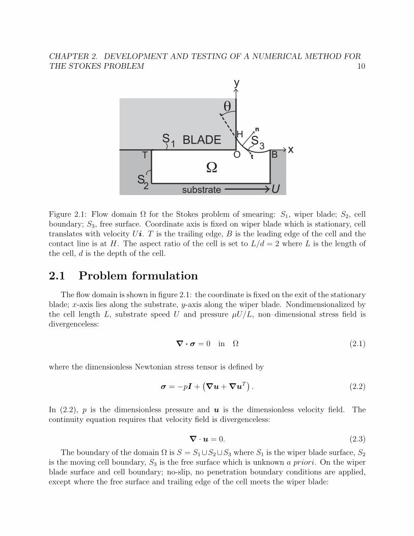
2.1 Flow domain Ω for the Stokes problem of smearing: S1, wiper blade; S2, cellboundary; S3, free surface. Coordinate axis is fixed on wiper blade which isstationary, cell translates with velocity Ui. T is the trailing edge, B is the leadingedge of the cell and the contact line is at H. The aspect ratio of the cell is set toL/d = 2 where L is the length of the cell, d is the depth of the cell. . . . . . . . 10
2.2 Nodal points in the isoparametric plane: 1 to 6 is used for P2 element, 1 to 3 isused for P1 element. . . . . . . . . . . . . . . . . . . . . . . . . . . . . . . . . . 14
2.3 Geometry for the flow through a slit. . . . . . . . . . . . . . . . . . . . . . . . . 172.4 Comparison of the numerical solution of the Stokes problem with exact solution
of flow through a slit at x = 0. . . . . . . . . . . . . . . . . . . . . . . . . . . . . 192.5 Streamlines of the flow through a slit, corresponding to figure 2.3. . . . . . . . . 192.6 Overdamped capillary wave problem: solution domain; streamlines are obtained
from the numerical solution corresponding to the interface perturbed with am-plitude a=0.01 at t = 0. . . . . . . . . . . . . . . . . . . . . . . . . . . . . . . . 20
2.7 Comparison of numerical solution of the Stokes problem with the exact solutionof overdamped capillary–wave problem: (a) v–velocity on free surface at t = 0,2–norm of the difference is 3.0525e-6, (b) Comparison of the Stokes solution andperturbation solution: u–velocity on free surface at t = 0, 2–norm of the differenceis 2.3769e-05. See text for the discussion on the discrepancy in u-velocity and thedefinition of the 2–norm is given in (2.35). . . . . . . . . . . . . . . . . . . . . . 21
2.8 Comparison of the numerical solution of the Stokes problem and perturbationsolution of the overdamped capillary–wave problem: x and y–velocity at the midof the domain at t = 0; 2-norm of the difference in u is 1.0259e-5 and in v is1.1537e-05. . . . . . . . . . . . . . . . . . . . . . . . . . . . . . . . . . . . . . . 22
2.9 Comparison of the numerical solution of the Stokes problem and perturbationsolution of the overdamped capillary–wave problem: evolution of the interface. . 23
2.10 Comparison of the numerical solution of the Stokes problem and perturbationsolution of the overdamped capillary–wave problem: pressure on interface at t = 0.1. 24
2.11 Stick–slip problem domain. . . . . . . . . . . . . . . . . . . . . . . . . . . . . . 25

v
2.12 Comparison of the numerical solution of the Stokes problem and Richardsonsolution for stick–slip problem: centerline and slip plane u-velocity. . . . . . . . 26
2.13 Comparison of the numerical solution of the Stokes problem and Richardsonsolution for stick–slip problem: centerline pressure. . . . . . . . . . . . . . . . . 27
2.14 Convergence of the method: convergence is given both in terms of infinity and2-norm errors for pressure and u-velocity (error is obtained by taking the normof the difference between computed and correct solution), h is the element size,s is the slope. . . . . . . . . . . . . . . . . . . . . . . . . . . . . . . . . . . . . . 28
3.1 Flow domain Ω for the Stokes problem of smearing: S1, wiper blade; S2, cellboundary; S3, free surface. Wiper blade is stationary, cell translates with velocityUi. . . . . . . . . . . . . . . . . . . . . . . . . . . . . . . . . . . . . . . . . . . . 30
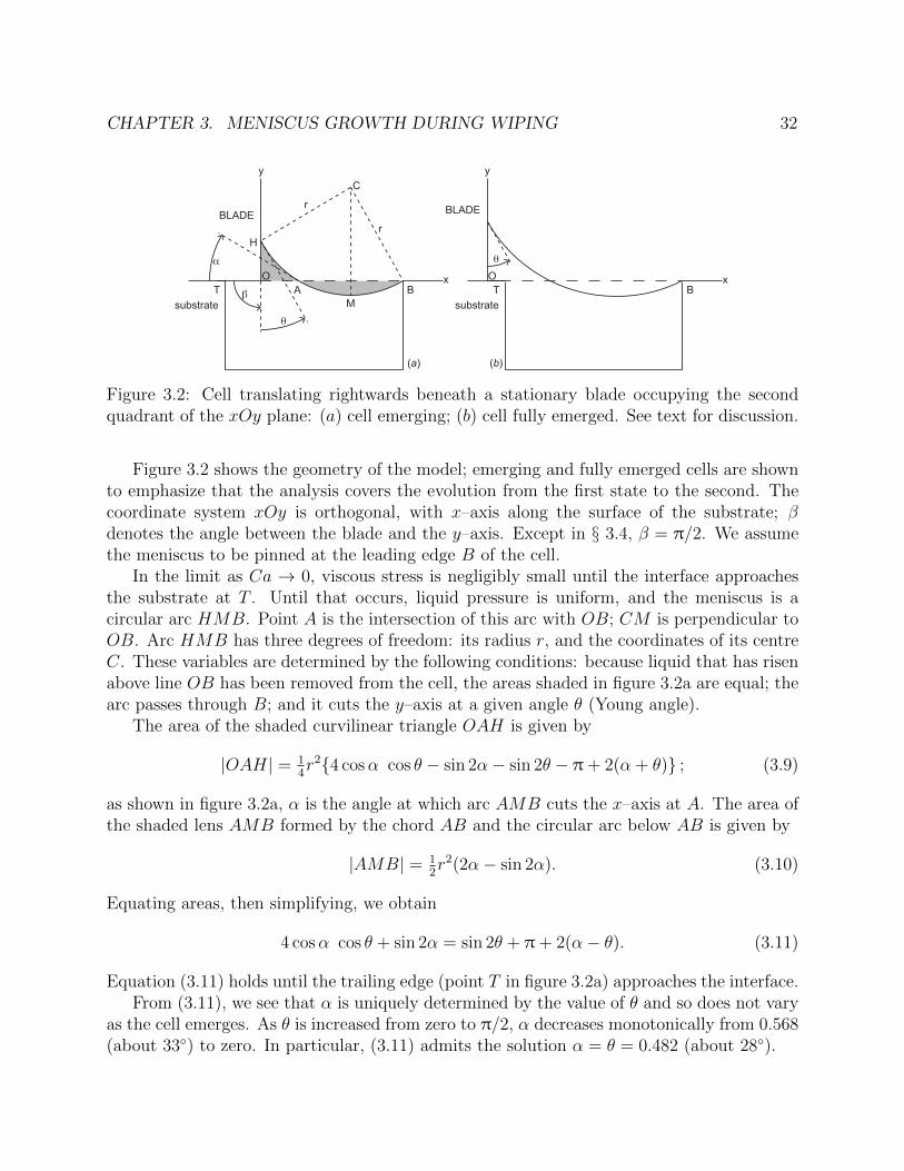
3.2 Cell translating rightwards beneath a stationary blade occupying the secondquadrant of the xOy plane: (a) cell emerging; (b) cell fully emerged. See text fordiscussion. . . . . . . . . . . . . . . . . . . . . . . . . . . . . . . . . . . . . . . . 32
3.3 Interface shape at the instant t = 0.95 the trailing edge of the cell leaves theblade; L/d=2, θ = π/6. Curve (a) hydrostatic; curves (b) to (g), computed forCa = 0.025, 0.1, 0.25, 0.5, 1 and 2. Inset, ratio v0/U of contact line velocity tosubstrate velocity. . . . . . . . . . . . . . . . . . . . . . . . . . . . . . . . . . . . 35
3.4 Streamlines corresponding to curves (b) to (d) in figure 3.3. Region 0 < x/L < 0.5,−0.125 < y/L < 0.25 and (a), Ca= 0.025; (b), 0.10 and (c) 0.25. . . . . . . . . . 35
3.5 Interface shape at the instant t = 1.35 the trailing edge of the cell is at x/L = 0.4.For θ and L/d, see caption to figure 3.3. Curve (a), hydrostatic; curves (b) to(e), computed for Ca = 0.0025, 0.005, 0.01 and 0.025. Inset, ratio v0/U of contactline velocity to substrate velocity. . . . . . . . . . . . . . . . . . . . . . . . . . . 36
3.6 Flow rate at the trailing edge of the cell; configuration as in figure 3.5. . . . . . 373.7 Relation defined by (3.15) and (3.16) for L/d=2, and contact angle θ ↑ π/2. Solid
curve, equation (3.16); dotted curve, small–β asymptote (3.17). . . . . . . . . . 393.8 Meniscus of a marginally wetting liquid beneath a parabolic blade. . . . . . . . 40
4.1 Meniscus sitting between blade and trailing edge (T ) of the cell. . . . . . . . . . 414.2 Relation between r and distance xT = |OT | for θ = 0 (solid line), θ = π/6 (dashed
line). . . . . . . . . . . . . . . . . . . . . . . . . . . . . . . . . . . . . . . . . . . 434.3 Inner problem: meniscus pinned at the trailing edge T of the cell, x grows into
the meniscus. . . . . . . . . . . . . . . . . . . . . . . . . . . . . . . . . . . . . . 444.4 Inner viscous solution for the meniscus printing problem, (a) φ = 0, (b) steady
state solution. φ0 = 0.468 is taken to be corresponding to the problem withcontact angle on the blade is θ = π/6. Inset: the neighborhood of the contactline in linear scale corresponding to curve (a). . . . . . . . . . . . . . . . . . . . 46
4.5 Effect of viscosity: meniscus is displaced by an amount δ as the trailing edge Tadvances. . . . . . . . . . . . . . . . . . . . . . . . . . . . . . . . . . . . . . . . 47
4.6 Geometry for the composite expansion. . . . . . . . . . . . . . . . . . . . . . . . 48

vi
4.7 Composite expansion (yC − yP )/L for θ = 5π/12; (top) Ca = 10−7,(bottom)Ca = 10−8; we have subtracted parabolic interface to be able to see the structureat the tip. The inset scale is the same as the main figure axes. See text for thevalues of α and φ. . . . . . . . . . . . . . . . . . . . . . . . . . . . . . . . . . . 51
4.8 Coating of a Landau–Levich film. . . . . . . . . . . . . . . . . . . . . . . . . . . 524.9 For a fixed point on substrate, expected tail formation. . . . . . . . . . . . . . . 534.10 Geometry of the meniscus sitting between blade and trailing edge (T ) of the cell. 544.11 Time evolution of meniscus printing computed using Stokes equations, Ca =
0.001, θ = π/6. . . . . . . . . . . . . . . . . . . . . . . . . . . . . . . . . . . . . 554.12 Comparison of the static prediction and Stokes solution of meniscus printing
problem, Ca = 0.001, θ = π/6: (a) x/L = 0.5096, (b) x/L = 0.5596, (c) x/L =0.6596; (—) Stokes solution, (- - -) static prediction. . . . . . . . . . . . . . . . . 56
4.13 Comparison of the inner viscous solution and Stokes solution. - - -: inner solutionsolution, —: the difference u/L between Stokes solution and static prediction atthe corresponding time. Inner solution is obtained using α and x/L correspondingto Stokes problem solved for Ca = 0.001, θ = π/6, x/L = x0/L+ 0.23. . . . . . 57
4.14 Comparison of the inner viscous solution and Stokes solution. - - -: innersolution, —: the difference u/L between Stokes solution and static predictionat the corresponding time. Inner solution solution is obtained using α andx/L corresponding to Stokes problem solved for Ca = 0.001, θ = 5π/12,x/L = x0/L+ 0.2. . . . . . . . . . . . . . . . . . . . . . . . . . . . . . . . . . . 58
4.15 Geometry of the domain for tail formation problem, cell translating rightwardsbeneath a stationary blade occupying the second quadrant of the xOy plane: (a)cell fully emerged; (b) cell is away from the blade. . . . . . . . . . . . . . . . . . 59
4.16 Interface evolution into tail shape for Ca = 0.1, θ = π/6. The history of theinterface profiles are plotted starting from xT/L=0.05 to xT/L=0.75 with 0.1 in-crements. Each curve is overlaid relative to the distance of leading edge of the cellto the blade. Solid circles along ξ axis show the corresponding location of the trail-ing edge of the cell: ξ = 0.0476, 0.1304, 0.2, 0.2593, 0.3103, 0.3548, 0.3939, 0.4286,respectively. . . . . . . . . . . . . . . . . . . . . . . . . . . . . . . . . . . . . . 60
4.17 Streamlines corresponding to figure 4.16, xT/L=0.2,0.4 and 0.6. . . . . . . . . . 614.18 Interface shape at the instant the minimum film thickness behind the tail is 0.01.
Curves are for Ca=1,0.5 and 0.1. Each curve is overlaid relative to the distanceof leading edge of the cell to the blade. Solid circles along ξ axis show thecorresponding location of the trailing edge of the cell: ξ = 0.0834, 0.1797, 0.4595,respectively. . . . . . . . . . . . . . . . . . . . . . . . . . . . . . . . . . . . . . . 62
4.19 Comparison of interface profiles computed from the Stokes equations for Ca =0.025, 0.01 and 0.005 at t = 1.773. . . . . . . . . . . . . . . . . . . . . . . . . . . 63
4.20 See caption for figure 4.19, t = 2.368. . . . . . . . . . . . . . . . . . . . . . . . . 644.21 Change of film thickness with time at (left)x = 0.5L away from the blade,
Ca=0.025, (right)x = 0.6L away from the blade, Ca=0.005; s is the slope ofthe line; θ = π/6. . . . . . . . . . . . . . . . . . . . . . . . . . . . . . . . . . . . 64

vii
4.22 Schematic of a cell emerging beneath the stationary blade used in the lubricationanalysis of tail formation. . . . . . . . . . . . . . . . . . . . . . . . . . . . . . . 65
4.23 Comparison of lubrication model and the numerical solution of the Stokes prob-lem, Ca = 0.01, θ = π/3. The power series expansion uses two terms in (4.44).The bottom of the cell is at y = 0. . . . . . . . . . . . . . . . . . . . . . . . . . 69
4.24 Geometry of meniscus printing problem . . . . . . . . . . . . . . . . . . . . . . . 704.25 Comparison of the meniscus printing problem obtained from lubrication model
and Stokes solution, Ca=0.001, θ = 5π/12, (a) tip advanced x/L = 0.2 awayfrom its initial position (solid line), (b) tip advanced x/L = 0.4 away from itsinitial position, (c) tip advanced x/L = 0.8 away from its initial position. . . . . 71
4.26 Comparison of lubrication solution of meniscus printing problem with compositeexpansion, Ca = 10−8. This comparisons are made at the time when α drops to0.00327. . . . . . . . . . . . . . . . . . . . . . . . . . . . . . . . . . . . . . . . . 72
4.27 Interface profile when the tip advances x/x0 = 1 away from its initial position,Ca = 10−5, θ = 5π/12, (solid line) interface profile, (dashed line) correspondingpressure distribution. . . . . . . . . . . . . . . . . . . . . . . . . . . . . . . . . . 73
4.28 Film shape at t′=20 with two cells, Ca=0.01, θ = 55o, ε = 0.01, cell spacing (top)L/2, (bottom) L. . . . . . . . . . . . . . . . . . . . . . . . . . . . . . . . . . . . 75
4.29 Film shape at t′=20 with three cells, Ca=0.01, θ = 55o, ε = 0.01, cell spacing L/4. 76
viii
Acknowledgments
‘...He looked across the sea and knew how alone he was now. But he could see the prismsin the deep dark water and the line stretching ahead and the strange undulation of the calm.The clouds were building up now for the trade wind and he looked ahead and saw a flightof wild ducks etching themselves against the sky over the water, then blurring, then etchingagain and he knew no man was ever alone on the sea...’1 I am grateful to my tremendousmentor, Prof. Stephen Morris, for his investments into my education and life experiences,for his time, support and perseverance throughout my journey at Berkeley. Prof. StephenMorris has taught me how to fish, and now it is time to start eating.
I thank Prof. Andrew Szeri, Prof. Per-Olof Persson, Prof. Vivek Subramanian and hisprinted electronics group for the fruitful discussions and comments on the dissertation.
Finally, I could not have accomplished this journey if i did not have endless love, supportand patience of my parents. There is no need to say more, but ‘i love you too! ’.
1Ernest Hemingway, The Old Man and the Sea, New York: Charles Scribner’s Sons, 1952, p.67.

1
Chapter 1
Introduction
1.1 Gravure printing and smear formation during
gravure printing of electronics
Gravure printing is a transfer printing method and is suitable for low-cost, large area andhigh-throughput printing. Figure 1.1 shows a basic schematic of gravure printing method. Agravure roll with engraved cells (generally engraved by chemical etching) translates beneatha stationary blade. Liquid placed upstream of the blade fills the cells as they enter the gapbetween the blade and substrate. The objective of the blade is to wipe the excess liquidfrom the unengraved parts of the gravure roll leaving liquid-filled cells. The pattern definedby those cells can then be printed onto another substrate by a transfer method.
Printing by gravure method is different than coating which has been studied to coat auniform film over a substrate (Ruschak, 1985). Coating a uniform film is a steady process.Printing, on the other hand, is inherently an unsteady process due to existence of movingboundaries, contact lines and moving interfaces; all are associated with the topographicfeatures of the gravure roll.
Femtoliter intaglio (gravure) printing is one of the printing methods which includestransfer of ink to print electronics onto flexible substrates. A representative length scaleof the method is 3–orders of magnitude smaller than the conventional gravure printing usedfor printing books, newspaper etc. In the conventional size printing, any defect smaller than50µm cannot be recognized by human eye (Kumar, 2015). In printed electronics, on the otherhand, micron–sized defects degrade the printed features at this scale. For instance, organicfield-effect transistor (OFET) is an example of printed electronics. It consists of severallayers to be printed and the layer patterning should be precise, except the dielectric layer.The precision of the printed source/drain electrodes layer determines the OFET’s function(Kang et al., 2013). These electrodes are rectangular channels whose length and width affectthe function, therefore any defect in the pattern affects the performance. Smaller channellength increases the operating speed of the transistor (Noh et al., 2007); however, as thepatterns become smaller, defects become more important throughout the printing process.

CHAPTER 1. INTRODUCTION 2
gravure
plate
doctor
blade
substrate
ink
blade
Figure 1.1: Schematic of gravure printing.
Kitsomboonloha et al. (2012) describe the deposition of femtoliter drops by the gravuremethod. In their experiments, the substrate (gravure plate) translates beneath a stationaryblade. In plan view, engraved cells are square with edge length ranging from 1 to 10 µm; celldepth is half the edge length. Liquid placed on the substrate upstream of the blade fills thecells as they enter the gap between the blade and substrate. Motion of the substrate beneaththe blade is intended to sweep excess liquid from the unengraved parts of the substrate,leaving liquid–filled cells. The pattern so defined can then be printed onto another material.
The objective is not completely attained. As each cell leaves the blade, some liquidis drawn from the cell (top magnified view in figure 1.1) and left behind as a tail on thesubstrate later in time (bottom left magnified view in figure 1.1) and that tail smears theprinted feature (bottom right magnified view in figure 1.1).

CHAPTER 1. INTRODUCTION 3
1.2 Fluid mechanics problems during wiping and
outline of the dissertation
The smear formation problem consists of two main problems to be addressed. The firstproblem is the growth of a meniscus due to capillarity while the cell emerges from beneaththe wiper blade. The second problem is printing of that meniscus as a tail behind the cell.
Several dimensionless numbers are useful to determine the relative strength of forces inthe smear formation problem. Owing to the small size of the cell, the flow is not affected byinertial and gravitational forces. Reynolds number (Re) is a dimensionless number giving theratio of inertial forces to viscous forces and Weber number (We) is another dimensionlessnumber giving the ratio of inertial forces to surface tension forces. Bond number (Bo)determines the strength of gravitational forces over surface tension forces. Defined by fluiddensity ρ, fluid dynamic viscosity η, surface tension γ, substrate speed U , characteristic cellsize L and gravitational acceleration g; all three, Reynolds number (Re = ρUL/η < 10−6),Weber number (We = ρU2L/γ < 10−5) and Bond number (Bo = ρgL2/γ < 10−8), are smallcompared with one. The flow is governed by the Stokes equations of motion which is thelinearization of the Navier–Stokes equations because the inertial forces are small comparedwith the viscous forces. Capillary number (Ca = ηU/γ), on the other hand, is a dimensionlessnumber giving the strength of viscous forces over surface tension forces. Ca is used todetermine the flow characteristics in printed electronics.
While the cell emerges from beneath the blade, the liquid interface meets the blade surfaceat a contact angle θ and it is in contact with solid surfaces and a gas (vapor). Assuming thateach interface has a well–defined surface energy (defined by surface tension γ) and atomicallysmooth and chemically homogeneous substrates, the liquid–vapor interface may advance orstay static depending on the force balance tangent to the blade surface. By the balanceof forces along the substrate direction, we can write a relation between surface tension andcontact angle θ as follows:
cosθ =γSV − γSL
γLV. (1.1)
In (1.1), γSV refers to the surface tension along the solid–vapor interface, γSL refers to thesurface tension along the solid–liquid interface and γLV refers to the surface tension alongthe liquid–vapor interface. This equation is defined by Young (1805) and is known as ‘Youngcondition’.
A spreading parameter S can be defined as the difference between energies per unit areaof the unwetted and wetted substrates (Marangoni, 1871) by
S = γSV − (γSL + γLV ) . (1.2)
If S > 0, liquid spreads to cover the substrate and the phenomenon is defined as ‘completewetting ’. If S < 0, liquid–vapor interface forms a contact angle θ > 0 whose value dependson the spreading parameter S and it is defined as ‘partial wetting ’. The same argument can
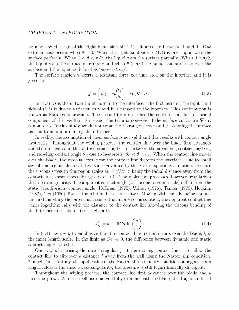
CHAPTER 1. INTRODUCTION 4
be made by the sign of the right hand–side of (1.1). It must lie between -1 and 1. Oneextreme case occurs when θ = 0. When the right hand side of (1.1) is one, liquid wets thesurface perfectly. When 0 < θ < π/2, the liquid wets the surface partially. When θ ↑ π/2,the liquid wets the surface marginally and when θ ≥ π/2 the liquid cannot spread over thesurface and the liquid is defined as ‘non–wetting ’.
The surface tension γ exerts a resultant force per unit area on the interface and it isgiven by
f =
[∇γ − n∂γ
∂n
]− n (∇ · n) . (1.3)
In (1.3), n is the outward unit normal to the interface. The first term on the right handside of (1.3) is due to variation in γ and it is tangent to the interface. This contribution isknown as Marangoni traction. The second term describes the contribution due to normalcomponent of the resultant force and this term is non–zero if the surface curvature ∇ · nis non–zero. In this study we do not treat the Marangoni traction by assuming the surfacetension to be uniform along the interface.
In reality, the assumption of clean surface is not valid and this results with contact anglehysteresis. Throughout the wiping process, the contact line over the blade first advancesand then retreats and the static contact angle is in between the advancing contact angle θAand receding contact angle θR due to hysteresis: θR < θ < θA. When the contact line movesover the blade, the viscous stress near the contact line distorts the interface. Due to smallsize of this region, the local flow is also governed by the Stokes equations of motion. Becausethe viscous stress in this region scales as ∼ ηU/r, r being the radial distance away from thecontact line, shear stress diverges as r → 0. The molecular processes, however, regularizesthis stress singularity. The apparent contact angle (at the macroscopic scale) differs from thestatic (equilibrium) contact angle. Hoffman (1975), Voinov (1976), Tanner (1979), Hocking(1983), Cox (1986) discuss the relation between the two. Moving with the advancing contactline and matching the outer meniscus to the inner viscous solution, the apparent contact linevaries logarithmically with the distance to the contact line showing the viscous bending ofthe interface and this relation is given by
θ3ap = θ3 − 9Ca ln
(y
li
). (1.4)
In (1.4), we use y to emphasize that the contact line motion occurs over the blade; li isthe inner length scale. In the limit as Ca → 0, the difference between dynamic and staticcontact angles vanishes.
One way of releasing the stress singularity at the moving contact line is to allow thecontact line to slip over a distance l away from the wall using the Navier–slip condition.Though, in this study, the application of the Navier–slip boundary conditions along a certainlength releases the shear stress singularity, the pressure is still logarithmically divergent.
Throughout the wiping process, the contact line first advances over the blade and ameniscus grows. After the cell has emerged fully from beneath the blade, the drag introduced

CHAPTER 1. INTRODUCTION 5
by the gravure land pulls that meniscus; the contact line retreats and the meniscus is printedas a tail behind the cell extending back toward the blade. Over the range of capillary numbers(Ca, based on substrate velocity) studied by Kitsomboonloha et al. (2012), tails were alwayspresent; tail length is comparable with the cell length for Ca O(1), and increases as Ca isreduced. Maximum tail width (dimension normal to substrate velocity) is comparable withcell width. As shown by Kitsomboonloha et al. (2012, figure 13), tails are manifested assmearing of printed features. Similar behavior is described by Nguyen et al. (2014) and bySecor et al. (2014).
Kitsomboonloha et al. (2012) propose that tails form owing to lateral wicking along theapparent line between the blade and substrate (when the substrate motion is in the x–direction, lateral wicking refers to wicking of liquid in the z–direction which is out of pageconsidering figure 1.1; a cross–section in the x–y plane).
The value of the advancing contact angle determines the smear volume. For Ca fixed,it attains its maximum value for a perfectly wetting fluid. Because wicking requires liquidto wet the blade, tails could, therefore, be eliminated by making the blade non–wetting. Byverifying experimentally that tails do not occur if the blade is non–wetting, Kitsomboonlohaet al. (2012) demonstrate a connection between wettability and tail formation.
It can not be concluded that wicking causes tail formation, however. Owing to small sizeof the cell, the flow is governed by the Stokes equations of motion. For a small slope interface,when the pressure gradient along the substrate balances the shear stress and pressure acrossthe streamlines is uniform, the Stokes equations of motion can be reduced to lubricationequations. If the blade is assumed to be perpendicular to the substrate, lubrication theoryholds throughout the entire liquid film if the cell is shallow, and the contact angle θ on theblade is only slightly less than π/2. By numerically solving the evolution equation describingthe unsteady film, we show that tails form in plane flow (where wicking can not occur). Weconclude that tail formation is a problem in plane Stokes flow. This conclusion leads us tothe mechanism being analyzed here.
To be able to integrate the Stokes equations of motion corresponding to the smearformation problem, we wrote a finite element based solver and have validated our solverby solving several Stokes problems and by making comparison of a lubrication model ofsmear formation problem and numerical solutions of the Stokes equations of motion for thecorresponding problem. We give the details of the numerical method and validation problemsin chapter 2.
As the leading edge of a liquid–filled cell emerges from beneath the blade, liquid rises onthe blade to satisfy the Young condition (now, of course, with θ arbitrary). From our studiesusing lubrication theory, we know that the meniscus can be taken as being pinned to theleading edge of the cell. As the cell moves away from the blade, its trailing edge eventuallyapproaches the meniscus, isolating a certain volume of liquid from the cell. This isolatedmeniscus is then deformed by the drag exerted by the moving substrate. As far as thequality of the printing application is concerned, we believe the solution involves minimizingthe quantity of liquid drawn into the meniscus. The evolution of the isolated meniscus into atail is, however, of considerable hydrodynamic interest. In § 3.2, we give a geometric analysis

CHAPTER 1. INTRODUCTION 6
of meniscus growth; this (hydrostatic) analysis describes the limit of vanishing Ca based onsubstrate speed U . The radius of curvature of the blade tip is 7.5-75 times larger than atypical cell size (Kitsomboonloha et al., 2012, Table 1). During wiping stage, the blade tipentirely fills the top of the cell acting as a lid. To avoid detail, we approximate the bladetip as horizontal to the substrate with its trailing edge face, initially, to be perpendicularto the substrate. Evidently the hydrostatic theory would be of limited interest if viscous(normal) stresses exerted by the blade caused even more liquid to be removed from thecell. In § 3.3, numerical solutions of the free boundary problem, a problem in which flowvariables and the flow domain are unknown, for the Stokes equations of motion are usedto show that the hydrostatic theory closely describes the process of meniscus formation ifCa < 10−2; moreover, as Ca is increased, less liquid is removed from the cell. Because weshow that hydrostatics provides an upper bound to the volume removed, the problem ofcontrolling tail formation now reduces to the conceptually simpler problem of reducing thesize of the meniscus. In § 3.4, we use the hydrostatic theory to explain why Kitsomboonlohaand Subramanian (2014) were able to minimize smearing by polishing the blade to reduceits tip radius.
Tail formation extending back toward the blade occurring later in stage is also ofconsiderable hydrodynamic interest. The meniscus drawn from the cell is printed as a tailbehind the cell, and this smear formation degrades the printed features at the scale of micronsize printed features. In chapter 4, we analyze the mechanism of tail formation. Meniscusdrawn from the cell is separated from the cell in the limit as Ca → 0, and that meniscussitting between blade and the trailing edge of the cell is printed as a tail: the mechanismoccurs between these two points, the cell is irrelevant.
This limit shows that the second fluid mechanics problem can be connected to two otherreal life problems. The first one is is the deposition of the tear film when we blink. Wonget al. (1996) study the deposition and thinning of the human tear film. This film covers theexposed part of the eyeball by the rise of a meniscus of the upper lid during a blink and thatmeniscus is used to coat the tear film. The second problem is the liquid entrainment fromthe meniscus of a liquid wedge during coating (Gutenev et al., 2002, Reznik et al., 2009).A film of tail shape is printed onto a horizontal substrate to be used in the deposition ofmicro–nano particle suspensions such as blood smears for histological analysis. The problemdiffers from the film drawing problem first shown by Landau and Levich (1942) because of thefinite volume meniscus. As the coating film is drawn from this meniscus, the changes in thevolume of the meniscus must be considered throughout the process. In the Landau-Levichproblem, on the other hand, a steady film of constant thickness of 1.34rCa2/3 is coated on thesubstrate far from an infinite bath where r is the radius of curvature of the static meniscusforming on the bath surface. Capillary pressure gradient and substrate motion (convection)balance to produce, asymptotically, a uniform film thickness.
Though we reduce the problem to the entrainment of a film from the meniscus of liquidwedge, this reduction is valid for the limiting case of Ca → 0 in the printed electronicsproblem. Gutenev et al. (2002) analyze the problem of film entrainment in the low capillaryregime. Reznik et al. (2009) extend it to finite Ca regime using boundary integral method.

CHAPTER 1. INTRODUCTION 7
Even in the finite Ca regime, they take the contact lines both on the blade and substrateto be pinned at all times. According to our analysis in chapter 3, even for Ca = 0.0025, thecontact line on the blade retreats due to the increased effect of drag (horizontal substratemotion). In the current problem of interest, the contact line at the trailing edge of the cellcan only be taken as pinned for Ca→ 0, and the volume under the meniscus is not arbitrary.As Ca is increased, there is leakage from meniscus into the cell; the existence of cell shouldalso be considered.
With this motivation, we analyze the problem in two different regimes. In the limit asCa → 0, the meniscus is separated from the cell and the problem has an inner and outerstructure: in the neighborhood of pinned contact line, the viscous forces are important (innerstructure); away from this inner region, viscous forces are irrelevant and this inner regionconnects to a bulk meniscus (outer structure). By solving the outer problem (§ 4.1), we firstpredict the meniscus shape in the static regime; we formulate the inner problem (§ 4.2) bymaking a local analysis near the tip (where the contact line is pinned at the trailing edge ofthe cell), and then we form the composite expansion (§ 4.3) of the inner and outer problemto show that the interface is rotated around the pinned contact line by viscosity and connectsto the static bulk meniscus away from the tip. In § 4.4, we predict that the thickness of thefilm coated away from the bulk meniscus decreases linearly in time forming a tail shape.
By matching the outer limit of the inner problem to the inner limit of the outer problem,we form a composite expansion. A comparison of composite expansion with the Stokessolution requires Ca to be small. It is computationally expensive to solve the Stokes problemat this low Ca. The computations required for the surface force integration include a factorof Ca−1 and as Ca is decreased, any numerical error in the computations multiplied byCa−1 and this requires the use of extremely small time step due to the explicit time stepintegration of the solver and this results with computationally expensive method.
In § 4.5, we solve the corresponding problem in Stokes regime for Ca = 10−3, and showthat as the angle of the interface at the tip decreases, inner viscous solution given in § 4.2agrees with the numerical solution of the Stokes problem within a region which scales as∼ 0.1 away from the tip. In §4.6, we include the cell into the computations of the Stokesproblem of tail formation.
A tail forms faster as Ca is increased. As the smear volume drawn from the cell is lessfor higher Ca regime, the tail length shortens. As Ca is reduced, however, the tail formationprocess takes longer and tail length increases with decreasing Ca first because the meniscusvolume increases as Ca is reduced, as shown in chapter 3: the limit Ca → 0 sets an upperbound to the smear volume, as a result tail formation takes longer; second the coated filmthickness scales like rCa2/3 as Ca gets smaller.
Solver’s being computationally expensive for small Ca motivates us to model the cor-responding problem in the lubrication regime. The earlier analyses are valid for arbitrarycontact angles on the blade; 0 ≤ θ < π/2. For small slope interface, on the other hand,lubrication theory is appropriate to analyze the tail formation mechanism.
In § 4.7, lubrication theory is used to model the tail formation problem. Comparisonbetween the Stokes solution and lubrication model shows that, for contact angle θ = π/3

CHAPTER 1. INTRODUCTION 8
and Ca = 10−2, the lubrication theory closely predicts the interface evolution. Becausethe contact line on the blade moves freely in the lubrication model, it over–predicts themeniscus growth stage resulting with longer tail behind the cell. As θ approaches π/2 andCa is decreased, on the other hand, the Stokes solution and lubrication model agree for themeniscus printing problem. This motivates us to analyze the smear formation mechanism byusing lubrication theory for Ca < 10−3. When Ca is O(10−8), the slope of the linear decreaseobserved in the thickness of coated film computed from the numerical solution approachesthe slope predicted in § 4.4. The composite expansion predicts the interface profile closelywhen Ca = 10−8. We also observe the inner and outer structure; the meniscus rotatesaround the tip at the trailing edge of the cell by the squeeze film flow, the film of decreasingthickness connects to a thin film region of thickness ∼ rCa2/3 (Landau-Levich film) which iscoated away from the static outer meniscus.
Finally, in §4.7.3, we consider the effect of a sequence of cells in the tail formationmechanism. We show that although smear formation is reduced between cells as the gapbetween cells is reduced, the liquid drawn from the cells accumulates under the meniscusresulting with tail formation behind the last cell in the sequence.

9
Chapter 2
Development and Testing of aNumerical Method for the StokesProblem
In gravure printing of electronics, the flow is not affected by inertial and gravitationalforces: the Reynolds number (Re = ρUL/µ) based on substrate length L < 10µm, substratespeed U < 1 mm/s and viscosity µ=29Pa.s is less than 10−6 and Weber number (We =ρUL2/γ) based on corresponding cell length, substrate speed and surface tension γ of 0.0269N/m is less than 10−5. The flow is governed by the Stokes equations of motion.
Our objective here is to analyze the smear formation problem without any complications.Because the radius of curvature r of the blade tip is large compared with a representativelength scale of the cell such as its length L, we model the blade as horizontal to the substrateand its trailing edge face, at the first attempt, to be perpendicular to the substrate motionas shown in figure 2.1. We assume the blade covers the top of the cell acting as a lid and thecell is assumed to be full of liquid when it enters under the gap between the blade and thesubstrate. As we analyze the problem in the following chapters by using the Stokes equationsof motion, in this chapter, we first formulate the corresponding Stokes problem in §2.1, andthen, give the details of the numerical method to solve the free-boundary problem in §2.2and validate the solver in §2.3.
CHAPTER 2. DEVELOPMENT AND TESTING OF A NUMERICAL METHOD FORTHE STOKES PROBLEM 10
BLADE
Ω
θ
x
y
U
S3
Ssubstrate
S1
H
T O
2
n
t B
Figure 2.1: Flow domain Ω for the Stokes problem of smearing: S1, wiper blade; S2, cellboundary; S3, free surface. Coordinate axis is fixed on wiper blade which is stationary, celltranslates with velocity Ui. T is the trailing edge, B is the leading edge of the cell and thecontact line is at H. The aspect ratio of the cell is set to L/d = 2 where L is the length ofthe cell, d is the depth of the cell.
2.1 Problem formulation
The flow domain is shown in figure 2.1: the coordinate is fixed on the exit of the stationaryblade; x-axis lies along the substrate, y-axis along the wiper blade. Nondimensionalized bythe cell length L, substrate speed U and pressure µU/L, non–dimensional stress field isdivergenceless:
∇ · σ = 0 in Ω (2.1)
where the dimensionless Newtonian stress tensor is defined by
σ = −pI +(∇u+∇uT
). (2.2)
In (2.2), p is the dimensionless pressure and u is the dimensionless velocity field. Thecontinuity equation requires that velocity field is divergenceless:
∇ · u = 0. (2.3)
The boundary of the domain Ω is S = S1∪S2∪S3 where S1 is the wiper blade surface, S2
is the moving cell boundary, S3 is the free surface which is unknown a priori. On the wiperblade surface and cell boundary; no-slip, no penetration boundary conditions are applied,except where the free surface and trailing edge of the cell meets the wiper blade:

CHAPTER 2. DEVELOPMENT AND TESTING OF A NUMERICAL METHOD FORTHE STOKES PROBLEM 11
u = 0 on S1, (2.4a)
u = i on S2. (2.4b)
On the interface the normal n is the outward pointing unit normal vector, and the corre-sponding unit tangent vector t along the interface is given by t = k × n (k is the unitnormal in z-direction which is out of page). Free surface boundary conditions are obtainedby balance of interfacial mass and momentum. Neglecting the traction on the interface dueto outside fluid (e.g. low viscosity gas) and neglecting the Marangoni traction, there is onlynormal component of the stress on the interface which is given by
n · (σ · n) = − 1
Ca∇ · n. (2.5)
In (2.5), Ca is defined by Ca = µU/γ which is a dimensionless number showing the strengthof viscous forces over surface tension forces. The contact line where the free surface meetsthe wiper blade is free to move (Point H in figure 2.1). The stress singularity at the contactline is released by applying the Navier-slip condition (Silliman and Scriven, 1978) given by
twiper · (σ · nwiper) =1
stwiper · (uslip − uwiper) (2.6)
where s is the dimensionless slip coefficient with s→ 0 recovering no-slip, s→∞ recoveringperfect–slip conditions.
We assume that the contact line is pinned at the leading edge of the cell and the movingcontact line at H meets the blade at Young angle:
tinterface · twiper = cosθ. (2.7)
If there is an effect of dynamic contact angle, it will emerge from the solution. We use thestatic solution given in § 3.2 for the free surface profile when the leading edge of the cell(point B in figure 2.1) has emerged 0.1d from the wiper blade as initial condition.
CHAPTER 2. DEVELOPMENT AND TESTING OF A NUMERICAL METHOD FORTHE STOKES PROBLEM 12
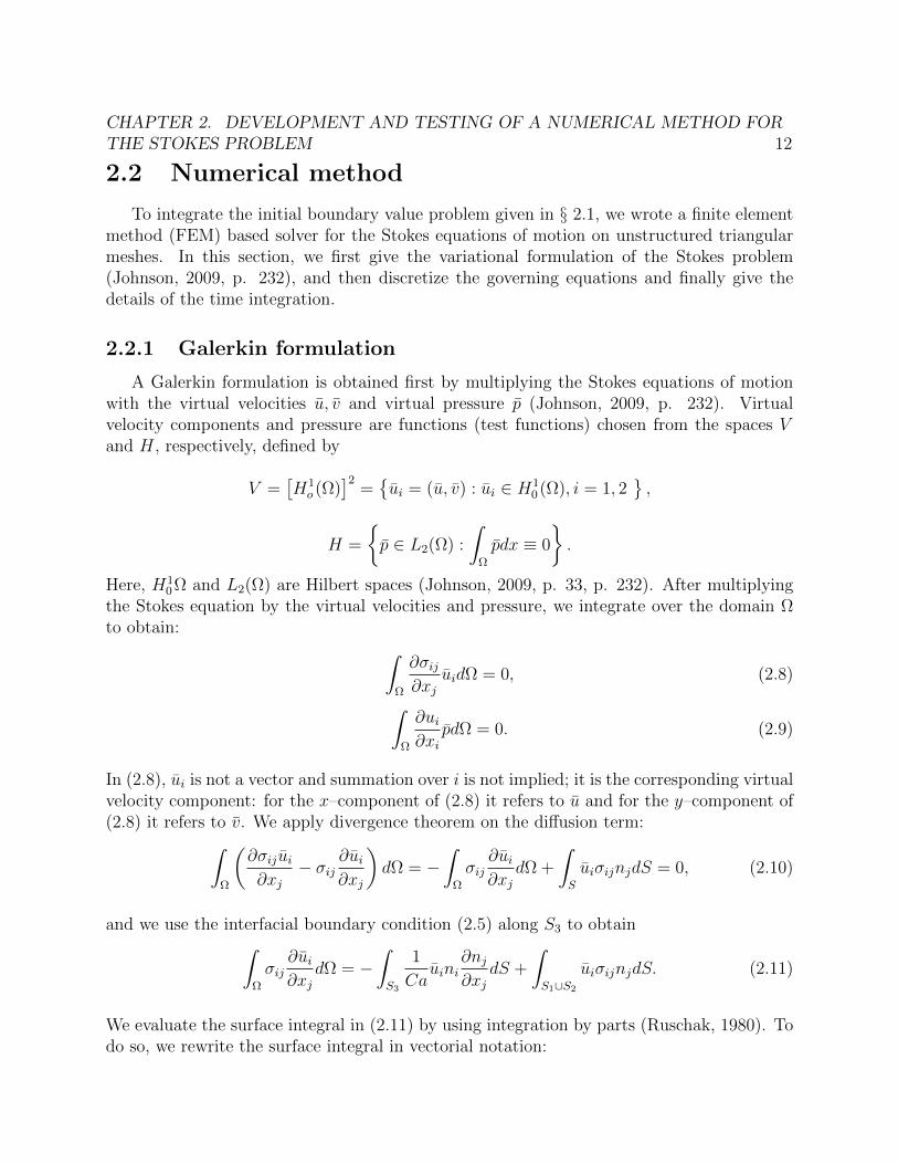
2.2 Numerical method
To integrate the initial boundary value problem given in § 2.1, we wrote a finite elementmethod (FEM) based solver for the Stokes equations of motion on unstructured triangularmeshes. In this section, we first give the variational formulation of the Stokes problem(Johnson, 2009, p. 232), and then discretize the governing equations and finally give thedetails of the time integration.
2.2.1 Galerkin formulation
A Galerkin formulation is obtained first by multiplying the Stokes equations of motionwith the virtual velocities u, v and virtual pressure p (Johnson, 2009, p. 232). Virtualvelocity components and pressure are functions (test functions) chosen from the spaces Vand H, respectively, defined by
V =[H1o (Ω)
]2=ui = (u, v) : ui ∈ H1
0 (Ω), i = 1, 2,
H =
p ∈ L2(Ω) :
∫Ω
pdx ≡ 0
.
Here, H10 Ω and L2(Ω) are Hilbert spaces (Johnson, 2009, p. 33, p. 232). After multiplying
the Stokes equation by the virtual velocities and pressure, we integrate over the domain Ωto obtain: ∫
Ω
∂σij∂xj
uidΩ = 0, (2.8)∫Ω
∂ui∂xi
pdΩ = 0. (2.9)
In (2.8), ui is not a vector and summation over i is not implied; it is the corresponding virtualvelocity component: for the x–component of (2.8) it refers to u and for the y–component of(2.8) it refers to v. We apply divergence theorem on the diffusion term:∫
Ω
(∂σijui∂xj
− σij∂ui∂xj
)dΩ = −
∫Ω
σij∂ui∂xj
dΩ +
∫S
uiσijnjdS = 0, (2.10)
and we use the interfacial boundary condition (2.5) along S3 to obtain∫Ω
σij∂ui∂xj
dΩ = −∫S3
1
Cauini
∂nj∂xj
dS +
∫S1∪S2
uiσijnjdS. (2.11)
We evaluate the surface integral in (2.11) by using integration by parts (Ruschak, 1980). Todo so, we rewrite the surface integral in vectorial notation:

CHAPTER 2. DEVELOPMENT AND TESTING OF A NUMERICAL METHOD FORTHE STOKES PROBLEM 13
∫S3
1
Caui (∇ · n)ndS =
∫S3
1
Cauidt
dsds (2.12)
where t is the unit tangent vector in the increasing s direction. Integrating by parts, weobtain: ∫
S3
1
Cauidt
dsds =
[1
Cauit
]BH
−∫ B
H
1
Catduidsds, (2.13)
where H and B are the positions of the contact lines on the solid boundaries as shown infigure 2.1. As the model problem lies in the plane, we rewrite x and y components of themomentum equation using the stress tensor definition given in (2.2):
x :
∫Ω
−p∂u∂xdΩ+
∫Ω
2∂u
∂x
∂u
∂xdΩ+
∫Ω
∂u
∂y
∂u
∂y+
∫Ω
∂u
∂y
∂v
∂xdΩ+
[1
Cautx
]BH
−∫ B
H
1
Catxdu
dsds = 0,
(2.14)
y :
∫Ω
−p∂v∂ydΩ +
∫Ω
2∂v
∂y
∂v
∂ydΩ +
∫Ω
∂v
∂x
∂v
∂x+
∫Ω
∂v
∂x
∂u
∂ydΩ +
[1
Cavty
]BH
−∫ B
H
1
Catydv
dsds = 0,
(2.15)
and the continuity equation: ∫Ω
(∂u
∂x+∂v
∂y
)pdΩ = 0. (2.16)
At the moving contact line, tx and ty are computed by the use of (2.7) to set the contactangle. We should note that the last term in (2.11) is zero when Dirichlet boundary conditionis applied along the boundary because the virtual velocities are set to zero at correspondingnodes. However, when we apply the slip boundary condition along the distance l, we addthat integral to the corresponding x, y component of the equation (2.14),(2.15) with the useof slip boundary condition. In the model geometry shown in figure 2.1, this occurs at the freesurface and blade intersection (point H), and at the intersection of blade and trailing edgeof the cell (point T ) and blade and substrate intersection (point O) after the cell emergesfully from beneath the blade. With the use of (2.6), we add these two surface integrals to(2.14) and (2.15), respectively:
x : +
∫S1(slip)
1
suudS, (2.17)
y : +
∫S1(slip)
1
svvdS. (2.18)
This ends the Galerkin formulation of the problem.

CHAPTER 2. DEVELOPMENT AND TESTING OF A NUMERICAL METHOD FORTHE STOKES PROBLEM 14
2.2.2 Discretization
We use P2 − P1 isoparametric triangular elements (Bathe, 1996, figure 5.11) for thesolution variables: Figure 2.2 shows a representative element in the isoparametric domainwith the numbers of the nodes. The velocity components are represented by the values atthe six nodes per element (1 to 6 in figure 2.2) and interpolated using quadratic polynomials(P2 element), pressure is represented by the three corner nodes (1 to 3 in figure 2.2) andinterpolated using linear polynomial (P1 element). This choice of element satisfies theLadyzhenskaya-Babushka-Brezzi stability condition (Johnson, 2009, p. 232).
1
2
3
4
56
s
r
Figure 2.2: Nodal points in the isoparametric plane: 1 to 6 is used for P2 element, 1 to 3 isused for P1 element.
The quadratic interpolation for the velocity components are defined as follows (with rand s defined in figure 2.2):
hq1(r, s) = 1− 3r − 3s+ 2r2 + 4rs+ 2s2, (2.19a)
hq2(r, s) = −r + 2r2, (2.19b)
hq3(r, s) = −s+ 2s2, (2.19c)
hq4(r, s) = 4r − 4rs− 4r2, (2.19d)
hq5(r, s) = 4rs, (2.19e)
hq6(r, s) = 4s− 4rs− 4s2. (2.19f)
Similarly, the linear functions used for the pressure are given by
hl1(r, s) = 1− r − s, (2.20a)
hl2(r, s) = r, (2.20b)
hl3(r, s) = s. (2.20c)

CHAPTER 2. DEVELOPMENT AND TESTING OF A NUMERICAL METHOD FORTHE STOKES PROBLEM 15
We approximate the velocity components and pressure in the isoparametric plane asfollows:
u(r, s) =6∑i=1
hqiui, (2.21)
v(r, s) =6∑i=1
hqivi, (2.22)
p(r, s) =3∑i=1
hlipi. (2.23)
Here hqi , hli are quadratic and linear interpolations; ui, vi and pi are the corresponding nodal
values. Subscripts denote the nodal points shown in figure 2.2.The unit tangent vector in the xOy is computed by
t =
∑3i=1 si
dhqids∥∥∥∑3
i=1 sidhqids
∥∥∥ (2.24)
with si being nodal position vector and dhqi/ds being scalar corresponding to the elementedge over which the computation is carried out. The normal component is found simply byn = k × t.
The coordinates are interpolated with the quadratic interpolation functions:
x(r, s) =6∑i=1
hqixi, (2.25)
y(r, s) =6∑i=1
hqiyi, (2.26)
where xi and yi are the coordinates of the node points in the element and hqi is definedin (2.19). Because the computations are performed in the isoparametric domain, we needto express the mapping for the derivatives from the xOy plane to the isoparametric plane,which is given by ∂
∂x
∂∂y
= J−1
∂∂r
∂∂s
. (2.27)
Jacobian (J) of the transformation in (2.27) is given by

CHAPTER 2. DEVELOPMENT AND TESTING OF A NUMERICAL METHOD FORTHE STOKES PROBLEM 16
J =
∂x∂r ∂y∂r
∂x∂s
∂y∂s
. (2.28)
We use Gauss quadrature to carry out the integrations. Plane integrations are evaluatedover triangles using 7–point Gauss integration rule (Bathe, 1996, §5.5.4 and 5.5.5). r ands are evaluated at the Gauss points of integration over triangles. Boundary integrals areevaluated using 3–point Gauss integration rule (Bathe, 1996, §5.5.3). In both cases, theGauss quadrature integrates exactly polynomials of order at most 5. The highest orderpolynomial in the integrations is 4, therefore the integrations are exact throughout thenumerical method.
After forming the element matrix Ak and right hand side vector Rk over each elementek for the unknowns by using (2.14) to (2.16), we form a global stiffness matrix A, andright hand side vector R. We impose constraints on certain solution variables with theuse of Lagrange multiplier method: we extend the solution vector by adding the Lagrangemultipliers λ for the constraints and extending the system of equations toA nTi
ni 0
uλ
=
Ru∗i
(2.29)
where ni is a vector with all entries equal to zero, but its ith entry which is equal to 1, u∗iis the imposed constraint at node i. The unstructured mesh is generated using the methodsexplained by Persson (2004), Persson and Strang (2004).
2.2.3 Time integration
The Stokes equations are quasi-steady, it is the moving boundaries that introduce timedependence.
Mass conservation along the interface requires that no fluid can cross it and the conditionis given by the kinematic boundary condition:
n · (u− s) = 0, (2.30)
where s is the velocity of a material point along the free surface.Time integration is performed explicitly: at time t, the linear Stokes problem is solved
using the boundaries determined at the previous time t−∆t; boundaries are then displacedin the normal direction to the interface using the velocity field from the same time t −∆t.Because this method is explicit, we restrict the magnitude of ∆t using a Courant condition:∆t < c∆x/u where ∆x is the minimum edge length in the mesh and u is the maximumvelocity. We take c < 1/4. To maintain resolution, the quality of the mesh was checkedregularly to refine the mesh; between refinements, the mesh was simply displaced from one
CHAPTER 2. DEVELOPMENT AND TESTING OF A NUMERICAL METHOD FORTHE STOKES PROBLEM 17
time step to the next using the local fluid velocity. The mesh is dynamic so the number ofelements varies throughout the integration. Generally, we use approximately 1000 elementsdistributed non-uniformly over the domain. During mesh movement and remeshing, themass of liquid must remain constant in the model problem for smear formation. In thecorresponding computations, mass is conserved to within an error of 0.01%.
2.3 Validation of the solver
Before solving model problem for smear formation in chapters 3 and 4, the method wastested against problems in plane Stokes flow having explicit solutions: biharmonic problemssuch as flow through a slit (Green, 1944), the problem of over–damped capillary-wave, andstick–slip problem (Richardson, 1970) describing a free jet emerging from a slit in a thickwall. Apart form these problems, we also compare the numerical solution of the Stokesequations of motion for the smear formation problem with the corresponding lubricationmodel in chapter 4.
2.3.1 Flow through a slit
x
y
a/2-a/2
S4
S2S1 S3
ν=π/2
μ=1
μ=2
μ=0 ν=0
ν=2π
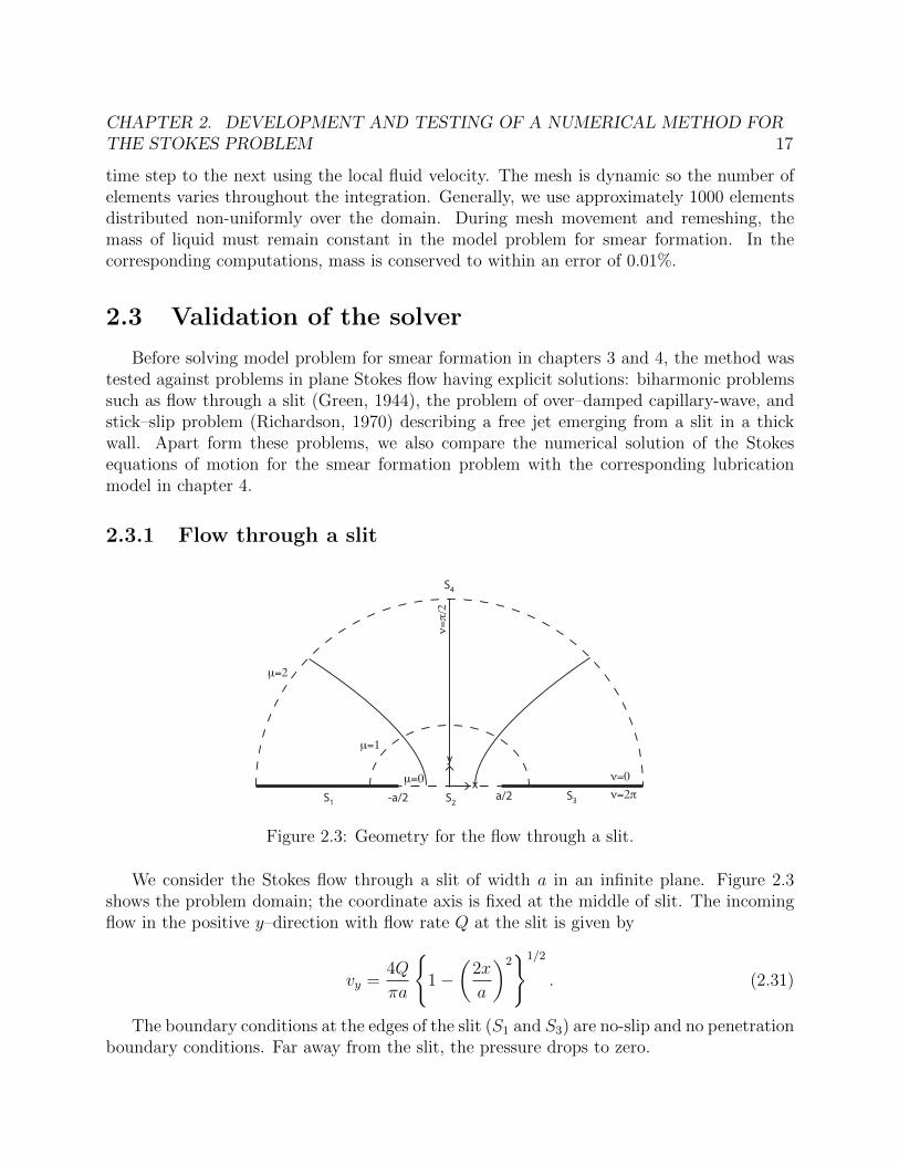
Figure 2.3: Geometry for the flow through a slit.
We consider the Stokes flow through a slit of width a in an infinite plane. Figure 2.3shows the problem domain; the coordinate axis is fixed at the middle of slit. The incomingflow in the positive y–direction with flow rate Q at the slit is given by
vy =4Q
πa
1−
(2x
a
)21/2
. (2.31)
The boundary conditions at the edges of the slit (S1 and S3) are no-slip and no penetrationboundary conditions. Far away from the slit, the pressure drops to zero.
CHAPTER 2. DEVELOPMENT AND TESTING OF A NUMERICAL METHOD FORTHE STOKES PROBLEM 18
According Green (1944), solution to the boundary value problem is that the streamlinesare hyperbolas with foci at x = ±1/2a. We first introduce the elliptic cylindrical coordinates(µ, ν) that we have used. Note that in this subsection (µ, ν) are unrelated to viscosity. Thecurve µ=const. is the ellipse
x2
a2cosh2µ+
y2
a2sinh2µ=
1
4. (2.32)
The curve ν=const. is the hyperbola
x2
a2cos2ν− y2
a2sin2ν=
1
4. (2.33)
The mapping from elliptic coordinates to Cartesian coordinates is given by
x =a
2coshµ cosν, (2.34a)
y =a
2sinhµ sinν. (2.34b)
We use the mapping (2.34a,b) in the numerical solution because the solver is written inCartesian coordinates. According to Green (1944), the velocity filed is given by
vµ =4Q
πa
sin2ν(sinh2µ+ sin2ν
)1/2, vν = 0, (2.35)
and the pressure distribution is given by
p =8ηQ
πa2
(2− sinh2µ
sinh2µ+ sin2ν
), (2.36)
where η is the dynamic viscosity, Q is the flow rate through the slit. Note that p → 0 asµ→∞. As shown in figure 2.3, through the slit, µ = 0 and ν varies between 0 and π.
We solve the corresponding Stokes problem on the domain shown in figure 2.3. For theouter boundary S4 we choose the ellipse with µ = 2: on this surface we impose as boundaryconditions the velocity and pressure given by the exact solution (2.35), (2.36), by settinga = 1 and µ = 2. On the slit (S2), vertical velocity is set to (2.31) and u = 0 and weapply no–slip, no penetration boundary conditions on the walls (S1 and S3). We use 2300triangular elements.
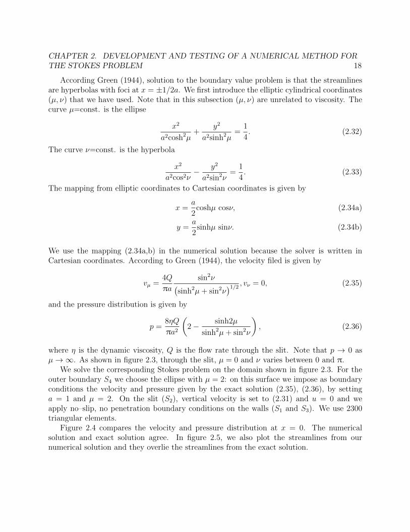
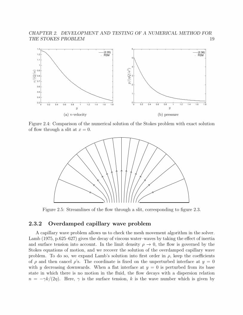
Figure 2.4 compares the velocity and pressure distribution at x = 0. The numericalsolution and exact solution agree. In figure 2.5, we also plot the streamlines from ournumerical solution and they overlie the streamlines from the exact solution.
CHAPTER 2. DEVELOPMENT AND TESTING OF A NUMERICAL METHOD FORTHE STOKES PROBLEM 19
y0 0.2 0.4 0.6 0.8 1 1.2 1.4 1.6 1.8
v/(Q/a
)
0.3
0.4
0.5
0.6
0.7
0.8
0.9
1
1.1
1.2
1.3
(2.35)FEM
(a) v-velocity
y0 0.2 0.4 0.6 0.8 1 1.2 1.4 1.6 1.8
p/(ηQ/a2)
0
1
2
3
4
5
6
(2.36)FEM
(b) pressure
Figure 2.4: Comparison of the numerical solution of the Stokes problem with exact solutionof flow through a slit at x = 0.
Figure 2.5: Streamlines of the flow through a slit, corresponding to figure 2.3.
2.3.2 Overdamped capillary wave problem
A capillary wave problem allows us to check the mesh movement algorithm in the solver.Lamb (1975, p.625–627) gives the decay of viscous water–waves by taking the effect of inertiaand surface tension into account. In the limit density ρ → 0, the flow is governed by theStokes equations of motion, and we recover the solution of the overdamped capillary waveproblem. To do so, we expand Lamb’s solution into first order in ρ, keep the coefficientsof ρ and then cancel ρ’s. The coordinate is fixed on the unperturbed interface at y = 0with y decreasing downwards. When a flat interface at y = 0 is perturbed from its basestate in which there is no motion in the fluid, the flow decays with a dispersion relationn = −γk/(2η). Here, γ is the surface tension, k is the wave number which is given by
CHAPTER 2. DEVELOPMENT AND TESTING OF A NUMERICAL METHOD FORTHE STOKES PROBLEM 20
(-0.25,0) (0.75,0)
(0.75,-0.5)(-0.25,-0.5)
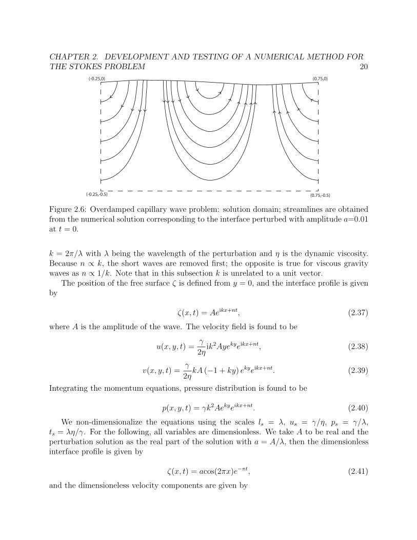
Figure 2.6: Overdamped capillary wave problem: solution domain; streamlines are obtainedfrom the numerical solution corresponding to the interface perturbed with amplitude a=0.01at t = 0.
k = 2π/λ with λ being the wavelength of the perturbation and η is the dynamic viscosity.Because n ∝ k, the short waves are removed first; the opposite is true for viscous gravitywaves as n ∝ 1/k. Note that in this subsection k is unrelated to a unit vector.
The position of the free surface ζ is defined from y = 0, and the interface profile is givenby
ζ(x, t) = Aeikx+nt, (2.37)
where A is the amplitude of the wave. The velocity field is found to be
u(x, y, t) =γ
2ηik2Ayekyeikx+nt, (2.38)
v(x, y, t) =γ
2ηkA (−1 + ky) ekyeikx+nt. (2.39)
Integrating the momentum equations, pressure distribution is found to be
p(x, y, t) = γk2Aekyeikx+nt. (2.40)
We non-dimensionalize the equations using the scales ls = λ, us = γ/η, ps = γ/λ,ts = λη/γ. For the following, all variables are dimensionless. We take A to be real and theperturbation solution as the real part of the solution with a = A/λ, then the dimensionlessinterface profile is given by
ζ(x, t) = acos(2πx)e−πt, (2.41)
and the dimensioneless velocity components are given by

CHAPTER 2. DEVELOPMENT AND TESTING OF A NUMERICAL METHOD FORTHE STOKES PROBLEM 21
x
-0.2 -0.1 0 0.1 0.2 0.3 0.4 0.5 0.6 0.7
103v
-4
-3
-2
-1
0
1
2
3
4
FEM
Pert.
(a) v-velocity
x
-0.2 -0.1 0 0.1 0.2 0.3 0.4 0.5 0.6 0.7
105u
-1
-0.8
-0.6
-0.4
-0.2
0
0.2
0.4
0.6
0.8
1
(b) u-velocity
Figure 2.7: Comparison of numerical solution of the Stokes problem with the exact solutionof overdamped capillary–wave problem: (a) v–velocity on free surface at t = 0, 2–norm ofthe difference is 3.0525e-6, (b) Comparison of the Stokes solution and perturbation solution:u–velocity on free surface at t = 0, 2–norm of the difference is 2.3769e-05. See text forthe discussion on the discrepancy in u-velocity and the definition of the 2–norm is given in(2.35).
u(x, y, t) = −2π2aye2πysin(2πx)e−πt, (2.42)
v(x, y, t) = πa(−1 + 2πy)e2πycos(2πx)e−πt. (2.43)
The corresponding dimensionless pressure distribution is given by
p(x, y, t) = 4π2ae2πycos(2πx)e−πt. (2.44)
To test the solver, we use the problem domain shown in figure 2.6. We set the wavelength tounity and depth to 0.5. We use non–uniform mesh with finer mesh close to the free surfacewith a total of 994 triangular elements. We set the velocity distribution along the boundaryexcept the free surface from the perturbation solution as boundary condition. Initially, fora small amplitude perturbation, we set a to 10−3. In figure 2.7a,b we compare, on the freesurface, the v and u–velocities respectively. The two norm of the error (defined in (2.45)) isorder 10−5. The discrepancy observed in the u–velocity, although the solution predicts thecorrect wave pattern, is due to the perturbation analysis in which zero shear stress conditionis applied at y=0. A rough computation of the shear stress from the perturbation solutionat the interface gives that shear is of order 10−4 for the maximum amplitude. Therefore, anyerror of order 10−4 or smaller in the resulting solution is expected.

CHAPTER 2. DEVELOPMENT AND TESTING OF A NUMERICAL METHOD FORTHE STOKES PROBLEM 22
x-0.2 -0.1 0 0.1 0.2 0.3 0.4 0.5 0.6 0.7
ve
locity c
om
po
ne
nts
at
y=
-0.2
5×10
-3
-2
-1.5
-1
-0.5
0
0.5
1
1.5
2
FEMPerturbation
u
v
Figure 2.8: Comparison of the numerical solution of the Stokes problem and perturbationsolution of the overdamped capillary–wave problem: x and y–velocity at the mid of thedomain at t = 0; 2-norm of the difference in u is 1.0259e-5 and in v is 1.1537e-05.
We also compare the solutions at the middle of the domain, y=-.25 in figure 2.8 whichshows good agreement with the perturbation solution.
We now increase the amplitude of the perturbation 10 times and check the time evolutionby plotting the free surface profiles at various times for a = 10−2 and compare with theperturbation solution in figure 2.9, plot the pressure distribution in figure 2.10. All resultsagree with the perturbation solution.

CHAPTER 2. DEVELOPMENT AND TESTING OF A NUMERICAL METHOD FORTHE STOKES PROBLEM 23
x
-0.2 -0.1 0 0.1 0.2 0.3 0.4 0.5 0.6 0.7
y
-0.01
-0.008
-0.006
-0.004
-0.002
0
0.002
0.004
0.006
0.008
0.01
FEM
Perturbationinitialt=0.1
t=0.2
t=0.4
Figure 2.9: Comparison of the numerical solution of the Stokes problem and perturbationsolution of the overdamped capillary–wave problem: evolution of the interface.

CHAPTER 2. DEVELOPMENT AND TESTING OF A NUMERICAL METHOD FORTHE STOKES PROBLEM 24
x
-0.2 -0.1 0 0.1 0.2 0.3 0.4 0.5 0.6 0.7
p(ζ,t=
0.1)
-0.4
-0.3
-0.2
-0.1
0
0.1
0.2
0.3
0.4
0.5
FEM
Perturbation
Figure 2.10: Comparison of the numerical solution of the Stokes problem and perturbationsolution of the overdamped capillary–wave problem: pressure on interface at t = 0.1.

CHAPTER 2. DEVELOPMENT AND TESTING OF A NUMERICAL METHOD FORTHE STOKES PROBLEM 25
2.3.3 Stick–slip problem
Richardson (1970) gives the exact solution of the stick–slip problem which is a flow of aNewtonian fluid emerging between parallel plates in plane. The problem includes a stresssingularity at the exit of the top plate (x=0,y=1) as shown in figure 2.11. The singularityarises from the change from a no-slip boundary condition to a perfect slip boundary condition.The velocity around the singularity varies like r1/2, r being the radial distance from thesingular point, therefore the stress varies like ∼ r−1/2.
x
y
u=v=0
t(σn)=0,v=0
t(σn)=0,v=0
n(σn)=0
v=0u=1.5(1-y2)
v=0
-3 3
1
0
Figure 2.11: Stick–slip problem domain.
Though we do not resolve singularity there, by solving this problem, we show that oursolver predicts the velocity distribution on the free surface correctly.
The free surface for x > 0 is replaced by a plane on which the shear stress vanishes. Wesolve the problem for the half domain; symmetry boundary conditions are imposed on thecenterline. At the inlet, parabolic velocity profile; at the outlet plug flow are imposed. Forx < 0, y = 1 no–slip, no penetration; for x > 0, y = 1 slip boundary conditions are imposed.Figure 2.12 compares the centerline and slip plane velocity with Richardson solution. Figure2.13 shows comparison of the centerline pressure as well.
Lastly, we show the convergence of the method for two different error definitions: L2 andL∞ norm errors. L2 norm of a vector u is defined by
||u||2 =
√∑i
|ui|2, (2.45)
and L∞ norm of a vector u is defined by
||u||∞ = max (|ui|) . (2.46)
We note that u in (2.45) and (2.46) is unrelates to the velocity field. The convergence ofthe method is shown in figure 2.14. With h being the largest edge of the element, the errorsin u and in p scale respectively as h3 and h2. This is expected because pressure is interpolatedusing a polynomial with one degree less than the velocity integration polynomial.
After validating the Stokes solver, we use it to analyze the smear formation problem inChapters 3 and 4.

CHAPTER 2. DEVELOPMENT AND TESTING OF A NUMERICAL METHOD FORTHE STOKES PROBLEM 26
x-2.5 -2 -1.5 -1 -0.5 0 0.5 1 1.5 2 2.5
u
0
0.5
1
1.5
FEM, u(x,0)Richardson, u(x,0)FEM, u(x,1)Richardson, u(x,1)
Figure 2.12: Comparison of the numerical solution of the Stokes problem and Richardsonsolution for stick–slip problem: centerline and slip plane u-velocity.

CHAPTER 2. DEVELOPMENT AND TESTING OF A NUMERICAL METHOD FORTHE STOKES PROBLEM 27
x-2 -1.5 -1 -0.5 0 0.5 1 1.5 2
p(x
,0)
-1
0
1
2
3
4
5
6
7
FEM
Richardson
Figure 2.13: Comparison of the numerical solution of the Stokes problem and Richardsonsolution for stick–slip problem: centerline pressure.

CHAPTER 2. DEVELOPMENT AND TESTING OF A NUMERICAL METHOD FORTHE STOKES PROBLEM 28
h
0.05 0.1 0.15 0.2 0.25 0.3
error
10-3
10-2
10-1
100
L2(error
u)
L∞
(erroru)
L2(error
p)
s=1.72
s=2.89
s=2.01
s=2.94
L∞
(errorp)
Figure 2.14: Convergence of the method: convergence is given both in terms of infinityand 2-norm errors for pressure and u-velocity (error is obtained by taking the norm of thedifference between computed and correct solution), h is the element size, s is the slope.
29
Chapter 3
Meniscus Growth During Wiping
Cells filled with ink upstream are wiped by doctor blade to remove the excess ink fromthe land. As a cell translates beneath the wiper blade, some liquid is drawn from the celland rises over the blade to satisfy the contact angle condition. In the experiments, the wiperis a carbon steel blade having roughness comparable with the cell depth (Kitsomboonlohaand Subramanian, 2014, Kitsomboonloha et al., 2012). The radius of curvature of blade tipis 7.5 to 75 times larger than a typical cell size of length 1-10µm. Figure 3.1 shows thegeometry of the model. In the model, we have left out certain complications. For example,all surfaces are depicted as planes, except where cells have been etched. The blade coversupper left quadrant of x − y plane, the coordinate axis is fixed at the trailing edge of thestationary blade. We assume that the cell is filled fully with ink, we also do not explicitlyaccount for liquid flow in the thin gap between the stationary wiper blade and the movingsubstrate. According to Kitsomboonloha and Subramanian (2014), at low speeds, liquid inthe gap contributes only about 1% of the total volume flow rate Ud at the trailing edge ofthe cell where U is the substrate speed, d is the cell depth. This simplification allows us tomodel the problem without including the thin coating film downstream: the contact line ispinned at the leading edge of the cell.
The flow is not affected by inertial and gravitational forces: the Reynolds number (Re =ρUL/µ) is less than 10−6, the Weber number (We = ρU2L/γ) is less than 10−5 and the Bondnumber (Bo = ρgL2/γ) is less than 10−8. The flow is governed by the Stokes equations ofmotion.
In this chapter, we first analyze the problem in the limit of vanishing capillary number(Ca based on substrate speed U) to predict the smear volume. We, then, solve correspondingStokes problem by using the methods of chapter 2 for a range of Ca numbers and show thathydrostatics sets an upper bound on the smear volume. Finally, we investigate the effect ofblade orientation.

CHAPTER 3. MENISCUS GROWTH DURING WIPING 30
BLADE
Ω
θ
x
y
U
S3
Ssubstrate
S1
H
T O
2
Figure 3.1: Flow domain Ω for the Stokes problem of smearing: S1, wiper blade; S2, cellboundary; S3, free surface. Wiper blade is stationary, cell translates with velocity Ui.
3.1 Analysis as Ca→ 0
In this section we make an analysis in the limit as Ca → 0 to show that the interfacegrows as circular arc while emerging from beneath the wiper blade. Non-dimensionalized bythe length scale ls = d, pressure scale ps = γ/d and velocity scale us = U where d is thecell depth, γ is the surface tension and U is the substrate speed; dimensionless stress field isdivergenceless:
∇ · σ = 0. (3.1)
Non-dimensional Newtonian stress-tensor is given by
σ = −pI + Ca(∇u+∇uT
). (3.2)
In equation (3.2), capillary number is defined as Ca = ηU/γ with η being dynamic viscosity.p is the dimensionless pressure field and u is the dimensionless velocity field. Continuityequation requires that velocity field is divergenceless:
∇ · u = 0. (3.3)
Boundary conditions are given in § 2.1. The scales used in this section differs from § 2.1,though. Therefore, the normal component of the stress on the interface is different from(2.5). The interfacial boundary condition, now, is given by
CHAPTER 3. MENISCUS GROWTH DURING WIPING 31
n · (σ · n) = −∇ · n. (3.4)
By defining the interface height as ζ(x) measured from substrate level, we can write theoutwatd unit normal on the interface by
n =∇ (y − ζ(x))
|∇ (y − ζ(x)) |=ey − exζx(1 + ζ2
x)1/2, (3.5)
and the curvature term is found to be
∇ · n =1− ζxx(1 + ζ2
x). (3.6)
By using (3.2) and (3.6), we can rewrite the interfacial boundary condition (3.4) as
p+ 2Ca
(∂u
∂y+∂v
∂x
)ζx
1 + ζ2x
+ 2Ca∂u
∂x
1− ζ2x
1 + ζ2x
= − ζxx
(1 + ζ2x)3/2
. (3.7)
The contact line is pinned at the leading edge of the cell, and free to move where the freesurface meets the wiper blade. Although, as discussed by Cox (1986), when the contact lineadvances over the wiper blade, the apparent contact angle is a flow property, the differencebetween the apparent contact angle and static (advancing) angle vanishes as the cube rootof the Ca based on the contact line velocity, so we assume contact angle at the moving lineover the wiper blade remains at its pre-defined static value given by
tinterface · twiper = cosθ. (3.8)
In the limit as Ca → 0, dp/dx = 0 from (3.2). By taking the x–derivative of (3.7) andintegrating for the free surface profile, we find the free surface profile ζ(x), to a firstapproximation, to be a circular arc which is pinned at the leading edge of the cell andsatisfying the contact angle condition (3.8) on the wiper blade. The shape of the interfaceis decoupled from the flow beneath itself; the meniscus grows as a circular arc. Now, wediscuss the hydrostatic stage.
3.2 Hydrostatic limit when Ca→ 0
After showing that the interface grows as a circular arc while emerging from beneath theblade, in this section we analyze the hydrostatic limit, show that the contact line rises overthe blade with a constant speed and predict the smear volume at the end of meniscus growthstage.
CHAPTER 3. MENISCUS GROWTH DURING WIPING 32
T T
O
A
M
B
H
C
y y
x x
r
r
B
θ
α θ
O
(a) (b)
β
BLADEBLADE
substrate substrate
Figure 3.2: Cell translating rightwards beneath a stationary blade occupying the secondquadrant of the xOy plane: (a) cell emerging; (b) cell fully emerged. See text for discussion.
Figure 3.2 shows the geometry of the model; emerging and fully emerged cells are shownto emphasize that the analysis covers the evolution from the first state to the second. Thecoordinate system xOy is orthogonal, with x–axis along the surface of the substrate; βdenotes the angle between the blade and the y–axis. Except in § 3.4, β = π/2. We assumethe meniscus to be pinned at the leading edge B of the cell.
In the limit as Ca → 0, viscous stress is negligibly small until the interface approachesthe substrate at T . Until that occurs, liquid pressure is uniform, and the meniscus is acircular arc HMB. Point A is the intersection of this arc with OB; CM is perpendicular toOB. Arc HMB has three degrees of freedom: its radius r, and the coordinates of its centreC. These variables are determined by the following conditions: because liquid that has risenabove line OB has been removed from the cell, the areas shaded in figure 3.2a are equal; thearc passes through B; and it cuts the y–axis at a given angle θ (Young angle).
The area of the shaded curvilinear triangle OAH is given by
|OAH| = 14r24 cosα cos θ − sin 2α− sin 2θ − π + 2(α + θ) ; (3.9)
as shown in figure 3.2a, α is the angle at which arc AMB cuts the x–axis at A. The area ofthe shaded lens AMB formed by the chord AB and the circular arc below AB is given by
|AMB| = 12r2(2α− sin 2α). (3.10)
Equating areas, then simplifying, we obtain
4 cosα cos θ + sin 2α = sin 2θ + π + 2(α− θ). (3.11)
Equation (3.11) holds until the trailing edge (point T in figure 3.2a) approaches the interface.From (3.11), we see that α is uniquely determined by the value of θ and so does not vary
as the cell emerges. As θ is increased from zero to π/2, α decreases monotonically from 0.568(about 33) to zero. In particular, (3.11) admits the solution α = θ = 0.482 (about 28).
CHAPTER 3. MENISCUS GROWTH DURING WIPING 33
From the geometry of figure 3.2, the arc radius r is given in terms of |OB| = b, α and θby
b = r(cos θ + sinα). (3.12)
Further, because |OH| = h = r(cosα− sin θ),
h = bcosα− sin θ
cos θ + sinα. (3.13)
Because α is fixed by (3.11), both the radius r of the meniscus, and its height h, areproportional to distance b of the leading edge of the cell from the blade. In particular,the meniscus rises with constant velocity until the interface approaches the substrate. Wenote that, although viscosity is locally important near the advancing contact line, its effectthere is, merely, to distort the interface locally, and so to produce the dynamic contact angle.That effect is irrelevant here; we are assuming that, in the limit as Ca → 0, the differencebetween the dynamic and static angles vanishes, as discussed by Hoffman (1975).
Viscous stress becomes essential to the process when the interface approaches the sub-strate. This can occur either if the trailing edge T of the cell approaches the interface (pointsA and T coincide), or at the bottom of the cell (point M approaches the cell bottom). Inthe first case, the hydrostatic stage ends when |AB| is equal to the cell length L. Because,from the geometry of figure 3.2a, |AB| = 2r sinα, the radius r1 at the end of hydrostaticstage is given by r1 = L/(2 sinα). In the second case, the hydrostatic stage ends when thedistance of point M to OB is equal to the cell depth d: r − r cosα = d. The correspondingvalue r2 of the radius is r2 = d/(1− cosα).
Cell aspect ratio L/d determines which case is relevant. As the cell emerges, r increasesfrom zero and the hydrostatic stage ends when r is equal to the smaller of r1 and r2.Comparing the expressions for r1 and r2, we find that r1 < r2 if
L/d < 2 cot(12α). (3.14)
For perfect wetting (θ = 0), (3.14) corresponds to L/d < 6.84. For marginal wetting (θ →π/2), and α → 0: for this system, the hydrostatic stage ends when the trailing edge of thecell approaches the interface, even for a very long shallow cell. In the Kitsomboonloha et al.(2012) experiments, the cells are square in planform, with L/d = 2. Because this is withinthe range defined by (3.14), we now consider only the first case.
As a result of the trailing edge approaching the interface, liquid between O and A isisolated from the cell. We conclude that the amount of liquid removed from the cell isdetermined by hydrostatics, whereas viscosity will be important in determining how thatfixed amount of liquid is smeared over the substrate. The mechanism producing tails operatessolely between points O and A; the cell plays no further part.
The area A∗ removed from the cell of length L is given by (3.10), with r = r1:
A∗ = L2 2α− sin 2α
8 sin2 α. (3.15)
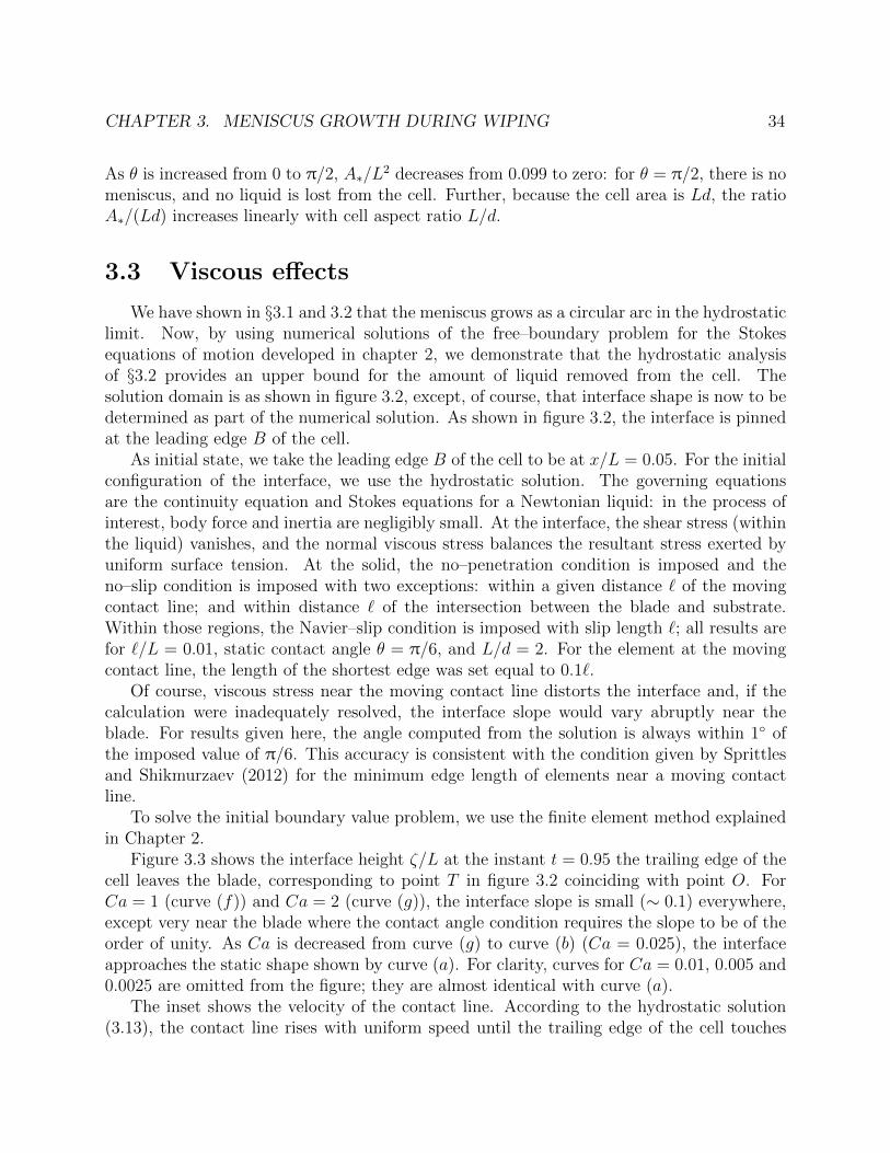
CHAPTER 3. MENISCUS GROWTH DURING WIPING 34
As θ is increased from 0 to π/2, A∗/L2 decreases from 0.099 to zero: for θ = π/2, there is no
meniscus, and no liquid is lost from the cell. Further, because the cell area is Ld, the ratioA∗/(Ld) increases linearly with cell aspect ratio L/d.
3.3 Viscous effects
We have shown in §3.1 and 3.2 that the meniscus grows as a circular arc in the hydrostaticlimit. Now, by using numerical solutions of the free–boundary problem for the Stokesequations of motion developed in chapter 2, we demonstrate that the hydrostatic analysisof §3.2 provides an upper bound for the amount of liquid removed from the cell. Thesolution domain is as shown in figure 3.2, except, of course, that interface shape is now to bedetermined as part of the numerical solution. As shown in figure 3.2, the interface is pinnedat the leading edge B of the cell.
As initial state, we take the leading edge B of the cell to be at x/L = 0.05. For the initialconfiguration of the interface, we use the hydrostatic solution. The governing equationsare the continuity equation and Stokes equations for a Newtonian liquid: in the process ofinterest, body force and inertia are negligibly small. At the interface, the shear stress (withinthe liquid) vanishes, and the normal viscous stress balances the resultant stress exerted byuniform surface tension. At the solid, the no–penetration condition is imposed and theno–slip condition is imposed with two exceptions: within a given distance ` of the movingcontact line; and within distance ` of the intersection between the blade and substrate.Within those regions, the Navier–slip condition is imposed with slip length `; all results arefor `/L = 0.01, static contact angle θ = π/6, and L/d = 2. For the element at the movingcontact line, the length of the shortest edge was set equal to 0.1`.
Of course, viscous stress near the moving contact line distorts the interface and, if thecalculation were inadequately resolved, the interface slope would vary abruptly near theblade. For results given here, the angle computed from the solution is always within 1 ofthe imposed value of π/6. This accuracy is consistent with the condition given by Sprittlesand Shikmurzaev (2012) for the minimum edge length of elements near a moving contactline.
To solve the initial boundary value problem, we use the finite element method explainedin Chapter 2.
Figure 3.3 shows the interface height ζ/L at the instant t = 0.95 the trailing edge of thecell leaves the blade, corresponding to point T in figure 3.2 coinciding with point O. ForCa = 1 (curve (f)) and Ca = 2 (curve (g)), the interface slope is small (∼ 0.1) everywhere,except very near the blade where the contact angle condition requires the slope to be of theorder of unity. As Ca is decreased from curve (g) to curve (b) (Ca = 0.025), the interfaceapproaches the static shape shown by curve (a). For clarity, curves for Ca = 0.01, 0.005 and0.0025 are omitted from the figure; they are almost identical with curve (a).
The inset shows the velocity of the contact line. According to the hydrostatic solution(3.13), the contact line rises with uniform speed until the trailing edge of the cell touches
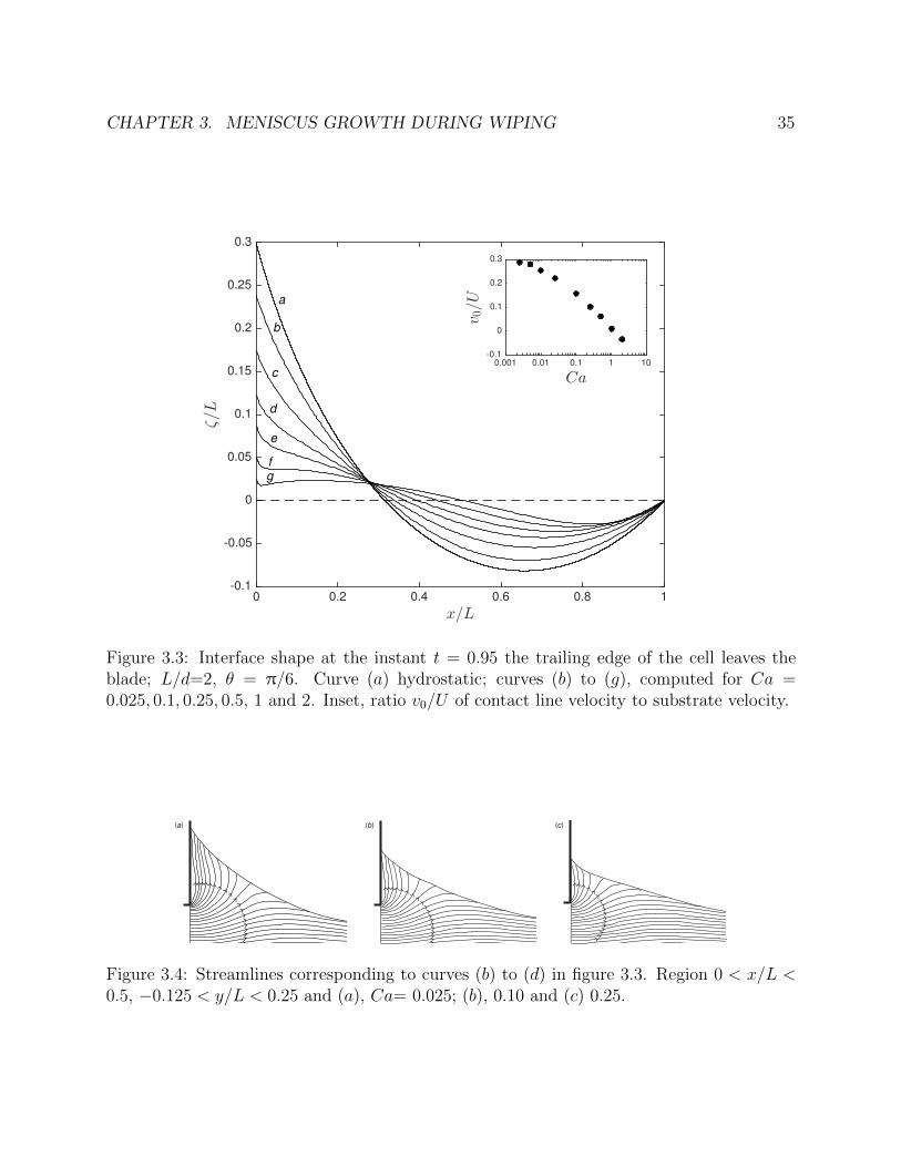
CHAPTER 3. MENISCUS GROWTH DURING WIPING 35
x/L0 0.2 0.4 0.6 0.8 1
ζ/L
-0.1
-0.05
0
0.05
0.1
0.15
0.2
0.25
0.3
Ca0.001 0.01 0.1 1 10
v 0/U
-0.1
0
0.1
0.2
0.3
d
e
a
fg
b
c
Figure 3.3: Interface shape at the instant t = 0.95 the trailing edge of the cell leaves theblade; L/d=2, θ = π/6. Curve (a) hydrostatic; curves (b) to (g), computed for Ca =0.025, 0.1, 0.25, 0.5, 1 and 2. Inset, ratio v0/U of contact line velocity to substrate velocity.
(a) (b) (c)
Figure 3.4: Streamlines corresponding to curves (b) to (d) in figure 3.3. Region 0 < x/L <0.5, −0.125 < y/L < 0.25 and (a), Ca= 0.025; (b), 0.10 and (c) 0.25.

CHAPTER 3. MENISCUS GROWTH DURING WIPING 36
x/L0 0.2 0.4 0.6 0.8 1 1.2 1.4
ζ/L
-0.2
-0.1
0
0.1
0.2
0.3
0.4
0.5
Ca10
-310
-210
-1
v 0/U
-0.14
-0.12
-0.1
-0.08
-0.06
substrate
c
e
d
b
a
Figure 3.5: Interface shape at the instant t = 1.35 the trailing edge of the cell is at x/L = 0.4.For θ and L/d, see caption to figure 3.3. Curve (a), hydrostatic; curves (b) to (e), computedfor Ca = 0.0025, 0.005, 0.01 and 0.025. Inset, ratio v0/U of contact line velocity to substratevelocity.
the interface; for θ = π/6, v0/U = 0.298. The numerical solutions show that v0 decreasesmarkedly as Ca is increased. To explain that effect, we show streamlines in the next figure.
Figure 3.4 shows, in particular, the behaviour of the streamline that divides liquid risingalong the blade from that moving rightwards with the substrate. In all three cases, thecontact line is rising over the blade but, as the viscous pressure increases relative to capillarypressure (increasing Ca), an increasing fraction of the liquid is pulled to the right. As aresult, the dividing streamline moves leftwards along the interface; this is consistent withthe flattening of the interface seen in figure 3.3.
Figure 3.5 shows the interface height at a later time (t = 1.35). The trailing edge Tof the cell has now advanced to x/L = 0.4; this value of x/L is slightly less than that(0.460) at which the hydrostatic analysis predicts that T reaches the interface. Curve (e)for Ca = 0.025 shows the later stage of the solution given as curve (b) in figure 3.3: there,viscosity has only a modest effect on interface shape. By contrast, the inflection on curve (e)shows that viscosity now has a significant effect: for the larger values of Ca, the meniscus isbeginning to be printed as a tail.
The pronounced effect of viscosity is also apparent in the inset showing the ratio v0/U :

CHAPTER 3. MENISCUS GROWTH DURING WIPING 37
Ca0 0.005 0.01 0.015 0.02 0.025 0.03
QUL
0.01
0.011
0.012
0.013
0.014
0.015
0.016
0.017
Figure 3.6: Flow rate at the trailing edge of the cell; configuration as in figure 3.5.
even for the smallest value of Ca = 0.0025, the contact line is retreating (v0/U ' −0.08),whereas in the hydrostatic solution, the contact line advances with uniform speed (v0/U =0.298) until the trailing edge of the cell touches the interface.
We note that the retreating meniscus deposits no film on the blade x = 0. Twoexplanations offer themselves. First, the geometry differs from that in dip coating. Viscousstress here plays a double role; shear stress near the contact line promotes film depositionbut substrate drag opposes it. Second, even if that effect were absent, as in dip coating orbubble flow in a tube, no film is deposited if the capillary number Ca0, based on contact linevelocity v0, is less than a critical value: Ca′ depends on static contact angle θ and, weakly,on slip length ` and on the radius r of curvature of the outer meniscus (Quere 1991, equation5; Eggers 2005, equation 41). Because Ca′ is an increasing function of `/r, the relativelylarge value of `/r ∼ 10−2 used here would inhibit coating.
The preceding figures show clearly that the area under the meniscus is a decreasingfunction of Ca. It remains to show that, with decreasing Ca, liquid is increasingly trappedas the trailing edge of the cell approaches the interface.
From figure 3.6, we see that, for the configuration shown in figure 3.5, the flow rateQ =
∫ ζ0vx dy through the restriction between the interface and trailing edge of the cell is
∼ 1% of the characteristic flow rate UL within the cell itself. The ratio Q/(UL) decreaseswith decreasing Ca. We conclude that hydrostatics provides an upper bound to the volumeleft behind on the substrate. The problem of minimizing smearing simplifies to one ofreducing that upper bound.

CHAPTER 3. MENISCUS GROWTH DURING WIPING 38
3.4 Blade geometry
The smears shown in Kitsomboonloha et al. (2012, figure 7) were observed in experimentsin which the cell length L = 7.5µm, and the radius of the blade tip, 75 µm. Kitsomboonlohaand Subramanian (2014, figure 8) show that printed features become more sharply when theblade is polished to reduce the tip radius to 3 µm. In this section, we use hydrostatic theoryto suggest why polishing is effective.
In the first case, the tip radius is 10L, and a careful sketch shows that the curved surfaceof the blade can be modeled, at the scale of the cell, by a flat blade making an acute angle βwith the x–axis. (Though in figure 1b of Kitsomboonloha et al. (2012), the blade as a wholeis shown as making an obtuse angle with the x–axis, we are concerned here the local anglewhere the cell leaves the blade; that angle is acute.)
Assuming now that the angle made by the blade with the x–axis is now β, rather than π/2,the angle made by the interface with the vertical at the contact line H is θ′ = θ + β − π/2.The effect of tilting the blade is to create additional area beneath it. To illustrate thiseffect, we consider the case θ′ ≥ 0 in which the area A of the meniscus can be calculatedusing results already given: to obtain the area AC of the curvilinear triangle formed by theinterface, x–axis, and abscissa passing through H, we need only replace θ in (3.9) by θ′. Theother contribution is the area AT of the right triangle formed by that same abscissa, theblade, and x–axis: AT = (r2/2)(cosα− sin θ′)2 cot β. As β is reduced, AT increases withoutbound. As far as the cell is concerned, tilting a flat blade creates a large volume sink.
Equating the total area A = AC + AT to the area |AMB| removed from the cell, thensimplifying, we find that α, β and χ = β + θ satisfy the relation
4 cosα sinχ+ sin 2χ+ sin 2α + 2(cosα + cosχ)2 cot β = 2(π + α− χ). (3.16)
This equation holds for χ ≥ π/2.For a system that is only marginally wetting, so that θ ↑ π/2, the condition χ ≥ π/2 is
satisfied even for β 1. To obtain the solution of (3.16) in that case, we note that arc AHin figure 3.2 then approximates to chord AH. From the geometry of the triangle formed bythe blade, chord AH and the x–axis, β+ θ+α = π, whence α→ π− θ as β → 0. To obtainthe next term in this approximation, we substitute the series
α ∼ π− θ + cβ1/2, (3.17)
into (3.16), and find that c = −(2π + sin 2θ − 2θ)1/2/ sin θ. Together, (3.15) and (3.16)determine the area A∗ that has been removed from the cell when its trailing edge reachesthe interface.
Figure 3.7 shows A∗/(Ld) as a function of blade angle β for contact angle θ ↑ π/2.According to the results in §3.2, for this value of θ, and blade angle β = π/2, a negligiblysmall amount of liquid is removed: A∗ → 0 at the right end of the figure. At the otherextreme, β → 0; in this case, α → π/2. The inset shows the corresponding meniscus: it isa semi–circle spanning the cell and having a little finger that reaches up to touch the blade,

CHAPTER 3. MENISCUS GROWTH DURING WIPING 39
β
0 π/12 π/6 π/4 π/3 5π/12 π/2
A∗
Ld
0
0.1
0.2
0.3
0.4
0.5
0.6
0.7
0.8
β
O BT
Figure 3.7: Relation defined by (3.15) and (3.16) for L/d=2, and contact angle θ ↑ π/2.Solid curve, equation (3.16); dotted curve, small–β asymptote (3.17).
thereby completing the right triangle whose area is the very AT described above. It remainsto verify that this extreme situation is not an artefact of assuming a flat blade.
Figure 3.8 shows the corresponding situation for the parabolic blade y = (x+ x0)2/(2ρ),and cell aspect ratio L/d = 2. The coordinate origin O is at the centre of the top of thecell; the ends of the cell are at x = ±d. The sketch is drawn to scale for ε = L/ρ = 0.1; itsuggests that the following assumptions hold in the limit as ε→ 0: (a) the contact line is atx = −L/2; (b) when the trailing edge reaches the meniscus, as shown in the figure, the cellhas emerged a distance x0 L; and (c) the slope of the parabola at the contact line H isvanishingly small. We assume, then verify, these properties.
First, by assumption (a), the area of the meniscus is given by A2 =∫ −L/2−x0 y dx. Equating
that area to the area A1 = 1/2L2(1− π/4) removed from the cell, then using (b) to neglecta small term of the order of L/x0, we find that in the limit as ε→ 0,
x0/L ∼ 0.863/ε1/3; (3.18)
this justifies assumption (b). Next, the contact line H is located at the intersection of theparabola y = (x + x0)2/(2ρ) with the circular arc x2 + y2 = L2/4. Eliminating y betweenthese equations, then using (b) to neglect terms of the order of L/x0, we find that
xc ∼ −(L/2)(1− 0.373ε4/3); (3.19)
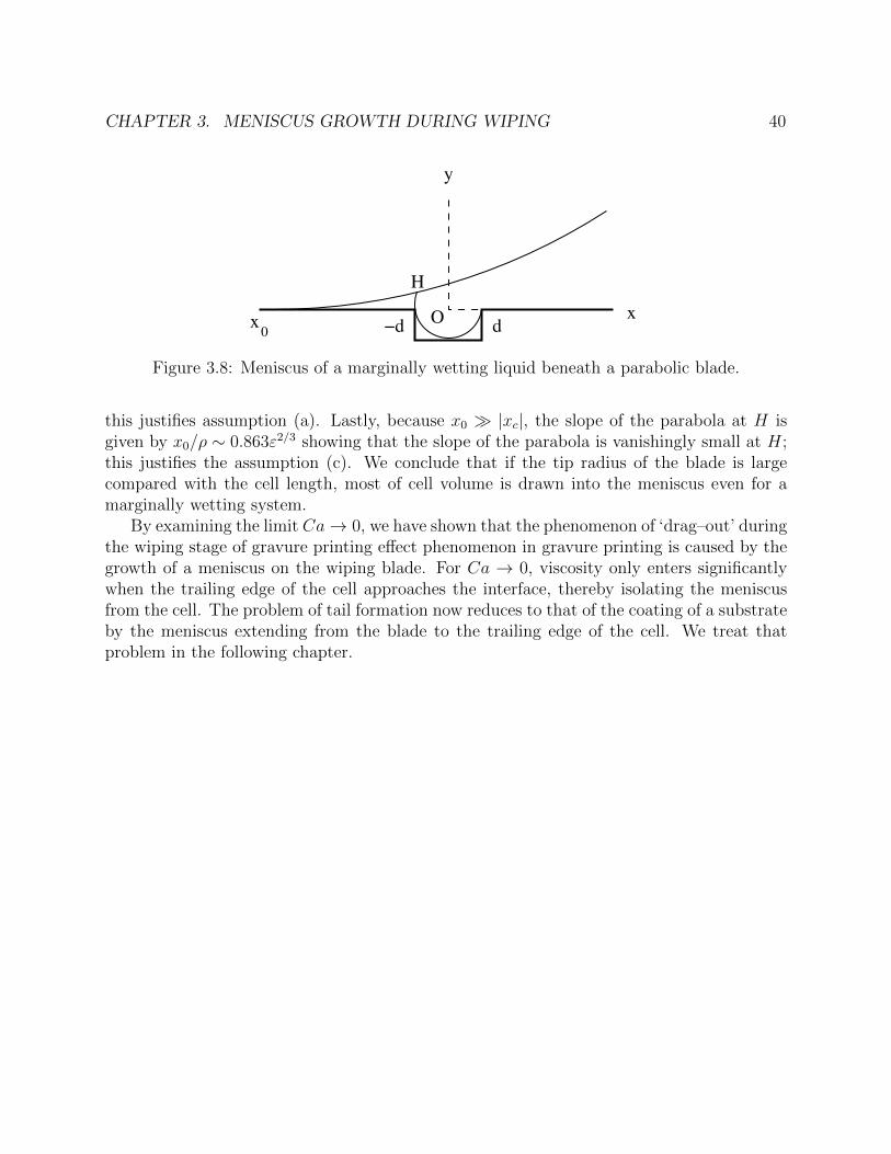
CHAPTER 3. MENISCUS GROWTH DURING WIPING 40
x0
x
y
O
H
−d d
Figure 3.8: Meniscus of a marginally wetting liquid beneath a parabolic blade.
this justifies assumption (a). Lastly, because x0 |xc|, the slope of the parabola at H isgiven by x0/ρ ∼ 0.863ε2/3 showing that the slope of the parabola is vanishingly small at H;this justifies the assumption (c). We conclude that if the tip radius of the blade is largecompared with the cell length, most of cell volume is drawn into the meniscus even for amarginally wetting system.
By examining the limit Ca→ 0, we have shown that the phenomenon of ‘drag–out’ duringthe wiping stage of gravure printing effect phenomenon in gravure printing is caused by thegrowth of a meniscus on the wiping blade. For Ca → 0, viscosity only enters significantlywhen the trailing edge of the cell approaches the interface, thereby isolating the meniscusfrom the cell. The problem of tail formation now reduces to that of the coating of a substrateby the meniscus extending from the blade to the trailing edge of the cell. We treat thatproblem in the following chapter.

41
Chapter 4
Tail Formation
We show in chapter 3 that liquid is drawn from a cell passing beneath the wiper blade.In the limit of vanishing Ca, that liquid becomes isolated from the cell. In this chapter, wefirst analyze printing of the resulting meniscus in this limit. As Ca is increased, however,we consider the existence of the cell due to the leakage from meniscus into the cell as shownin figure 3.6 of chapter 3.
4.1 Outer problem: static prediction
From the hydrostatic analysis in §3.2, the meniscus is separated from the cell as shownin figure 4.1, the contact line is pinned at the trailing edge T of the cell. As a result, theangle α, the angle at which the interface makes with the horizontal as shown in figure 4.1,is no longer fixed but, instead, decreases as the distance xT = |OT | increases. Because thearea under the meniscus is now constant, and equal to A∗ given in (3.15), equation (3.10)determines radius of curvature r of the circular arc meniscus as a function of α. Solving the
TO
H
θ
xα
BLADE
substrate
y
Figure 4.1: Meniscus sitting between blade and trailing edge (T ) of the cell.
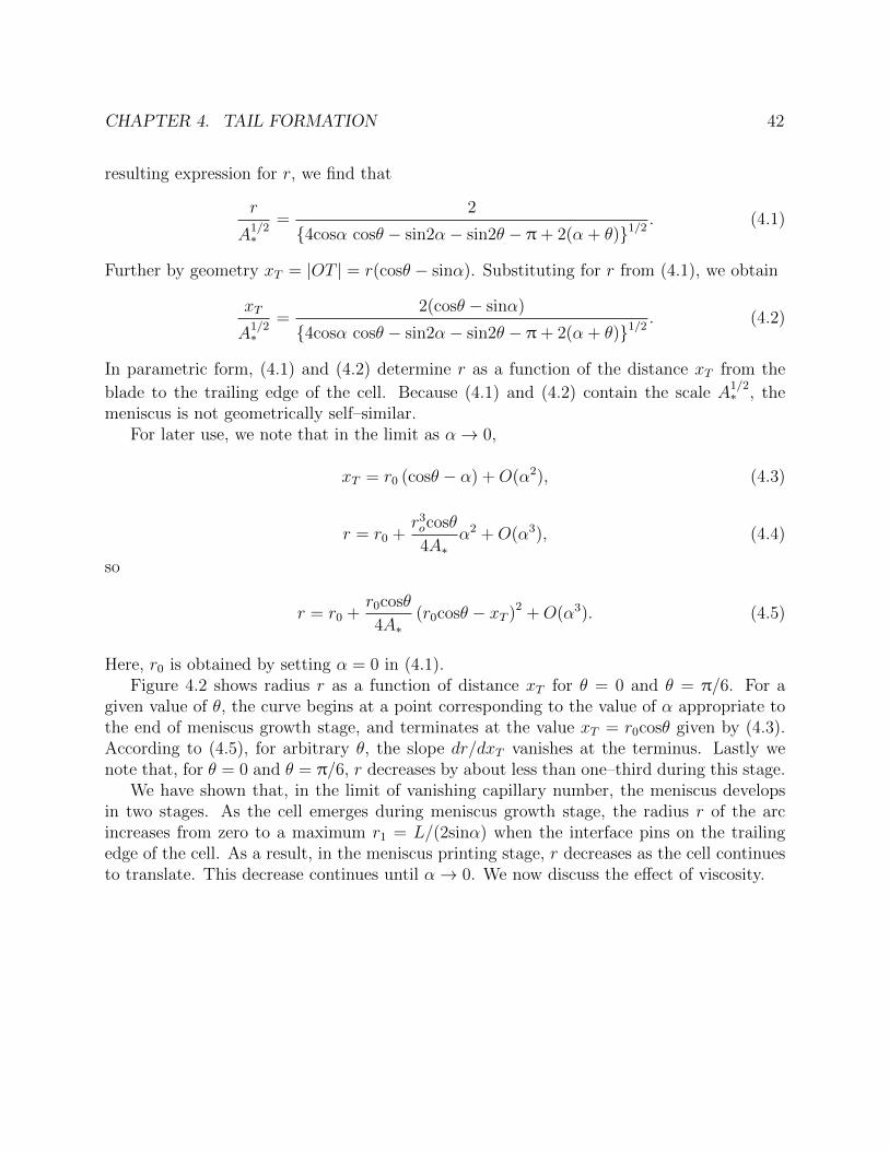
CHAPTER 4. TAIL FORMATION 42
resulting expression for r, we find that
r
A1/2∗
=2
4cosα cosθ − sin2α− sin2θ − π + 2(α + θ)1/2. (4.1)
Further by geometry xT = |OT | = r(cosθ − sinα). Substituting for r from (4.1), we obtain
xT
A1/2∗
=2(cosθ − sinα)
4cosα cosθ − sin2α− sin2θ − π + 2(α + θ)1/2. (4.2)
In parametric form, (4.1) and (4.2) determine r as a function of the distance xT from the
blade to the trailing edge of the cell. Because (4.1) and (4.2) contain the scale A1/2∗ , the
meniscus is not geometrically self–similar.For later use, we note that in the limit as α→ 0,
xT = r0 (cosθ − α) +O(α2), (4.3)
r = r0 +r3ocosθ
4A∗α2 +O(α3), (4.4)
so
r = r0 +r0cosθ
4A∗(r0cosθ − xT )2 +O(α3). (4.5)
Here, r0 is obtained by setting α = 0 in (4.1).Figure 4.2 shows radius r as a function of distance xT for θ = 0 and θ = π/6. For a
given value of θ, the curve begins at a point corresponding to the value of α appropriate tothe end of meniscus growth stage, and terminates at the value xT = r0cosθ given by (4.3).According to (4.5), for arbitrary θ, the slope dr/dxT vanishes at the terminus. Lastly wenote that, for θ = 0 and θ = π/6, r decreases by about less than one–third during this stage.
We have shown that, in the limit of vanishing capillary number, the meniscus developsin two stages. As the cell emerges during meniscus growth stage, the radius r of the arcincreases from zero to a maximum r1 = L/(2sinα) when the interface pins on the trailingedge of the cell. As a result, in the meniscus printing stage, r decreases as the cell continuesto translate. This decrease continues until α→ 0. We now discuss the effect of viscosity.
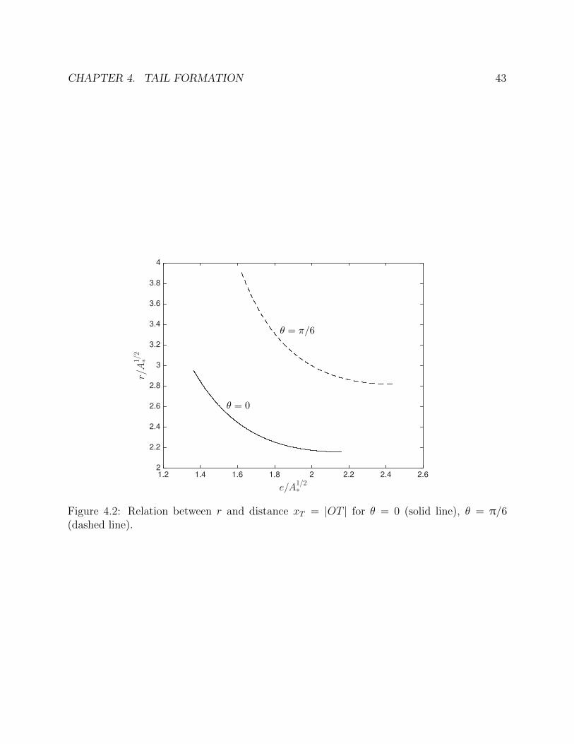
CHAPTER 4. TAIL FORMATION 43
e/A1/2∗
1.2 1.4 1.6 1.8 2 2.2 2.4 2.6
r/A
1/2∗
2
2.2
2.4
2.6
2.8
3
3.2
3.4
3.6
3.8
4
θ = π/6
θ = 0
Figure 4.2: Relation between r and distance xT = |OT | for θ = 0 (solid line), θ = π/6(dashed line).
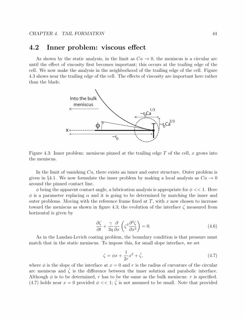
CHAPTER 4. TAIL FORMATION 44
4.2 Inner problem: viscous effect
As shown by the static analysis, in the limit as Ca → 0, the meniscus is a circular arcuntil the effect of viscosity first becomes important; this occurs at the trailing edge of thecell. We now make the analysis in the neighborhood of the trailing edge of the cell. Figure4.3 shows near the trailing edge of the cell. The effects of viscosity are important here ratherthan the blade.
~r
~r Ca
Into the bulk
meniscus
xTφ
1/3
~r Ca2/3
0
0
0
Figure 4.3: Inner problem: meniscus pinned at the trailing edge T of the cell, x grows intothe meniscus.
In the limit of vanishing Ca, there exists an inner and outer structure. Outer problem isgiven in §4.1. We now formulate the inner problem by making a local analysis as Ca → 0around the pinned contact line.
φ being the apparent contact angle, a lubrication analysis is appropriate for φ << 1. Hereφ is a parameter replacing α and it is going to be determined by matching the inner andouter problems. Moving with the reference frame fixed at T , with x now chosen to increasetoward the meniscus as shown in figure 4.3; the evolution of the interface ζ measured fromhorizontal is given by
∂ζ
∂t+
γ
3η
∂
∂x
(ζ3 ∂
3ζ
∂x3
)= 0. (4.6)
As in the Landau-Levich coating problem, the boundary condition is that pressure mustmatch that in the static meniscus. To impose this, for small slope interface, we set
ζ = φx+1
2rx2 + ζ , (4.7)
where φ is the slope of the interface at x = 0 and r is the radius of curvature of the circulararc meniscus and ζ is the difference between the inner solution and parabolic interface.Although φ is to be determined, r has to be the same as the bulk meniscus: r is specified.(4.7) holds near x = 0 provided φ << 1; ζ is not assumed to be small. Note that provided
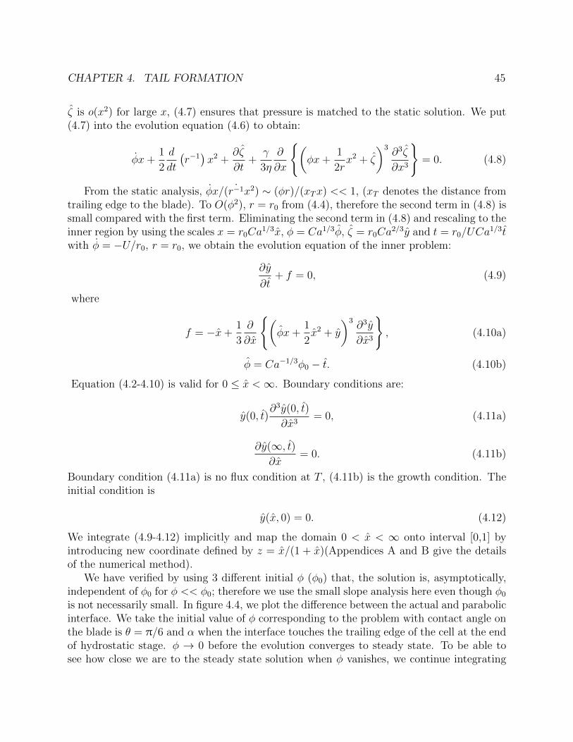
CHAPTER 4. TAIL FORMATION 45
ζ is o(x2) for large x, (4.7) ensures that pressure is matched to the static solution. We put(4.7) into the evolution equation (4.6) to obtain:
φx+1
2
d
dt
(r−1)x2 +
∂ζ
∂t+
γ
3η
∂
∂x
(φx+
1
2rx2 + ζ
)3∂3ζ
∂x3
= 0. (4.8)
From the static analysis, φx/( ˙r−1x2) ∼ (φr)/(xTx) << 1, (xT denotes the distance fromtrailing edge to the blade). To O(φ2), r = r0 from (4.4), therefore the second term in (4.8) issmall compared with the first term. Eliminating the second term in (4.8) and rescaling to theinner region by using the scales x = r0Ca
1/3x, φ = Ca1/3φ, ζ = r0Ca2/3y and t = r0/UCa
1/3twith φ = −U/r0, r = r0, we obtain the evolution equation of the inner problem:
∂y
∂t+ f = 0, (4.9)
where
f = −x+1
3
∂
∂x
(φx+
1
2x2 + y
)3∂3y
∂x3
, (4.10a)
φ = Ca−1/3φ0 − t. (4.10b)
Equation (4.2-4.10) is valid for 0 ≤ x <∞. Boundary conditions are:
y(0, t)∂3y(0, t)
∂x3= 0, (4.11a)
∂y(∞, t)∂x
= 0. (4.11b)
Boundary condition (4.11a) is no flux condition at T , (4.11b) is the growth condition. Theinitial condition is
y(x, 0) = 0. (4.12)
We integrate (4.9-4.12) implicitly and map the domain 0 < x < ∞ onto interval [0,1] byintroducing new coordinate defined by z = x/(1 + x)(Appendices A and B give the detailsof the numerical method).
We have verified by using 3 different initial φ (φ0) that, the solution is, asymptotically,independent of φ0 for φ << φ0; therefore we use the small slope analysis here even though φ0
is not necessarily small. In figure 4.4, we plot the difference between the actual and parabolicinterface. We take the initial value of φ corresponding to the problem with contact angle onthe blade is θ = π/6 and α when the interface touches the trailing edge of the cell at the endof hydrostatic stage. φ → 0 before the evolution converges to steady state. To be able tosee how close we are to the steady state solution when φ vanishes, we continue integrating

CHAPTER 4. TAIL FORMATION 46
x
10-4
10-2
100
102
104
y
0
0.5
1
1.5
2
2.5
0 5 10 15 200
0.5
1
1.5
2
(a)
(b)
Figure 4.4: Inner viscous solution for the meniscus printing problem, (a) φ = 0, (b) steadystate solution. φ0 = 0.468 is taken to be corresponding to the problem with contact angle onthe blade is θ = π/6. Inset: the neighborhood of the contact line in linear scale correspondingto curve (a).
in time by setting φ = 0 after that point (when y ∼ 1.7). y converges to 2.136 as x→∞ as1/x.
As shown by the inset in figure 4.4, the ζ is concave down, approaches a constant veryslowly like 1/x. The curvature is positive everywhere, highest at T ; pressure perturbation isproduced by a squeeze film flow.
Because ζ approaches to limiting value at infinity very slowly, separation of length scalesexists under one of the two conditions: if π/2−θ >> Ca1/3 or if the mass under the meniscusis infinite. The second condition is not valid for the meniscus printing problem because themass under the meniscus is limited by the meniscus growth stage. First condition, on theother hand, is observable. Though it is not practical to solve the corresponding Stokesproblem of meniscus printing for too small Ca numbers, lubrication analysis is valid whenthe interface slope is small and we treat this problem in §4.7. We, of course, compare theinner viscous solution with the Stokes solution even though the separation of length scalesdoes not exist for the Ca values of order 10−3 studied.

CHAPTER 4. TAIL FORMATION 47
4.3 Composite expansion
In this section we form the composite expansion of meniscus printing problem by matchingthe outer limit of the inner problem to the inner limit of the outer problem.
For φ << φ0, at a fixed instant, the overall effect of viscous flow (squeeze film) near T , isto displace the interface upwards by an amount δ = limx→∞ y. This value varies with timet, but since φ = fn(t), δ can also be considered to be a function of the single variable φ. Thedisplacement thickness δ is as shown in figure 4.5. To ensure mass conservation, radius r andangle α are defined as the solutions of (4.1) and (4.2). However, the quantity xA is no longerexactly equal to the distance |OT | = xT to the trailing edge of the cell. Instead xA now refersto the distance |OA| to the point A at which the static meniscus extrapolates to the x–axis,an apparent point. From the rotating meniscus solution, the displacement |TG| = r0Ca
2/3
(to within a constant factor); from the geometry of 4TAG, |TA| = |TG|/α = r0Ca1/3/α
where the scaling α = Ca1/3α has been used. The area under the actual interface (solidcurve), differs from that A∗ under the circular arc meniscus by an amount of the order ofthe area of triangle TAG; that area is of the order of r2
0Ca/α. Mass is, therefore, conservedto within an error of the order of Ca; this error is of the same order as that made in takingthe outer meniscus to be a circular arc.
Into the bulk
meniscus
xT
φ
Aδα
δ ~r Ca2/3
0
G
α
Figure 4.5: Effect of viscosity: meniscus is displaced by an amount δ as the trailing edge Tadvances.
Figure 4.6 shows the geometry of the whole meniscus. We let xT be the abscissa at thetrailing edge of the cell and xA be the abscissa at an apparent point where the outer meniscuscuts the x–axis.
The outer region is defined by the limit Ca → 0 (x 6= xT ) as given in § 4.1. To O(Ca),the pressure in the outer region meniscus is uniform and the interface is a circular arc. Thearea A∗ beneath the arc is defined by the initial condition (for meniscus printing stage).
We let the radius of this arc be r and the angle at which the arc cuts the x–axis be α.Expressed in terms of r, α and the contact angle θ, the coordinates of the centre C of thecircular arc are r cos θ, r cosα. The equation of the circle is

CHAPTER 4. TAIL FORMATION 48
T
φ
Aδα
δ ~r Ca2/3
0Gα
y
x
BLADE
SUBSTRATE
Figure 4.6: Geometry for the composite expansion.
(x− r cos θ)2 + (y − r cosα)2 = r2. (4.13)
The area A∗ under the interface is imposed by the initial condition: this constraintmeans that r is a known function of the parameter α. Consequently, the abscissa a of thepoint A at which the arc cuts the x–axis is also a known function of α: setting y = 0 in(4.13), then solving for x = xA, we obtain xA = r(cos θ − sinα). In particular, for α → 0,r ∼ r01 +O(α2), and
xA = r0(cos θ − α) +O(α2). (4.14)
Matching to inner viscous solution gives the remaining condition needed to determinethe interface. Expressing (4.13) in terms of x− xA, then solving for yO, the ordinate of theouter meniscus, we obtain:
yO = r cosα− r cosα[1 + 2(x− xA)r−1 tanα secα− (x− xA)2r−2 sec2 α
]1/2. (4.15)
We find the inner limit of the outer solution by expanding (4.15) to O([x− xA]2):
yO ∼ (xA − x) tanα +1
2r(x− xA)2 sec3 α. (4.16)

CHAPTER 4. TAIL FORMATION 49
Equation (4.16) can also be obtained by forming the Taylor expansion about x = xA,using y′ = − tanα and y′′(1 + y′2)−3/2 = r−1.
The inner solution is defined by the limit Ca → 0 (fixed [xT − x]/Ca1/3). The functionyI vanishes at xT . The outer limit of the inner solution is defined by Ca → 0 (x 6= xT ). Inthis limit
yI ∼ φ(xT − x) +1
2r0
(xT − x)2 + r0Ca2/3δ. (4.17)
In (4.17), the coefficient of (xT − x)2 must equal limα→0 r, because matching of thepressure requires the outer limit of the (inner) curvature to equal the uniform curvature ofthe outer interface. The apparent contact angle φ is to be determined by matching. Becauseφ appears as a parameter (replacing α) in the statement of the inner viscous problem, thedisplacement thickness δ is a function of φ.
We now perform the matching: for xT − x = O(r0Ca1/3), the second and third terms in
(4.16) are O(r0Ca2/3). Matching consists of making the difference yO − yI = o
(r0Ca
2/3)
;
the difference is then small compared with either yO or yI .Using the identity xA − x = (xA − xT ) + (xT − x) to express yO in terms of x− xT , then
rearranging, we obtain
yO ∼ α(xA − xT ) + 12r0
(xA − xT )2 + (xT − x)[α + 1r0
(xA − xT )] + 12r0
(xT − x)2;
yI ∼ r0Ca2/3δ + (xT − x)φ + 1
2r0(xT − x)2.
(4.17a,b)Equating coefficients in (4.17a,b), we obtain
r0φ = r0α + (xA − xT ), (4.18a)
α(xA − xT ) + (xA − xT )2/(2r0) = r0Ca2/3δ. (4.18b)
In this system, δ is computed as a function of φ as part of the inner viscous solution.The unknowns are therefore φ, α and xA. Equation (4.14) provides the remaining relationneeded to determine the three unknowns. Eliminating xA + r0α between (4.18a) and (4.14),we find that
φ = (cos θ − xT/r0). (4.19)
This equation determines the coefficient entering into the inner viscous problem. Solving theinner problem then determines δ.
With δ determined, α is found by eliminating xA− xT between (4.18a) and (4.18b): thisgives
α =[φ2 − 2Ca2/3δ
]1/2. (4.20)

CHAPTER 4. TAIL FORMATION 50
Lastly, according to (4.18a), xA − xT = r0(φ− α):
xA − xT = r0
φ−
[φ2 − 2Ca2/3δ
]1/2. (4.21)
The quantities xA, α and φ have been determined; mass is conserved; and the inner andouter solutions have been matched.
The composite solution is
yC ∼ yO + r0Ca2/3ynum − δ ; (4.22)
In (4.22), yO is given by (4.15), and ynum denotes the numerical solution of the inner viscousproblem, specifically the component that approaches δ far from xT . In the outer limit,yC ∼ yO. Using (4.17a,b), in the inner limit
yO ∼ r0Ca2/3δ + (xT − x)φ+
1
2r0
(xT − x)2; (4.23)
so that
yC ∼ (xT − x)φ+1
2r0
(xT − x)2 + r0Ca2/3 ynum. (4.24)
The matching allows for the variation in slope that occurs between xT and xA as theviscous effect becomes stronger.
To show the meniscus rotation, we form the composite solution for θ = 5π/12. Thecomposite solution is for fixed time, the corresponding static solution at the same time isfound from (4.1) and (4.2) and the parabolic approximation is computed at the correspondingtime by using (4.25).
Figure 4.7 shows the composite expansion for Ca = 10−7 and Ca = 10−8 and θ = 5π/12.The matching is valid provided φ2 > 2r0Ca
2/3δ. In figure 4.7; α = 0.0030, φ = 0.0065,|xA − xT | = 0.0095 for Ca = 10−7; α = 0.0012, φ = 0.0030, |xA − xT | = 0.0049 forCa = 10−8. To be able to show the structure at the tip, we subtract the parabolic interfacewhich given by
yP = (xT − x)φ+1
2r0
(xT − x)2 (4.25)
from the actual interface yO. As shown by the insets, the rotation of meniscus is visible atthe tip region and as Ca is decreased separation of length scales is also visible close to thetip (T ).
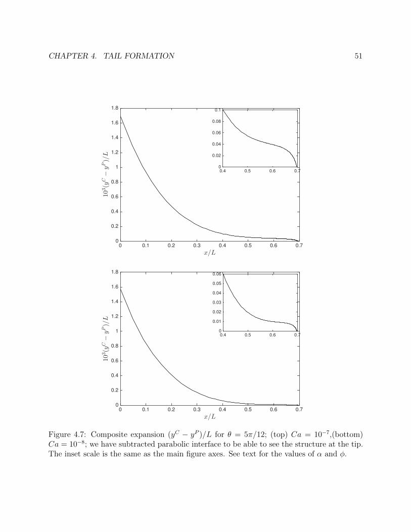
CHAPTER 4. TAIL FORMATION 51
x/L0 0.1 0.2 0.3 0.4 0.5 0.6 0.7
103(y
C−yP)/L
0
0.2
0.4
0.6
0.8
1
1.2
1.4
1.6
1.8
0.4 0.5 0.6 0.70
0.02
0.04
0.06
0.08
0.1
x/L0 0.1 0.2 0.3 0.4 0.5 0.6 0.7
103(y
C−yP)/L
0
0.2
0.4
0.6
0.8
1
1.2
1.4
1.6
1.8
0.4 0.5 0.6 0.70
0.01
0.02
0.03
0.04
0.05
0.06
Figure 4.7: Composite expansion (yC − yP )/L for θ = 5π/12; (top) Ca = 10−7,(bottom)Ca = 10−8; we have subtracted parabolic interface to be able to see the structure at the tip.The inset scale is the same as the main figure axes. See text for the values of α and φ.

CHAPTER 4. TAIL FORMATION 52
4.4 Later stage of tail formation in the limit Ca→ 0
Figure 4.8 shows the film to be coated with continuing motion of the substrate at alater stage. As shown in the control volume (C.V.), the mass exiting the C.V. is Uh∞.When the radius of curvature of the meniscus is r, h∞ is the film thickness to be coated atthis instant; that film thickness is at a distance r away from the blade (assuming perfectlywetting case) where the interface slope is zero. The corresponding film thickness is given byh∞ = 1.34rCa2/3 (Landau and Levich, 1942). As the tip advances, however, the thicknessof the film decreases with time because the volume of the meniscus is finite.
O x
BLADE
substrate
y
C.V.
h∞
r
Figure 4.8: Coating of a Landau–Levich film.
Figure 4.9 shows the expected tail shape. From T to M , we expect the film thicknessto increase from the inner analysis. To the left of M , the film thickness is controlled by thevolume under the meniscus because the meniscus is coating the substrate.
Assume that at time t, the radius of curvature of the meniscus from which a thin film iscoated be r. Here, r is not constant in time. The volume constraint, for arbitrary contactangle θ on the vertical blade, requires that
d
dtr2
cosθ
(1− 1
2sinθ
)+θ
2− π
4
= −Uh∞ = −1.34UrCa2/3. (4.26)
Using (4.26), time rate of change of the film thickness away from the bulk meniscus is foundto be
dh∞dt
=(1.34)2UCa4/3
2
cosθ(1− 1
2sinθ
)+ θ
2− π
4
. (4.27)
As the radius of curvature of the bulk meniscus decreases linearly in time, so does the coated

CHAPTER 4. TAIL FORMATION 53
Deposited earlierDeposited later
ζ ∼ rCa
y
xT
2/3
∼rCa1/3
∼ 2/3r
CaM
Figure 4.9: For a fixed point on substrate, expected tail formation.
film thickness. (4.27) is valid, in the limit as Ca→ 0, and when r changes slowly comparedwith either of the terms, h∞ or Ca2/3, in Landau–Levich equation. Gutenev et al. (2002)makes a similar analysis for liquid entrainment from the meniscus of a liquid wedge in thelimit as Ca→ 0, but they do not consider the viscous effects.
The draining time of the mass scales as td ∼ rU−1Ca−2/3; therefore the correspondingtail length scales like ∼ Utd ∼ rCa−2/3.

CHAPTER 4. TAIL FORMATION 54
4.5 Tail formation studied using numerical solution of
Stokes equations with no cell
In the previous sections, we have demonstrated the physical picture. We now demonstrateusing numerical solution that the physical picture is correct.
As shown in §3.3, for vanishing capillary number, there is no leakage into the cell: theinterface touches the trailing edge of the cell and pins at the trailing edge of the cell. Themeniscus is separated from the cell and printed with the continuing motion of the substrate.
TO
H
θ
xα
BLADE
substrate
y
Figure 4.10: Geometry of the meniscus sitting between blade and trailing edge (T ) of thecell.
Figure 4.10 shows the geometry of the meniscus printing problem. In this section weassume that the contact line is pinned at T and free to move atH. We solve the correspondingStokes problem between points O and T with initial free surface profile predicted at the endof meniscus growth stage with Ca = 0.001, θ = π/6 which is given in chapter 3.
Figure 4.11 shows the interface evolution with continuing motion of substrate for θ = π/6.The interface rotates around the pinning point T at the trailing edge of the cell and startscoating a thin film downstream.
The static solution given by (4.1) and (4.2) predicts the meniscus printing problem closelyuntil the trailing edge of the cell has advanced to about 0.1L from its initial location (atx0 = 0.4596L). At the time when the trailing edge of the cell advances x/L = 0.2 from itsinitial position, the difference between static prediction and Stokes solution is visible closeto the tip region with maximum absolute error of 0.004.
Figure 4.12 shows the tip region for the tip locations (xT − x0)/L = 0.05, 0.1, 0.2. Thedifference between Stokes solution and static prediction grows as the tip advances.
According to static prediction, α vanishes when the trailing edge of the cell has advancedby a distance of 0.2323L from its initial position. At this position, the maximum absoluteerror is 0.006. We plot the difference between the Stokes solution and the static predictionwhen the trailing edge of the cell advances x/L = 0.23 from its initial position, and compare

CHAPTER 4. TAIL FORMATION 55
x/L0 0.2 0.4 0.6 0.8 1 1.2
y/L
0
0.05
0.1
0.15
0.2
0.25
0.3
0.35
0.4
0.45
Figure 4.11: Time evolution of meniscus printing computed using Stokes equations, Ca =0.001, θ = π/6.
it with the inner viscous solution in figure 4.12. From static prediction, α = 0.0029 andr = 0.799. Inner solution predicts the solution closely for x/L up to 0.02. As the contactangle θ over the blade is decreased, the difference between the two reduces. Figure 4.13shows the corresponding comparison for θ = 5π/12. In this case, α0 = 0.13011, and αvanishes when T advances x/L = 0.20877 away from its initial position, therefore we givethe results for the time when T advances x/L = 0.2 away from its initial position. Theinner prediction approaches the Stokes solution as θ is increased. For θ = π/6, the innersolution predicts Stokes solution closely up to x/L = 0.03 away from the tip, on the otherhand, for θ = 5π/12, the corresponding value of x/L is approximately 0.1. It is expectedthat as θ → π/2, and α→ 0, this range is going to increase because the parabolic interfaceapproximates the circular arc interface closely away from the tip as θ → π/2. From figures4.12,4.13 and 4.14, we observe that the interface is pushed upwards as predicted from theinner analysis in §4.2.
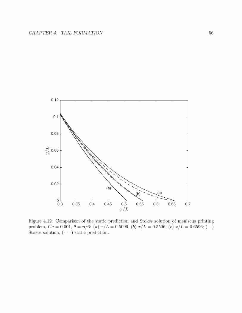
CHAPTER 4. TAIL FORMATION 56
x/L0.3 0.35 0.4 0.45 0.5 0.55 0.6 0.65 0.7
y/L
0
0.02
0.04
0.06
0.08
0.1
0.12
(a)
(b) (c)
Figure 4.12: Comparison of the static prediction and Stokes solution of meniscus printingproblem, Ca = 0.001, θ = π/6: (a) x/L = 0.5096, (b) x/L = 0.5596, (c) x/L = 0.6596; (—)Stokes solution, (- - -) static prediction.
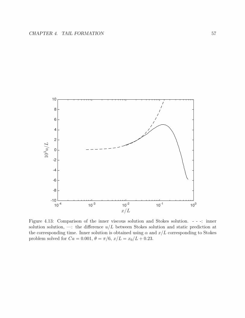
CHAPTER 4. TAIL FORMATION 57
x/L10
-410
-310
-210
-110
0
103u/L
-10
-8
-6
-4
-2
0
2
4
6
8
10
Figure 4.13: Comparison of the inner viscous solution and Stokes solution. - - -: innersolution solution, —: the difference u/L between Stokes solution and static prediction atthe corresponding time. Inner solution is obtained using α and x/L corresponding to Stokesproblem solved for Ca = 0.001, θ = π/6, x/L = x0/L+ 0.23.

CHAPTER 4. TAIL FORMATION 58
x/L10
-410
-310
-210
-110
0
103u/L
-10
-8
-6
-4
-2
0
2
4
6
8
10
Figure 4.14: Comparison of the inner viscous solution and Stokes solution. - - -: innersolution, —: the difference u/L between Stokes solution and static prediction at thecorresponding time. Inner solution solution is obtained using α and x/L correspondingto Stokes problem solved for Ca = 0.001, θ = 5π/12, x/L = x0/L+ 0.2.

CHAPTER 4. TAIL FORMATION 59
4.6 Tail formation studied using numerical solution of
Stokes equations with cell
As Ca increases, the no–leakage back into the cell assumption is not valid. Now weinclude the cell: The difference from the meniscus printing problem is that the flow domainincludes the cell as well because the interface does not touch the trailing edge of the cell atthe location predicted in the hydrostatic analysis (§3.2) and the leakage is shown in §3.3.Figure 4.15 shows the domain of the problem. The interface shape is determined as part ofthe solution. We continue integrating the problem from the point when the cell has emergedfully beneath the blade (figure 4.15a) by taking the interface shapes given in chapter 3.
T T
O
A B
H
y y
x xB
θ
α
θ
O
(a) (b)
β
Figure 4.15: Geometry of the domain for tail formation problem, cell translating rightwardsbeneath a stationary blade occupying the second quadrant of the xOy plane: (a) cell fullyemerged; (b) cell is away from the blade.
In figure 4.16, the evolution of the interface into a tail shape for Ca = 0.1 is plotted. Foreach time step, each curve is overlaid relative to the horizontal distance of the leading edgeof the cell to the blade. The history of the interface profiles are plotted starting from t = 1to t = 1.7 with ∆t = 0.1 increments. As shown by the inset in figure 4.16, the contact lineon the blade retreats while evolving into a tail shape. The drag due to substrate motionpulls the meniscus down as shown with the corresponding streamlines for xT/L=0.2,0.4 and0.6 in figure 4.17; the free surface evolves into a tail shape.
For relatively large Ca numbers, tail formation occurs faster. In figure 4.18, we showthe interface profiles for Ca numbers of 0.1, 0.5 and 1. We show the interfaces at the timeswhen the minimum film thickness behind the tail is 0.01. This occurs when the trailing edgeof the cell is 0.091, 0.219 and 0.85 away from the blade for Ca=1, 0.5 and 0.1, respectively.The horizontal is scaled with the horizontal distance of the leading edge of the cell to theblade. The tail forms faster as Ca is increased and tail length grows as Ca is reduced. Thisis consistent with the analysis given in chapter 3 because less liquid is trapped under themeniscus as Ca increases.

CHAPTER 4. TAIL FORMATION 60
ξ0 0.1 0.2 0.3 0.4 0.5 0.6 0.7 0.8 0.9 1
y/L
-0.1
-0.05
0
0.05
0.1
0.15
0.2
t0 0.25 0.5 0.75
y cl
0.05
0.1
0.15
0.2
t=0.05
t=0.75
Figure 4.16: Interface evolution into tail shape for Ca = 0.1, θ = π/6. The history of theinterface profiles are plotted starting from xT/L=0.05 to xT/L=0.75 with 0.1 increments.Each curve is overlaid relative to the distance of leading edge of the cell to the blade.Solid circles along ξ axis show the corresponding location of the trailing edge of the cell:ξ = 0.0476, 0.1304, 0.2, 0.2593, 0.3103, 0.3548, 0.3939, 0.4286, respectively.
As Ca is decreased below Ca = 0.1, on the other hand, the interface approaches thetrailing edge of the cell as it translates further away. This slows down the computations interms of meshing of the domain and computational effort spent within the cell. When theinterface is almost touching the trailing edge of the cell, we cut the cell from computationaldomain, pin the interface at T and continue integrating in time. After this point, we cantreat the problem as meniscus printing which occurs between points O and T as shown infigure 4.10. In figures 4.19 and 4.20, comparison of the interface profiles for Ca = 0.025, 0.01and 0.005 at t = 1.773 and t = 2.368 shows that tail formation takes longer for smaller Ca.As Ca is increased, the interface rotates faster and the interface slope away from the pinnedcontact line reaches zero and after this point maximum formation occurs. In all three cases,maximum formation is visible in figure 4.20. We should note that tail thickness decreaseslinearly as predicted in (4.27); the mass under the meniscus is used to coat the tail. In figure4.21, for a fixed point away from the blade, we plot the change of film thickness with time
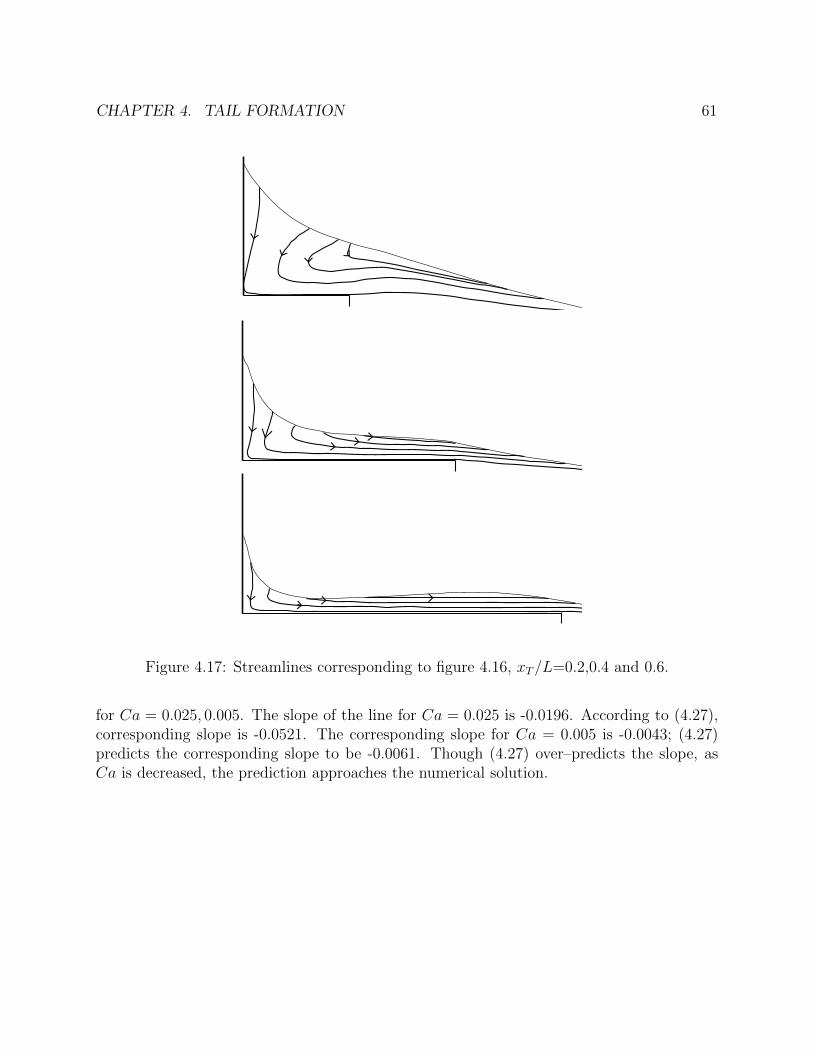
CHAPTER 4. TAIL FORMATION 61
Figure 4.17: Streamlines corresponding to figure 4.16, xT/L=0.2,0.4 and 0.6.
for Ca = 0.025, 0.005. The slope of the line for Ca = 0.025 is -0.0196. According to (4.27),corresponding slope is -0.0521. The corresponding slope for Ca = 0.005 is -0.0043; (4.27)predicts the corresponding slope to be -0.0061. Though (4.27) over–predicts the slope, asCa is decreased, the prediction approaches the numerical solution.
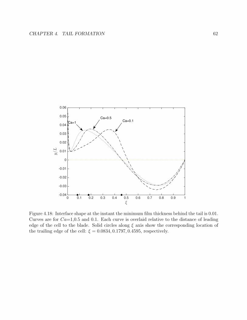
CHAPTER 4. TAIL FORMATION 62
ξ0 0.1 0.2 0.3 0.4 0.5 0.6 0.7 0.8 0.9 1
y/L
-0.04
-0.03
-0.02
-0.01
0
0.01
0.02
0.03
0.04
0.05
0.06
Ca=0.1Ca=0.5
Ca=1
Figure 4.18: Interface shape at the instant the minimum film thickness behind the tail is 0.01.Curves are for Ca=1,0.5 and 0.1. Each curve is overlaid relative to the distance of leadingedge of the cell to the blade. Solid circles along ξ axis show the corresponding location ofthe trailing edge of the cell: ξ = 0.0834, 0.1797, 0.4595, respectively.

CHAPTER 4. TAIL FORMATION 63
x/L0 0.1 0.2 0.3 0.4 0.5 0.6 0.7 0.8
y/L
0
0.05
0.1
0.15
0.2
0.25
0.3
Ca=0.005
Ca=0.010
Ca=0.025
Figure 4.19: Comparison of interface profiles computed from the Stokes equations for Ca =0.025, 0.01 and 0.005 at t = 1.773.

CHAPTER 4. TAIL FORMATION 64
x/L0 0.5 1 1.5
y/L
0
0.05
0.1
0.15
0.2
0.25
0.3
Ca=0.005
Ca=0.010
Ca=0.025
Figure 4.20: See caption for figure 4.19, t = 2.368.
t2 2.1 2.2 2.3 2.4 2.5
ζ/L
(0.5,t)
0.018
0.02
0.022
0.024
0.026
0.028
0.03
s=-0.0196
t2.4 2.6 2.8 3 3.2 3.4
ζ/L
(0.6,t)
0.0135
0.014
0.0145
0.015
0.0155
0.016
0.0165
0.017
0.0175
0.018
0.0185
s=-0.0043
Figure 4.21: Change of film thickness with time at (left)x = 0.5L away from the blade,Ca=0.025, (right)x = 0.6L away from the blade, Ca=0.005; s is the slope of the line;θ = π/6.
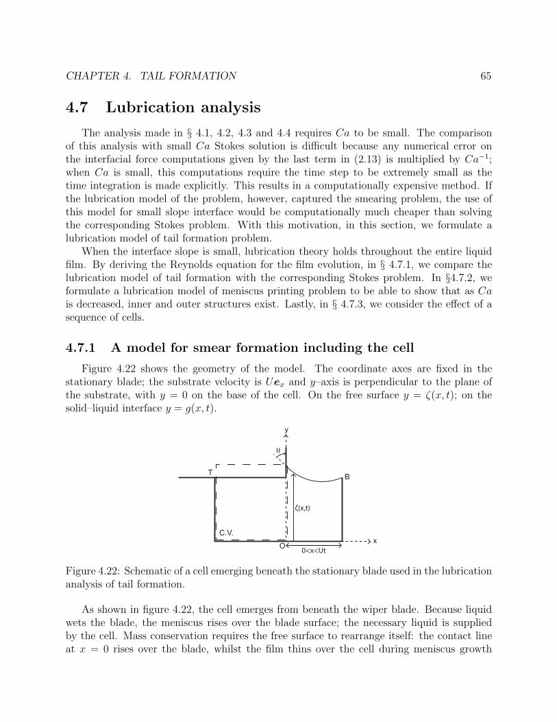
CHAPTER 4. TAIL FORMATION 65
4.7 Lubrication analysis
The analysis made in § 4.1, 4.2, 4.3 and 4.4 requires Ca to be small. The comparisonof this analysis with small Ca Stokes solution is difficult because any numerical error onthe interfacial force computations given by the last term in (2.13) is multiplied by Ca−1;when Ca is small, this computations require the time step to be extremely small as thetime integration is made explicitly. This results in a computationally expensive method. Ifthe lubrication model of the problem, however, captured the smearing problem, the use ofthis model for small slope interface would be computationally much cheaper than solvingthe corresponding Stokes problem. With this motivation, in this section, we formulate alubrication model of tail formation problem.
When the interface slope is small, lubrication theory holds throughout the entire liquidfilm. By deriving the Reynolds equation for the film evolution, in § 4.7.1, we compare thelubrication model of tail formation with the corresponding Stokes problem. In §4.7.2, weformulate a lubrication model of meniscus printing problem to be able to show that as Cais decreased, inner and outer structures exist. Lastly, in § 4.7.3, we consider the effect of asequence of cells.
4.7.1 A model for smear formation including the cell
Figure 4.22 shows the geometry of the model. The coordinate axes are fixed in thestationary blade; the substrate velocity is Uex and y–axis is perpendicular to the plane ofthe substrate, with y = 0 on the base of the cell. On the free surface y = ζ(x, t); on thesolid–liquid interface y = g(x, t).
B
O
θ
y
xC.V.
ζ(x,t)
0<x<Ut
T
Figure 4.22: Schematic of a cell emerging beneath the stationary blade used in the lubricationanalysis of tail formation.
As shown in figure 4.22, the cell emerges from beneath the wiper blade. Because liquidwets the blade, the meniscus rises over the blade surface; the necessary liquid is suppliedby the cell. Mass conservation requires the free surface to rearrange itself: the contact lineat x = 0 rises over the blade, whilst the film thins over the cell during meniscus growth

CHAPTER 4. TAIL FORMATION 66
process. After the cell has emerged fully from beneath the blade, drag is introduced due tothe change in topography. The substrate motion pulls the meniscus down on the blade. Theliquid retained in the meniscus is printed as a tail later in time.
We allow the contact line on the blade to move freely with a predefined static contactangle θ. We are assuming that, because the capillary number based on substrate velocity issmall, so too is that based on the contact line velocity. We show in Chapter 3, figure 3.3that as Ca is reduced, the contact line velocity approaches the hydrostatic prediction. Thecontact line on the leading edge of the cell is pinned at the corner of the cell.
The volume flow rate
q =
∫ ζ
g
(vxex + vyey) dy (4.28)
is related to the film thickness (ζ − g) by the mass balance:
∂(ζ − g)
∂t+∇ · q = 0. (4.29)
The gradient operator in the xOy plane is defined by ∇ = ex∂∂x
+ ey∂∂y
.In the lubrication approximation, q is related to dynamic viscosity η. liquid pressure p
and film thickness ζ − g by
q = − 1
2η(ζ − g)3∇p+ U (ζ − g) ex. (4.30)
This relation holds provided no–slip condition holds at the substrate liquid interface, andthe shear stress vanishes on an interfacial element: provided the interface slope is small,
−p = γ∇2ζ. (4.31)
Our point here is to describe the tail formation mechanism without complication. Becauseof this reason, we do not include disjoining pressure. Eliminating p and q and then usingthe identity ∂g
∂t+ U ∂g
∂x= 0, we obtain the Reynolds equation for ζ:
∂ζ
∂t+ U
∂ζ
∂x+
γ
3η∇ ·
(ζ − g)3∇∇2ζ
= 0. (4.32)
The film is parametrically forced by the cell; in (4.32), this effect is represented by thefunction g in the third term. We define the cell function by arctan as in Stillwagon andLarson (1988), but moving with speed U ;
g(x, t) = d
1
2+
1
πarctan
(−x− L+ Ut
Lε
)(4.33)
where L is the length, d is the depth of the cell, and ε is the edge smoothness parameter.In the model problem, (4.32) holds in the domain 0 < x < Ut; in that domain g
varies between zero and d according to its definition. The initial condition for the interface

CHAPTER 4. TAIL FORMATION 67
shape is determined by the power series expansion of the governing equation which holds forarbitrarily small length Ut → 0. For t > 0, two boundary conditions are applied at x = 0.First, we allow the contact line to move freely with a predefined contact angle at x = 0:
∂ζ
∂x= −cotθ. (4.34)
The second boundary condition at x = 0 is obtained by a mass balance on the controlvolume shown in figure 4.22. This is the key boundary condition that allows us to determinethe location of the meniscus on the blade as part of the initial boundary value problem.Because the trailing edge of the cell acts as a piston displacing to the right, the incomingflow to the control volume is U(d− g); and this inflow rate is equal to the axial flux acrossthe interface at x = 0:
U(d− g) = U(ζ − g) +γ
3η
(ζ − g)3 ∂
3ζ
∂x3
, (4.35)
simplifying, we find that at x = 0
∂3ζ
∂x3= −3Ca
ζ − d(ζ − g)3 . (4.36)
Equation (4.36) holds throughout the process. When g jumps from zero to d, the incomingflux is zero and same equation applies after the cell has emerged fully from beneath the blade.At x = Ut, we pin the contact line the upper corner of the leading edge of the cell:
ζ = d, (4.37)
and continuity of volume flow rate requires pressure gradient to vanish there:
∂3ζ
∂x3= 0. (4.38)
This ends the problem statement.Because the cell is moving, we solve the problem using a stretched domain which is fixed.
To do so, we define new variables: ζ = df(ξ, t′) where ξ = x/(Ut) and t′ = Ut/dCa1/3. Thedimensionless Reynolds equation (4.32) in terms of the new variables is valid for 0 < ξ < 1and given by
3t′t′∂f
∂t′+ (1− ξ)∂f
∂ξ
+
∂
∂ξ
(f − g′)3∂
3f
∂ξ3
= 0. (4.39)
The corresponding boundary conditions at ξ = 0 are
∂f
∂ξ= −t′Ca−1/3cotθ, (4.40)

CHAPTER 4. TAIL FORMATION 68
∂3f
∂ξ3= −3t′3
f − 1
(f − g′)3. (4.41)
At ξ = 1:
f = 1, (4.42)
∂3f
∂ξ3= 0. (4.43)
The dependent variable f can be expanded as a power series in t′ whose coefficients arefunctions of ξ only. Initially f = 1 and (4.40) requires the next term in the expansion tovary as t′, so f = 1 + A(ξ)t′ + .... Then (4.41) requires the next term to vary as t′4:
f = 1 + A(ξ)t′ +B(ξ)t′4 + ... (4.44)
Substituting the power series (4.44) into (4.39), then equating to zero the coefficients ofsuccessive powers of t′, we obtain boundary value problems for the coefficients A and B.Solving for A and B, we obtain
A(ξ) =1
4Ca−1/3cotθ (3ξ − 1) (ξ − 1) , (4.45)
B(ξ) = Ca−1/3cotθ
(1
160ξ6 − 9
240ξ5 +
9
96ξ4 − 1
8ξ3 +
15
224ξ2 − 1
224
). (4.46)
At O(t′), the meniscus rises linearly in time in order to satisfy contact angle condition (4.40),and the volume constraint requires A to change sign within the interval 0 < ξ < 1. This isexplicitly shown in (4.45). Growth slows when the dimensional time t ∼ d
5UCa−1/3; for times
of this order, the two terms in the expansion (4.44) are comparable.Here, we should be careful about the influx boundary condition at x = 0 which is applied
to the lubrication region downstream. The existence of blade at x = 0 requires the Stoke’ssolution within a region of O(d) to impose the impermeability on the blade. However, thelubrication approximation computes the axial component of the velocity, so the motion ofthe contact line on the blade is determined by the continuity equation, and it does notsee the no–slip condition on the blade. With small slope assumption, however, the verticalvelocity is small compared with horizontal velocity; so it is expected that this Stokes regionis small compared with horizontal scale within which the lubrication equation is solved. Thepower series expansion is a useful tool to prove this claim. The expansion to O(t′4) is goodapproximation up to t′ ∼ 2, at that time the contact line is at O(d), whereas the film lengthis ∼ 2dCa−1/3 >> d. Imposing the inflow condition to the inlet of the lubrication model isself–consistent.

CHAPTER 4. TAIL FORMATION 69
x/d0 0.2 0.4 0.6 0.8 1 1.2 1.4 1.6 1.8 2
y/d
0.9
0.95
1
1.05
1.1
1.15
1.2
1.25
1.3
lubrication(4.44)Stokes
(a) cell has emerged fully
x/d0 0.5 1 1.5 2 2.5 3 3.5 4
y/d
0.8
0.85
0.9
0.95
1
1.05
1.1
1.15
1.2
(b) T is x/d=2.0 away from the blade(x = 0)
Figure 4.23: Comparison of lubrication model and the numerical solution of the Stokesproblem, Ca = 0.01, θ = π/3. The power series expansion uses two terms in (4.44). Thebottom of the cell is at y = 0.
We integrate the equations in time implicitly and employ a positivity preserving schemefor the diffusion coefficient (Zhornitskaya and Bertozzi, 2000). Details of the numericalmethod is given in Appendix A. We set Ca = 0.01, θ = π/3, ε = 0.0001, L/d = 2. In figure4.23, we compare the interface profiles at two different times. Figure 4.23a is at the timewhen the cell emerges fully from beneath the blade. Lubrication theory closely captures theinterface profile. As shown by the Stokes solution, the lag in contact line velocity comparedto the hydrostatic prediction causes the meniscus to rise below the lubrication prediction asexpected. Tail formation is shown in figure 4.23b. The competition between convection andcapillary pressure determines the axial flux gradient. Depending on the sign of this gradient,the interface evolves into a tail shape. Lubrication theory over–predicts tail formation forthe reasons stated above.
4.7.2 Model for meniscus printing
As contact angle approaches π/2, the lubrication model predicts the meniscus printingproblem very closely. This provides us to solve the problem at low Ca, to compare the resultswith the composite expansion given in § 4.3 and to show that the film thickness coated awayfrom the bulk meniscus is consistent with the Landau-Levich film thickness. In this section,we first formulate the lubrication model of the meniscus printing problem and show thatlubrication model captures the solution very closely compared with the corresponding Stokessolution. We then use the lubrication model for smaller Ca.
In the lubrication regime, we solve the evolution equation now between points O and T .Figure 4.24 shows the geometry of the model. Coordinate is fixed on the wiper blade; thesubstrate velocity is Uex and y-axis is perpendicular to the plane of substrate, with y = 0

CHAPTER 4. TAIL FORMATION 70
TO
H
θ
xα
BLADE
substrate
y
Figure 4.24: Geometry of meniscus printing problem
on the land and the trailing edge of the cell is at x0 + Ut. On the free surface, y = ζ(x, t)and it is initially a circular arc profile, obtained using the relations given in Chapter 3. Theinterface evolution is governed by (4.32), however because we have no longer a cell, g = 0;the corresponding Reynolds equation is given by,
∂ζ
∂t+ U
∂ζ
∂x+
γ
3η∇ ·
ζ3∇∇2ζ
= 0. (4.47)
The slope condition at x = 0 is the same as in (4.34). The flux condition at x = 0 differsfrom (4.35) and it is given by
Uζ +γ
3η
ζ3 ∂
3ζ
∂x3
= 0, (4.48)
simplifying, we find that at x = 0
∂3ζ
∂x3= −3Caζ−2. (4.49)
At x = x0 + Ut, we pin the contact line to the upper corner of the trailing edge of the cell:
ζ = 0, (4.50)
and the continuity of volume flow rate requires the pressure gradient to vanish there:
∂3ζ
∂x3= 0. (4.51)
We integrate the meniscus printing problem over a fixed domain by defining the followingvariables: ζ = x0f(ξ, t′), ξ = x/(x0 +Ut) and t′ = (x0 +Ut)/x0Ca
1/3. The numerical methodof integration is same as used for (4.39) to (4.43).
In figure 4.25, we compare the lubrication solution and Stokes solution of the meniscusprinting problem for a case in which we set Ca = 10−3, θ = 5π/12. The interface profiles are

CHAPTER 4. TAIL FORMATION 71
x/L0 0.2 0.4 0.6 0.8 1 1.2
y/L
0
0.01
0.02
0.03
0.04
0.05
0.06
0.07
0.08
0.09
0.1
Initial profileLubricationStokes
(a)
(b)
(c)
Figure 4.25: Comparison of the meniscus printing problem obtained from lubrication modeland Stokes solution, Ca=0.001, θ = 5π/12, (a) tip advanced x/L = 0.2 away from itsinitial position (solid line), (b) tip advanced x/L = 0.4 away from its initial position, (c) tipadvanced x/L = 0.8 away from its initial position.
graphically the same when the trailing edge of the cell advances x/L = 0.2, x/L = 0.4 andx/L = 0.8 away from its initial position. The pressure distributions under the film alongthe interface agree as well. The pressure gradient close to the blade is not zero becauseseparation of length scales does not exist at this capillary number; the film thickness iscomparable to the meniscus height. Solving the corresponding Stokes problem for lowercapillary numbers is not practical, at least with the current version of our solver. However,because the lubrication model agrees with the Stokes solution as shown in figure 4.25, weare able to solve (practically) a corresponding lubrication problem for lower Ca numbers.
With this motivation, we solve the lubrication model for Ca = 10−8, θ = 5π/12. Infigure 4.26, we compare the lubrication solution of meniscus printing problem with compositeexpansion given in § 4.3 at the time when α drops to 0.00327. Within the inner region whenx << 1, the ratio ζ/(αx) scales like ∼ αCa−1/3. For Ca = 10−8, this corresponds toαCa−1/3 ∼ 1.5, therefore y is not small. As shown in figure 4.26, the composite expansionagrees with the interface profile obtained from the lubrication model.

CHAPTER 4. TAIL FORMATION 72
x/L0 0.1 0.2 0.3 0.4 0.5 0.6 0.7
ζ/L
10-8
10-7
10-6
10-5
10-4
10-3
10-2
10-1
composite expansionlubrication
Figure 4.26: Comparison of lubrication solution of meniscus printing problem with compositeexpansion, Ca = 10−8. This comparisons are made at the time when α drops to 0.00327.
Finally in this section, we solve a meniscus printing problem for Ca = 10−5, θ = π/12 andintegrate the Reynolds equation in time until the trailing edge of the cell advances x/x0 = 1away from its initial position. Figure 4.27 shows the interface profile and the correspondingpressure distribution under the film. The pressure gradient drops to zero towards the bladeshowing that the outer profile remains a circular arc. The pressure distribution is differentfrom Landau–Levich; in that case the pressure goes to zero away from the meniscus, but herethe pressure is positive and highest at the tip due to squeeze film flow. Pressure ranges from∼ −7×10⁴ (static meniscus) to 1.6×10⁴(squeeze film). The radius of curvature of the outerproblem is r0 = 2.728. The maximum thickness of the film away from the bulk meniscus is0.00154. This thickness is consistent with the Landau–Levich coating film thickness whichscales like 1.34r0Ca
2/3.

CHAPTER 4. TAIL FORMATION 73
x
0 0.5 1 1.5
ζ
0
0.05
0.1
10−5p
-1
0
1
Figure 4.27: Interface profile when the tip advances x/x0 = 1 away from its initial position,Ca = 10−5, θ = 5π/12, (solid line) interface profile, (dashed line) corresponding pressuredistribution.

CHAPTER 4. TAIL FORMATION 74
4.7.3 Effect of a sequence of cells on tail formation
One way of reducing the tail formation could be by adding sequence of cells. To show theeffect of multiple cells, we add a second cell into the domain by modifying the cell functionin the stretched domain as follows:
g′(ξ, t′) = 1 +1
π
(atan
(−ξ − L
dt′+ 1
L/dεt′
)+ atan
(ξ − 1
L/dεt′))
+1
π
(atan
(−ξ − L
dt′− sL
dt′+ 1
L/dεt′
)+ atan
(ξ + sL
dt′− 1
L/dεt′
)). (4.52)
In figure 4.28, we plot the film shape at t′ = 20 for cell spacings L/2 and L. A cell spacingof cell length produces a film of almost the same thickness as the tail thickness behind thesecond cell. However, when the cell spacing is halved, i.e., L/2, the thickness of the filmabove the spacing is small compared with the the tail thickness behind the second cell, ∼1/5 th of the thickness. For L/4, the film almost follows the pattern of the land in between.We should note that the drag–out is the same from both of the cells.
As we add more cell in the sequence, the liquid accumulates under the meniscus as thecells translates away from the blade (see figure 4.29) and as there must be an end to thesequence of cells, smearing still exists behind the last cell in the sequence in this configuration.

CHAPTER 4. TAIL FORMATION 75
ξ0 0.2 0.4 0.6 0.8 1
y
0
0.2
0.4
0.6
0.8
1
1.2
1.4
1.6
1.8
2
fg'
ξ0 0.2 0.4 0.6 0.8 1
y
0
0.2
0.4
0.6
0.8
1
1.2
1.4
1.6
1.8
2
fg'
Figure 4.28: Film shape at t′=20 with two cells, Ca=0.01, θ = 55o, ε = 0.01, cell spacing(top) L/2, (bottom) L.
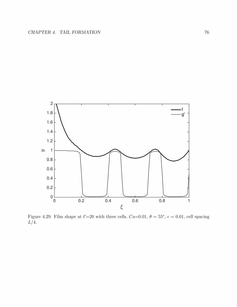
CHAPTER 4. TAIL FORMATION 76
ξ0 0.2 0.4 0.6 0.8 1
y
0
0.2
0.4
0.6
0.8
1
1.2
1.4
1.6
1.8
2
fg'
Figure 4.29: Film shape at t′=20 with three cells, Ca=0.01, θ = 55o, ε = 0.01, cell spacingL/4.

77
Chapter 5
Conclusions
Smear formation during gravure printing of organic electronics degrades the printedfeatures and it forms throughout the wiping stage of the process. The fluid mechanicsproblems motivated from this have been analyzed showing that smear formation mechanismoccurs in a plane flow approximation, also.
We have reduced the problem into two canonical problems: meniscus growth and tailformation. The fluid mechanics of the problem is governed by the Stokes equations of motionowing to the small size of the cell, and to be able to solve corresponding Stokes problems,we wrote a finite element based solver using an unstructured moving mesh.
In the first stage, we have shown that liquid is drawn from the cell as it translatesbeneath the stationary blade; the limit Ca → 0 sets an upper bound for the smear volumeto be printed as tail later in time. This volume is function of Ca number, contact angle θbetween liquid and blade and blade angle β. It be decreased by increasing θ, contact anglehysteresis, Ca and/or β.
We have shown that, for vanishing Ca, as the substrate continues translating, themeniscus is separated from the cell; the mechanism forming the tail operates solely betweenthe blade and the trailing edge of the cell. Viscosity enters when the interface touches thetrailing edge of the cell. An inner and outer analysis of the meniscus printing problem inthe limit of Ca → 0 shows that viscosity rotates the meniscus around the trailing edge ofthe cell by a squeeze film flow.
By solving the corresponding Stokes problem of meniscus printing, we have observed thepredicted meniscus rotation. As Ca is decreased, tail length increases. As Ca approachesorder unity, however, tail formation occurs on a shorter length scale, because the meniscusgrowth stage is limited by the viscous effects as Ca is increased.
As the Stokes solution of the problem is computationally expensive for small Ca, weformulated corresponding problem in the lubrication regime and showed that there existsan inner (squeeze film) and outer (static) structure as Ca → 0. The Stokes solver shouldbe improved to be able to integrate Stokes equations of motions for small Ca, as well as toincrease the resolution in the neighborhood of the moving contact line.
By adding a sequence of cells into the model, we concluded that tail formation still exists

CHAPTER 5. CONCLUSIONS 78
behind the last cell in the sequence because of the accumulation of liquid under the meniscuswhich is contributed from each individual cell.
There are two key intellectual contributions of the dissertation. The first contribution isthat we have reduced the problem of minimizing the smear volume formation during wipingstage of gravure printing of electronics to one of reducing the upper bound set by the analysisas Ca→ 0. We showed that this volume can be decreased by increasing θ, Ca and β eitherindependently or together. The second contribution is that the inner and outer analysis ofprinting a meniscus set the foundation of understanding the effect of viscosity which entersfirst from the contact line when the interface touches the trailing edge of the cell. Thereis one analytic problem still open: the connection between the two dynamic regions, fromsqueeze film flow to the Landau–Levich film, as the substrate translates further away.

79
Appendix A
Numerical Method for LubricationAnalysis
In this section, we give the numerical method used to integrate the free initial boundaryvalue problem used in the lubrication models. We give the method as general and modify itaccording to the model problem in a stretched domain.
We employ a finite difference method. We first discretize the equations in space, andthen in time and employ Newton’s method because the evolution equation is a fourth ordernon–linear diffusion equation.
We approximate the solution ζ at a grid point xi and time tn by ui, i.e.
ui ≈ ζ(xi, tn), (A.1)
and we let fi represent the discretization of the terms in space. Then at every node xi, wedefine an ODE in the form:
duidt
+ fi = 0. (A.2)
The components of fi include the space discretization of the convective and diffusion terms.The convective term can be discretized using a second order finite difference as follows:(
∂ζ
∂x
)i
≈ 1
2∆x(ui+1 − ui−1) . (A.3)
The diffusion term:We first define the diffusion coefficient as
d(ζ) = (ζ − g)3, (A.4)

APPENDIX A. NUMERICAL METHOD FOR LUBRICATION ANALYSIS 80
and then rewrite the diffusion term and approximate by
∂
∂x
(d(ζ)
∂3ζ
∂x3
)=
∂
∂x(D(ζ)) ≈ 1
∆x
(Di+1/2(u)−Di−1/2(u)
), (A.5)
Di+1/2 = di+1/2
(∂3u
∂x3
)i+1/2
, (A.6)
Di−1/2 = di−1/2
(∂3u
∂x3
)i−1/2
. (A.7)
To discretize the third order derivative, we employ a second order central difference schemewhich is given by
∂3u
∂x3=
1
∆x3(−ui−1 + 3ui − 3ui+1 + ui+2) . (A.8)
The approximation of the diffusion coefficient should be second order as well to get a secondorder scheme. We employ the Positivity Preserving Scheme of Zhornitskaya and Bertozzi(2000) as follows:
di+1/2 =
2(ui+1−gi+1)2(ui−gi)2(ui+1−gi+1)+(ui−gi) (ui+1 − gi+1) 6= (ui − gi)
(ui − gi)3 (ui+1 − gi+1) = (ui − gi), (A.9)
di−1/2 =
2(ui−gi)2(ui−1−gi−1)2
(ui−gi)+(ui−1−gi−1)(ui − gi) 6= (ui−1 − gi−1)
(ui − gi)3 (ui − gi) = (ui−1 − gi−1). (A.10)
We use a standard implicit θ–scheme to integrate the ODE set given by
un+1i − uni
∆t+ θfni + (1− θ)fn+1
i = 0, i = 1, ..., N + 1, (A.11)
where 0 < θ < 1 and N is the number of elements used in the discretization. When θ = 1, thescheme is explicit, when θ = 0, the scheme is implicit and first order backward Euler scheme,when θ = 1/2 the scheme is a second order Crank–Nicholson scheme. The resulting systemis a system of N + 1 nonlinear algebraic equations for the unknown un+1
i for i=1,...,N+1;therefore we employ Newton’s method.
To do so, we linearize the system of equations around a guess of the solution, u∗, thensolve the resulting linear system for the correction, c. We then correct the guess and continuethe iteration until we reach to a predefined convergence criteria. The solution at time n+ 1in terms of guess and correction is given by
un+1i = u∗i + ci, i = 1, ..., N + 1. (A.12)

APPENDIX A. NUMERICAL METHOD FOR LUBRICATION ANALYSIS 81
A possible guess is the solution from the previous time step, uni . fi includes the non–linearterms. We linearize it by expanding into a Taylor series around u∗i :
fn+1i = f ∗i +
∂fi∂cj
∣∣∣∣∗cj, i = 1, ..., N + 1. (A.13)
We now rewrite (A.11):
un+1i − uni + ∆tθfni + ∆t(1− θ)fn+1
i = 0, (A.14)
and by using (A.12) and (A.13), we obtain
u∗i + ci − uni + ∆tθfni + ∆t(1− θ)(f ∗i +
∂fi∂cj
∣∣∣∣∗cj
)= 0. (A.15)
By rearranging (A.15), we obtain(δij + ∆t(1− θ) ∂fi
∂cj
∣∣∣∣∗
)cj = uni − u∗i −∆tθfni −∆t(1− θ)f ∗i = Ri. (A.16)
Here, ∂fi∂cj
is the Jacobian matrix which is evaluated using the guess u∗i . Solve for the correction
cj and correct the guess to reach the tolerance.Finally, we form the linear system for the correction evaluating (A.16) at the discretization
points asA c = R. (A.17)
The matrix A and the residual vector R are modified for the boundary conditions, generally,first and last two nodes.

82
Appendix B
Numerical Integration of InnerViscous Problem over Semi–InfiniteDomain
The inner viscous problem is of the form
∂y
∂t+ f = 0, (B.1)
where
f = −x+1
3
∂
∂x
(φx+
1
2x2 + y
)3
+∂3y
∂x3
, (B.2)
which is valid for 0 ≤ x < ∞. The implicit solver is as in Appendix A. The only differencehere is that we map the semi–infinite region 0 ≤ x < ∞ onto a finite region 0 ≤ z < 1using a uniform grid. This mapping helps in a way that the boundary conditions at infinitybecome boundary conditions at a finite location, therefore catching the correct behavior asx→∞ and better resolution as x→ 0. We consider a general mapping of the form
z = m(x), (B.3)
and we use an algebraic mapping of the form
z =x
x+ 1or
(x =
z
1− z
). (B.4)
The solution is now given in terms of y(z) and the third derivative of y is given by
∂3y
∂x3=
(∂z
∂x
)3∂3y
∂z3+ 3
∂z
∂x
∂2z
∂x2
∂2y
∂z2+∂3z
∂x3
∂y
∂z. (B.5)
APPENDIX B. NUMERICAL INTEGRATION OF INNER VISCOUS PROBLEMOVER SEMI–INFINITE DOMAIN 83
with the derivatives of mapping:
dz
dx= (1− z)2, (B.6)
d2z
dx2= −2(1− z)3, (B.7)
d3z
dx3= 6(1− z)4. (B.8)

84
Bibliography
K. J. Bathe. Finite Element Procedures. Prentice Hall, 1996.
R. G. Cox. J. Fluid Mech., 168:169–194, 1986.
J. Eggers. Phys. Fluids, 17:082106–1–10, 2005.
G. Green. Philos. Mag., 35:250–262, 1944.
P. I. Gutenev, A. M. Pyatnitskii, and N. V. Klimova. Colloid Journal, 65:301–304, 2002.
L. M. Hocking. Q. J. Mechanics Appl. Math., 36:55–69, 1983.
R. Hoffman. J. Colloid Sci., 50:228–241, 1975.
C. Johnson. Numerical Solution of Partial Differential Equations by the Finite ElementMethod. Dover, 2009.
B. Kang, W. H. Lee, and K. Cho. ACS Appl. Mater. Interfaces, 5:2302–2315, 2013.
R. Kitsomboonloha and V. Subramanian. Langmuir, 30:3612–3624, 2014.
R. Kitsomboonloha, S. J. S. Morris, X. Rong, and V. Subramanian. Langmuir, 28:16711–16723, 2012.
S. Kumar. Annu. Rev. Fluid Mech., 47:67–94, 2015.
S. H. Lamb. Hydrodynamics. Dover, 6th edition, 1975.
L. Landau and B. Levich. Acta Physicochim., 17:42–54, 1942.
C. Marangoni. Ann. Phys. Chem., 143:337–354, 1871.
H. A. D. Nguyen, K.-H. Shin, and D. Lee. Jpn. J. Appl. Phys., 53:05HC04–1–05HC04–6,2014.
Y. Y. Noh, N. Zhao, M. Caironi, and H. Sirringhaus. Nat. Nanotechnol., 2:784–789, 2007.
P.-O. Persson. PhD thesis, MIT, 2004.
BIBLIOGRAPHY 85
P.-O. Persson and G. Strang. SIAM Review, 46:329–345, 2004.
D. Quere. C.R. Acad. Sci. Paris, 313:313–318, 1991.
S. N. Reznik, W. Salalha, Y. Sorek, D. Avramov, and E. Zussman. Phys. Fluids, 21:102001–1–14, 2009.
S. Richardson. Math. Proc. Camb. Phil. Soc., 67:477–489, 1970.
K. J. Ruschak. Int. J. Num. Meth. Engng., 15:639–648, 1980.
K. J. Ruschak. Ann. Rev. Fluid Mech., 17:65–89, 1985.
E. B. Secor, S. Lim, H. Zhang, C. D. Frisbie, L. F. Francis, and M. C. Hersam. Adv. Mater.,26:4533–4538, 2014.
W. J. Silliman and L. E. Scriven. Phys. Fluids, 21:2115–2116, 1978.
J. E. Sprittles and Y. D. Shikmurzaev. Int. J. Numer. Meth. Fluids, 68:1257–1298, 2012.
L. E. Stillwagon and R. G. Larson. J. App. Phys., 63:5251–5258, 1988.
L. H. Tanner. J. Phys. D, 12:1473–1484, 1979.
O. V. Voinov. Fluid Dyn., 11:714–721, 1976.
H. Wong, I. Fatt, and C. J. Radke. J. Colloid Interface Sci., 184:44–51, 1996.
T. Young. Phil. Trans., 84, 1805.
L. Zhornitskaya and A. L. Bertozzi. J. Numer. Anal., 37:523–555, 2000.