Graduate Theses, Dissertations, and Problem Reports

2004

Biologically inspired evolutionary temporal neural circuits Biologically inspired evolutionary temporal neural circuits

Reza Derakhshani West Virginia University

Follow this and additional works at: https://researchrepository.wvu.edu/etd

Recommended Citation Recommended Citation Derakhshani, Reza, "Biologically inspired evolutionary temporal neural circuits" (2004). Graduate Theses, Dissertations, and Problem Reports. 2110. https://researchrepository.wvu.edu/etd/2110

This Dissertation is protected by copyright and/or related rights. It has been brought to you by the The Research Repository @ WVU with permission from the rights-holder(s). You are free to use this Dissertation in any way that is permitted by the copyright and related rights legislation that applies to your use. For other uses you must obtain permission from the rights-holder(s) directly, unless additional rights are indicated by a Creative Commons license in the record and/ or on the work itself. This Dissertation has been accepted for inclusion in WVU Graduate Theses, Dissertations, and Problem Reports collection by an authorized administrator of The Research Repository @ WVU. For more information, please contact researchrepository@mail.wvu.edu.

Biologically Inspired Evolutionary Temporal Neural Circuits

by

Reza Derakhshani

Dissertation submitted to the

College of Engineering and Mineral Resources at West Virginia University

in partial fulfillment of the requirements for the degree of

Doctor of Philosophy

in Computer Engineering

Approved by

Stephanie Schuckers, Ph.D., Committee Chairperson Bojan Cukic, Ph.D.

Lawrence Hornak, Ph.D. Mark Jerabek, Ph.D. George Spirou, Ph.D.

Lane Department of Computer Science and Electrical Engineering

Morgantown, West Virginia 2004

Keywords: Artificial Neural Networks, Time Delay Neural Networks,

Evolving Neural Networks, Evolutionary Algorithms, Sequence Analysis, Intelligent Signal Processing, Pattern Recognition

Copyright 2004 Reza Derakhshani

Abstract

Biologically Inspired Evolutionary Temporal Neural Circuits

by Reza Derakhshani

Biological neural networks have always motivated creation of new artificial

neural networks, and in this case a new autonomous temporal neural network system.

Among the more challenging problems of temporal neural networks are the design and

incorporation of short and long-term memories as well as the choice of network topology

and training mechanism. In general, delayed copies of network signals can form short-

term memory (STM), providing a limited temporal history of events similar to FIR filters,

whereas the synaptic connection strengths as well as delayed feedback loops (IIR

circuits) can constitute longer-term memories (LTM). This dissertation introduces a new

general evolutionary temporal neural network framework (GETnet) through automatic

design of arbitrary neural networks with STM and LTM. GETnet is a step towards

realization of general intelligent systems that need minimum or no human intervention

and can be applied to a broad range of problems. GETnet utilizes nonlinear moving

average/ autoregressive nodes and sub-circuits that are trained by enhanced gradient

descent and evolutionary search in terms of architecture, synaptic delay, and synaptic

weight spaces. The mixture of Lamarckian and Darwinian evolutionary mechanisms

facilitates the Baldwin effect and speeds up the hybrid training. The ability to evolve

arbitrary adaptive time-delay connections enables GETnet to find novel answers to many

classification and system identification tasks expressed in the general form of desired

multidimensional input and output signals. Simulations using Mackey-Glass chaotic time

series and fingerprint perspiration-induced temporal variations are given to demonstrate

the above stated capabilities of GETnet.

ii

DEDICATION

To Dr. Michael Henry, the man who introduced me to the amazing world of

Neurocomputing.

iii

ACKNOWLEDGEMENTS

I want to thank my advisor, Dr. Stephanie Schuckers, for her help, mentoring,

encouragement, and valuable advice. I would also like to extend my appreciation and

gratitude to my other committee members, Dr. Bojan Cukic, Dr. Lawrence Hornak,

Dr. Mark Jerabek, and Dr. George Spirou, for their guidance, support, and patience. I

want to thank Mr. Ray Lane for the generous support he provided me through the Lane

fellowship. I am also thankful to my colleagues at the Biomedical Signal Analysis Lab,

West Virginia University, especially Pisut Raphisak, Simona Crihalmeanu, and Rohin

Govindarajn for their help and cooperation.

Last but not the least, I want to thank my family: my wife Maria, my mother

Shahzad, my father Khalil, and my sisters Taraneh, Hanieh, and Sara, and my uncle

Mohammad, for their continuous love and support. Without your sacrifices I would never

have been where I am today. Thank you all.

iv

TABLE OF CONTENTS Abstract ............................................................................................................................... ii

DEDICATION.................................................................................................................... ii

DEDICATION................................................................................................................... iii

TABLE OF CONTENTS.................................................................................................... v

LIST OF FIGURES ......................................................................................................... viii

LIST OF TABLES............................................................................................................. xi

A: INTRODUCTION AND MOTIVATION ..................................................................... 1

B: BACKGROUND............................................................................................................ 7

B1 Classification Theory .................................................................................................... 7 B3 Artificial Neural Networks.......................................................................................... 16

Topology........................................................................................................... 17 Performance Measures...................................................................................... 17 Learning Algorithms......................................................................................... 19

B3-1 Static Linear Neural Networks......................................................................... 21 Neuron Model ....................................................................................................... 22 Training Algorithms.............................................................................................. 22 First Order Algorithms: LMS Method.................................................................. 22 Second Order Algorithm: Newton’s Method........................................................ 26 Lateral Inhibition .................................................................................................. 27 LMS and Hebbian Learning.................................................................................. 28

B3-2 Dynamic Linear Neural Networks ................................................................... 30 B3-3 Static Nonlinear Neural Networks ................................................................... 35

Neuron Model ....................................................................................................... 35 Training Algorithms.............................................................................................. 37 Multi-Layer Networks .......................................................................................... 37 Computation of Gradients in Ordered Networks .................................................. 41 Improving Backpropagation Learning.................................................................. 49 Second Order Algorithms ..................................................................................... 54 Improving Backpropagation For Unseen Data ..................................................... 58 Stopping the Training ........................................................................................... 58 Network Pruning................................................................................................... 59 Committee of Networks........................................................................................ 61

B3-4 Dynamic Nonlinear Neural Networks ............................................................. 62 Time Delay MLP (TDNN).................................................................................... 63 General Temporal Neuron Models ....................................................................... 68 Training Recurrent Neural Networks.................................................................... 71 Network Energy, Hopfield and Boltzmann Neural Networks .............................. 75

B4 Evolutionary Methods ................................................................................................. 78

v

B4-1 A Review of Evolutionary Computing ............................................................ 78 Evolutionary Algorithms (EA), General Concepts............................................... 78 Modes of Operation .............................................................................................. 79 Selection Methods and Variation.......................................................................... 81 Genetic Algorithms (GA) ..................................................................................... 81

Representation, Decoding and Encoding.......................................................... 81 Parent Selection ................................................................................................ 83 Search Operators............................................................................................... 85

Evolutionary Programming (EP) .......................................................................... 86 Search Operators............................................................................................... 87 Selection............................................................................................................ 87

Evolution Strategies (ES)...................................................................................... 88 B4-2 Application of Evolutionary Methods to Artificial Neural Networks ............. 91

Direct Method ....................................................................................................... 91 Graph-Generating Grammar ................................................................................. 91 Cell Space Method................................................................................................ 92 Co-Evolution of Architecture and Parameters...................................................... 93

C: SUGGESTED GENERAL EVOLUTIONARY TEMPORAL NEURAL NETWORK

GETnet .............................................................................................................................. 95

C1 Introduction ................................................................................................................. 95 C2 Description of the Algorithm ...................................................................................... 99

Network Structure..................................................................................................... 99 Execution: GETnet Module .................................................................................... 112 Genesis Module ...................................................................................................... 113 NewTDNN Module.................................................................................................. 117 Evaluate Module..................................................................................................... 119 Prune Module ......................................................................................................... 123 Dependency Module ............................................................................................... 125 Mutate Module........................................................................................................ 126 Stat Module............................................................................................................. 131 StatN Module .......................................................................................................... 132 GetCommittee Module ............................................................................................ 132

C3 Simulations................................................................................................................ 133 Mackey-Glass Chaotic Series 1 .............................................................................. 133

Problem Description ........................................................................................... 133 Data and Simulation Settings, 6-Step Prediction................................................ 134 Results................................................................................................................. 135 Comparison ......................................................................................................... 153 Discussion........................................................................................................... 154

Mackey-Glass Chaotic Series 2 .............................................................................. 157 Problem Description ........................................................................................... 157 Data and Simulation Settings, 36-Step Prediction.............................................. 157 Results................................................................................................................. 158 Comparison ......................................................................................................... 177

vi

Discussion........................................................................................................... 178 Fingerprint Perspiration Sequence Detection ......................................................... 181

Brief Introduction................................................................................................ 181 Data and Simulation Settings.............................................................................. 182 Results................................................................................................................. 184 Discussion........................................................................................................... 205

Conclusions and Future Work ........................................................................................ 207 Appendix A: More on Gradient Conjugate Methods...................................................... 213 Appendix B: Nguyen-Widrow Weight Initialization Algorithm.................................... 214 REFERENCES ............................................................................................................... 215

CURRICULUM VITAE 226

vii

LIST OF FIGURES Figure 1 Classifier based on discriminant functions gi(X). ............................................... 9 Figure 2 A kernel-based classifier. .................................................................................. 10 Figure 3 Plot of PN(M) demonstrates Cover’s Theorem................................................. 12 Figure 4 Solid curve shows fitting a quadratic to 4 points (not enough degrees of

freedom, model bias). Dashed curve shows fitting a 6th order curve (extra degrees of freedom, model variance). ........................................................................................ 14

Figure 5 Simple lateral inhibition. ................................................................................... 27 Figure 6 A moving-average linear neuron. ...................................................................... 31 Figure 7 In modified Mcculloch-Pitts neurons class boundary depends on the weight

ratios whereas the transition band depends on the actual weight values. ................. 36 Figure 8 MLPs can create arbitrary convex decision surfaces. ....................................... 38 Figure 9 Node notations used in multiple hidden layer MLP back-propagation............. 40 Figure 10 A snippet of an ordered network. .................................................................... 42 Figure 11 The problem of choosing the right number of hidden units. ........................... 48 Figure 13 Derivative of the sigmoid function has a maximum of 0.25 at the origin....... 52 Figure 14 The network should stop early at point A for optimum overall performance on

both the training (solid curve) and cross-validation data (dashed curve) and retain its generalization............................................................................................................ 59

Figure 15 A committee of networks. ............................................................................... 61 Figure 16 Dynamic modeling. ......................................................................................... 63 Figure 17 A focused time delay multilayer Perceptron. .................................................. 64 Figure 18 A delay line memory (left) vs. a recurrent or context memory (right)............ 65 Figure 19 Gamma memory (left) and its recurrent context element (right). ................... 65 Figure 20 Jordan temporal network (left) vs. Elman temporal network (right). Bold lines

represent multiple connections. ................................................................................ 68 Figure 21 A general nonlinear ARMA element............................................................... 69 Figure 22 Linear ordering selection probability for a population of µ=100 and β=1.2

(left), and µ=100, β=2.8 (right)................................................................................. 85 Figure 23 A network resulted from Nolfi and Parisi cell spacing encoding.................... 93 Figure 24 EPNet............................................................................................................... 94 Figure 25 GETnet’s flow and organization. The names of actual main modules are

italicized, and product of each stage appears after the colon. Secondary helper modules Stat and StatN are not shown for simplicity. .............................................. 98

Figure 26 A sample network such as the ones generated by the Genesis module........... 99 Figure 27 A hypothetical performance surface in a 2-D weight space. Ellipsoids show 2

different evolved stochastic search regions around deterministic optima marked with x............................................................................................................................... 108

Figure 28 Best evolved network for MG17 six-step prediction. Each line represents a delayed synaptic connection between one input and two layer nodes.................... 141

Figure 29 MSE of evolving networks............................................................................ 142 Figure 30 Histogram of the MSEs of the best networks through 203 generations. ....... 142 Figure 31 Size of evolving networks. ............................................................................ 143 viii

Figure 32 Training data, best evolved network. ............................................................ 143 Figure 33 Training data, magnified section, best evolved network............................... 144 Figure 34 Best evolved network, training error. ............................................................ 144 Figure 35 Best evolved network: training performance correlation. ............................. 145 Figure 36 Best evolved network, training data Fourier transform magnitude plots. ..... 145 Figure 37 Training data, committee of last generation networks. ................................. 146 Figure 38 Training data, magnified section for network committee. ............................ 146 Figure 39 Network committee, training error. ............................................................... 147 Figure 40 Network committee: training performance correlation. ................................ 147 Figure 41 Network committee, training data Fourier transform magnitude plots. ........ 148 Figure 42 Test data, best evolved network. ................................................................... 148 Figure 43 Test set performance, magnified. .................................................................. 149 Figure 44 Best network, test data error.......................................................................... 149 Figure 45 Best evolved network, test set performance correlation................................ 150 Figure 46 Best evolved network, test data Fourier transform magnitude plots. ............ 150 Figure 47 Test data, committee of last generation networks. ........................................ 151 Figure 48 Test set performance, magnified section for network committee. ................ 151 Figure 49 Network committee, test data error. .............................................................. 152 Figure 50 Network committee, test data performance correlation. ............................... 152 Figure 51 Network committee, test data Fourier transform magnitude plots. ............... 153 Figure 52 Best evolved network for MG17 thirty six-step prediction. There is a 30-line

delayed synaptic connection between the input and the layer nodes...................... 165 Figure 53 MSE of the evolving networks. ..................................................................... 166 Figure 54 Size of the evolving networks. ...................................................................... 166 Figure 55 Training data, best evolved network. ............................................................ 167 Figure 56 Training, magnified section for best evolved network.................................. 167 Figure 57 Best network, Training error. ........................................................................ 168 Figure 58 Best evolved network, training performance correlation. ............................. 168 Figure 59 Best evolved network, training data Fourier transform magnitude plots. ..... 169 Figure 60 Training data, committee of last generation networks. ................................. 169 Figure 61 Training, magnified section for the network committee. .............................. 170 Figure 62 Network committee, training error. ............................................................... 170 Figure 63 Network committee, training performance correlation. ................................ 171 Figure 64 Network committee, training data Fourier transform magnitude plots. ........ 171 Figure 65 Test data, best evolved network. ................................................................... 172 Figure 66 Test set performance, magnified section from the best evolved network. .... 172 Figure 67 Best network, test error.................................................................................. 173 Figure 68 Best evolved network, test set performance correlation................................ 173 Figure 69 Best evolved network, test data Fourier transform magnitude plots. ............ 174 Figure 70 Test data, committee of last generation networks. ........................................ 174 Figure 71 Test set performance, magnified section from the network committee. ....... 175 Figure 72 Network committee, test data error. .............................................................. 175 Figure 73 Network committee, test data performance correlation. ............................... 176 Figure 77 Network committee, test data Fourier transform magnitude plots. ............... 176

ix

Figure 78 Perspiration-based fingerprint liveness detection. Top and from left to right: temporal progression of fingerprints. Bottom: conversion of ridge gray levels to signals. .................................................................................................................... 183

Figure 79 Best evolved network for fingerprint liveness detection. Note the novel structure, delayed weight bus widths, and multiple feedback loops....................... 196

Figure 80 ROC curve for the 30 point test data. ............................................................ 198 Figure 81 Training data. Red: first capture signal, blue: last capture signal. Green high:

live signals, green low: nonliving signals. .............................................................. 199 Figure 82 Size of evolving networks. ............................................................................ 199 Figure 83 MSE of evolving networks............................................................................ 200 Figure 84 Training output, best evolved network.......................................................... 200 Figure 85 Training error, best network. ......................................................................... 201 Figure 86 Training data, committee of last generation networks. ................................. 201 Figure 87 Sample live test data output, best evolved network. ..................................... 202 Figure 88 Sample live test data output, committee of last generation networks. .......... 202 Figure 89 Sample cadaver test data output, best evolved network. ............................... 203 Figure 90 Sample cadaver test data output, committee of last generation networks. .... 203 Figure 91 Sample spoof test data output, best evolved network.................................... 204 Figure 92 Sample spoof test data output, committee of last generation networks. ....... 204

x

LIST OF TABLES Table 1 Confusion matrix. ............................................................................................... 19 Table 2 Test outputs for live subjects. Incorrect classifications are italicized............... 197 Table 3 Test outputs for cadaver subjects. Incorrect classifications are italicized. ....... 197 Table 4 Test outputs for spoof subjects. Incorrect classifications are italicized............ 197 Table 5 Confusion matrix for the test data. Threshold for network output is set at zero.

................................................................................................................................. 198

xi

A: INTRODUCTION AND MOTIVATION

Asim Roy1 mentioned the extensive and tedious steps for producing an effective

neural network as the major criticism for this otherwise very powerful paradigm. The

need for human experts to constantly intervene in the design and training processes of a

neural network is also known as the “baby sitting” problem of the artificial neural

networks, which according to Roy has degraded them to “just another way of solving a

problem”. He also mentions that the most significant, and currently absent, biological

resemblance of the artificial neural networks to real brains should be automatic learning,

and so suggests automating the learning and design processes to alleviate current

practical problems of artificial neural networks. However, this automation involves

fundamental issues that are considered open and unanswered. Addressing the baby-sitting

problem is the key to solving the current paradoxical situation of needing human experts

with vast knowledge to develop a much more restricted intelligent system. For instance,

classical neural networks need extensive human expertise to custom design each network

to the domain of the problem at hand. This matter becomes more exasperating when even

the experts do not readily know what type of neural network system to use.

Addressing this problem is more crucial for the temporal systems. Organisms

model and analyze the external world in their minds through the information that they

receive from their sensory inputs as a stream of multidimensional temporal signals. In

biological brains, the temporal association of synaptic inputs activates cellular

mechanisms that underlie such diverse brain processes as learning, memory and

coincidence detection for sound localization. Temporal factors can be built into real

neural assemblies through repeating units of cellular architecture as are most easily

recognized in cortical territories, and tapped delays via branches of axons traversing the

entire structure2,3,4,5.

1

In artificial neural networks, finding the right structure and adaptation algorithm

for temporal systems is hard. There are no analytical methods to ensure the quality and

capabilities of an arbitrary topology. For instance, in the case of short-term memories

implemented with input delay lines, what should be the depth of the delay line? Generally

speaking, the size of the feature space for time signals cannot be analytically determined.

The same problem exists for implementation of long-term memory structures such as

Gamma memories6.

Nature has found answers to the above-mentioned problems through genetics and

evolution. Biological evidence supports the role of genetics in both anatomy and behavior

of the brain. It has been known that learning and memory are related to synaptic

architecture and transmission strength7,8,9,10,11,12. Genes seem to have a direct role in brain

architecture and its learning and memory functions. Studies on artificially mutated

Drosophila show definite changes in individual functional components of learning and

memory such as loss of short-term memory13,14 which result from specific genes’

mutations. Some of these learning mutants show no sign of anatomical abnormalities in

their brain, while some display obvious neural architecture deformations15,16. It has also

been shown that synaptic development in Drosophila shares features with higher

mammals17,18. Thus one can find biological evidence in favor of the application of

evolutionary and genetic algorithms to the design of artificial neural circuits.

Based on the above, this dissertation explores a new framework for a unified

approach to temporal signal feature extraction, feature selection, and functional

approximation. Evolutionary algorithms are applied to determine the design of a temporal

neural network for each application, including both the general structure and the specific

weights and delays within the structure. The suggested general evolutionary temporal

neural networks or GETnet finds the topology, size, connection sparsity, distributed

memory depth and structure, synaptic connection strengths, and description complexity

of the sought neural network through a unique hybrid system of deterministic and

stochastic searches in weight, delay, and architecture spaces. GETnet evolves a general

2

class of nonlinear recurrent neural networks (RNN) with distributed delay structures.

RNNs can represent arbitrary dynamic systems19,20 and are at least as powerful as Turing

machines21. GETnet also introduces a novel and pragmatic regularization mechanism in

order to achieve minimum description length (MDL) solutions to address the bias-

variance dilemma and achieve better generalization with smaller data sets.

The following paragraphs summarize the GETnet’s algorithm. First, GETnet’s

algorithm (figure 25) randomly generates a population of temporal neural networks, with

single or multidimensional training sequences as input and outputs. Each neuron in a

network is connected either to itself or to other neurons with single or multiple branches,

each with a specific weight and delay. These connections can be either feed forward or

recurrent. Minimum trivial heuristics are used to ensure functionality, such as each

network and its nodes should have their input(s) and output(s) connected to somewhere,

and that zero-delay loops should be avoided.

Once functionality is checked, each neural network is trained partially on a

training dataset. The training in this phase is partial because the gradient descent time is

limited to favor more compact networks. This race against time is adjusted in each

generation to achieve a functioning minimum description length (temporal MDL) that

ensures fastest performance on the hosting hardware. After the networks are trained,

adaptive pruning reduces the size of evolving networks. The products of aggressive

network minimization through the novel temporal MDL and pruning, as well as fitness

scores that are based on unseen validation data, are compact evolved neural networks

with minimum variance resulting in excellent generalization capabilities.

Next, the fitness of each individual, pruned neural network in a generation is

calculated as the inverse of its mean squared error after partial training. The best

networks are chosen based on the fitness function using a roulette wheel form of selection

to parent the next generation.

The parents are then mutated in the simulated evolutionary process to form the

offspring. Evolution continues until the required precision or maximum time is reached.

Mutation is performed for three categories of variables: (1) strategy variables,

3

(2) branches (including delays), connections and nodes, and (3) network weights. First

mutations of strategy variables, described in section C, define the overall characteristics

of the evolution process. Second, additive or subtractive mutations on branch,

connection, and node levels are performed. When a structural element is to be added,

GETnet tries to follow the overall network pattern to make the augmentation seamless.

During the deletion process, chained dependencies are taken into account to calculate the

overall effect and avoid disruptive deletions such as removing a network’s output path if

possible. These smooth mutations reduce the noise in evolutionary assessment of

evolving parameters. Third, the remaining weights of the parent networks are mutated by

an adaptive, additive noise.

Once the offspring networks are generated, the networks are trained as described

above and evaluated in order to select a new set of parents, forming the basis of the next

cycle of evolution.

After finishing the evolutionary loop when either the required precision is

achieved or a timeout occurs, the last generation of networks is fully trained and the best

network output as well as the average outputs of all the survivors in the last generation

are produced. The latter creates a committee of networks that might yield a lower error in

case of independence of errors in a population that has not converged towards a single

blueprint. Please see section C for a detailed description of the algorithm.

GETnet offers the following new, unique contributions to the field of temporal

neural networks:

Autonomous learning with minimal human supervision.

General multidimensional temporal input-output format.

General distributed memory.

An adaptive mechanism to determine the structure, depth and distribution of short

and long term memories.

A novel, practical temporal minimum description length for regularization.

An adaptive, noisy Lamarckian evolution for weight transfer.

4

Non-disruptive mutations for continuous phenotypical and structural change.

Comprehensive framework integrating other useful established heuristics.

GETnet is also more flexible and comprehensive than the existing temporal neural

network paradigms such as TDNN22, FIRnet23, Elman24, Jordan25, PRNN26, and

NARMA27. In contrast to GETnet, all the mentioned networks need human experts to

determine their memory and network structures as well as the other learning parameters

(baby-sitting problem), which also entails the lack of an automated mechanism to

determine the minimum required network size, an essential issue in generalization.

Furthermore, none of the above paradigms offer an arbitrary distributed memory structure

comprised of recurrent nodes and sub-circuits as well as delay lines of variable degrees.

Please see the discussion at the end of section C “Conclusions and Future Work” for a

more detailed explanation.

This document is divided into three main parts. Section A is this introduction.

Section B goes through the relevant background theory. This section not only helps the

reader to understand the fundamentals upon which GETnet is based, but also impresses

upon the reader the sheer number of design parameters and issues that need to be

determined in regular neural networks, leading to the “baby sitting” problem that GETnet

avoids by automating almost everything. Section B is divided into four parts. The first

part briefly describes some fundamentals of connectionist learning machines. The second

and third parts go through linear and nonlinear neural networks, with each section being

divided into static and dynamic networks. These three sections were mainly adopted from

Principe’s excellent new book48. The fourth and last part of section B describes

evolutionary methods and their application in neural networks. Section C formally

introduces the suggested General Evolutionary Temporal Neural Network or GETnet in

detail, going through all the main modules. It is followed by the results and analysis of

three simulations: 6 step prediction of Mackey-Glass chaotic series, 36 step prediction of

Mackey-Glass chaotic series, and fingerprint perspiration sequence detection problem. A

5

final discussion, conclusion, and future work section concludes section C. References and

appendices go after this section and conclude this document.

Notation: In this document, bold letters (e.g. X) are used interchangeably for vectors or

matrices. The arrow notation (e.g. X ) is used for vectors as well. Formula numbers begin

with a letter that denotes their section, e.g. (B10), (C23), and so on.

6

B: BACKGROUND

B1 Classification Theory

Any artificial or biological adaptive system in interaction with its environment

needs to classify given inputs from the external world in order to produce the required

response. The system has to preprocess its inputs, extract features, select a salient subset,

and then make a sound decision by assigning input to a predefined class for supervised

classification or cluster it into emerging classes in case of unsupervised classification.

Here a very short survey of some fundamentals of supervised pattern recognition and its

relation to artificial neural networks is presented. Artificial Neural Networks (or in short

ANNs) can realize (optimal) adaptive statistical nonparametric classifiers in a fault

tolerant, distributed presentation suitable for parallel hardware. ANNs can also

implement unsupervised classifiers which will not be discussed here since this

dissertation focuses on supervised learning.

The events from the external world can be expressed as a stream of D-

dimensional vectors, with D being the number of basic acquisition elements (e.g. number

of transducer cells). The elements of such vectors can be the pixel intensities from a two

dimensional image, time samples of tactile transducers, etc. It is desired to reduce the

high dimensional input into a lower salient subset so the input data appears in compact

and disjoint clusters. These clusters are to be assigned to different classes according to

the training data. The boundaries assigned by the classifier between input classes are

called decision surfaces. Their choice has to minimize class assignment errors.

Linear regression networks are not suitable for classification since they try to

minimize fitting error rather than classification error. Output nonlinearities called

7

indicator functions are needed to bend regression hyper planes towards the class-specific

numerical tags.

Optimal Bayesian Classifiers: These statistical classifiers are based on

minimizing a misclassification risk given that the class conditional probabilities are

known28. Consider a vector X (random variable), and classes ci with given probability

density or mass functions. The loss function L(ci,cj) is the price paid when the classifier

decides X∈ci while in fact X∈cj. Using a posteriori probability P(ci|X), the risk of a

classifier for each pattern ci R(ci|X) is defined as the expected value of the loss L(ci,cj):

∑=j

jjii XcPccLXcR )|(),()|( (B1)

Obviously for i=j L(ci,cj)=0. R should be minimized for an optimal classifier. A Bayesian

classifier is optimal since for a given conditional probability it provides the best decision

for minimizing the risk as defined in (B1). Using the above idea, if L(ci,cj)=1 for all i≠j 0,

one can obtain a simpler condition for classification

X∈ci if P(X| ci)P(ci)>P(X| cj)P(cj) ∀ j≠i (B2)

For a simplified two class optimal classifier one can find a boundary X=T such that

p(X| c1)P(c1)=p(X| c2)P(c2) (B3)

This is the optimal classifier’s decision boundary, which depends on the classes’

conditional distributions (e.g. means and variances for Gaussian distributions).

Probability of overall classification error will be

P(X classified ∈c1 while X really ∈c2)+ P(X classified ∈c2 while X really ∈c1. That is

8

∫∫<>

+=TXTX

error XdcPcXpXdcPcXpP )()|()()|( 2211 (B4)

Generally speaking, the classification error is a function of both the class variances and

means, thus the metric for classification (separability) should not merely be Euclidean,

but it should also include class dispersion. An example of such a metric is Mahalanobis

distance29, which is proportional to σµ−x

, the distance of point X from a cluster with

mean µ and standard deviation σ.

Discriminant Functions: The scaled likelihood p(X| ci)P(ci) or any monotonically

increasing function of it such as the logarithmic function can constitute a discriminant

function gi(x) so that if icX ∈ then it maximizes the corresponding discriminant function

gi amongst other classes’ discriminant functions like gj: )()( XgXg ji > , ∀ j≠i.

Intersections of discriminant functions gi(X) are the decision surfaces, which partition

input (or pattern) space into regions associated with each class.

x X∈ci gi(X)

MAXIMUM

.

.

.

.

.

.

g2(X)

g1(X)

Figure 1 Classifier based on discriminant functions gi(X).

9

Kernel-based Machines: These classifiers try to make given classes linearly

separable by a nonlinear mapping from the input space to an intermediate space. Their

behavior can be described by Cover’s theorem30 which states that through nonlinear

transformations, any classification task can become linearly separable in a sufficiently

high dimensional intermediate space (i.e. the feature space). More specifically, assume N

patterns { }NXXXP …,, 21= in the input space. P can be categorized into two classes (a

dichotomy) in 2N different ways, which can be considered as all the possible subsets of P

and their complements {pi,pic}, ∀pi⊆P.

.

.

.w1M

w12

w11

gN(X)

g2(X)

g1(X)

Σ

Σ

Σ

kM(X)

x X∈cj gj(X)

MAX I MUM

.

.

.

.

.

.

k2(X)

k1(X)

Figure 2 A kernel-based classifier.

k1(X), k2(X),….kM(X) are the kernel functions in charge of nonlinear mapping of the

input space into feature space and g1(X), g2(X),….gN(X) are the discriminants,

where 1)(,,)()( 000

=== ∑=

XkbwXkwXgM

ijjij . The largest discriminant output

indicates the classifier’s decision. For instance, if kernels ki implements xi, xj, xi2, xj

2,

xixj,… then gi(X) can implement a quadratic discriminant function obtained from the

logarithm of Gaussian-distributed classes, and so forth.

10

Cover showed that the probability of any such randomly chosen dichotomy being

correctly classified by the above kernel-based machine is

≥

<

−

=∑=

−

NM

NMi

N

MP

M

i

N

N

1

121

)( 0

1

(B5)

Where each of the N inputs is mapped nonlinearly to a M–dimensional feature space and

classified by 2N linear discriminants. (B5) shows that for M≥N i.e. feature space

dimension equal or greater than number of input data points, this machine can always

classify any dichotomy correctly. For M<N, the given probability function has a sharp

knee at N=2(M+1) where PN(M) starts to decrease rapidly. This best performance trade-

off neighborhood (i.e. the maximum number of entries in input space that can be

classified with a small error into any dichotomy for a given machine) is defined as C, the

learning machines’ capacity:

C=2(M+1) (B6)

For a linear classifier, one can assume ki=1 (a direct connection for each input line to the

output linear discriminants) and thus M=D and C=2(D+1).

Kernel-based machines de-couple machine capacity from input space dimension

by going to a higher dimension feature space, where data clusters become more sparse

and thus easier for linear separation. However, bigger classifiers need many more training

points, which almost never are available. This leads to a famous paradoxical situation

known as curse of dimensionality and peaking phenomena. The high dimensional

problem should be more separable, but the higher number of free parameters, given the

limited number of training samples, will degrade the performance (e.g. Trunk’s

example31). On the other hand, by reducing the number of features we decrease the input-

11

Figure 3 Plot of PN(M) demonstrates Cover’s Theorem.

dimension and thus have fewer parameters to estimate, but at the same time reduce the

separability given by Cover’s theorem. The problem is that there are no exact rules

describing the number of required salient feature and free parameters versus the size of

the training set. This is one of the problems that will be addressed by the evolutionary

design of the suggested evolutionary temporal neural networks, or GETnet (please see

section C).

A related class of neural networks is the Support vector machine (SVM). SVM

was introduced by Vapnik32,33 based on the concept of kernel machines where the input

space is projected into a higher dimension kernel space. As mentioned above, the

dimension of the kernel space can be made high enough so that the classes become

linearly separable. SVM then chooses the largest margin discriminant using algorithms

such as Adatron34 that find the projected data support vectors that are closest to the class

margins and place the decision surface in between accordingly to achieve best

generalization with the given training set. SVM can solve some of complex classification

12

problems such as the intertwined spirals35 much better and faster. However, the kernel

Adatron algorithm assigns one kernel per data point, which makes it expensive for large

amounts of data. Furthermore, SVM’s reliance on support vectors in feature spaces might

make it sensitive to outliers, and most importantly SVM does not address temporal

structures.

Neural Networks as Optimal Bayesian Classifiers: As expressed earlier, an

optimal classifier with minimum error can be built based on a posteriori probability. That

is, probability of an outcome given an observation. For a neural network, it translates into

the probability of an output y given the input(s) X, P(y|X). It can be shown that under

certain conditions, a neural network can realize an optimal Bayesian classifier by learning

a posteriori probability of target values given the observed inputs. Artificial neural

networks implement this scheme robustly in a distributed manner and learn non-

parametrically from the examples.

The Bias-Variance Dilemma: consider a simple 1-D curve-fitting problem. One

can exactly fit a polynomial of the degree N to P sample points provided that N≥P-1.

However, if the degree of the polynomial is less than P-1, the regression generally cannot

accommodate all the sample points (over-constrained case) and thus the model will have

bias. On the other hand, if the regression has more or even just enough parameters to fit

the samples, it might overshoot or undershoot for the points in between compared to the

actual test data (under-constrained case). In this case our model is suffering from

variance (figure 4).

In general, one wishes to approximate the actual phenomena (function) f in

)(Xfd = by an adaptive approximant ),(ˆ WXfy = so that y follows d as closely as

possible. Thus for function approximation one needs to find an approximant that provides

the minimum model variance and bias at the same time by choosing the right number of

free parameters or model complexity. The complexity is also proportional to the number

of elementary functions, kernels, layers, etc. A large number of free parameters enables-

13

Figure 4 Solid curve shows fitting a quadratic to 4 points (not enough degrees of freedom, model bias). Dashed curve shows fitting a 6th order curve (extra degrees of freedom, model variance).

the model to memorize the training pattern but this usually hurts generalization by

introducing variance in the regions not covered by the training set (don’t-care areas in

training). Reducing the number of parameters reduces unwanted variance as well, but at

the cost of over-simplifying the network and introducing an inescapable bias error. This

trade-off in choosing the right model complexity is called the bias-variance dilemma.

Note that the average of different models in a committee of classifiers tends to cancel out

the variance. Early stopping in cross-validation tries to stop an under-constrained model

from introducing extra variance. This problem is being addressed by evolutionary design

of GETnet (see the following and section C).

Regularization: in order to include the above-mentioned phenomena in the design

of learning machines, instead of minimizing just the training error one can minimize a

new criterion that includes system complexity as well. This way a better design that can

minimize both the training error and model variance can be achieved. One such cost

function is the Akaike information criterion (AIC) which includes a linear penalty for

system size

NMJMAIC 2)ln()( += (B8)

14

M is the number of model’s free parameters (complexity) and N is the size of the training

set. Larger training sets require more parameters to encompass their possibly more

complicated mapping. This is accommodated by inclusion of N. This way one can use

more (or even all) of available data for training since limiting the number of parameters

reduces the unwanted model variance for the unseen data which is also the purpose of

cross-validation. Note that counting just the number of parameters is not a good measure

for multilayer neural networks since the role of each layer is very different from that of

say a single layer, kernel based machine. This is one the reasons behind the new time-

based regularization system of GETnet.

More generally, the extra penalties added to the original cost function are called

regulizers Γ

Jnew=J+λΓ (B9)

where J is the original error (e.g. MSE), λ is the regularization constant, and Γ is the

regulizer. Γ can penalize different aspects of the learning machine, including the size of

the first and second derivatives of the output vs. the inputs in order to keep the model

variance down.. Interestingly, a class of kernel-based machines called Radial Basis

Function Neural Networks can be derived as a solution for Tikhonov regulization

expressed in (B9)36. In section C, a more practical regularization method is introduced for

use in GETnet which is based on the minimum length of the neural network description

on the hosting machine and the actual execution times.

15

B3 Artificial Neural Networks

Artificial Neural Network (ANN) is a connectionist model motivated by

biological neural networks. It generally consist of simplified neuron-like nodes

interconnected through a set of adaptable weights. ANNs derive many of their

characteristics from their biological counterparts, including massively parallel

connections for fault tolerant parallel processing, local computation, decentralized

control, as well as associative and distributed memories. Using the hierarchy of minds,

brains, and machines used in the study of brain systems, ANNs fall under the machines

category. That is, the engineering aspect of these connectionist models that are applicable

to real world problems are of the most interest. It should be emphasized that the aim of

this research is not modeling the biological neural networks, but rather using general

ideas from their structure and function to help making better intelligent machines.

However, while the field of artificial neural networks and computational intelligence in

general is continuously utilizing the ideas taken from biological systems, ANNs are also

used by medical researchers to explain the mechanisms of biological brain

systems37,38,39,40.

To design an adaptive system in general and a neural network in particular, be it

linear or nonlinear, one has to choose system’s topology (including component models), a

performance criterion, and a learning algorithm. Training data collected for such a

system should be sufficient in number, capture fundamental principles at work, and have

the least observation noise. Such a system can be used for several purposes, including

system identification (finding input-output relations while treating the studied system as a

black box) and classification, among the other things. Among these three criteria, the first

has been the most complicated to answer. GETnet provides an automated solution to this

problem (please see section C).

16

Topology

Topology plays a very important role in the system performance. As a

connectionist system, incorporation of appropriate nodes as well as their number and

interconnections directly dictates the computational and adaptive capabilities of an ANN.

Topology and network architecture also heavily influence the bias-variation dilemma and

generalization capability of a network.

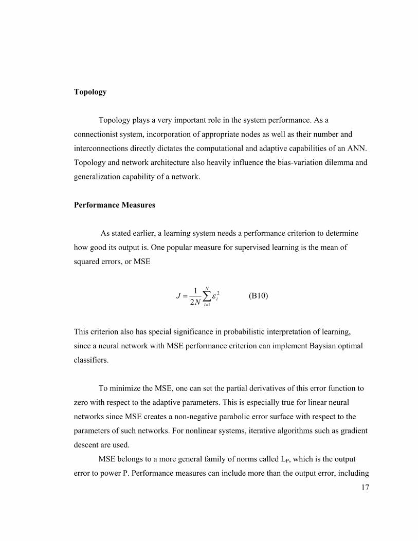
Performance Measures

As stated earlier, a learning system needs a performance criterion to determine

how good its output is. One popular measure for supervised learning is the mean of

squared errors, or MSE

∑=

=N

iiN

J1

2

21 ε (B10)

This criterion also has special significance in probabilistic interpretation of learning,

since a neural network with MSE performance criterion can implement Baysian optimal

classifiers.

To minimize the MSE, one can set the partial derivatives of this error function to

zero with respect to the adaptive parameters. This is especially true for linear neural

networks since MSE creates a non-negative parabolic error surface with respect to the

parameters of such networks. For nonlinear systems, iterative algorithms such as gradient

descent are used.

MSE belongs to a more general family of norms called LP, which is the output

error to power P. Performance measures can include more than the output error, including

17

penalty terms for topology as described in regularization. Temporal ANNs can use

similar performance measures that are summed over the duration of interest. Even though

ANNs usually use simplified single-objective performance criteria, multi-objective

performance criteria in general are also receiving attention recently41.

The following visualization tools are also useful for describing the learning and

testing phases of neural networks:

Performance Plots: also known as the learning curve or MSE plots include

graphing of MSE vs. iteration number. One can also plot weight tracks (i.e. plot each

connection weight vs. iteration number) for more insight. Weight tracks may demonstrate

over-damped, critically damped, or divergent behaviors based on the value of adaptation

step size η, with small step sizes resulting in a sluggish over-damped convergence and

large steps making the learning more prone to unstable and divergent regimes.

False Accepts and False Rejects, and the Confusion Matrix: a simple but effective

way to visualize and compare classifying machines is through the creation of a confusion

matrix using test data results. The matrix for a dichotomy follows. This method can also

be applied if more than two classes are involved. Having a diagonal matrix will be the

best case (no misidentification). Since this matrix is supposed to be built using the test

data set which is not used during the training, a populated diagonal also implies good

generalization. Each off-diagonal element indicates a class that was identified as another.

Furthermore, one can see which classes are more separable. Thus this will provide the

experimenter with valuable performance information that is not evident in other measures

such as MSE and weight tracks.

18

Table 1 Confusion matrix.

Neural Net Actual

Class 1

Class 2

Total Actual

Class 1

C11 Correct

C12 Misidentify

C11+C12

Class 2

C21 Misidentify

C22 Correct

C21+C22

Total Neural

Network

C11+C21

C12+C22

Total

Samples

Learning Algorithms

A learning algorithm is the search method that changes the system’s free

parameters such that the performance measure is optimized. For supervised learning,

besides an optimality criterion and learning method, one needs desired input-response

pairs. One method used extensively in first-order supervised adaptation algorithms for

many types of neural network is gradient descent on the error function. In conjunction

with the chain rule for multivariate functions, gradient descent is the cornerstone of the

famous and powerful Least Mean Squares (LMS) family of algorithms. LMS is local in

two different senses. First, because the nodes in a neural network can take part in the

global (network-wide) calculation for optimal performance just by using the local signals

from immediate nodes. Second, LMS finds local error minima and by itself cannot

distinguish between local and global answers. Enhancements such as adding momentum

and noise during the training phase or use of global search methods such as evolutionary

techniques can help alleviate this problem, as described during the later sections. Other

19

learning algorithm issues include choice of initial conditions and finding criteria to

determine when the training should be stopped.

20

B3-1 Static Linear Neural Networks

A learning linear system tries to adapt its parameters so that it can fit a hyperplane

with minimal or no error to given data points. This is also known as linear regression. A

neural network implementation of the linear regressor is called Adaline, which stands for

Adaptive linear element.

The Adaline (linear regression) model explains the relationship f in )( ii Xfd =

by minimizing the MSE. The first note of caution in using linear neural networks is the

limitation imposed by the first order regression: a linear network cannot map the given

data points {(xi,di)} well if they are not linearly correlated. One way to find out about the

co-trends between given data is calculating the correlation coefficient. The correlation

coefficient between x and y is defined as:

11)()(),(

)()(

))((

22+≤≤−=

−−

−−

=∑∑

∑

ryxyxCov

N

yy

N

xxN

yyxx

r

ii

ii

iii

σσ (B11)

r=+1 shows perfectly positive linear correlation between x and y , r=-1 shows

perfectly negative linear correlation between them, and r=0 means x and y are

uncorrelated. The closer the coefficient to 1± , the better a linear fit. Thus if the training

data covers most of possible cases with a correlation coefficient close , then we can

use a linear regression model for prediction of unseen data (generalization). This

coefficient can also be used to show quality of prediction in any neural network model by

setting x

1±

i to the actual target values and yi to the corresponding prediction, as shown in

the results section for Mackey-Glass chaotic series prediction tasks.

21

Neuron Model

The model used in linear neural networks is simply a weighted average of the

inputs, similar to that of the linear regression y=b+w1x1+w2x2+ … + wDxD. However, the

adaptation and implementation approaches are different.

Training Algorithms

Linear neural networks can utilize different algorithms to change their weights in

order to minimize their error. As in the linear regression case, if the number of free

parameters is equal or more than the number of training data a perfect linear fit can be

achieved (under-constrained). In this case the training data is memorized, which usually

is not the best case for fitting the test data (poor generalization). If the system has fewer

free parameters i.e. weights, (over-constrained), one can use an iterative algorithm such

as LMS to find the minimum-error fit as described below.

First Order Algorithms: LMS Method

Generally speaking, for a given dataset of N input-target pairs {(Xi,di)},

i=1,2,…,N and Xi=(xi1,xi2,…xiD), it is desired to fit a D-dimensional hyper plane. In

vector (matrix) notation:

1,;,,~00

1

0

1

0

0==

=

=⋅=⋅=== ∑=

xbiasw

x

xx

X

w

ww

WXWXWxwyd

DD

iT

i

D

jijjii (B12)

22

One can find the optimal weight set *W to minimize

iii

N

ii dd

NWJMSE ~,

21)(

1

2 −=== ∑=

εε by setting DkwJ

k

,...1,0,0 ==∂∂ and solving the

resulting D+1 equations. For iterative solution which is preferred for adaptive systems,

one can use the gradient-descent LMS algorithm. Both methods are described below.

Analytical Solution: The input autocorrelation matrix R (from D+1 input lines) is

defined as

TiiDDi

N

ii XXRwhereR

NR == +×+

=∑ )11(

1,1 (B13)

Since rmn=mean(xmxn)=mean(xnxm), then rmn=rnm and R is symmetric.

The input-output cross-correlation matrix P is defined as

iiDi

N

ii XdPwhereP

NP == ×+

=∑ )11(

1,1 (B14)

Since one can write ∑ ∂∂=

i iiW wu (.)ˆ(.)∇ , so grad (.) is a linear operator with

derivative-like properties. Thus one can write

WXXWdddN

WJ Tii

Ti

N

iii ==−= ∑

=

~,)~(21)(

1

2

∑∑==

−−=∇−−=∇N

ii

Tii

N

iiiiW XWXd

Nddd

NJ

11

))((1)~0)(~(221

RWPWXXN

XdN

WXXN

dXN

N

i

Tii

N

iii

N

i

Tii

N

iii +−=

+−=+− ∑∑∑∑

==== 1111

1111=

23

*0:; min RWPJJForPRWJ WW =→=∇−=∇ :

PRW 1* −= (B15)

Iterative Solution: instead of computing the optimal W* from (B15) for minimum

error, one can do an iterative search over the error surface. Since )(WJ∇ points towards

the maximum (rate of change) direction, then )(WJ∇− points towards the minimum

(fastest descending) direction of the error surface. To find the MSE gradient, one can

write

∑∑==

∇−−=

∇=∇

N

iiii

N

iiWW ddd

NNJ

11

2 )~0)(~(221

21 ε

∑=

−=N

iii X

N 1))((1 ε (B16)

for single data point i=k:

kkkkkkWkW XdddJ εε −=∇−−=

∇=∇ )~0)(~(

21 2 (B17)

To move in the direction of steepest descent by a single sample gradient (say kth), one can

write:

kkkkkk XWJWW ηεη +=∇−=+1 (B18)

η is a small, positive step size which is also called learning rate. This is a noisy estimate

since it is based on a single sample (xk,dk) of the whole set of N points. This noise might

24

be averaged out over many iterations. Iteration over the entire N data points is called an

epoch.

Step Size Control: based on the above calculations one can show that

*)()(* 01 WWRIWW k

k −−=−+ η (B19)

For convergence, it is sufficient that lim( , where

and λ

0) →Λ− ∞→kkI η

=Λ

Dλ

λλ

000

000

1

0

0, λ0,…, λD are the eigenvalues of R. Then we should have

11 <− iηλ which means Di ,...1,0, =i

20 <<λ

η . So for converging step size

max

2λ

η < (B20)

If one considers step k as a discrete time, then the convergence time constant in

the ith direction (wi) will be i

i ηλτ 1

= , implying a faster initial pace along the direction of

largest eigenvectors (larger λ, smaller τ), and continuing along smaller eigenvectors

afterwards.

In order to achieve both speed and precision especially for nonlinear multilayer

networks where the optimum step size cannot be calculated, one can use step size

scheduling by starting with a larger step size for initial speed and then reduce it for

accuracy near optimal weights (called learning-rate scheduling). The reduction of η can

be performed by using linear, geometric, or logarithmic schemes. This technique is also

known as annealing. There are other general heuristics for the LMS adaptation that are

described in the literature42. The above-mentioned details are just a small portion of all

25

the intricacies that one should go through in order to design and implement even a simple

neural network, a problem that GETnet tries to circumvent.

We must also mention two important modalities in training of neural networks: batch

and online learning. Updating Wi for each step is called online learning. One can use the

same starting W for calculating all the ∆Wi in an epoch and then average them to get the

new W. This is called batch learning. It involves fewer calculations and might provide a

smoother convergence. Batch learning is also important in temporal neural networks,

where each training pair represents a different moment in time. Such temporal batch

training is called trajectory learning.

Second Order Algorithm: Newton’s Method

Since we had PRWJW −=∇ , then )(11 JRWRPR ∇−= −− or

JRWW ∇−= −1* . Iteratively, one can write

kkk JRWW ∇−= −+

11 (B21)

This modified gradient-based training method is also called the Newton’s method. This

method changes the direction of search for skewed error surfaces by R-1. The original

gradient descent algorithm moves perpendicular to constant-error contours on the error

surface since ∇J⊥Jconst. Newton’s method changes this direction and finds a shorter path

to Jmin, because for skewed error surfaces contour plots from J=constant are non-circular

and this method compensates for different time constants τi in different directions. As one

can see from (B21), this method can get stuck at saddle points where the gradient is zero.

GETnet avoids this problem by adding adaptive noise components to the network

weights, as described later in section C.

26

Modified Newton (LMS/Newton) algorithm: one can add a step size η to the

second term in (B21) and replace the gradient with the sample-based approximation from

(B17) to get the iterative LMS/Newton form

kkkk XRWW εη 11

−+ += (B22)

Lateral Inhibition

The proposed network in section C can produce an arbitrary network structure,

including those with lateral inhibition. The decorrelating capabilities of such a formation

can shed a light into many of the capabilities of GETnet and will be briefly discussed

here.

Consider the paths in figure 5 for the network signals x2 and y1

y1 y2

y1 x2

c21 Σ Figure 5 Simple lateral inhibition.

This is a simple lateral inhibition where y1 adds a negative lateral signal c21y1 to x2 so that

12122 ycxy += (B23)

The sample-based cross-correlation between y1 and y2 can be written as 27

( ) ∑∑∑∑====

+=+==N

n

N

n

N

n

N

nyy nyc

Nnxny

Nnycnxny

Nnyny

Nr

1

2121

121

112121

121, )(1)()(1)()()(1)()(1

21

(B24)

One then can easily choose a c21 to decorrelate y1 and y2

∑

∑∑∑

=

=

==

−=→=+ N

n

N

nN

n

N

n ny

nxnycnyc

Nnxny

N1

21

121

211

2121

121

)(

)()(0)(1)()(1 (B25)

so the strength of such decorrelating lateral inhibition is equal to (minus) the inputs’

cross-correlation over the first signal’s energy.

LMS and Hebbian Learning

According to (B18) )()()()()()1( nXnnWnJnWn ηεη +=∇−=+W , or

)()()()()()1( nXnynXndnWnW ηη −+=+ (B26)

That is, the LMS algorithm for a linear node is composed of a forced-Hebbian term

)()( nXndη that drives the weight vector towards the correlation of input-target values

and an anti-Hebbian term )()( nXnyη− that is depositing a decorrelation of input-output

in the weight vector and driving the output towards zero, thus acting similar to the

stabilizing term in Oja’s rule43.

There is biological evidence for Hebbian learning, whereas LMS and back-

propagation type of learning have not been clearly observed in biological nervous

28

systems. However, it was shown above that Hebbian learning is a component of the LMS

gradient descent learning. Moreover, there is emerging new evidence of gradient descent

backpropagation learning in biological systems such as stem cell regulation44 as further

indication of biological relevance of gradient descent-based learning paradigms.

To conclude this section for static linear neural networks, it must be mentioned

that the reason for not introducing multi-layer linear ANN is the fact that combination of

any N hidden layers of linear PEs will yield a linear transfer function, so such

configuration is redundant and will degenerate to a single layer Adaline.

29

B3-2 Dynamic Linear Neural Networks

Consider a delay line with D taps and D-1 delay elements receiving a time-

sampled signal x(n). As long as the sampling frequency for x(n) is at least twice the

highest frequency of interest in x(t), x(n) will represent the input signal x(t) faithfully

(Nyquist’s theorem45). The delay line can be considered as a short-term memory (STM)

since the system will remember (D-1)*Tsampling of the input signal’s history. Three

different neuron models, namely moving average (MA), autoregressive (AR), and

autoregressive-moving average (ARMA)46 are used for temporal linear ANNs. The first

two can be considered as special cases of ARMA.

Moving Average Model: a D-point weighed average of the input from a tapped

input delay line represents a Moving Average (MA) filtering of x(n):

∑−

=

−=1

0)()(

D

ii inxwny (B27)

Since the impulse response of (B27) exists only for D clock ticks, it is also

referred to as a Finite Impulse Response or FIR filter. This form is easily realized from

the (zero bias) linear model studied earlier, with the input vector defined by the

instantaneous contents of the delay line:

+−

−=

)1(

)1()(

)(

Dnx

nxnx

nX (B28)

Similarly the discrete-time desired output is denoted by d(n) and the resulting

error is

30

)()()( nyndn −=ε

∑=

=N

nn

NJ

1

2 )(1 ε (B29)

x(n) x(n-1) x(n-2) . . . x(n-D+1)

z-1

z-1

i=D-1 z-1

wi

2

1

i=0

M

Figure 6 A moving-average linear neuron.

We also can extend this temporal interpretation to auto-correlation and cross-

correlation matrices P and R:

)()()(,)(1)1(

1nXndnPwherenP

NP D

N

n== ×

=∑ (B30)

and

)()()(,)(1)(

1nXnXnRwherenR

NR T

DD

N

n== ×

=∑ (B31)

where N is the number (length) of time samples available and XDx1(n) is the time-

sampled input signal x in the delay line as shown in figure 6. If the input-target samples

are ergodic, the above time averages can be replaced by the ensemble averages (or

31

statistical expected values). It can be seen that for temporal interpretation one can just

replace the sample index i with the discrete time index n and add an input tapped delay

line to a linear neuron according to Figure 6 for constructing X(n), and thus all the

previously derived results still hold. The time series can be padded with zeros for

unavailable samples (e.g. negative indices). There are other algorithms such as RLS

(Recursive Least Squares) for finding the optimal weights for the linear node in (B27)

and minimize the error in (B29). The linear MA filter of (B27) is also called a Wiener

filter.

Besides the usual applications of linear regression, one can train this linear neuron

for d(n)=x(n+k) to do prediction, with k usually set to 1. In this case since only the input

is being used for training, so it can be considered as some type of unsupervised learning.

This mode of operation is used to test GETnet with Mackey-Glass chaotic time series

(please see section C). Other applications of temporal linear neural networks include

interference and echo-cancellation, line enhancement and adaptive control, to name a

few.

Auto Regressive Model: this node model comes with a recursive time-delayed

connection to combine its past outputs with its present input

∑=

−+=D

ii inywnxany

10 )()()( (B32)

Here the tapped delay line is implemented at the output of the linear node and fed

back to the input. This constitutes the auto-regressive (AR) model.

Auto Regressive Moving Average Model: one can combine the moving average

model of (B27) with the auto-regressive model of (B32) to get a more flexible model

(and at the same time computationally more expensive to train) called ARMA:

∑∑==

−+−=P

jj

Z

ii jnybinxany

10)()()( (B32)

32

Because of the recursive connections from the output, the impulse response of the linear

neurons of (B32) and (B32) are stretched infinitely in time, so they are also called Infinite

Impulse Response or IIR filters as well. This makes AR and ARMA models prone to

becoming unstable, whereas the MA model will always have a bounded, finite response,

provided that it is given a bounded, finite input (bounded in, bounded out or BIBO

stability).

The frequency (steady state) responses of the MA, AR, and ARMA models can be

inspected from their transfer functions in z-domain:

∑=

−==D

i

iiMA zw

zXzYzH

0)()()( (B33)

∑=

−−== D

i

ii

AR

zw

azXzYzH

1

0

1)()()( (B34)

∑

∑

=

−

=

−

−== P

j

jj

Z

i

ii

ARMA

zb

za

zXzYzH

1

0

1)()()( (B35)

It can be seen that the MA model only has zeros and AR is an all pole model.

ARMA has both poles and zeros and thus the most versatile. In addition, because of their

poles, AR and ARMA can oscillate and become unstable. All these models can be

realized by a general linear neuron with summing tap delays both on its input and output

paths, realizing different variations of the difference equation

∑∑==

−=−P

jj

Z

ii jnybinxa

00)()( (B36)

33

Other Memory Kernels: besides the simple delay line, one can use more complex

memory structures (also called memory kernels) such as memories with recurrent

connections in different configurations like a tapped line. These recurrent memory

kernels such as Gamma memory units will be explained in nonlinear dynamic neural

networks, section B3-4.

34

B3-3 Static Nonlinear Neural Networks

Nonlinear neural networks are interconnected networks of adaptive, nonlinear

elements. They are capable of creating arbitrary discriminant functions, including that of

an optimal classifier. Nonlinear ANNs are usually arranged in different layers and can be

trained with different algorithms, including the popular backpropagation algorithm that is

based on gradient descent LMS technique and is applicable to supervised adaptation of

multi-layer ANNs with differentiable nonlinearities.

Neuron Model

The popular neuronal model used in these ANNs is a linear neuron cascaded with

a saturating nonlinearity f. The hyperplane created by the linear weighted summation

creates the decision surface

)(;,1; 00 netfybwxXWnet T ==== (B37)

For decision surface , i.e. the weight vector W is normal to the decision

surface. For instance For D=2 we have net=w

0== XWnet T

1x1+w2x2+b=0 or 2

12

12 w

bxwwx −−= , which

is a line determined by the weight ratios. Even though the placement of the decision

surface does not change as long as the ratios remain the same, the transition band through

the nonlinearity bending of the hyperplane does. This is because larger wis create a

steeper hyperplane that bends faster and thus creates a narrower transition band (see

figure 7). Introduction of the nonlinear activation function f may introduce multiple local

minima and saddle points in the error function ( )∑=

−=N

kk

Tk XWfd

NJ

1

2)(21 . However,

the nonlinearity helps classification by bending the regression hyperplane and fitting it to

the desired target classes. 35

Output Nonlinearities: the popular nonlinearities are

Hyperbolic tangent (tanh)

f(x)=tanh(x) xx

xx

eeee−+

−= , and f’=0.5(1-f2). (B38)

Sigmoid (logistic)

xexf α−+=

11)( , and f’=αf(1-f). (B39)

Hard limit (threshold)

<−≥

=0101

)(xx

xf , and f’ does not exist. (B40)

The last nonlinearity creates the Mcculloch-Pitts (M-P) neurons, whereas the first

two form the Modified M-P neurons. The tanh and logistic functions have derivatives that

are easy to compute. From now on by a neuron or node we mean a modified M-P neuron,

unless stated otherwise.

x2

2

1

21

2

12 ,

wwm

wbx

wwx −=−−=

x1 Transition Band

Figure 7 In modified Mcculloch-Pitts neurons class boundary depends on the weight ratios whereas the transition band depends on the actual weight values.

36

Note that the intersections of decision surfaces for neurons with smooth

nonlinearities create curves instead of piece-wise linear boundaries of hard thresholding.

The choice of sigmoidal functions also has biological basis. A single neuron’s

firing rate vs. its excitation voltage nonlinearly saturates to an upper bound that is

inversely proportional to its refractory period. Furthermore, from an averaging viewpoint,

if one considers the firing threshold of each cell to have a random value, an ensemble’s

firing threshold will have a Gaussian probability density function p(t). Thus on the

average, the probability of a cell firing for a stimulus of v volts is also

called the error function which has a general sigmoidal form

∫∞−

=v

dttpvP )()( ,

47. Sigmoidal nonlinearities

can also create competition between the neurons of a network48.

Training Algorithms

Here the most famous architecture for static nonlinear ANNs that is multiple layer

perceptron (MLP) will be introduced and some related supervised training algorithms

will be discussed.

Multi-Layer Networks

Multi-layer nonlinear ANNs are much more powerful than their single layer

counterparts. They can realize any decision surface. A two-layer network with k hidden

neurons can create 2k half-spaces in the input space that are then combined into decision

regions by the output layer nodes. For instance, a two input ANN with three or more

nodes in hidden layer can create a closed area in input space (see figure 8). One hidden

layer MLP with sigmoidal activation function and a large enough number of neurons in

37

the hidden layer is a universal mapper capable of approximating any continuous decision

region according to Kolmogorov’s theorem49.

Figure 8 MLPs can create arbitrary convex decision surfaces. 38

For two hidden layers, the discriminant function takes the form of

y=fout(Σf2nd-hid(Σf1st-hid(inputs))) with f1st-hid creating the hyperplanes in the input space,

f2nd-hid combining those hyperplanes into disjoint areas, and fout combining these disjoint

decision enclosures.

The two hidden layer MLP is also a universal approximator. Despite being slower

in adaptation, it is more versatile. However, a one hidden layer MLP can asymptotically

approximate the performance of a 2 hidden layer MLP when the number of neurons in

the hidden layer approaches infinity.

Back-propagation for Multiple Hidden Layer MLP: first let’s define the notation

, where the subscript i represents the node number within a layer, the superscript l

the layer number l=1,2,…L, and n the iteration number. The training data is given as

[ ] )(nli

( ){ }pp DX , where the pth input-output training pair ( )pp DX , is presented as

1,;, 003

2

1

02

01

00

2

1

0

==

=

=

= xbiaswddd

Dyyy

xxx

X

ii xy =0

. In a left to right network visualization,

l=0 denotes the input layer (so ), l=1 denotes the first hidden layer and so on, till

l=L that denotes the output layer. For any node, say j in layer l, wlj0=bl

j and y0l-1=1,

representing the bias term (see figure 9). Here the indices i, j, and k are used for

consecutive layer l-1, l, and l+1, respectively to show a typical three layer slice of an

MLP.

The local error (or injected error) δ for the jth PE in the lth layer at the nth iteration

is defined as

( ))(')()( nnetfnn lj

lj

lj εδ = (B41)

39

where

=−

= ∑ + otherwisennwlayeroutputLlifnynd

nk

lk

lkj

Ljjl

j )()()()()(

)( 1δε

)()()( 1 nynwnneti

li

lji

lj ∑ −= (B42)

.

.

.

y1l-1

wlj1

y0l-1=1 wl

j0=blj

yj=f(netj) net=WTY f(.)Σ

Figure 9 Node notations used in multiple hidden layer MLP back-propagation.

Using the chain formula for LMS, the backpropagation algorithm for the multiple hidden

layer MLP per each iteration n then can be expressed as follows.

1. Forward activation: compute output of each node, from network input to output.

( ) )()()(,)()( 1 nynwnnetnnetfnyi

li

lji

lj

lj

lj ∑ −== (B43)

2. Back-propagated error: Compute local (injected) error δ for each node, from

network output to input.

( )

=−

== ∑ + otherwisennwlayeroutputLlifnynd

nwherennetfnnk

lk

lkj

Ljjl

jlj

lj

lj )()(

)()()()()(')()( 1δεεδ

(B44)

40

3. Update weights:

1)()()()()1( −=∆∆+=+ l

ilj

lji

lji

lji

lji ynnwwherenwnwnw δη (B45)

η is the learning rate (step size). The vector form for the above equation (for weight

vector going to jth PE in the lth layer) can be written as:

1)()()()()1( −=∆∆+=+ llj

lj

lj

lj

lj YnnWwherenWnWnW δη (B46)

Note that 1)()( −−= lljW YnnJ l

jδ∇ , so 1)()()( −=∇−=∆ ll

jW

lj YnnJnW l

jδηη . A general

derivation that is also applicable to the temporal neural networks is given below.

Computation of Gradients in Ordered Networks

Paul Werbos50 introduced the powerful notion of ordered derivatives for

calculation of sensitivities in ordered networks, which befits many types of neural

networks including temporal. Here this method is introduced and the back propagation

equations in feed forward MLPs are derived through the general framework of ordered

networks.

Ordered Networks: An ordered network is network whose state variables can be

computed in a specific order, one at a time. One can number the nodes in such a network

according to their order of evaluation. A change in any state will ripple through the

network according to this order and state updates can be calculated accordingly. In such

networks, dependence of the sensitivity (derivative) of a variable with respect to a

preceding variable can be divided into two parts:

41

Explicit or direct,

Implicit or indirect.

Computation of sensitivities through such grouping of dependencies is the basis of

ordered derivative. For instance, consider the following three-node ordered network with

linear neurons. Sensitivity of y3 with respect to y1 in terms of ordered derivative is

computed as

2132311

2

2

3

1

3

1

3

1

3

1

3 wwwyy

yy

yy

yy

yy

yy inddirord

+=∂∂

∂∂

+∂∂

=∂

∂+

∂∂

=∂

∂ (B45)

█: Direct (explicit) ▒: Indirect (implicit)

y2

y3 y1

w21 w32

3

2

1 w31

Figure 10 A snippet of an ordered network.

The superscripts ord, dir, and ind indicate ordered, direct, and indirect derivatives,

respectively. This is similar to the partial derivative of a multivariate function. For

instance consider , whose dependencies are the same as those depicted in

figure 10 . The multivariate derivative can be written as

),( 213 yyfy =

22

31

1

33 21

ydyy

ydyy

dfdfyddf yy ∂∂

+∂∂

=+==

1

2

2

3

1

3

1

3

dyyd

yy

yy

ydyd

∂∂

+∂∂

= (B46)

42

Note that the state of the node j (yj) cannot be computed unless the states of the variables

such as yi that yj is dependent on are already known, either directly on indirectly (i<j in

feed forward networks).

In general, for an ordered network one can arrange the node states in the order

that they affect each other’s updates and write:

∑> ∂

∂

∂∂

+∂∂

=∂∂

+∂∂

=∂∂

ij i

jdir

j

ord

i

dir

i

ind

i

dir

i

ord

yy

yJ

yJ

yJ

yJ

yJ (B47)

where J is the dependent variable of interest.

In a feed forward neural network, this will be the network error (sum of output

node errors Ji over all training patterns), subject to minimization through gradient descent

ii

dir

iiiii

i yJydJJ

NJ εε −=

∂∂

−=== ∑ ,)(21

21,1 22 (Summation through pattern

indices p has been omitted for clarity). One can consider J in the above format as the

output of another node receiving its inputs from yi and di. Note that in (B47) i

dir

yJ

∂∂ is

zero unless yi is an output node. i

jdir

yy

∂

∂ in ∑

> ∂

∂

∂∂

ij i

jdir

j

ord

yy

yJ is also zero for any yj that is

not directly connected to yi, so the term will be reduced to direct derivative(s) of

whatever node(s) yj that are connected to yi on the path from output to yi times the

ordered derivative of J vs. yj (backward in terms of indices). Consequently the

summation index is only for the nodes j>i since these intermediate nodes are “after” the

origin node yi. In other words, in such an ordered feed forward configuration 0=∂

∂

i

jdir

yy

for i>j , which means that yj changes with respect to yi and not the other way around. By

the same token, replacing yi with wji, one can write:

43

∑ ∂∂

∂∂

+∂∂

=∂∂

+∂∂

=∂∂

k ji

kdir

k

ord

ji

dir

ji

ind

ji

dir

ji

ord

wy

yJ

wJ

wJ

wJ

wJ (B48)

The first term ji

dir

wJ

∂∂ is zero since J, if considered as a node, receives its direct inputs

from yi and di and not the connection weights. For the indirect part ∑ , the

non-zero term will be for the intermediate node k=j, since this is the only node connected

directly to w

∂∂

∂∂

k ji

kdir

k

ord

wy

yJ

ji. Hence, (B48) will be reduced to:

ijj

ord

ji

j

j

ord

ji

jdir

j

ord

ji

ord

ynetfy

Jwnetf

yJ

wy

yJ

wJ )('

)(∂∂

=∂

∂

∂∂

=∂

∂

∂∂

=∂∂ (B49)

Now one can derive the backpropagation formulas with ordered derivatives. Starting

from (B47):

Explicit (direct) term:

−

=∂∂

otherwiseoutputisy

yJ ii

i

dir

0ε

(B50)

For j

ord

yJ∂∂ , the first part of the implicit term in (B47) as well as the first term in (B49),

we define

jj

ord

ey

J ∆

=∂∂ (B51)

44

The ordered derivative of J with respect to yi reduces to -εi for the output layer (ei=-εi)

since 222 )(21,1

iiij

i ydN

J −== ∑ εε , and with yi having only direct ordered connection

to J ii

dir

i

ind

i

dir

i

ord

yJ

yJ

yJ

yJ ε−=+

∂∂

=∂∂

+∂∂

=∂∂ 0 . Alternatively, one can say since the

term ∑> ∂

∂

∂∂

=∂∂

ij i

jdir

j

ord

i

ind

yy

yJ

yJ and for the output nodes yi, there are no other nodes j to the

right (¬∃j>i), then the summation vanishes and reduces to zero.

For i

jdir

yy

∂

∂ part of the implicit term in (B47):

jiji

j

j

j

i

jdir

wnetfy

netnety

yy

)('=∂

∂

∂

∂=

∂

∂ (B52)

As stated earlier, this term is calculated for the nodes yj directly connected to yi (j>i),

otherwise the term will be zero (or connection weight is zero).

We also define

)(' iii

i

i

ord

i

ord

i netfenety

yJ

netJ

=∂∂∂

=∂∂

=∆

δ (B53)

We used (B51) in the substitution above.

Now, we can re-write our main equations (B47) and (B49). For (B47), using

(B50), (B51), and (B52) we can write

(a) yi is an output:

45

iii

ind

i

dir

i

ord

i yJ

yJ

yJe εε −=+−=

∂∂

+∂∂

=∂∂

= 0 (B54)

)(')(' iiiii netfnetfe εδ −== (B55)

(b) yi is intermediate (not an output):

∑∑∑>>>

=+=∂

∂

∂∂

+∂∂

=∂∂

+∂∂

=∂∂

=ij

jijij

jijjij i

jdir

j

ord

i

dir

i

ind

i

dir

i

ord

i wwnetfeyy

yJ

yJ

yJ

yJ

yJe δ)('0

(B56)

∑>

==ij

jijiiii wnetfnetfe δδ )(')(' (B57)

In either (a) or (b), using (B51) and (B53) we can write (B49) as

ijijjijj

ord

ji

ord

yynetfeynetfy

Jw

J δ==∂∂

=∂∂ )(')(' (B58)

Which is for the direct connection between yi and yj by wji.

One can observe that (B58) yields the error gradient vs. connection weights

necessary for the gradient descent algorithm. (B55) and (B57) provide the required local

(or injected) error for (B58). This error computation starts from the output and propagates

back to the input (i.e. backpropagation) because of constraint j>i in computation of inject

errors in (B57).

In summary, for each iteration n:

1. Compute forward activations using

46

= ∑

< jiijij ywfy (B59)

Direct inputs to node j can be considered as a yi from a preceding node (e.g. a

sensor). The activations will be computed from input to output, according to

ascending (forward) node indices.

2. Compute backward local errors δi using (B55) and (B57):

−

= ∑>

otherwisewnetfoutputisinetf

ijjiji

ii

i δε

δ )(')('

(B60)

These injected errors will be computed from the output to the input, i.e. according

to descending (backward) node indices. net values(e.g. ) are

already known from step 1.

∑<

=ji

jiij wynet

3. Compute weight updates for next iteration n+1 using (B58) and substituting

results from steps 1 and 2:

ijji

ywJ δ=

∂∂

)()()1( nwJnwnw

jijiji ∂

∂−=+ η (B61)

4. Proceed to the iteration n+1, using inputs from the current pattern pX or the next

pattern 1+pX .

47

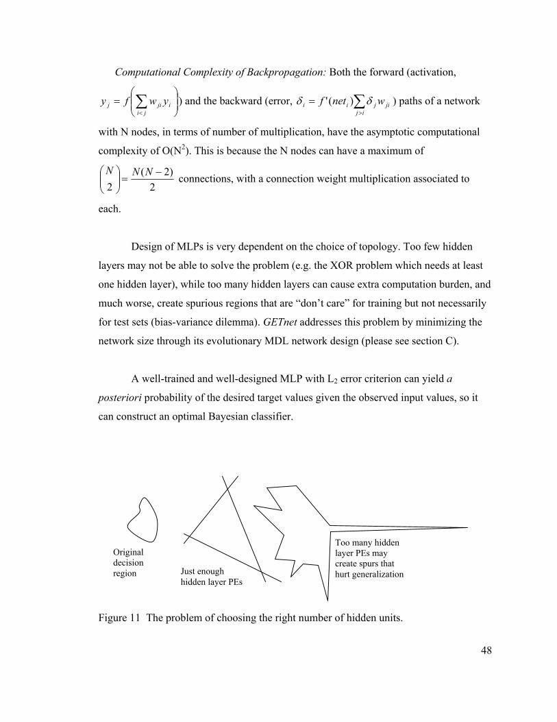
Computational Complexity of Backpropagation: Both the forward (activation,

) and the backward (error,

= ∑

< jiijij ywfy ∑

>

=ij

jijii wnetf δδ )(' ) paths of a network

with N nodes, in terms of number of multiplication, have the asymptotic computational

complexity of O(N2). This is because the N nodes can have a maximum of

2)2(

2−

=

NNN connections, with a connection weight multiplication associated to

each.

Design of MLPs is very dependent on the choice of topology. Too few hidden

layers may not be able to solve the problem (e.g. the XOR problem which needs at least

one hidden layer), while too many hidden layers can cause extra computation burden, and

much worse, create spurious regions that are “don’t care” for training but not necessarily

for test sets (bias-variance dilemma). GETnet addresses this problem by minimizing the

network size through its evolutionary MDL network design (please see section C).

A well-trained and well-designed MLP with L2 error criterion can yield a

posteriori probability of the desired target values given the observed input values, so it

can construct an optimal Bayesian classifier.

Too many hidden layer PEs may create spurs that hurt generalization Just enough

hidden layer PEs

Original decision region

Figure 11 The problem of choosing the right number of hidden units.

48

Improving Backpropagation Learning

The simple backpropagation algorithm introduced earlier has many advantages

such as simplicity, locality, and online implementation. Nevertheless, it can be improved

to avoid more or less situations such as stalling on flat regions of the error surface, local

minima, etc. Some of the human-tuned improvement techniques are as follows. Please

note how many parameters have to be guessed by the designer with no given definite

analytical guideline, further demonstrating the baby-sitting problem.

Momentum learning: Consider a hypothetical weight track such as the one

depicted in figure 12, where the network under training is rolling down under an

imaginary gravity and surface friction. Then each weight such as wji will not only change

because of the error gradient, but also the gained momentum under the imaginary

gravitational acceleration. To incorporate this concept, (B61) can be augmented with a

fraction of last weight change as

( ))1()()()()1( −−++=+ nwnwnGnwnw jijijjiji α (B62)

where α is the momentum constant, usually between 0.5 and 0.9 and chosen manually,

and Gj is the gradient descent update term ijji

j ywJ ηδη −=

∂G ∂

−= .

DC

BA

wj

J

Figure 12 An imaginary error surface with local minimum and a plateau to demonstrate momentum learning.

49

This way if the network hits a finite plateau (A in figure 12), the gained momentum,

depending on the value of α, can push the operating point further to the next downhill

(point B), if any. Furthermore, momentum can move the network out of shallow minima

(point C). This way the network can hopefully find a better next minimum (point D).

Adaptive Step Size: for problems such as linear regression, the step size should be

adjusted according to the eigenvalues in each direction. One can also adjust the step size

for a faster and more stable learning by using simple heuristics such as increasing the step

size when the learning curve is flat and decreasing it if the learning network starts to

oscillate around a minimum. This observation should be made for each connection’s step

size. As long as two successive weight updates ji

ji wJ

∂∂

−η (or the last gradient vs. a

running sum of previous gradients) have the same sign the step size for that particular

weight should be increased, and if the sign for a weight toggles, then the corresponding

step size should be decreased. One can increase the learning rate for each connection by a

small constant per iteration for a linear and slow step size growth. If the learning rate is

too high, it can be decreased by a fraction of the previous step size for geometric and fast

reduction. This step size adaptation algorithm is called Delta-bar-Delta, and is expressed

mathematically as

=

∂∂

−+∂

−∂∂∂

<

∂∂

−+∂

−∂∂∂

>

∂∂

−+∂

−∂∂∂

+

=+

∑

∑

∑

−

=

−−

−

=

−−

−

=

−−

0)()1()1()()(

0)()1()1()()(

0)()1()1()()(

)1(

2

1

1

2

1

1

2

1

1

n

m ji

mn

jijiji

n

m ji

mn

jijiji

n

m ji

mn

jijiji

ji

wmJ

wnJ

wnJifn

wmJ

wnJ

wnJifnb

wmJ

wnJ

wnJifan

n

γγη

γγη

γγη

η (B63)

0<γ≤1 and is set manually to determine contribution of previous gradients’

history. For instance, γ=1 only compares the previous gradient to the current. 0<b<1 for

50

step reduction and should be set manually as well. Variations of this scheme such as

Almeida51 or Fahlman52 are also used utilized.

One other method for step size control is through scheduling. The error criterion

is a function of the network’s adaptive parameters, here the weight vector; W. If the

direction of search in the adaptive parameter space, e.g. the fastest local descent -∇J (W)

is denoted by S, then we desire to find the best step size η in order to have the fastest

possible descent to the error minimum for each step k by minimizing J(Wk+ηkSk). One

may be able to find an analytical solution for the best step size, but usually for more

complicated networks one should use a heuristic such as scheduling or use trial and error,

with the tradeoff being between speed (bigger step size) and accuracy (smaller step size).

One popular learning rate scheduling is method is simulated annealing53. In this method,

learning will start with bigger step sizes to enjoy initial speed (provided that the network

is not initially near its goal) and then later, when the network is nearer to an error

minimum, the step size is decreased to achieve greater accuracy. One formulation for this

scheduling can be written as:

0

1

11n

kk −+

=η

η (B64)

Where η1 is the initial step size, k the iteration number. Constants η1and n0 should be set

experimentally by the designer.

Another issue that can be helped through step size is to adjust for the nonlinearity

attenuation of back-propagated error. According to (B60) which

determines the amount of weight update as expressed in (B61)

∑>

=jk

kjkjj wnetf δδ )(' ,

ijji yw ηδ−=∆ . However,

for sigmoidal activation function f’=f(1-f) which is always smaller than 1, so the

51

weighted sum of errors from the next layer ∑> jk

kjk wδ

ij y

is always attenuated by the factor

f’(net).

ηδ

0.25

f’(net)

net

Figure 13 Derivative of the sigmoid function has a maximum of 0.25 at the origin.

This will make the weight update jiw −=∆ shrink from the output to the input

layers, so the first layer’s adaptation may become very sluggish. One remedy is

increasing the step size η from output layer to the input layer, with the ratio determined

manually. The rule of thumb is increasing η 2 to 5 times, from each layer to the one

preceding it.

Random Perturbation During Learning: borrowing from the idea of simulated

annealing, one can add random perturbation (usually zero-mean noise) to the adapting

parameters (e.g. weights) during the learning period to move them out of local minima or

plateaus. This noise can be scheduled so it would become negligible during final

iterations, when the network is hopefully converging to the desired goal. This is one of

the motivations behind weight perturbations in GETnet, as explained later in section C.

However, in GETnet the Baldwin effect replaces the scheduling for reduction of

perturbation.

Initial Conditions: assigning initial weights to nonlinear MLPs is an important

issue, since the starting point for training should not be far from the intended goal. This is

not an issue for linear networks since their MSE error surface is hyperbolic with a unique

52

minimum, whereas nonlinear neural networks can have multiple, non-global minima on

their performance surfaces. An undesirable initial condition can also lead to undesirable

local minima, slow convergence, or degenerate answers (such as all 0 weights in an XOR

problem). Furthermore, neurons that are initialized in their linear region (|net|<<1) train

faster since this results in higher ∑>

−=jk

kjkjiji wnetfyw δη )('∆ because of higher f’(netj).

There are no comprehensive analytical solutions to this problem, so usually random

weights in conjunction with trial and error are used. However, there are some rules of

thumb for guiding the random initialization, such as Nguyen-Widrow so neurons will be

initialized in a region for faster training54,55, which is used in GETnet during instantiation

of new networks (please see appendix B for more details). Subsequent networks partially

inherit their contents from the previous generation.

Training set size: it can be shown56 that for an MLP with NW weights, the number

of required training data points N for reaching an error ε, given that the training data is

representative of the test data, obeys the inequality

εWNN > (B65)

This shows a linear growth of training set with respect to network parameters, which is

another advantage of MLPs compared to the other classifiers. It also shows that as a rule

of thumb, for a 10% error, one needs 10 training data points per weight. However, in the

real world we usually do not have such a big training set, so we might need to downsize

the network by reducing the number of nodes or connection weights (sparse

connectivity). One can also decrease the number of input nodes by preprocessing the data

and extracting fewer features for the network input. GETnet implements these notions by

competitive regularization and adaptive pruning.

53

Second Order Algorithms

The introduced gradient based back propagation only uses the information of the

first derivative of the cost function with respect to the adaptive parameters, with a

sample-based noisy estimation of the gradient. There are other search methods that use

more information from the curvature of the error surface through higher order derivatives

as well as global search methods such as evolutionary algorithms. The advantage of the

gradient-based back-propagation is in its simplicity (just a few additions and

multiplications per weight update), dependence on local parameters, and capability of

online, real time training.

The more complex second order algorithms can be derived from the Taylor

approximations. Going back to the basic problem of minimizing the error function J(W),

its expansion by the multivariate Taylor series around the operating point W0 can be

written as

( )( )∑∞

= =

∇⋅−=0

0

0

)(!

1)(k WW

kW WJWW

kWJ or

( )∑ ∑∞

==

=

∂∂

−=0

211

021

0

),,(!

1),,(k

WW

M

l

l

M

lllM wwwJ

www

kwwwJ …… (B66)

where ∇W is the gradient operator, the variable vector ∑=

=M

llluw

1

ˆW represents all the

network weights in the M-dimensional weight space with unit vectors u , and lˆ

∑=

=M

llluwW

100 ˆ is the initial weight vector close to W. (B66) can be obtained from the

repeated integration of the n+1th derivative of J with respect to the weights:

54

( )1

11

0

)(

+

++

∫ ∫∇

n

W

W

nnW WdWJ (B67)

Using (B66), the second order truncated vector Taylor approximation can be written as57

( ) ( ) ( ) ( )

∇∇⋅−⋅−+

∇⋅−+=

== 00

)(21)()()( 0000

WWww

WWw WJWWWWWJWWWJWJ

(B68)

(B68) can be written in matrix notation as

+−−+∇−+= ))(()(21)()()()( 000000 WWWHWWWJWWWJWJ TT (B69)

W=[wi]M×1 is the column matrix of all the network weights (total weight vector made of

concatenation of all the nodes’ weight vectors) and W0=[w0i]M×1 is the initial center close

to W. ∇J(W0) is the gradient in the form of a column vector ∇J(W)=[(∂/∂wi)J]M×1

evaluated at W=W0. H is the Hessian matrix of the error function J(W):ℜM→ℜ. The

Hessian itself is a function of the network weights and defined as

ji

MijMMij ww

wwwJhhWH∂∂

∂== ×

),,,(,][)( 21 … (B70)

H(W0) is a symmetric matrix of partial derivatives evaluated at W0. Thus gradient of J in

with respect to W results in

+−+∇=∇ ))(()()( 000 WWWHWJWJ (B71)

The first order methods such as gradient descent use the first term, and the second order

methods such as Newton use the second order approximation which involves the Hessian. 55

In fact, equating the second order truncation of (B66) with zero to find coordinates of

minimum error in weight space (W for which ∇J(W)=0) results in

))(()(0 000 WWWHWJ −+∇= or )()()( 0001 WWWJWH −+∇= −0 , yielding

00

10

WWJHWW ∇−= − (B72)

Which is the same as our earlier formula for the Newton method in linear ANN, since

from (B15) PRWJW −=∇ so ( ) RJH =∇∇= . (B72) can be used iteratively as

)()(

1)()1(nWnW

JHnWnW ∇−=+ − (B73)

Note that in both (B72) and (B73) W is considered to be a column matrix representation

of the total network weight vector. The Hessian is not local as it needs non-local

information (e.g. partial derivatives of J with respect to all weight combinations wiwj

across the whole network), and increases quadratically in size with the number of weights

which makes it computationally expensive, not to mention the computation of its inverse

provided that it exists. One can either improve the first order method (e.g. line search

methods) or approximate the Hessian (e.g. for the pseudo Newton methods), as described

below.

Line Search: As discussed earlier in learning step size control, the goal of learning

is minimizing the error function, J(W). The direction of fastest local descent in each step

is -∇J(W(n)), which is perpendicular to the J=constant contours. Based on the

eccentricity and skew of the error surface J(W), the first order gradient search will go

through a zigzag path. One can reduce this longer jagged path by combining the two most

recent update directions as:

56

+=+∆+∇−=+

)1()1()()()()1(

nsnWnsnnJns W

ηα (B74)

This is called the conjugate gradient method58. α can be determined through different

methods as described in appendix A. Scaled Conjugate Gradient method, or SCG, is the

method of choice used for GETnet, since it avoids a plethora of manually set constants

and complexities of the other accelerated gradient searches described earlier. Please refer

to section C for more information.

Pseudo-Newton Methods: In these methods a computationally less complex

approximation to the Hessian in conjunction with (B73) is used. One method is to keep

only the diagonal terms of the Hessian so (B73) can be written as

2

2

)()()()(

)()1(

nwnJnwnJ

nwnw

i

iii

∂∂∂∂

−=+ (B75)

or use the absolute value of the second derivative plus a small positive constant c to avoid

division by zero:

cnwnJ

nwnJ

nwnw

i

iii

+∂∂

∂∂

−=+

2

2

)()(

)()(

)()1( (B76)

There are also better approximation methods such as Levenberg-Marquardt, Davidson-

Fletcher-Powell, and the Broyden-Fletcher-Goldfarb-Shanno59.

57

Improving Backpropagation For Unseen Data

To improve generalization, one should find measures indicating when the network

has learned the problem in a general sense. This can be done among other methods by

observing the performance on a portion of the test data as the criteria to end training (to

avoid overtraining and memorization), or pruning a network that has too many free

parameters (to reduce don’t care regions). One can also take the democratic approach and

ask different classifiers to cast their votes which averages out their output errors. All of

the above techniques are utilized by GETnet.

Stopping the Training

A simple criterion is using a stopping threshold for training error. For instance,

one can stop training when the network error (e.g. MSE) reaches a threshold, say 0.02.

However, general network errors such as MSE are indirect measures of performance and

are based on the training set and do not carry information on the test set and thus

generalization cannot be guaranteed. Setting too low a threshold for training set error

might make the network over-fit or memorize the training or the preset threshold might

never be achieved (a maximum number of iterations can be set to avoid an infinite loop in

this case). Increasing the error will stop training before appropriate class boundaries are

obtained. It is also possible to set a stopping threshold to the performance measure’s rate

of change. However this criterion still suffers from the above stated issues, plus some

networks start converging to the answer after a period of low MSE slopes, in which case

the network might exit training prematurely. Based on the above, it would be much better

to base the stop criterion on generalization. The goal is stopping the network from

overtraining, when the discriminants start to leak to the don’t care areas where some of

the unseen test data may reside. One can keep a portion of the training set as the cross-

validation set (usually 10% of the training data). The network should check after every

few iterations to see whether the cross validation error is increasing, and stop early in the

58

interest of generalization even if the training error is still decreasing (see figure 14). This

method is also known as early stopping.

A

Error

n

Figure 14 The network should stop early at point A for optimum overall performance on both the training (solid curve) and cross-validation data (dashed curve) and retain its generalization.

Network Pruning

Earlier the relation between network size and architecture vs. its classification

capabilities (bias-variance dilemma) was discussed. Methods such as early stopping with

cross validation help generalization by avoiding over-training but they do not address the

problem in terms of model size and extra free parameters. One might want to follow

Occam’s razor principle and use a network just big enough to solve the problem at hand.

To achieve an ANN of such size, one can either start from a smaller network and grow it

to reach a working network, or start from a bigger ANN and downsize it by pruning the

network (removing inconsequential parameters). GETnet tries to eliminate unnecessary

connections while adding the new ones according to evolutionary experience, thus it is

capable of both growing and shrinking the network.

Weight Decay: The idea is to decrease all the weights just a little during each

iteration. If a weight was not to be decreased, the learning algorithm will increase it in

next iteration. Otherwise the weight will be gradually driven to zero and eliminated after

falling below a threshold. 59

Finding Importance of a Parameter: a good but complicated method for finding

the most suitable candidates for weight elimination is calculation of each parameter’s

saliency, by finding the effect of setting it to zero in the error function. It can be shown60

that the Hessian has this information and a local approximation for weight saliency can

be obtained from:

2

22

2

21

2 kk

kkkk u

JuuH

s∂∂

∂== (B77)

where uk=wji, and k∈{all weight index pairs}. To implement this method, also

known as optimal brain damage, one should first train the original network, then

calculate the saliency of its weights and sort them accordingly, and keep a predefined top

percentage. Then the network should be retrained with this new smaller set of weights

and their original initial values. This process will be repeated until the desired number of

weights (based on the size of available training data set, etc) and generalization is

achieved, i.e. the optimal damage (reduction) to the brain (neural network) has been

found.

Another pruning technique is keeping only the most important inputs. Selection

can be performed by calculating output sensitivity with respect to each input. One should

first train the network and then add random perturbation to the inputs one by one and

measure the resulting swing in the output(s). The sensitivity then can be found from the

ratio of resulting output variance to input variance. In any case, one should always

consider the negative effects of network complexity, as in the regularization term in (B9).

GETnet prunes the synaptic weights using a relative importance (C18). The

evolutionary part of GETnet also estimates the sensitivity of network in terms of the

fitness score with respect to connections and nodes by changing them according to the

strategy parameters.

60

Committee of Networks

A neural network has a stochastic learning nature since each training episode

results in a different set of weights. Even if the training errors of some of the runs are not

minimal, they might prove to be the better solution based on their performance on the

unseen test data (generalization). It was also mentioned that architecture and size

influence network behavior and performance. One approach for getting a better

performance is to retain all those solutions obtained from different training runs on the

same network as well as different topologies and average the results, also known as

committee of networks method. It can be shown that for such an approach, given that each

network’s error is statistically independent, the MSE error of the committee of networks

can be reduced N times compared to the mean error of an individual network with N

being the number of networks in the committee61. In practice the errors are higher since

the errors of the networks are not independent. In the case of using one topology with

different parameters in a committee, the resulting system can be viewed as a sparsely

connected network, i.e. a special case of a weight-eliminated network that has resulted in

parallel modules.

1/N Σ ...

Network 2

Network 1

X

Figure 15 A committee of networks.

61

B3-4 Dynamic Nonlinear Neural Networks

All the biological neural networks perceive and process information in time.

Though more complicated, temporal processing can give an adaptive system a lot more

information about the input sequences. Inputs with the same static distribution might

have different dynamic progressions (i.e. different signal trajectories in time). For

instance, a time sequence of the sum of two sinusoidal signals with different frequencies

but equal amplitudes can be separated by filters, while their cumulative amplitude traces

are non-separable if the time progression (frequency) information is not available. In

other words, in dynamic systems the order as well as the pace of presented data is given

and important, whereas in static systems it is not.

Temporal inputs along with temporal pattern processing gives rise to the notion of

memory. Path delay lines (both forward and feedback) can store a moving window of the

signal history and can be considered as a form of Short Term Memory (STM)62, such as

the one discussed in MA model of a linear neuron. Information stored in form of

connection weights of an artificial neural network such as the distributed memory of a

Linear Associative Memory (LAM)63 as well as the infinite delayed feedback loops can

be considered as Long Term Memory (LTM).

Dynamic systems with temporal connections can be feed-forward or have

feedbacks (recurrent systems). In either case, because of time delays the output will have

a transient period before reaching steady state, given that system is stable. Use of delay

lines as memory structures inside the feed forward neural network provides static

snapshots of the signal’s past within a time window, giving rise to a Finite Impulse

Response (FIR) system64. The length of the delay line must be carefully chosen to capture

the desired information. If the sought features are stationary, their derivation should

remain the same in spite of the sliding input time window, given enough length of the

static window.

62

In theory, recurrent systems offer infinite recall through feedback loops and create

Infinite Impulse Response (IIR) systems. However, such systems may become unstable

or oscillate, which sometimes may be desirable in neurocomputing. In fact, nodes in a

recurrent neural network with sigmoidal activation function can saturate towards either

output extreme, mimicking a finite-state machine. One can consider the states of such a

network (i.e. outputs of the nodes) with N nodes being represented by a hyper N-cube. A

saturating network approaches one of the vertices, which is called an attractor. This

topic is further discussed under network energy later on in this section. Computation

through attractors can display regular or chaotic behavior. However, the training of such

a network is much more involved. It is possible to unroll the feedback loops and simulate

recurrent systems with feed forward time delay neural networks (TDNN) for a given time

span, or to use temporal versions of back propagation65.

Time Delay MLP (TDNN)

If one places a delay line (such as the one used in the MA filter) at the input of a

multilayer Perceptron, the resulting structure is called a focused Time Delay Neural

Network, or simply a TDNN. The term focused emphasizes the fact that the short-term

memory structure is focused in the input. Such structures were introduced by Waibel for

speech processing22. TDNN can also be used for other nonlinear temporal mappings such

as nonlinear dynamic system identification and nonlinear time series prediction. In fact,

an adequate predictor can autonomously reproduce a time series (dynamic modeling). It

is enough to set the right initial conditions (seeding the system) and connect the output of

the adapted predictor y(n)=f(x(n))=x(n+1) to its input, as shown below.

y(n)=f(x(n))= x(n+1) f

Figure 16 Dynamic modeling. 63

As can be seen from figure 17, the first layer of the TDNN is essentially a bank of

moving average (MA) filters with nonlinearities after each weighted time delay average.

The subsequent layers simply function like regular MLPs, nonlinearly mapping the

results of the various filterings of the input signals to the (desired) output signals.

.

.

.

.

.

.

.

. N

2

1

.

.

.

z-1

z-1

τ=Mz-1

wji

2

1

τ=0

M

2

1

.

.

.

x(n) x(n-1) x(n-2) . . . x(n-M)

y1

y2

yN

Figure 17 A focused time delay multilayer Perceptron.

In temporal paradigms the input as well as desired and network outputs will all be

single or multidimensional sequences. As long as the desired output for each time step

exists, the network weights can be trained with the static algorithms such as back-

propagation. A TDNN with appropriate MLP topology and memory resolution and depth

can be a universal temporal mapper66.

Generally speaking, the short-term memory in a neural network can be

implemented either by a delay line as described earlier or by a delayed feedback

connection (e.g. from the output to the input of a node) to create a recurrent element.

Such elements are also known as a context node (see figure 18). The depth of the memory

(time extent of impulse response) of the delay line memory kernel is equal to the length

of the delay line, whereas in the case of recurrent context memory it is theoretically

infinite but practically limited depending on the feedback strength. In either case, the

resolution of the memory (temporal sampling grain) depends on the value of d, the

inverse of the sampling rate of the delay element.

64

The delay line STM can also be seen as a linear projector of the input signal into a

space whose coordinates are the consecutive delayed values of input within the delay

line. The deeper a delay line of adequate resolution, the higher the dimension of this

representation. This translates into a higher chance of separation of the input patterns by

the subsequent MLP since the signal trajectories will hopefully be further apart and have

fewer overlaps, i.e. longer histories may potentially reveal more distinctive features.

d

.

.

.

Σ f(.)

.

.

.

d

d

.

.

.

d

.

.

.

Σ f(.)

Figure 18 A delay line memory (left) vs. a recurrent or context memory (right).

A combination of the delay line memory and recurrent context memory creates a

special memory system called the Gamma Memory6. Each memory element of the

Gamma memory delay line is made of a simple first-order recurrent kernel (figure 19).

y0(n)

z-1

yD-1(n)

y1(n)

g

…

1-µ

µ Σ…

g

g

g

Figure 19 Gamma memory (left) and its recurrent context element (right).

65

The delay element’s output for the kth tap is given by

( ) )1(1)()( 1 −−+= − nynyny kkk µµ (B78)

In the z-domain, (B78) can be written as ( ) )(1)()( 11 zYzzYzY kkk µµ −+= −− or

( )µµ−−

==− 1)(

)()(1 z

zzY

zYzGk

k (B79)

In the time domain, yk(n) can also be written as yk(n)=yk-1(n)*g(n) where

g(n)=Z-1{ G(z)}, equal to Yk(z)= Yk-1(z)G(z). Iteratively

)()()( 1 zGzXzY kk

−= (B80)

g(n) has the form of the Gamma function’s integrand, and hence comes the name

Gamma memory. If the tap outputs of the Gamma memory delay line are fed to a linear

neuron for weighed sum, the resulting configuration is called a Gamma Filter.

It should be noted that if µ=1, then the Gamma memory turns into a simple delay

line. The feedback portion of the delay element creates an exponentially decaying infinite

impulse response (IIR) filter with h(n)= µ(1-µ)n-1 since ( ) )1(1)()( −−+= nynxny µµ .

This theoretically infinite impulse response of the Gamma memory gives it more memory

depth (in recall of the past) with a shorter delay line. However, in contrast to the arbitrary

impulse response of an FIR, the impulse response of the recurrent IIR has only one

control parameter µ.

Time-delay RBF Neural Networks: Besides MLP, one can feed the tap outputs of

a memory structure to a RBF neural network. For a simple delay line focused architecture

66

such as the one given in figure 17 the overall signal swing will be the same along each

time delay axis (tap) since the input signal traverses all the stages in turn, thus the input

space will be extensively covered. Since many basis functions such as Gaussian are local

(i.e. their magnitudes decrease rapidly as their arguments increase), one may have to use

many input bases in order to cover the signal space spanned by tap-delay. The choice of

Gamma memory over a simple delay line may help since it has more depth with fewer

taps. However, Gamma memories have less resolution because of the low pass averaging

action of their recurrent context elements.

Jordan Networks: these networks have a context layer whose outputs go to

network’s hidden layer. The context layer is made of context memory elements with pre-

defined fixed feedback gain (for instance the Gamma delay kernel shown in Figure 19).

The context layer receives its input from the network output. This way, based on the

output history (output context) the system can differentiate between incoming temporal

patterns (figure 20).

Elman Networks: these networks are similar to Jordan networks with a hidden

context layer made of context memory elements with pre-defined fixed (or even adaptive)

feedback gains. However, their context layer receives its input from the network’s hidden

layer (see figure 20). Then based on the on system’s internal state history (internal

context), the system can differentiate between incoming temporal patterns.

Jordan and Elman networks are capable of producing different results for the

same input patterns based on network context layer contents (i.e. different past histories

and scenarios). Since the feedback weights are constant, one can use backpropagation

during each time step to find the corresponding error-descent weight gradients. The non-

adapting feedback weights as well as the general network size and topology leave quite a

bit for guessing and trial and error. In Jordan networks erroneous outputs will be fed back

to the context layer and may corrupt its contents for future steps.

67

Based on the versatile arbitrary configurations that GETnet can assume, Elman

and Jordan networks, as well as all memory kernels described above can be realized by it.

Input

O/P

Context Layer

Hidden Layer

Input

O/P

Context Layer

Hidden Layer

Figure 20 Jordan temporal network (left) vs. Elman temporal network (right). Bold lines represent multiple connections.

General Temporal Neuron Models

All the studied neural elements studied so far can be categorized as special cases

of a Nonlinear Auto-Regressive Moving-Average, or NARMA processing element. A

single input, single output causal discrete-time NARMA element of order (M, N) is

defined as

( ) 0)(,),1(),(;);(,),1(),(;);(,),1(),( 1111 =−−−−−− NnynynyMnxnxnxMnxnxnxf DDDD …………… (B81)

The above formula corresponds to a discrete-time system described by a set of difference

equations. (B81) can be re-arranged as

y(n)=fio(…;xi(n),xi(n-1),…;y(n-1),y(n-2),…) (B82)

68

and depicted as

y(n) . . .

xi(n)

Mi N...

d

d

.

.

.

d

.

.

.

d

d

.

.

.

d f(.)

Figure 21 A general nonlinear ARMA element.

In fact the term “moving average” befits a simpler arrangement given later here by

(B87) since the nonlinear function f here is not essentially averaging the contents of the

sliding time windows captured by delay lines Mi.

Special cases of NARMA include

∃Mi≠0, N=0 (no feedback): (B82) reduces to a nonlinear moving average or NMA

described by y(n)=fio(…xi(n),xi(n-1),…).

∀xi=0, N≠0 (no input, just feedback loops): we will have a nonlinear auto-

regressive element or NAR which displays an output based on its initial

conditions described by y(n)=f(y(n-1),y(n-2),…).

∀Mi=0, ∃xi≠0 (no input delay): we will have a nonlinear auto-regressive element

with external input (NARX).

NARMA is the most comprehensive model and encompasses the existing ANN and

biological models such as Grossberg’s additive model and Freeman’s model. The

continuous version of Grossberg’s model is given by

69

)()()()(

,tIbtywfty

dttdy

jjjii

ijijj +

++−= ∑

≠

µ (B83)

bj is the jth node bias and Ij(t) is its external input. Note how this equation resembles that

of a leaky integrator (parallel RC circuit) which is indicative of a simple, passive, single

compartment biological neural state space model:

( )

=

++−= ∑=

)()(

)()(1)(1)(1

tvftyCtItxw

Ctv

RCtdtvd

sigmoid

i

N

ii (B84)

with v(t) being the instantaneous membrane voltage, I(t) the external injected current

signal, and wixi(t) the weighed ith input current from other node(s). The second equation

in (B84) approximates the integrate and fire action of an excitable membrane that

converts the internal variable v(t) (membrane voltage) to an instantaneous spiking

frequency y(t). Substituting y(n) for y(t) and y(n)-y(n-1) for dy(t)/dt in (B84) yields the

discrete time version of Grossberg’s model. In general:

)()()()1()1(,

nIbnywfnyny jjjii

ijijj +

++−=+ ∑

≠

µ (B85)

Variations of this model are the predominant neural models used in artificial neural

networks. Note that µ=1 yields the famous McCulloch-Pitts static neural element.

Higher order model such as Freeman’s67 are used in the modeling of biological

systems. Freeman’s model represents the rabbit olfactory system and is given as an

ensemble of second order neuronal assemblies. The building blocks are defined by the

second order differential equation

70

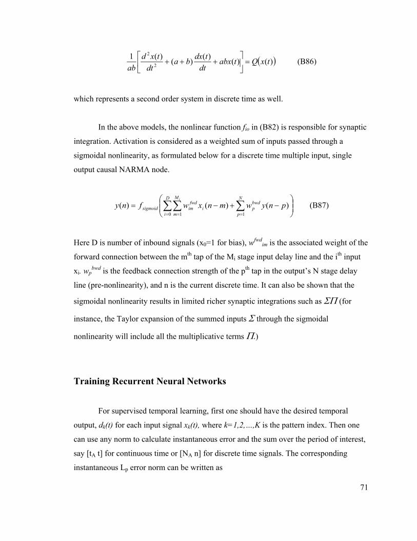
( )()()()()(12

2

txQtabxdt

tdxbadt

txdab

=

+++ ) (B86)

which represents a second order system in discrete time as well.

In the above models, the nonlinear function fio in (B82) is responsible for synaptic

integration. Activation is considered as a weighted sum of inputs passed through a

sigmoidal nonlinearity, as formulated below for a discrete time multiple input, single

output causal NARMA node.

−+−= ∑∑∑

== =

N

p

bwdp

D

i

M

mi

fwdimsigmoid pnywmnxwfny

i

10 1)()()( (B87)

Here D is number of inbound signals (x0=1 for bias), wfwdim is the associated weight of the

forward connection between the mth tap of the Mi stage input delay line and the ith input

xi. wpbwd is the feedback connection strength of the pth tap in the output’s N stage delay

line (pre-nonlinearity), and n is the current discrete time. It can also be shown that the

sigmoidal nonlinearity results in limited richer synaptic integrations such as ΣΠ (for

instance, the Taylor expansion of the summed inputs Σ through the sigmoidal

nonlinearity will include all the multiplicative terms Π.)

Training Recurrent Neural Networks

For supervised temporal learning, first one should have the desired temporal

output, dk(t) for each input signal xk(t), where k=1,2,…,K is the pattern index. Then one

can use any norm to calculate instantaneous error and the sum over the period of interest,

say [tA t] for continuous time or [NA n] for discrete time signals. The corresponding

instantaneous Lp error norm can be written as

71

( )ptdtyt )()()( −=ε (B88)

Replacing t with n will yield the discrete-time version, ( )pndnyn )()()( −=ε . The

resulting aggregated temporal errors will be given by

∑ ∑= =

=K

k

n

Nik

A

inJ1

)()( ε (B89)

∑ ∫= =

=K

k

t

tk

A

dtJ1

)()(τ

ττε (B90)

Two general modes of training can be applied to error signals described in (B88)

through (B90): fixed-point or trajectory learning.

For fixed-point back propagation learning, the input is applied and clamped at

each time instance n till the transients of the network are over. Then the

corresponding error at that clamped instance is calculated and propagated back

through the dual network. Corresponding weight gradients are calculated after the

transients of the dual network have died out.

For trajectory learning, the cumulative temporal error over the period of interest

as given by (B89) or (B90) is used. One has to wait for the changes to propagate

through all the path delays and show their effects over the whole period of interest

(time trajectory) in order to be able to calculate required derivatives.

Static back-propagation cannot be used in adapting recurrent parameters since a

change in feedback parameters loops and propagates in time forever. However, the

network topology imposes a specific order on system state updates that remains constant.

This leads to an ordered list such as the one implied for ordered derivatives in (B47) and

enables one to derive networks’ variable sensitivities through time. More specifically, 72

consider a temporal neural network of N nodes and their corresponding internal states

(instantaneous node activations) S(n)={yi(n)} and connection weights W={wji}. The N-

tuple S(n) describes a static, non-recurrent network in each time-snapshot n and has an

ordered list of the instant feed-forward dependencies of the network. The overall

temporal dependency list can be written as

{ } { }…………… ),1(,)0(,,,),1(),0(, iiji yywSSWL == (B91)

One can also arrange weights of an ordered network in a matrix format W=[wji] so

that the row index j designates the destination node and the column index i designates the

source node of the connection weight wji. Since for a feed-forward network connections

j>i, such a network will have all its upper-triangle elements equal to zero, and vice versa.

The nonzero diagonal elements indicate the strength of self-feedback in corresponding

nodes. Note that no feedback loop can exist without delay; otherwise unrealistic races

will take place. Based on the ordered dependence list of (B91) one can derive ordered

derivatives needed for back-propagation. Recalling the earlier definition of ordered

derivative in an ordered network from (B47) and taking into account the new extended

ordered list of (B91) one can write

∑∑> > ∂

∂

∂∂

+∂∂

=∂∂

+∂∂

=∂∂

n ij i

jdir

j

ord

i

dir

i

ind

i

dir

i

ord

nyy

yJ

nyJ

nyJ

nyJ

nyJ

τ

ττ )(

)()()()()()(

(B92)

The index τ>n ensures that the temporal order in the list L is preserved, and j>i

implements the same ordering imposed by the (spatiotemporal-unrolled) structure.

Similarly, if we replace y with w in (B92) and simplify, we will have:

∑∑≥ ∂

∂∂∂

=∂∂

+∂∂

=∂∂

n jk ji

kdir

k

ord

ji

ind

ji

dir

ji

ord

wny

nyJ

wJ

wJ

wJ )(

)( (B93)

73

Note that the direct derivative of error as described in (B88) through (B90) with respect

to weights is zero. In addition, since the weights are before all the states in (B91), the

time index should run its full course. ∑≥ ∂

∂∂∂

jk ji

kdir

k

ord

wny

nyJ )(

)( is nonzero only for k=j because

of the second term. Thus (B93) can be further simplified into

∑ ∂

∂

∂∂

=∂∂

n ji

jdir

j

ord

ji

ord

wny

nyJ

wJ )(

)( (B94)

Similar to the procedure shown in (B47) through (B61), (B92) and (B94) will

yield the required weight gradients for backpropagation in a recurrent temporal ordered

network of N nodes within the given time frame n∈[1 nf]. Now (B94) can be substituted

in (B92) to yield the sought gradient component

∑ ∑∑= > > ∂

∂

∂∂

∂∂

+∂∂

=∂∂ f fn

n ji

jdirn

n

N

jk j

kdir

k

ord

j

dir

ji

ord

wny

nyy

yJ

nyJ

wJ

1

)()()(

)()( τ

ττ

(B95)

The main challenges for using the above scheme to train temporal recurrent neural

networks include:

1. (B95) becomes rapidly costly for bigger networks and longer time

spans (bigger N and nf).

2. One has to find a method for choosing appropriate delays.

3. Co-adapting of weights and delays makes the performance estimate

very noisy, and introduces many local minima.

4. It has been shown that it is hard for backpropagation in time to learn

long-term dependencies.

Two other remaining issues are the non-causality of the summations in (B95)

which can be solved by deferring the calculations to the end of the time trajectory n=nf,

74

similar to the batch mode; as well as the infamous problem of finding the optimal

topology as discussed earlier in terms of the bias-variance dilemma. Gradient descent

learning can actually be applied to network delays68,69 but still the other mentioned

challenges remain. GETnet tries to circumvent these problems by introducing hybrid

training and using partial temporal backpropagation, while finding suitable delay

structures through an evolutionary process, as described in section C.

Network Energy, Hopfield and Boltzmann Neural Networks

A different way of looking at temporal networks is through the concept of

network energy. Especially in recurrent networks with saturating nonlinearities, one can

consider the transition of the network’s N internal states towards a vertex in the N-cube

as the convergence of a dynamic system to an equilibrium state under the given

constraints and energy function, also known as computing through attractors. Once the

given transient state falls within a basin of attraction, the network will converge to the

attractor on the bottom of that basin. This convergence, contingent upon its existence, can

be straight forward or through a chaotic path or a limit cycle.

The stability of such networks as well as other neural networks with a defined

energy function has been studied using stability analysis methods of control systems

theory70,71,72. Note that neural networks such as GETnet with saturating activation

functions such as the sigmoid always have bounded outputs and are stable in the sense of

BIBO (bounded in, bounded out). This is further reinforced by the fact that that the

teaching data are bounded themselves. Moreover, saturation of nodes in such networks is

seen as a form of computation with attractors and is thus deemed an essential part of their

function under certain regimes73. Convergence of recurrent networks under the concept of

network energy is briefly introduced below for a Hopfield nets.

Hopfield Networks: a symmetric, fully connected recurrent network with a hard

limiting bipolar activation function is called a Hopfield Neural Network. The input is fed

75

to the network as initial states, and then the network is allowed to run freely with nodes’

state transition given by

+=+ ∑

ijijij bnywny )(sgn)1( (B96)

This network will settle down when yj(n+1)=yj(n), ∀j. If the weight vector is computed

from the inner product of input patterns )(T

XXE ⋅=W then the Hopfield network will

act as an associative memory and is able to converge to a desired pattern even if it

receives a partial or corrupted initial pattern key. One can define an energy function for

such network as

∑∑−=i j

jiji yywH21 (B97)

It can be shown that a Hopfield network with symmetric weights (a sufficient

condition) and the above energy function is stable in the sense of Lyapunov since the

network energy H is non-increasing during the course of node transitions. Based on the

initial state which can be considered as the network’s input, the system will converge to

the nearest minimum on the energy surface defined by H (i.e. an attractor). This is similar

to a solid body moving down towards a resting point under the constraints of a surface in

order to minimize its gravitational potential energy.

Hopfield networks (and their variants such as Boltzmann machines) are dynamic

and undergo temporal changes. They also utilize the notion of computational energy,

similar to potential energy in mechanics, in order to simplify the otherwise complex

behavior of the recurrent network and explain their computations in terms of attractors.

However, the internal temporal changes of such networks do not represent the temporal

contents of the external world data, but rather the networks’ internal state changes. The

same can be said about self-organizing maps. Moreover, the real world networks receive 76

and process the temporal information continually, whereas the Hopfield networks receive

their inputs only as an initial condition and then are left running free receiving no more

information. These networks also suffer from low memory capacity since the number of

stored patterns is only 15% of number of nodes. The other problem is spurious memories

(false energy minima), which results in false recalls. Translating other types of problems

for Hopfield networks (e.g. coding the problem into an appropriate energy function to be

optimized) is also hard, if not impossible.

It is possible to study stability of other neural networks in the sense of Lyapunov

through definition of network energy in similar fashion under different update regimes

and network architectures74,75,76.

77

B4 Evolutionary Methods

B4-1 A Review of Evolutionary Computing

Evolutionary computing started mainly through works of Holland, Rechenberg,

Schwefel, and Fogel as a general purpose and adaptable problem solver. Recently this

field has seen an exponential growth because of its flexibility as well as the availability of

powerful and affordable computers. Having roots in the evolutionary processes of nature

and specially the neo-Darwinian scheme, this discipline tries to mimic the general

process that resulted in creation of intelligent and adaptive living organisms. In what

follows the focus is mainly on those evolutionary approaches that are of some interest to

this research and thus other topics have intentionally received less attention.

Evolutionary Algorithms (EA), General Concepts

Here a brief introduction to the Evolutionary Algorithms (EA) 77,78,79,80,81,82,83,84 is

given. EA is an essential part of GETnet since it governs both alterations in contents as

well as architecture of the sought neural network solutions.

Consider a general optimization problem of finding a vector of parameters X∈M

such that a quality criterion which usually is a real-valued function also known as an

objective function f: M→ℜ is maximized. X* is called a global solution if:

*)()(: XfXfMX ≤∈∀ (B98)

X* is called a local solution if:

*)()(*),(:,0 XfXfXXMX ≤⇒<∈∀>∃ ερε (B99)

78

where ρ denotes a distance measure. The existence of several such local maxima is called

multimodality. There might also exist constraints such that only a subset of M like F is

considered feasible. Notice that f and F need not to be mathematically defined, especially

for real world problems.

The search space M is composed of variables that represent solutions to be

optimized (such as neural network parameters). M can even include the adaptation

parameters themselves, such as the standard deviation of mutations in GETnet. M is also

called the phenotype space. The phenotypes can be encoded into more abstract objects,

for instance binary or real-valued strings called genomes or chromosomes. In this case,

the space of these encoded parameters is called genotype space. Evolutionary algorithms

have a population of µ, which in each generation produces λ offspring through search

operators such as mutation and recombination (crossover). Each of these search operators

has several variants and operates on those parents selected due to their higher fitness

values. Through another fitness-based selection (i.e. performance with respect to

environment), applied to the pool of offspring and parents, the next generation is selected.

In the real world, natural selection chooses organisms that are more successful in

garnering the limited available resources while competing against each other in a finite

environment. Those are more likely to survive and propagate their genetic material

through reproduction. Reproduction is either asexual (e.g. in bacteria, where genome is

only subject to transcription error or mutation) or sexual (e.g. mammals, where genome is

subject to a further change through parental information recombination).

Modes of Operation

If µ parents produce λ offspring, and then from the offspring µ individuals replace

the older generation, we have EA(µ,λ), also called the comma strategy. Note that if some

parents have a higher fitness value they would be replaced by their variant offspring

79

anyway. Such mode is non-elitist in the hope of avoiding local optima by not allowing

such solutions to stay and propagate in population and tolerating temporary deterioration

of solutions by the replacing the whole generation.

If µ parents produce λ offspring that compete with parents, µ individuals from

both sides are selected for the next generation and we have EA(µ+λ), also called the plus

strategy. Depending on the selection scheme, this can be an elitist search since the best of

the population can always survive unless a score of better solutions oust it.

An intermediate mode will allow each solution to have a lifespan of κ

generations, e.g. EA(µ,κ,λ). In this view, one can consider the comma strategy at one

extreme with κ=0 and the plus strategy at the other extreme with κ=∞.

Evolutionary algorithm needs diversity to operate. Search operators such as

mutation and crossover create this diversity. Initial population is created randomly, either

entirely or by mutating one individual µ times. In pseudo-code one can summarize

evolutionary algorithms as follows

t=0;

initialize P(t); //random initial population

evaluate P(t);

while not terminate //e.g. fitness goal achieved, timeout, etc.

P’(t)=variation[P(t)]; //e.g. mutation, crossover

evaluate [P’(t)]; //e.g. assign fitness

P(t+1)=select_survivors[P’(t)∪Q(t)] //Fittest to survive for the next generation

t=t+1 ;

endwhile

An EA with a higher µ/λ tends to search more globally and converge slower,

while a lower µ/λ does a faster but more local search. Notice that EAs are not purely

random, since an offspring is not instantiated independently from its parent(s), and it

carries its lineage’s search history. EAs can be adapted to a wide range of multi

80

parameter combinatorial optimization problems, be they linear or nonlinear. The fitness

function does not have to be differentiable either, in contrast with methods such as

gradient search.

Selection Methods and Variation

Some search operators for EA are discussed below. Since most of these

approaches share concepts and methods for variation and specially selection, the first part

on genetic algorithms describes the shared methods in more detail and for subsequent

parts only the differences will be mentioned.

Genetic Algorithms (GA)

This type of EA was introduced by Holland in 1975. GA uses genetic operators

on an encoded genotype, which is then decoded back into a phenotype. GA is widely

used for optimization problems. Genotypes that eventually represent individuals are

binary strings of fixed length (in contrast to genetic programming GP) composed of the

encoded parameters to be optimized. Genotype elements (usually binary bits) are called

genes. Specific positions where each gene appears are called alleles.

Representation, Decoding and Encoding

An encoder function like h is needed to map the phenotype space M into genotype

space. For instance, the phenotype space could consist of n-dimensional real vectors

(M⊆ℜn) that are mapped into an (n×b) binary strings (chromosomes) through linear

scaling of each phenotype (i.e. vector component) to [0,2b-1] and then into a b-bit binary

number

81

h: ℜn→{0,1}(n×b) (B100)

This binary chromosome then will be subject to search operators such as mutation and

crossover. The resulting new generation of chromosomes should be mapped back to

phenotype space for fitness assessment, etc., through the inverse function h-1:

h-1: {0,1}(n×b)→ℜn (B101)

The objective function then can assess the fitness of the solution represented by the

phenotype

fR : ℜn→ℜ (B102)

or equivalently from the binary chromosome

f : {0,1}n×b→ℜn (B103)

where f= fR o h-1

Note that the genetic encoding and decoding functions h and h-1 and the more

complex objective function f= fR o h-1 may introduce more complexity and even

multimodality compared to the original fR. GETnet uses direct mapping and phenotype

evaluation based on fR.

The choice of binary representation has been justified by interpreting GAs’

behavior in light of schema theory, where it is assumed that detrimental effects of

mutation and crossover lead to survival of the shortest and lowest-order schemas that are

supposed to be the data building blocks of the evolving solutions. However, this analogy

is not very strong. Moreover, for some theoretical and many practical problems such as

82

GETnet, real valued representations are more suitable than binary. Real-valued genotypes

are discussed later under evolution strategies (ES).

Parent Selection

In GA, one needs to know whether all the computing resources for the next

generation should be devoted to individuals currently occupying a promising

neighborhood (strict parent selection) or rather dispersed randomly across the entire

search space. These two extremes depict the trade-off between degenerating to a local

search on one hand and a very slow global search on the other hand. Usually an in-

between compromise is made. The parent selection policies can be classified as follows:

Dynamic vs. Static: In static methods, selection is made based on the fitness of the

whole population, while in the dynamic method the selection is based on local

tournaments.

Preservative vs. Extinctive: In preservative methods, each individual is

guaranteed to receive a reproduction probability bigger than zero, e.g. linear ordering

with β<2 or roulette wheel selection as described later here. However, in extinctive

selection methods, some individuals may not be given a chance for reproduction, e.g.

linear ordering with β≥2.

Elitist vs. Purist: Elitist methods guarantee selection of the fittest member, while

in the purist version this does not hold. It has been shown that the canonic purist GAs will

never converge to a global optimum regardless of initialization, crossover operator and

objective function85.

83

Selection Techniques: some more popular schemes are described below.

Relative Fitness Selection: This technique is also known as stochastic sampling

with replacement or a roulette-wheel based selection scheme. In this technique, the

relative chance of an individual such as Xi for reproduction is given by:

∑=

=µ

1)(

)()(

jj

iiparent

Xf

XfXP (B104)

Positive fitness values are needed for the above selection. Roulette wheel selection needs

a selection fitness function f. There might be the problem of a super individual, i.e. an

individual with very high relative fitness. This individual will parent most of the next

generation and the search may prematurely converge to a local optimum. However,

roulette wheel selection is preservative and may help faster convergence by giving

relatively better solutions more reproduction chance.

Linear Ordering: One can assign the reproduction probability linearly to the N

individuals according to their sorted fitness

µβµ

βββ

,...2,1,10),11)1(2(1)( =≥

−−

−−= iiMAXiP (B105)

β controls the selection pressure. If β=1, then P(i)=1 for all i, and thus this method

degenerates into a uniform random sampling. For 1<β<2 the method is preservative, and

for β≥2 it becomes extinctive (see figure 22). A variation of this method called

exponential ordering is also used.

84

Figure 22 Linear ordering selection probability for a population of µ=100 and β=1.2 (left), and µ=100, β=2.8 (right).

Tournament Selection: In this method, T individuals from the parent generation

(with T being the tournament size) are randomly drawn λ times. The best of each

subgroup is the one that scores the most wins (one out of T, λ times). A bigger

tournament size increases selection pressure.

Truncation: This method was invented and used in the earlier works in the field.

Simply a fitness threshold is chosen, and the individuals with fitness values above this

threshold are selected for reproduction.

GAs usually use (µ,λ) mode. That is, the new population replaces the old one.

Search Operators

Mutation: This is an asexual search operator resembling genetic transcription

error. It is used to avoid stagnation in an evolving population and for introduction of new

solutions. Individuals are selected for mutation with a low probability pm. Then alleles are

85

randomly chosen and their bits are negated. In binary encoded parameters the bit

inversion might act upon any bit of the parameter regardless of its significance, thus

sometimes the Gray code is used. Then the Hamming distance of 1 resulting from such a

single bit mutation will result in single increment in binary parameter value, regardless of

mutated bit position. One can also start with larger pm and decrease it over the course of

the evolution as it reaches an optimum, similar to simulated annealing. Both the smooth

mutations and their extent are controlled through novel real methods in GETnet. Self-

adaptation of GA mutation has been suggested by incorporation of pm as a binary number

into the chromosome and thus subjecting it to evolutionary optimization. Self-adaptation

will be described later in Evolutionary Strategies (ES), since it is one of main features of

ES.

Crossover: This is a sexual search operator resembling genotype mixing in multi-

parent reproduction. It reveals dominant or non-dominant phenotypes or intra-species

variations. Individuals are selected with a probability pc for recombination. The selected

parents will have parts of their chromosomes marked by random pointers and swapped.

Self-adaptation of crossover in GA has been suggested by including the number and

position of crossover points into the chromosome, so they would adapt automatically to

the problem at hand (called punctuated crossover). A simpler method includes a bit in the

chromosome that chooses between simple and two-point crossover. Crossover is not used

in GETnet since in practice it destroys the distributed knowledge spread throughout a

neural network.

Evolutionary Programming (EP)

Mainly introduced by L.J. Fogel in 1960s as an approach to artificial intelligence,

this is another optimization technique very close to evolution strategies (ES). However,

EP was developed independently, initially to evolve finite state machines (FSM) that

86

could learn and predict a sequence of symbols. The mechanisms that are different from

GA are described briefly below.

Search Operators

Mutation: In original EP mutations were discrete (FSM state transitions, their

number, changing the initial state). When real valued parameters are used, EP becomes

very similar to ES. Instead of emphasizing on imitating the complex genetic encoding as

it happens in nature (i.e. genotypical evolution), EP focuses on behavioral evolution of a

population on the species-level (i.e. phenotypical evolution). Thus, the solutions can

directly represent the problem parameters, usually real vectors M⊆ℜn. For instance,

parameters can directly represent weights of a neural network, perturbed by zero mean

Gaussian mutations then and connections can also be randomly added or deleted, as is the

case in GETnet. The perturbations are supposed to be in a way that small ones are more

likely to happen so a strong behavioral linkage between offspring and parents is

maintained while the macroevolution caused by mega-mutations (as seen in punctuated

equilibrium) is not ruled out. As in GA, it is assumed that there is an optimal solution and

that solutions can be coded into a set of variables. Fitness of a solution is calculated from

its objective function values. EP uses a range of mutation operators on the current

generation to produce competing offspring. Composition of the next generation is based

on the fitness, usually through randomly drawn tournaments. No crossover is used since

EP is supposed to be at the species level and not individual. Population size might vary as

well. EP also subjects the mutation parameters to evolution by bundling individual

solutions with search parameters (e.g. variance of Gaussian mutations). These parameters

themselves will be subjected to adaptation through perturbation and eventually selection,

based on the quality of the offspring for which they are responsible.

Selection

Probabilistic methods described in the GA selection section apply to EP as well.

87

Evolution Strategies (ES)

ES was introduced by a group of German researchers, most notably Hans-Paul

Schwefel. Besides a deterministic selection and utilization of crossover, ES is identical to

EP. An ES solution includes a vector of object variables Xi and a vector of strategy

variables σi. Adaptation of strategy variables makes the solutions learn the fitness

landscape of the given problem.

Mutation: mutation takes place in the form of additive, zero mean Gaussian

perturbations σi applied afresh and individually to each element in a solution

X=(x1,x2,…xn)

xi’=xi+ σiNi(0,1) (B106)

Self-Adaptation: adjustment of the step size σi is a non-trivial problem. In ES,

problems of this type are solved by bundling the strategy parameters with the solution

and letting them adapt together. Thus an individual will consist of the solution plus the

mutation strategy parameter σ=(σ1,σ2,…σn)

a=(X, σ) (B107)

where σ∈ℜ+n and usually X∈ℜn. For strategy parameter σ Schwefel86 suggested that

σi’=σI exp[τ′N(0,1)+τNi(0,1)] (B108)

τ′∝2-0.5n-0.5, τ∝2-0.5n-0.25

The older form of self adaptation is additive:

σi’=σi[1+α.Ni(0,1)] (B109)

88

The additive adaptation can be thought of as the first order Taylor series

approximation of (B108). It has been shown that (B109) actually performs similar to

(B108) for small α and τ. The linear model might also perform better with noisy

objective functions.

Note that the first part of a parameter variance τ′N(0,1) is the same for all

parameters in the solution but the second part τNi(0,1) is initialized and applied

individually to each xi∈X. Existence of a separate, independent σi for every dimension of

the search space means that the perturbation will be within a hyper-ellipsoid. This is the

evolution method used in GETnet, and in section C these principles are demonstrated

through simulations. If all σi are equal, the search neighborhood will reduce to a hyper-

sphere. More elaborate schemes include correlated σi that will allow rotations of the

mutation hyper-ellipsoids in the search space. All these degrees of freedom will lead to a

better adaptation of evolution to the given problem’s fitness landscape, but at the expense

of increased computational time complexity.

The order in application of mutation is very important. The strategy parameter

vector σ should be mutated before being used at each step, since an offspring with a good

object vector X but a poor strategy vector σ might be created otherwise. That is, the

individual mutated towards a worse situation while its σ has no role in its current

placement.

Crossover: in ES, unlike GA, recombination is performed on either the whole

population or none. It can take the form of simple swapping or linear combination of two

or more parents over the whole population µ, λ times, as well as other forms of averaging

such as geometric averages. Deciding on the type of ES crossover depends on the

problem, objective function, search space dimension, and the number of strategy

parameters. Usually the recombination type for object variables differs from that of

strategy variables. The number of parents is usually either 2 or µ. ES and EP both usually 89

act directly on real valued solutions from M⊆ℜn to solve combinatorial optimization

problems, without the genetic mapping of GA. Other variants such as mixed integer and

real parameters are also possible. ES and EP both include self-adaptation of search

operators’ parameters. EP selects those solutions receiving the most wins against others

in randomly drawn competitions but ES uses deterministic selection based on relative

fitness values.

Selection: deterministic versions of the methods described in GA selection are

used for the ES selection processes.

There are various other evolutionary algorithm spin-offs such as Genetic

Programming (GP), where the evolving solutions are not fixed length strings of

parameters but actual computer programs (series of instruction) that provide solutions to

a problem. These forms of EA are out of the scope of this research and will not be

addressed here.

90

B4-2 Application of Evolutionary Methods to Artificial Neural Networks

Evolution can be used to evolve neural networks’ connection weights,

architecture, and even learning rules. Methods described below use the performance

(defined as the inverse of an error norm) of each network in a population as well as other

parameters such as regularization metrics as measures for fitness of a neural network.

These methods are classified according to their encoding, and the focus is mainly on the

evolution of architecture. Regular gradient descent techniques can be used to measure

quality of classification and thus the fitness score of each resulting network87,88,89.

Direct Method

In this encoding, neurons are ordered and labeled from 1 to N and a binary NxN

matrix (i.e. network’s directed graph matrix) is formed as follows: existence of a 1 in row

i, column j implies that neuron i is receiving an input from neuron j. If the upper triangle

is forced to zero, then the network will be feed-forward. The diagonal elements of the

matrix can be interpreted as presence of self-feedback on the corresponding neuron. GA

can be applied to a population of such individuals as described earlier. If one uses the

connection weights in the above matrix, application of ES can evolve the weights at the

same time. A variation of this encoding method is used in GETnet.

Graph-Generating Grammar

In biological systems, there is no direct mapping from genotype to phenotype;

instead production processes are responsible for development of the individuals, also

called ontogenesis. The Lindmayer system (L-system), which was originally used for the

91

simulation of plant development, is an example of such a production processes that has

been applied to evolutionary neural network construction. Grammar rules such as S aSb

are applied repeatedly until a string for description of the network is produced. S, a, and b

are called the generation grammar alphabets. Graph generation grammar is such an L-

system used for creation and evolution of neural network architecture.

The evaluation of genotypes based on the phenotype as well as enforcing tight

behavioral links between generations is not very easy with such methods. Furthermore

application of this method to evolving networks with distributed memory structures is not

straightforward.

Cell Space Method

This method also was inspired by observations from the development of

biological systems’ central nervous systems, where each neuron occupies a specific

spatial location and then grows its axonal and dendritic trees to make connections to the

other neurons in its vicinity. In this scheme, each chromosome is divided into sub-

sections that define a neuron as follows:

| Neuron type (input, output…) | bias | weights | segment length | branching angle | x | y |

So each neuron knows where to go (x,y), how to form its dendritic tree (branching angle,

segment length), and what weights and biases assign to them. One of such networks by

Nolfi and Parisi is depicted in figure 23.

Another method derived from cell space is generative cell space encoding that

includes cell division and migration as well to allow the neuronal population to grow.

92

Figure 23 A network resulted from Nolfi and Parisi cell spacing encoding.90

Based on the same reasons described for graph generating methods, this method was not

chosen for GETnet.

Co-Evolution of Architecture and Parameters

In addition to described methods, another suggested variation of a direct mapped

method that adds training error evaluation is EPNet91. It does not use crossover, because

as for many other evolutionary neural network methods, crossover usually has a

destructive effect on the system. This should not come as a surprise since the basic idea

behind neural networks is distributed representation, while crossover swaps localized

blocks and thus will destroy the distributed contents.

In EPNet, first a random population is trained briefly. Then in an evolution loop,

after partial training of the current generation, four mutations are applied to the network:

neuron deletion, connection deletion, connection addition, and neuron addition. These

mutations are applied sequentially and in turn, one at a time. At any point, if a mutation 93

results in better performance, no further mutations are applied to that net. This,

considering the order of mutations, encourages evolution of more compact neural nets. A

flowchart for EPNet is given below.

no

no

no

no

no

yes

yes

yes

yes

yes

Random initial population

Better?

Better?

Stop?Better?

Better?

Connection deletion

Neuron addition

Connection addition

Neuron deletion

Hybrid training

Mutations

Further trainings

Extract new generation

Rank based selection

Initial partial training

Figure 24 EPNet.

94

C: SUGGESTED GENERAL EVOLUTIONARY

TEMPORAL NEURAL NETWORK GETnet

C1 Introduction

As described earlier, one of the main hindrances of using existing intelligent

systems especially neural networks has been the need for extensive human expert

involvement for customizing each network to the given task. This issue becomes worse

when even the experts do not readily know what type of network arrangement to use,

which is usually the case for temporal data and sequence analysis. Even in the event of a

rather good guess for topology of a network, there are no analytical methods to ensure the

quality of the chosen formation. The author has developed a framework for a general

evolutionary temporal neural network, or GETnet, as one approach to address the

mentioned issues. The naming convention follows Yao’s EPnet91, a term he coined for

his evolutionary programming networks discussed earlier during the background section

B4-2. GETnet utilizes a combination of Lamarckian and Darwinian evolutions and

existing training rules to guide each generation of temporal neural networks towards their

predefined goals under hybrid supervised training. The evolutionary component also

makes GETnet adaptive, since a changing environment reflects its dynamism in training

and evaluation data and thus will steer the hybrid training and the evolutionary design

accordingly. This is especially true for the evolutionary strategies (ES) method used for

GETnet, since the strategy parameters themselves are a part of the evolution and thus

adaptable.

GETnet finds the topology, size, connection sparsity, distributed memory depth

and structure, synaptic connection strengths, and description complexity of the answer

through a hybrid system of deterministic and stochastic searches in weight, delay, and

architecture spaces. GETnet can evolve a general class nonlinear recurrent neural

networks (RNN) with distributed delay structures. RNNs can represent arbitrary dynamic

95

systems19,20 and are at least as powerful as Turing machines21. However, learning long-

term dependencies with gradient descent becomes difficult because of vanishing

gradients or forgetting behavior92,93, since for information latching the Jacobian of a

network’s internal states exponentially approaches zero with back-propagation through

time (BPTT). Alternative methods have been suggested94,95,96, but each has its own

deficiencies. For instance, one can feed the network global features or boost the

information from far past, but the network may miss short-term dependencies or not

converge, also adding to the baby-sitting problem of the network. The addition of

evolutionary search component in GETnet is an attempt to overcome the mentioned

problem as well as an escape mechanism from local minima.

Recalling from the introduction and according to the flowchart of figure 25,

GETnet’s algorithm starts with importing the teacher data, and then it generates the initial

population of temporal neural networks randomly, with each neuron connected either to

itself or to other neurons with single or multiple branches (feed forward, recurrent, or

both). Each branch has its own weight and delay. This population then enters the main

evolution loop. The termination condition is either reaching desired precision or a

maximum time. The evolution adapts number of branches, connections, and nodes as

well as other network and strategy variables. Structural mutations try to be non-disruptive

to reduce the noise in evolutionary assessment of parameters and avoid obvious dead-

ends. The fitness of each individual is calculated as the inverse of its MSE. Partial

gradient descent training is performed before each evaluation. The training time is limited

to favor more compact networks over bulky and sluggish networks and achieve a

temporal MDL. Pruning also reduces the size of the evolving networks, resulting in

minimum model variance and thus better generalization. The weight contents are

inherited by the mutant offspring. This transfer is perturbed by an evolving controlled

noise to allow room for “individual ingenuity”. After the evolution phase, the last

generation is fully trained and the best and committee of networks’ outputs are computed.

96

During the following sections, first the structure of a network in GETnet as an

individual with a direct-mapped genotype will be explained. Then a description of each

participating module and its function, as depicted in figure 25, will be given. Simulation

results are presented at the end, and a final discussion concludes this last section of this

dissertation.

97

NewTDNN: pruned trained offspring

NewTDNN: mutant offspring

NewTDNN: pruned new nets

Genesis: First generation

Dependency/ structure

Evolution Loop

Dependency/ structure

Prune

Dependency/structure

Committee/ further training, ensemble output:Final answer

Evaluate/ hybrid training: Offspring

Prune

GETnet/ roulette parent selection

Mutate/ reproduction:Offspring

GETnet/ select best: Next generation parents

NewTDNN: Initial networks

Evaluate/ hybrid training: First generation

GETnet/ entry: preprocessing

Figure 25 GETnet’s flow and organization. The names of actual main modules are italicized, and product of each stage appears after the colon. Secondary helper modules Stat and StatN are not shown for simplicity. 98

C2 Description of the Algorithm

Note: the terms node and neuron are used interchangeably, both denoting a

modified Mcculloch-Pitts neuron with summing inputs, sigmoidal activation function,

multiple weighted delayed inputs, and delayed self feedbacks.

Network Structure

GETnet is written with Matlab version 6.5 and its neural network toolbox version

4. It uses a modified formalism for network object description based on Matlab’s neural

network toolbox. The following is a short description of the direct-mapped genotype

contents defining each network. The genotype parameters form weight, delay, structure,

and strategy search spaces that drive participating networks towards the desired

phenotypical goal.

To illustrate the network’s genetic representation, consider the following

example:

d

dd

d

dO1

O2

d

d

d

I2

d

5

3

1

2

4

I3

I1

Figure 26 A sample network such as the ones generated by the Genesis module.

99

A network is described by its direct genetic encoding under the following four general

categories: (1) connection maps, (2) connection branch weight matrices, (3) connection

branch delay matrices, and (4) Darwinian input and layer standard deviation matrices,

described each in the following section.

1-Connection maps input_connect, layer_connect, and output_connect:

Connection map between inputs and nodes (input_connect): This is a binary

matrix with each column referring to an external input, and rows indicating network

nodes (hidden and output). That is, input_connect(r,c)=1 indicates that the external input

c is fed to network node r. Since the flow of signals is unidirectional, this type of matrix

represents the directed graph (digraph) of the network’s input-to-node communications.

The columns indicate inputs while the rows indicate nodes, 1 for connection and 0 for no

connection between input and nodes. These connections can be with no delay or through

a series of parallel delays (connection branches), as described by input_delay and

input_weight structures, described in the next sections. For instance, consider the network

depicted in figure 26 with 5 neurons, 3 external inputs, and 2 nodes designated as output.

The first input I1 is connected to the first node, the second input I2 connected to the first

and second nodes, and the third input connected to the fifth node. Then the input_connect

matrix will be as follows:

=

100000000010011

_ connectinput (C1)

Connection map between nodes (layer_connect): This binary matrix represents a

digraph similar to input_connect. However, it describes the node-to-node and each node’s

self feedback connections. Columns correspond to the source nodes and rows correspond

100

to the destination nodes. That is, layer_connect(r,c)=1 indicates that the output from node

c is connected to the input from node r. These connections can be with no delay or

through series of parallel delays (connection branches), as described by layer_delay and

layer_weight structures, described in the next sections. Based on what was discussed

above, the layer_connect matrix of the network depicted in figure 26 will be as follows

=

0001000100001110001001000

_ connectlayer (C2)

The numbering scheme used for GETnet nodes assumes that they have a

sequential order, indexed in an ascending manner from left to right. That is, a network of

N neurons, in terms of its constituting nodes, can be by described by an ordered list:

{ }Nrc nnnnnnet ,,,,,,, 21 ………= (C3)

Note that this spatial scheme does not impose any constraints on an arbitrary desired

network topology. More formally, the mentioned indexing scheme is used for creation of

the network connection digraph defined as a binary relation on the set of N indexed

nodes, and the entire N! possible different connection matrices represent isomorphic

digraphs.

Consider a feed-forward network in a layered arrangement with one node per layer and

left to right indexing. The nonzero elements of such network’s layer_connect matrix of

have source node indices that are less than those of the destination nodes

{ } 0),(_,1,0),(_,, =↔<∈↔>∈∀ crconnectlayercrcrconnectlayercrnetnn cr (C4)

101

This means that for a feed forward network, the upper triangle and main diagonal

elements of layer_connect are zero. The upper triangle and main diagonal elements

(row≥column) of a recurrent network will have nonzero elements. Nonzero elements on

the main diagonal (layer_connect(i,i)=1) indicate self-feedback for node i (digraph

loops). Such feedback loops, as mentioned during the background section, are the basis of

longer-term memory kernels such as the Gamma memory. Creating a minor zero triangle

(with each side having no zeros) on bottom right of layer_connect will remove lateral

connections for the last no neurons. This is used in Genesis for feed-forward option to

start from a traditional output layer with no lateral connections, which is subject to

change by mutation later on. Other lateral connections can act as decorrelators according

to (B25).

Output connection map (output_connect): This binary vector designates nodes

whose outputs will serve as the network output. If ni is an output node, then the ith

component of output_connect is 1, 0 otherwise. For our example in figure 26

output_connect will be given by:

=

10100

_ connectoutput (C5)

2- Connection branch weight matrices input_weight and layer_weight:

Weights between inputs and nodes (input_weight): This is a matrix with the same

dimensions as input_connect. Its elements are null vectors when the corresponding

element in input_connect is zero i.e. input_weight(r,c)=[] iff input_connect(r,c)=0, and a

vector of weight values for each connection branch otherwise, i.e. input_weight(r,c)=[w1i

102

r,c w2i r,c … wD

i r,c] iff input_connect(r,c)=1. wji r,c indicates the jth branch weight for the

connection between input c and destination node r. i indicates that these weights come

from inputs. For the network in figure 26 we have

[ ] [ ][ ]

[ ]

=

13,5

12,2

31,2

21,2

11,2

31,1

21,1

11,1

00000000000

_

i

i

iiiiii

w

wwwwwww

weightinput (C6)

Weights between nodes (layer_weigh)t: this is a matrix similar to input_weight

and with the same dimensions as layer_connect. Its elements are null vectors when the

corresponding element in input_connect is equal to zero, i.e. layer_weight(r,c)=[] iff

layer_connect(r,c)=0, and a array of weight values for each connection branch otherwise

i.e. layer_connect (r,c)=[w1l r,c w2

l r,c … wDl r,c] iff layer_connect (r,c)=1. wj

l r,c indicates

the jth parallel branch weight for the connection between the source node c and

destination node r. l indicates that these weights run between nodes. These parallel,

scaled, and delayed copies of a traveling signal constitute the FIR (Finite Impulse

Response) action of the feed forward paths and the IIR (Infinite Impulse Response)

properties of the feedback loops of GETnet. For the network in figure 26 we have

[ ][ ]

[ ] [ ] [ ][ ]

[ ]

=

[][][][][][][][][][][][][][][][][][]

_

12,5

13,4

23,3

13,3

22,3

12,3

51,3

41,3

31,3

21,3

11,3

12,2

24,1

14,1

l

l

lllllllll

l

ll

ww

wwwwwwwwww

ww

weightlayer

(C7)

3- Connection branch delay matrices input_delay and layer_delay:

103

These two genotype matrices carry the delay information for every connection

branch in the network, as described below.

Delays between inputs and nodes (input_delay): this map is similar to

input_weight in structure, but its elements show the ascending delays associated with

corresponding branches. For instance, the input_delay matrix of our example network

will be a matrix of delay vectors as follows

[ ] [ ][ ]

[ ]

=

13,5

12,2

31,2

21,2

11,2

31,1

21,1

11,1

[][][][][][][][][][][]

_

i

i

iiiiii

d

ddddddd

delayinput (C8)

Delays between nodes (layer_delay): this map is similar to layer_weight in

structure, but its elements show the ascending delays associated with corresponding

branches. For instance, the layer_delay matrix of our example network will be a matrix of

delay vectors as follows

[ ][ ]

[ ] [ ] [ ][ ]

[ ]

=

[][][]0[][][]0[][][][][][][][][][][][]

_ 23,3

13,3

22,3

12,3

51,3

41,3

31,3

21,3

11,3

12,2

24,1

14,1

lllllllll

l

ll

dddddddddd

dd

delaylayer (C9)

4- Darwinian weight mutations Dar_input_SD and Dar_layer_SD:

In order to avoid local minima traps one can add noise to the deterministically

acquired knowledge that LMS has deposited in input_weight and layer_weight. This can

be compared to alterations in non-exact knowledge transfer from parent to offspring or

104

thermal cool down of system in simulated annealing if evolution monotonically decreases

the noise added to connection weights. Each weight will have a corresponding Gaussian

standard deviation for Darwinian mutation, which will be adjusted through the genotype

objects Darwinian input standard deviation (Dar_input_SD), Darwinian layer standard

deviation (Dar_layer_SD), Darwinian alternative input weights (Dar_Alt_Inp_Wts), and

Darwinian alternative layer weights (Dar_Alt_Lay_Wts).

Darwinian input standard deviation (Dar_input_SD): if one considers each

network weight as a point in a n-dimensional space with n being the total number of

branches in the network, then the Dar_input_SD describes a n dimensional hyper-

ellipsoid centered at that point in weight space with its axes aligned with the weight space

axes. The size of the ellipsoid axes determines the Gaussian weight mutation standard

deviations along different directions in the n-dimensional weight space. Evolution will

find the best standard deviation for the given surface to complement the deterministic

LMS search. One can let the mutation standard deviation ellipsoid align itself along

directions that are non-parallel to weight axes. However, that will make the evolutionary

search space larger and as a result evolution time may become much longer. The

Dar_input_SD for our example network will be as follows

[ ] [ ][ ]

[ ]

=

13,5

12,2

31,2

21,2

11,2

31,1

21,1

11,1

00000000000

__

i

i

iiiiii

wd

wdwdwdwdwdwdwd

SDinputDar (C10)

Darwinian layer standard deviation (Dar_layer_SD): This object is the same as

Dar_input_SD but for layer (node to node) connection branches. For instance, the

Dar_input_SD for our example network will be as follows

105

[ ][ ]

[ ] [ ] [ ][ ]

[ ]

=

[][][][][][][][][][][][][][][][][][]

__

12,5

13,4

23,3

13,3

22,3

12,3

51,3

41,3

31,3

21,3

11,3

12,2

24,1

14,1

l

l

lllllllll

l

ll

wdwd

wdwdwdwdwdwdwdwdwdwd

wdwd

SDlayerDar

(C11)

Darwinian alternative input weights (Dar_Alt_Inp_Wts): this object contains

alternative input_weight matrices. Each weight matrix has exactly the same structure as

input_weight. The Dar_Alt_Inp_Wts elements are derived from their counterparts in

input_weight with the following Gaussian mutation:

Dar_Alt_Inp_Wts (r,c)d = input_weight(r,c)d + Dar_input_SD (r,c)d ' × N0,1 (C12)

The standard deviation Dar_input_SD (r,c)d is used after its own mutation, according to

Schwefel's suggestion86

Dar_input_SDdr,c' = Dar_input_SDd

r,c×exp(τ2×N0,1+ τ1×Ni 0,1),

nn 22

1,21

12 == ττ (C13)

(r,c)d indicates the dth element in the delay vector corresponding to the connection

between source c and destination r. Superscript d denotes the branch number in a

connection. Normal random number Ni is generated afresh for each element (r,c)d,

whereas normal random number N is generated only once per each offspring. The prime

symbol ‘ indicates the recently mutated standard deviation and n is the number of all

current network branches. Parameters’ mutations takes place before their utilization so

the resulting fitness values will correspond to the actual values used.

106

We need to evaluate the fitness of the resulting Darwinian search described by

Dar_input_SD and Dar_layer_SD and not just one potential lucky mutation. The correct

shape of the hyper-ellipsoid described by the Dar_input_SD Dar_layer_SD matrices

describes the perception of the performance surface by the evolved network (see figure

27). Based on what was explained, one can evaluate the fitness of a network by averaging

the fitnesses resulting from different starting points within the hyper-ellipsoid determined

by Dar_input_SD and Dar_layer_SD Gaussian mutations. The function determining the

number of corresponding alternate weight sets or starting points should take the size of

weight mutation hyper-ellipsoid into account. In order to save time, this simplified linear

function was created and used in GETnet:

+= ∑ ∑ ∑∑

∑ ∑ ∑∑ = = =

=

= = =

=

nodes

r

nodes branchescr

dbranchescr

d

d

dcr

nodes

r

inputs branchescr

dbranchescr

d

d

dcr

w

SDlayerDar

w

SDinputDarWtsAlt

#

1

#

1c

),(#

1),(#

1cr,

,#

1

#

1c

),(#

1),(#

1cr,

, ____2_#

(C14)

The above formula simply takes into account the sum of the ratios of the Gaussian

mutation standard deviations to the magnitude of corresponding weights throughout a

network. This means that bigger search radii will get more random shots to evaluate their

search field. The range of the above function is clamped at 1 and 10 in order to keep the

evaluated extra weight sets and consequently training time within a manageable size.

This function can be replaced with any other function with a better approximation of the

stochastic search domain if enough computing power is available. The network saves all

these alternative weights under Alt_Inp_Wts in the genotype. However, GETnet selects

the best weight (in terms of evaluated performance) as the active weight set, which is the

basis of the Lamarckian evolution and Baldwin effects. Up to 9 other weights remain

dormant in Alt_Inp_Wts. This is similar to a multiple (semi) randomized starting point

technique for neural network and enhances the network performance even further.

107

Darwinian alternative layer weights (Dar_Alt_Lay_Wts): This object contains

alternative layer_weight matrices. The structure is similar to that of Dar_Alt_Inp_Wts but

for the layer weights.

Dar_lay_SDdr,c' = Dar_lay_SDd

r,c'×exp(τ2×N0,1+ τ1×Ni 0,1),

nn 22

1,21

12 == ττ (C15)

x

x

w2

w1

Figure 27 A hypothetical performance surface in a 2-D weight space. Ellipsoids show 2 different evolved stochastic search regions around deterministic optima marked with x.

108

n is the total number of weight branches. These Alt_Lay_Wts weight sets along with

Alt_Inp_Wts are saved in the genotype, besides the best set which is chosen as the active

weight set of the individual.

GETnet and the Baldwin Effect: It is important to note that the aforementioned

mechanism can give rise to what is known as the “Baldwin Effect”97,98 in GETnet. In

short, the Baldwin effect states that the ontogenetic characteristics (acquired during

individual’s lifetime) can eventually affect the phylogenetic (lineage) characteristics and

thus guide the evolution by some kind of indirect Lamarckian transmission through

evolutionary pressure. Baldwin effect can be seen in evolutionary systems that can

perform local search (such as the hybrid training system of GETnet) and can result in

faster learning. The phenotypical plasticity of a learning system can increase the fitness

of an individual by ontogenetic acquisitions (e.g. SCG local learning in GETnet). The

facilitation of the acquired phenotypes by some genotypes, which otherwise might be

useless without local search and ontogenetic learning, is the first phase of the Baldwin

effect. However, local searches (such as gradient descent learning) are expensive and

consume resources (limited learning time in case of GETnet). Now if these desired

phenotypes that start to appear in the population by local search and learning are created

in some offspring by virtue of evolutionary stochastic processes (Gaussian weight

perturbations in Dar_Alt_Wts facilitated by the best weight selected from Alt_Inp_Wts

and Alt_Inp_Wts), then those with such inherited superior weights (co-adapted alleles) do

not need to waste precious limited search time to find the already available better starting

point. Especially in the event of shrinking search hyper-ellipsoids defined by

Dar_inp_SD and Dar_lay_SD in conjunction with the limited number of multiple starts

within the search range as defined by the saturating function (C14), this effect will be

assisted by fine-tuning of the multiple starts within the narrowly guided stochastic search.

These fitter and faster offspring (good mutation, smaller search radius, faster

convergence to locally available optima and more relative search time) will dominate the

population by increasing selection pressure on the rest of population that lack these

characteristics through GETnet’s temporal MDL. Please note that the inheritance of co-

109

adapted alleles is built into the GETnet through noisy Lamarckian transfer of the best-

learned weight set from parent to offspring in the Evaluate module (see the description of

the module below to see how the best weight set is set as active). This is the second and

last phase of the Baldwin effect.

GETnet Noisy Weight Transfer vs. Simulated Annealing: One can see

resemblances and parallels between the random search within the hyper-ellipsoid that

adds a Gaussian noise to the inherited weights and simulated annealing, in the sense that

they both utilize some controlled random search in free variable space to avoid local

minima. However, GETnet’s noisy weight transfer is arguably superior, especially for

adaptive environments:

a) Simulated annealing assumes a static error landscape, with the chances for bigger

leaps reducing in time as the system temperature decreases. The static

performance landscapes used in the given simulations here lead to smaller search

radii since as the population moves towards an optimum, smaller search domains

yield a better evolutionary advantage. However, this behavior was not scheduled

but the evolution found it to be the best approach, thus GETnet effectively

invented a simulating annealing type of algorithm by itself. However, if the

performance landscape changes with time and a new optimum appears outside the

current random search hyper ellipsoid, then the mutants with bigger search radius

will have an explorative advantage and thus will prevail since they can throw the

operation point towards the new optimum basin. Thus under such dynamic

circumstances, it is conceivable to see expanding rather than shrinking random

search hyper ellipsoids and better coping with a changing environment.

b) Simulated annealing operates on finite discrete state vectors, whereas GETnet’s

noisy weight transfer operates on real valued vectors. Simulated annealing-based

statistical neural networks such as Boltzmann machines (please see section B,

background) also have finite states.

110

c) GETnet’s noisy weight transfer is augmented with gradient descent search, and

the balance between these two mechanisms is found through standard deviation

matrices through evolution.

d) Last but not the least, simulated annealing is not automatic since it needs human

expert to design a cooling scheduling for it, i.e. it suffers from the “baby sitting”

problem.

4- Other structural genotype:

Strategy Parameters: Four other major evolvable parameters are used to find the

appropriate temporal network structure. These strategy parameters are prune_SD,

node_mutation_SD, connection_mutation_SD, and delay_mutation_SD. Being general

structure parameters, they are evolved in their own space with n=4 in Schwefel’s

mutation formula. Pruning parameter prune_SD is the standard deviation of the pruning

threshold that is mutated with a Gaussian perturbation. The final product is stored in the

genotype parameters prune_threshold. Pruning starts its operation from input_weight and

layer_weight. More details will be given in the description of the modules Prune and

Mutate. node_mutation_SD is the standard deviation for the Gaussian mutation that

changes the number of existing nodes in a network. connection_mutation_SD is the

standard deviation for the Gaussian mutation that changes the number of existing node to

node connections in a network. That is, it operates on input_connect and layer_connect.

delay_mutation_SD is the standard deviation for the Gaussian mutation that changes the

number of existing delay branches in the network. That is, it operates by increasing or

decreasing the length of vector elements in input_delay, layer_delay, input_weight, and

layer_weight. More details about node, connection, and delay mutations will be given in

the description of the module Mutate.

Non-strategy parameters: There are other genotype contents that are not subject

to evolution but keep track of different behavioral properties. They include training

parameters epochs, goal, time, min_grad, and max_fail, among the others. They will be

111

described in module Evaluate and GetCommittee. Other record keeping components

include parent tags to enable backtracking a lineage, performance error, and average

training time.

Execution: GETnet Module

GETnet starts from a main module by the same name. It accepts training input and

target sequences as well as validation information. It normalizes all the teacher data

linearly from –1 to 1 for ease of training. The outputs are denormalized using the inverse

of this linear transform at the end. GETnet accepts input sequences of any dimensionality

X(t) (any multi-dimensional signal) along with a single or multi-dimensional target signal

Y(t) and will try to find the corresponding nonlinear temporal mapping f so that

Y=f(X) (C16)

The evolved temporal model approximates the relationship f in (C16) by minimizing the

MSE for unknown experimental rule f. The approximant to the function f will consider

the history of X(t) through long and short-term memory structures. GETnet also asks for

a validation subset of training data (please see Evaluate module for more explanation).

Validation data will be used for performance evaluation in the evolution phase since

fitness scores are based only on validation data or validation-based early stopping. This

way the evolving networks will be evaluated based on the ultimate goal, their

generalization performance. Another option is mixing training and unseen data for

validation so the networks will be graded both for training and generalization quality. In

this case the early stopping mode in Evaluate maybe deactivated.

Initial population is another parameter passed to the GETnet module. Larger

populations are better since they increase the breadth of evolutionary search, but that will

increase evolution time linearly so a reasonable value should be chosen based on

112

available time and computing power. All of the experiment results given here were

obtained using a population size of 25. Other input parameters are a feed-forward-only

switch (in order to limit evolution to feed-forward subsets of answers when a faster, no-

long term memory solution is desired), minimum desired MSE precision, a time-out

value, and the number of different examples provided for training and validation (for

batch processing). Please note that at the time of preparation of this dissertation

Mathworks was recommending the batch mode not to be used with their neural network

toolbox in conjunction recurrent networks (version 4 for Matlab 6.5). Thus serial

concatenation of different sequences was used when needed to avoid potential problems.

During its execution, GETnet goes through the following evolution steps:

Create the initial population (Genesis).

Evaluate the initial population.

While (desired goal has not been attained):

offspring=Mutate(parents).

Evaluate offspring.

Select between parents and offspring.

Create a Committee of further trained last generation.

The GETnet module assigns the number of mutant offspring that each parent can

have according to the roulette wheel selection described in the background section B4-1.

Since roulette wheel selection uses the values produced by the Evaluate module, its

description will be given in the Evaluate module section.

Genesis Module

The module Genesis is responsible for creation of the first generation (initial

population). It creates λ nonlinear recurrent time delay neural networks almost randomly

and with a minimum number of heuristic guidelines, such as each node should have at

113

least one input and one output, and that zero delay loops should be avoided. A switch can

force the optional feed-forward structure (not used in any of the simulations). The

network can have 1 to M inputs and 1 to N outputs, with M and N being detected

automatically from teacher data. The initial number of neurons is chosen to be from

num_outputs (good for linearly separable problems) to (4×num_inputs)+num_outputs.

2×num_inputs is enough for at least one closed decision surface, and

(4×num_inputs)+num_outputs is enough for at least two disjoint closed decision surfaces.

These are chosen as reasonable initial ranges and can change through evolution if the

need arises to obtain the required number of disjoint decision regions.

A maximum delay depth of 20 on any connection branch and a maximum of 10

initial parallel delays branch per connection is chosen in Genesis. These are approximate

initial lower limits since for instance, if maximum branch number for a connection is

larger than its maximum delay depth, the delay depth will be increased to accommodate

the extra parallel branches and avoid redundant same-delay branches. Again, these are

initial delay structure values and will be evolved to reach the required memory through

FIR and IIR subunits and paths.

Lamarckian and Darwinian Evolution: As mentioned during description of

Dar_input_SD and Dar_layer_SD, GETnet networks simultaneously evolve under two

evolutionary forces, namely Lamarckian and Darwinian. The garnered knowledge under

backpropagation (i.e. acquired characteristic) is partially passed on to the next generation

through input_weights and layer_weights. This is similar to the knowledge transfer from

parent to offspring through an educational system in a society of evolving species,

creating further phenotypical resemblance between parent and offspring and facilitating

the Baldwin effect. In this case, since the reproduction is asexual and mutation-based, the

transfer is one to many, from parent to its direct mutant offspring. This transfer is not

exact since it is distorted by a Gaussian noise whose standard deviation is subject to

evolution (see definition of Dar_input_SD and Dar_layer_SD). This process creates

reasonable room for new generation stochastic plasticity by giving them the ability to

114

explore the landscape around the inherited starting point. This can be viewed as some sort

of multiple starting point technique that enhances neural network performance. The zero

mean Gaussian distribution of additive weight noise helps the general weight

resemblance (i.e. content or knowledge similarity) between parent and offspring. The

offspring will go through deterministic partial gradient descent training from these

inherited noisy starting points. In addition, the added noise will help shake the network

out of local minima. It can be shown that the effects of adding noise are similar to adding

noise to the target values to improve generalization and convergence99. Since the standard

deviation itself is an evolutionary parameter, it can adapt itself to the peculiarities of the

error landscape.

Genesis uses two uniformly distributed random numbers, from 0 to 1, to

determine input-to-network and node-to-node connection densities. To give the network

the advantage of being able to explore all novel structures, very few assumptions and

rules are imposed. One trivial rule is making sure that there is at least one input and one

output connection for each node, whether it is an input from another node or an external

input, or an output to another node or an external output. The feed-forward switch is

imposed by forcing the binary layer_connect matrix upper triangle and main diagonal to

remain zero. Furthermore, for feed-forward initial connectivity, the last N nodes are

designated to be the output nodes. The default recurrent architecture does not need this

stipulation since there is no forward ordering and thus an output layer or node(s) need not

appear at any specific location. The recurrent structure is the default and preferred mode

since it can fall back into feed forward by deleting its feedback loops through mutation

and pruning as needed. The feed forward switch is just a shortcut when one needs a faster

convergence under special circumstances (e.g. no need for longer term memories and

faster evolution) and should generally be avoided to let the evolution choose the

topology, as is the case for the simulations presented in this document. Genesis also

enforces a minimum loop delay of 1 step to avoid the impossible zero-delay loops. Small

initial random values for Dar_input_SD, Dar_layer_SD, prune_SD, prune_threshold,

115

node_mutation_SD, connection_mutation_SD, and delay_mautation_SD are chosen in

this module, as described below.

1. Node deletion/addition node_mutation_SD:

This is the standard deviation for a Gaussian mutation dictating what percentage

of nodes will be added or deleted by the Mutate module. This parameter is an

evolution strategy and subject to mutation itself. A small uniform random initial

value (up to 0.2) is chosen here. Note that in long run, the search is not usually

sensitive to these starting points since they will be adjusted during the course of

evolution. However, to speed up the process and keeping the general phenotypical

resemblance of offspring to parent rule of thumb in mind, this initial value is

chosen to be generally less than the next two general strategy mutation values

connection_mutation_SD and delay_mautation_SD since changing the number of

nodes is usually a more drastic and thus less function-preserving mutation. When

adding a node, GETnet uses the network’s branching statistics to further preserve

general connectivity resemblance (see Mutate).

2. Connection deletion/addition connection_mutation_SD:

This is the standard deviation of the Gaussian mutation that determines the

percentage of connections that will be added or deleted. Connection deletion will

take out all the constituting delay branches, while the addition will create delay

branches that conform to the general network statistics (see Mutate). The

uniformly distributed random initial value for this parameter is higher than the

one for node mutation (0.4), since connection mutation is usually less disruptive.

3. Delay branch addition/deletion delay_mautation_SD:

This strategy parameter is the standard deviation of the Gaussian mutation that

determines the percentage of network delay branches to be randomly added or

deleted. The uniformly distributed random initial values for this parameter is

116

higher than the others (0.8), since changes in the parallel branches are relatively

less disruptive.

4. Pruning threshold standard deviation prune_SD:

This Gaussian mutation will determine the change of prune_threshold, the

connection deletion threshold (see Prune). prune_SD is the strategy parameter

that is subject to mutation, and the prune_threshold is initialized with small

uniform random positive numbers (between 0 and 0.05) here.

The above four standard deviations are later mutated in their own strategy space using

Schwefel’s formula with n=4 (see (C21) to (C25) ). Genesis calls the NewTDNN module

(new time delay neural network) for creation of the required initial networks according to

the parameters described above. NewTDNN creates the network object but the genotype

contents are created and inserted by Genesis. Later modules such as Prune and Mutate

access and change this genotype as needed.

NewTDNN Module

NewTDNN accepts input connection matrix input_connect, input delay matrix

input_delay, input weight matrix input_weight, layer connection matrix layer_connect,

layer weight matrix layer_weight, and output connection vector output_connect, and

returns a new time delay neural network object with the specified parameters. All neurons

have bias connections and their input range is set to –1 to +1 since GETnet normalizes

training data in this range at its entry point for better convergence. NewTDNN also sets

the weight by the Nguyen-Widrow initialization method so neurons will be initialized in

their active region for higher initial gradient since the sigmoidal activation function has

maximum derivative at the middle of its active region. Mutate and Prune force the

weights by specifying input_weight and layer_weight. This module also sets the

network’s performance function to mean squared error (MSE).

117

The training method is the scaled conjugate gradient (SCG), an advanced LMS

method. SCG is used because of its generality (according to Matlab’s benchmark results

reported in neural network v4 help documents), speed (superlinear convergence rate),

reduced memory requirements compared to other second degree methods especially when

it is used with back propagation through time (BPTT), and performance on sharp error

surface valleys that may be produced by GETnet’s favoring of compact solutions. SCG is

based upon the general conjugate gradient optimization methods and uses second order

information from the neural network. However it requires only O(N) memory usage,

where N is the number of weights in the network. SCG yields a speed-up of at least an

order of magnitude relative to regular backpropagation. SCG is fully automated, which is

in accordance with GETnet’s “no baby sitting” philosophy. Other gradient descent

methods depend on parameters which have to be specified by the user, and usually no

theoretical basis for choosing those parameters (e.g. learning rate and momentum

constant in backpropagation). Since GETnet tries to optimize a large number of

parameters, conjugate gradient (CG)100,101,102,103 methods are more practical. However,

other CG algorithms suffer from problems that SCG avoids. These including the time

consuming line-search, which other conjugate gradient algorithms use to find a suitable

step size by utilizing the Levenberg-Marquardt method100 for scaling the step size. The

direction of search is determined from a second order approximation of the error function

which avoids the O(N2) memory complexity and O(N3) time complexity for calculating

the Hessian matrix. GETnet, with its temporal MDL policy, tends to find smaller

solutions and thus simpler networks. This increases the possibility that the weight space

contains long ravines characterized by sharp curvature. While backpropagation is

inefficient on these ravine phenomena, it is shown that SCG handles them effectively.

Unlike the other conjugate gradient methods, SCG is convergent for non-quadratic error

surfaces (please see appendix A). The specifics of both theory and implementation of

SCG can be found in Moller’s original paper104.

118

In GETnet, the following default SCG parameters are used:

Maximum validation failures max_fail = 5 (for early stopping, please see “Stopping the

Training” in B3-3 and figure 14).

Sigma (for change in weight for second derivative approximation) = 5×10-5.

Lambda (for regulating the indefiniteness of the Hessian) = 5×10-7.

The above default values were experimentally found to be satisfactory. Moreover,

they are used in partial training and within the stochastic evolutionary search, which

makes the overall process less sensitive to their precision.

Evaluate Module

After creation of the first generation (i.e. initial parents), Genesis needs to

estimate their fitness before they enter the evolutionary loop by calling Evaluate. Once

inside the evolution loop, Evaluate is applied to each generation to find the fitness and

reproduction chance of each individual (see figure 25). These fitness scores are used to

determine chances of reproduction and survival. Evaluate accepts a generation of

networks as well as training and validation data sets through the GETnet module.

Evaluate then partially trains each network in the given generation and determines their

fitness score, which is written into the network genotype. There are three aspects which

are further described in the sections below. (1) The data used for training and validation

can be defined in different ways. (2) The time allotted for partial training before

evaluation is controlled by a new method for regularization called temporal MDL. (3)

The fitness score is calculated for each parent and the offspring are generated based on

the roulette wheel method of selection. (4) The other standard training termination

policies are given.

119

The fitness score itself is simply ( )MSEmean1 . MSE is averaged over the main

and alternative network weight sets to evaluate the random search ranges as defined by

Dar_input_SD. Dar_layer_SD, and (C14) (please refer to their descriptions earlier in

section C2). The weight set (i.e. input_weight and layer_weight) with the best score is set

as active and is transferred to the offspring.

Temporal MDL: Evaluate implements a new, more realistic version of minimum

description length (MDL) as a regularization mechanism. Time is usually the most

important factor in computer applications. Regularization is necessary for helping

networks’ generalization capabilities by penalizing bigger, more complex solutions105.

Furthermore, temporal agility has been specified as an indicator of machine

intelligence106. Traditional regularizations such as Akaike information criteria107 (AIC)

do not measure either the neural network actual implementation complexity or its actual

time complexity. The usual approaches such as counting the number of weights in a

network do not yield a direct measure of model complexity and thus model variance. For

instance, AIC does not differentiate between different network connections while the

function of a weight in input is very different from that of a weight in a hidden layer. One

can hypothesize that since the actual training time for a network on a computational

platform is proportional to its size and complexity, then penalizing each offspring

according to its CPU time is one method to perform regularization. On the other hand,

since we will be favoring parsimony in terms of the actual time on a given platform, we

will produce solutions that are pragmatic and best fit for the available computing

technology. Favoring the less time complex solutions will lead to a temporal MDL

solution that is the equivalent of Occam’s razor in digital computing. These faster

networks can be considered to be more intelligent as well. The implementation of this

new method for time-based regularization is explained below.

120

The 3rd quartile-size network’s average training time for five epochs is the basis

for the desired regularizing pressure. A five-epoch training time is almost enough for a

nominal large network (3rd quartile) to descend towards a minimum on the error surface,

while it will be plenty for smaller networks to take their time and lower their performance

error to the extent that SCG can. For this purpose, first each generation’s networks are

sorted according to their total number of connection branches in ascending order. Then

the network that is on the 3rd quartile slot is chosen and is trained for five epochs using its

main as well as all alternate weights. The average time is then set as the maximum SCG

training timeout parameter for all the offspring in the current generation. This gives the

smaller networks an advantage for improving their performance given that their

configuration and size is capable of doing so. Thus the smaller and faster solutions will

have a higher chance in roulette wheel selection (please see formula (C17) and its

explanation) and in the case of feasible simple and compact solutions, they will dominate

future generations. This way parsimony, and thus MDL, and generalization through

penalizing complexity are encouraged. If the smaller networks cannot achieve higher

performance, i.e. when the given problem cannot be solved by the compact networks,

then the five-epoch average 3rd quartile training time will provide the more complex

networks in the evolution pool with the chance to demonstrate their performance and

gradually shifts the average generation size towards the larger solutions. However, the

shift will stop when an acceptable balance between size and performance has been

reached since the described MDL mechanism always exerts a pressure towards

parsimony of answers. Pruning will also act towards this goal, which will be described

later.

Pre-evaluation Training Modes: In order to achieve better generalization,

Evaluate calculates MSE using validation data. The validation data can be utilized in two

different modes:

1- Training does not use early stopping through validation data, but the score is

based on the network’s validation data MSE after pruning. This way, both the

generalization and pruning parameters are included in the final score and are thus

subject to evolutionary selection. One can also concatenate training data and the

unseen validation data for validation to evaluate both network generalization and

network trainability. This is the default method but may have a slower

121

convergence due to the bigger search space that includes pruning search

parameters. Please see Mackey-Glass prediction task for an example.

2- Training does use early stopping. The fitness score will take into account the

generalization by stopping the MSE from delusive improvements when the

validation MSE increases for 5 epochs (as set by earlier described max_fail

parameter). This mode is used when one wishes to bypass pruning so GETnet will

converge faster in a smaller search space. In this case, GETnet will rely on

mutation and MDL forces for parsimony. This mode can be used for large multi-

dimensional data that may consume a lot of time. Please see fingerprint vitality

test case for an example.

Roulette Wheel Selection: The inverse of the MSE (i.e. the fitness score) is used

for this selection scheme. This method was described in the background section B4-1.

Since the fitness function is defined as the inverse of the validation MSE as given by the

Evaluate module, then (B104) for GETnet can be written as:

∑=

−

−

= #

1

1

1

)(

)()( population

jj

iiparent

netEEvaluateMS

netEEvaluateMSnetP (C17)

Where is the MSE of the i)( inetEEvaluateMS

)( iparent netP

th network in the population obtained

according to the methods described earlier. To understand (C17) better, one can imagine

a pie chart with unit area and population# slices. Each slice has the area . The

pie chart then receives population# random shots. The number of offspring for each

individual i is then the number of shots that its slice has received. That is, the

larger , proportionally the higher the chance of producing more offspring.

)( iparent netP

122

Additional Termination Policies: After finding the mean time for the 3rd quartile

network for 5-epoch training, Evaluate stops the partial training for each network in the

current generation when any of these conditions occur:

1- Maximum amount of time, based on the 3rd quartile five-epoch training time, is

exceeded (see temporal MDL description above).

2- Error has been minimized to 0 (extremely unlikely).

3- The gradient has fallen below 0.025, which implies no significant gradient descent

will takes place (this number was chosen experimentally and based repeated observations

from test runs).

4- Validation MSE has increased more than max_fail times (see pre-evaluation

training mode 2 above).

Evaluate finally returns partially trained and pruned networks with their

corresponding fitness scores.

Prune Module

This unit prunes any given temporal network according to the pruning threshold

encoded into network’s genotype. Prune also calls Dependency and NewTDNN modules

for their services. The pruning process reduces model variance even further by

eliminating weaker connections. This process is reminiscent of synaptic pruning of over-

connected young brains both in humans and other vertebrates108, reflecting activity or

energy based synaptic elimination.

Prune browses all the available connection branches mapped in input_weights and

layer_weights, and finds the relative importance of each incoming weight branch i from

source c to destination r by

123

∑ ∑= =

=nodes

c

branchescr

d

d

icri

cr

w

wwIMPORTANCE

#

1

),(#

1cr,

,, )( (C18)

if this relative synaptic strength of lth branch from node c to node r with respect to other

incident branches to node r falls below the pruning threshold prune_threshold, the

corresponding branch along with its delay will be deleted. More advanced pruning

techniques such as optimal brain damage described in background section can be used as

well. However, that would increase the time complexity of GETnet.

Prune checks to see if it renders a given network useless (e.g. deleting an output

or all inputs, or in the worst case, all the connections) and will return an empty object if

so. Pruning the only branch in any connection deletes that connection. Prune then checks

to see whether it is disconnecting all of a node’s inputs from other sources or its output

(self feedback obviously does not count as the sole input). If so, then the node should be

deleted. Dependency is invoked next to see whether such deleted nodes were the bases of

other nodes, in which case the whole chain should be deleted (the concept of dependent

nodes and their bases will be explained in the module Dependency). Prune then checks to

see if all external inputs to the network or any of its external outputs are disconnected, in

which case the network is useless and will be deleted and an empty object is returned. All

the genotype structure maps i.e. input_connect, layer_connect, output_connect,

input_weights, layer_weights, ,input_delay, layer_delay, Dar_Alt_Inp_Wts

Dar_Alt_Lay_Wts, Dar_input_SD, and Dar_layer_SD are adjusted accordingly. The new

pruned network is instantiated by calling NewTDNN.

The heuristics for excluding nonfunctioning networks from being evaluated are

trivial and will not limit evolution’s degrees of freedom since a nonfunctioning network

stands no chance against even the worst performing individual (zero offspring with

roulette wheel selection). However, deletion of nonfunctioning networks will reduce the

burden of evolution’s extensive search.

124

As mentioned earlier, Evaluate calls Prune. Both the prune_threshold and its

evolving standard deviation prune_SD are a part of the evolutionary strategy influencing

network parsimony. If the evolution or deterministic training weakens any connection

below this threshold, then Prune deletes that connection. This also helps in reducing the

network description length that might in turn help network’s generalization and execution

speed, which gives a network double evolutionary advantage by allowing more training

epochs in the allotted time.

It was observed earlier that Prune deletes networks that are rendered non-

functional. This makes GETnet’s evolution not to be strictly EA(λ+µ). For instance, λ

can drop for a parent generation based on the effect just described. µ can also drop below

its initial value because of a similar effect during mutation-based reproduction in the

Mutation module described later. Thus one can describe GETnet’s variable-size evolution

policy as

EA( Λ(n)+Μ(n) ), max( Λ(n) ) = λ, max( Μ(n) ) = µ (C19)

where n is the generation counter and Λ(n) and Μ(n) are the population of parent and

offspring for the current generation. Here we set λ=µ=initial population in GETnet’s

entry point. It must be mentioned that mechanisms have been built into the Genesis

module that avoid degenerative conditions for the initial population, making sure that the

evolution loop starts with a working non-empty set of parents.

Dependency Module

This module finds node dependencies needed for correct node deletions by the Mutate

and Prune modules. It accepts network connection maps input_connect, layer_connect,

and output_connect, and returns the list of nodes that are directly or indirectly dependent

125

on each network node, i.e. dependents vs. their bases. Dependency first finds the direct

reliance of each node d on the other nodes bi or bo by finding out:

1. If there is a node such as bi that is the only sources of this node d, or

2. If there is a node such as bo that is the only destination of the node d.

In either case, d is dependent on bi and bo since without them, d serves no purpose (direct

dependency).

In its second pass, Dependency makes a series of logical deductions on

interconnected direct dependencies through a chain of hypothetical syllogism (transitive

dependencies):

( ) )()()( rDprDqqDp =→=∧= (C20)

where x=D(y) is the predicate form stating ‘x is directly dependent on y’, as described in

Dependency’s first pass. This phase yields the rest of node dependencies, which we shall

call indirect. These dependencies are returned in form of a binary matrix. This matrix is

used in the Prune and Mutate modules to delete chains of nodes which have been

affected by pruning or mutations and made useless.

Mutate Module

The unit Mutate is in charge mutation-based (asexual) reproduction. As

mentioned earlier, crossover is not recommended for evolving neural networks. These

mutated networks explore strategy, structure, weight, and delay spaces in Darwinian part

of the evolution. Mutate follows Schwefel’s guidelines for Evolutionary Strategies (ES),

making the given network change parameters through additive zero mean Gaussian

perturbations.

Mutate returns either the mutated network or an empty object if mutation renders

the network unusable. To further help genotypical and eventually phenotypical linkage of

126

a lineage, besides deterministic training with the same teacher data, the following

heuristics are applied:

In case of additions (network expansion), through helper statistical data

gatherer units Stat and StatN, Mutate uses the network’s overall structure for

adding sub-structures such as connections, delay branches, and nodes in a way

that would not deviate drastically from that of the parent. This helps

genotypical and eventually phenotypical linkage of the lineage.

In case of deletions (network reduction), while trying to perform reduction

operations randomly, GETnet tries to find reasonable candidates for a pool of

random selections. The philosophy behind this heuristic is as follows: in a

sense, by testing the fitness of a mutant offspring, the evolution is calculating

sensitivity of the individual’s overall fitness score with respect to a perturbed

parameter. If the parameter creates an unrepresentative change (e.g.

disconnecting an output instead of many other available and nondestructive

elimination candidates), the ratio of fitness change with respect to this

parameter change will be unrepresentative. GETnet’s Mutate module tries to

avoid these extreme cases in order to speed up the process and avoid obvious

dead-ends.

The above heuristics are among the unique contributions of GETnet for

evolutionary lineage continuity.

One needs to mutate each parameter before using it. First the standard deviations

prune_SD, node_mutation_SD, connection_mutation_SD, and delay_mautation_SD are

mutated according to Schwefel’s method with the following parameters

4,22

1,21

12 === nnn

ττ (C21)

127

Then structure and delay maps are mutated accordingly. In the following formulas, N0,1 is

a normal Gaussian number generated once per mutated offspring for the 4-member

strategy parameter space. N and Nj 0,1 are normal Gaussian random numbers generated

afresh per parameter. i 0,1

Structural changes occur in the following order. For all these mutations, τ1, τ2,

and n are given by (C21).

1- Branch add/delete

The following will determine the mutant’s new total delay branches:

BranchBranchestotalBranchestotal parentoffspring ∆+= __

where

( )1,011,02exp____ iold NNSDmutationdelaySDmutationdelay ττ +×=

( )SDmutationdelayNBranchestotalroundBranch j ___ 1,0 ××=∆

(C22)

When ∆Branch>0, mutation acts on the existing connections in layer_connect

and input_connect and randomly adds that total number of branches. The

corresponding weight and Darwinian standard deviation is randomly initiated from

normal distributions of the other branches on the receiving node (assuming Gaussian

distribution) to make these additions more homogenous. The new branch delay is

randomly (uniformly) chosen to be up to twice the network maximum delay. This

way the network can increase its memory depth during branch additions.

128

When ∆Branch<0, mutation tries to randomly decrease the total branch delay

depth by that amount, while staying away from single-branch connections. If the

number of such connections is bigger than the number of required deletions, then the

excess will be carried over to connection mutation for the resulting connection

deletion.

2- Connection add/delete

The following will determine the mutant’s new total connections:

( )1,011,02exp____ iold NNSDmutationconnectionSDmutationconnection ττ +×=

( )SDmutationconnectionNsConnectiontotalroundsConnection jparent ___ 1,0 ××=∆

sConnectionsConnectiontotalsConnectiontotal parentoffspring ∆+= __ (C23)

When ∆Connections>0, mutation acts on the non-existing connections in

layer_connect and input_connect and randomly adds that total number of connections

with parallel delay branches. The new connection branches’ weights and Darwinian

standard deviations are randomly initiated from the normal distributions of the other

branches incident on the receiving node (assuming Gaussian distribution). However,

the new connection’s number of branches and delay depths are chosen from the

means of other incident connections to the receiving node. This is because it is the job

of branch mutation and not connection mutation to randomly change those values.

Thus a connection memory depth change happens during connection branch

mutation.

When ∆Connections<0, mutation tries to randomly decrease the total number of

connections by that amount. In this case, ∆Connections may contain carry-overs from

delay branch disconnecting reductions. Mutate does not consider critical connections. 129

A connection is deemed to be critical if its deletion will leave one or more node

without input from other node(s) or output to other node(s). In this case, not only the

connection, but also the whole node should be taken out, making the mutation noisier.

If no non-critical connections are left and Mutate has to delete such node-reducing

connections, it will pass on the job to node mutation below.

3- Node add/delete

The following will determine the mutant’s new total number of nodes:

( )1,011,02exp____ iold NNSDmutationnodeSDmutationnode ττ +×=

( )SDmutationnodeNNodestotalroundNodes jparent ___ 1,0 ××=∆

NodesNodestotalNodestotal parentoffspring ∆+= __ (C24)

When ∆Nodes>0, Mutate first generates a suitable but random location where the

new node will be inserted. Output locations are avoided for the sake of being less

disruptive. Note that for the feed-forward mode this location cannot be after the last

output node. The new nodes’ numbers of incoming and outgoing connections (fan in and

fan out) are calculated from the entire network averages. Number of parallel delay

branches, their weight, and Darwinian standard deviations are randomly initialized from

the normal distributions of the other nodes in the whole network (assuming Gaussian

distribution), which makes these additions more homogenous and less disruptive. New

node’s branch delays are randomly (uniformly) chosen to be up to the maximum network

delay. Similar to connection mutation case, the increase of this existing depth is left to

branch mutation. Module Stat provides the required network statistics. The network

statistics used for new node instantiation come from the state of the network before

entering these successions of mutations.

130

When ∆Nodes<0, mutation tries to randomly decrease the network size by that

amount. In this case, ∆Nodes can contain carry-overs from critical connection removals.

Mutate first finds node chains by calling Dependency. Then it searches all the node

chains for the longest that are non-critical. That is, it tries to exclude chains that contain

outputs. Mutate then chooses connected chains randomly, but in a descending order of

length if possible, till the number of required nodes are deleted. If the network is shrunk

to an inoperable level, Mutate returns an empty object.

4- Weight mutations

Weights are mutated according to (C13) and (C15) in their own weight space. The

number of dormant weights are given by (C14). The matrices Dar_inp_SD and

Dar_lay_SD should first mutate before being utilized.

5- Pruning parameter mutation

Mutate is also in charge of pruning parameter alterations, which are calculated in the

four-member strategy space and recorded into the network’s genotype as follows

( )1,011,02exp__ iold NNSDpruneSDprune ττ +×=

STDpruneNthresholdprunethresholdprune jold ___ 1,0 ×+= (C25)

Stat Module

This unit is in charge of collecting global and local statistics that are used both by

Prune and Mutate. It accepts a network object and returns the total number of network

branches, number of parallel branches between each two nodes (r,c) both in

131

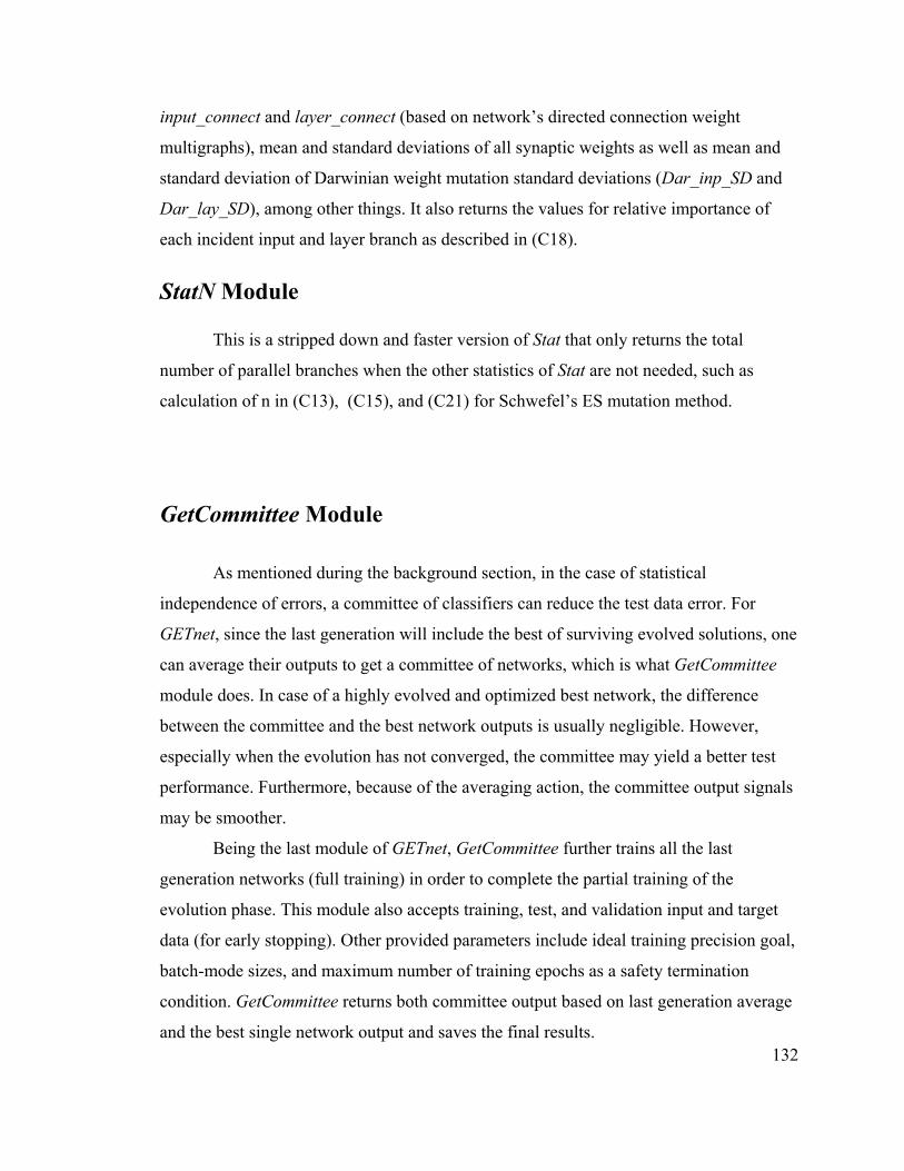
input_connect and layer_connect (based on network’s directed connection weight

multigraphs), mean and standard deviations of all synaptic weights as well as mean and

standard deviation of Darwinian weight mutation standard deviations (Dar_inp_SD and

Dar_lay_SD), among other things. It also returns the values for relative importance of

each incident input and layer branch as described in (C18).

StatN Module

This is a stripped down and faster version of Stat that only returns the total

number of parallel branches when the other statistics of Stat are not needed, such as

calculation of n in (C13), (C15), and (C21) for Schwefel’s ES mutation method.

GetCommittee Module

As mentioned during the background section, in the case of statistical

independence of errors, a committee of classifiers can reduce the test data error. For

GETnet, since the last generation will include the best of surviving evolved solutions, one

can average their outputs to get a committee of networks, which is what GetCommittee

module does. In case of a highly evolved and optimized best network, the difference

between the committee and the best network outputs is usually negligible. However,

especially when the evolution has not converged, the committee may yield a better test

performance. Furthermore, because of the averaging action, the committee output signals

may be smoother.

132

Being the last module of GETnet, GetCommittee further trains all the last

generation networks (full training) in order to complete the partial training of the

evolution phase. This module also accepts training, test, and validation input and target

data (for early stopping). Other provided parameters include ideal training precision goal,

batch-mode sizes, and maximum number of training epochs as a safety termination

condition. GetCommittee returns both committee output based on last generation average

and the best single network output and saves the final results.

C3 Simulations In this section, the results of three simulation tasks are presented. Each simulation

starts with a problem description, followed by the simulation settings and then detailed

results. A discussion concludes each simulation description, pointing out the earlier

theorized characteristics of GETnet in practice.

Mackey-Glass Chaotic Series 1

This is a prediction benchmark time series with a real valued one-dimensional

discrete time input signal and a one-dimensional signal as the target output. Prediction of

the time series based on its history is desired. Such predictive models are useful when

mathematical description of the sequence does not exist or it is incomplete. Stochastic

models are usually based on linear methods which are not suitable for nonlinear

processes. Neural networks are among nonlinear methods proposed for these problems.

Here we will show how GETnet can find a minimal predictor network through evolution

and training.

Given the properties of this series, Mackey-Glass is used to benchmark time

series processing capabilities of many neural networks109,110,111. This series is

recommended by IEEE Neural Networks Council Standards Committee Working Group

on Data Modeling Benchmarks as a reference for comparisons112.

Problem Description

Mackey-Glass is a chaotic, non-periodic (pseudo-periodic), non-convergent

univariate time series when its initial condition is set to x(0)=1.2 and its depth parameter

to τ=17. The series’ behavior is very dependent on the values of the initial condition and

the parameter τ. The Mackey-Glass series is defined by the following differential

133

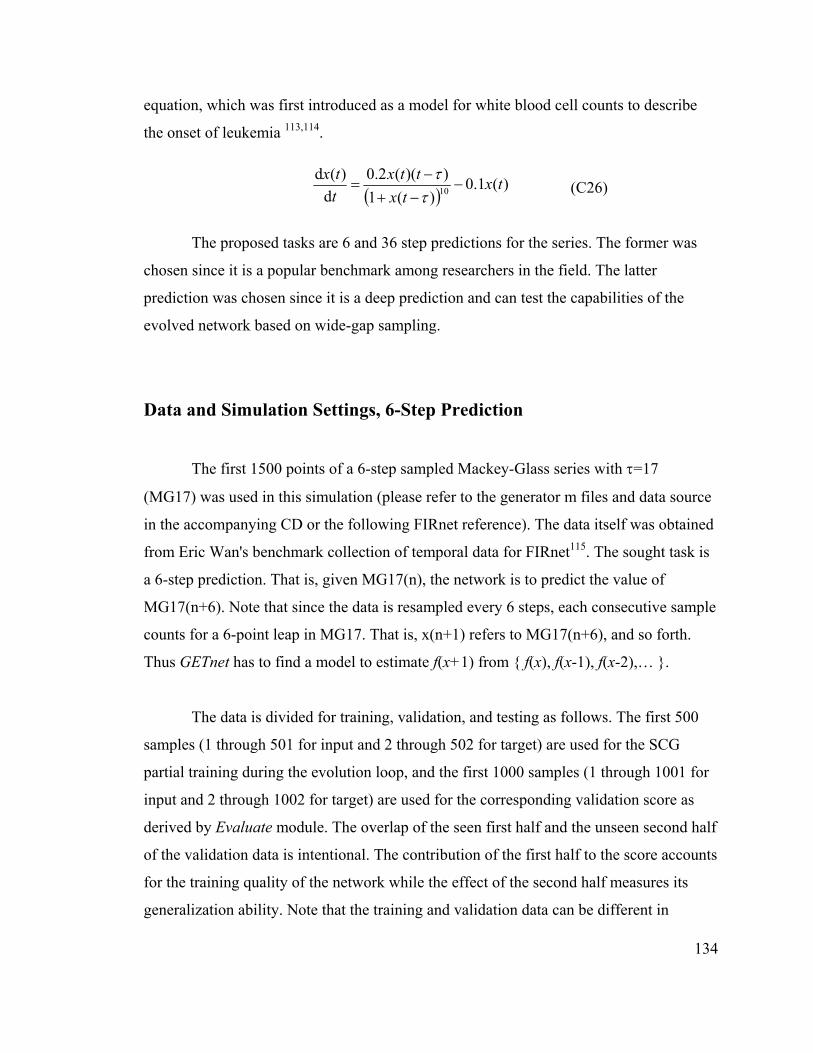
equation, which was first introduced as a model for white blood cell counts to describe

the onset of leukemia 113,114.

( ))(1.0

)(1))((2.0

d)(d

10 txtx

ttxttx

−−+−

=ττ

(C26)

The proposed tasks are 6 and 36 step predictions for the series. The former was

chosen since it is a popular benchmark among researchers in the field. The latter

prediction was chosen since it is a deep prediction and can test the capabilities of the

evolved network based on wide-gap sampling.

Data and Simulation Settings, 6-Step Prediction

The first 1500 points of a 6-step sampled Mackey-Glass series with τ=17

(MG17) was used in this simulation (please refer to the generator m files and data source

in the accompanying CD or the following FIRnet reference). The data itself was obtained

from Eric Wan's benchmark collection of temporal data for FIRnet115. The sought task is

a 6-step prediction. That is, given MG17(n), the network is to predict the value of

MG17(n+6). Note that since the data is resampled every 6 steps, each consecutive sample

counts for a 6-point leap in MG17. That is, x(n+1) refers to MG17(n+6), and so forth.

Thus GETnet has to find a model to estimate f(x+1) from { f(x), f(x-1), f(x-2),… }.

The data is divided for training, validation, and testing as follows. The first 500

samples (1 through 501 for input and 2 through 502 for target) are used for the SCG

partial training during the evolution loop, and the first 1000 samples (1 through 1001 for

input and 2 through 1002 for target) are used for the corresponding validation score as

derived by Evaluate module. The overlap of the seen first half and the unseen second half

of the validation data is intentional. The contribution of the first half to the score accounts

for the training quality of the network while the effect of the second half measures its

generalization ability. Note that the training and validation data can be different in

134

evolution and the final complete training in GetCommittee phase. Furthermore, one can

choose not to use the aforementioned technique in combining training and validation

scores for fitness evaluation and instead use the training error with early stopping. In this

case, the generalization capabilities of the network will be reflected in its fitness score by

stopping the reduction of training MSE when the validation MSE starts to go up.

Finally, for GetCommittee, the former validation data (1 through 1001 for input

and 2 through 1002 for target) were used for complete post-evolution SCG training and

the rest of the data (1003 through 1499 for input and 1004 through 1500 for the

corresponding targets) were used for test results.

Results

Best evolved network and committee of networks after post-evolution training by

GetCommittee provided the following results:

Best_Net_MSE_Train =0.0052

Best_Net_MSE_Test = 0.0054

Committee_MSE_Train =0.0052

Committee_MSE_Test =0.0054

Please see figures 29 through 51 for more details.

Connection maps:

1- Connection maps of the original ancestor of the best-evolved network are

135

=

11

_ connectinput

=

0101

_ connectlayer

=

10

_ connectoutput

2- Connection maps of the best-evolved network after 15 generations are

=

11

_ connectinput

=

0100

_ connectlayer

=

10

_ connectoutput

General descriptors and strategy parameters:

1-The original ancestor of the best-evolved network:

size (total branches)= 22

prune_threshold = 0.0467

prune_threshold_SD = 0.0026

node_mutation_SD = 0.0076

connection_mutation_SD = 0.1834

delay_mutation_SD = 0.6959

Darwinian mutation’ standard deviation (for Dar_inp_SD and Dar_lay_SD) = 0.0235

136

Darwinian mutation’ mean (for Dar_inp_SD and Dar_lay_SD) = 0.0413

Connection weights’ standard deviation = 0.5257

Connection weights’ mean = -0.1525

Training/validation time (mean of multiple starts) = 22.5430 sec

2- The best evolved network, after 203 generations:

size (total branches) = 16

prune_threshold = 0.0037

prune_threshold_SD = 0.0005307

node_mutation_SD = 0.0101

connection_mutation_SD = 0.0001917

delay_mutation_SD = 0.0012

Darwinian mutation’ standard deviation (for Dar_inp_SD and Dar_lay_SD) = 0.0026

Darwinian mutation’ mean (for Dar_inp_SD and Dar_lay_SD) = 0.0014

Connection weights’ standard deviation = 0.5721

Connection weights’ mean = -0.1326

Training/validation time (mean of multiple starts) = 6.2690 sec

Weights:

1- Connection weights, original ancestor of the best-evolved network:

137

=

21

11_iwiwweightsinput

=

[][]_

21

11

lwlwweightslayer

Starting with the following vector elements:

iw11=[-0.3326 0.4959 -0.3630 0.4135 0.5539 -0.3637 -0.3536 -0.6107]

iw21=[0.9449 -0.6799 -0.2356]

lw11=[-0.5719]

lw21=[-0.6754 -0.3571]

2- Connection weights, best evolved network after 203 generations:

=

21

11_iwiwweightsinput

=

[][][]

_21lw

weightslayer

with the following vector element:

iw11=[-0.4787 0.8929 -0.8379 -0.6025 -0.6077 0.7196]

iw21=[1.0053 -0.7330 0.0845 -0.1311]

lw21=[-0.6401 0.1007 -0.3075 -0.2656 -0.1229 -0.1971]

138

Weight Evolution

1- Standard deviation matrices of weight perturbation, original ancestor of the best-

evolved network:

=

21

11__diSDdiSDSDinpDar

=

[][]__

21

11

dlSDdlSDSDlayDar

Starting with the following vector elements:

diSD11=[0.0207 0.0607 0.0630 0.0370 0.0575 0.0451 0.0044 0.0027]

diSD21=[0.0035 0.0612 0.0609]

dlSD11=[0.0587]

dlSD21=[0.0478 0.0555]

2- Standard deviation matrices of weight perturbation, best-evolved network after 203

generations:

=

21

11__diSDdiSDSDinpDar

=

[][][]

__21dlSD

SDlayDar

with the following vector elements:

139diSD11=[ 0.0012 0.0016 0.0091 0.0064 0.0000 0.0000]

diSD21=[0.0000032 0.0000889 0.0008957 0.0008392]

dlSD21=[0.0005 0.0001 0.0004 0.0000 0.0000 0.0015]

Delays

1- Branch delays matrices of the original ancestor of the best-evolved network:

=

21

11_ididdelayinput

=

[][]_

21

11

ldlddelaylayer

Starting with the following vector elements:

id11=[2 3 4 7 9 10 13 14]

id21=[0 1 6]

ld11=[3]

ld21=[2 5]

2- Branch delays, best evolved network after 203 generations:

=

21

11_ididdelayinput

=

[][][]

_21ld

delaylayer

140

with the following vector elements:

id11=[ 2 3 4 13 14 21]

id21=[ 0 1 10 15]

ld21=[ 2 4 5 9 18 34]

The following figure shows the best evolved network.

Figure 28 Best evolved network for MG17 six-step prediction. Each line represents a delayed synaptic connection between one input and two layer nodes.

141

Figure 29 MSE of evolving networks.

Figure 30 Histogram of the MSEs of the best networks through 203 generations.

142

Figure 31 Size of evolving networks.

Figure 32 Training data, best evolved network. 143

Figure 33 Training data, magnified section, best evolved network.

144Figure 34 Best evolved network, training error.

Figure 35 Best evolved network: training performance correlation.

145Figure 36 Best evolved network, training data Fourier transform magnitude plots.

Figure 37 Training data, committee of last generation networks.

Figure 38 Training data, magnified section for network committee.

146

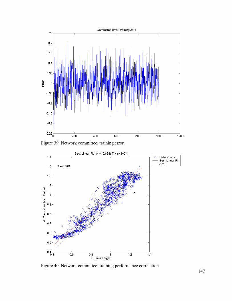
Figure 39 Network committee, training error.

147Figure 40 Network committee: training performance correlation.

Figure 41 Network committee, training data Fourier transform magnitude plots.

Figure 42 Test data, best evolved network. 148

Figure 43 Test set performance, magnified.

149Figure 44 Best network, test data error.

Figure 45 Best evolved network, test set performance correlation.

Figure 46 Best evolved network, test data Fourier transform magnitude plots. 150

Figure 47 Test data, committee of last generation networks.

Figure 48 Test set performance, magnified section for network committee.

151

Figure 49 Network committee, test data error.

152Figure 50 Network committee, test data performance correlation.

Figure 51 Network committee, test data Fourier transform magnitude plots.

Comparison

For comparison, three similar networks in terms of size and structure were used.

A closely comparable standard temporal architecture to this two-node network is a 2-

node, two-layer focused TDNN. Three such networks were evaluated. Each is a two layer

focused TDNN with one neuron in the hidden layer, one neuron in the output layer, and

three different 11-branch input delay lines: [0 1 2 … 10], [0 5 10 … 50] and [0 10 20 …

100]. The 11-tap input delay line was selected based on the size of a similar structure in

the best-evolved network. The same training and test sets along with the same SCG

training algorithm (same default) parameters were used.

153

For the first focused TDNN, after several initializations these were the best results:

MSE train = 0.0230

MSE test = 0.0240

For the second focused TDNN, after several initializations these were the best results:

MSE train = 0.0482

MSE test = 0.0489

For the third focused TDNN these results were obtained:

MSE train = 0.0687

MSE test = 0.0723

Recall that the MSE for the GETnet evolved solution were 0.0052 for train and 0.0054

for test data. That is, the evolved network has found a structure that has a training and test

MSE more than 4 to 13 times better than MSEs of similar focused time delay neural

networks, as described above.

Discussion

The MG17 is a famous benchmark for time delay neural networks. Here it was

observed how GETnet arrived at a compact solution that can perform the 6-step

prediction task. The prediction closely tracks the target values in the time domain as can

be seen from figures 32, 33, 37, 38, 42, 43, 47, and 48. Figures 30, 35, 40, 45, and 50

show a correlation coefficient of 0.948 for training and 0.946 for testing (time domain)

154

data pairs. Furthermore, the MSEs for train and test data are 0.0052 and 0.0054,

respectively. Some important observations can be made here:

1. There is almost no difference between the performance of the network on training

and test data sets. This shows an excellent generalization based on minimization

of the model variance through aggressive regularization and pruning. This is

especially important since one can use all the valuable training data for final

complete training without having to be overly concerned about setting aside

validation sets, since extraneous free parameters are already taken out.

2. The best network and network committee results show no discernable differences.

This is another indication of minimization of model variance, which the

committee was supposed to cancel out through output averaging. However,

committee will improve the results if the population of answers does not converge

to an optimum.

It is also worth noting that the spectra of the prediction and target signals are

almost identical in frequency domain (figures 36, 41, 46, and 51). This is important since

the MG17 series is chaotic and pseudo periodic however the evolved neural network

prediction is still closely following the target frequency contents using just two neurons.

Figure 31 shows the evolution of network size in terms of the number of branches

(delayed weighed connections). As it can be seen, GETnet’s strong tendency towards

parsimony of the answers drives down the size of the evolved network sharply from the

very beginning. However, after about 100 generations GETnet settles towards a solution

that is slightly larger since the smaller networks were unable to improve the performance.

Also note that through the course of evolution, the reduction of network size in terms of

branches is 1.375 while the speedup in training time is about 3.6. This is what we desired

by choosing a selection pressure that is related to the network complexity while

emphasizing the actual execution time on the hosting hardware.

155

As can be seen from the mean and median of the first and last best network in the

evolution, the range of all mutation standard deviations has gone down many times while

the MSE is improving. Especially, the weight perturbation standard deviation has reduced

almost 30 times. This shows the convergence of the evolutionary search while it points

towards the Baldwin effect, where the inherited garnered experience gradually replaces

random mutations through guided evolution. This effect is also comparable to simulated

annealing. It is interesting to note that this phenomenon was not dictated to the network,

but it emerged from the evolutionary process. It is also interesting to take a closer look at

figures 29 and 30, where the stepwise drops in the former figure and patchy grouping of

individual fitness scores in the latter can be seen. The Baldwin effect was originally an

attempt to describe punctuated equilibrium in natural evolution, and the jumps in figures

29 and 30 seem to suggest a similar phenomenon.

Finally, the comparisons show that the evolved network both on training and test

sets does 4 to 13 times better than a regular similar TDNN. To make this comparison

more tangible, the number of input branches for the base TDNN were chosen to be the

same as the number that the evolutionary network had found. This might sound as

hindsight in favor of the competing regular TDNN. Even so, one can see that the evolved

network is still doing much better than the regular comparable networks by virtue of its

evolutionary structural fine-tuning and hybrid training.

156

Mackey-Glass Chaotic Series 2

For this simulation, the same Mackey-Glass time series as the previous

experiment is used. However, the prediction task is six times deeper now. It will be

shown here how GETnet finds a very compact architecture through evolution and hybrid

training.

Problem Description

Mackey-Glass is a chaotic, non-periodic (pseudo-periodic), non-convergent

univariate time series when x(0)=1.2 and τ=17. The series’ behavior is dependent on the

values of the initial condition and the parameter τ. The task is the 36 step predictions for

the series.

Data and Simulation Settings, 36-Step Prediction

The first 1500 points of 6-sampled Mackey-Glass with τ=17 data (MG17) was

used in this simulation (see the generator m files and data source in the accompanying

disk or the following FIRnet reference). The data itself was obtained from Eric Wan's

benchmark collection of temporal data for FIRnet116. The sought task is a 36-step

prediction. That is, given MG17(n), the network is to predict the value of MG17(n+36).

Note that the data is resampled every 6 step so that each consecutive sample counts for a

6-point leap in MG17. That is, x(n+6) refers to MG17(n+36). Thus GETnet is trying to

find a model to estimate f(x+36) from { f(x), f(x-6), f(x-12),… }. The first 500 samples

(1 through 501 for input and 7 through 507 for target) are used for SCG partial training

during the evolution loop, and the first 1000 samples (1 through 1001 for input and 7

through 1007 for target) are used for the corresponding validation score derived by

Evaluate. The overlap of the seen first half and the unseen second half of the validation

157

data is intentional. The contribution of the first half to the score accounts for the training

quality of the network while the effect of the second half measures the generalization

ability of the network under study. For GetCommittee, the initial validation data (1

through 1001 for input and 7 through 1007 for target) was used for complete post

evolution SCG training and the rest of the data, i.e. 1008 through 1494 for input and 1014

through 1500 for the corresponding targets was used for test results.

Results Here are the results of the best evolved network and committee of networks after post-

evolution training by GetCommittee:

Best_Net_MSE_Train =0.0077

Best_Net_MSE_Test = 0.0114

Committee_MSE_Train =0.0077

Committee_MSE_Test =0.0114

Please refer to figures 53 through 77 for and the following discussion for more details.

General descriptors and strategy parameters:

1-Original ancestor of the best-evolved network:

size (total branches)= 33

prune_threshold = 0.0227

prune_threshold_SD = 0.0025

node_mutation_SD = 0.1749

connection_mutation_SD = 0.0243

delay_mutation_SD = 0.6778 158

Darwinian mutation’ standard deviation (for Dar_inp_SD and Dar_lay_SD) = 0.0257

Darwinian mutation’ mean (for Dar_inp_SD and Dar_lay_SD) = 0.0465

Connection weights’ standard deviation = 0.4810

Connection weights’ mean = 0.1573

Training/validation time (mean of multiple starts) = 53.7780 sec

2- Best evolved network, after 175 generations:

size (total branches) = 30

prune_threshold = 0.0059

prune_threshold_SD =0 .0001416

node_mutation_SD = 0.1396

connection_mutation_SD = 0.0702

delay_mutation_SD = 0.00061462

Darwinian mutation’ standard deviation (for Dar_inp_SD and Dar_lay_SD) = 0.0023

Darwinian mutation’ mean (for Dar_inp_SD and Dar_lay_SD) = 0.0016

Connection weights’ standard deviation = 0.1835

Connection weights’ mean = 0.0435

Training/validation time (mean of multiple starts) = 4.4010 sec

159

Connection maps:

1- Connection maps of the original ancestor of the best-evolved network

=

1011

_ connectinput

=

0010100111000000

_ connectlayer

=

0010

_ connectoutput

2- Connection maps of the best-evolved network after 175 generations:

[ ]1_ =connectinput

[ ]0_ =connectlayer

[ ]1_ =connectoutput

Weights

1- Connection weights, original ancestor of the best-evolved network:

160

=

41

21

11

[]_

iw

iwiw

weightsinput

=

[][][][][]

[][][][][][]

_

42

3431

2423

lwlwlwlwlw

weightslayer

Starting with the following vector elements:

iw11=[1.4000]

iw21=[0.1946 0.1283]

iw41=[0.6437 -0.2232 -0.4367 -0.5845 0.2212 0.1541 0.4524]

lw31=[0.9795 -0.4405 0.2838]

lw42=[-0.5909 -0.5778]

lw23=[0.3525 0.2779 -0.2366 -0.4286 0.1583 0.1533]

lw24=[0.1715 0.3545 0.5586 0.2356]

lw34=[0.7992 0.1819 0.2210]

2- Connection weights, best evolved network after 175 generations:

[ ]11_ iwweightsinput =

[ ]=weightslayer _

161

with the following vector element:

iw11=[0.2014 0.5351 -0.2086 0.2796 -0.1534 0.1616 0.2578 -0.2070 0.2556 0.0531

0.0587 -0.1154 -0.0914 0.1594 0.1833 -0.0881 -0.1362 0.0858 -0.0577 0.28822180

-0.1746 -0.0421 0.0505 -0.1927 -0.0788 0.0426 0.0888 -0.1230 0.0552]

Weight Evolution

Evolutionary training of weight values is performed through individual Gaussian

perturbations, which are determined by the standard deviation matrices given below.

1- Original ancestor of the best-evolved network evolution:

=

41

21

11

[]__

diSD

diSDdiSD

SDinpDar

=

[][][][][]

[[][][][][][]

__

42

3431

2423

dlSDdlSDdlSDdlSDdlSD

SDlayDar

Starting with the following vector elements:

diSD11=[0.0384]

diSD21=[ 0.0301 0.0180]

diSD41=[ 0.0897 0.0767 0.0244 0.0455 0.0272 0.0423 0.0699]

162

dlSD31=[ 0.0256 0.0610 0.0447]

dlSD42=[ 0.0340 0.0542]

dlSD23=[ 0.0044 0.0100 0.0957 0.0609 0.0247 0.0930]

dlSD24=[ 0.0727 0.0489 0.0686 0.0363]

dlSD34=[ 0.0149 0.0661 0.0237]

2- Standard deviation matrices of weight perturbation, best-evolved network after 175

generations:

[ ]11__ diSDSDinpDar =

[ ]=SDlayDar __

with the following vector elements:

diSD11=[0.0006 0.0011 0.0075 0.0001 0.0014 0.0003 0.0006 0.0059 0.0093 0.0002

0.0001 0.0033 0.0001 0.0012 0.0001 0.0001 0.0019 0.0000 0.0017 0.0036 0.0003

0.0001 0.0037 0.0004 0.0000 0.0004 0.0018 0.0004 0.0004 0.0003]

Delays

1- Branch delays matrices of the original ancestor of the best-evolved network:

163

=

41

21

11

[]_

id

idid

delayinput

=

[][][][][]

[][][][][][]

_

42

3431

2423

ldldldldld

delaylayer

Starting with the following vector elements:

id11=[6]

id21=[1 4]

id41=[ 2 4 5 6 7 13 14]

ld31=[1 5 8]

ld42=[13 14]

ld23=[3 6 7 11 13 14]

ld24=[1 10 14 15]

ld34=[2 6 11]

2- Branch delays, best evolved network after 175 generations:

[ ]11_ iddelay =input

[ ]=delaylayer _

164

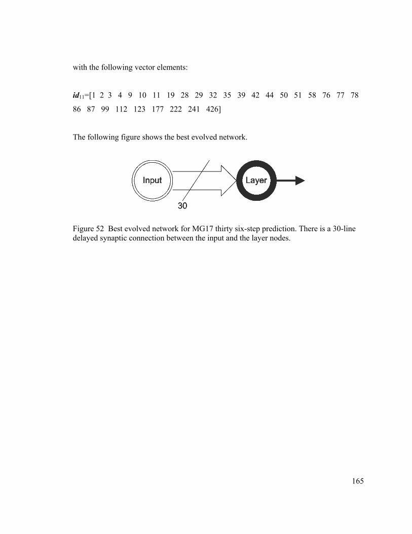
with the following vector elements:

id11=[1 2 3 4 9 10 11 19 28 29 32 35 39 42 44 50 51 58 76 77 78

86 87 99 112 123 177 222 241 426]

The following figure shows the best evolved network.

Figure 52 Best evolved network for MG17 thirty six-step prediction. There is a 30-line delayed synaptic connection between the input and the layer nodes.

165

Figure 53 MSE of the evolving networks.

Figure 54 Size of the evolving networks.

166

Figure 55 Training data, best evolved network.

Figure 56 Training, magnified section for best evolved network.

167

Figure 57 Best network, Training error.

168Figure 58 Best evolved network, training performance correlation.

Figure 59 Best evolved network, training data Fourier transform magnitude plots.

Figure 60 Training data, committee of last generation networks. 169

Figure 61 Training, magnified section for the network committee.

170Figure 62 Network committee, training error.

Figure 63 Network committee, training performance correlation.

Figure 64 Network committee, training data Fourier transform magnitude plots. 171

Figure 65 Test data, best evolved network.

Figure 66 Test set performance, magnified section from the best evolved network. 172

Figure 67 Best network, test error.

173Figure 68 Best evolved network, test set performance correlation.

Figure 69 Best evolved network, test data Fourier transform magnitude plots.

174Figure 70 Test data, committee of last generation networks.

Figure 71 Test set performance, magnified section from the network committee.

175Figure 72 Network committee, test data error.

Figure 73 Network committee, test data performance correlation.

Figure 77 Network committee, test data Fourier transform magnitude plots.

176

Comparison

For comparison, three similar networks in terms of size and structure were used.

The single layer, single-neuron focused TDNNs used for comparison were given 30 input

branches similar to that of the evolved network, with three different input delay line

spacing. The same training and test sets along with same SCG training algorithm and

default parameters were used.

For a single neuron with 30 input branches (focused TDNN with a delay window of 30

consecutive delays [0 1 2 … 29]), these were the best results after several attempts with

different initializations:

MSE train = 0.0378

MSE test = 0.0476

For another single neuron with 30 input branches (focused TDNN with a delay window

of 30, 5-step apart delays [0 5 10 ... 145]) these were the best results after several

attempts with different initializations:

MSE train = 0.0635

MSE test = 0.0700

For the last single neuron with 30 input branches (focused TDNN with a delay window of

30, 10-step apart delays [0 10 20 ... 290]) these were the best results after several attempts

with different initializations:

MSE train = 0.0716

MSE test = 0.0903

177

Recall that the MSE for the GETnet evolved solution were 0.00577 for train and 0.0114

for test data. That is, GETnet has found a structure that has a training MSE more than 4 to

9 times and test MSE more than 4 to 7 times better than that of similar focused time delay

neural networks as described above.

Discussion

Following the previous benchmark test, this time the MG17 was applied for a 36-

step prediction task. After 175 generation, GETnet arrived at a very compact solution

consisting of only 1 non-recurrent neuron with 30 parallel input branches from a 4-

neuron recurrent ancestor network. The prediction closely tracks the target values in the

time domain as can be seen from figures 55, 56, 60, 61, 65, 66, 70, and 71. Figures 58,

63, 68, and 73 show a correlation coefficient of 0.922 for training and 0.882 for testing

time domain data pairs. Furthermore, the MSEs for train and test data are 0.0077 and

0.0114, respectively. The results are slightly worse than the previous task as expected,

since this is a 6 fold deeper prediction.

As for the previous prediction task, there is only a small difference between the

performance of the network on training and test data sets, which indicates the

generalization capability acquired by minimizing model variance through aggressive

regularization and pruning. This property of GETnet lets us use all the valuable training

data for final complete training without having to be much concerned about setting aside

validation sets, especially if the training data points are scarce. The similarity between

best network and network committee results can also be explained in light of this reduced

model variance.

Here too in the frequency domain the spectra of the prediction and target signals

are almost identical (figures 59, 64, 69, and 77). This is important since the MG17 series

178

is chaotic and pseudo periodic, and the evolved predicting neural network is able to

almost duplicating the target frequency contents using just one neuron.

Figure 54 shows the evolution of the network size in terms of the number of

branches (weights) per generation. As can be seen, GETnet’s strong tendency towards

parsimony of the answers reduces the size of the evolved network sharply from the very

beginning and the population settles towards a solution after some transient fluctuations.

Also note that through the course of evolution, the reduction of network size in terms of

branches is 1.1 (or 4 times if number of nodes is considered) while the speedup in

training time is about 12.2. This is what we desired by choosing a selection pressure that

is related to the network complexity by utilizing the actual execution time on the hosting

hardware, having in mind that simple weight counting is not a very good measure of

system complexity.

As can be seen from the mean and median of the weight noise from the first and

the last best network in the evolution, the range of all mutation standard deviations has

gone down drastically reduced while the MSE has improved. Especially, the weight

perturbation standard deviation mean has reduced about 29 times. This shows the

convergence of the evolutionary search through generations, which is similar to simulated

annealing. It also suggests the emergence of the Baldwin effect. Figure 53 also shows

step-wise reductions in MSE after every several generations, resembling the punctuated

equilibrium.

Finally, the comparisons show that the evolved network does 4 to 9 times better

on training and 4 to 7 times better on test sets compared to a similar single layer, single

node TDNN. To make this comparison more tangible, the number of input branches for

the base TDNN were chosen to be the same as the number that the evolutionary network

had found. This might sound as hindsight in favor of the competing regular TDNN. Even

so, one can see that the evolved network is still doing much better than the regular

179

comparable networks by virtue of its evolutionary structure fine-tuning and hybrid

training.

180

Fingerprint Perspiration Sequence Detection

In the following section, applicability of GETnet to a real world problem,

fingerprint liveness detection, will be demonstrated. Note that it is the system capability

rather than the benchmark that is of a concern here. The inputs are 2-D real-valued

signals and the outputs are the corresponding 1-D classification signals.

Brief Introduction

There has been a growing interest in biometrics for verification or authentication

of individuals under different scenarios. Not only for being historically one of the more

popular biometrics, but also because of the introduction of cheap, small, and fast CMOS

scanners, fingerprints have been receiving more attention. However, one of the associated

security concerns is the possibility of intrusion by presenting a nonliving finger, be it a

duplicate or a severed finger to an automated electronic fingerprint scanner in order to

gain access to a protected entity. It has been shown that this threat is real and one can

spoof fingerprint scanners even with play-doh117 and gummy fingers118,119.

In order to circumvent this problem, one can read signals from the finger that can

verify its liveness and thus eliminate the threat of synthesized and cadaver finger attacks.

However, reading the more obvious signs of life such as those obtained for

electrocardiograms and pulse oximetry requires extra hardware. Earlier research of the

author showed that the process of perspiration on live fingertip skin can be seen from the

consecutive captures of electronic scanners within the first few seconds of each scan. The

ongoing perspiration presents a specific time progression that cannot be seen in cadaver

and synthetic fingerprint scans. This led to the development of an algorithm by the author

that quantifies and subsequently detects liveness of fingerprints based on the

aforementioned phenomena120. The algorithm uses two captures of a fingerprint in 5 181

seconds, and concatenates the gray levels of the fingerprint ridges to obtain a ridge-signal

that reflects moisture levels for each fingerprint capture (figure 78). Features from the

ridge-signal pair (initial and after 5 seconds) are derived afterwards and fed to a classifier

for final liveness decision.

It has been shown that other fingerprint capturing technologies such as optical and

electro-optical scanners can record this process. It has also been shown that the

perspiration based detection algorithm, originally developed for capacitive-DC CMOS

scanners, is applicable to these other scanners with a varying degree of success. However,

the algorithm provides different feature values for different scanning technologies and

thus a scanner-specific approach might be needed121,122

Data and Simulation Settings

Given the above short introduction to the problem, the fingerprint data for

liveness detection task was provided to GETnet as another test case for the following

reasons:

1. The fingerprint is converted to two ridge signals from the first and last captures, and

the decision can be considered as a corresponding bivalued target signal. This is a 2-

D to 1-D sequence mapping, which is an ideal form for GETnet.

2. This is a non-standard problem for which an optimal classical solution has not been

offered. It is hard to find a near optimal and orthogonal feature set for a rather vague

physiological phenomenon such as perspiration. Furthermore, it is possible that the

observed changes are not clear enough to the human researcher for manual feature

extraction. For instance, what if the knowledge about the perspiration-related pattern

changes e.g. the fact that perspiration starts from moisture-saturated pores that are

0.5mm apart and flows towards the drier ridge areas, did not exist? It is also

182

interesting to see a general intelligent framework such as GETnet to arrive at the same

kind of solutions within a fraction of the time a human expert might need.

3. As mentioned earlier, studies have shown that the perspiration detection algorithm

should be customized for different capturing technologies. With given variety of

scanners as well as operation conditions (climate, demographic, etc), it is more

efficient to solve the problem through a general framework such as GETnet and avoid

resolving manually for each setting.

The aim of this task is demonstrating the ability of GETnet in evolving

appropriate compact networks for the mentioned type of data. Optimal customized

solutions for each dataset requires an adequate evolutionary search on the representative

training sets.

Figure 78 Perspiration-based fingerprint liveness detection. Top and from left to right: temporal progression of fingerprints. Bottom: conversion of ridge gray levels to signals.

183

In order to accelerate the GETnet’s evolutionary process and put into test its ability to

learn from small data sets, the following settings were used:

1- Training data: 4 from spoof, 8 from live, and 4 from cadaver. Each passage only

150 samples wide.

2- Validation (early stopping) data: same composition as in training, but each

passage is only 50 samples wide.

3- Test data: 10 samples from each category (live, cadaver, spoof). Full length,

typically 3000 to 5000 samples wide.

4- Prune module was disabled to achieve smaller search space and thus faster

evolution.

Given the nominal length of 3000 to 5000 for fingerprint ridge signals, training

and early stopping data used for training and evolution (150+50 samples) constitute only

5 to 10 percent of each sample. Bipolar target signals (-1 for non-living and +1 for live)

were used. The data is the same used for the author’s Master’s thesis123. Please see the

accompanying CD for more details about the data set.

Results

Below are the results obtained from running GETnet for the mentioned problem.

First, the results of the best evolved network and committee of networks after post-

evolution training by GetCommittee:

Best_Net_MSE_Train = 0.3774

Committee_MSE_Train = 0.3694

Please refer to figures 53 through 77 for and the following discussion for more details.

184

Connection maps:

1- Connection maps of the original ancestor of the best-evolved network

=

11111111

_ connectinput

=

0111111101111110

_ connectlayer

=

0010

_ connectoutput

2- Connection maps of the best-evolved network after 15 generations:

=

01101101

_ connectinput

185

=

0011111001100110

_ connectlayer

=

0010

_ connectoutput

General descriptors and strategy parameters:

1-Original ancestor of the best-evolved network:

size (total branches)= 95

node_mutation_SD= 0.0460

connection_mutation_SD= 0.0585

delay_mautation_SD= 0.0816.

Darwinian mutation’ standard deviation (for Dar_inp_SD and Dar_lay_SD) = 0.0285

Darwinian mutation’ mean (for Dar_inp_SD and Dar_lay_SD) = 0.0465

Connection weights’ standard deviation = 0.2830

Connection weights’ mean = -0.0048

MSE validation (mean of multiple starts) = 0.9641

Training/validation time (mean of multiple starts) = 314.5720 sec

186

2- Best evolved network, after 15 generations:

size (total branches)= 59

node_mutation_SD=0.0041

connection_mutation_SD=0.0230

delay_mautation_SD=0.0028

Darwinian mutation’ standard deviation (for Dar_inp_SD and Dar_lay_SD) = 0.0396

Darwinian mutation’ mean (for Dar_inp_SD and Dar_lay_SD) =0.0382

Connection weights’ standard deviation =0.3099

Connection weights’ mean =0.0209

Validation MSE (mean of multiple starts) = 0.3949

Training/validation time (mean of multiple starts) =151.5210 sec

Weights

1- Connection weights from original ancestor of the best-evolved network:

=

4241

3231

2221

1211

_

iwiwiwiwiwiwiwiw

weightsinput

=

[]

[][]

_

434241

34333231

232221

141312

lwlwlwlwlwlwlw

lwlwlwlwlwlw

weightslayer

187

with the following vector elements:

iw11=[-0.2078 -0.2955 0.1899 0.1313 0.3500 0.0942 0.0795]

iw21=[ 0.6064 -0.1335 -0.0257 0.0617 0.4298 -0.1418 0.4980]

iw31=[-0.0688 0.2004 -0.2285 0.3354 -0.1654 -0.1459 0.1552 -0.4115]

iw41=[-0.5504 0.6774 -0.1826 -0.2261 -0.3822]

iw12=[ 0.3688 -0.2549 -0.4596 0.1880]

iw22=[-0.2716 -0.3174 -0.1624 -0.0181]

iw32=[0.0384 0.0748]

iw42=[0.3145 -0.2330 -0.2811 0.1552]

lw21=[0.1169 0.0416]

lw31=[0.4308 -0.3493 0.1954 0.2224 -0.1720 -0.0747 0.0131 0.0193]

lw41=[-0.2146]

lw12=[ 0.0230 0.0919 0.0769 0.0346 0.1383]

lw22=[ 0.1718 -0.5430 0.3511 0.0438 -0.0395]

lw32=[-0.2343 0.2491 -0.3697 -0.3326 0.0545 -0.1685]

lw42=[-0.2013]

lw13=[0.3567 -0.4379 0.4527 0.4143 -0.3949]

lw23=[-0.2032 0.0119 0.1030 0.1804 0.0872 -0.1825 0.1253]

lw33=[0.3431]

lw43=[-0.7662 0.1942]

lw14=[-0.3407 0.4119 -0.1364

lw34=[-0.1999 0.3627 -0.4002 0.2020 -0.1310 0.2287 -0.2853 0.1839]

188

2- Connection weights, best evolved network after 15 generations:

=

[][]

[]

_

41

32

2221

11

iwiwiwiw

iw

weightsinput

=

[][][]

[][][][]

_

4241

343332

2322

1312

lwlwlwlwlw

lwlwlwlw

weightslayer

with the following vector elements:

iw11=[0.1227 -0.4563 0.0416 0.0323 0.3904 0.1189 -0.0442]

iw21=[0.5965 -0.0059 0.2059 0.4281 -0.1612 0.4099]

iw41=[-0.5529 0.6610 -0.1684 -0.2170 -0.2612]

iw22=[-0.4758 -0.4940 -0.1207 -0.3859]

iw32=[-0.0672]

lw41=[0.2199]

lw12=[0.0529 0.3611 -0.2631 -0.0079 0.1429 0.2538]

lw22=[0.3475 0.0996 0.5685 0.1643]

lw32=[-0.2356 0.5886 -0.2182 0.1493 -0.1237]

lw42=[-0.0520]

189

lw13=[-0.4093 0.4574 -0.3648]

lw23=[-0.1261 -0.1175 0.1408 -0.0500 -0.2361 -0.1409]

lw33=[0.1877]

lw34=[-0.0608 0.4284 -0.3131 -0.1515 -0.2425 0.2088 -0.2885 0.5958 0.2723]

Weight Evolution

Evolutionary training of the weights is performed through Gaussian perturbations, which

is determined by the standard deviation matrices.

1- Original ancestor of the best-evolved network:

=

4241

3231

2221

1211

__

diSDdiSDdiSDdiSDdiSDdiSDdiSDdiSD

SDinpDar

=

[]

[][]

__

434241

34333231

232221

141312

dlSDdlSDdlSDdlSDdlSDdlSDdlSD

dlSDdlSDdlSDdlSDdlSDdlSD

SDlayDar

Starting with the following vector elements:

diSD11=[0.0603 0.0586 0.0919 0.0294 0.0790 0.0642 0.0483]

diSD21=[0.0011 0.0178 0.0879 0.0906 0.0009 0.0383 0.0424]

diSD31=[0.0317 0.0540 0.0006 0.0579 0.0402 0.0356 0.0238 0.0569]

diSD41=[0.0103 0.0862 0.0093 0.0118 0.0960]

190

diSD12=[0.0998 0.0205 0.0314 0.0343]

diSD22=[0.0060 0.0242 0.0641 0.0622]

diSD32=[0.0275 0.0562]

diSD42=[0.0156 0.0575 0.0274 0.0423]

dlSD21=[0.0540 0.0977]

dlSD31=[0.0476 0.0661 0.0933 0.0784 0.0554 0.0460 0.0669 0.0294]

dlSD41=[0.0101]

dlSD12=[0.0337 0.0833 0.0380 0.0796 0.0249]

dlSD22=[0.0190 0.0656 0.0088 0.0406 0.0098]

dlSD32=[0.0456 0.1000 0.0135 0.0152 0.0571 0.0980]

dlSD42=[0.0627]

dlSD13=[0.0512 0.0077 0.0039 0.0617 0.0166]

dlSD23=[0.0392 0.0689 0.0149 0.0501 0.0864 0.0655 0.0085]

dlSD33=[0.0493]

dlSD43=[ 0.0970 0.0320]

dlSD14=[0.0198 0.0396 0.0112]

dlSD34=[0.0420 0.0901 0.0636 0.0886 0.0762 0.0186 0.0201 0.0570]

2- Standard deviation matrices of perturbation, best-evolved network:

=

[][]

[]

__

41

32

2221

11

diSDdiSDdiSDdiSD

diSD

SDinpDar

191

=

[][][]

[][][][]

__

4241

343332

2322

1312

dlSDdlSDdlSDdlSDdlSD

dlSDdlSDdlSDdlSD

SDlayDar

with the following vector elements:

diSD11=[0.1217 0.0920 0.0478 0.0217 0.1906 0.0383 0.0162]

diSD21=[0.0004 0.0052 0.0688 0.0005 0.0096 0.0172]

diSD41=[0.0112 0.0865 0.0143 0.0064 0.1700]

diSD22=[0.0042 0.0194 0.0383 0.0188]

diSD32=[0.0254]

dlSD41=[0.0038]

dlSD12=[0.0190 0.0263 0.0913 0.0723 0.0178 0.0431]

dlSD22=[0.0114 0.0668 0.0069 0.0185]

dlSD32=[0.0163 0.0837 0.0277 0.0478 0.0377]

dlSD42=[0.0140]

dlSD13=[0.0043 0.0022 0.0130]

dlSD23=[0.0411 0.0061 0.0224 0.0476 0.0340 0.0068]

dlSD33=[0.0239 0.0781 0.0328 0.0510 0.0245 0.0172 0.0244 0.0976 0.0836]

diSD34=[0.0239 0.0781 0.0328 0.0510 0.0245 0.0172 0.0244 0.0976 0.0836]

192

Delays

1- Branch delay matrices of the ancestor of the best-evolved network:

=

4241

3231

2221

1211

_

idididididididid

delayinput

=

[]

[][]

_

434241

34333231

232221

141312

ldldldldldldld

ldldldldldld

delaylayer

Starting with the following vector elements:

id11=[1 2 4 5 6 7 8]

id21=[1 2 4 5 6 7 8]

id31=[0 1 2 3 4 5 7 8]

id41=[0 1 3 4 5]

id12=[1 3 4 6]

id22=[2 3 4 5 6]

id32=[1 4]

id42=[2 3 5 6]

ld21=[1 5]

ld31=[0 1 2 3 4 5 6 8]

ld41=[4]

193

ld12=[1 2 6 7 8]

ld22=[2 3 4 6]

ld32=[ 1 2 3 4 6 7]

ld42=[1]

ld13=[1 5 6 7 8]

ld23=[3 4 5 6 7 8 9]

ld33=[1]

ld43=[3 4]

ld14=[1 5 6]

ld34=[1 2 3 4 5 6 7 8]

2- Branch delays, best evolved network:

=

[][]

[]

_

41

32

2221

11

idididid

id

delayinput

=

[][][]

[][][][]

_

4241

343332

2322

1312

ldldldldld

ldldldld

delaylayer

with the following vector elements:

id11=[1 2 4 5 6 7 8]

194

id21=[1 2 4 6 7 8]

id41=[0 1 3 4 5]

id22=[0 4 5 7]

id32=[1]

ld41=[4]

ld12=[1 2 6 7 8 12]

ld22=[2 3 4 6]

ld32=[ 1 2 4 6 7]

ld42=[1]

ld13=[5 6 8]

ld23=[4 5 6 7 8 9]

ld33=[1]

ld34=[1 2 3 4 5 6 7 8 12]

A summary of the results is given through the following tables. As it can be seen, 3 live

specimens were falsely recognized as nonliving, whereas one out of 10 for each spoof

and cadaver test data sets were falsely recognized as live. The overall precision is

therefore (30-3-1-1)/30=83.3%. The output values in the tables are calculated as the net

area under output curve

∫=signalridge

dyOutput ii_

)( ττ (C27)

For discrete outputs of the GETnet program, (C27) is simply evaluated as a summation of

the output array.

195

The liveness results are determined as

( )ii OutputthresholdhardLiveness _= (C28)

Hard limiting threshold function (see B40) returns –1 for nonliving and 1 for living as the

final classification result. The final evolved network is depicted below.

Figure 79 Best evolved network for fingerprint liveness detection. Note the novel structure, delayed weight bus widths, and multiple feedback loops.

196

Table 2 Test outputs for live subjects. Incorrect classifications are italicized. Subject Best Net Output Committee Output Liveness

LivTst1 0.7596 0.7701 1 LivTst2 0.8251 0.8332 1 LivTst3 0.6708 0.6771 1 LivTst4 0.2159 0.3300 1 LivTst5 0.6020 0.6617 1 LivTst6 0.7852 0.7893 1 LivTst7 -0.6284 -0.5962 -1 LivTst8 -0.2923 -0.2121 -1 LivTst9 -0.4239 -0.3580 -1 LivTst10 0.5883 0.5769 1 Table 3 Test outputs for cadaver subjects. Incorrect classifications are italicized. Subject Best Net Output Committee Output Liveness

CdvTst1 -0.6553 -0.6383 -1 CdvTst2 0.6934 0.7149 1 CdvTst3 -0.1882 -0.0134 -1 CdvTst4 -0.1677 -0.1583 -1 CdvTst5 -0.7048 -0.6803 -1 CdvTst6 -0.4266 -0.3572 -1 CdvTst7 -0.6014 -0.5773 -1 CdvTst8 -0.6168 -0.5845 -1 CdvTst9 -0.6919 -0.6822 -1 CdvTst10 -0.5695 -0.5621 -1 Table 4 Test outputs for spoof subjects. Incorrect classifications are italicized. Subject Best Net Output Committee Output Liveness

SpfTst1 -0.5984 -0.5494 -1 SpfTst2 -0.6311 -0.6057 -1 SpfTst3 -0.6563 -0.6423 -1 SpfTst4 -0.6493 -0.6250 -1 SpfTst5 -0.3486 -0.1599 -1 SpfTst6 -0.0479 -0.1518 -1 SpfTst7 0.0229 0.0309 1 SpfTst8 -0.2592 -0.3232 -1 SpfTst9 -0.4689 -0.4283 -1 SpfTst10 -0.2772 -0.2025 -1

197

Table 5 Confusion matrix for the test data. Threshold for network output is set at zero.

Neural Net Actual

Live

Non-living

Total Actual

Live

C11=7 Correct

C12=3 Misidentify

C11+C12=10

Non-living

C21=2 Misidentify

C22=18 Correct

C21+C22=20

Total Neural

Network

C11+C21=9

C12+C22=21

Total

Samples=30

Figure 80 ROC curve for the 30 point test data.

198

Figure 81 Training data. Red: first capture signal, blue: last capture signal. Green high: live signals, green low: nonliving signals.

Figure 82 Size of evolving networks.

199

Figure 83 MSE of evolving networks.

Figure 84 Training output, best evolved network.

200

Figure 85 Training error, best network.

201Figure 86 Training data, committee of last generation networks.

Figure 87 Sample live test data output, best evolved network.

202Figure 88 Sample live test data output, committee of last generation networks.

Figure 89 Sample cadaver test data output, best evolved network.

203Figure 90 Sample cadaver test data output, committee of last generation networks.

Figure 91 Sample spoof test data output, best evolved network.

Figure 92 Sample spoof test data output, committee of last generation networks.

204

Discussion

In this example, GETnet showed that it could arrive at a succinct network that not

only classifies, but also performs feature extraction by accepting the raw fingerprint ridge

signals and creating an internal representation through a recurrent time delay network of

four neurons. The assigned task was detection of live finger perspiration temporal pattern

in order to separate live fingerprints from the nonliving.

The network was evolved on less that 10% of 16 training fingerprints ridge

signals. The fact that GETnet could create a reasonably accurate classifier using this

scarce amount of training data confirms the fact that even without Prune, the temporal

MDL and validation-based fitness score assessment mechanisms of GETnet can form a

minimal, robust, and fast solution (see figures 82 and 83). The compactness of the

solution can partially be credited to the ability of GETnet to evolve recurrent structures.

The effect of recurrence can also be seen in the short transient time of the outputs,

especially for the nonliving samples.

The other observation is that even though during the course of evolution the

number of parallel branches was reduced, the evolved network could do well with the

original 4 nodes and thus kept that number of nodes. This confirms the usefulness of the

heuristic used for initialization of first generation by Genesis, so that evolution can find a

suitable answer with fewer generations by having its starting point placed close to an

optimum in the search space. It is interesting to note that two explicit long-term memory

kernels, a fourth order in neuron 2 and a first order in neuron 3 have been developed.

Considering the use of less than 10% of only 16 fingerprint signal pairs and

evolving for only 15 generations, the 83.3% accuracy of the resulting solution on the test

data is indeed a very good performance. After reviewing the actual fingerprints, one can

see that the misclassification of the 3 live and 2 nonliving samples stands to reason, since

205

most of those fingerprints have bad quality (please see the dataset in the accompanying

CD). Given that the teacher signals were chosen from images with better quality, the

acquired classification and generalization is what one should expect. The utilized signals

are also rough concatenations of individual ridge signals, which introduce a lot of noise

by adding false jumps at the concatenation points. Even so, GETnet managed to arrive at

a reasonable answer.

The other interesting observation is that the standard deviation of weight

perturbations went up while the mean went down. This means that the weight search

ellipsoids are being elongated to match the performance landscape while the size of their

random search space is decreasing. The other mutation standard deviations were also

reduced. The fact that the changes in these parameters are not as striking as the previous

two runs on MG17 should not come as a surprise, since this simulation was conducted

only for 15 generations and it has not fully converged. This can also be seen from the

distance between train and test errors. One should also keep two things in mind. First, the

intent of this simulation, contrary to the previous two problems, was not benchmarking

but demonstrating the applicability of GETnet to complex real world applications that are

considered to be hard and vague by human experts. Such problems call for application of

black box approaches. Second, perspiration naturally has a high variation in its

occurrences and cannot be accurately modeled with closed and tractable mathematical

forms such as the ones that neural networks create. Thus, perspiration data should not be

considered as a benchmarking dataset since no ideal perspiration sequence as a point of

reference exist. Since GETnet showed reasonable performance even with few

generations, the goal of this feasibility experiment was considered met.

As can be seen from the connection digraphs matrices, GETnet’s solution besides

being compact, is nonstandard and novel in terms of the known architectures. Such novel

solutions are especially important for problems such as perspiration-based liveness

detection where no standard starting point, neither for feature extraction nor

classification, exists.

206

Conclusions and Future Work

The perceived external world, i.e. the mental image of the existence as captured

by the sensory inputs of an individual, is initially conveyed through a series of

multidimensional time signals. Under normal circumstances and borrowing from the

concept of mapping in mathematics, order can be considered as an invariant for the

internal representations (images in the realm of mental) and the external world pre-

images. Biological nervous systems continuously adapt their image of the external world

through multidimensional temporal sensory data. The massively parallel biological brain

systems may take advantage the time delays for creation of memories and process

signals. The internal states of functional units stored in memory structures plus the

transition functions of neuronal circuits that create future states and outputs can be

considered as the common ground between state space description of artificial and

biological neural networks. GETnet adopts its design philosophy from the

aforementioned ontology of the external world and theory of adaptive temporal neural

networks. GETnet is an attempt by the author to address some of the most important

issues among many complexities of the design and implementation of general, temporal

intelligent systems by an automated and adaptive framework that requires very little

human supervision and meddling. GETnet uses an elitist, preservative, static evolutionary

search on top of its LMS neighborhood search. Given enough time, the evolutionary

search is guaranteed to converge asymptotically to a global optimum124.

Based on what was told about GETnet in this document, one can summarize its

main characteristics as

1. Generality

2. Convergence

3. Adaptive architecture

4. Finding novel answers

5. Requiring minimum human intervention.

207

6. Promising initial results on single and multidimensional sequence analysis.

7. Inventing memory structures with appropriate depth and placement.

8. Minimal model variance which is especially important for small training sets.

9. New pragmatic temporal MDL for regularization.

10. Accelerated hybrid learning with Baldwin effect.

11. Can readily be parallelized.

GETnet is arguably more comprehensive and flexible compared to the other

temporal neural networks. Based on the memory kernels discussed in B3-2 and B3-4,

different temporal neural network architectures have been suggested. The most notable

temporal designs include:

1. Time Delay Neural Networks (TDNN), introduced by Waibel et al for speech

processing22.

2. Finite Impulse Response Neural Networks (FIRnet), introduced by Wan23.

3. Elman24 and Jordan25 recurrent networks, named after their inventors.

4. Pipelined Recurrent Neural Networks (PRNN) introduced by Haykin and Li26.

5. Nonlinear autoregressive moving average (NARMA) neural networks explored by

Narendra27 for control systems.

A short comparison of the above temporal neural networks with GETnet is given blow.

TDNN is a feed forward structure with input-focused, finite, and predetermined

delay line STM (see section B3-4 and figure 17). One major problem with TDNN is the

fact that the best length of the input sliding window is problem-dependent and generally

unknown. TDNN needs human expertise for the length of the input delay line and the

general structure of the static network that comes after it. In essence, TDNN just takes a

snapshot of the input sequence at each time step and from there on the system is static.

TDNN lacks the infinite memory retention of recurrent memory kernels and its delay

lines can only be found at the input stage. By contrast, GETnet uses more complex and

208

versatile distributed memory structures that can include recurrent sub-circuits. Moreover,

GETnet’s memory and network structures emerge automatically through evolution.

FIRnet is the first multi-layered temporal neural network to officially implement

distributed memory and thus can be called a Distributed Time-Lagged Neural Network

(DTLNN). Variations of this theme, like Day and Davenport’s version125 with adaptable

time delays, also exist. However, FIRnet is strictly feed forward and uses only finite,

predetermined delay lines. Thus, even though more versatile than TDNN, it suffers from

the same lack of feedback delay loop LTM and problem of STM depth selection. The

number of nodes and layers of FIRnet should also be guessed by its designer. As

described earlier, GETnet does not suffer from the mentioned limitations.

Jordan, and shortly after Elman, proposed simple recurrent kernels to retain

context and output activities (see figure 20). However, compared to GETnet, these

networks have the following shortcomings:

They only have recurrent memory kernels which have lower resolution.

The recurrent connections, in the original version, are non-adaptable.

Recurrent connections only have single step delays.

The recurrence is restricted to the context units.

The overall architecture needs human expert design.

PRNN is made of a layer of recurrent neurons followed by a linear tapped delay

line for prediction of non-stationary time series. However, compared to GETnet, PRNN

has the following limitations and disadvantages:

The recurrent modules only have single-step delays in feedback (first order),

whereas in GETnet this limitation does not exist.

The architecture is predetermined and non-dynamic, compared to GETnet’s

evolutionary adaptive architecture.

209

PRNN suffers from the “baby sitting” problem since its following

fundamental parameters need to be guessed by an experienced human

designer:

Number of recurrent modules.

Number of neurons per each recurrent module.

Number of taps in the nonlinear adaptive filter.

Proper sample size for pre-training, since inadequate initial weights

may cause divergence.

The NARMA models, as studied by Narendra, can be considered as simpler cases

of GETnet networks that have feed forward layers with no internal memory structs and

delay lines only at input and output layers, and with recurrent connections only from

output to input. In this light, GETnet is a more general, powerful, and complex superset

of NARMA model. GETnet also offers many more features within its framework,

including fully automated architecture design and training. Even under the restricted

NARMA configuration, GETnet offers clear advantages through its evolutionary

determination of input window size, feedback delay depth, and network size and structure

as well as hybrid training of connection weights. Please note that in his original work27

Narendra uses parallel-series implementation, i.e. the fed-back outputs are not from the

NARMA neural network output but the teacher signal output values. Thus the mentioned

neural network is not really recurrent, compared to the full recurrency of GETnet.

For future enhancement, parallel implementation will arguably have the greatest

impact. First because GETnet can easily be ported into clusters and multi-processors for

parallel processing, in which case its time complexity will reduces linearly (and possibly

superlinearly based on locality of the code) by the number of parallel nodes. The only

parts of data that need to be shared and communicated are genotypes and small

synchronization messages. These inter-node communications are very manageable in

size and can easily be sent over a say 100 base-T Ethernet backbone. Second, due to

object-oriented design of GETnet using Matlab’s neural network toolbox, there are many

210

more useful parameters that are already implemented in the genotype of GETnet’s

network objects but are treated as constants since their inclusion into the evolution

search space slows down GETnet. These parameters include different learning

algorithms and their parameters, activation functions, and so on. By activating all those

parameters, GETnet can further learn how to learn and become even more versatile,

which is not very practical unless a parallel implementation is used.

It was also observed that based on GETnet’s aggressive MDL and pruning, model

variance in the evolved networks is so minimized that the solutions may not need extra

validation sets for the final full training. Using all the data for training is especially

beneficial for scarce training data. This is similar to biological intelligent organisms that

are able to generalize using very small data sets using their intuitions or inherited model

of the external world. Temporal MDL also creates fast networks, which is considered to

be another sign of intelligence.

We also observed the emergence of the Baldwin effect in GETnet. This should not

come as a surprise, since the first phase of the Baldwin effect is implemented by genetic

transmission of structural modifications followed by partial local training through SCG.

The second phase is carried out by the (noisy) best weight transfer. This is another way

of describing Lamarckian evolution in weight space. The Baldwin effect accelerates the

evolution towards the desired goal and avoids relying on the global but very slow

phylogenetic evolutionary search, which sometimes can be similar to finding “a needle

in a haystack”.

Simulations showed that during the course of evolution, the radius random search

always decreases. This effect can be compared to simulated-annealing. The interesting

point is that this behavior emerged through evolution and was not coded into GETnet.

This is a good example of how GETnet as a general intelligent system can learn the

learning methodology itself. One can also expect that in case of changing environment

(changing input-target data sets) this versatility may allow for more stochastic search if

211

the dynamism gives this type of learning a better advantage compared to the gradient

descent.

Besides parallel implementation and expansion of evolutionary search space that

will lead to improvement of GETnet by allowing extra plasticity, one other suggested

evolution enhancement could be avoiding the possible problem of a dominating super

individual in the evolving population of solutions. This can be achieved through parent

selection policy or injecting a small number of random individuals into the parent pool

(immigration policy). This should create more statistical diversity in the evolved answers

and also make the results of a committee of diverse solutions more robust and accurate

for the unseen data. Another course of action is limiting the lifespan of each individual

using a EA(µ,κ,λ) evolution scheme, as described earlier in the section B4-1.

The last but not the least, it would be interesting and essential to solve more real

world problems with GETnet after this feasibility phase. There are plethoras of different

problems that are readily in an ideal form for GETnet. One such problem is protein

secondary structure detection and similar problems in Bioinformatics. For secondary

structure analysis, one needs to identify (predict) 3 alphabet strings (helix, strand, and

coil secondary structures) from 20 alphabet strings (amino acids)126. As one can see, the

problem is already in form of sequence prediction. The required mapping is complex and

long-term dependencies may exist127.

The future applications can also explore field of biomedical signal analysis. For

instance, one may be interested in finding a robust and compact real time system that can

monitor one or multi-channel ECGs and detect the onset of an abnormal cardiac activity.

In conclusion, based on the very general format of GETnet’s inputs and outputs,

provided the availability of the required computing power, one can find novel answers to

many problems. However, it must be mentioned that black box methods such as GETnet

should be only utilized where good, examined classical solutions do not exist.

212

Appendix A: More on Gradient Conjugate Methods

There are different methods for calculating α in conjugate gradient method,

including:

Fletcher-Reeves,

)1()1()()()(−∇⋅−∇

∇⋅∇=

nJnJnJnJnα (A1)

Polak-Ribiere,

( ))1()1(

)()1()()(−∇⋅−∇

∇⋅−∇−∇=

nJnJnJnJnJnα (A2)

and Hestenes-Steifel:

( ))1()1(

)()1()()(−∇⋅−∇

∇⋅−∇−∇=

nsnJnJnJnJnα (A3)

The above formulas are convergent and equal for quadratic error surfaces. There are two

other methods, direct search and the scaled conjugate gradient method (SCG) that are

convergent for non-quadratic error surfaces as well128. There are similarities between

conjugate gradient and momentum learning methods. However they differ because α is

adaptive in case of conjugate gradient. Based on its generality and power, SCG is the

method of choice for GETnet. Please see section C for more explanations.

213

Appendix B: Nguyen-Widrow Weight Initialization

Algorithm

GETnet uses Nguyen-Widrow method to initialize network weights in order to

achieve higher training speeds. This method is implemented in Matlab’s neural network

toolbox v. 4. Considering the connection weight wij from node j to node i, the algorithm

first initializes network weights wij randomly between –0.5 and 0.5. Then, the weights are

initialized again according to the following formula

∑=

=h

i

n

nij

ijn

hij

w

wnw

1

2

7.0 (A4)

where ni is the number of nodes in the input layer and nh is the number of neurons in the

hidden layer. The bias for each neuron, say the ith, is then set randomly between wij and

-wij.

214

REFERENCES 1 Roy A. (2003), “Neural Networks: How do we make a widely used technology out of

it?” IEEE NNS Connections, Vol. 1, No. 2, pp. 8-12.

2 Medina J., and Mauk M. (2000), “Computer Simulation of Cerebellar Information

processing,” Nature Neuroscience Supplement, Vol. 3, November, pp. 1205-1211.

3 Voogd J,, and Glickstein M. (1998), “The Anatomy of the Cerebellum,” Trends

Neuroscience 21:370– 375.

4 Eccles J. C., Ito M., and Szentágothai, J. (1967), The Cerebellum as a Neuronal

Machine, Springer, Berlin, New York.

5 Ito, M. (1984), The Cerebellum and Neural Control, Raven, New York.

6 Principe, J. (1994). “An Analysis of the Gamma Memory in Dynamic Neural

Networks.” IEEE Trans. on Neural Networks, 5 (2), 331-337.

7 Bailey C. H., Kandel E. R., “Structural Changes Accompanying Memory Storage,”

Ann Rev Physiol 55:397-426,1993.

8 Bailey, C. H., and Kandel, E. R. (1994), “Structural Changes Underlying Long-term

Memory Storage in Aplysia: A Molecular Perspective,” Seminars Neuroscience. 6, 35-

44.

9 Genisman, Y., deToledo Morrell F., Heller R. E., Rossi M., and Parshall, R. F. (1993),

“Structural Synaptic Correlate to Long-term Potentiation: Formation of Axospinous

Synapses with Multiple, Completely Partitioned Transmission Zones,” Hippocampus 3

(4), 435-445.

10 Jessel, T. M., and Kandel, E. R. (1993), “Synaptic Transmission: A Bidirectional and

Self Modifiable form of Cell-Cell Communication,” Cell Supplement, 1-30.

11 Nicoll, R. A., and Malenka, R. C. (1995), “Contrasting Two Forms of LTP in the

Hippocampus,” Nature 377, 115-118.

215

12 Villa, A., Tsien, R. W., and Scheller, R. H. (1995), “Presynaptic Component of Long-

term Potentiation Visualized at Individual Hippocampal Synapses,” Science 268, 1624-

1628.

13 Feany, M. B., and Quinn, W. G. (1995), “A Neuropeptide Gene Defined by the

Drosophila Memory Mutant Amnesiac,” Science 268, 869-873.

14 Quinn W.G., Sziber P.P., Booker R. (1979), “Drosophila Memory Mutant Amnesiac,”

Nature 277:212-4.

15 de Belle J. S., and Heisenberg, M. (1995), “Genetic, Neuroanatomical and Behavioral

Analyses of the Mushroom Body Miniature Gene in Drosophila Melanogaster,” J

Neurogenet 10:24-30.

16 Bouhouche, A., and Vaysse, G. (1991), “Behavioral Habituation of the Proboscis

Extension Reflex in Drosophila Melanogaster: Effect of the no Bridge,” J. Neurogenet. 7,

117-128.

17 Broadie, K., and Bate, M. (1995), “The Drosphila NMJ: A Genetic Model System for

Synapse Formation and Function,” Sem. Dev. Biol. 6, 221-231.

18 Broadie, K. (1994), “Synaptogenesis in Drosophila: Coupling Genetics and

Electrophysiology,” J. Physiology 88, 123-139.

19 Seidl D.R. and Lorenz D., (1991) “A Structure by Which a Recurrent Neural Network

can Approximate a Nonlinear Dynamic System,” Proc. Int. Joint Conf. Neural Networks,

Vol. 2, pp. 709-714.

20 Siegelmann H. T. and Sontag E. D., (1995) “On the Computational Power of Neural

Networks,” J. Comput. Syst. Sci., vol. 50, no. 1, pp. 132-150.

21 Siegelmann, H.T., Horne, B.G., Giles, C.L. (1997), “Computational Capabilities of

Recurrent NARX Neural Networks” Systems, IEEE Transactions on Man and

Cybernetics, Part B, Vol.27, Issue 2, pp 208-215.

22 Waibel, A.; Hanazawa, T.; Hinton, G.; Shikano, K.; Lang, K.J. (1989) “Phoneme

Recognition Using Time-Delay Neural Networks” [see also IEEE Transactions on Signal

Processing], IEEE Transactions on Acoustics, Speech, and Signal Processing, Vol.37,

Issue 3. pp 328-339.

216

23 Wan E., (1993) "Time Series Prediction Using a Neural Network with Embedded

Tapped Delay-Lines", in Predicting the Future and Understanding the Past, SFI Studies in

the Science of Complexity, Eds. A. Weigend , N. Gershenfeld Addison-Wesley.

24 Elman, J (1990) “Finding Structure in Time, ”Cognitive Science, 14, pp 179-211.

25 Jordan, M. (1986) “Serial order: A Parallel Distributed Processing Approach,”

Institute for Cognitive Science Report 8604. University of California, San Diego.

26 Haykin, S. and Liang Li (1995) “Nonlinear Adaptive Prediction of Nonstationary

Signals,” IEEE Transactions on Signal Processing, [see also Acoustics, Speech, and

Signal Processing, IEEE Transactions on], Vol.43, Issue 2, pp 526-535.

27 Narendra, K.S.and Parthasarathy, K. (1990). “Identification and Control of Dynamical

Systems Using Neural Networks” IEEE Transactions on Neural Networks, Vol.1, No.1,

pp 4-27.

28 Duda R.O.and Hart P.E. (1973), Pattern Classification and Scene Analysis, New York,

John Wiley and Sons.

29 Fukunaga K. (1990), Introduction to Statistical Pattern Recognition. Second edition,

New York: Academic Press.

30 Cover T. (1965) “Geometrical and Statistical Properties of Systems of Linear

Inequalities with Applications in Pattern Recognition,” IEEE Transaction on Electronic

Computers, pp. 326-334, 1965.

31 Trunk G. (1979) "A Problem of Dimensionality: A Simple Example," IEEE

Transactions on Pattern Analysis and Machine Intelligence vol 1, No 3, pp 306-307.

32 Vaptnik, L (1995) The Nature of Statistical Learning Theory, Springer Verlag.

33 Vaptnik, L (1998) Statistical Learning Theory, Wiley.

34 Anlauf J.K. and Biehl M. (1989) ”The AdaTron: an adaptive perceptron algorithm,”

Europhys. Letter., 10(7) pp 687-692.

35 Lang K. J. and Witbrock M. J. (1988)"Learning to tell two spirals apart," in

Proceedings of Connectionist Models Summer School, Morgan Kaufmann.

36 Poggio, T. and Girosi, F. (1990) “Networks for approximation and learning,”

Proceedings IEEE vol 78, No 9 pp 1481-1497.

217

37 Greenstein-Messica A.and Ruppin E. (1998), “Synaptic Runaway in Associative

Networks and the Pathogenesis of Schizophrenia.” Neural Computation, 10(2), 451-465.

38 Aharonov R., Segev L., Meilijson I., and Ruppin E. (2003) “Localization of Function

Via Lesion Analysis.” Neural Computation, 15(4), pp 885-913.

39 Kohonen, T. (1982). “Self-organized formation of topologically correct feature maps,”

Biological Cybernetics, 43:59 - 69.

40 Weinrich M, Sutton G, Reggia J and D'Autrechy C. (1994) ”Adaptation of Non-

Competitive and Competitive Neural Networks to Focal Lesions,” J. Artificial Neural

Networks, 1, pp 51-60.

41 Corne D, et al (2003), “The Good of the Many Outweighs the Good of the One:

Evolutionary Multi-Objective Optimization.” IEEE NNS Connections, Vol. 1, No. 1, pp.

9-13.

42 Orr G. and Muller K., (1998). “Neural Networks: Tricks of the Trade,” Lecture notes

in computer science, vol. 1524. Springer Verlag, New York.

43 Oja E., (1995) "Principal Component Analysis," in The Hand Book of Brain Theory

and Neural Networks, M. A. Arbib, Ed. Cambridge, Massachusetts: The MIT press.

44 Szu H. and Hwang W. (2003), “Self Supervised Backpropagation in Stem Cells.”

IEEE NNS Connections, Vol. 1, No. 3, pp. 8-9.

45 Eric W. Weisstein. "Sampling Theorem." From MathWorld--A Wolfram Web

Resource. http://mathworld.wolfram.com/SamplingTheorem.html

46 S. Haykin (1995), Adaptive Filter Theory, 3rd Edition. Prentice Hall.

47 Levine D.S. (1991), Introduction to Neural and Cognitive Modeling, Lawrence

Erlbaum Associates, Publishers.

48 Principe J., Euliano N., and Lefebvre W. (2000) "Neural and Adaptive Systems:

Fundamentals Through Simulations.” Wiley.

49 Kurkova V. (1995) “Kolmogorov's theorem,” In Michael A. Arbib, editor, The

Handbook of Brain Theory and Neural Networks, pp 501-502. MIT Press, Cambridge,

Massachusetts.

50 Werbos P. J. (1974) “Beyond Regression: New Tools for Prediction and Analysis in

the Behavioral Sciences,” PhD thesis, Harvard University.

218

51 Almeida, L., Langlois T., and Amaral, J. (1997) “On-line Step Size Adaptation,”

Technical Report, INESC RT07/97.

52 Fahlman, S. E. (1988) "Faster-Learning Variations on Back-Propagation: An

Empirical Study" in Proceedings, Connectionist Models Summer School, Morgan-

Kaufmann, Los Altos CA.

53 Kirkpatrick S., Gelatt Jr. C. D., and Vecchi M. P. (1983), "Optimization by Simulated

Annealing", Science, Vol. 220, No. 4598, pp. 671-680.

54 Demuth H. and Beale M., Neural Network TOOLBOX User’s Guide for use with

MATLAB. The MathWorks Inc.

55 Nguyen D., and Widrow, B (1990), “ Improving the Learning Speed of the 2-Layer

Neural Networks by Choosing Initial Values of Adapting Weights,” in Proceedings of the

International Joint Conference on Neural Networks, Vol. 3, pp. 21-26, San Diego, CA.

56 Haykin S. (1999), Neural Networks, A Comprehensive Foundation, 2nd Edition,

Prentice Hall.

57 Weisstein, Eric W. "Taylor Series." Eric Weisstein's World of Mathematics.

http://mathworld.wolfram.com/TaylorSeries.html

58 Barrett, R. et al (1994) “Templates for the Solution of Linear Systems: Building

Blocks for Iterative Methods,” 2nd Edition, SIAM: Philadelphia, PA.

59 Luenberger D. (1986). Linear and Nonlinear programming, Addison-Wesley, Reading

MA.

60 LeCun Y., Denker J. S., and Solla S. A. (1990) “Optimal Brain Damage.” In D. S.

Touretzky, editor, Advances in Neural Information Processing Systems 2, pp 598-605.

Morgan Kaufmann, San Mateo, CA.

61 Perrone M.P., and Cooper L.N. (1993) “When Networks Disagree: Ensemble Methods

for Hybrid Neural Networks,” Neural Networks for Speech and Image Processing. R.J.

Mammone, editors, Chapman-Hall.

62 Guigon, A., and Burnod Y. (1995) “Short Term Memory,” The Handbook of Brain

Theory and Neural Networks, Arbib M. editor, MIT Press, Cambridge, MA.

219

63 Wang Z-O (1996) “A Bidirectional Associative Aemory Based on Optimal Linear

Associative Memory” IEEE Transactions on Computers, Volume: 45 , Issue 10. pp 1171-

1179.

64 Oppenheim, A. and Willsky, A. (1983), Signals and Systems, Prentice Hall,

Englewood Cliffs, NJ.

65 Werbos, P.J. (1990).”Backpropagation Through Time: What It Does and How to Do

It.” Proceedings of the IEEE, Vol.78, Issue, pp1550-1560.

66 Sandberg, I. W. and Xu L. (1997) "Uniform Approximation of Multidimensional

Myopic Maps." IEEE Transactions on Circuits and Systems I: Fundamental Theory and

Applications [see also IEEE Transactions on Circuits and Systems I: Regular Papers],

Vol.44, Issue6, pp 477-500

67 Freeman W. J., Yao Y., and Burke B. (1988) “Central Pattern Generation and

Recognizing in Olfactory Bulb: A Correlation Learning Rule,” Neural Networks. Vol. 1.

pp. 277-288.

68 Derakhshani R, Schuckers SAC, “Continuous Time Delay Neural Networks for

Detection of Temporal Patterns in Signals.” Proceedings of the IEEE 2004 International

Joint Conference on Neural Networks, Budapest, Hungary.

69 Day S. P. and Davenport M. R., (1993) “Continuous-time Temporal Backpropagation

with Adaptable Time Delays,” IEEE Trans. Neural Networks, vol. 4, pp. 348-354.

70 Murray R. M., Li, Z. X., and Sastry S. S. (1994). A Mathematical Introduction to

Robotic Manipulation. CRC Press.

71 Vidyasagar M.(1993), Nonlinear Systems Analysis, Prentice-Hall, NJ.

72 Wang X., and Blum E. K. (1995) ”Dynamics and Bifurcation of Neural Networks”,

The handbook of Brain Theory and Neural Networks, Arbib M.A. editor, MIT Press.

73 Hertz J. (1995) ”Computing with Attractors”, The handbook of Brain Theory and

Neural Networks, Arbib M.A. editor, MIT Press.

74 Goles E. (1995) ”Energy Functions for Neural Networks”, The handbook of Brain

Theory and Neural Networks, Arbib M.A. Ed., MIT Press.

75 Vidyasagar M.(1993), Nonlinear Systems Analysis, Prentice-Hall, NJ.

76 Khalil H. K..(1992), Nonlinear Systems, Macmillan, NY.

220

77 Lakhmi C. Jain Ed., (1999) Evolution of Engineering and Information Systems and

their Applications, CRC Press.

78 Bäck T., Hammel U., and Schwefel H.P. (1997) “Evolutionary Computation:

Comments on the History and Current State,”IEEE Trans. On Evolutionary Computation,

Vol. 1, No.1.

79 J. Heitkoetter J.,and Beasley D. (2001), The Hitch-Hiker's Guide to Evolutionary

Computation (FAQ for comp.ai.genetic). online: http://www.faqs.org/faqs/ai-faq/genetic/

80 Bäck T. (1995) “Evolution Strategies: An Alternative Evolutionary Algorithm,”

Artificial Evolution: European Conference, Ae 95 Brest, France, Selected Papers Lecture

Notes in Computer Science; Alliot J.-M., Lutton E., Schoenauer M., and Ronald E.

editors, Vol 1063, pp. 3-20.

81 Fogel D.B., and Fogel L.J. (1995) “An Introduction to Evolutionary Programming,”

Artificial Evolution: European Conference, Ae 95 Brest, France, Selected Papers Lecture

Notes in Computer Science; Alliot J.-M., Lutton E., Schoenauer M., and Ronald E.

editors, Vol 1063, pp. 21-33.

82 Fogel L.J. (1999), Intelligence Through Simulated Evolution: Forty Years of

Evolutionary Programming, Wiley Series on Intelligent Systems.

83 Bäck T., Rudolph G., and Schwefel H.-P.,(1992)"Evolutionary Programming and

Evolution Strategies: Similarities and Differences," Fogel D.B., and Atmar W.editors, pp

11-22, IEEE Proceedings of the Second Annual Conference on Evolutionary

Programming, La Jolla, CA, USA.

84 Sipper M. (1995) “An Introduction to Artificial Life”, Explorations in Artificial Life

(special issue of AI Expert), pp. 4-8, September Issue, Miller Freeman.

85 Rudolph, G. (1994) "Convergence Analysis of Canonical Genetic Algorithms". IEEE

Trans. on Neural Networks, special issue on Evolutionary Computation, Vol. 5, No. 1, pp

96-101.

86 Schwefel H. P. (1981). Numerical Optimization of Computer Models, John Wiley &

Sons, New York.

87 Nolfi, S., and Parisi, D. (1995) “Genotypes for Neural Networks”, The handbook of

Brain Theory and Neural Networks, Arbib M.A. editor., MIT Press pp. 431-434.

221

88 Yao, X. (1999), “Evolving Artificial Neural Networks,” Proceedings of IEEE,

September, 87 (9) pp. 1423-1447.

89 Whitley, D. (1995) “Genetic Algorithms and Neural Networks” in Genetic Algorithms

in Engineering and Computer Science, Periaux J., Galan M., and Cuesta P. editors, John

Wiley, pp. 203-216.

90 Grönroos, M. (1999) “A Comparison of Some Methods for Evolving Neural

Networks” Proceedings of GECCO'99, Vol 2. Morgan Kaufmann Publishers, San

Francisco, California.

91 Yao, X. and Lio Y (1997). “A New Evolutionary System for Evolving Artificial

Neural Networks.” IEEE Transactions on Neural Networks, Vol 8 No 3 pp 694-713.

92 Bengio Y., Simard P., and Frasconi P., (1994) “Learning Long-term Dependencies

with Gradient is Difficult,” IEEE Trans. Neural Networks, vol. 5, pp. 157-166.

93 Frasconi P., Gori M., and Soda G., (1992) “Local Feedback Multilayered Networks,”

Neural Computation, vol. 4, pp. 120-130.

94 Gori M., Maggini M., and Soda G. (1994), “Scheduling of Modular Architectures for

Inductive Inference of Regular Grammars,” Proc. ECAI'94 Workshop, Combining

Symbolic Connectionist Procedures, Amsterdam, The Netherlands, pp. 78-87.

95 El Hihi S. and Bengio Y., (1996) “Hierarchical recurrent neural networks for long-

term dependencies,” Neural Information Processing Systems 8. Cambridge, MA: MIT

Press.

96 Hochreiter S. and Schmidhuber J. (1995) “Long Short-term Memory,”

Forschungsberichte Künstliche Intelligenz FKI-207-95, Germany: Institut für Informatik,

Technische Universität München.

97 Baldwin, J. M. (1896) "A New Factor in Evolution." American Naturalist 30: 441-

451. Reprinted in Adaptive Individuals in Evolving Populations: Models and Algorithms,

edited by R. K. Belew and M. Mitchell (SFI Studies in the Sciences of Complexity, Proc.

Vol. XXVI, Addison-Wesley, Reading, MA, 1996).

98 Hinton, G. E. and Nowlan, S. J. (1987) “How Learning can Guide Evolution,”

Complex Systems, 1, 495-502.

222

99 Jim K., Giles C.L., and Horne B.G. (1996) "An Analysis of Noise in Recurrent Neural

Networks: Convergence and Generalization", IEEE Trans. Neural Networks, Vol. 7, No.

6, pp. 1424-1439.

100 Fletcher, R. (1975). Practical Methods of Optimization, John Wiley & Sons.

101 Gill, P.E., W. Murray, M.H. Wright (1980). Practical Optimization, Academic Press.

102 Hestenes, M. (1980). Conjugate Direction Methods in Optimization, Springer

Verlag, New York.

103 Powell, M. (1977). Restart Procedures for the Conjugate Gradient Method, in:

Mathematical Programming, pp 241–254.

104 Moller M. (1993) “A Scaled Conjugate Gradient Algorithm for Fast Supervised

Learning,” Neural Networks, 6:525-533.

105 Sathyanarayan S. R., and Kumar C. (1996) "Evolving Recurrent Bilinear Perceptrons

for Time Series Prediction", ASME Press Series on Intelligent Engineering Systems

through Artificial Neural Networks ANNIE-1996 Proceedings, St. Louis, Missouri.

106 Kurzweil R (2000), The Age of Spiritual Machines: When Computers Exceed

Human Intelligence, Penguin.

107 Box, G.E.P., Jenkins G.M., and Reinsel G.C. (1994), Time Series Analysis:

Forecasting and Control, Third edition, Prentice Hall.

108 Chechik G., Meilijson I., Ruppin E. (1998), “Synaptic Pruning in Development: A

Computational Account.” Neural Computation, 10(7), 1759-1777.

109 Prinicipe J, Rathie A., and Kuo J.M. (1992) "Prediction of Chaotic Time Series with

Neural Networks and the Issue of Dynamic Modeling", International Journal of

Bifurcation and Chaos, Vol. 2, pp. 989-996.

110 Yao X. and Liu Y. (1997), "EPNet for chaotic time-series prediction," in Selected

Papers from the Frist Asia-Pacific Conference on Simulated Evolution and Learning

SEAL'96, X. Yao, J.-H. Kim, and T. Furuhashi, editors, Vol. 1285 of Lecture Notes in

Artificial Intelligence, pp. 146-156, Springer-Verlag, Berlin.

111 De Falco A. et all (1998). “Optimizing Neural Networks for Time Series Prediction.”

Third World Conference on Soft Computing WSC3.

112 http://neural.cs.nthu.edu.tw/jang/benchmark/

223

113 Mackey, M. C., and Glass, L. (1977) “Oscillation and Chaos in Physiological

Control Systems,” Science: 197, 287-289.

114 de Menezes M. A., and dos Santos R. M. Z. (2000). "The Onset of Mackey-Glass

Leukemia at the Edge of Chaos," International Journal of Modern Physics C, Vol. 11, No.

8.

115 http://www.cse.ogi.edu/~ericwan/data.html

116 http://www.cse.ogi.edu/~ericwan/data.html

117 Schuckers S. A. C. (2002) “Spoofing and anti-spoofing measures,” Information

Security Technical Report, Vol. 7, No. 4, pages 56-62,.

118 Matsumoto T., Matsumoto H., Yamada K., and Hoshino S. (2002) “Impact of

Artificial ‘gummy’ Fingers on Fingerprint Systems”, Proceedings of SPIE, vol. 4677.

119 van der Putte T., and Keuning J. (2000), “Biometrical Fingerprint Recognition:

Don’t Get Your Fingers Burned,” in Proceedings of the Fourth Working Conference on

Smart Card Research and Advanced Applications, Kluwer Academic Publishers, pp. 289-

303.

120 Derakhshani R, Schuckers S. A. C., Hornak L, and O’Gorman L (2003)

“Determination of Vitality from A Non-Invasive Biomedical Measurement for Use in

Fingerprint Scanners.” Pattern Recognition Journal, Vol. 36, No.2, pp. 383-396.

121 Schuckers S. A. C., Derakhshani R, Parthasaradhi S, and Hornak L (2004)

“Improvement of an Algorithm for Recognition of Liveness using Perspiration in

Fingerprint Devices.” Proceedings of SPIE, Vol. 5404.

122 Schuckers S. A. C., Parthasaradhi S., Derakhshani R., Hornak L. (2004)

“Comparison of Classification Methods for Time-Series Detection of Perspiration as a

Liveness Test in Fingerprint Devices.” To appear in the proceedings of the International

Conference on Biometric Authentication, Hong Kong (Springer-Verlag LNCS series).

123 Derakhshani R. (1999), “Determination of Vitality from a Non-invasive Biomedical

Measurement for use in Integrated Biometric Devices.” Master's Thesis, West Virginia

University, https://etd.wvu.edu/etd/etdDocumentData.jsp?jsp_etdId=1035

124 Fogel D.B. (1995), Evolutionary Computation: Toward a New Philosophy

of Machine Intelligence, IEEE Press, NY.

224

125 Day, S. and M. Davenport (1993),”Continuous-time Temporal Back-propagation

with Adaptable Time Delays,” IEEE Transactions on Neural Networks, Vol. 4 No. 2 pp.

348-354.

126 Rost B, and Sanders C., (1995) ”Protein Structure Prediction”, The handbook of

Brain Theory and Neural Networks, Arbib M.A. editor, MIT Press.

127 Baldi P., Brunak S., Frasconi P., Pollastri G., and Soda G., (1999) "Exploiting the

Past and the Future in Protein Secondary Structure Prediction", Bioinformatics, 15, 937-

946.

128 Shepherd, A. (1997) Second-Order Methods for Neural Networks: Fast and Reliable

Training Methods for Multi-Layer Perceptrons, Springer Verlag.

225

REZA DERAKHSHANI

CURRICULUM VITAE

RESEARCH INTERESTS Computational Intelligence and its applications in Biomedical Signal Processing, Bioinformatics, and Biometrics. EDUCATION August 2004 (Expected)

Ph.D. in Computer Engineering. West Virginia University, Morgantown, WV. Dissertation topic: “Biologically Inspired Temporal Evolutionary Neural Circuits.” Advisor: Dr. Stephanie A.C. Schuckers.

December 1999

M.S. in Electrical Engineering (Major: Digital Systems, Minor: Software Engineering) West Virginia University, Morgantown, WV.

January 1994

B.S. in Electrical and Electronics Engineering. Iran University of Science and Technology, Tehran, Iran.

PROFESSIONAL EXPERIENCE A. Teaching January 2004 – May 2004

Adjunct Faculty, Computer Science Department, Georgetown University. Teaching COSC 127/COSC 506: Mathematical Methods for Computer

Science/Concrete Mathematics and Complexity.

Teaching COSC 251 Computer Systems Fundamentals II.

January 2003 – May 2003

Adjunct Faculty, Computer Science Department, Georgetown University. Taught COSC 251: Computer Systems Fundamentals II.

226

B. Academic Research October 1998 – May 2004

Research Assistant, Biomedical Signal Analysis Lab (BioSAL), and NSF IUCRC Center for Identification Technology Research (CITeR), Lane Department of Computer Science and Electrical Engineering, West Virginia University. Research on biometric systems and their vulnerabilities, including design of

novel perspiration-based liveness detection algorithms for making fingerprint scanners spoof-proof (2 pending patents).

Researched on processing techniques for cardiovascular ultrasound Doppler signals and images.

Research on new evolving temporal artificial neural networks and their applications.

Tested and evaluated different biometric systems. C. Industry

May 1996 - October 1997 Data Communication Engineer, R&D Department, Kish Communications Industries (KCI), Tehran, Iran. Increased Pars-Telefonkar PBXs’ modem connection speeds from 1200 to

28800 BPS through circuit correction. Created remote connection between corporate LANs. Advised KCI in technology purchasing. Designed/supervised several projects in KCI R&D, including fax/voice/data

switch, experimental modem, etc. April 1994 - May 1996

Electronic Circuit Designer, Atbin Co. Tehran, Iran. Designed and constructed several economical internal and external EPROM

and/or micro-controller programmers using three different algorithms for generic memory families.

April 1994- February 1996

Electronic Circuit Designer, Telecommunication College’s Repair Department, Army Telecommunication & Electronics Training Center (Compulsory Military Service), Tehran, Iran. Designed and constructed high precision and temperature compensated RF

synthesizers using PLL for military communication devices. D. Other

May 1998 - October 1998 Application Programmer, West Virginia University Student Affairs Business Operations (SABO). Created simultaneous multi-user online spreadsheets.

227

January 1998 - May 1998

Home Page Developer, West Virginia NASA Space Grant Consortium. Created and maintained multi-media web pages for the consortium.

PATENTS 1. Schuckers SAC, Derakhshani R, Hornak L, “Liveness Detection Technique for

Multi- Technology Fingerprint Sensors,” Disclosure filed January 4, 2003, patent application in process.

2. O’Gorman L, Schuckers SAC, Derakhshani R, Hornak L, “Method and Apparatus for

Determining a Living Finger on a Fingerprint Sensor,” US Provisional Patent Application, Docket Number P-7653 US. Filed October 7, 1999.

PUBLICATIONS A. Peer-Reviewed Journal Papers 1. Parthasaradhi S, Derakhshani R, Hornak L, Schuckers SAC, “Time-Series Detection

of Perspiration as a Liveness Test in Fingerprint Devices.” To appear on the IEEE Transactions on Systems, Man, and Cybernetics, Part C: Applications and Reviews.

2. Derakhshani R, Schuckers SAC, Hornak L, O’Gorman L, “Determination of Vitality

from A Non-Invasive Biomedical Measurement for Use in Fingerprint Scanners.” Pattern Recognition Journal, Vol. 36, No.2, pp. 383-396, 2003.

B. Conference Proceedings 1. Derakhshani R, Schuckers SAC, “Continuous Time Delay Neural Networks for

Detection of Temporal Patterns in Signals.” To appear on the proceedings of the IEEE 2004 International Joint Conference on Neural Networks, Budapest, Hungary.

2. Schuckers SAC, Parthasaradhi S, Derakhshani R, Hornak LA, “Comparison of

Classification Methods for Time-Series Detection of Perspiration as a Liveness Test in Fingerprint Devices.” To appear on the proceedings of the 2004 International Conference on Biometric Authentication, Hong Kong (Springer-Verlag LNCS series).

3. Schuckers SAC, Derakhshani R, Parthasaradhi S, Hornak LA, “Improvement of an

algorithm for recognition of liveness using perspiration in fingerprint devices.” Proceedings of SPIE Vol. #5404, 2004.

228

4. Schuckers SAC, Hornak LA, Derakhshani R, Parthasaradhi S, “Initial Results of Spoofing and Liveness Detection in Fingerprint Scanners.” Abstract in the Proceedings of Biometrics 2002, London, UK, November 2002.

5. Schuckers SAC, Hornak L, Norman T, Derakhshani R, Parthasaradhi S, “Issues for

Liveness Detection in Biometrics.” Abstract in the Proceedings of the Biometrics Consortium Conference, Arlington, VA, September 2002.

6. Derakhshani R, Schuckers SAC, “Biologically Inspired Evolutionary Temporal Neural Circuits.” Proceedings of IEEE World Congress on Computational Intelligence, Honolulu, HI, 2002

7. Derakhshani R, Schuckers SAC, Hornak L, O’Gorman L, “Neural Network-Based

Approach for Detection of Liveness in Fingerprint Scanners.” Proceedings of the International Conference on Artificial Intelligence, Las Vegas, NV. CSREA Press, pp. 1099-1105, 2001.

8. Derakhshani R, Schuckers SAC, “Determination of Vitality From A Non-Invasive

Biomedical Measurement for Use in Fingerprint Scanners.” Abstract in Proceedings of World Congress on Medical Physics and Biomedical Engineering, Chicago, IL, 2000.

9. Derakhshani R, Schuckers SAC, “Determination of Vitality From A Non-Invasive

Biomedical Measurement for Use in Fingerprint Scanners.” Abstract in Proceedings of International Association for Identification 85th International Educational Conference, Charleston, WV, 2000.

AWARDS 1. January 2002 – January 2004. Lane Fellowship for the highest academic achievement

in the field of study. Lane Department of Computer Science and Electrical Engineering, West Virginia University.

2. May 2002 - IEEE Travel Award for 2002 World Congress on Computational

Intelligence, Honolulu, HI. MEMBERSHIPS AND CERTIFICATIONS 1. West Virginia Society of Professional Engineers (Engineer in Training). 2. Canadian Society of Professional Engineers (Certified). 3. IEEE Engineering in Medicine and Biology Society (Member). 4. IEEE Neural Network Society (Member). 5. IEEE Computer Society (Member).

229

COMPUTER KNOWLEDGE Languages: JAVA, Visual BASIC, C/C++, IA32 Assembly, LISP, FORTRAN. OS: Windows, UNIX, DOS, and VMS. Software: MATLAB/SimuLink, NeuroSolutions, PlaNet, Maple, LASI, ORCAD, Active VHDL, MicroCap, Electronic Workbench, MS Visio, Front Page, and Office. LANGUAGE SKILLS English: Near-native fluency. Farsi: Native speaker.

230