DESIGN AND DEVELOPMENT OF A BIOLOGICALLY ...

DESIGN AND DEVELOPMENT OF A BIOLOGICALLY INSPIRED

HYPER-REDUNDANT ROBOT JOINT MECHANISM

By

AFOLAYAN, Matthew Olatunde PhD/Eng/39544/2004-05

Mechanical Engineering Department Ahmadu Bello University

Zaria

A DISSERTATION SUBMITTED TO THE SCHOOL OF POST GRADUATE

STUDIES, AHMADU BELLO UNIVERSITY, ZARIA.

IN FULFILLMENT OF THE REQUIREMENT FOR THE AWARD OF

DOCTOR OF PHILOSOPHY DEGREE (PhD) IN MECHANICAL

ENGINEERING

FEBRUARY 2013

ii

DECLARATION

I hereby declare that this project work was written by me, and that it is a record of my

own research study. It has not been presented in any other institution of higher learning

for award of any degree.

All quotations and sources of information are to the best of my knowledge duly referenced. _________________________________ ___________ AFOLAYAN MATTHEW OLATUNDE DATE

iii

CERTIFICATION

This project entitled “DESIGN AND DEVELOPMENT OF A BIOLOGICALLY INSPIRED HYPER-REDUNDANT ROBOT JOINT MECHANISM” by AFOLAYAN MATTHEW OLATUNDE meets the regulations governing the award of Doctor of Philosophy in Mechanical Engineering of Ahmadu Bello University Zaria and is approved for its contribution to scientific knowledge and literary presentation. _______________________________ _____________ Dr. D.S. Yawas Date Chairman, Supervisory committee _______________________________ _____________ Prof C.O. Folayan Date Member, Supervisory committee _______________________________ _____________ Prof S.Y. Aku Date Member, Supervisory committee ______________________________ ______________ Dr. M. Dauda Date Head of Department

_______________________________ _____________ Prof A.A. Joshua Date Dean, School of Postgraduate Studies

iv

DEDICATION

This project is dedicated to God, the creator of heaven and the earth who saw me

through, who heard my cries when nature refused to corporate with me; who consoled

me and bailed me out when I had to bear the pain and memory of my late son, David

and had to still keep moving. Lord all my life will be for your glory in Jesus name.

Amen.

v

ACKNOWLEDGEMENT

I want to say thank you to all my supervisory committee: Dr. D.S. Yawas, Prof

C.O. Folayan and Prof S.Y. Aku. I want to also thank the MacArthur Foundation,

Ahmadu Bello University Board of Research and STEP B for their financial support

of this work. I cannot forget the former Vice Chancellor, Professor S.U. Abdullahi for the

special money he approved for me to buy some of the equipment I needed for this work.

I want to thank Dr. D.S. Yawas (chairman, supervisory committee) who has

shown me the way even before he joined the supervisory committee. May the Lord of

heaven remember you always and shine his light in your paths daily. Amen

I want to thank Prof C.O. Folayan for all his efforts at ensuring that I get the

equipment for this work – volumes of letters were written and he took it upon himself to

help me get the funding, may you always have and remain to give to all. Thanks for all

your pastoral prayer too, especially when my BP was abnormal at the peak of my

simulation, I will not forget those things you have done.

Prof S.Y. Aku has been someone who for a wonderful reason waded in to bail

me out of supervisory quagmire I was in. He is the Nigerian equivalent of Japanese JIT

– just in time. I and my colleagues have been wondering how he gets to package so

much into so little and finite daily time. My write ups are out JIT, comments, JIT etc. I

will always remember all the help rendered to me and my wife also while we sought for

extra family funds in the name of employment, sincerely sorry for all you received

while pursuing a cause not yours. It still touches my heart up till tomorrow.

I want to say thank you to late Prof Madakson whom I started this work with,

your contributions to my life cannot be shoveled under the carpet; you really gave me

the encouragement to start research in such an area many are shying away from. Thanks

for the computer, personal counsel, concern about my progress, my family, health etc.

vi

Prof Obi, Dr Pam, Dr Dauda, Dr Kulla, Dr (Mrs) Suleiman, Dr Anafi, Engr

Malachi, Engr Laminu, Engr Alabi Abdulmumin, Engr Itonya and virtually all my other

colleagues have shown practical interest in my progress, you are all wonderful to relate

with. I shall not forget Tayo Ogunwede and Otopa Zubairu,

I greatly appreciate the following for their contributions; Dr Idris Abubakar of

Civil engineering for helping me with ANSYS Multiphysis software, Dr Oricha for the

Oscilloscope, Mr Matthew of Electrical Engineering laboratory for all his suggestions,

Prof D.D. Yusuf for the journal material, suggestions, counsels, visitation etc to me.

Bro Samuel Ohimakhare (UK) for sourcing the equipment for me from USA, Dr

Akerejola for sourcing CoreChart software from Australia, Prof Ogundipe for all his

practical counsel, Dr Azi Joseph (Industrial design) for sourcing my servo motors and

parallax ping))) sensors and his counsels, Dr Henry Igbadun, Mr Owolabi and Mr Femi

of Agric Engineering for all their counsel, prayer and encouragements. Big thanks go to

a friend and counselor, Dr Akinsanmi (Electrical Engineering), he gave me the

equipment I used for the rubber testing, it is nice to have you around at such a difficult

time (academic, spiritual etc).

I want to express my gratitude to Dr Ati (Geography) for all his pastoral care

and counsels, Pastor S.I.A Odeme (Deeper Life) for all his pastoral prayer for me and

counsels also. I want to thank Pastor Elachi for his prayers and counsel, Bro Philemon

and Dr Stephen of Civil engineering for their counsel, encouragements and prayers too.

The Lord will surely not forget all your labour of love in Jesus name. Amen. I want to

thank the brethren of Deeper Life Bible Church and other ministries too, who have

made a mark upon my life by their godly concern for me.

My acknowledgment will be like a broken bridge without thanking Dr Z.O.

Oyedokun (Namibia) and family for laying the foundation in my life and enabling me to

vii

learn all I need to learn and experiment with digital equipment when he was in Nigeria -

he was my mentor. He gave me practically all the knowledge, social re-orientation,

spiritual re-acclimatization I needed in an academic world.

My parents are such a wonderful pair you will be amused to live with. They

never see me as an independent individual but as a child that must receive counsel all

the time, almost pampering me. I am grateful to God for always having them around. I

will not forget my junior ones (Yinka, Bola, Tayo and Ayo) for all their concerns,

counsel and especially their prayers, the good Lord heard it all, he will surely crown

each of your concerns with a testimony in Jesus name, Amen. What shall I say of

Jumoke (my sister in law) she did contribute her quota of concern to the work. I pray

God will always remember you for all this too. I remember the likes of Kemi (a cousin),

always proud that her cousin is into robotics, I am equally proud of you too as you make

much progress in your works too.

I am at a loss on use of words on how to thank my precious wife (Moji) and my

kids (Benjamin, Favour and Hannah) for all their patience with me, for bearing my

frustrations, joy, ups, downs, exhilaration, tenebrous and disconsolate attitudes. My

special thanks to Moji for all those sessions of prayers and fasting. And for the kids,

each was practically helping me to press the computer keyboard while sitting on my

laps (which is their favourite chair) when they were all very young and research had to

proceed even while taking naps also on my laps. I didn’t really have time to take them

out as the work got hotter except to entertain them while working. Thank you for all the

patience and understanding with daddy. My son designed and constructed his own

snake robot ahead of my own to prove he understood the work daddy was doing!

Finally, I want to acknowledge those who are so mendacious in mind as to take

it upon themselves to frustrate this work for whatever reasons that is best known to

viii

them and of cause to God who created all too. May the Lord give you all another heart

and open up your obscured reasoning. Amen.

ix

ABSTRACT

This work presents a design and development of biomorphic hyper-redundant

joint mechanism for robotic applications using carbon filled natural rubber. A teleost

species of fish (a 394.1 mm Mackerel) was modeled using the biomorphic hyper-

redundant joint developed. The control algorithm uses built in motion patterns and the

path planning algorithm is sensor based; both were hosted within a single PIC18F4520

microcontroller. Three Futaba 3003 servomotors drive the joints under the control of the

microcontroller control algorithm. Frequency softening test on the rubber used for the

joints yielded a critical value of 25Hz at a temperature range of 33.8o to 34.9o. The joints

were able to oscillate at a maximum of 4.3Hz in open air test and down to 1.7Hz when

the robot was tested inside water. A test of the robot inside a body of water showed that

the relationship between tail frequency and speed is not linear. Furthermore, the robot

was able to attain a maximum linear speed of 0.985 m/s in the water. This speed is

about 1/3 of that of a live mackerel and is attributed to the use of rubber in the tail

design when compared to similar robots (Essex G9 and Japanese PFU series fish robots)

by other researchers. The computer simulations predicted the maximum stress that the

rubber for the joint will experience are 4.64kN/m2 and 9.24 kN/m2 for the plywood

material. Also, the design did not warp as predicted in the computer simulation

especially as the oscillation did not reach the critical speed of 25Hz where the Payne

effect will occur and cause frequency induced softening. The servo motors rating

(0.29Nm) was adequate to handle the torque of 0.0000237Nm(at 0.5Hz) to

0.00088804Nm(at 1.7Hz) and at peduncle displacement of 90o actually experienced by

the robot while being tested. Furthermore, stability analysis indicates that the controller

design is unstable when hydro dynamic drag is considered and marginally stable

without it. The controller is also very sensitive to perturbation as implemented.

x

TABLE OF CONTENTS

Page

TITLE PAGE i

DECLARATION ii

CERTIFICATION iii

DEDICATION iv

ACKNOWLEDGEMENT v

ABSTRACT viii

TABLE OF CONTENTS ix

LIST OF FIGURES xxi

LIST OF TABLES xxx

LIST OF APPENDICES xxxi

CHAPTER ONE INTRODUCTION

1.1 BACKGROUND 1

1.2 ROBOTICS 3

1.3 USES OF ROBOTS 5

1.4 ROBOTIC TRENDS 5

1.5 HYPER-REDUNDANT ROBOTS 8

1.6 ADVANTAGES AND DISADVANTAGES OF AN HYPER-REDUNDANT ROBOTS

9

1.7 EXAMPLES OF BIOLOGICAL HYPER-REDUNDANT BODIES 10

1.8 SCENARIOS WHERE HYPER-REDUNDANT ROBOT CAN PERFORM

11

1.9 STATEMENT OF THE PROBLEM 11

1.1 0 AIM AND OBJECTIVES 13

1.11 JUSTIFICATION 13

1.12 SCOPE OF THE RESEARCH 15

xi

CHAPTER TWO LITERATURE REVIEW 16

2.1 JOINT DESIGNS 16

2.1.1 Robotic Joint Designs 16

2.1.1.1 Hyper-redundant robot joint implementations 16

2.1.2 Joint Types Found in Biological Models 19

2.1.2.1 Bony joints 19

2.1.2.2 Hydrostatic joints 19

2.2 ISOCHORIC NATURE OF HYDROSTATIC JOINTS 21

2.2.1 Sectional Isochoric Hydrostatic Joints/Support 21

2.2.2 Whole Body Isochoric Hydrostatic Joints/Support 22

2.3 BIOMECHANISM AND HYDROSTATIC JOINTS/SUPPORT 22

2.4 REVIEW OF SELECTED HYDROSTATIC SKELETONS MODELS 24

2.4.1 Leech - Hirudo Medicinalis 24

2.4.2 Tobacco Hornworm Caterpillar 26

2.4.3 Octopus Vulgaris 28

2.4.4 Tongues 31

2.4.5 Mammalian Penis 34

2.5 HYPER–ELASTICITY AND BIOLOGICAL MATERIALS 35

2.5.1 The Nature of Hyper – Elastic Materials 35

2.5.2 Hyper – Elastic Materials Mathematical Models (Constitutive Equations)

35

2.5.2.1 Neo–Hookean model 36

2.5.2.2 Mooney – Rivling model 37

2.5.2.3 Ogden model 37

2.5.2.4 Yeoh model 38

2.5.2.5 Polynomial model 39

xii

2.5.3 Extensions To The Constitutive Equations and Modifying Factors 39

2.5.3.1 Temperature 40

2.5.3.2 Homogeneity of material 40

2.5.3.3 Compressibility 41

2.5.3.4 Mullin effect 41

2.5.3.5 Reinforcement 41

2.5.3.6 Cavitation 42

2.5.3.7 Payne effect 42

2.6 ADVANTAGES OF TRANSFORMING HYDROSTATIC JOINT AND SUPPORTS INTO ROBOTIC JOINTS

43

2.7 HYPER REDUNDANT ROBOTS 45

2.7.1 Mobile Hyper-Redundant Robots Such as Snake Robots and Serpentine Robots

45

2.7.2 Fixed Base Robots 45

2.8 SOME EXAMPLES OF HYPER REDUNDANT ROBOTS AND THEIR APPLICATION AREAS

45

2.8.1 Active Cord Mechanism (ACM) 45

2.8.2 GMD Robot 47

2.8.3 Carnegie Mellon University Elephant Trunk Robot. 47

2.8.4 Germany Sewer and Pipe Inspection Robot 48

2.8.5 Pneu-Worm Robot or Wormbot 49

2.8.6 NASA Snakebot 50

2.8.7 OBLIX and MOGURA 52

2.8.8 OmniTread 52

2.9 OTHER APPLICATIONS OF HYPER-REDUNDANT ROBOTS 55

2.9.1 Military Purposes 55

2.9.2 Medical Purposes (Minimally Invasive Surgery) 56

xiii

2.10 STRATEGIES USED FOR CONTROLLING HYPER-REDUNDANT ROBOT JOINTS

58

2.10.1 The Serpenoid Curve 60

2.10.2 Follow the Leader Approach 60

2.10.3 Built In Motion Pattern 61

2.11 PATH PLANNING 62

2.11.1 Roadmap 62

2.11.2 Tunnels 62

2.11.3 Local Sensor Based Planning. 62

2.11.4 Generalized Voronoi Graph (GVG) 63

2.11.5 Classical Planning 64

2.11.6 Motion Planning for Fixed Base Hyper-Redundant Robots 65

2.12 A REVIEW OF ACTUATORS FOR ROBOTIC JOINTS 65

2.12.1 Brief Description of Actuators 66

2.12.2 Tested Method of Actuating Hyper-Redundant Robots 68

2.13 REVIEW OF PAST WORK ON ROBOTIC FISH AS AN EXAMPLE OF HYPER-REDUNDANT ROBOTS

69

2.13.1 Robotuna 70

2.13.2 Robopike 71

2.13.3 Japanese PF-300, PF-600, PF-700,UPF-2001 Robotic Fishes 72

2.13.4 Essex G9 Robotic Fish 73

CHAPTER THREE DESIGN CONSIDERATIONS, THEORIES AND CALCULATION

75

3.1 DESIGN CONSIDERATIONS 75

3.1.1 Biomimicry 75

3.1.2 Simplified Control Scheme Of The Hyper-Redundant Joints 75

3.1.3 Simplified And Functional Joint Design 76

xiv

3.1.4 Material Selection 76

3.1.5 Capturing The Model Geometry/Design 76

3.2 FRAMEWORK FOR THE HYDROSTATIC JOINTS 76

3.2.1 Description Of The Rubber Based Artificial Hydrostatic Joint 77

3.2.2 Kinematics Of The Model 78

3.2.3 Comparison Of The Two Diamond Design 79

3.2.4 Strength And Weakness of the Evolved Artificial Hydrostatic Joint 80

3.3 ADAPTATION OF THE ARTIFICIAL HYDROSTATIC JOINTS TO A FISH MODEL

81

3.3.1 Selection Of A Biological Hyper-Redundant Body Model 81

3.3.2 Selection Of A Fish Model 81

3.3.3 The Active Joint Area Of The Fish Model 82

3.3.4 Description Of The Hydrostatic Joint Mechanism As Adapted for the Fish Model

82

3.4 MATERIALS SELECTION 90

3.4.1 List Of Materials 90

3.4.2 Description Of The Materials 90

3.5 COMPONENT DESIGN 91

3.5.1 Finite Element Analysis (FEA) for General Simulation 92

3.5.2 Stress Within An Elastomer (Rubber) 93

3.5.3 Stress Within The Plywood Material 93

3.5.4 Forces Experienced By A Moving Foil (Or Plate) Inside Water 94

3.5.5 Forces On Rings 95

3.5.6 Bending Stress Within A Cantilevered Object 95

3.5.7 Stress in a Cable 96

3.5.8 Tensile Stress Within a Glue 96

3.5.9 Large-Amplitude Elongated-Body Motion Theory 97

xv

3.5.10 Mullins Effect – Preconditioning 98

3.5.11 Payne Effect – Frequency Induced Softening 99

3.5.12 Power Requirements of an Electric Motor 100

3.6 CALCULATIONS OF FORCES AND LOADS EXPERIENCED BY THE COMPONENTS

101

3.6.1 Component: Rings. 101

3.6.2 Component: Quarter Pulleys 102

3.6.3 Component: Nylon Cable 103

3.6.4 The Wooden Supports, Rubber Stripes and the Fin for the Peduncle

104

3.6.4.1 Parameters that were simulated 104

3.6.4.2 Setup of the finite element tool and the constraints used for the simulation

105

3.6.5 The Servo Motor 112

3.6.6 The Battery Size Required 114

3.6.7 The Rubber Joints; Estimating the Mullins Effect 115

3.6.8 The Rubber Joints; Estimating the Payne Effect 115

3.7 STABILITY AND SENSITIVITY ANALYSIS OF THE ROBOTIC FISH DEVELOPED

117

3.7.1 The Hydrodynamic Drag 118

3.7.2 Teleost Fish Swimming Equation 118

3.7.3 Derivation Of The Mathematical Model And Transfer Function Of The Fish Model

119

3.7.3.1 The servo motor 119

3.7.3.2 The hydrodynamic drag 119

3.7.3.3 The rubber joint resistance to bending 120

3.7.3.4 The tail fin resistance to paddling 120

3.7.4 Mathematical Model Of The Robotic Fish 120

3.7.5 Stability Response Of The Robotic Fish Control 122

xvi

3.8 RESULTS OF THE CALCULATIONS AND SIMULATIONS 125

3.8.1 Forces On Rings 125

3.8.2 Bending Stress Experienced By The Haul 126

3.8.3 Stress The Cables Will Experience 126

3.8.4 The Forces Acting On The Quarter Pulleys 126

3.8.5 Tensile Stress Within The Glue 127

3.8.6 Stress Within The Rubber Joints 128

3.8.7 Stress Within The Plywood Material 132

3.8.8 Maximum Stress Within The Fin 132

3.8.9 Test For Warping/ Bending Result 133

3.8.10 Frequency Induced Softening 133

3.8.11 Result Of Dynamic Torque / Motor Loads For Various Mode (Frequency, Angle Of Oscillation) Of The Peduncle

139

3.8.12 The Battery Requirement To Drive The Servo Motor 141

3.8.13 Stability Response Of The Robotic Fish Control 141

3.8.14 Sensitivity Of The Robotic Fish Control 142

CHAPTER FOUR CONSTRUCTION PROCESSES AND PERFORMANCE EVALUATION OF THE FISH ROBOT

143

4.1 CONSTRUCTION SEQUENCE 143

4.2 CONSTRUCTION PROCESS OF THE HARDWARE 143

4.3 FIRMWARE (SOFTWARE) CODE ASSEMBLY 162

4.3.1 Development Environment 162

4.3.1.1 Integrated development environment (Microchip MPLAB v8.56.00 IDE)

162

4.3.1.2 Assembler (MPASM Assembler v5.37) 162

4.3.1.3 Linker (MPLINK Object Linker v4.37) 162

4.3.1.4 Library (MPLIB v4.37) 162

4.3.1.5 Debugger (MPLAB SIM and PICkit 2) 162

xvii

4.3.1.6 Programmer (PICkit 2) 163

4.3.1.7 Clock (8MIP or 32Mhz) 163

4.3.1.8 Operating system (OS) - Windows 7 Home Basic, 6.1.7601.2 SP1

163

4.3.1.9 Oscilloscope (TFD Scope v2.0 http://www.adrosoft.com ) 163

4.3.1.10 Logic analyzer (MPLAB SIM Simulator logic analyzer) 163

4.3.2 Capabilities Built Into The Robot Firmware 164

4.3.3 Description Of The Robot Firmware 164

4.3.3.1 The firmware generalize flowchart 164

4.3.3.2 Bump switch based obstacle detection subroutine flowchart

165

4.3.3.3 Ultrasonic based obstacle detection subroutine flowchart 165

4.3.3.4 Human override subroutine flowchart 167

4.3.3.5 The tail oscillation amplitude control subroutine flowchart

169

4.3.3.6 The speed of oscillation control subroutine flowchart 171

4.3.3.7 The turning subroutine flow chart 172

4.3.3.8 Pulse width modulator (PWM) protocol generator 174

4.4 THE LABORATORY TESTS 177

4.4.1 Test On The Pulse Width Modulation (PWM) Code Generation 177

4.4.1.1 Equipment used 178

4.4.1.2 Test procedure 178

4.4.2 Test For The Microcontroller Concurrent Pulse Width Modulation (PWM) Code Generation

178


4.4.2.2 Test procedure carried out 179

4.4.3 Test For Establishing Correct Angular Displacement (Swing) Of The Motor

179


xviii


4.4.4 Test Of The Sonar Sensor. 181



4.4.5 Test Of The Bump Sensor Routine And Performance 183





4.4.6 Test of the Human Override Control i.e. the Remote Control 185



4.4.7 Test For Motion Pattern 187



4.4.8 Test For Water Leakages 189



4.5 FIELD TESTS 190

4.5.1 Experimental Conditions – Water Tank 190

4.5.1.1 Equipment required for the experiment in the water tank

190


4.5.2 Experimental Conditions – Shallow Pond 192



xix

CHAPTER FIVE RESULTS AND DISCUSSIONS 196

5.1 LABORATORY TEST RESULTS 196

5.1.1 Result Of Test On The Pulse Width Modulation (PWM) Code Generation

196

5.1.2 Result Of Concurrency PWM (Pulse Width Modulation) Code Generation

196

5.1.3 Result Of The Test For Correct Angular Displacement (Swing) Of The Motor

197

5.1.4 The Result Of The Test On The Sonar Sensor 197

5.1.4.1 The result of the test on the sonar sensor in the air 197

5.1.4.2 The result of the test on the sonar sensor in the water 198

5.1.5 Result Of The Test Of The Bump Sensor Routine And Performance

198

5.1.5.1 The switch debounce test result 198

5.1.5.2 Activation load test result 200

5.1.5.3 Foam compression test result 200

5.1.6 Result Of The Test Of The Human Override Control 201

5.1.7 Test For Motion Pattern 201

5.2 RESULT OF THE FIELD TESTS 203

5.2.1 Tail Oscillation Speed 203

5.2.2 Dynamic Turning (Turning While Swimming) 203

5.2.3 Amplitude Of Oscillation Of The Tail 204

5.2.4 Sharp Turning 204

5.2.5 Swimming Speed At Different Peduncle Amplitude And Different Tail Frequencies

204

5.2.6 Maximum Linear Speed 205

5.2.7 Other Field Test Result 205

5.3 DISCUSSION OF THE LABORATORY TESTS RESULTS 205

5.3.1 Pulse Width Modulation (PWM) Code Generation 205

xx

5.3.2 Concurrent Pulse Width Modulation (PWM) Code Generation 206

5.3.3 Angular Displacement (Swing) Of The Motor 206

5.3.4 The Sonar Sensor 206

5.3.4.1 The test of the sonar sensor in the air 206

5.3.4.2 The test of the sonar sensor in the water 206

5.3.5 The Bump Sensor Routine And Performance 206

5.3.5.1 The switch debounce test 206

5.3.5.2 Activation load test 207

5.3.6 The Human Override Control 209

5.3.7 Discussion On The Test For Motion Pattern 209

5.4 DISCUSSION OF THE FIELD TESTS RESULTS 210

5.4.1 Tail Oscillation Speed 210

5.4.2 Dynamic Turning (Turning While Swimming) 210

5.4.3 Amplitude Of Oscillation Of The Tail 210

5.4.4 Sharp Turning 211


211

5.4.6 Maximum Linear Speed 212

CHAPTER SIX CONCLUSIONS AND RECOMMENDATIONS 213

6.1 CONCLUSIONS 213

6.2 RECOMMENDATIONS 214

REFERENCES 215

APPENDICES 234

xxi

LIST OF FIGURES Page

Figure 1.1 Examples of Biomimetic robots 6

Figure 1.2 The meaning of 1, 2 and 3 degree of freedom (DOF) mechanism 9

Figure 1.3 An hyper-redundant bodies have large possible configurations without any constraints.

9

Figure 1.4 Examples of biological hyper-redundant bodies 11

Figure 2.1 Hyper-redundant robot joint type and their implementation 17

Figure 2.2. Generalized oblique mechanism 19

Figure 2.3 Examples of joints found in vertebrates 20

Figure 2.4 Segementally isochoric Leech body. 21

Figure 2.5 Manduca sexta Caterpillar. 22

Figure 2.6 Manduca sexta Caterpillar body have internally connected chambers

22

Figure 2.7 Muscle layouts in Muscular Hydrostat 24

Figure 2.8 Picture of a leech 24

Figure 2.9 Compartmentalized cylindrical model of a leech. 25

Figure 2.10 The ventral interior longitudinal (VIL) muscle of M. Sexta. 27

Figure 2.11 Similarity in the pseudo-elastic behaviour of the VIL of Manduca Muscle (A) and Carbon-black-reinforced natural rubber (B) during loading and unloading

28

Figure 2.12 A multi-segment model of an octopus arm 30

Figure 2.13 The torus model used in modeling Aplysia Californica 32

Figure 2.14 A chameleon hyoid. Source 32

Figure 2.15 Dorso-Ventral model of Python molurus – packed and extended 33

Figure 2.16 Dynamic sinusoidal loading superimposed on a large mean strain in an elastomer

40

Figure 2.17 Stress-softening effects in the transverse vibrational frequency of a bio-material membrane. (f = frequency of vibration, α = preconditioning extent, γ=a dimensionless constant, λ=stretch.

43

xxii

Figure 2.18 Some Hirose’s Active Cord Mechanism (ACM). 46

Figure 2.19 Paap’s GMD Snake crossing an obstacle. 47

Figure 2.20 Urban Search and Rescue elephant trunk robot with camera on its end

48

Figure 2.21 MAKRO an autonomous robot for sewer inspection 49

Figure 2.22 Pneu-Worm Robot 50

Figure 2.23 NASA Snakebot A) closer view of the robot. B) Field test of the robot

51

Figure 2.24 Yim’s Polybot Robot as used by NASA. 51

Figure 2.25 OBLIX and MOGURA in different configurations 53

Figure 2.26 Conditions for the waterwheel grinding operations, men have to enter to grind with hand

53

Figure 2.27 Configuration of the MOGURA system when used for grinding operations

54

Figure 2.28 OmniTread 8” 54

Figure 2.29 OmniTread 4” with the segment internals on the left. 55

Figure 2.30 An endoscope (A) The endoscope device (B) The endoscope is being inserted behind a pig heart

57

Figure 2.31 Nereis diversicolor: A) Slow and B) Fast crawling. 58

Figure 2.32 A snake equipped with EMG and normal force detectors 59

Figure 2.33 Snake motion (A) Sinus Lifting to reduce friction (B) Sketch of normal force distribution about the sinus

59

Figure 2.34 Serpenoid curves showing pattern as the snake take turns to left, right and forward motion

60

Figure 2.35 The ticked line segments are the planar GVG for the bounded environment

64

Figure 2.36 Laser crosshair projector 65

Figure 2.37 Robotuna 70

Figure 2.38 Robotuna tail construction 71

Figure 2.39 Robopike 71

xxiii

Figure 2.40 Robopike spiral spring exoskeleton of the tail section. 72

Figure 2.41 PF-300 robot 73

Figure 2.42 PF-2001 robot 73

Figure 2.43 Essex G9 robotic fish 74

Figure 2.44 Mechanical Configuration of the Essex Robot Fish 74

Figure 3.1 Diamond design of the evolved joint – short and long elastomer designs

77

Figure 3.2 The diamond design - cross-section of the model 78

Figure 3.3 Kinematics of the diamond designs 78

Figure 3.4 The minimum radius of curvature of the joints 79

Figure 3.5 3-Dimensional motions capabilities about other axis 80

Figure 3.6 Cantilever of multiple links 80

Figure 3.7 A lateral view of the Mackerel used for this project. 84

Figure 3.8 The CAD model of the Mackerel shown in figure 4.6. – not to scale

84

Figure 3.9 Isometric CAD view of the haul (front rigid part) – not to scale 84

Figure 3.10 Isometric CAD view of the tail section (flexible part) – not to scale 84

Figure 3.11 The critical dimensions (in mm) of the model 85

Figure 3.12 CAD model of the hydrostatic joints showing cables connected to the first segment only.

87

Figure 3.13 How the tail fin will respond as the servomotor pull on the cables 88

Figure 3.14 The detail design of the cable showing one side only 89

Figure 3.15 The ring geometry 90

Figure 3.16 Instantaneous force and velocity component of an active tail fin 98

Figure 3.17 Experimental elastomer membrane subjected to stress induced softening

99

Figure 3.18 A fish peduncle 105

Figure 3.19 Uniaxial tensile test data plotted using ANSYS multiphysis 10 106

xxiv

Figure 3.20 Biaxial tensile test data plotted using ANSYS multiphysis 10 107

Figure 3.21 Mooney-Rivling parameter constitutive equation used within the ANSYS 10 shows very close prediction of the rubber sample behavior. It means that Mooney-Rivling parameter can be safely used for the Finite element analysis of the rubber sample.

108

Figure 3.22 Optimized ANSYS 10 generated mesh pattern used for the finite element analysis.

109

Figure 3.23 The simulation inputs: 0.001N on the fin, 0.00141421N (vector sum of 0.001N –z axis and 0.001 N - x axis) on the plywood support.

111

Figure 3.24 Simulated input loads – plan and side views. The finite element tool determines the centroid of the area.

111

Figure 3.25 The precision frequency induced machine assembled for the frequency induced softening test

116

Figure 3.26 The geometrical parameter used in modeling the robotic fish 117

Figure 3.27 The SIMULINK block diagram of the robotic fish model 120

Figure 3.28 Step response of the robotic fish control system 122

Figure 3.29 Nyquist Diagram for the robotic fish control system 123

Figure 3.30 Pole-Zero Map Diagram for the robotic fish control system 123

Figure 3.31 Bode diagram for the robotic fish control system 124

Figure 3.32 Nyquist Diagram for the robotic fish motor control system (equivalent to behaviour outside water – no hydrodynamic drag)

124

Figure 3.33 Impulse response of the robotic fish control system 125

Figure 3.34 The contact analysis of the composite material. All the glued contacts show a complete sticking which implies that the weight and loads will be spread/absorbed properly.

127

Figure 3.35 Simulation Result – von Mises stress acting within the peduncle using the simulated loads

128

Figure 3.36 The maximum and minimum stress within the rubber used for the joints

129

Figure 3.37 von Mises stress within the peduncle under its own static weight. 130

Figure 3.38 The load distributions on the tail due to the components weights 131

Figure 3.39 The maximum and minimum stress within the plywood support 133

xxv

Figure 3.40 Simulation Result – Directional deformation – It shows vertical straight patterns. The top view further shows the evidence of rigid non warping bending. The implication of this is that a rigid support is guaranteed for the Hydrostatic skeleton.

134

Figure 3.41 Lag at 0.5Hz frequency of oscillation. 135

Figure 3.42 Lag at 1Hz frequency of oscillation. 135







Figure 3.49 Different room temperature at which test was carried out. 139

Figure 3.50 Progressive drops in response time with increasing frequency 139

Figure 3.51 Torque developed at different peduncle oscillation frequency and swing angle

141

Figure 4.1 The assembled fish robot 150

Figure 4.2 The rings (A) for building the robot haul which are then glued together to form the front part of the robot fish (B).

151

Figure 4.3 Assembling the bump detector on the haul 152

Figure 4.4 The cone holds the ultrasonic sensors – the receiver is at the tip and the transmitter is at the top.

152

Figure 4.5 The haul with foundation coating of TOP BOND® wood glue 153

Figure 4.6 The haul with wood glue soaked fine sawdust ~3mm 153

Figure 4.7 Microwave oven being used for preliminary drying at 5 min at 100watt.

154

Figure 4.8 The bump switch was waterproofed with the haul using silicone rubber.

154

Figure 4.9 The slabs used for building the robot tail support structures according to drawing nos 6 to 11

155

Figure 4.10 Kings tire rubber tube used (size=165/175-13) 155

xxvi

Figure 4.11 The rubber is cut according to the dimensions taken from drawing nos 12 to 16. The first 2 stripes from the tail fin (left on this picture are 20mm wide and the remaining ones are 25mm wide).

155

Figure 4.12 The quarter pulleys and unplasticized PVC tubings glued in place 156

Figure 4.13 The fin, made from plywood board. 156

Figure 4.14 The rings – half ring pairs used for the tail contour 157

Figure 4.15 The head board 157

Figure 4.16 Water proofing the servomotor. 158

Figure 4.17 The battery before (A) and after (B) it was covered with epoxy glue.

158

Figure 4.18 The Li-Po battery were glued to the side of the motors, 2 per side, viewed from the side

159

Figure 4.19 The Li-Po battery were glued to the side of the motors, 2 per side, viewed from above

159

Figure 4.20 The half rings glued to the supporting board with epoxy glue 160

Figure 4.21 The three servomotors are connected serially and then glued to the head board

160

Figure 4.22 The final tail assembly 160

Figure 4.23 The assembled electronic and controller parts showing the remote control receiver (A), the microcontroller board (B), the inputs diode board (C), the programmer/debugger connectors (D)

161

Figure 4.24 The electronic and controller after covering with silicone. 161

Figure 4.25 The finished electronic and controller assembly is placed externally to the haul, just at the middle of the robot

161

Figure 4.26 The generalized flow chart of the firmware controlling the robot. 165

Figure 4.27 Bump switch based obstacle detection subroutine 166

Figure 4.28 Ultrasonic based obstacle detection subroutine 167

Figure 4.29 Human override control subroutine 168

Figure 4.30 Tail oscillation amplitude control routine 170

Figure 4.31 Tail oscillation speed control routine 171

Figure 4.32 Turning routine 172

xxvii

Figure 4.33 Concurrent Pulse Width Modulator (PWM) generation routine 174

Figure 4.34 An exaggerated illustration of lag present in the concurrent PWM generator.

176

Figure 4.35 PWM control protocol for Futaba remote control servomotors. 178

Figure 4.36 Angular displacement measurement setup using protractor 180

Figure 4.37 The setups (A and B) used to test the ultrasonic sender and receiver fidelity.

182

Figure 4.38 The micro switch used for the bump sensor 184

Figure 4.39 Measuring the force required to activate the bump switch 185

Figure 4.40 The modified remote control transmitter and receiver 186

Figure 4.41 Teleost fish swimming pattern – tail amplitude increases toward the tail fin

188

Figure 4.42 Sharp turning behavior 188

Figure 4.43 The tail and servomotors are placed inside a bucket of water for test against water leakages and soaking of wood.

190

Figure 4.44 The robot inside the wooden water tank 191

Figure 4.45 Static picture of the robotic fish swimming in the shallow pond of Ahmadu Bello University Faculty of Engineering quadrangle pond.

193

Figure 5.1 Oscilloscope output of the microcontroller generating the PWM 196

Figure 5.2 Logic analyzer output of the microcontroller generating 3 concurrent pulse width modulated signal

197

Figure 5.3 Oscilloscope displaying the undebounced micro switch signal output. Signals from 0-20ms and 30-100ms are artifact due to the 50Hz power line

198

Figure 5.4 Spectrum analyzer display of the undebounced micro switch signal output

199

Figure 5.5 A plot of force to activate the left and right bump switch 200

Figure 5.6 A plot of force to activate the left and right bump switch 201

Figure 5.7 Result of the motion pattern 202

Figure 5.8 Pause/coasting mode – in this mode, the robot is straighten up, the servomotors are receiving commands to turn their horns to 90o and

203

xxviii

remains at it.

Figure 5.9 Speed of robot against peduncle (last segment) oscillation at different peduncle amplitude

205

Figure 5.10 Relationship between swim speed and tail flapping speed. 212

Figure A1 a) Ball-Socket-Tendon Design b) Closer View c) Another Closer view d) Cross-section of the model

234

Figure A2 Spinal-Chord / Bead Model a) Top View b) Perspective view b) Cross-section of the model

234

Figure A3 Ball-Socket-Tendon Design Kinematics 235

Figure A4 Spinal-Chord/Bead Model Kinematics 236

Figure A5 Tree climbing robot 237

Figure A6 Underwater devices in form of fish 238

Figure A7 Snake/serpentine robot can be assembled from the artificial hydrostatic joint

238

Figure A8 A rod shape endoscope with section bearing different payload (equipment). It can be self propelling if actuators are attached.

239

Figure A9 A short and sturdy design can be used as manufacturing arm 240

Figure B1 The Lateral and dorsal view of the life Mackerel used in the modeling

241

Figure B2a Projecting the mackerel image on a board and tracing it out (scale 1:1)

242

Figure B2b Projecting the mackerel image on a board and tracing it out (scale 1:1) - continuation

242

Figure B2c Projecting the mackerel image on a board and tracing it out (scale 1:1) – continuation

243

Figure B3 CAD model of the live fish after copying it – here the tail has not being covered. The life fish lateral view is displayed again as a show of the precision of the translation process

243

Figure B4 The dimensions of the rings used for the haul. 243

Figure C1 The frequency loss determination equipment 244

Figure C2 Closer view of the test board 245

Figure C3 The DAQ signal accessories (Left) showing its interfacing to a 246

xxix

computer (Right)

Figure C4 Signal pattern showing presence and absence of sample rubber. 246

Figure C5 Linear motor design and its component 247

Figure C6 Linear motor components dimensions. 247

Figure C7 Expanded view for header inertia at 0.5Hz 248

Figure C8 Expanded view for header inertia at 1Hz 249




Figure C12 Circuit diagram of the motor driver 251

Figure C13 Internal design of the displacement sensor 253

Figure C14 The Spectral Plus 5.0 Signal Generator software interface showing the dialog boxes for the signal frequency and type setting. Inset is the timing for the selected setting.

255

Figure C15 National Instrument VI Logger interface – showing result at 25Hz input frequency

255

Figure C16 Signal pattern showing presence and absence of sample rubber 257

Figure E1 Parallax ping))) exemplifies commercial piezo sensor 269

Figure E2 The signal response of matched piezo crystal transmitter and receiver

270

Figure E3 Watch Buzzer crystal plates 271

Figure E4 The response of watch buzzer plates to various input frequencies. 271

Figure E5 Watch buzzer plate radiation is in all direction 272

Figure E6 Radiation pattern of Parallax ping))) 272

Figure E7 Transmitter-receiver pair using buzzer plate piezo crystals 273

xxx

LIST OF TABLES

Page

Table 3.1 Some common family member of teleost species of fish with their peak speed, average body length, speed to length ratio (V/L)

83

Table 3.2 Forces within the rings for building the hauls 101

Table 3.3 Forces acting on the quarter pulleys 102

Table 3.4 Stress within the Nylon cable 103

Table 3.5 Simulated inputs loads for the finite element analysis and how they were derived

110

Table 3.6 Estimating the motor requirements 112

Table 3.7 Calculating the dynamic torque for 1Hz oscillation speed 113

Table 3.8 Other parameters used in simulating the control action of the robotic fish.

117

Table 3.9 The maximum and minimum stress within the rubber joints 129

Table 3.10 The weights and centroid of action of the rubber joints and the supports

131

Table 3.11 The maximum and minimum stress within the plywood support 132

Table 3.12 Summary of dynamic torque developed as a function of angle of oscillation and its frequency (medium is water of density=990kg/m3)

140

Table 4.1 Step by step construction process of the hardware 143

Table 4.2 The 16 possible combinations a 4 bit can generate. The counting start from 0

169

Table 4.3 Bill of Quantities

Table F1 Polyurethane foam association IFD table 276

xxxi

LIST OF APPENDICES

APPENDIX A HYDROSTATIC JOINTS 223

APPENDIX B TRANSLATING THE LIFE MACKEREL MODEL TO A CAD MODEL

231

APPENDIX C THE FREQUENCY LOSS PATTERN MACHINE 235

APPENDIX D CODE LIST (PSEUDO CODE) USED IN THE ROBOT FIRMWARE

250

APPENDIX E PIEZO CRYSTAL BASED ULTRASONIC SENSORS – POSSIBLE REASONS WHY ITS NOT WORKING

260

APPENDIX F INDENTATION FORCE DEFLECTION (IFD) UNIT 266

APPENDIX G INTERPRETING THE NYQUIST DIAGRAM 278

1

CHAPTER ONE

INTRODUCTION

1.1 BACKGROUND

In 1921 - the term "robot" was first used in a play called "R.U.R." (that is

"Rossum's Universal Robots") by the Czech writer Karel Capek (Ceska, 2011). This

play has led to many science fiction writers emerging of which the most well know is

Isaac Asimov (Isaac, 1950) who propagated the three laws of robotics as earlier as 1942

and reinstated them in all his science fiction books.

Robots are defined as "reprogrammable, multifunctional manipulators designed

to move material, parts, tools, or specialized devices through various programmed

motions for the performance of a variety of tasks" (Robot Institute of America, 1979)

(now renamed Robotic Industries Association – www.robotics.org). Another definition

from the Webster dictionary says it is an automatic device that performs functions

normally ascribed to humans or a machine in the form of a human. This definition is not

too concise as some hazardous functions cannot be done by human beings at all (like

handling radioactive waste) and many robots do not have the form or shape of human

being at all.

According to Igor (2005), no robot maker has the same definition of what a robot

is, all the organization interviewed at RoboNexus 2005 robot exhibition has their own

definition of what a robot is supposed to be. Furthermore, there is no consensus on

which machines qualify as robots but there is general agreement among experts, and the

public, that robots tend to do some or all of the following: move around, operate a

mechanical limb, sense and manipulate their environment, and exhibit intelligent

behavior — especially behavior which mimics humans or other animals. A robot is a

2

mechanical device that can perform physical tasks. A robot may act under the direct

control of a human (e.g. the robotic arm of the space shuttle) referred to as telerobotic or

autonomously under the control of a pre-programmed computer. Autonomy is a key

difference between a robot and a remote control gadget, it is the application of artificial

intelligence to machine operations. Robots may be used to perform tasks that are too

difficult for humans to do directly (e.g. arm disposal, hazardous waste cleaning) or may

be used to automate repetitive tasks, which are performed more cheaply by a robot than

by the employment of a human (e.g. automobile production).

Robotics has its roots in automatic control, that is, human quest for freedom to

have all things done for him at his wish or command. The first recorded attempt was

around 350B.C or 450BC by Greek mathematician, Archytas of Tarentum who built a

mechanical bird dubbed "the Pigeon" that was propelled by steam. It serves as one of

history’s earliest studies of flight, not to mention probably the first model airplane.

Another one was in 270BC by an ancient Greek engineer named Ctesibus who made

organs and water clocks with movable features (James, 2005 and Robotshop, 2008).

Robot development over the years has ranged from toys to space probes and the

planet surface explorer, from completely mechanized humanoid to the highly

computerized Honda ASIMO and Sony AIBO. In advanced economies, robotic arms

have replaced humans in many manufacturing processes because of their consistent

precision, absence of fatigue, zero pay and pay rise (except maintenance costs). The

scale has now ranged from very large and elaborate space lab arms to nanorobots

(Bjorn, 2005) that require microscopes to even view them. Applications range from the

hazardous to entertainment, routine jobs like welding and expert works like invasive

surgery. The truth of robots capability ranges from fictitious (like star war robots) to

makeup ones like the vision based robots – for most are at their infancy but almost all

3

their makers announce their result as if there is no more need for research in that area –

personal opinion. Hundreds of research centers and laboratories, universities, and

government agencies as well as industrial giants and startup are into various researches

related to robotics.

1.2 ROBOTICS

Robotics is the science and technology of robots, their design, manufacture, and

application. Robotic researches are either abstract or biomimetic (biologically inspired).

The biologically inspired robots imitate some characteristics of life forms such as

mobility (Brooks, 1989), vision (Srinivasan, 1992; Harrison and Koch, 2000; Brett et al,

2003; Zufferey and Floreano, 2005), flying (Srinivasan et al, 2004; Zufferey and

Floreano, 2005; Park et al, 2007) and navigational methodology. Biomimetic systems

are greatly desired because natural systems are highly optimized and efficient.

Srinivasan (1992) calls them shortcuts to mathematically complex issues of life. Take a

look at the fly or honey bee. They have very small brain and processing power but no

literature has a robot with such visual capabilities like them. Nearly all the five senses

of living being i.e. sight or vision (Srinivasan et al, 2004; Zufferey and Floreano, 2005),

hearing and touch (http://world.honda.com/ASIMO/ and http://www.sony.net/Products/aibo

/index.html), smell - (Grasso, 2000) and taste (http://www.21stcentury.co.uk/ robotics/nomad.asp) are

imitated. Zufferey and Floreano (2005) semi-autonomous indoor airplane was only

possible because of its mimicry of insect vision using optical flow. The abstract ones are

designed to solve specific problems and mostly use the most sophisticated and

expensive hardware available. Of these categories are industrial assembly robots. Their

design is a direct solution to problem ahead without an attempt to shortcut it, i.e. formal

4

methods and formal specification are used for designing such robots especially where

safety and no failure are important.

Robotics requires a working knowledge of electronics, mechanics, and computer

programming. Furthermore, the “development of either biomimetic or biohybrid

systems requires a deep understanding of the operation of living systems” according to

Convergent Science Network (CSN, 2011).

Robots can be grouped generally as mobile robots (e.g. autonomous vehicles) or

manipulator robots (e.g. industrial robots). A list of specific research areas related to

robotics is:

1. Behavior based robotics

2. Developmental robotics

3. Epigenetic robotics

4. Evolutionary robotics

5. Cognitive robotics

6. Robot control

7. Automated planning and scheduling

8. Mechatronics

9. Neural networks

10. Cybernetics

11. Artificial consciousness

12. Telerobotics / Telepresence

13. Nanotechnology and Micro-Electrical Mechanical Systems (MEMS)

14. Swarm robotics

15. Robot software

To improve intelligence, knowledge database with inference engine for artificial

intelligent programmes exist (Lenat, 1995; Witbrock et al., 2005) such that people all

over the world can contribute their common knowledge. An example is the Cyber Corps

(CYC) located at http://www.cyc.com/ and is supported by several a number of

5

organizations such as Microsoft, Apple, Bellcore, Digital Equipment Corporation, US

Department of Defense, Interval, and Kodak (Kalev, 2002).

1.3 USES OF ROBOTS

According to Lilianes (2000), some uses of robots include:

1. Domestic – Vacuum Cleaner (Irobot's Scooba and Roomba robots.), Errand boy

(Honda ASIMO) and Sony’s AIBO), Lawn mower, cooking.

2. Military – Autonomous Vehicles by Defense Advance Research Project Agency

of USA (DARPA), Park robot (used in Afghanistan cave fights)

3. Industrial – Industrial arms too numerous to mention. Example is Puma.

4. Health – Robot assisted invasive surgery.

5. Information - webots, spybots, ircbots used on the internet. Google incorporation

uses webot (or webcrawler) for searching and indexing webpages.

6. Entertainment or Social robots aim to interact and provide companionship to

people. Example of social robots are Ludobot and Wakamaru, Toyota humanoid

robot,

7. Space, Luna and Mars explorers

8. Research - Arrick robots, Leggo robots

9. Civil purposes, rescue, road construction

10. Agriculture – Harvesting such as picking fruits and repetitive task such as

welding (Dohi et al., 2002 and Hirakawa et al., 2002),

11. Automated Guided Vehicles (AGVs) are moveable robots that are used in large

facilities such as warehouses, hospitals and container ports, for the movement of

goods.

1.4 ROBOTIC TRENDS

According to Lilianes (2000), biomimetic robots, evolutionary robots, emotion

controlled robots are ideas imitating life with different approaches but with a common

goal of improving the adaptivity and learning capabilities of robots, ‘breeding’ a new

generation of robots with better ‘survival’ chances in their specific operational

environments. Another area of technological challenge for the next decade is the

6

development of microrobots and nanorobots for medical applications

(http://www.robovectors.com/trends.html). Robots for cleaning clogged blood vessels

or repairing damaged tissues are still to be developed. But still the biggest challenge in

robotics for the next decade will be how to find the proper balance between human

assisted systems and fully autonomous ones, thus to combine technological capabilities

with social expectations and requirements. Several functional biologically inspired

robots are already in service (Meyer and Guillot, 2008). Figure 1.1 shows a gallery of

some existing biomimetic robots.

Figure 1.1 Examples of Biomimetic robots – (Meyer and Guillot, 2008)

(A) Sony Aibo – modeled after dog (B) A robot modeled after lobster

(C) Dinosaur – an example of robotic toy (D) Toyota Flute playing robot – an example of an android

(E) Robot modeled on dragon (F) Another flapping wing robot

7

Figure 1.1 Examples of Biomimetic robots – (Meyer and Guillot, 2008) - continuation

(G) An android, Geminoid HI-1, developed by the ATR Intelligent Robotics and Communication Laboratories

(F) A gynoid, Face robots, developed at the Science University of Tokyo

(H) An humanoid: Kismet from MIT

(J) Khepera robot equipped with a cricket-like auditory system.

(K) Hopping robot, modeled after grasshopper

(I) A worm-inspired robot designed to crawl through intestines

8

Figure 1.1 Examples of Biomimetic robots – (Meyer and Guillot, 2008) - continuation

1.5 HYPER-REDUNDANT ROBOTS

These are robots with a very large or infinite relative degree of kinematic

redundancy i.e. has many more degrees of freedom than required to perform a certain

task. They have the form of serpentine or snake or rod shape. Tentacle, trunk and fish

are examples of biological hyper-redundant bodies. The redundancy means different

ways to perform the same movement and is usually denoted in terms of degrees of

freedom as shown in Figure 1.2. Figure 1.3 further elaborates on the issue of degrees of

freedom, an hyper-redundant body can have very large possible configurations to

achieve the same task if not constrained. In Figure 1.3, the ends A and B have the same

(L) A gynoid, Uando – model after a woman

(M) Robotic bat head, designed to explore bat object detection methods in the dark

(N) The cricket-robot from Case Western Reserve University.

(O) Wall climbing robots at Stanford – a practical application of nano technology for surface adhesion

9

relative positions to each other for each configuration, while the links have very

different arrangements.

1 DOF 2 DOF 3 DOF

Figure 1.2 The meaning of 1, 2 and 3 degree of freedom (DOF) mechanism

Figure 1.3 An hyper-redundant bodies have large possible configurations without any constraints.

1.6 ADVANTAGES AND DISADVANTAGES OF AN HYPER-REDUNDANT ROBOTS

A hyper-redundant robot has the following advantages;

1. The redundancy allows them to still function after losing mobility in one or

more sections.

2. Stability in all terrain because of low center of gravity

3. Terrainability which is the ability to traverse rough terrain

4. Traction is very high as the whole body is involved.

A A A A

B B B B

10

5. High efficiency in energy use as there is no need to lift the body

6. Small size that can penetrate small crevices.

7. Amphibious – by sealing the whole body, the same body motion on land is used

for swimming in water as exemplified by ACM-R5 (Yamada et al, 2005 and

William, 2006).

The disadvantages according to Kevin (1997) include;

1. Low speed as the whole body is used for motion.

2. Poor thermal control because of low surface to volume ratio, (Shugen and

Mitsuru, 2002).

3. The need to know how to control, programme and build an efficient control

system for the several degrees of freedom (DOF) links or joints.

1.7 EXAMPLES OF BIOLOGICAL HYPER-REDUNDANT BODIES

Figure 1.4 shows some examples of biological hyper-redundant bodies. The worm,

millipede and elephant trunk have no bone while the fish and snake have bony support.

Worm Snake Millipede

Elephant trunk Fish

Figure 1.4 Examples of biological hyper-redundant bodies (Source: Microsoft Encarta Reference Library DVD 2005)

11

1.8 SCENARIOS WHERE HYPER-REDUNDANT ROBOTS CAN PERFORM

Examples of scenarios requiring hyper-redundant robots are:

1. Under water devices:

- Military: Anti diver, anti submarine, search operation etc

- Civil: Oil installation, Oil platform superstructure surveillance

- Fish decoy, mining, etc

2. Search and rescue among tangle mass of rubbles

3. Cheap and distributed space exploration robots - Brooks and Flynn (1989)

4. Fire fighting – (acting like intelligent fire hose)

5. Manufacturing and machine maintenance in a convoluted environments

(Matsuura et al,1985).

6. General manufacturing –can act as robotic arm with great dexterity

7. Minimally invasive surgery – as laparoscope or endoscope that can follow a

very complex path without colliding or penetrating organs.

8. Pipe inspection and other underwater facilities inspection.

9. Stealth perimeter surveillance especially if the model is mobile, for example

snake form for residential areas, fish form for anti scuba in lagoons and

estuaries. If made smaller i.e. as autonomous micro–robots, they can be used for

security checks in difficult scenarios e.g. hostage, enemy camps, collapsed

structures, pipe inspection, etc where human presence is not desirable.

1.9 STATEMENT OF THE PROBLEM

Hyper-redundant robots have been researched into for over 40 years, they were

first documented by Hirose in Japan in 1972 (Kevin, 1997). The problems with this type

of robot that every researcher will encounter are as follows:

12

1. How do we control the multiple degree of freedom joints to produce usable

motions? A hyper-redundant body can take a very large number of possible

shapes without constraint as shown in Figure 1.3. For every new design, it is still

fundamental that a method must be sort on how to make the several joint

produce useful motions (Kier and Smith, 1985; Yim, 1994; Skierczynski et al,

1996; Choset and Lee, 2001; Wilbur et al, 2002; Ma and Mitsuru, 2002; Crespi

et al, 2005; Masayuki et al, 2008).

2. Which actuator design will have enough strength and tenacity to carry the

weight of other links (or parts) and still be fast enough while not generating too

much heat? Hyper-redundant bodies have low surface to volume ratio which

makes them dense after packaging them and thus heat dissipation is a concern as

advised by Skierczynski et al. (1996), Robinson and Davies (1999).

3. Another problem is how a better biomimicry (i.e. imitating living object) can be

achieved in designing a hyper-redundant joint. Biological systems, for example

hydrostatic joints are commonly found as integral parts of organisms and as

parts or complete organs in the case of vertebrates – e.g. tongue and penis. Some

invertebrates have almost a continuum body while vertebrates such as snakes

have over 200 vertebras (200-1 joints) to support their bodies. An elephant trunk

has no single joint i.e. it is a continuum.

4. Furthermore, how can we simplify the complex control strategy just like that of

the biological systems? Most researchers have been extrapolating convectional

joints – hinges, universal, even ball and sockets in an attempt to build a hyper-

redundant robot. These approaches have made many of those robots

unsuccessful in their imitation of nature. The octopus has no bone in its tentacles

but it is still able to control its motion so effectively as to attract researchers

13

(Yekutieli et al, 2002, Yekutieli et al, 2005a and 2005b). The simplicity of the

control strategy it use was referred to as being stereotypical and is worthy of

imitating.

1.10 AIM AND OBJECTIVES

The overall objective of this research is to design and develop a biomorphic hyper-

redundant joint mechanism for robotic applications.

The specific objectives are;

1. To design a simple hyper-redundant robot joint using materials closest to

biological tissues,

2. To assess the possibility of using carbon filled natural rubber as the biomimetic

material,

3. To base the designed hyper-redundant joint on hydrostatic skeleton

4. To construct and test a simple robot (in the form of a fish model) to demonstrate

the capability of the designed hydrostatic joint in a stationary body of water.

5. To carry out stability analysis on the design control methodology employed.

1.11 JUSTIFICATION

Nigeria has many areas where hyper-redundant robots could contribute

significantly. These include;

1. Monitoring and inspecting and repairing leakages of underwater petroleum

pipes and other offshore installations. The recent oil leakage at the Gulf of

Mexico by BP oils of America (April 2010) was salvaged by underwater robots.

Nigeria being one of the largest oil producing countries in the world can face the

same problem anytime which will be disastrous and very expensive especially if

14

Nigerians are not involved in the process of cleaning or management of such a

situation.

2. Submarine telecommunications cable inspection: Recently (Radio Nigeria

Abuja, August 2010), Globalcom Telecommunication Nigeria Limited (GLO)

announced a successful laying of submarine telecommunications cables (GLO-

1) from United Kingdom to Lagos. An autonomous underwater device to locate

any fault and repair or replace it if there is problem will surely be needed for

this cable. A warning device is also needed in case there is sabotage or an

accident at any point along the cable lenght.

3. Fresh water ecological monitoring and study: A stationary device may be better,

but we can also imagine a portable device that can relocate itself and even take

samples back to the base station located somewhere along the river basin or

perform on the spot analysis. Rivers passing through jungles can easily be

studied ecologically if a robot in the form of a limbless rod is used. The absence

of a limb will allow it to pass through tangled mass of twigs and rocks.

4. Military reconnaissance and early warning device:. Any nation with a water

boundary – especially oceans and seas can have its security compromised by

scuba divers, submarines and even unmanned mobile bombs etc. A distributed

and cheap robot can be camouflaged as fish or snake which will then give an

early warning to the military for appropriate action.

5. Biomedical engineering can apply the technology into building devices for

viewing internal organs and for surgery assistance with minimal body opening –

thus lowering operating costs and lengths of stays in hospitals. The devices can

be built to resemble a worm that moves among organs while reporting on its

findings or in the form of laparoscope for robotic assisted surgery or for

15

minimally invasive surgery or scar less surgery (that is surgery through natural

orifices like the mouth, nose, vagina, anus and the navel).

6. Nigeria does not have much automated manufacturing, but we have a lot of

engines that need constant inspection at lower cost. The cost of inspection

discourages people from constant engine inspection. Aircraft engines, turbines at

power stations etc may be inspected without opening them up using these rod

shape robots. A rod-shaped robot that can be made to bend into any shape

dynamically under a program and will be able to pass through convoluted

spaces.

7. There is a need to acquire a platform for experimenting with bio-hybrid robots

as this is the robotic trend and hyper-redundant robot is an example. This

research work will allow students and other interested researchers within

Ahmadu Bello University to experiment with a bio-hybrid robot in the form of a

fish.

1.12 SCOPE OF THE RESEARCH

The scope is limited to:

1. Designing and constructing the joint using biomimetic materials.

2. Assembling it with the necessary electronics and servomotors.

3. Developing (writing) the control program (software) that will be used in the robot.

4. Using a single microcontroller – since biological bodies do not have multiple

brains, it is desired not to use more than one microcontroller to control its

operations.

5. Testing it in a stationary body of water to confirm that the motion is exactly or at

least very close to the biological models.

16

CHAPTER TWO

LITERATURE REVIEW

2.1 JOINT DESIGNS

2.1.1 Robotic Joint Designs

Conventional robots can best be described as discrete manipulators (Robinson

and Davies, 1999), where the designs are based on a small number of actuatable joints

that are serially connected by discrete rigid links. The hyper redundant robots on the

other hand have a larger number of joints while continuum robots theoretically have no

joints at all or the joints are not distinct.

2.1.1.1 Hyper-redundant robot joint implementations

According to Trimmer et al. (2006), most researchers build their biologically

inspired hyper-redundant robots from concatenated rigid modules with multi-axis joints

(Shammas et al., 2003) such as universal joint (Yamada, and Hirose, 2006; Mori and

Hirose, 2006) or revolute joints (Kevin, 2003), parallel mechanisms (Masayuki et al.,

2008) and some are hybrid (Choset and Lee, 2001). Similar modular designs have been

used as re-conformable machines (Yim, 1994) and form the basis for many undulating

or swimming robots (Wilbur et al., 2002; Crespi et al., 2005). Examples of hyper-

redundant robot joint implementations are shown in Figure 2.1.

Figure 2.2 shows an obliquely cut mechanism. Joints based on oblique mechanisms are

used for slowly changing joint angle such as used by MOGURA (Figure 2.25) for

manufacturing and Carnegie Mellon University elephant trunk robot (Figure 2.20).

17

(A) Revolute Joint as used by NASA snakebot (Kevin, 2003)

(B) Universal Joint was used by Miller (2010), Hirose ACM -R5 (William, 2006). It is

the most popular joint adopted for hyper-redundant robot designs.

(C) Parallel mechanism as used by Masayuki et al. (2008).

Figure 2.1 Hyper-redundant robot joint type and their implementation

18

(D) Angular swivel joint with universal joint (Elie et al., 2003)

(E) Angular swivel joint with bevel gear train (Wolf et al., 2003)

Figure 2.1 Hyper-redundant robot joint type and their implementation - continuation

19

Figure 2.2. Generalized oblique mechanism (Source http://www-robot.mes.titech.ac.jp/robot/snake/oblix/oblix_e.html)

2.1.2 Joint Types Found in Biological Models

There are two categories of joints found in biological models, they are bony joints and

hydrostatic joints.

2.1.2.1 Bony joints

The vertebrates such as mammals, reptiles and birds have these supports (or

joints designs) exemplified by the human skeletal system of Figure 2.3.

2.1.2.2 Hydrostatic joints

Most invertebrate organisms have very simple body structures, mostly tubular.

Their body is supported by water or their fluidic habitat (Farabee, 2001). For the larger

ones, two methods were evolved; one method uses fluid-filled balloon like elastic

structure for support (Alscher and Beyn, 1998; Farabee, 2001; Kelly, 2007). The fluid

20

includes blood, intracellular fluid, seawater etc depending on the animal Taxa. The

incompressibility of these water based fluids and a flexible restraints/container act as the

support – hence hydrostatic skeletons.

Ball and Socket Elipsoid Joint

Pivot Joint Hinge or revolute Joint

Saddle Joint Plane Joint

Figure 2.3 Examples of joints found in vertebrates (Source: www.sinauer.com)

The vertebrates also have boneless joints (and supports) referred to as muscular

hydrostat (Kier and Smith, 1985) or hydrostatic skeleton (Skierczynski et al., 1996).

Examples of muscular hydrostat are the trunk (elephant and opossum), tentacles

(octopus and squid), tongue, and intestine and those of the hydrostatic skeleton are the

mammalian penis, cochlea (hearing frequency filter which is fluid filled).

21

2.2 ISOCHORIC NATURE OF HYDROSTATIC JOINTS

Hydrostatic joints (i.e. skeletal system that base their structural rigidity on the

incompressibility of water or water based fluid in a container of some sort) are of two

forms in terms of volume;

– Sectional isochoric

– Whole body isochoric

2.2.1 Sectional Isochoric Hydrostatic Joint/Support

In the sectional isochoric implementation, the hydrostatic joint is chambered and fluid

exchange is not permitted. Each section maintains constant volume (isochoric) while in

action by extending and getting thinner diametrically. An example is the leech; Hirudo

medicinalis (Skierczynski et al.., 1996; Sfakiotakis and Tsakiris, 2006; Alscher, 1990).

Figure 2.4 shows a Leech model in extension and contraction while still segmentally

isochoric.

Figure 2.4 Segementally isochoric Leech body. The body grows thinner when extending to keep volume constant. Also each section maintains constant volume (isochoric) while in action. (Source: Skierczynski et al.., 1996)

22

2.2.2 Whole Body Isochoric Hydrostatic Joint/Support

For the whole body isochoric implementations, there may be chamber but fluid

exchange is unrestrained. Examples are the hornworm caterpillar (Manduca sexta),

Figure 2.5, wild-type nematode, (Caenorhabditis elegans). In this nature design, the

whole body still exhibits isochoric behaviour so as to maintain rigidity. Any

compression (for example) in any part will lead to other parts extending so as to keep

the body volume constant, as shown in Figure 2.6, they have internally connected

chambers.

Figure 2.5 Manduca sexta Caterpillar.

(Source: Yim, 1994).

Figure 2.6 Manduca sexta Caterpillar body have internally connected chambers

2.3 BIOMECHANISM AND HYDROSTATIC JOINT/SUPPORT

Biomechanics is the study of the structure and function of biological systems by

means of the methods of mechanics (Hatze, 1974). “Biomechanics is closely related to

engineering, because it often uses traditional engineering sciences to analyze biological

systems. Some simple applications of Newtonian mechanics and/or materials sciences

23

can supply correct approximations to the mechanics of many biological systems.

Applied mechanics, most notably mechanical engineering disciplines such as continuum

mechanics, mechanism analysis, structural analysis, kinematics and dynamics play

prominent roles in the study of biomechanics. Usually biological systems are more

complex than man-built systems. Numerical methods are hence applied in almost every

biomechanical study. Research is done in an iterative process of hypothesis and

verification, including several steps of modeling, computer simulation and experimental

measurements” (Peterson and Bronzino, 2008).

Hookes law cannot be used in analyzing biological bodies because the substance

they are made of (protein such as collagen and elastin) exhibit nonlinear behaviour. The

non linear phenomenon is due to the large strains they normally experienc (>100%).

Soft tissues are modeled as hyperelastic materials using models such as Neo-Hookean

and Fung-elastic exponential models (Richard and Thomas, 2008).

The biomechanical principle of movement generation is different in vertebrates

and invertebrates. The invertebrate uses a dynamic muscle system in combination with

fluid or other tissue to form hydrostatic skeleton/ support. The muscle and fluid are

incompressible. There are 2 types of hydrostatic support; the first type is called

muscular hydrostats. It has muscle and other tissues forming a solid structure without a

separate enclosed fluid volume (e.g. cephalopod tentacles, elephant trunks, and

vertebrate tongue (Kier and Smith, 1985; Yekutieli et al.., 2005a and 2005b). In the

second type, muscle composed of a body wall-like balloon and surrounds a fluid-filled

space (e.g. sea anemones and worms), Farabee (2001). According to Kier and Smith

(1985), Yekutieli et al.. (2002) and Yekutieli et al.. (2005a and 2005b), a muscular

hydrostat consists of closely packed arrays of muscle fibers organized in 3 main

directions – parallel, perpendicular and helical or oblique to the long axis (Figure 2.7).

24

According to Kier and Smith (1985), there are 4 elementary movements that a hydrostat

body can make; elongation, shortening, torsion and bending at any point in its length.

A B

2.4 REVIEW OF SELECTED HYDROSTATIC SKELETON MODELS

The hydrostatic skeleton implementation found in nature is highly varied in

detail and especially in the neurological control strategy employed. The review here is

basically on their mechanical designs.

2.4.1 Leech - Hirudo Medicinalis

This is an example of a sectionally isochoric hydrostatic body. Leeches are

annelid worms from the class Hirudinea (Figure 2.8). They have a sucker at either end

of their body with 21 segments. Adults are 2 to 10cm long and some can reach 20cm

when fully extended. Its medicinal use is for painless blood volume reduction (Anne,

1990).

Figure 2.8 Picture of a leech. (Source http//:www. Hirudolab.com)

Figure 2.7 Muscle layouts in Muscular Hydrostat (Source: A - Skierczynski et al, 1996 and B - Yekutieli et al, 2002)

25

They have fluid filled compartmentalized cylindrical bodies as shown in Figure 2.6. The

muscle arrangement follows Figure 2.7. It moves by crawling or swimming – Kristan et

al.. (1974) and Stern et al.. (1986) gave details of the kinematics of these motions. The

crawling motion involves sequential grasping and releasing of the front and rear suckers

while shortening and elongating the body using the longitudinal and oblique muscles

(Alscher and Beyn, 1998). The swimming action is done by a wavy activation of the

ventral longitudinal muscles, while the dorsal longitudinal muscles are activated with

phase shift. The body is held flattened throughout the movement by activation of the

dorso-ventral muscles. The simplicity of these motions has encouraged researchers such

as Skierczynski et al.. (1996), Alscher and Beyn (1998) and Alscher (1990) to study it

with the hope of gaining insight into how its hydrostatic skeleton functions. Fortunately,

its behaviour and physiological structure have been documented by Kristan et al..

(1974) and Stern et al. (1986). The neuronal control and properties of the muscles are

well understood also by Mann, (1962). Muller et al. (1981), Wilson et al. (1996).

Several models of Hirudo Medicinalis exist – quasi-static model (Wadepuhl and Beyn

(1989), Wadepuhl et al. (1997)), extended steady state model (Skierczynski et al., 1996)

and a dynamic model (Alscher and Beyn, 1998). The quasi-static model model was

extended by Alscher and Beyn (1998) for dynamic situations such as collision with an

object and lift-off behaviour – more or less extending it to 3D behaviour.

Figure 2.9 Compartmentalized cylindrical model of a leech. (Source: Skierczynski et al., 1996)

26

2.4.2 Tobacco Hornworm Caterpillar – (Manduca sexta)

Manduca sexta (Figure 2.5) is an example of whole body isochoric hydrostatic body.

Manduca sexta has been studied much at the neurological level by Woods et al. (2008)

and Mezoff et al. (2004), but the material property that accomplished the very

interesting movement of such a simple neurological body has started to receive attention

as indicated by Mezoff et al. (2004), Dorfmann et al. (2007) and Woods et al. (2008).

Most of these works are on kinematics of its motion or neurological control or both.

Dorfmann et al. (2007) discussed the biochemical property of Manduca sexta muscles

as well. Manduca is capable of fast crawling, climbing irregular surfaces at any angle, inverted

motions, burrowing and tunneling before pupating according to Woods et al. (2008).

Its muscles are small (2-14 fibers and 4-6mm long – typically) with about 70

muscles per segment layered beneath the soft cuticle to which they are attached. Nearly

all are oriented longitudinally or obliquely and none circumferentially as in earthworms

according to Quillin (2000).

Dorfmann et al. (2007) created a model of the muscle of Manduca by comparing

it with rubber. The 3rd abdominal segment has been of particular interest in the

derivation of this model. The VIL (ventral interior longitudinal) muscle at this 3rd

segment (Figure 2.10) was kinematically and neurologically studied by Belanger and

Trimmer (2000); Woods et al. (2008). The VIL is a comparatively large muscle in the

innermost layers of muscles. The first pro leg is attached to it. The muscle of the lava is

different from that of the adult according to Dorfmann et al. (2007), it is slow and

stretchy. The adult muscles contract rapidly with little strain of about 7% and at a speed

of 0.018m/s, which is good for flight. In contrast, that of the lava strains at 30% and

takes a full second to shorten during the crawling cycle (Stevenson and Josephson

(1990), Woods et al. (2008)). The strain rate is 0.5 to 1.5 times resting length.

27

Figure 2.10 The ventral interior longitudinal (VIL) muscle of M. Sexta.

(Source: Woods et al., 2008).

In deriving the constitutive model, the VIL muscle was subjected to loading

and unloading as shown in Figure 2.11. Stress softening effect called Mullins

effect was developed – just as found in particle reinforced natural rubber and

some elastomers (Dorfmann and Ogden (2003), Dorfmann and Ogden (2004),

Horgan et al. (2004)).The Manduca sexta muscle is thus a nonlinear pseudo-

elastic composite - with isotropic base material embedding a number of

fibres. It is also transversely isotropic. According to Fung (1980), a pseudo-

elastic material will have the above characteristics. Based on the result, the

theory of non-linear elasticity proposed by Ogden and Roxburgh (1999) was

used to model manduca sexta muscle – in the passive state .

ventral interior longitudinal muscle (VIL)

28

(A) (B)

Figure 2.11 Similarity in the pseudo-elastic behaviour of the VIL of Manduca Muscle (A) and Carbon-black-reinforced natural rubber (B) during loading and unloading. (Source: Dorfmann et al., 2007).

It is the similarity to rubber that forms the model derivation premises - the mechanical

property of rubber (unfilled and carbon filled) and biological tissues are thus

qualitatively similar. A major difference is that biological tissue is composed of

isotropic matrix embedding multiple oriented families of protein fibre hence they have

anisotropic behaviour, but rubber is generally isotropic.

2.4.3 Octopus Vulgaris

Octopus Vulgaris is an example of large muscular hydrostatic body in the form

of tentacles. The octopus, squids and cuttle fish (cephalopoda) are organisms having

tentacles. Tentacles have large DOFs like any other hydrostatic muscular system. The

reason for its study is the question of how do they manage these DOFs on so many

arms? How is the muscle activation coordinated? What lesson can we gain about its

control principle? Octopus Vulgaris has 5 x 107 neuron cells and 30,000 neural cells

29

in its tentacles, which indicates that the computational task is handled by the tentacle itself –

large number of neurons is an indication of computational activities just like the brain.

In its reaching movement, the octopus solved the non-trivial inverse–kinematics

problem by reducing the degree of freedom (DOF) to three by using stereotypical

motion. It creates a bend somewhere and propagates it toward an object. If it misses it, it

starts all over again. The base of the arm points to the object – 1 DOF, then angle of

Yaw – 1 DOF and another for pitch around the arm base – 1 DOF. The forces involved

in meeting the inverse kinematics require inverse-dynamics - this shows which muscle

forces are needed (Yekutieli et al.; 2005c, 2007).

Gutfreund et al. (1996), Yekutieli et al. (2005c), Yekutieli et al. (2007), have

studied the Octopus Vulgaris as a muscular hydrostat for more than a decade. Yekutieli

et al. (2005c), started by taking a 3D video (using 2 cameras at approximately 900 to

each other) of three octopus in captivity and estimating the kinematics (position and

velocity) from the recording. The 3D position was extracted from the combined video

image using direct liner transformation method – between the camera coordinates and

external XYZ coordinate

Customized software was developed to tackle the problem associated with 3D

kinematics reconstruction of the video images such as occlusion of image by others,

background noise and water surface refraction. The process was actually semi-

automatic because manual tracking of images were done also.

With good back ground information on the 3D reconstruction of a live Octopus

Vulgaris, a dynamic model was created that can predict the arm motion and the result

used for a flexible robotic manipulator. The model is a 2D array of point masses and

springs (Voigt body), the same principle used for modeling leech was applied here. The

model is a multi-segment structure shown in Figure 2.12, and each segment contain

30

longitudinal and transverse muscles and maintains constant volume (isochoric) – a

prominent feature of muscle hydrostat. The input to the model is the degree of

activation of each of its muscles. The external forces – gravity, buoyancy, water and

drag were included in the model. Internal forces by the arm muscles and forces for

maintaining constant volume were also included.

Figure 2.12 A multi-segment model of an octopus arm. (Source: Yekutieli et al., 2005c)

Furthermore the model uses discrete rather than continuous descriptions of the body to

simplify the processes – 20 segments were used in all. A single planar force system was

also used. To simplify the derivation even more, the drag forces of the reaching arm

movement were found experimentally.

The muscle forces were modeled using two methods for comparative purposes:

a) As a nonlinear body – using nonlinear force-length and force-velocity relations

b) As a linear damped spring model

The nonlinear model gave a better result and was used in all their simulation (as

expected since living objects are nonlinear (Dorfmann et al., 2007).

31

2.4.4 Tongues

Tongues are highly varying muscular hydrostatic bodies among biological models. The

tongue as a hydrostatic body was first described by Kier and Smith (1989). Most work

related to the tongue has been found to be general in treatment. The following are

examples of literature on tongues of different organisms;

Aplysia Californica , a marine mollusk (Neustadter et al., 2007; Drushel et al.,

1998)

Chameleon (Wainwright and Bennett, 1992; Herrel et al., 2001)

Microhylid frogs (Meyers et al., 2003)

Python molurus (DeGroot et al., 2004)

Human being (Gilbert et al., 2007) and

A generic treatment by Sokoloff (2004).

It was argued by Drushel et al. (1998) that Aplysia Californica buccal mass being

primarily muscle and cartilage with small internal vascular system are good material for

studying muscular hydrostatic systems. The kinetic model developed involves studying

a transilluminated specimen swallowing and tearing mouth movement. This process

allow them to describe the kinematics of the buccal mass of an intact animal (unlike

others that have to deal with anesthetized or dead bodies).

The following diagram - Figure 2.13 shows the modeling of the Aplysia Californica

buccal mass as a torus in which a change in diameter leads to a compensatory change in

its cross-sectional area – that is it is whole body isochoric.

32

Aplysia Californica The torus model of the mouth

Figure 2.13 The torus model used in modeling Aplysia Californica. (Source: Drushel et al., 1998).

Another model is that of the chameleon. The ballistic nature of the chameleon and

frog/toad and some lizard interested quite a number of researchers (Wainwright and

Bennett, 1992; Herrel et al., 2001 and Meyers et al., 2003). A chameleon can extend its

tongue by about 600% of its resting length and catches even relatively large pray

according to Herrel et al. (2001). This extreme behavior is very attractive for actuator

design in robotics. An experiment conducted on Chamaeleo Onstaleti Mocquard and

Chamaeleo Calyptraths Dumeril indicates that there is a constant retractive force due to

(i) active hyoid retraction (Figure 2.14). (ii) Large muscle filament overlap at maximal

tongue extension and (iii) the super contractile property of the tongue retractor muscles.

Figure 2.14 A chameleon hyoid. (Source: Herrel et al., 2001).

33

A 3D kinematic analysis of tongue flickering by Python molurus was documented by

DeGroot et al. (2004). This snake tongue is capable of 1% of the body length in

elongation. They found that the posterior protruding part elongates up to 130% and the

anterior elongates by 60% maximally. This behaviour was concluded to be due to the

hydrostatic elongation mechanism. It is only pseudo elastic materials such as rubber

that have such behavior. Figure 2.15 shows the dorso-ventral representation of the

Python molurus tongue.

Figure 2.15 Dorso-Ventral model of Python molurus – packed and extended

(Source: DeGroot et al., 2004).

According to Gilbert et al. (2007), the human tongue working principle was described

as based on a hydrostatic mechanism. According to Sokoloff (2004), much work is

needed to be done in modeling tongues (generally); the basis for this is the way the

tongue muscles are coordinated by the motor neurons. There is a difference in co-

ordination during inspiration and expiration for example. He suggested that the tongue

entire musculature be studied and not an isolated portion.

Packed Extended

34

2.4.5 Mammalian Penis

The mammalian penis is an example of inflatable hydrostatic skeleton. The

mammalian penis has been described as an inflatable hydrostatic skeleton by Hanyu

(1988) and Kelly (2002) and has an entirely different design from all the previous

hydrostatic skeletons described in this work. When inflated, it can be classified as whole

body isochoric. This organ can be stored away when not in use as evidenced by the

study of boeciliid fish and many mammals. The design allows quick change in size,

shape and flexural stiffness.

This design should greatly interest any designer of portable robots especially

hyper-redundant robots or continuum robots such as exemplified by Trimmer et al.

(2006) Softbot, though Softbot was modeled after catapillar – manduca sexta.

The change in shape and flexural rigidity starts when blood (the main hydrostatic

fluid) fills the tunica albugiunea - which comprises primarily thick bundles of type I

collagen fibers (Hanyu, 1988 and Moreland et al. 1995) which act as force distributors.

This collagen can bear a tensile load of up to 100MPa according to Wainwright (1976).

The axial orthogonal array of the collagen fiber arrangement is found by investigators

Quillin (2000) and Kelly (2002) to have much higher flexural stiffness than those with

cross-helical fiber arrangement as found in most hydrostats such as caterpillars and

leeches. Burrowing worms, according to Dorgan et al. (2007) and Koehl et al. (2000), and

nematodes (CaenorhabditIs Elegans) according to Park et al. (2007), experience very

high frontal trust forces. For example, they develop 2-30kPa internal pressure and ability

to support this load is attributed to the multilayered collagen.

Conclusively, the behavior of these biological models shows nonlinearity and much

varied control strategies. Furthermore, their control scheme is highly tied to their mechanical

designs.

35

2.5 HYPER–ELASTICITY AND BIOLOGICAL MATERIALS

Biological materials stress–strain relationships have been treated and shown to

be hyper–elastic in nature according to Dorfmann et al. (2007). The stress–strain

behaviour is qualitatively the same with non biological materials, especially rubber as

shown in Figure 2.11. For examples, Neo-Hookean and Fung-elastic exponential

models (equations) normally used for hyper-elastic materials have been used to model

elastin (a protein) according to Richard and Thomas (2008) while manduca sexta

muscle was modeled by Dorfmann et al. (2007) using Ogden and Roxburgh (1999)

hyper elastic model. The stress–strain relationship of the hyper-elastic models are

derived from a strain energy density function according to Ogden (1997).

2.5.1 The Nature of Hyper – Elastic Materials

Hyper–elastic materials (also known as green elastic) are ideally elastic

materials. The stress–strain patterns are non–linear, the unloading paths do not follow

the loading curve. There is residual strain (or memory effect) that goes with time. This

phenomenon is referred to as the Mullin effect. Some hyper–elastic materials are

isotropic and some are anisotropic. They are incompressible or nearly incompressible

with Poisson’s ratio of ~0.5.

2.5.2 Hyper – Elastic Materials Mathematical Models (Constitutive Equations)

The models all aimed at describing the loading and unloading behaviour of

elastomers as closely as possible. The complexity of elastic materials such as filled

elastomers (rubber for example) and biological tissues have led to the creation of

various models that are good in some areas and inadequate in others. There are lots of

models, and most are modifications to one or more phenomenological models like the

36

Fung elastic model and the Ogden model or a modification to mechanistic models like

the Neo-Hookean model. The phenomenological models are based on observed

behaviours while the mechanistic models are based on the underlying material

properties.

The following models are reviewed in this work:

Neo–Hookean

Mooney – Rivling Model

Ogden Model

Yeoh Model

Polynomial Model

2.5.2.1 Neo–Hookean model

This is a mechanistic model describing the observed stress – strain behaviour

(Ogden, 1997). It is an extension of Hooke’s law when large deformation is involved.

The model was proposed by Ronald Rivling in 1948 and is meant for incompressible

materials (plastic and elastic). The strain energy W (using ANSYS Multiphysis 10

software help system) is expressed as;

(2.1)

where

J = determinant of the elastic deformation gradient 퐹

I1 = first deviatoric strain invariant

The initial shear modulus is defined as:

μ = 2(푐 + 푐 )

and the initial bulk modulus is defined as:

K = 2/d

where

d=(1-2*푣)/(푐 + 푐 )

_

37

2.5.2.2 Mooney – Rivling model

This is a phenomenological based model – (Ogden, 1997). It is a more

generalized version of Neo–Hookean’s solid created in 1952. Here the strain energy W

(from ANSYS Multiphysis 10 software help system); is a linear combination of two

invariants I1 and I2 of finger tensor B and is given as:

, (2.2)

where

2.5.2.3 Ogden model

This model (also a phenomenological model) is also based on strain energy

density function. In the Ogden model, stretches (l/lo = λ) are used instead of the strain

and is λ1, λ2 and λ3 in the 3 directions. The strain energy W (from equation 2) is taken

from ANSYS Multiphysis 10 software help system and defined as follows;

, (2.3)


I1= first deviatoric strain invariant

I2= second deviatoric strain invariant

푐10, 푐01 = material constants characterizing the deviatoric

deformation of the material

d = material incompressibility parameter


μ = 2(푐 + 푐 )


K = 2/d,

where

d=(1-2*푣)/(푐 + 푐 )

38

where

2.5.2.4 Yeoh model

For nearly incompressible materials. It is based on Rivlin observation of the

effect of incompressibility on the earlier models such as Mooney – Rivlin model which

he co-authored. ANSYS Multiphysis 10 software help system stated it as;

푊 = c (I ̅ − 3) + ∑ (J − 1) , (2.4)

where

The terms/parameters are the same with Mooney Rivling.

휆푝 (p=1,2,3) = deviatoric principal stretches, defined as 휆푝 = J−13휆푝

휆푝 = principal stretches of the left Cauchy-Green tensor

J = determinant of the elastic deformation gradient

N, μp,αp and dp = material constants


μ = ∑ α μ


K = 2/d1

N=3

c10, c20, c30, d1, d2, d3 = material constants

휆푝 (p=1,2,3) = deviatoric principal stretches, defined as 휆푝 = J−13휆푝

휆푝 = principal stretches of the left Cauchy-Green tensor

J = determinant of the elastic deformation gradient

N, μp,αp and dp = material constants


μ = ∑ α μ

and the initial bulk modulus is defined as: K = 2/d1

39

2.5.2.5 Polynomial model

The energy density function W, using ANSYS Multiphysis 10 software help system is

stated as;

(2.5)

The terms/parameters are the same with Mooney Rivling.

If N = 1. This is equivalent to Mooney-Rivlin 2 Parameter.

N = 2. This is equivalent to Mooney-Rivlin 5 Parameter.

N = 3. This is equivalent to Mooney-Rivlin 9 Parameter

N = 1 and c01 = 0, it is equivalent to Neo-Hookean.

2.5.3 Extensions To The Constitutive Equations And Modifying Factors

In the words of Miller and Arbor, (2008) and also according to Ahmadi and

Muhr (2002) the models described earlier do not entirely describe the stress–

strain/stress-stretch relationship in a material under all loading conditions. The models

are for quasi-static behaviour. This has led many other researchers to create specific

models for specific functions. Many products have small dynamic strain behaviour

superimposed on a large mean (one time) strain - Figure 2.16. Ogden (2004) summarize

some phenomenon not captured without extending the theory. The effect of mean strain

on dynamic modulus and the effect of dynamic strain amplitude on dynamic modulus is

that the material models such as Ogden, Mooney-Rivlin can only be used with caution

and under static or quasi-static loading if they are to give a reliable result.

40

Figure 2.16 Dynamic sinusoidal loading superimposed on a large mean strain in an elastomer. (Source: Miller and Arbor, 2008).

Some common factors that affect the constitutive equations and are not properly

captured are temperature, homogeneity of material, compressibility, the Mullin effect,

reinforcement, cavitation and the Payne effect.

2.5.3.1 Temperature

Temperature has very strong influence on the stress–strain/ stress–stretch

behaviour that the generalized model cannot fit (Dunwoody and Ogden, 2002;

Dunwoody, 2005; Miller and Arbor, 2008). It was recommended that the exact

temperature at which the experiment is performed should be close to that at which the

material will be subjected to when in service.

2.5.3.2 Homogenity of material

Friedrich et al. (1999) cautioned that most models have assumed homogenous

materials, which is an ideal situation. An investigator (Bilgili, 2002) had to develop a

computerized simulation facility to investigate the shearing deformation of non–

41

homogenous elastomers and it was found that in homogeneity does cause a localized

stress–strain field (not accounted for by the equations).

2.5.3.3 Compressibility

The input data used for creating the constitutive equations are based on uniaxial

tensile test, planar biaxial tensile test and volumetric tensile/compressive data and were

presumed to be enough to predict the behavior of the material. Compressibility

influence (that is if all test data were compressive) was examined by Ogden (2000),

Jiang and Ogden (2000) and Kirkinis and Ogden (2002). The azimuth shear of a pseudo

elastic circular cylinder such as used in automobile suspension was used to confirm the

implication of compression. It was found to give a different result from that predicted.

Furthermore, claims that planar biaxial testing can fully characterize the 3D

anisotropic elastic properly of soft tissue was found to be incorrect according to

Holzapfel (2008).

2.5.3.4 Mullin effect

The Mullin effect is closely related to the fatigue of elastomers parts - used in

engineering applications. It is a memory behavior where a stretched elastomer returns to

a residual dimension after some time after removing the tensile load applied to it. It is

removed by subjecting the elastomer through a cycle of stretching and removing the

load applied. Understanding the Mullins effect will enable the life of a rubber product to

be predicted - Beatty (2002).

2.5.3.5 Reinforcement

Rubber for example is normally reinforced with other materials such as carbon

black. The influences of exact amounts of reinforcement are not included in the

42

constitutive equations. Reinforcement effects which show much as Mullins effect

during loading and unloading were the focus of Merodio and Ogden (2003), Dorfmann

and Ogden (2003), Dorfmann and Ogden (2004), Merodio and Ogden (2005). This led

to a model referred to as a reinforcing model according to Merodio and Ogden (2005).

Anisotropy influence was also observed in the fiber reinforced incompressible non–

linearly elastic solids. Demirxoparan and Pence (2007a and 2007b) link the effects of

the reinforcement to swelling – a situation to be found in cylindrical tube and soft body

organisms like caterpillars and worms.

2.5.3.6 Cavitation

Cavitation damage occurs when the hyper-elastic material develop spaces or voids

internally due to hydrostatic tensile stress. This could cause internal rupture of the

material. Dorfmann et al. (2002) present results on cavitation damage and its effect on

loss of rubber stiffness. In their work, they noticed void nucleation and the growth of

micro cavities in natural rubber which was said to cause the break of bonds in its

polymer network. Cavitation effect is not captured along in the constitutive equations,

hence the researcher is expected to be aware of its development.

2.5.3.7 Payne effect

The Payne effect is an effect where an elastic material becomes more softened as

it is excited by loading and unloading it at a particular frequency. The frequency of

excitation in any mode has critical inelastic effects on elastomers according to Beatty

(2002), Miller and Arbor (2008). In Beatty (2002) it was noted that fundamental

frequencies decrease with increasing softening as exemplified in Figure 2.17, which is

the result of the material response to frequency changes. In other words, as the

frequency increases, the material becomes softened.

43

Figure 2.17 Stress-softening effects in the transverse vibrational frequency of a bio-

material membrane. (f = frequency of vibration, α = preconditioning

extent, γ=a dimensionless constant, λ=stretch. (Source: Beatty, 2002).

2.6 ADVANTAGES OF TRANSFORMING HYDROSTATIC JOINTS AND

SUPPORTS INTO ROBOTIC JOINTS

Living organisms are very complex and difficult to imitate - CSN (2011). Truly

there is significant progress being made such as Softbot (Trimmer et al., 2006), but on a

new frontier, it is better to first understand some basic form and function of the simpler

organisms in terms of mobility before moving on to a more complex neurological

control of the same organism. A successful prediction in the form of a mathematical

model implies a thorough understanding of the organism. Lamprey swimming

(Skierczynski et al., 1996) and slime mold - Physarum polycephalum (Meyer and

Guillot, 2008) are exemplary of lower organism successfully modeled neurologically.

Lamprey was even used to control Khepera mobile robot while the slime mold

controlled an hexapod robot (Meyer and Guillot, 2008).

44

There are clear advantages a hydrostatic joint has over the normal musculo-

skeletal systems – from the biomimetic point of view, they are:

a) Simple implementation – mostly tubular flexible bodies - fluid filled as earlier

described. A tubular elastomeric material filled with fluid or stuffed could

represent the simplest of this structure.

b) Unlimited joints – If the above tube is not chambered, a rigid support with

unlimited joints is easily created. The limitation will be due to the number of

actuators and the control strategy. How the simple organisms control their

bodies with such little brain has been the subject of much research -

Skierczynski et al. (1996), Yekutieli et al. (2002), Mezoff et al. (2004), Rooney

and Carroll (2007), Gutfreund et al. (1996) and Alscher and Beyn (1998).

c) Continuum Robotics – Though this research work is on hyper-redundant

robots, the result can be extended to building continuum robots also as

exemplified by Hannan and Walker (2003) and Yekutieli et al. (2002).

d) Anisotropic (like in caterpillar, Meduca sexta and worms), a directional motion

can be built and thus simplifying the control.

e) Isotropism of hydrostatic body can be used advantageously in the design of

robots for search and rescue missions in collapsed structures. The robot (such as

softbot of Trimmer et al., (2006) can be extended to become load lifter by

inflating it and is extremely simpler than the mechanically complex design used

by Shammas et al. (2003).

f) Weight – This is debatable but cheaper material can be used for a light weight

hydrostatic robot than those complex metal based ones like that of Shammas et

al. (2003).

45

2.7 HYPER REDUNDANT ROBOTS

The term hyper-redundant robots was introduced by Chirikjian and Burdick

(Chirikjian and Burdick, 1991) in the early 1990s to describe robots with numerous

independent degrees of freedom (DOF). The hyper-redundant robot falls into two broad

categories: mobile hyper-redundant robots such as snake robots and serpentine robots

and fixed base robots

2.7.1 Mobile Hyper-Redundant Robots Such As Snake Robots And Serpentine

Robots

The snake robots are multi-segment mechanisms that derive propulsion from the

relative motion of the joints only. They use no wheels, legs, or tracks for propulsion.

Examples are Gavin Miller S1 to S7 snake robots (Miller, 2010). Some researchers refer

to them as snakebot. The serpentine robots are multi-segment mechanisms that derive

propulsion from wheels, legs or tracks. Joints connecting the segments may be powered.

Examples are KR-I (Hirose and Morishima, 1990), MOIRA (Osuka and Kitajima,

2003), OmniTread and OmniPede (Grzegorz et al., 2005).

2.7.2 Fixed Base Robots

This is a hyper-redundant robot that has one of its ends fixed. An example is the

urban search and rescue elephant trunk robot (USAR ETR) from Carnegie Mellon

University (http://www.snakerobot.com)).

2.8 SOME EXAMPLES OF HYPER REDUNDANT ROBOTS AND THEIR

APPLICATION AREAS

2.8.1 Active Cord Mechanism (ACM)

The first serpentine robot called Active Cord Mechanisms (ACM), (Figure 2.18)

was built by Shiego Hirose in 1970 at the Tokyo Institute of Technology. ACM III and

46

ACM R2 (Revision 2) were both planar. That is each segment can only move in a plane

relative to the other (1 degree of freedom). ACM - R3 and ACM - R5 have two degree

of freedom joints and ACM-R5 is amphibious with replaceable joints (auto configured)

in case of failures. All the ACM have passive wheels except ACM-R3 that uses active

wheels for locomotion. ACM-R5 uses 32 bit microcontroller. The joints were made with

stainless steel and plastics.

ACM III.

ACM-R2

ACM-R3

ACM-R5 Source Yamada et al., 2005

Figure 2.18 Some Hirose’s Active Cord Mechanism (ACM). (Source: http://www.robot.mess.titech.ac.jp/robot/snakes_e.html)

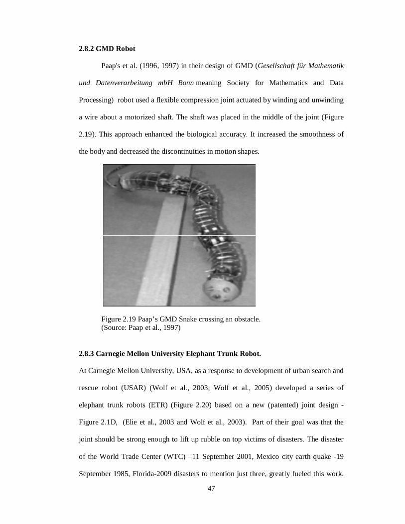
47

2.8.2 GMD Robot

Paap's et al. (1996, 1997) in their design of GMD (Gesellschaft für Mathematik

und Datenverarbeitung mbH Bonn meaning Society for Mathematics and Data

Processing) robot used a flexible compression joint actuated by winding and unwinding

a wire about a motorized shaft. The shaft was placed in the middle of the joint (Figure

2.19). This approach enhanced the biological accuracy. It increased the smoothness of

the body and decreased the discontinuities in motion shapes.

Figure 2.19 Paap’s GMD Snake crossing an obstacle. (Source: Paap et al., 1997)

2.8.3 Carnegie Mellon University Elephant Trunk Robot.

At Carnegie Mellon University, USA, as a response to development of urban search and

rescue robot (USAR) (Wolf et al., 2003; Wolf et al., 2005) developed a series of

elephant trunk robots (ETR) (Figure 2.20) based on a new (patented) joint design -

Figure 2.1D, (Elie et al., 2003 and Wolf et al., 2003). Part of their goal was that the

joint should be strong enough to lift up rubble on top victims of disasters. The disaster

of the World Trade Center (WTC) –11 September 2001, Mexico city earth quake -19

September 1985, Florida-2009 disasters to mention just three, greatly fueled this work.

48

The WTC attack saw the first use of USAR in action. The robots used have wheels or

tracks and access places unreachable or too dangerous for rescue workers and dogs. It

was then many realize that these robots can only show and assist in locating victims but

cannot actually rescue them and where there is tangled mesh, they cannot pass through

either. They are also mostly tethered hence not autonomous and short ranged. This led

attention to robots that could move on all terrain and through small spaces. The joints

were made from hardened steel.

Figure 2.20 Urban Search and Rescue elephant trunk robot with camera on its end. (Source: Wolf et al. 2003)

Similar work on USAR robot was done by Kazuyki et al. (2005), Fumitoshi

(2002) and Miller (2010).

2.8.4 Germany Sewer And Pipe Inspection Robot

The public sewage system in Germany is about 400,000 km long and if it is in

no good condition, sewage may leak out, possibly polluting soil and ground water and

possibly eroding away building foundations. Most of their sewage piping are circular

and are between 30 to 60cm in inner diameter. Teleoperated platforms were used with

cabling length of about 200m. The size of the pipe, water presence, slurry, varying

construction material will not allow just any robot to operate in such an environment. A

49

four wheel mobile platform was tested according to Joachim and Frank (1997), Marina

and Hermann, (2002) and (Joachim, 2003), but climbing the steps at intersections

defeated its use in very slippery sewage environments. The solution was MAKRO

(multi-segment robot, operating autonomously in sewer pipes)- Figure 2.21. To aid

autonomous navigation it carries several sensors on both ends – Laser cross air, 2-

infrared sensor, ultrasonic sensor and transmitter and a camera. The joints are oblique

made from steel plates.

Figure 2.21 MAKRO an autonomous robot for sewer inspection (Source: www.ais.fraunhofer.de/projects/Makro/makro-engl/makro-e.html)

2.8.5 Pneu-Worm Robot or Wormbot

This is a commercial robot and much is not disclosed about its operation.

Wormbot (Figure 2.22) is already in service for pipe inspection (Borenstein, 2006). It

MAKRO in action at a T-Joint

View from top End view showing sensor arrays

50

uses twin bellow and inchworm motion method for moving within the pipe. The robot is

tethered (power and air line supplying the bellows). It carries a camera on its front end

and a remote monitor is supplied with it.

Figure 2.22 Pneu-Worm Robot (Source: www.ornl.gov/info/ornlreview/rev26-34/text/tramain.html)

2.8.6 NASA Snakebot

Until the publication by Brooks and Flynn of a paper titled "Fast, Cheap and Out

of Control: A Robot Invasion of the Solar System" (Brooks and Flynn, 1989), robots for

space exploration have always been expensive projects. The paper led to changes in

design of the rover (i.e. lunar rovers) research from building the one, big, expensive

robot to building lots of little cheap ones.

At NASA’s Ames research center, USA, different small scale robots are being

developed for space and planet exploration (Kevin, 2003 and Haith et al. 2000),

Snakebots is one of them. NASA snakebots (Figure 2.23) are based on Mark Yim

polybot - Figure 2.24. The polybot is capable of countless reconfiguration and

accidental loss of a segment will not affect the other - in fact, they will be able to

function independently as each segment has its own microcontroller. The NASA robot

will carry touch sensor over its body. They are expected to help with Martian landscape

exploration as they dig into soil, burrow down to depths that other robotic probes can’t

get into, slither into cracks, navigate rough terrain where wheeled and legged robots will

51

get stuck or topple. Since they will be more durable and cheaper, a large number can be

sent to explore MARS.

A B

Figure 2.23 NASA Snakebot A) closer view of the robot. B) Field test of the robot (Source: Kevin, 2003)

Figure 2.24 Yim’s Polybot Robot as used by NASA. (Source: Kevin, 2003)

The polybot was built at Xerox PARC USA. It is planar i.e. 1-degree of freedom

per segment. Yims polybot modules are good for quick assembly but produce very weak

joints at high cost. The joints were revolute and use stamped metal and plastic.

52

2.8.7 OBLIX and MOGURA

MOGURA (Figure 2.25c) was developed between 1982-84 by Hirose and Yoneda

Robotics Lab (Japan) according to Hirobumi (1985), for grinding the water runner of

the water wheel for hydro electric power generation. The MOGURA arm which utilizes

an oblique swivel mechanism was developed in cooperation with Toshiba Company

based on OBLIX (Figure 2.25a and 2.25b). (http://wwwrobot.mes.titech.ac.jp /robot/

snake/oblix/oblix_e.html)

After casting a water wheel for hydroelectric power generation with a diameter of

about 4-5m, MOGURA acts as the robot arm that performs the grinding operation on

the water runners that follow along the fins of the interior part. Until this time, workers

have to climb into the curved runners to measure the surface conditions and do the

grinding as shown in Figure 2.6. MOGURA is made from an oblique swivel mechanism

that forms a compact and highly rigid arm. It is assembled and used as shown in Figure

2.27. The total length is 2.5m, the diameter is 200 mm, and the oblique swivel angle is 150.

The joints used by OBLIX and MOGURA are made from steel.

2.8.8 OmniTread

This is an example of serpentine robot. The OmniTread is shown in Figure 2.28 in

different environments. OmniTread 8” is pneumatically driven externally with dual

rubber tracks per side (i.e. 8 per segment). The OmniTread 4” (Figure 2.29) carries its

own air supply onboard and has one track per side (or 4 tracks per segment). Both have

bellow joint for turning.

53

Figure 2.25 OBLIX and MOGURA in different configurations (Source http://www-robot.mes.titech.ac.jp/robot/snake/oblix/ oblix_e.html)

Figure 2.26 Conditions for the waterwheel grinding operations, men have to enter to grind with hand. (Source: http://www-robot.mes.titech.ac.jp /robot/snake/oblix/ oblix_e.html)

A) OBLIX 3D motion

B) OBLIX with wheel

C) MOGURA assembled

Human operator

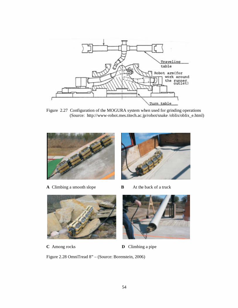
54

A Climbing a smooth slope B At the back of a truck

C Among rocks D Climbing a pipe

Figure 2.28 OmniTread 8” – (Source: Borenstein, 2006)

Figure 2.27 Configuration of the MOGURA system when used for grinding operations (Source: http://www-robot.mes.titech.ac.jp/robot/snake /oblix/oblix_e.html)

55

Figure 2.29 OmniTread 4” with the segment internals on the left.

(Source: Borenstein, 2006)

2.9 OTHER APPLICATIONS OF HYPER-REDUNDANT ROBOTS

2.9.1 Military Purposes

They can be used for detonating unexploded ordnance (UXO) and bomb

disposal, spying and espionage, surveillance. Wolf et al. (2003) gave description of a

surgical bomb disarming robot that moved slowly. It was developed at Pacific

Northwest Labs in the USA. It was to be used for probing the internal of UXO without

accidentally detonating it - hence its slow motion. The mechanism is kinematically a

sequence of linearly actuated universal joints stacked on top of each other - Figure 2.1D.

For stealth purposes, a snake robot will need to be autonomous in selecting its

paths among obstacles. This is an undeclared goal by Sensor Base Planning Laboratory

of Carnegie Mellon University (http://www.snakerobot.com) and Zhang et al. (2002) in

56

the development of motion planning for hyper-redundant robots. The extension of the

achievement of such a feat is staggering. It means a very slender and camouflaged rod

can move about with ability to spy on enemies positions, steal information from them

and enter highly fortified places or carrying ordinances even right to the door of the

defense head quarter and much more than the mind can conceive now.

Kevin (1997), in his introduction to his works wrote that the FBI and Special

Forces of USA made enquiry about his work because they can see future use of it.

In a 2005 expo at Japan, Hirose demonstrated a very realistic swimming snake

robot (Figure 2.18 – ACM R5) to which the most comment on it was that the Japanese

will surely load it one day with a bomb.

2.9.2 Medical Purposes (Minimally Invasive Surgery)

Surgery now uses robotic and image processing systems in order to interactively

assist medical teams, both in planning surgical interventions, and in their execution. The

objective of this new technique is to enhance the quality of surgical procedures by

minimizing their side effects (smaller incisions, lesser trauma, more precision etc), thus

increasing patient benefit while decreasing the surgical cost. These techniques are being

successfully introduced in several areas of surgery: Neurosurgery, orthopaedics, micro-

surgery, cardiovascular and general surgery etc (Jean-Pierre, 2000).

Minimally invasive surgery helps patients by accelerating postoperative

recovery, Nobuto (2003). It is usually aided by use of laparoscopic and endoscope

devices which are used for getting images from remote locations in machines and the

human body. The end bending and direction is controlled by cable at its base. The

motion of the tip of the laparoscope and endoscope devices are not accurate and

complex shapes can neither be followed accurately because they are both rigid tools.

57

A serpentine device (Figure 2.30) is being tested, that could solve the problem of

the endoscope in handling complex path successfully. A successful test was done on a

pig (http://www.snakerobot.com) at Carnegie Mellon Biorobotic Laboratory, USA.

A B

Figure 2.30 An endoscope (A) The endoscope device (B) The endoscope is being inserted behind a pig heart. (Source: http://www.snakerobot.com)

The device was designed to be pushed into the body with a servo motor just like any

other endoscope. It uses cable to adjust its direction of bending. According to Kevin,

(1997) and Thomas et al. (2005), a self propelled endoscope will open up a wide market

and benefit the people as it will reduce discomfort associated with the pushing.

Thomas et al. (2005) presented their investigation on self moving endoscope.

They reported that the main problem is the generation of sufficient friction between the

device and the slippery mucous-lined tract wall. A biomimetic approach was followed.

The common ragworm, Nereis diversicolor (Figure 2.31), successfully moves in a

variety of slippery environments such as mud and is capable of burrowing through the

substrate, crawling over the substrate and swimming in open water. During fast

crawling and swimming the body undulates from side to side with each body wave

moving from the posterior region to the anterior. Lateral appendages (parapodia) are

synchronized with the body waves and aid in thrust generation by acting as paddles

58

during swimming and legs during crawling. During slow crawling no or only small

amplitude body waves are present and thrust is generated by the parapodia. Extruding

distally from the parapodium are three bundles of hairs (setae), which are the structures

that allow the worm to crawl effectively in slippery substrates.

A B

Figure 2.31 Nereis diversicolor: A) Slow and B) Fast crawling. (Source: Thomas et al., 2005)

2.10 STRATEGIES USED FOR CONTROLLING HYPER-REDUNDANT ROBOT JOINTS

In the cause of developing a biomimetic hyper-redundant robots, various motions

employed by the biological counterpart have to be programmed into the robot

controller. Biomimicry requires that the object be studied scientifically and its result

quantified, this was what Hirose (Hirose and Morishima, 1990) did using live snakes,

Figure 2.32. Similarly, Miller (2010) built his S7 prototype as a result of his encounter

with a python. Hirose discovered that motion was more than a two-dimensional problem

in his study of live snakes. His first ACM robot is planar and has very poor

performance. There is a slight body raise called sinus lifting (Figure 2.33) were friction

with the surface will rather hamper motion.

59

Figure 2.32 A snake equipped with EMG and normal force detectors (Source: http://www.robot.mess.titech.ac.jp/robot/snakes_e.html)

(A) (B)

Figure 2.33 Snake motion (A) Sinus Lifting to reduce friction (B) Sketch of normal force distribution about the sinus

(Source: http://www.robot.mess.titech.ac.jp/robot/snakes_e.html)

There are three approaches according to Kevin (1997) used in controlling hyper-

redundant robot joints, they are:

1. Serpenoid curve method

2. Follow the leader approach and

3. Built in motion pattern

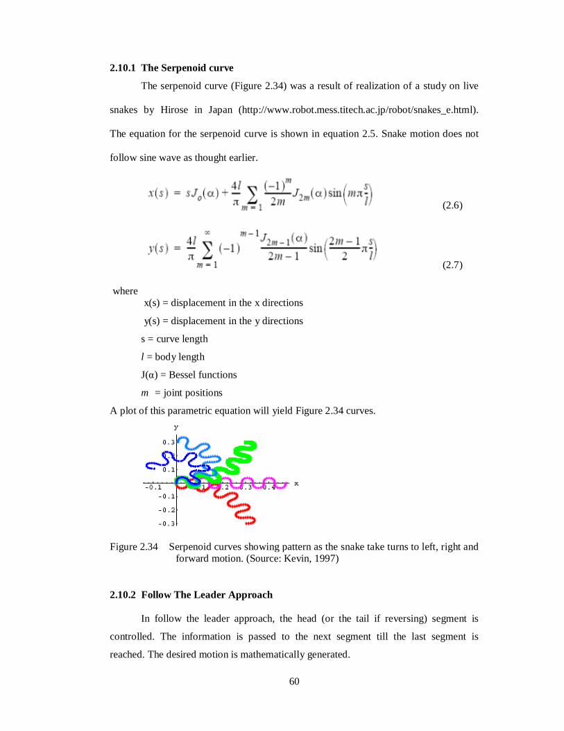
60

2.10.1 The Serpenoid curve

The serpenoid curve (Figure 2.34) was a result of realization of a study on live

snakes by Hirose in Japan (http://www.robot.mess.titech.ac.jp/robot/snakes_e.html).

The equation for the serpenoid curve is shown in equation 2.5. Snake motion does not

follow sine wave as thought earlier.

where x(s) = displacement in the x directions

y(s) = displacement in the y directions

s = curve length

l = body length

J(α) = Bessel functions

m = joint positions

A plot of this parametric equation will yield Figure 2.34 curves.

Figure 2.34 Serpenoid curves showing pattern as the snake take turns to left, right and forward motion. (Source: Kevin, 1997)

2.10.2 Follow The Leader Approach

In follow the leader approach, the head (or the tail if reversing) segment is

controlled. The information is passed to the next segment till the last segment is

reached. The desired motion is mathematically generated.

(2.7)

(2.6)

61

2.10.3 Built In Motion Pattern

The use of built in motion pattern means that the microcontroller (or

microprocessor) will have to adjust each segment according to the predefined motion

stored in its memory. This is less mathematically involving but not very flexible.

Researchers who use microcontrollers prefer the last two methods as floating point

mathematics are avoided. The use of serpenoid curve equation involves floating point

calculations.

2.11 PATH PLANNING

Path planning in the parlance of hyper-redundant robotics refers to the methods

used in making the joints to form the desired shape and curve and follow a desired path

while avoiding obstacles during operation.

Coordinating all the actuators and joints to produce useful motion/gait is a major

challenge in hyper-redundant robot implementations. Many of the research work

published are those of robots being tested in either an uncluttered environment – i.e. no

tangled mass to navigate, or use of geometrically fixed environment as in the MAKRO

robot used for sewer environment inspection (Marina and Hermann, 2002). The reason

is that each segment activity is not an isolated act. It is a duplication of the first segment

on the link (the head) if it is a snake robot, or the memorized path followed by the

previous link in case of fixed base ones (i.e. robotic arms). The motion requirement is

that of 3-D in an unmapped environment. The problem is referred to as path planning or

motion planning. Choset and Henning (1999) are the few researchers working explicitly

on serpentine motion planning.

Some solutions tried in hyper-redundant robot motion planning strategy include;

roadmap, tunnels, local sensor based planning, generalized voronoi graph (GVG) and

Classical planning.

62

2.11.1 Roadmap

This was introduced by Chirikjian and Burdick (1990b). Roadmaps have the

following properties: accessibility, connectivity and departability according to Choset

and Wade (1999). The meaning of this is that the end of the robot can move between

two points via a path in a connected component of the robot free space by first finding a

path onto the roadmap (accessibility), traversing the path to the vicinity of the goal

(connectivity) and then constructing a path from the roadmap to the goal (departability).

2.11.2 Tunnels

This is another path planning method by Chirikjian and Burdick (1990a). One

suggestion is based on the definition of tunnels through obstacle field into which the

serpentine mechanism slips through. They did not prescribe any strategy of constructing

such tunnels.

2.11.3 Local Sensor Based Planning.

In this case, the serpentine device maintains its end effector location

while it locally adapts to a time varying environment. The entire body fits

within a tunnel and then part of the tunnel is continuously adapted away from

any object that became unacceptably close as sensed by the mounted body

sensor - (Takanashi et al., 1993).

Sensor based planning incorporates sensor information, reflecting the

current state of the environment, into a robot's planning process, as opposed to

classical planning, where full knowledge of the world's geometry is assumed to

be known prior to the planning event. Processing the sensory data for

subsequent use in planning also offers many challenges

63

(http://robotics.caltech.edu/).

A global sensor based planning (Reznik and Lumelsky, 1992) assumed a

perfect sensor all over the body of the robot to detect obstacles, research is on-

going in this area – such as NASA snakebot which will have sensors all over

the body for motion planning or just normal touch sensors.

2.11.4 Generalized Voronoi Graph (GVG)

This is a modified roadmap - Choset and Burdick, (1994, 1995a, 1995b

and 1996). GVG is the set of points equidistance to m obstacle in m dimensions.

In the plane, the GVG is simply the generalized Voronoi diagram (O’Dunlaing

and Yap, 1985) which is the set of points equidistance to two obstacles. In R3

(i.e. 3 dimension), the GVG is the one-dimensional set of points equidistant to

three obstacles. According to Choset et al. (1997), Konukseven and Choset

(1997), Nagatani et al. (2002), Choset and Henning (1999), Lee and Choset

(2004), Lee and Choset (2005a, 2005b), follow-the-leader approach (section

2.10.2) will be capable of using GVG for its path planning because it is a sensor

based planning. The head of the serpentine device moves along the GVG, while

the rest of the body follows. This way a set of curves known as backbone

curves (Chirikjian and Burdick, 1990b) are created. For example, Figure 2.35

is generated while the segments are adjusted as the serpentine device moves

between the obstacles. Where there are sharp corners an approximate curve is

formed due to the limit in the mechanical joints – this is referred to as curve

deformation (Choset and Lee, 2001).

64

Figure 2.35 The ticked line segments are the planar GVG for the bounded environment. (Source: Choset and Lee, 2001).

2.11.5 Classical Planning

This is a method which requires the full knowledge of the environment in which

to operate ahead of time. This is not a realistic method especially in an outdoor

environment according to Konukseven and Choset, (1997).

In geometrically fixed environment such as sewer pipes that are at right angle

to each other, path planning is not needed – (Marina and Hermann, 2002). It was

demonstrated that simple vision using shape deformation of Laser cross-hair (Figure

2.36) on surfaces has enabled MAKRO to navigate the sewer networks. The basis for

the success was that vision was never to be viewed in isolation but by taking into

account the environmental constraints. In other word when a laser pattern is projected

onto a scene, the shape of the footprints is like a condensed print, which carries

information about the scene geometry from which useful navigational information can

be derived. This falls into the class of vision termed cheap vision- Horswill (1992).

65

A B C D

Figure 2.36 Laser crosshair projector (A). (B), (C) and (D) three surface types with overlaid laser footprints. The pattern is an indicator of the environment configuration. (Source: Marina and Hermann, 2002).

2.11.6 Motion Planning For Fixed Base Hyper-Redundant Robots

For tethered robot (i.e. one end fixed as in elephant trunk robot (ETR) an

approach for motion planning is based on topological decomposition of space called

WAFT (WAve Front Topology) - Ohno and Hirose (2001). This decomposition of

space allows for path planning that is path-dependent, meaning that veering left around

the first obstacle encountered will change the options that are available in the future as

compared to the options had the path to the right of the first obstacle been chosen. The

WAFT planner also uses sensor based method (http://voronoi.sbp.ri.cmu.edu

/research/rsch_rodgvg.html).

2.12 A REVIEW OF ACTUATORS FOR ROBOTIC JOINTS

The actuator is the component that moves the segment under the control of

signal from the microprocessor or microcontroller to give it a desired gait/motion.

Selection of an actuator is based on things like:

a) Power requirement

b) Speed of operation (of the joint)

c) Torque to lock a link into the generated angle into place

d) Response to control signal

e) Fidelity – faithfulness to the control signal pattern

66

2.12.1 Brief Description Of Actuators (Kevin, 1997);

a) Polymer Gels

Some polymers are capable of converting chemical energy to mechanical work in

isothermal conditions. These polymers significantly change their length in response

to chemical changes involving altered temperature, pH, or applied electric fields.

Volume changes can be as high as a factor of 1000. For polymer gels to be useful

there are many technical issues to resolve. There are issues of strength, response,

stress-strain relations, fatigue life, thermal and electrical conductivity. Other issues

include efficiency, power and force densities.

b) Shape Memory Alloys (SMA)

This refers to NiTiNoL (nickel-titanium alloys). These alloys in the form of wires

will stretch easily at room temperature but will return to their original forms when

carrying current that also heats them up. Longer stretches such as 8% are possible

for a few cycles of operation but a shorter strain like 5% will allow millions of

cycles. The 8% strain will correspond to 600N/mm2. The response time is slow, and

depends on the rate of heat removal.

c) Piezoelectric Devices

These are crystalline materials that change size when electric voltage is applied.

They also generate electric voltage when strained. Their limitation is that the size

changes are very small, they have non-linear behaviour, high hysterisis and creep.

They however have very fast response and could produce very large forces.

d) Electrostriction Devices

These are similar to piezo crystal materials but with the fact that electrostrictive

crystals are symmetric. The strain is proportional to the square of electric field. This

67

property is independent of piezoelectric effect and is due to rotation of polar

domains in ceramic through the field. It has the advantages that it can use lower

voltages - compared to piezo crystals. It also has very low length changes and some

of piezo crystals problems according to Kelvin (1997).

e) Magnetostriction

Magnetostriction is the mechanical deformation of a ferromagnetic material when

subjected to a uniform magnetic field. Unlike piezo electrics, the displacement per

unit field actually increases with length. Internal stresses in the material due to

anisotropy energy are required to magnetize it in certain directions relative to the

crystal axes and vice versa. The strains and displacements can be significantly more

than piezo electrics but piezo electric materials can be stacked to give nearly the

same stroke per length. Terfenol-D, used in several magnetostrictive commercial

products, offers high forces and good strain.

f) MEMS (Micro-Electrical Mechanical Systems) actuator

These are actuators based on the use of semiconductor technology to fabricate

mechanical parts that can move objects.

g) Thermal actuators

They use the thermal expansion property of materials to actuate. We see this in the

electric pressing iron for example. The force generated is very high but the speed of

response is slow. Thermopolymers are new materials that have faster response and

are being researched upon.

h) Electro-magnetic motors

The current carrying conductor within a magnetic field will generate motion. This is

used to form an electric motor. The technology is well established and is improving

68

as power density of the conductor increases with newer superconductors.

i) Pneumatic actuators

These use compressed air or other gas to move a ram or pneumatic motor. High

force, high speed actuation can be generated within a small space. The limitation

however has to do with the gas source/supply and precision position control.

Another limitation is possible leakage and material wear.

j) Hydraulic actuators

Hydraulic actuators work similarly to pneumatic actuator but uses fluid instead of air.

The most desired actuating device is artificial muscle using any of the above

technology, but up till now, research is still vigorously on. Some progress has been

made, for example, platinum plated perfluorosulfonic acid polymer (ICPF) operating in

water (a must condition) has been used to design an underwater robot that operate as

linear (muscle like) actuator – Guo et al. (1998).

2.12.2 Tested Method Of Actuating Hyper-Redundant Robots

Various actuating devices have been tested all with the aim of higher power to

weight ratio and lower power consumption and small volume.

The commonest approach of actuating the segment of hyper-redundant robot is

to place a motor inside each one. For planar robot such as Hirose ACM, a single motor

is used per joint giving each joint a single degree of freedom. Those that have two or

more DOFs are equipped with two motors. This arrangement has the advantage of ease

of controlling each segment independently. However, the large number of motors used

increase weight, power consumption and reduced maneuverability.

69

Examples of tried actuators are:

1. Remote control servomotors (Kevin, 1997 and Miller, 2010)

2. Permanent magnet DC motors (Anani et al., 2004),

3. Pneumatic motor (Grzegorz et al., 2005; Ohno and Hirose, 2000; Paulina and

Jörg, 2003 and Hitoshi et al., 2006)

4. Hydraulic (water) motor - Hitoshi et al. 2006,

5. Artificial muscle platinum plated perfluorosulfonic acid polymer (ICPF), Guo

et al. (2004), electro-actuated polymer (EAP)), Piezocrystal, Magnetostrictive,

Shape-Memory Alloy (SMA), Shigeo et al. (1989).

Examples of tried mechanisms are:

1. Cable - Wolf et al. (2003), Ma et al. (1992)

2. Hydraulic cylinders - http://www.act.sys.okayama-u.ac.jp/wormrobot.html

3. Gear box - Paulina and Jörg (2003), Miller (2010)

For the serpentine robots, a variety of methods have been employed in driving the

mechanism for locomotion used by serpentine robots. Most are the same as with snake

robots. The locomotion devices tested are

1. Legs - Grzegorz et al. (2005),

2. Tracks - Grzegorz et al. (2005), Paulina and Jörg (2003), Kazuyki et al. (2005)

3. Wheels - Marina and Hermann (2002), Joachim (2002)

4. Scale (rubber) - Charles and Antonio (1998).

2.13 REVIEW OF PAST WORKS ON ROBOTIC FISH

Fish are known for their fulgurating acceleration inside water. “It is well known

that the tuna swims with high speed and high efficiency, the pike accelerates in a flash

70

and the eel swims skillfully into narrow holes. Such astonishing swimming ability

inspired researchers (Streitlien, et al., 1996; Anderson, 1996; Guo et al., 1998; Kato,

2000; Liang, 2002; Yu, 2002; Jindong and Huosheng, 2004) to improve the

performance of aquatic man-made systems. Instead of the conventional rotary propeller

used in ships or underwater vehicles, the undulation movement like fish provides the

main energy of the robotic fish. The observation on the real fish shows that this kind of

propulsion is more noiseless, effective, and manoeuvrable than the propeller-based

propulsion” - Jindong and Huosheng, (2003).

Four robotic fish models will be reviewed in this work; they are Robotuna,

Robopike, PF series and University of Essex fish robot.

2.13.1 Robotuna

Description: David (1994) developed Robotuna (Figure 2.37) in MIT. Delrin plastic

was used for most of its construction and epoxy for sealing. The electronics is Onset

model 8 computer (68332) with digital wireless modem and DC-DC converter. The tail

(Figure 2.38) is made of rings of delrin plastic.

Limitation: It could not float nor swim because of its weight (3.6kg) and other heavy

material used for its construction.

Figure 2.37 Robotuna (Source: http://web.mit.edu/towtank/www/Tuna/tuna.html)

71

Figure 2.38 Robotuna tail construction (Source: http://web.mit.edu/towtank/www/Tuna/tuna.html)

2.13.2 Robopike

Description: Robopike (Figure 2.39) is also from MIT and is a creation of John Muir

Kumph (Kumph, 1996). It was a continuation of work on Robottuna. The pike (a fish)

was chosen because of its excellent accelerating and turning abilities. Pike has very

quick turning and fast acceleration from rest. In the wild, the pike accelerates at rates of

8-12 m/s2.

Figure 2.39 Robopike (Source: http://web.mit.edu/towtank/www/Pike/pike.html)

Robopike is controlled by a supervisory controller. The navigation is performed by a

human, and a computer interprets the controls so that the robot can perform as expected.

72

Comment: Robopike uses only three segments, thus the size of the fish is reduced,

allowing the use of inexpensive actuators. This means that while the shape of the fish

cannot be made to resemble exactly the shape of a real fish, a close shape can be

obtained. The tail is made up of spiral spring exoskeleton (Figure 2.40) using delrin.

Robopike was used for studying drag reduction in fish like locomotion.

Figure 2.40 Robopike spiral spring exoskeleton of the tail section. (Source: http://web.mit.edu/towtank/www/Pike/pike.html)

2.13.3 Japanese PF-300, PF-600, PF-700,UPF-2001 Robotic Fishes

Description: These Japanese robotic fishes (http://www.nmri.go.jp/eng/ khirata/fish)

were designed for different purposes.

1. The PF-300 (Figure 2.41) was for studying turning performance and straight line

propulsion.

2. The PF-600 is designed to study propulsion and improve on PF-300.

3. PF-700 was designed for high speed, and had a DC motor as a power source.

The shape was modeled after mackerel and pike, so PF-700 had a very slim

body. A maximum speed of 0.6m/s was obtained by PF-700 at tail swing of 15o

amplitude.

4. PF-2001 (Figure 2.42) was designed to exploit 3D motion. It has the up -down

motion mechanism with a moving weight. A maximum speed of 0.97m/s was

obtained by the PF 2001.

73

Comment: These fishes carried their own float (i.e. they have fixed depth) except PF-

2001. They all have their flexible parts made up of plastic revolute joints.

Figure 2.42 PF-2001 robot (Source: http://www.nmri.go.jp/eng/khirata/fish)

2.13.4 Essex G9 Robotic Fish

Description: Essex G9 robotic fish (Figure 2.43) is about 32cm long and has 3 R/C

servo motors and 2 DC motors. Three servomotors are concatenated together in the tail

to act as 3 joints (for the G9 but more than that for other series like the one shown in

Figure 2.44), 1 DC motor is fixed in the head to change center of gravity (COG) of the

Figure 2.41 PF-300 robot (Source: http://www.nmri.go.jp/eng/khirata/fish)

74

fish and 1 DC motor controls the micro-pump for float control. On the back of the fish

body, a dorsal fin is fixed vertically to keep the fish from swaging. The central

controller of the robotic fish is based on a 400Mhz Gumstix Linux computer and is

responsible for sampling data from sensors, processing data and making decisions.

Comments: It has a linear speed of 0.2m/s, at maximum tail beat frequency of 0.5Hz. It

is able to bend its body at a big angle in a short time (about 90°/0.20sec). The researcher

idea is to directly link the servomotors (thus the motors themselves form the joints), this

introduces inertial and hence low tail oscillation speed obtainable to 0.5Hz.

Figure 2.43 Essex G9 robotic fish – (Source: Jindong and Huosheng, 2003)

Figure 2.44 Mechanical Configuration of the Essex Robot Fish. (Source: Jindong and Huosheng, 2004)

75

CHAPTER THREE

DESIGN CONSIDERATIONS, THEORIES AND CALCULATIONS

3.1 DESIGN CONSIDERATIONS

The design considerations are (1) biomimicry, (2) simplified control scheme of the

hyper-redundant joints (3) simplified and functional joint design, (4) material selection and

(5) capturing the model geometry/design.

3.1.1 Biomimicry

This refers to close performance to the biological model being imitated specifically in

motion pattern. To achieve this design consideration, carbon-black-reinforced rubbers is

used. It is has been shown to have very close mechanical properties to biological tissues.

Natural rubber (polyisoprene) is a flexible material with very wide compositions.

Fundamentally, they are made from latex extracted from the para rubber tree (Hevea

brasiliensis) plus carbon sooth (as filler), sulphur (as vulcanizing ingredient) and several other

proprietary materials added for different end purposes.

Using rubber for artificial hydrostatic joint design requires that Mullins effect, Payne

effect and temperature be taken into cognizance as shown in the literature review; they have

significant effect on the performance of the end product. Rubber was also shown earlier to

have similarity to living tissue especially hydrostatic support used by invertebrate bodies.

3.1.2 Simplified Control Scheme Of The Hyper-Redundant Joints

It is desired to use control scheme on the joints that is achievable without very high

computational cost. The use of built in pattern(s) for motion control strategy simplifies the

need for floating point calculations especially for the serpenoid curves that describe hyper-

redundant body motions. Furthermore, sensor based path planning is computationally less

tasking and is hereby adapted for this work.

76

3.1.3 Simplified And Functional Joint Design

Biological bodies have simple mechanical designs that function because of the nature

of the materials used in building them, and actuating them. The goal of achieving this is

possible by copying nature and using materials very close to those used by nature. One of the

simplest and functional joints found in nature is the hydrostatic joint.

3.1.4 Material Selection

Carbon-black-reinforced rubbers have mechanical properties close to those of living

tissues and hence qualify for use for the hydrostatic components. A fluid filled design is not

desired, therefore the design will imitate muscular hydrostat as closely as possible – with a

more rigid support equivalent to cuticle (the hardened coat of an insect). Cuticle itself is

equivalent to plastic in nature. Wood and any plastic can therefore be a perfect artificial

support.

3.1.5 Capturing The Model Geometry/Design

Copying a biological model design is essential if biomimicry is to actually take place.

Fish as the model used in this work vary greatly in their designs. A life model has to be

measured and used to build the robotic model.

3.2 FRAMEWORK FOR THE HYDROSTATIC JOINTS

The design presented in this work is hereby named diamond cross-sectional design. It is

an hydrostatic joint modeled using lessons from hornworm caterpillar- maduca sexta. The

lessons are:

1. The caterpillar is whole body isochoric which means no change to the geometry.

Rubber also does not change volume when stretched or compressed.

2. The rubber stress-stretch nature has very close resemblance to that of the muscle

(qualitatively)

77

3. It is round and long, qualifying it adequately as an hyper-redundant body

Though it is fluid filled, muscular hydrostat such as the human tongue approach of control is

imitated, that is, the actuator will pull on the support structure to generate motions.

Appendix A shows other design that could also be exploited for translating rubber

into artificial hydrostatic joint.

3.2.1 Description Of The Rubber Based Artificial Hydrostatic Joint

The diamond design – Figure 3.1, is of two types – the shorter model that uses much

smaller elastomer length and the longer one that uses longer elastomer length in between the

supports. Figure 3.2 shows the cross-sectional sketch of the design. The diamond shape is

needed to avoid interference from adjacent support during bending. The elastomer strip will

be held in the support using glue or screws.

A Short elastomer design

B Long elastomer design

C The two designs put side by side for length comparison Figure 3.1 Diamond design of the evolved joint – short and long elastomer designs

Natural Rubber

Support

Support

78

Figure 3.2 The diamond design - cross-section of the model 3.2.2 Kinematics Of The Model

The kinematic of the model gives a visualization of the joints and a comparison can be

made in terms of potential for 3D motions, rigidity, minimum curvature or radius and

twisting. The kinematics of the two models are presented in Figure 3.3.

Figure 3.3 Kinematics of the diamond designs

A A

A Long elastomer model showing twist and planar bending simultaneously

B Long elastomer model showing planar bending only

C Short elastomer model showing planar bending - viewed from the top

D Short elastomer model showing planar bending – oblique view

79

3.2.3 Comparison Of The Two Diamond Design

1. On potential for 3D motions, the model with longer elastomer can be used for a hyper-

redundant robot that requires 3D body motion. The shorter model is too rigid to twist.

2. On rigidity, the shorter model will excel since it is more compact and has less

elastomer exposure.

3. Minimum curvature – the three segments shown for the model with longer elastomer

will easily form a complete circle while the shorter model will require more number of

links to form a circle. Larger number of links will translate to more number of actuators

to manage each link and more complex control schemes will ultimately be needed.

Summarily, an hyper-redundant joint system that will operate mostly in plain should not have

too long rubber in between the supports while those that will require 3D motions should not

use too little rubber length that will hamper motion. An optimum should be based on the

following criteria:

(1) The minimum radius of curvature (r) expected of the joint as shown in Figure 3.4.

Figure 3.4 The minimum radius of curvature of the joints

(2) The amount of 3D motion expected if it will not be a pure planar motion, Figure 3.5

shows motion about θ and β polar axis.

r

80

Figure 3.5 3-Dimensional motions capabilities about other axis

(3) The presence of cantilever (Figure 3.6), that is the ability to carry other links or segments

without collapsing. This calls for a rigid design.

Figure 3.6 Cantilever of multiple links

3.2.4 Strength And Weakness Of The Evolved Artificial Hydrostatic Joint

The following are the advantages expected of the evolved artificial hydrostatic joint

1. It has potential for miniaturization – which may be extremely difficult to

achieve using rigid metal joints.

2. Cheaper material – rubber and any rigid support – wood, plastic etc

3. Mass production will be easier

4. High speed of bending

5. It can be made with medical grade rubber like silicones and used for medical

purposes without causing hazard to the organ. In event of collusion with organ,

damage will be minimal or nonexistence.

6. It can be used for precision positioning purposes if used with micro stepper

motors.

7. Maintenance will be low as the rubber will need no lubrication or adjustment

8. Noiseless operations will be possible with the design

β θ

h

81

Also there are obvious/inherent weaknesses of the design which are a carry-over from

biological models. They are:

1. The design cannot be used where there is an extremely high temperature or very

low temperature. The rubber used and the support materials will determine the

useful temperature range.

2. Since this is not an inflatable design, it cannot be used to lift heavy load

3. The design will not work in a radioactive environment, as the rubber may

dissociate.

Appendix A shows other configurations/ design and possible use of the evolved artificial

hydrostatic joint.

3.3 ADAPTATION OF THE ARTIFICIAL HYDROSTATIC JOINTS TO A FISH MODEL

3.3.1 Selection Of A Biological Hyper-Redundant Body Model

This work requires that a biological hyper-redundant body model be selected for

imitation. Biological hyper-redundant bodies vary in length, some are longer like the snake

and some are relatively short – like the fish. The control system grows in complexity with

their length; many actuators (“muscles”) will have to be managed simultaneously. A shorter

model (fish) is adapted as a model for demonstrating the use of the artificial hydrostatic joint

in this work.

3.3.2 Selection Of A Fish Model

The high speed teleost species of fish is selected for this work. Table 3.1 shows some

common member of the families of the teleost fish and their peak speed in increasing order.

The specie of teleost fish selected was mackerel (Figure 3.7) because of the following

reasons;

82

1 It is very common

2 It is capable of fair speed, 11 km/h, (fastest fish is sail fish with speed > 96km/h)

3 The natural ones move in schools (up to 20km long). It means that they can be

concealed easily among fish schools for military purpose and also used as fish

tracker by fishermen and biologists.

4 It is small enough for stream monitoring and ecological study.

3.3.3 The Active Joint Area Of The Fish Model

For the teleost species of fish, the tail is where the oscillation is based and it is where

the hyper-redundancy is significant. It is also the main organ of propulsion, therefore, the

main area of the joint design will focus on the tail; the frontal part is considered rigid.

3.3.4 Description of the Hydrostatic Joint Mechanism As Adapted for the Fish Model

Figure 3.8 is the computer aided design (CAD) model of the live fish assembled,

while figures 3.9 and 3.10 are the isometric views of the haul and tail assembly (both CAD

drawings). A more detailed drawings of the design are found in the assembly drawings 1, 2

and 3 and parts drawings 4 to 23. The dimensions are directly taken from the live fish at 1:1

scale – Appendix B shows the steps taken in translating the life fish to the CAD model.

Figure 3.11 shows the critical dimensions. To be noted in this design are:

1. The rubber strips are 5mm wide – since the motion expected will be planar

2. The 5mm is also adequate to prevent interference between adjacent supports

when bending

3. Maximum bending will not exceed 90o.

83

Table 3.1 Some common family member of teleost species of fish with their peak speed, average body length, speed to length ratio (V/L)

(Source http://www.nmri.go.jp/eng/khirata/fish/general/speed/speede.htm)

Herring

Speed = 6 km/h = 1.67 m/s = 3.7 MPH Length = 0.3 m V/L = 5.6

Pike


Carp


Cod

Speed = 8 km/h = 2.22 m/s = 5 MPH Length = 1.2 m V/L = 1.9

Mackerel


Salmon


Bonito


Small Tuna


Black Tuna


Swordfish


84

Figure 3.7 A lateral view of the Mackerel used for this project.

Figure 3.8 The CAD model of the Mackerel shown in Figure 4.6. – not to scale

Figure 3.9 Isometric CAD view of the haul (front rigid part) – not to scale

Figure 3.10 Isometric CAD view of the tail section (flexible part) – not to scale

85

Lateral view

Top view

Figure 3.11 The critical dimensions (in mm) of the model

The active part of the robotic fish model described here is the tail section, the front part is a

rigid haul. Using the sketch model shown in Figure 3.12 – 3.14, the manner the joint works is

described as follows;

1. From Figure 3.12 the rubber joint (A) (strips of rubber) is sandwiched between pairs of

rigid support segments (1) to (6).

2. The support (6) is attached to oval support (B) having six pass through holes (C) for the

cables support.

3. The servo motor (D) is attached to the oval support (B) having pass through holes for

the cables.

4. The cables are connected to the servo motor horn (E) by tying

5. The servo motor horn oscillates at angle (F). To get a serpentine motion, the

microcontroller uses its built in pattern generator to control the sequence of turning of

5

86

the servo motors (D). It sends the angular displacement information to the servo motors

in such a manner that its horn (E) will oscillate +/- angle (F).

6. On both sides of each segment (1) to (6) are located quarter pulleys (H) over which the nylon

cable (G) passes before hooking to those segments. Only one cable is shown for clarity.

7. The nylon cables (G) are attached to the servo motor horn (E). Its support passes

through the pass-through holes (C).

8. To get a serpentine motion, the microcontroller uses its built in pattern generator to

control the sequence of segment (1 to 6) turning by activating the servo motors (B)

(one is shown for clarity) according to the pattern.

9. The segments (1), (3) and (5) are connected to a servomotor each.

10. The other segment simplifies the design as they act to restore the joints to their static

states. Also, they help in getting the desired serpentine shape without complicated design

– just like nature has simplified its designs by appropriate use of material. Furthermore

this approach simplifies the number of motors required and hence the control scheme.

11. Figure 3.13 shows how the tail fin will bend to the left or right when the left or right

cable is pulled respectively by the servomotor (D).

12. Figure 3.14 shows the detail of the Nylon cable (H) design that will connect the motor

horn to the support structure (segments). It uses clutch cable design (as used in bicycles

and cars). It is made up of flexible plastic with the nylon cable running inside it.

13. For swimming to take place, the microcontroller sends angle data to each servo motor

using pulse-width-modulated scheme. The servo motors then turn to that angle which is

at 60o phase difference to the next servo motor. The servo motor then pulls the cable

which in turn pulls the segment it is attached to. In this manner, the tail generates a

travelling wave that has its origin at the segment (6) and ends at segment (1). The

amplitude increases from segment (6) to segment (1).

87

79

86

Figure 3.12 CAD model of the hydrostatic joints showing cables connected to the first segment only.

A

E

I

1 2 3

4 5

6

H

B

C

F

D

G

Legend (A) Rubber strip (B) Oval support (head board) (C) Pass-through hole (D) Servo motor (E) Servo motor horn (F) Angle of oscillation (G) Cable and its support (H) Quarter pulley (I) Tail fin

Signal cables from the microcontroller

80

Figure 3.13 How the tail fin will respond as the servo motor pull on the cables

Left

Left

Right

Right

Right cable is pulled by servomotor

Left cable is pulled by servomotor

Servo motor

88

81

Figure 3.14 The detail design of the cable showing one side only

Cable is pulled by the servo motor Support

(the robot frame)

Flexible casing for the cable

Support (the quarter pulley on the segment adjacent to the segment the cable is connected to)

Cable end is attached to a segment

Segments

A rubber joint

89

90

3.4 MATERIALS SELECTION

The forces and loads the artificial hydrostatic joint will experience are dependent

on its function and to some extent on the materials that are used in constructing it. Also,

the use of rubber means that the way and the manner it will be used will affect its

performance, specifically the oscillatory motion will incur the frequency softening

effect (Payne effect).

3.4.1 List of Materials

The following materials were used in constructing the fish robot;

1. Vulcanized rubber – 1.5mm thick.

2. 1/8 inch (3.175mm) thick seasoned plywood.

3. ¾ (19.05mm) inch plywood.

4. ABRO® steel reinforced 4 minutes setting Epoxy glue – Araldite.

5. Nylon 1010 cables – 0.5mm diameter.

6. 2.5mm diameter unplasticized PVC tubing.

7. Remote control servomotors (Futaba 3003 and Futaba 148).

8. Microcontroller – PIC18F4520

9. Latex rubber – from Population Services International (PSI)

10. Silicone rubber

11. Micro switches.

12. Parallax Ping)))

13. Collapsed polyurethane foam

14. Cyanoacrylate glue (super glue)

3.4.2 Description Of The Materials

The rubber is carbon filled vulcanized motor car inner tube (14inch or

91

35.56cm) from King Rubber Tire Company of China. This rubber was used for the

artificial hydrostatic joint. The 1/8 inch thick seasoned plywood acts as the support for

the rubber material. The open air seasoning is for dimensional stability. The ¾ inch

plywood is used for the pulleys. The epoxy glue is used for assembly of the parts.

ABRO® 4 minute epoxy glue is selected because the manufacturer states on its label

that it does not shrink after setting, meaning the parts will maintain their dimensions

after setting. The 0.5mm nylon cables connect the servo motor horn (lever) to the joints

supports (the plywood). The 2.5mm unplasticized PVC tubing acts as support for the

nylon cables. The remote control servo motors (Futaba 3003) are the programmable

actuators. The microcontroller manages the control of the artificial joints so that a

usable and varying motion can be achieved. The latex rubber and silicone rubber are

used for sealing against water. The micro switch is used as the sensor for collision

detection. Two pieces were used, one to detect collision on the left, the other is for the

right. The parallax ping))) are ultrasonic transmitter-receiver pairs that are used for

detecting objects. The polyurethane foam is used for padding purposes. The

cyanoacrylate glue was used for water proofing all the wooden parts – wood easily

absorbs it to form a water phobic layer.

3.5 COMPONENTS DESIGN

The components are designed based on the following theories; finite element analysis,

stress behavior in elastomers, stress in elastic materials, forces experienced by a moving

foil inside water, large-amplitude elongated-body motion theory, Mulling and Payne

effects. These are finally used in selecting the actuator for driving the joints and

assembling it.

92

3.5.1 Finite Element Analysis (FEA) for General Simulation

Finite element analysis (FEA) is a numerical technique for finding approximate

solutions of partial differential equations (PDE) as well as of integral equations. A

structure is normally partitioned into small sections referred to as elements, with depth

added for a 3-D environment. The connection between them is referred to as nodes. At

each node, there are forces F1, F2, F3, F4, F5 and F6 operating in the direction +x, -x, +y,

-y, +z and -z with displacements u1,u2, u3, u4, u5, and u6 (for 3-D situation); adapted

from Jason (2011) .

kij*uj = Fi

and kij is the stiffness coefficient relating Fj to uj (linearity is assumed here for

simplicity)

For two linked node we can write a matrix of the relationship as:

(3.1)

This matrix is called the stiffness matrix and it defines the geometric and material

properties of the object being analyzed. This matrix is solved for each linked node and

in relation to adjacent nodes to get all the unknowns i.e the loads experienced and the

corresponding displacements. Thus, the more the elements, the more the nodes, and

irregular shapes or boundary elements usually have more nodes to capture the geometry

F1

F2

F3

F4

F5

F6

k11 k12 k13 k14 k15 k16

k21 k22 k23 k24 k25 k26

k31 k32 k33 k34 k35 k36

k41 k42 k43 k44 k45 k46

k51 k52 k53 k54 k55 k56

k61 k62 k63 k64 k65 k66

u1

u2

u3

u4

u5

u6

=

93

of the structure. More elements means that the analysis can be more accurate as it will

be more refined in its capture of the structure geometry.

3.5.2 Stress Within An Elastomer (Rubber)

The loads in the rubber are determined using finite strain elasticity theory or constitutive

equations because it has unique properties, in particular exceptionally low shear

modulus and high elastic strain capability. The equations are solved using finite element

analysis (FEA). The equations relating the displacements u to the load F (see equation

3.1) are defined by constitutive equations and are normally solved using a computer

because of the matrix of matrix in algebraic form (i.e. tensors) involved (Kolecki,

2002).

3.5.3 Stress Within The Plywood Material

The plywood is treated as a linear material (i.e. Hooke’s law is used) and the following

mechanical properties are used in its finite element analysis (Ryder, 1990; Kelly, 2011);

a. Stress (3.2)

b. Strain (3.3)

c. Modulus of elasticity or Young’s modulus; (3.4)

d. Poisson’s ratio (3.5)

94

e. Density, (3.6)

f. Yield strength

Yielding occurs when the design stress exceeds the material yield strength.

Design stress is typically maximum surface stress (simple loading) or von Mises

stress (complex loading conditions). The von Mises yield criterion states that

yielding occurs when the von Mises stress, σν exceeds the yield strength in

tension. Often, finite element analysis stress results use von Mises stresses. von

Mises stress is:

(3.7)

where σ1, σ2 and σ3 are the principal stresses

3.5.4 Forces Experienced By A Moving Foil (Or Plate) Inside Water

When the fish tail oscillates inside the water, it behaves like a plate. The main force

acting on the plate with area A is the drag force, Fd. (John, 1993).

The drag force is given as Fd = 휌푣 퐶 퐴 (3.8)

where ρ = density of fluid (water in this case)

퐶 = coefficient of drag. It is shape dependent, in this work, it is assumed to be perfectly flat.

95

σ1 σ1

σ2

σ2

P Pi Pe

Figure 3.15 The ring geometry

A = Area of plate

v = velocity of the plate (peduncle)

3.5.5 Forces On Rings

The rings are hereby treated as thin cylinders, Figure 3.15, with internal pressure

Pi and external pressure, Pe

If the internal diameter is d and the thickness t, and σ1, σ2 are the hoop and longitudinal

stress, then

σ1 = Pd/2t (3.9)

σ2 = Pd/4t (3.10)

where P = Pe-Pi (3.11)

3.5.6 Bending Stress Within A Cantilevered Object

The classic formula (Ryder, 1990) for determining the bending stress in a beam under

96

simple bending is:

σb = (3.12)

퐼 = (3.13)

where σb = the bending stress

M = the moment about the neutral axis

y = the perpendicular distance to the neutral axis

Ixx = the second moment of area about the neutral axis x

b = the width of the beam

d = height of the beam

3.5.7 Stress In The Nylon Cable

According to Ryder, 1990, the stress in the nylon cable is calculated as

휎 = (3.14)

where 푃 = pull acting on the cable

Ac= area of the cable

3.5.8 Tensile Stress Within A Glue

휎 = (3.15)

where 푃 = separating forces acting on the glued bodies

Ag= area of glue

Mechanical interlocking theory is assumed which is based on the fact that at the

97

microscopic level all surfaces are very rough consisting of crevices, cracks and pores.

The adhesive penetrates these features and hardens such that it keys into the surfaces

and forms a strong surface bond (Roy, 2010).

3.5.9 Large-Amplitude Elongated-Body Motion Theory

The dynamic pressure, Pv caused by the tail pushing water at velocity ω is given by

Bernoulli’s equation of the form

Pv = 0.5 ρ ωv2 (N m-2), (3.16)

according to John (1993)

where Pv = dynamic pressure

ρ = water density

ωv = angular velocity of the fish tail

This dynamic pressure was derived using large-amplitude elongated-body motion

theory by Lighthill (1971) which allowed the prediction of instantaneous reactive force

between fish and water for fish motions of arbitrary amplitude. Figure 3.16 is used to

explain all the parameters involved in the derivation of the dynamic torque. It shows the

force components and velocity components of a fish peduncle as well as the torque and

angular velocity experienced by it. The Force Fv is zero (Fv=0 N) for a fish that is

stationary or coasting; also ω=0. Coasting arises when a fish stops wagging its tail and

just glides along its path in a straight manner. Force Fv is non zero when there is tail

motion.

Thus we have (with equation 3.16)

퐹 = 00.5ρω 푐표푎푠푡푖푛푔푠푤푖푚푖푛푔 (3.17)

98

From which the dynamic torque T, is calculated.

Figure 3.16 Instantaneous force and velocity component of an active tail fin

Horizontal velocity component ωh is assumed negligible - disturbance to

water along that axis is small (John, 1993).

3.5.10 Mullins Effect – Preconditioning

Preconditioning rubber material by uniaxial loading and unloading is known as

stress-softening and is referred to as Mullins effect. Stress-softening of elastomer is an

incompressible, isotropic and nonlinear behaviour whose mechanical response depends

on its deformation history. Mullins materials have a selective memory of only previous

maximum strain experienced during its deformation history but not how it got there.

The magnitude of strain m is defined as

푚 ≡‖퐁‖ = √퐁.퐁 Beatty (2002) (3.18) in terms of the left Cauchy-Green deformation tensor 퐁 ≡ 퐅퐅퐓.

In the undistorted state for which B = 1, we have m=√3; otherwise, m>√3 for all

isochoric deformations. For a virgin material, the maximum previous strain is the

current value of m. When the material is stretched, the magnitude of strain value

changes to M=mmax it experienced. As long as any subsequent stretching does not pass

this M, it retraces its steps / pattern when stretched again.

Fv, ωv

T, ω

Fh, ωh Peduncle

99

3.5.11 Payne Effect – Frequency Induced Softening

Figure 3.17 Experimental elastomer membrane subjected to stress induced softening - Beatty (2002) Using Figure 3.17, a membrane with mass density of ρ will have fundamental/ natural

frequency ν as

ν = γ , (3.19)

where T = the tension within the elastomer

ρ = mass density

A = Area of elastomer

γ= a dimensionless constant

For a virgin material the frequency can be written as

ν = ν(T,λ)= 휈 , (3.20)

where λ = the isochoric equibaxial stretch

μo = shear modulus of the material in its undisturbed state

νo = 훾 푡 휇 /휌 퐴

t0 = current elastomer thickness

ρ0 = current density

A0 = current area of elastomer

Vibrating membrane support

100

For a stress-softened material, the frequency is

νs = ν(τ,λ)= 휈 , (3.21)

where τ = the stress within the softened material and 푇 ≥ 휏 , (3.22)

therefore = ≥ 1 , (3.23)

hence the vibration frequency of the virgin material is greater than the corresponding

frequency of the stress-softened material for each fixed stretch value.

3.5.12 Power Requirements Of An Electric Motor

The power to drive an ordinary permanent magnet motor is given as

w= (V*I)/ η , (3.24)

where V = applied voltage

I = current flowing = Irunning + Iidle

Irunning = current consumed while running

I idle = current consumed while idle

η = efficiency of the motor

Also W = 2π*N*T , (3.25) where N = circular speed (rev /s)

T = Torque (Nm)

101

3.6 CALCULATIONS OF FORCES AND LOADS EXPERIENCED BY THE COMPONENTS

The forces and loads experienced by the components are hereby calculated. 3.6.1 Component: Rings.

Forces acting on the rings that will be used for building the rigid haul is calculated

as shown in Table 3.2

Table 3.2 Forces within the rings for building the hauls

Initial data Calculations Result Remark

Pe = external water pressure

Pi = internal haul pressure

hoop stress= σ1

longitudinal stress= σ2

bending stress on the haul

assembly = σb

P = Pe - Pi

= 0

from equation

3.9

σ1 = Pd/2t =0

from equation

3.10

σ2 = Pd/4t =0

from equation

3.12

Fby = mg

therefore M = 0

σb = = 0

hoop stress = 0

longitudinal

stress = 0

bending stress =

0

Flood filled approach

is intended, therefore

the internal and

external pressure will

be equal. The robot

haul will not be sealed

i.e. water is allowed to

enter it.

The bending stress is

expected to be 0 for a

weightless object

because buoyancy

force Fby is cancelled

by the force of gravity

mg while inside water

Pe Pi

mg

Fby

M

102

3.6.2 Component: Quarter Pulleys

Forces acting on the quarter pulleys that will be used for supporting the nylon cable and

the nylon cable container are calculated as shown in Table 3.3

Table 3.3 Forces acting on the quarter pulleys


i denote ith segement

FHi = the cable pull

FVi = vertical reaction

Ri = resultant pull

ri = radius

Ti = Torque

Maximum torque the

intended motor can

generate is 0.29Nm at

a (horn) radius of

15mm, therefore

assumed maximum

cable pull on any

pulley is approx. 20N

FH1=FH3=FH5= 20N

FH2=FH4=0 as they are

idlers.

r1 = 3mm

r2 = 6mm

r3 = 8mm

r4 = 10mm

r5 = 15mm

From tail fin

Segment 1

T1 = 20N x 3= 0.06Nm

FV1 = FH1 = 20N

R1 = 퐹 + 퐹

= 28.28N

Segment 3

T3 =20N x8= 0.16Nm

FV3 = FH3 = 20N

R3 = 퐹 + 퐹

= 28.28N

Segment 5

T5 =20N x 15= 0.30Nm

FV5 = FH5 =20N

R5 = 퐹 + 퐹

= 28.28N

Torque on the

segments are;

T1 = 0.06Nm

T3 = 0.16Nm

T5 = 0.30Nm

T2 =T4 = 0Nm

Maximum vertical

reaction forces on

the segments are all

equal to the pulls =

28.28N

The pull varies with

speed of oscillation.

Therefore maximum

value is used.

The radius are

selected to be less

than the width of the

fish robot at each

position, guided by

measuring live fish

FHi ri

FVi Ri

FVi

103


stress within the glue

A =

w1 = 10mm

w3 = w5 = 15mm

wi = width of pulley

from equation 3.15

σg1= 20N/3x10 =

0.67N/mm2= 670kPa

σg3= 20N/8x15 =

0.167N/mm2= 167kPa

σg5= 20N/15x15 =

0.088N/mm2= 88kPa

Stress within the

glue

σg1= 670kPa

σg3=167kPa

σg5=88kPa

This is the stress the

glue will have to

withstand in

operation

3.6.3 Component: Nylon Cable

Forces acting within the nylon cable that will be used for connecting the servomotor

horns to the tail segments are calculated as shown in Table 3.4

Table 3.4 Stress within the nylon cable

Initial data Calculation Result Remark

The cable is treated

as a rod undergoing

tensile loading

P = 20N

Radius, r = 0.25mm

퐴 = 휋푟

= 휋 × 0.25

= 0.1963mm2

= 1.963x10-7 m2

from equation 3.14 σ = P / A σ = 20N/1.963x10-7 m2

= 101,884,870 N/m2

≅ 102Mpa

σ ≅ 102Mpa Nylon 1010 is used

and has the tenacity

required, it has

tensile strength of

about 210 MPa

P P

ri wi

104

3.6.4 The Wooden Supports, Rubber Stripes And The Fin For The Peduncle

The forces within this set of three components are interrelated – that is, each

component cannot be treated in isolation. Since rubber is involved, the stresses within

the components are found using computer simulation and finite element analysis.

Practical finite element analysis is known to be mathematically involving (Cadiff,

2006) as shown in equation 3.1, generally and even much more for non-linear materials

like rubber - which requires constitutive equations. A multi-cluster system or super

computer is needed for solving such equations to get a very accurate result; there is a

limitation to what an office computer can do. The approach here is to concentrate on the

part that will experience the most loading and make it the reference for all other parts.

This was what Frank et al (2011) also did in their experimental verification of their soft-

robot gaits.

Because of the computing power limitation above, the stress within the tail

peduncle (Figure 3.18) will be simulated and the result used as the basis for the design

of the other tail portion. The peduncle is unique for the following reasons;

1. The tail peduncle is the main propulsive organ for teleost species of fish (like

mackerel) and is thus expected to experience the greatest load.

2. It is required to bend at about ±45o while in action.

3. It is the thinnest portion of the whole body – thus it is the “weakest link of a

chain”.

4. It has the highest angular velocity than the other tail sections.

3.6.4.1 Parameters that were simulated are;

1. Stress within the peduncle assembly

105

2. Stress due to static weight of the fin (or links) – cantilever effect

3. Glue tenacity between the rubber and the support, the support and the tail fin.

4. Warping/rigidity of the assembly

Live fish CAD model

3.6.4.2 Setup of the finite element tool and the constraints used for the simulation

The finite element tool selected is ANSYS Multiphysis version 10. For all the

geometry, Autodesk Inventor 7 was used i.e. the 3D diagrams of the tail peduncle. The

following steps were taken in setting up the finite element tool;

1. Input of material physical data

2. Selecting the constitutive equation to use

3. Design of mesh element pattern,

4. Input of simulated loads,

(I) Specification of the material physical data

The following data was used as the physical property of the materials;

Figure 3.18 A fish peduncle

Rubber strip

Plywood support

Plywood tail fin

106

Input data for the plywood material

Young’s modulus 5x109 Pa Plywood is used for the

support forming the segment

and the fin.

Poisson’s ratio 0.25

Density 500kg/m3

Tensile yield strength 1.5x107 Pa

Compressive yield strength 3.6 x107 Pa

Tensile ultimate strength 3.1 x107 Pa

Compressive ultimate strength 2.0 x107 Pa

Input data for the rubber material

The inputs are uniaxial and biaxial test data shown graphically in Figure 3.19 and

Figure 3.20 respectively.

Figure 3.19 Uniaxial tensile test data plotted using ANSYS multiphysis 10

107

Figure 3.20 Biaxial tensile test data plotted using ANSYS multiphysis 10

(II) Selecting constitutive equation

Determining which constitutive equation will best predict the beahaviour of the

particular sample being tested require curve fiting using the tools provided in the

ANSYS Multiphysis version 10. The tool indicates that Mooney –Rivlin parameter

(equation 3.24) constitituve equation is adequate to predict the behaviour of the rubber

sample.

, (3.24)

108

where

To use this model in ANSYS, minimum of two inputs are required, biaxial and

uniaxial tension test results on the rubber. Figure 3.21 shows the inputs and the

predicted plot using Mooney –Rivlin parameter constitutive equation. The dotted lines

are the predicted, while the smoothlines are the inputs (biaxial and uniaxial).

Figure 3.21 Mooney-Rivling parameter constitutive equation used within the ANSYS 10 shows very close prediction of the rubber sample behavior. It means that Mooney-Rivling parameter can be safely used for the Finite element analysis of the rubber sample.

W = strain energy


I = first deviatoric strain invariant

I = second deviatoric strain invariant

푐 , 푐 = material constants characterizing the deviatoric deformation

of the material

d = material incompressibility parameter


μ = 2(푐 + 푐 )


K = 2/d where d=(1-2*푣)/(푐 + 푐 )

109

(III) Mesh element design The mesh element design Figure 3.22 was done using the mesh tools built into

the ANSYS multiphysis 10. The number of elements = 7442, the number of nodes =

11817 and the depth of refinement = 2. These values were arrived at by trial and error

based on the combination that was able to give convergence (i.e. solution). Higher

values will also work but experience shows for each increase in refinement for example,

the processing time increases exponentially – this is the core reason while a multi-

cluster system or supercomputers are used for such simulations.

Figure 3.22 Optimized ANSYS 10 generated mesh pattern used for the finite element analysis.

(IV) Simulated inputs loads and its derivation for the finite element analysis

The simulated loads are shown in Figure 3.23. The following assumptions were

made:

1 The tail section is oscillating at max of 90o (+45o to -45o)

2 It is oscillating at frequency of 1Hz

3 It will operate in water with density of 990kg/m3 (sea water)

The simulated loads are derived as follows as shown in Table 3.5;

110

Table 3.5 Simulated inputs loads for the finite element analysis and how they were derived

Initial data Calculation Result Remark

Angular velocity, ω

over 90o (from +45o)

to -45o)

ω = 2π x 90o/360o = ¼

x 2π

½π rad/s Angular velocity (from the

assumption earlier made)

Speed is the frequency of

oscillation of the peduncle

Centroid, r ≈ 20mm The non standard shape

was estimated by CAD

program. See figures 3.23

and 3.24

Area, A 0.002427 m2

Drag force, Fd

퐶 = 1.28

ρ = 990kg/m3

From equation 3.8

½ x 990 x (0.03142)2

x 1.28 x 0.002427

= 0.001N The force that will act on

the peduncle will be equal

to the drag force on the fin

It’s interaction with water

will be as a flat plate with

area A, hence 퐶 = 1.28

Perpendicular load on

the peduncle = Drag

force, Fd

0.001N Perpendicular loading

across its surface is

expected to be the major

load as it moves inside

water which is the same as

the drag force

See figures 3.23 and 3.24

Load on the wooden

segment (plywood)

Z axes = 0.001N

X axes = 0.001N

0.00141421N Vector sum

Contact specification Sticking ANSYS Multiphysis 10

did not provide a place to

specify the nature of the

glue except the mode of it.

111

Figure 3.23 The simulation inputs: 0.001N on the fin, 0.00141421N (vector sum of

0.001N –z axis and 0.001 N - x axis) on the plywood support.

Figure 3.24 Simulated input loads – plan and side views. The finite element tool

determines the centroid of the area.

Plan view of the tail peduncle

Lateral view of the tail peduncle

r ≈ 20mm

drag force Fd = 0.001N

centroid

0.001N 0.001N

Resultant = 0.00141421N

Centroid

112

3.6.5 The Servo Motor

Servo motor designed for remote controlled gadgets will be used as the actuators for the

artificial hydrostatic joint developed. The motor requirements are estimated as shown in

Table 3.6. The step by step calculation of the dynamic torque for a 1Hz oscillation

speed of the tail is shown in Table 3.6.

Table 3.6 Estimating the motor requirements Parameter Value Remark

1 Torque to overcome

drag force Fd of the

oscillating tail fin

0.002Nm Fd = 0.001N

r = 20mm

Torque = Fd * r

2 Reaction time 50ms or less Oscillation expected will not exceed

20Hz i.e. a period of 50ms cycle. The

motor response must be less than this

value

3 Dynamic Torque 0.0000949Nm

at 1Hz

The torque that will be experienced

by the motor driving the tail fin at

1Hz. Table 3.7 shows how the

dynamic torque is derived for 1Hz

113

Table 3.7 Calculating the dynamic torque for 1Hz oscillation speed Parameter Calculation Result Remark

ρ ~= 990 kg/m3 Water density

A= 0.002427 m2 Tail fin surface area is

calculated using

AutoCAD Inventor 7 –

since it is an irregular

shape

R~=20mm approximately centroid

from AutoCAD

Inventor 7

maximum oscillating angle (+45o to -45o) =

90 o = π/2

π/2 The maximum

oscillating angle is

= 90 o = π/2

angular displacement

= π/2 * 2 π maximum oscillating

angle * 2 (a complete

cycle)

time to perform the

displacement

1/1Hz 1s period of oscillation

= 1/frequency of

oscillation

using the simulation

frequency of 1Hz

angular velocity

π * 1 π rad/s angular displacement /

time to perform the

displacement

Linear velocity π rad/s * 0.02m 0.0628m/s = angular velocity * r

ωv

is equivalent to the linear

ωv

= Linear velocity

0.0628m/s Instantaneous velocity

of the tail.

114

Parameter Calculation Result Remark

velocity in this scenario (John,

1993).

The minimum is 0m/s

(stationary or

coasting).

dynamic pressure

from equation

3.17

0.5 * 990 kg/m3

* (0.0628m/s)2

1.9522 N/m2

Fv = Pv * A 1.9522 N/m2

* 0.002427m2 0.00474 N

Dynamic torque = Fv * r

0.00474 N * 0.02m

0.0000949Nm torque at the peduncle

centroid.

This is the torque

required for 1Hz tail

beat frequency at 90o

angular displacement

inside water of density

990kg/m3.

3.6.6 Battery Size Required

For a remote control (RC) servo motor by www.Futaba-rc.com, the following condition

exist;

1. input voltage is fixed and can be between 4.8V to 6.0V

2. torque output when activated is also a range (0.3 - 0.4 Nm) and is

dependent on the current flowing at a given time

3. current demand is dependent on the angle it transverses at any time

4. rotation is not continuous at least as used in this project and is intermittent

The limiting factor is therefore the current demand to drive the motor. Therefore

equation 3.24 is rearranged as

115

I= w / V* η , (3.25)

where

w will be the maximum power the motor will encountered

V = applied voltage = 4.8v for this project

η = is less than 100% as the motor is servo motor, a worst scenario of 50% is assumed

Therefore

I > w/(4.8*0.5) (3.26)

3.6.7 The Rubber Joints; Estimating The Mullins Effect

From section 3.2.8, Mullins effect is a memory effect, where the elastomer stays

within the bound of previous maximum strain when unloaded. All that is needed is to

precondition the rubber used for the artificial hydrostatic joint by stretching the sample

to maximum range it will ever encounter in operations 10-20 times or more – imitating

the experience it will encounter.

The maximum bending the rubber joint will encounter is +45o to -45o and all we

need to do is to bend it a couple of times say 20 times slowly to get it preconditioned

permanently.

3.6.8 The Rubber Joints; Estimating The Payne Effect

The Payne effect was estimated experimentally as the rubber constituents could

not be verified from the manufacturer. A precision computerized machine (Figure 3.25)

was therefore setup to estimate it - see Appendix C for detailed information on the

machine and how it was used.

116

Figure 3.25 The precision frequency induced machine assembled for the frequency induced softening test

3.7 STABILITY AND SENSITIVITY ANALYSIS OF THE DEVELOPED

ROBOTIC FISH

This analysis is done by creating a mathematical model of each major component

in time domain and then translating it into complex domain using Laplace transform.

The transformed equations are then used in MATLAB/SIMULINK block. Thereafter

the input-output response was carried out and various charts like step response, Nyquist

diagram, Bode diagram were created in the MATLAB/SIMULINK environment. These

charts were then used for the stability and sensitivity analysis of the robotic system.

The fish body dynamic model is based on the parameters indicated in figure 3.26

and table 3.8. These parameters are used within MATLAB/SIMULINK environment to

Test Board

Linear Motor Driver

Data Logger (National Instrument)

Setup

Precision Signal

Generator

117

determine the stability and sensitivity of the control system built into the robotic fish.

Figure 3.26 The geometrical parameter used in modeling the robotic fish

Table 3.8 Other parameters used in simulating the control action of the robotic fish. Parameter Value

Armature resistance, R 2 Ω

Inductance, L 0.5H

Back emf constant, Kemf 0.1 V

Friction coefficient, Kf 0.2

Inertial load, J 0.1Nm

Damping ratio zeta, ζ 0.5

Tail oscillation frequency, f 1 rad/s

Tail length, LT 0.24 m

Linear wave amplitude factor, c1 0.1

Quadratic wave amplitude factor, c2 0.05

Tail length

Am

plitude of

tail oscillation

Forward direction

118

Peduncle (Tail fin Area), Ta 0.002427

Water Density, ρ 990

Coefficient of drag: Tail , CdT 1.28

Coefficient of drag: Body, CdB 0.04

Strouhal Number, Sh 0.3

Area the fish uses to for the drag, Sa 0.00094m2

Rubber Spring constant - linear model

assumed, Kspring

0.01

Kinematic viscosity of water, υ 00.00000112 m2/s

3.7.1 The Hydrodynamic Drag

Hydrodynamic drag is the resistant force the robotic fish will encounter while

swimming, it is given as (Jindong and Huosheng, 2004);

Dv = ½*Cd*Sa*V2* ρ (3.27)

where the terms are as defined in table 3.8.

And

Cf = 1.328Re-0.5 + 0.074Re-0.2 (3.28)

Where Cf is the a sum of laminar and turbulent component of the drag derived from

Reynolds number given as

Re = LTV/ υ (3.29)

3.7.2 Teleost Fish Swimming Equation (Jindong and Huosheng, 2004)

For fishes that use their tails mostly for swimming, to which group teleost species

belong, the forward speed, V is given as

V = fA / St (3.30)

and

119

the peak to peak amplitude of the tail motion is given as

A = 2(c1*LT – c2 *L ) (3.31)

3.7.3 Derivation Of The Mathematical Model And Transfer Function Of The Fish

Model

The major components involved in deriving the mathematical model of the fish are

discussed in this section. Note that TF stands for transfer function of the component (the

subscript) in each section.

3.7.3.1 The servo motor

The RC servomotor is modeled as a DC motor since it is an open loop device.

In Laplace transform it is derived as

TFmotor = (Km/(L.s + R) * (1/(J.s + Kf)) (3.32)

where the first term models the motor electrical system and the second term models

the mechanical aspects.

3.7.3.2 The hydrodynamic drag

The hydrodynamic drag (Dhydro) is first separated into laminar (Dlaminar) and

turbulent (Dturbulent) portion as follows

Dhydro = Dlaminar + Dturbulent

Dlaminar = ½ *Sa*ρ*V2(1.328* LT *V/υ)-0.5 (3.33)

The transfer function is determined using MATLAB as

TFlaminar = kA /s , (3.34)

where kA = ½ *Sa*ρ*(1.328LT/υ)-0.5

Dturbulent= ½ *Sa*ρ*V2(0.074*LT*V/υ)-0.2 (3.35)

The transfer function is determined using MATLAB as

TFturbulent = kB /s , (3.36)

where kB = ½ *Sa*ρ*(0.074LT/υ)-0.2

120

3.7.3.3 The rubber joint resistance to bending

The rubber joint is modeled as a voigt body (linear resistance is assumed)

Frubber = Kspring * x

TFrubber = Kspring * X(s) (3.37)

3.7.3.4 The tail fin resistance to paddling

The dynamic load on the tail fin is given in equation 3.8. The velocity in this

case (unlike equation 3.27) is the angular velocity, ω. The transfer function between the

fin angular velocity and dynamic load Fv is determined to be

TFfin = X(s)/Fv(s) = 1/kc . s (3.38)

3.7.4 Mathematical Model Of The Robotic Fish

To derive the mathematical model, MATLAB/SIMULINK was used. A model was

designed as shown in figure 3.27 and thereafter the overall transfer function was derived

between the main input (the driving clock) and output which is the speed of the fish.

Figure 3.27 The SIMULINK block diagram of the robotic fish model

121

(1) The overall transfer function of the model fish is given as

0.2816 s ------------------------------------ (3.39) s4 + 26s3 + 141.8s2 + 214.4s

(2) The state space representation is given as

x' = Ax + B u (3.40)

y = Cx + Du

where A =

x1 x2 x3 x4

x1 -4 -1 0 0

x2 0.2 -22 -5.359 0

x3 0 10 0 0

x4 0 10 0 0

B =

Trigger point (input)

x1 1

x2 0

x3 0

x4 0

C =

x1 x2 x3 x4

Swim speed 0 0 0 0.1408

D =

Trigger point

Swim speed 0

State Names:

x1 - Motor System - Electrical

x2 - Motor System1 - Mechanical

x3 - Tail fin

x4 – Angular to Forward speed converter

122

(3) The zero pole gain (zpg) representation is given as

0.2816 s ------------------------------ (3.41) s (s+19.2) (s+4.043) (s+2.762)

3.7.5 Stability Response Of The Robotic Fish Control

The mathematical model was subjected to a step input defined as

f (t) =0, for t<0

= A, for t>0

where A = amplitude of the step input signal and is set to unity (1) in this work.

And the following results were gotten from the step response (figure 3.28), they are the

Nyquist plot (figure 3.29), Pole-Zero map (figure 3.30), Bode Plot (figure 3.31), and the

Nichols plot (figure 3.32). An impulse response of the control (figure 3.33) was also

investigated in the work.

Figure 3.28 Step response of the robotic fish control system

123

Figure 3.29 Nyquist Diagram for the robotic fish control system

Figure 3.30 Pole-Zero Map Diagram for the robotic fish control system

124

Figure 3.31 Bode diagram for the robotic fish control system

Figure 3.32 Nyquist Diagram for the robotic fish motor control system (equivalent tobehaviour outside water – no hydrodynamic drag)

125

Figure 3.33 Impulse response of the robotic fish control system

3.8 RESULTS OF THE CALCULATIONS AND SIMULATIONS 3.8.1 Forces On Rings

Since flood filled approach is to be used, the water pressure inside and outside the rings

for constructing the robot fish haul will be equal, leading to these results as derived in

Table 3.2;

Pressure difference P = Pe - Pi = 0, therefore

hoop stress = 0

longitudinal stress = 0

bending stress = 0

126

3.8.2 Bending Stress Experienced By The Haul

The haul is lumped as a single rod supported at the end (see Table 3.2). The fact

that flood filled approach will be used implies that the upward thrust due to buoyancy

will be canceled by the downward force due to gravitational pull. There will be a

weightlessness of the body. This is the same principle used by submarine and

supertankers to get support despite their lengths. Thus

the bending stress = σb = = 0 , My = 0

3.8.3 Stress The Cables Will Experience The stress the Nylon 1010 cable will experience is ≅102MPa as shown in Table 3.4.

This falls within the range of commercial values of the Nylon 1010 which is about

210MPa.

3.8.4 The Forces Acting On The Quarter Pulleys

There are 5 quarter pulleys out of which 2 are idlers and the remaining 3 bear loads. The

resultant loads on them from Table 3.3 are:

Segment 1 quarter pulley

Torque = 0.06Nm

Vertical reaction/separating forces = 28.28N


Torque = 0.16Nm



Torque = 0.30Nm

127


Segment 2 and 4 quarter pulleys

Torque = 0Nm


3.8.5 Tensile Stress Within The Glue

Stress within the glue for the segments 1, 3 and 5 that are bearing loads are (using Table

3.3)

σg1= 670kPa

σg3=167kPa

σg5=88kPa

Furthermore Figure 3.34 shows the contact analysis result after the simulation. It was

scaled as being sticking, sliding, near and far. The two contacts analyzed show that both

are sticking, that is, the materials will be bonded properly.

Figure 3.34 The contact analysis of the composite material. All the glued contacts shows a complete sticking which implies that the weight and loads will be spread/absorbed properly.

128

3.8.6 Stress Within The Rubber Joints

The result of the computer simulation of forces on the surface of the peduncle is

shown in Figure 3.35 from which the von Mises maximum stress in the rubber is

0.464x104Pa = 4.64kN/m2 and the minimum is 0.003x104Pa = 0.03kN/m2.

Figure 3.35 Simulation Result – von Mises stress acting within the peduncle using the

simulated loads

If the result is extrapolated for each rubber section, the stress factor for any rubber joint

will be approximated by:

휎 = × 휎 (3.42)

where Hp = Average height of rubber at the peduncle

Hx = Average height of rubber at any section

σp = Stress within the rubber at the peduncle

σx = Stress at any section of the tail

for each section we have the result shown in Table 3.9 using average dimensions from the

drawing No’s 12 to 16. Furthermore, Figure 3.26 elaborates on the stress distribution pattern,

it drops rapidly toward the head board.

129

Table 3.9 The maximum and minimum stress within the rubber joints Section Maximum stress

within the rubber

joints

Minimum stress

within the rubber

joints

1 4.64 kN/m2 0.030kN/m2

2 2.37 kN/m2 0.015kN/m2

3 1.46 kN/m2 0.009kN/m2

4 1.14 kN/m2 0.007kN/m2

5 1.00 kN/m2 0.006kN/m2

Figure 3.36 The maximum and minimum stress within the rubber used for the joints

Figure 3.37 shows the simulation result of the peduncle under vertical loading or

its own weight (i.e. the cantilever effect). For the rubber component the maximum von

Mises stress experienced in the rubber is 3.803x103Pa = 3.8kN/m2 and the minimum

von Mises stress experienced is 0 Pa = 0 kN/m2

0.000

0.005

0.010

0.015

0.020

0.025

0.030

0.035

0.0

0.5

1.0

1.5

2.0

2.5

3.0

3.5

4.0

4.5

5.0

1 2 3 4 5

Min

imum

stre

ss in

kN

/m2

Max

imum

stre

ss in

kN

/m2

Rubber section

Max Stress

Min Stress

Head board Tail fin

130

Figure 3.37 von Mises stress within the peduncle under its own static weight.

Using Figure 3.38, the stress acting on the links of the tail is arrived at as follows;

The weight of each part made with ply wood are FP6, FP5 ,FP4,FP3,FP2, FP1 and those

of the rubber joints are FR5, FR4,FR3,FR2, FR1. The weight of these irregularly shaped

bodies are computed with ANSYS 10 multiphysis during simulation. To derive the

centroid of each element relative to the head board, Autodesk Inventor 7.0 was used.

Geometrical data (average height of each element) were taken from the drawing nos 5 to

16. The result of the loads, separating torque due to localized weight and cumulative

torque due to other links (cantilever effect) and average stress are tabulated in Table

3.10 using equation 3.42. The centroid r for each part relative to the head board is

shown in Figure 3.38, only one is shown for clarity.

Rubber

Support

Fin

131

Figure 3.38 The load distributions on the tail due to the components weights

Table 3.11 The weights and centroid of action of the rubber joints and the supports

Part Weight Centroid (x-axis) in mm

Separating torque (Nm)

Cumulative torque

Cumulative load due to weight of previous

link

Stress (N/m2)

FP6 0.28110555N 2.238 0.000629 0.000676 1.198177 5145.58

FP5 0.38000016N 10.395 0.000047 0.010449 0.917072 8531.69

FP4 0.26762661N 27.373 0.010402 0.010544 0.91253 4274.04

FP3 0.17935623N 44.417 0.000142 0.015808 0.53253 5663.10

FP2 0.07039558N 58.536 0.015666 0.015867 0.529325 2946.10

FP1 0.00208875N 73.643 0.000201 0.015799 0.261698 3550.02

FR5 0.00454199N 86.966 0.015598 0.015745 0.258971 2047.20

FR4 0.00320469N 101.434 0.000147 0.007933 0.079615 1754.31

FR3 0.00272722N 110.602 0.007786 0.007861 0.078168 1060.90

FR2 0.00144725N 120.670 0.000075 0.000346 0.007772 335.04

FR1 0.00062426N 129.457 0.000270 0.001084 0.007148 185.31

Ffin 0.00505912N 160.735 0.000813 0.000813 0.005059 0.53

FP6 FP5 FP4

FP3 FP2

FP1

Ffin

FR5 FR4

FR3

FR2 FR1

x

y

r

132

3.8.7 Stress Within The Plywood Material

The result of the computer simulation of forces on the surface of the peduncle is

shown in Figure 3.25. For the plywood support, the von Mises Maximum stress is

0.924x104Pa = 8.24kN/m2 occurring at the junction between it and the fin. The

minimum von Mises stress is 0.003x104Pa = 0.03kN/m2 occurring at the junction

between it and the rubber joint. Equation 3.42 is also used to approximate the stress

experienced by the other supports. The result for other plywood parts is shown in Table

3.11 using equation 3.42. The graphical representation is shown in Figure 3.39 which shows

a rapidly declining pattern toward the head board.

Table 3.11 The maximum and minimum stress within the plywood support

Section Maximum stress within

the plywood support

Minimum stress within

the plywood support

1 9.24 kN/m2 0.03kN/m2

2 4.62 kN/m2 0.015kN/m2

3 2.68 kN/m2 0.009kN/m2

4 1.94 kN/m2 0.006kN/m2

5 1.57 kN/m2 0.005kN/m2

6 1.48 kN/m2 0.005kN/m2

3.8.8 Maximum Stress Within The Fin

The result of the computer simulation of forces on the surface of the fin is shown

in peduncle stress simulation of Figure 3.35 from which the von Mises maximum stress

in the fin is 4.148x104Pa = 41.48kN/m2 and the minimum is 0.003x104Pa = 0.03kN/m2.

133

The maximum occurred at the top bend and lower bend just before the connector to the

last segment rubber.

Figure 3.39 The maximum and minimum stress within the plywood support

3.8.9 Test For Warping/ Bending Result

Figure 3.40 shows the deformation (or warping) simulation result. The isoline shows

straight pattern. A warped assembly will show contoured lines. It can thus be concluded

that the assembly will maintain the rigidity required in operation.

3.8.10 Frequency Induced Softening Figures 3.41 to 3.48 show the lags due to the rubber stiffness at various

experimental frequencies used. The frequencies used are 0.5Hz, 1Hz, 5Hz, 10Hz, 15Hz,

20Hz, 25Hz and 30Hz. Three experiments were conducted for each frequency at the

0.000

0.005

0.010

0.015

0.020

0.025

0.030

0.035

0.0

1.0

2.0

3.0

4.0

5.0

6.0

7.0

8.0

9.0

10.0

1 2 3 4 5 6

Min

imum

stre

ss in

kN

/m2

Max

imum

stre

ss in

kN

/m2

Plywood section

Max Stress

Min Stress

134

Figure 3.40 Simulation Result – Directional deformation – It shows vertical straight

patterns. The top view further shows the evidence of rigid non warping

bending. The implication of this is that a rigid support is guaranteed for the

Hydrostatic skeleton.

temperatures shown in Figure 3.49. The x-axis indicates the number of data used for the

plots. Some outlier data were discarded. Figure 3.50 is a consolidated data from figures

3.41 to 3.48. From Figure 3.50 it is observed that there is progressive drop in the

response time as frequency increases. The meaning is that the material becomes softer

as the frequency increases. At above 25Hz, softening becomes more glaring and

therefore this particular rubber should not be used above that value for oscillatory

motions. The artificial hydrostatic joint should not be run at a frequency above 25Hz for

this particular rubber sample.

Load direction

Isometric View Top view

135

Figure 3.41 Lag at 0.5Hz frequency of oscillation.

The legends 0.5Hz, 0.5Hz_2, 0.5Hz_3 correspond to temperature a, b and c of Figure 3.49 respectively.

Figure 3.42 Lag at 1Hz frequency of oscillation.

The legends 1Hz, 1Hz_2, 1Hz_3 correspond to temperature a, b and c of Figure 3.49 respectively.

0.0000

0.0050

0.0100

0.0150

0.0200

0.0250

0.0300

0.0350

0.0400

1 2 3 4 5 6 7 8 9 10 11 12 13 14 15

0.5Hz0.5Hz_20.5Hz_3

0

0.005

0.01

0.015

0.02

0.025

0.03

0.035

0.04

1 2 3 4 5 6 7 8 9 10 11 12 13 14

1Hz1Hz_21Hz_3

Data Points

Lag

in m

illis

econ

ds

Lag

in m

illis

econ

ds

Data Points

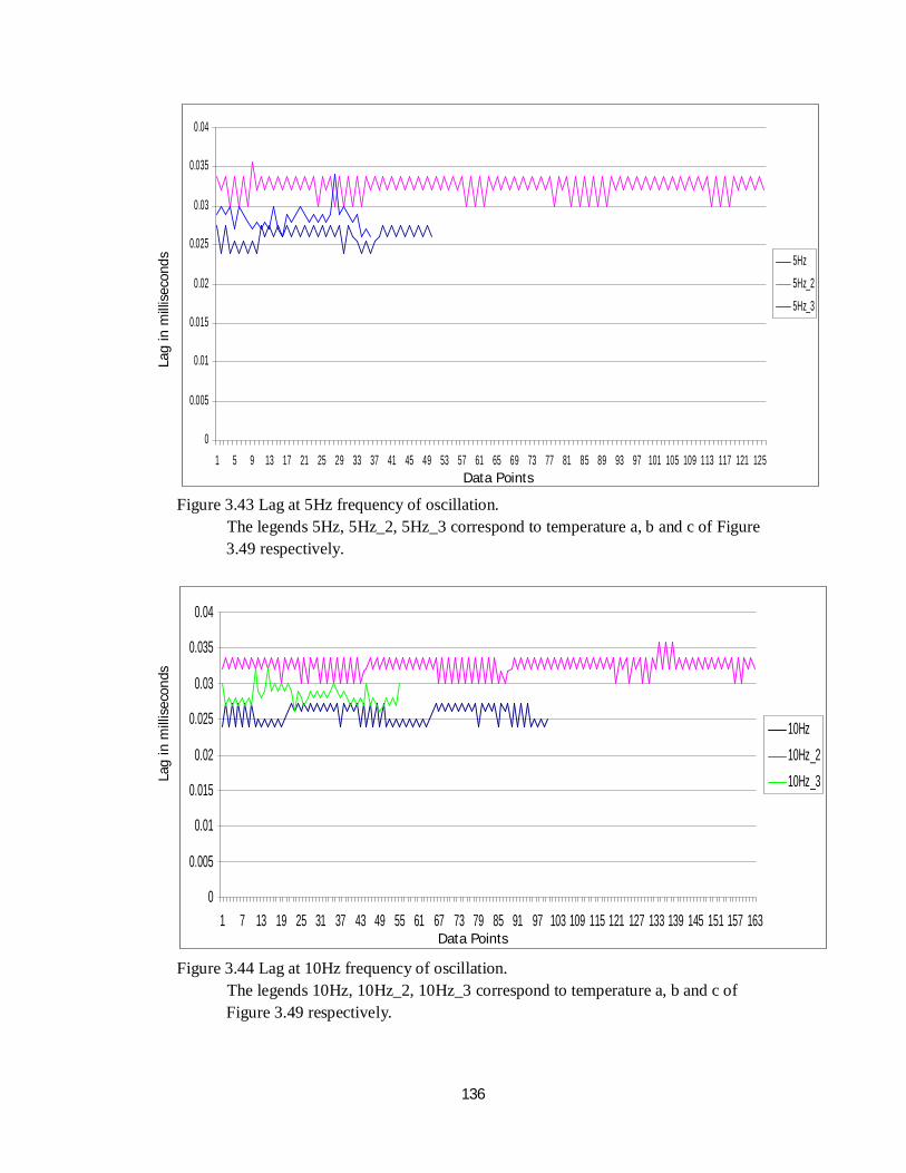
136





0

0.005

0.01

0.015

0.02

0.025

0.03

0.035

0.04

1 5 9 13 17 21 25 29 33 37 41 45 49 53 57 61 65 69 73 77 81 85 89 93 97 101 105 109 113 117 121 125

5Hz

5Hz_2

5Hz_3

0

0.005

0.01

0.015

0.02

0.025

0.03

0.035

0.04

1 7 13 19 25 31 37 43 49 55 61 67 73 79 85 91 97 103 109 115 121 127 133 139 145 151 157 163

10Hz10Hz_210Hz_3

Lag

in m

illis

econ

ds

Lag

in m

illis

econ

ds

Data Points

Data Points

137


The legends 15Hz, 15Hz_2, 15Hz_3 correspond to temperature a, b and c of Figure 3. 49 respectively.



0

0.005

0.01

0.015

0.02

0.025

0.03

0.035

0.04

1 10 19 28 37 46 55 64 73 82 91 100 109 118 127 136 145 154 163 172 181 190 199 208 217 226 235 244

15Hz15Hz_215Hz_3

0

0.005

0.01

0.015

0.02

0.025

0.03

0.035

0.04

1 10 19 28 37 46 55 64 73 82 91 100 109 118 127 136 145 154 163 172 181 190 199 208 217 226 235 244 253 262 271 280 289 298

20Hz20Hz_220Hz_3

Lag

in m

illis

econ

ds

Lag

in m

illis

econ

ds

Data Points

Data Points

138





0

0.005

0.01

0.015

0.02

0.025

0.03

0.035

0.04

1 12 23 34 45 56 67 78 89 100 111 122 133 144 155 166 177 188 199 210 221 232 243 254 265 276 287 298 309 320 331 342 353 364

25Hz25Hz_125Hz_2

0

0.005

0.01

0.015

0.02

0.025

0.03

0.035

1 11 21 31 41 51 61 71 81 91 101 111 121 131 141 151 161 171 181 191 201 211 221 231 241 251 261 271 281 291 301 311 321

30Hz30Hz_230Hz_3

Lag

in m

illis

econ

ds

Lag

in m

illis

econ

ds

Data Points

Data Points

139

Figure 3.49 Different room temperature at which test was carried out. Maximum variation is 1.1oC.

Figure 3.50 Progressive drops in response time with increasing frequency. The legend (a,b,c) refers to the environmental temperature as shown in Figure 3.49

3.8.11 Result Of Dynamic Torque / Motor Loads For Various Mode (Frequency,

Angle Of Oscillation) Of The Peduncle

The summary of the torque the motor attached to the peduncle will encountered

33.20

33.40

33.60

33.80

34.00

34.20

34.40

34.60

34.80

35.00

35.20

0.5Hz 1Hz 5Hz 10Hz 15Hz 20Hz 25Hz 30Hz

abc

Frequency

Tem

pera

ture

in o C

Frequency

140

for different frequency ranges and various angles of oscillation is shown in Table 3.12.

The steps used in Table 3.6 and 3.7 were applied for each combination of frequencies

and angles of oscillation to arrive at the dynamic torque developed. The frequencies

indicated here were selected to tally with those used for the frequency softening effect

experimentation. The maximum torque that will be encountered within the designed

limit of 0 to 25Hz and peak displacement is 0.0592850Nm. From Futaba S3003 servo

motor datasheet, its rating is 0.29Nm, which means that it is capable of handling the

dynamic load effectively as it is greater than the largest value of 0.0592850Nm

expected.

Furthermore, Figure 3.51 which is the graphical representation of the Table 3.12,

shows that the torque requirement increases greatly with the angle of oscillation.

Table 3.12 Summary of dynamic torque (Nm) developed as a function of angle of

oscillation and its frequency (medium is water of density=990kg/m3) Angle of oscillation in degree

Freq

(Hz)

90 45 30 20 10 5

0.5 0.0000237 0.0000059 0.00000263 0.0000012 0.0000003 0.00000007

1 0.0000949 0.0000237 0.00001054 0.0000047 0.0000012 0.00000029

5 0.0023714 0.0005929 0.00026349 0.0001171 0.0000293 0.00000732

10 0.0094856 0.0023714 0.00105396 0.0004684 0.0001171 0.00002928

15 0.0213426 0.0053357 0.00237140 0.0010540 0.0002635 0.00006587

20 0.0379424 0.0094856 0.00421582 0.0018737 0.0004684 0.00011711

25 0.0592850 0.0148213 0.00658722 0.0029277 0.0007320 0.00018298

141

Figure 3.51 Torque developed at different peduncle oscillation frequency and swing angle

3.8.12 The Battery Requirement To Drive The Servo Motor

From Table 3.12, the maximum dynamic torque that will be encountered is

0.0592850Nm.

Rated speed for Futaba S3003 at 4.8v = 0.23 sec/60o = 0.72 rev/s

Hence maximum power needed from equation 3.42 = 2π * 0.72 * 0.0592850 ≈

0.27W

Hence current requirement is I > w/(4.8*0.5) = 0.27/(4.8*0.5) = 0.11A

For 3 servo motors

Current to drive them = 3 * 0.11A= 0.33A=333mA

An LiPo battery rated 900mAh will drive the three motors successfully for

900/333 h= 2.7hrs

3.8.13 Stability Response Of The Robotic Fish Control

Using MATLAB pole(sys) command, the system was found to have four poles; 0,

-2.7631, -4.0426, and -19.1943. Although three of the poles are negative real value

with 3 of them greater than -1 on the real axis of figure 3.29, it can be safely said that

the system is stable for open loop design but as confirmed by the Bode diagram, Figure

3.31, the system is unstable if used in closed loop mode, a negative gain margin is an

indication of an unstable system. From Figure 3.30 Pole-Zero Map diagram, all the

0

0.01

0.02

0.03

0.04

0.05

0.06

0.07

0.5 1 5 10 15 20 25

Torq

ue (N

m)

Frequency of oscillation (Hz)

90 deg

45 deg

30 deg

20 deg

10 deg

5 deg

142

poles lies on zero imaginary axis meaning a non oscillatory system. From figure 3.29

the system maximum gain is -20dB, see appendix G.

3.8.14 Sensitivity Of The Robotic Fish Control

On the system sensitivity, it can be seen from Figure 3.33 that the system swim speed

response to impulsive input is rather slow, it takes about 2.17 seconds to settle after an

impulsive perturbation. It means that the system is very sensitive to perturbation

(Ashish, 2002). From the Nyquist diagram of Figure 3.32, which is for the robot

controller without hydrodynamic drag, the stability is within a very narrow range, its

characteristic equation roots are -19.1943, -4.0426 and -2.7631 and are all far from the

frequency (jω) plot as indicated in the Nyquist diagram.

143

CHAPTER FOUR

CONSTRUCTION PROCESSES AND PERFORMANCE EVALUATION OF THE FISH ROBOT

4.1 CONSTRUCTION SEQUENCE

The construction and assembly of this robot was done on two fronts; the hardware

and the firmware. The hardware is all about the tangible components including the

artificial hydrostatic joints while the firmware is all about the software that controls the

joints so that biomimicry can be achieved.

4.2 CONSTRUCTION PROCESS OF THE HARDWARE

The following steps were taken in translating the biological model (394.01mm

long mackerel) into a 1:1 scale robotic model of figure 4.1:

Table 4.1 Step by step construction process of the hardware

Component Material Construction process Equipment used

Haul 6.35mm (1/4inch) Plywood

The haul is made from plywood rings constructed

according to drawing no 4. These rings (figure

4.1) were cut using a jig saw. The rings were then

glued according to their positions as indicated in

the drawing no 2 using epoxy glue to form the

haul (figure 4.2). However, the ring at position 10

was not used as its position was replaced by the

micro switch of figure 4.3.

Jig saw,

Epoxy glue

144


Bump switch

1. Micro switch

2. Wires 3. Vero

board

The bump switch is a micro switch and is made as

an integral part of the haul as shown in figure 4.3.

The two switches are first soldered on a circuit

board and then glued to the 3mm deep recess on

the haul using epoxy glue.

Soldering iron Epoxy glue

Ultrasonic sensor assembly

Parallax Ping))) pair

The cone of the hauls (after ring no 10) holds the

ultrasonic sensors – figure 4.4. The receiver was

glued to the ring no 1 (see drawing no 2) with

epoxy glue and the transmitter was glued to the

base of the cone as shown in figure 4.4.

Soldering Iron Epoxy glue

Water proofing of the haul

Plywood Haul

The haul was water proofed in stages.

1 . First, the outside of the hau l was given a foundat ion coat of TOP BOND® wood glue (figure 4.5).

2 . Then a coat of wood glue soaked fine sawdust was applied (~3mm thick) – figu re 4.6. The aim is to produce a smooth outer coat.

3. The haul was then oven dried for 5 min at

100watt using Samsung microwave oven - figure 4.7 to prevent soaking of the haul.

4. The haul was left in open air to allow it to

dry slowly for 1 year (August 2010 to August 2011) – to allow stability and strength.

5. A blue silicone layer was added to the

external to make it impermeable to water. At this stage, the bump switch was already in place. Figure 4.8.

6. The inside was coated with cyanoacrylate

glue (super glue) to make the inside of the haul water proof.

Wood glue (TOP BOND)

Fine saw dust (sieve size = Mesh 10 = 2.0mm maximum particle size)

Microwave oven

Blue silicone

Cyanoacrylate glue (super glue)

145


The tail support structure

3.175 mm (1/8inch) Ply wood

The tail support structure is made from plywood

slabs constructed according to drawing nos 6 to

11. These slabs (figure 4.9) were cut using jig saw.

Jig saw

The tail rubber joints

Rubber

strips from

Kings tire

rubber

The tail rubber joints were made from Kings tire

rubber tube (size=165/175-13) (figure 4.10). The

dimensions were taken from drawing nos 12 to 16

to get the shapes of figure 4.11. A Tiger razor

blade and scissors were used to get the contours

from paper stencils with the drawing printed on

them

1. Tiger razor blade

2. Scissors

3. Paper (as stencil)

Quarter pulleys assembly

¾inch (19.05mm) plywood

PVC tubings

The quarter pulleys were made from ¾inch

(19.05mm) plywood using drawing nos 17 to 21

dimensions. The cuttings were made with a power

jig saw (Bosh PST 54E), fine grained sand paper

was used for polishing it. A 2.5mm round file was

used for creating the slots to hold the 2.5mm

unplasticized PVC tubings – figure 4.12. The

tubes were held in place with epoxy glue.

1. Power jig saw (Bosh PST 54E)

2. Fine grained sand paper

3. 2.5mm round file

4. Epoxy glue

The cable and flexible plastic support

Nylon 1010,

Unplasticised Polyvinly chloride (PVC) tubes

The nylon cables were threaded through the PVC

tubings using thin nichrome wires. Each cable

length was made much longer than the length of

the tail assembly (198.41mm from drawing no 1).

Nichrome

wire for

threading

purposes

146


The tail fin ¾inch (19.05mm) plywood

The fin structure is made from plywood slabs

constructed according to drawing no 5. Its contour

was traced out on the 1/8 inch (3.175mm) thick

plywood board - figure 4.13.

Jig saw

The tail – wooden and foams half rings

6.35mm (1/4inch) plywood Collapsed polyurethane foam

The tail rings and foam (figure 4.14) are to give

the tail the streamline contour while still allowing

flexibility. The dimensions were taken from

drawing no 22. The wooden part was cut using a

jig saw while the foam was cut using a hot

nichrome wire cutter. A paper stencil with the

shape printed out was used for the tracing. The

rings were then cut into half.

1. Jig saw

2. Hot Nichrome wire cutter

3. Paper

stencil

The head board

6.35mm (1/4inch) plywood

The oval head board is made from plywood slabs

constructed according to drawing no 23. This head

board (figure 4.15) was an off cut from the last

ring used for the haul- this will ensure a perfect fit.

The pass thru holes were created with nails and

expanded with a round file all in accordance to

drawing no 23.

Jig saw

3mm

diameter

nails

2.5mm file

The servomotor – water proofing process

Futaba 3003 Remote Control Servomotor

The servomotors were opened up (figure 4.16A)

and the electronic components covered with blue

gasket silicone (figure 4.16–D,E) . The rotor shaft

was covered with vaseline (figure 4.16–B, F). The

Philip screw driver Blue gasket silicone Vaseline Light

147


gear area was filled with light mineral oil (sewing

machine oil) (figure 4.16 -C). The casing joints

were then sealed with cyanoacrylte glue after

closing it back.

mineral oil Cyanoacrylte glue

The battery – waterproofing and assembly of the Lithium ion-Polymer battery

Lithium-Polymer battery

The four onboard Lithium ion-Polymer batteries

were water proofed by covering them with epoxy

glue as shown in figure 4.17. The wires were also

coated with cyanoacrylate glue to cover any crack

or bruise in them.

They were then glued to the side of the

servomotors (2 on each side) as shown in figure

4.18 and 4.19. The 4 batteries were then wired in

parallel to give 4.3v 4x900mAh capacity.

1. Epoxy

glue

2. Cyanoacrylate glue

Assembly of tail components

1. Plywood fin

2. Plywood support structure

3. Rubber strips

4. quarter

pulley (with the PVC cable support

1. The tail was assembled first by arranging

the wood support (see table 4.5) in their

correct order.

2. The rubber strips (see table 4.6) were then

placed in between the wood support.

3. These were then glued using epoxy glue

and allowed to set. The spacing between

the plywood supports is 5mm.

Epoxy glue

148


5. head board

6. half rings

(plywoods)

7. Futaba

3003 servomotors

4. Next, the quarter pulley (with the PVC

cable support already attached – table 4.7)

were placed on the wooden support

according to the drawing no 3

5. The head board drawing no 23 (item 18 on

drawing no 3) was then glued to item no 5

on drawing no 3 – the last wooden support

of the tail using epoxy glue

6. The cables were then run through the pass

thru holes in the head board – to be

connected to the servomotor horns.

7. The half rings were then glued as shown in

figure 4.20 to give the tail its streamline

shape. The foam (not shown) come in

between the wooden ones according to

drawing 22.

8. The Futaba 3003 servomotors were then

attached to the head board serially (figure

4.21) and the cables connected to their

horns. The servomotors are glued to each

other before gluing them to the head board.

The serial arrangement is to help with

weight distribution

149


9. Figure 4.22 shows the final assembly of

the tail.

Water

proofing

the tail

structure

The

assembled

tail

All the wooden parts used for the tail were water

proofed by applying a coat of cyanoacrylate glue

to them with care not to allow it to touch the

rubber joint, the nylon cables and the PVC tubing

parts. This hardens within 1 to 3 minutes

depending on the quantity applied. The treatment

was done in a well ventilated environment.

Cyanoacryl

ate glue

The tail outer skin

The

assembled

tail

The outer skin was made from blue coloured pvc

sheet. This sheet was cut with tailor scissors and

glued with epoxy over the tail rings to cover the

gaps – they had no specific dimensions (length or

breadth).

Epoxy glue

Tailor

scissors

The electronic and controller components

1. PIC18F4520 microcontroller

2. Diodes

(1N400)

3. Resistors (1kΩ, 10kΩ, 100 kΩ), 5W 10% tolerance

Drawing no 24 shows the complete schematic of

the electronic devices used for the robotic fish.

The final assembly was soldered on two Vero

boards – figure 4.23. One Vero board carries the

input diode conditioner while the other carries the

microcontroller, resistors, capacitors and the

debugger connectors. The third board is a 4

1. 3W soldering iron

2. Soldering tin

3. Candle-vaseline wax (50:50 ratio)

4. Latex rubber

150


4. 10μF electrolytic capacitor

5. Remote control receiver

6. Vero board

7. 6 pins programmer debugger connectors

channels remote control receiver.

The components were then waterproofed by

covering them in candle-vaseline wax (50:50

ratio) to allow easy removal if need be. Also each

board was wrapped in latex rubber and the mouth

sealed with epoxy glue and cyanocrylate glue. The

outer layer was finally coated with silicone to

make it scratch and puncture resistant – figure

4.24. The wire junctions were also coated with

epoxy glue and cynoacrylate glue to prevent

shorting. The waterproofed electronic and

controller were placed below the haul as shown in

figure 4.25

5. Epoxy

glue

6. Cyanocrylate glue

7. Blue gasket silicone

Figure 4.1 The assembled fish robot

Haul Nose cone Tail

Ultrasonic transmitter and receiver

151

Figure 4.2 The rings (A) for building the robot haul which are then glued together to form the front part of the robot fish (B).

A

B

152

Figure 4.3 Assembling the bump detector on the haul

Figure 4.4 The cone holds the ultrasonic sensors – the receiver is at the tip and the

transmitter is at the top.

Ultrasonic sensors

153

Figure 4.5 The haul with foundation coating of TOP BOND® wood glue

Figure 4.6 The haul with wood glue soaked fine sawdust ~3mm

154

Figure 4.7 Microwave oven being used for preliminary drying at 5 min at 100watt. This will quickly eliminate the water in the applied mixture.

Figure 4.8 The bump switch was waterproofed with the haul using silicone rubber.

The bump switch coated with silicone

155

Figure 4.9 The slabs used for building the robot tail support structures according to

drawing nos 6 to 11. The labels tallies with the drawing numbers and are in pairs

Figure 4.10 Kings tire rubber tube used (size=165/175-13)

Figure 4.11 The rubber is cut according to the dimensions taken from drawing nos 12

to 16. The first 2 stripes from the tail fin (left on this picture are 20mm wide and the remaining ones are 25mm wide).

11

10

11

10

9

8

6

7

8

7

9

156

Figure 4.12 The quarter pulleys and unplasticized PVC tubings glued in place

Figure 4.13 The fin, made from plywood board.

PVC tubings Wooden support Rubber Joint

Quarter pulleys

157

Figure 4.14 The rings – half ring pairs used for the tail contour

Figure 4.15 The head board

158

Figure 4.16 Water proofing the servomotor.

. A B Figure 4.17 The battery before (A) and after (B) it was covered with epoxy glue.

The original servomotor

159

Figure 4.18 The Li-Po battery were glued to the side of the motors, 2 per side, viewed from the side

Figure 4.19 The Li-Po battery were glued to the side of the motors, 2 per side, viewed

from above

Li-Po battery with

water proof coating Servo motor head Nylon cables

Li-Po battery with water proof coating Servo motor head Nylon cables

160

Figure 4.20 The half rings glued to the supporting board with epoxy glue

Figure 4.21 The three servomotors are connected serially and then glued to the head board

Figure 4.22 The final tail assembly

Rubber joints Wooden support

Half rings

Servo motors Head board

161

Figure 4.23 The assembled electronic and controller parts showing the remote control

receiver (A), the microcontroller board (B), the inputs diode board (C), the programmer/debugger connectors (D)

Figure 4.24 The electronic and controller after covering with silicone.

Figure 4.25 The finished electronic and controller assembly is placed externally to the haul, just at the middle of the robot

A B

C

D

162

4.3 FIRMWARE (SOFTWARE) CODE ASSEMBLY

4.3.1 Development Environment

The development environments are the utilities used in assembling the firmware used in

programming the robot microcontroller, they are;

4.3.1.1 Integrated development environment (Microchip MPLAB v8.56.00 IDE)

This is the software that manages all the source codes and other utilities.

4.3.1.2 Assembler (MPASM Assembler v5.37)

This is the software utility that parses the assembly source code and handles all

the assembly language syntax. Assembly languages are hardware and vendor

(manufacturer) specific.

4.3.1.3 Linker (MPLINK Object Linker v4.37)

This is the software utility that translate the assembly language to intermediate

language (called object code or op-code) and then (based on the instruction given)

translate it into machine language or executable program often called hex

code/file.

4.3.1.4 Library (MPLIB v4.37)

The library is a software utility that merges object codes generated by the

assembler and feeds them into the linker. This is a tool needed especially when

the program has multiple parts (multipart).

4.3.1.5 Debugger (MPLAB SIM and PICkit 2)

Debugger is the software (MPLAB SIM ) or hardware (PICkit 2) utility that is

used to locate errors in program construct or flow that often prevent the program

from executing as intended.

163

4.3.1.6 Programmer (PICkit 2)

The programmer is the software cum hardware utility that copies and burn the

hex code (executable code) generated into the targeted microcontroller. It also

configure the microcontroller functions like clock speed, watch dog timer (WDT),

power-on reset (POR), brown-out reset (BOR) etc.

The clock directs all the timing and synchronizations of signals, the watchdog

timer (WDT) gives the code developer a way to reset the device in the event of

unexpected code operation. Power-on reset (POR) is a reset that occurs at

microcontroller power on. Brown-out reset (BOR) is a circuit that forces the

microprocessor to reset if there is a short interruption of power - one that is long

enough to disrupt operation, but not long enough to force a normal power on reset.

4.3.1.7 Clock (8MIP or 32Mhz)

The Microchip microcontroller uses ¼ of its system (or input) clock. This project

uses 8MIP (million instructions per second) which is ¼ of the 32Mhz built in

clock.

4.3.1.8 Operating system (OS) - Windows 7 Home Basic, 6.1.7601.2 SP1

This is the host computer instruction language on which all the development of

the robot code was performed.

4.3.1.9 Oscilloscope (TFD Scope v2.0 http://www.adrosoft.com )

The TFD scope is a software based oscilloscope that comes with a spectrum

analyzer built in. The maximum frequency it handles is 22kHz.

4.3.1.10 Logic analyzer (MPLAB SIM Simulator Logic Analyzer)

The logic analyzer is also a software based utility that shows the status of each

input or output pin (logic levels) of the microcontroller when being debugged in

real time.

164

4.3.2 Capabilities Built Into The Robot Firmware

The following abilities were programmed into the robot microcontroller;

1. turning left/ right while swimming

2. sharp/ quick turn

3. increase/decrease oscillation amplitude,

4. increase/decrease speed,

5. detect obstacle and avoid it by intelligently choosing which direction to go,

6. locate a simulated object – a sonar source

7. permit human override as long as the override is valid.

Appendix D contains the complete listing of the firmware pseudo code.

4.3.3 Description Of The Robot Firmware

The flowcharts (figures 4.26 to 4.32) describe the internal workings/logic of the

firmware used within the microcontroller (PIC18F4520) used for the robotic fish.

4.3.3.1 The firmware generalize flowchart

Figure 4.26 is the generalized flowchart of the firmware. It is sectioned into three

– (1) bump sensor based obstacle detection, (2) ultrasonic based obstacle detection and

(3) human override controller all interacting with the turning, tail speed and tail

oscillation amplitude routines.

165

Figure 4.26 The generalized flow chart of the firmware controlling the robot.

4.3.3.2 Bump switch based obstacle detection subroutine flowchart

Figure 4.27 shows the details of the bump switch based obstacle detection and

avoidance routine. It uses the bump sensor information for its inputs. The time the two

are on are measured and compared. The one with the larger value is the one that got

switched on first and longer and therefore, the robot is stirred away from it. If the results

are equal, a random number is generated, an odd value implies stir left and even value

implies stir right.

4.3.3.3 Ultrasonic based obstacle detection subroutine flowchart

Figure 4.28 is the ultrasonic based object detection flowchart, it works similar to

the bump switch obstacle detection. It uses 40kHz ultrasonic piezo crystal transmitter

receiver pair.

Bump sensor based obstacle detection

Ultrasonic based obstacle detection

Speed control routines

Tail oscillation amplitude control routines Human override

controller

Turning routines

Swimming control using built in pattern algorithm for its control scheme

166

Figure 4.27 Bump switch based obstacle detection subroutine

Turn right

Turn left

Scan left bump sensor

Scan right

bump sensor

Obstacle detection

Next routine

Repeat scan 1 more time

Compute period bump

switches were on

Right switch is on longer

Left switch is on longer

Equal on time

Perform random value generation

Even number Odd number

debounce process

167

Figure 4.28 Ultrasonic based obstacle detection subroutine

4.3.3.4 Human override subroutine flowchart

The human override subroutine (figure 4.32) uses a 4 channels remote control that

works on bang-bang protocol, that is, the output is either ON or OFF not a proportional

output. The firmware scans the receiver 4 outputs through the microcontroller 4 input

ports in turn continuously and generates an interrupt whenever it senses an input is ON.

The input is then used to control the behavior of the robot firmware instruction

execution/branching. The following HEX code shows the port input order –PORTC,4;

PORTC,5; PORTC,6 and PORTC,7 and their state is used to set a corresponding bit in

a symbol ( a memory location) named temp_temp. Thus a maximum of 4 bits of

temp_temp can be set as 1 or 0 as shown in the following assembly code line 478-

486:

Turn right Turn left

Turn right and left randomly sonar sensor

Listen to sonar signal burst

Compute right and left sense offset

Offset is positive Offset is negative

Next routine

Signature detected

Signature not detected

168

473: ;----code list: Remote control output polling--------

474: Ext_Int_Code

475: bcf INTCON,1

476:

477: ;Capture port state

478: clrf temp_temp

479: btfss PORTC,4

480: bsf temp_temp,4

481: btfss PORTC,5


483: btfss PORTC,6


485: btfss PORTC,7


This means that from a 4 bit input, we can make a controller with 16 possible

outputs as shown in the table 4.2. The routine polls the value of temp_temp and branch

to the code that is appropriate.

Figure 4.29 Human override control subroutine

Increase oscillation amplitude

Decrease oscillation amplitude

Speed up

Interrupt service request routine

Bang-bang wireless receiver

Speed down

Turn Left

Turn Right

169

Table 4.2 The 16 possible combination a 4 bit can generate. The counting start from 0

4.3.3.5 The tail oscillation amplitude control subroutine flowchart

Figure 4.30 is the flowchart for the tail amplitude control. The amplitude is the

amount of excursion the tail will make from left to right. The bigger it is the more the

fluid in its environment is affected. The width of the pulse determines the angle to

sno Bit 1 Bit 2 Bit 3 Bit 4

0 0 0 0 0

1 0 0 0 1

2 0 0 1 0

3 0 0 1 1

4 0 1 0 0

5 0 1 0 1

6 0 1 1 0

7 0 1 1 1

8 1 0 0 0

9 1 0 0 1

10 1 0 1 0

11 1 0 1 1

12 1 1 0 0

13 1 1 0 1

14 1 1 1 0

15 1 1 1 1

170

which the motor will move to. Changing the pulse width data causes the PWM

generator for each servomotor to adjust accordingly. See section 4.3.3.7 for more

information on the PWM generator.

Figure 4.30 Tail oscillation amplitude control routine

Servomotor 1

Reduce maximum PWM signal period

Pulse Width Modulation

(PWM) generator 1

Servomotor 2


(PWM) generator 2

Servomotor 3


(PWM) generator 3

Note: the servomotors are open loop circuit device

Increase minimum PWM signal period

Increase maximum PWM signal period

Reduce minimum PWM signal period

Reduce amplitude command input

Increase amplitude command input

171

4.3.3.6 The speed of oscillation control subroutine flowchart

Figure 4.31 is the flowchart of the speed of oscillation control. The speed is

managed by changing the pulse-width-modulation (PWM) signal width and how long it

remain so before changing the value again in either direction during oscillation.

Essentially, the delay are what is adjusted. If the delay is longer, the speed is lowered

and vice versa for each servomotor. See section 4.3.3.8 for more information on the

PWM generator.

Figure 4.31 Tail oscillation speed control routine

Servomotor 3

Reduce PWM pulse delay


(PWM) generator 3

Note: the servomotors are open loop circuit device

Increase PWM pulse delay

Reduce speed command input

Increase speed command input

Servomotor 1


(PWM) generator 1

Servomotor 2


(PWM) generator 2

Delay Delay Delay

172

4.3.3.7 The turning subroutine flow chart

Figure 4.32 is the flowchart of the turning routine. The turning is done by

restraining the motion to half of the fish midline as shown in figure 4.32. The PWM

generator is commanded to keep the maximum PWM pulse width to 1.5ms if turning to

left and minimum PWM pulse width to 1.5ms if turning to right. The 1.5ms is

approximately the pulse width command for the servomotor to turn to the middle or 90o.

Figure 4.32 Turning routine

Servomotor 3

*Set maximum PWM pulse =1.5ms minimum PWM pulse = Current amplitude


(PWM) generator 3

Note: 1.5ms is the approximate PWM at which the servomotor is set to their middle line.

*Set maximum PWM pulse = Current amplitude minimum PWM pulse = 1.5ms

Turn Right while swimming

Turn Left while swimming

Servomotor 1


(PWM) generator 1

Servomotor 2


(PWM) generator 2

173

4.3.3.8 Pulse width modulator (PWM) protocol generator

For this project, the specifications for the PWM signal needed are:

1 Three concurrent (or rigidly coupled) PWM signal that is out of phase by 60o.

2 Continuously varying duty cycle

3 Different duty cycles at any point in time

4 The three PWM signal will have the same period

5 Repeated (introduced dead band)

6 Less load on the microcontroller time

The flow chart shown in figure 4.33 is used for describing the working of the

concurrent PWM protocol generator being described here. The concurrent PWM signal

generator is a modified timer based interrupt method with much contribution from

instruction time method. Timer0 interrupt (INT0) was used as the trigger. The period is

to be fixed at ≈20ms. The pulse length is a table of pre calculated values (built in

motion pattern). It could also be mathematically generated also. The processes involved

in calculating the pulse length are performed during the microcontroller idle time.

As soon as there is an interrupt, critical register are saved and the Timer0 is

prepared for the next interruption. The ports are all set high, the difference (lag)

between the start of the first and the last is calculated as follows:

174

If Port 0 start time = Tport0

Then Port X start time = Tport0 + Tport1 + Tport2 + ….+ Tport x-1

= Tport0 + (x-1)* TCY,

where TCY is the length of an instruction cycle

The PIC microcontroller used was run at 32Mhz and

therefore the TCY = (1/32Mhz)*4 = 0.000000125s or 125ns

lag for Port X = (x-1)* TCY = (x-1) * 125ns

As an example, the lag between the first port and last port of a 3 PWM concurrent

generator will be

Lag = (3-1) * 125ns = 250ns

Fortunately, this lag will be fixed as the PWM signals have the same reference, i.e. they

have the same period that is fired up by a single timer (Timer0). The period for any

channel will therefore remain constant at ≈20ms as designed. Using figure 4.34,

T1 = T2 = T3 ≈20ms.

The count down process checked and compared the RAM value of the pulse against the

current count, if greater or equal, the corresponding port is set low. The routine is exited

as soon as all the ports are set low.

175

Figure 4.33 Concurrent Pulse Width Modulator (PWM) generation routine

Prepare Timer0 interrupt INT0

Clear INT0 default state

Start Timer0

Wait routine / other process

Pulse length data 1,2,3

Load into RAM

Save critical register value

Prepare Timer0 for next interrupt

Set Port 1,2,3,…to high(Vdd)

Start a count down

Port1

Port2

Port3

Set Port 1 Low (Vss)



Port X Set Port n Low (Vss)

Counter count >= stored pulse length value




Is all port cleared?

Yes

No

Phase data 1,2,3,…

Timer0 timed out

Load new value

Don’t load new value

These RAM are updated whenever the Ports are cleared

176

A phase difference is needed for the robotic fish segment for motion to take place.

These motors can be made to rotate at different phase angle by adjusting their duty

cycles at different rate. The phase data is a table of pre calculated values (it can be

mathematically generated also). The reference to when to change the motor phases is

derived from the current state of the ports. The phase data modifies the pulse length data

by simply controlling whether to load new values or not. This automatically creates a

dead band. This dead band is used advantageously by the fact that the inertia of the

servomotor motor, shaft and gear cannot keep up with a rapidly changing PWM duty

Figure 4.34 An exaggerated illustration of lag present in the concurrent PWM generator.

PWM1

PWM2

PWM3 T3

T2 T1

177

cycle. The phase controller is therefore actually causing the PWM signal generator to

“wait” for the motor to finish up. These waiting periods are varied for different servo

motor and thus lead to phase lags or leads.

4.4 THE LABORATORY TESTS

The laboratory tests were tests performed while the robot is out of water. An

exception is the water leakage tests which require that the parts be placed inside water

while the power supply is disconnected. The following laboratory tests were conducted;

1. Test on the concurrent PWM (pulse-width-modulation) generation module

2. Test for correct angular displacement (swing) of the motors

3. Test of the sonar sensor fidelity to input signal and the peak response test.

4. Test of the bump sensor routine

5. Test of the Left/Right turning while swimming

6. Test of the Left/Right sharp turn

7. Test of the human override control

8. Test for water leakages

4.4.1 Test On The Pulse Width Modulation (PWM) Code Generation According to the remote control servomotor manufacturer (Futaba incorporation of

USA), the PWM control scheme is a pulse signal (<=5V+ peak) lasting for 1 to 2 ms

and repeated at 20ms (50Hz) interval –depicted in Figure 4.35.

178

4.4.1.1 Equipment used

1. PICkit 1 signal analysis Oscilloscope

2. An Acer Aspire 5600 computer USB 2.0 port

time-->

Figure 4.35 PWM control scheme for Futaba remote control servomotors.

4.4.1.2 Test procedure

1. The microcontroller was switched on and powered with 5v input

2. The output pin that will go to the servomotors input pins were connected to the

PICkit 1 signal analysis oscilloscope input.

3. The PICkit 1 signal analysis oscilloscope output was then connected through a

USB port of the computer used.

4. The PICkit 1 signal analysis oscilloscope was set to Continuous

5. The computer output was then capture and saved.

4.4.2 Test For The Microcontroller Concurrent Pulse Width Modulation (PWM) Code Generation

The microcontroller is to generate three PWM code at the same time. Each is to drive

the one of the three servomotors in real time. A delay will cause the servomotor to treat

20ms 1-2ms

Vol

tage

(<=5

v+)

179

it as a new command and will respond to it by turning left or right. This could lead to

jittering of the motors.


1. Logic analyzer built into the MPLAB IDE (integrated development

environment) used for the firmware development.

2. MPLab SIM simulator


1. The MPLAB IDE was switched to debug mode.

2. MPLab SIM simulator was started – which automatically starts a virtual model

of the PIC18F4520 microcontroller being programmed

3. The logic analyzer was started also

4. The software was then started

5. The logic analyzer was then used to capture the signal level on the output pins of

the virtual microcontroller.

4.4.3 Test For Establishing Correct Angular Displacement (Swing) Of The Motor

The servomotors are capable of 0 to 180o swing, these angles do not precisely

correspond to 1ms and 2ms nor 1.5ms equal 90o, a test is required to establish the center

timing signal. This test automatically leads to calibrating the servomotor.


1. A Futaba 3003 servomotor

2. An ordinary transparent plastic protractor

180

3. Three 5cm long nails to support the protractor

4. A wooden board to hold the nail, protractor and a servomotor

5. PICKit 2 debugger

6. MPLAB v8.56 simulator software stopwatch


1. The equipment was setup as shown in Figure 4.36.

2. The microcontroller was connected to the computer using PICkit 2 debugger

3. The development environment was started and switched to debug mode

4. The firmware was instructed to generate 1.5ms width pulse length which will

approximately correspond to mid value of the servomotor. MPLAB v8.56

simulator software stopwatch was used to measure the timing intervals.

5. The code for generating the center signal was adjusted until the servomotor

points to 90o approximately. The initial and final values were noted

Figure 4.36 Angular displacement measurement setup using protractor

Protractor

Servomotor

Servomotor motion direction

181

4.4.4 Test Of The Sonar Sensor

Test on the sonar sensors was performed to see if it will respond as designed and

detect objects also. Tests carried out are;

1 Maximum distance covered, that is the distance between the transmitter and the

receiver

2 Beam arc – this is the arc of coverage of the transmitted signal. See appendix E for the

sensor datasheet for more information on this.

3 Placing different obstacles between the transmitter and sensors

4 Making the objects to reflect the sent signal to the sensors


1. A dedicated 1Hz pulse rate sonar transmitter. Sonar signal is at 40kHz.

2. A matched pair of 5mm diaphragm piezo crystal transducers, one for transmitter

and the other one is the receiver.

3. Obstacles – CD plastic, plastic with oil inside, A4 paper sheet, human hand,

glass lens.

4. Ruler for distance measurement and protractor for angular displacements

5. Water tank of 60.96cm x 121.92cm x 60.96cm made up of wood filled with

water to depth of 30cm or pressure head of 2.91kPa.

Furthermore, the environmental condition (July 2011) for the open air test was

• Mean temperature (ºC) = 25.9

• Maximum temperature (ºC) = 28.2

• Minimum temperature (ºC) = 24.1

• Mean humidity (%) = 77

while environmental condition (July 2011) for test in the water (rain water) is

• Water Temperature (ºC) = 23

• Water density kg/m3 = 997

182


1. The setup of Figure 4.37 was used inside and outside the water.

2. The dedicated 1Hz pulse rate sonar transmitter is switched on

3. The receiver respond by blinking an LED at 1s interval. The LED is connected

to the receiver output of the microcontroller.

4. The arrangement of Figure 4.37 (A) was used to test for distance between the

receiver and sender. The receiver LED will stop blinking if it could no longer

detect any signal sent to it. The distance between them was measured.

5. The arrangement of Figure 4.37 (A) was also used to measure the beam arc at a very

close range of 30cm by moving the receiver about an arc in a plane perpendicular to

them. The protractor was placed underneath for measuring the angle.

6. The arrangement of Figure 4.37 (B) was used for the obstacle detection.

Obstacle were placed from the transmitter-receiver pairs at 30cm.

7. The environmental condition were also noted during the tests

Figure 4.37 The setups (A and B) used to test the ultrasonic sender and receiver fidelity.

Ultrasonic receiver

Led light blinks at 1Hz in synchronous to received signal

Objects are placed here

Led light blinks at 1Hz in synchronous to received signal

Objects are placed here at 30cm from transmitter

Ultrasonic receiver

Transmitter send signal at 40kHz with a 1s period

A

B

183

4.4.5 Test Of The Bump Sensor Routine And Performance

Two type of test were performed, the debounce test and activation load test.

A. The bump sensor (Figure 4.38) is a plain mechanical switch (a micro switch),

therefore there will be bouncing of the contact (the click noise). To the

microcontroller running at 32MHz (or 8MIP (million instructions per second)

for Microchip microcontrollers), a single click can be interpreted to mean

thousands of inputs and that will be a meaningless input to it. A way out is to

debounce it in the firmware – this is done by waiting for the switch to

stabilize before beginning to take readings.

B. The activation load test involved finding out the minimum force to actually

cause a response (or to close the switch). The lower the force is, the

likelihood of the switch closing when the robot hits an object especially at

slow speed. The micro switch requires 0.015N to depress according to the

manufacturer (www.ck-components.com).

4.4.5.1 Equipment for the switch debounce test

1. MPLAB IDE (integrated development environment)

2. PICkit 2 as debugger

3. TFD Scope 2.0 Spectrum analyzer and Oscilloscope


1. The MPLAB IDE was started and switched to debug mode

2. The PICkit 2 was connected to the microcontroller and the computer hosting

the MPLAB IDE.

3. The buttons were pressed slowly and then fast to see if the program execution

will branch appropriately.

184

4. Both were pressed at once to see if a random number will be generated as an

indication that the collision was headlong.

5. Furthermore, the micro switch frequency spectrum and time series value were

captured by the TFD scope 2.0 spectrum analyzer and oscilloscope

respectively.

Figure 4.38 The micro switch used for the bump sensor

4.4.5.3 Equipment for activation load test

1. CAMRY® Load cell with digital output

2. 1 cm3 sample of the collapsed polyurethane foam used in between the haul and

the cone.


1. The robot nose cone was depressed on one side with the load cell until a click of

the micro switch was heard. The diagram of Figure 4.39 shows a sketch of this

arrangement.

2. The load cell reading was then taken.

3. Both sides were treated 5 times to get an average reading.

4. The polyurethane foam sample was also subjected to a compressive test by

putting it on the load cell and depressing to 50% of its original height. This is a

modification to Polyurethane Foam Association standard (PFA,1994).

185

Polyurethane Foam Association uses IFD (Indentation Force Deflection) table

(see appendix F) which is defined as the amount of force, in pounds, required to

indent a fifty square inch, round indentor foot into a predefined foam specimen a

certain percentage of the specimen's total thickness. This modification allows the

resistive force to compression to be determined.

5. The compressive test was performed for each side of the 1 cm3 foam sample.

Five samples were tested.

Figure 4.39 Measuring the force required to activate the bump switch

4.4.6 Test Of The Human Override Control i.e. The Remote Control

The remote control transmitter (Figure 4.40) and receiver have 4 channels and

that means without further modification only 4 items can be controlled. It was modified

to produce 12 more channels and thus giving a total of 16 possible outcomes. 11 are

actually used in the robot, they are

1. speed oscillation up

2. speed oscillation down

3. amplitude up

4. amplitude down,

5. turn left while swimming

Support Micro switch

186

6. turn right while swimming,

7. sharp turn left

8. sharp turn right

9. pause (and straighten up),

10. switch mode – allows a button to be used for other purposes like shift key

on computer keyboard

11. start up/switch off

The transmitter (modified by adding extra buttons)

The receiver

Figure 4.40 The modified remote control transmitter and receiver


1. The remote control itself

2. MPLAB SIM simulator (within MPLAB IDE)

3. PICkit 2

Legend SU – Speed up SD – Speed down ON – Start up/Pause MD – Mode 1/ Mode 2 Switch AU – Amplitude Up AD – Amplitude Down TL – Turn left (while swimming (sharp turn left, mode 1 on – joystick only) TR – Turn right (while swimming (sharp turn right, mode 1 on – joystick only)

SU

SD

TL TR

MD

ON

AU/TL

AD/TR

187


1. The MPLAB IDE was started and the MPLAB SIM simulator was started also.

2. The PICkit 2 was connected to the microcontroller and to the computer hosting

the MPLAB IDE.

3. The MPLAB IDE debugger mode was started.

4. On the remote control, key combinations were pressed to see if the correct

routine was executed.

5. The MPLAB SIM simulator built into the development environment was used to

confirm the routine branched into.

4.4.7 Test For Motion Pattern

There are three strategies employed for controlling hyper-redundant robot joints

– the serpenoid curve, follow the leader approach and built in motion pattern. For

mobile robots, onboard power is much limited and the processing is commonly done by

microcontrollers. This implies a method that uses less power and is less mathematically

involving will be preferred automatically. Built in motion pattern is the best at handling

this limitation; pre-calculated values or lookup table are used for determining the

motion patterns. In this project, six motion patterns were built into the robot firmware;

1. Swim only mode – moving wave pattern of the tail

2. Turn left while swimming

3. Turn right while swimming

4. Sharp turn – left

5. Sharp turn – right

6. Pause (coasting)

188

The motion pattern requires studying of life fish while swimming and turning and

watching a slowed motion video of the fish. The swimming motion is a sine wave but

with the amplitude increasing toward the tail fin – Figure 4.41. Lighthill (1960)

described it as a travelling wave. The sharp turning left and right involves bending

suddenly in the direction of interest and forming a curve that increases in its radius of

curvature from the tail towards the head – much like a spring, and then uncoiling it

rapidly – Figure 4.42. Turning while swimming involve one sided swinging of the tail.

Amplitude a1 < a2 < a23

Figure 4.41 Teleost fish swimming pattern – tail amplitude increases toward the tail fin

A B Figure 4.42 Sharp turning behavior – sources (A) (Jindong and Huosheng, 2005) (B)

(Huosheng et al, 2006)

a3

a2 a1

Toward the head Toward the tail

189


1. A digital camera - Sony Cyber-shot digital camera (model DSC-S730) set to

VGA mode for video capture.


1. The test was carried out by issuing the commands (i.e. pressing the buttons on

the remote control transmitter) and documenting the responses of the robot to

each command – listed in section 4.4.7.

4.4.8 Test For Water Leakages

Since the robot is intended to work inside water, any leakage will damage the electronic

components. The wooden parts will also get soaked and the glues will part if there is

any leak.


1. A plastic bucket for water - capacity – 30cl

2. Stop watch – for timing purposes.


1. The bucket was filled with water to a depth of 30cm as shown in Figure 4.43.

Thus the pressure head is

= (ρ*a*h) = 2,913.57 Pa ≈2.91kPa

where

h=30cm =0.3m = height of water in the bucket used for the test

ρ=990kg/m3 = density of the water

a=9.81m/s2 = acceleration due to gravity

2. The parts (the tail assembly with the servomotors, the electronic and controller

pod, the battery, the sensors, the wires) were immersed inside water for

30minutes

3. A visual inspection was done on them to see if there were any leakages.

4. Furthermore, the servomotors were tested for leakages by powering them up and

applying control signals to see if they will still work.

190

Figure 4.43 The tail and servomotors are placed inside a bucket of water for test against water leakages and soaking of wood.

4.5 FIELD TESTS

The purpose of the field tests are;

1. To find out if the joint developed can work effectively with the control scheme

built into the microcontroller controlling it and

2. To also find out the performance of the fish robot inside a body of water

The field tests were done in two environments:

1. Water tank – to demonstrate turning in a tight corner (sharp turning) and test

the behaviour of the bump sensor.

2. A shallow pool - to demonstrate dynamic turning, effect of amplitude of tail

oscillation, frequency of tail oscillation, linear speed.

4.5.1 Experimental Conditions – Water Tank

This is about test carried out in the water tank.

4.5.1.1 Equipment required for the experiment in the water tank

1. The water tank is a 60.96cm x 121.92cm x 60.96cm wooden box filled with

water to a depth of 30cm or pressure head of 2.91kPa. (Figure 4.44).

191



3. Ballast material; polystyrene foam block, black tape and stones.


1. The ballast materials were attached to the robot bottom using black tape. The

foam was used to lift the head/haul as it is heavier.

2. The robot was then placed inside the tank previously filled with water to a depth

of 30cm.

3. Control signals were then applied, that is, the remote control was used to start it

up, then the robot was allowed to swim freely.

4. The video camera was used to capture all the motions for evaluation.

Figure 4.44– The robot inside the wooden water tank

This float holds the receiver antenna

192

4.5.2 Experimental Conditions – Shallow Pond

4.5.2.1 Equipment required for the experiment in the shallow pond

1. The shallow pond located at Ahmadu Bello University, Faculty of Engineering

quadrangle – with a depth range of 25cm to 50cm (equivalent pressure head of

2.4kPa – 4.9kPa). Figure 4.45 shows the static picture of the robot inside the

pond.



3. Ballast material such as polystyrene foam block, black tape and stones.


1. The ballast materials were attached to the robot bottom using black tape. The

foam was used to lift the head/haul as it is heavier.

2. The robot was then placed inside the pond at the lower side.

3. The maximum depth at which the experiment was performed was 10cm because

of visibility inside the murky water. The depth was adjusted using different

ballast weights.

4. The control signals were then applied in turn, that is, the remote control was

used to start it up, then the various instructions was made to be executed by

pressing the corresponding buttons.

5. The video camera was used to document all the experimental processes for

evaluation later on.

193

Figure 4.45 Static picture of the robotic fish swimming in the shallow pond of

Ahmadu Bello University Faculty of Engineering quadrangle pond.

Table 4.3 BILL OF QUANTITIES

s/no Material Dimension Quantity Cost (NGN)

1 Vulcanized rubber – 1.5mm

thick.

100cmX100cm 1 500.00

2 1/8 inch (3.175mm) thick

seasoned plywood.

60.96cmX60.96cm

(12” by 12”)

1 750.00

3 ¾ (19.05mm) inch plywood. 15.24cmX30.48cm

(6” by 12”)

1 750.00

30cm

194

4 ABRO® steel reinforced 4

minutes setting Epoxy glue –

Araldite.

-

5 1000.00

5 Nylon 1010 cables – 0.5mm

diameter.

1m 1 50.00

6 2.5mm diameter unplasticized

PVC tubing.

1m 1 200.00

7 Remote Control Servomotors

(Futaba 3003 and Futaba

148).

- 3 10500.00

8 Microcontroller –

PIC18F4520

- 1 600.00

9 Latex Rubber – from

Population Services

International (PSI)

- 2 40.00

10 Silicone rubber - 2 400.00

11 Micro switches. - 2 100.00

12 Parallax Ping))) - 1 5000.00

13 Collapsed polyurethane foam 15.24cmX30.48cm (6” by 12”)

1 100.00

14 Cyanoacrylate glue (super - 20 1000.00

195

glue)

15 Resistor 1kΩ - 15 75.00

16 Resistor 100kΩ - 12 60.00

Resistor 100kΩ - 1 5.00

17 Diode 1N400 - 9 45.00

18 PCB Board 5cm X 10cm 1 200.00

19 Remote control (transmitter

and receiver)

- 1 4500.00

20 Capacitor 10μF - 1 10.00

21 Candle wax - 1 20.00

22 Vaseline - 1 100.00

23 Lithium polymer battery - 4 2000.00

24 Power switch - 1 100.00

Total material cost N28,105.00

196

CHAPTER FIVE

RESULTS AND DISCUSSIONS

5.1 LABORATORY TEST RESULTS

5.1.1 Results Of Tests On The Pulse Width Modulation (PWM) Code Generation Figure 5.1 shows the oscilloscope output of the microcontroller generating the PWM

control signal at 1ms latency and 20ms period accurately.

Figure 5.1 Oscilloscope output of the microcontroller generating the PWM

5.1.2 Result Of Concurrency Pulse Width Modulation (PWM) Code Generation Figure 5.2 shows the Logic analyzer output of the microcontroller generating 3

concurrent PWM control signals for the three servomotor output pin labeled RD0, RD1

and RD2. The horizontal axis is the time scale in microseconds.

197

Figure 5.2 Logic analyzer output of the microcontroller generating 3 concurrent pulse

width modulated signal

5.1.3 Result Of The Test For Correct Angular Displacement (Swing) Of The Motor

For the Futaba 3003 servo motors used, it was found to be 1.5275ms, the time was

measured using MPLAB v8.56 simulator software stopwatch.

5.1.4 The Result Of The Test On The Sonar Sensor

5.1.4.1 The result of the test on the sonar sensor in the air

Maximum distance at which signal was sensed = ~3m

Beam arc at 3m = θ = 30cm

Table 5.1 shows the result of the object detection tests in the air for signal blocking and

signal reflection modes.

θ 3m

198

Table 5.1 Results of different objects effect on sonar signal transmitted and received in the air

Material Signal blocking Signal reflection (at 30cm)

CD plastic Blocked Perfect reflector

Plastic with sewing machine oil

Blocked Fair reflector, as the oil seems to absorb the signal

Paper sheet Blocked at about 1m (effective as distance increases)

Poor reflector – although signal is still detected

Human hand Blocked Poor reflector – although signal is still detected

Glass lens Blocked As a lens, the signal is scattered but sensed if properly aligned

5.1.4.2 The result of the test on the sonar sensor in the water

Maximum distance covered = 0m

Beam arc; no signal detected

5.1.5 Result Of The Test Of The Bump Sensor Routine And Performance

5.1.5.1 The switch debounce test result

The undebounced micro switch signal output is shown in Figure 5.3, while Figure

5.4 shows the spectrum analyzer output of the micro switch.

Figure 5.3 Oscilloscope displaying the undebounced micro switch signal output.

Signals from 0-20ms and 30-100ms are artifact due to the 50Hz power line

199

Figure 5.4 Spectrum analyzer display of the undebounced micro switch signal output

5.1.5.2 Activation load test result

The force to cause each button to be activated is shown in Table 5.2 and Figure 5.5.

Table 5.2 Activation force (in N) to cause the left and right bump switch

(micro switch) to be activated.

Time in minutes Left button (N)

Right button (N)

0 3.88 6.06

5 3.85 6.11

10 3.73 5.87

15 3.78 5.59

20 3.70 5.75

25 3.72 5.79

Mean 3.78 5.86

Standard deviation 0.07 0.18

A dorsal view is implied in identifying the left and right switch

200

Figure 5.5 A plot of force to activate the left and right bump switch

5.1.5.2 Foam compressive test result

The result of the modified IFD test (compressive tests) on five samples of the 1

cm3 collapsed polyurethane foams is shown in Table 5.3 and Figure 5.6.

Table 5.3 shows the result of the modified IFD test (compressive tests) on five

samples of the 1 cm3 collapsed polyurethane foams. Values are in Newton. Foam sample

Side Sample 1 Sample 2 Sample 3 Sample 4 Sample 5

1 0.44 0.29 0.37 0.29 0.47

2 0.48 0.24 0.35 0.31 0.31

3 0.34 0.25 0.26 0.28 0.30

4 0.36 0.48 0.28 0.29 0.26

5 0.45 0.34 0.39 0.39 0.41

6 0.39 0.33 0.36 0.39 0.35

Mean 0.41 0.32 0.34 0.33 0.35

STD 0.05 0.08 0.05 0.05 0.07

0.00

1.00

2.00

3.00

4.00

5.00

6.00

7.00

0 5 10 15 20 25

Forc

e to

act

ivat

e sw

itch

-in

N

Time in minutes

Left button

Right button

201

Figure 5.6 A plot of force to activate the left and right bump switch

5.1.6 Result Of The Test Of The Human Override Control

There were no errors or wrong response to the control signals, however the robot

responds randomly whenever the robot battery drops to 4.0v or less.

5.1.7 Test For Motion Pattern

Figure 5.7 shows the static result of the 3 patterns – straight swim, sharp turn left

and sharp turn right. The pause/coasting pattern means the robot should straighten up as

shown in Figure 5.8. In the swimming mode, the maximum tail frequency achieved was

4.3Hz in the air.

0.00

0.10

0.20

0.30

0.40

0.50

0.60

1 2 3 4 5 6

Com

pres

sive

forc

e in

N

Sides of foam

Sample 1

Sample 2

Sample 3

Sample 4

Sample 5

202

Straight swim

Turning left

Figure 5.7 Result of the motion pattern

Robotic fish tail developed showing bend pattern when executing left turn

Robotic fish tail developed showing bend pattern when executing right turn

Five sequence of still picture of the robot showing swimming mode. Frame interval is 0.5s. Maximum frequency achieved was 4.3Hz

Turning right

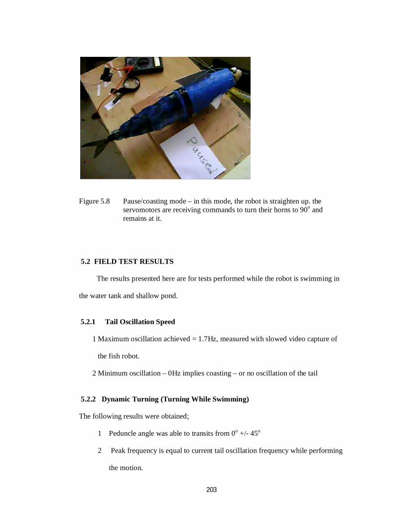
203

Figure 5.8 Pause/coasting mode – in this mode, the robot is straighten up. the servomotors are receiving commands to turn their horns to 90o and remains at it.

5.2 FIELD TEST RESULTS

The results presented here are for tests performed while the robot is swimming in

the water tank and shallow pond.

5.2.1 Tail Oscillation Speed

1 Maximum oscillation achieved = 1.7Hz, measured with slowed video capture of

the fish robot.

2 Minimum oscillation – 0Hz implies coasting – or no oscillation of the tail

5.2.2 Dynamic Turning (Turning While Swimming)

The following results were obtained;

1 Peduncle angle was able to transits from 0o +/- 45o

2 Peak frequency is equal to current tail oscillation frequency while performing

the motion.

204

3 The transition between normal swimming and dynamic turning is noticeably

smooth.

5.2.3 Amplitude Of Oscillation Of The Tail

This is the amount of excursion the tail section makes from the middle line to either

side. Table 5.4 shows the results obtained.

Table 5.4 The result of the amplitude variation of the tail sections

Segment Maximum Minimum Steps/division

1 (close to base) ~10o from center

~5

o from center

0x40/0x5 =C=d12

2 (middle) ~45o from center ~10

o from center - do -

3 (Attached to

peduncle)

~90o from center ~45

o from center - do -

5.2.4 Sharp Turning

The following results were obtained;

1 Minimum turning radius was 0.8m

2 The uncoiling delay was approximately 1second.


Figure 5.9 shows in graphical form the swimming speed with respect to different tail

(peduncle) amplitudes at frequencies of 0.5, 0.7, 0.9, 1.1, 1.3, 1.5 and at the maximum

(1.7Hz obtained inside water). Frequencies 0.7, 0.9, 1.1, 1.3, 1.5 were estimated by

interpolation from the slowed video of the swimming robot.

205

Figure 5.9 Speed of robot against peduncle (last segment) oscillation at different peduncle amplitude

5.2.6 Maximum Linear Speed

From Figure 5.9, the average maximum linear speed achieved was 0.985 m/s at

maximum tail beat frequency of 1.7Hz inside water.

5.2.7 Other Field Test Results

The sealing worked perfectly as water would have destroyed the electronics if there

is any leakage. In one of the test, a little leakage damaged the wireless receiver

transistors and the whole receiver (transmitter and receiver pair had to be changed)

5.3 DISCUSSION OF THE LABORATORY TESTS RESULTS

5.3.1 Pulse Width Modulation (PWM) Code Generation

From Figure 5.1, the microcontroller output is reliably accurate or rather the

code for the PWM scheme generation is working fine. If the code is faulty, there will be

jittering of the motor and the output will not also be as desired.

0

0.2

0.4

0.6

0.8

1

1.2

0.5 0.7 0.9 1.1 1.3 1.5 1.7

Spee

d (m

/s)

Peduncle oscillation frequency (Hz)

15 deg

30 deg

45 deg

60 deg

90 deg

206

5.3.2 Concurrent Pulse Width Modulation (PWM) Code Generation Since the three concurrent PWM control signals have different latency and starting up

simultaneously, it means the servomotors are at different angles; or precisely 60o out of

phase to each other as designed (Figure 5.2). If servomotor connected to RD0 is at 120o,

then that connected to RD1 will be at 60o and RD2 will be at 180o.

5.3.3 Angular Displacement (Swing) Of The Motor

The servomotors swing from 0o to 180o with 1ms PWM input corresponding to 0o

and 2ms corresponding to 180o. Naturally, 1.5ms PWM input to the motor is supposed

to give 90o. For the servomotors used it was found to be 1.5275ms. This value was

updated in the firmware after the test so as to correct this error.

5.3.4 The Sonar Sensor

5.3.4.1 The test of the sonar sensor in the air

The value are consistent with the manufacturer data as shown in Appendix E.

5.3.4.2 The test of the sonar sensor in the water

The reason for the zero signal detection is attributed to diaphragm overloading

as explained in appendix E.

5.3.5 The Bump Sensor Routine And Performance

5.3.5.1 The switch debounce test

This test aim at removing false signal input to the microcontroller due to switch

contact bounce. From the spectrum analyzer display, the switch bounce frequency is at

8.5khz approximately. From this information we can deduce;

The number of inputs to the microcontroller as

207

=Microcontroller MIP / Switch bounce frequency

where

Microcontroller MIP = microcontroller clock/4 (for microchip microcontrollers)

= 32Mhz/4 = 8Mhz = 8,000,000Hz

Therefore, the number of inputs to the microcontroller is;

= 8,000,000/85000

=941.18 inputs per second (that is one click of the switch will generate

> 941 inputs)

In periodic notation, this is equal to

T = 1/941.18

= 0.0010625 seconds

= 1,062.5 μs

The microcontroller execute one instruction in 0.125μs, it implies that it will

always have to wait or idle for T / 0.125 instructions before deciding whether

the switch contact was closed or opened and is given as;

= 1,0625.5μs /0.125μs

= 8,500 instructions Or (0x100)*(0x21) in hexadecimal notations

5.3.5.2 Activation load test

From Table 5.2 and Figure 5.5, the right button is stiffer, requiring 5.86N on

average to activate it. This value is about 35% higher than the left button average

activation force.

From Table 5.3 and Figure 5.6 it can be seen that the force ranges between 0.24N

to 0.48N with the mean varying between 0.32 to 0.41. The standard deviation for three

samples is 0.5 meaning the other two are skewed perhaps due to measurement errors.

208

According to the manufacturer datasheet, 0.015N is required to activate the micro

switches. The 0.24N to 0.48N require for the foam is 16 to 32 times additional load

required to depress the micro switch. Therefore, the actual force required to activate the

switch is

(3.78-0.24) to (3.78-0.48) For left bump switch

= 3.54N to 3.30N

Or averagely 3.42N

(5.86-0.24) or (5.86-0.48) For right bump switch

= 5.62 to 5.38

Or averagely 5.50N

These high values (compared to 0.015N by the manufacturer of the micro

switches) are due to the water proof coating using silicone.

The question that arise is that, at what minimum speed should the robot be

moving so as to activate the bump switches.

If we work by the right bump switch that requires maximum force to depress it i.e.

5.50N and drag forces are ignored, then from Newton’s second law of motion, impulse

is defined as

F.t = mv1-mv2

F= force acting

t=period of action

m=mass of the body

v1=final velocity after impact

v0=initial velocity before impact

209

The minimum speed will be just enough to bring the robot to stand still, i.e.

v1 = 0

m = 592g = mass of the robot

F = 5.86N the total force required to depress the switch

therefore

F*t = mv1-mv2 = 5.86 * t = 0.592*0 - 0.592*v2

Or 5.86 = - 0.592*v2/t implying a deceleration

v2/t = 0.592/5.86 = 0.096m/s2

and hence

v2 = 0.096 m/s over a period of 1s

5.3.6 The Human Override Control i.e. The Remote Control

The random behavior of the robot whenever its battery drops to 4.0V and less is

expected as the documentation for the PIC18F4520 used for the microcontroller

specifies that the nominal voltage should be 4.5V to 5V.

Furthermore, the robot was made to “swim” for over 10minute before the

anomaly started showing up against the calculated 2.7 hours. This is the result of the use

of battery in which the label and manufacturer name and logo had been compromised or

are false.

5.3.7 Discussion On The Test For Motion Pattern

The other two patterns (turn left while swimming and turn right while swimming)

are best appreciated when viewed as video. The pause/coasting pattern means the robot

should straighten up as shown in Figure 5.8. In the swimming mode, the maximum tail

frequency achieved was 4.3Hz – (in the air).

210

5.4 DISCUSSION OF THE FIELD TESTS RESULTS 5.4.1 Tail Oscillation Speed

This is the frequency at which the tail section moves from left to right and back

again, the;

1 Maximum oscillation achieved = 1.7Hz, measure with slowed video capture of

the fish robot.

2 Minimum oscillation – 0Hz which implies coasting – or no oscillation of the tail

5.4.2 Dynamic Turning (Turning While Swimming)

This is the turning performed while cruising and involve the tail oscillation

being restricted to one axis. The transition between normal swimming and dynamic

turning is noticeably smooth, this is essential for successful swimming. If transition is

not smooth, a jerky or wobbling motion may result.

5.4.3 Amplitude Of Oscillation Of The Tail

This is the amount of excursion the tail section makes from the middle line to

either side. For the values shown in Table 5.4,

1 the segments referred to are the positions the cables from the motors are

attached to, also

2 the measurements are in degree from center line, and

3 the values were taken with respect to the peduncle as it has the largest

excursion.

The ~90o maximum for the peduncle is an out of bound data resulting from the

water pressure on it, that is the peduncle was forced to bend that far while pushing the

water away.

211

5.4.4 Sharp Turning

Sharp turning routine is only activated by the bump switch. The turn involves

bending like a coil or letter C and then uncoiling rapidly (limited by the current tail

oscillation frequency that is, fast oscillation, fast coiling or uncoiling). The turning

radius is always the minimum as maximum turning radius implies straight line motion.

On the uncoiling delay which is approximately 1second, the built in delay was

set to 0x1E which by the program structure, it will yield 600ms, the extra 400ms lag (1s

minus 600ms) is due to the motor inertia and the water environment.


Figure 5.9 shows in graphical form the swimming speed with respect to different

tail (peduncle) amplitudes at frequencies of 0.5, 0.7, 0.9, 1.1, 1.3, 1.5 and at the

maximum (1.7Hz obtained inside water). The result is comparable to that obtained by

Jindong and Huosheng (2007) reproduced here in Figure 5.10 for comparison. For this

work and theirs, the speed of the fish robots increases with tail frequency. Also the

increase amplitude leads to a relative increment in speed for each tail oscillation

frequency. The relationship between tail frequency and speed is not linear.

5.4.6 Maximum Linear Speed

From Figure 5.9, the average maximum linear speed achieved was 0.985 m/s at

maximum tail beat frequency of 1.7Hz inside water. This is approximately 1/3 of that of

live mackerel which is 3.06m/s (http://www.nmri.go.jp/eng/khirata/fish

/general/speed/speede.htm).

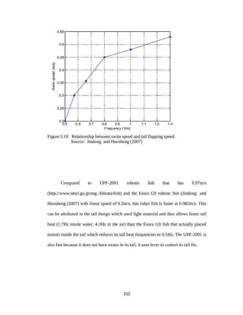
212

Figure 5.10 Relationship between swim speed and tail flapping speed.

Source: Jindong and Huosheng (2007)

Compared to UPF-2001 robotic fish that has 0.97m/s

(http://www.nmri.go.jp/eng /khirata/fish) and the Essex G9 robotic fish (Jindong and

Huosheng (2007) with linear speed of 0.2m/s, this robot fish is faster at 0.985m/s. This

can be attributed to the tail design which used light material and thus allows faster tail

beat (1.7Hz inside water, 4.3Hz in the air) than the Essex G9 fish that actually placed

motors inside the tail which reduces its tail beat frequencies to 0.5Hz. The UPF-2001 is

also fast because it does not have motor in its tail, it uses lever to control its tail fin.

213

CHAPTER SIX

CONCLUSIONS AND RECOMMENDATIONS

6.1 CONCLUSIONS

The following conclusions are hereby drawn from this research work;

1. A biomorphic hyper-redundant joint mechanism for robotic applications has been

successfully designed and developed,

2. Carbon filled natural rubber was found to be a suitable biomimetic material and

was used successfully for building the robot joints. Other researchers have shown it

to have qualitatively similar mechanical properties to living tissues.

3. Muscular hydrostatic skeleton was successfully imitated in achieving the goal of

using hydrostatic skeleton as the structural design basis.

4. The goal of constructing and testing a simple robot based on the joint developed and

designed was achieved by applying the designed joint to a fish robot tail –

specifically a teleost specie of fish, mackerel.

5. The robot fish developed was successfully tested inside stationary body of water

and had a linear speed that is one third (1/3) of a live mackerel fish, and a maximum

tail beat frequency of 1.7Hz inside water and 4.3Hz outside water.

6. The control scheme is simple as three (3) servo motors were used for actuation and

one microcontroller for their control compared to an earlier version of Essex G9

robotic fish which uses up to 5 motors.

7. The computer simulations that predicted the maximum stress (4.64kN/m2 for

rubber, and 9.24 kN/m2 for plywood material) that the peduncle will experience

were also accurate as peduncle did not fail in any of the tests (laboratory and field)

carried out on the robot. Also, the design did not warp as predicted especially as the

oscillation did not reach the critical speed of 25Hz where Payne effect will occur

214

and cause frequency induced softening. The servo motors rating (0.29Nm) is

adequate enough to handle the torque of 0.0000237Nm (at 0.5Hz) to

0.00088804Nm (at 1.7Hz) and peduncle displacement of 90o actually experienced

by the robot while being tested.

8. Furthermore, stability analysis indicates that the controller design is unstable when

hydro dynamic drag is considered and marginally stable without it. The controller is

also very sensitive to perturbation as implemented.

6.2 RECOMMENDATIONS

The followings are therefore recommended in a future work on this same project or any

similar one to it;

1. There is still much work to be done especially on the sonar navigation system. In

the course of this research exhaustive literature search for documents or

publications on sonar navigation underwater at a small scale (less 0.5m) was not

found. There is need to solve this problem as the object detection using visible light

or infrared light or even ultraviolet rays may likely not be effective inside mucky

water.

2. Furthermore, a bigger model will allow much onboard power, more

instrumentations and capabilities to be built in. For example, the model developed

could have demonstrated 3D motion also, but there was no place to put buoyancy

devices inside it.

3. Rubber is a nonlinear material and simulating its behavior is a non trivial issue. It is

recommended that further work be done on simulating the complete fish model

with a cluster computing system or super computer. The design is very promising

as the robot was able to swim at about 1/3 that of a live fish, it is good to perform a

complete simulation to find out how to improve on this speed even more.

215

REFERENCES

Afolayan, M.O. (2010). Potential of Watch Buzzer as Underwater Navigation Device in

Shallow Water Streams. Research Journal of Applied Sciences, Engineering and

Technology 2(5): 436-446.

Afolayan, M.O. and Madakson, P.B. (2009). A design description of mobile robotic

endoscope. Proceedings of the 28th Committee of directors of health services in

Nigerian universities & 13th National Association of Doctors in University health

Services, held at Institute for Development Research (I.D.R.), Ahmadu Bello

University, Zaria. pp 100-108.

Ahmadi, H. and Muhr, A. (2002). Design of elastomeric engineering components using

FEA: current practice and future trends. FENet Thematic Network Competitive

and Sustainable growth programme. Available online at: http://www.fe-

net.org/downloads/FENet_Meetings/Wiesbaden_Germany_Nov_2001/FENET_Wi

esbaden_Nov2001_Tech_Issues_DLE_Ahmadi.pdf. pp 1-10.

Alessandro, C., Auke, J. I. (2008). Salamandra robotica: a biologically inspired

amphibious robot that swims and walks. Internal Review of Biologically Inspired

Robotics Group, Ecole Polytechnique Federale De Lausanne (EPFL) Biorobotic

Laboratory internal review, Lausanne, Switzerland. pp 1-20.

Alscher, C. (1990). Numerical Simulation of impact and Lift-off events in the

Hydrostatic Skeleton of the Leech. Department of Mathematics, University of

Bielefeld, Bielefeld, Germany. pp 1-20.

Alscher, C. and Beyn, W.J. (1998). Simulating the motion of the Leech, A

biomechanical application of DAEs, Numerical Algorithms 19 (1998): 1-12.

Anani, A., Ivan, K., Evgeni, P. and Banko, H. (2004). Single-Motor Driven

Construction of Hyper-Redundant Robot. Available online at: www.oru.se/oru-

upload/institutioner/teknik/document/forskining/ASS/publication%202004

%20single-motor.pdf

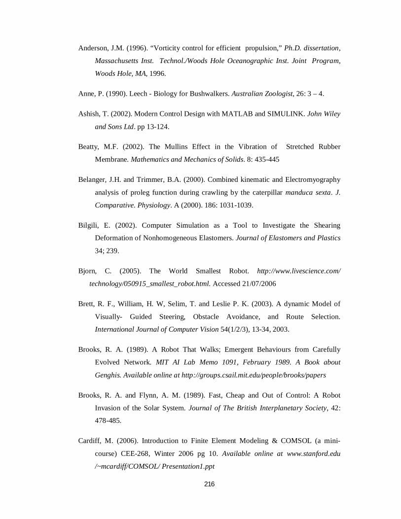
216

Anderson, J.M. (1996). “Vorticity control for efficient propulsion,” Ph.D. dissertation,

Massachusetts Inst. Technol./Woods Hole Oceanographic Inst. Joint Program,

Woods Hole, MA, 1996.

Anne, P. (1990). Leech - Biology for Bushwalkers. Australian Zoologist, 26: 3 – 4.

Ashish, T. (2002). Modern Control Design with MATLAB and SIMULINK. John Wiley

and Sons Ltd. pp 13-124.

Beatty, M.F. (2002). The Mullins Effect in the Vibration of Stretched Rubber

Membrane. Mathematics and Mechanics of Solids. 8: 435-445

Belanger, J.H. and Trimmer, B.A. (2000). Combined kinematic and Electromyography

analysis of proleg function during crawling by the caterpillar manduca sexta. J.

Comparative. Physiology. A (2000). 186: 1031-1039.

Bilgili, E. (2002). Computer Simulation as a Tool to Investigate the Shearing

Deformation of Nonhomogeneous Elastomers. Journal of Elastomers and Plastics

34; 239.

Bjorn, C. (2005). The World Smallest Robot. http://www.livescience.com/

technology/050915_smallest_robot.html. Accessed 21/07/2006

Brett, R. F., William, H. W, Selim, T. and Leslie P. K. (2003). A dynamic Model of

Visually- Guided Steering, Obstacle Avoidance, and Route Selection.

International Journal of Computer Vision 54(1/2/3), 13-34, 2003.

Brooks, R. A. (1989). A Robot That Walks; Emergent Behaviours from Carefully

Evolved Network. MIT AI Lab Memo 1091, February 1989. A Book about

Genghis. Available online at http://groups.csail.mit.edu/people/brooks/papers

Brooks, R. A. and Flynn, A. M. (1989). Fast, Cheap and Out of Control: A Robot

Invasion of the Solar System. Journal of The British Interplanetary Society, 42:

478-485.

Cardiff, M. (2006). Introduction to Finite Element Modeling & COMSOL (a mini-

course) CEE-268, Winter 2006 pg 10. Available online at www.stanford.edu

/~mcardiff/COMSOL/ Presentation1.ppt

217

Ceska, V. (2011). Who did actually invent the word "robot" and what does it mean?

Available online at http://capek.misto.cz/english/robot.html.

Charles, W. E. and Antonio, A. A. (1998). Jormungand, an Autonomous Robotic Snake.

Machine Intelligent Laboratory, University of Florida, Department of Electrical

Engineering.

Chirikjian, G.S. and Burdick, J.W. (1990). An Obstacle Avoidance Algorithm for

Hyper-Redundant Manipulators. Proceeding of IEEE International Conference

on Robotics and Automation. pp 625-631

Chirikjian, G.S. and Burdick, J.W. (1990). Kinematics of Hyper-Redundant

Manipulators. Proceeding of ASME Mechanism Conference. pp 391-396.

Chirikjian, G.S. and Burdick, J. (1991). Kinematics of Hyper-redundant locomotion

with applications to grqasping. In Proceeding of IEEE International Conference

on Robotics and Automation, pp 720-727.

Choset, H. and Burdick, J. (1994). Sensor Based Planning and Nonsmooth Analysis.

In Proceeding of IEEE International Conference on Robotics and Automation, pp

3034-3041.

Choset, H. and Burdick, J. (1995a). Sensor Based Planning, Part I: The Generalized

Voronoi Graph. IEEE International Conference on Robotics and Automation. 2:

1649-1655.

Choset, H. and Burdick, J. (1995b). Sensor Based Planning, Part II: Incremental

Construction of the Generalized Voronoi Graph. IEEE International Conference

on Robotics and Automation. 2:1643-1648.

Choset, H. and Burdick, J. (1996). Sensor Based Planning for a Planar Rod Robot.

Proceedings of IEEE International Conference on Robotics and Automation,

Minneapolis, Minnesota – April 1996. 4: 3584 - 3591

Choset, H. and Henning, W. (1999). A Follow-The-Leader Approach to Serpentine

Robot Motion Planning. ASCE Journal of Aerospace Engineering. pp 1-25.

218

Choset, H., Konukseven, I. and Rizzi, A. (1997). Sensor Based Planning: A Control

law for Generating the Generalized Voronoi Graph. ICAR ’97, Montery, CA July

7-9, 1997. pp 435-449.

Choset, H and Lee, J. Y. (2001). Sensor-Based Construction of a Retract-Like Structure

for a Planar Rod Robot. IEEE Transactions on Robotics. pp 435- 449.

Crespi, A, Badertscher, A, Guignard, A and Ijspeert, A. J. (2005). Amphibot I: an

amphibious snake-like robot. Robots and Autonomous System, 50: 163-175.

CSN, (2011). Convergent Science Network of biomimetic and biohybrid systems.

http://csnetwork.eu/conf2012/conference. Accessed 7.35pm 24, November 2011

David, B. (1994). Robotuna. Available online at: http://web.mit.edu/towtank/www

/Tuna/tuna.html. Accessed 8.00pm 24, August 2010

Degani, A., Choset, H., Wolf, A. and Zenati, M.A. (2006). Highly articulated robotic

probe for minimally invasive surgery. ICRA 2006. Proceedings 2006 IEEE

International Conference on Robotics and Automation, 2006. 15(19) : 4167 -

4172. DOI 10.1109 / ROBOT.2006.1642343

DeGroot, J.H., van der Sluijs, I., Snelderwaard, P.C. and van Leeuwen, J.L. (2004). A

three-dimensional kinematic analysis of tongue flicking Python Molurus. Journal

of Experimenatl Biology. 207:827-839.

Demirkoparan, H. and Pence, T.J. (2007a). Swelling of an internally pressurized

nonlinearly elastic tube with fiber reinforcing. International Journal of Solids and

Structures 44 :4009-4029. (doi:10.1016/j.ijsolstr.2006.11.006).

Demirkoparan, H. and Pence, T.J. (2007b). The effect of fiber recruitment on the

swelling of a pressurized anisotropic nonlinearly elastic tube. International

Journal of Nonlinear Mechanics 42 :258-270. (doi: 10.1016/j.ijnonlinmec.

2007.01.013).

Dohi, M., Fujiura, T and Yano, A. (2002). Hexapod Walking Robot for Agricultural

Field (i) – Mechanism of leg and gait control. Automation Technology for Off-Road

219

Equipment, Proceedings of the July 26-27, 2002 Conference (Chicago, Illinois,

USA) 701P0502. PP 196-203.

Dorfmann, A., Fuller, K.N.G., Ogden, R.W. (2002). Shear, compressive and dilatational

response of rubberlike solids subject to cavitation damage. International Journal

of Solids and Structures, 39 (7):1845-1861

Dorfmann, A. and Ogden, R.W. (2003). A pseudo-elastic model for loading, partial

unloading and reloading of particle-reinforced rubber. International Journal of

Solids and Structures 40: 2699-2714.

Dorfmann, A. and Ogden, R.W. (2004). A constitutive Model for the Mullins effect

with permanent set in particle-reinforced rubber. International Journal of Solids

and Structures 41:1855-1878.

Dorfmann, A., Trimmer, B.A. and Woods, W.A. Jr. (2007). A constitutive Model for

Muscle properties in Soft-bodied Arthropod. Journal of Royal Society

International. 4: 257-269.

Dorgan, K.M., Arwade, S.R. and Jumars, P.A. (2007). Burrowing in marine muds by

crack propagation: kinematics and forces. The Journal of Experimental Biology

210: 4198-4212.

Drushel, R.F., Neustadter, D.M., Hurwitz, I., Crago, P.E. and Chiel, H.J. (1998).

Kinematic Models of the Bucca Mass Aplysia Californica. The Journal of

Experimental Biology. 1563-1583.

Dunwoody, J. (2005) Heat Conduction and Controlled Deformations in Incompressible

Isotropic Elasticity. Mathematics and Mechanics of Solids, 10 (5): 487-502.

Dunwoody, J. and Ogden, R. W. (2002). On the Thermodynamic Stability of Elastic

Heat-Conducting Solids Subject to a Deformation—Temperature Constraint.

Mathematics and Mechanics of Solids. 7: 285-306.

Elie, S., Wolf, A., Brown, H.B., Jr. and Choset, H. (2003). New Joint Design for Three-

dimensional Hyper Redundant Robots. Proceedings of the 2005 IEEE

220

International Conference on Robotics and Automation, Las Vegas, Nevada,

October 2003. pp 3594- 3599.

Farabee, M.J. (2001). Muscular and Skeletal Systems. Available online at:

www.emc.maricopa.edu/faculty/farabee/BIOBK/BioBookMUSSKEL.html

(Accessed 10/23/2008 6:29pm)

Frank, S., Ethan, G., Robert, D. W. and Jason, R. (2011). Experimental verification of

soft-robot gaits evolved by a lumped dynamic model. Robotica. 29(6):823-830.

Friedrich, M., Baltes, J., Schütz, M. and Gärtner, H. (1999). Automatic Shape

Optimisation of Elastomeric Products. Available online:

www.mscsoftware.com/support/library/conf/auto99/p02199.pdf. pp 1-10

Fumitoshi, M. (2002). A mobile robot for collecting disaster information and a snake

robot for searching. Advanced Robotics. 16(6): 517-520.

Fung, Y.C. (1980). On Pseudo-elasticity of living tissues mechanics today. Vol 5 (ed

S.N. Nasser), Pergamon Mechanics Today series,. New York NY Pergamon Press.

pp. 49-66.

Gilbert, R. J., Napadow, V. J., Gaige, T. A. and Wedeen, V. J. (2007). Anatomical

basis of lingual hydrostatic deformation. Journal of Experimental Biology, 210

(23): 4069-4082.

Grasso, F. W. (2000). Flow and Chemo~sense for Robot and Lobster Guidance in Odor

Source Tracking. Neurotechnology for Biomimetic Robots Conference May-14-

16, 2000 at Northeastern University East Point, Nahant, MA 01908. pp 1-10.

Grzegorz, G., Malik, G. H. and Johann, B. (2005). Industrial Robots. International

Journal on Industrial Robots, Special Issue on Mobile Robots, vol IR32-2, March

18th, 2005, pp. 139-148.

Guo, S., Fukuda, T., Kato, N. and Oguro, K. (1998). “Development of Underwater

Microrobot Using ICPF Actuator”. Proceedings of the 1998 IEEE International

Conference on Robotics & Automation. Pp 1829-1834.

221

Gutfreund, Y., Flash, T, Yarom, Y., Fiorito, G., Segev, I. and Hochner, B. (1996).

Organization of Octopus Arm movements: a Model System for Studying the

Control of Flexible Arms. The Journal of Neuroscience. 16(22): 7292-7307.

Haith, G.L., Thomas, H., Wright, A. (2000). A Serpentine Robot for Planetary and

Asteroid Surface Exploration. Oral Presentation at the Fourth IAA International

Conference on Low-Cost Planetary Missions, May 2-5, 2000, Laurel, MD. pp 1-10.

Hannan, M.W. and Walker, I.D. (2003). Kinematics and the implementation of an

Elephant’s Trunk manipulator and other continuum style Robots. Journal of

Robot System. 20(2):45-63.

Hanyu, S. (1988). Morphological changes in penile vessels during erection: The

mechanism of obstruction of arteries and veins at the tunica albuginea in dog

corpora cavernosa. Urology International. 43: 219–224.

Harrison, R. R. and Koch, C. (2000). A Silicon Implementation of the Fly’s Optomotor

Control System In: Letter by M.V. Srinivasan and Stephen DeWeerth. Neural

Computation, Massachusetts Institute of Technology. 12: 2291-2304

Hatze, H. (1974). "The meaning of the term biomechanics". Journal of Biomechanics.

7: 189–190.

Herrel, A., Meyers, J.J., Aerts, P. and Nishikawa, K.C. (2001). Functional implications

of Supercontracting muscles in the Chameleon tongue retractors. Journal of

Experimental Biology. 204: 3621-3627.

Hirakawa, A. R., Saraiva, A. M. and Cugnasca, C. E. (2002). Wireless Robust Robot for

Agricultural Applications. Proceedings of the World Congress of Computers in

Agriculture and Natural Resources (13-15, March 2002, Iguacu Falls, Brazil)

701P0301. pp 414-420

Hirobumi, M., Morihiro, M., Yoshihiro, M., Hiroshi, S.A., Shigeo, H., Yoji, U. (1985).

Measuring/Grinding System for Water Turbine Runner, Proceeding 2nd

International Conference on Advanced Research, pp.199-206

222

Hirose, S. and Morishima, A. (1990). "Design and Control of a Mobile Robot with an

Articulated Body", The International Journal of Robotics Research. 9(2):99-113.

Hitoshi, K., Fumihiro, K., Daisuke, M., Michihiko, K., and Norio, I. (2006). Flexible

Hermetically-Sealed Mobile Robot for Narrow Spaces Using Hydrostatic Skeleton

Driving Mechanism. Proceedings of the 2006 IEEE/RSJ International Conference

on Intelligent Robots and Systems October 9 - 15, 2006, Beijing, China. pp 4006

- 4011

Horgan, C.O., Ogden, R.W. and Saccomandi, G. (2004). A theory of stress softening of

Elastomers based on finite chain extensibility. Proceeding Royal. Society. pp

1737-1754.

Horswill, I. (1992). Characterizing adaptation by constraint. In F. J. Varela and P.

Bourgine (Eds.), Toward a practice of autonomous systems: Proceedings of the

First European Conference on Artificial Life. pp 58-64.

Igor, P. (2005). What is a robot? RoboNexus 2005 robot exhibition virtual tour

November 16, 2005. Available online at: http://www.virtuar.com/click/2005/

robonexus/index.htm Accessed on 23/03/2005

Isaac, A. (1950) I, Robot. Gnome Press, available through

http://www.asimovonline.com/oldsite/asimov_titles.html

James, I. (2005). A Brief History of Robotics. Available online at:

http://robotics.megagiant.com/history.html. Accessed on 23/03/2005

Jason, M. (2011). Fracture. Available online at http://www.sv.vt.edu/

classes/MSE2094_NoteBook/97ClassProj/num/midkiff/theory.html

Jean-Pierre, M. (2000). The Design of the MIPS Micro-Robot for Endoscopy

Applications in European Research Consortium for Information and Mathematics,

ERIC NEWS, July 2000, Number 42. Special Theme: Robotics. pp 35-36.

Jiang, X. and Ogden, R.W. (2000). Some new solutions for the axial shear of a circular

cylindrical tube of compressible elastic material. International Journal of Non-

Linear Mechanics. 35: 361-369

223

Jindong, L. and Huosheng, H. (2003). Building a Simulation Environment for

Optimising Control Parameters of an Autonomous Robotic Fish. Proceedings of

the 9th Chinese Automation & Computing Society Conference in the UK, Luton,

England, 20 September 2003. Pp 317 -322

Jindong, L. and Huosheng, H. (2004). Building a 3D Simulator for Autonomous

Navigation of Robotic Fishes. Proceedings of 2004 IEEE/RSJ International

Conference on Intelligent Robots and Systems. September 28-October 2, 2004,

Sendai, Japan. pp 613 - 618

Jindong, L. and Huosheng, H. (2007). A Methodology of Modelling Fish-like Swim

Patterns for Robotic Fish. Proceedings of the 2007 IEEE International Conference

on Mechatronics and Automation, August 5 - 8, 2007, Harbin, China pp 1316

- 1321

Joachim, H. (2003). MAKRO & MAKROplus (Multi segment autonomous sewer

robot). Available online at: wwwais.fhg.de/projects/Makro/makro.html

Joachim, H. and Frank, K. (1997). Landmark-Based Autonomous Navigation in

Sewerage Pipes. GMD– German National Research Center for Computer Science

Schloß Birlinghoven, 53754 Sankt Augustin, Germany. Pp 1-5

John, J.V. (1993). Fish Swimming. Chapman and Hall, 2-6 Boundary Row, London SE1

8HN, UK. pp 1-10.

Kalev, H.L. (2002).Cyc: An Expert Framework for Consensus Knowledge

Quantification. Available online at http://www.kalevleetaru.com/Publish

/Cyc_Consensus_Knowledge_Quantification.pdf

Kato, N. (2000). “Control performance in the horizontal plane of a fish robot with

mechanical pectoral fins”. IEEE Journal of Oceanic Engineering. pp 121-129.

Kazuyki, I., Zhixiao, Y., Kazuhiko, S., Kazuyki, H., Akio, G. and Fumitoshi, M. (2005).

A rescue system for collecting information designed for ease of use – a proposal

of a rescue systems concept. Advanced Robotics, 19(3): 249-272.

224

Katsuihiko, O. (2005). Modern Control Engineering, 4th edition. Pearson Education

Inc. (www.pearsoned.co.in). pp 69-70.

Kelly, B. (2011). Strength/Mechanics of Materials. Available online at

http://www.engineersedge.com/ strength_of_materials.htm

Kelly, D.A. (2002). The functional morphology of penile erection: tissue Designs for

increasing and maintaining stiffness. Integrated and Comparative Biology. 42:

216-221.

Kelly, D.A. (2007). Penises as Variable-Volume Hydrostatic Skeletons. Ann N.Y.

Academic. Science 1101: 453-463.

Kevin, B. (2003). How snakebots work. Available online at:

http://electronics.howstuffworks.com /snakebot.htm. Accessed 8.00pm 11, August

2007

Kevin, J. D. (1997). Limbless Locomotion: Learning to Crawl with a Snake Robot. A

PhD thesis at the Robotics Institute Carnegie Mellon University, 5000 Forbes

Avenue, Pittsburg, PA 15213.

Kier, W.M and Smith, K. K. (1985). Tongues, tentacle and trunks: the biomechanics of

movement in muscular-hydrostat. Zoological Journal of the Linnean Society. 83:

307-324.

Kirkinis, E. and Ogden, R. W. (2002). On Extension and Torsion of a Compressible

Elastic Circular Cylinder. Mathematics and Mechanics of Solids 7: 373

Koehl, M. A. R., Quillin, K. J. and Pell, C. A. (2000). Mechanical Design of Fiber-

Wound Hydraulic Skeletons: The Stiffening and Straightening of Embryonic

Notochords. America. Zoologist., 40:28–41.

Kolecki, J. C. (2002). An Introduction to Tensors for Students of Physics and

Engineering. NASA/TM—2002-211716. National Aeronautics and Space

Administration, Glenn Research Center. Available online at

http://www.sti.nasa.gov. pp 1-10.

225

Konukseven, I. and Choset, H. (1997). Mobile Robot Navigation: Implementing the

GVG in the presence of Sharp Corners. Proceedings of IROS 97. pp 1-10.

Kristan, W.B., Stent, G.S. and Ort, C.A. (1974). Neuronal control of swimming in the

medicinal leech: I. Dynamics of the swimming rhythm. Journal of Comparative

Physiology. 94: 97-119.

Kumph, J. M. (1996). RoboPike. Available online at: http://web.mit.edu/towtank/

www/Pike/pike.html. Access in December 5, 2010

Lee, J. Y. and Choset, H. (2004). Motion Planning for a Rod-shaped Robot in R3:

Connecting the Rod-HGVG using the Point-HGVG. Proceedings of the 2004

IEEE International Conference on Robotics & Automation New Orleans, LA,

April 2004. Pp 1-10

Lee, J. Y. and Choset, H. (2005a). Sensor-based Exploration for Convex Bodies: A new

Roadmap for a Convex-Shaped Robot. IEEE Transactions on Robotics. 21(2), pp

1-10.

Lee, J. Y. and Choset, H. (2005b). Sensor-Based Planning for a Rod-shaped Robot in

Three Dimensions: Piecewise Retract of R3 x S2. The International Journal of

Robotics Research. 24(5): 343-383.

Lenat, D. B. (1995), “Cyc: A Large-Scale Investment in Knowledge Infrastructure,

Communications of the ACM 38, no. 11.

Liang, J. (2002). “Researchful Development of Underwater Robofish II- Development

of a Small Experimental Robofish”. Robot. 24(3): 234-238.

Lighthill, M. J. (1960) “Note on the swimming of slender fish,” Journal of Fluid

Mechanics. 9:305–317. Abstract and introduction only.

Lighthill, M. J. (1971). Large-amplitude elongated-body motion theory. Proceeding of

Royal Society. London. 179: 125-138. Abstract and introduction only.

Lilianes, P. (2000). Robotics. ERCIM News No. 42.pdf, July 2000, pg 8-9

(www.ercim.org)

226

Ma, S., Shigeo, H. and Hiroshi, Y. (1992). CT ARM-I: Coupled Tendon-Driven

Manipulator Model I -Design and Basic Experiments. Proceeding. IEEE

International Conference on Robotics and Automation pp.2094- 2100.

Ma, S. and Mitsuru, W. (2002). Time-optimal control of kinematically redundant

manipulators with limit heat characteristics of actuators. Advanced Robotics. 16(8)

: 735-749.

Mann, K.H. (1962). Leeches (Hirudinea). Their structure, physiology, ecology and

embryology. Pergamon Press. pp 1-10

Marina, K. and Hermann, S. (2002). Visual Orientation and Motion Control of MAKRO

– Adaptation to Sewer Environment. Available online at:

www.ais.fraunhofer.de/projects/Makro/makro-engl/makro-e.html

Masayuki, A., Yoshinori, T. and Hirose, S. (2008). Development of "Souryu-VI" and

"Souryu-V:" Serially Connected Crawler Vehicles for in-Rubble Searching

Operations. Journal of Field Robotics, 25: 31–65. (DOI: 10.1002/rob.20229)

Matsuura, H., Mizutame, M., Moriyama, Y., Shimada, H., Hirose, S. and Umetani, Y.

(1985); Measuring/Grinding System for Water Turbine Runner, Proceeding 2nd

International Conference on Advanced Research. pp 199-206.

Merodio, J. and Ogden, R. W. (2003). Instabilities and loss of ellipticity in fiber-

reinforced compressible non-linearly elastic solids under plane deformation.

International Journal of Solids Structures. 40: 4707–4727. (doi:10.1016/S0020-

7683(03)00309-3)

Merodio, J. and Ogden, R. W. (2005). Mechanical response of fiber-reinforced

incompressible non-linearly elastic solids. International Journal of Nonlinear.

Mechanics. 40: 213–227. (doi:10.1016/j.ijnonlinmec.2004.05.003)

Meyer, J, and Guillot, A. (2008). Biologically Inspired Robots. Handbook of Robotics -

Springer (Malestrom), Edts Bruno Siciliano, Oussama Khatib. pp 1395-1422

227

Meyers, J.J., O’Reilly, J.C., Monroy, J.A. and Nishikawa, K.C. (2003). Mechanism of

Tongue protraction in microhylid frogs. Journal of Experimental Biology. 207:

21-31.

Mezoff, S., Papastathis, N., Takesian, A. and Trimmer, B.A. (2004). The Biomechanical

and Neural Control of Hydrostatic Limb movement in Manduca Sexta. The

Journal of Experimental Biology. 207: 3043-3053.

Miller, G. (2010). Snakerobots. http://www.snakerobots.com. Accessed 6pm,

06/06/2006.

Miller, K. and Arbor, A. (2008) Experimental Loading Conditions used to implement

Hyperelastic and Plastic Material Models. Available online at

www.axelproducts.com. Accessed 8.00am 06/06/2008.

Moreland, R.B., Traisch, A., Mcmillin, M.A. (1995). PGE1 suppresses the induction of

collagen synthesis by transforming growth factor-B1 in human corpus cavernosum

smooth muscle. Journal of Urology. 153: 826–834.

Mori, M. and Hirose, S. (2006). Locomotion of 3D Snake-Like Robots; Shifting and

Rolling Control of Active Cord Mechanism ACM-R3. Journal of Robotics and

Mechatronics. 18(5): 521-528.

Muller, K.J., Nicholls, J.G. and Stent, G.S. (1981). Neurobiology of the leech. Cold

Spring Harbor Laboratory: New York.pp 1-50

Nagatani, K., Hirayama, T., Gofuku, A. and Tanaka, Y. (2002). Motion planning for

mobile manipulator with keeping manipulability. Proceedings of the IEEE/RSJ

International Conference on Intelligent Robots and Systems. pp 1663–1668.

Nagrath, I.J. and Gopal, M. (2005). Control Systems Engineering, 4th edition. Publisher

New Age International Publishers (www.newagepublishers.com). pp 194-197.

Neustadter, D. M., Herman, R. L., Drushel, R. F., Chestek, D. W., and Chiel, H. J.

(2007). The kinematics of multifunctionality: comparisons of biting and

swallowing in Aplysia californica, Journal of Experimental Biology. 210(2): 238 -

260.

228

Nobuto, M., Makoto, J., Toyomi, M., Takamitsu, S., Takehiro, H., Yasuhidemorikawa,

T., Soji O., Masaki K. and Kazuo, N. (2003). Development of a functional model

for a master–slave combined manipulator for laparoscopic surgery. Advanced

Robotics. 17(6) : 523-539

O’Dunlaing, C. and Yap, C.K. (1985). A “Retraction” Method for Planning the Motion

of a Disc, Algorithmica. 6:104-111.

Ogden, R.W. (1997). Non-Linear Elastic Deformations. Publisher: Courier Dover pp

169-229

Ogden, R.W. (2000). Stress Softening and residual strain in the aximuthal shear of a

pseudo-elastic circular cylindrical tube. International Journal of Non- linear

mechanics. 36(3):477-487

Ogden, R.W. (2004). Mechanics of Rubberlike Solids. Xxi ICTAM, 15-21 August

2004, Warsaw, Poland. pp 1-2.

Ogden, R.W. and Roxburgh, D.G. (1999). A pseudo-elastic model for the Mullins effect

in filled rubber. Proceeding of Royal Society A. 455: 2861-2877

Ohno, H. and Hirose, S. (2000). Study on Slime Robot (Proposal of Slime Robot and

Design of Slim Slime Robot), Proceeding of IROS 00 Kagawa, pp.2218-2223.

Ohno, H. and Hirose, S. (2001). Design of Slim Slime Robot and its Gait of

Locomotion, Proceeding of IROS 01 Hawaii.pp 1-10

Osuka, K, and Kitajima, H. (2003). “Development of Mobile Inspection Robot for

Rescue Activities: MOIRA”, Proceeding. of the 2003 IEEE/RSJ Int’l Conference

on Intelligent Robots and Systems, Las Vegas, Nevada. Pp 3373-3377.

Paap, K.L., Dehlwisch, M. and Klaassen, B. (1996). “GMD-Snake: A Semi-

Autonomous Snake-like Robot,” 3rd International Symposium on Distributed

Autonomous Robot Systems (DARS 96), RIKEN, Saitama, Japan. pp 1-10

Paap, K.L., Dehlwisch, M. and Klaassen, B. (1997). “GMD-snake: A semi-autonomous

snake-like robot”. Available online at: http://set.gmd.de/rs/snake/ Accessed

August 2007.

229

Park, S.J., Goodman, M.B. and Pruitt, B.L. (2007). Analysis of nematode mechanics by

piezoresistive displacement clamp. PNAS. 104 (44):1-10

Paulina, V. and Jörg, C. (2003). WormBot – A Mobile Robotic Worm. Progress Report

January 2003. Available online at: http://www.iniunizh.ch /~conradt/projects/

WormBot/. Accessed August 2007.

Peterson, D. R. and Bronzino, J. D. (2008). Biomechanic: Priciples and Applications.

CRC Press, New York pp 1-10.

PFA, (1994). Joint Industry Foam Standards and Guidelines, SECTION 4.0. Published

by Polyurethane Foam Association: July, 1994. Available online at

http://www.pfa.org.

Quillin, K.J. (2000) Ontogenetic scaling of burrowing forces in the earthworm

lumbricus terrestris. Journal of Experimental Biology. 203: 2757-2770.

Reznik, D. and Lumelsky, V. (1992). Motion Planning with Uncertainty for Highly

Redundant Kinematic Structures I. ‘Free Snake’ Motion. IEEE/RSJ International

Conference on Intelligent Robots and Systems. pp 1-10

Richard, L. L. and Thomas, J. B. (2008). Musculoskeletal Soft Tissue Mechanics.

Biomechanics: Principles and Applications. CRC Press. Edt: Donald R.P and

Joseph D. Bronzino pp 1-13.

Robinson, G. and Davies, J.B.C. (1999) “Continuum Robots - A State of the Art,” IEEE

Conference on Robotics and Automation, pp. 2849-2854.

Robotshop Incorporation (2008). History of Robotics: Timeline. Available online at:

http://www.robotshop.com/content/PDF/timeline.pdf Accessed August 2011.

Rooney, F.J. and Carroll, M.M. ( 2007). Some exact solutions for a class of

compressible non-linearly elastic materials. International Journal of Non-Linear

Mechanics, 42 (2) : 321-329. (doi:10.1016/j.ijnonlinmec.2007.01.007)

Roy, B. (2010). The theory of adhesive bonding. Available online at

http://www.roymech.co.uk/Useful_Tables/Adhesives/Adhesive_Bond.html.

Accessed August 2011.

230

Ryder, G.H. (1990). Strength of Materials, 3rd Edition. ELBS McGraw-Hill. pp 1-129,

259-286.

Seibel, E.J., Carroll, R.E., Dominitz, J.A., Johnston, R.S., Melville, C.D., Lee, C.M.,

Seitz, S.M. and Kimmey, M.B. (2008). Tethered capsule endoscopy, a low-cost

and high-performance alternative technology for the screening of esophageal

cancer and Barrett's esophagus. IEEE Transaction on Biomedical Engineering.

55(3):1032-42.

Sfakiotakis, M. and Tsakiris, D.P. (2006). SIMUUN: A simulation environment for

undulatory locomotion. International Journal of Modelling and Simulation, Vol.

26 (2006), pp. 350-358.

Shammas, E., Wolf, A., Brown, H. B., and Choset, H. (2003). New Joint Design for

Three-dimensional Hyper Redundant Robots. Proceedings of the 2005 IEEE

International Conference on Robotics and Automation, Las Vegas, Nevada,

October 2003. pp 1-10.

Shigeo, H., Koji, I., Yoji, U. (1989). Development of Shape-Memory Alloy Actuators.

Performance Assessment and Introduction of a New Composing Approach,

Advanced Robotics. 3(1): 3-16.

Skierczynski, B.A., Wilson, R.J.A., Kristian, W.B. Jr and Skalak, R. (1996). A model of

the Hydrostatic Skeleton of the Leech. Journal of Theoretical Biology 181: 329-

342.

Sokoloff, A. J. (2004). Activity of tongue muscles during respiration: it takes a village?

Journal Applied Physiology 96:438-439. doi:10.1152/japplphysiol.01079.2003

Srinivasan, M. V. (1992). Distance Perception in Insects. Centre for Visual Sciences,

Research School of Biological Sciences, Australian National University,

Australia. Published by Cambridge University Press. pp 1-10.

Srinivasan, M.V., Zhang, S.W., Chahl, J. S., Stange, G. and Garratt, M. (2004). An

overview of insect-inspired guidance for application in ground and airborne

platforms. Proc. Instn mech Engrs Vol 218 Part G: Journal of Aerospace

Engineering, 375-388

231

Stern, T.W., Nusbaum, M.P., Perez, L.E. and Kristan, W.B. (1986). A kinematic study

of crawling behavior in the leech, Hirudo medicinalis. Journal of Comparative

Physiolology. A158: 593-603.

Stevenson, R.D. and Josephson, R.K. (1990). Effect of Operating Frequency and

Temperature on Mechanical Power Output from Moth Flight-Muscle. Journal of

Experimental Biology. 149: 61-78.

Streitlien, K., Triantafyllou, G. S., and Triantafyllou, M. S. (1996). “Efficient foil

propulsion through vortex control,” AIAA Journal. 34: 2315–2319.

Takanashi, N., Choset, H. and Burdick, J.W. (1993). Local Sensor based Planning for

Hyper-Redundant Manipulator. Proceeding of IEEE International Conference on

Intelligent Robots and Systems. July 1993. Pp 1-10

Thomas, H., John, W., Julian, V. (2005).Biologically inspired solutions to colonic

endoscope propulsion Available online at: http://biro-

net.aber.ac.uk/Symposium_2005/BIRO%20Proceedings/posters/Poster_bioloch20

05.pdf

Trimmer, B.A., Takesian, A.E., Sweet, B.M., Rogers, C.B., Hake, D.C. and Rogers,

D.J. (2006). Caterpillar Locomotion and Burrowing Robots. 7th International

Symposium on Technology and Mine Problem, Monterey, CA. pp 1-10

Wadepuhl, M. and Beyn, W.J. (1989). Computer simulation of the hydrostatic skeleton.

The physical equivalent, mathematics and application to worm like forms. Journal

of Theoretical Biology 136: 379-402.

Wadepuhl, M., Beyn, W.J. and Alscher, C. (1997). Stepwise adaptation of a computer

model to the leech Hirudo medicinalis L. II. Effects of geometry,

compartmentalization and nonlinear length tension curves. Preprint, University of

Bielefeld. Pp 1-100

Wainwright, P.C. and Bennett, A.F. (1992). The Mechanism of tongue projection in

Chameleons. Journal of Experimental Biology 168: 1-21.

232

Wilbur, C., Vorus, W., Cao, Y., and Currie, S. (2002) A Lamprey-Based Undulatory

Vehicle. Neurotechnology for Biomimetic Robots, Edts: J. Ayers, J. Davis and A.

Rudolph. MIT Press, pp 285-296.

William, C. (2006). Snake-Like Robot Can Crawl on Land or Swim. Available online at

http://www.gorobotics.net/The-News/Latest-News/Snake%11Like-Snake-Like-

Robot-Can-Crawl-on-Land-or-Swim/

Wilson, R.J.A., Skierczynski, B.A., Blackwood, S., Skalak, R. and Kristan, W.B.

(1996). Mapping motor neuron activity to overt behaviour in the leech: Passive

biomechanical properties of the body wall. Journal of Comparative Physiolology.

178:637-654.

Witbrock, M., Matuszek, C., Brusseau, A., Kahlert, R.C., Fraser, C.B., Lenat, D.B.

(2005). Knowledge Begets Knowledge: Steps towards Assisted Knowledge

Acquisition in Cyc in Papers. 2005 AAAI Spring Symposium on Knowledge

Collection from Volunteer Contributors (KCVC), Stanford, California, March

2005. pp. 99-105

Wolf, A., Brown, H.B., Casciola, R., Costa, A., Schwerin, M., Shamas, E. and Choset,

H. (2003). Proceedings of the 2003 IEEE/RSJ International Conference on

Intelligent Robots and Systems, Las Vegas, Nevada, October 2003. pp 1-10

Wolf, A., Choset, H. H., Brown, H. B., and Casciola, R. W. (2005). Design and control

of a mobile hyper-redundant urban search and rescue robot. Advanced Robotics.

19(3): 221-248.

Woods, W.A. Jr, Fusillo, S.J. and Trimmer, B.A. (2008). Dynamic properties of a

Locomotory muscle of the tobacco hornworm Manduca Sexta during strain

cycling and Simulated natural crawling. The Journal of Experimental Biology

211:873-882.

Yamada, H., Chigisaki, S., Mori, M., Takita, K., Ogami, K. and Hirose, S. (2005).

Development of Amphibious Snake-like Robot ACM-R5, ISR2005, Proceeding

ISR 2005, pp. 133,2005.

233

Yamada, H. and Hirose, S. (2006). Development of Practical 3-Dimentinal Active Cord

Mechanism ACM-R4. Journal of Robotics and Mechatronics, 18(3): 305-311.

Yekutieli, Y., Sagiv-Zohar, R., Hahner, B. and Flash, T. (2005a). Dynamic Model of

the Octopus Arm II. Control of Reaching Movements. Journal of Neurophysiology

94: 1459 -1468.

Yekutieli, Y., Sagiv-Zohar, R., Aharonov, R., Engel, Y., Hochner, B. and Flash, T.

(2005b). Dynamic Model of the Octopus Arm I. Biomechanics of the Octopus

Reaching Movement. Journal of Neurophysiology 94:1443-1458.

Yekutieli, Y., Sagiv-Zohar, R., Hahner, B. and Flash, T. (2005c). Analyzing octopus

movements using three-dimensional reconstruction. Journal of Neurophysiology

98: 1775-1790.

Yekutieli, Y., Sumbre, G., Flash, T. and Hochner, B. (2002). How to move with no rigid

skeleton? The Octopus has the answers. Biologist 49(6): 1-10

Yim, M. (1994). Locomotion with a Unit Modular Reconfigurable Robot. Department

of Mechanical Engineering . Palo Alto: Stanford University. Pp 1-20

Yu, J.Z., Chen, E.K., Wang, S. and Tan, M. (2002). “Research Evolution and Analysis

of Biomimetic Robot Fish”. Control Theory and Application. 20(4):1-10

(DOI:cnki:ISSN:1000-8152.0.2003-04-000)

Zhang, Y., Schervish, M. and Choset, H. (2002). Probabilistic Hierarchical Spatial

Model for Mine Locations and its Application in Robotic Landmine Search.

Proceedings of the 2002 IEEE/RSJ Conference on Intelligent Robots and Systems.

EPFL, Lausanne, Switzerland. October 2002. Pp 1-10

Zufferey, J. and Floreano, D. (2005). Toward 30-gram Autonomous Indoor Aircraft:

Vision-based Obstacle Avoidance and Altitude Control. Proceedings of the 2005

IEEE International Conference on Robotics & Automation Barcelona, Spain April

pp 18-22.

234

APPENDIX A

HYDROSTATIC JOINTS

A1 OTHER RUBBER BASED HYDROSTATIC JOINTS DESIGNS

The following rubber based design can be exploited also for making artificial hydrostatic

joints

(a) (b) (c) Figure A1 a) Ball-Socket-Tendon Design b) Closer View c) Another Closer view d) Cross-

section of the model

(a) (b) (c)

Figure A2 Spinal-Chord / Bead Model a) Top View b) Perspective view b) Cross-section of the model

B B

(d)

C C

235

Figure A3 Ball-Socket-Tendon Design Kinematics

The Ball-Socket-Tendon Design is even more rigid than the Diamond design. It excels it also at twisting, complexity and biomimicry. Hydrostatic bodies are known for their great flexibility and strong rigidity at load bearing.

236

Figure A4 Spinal-Chord/Bead Model Kinematics

Spinal-Chord/Bead Model has greater

flexibility and rigidity in its implementation. As

shown in the last diagram (on the right) twisting

while remaining planar is even more easier.

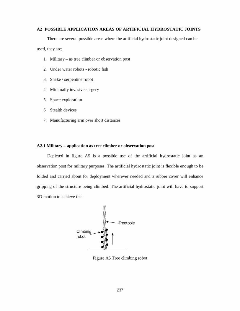
237

A2 POSSIBLE APPLICATION AREAS OF ARTIFICIAL HYDROSTATIC JOINTS

There are several possible areas where the artificial hydrostatic joint designed can be

used, they are;

1. Military – as tree climber or observation post

2. Under water robots - robotic fish

3. Snake / serpentine robot

4. Minimally invasive surgery

5. Space exploration

6. Stealth devices

7. Manufacturing arm over short distances

A2.1 Military – application as tree climber or observation post

Depicted in figure A5 is a possible use of the artificial hydrostatic joint as an

observation post for military purposes. The artificial hydrostatic joint is flexible enough to be

folded and carried about for deployment wherever needed and a rubber cover will enhance

gripping of the structure being climbed. The artificial hydrostatic joint will have to support

3D motion to achieve this.

Figure A5 Tree climbing robot

Tree/pole

Climbing robot

238

A2.2 Under water robots

Rubber does not soak water and does not react with it, it can withstand saline environments

also. Under water robots like a fish robot (figure A6) can use the artificial hydrostatic joint

for its flexible tail without the need to ever worry about maintenance. Submarine and ship

hauls are commonly coated with rubber, vehicles in salt laden environments like Lagos in

Nigeria are commonly coated with rubber spray underneath.

Figure A6 Underwater devices in form of fish

A2.3 Snake robot

The artificial hydrostatic joint can be used to build a 3D device that has a rod shape and is

programmed to behave and move as a snake or serpentine robot – figure A7. Furthermore,

covering the structure with rubber will give a firm grasp of different terrain.

Figure A7 Snake/serpentine robot can be assembled from the artificial hydrostatic joint

Rigid frontal part

Flexible tail

Rolled up Head lifting

Crawling/wriggling motion

239

A2.4 Minimally invasive surgery

Minimally invasive surgery (MIS) or band aid surgery or keyhole surgery is a modern

surgical technique in which operations especially in the abdomen are performed through

small incisions (usually 0.5-1.5cm) as compared to larger incisions needed in traditional

surgical procedures. Minimally invasive surgery depends heavily on one or more form of

endoscopy. Since its inception in design, it has gone in sophistication from rigid lens system

and later fibre optic light guide to robotic guided flexible arms, to hyper-redundant robotic

based arm currently. Precision in locating the diseased part (i.e. access port location) brings

about true minimally invasive surgery in the form of tethered capsule endoscope and wireless

capsule endoscope especially in the digestive tract- Degani et al, 2006; Seibel et al, 2008.

The fact that the artificial hydrostatic joint presented in this work can be miniaturized

means that a rod shaped, cable controlled or active on board actuator as described by

Afolayan and Madakson (2009) can make it very useful for this type of surgical operation.

Also, a medical grade rubber or silicone will have less impact (bruising and laceration) on the

internal organs. The model shown in figure A8 has onboard space to carry miniature loads

like camera, battery, controller and drug to the operation site. It can be self propelling with

actuators attached.

Figure A8 A rod-shaped endoscope with sections bearing different payloads (equipment). It can be self propelling if actuators are attached.

On board spaces bearing different payloads

240

A2.5 Space exploration

Following the foot print of the NASA snakebot, the artificial hydrostatic joint can be

used to make large numbers of crawling robots that can be deployed over large areas. Beside

this, it can access crevices and terrains larger robots will not be able to access.

A2.6 Stealth devices

A stealth device can be made to look like a harmless rod that can move about on its

own like a snake robot. It can also be deployed inside water and remain there while giving

feedback of the information captured.

A2.7 Manufacturing arm over short distance

If one of its end is fixed, it can be made to follow a convoluted path to reach a

component for repair or adjustment or for inspection – figure A9.

Figure A9 A short and sturdy design can be used as manufacturing arm

241

APPENDIX B

TRANSLATING THE LIFE MACKEREL MODEL TO A CAD MODEL

1. A lateral and dorsal picture of the live fish (figure B1) was taken using Sony Cyber-

shot digital camera (model DSC-S730) at a resolution of 3 megapixels, F-stop of

f/2.8, exposure time of 1/40sec, ISO speed of 100 and JPEG compression mode.

2. The 1:1 scale image (lateral and dorsal view) of the fish was projected on a cardboard,

figure B2 (A,B,C) and manually traced.

3. This cardboard picture is then used to create the CAD geometry (figure B3).

4. Furthermore, all the dimensional constraints such as quarter pulley heights and width

were taken from it. As an example the rings major and minor axes used for the haul

and tail was taken as shown in figure B4.

Lateral view

Figure B1 The Lateral and dorsal view of the life Mackerel used in the modeling

Dorsal view

242

Figure B2a Projecting the mackerel image on a board and tracing it out (scale 1:1)

Figure B2b Projecting the mackerel image on a board and tracing it out (scale 1:1)

Multimedia projector

Laptop showing fish image

Screen showing 1:1 image

A

B

243

Figure B2c Projecting the mackerel image on a board and tracing it out at scale 1:1 - continuation

Figure B3 CAD model of the live fish after copying it – here the tail has not being covered.

The life fish lateral view is displayed again as a show of the precision of the translation process

Figure B4 The dimensions of the rings used for the haul.

Manual tracing of the projected image

C

Major axis

Minor axis

Lateral view

Dorsal view

rings

244

APPENDIX C

THE FREQUENCY LOSS PATTERN MACHINE

C1 DESCRIPTION

The test equipment was designed to test rubber in the cantilever mode. Figure C1

shows the equipment consisting of data logger, linear motor driver, test board and precision

signal generator.

Figure C1 The Frequency Loss Determination Equipment

Test Board

Linear Motor Driver

Data Logger (National Instrument) Setup

Precision Signal

Generator

245

Figure C2- Closer View of the Test Board

The test board (figure C2) consists of a linear motor, displacement sensor, thermocouple

junction, and load sensor. The motor driver electronics is on a separate board. The sample is

held in place by the clamp while the linear motor oscillates at a frequency determined by the

pulse rate from a power amplifier connected to the computerized signal generator. The plastic

strip holding the rubber sample is not transparent in some part (about two thirds) so that when

it moves in and out, it activates the photocell and makes it to generate an on-off signal. The

signal accessory (figure C3) captures all the voltage levels from the signal generator, linear

motor, photocell, thermocouple junction nearby and even the sample holder (that has built in

piezo sensor). The really critical signal is outlined in figure C4. The delay in signal is a

function of the property of the rubber and the frequency of the oscillation. The amplitude of

the signals are not so relevant but the timing.

Sample Clamp

Rubber Sample

Displacement Sensor

Thermocouple Junction

Linear Motor

246

Figure C3 The DAQ Signal Accessories (Left) Showing its interfacing to a computer (Right)

Figure C4 Signal pattern showing presence and absence of sample rubber. The delay is increased when sample is in place. The absolute value of this delay is obtained from tsample - tno sample - tref

Timing signal from the motor driver. It

forms the reference time (tref)

Displacement sensor signal showing lag due to motor and sample holder inertial – Sample not in place

Displacement sensor signal showing lag due to motor and sample holder inertial and sample - Sample in place

t = period tsample

tno sample

t0=tref

Sign

al A

mpl

itude

247

C1.1 Design of the linear motor

The linear motor provides the motive force for the oscillatory motion. Figure C5 and C6

show the assembly drawing of the motor and the semi darkened polystyrene plastic stripe

which it used for holding the sample and modulating the photocell.

Figure C5 Linear motor design and its component

Figure C6 Linear motor components dimensions.

Motor Assembly dimensions (not to scale)

10mm

10mm 10mm 30mm

Plastic Strip dimensions (not to scale)

10mm 30mm

5mm

10mm

6m

5mm

10mm 1mm

Moving coil dimensions (not to scale)

N

S S

N

Alnico Magnets oriented in the same direction

Moving Copper coil (AWG 35)

Thin polystyrene plastic strip plan view ~0.5mm thick

Steel pin inserted

for holding sample

Black portion Transparent portion

Fixed iron cores

Oscillation

248

This design approach greatly reduces inertial by using light weight materials – copper coil

without iron core (~43.0mg) and polystyrene plastic (~1.0mg). It was tested and found to be

capable of oscillation greater than 50Hz – figures C7-C11 show the motor head inertia at

frequencies 0.5,1.0, 10, 15 and 25Hz.

Figure C7 Expanded view for header inertia at 0.5Hz

0.5Hz (Peak = 0.0363)

0

0.5

1

1.5

2

2.5

0.0280

0.0340

0.0360

0.0363

0.0400

0.0523

Delay in milliseconds

Freq

uenc

y of

occ

uren

cy

249

Figure C8 Expanded view for header inertia at 1Hz


1Hz (Peak = 0.0271)

0

2

4

6

8

10

12

14

16

18

20

0.0271

0.0280

0.0291

0.0300

0.0320


Freq

uenc

y of

occ

uren

cy

10Hz (Peak = 0.0335)

0

2

4

6

8

10

12

0.0240

0.0260

0.0300

0.0320

0.0335

0.0340

0.0360

0.0380

0.0400

0.0420


Freq

uenc

y of

occ

uren

cy

250



15Hz (Peak = 0.0333)

0

2

4

6

8

10

12

14

0.024

0.026

0.028

0.032

0.0333

0.034

0.0353

0.036

0.038

0.04

0.042


Freq

uenc

y of

occ

uren

cy

25Hz (Peaks = 0.026 and 0.0316)

0

1

2

3

4

5

6

7

8

9

10

0.0196

0.0216

0.0236

0.0240

0.0256

0.0260

0.0276

0.0280

0.0290

0.0296

0.0300

0.0316

0.0320

0.0336

0.0340

0.0360

0.0380


Freq

uenc

y of

occ

uren

cy

251

Its speed is precisely controlled by the computerized motor driver. The motor driver

interfaces with the Spectral Plus 5.0 software that generates the timing signal. The motor

driver (figure C12) is controlled by pulses from the computer sound card line out port which

it converts to an alternating square wave signal using 4027 J-K flip flop bistable

multivibrator. The 4027 bistable multivibrator drives a power transistor bridge to which the

motor coil is connected. The square wave signal has 50% duty cycle.

Although the signal input to the motor (and hence the rubber sample) is a square

wave, the actual influence on the sample is rather like a shock load or technically an

impulsive loading. This is more so for the fact that the rubber response is much slower than

the slew rate of the motor <20ms and the period of measurement is also

Figure C12 Circuit diagram of the motor driver

very short (the time it takes for the photocell to signal block its light path). Also if the rubber

sample is approximated by a linearly damped-mass-spring body (voigt body), the impulsive

input implies that its response will give its dynamic characteristic (Katsuihiko, 2005; Nagrath

and Gopal, 2005). For linear-time-invariant system (for which it is an approximation in this

scenario), the impulsive response is given by

Q1

Q4

Q3

Q2

10k

10k 10k

10k

Linear motor

13579111315

2468

10121416

10k

10k

10k

V1 5

SW-S

PST1

Q5

10k

10k

GD4027B

To computer line out port

252

C(s)=G(s)R(s)=G(s)

where L δ(t)=1=R(s) and transfer function = C(s)/R(s)=G(s),

therefore c(t) = L-1G(s)=g(t)

and using convolution integral;

c(t) = t

drtg0

)()(

the system’s response can be found to any input (Katsuihiko, 2005; Nagrath and Gopal,

2005). Summarily, driving the sample with a square wave signal allows the rubber to give

realistic response that is a function of its nature.

C1.2 Design of the displacement sensor

This uses a photocell (figure C13) to measure the reaction time of the sample, header

and the motor. The reaction time measured is rather relative – that is, it sends signal to the

data logger as soon as its light path is blocked without recourse to how long the motion was

started. This design is used instead of absolute reaction time to reduce measurement error.

The plastic strip has to travel the same distance for it to block the light. The time the signal

generator sends its signal and the time the photocell sends its signal are functions of the

sample (rubber) stiffness, the stiffer the rubber, the longer the lagging of the photocell signal

behind the motor signal (tref of figure C4). The accuracy of the measurement is thus left to the

National Instrument PCI data logger built in timing facilities (which is already factory

calibrated).

C1.3 Temperature monitoring using thermocouple junction

A nichrome-constantan thermocouple junction is placed near the sample (within 1cm) so as

253

to measure the environmental temperature while the experiment is going on. The National

Instrument Data Signal Accessories used in this experiment provides a built-in cold junction

and all the necessary compensation required. The sample was temperature stabilized using

fan before each experiment.

Figure C13 Internal design of the displacement sensor

C1.4 The sample clamp

This has a built in force sensor using a piezoelectric plate for its transducer. The

clamp was not designed to measure the absolute force (as a function of the sample stiffness)

and was not calibrated. Its function is to act as a double check on the photocell reaction

response in case it misses any data point for whatever reason. It might be possible to deduce

parameters like shear complex, phi or loss angle of the sample if calibrated.

C1.5 Computerized Signal Generator

The signal generator uses Spectral Plus 5.0 software (figure C14 is the interface) for

its precision signal source. It is hosted on Dell Latitude CPt S500GT laptop with these

specifications: BIOS – Phoenix ROM BIOS PLUS Version 1.10 A05, OS - Microsoft XP

Professional Version 2002 with service pack 2, DirectX Version 9.0c, RAM – 192MB,

Infra-red LED - source

Optical Slit and filter

Polystyrene Plastic strip connected to the motor

Infra-red transistor - sensor

254

Microprocessor – Intel Celeron 498MHz, Display Resolution (used) – 1024 X 768

(32bit),Sound Card ESS Maestro 3PCI, Sound Driver es198x.sys

The signal generator output is via the line out port which is then amplified using a

power amplifier to drive the linear motor. The signal pattern is pulsed with a fixed width of

0.2 ms (200µs) for all the frequencies used for the experiment.

C1.6 Data Logger and Signal Accessories

The National Instrument VI logger (figure C4 and C15) was hosted on Mercury

Model P25G System with the following specification: BIOS – American Megatrends Inc

080012, 12/28/2005, OS - Microsoft XP Professional Version 2002 with service pack 2,

DirectX Version 8.1, RAM – 256MB, Microprocessor – Intel Pentium 4 1.80GHz, Display

Resolution (used) – 1280 X 1024 (32bit). The data logger has capability to export the data in

different file format for further processing on different software. CSV format was used in this

project and further data mining was done using MS Excel® 2003.

C2 HOW TO USE THE MACHINE

C2.1 Sample preparations and mounting on the machine

A rubber sample is cut into strips of 20mm x 10mm. The rubber samples are then

preconditioned by bending them (+/-45o) and extending to 200% and relaxing them 30 times.

Furthermore, they are to be allowed to stabilize geometrically and thermally before

proceeding with the test by leaving them in a temperature stabilized environment at which the

test will be performed.

255

Figure C14 - The Spectral Plus 5.0 Signal Generator software interface showing the dialog boxes for the signal frequency and type setting. Inset is the timing for the selected setting.

Figure C15 - National Instrument VI Logger interface – showing result at 25Hz input frequency

256

C2.2 Performing the test

1. The National Instrument VI Logger interface is started up and allowed to warm up for

minimum of 30min as recommended by the manufacturer. This is to allow the data

capture card to stabilize also thermally.

2. A sample is then mounted in the sample holder and the machine powered up.

3. The test frequency value is then entered into the Spectral Plus 5.0 Signal Generator

software. The moment the OK button is clicked, the holder and sample begins to

oscillate.

4. The National Instrument VI Logger interface is then commanded to start capturing

data.

5. Data is captured for a 1min period.

6. The signal generator is stopped.

7. A new test frequency is then entered into Spectral Plus 5.0 Signal Generator software

and step 4 and 5 repeated until the frequency range desired is covered

8. The data captured is then exported into MS Excel for data mining

C2.3 Possible sources of error in measurement and the precaution to take

C2.3.1 Timing errors caused by motor inertia

Absolute timing was not used but the relative time lag. It means motor lag will be

constant as long as (1) the supply current to the windings is constant, and (2) the sample

holder does not change weight i.e. the holder is not being eroded by the oscillatory motion.

Pulsing the motor winding at very small interval removes the first problem. The use of plastic

material for the parts the plastic strip glides over (only one, at the entrance into the photocell

casing) ensures reduced erosion and thus weight loss.

257

Furthermore the use of very light weight material for this moving part ensures that it

can follow the input signal in a timely manner. The motor was tested and found to be capable

of oscillations greater than 50Hz (reaction time of ≤ 20ms) which is much greater than the

maximum frequency range of 30Hz (Period T=33.33ms) used in this experiment.

C2.3.2 Analog-Digital conversion time

The NI PCI 1064 D/A conversion card to which the DAQ Signal accessories is

connected to is a 16 channel device capable of 20Mhz conversion rate multiplexed between

the channels. That is approximately 1.25Mhz per channel, this is more than adequate for this

work that requires testing at maximum of 30Hz.

C2.3.3 Out of synchronization error due to signal generator and the recorded values by the data logger.

This is solved by recording the signal generator output (driving the motor) and using

it as the reference (figure C16) for all other values. It was found that this lag is constant and

can thus be treated as a bias.

Figure C16 Signal pattern showing presence and absence of sample rubber. The delay is increased when sample is in place. The absolute value of this delay is obtained from tsample - tno sample - tref. tno sample is fixed and is the lag due to the motor inertia. tref interval is controlled by the precision signal generator.

Timing signal from the motor driver. It forms the reference time (tref)

Displacement sensor signal showing lag due to motor and sample holder inertial

– Sample not in place

Displacement sensor signal showing lag due to motor and sample holder inertial

and sample - Sample in place

t = period tsample

tno sample

t0=tref

Sign

al A

mpl

itude

258

C2.3.4 Temperature

Temperature has very serious influence on the property of elastomers, even filled

ones. Compounding, vulcanization and filling reduce this influence as much as possible. The

environmental temperature was stabilized using fan and the experiments were performed

quickly – each requiring about a minute to do. The maximum temperature variation between

the experiments is 1.1oC as captured by the data logger using the nichrome-constantan

thermocouple junction.

259

APPENDIX D CODE LIST (PSEUDO CODE) USED IN THE ROBOT FIRMWARE

--- C:\Tunde\PhD\3rd Presentation\BlueMac\BlueMac.asm ------------------ 1: ; start date 20th May 2010 2: 3: ;the following routines are intended 4: ; 1 Oscillating PWM x3 -> for straight swimming 5: ; 2 Left enhanced Oscillating PWM x3 -> turn left 6: ; 3 Right enhanced Oscilating PWM x3 -> turn right 7: ;Other embelishments as follows 8: ; 4 Depth Control 9: ; 5 Obstacle detection and avoidance 10: ; 6 Object detection and tracking 11: ; 7 Human overide 12: ; 8 Another swimming mode -> derived from turning algorithm 13: 14: 15: ;------------------------PRELIMINARIES---------------------- 16: list p=18F4520, n=48, t=ON, st=OFF 17: #include "p18F4520.inc" 18: ;Oscillator switch enabled, RC oscillator with OSC2 as I/O pin. 19: CONFIG OSC=INTIO67 20: CONFIG PBADEN=OFF 21: CONFIG WDT=OFF

0000 D004 BRA 0xa 0008 D0A1 BRA 0x14c 000A 0EF0 MOVLW 0xf0 000C 6ED3 MOVWF 0xfd3, ACCESS 000E 8C9B BSF 0xf9b, 0x6, ACCESS 0010 A6D3 BTFSS 0xfd3, 0x3, ACCESS 0012 EF08 GOTO 0x10 0014 F000 NOP 0016 6A13 CLRF 0x13, ACCESS 0018 6A14 CLRF 0x14, ACCESS 001A 6A2D CLRF 0x2d, ACCESS 001C 6A31 CLRF 0x31, ACCESS 001E 0E05 MOVLW 0x5 0020 6E30 MOVWF 0x30, ACCESS 0022 6E2F MOVWF 0x2f, ACCESS 0024 0EB7 MOVLW 0xb7 0026 6E35 MOVWF 0x35, ACCESS 0028 0E01 MOVLW 0x1 002A 6E03 MOVWF 0x3, ACCESS 002C 0E00 MOVLW 0 002E 6E04 MOVWF 0x4, ACCESS 0030 0E05 MOVLW 0x5 0032 6E05 MOVWF 0x5, ACCESS 0034 0E05 MOVLW 0x5 0036 6E0D MOVWF 0xd, ACCESS

260

0038 0E40 MOVLW 0x40 003A 6E0E MOVWF 0xe, ACCESS 003C 0E00 MOVLW 0 003E 6E0F MOVWF 0xf, ACCESS 0040 0E8E MOVLW 0x8e 0042 6E10 MOVWF 0x10, ACCESS 0044 0EE8 MOVLW 0xe8 0046 6E11 MOVWF 0x11, ACCESS 0048 0E0F MOVLW 0xf 004A 6E29 MOVWF 0x29, ACCESS 004C 0E00 MOVLW 0 004E 6E28 MOVWF 0x28, ACCESS 0050 0E29 MOVLW 0x29 0052 6E2A MOVWF 0x2a, ACCESS 0054 0E01 MOVLW 0x1 0056 6E2B MOVWF 0x2b, ACCESS 0058 6A83 CLRF 0xf83, ACCESS 005A 0EC8 MOVLW 0xc8 005C 6E95 MOVWF 0xf95, ACCESS 005E 6A81 CLRF 0xf81, ACCESS 0060 0E0F MOVLW 0xf 0062 6EC1 MOVWF 0xfc1, ACCESS 0064 0E07 MOVLW 0x7 0066 6E93 MOVWF 0xf93, ACCESS 0068 6A82 CLRF 0xf82, ACCESS 006A 6894 SETF 0xf94, ACCESS 006C 6A80 CLRF 0xf80, ACCESS 006E 8092 BSF 0xf92, 0, ACCESS 0070 8292 BSF 0xf92, 0x1, ACCESS 0072 6AD5 CLRF 0xfd5, ACCESS 0074 80D5 BSF 0xfd5, 0, ACCESS 0076 6AF2 CLRF 0xff2, ACCESS 0078 94F2 BCF 0xff2, 0x2, ACCESS 007A B4F2 BTFSC 0xff2, 0x2, ACCESS 007C D7FE BRA 0x7a 007E 0EC0 MOVLW 0xc0 0080 6ED6 MOVWF 0xfd6, ACCESS 0082 0E63 MOVLW 0x63 0084 6ED7 MOVWF 0xfd7, ACCESS 0086 0E1E MOVLW 0x1e 0088 6E0C MOVWF 0xc, ACCESS 008A 0E1E MOVLW 0x1e 008C 6E0B MOVWF 0xb, ACCESS 008E 0E0A MOVLW 0xa 0090 6E0A MOVWF 0xa, ACCESS 0092 0E14 MOVLW 0x14 0094 6E09 MOVWF 0x9, ACCESS 0096 0E82 MOVLW 0x82 0098 6E17 MOVWF 0x17, ACCESS 009A 0EA2 MOVLW 0xa2 009C 6E1C MOVWF 0x1c, ACCESS 009E 0EAC MOVLW 0xac 00A0 6E21 MOVWF 0x21, ACCESS

261

00A2 0EEC MOVLW 0xec 00A4 6E18 MOVWF 0x18, ACCESS 00A6 0ED2 MOVLW 0xd2 00A8 6E1D MOVWF 0x1d, ACCESS 00AA 0EBF MOVLW 0xbf 00AC 6E22 MOVWF 0x22, ACCESS 00AE 8013 BSF 0x13, 0, ACCESS 00B0 C021 MOVFF 0x21, 0x20 00B2 F020 NOP 00B4 C01D MOVFF 0x1d, 0x1b 00B6 F01B NOP 00B8 C018 MOVFF 0x18, 0x16 00BA F016 NOP 00BC 9ED0 BCF 0xfd0, 0x7, ACCESS 00BE 0E70 MOVLW 0x70 00C0 6EF2 MOVWF 0xff2, ACCESS 00C2 0E00 MOVLW 0 00C4 6EF1 MOVWF 0xff1, ACCESS 00C6 6AF0 CLRF 0xff0, ACCESS 00C8 92F2 BCF 0xff2, 0x1, ACCESS 00CA 8EF2 BSF 0xff2, 0x7, ACCESS 00CC 8ED5 BSF 0xfd5, 0x7, ACCESS 00CE 0E03 MOVLW 0x3 00D0 6E32 MOVWF 0x32, ACCESS 00D2 8C14 BSF 0x14, 0x6, ACCESS 00D4 A013 BTFSS 0x13, 0, ACCESS 00D6 EC72 CALL 0xe4, 0 00D8 F000 NOP 00DA B413 BTFSC 0x13, 0x2, ACCESS 00DC ECD2 CALL 0x3a4, 0 00DE F001 NOP 00E0 EF6A GOTO 0xd4 00E2 F000 NOP 00E4 B614 BTFSC 0x14, 0x3, ACCESS 00E6 EF86 GOTO 0x10c 00E8 F000 NOP 00EA C021 MOVFF 0x21, 0x20 00EC F020 NOP 00EE B813 BTFSC 0x13, 0x4, ACCESS 00F0 C022 MOVFF 0x22, 0x20 00F2 F020 NOP 00F4 C01C MOVFF 0x1c, 0x1b 00F6 F01B NOP 00F8 BA13 BTFSC 0x13, 0x5, ACCESS 00FA C01D MOVFF 0x1d, 0x1b 00FC F01B NOP 00FE C017 MOVFF 0x17, 0x16 0100 F016 NOP 0102 BC13 BTFSC 0x13, 0x6, ACCESS 0104 C018 MOVFF 0x18, 0x16 0106 F016 NOP 0108 7013 BTG 0x13, 0, ACCESS 010A 0012 RETURN 0

262

010C 5035 MOVF 0x35, W, ACCESS 010E B414 BTFSC 0x14, 0x2, ACCESS 0110 EF98 GOTO 0x130 0112 F000 NOP 0114 6E20 MOVWF 0x20, ACCESS 0116 B813 BTFSC 0x13, 0x4, ACCESS 0118 C022 MOVFF 0x22, 0x20 011A F020 NOP 011C 6E1B MOVWF 0x1b, ACCESS 011E BA13 BTFSC 0x13, 0x5, ACCESS 0120 C01D MOVFF 0x1d, 0x1b 0122 F01B NOP 0124 6E16 MOVWF 0x16, ACCESS 0126 BC13 BTFSC 0x13, 0x6, ACCESS 0128 C018 MOVFF 0x18, 0x16 012A F016 NOP 012C 7013 BTG 0x13, 0, ACCESS 012E 0012 RETURN 0 0130 C021 MOVFF 0x21, 0x20 0132 F020 NOP 0134 B813 BTFSC 0x13, 0x4, ACCESS 0136 6E20 MOVWF 0x20, ACCESS 0138 C01C MOVFF 0x1c, 0x1b 013A F01B NOP 013C BA13 BTFSC 0x13, 0x5, ACCESS 013E 6E1B MOVWF 0x1b, ACCESS 0140 C017 MOVFF 0x17, 0x16 0142 F016 NOP 0144 BC13 BTFSC 0x13, 0x6, ACCESS 0146 6E16 MOVWF 0x16, ACCESS 0148 7013 BTG 0x13, 0, ACCESS 014A 0012 RETURN 0 014C 0000 NOP 014E 6E00 MOVWF 0, ACCESS 0150 CFD8 MOVFF 0xfd8, 0x1 0152 F001 NOP 0154 CFE0 MOVFF 0xfe0, 0x2 0156 F002 NOP 0158 B4F2 BTFSC 0xff2, 0x2, ACCESS 015A D007 BRA 0x16a 015C D040 BRA 0x1de 015E C002 MOVFF 0x2, 0xfe0 0160 FFE0 NOP 0162 5000 MOVF 0, W, ACCESS 0164 C001 MOVFF 0x1, 0xfd8 0166 FFD8 NOP 0168 0011 RETFIE 0x1 016A 94F2 BCF 0xff2, 0x2, ACCESS 016C 0EC3 MOVLW 0xc3 016E 6ED6 MOVWF 0xfd6, ACCESS 0170 0E63 MOVLW 0x63 0172 6ED7 MOVWF 0xfd7, ACCESS 0174 B214 BTFSC 0x14, 0x1, ACCESS

263

0176 EFD3 GOTO 0x1a6 0178 F000 NOP 017A A014 BTFSS 0x14, 0, ACCESS 017C D7F0 BRA 0x15e 017E B015 BTFSC 0x15, 0, ACCESS 0180 D0AB BRA 0x2d8 0182 2E0B DECFSZ 0xb, F, ACCESS 0184 D004 BRA 0x18e 0186 C00C MOVFF 0xc, 0xb 0188 F00B NOP 018A 7813 BTG 0x13, 0x4, ACCESS 018C 9013 BCF 0x13, 0, ACCESS 018E 2E0A DECFSZ 0xa, F, ACCESS 0190 D004 BRA 0x19a 0192 C00C MOVFF 0xc, 0xa 0194 F00A NOP 0196 7A13 BTG 0x13, 0x5, ACCESS 0198 9013 BCF 0x13, 0, ACCESS 019A 2E09 DECFSZ 0x9, F, ACCESS 019C D004 BRA 0x1a6 019E C00C MOVFF 0xc, 0x9 01A0 F009 NOP 01A2 7C13 BTG 0x13, 0x6, ACCESS 01A4 9013 BCF 0x13, 0, ACCESS 01A6 8483 BSF 0xf83, 0x2, ACCESS 01A8 8283 BSF 0xf83, 0x1, ACCESS 01AA 8083 BSF 0xf83, 0, ACCESS 01AC 6A06 CLRF 0x6, ACCESS 01AE 0E00 MOVLW 0 01B0 6416 CPFSGT 0x16, ACCESS 01B2 9483 BCF 0xf83, 0x2, ACCESS 01B4 641B CPFSGT 0x1b, ACCESS 01B6 9083 BCF 0xf83, 0, ACCESS 01B8 6420 CPFSGT 0x20, ACCESS 01BA 9283 BCF 0xf83, 0x1, ACCESS 01BC ECE9 CALL 0x1d2, 0 01BE F000 NOP 01C0 2A06 INCF 0x6, F, ACCESS 01C2 0E07 MOVLW 0x7 01C4 1483 ANDWF 0xf83, W, ACCESS 01C6 6E33 MOVWF 0x33, ACCESS 01C8 5006 MOVF 0x6, W, ACCESS 01CA 6633 TSTFSZ 0x33, ACCESS 01CC D7F1 BRA 0x1b0 01CE 8413 BSF 0x13, 0x2, ACCESS 01D0 D7C6 BRA 0x15e 01D2 0E0F MOVLW 0xf 01D4 6E07 MOVWF 0x7, ACCESS 01D6 2E07 DECFSZ 0x7, F, ACCESS 01D8 EFEB GOTO 0x1d6 01DA F000 NOP 01DC 0012 RETURN 0 01DE 92F2 BCF 0xff2, 0x1, ACCESS

264

01E0 6A34 CLRF 0x34, ACCESS 01E2 A882 BTFSS 0xf82, 0x4, ACCESS 01E4 8834 BSF 0x34, 0x4, ACCESS 01E6 AA82 BTFSS 0xf82, 0x5, ACCESS 01E8 8A34 BSF 0x34, 0x5, ACCESS 01EA AC82 BTFSS 0xf82, 0x6, ACCESS 01EC 8C34 BSF 0x34, 0x6, ACCESS 01EE AE82 BTFSS 0xf82, 0x7, ACCESS 01F0 8E34 BSF 0x34, 0x7, ACCESS 01F2 0000 NOP 01F4 B834 BTFSC 0x34, 0x4, ACCESS 01F6 EF07 GOTO 0x20e 01F8 F001 NOP 01FA BA34 BTFSC 0x34, 0x5, ACCESS 01FC EF0F GOTO 0x21e 01FE F001 NOP 0200 BC34 BTFSC 0x34, 0x6, ACCESS 0202 EFBE GOTO 0x37c 0204 F001 NOP 0206 BE34 BTFSC 0x34, 0x7, ACCESS 0208 EFA8 GOTO 0x350 020A F001 NOP 020C D7A8 BRA 0x15e 020E BC34 BTFSC 0x34, 0x6, ACCESS 0210 EF23 GOTO 0x246 0212 F001 NOP 0214 BE34 BTFSC 0x34, 0x7, ACCESS 0216 EF98 GOTO 0x330 0218 F001 NOP 021A EF4A GOTO 0x294 021C F001 NOP 021E BC34 BTFSC 0x34, 0x6, ACCESS 0220 EF88 GOTO 0x310 0222 F001 NOP 0224 BE34 BTFSC 0x34, 0x7, ACCESS 0226 EF18 GOTO 0x230 0228 F001 NOP 022A EF5E GOTO 0x2bc 022C F001 NOP 022E 0012 RETURN 0 0230 A014 BTFSS 0x14, 0, ACCESS 0232 D795 BRA 0x15e 0234 8A14 BSF 0x14, 0x5, ACCESS 0236 7C14 BTG 0x14, 0x6, ACCESS 0238 D792 BRA 0x15e 023A 9A14 BCF 0x14, 0x5, ACCESS 023C 8C14 BSF 0x14, 0x6, ACCESS 023E 0012 RETURN 0 0240 EC1D CALL 0x23a, 0 0242 F001 NOP 0244 D78C BRA 0x15e 0246 BA14 BTFSC 0x14, 0x5, ACCESS 0248 EF20 GOTO 0x240

265

024A F001 NOP 024C 7014 BTG 0x14, 0, ACCESS 024E A014 BTFSS 0x14, 0, ACCESS 0250 EF2E GOTO 0x25c 0252 F001 NOP 0254 B214 BTFSC 0x14, 0x1, ACCESS 0256 EF3C GOTO 0x278 0258 F001 NOP 025A D781 BRA 0x15e 025C 9A14 BCF 0x14, 0x5, ACCESS 025E 8214 BSF 0x14, 0x1, ACCESS 0260 C016 MOVFF 0x16, 0x25 0262 F025 NOP 0264 C01B MOVFF 0x1b, 0x26 0266 F026 NOP 0268 C020 MOVFF 0x20, 0x27 026A F027 NOP 026C 5035 MOVF 0x35, W, ACCESS 026E 6E16 MOVWF 0x16, ACCESS 0270 6E1B MOVWF 0x1b, ACCESS 0272 6E20 MOVWF 0x20, ACCESS 0274 EF43 GOTO 0x286 0276 F001 NOP 0278 9214 BCF 0x14, 0x1, ACCESS 027A C025 MOVFF 0x25, 0x16 027C F016 NOP 027E C026 MOVFF 0x26, 0x1b 0280 F01B NOP 0282 C027 MOVFF 0x27, 0x20 0284 F020 NOP 0286 D76B BRA 0x15e 0288 BC14 BTFSC 0x14, 0x6, ACCESS 028A EFA8 GOTO 0x350 028C F001 NOP 028E EC1D CALL 0x23a, 0 0290 F001 NOP 0292 D038 BRA 0x304 0294 AA14 BTFSS 0x14, 0x5, ACCESS 0296 D036 BRA 0x304 0298 D000 BRA 0x29a 029A 9A14 BCF 0x14, 0x5, ACCESS 029C EC51 CALL 0x2a2, 0 029E F001 NOP 02A0 D75E BRA 0x15e 02A2 0E01 MOVLW 0x1 02A4 6E15 MOVWF 0x15, ACCESS 02A6 C010 MOVFF 0x10, 0x16 02A8 F016 NOP 02AA C00C MOVFF 0xc, 0x12 02AC F012 NOP 02AE 0012 RETURN 0 02B0 BC14 BTFSC 0x14, 0x6, ACCESS 02B2 EFBE GOTO 0x37c

266

02B4 F001 NOP 02B6 EC1D CALL 0x23a, 0 02B8 F001 NOP 02BA D027 BRA 0x30a 02BC AA14 BTFSS 0x14, 0x5, ACCESS 02BE D025 BRA 0x30a 02C0 D000 BRA 0x2c2 02C2 9A14 BCF 0x14, 0x5, ACCESS 02C4 EC65 CALL 0x2ca, 0 02C6 F001 NOP 02C8 D74A BRA 0x15e 02CA 0E03 MOVLW 0x3 02CC 6E15 MOVWF 0x15, ACCESS 02CE C011 MOVFF 0x11, 0x16 02D0 F016 NOP 02D2 C00C MOVFF 0xc, 0x12 02D4 F012 NOP 02D6 0012 RETURN 0 02D8 2E12 DECFSZ 0x12, F, ACCESS 02DA D001 BRA 0x2de 02DC D010 BRA 0x2fe 02DE B215 BTFSC 0x15, 0x1, ACCESS 02E0 D007 BRA 0x2f0 02E2 C018 MOVFF 0x18, 0x16 02E4 F016 NOP 02E6 C01D MOVFF 0x1d, 0x1b 02E8 F01B NOP 02EA C022 MOVFF 0x22, 0x20 02EC F020 NOP 02EE D75B BRA 0x1a6 02F0 C017 MOVFF 0x17, 0x16 02F2 F016 NOP 02F4 C01C MOVFF 0x1c, 0x1b 02F6 F01B NOP 02F8 C021 MOVFF 0x21, 0x20 02FA F020 NOP 02FC D754 BRA 0x1a6 02FE 9013 BCF 0x13, 0, ACCESS 0300 6A15 CLRF 0x15, ACCESS 0302 D72D BRA 0x15e 0304 7614 BTG 0x14, 0x3, ACCESS 0306 9414 BCF 0x14, 0x2, ACCESS 0308 D72A BRA 0x15e 030A 7614 BTG 0x14, 0x3, ACCESS 030C 8414 BSF 0x14, 0x2, ACCESS 030E D727 BRA 0x15e 0310 BA14 BTFSC 0x14, 0x5, ACCESS 0312 EF44 GOTO 0x288 0314 F001 NOP 0316 0EDC MOVLW 0xdc 0318 6022 CPFSLT 0x22, ACCESS 031A D721 BRA 0x15e 031C 0E01 MOVLW 0x1

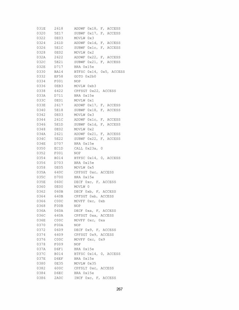
267

031E 2618 ADDWF 0x18, F, ACCESS 0320 5E17 SUBWF 0x17, F, ACCESS 0322 0E03 MOVLW 0x3 0324 261D ADDWF 0x1d, F, ACCESS 0326 5E1C SUBWF 0x1c, F, ACCESS 0328 0E02 MOVLW 0x2 032A 2622 ADDWF 0x22, F, ACCESS 032C 5E21 SUBWF 0x21, F, ACCESS 032E D717 BRA 0x15e 0330 BA14 BTFSC 0x14, 0x5, ACCESS 0332 EF58 GOTO 0x2b0 0334 F001 NOP 0336 0EB3 MOVLW 0xb3 0338 6422 CPFSGT 0x22, ACCESS 033A D711 BRA 0x15e 033C 0E01 MOVLW 0x1 033E 2617 ADDWF 0x17, F, ACCESS 0340 5E18 SUBWF 0x18, F, ACCESS 0342 0E03 MOVLW 0x3 0344 261C ADDWF 0x1c, F, ACCESS 0346 5E1D SUBWF 0x1d, F, ACCESS 0348 0E02 MOVLW 0x2 034A 2621 ADDWF 0x21, F, ACCESS 034C 5E22 SUBWF 0x22, F, ACCESS 034E D707 BRA 0x15e 0350 EC1D CALL 0x23a, 0 0352 F001 NOP 0354 B014 BTFSC 0x14, 0, ACCESS 0356 D703 BRA 0x15e 0358 0E05 MOVLW 0x5 035A 640C CPFSGT 0xc, ACCESS 035C D700 BRA 0x15e 035E 060C DECF 0xc, F, ACCESS 0360 0E00 MOVLW 0 0362 060B DECF 0xb, F, ACCESS 0364 640B CPFSGT 0xb, ACCESS 0366 C00C MOVFF 0xc, 0xb 0368 F00B NOP 036A 060A DECF 0xa, F, ACCESS 036C 640A CPFSGT 0xa, ACCESS 036E C00C MOVFF 0xc, 0xa 0370 F00A NOP 0372 0609 DECF 0x9, F, ACCESS 0374 6409 CPFSGT 0x9, ACCESS 0376 C00C MOVFF 0xc, 0x9 0378 F009 NOP 037A D6F1 BRA 0x15e 037C B014 BTFSC 0x14, 0, ACCESS 037E D6EF BRA 0x15e 0380 0E35 MOVLW 0x35 0382 600C CPFSLT 0xc, ACCESS 0384 D6EC BRA 0x15e 0386 2A0C INCF 0xc, F, ACCESS

268

0388 520C MOVF 0xc, F, ACCESS 038A 2A0B INCF 0xb, F, ACCESS 038C 600B CPFSLT 0xb, ACCESS 038E C00C MOVFF 0xc, 0xb 0390 F00B NOP 0392 2A0A INCF 0xa, F, ACCESS 0394 600A CPFSLT 0xa, ACCESS 0396 C00C MOVFF 0xc, 0xa 0398 F00A NOP 039A 2A09 INCF 0x9, F, ACCESS 039C 6009 CPFSLT 0x9, ACCESS 039E C00C MOVFF 0xc, 0x9 03A0 F009 NOP 03A2 D6DD BRA 0x15e 03A4 2A2D INCF 0x2d, F, ACCESS 03A6 A080 BTFSS 0xf80, 0, ACCESS 03A8 2A30 INCF 0x30, F, ACCESS 03AA B080 BTFSC 0xf80, 0, ACCESS 03AC 0630 DECF 0x30, F, ACCESS 03AE A280 BTFSS 0xf80, 0x1, ACCESS 03B0 2A2F INCF 0x2f, F, ACCESS 03B2 B280 BTFSC 0xf80, 0x1, ACCESS 03B4 062F DECF 0x2f, F, ACCESS 03B6 9413 BCF 0x13, 0x2, ACCESS 03B8 0E05 MOVLW 0x5 03BA 602D CPFSLT 0x2d, ACCESS 03BC D001 BRA 0x3c0 03BE 0012 RETURN 0 03C0 C032 MOVFF 0x32, 0xffa 03C2 FFFA NOP 03C4 6A2D CLRF 0x2d, ACCESS 03C6 7613 BTG 0x13, 0x3, ACCESS 03C8 6A31 CLRF 0x31, ACCESS 03CA 0E08 MOVLW 0x8 03CC 602F CPFSLT 0x2f, ACCESS 03CE 8231 BSF 0x31, 0x1, ACCESS 03D0 6030 CPFSLT 0x30, ACCESS 03D2 8431 BSF 0x31, 0x2, ACCESS 03D4 0E05 MOVLW 0x5 03D6 6E2F MOVWF 0x2f, ACCESS 03D8 6E30 MOVWF 0x30, ACCESS 03DA 9080 BCF 0xf80, 0, ACCESS 03DC 9280 BCF 0xf80, 0x1, ACCESS 03DE 5031 MOVF 0x31, W, ACCESS 03E0 26F9 ADDWF 0xff9, F, ACCESS 03E2 0012 RETURN 0 03E4 D75E BRA 0x2a2 03E6 D771 BRA 0x2ca 03E8 A613 BTFSS 0x13, 0x3, ACCESS 03EA 0000 NOP 03EC 0000 NOP 03EE 0012 RETURN 0

269

APPENDIX E

PIEZO CRYSTAL BASED ULTRASONIC SENSORS - POSSIBLE REASONS WHY IT IS NOT WORKING

Commercial piezo crystal devises comes standardized at 40kHz. The reason is because the

frequency cannot be perceived by animals such as dogs and bats that have hearing

capabilities in the ultrasonic ranges. Figure E1 is a typical example of a commercial piezo

crystal transmitter and receiver pair.

Figure E1 Parallax ping))) exemplifies commercial piezo sensor.

They are made as matched pairs. The transmitter transmits at an optimum value that is fixed,

but itself is not sensitive to that frequency. The receiver in the other hand is designed to be

very sensitive to a frequency (which is the transmitter frequency) and reject all other

frequencies (kind of a mechanical notch filter) - this behavior is shown in figure E2.

A piezo element's oscillations first approach the minimum impedance frequency (fm) /

resonance frequency (fr), at which the element vibrates most readily, and most efficiently

converts electrical energy into mechanical energy. As cycling frequency is further increased,

impedance increases to the maximum impedance frequency (fn) / anti-resonance frequency

(fa), thus the piezo crystal will naturally reject frequency about fm (or fr) but will respond very

well to frequencies at fn (or fa).

270

Figure E2 The signal response of matched piezo crystal transmitter and receiver.

The piezo crystal plates for the sensors are 5mm in diameter. When electricity is applied, the

crystal bends and reverses its bending direction when the polarity is changed. This can be

done at rates up to million times per second for some materials, the one used in this project is

optimized for 40kHz. The recommended voltage is less or equal to 20V to avoid crystal

breakdown due to excessive bending stress. The higher voltage generate more signal

strength.

The piezo crystal plates drive the medium forward and backward at the designed or applied

frequency. This action is not a problem when the fluid its interacting with is air, with average

density of 1.184kg/m3 (if mean temperature is equals 25.9 ºC). If the fluid is water, the

density becomes approximately 1000 kg/m3 , that is 847 fold increment of mass of fluid to

move. This seems to be an overload for the sensor used by the fish robot.

An alternative proposition was to use common buzzer plates, figure E3 (10mm to 20mm

sizes) also made up of piezo crystal material by Afolayan (2010).

Unfortunately, a rigorous experimentation and calculation shows that this idea will not work

for the robot as follows;

Log

of im

peda

nce

Frequency

Fs (≈fm)

Fp (≈fn)

271

1. An experiment on this crystal response (figure E4) shows that these buzzers are made

for audible ranges. The response is perfect for the 10kHz and distorted at 20kHz

range. At 60kHz, it becomes triangular wave and discontinue at 100khz. The input is

a square wave and with constant 5V peak values. The microcontroller inputs are logic

gates and run at 8MIP (125ns per instruction), any discontinuity or drop from 5V

could be interpreted as separate data input.

Figure E3 Watch Buzzer crystal plates

10kHz 20kHz 60kHz 100kHz

Figure E4 The response of watch buzzer plates to various input frequencies. The top chart is the transmitter output and the bottom plot is the receiver response to the transmitted signal

2. Back plane transmission. The buzzers are designed to transmit sound in all direction –

figure E5. It means if used for this work, there will not be any localization of any

272

detectable objects. Compared to the commercial one of figure E6, the beam is

concentrated and narrow.

Figure E5 Watch buzzer plate radiation is in all direction

Figure E6 Radiation pattern of Parallax ping)))

3. Tuning and matching – since they don’t come in pairs, optimum transmission cannot

be achieved as shown in figure E2. A dedicated notch filter will be needed to remove

unwanted signals. If no filter is built in, it means every sound and vibration will be

picked up rendering it useless for any pure sensing purposes.

273

4. Audible frequencies will not work

Figure E7 Transmitter-receiver pair using buzzer plate piezo crystals

If the object is located at distance X

And the speed of sound in water is ≈1500m/s.

Time of flight = Tf = 2X / (1500m/s) time to go and come back

If X= 30cm = 0.3m - a value selected being less that the robot length of 394.01cm

Tf = 0.0002s

= 0.2ms

If transmitter frequency were 4.5kHz as recommended by Afolayan (2010), the

period T of oscillation =

T = 1/ 4.5kHz = 0.222ms

Since T > Tf then there will be no single complete oscillation before the signal

is expected back.

X

Object being detected

Transmitter

Receiver

274

If transmitter frequency were 10kHz, using the information from figure E4 the

period T of oscillation =

T = 1 / 10 kHz = 0.1ms

T : Tf = 0.2 /0.1 = 2

there will be two complete oscillations before the signal is expected back but

will not be enough to saturate the plate acting as sensor.

If transmitter frequency were 20kHz - that is the edge of human audible range

the crystal were designed for as evidence in figure E4 where the response start to

deteriorate, the period T of oscillation will be =

T = 1 / 20 kHz = 0.05ms

T : Tf = 0.2 /0.05 = 4

there will be 4 complete oscillations before the signal is expected back but may just be

enough to saturate the plate acting as sensor. Another problem that arises automatically is

called ringing, that is the dying off of the vibration with time since they are mechanical

objects. The sensor will continue to send signals even after the driver has stopped

supplying voltage to it.

275

APPENDIX F

INDENTATION FORCE DEFLECTION (IFD) UNIT

Indentation Force Deflection (IFD) is defined as the amount of force, in pounds,

required to indent a fifty square inch, round indentor foot into a predefined foam specimen a

certain percentage of the specimen's total thickness according to the Polyurethane Foam

Association (http://www.pfa.org). The value 6 is assumed for a collapsed and very succulent

polyurethane foam as used in this project – the foam used is from an old cushion chair. Table

F1 list the Polyurethane foam association IFD table.

Table F1 Polyurethane foam association IFD table

IFD value Common usage

6-12 Bed pillows, thick back pillows

12-18 back pillows, upholstery padding, wraps

18-24 thin back pillows, tufting matrix, very thick seat cushions,wraps

24-30 average seat cushions, upholstery padding, tight seats, certain mattress

types, quilting

30-36 firmer seat cushions, mattresses

36-45 thin seat cushioning and firm mattresses

45 and upward shock absorbing foams, packaging foams, carpet pads, and other uses

requiring ultra-firm foams

(Source: http://www.pfa.org)

276

APPENDIX G

INTERPRETING THE NYQUIST DIAGRAM

Source: http://www.roymech.co.uk/Related/Control/Nyquist.html

In the Nyquist plots below the area covered to the right of the locus(shaded) is the Right

Hand Plane (RHP)

A closed loop control system is absolutely stable if the roots of the characteristic equation

have negative real parts. This means the poles of the closed loop transfer function, or the

zeros of the denominator ( 1 + GH(s)) of the closed loop transfer function, must lie in the

(LHP). The Nyquist stability criterion establishes the number of zeros of (1 + GH(s) in the

RHP directly from the Nyquist stability plot of GH(s) as indicated below.

The closed loop control system whose open loop transfer function is GH(s) is stable only if..

N = -Po ≤ 0

277

where

1) P o = the number of G(s) poles in the RHP ³ 0

2) N = total number of CW encirclements of the (-1,0) in the G(s) plane.

If N > 0 the number of zeros (Z o) in the RHP is determined by Z o = N + P o

If N ≤ 0 the (-1,0) point is not enclosed by the Nyquist plot.

If N ≤ and P 0 then the system is absolutely stable only if N = 0. That is if and only if the (-

1,0) point does not lie in the shaded region..

Considering the LH plot above of 1/s(s+1). The (-1,0) point is not in the RHP therefore N<=

0. The poles are at s =0, and s=-1, both outside of the RHP and therefore P o = 0.

Thus N = -P o = 0 and the system is therefore stable.

Considering the RH plot above of 1/s(s-1). The (-1,0) point is enclosed in the RHP and

therefore N > 0 (N= 1). The poles of GH are at s= 0 and s = +1 . S= +1 is in the RHP and

therefore P o = 1.

N ¹ - P o Indicating that this system is unstable..

There are Z o = N + P o zeros of 1+GH in the RHP.

Autodesk Inventor 7

Approved by:

Date:

Software:

1

Material:

Scale

MECHANICAL ENGINEERING DEPARTMENTAHMADU BELLO UNIVERSITY

Part name: Fish robot assembly

Drawn by: AFOLAYAN M.O.

Dr. D.S. Yawas

Unit: mm

2:1

Drawing No

394.0191

.5195.6 198.41

58.4

49.8

2

1 2

1 Haul Assembly (Drawing no 2)

2 Tail Assembly (Drawing no 3)

SECTION A-ASCALE 1 / 2

Autodesk Inventor 7

Approved by:

Date:

Software:

2

Material:

Scale


Part name: Haul Assembly


Dr. D.S. Yawas

Unit: mm

Plywood

1:2

Drawing No

A A

1

38 The balloons (1,2.....38) refers to the rings position in drawing number 4.

2

Isometric view

Front elevation

Plan

Side view

SECTION B-BSCALE 1 / 2

Autodesk Inventor 7

Approved by:

Date:

Software:

3

Material:

Scale


Part name: Tail assembly


Dr. D.S. Yawas

Unit: mm

1:2

Drawing No

B B

18 1 Base Base17 2 QTR_1 Quarter pulley 14 2 QTR_2 Quarter pulley 23 2 QTR_3 Quarter pulley 32 2 QTR_4 Quarter pulley 41 2 QTR_5 Quarter pulley 55 1 6b6 1 r47 1 58 1 49 1 r2

10 1 311 1 r112 1 213 1 r014 1 115 1 016 1 r3_

Parts ListITEM QTY PART NUMBE DESCRIPTION

5

7 8 10 1214

15

64 3 2

111

17

18

16

9

13

Ring Position

1 2 3 4 5 6 7 8 9 10 11 12 13 14 15 16 17 18 19 20

a 8 15 21 23.2 25 28 32 36.5 38.4 43.2 46.4 48 49.6 51.2 52.8 53.6 54.4 55.2 56 56 b 12 17.6 24 30 35 39.5 43 48 51 55 58 61 63 65 67 70 72 74 76 77 Ring Position

21 22 23 24 25 26 27 28 29 30 31 32 33 34 35 36 37 38

a 56.8 57.6 57.6 57.6 57.6 57.6 57.6 57.6 57.6 57.6 57.6 57.6 57.6 58.4 58.4 58.4 58.4 58.4 b 79 80 82 83.5 84.5 85.5 86.5 88 89 90 91 91 91 91 91 91 91.5 91

Autodesk Inventor 7

Approved by:

Date:

Software:

Drawing No 4

Material:

Scale


Part name: Rings (for the haul)


Dr. D.S. Yawas

1:1

Plywood

Isometric view of ring

5mm 5mm

b

a

Fixed rim width

Fixed thickness

Autodesk Inventor 7

Approved by:

Date:

Software:

Drawing No 5

Material:

Units: mm


Part name: Tail Fin


Dr. D.S. YawasPlywood

Scale: 1:1

48.71

49.8

3

22.3848.71

1

Autodesk Inventor 7

Approved by:

Date:

Software:

Drawing No 6

Material:

Units: mm


Part name: Tail support structure - segment 1



Scale: 1:1

7.48

15.24

3.18

9.56

14.7

2.34

2.16

0.63

Autodesk Inventor 7

Approved by:

Date:

Software:

Drawing No 7

Material:

Units: mm





Scale: 1:1

15.51

7.93

29.0

3

3.18

3.43 2.

613.

39

2.29

17.3

1

Autodesk Inventor 7

Approved by:

Date:

Software:

Drawing No 8

Material:

Units: mm


Part name: Tail support structure - segement 3



Scale: 1:1

23.42

3.18

32.0

16.

549.

02

47.5

6

Autodesk Inventor 7

Approved by:

Date:

Software:

Drawing No 9

Material:

Units: mm





Scale: 1:1

24.7

3.18

50.2

3

61.5

4

3.37 1.22

3.83

2.88

12.66 8.68

Autodesk Inventor 7

Approved by:

Date:

Software:

Drawing No 10

Material:

Units: mm





Scale: 1:1

29.16

14.25

63.1

72.

68

2.34

2.86

0.85

71.0

8

3.18

Autodesk Inventor 7

Approved by:

Date:

Software:

Drawing No 11

Material:

Units: mm





Scale: 1:1

19.83

0.98

71.6

7

1.58

74.2

8

3.18

8.288.67

Autodesk Inventor 7

Approved by:

Date:

Software:

Drawing No 12

Material:

Scale


Part name: Rubber stripe - 1


Dr. D.S. Yawas

Unit: mm

Vulcanized Rubber (tire inner tube)

2:1

1.50

5.00

14.3

31.

320.

97

16.6

1

Autodesk Inventor 7

Approved by:

Date:

Software:

Drawing No 13

Material:

Scale




Dr. D.S. Yawas

Unit: mm


1:1

1.50

5.00

28.9

31.

431.

35

31.7

2

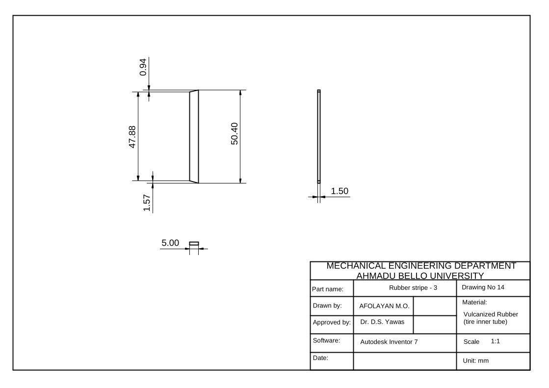
Autodesk Inventor 7

Approved by:

Date:

Software:

Drawing No 14

Material:

Scale




Dr. D.S. Yawas

Unit: mm


1:1

5.00

1.50

47.8

80.

941.

57

50.4

0

Autodesk Inventor 7

Approved by:

Date:

Software:

Drawing No 15

Material:

Scale




Dr. D.S. Yawas

Unit: mm


1:1

5.00

1.50

61.8

1

63.5

9

0.83

0.95

Autodesk Inventor 7

Approved by:

Date:

Software:

Drawing No 16

Material:

Scale




Dr. D.S. Yawas

Unit: mm


1:1

5.00

1.50

70.7

7

72.9

5

1.07

1.10

Autodesk Inventor 7

Approved by:

Date:

Software:

17

Material:

2:1


Part name: Quarter Pulley 1



Units: mm

Scale

Drawing No

3.0R 3.0

10

Autodesk Inventor 7

Approved by:

Date:

Software:

Drawing No

Material:

2:1


Part name: 18



Units: mm

Scale

Quarter Pulley 2

R6

2

2

7 83.5

R 1.5

Autodesk Inventor 7

Approved by:

Date:

Software:

Drawing No

Material:

2:1


Part name: 19



Units: mm

Scale

Quarter Pulley 3

2

2

R8

7 8

3.5

R 1.5

Autodesk Inventor 7

Approved by:

Date:

Software:

Drawing No

Material:

2:1


Part name: 20



Units: mm

Scale

Quarter Pulley 4

R 10.0

2

2

7 8

R 1.5

3.5

Autodesk Inventor 7

Approved by:

Date:

Software:

Drawing No

Material:

2:1


Part name: 21



Units: mm

Scale

Quarter Pulley 5

2

2

R15

3.5

7 8

R 1.5

Ring Position

1 2 3 4 5 6 7 8 9 10 11 12 13 14 15 16 17 18 19 20

a 57.6 57.6 56.8 56.8 56.8 56 56 54.4 54.4 54.4 52.8 51.2 51.2 49.6 48 48 46.4 44.8 43.2 41.6 b 91 90.5 90 89 89 88 86 85.5 83 81 79.5 78 76 74 73 71 69 67 65 62 Material U U P U U P U U P U U P U U P U U P U U Ring Position

21 22 23 24 25 26 27 28 29 30 31 32 33 34 35 36

a 40 38.4 35.2 33.6 32 30.4 28.8 25.6 23.2 20.8 17.6 14.4 11.2 9.6 8 8 b 60 56 53 49.5 46 43 39.5 36 32 28 24 20 18 15 13 12 Material P U U P U U P U U P U U P U U P

Autodesk Inventor 7

Approved by:

Date:

Software:

Drawing No 22

Material:

Scale


Part name: Rings (for the tail)


Dr. D.S. Yawas

P= PlywoodU= Collapsed Polyurethane foam

5mm5mm

Fixed thickness

Fixed rim width

b

aIsometric view

Autodesk Inventor 7

Approved by:

Date:

Software:

Drawing No 23

Material:

1:1


Part name: Head board



Units: mm

Scale

20 1510

12

1416

201510

12

1416

40.5

24.2

C1

R1

R1

R2

R1

R2

BSW

BSW

R1

R1

R1

R2

R3

R1

R1

R1

R1

R2

R2

R2

R2

R2

R2

R2

R2

R2

R1

R1

R1

R1

R1

DDDDDDDDD

ANTENNA

SERVOMOTOR 3

SERVOMOTOR 2

SERVOMOTOR 1

DESIGN AND DEVELOPMENT OF A BIOLOGICALLY ...

Documents

Transcript of DESIGN AND DEVELOPMENT OF A BIOLOGICALLY ...