#2010-050

Efficient Development Portfolio Design for Sub Saharan Africa

Adriaan van Zon and Kirsten Wiebe

United Nations University – Maastricht Economic and social Research and training centre on Innovation and Technology

Keizer Karelplein 19, 6211 TC Maastricht, The Netherlands

Tel: (31) (43) 388 4400, Fax: (31) (43) 388 4499, email: info@merit.unu.edu, URL: http://www.merit.unu.edu

Working Paper Series

Efficient Development Portfolio Design for Sub Saharan Africa

by

Adriaan van Zon

and

Kirsten Wiebe

(UNU-MERIT/SBE Maastricht University, August 2010)

Adriaan.vanZon@MaastrichtUniversity.NL

Wiebe@merit.unu.edu

Abstract

The Stiglitz Report published in September 2009 has brought back to the attention of policy

makers and researchers that measuring a country's development solely on the basis of GDP

or GDP per capita is not sufficient. An early attempt at multidimensional measurement is

the Human Development Index (HDI) developed by the United Nations Development

Program in 1990. This measure consists of three components: a health index, an education

index, and a standard of living index. Even though it was and still is subject to criticism, it is

the only multidimensional measure that has been around for 20 years and is widely

accepted by policy makers, who use this measure to compare the state of development of

their country with those of other countries. They would like to maximize the HDI to improve

their position in the ranking. As it is a multi-dimensional measure, it is necessary to

influence different fields of development, which can be done by policy makers via public

spending. We differentiate between public spending on education, health and general

spending. This corresponds to the three components of the HDI. In Sub-Saharan Africa,

which is the region of interest here, the total government budget is limited in most

countries, so that the only option policy makers have is to allocate the given budget

efficiently over the three categories. To find the best possible budget allocation, we use an

optimum portfolio theory approach, which has been adapted to the problem at hand.

The approach consists of two stages. The first stage is concerned with the econometric

estimation of a linear model that links variation in the policy instruments to the

corresponding variation in the individual components of the HDI in a given general

environment implicitly defined by a set of exogenous variables, such as the HIV-rate,

colonial ancestry, and so on. Using the method of Seemingly Unrelated Regression, we

estimate the contribution of each instrument to each target as part of a simultaneous

equations system. As a bonus, we obtain the covariance matrix of the parameter estimates.

In a second stage, we use these estimation results, including the covariance matrix of the

parameter estimates, to define a portfolio-selection problem, known from financial

optimum portfolio analysis. In our case, however, the distribution of a given budget of

government expenditures over the various HDI components constitutes the portfolio

selection problem, rather than distributing funds over a portfolio of financial assets. In our

case, an efficient portfolio minimizes the variance (further called V) in the HDI for a given

expected value of the HDI. We are able to calculate efficient HDI portfolios by varying the

degree of risk-aversion over a preset range, and tracing the corresponding set of optimum

portfolios which are necessarily efficient as well. This set can be interpreted as the hull of all

feasible portfolios in the V,HDI-plane. This set turns out to be convex, as in ordinary financial

portfolio applications.

We also show how, as the budget increases, these efficient portfolios move through the

V,HDI-plane in a North-Easterly direction in most cases, following convex expansion paths

for a given level of risk-aversion, indicating a more than proportional increase of V for a

given increase in HDI. In some cases we find that these expansion paths are U-shaped,

suggesting that there is a double dividend in expanding a low total budget in terms of HDI

gained and V lost, or a 'double punishment' for decreasing an already low budget. We have

also performed a sensitivity analysis that illustrates the working principles of the general

approach and the importance of the selection of statistically significant model specifications,

as statistically insignificant contribution parameters in one or more of the model equations

in combination with risk-aversion provides a bias against inclusion of corresponding

expenditures in the optimum development portfolio.

In most country/year combinations we have included in the analysis we find that actual HDI

performance lags significantly behind the HDI range achievable through efficient spending

of the actual available budget. Our approach enables us to indicate how existing budgets

should then be reallocated and how much would be gained in terms of the accompanying

HDI improvement.

Keywords Human Development Index, Public spending, Optimum Portfolio Theory

JEL classification H5, I, O2

UNU-MERIT Working Papers

ISSN 1871-9872

Maastricht Economic and social Research and training centre on Innovation and Technology, UNU-MERIT

UNU-MERIT Working Papers intend to disseminate preliminary results of research

carried out at the Centre to stimulate discussion on the issues raised.

5

1. Introduction

In this article we present an approach to designing development policies that takes into account the

intrinsic uncertainties surrounding the impact of individual development instruments on the

development goals to be achieved. Instead of using a fully specified structural model that relates

policy instruments to policy goals and targets, either directly or indirectly, we use a (linear) reduced

form model that describes the statistical connection between instruments and targets. The benefits of

this approach are obvious: the time necessary to specify and estimate the model is far less than for a

fully specified structural model. The disadvantage is also obvious: the model is essentially a black

box. However, as Friedman (1953) pointed out in the Fifties already, from a practical policy design

point of view, the most important thing is that the black box actually works, i.e. that a significant link

between targets and instruments does indeed exist and can be quantified to a sufficiently precise

degree on the relevant policy range. Because the main aim of this article is to illustrate the working

principles of our design approach, we will adopt Friedman’s pragmatic stance.

In policy making, the statistical nature of the relation between targets and instruments is

usually ignored, except for instances where one uses Monte-Carlo simulations. However, a bonus of

explicitly acknowledging the statistical nature of the relation between instruments and targets is that it

is easy to obtain the variance of some linear combination of targets (i.e. of a linear ‘objective

function’) in terms of the variances in the measured contributions of the individual instruments to

those targets. The Human Development Index (HDI) takes the form of a linear combination of such

targets. Maximization of the HDI as the ultimate development target under some scarce resource

constraint then requires the matrix of the expected values of the contribution coefficients of the

instruments to the various sub-targets. The econometric estimation of these coefficients usually results

in a situation where some non-zero (co-) variance of the estimates of the contribution coefficients

remains. But then, picking some value of a particular instrument also implies picking a contribution of

that instrument to the variance in the objective-function value. The latter is important, because policy

makers tend to be risk-averse, and consequently, they could be expected to select from the collection

of all feasible sets of instruments the one set that would generate the lowest variance for that particular

objective function value. This particular set is efficient in the sense that it provides the highest

positively valued result (the HDI) for a given value of a negatively valued result (the corresponding

HDI variance).

The linearity of the HDI implies that its components are perfect substitutes for each-other,

which is one of the criticisms raised against the HDI, see e.g. Sagar and Najam (1998) and section 2.

Still, it has been widely accepted as a relevant measure of development, and so do we (also for

pragmatic reasons). Given the existence of some resource constraint, this causes the exclusive

selection of the instrument that would generate the highest contribution to the objective function per

unit of the resource spent. With multiple resource constraints, the set of feasible instruments may

6

become strictly convex, and a combination of different instruments may become optimal rather than

just a single one. With risk-aversion, such a collection of instruments (further called instruments-

portfolio, or IPF for short) may exist, regardless of the existence of multiple resource constraints, since

the instruments become effectively imperfect substitutes because of the non-linearities involved in the

contribution of each instrument to the variance in the objective function, or the portfolio-variance (as

opposed to the single-instrument variance). Problems of this kind are familiar from financial optimum

portfolio theory put forward by Markovitz (1952), and later extended by many others (Merton 1969;

Samuelson, 1969) also in non-financial directions (Helfat, 1988; Seitz and Ellison, 1995; Awerbuch

and Berger 2003; van Zon and Fuss, 2008; Fuss, 2008). The current article fits into the latter category,

and is, as far as we know, the first application of the ideas of financial optimum portfolio theory to the

design of development policies.

The article serves two purposes. The first is to show the working principles of the approach,

also in a development context. To do this, we construct the simplest possible portfolio version of the

development problem that contains all the components that are strictly necessary to define such a

problem, no more, no less. The second purpose is to assess its potential relevance for the development

problem. Therefore the components of the portfolio composition problem themselves are directly

linked to concepts used in development policy decision making and implementation. The objective

function, for instance, is translated into manageable modeling terms by taking it to be the

maximization of a weighted sum of the HDI and its corresponding variance by means of controllable

public spending on the targets directly contributing to the HDI. We specify this set-up for a large

group of Sub-Saharan African (SSA) countries, asking ourselves how these countries should spend a

given budget on the various targets, given the measured variances in the contribution coefficients, and

given the existence of (different degrees of) risk aversion. It should be noted that limited data-

availability for this group of SSA-countries has forced us to choose as simple a model specification as

possible for purely pragmatic reasons. Still, the specification chosen works well in statistical terms

(see also section 4).

The article is further organized as follows. Section 2 provides an overview of the different

parts that make up our approach as well as the alterations/extensions we have made to be able to cover

the design of efficient development portfolios. In section 3, we give a short overview of the data we

have collected for our portfolio-exercise, while section 4 provides the estimation results. In section 5

we discuss the outcomes of our portfolio optimization problem, and investigate the efficiencies and

inefficiencies involved in the development portfolios of individual SSA-countries as compared to the

efficient portfolio frontier (further called EPF, for short). We try to assess how much of their

inefficiencies are due to pure chance and how much due to inefficiencies in the allocation of resources.

In section 6 we provide some concluding remarks.

7

2. Setting the Stage

2.1 General Outline

We feel that policy design should take into account that the impact of policies on the development

process can not be known with complete certainty, and that some combinations of policy measures

may generate less risk1 than others. In fact, as people (and policy makers) are generally risk-averse,

policy design should favor combinations of policies that generate the lowest risk for a given expected

result at the aggregate level and for a given total budget, i.e. the policy portfolio should be efficient.

Under conditions of risk, the allocation of resources that have alternative uses, in our case

public expenditures that could be directed towards alternative expenditure categories, is bound to not

have the expected/desired effect, or at least not exactly. In addition, it may well be the case that

realization ‘errors’ for different expenditure categories are correlated with each other. For example, an

unexpectedly high effectiveness of education expenditures may make health and sanitation

expenditures ‘unexpectedly’ more effective too. In Optimum Portfolio Theory, further called OPT for

short, these correlations are taken into account from the outset, in defining efficient financial

investment portfolios. We want to do the same when defining efficient development portfolios

(EDPs).

We will show that the extension of OPT to cover the design of EDPs is relatively straight

forward because of the correspondence between assets returns and HDI components on the one hand,

and adding-up constraints on portfolio shares and those on expenditures on the HDI components on

the other. The fundamental change in the OPT framework that is necessary for the design of EDPs is

that of the addition of a (linear) system of simultaneous equations that describes how expenditures on

the various HDI-components influence these components. We have estimated the parameters of that

linear system (and their co-variances) for the SSA-countries in our sample. The co-variance matrix

associated with the estimated contribution coefficients serves much the same function in our set-up as

the co-variances between the individual asset rates of return in a pure OPT setting.

2.2 The Human Development Index

The recent report by the Commission on the Measurement of Economic Performance and Social

Progress (Stiglitz et al., 2009) has made both policy makers and researchers acknowledge that

measuring a country’s development solely on the basis of GDP or GDP per capita is not sufficient,

suggesting that a composite measure including different aspects such as income, health, education,

environment, freedom, or equality would be more suitable. The biggest drawback to actually

1 In the literature, a distinction between risk and uncertainty is made. Risk is measurable through a known probability distribution, and uncertainty isn’t. Cf. Knight (1921).

8

establishing such a composite measure is data availability, especially concerning the quality of

education, health, and the environment on a macroeconomic level as well as inequality. Nonetheless, a

multidimensional indicator for human development has been around for about 20 years in the form of

the Human Development Index (HDI) developed by the United Nations Development Program

(UNDP). The HDI was first published in the 1990 Human Development Report (UNDP, 1990). It

measures “the average achievements in a country in three basic dimensions of human development: a

long and healthy life, knowledge and a decent standard of living.”2 HDI data are available for more

than 175 countries and regions. Even though the HDI was criticized from the very beginning regarding

its incompleteness (e.g. measures of inequality were lacking), the way the index was calculated

relative to the observed range of variation in the sample, but also the additive fashion in which the

individual HDI components contributed to the aggregate index, the HDI has, since 1997, converged

upon a final set of components, i.e. income, health and education (Klugmann et al., 2008). These

components ensure that the HDI is a measure that can be characterized as ‘universal’, ‘basic to life’,

and ‘measurable’ (Bérenger and Verdier-Chouchane, 2007). Meanwhile, other indicators addressing

(some of) the shortcomings of the HDI have been made available as well.3 Aggregate indicators that

can be seen as complementary to the HDI are for example the Happy Planet Index (Abdallah et al.,

2009), including happy life years and the ecological footprint, or the Human Poverty Index and the

Gender Related Development Index developed by UNDP. However, for the purpose of illustrating our

approach, but also because HDI-data are now readily available, we have opted for the HDI as our

primary measure of development. This has the added bonus of us being able to rephrase the HDI in

terms of the expected contribution coefficients of the estimated expenditure system, further explained

in sections 2.4 and 4. Likewise, the variance in the HDI can be shown to depend directly on the co-

variance matrix of these distribution coefficients (see Appendix A for more details).

2.3 Public Spending

Adopting a particular measure of development like the HDI as an adequate description of the state of

development then logically implies that policies that are effective in raising the measured level of the

HDI are to be preferred above policies that are less effective, ceteris paribus. Hence, the measurable

impacts that alternative policies may have on the HDI may function as a screening device for the

selection of policies, indeed for the design of a set of policies that may complement each other, i.e. a

policy-portfolio. Development economists have dealt with the issue of designing effective

development policies for quite some time. Indeed, there is a wide literature on the effect of aid on

2 http://hdr.undp.org/en/statistics/indices/. 3 For a short overview on other alternative indicators, see Berenger and Verdier-Chouchane (2007), p.1261.

9

development, see for example the special issue of the Review of Development Economics from 2009

(Mavrotas, 2009).

The focus of our attention in this article is on the design of internal spending policies, rather

than on how external aid may affect development. This is in line with the views of African economists

such as James Shikwati (Shikwati, 2006) or Dambisa Moyo (Moyo, 2009), who criticize monetary

development aid and propose its complete removal since aid-recipients only become dependent and

most of it ends up in the hands of corrupt elites (Grill, 2009). Rajan and Subramania (2005) even find

that aid has a negative impact on growth. In addition to this, if aid is directly channeled to specific

programs or projects, local policy makers do not necessarily have much of a say in where the aid flows

go. In light of this discussion we will explore how African policy makers would be able to influence

development through a better channeling of their public expenditures. Gomanee et al. (2005) take a

step in that direction by examining the effect of aid on development through public expenditures.

There are three main approaches to analyzing public expenditure in developing countries.

First, there is the more descriptive literature about how much the government spends in total, as a

percentage of GDP, or, more specifically, on which sector; how public spending develops over time

and how it compares across countries. These descriptions are mostly followed by other types of

analysis, e.g. the analysis of the impacts of public spending on growth as in Fan and Rao (2003).

Second, there is the analysis of public spending efficiency, i.e. how effective are, for example, health

or education expenditures in determining health and education outcomes in different countries and at

different times (e.g. Herrera and Pang, 2005; Herrera, 2007; Gupta et al., 1997; Jayasuriya and

Wodon, 2008). Murillo-Zamorano (2004) surveys different efficiency frontier techniques (FDH and

DEA) in this context. The third strand of literature stems from growth theory, where the effect of

public spending on long-run economic growth is analyzed, e.g. Aschauer (1989), Barro (1990),

Devarajan et al. (1996), or Fan and Rao (2003). Only some of these authors distinguish between

different spending categories such as education or health. Furthermore, this literature measures the

effects of government expenditure just on economic growth, which, by now, is an indicator considered

to be too narrow a measure of a country’s overall development.

Obviously, the EDP-approach we develop in this article fits in with the second (‘efficiency’)

strand of literature, but it does not stop with the measurement of inefficiencies. It also provides a direct

indication as to how a reallocation of the public spending budget may improve the effectiveness of

total spending in improving the Human Development Index. The only thing that is different is the

notion of the efficiency of the public spending portfolio itself. The latter is defined not just in terms of

the maximization of the returns/HDI for a given level of resources available (the ‘traditional’

efficiency concept), but also for a given level of the variance in the expected returns/HDI (the

10

‘extended’ efficiency concept from OPT): an EDP requires both ‘traditional’ and ‘extended’ efficiency

of the allocation of resources.

2.4 Optimum Portfolio Theory and Efficient Development Portfolio Design

Optimum Portfolio Theory (OPT) was first described in Markovitz (1952). It refers to the problem of

distributing a given budget over different financial assets, each of them with its own expected rate of

return and a given co-variance matrix between the expected rates of return of these assets. A

mathematical formulation of the static portfolio model is relatively straight forward, and we will use it

as a template for the construction of our Efficient Development Portfolio (EDP) counterpart. In OPT

an efficient portfolio maximizes the expected portfolio return for a given level of variance in that

return, or, equivalently, minimizes the variance in the expected return for a given level of that return,

by a suitable allocation of the budget over all alternatives. So an efficient portfolio exists without

reference to risk-aversion. The notion of risk-aversion helps to define an optimum portfolio as the

efficient portfolio for which an infinitesimal reallocation of the budget results in an infinitesimal small

change in the positively valued expected portfolio return that is exactly offset by an infinitesimal

change in the negatively valued corresponding portfolio variance. We will use the simplest possible

portfolio valuation function (i.e. ),( VRΘ ) with a positive contribution of portfolio return (R) and a

negative contribution of portfolio variance (V), i.e. VR α−=Θ , where 0≥α is a constant parameter

and is a measure of the degree of risk-aversion. Consequently, iso-valuation lines in the V,R-plane in

Figure 1 are defined by: αα // Θ−= RV , where Θ represents a given and constant level of the

valuation function. Note that the iso-valuation lines (labeled I, II, III) are straight and have a slope

given by α/1 . The objective function value is increasing when going from I to II to III, since for a

given value of V ‘going to the right’ in Figure 1 means an increase in R, hence an increase in the value

of Θ .

Figure 1 shows the U-shaped efficient portfolio frontier, where the variance minimizing

portfolio is represented by point A. This point corresponds to the highest possible degree of risk

aversion, i.e. an infinitely high α implying a slope of the iso-valuation-lines equal to 01 →α . The

optimum portfolio, for some given positive and finite value of α is point B. Note that point C has the

same V-value as B, but can never be an optimum portfolio, since B has higher return R than C. The

upward sloping part of the U-shaped curve is therefore the economically relevant part of the curve. It

follows moreover that for finite values of α the optimum portfolio given by point B will have both

higher variance and a higher return than the minimum variance portfolio as given by point A. In

addition to this, it should be noted that because of the convexity of the relevant part of the EPF the

same increase in R tends to be associated with ever stronger increases in V.

11

Figure 1: The optimum portfolio selection problem

This OPT framework can serve as a template for the design of development policy. For the

present article, we will be using a static framework, where decisions made in the present do not

(explicitly) influence those that can be taken in the future. In such a static setting, policy design à la

Friedman is relatively straightforward. The extension of the approach to an intertemporal setting is left

for future research at this point.

Let t be the T×1 column-vector of HDI components (the policy targets), y be the Y×1 column-

vector of per capita expenditures on Y expenditure categories and let x be the X×1 column-vector of

exogenous variables of the expenditure system. Furthermore, J is the T×Y matrix of coefficients

describing the unit-contributions of the expenditure categories to the HDI components, while K is the

T×X matrix of coefficients linking the exogenous variables to the HDI components. Finally, z’ is the

transpose of z for any z, while z is the estimated/expected value of z, i.e. )(ˆ zEz = , and zε is the

associated error-vector/matrix (depending on the dimension(s) of z), i.e. zzz ˆ−=ε . Using this

notation, we can write the expected HDI (denoted by H ) as:

TtiH /ˆˆ ′= (1)

where i’ is the 1×T summation row-vector. Moreover, the vector of the expected values of the HDI

components can be written as4:

4 This can be regarded as the reduced form of a simplified structural model of African economies. A more detailed exposition concerning the choice of this model is given in section 4.

12

xKyJt ˆˆˆ += (2)

The maximization problem we need to solve is:

)(

ˆˆˆ

)(ˆˆ

/ˆˆ..

ˆˆmax

yExpiB

xKyJt

yVV

TtiHts

VHy

′=+=

=

′=

−=Θ α

(3)

where V is the expected variance in the HDI and where B is the per capita budget of government

expenditures and ∑=

=′=Y

iiyyExpiB

1

)exp()( is the budget constraint.5 The only qualitative

difference between this problem and a standard OPT problem is the presence of equation (2) as an

additional constraint. However, equation (2) can essentially be removed through direct substitution of

(2) into (1). This step redefines H (comparable in nature to the portfolio return R in the original OPT

framework) in terms of the products of a number of matrices (J and K), the vector of decision variables

(y) and the vector of exogenous variables (x), rather than just being the inner-product of the asset

returns vector r’ and the vector of budget shares as in a standard OPT problem. This makes the

calculations more cumbersome, but the biggest problem, numerically speaking, is the non-linearity of

the budget-constraint. The latter implies that the FOC’s that implicitly describe the optimal solution to

(3) become non-linear themselves. However, using Wolfram’s © Mathematica software, we were able

to calculate y numerically (and directly) as the solution to a set of simultaneous non-linear equations.

The derivation of this set of non-linear equations is described in detail in Appendix A.

3. The Data

For our analysis we need data on the HDI-components, and on public expenditures by HDI-

component. The HDI data stems from HDRO (2009) and is calculated as the arithmetical average of a

health index (denoted by lex in Table 1) represented by life expectancy, a standard of living index

(denoted by gdp in Table 1) represented by GDP per capita, and an education index (denoted by edu in

Table 1), i.e. 3/)( gdpedulexHDI ++= . Using weights other than 1/3 does not substantially change

the ranking of countries in accordance with their HDI-score, although, of course, it does change the

5 The variance V is a relatively complicated expression in y that is derived in Appendix A. The non-linearity of the budget constraint arises because the coefficient matrices J and K have been econometrically estimated with the variables y measured as the natural logarithms of public expenditures on the various expenditure categories.

13

value of the index (Klugman et al., 2008). Note that the three components of the HDI, i.e. edu, lex, and

gdp, are the elements of our vector of target variables t.

Data sources for government expenditures are the WHO (2009) and WDI (2009) databases.

WHO (2009) provides data for per capita government expenditure on health in international PPP$ (our

variable geh) and for general government expenditure on health as percentage of total government

expenditure (for now called percenth). From these two we were able to calculate total government

expenditure in international PPP$ as get = geh/percenth. WDI (2009) provides data on public

spending on education as a percentage of government expenditure (percentedu). Per capita

government expenditure on education then is ged = get × percentedu. Remaining government

expenditures were simply calculated as the residual: geg = get – geh – ged.

For our computations we use 5-year averages to overcome frequent data gaps, as has for

example been done in Adler et al. (2009). Thus we end up with values for 1995, 2000, and 2005 for

about 30 SSA countries. The HDI shows some significant advances over these years, but,

unfortunately, also a worsening of the index for some countries. The range of HDI values in 1995 was

between 25% and 75%, which increased to values between 28% and 80% in 2005, while its mean

remained at 47%. The highest HDI in our sample of SSA countries can be found in Mauritius and the

lowest in Niger. Most countries have an HDI-score between 0.3 and 0.5.

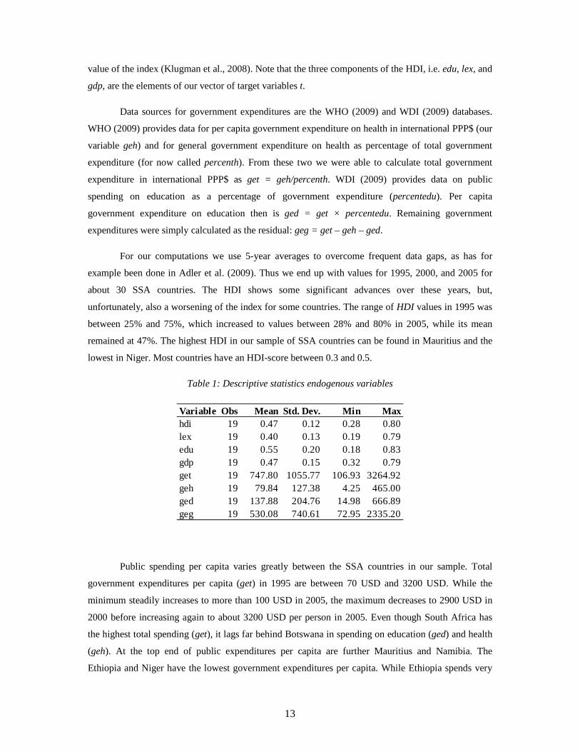
Table 1: Descriptive statistics endogenous variables

Variable Obs Mean Std. Dev. Min Maxhdi 19 0.47 0.12 0.28 0.80lex 19 0.40 0.13 0.19 0.79edu 19 0.55 0.20 0.18 0.83gdp 19 0.47 0.15 0.32 0.79get 19 747.80 1055.77 106.93 3264.92geh 19 79.84 127.38 4.25 465.00ged 19 137.88 204.76 14.98 666.89geg 19 530.08 740.61 72.95 2335.20

Public spending per capita varies greatly between the SSA countries in our sample. Total

government expenditures per capita (get) in 1995 are between 70 USD and 3200 USD. While the

minimum steadily increases to more than 100 USD in 2005, the maximum decreases to 2900 USD in

2000 before increasing again to about 3200 USD per person in 2005. Even though South Africa has

the highest total spending (get), it lags far behind Botswana in spending on education (ged) and health

(geh). At the top end of public expenditures per capita are further Mauritius and Namibia. The

Ethiopia and Niger have the lowest government expenditures per capita. While Ethiopia spends very

14

little on all categories, Niger is doing comparably well on education and health spending. Burundi

spends least on health (about 4USD per capita per year in all years).

Originally we employed 20 different exogenous variables which are commonly used as control

variables when measuring development achievements of different countries (see, for example, the

literature referenced in section 2). These exogenous variables can be grouped into different indicator

categories: structural indicators, development indicators and dummies (former British (GBCD) or

French (FRCD) colony dummy). Structural indicators, that were used here, are population density

(POPD), urbanization rate (URBR), employment rate (EMPR), the share of agriculture (EAGR),

industry (EIND), services (ESER), and trade (TRAD) in value added, and the crop production index

(CROP). Development indicators mostly relate to health issues: immunization against measles

(IMMU), malaria cases (MALC), HIV (HIVR) and tuberculosis (TBPR) prevalence rates, and access to

improved water sources (ATSW) and to sanitation facilities (ATSS). We also included aid per capita

(AIDC), but this turned out to be insignificant in all regression equations, as did several of the other

variables, given that we included the three government expenditure categories. Descriptive statistics

for those variables that were finally used in the estimation are presented in Table 2.

Table 2: Descriptive statistics of exogenous variables

Variable Obs Mean Std. Dev. Min Maxgbcd 60 0.18 0.39 0.00 1.00popd 60 94.42 138.29 2.01 612.13urbr 60 32.98 14.51 7.22 60.20empr 60 65.03 13.51 38.64 86.46eind 60 26.83 14.38 9.96 82.00eser 60 45.45 11.47 6.51 65.76trad 60 75.52 38.32 24.32 200.76hivr 60 5.71 6.60 0.05 24.88tbpr 60 397.60 160.67 38.88 682.72atss 60 34.75 20.76 5.00 94.00

4. Estimation Results

4.1 Estimated Model

Recall equation (2), i.e. xKyJt ˆˆˆ += . The vector t of policy targets consists of T=3 variables, i.e.

lex, edu, and gdp, while the vector y consists of M=3 government spending strategies, i.e. government

expenditures on health (geh), education (ged) and remaining (general) government expenditures (geg).

Equation (2) can be thought of as the reduced form of a more general structural model, in which the

target variables themselves are in part dependent on the values of the other target variables as given

15

by: tVxHyLt ˆˆˆˆˆ ++= . Obviously, the latter equation is equivalent to equation (2) when we define

LVIJ ˆ)ˆ(ˆ 1−−= and HVIK ˆ)ˆ(ˆ 1−−= . For reasons of simplicity, we stick to equation (2) instead of

the more general specification including the direct interaction between targets.6

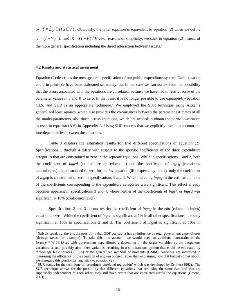
4.2 Results and statistical assessment

Equation (2) describes the most general specification of our public expenditure system. Each equation

could in principle have been estimated separately, but in our case we can not exclude the possibility

that the errors associated with the equations are correlated, because we have had to restrict some of the

parameter values in J and K to zero. In that case, it is no longer possible to use equation-by-equation

OLS, and SUR is an appropriate technique.7 We employed the SUR technique using Aitken’s

generalized least squares, which also provides the co-variances between the parameter estimates of all

the model-parameters, also those across equations, which are needed to obtain the portfolio-variance

as used in equation (A.6) in Appendix A. Using SUR ensures that we explicitly take into account the

interdependencies between the equations.

Table 3 displays the estimation results for five different specifications of equation (2).

Specifications 1 through 4 differ with respect to the specific coefficients of the three expenditure

categories that are constrained to zero in the separate equations. While in specifications 1 and 2, both

the coefficient of lnged (expenditure on education) and the coefficient of lngeg (remaining

expenditures) are constrained to zero for the lex-equation (life expectancy index), only the coefficient

of lngeg is constrained to zero in specifications 3 and 4. When including lngeg in the estimation, none

of the coefficients corresponding to the expenditure categories were significant. This effect already

becomes apparent in specifications 3 and 4, where neither of the coefficients of lngeh or lnged was

significant at 10% (confidence level).

Specifications 2 and 3 do not restrict the coefficient of lngeg in the edu (education index)

equation to zero. While the coefficient of lngeh is significant at 1% in all other specifications, it is only

significant at 10% in specifications 2 and 3. The coefficient of lnged is significant at 10% in

6 Strictly speaking, there is the possibility that GDP per capita has an influence on total government expenditures (through taxes, for example). To take this into account, we would need an additional constraint of the form: xUtWy += , with government expenditures y depending on the target variables t , the exogenous

variables x and possibly also other variables, resulting in a simultaneous system that could be estimated by three-stage least squares (3SLS) or the generalized methods of moments (GMM). Since we are interested in measuring the efficiency of the spending of a given budget, rather than explaining how that budget comes about, we disregard this possibility, and stick to equation (2). 7 SUR stands for the technique of ‘seemingly unrelated regression’ which was developed by Zellner (1962). The SUR technique allows for the possibility that different equations that are using the same data and that are supposedly independent of each other, may still have errors that are correlated across the equations (Greene, 2003).

16

specification 4 only, when it is also included in the lex equation. Still, its value is between 0.03 and

0.04 in all specifications except for those not restricting lngeg. Also, Aikaike and Schwarz-Bayesian

Information Criteria (AIC and BIC) are highest for specifications 2 and 3, so these two seem to be the

least appropriate of the five specifications. AIC and BIC are third highest for specification 4, where

neither coefficient of lngeh and lnged are significant in the lex equation.

Table 3: Estimation results

Specifications Spec 1 Spec 2 Spec 3 Spec 4 Spec 5lex

lngeh 0.0205 * 0.0204 * 0.0005 0.0005 0.0287 **lnged 0.0289 0.0290lngeglnurbr 0.0578 ** 0.0583 ** 0.0620 ** 0.0616 ** 0.0616 **lnpopd 0.0163 * 0.0165 * 0.0132 0.0130 0.0111lnempr 0.0832lneser 0.1002 *** 0.0999 *** 0.0588 0.0592 0.1086 ***lntrad 0.0418 0.0418 0.0249 0.0249 0.0425 *lntbpr -0.0420 ** -0.0419 ** -0.0491 ** -0.0492 ** -0.0432 **lnhivr -0.0266 *** -0.0266 *** -0.0293 *** -0.0293 *** -0.0253 ***gbcd -0.0418 -0.0418 -0.0312 -0.0313 -0.0460 *const -0.1840 -0.1849 0.0336 0.0346 -0.5782RMSE 0.0751 0.0751 0.0733 0.0734 0.0747R-squared 0.6549 0.6549 0.6708 0.6707 0.6585

edulngeh 0.0722 *** 0.0555 * 0.0543 * 0.0698 *** 0.0734 ***lnged 0.0379 0.0253 0.0273 0.0401 * 0.0381lngeg 0.0415 0.0401lneind 0.1375 *** 0.1202 *** 0.1211 *** 0.1380 *** 0.1384 ***lnempr 0.2985 *** 0.3046 *** 0.3018 *** 0.2958 *** 0.3080 ***lnatss 0.0685 *** 0.0616 ** 0.0620 ** 0.0685 *** 0.0676 ***gbcd 0.0307 0.0387 0.0386 0.0310 0.0307freeconst -1.7606 *** -1.8329 *** -1.8212 *** -1.7523 *** -1.8051 ***RMSE 0.1068 0.1061 0.1061 0.1068 0.1068R-squared 0.6857 0.6900 0.6900 0.6858 0.6858

gdplngeh 0.0431 *** 0.0439 *** 0.0413 *** 0.0405 *** 0.0444 ***lngedlngeg 0.0797 *** 0.0786 *** 0.0819 *** 0.0830 *** 0.0780 ***lnurbr 0.0328 ** 0.0329 ** 0.0323 ** 0.0322 ** 0.0332 **lnpopd 0.0099 ** 0.0099 ** 0.0098 ** 0.0098 ** 0.0100 **gbcd -0.0180 -0.0181 -0.0176 -0.0174 -0.0182const -0.2513 *** -0.2486 *** -0.2557 *** -0.2583 *** -0.2477 ***RMSE 0.0483 0.0483 0.0482 0.0482 0.0483R-squared 0.8923 0.8922 0.8924 0.8925 0.8922

Number of obs. 60 60 60 60 60D o F 22 23 24 23 23AIC -394.85 -393.43 -392.82 -394.26 -393.96BIC -348.78 -345.26 -342.55 -346.09 -345.79Note. Significance levels: *** 1%, ** 5%, * 10%

17

Specification 5 differs from specification 1 in the control variables. It additionally includes

lnempr in lex. Including the employment rate, which is not significant in lex, slightly improves the fit

of the regression (measured by 2R ) and lowers the mean squared error (RMSE). The value of this

coefficient is similar to those in specifications 1 and 4, but neither AIC nor BIC indicate that

specification 4 outperforms specification 1, which therefore seems to be the most appropriate.

There is no indication of either heteroscedasticity or autocorrelation, so that specification 1 is

valid and efficient. Still, as shown in our analysis in section 5.4 regarding the sensitivity of the final

outcomes with respect to specifications spec1-spec5, we do have to keep in mind that the results do

depend on the correct specification of the model. From now on we will concentrate on the results from

specification 1, to show the applicability of the EDP method to developing development policies.

4.3 Results and impact of policy instruments on HDI components

As the signs of the coefficients of all types of government expenditures in Table 3 are positive, an

increase in government spending improves the value of the individual HDI components. However, not

all expenditure categories are equally important for all the HDI components. Only government

expenditures on health seem to have an impact on the life expectancy index. These expenditures are

also important for the other two indices (edu and gdp). Education expenditures have a lower impact

(about 0.038) on the education index than health expenditures (about 0.072). Remaining government

expenditures are not significant for lex or edu, but are important for the GDP index (the coefficient is

positive and significant at 1%).

The index for life expectancy at birth is higher if urbanization rate (lnurbr), population density

(lnpopd), employment rate (lnempr), share of services in total value added (lneser), and trade as

percentage of total value added (lntrad) are higher, and if tuberculosis and HIV prevalence rate are

lower. Former British colonies (gbcd) seem to have a lower life expectancy at birth index but better

education index than former non-British colonies. The share of industry in total value added (lneind),

the employment rate (lnempr), and the percentage of population with access to safe sanitation (lnatss)

have a positive impact on the education index. The GDP index (gdp) is positively influenced by the

degree of urbanization (lnurbr) and higher population density (lnpopd). Again, being a former British

colony has a negative, though not very significant, impact.

18

5. Portfolio Application Results

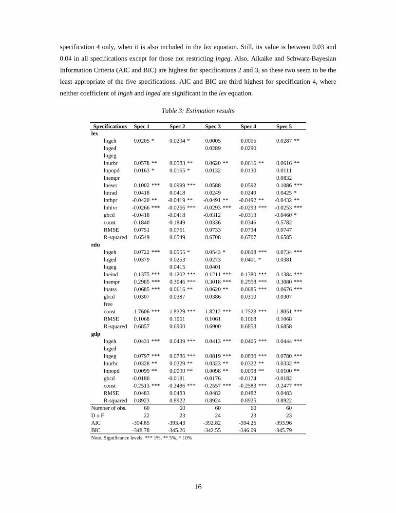
5.1 Tracing the EPF

Given the estimates for the matrices J and K, including the cross-equation co-variances of the

parameter estimates, the variance of the HDI (V) can be calculated as described in Appendix A,

equation (A.6), and the EDP optimization problem, equation (A.7), can be solved for every country

and for every year for which a full data-set is available. The EPF for a given budget for some country

in some year can be (graphically) traced by calculating a sequence of optimum development

portfolio’s for a range of values of the risk-aversion parameterα . In our case, the range for all values

of α is given by x5.1=α for all integer values of x from -19 to 9, implying that α increases by 50

percent for each unit increase in x.8 We also varied the budget over a range as given by aB 250⋅=

for all integer values of a in between 0 and 6 (cf. varying colors in Figures 2a and 2b). This budget

range coincides with the observed range of variation for the actual budgets over the countries and

years under consideration. The actual ETH 1995 (Ethiopia) per capita budget is only slightly higher

than the budget low-bound of 50$ per capita, while MUS 2005 (Mauritius) is close to the budget

high-bound of 3200$ per capita. In addition to this, we traced the EPF for the actually observed per

capita budget (black curve). In the graphs, the variance (V) of an efficient development portfolio is

plotted against its corresponding HDI-value (H).9 The resulting EPF has a convex shape, as we would

expect, given the resemblance of our EDP-composition-problem with an ‘ordinary’ OPF-problem. The

results shown below include the actual HDI given by UNDP (represented by the vertical line), and the

predicted HDI from our model (obtained by substituting equation (2) into (1)) and its corresponding

variance for the actual budget (denoted by the position of the ‘star’). Therefore, if the actual budget

would be spent efficiently, the ‘star’ would need to be on the black EPF, save for the occurrence of

random shocks in the contribution to the various targets of our model variables. Each point in the V,H-

plane corresponds to a specific probability distribution, the higher the variance, the thicker the tails of

the corresponding distribution and hence, the more likely to draw an HDI value that is further away

from the expected value. Burkina Faso (Figure 2a), for example, has been ‘unlucky’, while Botswana

(Figure 2b) has had a lucky draw as the actual HDI of the latter country exceeds the predicted HDI,

and that of the former country falls below the predicted value. We will come back to this in more

8 We found no significant numerical trouble in calculating the OPF’s for this wide range of values, but for even

slightly wider ranges we did. For 205.1 −=α LSO 2005 starts giving numerical trouble. Such trouble also arises

for 105.1≥α . However, the remaining range for α is wide enough to be empirically relevant, as the implied slopes of the iso-valuation lines get close enough to zero and infinity. 9 To avoid numerical problems, we have multiplied the K and J matrices by a factor 103, and the elements of the

covariance matrix Ω by 106 (Var(1000x) = 1000²Var(x)) in order to retain a sufficient degree of numerical precision while tracing the EPFs for a wide range of α ’s. This has the effect of multiplying the expected HDI and its standard-deviation (being the square root of the variance) by a factor 103 as well.

19

detail in the next section that deals with the measurement of the impact of policy inefficiencies and

pure chance on HDI scores.

The sequence of EPFs obtained by varying the budget over the budget-range of 50-3200

dollars per capita can essentially be classified using two different ‘shape-classes’. First, there are EPF

sequences that have (near) constant variance for low budgets, but then increasing variance for higher

budgets (and correspondingly higher levels of HDI) for the highest value of α (i.e. the low-end of the

EPF). An example that falls into this particular ‘increasing’ shape-class is Burkina Faso in 1995, see

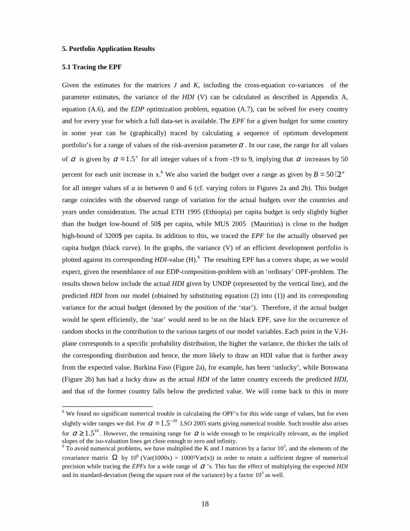
Figure 2a10. But sometimes it is the case that for the lowest budgets, the low-ends of the low budget-

EPFs exceed those of higher budget EPFs. This suggests that in some cases, an expansion of the

budget may give rise to a ‘development double dividend’ for risk-averse development policy makers:

they could simultaneously improve their HDI score and reduce the riskiness of that score by

increasing spending. In fact, in the example provided in Figure 2b, we see that the Botswana policy-

makers have apparently been able to identify the size of the budget for which the double dividend

becomes a trade-off between risk and return again, since an increase in the budget above the actual

budget would tend to raise HDI but at the expense of a higher associated risk. The shape explained

here is called ‘U-shape’ in the remainder of the article. 11

Figure 2a: EPFs in Burkina Faso (1995)

400 500 600 700H

250

500

750

1000

1250

1500

1750

V BFA1995 ,BUDG 50 3200

10 One should keep in mind that the observations for 1995 are actually the 5 year averages over the years 1993-1997. The same holds, mutatis mutandis, for the observations for 2000 and 2005. 11 Strictly speaking, it is possible that there is only one U-shaped class, of which the monotonically increasing shape class is a special case (i.e. numerically covering only the right-arm of the U-shape). For the moment this question is left for future research.

20

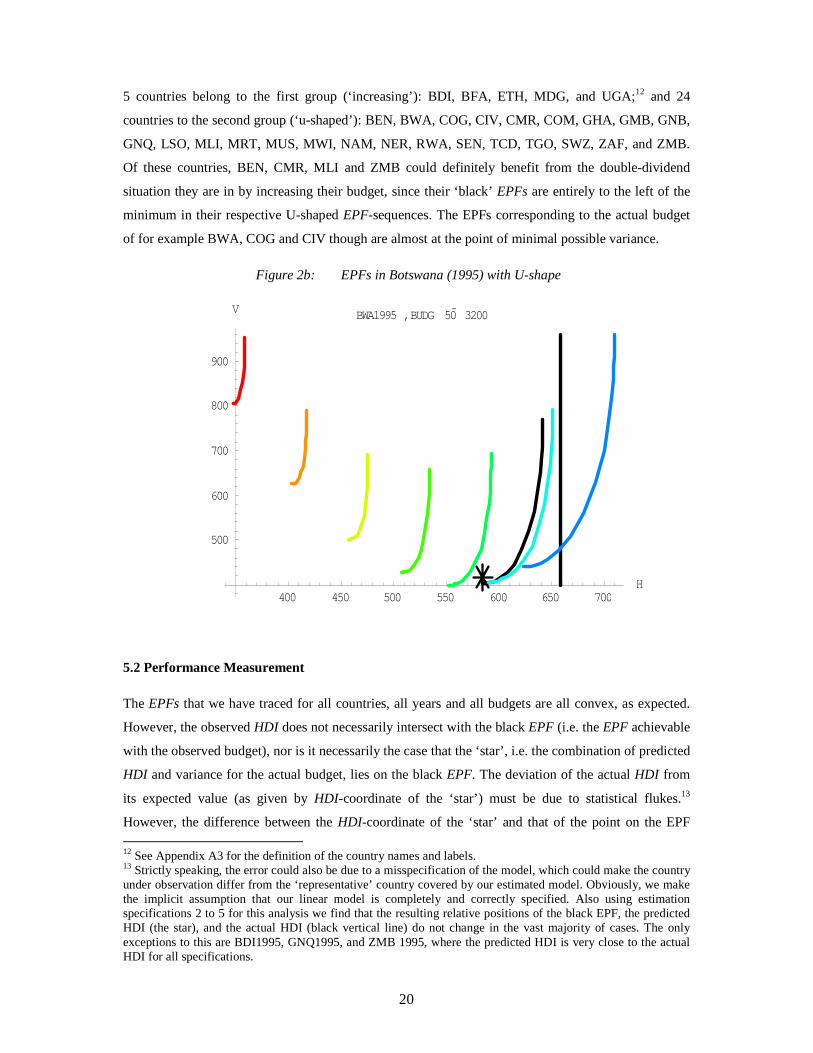
5 countries belong to the first group (‘increasing’): BDI, BFA, ETH, MDG, and UGA;12 and 24

countries to the second group (‘u-shaped’): BEN, BWA, COG, CIV, CMR, COM, GHA, GMB, GNB,

GNQ, LSO, MLI, MRT, MUS, MWI, NAM, NER, RWA, SEN, TCD, TGO, SWZ, ZAF, and ZMB.

Of these countries, BEN, CMR, MLI and ZMB could definitely benefit from the double-dividend

situation they are in by increasing their budget, since their ‘black’ EPFs are entirely to the left of the

minimum in their respective U-shaped EPF-sequences. The EPFs corresponding to the actual budget

of for example BWA, COG and CIV though are almost at the point of minimal possible variance.

Figure 2b: EPFs in Botswana (1995) with U-shape

400 450 500 550 600 650 700H

500

600

700

800

900

V BWA1995 ,BUDG 50 3200

5.2 Performance Measurement

The EPFs that we have traced for all countries, all years and all budgets are all convex, as expected.

However, the observed HDI does not necessarily intersect with the black EPF (i.e. the EPF achievable

with the observed budget), nor is it necessarily the case that the ‘star’, i.e. the combination of predicted

HDI and variance for the actual budget, lies on the black EPF. The deviation of the actual HDI from

its expected value (as given by HDI-coordinate of the ‘star’) must be due to statistical flukes.13

However, the difference between the HDI-coordinate of the ‘star’ and that of the point on the EPF 12 See Appendix A3 for the definition of the country names and labels. 13 Strictly speaking, the error could also be due to a misspecification of the model, which could make the country under observation differ from the ‘representative’ country covered by our estimated model. Obviously, we make the implicit assumption that our linear model is completely and correctly specified. Also using estimation specifications 2 to 5 for this analysis we find that the resulting relative positions of the black EPF, the predicted HDI (the star), and the actual HDI (black vertical line) do not change in the vast majority of cases. The only exceptions to this are BDI1995, GNQ1995, and ZMB 1995, where the predicted HDI is very close to the actual HDI for all specifications.

21

with the same V-coordinate must be due to inefficiencies in the allocation of the public development

budget. This non-stochastic part of the extended efficiency losses associated with such inefficiency

can be removed by changing the budget allocation such that the ‘star’ will be on the (black) EPF.

Recall that the extended efficiency is the objective function value Θ , i.e. the positively valued HDI

minus its variance multiplied by α . In this section we will measure the minimum amount by which

extended efficiency could be improved for a given budget, by efficiently spending that budget.

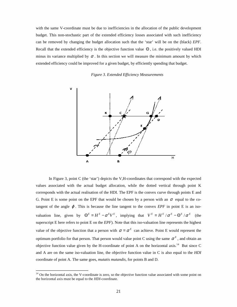
Figure 3. Extended Efficiency Measurements

In Figure 3, point C (the ‘star’) depicts the V,H-coordinates that correspond with the expected

values associated with the actual budget allocation, while the dotted vertical through point K

corresponds with the actual realisation of the HDI. The EPF is the convex curve through points E and

G. Point E is some point on the EPF that would be chosen by a person with an α equal to the co-

tangent of the angle ϕ . This is because the line tangent to the convex EPF in point E is an iso-

valuation line, given by EEEE VH α−=Θ , implying that EEEEE HV αα // Θ−= (the

superscript E here refers to point E on the EPF). Note that this iso-valuation line represents the highest

value of the objective function that a person with Eαα = can achieve. Point E would represent the

optimum portfolio for that person. That person would value point C using the same Eα , and obtain an

objective function value given by the H-coordinate of point A on the horizontal axis.14 But since C

and A are on the same iso-valuation line, the objective function value in C is also equal to the HDI

coordinate of point A. The same goes, mutatis mutandis, for points B and D.

14 On the horizontal axis, the V-coordinate is zero, so the objective function value associated with some point on the horizontal axis must be equal to the HDI-coordinate.

22

In order to measure the potential size of extended efficiency improvements due to more

efficient spending, we would like to know the minimum improvement that people could achieve by

moving from a point like C to some point on the EPF, say a point like E, i.e. we are looking for (a

person with) a degree of risk-aversion Eα that implicitly defines point E such that the extended

efficiency gain (∆Θ ) from the move from C to E would be minimal. Hence, having any other degree

of risk aversion results in an even larger gain, implying that everybody will at least be as well off as

the person with risk-aversion Eα .

The extended efficiency gain from a move from C to E is given by:

)( CEECECE VVHH −−−=Θ−Θ=∆Θ α (4)

A movement along the EPF can be interpreted as a change in V that comes from a change in H

that in turn is caused by a change in Eα . But then, minimisation of (4) with respect to Eα implies:

0)( =∂∂

∂∂−−−

∂∂=

∂∆Θ∂

E

E

E

EECE

E

E

E

H

H

VVV

H

αα

αα (5)

Since EE HV ∂∂ / is the slope of the EPF in point E, we must have that EEE HV α/1/ =∂∂ . But then

(5) implies that CE VV = , i.e. the point on the EPF that represents the smallest improvement of the

objective function relative to point C must have the same V-coordinate as point C. Hence, the point we

are looking for must be point G 15, and the extended efficiency gain involved in moving from C to G is

given by the length of the line-segment in between those two points and is measured in HDI-units.

Note, however, that the corresponding extended efficiency levels (in equivalent HDI-terms) are given

by the HDI coordinates of the points of intersection of the parallel dotted lines (with single arrow

heads) through C and G with the horizontal axis. 16

Unfortunately, the extended efficiency function that we use does not have a ‘natural’ point

zero. People with high degrees of risk-aversion may be faced with negative values of the objective

15 The second derivative 0///22 >∂∂⋅∂−∂=∂∆Θ∂ EEEEE HHV αα since a higher degree of risk-

aversion would lower both H and V, i.e. 0/ <∂∂ EEH α . The extended efficiency gain is therefore indeed

minimised when moving from C to G, since the second derivative is positive.

16 Obviously, since the dotted lines with single arrows in Figure 3 are parallel, the HDI-difference between points C and G is exactly equal to the HDI difference between points A and B. The latter difference, however, represents the extended efficiency difference between points A and B (since the variance component is zero in both points A and B), and so the HDI-difference between points C and G is also equal to the extended efficiency difference between these points, we can therefore interchange extended efficiency and HDI differences, as we have done in Figure 3.

23

function and be perfectly happy with that. In that case relative changes in the objective function value

make little sense, even though absolute changes still do. We will therefore provide information in

terms of absolute changes.

The extended efficiency contributions of both the transitory and the structural components are

shown in Figure 4 for all country/year combinations for which a full data-set is available. The

calculations are based on Figure 3, where point G is the point of reference, and the total extended

efficiency surplus consists of two components, since GCCKGK Θ−Θ+Θ−Θ=Θ−Θ . The

first bracketed term represents the extended efficiency surplus over the expected value of extended

efficiency, given the way in which the budget was spent in actual fact (if positive, we were lucky). The

second bracketed term represents the extended efficiency surplus of the way in which the actual

budget was spent over the extended efficiency associated with an efficient spending of the same

budget. Obviously, one would expect the latter surplus to be negative, or at most equal to zero if the

actual budget allocation would have proved to be efficient, and this is what we can observe in Figure

417, where the extended efficiency changes mentioned above have been expressed in equivalent HDI

changes (see Figure 3 and note 16).

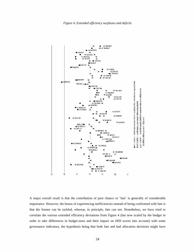
5.3 Allocation inefficiencies

Figure 4 below has some striking features. First of all, allocation inefficiencies are relatively important

for Burundi (BDI), and consistently so. At the same time, the contribution of pure chance has been of

limited size, so that the negative extended efficiency effects for Burundi are mainly structural in

nature. However, these extended efficiency deficits could be fixed, by adopting more efficient

spending programs. By contrast, Ethiopia (ETH) has consistently been lucky, although the

contribution of pure luck has fallen and that of efficient resource allocation has risen over time. Other

countries that have seriously suffered from bad luck, which is defined here as a transitory loss of more

than 5 percentage points are BWA2005, BFA1995, BFA2005, GMB1995, LSO2005, MLI2000,2005,

RWA2005, SEN2005 whereas such countries as BWA1995, CMR2000,2005, GHA1995, MDG2000,

NAM1995,2000, ZAF1995, but also TOG1995-2000 and UGA1995 have been lucky using the same

measure.

17 There are some minor positive deviations, however, that are due to the fact that we obtain the value of Gα numerically using Mathematica’s Interpolation function that represents the black EPF as an interpolation of the outcomes of the efficient combinations of V and H that we have calculated for the range of α ’s discussed above. We then invert this interpolated function to obtain the α corresponding to a certain value of the variance V. This variance V is the value that we can calculate using equation (A.6) for the observed budget allocation. The resulting value of α is then used to evaluate the implied objective function value for that interpolated value of V, as we also have obtained HDI along the EPF as an interpolated function of α .

24

Figure 4. Extended efficiency surpluses and deficits

A major overall result is that the contribution of pure chance or ‘fate’ is generally of considerable

importance. However, the bonus of experiencing inefficiencies instead of being confronted with fate is

that the former can be tackled, whereas, in principle, fate can not. Nonetheless, we have tried to

correlate the various extended efficiency deviations from Figure 4 (but now scaled by the budget in

order to take differences in budget-sizes and their impact on HDI scores into account) with some

governance indicators, the hypothesis being that both fate and bad allocation decisions might have

25

something to do with the lack of quality of governance. To this end, we calculated the correlations (K-

tau and Spearman because of their small sample properties) between extended efficiency deviations

and different governance indicators. The latter are the Freedom house political rights (FHPR) and civil

liberty (FHCL) index and a combination of these two, called FREE.18

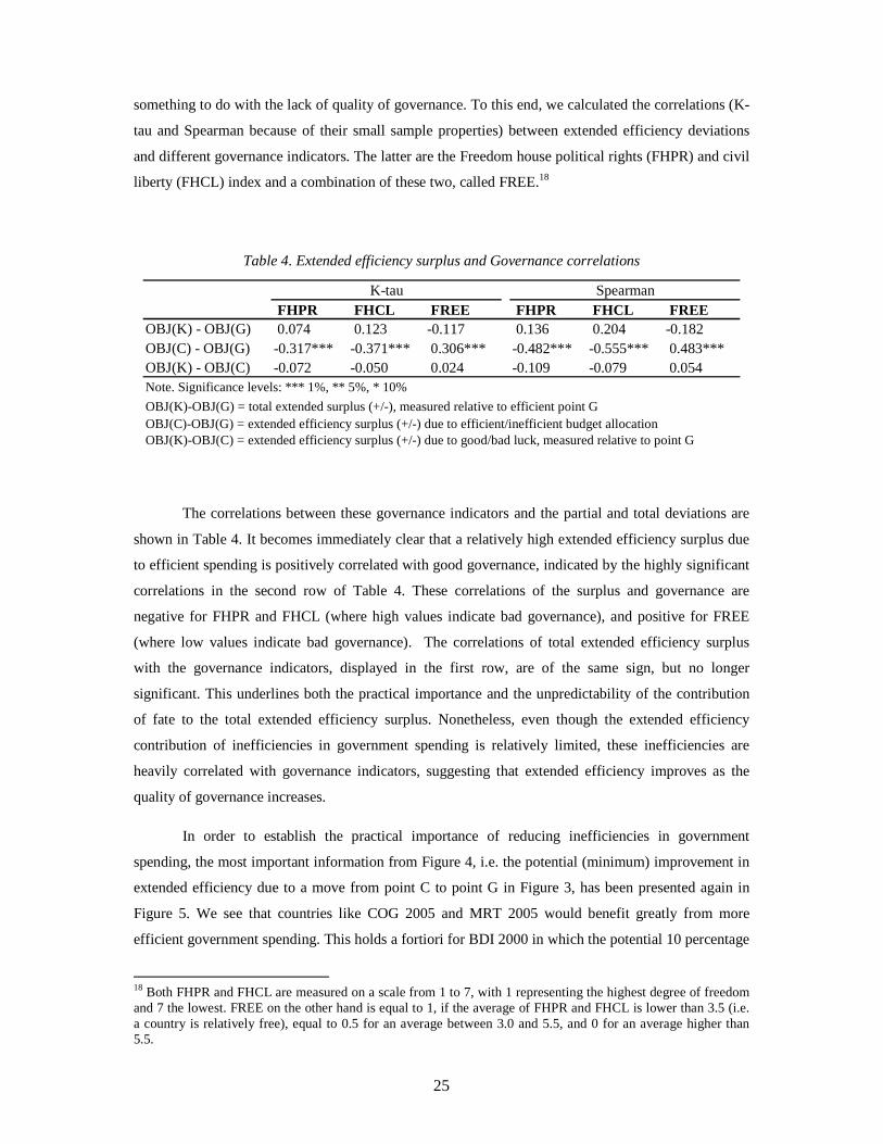
Table 4. Extended efficiency surplus and Governance correlations

FHPR FHCL FREE FHPR FHCL FREEOBJ(K) - OBJ(G) 0.074 0.123 -0.117 0.136 0.204 -0.182OBJ(C) - OBJ(G) -0.317*** -0.371*** 0.306*** -0.482*** -0.555*** 0.483***OBJ(K) - OBJ(C) -0.072 -0.050 0.024 -0.109 -0.079 0.054Note. Significance levels: *** 1%, ** 5%, * 10%

OBJ(K)-OBJ(G) = total extended surplus (+/-), measured relative to efficient point GOBJ(C)-OBJ(G) = extended efficiency surplus (+/-) due to efficient/inefficient budget allocationOBJ(K)-OBJ(C) = extended efficiency surplus (+/-) due to good/bad luck, measured relative to point G

K-tau Spearman

The correlations between these governance indicators and the partial and total deviations are

shown in Table 4. It becomes immediately clear that a relatively high extended efficiency surplus due

to efficient spending is positively correlated with good governance, indicated by the highly significant

correlations in the second row of Table 4. These correlations of the surplus and governance are

negative for FHPR and FHCL (where high values indicate bad governance), and positive for FREE

(where low values indicate bad governance). The correlations of total extended efficiency surplus

with the governance indicators, displayed in the first row, are of the same sign, but no longer

significant. This underlines both the practical importance and the unpredictability of the contribution

of fate to the total extended efficiency surplus. Nonetheless, even though the extended efficiency

contribution of inefficiencies in government spending is relatively limited, these inefficiencies are

heavily correlated with governance indicators, suggesting that extended efficiency improves as the

quality of governance increases.

In order to establish the practical importance of reducing inefficiencies in government

spending, the most important information from Figure 4, i.e. the potential (minimum) improvement in

extended efficiency due to a move from point C to point G in Figure 3, has been presented again in

Figure 5. We see that countries like COG 2005 and MRT 2005 would benefit greatly from more

efficient government spending. This holds a fortiori for BDI 2000 in which the potential 10 percentage

18 Both FHPR and FHCL are measured on a scale from 1 to 7, with 1 representing the highest degree of freedom and 7 the lowest. FREE on the other hand is equal to 1, if the average of FHPR and FHCL is lower than 3.5 (i.e. a country is relatively free), equal to 0.5 for an average between 3.0 and 5.5, and 0 for an average higher than 5.5.

26

point increase in HDI represents a proportional increase of 30 percent relative to the expected HDI,

which is extremely low to start with for BDI 2000, i.e. slightly above 30 percent. For some other

countries too, more efficient government spending can bring about relative changes in those countries’

HDI of more than 10 percent. Examples are MWI 1995, MLI 2000, GNQ 2000 and LSO 2000. Given

that the average HDI of the sample countries is 0.47, for most countries the potential increase in HDI

is limited to less than 10 percent of the expected HDI. Nonetheless, an increase of even a few

percentage points in the HDI of a country may be of considerable practical importance for the people

involved, as it could make the difference between being just alive and being able to make a living.

Figure 5. Possible improvement in HDI (in % points) with efficient spending

The question now is what the removal of inefficiencies requires in terms of the reallocation of

the government budget. To answer this question, we have calculated the percentage point differences

between the budget distributions in points G and point K in Figure 3, for each country/year

combination for which we have a complete data-set. In order to be able to assess the practical

significance of the changes in the budget allocation thus calculated, we also present the actual budget

allocation as a radar plot in Figure 6, to give an impression of the size of the numbers involved and the

variation in these numbers over countries and over time. Figure 7 contains the differences between the

efficient budget distribution and the actual budget distribution over the three categories, i.e. the

percentage point change in the budget allocation that would be needed to make the development

portfolio efficient and to realize the percentage point HDI gains shown in Figure 5.

27

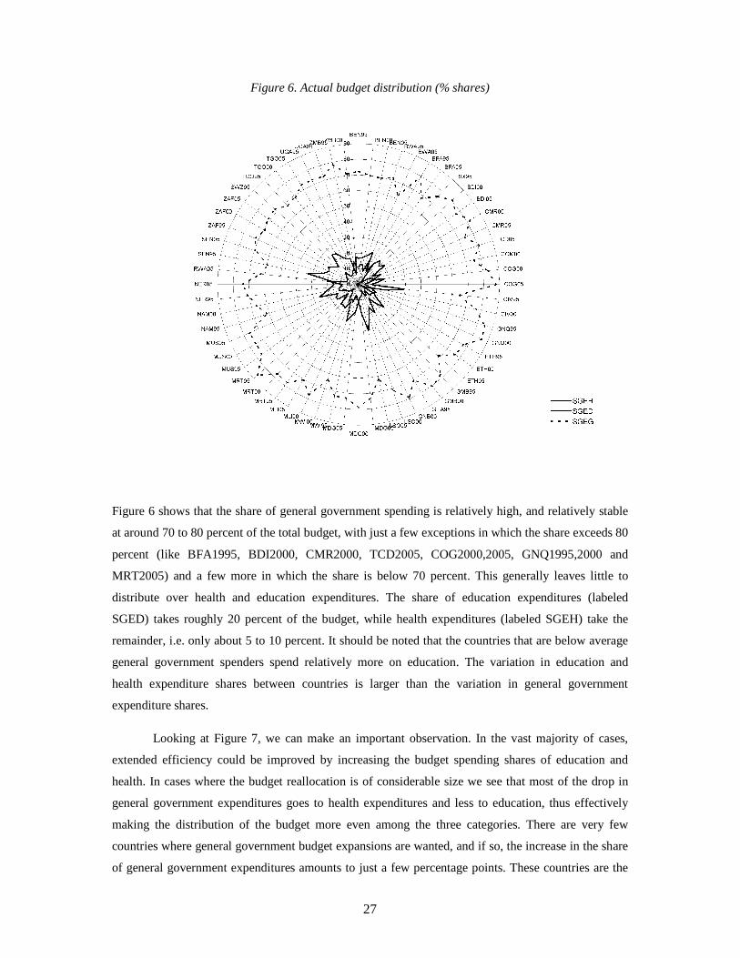
Figure 6. Actual budget distribution (% shares)

Figure 6 shows that the share of general government spending is relatively high, and relatively stable

at around 70 to 80 percent of the total budget, with just a few exceptions in which the share exceeds 80

percent (like BFA1995, BDI2000, CMR2000, TCD2005, COG2000,2005, GNQ1995,2000 and

MRT2005) and a few more in which the share is below 70 percent. This generally leaves little to

distribute over health and education expenditures. The share of education expenditures (labeled

SGED) takes roughly 20 percent of the budget, while health expenditures (labeled SGEH) take the

remainder, i.e. only about 5 to 10 percent. It should be noted that the countries that are below average

general government spenders spend relatively more on education. The variation in education and

health expenditure shares between countries is larger than the variation in general government

expenditure shares.

Looking at Figure 7, we can make an important observation. In the vast majority of cases,

extended efficiency could be improved by increasing the budget spending shares of education and

health. In cases where the budget reallocation is of considerable size we see that most of the drop in

general government expenditures goes to health expenditures and less to education, thus effectively

making the distribution of the budget more even among the three categories. There are very few

countries where general government budget expansions are wanted, and if so, the increase in the share

of general government expenditures amounts to just a few percentage points. These countries are the

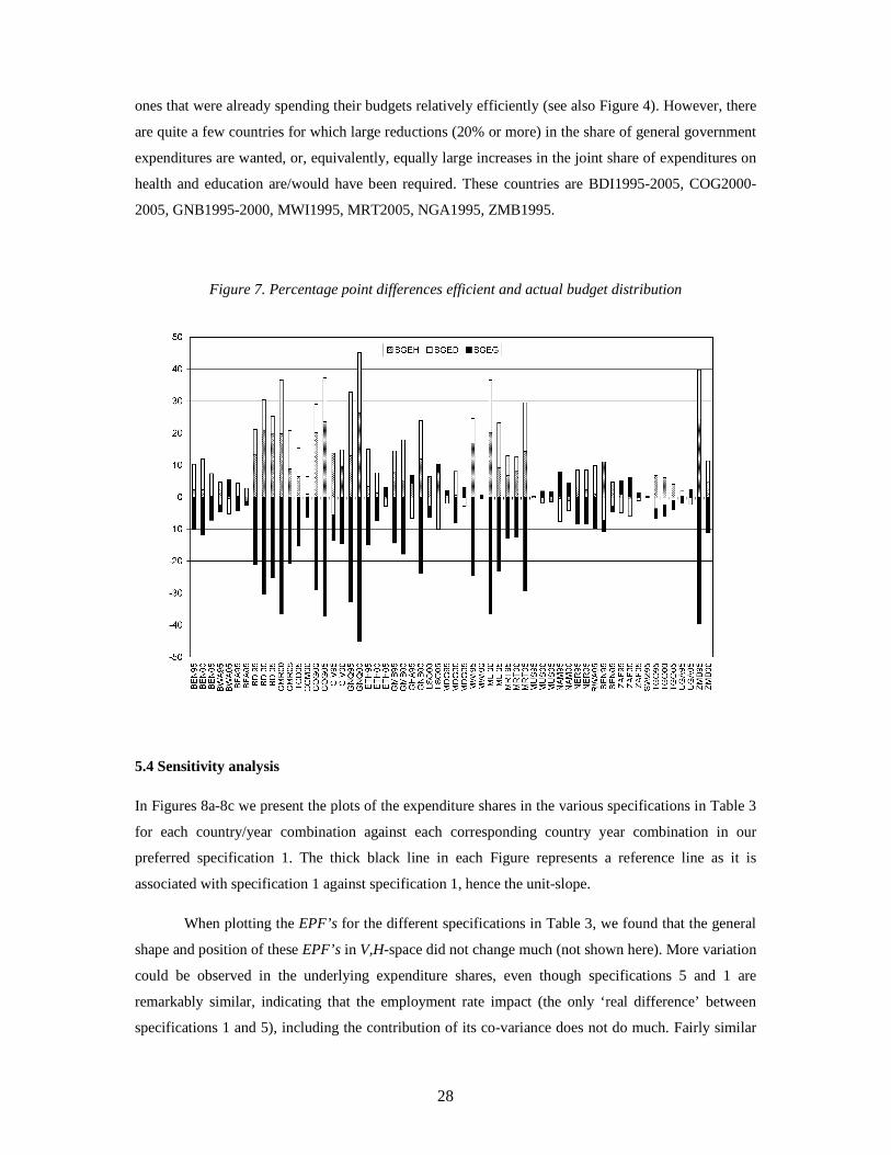
28

ones that were already spending their budgets relatively efficiently (see also Figure 4). However, there

are quite a few countries for which large reductions (20% or more) in the share of general government

expenditures are wanted, or, equivalently, equally large increases in the joint share of expenditures on

health and education are/would have been required. These countries are BDI1995-2005, COG2000-

2005, GNB1995-2000, MWI1995, MRT2005, NGA1995, ZMB1995.

Figure 7. Percentage point differences efficient and actual budget distribution

5.4 Sensitivity analysis

In Figures 8a-8c we present the plots of the expenditure shares in the various specifications in Table 3

for each country/year combination against each corresponding country year combination in our

preferred specification 1. The thick black line in each Figure represents a reference line as it is

associated with specification 1 against specification 1, hence the unit-slope.

When plotting the EPF’s for the different specifications in Table 3, we found that the general

shape and position of these EPF’s in V,H-space did not change much (not shown here). More variation

could be observed in the underlying expenditure shares, even though specifications 5 and 1 are

remarkably similar, indicating that the employment rate impact (the only ‘real difference’ between

specifications 1 and 5), including the contribution of its co-variance does not do much. Fairly similar

29

are the results of specification 1 and 4. Still, specification 4 involves a structural three percentage point

change in the share of education expenditures at the expense of general expenditures. This is because

education now also has an impact on health, so there is a double-dividend to education expenditures in

specification 4 as compared to specification 1.

Figure 8a. Health expenditure sensitivity results

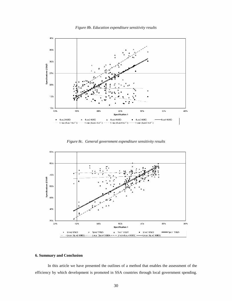
There is a striking difference between specifications 2 and 3 on the one hand, and

specification 1 on the other. The cause of the difference is the relatively large positive coefficient of

lngeg in the edu equation in combination with that coefficient being insignificant, i.e. showing a

relatively large (co-)variance. Both aspects are important, because on the one hand the double

dividend of general expenditures now raises the share of the latter, while on the other hand the

increased contribution of lngeg to portfolio variance introduces a motive to move out of these

expenditures, and more so if these expenditures are relatively high raising the other expenditure shares

in the process. This has the effect of reducing the slopes of the lines reflecting the correlations between

specifications 2 and 3 on the one hand and specification 1 on the other. Still, according to the

econometric model, lngeg is not significant in edu, and even though the adjusted R-squared suggest a

better fit of either specifications 2 or 3, the Aikaike and Bayesian-Schwarz Information Criteria are

higher for these two specifications compared to the other three specifications, suggesting that

specifications 1, 4, and 5 are to be preferred over specifications 2 and 3 on purely statistical grounds.

30

Figure 8b. Education expenditure sensitivity results

Figure 8c. General government expenditure sensitivity results

6. Summary and Conclusion

In this article we have presented the outlines of a method that enables the assessment of the

efficiency by which development is promoted in SSA countries through local government spending.

31

We describe the process of development through its associated impact on the Human Development

Index (HDI). A sensitivity analysis concerning the widely criticized linear aggregation scheme with

equal weights for the three indexes is left for future research. The purpose of the present exercise is to

show the application possibilities of the method in this field.

To this end, we estimate a simple cross SSA country simultaneous system of equations that

links government expenditures on the three HDI components to the scores on the three HDI

components in a setting that allows for exogenous differences between countries that would determine

the general setting in which the underlying development processes are taking place, and that define in

part the effectiveness of government spending in raising the HDI components. By estimating this

system of equations, we obtain measures of the risk associated with using the three spending

instruments. We make the assumption that policy-makers are risk-averse, implying that they would

prefer a policy outcome of spending a given budget on the three HDI components with a particular

expected value of the HDI outcome and a corresponding variance of that outcome above a policy with

the same expected HDI but a higher variance of that outcome. This setting resembles the one known

from Optimum Portfolio Theory (OPT), but it extends the OPT setting by allowing for multiple

constraint on the use of (policy-) instruments. In our case, the simultaneous estimation model forms an

additional set of constraints next to the government budget adding-up constraint and the one that links

the value of the HDI to its components.

In our setting, an efficient development portfolio is a distribution of the government budget

that minimizes the variance of the HDI for a given expected value of the HDI. We find that the EPF’s

can be represented as convex upward sloping graphs in the variance, HDI-plane. Using this setting, we

are able to define a point on the EPF of each SSA country that marks the minimum increase in

extended efficiency (a measure that includes both the expected HDI and its variance) that could be

realized by an efficient spending of the government budget. We then show how the actual performance

of each SSA country can be split into a transitory component brought upon these countries by good or

bad luck, and a structural component that is linked to good/bad budget allocation decision making. We

show that the good/bad luck component is of considerable importance. However, to some extent it

may be the case that what we have called ‘luck’, is actually a ‘measure of our ignorance’. For now we

have to leave the potential reduction of that ignorance for future research.

The structural extended efficiency loss component is correlated with a number of governance

indicators pointing to the ‘rule of thumb’ that good governance is associated with efficient budget

spending and bad governance with inefficient spending. We also show that the changes in the

composition of the budget for countries that are spending inefficiently are considerable, i.e.

expenditures on health and education should be increased by 20 percentage points or more, whereas in

most cases expenditures on health and education are of the order of 20 percent to start with. Hence,

32

efficient reallocation requires a doubling of the health and education budget, and a more equal

distribution of the overall budget over the three expenditure categories. For some countries, general

government expenditures need to be raised, but only by a small amount, and the other categories need

to be adjusted accordingly. This is the case only for countries that are already spending relatively

efficiently.

The sensitivity analysis we performed led to the conclusion that the shape and position of the

EPF as well as the predicted HDI are robust to different estimation specifications, while the necessary

budget changes to get to the EPF show more variability. Using specifications with insignificant

parameter contributions by some expenditure category does introduce a bias against using that

category through its relatively high (co-) variance in combination with risk-aversion. We conclude that

estimating the model correctly is essential for applying the method and interpreting the results.

33

Appendix A. Derivation of the EDP FOC’s

In this appendix we show how the FOC’s can be derived that implicitly describe the solution

to the maximization problem provided in (3). First, it should be noted that errors in H can only be

caused by errors in t. Hence, from (1) it follows that:

Ti tH /εε ′= (A.1)

Moreover, assuming that we know both y and x with absolute certainty19, it follows from (2) that:

xyxKKyJJxKyJxKyJtt KJt εεε +=−+−=−−+=−= )ˆ()ˆ()ˆˆ()(ˆ (A.2)

Note that (A.2) assumes that there are no measurement errors in x or implementation errors in y nor

any other (forecast) errors. Using (A.1), the variance in the HDI is given by:

2

1 1

22 /)(/)()/()( TETiEiTiiEEV tj

T

i

T

j

ti

ttttHH εεεεεεεε ∑∑= =

=′′=

′′=′

= (A.3)

with

=′⋅tttttt

tttttt

tttttt

tt

332313

322212

312111

εεεεεεεεεεεεεεεεεε

εε .

In equation (A.3) tiε is the i-th element in the error-vectortε , i.e. it represents the error (i.e. the

deviation from expectation) in target variable i. Using equation (A.2), it follows that:

∑∑==

+=X

ll

Kli

T

kk

Jki

ti xy

1,

1, εεε (A.4)

Substituting (A.4) into (A.3), we get:

∑∑∑∑

∑∑∑∑

====

====

+

++=⋅

X

mm

Kmj

Kki

X

kk

X

mm

Jmj

Kki

X

kk

X

mm

Kmj

Jki

Y

kk

Y

mm

Jmj

Jki

Y

kk

tj

ti

xExyEx

xEyyEyE

1,,

11,,

1

1,,

11,,

1

)()(

)()()(

εεεε

εεεεεε (A.5)

19 The assumption that we know y with certainty is always valid as policy makers set the amount of

government spending. However, it is possible that x cannot be known with complete certainty due to measurement errors or something similar, in which case we would also have to include the variation in x in the

calculation of tε . Even though it is relatively straight forward to include this source of variance (by means of a

linearization of the term xK in equation (A.2) around its expected value), we haven’t done this here for reasons

of simplicity.

34

The expectation terms in equation (A.5) actually refer to specific elements from the co-variance matrix

of the parameter estimates of our linear system. This co-variance matrix is symmetric, and consists of

T2 sub-matrices (associated with each combination of targets) further called Yjiji ..1,, =∀Ω with

dimensions (Y+X) × (Y+X). Each sub-matrix in turn is partitioned into 4 sub-matrices of dimensions

Y×Y, Y×X, X×Y and X×X, further called YYji ,Ω , YX

ji ,Ω , XYji ,Ω and XX

ji ,Ω , respectively (see also Figure A.1

below). YYji ,Ω is the co-variance matrix between the expenditure parameter estimates (as captured by

the J matrix in equation (2)) for the target variables i and j, while YXji ,Ω is the co-variance matrix of the

expenditure parameter estimates in the equation for target variable i and the parameter estimates of the

exogenous variables (as captured by the matrix K) in the equation for target variable j. XYji ,Ω and XX

ji ,Ω

are similarly defined. Using this notation, it follows from (A.3) and (A.5) that the variance in H, i.e. V,

can be written as:

( )xxyxxyyy

xxyxxyyyTV

XXXYYXYY

T

i

T

j

XXji

XYji

YXji

YYji

Ω+Ω+Ω+Ω⋅=

=Ω+Ω+Ω+Ω= ∑∑= =

''''

''''/11 1

,,,,2

(A.6)

where ZΩ represents the arithmetical average over all XXYXXYYYZZji ,,,, =∀Ω .20

Replacing t in (1) by (2), and inserting (2) into the objective function, the Lagrangian of the

maximization problem (3) is given by:

))((/)ˆˆ())((ˆ yExpiBVTxKyJiyExpiBVH ′−+−+′=′−+−=Φ λαλα (A.7)

where λ is the Lagrange multiplier of the budget constraint, and )(yExp stands for the column-

vector ))(..)()(( 21 ′TyExpyExpyExp . Maximizing (A.7) by a suitable choice of y results in the

following FOC for y:

0)()()(ˆ

)(ˆ

=−

′Ω+Ω+′Ω+Ω−′

=

=−∂∂−

′=

∂Φ∂

yExpxyT

iJ

yExpy

V

T

iJ

y

XYYXYYYY λα

λα (A.8)

Note that equations (A.8) and the per capita budget constraint )(yExpiB ′= define T+1 non-linear

simultaneous equations in the T+1 unknowns y and λ , the solution of which we obtain using

20 Note that the term 1/T2 vanishes in the RHS of (A.6) since ∑∑Ω≡Ωi j

Zji

Z T 2, / .

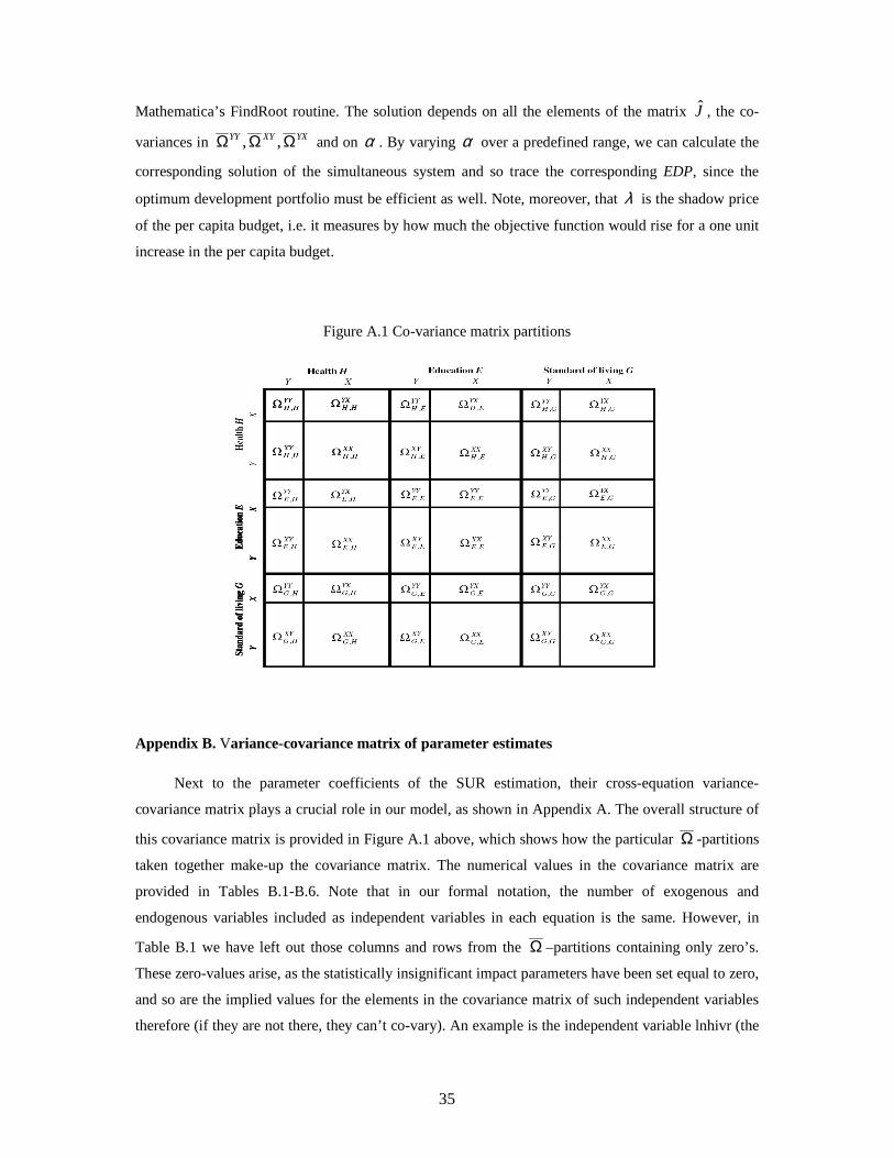
35

Mathematica’s FindRoot routine. The solution depends on all the elements of the matrix J , the co-

variances in YXXYYY ΩΩΩ ,, and on α . By varying α over a predefined range, we can calculate the

corresponding solution of the simultaneous system and so trace the corresponding EDP, since the

optimum development portfolio must be efficient as well. Note, moreover, that λ is the shadow price

of the per capita budget, i.e. it measures by how much the objective function would rise for a one unit

increase in the per capita budget.

Figure A.1 Co-variance matrix partitions

Appendix B. Variance-covariance matrix of parameter estimates

Next to the parameter coefficients of the SUR estimation, their cross-equation variance-

covariance matrix plays a crucial role in our model, as shown in Appendix A. The overall structure of

this covariance matrix is provided in Figure A.1 above, which shows how the particular Ω -partitions

taken together make-up the covariance matrix. The numerical values in the covariance matrix are

provided in Tables B.1-B.6. Note that in our formal notation, the number of exogenous and

endogenous variables included as independent variables in each equation is the same. However, in

Table B.1 we have left out those columns and rows from the Ω –partitions containing only zero’s.

These zero-values arise, as the statistically insignificant impact parameters have been set equal to zero,

and so are the implied values for the elements in the covariance matrix of such independent variables

therefore (if they are not there, they can’t co-vary). An example is the independent variable lnhivr (the

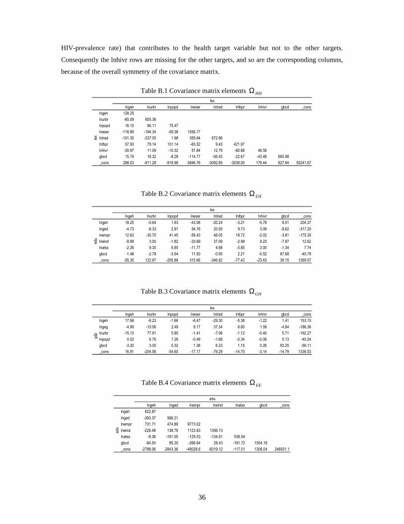
36

HIV-prevalence rate) that contributes to the health target variable but not to the other targets.

Consequently the lnhivr rows are missing for the other targets, and so are the corresponding columns,

because of the overall symmetry of the covariance matrix.

Table B.1 Covariance matrix elements HHΩ

lngeh lnurbr lnpopd lneser lntrad lntbpr lnhivr gbcd _cons

lngeh 128.25

lnurbr -65.09 605.36

lnpopd 16.10 66.11 75.47

lneser -118.99 -194.34 -59.38 1056.77

lntrad -101.30 -237.05 1.98 355.64 672.86

lntbpr 57.93 79.14 101.14 -65.52 9.43 421.97

lnhivr -30.97 11.09 -10.32 51.84 12.79 -60.88 48.58

gbcd 15.79 18.32 -8.28 -114.77 -56.43 -22.67 -43.48 685.98

_cons 288.03 -811.29 -918.98 -3846.76 -3092.65 -3038.00 179.44 627.94 50241.67

lex

lex

Table B.2 Covariance matrix elements EHΩ

lngeh lnurbr lnpopd lneser lntrad lntbpr lnhivr gbcd _cons

lngeh 18.25 -0.64 1.63 -43.08 -20.24 -3.21 -5.78 8.51 204.37

lnged -4.73 -8.33 2.97 54.76 20.50 9.73 3.06 -9.62 -317.25

lnempr 12.63 -30.70 41.45 -59.43 48.05 18.72 -2.02 -3.81 -175.35

lneind -9.99 3.00 -1.82 -33.69 37.09 -2.99 9.23 -7.87 12.62

lnatss -2.26 9.35 6.85 -11.77 4.68 -5.85 3.00 -1.34 7.74

gbcd -1.48 -2.78 -3.54 11.50 -0.93 2.21 -0.52 87.68 -40.78

_cons -55.35 122.87 -205.88 315.66 -346.82 -77.42 -23.63 39.15 1269.57

lex

edu

Table B.3 Covariance matrix elements GHΩ

lngeh lnurbr lnpopd lneser lntrad lntbpr lnhivr gbcd _cons

lngeh 17.99 -8.23 -1.66 -6.47 -29.30 -5.38 -1.22 1.41 153.15

lngeg -4.99 -10.06 2.49 8.17 37.34 6.80 1.59 -4.84 -186.36

lnurbr -15.13 77.81 5.85 -1.41 -7.06 -1.12 -0.40 5.71 -192.27

lnpopd 0.52 6.76 7.29 -0.49 -1.68 -0.34 -0.06 0.13 -40.24

gbcd -3.20 3.05 0.32 1.38 6.23 1.15 0.26 93.25 -56.11

_cons 16.91 -204.56 -54.60 -17.17 -79.29 -14.70 -3.14 -14.79 1336.53

lex

gdp

Table B.4 Covariance matrix elements EEΩ

lngeh lnged lnempr lneind lnatss gbcd _cons

lngeh 622.87

lnged -393.37 566.21

lnempr 731.71 474.89 9773.02

lneind -226.48 138.76 1123.83 1356.13

lnatss -9.36 -161.05 -129.53 -134.61 538.54

gbcd -84.04 95.20 -266.64 28.43 -191.72 1354.19

_cons -2788.06 -2843.36 -48028.6 -8319.12 -117.01 1308.04 246931.1

edu

edu

37

Table B.5 Covariance matrix elements GEΩ

lngeh lnged lnempr lneind lnatss gbcd _cons

lngeh -31.90 17.31 -22.68 25.09 5.87 1.76 32.44

lngeg 30.23 -22.99 16.56 -29.63 -7.07 -0.91 39.61

lnurbr -1.35 5.45 14.86 1.57 -5.25 1.76 -66.84

lnpopd -2.29 -0.92 -23.97 5.16 -4.77 2.44 110.01

gbcd 6.26 -3.62 5.63 -5.49 -1.27 -63.63 3.44

_cons -48.25 54.62 21.05 56.45 54.79 -4.09 -514.84

edu

gdp

Table B.6 Covariance matrix elements GGΩ

lngeh lngeg lnurbr lnpopd gbcd _cons

lngeh 187.91

lngeg -190.25 242.19

lnurbr -7.72 -44.01 207.07

lnpopd 8.93 -10.17 18.27 20.43

gbcd -38.22 40.48 5.04 -2.00 267.05

_cons 421.37 -522.20 -497.07 -109.70 -154.17 3618.29

gdp

gdp

Appendix C. Country names and labels

Table C.1 Country data availability and labels

1995 2000 2005 1995 2000 2005BEN Benin x x x MDG Madagascar x x x

BWA Botswana x x MWI Malawi x x

BFA Burkinoa Faso x x MLI Mali x x

BDI Burundi x x x MRT Mauritania x x x

CMR Cameroon x x MUS Mauritius x x x

TCD Chad x NAM Namibia x x

COM Comoros x NER Niger x x

COG Congo, Republic of x x RWA Rwanda x

CIV Côte d'Ivoire x x SEN Senegal x x

GNQ Equatorial Guinea x x ZAF South Africa x x x

ETH Ethiopia x x x SWZ Swaziland x

GMB Gambia, The x x TGO Togo x x x

GHA Ghana x UGA Uganda x x

GNB Giunea-Bisseau x ZMB Zambia x x

LSO Lesotho x x

38

References

Adler, N., E. Yazhemsky and R. Tarverdyan (2009). A framework to measure the relative socio-

economic performance of developing countries. Socio-Economic Planning Sciences in print , 1-16.

Aschauer, D.A. (1989). Is public expenditure productive?. Journal of Monetary Economics 23, 177.

Awerbuch, S., and M. Berger (2003): Applying Portfolio Theory to EU Electricity Planning and

Policy-Making, Working Paper EET/2003/03, International Energy Agency.

Barro, R.J. (1990). Government spending in a simple model of endogenous growth. The Journal of

Political Economy 98(5), S103-S125.

Bérenger, V. and A. Verdier-Chouchane (2007). Multidimensional measures of well-being: standard

of living and quality of life across countries. World Development 35(7), 1259-1276.

Devarajan, S., V. Swaroop and H. Zou (1996). The composition of public expenditure and economic

growth. Journal of Monetary Economics 37, 313-344.

Fan, S. and N. Rao (2003). Public spending in developing countries: trends, determination, and

impact. EPTD Discussion Paper No. 99.

Friedman, M. (1953), Essays in Positive Economics, University of Chicago Press.

Fuss, Sabine (2008). Sustainable energy development under uncertainty. PhD Thesis Maastricht

University School of Business and Economics, United Nations University Maastricht Economic and

Social Research and Training Centre on Innovation and Technology (UNU MERIT).

Gomanee, K., O. Morrissey, P. Mosley and A. Verschoor (2005). Aid, government expenditure, and

aggregate welfare. World Development 33(3), 355-370.

Greene, W.H. (2003). Econometric Analysis - International Edition. Pearson Education, Inc., Upper

Saddle River.

Grill, B. (2009). Hilfe? Nein danke!. Die ZEIT.

Gupta, S., K. Honjo and M. Verhoeven (1997). The efficiency of government expenditure: experiences

from Africa. IMF Working Paper WP/97/153.

HDRO, Human Development Report Office (2009). HDR trend calculation send file.zip. Email from

hdro@undp.org on January 23, 2009.

39

Helfat, C. (1988): Investment Choices in Industry. MIT, Cambridge.

Herrera, S. (2007). Public expenditure and growth. World Bank Policy Research Working Paper 4372.

Herrera, S. and G. Pang (2005). Efficiency of public spending in developing countries: an efficiency

frontier approach. World Bank Policy Research Working Paper 3645.

Jayasuriya, R. and Q. Wodon (2008). Measuring and explaing country efficiency in improving health

and education indicators. Munich Personal RePEc Archive Paper No. 11183.

Klugman, J., C. Ugaz, A. Kennedy, L. Carvajal, A. Gaye, P. Seck, C. Aiello and others from HDRO

(2008). Human Development Indices - a statistical update 2008. Published for the United Nations

Development Programme.

Knight, F.H. (1921) Risk, Uncertainty, and Profit. Boston, MA: Hart, Schaffner & Marx; Houghton

Mifflin Company.

Markowitz, Harry M. (1952). "Portfolio Selection". Journal of Finance 7 (1): 77–91.

Mavrotas, George (2009). Introduction: Development aid – theory, policies, and performance, Review

of Development Economics 13(3), 373-381.

Merton, R. (1969): Lifetime Portfolio Selection Under Uncertainty: The Continuous-Time Case,

Review of Economics and Statistics, 51(3), 247–257.

Moyo, D. (2009). Dead Aid: Why Aid Is Not Working and How There Is a Better Way for Africa. London: Allen Lane.

Murillo-Zamorano, L. (2004). Economic efficiency and frontier techniques. Journal of Economic

Surveys 18, 1.

Raghuram G. Rajan and A. Subramanian, 2005. What Undermines Aid’s Impact on Growth?, IMF

Working Paper 05/126.

Samuelson, P. (1969): Lifetime Portfolio Selection by Dynamic Stochastic Programming, Review of

Economics and Statistics, 51(3), 239–246.

Sagar, A.D. and A. Najam (1998). The Human Development Index: A critical review. Ecological

Economics 25, 249-264.

Seitz, N., and M. Ellison (1995): Capital Budgeting and Long-Term Financing Decisions. Dryden

Press.

40

Shikwati, J. (2006). Fehlentwicklungshilfe. Mit eigenständigen Lösungen kann Afrika eine neue Rolle

spielen, Internationale Politik, April 2006

Stiglitz, J.E., A. Sen and J.-P. Fitoussi (2009). Report by the Commission on the Measurement of

Economic Performance and Social Progress. http://www.stiglitz-sen-fitoussi.fr.

UNDP (1990). Human Development Report. New York: Oxford University Press.

Van Zon, A., and S. Fuss (2008): Risk, Embodied Technical Change and Irreversible Investment

Decisions in UK Electricity Production: an Optimum Technology Portfolio Approach, in: Bazilan, M.

And F. Roques, 2008, Analytical Methods for Energy Diversity & Security, pp. 275-303, Elsevier

ublishers.

WHO, World Health Organization (2009), Data and Statistics: National Health Accounts.

WDI, World Development Indicators Online (2009). World Bank Group, Washington.

Zellner, (1962) An Efficient Method of Estimating Seemingly Unrelated Regressions and Tests for

Aggregation Bias. Journal of the American Statistical Association, 57, 348-368.

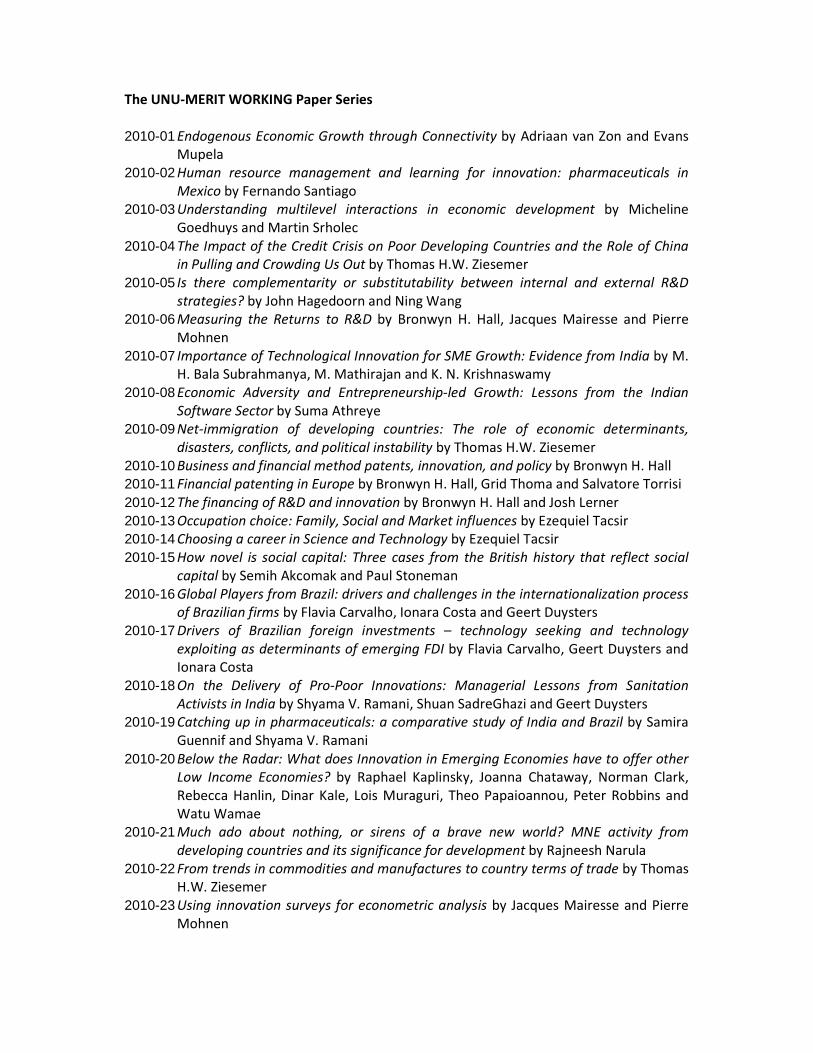
The UNU-MERIT WORKING Paper Series

2010-01 Endogenous Economic Growth through Connectivity by Adriaan van Zon and Evans

Mupela

2010-02 Human resource management and learning for innovation: pharmaceuticals in

Mexico by Fernando Santiago

2010-03 Understanding multilevel interactions in economic development by Micheline

Goedhuys and Martin Srholec

2010-04 The Impact of the Credit Crisis on Poor Developing Countries and the Role of China

in Pulling and Crowding Us Out by Thomas H.W. Ziesemer

2010-05 Is there complementarity or substitutability between internal and external R&D

strategies? by John Hagedoorn and Ning Wang

2010-06 Measuring the Returns to R&D by Bronwyn H. Hall, Jacques Mairesse and Pierre

Mohnen

2010-07 Importance of Technological Innovation for SME Growth: Evidence from India by M.

H. Bala Subrahmanya, M. Mathirajan and K. N. Krishnaswamy

2010-08 Economic Adversity and Entrepreneurship-led Growth: Lessons from the Indian

Software Sector by Suma Athreye

2010-09 Net-immigration of developing countries: The role of economic determinants,

disasters, conflicts, and political instability by Thomas H.W. Ziesemer

2010-10 Business and financial method patents, innovation, and policy by Bronwyn H. Hall

2010-11 Financial patenting in Europe by Bronwyn H. Hall, Grid Thoma and Salvatore Torrisi

2010-12 The financing of R&D and innovation by Bronwyn H. Hall and Josh Lerner

2010-13 Occupation choice: Family, Social and Market influences by Ezequiel Tacsir

2010-14 Choosing a career in Science and Technology by Ezequiel Tacsir

2010-15 How novel is social capital: Three cases from the British history that reflect social

capital by Semih Akcomak and Paul Stoneman

2010-16 Global Players from Brazil: drivers and challenges in the internationalization process

of Brazilian firms by Flavia Carvalho, Ionara Costa and Geert Duysters

2010-17 Drivers of Brazilian foreign investments – technology seeking and technology

exploiting as determinants of emerging FDI by Flavia Carvalho, Geert Duysters and

Ionara Costa

2010-18 On the Delivery of Pro-Poor Innovations: Managerial Lessons from Sanitation

Activists in India by Shyama V. Ramani, Shuan SadreGhazi and Geert Duysters

2010-19 Catching up in pharmaceuticals: a comparative study of India and Brazil by Samira

Guennif and Shyama V. Ramani

2010-20 Below the Radar: What does Innovation in Emerging Economies have to offer other

Low Income Economies? by Raphael Kaplinsky, Joanna Chataway, Norman Clark,

Rebecca Hanlin, Dinar Kale, Lois Muraguri, Theo Papaioannou, Peter Robbins and

Watu Wamae

2010-21 Much ado about nothing, or sirens of a brave new world? MNE activity from

developing countries and its significance for development by Rajneesh Narula

2010-22 From trends in commodities and manufactures to country terms of trade by Thomas

H.W. Ziesemer

2010-23 Using innovation surveys for econometric analysis by Jacques Mairesse and Pierre

Mohnen

2010-24 Towards a New Measurement of Energy Poverty: A Cross-Community Analysis of

Rural Pakistan by Bilal Mirza and Adam Szirmai

2010-25 Discovery of the flower industry in Ethiopia: experimentation and coordination by

Mulu Gebreeyesus and Michiko Iizuka

2010-26 CSR and market changing product innovations: Indian case studies by Shyama V.

Ramani and Vivekananda Mukherjee

2010-27 How firms innovate: R&D, non-R&D, and technology adoption by Can Huang,

Anthony Arundel and Hugo Hollanders

2010-28 Sure Bet or Scientometric Mirage? An Assessment of Chinese Progress in

Nanotechnology by Can Huang and Yilin Wu

2010-29 Convergence of European regions: a reappraisal by Théophile T. Azomahou, Jalal El

ouardighi, Phu Nguyen-Van and Thi Kim Cuong Pham

2010-30 Entrepreneurship and the National System of Innovation: What is Missing in Turkey?

by Elif Bascavusoglu-Moreau

2010-31 Keeping the eclectic paradigm simple: a brief commentary and implications for

ownership advantages by Rajneesh Narula

2010-32 Brazilian Aerospace Manufacturing in Comparative Perspective: A Brazil/USA

Comparison of Output and Productivity by Daniel Vertesy and Adam Szirmai

2010-33 Economic restructuring and total factor productivity growth: Tunisia over the period

1983-2001 by Sofiane Ghali and Pierre Mohnen

2010-34 Impact of government support on R&D and innovation by Abraham Garcia and

Pierre Mohnen

2010-35 Product, process and organizational innovation: drivers, complementarity and

productivity effects by Michael Polder, George van Leeuwen, Pierre Mohnen and

Wladimir Raymond

2010-36 Entrepreneurship Development and the Role of Economic Transition in

Entrepreneurial Activities in China by Ying Zhang and Geert Duysters

2010-37 Pro-Poor, Entrepreneur-Based Innovation and it’s Role in Rural Development by Lina

Sonne

2010-38 Financing pro-poor entrepreneur-based innovation: A review of existing literature

by Lina Sonne

2010-39 India’s Rural Financial System: Does it Support Pro-Poor Innovation? by Lina Sonne

2010-40 How effective are level-based R&D tax credits? Evidence from the Netherlands by

Boris Lokshin and Pierre Mohnen

2010-41 Analysing Multidimensional Poverty in Guinea: A Fuzzy Set Approach by Fatoumata

Lamarana Diallo

2010-42 Bottom-up, Bottom-line: Development-Relevant Enterprises in East Africa and their

Significance for Agricultural Innovation by Andy Hall, Norman Clark and Andy Frost

2010-43 Assessing Innovations in International Research and Development Practice by Laxmi

Prasad Pant

2010-44 Research Into Use: Investigating the Relationship between Agricultural Research

and Innovation by Andy Hall, Jeroen Dijkman and Rasheed Sulaiman V.

2010-45 The global institutional frameworks and the diffusion of renewable energy

technologies in the BRICS countries by Isabel Maria Freitas, Eva Dantas & Michiko

Iizuka

2010-46 The role of patent protection in (clean/green) technology transfer by Bronwyn H.

Hall and Christian Helmers

2010-47 Localisation Strategies of Firms in Wind Energy Technology Development by Radhika

Perrot and Sergey Filippov

2010-48 The R&D activity of multinational enterprises in peripheral economies: evidence

from the EU new member states by Rajneesh Narula and José Guimón

2010-49 Bridging the Financing Gap for Pro-Poor Innovation: Towards a Framework by Lina

Sonne

2010-50 Efficient Development Portfolio Design for Sub Saharan Africa by Adriaan van Zon

and Kirsten Wiebe