RGB Histogram based Color Image Segmentation Using Firefly Algorithm
Upload
khangminh22Category
view
2download
0
Pedro Miguel Oliveira Girão
3D Object Tracking Using RGBCamera and 3D-LiDAR Data
Dissertação submetida para a satisfação parcial dos requisitos do grau de Mestre em Engenharia Electrotécnica e de Computadores
Setembro de 2016


3D Object Tracking Using RGB
Camera and 3D-LiDAR Data
Pedro Miguel Oliveira Girão
Coimbra, Setembro 2016


3D Object Tracking Using RGB Camera and
3D-LiDAR Data
Supervisor:
Professor Paulo Peixoto
Co-Supervisor:Professor Doutor Urbano Nunes
Jury:
Professor Doutor João Pedro de Almeida Barreto
Doutor Cristiano Premebida
Dissertation submitted in partial fulfillment for the degree of Master of Science in Electrical and
Computer Engineering.
Coimbra, Setembro 2016


ACKNOWLEDGEMENTS
Em primeiro lugar, gostaria de demonstrar a minha gratidão ao Professor Paulo Peixoto por
ter aceite o meu pedido para orientação, bem como pelo apoio e ajuda prestados ao longo da tese
e por me ter apresentado à área da investigação académica (com todas as alegrias e frustrações
inerentes). O encorajamento foi também uma constante ao longo destes meses, estando-lhe grato
por isso.
Agradeço também ao Professor Doutor Urbano Nunes pelo feedback prestado nos papers técnicos
submetidos no decorrer da tese.
I also want to give special thanks to Alireza Asvadi for all the knowledge, patience, insight
and friendship he provided me throughout the entire process. His technical know-how and tireless
guidance were key factors for the success of the thesis. By always pointing me in the right direction,
never refusing any request for help, I am indebted to him.
Um abraço para o Pedro, Ricardo, Bruna e Zé pela companhia e boa disposição constante, pelos
almoços e cafés, pela ajuda e pela partilha das “dores de crecimento” das dissertações. Reza a lenda
que um dia ainda me vêm visitar à terra natal.
Aos meus pais agradeço ainda o apoio incondicional, não apenas nestes últimos meses mas em
todo este percurso. Obrigado por acreditarem em mim e me fazerem acreditar em mim próprio, por
me fazerem crescer enquanto pessoa e por estarem sempre presentes.
Por fim, o mais especial dos agradecimentos vai para a Susana. O encorajamento, paciência e
acima de tudo, amor nos últimos meses tornaram esta dissertação possível. O percurso da tese
foi difícil, em que nem sempre tudo correu de feição, mas o apoio mútuo fez com que tenhamos
conseguido ultrapassar mais esta etapa (sem enlouquecer).
A todos, o meu obrigado.
iii

RESUMO
Ao longo destes últimos anos, o campo da segurança rodoviária na indústria automóvel tem sido
foco de muita investigação e desenvolvimento. A evolução verificada neste campo fez com que as
principais empresas do ramo tenham começado a desenvolver as suas próprias soluções de segurança
de modo a obter veículos mais seguros. Um dos resultados desta investigação foi o aparecimento de
sistemas de assistência à condução autónoma e veículos de condução automatizada. Estes veículos
dependem de sensores precisos, montados no próprio veículo, para compreender os ambientes que
os rodeiam. Assim, apenas poderão ser obtidos veículos verdadeiramente autónomos quando estes
dependerem apenas da informação sensorial.
No entanto, é necessário aplicar pós-processamento aos dados oriundos dos sensores de modo a
que o veículo detete obstáculos e objetos enquanto navega. Entre outros, estes algoritmos permitem
a extração da localização, forma e orientação do objeto. A navegação em ambientes urbanos
continua a ser um problema sem soluções aceites de modo unânime, apesar das muitas propostas
apresentadas. Isto prende-se principalmente com o fato dos cenários de tráfego urbano apresentarem
complexidade superior a outros cenários. Os sensores existentes atualmente apresentam ainda
capacidades limitadas quando usados individualmente.
O pipeline da perceção é um módulo crítico para o bom funcionamento destes veículos. Em
particular, o seguimento de objetos num ambiente 3D dinâmico é uma das componentes chave
deste pipeline. Ao seguir um objeto, informação sobre a sua localização, forma, orientação e até
velocidade podem ser obtidas. Previsões sobre os estados futuros do objeto seguido também podem
ser utilizadas para que o veículo possa planear ações futuras.
Na presente dissertação é apresentada uma abordagem para o seguimento online de objetos, que
iv

recorre a informação de uma imagem 2D RGB obtida por uma câmara a cores e uma nuvem de
pontos 3D capturada por um sensor LiDAR, de modo a detetar e seguir um objeto em cada novo
scan. O objeto alvo está inicialmente definido. Foi considerado um sistema de navegação inercial
para a auto-localização do veículo. A integração de dados 2D e 3D pode provar-se benéfica para o
seguimento de objetos, como é demonstrado pela abordagem apresentada. São usados algoritmos
mean-shift nos espaços 2D e 3D em paralelo de modo a obter as novas localizações do objeto, e
filtros Bayesianos (filtros de Kalman) para fazer a fusão da informação e, de seguida, para o próprio
seguimento do objeto no espaço 3D. Este método calcula então estimativas para a localização,
orientação 2D e velocidade instantânea do objeto, bem como uma estimativa da próxima localização
do objeto.
O método desenvolvido foi sujeito a uma série de testes, estando os resultados qualitativos e
quantitativos obtidos apresentados no documento. Estes resultados mostram que o método é capaz
de estimar a localização, orientação e velocidade do objeto com boa precisão. Foi feita ainda uma
comparação com dois métodos de referência (baseline). Os testes utilizam informação ground truth
proveniente da base de dados KITTI para o propósito de avaliação. Tendo como base os testes
efetuados, é proposto um conjunto de métricas (benchmark) para facilitar a avaliação de métodos
de modelação da aparência de objetos. Este benchmark consiste em cinquenta sequências compostas
pela trajetória completa (e ininterrupta) do objeto em particular, sendo categorizadas com base em
quatro fatores desafiantes.
Palavras Chave
Seguimento de objetos em 3D, fusão sensorial, condução autónoma, mean-shift, filtros de
Kalman
v

ABSTRACT
The field of vehicle safety in the automotive industry has been the focus of much research and
development in recent years. This evolution in the field has made it possible for major players in the
automotive business to start developing their own active safety solutions to achieve safer cars. One
of the outcomes of these efforts has been the development of autonomous driving assistance systems
and highly automated vehicles. These vehicles rely on accurate on-board sensor technologies to
perceive their surrounding environments. Truly autonomous vehicles will only be a reality when
they can reliably interpret the environment based on sensory data alone.
However, some post processing needs to be applied to the raw data given by the sensors, so that
the vehicle can perceive obstacles and objects as it navigates. Such algorithms allow, among other
things, the extraction of the location, shape and orientation of object. The navigation in urban
environments is still an open problem, despite the many approaches presented. This is mainly due
to the fact that urban traffic situations offer additional complexity. In addition, current on-board
sensors also have limited capabilities when used individually.
The perception pipeline is thus a critical module of these vehicles. In particular, object tracking
in a dynamic 3D environment is one of the key components of this pipeline. By tracking an object,
information about location, shape, orientation and even velocity of that object can be obtained. A
prediction of the future states of the tracked objects can also be obtained allowing for the planning
of future actions taken by the vehicle.
In the present thesis, an online object tracking approach has been developed that used information
from both 2D RGB images obtained from a colour camera and 3D point clouds captured from
a LiDAR sensor to detect and track an initially defined target object in every new scan. An
vi

inertial navigation system was also considered for vehicle self-localization. Integration of 2D and 3D
data can provide some benefits, as demonstrated by this approach. The tracker uses two parallel
mode-seeking (mean-shift) algorithms in the 2D and 3D domains to obtain new object locations
and Bayesian (Kalman) filters to fuse the output information and afterwards track the object in the
3D space. Our approach outputs the target object location, 2D orientation, and instant velocity
estimates, as well as a prediction about the next location of the object.
The tracker was subject to a series of tests. The quantitative and qualitative results obtained
are presented in the document. These results show that the proposed tracker is able to achieve
good accuracy for location, orientation and velocity estimates. A comparison with two baseline 3D
object trackers is also presented. The test cases used ground truth information from the KITTI
database for evaluation purpose. A benchmark based on the KITTI database is also proposed in
order to make the evaluation of object appearance modelling and tracking methods easier. This
benchmark features 50 sequences labelled with object tracking ground-truth, categorized according
to four different challenging factors.
Keywords
3D object tracking, sensor fusion, autonomous driving, mean-shift, Kalman filters
vii


“I would like to die on Mars. Just not on impact."
— Elon Musk
ix


CONTENTS
Acknowledgements iii
Resumo iv
Abstract vi
List of Acronyms xiv
List of Figures xvi
List of Tables xviii
1 Introduction 1
1.1 Motivation and Context . . . . . . . . . . . . . . . . . . . . . . . . . . . . . . . . . . 2
1.2 Problem Formulation . . . . . . . . . . . . . . . . . . . . . . . . . . . . . . . . . . . . 4
1.3 System Overview . . . . . . . . . . . . . . . . . . . . . . . . . . . . . . . . . . . . . . 4
1.4 Objectives . . . . . . . . . . . . . . . . . . . . . . . . . . . . . . . . . . . . . . . . . . 5
1.5 Main Contributions . . . . . . . . . . . . . . . . . . . . . . . . . . . . . . . . . . . . . 5
1.6 Outline . . . . . . . . . . . . . . . . . . . . . . . . . . . . . . . . . . . . . . . . . . . 6
2 State of the Art 7
2.1 Sensors . . . . . . . . . . . . . . . . . . . . . . . . . . . . . . . . . . . . . . . . . . . 8
2.1.1 Vision Sensors . . . . . . . . . . . . . . . . . . . . . . . . . . . . . . . . . . . 8
2.1.2 Range Sensors . . . . . . . . . . . . . . . . . . . . . . . . . . . . . . . . . . . 9
2.1.3 Sensor Fusion . . . . . . . . . . . . . . . . . . . . . . . . . . . . . . . . . . . . 11
xi

2.1.4 Point Clouds . . . . . . . . . . . . . . . . . . . . . . . . . . . . . . . . . . . . 11
2.1.5 Summary (Sensors) . . . . . . . . . . . . . . . . . . . . . . . . . . . . . . . . . 12
2.2 Object Trackers . . . . . . . . . . . . . . . . . . . . . . . . . . . . . . . . . . . . . . . 13
2.2.1 3D / Fusion Trackers . . . . . . . . . . . . . . . . . . . . . . . . . . . . . . . . 14
2.2.2 Summary (Object Trackers) . . . . . . . . . . . . . . . . . . . . . . . . . . . . 17
3 Proposed Method 18
3.1 Approach Formulation . . . . . . . . . . . . . . . . . . . . . . . . . . . . . . . . . . . 20
3.1.1 Relevant Notation . . . . . . . . . . . . . . . . . . . . . . . . . . . . . . . . . 20
3.2 System Overview . . . . . . . . . . . . . . . . . . . . . . . . . . . . . . . . . . . . . . 20
3.3 3D Tracking . . . . . . . . . . . . . . . . . . . . . . . . . . . . . . . . . . . . . . . . . 22
3.3.1 Ground Removal . . . . . . . . . . . . . . . . . . . . . . . . . . . . . . . . . . 22
3.3.2 Detection and Localization . . . . . . . . . . . . . . . . . . . . . . . . . . . . 23
3.4 2D Tracking . . . . . . . . . . . . . . . . . . . . . . . . . . . . . . . . . . . . . . . . . 24
3.4.1 Discriminant Colour Model . . . . . . . . . . . . . . . . . . . . . . . . . . . . 25
3.4.2 Detection and Localization . . . . . . . . . . . . . . . . . . . . . . . . . . . . 25
3.4.3 Adaptive Updating of < Bins . . . . . . . . . . . . . . . . . . . . . . . . . . . 26
3.5 2D/3D Projection . . . . . . . . . . . . . . . . . . . . . . . . . . . . . . . . . . . . . 27
3.6 Fusion and Tracking . . . . . . . . . . . . . . . . . . . . . . . . . . . . . . . . . . . . 29
3.6.1 2D/3D Fusion for Improved Localization . . . . . . . . . . . . . . . . . . . . . 30
3.6.2 3D Object Tracking . . . . . . . . . . . . . . . . . . . . . . . . . . . . . . . . 32
4 Experimental Results 35
4.1 Dataset . . . . . . . . . . . . . . . . . . . . . . . . . . . . . . . . . . . . . . . . . . . 36
4.1.1 Synchronization . . . . . . . . . . . . . . . . . . . . . . . . . . . . . . . . . . 36
4.1.2 Dataset Sequences . . . . . . . . . . . . . . . . . . . . . . . . . . . . . . . . . 37
4.2 Evaluation . . . . . . . . . . . . . . . . . . . . . . . . . . . . . . . . . . . . . . . . . . 39
4.2.1 Quantitative Evaluation Metrics . . . . . . . . . . . . . . . . . . . . . . . . . 39
4.3 Baseline Methods . . . . . . . . . . . . . . . . . . . . . . . . . . . . . . . . . . . . . . 40
4.3.1 Baseline KF 3D Object Tracker (3D-KF) . . . . . . . . . . . . . . . . . . . . 41
4.3.2 Baseline MS 3D Object Tracker (3D-MS) . . . . . . . . . . . . . . . . . . . . 41
4.4 Results . . . . . . . . . . . . . . . . . . . . . . . . . . . . . . . . . . . . . . . . . . . . 41
4.4.1 Qualitative Evaluation . . . . . . . . . . . . . . . . . . . . . . . . . . . . . . . 46
4.5 Benchmark . . . . . . . . . . . . . . . . . . . . . . . . . . . . . . . . . . . . . . . . . 48
5 Conclusions 49
5.1 Future Work . . . . . . . . . . . . . . . . . . . . . . . . . . . . . . . . . . . . . . . . 51
xii

6 Bibliography 52
Appendices 59
A Kalman Filter Theory 59
B Submitted Paper: 3D Object Tracking using RGB and LIDAR Data 62
C Submitted Paper: 3D Object Tracking in Driving Environment: a short review
and a benchmark dataset 71
xiii

LIST OF ACRONYMS
3D BB 3D Bounding Box
ABS Antilock Braking System
ADAS Autonomous Driver Assistance System
CA KF Constant Acceleration Kalman Filter
CV KF Constant Velocity Kalman Filter
DA Data Association
DARPA Defense Advanced Research Projects Agency
DATMO Detection and Tracking of Moving Objects
DEM Digital Elevation Map
DGPS Differential Global Positioning System
EKF Extended Kalman Filter
ESC Electronic Stability Control
FOV Field of View
FPS Frames Per Second
GNN Generalized Neural Network
GNSS Global Navigation Satellite System
xiv

GPS Global Positioning System
HDR High Dynamic Range
ICP Iterative Closest Point
IMU Inertial Measurement Unit
INS Inertial Navigation System
IR Infrared
KDE Kernel Density Estimation
KF Kalman Filter
Laser Light Amplification by Stimulated Emission of Radiation
LiDAR Light Detection And Ranging
LLR Log-Likelihood Ratio
MHT Multiple Hypothesis Tracking
MS Mean-Shift
PCD Point Cloud
PDF Probability Density Function
RADAR Radio Detection And Ranging
RANSAC Random Sample Consensus
RGB Red Green Blue
ROI Region of Interest
SONAR Sound Navigation And Ranging
SNR Signal-to-Noise Ratio
ToF Time of Flight
UV Ultraviolet
xv

LIST OF FIGURES
1.1 High-level overview of the proposed 3D object tracker. . . . . . . . . . . . . . . . . . 5
2.1 Examples of cameras in the market. . . . . . . . . . . . . . . . . . . . . . . . . . . . 9
2.2 Examples of range sensors in the market. . . . . . . . . . . . . . . . . . . . . . . . . 10
2.3 Point clouds produced by stereo vision setup. . . . . . . . . . . . . . . . . . . . . . . 11
2.4 Point clouds produced by Velodyne HDL-64E. . . . . . . . . . . . . . . . . . . . . . . 12
2.5 Autonomous vehicle examples from the DARPA Urban Challenge in 2007. . . . . . . 17
3.1 Input data from 3D and 2D sensors. . . . . . . . . . . . . . . . . . . . . . . . . . . . 19
3.2 Object coordinate systems. . . . . . . . . . . . . . . . . . . . . . . . . . . . . . . . . 20
3.3 Major pipeline of the proposed approach. . . . . . . . . . . . . . . . . . . . . . . . . 21
3.4 Ground removal process. . . . . . . . . . . . . . . . . . . . . . . . . . . . . . . . . . . 23
3.5 MS procedure in 3D PCD . . . . . . . . . . . . . . . . . . . . . . . . . . . . . . . . . 24
3.6 MS procedure in 2D RGB image. . . . . . . . . . . . . . . . . . . . . . . . . . . . . . 26
3.7 Bilinear interpolation diagram. . . . . . . . . . . . . . . . . . . . . . . . . . . . . . . 28
3.8 Bilinear interpolation process. . . . . . . . . . . . . . . . . . . . . . . . . . . . . . . . 29
3.9 Overview of the tracking system. . . . . . . . . . . . . . . . . . . . . . . . . . . . . . 30
4.1 Recording platform for the KITTI Dataset. . . . . . . . . . . . . . . . . . . . . . . . 37
4.2 Initial frames from the selected sequences. . . . . . . . . . . . . . . . . . . . . . . . . 38
4.3 Pose error representation. . . . . . . . . . . . . . . . . . . . . . . . . . . . . . . . . . 39
4.4 Bounding boxes overlap calculation. . . . . . . . . . . . . . . . . . . . . . . . . . . . 40
4.5 Location error comparison plot. . . . . . . . . . . . . . . . . . . . . . . . . . . . . . . 44
xvi

4.6 Pose error comparison plot. . . . . . . . . . . . . . . . . . . . . . . . . . . . . . . . . 45
4.7 Velocity error comparison plot. . . . . . . . . . . . . . . . . . . . . . . . . . . . . . . 45
4.8 3D BB overlap comparison plot. . . . . . . . . . . . . . . . . . . . . . . . . . . . . . 46
4.9 3D BB overlap precision plot. . . . . . . . . . . . . . . . . . . . . . . . . . . . . . . . 46
4.10 Sequence 1, tracking modules in frames 40 & 130. . . . . . . . . . . . . . . . . . . . . 47
4.11 Sequence 2, tracking modules in frames 34 & 80. . . . . . . . . . . . . . . . . . . . . 47
4.12 Sequence 15, tracking modules in frames 30 & 57. . . . . . . . . . . . . . . . . . . . . 48
5.1 Object shape reconstruction results. . . . . . . . . . . . . . . . . . . . . . . . . . . . 51
A.1 Kalman filter overview. . . . . . . . . . . . . . . . . . . . . . . . . . . . . . . . . . . 60
xvii

LIST OF TABLES
2.1 Summary of discussed sensor technologies. . . . . . . . . . . . . . . . . . . . . . . . . 12
2.2 Summary on considered 3D object trackers. . . . . . . . . . . . . . . . . . . . . . . . 17
4.1 Detailed information and challenging factors for each sequence. . . . . . . . . . . . . 38
4.2 Error results. . . . . . . . . . . . . . . . . . . . . . . . . . . . . . . . . . . . . . . . . 42
A.1 Discrete KF filter time and measurement update equations. . . . . . . . . . . . . . . 61
xviii

xix

CHAPTER
1
INTRODUCTION
Contents1.1 Motivation and Context . . . . . . . . . . . . . . . . . . . . . . . . . . . . 2
1.2 Problem Formulation . . . . . . . . . . . . . . . . . . . . . . . . . . . . . . 4
1.3 System Overview . . . . . . . . . . . . . . . . . . . . . . . . . . . . . . . . . 4
1.4 Objectives . . . . . . . . . . . . . . . . . . . . . . . . . . . . . . . . . . . . . 5
1.5 Main Contributions . . . . . . . . . . . . . . . . . . . . . . . . . . . . . . . 5
1.6 Outline . . . . . . . . . . . . . . . . . . . . . . . . . . . . . . . . . . . . . . . 6
1

1.1. MOTIVATION AND CONTEXT CHAPTER 1. INTRODUCTION
The present document acts as the author’s MSc thesis dissertation. The carried out work falls
within the domain of perception systems for intelligent vehicles, applied to the particular case of
single object tracking in 3D. In this chapter, the motivation behind the developed work is presented,
and the context explained by stating some studies and statistics that show the importance of the
perception pipeline in intelligent vehicles currently being developed. The problem at hand is then
defined. Additionally, an overview of the work’s key points and ideas is provided, along with the
flow of information in the proposed work. Afterwards, the objectives and main contributions are
presented, as well as the structure of the remainder of the document.
1.1 Motivation and Context
Injuries resulting from road transportation (or traffic) accidents claim an estimated 1.25 million
lives globally each year (being the leading cause of death from young people aged from 15 to 29)
[1, 2]. A recent report concerning just data from European countries states that roughly 85000
people have perished due to road traffic injuries in 2013 and, statistically speaking, for every person
that dies from a road accident at least 23 people suffer non-fatal injuries that require urgent hospital
care [3]. Furthermore, pedestrians, cyclists and motorcyclists compose near 40% of the total number
of deaths related to these road accidents. In turn, a statistical summary released by the United
States Department of Transportation projected that in 2015 the total numbers of vehicle traffic
fatalities grew in comparison to previous years by almost 8% [4].
Human errors remain the main reason behind road accidents, namely through distracted driving,
with all the factors typically involved: talking/texting on the phone, eating, reading, falling asleep,
tuning the radio or even just talking to someone inside the car [5, 6]. According to the same study,
the second and third most common causes of traffic accidents were speeding and drunk driving,
which highlights the drivers responsibility and ability to avoid these unfortunate events (backed
by the numbers in [7] as aforementioned, where 94% of accidents in the study were due to human
errors).
As a direct consequence of this reality, safety protocols and policies have been implemented over
the years, from building safer roads to enforcing the usage of a seatbelt. These safety systems can
be categorized in two groups: protective and preventive [8].
Protective safety systems include the most common safety measures implemented in the last
half century. Its aim is to disperse the kinetic energy in an accident in order to efficiently protect
both the driver and other possible occupants of the vehicles. These mechanisms include bumpers,
seat belts and air-bags.
On the other hand, preventive (or active) safety systems are meant to help drivers safely
guide the vehicle while avoiding, mitigating or possibly even preventing accidents along the way.
2

CHAPTER 1. INTRODUCTION 1.1. MOTIVATION AND CONTEXT
Some examples of these systems are Antilock Braking System (ABS) and Electronic Stability
Control (ESC). Through the monitoring and analysis of traffic scenarios surrounding the vehicle,
preventive safety systems can act as a support to the driver. An additional category called integrated
safety considers information that is perceived (preventive) to make better use of the protective
system (seat readjustment before crash, earlier deployment of air bags, etc.).
With the goal of reducing the aforementioned number of deaths and injuries from vehicle related
accidents, a lot of research has been put into preventive safety systems. One of the main ideas
behind this research is the change in the driver’s stance, from a direct actuator towards a spectator
role, i.e., a supervisor of the vehicle, only acting when needed [9]. A direct outcome of such efforts
has been the creation of intelligent vehicles, capable of perceiving the environment that surrounds
them and able to take appropriate decisions regarding the navigation task previously determined by
the driver, being therefore safer for both the occupants of the vehicle and other agents on the road
like other drivers and pedestrians.
In recent years, an increasing number of innovative technological approaches have been suggested
to improve the behaviour of intelligent vehicles (otherwise referred to as Autonomous Driver
Assistance System (ADAS)). Research in areas like computer vision and machine learning have
proved the potential of autonomous driving. Nonetheless, acceptance by both governmental laws
and public opinion remains divided, with several legal and policy situations being currently under
evaluation [10].
Since the decision making process involved in a typical ADASs must rely on its perception of the
surrounding traffic condition, nature and man-built structures and even road or weather conditions,
the perception pipeline becomes of the utmost importance. In order to achieve this situational
awareness, the intelligent vehicle in question (or ego vehicle) needs to know the location of objects
of interest on a known spatial reference system (either local or absolute/world). This goal can
be achieved by using on-board sensors relying on different technologies, such as vision (mono and
stereo cameras) and range sensors (Radio Detection And Ranging (RADAR), Sound Navigation
And Ranging (SONAR), Light Detection And Ranging (LiDAR)). In addition to these sensors, an
Inertial Navigation System (INS) can also be used to directly obtain the ego vehicle’s location.
Even with the successful autonomous driving tests reported on highways and urban scenarios
in recent years, there are still open issues regarding the reliable perception and navigation in
unconstrained environments mainly due to the limited capabilities of current sensors as well as the
image processing algorithms used for the purpose of scene understanding [11].
3

1.2. PROBLEM FORMULATION CHAPTER 1. INTRODUCTION
1.2 Problem Formulation
ADASs obey to the robotic paradigms in the sense that they integrate three robot primitives:
sense, plan and act [12]. The system has to gather the information (sense), evaluate it (plan) and
then act accordingly. The perception pipeline belongs to the “sense” primitive, enabling a vehicle to
comprehend the surrounding environment through its sensory input. Usually, perception modules
are composed of, among others, an initial object detection (and possibly segmentation) module, as
well as an object tracking module.
For the purpose of this thesis, we will just focus on the particular problem of 3D single object
tracking. To do so, sensor data is obtained from a 3D Light Amplification by Stimulated Emission of
Radiation (Laser) scanner and a stereo vision system for environment perception. In addition, an
INS (GPS/IMU) is used to know the ego vehicle’s location. For the current approach it is assumed
that the initial position and characteristics of the target object are known.
Usually, perception modules are also composed of, among others, an initial object detection
(and possibly segmentation) sub-module; however, for the current purpose it is assumed that the
initial position and characteristics of the target object are known.
The focus of the present thesis is therefore on the modelling and tracking of a generic object
in 3D, by fusion of sensor data (LiDAR and monocular camera) to enable better results when
comparing with single-sensor approaches. Using an INS allows for better velocity estimates for
object tracking. Through usage of Kalman Filter (KF) theory, the system can also predict the
object location in the 3D world coordinate system in the next time-step.
1.3 System Overview
A generic overview of the proposed 3D object tracker is shown in Figure 1.1. It is assumed
that the initial characteristics of the object represented in the form of a 3D Bounding Box (3D BB)
are known. A 3D BB is considered to describe the object’s location, width, height, length and pose.
As aforementioned, this information is normally obtained by object [13] or motion detectors [14].
The initial 3D BB is obtained in the 3D Point Cloud (PCD) from ground truth information.
Points inside the 3D BB are projected into the image simultaneously acquired from the 2D Red
Green Blue (RGB) and the convex hull of the projected points is calculated to define the object
in the 2D domain. For the following scans, the object is located in the current PCD and image
by applying a mode-seeking Mean-Shift (MS) algorithm in each domain. These locations are the
tracker’s initial estimates for the 3D location of the target object. Information obtained from both
the 3D and 2D domains is fused, and another Bayesian filter effectively tracks the object in the 3D
world space. The computed object 3D BB is used as the reference object information for the next
scan. The overview of the process can be seen in Figure 1.1.
4

CHAPTER 1. INTRODUCTION 1.4. OBJECTIVES
2D-RGB Data
3D-LiDAR Data
Initialization in 2D
INS Data
MS object localization in 2D
MS object localization in 3DInitialization in 3D
Projection of 2D to 3D
Outputs:
º Locationº Orientationº Velocity estimation
Fusion in 3D and apply ltering
2D-RGB Data
3D-LiDAR Data
Initialization in 2D
GPS Data
New object localization in 2D
New object localization in 3DInitialization in 3D
Projection of 2D to 3D
Outputs:
º Locationº Orientationº Velocity estimation
Fusion in 3D and apply ltering
Figure 1.1: High-level overview of the proposed 3D object tracker. A more detailed diagram and extensive description
of the system behaviour can be found in Chapter 3.
1.4 Objectives
As stated before, the main goal of this thesis is to develop an object tracker capable of tracking
a single object in 3D as it moves around a scene, using information from several onboard sensor
technologies. The tracker will thus track and maintain updated information about the object in
both 3D and 2D spaces. The proposed approach should provide a stronger representation and
understanding of the ego vehicle surroundings by handling and fusing the information perceived by
each sensor. To summarize, the proposed objectives are:
• Provide a robust 2D/3D fusion-based 3D object tracking approach;
• Provide location, orientation (2D angle) and velocity estimations of the tracked object on a
3D coordinate space related to world coordinates (i.e. real world coordinates);
• Report both quantitative and qualitative evaluation of the proposed method;
• Create a benchmark for object appearance modelling evaluation;
1.5 Main Contributions
In this thesis, an object tracker that makes use of combined information obtained from a
3D-LiDAR and a 2D-RGB camera is proposed. The main contribution of this work is to provide
a robust 2D/3D fusion-based 3D object tracking approach. Since it is hard to properly evaluate
and compare most of the currently available approaches for object tracking in the literature (as
these are subject to different parameters and constraints and may come from different theoretical
5

1.6. OUTLINE CHAPTER 1. INTRODUCTION
backgrounds) another contribution of this thesis is the proposal of a benchmark to enable an easier
comparison and quantitative evaluation of different 3D object trackers in driving environments
(particularly those based on object appearance modelling).
1.6 Outline
The present document is organized in five chapters, beginning with the current introduction,
where the problem is contextualized and a solution is proposed to mitigate it.
In Chapter 2 modern sensors and object tracking state of the art are discussed, summarizing
some of the most important aspects of recent research and how they influenced the direction followed
by the work presented in this document.
Chapter 3 will then focus on the detailed description of the proposed approach, showing how it
handles incoming data from different sensors and how it fuses the sensory data to provide meaningful
information.
Afterwards, quantitative and qualitative experimental results of the proposed tracker are
presented in Chapter 4. The used dataset is also described, with some notes on how the information
was extracted and how it can be used to test the developed object tracker.
Chapter 5 is reserved for the presentation of conclusions drawn from the presented work, as well
as pointing towards future work that could be done to extend/improve the developed framework.
6

CHAPTER
2
STATE OF THE ART
Contents2.1 Sensors . . . . . . . . . . . . . . . . . . . . . . . . . . . . . . . . . . . . . . . 8
2.1.1 Vision Sensors . . . . . . . . . . . . . . . . . . . . . . . . . . . . . . . . . . 8
2.1.2 Range Sensors . . . . . . . . . . . . . . . . . . . . . . . . . . . . . . . . . . 9
2.1.3 Sensor Fusion . . . . . . . . . . . . . . . . . . . . . . . . . . . . . . . . . . . 11
2.1.4 Point Clouds . . . . . . . . . . . . . . . . . . . . . . . . . . . . . . . . . . . 11
2.1.5 Summary (Sensors) . . . . . . . . . . . . . . . . . . . . . . . . . . . . . . . . 12
2.2 Object Trackers . . . . . . . . . . . . . . . . . . . . . . . . . . . . . . . . . 13
2.2.1 3D / Fusion Trackers . . . . . . . . . . . . . . . . . . . . . . . . . . . . . . . 14
2.2.2 Summary (Object Trackers) . . . . . . . . . . . . . . . . . . . . . . . . . . . 17
7

2.1. SENSORS CHAPTER 2. STATE OF THE ART
Autonomous cars and ADASs need to be able to understand their surrounding environments,
as aforementioned. In this sense, the quality of the perception pipeline is critical for the correct
performance of these systems. This perception pipeline depends directly on the quality of perception
sensors and algorithms [15]. Object tracking stands as one of the main components of the perception
process.
In this chapter a discussion of current literature is provided, regarding sensing systems and
object tracker approaches. Taking into consideration the number of considered approaches and
studies, a table with the most salient aspects of each work will be provided.
2.1 Sensors
In order to detect and track on-road agents (such as vehicles, cyclists and pedestrians) a number
of different sensor technologies can be used. Typically it is necessary to measure object properties
such as position, orientation (or pose), distance to ego vehicle, speed and acceleration, among others.
Algorithms that process information provided by these sensors are of utmost importance for ADASs,
with the action pipeline being dependent of the output of the perception phase. The use of these
technologies recently showed that there is an enormous potential for saving lives, like in the case of
a Tesla vehicle owner claiming that the car alone prevented him from hitting a pedestrian during
the night in low visibility conditions [16]. However, this comes in contrast to news that another
vehicle by the same manufacturer was involved in a fatal death in Florida due to cameras not being
able to differentiate “the white side of [a] tractor trailer against a brightly lit sky.”, showing that
these systems are still not perfected [17].
2.1.1 Vision Sensors
As with the retinas in human eyes, colour cameras are able to capture the colour and resolution
of a scene with varying amounts of detail. Over the past decade, the improvement on vision-based
perception algorithms has been noticeable; detection and tracking of moving objects can thus be
obtained by equipping ADASs with on-board sensors such as monocular or stereo cameras.
Vision sensors can be categorized as passive sensors in the sense that collected information is
resultant from the reception of non-emitted signals, as there is no electromagnetic energy emission
but rather the measurement of light in the perceived environment (i.e. image capturing) [18].
Therefore, it is common practice for vision-based perception systems to install one or more cameras
in the vehicle, either inside (close to rear mirror) or outside.
With the on-going improvement of vision sensors, the associated costs of camera acquisition
have dropped, being one of the most interesting aspects of this approach; given the usually low Field
of View (FOV) of such cameras, the installation of multiple sensors can be used to obtain a full
8

CHAPTER 2. STATE OF THE ART 2.1. SENSORS
360 view of the vehicle surroundings and thus a more rich description of the latter (in comparison
to those obtained from active sensors).
(a) PointGrey Flea3 (b) PointGrey Bumblebee2
Figure 2.1: Examples of cameras in the market. The first is a monocular colour camera [19] while the second consists
on a stereo vision setup [20].
Stereo vision systems make use of the presence of multiple cameras in order to obtain relevant
range data and, in addition to the low cost, present low energy consumption whilst outputting
meaningful colour data and accurate depth information. It should be noted that the performance of
stereo vision approaches tends to deteriorate in regard to objects located far from the ego vehicle,
which results in losing losing fidelity proportionately with the distance to scene objects. In addition
to this downside, detection and tracking approaches based on monocular and stereo cameras are also
directly affected by changes in lighting and weather conditions (such as fog or snow) [21] or time of
the day. Some approaches try to solve these problems by utilizing specific sensors to deal with these
situations. For example, Sun et al. [22] showed that the usage of High Dynamic Range (HDR) or
low-light cameras made it possible to employ the same detection and recognition models to both
day and night time.
Stereo vision-based sensors tend to produce very dense point clouds (seeing as the basis for their
generation are rich images as opposed to active sensors); however these point clouds tend to be a
little noisy. Some problems with stereo matching algorithms (and thus with generated stereo vision
point clouds) are mainly due to sensor noise distorting images (particularly problematic in poorly
textured regions due to low Signal-to-Noise Ratio (SNR)), lack of correspondence between pixels of
half occluded regions in the two images (incorrect or no matching) and the fact that the constant
brightness assumption is not commonly satisfied in practice [23].
2.1.2 Range Sensors
As opposed to vision-based sensors, range sensors are considered active as they receive and
measure signals transmitted by them that are reflected by the surrounding objects and/or scene.
RADAR, SONAR and LiDAR sensors fall within this category; LiDAR systems transmit and receive
Ultraviolet (UV), Infrared (IR) and visible waves of the electromagnetic spectrum and, through
Time of Flight (ToF) theory, are received and interpreted as a function of time. Paired with the
9

2.1. SENSORS CHAPTER 2. STATE OF THE ART
knowledge of the speed of light, the systems then calculate the distance travelled by the emitted
particles (forth and back).
In direct comparison with passive sensors, some active sensors like LiDAR are able to provide a
360 view of the area around the ego vehicle by using just one sensor. The output of these sensors
comes in the form of a dense point cloud (very dense for objects or parts of the surrounding scene
closer to ego vehicle, but sparser as distance to objects increases).
(a) BOSCH LRR3 (b) SICK LMS 210 (c) HOKUYO URG-04LX (d) Velodyne HDL-64E
Figure 2.2: Examples of range sensors in the market. The first sensor is based on RADAR technology [24], whilst
the rest are based on LiDAR technology [25–27].
Active sensors provide a viable option for real-time detection applications, countering some
of the vision-based problems (robustness under different weather conditions, for example) and
measuring object characteristics such as location with little computational power needed [21].
Among themselves, RADAR presents more reliability than others sensors for greater distances,
albeit the presence of less expensive LiDAR sensors in the market (but with lower range as well). In
addition, most LiDAR sensors are cheaper and are easier to apply than RADAR. The latter sensors
also retrieve less information than Laser based sensors and are more prone to misreadings, given the
fact that environments might be dynamic and/or noisy and that there might be road traffic as well.
3D Laser based technology has gained attention in the past few years, being the main contenders
in challenges such as Defense Advanced Research Projects Agency (DARPA) Urban Challenge. In
2007, most approaches were based on high-end LiDAR systems, such as the works presented by
Montemerlo et al. [28] or Kammel et al. [29], with the latter becoming the working basis for the
KITTI Vision Benchmark Suite [30].
Some of the disadvantages of LiDAR systems are that no colour data is directly obtained, and
reflective and foggy environments tend to distort the results. In addition, darker coloured objects
have lower reflection values since they absorb light, meaning the sensor could not get a return from
the emitted Laser. A LiDAR sensor tends to receive less information in these cases; studies such as
Petrovskaya et al. [31] show that looking at the absent data (no points being detected in a range
of vertical angles in a given direction) can represent space that is likely occupied by a black (or
darker) objects, since otherwise the emitted rays would have hit an obstacle or the ground.
Velodyne [32] has recently created a smaller 3D LiDAR sensor, the Velodyne HDL-64E. Details
about the sensor can be found in Chapter 4.1. This sensor has become an interesting option for
10

CHAPTER 2. STATE OF THE ART 2.1. SENSORS
obstacle detection and navigation in urban and highway areas, being used in setups such as KITTI
[30] and Google’s Self-Driving Car Project (in the latter, as their main sensor) [33].
2.1.3 Sensor Fusion
Taking into account the pros and cons of passive and active sensors, multiple sensor approaches
have been studied with the goal of yielding better results (hence safer ADASs) than using a single
sensor. Sensor fusion is achieved by combining data from several sensors to overcome the deficiencies
of individual usage. This can either be done to achieve simultaneous data capture for detection and
tracking purposes, with each sensor validating the results produced by the others, or having one
sensor detect and track while other sensors validate the results.
With prices for LiDAR systems getting lower, fusion of vision and LiDAR systems has been the
focus of recent research. Premebida et al. [34] initially used LiDAR data for detection and tracking
(to obtain a reliable object detection), but later in the process simultaneous accessed both LiDAR
and vision sensory data along with a probability model for object classification.
Zhao et al. [35] presented an approach which performed scene parsing and data fusion for a
3D LiDAR scanner and a monocular video camera. Although the focus of the approach was not
based on object tracking, one of the conclusion of the work was that fused results provided more
reliability than those provided by individual sensors.
2.1.4 Point Clouds
A common representation for the surrounding scene when captured through LiDAR based
sensors (or stereo vision setups after processing) is through a point cloud. A point cloud is thus a
set of points in a given 3D coordinate system which are intended to represent the external surfaces
(physical world surfaces) of surrounding objects. Some examples of points clouds obtained through
two different technologies can be seen in Figures 2.3 and 2.4.
Figure 2.3: Point clouds produced by stereo vision setup [36].
11

2.1. SENSORS CHAPTER 2. STATE OF THE ART
Figure 2.4: Point clouds produced by Velodyne HDL-64E [27]. Colour is displayed for better representation as LiDAR
based sensors have no colour information directly available.
2.1.5 Summary (Sensors)
In this section a summary of sensor technologies is presented in Table 2.1. Here, a concise
comparison between the considered sensor types is done in the shape of a brief description of the
pros and cons of each sensor technology as a whole without looking into particular devices.
Type Energy Data Cost Advantages Disadvantages
LiDAR Laser Distance
(m)
Medium
/ High
• Dense high resolution 3D data in form
of PCD;
• Sensible to outdoor conditions (refrac-
tion of laser might occur);
• Very precise; • More costly than other sensors;
• Small beam-width; • Higher power consumption;
• Fast acquisition and processing rates; • Sensor made of moving parts;
• Reflectance information can be useful
for object recognition purposes;
• No colour information;
RADAR Radio
wave
Distance
(m)
Medium • Low sensibility to both outdoor condi-
tions and time of day;
• Still higher power consumption than
vision sensors;
• Precise; • Larger beam-width;
• Long range; • Lower resolution than LiDAR;
• Measurements done with less computa-
tional resources;
• Bigger sensor size than cameras;
• Good for environments with reflections;
Vision None Image
(px)
Low • Low cost with low installa-
tion/maintenance costs;
• Image quality highly dependant on out-
door conditions;
• Meaningful information in captured im-
age;
• Heavy computational power to process
images;
• Non-intrusive data acquisition; • Low performance on texture-less envi-
ronments (stereo vision);
Sensor
Fusion
Depends Depends Depends • Increases system reliability; • Algorithms to properly fuse informa-
tions;
on the on the on the • More diverse information captured; • Costs spread by several sensors;
sensors sensors sensors • Compensation of individual sensor
shortcoming;
Table 2.1: Summary of discussed sensor technologies.
12

CHAPTER 2. STATE OF THE ART 2.2. OBJECT TRACKERS
Additionally, a literature study conducted in [37] further details characteristics of individual
sensors used in ADASs and highlights the importance of combining different sensors in order to
achieve better results for several tasks, including object tracking.
2.2 Object Trackers
After having sensor data available, some processing needs to be applied in order to extract the
relevant information for tracking purposes. A very basic definition of object tracking would consist
on estimating the trajectory of a target object as it moves around a scene (in an image plane or 3D
space), inferring about its motion in a sequence of scans. Another definition (in the image domain)
was provided by Smeulders et. al [38] as “tracking (being) the analysis of video sequences for the
purpose of establishing the location of the target over a sequence of frames (time)”.
The tracker thus labels an object in different scans, being able to provide information such
as location, orientation, velocity and shape. As mentioned in Chapter 1, visual tracking is a
fundamental task in the perception pipeline of intelligent vehicles and ADASs and has therefore
been well studied in the last decades, especially in the image domain.
Even with the high number of proposed approaches to handle visual tracking, this topic still
remains a big challenge, with the majority of difficulties arising from changes in object motion,
perceived appearance, occlusion and movement of the capturing camera [39]. Given the high number
of challenging variables, most approaches tend to provide robust solutions to only a given subset of
problems.
There has been extensive research regarding object tracking in the image domain (with important
surveys provided in [38–43], who considered the usage of monocular cameras). With new and
improved stereo matching algorithms, along with the appearance of 3D sensing technologies as
discussed in the previous section, object tracking in 3D environments became a viable alternative.
Usually, object trackers are composed by three major modules: defining the representation of the
target object, searching for that target object in the scene and updating the correspondent object
model. In order to be able to update object information (namely its model representation) Yang et.
al [39] have proposed the categorization of object tracking approaches into 2 groups: generative and
discriminative approaches.
The first category consists of methods tuned to learn the appearance of an object (later this
appearance model will be used to search for the region that correspond to the next location of the
object). The second category focuses on methods otherwise designated as “tracking-by-detection”
(such as the approach considered in [11]) where the object identified in the first scan is described by
a set of features, the background by another set of distinguishing features, and a binary classifier is
used to separate them (updating the appearance model afterwards). Generative approaches are
considered class-independent and are suitable for usage with a wider range of object classes.
13

2.2. OBJECT TRACKERS CHAPTER 2. STATE OF THE ART
One example of scene understanding was developed by Geiger et al. [11], where the proposed
method estimates the layout of urban intersections based on a stereo vision setup alone. They
required no previous knowledge, inferring needed information from several visual features describing
the static environment and objects motion. One conclusion of this method was that the particular
cases of occupancy grids, vehicle tracklets and 3D scene flow proved to be the most meaningful cues
for that purpose. Since visual information is also subject to some ambiguities, a probabilistic model
to describe the appearance of the proposed features was implemented, which in turn also helped
to improve the performance of state-of-the-art object detectors (in both detection and orientation
estimation).
With the focus of the present thesis being on 3D object tracking algorithms a more detailed
review of current correspondent literature will thus be presented in the next section.
2.2.1 3D / Fusion Trackers
Tracking theory in the current automotive research has been subject to numerous changes,
with new dynamic object tracking methods using LiDAR data becoming more common.
Detection and Tracking of Moving Objects (DATMO) (an expression originally coined by [44])
in dynamic environments has also been the subject of extensive research in a near past. Generative
object tracking methods attracted more attention for object tracking in 3D environments. The
considered object model is often updated online to adapt to appearance variation, as mentioned.
A comparative study on tracking modules (using LiDAR) was developed by Morton et al. [45].
The focus of this study was on object representation throughout the tracking process. As the
authors noted, only the case of pedestrian tracking was considered. The considered baseline method
was a centroid (or centre of gravity) representation for an object. This baseline was compared
against 3D appearance as the object representation. In addition, and to verify the effect filtering
had in object tracking (if any), the authors used either no filter or a Constant Velocity Kalman
Filter (CV KF). To associate new measurements to already existing tracklets, the authors relied on
the Hungarian method for centroid association and Iterative Closest Point (ICP) for 3D appearance
representation association, respectively. According to their results, the best object representation
from those considered in the study was the simplest (centroid) representation, as it provided the
lowest location errors when tracking the pedestrians. It was additionally seen that applying a KF
yielded better results than no filtering at all (the error in speed measurements was significantly
higher when no filtering was considered).
Held et. al [46] presented a method that combined LiDAR and data from images to obtain
better object velocity estimates, whether moving or stationary. In this approach, fusion was done
at an earlier stage since they combined a 3D PCD with the 2D image captured by the camera
(using bilinear interpolation for estimating the 3D location of each pixel) to build an upsampled
14

CHAPTER 2. STATE OF THE ART 2.2. OBJECT TRACKERS
coloured 3D PCD. For tracking purposes, a colour-augmented search algorithm was used for aligning
successive PCDs, effectively tracking the object. A direct outcome of their research was that using
an accumulated (and reconstructed) dense model of the object yields better velocity estimates,
since the location error is also lower. Two versions of the approach are provided, with one of them
suited for offline behavior modelling and the other one suited for real-time tracking (although less
accurate). Like in the approach proposed on this thesis, [46] assumes that initial information about
the object (such as position) is given. Contrary to Held’s early fusion proposal, a later fusion is
considered in our proposed approach, where the object is detected and localized in the raw 3D PCD
and in the 2D image separately (with some connected data) and later the 2D/3D object locations
are fused and tracked.
Based on a different idea, Dewan et al. [47] developed an approach for object detection and
tracking that required no information about the object model nor any other source of previous
information. Differently from common model-free approaches who rely on detecting dynamic objects
(i.e. based on perceived changes in the environment), distinct objects were segmented using motion
cues. In this sense, both static structures and dynamic objects can be recovered based on detected
motion alone. In order to estimate motion models, Random Sample Consensus (RANSAC) [48]
was used. A Bayesian method was proposed to segment multiple objects. One problem with this
approach however is that pedestrian detection and tracking is not possible due to lower number
of detected object points and the slower movement not suitable for motion cue based approaches.
The focus of the proposed approach in this thesis is however on single object tracking, and strongly
relies on the initial considered model for the object (namely, the 3D BB). Unlike the considered
study, the presented approach is a general object tracker capable of tracking pedestrians as well as
cyclists and other vehicles.
Another possible way to detect and track objects is through segmentation. Vatavu et al. [49]
designed an approach to estimate the position, speed, and geometry of objects from noisy stereo
depth data; in opposition to previous methods, the setup they considered does not consist of a
LiDAR sensor, rather relying on a stereo vision setup. They built a model for the (static) background
by combining information about ego vehicle locations (obtained from an INS) and a manipulated
representation of the 3D PCDs. The model consists of a 2.5D elevation grid (or Digital Elevation
Map (DEM)). Next, obstacles were segmented through the extraction of free-form delimiters of the
objects (represented by their position and geometry). Lastly, these delimiters were tracked using
particle filters. Since the delimiters are considered to have free-form, and thus subject to slight
changes between scans, KFs were also used to update the delimiters’ models.
In another attempt to solve the problem of generic object tracking, Ošep et al. [50] made use
of stereo depth scene information to generate generic object proposals in 3D for each scan, and
keep only those that can be tracked consistently over a sequence of scans. The considered 3D PCD
15

2.2. OBJECT TRACKERS CHAPTER 2. STATE OF THE ART
was generated from the disparity map obtained from the stereo camera setup. To do so, a two-
stage segmentation method was suggested to extract aforementioned (multi-scale) object proposals
followed by multi-hypothesis tracking of these proposals. The two steps in the segmentation are a
coarse supervised segmentation (removing non-object regions corresponding to known background
categories) and a fine unsupervised multi-scale segmentation (extracting scale-stable proposals from
the remaining regions in the scene).
Another approach was proposed by Asvadi et al. [51], where generic moving objects are detected
and tracked based on their motion. The considered scene is obtained from a 3D LiDAR sensor
mounted on top of a vehicle that can either be stationary or moving. Data points corresponding to
the road are removed, and the remaining data is mapped into a static 2.5D grid map of the local
environment. Another motion 2.5D grid is obtained through comparison between the last generated
2.5D elevation map and the static grid map. A mechanism based on spatial properties was also
implemented that suppressed false detections due to small localization errors. In addition, and
taking into consideration the 2.5D motion grids, tracking of a given object could then be obtained
by fitting a 3D BB to segmented motions (detected motions were segmented into objects using
connected component morphology) and keeping track of that 3D BB using data association and
applying KF.
In Choi et. al [52] a tracker was proposed that took into consideration only LiDAR data.
Similarly to other works such as [51] ground removal was applied so that only on-ground points
were processed. A Region of Interest (ROI) was defined so that only objects inside that region
were considered candidates for tracking. The remaining information is then clustered into segments,
representing the different types of objects in the environment. Since the approach was suited for
multi-target tracking, the problem of interconnected dependency between geometric and dynamic
properties was solved by using a model based approach that used object geometry to eliminate
the ambiguity between shape and motion of the object (instead of typical approaches where it is
used for classification). Shape and motion properties for a tracked object were estimated from the
LiDAR data and interpreted as a 2D virtual scan paired with a Rao-Blackwellized particle filter
based on [53]. However, due to computational costs, the particle filter was later substituted by a
KF.
Miyasaka et. al [54] also relied on LiDAR information to estimate ego vehicle motion, build and
update a 3D local grid map and detect and track moving objects. To estimate ego-motion, an initial
estimation is provided by ICP along with motion parameters. These parameters are used as an
initial guess in the second step. The last available range scan is matched onto the local (denser) map
and map-matching provides the final parameters. Candidate moving object points are extracted as
either outlier in the ICP method, points in free-space in the occupancy grid map or points derived
from the unknown space. To divide the points into possible objects, a clustering algorithm was
16
CHAPTER 2. STATE OF THE ART 2.2. OBJECT TRACKERS
applied and dynamic points can be considered to produce candidate dynamic objects. Tracking is
then applied by matching and association algorithms, where an Extended Kalman Filter (EKF) was
used. An object tracked for more than a minimum threshold of frames was considered to be moving.
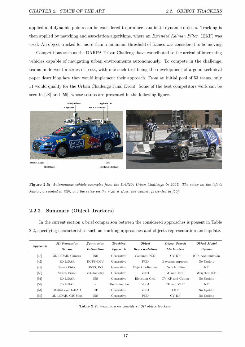
Competitions such as the DARPA Urban Challenge have contributed to the arrival of interesting
vehicles capable of navigating urban environments autonomously. To compete in the challenge,
teams underwent a series of tests, with one such test being the development of a good technical
paper describing how they would implement their approach. From an initial pool of 53 teams, only
11 would qualify for the Urban Challenge Final Event. Some of the best competitors work can be
seen in [28] and [55], whose setups are presented in the following figure.
6
IBEO laser
6
DMI
6
BOSCH Radar
6
SICK LDLRS laser
?
Velodyne laser
?
Riegl laser
?
SICK LMS laser
?
Applanix INS
Figure 1: Junior, our entry in the DARPA Urban Challenge. Junior is equipped with five differentlaser measurement systems, a multi-radar assembly, and a multi-signal inertial navigation system,as shown in this figure.
RNDF. The RNDF contained geometric information on lanes, lanemarkings, stop signs, parkinglots, and special checkpoints. Teams were also provided with a high-resolution aerial image ofthe area, enabling them to manually enhance the RNDF before the event. During the Urban Chal-lenge event, vehicles were given multiple missions, definedas sequences of checkpoints. Multiplerobotic vehicles carried out missions in the same environment at the same time, possibly withdifferent speed limits. When encountering another vehicle,each robot had to obey traffic rules.Maneuvers that were specifically required for the Urban Challenge included: passing parked orslow-moving vehicles, precedence handling at intersections with multiple stop signs, merging intofast-moving traffic, left turns across oncoming traffic, parking in a parking lot, and the executionof U-turns in situations where a road is completely blocked.Vehicle speeds were generally limitedto 30mph, with lower speed limits in many places. DARPA admitted eleven vehicles to the finalevent, of which the present vehicle was one.
“Junior,” the robot shown in Figure 1, is a modified 2006 Volkswagen Passat Wagon, equippedwith five laser rangefinders (manufactured by IBEO, Riegl, Sick, and Velodyne), an ApplanixGPS-aided inertial navigation system, five BOSCH radars, two Intel quad core computer systems,and a custom drive-by-wire interface developed by Volkswagen’s Electronic Research Lab. Thevehicle has an obstacle detection range of up to 120 meters, and reaches a maximum velocity of30mph, the maximum speed limit according to the Urban Challenge rules. Junior made its drivingdecisions through a distributed software pipeline that integrates perception, planning, and control.This software is the focus of the present article.
Urmson et al.: Autonomous Driving in Urban Environments: Boss and the Urban Challenge • 427
Figure 1. Boss, the autonomous Chevy Tahoe that won the 2007 DARPA Urban Challenge.
lane. For unstructured driving, such as entering/exiting a parking lot, a planner with a four-dimensional search space (position, orientation, di-rection of travel) is used. Regardless of which plan-ner is currently active, the result is a trajectory that,when executed by the vehicle controller, will safelydrive toward a goal.
The perception subsystem (described inSection 4) processes and fuses data from Boss’smultiple sensors to provide a composite model of theworld to the rest of the system. The model consistsof three main parts: a static obstacle map, a list ofthe moving vehicles in the world, and the location ofBoss relative to the road.
The mission planner (described in Section 5) com-putes the cost of all possible routes to the next missioncheckpoint given knowledge of the road network.The mission planner reasons about the optimal pathto a particular checkpoint much as a human wouldplan a route from his or her current position to a desti-nation, such as a grocery store or gas station. The mis-sion planner compares routes based on knowledgeof road blockages, the maximum legal speed limit,and the nominal time required to make one maneu-ver versus another. For example, a route that allowsa higher overall speed but incorporates a U-turn mayactually be slower than a route with a lower overallspeed but that does not require a U-turn.
The behavioral system (described in Section 6)formulates a problem definition for the motion plan-
ner to solve based on the strategic information pro-vided by the mission planner. The behavioral subsys-tem makes tactical decisions to execute the missionplan and handles error recovery when there are prob-lems. The behavioral system is roughly divided intothree subcomponents: lane driving, intersection han-dling, and goal selection. The roles of the first two sub-components are self-explanatory. Goal selection is re-sponsible for distributing execution tasks to the otherbehavioral components or the motion layer and forselecting actions to handle error recovery.
The software infrastructure and tools that enablethe other subsystems are described in Section 7. Thesoftware infrastructure provides the foundation uponwhich the algorithms are implemented. Additionally,the infrastructure provides a toolbox of componentsfor online data logging, offline data log playback, andvisualization utilities that aid developers in buildingand troubleshooting the system. A run-time execu-tion framework is provided that wraps around algo-rithms and provides interprocess communication, ac-cess to configurable parameters, a common clock, anda host of other utilities.
Testing and performance in the NQE and UCFEare described in Sections 8 and 9. During the develop-ment of Boss, the team put a significant emphasis onevaluating performance and finding weaknesses toensure that the vehicle would be ready for the UrbanChallenge. During the qualifiers and final challenge,Boss performed well, but made a few mistakes.
Journal of Field Robotics DOI 10.1002/rob
Figure 2.5: Autonomous vehicle examples from the DARPA Urban Challenge in 2007. The setup on the left is
Junior, presented in [28], and the setup on the right is Boss, the winner, presented in [55].
2.2.2 Summary (Object Trackers)
In the current section a brief comparison between the considered approaches is present in Table
2.2, specifying characteristics such as tracking approaches and objects representation and update.
Approach3D Perception
Sensor
Ego-motion
Estimation
Tracking
Approach
Object
Representation
Object Search
Mechanism
Object Model
Update
[46] 3D LiDAR, Camera INS Generative Coloured PCD CV KF ICP, Accumulation
[47] 3D LiDAR DGPS/IMU Generative PCD Bayesian approach No Update
[49] Stereo Vision GNSS, INS Generative Object Delimiters Particle Filter KF
[50] Stereo Vision V-Odometry Generative Voxel KF and MHT Weighted ICP
[51] 3D LiDAR INS Generative Elevation Grid CV KF and Gating No Update
[52] 3D LiDAR - Discriminative Voxel KF and MHT KF
[54] Multi-Layer LiDAR ICP Generative Voxel EKF No Update
[56] 3D LiDAR, GIS Map INS Generative PCD CV KF No Update
Table 2.2: Summary on considered 3D object trackers.
17

CHAPTER
3
PROPOSED METHOD
Contents3.1 Approach Formulation . . . . . . . . . . . . . . . . . . . . . . . . . . . . . 20
3.1.1 Relevant Notation . . . . . . . . . . . . . . . . . . . . . . . . . . . . . . . . 20
3.2 System Overview . . . . . . . . . . . . . . . . . . . . . . . . . . . . . . . . . 20
3.3 3D Tracking . . . . . . . . . . . . . . . . . . . . . . . . . . . . . . . . . . . . 22
3.3.1 Ground Removal . . . . . . . . . . . . . . . . . . . . . . . . . . . . . . . . . 22
3.3.2 Detection and Localization . . . . . . . . . . . . . . . . . . . . . . . . . . . 23
3.4 2D Tracking . . . . . . . . . . . . . . . . . . . . . . . . . . . . . . . . . . . . 24
3.4.1 Discriminant Colour Model . . . . . . . . . . . . . . . . . . . . . . . . . . . 25
3.4.2 Detection and Localization . . . . . . . . . . . . . . . . . . . . . . . . . . . 25
3.4.3 Adaptive Updating of < Bins . . . . . . . . . . . . . . . . . . . . . . . . . . 26
3.5 2D/3D Projection . . . . . . . . . . . . . . . . . . . . . . . . . . . . . . . . 27
3.6 Fusion and Tracking . . . . . . . . . . . . . . . . . . . . . . . . . . . . . . . 29
3.6.1 2D/3D Fusion for Improved Localization . . . . . . . . . . . . . . . . . . . . 30
3.6.2 3D Object Tracking . . . . . . . . . . . . . . . . . . . . . . . . . . . . . . . 32
18

CHAPTER 3. PROPOSED METHOD
In the previous chapter an overview of the current object trackers literature was given, as well
as for sensor technologies. The presented studies highlighted the fact that 3D spatial data processing
has gained attention in fields such as computer vision and robotics, powered by the arrival of new
3D sensing alternatives and new capable stereo matching algorithms. The aforementioned 3D spatial
data comes in the shape of dense 3D PCDs.
In order for intelligent vehicles to understand their relevance and how exactly they characterize
the scene, developed perception systems need to interpret the surrounding environment as well as
perceive objects physical properties.
(a) Sample output point cloud. (b) Zoomed in point cloud.
(c) Sample output RGB image.
Figure 3.1: Input data from 3D and 2D sensors. Both PCD and RGB image correspond to the same scan in a given
sequence from the KITTI dataset. The RGB arrows represent the local (car) reference system.
From the presented sensors, 2D cameras have been widely used for the goal of scene representation;
one of its main advantages is that it provides a very rich and high resolution colour representation.
This in turn provides a very good complement to 3D LiDAR sensors, whose lack of colour information
is one of their main disadvantages.
The proposed framework has thus used both of these technologies, looking into combining highly
accurate 3D LiDAR PCDs with rich and dense 2D RGB corresponding camera images. This data
comes from the conjugation of two sensors: a Velodyne HDL-64E and a PointGrey Flea 2 colour
19

3.1. APPROACH FORMULATION CHAPTER 3. PROPOSED METHOD
camera. These sensors are mounted on the vehicle that provided the KITTI Dataset as explained in
Section 4.1. Additionally, an INS is also used to obtain the location of the ego vehicle. Figure 3.2
shows the considered reference system axes.
v
v v
height (h)
width (w
)
length (l)
Figure 3.2: Object coordinate system in the 3D space [30].
3.1 Approach Formulation
The task of 3D single object tracking can be defined as the estimation of the trajectory of an
object as it moves around a scene (with the ego vehicle either static or moving), with an object
being identified as a 3D BB (with a given width, height and length).
As mentioned in Section 1.2 it is assumed that an initial 3D BB is known, i.e., that a previous
3D object detection or motion detection method has been applied in the reference 3D PCD and that
object characteristics such as location and orientation are provided for the initial reference scan.
3.1.1 Relevant Notation
Input data for the proposed framework will then consist of:
• 3DBB: 3D BB (initial is assumed to be known);
• Ii: RGB image obtained from camera in scan i;
• Li: 3D PCD from LiDAR in scan i;
• LGi : 3D PCD in scan i with ground points removed;
• Pi: Set of 3D points projected in 2D image plane in scan i;
• Ω: Convex-hull of points in P ;
With this information, the tracker will be able to estimate the trajectory of the object, represent-
ing this trajectory as Xi = X1, · · · , XN in the 3D world coordinate system. Each element of X
will hence be the x y z coordinates of the considered object centroid in a certain instant of time.
3.2 System Overview
In the following figure, a diagram representing the conceptual pipeline of the approach is shown.
It follows the same flow as the diagram presented in Figure 1.1 but presents a more detailed insight.
20

CHAPTER 3. PROPOSED METHOD 3.2. SYSTEM OVERVIEW
3D KF-based Fusion 3D KF-based Tracking
2D to 3D Projection
Initialization in 3D-PCD
Automatic Initialization in
Image Using Convex-hull
3D MS-based Object Detection and
Localization in the PCD
2D MS-based Object Detection and
Localization in the RGB Image
3D-BB
Ω
P
Cpcd
Crgb
C’rgb
C3D
Outputs the object’s:- Trajectory
- Velocity estimation
- Predicted location
- 3D-BB in PCD
- Orientation
- 2D convex-hull in Image
Figure 3.3: Major pipeline of the proposed approach. 2D and 3D information is fused and used for 3D tracking of
the objects.
The raw PCD in any given scan is of a form similar to the one present in Figure 3.1b. For the
purpose of object detection, recognition and tracking, it is not desired to take ground points into
consideration, as these can severely hinder the correct results provided by the proposed algorithms.
In the particular case of the presented object tracking approach, removal of ground points is a
particularly important process for the construction of the object model. Without this process, the
constructed object model would be degraded.
In this framework, the process of object tracking starts with a known 3DBB in L1. A new
PCD with no ground points LG1 is obtained. The remaining object points (points from LG1 inside
3DBB) are projected onto the image plane (I1) resulting in a set of projected points, P ∗. The
corresponding 2D convex-hull (Ω) is calculated. It is useful to have Ω since the convex-hull effectively
and accurately segments what are object pixels from non-object (or background) pixels.
Having this information, it is possible to initialize the tracking in both the 3D PCD and 2D
image plane. For tracking purposes a Mean-Shift (MS) based object localizer [57] is run for each
information domain (3D PCD and 2D image) in order to obtain the new object location. Each MS
has different characteristics: to localize an object in the 3D domain, a MS gradient estimation of
those points inside the 3D BB is considered; to localize the object in 2D, and adaptive color based
MS algorithm was applied. After obtaining the new 2D location of the object, its projection is
calculated back onto the 3D domain using bilinear interpolation.
In this approach, and in order to fuse data from two sources of information, a Constant
Acceleration Kalman Filter (CA KF) is considered (measurement fusion model as discussed in [58]).
After this process, another CA KF is used for the purpose of object tracking, as the newly detected
location and orientation are used to initialize the 3D BB in the next scanned PCD.
21

3.3. 3D TRACKING CHAPTER 3. PROPOSED METHOD
3.3 3D Tracking
For the purpose of 3D object tracking, it is common to apply a ground estimation algorithm
to determine what points in the PCD belong to the road and not to objects in the scene. As
aforementioned, the construction of an object model without removal of ground points would result
in a degraded result, since the inclusion of road or sidewalk points would directly impact the centroid
estimation.
3.3.1 Ground Removal
A significant number of points in a typical LiDAR PCD are ground points. By selecting an
appropriate set of features that characterize these points, the corresponding Probability Density
Function (PDF) can be calculated. The notion of a given variable being close to a target value
can be captured by a PDF; the highest (or peak) value indicates the highest probability that the
variable is close to the target value. Hence, the peak value from the computed PDF will indicate
the ground points in the current scan.
To take advantage of this information, a Kernel Density Estimation (KDE) was also applied.
This estimator gauges the PDF of all angles that lie between the ground (XY plane) and the set of
lines passing through the origin point (projection of the LiDAR center of mass onto the ground)
and the end points (remaining points that belong to the PCD).
Considering Θ = θ1, . . . , θN 1D angles in the XZ plane for a given PCD (where θi =
arctan(zi/xi)) a univariate KDE estimated can be obtained from
f(θ) = 1N
N∑i=1
Kσ(θ − θi) (3.1)
In this expression, Kσ(·) is a Gaussian kernel function that has σ bandwidth, and N is the
total number of points in the PCD. For this model, the ground is assumed to be plane, and the
pitch angle of the ground plane is identified as the peak value θρ in the KDE. Having identified
the ground plane, all points whose z coordinate (height) fall under a given threshold dmin are thus
considered ground points. dmin is chosen as an arbitrarily low value designed to represent a safety
boundary for the process.
To smooth the process of determining the ground plane pitch angle in consecutive scans, an
additional CA KF was used for this estimation. This provides additional robustness and accuracy
to the ground removal process. Given the size of the PCD, outliers are also eliminated by limiting
the angle search area to a gate in the neighbourhood of the predicted value from the KF in the
previous step. If no measurements become available inside the provided gate, the predicted value
from the filter is used. The ground removal process is illustrated in Figure 3.4.
22

CHAPTER 3. PROPOSED METHOD 3.3. 3D TRACKING
ix
izithe origin point
the end point i
(a)
(b)
(c)
X axis
Figure 3.4: Ground removal process. (a) Computation of the θi angle. (b) KDE of the set of 1D angles Θ with pitch
angle of the ground plane θρ. (c) End result, with detected ground points (red) and points above ground (blue). The
green ellipse shows an example of the ground points extraction for a car. The corresponding car in the image is shown
with a red ellipse.
3.3.2 Detection and Localization
After removing ground points, detection and tracking of the target object can be achieved. To
do so, a MS approach was considered. This iterative procedure, based on a KDE, shift point(s) in a
set by an amount equal to the average of the data points in their neighbourhood.
The MS procedure can be summarized as:
1. Computing the shift vector: Given the known object centroid (centre of the last known
3D BB) as χ, the shift vector between χ and the point set P ′ (points from the current scan
PCD inside previous time step 3D BB) is computed using
mk = χk − µ(P ′) (3.2)
where µ(.) indicates the “mean” function, and k is the iteration index.
23

3.4. 2D TRACKING CHAPTER 3. PROPOSED METHOD
2. Translating the 3D BB: The 3D BB is translated using the shift vector
χk+1 = χk +mk (3.3)
with the shift vector always pointing toward the direction of the maximum increase in the
density.
3. Iterating steps 1. and 2. until convergence: The MS iteratively shifts the 3D BB until
the object is placed entirely within the 3D BB. A centroid movement |mk| less than 5 cm or
a maximum number of iterations equal to 5 are considered as the MS convergence. These
values were chosen after testing performance with different scenarios.
An example of the MS in action can be seen in the figure below: From the initial 3D BB (from
previous scan) and set P ′, a MS was employed to obtain the 3D BB that defines the object in the
current scan.
Figure 3.5: MS procedure in the PCD. The figure on the left represents a bird’s-eye view of the object (cyclist) and
the right figure shows the top view. In this example, the MS convergence (the centroid movement less than 5 cm)
was achieved in three iterations. The darker blue colour represents the initial 3D BB whilst the brighter blue colour
3D BBs show the most recent iterations (with brightest blue equalling the 3D BB when convergence was met).
As mentioned earlier in this chapter, current object position is represented by the centroid of
object points inside the 3D BB. This point model representation is feasible even with a low number
of detected object points, which happens in sparse 3D LiDAR PCDs, specially for objects located
further away from the LiDAR. The resulting centroid after convergence is denoted by Cpcd and
outputted to the projection module.
3.4 2D Tracking
To initialize the object tracking process in the 2D image, the object initially needs to be
detected. To do so, the 3D object points P after ground removal are projected onto the image plane.
In the same manner that a 3D BB was used to describe the 3D object, a 2D convex hull (Ω) was
24

CHAPTER 3. PROPOSED METHOD 3.4. 2D TRACKING
chosen to identify the 2D object in the image. Therefore, the convex hull Ω of the projected point
set P ∗ = p∗1, · · · , p∗n is then computed. Ω can be defined as the smallest 2D convex polygon that
encloses P ∗. By considering a 2D convex hull it is possible to more accurately segment the object
from the background in comparison with a traditional 2D bounding box. A surrounding area Ω†
is defined automatically by expanding Ω by a factor equal to√
2 with respect to its centroid, so
that the number of pixels in (Ω† − Ω) (the region between Ω and Ω†) is approximately equal to the
number of pixels inside Ω.
3.4.1 Discriminant Colour Model
For tracking the object in the image domain a discriminant colour model of the object is
created and updated in every new scan. To do so, an RGB histogram of the object is calculated.
The considered pixels for the calculation lie within the Ω region and the (Ω† − Ω) region. Two
colour models are then calculated: one for Ω and one for (Ω† − Ω).
The next step is to calculate the Log-Likelihood Ratio (LLR) of the computed RGB histograms.
The LLR expresses how many times more likely the data are under one model than the other. In
our application, the LLR expresses how much more likely each histogram bin is under the Ω colour
model than the (Ω† − Ω) colour model. This is achieved by knowing that in the LLR positive bins
likely belong to Ω, with negative valued bins likely belonging to (Ω† − Ω). Bins that are shared by
both Ω and (Ω† − Ω) tend towards zero. The positive bins in the LLR are thus used to represent
the discriminant object colour model. The discriminant object colour model can be represented by
<(i) = max
log maxHΩ(i), εmaxHΩ†(i), ε
, 0
(3.4)
In this representation, HΩ and HΩ† are the computed histograms from Ω and (Ω† − Ω) regions,
respectively, and ε is a small value that prevents either divisions by zero or log of zero operations.
The variable i ranges from 1 to the total number of histogram bins. The discriminant colour model
of the object (<) is normalized and used for object detection and localization in the next frame
using the MS procedure described in the next section.
3.4.2 Detection and Localization
With the location of the object in the previous scan known and described as the shape of
a convex hull (Ω), object detection in the current scan can be achieved using a MS based object
detection and localization from previous known information.
Initially, a confidence map (represented by f) of the Ω region in the previous frame is calculated.
The centroid of this region is obtained and MS process start in this point. The confidence map can
be achieved by replacing the colour value of each pixel in the Ω region by its corresponding bin
25

3.4. 2D TRACKING CHAPTER 3. PROPOSED METHOD
value in the colour model <.
In each iteration the centre of Ω from the previous step is shifted to the centroid of f (the
current confidence map of the object). This centroid can be calculated by
Citer = 1m
m∑i=1
fi Ci (3.5)
In this notation, Ci = ri, ci denotes the pixel position (row and column) in Ω and m is the
total number of pixels inside the Ω region.
An empirical value of 4 was chosen as the threshold for MS iterations needed to achieve
convergence. If the method achieves centroid movement smaller than a pixel then it is also
considered to have achieved convergence. The computed 2D object centroid after convergence is
denoted by Crgb and outputted to the fusion module. An overview of the detection and tracking
process in 2D can be observed in Figure 3.6.
2D MS Localization
in the RGB Image
The Discriminant Color Model and
the Confident Map of the Object
Object and Background
Convex-hulls
Figure 3.6: MS procedure in the 2D RGB image. The left figure represents both Ω (in blue) and Ω† (in red). The
middle represents the computed < and the correspondent confident map (f). Each non-empty bin in the < is shown
with a circle with a value correspondent to the area of its circle. Circle locations represent the correspondent colour in
the joint RGB histogram. The right figure shows the MS localization procedure, with the brighter blue Ω indicating that
it was computed in the most recent MS iteration. The final Ω centroid is shown as a yellow point.
3.4.3 Adaptive Updating of < Bins
As mentioned in Chapter 2, dense 2D RGB images are very informative. However, they are
sensitive to variations in illumination conditions. In order to adapt the object colour model with
illumination variations (surmounting changes in the object colour appearance during tracking), a
bank of 1D CA KFs model was applied.
The goal of these KFs is to estimate and predict < bin values for the next frames. A new
1D CA KF is initialized and associated for each newly observed colour bin. When the bin values
become zero or negative, the corresponding CA KFs are removed. Based on a series of tests where
26

CHAPTER 3. PROPOSED METHOD 3.5. 2D/3D PROJECTION
8× 8× 8 histograms (512 bins) were considered, the average number of utilized KFs in each frame
were about 70 (or 14% of the total number of bins).
Histogram KF The following is the considered CA KF formulation used for the updating
process of the object histogram. Each time a new colour is observed a CA KF is initialized. The
corresponding state vector is based on the value of that bin (between 0 and 1)
xk = [binvalue 0 0]T (3.6)
The state transition matrix A becomes
A =
1 dt
12d
2t
0 1 dt
0 0 1
(3.7)
H was set to
H =(
1 0 0)
(3.8)
The histogram CA KFs covariance matrices R, Q and P were set to
R = 0.5; (3.9)Q =
5 0 0
0 5 0
0 0 5
(3.10) P =
15 0 0
0 15 0
0 0 15
(3.11)
Bin Updating For the first scan (and object detection) non empty histogram bins are found,
with a KF initialized for each. In the next scans, a search for non empty histogram bins is also
applied. If an empty bin in the previous scan has a value in the current scan, a KF is initialized for
that bin. If a non empty bin in the current scan was also not empty in the bin before, its value must
be updated through an iteration of the KF, with the current value in the bin used as a measurement.
A last case may happen when a previously non empty given bin no longer has a value, resulting in
the corresponding KF being deleted.
3.5 2D/3D Projection
The computed 2D location of the object in the RGB image (Crgb) is projected back to 3D
(C ′rgb). To do so, a method described by Held et. al [46] for PCD upsampling was used. In our
approach however, the method is used solely to project Crgb back to the 3D LiDAR space.
Having found the 2D centroid, the nearest projected points (inside the convex hull) in each
of the four quadrants are found (f1, f2, f3 and f4 for upper left, upper right, lower left and lower
right quadrants, respectively). Bilinear interpolation using these projected points is obtained by
27

3.5. 2D/3D PROJECTION CHAPTER 3. PROPOSED METHOD
first linearly interpolating between the points on top (pt), then the points below (pb) and finally
interpolating between the previous two interpolated positions, obtaining the position of the image
pixel p (see Figure 3.7).
pt = f1 + f22
pt = f3 + f42
p = pt + pb2
Figure 3.7: Bilinear interpolation diagram.
Fractions of the horizontal distances (s1 and s2) between p and each neighbouring pixel pair are
obtained from
s1 = pu − f1,uf2,u − f1,u
s2 = pu − f3,uf4,u − f3,u
with (u,v) being the pixel horizontal and vertical coordinates. Bilinear interpolation can then be
defined as
pt = f1 + s1(f2 − f1)
pb = f3 + s2(f4 − f3)
s3 = p− pbpt − pb
pinterpolated = pb + s3(pt − pb)
The resulting pinterpolated is calculated in both pixel space and in 3D coordinates. pinterpolated is
close to p in pixel space and the corresponding 3D location is then considered to be the 3D location
28

CHAPTER 3. PROPOSED METHOD 3.6. FUSION AND TRACKING
(C ′rgb) of the 2D computed centroid (Crgb).
One example of the bilinear interpolation process can be seen in Figure 3.8 for a tracked van.
Figure 3.8: Bilinear interpolation process. The black dot represents Crgb, with the four quadrants represented in red,
green, blue and yellow points. The dot in magenta is the calculated interpolation point (in 2D), with the corresponding
3D coordinates obtained from the previous formulation.
3.6 Fusion and Tracking
After converting the object 2D location in the RGB image into the 3D space, two different 3D
centroids are available. To fuse both centroids, a CA KF was applied. After the fusion, another CA
KF was used to filter and track the resulting fused 3D centroid along time. A visual representation
of the data flow (centroid wise) is presented in Figure 3.9, taking into consideration the two centroids
outputted from previous modules. On the following section both fusion and tracking KFs are
explained.
29

3.6. FUSION AND TRACKING CHAPTER 3. PROPOSED METHOD
Figure 3.9: Overview of the tracking system. The fusion and Kalman tracking modules are based on CA KFs.
3.6.1 2D/3D Fusion for Improved Localization
To integrate information from two different sensors (after some processing) a KF based fusion
was considered. Based on the measurement fusion model from Gao et. al [58], a KF is applied to
integrate the centroid from the 2D tracking module C ′rgb with the computed 3D object location in
the PCD Cpcd. An assumption of identical sample rates between sensors was made. The sensors are
also assumed as independent of each other. To define the fusion model, object dynamics is first
represented as
xk+1 = Fkxk + Γkvk
where xk is the state vector at time k and vk the state noise such that E[vk] = 0 and E[vkvTl ] = Qkδkl.
The corresponding measurements are
zmk = Hmk xk + wmk ,m = 1, 2
with zmk being the measurement from sensor m at time k and measurement noises wmk being zero
mean, white noise with covariances Rmk and mutually independent.
The measurement fusion is done at state vector level as an augmented observation vector,
combining z1k and z2
k into the augmented observation vector
zk = [(z1k)T (z2
k)T ]T
Assuming that Hk = [(H1k)T (H2
k)T ]T and wk = [(w1k)T (w2
k)T ]T a new measurement equation can
30

CHAPTER 3. PROPOSED METHOD 3.6. FUSION AND TRACKING
be obtained as
zk = Hkxk + wk
Finally, and since statistical independence was assumed, the merged measurement noise wk is
defined as
Rk =
R1k 0
0 R2k
The estimate of the state vector is obtained by conventional Kalman filtering.
The considered dynamics of the object and the fused measurement model of the object localizers
(both in 3D and 2D in the presented approach), as well as the used notation and variable meaning,
are described below.
Fusion CA KF The following is the formulation considered for the CA KF used for fusing
information (centroids provided by 3D MS and re projected 2D MS). The state vector composed as
xk = [xproj2Dk yproj2Dk zproj2Dk x3Dk y3Dk z3Dk ]T (3.12)
The state transition matrix A becomes
A =
1 dt12d
2t 0 0 0 0 0 0
0 1 dt 0 0 0 0 0 0
0 0 1 0 0 0 0 0 0
0 0 0 1 dt12d
2t 0 0 0
0 0 0 0 1 dt 0 0 0
0 0 0 0 0 1 0 0 0
0 0 0 0 0 0 1 dt12d
2t
0 0 0 0 0 0 0 1 dt
0 0 0 0 0 0 0 0 1
(3.13)
H was set to
H =
1 0 0 0 0 0 0 0 0
0 0 0 1 0 0 0 0 0
0 0 0 0 0 0 1 0 0
1 0 0 0 0 0 0 0 0
0 0 0 1 0 0 0 0 0
0 0 0 0 0 0 1 0 0
(3.14)
31

3.6. FUSION AND TRACKING CHAPTER 3. PROPOSED METHOD
Fusion CA KF covariance matrices R, Q and P were set to
R =
5 0 0 0 0 0
0 5 0 0 0 0
0 0 5 0 0 0
0 0 0 5 0 0
0 0 0 0 5 0
0 0 0 0 0 5
(3.15)
Q = P =
1 0 0 0 0 0 0 0 0
0 1 0 0 0 0 0 0 0
0 0 1 0 0 0 0 0 0
0 0 0 1 0 0 0 0 0
0 0 0 0 1 0 0 0 0
0 0 0 0 0 1 0 0 0
0 0 0 0 0 0 1 0 0
0 0 0 0 0 0 0 1 0
0 0 0 0 0 0 0 0 1
(3.16)
In order to obtain a better initial prediction and to maintain the internal coherence of the system,
a linear least squares method is used to estimate the initial state based on the initial observation.
Doing so is equivalent to solve a system of linear equation in the shape of Ax = B for x with left
matrix division (in this case, solve Hxk = xkinitial for xk).
The dynamics of the object and the fused measurement model are then given by Equations
(3.17) and (3.18) respectively.
xf = AF · xf−1 (3.17)
zf = HF · xf (3.18)
For fusion purposes, the augmented measurement vector zf is then given by
zt =[(Cpcd)T (C ′rgb)T
]T(3.19)
The end result of this integration is a fused 3D centroid (noted as C3D). By having an approach
based on a KF, it is possible to give a higher weight to a method that performed better in the recent
past iterations, thus providing a more accurate estimate than applying each method individually.
3.6.2 3D Object Tracking
For the purpose of tracking the final object estimation, another CA KF was used. This
assumption is useful to model target motion when it is believed to be smooth in both position and
velocity changes. For the purpose of object tracking in urban scenarios, 3D objects (read pedestrians,
cyclists or vehicles) are subject to changes in instant velocity during a sequence of scans.
32

CHAPTER 3. PROPOSED METHOD 3.6. FUSION AND TRACKING
Object Tracking CA KF The following is the formulation considered for the CA KF used
for object tracking. In this case, object representation is defined in a state vector composed as
xk = [xk yk zk xk yk zk xk yk zk]T (3.20)
Since object representation is done as a point model, the centroid of the object is located in the
x y z coordinates. xk yk zk and xk yk zk represent object velocity and acceleration in each
coordinate, respectively.
The state transition matrix A becomes
A =
1 dt12d
2t 0 0 0 0 0 0
0 1 dt 0 0 0 0 0 0
0 0 1 0 0 0 0 0 0
0 0 0 1 dt12d
2t 0 0 0
0 0 0 0 1 dt 0 0 0
0 0 0 0 0 1 0 0 0
0 0 0 0 0 0 1 dt12d
2t
0 0 0 0 0 0 0 1 dt
0 0 0 0 0 0 0 0 1
(3.21)
with dt being the sampling rate. In the case of Velodyne LiDAR this sampling rate is 10 Hz (ten
scans every second). The PointGrey camera has been calibrated to acquire images at the same rate.
H was set to
H =
1 0 0 0 0 0 0 0 0
0 0 0 1 0 0 0 0 0
0 0 0 0 0 0 1 0 0
(3.22)
33

3.6. FUSION AND TRACKING CHAPTER 3. PROPOSED METHOD
And covariance matrices R, Q and P were set to
R =
1 0 0
0 1 0
0 0 1
(3.23)
Q = P =
3 0 0 0 0 0 0 0 0
0 3 0 0 0 0 0 0 0
0 0 3 0 0 0 0 0 0
0 0 0 3 0 0 0 0 0
0 0 0 0 3 0 0 0 0
0 0 0 0 0 3 0 0 0
0 0 0 0 0 0 3 0 0
0 0 0 0 0 0 0 3 0
0 0 0 0 0 0 0 0 3
(3.24)
Equations (3.25) and (3.26) represent the discrete time process model and the measurement
model of the system, respectively
xt = AT · xt−1 (3.25)
zt = HT · xt (3.26)
To eliminate outliers and increase robustness of the process, the search area is limited to a gate
in the vicinity of the predicted KF location (available from xt = AT × xt−1). If no measurement is
available inside the gate area, the predicted value given by the KF is used.
The result of the proposed algorithm is the estimated trajectory of an object in the 3D world
coordinate system, its current estimated velocity (obtained directly from the tracking Kalman filter),
and the predicted location of the object in the next time step. The object orientation is achieved
by subtracting the current estimated location from its previous location. The object region in the
image is obtained by computing the 2D convex-hull of the projected object points (the points inside
the 3D-BB) into the image.
34

CHAPTER
4
EXPERIMENTAL RESULTS
Contents4.1 Dataset . . . . . . . . . . . . . . . . . . . . . . . . . . . . . . . . . . . . . . 36
4.1.1 Synchronization . . . . . . . . . . . . . . . . . . . . . . . . . . . . . . . . . 36
4.1.2 Dataset Sequences . . . . . . . . . . . . . . . . . . . . . . . . . . . . . . . . 37
4.2 Evaluation . . . . . . . . . . . . . . . . . . . . . . . . . . . . . . . . . . . . . 39
4.2.1 Quantitative Evaluation Metrics . . . . . . . . . . . . . . . . . . . . . . . . 39
4.3 Baseline Methods . . . . . . . . . . . . . . . . . . . . . . . . . . . . . . . . 40
4.3.1 Baseline KF 3D Object Tracker (3D-KF) . . . . . . . . . . . . . . . . . . . 41
4.3.2 Baseline MS 3D Object Tracker (3D-MS) . . . . . . . . . . . . . . . . . . . 41
4.4 Results . . . . . . . . . . . . . . . . . . . . . . . . . . . . . . . . . . . . . . . 41
4.4.1 Qualitative Evaluation . . . . . . . . . . . . . . . . . . . . . . . . . . . . . . 46
4.5 Benchmark . . . . . . . . . . . . . . . . . . . . . . . . . . . . . . . . . . . . 48
35

4.1. DATASET CHAPTER 4. EXPERIMENTAL RESULTS
This chapter outlines the considered dataset for testing purposes, as well as the experimental
results obtained during the development of this thesis. In the previous chapter a detailed description
of the proposed approach was made, highlighting the behaviour of each system module and its
outputs. The results obtained from running this approach on selected test cases (from the KITTI
dataset) are presented in this chapter. Section 4.1 details the KITTI dataset and how data acquisition
was performed and presents the considered test sequences. Section 4.2 explains the evaluations
metrics used to obtain the practical results of the implementation. Section 4.3 presents two baseline
methods that the proposed method was tested against. Finally, Section 4.4 presents the resulting
data obtained by applying each of the considered methods and makes a critical analysis of the
results.
4.1 Dataset
The developed approach was tested on sequences extracted from the KITTI Dataset [30]. This
dataset was obtained by driving around the mid-size city of Karlsruhe, in both rural areas and
on highways. The information present in the dataset was obtained using a Velodyne 3D LiDAR
and a high-precision INS (GPS/IMU). The Velodyne HDL-64E [27] rotates at 10 Frames Per
Second (FPS) counter-clockwise with vertical resolution of 64 layers, angular resolution of 0.09
and 2cm distance accuracy. Both the horizontal and vertical fields of view are 360 and 26.8,
respectively, and the maximum range is 120m. The Velodyne point cloud is compensated for the
vehicle ego-motion. The inertial navigation system is a OXTS RT3003 and GPS navigation system
[59], with a frame rate of 100Hz and a resolution of 0.02m/0.1. The color cameras are PointGrey
Flea 2 global shutter cameras [19] with a maximum resolution of 1384 × 1032 and a maximum
capture rate of 15 FPS.
When spinning at 10 Hz, Velodyne’s HDL-64E model produces about 2.5 million distance
estimations per second. Sensor coverage is dependant on the mounting position, which directly
influences the size of the blind area around the vehicle, the fixed angular resolution, and the
reflectance of the measured targets. It should also be noted that the HDL-64E rolling shutter causes
a deformation in the resulting data as noted by [60]; when travelling straight at 10 m/s (i.e. 36
km/h) and operating at 10 Hz, the reference system moves 1 m between the start and the end of
the scan, producing even larger errors when other objects move as well.
4.1.1 Synchronization
With every sensor mounted on the vehicle having different acquisition rates, it was necessary
to have the information coming from the different sensors synchronized. In [30] it is explained that
36

CHAPTER 4. EXPERIMENTAL RESULTS 4.1. DATASET
Figure 4.1: Recording platform for the KITTI Dataset. The base platform is a Volkswagen Passat B6, which has
been modified with actuators for the pedals (acceleration and brake) and the steering wheel. The data is recorded using
an eight core i7 computer equipped with a RAID system, running Ubuntu Linux and a real-time database [30].
timestamps of the Velodyne 3D Laser scanner were used in order to set it as the reference and
thus consider each LiDAR spin as a frame. The cameras were also triggered when the LiDAR is
facing forward. For INS synchronization a collection of information with the closest time stamp to
the LiDAR time stamp was done (worst-case time difference of 5 ms between data from the two
sensors).
4.1.2 Dataset Sequences
In the KITTI Dataset objects are identified by a tracklet. This is mainly due to the fact that
the dataset is more focused towards the evaluation of data association approaches. To evaluate
the considered approach (as well as two generative baseline approaches described in literature for
comparison) tracklet information alone is not useful on its own. Hence, and instead of using the plain
tracklets provided, the tracks of a selected number of objects were considered (for as much frames
in the sequence without full occlusions as possible). For the purpose of evaluation 20 annotated
sequences were selected to evaluate the performance of the mentioned approaches. The general
specifications of each sequence as well as the challenging factors they face are reported in Table 4.1.
In this table, information for each sequence is described based on a number of characteristics.
These include existing number of frames, object type (C for car, Y for cyclist and P for pedestrian),
object and ego vehicle status (M for moving and S for stopped) and the scene conditions (either being
characterized as either roads on urban (U) or alleys/avenues in downtown (D) areas). Information
about the initial 2D BB width and height (in pixels) and 3D BB width, height and length (in
meters) is also present. Regarding the challenging factors of each sequence, four major categories
were chosen: objects undergo occlusion (OCC), object pose varies (POS), the distance between
ego vehicle and target object varies (DIS) and the relative velocity between ego vehicle and target
37

4.1. DATASET CHAPTER 4. EXPERIMENTAL RESULTS
IDNum.
Frames
Object
Type
Object
Status
Ego
Status
Scene
Condition
2D BB
Width
2D BB
Height
3D BB
Height
3D BB
Width
3D BB
LengthOCC POS DIS RVL
1 154 C M M U 178 208 1.73 0.82 1.78 * * *
2 154 Y M M U 154 127 2.00 1.82 4.43 * *
3 144 P S M U 16 42 1.72 0.73 0.55 *
4 51 C M M U 52 34 1.57 1.65 4.10 * *
5 31 C S M U 52 34 1.45 1.60 4.22 *
6 24 C M M U 30 32 3.43 2.81 7.02 *
7 63 P M M U 16 30 1.63 0.40 0.83 *
8 99 Y M M D 39 39 1.81 0.59 1.89 * * *
9 41 P M M D 25 42 1.53 0.61 0.73 *
10 323 Y S M U 25 38 1.72 0.78 1.70 *
11 188 C M M U 30 21 1.44 1.74 4.23 * * *
12 41 P M S D 70 105 1.63 0.66 0.89 *
13 132 P M S D 43 72 1.89 0.84 1.05 * *
14 112 P M S D 33 66 1.84 0.78 1.03 * *
15 45 P M S D 196 224 1.64 0.55 0.94 *
16 264 C M M U 28 24 1.40 1.54 3.36 * *
17 71 P M M D 89 124 1.61 0.91 0.91 *
18 125 P M M D 36 62 1.64 0.88 0.49 * *
19 45 P M M D 29 58 1.67 0.70 0.94 * *
20 188 P M M D 31 67 1.76 0.76 1.01 * *
Table 4.1: Detailed information and challenging factors for each sequence.
object is also subject to changes (RVL).
The first frame of each selected sequence can be seen in Figure 4.2. The initial 2D BB (obtained
from the projection of the initial 3D BB onto the image) is also present to identify the target object.
Figure 4.2: Initial frames from the selected sequences. In a left-right, top-bottom manner, this figure represents the
initial frame from each of the 20 sequences presented in Table 4.1. The displayed 2D BB in red is the projection of the
initial ground truth 3D BB onto the image.
38

CHAPTER 4. EXPERIMENTAL RESULTS 4.2. EVALUATION
4.2 Evaluation
In order to evaluate the presented method and the baseline methods some metrics were defined.
They contemplate the error distance between the calculated and ground-truth centroids (in 3D and
2D), as well as the difference in pose (2D angle since only yaw rotation is considered) and instant
velocity estimations. Additionally, and since all methods output objects 3D BBs, an overlap success
metric is also presented.
4.2.1 Quantitative Evaluation Metrics
Localization Estimation Evaluation In the 3D case, the average centroid location error
was computed for three methods: 3D-KF, 3D-MS and the proposed method (3D-Fusion). To
evaluate the centroid location error in 2D, the resulting 3D BBs of the 3D tracking methods were
projected into the image in order to compute and compare the corresponding 2D BBs. This metric
is computed as the Euclidean distance between the calculated 3D (or 2D) centroids from the 3D (or
2D) ground truth. The average centroid location errors in 3D and 2D are given by Equation (4.1)
and Equation (4.2), respectively
E3D = 1N
N∑i=1
√(xi − xgi )2 + (yi − ygi )2 + (zi − zgi )2 (4.1)
E2D = 1N
N∑i=1
√(ri − rgi )2 + (ci − cgi )2 (4.2)
In this representation, ri ci refer to the 2D computed centroid and rgi cgi denotes the 2D
ground truth centroid. xi yi zi indicates the 3D centroid of the detected 3D BB. Similarly,
xgi ygi z
gi represents the 3D centroid obtained from ground truth. N is the total number of
frames/scans in the given sequence.
Orientation Estimation Evaluation The ground truth orientation of the object is given
only by the yaw angle (The yaw angle describes the direction of the object, given by rotation around
Y-axis in camera coordinates in the KITTI dataset [30]). The orientation error can be computed by
Eϕ = 1N
N∑i=1
∣∣∣∣∣arctan |−→ϕ ×−→ϕ g
−→ϕ · −→ϕ g|∣∣∣∣∣ (4.3)
−→ϕ g is the ground-truth orientation of the object as seen in Figure 4.3.
Ego
g
Target
Figure 4.3: Pose error representation.
39

4.3. BASELINE METHODS CHAPTER 4. EXPERIMENTAL RESULTS
Velocity Estimation Evaluation To estimate the instant velocity error, a simple subtraction
between the current velocity estimated as the norm of the three velocity components and the ground
truth velocity in the same frame is calculated (either on km/h or m/s). The average absolute error
can be thus represented by
Eϑ = 1N
N∑i=1| ϑ− ϑg| (4.4)
Overlap Success Evaluation The overlap success rate (also referred to as the intersection-
over-union metric) in 3D can be defined as the volume between the computed 3D BB and the
ground truth 3D BB. A visual representation can be found in Figure 4.4.
To calculate the intersection between two 3D BBs, the overlapping area between the top-down
2D projection of the 3D BBs is obtained (overlapA). Afterwards, and given that each 3D BB base
might be at different heights, the difference between the height of the obtained 3D BB (fob) and
the ground truth 3D BB (fgt) is calculated. The considered height is then h = h − |fob − fgt|.
The intersection volume is obtained by having Intervol = overlapA × h. The union volume can be
calculated based on the total and intersection volumes as Unionvol = (2× 3D BBvol)− Isectvol.
Figure 4.4: Bounding boxes overlap calculation.
The overlap percentage in a given frame can be given by
O3D = IntervolUnionvol
× 100 (4.5)
In order for an object tracker to be considered correct, the overlap ratio O3D must exceed a standard
threshold of 25% [61–63]. The average of the overlap ratio along the sequence can be used as a
metric for the tracking performance of each approach.
4.3 Baseline Methods
For evaluation purposes two generative 3D object tracking methods were implemented as
baselines for the evaluation purpose. These baseline methods take LiDAR PCDs as the input
and, like in the proposed approach, the ground points are removed. The initial position of the
object 3D BB is again also known and its size assumed constant. Additionally, the point model
representation was also considered.
40

CHAPTER 4. EXPERIMENTAL RESULTS 4.4. RESULTS
4.3.1 Baseline KF 3D Object Tracker (3D-KF)
A 3D CA KF with a gating Data Association (DA) method is used for tracking of the
object centroid in the consecutive PCDs. Like in the proposed approach, the state of the filter is
xk = [xk yk zk xk yk zk xk yk zk]T . The discrete time process model and the measurement model of
the system are given by Equations (3.25) and (3.26), respectively. To further eliminate outliers and
provide more reliable information, the search area is limited to a gate (defined as twice the area
of the projection of the object 3D BB onto the ground) near the the predicted KF location from
the previous-step from xt = At × xt−1). If no measurement is available inside the gate area, the
predicted KF value is used.
4.3.2 Baseline MS 3D Object Tracker (3D-MS)
In turn, the baseline 3D MS approach works by iterative repetition of the procedures described
in the cycle present in Section 3.4.2. For the baseline MS method a maximum of 3 iterations was
chosen to be the threshold.
In both cases, the object orientation is achieved by subtracting the estimated current and the
previous location of the object (resulting in a vector pointing towards the direction of movement),
with the velocity estimation being obtained by subtraction of the current and previous centroid
over the time step.
4.4 Results
In the previous sections, the KITTI dataset was described, and information about the selected
sequences was detailed in Table 4.1 and Figure 4.2. The evaluations metrics used for the evaluation
of the proposed methods were also described. In the present section, the evaluation results are
presented in Table 4.2 for the proposed fusion, baseline KF and baseline MS approaches, respectively.
In these tables, for each sequence (S#), the errors are discriminated as distance to object ground
truth location in 3D (E3D) in meters and 2D (E2D) in pixels, difference to ground truth pose (Eϕ) in
radians and to velocity (Eϑ) in km/h. The average 3D BB overlap success (O3D) in percentage and
data processing rate or runtime per frame (Rtime) in FPS are also displayed. These 20 sequences
are composed by a total of 2295 scans.
In the table, for the baseline KF method, a dashed row (—) means that in addition to losing track
of the target object, no points from the PCD were detected inside the gating area and thus numerical
calculations inside the tracker failed. In these cases, no error data is considered. Consequently, such
sequences for the baseline KF method will not be represented in the figures.
41

4.4.R
ESULT
SC
HA
PTER
4.EX
PERIM
ENTA
LR
ESULT
S
S# E3D E2D Eϕ Eϑ O3D Rtime E3D E2D Eϕ Eϑ O3D Rtime E3D E2D Eϕ Eϑ O3D Rtime
1 0.304 9.663 0.412 0.561 61.040 4.857 0.210 9.186 0.287 5.118 68.208 11.647 — — — — — —
2 1.979 11.762 0.413 1.555 29.831 5.650 1.845 19.196 0.443 5.940 30.556 12.183 16.794 465.322 0.799 28.774 1.432 12.346
3 0.233 6.414 1.467 0.434 40.310 5.193 0.155 7.221 1.885 0.091 52.023 6.271 0.182 29.133 1.696 0.902 91.832 6.610
4 1.002 758.314 1.281 3.291 34.849 2.408 0.910 1340.386 2.079 3.161 33.276 6.060 13.063 1549.315 1.365 16.968 7.522 5.964
5 0.784 11.190 1.333 2.090 25.418 3.742 0.771 19.650 1.721 -2.477 25.098 6.384 11.754 316.650 1.427 3.041 4.887 6.394
6 1.715 29.824 0.109 24.895 37.620 4.065 2.239 25.029 2.837 3.366 32.808 6.913 8.900 164.293 2.090 53.390 29.794 6.511
7 0.311 4.784 0.147 0.700 40.977 5.632 0.249 4.580 1.583 -0.002 46.584 7.552 0.500 11.811 1.439 5.394 56.609 7.689
8 0.626 10.918 0.190 19.934 41.914 4.457 0.528 12.840 0.452 23.549 45.937 6.451 — — — — — —
9 0.227 10.764 0.485 1.421 49.123 4.231 0.340 19.309 0.317 0.773 32.324 6.561 0.274 12.194 0.219 5.765 82.287 6.175
10 0.596 21.767 1.483 -0.571 25.427 5.135 0.571 22.888 1.639 -2.591 26.498 6.907 9.531 242.133 1.648 0.451 1.214 6.837
11 1.891 15.824 0.837 21.273 19.037 7.622 19.293 315.599 1.777 19.996 1.283 13.404 27.349 459.618 1.683 32.227 0.731 12.910
12 0.407 13.727 0.222 1.377 39.937 3.853 0.186 15.129 2.502 1.390 58.118 6.426 0.632 46.630 2.536 5.914 52.303 6.838
13 0.227 12.201 0.220 0.395 58.834 4.092 0.233 17.468 2.289 1.943 59.366 8.114 1.290 52.518 2.317 7.575 19.287 13.229
14 0.234 9.532 0.175 0.284 58.225 6.398 0.181 9.486 2.396 1.504 65.096 12.777 2.956 182.408 2.341 6.933 5.216 7.516
15 0.184 12.702 0.215 2.112 55.894 3.255 0.104 8.964 1.098 1.745 71.949 6.330 — — — — — —
16 1.483 14.441 0.230 0.811 27.938 3.403 1.368 8.101 0.054 3.543 30.713 6.614 — — — — — —
17 0.233 17.806 0.200 0.565 57.456 3.436 0.161 13.633 0.167 0.646 67.605 6.110 2.229 254.426 0.646 5.896 14.849 6.297
18 0.204 12.005 0.240 0.802 55.966 4.976 0.189 10.834 0.223 1.243 58.793 8.148 — — — — — —
19 0.140 4.822 0.123 1.575 69.513 4.345 0.103 4.515 0.183 0.707 75.319 5.787 2.424 24.296 0.425 5.964 3.548 5.422
20 0.179 24.363 0.151 0.279 64.255 3.386 0.159 17.848 0.332 1.021 67.532 10.641 0.819 46.243 0.347 5.713 50.177 5.744
Table 4.2: Error results for the proposed approach (left), baseline MS (middle) and baseline KF (right).
42

CHAPTER 4. EXPERIMENTAL RESULTS 4.4. RESULTS
As stated in Equation (4.2) the 2D location error is based on an Euclidean distance. While low
on average, the proposed method presents a higher error value in sequence 4. This is due to the
fact the 2D estimated and ground truth centroids are obtained by projecting the estimated and
ground truth 3D BB onto the image and then obtaining the centroid of the corresponding 2D BBs.
However, in sequence 4, the target object moves close to the ego vehicle in the opposite direction,
and the projection of the 3D BBs is not correctly done, leading to the calculated 2D centroids not
correctly representing the output of the tracker.
The proposed method processes incoming data at an average rate of 4.5 FPS, and thus is not
suited for real-time applications (data acquisition is done at a rate of 10 FPS). This data was
obtained by running the approach on a Windows 10, 64-bit, 2.3 GHz Intel® Core™ i7 3610QM
processor laptop with 6GB of RAM in Matlab R2015b (in a simulation environment). However,
both baseline methods also perform data processing, on average, below the 10 FPS threshold to
belong to real-time processing applications (8.06 FPS for the baseline MS and 7.77 FPS for the
baseline KF when it does not fail). A dedicated implementation in a language such as C++ could
potentially accelerate the process up to a point where the framework became usable in real-time
systems.
The critical module of the proposed approach in terms of computational power is the one
responsible for the 2D tracking, because it has to keep track of the object colour histograms,
initializing, updating or removing them for each occupied cell KF, recalculating the confidence map
for each frame. In addition, and instead of the 2D MS tracking module for the image domain, well
known computer vision based object trackers such as SCM [64] and ASLA [65] were considered.
These approaches have also been used in benchmarks such as the Visual Tracker Benchmark [66].
However, SCM and ASLA alone run at about 1 and 6.5 FPS, respectively; 3D LiDAR based solution
generally have superior performance over approaches in the computer vision field since both the
ego vehicle and target object(s) are often moving. These size and pose changes, also reflected on
the captured RGB images, can mislead purely visual object tracker approaches. By mapping the
3D object points onto the image, colour information about the object is kept and a robust 2D
object tracker was implemented. In addition, some of the computation time is also due to utilizing
non-optimized built-in Matlab functions such as inpolygon that require more computation time.
In Figures 4.5 to 4.8 a graphical comparison of each result for each sequence is done. Figure 4.9
represents the percentage of scans for which the proposed method was considered to be successful
according to the overlap success metric given in Equation (4.5).
43

4.4. RESULTS CHAPTER 4. EXPERIMENTAL RESULTS
0 2 4 6 8 10 12 14 16 18 20
0
5
10
15
20
25
30Location errors
Fusion
Baseline MS
Baseline KF
Figure 4.5: Location error comparison plot (in meters). The proposed fusion approach produces in most cases a
smaller location error than the baseline methods (with few exceptions for the baseline MS).
The proposed approach is able to provide relatively low average location errors for all sequence,
with the highest (average) location error of 1.979m for sequence 2 (in which the target object is a
van). In this same sequence, the lowest average error was obtained by the baseline MS at 1.845m,
with the highest average error being 16.794m provided by the baseline KF.
In addition to the cases identified by a “—” in Table 4.2, the baseline KF provided the worst
results all around, with the exception being sequence 9 where the average location error was lower
than the one provided by the baseline MS (as well as the average overlap success for that sequence);
however, the difference is not significant. One of the reasons as to why this might happen can be
related to the gating area; having a fixed size gate (either small or big) does not suit all cases. By
being too small, the associated KF might not have enough target object points to detect, and thus
the predictions would tend to suffer from a “drag” effect, lagging behind the tracked object until it
effectively loses track of the object. On the other hand, a gate too big might produce a different
effect, since the centroid is calculated as the average of all the detected points inside the gating area.
In turn, the proposed approach applies a MS algorithm to keep track of object points, and
further corrects the estimated location based on this observation. Errors based on the proposed
approach and the baseline MS tend to be low and close to each other due to this, with some
exceptions such as presented in sequence 11. In this case, some challenges were verified: the target
object, initially stopped at a stop light and partially occluded, starts moving and turning; the planar
ground assumption made for the ground removal function is not well suited for the slanted road
present in this sequence. However, due to the use of the applied CA KF the proposed approach is
able to track the car, even though with a higher than the average associated location error (with
the average overlap success percentage falling below the defined threshold for all cases).
44

CHAPTER 4. EXPERIMENTAL RESULTS 4.4. RESULTS
Figure 4.6 represents the average pose errors for each method, with the proposed approach
yielding the lowest errors. The associated CA KF makes the proposed approach more robust as it
tends to rely less on the direct observation from the 3D MS module when the object points count is
lower and thus avoiding sudden pose changes in between consecutive scans. Stopped vehicles and
pedestrians offer the greatest challenges when estimating their orientation.
2 4 6 8 10 12 14 16 18 20
0
0.5
1
1.5
2
2.5
Pose errors
Fusion
Baseline MS
Baseline KF
Figure 4.6: Pose error comparison plot (in radians). The proposed fusion approach handles pose variation better
than the baseline methods.
Figure 4.7 shows the average velocity errors. Both instant velocity values, v and vg, were obtained
by having the spatial shift between two consecutive ground truth 3D centroids over the elapsed time
step. Since a point model object representation was considered, changes in the perceived object
pose influence the measured instant velocity estimation even with the application of the CA KF.
2 4 6 8 10 12 14 16 18 20
0
5
10
15
20
25
30
35
40
45
50
Velocity (absolute) errors
Fusion
Baseline MS
Baseline KF
Figure 4.7: Velocity error comparison plots (in km/h). The plot represents the difference between the measured and
ground-truth as an absolute difference. The proposed fusion approach yields a better instant velocity estimation when
compared to the baseline methods.
Figure 4.8 shows the average 3D BB overlap ratios for each method. For this particular metric,
the MS baseline method obtained an overall average better than the other cases; however, just as
demonstrated by the average localization error, in sequence 11 the MS baseline tracker loses the
object.
45

4.4. RESULTS CHAPTER 4. EXPERIMENTAL RESULTS
2 4 6 8 10 12 14 16 18 20
10
20
30
40
50
60
70
80
90
3D BB overlap
Fusion
Baseline MS
Baseline KF
Figure 4.8: 3D BB overlap comparison plot (in percentage). An approach yielding an average overlap ratio greater
or equal to 25% is considered as successfully tracking an object.
In Figure 4.9 the 3D BB precision plot is present. Based on the information present in Figure
4.8, the precision plot specifies the percentage of scans for which the method provides an overlap
percentage O3D greater than the defined threshold by cumulatively summing each time that it
happens. In doing so, the method was able to achieve a ratio of O3D > 25% for 77.69% of the scans.
200 400 600 800 1000 1200 1400 1600 1800 2000 22000
10
20
30
40
50
60
70
80
90
1003D-BB overlap precision plot (%)
3D Fusion Approach
Figure 4.9: 3D BB overlap precision plot.
4.4.1 Qualitative Evaluation
In the current section some examples of the proposed approach in action are presented. In a
given scan in a sequence, each figure (composed by top and bottom sub-figures) represents the 2D
and 3D tracking modules, respectively.
46
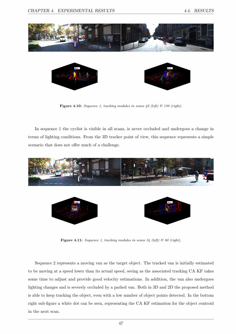
CHAPTER 4. EXPERIMENTAL RESULTS 4.4. RESULTS
Figure 4.10: Sequence 1, tracking modules in scans 40 (left) & 130 (right).
In sequence 1 the cyclist is visible in all scans, is never occluded and undergoes a change in
terms of lighting conditions. From the 3D tracker point of view, this sequence represents a simple
scenario that does not offer much of a challenge.
Figure 4.11: Sequence 1, tracking modules in scans 34 (left) & 80 (right).
Sequence 2 represents a moving van as the target object. The tracked van is initially estimated
to be moving at a speed lower than its actual speed, seeing as the associated tracking CA KF takes
some time to adjust and provide good velocity estimations. In addition, the van also undergoes
lighting changes and is severely occluded by a parked van. Both in 3D and 2D the proposed method
is able to keep tracking the object, even with a low number of object points detected. In the bottom
right sub-figure a white dot can be seen, representing the CA KF estimation for the object centroid
in the next scan.
47

4.5. BENCHMARK CHAPTER 4. EXPERIMENTAL RESULTS
Figure 4.12: Sequence 15, tracking modules in scans 30 (left) & 57 (right).
In sequence 15, the target object is a walking pedestrian that undergoes nearly full occlusion
due to a pedestrian closer to the ego vehicle walking in the opposite direction. Such a scenario is
frequent in downtown and rural areas. In this particular example, the proposed tracker can be seen
making use of the prediction for the next frame to balance out the low number of detected object
points, both maintaining the correct pose as well as not jumping to the nearby pedestrians.
4.5 Benchmark
The 20 considered sequences for testing were selected amongst a group of 50 sequences extracted
from the KITTI dataset. These total 50 sequences compose the 3D Object Tracking in Driving
Environments (or 3D-OTD) proposed benchmark. Most of the existing object tracking benchmark
tools available are based on monocular or stereo cameras approaches or focused on data association
problems. Hence, the created benchmark is aimed at 3D object appearance modelling.
As mentioned in Section 4.1.2, instead of using object tracklets the full track of each object was
extracted. Since information in the dataset is given as tracklets, the selection of the sequences had
to be based on objects who were never fully occluded, i.e., from the first to the last frame of an
extracted sequence, the respective target object will never go under full occlusion. In addition, if
a given scenario in the dataset features several candidate target objects, then a sequence will be
extracted for each object. Based on these considerations, 50 sequences were extracted to create the
benchmark. The general specification of these sequences and the considered challenging factors are
as defined and described as in Section 4.1.2. As a starting point, the two baseline methods here
presented were also considered the baseline evaluators in the benchmark.
The full benchmark, with the total 50 sequences, can be observed in Appendix C as a workshop
paper. This paper has been accepted in IEEE Intelligent Transportation Systems Conference (ITSC)
2016, in the Int. Workshop on Advanced Perception, Machine Learning and Datasets workshop.
48

CHAPTER
5
CONCLUSIONS
Contents5.1 Future Work . . . . . . . . . . . . . . . . . . . . . . . . . . . . . . . . . . . 51
49

CHAPTER 5. CONCLUSIONS
With the increasing effort being put in developing robust ADASs, autonomous driving has
proved to be a successful concept with a lot of direct benefits, from safety (pedestrian detection
and emergency braking) and Quality of Life (parking assistance) to energy savings. Big automotive
companies are making efforts to make driverless cars available to the public in a near future. An
ADAS system can be composed of several modules, from perception systems to actuators. By
moving from research and experimental environments to the real world, perception modules must
become more robust and able to deal with data acquisition, modelling and scene interpretation.
Object tracking is one of the critical components of these perception modules, responsible by the
task of following each target object in the environment. Future predictions of the target object
trajectory are very useful since the ego vehicle can understand what is most likely to happen in the
next time step and plan to act accordingly.
Thus, the main goal of this thesis was to develop a fusion based 3D object tracker. The fusion
of information from different sensor technologies aimed to maximize the benefits of the dense
information present in the RGB image as well as the inherent spatial information provided by the
LiDAR sensor. This resulted in the two main contributions of this thesis:
• A robust, online, 2D/3D fusion based approach was developed. It takes both sequential 2D
RGB images and 3D PCDs as inputs as well as the location of the ego vehicle, given by an
INS. An assumption was made to consider that an initial 3D BB of the target object is known
known and outputted by a previous object detection and/or segmentation module. From this
data two independent and parallel MS algorithms are applied to each considered data space
(2D image and 3D PCD) to detect and track the target object. Following this step, a robust
CA KF is applied to fuse information from both 2D and 3D tracking modules, and a final
CA KF is considered for 3D tracking purposes.
• To test the developed work, a series of experiments were designed with different types of
target objects, scene conditions and associated challenging factors (inherent or relative to the
surrounding scene) to create a benchmark. The benchmark can be used to evaluate 3D object
trackers, even if the base assumptions or theoretical backgrounds are different. Based on this
benchmark, a subset of 20 sequence were selected. An analysis of the obtained results of
testing the proposed approach with these sequences was provided, demonstrating the viability
of the proposed object tracker.
50

CHAPTER 5. CONCLUSIONS 5.1. FUTURE WORK
5.1 Future Work
The proposed approach is able to achieve satisfying results in its current state. However, and
as aforementioned, the execution times are not high enough to process incoming data in real-time.
One direction of future work could be the improvement of the existing code as well as the study of
different methodologies or functions that could further reduce computation times. Taking advantage
of the fact that the 3D and 2D trackers run independently and in parallel, exploration of parallel
computing architectures could also be considered.
In the current method, the point model was used for object representation. Even though the
applied KFs were able to apply trajectory correction when the information was sparse, different
object representation models could also be considered. One such hypothesis could be to apply
3D reconstruction of the shape of the target object. In consecutive frames, since target object
location and orientation are known in real world coordinates in each scan, reconstruction of the
object shape can be obtained by aligning the detected object points (or the current 3D BB) with
reference information (e.g. last scan’s 3D BB). Initial attempts at this reconstructions were made,
with promising results obtained as observable in Figure 5.1. However, due to time constraints and
the lack of robustness of the reconstruction module (in some cases, the module failed to correctly
reconstruct the shape due to wrong rotation values in the alignment process), it was not included in
the final framework.
Figure 5.1: Object shape reconstruction result. The sub-figure on the left represents the detected object points in
the first scan from sequence 2 (940 total). The middle sub-figure shows the detect object points for scan 80 in the
same sequence without object reconstruction. Without reconstruction, the direct readings from the LiDAR provide
only 49 points in the entire PCD. By registration and accumulation of all the detected object points from previous
frames without any further processing, the accumulated model of the object can be used when less points are detected to
overcome occlusion problems. This is highlighted in the right sub-figure; for the same scan as the middle sub-figure
(scan 80), the accumulated object model has much more information present (38163 points) and can be used in its
stead.
51

CHAPTER
6
BIBLIOGRAPHY
[1] World Health Organization (WHO), Global status report on road safety 2015. World Health
Organization, 2015, no. 978 92 4 156506 6, accessed: 18-07-2016. [Online]. Available:
http://www.who.int/violence_injury_prevention/road_safety_status/2015/en/
[2] ASIRT, “Annual global road crash statistics,” Accessed: 04-08-2016. [Online]. Available:
http://asirt.org/initiatives/informing-road-users/road-safety-facts/road-crash-statistics
[3] J. Jackisch, D. Sethi, F. Mitis, T. Szymañski, and I. Arra, “European facts and the
global status report on road safety 2015,” World Health Organization, Tech. Rep., 2015,
accessed: 18-07-2016. [Online]. Available: http://www.euro.who.int/__data/assets/pdf_file/
0006/293082/European-facts-Global-Status-Report-road-safety-en.pdf
[4] National Highway Traffic Safety Administration (NHTSA), “Early estimate of motor
vehicle traffic fatalities in 2015,” 2015, accessed: 18-07-2016. [Online]. Available:
https://crashstats.nhtsa.dot.gov/Api/Public/ViewPublication/812269
[5] M. Pines, “Top 3 causes of car accidents,” Accessed: 04-08-2016. [Online]. Available:
http://www.drivers.com/article/1173/
[6] S. G. Klauer, T. A. Dingus, V. L. Neale, J. D. Sudweeks, and D. J. Ramsey, “The impact of
driver inattention on near-crash/crash risk: An analysis using the 100-car naturalistic driving
study data,” Virginia Tech Transportation Institute, Tech. Rep., April 2006.
52

CHAPTER 6. BIBLIOGRAPHY
[7] National Highway Traffic Safety Administration (NHTSA), “Critical reasons for crashes
investigated in the national motor vehicle crash causation survey,” 2015, accessed: 18-07-2016.
[Online]. Available: https://crashstats.nhtsa.dot.gov/Api/Public/ViewPublication/812115
[8] L. Danielsson, Tracking and radar sensor modelling for automotive safety systems, ser. Doktor-
savhandlingar vid Chalmers tekniska högskola. Ny serie, no: 3064. Institutionen för signaler
och system, Signalbehandling, Chalmers tekniska högskola, 2010, 279.
[9] J. Thalen, “ADAS for the Car of the Future ,” Universiteit Twente, Technical Report, April/June
2006.
[10] S. A. Beiker, “Legal aspects of autonomous driving,” Santa Clara University, Tech. Rep., 12
December 2012.
[11] A. Geiger, M. Lauer, C. Wojek, C. Stiller, and R. Urtasun, “3D Traffic Scene Understanding
From Movable Platforms,” IEEE Transactions on Pattern Analysis and Machine Intelligence,
vol. 36, no. 5, pp. 1012–1025, May 2014.
[12] R. R. Murphy, Introduction to AI Robotics. The MIT Press, 2000, ISBN: 9780262133838.
[13] X. Chen, K. Kundu, Y. Zhu, A. G. Berneshawi, H. Ma, S. Fidler, and R. Urtasun, “3d object
proposals for accurate object class detection,” in Advances in Neural Information Processing
Systems, 2015, pp. 424–432.
[14] A. Asvadi, P. Peixoto, and U. Nunes, Two-Stage Static/Dynamic Environment Modeling Using
Voxel Representation. Cham: Springer International Publishing, 2016, pp. 465–476. [Online].
Available: http://dx.doi.org/10.1007/978-3-319-27146-0_36
[15] M. Brahmi, K.-H. Siedersberger, A. Siegel, and M. Maurer, “Reference systems for environmental
perception: Requirements, validation and metric-based evaluation,” Automotive Systems
Engineering, pp. 205–211, 2013.
[16] P. E. Ross, “Tesla’s Autopilot May Have Saved A Life,” July 2016, Accessed: 04-08-2016.
[Online]. Available: http://spectrum.ieee.org/cars-that-think/transportation/self-driving/
teslas-autopilot-may-have-saved-a-life-cars-that-think
[17] E. Ackerman, “Fatal Tesla Self-Driving Car Crash Reminds Us That Robots Aren’t Perfect,”
July 2016, Accessed: 04-08-2016. [Online]. Available: http://spectrum.ieee.org/cars-that-think/
transportation/self-driving/fatal-tesla-autopilot-crash-reminds-us-that-robots-arent-perfect
[18] S. Sivaraman and M. M. Trivedi, “Looking at vehicles on the road: A survey of vision-
based vehicle detection, tracking, and behavior analysis,” IEEE Transactions on Intelligent
Transportation Systems, vol. 14, no. 4, pp. 1773–1795, Dec 2013.
53

CHAPTER 6. BIBLIOGRAPHY
[19] PointGrey, “Flea 3,” Accessed: 04-08-2016. [Online]. Available: https://www.ptgrey.com/
flea3-usb3-vision-cameras
[20] ——, “Bumbleebee 2,” Accessed: 04-08-2016. [Online]. Available: https://www.ptgrey.com/
bumblebee2-firewire-stereo-vision-camera-systems
[21] A. Mukhtar, L. Xia, and T. B. Tang, “Vehicle detection techniques for collision avoidance
systems: A review,” IEEE Transactions on Intelligent Transportation Systems, vol. 16, no. 5,
pp. 2318–2338, Oct 2015.
[22] Z. Sun, G. Bebis, and R. Miller, “Monocular precrash vehicle detection: features and classifiers,”
IEEE Transactions on Image Processing, vol. 15, no. 7, pp. 2019–2034, July 2006.
[23] A. Klaus, M. Sormann, and K. Karner, “Segment-based stereo matching using belief propaga-
tion and a self-adapting dissimilarity measure,” in 18th International Conference on Pattern
Recognition (ICPR’06), vol. 3, 2006, pp. 15–18.
[24] BOSCH, “Bosch Engineering Long-Range-Radar LRR3,” Accessed: 04-08-2016.
[Online]. Available: http://www.bosch-engineering.de/media/de/pdfs/einsatzgebiete_1/
produktdatenblaetter/120903_LRR3_EN_V05_final.pdf
[25] SICK, “Lms200/211/221/291 laser measurement systems,” Accessed: 04-08-2016. [Online].
Available: http://sicktoolbox.sourceforge.net/docs/sick-lms-technical-description.pdf
[26] HOKUYO, “Scanning range finder (sokuiki sensor),” Accessed: 04-08-2016. [Online]. Available:
https://www.hokuyo-aut.jp/02sensor/07scanner/urg_04lx.html
[27] Velodyne, “Velodyne LiDAR™ HDL-64E,” Accessed: 04-08-2016. [Online]. Available:
http://velodynelidar.com/hdl-64e.html
[28] M. Montemerlo, J. Becker, S. Bhat, H. Dahlkamp, D. Dolgov, S. Ettinger, D. Haehnel,
T. Hilden, G. Hoffmann, B. Huhnke, D. Johnston, S. Klumpp, D. Langer, A. Levandowski,
J. Levinson, J. Marcil, D. Orenstein, J. Paefgen, I. Penny, A. Petrovskaya, M. Pflueger,
G. Stanek, D. Stavens, A. Vogt, and S. Thrun, Junior: The Stanford Entry in the Urban
Challenge. Berlin, Heidelberg: Springer Berlin Heidelberg, 2009, pp. 91–123. [Online].
Available: http://dx.doi.org/10.1007/978-3-642-03991-1_3
[29] S. Kammel, J. Ziegler, B. Pitzer, M. Werling, T. Gindele, D. Jagzent, J. Schöder,
M. Thuy, M. Goebl, F. von Hundelshausen, O. Pink, C. Frese, and C. Stiller,
Team AnnieWAY’s Autonomous System for the DARPA Urban Challenge 2007. Berlin,
Heidelberg: Springer Berlin Heidelberg, 2009, pp. 359–391. [Online]. Available:
http://dx.doi.org/10.1007/978-3-642-03991-1_9
54

CHAPTER 6. BIBLIOGRAPHY
[30] A. Geiger, P. Lenz, C. Stiller, and R. Urtasun, “Vision meets robotics: The KITTI dataset,”
The International Journal of Robotics Research, vol. 32, no. 11, pp. 1231–1237, aug 2013.
[Online]. Available: http://dx.doi.org/10.1177/0278364913491297
[31] A. Petrovskaya and S. Thrun, “Model based vehicle detection and tracking for autonomous
urban driving,” Autonomous Robots, vol. 26, no. 2, pp. 123–139, 2009. [Online]. Available:
http://dx.doi.org/10.1007/s10514-009-9115-1
[32] V. LiDAR™, Accessed: 04-08-2016. [Online]. Available: http://velodynelidar.com/
[33] Google, “Google Self-Driving Car Project,” Accessed: 04-08-2016. [Online]. Available:
https://www.google.com/selfdrivingcar/
[34] C. Premebida, G. Monteiro, U. Nunes, and P. Peixoto, “A lidar and vision-based approach
for pedestrian and vehicle detection and tracking,” in 2007 IEEE Intelligent Transportation
Systems Conference, Sept 2007, pp. 1044–1049.
[35] G. Zhao, X. Xiao, J. Yuan, and G. W. Ng, “Fusion of 3d-lidar and camera data for scene
parsing,” Journal of Visual Communication and Image Representation, vol. 25, no. 1, pp. 165 –
183, 2014, visual Understanding and Applications with RGB-D Cameras. [Online]. Available:
http://www.sciencedirect.com/science/article/pii/S1047320313001211
[36] D. Lee, “Producing 3d point clouds with a stereo camera in opencv,” April 2014,
Accessed: 04-08-2016. [Online]. Available: https://erget.wordpress.com/2014/04/27/
producing-3d-point-clouds-with-a-stereo-camera-in-opencv/
[37] M. Pijpers, “Sensors in ADAS,” Universiteit Twente, Technical Report, January 2007.
[38] A. W. M. Smeulders, D. M. Chu, R. Cucchiara, S. Calderara, A. Dehghan, and M. Shah,
“Visual tracking: An experimental survey,” IEEE Transactions on Pattern Analysis and Machine
Intelligence, vol. 36, no. 7, pp. 1442–1468, July 2014.
[39] H. Yang, L. Shao, F. Zheng, L. Wang, and Z. Song, “Recent advances and trends in visual
tracking: A review,” Neurocomputing, vol. 74, no. 18, pp. 3823 – 3831, 2011. [Online]. Available:
http://www.sciencedirect.com/science/article/pii/S0925231211004668
[40] A. Yilmaz, O. Javed, and M. Shah, “Object tracking: A survey,” ACM Comput. Surv., vol. 38,
no. 4, Dec. 2006. [Online]. Available: http://doi.acm.org/10.1145/1177352.1177355
[41] X. Li, W. Hu, C. Shen, Z. Zhang, A. Dick, and A. V. D. Hengel, “A survey of appearance
models in visual object tracking,” ACM Trans. Intell. Syst. Technol., vol. 4, no. 4, pp.
58:1–58:48, Oct. 2013. [Online]. Available: http://doi.acm.org/10.1145/2508037.2508039
55

CHAPTER 6. BIBLIOGRAPHY
[42] M. Kristan, J. Matas, A. Leonardis, M. Felsberg, L. Cehovin, G. Fernandez, T. Vojir, G. Hager,
G. Nebehay, R. Pflugfelder, A. Gupta, A. Bibi, A. Lukezic, A. Garcia-Martin, A. Saffari,
A. Petrosino, and A. S. Montero, “The visual object tracking vot2015 challenge results,” in
2015 IEEE International Conference on Computer Vision Workshop (ICCVW), Dec 2015, pp.
564–586.
[43] Y. Wu, J. Lim, and M. H. Yang, “Object tracking benchmark,” IEEE Transactions on Pattern
Analysis and Machine Intelligence, vol. 37, no. 9, pp. 1834–1848, Sept 2015.
[44] C.-C. Wang, C. Thorpe, and S. Thrun, “Online simultaneous localization and mapping with
detection and tracking of moving objects: Theory and results from a ground vehicle in crowded
urban areas,” in Proceedings of the IEEE International Conference on Robotics and Automation
(ICRA), 2003.
[45] P. Morton, B. Douillard, and J. Underwood, “An evaluation of dynamic object tracking with 3d
lidar,” in Proceedings of Australasian Conference on Robotics and Automation (ACRA), 2011.
[46] D. Held, J. Levinson, and S. Thrun, “Precision tracking with sparse 3d and dense color 2d
data,” in Robotics and Automation (ICRA), 2013 IEEE International Conference on, May
2013, pp. 1138–1145.
[47] A. Dewan, T. Caselitz, G. D. Tipaldi, and W. Burgard, “Motion-based detection and tracking
in 3d lidar scans,” in ICRA, 2016.
[48] M. A. Fischler and R. C. Bolles, “Random sample consensus: A paradigm for model fitting
with applications to image analysis and automated cartography,” Commun. ACM, vol. 24,
no. 6, pp. 381–395, Jun. 1981. [Online]. Available: http://doi.acm.org/10.1145/358669.358692
[49] A. Vatavu, R. Danescu, and S. Nedevschi, “Stereovision-based multiple object tracking in
traffic scenarios using free-form obstacle delimiters and particle filters,” IEEE Transactions on
Intelligent Transportation Systems, vol. 16, no. 1, pp. 498–511, Feb 2015.
[50] A. Ošep, A. Hermans, F. Engelmann, D. Klostermann, M. Mathias, and B. Leibe, “Multi-scale
object candidates for generic object tracking in street scenes,” in 2016 IEEE International
Conference on Robotics and Automation (ICRA), May 2016, pp. 3180–3187.
[51] A. Asvadi, P. Peixoto, and U. Nunes, “Detection and tracking of moving objects using 2.5d
motion grids,” in 2015 IEEE 18th International Conference on Intelligent Transportation
Systems, Sept 2015, pp. 788–793.
56

CHAPTER 6. BIBLIOGRAPHY
[52] J. Choi, S. Ulbrich, B. Lichte, and M. Maurer, “Multi-target tracking using a 3d-lidar sensor
for autonomous vehicles,” in 16th International IEEE Conference on Intelligent Transportation
Systems (ITSC 2013), Oct 2013, pp. 881–886.
[53] A. Elfes, “Using occupancy grids for mobile robot perception and navigation,” Computer,
vol. 22, no. 6, pp. 46–57, June 1989.
[54] T. Miyasaka, Y. Ohama, and Y. Ninomiya, “Ego-motion estimation and moving object tracking
using multi-layer lidar,” in Intelligent Vehicles Symposium, 2009 IEEE, June 2009, pp. 151–156.
[55] C. Urmson, J. Anhalt, D. Bagnell, C. Baker, R. Bittner, M. N. Clark, J. Dolan, D. Duggins,
T. Galatali, C. Geyer, M. Gittleman, S. Harbaugh, M. Hebert, T. M. Howard, S. Kolski,
A. Kelly, M. Likhachev, M. McNaughton, N. Miller, K. Peterson, B. Pilnick, R. Rajkumar,
P. Rybski, B. Salesky, Y.-W. Seo, S. Singh, J. Snider, A. Stentz, W. R. Whittaker,
Z. Wolkowicki, J. Ziglar, H. Bae, T. Brown, D. Demitrish, B. Litkouhi, J. Nickolaou,
V. Sadekar, W. Zhang, J. Struble, M. Taylor, M. Darms, and D. Ferguson, “Autonomous
driving in urban environments: Boss and the urban challenge,” Journal of Field Robotics,
vol. 25, no. 8, pp. 425–466, 2008. [Online]. Available: http://dx.doi.org/10.1002/rob.20255
[56] S. Hosseinyalamdary, Y. Balazadegan, and C. Toth, “Tracking 3d moving objects based on
gps/imu navigation solution, laser scanner point cloud and gis data,” ISPRS International
Journal of Geo-Information, vol. 4, no. 3, pp. 1301–1316, 2015.
[57] Y. Cheng, “Mean shift, mode seeking, and clustering,” IEEE Transactions on Pattern Analysis
and Machine Intelligence, vol. 17, no. 8, pp. 790–799, Aug 1995.
[58] J. Gao and C. Harris, “Some remarks on kalman filters for the multisensor
fusion,” Information Fusion, vol. 3, no. 3, pp. 191 – 201, 2002. [Online]. Available:
http://www.sciencedirect.com/science/article/pii/S1566253502000702
[59] Oxford Technical Solutions, “RT3000 v2 Family.” [Online]. Available: http://www.oxts.com/
products/rt3000-family/
[60] A. Broggi, P. Grisleri, and P. Zani, “Sensors technologies for intelligent vehicles perception
systems: A comparison between vision and 3d-lidar,” in 16th International IEEE Conference
on Intelligent Transportation Systems (ITSC 2013), Oct 2013, pp. 887–892.
[61] C. J. Olsson, “Scene Category Context for 3d Object Detection with RGBD Cameras,” 2016.
[62] S. Song and J. Xiao, Sliding Shapes for 3D Object Detection in Depth Images.
Cham: Springer International Publishing, 2014, pp. 634–651. [Online]. Available:
http://dx.doi.org/10.1007/978-3-319-10599-4_41
57

CHAPTER 6. BIBLIOGRAPHY
[63] Z. Ren and E. B. Sudderth, “Three-dimensional object detection and layout prediction using
clouds of oriented gradients,” in Proceedings of the IEEE Conference on Computer Vision and
Pattern Recognition, 2016.
[64] M.-H. Y. W. Zhong, H. Lu, “Robust object tracking via sparse collaborative appearance model,”
IEEE Transactions on Image Processing, vol. 23, no. 5, pp. 2356–2368, 2014.
[65] X. Jia, H. Lu, and M. H. Yang, “Visual tracking via adaptive structural local sparse appearance
model,” in Computer Vision and Pattern Recognition (CVPR), 2012 IEEE Conference on,
June 2012, pp. 1822–1829.
[66] “Visual tracker benchmark.” [Online]. Available: http://cvlab.hanyang.ac.kr/tracker_
benchmark/
[67] R. E. Kalman, “A New Approach to Linear Filtering and Prediction Problems,” Transactions
of the ASME – Journal of Basic Engineering, no. 82 (Series D), pp. 35–45, 1960. [Online].
Available: http://www.cs.unc.edu/~welch/kalman/media/pdf/Kalman1960.pdf
58

APPENDIX
A
KALMAN FILTER THEORY
Although more than 50 years old, KF and its variants such as EKF still remain popular
choices in information processing and fusion. Presented by R. E. Kalman in 1960 [67], the algorithm
described a recursive approach to the problem of discrete-data linear filtering. The KF is a set of
mathematical equations used to recursively estimate the state of a given process, typically derived
by vector algebra as a minimum mean square error estimator. Furthermore, the filter supports
estimation of past, present and future states even when the system model is unknown.
As highlighted on the previous chapter, most object tracking approaches are based on some sort
of Bayesian tracking theory. The main idea when using these filters is to set up a discrete time
model with a state vector to describe a given object with the goal of estimating the state x ∈ <n
of the process based on a measurement z ∈ <m. The object motion model can be seen as a linear
stochastic difference equation
xk = Axk−1 +Buk−1 + wk−1
and a measurement model in the shape of
zk = Hxk + vk
with k representing the current time step. Time between consecutive time steps can be variable
but in most cases is consistent, since observations (or measurements) are made in specific and
well-behaved time intervals.
59

APPENDIX A. KALMAN FILTER THEORY
The n× n A matrix (state transition matrix) corresponds to the relationship between the state
at time steps k − 1 and k (assumed constant), applying the effect of system parameters at k − 1
on the system at time k. The n × l matrix B (optional) relates the control input u ∈ <l to the
state x. The random variables w and v contain the process noise and measurement noise terms
(respectively) for the parameters in the state vector. These variables are assumed independent of
each other, as being white noise and having a normal probability distribution. In this approach,
they are also considered constant (zero-mean Gaussians). The m × n H matrix (transformation
matrix) relates the current state to the measurement zk. Even though H can change with each time
step, it is also assumed constant.
To estimate a process, KF uses feedback control. First, it estimates the process state and then
obtains feedback in the form of noisy measurements. The equations for the KF can be categorized
as either being time update or measurement update equations. Time update equations project
the current state forward in time as to acquire the a priori estimates for the next time step.
Measurement update equations goal is to provide the new measurement to the existing a priori
estimate to get a better estimate (also called the a posteriori estimate). In this sense, the first set of
equations can be considered the predictor equations, with the other being the corrector equations.
Time UpdatePREDICT
Measurement UpdateCORRECT
Initial estimates for
x^ and Pk-1k-1
Figure A.1: Kalman filter overview. The prediction projects the current state forward; the correction fits the projected
estimate to the measurement taken at that time.
After prediction, computation of the Kalman gain is done and afterwards a new process
measurement is obtained. An a posteriori estimate for the state is generated by taking into account
the obtained measurement and afterwards an a posteriori estimate for the error covariance is
obtained as well. The recursive nature of the KF lies on the fact that after each prediction and
correction, the whole process is repeated with the previous a posteriori estimates as new a priori
estimates. In the presented notation, R is the measurement error covariance, Q is the process noise
covariance and P a priori covariance matrix.
60

APPENDIX A. KALMAN FILTER THEORY
Time update (prediction) equations Measurement update (correction) equations
Projection of the current state Computation of Kalman gain
x−k = Axk−1 (A.1) Kk = P−k HT (HP−k H
T +R)−1 (A.2)
Projection of error covariance Updating estimate with measurement
P−k = APk−1AT +Q (A.3) xk = x−k +Kz(zk −Hx−k ) (A.4)
Updating error covariance
Pk = (I −KkH)P−k (A.5)
Table A.1: Discrete KF filter time and measurement update equations. From initial estimates xk−1 and Pk−1 a
prediction is made, which is then corrected and fed back to the prediction equations in a recursive fashion (as seen in
Figure A.1).
61

APPENDIX
B
SUBMITTED PAPER: 3D OBJECT
TRACKING USING RGB AND LIDAR
DATA
62

3D Object Tracking using RGB and LIDAR Data
Alireza Asvadi∗†, Pedro Girao∗, Paulo Peixoto∗†, and Urbano Nunes∗†∗Department of Electrical and Computer Engineering (DEEC)
†Institute of Systems and Robotics (ISR)University of Coimbra, Portugal
asvadi, peixoto, [email protected]
Abstract—Object tracking is one of the key components ofthe perception system of autonomous cars and ADASs. Usingtracking, an ego-vehicle can make a prediction about the locationof surrounding objects in the next time epoch and plan for nextactions. Object tracking algorithms typically relay on sensorydata either from RGB cameras or LIDAR. In fact, integrationof 2D-RGB image from camera and 3D-LIDAR data can pro-vide some distinct benefits. This paper proposes a 3D objecttracking algorithm using a 3D-LIDAR, a RGB camera, and INS(GPS/IMU) data. The proposed method analyzes sequential 2D-RGB, 3D point-cloud, and the ego-vehicle’s localization data andoutputs the trajectory of the tracked object, an estimation ofits current velocity, and its predicted location in the 3D worldcoordinate system in the next time-step. Tracking starts with aknown initial 3D bounding box for the object. Two parallel mean-shift algorithms are applied for object detection and localizationin the 2D image and 3D point-cloud, followed by a robust2D/3D Kalman filter based fusion and tracking. Reported results,from quantitative and qualitative experiments using the KITTIdatabase, demonstrate the applicability and efficiency of theproposed approach in driving environments.
I. INTRODUCTION AND MOTIVATION
Visual object tracking is one of the rapidly evolving re-search fields in the computer vision community and becamea key-feature of perception system of autonomous cars andadvanced driver assistance systems (ADASs). The goal ofobject tracking is to estimate the trajectory of an object in asequence of images given a known initial position [1]. Objecttracking algorithms in image sequences have been studiedcomprehensively in the last few decades [1], [2], [3]. Thesemethods mainly differ in the way they model the motion orappearance of the object. Considering the intended applicationeach approach has strengths and weaknesses. However, mostof these methods work only on monocular image sequences.
3D spatial data processing has recently gained much atten-tion in computer vision and robotics. Recently, with the arrivalof modern stereo matching algorithms and new 3D sensingtechnologies, providing an accurate and dense 3D point-cloud(PCD), perception systems of intelligent/autonomous vehiclesbecame able to interpret surrounding environment in 3D andperceive objects physical properties. Stereo vision and 3DLIDAR are the first options to acquire 3D spatial informationin the IV/ITS industries. The major limitations of stereovision approaches are their poor performance in texture-lessenvironments and their dependency on the calibration quality.The main disadvantages with LIDARs are the costly price andthe moving parts of the sensor. In comparison with stereocameras, LIDAR sensors have higher precision but do notacquire color data [4].
Fig. 1. The results of the proposed object tracking method for a given framefrom the KITTI dataset. The bottom figure shows the result in the 3D-PCD,where the 3D Bounding Box (3D-BB) of the tracked object (here a cyclist)is shown in blue, object trajectory is represented with a yellow-curve, objectpoints in 3D-BB are shown in yellow, and the current estimated velocity of theobject is denoted with a text-box (27.3 km/h). The ego-vehicle trajectory, givenby an INS system, is represented by a magenta-curve. The current positionof the ego-vehicle and the tracked object are represented with red-green-bluevectors. Parts of the 3D-LIDAR PCD that are in the field of view of the cameraare shown in white and red, where red denotes the detected ground points andwhite indicates the on-ground obstacle points. LIDAR points outside the imagefield are shown in blue. The top figure represent the tracking result in the 2D-RGB image for the current frame, where the detected object region and itssurrounding area are shown in blue and red, respectively. Please refer to thePDF version for a high-resolution color representation of the figure.
2D cameras have been the most common sensor used forperceiving the environment. The high-spatial-resolution colordata provided by 2D cameras can be used as a complement of3D-LIDARs. The combined use of 3D-LIDAR with 2D-RGBcamera, has attracted a lot of attention recently, to name a few,in applications such as object detection [5], road detection [6],scene parsing [7] and dense depth mapping [8].
This paper proposes an on-board 3D object tracking sys-tem benefiting from ‘highly accurate 3D-LIDAR PCDs’ and‘dense 2D-RGB camera images’ with application in ADASsand autonomous driving (see Fig. 1). Specifically, the maincontributions of this paper are as follows:
– A robust 2D/3D fusion-based 3D object tracking.
– A new ground plane estimation method.
CONFIDENTIAL. Limited circulation. For review only.
Preprint submitted to 19th IEEE Intelligent Transportation Systems Conference.Received June 16, 2016.

In addition, the proposed method provides a velocity esti-mation of the object, using the ego-vehicle localization datagiven by an INS (GPS/IMU). This enables the ego-vehicle topredict the object location in the 3D world coordinate systemin the next time-step. The proposed method can be used ina wide range of applications from object behavior model-ing to collision avoidance and planning systems. Extensivequantitative and qualitative experiments with different criteriawere performed to evaluate the performance of the proposedapproach.
The rest of the paper is organized as follows: Section IIreviews the related work in object tracking for autonomousvehicles applications using 3D-LIDARs or stereo systems.Section III describes the proposed adaptive fused 3D objecttracker. Experimental results are presented in Section IV, andSection V brings some concluding remarks.
II. RELATED WORK
Object tracking algorithms can be divided into two cat-egories [2]: Tracking-by-detection methods (or discrimina-tive methods) and generative methods. Tracking-by-detectionmethods such as [9] detect an object in every time instant usinga pre-trained detector (e.g., DPM [10]) and link-up the detectedpositions over time to have the object track. The requirementof having all object categories being previously trained limitsthe application of this approach. Recently, generative objecttracking methods attracted more attention for object trackingin driving environments. These approaches usually learn theappearance of an object. The object model is often updatedonline to adapt to appearance variation. Due to their class-independent generic nature, these approaches can be usedfor a wide range of object classes. Next, we will present abrief survey on generative 3D object tracking algorithms basedon 3D sensing technologies (stereo vision and 3D LIDAR)including when they are fused with other sensors.
Held et al. [11] combined a 3D-PCD with a 2D cameraimage to construct an up-sampled colored 3D-PCD. They useda color-augmented search algorithm to align the colored PCDsfrom successive time frames. They utilized 3D shape and colordata to perform joint 3D reconstruction and tracking of anobject. They showed that the accumulated dense model of theobject leads to a better object velocity estimate. In contrastwith their early fusion of a 3D-PCD with a 2D-RGB data,we used a later fusion. In our approach, the object is detectedand localized in the 2D-RGB image and 3D-PCD data spaces(with some interconnected data flow), and the 2D/3D objectlocations are then fused and tracked.
Some approaches try to use segmentation for object detec-tion and tracking. Osep et al. [12] used the PCD generatedfrom a disparity map (obtained from a stereo camera pair) tofind and track generic objects. They suggested a two-stage seg-mentation approach for extracting multi-scale object proposal,followed by multi-hypothesis tracking at the level of objectproposals. Their two-stage segmentation method consists of acoarse supervised segmentation to removes non-object regions(e.g., road and buildings) and a fine unsupervised multi-scalesegmentation to extract object proposals. Vatavu et al. [13]built a Digital Elevation Map (DEM) from PCD obtained froma stereo vision system. They segmented on-ground obstacles
by extracting the object delimiters. The object delimiters arerepresented by their positions and geometries, and then trackedusing particle filters.
Other approaches detect and track objects based on theirmotion. Asvadi et al. [14] used 3D-LIDAR data to find andtrack generic moving objects based on their motion. In theirapproach, a static 2.5D grid map of the local environmentsurrounding the ego-vehicle is built and maintained. The 2.5Dmotion grid is achieved by comparing the last generated2.5D grid with the static grid map. They fitted 3D-BB objectmodels to 2.5D motion grids, followed by tracking of 3D-BBsusing Kalman Filters (KFs). Dewan et al. [15] detect motionsbetween consecutive scans by sequentially using RANSAC andproposed a Bayesian approach to segment and track multipleobjects in 3D-LIDAR data.
In contrast to the segmentation-based tracking and motion-based tracking methods, we assume that the initial positionof the object is given (similar to [11]), and hence the focusis on the robust appearance-based modeling and tracking ofa generic object. In particular, this paper proposes a generalfusion framework for integrating data from a 3D-LIDAR anda RGB camera for object tracking.
III. ADAPTIVE FUSED 3D OBJECT TRACKER
A. Problem Formulation and System Overview
In this paper, and considering sensory inputs from a colorcamera, a Velodyne LIDAR and an Inertial Navigation System(INS) mounted on-board an ego-vehicle, the 3D single-objecttracking is defined as: Given a set of input data, RGB image Ii,3D-LIDAR PCD Li, and an ego-vehicle pose Ei and given anobject’s 3D Bounding Box (3D-BB) initial position in the firstPCD, estimate the trajectory of the object, X= X1, · · · ,XN, inthe 3D world coordinate system as the ego-vehicle and objectmove around a scene.
The conceptual model of the proposed adaptive fused 3Dobject tracker is shown in Fig 2. Typically object tracking isone of the components of the perception pipeline, that shouldalso include an object segmentation or detection module. Inthis paper, we assume that an initial 3D-BB is given by a3D object detection [16] or a 3D motion detection method[17]. Object tracking starts with the known 3D-BB in L1.Next, the ground plane is estimated, and ground points areeliminated from the points inside the 3D-BB. The remainingobject points P are projected into the image plane and the 2Dconvex-hull (Ω) of the projected point set P∗ is computed.The convex-hull Ω accurately segments object pixels from therest of the image. The pairs of object points inside the 3D-BBand its corresponding Ω are used for the initialization of thetracking in the PCD and in the RGB image. In the next time-step, two Mean-Shift (MS) [18] based object localizers are runindividually to estimate the 2D and 3D object locations in theRGB image and PCD, respectively. An adaptive color-basedMS localizer is used to identify and localize the object in theRGB image, while the object localization in PCD is performedusing the MS gradient estimation of the object points in the3D-BB. The 2D location of the object in the RGB image isprojected back to 3D. Kalman Filters (KFs) [19] with ConstantAcceleration (CA) model are used for the fusion and tracking
CONFIDENTIAL. Limited circulation. For review only.
Preprint submitted to 19th IEEE Intelligent Transportation Systems Conference.Received June 16, 2016.

3D KF-based Fusion 3D KF-based Tracking
2D to 3D Projection
Initialization in 3D-PCD
Automatic Initialization in
Image Using Convex-hull
3D MS-based Object Detection and
Localization in the PCD
2D MS-based Object Detection and
Localization in the RGB Image
3D-BB
Ω
P
Cpcd
Crgb
C’rgb
C3D
Outputs the object’s:- Trajectory
- Velocity estimation
- Predicted location
- 3D-BB in PCD
- Orientation
- 2D convex-hull in Image
Fig. 2. The diagram of the major pipeline of the proposed 2D/3D fusion-based 3D object tracking algorithm. For details, please refer to the text.
of detected object locations in the 2D-RGB image and 3D-PCD. The predicted object’s location and orientation are usedfor the initialization of the 3D-BB in the next PCD.
B. 3D Object Detection and Localization in the PCD
Incoming PCD first need to be processed to remove theground points. This step is essential to remove object pointsinside the 3D-BB that correspond to ground points, avoidingdegrading the quality of the object model.
1) Removing the Ground Points: Ground points typicallyconstitute a large portion of a 3D-LIDAR’s PCD. Therefore, ifan appropriate feature is selected and the corresponding PDFis computed, the peak-value in the PDF indicates the groundpoints. Leveraging this fact, a Kernel Density Estimation(KDE) is used to estimate the PDF of the angles between theX-Y plane and the set of lines that pass through the center ofthe ego-vehicle (the origin-point) and every point belongingto the PCD (end-points). Let Θ = θ1, · · · ,θN denotes theset of 1-dimensional angle values (measured in X-Z plane)for a certain PCD, where θi = arctan(zi / xi). Given this, theunivariate KDE estimate is obtained using (1).
f (θ) =1N
N
∑i=1
Kσ (θ −θi) (1)
where Kσ (.) is a Gaussian kernel function with bandwidth σ ,and N is the number of points in the PCD. The planar groundassumption is adopted, and the pitch angle of the ground planeis identified as the peak value θρ in the KDE. The points undera height dmin from the estimated ground plane are consideredas ground points and removed, where dmin is a small valueindicating a safe boundary for the ground removal process.The remaining points in the PCD represent obstacles’ points(see Fig. 3).
In order to increase the robustness and accuracy of theground removal process, a KF with Constant Acceleration(CA) model is used for the estimation of the ground plane’spitch angle in consecutive PCDs. To eliminate outliers, theangle search area is limited to a gate in the vicinity of the
Fig. 3. The ground removal process. (a) Computation of the angle value θifor a point i in the PCD. (b) The Kernel Density Estimation (KDE) of theset Θ. The detected pitch angle of the ground plane is denoted by θρ . (c)The ground removal result where red denotes the detected ground points andblue indicates the obstacle points. The green ellipse shows an example of theground points extraction for a car. The green ellipse in the right shows the carin the top view. For a better illustration, the corresponding car in the image isshown with a red ellipse. Please refer to the PDF version for a high-resolutioncolor representation of the figure.
predicted KF value from the previous-step. If no measurementsare available inside the gate area, the predicted KF value isused.
2) MS-based Detection and Localization in the PCD: Theobject detection and localization in the PCD is performed usingMS procedure, as follow:
1) Computing the shift-vector: Given the center of the3D-BB as χ , the shift-vector between χ and the pointset P′ inside the 3D-BB is computed using,
mk = χk−µ(P′) (2)
CONFIDENTIAL. Limited circulation. For review only.
Preprint submitted to 19th IEEE Intelligent Transportation Systems Conference.Received June 16, 2016.

Fig. 4. The MS procedure in the PCD. The left figure represents a bird’s-eye view and the right figure shows the top view. The MS convergence (thecentroid movement less than 5 cm) is achieved in three iterations. The brighterblue color of the 3D-BB shows the more recent iteration.
where µ(.) indicates the ‘mean’ function, and k is theiteration index.
2) Translating 3D-BB: The 3D-BB is translated using theshift-vector,
χk+1 = χk +mk (3)
The shift-vector always points toward the direction ofthe maximum increase in the density.
3) Iterating steps 1 and 2 until convergence: The MSiteratively shifts the 3D-BB until the object is placedentirely within the 3D-BB. A centroid movement |mk|less than 5 cm or a maximum number of iterationsequal to 5 are considered as the MS convergence.
The MS process in PCD is shown in Fig. 4. The objectposition is represented by the centroid of object points (so-called ‘point model’) inside the 3D-BB. The ‘point model’ isfeasible even with a few number of object points which is thecase in sparse 3D-LIDAR’s PCD, specially for far objects. Thecentroid after convergence is denoted by Cpcd and outputtedto the fusion module.
C. 2D Object Detection and Localization in the RGB Image
The object points P (after ground removal) are projectedonto the image plane and the corresponding 2D convex-hull(Ω) of the projected point set P∗ = p∗1, · · · , p∗n is computed.The 2D convex-hull can be defined as the smallest 2D convexpolygon that encloses P∗. The 2D convex-hull more accuratelysegments the object from the background in comparison withthe traditional 2D Bounding Box (2D-BB). A surroundingarea Ω† is computed automatically by expanding Ω by afactor equal to
√2 with respect to its centroid, so that the
number of pixels in Ω†−Ω (the region between Ω and Ω†) isapproximately equal to the number of pixels within the Ω.
1) Discriminant Color Model of the Object: Two jointRGB histograms are calculated from the pixels within Ω
and Ω†−Ω regions. The Log-Likelihood Ratio (LLR) of thecomputed RGB histograms expresses how much more likelyeach bin is under Ω color model than Ω†−Ω color model. Inthe computed LLR, positive bins are more likely belonging toΩ, bins with negative values are more likely part of Ω†−Ω,and bins shared by both Ω and Ω†−Ω tend towards zero.Therefore, the positive part of the LLR is used to representthe discriminant object color model,
ℜ(i) = max
logmaxHΩ(i),εmaxH
Ω†(i),ε, 0
(4)
2D MS Localization
in the RGB Image
The Discriminant Color Model and
the Confident Map of the Object
Object and Background
Convex-hulls
Fig. 5. The MS procedure in the RGB image. The left figure represents Ω
and Ω† in blue and red, respectively. The computed ℜ and the confident map(f) are shown in the middle. Each non-empty bin in the ℜ is shown witha circle. A bin-value is represented as the area of the circle. Each circle’slocation represents a color in the joint RGB histogram (the same as its facecolor). The right figure shows the MS localization procedure. The brighterblue Ω indicates that it is computed in the more recent MS iteration. The finalΩ centroid is shown by a yellow point.
where HΩ and HΩ† are the computed histograms from Ω
and Ω† −Ω regions, respectively, and ε is a small valuethat prevents dividing by zero or taking the log of zero. Thevariable i ranges from 1 to the number of histogram bins. Thediscriminant color model of the object (ℜ) is normalized andused for the object detection and localization in the next frameusing the MS procedure.
2) MS-based Detection and Localization in the RGB Image:MS-based object detection and localization for the next framestarts at the centroid of the confident map (f) of the Ω regionin the current frame. This confidence map is computed byreplacing the color value of each pixel in Ω region by itscorresponding bin value in ℜ. In each iteration, the center ofΩ, from the previous step, is shifted to the centroid of f (thecurrent confidence map of the object) computed by Equation5.
Cnew =1m
m
∑i=1
fi Ci (5)
where Ci = ri,ci denotes pixel positions in Ω, and m is thetotal number of pixels in Ω. The maximum number of MSiterations needed to achieve convergence is limited to 4 unlessthe centroid movement is smaller than a pixel (see Fig. 5). Thecomputed 2D object centroid after convergence is denoted byCrgb and outputted to the fusion module.
3) Adaptive Updating of ℜ Bins: The dense 2D-RGBimages obtained from cameras are very informative but theyare sensitive to light and illumination conditions. To adapt theobject color model with illumination variations and to over-come changes in the object color appearance during tracking,a bank of 1D-KFs with a CA model is applied. KFs estimateand predict ℜ bin values for next frames. A new 1D-KFis initialized and associated for each newly observed colorbin, and when the bin values become zero or negative thecorresponding KFs are removed. We conducted an experimentwith 8× 8× 8 histogram (512 bins) and observed that theaverage number of utilized KFs in each frame were 70 (about14% of bins).
CONFIDENTIAL. Limited circulation. For review only.
Preprint submitted to 19th IEEE Intelligent Transportation Systems Conference.Received June 16, 2016.

D. KF-based 2D/3D Fusion and Tracking
A 3D CA-KF is applied for the integration of the computedobject centroids from 2D-RGB image and 3D-LIDAR PCD,followed by another 3D CA-KF for the robust tracking of thefused 3D location of the object over time.
1) 2D/3D Fusion for Improved Localization: The com-puted 2D location of the object in the RGB image (Crgb) isprojected back to 3D (C′rgb) using a method described in [11].Although this method was originally used for up-sampling aPCD, we employ it for projecting the computed object centroidin the 2D-RGB image back to the 3D-LIDAR space. ThePCD is projected to the RGB image and the nearest projectedpoints in each of the 4 quadrants (upper left, upper right, lowerleft, and lower right) surrounding Crgb are found. The bilinearinterpolation on the corresponding 4 points in the PCD (beforethe projection to the RGB image) is computed to estimate C′rgb.
A KF-based fusion (the measurement fusion model [20]) isapplied to integrate C′rgb with the computed 3D object locationin the PCD (Cpcd) and estimate the fused 3D centroid C3D.The main idea is to give a higher weight to a method thatperforms better, thus providing a more accurate estimate thaneach method individually. The dynamics of the object and thefused measurement model of the object localizers in the 3D-PCD and the 2D-RGB image are given by Equations (6) and(7) respectively.
xt = AF · xt−1 +wt (6)
zt = HF · xt + vt (7)
where wt and vt represent the process and measurement noise,respectively, AF is the fusion state transition matrix, and HF isthe fusion transformation matrix. The augmented measurementvector zt is given by,
zt =[(Cpcd)
T (C′rgb)T ]T (8)
2) 3D Object Tracking: A 3D CA-KF is used for therobust tracking of the fused centroid C3D. Let the state ofthe filter be x = [x, x, x,y, y, y,z, z, z]T , where x, y, z and x, y, zdefine the velocity and acceleration corresponding to the x,y,zlocation, respectively. The discrete time process model and themeasurement model of the system are given by Equations (9)and (10), respectively.
xt = AT · xt−1 +wt (9)
zt = HT · xt + vt (10)
where AT and HT are the state transition matrix and thetransformation matrix for object tracking, respectively. Toeliminate outliers and increase the robustness of the process,the search area is limited to a gate in the vicinity of thepredicted KF location (accessible from: xt = AT × xt−1). If nomeasurement is available inside the gate area, the predictedvalue given by the KF is used.
The result of the proposed algorithm is the estimatedtrajectory of an object in the 3D world coordinate system,its current estimated velocity, and the predicted location ofthe object in the next time-step. The object orientation isachieved by subtracting the current estimated location from itsprevious location. The object region in the image is obtainedby computing the 2D convex-hull of the projected object points(the points inside the 3D-BB) into the image.
IV. EXPERIMENTS AND ANALYSIS
A. Experimental Setup
1) Dataset - Object Tracking Evaluation: The KITTIdataset [21] was captured using RGB color cameras, a Velo-dyne 3D-LIDAR and a high-precision GPS/IMU inertial nav-igation system. The Velodyne HDL-64E spins at 10 framesper second and consists of 64 layers. The maximum recordingrange is 120 m. Front facing cameras have the resolution of1.4-Megapixel and are synchronized with the LIDAR. Theinertial navigation system has a 100 Hz sampling rate anda resolution of 0.02 m / 0.1.
For the evaluation purpose, we extracted a variety ofchallenging object sequences from the ‘Object Tracking Eval-uation’ set of the KITTI Vision Benchmark Suite. We con-ducted experiments on the extracted sequences. The 8 mostrepresentative sequences are reported in this paper. The detailsof each sequence and the challenging factors are summarizedin Table I. When there are multiple entries, the order is relatedto the temporal occurrence, and each entry is denoted by itsfirst letter. For example in the case of distance to the object (inthe 3D-LIDAR’s challenging factors columns), the entry N-M-F express that the object was first near to the ego-vehicle, nextwent to the middle range and after went far.
2) Implementation Details: The presented approach wasimplemented in MATLAB, and the experiments were carriedout using a quad core 3.4 GHz processor with 8 GB RAMunder MATLAB R2015a. The parameter values used in theimplementation of the proposed method are reported in TableII. The first two parameters η and η ′ are the maximum numberof MS iterations in the PCD and RGB image, respectively.The next two (δ` and δ`′) are also related to the terminationconditions of the MS. A displacement in the MS less than 5cm (δ`) in the PCD and less than 1 pixel (δ`′) in the imageare considered to guarantee convergence. The value dmin is athreshold in centimeters for the ground removal process. Pointswith heights lower than dmin from the estimated ground planeare considered as part of the ground and removed. The lastparameter b = 8 is the selected number of histogram binsfor each color channel. With these parameters the proposedalgorithm un-optimized implementation runs at about 4 f ps.
3) Description of the Evaluated Methods: The proposedmethod was evaluated against five object tracking methods.The selected methods operate on the image or PCD or on thefusion of both of them. Two of them are publicly availableMS variants that take a RGB image as the input: (1) Theoriginal MS (MS) [22] and (2) MS with Corrected BackgroundWeighted Histogram (CBWH) [23]. MS uses a color histogramregularized by a kernel to describe the appearance of anobject. CBWH uses a color histogram with new weights topixels in the target candidate region to reduce background’sinterference in object localization. Two PCD-based methodswere implemented for evaluation: (3) The first one is thebase-line KF-based object tracking method that uses the ‘pointmodel’ and 3D CA-KF with a Gating DA (3D-KF). (4) Thesecond method is actually the first part of the proposed method,which is the MS-based object detection and localization in 3D-PCD (3D-MS). (5) A color-based 3D object tracker (3D-MS-KF) is also implemented that uses the colored PCD obtainedby combining PCD and RGB data. It uses a color-based MS
CONFIDENTIAL. Limited circulation. For review only.
Preprint submitted to 19th IEEE Intelligent Transportation Systems Conference.Received June 16, 2016.

TABLE I. DETAILED INFORMATION ABOUT EACH SEQUENCE.
Seq.name
general specifications RGB camera’s challenging factors 3D-LIDAR’s challenging factorsNo. offrames
Scenecondition
Ego-vehiclesituation
Obj.type Occlusion Illumination
variationsObj. posevariations
Change in theobj. size
No. of obj.points
Distanceto the obj.
Velocityvariations
(1) 154 urban moving cyclist no yes yes yes high N-M no(2) 154 urban moving car partial yes yes yes high-low M-F yes(3) 373 urban S-M car no yes no yes high-low N-M-F yes(4) 41 urban stopped cyclist partial no no no high near no(5) 149 downtown stopped pedestrian partial no no yes high near no(6) 45 downtown stopped pedestrian F-P yes no yes high-low near no(7) 71 downtown S-M pedestrian P-F yes no yes low-high near no(8) 188 downtown M-S pedestrian no yes yes yes low-high M-N yes
TABLE II. MAIN PARAMETER VALUES USED IN THE PROPOSEDALGORITHM.
η η ′ δ` δ`′ dmin b5 4 5 1 20 8
localization for the object detection and localization in thecolored PCD, and a CA-KF for the object tracking.
B. Quantitative Evaluation
To assess the proposed method’s performance, the centerlocation errors in 2D and 3D, as well as the orientation in 3Dare used.
1) Localization Estimation Evaluation: In the 3D case, theaverage center location error were computed for four methods:3D-KF, 3D-MS, 3D-MS-KF and the proposed method (3D-Fusion). For the 2D case, all methods were considered for theevaluation (the resulting 3D-BBs of the 3D tracking methodswere projected into the image to compute and compare the2D-BBs). This metric is computed as the Euclidean distance ofthe center of the computed 2D-BB or 3D-BB from the 2D/3Dground-truth (the ground-truth is extracted from the KITTIdataset). The average center location errors in 2D and 3D aregiven by Equations (11) and (12), respectively.
E2D =1N
N
∑i=1
√(ri− rg
i )2 +(ci− cg
i )2 (11)
E3D =1N
N
∑i=1
√(xi− xg
i )2 +(yi− yg
i )2 +(zi− zg
i )2 (12)
where ri,ci shows the detected object location (the center ofthe 2D-BB) in the image and rg
i ,cgi denotes the center of
the ground-truth 2D-BB, xi,yi,zi indicates the center of thedetected 3D-BB in the PCD, xg
i ,ygi ,z
gi is the center of the
ground-truth 3D-BB, and N is the total number of frames/scans.
Table III represents the results in terms of E2D and E3D,where a dash entry (-) represents a failure of the correspondentalgorithm to track the selected object. The 3D-MS providesthe smallest error when it does not fails, however, it is proneto errors, mostly because it starts diverging to the nearestobject or obstacle in cluttered environments (e.g., a group ofpedestrians). It can be seen that the proposed method is theonly one with stable results (without failures), while keepingthe center location error low. The MS and CBWH methods(that work only on images) are very fragile because essentiallythey are not designed to overcome most challenging factors indriving environments as evidenced in Table I.
2) Orientation Estimation Evaluation: The orientationevaluation was only performed for the 3D approaches (3D-KF, 3D-MS, 3D-MS-KF, and 3D-Fusion). The ground-truthorientation of the object is given only in Yaw angle (Yaw angledescribes the heading of the object, and in the KITTI dataset itis given by rotation around Y-axis in camera coordinates. Formore information please refer to [21]). The orientation errorcan be computed by,
Eϕ =1N
N
∑i=1
∣∣∣∣arctan |−→ϕ ×−→ϕ g
−→ϕ ·−→ϕ g
|∣∣∣∣ (13)
where −→ϕ g is the ground-truth orientation of the object (seeTable IV).
C. Qualitative Evaluation
Sample results of the application of the proposed algorithmon the selected sequences are shown in Fig. 6, and the mostchallenging factors are discussed here. The proposed methodsuccessfully tracks the objects throughout the considered se-quences.
1) Occlusion: The objects in sequences (2), (5), (6) and(7) undergo partial or full occlusions. In sequence (2) thetracked car goes under severe occlusion caused by a red parkedvan, and in sequences (5) and (6) the tracked pedestrians areoccluded by other moving pedestrians. In sequence (7) thepedestrian was partially occluded by bushes for a number offrames.
2) Illumination Change: In sequences (1), (2), (3), (6), (7)and (8), the tracked objects go through illumination changes,mainly due to moving from shadow to sunlight areas or vice-versa.
3) Velocity Change: In sequences (2), (3) and (8), theobject of interest moves with variable velocity throughout thesequence. For example in sequence (3) the red car acceleratesand then stops in a crossroad and a crosswalk. In the remainingsequences the object moves with a fairly constant speed.
4) Pose/Size Changes: In sequences (2), (3) and (8), largevariations in the object size occur, mainly because the distanceto the ego-vehicle is also changing. In addition, the objectpose varies in almost all sequences. For example in the secondsequence, the car size and orientation with respect to the ego-vehicle changes constantly.
V. CONCLUDING REMARKS AND FUTURE WORK
In this paper, we developed an on-board object trackingsystem using data from 3D-LIDAR and RGB camera with
CONFIDENTIAL. Limited circulation. For review only.
Preprint submitted to 19th IEEE Intelligent Transportation Systems Conference.Received June 16, 2016.

TABLE III. THE AVERAGE CENTER LOCATION ERRORS IN 2D (PIXELS) AND 3D (METERS).
Seq. no. The average center location errors (3D) The average center location errors (2D)3D-Fus. 3D-KF 3D-MS 3D-MS-KF 3D-Fus. 3D-KF 3D-MS 3D-MS-KF MS CBWH
(1) 0.306 - 0.215 0.250 9.237 - 8.439 11.749 263.680 298.199(2) 1.983 17.693 1.844 - 12.095 407.186 15.190 - 208.392 306.135(3) 1.672 - 1.540 1.622 3.975 - 7.270 8.617 16.351 37.508(4) 0.395 - - - 5.799 - - - 217.836 333.193(5) 0.229 2.903 0.187 1.442 12.443 157.052 12.119 53.626 279.050 128.952(6) 0.191 - 0.114 0.153 13.645 - 10.257 15.890 420.643 418.760(7) 0.264 2.301 0.198 0.181 19.581 186.937 16.356 14.585 118.836 192.681(8) 0.174 0.820 0.153 0.207 22.843 51.262 17.172 25.837 225.073 162.179
TABLE IV. ORIENTATION ESTIMATION EVALUATION (IN RADIAN)
MethodsSeq. no. 3D-Fus. 3D-KF 3D-MS 3D-MS-KF
(1) 0.411 - 0.393 0.393(2) 0.416 1.255 0.427 -(3) 0.118 - 0.135 0.145(4) 0.108 - - -(5) 0.208 0.569 0.136 0.242(6) 0.203 - 0.149 0.163(7) 0.260 0.921 0.155 0.168(8) 0.155 0.297 0.148 0.159
application in automotive driver assistance systems (ADASs)and autonomous driving. A fusion scheme was proposed tomaximize the benefits of using dense 2D-RGB images andsparse 3D-PCDs as inputs. The ego-vehicle localization data,given by an INS (GPS/IMU), was applied to achieve a velocityestimate of the object. KFs with Constant Acceleration (CA)models were used to keep track of object changes in locationand color appearance. The proposed method can be used in awide range of applications from object behavior modeling tocollision avoidance and planning for future actions. A set ofassorted experiments, and corresponding result analysis, aimedat evaluating the performance of the proposed approach wereperformed.
A planar ground assumption was adopted by the proposedmethod, with only a pitch angle (which is the rotation aroundthe X-axis, uphill/downhill ground cases). This assumptionworks fine with most of the cases available in the KITTIdataset. In addition to the pitch angle θ , the Y values of thePCD could also be considered in the KDE estimation processto take into account the rolling angle of the ground.
ACKNOWLEDGMENTS
This work has been supported by the FCT project ”AMS-HMI2012 - RECI/EEIAUT/0181/2012” and project ”ProjB-Diagnosisand Assisted Mobility - Centro-07-ST24-FEDER- 002028” withFEDER funding, programs QREN and COMPETE.
REFERENCES
[1] A. Yilmaz, O. Javed, and M. Shah, “Object tracking: A survey,” Acmcomputing surveys (CSUR), vol. 38, no. 4, p. 13, 2006.
[2] H. Yang, L. Shao, F. Zheng, L. Wang, and Z. Song, “Recent advancesand trends in visual tracking: A review,” Neurocomputing, vol. 74,no. 18, pp. 3823–3831, 2011.
[3] X. Li, W. Hu, C. Shen, Z. Zhang, A. Dick, and A. V. D. Hengel,“A survey of appearance models in visual object tracking,” ACMtransactions on Intelligent Systems and Technology (TIST), vol. 4, no. 4,p. 58, 2013.
[4] A. Broggi, P. Grisleri, and P. Zani, “Sensors technologies for intelligentvehicles perception systems: A comparison between vision and 3d-lidar,” in Intelligent Transportation Systems-(ITSC), 2013 16th Inter-national IEEE Conference on. IEEE, 2013, pp. 887–892.
[5] C. Premebida, J. Carreira, J. Batista, and U. Nunes, “Pedestrian detec-tion combining rgb and dense lidar data,” in Intelligent Robots andSystems (IROS 2014), 2014 IEEE/RSJ International Conference on.IEEE, 2014, pp. 4112–4117.
[6] L. Xiao, B. Dai, D. Liu, T. Hu, and T. Wu, “Crf based road detectionwith multi-sensor fusion,” in Intelligent Vehicles Symposium (IV), 2015IEEE. IEEE, 2015, pp. 192–198.
[7] G. Zhao, X. Xiao, J. Yuan, and G. W. Ng, “Fusion of 3d-lidar andcamera data for scene parsing,” Journal of Visual Communication andImage Representation, vol. 25, no. 1, pp. 165–183, 2014.
[8] Y. He, L. Chen, and M. Li, “Sparse depth map upsampling withrgb image and anisotropic diffusion tensor,” in Intelligent VehiclesSymposium (IV), 2015 IEEE. IEEE, 2015, pp. 205–210.
[9] A. Geiger, M. Lauer, C. Wojek, C. Stiller, and R. Urtasun, “3d trafficscene understanding from movable platforms,” Pattern Analysis andMachine Intelligence (PAMI), 2014.
[10] P. F. Felzenszwalb, R. B. Girshick, D. McAllester, and D. Ramanan,“Object detection with discriminatively trained part-based models,”Pattern Analysis and Machine Intelligence, IEEE Transactions on,vol. 32, no. 9, pp. 1627–1645, 2010.
[11] D. Held, J. Levinson, and S. Thrun, “Precision tracking with sparse 3dand dense color 2d data,” in Robotics and Automation (ICRA), 2013IEEE International Conference on. IEEE, 2013, pp. 1138–1145.
[12] A. Osep, A. Hermans, F. Engelmann, D. Klostermann, , M. Mathias,and B. Leibe, “Multi-scale object candidates for generic object trackingin street scenes,” in ICRA, 2016.
[13] A. Vatavu, R. Danescu, and S. Nedevschi, “Stereovision-based multipleobject tracking in traffic scenarios using free-form obstacle delimitersand particle filters,” Intelligent Transportation Systems, IEEE Transac-tions on, vol. 16, no. 1, pp. 498–511, 2015.
[14] A. Asvadi, P. Peixoto, and U. Nunes, “Detection and tracking of movingobjects using 2.5 d motion grids,” in Intelligent Transportation Systems(ITSC), 2015 IEEE 18th International Conference on. IEEE, 2015,pp. 788–793.
[15] A. Dewan, T. Caselitz, G. D. Tipaldi, and W. Burgard, “Motion-based detection and tracking in 3d lidar scans,” in Proc. of the IEEEInt. Conf. on Robotics & Automation (ICRA), Stockholm, Sweden, 2016.
[16] X. Chen, K. Kundu, Y. Zhu, A. G. Berneshawi, H. Ma, S. Fidler, andR. Urtasun, “3d object proposals for accurate object class detection,”in Advances in Neural Information Processing Systems, 2015, pp. 424–432.
[17] A. Asvadi, P. Peixoto, and U. Nunes, “Two-stage static/dynamic envi-ronment modeling using voxel representation,” in Robot 2015: SecondIberian Robotics Conference. Springer, 2016, pp. 465–476.
[18] Y. Cheng, “Mean shift, mode seeking, and clustering,” Pattern Analysisand Machine Intelligence, IEEE Transactions on, vol. 17, no. 8, pp.790–799, 1995.
[19] R. E. Kalman, “A new approach to linear filtering and predictionproblems,” Journal of basic Engineering, vol. 82, no. 1, pp. 35–45,1960.
[20] J. Gao and C. J. Harris, “Some remarks on kalman filters for themultisensor fusion,” Information Fusion, vol. 3, no. 3, pp. 191–201,2002.
CONFIDENTIAL. Limited circulation. For review only.
Preprint submitted to 19th IEEE Intelligent Transportation Systems Conference.Received June 16, 2016.

Frame #28/154 Frame #73/154 Frame #9/154 Frame #84/154
Frame #6/373 Frame #87/373 Frame #6/41 Frame #35/41
Frame #38/170 Frame #55/170 Frame #26/63 Frame #30/63
Frame #2/71 Frame #20/71 Frame #221/387 Frame #291/387
Fig. 6. Sample screenshots of the object tracking results obtained for sequences 1 to 8 as listed in Table I and its corresponding representation in the 3D space.Each of the right/left halves of each row represents one sequence (with two images and two corresponding PCDs for each sequence). The tracking results inthe 2D-RGB image are shown by blue and red polygons, where they denote the detected object region and its surrounding area, respectively. In the 3D-PCD,the object trajectory is represented with a yellow-curve, the 3D-BB of the tracked object is shown in blue, and the 3D-BB of the ground-truth data is shown inred. The object points in 3D-BB are represented in yellow and the current velocity estimation of the object is denoted with a text-box over the 3D-BB of theobject. The detected ground points are shown in red. Please refer to the PDF version for a high-resolution color representation of the figure.
[21] A. Geiger, P. Lenz, and R. Urtasun, “Are we ready for autonomousdriving? the kitti vision benchmark suite,” in Conference on ComputerVision and Pattern Recognition (CVPR), 2012.
[22] D. Comaniciu, V. Ramesh, and P. Meer, “Kernel-based object tracking,”Pattern Analysis and Machine Intelligence, IEEE Transactions on,vol. 25, no. 5, pp. 564–577, 2003.
[23] J. Ning, L. Zhang, D. Zhang, and C. Wu, “Robust mean-shift trackingwith corrected background-weighted histogram,” Computer Vision, IET,vol. 6, no. 1, pp. 62–69, 2012.
CONFIDENTIAL. Limited circulation. For review only.
Preprint submitted to 19th IEEE Intelligent Transportation Systems Conference.Received June 16, 2016.

APPENDIX
C
SUBMITTED PAPER: 3D OBJECT
TRACKING IN DRIVING ENVIRONMENT:
A SHORT REVIEW AND A BENCHMARK
DATASET
71

3D Object Tracking in Driving Environment:a short review and a benchmark dataset
Pedro Girao, Alireza Asvadi, Paulo Peixoto, and Urbano Nunes
Abstract— Research in autonomous driving has matured sig-nificantly with major automotive companies making importantefforts to have their autonomous or highly automated carsavailable in the near future. As driverless cars move fromlaboratories to complex real-world environments, the perceptioncapabilities of these systems to acquire, model and interpretthe 3D spatial information must become more powerful. Objecttracking is one of the challenging problems of autonomous driv-ing in 3D dynamic environments. Although different approachesare proposed for object tracking with demonstrated successin driving environments, it is very difficult to evaluate andcompare them because they are defined with various constraintsand boundary conditions. The appearance modeling for objecttracking in the driving environments, using a multimodalperception system of autonomous cars and advanced driverassistance systems (ADASs), and the evaluation of such objecttrackers are the research focus of this paper. A benchmarkdataset, called 3D Object Tracking in Driving Environments(3D-OTD), is also proposed to facilitate the assessment of objectappearance modeling in object tracking methods.
I. INTRODUCTION
Object tracking is an essential component in the perceptionpipeline of autonomous cars and ADASs. Using tracking,an ego-vehicle can make a prediction about its surroundingobjects locations and behaviors, and based-on that makeproper decisions and plan next actions.
There is an extensive research literature on object trackingin image sequences [1–6]. These surveys are mainly focusedon 2D object tracking algorithms, which work with imagesfrom monocular cameras. 3D spatial data processing hasgained much attention in computer vision and robotics inthe last few years. Recently, with the arrival of modernstereo matching algorithms and new 3D sensing technolo-gies, providing an accurate and dense 3D point-cloud (PCD),perception systems of intelligent/autonomous vehicles be-came able to interpret surrounding environment in 3D andperceive objects physical properties. Generally, autonomousvehicles [7–9] are equipped with a number of on-boardsensors e.g., mono and stereo cameras, thermal, night vision,LIDAR, Radar, Inertial Navigation System (INS), GlobalPositioning System (GPS), and Inertial Measurement Unit(IMU), to have a multimodal robust observation of the scene.Such a sensor setup makes autonomous cars capable with amore robust sensory perception in comparison with a singlemonocular observation. This paper reviews different objecttracking techniques and approaches that have been developedfor autonomous driving with a focus on using stereo vision
Institute of Systems and Robotics (ISR), Department of Electricaland Computer Engineering (DEEC), University of Coimbra, [email protected]
and 3D LIDAR, which are the first options to acquire 3Dspatial information in the IV/ITS industries, including whenthey are fused with other sensors. The major limitationsof stereo vision approaches are their poor performancein texture-less environments and their dependency on thecalibration quality. The main disadvantages with LIDARsare the costly price and the moving parts of the sensor. Incomparison with stereo cameras, LIDAR sensors are robustagainst illumination changes and have higher precision but donot acquire color data [10]. 2D cameras have been the mostcommon sensor used for perceiving the environment. Thehigh-spatial-resolution color data provided by 2D camerascan be used as a complement of 3D-LIDARs.
This paper gives a brief survey of the 3D object trackingmethods, focusing on algorithms actually designed and usedfor ADASs and autonomous driving. In this work, a bench-mark dataset is constructed out of the ‘KITTI Object TrackingEvaluation’, and the sequence attributes and challengingfactors are extracted. Two baseline object trackers wereimplemented. Experiments with various evaluation criteriawere performed for the performance analysis. The evaluationscripts, source codes for the baseline object trackers and theground-truth data corresponding to this work are availableonline1.
The remainder of this paper is organized as follows, in thenext section, a brief overview of object tracking algorithmsfor autonomous driving using 3D sensors is presented, Sec-tion III is devoted to describe the benchmark dataset and itscharacteristics. Section IV presents the baseline 3D objecttrackers, while Section V focuses on the selected metrics andevaluation methodology. Evaluation results are detailed inSection VI, and finally Section VII brings some concludingremarks.
II. OVERVIEW OF 3D OBJECT TRACKING METHODS FORAUTONOMOUS DRIVING
This section gives an overview 3D object tracking methodsfor purposes of autonomous driving and relevant concepts.Fig. 1 presents a taxonomy of 3D object tracking methodsin driving environments in terms of approaches for objectrepresentation and the main tracking components. The detailsare discussed in the following subsections.
A. Object Tracking Approaches
Object tracking algorithms can be divided into two cate-gories based-on representation scheme for the object [2]:
1http://a-asvadi.ir/3d-object-tracking-in-driving-environments/
CONFIDENTIAL. Limited circulation. For review only.
Preprint submitted to 19th IEEE Intelligent Transportation Systems Conference.Received July 11, 2016.

Object
Representation
3D Object Tracking for Automotive Applications
Object Search
Mechanism
Tracking Approach
Object Model
Update
GenerativeDiscriminative
Supervised Object
Detectors
Motion-based
Approaches
Segmentation-based
Approaches
Model-based
Approaches
Object Tracking Components
Kalman
Filter Particle Filter
PCD based
Grid based
Point
Model
Object Delimiter
Adaptive model
Kalman FilterICP based
Accumulation
background modeling
and subtraction
frame
differencing
Fig. 1: Taxonomy of object tracking using 3D sensors for autonomous driving.
1) Tracking-by-detection (or Discriminative) Approaches:Discriminative object trackers localize the object using apre-trained detector (e.g., DPM [22]) that learns a decisionboundary between the appearance of the target object andother objects and obstacles, and next link-up the detectedpositions over time. Many approaches [23–28] have beenproposed for discriminative object tracking, with most ofthem focused on the data association problem. An overviewof such approaches is given in the ‘KITTI Object TrackingEvaluation Benchmark’2 [9]. In MOT15 [29] and MOT163
[30] another review of multi-object tracking methods, andtheir evaluation is given. However, the requirement of havingall object categories being known and previously trainedlimits the application of discriminative approaches. More-over, most of these approaches are only based-on monocularcameras.
2) Model-free (or Generative) Approaches: In order tohave a reliable perception system for autonomous cars inreal-world driving scenarios a generic object tracker [14],[19], [31–33] is also required. A generic tracker should beable to track all kinds of objects, even if their existence is notpreviously predicted or trained. Generative methods build amodel to describe the appearance of an object and then looksfor the next occurrence of the object by searching for theregion most similar to the model. To handle the appearancevariations of the target object, the object model is oftenupdated online.
B. Object Tracking Components
Object tracking algorithms are composed of three maincomponents: object representation, search mechanism, andmodel update. The object appearance model can be dependsolely on the target object (generative approaches) or can bebuilt by considering its discriminative power with respect tothe appearance of other objects or obstacles (discriminativeapproaches). A search mechanism is needed to localizeobject in the next sensor input (frame/scan) using theirappearance models. It is essential to update the target object
2http://www.cvlibs.net/datasets/kitti/eval tracking.php3https://motchallenge.net/
model to compensate changes caused by observing objectsin different view points, scene conditions, etc.
There are many approaches for object tracking usingmonocular cameras or 2D-LIDARs [35], [36]. Recently, mostof them have been revisited based-on stereo vision and3D-LIDARs. These 3D sensors enables the 3D appearancemodeling of the objects of interest. The simplest repre-sentation of a target object is by the centroid of objectpoints, so-called the ‘point model’. The point model isfeasible even with a few number of object points, however,a richer appearance modeling can be exploited to improvetracking performance. Other approaches were proposed forthe appearance modeling of the objects, like 2D rectangularshape [12], 2.5D box [13], 2.5D grid [14], 3D voxel grid [15],[16], octree data structure-based representation [17], [18],object delimiter representation [19], and 3D reconstruction ofthe shape of the target object [20], [21]. The main advantageof the later one is a higher robustness against occlusion (SeeFig. 2).
Some approaches [12], [14–17] detect and track genericobjects based-on their motion. This group of methods arethe most widely used and are closely related to the De-tection and Tracking of Moving Object (DATMO) [37]approaches. These methods are unable to detect stationaryobjects which potentially can move. Moving object detectioncan be achieved by detecting changes that occur between twoor three consecutive observations (which can be interpretedas ‘frame differencing’). Generally, such methods can be usedfor detecting generic moving objects. However, Petrovskayaand Thrun [12] narrow it to vehicle tracking by fitting a 2Drectangular object model to detected motions.
Moving object detection can also be achieved by buildinga consistent static model of the scene, called the backgroundmodel, and then finding deviations from the model for eachincoming frame [14], [17]. This process can be referencedas ‘background modeling and subtraction’. The backgroundmodel is usually a short-term map of the surrounding envi-ronment of the ego-vehicle. Generally, the static backgroundmodel is built by combining the ego-vehicle localization dataand a representation of 3D sensor inputs such as: PCD [12],2.5D elevation grid [14], [19], 3D voxel grid [15], [16] or
CONFIDENTIAL. Limited circulation. For review only.
Preprint submitted to 19th IEEE Intelligent Transportation Systems Conference.Received July 11, 2016.

observer
obstacle
(a) (b) (c) (e) (f)(d)
Fig. 2: Some approaches for the appearance modeling of a target object. (a) represents a scan of a vehicle which is split upby an occlusion from top view [11] , (b) the centroid (the point model) representation of the target object, (c) 2D rectangular[12] or 2.5D box [13] shape based representations, (d) 2.5D grid [14], 3D voxel grid [15], [16] or octree data structure-basedrepresentation [17], [18], (e) object delimiter-based representation [19], and (f) 3D reconstruction of the shape of the targetobject [20], [21].
TABLE I: Some of the recent 3D object tracking methods for autonomous driving applications.
Ref. 3D Perception Sensor Ego-motionEstimation
TrackingApproach
ObjectRepresentation
Object SearchMechanism
Object Modelupdate
[19] Stereo Vision GNSS, INS Generative Object Delimiters Particle Filter KF[15] Multi-Layer LIDAR ICP Generative Voxel EKF No Update[11] 3D-LIDAR, GIS Map INS Generative PCD CV-KF No Update[31] Stereo Vision V-Odometry Generative Voxel KF and MHT Weighted ICP[21] 3D-LIDAR - Generative PCD CV-KF ICP, Accumulation[20] 3D LIDAR, Camera INS Generative Colored PCD CV-KF ICP, Accumulation[34] 3D-LIDAR DGPS/IMU Generative PCD Bayesian approach No Update[16] Stereo Vision V-Odometry Generative Voxel KF No Update[17] 3D-LIDAR INS, ICP Discriminative Octree KF and GNN No Update[12] 3D-LIDAR INS Discriminative 2D Rectangle Particle Filter CV-KF[14] 3D LIDAR INS Generative Elevation Grid CV-KF and Gating No Update
octree data structure-based representation [17], [18]. Ego-motion estimation usually is achieved using Visual Odometry[16], INS (GPS/IMU) [14], [19], variants of Iterative ClosestPoint (ICP) scan matching algorithm [15] or a combination ofthem [17]. Moosmann and Stiller [21] used a local convexitybased segmentation method for object hypotheses detection.A combination of KF and ICP is used for tracking movingobjects and a classification method for managing tracks.Their method includes the 3D reconstruction of the shapeof moving objects. Hosseinyalamdary et al. [11] used priorGeospatial Information System (GIS) map to reject outliers.They tracked moving objects in a scene using ConstantVelocity (CV) KFs and used ICP for pose estimation. Dewanet al. [34] detect motions between consecutive scans usingRANSAC and use a Bayesian approach to segment and trackmultiple objects in 3D-LIDAR data. However, they admittedthemselves that their approach does not work well withpedestrians.
The majority of these approaches have only been devel-oped for detection and tracking of moving objects. However,in real-world applications, static objects should be takeninto account. Segmentation-based approaches are proposedto partition the PCD into perceptually meaningful regionsthat can be used for object detection. Osep et al. [31] usedthe PCD generated from a disparity map (obtained from astereo camera pair) to find and track generic objects. Theysuggested a two-stage segmentation approach for multi-scale
object proposal generation, followed by Multi HypothesisTracking (MHT) at the level of object proposals. Vatavu etal. [19] built a Digital Elevation Map (DEM) from PCDobtained from a stereo vision system. They segmented on-ground obstacles by extracting free-form object delimiters.The object delimiters are represented by their positions andgeometries, and then tracked using particle filters. KFs areused for adapting object delimiter models.
In another approach, Held et al. [20] combined a PCDwith a 2D camera image to construct an up-sampled coloredPCD. They used a color-augmented search algorithm to alignthe colored PCDs from successive time frames. Assuming aknown initial position of the object, they utilized 3D shape,color data and motion cues in a probabilistic framework toperform joint 3D reconstruction and tracking. They showedthat the accumulated dense model of the object leads toa better object velocity estimate. A summary of the mostrepresentative tracking approaches is provided in Table I.
III. DATASET AND EXPERIMENTAL SETUP
Previous attempts to propose object tracking benchmarksfor automotive applications were mostly based on monoc-ular cameras [29], [30], or were just focused on the dataassociation problem [23]. In this paper a new framework toevaluate the performance of the appearance modeling of atarget object using 3D sensors, based on the ‘KITTI ObjectTracking Evaluation’ dataset is proposed.
CONFIDENTIAL. Limited circulation. For review only.
Preprint submitted to 19th IEEE Intelligent Transportation Systems Conference.Received July 11, 2016.

Fig. 3: From left to right and top to bottom shows initial frames of 50 sequences for performance evaluation, as listed inTable. The projected 3D Bounding Box of the target object to 2D is shown by a red rectangle. Please refer to the PDFversion for a high-resolution color representation of the figure.
A. KITTI - Object Tracking Evaluation
The KITTI dataset [9] was captured using gray scale andRGB color cameras, a Velodyne 3D-LIDAR and a high-precision GPS/IMU inertial navigation system. The VelodyneHDL-64E spins at 10 frames per second with 26.8 degreevertical field of view (+2/−24.8 up and down), consistsof 64 equally spaced angular subdivisions (approximately0.4) and angular resolution of 0.09 degree. The maximumrecording range is 120 m. Front facing cameras with aresolution of 1.4-Megapixel are also used, with their imagessynchronized with the LIDAR data. The inertial navigationsystem is an OXTS RT3003 inertial and GPS system with100 Hz sampling rate and a resolution of 0.02 m / 0.1.
B. 3D-OTD Benchmark Dataset
In the original KITTI dataset, objects are annotated withtheir tracklets, and generally the dataset is more focused onthe evaluation of data association problem in discriminativeapproaches. Our goal is to provide a tool for the assessmentof object appearance modeling in both the discriminative andgenerative methods. Therefore, instead of tracklets, full trackof each object is extracted. A benchmark dataset with 50annotated sequences is constructed out of the ‘KITTI ObjectTracking Evaluation’ to facilitate the performance evaluation.In the constructed benchmark dataset, each sequence denotes
a trajectory of only one target object (i.e., if one scenario in-cludes two target objects, it is considered as two sequences).The initial frames of sequences are shown in Fig. 3, andthe general specifications of each sequence and the mostchallenging factors are extracted and reported in Table II.The table contains the description of the scene, sequence, andobjects including the number of frames for each sequence,object type: car ‘C’, pedestrian ‘P’ and cyclist ‘Y ’, objectand Ego-vehicle situations: moving ‘M’ or stationary ‘S’,scene condition: roads in urban environment ‘U’ or alleysand avenues in downtown ‘D’. The object width (Im-W)and height (Im-H) in the first frame (in pixels), and width(PCD-W), height (PCD-H), and length (PCD-L) in the firstPCD (in meters) of each sequence are also reported. Eachof the sequences are categorized according to the followingchallenges: occlusion (OCC), object pose (POS) and distance(DIS) variations to Ego-vehicle, and changes in the relativevelocity (RVL) of the object to the Ego-vehicle.
IV. BASELINE 3D OBJECT TRACKING ALGORITHMS
As a starting point for the benchmark, two generative 3D-LIDAR-based methods were implemented as baselines forthe evaluation purpose. The baseline methods take LIDARPCDs as the input and the ground points are removed. Theinitial position of the Object’s 3D Bounding Box (3D-OBB)
CONFIDENTIAL. Limited circulation. For review only.
Preprint submitted to 19th IEEE Intelligent Transportation Systems Conference.Received July 11, 2016.

TABLE II: Detailed information and challenging factors for each sequence.
ID No.Frames Obj. Obj.
StatusEgo.
StatusSceneCond. Im-W Im-H PCD-H PCD-W PCD-L OCC POS DIS RVL
1 154 C M M U 178 208 1.73 0.82 1.78 * * *2 154 Y M M U 154 127 2.00 1.82 4.43 * *3 101 C S M U 93 42 2.19 1.89 5.53 * *4 18 C S M U 77 52 1.52 1.55 3.57 *5 58 C S M U 19 17 1.54 1.66 4.14 *6 144 P S M U 16 42 1.72 0.73 0.55 *7 78 C M M U 54 21 1.48 1.59 3.46 * * *8 78 C M M U 193 77 3.01 2.59 11.84 * *9 122 C M M U 100 302 1.59 1.65 3.55 *
10 314 C M M U 152 87 1.64 1.67 3.63 * * *11 297 C M M U 36 36 1.62 1.62 4.50 *12 101 Y M M U 8 26 1.64 0.33 1.57 *13 42 Y M M U 15 36 1.64 0.33 1.57 * *14 136 C M M U 95 34 1.47 1.35 3.51 * * * *15 38 C S M U 98 34 1.45 1.63 4.20 *16 51 C M M U 52 34 1.57 1.65 4.10 * *17 42 C M M U 22 19 1.85 1.67 4.09 *18 31 C S M U 52 34 1.45 1.60 4.22 *19 24 C M M U 30 32 3.43 2.81 7.02 *20 390 C M M U 18 13 1.25 1.59 3.55 *21 36 C S M U 28 32 2.71 1.89 5.77 *22 65 C S M U 76 28 1.72 1.73 4.71 *23 56 C M M U 152 57 3.52 2.89 10.81 * * *24 474 C M M U 274 97 3.52 2.89 10.81 * * * *25 63 P M M U 16 30 1.63 0.40 0.83 *26 99 Y M M D 39 39 1.81 0.59 1.89 * * *27 41 P M M D 25 42 1.53 0.61 0.73 *28 323 Y S M U 25 38 1.72 0.78 1.70 *29 188 C M M U 30 21 1.44 1.74 4.23 * * *30 51 C M M U 126 37 1.50 1.54 4.09 * * * *31 41 P M S D 70 105 1.63 0.66 0.89 *32 131 P M S D 46 65 1.76 0.90 1.11 * * *33 132 P M S D 43 72 1.89 0.84 1.05 * *34 140 P M S D 33 63 1.83 0.73 1.16 * *35 141 P M S D 27 58 1.70 0.65 1.10 * *36 112 P M S D 33 66 1.84 0.78 1.03 * *37 31 Y M S D 35 47 1.84 0.50 1.60 * *38 112 P M S D 20 54 1.67 0.44 0.75 * *39 145 P M S D 19 53 1.95 0.62 0.74 * *40 54 P M S D 101 160 1.71 0.48 0.93 *41 45 P M S D 196 224 1.64 0.55 0.94 *42 264 C M M U 28 24 1.40 1.54 3.36 * *43 71 P M M D 89 124 1.61 0.91 0.91 *44 125 P M M D 36 62 1.64 0.88 0.49 * *45 146 V S M D 45 56 2.56 2.05 5.86 *46 156 P M M D 25 48 1.88 0.95 0.94 *47 45 P M M D 29 58 1.67 0.70 0.94 * *48 188 P M M D 31 67 1.76 0.76 1.01 * *49 359 P M M D 28 51 1.80 0.90 0.94 * *50 360 P M M D 26 49 1.72 0.84 0.85 * *
is known, the size of the 3D-BB is assumed fixed duringthe tracking, and the ‘point model’ is used for the objectrepresentation.
A. Baseline KF 3D Object Tracker (3D-KF)A 3D Constant Acceleration (CA) KF with a Gating Data
Association (DA) is used for the robust tracking of theobject centroid in the consecutive PCDs. Let the state of thefilter be x =
[x, x, x,y, y, y,z, z, z
]T , where x, y, z and x, y, z arevelocity and acceleration in x,y,z location, respectively. Thediscrete time process model and the measurement model ofthe system are given by Equations (1) and (2), respectively.
xt = A · xt−1 +wt (1)
zt = H · xt + vt (2)
where wt and vt represent the process and measurementnoise, respectively, and A is the state transition matrix whichapplies the effect of each state parameter at time t−1 on thestate at time t, and H is the transformation matrix that mapsthe state vector parameters into the measurement domain. Toeliminate outliers and increase the robustness of the process,the search area is limited to a gate in the vicinity of thepredicted KF location from the previous-step (accessiblefrom: xt = AT ×xt−1). If no measurement is available insidethe gate area, the predicted KF value is used. Experimentswith different gate sizes (1× 3D-OBB, 1.5× 3D-OBB and2×3D-OBB) were performed to conclude that the gate sizeof 1×3D-OBB provides a better result. The object orientationis achieved by subtraction of the current estimated location
CONFIDENTIAL. Limited circulation. For review only.
Preprint submitted to 19th IEEE Intelligent Transportation Systems Conference.Received July 11, 2016.

0 0.1 0.2 0.3 0.4 0.5 0.6 0.7 0.8 0.9 1
0
0.1
0.2
0.3
0.4
0.5
0.6
0.7
0.8
0.9
13D-BB Overlap - OCC
3D-KF
3D-MS
0 0.1 0.2 0.3 0.4 0.5 0.6 0.7 0.8 0.9 1
0
0.1
0.2
0.3
0.4
0.5
0.6
0.7
0.8
0.9
13D-BB Overlap - POS
3D-KF
3D-MS
0 0.1 0.2 0.3 0.4 0.5 0.6 0.7 0.8 0.9 1
0
0.1
0.2
0.3
0.4
0.5
0.6
0.7
0.8
0.9
13D-BB Overlap - DIS
3D-KF
3D-MS
0 0.1 0.2 0.3 0.4 0.5 0.6 0.7 0.8 0.9 1
0
0.1
0.2
0.3
0.4
0.5
0.6
0.7
0.8
0.9
13D-BB Overlap - RVL
3D-KF
3D-MS
0 0.1 0.2 0.3 0.4 0.5 0.6 0.7 0.8 0.9 1
0
0.1
0.2
0.3
0.4
0.5
0.6
0.7
0.8
0.9
1Pose - OCC
3D-KF
3D-MS
0 0.1 0.2 0.3 0.4 0.5 0.6 0.7 0.8 0.9 1
0
0.1
0.2
0.3
0.4
0.5
0.6
0.7
0.8
0.9
1Pose - POS
3D-KF
3D-MS
0 0.1 0.2 0.3 0.4 0.5 0.6 0.7 0.8 0.9 1
0
0.1
0.2
0.3
0.4
0.5
0.6
0.7
0.8
0.9
1Pose - DIS
3D-KF
3D-MS
0 0.1 0.2 0.3 0.4 0.5 0.6 0.7 0.8 0.9 1
0
0.1
0.2
0.3
0.4
0.5
0.6
0.7
0.8
0.9
1Pose - RVL
3D-KF
3D-MS
Fig. 4: The precision plot of 3D overlap rate and orientation error based-on OCC, POS, DIS and RVL challenges.
and the kalman prediction for the next time-step.
B. Baseline MS 3D Object Tracker (3D-MS)
In the 3D-MS approach, the Mean Shift (MS) iterativeprocedure is used to locate the object, as follows:
1) Compute the shift-vector: Given the center of the 3D-BB as χ , the shift-vector between χ and the point setP inside the 3D-BB is computed using,
mk = χk−µ(P) (3)
where µ(.) indicates the ‘mean’ function, and k is theiteration index.
2) Translate 3D-BB: The 3D-BB is translated using theshift-vector,
χk+1 = χk +mk (4)
The shift-vector always points toward the direction ofthe maximum increase in the density.
3) Iterate steps 1 and 2 until convergence: The MSiteratively shifts the 3D-BB until the object is placedentirely within the 3D-BB. MS is considered convergedwhen the centroid movement |mk|< 0.5m or the max-imum number of iterations is met.
We conducted an experiment with different maximum num-ber of iterations (3, 5 and 10) and observed that a maximumof 3 iterations provides a better result. The object orientationis achieved by subtracting the current estimated location andthe previous location of the object.
V. QUANTITATIVE EVALUATION METHODOLOGY
Different metrics have been proposed for the evaluationof object tracking methods [5], [6], [38]. For the quantita-tive evaluation, two assessment criteria are used: 1)- Theprecision plot of overlap success, and 2)- The precision
plot of orientation success. The overlap rate (score or theintersection-over-union metric) in 3D is given by,
O3D =volume(3D-BB∩3D-BBg)
volume(3D-BB∪3D-BBg)(5)
where 3D-BBg is the ground-truth 3D bounding boxes avail-able in the KITTI dataset. The overlap rate ranges from 0to 1. To be correct (to be considered a success), the overlapratio O3D must exceed 0.25, which is a standard threshold.The percentage of frames with successful occurrence is usedas a metric to measure tracking performance.
The ground-truth for the orientation of the object inthe KITTI dataset is given by the Yaw angle (Yaw angledescribes the heading of the object, and corresponds tothe rotation around Z-axis) The orientation error can becomputed by,
Eθ = |−→θ −−→θ
g| (6)
where−→θ g is the ground-truth orientation of the object. The
precision plot of orientation is given by the percentage offrames with Eθ less than certain threshold of about 10degrees.
VI. EVALUATION RESULTS AND ANALYSIS OF METRICBEHAVIORS
The metrics for the two baseline trackers (3D-MS and3D-KF) are computed based-on OCC, POS, DIS and RVLchallenges and plotted in Fig. 4. The 3D-KF achieves highersuccess rate because the 3D-MS tracker may diverge to adenser nearby object (a local minima) instead of trackingthe target object. Interestingly, 3D-KF performs much betterin the RVL challenge because of a more accurate estimationof the object dynamics. However, the 3D-MS tracker hasa higher precision in orientation estimation. The averagecomputation time of baseline trackers is about 15 fps. The
CONFIDENTIAL. Limited circulation. For review only.
Preprint submitted to 19th IEEE Intelligent Transportation Systems Conference.Received July 11, 2016.
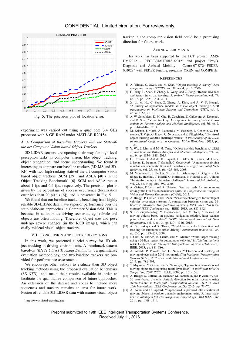
0 0.1 0.2 0.3 0.4 0.5 0.6 0.7 0.8 0.9 1
0
0.1
0.2
0.3
0.4
0.5
0.6
0.7
0.8
0.9
1Precision Plot - LOC
3D-KF
3D-MS
SCM
ASLA
Fig. 5: The precision plot of location error.
experiment was carried out using a quad core 3.4 GHzprocessor with 8 GB RAM under MATLAB R2015a.
A. A Comparison of Base-line Trackers with the State-of-the-art Computer Vision based Object Trackers
3D-LIDAR sensors are opening their way for high-levelperception tasks in computer vision, like object tracking,object recognition, and scene understanding. We found itinteresting to compare our baseline trackers (3D-MS and 3D-KF) with two high-ranking state-of-the-art computer visionbased object trackers (SCM [39], and ASLA [40]) in theObject Tracking Benchmark4 [6]. SCM and ASLA run atabout 1 fps and 6.5 fps, respectively. The precision plot isgiven by the percentage of success occurrence (localizationerror less than 20 pixels [6]), and is presented in Fig. 5.
We found that our baseline trackers, benefiting from highlyreliable 3D-LIDAR data, have superior performance over thestate-of-the-art approaches in Computer Vision field. This isbecause, in autonomous driving scenarios, ego-vehicle andobjects are often moving. Therefore, object size and poseundergo severe changes (in the RGB image), which caneasily mislead visual object trackers.
VII. CONCLUSION AND FUTURE DIRECTIONS
In this work, we presented a brief survey for 3D ob-ject tracking in driving environments. A benchmark datasetbased-on ‘KITTI Object Tracking Evaluation’, a quantitativeevaluation methodology, and two baseline trackers are pro-vided for performance assessment.
We encourage other authors to evaluate their 3D objecttracking methods using the proposed evaluation benchmark(3D-OTD), and make their results available in order tofacilitate the quantitative comparison of future approaches.An extension of the dataset and codes to include moresequences and trackers remains an area for future work.Fusion of reliable 3D-LIDAR data with mature visual object
4http://www.visual-tracking.net
tracker in the computer vision field could be a promisingdirection for future work.
ACKNOWLEDGMENTS
This work has been supported by the FCT project ”AMS-HMI2012 - RECI/EEIAUT/0181/2012” and project ”ProjB-Diagnosis and Assisted Mobility - Centro-07-ST24-FEDER-002028” with FEDER funding, programs QREN and COMPETE.
REFERENCES
[1] A. Yilmaz, O. Javed, and M. Shah, “Object tracking: A survey,” Acmcomputing surveys (CSUR), vol. 38, no. 4, p. 13, 2006.
[2] H. Yang, L. Shao, F. Zheng, L. Wang, and Z. Song, “Recent advancesand trends in visual tracking: A review,” Neurocomputing, vol. 74,no. 18, pp. 3823–3831, 2011.
[3] X. Li, W. Hu, C. Shen, Z. Zhang, A. Dick, and A. V. D. Hengel,“A survey of appearance models in visual object tracking,” ACMtransactions on Intelligent Systems and Technology (TIST), vol. 4,no. 4, p. 58, 2013.
[4] A. W. Smeulders, D. M. Chu, R. Cucchiara, S. Calderara, A. Dehghan,and M. Shah, “Visual tracking: An experimental survey,” IEEE Trans-actions on Pattern Analysis and Machine Intelligence, vol. 36, no. 7,pp. 1442–1468, 2014.
[5] M. Kristan, J. Matas, A. Leonardis, M. Felsberg, L. Cehovin, G. Fer-nandez, T. Vojir, G. Hager, G. Nebehay, and R. Pflugfelder, “The visualobject tracking vot2015 challenge results,” in Proceedings of the IEEEInternational Conference on Computer Vision Workshops, 2015, pp.1–23.
[6] Y. Wu, J. Lim, and M.-H. Yang, “Object tracking benchmark,” IEEETransactions on Pattern Analysis and Machine Intelligence, vol. 37,no. 9, pp. 1834–1848, 2015.
[7] C. Urmson, J. Anhalt, D. Bagnell, C. Baker, R. Bittner, M. Clark,J. Dolan, D. Duggins, T. Galatali, C. Geyer et al., “Autonomous drivingin urban environments: Boss and the urban challenge,” Journal of FieldRobotics, vol. 25, no. 8, pp. 425–466, 2008.
[8] M. Montemerlo, J. Becker, S. Bhat, H. Dahlkamp, D. Dolgov, S. Et-tinger, D. Haehnel, T. Hilden, G. Hoffmann, B. Huhnke et al., “Junior:The stanford entry in the urban challenge,” Journal of field Robotics,vol. 25, no. 9, pp. 569–597, 2008.
[9] A. Geiger, P. Lenz, and R. Urtasun, “Are we ready for autonomousdriving? the kitti vision benchmark suite,” in Conference on ComputerVision and Pattern Recognition (CVPR), 2012.
[10] A. Broggi, P. Grisleri, and P. Zani, “Sensors technologies for intelligentvehicles perception systems: A comparison between vision and 3d-lidar,” in Intelligent Transportation Systems-(ITSC), 2013 16th Inter-national IEEE Conference on. IEEE, 2013, pp. 887–892.
[11] S. Hosseinyalamdary, Y. Balazadegan, and C. Toth, “Tracking 3dmoving objects based on gps/imu navigation solution, laser scannerpoint cloud and gis data,” ISPRS International Journal of Geo-Information, vol. 4, no. 3, pp. 1301–1316, 2015.
[12] A. Petrovskaya and S. Thrun, “Model based vehicle detection andtracking for autonomous urban driving,” Autonomous Robots, vol. 26,no. 2-3, pp. 123–139, 2009.
[13] J. Choi, S. Ulbrich, B. Lichte, and M. Maurer, “Multi-target trackingusing a 3d-lidar sensor for autonomous vehicles,” in 16th InternationalIEEE Conference on Intelligent Transportation Systems (ITSC 2013).IEEE, 2013, pp. 881–886.
[14] A. Asvadi, P. Peixoto, and U. Nunes, “Detection and tracking ofmoving objects using 2.5 d motion grids,” in Intelligent TransportationSystems (ITSC), 2015 IEEE 18th International Conference on. IEEE,2015, pp. 788–793.
[15] T. Miyasaka, Y. Ohama, and Y. Ninomiya, “Ego-motion estimation andmoving object tracking using multi-layer lidar,” in Intelligent VehiclesSymposium, 2009 IEEE. IEEE, 2009, pp. 151–156.
[16] A. Broggi, S. Cattani, M. Patander, M. Sabbatelli, and P. Zani, “A full-3d voxel-based dynamic obstacle detection for urban scenario usingstereo vision,” in Intelligent Transportation Systems - (ITSC), 201316th International IEEE Conference on, Oct 2013, pp. 71–76.
[17] A. Azim and O. Aycard, “Layer-based supervised classification ofmoving objects in outdoor dynamic environment using 3d laser scan-ner,” in Intelligent Vehicles Symposium Proceedings, 2014 IEEE, June2014, pp. 1408–1414.
CONFIDENTIAL. Limited circulation. For review only.
Preprint submitted to 19th IEEE Intelligent Transportation Systems Conference.Received July 11, 2016.

[18] J. Cesic, I. Markovic, S. Juric-Kavelj, and I. Petrovic, “Short-termmap based detection and tracking of moving objects with 3d laseron a vehicle,” in Informatics in Control, Automation and Robotics.Springer, 2016, pp. 205–222.
[19] A. Vatavu, R. Danescu, and S. Nedevschi, “Stereovision-based mul-tiple object tracking in traffic scenarios using free-form obstacledelimiters and particle filters,” Intelligent Transportation Systems,IEEE Transactions on, vol. 16, no. 1, pp. 498–511, 2015.
[20] D. Held, J. Levinson, and S. Thrun, “Precision tracking with sparse 3dand dense color 2d data,” in Robotics and Automation (ICRA), 2013IEEE International Conference on. IEEE, 2013, pp. 1138–1145.
[21] F. Moosmann and C. Stiller, “Joint self-localization and tracking ofgeneric objects in 3d range data,” in Robotics and Automation (ICRA),2013 IEEE International Conference on. IEEE, 2013, pp. 1146–1152.
[22] P. F. Felzenszwalb, R. B. Girshick, D. McAllester, and D. Ramanan,“Object detection with discriminatively trained part-based models,”Pattern Analysis and Machine Intelligence, IEEE Transactions on,vol. 32, no. 9, pp. 1627–1645, 2010.
[23] A. Geiger, M. Lauer, C. Wojek, C. Stiller, and R. Urtasun, “3d trafficscene understanding from movable platforms,” Pattern Analysis andMachine Intelligence (PAMI), 2014.
[24] L. Zhang, Y. Li, and R. Nevatia, “Global data association for multi-object tracking using network flows,” in Computer Vision and PatternRecognition, 2008. CVPR 2008. IEEE Conference on. IEEE, 2008,pp. 1–8.
[25] H. Pirsiavash, D. Ramanan, and C. C. Fowlkes, “Globally-optimalgreedy algorithms for tracking a variable number of objects,” in Com-puter Vision and Pattern Recognition (CVPR), 2011 IEEE Conferenceon. IEEE, 2011, pp. 1201–1208.
[26] A. Milan, S. Roth, and K. Schindler, “Continuous energy minimizationfor multitarget tracking,” IEEE transactions on pattern analysis andmachine intelligence, vol. 36, no. 1, pp. 58–72, 2014.
[27] P. Lenz, A. Geiger, and R. Urtasun, “Followme: Efficient onlinemin-cost flow tracking with bounded memory and computation,”in Proceedings of the IEEE International Conference on ComputerVision, 2015, pp. 4364–4372.
[28] J. Hong Yoon, C.-R. Lee, M.-H. Yang, and K.-J. Yoon, “Onlinemulti-object tracking via structural constraint event aggregation,” inProceedings of the IEEE Conference on Computer Vision and PatternRecognition, 2016, pp. 1392–1400.
[29] L. Leal-Taixe, A. Milan, I. Reid, S. Roth, and K. Schindler, “Motchal-lenge 2015: Towards a benchmark for multi-target tracking,” arXivpreprint arXiv:1504.01942, 2015.
[30] A. Milan, L. Leal-Taixe, I. Reid, S. Roth, and K. Schindler,“Mot16: A benchmark for multi-object tracking,” arXiv preprintarXiv:1603.00831, 2016.
[31] A. Osep, A. Hermans, F. Engelmann, D. Klostermann, , M. Math-ias, and B. Leibe, “Multi-scale object candidates for generic objecttracking in street scenes,” in ICRA, 2016.
[32] A. Teichman and S. Thrun, “Tracking-based semi-supervised learn-ing,” The International Journal of Robotics Research, vol. 31, no. 7,pp. 804–818, 2012.
[33] R. Kaestner, J. Maye, Y. Pilat, and R. Siegwart, “Generative objectdetection and tracking in 3d range data,” in Robotics and Automation(ICRA), 2012 IEEE International Conference on. IEEE, 2012, pp.3075–3081.
[34] A. Dewan, T. Caselitz, G. D. Tipaldi, and W. Burgard, “Motion-based detection and tracking in 3d lidar scans,” in Proc. of the IEEEInt. Conf. on Robotics & Automation (ICRA), Stockholm, Sweden,2016.
[35] S. Sivaraman and M. M. Trivedi, “Looking at vehicles on the road:A survey of vision-based vehicle detection, tracking, and behavioranalysis,” Intelligent Transportation Systems, IEEE Transactions on,vol. 14, no. 4, pp. 1773–1795, 2013.
[36] A. Mukhtar, L. Xia, and T. B. Tang, “Vehicle detection techniquesfor collision avoidance systems: A review,” IEEE Transactions onIntelligent Transportation Systems, vol. 16, no. 5, pp. 2318–2338,2015.
[37] A. Petrovskaya, M. Perrollaz, L. Oliveira, L. Spinello, R. Triebel,A. Makris, J.-D. Yoder, C. Laugier, U. Nunes, and P. Bessiere,“Awareness of road scene participants for autonomous driving,” inHandbook of Intelligent Vehicles. Springer, 2012, pp. 1383–1432.
[38] L. Cehovin, A. Leonardis, and M. Kristan, “Visual object trackingperformance measures revisited,” IEEE Transactions on Image Pro-cessing, vol. 25, no. 3, pp. 1261–1274, 2016.
[39] W. Zhong, H. Lu, and M.-H. Yang, “Robust object tracking viasparse collaborative appearance model,” IEEE Transactions on ImageProcessing, vol. 23, no. 5, pp. 2356–2368, 2014.
[40] X. Jia, H. Lu, and M.-H. Yang, “Visual tracking via adaptive structurallocal sparse appearance model,” in Computer vision and patternrecognition (CVPR), 2012 IEEE Conference on. IEEE, 2012, pp.1822–1829.
CONFIDENTIAL. Limited circulation. For review only.
Preprint submitted to 19th IEEE Intelligent Transportation Systems Conference.Received July 11, 2016.

APPENDIX C. SUBMITTED PAPER: 3D OBJECT TRACKING IN DRIVINGENVIRONMENT: A SHORT REVIEW AND A BENCHMARK DATASET
80
Copyright © 2022 FDOKUMEN