3D scanning for personal 3D printing

3D Scanning for Personal 3D Printing:

Build Your Own Desktop 3D Scanner

Gabriel TaubinBrown University

[email protected]

Daniel MorenoBrown University

daniel [email protected]

Douglas LanmanOculus VR R&D

http://dlanman.info

Version 1.0 June 11 2014Download latest version from http://mesh.brown.edu/desktop3dscan

mailto:[email protected]


http://dlanman.info

http://mesh.brown.edu/desktop3dscan

Siggraph 2014 Studio Course

Abstract

3D Printing has entered the mainstream. Multiple low cost desktop 3D printers are currently avail-able from various vendors, and open source projects let hobbyists build their own. This courseaddresses the problem of creating 3D models for 3D printing. As is the case for 3D printers,low-cost homemade 3D scanners are now within reach of students and hobbyists with a modestbudget. This course provides the students with the necessary mathematics, software, and practicaldetails to leverage projector-camera systems to build their own desktop 3D scanner. An example-driven approach is used throughout, with each new concept illustrated using a practical scannerimplemented with off-the-shelf parts. First, the mathematics of triangulation is explained usingthe intersection of parametric and implicit representations of lines and planes in 3D. The particularcase of ray-plane triangulation is illustrated using a scanner built with a single camera and a mod-ified laser pointer. Camera calibration is explained at this stage to convert image measurementsto geometric quantities. The mathematics of rigid-body transformations are covered through thisexample. Next, the details of projector calibration are explained through the development of aclassic structured light scanning system using a single camera and projector pair. A minimal post-processing pipeline is described to convert the point-based representations produced by thesescanners to watertight meshes. Key topics covered in this section include: surface representations,file formats, data structures, polygonal meshes, and basic smoothing and gap-filling operations.The course concludes with the description of some commercially available low cost desktop 3Dscanners.

Prerequisites

Attendees should have a basic undergraduate-level understanding of linear algebra. While exe-cutables are provided for beginners, attendees with prior knowledge of Matlab, C/C++, and Javaprogramming will be able to directly examine and modify the provided source code.

i

Course Speakers

Gabriel TaubinBrown University, [email protected], http://mesh.brown.edu/taubin

Gabriel Taubin is Associate Professor of Engineering and Computer Science at Brown University.He earned a Licenciado en Ciencias Matemticas degree from the University of Buenos Aires, Ar-gentina, and a Ph.D. degree in Electrical Engineering from Brown University. He was named IEEEFellow for his contributions to three-dimensional geometry compression technology and multime-dia standards, won the Eurographics 2002 Gunter Enderle Best Paper Award, and was named IBMMaster Inventor. From January 2010 to December 2013 he served as Editor-in-Chief of the IEEEComputer Graphics and Applications Magazine. He also serves as member of the Editorial Boardof the Geometric Models journal, and has served as associate editor of the IEEE Transactions ofVisualization and Computer Graphics. From 1990 to 2003 he held various positions at the IBMT.J. Watson Research Center, including Research Staff Member and Research Manager. He wasappointed Visiting Professor of Electrical Engineering at Caltech during the 2000-2001 academicyear, Visiting Associate Professor of Media Arts and Sciences at the MIT Media Lab during theSpring semester of 2010, Visiting Professor of Computer Science at the University of Buenos Aires,during the Spring semester of 2013. In 2014 he won a Fulbright Specialist grant. He has authorednumerous reviewed book chapters, journal, or conference papers, and is a co-inventor of 48 inter-national patents. He has made significant theoretical and practical contributions to the field nowcalled Digital Geometry Processing, comprising: 3D shape capturing and surface reconstruction,geometric modeling, geometry compression, progressive transmission, signal processing, and dis-play of discrete surfaces. He teaches courses on 3D Photography and Digital Geometry Processingat Brown University on a regular basis.

Daniel MorenoBrown University, daniel [email protected]

Daniel A. Moreno received a degree of Licenciado en Ciencias de la Computacion from Universi-dad Nacional de Rosario, Argentina, in 2011. The same year, he joined Brown University wherehe is currently pursuing a PhD in Engineering. His research topic is Computer Vision, specificallythe area of 3D models acquisition and processing. Recently, he has been working on structured-light systems calibration and low-cost 3D scanners. He has written a fully functional opensource3D scanning software and collaborated with the implementation of the Smooth Signed Distancesurface reconstruction algorithm. His work experience includes internships at Evolution Roboticsin 2008, and NVIDIA Corp. in the summer of 2013.

ii


http://mesh.brown.edu/taubin


Contributing to Lecture Notes

Douglas LanmanResearch Scientist, Oculus VR R&D, http://dlanman.info

Douglas Lanman is a Research Scientist at Oculus VR R&D. His research is focused on compu-tational displays and imaging systems, emphasizing compact optics for head-mounted displays(HMDs), glasses-free 3D displays, light field cameras, and active illumination for 3D reconstruc-tion and interaction. He received a B.S. in Applied Physics with Honors from Caltech in 2002 andM.S. and Ph.D. degrees in Electrical Engineering from Brown University in 2006 and 2010, respec-tively. He was a Senior Research Scientist at NVIDIA from 2012 to 2014, a Postdoctoral Associateat the MIT Media Lab from 2010 to 2012, and an Assistant Research Staff Member at MIT LincolnLaboratory from 2002 to 2005. He has worked as an intern at Intel, Los Alamos National Labora-tory, INRIA Rhne-Alpes, Mitsubishi Electric Research Laboratories (MERL), and the MIT MediaLab. Douglas has presented the following SIGGRAPH courses: ”Build Your Own 3D Scanner”(2009), ”Build Your Own 3D Display” (2010, 2011), ”Computational Imaging” (2012), ”Compu-tational Displays” (2012), and ”Put on Your 3D Glasses Now: The Past, Present, and Future ofVirtual and Augmented Reality” (2014).

iii

http://dlanman.info

Contents

1 Introduction 11.1 3D Scanning Technology . . . . . . . . . . . . . . . . . . . . . . . . . . . . . . . . . . . 1

1.1.1 Passive Methods . . . . . . . . . . . . . . . . . . . . . . . . . . . . . . . . . . . 21.1.2 Active Methods . . . . . . . . . . . . . . . . . . . . . . . . . . . . . . . . . . . . 3

1.2 3D Scanners studied in this Course . . . . . . . . . . . . . . . . . . . . . . . . . . . . . 5

2 The Mathematics of Triangulation 72.1 Perspective Projection and the Pinhole Model . . . . . . . . . . . . . . . . . . . . . . . 72.2 Geometric Representations . . . . . . . . . . . . . . . . . . . . . . . . . . . . . . . . . . 7

2.2.1 Points and Vectors . . . . . . . . . . . . . . . . . . . . . . . . . . . . . . . . . . 82.2.2 Parametric Representation of Lines and Rays . . . . . . . . . . . . . . . . . . . 82.2.3 Parametric Representation of Planes . . . . . . . . . . . . . . . . . . . . . . . . 92.2.4 Implicit Representation of Planes . . . . . . . . . . . . . . . . . . . . . . . . . . 102.2.5 Implicit Representation of Lines . . . . . . . . . . . . . . . . . . . . . . . . . . 10

2.3 Reconstruction by Triangulation . . . . . . . . . . . . . . . . . . . . . . . . . . . . . . 102.3.1 Line-Plane Intersection . . . . . . . . . . . . . . . . . . . . . . . . . . . . . . . . 112.3.2 Line-Line Intersection . . . . . . . . . . . . . . . . . . . . . . . . . . . . . . . . 12

2.4 Coordinate Systems . . . . . . . . . . . . . . . . . . . . . . . . . . . . . . . . . . . . . . 142.4.1 Image Coordinates and the Pinhole Camera . . . . . . . . . . . . . . . . . . . 142.4.2 The Ideal Pinhole Camera . . . . . . . . . . . . . . . . . . . . . . . . . . . . . . 152.4.3 The General Pinhole Camera . . . . . . . . . . . . . . . . . . . . . . . . . . . . 152.4.4 Lines from Image Points . . . . . . . . . . . . . . . . . . . . . . . . . . . . . . . 172.4.5 Planes from Image Lines . . . . . . . . . . . . . . . . . . . . . . . . . . . . . . . 17

3 Camera and Projector Calibration 193.1 Camera Calibration . . . . . . . . . . . . . . . . . . . . . . . . . . . . . . . . . . . . . . 19

3.1.1 Camera selection and interfaces . . . . . . . . . . . . . . . . . . . . . . . . . . 193.1.2 Calibration Methods and Software . . . . . . . . . . . . . . . . . . . . . . . . . 213.1.3 Calibration Procedure . . . . . . . . . . . . . . . . . . . . . . . . . . . . . . . . 22

3.2 Projector Calibration . . . . . . . . . . . . . . . . . . . . . . . . . . . . . . . . . . . . . 243.2.1 Projector Selection and Interfaces . . . . . . . . . . . . . . . . . . . . . . . . . . 243.2.2 Calibration Software and Procedure . . . . . . . . . . . . . . . . . . . . . . . . 25

4 The Laser Slit 3D Scanner 284.1 Description . . . . . . . . . . . . . . . . . . . . . . . . . . . . . . . . . . . . . . . . . . . 284.2 Turntable calibration . . . . . . . . . . . . . . . . . . . . . . . . . . . . . . . . . . . . . 29

4.2.1 Camera extrinsics . . . . . . . . . . . . . . . . . . . . . . . . . . . . . . . . . . . 314.2.2 Center of rotation and rotation angle . . . . . . . . . . . . . . . . . . . . . . . . 32

iv

Contents

4.2.3 Global optimization . . . . . . . . . . . . . . . . . . . . . . . . . . . . . . . . . 334.3 Image Laser Detection . . . . . . . . . . . . . . . . . . . . . . . . . . . . . . . . . . . . 334.4 Background detection . . . . . . . . . . . . . . . . . . . . . . . . . . . . . . . . . . . . 354.5 Plane of light calibration . . . . . . . . . . . . . . . . . . . . . . . . . . . . . . . . . . . 364.6 3D model reconstruction . . . . . . . . . . . . . . . . . . . . . . . . . . . . . . . . . . . 37

5 Structured Lighting 395.1 Structured Light Scanner . . . . . . . . . . . . . . . . . . . . . . . . . . . . . . . . . . . 39

5.1.1 Scanner Hardware . . . . . . . . . . . . . . . . . . . . . . . . . . . . . . . . . . 395.1.2 Structured Light Sequences . . . . . . . . . . . . . . . . . . . . . . . . . . . . . 40

5.2 Image Processing . . . . . . . . . . . . . . . . . . . . . . . . . . . . . . . . . . . . . . . 425.3 Calibration . . . . . . . . . . . . . . . . . . . . . . . . . . . . . . . . . . . . . . . . . . . 445.4 Reconstruction . . . . . . . . . . . . . . . . . . . . . . . . . . . . . . . . . . . . . . . . . 445.5 Sample software . . . . . . . . . . . . . . . . . . . . . . . . . . . . . . . . . . . . . . . . 45

6 Surfaces from Point Clouds 476.1 Representation and Visualization of Point Clouds . . . . . . . . . . . . . . . . . . . . 47

6.1.1 File Formats . . . . . . . . . . . . . . . . . . . . . . . . . . . . . . . . . . . . . . 476.1.2 Visualization . . . . . . . . . . . . . . . . . . . . . . . . . . . . . . . . . . . . . 48

6.2 Merging Point Clouds . . . . . . . . . . . . . . . . . . . . . . . . . . . . . . . . . . . . 486.2.1 Computing Rigid Body Matching Transformations . . . . . . . . . . . . . . . 496.2.2 The Iterative Closest Point (ICP) Algorithm . . . . . . . . . . . . . . . . . . . . 50

6.3 Surface Reconstruction from Point Clouds . . . . . . . . . . . . . . . . . . . . . . . . . 516.3.1 Continuous Surfaces . . . . . . . . . . . . . . . . . . . . . . . . . . . . . . . . . 516.3.2 Discrete Surfaces . . . . . . . . . . . . . . . . . . . . . . . . . . . . . . . . . . . 516.3.3 Isosurfaces . . . . . . . . . . . . . . . . . . . . . . . . . . . . . . . . . . . . . . . 526.3.4 Isosurface Construction Algorithms . . . . . . . . . . . . . . . . . . . . . . . . 526.3.5 Algorithms to Fit Implicit Surfaces to Point Clouds . . . . . . . . . . . . . . . 55

7 Conclusion 56

Bibliography 57

v

Chapter 1

Introduction

3D Printing has become a popular subject these days. More and more low cost desktop 3D printersare introduced, and open source projects let hobbyists build their own. Without models, a 3Dprinter is not really useful. Professionals have access to complete CAD software or modelersthat costs thousands and need extensive training. They can also acquire a scene/object using 3Dscanners. This course addresses the problem of creating 3D models for 3D printing by copyingand modifying existing objects. As is the case for desktop 3D printers this course teaches themathematical foundations of the various methods used to build 3D scanners, and includes specificinstructions to build several low-cost homemade 3D scanners which can produce models of equalor better quality as many commercial products currently in the market.

These course notes are organized into three primary sections, spanning theoretical concepts,practical construction details, and algorithms for constructing high-quality 3D models. Chapters 1and 2 survey the field and present the unifying concept of triangulation. Chapters 3–5 documentthe construction of projector-camera systems, slit-based 3D scanners, and 3D scanners based onstructured lighting. The post-processing processes for generating polygon meshes from pointclouds are covered in Chapter 6.

Revised course notes, updated software, recent publications, and similar do-it-yourself projectsare maintained on the course website at http://mesh.brown.edu/desktop3dscan.

1.1 3D Scanning Technology

Metrology is an ancient and diverse field, bridging the gap between mathematics and engineering.Efforts at measurement standardization were first undertaken by the Indus Valley Civilization asearly as 2600–1900 BCE. Even with only crude units, such as the length of human appendages, thedevelopment of geometry revolutionized the ability to measure distance accurately. Around 240BCE, Eratosthenes estimated the circumference of the Earth from knowledge of the elevation angleof the Sun during the summer solstice in Alexandria and Syene. Mathematics and standardizationefforts continued to mature through the Renaissance (1300–1600 CE) and into the Scientific Rev-olution (1550–1700 CE). However, it was the Industrial Revolution (1750–1850 CE) which drovemetrology to the forefront. As automatized methods of mass production became commonplace,advanced measurement technologies ensured interchangeable parts were just that–accurate copiesof the original.

Through these historical developments, measurement tools varied with mathematical knowl-edge and practical needs. Early methods required direct contact with a surface (e.g., callipersand rulers). The pantograph, invented in 1603 by Christoph Scheiner, uses a special mechani-

1

http://mesh.brown.edu/desktop3dscan

Introduction 3D Scanning Technology

Figure 1.1: Contact-based shape measurement. (Left) A sketch of Sorenson’s engraving panto-graph patented in 1867. (Right) A modern coordinate measuring machining (from Flickr userhyperbolation). In both devices, deflection of a probe tip is used to estimate object shape, eitherfor transferring engravings or for recovering 3D models, respectively.

cal linkage so movement of a stylus (in contact with the surface) can be precisely duplicated bya drawing pen. The modern coordinate measuring machine (CMM) functions in much the samemanner, recording the displacement of a probe tip as it slides across a solid surface (see Figure 1.1).While effective, such contact-based methods can harm fragile objects and require long periods oftime to build an accurate 3D model. Non-contact scanners address these limitations by observing,and possibly controlling, the interaction of light with the object.

1.1.1 Passive Methods

Non-contact optical scanners can be categorized by the degree to which controlled illumination isrequired. Passive scanners do not require direct control of any illumination source, instead relyingentirely on ambient light. Stereoscopic imaging is one of the most widely used passive 3D imagingsystems, both in biology and engineering. Mirroring the human visual system, stereoscopy esti-mates the position of a 3D scene point by triangulation [LN04]; first, the 2D projection of a givenpoint is identified in each camera. Using known calibration objects, the imaging properties of eachcamera are estimated, ultimately allowing a single 3D line to be drawn from each camera’s centerof projection through the 3D point. The intersection of these two lines is then used to recover thedepth of the point.

Trinocular [VF92] and multi-view stereo [HZ04] systems have been introduced to improve theaccuracy and reliability of conventional stereoscopic systems. However, all such passive triangu-lation methods require correspondences to be found among the various viewpoints. Even for stereovision, the development of matching algorithms remains an open and challenging problem in thefield [SCD∗06]. Today, real-time stereoscopic and multi-view systems are emerging, however cer-tain challenges continue to limit their widespread adoption [MPL04]. Foremost, flat or periodictextures prevent robust matching. While machine learning methods and prior knowledge arebeing advanced to solve such problems, multi-view 3D scanning remains somewhat outside thedomain of hobbyists primarily concerned with accurate, reliable 3D measurement.

Many alternative passive methods have been proposed to sidestep the correspondence prob-lem, often times relying on more robust computer vision algorithms. Under controlled conditions,such as a known or constant background, the external boundaries of foreground objects can be

2


reliably identified. As a result, numerous shape-from-silhouette algorithms have emerged. Lau-rentini [Lau94] considers the case of a finite number of cameras observing a scene. The visual hullis defined as the union of the generalized viewing cones defined by each camera’s center of pro-jection and the detected silhouette boundaries. Recently, free-viewpoint video [CTMS03] systemshave applied this algorithm to allow dynamic adjustment of viewpoint [MBR∗00, SH03]. Cipollaand Giblin [CG00] consider a differential formulation of the problem, reconstructing depth byobserving the visual motion of occluding contours (such as silhouettes) as a camera is perturbed.

Optical imaging systems require a sufficiently large aperture so that enough light is gatheredduring the available exposure time [Hec01]. Correspondingly, the captured imagery will demon-strate a limited depth of field; only objects close to the plane of focus will appear in sharp contrast,with distant objects blurred together. This effect can be exploited to recover depth, by increasingthe aperture diameter to further reduce the depth of field. Nayar and Nakagawa [NN94] estimateshape-from-focus, collecting a focal stack by translating a single element (either the lens, sensor,or object). A focus measure operator [WN98] is then used to identify the plane of best focus, andits corresponding distance from the camera.

Other passive imaging systems further exploit the depth of field by modifying the shape ofthe aperture. Such modifications are performed so that the point spread function (PSF) becomesinvertible and strongly depth-dependent. Levin et al. [LFDF07] and Farid [Far97] use such codedapertures to estimate intensity and depth from defocused images. Greengard et al. [GSP06] modifythe aperture to produce a PSF whose rotation is a function of scene depth. In a similar vein,shadow moire is produced by placing a high-frequency grating between the scene and the camera.The resulting interference patterns exhibit a series of depth-dependent fringes.

While the preceding discussion focused on optical modifications for 3D reconstruction from2D images, numerous model-based approaches have also emerged. When shape is known a priori,then coarse image measurements can be used to infer object translation, rotation, and deforma-tion. Such methods have been applied to human motion tracking [KM00, OSS∗00, dAST∗08], vehi-cle recognition [Sul95, FWM98], and human-computer interaction [RWLB01]. Additionally, user-assisted model construction has been demonstrated using manual labeling of geometric primi-tives [Deb97].

1.1.2 Active Methods

Active optical scanners overcome the correspondence problem using controlled illumination. Incomparison to non-contact and passive methods, active illumination is often more sensitive to sur-face material properties. Strongly reflective or translucent objects often violate assumptions madeby active optical scanners, requiring additional measures to acquire such problematic subjects.For a detailed history of active methods, we refer the reader to the survey article by Blais [Bla04].In this section we discuss some key milestones along the way to the scanners we consider in thiscourse.

Many active systems attempt to solve the correspondence problem by replacing one of thecameras, in a passive stereoscopic system, with a controllable illumination source. During the1970s, single-point laser scanning emerged. In this scheme, a series of fixed and rotating mirrorsare used to raster scan a single laser spot across a surface. A digital camera records the motion ofthis “flying spot”. The 2D projection of the spot defines, with appropriate calibration knowledge, aline connecting the spot and the camera’s center of projection. The depth is recovered by intersect-ing this line with the line passing from the laser source to the spot, given by the known deflectionof the mirrors. As a result, such single-point scanners can be seen as the optical equivalent ofcoordinate measuring machines.

3


Figure 1.2: Active methods for 3D scanning. (Left) Conceptual diagram of a 3D slit scanner, con-sisting of a mechanically translated laser stripe. (Right) A Cyberware scanner, applying laserstriping for whole body scanning (from Flickr user NIOSH).

As with CMMs, single-point scanning is a painstakingly slow process. With the developmentof low-cost, high-quality CCD arrays in the 1980s, slit scanners emerged as a powerful alterna-tive. In this design, a laser projector creates a single planar sheet of light. This “slit” is thenmechanically-swept across the surface. As before, the known deflection of the laser source definesa 3D plane. The depth is recovered by the intersection of this plane with the set of lines passingthrough the 3D stripe on the surface and the camera’s center of projection.

Effectively removing one dimension of the raster scan, slit scanners remain a popular solutionfor rapid shape acquisition. A variety of commercial products use swept-plane laser scanning,including the Polhemus FastSCAN [Pol], the NextEngine [Nex], the SLP 3D laser scanning probesfrom Laser Design [Las], and the HandyScan line of products [Cre]. While effective, slit scannersremain difficult to use if moving objects are present in the scene. In addition, because of thenecessary separation between the light source and camera, certain occluded regions cannot bereconstructed. This limitation, while shared by many 3D scanners, requires multiple scans to bemerged—further increasing the data acquisition time.

A digital “structured light” projector can be used to eliminate the mechanical motion requiredto translate the laser stripe across the surface. Naıvely, the projector could be used to display asingle column (or row) of white pixels translating against a black background to replicate the per-formance of a slit scanner. However, a simple swept-plane sequence does not fully exploit the pro-jector, which is typically capable of displaying arbitrary 24-bit color images. Structured lightingsequences have been developed which allow the projector-camera correspondences to be assignedin relatively few frames. In general, the identity of each plane can be encoded spatially (i.e., withina single frame) or temporally (i.e., across multiple frames), or with a combination of both spatialand temporal encodings. There are benefits and drawbacks to each strategy. For instance, purelyspatial encodings allow a single static pattern to be used for reconstruction, enabling dynamicscenes to be captured. Alternatively, purely temporal encodings are more likely to benefit fromredundancy, reducing reconstruction artifacts. We refer the reader to a comprehensive assessmentof such codes by Salvi et al. [SPB04].

Both slit scanners and structured lighting are ill-suited for scanning dynamic scenes. In addi-tion, due to separation of the light source and camera, certain occluded regions will not be recov-ered. In contrast, time-of-flight rangefinders estimate the distance to a surface from a single centerof projection. These devices exploit the finite speed of light. A single pulse of light is emitted.The elapsed time, between emitting and receiving a pulse, is used to recover the object distance

4

Introduction 3D Scanners studied in this Course

Figure 1.3: Desktop 3D Scanners based on Laser Plane Triangulation. From left to right: MakerBotDigitizer, Matterform Photon, and NextEngine 3D Scanner HD.

(since the speed of light is known). Several economical time-of-flight depth cameras are now com-mercially available, including Canesta’s CANESTAVISION [HARN06] and 3DV’s Z-Cam [IY01].However, the depth resolution and accuracy of such systems (for static scenes) remain below thatof slit scanners and structured lighting.

Active imaging is a broad field; a wide variety of additional schemes have been proposed,typically trading system complexity for shape accuracy. As with model-based approaches in pas-sive imaging, several active systems achieve robust reconstruction by making certain simplifyingassumptions about the topological and optical properties of the surface. Woodham [Woo89] intro-duces photometric stereo, allowing smooth surfaces to be recovered by observing their shadingunder at least three (spatially disparate) point light sources. Hernandez et al. [HVB∗07] furtherdemonstrate a real-time photometric stereo system using three colored light sources. Similarly, thecomplex digital projector required for structured lighting can be replaced by one or more printedgratings placed next to the projector and camera. Like shadow moire, such projection moire sys-tems create depth-dependent fringes. However, certain ambiguities remain in the reconstructionunless the surface is assumed to be smooth.

Active and passive 3D scanning methods continue to evolve, with recent progress reportedannually at various computer graphics and vision conferences, including 3-D Digital Imaging andModeling (3DIM), SIGGRAPH, Eurographics, CVPR, ECCV, and ICCV. Similar advances are alsopublished in the applied optics communities, typically through various SPIE and OSA journals.

1.2 3D Scanners studied in this Course

This course is grounded in the unifying concept of triangulation. At their core, stereoscopic imag-ing, slit scanning, and structured lighting all attempt to recover the shape of 3D objects in the samemanner. First, the correspondence problem is solved, either by a passive matching algorithm orby an active “space-labeling” approach (e.g., projecting known lines, planes, or other patterns).After establishing correspondences across two or more views (e.g., between a pair of cameras ora single projector-camera pair), triangulation recovers the scene depth. In stereoscopic and multi-view systems, a point is reconstructed by intersecting two or more corresponding lines. In slitscanning and structured lighting systems, a point is recovered by intersecting corresponding linesand planes.

To elucidate the principles of such triangulation-based scanners, this course describes howto construct a classic turntable-based slit scanner, and a structured lighting system. The coursealso covers methods to register and merge multiple scans, to reconstruct polygon mesh surfacesfrom multi-scan registered point clouds, and to optimize the reconstructed meshes for variouspurposes. In all 3D scanner designs, the methods used to calibrate the systems are integral part of

5

Introduction 3D Scanners studied in this Course

Figure 1.4: Industrial 3D Scanners based on Structured Lighting. From left to right: BreuckmannSmartScan, ATOS CompactScan, and Geomagic Capture.

the design, since they have to be carefully constructed to produce accurate and precise results.We first study the slit scanner, where a laser line projector iluminates an abject, and a camera

captures an image of some or all the illuminated object points. Figure 1.3 shows some commercialdesktop 3D scanners based on this method. Image processing techniques are used to detect thepixels corresponding to illuminated points visible by the camera. Ray-plane triangulation equa-tions are used to reconstruct 3D points belonging to the intersection of the plane of laser light andthe object. To recover denser sets of 3D points, the laser projector has to be moved while the cam-era remains static with respect to the object, and the process has to be repeated until a satisfactorynumber of points has been reconstructed. Alternatively, the object is placed on a linear stage or aturntable, the laser projector is kept static with respect to the camera. The linear stage or turntableis iteratively moved to a new position where an image is captured by the camera. As in the firstcase, a large number of images must be captured to generate a dense point cloud. In both casestracking and estimating the motion with precision is required. Computer-controlled motorizedlinear stages or turntables are normally used for this purpoose. In chapter 4 we describe how tobuild a low cost turntable-based slit scanner.

Since slit-based scanning systems are line scan systems, they require capturing and processinglarge numbers of images to produce dense area scans. Structured lighting systems can be usedto significantly reduce the number of images (typically by two or more orders of magnitude)required to generate dense 3D scans. Figure 1.4 show some examples of commercial 3D scannersbased on structured lighting. In Chapter 5 we describe how to build a low cost structured lightingsystem using a single LED pico-projector and one or more digital cameras. Many good HD USBweb-cameras exist today which can be used for this purpose, but many other options exist todayranging from high end DSLRs to smartphone cameras.

By providing example data sets, open source software, and detailed implementation notes, wehope to enable beginners and hobbyists to replicate our results. We believe the process of buildingyour own 3D scanner to complement your 3D printer will be enjoyable and instructive. Along theway, you’ll likely learn a great deal about the practical use of projector-camera systems, hopefullyin a manner that supports your own research.

6

Chapter 2

The Mathematics of Triangulation

This course is primarily concerned with the estimation of 3D shape by illuminating the world withcertain known patterns, and observing the illuminated objects with cameras. In this chapter wederive models describing this image formation process, leading to the development of reconstruc-tion equations allowing the recovery of 3D shape by geometric triangulation.

We start by introducing the basic concepts in a coordinate-free fashion, using elementary al-gebra and the language of analytic geometry (e.g., points, vectors, lines, rays, and planes). Co-ordinates are introduced later, along with relative coordinate systems, to quantify the process ofimage formation in cameras and projectors.

2.1 Perspective Projection and the Pinhole Model

A simple and popular geometric model for a camera or a projector is the pinhole model, composedof a plane and a point external to the plane (see Figure 2.1). We refer to the plane as the imageplane, and to the point as the center of projection. In a camera, every 3D point (other than thecenter of projection) determines a unique line passing through the center of projection. If this lineis not parallel to the image plane, then it must intersect the image plane in a single image point.In mathematics, this mapping from 3D points to 2D image points is referred to as a perspectiveprojection. Except for the fact that light traverses this line in the opposite direction, the geometryof a projector can be described with the same model. That is, given a 2D image point in theprojector’s image plane, there must exist a unique line containing this point and the center ofprojection (since the center of projection cannot belong to the image plane). In summary, lighttravels away from a projector (or towards a camera) along the line connecting the 3D scene pointwith its 2D perspective projection onto the image plane.

2.2 Geometric Representations

Since light moves along straight lines (in a homogeneous medium such as air), we derive 3D recon-struction equations from geometric constructions involving the intersection of lines and planes, orthe approximate intersection of pairs of lines (two lines in 3D may not intersect). Our derivationsonly draw upon elementary algebra and analytic geometry in 3D (e.g., we operate on points, vec-tors, lines, rays, and planes). We use lower case letters to denote points p and vectors v. All thevectors will be taken as column vectors with real-valued coordinates v ∈ IR3, which we can alsoregard as matrices with three rows and one column v ∈ IR3×1. The length of a vector v is a scalar‖v‖ ∈ IR. We use matrix multiplication notation for the inner product vt1v2 ∈ IR of two vectors v1

7

The Mathematics of Triangulation Geometric Representations

center of projection

imagepoint

image plane

3D point

light directionfor a projector

light directionfor a camera

center of projection

imagepoint

image plane

3D point

light directionfor a projector

light directionfor a camera

Figure 2.1: Perspective projection under the pinhole model.

and v2, which is also a scalar. Here vt1 ∈ IR1×3 is a row vector, or a 1×3 matrix, resulting from trans-posing the column vector v1. The value of the inner product of the two vectors v1 and v2 is equal to‖v1‖‖v2‖ cos(α), where α is the angle formed by the two vectors (0 ≤ α ≤ 180◦). The 3×N matrixresulting from concatenating N vectors v1, . . . , vN as columns is denoted [v1| · · · |vN ] ∈ IR3×N . Thevector product v1 × v2 ∈ IR3 of the two vectors v1 and v2 is a vector perpendicular to both v1 andv2, of length ‖v1 × v2‖ = ‖v1‖ ‖v2‖ sin(α), and direction determined by the right hand rule (i.e.,such that the determinant of the matrix [v1|v2|v1 × v2] is non-negative). In particular, two vectorsv1 and v2 are linearly dependent ( i.e., one is a scalar multiple of the other), if and only if the vectorproduct v1 × v2 is equal to zero.

2.2.1 Points and Vectors

Since vectors form a vector space, they can be multiplied by scalars and added to each other.Points, on the other hand, do not form a vector space. But vectors and points are related: a pointplus a vector p+ v is another point, and the difference between two points q − p is a vector. If p isa point, λ is a scalar, and v is a vector, then q = p + λv is another point. In this expression, λv is avector of length |λ| ‖v‖. Multiplying a point by a scalar λp is not defined, but an affine combinationof N points λ1p1 + · · ·+ λNpN , with λ1 + · · ·+ λN = 1, is well defined:

λ1p1 + · · ·+ λNpN = p1 + λ2(p2 − p1) + · · ·+ λN (pN − p1) .

2.2.2 Parametric Representation of Lines and Rays

A line L can be described by specifying one of its points q and a direction vector v (see Figure 2.2).Any other point p on the line L can be described as the result of adding a scalar multiple λv, of thedirection vector v, to the point q (λ can be positive, negative, or zero):

L = {p = q + λv : λ ∈ IR} . (2.1)

This is the parametric representation of a line, where the scalar λ is the parameter. Note that thisrepresentation is not unique, since q can be replaced by any other point on the line L, and v

8

The Mathematics of Triangulation Geometric Representations

lineq

v

vqp λ+=

rayq

v

vqp λ+=

lineq

v

vqp λ+=

rayq

v

vqp λ+=

Figure 2.2: Parametric representation of lines and rays.

2211 vvqp λλ ++=

1v

2vq

p

P

n

qp

0)( =− qpntP

parametric implicit

2211 vvqp λλ ++=

1v

2vq

p

P

n

qp

0)( =− qpntP

parametric implicit

Figure 2.3: Parametric and implicit representations of planes.

can be replaced by any non-zero scalar multiple of v. However, for each choice of q and v, thecorrespondence between parameters λ ∈ IR and points p on the line L is one-to-one.

A ray is half of a line. While in a line the parameter λ can take any value, in a ray it is onlyallowed to take non-negative values.

R = {p = q + λv : λ ≥ 0}

In this case, if the point q is changed, a different ray results. Since it is unique, the point q is calledthe origin of the ray. The direction vector v can be replaced by any positive scalar multiple, but notby a negative scalar multiple. Replacing the direction vector v by a negative scalar multiple resultsin the opposite ray. By convention in projectors, light traverses rays along the direction determinedby the direction vector. Conversely in cameras, light traverses rays in the direction opposite to thedirection vector (i.e., in the direction of decreasing λ).

2.2.3 Parametric Representation of Planes

Similar to how lines are represented in parametric form, a plane P can be described in parametricform by specifying one of its points q and two linearly independent direction vectors v1 and v2(see Figure 2.3). Any other point p on the plane P can be described as the result of adding scalarmultiples λ1v1 and λ2v2 of the two vectors to the point q, as follows.

P = {p = q + λ1v1 + λ2v2 : λ1, λ2 ∈ IR}

9

The Mathematics of Triangulation Reconstruction by Triangulation

As in the case of lines, this representation is not unique. The point q can be replaced by any otherpoint in the plane, and the vectors v1 and v2 can be replaced by any other two linearly independentlinear combinations of v1 and v2.

2.2.4 Implicit Representation of Planes

A plane P can also be described in implicit form as the set of zeros of a linear equation in threevariables. Geometrically, the plane can be described by one of its points q and a normal vector n.A point p belongs to the plane P if and only if the vectors p− q and n are orthogonal, such that

P = {p : nt(p− q) = 0} . (2.2)

Again, this representation is not unique. The point q can be replaced by any other point in theplane, and the normal vector n by any non-zero scalar multiple λn.

To convert from the parametric to the implicit representation, we can take the normal vectorn = v1 × v2 as the vector product of the two basis vectors v1 and v2. To convert from implicit toparametric, we need to find two linearly independent vectors v1 and v2 orthogonal to the normalvector n. In fact, it is sufficient to find one vector v1 orthogonal to n. The second vector can bedefined as v2 = n× v1. In both cases, the same point q from one representation can be used in theother.

2.2.5 Implicit Representation of Lines

A line L can also be described in implicit form as the intersection of two planes, both representedin implicit form, such that

L = {p : nt1(p− q) = nt2(p− q) = 0}, (2.3)

where the two normal vectors n1 and n2 are linearly independent (if n1 an n2 are linearly depen-dent, rather than a line, the two equations describe the same plane). Note that when n1 and n2are linearly independent, the two implicit representations for the planes can be defined with re-spect to a common point belonging to both planes, rather than to two different points. Since aline can be described as the intersection of many different pairs of planes, this representation isnot unique. The point q can be replaced by any other point belonging to the intersection of thetwo planes, and the two normal vectors can be replaced by any other pair of linearly independentlinear combinations of the two vectors.

To convert from the parametric representation of Equation 2.1 to the implicit representationof Equation 2.3, one needs to find two linearly independent vectors n1 and n2 orthogonal to thedirection vector v. One way to do so is to first find one non-zero vector n1 orthogonal to v, andthen take n2 as the vector product n2 = v× n1 of v and n1. To convert from implicit to parametric,one needs to find a non-zero vector v orthogonal to both normal vectors n1 and n2. The vectorproduct v = n1 × n2 is one such vector, and any other is a scalar multiple of it.

2.3 Reconstruction by Triangulation

As will be discussed in Chapters ?? and 5, it is common for projected illumination patterns to con-tain identifiable lines or points. Under the pinhole projector model, a projected line creates a planeof light (the unique plane containing the line on the image plane and the center of projection), and

10


p

pqn

}0)(:{ =−= pt qpnpP

}{ vqpL L λ+==

camera ray

object being scanned

intersectionof light plane

with object

projected light plane Lq

v

p

pqn

}0)(:{ =−= pt qpnpP

}{ vqpL L λ+==

camera ray


intersectionof light plane

with object

projected light plane Lq

v

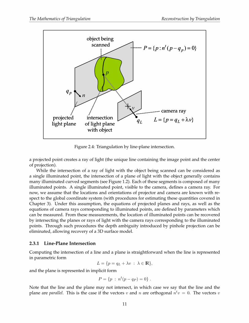
Figure 2.4: Triangulation by line-plane intersection.

a projected point creates a ray of light (the unique line containing the image point and the centerof projection).

While the intersection of a ray of light with the object being scanned can be considered asa single illuminated point, the intersection of a plane of light with the object generally containsmany illuminated curved segments (see Figure 1.2). Each of these segments is composed of manyilluminated points. A single illuminated point, visible to the camera, defines a camera ray. Fornow, we assume that the locations and orientations of projector and camera are known with re-spect to the global coordinate system (with procedures for estimating these quantities covered inChapter 3). Under this assumption, the equations of projected planes and rays, as well as theequations of camera rays corresponding to illuminated points, are defined by parameters whichcan be measured. From these measurements, the location of illuminated points can be recoveredby intersecting the planes or rays of light with the camera rays corresponding to the illuminatedpoints. Through such procedures the depth ambiguity introduced by pinhole projection can beeliminated, allowing recovery of a 3D surface model.

2.3.1 Line-Plane Intersection

Computing the intersection of a line and a plane is straightforward when the line is representedin parametric form

L = {p = qL + λv : λ ∈ IR},and the plane is represented in implicit form

P = {p : nt(p− qP ) = 0} .

Note that the line and the plane may not intersect, in which case we say that the line and theplane are parallel. This is the case if the vectors v and n are orthogonal ntv = 0. The vectors v

11


p

}{ 2222 vqpL λ+==camera ray


projected light ray

2q

2v1q

1v

}{ 1111 vqpL λ+==

p

}{ 2222 vqpL λ+==camera ray


projected light ray

2q

2v

2q

2v1q

1v

}{ 1111 vqpL λ+==

Figure 2.5: Triangulation by line-line intersection.

and n are also orthogonal when the line L is contained in the plane P . Whether or not the pointqL belongs to the plane P differentiates one case from the other. If the vectors v and n are notorthogonal ntv 6= 0, then the intersection of the line and the plane contains exactly one point p.Since this point belongs to the line, it can be written as p = qL+λv, for a value λ which we need todetermine. Since the point also belongs to the plane, the value λ must satisfy the linear equation

nt(p− qp) = nt(λv + qL − qp) = 0 ,

or equivalently

λ =nt(qP − qL)

ntv. (2.4)

Since we have assumed that the line and the plane are not parallel (i.e., by checking that ntv 6= 0beforehand), this expression is well defined. A geometric interpretation of line-plane intersectionis provided in Figure 2.4.

2.3.2 Line-Line Intersection

We consider here the intersection of two arbitrary lines L1 and L2, as shown in Figure 2.5.

L1 = {p = q1 + λ1v1 : λ1 ∈ IR} and L2 = {p = q2 + λ2v2 : λ2 ∈ IR}

Let us first identify the special cases. The vectors v1 and v2 can be linearly dependent (i.e., ifone is a scalar multiple of the other) or linearly independent.

The two lines are parallel if the vectors v1 and v2 are linearly dependent. If, in addition, thevector q2 − q1 can also be written as a scalar multiple of v1 or v2, then the lines are identical. Ofcourse, if the lines are parallel but not identical, they do not intersect.

If v1 and v2 are linearly independent, the two lines may or may not intersect. If the two linesintersect, the intersection contains a single point. The necessary and sufficient condition for two

12


1q1v

2q

2v

1111 vqp λ+=

2222 vqp λ+=

),( 2112 λλp1q

1v

2q

2v

),( 2112 λλpoptimal

1q1v

2q

2v

2q

2v

1111 vqp λ+=

2222 vqp λ+=

),( 2112 λλp1q

1v

2q

2v

2q

2v

),( 2112 λλpoptimal

Figure 2.6: The midpoint p12(λ1, λ2) for arbitrary values (left) of λ1, λ2 and for the optimal values(right).

lines to intersect, when v1 and v2 are linearly independent, is that scalar values λ1 and λ2 exist sothat

q1 + λ1v1 = q2 + λ2v2,

or equivalently so that the vector q2 − q1 is linearly dependent on v1 and v2.Since two lines may not intersect, we define the approximate intersection as the point which is

closest to the two lines. More precisely, whether two lines intersect or not, we define the approxi-mate intersection as the point p which minimizes the sum of the square distances to both lines

φ(p, λ1, λ2) = ‖q1 + λ1v1 − p‖2 + ‖q2 + λ2v2 − p‖2 .

As before, we assume v1 and v2 are linearly independent, such the approximate intersection is aunique point.

To prove that the previous statement is true, and to determine the value of p, we follow analgebraic approach. The function φ(p, λ1, λ2) is a quadratic non-negative definite function of fivevariables, the three coordinates of the point p and the two scalars λ1 and λ2.

We first reduce the problem to the minimization of a different quadratic non-negative definitefunction of only two variables λ1 and λ2. Let p1 = q1 + λ1v1 be a point on the line L1, and letp2 = q2 + λ2v2 be a point on the line L2. Define the midpoint p12, of the line segment joining p1and p2, as

p12 = p1 +1

2(p2 − p1) = p2 +

1

2(p1 − p2) .

A necessary condition for the minimizer (p, λ1, λ2) of φ is that the partial derivatives of φ, withrespect to the five variables, all vanish at the minimizer. In particular, the three derivatives withrespect to the coordinates of the point p must vanish

∂φ

∂p= (p− p1) + (p− p2) = 0 ,

or equivalently, it is necessary for the minimizer point p to be the midpoint p12 of the segmentjoining p1 and p2 (see Figure 2.6).

As a result, the problem reduces to the minimization of the square distance from a point p1 online L1 to a point p2 on line L2. Practically, we must now minimize the quadratic non-negativedefinite function of two variables

ψ(λ1, λ2) = 2φ(p12, λ1, λ2) = ‖(q2 + λ2v2)− (q1 + λ1v1)‖2 .

13

The Mathematics of Triangulation Coordinate Systems

Note that it is still necessary for the two partial derivatives of ψ, with respect to λ1 and λ2, to beequal to zero at the minimum, as follows.

∂ψ

∂λ1= vt1(λ1v1 − λ2v2 + q1 − q2) = λ1‖v1‖2 − λ2vt1v2 + vt1(q1 − q2) = 0

∂ψ

∂λ2= vt2(λ2v2 − λ1v1 + q2 − q1) = λ2‖v2‖2 − λ2vt2v1 + vt2(q2 − q1) = 0

These provide two linear equations in λ1 and λ2, which can be concisely expressed in matrix formas (

‖v1‖2 −vt1v2−vt2v1 ‖v2‖2

)(λ1λ2

)=

(vt1(q2 − q1)vt2(q1 − q2)

).

It follows from the linear independence of v1 and v2 that the 2 × 2 matrix on the left hand side isnon-singular. As a result, the unique solution to the linear system is given by(

λ1λ2

)=

(‖v1‖2 −vt1v2−vt2v1 ‖v2‖2

)−1(vt1(q2 − q1)vt2(q1 − q2)

)or equivalently (

λ1λ2

)=

1

‖v1‖2‖v2‖2 − (vt1v2)2

(‖v2‖2 vt1v2vt2v1 ‖v1‖2

)(vt1(q2 − q1)vt2(q1 − q2)

). (2.5)

In conclusion, the approximate intersection p can be obtained from the value of either λ1 or λ2provided by these expressions.

2.4 Coordinate Systems

So far we have presented a coordinate-free description of triangulation. In practice, however,image measurements are recorded in discrete pixel units. In this section we incorporate such co-ordinates into our prior equations, as well as document the various coordinate systems involved.

2.4.1 Image Coordinates and the Pinhole Camera

Consider a pinhole model with center of projection o and image plane P = {p = q + u1v1 + u2v2 :u1, u2 ∈ IR}. Any 3D point p, not necessarily on the image plane, has coordinates (p1, p2, p3)t

relative to the origin of the world coordinate system. On the image plane, the point q and vectorsv1 and v2 define a local coordinate system. The image coordinates of a point p = q+u1v1+u2v2 arethe parameters u1 and u2, which can be written as a 3D vector u = (u1, u2, 1). Using this notationpoint p is expressed as p1p2

p3

= [v1|v2|q]

u1u21

.

14


world coordinate system

1v3v

2v

=1

2

1

uu

u0=q

=3

2

1

ppp

p

1=f

camera coordinate system

world coordinate system

1v3v

2v

=1

2

1

uu

u0=q

=3

2

1

ppp

p

1=f


1v3v

2v

=1

2

1

uu

u0=q

=3

2

1

ppp

p

1=f


Figure 2.7: The ideal pinhole camera.

2.4.2 The Ideal Pinhole Camera

In the ideal pinhole camera shown in Figure 2.7, the center of projection o is at the origin of the worldcoordinate system, with coordinates (0, 0, 0)t, and the point q and the vectors v1 and v2 are definedas

[v1|v2|q] =

1 0 00 1 00 0 1

.

Note that not every 3D point has a projection on the image plane. Points without a projection arecontained in a plane parallel to the image passing through the center of projection. An arbitrary3D point p with coordinates (p1, p2, p3)t belongs to this plane if p3 = 0, otherwise it projects ontoan image point with the following coordinates.

u1 = p1/p3

u2 = p2/p3

There are other descriptions for the relation between the coordinates of a point and the image co-ordinates of its projection; for example, the projection of a 3D point p with coordinates (p1, p2, p3)t

has image coordinates u = (u1, u2, 1) if, for some scalar λ 6= 0, we can write

λ

u1u21

=

p1p2p3

. (2.6)

2.4.3 The General Pinhole Camera

The center of a general pinhole camera is not necessarily placed at the origin of the world coor-dinate system and may be arbitrarily oriented. However, it does have a camera coordinate systemattached to the camera, in addition to the world coordinate system (see Figure 2.8). A 3D point p hasworld coordinates described by the vector pW = (p1W , p

2W , p

3W )t and camera coordinates described

by the vector pC = (p1C , p2C , p

3C)t. These two vectors are related by a rigid body transformation

specified by a translation vector T ∈ IR3 and a rotation matrix R ∈ IR3×3, such that

pC = RpW + T .

15


WΧ

CΧ

1 2

31

2 3 up world

coordinate systemcamera

coordinate system

TRXWC +=Χ

WΧ

CΧ

1 2

31

2 3 up world

coordinate systemcamera

coordinate system

TRXWC +=Χ

Figure 2.8: The general pinhole model.

In camera coordinates, the relation between the 3D point coordinates and the 2D image coordi-nates of the projection is described by the ideal pinhole camera projection (i.e., Equation 2.6), withλu = pC . In world coordinates this relation becomes

λu = RpW + T . (2.7)

The parameters (R, T ), which are referred to as the extrinsic parameters of the camera, describe thelocation and orientation of the camera with respect to the world coordinate system.

Equation 2.7 assumes that the unit of measurement of lengths on the image plane is the sameas for world coordinates, that the distance from the center of projection to the image plane is equalto one unit of length, and that the origin of the image coordinate system has image coordinatesu1 = 0 and u2 = 0. None of these assumptions hold in practice. For example, lengths on the imageplane are measured in pixel units, and in meters or inches for world coordinates, the distance fromthe center of projection to the image plane can be arbitrary, and the origin of the image coordinatesis usually on the upper left corner of the image. In addition, the image plane may be tilted withrespect to the ideal image plane. To compensate for these limitations of the current model, a matrixK ∈ IR3×3 is introduced in the projection equations to describe intrinsic parameters as follows.

λu = K(RpW + T ) (2.8)

The matrix K has the following form

K =

f s1 f sθ o1

0 f s2 o2

0 0 1

,

where f is the focal length (i.e., the distance between the center of projection and the image plane).The parameters s1 and s2 are the first and second coordinate scale parameters, respectively. Notethat such scale parameters are required since some cameras have non-square pixels. The param-eter sθ is used to compensate for a tilted image plane. Finally, (o1, o2)t are the image coordinatesof the intersection of the vertical line in camera coordinates with the image plane. This point iscalled the image center or principal point. Note that all intrinsic parameters embodied in K are in-dependent of the camera pose. They describe physical properties related to the mechanical andoptical design of the camera. Since in general they do not change, the matrix K can be estimatedonce through a calibration procedure and stored (as will be described in the following chapter).

16


center of projectionq

n

image plane

}0)(:{ =−= qpnpP t

}0:{ == uluL tcenter of projection

qn

image plane

}0)(:{ =−= qpnpP t

}0:{ == uluL t

Figure 2.9: The plane defined by an image line and the center of projection.

Afterwards, image plane measurements in pixel units can immediately be “normalized”, by mul-tiplying the measured image coordinate vector by K−1, so that the relation between a 3D point inworld coordinates and 2D image coordinates is described by Equation 2.7.

Real cameras also display non-linear lens distortion, which is also considered intrinsic. Lensdistortion compensation must be performed prior to the normalization described above. We willdiscuss appropriate lens distortion models in Chapter 3.

2.4.4 Lines from Image Points

As shown in Figure 2.9, an image point with coordinates u = (u1, u2, 1)t defines a unique linecontaining this point and the center of projection. The challenge is to find the parametric equationof this line, as L = {p = q + λ v : λ ∈ IR}. Since this line must contain the center of projection, theprojection of all the points it spans must have the same image coordinates. If pW is the vector ofworld coordinates for a point contained in this line, then world coordinates and image coordinatesare related by Equation 2.7 such that λu = RpW + T . Since R is a rotation matrix, we haveR−1 = Rt and we can rewrite the projection equation as

pW = (−RtT ) + λ (Rtu) .

In conclusion, the line we are looking for is described by the point q with world coordinates qW =−RtT , which is the center of projection, and the vector v with world coordinates vW = Rtu.

2.4.5 Planes from Image Lines

A straight line on the image plane can be described in either parametric or implicit form, bothexpressed in image coordinates. Let us first consider the implicit case. A line on the image planeis described by one implicit equation of the image coordinates

L = {u : ltu = l1u1 + l2u2 + l3 = 0} ,

where l = (l1, l2, l3)t is a vector with l1 6= 0 or l2 6= 0. Using active illumination, projector patternscontaining vertical and horizontal lines are common. Thus, the implicit equation of an horizontalline is

LH = {u : ltu = u2 − ν = 0} ,

17


where ν is the second coordinate of a point on the line. In this case we can take l = (0, 1,−ν)t.Similarly, the implicit equation of a vertical line is

LV = {u : ltu = u1 − ν = 0} ,

where ν is now the first coordinate of a point on the line. In this case we can take l = (1, 0,−ν)t.There is a unique plane P containing this line L and the center of projection. For each image pointwith image coordinates u on the line L, the line containing this point and the center of projectionis contained in P . Let p be a point on the plane P with world coordinates pW projecting onto animage point with image coordinates u. Since these two vectors of coordinates satisfy Equation 2.7,for which λu = RpW + T , and the vector u satisfies the implicit equation defining the line L, wehave

0 = λltu = lt(RpW + T ) = (Rtl)t (pW − (−RtT )) .

In conclusion, the implicit representation of plane P , corresponding to Equation 2.2 for whichP = {p : nt(p− q) = 0}, can be obtained with n being the vector with world coordinates nW = Rtland q the point with world coordinates qW = −RtT , which is the center of projection.

18

Chapter 3

Camera and Projector Calibration

Triangulation is a deceptively simple concept, simply involving the pairwise intersection of 3Dlines and planes. Practically, however, one must carefully calibrate the various cameras and pro-jectors so the equations of these geometric primitives can be recovered from image measurements.In this chapter we lead the reader through the construction and calibration of a basic projector-camera system. Through this example, we examine how freely-available calibration packages,emerging from the computer vision community, can be leveraged in your own projects. Whiletouching on the basic concepts of the underlying algorithms, our primarily goal is to help begin-ners overcome the “calibration hurdle”.

In Section 3.1 we describe how to select, control, and calibrate a digital camera suitable for3D scanning. The general pinhole camera model presented in Chapter 2 is extended to addresslens distortion. A simple calibration procedure using printed checkerboard patterns is presented,following the established method of Zhang [Zha00]. Typical calibration results, obtained for thecameras used in Chapters 4 and 5, are provided as a reference.

Well-documented, freely-available camera calibration tools have been known for several yearsnow, but projector calibration received broader attention just recently with the increasing interestin building white-light scanners. In Section 3.2, we describe an open-source Projector-Camera Cal-ibration tool [MT12] which extends the printed checkerboard method to calibrated both projectorand camera. We conclude by reviewing calibration results for the structured light projector usedin Chapter 5.

3.1 Camera Calibration

In this section we describe both the theory and practice of camera calibration. We begin by brieflyconsidering which cameras are best suited for building your own 3D scanner. We then present thewidely-used calibration method originally proposed by Zhang [Zha00]. Finally, we provide step-by-step directions on how to use a freely-available MATLAB-based implementation of Zhang’smethod.

3.1.1 Camera selection and interfaces

Selection of the “best” camera depends on your budget, project goals, and preferred develop-ment environment. Probably the most confusing part for the inexperienced user is the variety ofcamera buses available raging from the traditional IEEE 1394 FireWire, the more common USB2.0 and 3.0, to Camera Link and GigE Vision buses. Selection of the right bus must begin con-sidering the throughput requirement for the application, the chosen bus must be able to transfer

19

Camera and Projector Calibration Camera Calibration

Figure 3.1: Vision camera buses comparison (Source: National Instruments white paper. [ Na13]).

images at the required framerate. Other aspects to consider are camera cable length, effective cost,and whether hardware synchronization triggers will be used. These characteristics are comparedgraphically in Figure 3.1. We refer the user interested in learning more about vision camera busesto [ Na13]. Besides camera buses, other aspects to consider when choosing a camera are their sen-sor specifications (size, resolution, color or grayscale) and whether they have a fixed lens or a lensmount. When choosing lenses the focal length must be considered, which determines—togetherwith sensor size—the effective field of view of the camera. In this course we recommend standardUSB cameras because they are low cost and they do not require special hardware or software,this come at a price of a low throughput and limited control and customization. Specifically, wewill use a Logitech C920 which can capture images with a resolution of 1920×1080, Figure 3.2(a).Although more expensive, we also recommend cameras from Point Grey Research. The camerainterface provided by this vendor is particularly useful if you plan on developing more advancedscanners than those presented here, and particularly if you need access to raw sensor data. As apoint of reference, we have tested a Point Grey GRAS-20S4M/C Grasshopper, Figure 3.2(b), at aresolution of 1600×1200 up to 30 Hz [Poi].

At the time of writing, the accompanying software for this course was primarily written inMATLAB. If readers wish to collect their own data sets using our software, we recommend ob-taining a camera supported by the Image Acquisition Toolbox for MATLAB [Mat]. Note that thistoolbox supports products from a variety of vendors, as well as any DCAM-compatible FireWirecamera or webcam with a Windows Driver Model (WDM) or Video for Windows (VFW) driver.For FireWire cameras the toolbox uses the CMU DCAM driver [CMU]. Alternatively, we encour-age users to write their own image acquisition tools using standard libraries as OpenCV [Ope]or SimpleCV [Sim]. OpenCV has a variety of ready-to-use computer vision algorithms—such as

20


(a) Logitech HD Pro Webcam C920 (b) Point Grey Grasshopper IEEE-1394b (with-out lens)

Figure 3.2: Recommended cameras for course projects.

camera calibration—optimized for several platforms, including Windows, Mac OS X, Linux, andAndroid; which can be accessed in C++, Java, and Python. SimpleCV is a high-level framework,with a faster learning curve, for developing computer vision software in Python.

3.1.2 Calibration Methods and Software

Camera Calibration Methods

Camera calibration requires estimating the parameters of the general pinhole model presentedin Section 2.4.3. This includes the intrinsic parameters, being focal length, principal point, andthe scale factors, as well as the extrinsic parameters, defined by a rotation matrix and translationvector mapping between the world and camera coordinate systems. In total, 11 parameters (5intrinsic and 6 extrinsic) must be estimated from a calibration sequence. In practice, a lens distor-tion model must be estimated as well. We recommend the reader review [HZ04, MSKS05] for anin-depth description of camera models and calibration methods.

At a basic level, camera calibration requires recording a sequence of images of a calibrationobject, composed of a unique set of distinguishable features with known 3D displacements. Thus,each image of the calibration object provides a set of 2D-to-3D correspondences, mapping imagecoordinates to scene points. Naıvely, one would simply need to optimize over the set of 11 cameramodel parameters so that the set of 2D-to-3D correspondences are correctly predicted (i.e., theprojection of each known 3D model feature is close to its measured image coordinates).

Many methods have been proposed over the years to solve for the camera parameters givensuch correspondences. In particular, the factorized approach originally proposed Zhang [Zha00]is widely-adopted in most community-developed tools. In this method, a planar checkerboardpattern is observed in two or more orientations (see Figure 3.3). From this sequence, the intrinsicparameters can be separately solved. Afterwards, a single view of a checkerboard can be used tosolve for the extrinsic parameters. Given the relative ease of printing 2D patterns, this method iscommonly used in computer graphics and vision publications.

21


Figure 3.3: Camera calibration images containing a checkerboard with different orientationsthroughout the scene.

Recommended Software

A comprehensive list of calibration software is maintained by Bouguet on the toolbox website1.We recommend course attendees use the MATLAB toolbox. Otherwise, OpenCV replicates manyof its functionalities, while supporting multiple platforms. A CALTag [AHH10] checkerboard andsoftware is yet another alternative. CALTag patterns are designed to provide features even if somecheckerboard regions are occluded, we wil use this feature in Section 4.2 to calibrate a turntable.

Although calibrating a small number of cameras using these tools is straightforward, calibrat-ing a large network of cameras is a relatively challenging problem. If your projects lead you in thisdirection, we suggest to consider the self-calibration toolbox [SMP05], or a new toolbox based ona feature-descriptor pattern [LHKP13] instead. The former, rather than using multiple views of aplanar calibration object, detects a standard laser point being translated through the working vol-ume and correspondences between the cameras are automatically determined from the trackedprojection of the pointer in each image. The latter, creates a pattern using multiple SIFT/SURFfeatures at different scales which can be automatically detected. In contrast with the checkerboardapproach, features can be uniquely identified—similar to CALTag cells—even when partial viewsof the pattern are available due to limited intersection of the multiple cameras field of view.

3.1.3 Calibration Procedure

In this section we describe, step-by-step, how to calibrate your camera using the Camera Cal-ibration Toolbox for MATLAB. We also recommend reviewing the detailed documentation andexamples provided on the toolbox website. Specifically, new users should work through the firstcalibration example and familiarize themselves with the description of model parameters (whichdiffer slightly from the notation used in these notes).

Begin by installing the toolbox, available for download at the software website1. Next, con-struct a checkerboard target. Note that the toolbox comes with a sample checkerboard image;print this image and affix it to a rigid object, such as piece of cardboard or textbook cover. Recorda series of 10–20 images of the checkerboard, varying its position and pose between exposures.Try to collect images where the checkerboard is visible throughout the image, and specially, thecheckerboard must cover a large region in each image.

Using the toolbox is relatively straightforward. Begin by adding the toolbox to your MATLAB

path by selecting “File→ Set Path...”. Next, change the current working directory to one contain-ing your calibration images (or one of our test sequences). Type calib at the MATLAB prompt

1 http://www.vision.caltech.edu/bouguetj/calib_doc/

22

http://www.vision.caltech.edu/bouguetj/calib_doc/


(a) Tangential Component (b) Radial Component

Figure 3.4: Camera calibration distortion model. Sample distortion model of the Logitech C920Webcam used in the Laser Stripe Scanner of Chapter 4. The plots show the center of distortion ×at the principal point, and the amount of distortion in pixel units increasing towards the border.

to start. Since we are only using a few images, select “Standard (all the images are stored inmemory)” when prompted. To load the images, select “Image names” and press return, then “j”(JPEG images). Now select “Extract grid corners”, pass through the prompts without entering anyoptions, and then follow the on-screen directions. The default checkerboard has 30mm×30mmsquares but the actual dimensions vary from printer to printer, you should measure your owncheckerboard and use those values instead. Always skip any prompts that appear, unless youare more familiar with the toolbox options. Once you have finished selecting corners, choose“Calibration”, which will run one pass though the calibration algorithm. Next, choose “Analyzeerror”. Left-click on any outliers you observe, then right-click to continue. Repeat the cornerselection and calibration steps for any remaining outliers (this is a manually-assisted form of bun-dle adjustment). Once you have an evenly-distributed set of reprojection errors, select “Recomp.corners” and finally “Calibration”. To save your intrinsic calibration, select “Save”.

From the previous step you now have an estimate of how pixels can be converted into normal-ized coordinates (and subsequently optical rays in world coordinates, originating at the cameracenter). Note that this procedure estimates both the intrinsic and extrinsic parameters, as wellas the parameters of a lens distortion model. Typical calibration results, illustrating the lens dis-tortion model is shown in Figure 3.4. The actual result of the calibration is displayed below asreference.

Logitech C920 Webcam sample calibration result:

Focal Length: fc = [ 1642.17076 1642.83775 ]+/- [ 2.91675 1.85405 ]

Principal point: cc = [ 1176.14705 714.90826 ]+/- [ 2.63232 3.58792 ]

Skew: alpha_c = [ 0.00000 ] +/- [ 0.00000 ]=> angle of pixel axes = 90.0000 +/- 0.0000 degrees

Distortion:kc = [ 0.09059 -0.16979 -0.00796 -0.00078 0.00000 ]+/- [ 0.00333 0.01042 0.00051 0.00065 0.00000 ]

Pixel error: err = [ 0.25706 0.27527 ]

23

Camera and Projector Calibration Projector Calibration

Figure 3.5: Recommended projectors for course projects: (Left) Dell M110 DLP Pico Projector,(Right) Optoma PK320 Pico Pocket Projector.

3.2 Projector Calibration

We now turn our attention to projector calibration. Following the conclusions of Chapter 2, wemodel the projector as an inverse camera (i.e., one in which light travels in the opposite directionfrom usual). Under this model, calibration proceeds in a similar manner as with cameras, wherecorrespondences between 3D points world coordinates and projector pixel locations are used toestimate the pinhole model parameters. For camera calibration, we use checkerboard corners asreference world points of known coordinates which are localized in several images to establishpixel correspondences. In the projector case, we will project a known pattern onto a checkerboardand to record a set of images for each checkerboard pose. The projected pattern is later decodedfrom the camera images and used to convert from camera coordinates to projector pixel locations.This way, checkerboard corners are identified in the camera images and, with the help of the pro-jected pattern, their locations in projector coordinates are inferred. Finally, projector-checkerboardcorrespondences are used to calibrate the projector parameters as it is done for cameras. This cali-bration method is described with detail in [MT12] and implemented as an opensource calibrationand scanning tool2. We will use this software for projector and camera calibration when workingwith structured light scanners in Chapter 5. A step-by-step guide of calibration process is givenbelow in Section 3.2.2.

3.2.1 Projector Selection and Interfaces

Almost any digital projector can be used in your 3D scanning projects, since the operating systemwill simply treat it as an additional display. However, we recommend at least a VGA projector,capable of displaying a 640×480 image. For building a structured lighting system select a camerawith equal (or higher) resolution than the projector. Otherwise, the recovered model will be lim-ited to the camera resolution. Additionally, those with DVI or HDMI interfaces are preferred fortheir relative lack of analogue to digital conversion artifacts.

The technologies used in consumer projectors have matured rapidly over the last decade. Earlyprojectors used an LCD-based spatial light modulator and a metal halide lamp, whereas recentmodels incorporate a digital micromirror device (DMD) and LED lighting. Commercial offer-ings vary greatly, spanning large units for conference venues to embedded projectors for mobilephones. A variety of technical specifications must be considered when choosing the “best” projec-tor for your 3D scanning projects. Variations in throw distance (i.e., where focused images can beformed), projector artifacts (i.e., pixelization and distortion), and cost are key factors.

Digital projectors have a tiered pricing model, with brighter projectors costing significantly

2http://mesh.brown.edu/scanning/software.html

24

http://mesh.brown.edu/scanning/software.html


Figure 3.6: TI DLP .45in Pico Projectors diamond pixel configuration.

more than dimmer ones. At the time of writing, a portable projector with output resolution of1280×800 and 100–500 lumens of brightness can be purchased for around $300–$500 USD. Exam-ples are the Optoma and Dell Pico projectors shown in Figure 3.5 commonly used by studentsbecause of their convenient small size and high contrast.

When considering projectors it is important to distinguish between their “native” and “out-put” resolutions. Native resolution refers to the number of pixels in the projection device (i.e.number of micromirrors in DLPs arrays), whereas, the output resolution is the screen size re-ported to the operating system. Ideally, we want both to be the same so that images sent by theoperating are displayed by the projector at the same resolution. However, many portable pro-jectors use Texas Instruments DLP Pico DMDs where projector pixels are rotated 45◦ as shownin Figure 3.6. In this configuration the pixel density in the horizontal and vertical directions aredifferent and images generated by the computer are resampled to match the DMD elements. Wehave used pico projectors in structured-light scanners successfully but the native resolution has tobe considered to decide the maximum resolution of the projected patterns.

While your system will treat the projector as a second display, your development environmentmay or may not easily support fullscreen display. For instance, MATLAB does not natively supportfullscreen display (i.e., without window borders or menus). One solution is to use Java displayfunctions integrated in MATLAB. Code for this approach is available online3. Unfortunately, wefound that this approach only works for the primary display. Another common approach is tosplit image acquisition and data processing in two separate programs and use standard software(i.e. as provided by camera manufacturers) to capture and save images, and to program yourscanning tool to read images from a permanent storage. This approach is used by the Camera Cal-ibration Toolbox [Bou]. Finally, for users working outside of MATLAB, we recommend controllingprojectors through OpenGL.

3.2.2 Calibration Software and Procedure

Projector calibration has received increasing attention, in part driven by the emergence of low-cost digital projectors. As mentioned at several points, a projector is simply the “inverse” of acamera, wherein points on an image plane are mapped to outgoing light rays passing throughthe center of projection. As in Section 3.1.2, a lens distortion model can augment the basic generalpinhole model presented in Chapter 2. In this section we will use the Projector-Camera Calibrationsoftware [MT] to calibrate both projector and camera, intrinsic and extrinsic parameters, includingradial distortion coefficients. This software is built for Windows, Linux, and Mac OS X, and sourcecode is available too.

Begin by downloading the software [MT] for your platform and setting up your projector and

3http://www.mathworks.com/matlabcentral/fileexchange/11112

25

http://www.mathworks.com/matlabcentral/fileexchange/11112


Figure 3.7: Sample setup of a structured light scanner. A projector and camera are placed at similarheight with a horizontal translation in stereo configuration. In this particular case, the camera ismuch forward than the projector to compensate between their different field of view.

camera in the scanning position. Once calibrated, projector and camera have to remain at fix posi-tions, and their lens settings unchanged (e.g. focus, zoom) for the calibration to remain valid. Thegeneral recommendation is to place them with some horizontal displacement, too much displace-ment will provide little overlap between projector and camera images, too few displacement willproduce a lot of uncertainty for triangulation, try to find some intermediate position, see Figure 3.7as example. A checkerboard pattern is required for calibration.

Run the software and click the “Capture...” button to open a preview window, Figure 3.8.Select your projector screen and your camera using the combo boxes, then check “Preview” toactivate the projector. Click “Prev” and “Next” buttons to navigate the projected pattern sequenceas desired. Use the camera live view to make sure camera and projector view points are correct.Note that only cameras supported by OpenCV will be recognized by the software; if your camerahappens to not be in this group, you can still use the tool for calibration but you will have toproject and capture the images with an external software, and use the tool only for calibration.Refer to the software website for more details.

Place the calibration checkerboard in the scene in such a way that all its cells are visible in thecamera and illuminated by the projector. Uncheck “Preview” and press “Capture”. The softwarewill project and capture a sequence of images. The checkerboard has to remain static at this time.The image output folder can be changed prior beginning, but it must not be changed after the firstcapture. Repeat the capture procedure several times to collect sequences with the checkerboard at

26


Figure 3.8: Projector-Camera Calibration software main screen and capture window.

different positions and orientations. Close the capture window to return to the main screen.The main screen will display a list with the different sequences captured, which can be browsed

to see any of the images. If images were captured with an external tool, or with this tool but at adifferent time, you can select their location by clicking “Change dir..”. Count the internal numberof corners of your checkerboard and fill the boxes labeled as “Corners”, also measure them inmillimeters, or your unit of choice, and enter their dimensions in the “Size” boxes. Now you areready for calibration, click “Calibrate”. The program will automatically detect the checkerboardcorners, decode the projected sequences, and run the calibration. The final result will be displayedas text and saved to a file. The main screen contains other parameters and buttons that can be usedto debug errors or to change the default decoding options, they will not be covered here but feelfree to read the documentation and modify them to improve your results.

27

Chapter 4

The Laser Slit 3D Scanner

In this chapter we describe how to build the “classic” desktop Laser Slit 3D Scanner consisting ofa single digital camera, a laser line projector, and a manual or motorized turntable. Specifically,we will describe how to setup the scanner using inexpensive elements, and we will describe itsoperating principle and the mathematics that allow to compute the 3D shape of an object beingscanned.

4.1 Description

The Laser Slit 3D Scanner is an “active line scanner”, meaning that it uses active illumination—thelaser line projected onto a scene—and that it recovers a single line of points from each capturedframe. Active illumination permits to scan objects more or less independently of their surfacecolor or texture, which is an important advantage over passive methods which have difficultyin recovering constant color regions. On the other hand, a single line is captured at each timeand it is necessary to move either the scanner or the object to acquire additional points and incre-mentally build a 3D model. In our case, we decided to put the target object onto an inexpensiveturntable which is rotated manually in order to create a 360◦ model. Some users may prefer touse a computerized turntable controlled by a stepper motor for more automation or may want todo other variations to the suggested setup. The mathematics and methods discussed here will beapplicable with little or no modification to many of these variations.

The scanner is setup as shown in Figure 4.1. The camera is fixed on a side, elevated from theturntable plane, and looking down to the turntable center. The optimal orientation and distancedepends on the camera field-of-view and the size of scanning volume. The general guideline isthat most of the turntable surface must be visible when there is no object on it, and the bottomand top of the object being scanned must be visible too when sitting on the turntable. It is not rec-ommended to put the camera farther than required because the image regions looking at neitherthe turntable nor the target object will not be used by the scanner. The Laser Line Generator mustbe placed on a side of the camera and with similar orientation, it is recommended that it passesthrough the turntable center point and be orthogonal to the turntable plane. Figure 4.2 showsthe materials we have used in our setup: a 650nm AixiZ 38◦ Line Generator, a Logitech HD ProWebcam C920, and a manually controlled turntable.

We will set the world coordinate system at the turntable center of rotation, with the xy-planeon the turntable and the z-axis pointing up, see Figure 4.1. Prior to scanning, we need to calibratethe camera intrinsic parameters and the location of both the camera and light plane generatedby the laser in respect to the world coordinate system. The turntable center of rotation must

28

The Laser Slit 3D Scanner Turntable calibration

Turntable

Target Object

Camera

Laser

x

z

y

Figure 4.1: Laser Slit 3D Scanner setup

Figure 4.2: Materials: (Left) 650nm AixiZ 38◦ Line Generator. (Center) Logitech HD Pro WebcamC920. (Right) Manual turntable.

be calibrated too. At scanning time, the light plane generated by the laser is invisible in the airbut we can see some of its points when the light hits a surface, they will have the color of theprojected light (red in our case). These points can be detected in an image captured by the cameraand its 3D location is found as the intersection of a ray beginning at the camera center, passingthrough the corresponding image pixel, and the plane of light (known), Figure 4.3. The locationof the points recovered from each image must be rotated through the z-axis to undo the currentturntable rotation angle.

4.2 Turntable calibration

A computer controlled turntable will provide us with the current rotation angle that correspondsto the stepper motor current rotation. Sometimes, as in the case of a manual turntable, that in-formation is not available and the rotation must be computed from the current image. We willdo so with the help of a CALTag checkerboard [AHH10] pasted flat on the turntable surface. TheCALTag checkerboard assigns a unique code to each checkerboard cell which is used to identifythe visible cells in an image even when a region of the checkerboard is occluded. We need this

29


x

z

y

α

Light Plane

Camera Center

pixel ray

Rotation Angle

Image

3D point(ray-plane intersection)

image pixel

Figure 4.3: Laser Slit 3D Scanner setup

property because the target object sitting on top the turntable will occlude a large region of theCALTag. The corners of the visible checkerboard cells is a set of points rotating together with theturntable and will allow us to compute a rotation angle for each captured image.

Figure 4.4: (Left) A CALTag checkerboard pasted on the turntable surface helps to recover thecurrent rotation angle. (Right) Sample CALTag pattern.

At this point we assume the camera is calibrated and a set of images of the turntable at differentrotations was captured. In addition, a set of 3D points on the turntable plane was identified in eachimage. Points coordinates are in reference to a known coordinate system chosen by the user. Wewill show how to find the unknown center of rotation and the rotation angle of the turntable foreach image. In the current example, we align the coordinate system with the checkerboard andwe identify the checkerboard and turntable planes with the plane z = 0.

30


4.2.1 Camera extrinsics

The first step is to find the pose of the camera for each image in reference to the known coordinatesystem. At this point we will compute a rotation matrix R and a translation vector T for eachimage independently of the others, such that a point p in the reference system projects to a pixelu, that is

λu = K(Rp+ T ) (4.1)

R =

r11 r12 r13r21 r22 r23r31 r32 r33

, T =

TxTyTz

(4.2)

where u, p, and K are known. Point p = [px, py, 0]T is in the checkerboard plane and u =[ux, uy, 1]T is expressed in homogenous coordinates. We define u = K−1u and rewrite Equation4.1 as follows

[0, 0, 0]T = u× (λu) = u× (Rp+ T ) (4.3)

u×

r11px + r12py + Txr21px + r22py + Tyr31px + r32py + Tz

=

000

(4.4)

−(r21px + r22py + Ty) + uy(r31px + r32py + Tz)(r11px + r12py + Tx) + ux(r31px + r32py + Tz)

−uy(r11px + r12py + Tx) + ux(r21px + r22py + Ty)

=

000

. (4.5)

Equation 4.5 provides 3 equations but only 2 of them are linearly independent. We select the firsttwo equations and we group the unknowns in a vector X = [r11, r21, r31, r12, r22, r32, Tx, Ty, Tz]

T[0 −px +uypx 0 −py +uypy 0 −1 +uypx 0 −uxpx py 0 −uxpy 1 0 −ux

]X =

[00

]. (4.6)

Until now we have considered a single point p; in general, we will have a set of points {pi|i :1 . . . n} for each image. Note that the number n of points visible will change from image to image.We use all the points to build a single system of the form AX = 0 where A ∈ R2n×9 contains 2rows as in Equation 4.6 for each point pi stacked together, and we solve

X = argminX||AX||, s.t. ||X|| = 1 (4.7)

We constrain the norm of X in order to get a non-trivial solution. Vector X has 8 degrees offreedom, thus, matrix A must be rank 8 so that a unique solution exists. Therefore, we need atleast 4 non-collinear points in order to get a meaningful result. After solving for X we need torebuild R as a rotation matrix.

r1 = [r11, r21, r31]T , r2 = [r21, r22, r23]

T , T = [Tx, Ty, Tz]T (4.8)

r1 =r1||r1||

, r3 =r1||r1||

× r2||r2||

, r2 = r3 × r1 (4.9)

R =[r1 r2 r3

], T = T (4.10)

Figure 4.5 shows the supplied software running the camera extrinsics computation as describedhere.

31


Figure 4.5: Screenshot of the supplied software running camera extrinsics computation. (Left)Image being processed: identified CALTag corners displayed in green. (Right) 3D view: CALTagcorners shown in green below, cameras displayed above with their z-axis on red, the referencecoordinate system was set at the origin of the checkerboard.

4.2.2 Center of rotation and rotation angle

In the previous section we showed how to estimate Rk and Tk for each of the N cameras inde-pendently. Now, we will use the fact that the turntable rotates in a plane and has a single de-gree of freedom to improve the computed camera poses. We begin finding the center of rotationq = [qx, qy, 0]T in the turntable plane which must satisfy the projection equations as any otherpoint

λkuk = Rkq + Tk (4.11)

By definition of rotation center its position remains unchanged before and after the rotation, thisobservation allow us to define Q ≡ λkuk, ∀k, and write

Rkq + Tk = Q (4.12)R1 −IR2 −I...

...RN TN

[qQ

]=

−T1−T2

...−TN

⇒ AX = b (4.13)

X = argminX||AX − b|| (4.14)

In order to fix qz = 0, we skip the third column in the rotation matrices reducing A to 5 columnsand changing X = [qx, qy, Qx, Qy, Qz]

T .Let be αi the rotation angle of the turntable in image i, then for every 1 ≤ k < j ≤ N , we

should have

RTkRj =

cos(αj − αk) − sin(αj − αk) 0sin(αj − αk) cos(αj − αk) 0

0 0 1

(4.15)

32

The Laser Slit 3D Scanner Image Laser Detection

The turntable position in the first image is designated as the origin: α1 = 0. We get an approximatevalue for each other αk by reading the values cosαk and sinαk from RT1Rk and setting

αk = tan−1(

sinαkcosαk

)(4.16)

Figure 4.6 shows the center of rotation obtained with this method drawn on top of an inputimage and its corresponding 3D view.

Figure 4.6: Center of rotation. (Left) Camera image: center of rotation drawn on top. (Right) 3Dview: world coordinate system at the center of the rotation.

4.2.3 Global optimization

The final step in turntable calibration is to refine the values of all the parameters using a globaloptimization. The goal is to minimize the reprojection error of the detected points in the images

E(qx, qy, R1, o1, α2, . . . , αN ) =

N∑k=1

∑i∈Jk

||uik −Π(KR1Rαk(pi − ok))||2 (4.17)

where

Rαk=

cos(αk) − sin(αk) 0sin(αk) cos(αk) 0

0 0 1

, ok = RTαk(o1 − q) + q, ∀k > 1, (4.18)

andΠ(x, y, z) = (x/z, y/z) (4.19)

Jk is the subset of checkerboard corners visible in image k, α1 = 0, and uik is the pixel locationcorresponding to pi in image k. We begin the optimization with the values q, R1, o1 = −RT1 T1, andαk found in the previous sections which are close to the optimal solution.

4.3 Image Laser Detection

In this section we show how to detect the laser slit in the captured images. A common approachto detection is to compare an image where the laser is seen with a reference image captured while

33

The Laser Slit 3D Scanner Image Laser Detection

the laser is off. That approach is appropriate for a scanner setup where the camera and the objectremains static while the laser changes location. Detection is done by subtracting the intensity inthe new image with the reference intensity and searching the pixels where a significance changeis observed. This method works independently of the laser color, would work even when colorimages are not available, it is computationally efficient, and most importantly, it is tuned to thecurrent scene and illumination, because a new reference image is captured for each new scanning.However, the method is not applicable if a reference image is not available, or as in the case of theturntable where we would need as many reference images as turntable positions.

Figure 4.7: The plot shows the red channel intensity along the line in the image highlighted inyelow. The maximum value does not corresponds to the laser line.

In our scanner we will apply a laser detection algorithm that considers the laser color and itdoes work with a single image. In our case we used a red laser and we could expect to examine theimage red channel and find a maximum at the laser location. This is not always true even if thereare no other red points in the scene. For instance, Figure 4.7 shows a typical input image, withoutany red color visible besides the laser line, but the highlighted line contains many pixels with redintensity above the value at the laser location, indicated with a blue line in the plot. The reason isthat red color is not the one with a high value in the red channel—white has high intensities in allchannels. The property of red color is that it only has a high intensity in the red channel. Based onthis observation we will perform the detection in a “channel difference image” defined as

Idiff = Ir −Ig + Ib

2(4.20)

where Ir, Ig, and Ib are the image red, green, and blue channels respectively. Figure 4.8 showsIdiff for the sample image. Now, there is a clear peak at the laser location.

Our detection algorithm involves computing the channel difference image with Equation 4.20and finding its maximum row by row. In general, we hope to find a single or no laser slit point ineach row because we have oriented the laser line generator vertically. However, in rare occasionsmay appear more than one laser slit per line due to object discontinuities. For simplicity, we willconsider only the one with maximum intensity.

34

The Laser Slit 3D Scanner Background detection

Figure 4.8: Channel difference. The image and plot show a clear peak at the laser line location.

Laser line generators made with a cylinder lens produce a Gaussian light distribution. Inpractice, cheap lenses have a profile not so well defined and the observed maximum will varyrandomly in a range close to the line center, Figure 4.9. In order to compensate and make theestimation more stable from row to row, it is recommended to apply Gaussian smoothing in thehorizontal direction prior to searching the maximum.

Figure 4.9: Laser line intensity plot of several image rows of similar color: (Left) there is no clearmaximum at the peak center, (Right) the maximum is well localized after smoothing.

Figure 4.10 shows the result of the single image laser stripe detection described to the sampleimage.

4.4 Background detection

It is desirable to detect and exclude the background from the scanning process. Doing so savescomputation on unwanted image regions, reduces detection errors, and produces a 3D model onlywith the object of interest. A pixel imaging a point on the turntable or the object sitting on top ofit will be considered as foreground, all the other pixels are considered background. The set offoreground and background pixels are disjoint and the union of them contains the whole image.

35

The Laser Slit 3D Scanner Plane of light calibration

Figure 4.10: Laser detection result: (Left) detected points overlapped in red to input image, (Right)detection result mask.

Additionally, a pixel location could be background in one image and foreground on a differentone. Our goal is to compute the intersection of all images background pixels, that is, identify thepixel locations that are never foreground and we would like exclude from further processing.

By definition, a pixel location that is always background will have constant intensity. In reality,a background pixel will have little intensity variations due to the image sensor noise and smallillumination changes. We can check this property by calculating the intensity variance of eachpixel in the whole image set and label as background those with small variances.

Figure 4.11 (Left and Middle) verifies the constant property of background pixels visually.The background in the mean image is seen sharp, whereas, foreground pixels are blurred due totheir changing intensities. Background pixels are close to zero (black) in the variance image. Thedetection result is displayed as a binary mask in Figure 4.11 (Right), foreground is shown in white.

Figure 4.11: Background detection: (Left) mean intensity image, (Middle) variance intensity im-age, (Right) background mask result.

4.5 Plane of light calibration

We need to calibrate the location of the plane of light generated by the laser. The calibrationconsists in identifying some points we know belong to the plane and finding the best plane, in theleast squares sense, that matches them. The projection of the laser line onto the turntable providesus with a set of such points, however, they are all in a straight line and define a pencil of planes

36

The Laser Slit 3D Scanner 3D model reconstruction

rather a single one. An easy way to find additional points is to place a checkerboard plane ontothe turntable and capture images at several rotations, Figure 4.12.

Figure 4.12: Light plane calibration: an extra plane is placed onto the turntable and is rotated toprovide a set of non-collinear points.

The orientation of the camera with respect to the checkerboard plane is calculated with themethod from Section 4.2.1. The laser pixels are identified with the detection algorithm and theyare triangulated using ray-plane intersection providing a set of 3D points on the checkerboardplane. We can choose to triangulate the laser points on the turntable plane too, which makespossible to calibrate with a single image. It is recommendable to capture additional images tohave more samples of the light plane for a better calibration. In special, we would like samples atdifferent depths in the scanning volume. Checkerboard images captured for the camera intrinsiccalibration can be reused to calibrate the plane of light, this way no extra images are required. Thisidea is illustrated in Figure 4.13.

4.6 3D model reconstruction

At this point the system is fully calibrated: camera internal parameters, camera pose, world coor-dinate system, turntable rotation angle in each image, and the plane of light are all known. The laststep is to identify the laser slits corresponding to the target object, triangulate them by ray-planeintersection with the light plane, and place the result in the world coordinate system by undoingthe turntable rotation at each image. To generate only points in the model only foreground pixelsare triangulated, and only the 3D points within the scanning volume are added to the model. Thescanning volume is easily defined as the rectangular region of the turntable checkerboard and ex-tending vertically in the direction of the z-axis by a user given height. Figure 4.14 shows the resultoutput following the methods from this chapter and without any additional post-processing.

37

The Laser Slit 3D Scanner 3D model reconstruction

Figure 4.13: Light plane calibration result. A checkerdboard plane was placed on the turntableand images at several rotations were captured. Images are used first for camera calibration, andlater for calibration of the light plane (shown in orange).

Figure 4.14: Laser Slit 3D Scanner result: (Left) 3D model in the sample software, (Right) 3D modeloutput.

38

Chapter 5

Structured Lighting

In this chapter we describe how to build a structured light scanner using one or more digitalcameras and a single projector. While the Laser Slit 3D Scanner implemented in the previouschapter is widely used, it needs hundreds of images to build a complete model with acceptabledetail. It could be argued that the scanning process is inefficient, in the sense that only a very smallset of pixels illuminated by the laser contribute to the scan in each image, and the rest are mostlyignored. On the contrary, a Structured Light Scanner replaces the projected laser line with a dataprojector capable of displaying 2-dimensional patterns covering a much larger object region, andgenerating a 3D model containing all the points being simultaneously illuminated by the projectorand visible from the cameras. More information is extracted from each image, thus, reducing thenumber of images required and the total scanning time. A turntable is still useful, but only a fewrotations will be required to build a full model.

The structured light scanner builds on top of the theory and algorithms developed in the previ-ous chapters. Reconstruction is now accomplished using ray-ray triangulation between projectorand camera pixels. The key concept here is that correspondences are established by decodingcertain structured light sequences. The methods described below are already implemented in theProjector-Camera Calibration software introduced in Chapter 3. Here we will expand on howprojector columns and rows are coded in the patterns and later decoded from the camera images.

5.1 Structured Light Scanner

Structured light scanners became highly popular in the recent years, mainly because of the lowcost and wide availability of quality data projectors and cameras. The concept of structured lightrefers to the idea of the scene being illuminated by specially designed patterns. A quick review ofthe literature will reveal that many different patterns have been proposed using different codingstrategies. Salvi et al. [SFPL10] give several pattern classifications depending on whether theymake use of color, the number of images required, the type of encoding, and whether they encodediscrete or continuous quantities, a few examples are shown in Figure 5.1. We will focus only ondiscrete binary patterns and a minor variant known as Gray code, both are shown in Figures 5.3and 5.4.

5.1.1 Scanner Hardware

Our scanner is built with a single camera and a single data projector. This choice replicates passivestereo scanners which observe a scene with a pair of cameras and build a 3D model by triangulat-ing points visible in both of them. Identifying the exact position where points from the first view

39

Structured Lighting Structured Light Scanner

(a) De Bruijn color stripes (b) Color M–Array (c) Phase shifting

Figure 5.1: Patterns with different coding strategies.

appear in the second view is a difficult task in general, known as “establishing pixel correspon-dences”. Here, we replace one camera by a projector to simplify this task. As with other systems,several cameras and projectors could be added to extend the scanned area, or to provide moreaccurate measurements, but we will not discuss those variants here, however, once understoodthe concepts from this chapter, it should be more or less straightforward to generalized them toother configurations.

We will use the Logitech C920 Webcam and an Optoma ML550 projector setup as in Figure 5.2.The target object may be placed on a turntable and several scans can be aligned to build a 360◦

model by calibrating the turntable as in Section 4.2. It is advisable to mount the camera andprojector in a tripod because they must remain fixed at all times.

Figure 5.2: Structured light scanner sample setup: Optoma ML550 projector, Logitech C920 Web-cam, target object on a turntable, and computer.

5.1.2 Structured Light Sequences

The primary benefit of introducing the projector is to eliminate the mechanical motion required inthe Laser Slit 3D Scanner. Assuming minimal lens distortion, the projector can be used to display

40

Structured Lighting Structured Light Scanner

Figure 5.3: Structured light illumination sequences. (Top row, left to right) The first four bit planesof a binary encoding of the projector columns, ordered from most to least significant bit. (Bottomrow, left to right) The first four bit planes of a Gray code sequence encoding the projector columns.

a single column (or row) of white pixels translating against a black background; thus, as manyimages as columns (or rows) in the projector would be required in order to assign the correspon-dences, in our implementation, between camera pixels and projector columns (or rows). Afterestablishing the correspondences and calibrating the system, a 3D point cloud is reconstructedusing familiar ray-plane triangulation. However, a simple strategy like this does not fully exploitthe projector. Since we are free to project arbitrary 24-bit color images, one would expect there toexist a sequence of coded patterns, besides a simple translation of a single stripe, that allow theprojector-camera correspondences to be assigned in relatively few frames. In general, the identityof each plane can be encoded spatially (i.e., within a single frame) or temporally (i.e., across mul-tiple frames), or with a combination of both spatial and temporal encodings. There are benefitsand drawbacks to each strategy. For instance, purely spatial encodings allow a single static pat-tern to be used for reconstruction, enabling dynamic scenes to be captured. Alternatively, purelytemporal encodings are more likely to benefit from redundancy, reducing reconstruction artifacts.

In this chapter we will focus on purely temporal encodings. While such patterns are not well-suited to scanning dynamic scenes, they have the benefit of being easy to decode and are robustto surface texture variation, producing accurate reconstructions for static objects (with the normalprohibition of transparent or other problematic materials). A simple binary structured light se-quence was first proposed by Posdamer and Altschuler [PA82] in 1981. As shown in Figure 5.3,the binary encoding consists of a sequence of binary images in which each frame is a single bitplane of the binary representation of the integer indices for the projector columns (or rows). Forexample, column 546 in our prototype has a binary representation of 1000100010 (ordered fromthe most to the least significant bit). Similarly, column 546 of the binary structured light sequencehas an identical bit sequence, with each frame displaying the next bit.

Considering the projector-camera arrangement as a communication system, then a key ques-tion immediately arises; what binary sequence is most robust to the known properties of thechannel noise process? At a basic level, we are concerned with assigning an accurate projectorcolumn/row to camera pixel correspondence, otherwise triangulation artifacts will lead to largereconstruction errors. Gray codes were first proposed as one alternative to the simple binary en-coding by Inokuchi et al. [ISM84] in 1984. The reflected binary code was introduced by Frank Gray

41

Structured Lighting Image Processing

(a) binary structured light sequence

(b) Gray code structured light sequence

Figure 5.4: Comparison of binary (top) and Gray code (bottom) structured light sequences. Eachimage represents the sequence of bit planes displayed during data acquisition. Image rows cor-respond to the bit planes encoding the projector columns, assuming a projector resolution of1024×768, ordered from most to least significant bit (from top to bottom).

BIN2GRAY(B)1 n← length[B]2 G[1]← B[1]3 for i← 2 to n4 do G[i]← B[i− 1] xor B[i]5 return G

GRAY2BIN(G)1 n← length[G]2 B[1]← G[1]3 for i← 2 to n4 do B[i]← B[i− 1] xor G[i]5 return B

Table 5.1: Pseudocode for converting between binary and Gray codes. (Left) BIN2GRAY accepts ann-bit Boolean array, encoding a decimal integer, and returns the Gray code G. (Right) Conversionfrom a Gray to a binary sequence is accomplished using GRAY2BIN.

in 1947 [Wik]. As shown in Figure 5.4, the Gray code can be obtained by reflecting, in a specificmanner, the individual bit-planes of the binary encoding. Pseudocode for converting between bi-nary and Gray codes is provided in Table 5.1. For example, column 546 in our implementation hasa Gray code representation of 1100110011, as given by BIN2GRAY. The key property of the Graycode is that two neighboring code words (e.g., neighboring columns in the projected sequence)only differ by one bit (i.e., adjacent codes have a Hamming distance of one). As a result, the Graycode structured light sequence tends to be more robust to decoding errors than a simple binaryencoding and binary codes should no be used in general.

5.2 Image Processing

The algorithms used to decode the structured light sequences described in the previous sectionare relatively straightforward. For each camera, it must be determined whether a given pixel isdirectly illuminated by the projector in each displayed image. If it is illuminated in any givenframe, then the corresponding code bit is set high, otherwise it is set low. The decimal integer

42

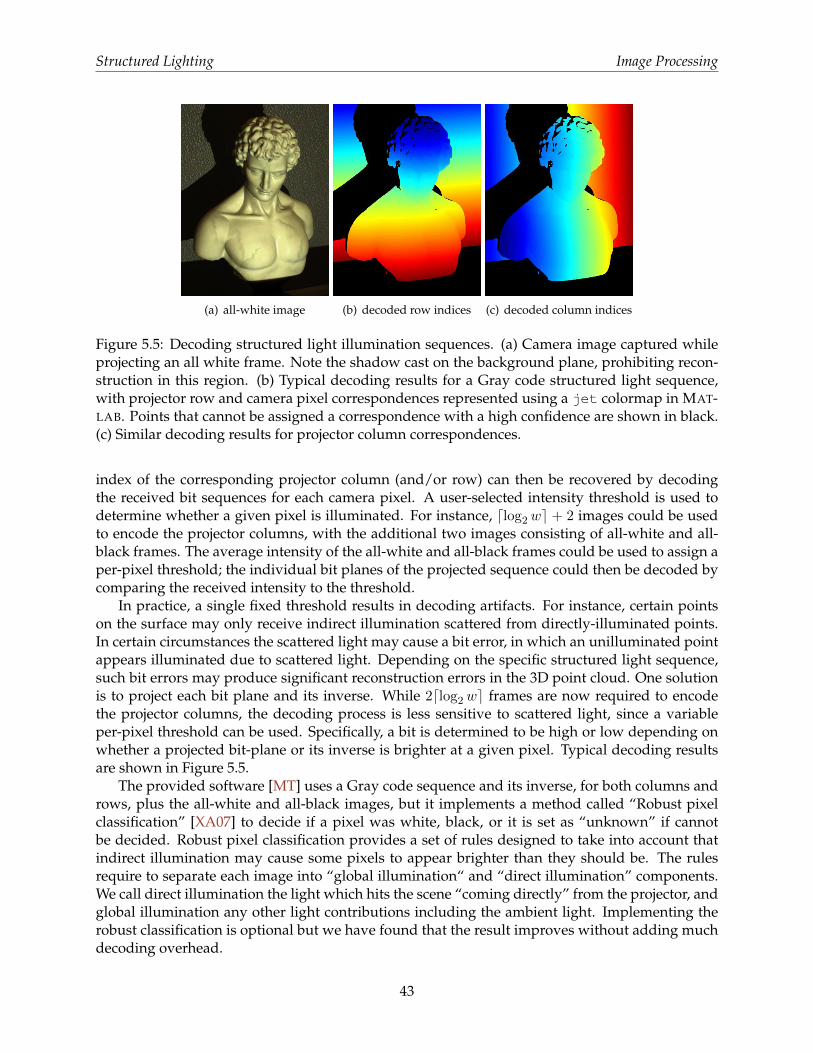
Structured Lighting Image Processing

(a) all-white image (b) decoded row indices (c) decoded column indices

Figure 5.5: Decoding structured light illumination sequences. (a) Camera image captured whileprojecting an all white frame. Note the shadow cast on the background plane, prohibiting recon-struction in this region. (b) Typical decoding results for a Gray code structured light sequence,with projector row and camera pixel correspondences represented using a jet colormap in MAT-LAB. Points that cannot be assigned a correspondence with a high confidence are shown in black.(c) Similar decoding results for projector column correspondences.

index of the corresponding projector column (and/or row) can then be recovered by decodingthe received bit sequences for each camera pixel. A user-selected intensity threshold is used todetermine whether a given pixel is illuminated. For instance, dlog2we + 2 images could be usedto encode the projector columns, with the additional two images consisting of all-white and all-black frames. The average intensity of the all-white and all-black frames could be used to assign aper-pixel threshold; the individual bit planes of the projected sequence could then be decoded bycomparing the received intensity to the threshold.

In practice, a single fixed threshold results in decoding artifacts. For instance, certain pointson the surface may only receive indirect illumination scattered from directly-illuminated points.In certain circumstances the scattered light may cause a bit error, in which an unilluminated pointappears illuminated due to scattered light. Depending on the specific structured light sequence,such bit errors may produce significant reconstruction errors in the 3D point cloud. One solutionis to project each bit plane and its inverse. While 2dlog2we frames are now required to encodethe projector columns, the decoding process is less sensitive to scattered light, since a variableper-pixel threshold can be used. Specifically, a bit is determined to be high or low depending onwhether a projected bit-plane or its inverse is brighter at a given pixel. Typical decoding resultsare shown in Figure 5.5.

The provided software [MT] uses a Gray code sequence and its inverse, for both columns androws, plus the all-white and all-black images, but it implements a method called “Robust pixelclassification” [XA07] to decide if a pixel was white, black, or it is set as “unknown” if cannotbe decided. Robust pixel classification provides a set of rules designed to take into account thatindirect illumination may cause some pixels to appear brighter than they should be. The rulesrequire to separate each image into “global illumination“ and “direct illumination” components.We call direct illumination the light which hits the scene “coming directly” from the projector, andglobal illumination any other light contributions including the ambient light. Implementing therobust classification is optional but we have found that the result improves without adding muchdecoding overhead.

43

Structured Lighting Calibration

As with any communication system, the design of structured light sequences must accountfor anticipated artifacts introduced by the communication channel. In a typical projector-camerasystem decoding artifacts are introduced from a wide variety of sources, including projector orcamera defocus, scattering of light from the surface, and temporal variation in the scene (e.g.,varying ambient illumination or a moving object). We have provided a variety of data sets fortesting your decoding algorithms. In particular, the man sequence has been captured using bothbinary and Gray code structured light sequences. Furthermore, both codes have been appliedwhen the projector is focused and defocused at the average depth of the sculpture. We encour-age the reader to study the decoding artifacts produced under these non-ideal, yet commonlyencountered, circumstances.

5.3 Calibration

The structured light scanner uses the triangulation principle to reconstruct the scanned model.In order to map pixel positions to world rays the system must be calibrated. In our case, weneed to find the intrinsic parameters of the camera and projector, and the relative rotation andtranslation between them. If a turntable is used, the world coordinate system must be placed atits center of rotation as in the previous chapter, which has to be calibrated, and the rotation andtranslation from world coordinates to camera coordinates must be found. Without a turntable,the world coordinate system may be placed at the camera (or projector) center and with the sameorientation. We will use the Projector-Camera Calibration software [MT] to calibrate everythingbut the turntable, which must be calibrated as in Section 4.2.

5.4 Reconstruction

The decoded set of camera and projector correspondences can be used to reconstruct a 3D pointcloud. Several reconstruction schemes can be implemented using the sample sequences. Theprojector column correspondences can be used to reconstruct a point cloud using ray-plane tri-angulation. A second point cloud can be reconstructed using the projector row correspondences.Finally, the projector pixel to camera pixel correspondences can be used to reconstruct the pointcloud using ray-ray triangulation (i.e., by finding the closest point to the optical rays defined bythe projector and camera pixels). A simple per-point RGB color can be assigned by sampling thecolor of the all-white camera image for each 3D point. Reconstruction artifacts can be further re-duced by comparing the reconstruction produced by each of these schemes. Typical results areshown in Figures 5.6–5.9.

The provided software implements ray-ray triangulation between camera and projector pixels,using the approximate intersection from Section 2.3.2. In order to remove errors, the minimumdistance between rays is also computed and compared with a user-set threshold, a small distanceis considered as intersection and a 3D point is created, otherwise the point is ignored. As usual,if the dimensions of the scanning volume is available, or can be roughly estimated, only pointswithin the volume must be added to the model.

44

Structured Lighting Sample software

Figure 5.6: Reconstruction of the chiquita Gray code sequence.

Figure 5.7: Reconstruction of the schooner Gray code sequence.

Figure 5.8: Reconstruction of the urn Gray code sequence.

Figure 5.9: Reconstruction of the drummer Gray code sequence.

5.5 Sample software

The structured light scanner produces a colored 3D point cloud. Only points that are both im-aged by a camera and illuminated by the projector can be reconstructed. As a result, a complete3D model of an object would typically require merging multiple scans obtained by moving thescanning apparatus or object (e.g., by using a turntable). These issues are considered in Chapter 6.

45

Structured Lighting Sample software

We encourage the reader to implement their own solution so that measurements from multiplecameras, projectors, and 3D point clouds can be merged. As a reference the Projector-CameraCalibration software described Chapter 3 implements both the calibration and scanning using astructured light system.

Data acquisition for scanning is identical as how the calibration sequences were collected. A re-construction for each individual sequence is performed by highlighting the sequence folder namein the list on the left part of the main screen and clicking “Reconstruct”. Once the reconstructionis complete a file save dialog will open asking a pointcloud file name. At the time of writing, thesoftware does not include a visualization of the result but the generated file can be opened usinga standard 3D viewer (e.g. Meshlab [mes]). The software can reconstruct as many scans of an ob-ject as required but it will not merge them into a single model, each reconstruction will be storedas a separate pointcloud and must be merged using a separate software. Optionally, the surfacenormal at each point is estimated and added to the output creating an “oriented pointcloud” in-stead. Normals are useful to create more interesting visualizations and they are usually requiredby surface reconstruction tools.

(a) Software main screen (b) 3D model result

Figure 5.10: Scanning example using the Projector-Camera Calibration software.

46

Chapter 6

Surfaces from Point Clouds

The objects scanned in the previous examples are solid, with a well-defined boundary surfaceseparating the inside from the outside. Since computers have a finite amount of memory andoperations need to be completed in a finite number of steps, algorithms can only be designedto manipulate surfaces described by a finite number of parameters. Perhaps the simplest surfacerepresentation with a finite number of parameters is produced by a finite sampling scheme, wherea process systematically chooses a set of points lying on the surface.

The triangulation-based 3D scanners described in previous chapters produce such a finite sam-pling scheme. The so-called point cloud, a dense collection of surface samples, has become a pop-ular representation in computer graphics. However, since point clouds do not constitute surfaces,they cannot be used to determine which 3D points are inside or outside of the solid object. Formany applications, being able to make such a determination is critical. For example, withoutclosed bounded surfaces, volumes cannot be measured. Therefore, it is important to constructso-called watertight surfaces from point clouds. In this chapter we consider these issues.

6.1 Representation and Visualization of Point Clouds

In addition to the 3D point locations, the 3D scanning methods described in previous chapters areoften able to estimate a color per point, as well as a surface normal vector. Some methods are ableto measure both color and surface normal, and some are able to estimate other parameters whichcan be used to describe more complex material properties used to generate complex renderings.In all these cases the data structure used to represent a point cloud in memory is a simple array.A minimum of three values per point are needed to represent the point locations. Colors mayrequire one to three more values per point, and normals vectors three additional values per point.Other properties may require more values, but in general it is the same number of parameters perpoint that need to be stored. If M is the number of parameters per point and N is the number ofpoints, then point cloud can be represented in memory using an array of length NM .

6.1.1 File Formats

Storing and retrieving arrays from files is relatively simple, and storing the raw data either inASCII format or in binary format is a valid solution to the problem. However, these solutions maybe incompatible with many software packages. We want to mention two standards which havesupport for storing point clouds with some auxiliary attributes.

47

Surfaces from Point Clouds Merging Point Clouds

Storing Point Clouds as VRML Files

The Virtual Reality Modeling Language (VRML) is an ISO standard published in 1997. A VRMLfile describes a scene graph comprising a variety of nodes. Among geometry nodes, PointSetand IndexedFaceSet are used to store point clouds. The PointSet node was designed to storepoint clouds, but in addition to the 3D coordinates of each point, only colors can be stored. Noother attributes can be stored in this node. In particular, normal vectors cannot be recorded. Thisis a significant limitation, since normal vectors are important both for rendering point clouds andfor reconstructing watertight surfaces from point clouds.

The IndexedFaceSet node was designed to store polygon meshes with colors, normals,and/or texture coordinates. In addition to vertex coordinates, colors and normal vectors can bestored bound to vertices. Even though the IndexedFaceSet node was not designed to representpoint clouds, the standard allows for this node to have vertex coordinates and properties such ascolors and/or normals per vertex, but no faces. The standard does not specify how such a nodeshould be rendered in a VRML browser, but since they constitute valid VRML files, they can beused to store point clouds.

The SFL File Format

The SFL file format was introduced with Pointshop3D [ZPKG02] to provide a versatile file formatto import and export point clouds with color, normal vectors, and a radius per vertex describingthe local sampling density. A SFL file is encoded in binary and features an extensible set of surfelattributes, data compression, upward and downward compatibility, and transparent conversionof surfel attributes, coordinate systems, and color spaces. Pointshop3D is a software system for in-teractive editing of point-based surfaces, developed at the Computer Graphics Lab at ETH Zurich.

6.1.2 Visualization

A well-established technique to render dense point clouds is point splatting. Each point is re-garded as an oriented disk in 3D, with the orientation determined by the surface normal evaluatedat each point, and the radius of the disk usually stored as an additional parameter per vertex. Asa result, each point is rendered as an ellipse. The color is determined by the color stored with thepoint, the direction of the normal vector, and the illumination model. The radii are chosen so thatthe ellipses overlap, resulting in the perception of a continuous surface being rendered.

6.2 Merging Point Clouds

The triangulation-based 3D scanning methods described in previous chapters are able to producedense point clouds. However, due to visibility constraints these point clouds may have large gapswithout samples. In order for a surface point to be reconstructed, it has to be illuminated bya projector, and visible by a camera. In addition, the projected patterns needs to illuminate thesurface transversely for the camera to be able to capture a sufficient amount of reflected light. Inparticular, only points on the front-facing side of the object can be reconstructed (i.e., on the sameside as the projector and camera). Some methods to overcome these limitations are discussed inChapter 7. However, to produce a complete representation, multiple scans taken from variouspoints of view must be integrated to produce a point cloud with sufficient sampling density overthe whole visible surface of the object being scanned.

48


6.2.1 Computing Rigid Body Matching Transformations

The main challenge to merging multiple scans is that each scan is produced with respect to adifferent coordinate system. As a result, the rigid body transformation needed to register onescan with another must be estimated. In some cases the object is moved with respect to the scan-ner under computer control. In those cases the transformations needed to register the scans areknown within a certain level of accuracy. This is the case when the object is placed on a computer-controlled turntable or linear translation stage. However, when the object is repositioned by hand,the matching transformations are not known and need to be estimated from point correspon-dences.

We now consider the problem of computing the rigid body transformation q = Rp+T to aligntwo shapes from two sets of N points, {p1, . . . , pN} and {q1, . . . , qN}. That is, we are looking for arotation matrix R and a translation vector T so that

q1 = Rp1 + T . . . qN = RpN + T .

The two sets of points can be chosen interactively or automatically. In either case, being able tocompute the matching transformation in closed form is a fundamental operation.

This registration problem is, in general, not solvable due to measurement errors. A commonapproach in such a case is to seek a least-squares solution. In this case, we desire a closed-formsolution for minimizing the mean squared error

φ(R, T ) =1

N

N∑i=1

‖Rpi + T − qi‖2 , (6.1)

over all rotation matrices R and translation vectors T . This yields a quadratic function of 12components in R and T ; however, since R is restricted to be a valid rotation matrix, there exist ad-ditional constraints on R. Since the variable T is unconstrained, a closed-form solution for T , as afunction ofR, can be found by solving the linear system of equations resulting from differentiatingthe previous expression with respect to T .

1

2

∂φ

∂T=

1

N

N∑i=1

(Rpi + T − qi) = 0⇒ T = q −Rp

In this expression p and q are the geometric centroids of the two sets of matching points, given by

p =

(1

N

N∑i=1

pi

)q =

(1

N

N∑i=1

qi

).

Substituting for T in Equation 6.1, we obtain the following equivalent error function which de-pends only on R.

ψ(R) =1

N

N∑i=1

‖R(pi − p)− (qi − q)‖2 (6.2)

If we expand this expression we obtain

ψ(R) =1

N

N∑i=1

‖pi − p‖2 −2

N

N∑i=1

(qi − q)tR(pi − p) +1

N

N∑i=1

‖qi − q‖2 ,

49


since ‖Rv‖2 = ‖v‖2 for any vector v. As the first and last terms do not depend on R, maximizingthis expression is equivalent to maximizing

η(R) =1

N

N∑i=1

(qi − q)tR(pi − p) = trace(RM) ,

where M is the 3× 3 matrix

M =1

N

N∑i=1

(pi − p)(qi − q)t .

Recall that, for any pair of matricesA andB of the same dimensions, trace(AtB) = trace(BAt). Wenow consider the singular value decomposition (SVD)M = U∆V t, where U and V are orthogonal3× 3 matrices, and ∆ is a diagonal 3× 3 matrix with elements δ1 ≥ δ2 ≥ δ3 ≥ 0. Substituting, wefind

trace(RM) = trace(RU∆V t) = trace((V tRU)∆) = trace(W∆) ,

where W = V tRU is orthogonal. If we expand this expression, we obtain

trace(W∆) = w11δ1 + w22δ2 + w33δ3 ≤ δ1 + δ2 + δ3 ,

where W = (wij). The last inequality is true because the components of an orthogonal matrixcannot be larger than one. Note that the last inequality is an equality only if w11 = w22 = w33 = 1,which is only the case whenW = I (the identity matrix). It follows that if V tU is a rotation matrix,then R = V tU is the minimizer of our original problem. The matrix V tU is an orthogonal matrix,but it may not have a negative determinant. In that case, an upper bound for trace(W∆), with Wrestricted to have a negative determinant, is achieved for W = J , where

J =

1 0 00 1 00 0 −1

.

In this case it follows that the solution to our problem is R = V tJU .

6.2.2 The Iterative Closest Point (ICP) Algorithm

The Iterative Closest Point (ICP) is an algorithm employed to match two surface representations,such as points clouds or polygon meshes. This matching algorithm is used to reconstruct 3Dsurfaces by registering and merging multiple scans. The algorithm is straightforward and canbe implemented in real-time. ICP iteratively estimates the transformation (i.e., translation androtation) between two geometric data sets. The algorithm takes as input two data sets, an initialestimate for the transformation, and an additional criterion for stopping the iterations. The outputis an improved estimate of the matching transformation. The algorithm comprises the followingsteps.

1. Select points from the first shape.

2. Associate points, by nearest neighbor, with those in the second shape.

3. Estimate the closed-form matching transformation using the method derived in the previoussection.

50

Surfaces from Point Clouds Surface Reconstruction from Point Clouds

4. Transform the points using the estimated parameters.

5. Repeat previous steps until the stopping criterion is met.

The algorithm can be generalized to solve the problem of registering multiple scans. Each scan hasan associated rigid body transformation which will register it with respect to the rest of the scans,regarded as a single rigid object. An additional external loop must be added to the previous stepsto pick one transformation to be optimized with each pass, while the others are kept constant—either going through each of the scans in sequence, or randomizing the choice.

6.3 Surface Reconstruction from Point Clouds

Watertight surfaces partition space into two disconnected regions so that every line segment join-ing a point in one region to a point in the other must cross the dividing surface. In this section wediscuss methods to reconstruct watertight surfaces from point clouds.

6.3.1 Continuous Surfaces

In mathematics surfaces are represented in parametric or implicit form. A parametric surfaceS = {x(u) : u ∈ U} is defined by a function x : U → IR3 on an open subset U of the plane.An implicit surface is defined as a level set S = {p ∈ IR3 : f(p) = λ} of a continuous functionf : V → IR, where V is an open subset in 3D. These functions are most often smooth or piecewisesmooth. Implicit surfaces are called watertight because they partition space into the two discon-nected sets of points, one where f(p) > λ and a second where f(p) < λ. Since the function f iscontinuous, every line segment joining a point in one region to a point in the other must cross thedividing surface. When the boundary surface of a solid object is described by an implicit equa-tion, one of these two sets describes the inside of the object, and the other one the outside. Sincethe implicit function can be evaluated at any point in 3D space, it is also referred to as a scalarfield. On the other hand, parametric surfaces may or may not be watertight. In general, it is diffi-cult to determine whether a parametric surface is watertight or not. In addition, implicit surfacesare preferred in many applications, such as reverse engineering and interactive shape design, be-cause they bound a solid object which can be manufactured; for example, using rapid prototypingtechnologies or numerically-controlled machine tools, such representations can define objects ofarbitrary topology. As a result, we focus our remaining discussion on implicit surfaces.

6.3.2 Discrete Surfaces

A discrete surface is defined by a finite number of parameters. We only consider here polygonmeshes, and in particular those polygon meshes representable as IndexedFaceSet nodes inVRML files. Polygon meshes are composed of geometry and topological connectivity. The geome-try includes vertex coordinates, normal vectors, and colors (and possibly texture coordinates). Theconnectivity is represented in various ways. A popular representation used in many isosurface al-gorithms is the polygon soup, where polygon faces are represented as loops of vertex coordinatevectors. If two or more faces share a vertex, the vertex coordinates are repeated as many times asneeded. Another popular representation used in isosurface algorithms is the IndexedFaceSet(IFS), describing polygon meshes with simply-connected faces. In this representation the geome-try is stored as arrays of floating point numbers. In these notes we are primarily concerned withthe array coord of vertex coordinates, and to a lesser degree with the array normal of face nor-mals. The connectivity is described by the total number V of vertices, and F faces, which are

51


stored in the coordIndex array as a sequence of loops of vertex indices, demarcated by values of−1.

6.3.3 Isosurfaces

An isosurface is a polygonal mesh surface representation produced by an isosurface algorithm.An isosurface algorithm constructs a polygonal mesh approximation of a smooth implicit sur-face S = {x : f(x) = 0} within a bounded three-dimensional volume, from samples of a defin-ing function f(x) evaluated on the vertices of a volumetric grid. Marching Cubes [LC87] andrelated algorithms operate on function values provided at the vertices of hexahedral grids. An-other family of isosurface algorithms operate on functions evaluated at the vertices of tetrahedralgrids [DK91]. Usually, no additional information about the function is provided, and various in-terpolation schemes are used to evaluate the function within grid cells, if necessary. The mostnatural interpolation scheme for tetrahedral meshes is linear interpolation, which we also adopthere.

6.3.4 Isosurface Construction Algorithms

An isosurface algorithm producing a polygon soup output must solve three key problems: (1)determining the quantity and location of isosurface vertices within each cell, (2) determining howthese vertices are connected forming isosurface faces, and (3) determining globally consistent faceorientations. For isosurface algorithms producing IFS output, there is a fourth problem to solve:identifying isosurface vertices lying on vertices and edges of the volumetric grid. For many vi-sualization applications, the polygon soup representation is sufficient and acceptable, despite thestorage overhead. Isosurface vertices lying on vertices and edges of the volumetric grid are in-dependently generated multiple times. The main advantage of this approach is that it is highlyparallelizable. But, since most of these boundary vertices are represented at least twice, it is not acompact representation.

Researchers have proposed various solutions and design decisions (e.g., cell types, adaptivegrids, topological complexity, interpolant order) to address these four problems. The well-knownMarching Cubes (MC) algorithm uses a fixed hexahedral grid (i.e., cube cells) with linear interpo-lation to find zero-crossings along the edges of the grid. These are the vertices of the isosurfacemesh. Second, polygonal faces are added connecting these vertices using a table. The crucial ob-servation made with MC is that the possible connectivity of triangles in a cell can be computedindependently of the function samples and stored in a table. Out-of-core extensions, where se-quential layers of the volume are processed one at a time, are straightforward.

Similar tetrahedral-based algorithms [DK91, GH95, TPG99], dubbed Marching Tetrahedra (MT),have also been developed (again using linear interpolation). Although the cell is simpler, MT re-quires maintaining a tetrahedral sampling grid. Out-of-core extensions require presorted traversalschemes, such as in [CS97]. For an unsorted tetrahedral grid, hash tables are used to save and re-trieve vertices lying on edges of the volumetric grid. As an example of an isosurface algorithm,we discuss MT in more detail.

Marching Tetrahedra

MT operates on the following input data: (1) a tetrahedral grid and (2) one piecewise linearfunction f(x), defined by its values at the grid vertices. Within the tetrahedron with vertices

52


Figure 6.1: In isosurface algorithms, the sign of the function at the grid vertices determines thetopology and connectivity of the output polygonal mesh within each tetrahedron. Mesh verticesare located on grid edges where the function changes sign.

x0, x1, x2, x3 ∈ IR3, the function is linear and can be described in terms of the barycentric coordi-nates b = (b0, b1, b2, b3)

t of an arbitrary internal point x = b0 x0 + b1 x1 + b2 x2 + b3 x3 with respectto the four vertices: f(x) = b0 f(x0) + b1 f(x1) + b2 f(x2) + b3 f(x3), where b0, b1, b2, b3 ≥ 0 andb0 + b1 + b2 + b3 = 1. As illustrated in Figure 6.1, the sign of the function at the four grid verticesdetermines the connectivity (e.g., triangle, quadrilateral, or empty) of the output polygonal meshwithin each tetrahedron. There are actually 16 = 24 cases, which modulo symmetries and signchanges reduce to only three. Each grid edge, whose end vertex values change sign, correspondsto an isosurface mesh vertex. The exact location of the vertex along the edge is determined by lin-ear interpolation from the actual function values, but note that the 16 cases can be precomputedand stored in a table indexed by a 4-bit integer i = (i3i2i1i0), where ij = 1 if f(xj) > 0 and ij = 0,if f(xj) < 0. The full table is shown in Table 6.1. The cases f(xj) = 0 are singular and require spe-cial treatment. For example, the index is i = (0100) = 4 for Figure 6.1(a), and i = (1100) = 12 forFigure 6.1(b). Orientation for the isosurface faces, consistent with the orientation of the contain-ing tetrahedron, can be obtained from connectivity alone (and are encoded in the look-up table asshown in Table 6.1). For IFS output it is also necessary to stitch vertices as described above.

Algorithms to polygonize implicit surfaces [Blo88], where the implicit functions are providedin analytic form, are closely related to isosurface algorithms. For example, Bloomenthal and Fergu-son [BF95] extract non-manifold isosurfaces produced from trimming implicits and parametericsusing a tetrahedral isosurface algorithm. [WvO96] polygonize boolean combinations of skeletalimplicits (Boolean Compound Soft Objects), applying an iterative solver and face subdivision forplacing vertices along feature edges and points. Suffern and Balsys [SB03] present an algorithmto polygonize surfaces defined by two implicit functions provided in analytic form; this samealgorithm can compute bi-iso-lines of pairs of implicits for rendering.

Isosurface Algorithms on Hexahedral Grids

An isosurface algorithm constructs a polygon mesh approximation of a level set of a scalar func-tion defined in a finite 3D volume. The function f(p) is usually specified by its values fα = f(pα)

53


i (i3i2i1i0) face0 0000 [-1]1 0001 [2,1,0,-1]2 0010 [0,3,4,-1]3 0011 [1,3,4,2,-1]4 0100 [1,5,3,-1]5 0101 [0,2,5,3,-1]6 0110 [0,3,5,4,-1]7 0111 [1,5,2,-1]8 1000 [2,5,1,-1]9 1001 [4,5,3,0,-1]

10 1010 [3,5,2,0,-1]11 1011 [3,5,1,-1]12 1100 [2,4,3,1,-1]13 1101 [4,3,0,-1]14 1110 [0,1,2,-1]15 1111 [-1]

e edge0 (0,1)1 (0,2)2 (0,3)3 (1,2)4 (1,3)5 (2,3)

Table 6.1: Look-up tables for tetrahedral mesh isosurface evaluation. Note that consistent faceorientation is encoded within the table. Indices stored in the first table reference tetrahedronedges, as indicated by the second table of vertex pairs (and further illustrated in Figure 6.1). Inthis case, only edge indices {1, 2, 3, 4} have associated isosurface vertex coordinates, which areshared with neighboring cells.

on a regular grid of three dimensional points

G = {pα : α = (α0, α1, α2) ∈ [[n0]]×[[n1]]×[[n2]]} ,

where [[nj ]] = {0, . . . , nj − 1}, and by a method to interpolate in between these values. The surfaceis usually represented as a polygon mesh, and is specified by its isovalue f0. Furthermore, theinterpolation scheme is assumed to be linear along the edges of the grid, so that the isosurfacecuts each edge in no more than one point. If pα and pβ are grid points connected by an edge, andfα > f0 > fβ , the location of the point pαβ where the isosurface intersects the edge is

pαβ =fα − f0fα − fβ

pβ +fβ − f0fβ − fα

pα . (6.3)

Marching Cubes

One of the most popular isosurface extraction algorithms is Marching Cubes [LC87]. In this algo-rithm the points defined by the intersection of the isosurface with the edges of the grid are thevertices of the polygon mesh. These vertices are connected forming polygon faces according tothe following procedure. Each set of eight neighboring grid points define a small cube called a cell

Cα = {pα+β : β ∈ {0, 1}3}.

Since the function value associated with each of the eight corners of a cell may be either aboveor below the isovalue (isovalues equal to grid function values are called singular and should beavoided), there are 28 = 256 possible configurations. A polygonization of the vertices within eachcell, for each one of these configurations, is stored in a static look-up table. When symmetries aretaken into account, the size of the table can be reduced significantly.

54


6.3.5 Algorithms to Fit Implicit Surfaces to Point Clouds

Let U be a relatively open and simply-connected subset of IR3, and f : U → IR a smooth function.The gradient ∇f is a vector field defined on U . Given an oriented point cloud, i.e., a finite set Dof point-vector pairs (p, n), where p is an interior point of U , and n is a unit length 3D vector, theproblem is to find a smooth function f so that f(p) ≈ 0 and ∇(p) ≈ n for every oriented point(p, n) in the data set D. We call the zero iso-level set of such a function {p : f(p) = 0} a surface fit,or surface reconstruction, for the data set D.

We are particularly interested in fitting isosurfaces to oriented point points. For the sake ofsimplicity, we assume that the domain is the unit cube U = [0, 1]3, the typical domain of an iso-surface defined on an hexahedral mesh, and the isolevel is zero, i.e., the isosurface to be fitted tothe data points is {p : f(p) = 0}, but of course, the argument applies in more general cases.

Figure 6.2: Early results of Vector Field Isosurface reconstruction from oriented point clouds introducedin [ST05].

Figure 6.2 shows results of surface reconstruction from an oriented point cloud using the sim-ple variational formulation presented in [ST05], where oriented data points are regarded as sam-ples of the gradient vector field of an implicit function, which is estimated by minimizing thisenergy function

E1(f) =m∑i=1

f(pi)2 + λ1

m∑i=1

‖∇f(pi)− ni‖2 + λ2

∫V‖Hf(x)‖2 dx , (6.4)

where f(x) is the implicit function being estimated, ∇f(x) is the gradient of f , Hf(x) is the Hes-sian of f(x), (p1, n1), . . . , (pm, nm) are point-normal data pairs, V is a bounding volume, and λ1and λ2 are regularization parameters. Minimizing this energy requires the solution of a simplelarge and sparse least squares problem. The result is usually unique modulo an additive con-stant. Given that, for rendering or post-processing, isosurfaces are extracted from scalar functionsdefined over regular grids (e.g., via Marching Cubes), it is worth exploring representations of im-plicit functions defined as a regular scalar fields. Finite difference discretization is used in [ST05],with the volume integral resulting in a sum of gradient differences over the edges of the regulargrid, yet Equation 6.4 can be discretized in many other ways.

55

Chapter 7

Conclusion

As low-cost mobile projectors enter the market, we expect students and hobbyists to begin incor-porating them into their own 3D scanning systems. Such projector-camera systems have alreadyreceived a great deal of attention in recent academic publications. Whether for novel human-computer interaction or ad-hoc tiled displays, consumer digital projection is set to revolutionizethe way we interact with both physical and virtual assets.

This course was designed to lower the barrier of entry to novices interested in trying 3D scan-ning in their own projects. Through the course notes, on-line materials, and open source software,we have endeavored to eliminate the most difficult hurdles facing beginners. We encourage atten-dees to email the authors with questions or links to their own 3D scanning projects that draw onthe course material. Revised course notes, updated software, recent publications, and similar do-it-yourself projects are maintained on the course website at http://mesh.brown.edu/byo3d.We encourage you to take a look and see what your fellow attendees have built for themselves!

56

http://mesh.brown.edu/byo3d

Bibliography

[ Na13] NATIONAL INSTRUMENTS CORP.: Choosing the Right Camera Bus, http://www.ni.com/white-paper/5386/en/. Tech. rep., 2013. 20

[AHH10] ATCHESON B., HEIDE F., HEIDRICH W.: CALTag: High precision fiducial markers forcamera calibration. In 15th International Workshop on Vision, Modeling and Visualization(Siegen, Germany, Nov. 2010). 22, 29

[BF95] BLOOMENTHAL J., FERGUSON K.: Polygonization of non-manifold implicit surfaces.In SIGGRAPH ’95: ACM SIGGRAPH 1995 papers (1995), pp. 309–316. 53

[Bla04] BLAIS F.: Review of 20 years of range sensor development. Journal of Electronic Imaging13, 1 (2004), 231–240. 3

[Blo88] BLOOMENTHAL J.: Polygonization of Implicit Surfaces. Computer Aided GeometricDesign 5, 4 (1988), 341–355. 53

[Bou] BOUGUET J.-Y.: Camera calibration toolbox for matlab. http://www.vision.caltech.edu/bouguetj/calib_doc/. 25

[CG00] CIPOLLA R., GIBLIN P.: Visual Motion of Curves and Surfaces. Cambridge UniversityPress, 2000. 3

[CMU] CMU IEEE 1394 digital camera driver, version 6.4.5.http://www.cs.cmu.edu/ iwan/1394/. 20

[Cre] CREAFORM: Handyscan 3D. http://www.creaform3d.com/en/handyscan3d/products/exascan.aspx. 4

[CS97] CHIANG Y., SILVA C. T.: I/O Optimal Isosurface Extraction. In IEEE Visualization 1997,Conference Proceedings (1997), pp. 293–300. 52

[CTMS03] CARRANZA J., THEOBALT C., MAGNOR M. A., SEIDEL H.-P.: Free-viewpoint videoof human actors. ACM Trans. Graph. 22, 3 (2003), 569–577. 3

[dAST∗08] DE AGUIAR E., STOLL C., THEOBALT C., AHMED N., SEIDEL H.-P., THRUN S.: Per-formance capture from sparse multi-view video. In SIGGRAPH ’08: ACM SIGGRAPH2008 papers (2008), pp. 1–10. 3

[Deb97] DEBEVEC P. E.: Facade: modeling and rendering architecture from photographs andthe campanile model. In SIGGRAPH ’97: ACM SIGGRAPH 97 Visual Proceedings (1997),p. 254. 3

57

http://www.ni.com/white-paper/5386/en/

http://www.ni.com/white-paper/5386/en/



http://www.creaform3d.com/en/handyscan3d/products/exascan.aspx

http://www.creaform3d.com/en/handyscan3d/products/exascan.aspx

Bibliography

[DK91] DOI A., KOIDE A.: An Efficient Method of Triangulating Equivalued Surfaces by Us-ing Tetrahedral Cells. IEICE Transactions on Communications and Electronics InformationSystems E74, 1 (Jan. 1991), 214–224. 52

[Far97] FARID H.: Range Estimation by Optical Differentiation. PhD thesis, University of Penn-sylvania, 1997. 3

[FWM98] FERRYMAN J. M., WORRALL A. D., MAYBANK S. J.: Learning enhanced 3d modelsfor vehicle tracking. In BMVC (1998), pp. 873–882. 3

[GH95] GUEZIEC A., HUMMEL R.: Exploiting Triangulated Surface Extraction Using Tetra-hedral Decomposition. IEEE Transactions on Visualization and Computer Graphics 1, 4(1995). 52

[GSP06] GREENGARD A., SCHECHNER Y. Y., PIESTUN R.: Depth from diffracted rotation. Opt.Lett. 31, 2 (2006), 181–183. 3

[HARN06] HSU S., ACHARYA S., RAFII A., NEW R.: Performance of a time-of-flight range cam-era for intelligent vehicle safety applications. Advanced Microsystems for AutomotiveApplications (2006). 5

[Hec01] HECHT E.: Optics (4th Edition). Addison Wesley, 2001. 3

[HVB∗07] HERNANDEZ C., VOGIATZIS G., BROSTOW G. J., STENGER B., CIPOLLA R.: Non-rigid photometric stereo with colored lights. In Proc. of the 11th IEEE Intl. Conf. onComp. Vision (ICCV) (2007). 5

[HZ04] HARTLEY R. I., ZISSERMAN A.: Multiple View Geometry in Computer Vision, second ed.Cambridge University Press, 2004. 2, 21

[ISM84] INOKUCHI S., SATO K., MATSUDA F.: Range imaging system for 3-d object recogni-tion. In Proceedings of the International Conference on Pattern Recognition (1984), pp. 806–808. 41

[IY01] IDDAN G. J., YAHAV G.: Three-dimensional imaging in the studio and elsewhere.Three-Dimensional Image Capture and Applications IV 4298, 1 (2001), 48–55. 5

[KM00] KAKADIARIS I., METAXAS D.: Model-based estimation of 3d human motion. IEEETransactions on Pattern Analysis and Machine Intelligence 22, 12 (2000), 1453–1459. 3

[Las] LASER DESIGN INC.: Surveyor DT-2000 desktop 3D laser scanner. http://www.laserdesign.com/quick-attachments/hardware/low-res/dt-series.pdf. 4

[Lau94] LAURENTINI A.: The Visual Hull Concept for Silhouette-Based Image Understanding.IEEE TPAMI 16, 2 (1994), 150–162. 3

[LC87] LORENSEN W. L., CLINE H. E.: Marching Cubes: A High Resolution 3D Surface Con-struction Algorithm. In Siggraph’87, Conference Proceedings (1987), ACM Press, pp. 163–169. 52, 54

[LFDF07] LEVIN A., FERGUS R., DURAND F., FREEMAN W. T.: Image and depth from a conven-tional camera with a coded aperture. ACM Trans. Graph. 26, 3 (2007), 70. 3

58

http://www.laserdesign.com/quick-attachments/hardware/low-res/dt-series.pdf



Bibliography

[LHKP13] LI B., HENG L., KOSER K., POLLEFEYS M.: A multiple-camera system calibrationtoolbox using a feature descriptor-based calibration pattern. In Intelligent Robots andSystems (IROS), 2013 IEEE/RSJ International Conference on (2013), IEEE, pp. 1301–1307.22

[LN04] LAND M. F., NILSSON D.-E.: Animal Eyes. Oxford University Press, 2004. 2

[Mat] MATHWORKS, INC: Image acquisition toolbox. http://www.mathworks.com/products/imaq/. 20

[MBR∗00] MATUSIK W., BUEHLER C., RASKAR R., GORTLER S. J., MCMILLAN L.: Image-basedvisual hulls. In SIGGRAPH ’00: ACM SIGGRAPH 2000 papers (2000), pp. 369–374. 3

[mes] Meshlab 3D viewer. http://meshlab.sourceforge.net/. 46

[MPL04] MARC R. Y., POLLEFEYS M., LI S.: Improved real-time stereo on commodity graphicshardware. In In IEEE Workshop on Real-time 3D Sensors and Their Use (2004). 2

[MSKS05] MA Y., SOATTO S., KOSECKA J., SASTRY S. S.: An Invitation to 3-D Vision. Springer,2005. 21

[MT] MORENO D., TAUBIN G.: Projector-Camera Calibration and Scanning Software.http://mesh.brown.edu/scanning/software.html. 25, 43, 44

[MT12] MORENO D., TAUBIN G.: Simple, accurate, and robust projector-camera calibration.In 3D Imaging, Modeling, Processing, Visualization and Transmission (3DIMPVT), 2012Second International Conference on (2012), IEEE, pp. 464–471. 19, 24

[Nex] NEXTENGINE: 3D Scanner HD. https://www.nextengine.com/indexSecure.htm. 4

[NN94] NAYAR S. K., NAKAGAWA Y.: Shape from focus. IEEE Trans. Pattern Anal. Mach. Intell.16, 8 (1994), 824–831. 3

[Ope] Open source computer vision library. http://opencv.org. 20

[OSS∗00] ORMONEIT D., SIDENBLADH H., SIDENBLADH H., BLACK M. J., HASTIE T., FLEET

D. J.: Learning and tracking human motion using functional analysis. In IEEE Work-shop on Human Modeling, Analysis and Synthesis (2000), pp. 2–9. 3

[PA82] POSDAMER J., ALTSCHULER M.: Surface measurement by space encoded projectedbeam systems. Computer Graphics and Image Processing 18 (1982), 1–17. 41

[Poi] POINT GREY RESEARCH, INC.: Grasshopper IEEE-1394b digital camera. http://www.ptgrey.com/products/grasshopper/index.asp. 20

[Pol] POLHEMUS: FastSCAN. http://www.polhemus.com/?page=Scanning_Fastscan. 4

[RWLB01] RASKAR R., WELCH G., LOW K.-L., BANDYOPADHYAY D.: Shader lamps: Animat-ing real objects with image-based illumination. In Proceedings of the 12th EurographicsWorkshop on Rendering Techniques (2001), Springer-Verlag, pp. 89–102. 3

59

http://www.mathworks.com/products/imaq/

http://www.mathworks.com/products/imaq/

http://meshlab.sourceforge.net/

http://mesh.brown.edu/scanning/software.html

https://www.nextengine.com/indexSecure.htm

https://www.nextengine.com/indexSecure.htm

http://opencv.org

http://www.ptgrey.com/products/grasshopper/index.asp

http://www.ptgrey.com/products/grasshopper/index.asp

http://www.polhemus.com/?page=Scanning_Fastscan

http://www.polhemus.com/?page=Scanning_Fastscan

Bibliography

[SB03] SUFFERN K. G., BALSYS R. J.: Rendering the intersections of implicit surfaces. IEEEComput. Graph. Appl. 23, 5 (2003), 70–77. 53

[SCD∗06] SEITZ S., CURLESS B., DIEBEL J., SCHARSTEIN D., SZELISKI R.: A comparison andevaluation of multi-view stereo reconstruction algorithms. In CVPR 2006 (2006). 2

[SFPL10] SALVI J., FERNANDEZ S., PRIBANIC T., LLADO X.: A state of the art in structured lightpatterns for surface profilometry. Pattern recognition 43, 8 (2010), 2666–2680. 39

[SH03] STARCK J., HILTON A.: Model-based multiple view reconstruction of people. In Pro-ceedings of the Ninth IEEE International Conference on Computer Vision (2003), p. 915. 3

[Sim] Computer vision platform using python. http://http://simplecv.org/. 20

[SMP05] SVOBODA T., MARTINEC D., PAJDLA T.: A convenient multi-camera self-calibrationfor virtual environments. PRESENCE: Teleoperators and Virtual Environments 14, 4 (Au-gust 2005), 407–422. 22

[SPB04] SALVI J., PAGES J., BATLLE J.: Pattern codification strategies in structured light sys-tems. In Pattern Recognition (April 2004), vol. 37, pp. 827–849. 4

[ST05] SIBLEY P. G., TAUBIN G.: Vectorfield Isosurface-based Reconstruction from Orientedpoints. In SIGGRAPH’05 Sketch (2005). 55

[Sul95] SULLIVAN G.: Model-based vision for traffic scenes using the ground-plane constraint.93–115. 3

[TPG99] TREECE G. M., PRAGER R. W., GEE A. H.: Regularised Marching Tetrahedra: Im-proved Iso-Surface Extraction. Computers and Graphics 23, 4 (1999), 583–598. 52

[VF92] VAILLANT R., FAUGERAS O. D.: Using extremal boundaries for 3-d object modeling.IEEE Trans. Pattern Anal. Mach. Intell. 14, 2 (1992), 157–173. 2

[Wik] WIKIPEDIA: Gray code. http://en.wikipedia.org/wiki/Gray_code. 42

[WN98] WATANABE M., NAYAR S. K.: Rational filters for passive depth from defocus. Int. J.Comput. Vision 27, 3 (1998), 203–225. 3

[Woo89] WOODHAM R. J.: Photometric method for determining surface orientation from mul-tiple images. 513–531. 5

[WvO96] WYVILL B., VAN OVERVELD K.: Polygonization of Implicit Surfaces with ConstructiveSolid Geometry. Journal of Shape Modelling 2, 4 (1996), 257–274. 53

[XA07] XU Y., ALIAGA D. G.: Robust pixel classification for 3d modeling with structuredlight. In Proceedings of Graphics Interface 2007 (2007), ACM, pp. 233–240. 43

[Zha00] ZHANG Z.: A flexible new technique for camera calibration. IEEE Trans. Pattern Anal.Mach. Intell. 22, 11 (2000), 1330–1334. 19, 21

[ZPKG02] ZWICKER M., PAULY M., KNOLL O., GROSS M.: Pointshop 3d: an interactive systemfor point-based surface editing. ACM Trans. Graph. 21, 3 (2002), 322–329. 48

60

http://http://simplecv.org/

http://en.wikipedia.org/wiki/Gray_code

3D scanning for personal 3D printing

Documents

Transcript of 3D scanning for personal 3D printing