symmetryS S

Article

Adaptive Image Matching Using Discrimination ofDeformable Objects

Insu Won 1, Jaehyup Jeong 1, Hunjun Yang 1, Jangwoo Kwon 2,* and Dongseok Jeong 1,*1 Department of Electronic Engineering, Inha University, 22212 Incheon, Korea; is.won@inha.ac.kr (I.W.);

jaehyup@inha.edu (J.J.); pinion@inha.edu (H.Y.)2 Department of Computer Science and Information Engineering, Inha University, 22212 Incheon, Korea* Correspondence: jwkwon@inha.ac.kr (J.K.); dsjeong@inha.ac.kr (D.J.); Tel.: +82-32-860-7443 (J.K.);

+82-32-860-7415 (D.J.)

Academic Editors: Ka Lok Man, Yo-Sub Han and Hai-Ning LiangReceived: 20 April 2016; Accepted: 13 July 2016; Published: 21 July 2016

Abstract: We propose an efficient image-matching method for deformable-object imagematching using discrimination of deformable objects and geometric similarity clustering betweenfeature-matching pairs. A deformable transformation maintains a particular form in the whole image,despite local and irregular deformations. Therefore, the matching information is statistically analyzedto calculate the possibility of deformable transformations, and the images can be identified usingthe proposed method. In addition, a method for matching deformable object images is proposed,which clusters matching pairs with similar types of geometric deformations. Discrimination ofdeformable images showed about 90% accuracy, and the proposed deformable image-matchingmethod showed an average 89% success rate and 91% accuracy with various transformations.Therefore, the proposed method robustly matches images, even with various kinds of deformationthat can occur in them.

Keywords: image matching; discrimination of deformable object; matching-pair clustering

1. Introduction

Computer vision lets a machine or computer see and understand objects, just like humanvision. The purpose of computer vision is to recognize object in an image and/or to understandthe relationships between objects. While recent research has focused on recognition based on bigdata and deep learning (DL) [1], traditional computer vision methods are still widely used in somespecific areas. While DL is not yet used in many applications due to the requirement for highcomputing power and big data, traditional research based on hand-craft techniques, like featuredetection and feature matching, are actively used in various applications, such as machine vision, imagestitching, object tracking, and augmented reality. Image matching is matching similar images or objects,even under geometric transformations, such as translation; optical, scale, and rotation transformations;affine transformations, which are complex transformations; and viewpoint change. The new currentchallenge is image matching of deformable objects [2]. In the real world, deformable objects encompassthe majority of all objects. In particular, research related to fashion items, such as clothes, is conductedbecause of the rapid growth in Internet shopping [3]. However, since deformable-object matching hasa different target than the existing image-matching methods, feature-detection and -matching methodsare not identical. As such, much research has been conducted into achieving both objectives at thesame time, but without substantial results. Since deformable models cannot be defined by a specifictransformation model, there are numerous difficulties in such research. Early deformable matchingmethods were researched for augmented reality, remote exploration, and image registration for medicalimages, and it was not until recently that research on deformable-object matching appeared.

Symmetry 2016, 8, 68; doi:10.3390/sym8070068 www.mdpi.com/journal/symmetry

Symmetry 2016, 8, 68 2 of 18

A good matching algorithm is characterized by robustness, independence, and a fast matchingspeed [4]. Robustness is recognizing that two images are identical if they have exactly the sameobjects in them. However, the algorithm must recognize identical objects even under transformation.Independence is recognizing the differences between two images containing objects that are different.Lastly, fast matching is the property of rapidly determining a match. Without fast matching,an algorithm cannot process many images, and hence, cannot be a good algorithm. The biggestdisadvantage to previous deformable object-matching algorithms is slow matching. Therefore, in thispaper, as a solution to the problems of the aforementioned methods (and by considering thesecharacteristics), we propose an efficient algorithm that operates the same way for both rigid anddeformable objects.

The rest of this paper is composed as follows. Section 2 introduces the existing image-matchingmethods. Section 3 introduces the proposed algorithm, followed by Section 4, where the experimentalresults from image sets with various deformable objects are examined and analyzed. Finally, Section 5evaluates the proposed algorithm, and concludes the paper.

2. Related Works

In this section, we introduce the known feature-matching methods for computer vision.Image-matching methods can be largely classified into matching rigid objects and matching deformableobjects. Rigid object-matching methods mostly consist of those that examine geometric relationshipsbased on feature correspondence, and that show good performance under transformations likeviewpoint change and affine transformation. However, matching performance degrades whendeformable objects are the target. For deformable object-matching, various methods are useddepending on the specific image set. In other words, there is no generalized procedure. Moreover,there is the common problem of generally slow execution time. We introduce three categories ofcommon feature-point matching methods, which are classified in terms of methodology [5].

2.1. Neighborhood-Based Matching

Early researchers used neighbor-pixel information around the points to find featurecorrespondence. Neighborhood-based methods include threshold-based, nearest neighbor (NN),and nearest neighbor distance ratio (NNDR) [6]. In the threshold-based method, if the distancebetween the descriptors is below a predefined threshold value, the features are considered to bematched. The problem in this method is that a single point in the source image may have severalmatched points in the target image. In the NN approach, two points are matched if their descriptor isin the nearest neighborhood and the distance is below a specific threshold. Therefore, the problemwith the threshold-based method is solved. However, this method may result in many false positivesbetween images, known as outliers. This is overcome by random sample consensus (RANSAC),which was proposed by Fischler and Bolles [7]. RANSAC is a good outlier-removal method, and iswidely used for object detection and feature matching.

2.2. Statistical-Based Matching

Logarithmic distance ratio (LDR), proposed by Tsai et al. [8], is a technique for fast imageindexing, which calculates the similarities in feature properties, including scale, orientation andposition, and recognizes similar images based on lower similarity distance. This technique is effectivelyused to rapidly search similar image candidates in large image datasets. Lepsøy et al. proposed thedistance ratio statistic (DISTRAT) method [9], which adopts LDR for image matching. They found thatthe LDR of inlier matching pairs has a specific ratio when LDR is calculated using feature coordinatesonly. Therefore, the final matching decision is based on a statistical analysis whereby the LDR histogramis narrower with more inliers. This method has the advantage of performance equivalent to RANSACwhile having a faster matching speed, and was eventually selected as the standard in Moving PictureExpert Group (MPEG)—Compact Descriptors for Visual Search (CDVS) [10].

Symmetry 2016, 8, 68 3 of 18

2.3. Deformable Object-Based Matching

The aforementioned matching algorithms are optimized for rigid objects. However, mostreal-world objects are deformable. Previously proposed feature-based deformable object-matchingmethods include transformation model-based [11], mesh-based [12], feature clustering [13],and graph-matching [14] methods. Transformation model-based methods require high complexity,because they operate under a pixel-based model. Therefore, feature-based methods that are notpixel-based were proposed. Agglomerative correspondence clustering (ACC), proposed by Cho andLee [15], is a method that calculates the correspondence between each matching pair, and clustersmatching pairs with a similar feature correspondence. ACC defines feature correspondence as thedifference between the points calculated using the homograph model of matching pairs and the pointthat was actually matched. Then, matching pairs with a small difference are considered to have alocally similar homography, and are hierarchically clustered. Unlike previous methods, ACC willcluster matching pairs with a similar homograph by calculating the geometric similarity betweeneach matching pair, rather than classifying matching pairs into inliers and outliers. While ACC hasthe disadvantages of appreciably high complexity and a high false positive rate, it shows the bestperformance when only the true rate is considered. As such, Improved ACC was introduced as anenhanced version of ACC [16].

3. Proposed Algorithm

RANSAC shows robust performance against geometric transformation of rigid objects. However,it does not offer good performance when matching deformable objects. Meanwhile, deformableobject-matching methods generally have high complexity, which presents difficulty in applications thatrequire fast matching. The easiest solution to this issue is to first perform rigid object-matching andmatch the remaining non-matched points using deformable object-matching methods. However,this is an inefficient solution. Therefore, it is more effective to selectively adopt the matchingmethod, as long as it can discriminate deformable objects. As a solution, we propose discrimination ofdeformable transformations based on statistical analysis of matching pairs, and the subsequent use ofthe corresponding matching method. For example, if there are no inliers at all from among numerousmatching pairs, then these are likely to be non-matching pairs. Moreover, even if there are some inliers,they are unlikely to be a match if the inlier ratio is low. Since the inlier ratio is low for deformable objects,it is impossible to obtain good results. This paper proposes discrimination of possible deformableobjects through statistical analysis of such matching information and supervised learning.

Figure 1 shows a diagrammatic representation of the proposed image-matching process.First of all, features are detected from the image, and candidate matching pairs are found.Final matching is examined through geometric verification. The algorithm is an adaptive matchingmethod wherein the possibility of the candidate matching pair being a deformable object is examinedthrough discrimination of the deformable object (using the proposed algorithm) within the candidatematching pairs that do not satisfy geometric verification, Deformable object-matching is onlyperformed on matching pairs that are determined to be deformable objects. If the algorithm cannotdiscriminate the deformable objects well, it is an inefficient algorithm. Therefore, how well thealgorithm discriminates deformable objects significantly affects the overall performance.

Symmetry 2016, 8, 68 4 of 18

Symmetry 2016, 8, 68 4 of 18

Figure 1. Proposed method for image matching using discrimination of deformable object images.

3.1. Feature Detection, and Making a Matched Pair

The proposed method requires feature coordinates and properties for deformable-object

matching. Therefore, a scale-invariant feature transform (SIFT) detector is used, which is a point-

based detector that includes the feature’s coordinates, scale, and dominant orientation [17]. Speeded

up robust features (SURF), maximally stable extremal regions (MSER), and affine detectors, which

have similar properties, can also be used. SIFT is a set of orientation histograms created on a 4 × 4-

pixel neighborhood with eight bins each. The descriptor then becomes a vector of all the values of

these histograms. Since there are 4 × 4 = 16 histograms, each with eight bins, the vector has 128

elements. The features extracted from each image are 𝐹(𝑖) = {𝑐𝑖 , 𝑠𝑖 , 𝑜𝑖 , 𝑑𝑒𝑠𝑐𝑖} (𝑖 = 0~𝑁) where 𝑐𝑖 is

a coordinate, 𝑠𝑖 is the scale, 𝑜𝑖 is the dominant orientation, and 𝑑𝑒𝑠𝑐𝑖 denotes 128-dimensional

descriptors. To form matching pairs, the features detected from each image are compared. The metric

used for the comparison is Euclidean distance, which is given by Equation (1):

𝑑(𝑓𝑅(𝑖), 𝑓𝑄(𝑗)) = √∑(𝑓𝑅(𝑖)𝑘

128

𝑘=1

− 𝑓𝑄(𝑗)𝑘 )2 (1)

which obtains the Euclidean distance between the i-th feature vector of the reference image, 𝑓𝑅(𝑖),

and the j-th feature vector of the query image, 𝑓𝑄(𝑗). The simplest feature matching sets a threshold

(maximum distance) and returns all matches from other images within this threshold. However, the

problem with using a fixed threshold is that it is difficult to set; the useful range of thresholds can

vary greatly as we move to different parts of the feature space [18]. Accordingly, we used NNDR

for feature matching [17] as follows:

𝑁𝑁𝐷𝑅 = 𝑑1

𝑑2=

‖𝐷𝐴 − 𝐷𝐵‖

‖𝐷𝐴 − 𝐷𝐶‖ (2)

where, d1 and d2 are the nearest and second nearest neighbor distances, DA is the target descriptor, DB

and DC are its closest two neighbors, and the symbol ‖•‖ denotes the Euclidean distance. Lowe

demonstrated that the probability of a false match (e.g., a feature with a similar pattern) significantly

increases when NNDR > 0.8 [17]. Thus, matching pairs with an NNDR higher than 0.8 are not

employed. Numerous studies showed that forming 1:1 matching pairs using NNDR leads to the best

performance. However, matching for deformable objects the single matching-pair can be outliers,

which would disrupt performance. Therefore, considering deformable-object matching, up to k

candidates are selected in decreasing order of ratio, rather than selecting a single candidate with

NNDR. A feature point forms 1:k matching pairs using k-NNDR. For rigid-object matching, matching

pairs with a k = 1 are used, and in the deformable object-matching method, k = 2 or 3 is used.

The N × M matching pairs formed as such undergo an overlap check process, as follows:

𝑜𝑣𝑙𝑝[𝑖, 𝑗] = { 1 if 𝑀𝑖(𝑝𝑖) = 𝑀𝑗(𝑝𝑗),

0 otherwise. (0 ≤ 𝑖, 𝑗 ≤ 𝑁𝑀) (3)

Figure 1. Proposed method for image matching using discrimination of deformable object images.

3.1. Feature Detection, and Making a Matched Pair

The proposed method requires feature coordinates and properties for deformable-object matching.Therefore, a scale-invariant feature transform (SIFT) detector is used, which is a point-based detectorthat includes the feature’s coordinates, scale, and dominant orientation [17]. Speeded up robust features(SURF), maximally stable extremal regions (MSER), and affine detectors, which have similar properties,can also be used. SIFT is a set of orientation histograms created on a 4 ˆ 4-pixel neighborhood witheight bins each. The descriptor then becomes a vector of all the values of these histograms. Since thereare 4 ˆ 4 = 16 histograms, each with eight bins, the vector has 128 elements. The features extractedfrom each image are F piq “ tci, si, oi, desciu p i “ 0 „ Nq where ci is a coordinate, si is the scale, oi isthe dominant orientation, and desci denotes 128-dimensional descriptors. To form matching pairs,the features detected from each image are compared. The metric used for the comparison is Euclideandistance, which is given by Equation (1):

d´

fRpiq, fQpjq

¯

“

g

f

f

e

128ÿ

k“1

p f kRpiq ´ f k

Qpjqq2 (1)

which obtains the Euclidean distance between the i-th feature vector of the reference image, fRpiq,and the j-th feature vector of the query image, fQpjq. The simplest feature matching sets a threshold(maximum distance) and returns all matches from other images within this threshold. However,the problem with using a fixed threshold is that it is difficult to set; the useful range of thresholds canvary greatly as we move to different parts of the feature space [18]. Accordingly, we used NNDR forfeature matching [17] as follows:

NNDR “d1

d2“||DA ´DB||

||DA ´DC||(2)

where, d1 and d2 are the nearest and second nearest neighbor distances, DA is the target descriptor,DB and DC are its closest two neighbors, and the symbol || ‚ || denotes the Euclidean distance.Lowe demonstrated that the probability of a false match (e.g., a feature with a similar pattern)significantly increases when NNDR > 0.8 [17]. Thus, matching pairs with an NNDR higher than0.8 are not employed. Numerous studies showed that forming 1:1 matching pairs using NNDR leadsto the best performance. However, matching for deformable objects the single matching-pair can beoutliers, which would disrupt performance. Therefore, considering deformable-object matching, up tok candidates are selected in decreasing order of ratio, rather than selecting a single candidate withNNDR. A feature point forms 1:k matching pairs using k-NNDR. For rigid-object matching, matchingpairs with a k = 1 are used, and in the deformable object-matching method, k = 2 or 3 is used.

The N ˆM matching pairs formed as such undergo an overlap check process, as follows:

ovlp ri, js “

#

1 if Mi ppiq “ Mj`

pj˘

,0 otherwise.

p0 ď i, j ď NMq (3)

Symmetry 2016, 8, 68 5 of 18

Matching pairs (Mk) consist of each of the feature points from the reference and query images.In Equation (3), Mk(pk) denotes the positions of the two feature points. Here, pk “

”

pRk , pQ

k

ı

, where pRk

is the position of the feature point extracted from the reference image, and pQk is the position of the

feature point extracted from the query image. If pRi is equal to pR

j , or if pQi is equal to pQ

j whencomparing the i-th matching pair (Mi) with the j-th matching pair (Mj), it is recognized as a repetition,and 1 is assigned to ovlp ri, js. In this manner, 1 or 0 is assigned to all ovlp ri, js, eventually generatingan NM ˆ NM overlap matrix, which has ovlp ri, js as elements. The generated overlap matrix is usedfor clustering during deformable-object matching.

3.2. Geometric Verification for Rigid Object-Matching

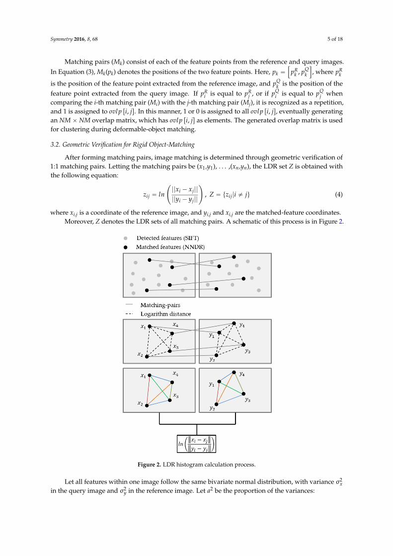
After forming matching pairs, image matching is determined through geometric verification of1:1 matching pairs. Letting the matching pairs be (x1,y1), . . . ,(xn,yn), the LDR set Z is obtained withthe following equation:

zij “ ln

˜

||xi ´ xj||

||yi ´ yj||

¸

, Z “ tzij|i ‰ ju (4)

where xi,j is a coordinate of the reference image, and yi,j and xi,j are the matched-feature coordinates.Moreover, Z denotes the LDR sets of all matching pairs. A schematic of this process is in Figure 2.

Symmetry 2016, 8, 68 5 of 18

Matching pairs (Mk) consist of each of the feature points from the reference and query images.

In Equation (3), Mk(pk) denotes the positions of the two feature points. Here, 𝑝𝑘 = [𝑝𝑘𝑅 , 𝑝𝑘

𝑄], where

𝑝𝑘𝑅 is the position of the feature point extracted from the reference image, and 𝑝𝑘

𝑄 is the position of

the feature point extracted from the query image. If 𝑝𝑖𝑅 is equal to 𝑝𝑗

𝑅, or if 𝑝𝑖𝑄 is equal to 𝑝𝑗

𝑄 when

comparing the i-th matching pair (Mi) with the j-th matching pair (Mj), it is recognized as a repetition,

and 1 is assigned to 𝑜𝑣𝑙𝑝[𝑖, 𝑗]. In this manner, 1 or 0 is assigned to all 𝑜𝑣𝑙𝑝[𝑖, 𝑗], eventually generating

an NM × NM overlap matrix, which has ovlp[i, j] as elements. The generated overlap matrix is used

for clustering during deformable-object matching.

3.2. Geometric Verification for Rigid Object-Matching

After forming matching pairs, image matching is determined through geometric verification of

1:1 matching pairs. Letting the matching pairs be (x1,y1),…,(xn,yn), the LDR set Z is obtained with the

following equation:

𝑧𝑖𝑗 = 𝑙𝑛 (‖𝑥𝑖 − 𝑥𝑗‖

‖𝑦𝑖 − 𝑦𝑗‖) , 𝑍 = {𝑧𝑖𝑗|𝑖 ≠ 𝑗} (4)

where xi,j is a coordinate of the reference image, and yi,j and xi,j are the matched-feature coordinates.

Moreover, Z denotes the LDR sets of all matching pairs. A schematic of this process is in Figure

2.

Figure 2. LDR histogram calculation process.

Let all features within one image follow the same bivariate normal distribution, with variance

σ𝑥2 in the query image and σ𝑦

2 in the reference image. Let 𝑎2 be the proportion of the variances:

𝜎𝑥2

𝜎𝑦2

= 𝑎2 (5)

Figure 2. LDR histogram calculation process.

Let all features within one image follow the same bivariate normal distribution, with variance σ2x

in the query image and σ2y in the reference image. Let a2 be the proportion of the variances:

Symmetry 2016, 8, 68 6 of 18

σ2x

σ2y“ a2 (5)

Then the LDR has the following probability distribution function (PDF):

fZ pz; aq “ 2ˆ

aez

e2z ` a2

˙2(6)

In addition, we examine the upper and lower bounds of the LDR for objects of this type.This behavior is studied by first forming LDR histogram h(k) for the matching pairs by countingthe occurrences over each bin:

h pkq “ #pZX ζkq (7)

The bins ζ1, . . . , ζK are adjacent intervals. The inlier behavior can be expressed by the followingdouble inequality:

a||xi ´ yi|| ď ||yi ´ yj|| ď b||xi ´ xj|| (8)

where a and b define the boundaries of the LDR for inliers. The LDR is restricted to an interval.The inliers would contribute to bins contained in (´lnb,´lna) which for most cases is a limited portionof the histogram. We used the interval (a, bq, which is (´2.6, 2.6).

The comparison of LDR histograms between incorrectly matched images and correctly matchedimages is presented in Figure 3. Since a geometric transform occurs mostly in rigid object images,each matching-pair will have a similar logarithm distance and will become narrow. Exploiting this,the match between two images can be determined.

Symmetry 2016, 8, 68 6 of 18

Then the LDR has the following probability distribution function (PDF): ( ; ) = 2 ee + (6)

In addition, we examine the upper and lower bounds of the LDR for objects of this type. This behavior is studied by first forming LDR histogram h(k) for the matching pairs by counting the occurrences over each bin: ℎ( ) = #( ∩ ) (7)

The bins , … , are adjacent intervals. The inlier behavior can be expressed by the following double inequality: ‖ ‖ (8)

where and define the boundaries of the LDR for inliers. The LDR is restricted to an interval. The inliers would contribute to bins contained in ( ln , ln ) which for most cases is a limited portion of the histogram. We used the interval ( , ),which is (−2.6, 2.6).

The comparison of LDR histograms between incorrectly matched images and correctly matched images is presented in Figure 3. Since a geometric transform occurs mostly in rigid object images, each matching-pair will have a similar logarithm distance and will become narrow. Exploiting this, the match between two images can be determined.

Figure 3. (a) Results of feature matching using NNDR (left: incorrectly matched images, right: correctly matched images); (b) the lines point to the positions of the matched features in the other image; and (c) the LDR histogram of the model function.

Pearson’s chi-square test is utilized to compare the correlation of h(k) and f(k). Let the LDR histogram have k bins. The histogram will be compared to the discretized model function f(k). We

Figure 3. (a) Results of feature matching using NNDR (left: incorrectly matched images, right:correctly matched images); (b) the lines point to the positions of the matched features in the otherimage; and (c) the LDR histogram of the model function.

Symmetry 2016, 8, 68 7 of 18

Pearson’s chi-square test is utilized to compare the correlation of h(k) and f(k). Let the LDRhistogram have k bins. The histogram will be compared to the discretized model function f(k). We usedthese quantities to formulate the test. Equation (9) is a formula to calculate the goodness-of-fitparameter for c. A high value for c if the shape of the LDR histogram differs much from that of f(k),implied that many of the matches are inliers:

c “Kÿ

k“1

phk ´ n fkq2

n fkě χ2

1´a,K´1 (9)

where n is the total number of matching pairs, and χ21´a,K´1 is the threshold of χ2 having K-1 degrees

of freedom. The threshold determination method is based on an experiment by Lepsøy [9]. To obtainthe false positive rate below, 1 ´ a = 0.01 (1%), set the threshold to 70. If c is higher than the threshold,d(k) is computed using Equation (10) to find the inliers:

d pkq “ h pkq ´β f pkq , β “

řKk“1 h pkq f pkqřK

k“1 p f pkqq2(10)

where β is a weight to normalize h(k) and f (k). Figure 4a shows the comparisons of h(k) to f (k) andto d(k), respectively, between matching images and non-matching images. We can see that the LDRof matching pairs is narrow with numerous inliers, and that a match can rapidly be identified bycalculating this difference.

Symmetry 2016, 8, 68 7 of 18

𝑐 = ∑(ℎ𝑘 − 𝑛𝑓𝑘)2

𝑛𝑓𝑘

𝐾

𝑘=1

≥ 𝜒1−𝑎,𝐾−12 (9)

where n is the total number of matching pairs, and 𝜒1−𝑎,𝐾−12 is the threshold of 𝜒2 having K-1

degrees of freedom. The threshold determination method is based on an experiment by Lepsøy [9].

To obtain the false positive rate below, 1 − 𝑎 = 0.01 (1%), set the threshold to 70. If c is higher than

the threshold, d(k) is computed using Equation (10) to find the inliers:

𝑑(𝑘) = ℎ(𝑘) − β𝑓(𝑘), β =∑ ℎ(𝑘)𝑓(𝑘)𝐾

𝑘=1

∑ (𝑓(𝑘))2𝐾

𝑘=1

(10)

where β is a weight to normalize h(k) and f(k). Figure 4a shows the comparisons of h(k) to f(k) and to

d(k), respectively, between matching images and non-matching images. We can see that the LDR of

matching pairs is narrow with numerous inliers, and that a match can rapidly be identified by

calculating this difference.

(a) (b)

Figure 4. Analysis for geometric verification based on LDR (k = 25): (a) example of LDR histogram h(k),

model function f(k), and difference d(k) (top: correctly matched images, bottom: incorrectly matched

images); and (b) eigenvector r for finding inliers (top), and the results in descending order (bottom).

After geometric verification based on LDR, matrix D is formed by quantizing d(k) in order to

predict the number of inliers, and eigenvalue u and dominant eigenvector r are calculated using

Dr = ur, used in Equation (11).

𝑖𝑛𝑙𝑖𝑒𝑟𝑛 = 1 +μ

𝑚𝑎𝑥𝑘=1,…,𝐾 𝑑(𝑘) (11)

Subsequently, eigenvector r is sorted in descending order, and the upper-range matching pairs

corresponding to the calculated number of inliers are finally determined to be the inliers. Figure 4b

shows a diagrammatic representation of this process.

Lastly, the weights of the matching pairs and the inliers are calculated, and matches are

determined by calculating the ratios of the weights. Weights are based on the conditional probability

Figure 4. Analysis for geometric verification based on LDR (k = 25): (a) example of LDR histogram h(k),model function f (k), and difference d(k) (top: correctly matched images, bottom: incorrectly matchedimages); and (b) eigenvector r for finding inliers (top), and the results in descending order (bottom).

After geometric verification based on LDR, matrix D is formed by quantizing d(k) in order topredict the number of inliers, and eigenvalue u and dominant eigenvector r are calculated usingDr = ur, used in Equation (11).

Symmetry 2016, 8, 68 8 of 18

inliern “ 1`µ

maxk“1,...,K d pkq(11)

Subsequently, eigenvector r is sorted in descending order, and the upper-range matching pairscorresponding to the calculated number of inliers are finally determined to be the inliers. Figure 4bshows a diagrammatic representation of this process.

Lastly, the weights of the matching pairs and the inliers are calculated, and matches are determinedby calculating the ratios of the weights. Weights are based on the conditional probability of the inlierswhen the ratio between the NN distance and second distance during feature matching is given.Equation (12) shows the corresponding conditional probability function.

p pc|rq “ppr|cq

p pr|cq ` ppr|cq(12)

where c and c denote the probability of inliers and outliers, respectively, and r is the distance ratio.

3.3. Discrimination of Deformable Object Images

After generating matching pairs from the two images, x and y, and performing geometricverification, the total number of matching pairs, the number of inliers, the matching-pair weight,and the inliers’ weights are calculated using the results. These can be defined as matching informationM(x,y) = { matchn, inliern, weightu. We analyzed which statistical distribution M(x,y) has, using theexample images. Non-matching and deformable-object images were used as training images, and themean, µ, and standard deviation, σ, of each property were calculated to form normal distributionNpµ,σ2q. However, since the non-matching and deformable-object images show similarity in M(x,y)from numerous aspects, discrimination of the two classes is vague. Therefore, the following is proposedto find the model that minimizes the error. Analyzing numerous training images, we observed thatdeformable-object matching does not lead to good results if the number of inliers is less than a certainnumber. In other words, there must be more than a certain number of inliers. Figure 5b was obtainedfrom experiment using more than four inliers corresponding to minimum error. Subsequently, the ratiobetween the number of inliers with the greatest difference in mean between the two classes, and thematching-pair weight with the least difference in variance is calculated, and t with the minimum erroris obtained using a Bayesian classifier.

Let the training set be X = (x1,c1), (x2,c2), . . . ,(xn,cn), xi for the i-th properties, and let ci be theclass index of xi, which represents non-matching (w1) and deformable-matching (w2). X is defined asthe ratio between the inlier number from matching information and matching-pair weight, as shownin Equation (13):

x “inliern

distn(13)

Figure 5 shows the graph obtained by separating matching information into that of incorrectlymatched images and deformable matching images. Figure 5a–d shows each property of the matchinginformation; however, it is difficult to distinguish the deformable matching pairs from non-matchingpairs. Figure 5e shows the normal distribution of x for the matching pairs with more than four inliersafter rigid-object matching. We can see that the distinction is clearer than in the previous graphs.Therefore, t with the minimum error was found and is used for the classifier.

However, discrimination of deformable objects does not exhibit good performance if it is basedon statistical analysis only. This is because a deformable transformation cannot be defined as a certainmodel. Therefore, the pattern for d(k), which was used for geometric verification, was identifiedthrough machine learning-based training, and the result was used. Figure 6 shows a graphicalillustration of d(k) from matching rigid-object, deformable-object, and non-matching-pair images.

Symmetry 2016, 8, 68 9 of 18

Symmetry 2016, 8, 68 9 of 18

Figure 5. Normal distribution model of matching information from matching pairs of deformable and

non-matching images: (a) number of matching pairs; (b) number of inliers; (c) sum of all matching

pairs’ distances; (d) sum of inliers’ distances; and (e) matching information of x.

(a)

(b)

(c)

Figure 6. Comparison of d(k) between matching images: (a) d(k) of rigid matching pair; (b) d(k) of

deformable-object matching pair; and (c) d(k) of non-matching pair.

Figure 6c appears to be completely different from the case above. It exhibits irregular patterns

over the entire range, most of which are small in size. This implies that the LDR and the PDF are

almost identical. Exploiting this characteristic, d(k) of a deformable matching-pair and d(k) of a non-

matching pair were extracted from the training set, and the characteristics of each pattern were

classified using support vector machine (SVM) [19], which is one of the supervised learning algorithms.

The probability of a deformable transformation is determined from the results of the previous

statistical analysis and machine learning, and the deformable objects are finally discriminated

through voting. The voting method combines the results obtained from various conditions, rather

than from using the results of the one with the best classification performance, which is appropriate

for unpredictable deformable transformations.

3.4. Deformable-Object Matching

Figure 5. Normal distribution model of matching information from matching pairs of deformable andnon-matching images: (a) number of matching pairs; (b) number of inliers; (c) sum of all matchingpairs’ distances; (d) sum of inliers’ distances; and (e) matching information of x.

Symmetry 2016, 8, 68 9 of 18

Figure 5. Normal distribution model of matching information from matching pairs of deformable and

non-matching images: (a) number of matching pairs; (b) number of inliers; (c) sum of all matching

pairs’ distances; (d) sum of inliers’ distances; and (e) matching information of x.

(a)

(b)

(c)

Figure 6. Comparison of d(k) between matching images: (a) d(k) of rigid matching pair; (b) d(k) of

deformable-object matching pair; and (c) d(k) of non-matching pair.

Figure 6c appears to be completely different from the case above. It exhibits irregular patterns

over the entire range, most of which are small in size. This implies that the LDR and the PDF are

almost identical. Exploiting this characteristic, d(k) of a deformable matching-pair and d(k) of a non-

matching pair were extracted from the training set, and the characteristics of each pattern were

classified using support vector machine (SVM) [19], which is one of the supervised learning algorithms.

The probability of a deformable transformation is determined from the results of the previous

statistical analysis and machine learning, and the deformable objects are finally discriminated

through voting. The voting method combines the results obtained from various conditions, rather

than from using the results of the one with the best classification performance, which is appropriate

for unpredictable deformable transformations.

3.4. Deformable-Object Matching

Figure 6. Comparison of d(k) between matching images: (a) d(k) of rigid matching pair; (b) d(k) ofdeformable-object matching pair; and (c) d(k) of non-matching pair.

Figure 6c appears to be completely different from the case above. It exhibits irregular patternsover the entire range, most of which are small in size. This implies that the LDR and the PDF are almostidentical. Exploiting this characteristic, d(k) of a deformable matching-pair and d(k) of a non-matchingpair were extracted from the training set, and the characteristics of each pattern were classified usingsupport vector machine (SVM) [19], which is one of the supervised learning algorithms.

The probability of a deformable transformation is determined from the results of the previousstatistical analysis and machine learning, and the deformable objects are finally discriminated throughvoting. The voting method combines the results obtained from various conditions, rather than

Symmetry 2016, 8, 68 10 of 18

from using the results of the one with the best classification performance, which is appropriatefor unpredictable deformable transformations.

3.4. Deformable-Object Matching

Deformable-object images are discriminated, and finally, deformable object-matching is performed.Rigid object-matching methods mostly calculate a homograph in order to examine the geometricconsistency of the features in the whole image. However, while deformable objects can have locallysimilar geometry, it is difficult to calculate a single homograph from the whole image. Therefore,we used a method to cluster matching pairs with similar geometric models, and we propose a methodwith enhanced performance through the use of clustering validation.

Letting two matching pairs be Mi, and Mj, transformations Ti and Tj and translations ti, and tjcan be calculated from the characteristics of each matching pair, using the enhanced weak geometricconsistency (WGC) [20], as shown in Equation (14).

«

x1qy1q

ff

“ s1«

cosθ1 ´sinθ1sinθ1 cosθ1

ff«

xp

yp

ff

, t “ˇ

ˇq1`

xq, yq˘

´ q`

xq, yq˘ˇ

ˇ (14)

where s denotes scale, θ is the dominant orientation, and tx and ty represent coordinate translations.Using Equation (9), the matching pairs can be expressed as Mi “

`

pxi, yiq , px1i , y1iq, Ti˘

and

Mj “´

`

xj, yj˘

, px1j, y1jq, Tj

¯

, and the geometric similarity of the two matching pairs is calculated usingEquation (15):

dgeo “`

Mi, Mj˘

“12p||X1j ´ TiXj|| ` ||X1i ´ TjXi||q “

12`

dmi ` dmj˘

(15)

where, Xk “ rxk, ykst , X1k “

“

x1k, y1k‰t , k “ i, j. If transformation models Ti and Tj are similar, dgeo(Mi,Mj)

will be close to 0. A graphical representation of this is shown in Figure 7.

Symmetry 2016, 8, 68 10 of 18

Deformable-object images are discriminated, and finally, deformable object-matching is

performed. Rigid object-matching methods mostly calculate a homograph in order to examine the

geometric consistency of the features in the whole image. However, while deformable objects can

have locally similar geometry, it is difficult to calculate a single homograph from the whole image.

Therefore, we used a method to cluster matching pairs with similar geometric models, and we

propose a method with enhanced performance through the use of clustering validation.

Letting two matching pairs be Mi, and Mj, transformations Ti and Tj and translations ti, and tj can

be calculated from the characteristics of each matching pair, using the enhanced weak geometric

consistency (WGC) [20], as shown in Equation (14).

[𝑥𝑞

′

𝑦𝑞′ ] = s′ [cosθ′ −sinθ′

sinθ′ cosθ′] [

𝑥𝑝

𝑦𝑝] , 𝑡 = |𝑞′(𝑥𝑞 , 𝑦𝑞) − 𝑞(𝑥𝑞 , 𝑦𝑞)| (14)

where s denotes scale, θ is the dominant orientation, and tx and ty represent coordinate translations.

Using Equation (9), the matching pairs can be expressed as 𝑀𝑖 = ((𝑥𝑖 , 𝑦𝑖), (𝑥𝑖′, 𝑦𝑖

′), 𝑇𝑖) and 𝑀𝑗 =

((𝑥𝑗 , 𝑦𝑗), (𝑥𝑗′, 𝑦𝑗

′), 𝑇𝑗), and the geometric similarity of the two matching pairs is calculated using

Equation (15):

𝑑𝑔𝑒𝑜 = (𝑀𝑖 , 𝑀𝑗) =1

2(‖𝑋𝑗

′ − 𝑇𝑖𝑋𝑗‖ + ‖𝑋𝑖′ − 𝑇𝑗𝑋𝑖‖) =

1

2(𝑑𝑚𝑖 + 𝑑𝑚𝑗) (15)

where, 𝑋𝑘 = [𝑥𝑘, 𝑦𝑘]𝑡 , 𝑋𝑘′ = [𝑥𝑘

′ , 𝑦𝑘′ ]𝑡 , 𝑘 = 𝑖, 𝑗 . If transformation models 𝑇𝑖 and 𝑇𝑗 are similar,

dgeo(Mi,Mj) will be close to 0. A graphical representation of this is shown in Figure 7.

Figure 7. Example of a geometric similarity measure.

Using this relationship, it can be assumed that the matching pairs with a small dgeo(Mi,Mj) have

a similar geometric relation. Therefore, similarity is computed by calculating the geometric

transformation between each matching pair, rather than by defining a transformation model of the

whole image.

Figure 8 shows an example of an affine matrix where the geometric similarity between the

matching pairs is calculated. The matrix is formed by calculating the geometric similarity between

each matching pair, assuming there are 10 matching pairs. In the example, the matching pairs with

high geometric similarity are the 9th and 10th matching pairs. Deformable objects are found through

hierarchical clustering of matching pairs with high similarity in the calculated affine matrix.

Figure 7. Example of a geometric similarity measure.

Using this relationship, it can be assumed that the matching pairs with a small dgeo(Mi,Mj)have a similar geometric relation. Therefore, similarity is computed by calculating the geometrictransformation between each matching pair, rather than by defining a transformation model of thewhole image.

Figure 8 shows an example of an affine matrix where the geometric similarity between thematching pairs is calculated. The matrix is formed by calculating the geometric similarity betweeneach matching pair, assuming there are 10 matching pairs. In the example, the matching pairs withhigh geometric similarity are the 9th and 10th matching pairs. Deformable objects are found throughhierarchical clustering of matching pairs with high similarity in the calculated affine matrix.

Symmetry 2016, 8, 68 11 of 18

Symmetry 2016, 8, 68 10 of 18

Deformable-object images are discriminated, and finally, deformable object-matching is

performed. Rigid object-matching methods mostly calculate a homograph in order to examine the

geometric consistency of the features in the whole image. However, while deformable objects can

have locally similar geometry, it is difficult to calculate a single homograph from the whole image.

Therefore, we used a method to cluster matching pairs with similar geometric models, and we

propose a method with enhanced performance through the use of clustering validation.

Letting two matching pairs be Mi, and Mj, transformations Ti and Tj and translations ti, and tj can

be calculated from the characteristics of each matching pair, using the enhanced weak geometric

consistency (WGC) [20], as shown in Equation (14).

[𝑥𝑞

′

𝑦𝑞′ ] = s′ [cosθ′ −sinθ′

sinθ′ cosθ′] [

𝑥𝑝

𝑦𝑝] , 𝑡 = |𝑞′(𝑥𝑞 , 𝑦𝑞) − 𝑞(𝑥𝑞 , 𝑦𝑞)| (14)

where s denotes scale, θ is the dominant orientation, and tx and ty represent coordinate translations.

Using Equation (9), the matching pairs can be expressed as 𝑀𝑖 = ((𝑥𝑖 , 𝑦𝑖), (𝑥𝑖′, 𝑦𝑖

′), 𝑇𝑖) and 𝑀𝑗 =

((𝑥𝑗 , 𝑦𝑗), (𝑥𝑗′, 𝑦𝑗

′), 𝑇𝑗), and the geometric similarity of the two matching pairs is calculated using

Equation (15):

𝑑𝑔𝑒𝑜 = (𝑀𝑖 , 𝑀𝑗) =1

2(‖𝑋𝑗

′ − 𝑇𝑖𝑋𝑗‖ + ‖𝑋𝑖′ − 𝑇𝑗𝑋𝑖‖) =

1

2(𝑑𝑚𝑖 + 𝑑𝑚𝑗) (15)

where, 𝑋𝑘 = [𝑥𝑘, 𝑦𝑘]𝑡 , 𝑋𝑘′ = [𝑥𝑘

′ , 𝑦𝑘′ ]𝑡 , 𝑘 = 𝑖, 𝑗 . If transformation models 𝑇𝑖 and 𝑇𝑗 are similar,

dgeo(Mi,Mj) will be close to 0. A graphical representation of this is shown in Figure 7.

Figure 7. Example of a geometric similarity measure.

Using this relationship, it can be assumed that the matching pairs with a small dgeo(Mi,Mj) have

a similar geometric relation. Therefore, similarity is computed by calculating the geometric

transformation between each matching pair, rather than by defining a transformation model of the

whole image.

Figure 8 shows an example of an affine matrix where the geometric similarity between the

matching pairs is calculated. The matrix is formed by calculating the geometric similarity between

each matching pair, assuming there are 10 matching pairs. In the example, the matching pairs with

high geometric similarity are the 9th and 10th matching pairs. Deformable objects are found through

hierarchical clustering of matching pairs with high similarity in the calculated affine matrix.

Figure 8. Example of an affinity matrix (10 matching pairs).

Hierarchical clustering will group the clusters through linkages by calculating the similaritywithin each cluster. In order to minimize the chain effect during linkage, a k-NN method was used.While this is similar to a single-linkage method, it was extended to have k linkages, and has theadvantage of robustness against the chain effect. Figure 9 shows the results of hierarchical clusteringbased on geometric similarity between matching pairs. Figure 9a shows the matching result when thereis a geometric transformation in an image containing a rigid object. We can see from the figure thatthe entire object is grouped into a single large cluster due to similar geometric relations. In Figure 9b,we can see that the objects are matched separately, with each object clustered distinctly under adeformable transformation.

Symmetry 2016, 8, 68 11 of 18

Figure 8. Example of an affinity matrix (10 matching pairs).

Hierarchical clustering will group the clusters through linkages by calculating the similarity

within each cluster. In order to minimize the chain effect during linkage, a k-NN method was used.

While this is similar to a single-linkage method, it was extended to have k linkages, and has the

advantage of robustness against the chain effect. Figure 9 shows the results of hierarchical clustering

based on geometric similarity between matching pairs. Figure 9a shows the matching result when

there is a geometric transformation in an image containing a rigid object. We can see from the figure

that the entire object is grouped into a single large cluster due to similar geometric relations. In Figure

9b, we can see that the objects are matched separately, with each object clustered distinctly under a

deformable transformation.

(a) (b)

Figure 9. Deformable image-matching results using hierarchical clustering of geometric similarity: (a)

matching results for rigid objects with geometric transformation; and (b) matching results of a

deformable object.

Hierarchical clustering eventually forms a single cluster. Therefore, clustering must be stopped

at some point. During the linkage of clusters, clustering is stopped when the geometric similarity of

the matching pair exceeds a set threshold. However, if such a thresholding method is the only one

used, the number of clusters becomes excessive, with most of the clusters likely being false clusters.

Therefore, clustering validation is used to remove false clusters. If the number of matching pairs that

form the clusters is too low, it is less likely that the resulting clusters become objects. Hence, two

methods are used for clustering validation. First, a cluster is determined to be a valid cluster only if

the number of matching pairs that form the cluster is greater than τm. Secondly, a cluster is determined

to be a valid cluster if the area of the matching pairs that form the cluster is larger than a certain

portion of the entire area (τa). The area of the matching pairs that form the cluster is calculated using

a convex hull. Figure 10 shows the results of removing the invalid clusters through clustering

validation for each case of inlier matching and outlier matching. From inlier matching, it was

observed that the clusters with a small area are removed, and for outlier matching, the accuracy was

enhanced by preventing the false positives that occur due to small clusters.

Figure 9. Deformable image-matching results using hierarchical clustering of geometric similarity:(a) matching results for rigid objects with geometric transformation; and (b) matching results of adeformable object.

Hierarchical clustering eventually forms a single cluster. Therefore, clustering must be stoppedat some point. During the linkage of clusters, clustering is stopped when the geometric similarity ofthe matching pair exceeds a set threshold. However, if such a thresholding method is the only oneused, the number of clusters becomes excessive, with most of the clusters likely being false clusters.Therefore, clustering validation is used to remove false clusters. If the number of matching pairsthat form the clusters is too low, it is less likely that the resulting clusters become objects. Hence,two methods are used for clustering validation. First, a cluster is determined to be a valid clusteronly if the number of matching pairs that form the cluster is greater than τm. Secondly, a cluster isdetermined to be a valid cluster if the area of the matching pairs that form the cluster is larger than acertain portion of the entire area (τa). The area of the matching pairs that form the cluster is calculatedusing a convex hull. Figure 10 shows the results of removing the invalid clusters through clusteringvalidation for each case of inlier matching and outlier matching. From inlier matching, it was observed

Symmetry 2016, 8, 68 12 of 18

that the clusters with a small area are removed, and for outlier matching, the accuracy was enhancedby preventing the false positives that occur due to small clusters.

Symmetry 2016, 8, 68 12 of 18

(a)

(b)

Figure 10. Comparison results from before (left) and after (right) clustering validation: (a) inlier-

matching pairs; and (b) outlier-matching pairs.

4. Experiment Results

In order to evaluate the performance of the proposed matching method, the Stanford Mobile

Visual Search (SMVS) dataset from Stanford University was used [21]. SMVS includes images of CDs,

DVDs, books, paintings, and video clips, and is currently the standard image set for performance

evaluation of image matching under MPEG-7 CDVS. The annotations of matching pairs and non-

matching pairs were compiled in SMVS, through which true positives and false positives can be

evaluated. Additionally, in order to evaluate deformable object-matching, performance was

evaluated with varying intensities of deformation using thin plate spline (TPS) [22]. Deformation

intensity was varied in three levels (light, medium, and heavy), and 4200 query images from SMVS

were extended to 12,800 images. Lastly, 600 clothing images, which are natural deformable objects

without artificial deformation, were collected and used. Figure 11 shows examples of SMVS images,

deformed SMVS images with each level of intensity, and clothing images.

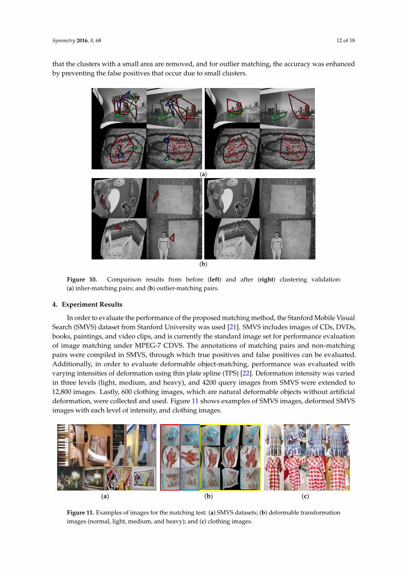
(a) (b) (c)

Figure 11. Examples of images for the matching test: (a) SMVS datasets; (b) deformable

transformation images (normal, light, medium, and heavy); and (c) clothing images.

True positive rate (TPR) and false positive rate (FPR) were used to evaluate matching

performance. TPR is an equation that examines robustness from among the characteristics of

matching algorithms, with greater value implying better performance. In contrast, FPR examines

Figure 10. Comparison results from before (left) and after (right) clustering validation:(a) inlier-matching pairs; and (b) outlier-matching pairs.

4. Experiment Results

In order to evaluate the performance of the proposed matching method, the Stanford Mobile VisualSearch (SMVS) dataset from Stanford University was used [21]. SMVS includes images of CDs, DVDs,books, paintings, and video clips, and is currently the standard image set for performance evaluationof image matching under MPEG-7 CDVS. The annotations of matching pairs and non-matchingpairs were compiled in SMVS, through which true positives and false positives can be evaluated.Additionally, in order to evaluate deformable object-matching, performance was evaluated withvarying intensities of deformation using thin plate spline (TPS) [22]. Deformation intensity was variedin three levels (light, medium, and heavy), and 4200 query images from SMVS were extended to12,800 images. Lastly, 600 clothing images, which are natural deformable objects without artificialdeformation, were collected and used. Figure 11 shows examples of SMVS images, deformed SMVSimages with each level of intensity, and clothing images.

Symmetry 2016, 8, 68 12 of 18

(a)

(b)

Figure 10. Comparison results from before (left) and after (right) clustering validation: (a) inlier-

matching pairs; and (b) outlier-matching pairs.

4. Experiment Results

In order to evaluate the performance of the proposed matching method, the Stanford Mobile

Visual Search (SMVS) dataset from Stanford University was used [21]. SMVS includes images of CDs,

DVDs, books, paintings, and video clips, and is currently the standard image set for performance

evaluation of image matching under MPEG-7 CDVS. The annotations of matching pairs and non-

matching pairs were compiled in SMVS, through which true positives and false positives can be

evaluated. Additionally, in order to evaluate deformable object-matching, performance was

evaluated with varying intensities of deformation using thin plate spline (TPS) [22]. Deformation

intensity was varied in three levels (light, medium, and heavy), and 4200 query images from SMVS

were extended to 12,800 images. Lastly, 600 clothing images, which are natural deformable objects

without artificial deformation, were collected and used. Figure 11 shows examples of SMVS images,

deformed SMVS images with each level of intensity, and clothing images.

(a) (b) (c)

Figure 11. Examples of images for the matching test: (a) SMVS datasets; (b) deformable

transformation images (normal, light, medium, and heavy); and (c) clothing images.

True positive rate (TPR) and false positive rate (FPR) were used to evaluate matching

performance. TPR is an equation that examines robustness from among the characteristics of

matching algorithms, with greater value implying better performance. In contrast, FPR examines

Figure 11. Examples of images for the matching test: (a) SMVS datasets; (b) deformable transformationimages (normal, light, medium, and heavy); and (c) clothing images.

Symmetry 2016, 8, 68 13 of 18

True positive rate (TPR) and false positive rate (FPR) were used to evaluate matching performance.TPR is an equation that examines robustness from among the characteristics of matching algorithms,with greater value implying better performance. In contrast, FPR examines independence fromamong the characteristics of matching algorithms, with a smaller value implying better performance.Moreover, for objective comparison, accuracy was used, which is defined in relation to TPR and FPR.

TPR “TP

TP` FN“

TPP

FPR “FP

FP` TN“

FPN

Accuracy “TP` TN

P` N

For a speed performance test, we used an Intel Xeon E3-1275 (8 core) CPU and with a clock speedof 3.5 GHz and 32 GB RAM running the Windows 7 (64-bit).

4.1. Geometric Verification Test for Rigid Object Matching

First, an NNDR higher than 0.8 was excluded in feature matching, and a Euclidean distance lessthan 0.6 was not used for fast calculation. This method was verified by Mikolajczyk and has beenapplied in most feature-matching cases [18]. Inliers were determined through LDR, while the matchingscore for a matching decision was calculated as follows:

matching score “ω

pω` Tmq(16)

where, ω is the sum of inlier distances, and Tm is the threshold value. Matching was determinedfor a matching score >0.5. Accordingly, the experiment was conducted by altering the Tm value.The optimum value for Tm was determined through the receiver operating characteristic (ROC)curve, and set at Tm = 3, allowing a comparison of the performances of standard matching methods.A rigid-object image from the SMVS dataset was employed as an experimental image.

Figure 12 illustrates the ROC curves of Approximate Nearest Neighbor (ANN) [23], RANSAC [7],and DISTRAT [9], which were employed in this study as rigid-object image-matching methods.A superior performance is indicated by a position closer to the top-left of the graph. DISTRAT andRANSAC exhibit similar performance in rigid-object matching. However, DISTRAT, which is basedon a statistical algorithm, has the advantage of a very fast matching speed compared to RANSAC,which is based on an iteration algorithm.

Symmetry 2016, 8, 68 13 of 18

independence from among the characteristics of matching algorithms, with a smaller value implying

better performance. Moreover, for objective comparison, accuracy was used, which is defined in

relation to TPR and FPR.

TPR = 𝑇𝑃

𝑇𝑃 + 𝐹𝑁=

𝑇𝑃

𝑃

FPR = 𝐹𝑃

𝐹𝑃 + 𝑇𝑁=

𝐹𝑃

𝑁

Accuracy = 𝑇𝑃 + 𝑇𝑁

𝑃 + 𝑁

For a speed performance test, we used an Intel Xeon E3-1275 (8 core) CPU and with a clock speed

of 3.5 GHz and 32 GB RAM running the Windows 7 (64-bit).

4.1. Geometric Verification Test for Rigid Object Matching

First, an NNDR higher than 0.8 was excluded in feature matching, and a Euclidean distance less

than 0.6 was not used for fast calculation. This method was verified by Mikolajczyk and has been

applied in most feature-matching cases [18]. Inliers were determined through LDR, while the

matching score for a matching decision was calculated as follows:

𝑚𝑎𝑡𝑐ℎ𝑖𝑛𝑔 𝑠𝑐𝑜𝑟𝑒 = 𝜔

(𝜔 + 𝑇𝑚) (16)

where, 𝜔 is the sum of inlier distances, and Tm is the threshold value. Matching was determined for

a matching score >0.5. Accordingly, the experiment was conducted by altering the Tm value. The

optimum value for Tm was determined through the receiver operating characteristic (ROC) curve,

and set at Tm = 3, allowing a comparison of the performances of standard matching methods. A rigid-

object image from the SMVS dataset was employed as an experimental image.

Figure 12 illustrates the ROC curves of Approximate Nearest Neighbor (ANN) [23], RANSAC

[7], and DISTRAT [9], which were employed in this study as rigid-object image-matching methods.

A superior performance is indicated by a position closer to the top-left of the graph. DISTRAT and

RANSAC exhibit similar performance in rigid-object matching. However, DISTRAT, which is based

on a statistical algorithm, has the advantage of a very fast matching speed compared to RANSAC,

which is based on an iteration algorithm.

Figure 12. ROC curve comparison of the representative rigid object-matching methods.

4.2. Discriminating Deformable Objects Using Voting Methods

Figure 12. ROC curve comparison of the representative rigid object-matching methods.

Symmetry 2016, 8, 68 14 of 18

4.2. Discriminating Deformable Objects Using Voting Methods

The voting method was used for discrimination of deformable object images. Two additionalmethods were used as conditions in each voting, as well as SVM and the statistical model describedin Section 3.3. The additional methods are the matching score used in rigid-object matching, and thesum of inliers distance. Matching score employs Equation (16). A low matching score indicates asmall number of inliers or insufficient weight for an image-matching determination. However, it isnecessary to slightly lower the matching parameter for deformable object images. Thus, a value that islower than 0.5, which is used in rigid-object matching, was selected, and the probability of deformableobject-matching was determined. The value was set at 0.2 and employed for the experiment. Second,the ratio of the total matching-pair weight and inlier weights was calculated. This value represents theproportion of inlier weights in the total matching pairs, regardless of the number of inliers. A valueof 0.28 was selected through experiment as the method for determining matching-pairs having theprobability of a deformable object.

Results of the proposed discrimination process for deformable objects are shown in Figure 13.The University of Kentucky (UKY) dataset was used as the training image set [23]. The UKY datasetconsists of 10,200 images of 2550 objects.

Four conditions were used for voting, and the voting value was varied throughout theexperiments, where voting > 0 implies conducting deformable-object matching for all cases that havenot been rigid-matched. In contrast, voting > 3 indicates no deformable-object matching in most cases.

Symmetry 2016, 8, 68 14 of 18

The voting method was used for discrimination of deformable object images. Two additional

methods were used as conditions in each voting, as well as SVM and the statistical model described

in Section 3.3. The additional methods are the matching score used in rigid-object matching, and the

sum of inliers distance. Matching score employs Equation (16). A low matching score indicates a

small number of inliers or insufficient weight for an image-matching determination. However, it is

necessary to slightly lower the matching parameter for deformable object images. Thus, a value that

is lower than 0.5, which is used in rigid-object matching, was selected, and the probability of

deformable object-matching was determined. The value was set at 0.2 and employed for the

experiment. Second, the ratio of the total matching-pair weight and inlier weights was calculated.

This value represents the proportion of inlier weights in the total matching pairs, regardless of the

number of inliers. A value of 0.28 was selected through experiment as the method for determining

matching-pairs having the probability of a deformable object.

Results of the proposed discrimination process for deformable objects are shown in Figure 13.

The University of Kentucky (UKY) dataset was used as the training image set [23]. The UKY dataset

consists of 10,200 images of 2550 objects.

Four conditions were used for voting, and the voting value was varied throughout the

experiments, where voting > 0 implies conducting deformable-object matching for all cases that have

not been rigid-matched. In contrast, voting > 3 indicates no deformable-object matching in most cases.

(a) (b)

(c) (d)

Figure 13. Performance per voting values (N: normal images; L: light deformable images; M: medium

deformable images; H: heavy deformable images; and C: clothing images): (a) true positive rate for

voting values; (b) false positive rate for voting values; (c) accuracy for voting values; and (d) execution

time for voting values.

While TPR is highest voting > 0, the execution time is inefficient, the FPR is high, and accuracy is

low, since all of the numerous deformable object-matching processes were run. If the voting value

increases, the TPR and accuracy decrease, overall, since the possibility of deformable objects

decreases. Therefore, the best performance for average accuracy was when voting > 1.

Figure 13. Performance per voting values (N: normal images; L: light deformable images; M: mediumdeformable images; H: heavy deformable images; and C: clothing images): (a) true positive rate forvoting values; (b) false positive rate for voting values; (c) accuracy for voting values; and (d) executiontime for voting values.

While TPR is highest voting > 0, the execution time is inefficient, the FPR is high, and accuracyis low, since all of the numerous deformable object-matching processes were run. If the voting valueincreases, the TPR and accuracy decrease, overall, since the possibility of deformable objects decreases.Therefore, the best performance for average accuracy was when voting > 1.

Symmetry 2016, 8, 68 15 of 18

4.3. Deformable Object-Matching Performance Test

Hierarchical clustering was used for deformable-object matching. Hierarchical clustering willcreate a single cluster without cutoff. Figure 14a presents experimental results obtained by changingthe cutoff. As the cutoff value increases, TPR and FPR increase. Accuracy was calculated to find theoptimum cutoff value. It was confirmed through experiment that the best accuracy was found at acutoff of 30. Moreover, linkage for the clustering employed a strong k-NN in a chain effect, and anexperiment was conducted to determine the optimum k. The results are presented in Figure 14b.For a higher k, the number of false positives is reduced, but complexity increases. Because there is nosignificant effect on accuracy when k is higher than 10, a k value equal to 10 was employed.

Symmetry 2016, 8, 68 15 of 18

4.3. Deformable Object-Matching Performance Test

Hierarchical clustering was used for deformable-object matching. Hierarchical clustering will

create a single cluster without cutoff. Figure 14a presents experimental results obtained by changing

the cutoff. As the cutoff value increases, TPR and FPR increase. Accuracy was calculated to find the

optimum cutoff value. It was confirmed through experiment that the best accuracy was found at a

cutoff of 30. Moreover, linkage for the clustering employed a strong k-NN in a chain effect, and an

experiment was conducted to determine the optimum k. The results are presented in Figure 14b. For

a higher k, the number of false positives is reduced, but complexity increases. Because there is no

significant effect on accuracy when k is higher than 10, a k value equal to 10 was employed.

(a) (b)

Figure 14. Experimental results according to parameters in clustering of geometric similarity for

deformable-object matching: (a) experimental result based on the cutoff of geometric similarity; and

(b) experimental result based on k of a k-NN linkage.

An experiment was conducted using the two proposed methods for clustering validation. When

clusters were formed using hierarchical clustering, the number of matching pairs contained in each

cluster and the area of each cluster consisting of matching pairs in the image are determined as shown

in Figure 15. Each cluster can be viewed as an object in an image. When the number of matching pairs

constituting an object is small, or the area is narrow, the resulting object has a low value. Hence,

cluster validation was performed using this result. Figure 15a illustrates the experiment regarding

false clusters when the number of matching pairs contained in a cluster has a small threshold value

(τm). The optimum value was determined through experiment to be τm = 5. Figure 15b shows the

calculated ratio of each cluster area and the entire image area. A false cluster was deemed to occur

when the ratio (τa) is low. From the experiment, the best value was confirmed to be τa = 0.01, and

hence, this value was employed.

(a) (b)

Figure 14. Experimental results according to parameters in clustering of geometric similarity fordeformable-object matching: (a) experimental result based on the cutoff of geometric similarity;and (b) experimental result based on k of a k-NN linkage.

An experiment was conducted using the two proposed methods for clustering validation.When clusters were formed using hierarchical clustering, the number of matching pairs containedin each cluster and the area of each cluster consisting of matching pairs in the image are determinedas shown in Figure 15. Each cluster can be viewed as an object in an image. When the number ofmatching pairs constituting an object is small, or the area is narrow, the resulting object has a lowvalue. Hence, cluster validation was performed using this result. Figure 15a illustrates the experimentregarding false clusters when the number of matching pairs contained in a cluster has a small thresholdvalue (τm). The optimum value was determined through experiment to be τm = 5. Figure 15b showsthe calculated ratio of each cluster area and the entire image area. A false cluster was deemed tooccur when the ratio (τa) is low. From the experiment, the best value was confirmed to be τa = 0.01,and hence, this value was employed.

Symmetry 2016, 8, 68 15 of 18

4.3. Deformable Object-Matching Performance Test

Hierarchical clustering was used for deformable-object matching. Hierarchical clustering will

create a single cluster without cutoff. Figure 14a presents experimental results obtained by changing

the cutoff. As the cutoff value increases, TPR and FPR increase. Accuracy was calculated to find the

optimum cutoff value. It was confirmed through experiment that the best accuracy was found at a

cutoff of 30. Moreover, linkage for the clustering employed a strong k-NN in a chain effect, and an

experiment was conducted to determine the optimum k. The results are presented in Figure 14b. For

a higher k, the number of false positives is reduced, but complexity increases. Because there is no

significant effect on accuracy when k is higher than 10, a k value equal to 10 was employed.

(a) (b)

Figure 14. Experimental results according to parameters in clustering of geometric similarity for

deformable-object matching: (a) experimental result based on the cutoff of geometric similarity; and

(b) experimental result based on k of a k-NN linkage.

An experiment was conducted using the two proposed methods for clustering validation. When

clusters were formed using hierarchical clustering, the number of matching pairs contained in each

cluster and the area of each cluster consisting of matching pairs in the image are determined as shown

in Figure 15. Each cluster can be viewed as an object in an image. When the number of matching pairs

constituting an object is small, or the area is narrow, the resulting object has a low value. Hence,

cluster validation was performed using this result. Figure 15a illustrates the experiment regarding

false clusters when the number of matching pairs contained in a cluster has a small threshold value

(τm). The optimum value was determined through experiment to be τm = 5. Figure 15b shows the

calculated ratio of each cluster area and the entire image area. A false cluster was deemed to occur

when the ratio (τa) is low. From the experiment, the best value was confirmed to be τa = 0.01, and

hence, this value was employed.

(a) (b)

Figure 15. Results of the parameter experiment for cluster validation: (a) threshold of matching-pairsconstituting a cluster; and (b) experimental results based on the ratio of clusters to the entire image area.

Symmetry 2016, 8, 68 16 of 18

4.4. Performance Evaluation for the Proposed Matching Method

Lastly, performance evaluation using all test images was compared to that of various matchingmethods. TPR, FPR, accuracy and execution time were compared, as shown in Table 1. The parametersfor performance evaluation were determined though the experiments described in the previousSections 4.1–4.3. The main parameters are as follows. A value of Tm = 3 for the matching scorewas employed for rigid-object matching. Moreover, rigid matching was deemed to occur when thecalculated matching score was higher than 0.5; voting > 1, which determines the best performance,was employed for voting on discrimination of deformable object images. Finally, cutoff = 30 wasemployed for cluster matching in deformable-object matching, while values of τm = 5 and τa = 0.01were employed for cluster validation. For the performance comparison, the same parameters wereemployed for DISTRAT [9] and ACC [15].

Table 1. Performance results of image-matching methods (averages).

Methods TPR FPR Accuracy Matching Time (s)

DISTRAT [9] 83.51% 6.41% 88.55% 0.446ANN [24] 70.27% 3.03% 83.62% 0.536ACC [15] 86.45% 6.46% 89.99% 3.759

CDVS(Global) [10] 67.27% 0.35% 83.46% 0.003CDVS(Local) [10] 74.94% 0.28% 87.33% 0.005

Proposed 89.78% 7.12% 91.33% 0.521

Compared to various matching methods, the average accuracy was highest with the proposedmethod, with no significant difference in execution time. DISTRAT [9] and ANN [24] are representativerigid object-matching methods, and show good results with normal images, where there is onlygeometric transformation rather than deformable transformation. However, a dramatic decrease inperformance was seen with an increase in the intensity of deformable transformation. Moreover,while the most recent method, CDVS [10], shows extremely fast execution time, since its objective is inretrieval rather than matching (and hence, compressed descriptors are used), this method also shows adecrease in performancebecause it is intended for rigid objects. While the clustering method [15] has aTPR equivalent to the proposed method, its FPR and time complexity are high, which will presentdifficulties in actual applications.

Figure 16 shows a comparison of various matching methods with different image types. TPR wasobserved to be the best in the proposed method. While it can be seen that both TPR and accuracy withthe previous methods indicate a significant decrease in performance with an increasing intensity ofdeformation, the proposed method shows the least amount of decrease, implying that it can be usedfor robust matching of any transformation.

Symmetry 2016, 8, 68 16 of 18

Figure 15. Results of the parameter experiment for cluster validation: (a) threshold of matching-pairs

constituting a cluster; and (b) experimental results based on the ratio of clusters to the entire image

area.

4.4. Performance Evaluation for the Proposed Matching Method

Lastly, performance evaluation using all test images was compared to that of various matching

methods. TPR, FPR, accuracy and execution time were compared, as shown in Table 1. The

parameters for performance evaluation were determined though the experiments described in the

previous Sections 4.1 to 4.3. The main parameters are as follows. A value of Tm = 3 for the matching

score was employed for rigid-object matching. Moreover, rigid matching was deemed to occur when

the calculated matching score was higher than 0.5; voting > 1, which determines the best performance,

was employed for voting on discrimination of deformable object images. Finally, cutoff = 30 was

employed for cluster matching in deformable-object matching, while values of τm = 5 and τa = 0.01

were employed for cluster validation. For the performance comparison, the same parameters were

employed for DISTRAT [9] and ACC [15].

Compared to various matching methods, the average accuracy was highest with the proposed

method, with no significant difference in execution time. DISTRAT [9] and ANN [24] are

representative rigid object-matching methods, and show good results with normal images, where

there is only geometric transformation rather than deformable transformation. However, a dramatic

decrease in performance was seen with an increase in the intensity of deformable transformation.

Moreover, while the most recent method, CDVS [10], shows extremely fast execution time, since its

objective is in retrieval rather than matching (and hence, compressed descriptors are used), this

method also shows a decrease in performancebecause it is intended for rigid objects. While the

clustering method [15] has a TPR equivalent to the proposed method, its FPR and time complexity

are high, which will present difficulties in actual applications.

Figure 16 shows a comparison of various matching methods with different image types. TPR

was observed to be the best in the proposed method. While it can be seen that both TPR and accuracy

with the previous methods indicate a significant decrease in performance with an increasing intensity

of deformation, the proposed method shows the least amount of decrease, implying that it can be

used for robust matching of any transformation.

(a) (b)

Figure 16. Performance results of the matching methods: (a) comparison of true positive rate; and (b)

comparison of accuracy.

Table 1. Performance results of image-matching methods (averages).

Methods TPR FPR Accuracy Matching Time (s)

DISTRAT [9] 83.51% 6.41% 88.55% 0.446

ANN [24] 70.27% 3.03% 83.62% 0.536

ACC [15] 86.45% 6.46% 89.99% 3.759

CDVS(Global) [10] 67.27% 0.35% 83.46% 0.003

Figure 16. Performance results of the matching methods: (a) comparison of true positive rate;and (b) comparison of accuracy.

Symmetry 2016, 8, 68 17 of 18

5. Conclusions

This paper introduced a method of matching images with geometric transformation anddeformable transformations using the same features. Previous methods were specialized for certaintransformations, and do not show good performance with other transformations. As a solution to thisissue, we proposed an adaptive image-matching method that adopts discrimination of deformabletransformations. The possibility of the occurrence of a deformable transformation is discriminatedusing the results from statistical analysis of the matching information and supervised learning.The proposed method showed discrimination performance of more than 90% accuracy, on average.Moreover, we proposed a method of calculating the geometric similarity of each matching pair,matching the pairs by clustering those with high similarity. Previous clustering-based methodshave an issue with high time complexity. However, since the use of the aforementioned methodof discriminating deformable transformations leads to most non-matching images being removed,and matching concerns only images with a deformable transformation, the discrimination methodbrings an increase in efficiency to the overall matching method. While the proposed image-matchingmethod exhibits a TPR of 89%, since it can generate both rigid- and deformable-matching results, it wasobserved that FPR does not increase, since most false positives are removed through discrimination ofdeformable transformations.

Future research tasks include improving the accuracy of the deformable transformationdiscrimination method, and developing a deformable image-matching method with a fast executiontime. The accuracy of the deformable transformation discrimination method greatly influencesperformance. In addition to local features, which were used as a solution to the problem of accuracy,the use of global features, like color or texture, can also be considered. Since this paper intends to usesingle-feature detection, it is believed that the use of such additional information in actual appliedsystems in the future can lead to improved performance. Moreover, if it is possible to perform fastindexing that can also be used for deformable transformations, it is expected that the system can beextended to an image-retrieval system that is also robust to image transformations.

Acknowledgments: This research was supported by Basic Science Research Program through the NationalResearch Foundation of Korea (NRF) funded by the Ministry of Education (2010-0020163).

Author Contributions: Insu Won and Dongseok Jeong provided the main idea of this paper, designed the overallarchitecture of the proposed algorithm. Jaehyup Jeong and Hunjun Yang conducted the test data collection anddesigned the experiments. Insu Won and Jangwoo Kwon wrote and revised the manuscript. All authors read andapproved the final manuscript.

Conflicts of Interest: The authors declare no conflict of interest.

References

1. Krizhevsky, A.; Sutskever, I.; Hinton, G.E. Imagenet classification with deep convolutional neural networks.In Proceedings of the Advances in Neural Information Processing Systems (NIPS), Lake Tahoe, NV, USA,3–8 December 2012; pp. 1097–1105.

2. Won, I.; Yang, H.; Jang, H.; Jeong, D. Adaptive Matching Method of Rigid and Deformable Object Imageusing Statistical Analysis of Matching-pairs. J. Inst. Electron. Inform. Eng. 2015, 52, 102–110. [CrossRef]

3. Liu, S.; Song, Z.; Liu, G.; Xu, C.; Lu, H.; Yan, S. Street-to-shop: Cross-scenario clothing retrieval via partsalignment and auxiliary set. In Proceedings of the IEEE Conference on Computer Vision and PatternRecognition (CVPR), Providence, RI, USA, 16–21 June 2012; pp. 3330–3337.

4. Na, S.; Oh, W.; Jeong, D. A Frame-Based Video Signature Method for Very Quick Video Identification andLocation. ETRI J. 2013, 35, 281–291. [CrossRef]

5. Kahaki, S.; Nordin, M.J.; Ashtari, A.H.; Zahra, S.J. Deformation invariant image matching based ondissimilarity of spatial features. Neurocomputing 2016, 175, 1009–1018. [CrossRef]

6. Awrangjeb, M.; Lu, G. Contour-Based Corner Detection and Robust Geometric Point Matching Techniques.Ph.D. Thesis, Monash University, Melbourne, Australia, 2008.

Symmetry 2016, 8, 68 18 of 18

7. Fischler, M.A.; Bolles, R.C. Random sample consensus: A paradigm for model fitting with applications toimage analysis and automated cartography. Commun. ACM 1981, 24, 381–395. [CrossRef]

8. Tsai, S.S.; Chen, D.; Takacs, G.; Chandrasekhar, V.; Vedantham, R.; Grzeszczuk, R.; Girod, B. Fast geometricre-ranking for image-based retrieval. In Proceedings of the International Conference on Image Processing(ICIP), Hong Kong, 26–29 September 2010; pp. 1029–1032.

9. Lepsøy, S.; Francini, G.; Cordara, G.; Gusmão, D.; Buarque, P.P. Statistical modelling of outliers for fast visualsearch. In Proceedings of the International Conference Multimedia and Expo (ICME), Barcelona, Spain,11–15 July 2011; pp. 1–6.

10. Duan, L.; Chandrasekhar, V.; Chen, J.; Lin, J.; Wang, Z.; Huang, T.; Girod, B.; Gao, W. Overview of theMPEG-CDVS Standard. IEEE Trans. Image Process. 2016, 25, 179–194. [CrossRef] [PubMed]

11. Zhu, J.; Hoi, S.C.; Lyu, M.R. Nonrigid shape recovery by Gaussian process regression. In Proceedings of theIEEE Conference on Computer Vision and Pattern Recognition (CVPR), Miami, FL, USA, 20–25 June 2009;pp. 1319–1326.

12. Pilet, J.; Lepetit, V.; Fua, P. Real-time nonrigid surface detection. In Proceedings of the IEEE Conference onComputer Vision and Pattern Recognition (CVPR), San Diego, CA, USA, 20–26 June 2009; pp. 822–828.

13. Kettani, O.; Ramdani, F.; Tadili, B. An Agglomerative Clustering Method for Large Data Sets. Int. J. Comp. Appl.2014, 92, 1–7. [CrossRef]

14. Zhou, F.; Torre, F. Deformable graph matching. In Proceedings of the IEEE Conference on Computer Visionand Pattern Recognition (CVPR), Portland, OR, USA, 23–28 June 2013; pp. 2922–2929.

15. Cho, M.; Lee, J.; Lee, K.M. Feature correspondence and deformable object matching via agglomerativecorrespondence clustering. In Proceedings of the IEEE International Conference on Computer Vision (ICCV),Kyoto, Japan, 27 September–4 October 2009; pp. 1280–1287.

16. Yang, H.; Won, I.; Jeong, D. On the Improvement of Deformable Object Matching. In Proceedings of theKorea-Japan Joint Workshop on Frontiers of Computer Vision (FCV), Okinawa, Japan, 4–6 February 2014;pp. 1–4.

17. Lowe, D.G. Distinctive image features from scale-invariant keypoints. Int. J. Comp. Vis. 2004, 60, 91–110.[CrossRef]

18. Krystian, M.; Cordelia, S. A Performance Evaluation of Local Descriptors. IEEE Trans. Pattern Anal.Mach. Intell. 2005, 27, 1615–1630.

19. Chapelle, O.; Haffner, P.; Vapnik, V.N. Support vector machines for histogram-based image classification.IEEE Trans. Neural Netw. 1999, 10, 1055–1064. [CrossRef] [PubMed]

20. Zhao, W.; Wu, X.; Ngo, C. On the annotation of web videos by efficient near-duplicate search.IEEE Trans. Multimed. 2010, 12, 448–461. [CrossRef]

21. Chandrasekhar, V.R.; Chen, D.M.; Tsai, S.S.; Cheung, N.; Chen, H.; Takacs, G.; Reznik, Y.; Vedantham, R.;Grzeszczuk, R.; Bach, J. The Stanford mobile visual search data set. In Proceedings of the Second AnnualACM Conference on Multimedia Systems, Santa Clara, CA, USA, 23–25 February 2011; pp. 117–122.

22. Bookstein, F.L. Principal warps: Thin-plate splines and the decomposition of deformations. IEEE Trans.Pattern Anal. Mach. Intell. 1989, 10, 567–585. [CrossRef]

23. Nister, D.; Stewenius, H. Scalable recognition with a vocabulary tree. In Proceedings of the IEEE ComputerSociety Conference on Computer Vision and Pattern Recognition (CVPR), New York, NY, USA, 17–22 June2006; pp. 2161–2168.

24. Arya, S.; Mount, D.M.; Netanyahu, N.S.; Silverman, R.; Wu, A.Y. An optimal algorithm for approximatenearest neighbor searching fixed dimensions. J. ACM 1998, 45, 891–923. [CrossRef]

© 2016 by the authors; licensee MDPI, Basel, Switzerland. This article is an open accessarticle distributed under the terms and conditions of the Creative Commons Attribution(CC-BY) license (http://creativecommons.org/licenses/by/4.0/).