Learning Structured Representations for Rigid and Deformable ...
213
Doctoral Thesis in Computer Science Learning Structured Representations for Rigid and Deformable Object Manipulation MICHAEL C. WELLE Stockholm, Sweden 2021 kth royal institute of technology
-
Upload
khangminh22 -
Category
Documents
-
view
0 -
download
0
Transcript of Learning Structured Representations for Rigid and Deformable ...

Doctoral Thesis in Computer Science
Learning Structured Representations for Rigid and Deformable Object Manipulation
MICHAEL C. WELLE
Stockholm, Sweden 2021
kth royal institute of technology

Learning Structured Representations for Rigid and Deformable Object Manipulation
MICHAEL C. WELLE
Doctoral Thesis in Computer Science
KTH Royal Institute of Technology
Stockholm, Sweden 2021
Academic Dissertation which, with due permission of the KTH Royal Institute of Technology, is submitted for public defence for the Degree of Doctor of Philosophy on Thursday the 9th December 2021, at 3:00 p.m. in , Ångdomen, Osquars backe 31, KTH Campus, Stockholm

© Michael C. Welle
ISBN 978-91-8040-050-3
TRITA-EECS-AVL-2021:72
Printed by: Universitetsservice US-AB, Sweden 2021

iii
Für Helga und Christoph

iv
Abstract
The performance of learning based algorithms largely depends on thegiven representation of data. Therefore the questions arise, i) how to obtainuseful representations, ii) how to evaluate representations, and iii) how toleverage these representations in a real-world robotic setting. In this thesis,we aim to answer all three of this questions in order to learn structured rep-resentations for rigid and deformable object manipulation. We firstly takea look into how to learn structured representation and show that imposingstructure, informed from task priors, into the representation space is bene-ficial for certain robotic tasks. Furthermore we discuss and present suitableevaluation practices for structured representations as well as a benchmarkfor bimanual cloth manipulation. Finally, we introduce the Latent SpaceRoadmap (LSR) framework for visual action planning, where raw observa-tions are mapped into a lower-dimensional latent space. Those are connectedvia the LSR, and visual action plans are generated that are able to performa wide range of tasks. The framework is validated on a simulated rigid boxstacking task, a simulated hybrid rope-box manipulation task, and a T-shirtfolding task performed on a real robotic system.

v
Sammanfattning
Prestandan av inlärningbaserade algoritmer beror på stor del av hur datanrepresenteras. Av denna anledning ställs följande frågor: (i) hur vi tar framanvändarbara representationer, (ii) hur utvärderar vi dem samt (iii) hur kanvi använda dem i riktiga robotikscenarier. I den här avhandlingen försöker viatt svara på dessa frågor för att hitta inlärda, strukturerade, representationerför manipulation av rigida och icke-rigida objekt. Först behandlar vi hur mankan lära in en strukturerad representation och visar att inkorporering avstruktur, genom användandet av statistiska priors, är fördelaktigt inom vissarobotikuppgifter. Vidare så diskuterar vi passande tillvägagångssätt för attutvärdera strukturerade representationer, samt presenterar ett standardiserattest för tygmanipulering för robotar med två armar. Till sist så introducerarvi ramverket Latent Space Roadmap (LSR) för visuell beslutsplanering, därråa observationer mappas till en lågdimensionell latent rymd. Dessa punkterkopplas samman med hjälp av LSR, och visuella beslutsplaner genereras fören simulerad uppgift för att placera objekt i staplar, för manipulation av ettrep, samt för att vika T-shirts på ett riktigt robotiksystem.

vi
Acknowledgements
These past four years of my Ph.D. have been a greatly positive experience ingeneral (≈ 77%). This would not have been the case would it not have been for alarge number of people that collaborated with me, shared my interests and personaltime with me, as well as those that provided useful supervision for me. I want touse these next lines to thank and acknowledge all those that contributed to the timebeing the positive experience that it was and also thank the people that helped meon my way in getting here in the first place.
First of course I want to thank my main supervisor, Dani, for giving me theopportunity to not only pursue a Ph.D. in her group but also allow me the freedomto explore the areas I found most interesting. Thank you for providing counsel notonly regarding the direction of my research but also considering collaborations andlong-term career goals.
I also want to thank the co-supervisors that contributed positively to my Ph.D:Firstly, and most importantly, Anastasia, you are probably the single most positiveinfluence of the last 4 years of my life. Thank you for being my co-supervisor andfriend. You were there to help me through tough times as well as celebrate goodtimes with me. Having you over at my place for dinner and whisky (among otherthings) constituted some of the best times during my Ph.D. Gaining you as a friendenriched my life and I’m looking forward to it continuing to do so. Thank you forbeing who you are.
Secondly, I also want to thank my other co-supervisor Hang, simply discussinga problem with you often helps coming closer to the solution. Your vast knowledgeabout any research direction I’m interested in was very helpful to make the contri-butions that I did. Also thanks for providing additional insights into the realm ofPortuguese Tinto. A short thanks is also extended to Robert, your supervision atthe beginning of my Ph.D. was short but appreciated nonetheless.
During my time as a Ph.D. student, I had the pleasure to collaborate with 25unique collaborators from four different universities, where 96% contributed in apositive manner. For the sake of space, I will not address each of the positivecollaborators individually but be reassured that your contribution made the finalpaper better than it would have been without you and I thank you for your contri-butions. This been said, some collaborators had a larger impact than others andI want to specifically thank the Foldingirls (FG’s)! I want to thank Martina, forbeing an amazing person to work with. The projects with you are always a joyand together we are productive and in sync as I have experienced only very veryseldom in my life so far. I consider myself exceptionally lucky that you selectedKTH as the destination for your research visit, and that you choose to continuethe collaborations even from Italy. I not only gained a superb collaborator overthe time of our projects but also a dear friend that I value and hope to get tomake more pancakes for. The other FG Petra (equally attractive), deserves similarthanks, as we are able to complement each other’s areas of expertise as well as our

vii
personalities. You also have a (positive) influence on me in regards to sports andfood. I’m very thankful you continue to light up the world and are always availablefor a quick discussion and ready to bounce ideas off each other or for a afterworksushi and/or beer. Also, I’m glad that there is finally another person that canappreciate fine single malt Whisky!
I also want to thank Judith, while we only collaborated to a small amount havingyou as a friend has enriched my life and I hope that I will develop the bread-makingskills worthy of your approval. A special thanks goes also out to Constantinos,thanks for being easy and fun to work with and I hope we see each other in personeventually. I was lucky enough to spend my Ph.D. in the RPL lab, which exhibits asurprising (for academia) nice and inviting atmosphere. I want to especially thankJoao and Vlad for participating in many fun tastings as well as having great taste inMovies. Joao - I will never forget the beautiful sunsets we saw at 101. Vlad - thanksfor providing a taste profile regarding liquor that can be used as a prediction modelwith high reliability. I also want to thank my RPL roommates over the years, Erikand Akshaya for welcoming me into the office and answering my many questions ina generally helpful way. I also want to thank Jonny for moving in eventually andproviding a fun atmosphere as well as reminding me that my skills in Smash arestill very lacking. The spirit of how great RPL can be is perfectly captured by Janawhich I also want to extend my thanks to for helping despite being super busy andbeing a generally pleasant person to be around. Ludvig also deserves a shoutoutfor not only being fun to be around during the Ph.D. but also already during themasters. Similarly Isac deserves thanks for helping me with MPC as well as hisongoing quest to teach me puns in the swedish language. Yosuha and Josuha alsodeserve thanks, one for being the happiest person I ever encountered the other forshowing that you can always have more experiments in your papers. I also want tothank Vlad (different Vlad), Özer, Silvia, and Alex for playing badminton duringthe beginning of my Ph.D. For more sports, I also want to thank the Italian gang:Alberta, Alfredo, and Marco for playing squash as well as being able to now startworking on interesting projects together. I hope your Ph.D. will bring you at leastas much joy as it did for me. And I thank everyone else that helps make RPL agood place to do a Ph.D at.
Outside of RPL, I want to extend my first thanks to Nadine - thank you forcoming to Sweden with me and taking on the Master, and thank you for convincingme I am capable of doing the Ph.D. as well. I would not have succeeded if itwould not have been for you. I am the person I am today thanks to you and Iwill always remember our time together fondly. I also want to thank Rares andold Hang for giving me insights into the Ph.D. life to make my decision moreinformed. Furthermore, I want to thank Daniel and his wife Anna, for welcomingme to Sweden and teaching me about the stables of Swedish cosine such as tacosand lemon pie. I also want to thank my friends Jakob and Emma - thank you guysespecially for being there during study times in the Masters as well as improvingmany evenings with your presents.
I also want to thank my German friends, first my clan 176 mate TT99 for

viii
bridging the gap to Sweden using games such as EEZDE and Breakpoint. A spe-cial thanks goes also out to the member of the Eiersalat group, Medhi, Treiber,Kev, Gutman, and Thomas for some nice gatherings. The sentiment is extendedto Maike, Miri, and Bierle for always being fun to be around. Finaly the Bredouil-latoren group: Simon Haas, schöne Thomas, Michix2, Stefan, Flo, and Methler aswell as Reinsen. I hope to have a beer again with all of you soon.
Zum schluss möchte ich auch noch meiner fammily danken. Meiner MutterHelga und meinem Vater Christoph ohne die buchstäblich nichts von all demmöglich gewesen wäre. Meinen Schwestern Katherina and Rebecca dafür das ihrdie besten schwestern seit wo man sich denken kann. Und meinen Großeltern, Omaund Opa Resel für stetiges freudiges beisamsein und guten Wein, und Mutsch fürdas austrahlen von lebensfreüde selbst sowie köstliche Maultaschen.
Michael C. Welle

Contents
I Overview 1
1 Introduction 31.1 Scope of the Thesis . . . . . . . . . . . . . . . . . . . . . . . . . . . . 31.2 List of Papers . . . . . . . . . . . . . . . . . . . . . . . . . . . . . . . 4
2 Learning Structured Representations 92.1 Overview of Existing Approaches . . . . . . . . . . . . . . . . . . . . 92.2 Motivation and Problem Definition: Structured Representations for
Object Manipulation . . . . . . . . . . . . . . . . . . . . . . . . . . . 122.3 Feature Extraction and Structuring Representations . . . . . . . . . 162.4 Evaluation of Frameworks and Structured Representations . . . . . . 182.5 Latent Space Roadmap - An Example of a Combined Framework . . 20
3 An Overview of Publications 25
4 Conclusion and Future Work 314.1 Cage-Flow - A Flow-based Cage Proposal Model . . . . . . . . . . . 314.2 Hierarchical-LSR - A LSR framework for Continuous Problems . . . 32
Bibliography 35
II Included Publications 43
A Partial Caging: A Clearance-Based Definition, Datasets, andDeep Learning A1
B Enabling Visual Action Planning for Object Manipulation throughLatent Space Roadmap B1
C Benchmarking Bimanual Cloth Manipulation C1
D Textile Taxonomy and Classification Using Pulling and Twisting D1
E Comparing Reconstruction- and Contrastive-based Models forVisual Task Planning E1
ix


Part I
Overview
1


Chapter 1
Introduction
1.1 Scope of the Thesis
Object manipulation has been a central focus of a large part of robotic research [1].Manipulation of rigid objects in an industrial environment is addressed by heavilycontrolling the environment and employing manipulators with high accuracy andrepeatability. Performing the same complex manipulation in semi-structured en-vironments such as shared workspaces between robots and humans, or completelyunstructured and unpredictable environments as found in people’s homes remainsan open problem. Moreover, rigid object manipulation has received the bulk ofthe research attention in earlier works, while the handling of deformable objectsonly recently enjoyed more and more considerations. One reason is the difficulty inestimating and controlling the state of deformable objects. The degrees of freedomof a deformable object are infinite in many cases and an analytical description isoften unfeasible. This facts alone makes transferring classical approaches developedfor rigid object manipulation that rely on exact state estimation and descriptionsunfeasible. With the onset of deep learning, a powerful new tool was added to therobotics researcher’s toolbox. Learning-based methods are a promising directionto tackle the challenges of very high dimensional state-spaces and how to describethe object state, assisting in the solution to challenging manipulation tasks suchas handling deformable objects. While these methods have their own shortcom-ings, the need for an extreme amount of data in an end-to-end setting or a generallack of interpretability, the ability to automatically extract beneficial features fromthe provided data and encode them into internal representations is a particularlyintriguing trait.
Specifically, the field of representation learning aims to represent given inputdata in a favorable format that can be efficiently exploited for further downstreamtasks. Downstream tasks in the computer vision community are defined as “... com-puter vision applications that are used to evaluate the quality of features learned byself-supervised learning. These applications can greatly benefit from the pretrainedmodels when training data are scarce. [2]”. In robotics, a downstream task can be
3

4 CHAPTER 1. INTRODUCTION
any task that uses the given representations to achieve a goal such as reaching,pushing, stacking, folding, etc. In general an example of a simple representationlearning scenario involves a supervised feedforward neural network, weights in thelast layer can be thought of as representations to perform the downstream classi-fication task. When updating these weights during the learning process, they areshaped into a more favorable representation. Therefore a simple way of obtaining apotentially useful representation is to take the internal representation of a certainlayer of a supervised trained model. The question of what layer to take as represen-tations from a pre-trained model highlights an important aspect of representationlearning, if an early layer is used the representations are still high dimensionalbut are more likely to contain all the relevant information. The deeper the layerthe more compact the representation becomes but the higher the risk that crucialinformation that is necessary for the success of the downstream task is missing.Therefore this approach can only succeed given that the structure of these internalrepresentations manage to strike the trade of between complexity and richness ofinformation preserved. As when using a to complex representation that containsall necessary (and unnecessary) information the downstream learner has to be veryexpressive and can be difficult to train.
Furthermore when considering robotic tasks such as folding one can also imposeexplicit constraints on these intermediate representations in a more direct mannerthus imposing structure into the representation. The information needed to imposethe wanted constraints can be informed by task priors instead of explicit classlabels like in a supervised learning setting. An aspiring goal for representationlearning is therefore to produce representations that can be leveraged by weaknetworks or methods that rely on more classical approaches to address a giventask. This requirement often requires imposing an additional degree of structureinto the learned representation, as the input needs to be fitting for the employeddownstream method.
In this thesis, we address the following two specific questions:
• How to learn structured representations for rigid and deformable object ma-nipulation?
• How to leverage the learned structured representations for improving the per-formance of challenging robotic tasks such as folding in a real-world setting?
1.2 List of Papers
The following is a list of all papers this thesis is based upon. Three papers are pub-lished papers (Chapters A, C, D) and two papers currently under review (ChaptersB, E) where paper B is an extension of the published paper (X-3). Papers notincluded are denoted X-1 to X-5. We indicate the respective robotics venue as wellas specify the contribution.

1.2. LIST OF PAPERS 5
Paper A: Partial Caging: A Clearance-Based Definition, Datasets, andDeep Learning (Extension of paper X-2)Michael C. Welle, Anastasiia Varava, Jeffrey Mahler, Ken Goldberg, DanicaKragic and Florian T. PokornyPublished in Autonomous Robots, 1-18, 2021Contributions by the author: Developed a partial caging metric, designed and imple-mented neural network approximation of partial caging method, developed partialcaging acquisition pipeline, performed experimental evaluation and ablation study,wrote the majority of the paper.
Paper B: Enabling Visual Action Planning for Object Manipulationthrough Latent Space Roadmap (Extension of paper X-3)
Martina Lippi*, Petra Poklukar*, Michael C. Welle*, Anastasia Varava,Hang Yin, Alessandro Marino, and Danica KragicUnder review in IEEE Transactions on Robotics, 2021Contributions by the author: formulated and proposed the problem, major contri-bution to algorithmic design and implementation, performed major parts of exper-imental evaluation and ablation study, wrote major parts of the paper.
Paper C: Benchmarking Bimanual Cloth ManipulationIrene Garcia-Camacho*, Martina Lippi*, Michael C. Welle, Hang Yin, RikaAntonova, Anastasia Varava, Julia Borras, Carme Torras, Alessandro Marino,Guillem Alenyà and Danica KragicPublished in IEEE Robotics and Automation Letters, 5, 1111-1118, 2020Contributions by the author: formulated and proposed benchmark tasks and eval-uation procedure, performed major parts of experimental evaluation, wrote partsof the paper.
Paper D: Textile Taxonomy and Classification Using Pulling and Twist-ingAlberta Longhini, Michael C. Welle, Ioanna Mitsioni and Danica KragicPublished in 2021 IEEE/RSJ International Conference on Intelligent Robots andSystems (IROS), 2021Contributions by the author: formulated and proposed the problem, designed partsof the experiment, setup the robotic platform, wrote minor parts of the paper.
* Authors contributed equally, listed in alphabetical order.

6 CHAPTER 1. INTRODUCTION
Paper E: Comparing Reconstruction- and Contrastive-based Models forVisual Task Planning
Constantinos Chamzas*, Martina Lippi*, Michael C. Welle*, Anastasia Varava,Lydia E. Kavraki, and Danica KragicUnder review in IEEE Robotics and Automation Letters, 2021Contributions by the author: formulated and proposed the problem, major con-tribution to algorithmic implementation, performed major parts of experimentalevaluation and ablation study, wrote major parts of the paper.
The following published papers are not included in the thesis:
Paper X-1: From visual understanding to complex object manipulation
Judith Bütepage, Silvia Cruciani, Mia Kokic, and Michael C. Welle, and DanicaKragicPublished in Annual Review of Control, Robotics, and Autonomous Systems, 2, 161- 179, 2019Contributions by the author: wrote minor parts of the paper about robotic tool use,proofread the paper and contributed to the scientific discussion.
Paper X-2: Partial Caging: A Clearance-Based Definition and DeepLearning
Anastasiia Varava*, Michael C. Welle*, Jeffrey Mahler, Ken Goldberg, DanicaKragic and Florian T. PokornyPublished in 2019 IEEE/RSJ International Conference on Intelligent Robots andSystems (IROS), 1533-1540, 2019Contributions by the author: Developed a partial caging metric, designed and im-plemented neural network approximation of partial caging method, performed ex-perimental evaluation, wrote major of the paper.
Paper X-3: Latent Space Roadmap for Visual Action Planning of De-formable and Rigid Object Manipulation
Martina Lippi*, Petra Poklukar*, Michael C. Welle*, Anastasia Varava, HangYin, Alessandro Marino, and Danica KragicPublished in 2020 IEEE/RSJ International Conference on Intelligent Robots andSystems (IROS),5619–5626, 2020Contributions by the author: formulated and proposed the problem, major contri-bution to algorithmic design and implementation, performed major parts of exper-imental evaluation and ablation study, wrote major parts of the paper.
* Authors contributed equally, listed in alphabetical order.

1.2. LIST OF PAPERS 7
Paper X-4: Fashion Landmark Detection and Category Classification forRoboticsThomas Ziegler, Judith Bütepage, Michael C. Welle, Anastasiia Varava, TonciNovkovic, and Danica KragicPublished in 2020 IEEE International Conference on Autonomous Robot Systemsand Competitions (ICARSC), 81-88, 2020Contributions by the author: Designed major parts of experiments, implementedand performed minor experiments, wrote minor parts of the paper.
Paper X-5: Learning Task Constraints in Visual-Action Planning fromDemonstrationsFrancesco Esposito, Christian Pek, Michael C. Welle, and Danica KragicPublished in 2021 30th IEEE International Conference on Robot & Human Inter-active Communication (RO-MAN), 131-138, 2021Contributions by the author: formulated and proposed the problem, designed majorparts of the experiments, wrote minor parts of the paper.


Chapter 2
Learning StructuredRepresentations
This chapter first provides a overview of existing approaches concerning the learningof representations. We follow by providing the problem definition as well as themotivation for employing addition structure. Next the three question posed atthe beginning, how to obtain, how to evaluate and how to leverage structuredrepresentation in a real world setting are addressed and related to the includedpublications.
2.1 Overview of Existing Approaches
A good representation to facilitate the manipulation of objects is one that makesit easier to perform state estimation, dynamic prediction, and planning. In [3]the authors perform an exhaustive review focused on deformable object manip-ulation. The authors split existing methods presented into two distinct groups,model-based and data-driven methods. Model-based approaches encompass worksthat base their models of deformable objects on physics-based approaches such asmass-spring systems, point-based dynamics, and continuum mechanics. In contrastthe data-driven approaches infer the required properties directly from the data.These different approaches often have an inherent trade-off between model accu-racy, robustness, and computational costs. A combination of physics-based modelapproaches has been integrated into simulation environments [4], [5], [6], [7], [8],with more and more focusing specifically on deformable objects recently. Whilethese simulators have achieved significant progress in recent years, the formentionedtrade-offs have to be considered when coupling them with deformable manipula-tion methods. Many approaches are opting therefore to learn their own, oftentask-specific representation.
The data-driven approaches can be divided into End-to-End and latent planningmethods. In End-to-End methods, there is no explicit separation between therepresentation produced and the downstream task, while in latent planning methods
9

10 CHAPTER 2. LEARNING STRUCTURED REPRESENTATIONS
the representations are constructed first, and planning is done leveraging theserepresentations. We will also discuss a subset of the latent planning methods calledvisual action planning, since they are at the focus of this thesis.End-to-End: The End-to-End setting was to a large extent popularised with theintroduction of Deep Q-Networks (DQN) [9], [10]. Which achived average human-level performance on a large number of Atari games taking the raw observationsas input and outputting directly the control actions required to play the games.The success of DQN established deep reinforcement learning as a separate researchdirection and spawned a number of now widely used methods such as for exampleDeep Deterministic Policy Gradients (DDPG) [11], Hindsight Experience Replay(HER) [12], and Proximal Policy Optimization (PPO) [13].
One of the earliest applications of deep reinforcement learning onto the fieldof object manipulation was presented in [14]. The authors framed the problemof manipulation skills as a policy search problem where the policy is producing aprobability distribution over possible actions given the current state. Leveragingthis formulation, the authors were able to demonstrate that their method can learncontrollers that are robust to small perturbations for contact-rich tasks such asstacking Lego blocks or screwing caps on bottles. In [15], the authors take theEnd-to-End deep reinforcement learning approach towards the manipulation of de-formable objects. DDPG was leveraged in order to facilitate policy learning insimulation with domain randomization, which was then applied to a real system.The authors considered manipulation tasks using a cloth towel; folding the towel aswell as draping it over a hanger. The policy learned in simulation is then to be ap-plied on a real-world system (Sim-to-Real). While Sim-to-Real is demonstrated tobe possible using a simulation environment and domain randomization, seeding thetraining with demonstration is necessary for the method to succeed. The qualityof the simulated data is a large potential impediment of data-hungry End-to-Endapproaches as getting accurate simulation data of more complex clothing items isstill an open problem.
Latent planning: In latent planning the goal is to create a representation that isnot only useful for neural networks but can also be leveraged by established planningand control methods, thereby aiming to use the best of two worlds. Deep learningmethods are employed to deal with the sparse high dimensional observations (oftenin form of images) that the system receives, while tried and proven concepts fromthe planning and control field are subsequently used directly on the latent represen-tations. In [16] one of the landmark frameworks is introduced: Embed to Control(E2C), where a Variational Autoencoder (VAE) [17] is used to learn so called imagetrajectories from a latent space where the dynamics are constrained to be locallylinear using an optimal control formulation. The authors showcased their methodon a simple planar system, swing-up of an inverted pendulum, balancing a cart-pole, and a two-joined robotic arm. They furthermore tested enforcing temporalslowness during the learning process, by augmenting the standard VAE loss func-tion with an additional Kullback-Leibler (KL)-divergence [18] term that enforces

2.1. OVERVIEW OF EXISTING APPROACHES 11
temporally close images to also be encoded close in the latent space. While theauthors showed a slightly better coherence of similar states, they remarked thatthe slowness term alone is not sufficient to impose the required structure in thelatent space. The idea of learning latent dynamics from raw observation is alsodiscussed in [19], where a Deep Planning Network (PlaNet) was proposed, withthe goal of modeling the environment dynamics from experience. The method istherefore iteratively collecting data by first performing a model fitting step on thedata collected so far and then using the achieved planning performance to collectadditional data. The authors showed that a recurrent state-space model is mostsuccessful when splitting the state into a stochastic and deterministic part. An-other core insight is to roll out multiple latent prediction steps and to incorporatethe results into the loss function. To plan using the latent model PlaNet employsthe cross entropy method (CEM [20], [21]) that aims to recover a probability distri-bution over actions given the model. Employing a sample-based motion planningmethod on the other hand was presented in [22]. In detail, the authors proposed toleverage an Autoencoder (AE) [23] network to construct the latent space, a dynam-ics network, and a collision checking network. These three components are thencombined to perform sampling-based motion planning - namely rapidly-exploringrandom tree (RRT). The authors showcased their learned latent RRT (L2RRT) on atop-down visual planning problem, as well as on a humanoid robot as an example ofa high-dimensional dynamical system. Using the latent representation directly forplanning is, however, not the only way to leverage the representation’s advantages.Another way is to deploy graph structures on top of the latent space to make plan-ning more suitable for the task at hand. For example, in [24] the idea of employinga graph directly in the latent space was considered. The authors encoded everynew observation obtained in a 3D maze exploration setting. Given a trajectory,the images are encoded using an encoder network and added to a memory graph,where subsequent encodings are connected to each other. A number of shortcutsare then build to connect the encodings of nodes that are close to each other. Thisprocedure results in a graph with a large number of nodes, where a single stepcan sometimes be too small of an increment to produce a meaningful action. Theauthors address this by employing a hyperparameter to select a sensible waypointto traverse.
Visual Action Planning: While planning can be performed directly on latentrepresentations, there are additional benefits if the method is also able to visualizethe planned steps in the form of images. In visual action planning, the goal is toproduce not only a sequence of actions but also a sequence of images showing theintermediate states on the path towards reaching goal. These images can be usedto perform the control step directly, for example as in [25], where a video predictionmodel is fed with a large number of raw observations from self-supervised objectmanipulation in a real robot scenario. The model is conditioned on the correspond-ing actions making it possible to generate images depending on planned actions.A Model Predictive Control (MPC) approach was then implemented directly onthe generated images. Interestingly the same authors observed in [26], a follow-

12 CHAPTER 2. LEARNING STRUCTURED REPRESENTATIONS
up work where they generated sub-goal images to guide the planning, that usingthe pixel distance was more beneficial than using representations. Work exploitingthe images directly is also presented in [27] where a model based upon the CausalInfoGAN framework was used in order to generate visually plausible images fromstart to goal state using data obtained in self-supervision. The “imagined” pathis then used in a visual servoing controller to move the rope into the desired con-figuration. The authors performed background removal and gray-scaling to makethe generated images easier to achieve and be invariant to potential color changesof the rope. [28] went a step further and directly learned a state representation ofthe rope consisting of 64 rope segments. This was achieved by first estimating 8straight segments using the Visual Geometry Group (VGG) network [29] followedby using three consecutive spatial transformer networks [30] to double the numberof segments at every step. Self-supervised approaches are, however, not limited to1D deformable objects like ropes. In [31] not only a rope was considered, but also a2D square cloth. In this case, the authors were able to learn the latent dynamics forthese deformable objects from simulation. Here the InfoNCE contrastive loss [32]was used, where a similar pair is defined as having a (small) action between thestates, while a negative/dissimilar pair is a given observation to any other obser-vation in the dataset. Note that this notion of similar pairs holds as long as theperpetuating action is very small. Simulated data of square cloth items was alsoleveraged in [33]. Here, no task demonstrations were needed and the CEM wasused to select promising action sequences. The authors not only considered specificfolds for the piece of cloth but also smoothing it from a crumbled starting position.While we employ similar and dissimilar pairs in our works as well, in contrast to[31] we employed higher-level action, that results in a guaranteed state change anddefined these pairs therefore as dissimilar pairs. The definition of the similar pairsis in agreement with [31] by having small permutations between the observations.
2.2 Motivation and Problem Definition: StructuredRepresentations for Object Manipulation
Before going into the details of learning structured representations that are favor-able for object manipulation, we clarify certain assumptions and desired propertiesthat the representations should exhibit.i) We assume that our method has access to observations and can change theunderlying states of the system by performing known actions.ii) We assume that we have access to enough observations and transition betweensome of the observations to cover the task-relevant part of the system.
This assumptions are illustrated in Fig. 2.1, and formalized in the following:
Assumption 1. Let the underlying system states x ∈ X of a system X be hidden,let A be the set of all possible actions for X , and let Z be the representation spaceof X . Let O be the space of all possible observations of a given system X , Let there

2.2. MOTIVATION AND PROBLEM DEFINITION: STRUCTUREDREPRESENTATIONS FOR OBJECT MANIPULATION 13
Figure 2.1: A hidden state x ∈ X in a system X can emit a number of differentobservations o ∈ O. An agent can interact with the system by performing actionsa ∈ A.
be a random agent f(·) that can interact with the system by performing a knownrandom action a ∈ A changing the system’s state.
We are interested in obtaining a mapping ξ : O → Z. Before detailing themapping ξ we define what kind of properties are desirable for the representationspace Z.Representation properties: As [34] points out, a good representation is “...one that captures the posterior distribution of the underlying explanatory factorsfor the observed input [34].” Furthermore, a good representation should also beuseful as input to a supervised predictor. [35] points to the particular case of staterepresentation learning, which focuses on learned features of low dimensionality,evolving through time and are influenceable by the actions of an agent. Similarlythe authors outline the desired state representations in [36] “...
• Markovian, i.e. it summarizes all the necessary information to be able tochoose an action within the policy, by looking only at the current state.
• Able to represent the true value of the current state well enough for policyimprovement.
• Able to generalize the learned value-function to unseen states with similarfutures.
• Low dimensional for efficient estimation. ”
Note that the desire for structured representation is not explicitly stated.
The Need for Structured Representation
As we can see in Fig. 2.1, the states xi, ..., xn have a one-to-many relationshipto the observations o, meaning that the same state can have an infinite number

14 CHAPTER 2. LEARNING STRUCTURED REPRESENTATIONS
Figure 2.2: An illustrative example of hidden states (“L”-shaped, “�”-shaped)emitting a number of visually different observations. The mapping ξ is used toobtain the representations z, the downstream classifier f(·) is subsequently used todetermine the class of the representations (mapping many representations to thesame underlying state).
of unique observations. Naturally, we would want to design the representationmapping ξ to have the inverse, a many-to-one relation (many different observationso get mapped to the one true underlying representation z). This relationship iscommon for state classification tasks. An illustrative example is shown Fig. 2.2,where the arrangement of the boxes constitute the hidden state. Each state emitsseveral visually different observations that then get mapped from observation spaceO to the representation space Z using the mapping ξ. A downstream classifierf(·)c is then subsequently used to determine the class of a given representation,performing a many-to-one mapping.
As we can see from the example above the performance of a downstream learnerf(·)c depends heavily on the representation space Z and therefore on the mappingξ. In principle the more expressive the downstream learner fc(·), the fewer require-ments are set on the mapping ξ. As a concrete example if ξ maps the observationto Z in such a way that the representations are linearly separable, the downstreamlearner only needs to be a simple linear classifier, while if it maps it to a less-favoredstructure the downstream learner needs to be more expressive. Fig. 2.3 illustratesthis example were two different mappings ξ1 and ξ2 map the same observations intodifferent representation spaces Z1 and Z2 respectively. We can easily see that Z1 islinearly separable, while Z2 is not. An expressive enough downstream learner cansolve the task given any of the representations, but a weaker, strictly linear classi-fier can only succeed in the case of Z1. We can therefore summarise the benefits of

2.2. MOTIVATION AND PROBLEM DEFINITION: STRUCTUREDREPRESENTATIONS FOR OBJECT MANIPULATION 15
Figure 2.3: Example of two different mappings ξ1 and ξ2 map the same observa-tion into different representation spaces. The resulting representation space Z1 islinearly separable while Z2 is not.
structure in the representations as follows:The more structured a representation is the less expressive a downstream learner
needs to be in order to fulfill the same objective.Given the benefits of structure in the representation space we add a fifth desired
property to the list [36] of desired properties for representations:
• Representations should be well structured.
Given the full list of desired representation properties we can formulate our goalof learning structured representations for object manipulation as follows:
Goal 1. The goal is to find a mapping ξ : O → Z that maps o ∈ O containing theunderlying state x to a structured representation z ∈ Z such that it is possible toconstruct a simple agent f(·) that fulfills a given downstream task by transitioningthe system from the current observation to the goal.
Dividing the Problem
Given the goal formulation, we can divide the overarching problem into three sub-problems that can then be addressed separately and later be combined to presenta complete framework.
The three sub-questions addressed are:
• How to build a mapping ξ such that we achieve representations exhibiting thedesired properties?
• How to leverage the obtained representations to fulfill the task?

16 CHAPTER 2. LEARNING STRUCTURED REPRESENTATIONS
• How to evaluate obtained structured representations and how to compare fullframeworks?
The next sections will address these questions and highlight the publicationsassociated with them. In detail, section 2.3 will address the question about how tobuild the mapping ξ and section 2.4 will discuss the evaluation of representationsand full frameworks. Finally we present the Latent Space Roadmap in section 2.5, acombined framework for learning structured representation for rigid and deformableobject manipulation.
2.3 Feature Extraction and Structuring Representations
When building a mapping ξ to encode given observations into a suitable represen-tation space Z, one often employs a pretext task. A pretext task is an pre-definedtasks for networks to learn that forces them to produce representation that are moregeneral in nature by optimising for the tasks objective. The intuitive reasoning foremploying pretext tasks is that while the task itself is arbitrary the network needsto construct general representation to solve it. These representations can have cer-tain structures or properties that can be exploited by a downstream task, in whichwe are actually interested.
A representation learning pretext task can be a specific supervised task, suchas object classification [29] and simply taking an intermediate layer as a represen-tation, or a generative model relying on reconstruction and KL-Divergence lossesas presented in [17]. Other pretext tasks are more arbitrary and are constructedfor the sole purpose of later extracting the obtained representation, such as solvinga jigsaw puzzle [37], motion segmentation [38], or instance discrimination [39], thelatter being the basis for the recent success of the state of art unsupervised visualrepresentation learning methods [40], [41], [42].
In our work in [43] (included as paper A) extending our earlier work [44], weemployed a standard VAE. It is based on the idea that similar-looking 2D objectsshould be encoded close to each other in the model’s representation space. The goalis to obtain representations that preserve their closeness from observation space torepresentation space. Since computing the euclidean distance between the 128dimensional representation is much faster than computing the Hamming Distancebetween the original images and query image, the use of representations makes thecage acquisition procedure viable for real-world settings.
One of the most appealing aspects of many of the mentioned representationlearning pretext tasks is that they are completely unsupervised. Furthermore, thecurrent state-of-the-art unsupervised representation learning methods [40], [45],[41], [46], [42], [47], [48], [49], [50] have been closing the gap between the represen-tation obtained from the fully supervised models. It is however important to notethat the supervised models are trained not on the instance discrimination task buton a classical multi-class classification task. The way the unsupervised models areable to achieve such useful representation despite not having access to the exact
2.3. FEATURE EXTRACTION AND STRUCTURING REPRESENTATIONS17
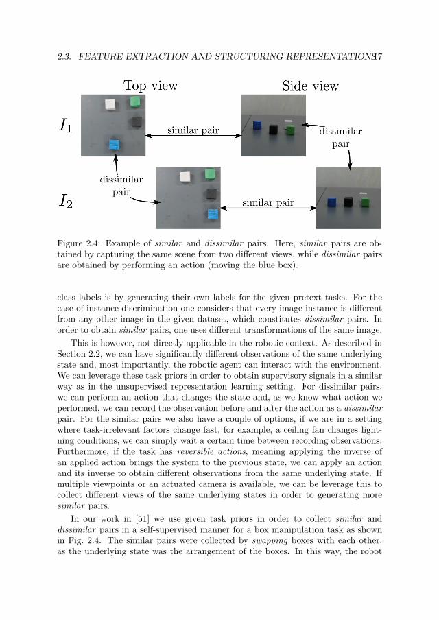
Figure 2.4: Example of similar and dissimilar pairs. Here, similar pairs are ob-tained by capturing the same scene from two different views, while dissimilar pairsare obtained by performing an action (moving the blue box).
class labels is by generating their own labels for the given pretext tasks. For thecase of instance discrimination one considers that every image instance is differentfrom any other image in the given dataset, which constitutes dissimilar pairs. Inorder to obtain similar pairs, one uses different transformations of the same image.
This is however, not directly applicable in the robotic context. As described inSection 2.2, we can have significantly different observations of the same underlyingstate and, most importantly, the robotic agent can interact with the environment.We can leverage these task priors in order to obtain supervisory signals in a similarway as in the unsupervised representation learning setting. For dissimilar pairs,we can perform an action that changes the state and, as we know what action weperformed, we can record the observation before and after the action as a dissimilarpair. For the similar pairs we also have a couple of options, if we are in a settingwhere task-irrelevant factors change fast, for example, a ceiling fan changes light-ning conditions, we can simply wait a certain time between recording observations.Furthermore, if the task has reversible actions, meaning applying the inverse ofan applied action brings the system to the previous state, we can apply an actionand its inverse to obtain different observations from the same underlying state. Ifmultiple viewpoints or an actuated camera is available, we can be leverage this tocollect different views of the same underlying states in order to generating moresimilar pairs.
In our work in [51] we use given task priors in order to collect similar anddissimilar pairs in a self-supervised manner for a box manipulation task as shownin Fig. 2.4. The similar pairs were collected by swapping boxes with each other,as the underlying state was the arrangement of the boxes. In this way, the robot

18 CHAPTER 2. LEARNING STRUCTURED REPRESENTATIONS
could collect the entire dataset in a self-supervised manner. We also establishedthe usefulness of generating additional dissimilar pairs by randomly sampling fromthe full dataset, even if the number of different states is not very high (i.e. ≈ 12).Models that leverage this similar/dissimilar information without relying on anyother type of loss exhibited the most structured representations.
In summary, when aiming for structured representations one wants to havesimilar pairs that are as visually different as possible while still being semanti-cally similar, as well as dissimilar pairs that are visually similar but semanticallydissimilar. When employing task priors and the fact that the agent can activelychange its environment and therefore the state of the system, further structuringof representations becomes possible.
2.4 Evaluation of Frameworks and StructuredRepresentations
Comparing methods and/or frameworks with each other in a fair and unbiased wayis paramount to the continuous improvement of the robotic research field. Whendealing with representation based methods there are two principal options:
1. To compare full resulting framework on standardized task(s).
2. To evaluate the representation directly.
The first option is not only restricted to the case that uses representations intheir framework, but also aims to compare a wider range of methods/frameworkson a representative benchmark task establishing clear rules and defined scoringfunctions. Indeed the prevalence of classification benchmark datasets in the field ofcomputer vision such as the well-known CIFAR-10 [52] and ImageNet [53] datasetsfor object classification, or the Coco [54] and the PASCAL-VOC [55] dataset for seg-mentation, shows that the community makes heavy use of standardized benchmarkdatasets that are accessible to anyone. In the field of robotics, making a datasetor a benchmark has additional challenges, as the goal of most robotic frameworksis to perform a specific task in a limited real-world setting. A method that worksfor one specific task might be unsuitable in another context. For example, whendeveloping grasping methods the success will heavily depend on the objects onewants to grasp. A big step towards standardizing and making approaches morecomparable was the YCB Object and model dataset [56] which is a standardizedset of objects (mostly rigid) that is available to order on the author’s website. Inthis way, different labs can benchmark their methods on the same set of objectsmaking them much more comparable.
In our work in [57] (included as paper C), we followed the YCB benchmarkoutlaid standards and produced a clear protocol for three different tasks consideringtypical deformable object manipulation for cloth. We used widely available andstandardized objects as well as laid out a precise way to score and compare differentapproaches.

2.4. EVALUATION OF FRAMEWORKS AND STRUCTUREDREPRESENTATIONS 19
Figure 2.5: Example of disentanglingfactors of variation, each latent code en-codes a specific factor of variation. Herez0 encodes the color of the box, z1 en-codes the scale, and z2 encodes the ori-entation.
Figure 2.6: Example of a representa-tion space in the shape of a hypersphere,Pushing different classes away from eachother on a hypersphere makes classifi-cation with a linear classifier possible.Figure inspired by [58].
Evaluating representation directly, on the other hand, has its own challenges.By definition, the representations are supposed to be useful for a certain task orrange of tasks, so finding surrogate scores is not a trivial endeavor. One approachthat got popularised in [34] is considering the notion of disentanglement.
The basic notion of disentanglement is illustrated in Fig. 2.5, where three latentcodes (z1, z2, z3) are associated with three underlying factors of variation (color,scale, and orientation). A representation is disentangled if changing a single latentcode results in a change of a single factor of variation i.e. one independent factorof variation or an underlying generative factor is associated with exactly one la-tent code, as defined by the authors in [34]. Over the following years a number ofdisentanglement scores have emerged [59], [60], [61], [62], [63], [64], [65]. However,there is currently no agreement in the community about what score serves best as asurrogate score to evaluate representations. In [66] the authors challenge a numberof common assumptions regarding unsupervised learning of disentangled represen-tations and demonstrate that the random initialization and model parameters canhave a much larger impact than the different models used for learning disentangledrepresentation. While there has been some works leveraging disentangled represen-tation in a reinforcement learning context [67], on the topic of Sim2real transfer[68] , and for predicting out-of-distribution (OOD) performance [69], the benefitsin a real-world robotic manipulation context are currently not established.
A more agreed-upon evaluation protocol in visual unsupervised representation

20 CHAPTER 2. LEARNING STRUCTURED REPRESENTATIONS
learning is to evaluate the representations by the accuracy of a simple linear clas-sifier [40], [45], [41], [46], [42]. The idea is that a representation that facilitatesgood classification results for a simple linear classifier is more useful than one thatneeds a more complex or expressive downstream learner. For example, [58] providesan in-depth analysis on normalizing the representation space onto a hypersphere,where a linear classifier is able to perform well if classes are correctly clustered.This concept is sketched in Fig. 2.6, where different observation instances are clus-tered together, and the different classes are uniformly distributed throughout thehypersphere. The caveat of this method, however, is that it requires ground truthstate labels, while they are readily available in computer classification tasks, or insimulated settings, they are seldom present in more complex robotic manipulationscenarios especially when dealing with deformable objects.
In our work in [51] (included as paper E), we were specifically interested inevaluating the structure of the representations, as well as their utility in a roboticsvisual planning task. Therefore, we propose a two-pronged approach:
i) As the structure we are interested in is very closely related to clusterability,we perform a number of cluster related scores such as recording the number ofclusters, the homogeneity and completeness [70], as well as the mean silhouettecoefficient [71], whereof the latter does not rely on ground truth labels.
ii) The planning performance is evaluated on our Latent Space Roadmap (LSR)framework [72] (paper X-3, not included) and the assumption that all potentialactions are always correct. With this setup, we compared the effect of differentkinds of loss functions. Namely we showed that a contrastive loss is more beneficialin the context of visual task planning in robotics than a reconstruction based one.
2.5 Latent Space Roadmap - An Example of a CombinedFramework
Our work presented in [73] (included as paper B ,currently under review) which isan extended version of our work presented in [72] (not included paper X-3) givesan example of a combined framework that learns representations and then employsthem in order to perform rigid and deformable object manipulation. An overviewof the framework is shown in Fig. 2.7, which consists of three components:
i) A Mapping Module ξ, which takes a start and goal observation and maps theminto the latent space Z. We realized this map ξ with a VAE where we added anadditional contrastive loss term (called action loss in [73]) that makes use of themanually obtained similar/dissimilar pairs information in order to produce a morestructured representation. We established that adding a contrastive term improvesthe structure of the latent space in our work in [51] (included as paper E (underreview)), however an important point in the provided framework is that we producevisual action plans, and we therefore decode any given latent representation with adecoder ω.

2.5. LATENT SPACE ROADMAP - AN EXAMPLE OF A COMBINEDFRAMEWORK 21
Figure 2.7: Overview of our LSR framework, consisting of the Mapping Module ξ,the Latent Space Roadmap (LSR), and the Action Proposal Module. The frame-work takes in a start and goal observation and produces a visual action plan thatcontains the intermediate observations and actions needed to reach the desired goalconfiguration (Figure is excerpt from our work in [73]).
ii) The Latent Space Roadmap (LSR) which is a graph built directly inside thelatent space where the nodes ideally represent the underlying states and the edgesrepresent possible transitions. It is constructed in three phases: a) in the first phasea reference graph is constructed using the information if a pair in the dataset is asimilar pair (no edge is built between them) or a dissimilar pair (an edge is built).b) For the second phase, the latent space is clustered using agglomerative clustering,we measure the distance of inter-cluster dissimilarity using the unweighted averagedistance between points in the considered clusters. The final clustering is then ob-tained by applying the clustering threshold τ to the obtained stepwise dendrogram,as shown in Fig. 2.8 top right. c) In the last phase, the LSR is built where eachcluster obtained in the previous phase corresponds to a node in the LSR, and theyare connected if there is an edge between the individual pairs (as obtained in phasea) located inside different clusters. We can have an optional additional pruning stepthat removes nodes that only have a certain number of data points as members oredges that have less than a specified number of edges connecting the same nodes.This step can be helpful if the collected training data is noisy and contains outliers.
The attentive reader might have noticed that the performance of the cluster-ing heavily depends on the clustering threshold τ , which is not trivial to tune andsubject to ongoing research [74], [75]. For this reason, we propose an outer op-timization loop that substitutes the hard-to-tune τ hyperparameter with a muchmore robust and easier to tune parameter cmax. In our outer optimization, weanalyze the number of edges as a measurement of LSR quality and optimize for a τthat gives the most edges in the LSR while having fewer than cmax separate graphconnected components. The intuitive motivation is that we want to have an LSRthat is well connected, and therefore should have many edges. But we also wantto have only a limited number of connected components as this lowers the connec-tivity significantly without affecting the total number of edges. When optimizing

22 CHAPTER 2. LEARNING STRUCTURED REPRESENTATIONS
Figure 2.8: Illustration of the outer optimisation for the clustering threshold τ . Areference graph (top left) results in a stepwise dendogram after applying agglom-erative clustering. The different thresholds τ1, τ2, and τ3 results in different LSRs.(Figure is excerpt from our work in [73])
with a set hyperparameter we can obtain an LSR that is very well connected andconsists of at least one large connected component. When employing a very low τthe LSR receives more edges but a large number of disconnected components, whileif τ is large it exhibits few disconnected components but also few edges. Fig. 2.8shows this principle. On the top row we see the reference graph and the resultingstepwise dendrogram. This dendrogram can then be cut by the clustering thresholdτ resulting in different LSRs (shown on the bottom row). The diamond markersindicate separate nodes while the edges are visualized with connecting black lines.We can see that the left most LSR (τ1) has the most edges but also two connectedcomponents, while the τ2 and τ3 result in a single connected component where τ2
obtains more edges.
iii) The final part of the framework is the action proposal model, which takes asinput a latent plan, produced by the LSR, and proposes actions to translate fromone state to the next. In our case, we employed a Multilayer Perceptron networktrained on the representations obtained with the mapping ξ. Note that it is alsopossible to integrate the action proposal directly into the LSR, for example, a simplebaseline action can be obtained by averaging the actions associated with each edge

2.5. LATENT SPACE ROADMAP - AN EXAMPLE OF A COMBINEDFRAMEWORK 23
Figure 2.9: Different tasks addressed with the LSR framework. A rigid box stackingtask in two variants shown in a), a hybrid rope-box manipulation task shown in b),and a folding task on a highly deformable object in c).
in the reference graph into the corresponding edges in the LSR.Overall the framework uses these three components to obtain visual action plans
that can be executed on a real robotic system. This framework works best in thesetting where the feasible states of the system are finite and can be distinguishedfrom each other in such a way that unambiguous actions to transition between themcan be defined. We extensively evaluated and showcased the performance of thisframework on three different tasks (shown in Fig. 2.9), namely a rigid box stackingtask, a hybrid rope-box task where two boxes are connected with a rope, and areal-world T-shirt folding task.


Chapter 3
An Overview of Publications
A general overview of the published papers (included and not-included in this thesis)is shown in Fig. 3.1. This will serve as an overall orientation, highlighting the linksbetween different publications and how they contributed by addressing the specificquestions asked in this thesis. Papers that are not included in this thesis are shownwith a purple background and marked with X-1 to X-5, while works included areappearing with a green background and labeled with the letters A-E.
Paper X-1 “From visual understanding to complex object manipulation” [76]gave an overview of the whole manipulation pipeline that is required to successfullymanipulate objects. The process starts with a visual step where relevant objectsand obstacles need to be identified, it continues with a planning step taking intoaccount the environment as well as the constraints imposed by the capabilitiesof the manipulator, the follow-up step is sensor feedback where several potentialsources of information like tactile readings or visual feedback can be considered.The final step is then the manipulation itself, where the grasped object is put intothe desired configuration or employed as a tool. The project gave a good overviewof the challenges to overcome when realizing such a system in the real world as wellas insights into each step required to successfully perform object manipulation.
One part that was of tangential interest was how a real-world vision systemspecialized for cloth manipulation could be realized and how to address the spe-cific scene encountered in robotic cloth manipulation. The resulting publicationX-4 “Fashion Landmark Detection and Category Classification for Robotics” [77]presents an elastic warping method to augment training data found in large fash-ion datasets to make them more relevant for a robotic context. It furthermoreinvestigated how robust landmark detection is under occlusion from a robotic arm.
Paper A “Partial caging: a clearance-based definition, datasets and deep learn-ing” [43] is the extended version of paper X-2. This paper is directly relevant forthe thesis as we are using a VAE trained on known objects to then encode novel ob-jects, select the closest known objects in the latent space and propose high-qualitypartial cages inspired by the known object for the novel object. Here the latentspace generated by the VAE was used in order to facilitate a different downstream
25

26 CHAPTER 3. AN OVERVIEW OF PUBLICATIONS
Figu
re3.1:
Overview
ofpublication
s.P
hD
startedw
ithth
etw
oprojects
inth
etop
leftcorn
er.T
he
arrows
symb
olisehigh
levelqu
estions
that
where
explored
and
ledto
the
subsequ
entpublication
s.Item
sw
ithgreen
backgrou
nd
arein
cluded
inth
isth
esisw
hile
items
with
purp
leare
not.

27
task (partial cage acquisition). Our findings however showed that while the use ofrepresentation was significantly faster compared to the Hamming distance from thenovel object to any other known object, the quality of the proposed partial cageswas higher using the Hamming distance compared to using the representation ofthe VAE. This showed that while representations are a promising direction oneneeds to introduce more structure that shapes the latent representation to a morefavorable state given the downstream tasks.
The lessons learned from paper X-1 regarding the real-world challenges and theusefulness of representations for downstream tasks from paper A laid the ground-work for paper X-3 “Latent Space Roadmap for visual action planning of deformableand rigid object manipulation” [72]. In this work, the core question was how tolearn structured representation as well as how to leverage it into a real-world sys-tem that is able to complete challenging robotic tasks like folding. We tackledthe problem of visual action planning where given a start and goal observation avisual action plan is produced that shows the planned steps as well as the actionsrequired to traverse from the start state to the desired goal state. We leveraged thetask priors that, when successfully performing an action, the subsequent state isdifferent from the initial one but the same if only minor changes are performed thatdo not change the underlying state. This knowledge is leveraged when generatingthe representation space using a VAE. We augmented the loss function of the VAEto include a contrastive term that pushes pairs of states that are dissimilar apartand contracts pairs of states that are similar. Using this representation the LSRwas built in the latent space by first performing clustering and then connectingthe cluster with edges representing the possible actions observed in the trainingdataset. We validated our LSR method on a simulated box stacking and real-worldshirt folding task. While this project addresses the core of the thesis, there weremany open questions: i) how to best achieve the mapping from observation intorepresentation space? Is a VAE the only option? ii) Which clustering methodfor building the LSR is most suited? Can the clustering hyperparameter be au-tomatically tuned? iii) How does the method compare to other methods? Whatare the limitations of the framework and can it perform on tasks where rigid anddeformable objects are combined? This questions directly relates to the LSR andare subsequently addressed in paper B. However, there were also more fundamentalquestions arising that are also relevant for the overall topic of this thesis. Namely,iv) how can one compare different cloth manipulation systems? v) Can additionalsensory readings be leveraged to gain more insights about the clothing items? Andvi) can specific task constraints be incorporated into the framework?
Question i-iii were answered in paper B “Enabling Visual Action Planning forObject Manipulation through Latent Space Roadmap” [73], where the frameworkis split into three distinct parts, a Mapping Module that can be realized withany encoder like model (we compared AE with VAE), the LSR built with a newcore clustering algorithm (unweighted average linkage) as well as the inclusion ofan outer optimization loop with easier-to-tune hyperparameters, and finally theAction Proposal Model realizable with either simple average action aggregations

28 CHAPTER 3. AN OVERVIEW OF PUBLICATIONS
or any neural network. Furthermore, an additional hard box stacking task wasintroduced to complement the normal box stacking task and make the ablationstudy more relevent and wider in scope. A new hybrid task, where two boxes areconnected with a deformable rope is also added. In this work, we showed extensivelyhow a system that learns structured representation is used for simulated rigid andreal-world deformable object manipulation.
Our work presented in paper C “Benchmarking Bimanual Cloth Manipulation”[57] takes a step towards resolving question iv), of how to compare different meth-ods/systems. We proposed a benchmark featuring three standardized tasks, spread-ing a tablecloth, folding a towel, and a dressing task. The tasks were designed insuch a way that they are easily reproducible and come with a consistent scoringprotocol that allows to benchmark and compare different approaches against eachother. Defining standardized tasks in a reproducible and comparable way is animportant step to make it easier to evaluate and compare different methods. It alsohighlights the strengths and weaknesses in a standardized manner such that futureresearch can be easily extended and improve existing approaches.
When dealing with deformable objects any information the system can obtainthanks to additional sensory readings might be of great benefit. In the specificcase of cloth manipulation, inferring the dynamic behavior by knowing somethingabout the material or construction techniques could be of significant benefit. In ourwork presented in paper D “Textile Taxonomy and Classification Using Pulling andTwisting” [78] we take a step towards this direction. First we introduced a taxonomythat not only considers the material of garments but also the constructing techniquesuch as if it is woven or knitted. We postulated that the construction techniqueplays a significant factor in the dynamics of garments that have not been consideredin prior work. In a small-scale experiment, we demonstrated that one can infer theconstruction technique with higher accuracy than the material using force/torquereadings and pulling actions.
The final question, whether specific task constraints can be incorporated, wasconsidered in our work published in paper X-5 “Learning Task Constraints in VisualAction Planning from Demonstration” [79], where we used Linear Temporal Logic(LTL) formulation to label demonstrated sequences that either fulfill the givenconstraint or not. An Long short-term memory (LSTM)-model [80] was then usedto distinguish between the binary case. Different LTL-formulated constraints canbe acquired this way and then combined with simple logical operators such as ANDor OR to combine simple constraints into more complex ones.
While we performed an extensive ablation study in paper B, the nature ofdeveloping a full system with many components is that one does not have the spaceto extensively analyse every aspect of such a framework. While we showed that aVAE is a more suitable mapping module than an AE for the tasks considered, wedid not perform a fundamental analysis that compared models based on the type ofloss function they employ and their usefulness for higher-level planning tasks. Thisis addressed in paper E “Comparing Reconstruction-and Contrastive-based Modelsfor Visual Task Planning” [51] (currently under review) where we first analyzed

29
an extensive body of related work and discovered that despite the introductionof contrasting losses in 2006, many current state-of-the-art methods and proposedframeworks still rely on the reconstruction loss. We performed a systematic studycomparing seven different models that either employed pure reconstruction loss,reconstruction- and KL-loss, pure contrastive loss, of a combination of the threedifferent loss types. We evaluated the models on three different visual planning taskswhere irrelevant factors of variations are present in the observations given to thesystem. We showed that purely contrastive-based losses are best suited to addresssuch tasks especially if observations of the same underlying state can significantlydiffer from each other because of task-irrelevant factors such as distractor objects,or different view angles.


Chapter 4
Conclusion and Future Work
In this thesis, we looked at how to learn representation for rigid and deformableobject manipulation. We presented our work and the contribution on learningstructured representations for rigid and deformable object manipulation, concludingwith a framework incorporating the lessens learned that was successfully appliedto tasks from the rigid, hybrid, and deformable object manipulation domain. Toconclude this thesis we will shortly highlight potential future work that expandsthe lessons learned and try to uncover more relevant insights.
4.1 Cage-Flow - A Flow-based Cage Proposal Model
The mapping ξ : O → Z considered so far was predominantly modeled using aVAE wich optimizes the evidence lower bound (ELBO). There exists however adifferent group of likelihood-based generative models - namely normalizing flowmodels [81], [82], [83]. In normalizing flow models, the goal is to map a simpledistribution (one that can easily be sampled from) to a more complex one (inferredfrom the data). A core difference to VAEs is that the mapping from observationspace O to the representation space Z is deterministic and invertible. A flow-based model therefore directly approximates the distribution of the given trainingdata. Flow-based models have been successfully applied in many domains like videogeneration [84], graph generation [85], and reinforcement learning [86], [87].
In our future work, we want to employ normalizing flow model to predict promis-ing cages for 2D and 3D objects, as well as investigate the estimated distributions.Another interesting aspect we want to consider is that cages can be represented indifferent ways. Therefore, an additional goal is to examine what kind of cage repre-sentations is most suitable for flow-based models. In order to achieve this goal, weproduce a number of promising cages on randomly generated objects (so far only2D), by employing a number of handcrafted heuristics such as placing a caging toolinside the symmetric difference of the object and it’s convex-hull, perpendicular tothe longest line, on opposite sides of the predominate object axis, and more. Werepresent these cages as geometric graphs with a central anchor node and define
31

32 CHAPTER 4. CONCLUSION AND FUTURE WORK
Figure 4.1: Example of 2D cages, represented as a graph having a center anchor-node. The cages where obtained employing a number of handcrafted heuristics.
the location of the caging points using polar coordinates. Another potential rep-resentation is a simple set of points in planar coordinates. Fig. 4.1 shows someexamples of cages obtained using the mentioned heuristics with varying amountsof caging points.
Our next step is to train a conditional flow-based model on either the graphstructure or the set of points representations while conditioning it on the object tobe caged. In detail, we plan to investigate the following questions:
1. Can promising caging configuration for novel objects be obtained for 2D and3D objects using Cage-Flow?
2. How does the estimated distribution change when adding more objects orcaging tools to the training data?
4.2 Hierarchical-LSR - A LSR framework for ContinuousProblems
The current LSR framework has been successfully applied to different domains anda number of diverse tasks. It works best in the setting of higher-level planning em-ploying action primitives, and considering systems that have a relatively low numberof clearly separated underlying states. We are planning to expand this frameworkalso to tasks of a more continuous nature. The problem of separating states canbe seen as a discretization problem with multiple layers, where the higher levelcorresponds to the current application of the LSR. A potential approach would beto develop a hierarchical approach where states are further discretized, for exam-ple, the highest level describes the arrangement of boxes while at a lower level thestate descriptor identifies the rotation or exact position. Such a framework couldbe employed to solve a wider range of tasks than the current one presented in thisthesis.
Furthermore, we are planning to investigate how to integrate the LSR in areinforcement learning setting. We plan to build an initial LSR and based on thisdecide what kind of states transitions are needed, actively explore those, and extendthe LSR step by step. Such an approach could also be leveraged to find shortcutsbetween states, currently, we can only transition between states with actions thathave been observed in the training data, however, there are some problem settings

4.2. HIERARCHICAL-LSR - A LSR FRAMEWORK FOR CONTINUOUSPROBLEMS 33
where the action observed between two different states could also be generalizedonto a different pair of states. An LSR explorer could attempt to traverse from onestate to another with the most promising action and extend the connectivity of theLSR in this way.
In conclusion, this thesis provided a step towards learning structured representa-tions for rigid and deformable object manipulation, by answering relevant researchquestions as well as advancing the state of the art with the new Latent SpaceRoadmap method.


Bibliography
[1] Y. Huang, M. Bianchi, M. Liarokapis, and Y. Sun, “Recent data sets on objectmanipulation: A survey,” Big data, vol. 4, no. 4, pp. 197–216, 2016.
[2] L. Jing and Y. Tian, “Self-supervised visual feature learning with deep neu-ral networks: A survey,” IEEE transactions on pattern analysis and machineintelligence, 2020.
[3] H. Yin, A. Varava, and D. Kragic, “Modeling, learning, perception, and controlmethods for deformable object manipulation,” Science Robotics, vol. 6, no. 54,2021.
[4] F. Faure, C. Duriez, H. Delingette, J. Allard, B. Gilles, S. Marchesseau, H. Tal-bot, H. Courtecuisse, G. Bousquet, I. Peterlik et al., “Sofa: A multi-modelframework for interactive physical simulation,” in Soft tissue biomechanicalmodeling for computer assisted surgery. Springer, 2012, pp. 283–321.
[5] X. Lin, Y. Wang, J. Olkin, and D. Held, “Softgym: Benchmarking deep rein-forcement learning for deformable object manipulation,” 2020.
[6] E. Todorov, T. Erez, and Y. Tassa, “Mujoco: A physics engine for model-basedcontrol,” in 2012 IEEE/RSJ International Conference on Intelligent Robotsand Systems. IEEE, 2012, pp. 5026–5033.
[7] E. Coumans and Y. Bai, “Pybullet, a python module for physics simulationfor games, robotics and machine learning,” http://pybullet.org, 2016–2021.
[8] “Nvidia, physx sdk,” https://developer.nvidia.com/physx-sdk, accessed: 2021-09-29.
[9] V. Mnih, K. Kavukcuoglu, D. Silver, A. Graves, I. Antonoglou, D. Wierstra,and M. Riedmiller, “Playing atari with deep reinforcement learning,” 2013,cite arxiv:1312.5602Comment: NIPS Deep Learning Workshop 2013. [Online].Available: http://arxiv.org/abs/1312.5602
[10] V. Mnih, K. Kavukcuoglu, D. Silver, A. A. Rusu, J. Veness, M. G. Bellemare,A. Graves, M. Riedmiller, A. K. Fidjeland, G. Ostrovski et al., “Human-levelcontrol through deep reinforcement learning,” nature, vol. 518, no. 7540, pp.529–533, 2015.
35

36 BIBLIOGRAPHY
[11] T. P. Lillicrap, J. J. Hunt, A. Pritzel, N. M. O. Heess, T. Erez, Y. Tassa, D. Sil-ver, and D. Wierstra, “Continuous control with deep reinforcement learning,”CoRR, vol. abs/1509.02971, 2016.
[12] M. Andrychowicz, D. Crow, A. Ray, J. Schneider, R. Fong, P. Welinder, B. Mc-Grew, J. Tobin, P. Abbeel, and W. Zaremba, “Hindsight experience replay,”2017.
[13] J. Schulman, F. Wolski, P. Dhariwal, A. Radford, and O. Klimov,“Proximal policy optimization algorithms.” CoRR, vol. abs/1707.06347,2017. [Online]. Available: http://dblp.uni-trier.de/db/journals/corr/corr1707.html#SchulmanWDRK17
[14] S. Levine, N. Wagener, and P. Abbeel, “Learning contact-rich manipulationskills with guided policy search,” 2015 IEEE International Conference onRobotics and Automation (ICRA), pp. 156–163, 2015.
[15] J. Matas, S. James, and A. J. Davison, “Sim-to-real reinforcement learning fordeformable object manipulation,” in Conference on Robot Learning. PMLR,2018, pp. 734–743.
[16] M. Watter, J. T. Springenberg, J. Boedecker, and M. A. Riedmiller, “Embed tocontrol: A locally linear latent dynamics model for control from raw images,”2015.
[17] D. P. Kingma and M. Welling, “Auto-encoding variational bayes,” CoRR, vol.abs/1312.6114, 2014.
[18] S. Kullback and R. A. Leibler, “On information and sufficiency,” The annalsof mathematical statistics, vol. 22, no. 1, pp. 79–86, 1951.
[19] D. Hafner, T. Lillicrap, I. Fischer, R. Villegas, D. Ha, H. Lee, and J. Davidson,“Learning latent dynamics for planning from pixels,” in International Confer-ence on Machine Learning. PMLR, 2019, pp. 2555–2565.
[20] R. Y. Rubinstein, “Optimization of computer simulation models with rareevents,” European Journal of Operational Research, vol. 99, no. 1, pp. 89–112,1997.
[21] K. Chua, R. Calandra, R. McAllister, and S. Levine, “Deep reinforcementlearning in a handful of trials using probabilistic dynamics models,” 2018.
[22] B. Ichter and M. Pavone, “Robot motion planning in learned latent spaces,”IEEE Robotics and Automation Letters, vol. 4, no. 3, pp. 2407–2414, 2019.
[23] D. H. Ballard, “Modular learning in neural networks.” in AAAI, vol. 647, 1987,pp. 279–284.

BIBLIOGRAPHY 37
[24] N. Savinov, A. Dosovitskiy, and V. Koltun, “Semi-parametric topological mem-ory for navigation,” 2018.
[25] C. Finn and S. Levine, “Deep visual foresight for planning robot motion,”in 2017 IEEE International Conference on Robotics and Automation (ICRA).IEEE, 2017, pp. 2786–2793.
[26] S. Nair and C. Finn, “Hierarchical foresight: Self-supervised learning of long-horizon tasks via visual subgoal generation,” International Conference onLearning Representations (ICLR), 2020.
[27] A. Wang, T. Kurutach, K. Liu, P. Abbeel, and A. Tamar, “Learning roboticmanipulation through visual planning and acting,” Robotics: Science and Sys-tems (RSS), 2019.
[28] M. Yan, Y. Zhu, N. Jin, and J. Bohg, “Self-supervised learning of state estima-tion for manipulating deformable linear objects,” IEEE robotics and automa-tion letters, vol. 5, no. 2, pp. 2372–2379, 2020.
[29] K. Simonyan and A. Zisserman, “Very deep convolutional networks for large-scale image recognition,” CoRR, vol. abs/1409.1556, 2015.
[30] M. Jaderberg, K. Simonyan, A. Zisserman et al., “Spatial transformer net-works,” Advances in neural information processing systems, vol. 28, pp. 2017–2025, 2015.
[31] W. Yan, A. Vangipuram, P. Abbeel, and L. Pinto, “Learning predictive repre-sentations for deformable objects using contrastive estimation,” CoRL, 2020.
[32] A. van den Oord, Y. Li, and O. Vinyals, “Representation learning withcontrastive predictive coding,” CoRR, vol. abs/1807.03748, 2018. [Online].Available: http://arxiv.org/abs/1807.03748
[33] R. Hoque, D. Seita, A. Balakrishna, A. Ganapathi, A. Tanwani, N. Jamali,K. Yamane, S. Iba, and K. Goldberg, “VisuoSpatial Foresight for Multi-Step,Multi-Task Fabric Manipulation,” 2020.
[34] Y. Bengio, A. Courville, and P. Vincent, “Representation learning: A reviewand new perspectives,” IEEE transactions on pattern analysis and machineintelligence, vol. 35, no. 8, pp. 1798–1828, 2013.
[35] T. Lesort, N. Díaz-Rodríguez, J.-F. Goudou, and D. Filliat, “State representa-tion learning for control: An overview,” Neural Networks, vol. 108, pp. 379–392,2018.
[36] W. Böhmer, J. T. Springenberg, J. Boedecker, M. Riedmiller, and K. Ober-mayer, “Autonomous learning of state representations for control: An emerg-ing field aims to autonomously learn state representations for reinforcement

38 BIBLIOGRAPHY
learning agents from their real-world sensor observations,” KI-Künstliche In-telligenz, vol. 29, no. 4, pp. 353–362, 2015.
[37] M. Noroozi and P. Favaro, “Unsupervised learning of visual representations bysolving jigsaw puzzles,” in European conference on computer vision. Springer,2016, pp. 69–84.
[38] D. Pathak, R. Girshick, P. Dollár, T. Darrell, and B. Hariharan, “Learningfeatures by watching objects move,” in Proceedings of the IEEE Conference onComputer Vision and Pattern Recognition, 2017, pp. 2701–2710.
[39] Z. Wu, Y. Xiong, S. X. Yu, and D. Lin, “Unsupervised feature learning via non-parametric instance discrimination,” in Proceedings of the IEEE conference oncomputer vision and pattern recognition, 2018, pp. 3733–3742.
[40] T. Chen, S. Kornblith, M. Norouzi, and G. Hinton, “A simple framework forcontrastive learning of visual representations,” in International conference onmachine learning. PMLR, 2020, pp. 1597–1607.
[41] K. He, H. Fan, Y. Wu, S. Xie, and R. Girshick, “Momentum contrast forunsupervised visual representation learning,” in Proceedings of the IEEE/CVFConference on Computer Vision and Pattern Recognition, 2020, pp. 9729–9738.
[42] M. Caron, I. Misra, J. Mairal, P. Goyal, P. Bojanowski, and A. Joulin, “Unsu-pervised learning of visual features by contrasting cluster assignments,” 2020.
[43] M. C. Welle, A. Varava, J. Mahler, K. Goldberg, D. Kragic, and F. T. Pokorny,“Partial caging: a clearance-based definition, datasets, and deep learning,”Autonomous Robots, pp. 1–18, 2021.
[44] A. Varava, M. C. Welle, J. Mahler, K. Goldberg, D. Kragic, and F. T.Pokomy, “Partial caging: A clearance-based definition and deep learning,” in2019 IEEE/RSJ International Conference on Intelligent Robots and Systems(IROS). IEEE, 2019, pp. 1533–1540.
[45] T. Chen, S. Kornblith, K. Swersky, M. Norouzi, and G. E. Hin-ton, “Big self-supervised models are strong semi-supervised learners,”2020. [Online]. Available: https://proceedings.neurips.cc/paper/2020/hash/fcbc95ccdd551da181207c0c1400c655-Abstract.html
[46] J.-B. Grill, F. Strub, F. Altché, C. Tallec, P. Richemond, E. Buchatskaya,C. Doersch, B. Avila Pires, Z. Guo, M. Gheshlaghi Azar, B. Piot,k. kavukcuoglu, R. Munos, and M. Valko, “Bootstrap your own latent- a new approach to self-supervised learning,” vol. 33, pp. 21 271–21 284,2020. [Online]. Available: https://proceedings.neurips.cc/paper/2020/file/f3ada80d5c4ee70142b17b8192b2958e-Paper.pdf

BIBLIOGRAPHY 39
[47] M. Kang and J. Park, “ContraGAN: Contrastive Learning for ConditionalImage Generation,” Conference on Neural Information Processing Systems(NeurIPS), 2020.
[48] T. Xiao, X. Wang, A. A. Efros, and T. Darrell, “What shouldnot be contrastive in contrastive learning,” 2021. [Online]. Available:https://openreview.net/forum?id=CZ8Y3NzuVzO
[49] X. Chen and K. He, “Exploring simple siamese representation learning,” inProceedings of the IEEE/CVF Conference on Computer Vision and PatternRecognition, 2021, pp. 15 750–15 758.
[50] M. Laskin, A. Srinivas, and P. Abbeel, “Curl: Contrastive unsupervisedrepresentations for reinforcement learning,” Proceedings of the 37th Interna-tional Conference on Machine Learning, Vienna, Austria, PMLR 119, 2020,arXiv:2004.04136.
[51] C. Chamzas, M. Lippi, M. C. Welle, A. Varava, L. E. Kavraki, and D. Kragic,“Comparing reconstruction-and contrastive-based models for visual task plan-ning,” arXiv preprint arXiv:2109.06737, 2021.
[52] A. Krizhevsky and G. Hinton, “Learning multiple layers of features from tinyimages,” no. 0, 2009.
[53] O. Russakovsky, J. Deng, H. Su, J. Krause, S. Satheesh, S. Ma, Z. Huang,A. Karpathy, A. Khosla, M. Bernstein et al., “Imagenet large scale visualrecognition challenge,” International journal of computer vision, vol. 115, no. 3,pp. 211–252, 2015.
[54] T.-Y. Lin, M. Maire, S. Belongie, J. Hays, P. Perona, D. Ramanan, P. Dollár,and C. L. Zitnick, “Microsoft coco: Common objects in context,” in Europeanconference on computer vision. Springer, 2014, pp. 740–755.
[55] M. Everingham, L. Van Gool, C. K. I. Williams, J. Winn,and A. Zisserman, “The PASCAL Visual Object ClassesChallenge 2012 (VOC2012) Results,” http://www.pascal-network.org/challenges/VOC/voc2012/workshop/index.html.
[56] B. Calli, A. Singh, A. Walsman, S. Srinivasa, P. Abbeel, and A. M. Dollar,“The ycb object and model set: Towards common benchmarks for manipula-tion research,” in 2015 international conference on advanced robotics (ICAR).IEEE, 2015, pp. 510–517.
[57] I. Garcia-Camacho, M. Lippi, M. C. Welle, H. Yin, R. Antonova, A. Varava,J. Borras, C. Torras, A. Marino, G. Alenya et al., “Benchmarking bimanualcloth manipulation,” IEEE Robotics and Automation Letters, vol. 5, no. 2, pp.1111–1118, 2020.

40 BIBLIOGRAPHY
[58] T. Wang and P. Isola, “Understanding contrastive representation learningthrough alignment and uniformity on the hypersphere,” in International Con-ference on Machine Learning. PMLR, 2020, pp. 9929–9939.
[59] I. Higgins, L. Matthey, A. Pal, C. P. Burgess, X. Glorot, M. M. Botvinick,S. Mohamed, and A. Lerchner, “beta-vae: Learning basic visual concepts witha constrained variational framework,” 2017.
[60] H. Kim and A. Mnih, “Disentangling by factorising,” in International Confer-ence on Machine Learning. PMLR, 2018, pp. 2649–2658.
[61] A. Kumar, P. Sattigeri, and A. Balakrishnan, “Variational inference ofdisentangled latent concepts from unlabeled observations,” CoRR, vol.abs/1711.00848, 2017. [Online]. Available: http://arxiv.org/abs/1711.00848
[62] T. Q. Chen, X. Li, R. Grosse, and D. Duvenaud, “Isolating sourcesof disentanglement in variational autoencoders,” 2018. [Online]. Available:https://openreview.net/forum?id=BJdMRoCIf
[63] C. Eastwood and C. K. Williams, “A framework for the quantitative evalua-tion of disentangled representations,” in International Conference on LearningRepresentations, 2018.
[64] K. Ridgeway and M. C. Mozer, “Learning deep disentangled embeddings withthe f-statistic loss,” 2018.
[65] R. Suter, D. Miladinovic, B. Schölkopf, and S. Bauer, “Robustly disentangledcausal mechanisms: Validating deep representations for interventional robust-ness,” in International Conference on Machine Learning. PMLR, 2019, pp.6056–6065.
[66] F. Locatello, S. Bauer, M. Lucic, G. Raetsch, S. Gelly, B. Schölkopf, andO. Bachem, “Challenging common assumptions in the unsupervised learning ofdisentangled representations,” in international conference on machine learning.PMLR, 2019, pp. 4114–4124.
[67] I. Higgins, A. Pal, A. Rusu, L. Matthey, C. Burgess, A. Pritzel, M. Botvinick,C. Blundell, and A. Lerchner, “Darla: Improving zero-shot transfer in re-inforcement learning,” in International Conference on Machine Learning.PMLR, 2017, pp. 1480–1490.
[68] M. W. Gondal, M. Wuthrich, D. Miladinovic, F. Locatello, M. Breidt,V. Volchkov, J. Akpo, O. Bachem, B. Schölkopf, and S. Bauer, “Onthe transfer of inductive bias from simulation to the real world: a newdisentanglement dataset,” in NeurIPS, 2019, pp. 15 714–15 725.

BIBLIOGRAPHY 41
[69] A. Dittadi, F. Träuble, F. Locatello, M. Wuthrich, V. Agrawal, O. Winther,S. Bauer, and B. Schölkopf, “On the transfer of disentangled representationsin realistic settings,” in International Conference on Learning Representations,2021. [Online]. Available: https://openreview.net/forum?id=8VXvj1QNRl1
[70] A. Rosenberg and J. Hirschberg, “V-measure: A conditional entropy-based ex-ternal cluster evaluation measure,” in Proceedings of the 2007 joint conferenceon empirical methods in natural language processing and computational naturallanguage learning (EMNLP-CoNLL), 2007, pp. 410–420.
[71] P. J. Rousseeuw, “Silhouettes: a graphical aid to the interpretation and vali-dation of cluster analysis,” Journal of computational and applied mathematics,vol. 20, pp. 53–65, 1987.
[72] M. Lippi, P. Poklukar, M. C. Welle, A. Varava, H. Yin, A. Marino, andD. Kragic, “Latent space roadmap for visual action planning of deformableand rigid object manipulation,” in 2020 IEEE/RSJ International Conferenceon Intelligent Robots and Systems (IROS). IEEE, 2020, pp. 5619–5626.
[73] ——, “Enabling visual action planning for object manipulation through latentspace roadmap,” arXiv preprint arXiv:2103.02554, 2021.
[74] D. Bruzzese and D. Vistocco, “Despota: Dendrogram slicing through a pemu-tation test approach,” Journal of classification, vol. 32, no. 2, pp. 285–304,2015.
[75] A. Pasini, E. Baralis, P. Garza, D. Floriello, M. Idiomi, A. Ortenzi, andS. Ricci, “Adaptive hierarchical clustering for petrographic image analysis.”in EDBT/ICDT Workshops, 2019.
[76] J. Bütepage, S. Cruciani, M. Kokic, M. Welle, and D. Kragic, “From visualunderstanding to complex object manipulation,” Annual Review of Control,Robotics, and Autonomous Systems, vol. 2, pp. 161–179, 2019.
[77] T. Ziegler, J. Butepage, M. C. Welle, A. Varava, T. Novkovic, and D. Kragic,“Fashion landmark detection and category classification for robotics,” in 2020IEEE International Conference on Autonomous Robot Systems and Competi-tions (ICARSC). IEEE, 2020, pp. 81–88.
[78] A. Longhini, M. C. Welle, I. Mitsioni, and D. Kragic, “Textile taxonomy andclassification using pulling and twisting,” 2021 IEEE/RSJ International Con-ference on Intelligent Robots and Systems (IROS), 2021.
[79] F. Esposito, C. Pek, M. C. Welle, and D. Kragic, “Learning task constraintsin visual-action planning from demonstrations,” in 2021 30th IEEE Interna-tional Conference on Robot & Human Interactive Communication (RO-MAN).IEEE, 2021, pp. 131–138.

42 BIBLIOGRAPHY
[80] S. Hochreiter and J. Schmidhuber, “Long short-term memory,” Neural compu-tation, vol. 9, no. 8, pp. 1735–1780, 1997.
[81] D. Rezende and S. Mohamed, “Variational inference with normalizing flows,”in International conference on machine learning. PMLR, 2015, pp. 1530–1538.
[82] I. Kobyzev, S. Prince, and M. Brubaker, “Normalizing flows: An introductionand review of current methods,” IEEE Transactions on Pattern Analysis andMachine Intelligence, 2020.
[83] G. Papamakarios, E. Nalisnick, D. J. Rezende, S. Mohamed, and B. Laksh-minarayanan, “Normalizing flows for probabilistic modeling and inference,”Journal of Machine Learning Research 22 (2021) 1-64, 2021.
[84] M. Kumar, M. Babaeizadeh, D. Erhan, C. Finn, S. Levine, L. Dinh, andD. Kingma, “Videoflow: A conditional flow-based model for stochastic videogeneration,” 2020. [Online]. Available: https://openreview.net/forum?id=rJgUfTEYvH
[85] K. Madhawa, K. Ishiguro, K. Nakago, and M. Abe, “Graph{nvp}: aninvertible flow-based model for generating molecular graphs,” 2020. [Online].Available: https://openreview.net/forum?id=ryxQ6T4YwB
[86] B. Mazoure, T. Doan, A. Durand, J. Pineau, and R. D. Hjelm, “Leveragingexploration in off-policy algorithms via normalizing flows,” in Conference onRobot Learning. PMLR, 2020, pp. 430–444.
[87] P. N. Ward, A. Smofsky, and A. J. Bose, “Improving exploration in soft-actor-critic with normalizing flows policies,” INNF workshop, InternationalConference on Machine Learning 2019, 2019.

Part II
Included Publications
43


Paper A


Paper A
Partial Caging: A Clearance-Based
Definition, Datasets, and Deep Learning
Michael C. Welle, Anastasiia Varava, Jeffrey Mahler, Ken Goldberg,
Danica Kragic and Florian T. Pokorny
Abstract
Caging grasps limit the mobility of an object to a bounded componentof configuration space. We introduce a notion of partial cage quality basedon maximal clearance of an escaping path. As computing this is a compu-tationally demanding task even in a two-dimensional scenario, we propose adeep learning approach. We design two convolutional neural networks andconstruct a pipeline for real-time planar partial cage quality estimation di-rectly from 2D images of object models and planar caging tools. One neuralnetwork, CageMaskNN, is used to identify caging tool locations that can sup-port partial cages, while a second network that we call CageClearanceNNis trained to predict the quality of those configurations. A partial cagingdataset of 3811 images of objects and more than 19 million caging tool con-figurations is used to train and evaluate these networks on previously unseenobjects and caging tool configurations. Experiments show that evaluation ofa given configuration on a GeForce GTX 1080 GPU takes less than 6 ms.Furthermore, an additional dataset focused on grasp-relevant configurationsis curated and consists of 772 objects with 3.7 million configurations. We alsouse this dataset for 2D Cage acquisition on novel objects. We study how net-work performance depends on the datasets, as well as how to efficiently dealwith unevenly distributed training data. In further analysis, we show that theevaluation pipeline can approximately identify connected regions of success-ful caging tool placements and we evaluate the continuity of the cage qualityscore evaluation along caging tool trajectories. Influence of disturbances isinvestigated and quantitative results are provided.
A1

A2PAPER A. PARTIAL CAGING: A CLEARANCE-BASED DEFINITION,
DATASETS, AND DEEP LEARNING
1 Introduction
A rigid object is caged if it cannot escape arbitrarily far from its initial position.From the topological point of view, this can be reformulated as follows: an objectis caged if it is located in a bounded connected component of its free space. Thisnotion provides one of the rigorous paradigms for reasoning about robotic graspingbesides form and force closure grasps [1], [2]. While form and force-closure areconcepts that can be analyzed in terms of local geometry and forces, the analysisof caging configurations requires knowledge about a whole connected componentof the free configuration space and is hence a challenging problem that has beenextensively studied analytically. However, since global properties of configurationspace may also be estimated more robustly than subtle local geometric featuresused in classical force closure analysis, caging may hold promise particularly as anoise-tolerant approach to grasping and manipulation.
Figure A.1: Given an image of an object (depicted in black) and 3 or 4 cagingtools (depicted in green), CageMaskNN determines whether a configuration belongsto the “partial cage" subset. If it does, CageClearanceNN, evaluates its qualityaccording to the clearance measure learned by the network. On the figure, theblue region corresponds to successful placements of the fourth finger according toCageMaskNN, and their quality predicted by CageClearanceNN.
In its topological formulation, caging is closely related to another global charac-teristic of configuration spaces – path-connectedness, and, in particular, is a specialcase of the path non-existence problem [3, 4]. This is a challenging problem, asit requires reasoning about the entire configuration space, which is currently notpossible to reconstruct or approximate [3, 4].
Another interesting global characteristic of a configuration space is the maxi-mum clearance of a path connecting two points. In path planning, paths with higherclearance are usually preferred for safety reasons. In contrast, in manipulation, ifan object can escape from the manipulator only through a narrow passage, escapingis often less likely. In practical applications, it might be enough to partially restrictthe mobility of the object such that it can only escape through narrow passagesinstead of completely caging it. Such configurations are furthermore less restrictivethan full cages, thus allowing more freedom in placing caging tools.

1. INTRODUCTION A3
This reasoning leads to the notion of partial caging. This generalization ofclassical caging was first introduced by Makapunyo et al. [5], where the authorsdefine a partial caging configuration as a non-caging formation of fingers that onlyallows rare escape motions. While [6] and [7] define a similar notion as energy-bounded caging, we propose a partial caging quality measure based on the maximumclearance along any possible escaping path. This value is directly related to themaximum width of narrow passages separating the object from the rest of the freespace. Assuming motion is random, the quality of a partial cage depends on thewidth of a “gate” through which the object can escape.
Our quality measure is different from the one proposed in [5], where the authorsintroduced a measure based on the complexity and length of paths constructed bya sampling-based motion planner, thus generalizing the binary notion of caging toa property parameterized by cage quality.
One challenge with using sampling-based path planners for partial caging eval-uation is that a single configuration requires multiple runs of a motion planner and– in the case of rapidly exploring random tree (RRT) – potentially millions of treeexpansion steps each, due to the non-deterministic nature of these algorithms. Thisincreases the computation time of the evaluation process which can be critical forreal-time applications, such as scenarios where cage quality needs to be estimatedand optimized iteratively to guide a caging tool from a partial towards a final cage.We significantly speed up the evaluation procedure for partial caging configurationsby designing a deep learning-based pipeline that identifies partial caging configu-rations and approximates the partial caging evaluation function (we measured anevaluation time of less than 6 ms for a single given configuration on a GeForce GTX1080 GPU). For this purpose, we create a dataset of 3811 two-dimensional objectshapes and 19055000 caging tool configurations and use it to train and evaluate ourpipeline.
Apart from evaluating given partial caging configurations, we also use the pro-posed quality measure to choose potentially successful placements of 1 out of 3 or 4caging tools, assuming the positions of the remaining tools are fixed. In Fig. A.1, werepresent the output as a heat map, where for every possible translational place-ment of a caging tool along a grid the resulting partial caging quality value iscomputed. Another application of the pipeline is the evaluation and scoring ofcaging configurations along a given reference trajectory.
Furthermore, we explore different shape similarity measures for objects andevaluate them from the partial caging perspective. We propose a way to generatepartial caging configurations for previously unseen objects by finding similar objectsfrom the training dataset and applying partial caging configurations that havegood quality score for these objects. We compare three different definitions ofdistance in the space of shapes: Hausdorff, Hamming, and the distance in thelatent space of a variational autoencoder (VAE) trained on a set of known objects.Out experiments show that Hamming distance is the best at capturing geometricfeatures of objects that are relevant for partial caging, while the VAE-induceddistance has the advantage of being computationally efficient.

A4PAPER A. PARTIAL CAGING: A CLEARANCE-BASED DEFINITION,
DATASETS, AND DEEP LEARNING
This paper is a revised and extended version of our previously published con-ference submission [8]. The contribution of the extension with respect to the con-ference paper can be summarized as follows:
1. we define a grasping band for planar objects – the area around the objectthat is suitable for placing caging tools, created a new dataset1 consisting ofpartial caging configurations located in the grasping band;
2. we approximate our partial caging quality measure with a deep neural networktrained on this new dataset;
3. we perform ablation studies to evaluate our deep network architecture;
4. we evaluate the adequacy of our partial caging quality measure by modelingthe escaping process as a random walk, and measuring the escape time;
5. we propose a cage acquisition method for novel objects based on known partialcaging configurations for similar objects; for this, we explore several differentdistance metrics;
6. we further evaluate the robustness of the cage acquisition with respect tonoise.
2 Related Work
One direction of caging research is devoted to point-wise caging, where a set ofpoints (typically two or three) represents fingertips, and an object is usually rep-resented as a polygon or a polyhedron , an example of a 2D cage can be seen inFig. A.2 on the left-hand side. Rimon and Blake in their early work [9] proposedan algorithm to compute a set of configurations for a two-fingered hand to cageplanar non-convex objects. Later, Pipattanasomporn and Sudsang [10] proposedan algorithm reporting all two-finger caging sets for a given concave polygon. Va-hedi and van der Stappen in [11] described an algorithm that returns all cagingplacements of a third finger when a polygonal object and a placement of two otherfingers are provided. Later, Rodriguez et al. [2] considered caging as a prerequisitefor a form closure grasp by introducing a notion of a pregrasping cage. Startingfrom a pregrasping cage, a manipulator can move to a form closure grasp withoutbreaking the cage, hence guaranteeing that the object cannot escape during thisprocess.
One can derive sufficient caging conditions for caging tools of more complexshapes by considering more complex geometric and topological representations.For example, an approach towards caging 3D objects with ‘holes’ was proposedby some of the authors in [12, 13, 14]. Another shape feature was later proposedin [15], where we presented a method to cage objects with narrow parts as seen
1https://people.kth.se/~mwelle/pc_datasets.html

2. RELATED WORK A5
in Fig. A.2 on the right-hand side. Makita et al. [16, 17] have proposed sufficientconditions for caging objects corresponding to certain geometric primitives.
Figure A.2: Example of a 2D cage (left) and a 3D cage exploiting a narrow part ofthe object.
Finally, research has studied the connectivity of the free space of the object byexplicitly approximating it. For instance, Zhang et al. [18] use approximate celldecomposition to check whether pairs of configurations are disconnected in the freespace. Another approach was proposed by Wan and Fukui [19], who studied cell-based approximations of the configuration space based on sampling. McCarthy etal. [3] proposed to randomly sample the configuration space and reconstruct itsapproximation as a simplicial complex. Mahler et al. [6, 7] extend this approachby defining, verifying and generating energy-bounded cages – configurations wherephysical forces and obstacles complement each other in restricting the mobility ofthe object. These methods work with polygonal objects and caging tools of arbitraryshape, and therefore are applicable to a much broader set of scenarios. However,these approaches are computationally expensive, as discretizing and approximatinga three-dimensional configuration space is not an easy task.
To enable a robot to quickly evaluate the quality of a particular configurationand to decide how to place its fingers, we design, train and evaluate a neural networkthat approximates our caging evaluation function (see [20] for an overview of data-driven grasping). This approach is inspired by recent success in using deep neuralnetworks in grasping applications, where a robot policy to plan grasps is learnedon images of target objects by training on large datasets of images, grasps, andsuccess labels. Many experiments suggest that these methods can generalize to awide variety of objects with no prior knowledge of the object’s exact shape, pose,mass properties, or frictional properties [21, 22, 23]. Labels may be curated fromhuman labelers [24, 25, 26], collected from attempts on a physical robot [27, 28], orgenerated from analysis of models based on physics and geometry [29, 30, 31, 32].We explore the latter approach, developing a data-driven partial caging evaluationframework. Our pipeline takes images of an object and caging tools as input and

A6PAPER A. PARTIAL CAGING: A CLEARANCE-BASED DEFINITION,
DATASETS, AND DEEP LEARNING
outputs (i) whether a configuration is a partial cage and (ii) for each partial cagingconfiguration, a real number corresponding to a predicted clearance, which is thenused to rank the partial caging configuration.
Generative approaches to training dataset collection for grasping typically fallinto one of three categories: methods based on probabilistic mechanical wrenchspace analysis [32], methods based on dynamic simulation [29, 31], and methodsbased on geometric heuristics [30]. Our work is related to methods based on graspanalysis, but we derive a partial caging evaluation function based on caging condi-tions rather than using mechanical wrench space analysis.
3 Partial Caging and Clearance
3.1 Partial Caging
In this section, we discuss the notion of partial caging defined in [8]. Let C be theconfiguration space of the object2, Ccol ⊂ C be its subset containing configurationsin collision, and let Cfree = C − Ccol be the free space of the object. Let us assumeCcol is bounded. Recall the traditional definition of caging:
Definition 1. A configuration c ∈ Cfree is a cage if it is located in a boundedconnected component of Cfree.
In practical applications, it may be beneficial to identify not just cages, but alsoconfigurations which are in some sense ‘close’ to a cage, i.e., configurations fromwhich it is difficult but not necessarily impossible to escape. Such partial cagingcan be formulated in a number of ways: for example, one could assume that anobject is partially caged if its mobility is bounded by physical forces, or it is almostfully surrounded by collision space but still can escape through narrow openings.
We introduce the maximal clearance of an escaping path as a quality measure.Intuitively, we are interested in partial caging configurations where an object canmove within a connected component, but can only escape from it through a nar-row passage. The ‘width’ of this narrow passage then determines the quality of aconfiguration.
Let us now provide the necessary definitions. Since, by our assumption, thecollision space of the object is bounded, there exists a ball BR ⊂ C of a finite radiuscontaining it. Let us define the escape region Xesc ⊂ C as the complement of thisball: Xesc = C − BR.
Definition 2. A collision-free path p : [0, 1] → Cfree from a configuration c toXesc is called an escaping path. The set of all possible escaping paths is denoted byEP(Cfree, c).
2Note that in this paper we focus on the case where C ⊂ SE(2), but the definition of partialcaging holds for arbitrary configuration spaces

3. PARTIAL CAGING AND CLEARANCE A7
Let cl : EP(Cfree, c) → R+ be a cost function defined as the minimum distancefrom the object along the path p to the caging tools: cl(p) = minc∈p(dist(oc, g))where oc is the object placed in the configuration c and g denotes the caging tools.We define the caging evaluation function as follows:
Qcl(c) =
�
minp∈EP(Cfree,c) cl(p), EP(Cfree, c) 6= ∅
0, EP(Cfree, c) = ∅.
3.2 The set Ccage
Observe that a low value of clearance measure on arbitrary configurations of Cfree
does not guarantee that a configuration is a sufficiently “good” partial cage. Forexample, consider only one convex caging tool located close to the object as inFig. A.3 (left). In this case, the object can easily escape. However, the clearance ofthis escaping path will be low, because the object is initially located very close tothe caging tool. The same clearance value can be achieved in a much better partialcaging configuration, see Fig. A.3 (right). Here, the object is almost completelysurrounded by a caging tool, and it can escape through a narrow gate. Clearly, thesecond situation is much preferable from the caging point of view. Therefore, wewould like to be able to distinguish between these two scenarios.
Figure A.3: On the left, an object (blue) can easily escape from the caging tool(grey); on the right, the object is partially surrounded by the caging tool andescaping is therefore harder. Both escaping paths will have the same clearance ε.
Assume that caging tools are placed such that the object can escape. We in-crease the size of the caging tools by an offset, and eventually, for a sufficiently largeoffset, the object collides with the enlarged caging tools; let us assume that the sizeof the offset at this moment is εcol > 0. We are interested in those configurationsfor which there exists an intermediate size of the offset 0 < εclosed < εcol, such thatthe object is caged by the enlarged caging tools, but is not in collision. This is not

A8PAPER A. PARTIAL CAGING: A CLEARANCE-BASED DEFINITION,
DATASETS, AND DEEP LEARNING
always possible, as in certain situations the object may never become caged beforecolliding with enlarged caging tools. Fig. A.4 illustrates this situation.
Figure A.4: The object (hook) is shown in blue while the caging tools are gray, thered symbolises the enlargement of the caging tools. The RRT nodes and edges aredepicted in purple. From left to right, three enlargements of the caging tools aredepicted. The object can always escape until its initial configuration stops beingcollision-free.
Let us formally describe this situation. Let Cεfree be the free space of the object
induced by ε−offset of caging tools. As we increase the size of the offset, we get anested family of spaces Cεcol
free ⊂ ... ⊂ Cεfree ⊂ ... ⊂ C0
free, where εcol is the smallestsize of the offset causing a collision between the object and the enlarged caging tools.There are two possible scenarios: in the first one, there is a value 0 < εclosed < εcol
such that when the offset size reaches it the object is caged by the enlarged cagingtools. This situation is favorable for robotic manipulation settings, as in this casethe object has some freedom to move within a partial cage, but cannot escapearbitrarily far as its mobility is limited by a narrow gate (see Fig. A.5)3.
Figure A.5: From left to right: the object (hook) can escape only in the first case,and becomes completely caged when we enlarge the caging tools before a collisionwith the object occurs.
We denote the set of all configurations falling into this category as the cagingsubset Ccage. These configurations are promising partial cage candidates, and ourprimary interest is to identify these configurations. In the second scenario, for anyε between 0 and εcol, the object is not caged in the respective free space Cε
free, asshown in Fig. A.4.
3In Fig. A.5 the enlarged caging tools (in red) cage the hook by trapping the larger base.

4. GATE-BASED CLEARANCE ESTIMATION ALGORITHM A9
We define the notion of partial caging as follows:
Definition 3. Any configuration c ∈ Ccage of the object is called a partial cage ofclearance Qcl(c).
Note that the case where EP(Ccage, c) = ∅ corresponds to the case of a complete(i.e., classical) cage. Thus, partial caging is a generalization of complete caging.
Based on this theoretical framework, we propose a partial caging evaluationprocess that consists of two stages. First, we determine whether a given configura-tion belongs to the caging subset Ccage. If it does, we further evaluate its clearancewith respect to our clearance measure Qcl, where, intuitively, configurations withsmaller clearance are considered more preferable for grasping and manipulationunder uncertainty.
4 Gate-Based Clearance Estimation Algorithm
Algorithm 1 Gate-Based Clearance Estimation
Require: object O, caging tools G, εmax
εmin ← 0while Can-Escape(O, G, ε0) do
εcl ← (εmin + εmax)/2if Can-Escape(O, G, εcl) then
εmin ← εcl
elseεmax ← εcl
return εcl # clearance of an escaping path
In this section, we propose a possible approach to estimate Qcl(c) – the Gate-Based Clearance Estimation Algorithm. Instead of finding a path with maximumclearance directly, we gradually inflate the caging tools by a distance offset untilthe object becomes completely caged. For this, we first approximate the object andthe caging tools as union of discs, see Fig. A.8. This makes enlarging the cagingtools an easy task – we simply increase the radii of the discs in the caging tools’approximation by a given value. The procedure described in Alg. 1 is then used toestimate Qcl(c).
We perform bisection search to find the offset value at which an object becomescompletely caged. For this, we consider offset values between 0 and the radii of theworkspace. We run RRT at every iteration of the bisection search in order to checkwhether a given value of the offset makes the object caged. In the experiments,we choose a threshold of 4 million iterations 4 and assume that the object is fully
4Our experimental evaluation for our test dataset suggested that if after 4 million iterationsRRT had not found an escaping path, then the object was caged with overwhelming likelihood.We thus considered RRT with this setting to provide a sufficiently good approximation for trainingthe neural network.

A10PAPER A. PARTIAL CAGING: A CLEARANCE-BASED DEFINITION,
DATASETS, AND DEEP LEARNING
caged if RRT does not produce an escaping path at this offset value. Note that thisprocedure, due to the approximation with RRT up to a maximal number of itera-tions, does not guarantee that an object is fully caged; however, since no rigorousbound on the number of iterations made by RRT is known, we choose a thresholdthat performs well in practice since errors due to this RRT-based approximationbecome insignificant for sufficiently large maximal numbers of RRT sampling iter-ations. In Alg. 1, Can-Escape(O, G, εcl) returns True if the object can escape andis in a collision-free configuration.
5 Grasping favorable configuration in Ccage
Depending on the size of the object with respect to the workspace, the bisectionsearch performed in Alg. 1 can be computationally expensive. Uniformly samplingcaging tools placements from the entire workspace in order to find configurationsin Ccage is also rather inefficient and the number of partial caging configurations ofhigh quality can be low.
Furthermore, not all partial caging configurations defined by Def. 3 (c ∈ Ccage)are equally suitable for certain applications like grasping or pushing under uncer-tainty. Namely, we would like to place caging tools such that they are not too closeand not too far away from the object.
To overcome these limitations, we define a region around the object called partialcaging grasping band (Fig. A.6 illustrates this concept):
Definition 4. Let O be an object and assume the caging tools have a maximalwidth5 ctd. Let Omin and Omax be objects where the composing disks are enlargedby dismin = 1
2 ctd · (1 + β) and dismax = dismin + 12 ctd · γ respectively.
We can then define the grasping band as follows:
GB = {x ∈ Cfree : (x ∈ Omin) ⊕ (x ∈ Omax)},
Here, β and γ are parameters that capture the impreciseness of the system, suchas vision and control uncertainties.
6 Learning Planar Qcl
As RRT is a non-deterministic algorithm, one would need to perform multipleruns in order to estimate Qcl. In real-time applications, we would like the robotto be able to evaluate caging configurations within milliseconds. Thus, the mainobstacle on the way towards using the partial caging evaluation function definedabove in real time is the computation time needed to evaluate a single partial cagingconfiguration.
5The caging tools are composed of disks with ctd as diameter. As we only consider composedline configurations as caging tools the width never exceeds ctd.

6. LEARNING PLANAR Qcl A11
Figure A.6: An illustration of a grasping band for a duck and hook object. Theobject O is in the center (gray) overlaid by Omin (O enlarged by dismin, light green)overlaid by Omax (O enlarged by dismax, light orange). The grasping band (GB) isthe disjunctive union between Omin and Omax.
Alg. 1 requires several minutes to evaluate a single partial cage, while a neuralnetwork can potentially estimate a configuration in less than a second.
To address this limitation of Alg. 1, we design and train two convolutional neuralnetworks. The first, called CageMaskNN, acts as a binary classifier that identifiesconfigurations that belong to Ccage following Def 3. The second, architecturallyidentical network, called CageClearanceNN, approximates the caging evaluationfunction Qcl to estimate the quality of configurations. The network takes twoimages as input that correspond to the object and the caging tools.The two networksare separated to make training more efficient, as both can be trained independently.Operating both networks sequentially results in pipeline visualized in Fig. A.1: first,we identify if a configuration is a partial cage, and if it is, we evaluate its quality.
Our goal is to estimate Qcl given O ⊂ R2 – an object in a fixed position, and
G = {g1, g2, .., gn} – a set of caging tools in a particular configuration. We assumethat caging tools are normally disconnected, while objects always have a singleconnected component. In our current implementation, we consider n ∈ {3, 4}, andmultiple caging tool shapes.
While neural networks require a significant time to train (often multiple hours),evaluation of a single configuration is a simple forward pass through the networkand its complexity is therefore not relying on the input size or data size but ratheron the number of neurons in the network. In this work, our goal is to show thatwe can successfully train a neural network that can generalise to unseen inputconfigurations and approximate the algorithm 1 in milliseconds.

A12PAPER A. PARTIAL CAGING: A CLEARANCE-BASED DEFINITION,
DATASETS, AND DEEP LEARNING
6.1 Dataset Generation
We create a dataset of 3811 object models consisting of two-dimensional slices ofobjects’ three-dimensional mesh representations created for the Dex-Net 2.0 frame-work [32]. We further approximate each model as a union of one hundred discs, tostrike a balance between accuracy and computational speed. The approximationerror is a ratio that captures how well the approximation (Aapp) represents the
original object (Aorg, and is calculated as follows: ae = Aorg−Aapp
Aorg. Given the set
of objects, two partial caging datasets are generated. The first dataset, called PC-general, consists of 3811 objects, 124435 partial caging configurations (belonging toCcage), and 18935565 configurations that do not belong to Ccage.
One of the limitations of the PC-general dataset is that it contains relatively fewpartial caging configurations of high quality. To address this limitation, generate asecond partial caging dataset called PC-band where caging tools placements are onlylocated inside the grasping bands of objects, as this strategy increases the chancethat the configuration will be a partial cage of low Qcl as well as the likelihood ofa configuration belonging to Ccage.
The PC-band dataset consists of 772 object with 3,785,591 configurations ofcaging tools, 127,733 of which do belong to the partial caging subset Ccage. We setβ to the approximation error ae for each object and γ = 6 to define the graspingband.
All configurations are evaluated with Qcl (see algorithm 1). The distribution ofpartial cages can be seen in Fig. A.7.
Figure A.7: Distribution of Qcl estimates for the PC-general (blue) and the PC-band(orange) datasets.

6. LEARNING PLANAR Qcl A13
Examples of configurations for both datasets can be seen in Fig. A.8. The diskapproximation of the object is shown in blue, while the original object is depictedin red. PC-general contains configurations placed in the entire workspace whilePC-band is limited to configuration sampled inside the grasping band.
Figure A.8: Left: original representations of a hook objects (red) and in blue theirapproximation by a union of discs of various sizes closely matching the polygonalshape (ae = 0.051); second and third column: configurations that do not belong toCcage; last column: a partial caging configuration(c ∈ Ccage). The top row is fromPC-general, the bottom from PC-band.
6.2 Architecture of Convolutional Neural Networks
We propose a multi-resolution architecture that takes the input image as 64x64x2,32x32x2, and 16x16x2 tensors. This architecture is inspired by inception blocks [33].The idea is that the global geometric structure can be best captured with differ-ent image sizes, such that the three different branches can handle scale-sensitivefeatures. The network CageMaskNN determines whether a certain configurationbelongs to Ccage, while CageClearanceNN predicts the clearance Qcl value for agiven input configuration.
The architecture of the networks is shown in Fig. A.9. Both networks take animage of an object and caging tools on a uniform background position and orien-tation belonging to the same coordinate frame constituting a two-channel image(64x64x2) as input. CageMaskNN performs binary classification of configurationsby returning 0 in case a configuration belongs to Ccage, and 1 otherwise. Cage-ClearanceNN uses clearance Qcl values as labels and outputs a real value – thepredicted clearance of a partial cage. The networks are trained using the Ten-sorflow [34] implementation of the Adam algorithm [35]. The loss is defined asthe mean-squared-error (MSE) between the prediction and the true label. Thebatch size was chosen to be 100 in order to compromise between learning speed

A14PAPER A. PARTIAL CAGING: A CLEARANCE-BASED DEFINITION,
DATASETS, AND DEEP LEARNING
Figure A.9: As caging depends on global geometric properties of objects, a CNNarchitecture with multi-resolution input was designed to capture these featuresefficiently.
and gradient decent accuracy. The networks were trained on both of our datasets– PC-general and PC-band.
7 Training and evaluation of the networks
In this section we describe how we train and evaluate the two networks and performan ablation study of the architecture. In detail, for CageMaskNN, we investigateto what extent the training data should consist of samples belonging to Ccage andevaluate the performance of the best such composition against a simpler networkarchitecture. Following that, we investigate how the number of different objects aswell as the choice of dataset influences the performance of CageMaskNN.
For CageClearanceNN, we also perform an analysis of the effect of the the num-ber of objects in the training data and to what extent the choice of dataset influencesthe performance and compare it to a simpler architecture. As a final investigation,we investigate the error for specific Qcl intervals.
Note that the training data is composed of samples where the ground truth of theconfiguration was obtained using algorithm 1. A main goal of the presented evalua-tion is hence to investigate how well the proposed networks are able to generalise toexamples that were not included in the training data (unseen test data). High suchgeneralization performance, is a key indicator for the potential application of theproposed fast neural network based approach (execution in milliseconds) instead ofthe computationally expensive underlying algorithm 1 (execution in minutes) thatwas used to generate the training data.

7. TRAINING AND EVALUATION OF THE NETWORKS A15
Single-res Architecture: In order to perform an ablation of the previous dis-cussed multi-resolution architecture we compare the performance so a architecturethat has only a single resolution as input. The Single-res Arch. Takes only the64x64x2 as input and is missing the other heads completely. In this way we wantto see if our assumption that different sized inputs are beneficial to the networksperformance.
7.1 CageMaskNN - % of Ccage and Ablation
We generate 4 datasets containing 5%, 10%, 15%, and 20% caging configurationsin Ccage respectively from PC-general. This is achieved by oversampling as wellas by performing rotational augmentation with 90, 180 and 270 degrees of theexisting caging configurations. The Single-res Arch. is trained with 10% cagingconfigurations in Ccage for comparison.
The evaluation is performed on a test set consisting of 50% caging examples fromCcage. In Fig. A.10, we show the F1-curve and Accuracy-curve. All five versions ofthe network where trained with 3048 objects with 2000 configuration each, using abatch size of 100 and 250000 iterations. To avoid overfitting, a validation set of 381objects is evaluated after every 100th iteration. The final scoring is done on a testset consisting of 381 previously unseen objects. The mean squared error (MSE)on the unseen test set was 0.0758, 0.0634, 0.0973 and 0.072 for the 5%, 10%, 15%and 20% version respectively, indicating that CageMaskNN is able to generalizeto novel objects and configurations from our test set. The MSE for the singleresolution network was 0.155 showing the significant gain obtained by utilizing themulti-resolution branches.
Figure A.10: F1-score and accuracy of the network depending on different thresh-olds
We observe that the network that was trained on the dataset where 10% of theconfigurations are partial cages performs slightly better than the other versions.Note however that only the one that was trained with 5% of partial cages performs

A16PAPER A. PARTIAL CAGING: A CLEARANCE-BASED DEFINITION,
DATASETS, AND DEEP LEARNING
significantly worse. All versions of the multi-resolution architecture outperform theSingle-res Arch, which justifies our architecture design.
7.2 CageMaskNN - Number of Objects and Datasets
We investigate how the performance of the networks depends on the size of thetraining data and how the two training datasets, PC-general and PC-band, affectthe performance of the networks. Table A.1 shows the area under ROC curve(AUC) andthe average precision (AP) for CageMaskNN for training set composedof 1, 10, 100, and 1000 objects from the dataset PC-general, as well as 1, 10, 100,and 617 objects from PC-band. We observe that having more objects in the trainingset results in better performance. We note that the network trained on PC-generalslightly outperforms the one trained on PC-band.
Training setpc-general pc-bandAUC AP AUC AP
1 object 0.92 0.88 0.88 0.8310 objects 0.91 0.88 0.88 0.84100 objects 0.97 0.92 0.92 0.891000 k 617 objects 1.00 1.00 1.00 0.96
Table A.1: The area under ROC curve (AUC) and the average precision (AP) fordifferent training set constitutions, evaluated on the test set with 50 % of partialcage configurations. In all training sets 10 % of configurations belong to Ccage. Weobserve that PC-general has a slightly better performance than PC-band.
Fig. A.11 demonstrates how the performance of the networks increases withthe number of objects in the training dataset by showing the F1-score as well asthe accuracy for both datasets. We observe that the network, independently of thetraining dataset, demonstrates acceptable performance even with a modest numbersof objects in the training dataset. One key factor here is the validation set whichdecreases the generalisation error by choosing the best performance during theentire training run, thus reducing the risk of overfitting. Similarly to the previousresults, PC-general slightly outperforms PC-band.
7.3 CageClearanceNN - Number of Objects and Ablation
The purpose of CageClearanceNN is to predict the value of the clearance mea-sure Qcl given a partial caging configuration. We trained CageClearanceNN on1, 10, 100 , 1000 and 3048 objects from PC-general as well as a single resolutionvariant with the same training sets. Additionally, we trained another instance ofCageClearanceNN with 1, 10, 100, and 617 objects from PC-band, and the cor-responding single-resolution architecture version for each number of objects. The

7. TRAINING AND EVALUATION OF THE NETWORKS A17
Figure A.11: F1-score and accuracy of the network trained with 1, 10, 100, and 1000k 617 objects,for PC-general (top row) and PC-band (bottom row) respectively ona test set with 50 % Ccage configuration .
label is scaled with a factor of 0.1, as we found that the networks performanceimproves for smaller training input values. The left-hand side of Fig.A.12 showsa rapid decrease of MSE as we increase the number of training data objects to1000, and a slight performance increase between 1000 and 3048 training objectsfor the PC-general dataset. We can also see that employing the multi-resolutionarchitecture only leads to significant performance increase when going up to 1000objects and more. The right-hand side of Fig.A.12 presents the analogous plot forthe network trained on PC-band. We observe the same rapid decrease of MSE aswe include more objects in the training set. Note that the different number ofparameter plays a role as well in the performance difference. Since our currentdataset is limited to 617 training examples of object shapes, we do not observe thebenefits of the multi-resolution architecture. Note that the difference in absoluteMSE stems from the different distributions of the two datasets (as can be seenin Fig. A.7). This indicates that further increases in performance can be gainedby having more training objects. Increasing the performance for more than 3000objects may however require a significant upscaling of the training dataset.

A18PAPER A. PARTIAL CAGING: A CLEARANCE-BASED DEFINITION,
DATASETS, AND DEEP LEARNING
Figure A.12: left: MSE of CageClearanceNN trained on PC-general with differentnumbers of objects and a single-resolution architecture; right: MSE of the single-resolution architecture trained on PC-band with different numbers of objects.
7.4 CageClearanceNN - Error for specific Qcl
We investigated the MSE for specific Qcl value intervals. Fig. A.13 shows the MSEon the test set with respect to the Qcl values (as before, scaled by 0.1). Unsur-prisingly, we observe that the network, trained on PC-general, that was trainedonly on one object, does not generalise over the entire clearance/label spectrum.As we increase the number of objects, the performance of the network increases.The number of outliers with large errors decreases significantly when the networkis trained on 1000 objects. On the right side, we can see the MSE for the finalCageClearanceNN network trained on PC-general. We observe that low values ofQcl are associated to higher error values. Analysing this behavior on CageClear-anceNN trained on PC-band demonstrates a very similar behavior and is thereforeomitted.
8 Planar Caging Pipeline Evaluation
8.1 Last caging tool placement
In this experiment, we consider the scenario where n − 1 out of n caging tools arealready placed in fixed locations, and our framework is used to evaluate a set ofpossible placements for the last tool to acquire a partial cage. We represent possibleplacements as cells of a two-dimensional grid and assume that the orientation of thecaging tool is fixed. Fig. A.15 illustrates this approach. We use the pipeline trainedwith PC-general as it covers the entire workspace. In the example a, we can seethat placing the caging tool closer to the object results in better partial caging con-figurations. This result is consistent with our definition of the partial caging qualitymeasure. We note furthermore, that CageMaskNN obtains an approximately cor-

8. PLANAR CAGING PIPELINE EVALUATION A19
Figure A.13: MSE for each test case sorted for labels. Left: shows performanceof 1, 10, 100, 1000 objects (top left, top right, bottom left, bottom right). Right:shows MSE of entire test set for the final CageClearanceNN. Note that the figureon the right is zoomed in as errors are significantly smaller (see the left y-axis ofthat figure).
rect region-mask of partial caging configurations for this novel object. Example bdemonstrates the same object with elongated caging tools. Observe that this resultsin a larger region for possible placement of the additional tool. Example c depictsthe same object but the fixed disc-shaped caging tool has been removed and weare considering three instead of four total caging tools. This decreases the numberof possible successful placements for the additional caging tool. We can see thatour framework determines the successful region correctly, but is more conservativethan the ground truth. In the example d, we consider an object with two largeconcavities and three caging tools. We observe that CageMaskNN identifies theregion for Ccage correctly and preserves its connectivity. Similarly to the previousexperiments, we can also observe that the most promising placements (in blue) arelocated closer to the object.
8.2 Evaluating Qcl along a trajectory
We now consider a use case of Qcl along a caging tool trajectory during manipula-tion enabled by the fact that the evaluation of a single caging configuration usingCageMaskNN and CageClearanceNN takes less than 6ms on a GeForce GTX 1080GPU.
The results for two simulated sample trajectories are depicted in Fig. A.14.In the first row, we consider a trajectory of two parallel caging tools, while in thetrajectory displayed in the bottom row, we consider the movement of 4 caging tools:caging tool 1 moves from the top left diagonally downwards and then straight up,caging tool 2 enters from the bottom left and then exits towards top, caging tool3 enters from the top right and then moves downwards, while caging tool 4 entersfrom the bottom right and then moves downwards.
The identification of partial caging configurations by CageMaskNN is rather

A20PAPER A. PARTIAL CAGING: A CLEARANCE-BASED DEFINITION,
DATASETS, AND DEEP LEARNING
stable as we move the caging tool along the reference trajectories, but occurs ata slight offset from the ground truth. The offset in CageClearanceNN is largerbut consistent, which can be explained by the fact that similar objects seen duringtraining had a lower clearance as the novel hourglass shaped object. In the secondexample, the clearance of the partial cage decreases continuously as the caging toolsget closer to the object. Predicted clearance values from CageClearanceNN displaylittle noise and low absolute error relative to the ground truth. Note that a valueof −1 in the quality plots refers to configurations identified as not being in Ccage
by CageMaskNN.
Figure A.14: Evaluation of the pipeline along two trajectories. The trajectory (left,green) is evaluated with CageMaskNN (middle) and CageClearanceNN (right),which evaluates Qcl for those configurations where CageMaskNN returns 0. Thepredictions by the networks are displayed in orange while ground truth is shown inblue.
8.3 Experimental evaluation of Qcl
In this section, we experimentally evaluate our partial caging quality measure Qcl
by simulating random shaking of the caging tools and measuring the needed time forthe object to escape. Intuitively, the escape time should be inversely proportionalto the estimated Qcl; this would indicate that it is difficult to escape the partialcage. A similar approach to partial caging evaluation has been proposed in [5].Where the escape time was computed using probabilistic motion planning methodslike RRT, RRT*, PRM, SBL as well as a random planner was measured.
8.3.1 Random partial caging trajectories
We apply a simple random walk Xn as a sequence of independent random variablesS1, S2, ..., Sn where each S is is randomly chosen from the set{(1, 0), (0, 1), (1, 1), (−1, 0), (0, −1), (−1, −1)} with equal probability.

8. PLANAR CAGING PIPELINE EVALUATION A21
Figure A.15: Here, we depict the results of four different experiments. The greenregion indicates configuration where the additional caging tool completes the con-figuration in such a way that the resulting configuration is a partial cage. The smallsquares in the ground truth figures depict the caging tools that are being placed(for simplicity the orientations are fixed). We plot the output for each configurationdirectly and visualize the result as a heatmap diagram (blue for partial caging con-figurations, white otherwise). The best placements according to CageClearanceNNare depicted in dark blue, and the worst ones in yellow. The results are normalizedbetween 0 and 1. Grey area corresponds to the placements that would result in acollision.
Xn = X0 + S1 + S2 + ... + Sn),
where X0 is the start position of the caging tools. and a stride factor α determinesat what time the next step of the random walk is performed.
In this experiment, unlike in the rest of the paper, caging tools are moving alongrandomly generated trajectories. We assume that the object escapes a partial cagewhen it is located outside of the convex hull of the caging tools. If the objectdoes not escape within tmax seconds, the simulation is stopped. The simulation isperformed with the software pymunk that is build on the physic engine Chipmunk2D [36]. We set the stride factor α = 0.05s so that a random step S of the randomwalk Xn is applied to the caging tool every 0.05 seconds. As pymunk also facilitatesobject interactions, the caging tool can push the object around as well as drag itwith them. Figure A.16 illustrates this process.
The experiment was performed on 5 different objects, depending on the objectwe used between 437-1311 caging tool configurations. For each of them the escapetime was estimated as described above. As it is not deterministic, we performed100 trials for each configuration and computed the mean value. The mean escapetime of 100 trials was normalized such that the values range between 0 and 1.Furthermore, for each configuration we computed Qcl and the Pearson correlationcoefficient6. Fig. A.17 illustrates the results.
6The Pearson correlation coefficient measures the linear correlation between the escape timefrom random shaking and the defined clearance measure Qcl.

A22PAPER A. PARTIAL CAGING: A CLEARANCE-BASED DEFINITION,
DATASETS, AND DEEP LEARNING
Figure A.16: Random trajectory for caging tools. Left: time t = 0s(transparent) tot = 0.83s(not escaped), middle: t = 0.83s(transparent) to t = 1.67s (not escaped),right: time t = 1.67s (transparent) to t = 2.47s (escaped). Note that the cagingtools do not necessarily run in a straight line but rather follow the randomly gener-ated trajectory with a new step every 0.05s. As a simple physics simulator is used,the caging tools can also induce movement of the object by colliding with it.
Figure A.17: Correlation between escape time from random shaking and Qcl. Toprow shows evaluated objects (disk, clench, cone, balloon animal, and hook, on thebottom row the partial cages are sorted according to respective average escapetime, and plot the average escape time (in blue), its variance (in gray), and Qcl
(in orange). Pearson correlation coefficient of the escape time and Qcl (from left toright) are: −0.608, −0.462, −0.666, −0.566, −0.599
Our results show that the longer it takes for the object to escape the partialcage, the higher the variance of the escape time is. This indicates that a partial cagequality estimate based on the average escape time would require a high number oftrials, making the method inefficient.
Furthermore, we demonstrate that our clearance-based partial caging qualitymeasure shows a trend with the average escape time for strong partial cages, whichsuggests the usefulness of the proposed measure.
8.4 Different metrics in the space of shapes for partial caging
A natural extension of our partial caging evaluation framework is partial cage ac-quisition: given a previously unseen object, we would like to be able to quickly

8. PLANAR CAGING PIPELINE EVALUATION A23
synthesise partial cages of sufficient quality. In this section, we make the first stepin this direction, and propose the following procedure: given a novel object, wefind similar objects from the training set of the PC-band, and consider those partialcaging configurations that worked well for these similar objects.
The key question here is how to define a distance function for the space of ob-jects that would capture the most relevant shape features for partial caging. Inthis experiment, we investigate three different shape distance functions: Hausdorffdistance, Hamming distance, and Euclidean distance in the latent space of a vari-ational autoencoder, trained on the set of objects used in this work. Variationalautoencoders (VAEs) are able to encode high-dimensional input data into a lower-dimensional latent space while training in an unsupervised manner. In contrastto a standard encoder/decoder setup, which returns a single point, a variationalautoencoder returns a distribution over the latent space, using the KL-cost termas regularisation.
We evaluate different distance functions with respect to the quality of the re-sulting partial cages. Given a novel object, we calculate the distance to each knownobject in the dataset according to the three distance functions under consideration,and for each of them we select five closest objects. When comparing the objects,orientation is an important factor.We compare 360 rotated versions of the novelobject with the known objects from the dataset and pick the one closest followingthe chosen metric.
8.4.1 VAE-based representation
For our experiment, we train a VAE based on the ResNet architecture with skipconnections with six blocks [37] for the encoder and the decoder. The imput imageshave resolution 256x256. We use a latent space with 128 dimensions, dropout of0.2 and a fully connected layer of 1024 nodes. The VAE loss was defined as follows:
Lvae(x) = Ez∼q(z|x)[log p(x|z)] + β · DKL(q(z|x)||p(z))
The first term achives reconstruction, while the second term tries to disentegel thedestinct features. z denotes latent variable, p(z) the prior distribution,and q(z|x)the approximate posterior distribution. Note that the Bernoulli distribution wasused for p(x|z), as the images are of a binary nature. The batch size was set to 32.As the sizes of the objects vary significantly, we invert half of the images randomlywhen loading a batch. This prevents the collapse to either pure black or pure whiteimages.
8.4.2 Hausdorff distance
The Hausdorff distance is a well known measure for the distance between two sets ofpoints in a metric space (R2 for our case). As the objects are represented with diskswe use the set of x and y points to represent the object. This is a simplification

A24PAPER A. PARTIAL CAGING: A CLEARANCE-BASED DEFINITION,
DATASETS, AND DEEP LEARNING
of the object as the radius of the circles is not considered. The general Hausdorffdistance can be computed with [38]:
dH(X, Y ) = max
�
supx∈X
infy∈Y
d(x, y), supy∈Y
infx∈X
d(x, y)
�
8.4.3 Hamming Distance
The Hamming distance [39] is defined as the difference of two binary data stringscalculated using the XOR operation. It captures the exact difference between thetwo images we want to match, as it calculates how many pixel are different. Wepre-process the images by subtracting the mean and reshaping the images to a 1Dstring.
8.5 Performance
We compare the performance of the three different similarity measures, as well asa random selection baseline, on 500 novel object. The percentage of collision-freecaging tools placements, as well as the average clearance score is shown in Table A.2.We report the average percentage of collision-free caging tool placements taken fromthe PC-band of partial cages for top 1 and top 5 closest objects.
Furthermore, we evaluate the collision-free configurations using Alg. 1 to pro-vide Qcl values as well as check if the configuration still belongs to Ccage. In theTable A.2, the top 1 column under cage evaluation shows the percentage of configu-rations that belong to Ccage. To the right is the average Qcl for the most promisingcage from the closest object. The top 25 column shows the same results for the fivemost promising cages for each of the five closest objects. Examples for three novelobjects and the closest retrieved objects are shown in Fig. A.18. In the left column,the closest objects with respect to the chosen metric are shown given the novelquery object. The right column shows the acquired cages, transferred from theclosest known objects. Note that a collision free configuration does not necessarilyhave to belong to Ccage.
collision-freecage evaluation
top 1 top 25top 1 top 5 ∈ Ccage Qcl ∈ Ccage Qcl
VAE 90.9% 86.6% 53.2% 5.05 48.4% 5.92Hausdorff 75.5% 75.2% 33.6% 5.21 32.2% 5.83Hamming 74.4% 73.9% 35.4% 3.87 34.3% 4.51Random 61.6% 62.3% 27.0% 13.31 25.4% 14.12
Table A.2: Average results for 500 novel objects cage acquisition using differentdistance metrics to find similar objects in PC-band, and applied cages from retrievedobjects to novel objects.

8. PLANAR CAGING PIPELINE EVALUATION A25
Figure A.18: On the left-hand side, we consider 3 different query objects washer(a),pin(b) and hook(c), and for each distance function visualize respective 5 closestobjects from the training dataset; on the right-hand side, for each of the queryobject (a)-c)) and each distance function, we visualize the acquired partial cagingconfigurations.
For the VAE-model, it takes approximately 5 milliseconds to generate the la-tent representation, any subsequent distance query can then be performed in 0.005milliseconds. The Hausdorff distance requires 0.5 milliseconds to compute, whilethe Hamming distance takes 1.7 milliseconds per distance calculation7.
7The time was measured on a Intel(R) Core(TM) i7-7700HQ CPU @ 2.80GHz.

A26PAPER A. PARTIAL CAGING: A CLEARANCE-BASED DEFINITION,
DATASETS, AND DEEP LEARNING
Figure A.19: Performance of CageMaskNN and CageClearanceNN given differentnumbers of training objects and evaluated on a single novel object. The top left(a1) displays the ground truth mask and clearance values for a fourth missing disc-shaped caging tool, a2: only 1 object is used for training, a3:10 objects are usedfor training, b1: 100 objects, b2: 1000 objects, b3: all 3048 objects are used fortraining. Note that the threshold had to be adjusted to 0.6 for the single object(a2) and 0.61 for the 10 object case (a3) to yield any discernible mask results atall.
Our experiments show that, while the VAE-induced similarity measure performsbest in terms of finding collision-free caging tools placements, Hamming distancesignificantly outperforms it in terms of the quality of acquired partial cages. Wedid not observe a significant difference between Hausdorff distance and the VAE-induced distance. While Hamming distance appears to be better at capturing shapefeatures that are relevant for cage acquisition task, it is the least efficient approachin terms of computation time. Furthermore, in our opinion, VAE-induced distancemay be improved significantly if instead of using a general-purpose architecture weintroduce task-specific geometric and topological priors.
9 Limitations and Challenges for Future Work
In this section, we discuss the main challenges of our work and the possible waysto overcome them.
9.1 Data generation challenges
One of the main challenges in this project is related to data generation: we need todensely sample the space of the caging tools’ configurations, as well as the spacesof shapes of objects and caging tools. This challenge is especially significant when

9. LIMITATIONS AND CHALLENGES FOR FUTURE WORK A27
using the PC-general dataset, as the space of possible caging tools configurationsis large.
While the experimental evaluation indicates that the chosen network architec-ture is able to achieve low MSE on previously unseen objects, in applications onemay want to train the network with either a larger distribution of objects, or adistribution of objects that are similar to the objects that will be encountered inpractice.
In Fig.A.19, we illustrate how a lack of training data of sufficiently similar shapescan lead to poor performance of CageMaskNN and CageClearanceNN, for example,when only 1, 10, 100, or 1000 objects are used for training. Similarly, even whenthe networks are trained on the full training dataset of 3048 objects, the subtlegeometric details of the partial caging region cannot be recovered for the novel testobject, requiring more training data and further refinement of the approach.
9.2 Robustness under noise
In the cage acquisition scenario, the VAE-induced and Hamming distances workdirectly with images, and hence can be susceptible to noise. To evaluate this effect,we generate salt and pepper noise as well as Gaussian blur and analyse the perfor-mance of the VAE-induced and Hamming metrics under four different noise levels(0.005%, 0.01%, 0.05%, 0.1%) and four different kernel sizes (11x11, 21x21, 41x41,61x61) 8. Fig. A.20 shows the result of the top 3 retrieved objects for the hookobject. Left column shows the query objects with respective disturbance. The nextthree columns depict the closest objects retrieved according to the VAE-inducedmetric, while the last three columns show the objects retrieved with Hammingmetric.
Table A.3 reports the performance with respect to finding collision-free config-urations, configurations belonging to Ccage, and their average values of Qcl. Theresults are averaged over 500 novel objects. We can see that the VAE-induced metricis affected by strong salt and pepper noise as the number of generated collision-freeand partial caging configurations decreases. Furthermore, the resulting Qcl of thegenerated partial cages increases, meaning it is easier to escape the cage. Accordingto the experiment, the Hamming distance-based lookup is not significantly affectedby salt and pepper noise. One explanation here may be that this kind of distur-bance leads to a uniform increase of the Hamming distance for all objects. TheGaussian blur has a more negative effect on the Hamming distance lookup then theVAE-based lookup, as can be seen in the retrieved example objects in Fig. A.20.Table A.3 shows small decrease in the percentage of collision-free and partial cagingconfigurations. Interestingly, the quality of the partial cages does not decrease.
8Note that sigma is calculated using the standard OpenCV [40] implementation (σ = 0.3 ·
((ksize − 1) · 0.5 − 1) + 0.8).

A28PAPER A. PARTIAL CAGING: A CLEARANCE-BASED DEFINITION,
DATASETS, AND DEEP LEARNING
Figure A.20: Top three retrieval results for query images with different levels of dis-turbance for the VAE-induced and Hamming metric. a results without disturbance,b show retrieval for different level of salt and pepper noise, c retrieved objects whenGaussian blur is applied to query object (hook).
9.3 Real World Example and Future Work
As the VAE-framework just takes an image in order to propose suitable cages fora novel object, we showcase a concluding application example in Fig. A.21 wherea novel object (a hand drill) is chosen as input to the VAE cage acquisition. Theimage is preprocessed by a simple threshold function to convert it to a black andwhite image, next the closest object from the dataset are found by comparingthe distances in the latent space of the VAE and the three best partial cagingconfigurations are retrieved and applied to the novel object.

9. LIMITATIONS AND CHALLENGES FOR FUTURE WORK A29
Dist.VAE Hamming
Cfree Ccage Qcl Cfree Ccage Qcl
no dist. 90.9 % 53.2 % 5.05 74.4 % 35.4 % 3.87S&P 0.005 91.1 % 52.8 % 4.94 74.9 % 34.5 % 3.86S&P 0.01 90.5 % 52.4 % 4.98 74.6 % 35.4 % 3.88S&P 0.05 83.4 % 45.0 % 10.12 71.8 % 35.0 % 3.81S&P 0.1 83.2 % 43.5 % 10.95 73.2 % 33.8 % 3.87Gb 11x11 91.8 % 52.5 % 4.93 73.7 % 34.6 % 3.78Gb 21x21 90.3 % 52.8 % 4.83 73.1 % 33.8 % 3.78Gb 41x41 84.7 % 49.2 % 4.59 69.8 % 33.4 % 3.74Gb 61x61 84.7 % 45.3 % 4.21 68.0 % 29.3 % 3.73
Table A.3: Performance for VAE-induced and Hamming metrics given differentlevel of salt and pepper noise as well as Gaussian blur for different kernel sizes.
Figure A.21: Proposed partial cages using the VAE cage acquisition method. Thenovel object (hand drill) is feed into the cage acquisition and the best three cagesfrom the closest object in the dataset are shown (in red).
Figure A.22: An example for future par-tial caging in 3D. A complex object needsto be safely transported without the needto firmly grasp it.
In the future, we would like to ex-tend our approach to 3-dimensional ob-jects, As illustrated in Fig. A.22, partialcages may be a promising approach fortransporting and manipulating 3D ob-jects without the need for a firm grasp,and fast learning based approximationsto analytic or planning based meth-ods may be a promising direction forsuch partial 3D cages. Furthermore, wewould also like to to investigate the pos-sibility of leveraging other caging veri-fication methods such as [4] for our ap-proach.

A30PAPER A. PARTIAL CAGING: A CLEARANCE-BASED DEFINITION,
DATASETS, AND DEEP LEARNING
10 Acknowledgements
This work has been supported by the Knut and Alice Wallenberg Foundation,Swedish Foundation for Strategic Research and Swedish Research Council.
References
1. A. Bicchi and V. Kumar, “Robotic grasping and contact: A review,” in Proceedings2000 ICRA. Millennium Conference. IEEE International Conference on Robotics andAutomation. Symposia Proceedings (Cat. No. 00CH37065), vol. 1. IEEE, 2000, pp.348–353.
2. A. Rodriguez, M. T. Mason, and S. Ferry, “From caging to grasping,” The Interna-tional Journal of Robotics Research, vol. 31, no. 7, pp. 886–900, 2012.
3. Z. McCarthy, T. Bretl, and S. Hutchinson, “Proving path non-existence using sam-pling and alpha shapes,” in 2012 IEEE International Conference on Robotics andAutomation. IEEE, 2012, pp. 2563–2569.
4. A. Varava, J. F. Carvalho, F. T. Pokorny, and D. Kragic, “Free space of rigid ob-jects: Caging, path non-existence, and narrow passage detection,” in Workshop onAlgorithmic Foundations of Robotics, 2018.
5. T. Makapunyo, T. Phoka, P. Pipattanasomporn, N. Niparnan, and A. Sudsang, “Mea-surement framework of partial cage quality,” in 2012 IEEE International Conferenceon Robotics and Biomimetics (ROBIO). IEEE, 2012, pp. 1812–1816.
6. J. Mahler, F. T. Pokorny, Z. McCarthy, A. F. van der Stappen, and K. Goldberg,“Energy-bounded caging: Formal definition and 2-d energy lower bound algorithmbased on weighted alpha shapes,” IEEE Robotics and Automation Letters, vol. 1,no. 1, pp. 508–515, 2016.
7. J. Mahler, F. T. Pokorny, S. Niyaz, and K. Goldberg, “Synthesis of energy-boundedplanar caging grasps using persistent homology,” IEEE Transactions on AutomationScience and Engineering, vol. 15, no. 3, pp. 908–918, 2018.
8. A. Varava, M. C. Welle, J. Mahler, K. Goldberg, D. Kragic, and F. T. Pokomy,“Partial caging: A clearance-based definition and deep learning,” in 2019 IEEE/RSJInternational Conference on Intelligent Robots and Systems (IROS). IEEE, 2019,pp. 1533–1540.
9. E. Rimon and A. Blake, “Caging planar bodies by one-parameter two-fingered grippingsystems,” The International Journal of Robotics Research, vol. 18(3), pp. 299–318,1999.
10. P. Pipattanasomporn and A. Sudsang, “Two-finger caging of concave polygon,” inProceedings 2006 IEEE International Conference on Robotics and Automation, 2006.ICRA 2006. IEEE, 2006, pp. 2137–2142.
11. M. Vahedi and A. F. van der Stappen, “Caging polygons with two and three fingers,”The International Journal of Robotics Research, vol. 27(11-12), pp. 1308–1324, 2008.

10. ACKNOWLEDGEMENTS A31
12. F. T. Pokorny, J. A. Stork, and D. Kragic, “Grasping objects with holes: A topologi-cal approach,” in 2013 IEEE International Conference on Robotics and Automation.IEEE, 2013, pp. 1100–1107.
13. J. A. Stork, F. T. Pokorny, and D. Kragic, “Integrated motion and clasp planningwith virtual linking,” in IEEE/RSJ International Conference on Intelligent Robotsand Systems (IROS), Tokyo, Japan, 2013.
14. J. A. Stork, F. T. Pokorny, and D. Kragic„ “A topology-based object representationfor clasping, latching and hooking,” in 2013 13th IEEE-RAS International Conferenceon Humanoid Robots (Humanoids). IEEE, 2013, pp. 138–145.
15. A. Varava, D. Kragic, and F. T. Pokorny, “Caging grasps of rigid and partially de-formable 3-d objects with double fork and neck features.” IEEE Transactions Robotics,vol. 32, no. 6, pp. 1479–1497, 2016.
16. S. Makita and Y. Maeda, “3d multifingered caging: Basic formulation and plan-ning,” in 2008 IEEE/RSJ International Conference on Intelligent Robots and Systems.IEEE, 2008, pp. 2697–2702.
17. S. Makita, K. Okita, and Y. Maeda, “3d two-fingered caging for two types of ob-jects: Sufficient conditions and planning,” International Journal of Mechatronics andAutomation, vol. 3, no. 4, pp. 263–277, 2013.
18. L. Zhang, Y. J. Kim, and D. Manocha, “Efficient cell labelling and path non-existencecomputation using c-obstacle query,” The International Journal of Robotics Research,vol. 27, no. 11-12, pp. 1246–1257, 2008.
19. W. Wan and R. Fukui, “Efficient planar caging test using space mapping,” IEEETransactions on Automation Science and Engineering, vol. 15, no. 1, pp. 278–289,2018.
20. J. Bohg, A. Morales, T. Asfour, and D. Kragic, “Data-driven grasp synthesis-a survey,”IEEE Transactions on Robotics, vol. 30, no. 2, pp. 289–309, 2013.
21. D. Kalashnikov, A. Irpan, P. Pastor, J. Ibarz, A. Herzog, E. Jang, D. Quillen, E. Holly,M. Kalakrishnan, V. Vanhoucke et al., “Qt-opt: Scalable deep reinforcement learningfor vision-based robotic manipulation,” arXiv:1806.10293, 2018.
22. J. Mahler and K. Goldberg, “Learning deep policies for robot bin picking by simulatingrobust grasping sequences,” in Conference on Robot Learning, 2017, pp. 515–524.
23. A. Zeng, S. Song, K.-T. Yu, E. Donlon, F. R. Hogan, M. Bauza, D. Ma, O. Taylor,M. Liu, E. Romo et al., “Robotic pick-and-place of novel objects in clutter with multi-affordance grasping and cross-domain image matching,” arXiv:1710.01330, 2017.
24. D. Kappler, J. Bohg, and S. Schaal, “Leveraging big data for grasp planning,” in 2015IEEE International Conference on Robotics and Automation (ICRA). IEEE, 2015,pp. 4304–4311.
25. I. Lenz, H. Lee, and A. Saxena, “Deep learning for detecting robotic grasps,” TheInternational Journal of Robotics Research, vol. 34, no. 4-5, pp. 705–724, 2015.

A32PAPER A. PARTIAL CAGING: A CLEARANCE-BASED DEFINITION,
DATASETS, AND DEEP LEARNING
26. A. Saxena, J. Driemeyer, and A. Y. Ng, “Robotic grasping of novel objects usingvision,” The International Journal of Robotics Research, vol. 27, no. 2, pp. 157–173,2008.
27. S. Levine, P. Pastor, A. Krizhevsky, J. Ibarz, and D. Quillen, “Learning hand-eyecoordination for robotic grasping with deep learning and large-scale data collection,”The International Journal of Robotics Research, vol. 37, no. 4-5, pp. 421–436, 2018.
28. L. Pinto and A. Gupta, “Supersizing self-supervision: Learning to grasp from 50ktries and 700 robot hours,” in 2016 IEEE international conference on robotics andautomation (ICRA). IEEE, 2016, pp. 3406–3413.
29. K. Bousmalis, A. Irpan, P. Wohlhart, Y. Bai, M. Kelcey, M. Kalakrishnan, L. Downs,J. Ibarz, P. Pastor, K. Konolige et al., “Using simulation and domain adaptation toimprove efficiency of deep robotic grasping,” in 2018 IEEE International Conferenceon Robotics and Automation (ICRA), 2018, pp. 4243–4250.
30. M. Gualtieri, A. Ten Pas, K. Saenko, and R. Platt, “High precision grasp pose de-tection in dense clutter,” in 2016 IEEE/RSJ International Conference on IntelligentRobots and Systems (IROS). IEEE, 2016, pp. 598–605.
31. E. Johns, S. Leutenegger, and A. J. Davison, “Deep learning a grasp function forgrasping under gripper pose uncertainty,” in 2016 IEEE/RSJ International Confer-ence on Intelligent Robots and Systems (IROS). IEEE, 2016, pp. 4461–4468.
32. J. Mahler, J. Liang, S. Niyaz, M. Laskey, R. Doan, X. Liu, J. A. Ojea, and K. Goldberg,“Dex-net 2.0: Deep learning to plan robust grasps with synthetic point clouds andanalytic grasp metrics,” arXiv preprint arXiv:1703.09312, 2017.
33. C. Szegedy, W. Liu, Y. Jia, P. Sermanet, S. Reed, D. Anguelov, D. Erhan, V. Van-houcke, and A. Rabinovich, “Going deeper with convolutions,” in Proceedings of theIEEE conference on computer vision and pattern recognition, 2015, pp. 1–9.
34. M. Abadi, P. Barham, J. Chen, Z. Chen, A. Davis, J. Dean, M. Devin, S. Ghemawat,G. Irving, M. Isard et al., “Tensorflow: A system for large-scale machine learning,” inSymposium on Operating Systems Design and Implementation, 2016, pp. 265–283.
35. D. Kinga and J. Adam, “A method for stochastic optimization int,” in Conf. onLearning Representations (ICLR,), 2015.
36. S. Lembcke, “Chipmunk 2d physics engine,” Howling Moon Software, 2013.
37. B. Dai and D. Wipf, “Diagnosing and enhancing vae models,” arXiv preprintarXiv:1903.05789, 2019.
38. A. A. Taha and A. Hanbury, “An Efficient Algorithm for Calculating the Exact Haus-dorff Distance,” IEEE Transactions on Pattern Analysis and Machine Intelligence,vol. 37, no. 11, pp. 2153–2163, 2015.
39. R. W. Hamming, “Error detecting and error correcting codes,” The Bell System Tech-nical Journal, vol. 29, no. 2, pp. 147–160, April 1950.
40. G. Bradski, “The OpenCV library,” vol. 25, no. 11, pp. 120, 122–125, Nov. 2000.[Online]. Available: http://www.ddj.com/ftp/2000/2000_11/opencv.txt

Paper B


Paper B
Enabling Visual Action Planning for
Object Manipulation through Latent
Space Roadmap
Martina Lippi*, Petra Poklukar*, Michael C. Welle*, Anastasia Varava,
Hang Yin, Alessandro Marino, and Danica Kragic
Abstract
We present a framework for visual action planning of complex manipu-lation tasks with high-dimensional state spaces, focusing on manipulation ofdeformable objects. We propose a Latent Space Roadmap (LSR) for taskplanning which is a graph-based structure globally capturing the system dy-namics in a low-dimensional latent space. Our framework consists of threeparts: (1) a Mapping Module (MM) that maps observations given in the formof images into a structured latent space extracting the respective states as wellas generates observations from the latent states, (2) the LSR which builds andconnects clusters containing similar states in order to find the latent plans be-tween start and goal states extracted by MM, and (3) the Action ProposalModule that complements the latent plan found by the LSR with the corre-sponding actions. We present a thorough investigation of our framework onsimulated box stacking and rope/box manipulation tasks, and a folding taskexecuted on a real robot.
1 Introduction
In task and motion planning, it is common to assume that the geometry of thescene is given as input to the planner. In contrast, modern representation learn-ing methods are able to automatically extract state representations directly from
* Authors contributed equally, listed in alphabetical order.
B1

B2PAPER B. ENABLING VISUAL ACTION PLANNING FOR OBJECT
MANIPULATION THROUGH LATENT SPACE ROADMAP
Figure B.1: Examples of visual action plans for a stacking task (top), a rope/boxmanipulation task (middle) and a shirt folding task (bottom).
high-dimensional raw observations, such as images or video sequences [1]. This isespecially useful in complex scenarios where explicit analytical modeling of states ischallenging, such as in manipulation of highly deformable objects which is recentlygaining increasing attention by the research community [2, 3].
Unsupervised State Representation Learning. Given raw observations, staterepresentation learning is commonly performed in an unsupervised way using forexample Autoencoders (AEs) [4] or Variational Autoencoders (VAEs) [5]. In theseframeworks, two neural networks – an encoder and a decoder – are jointly trainedto embed the input observation into a low-dimensional latent space, and to re-construct it given a latent sample. The resulting latent space can be used as alow-dimensional representation of the state space, where the encoder acts as a mapfrom a high-dimensional observation (an image) into the lower-dimensional state (alatent vector).
However, to be useful for planning, it is desirable to have a particular struc-ture in the latent space: states that are similar should be encoded close to eachother, while different states should be separated. Such information does not al-ways coincide with the similarity of the respective images: two observations canbe significantly different with respect to a pixel-wise metric due to task-irrelevantfactors of variation such as changes in the lighting conditions and texture, while theunderlying state of the system (e.g., the shape and the pose of the objects) may beidentical. The opposite is also possible: two observations may be relatively closein the image space, because the respective change in the configuration of the scene

1. INTRODUCTION B3
does not significantly affect the pixel-wise metric, while from the task planningperspective the two states are fundamentally different.
Challenges of State Representation Learning for Planning. For planning,the system dynamics should also be captured in the latent space. We thereforeidentify three main challenges when modeling the state space representation forplanning: i) it needs to be low dimensional, while containing the relevant informa-tion from high-dimensional observations; ii) it needs to properly reflect similaritiesbetween states; and iii) it needs to efficiently capture feasible transitions betweenstates allowing to perform complex tasks such as deformable object manipulation.
In this work, we address i) by extracting the low-dimensional states directlyfrom images of the scene through a Mapping Module (MM). For this, we deploy aVAE framework and compare it to AE. We address ii) by explicitly encouraging theencoder network to map the observations that correspond to different states furtheraway from each other despite their visual similarity. This is done by providing aweak supervision signal: we record a small number of actions between observationpairs, and mark the observations as “same" or “different" depending on whether ornot an action is needed to bring the system from one state to the successor one.We use this action information in an additional loss term to structure the latentspace accordingly. Finally, we tackle iii) by building the Latent Space Roadmap(LSR), which is a graph-based structure in the latent space used to plan a manipu-lation sequence given a start and goal image of the scene. The nodes of this graphare associated with the system states, and the edges model the actions connectingthem. For example, as shown in Fig. B.1, these actions can correspond to movinga box or a rope, or folding a shirt. We identify the regions containing the sameunderlying states using hierarchical clustering [6] which accounts for differences inshapes and densities of these regions. The extracted clusters are then connectedusing the weak supervision signals. Finally, the action specifics are obtained fromthe Action Proposal Module (APM). In this way, we capture the global dynamicsof the state space in a data-efficient manner without explicit state labels, whichallows us to learn a state space representation for complex long-horizon tasks.
Contributions. Our contributions can be summarized as follows: i) we define theLatent Space Roadmap that enables to generate visual action plans based on weaksupervision; ii) we introduce an augmented loss function with dynamic parameterto favourably structure the latent space; iii) we validate our framework on simulatedbox stacking tasks involving rigid objects, a combined rope and box manipulationtask involving both deformable and rigid objects, and on a real-world T-shirt foldingtask involving deformable objects. Complete details can be found on the website1.
This work is an extensively revised version of our earlier conference paper [7],where we first introduced the notion of Latent Space Roadmap. The main noveltiesof the present work with respect to [7] are:
1https://visual-action-planning.github.io/lsr-v2/

B4PAPER B. ENABLING VISUAL ACTION PLANNING FOR OBJECT
MANIPULATION THROUGH LATENT SPACE ROADMAP
1. Extension of the LSR building algorithm with an outer optimisation loopimproving its performance;
2. New training approach for the MM with a dynamic adjustment of the keyhyperparameter used in the additional loss term;
3. Large scale simulation campaigns investigating the effect of the additionalloss term and hyperparameter choices;
4. Restructuring of the framework into three main components leading to a moremodular setup;
5. Introduction of a more challenging box stacking task and a task involvingmanipulation of a rope and two boxes, enabling a thorough ablation study onall components of our framework;
6. Comparison with the state-of-the-art solutions in [8] and [9] on the simulationtasks as well as comparison of the improved framework with its predecessor [7]on the T-shirt folding task performed on a real robot;
7. Comparison with other potentially suitable clustering algorithms used to buildthe LSR;
8. Comparison of VAE and AE for the mapping module;
9. Comparison of different realizations of the APM.
2 Related Work
The state representation, in terms of shape and poses of objects in the robot’sworkspace, is generally assumed to be known in task and motion planning andrepresents an input to the planner. As an example, robot and grasping knowledgewas exploited in [10] to carry out sequential manipulation tasks, while semanticmaps were designed in [11] to integrate spatial and semantic information and per-form task planning. In addition, the notion of belief space, representing all possibledistributions over the robot state space, was introduced in [12] to tackle partiallyobservable control problems. Alternatively, sampling-based planning approaches,such as Rapidly exploring Random Tree (RRT) or Rapidly exploring Dense Tree(RDT) [13], can be adopted to probe the state space when an explicit representationof it is difficult to achieve.
However, traditional planning approaches, like the ones mentioned above, aregenerally prone to fail when high-dimensional states, such as images, are involved inthe system [14]. For this reason, data-driven low-dimensional latent space represen-tations for planning are gaining increasing attention, which, nonetheless, introduceproblems to properly capture the global structure and dynamics of the system,as discussed in Sec. 1. To tackle these, imitation learning can be leveraged as

2. RELATED WORK B5
in [15, 16]. In particular, a latent space Universal Planning Network was designedin [15] to embed differentiable planning policies. The process is learned in an end-to-end fashion from imitation learning and gradient descent is used to find optimaltrajectories. A controller based on random forests was built in [16] to performcloth manipulation assuming the presence of optimal demonstrations provided byexperts. Alternatively, a motion planning network with active learning procedurewas developed in [17] to reduce the data for training and actively ask for expertdemonstrations only when needed. In particular, the approach relies on an encodernetwork, that maps the robot surrounding environment in a low-dimensional statespace, and on a prediction network, that is iteratively queried to provide states inthe planned path on the basis of environment encoding and the robot initial andgoal states.
In contrast to imitation learning methods, self-supervised learning approachescan be applied to mitigate the reduced generalization capabilities of the former atthe expense of a costly data collection phase. Existing methods leverage physicalsimulators to acquire interaction data and then adapt skills from simulation to real-ity [18]. New simulation techniques have also opened up research on manipulatingcloth-like objects involving multiple actions [19, 20]. However, these methods areoften limited to handling objects of a simple shape, such as a square cloth, andsimplify the interaction modeling with kinematic constraints [18, 19, 20]. Simu-lating complex dynamics of deformable objects/robot interaction remains an openproblem. This was the motivation in [21] which learned folding directly on the realrobotic platforms by meticulously designing convolutional observation features anda discrete action space, managing to generalize to objects of untrained sizes. Still,the scalability of collecting real interactive data undermines the applicability ofself-supervised learning approaches. This problem becomes even more severe whendealing with long-horizon task planning, where the range of possible variations inthe state space is large. In this context, a framework for global search in latent spacewas designed in [22] which is based on three components: i) a latent state represen-tation, ii) a network to approximate the latent space dynamics, and iii) a collisionchecking network. Motion planning is then performed directly in the latent spaceby an RRT-based algorithm. Embed-to-Control (E2C) [23] pioneers in learning alatent linear dynamical model for planning continuous actions. Variational infer-ence is used to infer a latent representation and dynamical system parameters thatcan reconstruct a sequence of images. The extracted latent variables were shownto be well aligned to the underlying states in a visual inverted pendulum domain.In addition to estimating transition and observation models, [9] proposed a deepplanning network which also learns a reward function in the latent space. Then,the latter is used to find viable trajectories resorting to a Model Predictive Control(MPC) approach. A comparison between our method and a baseline inspired bythis approach can be found in Sec. 9.3.1. Reinforcement Learning (RL) using selfplay was employed in [24], where a VAE encodes trajectories into the latent spacethat is optimized to minimize the KL-divergence between proposed latent plansand those that have been encountered during self-play exploration. In contrast to

B6PAPER B. ENABLING VISUAL ACTION PLANNING FOR OBJECT
MANIPULATION THROUGH LATENT SPACE ROADMAP
using full plans, we optimized the structure of the latent space using pairs of states.The manipulation of a deformable rope from an initial start state to a desired goalstate was analyzed in [25]. It builds upon [26] and [27] where 500 hours worth ofdata collection were used to learn the rope inverse dynamics, and then producedan understandable visual foresight plan containing the intermediate steps to deformthe rope using a Context Conditional Causal InfoGAN (C3IGAN). Similarly, con-trastive learning was used in [28] to learn a predictive model in the latent space,which is used to plan rope and cloth flattening actions. Goal-conditioning was thenintroduced in [29] to carry out long-horizon visual planning by reducing the searchspace and performing hierarchical optimization. Visual foresight was also realizedin [30] where a video prediction model based on Long-Short Term Memory blockswas employed to predict stochastic pixel flow from frame to frame. Trained onvideo, action and state sequences, the model provides an RGB prediction of thescene that is then used to perform visual model predictive control. The data wascollected using ten identical real world setups with different camera angles. In thiswork, instead of performing imitation learning from experts or exploring the latentspace in a self-supervised manner, we leverage a weak supervision given by demon-strated actions in the dataset to capture the global structure of the state space andits dynamics in a data-efficient manner.
Finally, the idea of employing graphs as data representation has recently beeninvestigated in several works. In [31], the authors introduced contrastive learningfor structured world models. An end-to-end framework was presented that uses aConvolutional Neural Network (CNN) extractor to segment objects from the givenscene observations and a Multi-Layer Perceptron encoder to produce their repre-sentations. A graph neural network (GNN) was then learned to model the relationsand transitions given the representations of objects in the scene. Moreover, asgraphs naturally decompose a long-horizon task into short-horizon tasks, authorsof [32] improved RL performance on long-horizon tasks by building a graph whosenodes are the states contained in the replay buffer. Combining RL with the idea ofconnecting states in the latent space via a graph was proposed in Semi-ParametricTopological Memory (SPTM) framework [8], where an agent explores the envi-ronment and encodes observations into a latent space using a retrieval network.Each encoded observation forms a unique node in a memory graph built in thelatent space. This graph is then used to plan an action sequence from a start toa goal observation using a locomotion network. As discussed in Sec. 9.3.1, wherewe compare our method with the SPTM framework, the latter is optimized for thecontinuous domain, having action/observation trajectories as input and building onthe assumption that each observation is mapped to a unique latent code. Finally,the graph representation was also used in [33] for learning block stacking. Thescene/object relations are expected to be captured by a GNN so as to boost theefficiency of curriculum learning and to generalize to stacking untrained numberof blocks. In this work, we use graphs to capture the structure and the dynamicsof the system, where nodes represent states of the system and edges the possibletransitions between them.

3. PROBLEM STATEMENT AND NOTATION B7
3 Problem Statement and Notation
Variable MeaningI Space of observations, i. e. , imagesU Space of actionsZ Low-dimensional latent spacePI , Pu, Pz Planned sequence of images, actions and latent states from assigned
start and goal observations, respectivelyZi
sys Covered region i of the latent spaceZsys Overall covered region of the latent spaceρ Specifics of the action that took place between two images I1 and
I2
TI , Tz Datasets containing image tuples (I1,I2,ρ) and their embeddings(z1,z2,ρ), respectively
ξ Latent mapping function from I to Zω Observation generator function from Z to Idm Minimum distance encouraged among action pairs in the latent
spacep Metric Lp
τ Clustering threshold for LSR buildingcmax Maximum number of connected components of the LSRNεz
(z) The εz-neighbourhood of a covered state z containing same coveredstates
εi εz associated with all the states in the covered region Z isys, i. e.
εi = εz ∀z ∈ Zisys
Table B.1: Main notations introduced in the paper.
The goal of visual action planning, also referred to as “visual planning and act-ing" in [25], can be formulated as follows: given start and goal images, generatea path as a sequence of images representing intermediate states and compute dy-namically valid actions between them. We now formalize the problem and providenotation in Table B.1.
Let I be the space of all possible observations of the system’s states representedas images with fixed resolution and let U be the set of possible control inputs oractions.
Definition 5. A visual action plan consists of a visual plan represented as a se-quence of images PI = {Istart = I0, I1..., IN = Igoal} where Istart, Igoal ∈ I areimages capturing the underlying start and goal states of the system, respectively,and an action plan represented as a sequence of actions Pu = {u0, u1, ..., uN−1}where un ∈ U generates a transition between consecutive states contained in theobservations In and In+1 for each n ∈ {0, ..., N − 1}.

B8PAPER B. ENABLING VISUAL ACTION PLANNING FOR OBJECT
MANIPULATION THROUGH LATENT SPACE ROADMAP
Figure B.2: Illustrative representation of the latent space Z. In the middle, possibletransitions (arrows) between covered regions (sketched with circles) are shown. Onthe left, details of the covered regions with different shapes and representative pointsare provided. On the right, observations from a box stacking tasks are shown. Indetail, the ones obtained from covered regions (in pink and blue) contain meaningfultask states, while the ones generated from not covered regions (in red) show fadingboxes that do not represent possible states of the system.
To retrieve the underlying states represented in the observations as well as toreduce the complexity of the problem we map I into a lower-dimensional latentspace Z such that each observation In ∈ I is encoded as a point zn ∈ Z extractingthe state of the system captured in the image In. We call this map a latent mappingand denote it by ξ : I → Z. In order to generate visual plans, we additionallyassume the existence of a mapping ω : Z → I called observation generator.
Let TI = {I1, ..., IM } ⊂ I be a finite set of input observations inducing a set ofcovered states Tz = {z1, ..., zM } ⊂ Z, i. e. , Tz = ξ(TI). In order to identify a set ofunique covered states, we make the following assumption on Tz.
Assumption 2. Let z ∈ Tz be a covered state. Then there exists εz > 0 such thatany other state z′ in the εz−neighborhood Nεz
(z) of z can be considered as the sameunderlying state.
This allows both generating a valid visual action plan and taking into accountthe uncertainty induced by imprecisions in action execution. Let
Zsys =�
z∈Tz
Nεz(z) ⊂ Z (B.1)
be the union of εz-neighbourhoods of the covered states z ∈ Tz. Given Zsys, avisual plan can be computed in the latent space using a latent plan Pz = {zstart =z0, z1, ..., zN = zgoal}, where zn ∈ Zsys, which is then decoded with the observationgenerator ω into a sequence of images.
To obtain a valid visual plan, we study the structure of the space Zsys whichin general is not path-connected. As we show in Fig. B.2 on the right, linearinterpolation between two states z1 and z2 in Zsys may result in a path containingpoints from Z − Zsys that do not correspond to covered states of the system andare therefore not guaranteed to be meaningful. To formalize this, we define an

4. METHODOLOGY B9
equivalence relation in Zsys
z ∼ z′ ⇐⇒ z and z′ are path-connected in Zsys, (B.2)
which induces a partition of the space Zsys into m equivalence classes [z1], . . . , [zm].Each equivalence class [zi] represents a path-connected component of Zsys
Zisys =
�
z∈[zi]
Nεz(z) ⊂ Zsys (B.3)
called covered region. To connect the covered regions, we define a set of transitionsbetween them:
Definition 6. A transition function f i,jz : Zi
sys×U → Zjsys maps any point z ∈ Zi
sys
to an equivalence class representative zjsys ∈ Zj
sys, where i, j ∈ {1, 2, ..., m} andi 6= j.
Equivalence relation (B.2) and Assumption 2 imply that two distinct observa-tions I1 and I2 which are mapped into the same covered region Z i
sys contain thesame underlying state of the system, and can be represented by the same equiva-lence class representative zi
sys. Given a set of covered regions Z isys in Zsys and a set
of transition functions connecting them we can approximate the global transitionsof Zsys as shown in Fig. B.2 on the left. To this end, we define a Latent SpaceRoadmap (see Fig. B.2 in the middle):
Definition 7. A Latent Space Roadmap is a directed graph LSR = (VLSR, ELSR)where each vertex vi ∈ VLSR ⊂ Zsys for i ∈ {1, 2, ..., m} is an equivalence classrepresentative of the covered region Z i
sys ⊂ Zsys, and an edge ei,j = (vi, vj) ∈ ELSR
represents a transition function f i,jz between the corresponding covered regions Z i
sys
and Zjsys for i 6= j. Moreover, weakly connected components of an LSR are called
graph-connected components.
4 Methodology
We first present the structure of the training dataset and then provide an overviewof the approach.
4.1 Training Dataset
We consider a training dataset TI consisting of generic tuples of the form (I1, I2, ρ)where I1 ⊂ I is an image of the start state, I2 ⊂ I an image of the successorstate, and ρ a variable representing the action that took place between the twoobservations. Here, an action is considered to be a single transformation thatproduces any consecutive state represented in I2 different from the start state inI1, i. e. , ρ cannot be a composition of several transformations. On the contrary, we

B10PAPER B. ENABLING VISUAL ACTION PLANNING FOR OBJECT
MANIPULATION THROUGH LATENT SPACE ROADMAP
Figure B.3: Overview of the proposed method. Start and goal images (on theleft) are mapped to the latent space Z by the latent mapping ξ of the MappingModule. A latent plan is then found with the Latent Space Roadmap (cyan circlesand arrows) and is decoded to a visual plan using the observation generator ω ofthe Mapping Module. The Action Proposal Module (red) proposes suitable actionsto achieve the transitions between states in the visual plan. The final result is avisual action plan (green) from start to goal. A re-planning step can also be addedafter every action to account for execution uncertainties as shown in Fig. B.12 onthe T-shirt folding task.
say that no action was performed if images I1 and I2 are observations of the samestate, i. e. , if ξ(I1) ∼ ξ(I2) with respect to the equivalence relation (B.2). Thevariable ρ = (a, u) consists of a binary variable a ∈ {0, 1} indicating whether or notan action occurred as well as a variable u containing the task-dependent action-specific information. The latter, if available, is used to infer the transition functionsf i,j
z . We call a tuple (I1, I2, ρ = (1, u)) an action pair and (I1, I2, ρ = (0, u)) a no-action pair. For instance, Fig. B.4 shows an example of an action pair (top row)and a no-action pair (bottom row) for the folding task. In this case, the actionspecifics u contain the pick and place coordinates to achieve the transition from thestate captured by I1 to the state captured by I2, while the no-action pair imagesare different observations of the same underlying state of the system representedby slight perturbations of the sleeves. When the specifics of an action u are notneeded, we omit them from the tuple notation and simply write (I1, I2, a). Byabuse of notation, we sometimes refer to an observation I contained in any of thetraining tuples as I ∈ TI . Finally, we denote by Tz the encoded training dataset TI
consisting of latent tuples (z1, z2, ρ) obtained from the input tuples (I1, I2, ρ) ∈ TI
by encoding the inputs I1 and I2 into the latent space Zsys with the latent mappingξ. The obtained states z1, z2 ∈ Zsys are called covered states.
Remark 1. The dataset TI is not required to contain all possible action pairs ofthe system but only a subset of them that sufficiently cover the dynamics, whichmakes our approach data efficient.

4. METHODOLOGY B11
Figure B.4: Example of action (a) and no-action (b) pairs in folding task.
4.2 System Overview
Generation of visual action plans consists of three components visualized in Fig. B.3:
• Mapping Module (MM) used to both extract a low-dimensional repre-sentation of a state represented by a given observation, and to generate anexemplary observation from a given latent state (Sec. 5);
• Latent Space Roadmap (LSR) built in the low dimensional latent spaceand used to plan (Sec. 6);
• Action Proposal Module (APM) used to predict action specifics for ex-ecuting a latent plan found by the LSR (Sec. 7).
The MM consists of the latent mapping ξ : I → Z and the observation gen-erator ω : Z → I. To find a visual plan between a given start observation Istart
and goal observation Igoal, the latent mapping ξ first extracts the correspondinglower-dimensional representations zstart and zgoal of the underlying start and goalstates, respectively. Ideally, ξ should perfectly extract the underlying state of thesystem such that different observations containing the same state are mapped intothe same latent point. In practice, however, the unknown true latent embeddingξ is approximated with a neural network which implies that different observationscontaining the same state could be mapped to different latent points. In order toperform planning in Z, we thus build the LSR which is a graph-based structureidentifying the latent points belonging to the same underlying state and approxi-mating the system dynamics. This enables finding the latent plans Pz between theextracted states zstart and zgoal. For the sake of interpretability, latent plans Pz aredecoded into visual plans PI , consisting of a sequence of images, by the observationgenerator ω.
We complement the generated visual plan PI with the action plan Pu producedby the APM, which proposes an action ui that achieves the desired transitionf i,i+1
z (zi, ui) = zi+1 between each pair (zi, zi+1) of consecutive states in the latentplan Pz found by the LSR.

B12PAPER B. ENABLING VISUAL ACTION PLANNING FOR OBJECT
MANIPULATION THROUGH LATENT SPACE ROADMAP
The visual action plan produced by the three components can be executed byany suitable framework.
Remark 2. If open loop execution is not sufficient for the task, as for deformableobject manipulation, a re-planning step can be added after every action. This im-plies that a new visual action plan is produced after the execution of each actionuntil the goal is reached. A visualization of the re-planning procedure is shown inFig. B.12 on the T-shirt folding task presented in Sec. 10.
Remark 3. Our method is able to generate a sequence of actions {u0, . . . , uN−1}to reach a goal state in IN from a given start state represented by I0, even thoughthe tuples in the input dataset TI only contain single actions u that represent theweak supervision signals.
5 Mapping Module (MM)
The mappings ξ : I → Z and ω : Z → I as well as the low-dimensional spaceZ can be realized using any encoder-decoder based algorithms, for example VAEs,AEs or Generative Adversarial Networks (GANs) combined with an encoder net-work. The primary goal of MM is to find the best possible approximation ξ suchthat the structure of the extracted states in the latent space Z resembles the onecorresponding to the unknown underlying system. The secondary goal of MM is tolearn an observation generator ω which enables visual interpretability of the latentplans. Since the quality of these depends on the structure of the latent space Z, weleverage the action information contained in the binary variable a of the trainingtuples (I1, I2, a) to improve the quality of the latent space. We achieve this by in-troducing a contrastive loss term [34] which can be easily added to the loss functionof any algorithm used to model the MM.
More precisely, we introduce a general action term
Laction(I1, I2)=
�
max(0, dm − ||z1 − z2||p) if a = 1
||z1 − z2||p if a = 0(B.4)
where z1, z2 ⊂ Zsys are the latent encodings of the input observations I1, I2 ⊂ TI ,respectively, dm is a hyperparameter, and the subscript p ∈ {1, 2, ∞} denotes themetric Lp. The action term Laction naturally imposes the formulation of the coveredregions Zi
sys in the latent space. On one hand, it encodes identical states containedin the no-action pairs close by. On the other hand, it encourages different states tobe encoded in separate parts of the latent space via the hyperparameter dm.
As we experimentally show in Sec. 9.2.1, the choice of dm has a substantialimpact on the latent space structure. Therefore, we propose to learn its valuedynamically during the training of the MM. In particular, dm is increased untilthe separation of action and no-action pairs is achieved. Starting from 0 at thebeginning of the training, we increase dm by ∆dm every kth epoch as long as the

6. LATENT SPACE ROADMAP (LSR) B13
maximum distance between no-action pairs is larger then the minimum distancebetween action pairs. The effect of dynamically increasing dm is shown in Fig. B.5where we visualize the distance ||z1 − z2||1 between the latent encodings of everyaction training pair (in blue) and no-action training pair (in green) obtained atvarious epochs during training on a box stacking task. It can be clearly seen thatthe parameter dm is increased as long as there is an intersection between actionand no-action pairs. Detailed investigation of this approach as well as its positiveeffects on the structure of the latent space are provided in Sec. 9.2.1. Note that thedynamic adaptation of the parameter dm eliminates the need to predetermine itsvalue as in our previous work [7].
We use a VAE such that its latent space represents the space Z, while theencoder and decoder networks realize the mappings ξ and ω, respectively. Wevalidate this choice in Sec. 9.2.3 by comparing it to AE. In the following, we firstprovide a brief summary of the VAE framework [5, 35] and then show how the actionterm can be integrated into its training objective. Let I ⊂ TI be an input image, andlet z denote the unobserved latent variable with prior distribution p(z). The VAEmodel consists of encoder and decoder neural networks that are jointly optimized torepresent the parameters of the approximate posterior distribution q(z|I) and thelikelihood function p(I|z), respectively. In particular, VAE is trained to minimize
Lvae(I)=Ez∼q(z|I)[log p(I|z)] + β ·DKL (q(z|I)||p(z)) (B.5)
with respect to the parameters of the encoder and decoder neural networks. Thefirst term influences the quality of the reconstructed samples, while the secondterm, called Kullback-Leibler (KL) divergence term, regulates the structure of thelatent space. The trade-off between better reconstructions or a more structuredlatent space is controlled by the parameter β, where using a β > 1 favors thelatter [36, 37]. The action term (B.4) can be easily added to the VAE loss (B.5) asfollows:
L(I1, I2) =1
2(Lvae(I1) + Lvae(I2)) + γ · Laction(I1, I2) (B.6)
where I1, I2 ⊂ TI and the parameter γ controls the influence of the distances amongthe latent encodings on the latent space structure. Note that the same procedureapplies for integrating the action term (B.4) into any other framework that modelsthe MM.
6 Latent Space Roadmap (LSR)
The Latent Space Roadmap, defined in Definition 7, is built in the latent space Zobtained from the MM. LSR is a graph that enables planning in the latent spacewhich identifies sets of latent points associated with the same underlying state andviable transitions between them. Each node in the roadmap is associated witha covered region Z i
sys. Two nodes are connected by an edge if there exists anaction pair (I1, I2, ρ = (1, u1)) in the training dataset TI such that the transitionf1,2
z (z1, u1) = z2 is achieved in Zsys.

B14PAPER B. ENABLING VISUAL ACTION PLANNING FOR OBJECT
MANIPULATION THROUGH LATENT SPACE ROADMAP
Figure B.5: An example showing histograms of distances ||z1−z2||1 for latent action(in blue) and no-action pairs (in green) obtained at epochs 1, 5 and 50 during thetraining of VAE on the hard box stacking task (more details in Sec. 9). The figureshows the separation of the action and no-action distances induced by dynamicallyincreasing the minimum distance dm in Laction.
The LSR building procedure is summarized in Algorithm 2 and discussed inSec. 6.1. It relies on a clustering algorithm that builds the LSR using the encodedtraining data Tz and a specified metric Lp as inputs. The input parameter τ isinherited from the clustering algorithm and we automatically determine it usingthe procedure described in Sec. 6.2.
6.1 LSR Building
Algorithm 2 consists of three phases. In Phase 1 (lines 1.1 − 1.5), we build areference graph G = (V, E) induced by Tz and visualized on the top left of Fig. B.6.Its set of vertices V is the set of all the latent states in Tz, while edges exist onlyamong the latent action pairs. It serves as a look-up graph to preserve the edgesthat later induce the transition functions f i,j
z .In Phase 2, Algorithm 2 identifies the covered regions Z i
sys ⊂ Zsys. We achievethis by first clustering the training samples and then retrieving the covered regionsfrom these clusters. We start by performing agglomerative clustering [6] on theencoded dataset Tz (line 2.1). Agglomerative clustering is a hierarchical clusteringscheme that starts from single nodes of the dataset and merges the closest nodes,according to a dissimilarity measure, step by step until only one node remains. Itresults in a stepwise dendrogram M , depicted in the top right part of Fig. B.6,which is a tree structure visualizing the arrangement of data points in clusterswith respect to the level of dissimilarity between them. We choose to measure thisinter-cluster dissimilarity using the unweighted average distance between points ineach cluster, a method also referred to as UPGMA [38]. More details about otherpossible clustering algorithms and dissimilarity measures are discussed in Sec. 9.3.4.Next, the dissimilarity value τ , referred to as clustering threshold, induces the set

6. LATENT SPACE ROADMAP (LSR) B15
Algorithm 2 LSR building
Require: Dataset Tz, metric Lp, clustering threshold τPhase 1
1: init graph G = (V, E) := ({}, {})2: for each (z1, z2, a) ∈ Tz do3: V ← create nodes z1, z2
4: if a = 1 then5: E ← create edge (z1, z2)
Phase 21: M ← Average-Agglomerative-Clustering(Tz, Lp) [6]2: W ← get-Disjoint–Clusters(M, τ)3: Zsys ← {}4: for each Wi ∈ W do5: εi ← get-Cluster-Epsilon(W i)6: Zi
sys := ∪w∈Wi Nεi (w)7: Zsys := Zsys ∪ {Zi
sys}Phase 3
1: init graph LSR = (VLSR, ELSR) := ({}, {})2: for each Zi
sys ∈ Zsys do3: wi := 1
|Wi|
�
w∈Wi w
4: zisys := argminz∈Zi
sys||z − wi||p
5: VLSR ← create node zisys
6: for each edge e = (v1, v2) ∈ E do7: find Zi
sys, Zjsys containing v1, v2, respectively
8: ELSR ← create edge (zisys, zj
sys)return LSR
of disjoint clusters W, also called flat or partitional clusters [39], from the stepwisedendrogram M [6] (line 2.2). Points in each cluster W i are then assigned a uniformεi (line 2.5), i. e. the neighbourhood size from Assumption 2 of each point z ∈ W i
is εz = εi. We discuss the definition of the εi value at the end of this phase. Theunion of the εi-neighbourhoods of the points in W i then forms the covered regionZi
sys (line 2.6). Illustrative examples of covered regions obtained from differentvalues of τ are visualized on the bottom row of Fig. B.6 using various colors. Theoptimization of τ is discussed in Appendix12.3. The result of this phase is the setof the identified covered regions Zsys = {Zi
sys} (line 2.7).We propose to approximate εi as
εi = µi + σi (B.7)
where µi and σi are the mean and the standard deviation of the distances kzij −zi
kkp
among all the training pairs (zij , zi
k) ∈ Tz belonging to the ith cluster. The approx-imation in (B.7) allows to take into account the cluster density such that denserclusters get lower εi. In contrast to our previous work [7], we now enable clustersto have different ε values. We validate the approximation (B.7) in Secs. 9.3.5 and10.3.1 where we analyze the covered regions identified by the LSR.

B16PAPER B. ENABLING VISUAL ACTION PLANNING FOR OBJECT
MANIPULATION THROUGH LATENT SPACE ROADMAP
Figure B.6: Illustrative example visualising the LSR building steps and the effectof the clustering threshold τ . The top left shows the reference graph built in Phase1 of Algorithm 2. The top right part visualizes a dendrogram M obtained from theclustering algorithm in Phase 2. On the bottom row, three examples of LSRs areshown together with the covered regions (marked with various colors) correspondingto different clustering thresholds τ (with τ1 < τ2 < τ3) chosen from M .
In Phase 3, we build the LSR = (VLSR, ELSR). We first compute the mean valuewi of all the points in each cluster W i (line 3.3). As the mean itself might not becontained in the corresponding path-connected component, we find the equivalenceclass representative zi
sys ∈ Zisys that is the closest (line 3.4). The found representa-
tive then defines a node vi ∈ VLSR representing the covered region Z isys (line 3.5).
Lastly, we use the set of edges E in the reference graph built in Phase 1 to inferthe transitions f i,j
z between the covered regions identified in Phase 2. We createan edge in LSR if there exists an edge in E between two vertices in V that wereallocated to different covered regions (lines 3.6 − 3.8). The bottom row of Fig. B.6shows the final LSRs, obtained with different values of the clustering threshold τ .
Note that, as in the case of the VAE (Sec. 5), no action-specific information uis used in Algorithm 2 but solely the binary variable a indicating the occurrence ofan action.

6. LATENT SPACE ROADMAP (LSR) B17
6.2 Optimization of LSR Clustering Threshold τ
The clustering threshold τ , introduced in Phase 2 of Algorithm 2, heavily influencesthe number and form of the resulting clusters. Since there is no inherent way toprefer one cluster configuration over another, finding its optimal value is a non-trivial problem and subject to ongoing research [40], [41], [42]. However, in ourcase, since the choice of τ subsequently influences the resulting LSR, we can leveragethe information about the latter in order to optimize τ .
As illustrated in Fig. B.6, the number of vertices and edges in LSRτichanges
with the choice of τi. Moreover, the resulting LSRs can have different numberof graph-connected components. For example, LSRτ1
in Fig. B.6 has 2 graph-connected components, while LSRτ2
and LSRτ3have only a single one. Ideally, we
want to obtain a graph that exhibits both good connectivity which best approx-imates the true underlying dynamics of the system, and has a limited number ofgraph-connected component. Intuitively, high number of edges increases the possi-bility to find latent paths from start to goal state. At the same time, this possibilityis decreased when the graph is fragmented into several isolated components, whichis why we are also interested in limiting the maximum number of graph-connectedcomponents.
While we cannot analyze the clusters themselves, we can evaluate informationcaptured by the LSR that correlates with the performance of the task, i. e. , we canassess a graph by the number of edges and graph-connected components it exhibitsas discussed above. This induces an objective which we can use to optimize thevalue of the clustering threshold τ . We formulate it as
ψ(τ, cmax) =
�
|ELSRτ| if cLSRτ
≤ cmax,
−∞ otherwise,(B.8)
where |ELSRτ| is the cardinality of the set ELSRτ
, cLSRτrepresents the number
of graph-connected components of the graph LSRτ induced by τ , and the hyper-parameter cmax represents the upper bound on the number of graph-connectedcomponents. The optimal τ in a given interval [τmin, τmax] can be found by anyscalar optimization method. In this work, we use Brent’s optimization method [43]maximizing (B.8):
maxτmin≤τ≤τmax
ψ(τ, cmax). (B.9)
This optimization procedure is summarized in Algorithm 3. It takes as aninput the encoded training data Tz, the metric Lp, the search interval where theclustering parameter τ is to be optimized, and the upper bound cmax to computethe optimization objective in (B.8). After initialization of the parameter τ (line 1),for example, by considering the average value of its range, the Brent’s optimizationloop is performed (lines 2-5). Firstly, the LSR with the current τ is built accordingto Algorithm 2 (line 3). Secondly, the optimization objective (B.8) is computed onthe obtained LSRτ (line 4). Thirdly, the parameter τ as well as the bounds τmin
and τmax are updated according to [43] (line 5). The optimization loop is performed

B18PAPER B. ENABLING VISUAL ACTION PLANNING FOR OBJECT
MANIPULATION THROUGH LATENT SPACE ROADMAP
until the convergence is reached, i. e. , until |τmax − τmin| is small enough accordingto [43]. Lastly, the optimal τ ∗ (line 6) is selected for the final LSRτ∗ .
Note that even though Algorithm 3 still needs the selection of the hyperpa-rameter cmax, we show in Sec. 9.3.3 that it is rather robust to the choice of thisparameter.
Algorithm 3 LSR input optimization
Require: Dataset Tz, metric Lp, search interval [τmin, τmax], cmax
1: τ ← init(τmin, τmax)2: while |τmax − τmin| not small enough do3: LSRτ ← LSR-building(Tz, Lp, τ) [Algorithm 2]4: ψ ← Evaluate(LSRτ ) [Eq. (B.8)]5: τ, τmin, τmax ← Brent-update(ψ) [43]
6: τ∗ ← τ
return LSRτ∗
6.3 Visual plan generation
Given a start and goal observation, a trained VAE model and an LSR, the obser-vations are first encoded by ξ into the VAE’s latent space Z where their closestnodes in the LSR are found. Next, all shortest paths in the LSR between the identi-fied nodes are retrieved. Finally, the equivalence class representatives of the nodescomprising each of the found shortest path compose the respective latent plan Pz,which is then decoded into the visual plan PI using ω.
7 Action Proposal Module (APM)
The final component of our framework is the Action Proposal Module (APM) whichis used to complement a latent plan, produced by the LSR, with an action plan thatcan be executed by a suitable framework. The APM allows to generate the actionplans from the extracted low-dimensional state representations rather than high-dimensional observations. The action plan Pu corresponding to a latent plan Pz
produced by the LSR is generated sequentially: given two distinct consecutive latentstates (zi, zi+1) from Pz, APM predicts an action ui that achieves the transitionf i,i+1(zi, ui) = zi+1. Such functionality can be realized by any method that issuitable to model the action specifics of the task at hand.
We model the action specifics with a neural network called Action ProposalNetwork (APN). We deploy a multi layer perceptron and train it in a supervisedfashion on the latent action pairs obtained from the enlarged dataset Tz as de-scribed below. We validate this choice in Sec 10.4 where we compare it to differentalternatives that produce action plans either by exploiting the LSR or by using theobservations as inputs rather than extracted low-dimensional states.

8. ASSUMPTIONS, APPLICABILITY AND LIMITATIONS OF THEMETHOD B19
The training dataset Tz for the APN is derived from TI but preprocessed withthe VAE encoder representing the latent mapping ξ. We encode each trainingaction pair (I1, I2, ρ = (1, u)) ∈ TI into Z and obtain the parameters µi, σi ofthe approximate posterior distributions q(z|Ii) = N(µi, σi), for i = 1, 2. We thensample 2S novel points zs
1 ∼ q(z|I1) and zs2 ∼ q(z|I2) for s ∈ {0, 1, . . . , S}. This
results in S + 1 tuples (µ1, µ2, ρ) and (zs1, zs
2, ρ), 0 ≤ s ≤ S, where ρ = (1, u) wasomitted from the notation for simplicity. The set of all such low-dimensional tuplesforms the APN training dataset Tz.
Remark 4. It is worth remarking the two-fold benefit of this preprocessing step:not only does it reduce the dimensionality of the APN training data but also enablesenlarging it with novel points by factor S + 1. Note that the latter procedure is notpossible with non-probabilistic realizations of ξ.
8 Assumptions, Applicability and limitations of the method
In this section, we briefly overview our assumptions, describe tasks where ourmethod is applicable, and discuss its limitations. In order for our method to suc-cessfully perform a given visual action planning task, the observations contained inthe training dataset TI should induce the covered states (defined in Sec. 3) that areconsidered in the planning. Furthermore, it is required that sufficiently many tran-sitions among them are observed such that the obtained LSR adequately approxi-mates the true underlying system dynamics. For example, the training datasets TI
in the box stacking tasks consist of 2500 pairs of states of the system instead of all(i.e., 41616) possible combinations. On the other hand, if the system contains manyfeasible states, it can be challenging to collect a dataset TI that covers sufficientlymany states and transitions between them. Even though the performance of theLSR would deteriorate with such incomplete dataset, we do not consider this asthe limitation of the method itself as this can be mitigated with online learningapproaches, e. g. , [44], that dynamically adapt the LSR based on the interactionwith the environment.
Given the assumptions on the format of the dataset TI introduced in Sec. 4.1, ourmethod is best applicable to visual action planning tasks where feasible states of thesystem are finite and can be distinguished in TI such that meaningful unambiguousactions to transition among them can be defined.
Therefore, our approach does not generalize well to entirely novel states of thesystem not contained in the training set. This is expected, as the model has noprior knowledge about the newly appeared state, such as, for example, an entirelynew fold of a T-shirt or a new piece of garment. Such generalization could beachieved by integrating active learning approaches which is indeed an interestingfuture direction.
We emphasise that the proposed method is not limited by the dimensionalityof the system’s states since that is reduced via MM.

B20PAPER B. ENABLING VISUAL ACTION PLANNING FOR OBJECT
MANIPULATION THROUGH LATENT SPACE ROADMAP
9 Simulation results
We experimentally evaluated our method on three different simulated tasks: twoversions of a box stacking task (Fig. B.7 left) and a combined rope and box manip-ulation task (Fig. B.7 right), which we refer to as rope-box manipulation task. Weconsidered the initial box stacking task used in our previous work [7] (top left), anda modified one where we made the task of retrieving the underlying state of thesystem harder. We achieved this by i) using more similar box textures which madeit more difficult to separate the states, and ii) by introducing different lighting con-ditions which made observations containing the same states look more dissimilar.We refer to the original setup as the normal stacking task denoted by ns, and tothe modified one as the hard stacking task denoted by hs.
In the rope-box manipulation task (Fig. B.7 right), denoted by rb, a rope con-nects two boxes constraining their movement. To challenge the visual action plan-ning, we again introduced different lighting conditions as well as the deformabilityof the rope.
These three setups enable automatic evaluation of the structure of the latentspace Zsys, the quality of visual plans PI generated by the LSR and MM, andthe quality of action plans Pu predicted by the APN. Moreover, they enable toperform a more thorough ablation studies on the introduced improvements of ourframework which were not possible in our earlier version of the LSR [7] since theresulting visual action plans achieved a perfect evaluation score.
All setups were developed with the Unity engine [45] and the resulting imageshave dimension 256 × 256 × 3. In the stacking tasks, four boxes with differenttextures that can be stacked in a 3 × 3 grid (dotted lines in Fig. B.7). A gridcell can be occupied by only one box at a time which can be moved accordingto the stacking rules: i) it can be picked only if there is no other box on top ofit, and ii) it can be released only on the ground or on top of another box insidethe 3 × 3 grid. In both versions of the stacking task, the position of each box ina grid cell was generated by introducing ∼ 17% noise along x and y axes whichwas applied when generating both action and no-action pairs. The action-specificinformation u, shown in Fig. B.7 left, is a pair u = (p, r) of pick p and release rcoordinates in the grid modelled by the row and column indices, i. e. , p = (pr, pc)with pr, pc ∈ {0, 1, 2}, and equivalently for r = (rr, rc).
In the rope-box manipulation task, two boxes and a rope can be moved in a 3×3grid with 4 pillars according to the following manipulation rules: i) a box can onlybe pushed one cell in the four cardinal directions but not outside the grid, ii) therope can be lifted over the closest pillar, iii) the rope cannot be stretched over morethat two cells, meaning the boxes can never be more than one move apart frombeing adjacent. In this task, the action-specific information u, shown in Fig. B.7right, denotes whether the rope is moved over the closest pillar (top) or a box ismoved in the grid (bottom) with respective pick p and release r coordinates.
According to the above rules, the training datasets TI for stacking tasks containall possible 288 different grid configurations, i. e. , the specification of which box,

9. SIMULATION RESULTS B21
Figure B.7: Examples of actions u in the normal (top) and hard (bottom) boxstacking tasks (left) and in the rope-box task (right). The blue circle shows thepicking location p, and the green one the release position r. The action ‘rope’ formoving the rope over the closest pillar is shown in top right.
if any, is contained in each cell. In case of the rope-box manipulation task, TI
contains 157 different grid configurations comprising the position of the rope andboxes. These 288 /157 grid configurations represent the covered states in thesetasks. Note that the exact number of underlying states is in general not known.Given a pair of states and the task rules, it is possible to analytically determinewhether or not an action is allowed between them. In addition, we can determine thegrid configuration associated with an image (i. e. , its underlying state) containedin the produced visual plan PI using classifiers. These were trained on the decodedimages and achieved accuracy greater than 98.8% on a holdout dataset composedof 750 samples for both versions of the stacking task and the rope-box task. Allthe implementation details can be found on our code repository2.
9.1 Experiment Objectives and Implementation Details
Our experiments are designed to answer the following questions:
1. MM What is the impact of the action term (B.4) in the augmented lossfunction (B.6) on the structure of the latent space? How do the respectiveparameters (e. g. , minimum distance) influence the overall LSR performance?Lastly, how does the VAE framework perform compared to the AE one formodelling the mappings ξ and ω in the MM?
2 https://github.com/visual-action-planning/lsr-v2-code

B22PAPER B. ENABLING VISUAL ACTION PLANNING FOR OBJECT
MANIPULATION THROUGH LATENT SPACE ROADMAP
2. LSR What is the performance of the LSR compared to state of the art solu-tions like [8] and [9], and what is the influence of the action term (B.4) on it?How do the respective LSR parameters (e. g. , number of components) andthe choice of the clustering algorithm impact the overall LSR performance?How good is the LSR approximation of the covered regions?
3. APM What is the performance of the APN model?
In this section, we present the implementation details and introduce the nota-tion used to easily refer to the models in consideration. For VAEs (used in MM),each model is annotated by VAEld -task-d where ld denotes the dimension of thelatent space, task denotes the version of the task and is either ns, hs or rb for thenormal stacking task, hard stacking tasks or rope-box manipulation task, respec-tively. The parameter d indicates whether or not the model was trained with theaction loss term (B.4). We use d = b to denote a baseline VAE trained with theoriginal VAE objective (B.5), and d = L1 to denote an action VAE trained withthe loss function (B.6) including the action term (B.4) using metric L1. Comparedto [7], we consider only L1 metric in our simulated experiments due to its superiorperformance over the L2 and L∞ metrics established in [7].
All VAE models used a ResNet architecture [46] for the encoder and decodernetworks. They were trained for 500 epochs on a training dataset TI , composed of65% action pairs and 35% no-action pairs for stacking tasks, and 50% action pairsand 50% no-action pairs for rope-box manipulation task. For each combination ofparameters ld, task, and d, we trained 5 VAEs initialized with different randomseeds. Same seeds were also used to create training and validations splits of thetraining dataset. The weight β in (B.5) and (B.6) was gradually increased from 0to 2 over 400 epochs, while γ was fixed to 100. In this way, models were encouragedto first learn to reconstruct the input images and then to gradually structure thelatent space. The minimum distance dm was dynamically increased every fifthepoch starting from 0 using ∆dm = 0.1 as described in Sec. 5. The effect of thisdynamic parameter increase is shown in Fig. B.5.
For LSR, we denote by LSR -L1 a graph built using the metric L1 in Algorithm 2.The parameters τmin and τmax in the LSR optimization (B.9) were set to 0 and 3,respectively. Unless otherwise specified, we fixed ld = 12 for all tasks. Moreover,the number of graph-components cmax in the optimization of the clustering thresh-old (B.8) was set to 1 for ns, and 20 for hs and rb. These choices are explainedin detail in the following sections. Given an LSR, we evaluated its performance bymeasuring the quality of the visual plans found between 1000 randomly selectedstart and goal observations from an unseen holdout set containing 2500 images. Toautomatically check the validity of the found paths, we used the classifiers on theobservations contained in the visual plans to get the respective underlying states.We then defined a checking function (available on the code repository) that, giventhe states in the paths, determines whether they are allowed or not according tothe the stacking or the manipulation rules. In the evaluation of the planning per-formance we considered the following quantities: i) percentage of cases when all

9. SIMULATION RESULTS B23
shortest paths from start to goal observations are correct, denoted as % All, ii)percentage of cases when at least one of the proposed paths is correct, denoted as% Any, and iii) percentage of correct single transitions in the paths, denoted as %Trans. We refer to the % Any score in ii) as partial scoring, and to the combinationof scores i)-iii) as full scoring. Mean and standard deviation values are reportedover the 5 different random seeds used to train the VAEs.
For APNs, we use the notation APNld -task-d analogous to the VAEs. The APNmodels were trained for 500 epochs on the training dataset Tz obtained followingthe procedure described in Sec 7 using S = 1. Similarly as for LSR, we report themean and standard deviation of the performance obtained over the 5 random seedsused in the VAE training.
9.2 MM Analysis
In this section, we validate the MM module answering the questions in point 1)of Sec. 9.1. In the first experiment, we investigated the influence of the dynamicparameter dm on the LSR performance. We then studied the structure of the latentspace by analyzing the distance between encodings of different states. Lastly, wecompared the LSR performance when modelling MM with an AE framework insteadof a VAE.
9.2.1 Influence of dynamic dm
A key parameter in the action term (B.4) is the minimum distance dm encouragedamong the action pairs. We considered the hard stacking and rope-box manip-ulation tasks and validated the approach proposed in Sec. 5, which dynamicallyincreases dm to separate action and no-action pairs (see Fig. B.5). At the end ofthe training, the approach results in dm = 2.3±0.1 and dm = 2.6±0.2 for the hardstacking and rope-box tasks, respectively.
Figure B.8 shows the performance of the LSR using partial scoring on the hardstacking task (blue) and rope-box manipulation task (orange) obtained for thedynamic dm (solid lines), and a selected number of static dm parameters (crossmarkers with dashed lines) ranging from low (dm = 0) to high (dm = 100) values.Among the latter, we included the static dm = 11.6 and dm = 6.3 obtained usingour previous approach in [7] on the stacking and the rope-box tasks, respectively.We observed that: i) the choice of dm heavily influences the LSR performance,where same values of dm can lead to different behavior depending on the task (e. g., dm = 11.6), ii) the dynamic dm leads to nearly optimal performance regardless ofthe task compared to the grid searched static dm. Note that even though there arestatic dm values where the performance is higher than in the dynamic case (e. g., dm = 3 with 93.1% for stacking and dm = 9 with 91.2% for the rope-box task),finding these values a priori without access to ground truth labels is hardly possible.
This approach not only eliminates the need for training the baseline VAEs as in[7] but also reaches a value of dm that obtains a better separation of covered regions

B24PAPER B. ENABLING VISUAL ACTION PLANNING FOR OBJECT
MANIPULATION THROUGH LATENT SPACE ROADMAP
Figure B.8: Comparison of LSR performance using the dynamic dm (solid lines)and static dm (cross markers with dashed lines) for the hard stacking (blue) andrope-box manipulation (orange) tasks. Non linear x-axis scale showing the valuesof dm is used for better visualization.
Zisys without compromising the optimization of the reconstruction and KL terms.
In fact, as discussed in Sec. 5, the reconstruction, KL and action terms in the lossfunction (B.5) have distinct influences on the latent space structure which can bein contrast to each other. The proposed dynamic increase of dm results in a lowerdm value than in [7], which in turn yields small distances between the action pairstates while still being more beneficial than a simple static dm = 0. Such smalldistances in the action term are desirable as they do not contradict the KL term.This can explain why the LSRs with higher values of dm reach worse performancecompared to the dynamic one.
9.2.2 Separation of the states
We investigated the effect of the action loss (B.4) on the structure of the latentspace by analyzing the separation of the latent points z ∈ Tz corresponding todifferent underlying states of the system. For simplicity, we report only resultsfor the normal stacking task but we observed the same conclusions for the hardstacking and the rope-box manipulation tasks. Recall that images in TI containingthe same state looked different because of the introduced positioning noise in thestacking tasks (and different lightning conditions in the case of hs as well as thedeformability of the rope in rb).
Let zs be the centroid for state s defined as the mean point of the training latentsamples {zs,i}i ⊂ Tz associated with the state s. Let dintra(zs,i, zs) be the intra-state distance defined as the distance between the latent sample i associated with

9. SIMULATION RESULTS B25
the state s, namely zs,i, and the respective centroid zs. Similarly, let dinter(zs, zp)denote the inter-state distance between the centroids zs and zp of states s and p,respectively.
Figure B.9 reports the mean values (bold points) and the standard deviations(thin lines) of the inter- (in blue) and intra-state (in orange) distances for eachstate s ∈ {1, ..., 288} in the normal stacking task when using the baseline modelVAE12 -ns-b (top) and the action model VAE12 -ns-L1 (bottom). In case of thebaseline VAE, we observed similar intra-state and inter-state distances. This impliesthat samples of different states were encoded close together in the latent space whichcan raise ambiguities when planning. On the contrary, when using VAE12 -ns-L1,we observed that the inter- and intra-state distances approach the values 5 and 0,respectively. These values were imposed with the action term (B.4) as the minimumdistance dm reached 2.6. Therefore, even when there existed no direct link betweentwo samples of different states, and thus the action term for the pair was neveractivated, the VAE was able to encode them such that the desired distances in thelatent space were respected. Similar conclusions also hold for the hard stacking and
Figure B.9: Mean values (bold points) and standard deviations (thin lines) of inter-(blue) and intra- (orange) state distances for each state calculated using the baselineVAE (top) and the action VAE12 -ns-L1 model (bottom) on normal stacking task.
the rope-box manipulation tasks, whose plots are omitted for the interest of space.Finally, we analyzed the difference between the minimum inter-state distance
and the maximum intra-state distance for each state. The higher the value thebetter separation of states in the latent space since samples of the same state are

B26PAPER B. ENABLING VISUAL ACTION PLANNING FOR OBJECT
MANIPULATION THROUGH LATENT SPACE ROADMAP
in this case closer to each other than samples of different states. When the latentstates were obtained using the baseline VAE12 -ns-b, we observed a non-negativedistance for 0/288 states with an average value of ≈ −1.2. This implies that onlyweak separation occurred in the latent space for samples of different states. On theother hand, when calculated on points encoded with VAE12 -ns-L1, the differencebecame non-negative for 284/288 states and its mean value increased to ≈ 0.55, thusachieving almost perfect separation. In the hard stacking task, we similarly foundthat VAE12 -hs-b reached an average difference of −5.86 (being non-negative for0/288 states), while the action model VAE12 -hs-L1 reduced the average differenceto −0.04 (being non-negative for 121/288 states). This result demonstrates thedifference in the difficulty between the two versions of the box stacking task andhighlights the challenges of visual action planning on the harder stacking task whereworse separation of states was achieved. For the rope-box manipulation task weobtained, coherently with the box stacking results, an average difference of −2.95(being non-negative for 37/157 states) with the baseline model, which improved to0.15 with the action model VAE12 -rb-L1 (being non-negative for 100/157 states).
In Appendix12.2, we performed an ablation study on the latent space dimension,justifying the choice ld = 12 in our simulations. For each considered latent dimen-sion, we then additionally analyzed the influence of the action loss on the structureof the latent space by calculating relative contrast [47, 48] in Appendix12.1, whichevaluates the significance of distances among points in the latent space. We ob-served higher values for action VAEs compared to the baseline VAEs, showing thatthe action loss leads to higher relative contrast in the latent space.
We conclude that the action term (B.4) and the dynamic dm contribute to abetter structured latent space Zsys.
9.2.3 VAE compared to AE
VAE framework is only one of the possible models for the MM. We justify thismodeling choice by comparing it to the AE framework. Similarly as VAE, an AEmodel consists of an encoder and a decoder network which are jointly trained tominimize the the Mean Squared Error (MSE) between the original input and itsdecoded output. In contrast to VAEs, the two networks in AEs do not model aprobability distribution. Since the KL divergence in VAE acts as a regularizationterm, we employed the stable weight-decay Adam optimizer from [49] with defaultparameters to make the comparison more fair. We denote the model by AE-b.Analogously to VAE, the original AE loss was augmented with the action loss (B.4)weighted by the parameter γ, which we denote by AE-L1. Note that L1 refers onlyto the metric in (B.4) and not in the calculation of MSE.
We modelled the AE encoder and decoder networks using the same ResNet [46]architecture as in case of VAEs. We set ld = 12, γ = 1000 and increased theminimum distance dm dynamically every fifth epoch starting from 0 using ∆dm = 1,as described in Sec. 5. The LSR was built using the same τmin = 0 and τmax = 3(Algorithm 3).

9. SIMULATION RESULTS B27
Table B.2 shows the LSR performance using partial scoring on all simulatedtasks when MM was modelled as an AE (top two rows) and as a VAE (bottomrow). Not only we observed a superior performance of VAE compared to the AEbut once again the effectiveness of the action term (B.4) on all the tasks as itincreased the average AE performance from 0.1% to 36.3% for ns, from 0.1% to33.6% for hs, and 0.1% to 9.8% for rb. This comparison shows that the probabilisticmodeling adopted by VAEs resulted in a latent space that is more adequate for visualaction planning with respect to the considered AEs.
Model ns [%] hs [%] rb [%]AE-b+LSR-L1 0.1 ± 0.0 0.0 ± 0.0 0.1 ± 0.1
AE-L1+LSR-L1 36.3 ± 26.9 33.6 ± 10.3 9.8 ± 5.4VAE-L1+LSR-L1 100.0 ± 0 92.1 ± 2.9 90.4 ± 2.9
Table B.2: Comparison of the LSR performance using partial scoring when mod-elling MM with an AE (top two rows) and a VAE (bottom row) framework on allthe simulated tasks. Best results in bold.
9.3 LSR Analysis
In this section, we analyze the LSR performance by answering the questions statedin point 2) of Sec. 9.1. Firstly, we compared the LSR performance to the methodin [8] and one inspired by [9]. Secondly, we investigated the influence of the actionterm (B.4) on the LSR performance. Thirdly, we investigated the influence of theupper bound on the number of connected components cmax used in (B.8). Next, weperformed an extensive comparison of the LSR algorithm using different clusteringalgorithms in Phase 2 of Algorithm 2. Finally, we analyzed the covered regionsdetermined by the LSR.
9.3.1 LSR comparison
We compared the performance of the LSR on all simulated tasks with two bench-mark methods introduced below. In all the experiments, we considered the baselinemodels VAE12-b and the action VAE12-L1 trained with the action term (B.4).
We compared our method with Semi-Parametric Topological Memory (SPTM)framework presented in [8] and an MPC-based approach inspired by [9].
In SPTM, we connected action pairs (treated as one-step trajectories) andno-action pairs (considered temporarily close) in the latent memory graph. Asin [8], we added Nsc more shortcut edges connecting the encodings that are con-sidered closest by the retrieval network to the memory graph. In the localizationstep, we used the median of k = 5 nearest neighbours of the nodes in the mem-ory graph as recommended in [8]. To select the waypoint, we performed a gridsearch over sreach ∈ {0.75, 0.9, 0.95} and chose sreach = 0.95. We also performed

B28PAPER B. ENABLING VISUAL ACTION PLANNING FOR OBJECT
MANIPULATION THROUGH LATENT SPACE ROADMAP
a grid search over Nsc ∈ {0, 2 · 102, 1 · 104, 1 · 105, 1 · 106, 1.5 · 106, 2 · 106} and usedthe values Nsc = 1.0 · 106, 1.5 · 106, 2.0 · 106 for ns, hs and rb, respectively. Weused high number of shortcuts compared to Nsc = 2 · 102 in [8] because we onlyhad access to one-step trajectories instead of full roll-outs. Using low number ofshortcuts resulted in a memory graph consisting of large amount of disconnectedcomponents which impeded planning. For example, in hard stacking task usingNsc = 2 · 102 yielded a graph with 2243 connected components which led to almostzero correct transitions over the 1000 test paths. A higher number of shortcutsinstead improved the connectivity of the graph and thus its planning capabilities.
The MPC-inspired baseline is composed of a learned transition model ft(·) anda learned action validation model fa(·), both taking the current latent state z1
and the applied action u as inputs. The transition model then predicts the nextstate z2 = ft(z1, u), while the validation model fa(z1, u) predicts whether the givenaction u was allowed or not.
These models are used in a MPC-style approach, where first a search tree isconstructed for a given start state z1 by iterating over all allowed action usingfa(z1, u) with u ∈ U and predicting the consecutive states with the transitionmodel ft(·). The search is performed at each time step and until the search treehas reached a specified horizon N . Lastly, the path in the built tree leading tothe state closest to the goal using L1 distance is selected and the first action inthe sequence is applied. This procedure is repeated until all proposed actions leadfurther from the goal. In our case, the resulting state and action sequence is decodedinto a visual action plan and evaluated in the same way as the LSR.
We implemented ft and fa as a three layer MLP-regressor and MLP-classifier,respectively, with 100 hidden units. For a fair comparison, we trained ft and fa
using training encodings Tz from the same MM that was used for building the LSR.As Tz only includes allowed actions, we augmented the training data for fa(·) withan equal amount of negative examples by randomly sampling u ∈ U . We usedhorizon N = 4. The trained ft models achieved R2 coefficient of determination [50]of 0.96, 0.96, and 0.88 (highest 1) for the normal, hard stacking and rope-boxdatasets, respectively. The fa(·) model was evaluated on 1000 novel states andby applying all possible actions on each state. It achieved an accuracy score of88.5 ± 1.8, 97.3 ± 0.2, and 87.4 ± 0.8 for the normal, hard stacking and rope-boxdatasets, respectively. Note that the normal and hard stacking tasks has exactly 48unique actions with ≈ 9.4% of them being allowed on average. The rope-box taskon the other hand has 25 unique actions with an average of ≈ 17.1% being allowedper state.
Table B.3 shows the result of our method (VAE-L1 + LSR-L1), the SPTMframework and the MPC-based approach (VAE-L1 + MPC) evaluated on the fullscoring on the normal box stacking (top), hard box stacking (middle), and rope-boxmanipulation task (bottom). We observed that the proposed approach (VAE-L1 +LSR-L1) significantly outperformed the considered benchmark methods. This canbe explained by the fact that SPTM- and MPC-based methods are more suitedfor tasks where the provided data consists of rolled out trajectories in which small

9. SIMULATION RESULTS B29
state changes are recorded in consecutive states. In contrast, as discussed in Sec. 8,our method is best applicable when actions lead to distinguishable different obser-vations. This allows to consider only pairs of observations as input dataset insteadof requiring entire trajectories. Moreover, a core difference between our approachand SPTM is that we do not assume that each observation maps into a uniqueunderlying state, but rather, as described in Sec. 4, we structure and cluster obser-vations in such a way that observations associated with the same underlying stateare grouped together. We reiterate that this approach is best suited for tasks withfinite and distinguishable states, which differ from continuous RL setting used bySPTM.
Task Model % All % Any % Trans.
ns
VAE-L1 + MPC 2.3 ± 0.3 2.3 ± 0.3 69.3 ± 1.0SPTM [8] 0.2 ± 0.1 0.5 ± 0.3 51.9 ± 1.4
VAE-b+ LSR-L1 2.5 ± 0.5 4.1 ± 1.0 59.7 ± 4.9VAE-L1+ LSR-L1 100.0 ± 0 100.0 ± 0 100.0 ± 0
hs
VAE-L1 + MPC 2.1 ± 0.4 2.1 ± 0.4 76.8 ± 0.3SPTM [8] 0.0 ± 0.0 0.0 ± 0.0 23.6 ± 0.7
VAE-b+ LSR-L1 0.2 ± 0.1 0.2 ± 0.1 38.0 ± 2.0VAE-L1+ LSR-L1 90.9 ± 3.5 92.1 ± 2.9 95.8 ± 1.3
rb
VAE-L1 + MPC 6.2 ± 0.5 6.2 ± 0.5 73.8 ± 0.8SPTM [8] 0.0 ± 0.0 0.4 ± 0.3 25.2 ± 9.7
VAE-b+ LSR-L1 0.2 ± 0.1 0.2 ± 0.1 0.2 ± 0.1VAE-L1+ LSR-L1 89.7 ± 3.7 90.4 ± 2.9 96.2 ± 1.5
Table B.3: Planning performance using full scoring for the normal (top) and hard(middle) box stacking tasks and rope-box manipulation task (bottom) using MPCand SPTM [8] methods, baseline VAE-b and action VAE-L1. Best results in bold.
9.3.2 Influence of the action term
We investigated how the LSR performance is affected by the action term (B.4)by comparing it to the variant where MM was trained without it (VAE-b + LSR-L1). The results on the full scoring for all the tasks are shown in Table B.3. Weobserved deteriorated LSR performance when using baselines VAE12-b comparedto the action VAEs regardless the task. This indicates that VAEs-b were not ableto separate states in Zsys. We again conclude that the action term (B.4) needsto be included in the VAE loss function (B.6) in order to obtain distinct coveredregions Zi
sys. In addition, the results underpin the different level of difficulty of thetasks as indicated by the drop in the LSR performance on hs and rb compared tons using the action VAE-L1.
In summary, this simulation campaign demonstrates the effectiveness of the LSRon all the considered simulated tasks involving both rigid and deformable objects

B30PAPER B. ENABLING VISUAL ACTION PLANNING FOR OBJECT
MANIPULATION THROUGH LATENT SPACE ROADMAP
compared to existing solutions, as well as supports the integration of the actionterm in the VAE loss function.
9.3.3 Influence of the maximum number of connected components
The optimization method described in Sec. 6.2 requires setting an upper bound onthe number of graph-connected components cmax of the LSR. Table B.4 shows howdifferent choices of upper bounds influence the LSR performance on all simulatedtasks.
cmax ns [%] hs [%] rb [%]1 100.0 ± 0.0 65.3 ± 24.6 4.5 ± 5.65 99.5 ± 0.4 88.6 ± 5.4 55.8 ± 28.810 99.0 ± 0.3 91.5 ± 3.8 80.4 ± 10.620 97.5 ± 0.5 92.1 ± 2.9 90.4 ± 2.950 91.3 ± 1.1 88.2 ± 2.0 89.4 ± 1.9100 80.0 ± 1.4 77.9 ± 2.1 76.0 ± 2.8
Table B.4: LSR performance on all simulated tasks for different cmax values. Bestresults in bold.
We observed that the results are rather robust with respect to the cmax value.For all tasks, the performance dropped for a very high cmax, such as cmax = 100,while in the hard stacking task and especially in the rope-box manipulation task, weadditionally observed a drop for a very low cmax, such as cmax = 1. This behaviorcan be explained by the fact that the lower the cmax the more the system is sensitiveto outliers, while the higher the cmax the greater the possibility that the graph isdisconnected which potentially compromises its planning capabilities. For example,in the hard stacking task, outliers arise from different lightning conditions, whilein the rope-box manipulation task they arise from the deformability of the rope.In contrast, no outliers exist in the normal stacking task which is why a singleconnected component is sufficient for the LSR to perform perfectly. For all furtherevaluation, we set cmax = 1 for ns and cmax = 20 for hs and rb.
This result demonstrates the robustness of the approach with respect to cmax aswell as justifies the choices of the cmax values in the rest of simulations.
9.3.4 Comparing different clustering methods for Phase 2
We showcase the effect of the outer optimization loop described in Algorithm 3on several different clustering methods used in Phase 2 in Algorithm 2 on thehard stacking task. We considered Epsilon clustering used in our earlier work [7],Mean-shift [51], OPTICS [52], Linkage (single, complete and average) [53] andHDBSCAN [54] algorithms. We provide a summary of the considered algorithmsin Appendix12.3. The performance of the considered clustering methods (exceptfor HDBSCAN) depends on a single input scalar parameter that is hard to tune.

9. SIMULATION RESULTS B31
However, as described in Sec. 6.2, we are able to optimize it by maximizing theobjective in (B.8).
Table B.5 reports the LSR performance with different clustering algorithmswhen performing grid search to determine their input scalar parameters (left) andwhen using our automatic optimization (right). Partial scoring using VAE12 -hs-L1
is shown. Note that the grid search was only possible in this problem setting as theground truth can be retrieved from the trained classifiers but it is not generally ap-plicable. Firstly, the results show that average-linkage, used for our LSR in Sec. 6.1,together with our automatic input parameter optimization outperformed the otheralternatives. The results of the grid search show that the automatic criteria foridentifying different cluster densities, adopted by OPTICS and HBDSCAN, didnot effectively retrieve the underlying covered regions. Meanshift performed betterbut its approximation of spherical clusters did not lead to the optimal solution.Similar performance to Meanshift was obtained with single- and complete-linkagealgorithms showing that the respective distance functions are not either suited foridentifying covered regions. The same applies for the epsilon clustering.
Concerning the optimization results, they highlight the effectiveness of the op-timization procedure in Algorithm 3 as they are comparable to the ones obtainedwith the grid search for all clustering methods. Note that grid search led to aslightly lower performance than the optimization for meanshift, complete-linkageand average-linkage. In these cases, the grid was not fine enough which points outthe difficulty of tuning the respective parameters.
This investigation demonstrates the effectiveness of our proposed optimizationloop and shows that the average-linkage clustering algorithm led to the best LSRperformance among considered alternatives for the hard box stacking task.
Clust. method Grid Search [%] Optimization [%]Epsilon [7] 83.5 ± 4.8 65.8 ± 12.2Meanshift 78.2 ± 3.3 80.2 ± 5.9OPTICS 44.3 ± 8.7 40.8 ± 6.1HDBSCAN 16.1 ± 5.7 -Single-linkage 79.3 ± 8.8 65.8 ± 12.2Complete-linkage 79.1 ± 6.4 81.4 ± 4.8Average-linkage 91.1 ± 2.5 92.1 ± 2.9
Table B.5: Comparison of the LSR performance for different clustering algorithmsfor the hard box stacking task. Partial scoring is reported when applying grid search(left column) and when using the optimization in Algorithm 3 (right column). Bestresults in bold.
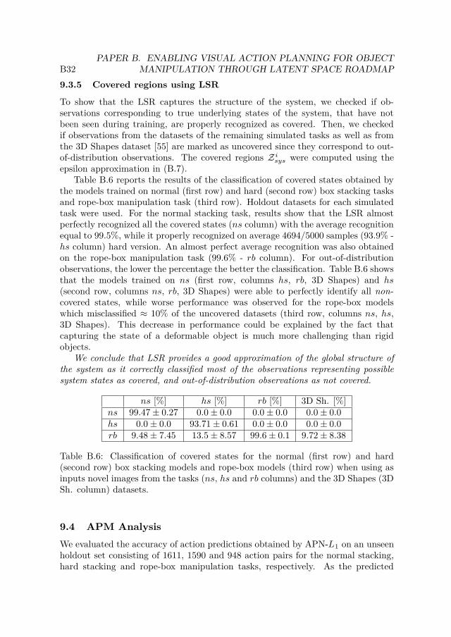
B32PAPER B. ENABLING VISUAL ACTION PLANNING FOR OBJECT
MANIPULATION THROUGH LATENT SPACE ROADMAP
9.3.5 Covered regions using LSR
To show that the LSR captures the structure of the system, we checked if ob-servations corresponding to true underlying states of the system, that have notbeen seen during training, are properly recognized as covered. Then, we checkedif observations from the datasets of the remaining simulated tasks as well as fromthe 3D Shapes dataset [55] are marked as uncovered since they correspond to out-of-distribution observations. The covered regions Z i
sys were computed using theepsilon approximation in (B.7).
Table B.6 reports the results of the classification of covered states obtained bythe models trained on normal (first row) and hard (second row) box stacking tasksand rope-box manipulation task (third row). Holdout datasets for each simulatedtask were used. For the normal stacking task, results show that the LSR almostperfectly recognized all the covered states (ns column) with the average recognitionequal to 99.5%, while it properly recognized on average 4694/5000 samples (93.9% -hs column) hard version. An almost perfect average recognition was also obtainedon the rope-box manipulation task (99.6% - rb column). For out-of-distributionobservations, the lower the percentage the better the classification. Table B.6 showsthat the models trained on ns (first row, columns hs, rb, 3D Shapes) and hs(second row, columns ns, rb, 3D Shapes) were able to perfectly identify all non-covered states, while worse performance was observed for the rope-box modelswhich misclassified ≈ 10% of the uncovered datasets (third row, columns ns, hs,3D Shapes). This decrease in performance could be explained by the fact thatcapturing the state of a deformable object is much more challenging than rigidobjects.
We conclude that LSR provides a good approximation of the global structure ofthe system as it correctly classified most of the observations representing possiblesystem states as covered, and out-of-distribution observations as not covered.
ns [%] hs [%] rb [%] 3D Sh. [%]ns 99.47 ± 0.27 0.0 ± 0.0 0.0 ± 0.0 0.0 ± 0.0hs 0.0 ± 0.0 93.71 ± 0.61 0.0 ± 0.0 0.0 ± 0.0rb 9.48 ± 7.45 13.5 ± 8.57 99.6 ± 0.1 9.72 ± 8.38
Table B.6: Classification of covered states for the normal (first row) and hard(second row) box stacking models and rope-box models (third row) when using asinputs novel images from the tasks (ns, hs and rb columns) and the 3D Shapes (3DSh. column) datasets.
9.4 APM Analysis
We evaluated the accuracy of action predictions obtained by APN-L1 on an unseenholdout set consisting of 1611, 1590 and 948 action pairs for the normal stacking,hard stacking and rope-box manipulation tasks, respectively. As the predicted

10. FOLDING EXPERIMENTS B33
actions can be binary classified as either true or false, we calculated the percentageof the correct proposals for picking and releasing, as well as the percentage ofpairs where both pick and release proposals were correct. For rope-box task, weadditionally calculated the percentage of the correct proposal for either rope orbox action. We evaluated all the models on 5 different random seeds. For bothstacking versions, all the models performed with accuracy 99% or higher, whilerope-box models achieved ≈ 96%. This is because the box stacking task results inan 18-class classification problem for action prediction which is simple enough tobe learned from any of the VAEs, while the classification task in the rope-box isslightly more challenging due to the required extra prediction whether to move arope or a box.
10 Folding Experiments
In this section, we validate the proposed approach on a real world experimentinvolving manipulation of deformable objects, namely folding a T-shirt. As opposedto the simulated tasks, the true underlying states were in this case unknown and itwas therefore not possible to define an automatic verification of the correctness ofa given visual action plan.
The folding task setup is depicted in Fig. B.12 (middle). We used a Baxterrobot equipped with a Primesense RGB-D camera mounted on its torso to fold aT-shirt in different ways. The execution videos of all the performed experimentsand respective visual action plans can be found on the project website. A summaryof the experiments can also be found in the accompanying video. For this task,we collected a dataset TI containing 1283 training tuples. Each tuple consistsof two images of size 256 × 256 × 3, and action specific information u defined asu = (p, r, h) where p = (pr, pc) are the picking coordinates, r = (rr, rc) the releasingcoordinates and h picking height. An example of an action and a no-action pairis shown in Fig. B.4. The values pr, pc, rr, rc ∈ {0, . . . , 255} correspond to imagecoordinates, while h ∈ {0, 1} is either the height of the table or a value measuredfrom the RGB-D camera to pick up only the top layer of the shirt. Note that theseparation of stacked clothing layers is a challenging task and active research areaon its own [56] and leads to decreased performance when it is necessary to performit, as shown in Sec. 10.5.2. The dataset TI was collected by manually selecting pickand release points on images showing a given T-shirt configuration, and recordingthe corresponding action and following configuration. No-action pairs, representing≈ 37% of training tuples in TI , were generated by slightly perturbing the clothappearance.
10.1 Experiment Objectives and Implementation Details
The experiments on the real robot were designed to answer the following questions:

B34PAPER B. ENABLING VISUAL ACTION PLANNING FOR OBJECT
MANIPULATION THROUGH LATENT SPACE ROADMAP
1. MM Does the action loss term (B.4) improve the structure of the latent spacefor the folding task?
2. LSR How good is the approximation of the covered regions provided by theLSR for a real world dataset?
3. APM How does the APN perform in comparison to alternative implementa-tions of the APM?
4. System How does the real system perform and how does it compare to ourearlier work [7]? What is the performance on a folding that involves pickingthe top layer of the shirt?
Following the notations introduced in Sec. 9.1, we denote by VAEld -f -d a VAEwith ld-dimensional latent space, where f stands for the folding task and d indicateswhether or not the model was trained with the action loss (B.4). We use d = b forthe baseline VAEs which were trained with the original training objective (B.5).We use d = Lp for the action VAEs trained with the objective (B.6) containingthe action term (B.4) using metric Lp for p ∈ {1, 2, ∞}. We modelled VAEs withthe same ResNet architecture and same hyperparameters β, γ and dm as in thebox stacking task introduced in Sec. 9 but increased the latent space dimension told = 16. We refer the reader to the code repository2 for implementation details.
For the LSR, we denote by LSR -Lp a graph obtained by using metric Lp inAlgorithm 2. We set the upper bound cmax in (B.8) to 5, and the search intervalboundaries τmin and τmax in Algorithm 3 to 0 and 3.5, respectively.
The performance of the APMs and the evaluation of the system was based onthe VAE16 -f -L1 realization of the MM. We therefore performed the experimentsusing APN16 -f -L1 which was trained on latent action pairs Tz extracted by thelatent mapping ξ of VAE16 -f -L1. We trained 5 models for 500 epochs using dif-ferent random seeds as in case of VAEs, and used 15% of the training dataset as avalidation split to extract the best performing model for the evaluation.
We compared the performance of our system S-OUR consisting of VAE16 -f -L1,LSR -L1 and APN16 -f -L1 with the systems S-L1, S-L2 and S-L∞ introduced in [7]on the same 5 folding tasks. The start configuration was the fully unfolded shirtshown in Fig. B.10 on the left, while the goal configurations are shown on the right.The latter are of increasing complexity requiring a minimum of 2, 2, 3, 3, and 4folding steps for folds 1-5, respectively.
Each fold was repeated 5 times and scored in the same way as in [7]. In partic-ular, we scored the system performance where a folding was considered successful ifthe system was able to fold the T-shirt into the desired goal configuration. As thestate space of the T-shirt is high-dimensional, there exists no objective measure thatwould evaluate the success of the fold automatically. Therefore, the evaluation ofthe full folding procedure was manually done by a human (one of the authors) butall execution videos of all folds and repetitions can be found on the project website.We additionally evaluated the percentage of successful transitions of the system.
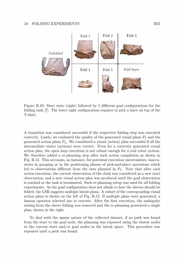
10. FOLDING EXPERIMENTS B35
Figure B.10: Start state (right) followed by 5 different goal configurations for thefolding task [7]. The lower right configuration requires to pick a layer on top of theT-shirt.
A transition was considered successful if the respective folding step was executedcorrectly. Lastly, we evaluated the quality of the generated visual plans PI and thegenerated action plans Pu. We considered a visual (action) plan successful if all theintermediate states (actions) were correct. Even for a correctly generated visualaction plan, the open loop execution is not robust enough for a real robot system.We therefore added a re-planning step after each action completion as shown inFig. B.12. This accounts, as instance, for potential execution uncertainties, inaccu-racies in grasping or in the positioning phases of pick-and-place operations whichled to observations different from the ones planned in PI . Note that after eachaction execution, the current observation of the cloth was considered as a new startobservation, and a new visual action plan was produced until the goal observationis reached or the task is terminated. Such re-planning setup was used for all foldingexperiments. As the goal configuration does not allude to how the sleeves should befolded, the LSR suggests multiple latent plans. A subset of the corresponding visualaction plans is shown on the left of Fig. B.12. If multiple plans were generated, ahuman operator selected one to execute. After the first execution, the ambiguityarising from the sleeve folding was removed and the re-planning generated a singleplan, shown in the right.
To deal with the sparse nature of the collected dataset, if no path was foundfrom the start to the goal node, the planning was repeated using the closest nodesto the current start and/or goal nodes in the latent space. This procedure wasrepeated until a path was found.

B36PAPER B. ENABLING VISUAL ACTION PLANNING FOR OBJECT
MANIPULATION THROUGH LATENT SPACE ROADMAP
Figure B.11: Histograms of action (in blue) and no-action (in green) pair distancesat different training epochs (1, 100 and 500 from the left, respectively) for thefolding task. Results obtained with baseline (top, a)) and action (bottom, b))models are shown.
10.2 MM Analysis
Analogously to the box stacking task in Sec. 9.2, we answered question 1) by ana-lyzing the relative contrast (reported in Appendix12.1) as well as by evaluating theseparation of action and no-action pairs during the training.
10.2.1 Influence of dynamic dm
We investigated the influence of the dynamic increase of dm in the action term (B.4)on the structure of the latent space. Figure B.11 shows the histogram of action (inblue) and no-action (in green) pair distances calculated at different epochs duringtraining using VAE16 -f -b (top row) and VAE16 -f -L1 (bottom row). We observedthat the separation was complete in case of action VAEs but was not achieved withthe baseline VAEs. To precisely quantify the amount of overlap between actionand no-action pairs, we calculated the difference between the minimum action-pairdistance and maximum no-action pair distance on the training dataset. Therefore,a positive value implies that action pairs were successfully separated from the no-action pairs. For VAE16 -f -b (top row), the difference evaluated to −31.8, −19.2,and −19.4 for epoch 1, 100, and 500, respectively, while it was improved to −6.3,−1.6, and 1.5 in case of the action VAE16 -f -L1 (bottom row). This shows that the

10. FOLDING EXPERIMENTS B37
Figure B.12: Execution of the folding task with re-planning. On the left, a setof initial visual action plans reaching the goal state is proposed. After the firstexecution, only one viable visual action plan remains.
dynamic selection of dm successfully separated the actions and no-action pairs alsofor the folding task.
10.3 LSR Analysis
Similarly to the simulated tasks, we exploited the LSR to investigate the coveredregions of the latent space Z, thus answering question 2) listed in Sec. 10.1. Notethat in Sec. 10.5, the LSR was also employed to perform the folding task with thereal robotic system.
10.3.1 Covered regions using LSR
We used VAE16 -f -L1 model and reproduced the experiment from Sec. 9.3.5, wherewe measured the accuracy of various novel observations being recognized as covered.We inputted 224 novel observations that correspond to possible states of the systemnot used during training, as well as 5000 out-of-distribution samples from each ofthe three datasets of the simulated tasks and the standard 3D Shapes dataset. Weobserved that the LSR achieved good recognition performance even in the foldingtask. More precisely, on average 213/224 samples representing true states of thesystem were correctly recognized as covered, resulting in 95 ± 2.4% accuracy aver-aged over the 5 different random seeds. For the four out-of-distribution datasets,all samples were correctly recognized as not covered.
This analysis illustrates the effectiveness of the LSR in capturing the coveredregions of the latent space.
10.4 APM Comparison
In this section we validate the choice of the APM by comparing it to several possiblealternatives.
The Action Proposal Network, described in Sec. 7, was built upon the one intro-duced in [7] to which we added dropout regularization layers. The APN receives asinputs latent action pairs contained in a latent plan found by the LSR, and outputs

B38PAPER B. ENABLING VISUAL ACTION PLANNING FOR OBJECT
MANIPULATION THROUGH LATENT SPACE ROADMAP
Method X Pick Y Pick X Releasee-APN [7] 144.1 ± 52.2 52.8 ± 18.3 317.2 ± 143.3C-APN 498.0 ± 63.8 47.4 ± 7.7 818.8 ± 121.9R-APN 697.2 ± 345.1 246.2 ± 174.9 792.4 ± 388.8AAB 113.0 22.4 201.4
APN (Ours) 82.6 ± 22.9 29.3 ± 2.2 270.6 ± 158.2
Method Y Release Height Totale-APN [7] 159.9 ± 17.4 0.0 ± 0.0 674.0 ± 147.6C-APN 226.5 ± 92.5 0.0 ± 0.0 1590.8 ± 155.0R-APN 268.9 ± 157.0 0.0 ± 0.0 2004.6 ± 908.2AAB 194.7 0.0 531.5
APN (Ours) 71.8 ± 15.0 0.0 ± 0.0 454.3 ± 153.8
Table B.7: Comparison of MSE achieved with different realizations of the ActionProposal Modules. Best results in bold.
the predicted action specifics. We refer to the earlier version in [7] as e-APN andto the current version APN16 -f -L1 as APN. We compared the performance of APNto e-APN as well as several alternatives introduced below.Action Averaging Baseline (AAB) Firstly, we investigated whether the actionpredictions can be retrieved directly from the LSR instead of a separate module.The basic idea is to use the latent action pairs in the training dataset to calculatethe average action specifics associated with each edge in the LSR. Let E ij
sys ={(z1, z2) ∈ E|z1 ∈ Zi
sys, z2 ∈ Zjsys} be the set of edges from the reference graph E
connecting covered regions Z isys and Zj
sys (Algorithm 2). We parameterized each
edge eijLSR = (zi
LSR, zjLSR) ∈ ELSR with the action uij
LSR obtained by averagingactions corresponding to the edges in E ij
sys
uijLSR =
1
|E ijsys|
�
(z1,z2)∈Eijsys
uz1z2 (B.10)
where uz1z2 is the action specification associated with the action pair (z1, z2) in thetraining dataset Tz. The parametrization (B.10) yields the action plan associatedwith a path Pz.
Secondly, we investigated how the use of the latent encodings as inputs to theAPM influences the LSR performance. We compared APN-d with two distinctversions of APMs that use images as inputs.C-APN is a neural network that uses a convolutional encoder followed by the APN.The encoder in C-APN was trained using only MSE loss. During the inference, theobservations given to C-APN as input are obtained by decoding the latent planfound by the LSR with the observation generator ω.

10. FOLDING EXPERIMENTS B39
R-APN is an extension of C-APN that uses a ResNet encoder identical to theVAE encoder.
Detailed architectures of all the models can be found in our code repository.The training details for APN and APN-d are described in Sec. 10.1. For C-APN-dand R-APN-d, we similarly trained 5 models using different random seeds but ona training dataset TI obtained by decoding Tz with the observation generator ω ofVAE16 -f -L1. This is because the visual plans, given to C-APN-d and R-APN-d,are produced by decoding the latent plans with ω. Moreover, C-APN-d and R-APN-d were trained for 1000 epochs to ensure the convergence of the initializedencoders. Note that we can only obtain one AAB model for a chosen VAE as AABis defined by the LSR.
We evaluated the performance of all the models on a holdout dataset consistingof 41 action pairs. Given a holdout action pair, we calculated the mean squarederror (MSE) between the predicted and the ground truth action specifics. Wereport the mean and standard deviation of the obtained MSE calculated across the5 random seeds (except for AAB). The results are shown in Table B.7 where weseparately report the error obtained on picking and releasing as well as the totalmodel error. Firstly, we observed that the added regularization layer positivelyaffected the result as APN achieved lower error than our earlier version e-APN [7].Secondly, APN significantly outperformed both C-APN and R-APN. Using thelatent encodings as inputs also significantly decreased the size of the models andreduces the computational power needed for their training. Lastly, our APN alsoon average outperformed AAB with respect to the total model error. Although theenhancement compared to the AAB was not as significant as for the other models,APN is beneficial since it is less prone to averaging errors obtained from the LSRand can be easily adapted to any realization of action specifics. Moreover, a neuralnetwork realization of the APM potentially allows more accurate modeling of morecomplex action specifics. In summary, using a separate neural network to predictaction specifics from latent representations led to a lower prediction error and canbe easily adapted to different types of actions.
10.5 System Analysis
We benchmarked our method against our earlier method in [7] on the same T-shirtfolding task, and additionally measured the performance on a more challenging foldinvolving picking a layer of the cloth on top of another layer.
10.5.1 Folding performance and comparison with [7]
We performed each fold 5 times per configuration using the goal configurationshown in Fig. B.10 and framework S-OUR, consisting of VAE16 -f -L1, LSR -L1
and APN16 -f -L1, and compared the performance with the results from our earlierwork [7] obtained using S-L1, S-L2 and S-L∞.

B40PAPER B. ENABLING VISUAL ACTION PLANNING FOR OBJECT
MANIPULATION THROUGH LATENT SPACE ROADMAP
Method Syst. Trans. PI PuFold 1 to 5 - comparison to [7]
S-OUR 96% 99% 100% 100%S-L1 [7] 80% 90% 100% 100%S-L2 [7] 40% 77% 60% 60%S-L∞ [7] 24% 44% 56% 36%
Fold layerS-OUR 50% 83% 100% 100%
Table B.8: Results (best in bold) for executing visual action plans on 5 foldingtasks (each repeated 5 times) shown in the top. The bottom row shows the resultson the fold requiring to pick the top layer of the garment (repeated 10 times).
The results are shown in Table B.8, while, as previously mentioned, all executionvideos, including the respective visual action plans, are available on the website1.We report the total system success rate with re-planning, the percentage of correctsingle transitions, and the percentage of successful visual plans and action plansfrom start to goal. We observed that S-OUR outperformed the systems from [7]with a notable 96% system performance, only missing a single folding step whichresults in a transition performance of 99%. As for S-L1, S-OUR also achievedoptimal performance when scoring the initial visual plans PI and the initial actionplans Pu. We thus conclude that the improved MM, LSR and APM modules togethercontribute to a significant better system than in [7].
10.5.2 Folding with multiple layers
As the previous folds resulted in nearly perfect performance of our system, wechallenged it with an additional much harder fold that requires to pick the toplayer of the garment. The fold, shown in Fig. B.10 bottom right, was repeated 10times. An example of the obtained visual action plan is shown in Fig. B.13 and thefinal results are reported in Table B.8 (bottom row).
Figure B.13: Visual action plan for the fold requiring to pick the top layer of thegarment. The step where the top layer is to be picked is indicated in purple (seeaccompanying video for further details).
Experiments showed that the system had no trouble planning the folding steps

11. CONCLUSIONS B41
from the initial configuration and was able to properly plan layer folds (with pick lo-cation marked in purple). Concerning the execution of the plan, the robot managedto correctly fold in 80% of the cases, excluding the last fold, using the re-planningstrategy. However, failure cases often occurred during the execution of the lastlayer fold, resulting in the robot picking up multiple layers at the same time. Whenthis happened, the T-shirt deformed into unseen states that were very dissimilarfrom the ones in TI and that rendered the re-planning step inefficient. A moreprecise manipulation system, either using a specialized gripper or custom methodsfor separating cloth layers, could potentially boost the performance of our systemon this specific folding task. We leave these improvements for future work.
11 Conclusions
In this work, we presented an extended version of the Latent Space Roadmap firstintroduced in [7] which allows visual action planning of manipulation tasks. Firstly,we improved the building procedure of the LSR in the latent space by introducingan outer optimization loop that eliminates the need for a hard-to-tune clusteringparameter. Secondly, we improved the training procedure of the VAE, used torepresent the Mapping Module, by dynamically increasing the desired distancebetween action pairs. We thoroughly investigated the structure of the latent space,and presented a deep insight into the effects that each of the improvements have forthe system. In addition, we compared different realizations of the Action ProposalModule and showcased the benefits of using latent representations for generatingaction plans. Lastly, we evaluated the LSR on three simulated tasks as well asreal-world folding task. We introduced a harder version of the box stacking taskand a rope-box manipulation task involving a rigid and deformable object, whichenabled a more informative ablation study. We showed that the improved LSRsignificantly outperforms the one presented in [7] on the same folding task.
We are convinced that in order to advance state-of-the-art manipulation tech-niques for rigid and deformable objects, improvements on two fronts are necessary:learning a structured latent space as well as its exploration. We believe that ourproposed method is a step toward achieving this goal which also opens many in-teresting future directions. For example, we wish to expand our method to encodefull trajectories that could be leveraged to further structure the latent space, or toapply it to reinforcement learning settings with active exploration.
12 Appendix
This section provides complementary results on the separability of data samples forthe simulation and the folding tasks, an ablation study considering different latentdimensions as well as a short overview of the different clustering methods.

B42PAPER B. ENABLING VISUAL ACTION PLANNING FOR OBJECT
MANIPULATION THROUGH LATENT SPACE ROADMAP
ns hs rbld VAE-b VAE-L1 VAE-b VAE-L1 VAE-b VAE-L1
4 73.9 159.7 ± 23.9 29.2 93.8 ± 10.1 23.4 97.6 ± 4.66 19.4 59.8 ± 4.1 11.7 39.2 ± 2.3 9.7 41.0 ± 5.18 11.7 45.6 ± 1.6 8.3 24.1 ± 1.8 6.3 30.7 ± 4.412 5.7 46.0 ± 7.0 4.8 20.6 ± 1.6 4.4 19.0 ± 1.916 4.4 40.4 ± 8.1 3.9 21.6 ± 2.3 3.8 18.8 ± 1.932 3.7 46.0 ± 4.3 3.7 29.9 ± 3.9 3.1 17.0 ± 1.4
Table B.9: Evaluation of the relative contrast rc on Tz obtained with baseline andaction VAEs. Results for all simulated tasks are reported.
12.1 Separability of data samples
To further analyze how the action loss influences the structure of the latent space,we resorted to the concept of relative contrast, introduced in [47] and based on [48].Given a dataset T containing ld-dimensional data points, the relative contrast rcof T with respect to the metric Lp is defined as
rc(T , ld, p) =Dmax − Dmin
Dmin(B.11)
where Dmax and Dmin denote the distances of the furthest and the closest points inthe dataset T from a chosen point [47], respectively. We calculated rc of the latenttraining dataset Tz using VAEs with different latent dimensions ld. The rc valueswere used to evaluate significance of distances among points in the latent space Z,where a lower rc implies diminishing contrast in distances. Authors of [48] showthat, under broad assumptions, rc converges to 0 when ld approaches infinity, asin this case the distance from a point to its nearest neighbor is identical to the oneto its furthest neighbor.
In our case, measuring rc on the full dataset can be misleading since the latentno-action pairs are encoded closeby because of the action term (B.4). This wouldlead to a deceptively small Dmin and therefore to a higher rc than warranted. To geta reliable estimate of rc given Tz, we therefore chose to measure it in the followingway. We split the latent training dataset Tz into datasets T 1
z and T 2z containing the
first and the consecutive states of all the training tuples in Tz, respectively. We thenmeasured Dmin and Dmax with respect to each state in T 1
z and T 2z separately. More
precisely, we considered each latent state zi ∈ T 1z as the origin, and calculated Dmin
(and Dmax) within T 1z \{zi}. We repeated the same process for all zi ∈ T 2
z . Finally,we used the average of the obtained Dmin and Dmax values in the computation ofrc as in (B.11).Simulation tasks: Table B.9 reports the relative contrast of Tz for all simulationtasks. We observed that VAEld-L1 achieved a higher rc than the baseline VAEld-b. This is because the action loss (B.4) encourages no-action pairs to be encodedcloseby, hence minimizing Dmin, and action pairs to be encoded at least dm apart,

12. APPENDIX B43
hence encouraging Dmax to be at least dm. From the same reason, rc decreasedwith increasing ld for baseline VAEs, while it was rather constant for the actionmodels VAEld-L1. Moreover, we obtained higher rc values for ns than hs or rbwhich once more highlights the differences in difficulty between the three tasks.
Folding task: Table B.10 shows the relative contrast rc of Tz produced by thebaseline models VAE16 -f -b (left) and action models VAE16 -f -L1 (right) when vary-ing the latent space dimension ld. For the action models (right) we report the meanand standard deviation of rc computed over 5 seeds.
ld VAEld-f -b VAEld-f -L1
4 24.2 37.7 ± 4.36 13.7 26.1 ± 2.78 10.2 22.3 ± 2.212 7.2 15.8 ± 3.216 5.8 12.1 ± 1.232 4.5 8.2 ± 0.864 3.7 8.1 ± 0.8
Table B.10: Relative contrast evaluation comparing baseline (left) and action VAEs(right) when varying ld.
We observed that the action term (B.4) significantly increased the relative con-trast for all tasks but clearly dropped for higher latent dimensions. We thus concludethat the action term and the dynamic setting of dm improve the relative contrast.
12.2 Latent space dimension
The problem of choosing a suitable latent space dimension has not received muchattention in the literature. Even though the action term alleviates the problemof indistinguishable distances in higher dimensions by increasing the relative con-trast, it is still important to choose a latent dimension large enough so that therelevant features can be encoded. In Table B.11 we report the partial scoring onnormal and hard stacking and rope-box tasks using VAE models with various la-tent dimensions. The results demonstrate an evident drop in the performance whenthe latent dimension was too small, such as ld = 4. As ld increased, we observedgradual improvements in the performance where a satisfactory level was achievedusing ld ≥ 6 for ns, and ld ≥ 12 for hs and rb. Therefore, hs and rb requiredmore dimensions in order to capture all the relevant and necessary features. Thisresult not only demonstrates the complexity of each task version but also justifiesthe choice ld = 12 in the simulations.

B44PAPER B. ENABLING VISUAL ACTION PLANNING FOR OBJECT
MANIPULATION THROUGH LATENT SPACE ROADMAP
ld ns [%] hs [%] rb [%]4 7.9 ± 2.2 8.8 ± 7.9 62.7 ± 13.96 99.96 ± 0.08 56.2 ± 23.1 74.9 ± 5.08 99.96 ± 0.08 62.7 ± 18.7 80.6 ± 5.312 100.0 ± 0.0 92.1 ± 2.9 90.4 ± 2.916 100.0 ± 0.0 95.9 ± 1.4 92.2 ± 1.132 97.5 ± 4.33 96.4 ± 0.4 92.6 ± 2.0
Table B.11: Comparison of the LSR performance when using VAEs with differentlatent dimensions for all the simulated tasks.
12.3 Overview of clustering algorithms
In this section, we provide a brief overview of the ablated clustering methods con-sidered in Sec. 9.3.4.
Epsilon clustering: used in our earlier work [7] and functionally coincident withDBSCAN [57]. Its performance is affected by the parameter ε, i. e. , radius ofthe ε-neighborhood of every point, and deteriorates when clusters have differentdensities.
Mean-shift: centroid-based algorithm [51] with moving window approach to iden-tify high density regions. At each iteration, the centroid candidates associated tothe windows are updated to the mean of the points in the considered region. Thewindow size has a significant influence on the performance.
OPTICS: improved version of DBSCAN introduced by [52] in which a hierarchicalreachability-plot dendrogram is built, whose slope identifies clusters with differentdensities. The parameter Ξ ∈ [0, 1] is used to tune the slope and heavily affectsthe outcome of the algorithm. However, its influence is not easy to understandintuitively, as discussed in [58].
Linkage: hierarchical, agglomerative clustering algorithm discussed in Sec. 6.1.Possible dissimilarity functions to merge points are single, based on the minimumdistance between any pair of points belonging to two distinct clusters, complete,based on the maximum distance, and average, based on the unweighted average ofthe distances of all points belonging to two distinct clusters. As discussed in Sec. 6.1,the clustering threshold τ determines the vertical cut through the dendrogram andconsequently influences the performance of the algorithm.
HDBSCAN: agglomerative clustering algorithm in which the branches of the den-drogram are optimized for non-overlapping clusters using a notion of “cluster sta-bility" based on their longevity. HDBSCAN automatically identifies clusters withdifferent densities and requires specifying only the minimum cluster size prior tothe training.

12. APPENDIX B45
References
1. J. Oh, X. Guo, H. Lee, R. L. Lewis, and S. Singh, “Action-conditional video predictionusing deep networks in atari games,” in Advances in neural information processingsystems, pp. 2863–2871, 2015.
2. I. Garcia-Camacho, M. Lippi, M. C. Welle, H. Yin, R. Antonova, A. Varava, J. Borras,C. Torras, A. Marino, G. Alenyà , and D. Kragic, “Benchmarking bimanual clothmanipulation,” IEEE Robot. Autom. Lett., vol. 5, no. 2, pp. 1111–1118, 2020.
3. H. Yin, A. Varava, and D. Kragic, “Modeling, learning, perception, and control meth-ods for deformable object manipulation,” Science Robot., vol. 6, no. 54, 2021.
4. D. H. Ballard, “Modular learning in neural networks.,” in AAAI, pp. 279–284, 1987.
5. D. P. Kingma and M. Welling, “Auto-encoding variational bayes,” Int. Conf. Learn.Represent., 2015.
6. D. Müllner, “Modern hierarchical, agglomerative clustering algorithms,” arXivpreprint arXiv:1109.2378, 2011.
7. M. Lippi, P. Poklukar, M. C. Welle, A. Varava, H. Yin, A. Marino, and D. Kragic,“Latent space roadmap for visual action planning of deformable and rigid object ma-nipulation,” in IEEE/RSJ Int. Conf. Intelligent Robots and Systems, pp. 5619–5626,2020.
8. N. Savinov, A. Dosovitskiy, and V. Koltun, “Semi-parametric topological memory fornavigation,” in Int. Conf. Learn. Represent., 2018.
9. D. Hafner, T. Lillicrap, I. Fischer, R. Villegas, D. Ha, H. Lee, and J. Davidson,“Learning latent dynamics for planning from pixels,” in Int. Conf. Mach. Learn.,pp. 2555–2565, 2019.
10. T. Lozano-Pérez and L. P. Kaelbling, “A constraint-based method for solving sequen-tial manipulation planning problems,” in IEEE/RSJ Int. Conf. Intelligent Robots andSystems, pp. 3684–3691, IEEE, 2014.
11. C. Galindo, J.-A. Fernández-Madrigal, J. González, and A. Saffiotti, “Robot taskplanning using semantic maps,” Robotics and Autonomous Systems, vol. 56, no. 11,pp. 955 – 966, 2008. Semantic Knowledge in Robotics.
12. L. P. Kaelbling and T. Lozano-Pérez, “Integrated task and motion planning in beliefspace,” Int. J. Robot. Res., vol. 32, no. 9-10, pp. 1194–1227, 2013.
13. S. M. LaValle, Planning Algorithms. Cambridge U.K.: Cambridge University Press,2006.
14. R. Bellman, “Curse of dimensionality,” Adaptive control processes: a guided tour.Princeton, NJ, vol. 3, p. 2, 1961.
15. A. Srinivas, A. Jabri, P. Abbeel, S. Levine, and C. Finn, “Universal planning net-works,” in Int. Conf. Mach. Learn., 2018.

B46PAPER B. ENABLING VISUAL ACTION PLANNING FOR OBJECT
MANIPULATION THROUGH LATENT SPACE ROADMAP
16. B. Jia, Z. Pan, Z. Hu, J. Pan, and D. Manocha, “Cloth manipulation using random-forest-based imitation learning,” IEEE Robot. Autom. Lett., vol. 4, no. 2, pp. 2086–2093, 2019.
17. A. H. Qureshi, Y. Miao, A. Simeonov, and M. C. Yip, “Motion planning networks:Bridging the gap between learning-based and classical motion planners,” IEEE Trans.Robot., pp. 1–19, 2020.
18. J. Matas, S. James, and A. J. Davison, “Sim-to-real reinforcement learning for de-formable object manipulation,” in Conf. Robot Learn., pp. 734–743, PMLR, 2018.
19. R. Hoque, D. Seita, A. Balakrishna, A. Ganapathi, A. Tanwani, N. Jamali, K. Yamane,S. Iba, and K. Goldberg, “VisuoSpatial Foresight for Multi-Step, Multi-Task FabricManipulation,” in Robotics: Science and Systems (RSS), 2020.
20. X. Lin, Y. Wang, J. Olkin, and D. Held, “Softgym: Benchmarking deep reinforcementlearning for deformable object manipulation,” in Conf. Robot Learn., 2020.
21. R. Lee, D. Ward, A. Cosgun, V. Dasagi, P. Corke, and J. Leitner, “Learning arbitrary-goal fabric folding with one hour of real robot experience,” Conf. Robot Learn., 2020.
22. B. Ichter and M. Pavone, “Robot Motion Planning in Learned Latent Spaces,” IEEERobot. Autom. Lett., vol. 4, no. 3, pp. 2407–2414, 2019.
23. M. Watter, J. Springenberg, J. Boedecker, and M. Riedmiller, “Embed to control:A locally linear latent dynamics model for control from raw images,” in Advances inNeural Information Processing Systems, vol. 28, 2015.
24. C. Lynch, M. Khansari, T. Xiao, V. Kumar, J. Tompson, S. Levine, and P. Sermanet,“Learning latent plans from play,” in Conf. Robot Learn., pp. 1113–1132, PMLR, 2020.
25. A. Wang, T. Kurutach, P. Abbeel, and A. Tamar, “Learning robotic manipulationthrough visual planning and acting,” in Robotics: Science and Systems, 2019.
26. T. Kurutach, A. Tamar, G. Yang, S. J. Russell, and P. Abbeel, “Learning plannablerepresentations with causal infogan,” in Advances in Neural Information ProcessingSystems, pp. 8733–8744, 2018.
27. A. Nair, D. Chen, P. Agrawal, P. Isola, P. Abbeel, J. Malik, and S. Levine, “Combiningself-supervised learning and imitation for vision-based rope manipulation,” in IEEEInt. Conf. Robot. Autom., pp. 2146–2153, 2017.
28. W. Yan, A. Vangipuram, P. Abbeel, and L. Pinto, “Learning predictive representationsfor deformable objects using contrastive estimation,” Conf. Robot Learn., 2020.
29. K. Pertsch, O. Rybkin, F. Ebert, C. Finn, D. Jayaraman, and S. Levine, “Long-horizon visual planning with goal-conditioned hierarchical predictors,” in Advances inNeural Information Processing Systems, 2020.
30. C. Finn and S. Levine, “Deep visual foresight for planning robot motion,” in IEEEInt. Conf. Robot. Autom., pp. 2786–2793, 2017.

12. APPENDIX B47
31. T. Kipf, E. van der Pol, and M. Welling, “Contrastive learning of structured worldmodels,” in Int. Conf. Learn. Represent., 2020.
32. B. Eysenbach, R. R. Salakhutdinov, and S. Levine, “Search on the replay buffer:Bridging planning and reinforcement learning,” in Advances in Neural InformationProcessing Systems, pp. 15246–15257, 2019.
33. R. Li, A. Jabri, T. Darrell, and P. Agrawal, “Towards practical multi-object manipula-tion using relational reinforcement learning,” IEEE Int. Conf. Robot. and Automation,pp. 4051–4058, 2020.
34. R. Hadsell, S. Chopra, and Y. LeCun, “Dimensionality reduction by learning an in-variant mapping,” in IEEE Computer Society Conf. Computer Vision and PatternRecognition, vol. 2, pp. 1735–1742, 2006.
35. D. J. Rezende, S. Mohamed, and D. Wierstra, “Stochastic backpropagation and ap-proximate inference in deep generative models,” in Int. Conf. Mach. Learn., pp. 1278–1286, 2014.
36. I. Higgins, L. Matthey, A. Pal, C. Burgess, X. Glorot, M. Botvinick, S. Mohamed,and A. Lerchner, “β-vae: Learning basic visual concepts with a constrained variationalframework,” Int. Conf. Learn. Represent., 2017.
37. C. P. Burgess, I. Higgins, A. Pal, L. Matthey, N. Watters, G. Desjardins, and A. Lerch-ner, “Understanding disentangling in β-vae,” arXiv preprint arXiv:1804.03599, 2018.
38. R. R. Sokal, “A statistical method for evaluating systematic relationships.,” Univ.Kansas, Sci. Bull., vol. 38, pp. 1409–1438, 1958.
39. M. E. Celebi, Partitional clustering algorithms. Springer, 2014.
40. P. Langfelder, B. Zhang, and S. Horvath, “Defining clusters from a hierarchical clustertree: the dynamic tree cut package for r,” Bioinformatics, vol. 24, no. 5, pp. 719–720,2008.
41. D. Bruzzese and D. Vistocco, “Despota: Dendrogram slicing through a pemutationtest approach,” J. Classif., vol. 32, no. 2, pp. 285–304, 2015.
42. A. Pasini, E. Baralis, P. Garza, D. Floriello, M. Idiomi, A. Ortenzi, and S. Ricci,“Adaptive hierarchical clustering for petrographic image analysis.,” in EDBT/ICDTWorkshops, 2019.
43. R. P. Brent, “An algorithm with guaranteed convergence for finding a zero of a func-tion,” Computer J., vol. 14, no. 4, pp. 422–425, 1971.
44. G. Maeda, M. Ewerton, T. Osa, B. Busch, and J. Peters, “Active incremental learningof robot movement primitives,” in Conf. Robot Learn., pp. 37–46, 2017.
45. Unity Technologies, “Unity.”
46. K. He, X. Zhang, S. Ren, and J. Sun, “Deep residual learning for image recognition,”in IEEE Conf. Computer Vision and Pattern Recognition, pp. 770–778, 2016.

B48PAPER B. ENABLING VISUAL ACTION PLANNING FOR OBJECT
MANIPULATION THROUGH LATENT SPACE ROADMAP
47. C. C. Aggarwal, A. Hinneburg, and D. A. Keim, “On the surprising behavior ofdistance metrics in high dimensional space,” in Int. Conf. Database Theory, pp. 420–434, Springer, 2001.
48. K. Beyer, J. Goldstein, R. Ramakrishnan, and U. Shaft, “When is “nearest neighbor”meaningful?,” in Int. Conf. Database Theory, pp. 217–235, Springer, 1999.
49. Z. Xie, I. Sato, and M. Sugiyama, “Stable weight decay regularization,” arXiv preprintarXiv:2011.11152, 2020.
50. R. Berk, “A primer on robust regression,” Modern methods of data analysis, pp. 292–324, 1990.
51. Y. Cheng, “Mean shift, mode seeking, and clustering,” IEEE Trans. Pattern. Anal.Mach. Intell., vol. 17, no. 8, pp. 790–799, 1995.
52. M. Ankerst, M. M. Breunig, H.-P. Kriegel, and J. Sander, “Optics: ordering pointsto identify the clustering structure,” ACM Sigmod record, vol. 28, no. 2, pp. 49–60,1999.
53. W. H. Day and H. Edelsbrunner, “Efficient algorithms for agglomerative hierarchicalclustering methods,” J. Classif., vol. 1, no. 1, pp. 7–24, 1984.
54. L. McInnes, J. Healy, and S. Astels, “HDBSCAN: Hierarchical density based cluster-ing,” J. of Open Source Software, vol. 2, no. 11, p. 205, 2017.
55. C. Burgess and H. Kim, “3d shapes dataset.” https://github.com/deepmind/3dshapes-dataset/, 2018.
56. J. Qian, T. Weng, L. Zhang, B. Okorn, and D. Held, “Cloth region segmentationfor robust grasp selection,” in IEEE/RSJ Int. Conf. Intelligent Robots and Systems,pp. 9553–9560, IEEE, 2020.
57. M. Ester, H.-P. Kriegel, J. Sander, X. Xu, et al., “A density-based algorithm fordiscovering clusters in large spatial databases with noise.,” in Kdd, vol. 96, pp. 226–231, 1996.
58. R. J. Campello, D. Moulavi, and J. Sander, “Density-based clustering based on hi-erarchical density estimates,” in Pacific-Asia Conf. Knowledge Discovery and DataMining, pp. 160–172, Springer, 2013.

Paper C


Paper C
Benchmarking Bimanual Cloth
Manipulation
Irene Garcia-Camacho*, Martina Lippi*, Michael C. Welle, Hang Yin,
Rika Antonova, Anastasia Varava, Julia Borras, Carme Torras, Alessandro
Marino, Guillem Alenyà and Danica Kragic
Abstract
Cloth manipulation is a challenging task that, despite its importance, hasreceived relatively little attention compared to rigid object manipulation. Inthis paper, we provide three benchmarks for evaluation and comparison ofdifferent approaches towards three basic tasks in cloth manipulation: spread-ing a tablecloth over a table, folding a towel, and dressing. The tasks canbe executed on any bimanual robotic platform and the objects involved inthe tasks are standardized and easy to acquire. We provide several complex-ity levels for each task, and describe the quality measures to evaluate taskexecution. Furthermore, we provide baseline solutions for all the tasks andevaluate them according to the proposed metrics.
1 Introduction
Manipulationof highly deformable objects, such as cloth, is an important area ofrobotics research that has applications both in industrial scenarios and in domesticenvironments. Despite its relevance, this research direction has historically receivedrelatively little attention compared to rigid object manipulation due to the chal-lenges it entails. Recently, a stronger interest in deformable object manipulationemerged and the survey in [1] presents the latest advances.
* Authors contributed equally, listed in alphabetical order.
C1

C2 PAPER C. BENCHMARKING BIMANUAL CLOTH MANIPULATION
In order to effectively evaluate robotics methods, it is beneficial to provide spe-cialized benchmarks [2]. A benchmark is a set of well-defined tasks to be performedin a standardized setup which needs to be easy to reproduce in different roboticslaboratories. Existing manipulation benchmarks include large object sets [3], uni-fied protocol procedures [4], robotic competitions [5], task specific benchmarks suchas [6] for the picking task and also manipulation task taxonomies [7]. However, tothe best of our knowledge, they all involve only rigid objects. In this paper, weprovide benchmarks that will help assess the capability of a robotic system formanipulation of cloth-like objects.
To handle high degree of uncertainty about deformable objects’ state, perceptionand manipulation often need to be intertwined. Furthermore, the choice of graspingand re-grasping strategies can significantly impact subsequent manipulation. Thus,one challenge in designing a benchmark for cloth manipulation is that differentcomponents of a robotic system, such as perception, grasping and manipulationplanning, are highly dependent on each other. Therefore, we propose to evaluate theperformance of the entire system rather than evaluating perception versus actioncomponents separately. We also recognize that for some tasks it is common totreat grasping of the initial target points as a sub-task. Hence, we provide a wayto evaluate grasp execution, followed by evaluation of the task after the cloth isgrasped.
We propose three benchmarks corresponding to three evaluation tasks that, inour opinion, form a basis for more complex tasks for handling clothes and dressinga human. (i) The first task is unfolding a tablecloth and spreading it over atable. The need to spread cloth-like objects, such as bed sheets and tablecloth, isubiquitous in our everyday life. In addition, this task can be seen as preparatory,e.g spreading on a flat surface for ironing or folding. (ii) The second task is foldinga towel on a table. This is one of the most common tasks in textile manipulationliterature [8], and can be seen as a preparatory action before placing on a shelf or in abox for storage/packaging. Although prior works proposed methods for folding [9,10, 11, 12, 13], these have never been systematically compared or benchmarked.(iii) The third task consists of fitting the neck of a T-shirt over a 3D printed head.This task is a simplification of a dressing scenario: a basis for more complex taskslike putting a T-shirt or a sweater on a human or mannequin.
We define performance metrics to evaluate a cloth manipulation method whichare based on success of the task, execution time, force measures and, if possible,quality of the final result, e.g., we define how a tablecloth should be placed onthe table. In this way, each proposed benchmark is well-equipped to distinguishapproaches that are likely to perform general cloth manipulation well. Finally,we provide baseline solutions for all the tasks and evaluate them according to theproposed scoring, recording decreasing success rate as the complexity of scenariosincreases.
Despite initial progress, cloth manipulation remains mostly unsolved, with in-novative techniques still under development. Our proposed benchmarks form asystematic testbed for the prototypical cloth manipulation tasks, helping to evalu-

2. THE BENCHMARKS C3
Code Objects for manipulation
Tablecloth IKEA Fullkomlig 1.45 × 2.4 m[st] Small towel IKEA towel Hären 0.3 × 0.5 m or 0.3 × 0.3 m[bt] Big towel IKEA towel Hären 0.5 × 1 m or 0.4 × 0.7 m
T-Shirt Any T-shirt in accordance to Figure C.1
Code Environmental objects
Table
Any table with dimension in the rangeLength: [1.2, 1.85] mWidth: [0.7, 0.8] mHeight: [0.72, 0.75] m
[sh] Small head Generate 3D model with provided script[bh] Big head Generate 3D model with provided script
Table C.1: List of objects with instructions for acquisition
ate emerging approaches and to gain technical insights for further improvement.
2 The Benchmarks
We propose three benchmarks for manipulation of highly deformable cloth-like ob-jects which can be performed by any bimanual setup. In particular, our benchmarksfocus on three basic tasks in cloth manipulation which involve textile objects of dif-ferent sizes and types: spreading a tablecloth, folding a towel, and dressing. Tofoster easy modular use of the benchmarks, we separate each task into sub-tasksthat can be evaluated individually, varying the level of difficulty on the basis ofthe cloth initial configuration and involved objects. Protocols (RAL-SI-2020-P19-0832_1-V1.0, RAL-SI-2020-P19-0832_2-V1.0, RAL-SI-2020-P19-0832_3-V1.0 forthe three tasks, respectively) can be found in the attached material and at thelink1 with their respective explanatory videos and benchmark documents.
In the following we give a summary of the benchmarks tasks, setup and evalu-ation. For the sake of clearness, setup, sub-task decomposition and evaluation arecommon to three benchmarks and will thus be presented jointly. Further informa-tion can also be found on the website1.
2.1 Tasks description
2.1.1 Task 1: Spreading a tablecloth
This task consists of grasping a tablecloth and spreading it on a table, using thetable and the tablecloth indicated in Table C.1. An example of implementation isshown in Figure C.2-left.
Similarly to the other tasks, this task requires to grasp the cloth at two graspingpoints, usually two of the corners, and then to manipulate it to spread it. Forthe first grasp, we consider different starting cloth configurations: from folded to
1https://ral-si.github.io/cloth-benchmark/

C4 PAPER C. BENCHMARKING BIMANUAL CLOTH MANIPULATION
T-shirt measures
A [0.13, 0.25] mB 0.5 mC [0.015, 0.05] mD [0.07, 0.13] m
Figure C.1: Representation of the allowed measures for the T-shirt; B measure isfixed to equalize the level of difficulty when performing the dressing.
Figure C.2: From left to right, example of implementations of tasks one to three,respectively.
crumpled on the table (see Figure C.3). Grasping crumpled cloth at a desiredgrasping point has been attempted many times in literature by localizing cornersor edges [9, 14] or more specific parts [15, 16, 17]. In contrast, starting from afolded configuration was rarely considered, despite it being a common cloth statein domestic environments. The challenge in this case lies in grasping just one singlecorner of the many layers that are folded together. After the first grasp, the clothneeds to be grasped at the second grasping point to unfold the cloth. Then itneeds to be spread on the table. The task requires manipulating a big piece ofcloth, which is challenging for many robots and may call for additional strategies.Overall, our protocol does not impose a specific strategy. This gives more freedomto researchers to develop and compare innovative approaches.
2.1.2 Task 2: Folding a towel
This task consists of grasping a towel and folding it. The task uses the same tableas the previous task and two different sizes of towels, as indicated in Table C.1.An example of implementation is shown in Figure C.2-middle. This is a classiccloth manipulation task. Since the early example of PR2 robot folding towels in2010 [9], there have been many other works focusing on folding towels and otheritems [11, 18, 12, 19, 20]. However, as stated in Section 1, this task has never been

2. THE BENCHMARKS C5
benchmarked or properly compared based on the quality of the folds or executiontime.
Folds location varies significantly depending on the garment geometry [13]. Evenfor a rectangular napkin or towel, there are multiple fold strategies one could follow.However, once the fold line has been decided, we want to focus on finding manipu-lation that can best realize it. For this reason, we focus on the simplest strategy forrectangular items: always fold in half and perform a maximum of three folds whichwe evaluate individually. This strategy has the advantage that it can be easily eval-uated by taking top view snapshots after every fold. Besides the starting crumpledconfiguration (as in Task 1), we also consider a ‘flat on the table’ configuration,also shown in Figure C.3.
When the cloth is crumpled, the main difference for grasping, compared toTask 1, is the size of the object. A small/medium versus large size would entailthe need for different strategies to enable initial grasping. We do not impose aspecific folding strategy. Small towels can be folded using the classic strategy ofplacing them on a table and picking two corners to fold [9, 12], but bigger onesmight require alternatives [21].
2.1.3 Task 3: Partial dressing
The goal of the third task is to put a T-shirt over a simple head model starting fromdifferent initial configurations of the garment, as shown in Figure C.2-right. Puttingon the sleeves is not included in the task. The complex geometric shape of T-shirtsmakes their manipulation towards desired states a difficult process that requires atight integration of perceptive sensors, such as cameras and force/torque sensors,into the manipulation strategy. Thus, the focus of this task lies in evaluating thecombination of perception and manipulation strategies.
Analogously to the previous tasks, the success of the manipulation task highlydepends on the way the garment is grasped, therefore we consider several initialconfigurations of the T-shirt which allow to explore different grasping strategies:crumpled, flat or folded on the table. Previous approaches to this task used rein-forcement learning and topology coordinates [22, 23], but with a different startingconfiguration and assuming the cloth is pre-grasped.
Another important aspect is the relative size of the head with respect to thecollar circumference: the larger the head is, the harder it is to execute the task. Forthis reason, we provide head models of two different sizes as reported in Table C.1.Finally, to avoid damaging the head and the garment, it is desirable to monitorapplied forces especially when the collar is tight.
2.2 Setup description
2.2.1 Hardware description
Any bimanual setup with grasping capabilities can be employed and any sensorthat can aid in completing the task is allowed (e.g., RGBD-cameras).

C6 PAPER C. BENCHMARKING BIMANUAL CLOTH MANIPULATION
[fd] [cr] [ft]
Figure C.3: Examples of starting configurations with a towel: [fd]: folded on theleft, [cr]: crumpled on the middle and [ft]: flat on the right.
2.2.2 Objects description
Table C.1 lists all the objects involved in the tasks with the link or information toacquire them. The YCB object set [4] includes two cloth items, that are a tableclothand a T-shirt. The YCB tablecloth is designed to cover a standard 1.8 m long tableuntil the floor. However, we propose a smaller IKEA tablecloth because its size isalready challenging for the current state of the art. Regarding the YCB T-shirt, weobserved how even T-shirts from the same batch have a high variance of measures.This also holds true for other available T-shirts. Therefore, we define a range ofmeasures that are accepted for the T-shirt as reported in Figure C.1. In this way,greater flexibility is guaranteed compared to the case of a predefined single T-shirtand the possibility of adopting the benchmark is maintained despite continuouschanges in fashion. Any size from S to XL of the YCB T-shirt should fall into theallowed range. The length of the T-shirt (measure B in Figure C.1) is fixed to allowcomparability of different methods, since it determines the amount of garment thatneeds to pass through the head. Note that every T-shirt that is used needs to bemeasured even if it comes from the same batch to account for production variance.Finally, concerning the towel for Task 2, we include two sizes, a small towel ([st])and a bigger one ([bt]). However, the sizes of the big and small towels slightlychange depending on the country, therefore, we provide two options for the smalltowel and two for the big towel. Note that the use of big towels is already a stepforward in the literature in terms of object size.
In addition, two environmental objects are required, a table (for Tasks 1 and 2)and a human-like head (for Task 3). Following the idea of flexibility to make thesetup easy to reproduce, we do not fix lightning conditions and we do not provide aspecific table model but just an interval of table sizes. Concerning the human-likehead, two different sizes are considered which are small ([sh]) and big ([bh]) andtheir models are defined according to the T-shirt measures. A script is provided inthe attached material to automatically generate the 3D model. Refer to protocolsfor further details.

2. THE BENCHMARKS C7
2.2.3 Initial cloth configuration descriptions
In general, when a task on cloth manipulation is attempted, the initial state of thecloth falls in one of these categories:
[pg2] Cloth is pre-grasped at two points.
[pg1] Cloth is pre-grasped at one point.
[ft] Cloth is lying flat on a table (Figure C.3-right).
[fd] Cloth is folded on a table (Figure C.3-left).
[cr] Cloth is crumpled on a table (Figure C.3-middle).
These starting configurations will be common for all the protocols benchmarkingeach task, although not all starting configurations are used for all task. For instance,it is pointless to consider the folded configuration for the folding task.
We will refer to the parts of the cloth that need to be grasped as grasping points.In a towel, the grasping points are usually the corners but they can be redefined;instead, for a T-shirt, these strictly depend on the manipulation strategy.
2.3 Sub-Tasks description
Given a task, the respective sub-tasks are obtained by considering all the possiblecombinations of involved objects and initial cloth configurations: a tablecloth with4 initial configurations for Task 1, two towels with 4 initial configurations for Task 2and two head sizes with 5 initial configurations for Task 3.
In addition, each sub-task can be decomposed in the following phases:
[GR1] Grasp first grasping point.
[GR2] Grasp second grasping point with other hand.
[MAN] Perform the manipulation (depending on the task).
Note that both [GR1] and [GR2] may require manipulation; for instance, in orderto grasp a crumpled cloth from a table and reach the first grasping point, the clothmay need to be pre-manipulated, and all this actions constitute the [GR1] phase.Obviously, no [GR1] and [GR2] phases are required in case of starting configuration[pg2] as well as no [GR1] phase is executed for the initial configuration [pg1].
Users can submit all phases of one sub-task, or just one phase alone. This sub-division in phases and sub-tasks allows to achieve incremental complexity, lettingthe user choose the desired level of difficulty to face, e.g., dressing task with smallhead and [pg2] initial configuration is clearly less challenging than the case of bighead with [fd] initial configuration.

C8 PAPER C. BENCHMARKING BIMANUAL CLOTH MANIPULATION
2.4 Evaluation of results
To enhance progress, allow reproducibility of results and easy comparison betweendifferent works, we propose the following list of performance metrics: success of eachphase, execution time, force measures (if available) and quality measures. The choicenot to provide a single value to assess goodness but a set of values is motivated bythe fact that, in such complex tasks, the former may be too reductive; in this way,instead, each user can focus on the aspects of interest, e.g solutions that requirelonger time but exert lower forces. In the following, the proposed performancemetrics are detailed.
2.4.1 Success of each phase
In light of the phases subdivision in Section 2.3, each phase can be evaluated in-dividually in regards to completeness. Phases [GR1] and [GR2] are consideredsuccessfully completed if the grasping is performed and is held during the wholemanipulation and, in Tasks 1 and 3, if the cloth is unfolded with starting configu-ration [fd]. The condition of success for phase [MAN] depends on the consideredtask: the tablecloth is successfully spread if it covers the table top; the folded towelis successfully folded if one fold is done and opposing corners are together (eachfold is evaluated individually); for the dressing task we assume this phase is accom-plished when the neck hole of the T-shirt is put over the head and the entirety ofthe T-shirt lies below the head. We let the users define different grasping points ac-cording to their strategy, not to limit the possible approaches in the [MAN] phase.In case the manipulation phase is successful, the grasping phases will be consideredsuccessful in turn.
To increase the flexibility of the benchmarks and promote participation, weleave the freedom to report only the manipulation part [MAN], which may be thecase for end-to-end learning-based approaches, or only the grasping part [GR1]
and [GR2] if a group is strong in grasping but lacks the perception solutions tosuccessfully execute the manipulation. We believe this can be valuable to sharesolutions and combine different approaches to push the solutions forward.
2.4.2 Execution time
The execution time comprises the times needed for all the phases, and it is measuredfrom the moment the first robot starts to move until the end of the manipulation.
2.4.3 Force measures
Force measures at the end effectors quantify the interaction between the robotsand the environment; they are only acquired during phase [MAN] and minimum,maximum and average norms are considered. Note that, in order not to limit thepossibility of using the benchmarks, force measures are not mandatory but are

2. THE BENCHMARKS C9
w
l
h4
h2h1
h3
h5
h6h2
h1
h6h3
Figure C.4: Representation of the measures to evaluate how well the tablecloth hasbeen placed.
highly encouraged especially in dressing task, where monitoring of exerted forceson the head represents a key feature.
2.4.4 Quality measures
For the tasks of tablecloth spreading and folding, the quality of the result of theexecution can be measured, e.g., poor results are achieved if the tablecloth is com-pletely tilted or if towels are folded wrinkly or with the corners not matching.
To take that into account, we define a quality function that measures the per-centage of error of the task result. Note that for the dressing task, no measures canbe defined because of the binary nature of the task.
Quality measures for Task 1We evaluate how much the tablecloth is rotated and translated with respect tothe table. To this aim, as represented in Figure C.4, a total of 6 tablecloth droplengths at different sides of the table need to be measured after the tablecloth isspread. Measures can be taken from the middle of each table edge. For a table withlength tl and width tw and a tablecloth with length cl and width cw, the proposedpercentage of errors are:
% rotation error: Eα =arctan( |h3−h1|
tl)
π/4
% length translation error: El =|h6 − h4|
cl − tl
% width translation error: Ew =|h2 − h5|
cw − tw
(C.1)
These quality functions can only be applied if the task has been successfully accom-plished, meaning that the tablecloth is covering all the table top. Then, a 100%rotation error occurs when the tablecloth is rotated by π/4 radians (45°), whichis unlikely to happen if the tablecloth is fully covering the table. The maximumtranslation error occurs when one of the hanging parts is zero, meaning the table is

C10 PAPER C. BENCHMARKING BIMANUAL CLOTH MANIPULATION
almost uncovered. If the hanging part of the table cloth is touching the floor, oneneeds to measure the tablecloth drop length ignoring the floor. If any circumstanceoccurs (e.g., one of the hanging parts of the tablecloth is wrinkled), one shouldreport this with a picture, even if it does not affect the quality function. Notethat this error measure is independent of the size of the table and tablecloth, thusallowing a fair comparison among different setups.
Quality measures for Task 2We assume a one fold manipulation is successful if the corners of the original spreadcloth are matching two by two. That means if one of the corners is bent, we assumethe robot should correct that, otherwise the task cannot be reported as a success. Inaddition, we measure how well the corners match by evaluating the ratio betweenthe surface of the spread cloth before and after the fold. Because our task isrestricted to folding in half, each fold needs to cut in half the area of the spreadcloth on the table. This has to be measured at each fold either by measuringmanually the area or by automatically computing it with a top view image.
Then, the proposed quality function for this task is
% of error in a fold Ef =100
0.5· k
Af
Ai− 0.5k, (C.2)
where Af is the final area of the cloth from the top view, and Ai is the initial areaof the cloth. Assuming Af will always be smaller than Ai, 100% error occurs whenAi = Af , but also if Af is less than half of Ai, which can only happen if there arewrinkles or extra folds.We promote the use of vision software to assess the area or the wrinkle state2 ofthe towel [24].
2.5 Reporting results
Based on the above, we require that, for each sub-task, five trials are performedand then, for each trial, measures 2.4.1-2.4.4 are acquired. In addition, videos ofthe experiments and snapshots (or equivalent stylized figures) clearly representingthe grasping points must be provided. A summary table, as shown in Table C.2,must be filled where, given a starting configuration, the success rate of each phaseand average and variance of execution time, force measures and quality functionsover the five trials are reported. When necessary, the size of the different elementsmust be reported as well, that are the table size for Tasks 1 and 2, the towel sizefor Task 2, and the head size for Task 3. Note that, in the folding task, resultsassociated with each fold must be provided and top view pictures of each fold statehave to be reported. Moreover, in order to assess the generality of the proposedapproach, it is required to specify which assumptions (in a set in the respectivescoring sheet) are made for completing the task, e.g., knowledge of the cloth colorand pattern. In the case new assumptions are considered with respect to those in
2https://gitlab.iri.upc.edu/labrobotica/algorithms/finddd_descriptor

3. BASELINE SYSTEMS C11
the scoring sheets, a detailed description on how they affect the solution must bereported. Finally, a discussion on:
• Employed hardware/software setup with specification of robots’ details andrespective number of motors;
• What makes the system successful;
• What makes the system fail;
• What is improved compared to other methods;
should be provided. A thorough description for the scoring of each task can befound in the provided Benchmark documents1.
3 Baseline Systems
To showcase how the presented Benchmarks should be used and promote compari-son of different methods, we describe our own systems tackling the Benchmarks.
3.1 Task 1: Spreading a tablecloth
The robotic system used for the baseline solution for Task 1 (and also 2) is composedof two TIAGo robots (shown in Figure C.2-left). Because the tablecloth size is large,we can take advantage of the base mobility. The arms are equipped with a modifiedparallel gripper that is flexible when it touches the table to allow to safely contactthe table before grasping but rigid in the grasped direction. A table with measures1.20 × 0.7 × 0.73 m is used.
The solution for [GR1] to unfold the tablecloth is to grasp the first graspingpoint and pull the cloth up (Figure C.5-left). The solution for [GR2] is to graspan edge point next to the first hand (Figure C.5-right) and trace the edge until thecorner is reached. This implies sliding the cloth inside the gripper without loosingit. This manipulation has been previously applied only to very small clothes in [10],and there are some cloth specialized grippers designed to ease this manipulation[25]. Each grasp is performed by a different TIAGo robot, and after they have thetablecloth grasped, they move across the table to spread the tablecloth. Note thatthis strategy is applicable to different sized tables because bimanual manipulationis achieved with two independent robots.
Our method depends on some simplifying assumptions, reported in the Bench-mark sheet. We assume the folded piece is oriented on the table so that the graspingpoint is the closest to the robot. However, the tablecloth can be placed anywhereon the table. The second grasp in [GR2], shown in Figure C.5-right, is assumed tobe at a fixed position with respect to the hand that is already grasping. This holdstrue for most of the cases, but may fail when the cloth is twisted differently thanexpected. Finally, the robot knows the size of the cloth and the table, so that we

C12 PAPER C. BENCHMARKING BIMANUAL CLOTH MANIPULATION
Tab
leC
.2:R
esult
sum
mary
tables.
Notation
“np”
den
otesth
atth
eresp
ectivesu
b-task
has
not
been
implem
entedin
the
baselin
e.F
orth
esake
ofsp
ace,no
variance
values
ofexecu
tiontim
esan
dforces
arerep
orted.

3. BASELINE SYSTEMS C13
Figure C.5: The circles in red signal the location of the first grasping point for[GR1] (left) and on the initial grasp for the edge tracing in [GR2].
can estimate beforehand the amount of displacement needed when both the robottracks the edge and puts the tablecloth.
3.2 Task 2: Folding a towel
For the task of folding a towel, we use the same robotic system as in the previoustask and we consider the big towel ([bt]) with measures 0.5 × 1 m. The two mobilemanipulators are placed at different sides of the table as shown in Figure C.2-middle. We only report the [MAN] phase, as the other phases are similar to thosein Task 1. Thus, we start with the two corners already grasped, and we then performthe folding motion. For the folding strategy, we focus on the first fold and we use aDynamic Movement Primitives (DMP) representation of the motion for each robotlearned by demonstration, and execute both trajectories in synchronization. Thesize of the towel and the localization of the robot with respect to the table areassumed to be known.
3.3 Task 3: Partial dressing
For the dressing task, we propose a human inspired solution based on a vision/force-feedback informed strategy with hand-tuned hyperparameters. All the possiblehead sizes described in 2.2.2 and starting configurations in 2.2.3 are considered.Moreover, experiments with two T-shirts are carried out to show the validity ofthe protocol as long as the T-shirt complies with the range of measures provided.In detail, the following set of measures {A, B, C, D} hold for the two T-shirts,respectively: {0.19, 0.5, 0.029, 0.1} m and {0.154, 0.5, 0.025, 0.08} m.
The robotic system, shown in Figure C.2-right, is composed of two FrankaEmika Panda 7-DOFs manipulators equipped with parallel grippers. Customizedlong fingers have been adopted for one robot in order to have the fabric slippinginto them during second grasping phase. The head is mounted on a podium standin the middle of the workspace and its configuration is assumed to be known (in

C14 PAPER C. BENCHMARKING BIMANUAL CLOTH MANIPULATION
particular, its position is represented by the upper point along the axis of symme-try). Moreover, a Logitech USB camera is mounted over the setup to provide a birdeye view of the workspace and link-side torque sensors at each link of the robotsare available; based on these, an estimate of the forces exerted at the end effectorof each robot is given. For details on sensors and estimates accuracy, the readercan refer to [26].
Concerning the grasping phases [GR1] and [GR2], pre-defined grasping posesare selected with all the initial configurations, thus no visual feedback is exploited inthese stages. Concerning the manipulation phase [MAN], the formulation in [27] isleveraged for the dual-arm manipulation according to which the cooperative motionis expressed in terms of centroid and formation of the two end effectors. The basicidea of the devised strategy is to use the visual information to guide the teammotion and, at the same time, to perform random wiggling motions which emulatehuman-like dressing. More specifically, the vision system splits the top-view circleassociated with the head into two halves and measures the free area in each of them(see top right of Figure C.2-right). These measures are then exploited to determinein which direction to move the team centroid in such a way that both areas exceed acertain threshold. When the latter condition is fulfilled, the opening of the T-shirtis such that a sufficient surface of the head is visible through it, thus the downwardmotion to put on the T-shirt is started. In addition, small wiggling motions areintroduced to facilitate the sliding of the garment along the head model. Finally, acontinuous monitoring of end effector forces and of the elapsed time is performed:a restart procedure is planned when either force measurement exceeds a maximumallowed value or the elapsed time exceeds a time limit. For further details on theproposed baseline, the reader is referred to the document with solution commentsin the accompanying material. Note that our baseline solution does not involvere-grasping phases but these are generally allowed.
4 Results
In this section, the evaluation of the baseline strategies according to the proposedBenchmarks is presented. Videos of each experiment and complete score sheets canbe found in the results section at the website1. A summary video is also providedin the accompanying multimedia material. For all the 3 tasks, performance resultsof the baseline solutions are shown in Table C.2.
4.1 Task 1: Spreading a tablecloth
Regarding the manipulation ([pg2] row), the mobile base of the robots is veryeffective. Only occasional entanglements of the tablecloth cause strong forces andmake the grippers loose the garment.
The second grasp ([pg1] row) is quite robust because the strategy of followingthe edge has proven to be effective: the first interest point is always at the samepoint under the other robot gripper, and the edge tracing takes advantage of the

4. RESULTS C15
robot mobile torso to keep a vertical trajectory during as much time as possible.Failures are due to this last edge tracing phase: as the gripper has no force sensors,the edge is sometimes lost at the beginning of the movement.
Finally, in both [fd] and [cr] initial configurations, the first grasping phase re-sulted challenging. When [fd], because sometimes several layers are grasped causingthe second grasp to fail. The image used to locate the corner is taken from the headof the robot, and the viewpoint and distance make difficult to localize a single gar-ment layer. When [cr], because the friction of the fingers does not allow them toslide gently under the garment. In both cases, grasping fails and the task cannotbe completed3.
4.2 Task 2: Folding a towel
Here we concentrate on the [MAN] itself and not on the [GR1] and [GR2] phases.Starting from initial configuration [pg2], [MAN] achieves quite a good success ratioof 80% and we only detected one problem in the final release step. In particular,in one of the trials our grippers, that have high friction fingertips, and the towelremained stuck until the arm moved away, creating an unwanted bending. Ascorners are not matching two and two, and our system is not able to correct this,we evaluated this trial as failure3.
4.3 Task 3: Partial dressing
Performance results of the baseline solution with one T-shirt sample are summa-rized in Table C.2. In detail, success rates for the different phases are reportedin case of both small and big heads which make evident the increasing complexityand challenges introduced by the different combinations of starting configurationsand head sizes. Indeed, different starting configurations lead to a wide variety ofachievable grasping points but our manipulation strategy is only able to deal witha subset of them; in particular, our manipulation strategy assumes that the T-shirtis grasped at two points along the neck collar and that one side of the T-shirt is en-closed in the fingers in such a way to minimize the amount of fabric hanging underthem. Indeed, most manipulation failures with starting configurations [ft] and [fd]
are due to the fact that there is too much fabric below the grasping points and therobots are unable to find an opening of the T-shirt to pass it through the head. Inaddition, blind pre-defined grasping poses make manipulation in [cr] configurationgenerally challenging. Finally, grasping failures are recorded with starting configu-rations [fd] when several layers of the T-shirt are grasped with the first gripper andunfolding does not happen. Table C.2 shows that the dressing task offers a widerange of possible improvements primarily in the manipulation phase but also in thegrasping phases as each phase influences the following. For the sake of space, nofurther results are reported herein but complete scoring sheets and videos of the
3The complete score sheets can be found at https://ral-si.github.io/cloth-benchmark/
#results

C16 PAPER C. BENCHMARKING BIMANUAL CLOTH MANIPULATION
experiments are available at the link3, for the other T-shirt sample as well. Finally,it is worth remarking that, even in cases with a 100% success rate, there is still aconsiderable margin for improvement with respect to execution times and exertedforces reported in Table C.2.
5 Conclusions
In this paper, we proposed benchmarks for cloth manipulation with three represen-tative tasks focusing on bimanual manipulation; they include cloth and garmentitems of various sizes. Each benchmark is hardware agnostic and flexible with re-spect to the strategies for solving the task. We believe that various robotics groupswould find the benchmarks easy to use for comparing existing works and reportingnew results. A simple well-defined object set and the possibility of reporting partialresults make these benchmarks accessible to researchers targeting different stagesof the tasks at various levels of difficulty. Our modular protocols also make thebenchmarks potentially extendable to other tasks in the future.
We believe the baseline solutions give a valid initial point for comparison andshow the increasing level of complexity of the different sub-tasks. Overall, thisprovides a good start for the research community to push the boundaries on whatis possible in cloth manipulation further.
References
1. J. Sanchez, J.-A. Corrales, B.-C. Bouzgarrou, and Y. Mezouar, “Robotic manipulationand sensing of deformable objects in domestic and industrial applications: a survey,”Int. J. Robot. Res., vol. 37, no. 7, pp. 688–716, 2018.
2. F. Bonsignorio and A. P. del Pobil, “Toward replicable and measurable robotics re-search [from the guest editors],” IEEE Robot. Autom. Mag., vol. 22, no. 3, pp. 32–35,2015.
3. B. Calli, A. Singh, A. Walsman, S. Srinivasa, P. Abbeel, and A. M. Dollar, “The ycbobject and model set: Towards common benchmarks for manipulation research,” inAdvanced Robotics (ICAR), 2015 Int. Conf. on, pp. 510–517, 2015.
4. B. Calli, A. Walsman, A. Singh, S. Srinivasa, P. Abbeel, and A. M. Dollar, “Bench-marking in manipulation research: Using the yale-CMU-berkeley object and modelset,” IEEE Robot. Autom. Mag., vol. 22, no. 3, pp. 36–52, 2015.
5. F. Amigoni, E. Bastianelli, J. Berghofer, A. Bonarini, G. Fontana, N. Hochgeschwen-der, L. Iocchi, G. Kraetzschmar, P. Lima, M. Matteucci, P. Miraldo, D. Nardi, andV. Schiaffonati, “Competitions for benchmarking: Task and functionality scoring com-plete performance assessment,” IEEE Robot. Autom. Mag., vol. 22, no. 3, pp. 53–61,2015.
6. J. Leitner, A. W. Tow, N. Sünderhauf, J. E. Dean, J. W. Durham, M. Cooper, M. Eich,C. Lehnert, R. Mangels, C. McCool, P. T. Kujala, and Lachlan, “The acrv picking

5. CONCLUSIONS C17
benchmark: A robotic shelf picking benchmark to foster reproducible research,” inIEEE Int. Conf. Robot. Autom., 2017.
7. A. H. Quispe, H. B. Amor, and H. I. Christensen, “A taxonomy of benchmark tasksfor robot manipulation,” in Springer Proceedings in Advanced Robotics, pp. 405–421,Springer International Publishing, 2017.
8. J. Borràs, G. Alenya, and C. Torras, “A grasping-centered analysis for cloth manipu-lation,” arXiv:1906.08202, 2019.
9. J. Maitin-Shepard, M. Cusumano-Towner, J. Lei, and P. Abbeel, “Cloth grasp pointdetection based on multiple-view geometric cues with application to robotic towelfolding,” in IEEE Int. Conf. Robot. Autom., pp. 2308–2315, 2010.
10. H. Yuba, S. Arnold, and K. Yamazaki, “Unfolding of a rectangular cloth from unar-ranged starting shapes by a dual-armed robot with a mechanism for managing recog-nition error and uncertainty,” Adv. Robot., vol. 31, no. 10, pp. 544–556, 2017.
11. A. Doumanoglou, J. Stria, G. Peleka, I. Mariolis, V. Petrik, A. Kargakos, L. Wagner,V. Hlavac, T.-K. Kim, and S. Malassiotis, “Folding clothes autonomously: A completepipeline,” IEEE Trans. Robot., vol. 32, no. 6, pp. 1461–1478, 2016.
12. Y. Li, Y. Yue, D. Xu, E. Grinspun, and P. K. Allen, “Folding deformable objectsusing predictive simulation and trajectory optimization,” in IEEE/RSJ Int. Conf.Intell. Robot. Syst., pp. 6000–6006, 2015.
13. S. Miller, J. Van Den Berg, M. Fritz, T. Darrell, K. Goldberg, and P. Abbeel, “Ageometric approach to robotic laundry folding,” Int. J. Robot. Res., vol. 31, no. 2,2012.
14. Y. Li, D. Xu, Y. Yue, Y. Wang, S.-F. Chang, E. Grinspun, and P. K. Allen, “Re-grasping and unfolding of garments using predictive thin shell modeling,” in IEEEInt. Conf. Robot. Autom., pp. 1382–1388, 2015.
15. C. Bersch, B. Pitzer, and S. Kammel, “Bimanual robotic cloth manipulation for laun-dry folding,” in IEEE/RSJ Int. Conf. Intell. Robot. Syst., pp. 1413–1419, 2011.
16. A. Ramisa, G. Alenyà, F. Moreno-Noguer, and C. Torras, “Learning rgb-d descriptorsof garment parts for informed robot grasping,” Engineering Applications of ArtificialIntelligence, vol. 35, pp. 246–258, 2014.
17. E. Corona, G. Alenyà, T. Gabas, and C. Torras, “Active garment recognition andtarget grasping point detection using deep learning,” Pattern Recognition, vol. 74,pp. 629–641, 2018.
18. M. Cusumano-Towner, A. Singh, S. Miller, J. F. O’Brien, and P. Abbeel, “Bring-ing clothing into desired configurations with limited perception,” in IEEE Int. Conf.Robot. Autom., 2011.
19. A. X. Lee, H. Lu, A. Gupta, S. Levine, and P. Abbeel, “Learning force-based ma-nipulation of deformable objects from multiple demonstrations,” in IEEE Int. Conf.Robot. Autom., 2015.

C18 PAPER C. BENCHMARKING BIMANUAL CLOTH MANIPULATION
20. J. Van Den Berg, S. Miller, K. Goldberg, and P. Abbeel, “Gravity-based robotic clothfolding,” in Algorithmic Foundations of Robotics IX, pp. 409–424, Springer, 2010.
21. K. Lakshmanan, A. Sachdev, Z. Xie, D. Berenson, K. Goldberg, and P. Abbeel,“A constraint-aware motion planning algorithm for robotic folding of clothes,” inExperimental Robotics, pp. 547–562, 2013.
22. T. Tamei, T. Matsubara, A. Rai, and T. Shibata, “Reinforcement learning of clothingassistance with a dual-arm robot,” in IEEE-RAS Int. Conf. on Humanoid Robots,pp. 733–738, 2011.
23. N. Koganti, T. Tamei, K. Ikeda, and T. Shibata, “Bayesian nonparametric learning ofcloth models for real-time state estimation,” IEEE Transactions on Robotics, vol. 33,no. 4, pp. 916–931, 2017.
24. A. Ramisa, G. Alenya, F. Moreno-Noguer, and C. Torras, “Using depth and appear-ance features for informed robot grasping of highly wrinkled clothes,” in IEEE Int.Conf. Robot. Autom., pp. 1703–1708, 2012.
25. K. S. M. Sahari, H. Seki, Y. Kamiya, and M. Hikizu, “Edge tracing manipulation ofclothes based on different gripper types,” J. Comput. Sci., vol. 6, no. 8, pp. 872–879,2010.
26. F. Ferraguti, A. Pertosa, C. Secchi, C. Fantuzzi, and M. Bonfè, “A methodology forcomparative analysis of collaborative robots for industry 4.0,” in Design, AutomationTest in Europe Conference Exhibition, pp. 1070–1075, March 2019.
27. P. Chiacchio, S. Chiaverini, and B. Siciliano, “Direct and inverse kinematics for coor-dinated motion tasks of a two-manipulator system,” J. of dynamic systems, measure-ment, and control, vol. 118, no. 4, pp. 691–697, 1996.

Paper D


Paper D
Textile Taxonomy and Classification
Using Pulling and Twisting
Alberta Longhini, Michael C. Welle, Ioanna Mitsioni and Danica Kragic
Abstract
Identification of textile properties is an important milestone toward ad-vanced robotic manipulation tasks that consider interaction with clothingitems such as assisted dressing, laundry folding, automated sewing, textile re-cycling and reusing. Despite the abundance of work considering this class ofdeformable objects, many open problems remain. These relate to the choiceand modelling of the sensory feedback as well as the control and planning ofthe interaction and manipulation strategies. Most importantly, there is nostructured approach for studying and assessing different approaches that maybridge the gap between the robotics community and textile production indus-try. To this end, we outline a textile taxonomy considering fiber types andproduction methods, commonly used in textile industry. We devise datasetsaccording to the taxonomy, and study how robotic actions, such as pullingand twisting of the textile samples, can be used for the classification. Wealso provide important insights from the perspective of visualization and in-terpretability of the gathered data.
1 Introduction
Interaction with deformable objects is an integral part of our everyday life but stilla challenge for robotic systems. Work on robotic handling of textile or fabric tracesback several decades [1] and, despite the clear need in industrial and domesticapplications, many of the problems related to perception, planning and controlremain open. From the industrial perspective, textile production and subsequentprocesses of garment design in fashion industry are largely not automated. Fashionindustry is also undergoing an important transformation to address sustainability
D1

D2PAPER D. TEXTILE TAXONOMY AND CLASSIFICATION USING
PULLING AND TWISTING
Figure D.1: System setup: Two 7 DoF Franka Emika Panda arms with force-toquesensors on the wrists, twisting and pulling a textile sample. Microscope images areused to define textile classes prior to training.
concerns, given that textile and clothing overproduction has a significant negativeimpact on the environment.
From the scientific perspective, robotic interaction with deformable materialshas gained significant attention recently [2, 3]. Important milestones regarding themodelling, perception, planning, control and simulation of deformable materialshave been identified but not yet reached. It may even be so that until robotsreach the dexterity, flexibility and sensing that to some extend resembles humancapabilities, successful interaction with deformable objects will remain a challenge.In robotics, textile has been used to study manipulation tasks like folding [4, 3, 5],robot-assisted dressing [6, 7, 8], garment recognition and classification [9, 10, 11, 12].In most of these works, only a subset of textile properties is commonly considered,and textile is merely a tool for testing sensors [13] or control strategies [14].
In our work, we aim to study textile materials and their properties using phys-ical interactions and wrist-mounted force-torque sensing. Similarly to humans, weaim at using actions such as pulling and twisting, to learn more about the textileproperties, see Fig. D.1. The properties are defined using a textile taxonomy thatfollows the classification used in the textile production industry. Textile propertiesin general, and thus interaction dynamics, are affected by factors such as fiber ma-terial and production method - the fiber may be raw, coated or it may be a blend ofseveral materials. Once used to produce garments or bed-clothing, the propertieswill change overtime based on washing, wearing, steaming - the textile can become

2. TEXTILE TAXONOMY D3
Figure D.2: Textile taxonomy considering yarn/fabric material and productionmethod. Classes considered in this work are highlighted in red.
harder or softer, less or more elastic, thinner. The change in properties will alsohave an impact on the planning and control strategies used to interact with it - howwe wash, iron and fold them, how we hold and manipulate garments when dressingsomebody, whether we decide to recycle or reuse old garments.
The focus of this paper is to asses how a dual arm robotic system can be usedto identify textile production methods through pulling and twisting. We proposeto do so by learning a classifier on a dataset of textile samples that are annotatedby their construction type, determined by inspecting their microscopic structure.We first outline a textile classification taxonomy related to both fiber type andproduction method, following notation used in textile industry. We then make athorough study using a subset of materials and production techniques to assessthe validity of our approach. We analyse two manipulation strategies as well asinvestigate which measurements are most relevant for classification. We concludeby discussing challenges and open problems.
2 Textile Taxonomy
Textile or fabric, is a deformable and flexible material made out of yarns or threads,which are put together by a construction or manufacturing process such as weaving,knitting, crocheting, knotting, tatting, felting, bonding or braiding. Most of theeveryday clothing items we wear are constructed through weaving or knitting priorto sewing, although in high fashion other processes are used frequently too. Yarnsand threads are produced by spinning raw fibers that may have different origin: an-imal, plant, mineral, synthetic or their blend. We summarize some of these aspectsin Fig. D.2, showing also some of the further distinctions in terms of differences inthe manufacturing process.
Woven fabric is usually produced by using two sets of yarn, while knitted fabricemploys a single set. To produce woven fabric, the yarn is interlaced, as opposed toknitting where it is interloped. Due to its construction, woven fabric is often hardand nonelastic, allowing it to hold creases well, and can be only stretched diagonallyif the yarn itself is not a blend that includes elastic material. It is commonly used

D4PAPER D. TEXTILE TAXONOMY AND CLASSIFICATION USING
PULLING AND TWISTING
Figure D.3: Textile can look thesame given regular camera (left), butvery different on the microscopic level(right). The different weaving styles(plain weave and satin weave) withthe same material determine the dy-namical properties that are impor-tant when manipulating fabric.
Figure D.4: Textile can look differenton the macro level, but very similaron the micro level. Left) two differentmaterials (Wool and Cotton) using aregular camera. The microscope im-age (right) reveals that they have thesame underlying construction - knit-ted jersey.
to produce garments such as shirts and jeans. On the other hand, knitted fabric issoft and can be stretched in all directions, making it rather wrinkle-resistant. Oneexample of its frequent use is for t-shirts. One important aspect is that it usuallydoes not stretch equally in all directions - for example, a t-shirt will stretch morehorizontally than vertically to more naturally follow body shape. A more completeaccount of the properties of fabric can be found in [15].
The above is of importance for various robotics applications that consider activeinteraction with the textile. For assisted dressing applications, it is important forthe robotic system to generate relevant control strategies when pulling up pants,helping with the sleeves or pulling down the t-shirt: hard textile may require com-pletely different manipulation strategies and safety considerations than the flexibleone. Most of the clothing items will have a content label attached to them andmay offer information about the type of yarn used. However, the manufacturingprocess is never described on the label, neither is the fact that a clothing item maybe a combination of woven and knitted parts and a combination of different typeof textiles being put together in the sewing step. For example, both a pair of jeansand a t-shirt may be made with 100% cotton textile that, in the first case, is wovenand in the second case, knitted. With the proposed taxonomy and the work in thispaper, we report on some initial insights on how some of the textile properties canbe examined by using force-torque measurements and actions such as pulling andtwisting of the textile samples.
Even for humans, the manufacturing method may not be visible with the nakedeye and the label only provides the yarn material. We use our experience of previ-ously interacting with clothing items to choose appropriate actions when dressing

3. DATA COLLECTION AND DATASET DESIGN D5
ourselves or others, washing, ironing, repairing or sewing. To shed some light onthis, we collected microscope images of our textile samples. While a regular cameraimage may not provide enough signal resolution in actual robot interaction withthe textile, the high-resolution microscope images show different ways of interlac-ing yarn that has a huge effect on the elasticity of the textile Fig. D.3. Similarly,garments with different reflection or texture properties may look rather differentunder a regular camera but their dynamical properties may be the same if themanufacturing method and yarn type are the same, see Fig. D.4.
In this paper, we therefore set out to investigate how force-torque measurementstogether with actions such as pulling and twisting may be used to classify the textilesaccording to the proposed taxonomy. We chose pulling and twisting since these arealso the two most common actions humans use for inspecting textile properties.
In robotics, textile materials have been considered from perception, learning,planning and control perspectives. Most notable applications consider folding, as-sisted dressing or material classification [16, 2].
Despite the broad interest in the computer vision community, most works con-centrate on building clothing item taxonomies [9] rather than identifying materialproperties. Problems such as garment motion prediction [17], classification [10],dressing 3D simulated humans [18], have also been addressed. It has also beenshown that wrinkle detection may be helpful for classification [19, 20]. However,with vision alone it may be difficult to estimate the physical attributes of textiles[21] although the results in [22] indicate that vibrations captured in video can becorrelated to the stiffness and density of fabrics.
In robotics, identifying textile properties is important, but there is no com-mon taxonomy that allows for comparison and benchmarking of the proposed ap-proaches. Recent work in [23] proposes a taxonomy of 184 materials includingleather, fur and plant fiber but there is no focus on textile in particular or theproduction method. Haptic feedback has often been used to label various types ofmaterials [24, 13, 25]. The authors in [26] study compliance and texture to classify32 materials including textile. Non-contact techniques have been used in [27] todistinguish among five material categories, one of which was textile. Thus, noneof these works focuses specifically on textile material, or considers fiber and pro-duction method in particular. When considering textile classification, it has beenstudied from the fiber material perspective [28, 7] or properties such as thickness,softness and durability [29]. Material texture identification has been addressed in[30, 31, 32], without considering the difference between fiber material and textileproduction method. Given these, we believe that our initial study and outlinedtaxonomy provides examples of how textile classification can be studied in a morestructured manner.
3 Data collection and dataset design
For this initial study, we relied on 40 textile samples, 10 each of polyester and wool,and 20 cotton samples. From the samples, we cut out pieces 40 × 17 cm in size.

D6PAPER D. TEXTILE TAXONOMY AND CLASSIFICATION USING
PULLING AND TWISTING
Polyester samples are woven and wool samples are knitted. Out of the 20 cottonsamples, 10 are woven and 10 are knitted. We cut the pieces so that the yarndirection is along the axis of pulling, with the more elastic direction of stretchingbeing orthogonal to the axis of pulling as can be seen in Fig. D.5. Two FrankaEmika Panda arms are equipped with wrist-mounted Optoforce 6-axis Force-Torque(FT) sensors and flat 3D-printed grippers.
Figure D.5: (Top) Flat 3D-printed grippers holding wool sample. The yarn direc-tion coincides with the pulling direction. FT sensors are mounted on the wrist ofthe manipulators. (Bottom) Schematic example of pull and twist.
For data collection, we aimed to capture the samples’ properties by means oftwo exploratory procedures [33], pulling and twisting, and investigate if they areconsistently classifiable. To further analyse different data collection strategies, wedecided to let just one arm move (also called active arm) while the other one is keptstill (passive arm), see Fig. D.5. A precise definition of these two manipulationactions is the following:
• Pull The active arm exerts force on the sample by steadily moving 2 cm awayfrom the static passive arm, maintaining a motion direction parallel to thegrasping plane.
• Twist The active arm’s end-effector rotates 90 degrees, while the arm ispulling to ensure the sample is stretched adequately to capture its reactionto torsion.

4. DATA VISUALIZATION AND DATASET INSIGHTS D7
Each textile sample was held with a grasping force of 20N by both robot armsand pulled and twisted 20 times. As each sequence of pulling and twisting mayresult in a slight offset of the contact point, we re-positioned the sample in the handto the original starting points after every five pulls/twists. Force and torque signalswere recorded for a duration of 2s from each sensor at a frequency of 1kHz. Thus,for each textile sample, we have 20 examples, one for each arm, with 2 × 1000 × 6raw FT measurements.
3.1 Dataset design
We first sub-sampled the raw measurements for each FT dimension. We performedaverage downsampling to 150 values as a trade-off between noise reduction andinformation loss. Given these, we build 6 datasets:
• Dtwistactive, Dpull
active, Dtwistpassive, Dpull
passive: 4 datasets corresponding to the two ac-tions for each arm individually.
• Dtwist and Dpull: 2 datasets corresponding to the two actions and the inte-grated measurements from the two arms.
In summary, the datasets were labelled to represent the samples of the tax-onomy in Fig. D.2 highlighted in red. Therefore, by considering the "ProductionMethod" branch we obtained 2 classes: woven and knitted, while on the "Yarn/FiberMaterial" branch, we obtained 3 classes: wool, polyester and cotton.
4 Data Visualization and Dataset Insights
We first inspect the generated datasets to assess to what extent the collected data,labelled according to the proposed taxonomy, are representative for classification.To this end, we employ t-SNE[34] and project the datasets into a two-dimensionalspace. More specifically, we want to answer the following questions:
• Can the generated data and employed actions show a clear distinction betweenwoven and knitted textiles?
• Is there a difference between pulling and twisting, in terms of how informativethey are, for the woven vs knitted classification?
• What is the effect of fiber type on the classification performance and can wedistinguish not only the production method, but also the fiber type given ourdatasets?

D8PAPER D. TEXTILE TAXONOMY AND CLASSIFICATION USING
PULLING AND TWISTING
Figure D.6: Effect of splitting construction method on Cotton samples. t-SNE plotof measurements obtained from the active (top row) and passive (bottom row) armsduring pulling Cotton samples.
4.1 Insight 1: Production Method
First, we visually inspect if the datasets are representative of the production method.Fig.D.6 shows the distribution of the data projected in 2D when only cotton is con-sidered, where the left side of the figures shows how the data are separated bythe production method, woven (also called Cotton-Twill) and knitted (also calledCotton-Jersey). The top row corresponds to the active arm and the bottom row tothe passive arm during a pulling trial. From the figure we observe that by consid-ering the actual production method we obtain clearly structured groups of samplesthat would have been otherwise masked by categorizing them as the same material.
4.2 Insight 2: Pulling vs Twisting
Second, we assess whether there is an advantage in using both pulling and twisting.As a first step, Fig. D.7 shows that measurements for the two actions exhibit dif-ferent behaviors. For example, the force measurements during pulling exhibit morevariety than they do for twisting, indicating that they may carry more informationfor the different classes.
To further examine how important the different measurements are and how theycan affect classification, we train a simple SVM [35] classifier to predict the sample’sclass, while trained on individual signals (Fx, Fy, Fz, Tx, Ty, Tz). The classifier

4. DATA VISUALIZATION AND DATASET INSIGHTS D9
Figure D.7: Pull vs twist measurements on the active arm.
has a linear kernel and it is implemented with Scikit-learn [36]. Table D.1 showsthe test set accuracy based on the individual signals for the pull (left) and the twist(right) strategies of the active arm, when learning on a material-based dataset anda construction-based ones.
SignalPull Twist
Material Construction Material Construction
Fx 30% 82% 45% 57%
Fy 32% 63% 38% 52%
Fz 70% 100% 53% 73%
Tx 42% 75% 38% 63%
Ty 44% 83% 38% 63%
Tz 40% 53% 45% 59%
All 80% 100% 70% 87%
Table D.1: SVM test set performance based on the individual signals for a datasetwith 3 classes for material distinction and 2 classes for the production methods.
From the SVM results, we observe that for the material-based classification, theaccuracy scores for the two actions are comparable and rather low. However, whenconsidering the proposed labels, the accuracy increases and in almost all signalcases, pulling outperforms twisting.
These results reinforce that following construction-based taxonomy is advanta-geous as well as the notion that the sensory feedback varies a lot depending on how

D10PAPER D. TEXTILE TAXONOMY AND CLASSIFICATION USING
PULLING AND TWISTING
textile is manipulated. It is therefore of fundamental importance to understand howto choose the proper exploration strategy. Moreover, as mentioned in Section 2,the way in which textile threads are interlocked leads to different elastic properties.Knitted textiles for example, can be stretched lengthwise or along the horizontaldirection. Woven textiles instead, are usually not stretchable, apart from a biasdirection that for example, for denim is the diagonal one. All these concepts playan important role in classification and highly increase the complexity of the task.
4.3 Insight 3: Fiber Material vs Production Method
Lastly, we assess to what extent the fiber type can be identified in addition to theproduction method. An example of this can be seen in Fig. D.8 for dataset Dtwist
passive
that depicts the difference between samples categorized using just their productionmethod and sample categorized using both their material and production method.More specifically, the figure portrays the differences between a simple categorizationof knitted/woven and a further distinction of the Cotton class, which is split intoCotton-Twill (woven) and Cotton-Jersey (knitted). We can see that Cotton-Twillvisually belongs to a separate cluster as observed in section 4.1. It can be alsonoticed that some of the Cotton-Twill samples are closer to Polyester as to Wool,while Cotton-Jersey is closer to Wool than to Polyester.
Figure D.8: Twist on the passive arm: visualization with respect to (left) productionmethod, (right) fiber material.
We can also observe the effect of the proposed taxonomy on the individual signallevel, by considering the dataset Dpull
active for example. Fig. D.9 depicts how the splitof Cotton by construction method highlights the difference between the mean forceused for Cotton-Twill and Cotton-Jersey at the end of the pulling action, furthershowing the necessity of splitting the Cotton class. Moreover, besides the detectabledistinction among Polyester, Wool, Cotton-Twill and Cotton-Jersey signals, wovenmaterials keep being the ones with higher mean force while knitted ones are ingeneral less tension-resistant, reflecting the behaviour of the construction methods.

5. CLASSIFICATION AND INTERPRETABILITY D11
Figure D.9: Mean and standard deviation of the measurements sensed by the activearm while pulling.
5 Classification and Interpretability
The next step is to assess the classification performance using a more complexarchitecture, like a CNN model. The input of the network are vectors of the sixconcatenated FT measurements, the network consists of four 2D convolutional lay-ers and its activations are rectified linear units (ReLU). Furthermore, we adoptrectangular kernels of size 5 × 1 which convolve across measurements of the samesignal as done in [37]. The output sizes of the convolutional layers are respectively24, 12, 8 and 4.
The features learned from the last convolutional layer are flattened and fed toa fully connected layer with 48 hidden neurons. The outputs of this block are thepredicted class probabilities. We also consider the case of the joined measurementsfor the active and passive arm, using the same architecture but adjusting the sizeof the fully-connected layer to accommodate the 150 × 12 signal.
We partitioned each dataset into 90/10 train/test splits. Table D.2 summarizesthe classification results. Firstly, we observe that the construction-based labelingoutperforms the material-based one for any dataset or action. More specifically,using our taxonomy both actions provide enough information for accurate predic-tions. However, twisting is consistently less accurate than pulling for all labelingand datasets considered.
These observations are validated in the case of the joined datasets with Dpull
achieving excellent performance in distinguishing the construction method of thetextile, leading to the conclusion that pulling is a better option for classification.

D12PAPER D. TEXTILE TAXONOMY AND CLASSIFICATION USING
PULLING AND TWISTING
Input Dataset Materials Construction
Dpullactive 87.5% 100%
Dpullpassive 85.8% 96.7%
Dtwistactive 76.7% 95.0%
Dtwistpassive 78.3% 89.2%
Dpull 95.0% 100%
Dtwist 79.0% 91.7%
Table D.2: Test accuracy with a CNN model for all the different datasets whenfollowing the material-based labelling and the proposed, construction-based one.
5.1 Interpretability and measurement assessment
To further examine the effect of the different measurements for classification, weinterpret the results from the CNN model through GradCAM [38]. GradCAM is aninterpretability technique that produces visual explanations in the form of heatmapsthat portray which parts of the input contribute the most to the predicted label.We follow the same methodology as in [39] to produce and inspect the contributionof each feature in samples from datasets Dpull and Dpull
active of Table D.2.
An example of the heatmaps can be seen in Fig. D.10 for two correctly classifiedsamples of woven cotton and knitted cotton from the dataset Dpull. Every rowcorresponds to a different measurement channel and its color is defined by howimportant it is for the prediction. The importance is scaled between 0 and 1 andfollows the colormap on the right of the images. Fig. D.10 shows that for bothcotton instances, the network is focusing on the same features between the passiveand the active arm. Concretely, for woven cotton, the forces on both axes Z are themost important features, followed by the torques T p
x , T ax and some parts of T p
y , T ay .
However, for knitted cotton, the network utilized all the force measurements forboth arms and the torque on axis Z for the active arm. These results indicatethat even when utilizing the material based-labeling, the CNN network focuseson different patterns when classifying samples of the same material but differentconstruction methods.
Finally, we inspect two classification results from dataset Dpullactive when it is
labelled according to the proposed taxonomy. The left heatmap corresponds toa correct classification of a woven sample and the right heatmap on the correctclassification of a knitted one. The important features agree with the intuition

6. DISCUSSION AND CONCLUSION D13
gained from Table D.1 as the decisions are heavily based on the ones highlightedalso by the SVM, namely forces Fz and torques Tx, Ty.
Figure D.10: Heatmaps of feature importance for the classification using datasetDpull. The intensity of each row (with red being the most important) denotes whatthe network focuses on to classify the sample.
Figure D.11: Heatmaps for the dataset Dpullactive: activations for a correctly classified
Woven sample (left) and a correctly classified Knitted sample (right)) correctlyclassified Knitted sample.
We note that the visualization shows only where the neurons of the network aremost active for single examples. It is possible for a network to construct multiplepatterns to classify the same class, making generalisation difficult. We can however,observe that certain measurements are more important for classification than others,which is a valuable insight when designing future active exploration strategies.
6 Discussion and Conclusion
In this work, we outlined a textile taxonomy and showed our initial results on textilesample classification using pulling and twisting actions. The focus of the study wasto assess to what extent a taxonomy used in textile industry is a viable model tostructure robotic interaction and provide a basis for a whole new area of structuredstudies of this class of deformable materials.
D14PAPER D. TEXTILE TAXONOMY AND CLASSIFICATION USING
PULLING AND TWISTING
We provided insights on how a combination of different actions and FT measure-ments vary with respect to textile production method and fiber material. Pullingand twisting, as inspired by the human interaction with textile, are viable choicesof actions and they provide relevant information for classification. One interestingquestion that arises is what other actions can be potentially employed and to whatextent dexterous hand/finger motion could be exploited in addition to pulling andtwisting. Other works in literature demonstrated the use of specialized fingers andsensors for this purpose and it is yet to be seen to what extent we can consider suchsolutions to become commercial.
Combining multiple actions, as well as passive and active interaction, is also aninteresting aspect to be explored. We may start with pulling/stretching and basedon the first step classification, subsequent routines may be performed more suitablyfor identifying categories of interest, such as for example fiber material, elasticity,whether the textile is wet or dry, etc. Here, reinforcement learning may be usedto learn actions that maximize the utility of the sensor readings for discriminatingvarious textile properties.
We also performed an initial study using visual feedback under pulling andtwisting. However, for the considered categories, regular cameras do not provideenough resolution to bring sufficient information on the production method or thefibre type. One could potentially rely on the reflectance properties of textile ma-terials, but most of the works in this area that stem from the computer visioncommunity, are not applicable in uncontrolled settings that would occur in real-lifeapplications. An idea supported by our experimental/empirical observations wasthe fact that creases and wrinkles on the textile fabric may be a useful featureto exploit for certain applications. When pulling or stretching the fabric in manydifferent directions, creases and wrinkles will vary dependent on the properties ofthe textile: dense and hard textile creases differently from soft and thin textile. Insuch cases, integrating vision and FT may be useful. Careful consideration on whatvisual features are used needs to be taken into account. For example, using flow-based methods [40] or specified wrinkle detectors [41] dealing with various textureproperties may be considered.
An additional important aspect to be considered is the ability to assess howtextile properties change over time. Certain textiles are made to be more durable,fibers are blended, their use and handling in terms of washing, ironing, folding, willaffect how clothing items deteriorate over time. In other words, the informationof the fiber content usually available on the label sewn on the clothing item, maybe helpful but it is not fully relevant. For example, a T-shirt made out of cotton,may be more elastic and thicker when new, and rather thin and almost non-elasticafter many washings. Thus, its handling in terms of washing and ironing will bedifferent, as well as one may decide to keep or reuse a newer one, and recycle awell-used one.
The outlined taxonomy, visualization, CNN classification and measurement in-terpretability are important tools that can provide more insight into the difficultyof the considered problem. The taxonomy provides a structured approach to study

7. ACKNOWLEDGEMENTS D15
textile materials and has not been previously considered in the area of robotics. Wealso need an approach that brings the robotics community closer to textile produc-tion industry and this is one way of achieving that. We provided several examplesof how the generated textile material classes are a viable approach and how thesecan be studied together with actions such as pulling and twisting.
Initial classification results using deep neural networks show a good potentialand we will build on these with a more extensive database of samples, actionsand multimodal sensory feedback. More specifically, we will study a richer set ofpulling actions, with samples of different sizes also considering standardized textilefor the purpose of repeatability, reproducibility and replicability. We believe thatthis study is an important step toward a more robust and versatile textile handlingand manipulation for applications such as various household tasks, assisted dressingand recycling.
7 Acknowledgements
This work has been supported by the European Research Council, Swedish ResearchCouncil and Knut and Alice Wallenberg Foundation.
References
1. K. Paraschidis, N. Fahantidis, V.-Petridis, Z. Doulgeri, L. Petrou, and G. Hasapis,“A robotic system for handling textile and non rigid flat materials,” Computers inIndustry, vol. 26, no. 3, pp. 303–313, 1995, computer Integrated Manufacturing andIndustrial Automation.
2. J. Sanchez, J.-A. Corrales, B.-C. Bouzgarrou, and Y. Mezouar, “Robotic manipulationand sensing of deformable objects in domestic and industrial applications: a survey,”The International Journal of Robotics Research, vol. 37, no. 7, pp. 688–716, 2018.
3. A. Doumanoglou, J. Stria, G. Peleka, I. Mariolis, V. PetrÃk, A. Kargakos, L. Wagner,V. Hlaváč, T. Kim, and S. Malassiotis, “Folding clothes autonomously: A completepipeline,” IEEE Transactions on Robotics, vol. 32, no. 7, pp. 688–716, 2018.
4. Y. Li, Y. Yue, D. Xu, E. Grinspun, and P. K. Allen, “Folding deformable objects usingpredictive simulation and trajectory optimization,” in 2015 IEEE/RSJ InternationalConference on Intelligent Robots and Systems (IROS), 2015, pp. 6000–6006.
5. M. Lippi, P. Poklukar, M. C. Welle, A. Varava, H. Yin, A. Marino, and D. Kragic, “La-tent space roadmap for visual action planning of deformable and rigid object manip-ulation,” in IEEE/RSJ International Conference on Intelligent Robots and Systems,2020.
6. A. Kapusta, W. Yu, T. Bhattacharjee, C. K. Liu, G. Turk, and C. C. Kemp, “Data-driven haptic perception for robot-assisted dressing,” in 2016 25th IEEE InternationalSymposium on Robot and Human Interactive Communication (RO-MAN), 2016, pp.451–458.

D16PAPER D. TEXTILE TAXONOMY AND CLASSIFICATION USING
PULLING AND TWISTING
7. G. Chance, A. Jevtić, P. Caleb-Solly, and S. Dogramadzi, “A quantitative analysisof dressing dynamics for robotic dressing assistance,” Frontiers in Robotics and AI,vol. 4, pp. 1–14, 05 2017.
8. I. Garcia-Camacho, M. Lippi, M. C. Welle, H. Yin, R. Antonova, A. Varava, J. Borras,C. Torras, A. Marino, G. Alenya et al., “Benchmarking bimanual cloth manipulation,”IEEE Robotics and Automation Letters, vol. 5, no. 2, pp. 1111–1118, 2020.
9. Z. Liu, P. Luo, S. Qiu, X. Wang, and X. Tang, “Deepfashion: Powering robust clothesrecognition and retrieval with rich annotations,” in Proceedings of the IEEE conferenceon computer vision and pattern recognition, 2016, pp. 1096–1104.
10. J. Huang, R. S. Feris, Q. Chen, and S. Yan, “Cross-domain image retrieval with a dualattribute-aware ranking network,” in Proceedings of the IEEE international conferenceon computer vision, 2015, pp. 1062–1070.
11. Y. Ge, R. Zhang, X. Wang, X. Tang, and P. Luo, “Deepfashion2: A versatile bench-mark for detection, pose estimation, segmentation and re-identification of clothingimages,” in Proceedings of the IEEE/CVF Conference on Computer Vision and Pat-tern Recognition, 2019, pp. 5337–5345.
12. T. Ziegler, J. Butepage, M. C. Welle, A. Varava, T. Novkovic, and D. Kragic, “Fash-ion landmark detection and category classification for robotics,” in 2020 IEEE In-ternational Conference on Autonomous Robot Systems and Competitions (ICARSC).IEEE, 2020, pp. 81–88.
13. E. Kerr, T. McGinnity, and S. Coleman, “Material recognition using tactile sensing,”Expert Systems with Applications, vol. 94, pp. 94–111, 2018.
14. V. Petrík and V. Kyrki, “Feedback-based fabric strip folding,” arXiv preprintarXiv:1904.01298, 2019.
15. S. Grishanov, “2 - structure and properties of textile materials,” in Handbook of Textileand Industrial Dyeing, ser. Woodhead Publishing Series in Textiles, M. Clark, Ed.Woodhead Publishing, 2011, vol. 1, pp. 28–63.
16. T. C. Jiménez P., “Perception of cloth in assistive robotic manipulation tasks,”vol. 19, pp. 409–431, 2020.
17. C. Patel, Z. Liao, and G. Pons-Moll, “Tailornet: Predicting clothing in 3d as a functionof human pose, shape and garment style,” in Proceedings of the IEEE/CVF Conferenceon Computer Vision and Pattern Recognition (CVPR), June 2020.
18. B. L. Bhatnagar, G. Tiwari, C. Theobalt, and G. Pons-Moll, “Multi-garment net:Learning to dress 3d people from images,” in Proceedings of the IEEE/CVF Interna-tional Conference on Computer Vision (ICCV), October 2019.
19. L. Sun, S. Rogers, G. Aragon-Camarasa, and J. P. Siebert, “Recognising the cloth-ing categories from free-configuration using gaussian-process-based interactive percep-tion,” in 2016 IEEE International Conference on Robotics and Automation (ICRA),2016, pp. 2464–2470.

7. ACKNOWLEDGEMENTS D17
20. J. Silvestre-Blanes, J. Berenguer-Sebastiá, R. Pérez-Lloréns, I. Miralles, andJ. Moreno, “Garment smoothness appearance evaluation through computer vision,”Textile Research Journal, vol. 82, no. 3, pp. 299–309, 2012.
21. S. Luo, J. Bimbo, R. Dahiya, and H. Liu, “Robotic tactile perception of object prop-erties: A review,” ArXiv, vol. abs/1711.03810, 2017.
22. A. Davis, K. L. Bouman, J. G. Chen, M. Rubinstein, F. Durand, and W. T. Freeman,“Visual vibrometry: Estimating material properties from small motion in video,” inProceedings of the IEEE Conference on Computer Vision and Pattern Recognition(CVPR), June 2015.
23. M. Strese, L. Brudermueller, J. Kirsch, and E. Steinbach, “Haptic material analysisand classification inspired by human exploratory procedures,” IEEE Transactions onHaptics, vol. 13, pp. 404–424, 2020.
24. A. J. Fishel and E. G. Loeb, “Bayesian exploration for intelligent identification oftextures,” Front. Neurorobot., 2012.
25. J. M. Romano and K. J. Kuchenbecker, “Methods for robotic tool-mediated hapticsurface recognition,” in 2014 IEEE Haptics Symposium (HAPTICS), 2014, pp. 49–56.
26. M. Kerzel, M. Ali, H. G. Ng, and S. Wermter, “Haptic material classification witha multi-channel neural network,” in 2017 International Joint Conference on NeuralNetworks (IJCNN), 2017, pp. 439–446.
27. Z. Erickson, E. Xing, B. Srirangam, S. Chernova, and C. Kemp, “Multimodal materialclassification for robots using spectroscopy and high resolution texture imaging,” inIEEE/RSJ International Conference on Intelligent Robots and Systems, 2020.
28. A. A. Khan, M. Khosravi, S. Denei, P. Maiolino, W. Kasprzak, F. Mastrogiovanni, andG. Cannata, “A tactile-based fabric learning and classification architecture,” in 2016IEEE International Conference on Information and Automation for Sustainability(ICIAfS), 2016, pp. 1–6.
29. W. Yuan, Y. Mo, S. Wang, and E. Adelson, “Active clothing material perception usingtactile sensing and deep learning,” 05 2018, pp. 1–8.
30. J. Sinapov, V. Sukhoy, R. Sahai, and A. Stoytchev, “Vibrotactile recognition andcategorization of surfaces by a humanoid robot,” IEEE Transactions on Robotics,vol. 27, no. 3, pp. 488–497, 2011.
31. F. V. Drigalski, M. Gall, S.-G. Cho, M. Ding, J. Takamatsu, T. Ogasawara, and T. As-four, “Textile identification using fingertip motion and 3d force sensors in an open-source gripper,” 2017 IEEE International Conference on Robotics and Biomimetics(ROBIO), pp. 424–429, 2017.
32. S. Luo, W. Yuan, E. Adelson, A. Cohn, and R. Fuentes, “Vitac: Feature sharingbetween vision and tactile sensing for cloth texture recognition,” 2018 IEEE Interna-tional Conference on Robotics and Automation (ICRA), pp. 2722–2727, 2018.

D18PAPER D. TEXTILE TAXONOMY AND CLASSIFICATION USING
PULLING AND TWISTING
33. S. J. Lederman and R. L. Klatzky, “Haptic classification of common objects:Knowledge-driven exploration,” Cognitive Psychology, vol. 22, no. 4, pp. 421–459,1990.
34. L. v. d. Maaten and G. Hinton, “Visualizing data using t-sne,” Journal of machinelearning research, vol. 9, no. Nov, pp. 2579–2605, 2008.
35. C. Cortes and V. Vapnik, “Support-vector networks,” Machine learning, vol. 20, no. 3,pp. 273–297, 1995.
36. F. Pedregosa, G. Varoquaux, A. Gramfort, V. Michel, B. Thirion, O. Grisel, M. Blon-del, P. Prettenhofer, R. Weiss, V. Dubourg, J. Vanderplas, A. Passos, D. Cournapeau,M. Brucher, M. Perrot, and E. Duchesnay, “Scikit-learn: Machine learning in Python,”Journal of Machine Learning Research, vol. 12, pp. 2825–2830, 2011.
37. Y. Gao, L. A. Hendricks, K. J. Kuchenbecker, and T. Darrell, “Deep learning for tactileunderstanding from visual and haptic data,” in 2016 IEEE International Conferenceon Robotics and Automation (ICRA), 2016, pp. 536–543.
38. R. R. Selvaraju, M. Cogswell, A. Das, R. Vedantam, D. Parikh, and D. Batra, “Grad-cam: Visual explanations from deep networks via gradient-based localization,” Inter-national Journal of Computer Vision, vol. 128, no. 2, pp. 336–359, Oct 2019.
39. I. Mitsioni, J. Mänttäri, Y. Karayiannidis, J. Folkesson, and D. Kragic, “Inter-pretability in contact-rich manipulation via kinodynamic images,” 2021.
40. V. Scholz and M. A. Magnor, “Cloth motion from optical flow.” in VMV, vol. 4, 2004,pp. 117–124.
41. M. Takamatsu, E. Iwata, T. Furukawa, and M. Hasegawa, “A study on garment wrin-kle detection through a 3d camera scanning with normal map and hough transform,”in International Workshop on Advanced Image Technology (IWAIT) 2019, vol. 11049.International Society for Optics and Photonics, 2019, p. 110492U.

Paper E


Paper E
Comparing Reconstruction- and
Contrastive-based Models for Visual Task
Planning
Constantinos Chamzas*, Martina Lippi*, Michael C. Welle*, Anastasia
Varava, Lydia E. Kavraki, and Danica Kragic
Abstract
Learning state representations enables robotic planning directly from rawobservations such as images. Most methods learn state representations byutilizing losses based on the reconstruction of the raw observations from alower-dimensional latent space. The similarity between observations in thespace of images is often assumed and used as a proxy for estimating simi-larity between the underlying states of the system. However, observationscommonly contain task-irrelevant factors of variation which are nonethelessimportant for reconstruction, such as varying lighting and different cameraviewpoints. In this work, we define relevant evaluation metrics and performa thorough study of different loss functions for state representation learning.We show that models exploiting task priors, such as Siamese networks witha simple contrastive loss, outperform reconstruction-based representations invisual task planning.
1 Introduction
Learning of low-dimensional state representations from high-dimensional observa-tions such as images have gained significant attention in robotics [1, 2]. For complexmanipulation planning tasks, this approach is a viable alternative since analytic
* Authors contributed equally, listed in alphabetical order.
E1

E2PAPER E. COMPARING RECONSTRUCTION- AND
CONTRASTIVE-BASED MODELS FOR VISUAL TASK PLANNING
Figure E.1: Examples of visually different observations (different views) of the samestate (arrangement of the boxes).
approaches may be computationally expensive or impossible to define. Existing ap-proaches are generally based on an implicit assumption that similar observations,close in the image space, correspond to similar system states. However, the sameunderlying state may be related to very different observations due to other factorsof variation, such as different views or background of the scene, see Figure E.1. Thisis especially true in task planning, which we focus on, where states are typicallydiscrete and their observations may be captured in very different time intervals,leading to the natural occurrence of task irrelevant factors of variation. Similarconsiderations also hold for task and motion planning (TAMP) settings [3].
To address this, it is crucial to identify the task-relevant factors of variation. Astep in this direction is done by [4], where an agent interacts with the environmentand tries to disentangle the controllable factors of variation. However, if data isbeing collected in realistic scenarios, irrelevant factors of variation may occur thatare difficult to control.
Although several solutions exist in literature, a unified analysis of representa-tion losses and their influence to the performance of learned representations forhigh-level visual task planning is currently missing. In this work, we perform a sys-tematic comparison of different representation learning methods which can possiblyleverage task priors in quasi-static tasks. To this aim, we also design and collectdatasets where the underlying states of the system do not uniquely correspond toobservations (images). We study a box manipulation task on a real robotic systemas well as a simulated shelf arrangement task. In all tasks, different task-irrelevantfactors, such as different viewpoints of the same scene or “distractor” objects, arepresent. Our work makes the following contributions: i) We introduce evaluationmetrics and provide a systematic study for assessing the effect of different loss

2. RELATED WORK E3
functions on state representation. Robotic tasks on both real hardware and sim-ulation are analyzed. ii) We examine a simple data augmentation procedure forcontrastive-based models. iii) We show how task priors in contrastive-based mod-els combined with simple data augmentations can lead to the best performance invisual task planning with task-irrelevant factors of variation and demonstrate theperformance of the best derived representations on a real-world robotic task. iv)We create and distribute datasets for comparing state representation models1.
2 Related Work
State representation learning from high-dimensional data has been successfully usedin a variety of robotic tasks. As shown in Table E.1, the used loss functions areusually a combination of the reconstruction, Kullback-Leibler (KL)-divergence, andcontrastive loss functions. A common approach to use learned state representationsis through learned forward dynamic models as in [5, 6, 7, 8]. These dynamic modelspredict future observations (images) and are trained to minimize the pixel distancebetween the observed image and the decoded predicted observation. Among theseworks, [5] also exploits a KL loss to regularize the latent space. Future rewards andactions are predicted instead in [9], and the image reconstruction loss is solely usedto regularize. Since in many cases predicting full images is not practical, some ap-proaches attempt to remove task-irrelevant information from the predicted images.In [10], the residual of goal and the current state is reconstructed which containsmore relevant information comparing to a raw image. Similarly, in [11] imagesare transformed through specialized layers that enhance spatial features, such asobject locations. Learned representations leveraging reconstruction loss have alsobeen used in specific robotic applications, such as [12] for fabric manipulation and[13] for pendulum swing up.
Related works Recon. KL Contr.[6, 7, 8, 9, 12, 13] ✓
[5, 10, 11, 25] ✓ ✓
[2, 15, 16, 17, 18] ✓
[23] ✓ ✓ ✓
Table E.1: Overview of loss functions (reconstruction, KL divergence and con-trastive) used by state-of-the-art methods.
As shown in Table E.1, all the aforementioned methods rely on the reconstruc-tion loss. However, in many real scenarios, full images might contain redundant in-formation, making the reconstruction loss not applicable. Inspired by the revival ofcontrastive methods in computer vision [14], some recent works rely on contrastivelosses to learn efficient state representations. The works in [2, 15, 16] augment pixel
1 https://state-representation.github.io/web/

E4PAPER E. COMPARING RECONSTRUCTION- AND
CONTRASTIVE-BASED MODELS FOR VISUAL TASK PLANNING
Figure E.2: Examples of mapping functions ξ∗, ξ1, ξ2 (arrows) from observationspace O (top row) to latent spaces Z∗, Z1, Z2 (bottom row). Boxes arrangementrepresents the system state and images marked with variations of the same colorcontain the same state.
frames through transformations and use a forward momentum encoder to gener-ate positive and negative examples. These examples are then exploited to learnstate representations directly in the latent space without the need for a decoder.In [17], a purely contrastive loss is used to learn robotic states from video demon-strations where states that are temporally close are considered similar. In addition,the authors of [18] remove task-irrelevant information by adding distractors duringsimulation and considering such states similar in their contrastive loss formulation.Contrastive-like losses have also been formulated using task or robotic priors [19]such as slowness [20]. The latter has been applied in reinforcement learning [21]with visual observations, and humanoid robotics state representation [22]. A no-action/action prior was also used in our previous work [23], which was used toformulate a combined reconstruction, KL, and contrastive loss. Here, we leveragethe same task prior of [23] as explained in section 3.
The vast majority of the aforementioned methods are concerned with continuouscontrol tasks, whereas in this work we are focusing on quasi-static states tailored to-wards long-horizon high-level planning [1]. In detail, we take representative modelsemploying different loss functions and perform a thorough study by analyzing theirperformance in robotic planning tasks with and without task priors. Such discretestate representations have been learned in literature by object-centric or compo-sitional models like [16, 24], however we do not assume any structural relationsbetween observations.
3 Problem Formulation
Our objective is to define appropriate state representations for visual task planninggiven high-dimensional observations provided as images. Let O be the observationspace and Z be a low-dimensional state space, also referred to as latent space. The

3. PROBLEM FORMULATION E5
goal is to define a mapping function ξ : O → Z which extracts the low-dimensionalrepresentation z ∈ Z given a high-dimensional observation o ∈ O. We considerthat task-irrelevant factors can be present in the observations which cause them tobe possibly visually dissimilar even if they contain the same underlying states.
An ideal mapping function ξ∗ should be able to perfectly capture the underlyingstates of the system despite possible task-irrelevant factors. This means that, giventwo observations oi and oj containing the same state, it holds ξ∗(oi) = ξ∗(oj), i.e.,they are mapped into the same latent encoding. We aim to understand how tomodel ξ such that it is as close as possible to ξ∗ when task-irrelevant factors arepresent in O.
Although a perfect mapping ξ∗ might not be achievable, a good approximationshould be able to properly structure the latent space such that encodings associatedwith the same states are close by, while encodings that are associated with differentstates are well separated in the latent space. This implies that the encodings shouldbe clustered in the latent space such that each cluster is associated with a possi-ble underlying state of the system. Note that if such clustering is achieved, taskplanning can be easily solved by properly connecting the clusters when an action isallowed between the respective states of the system. Therefore, better mapping re-sults in improved clusters and requires an easier planning algorithm. An illustrativeexample is provided in Figure E.2, where three latent spaces Z∗, Z1, Z2, obtainedwith different mapping functions, ξ∗, ξ1, ξ2, are shown. Considering that observa-tions (top row) in the same colored box contain the same underlying state, it canbe observed that i) the latent space Z∗ (bottom left) is optimal since observationscontaining the same states are mapped exactly into the same latent encoding, ii) asub-optimal latent space Z1 (bottom middle) is obtained since the latent encodingsare properly clustered according to the states of the system, iii) a very hard-to-uselatent space Z2 (bottom right) is obtained where the encodings are not structuredaccording to the states.
Training Dataset: To model the mapping function, we assume task priors areavailable to build the training dataset. In detail, a training dataset To is composedof tuples (oi, oj , s) where oi, oj ∈ O are observations of the system, and s ∈ {0, 1}is a signal, obtained from task priors, specifying whether the two observations aresimilar (s = 1), i.e., they correspond to the same state and ξ∗(oi) = ξ∗(oj), orwhether an action occurred between them (s = 0), i.e., they represent consecutivestates, implying that oi and oj are dissimilar and ξ∗(oi) 6= ξ∗(oj). An actionrepresent any high-level operation as in [1], e.g., pick and place, pushing, andpouring operations. We refer to the tuple as a similar pair when s = 1, and asan action pair when s = 0. In addition, the encoded training dataset composed oftuples (zi, zj , s), with zi = ξ(oi) and zj = ξ(oj), is denoted by Tz.
Note that in both similar and action pairs task-irrelevant factors can change inthe observations oi, oj , i.e., it generally holds oi 6= oj , while task-relevant factorsonly change through actions in action pairs. Moreover, no knowledge of the under-lying states of the training observations is assumed. Examples of action and similarpairs are shown in Figure E.3 for a box manipulation task (with interchangeable

E6PAPER E. COMPARING RECONSTRUCTION- AND
CONTRASTIVE-BASED MODELS FOR VISUAL TASK PLANNING
Figure E.3: Example of action (left) and similar (right) pairs. We consider theboxes interchangeable (only the resulting arrangement matters).
boxes), as detailed in section 7. The training dataset can be generally collectedin self-supervised manner. Indeed, action pairs can be obtained by randomly per-forming high-level actions with the environment similar to [1] and recording therespective consecutive observations. Regarding similar pairs, they can be obtained,for example, by recording observations in the tuple with a certain time separation,leading to the occurrence of different lighting conditions and/or the presence of fur-ther irrelevant objects in the scene, or, as in our experiments, by swapping objectsif they are interchangable for the task.
Data Augmentation: Inspired by the training procedure in [26], we considera synthetic procedure to generate an additional training dataset T o from To. LetOT be the set of all observations in To. The basic idea is that by randomly samplingpairs of observations in the dataset, they will likely be dissimilar. Therefore, T o
is first initialized to To. Then, for each similar pair (oi, oj , s = 1) ∈ To, we ran-domly sample n observations {os
1, ..., osn} ⊂ OT in the dataset and define the tuples
(oi, osk, s = 0), k = 1, .., n, which are added to T o. In this way, for each similar
pair, n novel tuples are introduced in T o with respect to To. We experimentallyvalidate that this procedure allows to improve the latent mapping despite possibleerroneous tuples in T o, i.e., novel tuples for which it holds ξ∗(oi) = ξ∗(os
k).

4. LATENT MAPPING MODELING E7
4 Latent Mapping Modeling
We employ and compare different unsupervised and prior-based, i.e., using thesimilarity signal s, models as follows.i) The classic Principal Component Analysis (PCA) method [27] is used as an unsu-pervised baseline method. It obtains the latent mapping by finding the eigenvectorswith the highest eigenvalue from the dataset covariance matrix.ii) Auto-Encoder (AE) [28] is considered as another unsupervised approach. AEis composed of an encoder and a decoder network trained jointly to minimize theMean Squared Error (MSE) between the input o and decoded output o:
Lae(o)=(o − o)2.
iii) A standard β-Variational Auto-Encoder (VAE) [29] is considered as an addi-tional unsupervised model. Similarly to the AE, the β-VAE consists of an encoderand a decoder network which are jointly trained to embody the approximate pos-terior distribution q(z|o) and the likelihood function p(o|z) providing generativecapabilities. The following loss function is minimized:
Lβ−vae(o)=Ez∼q(z|o)[log p(o|z)] + β ·DKL (q(z|o)||p(z))
with z the latent variable, p(z) the prior distribution realized as a standard normaldistribution and DKL(·) the KL divergence.iv) The similarity signal can be exploited through a Pairwise Contrastive (PC)loss [23], encouraging the encodings of action pairs to be larger than a certaindistance while minimizing the distance between similar pairs. This loss is used toaugment the standard AE loss as follows [30]:
Lpc−ae(oi, oj , s)=1
2(Lae(oi) + Lae(oj)) + αLpc(oi, oj , s)
with α a hyperparameter and Lpc(oi, oj , s) defined as
Lpc(oi, oj , s)=
�
max(0, dm − ||zi − zj ||21) if s = 0
||zi − zj ||21 if s = 1(E.1)
where dm is a hyperparameter denoting the minimum distance that is encouragedbetween encodings of the action pairs. We denote the resulting model as PC-AE.v) Similarly to the PC-AE, the task priors can also be used to combine the β-VAEloss with the PC loss, leading to the following loss function [23]
Lpc−vae(oi, oj , s) =1
2(Lβ−vae(oi) + Lβ−vae(oj))
+ γLpc(oi, oj , s)
with γ a hyperparameter. We denote this model as PC-VAE.vi) A pure contrastive-based model is then considered which is a Siamese network

E8PAPER E. COMPARING RECONSTRUCTION- AND
CONTRASTIVE-BASED MODELS FOR VISUAL TASK PLANNING
Model Recon. loss KL loss Contr. lossPCAAE ✓
β-VAE ✓ ✓
PC-AE ✓ ✓
PC-VAE ✓ ✓ ✓
PC-Siamese ✓
CE-Siamese ✓
Table E.2: Summary of the considered models with respect to their loss functions.
with pairwise contrastive loss [31], referred to as PC-Siamese. This model structuresthe latent space such that it minimizes the pairwise distance between similar pairsand increases it between dissimilar pairs. As dissimilar pairs, the action pairs areused (s = 0). This model is based on the sole PC loss Lpc(oi, oj , s) in (E.1), i.e., itonly relies on the similarity signal while no use of reconstruction loss is made.vii) A further Siamese network model is considered with different contrastive lossfunction. In particular, the following normalized temperature-scaled Cross Entropy(CE) loss [26, 32] is leveraged which minimizes the cross-entropy between similarpairs using the cosine similarity: This model relies on the following normalizedtemperature-scaled cross-entropy loss [26, 32]:
Lce(oi, oj)=− log
�
e(sim(zi,zj)/τ)
�2Nk=1 1k 6=ie
(sim(zi,zk)/τ)
�
(E.2)
where sim(u, v) = u⊤v/kukkvk is the cosine similarity, 1 is the indicator function,τ is the temperature parameter and N is the number of similar pairs that are givenin each batch. The resulting model is denoted by CE-Siamese. We use the trainingprocedure in [26] where, for every similar pair, the rest 2(N − 1) examples areconsidered dissimilar as in (E.2).
Models Summary: As summarized in Table E.2, the considered models allows tocover a wide range of losses. The PCA model is employed as a simple baseline toshow that the tasks at hand have adequate complexity and cannot be solved witha PCA model. The AE and β-VAE models are mostly based on the reconstructionloss and therefore implicitly assume that a visible change in the observations cor-responds to a state change. The latter models are then augmented in the PC-AEand PC-VAE models with a pairwise contrastive loss which exploits the task priorsameliorating the visual similarity assumption. In addition, PC-Siamese and CE-Siamese only rely on a contrastive loss without generative capabilities. However,the latter are often not required for downstream tasks. For the sake of complete-ness, in our experiments in section 8, we also compare to the case in which no modelis used, and raw observations are directly exploited.

5. LATENT PLANNING E9
5 Latent Planning
As we are interested in ultimately use learned representations for task planning, weleverage planning in the latent space as a quality measure itself of the representa-tion, as detailed in the following section. We resort to our latent space planningmethod from [23] that builds a graph structure in the latent space, called LatentSpace Roadmap (LSR). Algorithm 4 shows a high level description of the LSRbuilding procedure.
Algorithm 4 Adapted LSR building [23]
Require: Dataset Tz, min cluster size mG = build-reference-graph(Tz) # Phase 1Cz = HDBSCAN-clustering(Tz, m) # Phase 2LSR = build-LSR(G, Cz) # Phase 3return LSR
The basic idea is to first build a reference graph using the encodings of actionand similar pairs in Tz (Phase 1), i.e., nodes are created for each encoding andthey are connected in case of action pairs. Next, in Phase 2, the latent space isclustered. We substitute the ε-clustering used in [23] with the HDBSCAN [33]which only requires the minimum samples per cluster m to be set. The LSR isthen built in Phase 3 where each cluster is represented by a node that embodies theunderlying state and clusters are connected through edges if they are one actionapart, i.e., they contain encodings of action pairs. To use the LSR for planning,we first encode the start and goal observations with the model of interest and thenselect the respective closest nodes in the LSR as start and goal nodes of the path.Finally, we find the shortest paths from the start node to the goal one. Note thatthe objective of the planning is to produce a sequence of actions that lead fromstart to goal states. No decoded images are then needed and the LSR can be builtin the latent space generated by any model in section 4.
6 Representation Evaluation Metrics
To evaluate the performance of the different latent mapping models, we propose twotypes of metrics. First, as stated in section 3, the structure of the latent space canbe assessed through clustering, i.e., a good latent space should be easy to cluster.Second, the latent space should be suitable for task planning - a good latent spaceshould result in easier planning. Thus, we also evaluate the planning performanceof learned representations.
6.1 Clustering metrics
Homogeneity & Completeness: Given the ground truth states, the homogeneityscore [34], denoted by hc, measures the purity of the created clusters, i.e., that

E10PAPER E. COMPARING RECONSTRUCTION- AND
CONTRASTIVE-BASED MODELS FOR VISUAL TASK PLANNING
each cluster contains elements from the same state. Completeness, denoted by cc,measures the preservation of the states in clusters, i.e., that each state is assignedto the same cluster. Both the metrics have range [0, 1], with 1 being the best value.Assigning all elements in different clusters would results in hc = 1 and cc = 0, whileassigning all elements in the same cluster would results in hc = 0 and cc = 1. Thesequantities are calculated based on cross-entropy as formulated in [34].
Mean silhouette coefficient: The silhouette coefficient [35], denoted by sic, is
defined for each sample i and, in contrast to the previous metrics, does not relyon ground truth labels. Let di
intra be the mean distance between sample i and allthe other points in the same cluster and let di
closest be the mean distance betweensample i and all other points in the closest cluster. The silhouette coefficient forsample i is defined as:
sic =
(diclosest − di
intra)
max(diintra, di
closest)
which can assume values in [−1, 1], with higher values indicating dense and well-separated clusters. We report the mean silhouette coefficient sc over all samples.
6.2 Planning Evaluation
To assess the planning performance achieved through the LSR, we evaluate bothgraph structure and the obtained start to goal paths. We define the true represen-tative state for each node in the LSR as the state that is contained the most. Thefollowing metrics are considered:
Number of Nodes: It is the number of nodes in the LSR and is denoted by |V|.This number should ideally be equal to the number of possible underlying states ofthe system.
Number of Edges: It represents the number of edges that are built between nodesin the LSR and is denoted by |E|. In the case of optimal latent mapping and graph,the number of edges should be equal to the number of possible transitions betweenstates of the system.
Correctness of the Edges: It is denoted by ce and quantifies how many nodesare improperly connected in the LSR. In detail, it is defined as the number of legaledges, i.e., the edges associated to allowed state transitions according to the taskrules, divided by the total number of edges. This score has range [0, 1], with 1 beingthe best value.
Path Metrics: To evaluate the latent planning capabilities, we evaluate the cor-rectness of the shortest paths between random novel start and goal observations(taken from holdout datasets). We consider 1000 different start and goal observa-tions and evaluate the percentage that all found paths are correct, denoted by %all, and the percentage that at least one path is correct, denoted by % any.

7. VALIDATION SETTING E11
Figure E.4: a) Box manipulation dataset with two viewpoints. b) Shelf arrange-ment dataset with the task relevant objects (top object row) and the five distractorobjects (bottom object row).
7 Validation Setting
Two tasks are considered: a box manipulation task on a real robotic system, and asimulated shelf arrangement, in Unity [36] environment. An additional simulatedbox stacking task can be found in our preliminary workshop paper [37] as well asin Appendix 10.1. It is worth highlighting that the goal of this work is not to solvethese tasks in an innovative manner, but rather to gain general insights that canbe transferred to cases where a determination of the exact underlying state is notpossible.
In each task, the task-relevant objects are interchangeable – i.e., swapping twoobjects results in the same state. Their arrangement in the scene specifies theunderlying state of the system. Other objects that are irrelevant for the task,referred to as distractor objects, can be present in the observations. The objectiveof all tasks is to plan a sequence of states to arrange the relevant objects according toa goal observation. Transitions between states – i.e., actions, can be then retrievedthrough the LSR [23]. All datasets are available on the website1.Box Manipulation: The setup of this real-world case study is shown in Fig-ure E.4a). The task is composed of four interchangeable boxes, and each box canonly move to adjacent tiles in a 3 × 3 grid. The robot is tasked with moving theboxes to the state of the goal image. This task has 126 possible states with 420allowed state transitions. Two different viewpoints are considered to capture thescene and three datasets are built as follows: i) BMs, where all the observationsare taken from the side view (in orange in Figure E.4), ii) BMt, where the obser-vations are only taken from the top view (in blue in Figure E.4), and iii) BMst,where views are randomly picked from the side or top view. Images have naturallyoccurring task-irrelevant factors such as distractor objects changing in the back-

E12PAPER E. COMPARING RECONSTRUCTION- AND
CONTRASTIVE-BASED MODELS FOR VISUAL TASK PLANNING
ground (side view), as well as out-of-focus images. In Figure E.4a) the mean imageof all training images for side and top view are depicted. In the following, we reportthe considered self-supervised data collection procedure.
Real world Training. As actions, we employ pick and place operations realizedby the following sequence: moving the robot, through a motion planner, to thepick location, closing the gripper, moving to the place location, and opening thegripper. To generate an action pair, the robot performs a random action – moves abox to an adjacent tile. To create similar states, it swaps two boxes. The swappingis simply three consecutive pick and place operations. Before executing each actionthe robot needs to check that the preconditions of that action are true, e.g., picklocation is occupied and place location is empty. This can be verified by movingand closing the gripper to the pick and place locations. If the gripper fully closes(sensed through the gripper encoder), the location is empty, otherwise a box ispresent and can be picked. A similar verification could be achieved with a depthcamera. This formulation is consistent with the high-level actions in [1]. Usingthis procedure 2800 training data samples with 1330 action pairs were collected ina self-supervised manner by randomly performing actions. Note that no access tothe underlying state nor human labeling is required to generate this dataset. Seethe supplementary video for more details.Shelf Arrangement: As depicted in Figure E.4b), the scene of the shelf arrange-ment task is composed of two shelving units with a total of four shelves, and atable where four objects can be placed. Four task-relevant objects – a bowl, a pot,a mug and a plate (shown in the figure) – are present in the scene. This task has 70possible states and 320 possible transitions. In addition, distractor objects (bottomright part of Fig. E.4) can be present on the shelves and change their position. Twodatasets are thus defined: i) SA0d, that contains the four relevant objects and zerodistractor objects (2500 tuples with 1240 action pairs), ii) SA5d, that contains allfive distractor objects with each distractor having a probability of 0.8 to appear onthe shelf (2500 tuples with 1277 action pairs). For more information about thetasks and their rules see Appendix 10.2-10.3.
We trained each of the seven models in Sec. 4 (PCA, AE, β-VAE, PC-AE, PC-VAE, PC-Siamese, and CE-Siamese) with the datasets of the above defined tasks(BMs, BMt, BMst for box manipulation; SA0d, SA5d for shelf arrangement) aswell as their augmented versions (BMs, BMt, BMst, SA0d, SA5d), with n = 1in Sec. 3. The evaluation was performed on respective holdout datasets composedof 334 and 2500 novel tuples, respectively. Further details on the architectures,hyperparameters, and additional plots can be found in the Appendix 10.4, thewebsite1, and the code2.
8 Results and Discussion
Two main questions are discussed in detail:
2https://github.com/State-Representation/code

8. RESULTS AND DISCUSSION E13
ModelsDataset BMt
|V| hc cc sc |E| cePaths scores
% all % any- 1016 0.92 0.92 0.79 583 0.78 0.0 0.0PCA 496 0.75 0.78 0.52 452 0.52 0.0 0.0AE 233 0.49 0.57 0.29 234 0.27 0.0 0.0β-VAE 539 0.85 0.85 0.51 422 0.62 0.0 0.0PC-AE 246 0.54 0.6 0.3 258 0.28 0.0 0.0PC-VAE 570 1.0 1.0 0.58 488 1.0 29.9 29.9PC-Sia. 389 0.99 1.0 0.52 458 0.97 47.37 57.3CE-Sia. 150 1.0 1.0 0.67 325 1.0 98.3 98.3
Dataset BMt
PC-AE 218 0.99 1.0 0.71 375 0.98 72.12 82.5PC-VAE 395 1.0 1.0 0.56 461 1.0 89.7 89.7PC-Sia. 133 1.0 1.0 0.9 314 1.0 97.7 98.2
Dataset BMst
- 710 0.83 0.83 0.5 496 0.58 0.0 0.0PCA 400 0.59 0.62 0.46 453 0.25 0.0 0.0AE 554 0.87 0.88 0.56 454 0.69 0.0 0.0β-VAE 407 0.72 0.74 0.44 361 0.38 0.0 0.0PC-AE 318 0.62 0.91 0.61 325 0.47 0.0 0.0PC-VAE 381 0.84 0.85 0.42 295 0.65 0.1 0.1PC-Sia. 289 0.96 0.96 0.4 312 0.92 26.34 27.5CE-Sia. 232 0.99 0.99 0.41 354 0.99 78.39 78.7
Dataset BMst
PC-AE 158 0.93 0.98 0.5 310 0.79 26.01 36.4PC-VAE 164 0.89 0.94 0.36 198 0.77 7.39 9.2PC-Sia. 136 0.99 0.99 0.45 282 0.98 69.37 72.4
Table E.3: Evaluation results for the latent mapping models and raw observationson BMt(top row) and BMst (third row) and their augmented versions (second andforth row respectively) BMt and BMst for the box manipulation task. Best resultsin bold.
1. Do contrastive-based losses outperform reconstruction-based losses when task-irrelevant factors of variations are present in the observations?
2. Can simple data augmentation as described in Sec. 3 boost the representationperformance?
Influence of Contrastive Loss: To answer question 1, we carry out a quantitativeand a qualitative analysis on the box manipulation task. The former is summarizedin Table E.3 (top and third row). We observe that models PC-VAE, PC-Siameseand CE-Siamese, employing a contrastive loss, manage to achieve almost perfectperformance in terms of homogeneity (hc), completeness (cc) and edge score (ce)with top view dataset BMt, enabling planning in their latent spaces. In particular,best planning performance (98.3% for % any) is achieved by the pure contrastivemodel CE-Siamese, followed by PC-Siamese (57.3% for % any) and PC-VAE (29.9%for % any). In contrast, the case of no latent mapping (first row), i.e., the use of

E14PAPER E. COMPARING RECONSTRUCTION- AND
CONTRASTIVE-BASED MODELS FOR VISUAL TASK PLANNING
Figure E.5: Two-dimensional t-SNE plots for the box manipulation task for themixed view (top row) and the shelf arrangement task for the distractor case (secondrow). Each color is associated with a possible underlying state. On the third andforth row we display the plots for the augmented contrastive models. Full resultsare accessible on the website
raw observations, the PCA and the reconstruction-based models achieve very lowclustering and planning performance, reaching no correct paths. This also con-firms the unsuitability of directly using raw high-dimensional observations for taskplanning with task-irrelevant factors of variations. Similarly, model PC-AE obtainspoor performance, reporting ce = 0.28 which leads the planning to fail due to anexcessive number of erroneous edges. This suggests that the sole addition of thecontrastive loss to the reconstruction one may be not sufficient to effectively struc-ture the latent space. For the dataset BMst (third row), having observations takenfrom different viewpoints, it can be noticed that the pure contrastive-based modelsCE-Siamese and PC-Siamese obtain the best performance in terms of clustering andplanning, with CE-Siamese (78.7% for % any) outperforming PC-Siamese (27.5%for % any), while zero success correct paths are obtained by PC-VAE and PC-AE,mixing reconstruction and contrastive losses, as well as by PCA, AE and β-VAE.This confirms the relevance of leveraging task priors to handle task-irrelevant factorsof variation, like the different viewpoints. The effectiveness of the best performingmodel (CE-Siamese) in regards to planning was also validated on the real roboticsystem shown in the supplementary video. Results with BMs can be found inAppendix 10.5.
The above results are also reflected in the qualitative analysis in Figure E.5 (toptwo rows) where the latent encodings obtained with the different models as well asraw observations (O column) are visualized through 2D t-SNE [38] plots. Resultswith BMst are shown. We can notice that the raw observations, PCA and purelyreconstruction-based models AE and β-VAE fail in structuring the representations,forming spurious clusters in which different states are mixed up. Non-homogeneous

8. RESULTS AND DISCUSSION E15
ModelsDataset SA0d
|V| hc cc sc |E| cePaths scores
% all % anyPC-AE 5 0.28 1.00 0.93 4 0.75 0.00 0.00PC-VAE 5 0.28 1.00 0.78 4 0.75 0.00 0.00PC-Sia. 16 0.64 1.00 0.96 32 0.59 1.01 1.8CE-Sia. 296 1.00 1.00 0.54 842 1.00 95.90 95.90
Dataset SA0d
PC-AE 97 0.87 0.95 0.51 368 0.77 20.30 35.90PC-VAE 64 0.90 0.99 0.32 235 0.77 33.13 55.40PC-Sia. 225 1.00 1.00 0.74 772 1.00 100.0 100.0
Dataset SA5d
PC-AE 5 0.28 1.00 0.9 4 0.75 0.40 0.40PC-VAE 5 0.28 1.00 0.79 4 0.75 0.40 0.40PC-Sia. 16 0.64 1.00 0.98 32 0.69 2.42 4.10CE-Sia. 286 1.00 1.00 0.46 841 0.99 95.12 95.30
Dataset SA5d
PC-AE 18 0.49 0.98 0.01 34 0.44 0.24 0.40PC-VAE 16 0.64 1.00 0.52 32 0.69 2.42 4.10PC-Sia. 30 0.78 1.00 0.61 87 0.74 6.66 13.10
Table E.4: Evaluation results for the contrastive-based latent mapping models onSA0d (top row) and SA5d (third row) and their augmented versions SA0d (secondrow) and SA5d (forth row) for the shelf arrangement task. Best results in bold.
clusters are also obtained by PC-AE and PC-VAE, while a significant improvementof the latent space structure is recorded by the purely contrastive loss based Siamesenetworks (PC-Siamese and CE-Siamese), leading to visually distinct clusters.In summary, we observe that the contrastive-based models (PC-Siamese, CE-Siamese)outperform the other ones by a significant margin. Notably, the architectures of theSiamese networks are much shallower2 than the AE and VAE ones, leading to con-siderably faster training processes ( < 3.5 minutes vs ≈ 2.5 hours on a GeForceGTX 1080 Ti).
Influence of Data Augmentation: To evaluate the influence of the data aug-mentation in Sec. 3, we first analyze the representation performance on the shelfarrangement task when it is applied and when it is not. For the sake of space, wefocus only on the four contrastive-based models since the unsuitaibility of raw ob-servations, PCA, AE and β-VAE has been shown above. Full results can be foundin Appendix 10.6. Table E.4 reports the obtained evaluation metrics. When no aug-mentation is applied (top and third row), all the models, except for CE-Siamese,show very low performance for both clustering and planning on both datasets, cre-ating a small number of clusters (≪ 70) that are erroneously connected. In contrast,CE-Siamese generates a large amount of pure clusters (≃ 300 clusters with he ≃ 1for both datasets) which are almost perfectly connected (ce ≃ 1), leading to highpath metrics (% any ≃ 95% for both datasets). When the augmentation is used,the performance of all models improves for the no distractors dataset (second row),

E16PAPER E. COMPARING RECONSTRUCTION- AND
CONTRASTIVE-BASED MODELS FOR VISUAL TASK PLANNING
leading the PC-Siamese to reach perfect path metrics (100% for % any) and PC-AEand PC-VAE to reach ≃ 36% and ≃ 55% for % any. This confirms the beneficialeffect of the considered augmentation which, however, is not equivalently effectivewhen distractor objects are present in the scene (forth row). More specifically, onlyPC-Siamese is positively influenced by the augmentation with SA5d, reaching pathmetrics % any ≃ 13% (from ≃ 4%). This suggests that a higher number of dissim-ilar pairs should be synthetically generated for this case study, i.e., n ≫ 1. Notethe augmented datasets are only used for the latent mapping but not for the LSRbuilding to avoid building wrong edges. Moreover, the CE-Siamese is not evalu-ated with the augmentation technique since it does not use action pairs. Similarobservations also hold for the box manipulation dataset in Table E.3, where we cannotice that, when the augmentation is used (second and forth row), PC-Siamesemanages to achieve almost perfect performance on the top view dataset BMt, with|V| = 133 clusters and path performance 98.2% for % any, as well as good perfor-mance on the mixed view dataset BMst, with path performance 78.8% for % any.General improvements are also recorded for PC-AE and PC-VAE which, however,underperform the purely contrastive-based models.
Figure E.5 reports the t-SNE plots for the shelf stacking task with five distractors(SA5d) obtained with (forth row) and without (second row) augmentation. In thistask the optimal number of clusters is 70. It is evident from the t-SNE visualizationsthat, in the absence of augmentation, only the CE-Siamese model can structurethe encodings such that clusters of different states are not overlapping. This isdue to the training procedure of CE-Siamese [26], which only relies on similar pairsand synthetically builds a large number of dissimilar pairs [26]. In contrast, betterseparation of the states is observed with data augmentation. Notably, in SA5d, PC-Siamese, which solely relies on the contrastive loss, achieves a better clustering thanPC-AE and PC-VAE, which also exploit reconstruction loss. Similar considerationsalso hold for the box manipulation task (top and third row of Figure E.5). Insummary, we observe that a simple data augmentation boosts the performance ofthe contrastive-based models.
9 Conclusion
In this work, we investigated the effect of different loss functions for retrieving theunderlying states of a system from visual observations applied to task planning.We showed that purely reconstruction-based models are prone to fail when task-irrelevant factors of variation are present in the observations. In contrast, theexploitation of task priors in contrastive-based losses as well as of an easy dataaugmentation technique resulted in a significant representation improvement. Weanalyzed two robotics tasks with different task-irrelevant factors of variation: i) boxmanipulation, on a real robotic system with different viewpoints and occlusions, andii) shelf arrangement, with distractor objects that are irrelevant for the task itself.We thus believe that contrastive-based losses as well as simple data augmentations

10. APPENDIX E17
go a long way toward obtaining meaningful representations that can be used fora wide variety of robotics tasks and provide a promising direction for the researchcommunity.
10 Appendix
10.1 Simulated Box Stacking Task
Figure E.6: Box stacking simulation task setup. Three different views are consid-erate.
Box Stacking setup: The objective of this task is to plan a sequence of statesleading the boxes to be stacked according to a goal image observation. Transitionsbetween states, i.e., actions, can then be retrieved through the LSR [23]. The scene,shown in Figure E.6, is composed of four boxes that can be stacked in a 3×3 verticalgrid. The boxes are interchangeable i.e., color does not matter, and each cell canonly be occupied by one box at a time. The box stacking task has the followingrules: i) a box can only be moved if there is no other box on top of it, ii) a boxcan only be placed on the ground or on top of another box (but never outside thegrid), iii) no boxes can be added or completely removed from the grid (there arealways 4 boxes in play). The arrangement of the objects in the scene represents theunderlying state of the system.
Three different viewpoints are considered to capture the scene and four datasetsare built as follows: i) BSf , where all the observations are taken from view front

E18PAPER E. COMPARING RECONSTRUCTION- AND
CONTRASTIVE-BASED MODELS FOR VISUAL TASK PLANNING
Figure E.7: Example observations of the 12 different possible states of the system.Note that the color of the boxes does not matter, i.e. boxes are interchangeable.
Figure E.8: Two-dimensional t-SNE plots of the latent representations from allmodels for the box stacking task. The rows show the results of the front viewdataset (BSf ), the left view (BS l), right view (BSr) and the different viewpointsdataset (BSd).
(blue in Figure E.6), ii) BSr, where the observations are only taken from viewright (red in Figure E.6), iii) BS l, where the observations are only taken fromview left (green in Figure E.6), and iv) BSd, where we enforce that the views foroi and oj in a training tuple are different. In each dataset, we randomly changelighting conditions, background, and table color in the observations. Moreover,we introduce a planar position noise of ≈ 17% on the position of each box. Notethat all of these changes are irrelevant factors of variation i.e., do not change theunderlying system state for the box stacking task. For each dataset, we use 2500data samples for training, with 1598 action pairs.Underlying states: Given the box stacking rules, we can determine all thepossible underlying states of the system. In particular, each state is given by apossible grid configuration specifying for every cell whether it is occupied by a boxor not. Given the grid size and stacking rules, there are exactly 12 valid differentbox placements are shown in Figure E.7 and 24 legal state transitions.Result and Discussion: We describe the results of this additional simulated boxstacking task in the following section. In particular, we are interested to supplementthe answer to the question from section 8: Do contrastive-based losses outperformreconstruction-based losses when task-irrelevant factors of variations are present inthe observations?.

10. APPENDIX E19
Similar to the other two tasks, (box manipulation and shelf arrangement task),we carry out both a qualitative and quantitative analysis on the box stacking task.Regarding the qualitative analysis, we visualize the latent encodings obtained withthe different models using the respective 2D t-SNE [38] plots in Figure E.8 for thebox stacking task.
The top row shows the results from BSf , containing pairs taken from the frontalviewpoint. The second and third rows show the results with left BS l and right BSr
views, respectively. Note that retrieving the system state from the observationsin these datasets is more complex than in the frontal viewpoint dataset BSf sincethe boxes occupy different sized portions of the image depending on their location.Finally, the last row reports the results on the dataset BSd, where having obser-vations taken from different viewpoints, making it extremely difficult to relate anyvisual changes to underlying state changes.
We can observe that raw observations as well as PCA fail completely in structur-ing the representations on all datasets. The purely reconstruction-based AE is ableto exploit the visual similarity in the front view dataset (top row) to a certain ex-tent structuring the encodings in a promising manner, even if not exactly separatingdifferent underlying states. However, this model clearly fails in the other datasetswhere few spurious clusters are formed in which the different states are mixed up.Similar results are obtained with the β-VAE, which shows a less structured latentspace for the dataset BSf . A significant improvement of the latent space structureis recorded by introducing the PC loss term to the AE and β-VAE, leading to 12visually distinct clusters for BSf , BS l and BSr (corresponding to the 12 underly-ing states of the system). The same applies to both purely contrastive loss-basedSiamese networks (PC-Siamese and CE-Siamese). The different viewpoint datasethowever is clearly more challenging for all models.
The qualitative observations based on t-SNE plots are confirmed by the nu-merical analysis reported in Table E.5. We observe that all models employing acontrastive loss (PC-AE, PC-VAE, PC-Siamese, and CE-Siamese) perform nearlyperfectly for the frontal view dataset BSf (first row) in regard to all the perfor-mance metrics: the recorded homogeneity (hc) and completeness (cc) show a perfectclusterability and therefore enable the LSR to successfully plan in 100% of the cases(the exception being the CE-Siamese with 98.8% which indicates that only a startor goal state was misclassified). In contrast, directly using the raw observation,the PCA or reconstruction-based models achieve very low clustering and planningperformance, reaching values < 5% for the existence of at least one correct path.
As far as the left viewpoint dataset is concerned (third row), all the models notemploying any form of contrastive loss (PCA, AE, β-VAE) achieve low clustering(i.e., low hc, cc, sc) and planning performance (i.e., low ce, % any and % all withV 6= 12 and E 6= 24). The results show that the best performing model is thePC-AE that achieves 100% for % all and % any in the planning scores. It managesto build 16 clusters (only 4 clusters more than the ideal number) that have perfecthomogeneity, completeness and a good silhouette score (0.85).
The other purely contrastive-based models (PC-Siamese and CE-Siamese) achieve

E20PAPER E. COMPARING RECONSTRUCTION- AND
CONTRASTIVE-BASED MODELS FOR VISUAL TASK PLANNING
ModelsDataset BSf
|V| hc cc sc |E| cePaths scores
% all % any- 118 0.61 0.62 0.29 119 0.78 2.53 2.8PCA 107 0.67 0.72 0.33 123 0.79 4.04 4.20AE 28 0.85 0.87 0.38 19 1.00 2.60 2.60β-VAE 52 0.8 0.81 0.36 38 0.82 1.60 1.60PC-AE 23 1.00 1.00 0.86 59 1.00 100.0 100.0PC-VAE 19 1.00 1.00 0.84 48 1.00 100.0 100.0PC-Sia. 18 1.00 1.00 0.84 44 1.00 100.0 100.0CE-Sia. 13 1.00 1.00 0.35 28 0.96 98.80 98.80
Dataset BSd
- 92 0.15 0.24 0.28 157 0.61 0.95 1.0PCA 40 0.03 0.08 0.16 91 0.63 2.65 2.70AE 21 0.04 0.12 0.13 43 0.58 1.07 1.20β-VAE 29 0.05 0.10 0.05 49 0.61 2.17 2.40PC-AE 80 0.92 0.92 0.26 136 0.89 59.61 63.20PC-VAE 43 0.70 0.93 0.05 92 0.74 30.70 33.70PC-Sia. 28 0.94 0.99 0.48 60 0.83 57.23 66.30CE-Sia. 37 0.89 0.97 0.19 66 0.92 54.38 59.40
Dataset BS l
- 131 0.34 0.53 0.35 192 0.68 5.4 5.6PCA 85 0.32 0.51 0.27 154 0.75 13.74 15.90AE 33 0.28 0.52 0.12 33 0.67 8.90 8.90β-VAE 29 0.44 0.60 0.05 35 0.66 3.50 3.50PC-AE 16 1.00 1.00 0.85 38 1.00 100.0 100.0PC-VAE 18 0.90 1.00 0.75 40 1.00 76.30 76.30PC-Sia. 17 0.91 1.00 0.72 39 0.87 56.67 64.20CE-Sia. 16 0.92 1.00 0.33 39 0.87 61.40 69.20
Dataset BSr
- 123 0.67 0.71 0.3 124 0.69 0.6 0.6PCA 119 0.54 0.56 0.33 151 0.62 2.30 2.80AE 35 0.71 0.74 0.33 24 0.88 1.10 1.10β-VAE 41 0.76 0.79 0.37 32 0.81 1.20 1.20PC-AE 21 1.00 1.00 0.74 54 0.96 90.70 95.40PC-VAE 21 0.93 1.00 0.59 53 0.91 68.50 73.90PC-Sia. 22 0.96 1.00 0.63 54 0.91 73.56 80.80CE-Sia. 27 0.97 1.00 0.31 63 0.92 81.70 83.70
Table E.5: Evaluation results according to section 6 for the mapping models (rows2 − 8 of each table) and the raw observation (first row of each table) on datasetsBSf , BSd, BS l, and BSr from top to bottom for the simulated box stacking task.Best results in bold.
both lower performance of 65 − 70% and fall behind the PC-VAE with 76% plan-ning performance for % any path. This is explained by imprecise clustering (shownby sub-optimal homogeneity scores ≈ 0.9) that compromises the planning perfor-mance.
Similar considerations also hold for results of the right viewpoint dataset in

10. APPENDIX E21
Figure E.9: 70/126 example observation from the side and top view for the boxmanipulation task.
Table E.5 (forth row). More specifically, poor clustering and planning metrics areachieved by the models that do not rely on the contrastive loss, while best generalperformance is obtained with PC-AE, which reaches 95.4% for % any as well as bestclustering scores (hc = cc = 1 and sc = 0.74). Acceptable planning performanceis also achieved by the other models using the contrastive loss (≈ 73 − 83% for% any).
However, note that the good performance of the PC-AE does not translate tothe dataset where different views are enforced (BSd) (second row). This suggeststhat it is able to combine reconstruction and contrastive losses beneficially as longas all the observations are obtained with a fixed viewpoint, but fails when thedifferences in observation become too large. In contrast, the purely contrastivemodels can effectively handle such differences. In this regard, it can be noticed thatPC-AE, PC-Siamese, and CE-Siamese achieve the best (comparable) performancein terms of clustering and planning. Interestingly, the PC-AE is able to combinethe reconstruction loss with the additional contrastive loss more effectively thanthe PC-VAE model. Possibly this is due to a better PC loss coefficient α choiceor to the absence of the KL-term. Finally, on the performance of the other modelson dataset BSd, we observe poor clustering and planning performance when usingraw observations, PCA, AE, and β-VAE, confirming the relevance of task priors tohandle task-irrelevant factors of variation.
In summary, we observe that models involving the contrastive term (PC-AE,PC-VAE, PC-Siamese, CE-Siamese) outperform the ones that do not (PCA, AE,β-VAE) by a significant margin.
10.2 Box Manipulation Setup and Underlying States
Box Manipulation setup: The box manipulation task involves 4 boxes whichare arranged in a predetermined 3×3 grid. The rules for the task are the following:i) a box can not be moved into a cell that already contains a box, ii) a box canonly be moved into the four cardinal directions (as it happens in a box pushingtask), iii) a box can only be moved one cell at the time. A similar pair is done byswapping the position of boxes and an action pair by performing a random move.Before executing an action we check its validity (preconditions) as described in 7.

E22PAPER E. COMPARING RECONSTRUCTION- AND
CONTRASTIVE-BASED MODELS FOR VISUAL TASK PLANNING
During the collection, a number of task-irrelevant objects (hat, coffee-mug,mask, etc.) are placed in the view field of the side camera and people are moving inthe background along with several other objects. The top view often performs autofocus when the robotic arm is moving the boxes which lead to blurry observations.Example observations are shown in Figure E.9.
In total 2135 training data pairs were collected in a self-supervised manner in ≈30 hours. As the action between states are reversible, we also included the reversedversion of each action pair, i.e., given the tuple (o1, o2, s = 0) we add (o2, o1, s = 0).Underlying states: Given the box manipulation rules, we can determine all thepossible underlying states of the system. In particular, each state is given by apossible grid configuration specifying for every cell whether it is occupied by a boxor not. Given the grid size and manipulation rules, there are exactly 126 differentbox placements, i.e. grid configurations.
10.3 Shelf Arrangement Setup and Underlying States
Shelf arrangement setup: The shelf arrangement setup is composed of a tableand two shelves. The table has four potential slots for task relevant objects. Forthe shelves, each shelf slot can be occupied at most by one task relevant object.The task object can however be placed either to the left or the right inside theshelf itself. The task relevant objects are always present in the scene. An actionmoves a relevant object from the table to the shelf or vice-versa while a swappingmotion (a similar pair) exchanges the position of two objects. A small amount ofpositional noise for the objects is also introduced each time the scene is generated.Five distractor objects, that are not relevant for the task, can be present in theshelf slots. Their position inside the shelf slots is not fixed.Underlying states: The rules for the shelf arrangement task result in a systemthat has exactly 70 underlying distinct states and 320 legal transitions, which areobtained by considering all possible combinations of object configurations in the 8available slots. Figure E.10 shows examples of all 70 distinct underlying states forthe dataset with no distractors present.
10.4 Architectures and Hyperparameters
In this section, we describe the architectural details, as well as the hyperparametersfor all considered models. The input dimension for all models is a 256 × 256 × 3image. To make the comparison between the models as fair as possible, each usesthe same training data and latent space dimension.PCA: We used the popular scikit-learn [39] implementation of the principal com-ponent analysis based on [40]. The number of components was set to 12 and themodel fit to the training dataset. The dimension reduction was then applied to theholdout dataset for evaluation.AE: The implementation of encoder and decoder for the Auto-encoder [28] relies onthe ResNet architecture in [41], with a depth of two per block for the box stacking

10. APPENDIX E23
Fig
ure
E.1
0:E
xam
ple
obse
rvat
ions
ofth
e70
diff
eren
tp
ossi
ble
stat
esof
the
self
arra
ignm
ent
syst
em.
Not
eth
atth
ein
div
idual
obje
ctdoe
snot
mat
ter,
i.e.
obje
cts
are
inte
rchan
geab
le.

E24PAPER E. COMPARING RECONSTRUCTION- AND
CONTRASTIVE-BASED MODELS FOR VISUAL TASK PLANNING
and manipulation tasks and a larger ResNet architecture having six layers withdepth two for the shelf stacking task. We train each model for 500 epochs and abatch size of 64.β-VAE: The implementation of encoder and decoder of the β-VAE [29] is realizedby adding the probabilistic components to the AE architecture. We train the modelsfor 500 epochs with a scheduling for beta from 0 to 1.5 and a batch size of 64.PC-AE: The PC-AE uses the same architecture as the AE model.PC-VAE: The PC-VAE uses the same architecture as the β-VAE model.PC-Siamese:
The Siamese network [42] architecture is comprised of two identical encodernetworks. Each encoder has the following latent encoding architecture:
x1 = MaxPool(x, 2 × 2)
x2 = Conv(x1, 4 × 4, relu)
x3 = Conv(x2, 4 × 4, relu)
x4 = MaxPool(x3, 7 × 7)
z = FC(x4, 12, relu)
CE-Siamese: This model has the same architecture as the Siamese but uses thenormalized temperature-scaled cross entropy loss.Hyperparameters: The latent space dimension was set to 12 for all 56 mod-els. Concerning the hyperparameters in the loss functions, we employed the samescheduling as in [23] for α and γ for the losses employed in PC-AE and PC-VAE
and for β in (4), reaching α = 100, γ = 2500 and β = 2. In order to set theminimum distance dm in (E.1) for PC-AE and PC-VAE, we leveraged the approachin [23] based on measuring the average distance of the action pairs in the models AEand β-VAE, while we set it to 0.5 for PC-Siamese. The AE, β-VAE, PC-AE and PC-VAE where trained for 500 epochs while the PC-Sia. and CE-Sia were trained for100 epochs. Concerning the HDBSCAN parameter, denoting the minimum numberof samples in each cluster, we set it to 5 for the datasets obtained in simulationand to 2 for the real-world datasets. This is motivated by the fact that a smalleramount of data is available for the real-world setting.
10.5 Additional Experimental Results for Box Manipulation
Here we mention some additional results for the box manipulation task.Experimental Results: Table E.6 and Table E.7 show all the results for the boxmanipulation task for all 7 mapping models, as well as for the raw observations, onthe top view (BMt - first row in the table), side (BMs - third row in the table)and mixed view (BMst - Table E.7) datasets as well as their augmented versions(BMt, BMs, BMst) below them respectively. We will focus the discussion on theresults that were omitted in the discussion in section 8, i.e., we will focus on theside view dataset.

10. APPENDIX E25
Figure E.11: Two-dimensional t-SNE plots of the latent representations from allmodels for the box manipulation task. The rows shows the results of the top view(BMt), the side view (BMs), and the mixed viewpoints dataset (BMst), as wellas their augmented versions in descending order.
Concerning the side view dataset, we observe that, as for BMt and BMst, theCE-Siamese achieves overall best planning and clustering performance, reaching72.2% for % any and almost perfect homogeneity and completeness (hc = cc =0.99) with 298 clusters. General lower performance is obtained by the other purecontrastive-based model PC-Siamese, which reaches 34.2% for % any and createsa higher number of clusters (|V| = 345) which are less homogeneous and complete(hc = 0.5, cc = 0.98). A further decrease on the planning performance is observedwith PC-VAE (10.0% for % any) which leads to creating a large number of clusters(|V| = 548) with good homogeneity and completeness (hc = cc = 0.99). All theother models (PCA, AE, β-VAE, and PC-AE) are getting 0% planning performance.
Regarding the augmentation, we do not evaluate the case of the raw observationsor the models not using any contrastive component (PCA, AE, β-VAE) since suchmodels do not exploit the random action pairs generated by the augmentation.Similarly, we do not evaluate CE-Siamese as it does not use the action pairs inthe dataset. Concerning the other models, interestingly the augmentation propelsthe PC-AE from having 0% for % any on the dataset BMs to having 44.9% forthe augmented version BMs. An improvement of ≈ 25% is also recorded for thePC-VAE and PC-Siamese, with the latter outperforming the former (31.5% forPC-VAE, 55.6% for PC-Siamese for the score % any).

E26PAPER E. COMPARING RECONSTRUCTION- AND
CONTRASTIVE-BASED MODELS FOR VISUAL TASK PLANNING
ModelsDataset BMt
|V| hc cc sc |E| cePaths scores
% all % any- 1016 0.92 0.92 0.79 583 0.78 0.0 0.0PCA 496.0 0.75 0.78 0.52 452.0 0.52 0.0 0.0AE 233.0 0.49 0.57 0.29 234.0 0.27 0.0 0.0β-VAE 539.0 0.85 0.85 0.51 422.0 0.62 0.0 0.0PC-AE 246.0 0.54 0.6 0.3 258.0 0.28 0.0 0.0PC-VAE 570.0 1.0 1.0 0.58 488.0 1.0 29.9 29.9PC-Sia. 389.0 0.99 1.0 0.52 458.0 0.97 47.37 57.3CE-Sia. 150.0 1.0 1.0 0.67 325.0 1.0 98.3 98.3
Dataset BMt
PCA - - - - - - - -AE - - - - - - - -β-VAE - - - - - - - -PC-AE 218.0 0.99 1.0 0.71 375.0 0.98 72.12 82.5PC-VAE 395.0 1.0 1.0 0.56 461.0 1.0 89.7 89.7PC-Sia. 133.0 1.0 1.0 0.9 314.0 1.0 97.7 98.2CE-Sia. - - - - - - - -
Dataset BMs
- 1002 0.96 0.96 0.78 558 0.89 0.0 0.0PCA 539.0 0.74 0.75 0.59 479.0 0.35 0.0 0.0AE 532.0 0.77 0.78 0.57 459.0 0.41 0.0 0.0β-VAE 531.0 0.79 0.8 0.59 456.0 0.45 0.0 0.0PC-AE 550.0 0.79 0.8 0.59 456.0 0.47 0.0 0.0PC-VAE 548.0 0.99 0.99 0.57 460.0 0.98 10.0 10.0PC-Sia. 345.0 0.95 0.98 0.48 391.0 0.91 31.02 34.2CE-Sia. 298.0 0.99 0.99 0.41 407.0 0.94 71.57 72.2
Dataset BMs
PCA - - - - - - - -AE - - - - - - - -β-VAE - - - - - - - -PC-AE 420.0 0.98 0.99 0.53 456.0 0.95 40.89 44.9PC-VAE 519.0 1.0 1.0 0.57 448.0 0.99 31.5 31.5PC-Sia. 304.0 0.97 0.99 0.5 394.0 0.92 46.6 55.6CE-Sia. - - - - - - - -
Table E.6: Evaluation results of the models for the box manipulation task. DatasetsBMt (first row), and BMs (third row)with respective augmented versions reportedbelow them. Best results in bold.
The quantitative analysis is also reflected in the t-SNE plots in Figure E.11. Wecan observe that only CE-Siamese obtains a good separation for all datasets. More-over, the random sampling data augmentation significantly improves the structureof the latent spaces obtained by PC-AE, PC-VAE and PC-Siamese for the top andside views, while lower improvement is recorded for the mixed view dataset.
10.6 Additional Experimental Results for Shelf Arrangement
Table E.8 reports the evaluation results with all the datasets in the shelf arrange-ment task. The first and second rows reports the datasets that have no distractor

10. APPENDIX E27
ModelsDataset BMst
|V| hc cc sc |E| cePaths scores
% all % any- 710 0.83 0.83 0.5 496 0.58 0.0 0.0PCA 400.0 0.59 0.62 0.46 453.0 0.25 0.0 0.0AE 554.0 0.87 0.88 0.56 454.0 0.69 0.0 0.0β-VAE 407.0 0.72 0.74 0.44 361.0 0.38 0.0 0.0PC-AE 318.0 0.62 0.91 0.61 325.0 0.47 0.0 0.0PC-VAE 381.0 0.84 0.85 0.42 295.0 0.65 0.1 0.1PC-Sia. 289.0 0.96 0.96 0.4 312.0 0.92 26.34 27.5CE-Sia. 232.0 0.99 0.99 0.41 354.0 0.99 78.39 78.7
Dataset BMst
PCA - - - - - - - -AE - - - - - - - -β-VAE - - - - - - - -PC-AE 383.0 0.96 0.98 0.53 433.0 0.88 40.77 48.9PC-VAE 335.0 0.91 0.92 0.42 274.0 0.84 0.7 0.7PC-Sia. 235.0 0.99 0.99 0.41 337.0 0.99 77.7 78.8CE-Sia. - - - - - - - -
Table E.7: Evaluation results of the models for the box manipulation task. DatasetBMst (first row) with respective augmented versions reported below. Best resultsin bold.
Figure E.12: Two-dimensional t-SNE plots of the latent representations from allmodels for the shelf arrangement task. All the data augmentations are considered.
present, while the third and forth shows the performance for the dataset whereall five distractors are present (with probability 0.8). The first and third row areall models for the non-augumented datasets (SA0d and SA5d). The second andforth row block indicates the datasets augmented with randomly sampled dissimi-lar pairs like described in section 3 (SA0d and SA5d). Note that the CE-Siameseis not shown for the augmentations that only alter the dissimilar pairs as they arenot used in this particular model.
Concerning the non-augmented datasets SA0d and SA5d, also the performance

E28PAPER E. COMPARING RECONSTRUCTION- AND
CONTRASTIVE-BASED MODELS FOR VISUAL TASK PLANNING
ModelsDataset SA0d
|V| hc cc sc |E| cePaths scores
% all % any- 2 0.0 0.33 0.14 2 0.0 0.0 0.0PCA 3 0.05 0.29 0.17 5 0.00 0.00 0.00AE 2 0.00 0.38 0.17 2 0.00 0.00 0.00β-VAE 13 0.36 0.56 0.07 11 0.18 0.00 0.00PC-AE 5 0.28 1.00 0.93 4 0.75 0.00 0.00PC-VAE 5 0.28 1.00 0.78 4 0.75 0.00 0.00PC-Sia. 16 0.64 1.00 0.96 32 0.59 1.01 1.80CE-Sia. 296 1.00 1.00 0.54 842 1.00 95.9 95.90
Dataset SA0d
PCA - - - - - - - -AE - - - - - - - -β-VAE - - - - - - - -PC-AE 97 0.87 0.95 0.51 368 0.77 20.30 35.90PC-VAE 64 0.90 0.99 0.32 235 0.77 33.13 55.40PC-Sia. 225 1.00 1.00 0.74 772 1.00 100.0 100.0CE-Sia. - - - - - - - -
Dataset SA5d
- 1 0.0 0.36 0.06 0 0.0 0.0 0.0PCA 5 0.09 0.30 0.18 9 0.22 0.00 0.00AE 2 0.01 0.43 0.00 2 0.00 0.00 0.00β-VAE 2 0.01 0.52 0.08 2 0.00 0.00 0.00PC-AE 5 0.28 1.00 0.9 4 0.75 0.40 0.40PC-VAE 5 0.28 1.00 0.79 4 0.75 0.40 0.40PC-Sia. 16 0.64 1.00 0.98 32 0.69 2.42 4.10CE-Sia. 286 1.00 1.00 0.46 841 0.99 95.12 95.30
Dataset SA5d
PCA - - - - - - - -AE - - - - - - - -β-VAE - - - - - - - -PC-AE 18 0.49 0.98 0.01 34 0.44 0.24 0.40PC-VAE 16 0.64 1.00 0.52 32 0.69 2.42 4.10PC-Sia. 30 0.78 1.00 0.61 87 0.74 6.66 13.10CE-Sia. - - - - - - - -
Table E.8: Evaluation results of the models for the shelf arrangement task. DatasetsSA0d (first row) and SA5d (third row) with respective augmented versions belowthem are considered. Best results in bold.
of models PCA, AE and β-VAE are reported in addition to the ones in the sec-tion 8 confirming that none of the non-augmented datasets (except for CE-Siamese)achieve any meaningful performance. Regarding the augmented datasets, we canobserve they lead to much better structured latent spaces for all models in thecase of no distractors. Especially the PC-Siamese model achieves perfect clusteringscore for the homogeneity and compactness, as well as perfect planning perfor-mance of 100% for both % any and % all. However, the augmentation only helpsto a marginal extent for the case of five distractor objects present, where only the

10. APPENDIX E29
PC-Siamese model improves to 13.1% for % any.The numbers are easily confirmed with visually inspecting the t-SNE plots in
Figure E.12. We can see that a good separation is only achieved throughout alldatasets from the CE-Siamese models. The random sampling data augmentationin section 3 helps the models for the no distractor datasets.
References
1. G. Konidaris, L. P. Kaelbling, and T. Lozano-Perez, “From skills to symbols: Learningsymbolic representations for abstract high-level planning,” J. Artificial IntelligenceRes., vol. 61, pp. 215–289, 2018.
2. A. Stooke, K. Lee, P. Abbeel, and M. Laskin, “Decoupling representation learningfrom reinforcement learning,” arXiv preprint arXiv:2009.08319, 2020.
3. N. T. Dantam, Z. K. Kingston, S. Chaudhuri, and L. E. Kavraki, “Incremental taskand motion planning: A constraint-based approach.” in Robotics: Science and Syst.,vol. 12, 2016, p. 00052.
4. V. Thomas, E. Bengio, W. Fedus, J. Pondard, P. Beaudoin, H. Larochelle, J. Pineau,D. Precup, and Y. Bengio, “Disentangling the independently controllable factorsof variation by interacting with the world,” Learning Disentangling RepresentationsWksp. at NeurIPS, 2017.
5. B. Ichter and M. Pavone, “Robot motion planning in learned latent spaces,” IEEERobot. Autom. Letters, vol. 4, no. 3, pp. 2407–2414, 2019.
6. M. Watter, J. Springenberg, J. Boedecker, and M. Riedmiller, “Embed to control: Alocally linear latent dynamics model for control from raw images,” Adv. Neural Inf.Process. Syst., vol. 28, pp. 2746–2754, 2015.
7. D. Hafner, T. Lillicrap, I. Fischer, R. Villegas, D. Ha, H. Lee, and J. Davidson,“Learning latent dynamics for planning from pixels,” in Int. Conf. on Mach. Learn.,2019, pp. 2555–2565.
8. K. Pertsch, O. Rybkin, F. Ebert, S. Zhou, D. Jayaraman, C. Finn, and S. Levine,“Long-horizon visual planning with goal-conditioned hierarchical predictors,” Adv.Neural Inf. Process. Syst., vol. 33, 2020.
9. D. Hafner, T. Lillicrap, J. Ba, and M. Norouzi, “Dream to control: Learning behaviorsby latent imagination,” in Int. Conf. on Learn. Representations, 2019.
10. S. Nair, S. Savarese, and C. Finn, “Goal-aware prediction: Learning to model whatmatters,” in Int. Conf. on Mach. Learn., 2020, pp. 7207–7219.
11. C. Finn, X. Y. Tan, Y. Duan, T. Darrell, S. Levine, and P. Abbeel, “Deep spatialautoencoders for visuomotor learning,” in IEEE Int. Conf. Robot. Autom., 2016, pp.512–519.

E30PAPER E. COMPARING RECONSTRUCTION- AND
CONTRASTIVE-BASED MODELS FOR VISUAL TASK PLANNING
12. R. Hoque, D. Seita, A. Balakrishna, A. Ganapathi, A. K. Tanwani, N. Jamali, K. Ya-mane, S. Iba, and K. Goldberg, “Visuospatial foresight for multi-step, multi-taskfabric manipulation,” Robotics: Science and Syst., 2020.
13. H. van Hoof, N. Chen, M. Karl, P. van der Smagt, and J. Peters, “Stable reinforcementlearning with autoencoders for tactile and visual data,” in IEEE/RSJ Int. Conf. onIntell. Robots and Syst., 2016, pp. 3928–3934.
14. P. H. Le-Khac, G. Healy, and A. F. Smeaton, “Contrastive representation learning:A framework and review,” IEEE Access, vol. 8, p. 193907–193934, 2020.
15. M. Laskin, A. Srinivas, and P. Abbeel, “Curl: Contrastive unsupervised representa-tions for reinforcement learning,” in Int. Conf. on Mach. Learn., 2020, pp. 5639–5650.
16. T. Kipf, E. van der Pol, and M. Welling, “Contrastive learning of structured worldmodels,” in Int. Conf. on Learn. Representations, 2019.
17. P. Sermanet, C. Lynch, Y. Chebotar, J. Hsu, E. Jang, S. Schaal, S. Levine, andG. Brain, “Time-contrastive networks: Self-supervised learning from video,” in IEEEInt. Conf. Robot. Autom., 2018, pp. 1134–1141.
18. A. Zhang, R. T. McAllister, R. Calandra, Y. Gal, and S. Levine, “Learning invariantrepresentations for reinforcement learning without reconstruction,” in Int. Conf. onLearn. Representations, 2020.
19. R. Jonschkowski and O. Brock, “Learning state representations with robotic priors,”Autonomous Robots, vol. 39, no. 3, pp. 407–428, 2015.
20. L. Wiskott and T. J. Sejnowski, “Slow feature analysis: Unsupervised learning ofinvariances,” Neural computation, vol. 14, no. 4, pp. 715–770, 2002.
21. R. Legenstein, N. Wilbert, and L. Wiskott, “Reinforcement learning on slow featuresof high-dimensional input streams,” PLoS computational biology, vol. 6, no. 8, p.e1000894, 2010.
22. S. Höfer, M. Hild, and M. Kubisch, “Using slow feature analysis to extract behaviouralmanifolds related to humanoid robot postures,” in Int. Conf. on Epigenetic Robot.,2010, pp. 43–50.
23. M. Lippi, P. Poklukar, M. C. Welle, A. Varava, H. Yin, A. Marino, and D. Kragic,“Latent space roadmap for visual action planning of deformable and rigid object ma-nipulation,” IEEE/RSJ Int. Conf. on Intell. Robots and Syst., 2020.
24. N. Jetchev, T. Lang, and M. Toussaint, “Learning grounded relational symbols fromcontinuous data for abstract reasoning,” in Int. Conference on Robotics and Automa-tion (ICRA) - Workshop on Autonomous Learning 2013.
25. C. Finn and S. Levine, “Deep visual foresight for planning robot motion,” in IEEEInt. Conf. Robot. Autom., 2017, pp. 2786–2793.
26. T. Chen, S. Kornblith, M. Norouzi, and G. Hinton, “A simple framework for con-trastive learning of visual representations,” in International conference on machinelearning, 2020, pp. 1597–1607.

10. APPENDIX E31
27. H. Hotelling, “Analysis of a complex of statistical variables into principal components.”J. Educational Psychology, vol. 24, no. 6, p. 417, 1933.
28. M. A. Kramer, “Nonlinear principal component analysis using autoassociative neuralnetworks,” AIChE journal, vol. 37, no. 2, pp. 233–243, 1991.
29. I. Higgins, L. Matthey, A. Pal, C. Burgess, X. Glorot, M. Botvinick, S. Mohamed, andA. Lerchner, “beta-vae: Learning basic visual concepts with a constrained variationalframework,” in International Conference on Learning Representations (ICLR), 2016.
30. R. Goroshin, J. Bruna, J. Tompson, D. Eigen, and Y. LeCun, “Unsupervised featurelearning from temporal data,” arXiv preprint arXiv:1504.02518, 2015.
31. R. Hadsell, S. Chopra, and Y. LeCun, “Dimensionality reduction by learning an invari-ant mapping,” in IEEE Comput. Soc. Conf. Comput. Vis. Pattern Recognit., vol. 2,2006, pp. 1735–1742.
32. K. Sohn, “Improved deep metric learning with multi-class n-pair loss objective,” inAdv. Neural Inf. Process. Syst., 2016, pp. 1857–1865.
33. L. McInnes, J. Healy, and S. Astels, “hdbscan: Hierarchical density based clustering,”J. Open Source Software, vol. 2, no. 11, p. 205, 2017.
34. A. Rosenberg and J. Hirschberg, “V-measure: A conditional entropy-based externalcluster evaluation measure,” in Joint Conf. Empirical Methods in Natural LanguageProcess. and Computational Natural Language Learn., 2007, pp. 410–420.
35. P. J. Rousseeuw, “Silhouettes: a graphical aid to the interpretation and validationof cluster analysis,” J. Computational and Applied Mathematics, vol. 20, pp. 53–65,1987.
36. J. K. Haas, “A history of the unity game engine,” 2014.
37. C. Chamzas, M. Lippi, M. C. Welle, A. Varava, A. Marino, L. E. Kavraki, andD. Kragic, “State representations in robotics: Identifying relevant factors of varia-tion using weak supervision,” in Robot Learn. Wksp. at NeurIPS, 2020.
38. L. V. D. Maaten and G. Hinton, “Visualizing data using t-SNE,” J. Mach. Learn.Res., vol. 9, pp. 2579–2605, 2008.
39. F. Pedregosa, G. Varoquaux, A. Gramfort, V. Michel, B. Thirion, O. Grisel, M. Blon-del, P. Prettenhofer, R. Weiss, V. Dubourg, J. Vanderplas, A. Passos, D. Cournapeau,M. Brucher, M. Perrot, and E. Duchesnay, “Scikit-learn: Machine learning in Python,”J. Mach. Learn. Res., vol. 12, pp. 2825–2830, 2011.
40. M. E. Tipping and C. M. Bishop, “Probabilistic principal component analysis,” J.the Royal Statistical Society: Series B (Statistical Methodology), vol. 61, no. 3, pp.611–622, 1999.
41. K. He, X. Zhang, S. Ren, and J. Sun, “Deep residual learning for image recognition,”in IEEE Conf. Comput. Vis. Pattern Recognit., 2016, pp. 770–778.
42. D. Chicco, “Siamese neural networks: An overview,” Artificial Neural Networks, pp.73–94, 2020.