Template-free monocular reconstruction of deformable surfaces

Template-Free Monocular Reconstruction of Deformable Surfaces ∗

Aydin Varol

EPFL-CVLab

Switzerland

[email protected]

Mathieu Salzmann

EECS & ICSI

UC Berkeley

[email protected]

Engin Tola

EPFL-CVLab

Switzerland

[email protected]

Pascal Fua

EPFL-CVLab

Switzerland

[email protected]

Abstract

It has recently been shown that deformable 3D surfaces

could be recovered from single video streams. However, ex-

isting techniques either require a reference view in which

the shape of the surface is known a priori, which often may

not be available, or require tracking points over long se-

quences, which is hard to do.

In this paper, we overcome these limitations. To this end,

we establish correspondences between pairs of frames in

which the shape is different and unknown. We then estimate

homographies between corresponding local planar patches

in both images. These yield approximate 3D reconstruc-

tions of points within each patch up to a scale factor. Since

we consider overlapping patches, we can enforce them to

be consistent over the whole surface. Finally, a local defor-

mation model is used to fit a triangulated mesh to the 3D

point cloud, which makes the reconstruction robust to both

noise and outliers in the image data.

1. Introduction

Recovering the 3D shape of non-rigid surfaces, such as

the ones shown in Fig. 1, with a single camera has poten-

tial applications in many different fields, ranging from ac-

curate monitoring of non-rigid structures to modeling organ

deformations during endoscopic surgery and designing spe-

cial effects for entertainment purposes. However, because

the projections of very different 3D shapes can be highly

similar, such monocular shape recovery is inherently am-

biguous.

Over the years, two main classes of solutions have been

proposed to overcome these ambiguities. Some rely on a

priori knowledge about 3D surface shape and deformation,

be it in the form of a physics-inspired model [20, 5, 12, 11,

14, 13, 23, 2], of a deformation model learned from train-

ing data [6, 3, 18], or of a reference image in which the

∗This work has been supported in part by the Swiss National Science

Foundation.

Figure 1. 3D reconstruction of textured deformable surfaces from

single video sequences without using a reference image.

shape is known [16, 28, 17, 15]. They are effective but only

when the required a priori knowledge is available, which

limits their applicability. Others, such as recent non-rigid

structure-from-motion techniques [4, 25, 1, 8, 22, 24], re-

cover both 3D surface points and their deformation modes

from a video sequence. However they depend on suffi-

ciently many points being correctly tracked throughout the

whole sequence, which reduces their robustness.

In this paper, we introduce an approach to recovering the

shape of a 3D deformable surface from image pairs in short

video sequences that does not suffer from any of the above

limitations: We do not track points over many frames, re-

quire a sophisticated deformation model, or depend on a

reference image. Furthermore, all key algorithmic steps de-

picted by Fig. 2 only involve either solving linear or convex

optimization problems, which can be done reliably.

More specifically, given two images for which the shapes

are both unknown and different, we first establish image-

to-image correspondences. We then split each image into

small overlapping patches, which we assume to be flat. This

lets us estimate a homography between any two correspond-

��

��

��

��

��

��

��

��

��

��

��

��

��

��

��

��

��

��

��

��

��

��

��

��

��

��

��

��

��

��

��

��

��

��

��

��

��

��

��

��

��

��

��

��

��

��

��

��

��

��

��

��

��

��

��

��

��

��

��

��

��

��

��

��

��

��

��

��

��

��

��

��

��

��

��

��

��

��

��

��

��

��

��

��

��

��

��

��

��

��

��

��

��

��

��

��

��

��

��

��

��

��

��

��

��

��

��

��

��

��

��

��

��

��

��

��

��

��

��

��

��

��

��

��

��

��

��

��

��

��

��

��

��

��

��

��

��

��

��

��

��

��

��

��

��

��

(a) (b) (c)

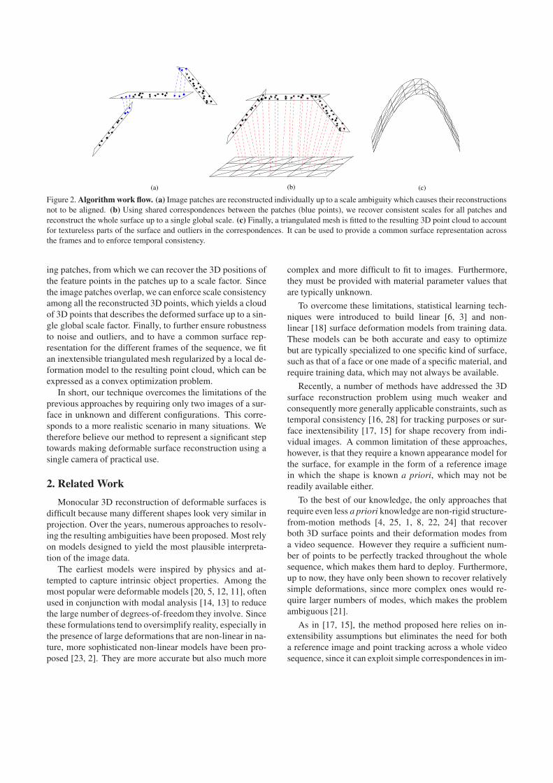
Figure 2. Algorithmwork flow. (a) Image patches are reconstructed individually up to a scale ambiguity which causes their reconstructions

not to be aligned. (b) Using shared correspondences between the patches (blue points), we recover consistent scales for all patches and

reconstruct the whole surface up to a single global scale. (c) Finally, a triangulated mesh is fitted to the resulting 3D point cloud to account

for textureless parts of the surface and outliers in the correspondences. It can be used to provide a common surface representation across

the frames and to enforce temporal consistency.

ing patches, from which we can recover the 3D positions of

the feature points in the patches up to a scale factor. Since

the image patches overlap, we can enforce scale consistency

among all the reconstructed 3D points, which yields a cloud

of 3D points that describes the deformed surface up to a sin-

gle global scale factor. Finally, to further ensure robustness

to noise and outliers, and to have a common surface rep-

resentation for the different frames of the sequence, we fit

an inextensible triangulated mesh regularized by a local de-

formation model to the resulting point cloud, which can be

expressed as a convex optimization problem.

In short, our technique overcomes the limitations of the

previous approaches by requiring only two images of a sur-

face in unknown and different configurations. This corre-

sponds to a more realistic scenario in many situations. We

therefore believe our method to represent a significant step

towards making deformable surface reconstruction using a

single camera of practical use.

2. Related Work

Monocular 3D reconstruction of deformable surfaces is

difficult because many different shapes look very similar in

projection. Over the years, numerous approaches to resolv-

ing the resulting ambiguities have been proposed. Most rely

on models designed to yield the most plausible interpreta-

tion of the image data.

The earliest models were inspired by physics and at-

tempted to capture intrinsic object properties. Among the

most popular were deformable models [20, 5, 12, 11], often

used in conjunction with modal analysis [14, 13] to reduce

the large number of degrees-of-freedom they involve. Since

these formulations tend to oversimplify reality, especially in

the presence of large deformations that are non-linear in na-

ture, more sophisticated non-linear models have been pro-

posed [23, 2]. They are more accurate but also much more

complex and more difficult to fit to images. Furthermore,

they must be provided with material parameter values that

are typically unknown.

To overcome these limitations, statistical learning tech-

niques were introduced to build linear [6, 3] and non-

linear [18] surface deformation models from training data.

These models can be both accurate and easy to optimize

but are typically specialized to one specific kind of surface,

such as that of a face or one made of a specific material, and

require training data, which may not always be available.

Recently, a number of methods have addressed the 3D

surface reconstruction problem using much weaker and

consequently more generally applicable constraints, such as

temporal consistency [16, 28] for tracking purposes or sur-

face inextensibility [17, 15] for shape recovery from indi-

vidual images. A common limitation of these approaches,

however, is that they require a known appearance model for

the surface, for example in the form of a reference image

in which the shape is known a priori, which may not be

readily available either.

To the best of our knowledge, the only approaches that

require even less a priori knowledge are non-rigid structure-

from-motion methods [4, 25, 1, 8, 22, 24] that recover

both 3D surface points and their deformation modes from

a video sequence. However they require a sufficient num-

ber of points to be perfectly tracked throughout the whole

sequence, which makes them hard to deploy. Furthermore,

up to now, they have only been shown to recover relatively

simple deformations, since more complex ones would re-

quire larger numbers of modes, which makes the problem

ambiguous [21].

As in [17, 15], the method proposed here relies on in-

extensibility assumptions but eliminates the need for both

a reference image and point tracking across a whole video

sequence, since it can exploit simple correspondences in im-

1

2

3

10

13

15

14

12

16

17

5

4 6

9

7

811

8

16 7

12

4

5

11

2

13

17

9

14

1315

10

6

Support ImageInput Image

Figure 3. Splitting the input image into overlapping patches.

Numbered circles represent the correspondences found between

the input and support frames and colored squares are the patches.

Note that some correspondences are shared by 2 or 4 patches.

These shared correspondences are used later to estimate the rel-

ative scale of these patches with respect to each other in order to

have a consistent shape.

age pairs.

3. Two-Frame Reconstruction

In this section, we show how we can reconstruct the

shape of a 3D deforming surface from 2 frames, provided

that we can establish enough correspondences and that the

surface changes from one frame to the other. Note that

this is very different both from conventional stereo, which

relies on the shape being the same in both frames, and

from recent monocular approaches to 3D shape recovery,

which require knowledge of the shape in a reference im-

age [16, 28, 17, 15].

In the following, we refer to the first image of the pair as

the input image in which we want to recover the 3D shape

and to the second as the support image. We assume the

camera to be calibrated and the matrix K of intrinsic pa-

rameters given. To simplify our notations and without loss

of generality, we express all 3D coordinates in the camera

referential. Finally, we assume that the surface is inextensi-

ble and model it as a set of overlapping planar patches 1 that

only undergo rigid transformations between the two images.

Given point correspondences between the input and sup-

port images established using SIFT [9], all subsequent algo-

rithmic steps depicted by Fig. 2 only involve solving linear

or convex optimization problems. We first split the input

image into small overlapping patches and compute homo-

graphies between pairs of corresponding patches. For each

patch, the corresponding homography can be decomposed

into relative rotation and translation, which let us compute

the 3D coordinates of all its feature points up to a scale fac-

tor. We can then recover a cloud of 3D points for the whole

surface up to a global scale factor, by enforcing consistency

1In practice, on images such as those presented in the result section, we

use patches of size 100 × 100 pixels that overlap by 50 pixels.

between neighboring patches. Finally, to fill the gaps in the

reconstructed points and to discard outliers, we fit a trian-

gulated surface model to this cloud. In the remainder of this

section, we describe these steps in more details.

3.1. Homography Decomposition

Since we model the surface as a set of rigidly moving

patches, we can define these patches over the input image

by splitting it into small overlapping regions as depicted by

Fig. 3. For each such patch, we estimate the homography

that links its feature points to the corresponding ones in the

support image. To this end, we perform a RANSAC-based

robust homography estimation [7] and label the correspon-

dences which disagree with the estimated homography as

outliers. This yields a reduced number of points on the im-

ages, which we now consider as our correspondences, and

which are grouped into local patches with an estimated ho-

mography for each.

Given the homography estimated for a patch, we now

seek to retrieve its 3D surface normal ni as well as its rigid

motion between the two frames expressed as a rotation and

translation. As depicted by Fig. 4, this is equivalent to as-

suming that the patch is fixed and that the camera is moving,

which yields one virtual camera per patch. Since we know

its internal parameters, its translation ti, its rotation Ri and

ni can be recovered up to a scale factor by decomposing the

homography [27, 10]. Let Pi = K[Ri|ti] be the projection

matrix of the virtual camera for patch i. The decomposition

of the corresponding homography Hi is expressed as

Hi = Ri −tin

Ti

di= Ri − t′in

Ti , (1)

where di is the unknown distance of the patch to the camera

and t′i is the scaled translation. This decomposition results

in two distinct solutions for the relative camera motion and

the patch normals. We pick the solution with the normal

whose sum of the angle differences with the neighboring

patches is smallest.

3.2. Reconstruction of a single patch

Given a virtual camera Pi, whose external parameters

were estimated from the homography, and the original cam-

era P0 = K[I|0], we seek to reconstruct the Ci 3D points

Xij , 1 ≤ j ≤ Ci of patch i. To this end, we minimize

the reprojection errors both in the input and support frames,

which, for a single point j can be formulated as the least-

squares solution to the linear system

BijX

ij = bi

j , (2)

P4

P3P2

P1 P0

P0

P0

t1t0

(b)(a)

Figure 4. Equivalence between a deforming surface and moving virtual cameras (a) A deformable surface in two different frames

observed with a fixed monocular camera setup. (b) Equivalent representation where the surface is now fixed, but each patch is seen from

two cameras: the original one, P0, and a virtual one, Pi, which can be found by decomposing the homography relating the patch at time

t0 and time t1.

where

bij =

−p014 + ri

j,xp034

−p024 + ri

j,yp034

−pi14 + si

j,xpi34

−pi24 + si

j,ypi34

4×1

, and (3)

Bij =

p011 − ri

j,xp031 p0

12 − rij,xp0

32 p013 − ri

j,xp033

p021 − ri

j,yp031 p0

22 − rij,yp0

32 p023 − ri

j,yp033

pi11 − si

j,xpi31 pi

12 − sij,xpi

32 pi13 − si

j,xpi33

pi21 − si

j,ypi31 pi

22 − sij,ypi

32 pi23 − si

j,ypi33

4×3

,

(4)

and where pkmn the (m, n)th entry of the kth projection ma-

trix Pk, and rij and si

j are the 2D coordinates on the input

frame and on the support frame, respectively.

Furthermore, to ensure that the patch remains flat, we

constrain its points to lie on a plane whose normal is the one

given by the homography decomposition of Eq. (1). Since

the reconstruction of the points in camera coordinates can

only be up to a scale factor, we can fix without loss of gen-

erality the depths of the plane to a constant value, di = d0.

For a single point j, the planarity constraint can then also

be formulated as a linear equation in terms of Xij as

nTi Xi

j = −d0 . (5)

We combine Eqs. (2) and (5) into the linear system

GijX

ij = gi

j , (6)

where Gij =

[

Bij

nTi

]

5×3

and gij =

[

bij

−d0

]

5×1

.

We can then group individual systems for each point inpatch i into the system

2

6

6

6

6

6

6

4

Gi1

. . .

Gij

. . .

GiCi

3

7

7

7

7

7

7

5

2

6

6

6

6

6

6

4

Xi1

..

.

Xij

...

XiCi

3

7

7

7

7

7

7

5

=

2

6

6

6

6

6

6

4

gi1

..

.

gij

...

giCi

3

7

7

7

7

7

7

5

, (7)

whose solution is valid up to a scale factor in camera coor-

dinates.

3.3. Reconstruction of Multiple Patches

The method described above lets us reconstruct 3D

patches individually each with its own depth in camera co-

ordinates. However, because the depths of different patches

are inconsistent, this results in an unconnected set of 3D

points. We therefore need to re-scale each patch with re-

spect to the others to form a consistent point cloud for the

whole surface. To this end, we use overlapping patches in

the input image where each patch shares some of the cor-

respondences with its neighbors. Let Y be a single point

shared by patches i and i′ such that Y = Xij = Xi′

j′ . The

scales di and di′ for the two patches can then be computed

by solving the linear system

Bij 04×2

nTi 1 0

Bi′

j′ 04×2

nTi′ 0 1

Y

di

di′

=

bij

0

bi′

j′

0

. (8)

As before, the equations for all the shared points of all the

patches can be grouped together, which yields the system

Q

Y

d1

...

dNp

= q , (9)

where Y is the vector of all shared 3D points, Np is the

number of planar patches and Q and q are formed by

adequately concatenating the matrices and the vectors of

Eq. (8). Solving Eq. (9) gives the relative scales[

d1...dNp]

for all the patches, which lets us compute a consistent 3D

point cloud for the whole surface. Note, however, that, since

these scales are relative, the resulting point cloud is recov-

ered up to a single global scale factor.

3.4. From Point Clouds to Surfaces

In the previous sections, we have presented an approach

to reconstructing 3D points from two images depicting two

different configurations of the surface. Because the recov-

ered point clouds may still contain some outliers and be-

cause in many applications having a common surface rep-

resentation for all the frames of a sequence is of interest,

we fit a triangulated mesh to the reconstructed point clouds

within a convex optimization framework.

3.4.1 Mesh Fitting for a Single Frame

Given the vector X obtained by concatenating the N recon-

structed 3D points , we seek to recover the deformation of

a given mesh with Nv vertices and Ne edges that best fits

X. Since X has been reconstructed up to a global scale fac-

tor, we first need to resize it, so that it matches the mesh

area. In camera coordinates, a rough approximation of the

scale of a surface can be inferred from the mean depth of

its points. Computing such values for both the mesh and

the point cloud allows us to resize the latter to a scale sim-

ilar to that of the mesh. Then, because the surface may

have undergone a rigid transformation, we align the mesh

to the point cloud by applying a standard Iterative Closest

Point (ICP) algorithm [26]. In the current implementation,

a coarse manual initialization is provided for ICP. This is

the only non fully automated step in the whole algorithm. It

is required to indicate an area of interest in the absence of a

reference image.

From this first alignment, we can deform the mesh to

fit the point cloud. To do so, we first estimate the loca-

tion of each 3D point Xj on the mesh. These locations

are given in barycentric coordinates with respect to the

mesh facets, and can be obtained by intersecting rays be-

tween the camera center and the 3D points with the mesh.

Given this representation, each 3D point can be written as

Xj =∑3

k=1 αkvkf(j), where f(j) represents the facet to

which point j was attached, and vkf(j) is its kth vertex. Fit-

ting a mesh to the whole point cloud can then be written as

the solution of the linear system

MV = X , (10)

where M is a 3N × 3Nv matrix containing the barycentric

coordinates of all 3D points, and V is the vector of concate-

nated mesh vertices.

Because the scale factor obtained from the depth of the

points is only a rough estimate of the true scale, we need

to refine it. This can be done by introducing a variable γ

accounting for the scale of the point cloud in the above-

mentioned reconstruction problem, and solve

MV = γX . (11)

However, without further constraints on the mesh, nothing

prevents it from shrinking to a single point and therefore

perfectly satisfy the equation. Assuming that the surface

is inextensible, we can overcome this issue by maximiz-

ing γ under inequality constraints that express the fact that

the edges of the mesh cannot stretch beyond their original

length. The problem can then be re-formulated as the opti-

mization problem

maximizeV,γ

wsγ − ‖MV − γX‖ (12)

subject to ‖vk − vj‖ ≤ lj,k , ∀(j, k) ∈ E

γlow ≤ γ ≤ γup ,

where E is the set of mesh edges, lj,k is the original length

of the edge between vertices vj and vk, and ws is a weight

that sets the relative influence between point distance min-

imization and scale maximization. To further constrain the

scale of the point cloud, we introduced a lower and an up-

per bounds γlow and γup. The advantage of using inequal-

ity constraints over edge length equalities is twofold. First,

the inequality constraints are convex, and can therefore be

optimized easily. Second, these constraints also are more

general than the equality ones, since they allow to account

for folds appearing between the vertices of the mesh, which

is bound to happen in real scenarios.

Finally, to account for outliers in the 3D reconstructed

points, we introduce a linear local deformation model. As

in [18], we model a global surface as a combination of local

patches. Note that these patches are different from those

used in the point cloud reconstruction, since we expect them

to deform. To avoid the complexity of the non-linear model

of [18], and to keep our formulation convex, we use a linear

local model, where the shape of a patch Vi is computed as

a linear combination of Nm deformation modes λj , 1 ≤j ≤ Nm, which we can write

Vi = V0i + Λci , (13)

where Λ is the matrix whose columns are the deformation

modes, V0i is the mean shape of patch i, and ci is the vector

of its mode coefficients. Thanks to the local deformation

models, this method is applicable to meshes of any shape,

be it rectangular, circular, triangular, or any other.

In practice, these modes are obtained by applying Prin-

cipal Component Analysis (PCA) to a set of inextensi-

ble patches deformed by randomly setting the angles be-

tween their facets. Since the deformation modes obtained

with PCA are orthonormal, the coefficients ci that define

a patch shape can be directly computed from Vi as ci =ΛT

(

Vi − V0i

)

. This, in contrast with the standard use of

linear deformation models, lets us express our deformation

model directly in terms of the mesh vertex coordinates. Fur-

thermore, we use all the modes, which lets us represent any

complex shape of a patch, and we regularize the projection

of the shape in the modes space by minimizing

∥

∥

∥Σ−1/2ci

∥

∥

∥=

∥

∥

∥Σ−1/2ΛT

(

Vi − V0i

)

∥

∥

∥, (14)

which penalizes overly large mode weights, and where Σis a diagonal matrix containing the eigenvalues of the train-

ing data covariance matrix. This lets us define the global

regularization term

Er(V) =

Nd∑

i=1

∥

∥

∥Σ−1/2ΛT

(

Vi − V0i

)

∥

∥

∥, (15)

by summing the measure of Eq. 14 over all Nd overlapping

patches in the mesh. This regularization can be inserted into

our convex optimization problem, which then becomes

maximizeV,γ

wsγ − ‖MV − γX‖ − wrEr(V) (16)

subject to ‖vk − vj‖ ≤ lj,k , ∀(j, k) ∈ E

γlow ≤ γ ≤ γup ,

where wr is a regularization weight. In practice, be-

cause the shape of the mesh is initially far from matching

that of the point cloud, we iteratively compute the barycen-

tric coordinates of the points on the surface and solve the

optimization problem of Eq. 16 using the available solver

SeDuMi [19].

3.4.2 Enforcing Consistency over Multiple Frames

While, in most cases, the mesh reconstruction presented in

the previous section is sufficient to obtain accurate shapes,

we can further take advantage of having a video sequence

to enforce consistency across the frames. In the previous

formulation nothing constrains the barycentric coordinates

of a point to be the same in every frame where it appears.

We now show that such constraints can be introduced in our

framework. This lets us reconstruct multiple frames simul-

taneously, which stabilizes the individual results in a way

that is similar to what bundle adjustment methods do.

The only additional requirement is to be able to identify

the reconstructed points in order to match them across dif-

ferent frames. This requirement is trivially fulfilled when

all points have been reconstructed using the same support

frame. With multiple support frames, such an identifica-

tion can easily be obtained by additionally matching points

across the different support frames. Given the identity of

all points, we only need to compute barycentric coordinates

once for each point, instead of in all frames as before. For

points shared between several frames, this is done in the

frame that gave the minimum point-to-surface distance.This lets us rewrite the optimization problem of Eq. 16

in terms of the vertex coordinates in the Nf frames of a

sequence as

maximizeV

1,...,Nf ,γ1,...,Nf

NfX

t=1

`

wsγt − ‖Mt

Vt − γ

tX

t‖ − wrEr(Vt)

´

subject to ‖vtk − v

tj‖ ≤ lj,k , ∀(j, k) ∈ E , ∀t ∈ [1, Nf ]

γlow ≤ γt ≤ γup ,∀t ∈ [1, Nf ] , (17)

where Vt, γt, Xt and Mt are similar quantities as in Eq. 16

but for frame t. As in the single frame case, we iteratively

solve this problem and recompute the barycentric coordi-

nates of the unique points.

4. Results

We first applied our approach to synthetic data to quan-

titatively evaluate its performance. We obtained the meshes

of Fig. 5 by capturing the deformations of a piece of pa-

per using a Vicontm optical motion capture system. We

then used those to create synthetic correspondences by ran-

domly sampling the mesh facets and projecting them using

a known projection matrix and adding varying amounts of

noise to the resulting image coordinates.

In Fig. 5(e), we superpose the reconstructions obtained

for the same input image using different images as the sup-

port frame and the ground truth mesh, without noise. Note

how well superposed the reconstructed surfaces are, thus

indicating the insensitivity of our approach to the specific

choice of support frame. The mean distances between the

recovered vertices and those of the ground truth mesh vary

from 3.8 to 5.6, which is quite small with respect to 20, the

length of the mesh edges before deformation.

We then used the first frame as the support frame and

all the others in turn as the input frame. In the graph of

Fig. 6(a), each curve represents the mean distance between

the reconstructed mesh vertices and their true positions in

successive frames for a specific noise level in the correspon-

dences. As evidenced by Fig. 5, a mean error of 2 is very

small and one of 5 remains barely visible. For comparison

purposes, we implemented the method of [17] that relies

on knowing the exact shape in one frame. At low noise

levels, the results using the same correspondences are com-

parable, which is encouraging since our approach does not

imply any a priori knowledge of the shape in any frame.

At higher noise levels, however, the performance of our ap-

proach degrades faster, which is normal since we solve a

much less constrained problem.

In practice, since SIFT provides inliers whose mean error

is less than 2 pixels and since we use a robust estimator, this

does not substantially affect our reconstructions. To demon-

strate this, in Figs. 7 and 8, we show results on real video

sequences of a deforming piece of paper2 and a T-shirt. We

2This sequence is publicly available at http://cvlab.epfl.ch/data/dsr/

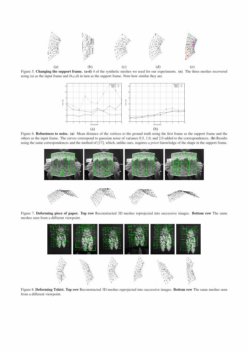
(a) (b) (c) (d) (e)Figure 5. Changing the support frame. (a-d) 4 of the synthetic meshes we used for our experiments. (e). The three meshes recovered

using (a) as the input frame and (b,c,d) in turn as the support frame. Note how similar they are.

0

2

4

6

8

10

12

1 2 3 4 5 6 7 8 9 10

Err

or

in 3

D

Frame Number

Noise=0.5

Noise=1

Noise=2

(a)

0

2

4

6

8

10

12

1 2 3 4 5 6 7 8 9 10

Err

or

in 3

DFrame Number

Noise=0.5

Noise=1

Noise=2

(b)Figure 6. Robustness to noise. (a) Mean distance of the vertices to the ground truth using the first frame as the support frame and the

others as the input frame. The curves correspond to gaussian noise of variance 0.5, 1.0, and 2.0 added to the correspondences. (b) Results

using the same correspondences and the method of [17], which, unlike ours, requires a priori knowledge of the shape in the support frame.

Figure 7. Deforming piece of paper. Top row Reconstructed 3D meshes reprojected into successive images. Bottom row The same

meshes seen from a different viewpoint.

Figure 8. Deforming Tshirt. Top row Reconstructed 3D meshes reprojected into successive images. Bottom row The same meshes seen

from a different viewpoint.

also supply corresponding video-sequences as supplemen-

tary material to allow the readers to judge for themselves

the quality of the reconstructions. In this material, we also

include results from the multi-frame fitting of Section 3.4.2,

which do not look very different from those of the single-

frame fitting of Section 3.4.1 on the printed page but give a

much smoother feel when seen in sequence.

5. Conclusion

We have presented an approach to deformable surface

3D reconstruction that overcomes most limitations of state-

of-the-art techniques. We can recover the shape of a non-

rigid surface while requiring neither points to be tracked

throughout a whole video sequence nor a reference image

in which the surface shape is known. We only need a pair

of images displaying the surface in two different configura-

tions and with enough texture to establish correspondences.

We believe this to be both a minimal setup for which a

correspondence-based 3D shape recovery technique could

possibly work and a practical one for real-world applica-

tions.

In future work, we will explore the use of multiple

frames to handle self-occlusions. In our current implemen-

tation, points that are occluded in one of the two images

cannot be reconstructed and we have to depend on surface

fitting using a local deformation model to guess the shape

around such points. However, since we can perform recon-

struction from any two pairs of images, we will work on

merging the results and filling the gaps without having to

rely solely on interpolation.

References

[1] A. Bartoli and S. Olsen. A Batch Algorithm For Implicit

Non-Rigid Shape and Motion Recovery. In ICCV Workshop

on Dynamical Vision, Beijing, China, October 2005.

[2] K. S. Bhat, C. D. Twigg, J. K. Hodgins, P. K. Khosla,

Z. Popovic, and S. M. Seitz. Estimating cloth simulation

parameters from video. In ACM Symposium on Computer

Animation, 2003.

[3] V. Blanz and T. Vetter. A Morphable Model for The Syn-

thesis of 3–D Faces. In SIGGRAPH, pages 187–194, Los

Angeles, CA, August 1999.

[4] M. Brand. Morphable 3d models from video. CVPR, 2001.

[5] L. Cohen and I. Cohen. Finite-element methods for active

contour models and balloons for 2-d and 3-d images. PAMI,

15(11):1131–1147, November 1993.

[6] T. Cootes, G. Edwards, and C. Taylor. Active Appearance

Models. In ECCV, pages 484–498, Germany, June 1998.

[7] R. Hartley and A. Zisserman. Multiple View Geometry in

Computer Vision. Cambridge University Press, 2000.

[8] X. Llado, A. D. Bue, and L. Agapito. Non-rigid 3D Fac-

torization for Projective Reconstruction. In BMVC, Oxford,

UK, September 2005.

[9] D. Lowe. Object recognition from local scale-invariant fea-

tures. In ICCV, pages 1150–1157, 1999.

[10] E. Malis and V. Manuel. Deeper understanding of the ho-

mography decomposition for vision-based control. Techni-

cal report, 2007.

[11] T. McInerney and D. Terzopoulos. A dynamic finite ele-

ment surface model for segmentation and tracking in mul-

tidimensional medical images with application to cardiac 4d

image analysis. Computerized Medical Imaging and Graph-

ics, 19(1):69–83, 1995.

[12] D. Metaxas and D. Terzopoulos. Constrained deformable su-

perquadrics and nonrigid motion tracking. PAMI, 15(6):580–

591, 1993.

[13] C. Nastar and N. Ayache. Frequency-based nonrigid motion

analysis. PAMI, 18(11), November 1996.

[14] A. Pentland and S. Sclaroff. Closed-form solutions for phys-

ically based shape modeling and recognition. PAMI, 13:715–

729, 1991.

[15] M. Perriollat, R. Hartley, and A. Bartoli. Monocular

template-based reconstruction of inextensible surfaces. In

BMVC, 2008.

[16] M. Salzmann, R. Hartley, and P. Fua. Convex optimization

for deformable surface 3–d tracking. In ICCV, Rio, Brazil,

October 2007.

[17] M. Salzmann, F. Moreno-Noguer, V. Lepetit, and P. Fua.

Closed-form solution to non-rigid 3d surface registration. In

ECCV, Marseille, France, October 2008.

[18] M. Salzmann, R. Urtasun, and P. Fua. Local deformation

models for monocular 3d shape recovery. In CVPR, Anchor-

age, Alaska, June 2008.

[19] J. F. Sturm. Using SEDUMI 1.02, a MATLAB∗ toolbox for

optimization over symmetric cones, 2001.

[20] D. Terzopoulos, A. Witkin, and M. Kass. Symmetry-seeking

Models and 3D Object Reconstruction. IJCV, 1:211–221,

1987.

[21] L. Torresani, A. Hertzmann, and C. Bregler. Learning non-

rigid 3d shape from 2d motion. In Advances in Neural Infor-

mation Processing Systems. MIT Press, MA, 2003.

[22] L. Torresani, A. Hertzmann, and C. Bregler. Nonrigid

structure-from-motion: Estimating shape and motion with

hierarchical priors. PAMI, 30(5):878–892, 2008.

[23] L. V. Tsap, D. B. Goldgof, and S. Sarkar. Nonrigid motion

analysis based on dynamic refinement of finite element mod-

els. PAMI, 22(5):526–543, 2000.

[24] R. Vidal and R. Hartley. Perspective nonrigid shape and mo-

tion recovery. In ECCV, France, October 2008.

[25] J. Xiao and T. Kanade. Uncalibrated perspective reconstruc-

tion of deformable structures. In ICCV, 2005.

[26] Z. Zhang. Iterative point matching for registration of free-

form curves and surfaces. IJCV, 13(2):119–152, 1994.

[27] Z. Zhang and A. R. Hanson. Scaled euclidean 3d reconstruc-

tion based on externally uncalibrated cameras. In In IEEE

Symposium on Computer Vision, Coral Gables, FL, pages

37–42, 1995.

[28] J. Zhu, S. C. Hoi, Z. Xu, and M. R. Lyu. An effective ap-

proach to 3d deformable surface tracking. In ECCV, 2008.

Template-free monocular reconstruction of deformable surfaces

Documents

Transcript of Template-free monocular reconstruction of deformable surfaces