HARDEE, JOHN D., M.A. Pseudospectra and Structured Pseudospectra. (2012)Directed by Dr. Richard Fabiano. 54 pp.

Pseudospectra and structured pseudospectra are subsets of the complex plane

which give a geometric representation, via eigenvalues, of the eects of perturbations

to a matrix. We survey the historical development of the subject, and the denitions

and characterizations of the various sets of pseudospectra. Motivated by the fact that

a nonnormal matrix in the 2-norm can become normal in a dierent norm, we describe

a numerical investigation into the question of characterizing which perturbations have

the greatest eect on the eigenvalues of the matrix.

PSEUDOSPECTRA AND STRUCTURED PSEUDOSPECTRA

by

John D. Hardee

A Thesis Submitted tothe Faculty of the Graduate School at

The University of North Carolina at Greensboroin Partial Fulllment

of the Requirements for the DegreeMaster of Arts

Greensboro2012

Approved by

Committee Chair

This thesis is dedicated to my family and friends, the faculty of the University of

North Carolina at Greensboro mathematics department, and to the Brevard College

mathematics department.

ii

APPROVAL PAGE

This thesis has been approved by the following committee of the Faculty of The

Graduate School at The University of North Carolina at Greensboro.

Committee ChairRichard Fabiano

Committee MembersMaya Chhetri

Paul Duvall

Date of Acceptance by Committee

Date of Final Oral Examination

iii

ACKNOWLEDGMENTS

Dr. Richard Fabiano, Dr. Maya Chhetri, and Dr. Paul Duvall.

iv

TABLE OF CONTENTS

Page

LIST OF FIGURES . . . . . . . . . . . . . . . . . . . . . . . . . . . . . . . . . . . . . . . vi

CHAPTER

I. INTRODUCTION AND DEFINITIONS . . . . . . . . . . . . . . . . . . . 1

I.I. Introduction . . . . . . . . . . . . . . . . . . . . . . . . . . . . . . . . . 1I.II. Notation and Motivation . . . . . . . . . . . . . . . . . . . . . . . . . 2I.III. Pseudospectra . . . . . . . . . . . . . . . . . . . . . . . . . . . . . . . . 6I.IV. Structured Pseudospectra . . . . . . . . . . . . . . . . . . . . . . . . . 8

II. CHARACTERIZATIONS AND NORMALITY . . . . . . . . . . . . . . . 12

II.I. Equivalent Characterizations of Pseudospectral Sets . . . . . . . 12II.II. Normal Matrices . . . . . . . . . . . . . . . . . . . . . . . . . . . . . . . 19II.III. Change of Norm . . . . . . . . . . . . . . . . . . . . . . . . . . . . . . . 22

III. NUMERICAL INVESTIGATIONS . . . . . . . . . . . . . . . . . . . . . . . 26

III.I. Constructing Perturbation Matrices . . . . . . . . . . . . . . . . . . 27III.II. Conjecture and Investigations . . . . . . . . . . . . . . . . . . . . . . 29III.III. Conclusion . . . . . . . . . . . . . . . . . . . . . . . . . . . . . . . . . . 36

REFERENCES . . . . . . . . . . . . . . . . . . . . . . . . . . . . . . . . . . . . . . . . . . 37

APPENDIX A. NOTATIONS . . . . . . . . . . . . . . . . . . . . . . . . . . . . . . . . 39

APPENDIX B. PROOFS . . . . . . . . . . . . . . . . . . . . . . . . . . . . . . . . . . . 41

APPENDIX C. MATLAB CODES . . . . . . . . . . . . . . . . . . . . . . . . . . . . . 44

v

LIST OF FIGURES

Page

Figure 1. Matrix showing how perturbations can cause instability . . . . . . . . . 4

Figure 2. Matrix showing how perturbations can cause instability . . . . . . . . . 5

Figure 3. `Poor Man's' method of estimating pseudospectra . . . . . . . . . . . . . 8

Figure 4. Plotting the norm of the resolvent over a mesh grid . . . . . . . . . . . 14

Figure 5. Plotting the contour lines for pseudospectra . . . . . . . . . . . . . . . . 15

Figure 6. Pseudospectra of a randomly generated normal matrix . . . . . . . . . 21

Figure 7. Pseudospectrum of random matrix for ε = 0.1 . . . . . . . . . . . . . . . 30

Figure 8. Pseudospectrum of random matrix for ε = 0.035 . . . . . . . . . . . . . . 31

Figure 9. Pseudospectrum of random matrix for ε = 0.005 . . . . . . . . . . . . . . 32

Figure 10. Pseudospectrum of random matrix for ε = 0.25 . . . . . . . . . . . . . . 33

Figure 11. Pseudospectrum of random matrix for ε = 0.1 . . . . . . . . . . . . . . . 34

Figure 12. Pseudospectrum - negative eigenvalues . . . . . . . . . . . . . . . . . . . . 35

Figure 13. Pseudospectrum - eigenvalues inside the unit circle . . . . . . . . . . . . 36

vi

CHAPTER I

INTRODUCTION AND DEFINITIONS

I.I Introduction

The research in this thesis is centralized in the study of error in mathematical

models of physical phenomena in the sciences and engineering. In this context, error

refers to the dierence between a value computed with the mathematical model and

the corresponding actual value in the real-world phenomenon being modeled. There

are many sources of error in mathematical models, such as inaccuracy in measurement

of data, simplifying assumptions in the modeling process, round-o error in computer

calculations, approximation error in numerical methods, etc. Therefore for any math-

ematical model it is important to understand the eect of small perturbations. For

linear mathematical models, particularly linear dierential equations and dierence

equations, an important issue is the eect of perturbations on the stability of solu-

tions. The stability of solutions is in turn determined by the location in the complex

plane of the eigenvalues of the relevant system matrix. This observation motivates

the issues investigated in this thesis, namely, the eects of small perturbations on the

location of eigenvalues of a matrix. The study of such issues lies within the general

area of perturbation theory, and leads naturally to the notion of pseudospectra. In

the remainder of this introductory chapter, notations and denitions will be given

while a more explicit understanding of the motivation of this paper is shown.

1

I.II Notation and Motivation

The set of all complex numbers will be denoted by C, the set of all vectors of length

n with complex entries by Cn, and the set of all matrices of size m× n with complex

entries by Cm×n. For notational purposes, all matrices will be denoted by a bold

uppercase English alphabet letter, all vectors will be denoted by a lowercase English

alphabet letter, and all complex scalars will be denoted by a lowercase Greek alphabet

letter. All of the denitions and results in the thesis generalize to linear operators on

nite dimensional vector spaces. The identity matrix in Cn×n will be denoted by I

unless otherwise dened. For a matrix A, the range is denoted by R(A), and the null

space by N (A). The orthogonal complement of a subspace Z of Cn will be denoted

by Z⊥. The norm of a vector in Cn will be denoted by ‖·‖. Any norm on Cn denes

an induced matrix norm on a matrix A ∈ Cn×n by ‖A‖ = maxx 6=0

‖Ax‖‖x‖ = max

‖x‖=1‖Ax‖

[5, pp.56].

Denition 1. Let A ∈ Cn×n. A non-zero vector v is an eigenvector of the matrix

A corresponding to the eigenvalue λ if Av = λv. The set of all eigenvalues of A is

called the spectrum of A, and will be denoted by Λ(A) [5, pp.332-333].

Thus Λ(A) ⊂ C, and it is known that there are at most n distinct eigenvalues

in Λ(A) [5, pp.332]. The Euclidean inner product on Cn is dened by (x, y) =∑nj=1 xjyj = y∗x where y∗ denotes the conjugate transpose of y [18, pp.17]. The

vector 2-norm on a vector x ∈ Cn dened by the Euclidean inner product is ‖x‖22 =

(x, x) =∑n

j=1 |xj|2 [18, pp.9,17]. It is known that the induced matrix 2-norm ‖A‖2

is equal to the largest singular value of A [5, pp.71].

2

One motivation for this paper is the issue of the stability of linear dierential equa-

tions. An important mathematical model is a system of rst order linear dierential

equations, which can be formulated as the matrix ordinary dierential equation

d

dtx(t) = Ax(t), x(0) = x0 ∈ Cn. (1)

A solution is an n × 1 vector-valued function x(t). The system (1) is said to be

exponentially stable if there exist M ≥ 1 and α > 0 such that for any x0 ∈ Cn,

‖x(t)‖ ≤Me−αt‖x(0)‖ for all t ≥ 0. In this case the solutions satisfy limt→∞‖x(t)‖ = 0.

It is known that (1) is exponentially stable if and only if the spectrum lies in the left

half complex plane. In this case we also say that A is stable. Because of the sources

of error in the mathematical model, it is often desirable to understand how small

perturbations toA aect its stability. For a system like (1), this means understanding

whether perturbations toA have eigenvalues in the right half of the the complex plane.

Figure 1 illustrates the possibilities for the built-in MATLAB [14] gallery matrix grcar.

The grcar matrices are n× n matrices, n ≥ 4, with 1's down the main diagonal, -1's

down the rst subdiagonal, 1's on the rst three superdiagonals and zero's as all other

elements. Figure 1 shows the eigenvalues of a matrix A denoted by which are all

in the left half complex plane, and the eigenvalues of the matrix A + E denoted by

. With ‖E‖2 = 0.01, A + E has eigenvalues in the right half complex plane.

3

Figure 1. Matrix showing how perturbations can cause instability

Another motivating example is the stability of linear dierence equations or recur-

sion equations. Given an initial vector x0 ∈ Cn a recursive sequence can be dened

as

xj+1 = Axj. (2)

The system is said to be stable if the solutions satisfy limn→∞

‖xn‖ = 0. It is known that

(2) is stable if and only if the spectrum ofA lies inside the unit circle. Just as with (1),

for (2) we may ask if small perturbations to A can have eigenvalues outside the unit

circle in C. Figure 2 illustrates the possibilities plotting the eigenvalues of a matrix

4

A denoted by which are all in the left half complex plane, and the eigenvalues of

the matrix A + E denoted by . With ‖E‖2 = 0.01, A + E has eigenvalues outside

the unit circle.

Figure 2. Matrix showing how perturbations can cause instability

5

I.III Pseudospectra

The notion of pseudospectra is used to describe the set of eigenvalues which arise

from small perturbations to a matrix.

Denition 2. Let ε > 0 be arbitrary. The ε-pseudospectrum of A, denoted by

T (A; ε) [18, pp.14], is the set of λ ∈ C such that λ ∈ Λ(A + E) for some E ∈ Cn×n

with ‖E‖ ≤ ε:

T (A; ε) = λ ∈ C : λ ∈ Λ(A + E) for some E with ‖E‖ ≤ ε. (3)

It should be noted that the ε-pseudospectrum depends on the choice of norm,

even though this is not explicitly indicated in the notation. In 1967, J.M. Varah in-

troduced the idea of ε-pseudoeigenvalue in his thesis where he dened r-approximate

eigenvalues [21]. His motivation came from his analysis of the accuracy of eigen-

pairs produced by computer implementations of the inverse iteration algorithm [18].

In between Varah's thesis [21] and his 1979 paper [22] where he denes the term ε-

spectrum, H.J. Landau introduced ε-pseudoeigenvalues under the term ε-approximate

eigenvalues [13]. Though for Varah in [21] the rst denition of pseudospectra is said

to be dened, the rst published denition of pseudospectra is thought to be by

Landau in [13]. Throughout the 1980s, following their work in in the study of how

nonnormality aects the numerical stability of discretized dierential equations [4],

the Novosibirsk group including Sergei Godunov and colleagues conducted research

related to pseudospectra, and published the rst sketch of pseudospectra which were

6

called 'spectral portraits of matrices' containing various 'patches of spectrum' [11].

Other research on pseudospectra in the mid-1980s was conducted by J.W. Demmel,

of which includes a paper that presents the rst published computer plot of pseu-

dospectra [2]. In 1986, J.H. Wilkinson introduces the modern interpretation of ε-

pseudospectrum where he denes it for an arbitrary matrix norm induced by a vector

norm [23]. L.N. Trefethen published his rst works on pseudospectra in 1990, [16]

and [15], where he talks of ε-approximate eigenvalues and ε-pseudospectrum. Follow-

ing their mid-1980s work on the stability radius of a matrix, in 1992 D. Hinrichsen

and A.J. Pritchard introduced the term spectral value set which categorized real

structured ε-pseudospectrum of nonnormal matrices [8][9]. In 1993, Hinrichsen and

B. Kelb extended on [8] to complex perturbations and also more general structured

perturbations [7]. Finally, in 2005, Trefethen and M. Embree published their book

Spectra and Pseudospectra: The Behavior of Nonnormal Matrices and Operators

[18] which is the basis of citations and references throughout this thesis.

We can generate a crude but reasonable numerical approximation of T (A; ε) by

simply plotting the eigenvalues of A + E for a large number of randomly generated

matrices E satisfying ‖E‖ ≤ ε as seen in Figure 3. The plot on the left is the

pseudospectra generated by PM(A,[1 1E-1 1E-2],500), Appendix C, and the plot

on the right is the pseudospectra generated by PM(A,[1 1E-1 1E-2],5000). In both,

represents the eigenvalues of the matrix A=grcar(50);. This 'brute force' approach

is sometimes referred to as the `poor man's' method, and yields a reasonably accurate

picture of T (A; ε) [18, pp.378-379].

7

Figure 3. `Poor Man's' method of estimating pseudospectra

One can observe whether the numerically generated approximation of T (A; ε) has

any parts outside the known stability region. We note that pseudospectra have the

following property: for ε1 > ε2 > 0, the respective pseudospectra are nested sets:

T (A; ε2) ⊆ T (A; ε1). Thus⋂ε>0 T (A; ε) = Λ(A) [18, pp.15]. Therefore restricting

the ε to a smaller value can in turn restrict the pseudospectrum to a certain stability

region. In other words, it is possible to use the `poor man's' method to estimate the

largest value of ε for which T (A; ε) stays inside the stability region.

I.IV Structured Pseudospectra

In some applications it might be known that only certain types of perturbations

can arise. In this case it is reasonable to modify the denition of ε-pseudospectrum

8

to consider only the eigenvalues which arise from these certain specied types of

perturbations. In other cases, it might be necessary and sometimes convenient to be

able to control how the perturbation eects the given matrix. This leads to the notion

of structured pseudospectra. In 1992-1993, Hinrichsen and Pritchard developed the

idea of spectral value sets which leads to one possible method for dening structured

pseudospectra [79].

Denition 3. Let A ∈ Cn×n, B ∈ Cn×s, C ∈ Ct×n. Let ε > 0. The

structured ε-pseudospectrum of A, denoted by T (A;B,C, ε) [7, pp.2], is the set of

λ ∈ C such that λ ∈ Λ(A + BEC) for some E ∈ Cs×t with ‖E‖ ≤ ε:

T (A;B,C, ε) = λ ∈ C : λ ∈ Λ(A + BEC) for some E with ‖E‖ ≤ ε. (4)

It should be noted that as for the ε-pseudospectrum, the structured pseudospec-

trum depends on the choice of norm, even though this is not explicitly indicated in

the notation. The idea behind this denition of structured pseudospectra is to ma-

nipulate the perturbing matrices such that the pseudospectra produces the results

that are specic to certain requirements. By constructing the matrices B and C in

certain ways, the perturbations of the pseudospectra can be restricted which can be

useful in certain situations. The following example illustrates this idea.

9

Example 1. Given a matrix A ∈ Cn×n, to perturb A only at the i, jth entry, dene

B ∈ Cn×n and C ∈ Cn×n by

Bk,l =

1 if k = i and l = i

0 otherwise

Ck,l =

1 if k = j and l = j

0 otherwise

.

Therefore the set T (A;B,C, ε) consists of all eigenvalues of matrices which arise from

perturbations only to the i, jth entry of A: for all E ∈ Cn×n such that ‖E‖ ≤ ε

(A + BEC)k,l =

Ak,l if k 6= i or l 6= j

Ai,j + Ei,j if k = i and l = j

.

This comes from the fact that |Ei,j| ≤ ‖E‖ ≤ ε. Other choices of B and C can give

the same pseudospectra. For example if we dene B ∈ Cn×1 and C ∈ C1×n by

Bk,1 =

1 if k = i

0 otherwise

C1,l =

1 if l = j

0 otherwise

,

we get the same structured pseudospectra as above. Another expansion on the ex-

ample is to allow B or C to be the identity in the example.

10

This will give the following respectfully:

(A + BEC)k,l =

Ak,l if k 6= i

Ai,l + Ei,l if k = i

or

Ak,l if l 6= j

Ak,j + Ek,j if l = j

.

Here we are only perturbing the ith row or jth column respectfully.

In the next chapter, we will discuss the characterization of the pseudospectrum

and structured pseudospectrum in terms of the resolvent operator of a given matrix

A, and how the behavior of these sets is related to the departure from normality of

A. We will then investigate how changing the norm can aect normality, and hence

the behavior of the pseudospectrum and structured pseudospectrum of A.

11

CHAPTER II

CHARACTERIZATIONS AND NORMALITY

II.I Equivalent Characterizations of Pseudospectral Sets

A dierent characterization of the pseudospectrum of a matrix can be obtained

from the resolvent of the given matrix.

Denition 4. Let A ∈ Cn×n. For λ ∈ C \Λ(A), the resolvent of A is dened as the

matrix (λI−A)−1.

The following equivalent characterization of T , which we will denote by the set S,

is constructed through the use of the norm of the resolvent matrix, and gives a more

tangible understanding of the movement of the eigenvalues.

Denition 5. Let ε > 0 be arbitrary. The set S(A; ε) [18, pp.13] is the set of λ ∈ C

such that ‖(λI−A)−1‖ ≥ ε−1:

S(A; ε) = Λ(A) ∪ λ ∈ C : ‖(λI−A)−1‖ ≥ ε−1. (5)

It should be noted that as for the ε-pseudospectrum, the set S depends on the

choice of norm, even though this is not explicitly indicated in the notation. It is known

that S(A; ε) = T (A; ε) [18, pp.16][17, http://www.cs.ox.ac.uk/pseudospectra/

thms/thm1.pdf]. In the Appendix B we provide a proof of this fact for a couple of

12

reasons. First, the ideas in the proof provide a motivation for our proof of theorems

to come later in this thesis. Second, in our later numerical investigations we shall

make use of certain rank one matrices similar to those constructed in the proof. In

this set as λ approaches an eigenvalue of the given matrix, the norm of the resolvent

will grow large without bound. Therefore as the norm of the resolvent approaches 1ε,

λ approaches the boundary of the pseudospectrum for ε. These ideas lead to methods

of generating approximations of the set S. One method is to generate a grid of points

in the complex plane that spans over the range of the expected pseudospectrum, and

then calculate the norm of the resolvent of the points in this grid. Therefore plotting

the points that satisfy the restriction on the norm of their respective resolvent i.e. the

points such that the norm of the resolvent of is greater than or equal to 1ε, will give

an approximation of the span of the pseudospectrum.

We see in Figure 4 a three dimensional representation of the norm of the resolvent.

Here we are using the surfc function of MATLAB to calculate the norm of the

resolvent of a mesh grid over the eigenvalues of the basor(10); matrix given as an

example in the eigtool.m code. Below the three dimensional data we have used the

contourf function of MATLAB to plot the level curves for various ε's. For each ε, we

get an approximation of the boundary of the ε-pseudospectrum which we will denote

as

C(A; ε) = λ ∈ C : ‖(λI−A)−1‖ =1

ε. (6)

13

Figure 4. Plotting the norm of the resolvent over a mesh grid

This lead to another method of construction of the pseudospectrum which is to con-

struct contour lines at specic ε's as seen in Figure 5. The plot on the left shows

the pseudospectra generated by PSA(A,[1 1E-1 1E-2],0.005), Appendix C. The

plot on the right has the right plot of Figure 3 superimposed under the left plot.

represents the eigenvalues of the matrix A=grcar(50);. This method is the basis of

the eigtool.m [18, pp.375, Figure 39.3] MATLAB code algorithm in Appendix C.

14

Figure 5. Plotting the contour lines for pseudospectra

It is possible to give a similar equivalent characterization for the structured pseu-

dospectra T (A;B,C, ε). In particular, dene the set S(A;B,C, ε) [7, pp.3] by

S(A;B,C, ε) = Λ(A) ∪ λ ∈ C : ‖C(λI−A)−1B‖ ≥ 1

ε.1 (7)

It is known that T (A;B,C, ε) = S(A;B,C, ε) [9, pp.813-814], Appendix B. The

structured ε-pseudospectrum can be approximated as in Figure 5 by using a variations

on PSA.m seen in Appendix C.

Matrices B and C characterize the types of perturbations in the set T (A;B,C, ε)

and S(A;B,C, ε). If we restrict our consideration to the cases in which B or C

1We say the ‖(λI−A)−1‖ =∞ for each λ ∈ Λ(A). Thus Λ(A) ⊂ S.

15

are orthogonal projections, it is possible to dene sets of structured pseudospectra

based on subspaces of Cn. We do this next. Although the equivalence of the char-

acterizations can be considered a special case of the equivalence T (A;B,C, ε) =

S(A;B,C, ε), we provide the proof for completeness, and for the explict construction

of the relavent rank one perturbation matrices E. For any subspace W of Cn, dene

the set T1(A;W, ε) by T1(A;W, ε) = λ ∈ C : λ ∈ Λ(A + E) for some E such that

‖E‖ ≤ ε,R(E) ⊂ W.

Theorem 2. Let A ∈ Cn×n and ε > 0 be arbitrary. LetW be a subspace of Cn. Dene

the set S1(A;W, ε) = λ ∈ C : ‖(λI−A)−1|W‖ ≥ 1ε ∪ Λ(A). Then T1(A;W, ε) =

S1(A;W, ε).

Proof. Observe that ‖(λI−A)−1|W‖ ≥ 1εif and only if there exist y ∈ W such that

‖y‖ ≤ ε‖(λI−A)−1y‖.

To prove T1 ⊂ S1 let λ ∈ T1. If λ ∈ Λ(A) then λ ∈ S1. Therefore assume

λ /∈ Λ(A), so (λI − A)−1 exists. Since λ ∈ T1, there exists E such that ‖E‖ ≤ ε,

R(E) ⊂ W , and λ ∈ (A + E). Thus there exists x 6= 0 such that (A + E)x = λx,

which implies (λI−A)x = Ex. Let y = Ex. It follows that y ∈ W , x = (λI−A)−1y,

and ‖y‖ = ‖Ex‖ ≤ ε‖x‖ = ε‖(λI−A)−1y‖. Thus λ ∈ S1.

To prove S1 ⊂ T1 let λ ∈ S1. If λ ∈ Λ(A) then λ ∈ T1. Therefore assume

λ /∈ Λ(A). Since λ ∈ S1, there exist y ∈ W such that ‖y‖ ≤ ε‖(λI−A)−1y‖.

Let x = (λI − A)−1y, which implies (λI − A)x = y. Let P : Cn → Cn be the

orthogonal projection onto the span of x. Thus Pz = αx where |α| ≤ ‖z‖‖x‖ since

‖P‖ = 1. In particular, P = 1‖x‖2xx

T . Dene E = (λI −A)P. Thus for all z ∈ Cn,

16

Ez = (λI − A)Pz = α(λI − A)x = αy which is in W . Thus R(E) ⊂ W. Also

(A+E)x = Ax+ (λI−A)Px = Ax+ (λI−A)x = λx. Thus λ ∈ Λ(A+E). Finally

for all z ∈ Cn,

‖Ez‖ = ‖(λI−A)Pz‖ = ‖α(λI−A)x‖

= |α|‖y‖ ≤ ‖z‖‖x‖

ε‖(λI−A)−1y‖ = ε‖z‖.

Thus ‖E‖ ≤ ε, and λ ∈ T1.

Thus S1 = T1.

For any subspace Z of Cn, dene T2(A;Z, ε) by T2(A;Z, ε) = λ ∈ C : λ ∈

Λ(A + E) for some E such that ‖E‖ ≤ ε, Z⊥ ⊂ N (E).

Theorem 3. Let A ∈ Cn×n and ε > 0 be arbitrary. Let Z be a subspace of Cn

and P be the orthogonal projection onto Z. Dene the set S2(A;Z, ε) = λ ∈ C :

‖P(λI−A)−1‖ ≥ 1ε ∪ Λ(A). Then T2(A;Z, ε) = S2(A;Z, ε).

Proof. To prove T2 ⊂ S2 let λ ∈ T2. If λ ∈ Λ(A) then λ ∈ S2. Therefore assume

λ /∈ Λ(A), so (λI − A)−1 exists. Since λ ∈ T2, there exists E such that ‖E‖ ≤ ε,

Z⊥ ⊂ N (E), and λ ∈ Λ(A + E). Thus there exists x 6= 0 such that (A + E)x = λx,

which implies (λI −A)x = Ex. Let y = Ex, which implies y = Ex = E(Px + (I −

P)x) = EPx. Thus ‖y‖ = ‖Ex‖ = ‖EPx‖ ≤ ε‖Px‖ = ε‖P(λI−A)−1y‖. Thus

λ ∈ S2.

To prove S2 ⊂ T2 let λ ∈ S2. If λ ∈ Λ(A) then λ ∈ T2. Therefore assume

λ /∈ Λ(A). Since λ ∈ S2, there exists y 6= 0 such that ‖y‖ ≤ ε‖P(λI−A)−1y‖.

17

Let x = (λI − A)−1y, which implies x 6= 0 and Px 6= 0. Dene E = 1‖Px‖2y(Px)T .

Since Ez = 1‖Px‖2y(Px)T z = 1

‖Px‖2yxTPz, it follows that Z⊥ ⊂ N (E). Also since

(Px)Tx = xTPx = xTPPx = (Px,PTx) = (Px,Px) = ‖Px‖2, we have

(A + E)x = Ax+ Ex

= Ax+1

‖Px‖2y(Px)Tx

= Ax+1

‖Px‖2(λI−A)x‖Px‖2

= Ax+ (λI−A)x = λx,

which shows λ ∈ Λ(A + E). Finally for all z,

‖Ez‖ =1

‖Px‖2‖y(Px)T z‖

=‖y‖‖z‖‖Px‖

≤ ε‖P(λI−A)−1y‖‖z‖

‖Px‖

= ε‖z‖,

so ‖E‖ ≤ ε. Thus λ ∈ T2.

Thus S2 = T2.

18

II.II Normal Matrices

Denition 6. A matrix A ∈ Cn×n is diagonalizable if and only if there exists a

matrix V ∈ Cn×n such that D = V−1AV, where D ∈ Cn×n is a diagonal matrix with

all entries equal to 0 except for the main diagonal entries which are the eigenvalues

of A [5, pp.338].

Denition 7. A matrix U ∈ Cn×n is unitary if and only if U∗U = UU∗ = I, where

U∗ is the conjugate transpose of U [12, pp.47].

Denition 8. A matrix A ∈ Cn×n is normal if and only if it is diagonalizable by a

unitary matrix U ∈ Cn×n; A = UDU∗ where D is a diagonal n × n matrix where

the diagonal entries are the eigenvalues of A, and the columns of the unitary matrix

U are the eigenvectors of A [10, pp.258].

This unitary diagonalization of a matrix plays an important role in analyzing

the pseudospectra of a matrix. In the matrix 2-norm, unitary matrices preserve the

norm; ‖Ux‖2 = ‖x‖2 for any unitary matrix U ∈ Cn×n and vector x ∈ Cn [10,

pp.257]. Thus the 2-norm of a unitary matrix U is ‖U‖2 = maxx 6=0

‖Ux‖2‖x‖2 = max

x 6=0

‖x‖2‖x‖2 = 1;

thus ‖U∗‖2 = 1 [10, pp.54]. Therefore for a normal matrix A, the norm of A is

equal to that of the diagonal matrix that exists by the unitary diagonalization of A;

‖A‖2 = ‖UDU∗‖2 = ‖D‖2 [8].

Our main interest is understanding when small perturbations can cause large

changes to the eigenvalues of a matrix. First we answer the question of what is the

best case scenario. That is, is there a 'minimum' conguration of the set T (A; ε) in

C? The answer is yes, and it is based on the observation that λ ∈ Λ(A) if and only

19

if λ + ω ∈ Λ(A + ωI) for all ω ∈ C. Observe that if λ ∈ Λ(A) and |γ − λ| ≤ ε,

then γ ∈ Λ(A + (γ − λ)I) and ‖(γ − λ)I‖ = |γ − λ| ≤ ε. Thus at a minimum, the

ε-pseudospectrum of a matrix A contains the set Ω(A; ε) dened by

Ω(A; ε) = γ ∈ C : |γ − λ| ≤ ε for some λ ∈ Λ(A). (8)

That is, we have Ω(A; ε) ⊂ T (A; ε), so the ε-pseudospectrum always contains the

union of the set of ε-balls centered at the eigenvalues of A. The next result shows

that this is all of T (A; ε) when A is a normal matrix. Thus this is the best case

scenario.

Theorem 4. If a matrix A is a normal matrix, then the pseudospectrum for a given

ε > 0 in the 2-norm is the set T (A; ε) = S(A; ε) = Ω(A; ε) [10, pp.94].

Proof. [18, pp.19] Let ε be arbitrary. For a normal matrix A the ε-pseudospectrum

of A is S(A; ε) = Λ(A) ∪ λ ∈ C : ‖(λI−A)−1‖2 ≥ 1ε. If λ ∈ Λ(A) then trivially

λ ∈ S(A; ε). Thus if we let λ ∈ S(A; ε) \ Λ(A) we get

‖(λI−A)−1‖2 = ‖(λI−UDU∗)−1‖2

= ‖U(λI−D)−1U∗‖2

= ‖(λI−D)−1‖2

=1

minγ∈Λ(A)

|λ− γ|≥ 1

ε. (9)

20

Thus the ε-pseudospectrum of a A in the 2-norm is Ω(A; ε).

From the perspective of stability analysis, the pseudospectrum of a normal matrix

is 'boring' i.e. small perturbations to a matrix A can only cause small movements

to the eigenvalues of A. This can be seen in Figure 6 where the pseudospectrum is

the union of the ε-balls centered around the eigenvalues of the randomly generated

normal matrix limited to the precision of PSA.m, Appendix C.

Figure 6. Pseudospectra of a randomly generated normal matrix

Denition 9. The condition number of a nonsingular matrix B is κ(B) = ‖B‖‖B−1‖

[12, pp.385].

The condition number is in the range 1 ≤ κ(·) <∞,2 though the condition number

of a matrix is equal to 1 if the matrix is unitary [18, pp.19]. Therefore the following

results from the Bauer-Fike theorem [1].

2We dene κ(B) =∞ for a singular matrix B.

21

Theorem 5. [18, pp.20] Suppose A is diagonalizable as above. Then for each ε > 0,

Ω(A; ε) ⊆ T (A; ε) ⊆ Ω(A; ε× κ(V)).

II.III Change of Norm

The idea of normal matrices producing ε-balls for their respective pseudospectra is

a valuable tool, but limiting matrices to being normal is not always conducive to the

intended results of a particular analysis. Therefore it is reasonable to ask if there is

a way the idea of a ε-ball-pseudospectrum of a normal matrix can be applied to non-

normal matrices. Since the normality of a matrix is dependent upon the underlying

norm and inner product, we shall explore the eect on the pseudospectra caused

by changing the underlying norm and inner product. A standard idea is that any

invertible matrix B can be used to dene a new inner product by (x, y)B ≡ y∗B∗Bx.

This gives us the vector norm ‖x‖B = ‖Bx‖, and thus we can dene a matrix norm

induced by this inner product. Thus for any A ∈ Cn×n, the matrix B-norm of A is

equal to the matrix 2-norm of BAB−1; ‖A‖B = ‖BAB−1‖2 [18, pp.379]. To see this,

observe that

‖A‖B = maxx∈Cn\0

(x∗A∗B∗BAx

x∗B∗Bx

)1/2

= maxy∈Cn\0

(y∗B−∗A∗B∗BAB−1y

y∗y

)1/2

= ‖BAB−1‖2. (10)

22

Therefore the ε-pseudospectrum of A in the matrix B-norm can be represented in

the Euclidean 2-norm, since the resolvent satises

‖(λI−A)−1‖B = ‖B(λI−A)−1B−1‖2. (11)

Let us introduce the notation SB(A; ε) and TB(A; ε) to denote the ε-pseudospectrum

of A with respect to the ‖·‖B norm. Thus

TB(A; ε) = λ ∈ C : Λ(A + E) for some E such that ‖E‖B ≤ ε (12)

and SB(A; ε) = λ ∈ C : ‖(λI−A)−1‖B ≥1

ε ∪ Λ(A). (13)

It turns out that such pseudospectra are equivalent to certain structured pseudospec-

tra in the 2-norm. In particular, for a given matrix A ∈ Cn×n, and arbitrary ε > 0,

SB(A; ε) = λ ∈ C : ‖(λI−A)−1‖B ≥ ε−1

= λ ∈ C : ‖B(λI−A)−1B−1‖2 ≥ ε−1

= S(A;B−1,B, ε). (14)

Thus TB(A; ε) = T (A;B−1,B, ε).

Recall that for a normal matrix A, we have T (A; ε) = Ω(A; ε) for all ε. If A is not

normal in the 2-norm, but is diagonalizable, it is known that there is an equivalent

norm in which A is normal. The following result shows that in this equivalent norm,

23

the pseudospectrum behaves as expected. In the next chapter, we will use this ob-

servation as a basis for a conjecture regarding which perturbations cause the greatest

movement of the eigenvalues of A.

Theorem 6. Let A ∈ Cn×n be diagonalizable by a matrix V such that D = V−1AV

is a diagonal matrix of eigenvalues of A . Then for all ε > 0, SV−1(A; ε) = Ω(A; ε).

Proof. Let A ∈ Cn×n be diagonalizable by a matrix V such that D = V−1AV is a

diagonal matrix of eigenvalues of A. Let ε > 0 be given.

SV−1(A; ε) = λ ∈ C : ‖(λI−A)−1‖V−1 ≥ ε−1

= λ ∈ C : ‖V−1(λI−A)−1V‖2 ≥ ε−1

= λ ∈ C : ‖(λI−V−1AV)−1‖2 ≥ ε−1

= λ ∈ C : ‖(λI−D)−1‖2 ≥ ε−1

= λ ∈ C : minγ∈Λ(A)

|λ− γ| ≤ ε

= Ω(A; ε) (15)

In other words, A is normal in the V−1-norm. It is possible to dene other

equivalent norms for diagonalizable matrices which give this result.

Theorem 7. Let A ∈ Cn×n be diagonalizable by a matrix V such that D = V−1AV

is a diagonal matrix of eigenvalues of A. Then there exist a positive denite matrix

Q such that for all ε > 0, SQ(A; ε) = Ω(A; ε).

24

Proof. Let A ∈ Cn×n be diagonalizable by a matrix V such that D = V−1AV is a

diagonal matrix of eigenvalues of A. Let Q =√V−∗V−1. Since V is nonsingular, Q

is positive denite. Let λ ∈ SQ(A; ε). Thus

1

ε≤ ‖(λI−A)−1‖Q = max

x∈Cn\0

(x∗(λI−A)−∗Q∗Q(λI−A)−1x

x∗Q∗Qx

)1/2

= maxx∈Cn\0

(x∗(λI−A)−∗QQ(λI−A)−1x

x∗QQx

)1/2

= maxx∈Cn\0

(x∗(λI−A)−∗V−∗V−1(λI−A)−1x

x∗V−∗V−1x

)1/2

= ‖(λI−A)−1‖V−1

= ‖(λI−V−1AV)−1‖2

= ‖(λI−D)−1‖2. (16)

Thus λ ∈ Ω(A; ε).

This leads to some interesting ideas surrounding the movement of the eigenvalues

of a matrix in each of its pseudospectra. In the next chapter we will discuss how

these matrix induced norms can help dene what perturbation matrices move the

eigenvalues of the given matrix the most in each pseudospectrum.

25

CHAPTER III

NUMERICAL INVESTIGATIONS

In this chapter we use our previous results about pseudospectra to motivate some

numerical explorations. First we make an observation which is important for numer-

ical computations of pseudospectra. We recall the denition

T (A; ε) = λ ∈ C : λ ∈ Λ(A + E) for some E ∈ Cn×n, ‖E‖ ≤ ε,

and dene the following set:

T (A; ε) = λ ∈ C : λ ∈ Λ(A + E) for some E ∈ Cn×n, ‖E‖ ≤ ε, and rank(E) = 1.

(17)

Clearly T (A; ε) ⊂ T (A; ε), but upon consideration of the proof in Appendix B, we

see that T (A; ε) = T (A; ε). In fact, for λ ∈ T (A; ε) the proof indicates how to

construct a rank one perturbation matrix E with ‖E‖ = ε and λ ∈ Λ(A + E).

From a computational perspective this observation is signicant since it means we

can considerably restrict the class of perturbation matrices to be considered. Also,

we have a recipe for constructing a rank one perturbation matrix for any λ ∈ T (A; ε),

indicated in the following three lines of MATLAB code.

26

Code 8.

1 n=length(A);

2 [U,S,V]=svd(A-lambda*eye(n));

3 E=-S(n,n)*U(:,n)*V(:,n)’;

III.I Constructing Perturbation Matrices

For a given matrix A, the pseudospectrum T (A; ε) gives a reasonable picture of

the behavior of the eigenvalues, and the stability, of A under perturbations. There-

fore a reasonable question to explore would be given A and ε > 0, which perturbation

matrices cause the greatest movement in the eigenvalues of A. Because of the ob-

servations above, we may restrict our attention to rank one perturbation matrices E.

Furthermore, because T (A; ε) = S(A; ε), we know that T (A; ε) is a closed subset of

C whose boundary C(A; ε) is a level set of ‖(λI−A)−1‖. If λ ∈ T (A; ε) then there

exists a v ∈ Cn and a matrix Eλ satisfying ‖Eλ‖ ≤ ε such that (A + Eλ)v = λv.

Therefore (λI−A)−1Eλv = v, and thus

‖(λI−A)−1‖‖Eλ‖ ≥= 1. (18)

Thus for all λ ∈ T (A; ε), there exists a matrix Eλ such that ‖Eλ‖ ≥ 1‖(λI−A)−1‖ .

Therefore if we apply the V−1-norm to Equation 18, we get for all λ ∈ TV−1(A; ε),

27

there exists a matrix Eλ such that

‖Eλ‖V−1 ≥ 1

‖(λI−A)−1‖V−1

= minγ∈Λ(A)

|λ− γ|. (19)

Therefore the distance an eigenvalue of a perturbed matrix moves must be less than

or equal to the V−1-norm of the perturbing matrix that produces the eigenvalue. Let

us dene

d(A;λ) = minγ∈Λ(A)

|λ− γ|, (20)

and

D(A; ε) = maxλ∈T (A;ε)

d(A;λ). (21)

Thus we have parameters on the maximizing perturbation matrices E.

Lemma 9. Let A be a diagonalizable matrix such that V−1AV = D. For each

λ ∈ T (A; ε) such that d(A;λ) = D(A; ε), all E such λ ∈ Λ(A + E) ⊂ T (A; ε) must

satisfy

(1) ‖E‖ = ε

(2) D(A; ε) ≤ ‖E‖V−1 ≤ ε× κ(V). (22)

Therefore we can pose our question as, given A and ε > 0, can we construct a E′

such that there exists λ′ ∈ Λ(A + E′) where d(A;λ′) =D(A; ε)?

28

Of course this question is trivial when A is normal. In that case D(A; ε) = ε and

for any λ ∈ C(A; ε) we can construct an E as above, and we get the desired property.

Therefore let us restrict our attention to matrices A which are diagonalizable, say

V−1AV = D. Thus even if A is nonnormal in the 2-norm we know it is normal in the

V−1-norm. Further, the eigenvalue λ′ of the E′ we are seeking will in fact lie on the

boundary C(A; ε). Thus the E′ we are seeking can be found by searching the set of

all rank one perturbation matrices E such that ‖E‖ = ε and Λ(A+ E)∩C(A; ε) 6= ∅.

III.II Conjecture and Investigations

We shall restrict our search to those rank one matrices E constructed as in the

proof in Appendix B, and we shall numerically explore the following conjecture:

Conjecture 10. For each λ ∈ C(A; ε), let Eλ be the rank one matrix as constructed

in the proof of T = S in Appendix B, satisfying ‖Eλ‖ = ε and λ ∈ Λ(A + Eλ). If

d(A;λ′) =D(A; ε), then ‖Eλ′‖V−1 ≥ ‖Eλ‖V−1 for all λ ∈ C(A; ε).

In other words, from the class of rank one perturbations which put an eigenvalue

on the boundary, the one which moves the eigenvalues of A the furthest is the one

with the largest V−1-norm. Our reasoning for this conjecture is as follows. For a

xed matrix A and ε > 0, let λ′ be a location on the curve C(A; ε) which is the

furthest from its closest eigenvalue of A. Therefore d(A;λ′) =D(A; ε). This is a

pseudospectrum value which represents an eigenvalue that has been moved furthest

under the ε-perturbations in the 2-norm. Now suppose we select ε so that the set

Ω(A; ε) encloses C(A; ε). The set Ω(A; ε) is the ε-pseudospectra in the V−1-norm.

29

Now visualize shrinking ε until the boundary of Ω(A; ε) just intersects C(A; ε). From

geometric considerations, this intersection should occur at λ′, and the remainder of

C(A; ε) should be in the interior of Ω(A; ε). Thus the λ values on the remainder of

C(A; ε) correspond to smaller ε values in the V−1-norm. We investigate this numeri-

cally by giving a discretization to the curve C(A; ε). For each λ in the discretization,

we calculate the values d(A;λ) and ‖Eλ‖V−1 , where Eλ is constructed as in Code 8.

We then plot both values for each λ along the curve C(A; ε).

Figure 7. Pseudospectrum of random matrix for ε = 0.1

In Figure 7, the top left picture is the pseudospectrum of the matrix which we

will denote as A with the top right being its magnication. The bottom left is a plot

of d(A;λ) for each λ ∈ C(A; 0.1), the lower line, and V−1-norm of the E constructed

from Code 8 for each λ ∈ C(A; 0.1), the upper line. The two plots in the bottom

30

right are the respective magnications of the two lines in the bottom left. In gure

7, represents the λ′ ∈ C(A; 0.1) such that d(A;λ′) =D(A; 0.1), and ♦· represents

λ ∈ C(A; ε) that gives the maximum of the ‖E‖V−1 constructed above, ‖E′‖V−1 . The

eigenvalues of A are represented by . We can see that for each λ, its respectively

constructed E has V−1-norm greater than one over the V−1-norm of the resolvent.

We can also see that, though they are dierent, the eigenvalue λ that gives the max-

imum of the V−1-norms of the E's, ‖E′‖V−1 , is close to the eigenvalue that gives the

maximum of the distance the λ's move from their closest eigenvalue of A, λ′.

Figure 8. Pseudospectrum of random matrix for ε = 0.035

In other words, this example gives numerical evidence that our conjecture is not

true. However, further consideration of the geometric motivation of the conjecture

indicates it is likely only valid if ε is suciently small enough so that the set C(A; ε)

31

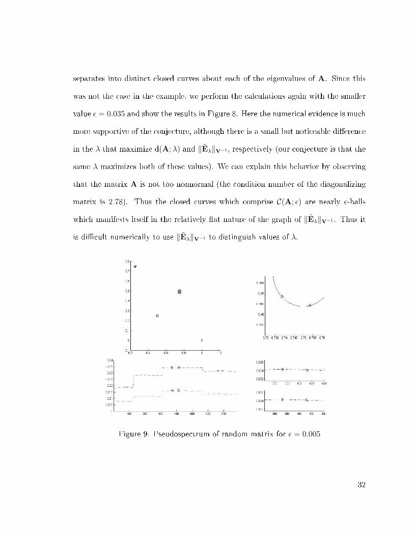
separates into distinct closed curves about each of the eigenvalues of A. Since this

was not the case in the example, we perform the calculations again with the smaller

value ε = 0.035 and show the results in Figure 8. Here the numerical evidence is much

more supportive of the conjecture, although there is a small but noticeable dierence

in the λ that maximize d(A;λ) and ‖Eλ‖V−1 , respectively (our conjecture is that the

same λ maximizes both of these values). We can explain this behavior by observing

that the matrix A is not too nonnormal (the condition number of the diagonalizing

matrix is 2.78). Thus the closed curves which comprise C(A; ε) are nearly ε-balls

which manifests itself in the relatively at nature of the graph of ‖Eλ‖V−1 . Thus it

is dicult numerically to use ‖Eλ‖V−1 to distinguish values of λ.

Figure 9. Pseudospectrum of random matrix for ε = 0.005

32

The problem is only made worse with a smaller value of ε, as illustrated in Figure

9. Based upon these observations, in order to see more compelling numerical evidence

in support of the conjecture, we likely need to consider a somewhat nonnormal matrix

with a suciently small ε. The results for such an example are presented next for a

matrix B where the condition number of the diagonalizing matrix is 28.2.

Figure 10. Pseudospectrum of random matrix for ε = 0.25

In Figure 10, we see again that for an ε value which does not give distinct closed

curves about each of the eigenvalues of the matrix, the numerical evidence does not

support our conjecture. Therefore in Figure 11 we reduce the ε, and we see that our

conjecture has merit to be true.

33

Figure 11. Pseudospectrum of random matrix for ε = 0.1

Our nal observation that we believe is relevant to our conjecture is on the subject

of stability. In [9, pp.811], the stability radius of a system represented by a matrix

A is dened to be the supremum of ε such that T (A; ε) is a subset of the stability

region. We know that if λ ∈ C(A; ε), all E such that λ ∈ Λ(A + E) ⊂ T (A; ε)

must have ‖E‖ = ε. Thus for every λ ∈ C \ Λ(A), there exists ε > 0 such that

ε = 1‖(λI−A)−1‖ and λ ∈ C(A; ε). Therefore for a given matrix A ∈ Cn×n where there

is a dened stability region Cs ⊂ C, if Λ(A)∩(C\Cs) = ∅, then for all ε > 0 such that

minγ∈C\Cs

[1

‖(γI−A)−1‖

]> ε > 0, T (A; ε)∩ (C\Cs) = ∅. In particular, if Cs is closed, then

for all ε > 0 such that minγ∈C\Cs

[1

‖(γI−A)−1‖

]≥ ε > 0, T (A; ε) ∩ (C \ Cs) = ∅. We give

two examples to numerically conrm this observation. Our rst example is a matrix

dened by a system with the stability region taken to be the left half complex plane.

34

We rst take the matrix A which is similar to the grcar(10) matrix, and nd the

minimum of one over the norm of the resolvent as dened above for a nite number of

points in the closure of the instability region C\Cs which is the complement of the left

half complex plane. In this case we see that C\Cs is closed. For this example we com-

pute minγ∈C\Cs

[1

‖(γI−A)−1‖

]= 0.220. The left plot in Figure 12 is T (A; 0.2204), and the

right plot is a magnication of the left. represents eigenvalues of A. represents

the points of intersection. We compute T (A; 0.2204)∩(C\Cs) = 0.3274i,−0.3274i.

Therefore for all ε such that 0.2204 > ε > 0, T (A; ε) ∩ (C \ Cs) = ∅.

Figure 12. Pseudospectrum - negative eigenvalues

Our second example is for a matrix B dened for a system with the stability

region taken to be the interior of the unit circle. We can numerically calculate the

minimum of one over the norm of the resolvent for a nite number of points in the

35

closure of the instability region C \Cs which is the complement of the interior of the

unit circle. In this case we see that C \ Cs is closed. For this example we compute

minγ∈C\Cs

[1

‖(γI−B)−1‖

]= 0.0424. The left plot in Figure 13 is T (B; 0.0424), and the right

plot is a magnication of the left. represents eigenvalues of B. represents the

points of intersection. We compute T (B; 0.0424) ∩ (C \ Cs) = −0.0125 − 0.9999i.

Therefore for all ε such that 0.0424 > ε > 0, T (B; ε) ∩ (C \ Cs) = ∅. Both examples

numerically conrm the expected observation pertaining to stability radius.

Figure 13. Pseudospectrum - eigenvalues inside the unit circle

III.III Conclusion

We have surveyed denitions and characterizations of pseudospectra and struc-

tured pseudospectra. By considering how the normality of a matrix can be aected

by changing the underlying norm, we posed a possible method for calculating those

perturbations which have the greatest eect on the eigenvalues of a matrix. This idea

was examined numerically and conrmed for certain cases.

36

REFERENCES

[1] F.L. Bauer and CT Fike, Norms and exclusion theorems, Numer. Math. 2 (1960),no. 1, 137141.

[2] J. Demmel, A counterexample for two conjectures about stability, IEEE Trans.on Auto. Control 32 (1987), no. 4, 340342.

[3] K. Du and Y. Wei, Structured pseudospectra and structured sensitivity of eigen-values, Journal of computational and applied mathematics 197 (2006), no. 2,502519.

[4] S.K. Godunov, Numerical solution of boundary-value problems for systems ofordinary dierential linear equations, Uspekhi Mat. Nauk 16 (1961), no. 3 (99),171174.

[5] G.H. Golub and C.F. Van Loan, Matrix computations, 2 ed., Johns HopkinsUniversity Press, 1989.

[6] N. Higham, The Matrix Computation Toolbox, http://www.mathworks.com/

matlabcentral/fileexchange/2360-the-matrix-computation-toolbox,MATLAB Central File Exchange, Accessed: 02/05/2012.

[7] D. Hinrichsen and B. Kelb, Spectral value sets: a graphical tool for robustnessanalysis, Systems & Control Letters 21 (1993), no. 2, 127136.

[8] D. Hinrichsen and A.J. Pritchard, On spectral variations under bounded realmatrix perturbations, Numer. Math. 60 (1992), no. 1, 509524.

[9] D. Hinrichsen and AJ Pritchard, Robustness measures for linear systems with ap-plication to stability radii of hurwitz and schur polynomials, International Journalof Control 55 (1992), no. 4, 809844, Taylor & Francis.

[10] T. Kato, Perturbation theory for linear operators, 2 ed., vol. Grundlehren dermathematischen Wissenschaften 132, A Series of Comprehensive Studies inMathematics, Springer Verlag, 1976.

[11] V.I. Kostin and S.I. Razzakov, On convergence of the power orthogonal method ofspectrum computing, Trans. Inst. Math. Sib. Branch Acad. Sci. 6 (1985), 5584.

37

[12] P. Lancaster and M. Tismenetsky, The theory of matrices: with applications,Academic Pr, 1985.

[13] H.J. Landau, On Szegö's eingenvalue distribution theorem and non-hermitiankernels, Journal d'Analyse Mathématique 28 (1975), no. 1, 335357.

[14] MATLAB, MATLAB®Student Version R2012a version 7.14.0.739, The Math-works Inc., February 9, 2012.

[15] S.C. Reddy and L.N. Trefethen, Lax-stability of fully discrete spectral methodsvia stability regions and pseudo-eigenvalues, Computer Methods in Applied Me-chanics and Engineering 80 (1990), no. 1, 147164.

[16] L.N. Trefethen, Approximation theory and numerical linear algebra, Algorithmsfor Approximation II, JC Mason and MG Cox, eds., Chapman and Hall, London(1990), 336360.

[17] L.N. Trefethen and M. Embree, Pseudospectra gateway, http://www.cs.ox.ac.uk/pseudospectra/index.html, Accessed: 01/12/2012.

[18] , Spectra and pseudospectra: the behavior of nonnormal matrices andoperators, Princeton Univ Pr, 2005.

[19] JLM Van Dorsselaer, J. Kraaijevanger, and MN Spijker, Linear stability analysisin the numerical solution of initial value problems, Cambridge Univ Press, 1992.

[20] Raf Vandebril, GenNormal, http://people.cs.kuleuven.be/~raf.

vandebril/homepage/software/normal/GenNormal.m, Accessed: 03/10/2012.

[21] J.M. Varah, The computation of bounds for the invariant subspaces of a gen-eral matrix operator, Technical Report CS 66, Computer Science Department,Stanford University, 1967.

[22] , On the separation of two matrices, SIAM Journal on Numerical Analysis16 (1979), no. 2, 216222.

[23] J.H. Wilkinson, Sensitivity of eigenvalues II, Util. Math 30 (1986), 243286.

38

APPENDIX A

NOTATIONS

C : The set of all complex numbers . . . . . . . . . . . . . . . . . . . . . . . . . . . . . . . . . . . . . . . . . . . . . . . 2

Cn : The set of all vectors of length n with complex entries . . . . . . . . . . . . . . . . . . . . . . . . 2

Cm×n : The set of all matrices of size m× n with complex entries . . . . . . . . . . . . . . . . . 2

I : The identity matrix in Cn×n . . . . . . . . . . . . . . . . . . . . . . . . . . . . . . . . . . . . . . . . . . . . . . . . . . . 2

R(A) : The range of the matrix A . . . . . . . . . . . . . . . . . . . . . . . . . . . . . . . . . . . . . . . . . . . . . . . . 2

N (A) : The null space of the matrix A . . . . . . . . . . . . . . . . . . . . . . . . . . . . . . . . . . . . . . . . . . . 2

‖·‖ : The norm of a vector in Cn or a matrix in Cm×n . . . . . . . . . . . . . . . . . . . . . . . . . . . . . 2

Λ(A) : The spectrum of the matrix A . . . . . . . . . . . . . . . . . . . . . . . . . . . . . . . . . . . . . . . . . . . . .2

(x, y) : The Euclidean inner product of x, y ∈ Cn . . . . . . . . . . . . . . . . . . . . . . . . . . . . . . . . . . 2

y∗ : The conjugate transpose of y . . . . . . . . . . . . . . . . . . . . . . . . . . . . . . . . . . . . . . . . . . . . . . . . . 2

‖x‖2 : The vector 2-norm of the vector x ∈ Cn . . . . . . . . . . . . . . . . . . . . . . . . . . . . . . . . . . . . 2

‖A‖2 : The induced matrix 2-norm of the matrix A ∈ Cn×n . . . . . . . . . . . . . . . . . . . . . . . 2

T (A; ε) : The set T (A; ε) = λ ∈ C : λ ∈ Λ(A + E) for some E with

‖E‖ ≤ ε . . . . . . . . . . . . . . . . . . . . . . . . . . . . . . . . . . . . . . . . . . . . . . . . . . . . . . . . . . . . . . . . . . . . . .6

T (A;B,C, ε) : The set T (A;B,C, ε) = λ ∈ C : λ ∈ Λ(A + BEC)

for some E with ‖E‖ ≤ ε . . . . . . . . . . . . . . . . . . . . . . . . . . . . . . . . . . . . . . . . . . . . . . . . . . . . . 9

(λI−A)−1 : The matrix dening the resolvent of A . . . . . . . . . . . . . . . . . . . . . . . . . . . . . 12

S(A; ε) : The set Λ(A) ∪ λ ∈ C : ‖(λI−A)−1‖ ≥ ε−1 . . . . . . . . . . . . . . . . . . . . . . . . . . 12

C(A; ε) : The boundary of the ε-pseudospectrum of A . . . . . . . . . . . . . . . . . . . . . . . . . . . . 13

S(A;B,C, ε) : The set Λ(A) ∪ λ ∈ C : ‖C(λI−A)−1B‖ ≥ ε−1 . . . . . . . . . . . . . . . . . 15

39

T1(A;W, ε) : The set λ ∈ C : λ ∈ Λ(A + E) for some E such that ‖E‖ ≤ ε,

R(E) ⊂ W . . . . . . . . . . . . . . . . . . . . . . . . . . . . . . . . . . . . . . . . . . . . . . . . . . . . . . . . . . . . . . . . . .16

S1(A;W, ε) : The set λ ∈ C : ‖(λI−A)−1|W‖ ≥ 1ε ∪ Λ(A) . . . . . . . . . . . . . . . . . . . . . .16

T2(A;Z, ε) : The set λ ∈ C : λ ∈ Λ(A + E) for some E such that ‖E‖ ≤ ε,

Z⊥ ⊂ N (E) . . . . . . . . . . . . . . . . . . . . . . . . . . . . . . . . . . . . . . . . . . . . . . . . . . . . . . . . . . . . . . . . .17

S2(A;Z, ε) : The set λ ∈ C : ‖P(λI−A)−1‖ ≥ 1ε ∪ Λ(A) . . . . . . . . . . . . . . . . . . . . . . . 17

Ω(A; ε) : The set γ ∈ C : |γ − λ|ε for some λ ∈ Λ(A) . . . . . . . . . . . . . . . . . . . . . . . . . . .20

κ(B) : The condition number of the nonsingular matrix B . . . . . . . . . . . . . . . . . . . . . . . 21

‖x‖B : The vector norm dened by the inner product (x, y)B = y∗B∗Bx

such that ‖x‖B = ‖Bx‖2 . . . . . . . . . . . . . . . . . . . . . . . . . . . . . . . . . . . . . . . . . . . . . . . . . . . . . 22

‖A‖B : The matrix norm induced by the vector norm ‖x‖B such that

‖A‖B = ‖BAB−1‖2 . . . . . . . . . . . . . . . . . . . . . . . . . . . . . . . . . . . . . . . . . . . . . . . . . . . . . . . . . . 22

TB(A; ε) : The set λ ∈ C : Λ(A + E) for some E such that ‖E‖B ≤ ε . . . . . . . . . . . 23

SB(A; ε) : The set λ ∈ C : ‖(λI−A)−1‖B ≥ 1ε ∪ Λ(A) . . . . . . . . . . . . . . . . . . . . . . . . . 23

E : A matrix where rank(E) = 1 . . . . . . . . . . . . . . . . . . . . . . . . . . . . . . . . . . . . . . . . . . . . . . . . . 26

T (A; ε) : The set λ ∈ C : λ ∈ Λ(A + E) for some E ∈ Cn×n, ‖E‖ ≤ ε . . . . . . . . . . . 26

d(A;λ) : The minγ∈Λ(A)

|λ− γ| . . . . . . . . . . . . . . . . . . . . . . . . . . . . . . . . . . . . . . . . . . . . . . . . . . . . . . .28

D(A; ε) : The maxλ∈T (A;ε)

d(A;λ) . . . . . . . . . . . . . . . . . . . . . . . . . . . . . . . . . . . . . . . . . . . . . . . . . . . . .28

Cs : A subset of C dening a stability region . . . . . . . . . . . . . . . . . . . . . . . . . . . . . . . . . . . . . 34

40

APPENDIX B

PROOFS

Proof S(A; ε) = T (A; ε)

Let A ∈ Cn×n and ε > 0 be arbitrary.

Proof. [17, http://www.cs.ox.ac.uk/pseudospectra/thms/thm1.pdf]

To prove T ⊂ S let λ ∈ T . If λ ∈ Λ(A) then λ ∈ S. Therefore assume

λ 6∈ Λ(A). Thus λ ∈ Λ(A + E) for some E ∈ Cn×n with 0 < ‖E‖ ≤ ε. Thus

there exists v ∈ Cn with ‖v‖ = 1 such that (A + E)v = λv. Thus Ev = (λI −A)v

which implies (λI −A)−1Ev = v. Now by taking the norm of both sides we get the

following: 1 = ‖v‖ = ‖(λI−A)−1Ev‖ ≤ ‖(λI−A)−1‖‖E‖‖v‖ ≤ ε‖(λI−A)−1‖.

Thus ‖(λI−A)−1‖ ≥ 1ε. Thus λ ∈ S.

To prove S ⊂ T let λ ∈ S. If λ ∈ Λ(A) then λ ∈ T . Therefore assume

λ 6∈ Λ(A). Thus ‖(λI−A)−1‖ ≥ 1ε. Thus there exists u ∈ Cn where u 6= 0 such that

‖(λI−A)−1u‖ ≥ 1ε‖u‖. Dene v = (λI−A)−1u which implies that (λI−A)v = u.

Thus ‖u‖ = ‖(λI−A)v‖ ≤ ε‖v‖. Dene Ex = (λI − A) (x,v)‖v‖2 v. Thus ‖Ex‖ ≤

‖(λI−A)v‖ |(x,v)|‖v‖2 ≤ ε‖v‖ ‖x‖‖v‖‖v‖2 = ε‖x‖. Thus ‖E‖ ≤ ε. Therefore (A + E)v =

Av + (λI−A) (v,v)‖v‖2 v = Av + (λI−A)v = λv. Thus λ ∈ T .

Thus S = T .

Proof S(A;B,C, ε) = T (A;B,C, ε)

Let A ∈ Cn×n, B ∈ Cn×s, C ∈ Ct×n and ε > 0 be arbitrary, B and C 6= 0.

41

Proof. [8]

To prove T ⊂ S let λ ∈ T . If λ ∈ Λ(A) then λ ∈ S. Therefore assume λ 6∈ Λ(A).

Thus there exists E such that λ ∈ Λ(A + BEC). Thus there exists v 6= 0, v ∈ Cn

such that (A + BEC)v = λv. Dene u = ECv. Thus u 6= 0 and

u = ECv

= EC(λI−A)−1BECv

= EC(λI−A)−1Bu.

This implies that ‖u‖ = ‖EC(λI−A)−1Bu‖; which implies

1 = ‖EC(λI−A)−1Bu‖‖u‖−1

≤ ‖EC(λI−A)−1B‖‖u‖‖u‖−1

≤ ‖E‖‖C(λI−A)−1B‖.

Thus ‖C(λI−A)−1B‖ ≥ ‖E‖−1 ≥ 1ε. Thus λ ∈ S.

To prove S ⊂ T let λ ∈ S. If λ ∈ Λ(A) then λ ∈ T . Therefore assume λ 6∈ Λ(A).

Thus there exist a u ∈ Cs, ‖u‖ = 1 such that ‖C(λI−A)−1Bu‖ = ‖C(λI−A)−1B‖.

Dene y =(

1‖C(λI−A)−1Bu‖

)C(λI−A)−1Bu.

42

Thus

y∗C(λI−A)−1Bu =

(1

‖C(λI−A)−1B‖

)u∗(C(λI−A)−1B)∗C(λI−A)−1Bu

=‖C(λI−A)−1Bu‖2

‖C(λI−A)−1Bu‖

= ‖C(λI−A)−1Bu‖.

Dene ε = 1‖C(λI−A)−1B‖ ≤ ε. Thus

u = ε‖C(λI−A)−1B‖u

= εu‖C(λI−A)−1Bu‖

= εuy∗C(λI−A)−1Bu.

Dene E = εuy∗. Thus E is an s × t matrix and ‖E‖ = ‖εuy∗‖ ≤ ε ≤ ε. Dene

x = (λI−A)−1Bu. Thus

ECx = EC(λI−A)−1Bu

= εuy∗C(λI−A)−1Bu

= u.

Thus x 6= 0 and x = (λI − A)−1BECx which implies λx = (A + BEC)x. Thus

λ ∈ T . Thus S(A;B,C, ε) = T (A;B,C, ε).

43

APPENDIX C

MATLAB CODES

PM.m − Poor Man′s Method to Construction Pseudospectra

1 % This function is based upon the 'Poor Man's' method presented in

2 % [17, pp.378−379], and developed from ps.m [6].

3 %%

4 function PM(matrix,epsilon,number)

5 % 'matrix' is the input matrix that the pseudospectra will be found

6 % for.

7 % 'epsilon' is the vector of epsilon values to be found.

8 % 'epsilon' must be a positive real number.

9 % 'number' is the number of perturbation per epsilon.

10 %%

11 % Check dimensions, and get basic values for computation.

12 [rows cols]=size(matrix);

13 if rows≤1 || cols≤1 || isempty(matrix)

14 error('Please choose a square matrix with minimum dimension ...

of two.')

15 end

16 if abs(rows−cols)>0

17 error('Please choose a square matrix')

18 end

19 n=length(matrix); lambda=eig(matrix); times=length(epsilon);

20 %%

21 % Other error checks.

22 if nargin<2 || isempty(epsilon)

44

23 epsilon=[1E−1 1E−2 1E−3];

24 end

25 if nargin<3 || isempty(number)

26 number=250;

27 end

28 for i=1:times

29 if real(epsilon(i))≤0 || abs(imag(epsilon(i)))>0

30 error('Please make sure all epsilon values are positive ...

real numbers.')

31 end

32 end

33 if number<1 || abs(fix(number)−number)>0

34 error('Please provide a positive non−zero integer for the ...

number of perturbations.')

35 end

36 %%

37 % Here store the eigenvalues of the ('times'*'number')

38 % perturbed given matrices which are perturbed by random

39 % matrices with norm equal to the respective epsilon.

40 epsilon=sort(epsilon,'descend'); X=zeros(number*n,times);

41 del=zeros(n,times*n);

42 for i=1:times;

43 for j=1:number;

44 del1=randn(n)+randn(n)*1i;

45 del(1:n,((i−1)*n+1):i*n)=epsilon(i)*del1/(norm(del1));

46 X((j−1)*n+1:j*n,i)=eig(matrix+del(1:n,((i−1)*n+1):i*n));

47 end;

45

48 end;

49 %%

50 % Plot the eigenvalues of the perturbations.

51 figure

52 hold on

53 % if length(epsilon)==1

54 % title('Epsilon Pseudospectrum');

55 % else title('Epsilon Pseudospectra');

56 % end

57 COLORS=gray(2*times);

58 for i=1:times

59 plot(real(X(1:number*n,i)),imag(X(1:number*n,i)),'o', ...

60 'color',COLORS(i,:),'markersize',4,'MarkerFaceColor', ...

61 COLORS(i,:));

62 end

63 % Plot eigenvalues of matrix

64 plot(lambda,'k+','MarkerSize',18,'LineWidth',4);

65 hold off;

66 %%

67 % Clean up the visual data

68 fig = gcf;

69 axis tight

70 axis equal

71 xlim=get(gca,'Xlim'); ylim=get(gca,'Ylim');

72 xtick=(xlim(2)−xlim(1))/100; ytick=(ylim(2)−ylim(1))/100;

73 axis([xlim(1)−xtick xlim(2)+xtick ylim(1)−ytick ylim(2)+ytick]);

74 axes = gca;

46

75 set (get (axes, 'XLabel'), 'FontSize', 20);

76 set (get (axes, 'YLabel'), 'FontSize', 20);

77 set (get (axes, 'Title'), 'FontSize', 24);

78 set (axes, 'Box', 'off', 'TickDir', 'out', 'XMinorTick', 'on', ...

'YMinorTick', 'on', 'FontSize', 16);

79 screen_size = get(0, 'ScreenSize');

80 set(fig, 'Position', [0 0 screen_size(3) screen_size(4)]);

81 end

PSA.m − Construction of Contour Lines of Pseudospectra

1 % This code is developed from the eigtool.m present by

2 % Trefethen and others.

3 % It utilizes the base algorithm to find the contour plot of the

4 % pseudospectra of a given matrix for given epsilons.

5 % Lines 92−113 are from the eigtool.m algorithm lines 368−390.

6 %%

7 function PSA(matrix,epsilon,d,maxit)

8 time=tic;

9 % 'matrix' is the input matrix that the pseudospectra will be found

10 % for.

11 % 'epsilon' is the vector of epsilon values to be found.

12 % 'epsilon' must be a positive real number.

13 % 'd' is the value of the distance between points in the meshgrid.

14 % The smaller the value of 'd', the more precision the contour plot

15 % will have.

16 % 'd' must be a positive real number.

17 % 'maxit' is a value used by the eigtool.m to max the true

47

18 % value of the norm of the resolvent at each point in the meshgrid;

19 % it reduces the difference in the calculated value and the true

20 % value due to calculation errors such as round error.

21 % 'maxit' must be a positive integer since it is being used as a

22 % counter.

23 % The user should normally not input a number in for maxit; 10 is

24 % sufficient for visual data, but for computational data with

25 % very small epsilon values or very non−normal matrices, a larger

26 % value should be used.

27 %%

28 % Check dimensions, and get basic values for computation.

29 [rows cols]=size(matrix);

30 if rows≤1 || cols≤1 || isempty(matrix)

31 error('Please choose a square matrix with minimum dimension ...

of two.')

32 end

33 if abs(rows−cols)>0

34 error('Please choose a square matrix')

35 end

36 if nargin<2 || isempty(epsilon)

37 epsilon=[1E−1 1E−2 1E−3];

38 end

39 n=length(matrix); lambda=eig(matrix); number=length(epsilon);

40 %%

41 % Other error checks.

42 if nargin<3 || isempty(d)

43 d=0.05;

48

44 end

45 if nargin<4 || isempty(maxit)

46 maxit=10;

47 end

48 if number<1

49 error('Please provide at least one positive real number ...

epsilon.')

50 end

51 for i=1:number

52 if real(epsilon(i))≤0 || abs(imag(epsilon(i)))>eps

53 error('Please make sure all epsilon values are positive ...

real numbers.')

54 end

55 if epsilon(i)<abs(d) || d≤0

56 error('Please choose a smaller postive value d>0 for the ...

mesh grid.')

57 end

58 end

59 if maxit<0 || abs(fix(maxit)−maxit)>eps

60 error('Please choose a positive integer for the computation ...

error.')

61 end

62 %%

63 % Set 'E' to be the reciprocal values of the 'epsilon' entry to set

64 % the contour values to be plotted.

65 % This is done for as in the S set, the norm of the resolvent is

66 % compared in the inequallity to the reciprocal of epsilon.

49

67 E=1./epsilon;

68 %%

69 % Here we are computing the area for and creating the meshgrid to

70 % make sure that we include enough points to include the

71 % contour plots for all epsilons.

72 % Find midpoint value between the largest and smallest real and

73 % imagenary values of the eigenvalues.

74 q=(max(real(lambda))+min(real(lambda)))/2;

75 p=(max(imag(lambda))+min(imag(lambda)))/2;

76 % Set the distance away from the midpoint values to be included in

77 % the meshgrid

78 r=norm(matrix)*norm(inv(matrix))+1.5*max(epsilon);

79 % Make all values integers to eliminate errors in the next step

80 q=fix(round(q)); p=fix(round(p)); r=fix(round(r));

81 % Set the intervals for the meshgrid

82 x=q−r:d:q+r; y=p−r:d:p+r;

83 % Meshgrid

84 [X,Y]=meshgrid(x,y);

85 %%

86 % This is the eigtool.m algorithm. The algorithm computes the value

87 % of the norm of the resolvent at each point in the mesh grid, but

88 % uses the Schur decompostion of the given matrix instead of the

89 % given matrix to speed up the function.

90 Z=zeros(length(y),length(x)); sigmin=Z; T=schur(matrix,'complex');

91 for k=1:length(x)

92 for j=1:length(y)

93 T1=(x(k)+y(j)*1i)*eye(length(matrix))−T; T2=T1';

50

94 sigold=0; qold=zeros(length(matrix),1); beta=0; H=[];

95 q=randn(length(matrix),1)+1i*randn(length(matrix),1);

96 q=q/norm(q);

97 for p=1:maxit

98 v=T1\(T2\q)−beta*qold; alpha=real(q'*v); v=v−alpha*q;

99 beta=norm(v); qold=q; q=v/beta; H(p+1,p)=beta;

100 H(p,p+1)=beta; H(p,p)=alpha; sig=max(eig(H(1:p,1:p)));

101 if abs(sigold/sig−1)<1e−3, break, end

102 sigold=sig;

103 end

104 sigmin(j,k)=sqrt(sig); Z(j,k)=sigmin(j,k);

105 end

106 end

107 %%

108 % Here we are going to develop the contour plot figure.

109 figure

110 hold on;

111 % if length(epsilon)==1

112 % title('Epsilon Pseudospectrum');

113 % else title('Epsilon Pseudospectra');

114 % end

115 % If the matrix is normal, input the epsilon balls around each

116 % eigenvalue of 'matrix' for each value in 'epsilon'.

117 % This is done first with black dotted lines so that they will be

118 % under the contour lines thus not interfering with the visual data

119 % of the contour lines.

120 if (norm(matrix*matrix'−matrix'*matrix)≤0.001)

51

121 ang=0:0.01:2*pi;

122 for e=1:n;

123 x1=real(lambda(e)); y1=imag(lambda(e));

124 for i=1:number;

125 x2=epsilon(i)*cos(ang)+x1; y2=epsilon(i)*sin(ang)+y1;

126 plot(x2,y2,'k−−','LineWidth',0.5);

127 end;

128 end;

129 end;

130 % Plot the contour lines

131 % The 'if else' is used due to the exclusive input needed when only

132 % one epsilon value is used.

133 if number==1

134 [¬,h]=contour(X,Y,Z,[E E]);

135 else

136 [¬,h]=contour(X,Y,Z,E);

137 end

138 set(h,'LineWidth',2)

139 colormap(gray(number))

140 % Plot the eigenvalues of 'matrix' for visual interpretation of the

141 % movement of said eigenvalues.

142 plot(lambda,'k+','MarkerSize',4);

143 hold off

144 % Clean up the visual data

145 fig = gcf;

146 axis tight

147 axis equal

52

148 xlim=get(gca,'Xlim'); ylim=get(gca,'Ylim');

149 xtick=(xlim(2)−xlim(1))/100; ytick=(ylim(2)−ylim(1))/100;

150 axis([xlim(1)−xtick xlim(2)+xtick ylim(1)−ytick ylim(2)+ytick]);

151 axes = gca;

152 set (get (axes, 'XLabel'), 'FontSize', 20);

153 set (get (axes, 'YLabel'), 'FontSize', 20);

154 set (get (axes, 'Title'), 'FontSize', 24);

155 set (axes, 'Box', 'off', 'TickDir', 'out', 'XMinorTick', 'on', ...

'YMinorTick', 'on', 'FontSize', 16);

156 screen_size = get(0, 'ScreenSize');

157 set(fig, 'Position', [0 0 screen_size(3) screen_size(4)]);

158 Time=toc(time)

159 end

Construction of Contour Lines of Structured Pseudospectra

For the computation of the contour line of a structured pseudospectrum

T (A;B,C, ε), replace lines 85-106 in PSA.m with the following:

1 %%

2 % Here we will calculate the norm of the resolvent with

3 % respect to the structure defined by B and C.

4 Z=zeros(length(y),length(x));

5 for k=1:length(x)

6 for j=1:length(y)

7 Z(j,k)=norm(C*inv((X(j,k)+Y(j,k)*1i)*eye(n)−matrix)*B);

8 end

9 end

53

GenNormal.m [20] − Construction of Random Normal Matrix

1 % GENNORMAL Generate any type of normal matrix

2 % N=GENNORMAL(n)

3 % Generates an arbitrary complex normal matrix of size n.

4 %

5 % Raf Vandebril

6 % raf.vandebril − a − cs.kleuven.be

7 % Revision Date: 1/9/2008

8 function N=GenNormal(n)

9 % Define I to be the square root of −1

10 I=sqrt(−1);

11 D=diag(rand(n,1)+I*rand(n,1));

12 A=rand(n,n)+I*rand(n,n);

13 [Q,R]=qr(A);

14 N=Q'*D*Q;

15 end

54