Feature Learning and Structured Prediction for Scene ...
141
Feature Learning and Structured Prediction for Scene Understanding Salman H. Khan This thesis is presented for the degree of Doctor of Philosophy of The University of Western Australia School of Computer Science and Software Engineering. 28 Feb 2016
-
Upload
khangminh22 -
Category
Documents
-
view
0 -
download
0
Transcript of Feature Learning and Structured Prediction for Scene ...

Feature Learning and Structured
Prediction for Scene Understanding
Salman H. Khan
This thesis is presented for the degree of
Doctor of Philosophy
of The University of Western Australia
School of Computer Science and Software Engineering.
28 Feb 2016

a
a © Copyright 2016 by S. H. Khan

a
a Dedicated to my parents,a

a

Abstract
When one talks about the visual comprehension ability of humans, even a young
child can easily describe events happening in a scene, differentiate between different
scene types, identify objects present in a scene and effortlessly reason about their
location and geometry. The ultimate goal of computer vision is to mimic the as-
tounding capabilities of human vision. However after ∼ 50 years of progress in this
area, computer vision is still far from the scene understanding capabilities of a tod-
dler. In this dissertation, we aim to further extend the frontiers of computer vision
by investigating robust feature learning and structured prediction frameworks for
visual scene understanding. This dissertation is organized as a collection of research
manuscripts which are either already published or submitted to internationally ref-
ereed conference and journals.
The dissertation explores two distinct aspects of scene understanding and analy-
sis. First, we explore improved feature representations for scene understanding tasks.
We investigate both hand-crafted as well as automatically learned feature represen-
tations using deep neural networks. Second, we propose new structured prediction
models to incorporate rich relationships between both low-level and high-level scene
elements. More specifically, we study some of the most important sub-tasks under
the umbrella of scene understanding such as semantic labelling, geometric and vol-
umetric reasoning, object shadow detection and removal, scene categorization and
change detection and analysis. The proposed algorithms in this dissertation pertain
to different data modalities including RGB images, RGB+Depth data, underwater
imagery, dermoscopy images, synthetic images and spectral data from satellites.
A major hurdle towards the goal of scene understanding is the limited availability
of data and annotations. This dissertation also contributes towards this aspect by
gathering two new datasets along with their annotations. Moreover, we present
methods to directly deal with specific data related issues e.g., recovery of missing
data, learning with only weak supervision and handling highly unbalanced datasets
during model learning. Our proposed approaches show very promising results on a
diverse set of scene understanding tasks. We hope that this dissertation will inspire
more such efforts to realise the ultimate objective of visual scene understanding in
machine vision.

Acknowledgements
I am deeply thankful to my supervisors, Mohammed Bennamoun, Roberto Togneri,
Ferdous Sohel and Imran Naseem. They provided me with their full support and
encouragement during my stay at UWA. I especially want to thank my Principal
Supervisor, Mohammed, for inspiring me to work hard, making himself available to
answer my questions at all the times and providing his continuous feedback on my
work. Had it not been his sheer academic and professional brilliance, this journey
would have been very difficult. Thank you for advice, guidance and contributions
to my research.
I want to express my gratitude towards Yvette Harrap and Kelli Pierce for their
administrative assistance; Ryan McConigly, Samuel Thomas and Daniel Ross for
their technical and IT support; Brian Skjerven and Ashley Chew for help with the
iVEC super computer. I am also thankful to Mark Reynolds (Head of School) and
other staff members at the School of Computer Science and Software Engineering
(CSSE) for their help and support during my candidature.
I am greatly in-debt to my colleagues and fellow postgraduate students at the
UWA for making this journey comfortable and sharing some pleasant moments to-
gether. I am especially thankful to my friends Ammar Mahmood, Umar Asif, Naveed
Akhter and Zohaib Khan. But this list is not complete without a special person,
Munawar Hayat, whose companionship was crucial to this thesis. We had many
fruitful discussions about science, religion, politics and life in general, which helped
me a lot in getting through tough times.
I am thankful to my mentors, peers, collaborators and organisations which sup-
ported me during this period. I would like to especially thank Xuming He and Fatih
Porikli (NICTA, ANU) for providing valuable support and supervising me during my
internship at NICTA. I am thankful to Faisal Shafait and Arif Mahmood for their
beneficial support and encouraging comments during our interactions. I appreciate
the financial and logistic support offered by the UWA (IPRS Scholarship), ARC
(DP150104251, DP110102166, DP150100294 and DE120102960), NICTA (hosting
my internship), NVIDIA (for donating GPUs) and Geoscience Australia (GA) for
providing the data and the expert annotations. I am grateful to numerous people,
including Prof. Dani Lischinski from Hebrew University , Jian Zhang from Stanford
University, Prof. Graham D. Finlayson from University of East Anglia, Prof. Mark
Drew from Simon Fraser University, who replied to my repeated queries regarding
their research. I am also thankful to my peers, whose quality research inspired me,
and anonymous reviewers, who provided valuable feedback and comments which

greatly helped me improve my publications.
I owe a great deal to my family. I want to thank my mother, Rukhsana, my
father, Abdul Hameed and all of my elder brothers and sisters, who brought me
up with their love and affection, and taught me the virtues of honesty, hard-work,
commitment and perseverance. I especially want to express my gratitude towards
my mother, for her devotion to our upbringing and countless prayers all through
these years. I am also indebted to my wonderful wife, who provided me with her
continuous support and care. To my little son, Qasim, you are the one whose smile
makes me forget all the worries after a long tiring day! Thank you for being with
us.
Finally, and above all, I am profoundly grateful to my Lord for holding me stead-
fast in the face of confusion, doubt and disappointment. He has been a continuous
driving force during this long journey. I wish I could thank him enough for his
blessings and favors. ‘Our Lord! Accept (this service) from us: For Thou art the
All-Hearing, the All-knowing. Our Lord! bestow on us Mercy from Thyself, and
dispose of our affair for us in the right way!’. (Al-Quran)

i
Contents
List of Tables vii
List of Figures ix
Publications Included in this Thesis xiv
Contribution of Candidate to Published Papers xvii
1 Introduction 1
1.1 Background and Definitions . . . . . . . . . . . . . . . . . . . . . . . 3
1.2 Contributions . . . . . . . . . . . . . . . . . . . . . . . . . . . . . . . 5
1.3 Thesis Overview . . . . . . . . . . . . . . . . . . . . . . . . . . . . . . 6
1.3.1 Geometry Driven Semantic Understanding of Scenes . . . . . . 7
1.3.2 Automatic Shadow Detection and Removal . . . . . . . . . . . 8
1.3.3 Joint Estimation of Clutter and Objects’ Spatial Layout . . . 8
1.3.4 A Discriminative Representation of Convolutional Features . . 9
1.3.5 Cost-Sensitive Learning of Deep Feature Representations . . . 10
1.3.6 Weakly Supervised Change Detection in a Pair of Images . . . 10
1.3.7 Forest Change Detection in Incomplete Satellite Images with
Deep Convolutional Networks . . . . . . . . . . . . . . . . . . 11
2 Geometry Driven Semantic Labeling of Indoor Scenes 13
2.1 Introduction . . . . . . . . . . . . . . . . . . . . . . . . . . . . . . . . 13
2.2 Related Work . . . . . . . . . . . . . . . . . . . . . . . . . . . . . . . 16
2.3 Proposed Conditional Random Field Model . . . . . . . . . . . . . . 17
2.3.1 Unary Energies . . . . . . . . . . . . . . . . . . . . . . . . . . 20
2.3.2 Pairwise Energies . . . . . . . . . . . . . . . . . . . . . . . . . 26
2.3.3 Proposed Higher-Order Energies . . . . . . . . . . . . . . . . . 27
2.4 Structured Learning and Inference . . . . . . . . . . . . . . . . . . . . 29
2.4.1 Learning Parameters . . . . . . . . . . . . . . . . . . . . . . . 29
2.4.2 Inference in CRF . . . . . . . . . . . . . . . . . . . . . . . . . 30
2.5 Planar Surface Detection . . . . . . . . . . . . . . . . . . . . . . . . . 31
2.6 Experiments and Analysis . . . . . . . . . . . . . . . . . . . . . . . . 36
2.6.1 Datasets . . . . . . . . . . . . . . . . . . . . . . . . . . . . . . 36
2.6.2 Results . . . . . . . . . . . . . . . . . . . . . . . . . . . . . . . 36

ii
2.6.3 Discussion . . . . . . . . . . . . . . . . . . . . . . . . . . . . . 49
2.7 Conclusion . . . . . . . . . . . . . . . . . . . . . . . . . . . . . . . . . 50
3 Automatic Shadow Detection and Removal from a Single Photo-
graph 51
3.1 Introduction . . . . . . . . . . . . . . . . . . . . . . . . . . . . . . . . 51
3.2 Related Work and Contributions . . . . . . . . . . . . . . . . . . . . 54
3.3 Proposed Shadow Detection Framework . . . . . . . . . . . . . . . . . 58
3.3.1 Feature Learning for Unary Predictions . . . . . . . . . . . . . 58
3.3.2 Contrast Sensitive Pairwise Potential . . . . . . . . . . . . . . 60
3.3.3 Shadow Contour Generation using CRF Model . . . . . . . . . 62
3.4 Proposed Shadow Removal and Matting Framework . . . . . . . . . . 62
3.4.1 Rough Estimation of Shadow-less Image by Color-transfer . . 65
3.4.2 Generalised Shadow Generation Model . . . . . . . . . . . . . 68
3.4.3 Bayesian Shadow Removal and Matting . . . . . . . . . . . . . 71
3.4.4 Parameter Estimation . . . . . . . . . . . . . . . . . . . . . . 73
3.4.5 Boundary Enhancement in a Shadow-less Image . . . . . . . . 74
3.5 Experiments and Analysis . . . . . . . . . . . . . . . . . . . . . . . . 74
3.5.1 Datasets . . . . . . . . . . . . . . . . . . . . . . . . . . . . . . 76
3.5.2 Evaluation of Shadow Detection . . . . . . . . . . . . . . . . . 76
3.5.3 Evaluation of Shadow Removal . . . . . . . . . . . . . . . . . 83
3.5.4 Applications . . . . . . . . . . . . . . . . . . . . . . . . . . . . 88
3.6 Conclusion . . . . . . . . . . . . . . . . . . . . . . . . . . . . . . . . . 91
4 Separating Objects and Clutter in Indoor Scenes via Joint Reason-
ing 93
4.1 Introduction . . . . . . . . . . . . . . . . . . . . . . . . . . . . . . . . 93
4.2 Related Work . . . . . . . . . . . . . . . . . . . . . . . . . . . . . . . 96
4.3 Our Approach . . . . . . . . . . . . . . . . . . . . . . . . . . . . . . . 96
4.3.1 CRF Formulation . . . . . . . . . . . . . . . . . . . . . . . . . 97
4.3.2 Potentials on Cuboids . . . . . . . . . . . . . . . . . . . . . . 98
4.3.3 Potentials on Superpixels . . . . . . . . . . . . . . . . . . . . . 102
4.3.4 Superpixel-Cuboid Compatibility . . . . . . . . . . . . . . . . 102
4.4 Cuboid Hypothesis Generation . . . . . . . . . . . . . . . . . . . . . . 103
4.5 Model Inference and Learning . . . . . . . . . . . . . . . . . . . . . . 104
4.5.1 Inference as MILP . . . . . . . . . . . . . . . . . . . . . . . . 104
4.5.2 Parameter Learning . . . . . . . . . . . . . . . . . . . . . . . . 105

iii
4.6 Experiments and Analysis . . . . . . . . . . . . . . . . . . . . . . . . 105
4.6.1 Dataset and Setup . . . . . . . . . . . . . . . . . . . . . . . . 105
4.6.2 Cuboid Detection Task . . . . . . . . . . . . . . . . . . . . . . 106
4.6.3 Clutter/Non-Clutter Segmentation Task . . . . . . . . . . . . 109
4.6.4 Foreground Segmentation Task . . . . . . . . . . . . . . . . . 112
4.6.5 Discussion . . . . . . . . . . . . . . . . . . . . . . . . . . . . . 112
4.7 Conclusion . . . . . . . . . . . . . . . . . . . . . . . . . . . . . . . . . 113
4.8 Supplementary Material:
“Separating Objects and Clutter in Indoor Scenes” . . . . . . . . . . 114
4.8.1 Inference as MILP . . . . . . . . . . . . . . . . . . . . . . . . 114
4.8.2 Parameter Learning . . . . . . . . . . . . . . . . . . . . . . . . 115
5 A Discriminative Representation of Convolutional Features 117
5.1 Introduction . . . . . . . . . . . . . . . . . . . . . . . . . . . . . . . . 117
5.2 Related Work . . . . . . . . . . . . . . . . . . . . . . . . . . . . . . . 120
5.3 The Proposed Method . . . . . . . . . . . . . . . . . . . . . . . . . . 121
5.3.1 Dense Patch Extraction . . . . . . . . . . . . . . . . . . . . . 121
5.3.2 Convolutional Feature Representations . . . . . . . . . . . . . 123
5.3.3 Scene Representative Patches (SRPs) . . . . . . . . . . . . . . 124
5.3.4 Feature Encoding from SRPs . . . . . . . . . . . . . . . . . . 126
5.3.5 Classification . . . . . . . . . . . . . . . . . . . . . . . . . . . 127
5.4 Experiments and Evaluation . . . . . . . . . . . . . . . . . . . . . . . 127
5.4.1 A Dataset of Object Categories in Indoor Scenes . . . . . . . . 128
5.4.2 Evaluated Datasets . . . . . . . . . . . . . . . . . . . . . . . . 132
5.4.3 Experimental Results . . . . . . . . . . . . . . . . . . . . . . . 133
5.4.4 Ablative Analysis . . . . . . . . . . . . . . . . . . . . . . . . . 135
5.4.5 Effectiveness of Mid-level Information . . . . . . . . . . . . . . 140
5.4.6 Dimensionality Analysis . . . . . . . . . . . . . . . . . . . . . 140
5.4.7 Timing Analysis . . . . . . . . . . . . . . . . . . . . . . . . . . 142
5.4.8 Sensitivity Analysis . . . . . . . . . . . . . . . . . . . . . . . . 143
5.5 Conclusion . . . . . . . . . . . . . . . . . . . . . . . . . . . . . . . . . 144
6 Cost-Sensitive Learning of Deep Feature Representations 145
6.1 Introduction . . . . . . . . . . . . . . . . . . . . . . . . . . . . . . . . 145
6.2 Related Work . . . . . . . . . . . . . . . . . . . . . . . . . . . . . . . 149
6.3 Proposed Approach . . . . . . . . . . . . . . . . . . . . . . . . . . . . 150
6.3.1 Problem Formulation for Cost Sensitive Classification . . . . . 150

iv
6.3.2 Our Proposed Cost Matrix . . . . . . . . . . . . . . . . . . . . 152
6.3.3 Cost-Sensitive Surrogate Losses . . . . . . . . . . . . . . . . . 153
6.3.4 Optimal Parameters Learning . . . . . . . . . . . . . . . . . . 158
6.3.5 Effect on Error Back-propagation . . . . . . . . . . . . . . . . 160
6.4 Experiments and Results . . . . . . . . . . . . . . . . . . . . . . . . . 164
6.4.1 Datasets and Experimental Settings . . . . . . . . . . . . . . . 164
6.4.2 Convolutional Neural Network . . . . . . . . . . . . . . . . . . 166
6.4.3 Results and Comparisons . . . . . . . . . . . . . . . . . . . . . 168
6.5 Conclusion . . . . . . . . . . . . . . . . . . . . . . . . . . . . . . . . . 176
7 Weakly Supervised Change Detection in a Pair of Images 179
7.1 Introduction . . . . . . . . . . . . . . . . . . . . . . . . . . . . . . . . 179
7.2 Related Work . . . . . . . . . . . . . . . . . . . . . . . . . . . . . . . 182
7.3 Two-stream CNNs for Change Localization . . . . . . . . . . . . . . . 183
7.3.1 Model overview . . . . . . . . . . . . . . . . . . . . . . . . . . 183
7.3.2 Deep network architecture . . . . . . . . . . . . . . . . . . . . 184
7.3.3 Model inference for change localization . . . . . . . . . . . . . 188
7.4 EM Learning with Weak Supervision . . . . . . . . . . . . . . . . . . 190
7.4.1 Mean-field E step . . . . . . . . . . . . . . . . . . . . . . . . . 190
7.4.2 M step for CNN training . . . . . . . . . . . . . . . . . . . . . 191
7.5 Experiments . . . . . . . . . . . . . . . . . . . . . . . . . . . . . . . . 191
7.5.1 CNN implementation . . . . . . . . . . . . . . . . . . . . . . . 191
7.5.2 Datasets and Protocols . . . . . . . . . . . . . . . . . . . . . . 192
7.5.3 Results . . . . . . . . . . . . . . . . . . . . . . . . . . . . . . . 195
7.6 Change Detection in Multiple Images . . . . . . . . . . . . . . . . . . 202
7.7 Conclusion . . . . . . . . . . . . . . . . . . . . . . . . . . . . . . . . . 203
8 Forest Change Detection in Incomplete Satellite Images 205
8.1 Introduction . . . . . . . . . . . . . . . . . . . . . . . . . . . . . . . . 205
8.2 Related Work . . . . . . . . . . . . . . . . . . . . . . . . . . . . . . . 208
8.3 Case Study: Data Description . . . . . . . . . . . . . . . . . . . . . . 213
8.4 Data Recovery . . . . . . . . . . . . . . . . . . . . . . . . . . . . . . . 214
8.4.1 Data Filling . . . . . . . . . . . . . . . . . . . . . . . . . . . . 214
8.4.2 Sparse Reconstruction based Image Enhancement . . . . . . . 216
8.4.3 Thin Cloud Removal . . . . . . . . . . . . . . . . . . . . . . . 217
8.5 Change Detection . . . . . . . . . . . . . . . . . . . . . . . . . . . . . 218
8.5.1 Multiscale Region Proposal Generation . . . . . . . . . . . . . 220

v
8.5.2 Candidate Suppression . . . . . . . . . . . . . . . . . . . . . . 221
8.5.3 Deep Convolutional Neural Network . . . . . . . . . . . . . . 221
8.6 Experimental Analysis . . . . . . . . . . . . . . . . . . . . . . . . . . 223
8.6.1 Evaluation Tasks . . . . . . . . . . . . . . . . . . . . . . . . . 223
8.6.2 Experimental Settings . . . . . . . . . . . . . . . . . . . . . . 224
8.6.3 Baseline Approaches . . . . . . . . . . . . . . . . . . . . . . . 225
8.6.4 Results . . . . . . . . . . . . . . . . . . . . . . . . . . . . . . . 225
8.7 Conclusion . . . . . . . . . . . . . . . . . . . . . . . . . . . . . . . . . 232
9 Conclusion 237
9.1 Summary . . . . . . . . . . . . . . . . . . . . . . . . . . . . . . . . . 237
9.2 Conclusion . . . . . . . . . . . . . . . . . . . . . . . . . . . . . . . . . 237
9.3 Future Directions and Open Problems . . . . . . . . . . . . . . . . . 238
A Disintegration of Higher-Order Energies 241
A.0.1 Disintegration of Higher-Order Energies to Second-Order Sub-
Modular Energies for Swap Moves . . . . . . . . . . . . . . . . 241
A.0.2 Disintegration of Higher-Order Energies to Second-Order Sub-
Modular Energies for Expansion Moves . . . . . . . . . . . . . 242
B Proofs Regarding Cost Matrix ξ′ 245

vi

vii
List of Tables
2.1 Comparison of plane detection results on the NYU-Depth v2 dataset 32
2.2 Results on the NYU-Depth v1, v2 and the SUN3D Datasets . . . . . 38
2.3 Class-wise Accuracies on NYU-Depth v1 . . . . . . . . . . . . . . . . 39
2.4 Class-wise Accuracies on NYU-Depth v2 (22 classes) . . . . . . . . . 39
2.5 Class-wise Accuracies on the NYU-Depth v2 (40 classes) . . . . . . . 40
2.6 Comparison of the results on the NYU-Depth v1 Dataset . . . . . . . 45
2.7 Comparison of results on the NYU-Depth v2 Dataset . . . . . . . . . 45
2.8 Comparison of results on the NYU-Depth v2 Dataset (4-class labeling
task) . . . . . . . . . . . . . . . . . . . . . . . . . . . . . . . . . . . . 46
2.9 Comparison of results on the NYU-Depth v2 Dataset (4-class labeling
task) . . . . . . . . . . . . . . . . . . . . . . . . . . . . . . . . . . . . 47
2.10 Comparison of results on the NYU-Depth v2 Dataset (40-class label-
ing task) . . . . . . . . . . . . . . . . . . . . . . . . . . . . . . . . . . 47
3.1 Evaluation of the Proposed Shadow Detection Scheme . . . . . . . . . 75
3.3 Results when ConvNets were trained and tested across different datasets. 78
3.2 Class-wise Accuracies of Our Proposed Framework in Comparison
with the State-of-the-art Techniques . . . . . . . . . . . . . . . . . . . 79
3.4 Quantitative Evaluation for Shadow Removal . . . . . . . . . . . . . 84
4.1 Inference Running time Comparisons for Variants of MILP Formulation105
4.2 An Ablation Study on the Model Potentials/Features . . . . . . . . . 109
4.3 Evaluation on Clutter/Non-Clutter Segmentation Task . . . . . . . . 110
4.4 Evaluation on Foreground/Background Segmentation Task . . . . . . 110
4.5 Statistics for Cuboids Fitted on Cluttered Regions . . . . . . . . . . . 114
5.1 Mean Accuracy on the MIT-67 Indoor Scene Dataset . . . . . . . . . 131
5.2 Mean Accuracy on the 15-Category Scene Dataset . . . . . . . . . . . 134
5.3 Mean Accuracy on the UIUC 8-Sports Dataset. . . . . . . . . . . . . 136
5.4 Mean Accuracy for the NYU v1 Dataset. . . . . . . . . . . . . . . . 137
5.5 Equal Error Rates (EER) for the Graz-02 dataset. . . . . . . . . . . 137
5.6 Ablative Analysis on MIT-67 Scene Dataset. . . . . . . . . . . . . . 141
5.7 Analysis of Feature Dimensions and their Corresponding Accuracies . 141
6.1 Evaluation on DIL Database. . . . . . . . . . . . . . . . . . . . . . . 168
6.2 Evaluation on MLC Database. . . . . . . . . . . . . . . . . . . . . . . 169

viii
6.3 Evaluation on MNIST Database. . . . . . . . . . . . . . . . . . . . . 169
6.4 Evaluation on CIFAR-100 Database. . . . . . . . . . . . . . . . . . . 170
6.5 Evaluation on Caltech-101 Database . . . . . . . . . . . . . . . . . . 171
6.6 Evaluation on MIT-67 Database. . . . . . . . . . . . . . . . . . . . . 172
6.7 Comparisons of Our Approach with the State-of-the-art Class-imbalance
Approaches . . . . . . . . . . . . . . . . . . . . . . . . . . . . . . . . 173
6.8 Comparisons of our Approach (Adaptive Costs) with the Fixed Class-
specific Costs . . . . . . . . . . . . . . . . . . . . . . . . . . . . . . . 176
7.1 Detection results in terms of average precision and overall accuracy . 196
7.2 Segmentation Results and Comparisons with Different Baseline Meth-
ods . . . . . . . . . . . . . . . . . . . . . . . . . . . . . . . . . . . . . 196
7.3 Ablative Analysis on the CDnet-2014 Dataset . . . . . . . . . . . . . 196
7.4 More Comparisons for the Segmentation Performance of our model
on the CDnet-2014 Dataset . . . . . . . . . . . . . . . . . . . . . . . 198
7.5 Segmentation Performance for Different Fixed τ on the CDnet-2014
Dataset . . . . . . . . . . . . . . . . . . . . . . . . . . . . . . . . . . 200
8.1 The flags included in the pixel quality map available with the Landsat
NBAR images. . . . . . . . . . . . . . . . . . . . . . . . . . . . . . . 212
8.2 Patch-wise classification and detection results for the temporal se-
quence are summarized above. . . . . . . . . . . . . . . . . . . . . . 227
8.3 Our results for onset/offset detection and comparisons with several
baseline techniques. . . . . . . . . . . . . . . . . . . . . . . . . . . . . 227

ix
List of Figures
1.1 Computer vision algorithms perform well on individual tasks, but lack
a full visual understanding to be able to answer intelligent questions
about the scene. . . . . . . . . . . . . . . . . . . . . . . . . . . . . . 1
1.2 Contextual information is important for scene understanding tasks . . 2
2.1 The figure summarizes our proposed approach to combine global ge-
ometric information with low-level cues. . . . . . . . . . . . . . . . . 18
2.2 A factor graph representation for our CRF model . . . . . . . . . . . 21
2.3 Effect of the Ensemble Learning Scheme . . . . . . . . . . . . . . . . 23
2.4 Learning Location Prior using Geometrical Context . . . . . . . . . . 26
2.5 Robust Higher-Order Energy . . . . . . . . . . . . . . . . . . . . . . . 28
2.6 An illustrative example showing the results of the planar surface de-
tection algorithm . . . . . . . . . . . . . . . . . . . . . . . . . . . . . 32
2.7 Comparison of our algorithm with [242] . . . . . . . . . . . . . . . . . 34
2.8 Examples of the semantic labeling results on the NYU-Depth v1 dataset 37
2.9 Examples of semantic labeling results on the NYU-Depth v2 dataset . 41
2.10 Examples of the semantic labeling results on the SUN3D dataset . . . 44
2.11 The introduction of HOE improves the segmentation accuracy around
the boundaries . . . . . . . . . . . . . . . . . . . . . . . . . . . . . . 46
2.12 Confusion Matrices for NYU-Depth and SUN3D Datasets . . . . . . . 48
3.1 Overview of Our Shadow Detection and Removal Scheme . . . . . . . 53
3.2 The Proposed Shadow Detection Framework . . . . . . . . . . . . . . 57
3.3 ConvNet Architecture used for Automatic Feature Learning to Detect
Shadows . . . . . . . . . . . . . . . . . . . . . . . . . . . . . . . . . . 59
3.4 The Proposed Shadow Removal Framework . . . . . . . . . . . . . . . 61
3.5 Detection of Object and Shadow Boundary . . . . . . . . . . . . . . . 63
3.6 Detection of Umbra and Penumbra Regions . . . . . . . . . . . . . . 64
3.7 Multi-level Color Transfer . . . . . . . . . . . . . . . . . . . . . . . . 69
3.8 Shadow Removal Steps . . . . . . . . . . . . . . . . . . . . . . . . . . 70
3.9 ROC curve comparisons of proposed framework with previous works. 78
3.10 Qualitative examples of our results . . . . . . . . . . . . . . . . . . . 80
3.11 Examples of Ambiguous Cases . . . . . . . . . . . . . . . . . . . . . . 81
3.12 Shadow Recovery Results on Sample Images . . . . . . . . . . . . . . 82
3.13 Comparison with Automatic/Semi-Automatic Methods . . . . . . . . 85

x
3.14 Comparison with Methods Requiring User Interaction . . . . . . . . . 87
3.15 Examples of Failure Cases . . . . . . . . . . . . . . . . . . . . . . . . 89
3.16 Different Applications of Shadow Detection, Removal and Matting . . 90
4.1 An Overview of Our Clutter Detection and Object Geometry Esti-
mation Framework . . . . . . . . . . . . . . . . . . . . . . . . . . . . 94
4.2 Graph Structure Representation for the Potentials . . . . . . . . . . . 97
4.3 The Distribution of Variation in Color for Cluttered and Non-cluttered
Regions . . . . . . . . . . . . . . . . . . . . . . . . . . . . . . . . . . 100
4.4 Jaccard Index Comparisons for all Annotated Cuboids . . . . . . . . 107
4.5 Comparison of Our Results with the State-of-the-art Technique [110] 109
4.6 Qualitative Results for Cuboid Detection . . . . . . . . . . . . . . . . 112
4.7 Ambiguous Cases in Cuboid Detection . . . . . . . . . . . . . . . . . 113
5.1 An Overview of the Scene Classification Framework . . . . . . . . . . 118
5.2 Deep Un-structured Convolutional Activations . . . . . . . . . . . . . 122
5.3 Multi-level Patches Contain Different Levels of Scene Details . . . . . 124
5.4 CMC Curve for the Benchmark Evaluation on the OCIS Dataset . . . 128
5.5 A Word Cloud Representation of Object Categories in Indoor Scenes
(OCIS) database . . . . . . . . . . . . . . . . . . . . . . . . . . . . . 129
5.6 Example Images from the ‘Object Categories in Indoor Scenes’ Dataset130
5.7 Confusion matrices for Three Scene Classification Datasets . . . . . . 138
5.8 The contributions of Distinctive Patches for the Correct Class Pre-
diction of a Scene . . . . . . . . . . . . . . . . . . . . . . . . . . . . . 139
5.9 Confusion Matrix for the MIT-67 Dataset . . . . . . . . . . . . . . . 142
5.10 Example Mistakes and the Limitations of Our Method . . . . . . . . 143
5.11 Time consumed to Associate Extracted Patches with the Codebook
Elements . . . . . . . . . . . . . . . . . . . . . . . . . . . . . . . . . . 144
6.1 Examples of Class Imbalance in the Popular Classification Datasets . 147
6.2 The CNN Parameters (θ) and Class Dependent Costs (ξ) used during
the Training Process of our Deep Network . . . . . . . . . . . . . . . 153
6.3 The 0-1 Loss along-with several other Common Surrogate Loss Func-
tions . . . . . . . . . . . . . . . . . . . . . . . . . . . . . . . . . . . . 155
6.4 The CE loss Function for the Case of Binary Classification . . . . . . 161
6.5 Confusion Matrices for the Baseline and CoSen CNNs on the DIL and
MLC datasets . . . . . . . . . . . . . . . . . . . . . . . . . . . . . . . 166

xi
6.6 The CNN Architecture used in This Work . . . . . . . . . . . . . . . 167
6.7 The Imbalanced Training Set Distributions used for the Comparisons
Reported in Table 6.7 . . . . . . . . . . . . . . . . . . . . . . . . . . . 174
6.8 Training and Validation Error on the DIL Dataset . . . . . . . . . . . 177
7.1 Overview of Change Detection in a Pair of Images . . . . . . . . . . . 181
7.2 Factor Graph Representation of the Weakly Supervised Change De-
tection Model . . . . . . . . . . . . . . . . . . . . . . . . . . . . . . . 186
7.3 CNN Architecture used in This Work . . . . . . . . . . . . . . . . . . 187
7.4 Qualitative Results on the CDnet-2014 Dataset . . . . . . . . . . . . 194
7.5 Qualitative Results on the GASI-2015 and PCD-2015 Datasets . . . . 197
7.6 Ambiguous Cases for Change Detection . . . . . . . . . . . . . . . . . 199
7.7 Sensitivity analysis on the Number of Nearest Neighbours used to
Estimate Foreground Probability Mass Parameter (τ) . . . . . . . . 200
7.8 More Qualitative Results of the Proposed Approach . . . . . . . . . . 200
8.1 Region of interest for change detection (Victoria, Australia) . . . . . 209
8.2 Gantt Chart of the Fire and Harvest Incidents . . . . . . . . . . . . . 211
8.3 Examples of artifacts in the data. . . . . . . . . . . . . . . . . . . . . 212
8.4 Examples of SLC-off artifacts. . . . . . . . . . . . . . . . . . . . . . . 213
8.5 Data Recovery Results on Single Frames . . . . . . . . . . . . . . . . 215
8.6 Our approach to detect and remove thin translucent clouds . . . . . . 217
8.7 Box proposals are generated at multiple scales to capture all sizes of
change events . . . . . . . . . . . . . . . . . . . . . . . . . . . . . . . 219
8.8 The CNN architecture used for forest change detection. . . . . . . . . 222
8.9 The trend of missed events and mean onset/offset difference when the
temporal threshold for valid detection is changed. . . . . . . . . . . . 226
8.10 Labeled change region coverage by the different number of bounding-
box change proposals. . . . . . . . . . . . . . . . . . . . . . . . . . . 226
8.11 On/Offset Detection Results for Individual Fire and Harvest Events. . 228
8.12 Example of ground-truth change patterns (left) and the change se-
quences predicted by our approach (right). . . . . . . . . . . . . . . 231
8.12 The figure shows detection results on the complete image plane en-
compassing the forest area under investigation . . . . . . . . . . . . . 233
8.13 Three small portions of patch sequences are shown in the above figure.234

xii

xiii
List of Algorithms
1 Region Growing Algorithm for Depth-Based Segmentation . . . . . . 33
2 Rough Estimation of Shadow-less Image by Color-transfer . . . . . . 66
3 Bayesian Shadow Removal . . . . . . . . . . . . . . . . . . . . . . . . 74
4 Parameter Learning using the Structured SVM Formulation . . . . . 115
5 Iterative optimization for parameters (θ, ξ) . . . . . . . . . . . . . . 159

xiv
Publications During the Candidature
Journal Publications (Refereed)
1. Salman H. Khan, Mohammed Bennamoun, Ferdous Sohel, and Roberto Togneri.
“Automatic Shadow Detection and Removal from a Single Image.” IEEE
Transactions on Pattern Analysis and Machine Intelligence (TPAMI), IEEE,
vol.38, no. 3, pp. 431-446, March 2016, doi:10.1109/TPAMI.2015.2462355.
[IF: 5.8]
IEEE TPAMI is the most cited journal in computer vision according to SJR
(SCImago Journal and Country Rank 1). It is the second highest ranked jour-
nal in computer science (among ∼ 1500 journals). The review process in this
journal is very rigorous with an acceptance rate of ∼ 15%. In 2014 (the year
in which this paper was submitted), TPAMI received 1018 submissions, out of
which 160 were accepted by November 2015 2.
2. Salman H. Khan, Mohammed Bennamoun, Ferdous Sohel, Roberto Togneri,
and Imran Naseem. “Integrating Geometrical Context for Semantic Labeling
of Indoor Scenes using RGBD Images.” International Journal of Computer
Vision (IJCV), 1-20, Springer, 2015. [IF: 3.8]
3. Salman H. Khan, Munawar Hayat, Mohammed Bennamoun, Roberto Togneri,
and Ferdous Sohel. “A Discriminative Representation of Convolutional Fea-
tures for Indoor Scene Recognition.” IEEE Transactions on Image Processing
(TIP), IEEE, 2016. [IF: 3.6]
4. Salman H. Khan, Mohammed Bennamoun, Ferdous Sohel, and Roberto Togneri.
“Cost Sensitive Learning of Deep Feature Representations from Imbalanced
Data.” IEEE Transactions on Pattern Analysis and Machine Intelligence
(TPAMI), IEEE, 2015. (Submitted) [IF: 5.8]
5. Salman H. Khan, Xuming He, Mohammed Bennamoun and Fatih Porikli.
“Forest Change Detection in Incomplete Satellite Images with Deep Convo-
lutional Networks.” Remote Sensing of Environment (RSE), Elsevier, 2016.
(Submitted) [IF: 6.4]
1http://www.scimagojr.com/journalrank.php?area=1700&category=1707&country=
all&year=2014&order=sjr&min=0&min_type=cd2https://www.computer.org/csdl/trans/tp/2016/02/07374795.pdf
xv
Conference Publications (Refereed)
6. Salman H. Khan, Mohammed Bennamoun, Ferdous Sohel, and Roberto Togneri.
“Automatic feature learning for robust shadow detection.” In Proceedings of
the IEEE Conference on Computer Vision and Pattern Recognition (CVPR),
pp. 1939-1946. IEEE, 2014.
7. Salman H. Khan, Mohammed Bennamoun, Ferdous Sohel, and Roberto Togneri.
“Geometry driven semantic labeling of indoor scenes.” In Proceedings of the
European Conference on Computer Vision (ECCV), pp. 679-694. Springer
International Publishing, 2014.
Based on this paper, we were invited by Aditya Khosla (MIT), Silvio Savarese
(Stanford University), James Hays (Brown University), and Jianxiong Xiao
(Princeton) to submit a paper at a CVPR 2015 workshop entitled SUNw: Scene
Understanding Workshop, which provides a yearly summary and compiles a
yearbook to summarize new progress in the field.
8. Salman H. Khan, Mohammed Bennamoun, Ferdous Sohel, and Roberto Togneri.
“Geometry driven semantic labeling of indoor scenes (II).” In Proceedings of
the Scene Understanding Workshop (SUNw) in conjunction with the IEEE
Conference on Computer Vision and Pattern Recognition (CVPR), IEEE,
2015. (Invited Paper)
9. Salman H. Khan, Xuming He, Mohammed Bannamoun, Ferdous Sohel, and
Roberto Togneri. “Separating Objects and Clutter in Indoor Scenes.” In Pro-
ceedings of the IEEE Conference on Computer Vision and Pattern Recognition
(CVPR), pp. 4603-4611. IEEE, 2015.
10. Salman H. Khan, Xuming He, Mohammed Bannamoun, Fatih Porikli, Ferdous
Sohel, and Roberto Togneri. “Weakly Supervised Change Detection in a Pair
of Images.” In Proceedings of the IEEE Conference on Computer Vision and
Pattern Recognition (CVPR), IEEE, 2016. (Submitted)
Non-Lead Author Publications (Refereed)
Non-lead author publications are not presented in this thesis.
11. Munawar Hayat, Salman H. Khan, Mohammed Bennamoun, Senjian An, “A
Spatial Layout and Scale Invariant Feature Representation for Indoor Scene
Classification.” IEEE Transactions on Image Processing (TIP), IEEE, 2016.
(In Revision RQ) [IF: 3.6]

xvi
12. Senjian An, Munawar Hayat, Salman H. Khan, Mohammed Bennamoun, Farid
Boussaid, Ferdous Sohel, “Contractive Rectifier Networks for Nonlinear Max-
imum Margin Classification”, In Proceedings of the IEEE International Con-
ference on Computer Vision (ICCV), 2015.
IEEE Transactions on Pattern Analysis and Machine Intelligence (TPAMI), In-
ternational Journal of Computer Vision (IJCV) and IEEE Transactions on Image
Processing (TIP) are respectively the 1st, 2nd and 3rd most cited journals in Com-
puter Vision and Pattern Recognition. Elsevier Remote Sensing of Environment
(RSE) is the most cited journal in Remote Sensing.
The IEEE Conference on Computer Vision and Pattern Recognition (CVPR)
is the best conference in Computer Vision, followed by the European Conference on
Computer Vision (ECCV) and the IEEE Conference on Computer Vision (ICCV).
During my PhD, I have had the privilege to present my research in all of these three
top-ranked conferences.
The above mentioned rankings are according to Google Metric 3.
3https://scholar.google.com.au/citations?view_op=top_venues&hl=en&vq=eng_
computervisionpatternrecognition and https://scholar.google.com.au/citations?
view_op=top_venues&hl=en&vq=eng_remotesensing.

xvii
Contribution of Candidate to Published Work
My contribution in all the first-authored papers was 85%. I conceived ideas, devel-
oped them into mature techniques, validated them through experiments and wrote
significant part of all the papers. My co-authors helped me through continuous
discussions providing me with their useful feedback during the course of my work.
They also reviewed my papers and improved the paper writing by providing their
useful comments and suggestions.

xviii

1CHAPTER 1
Introduction
It’s not what you look at that matters, it’s what you see.
H. D. Thoreau (1817-1862)
Current computer vision algorithms lack the ability to develop a higher level of
understanding of the visual content, which appears in the images and videos. As
an example, highly sophisticated and well-suited approaches have been developed to
segment an image into smaller parts, detect and track objects in a scene, recognize
human faces in images, read text in natural scenes and to classify an image into one
of the many categories. However, these algorithms do not fulfil the ultimate goal
of visual scene understanding, which aims to design algorithms which can perform
high-level reasoning about the scene type, object categories, the semantic classes
that are present in the image, their interactions, their spatial and geometric layout
and the illumination conditions in the scene. For example, given an indoor scene
(Fig., 1), a computer algorithm should be able to answer intelligent questions e.g.,
“which objects are occluded by the sofa?”, “how can we exit from the room?”,
“where are we located in the house?”, “in which direction a light source is located”,
and so on.
This dissertation contributes towards the bigger goal of holistic (or total) scene
understanding by proposing methods to effectively incorporate contextual informa-
Figure 1.1: Computer vision algorithms perform well on individual tasks, but lack a
full visual understanding to be able to answer intelligent questions about the scene.

2 Chapter 1. Introduction
tion. We cannot overstate the fact that contextual cues are an integral part of
human visual reasoning and understanding. By looking at the contextual infor-
mation, humans develop a perception of an object’s size, its geometric orientation,
physical location and even its category. For example, it is extremely challenging to
predict an object’s class, scale, location and orientation by just looking at that spe-
cific object in Fig. 1.2 (top row). However, if we consider its context as well, we can
very easily reason about the object and its properties (bottom row). We can even
determine the prevalent situation in a scene by combining contextual information
(e.g., a road is blocked or there is an emergency situation).
Although, contextual information makes a lot of sense to humans and it is in
fact an integral component of our day to day reasoning, modern computer vision
and machine learning techniques are currently inept at efficiently and optimally
incorporating all the relevant contextual information in order to perform highly
intelligent reasoning about the real world. This is mainly due to the complex and
ambiguous nature of this problem where the contextual relationships are not always
Figure 1.2: Contextual information is important for scene understanding tasks. If we
look at the individual objects in the above figure (top row), we cannot identify their
semantic class and their physical attributes. However, by considering their context,
we can easily understand scene information and can reason about the object’s class,
location, geometry, support surfaces, material affordance and other properties. The
above images are taken from the NYU and MIT-67 Indoor datasets.
1.1. Background and Definitions 3
easy to model. Moreover, only a limited amount of data is available during the
learning process and contextual information appears in a huge number of different
configurations and varieties, making it extremely challenging to learn and take into
consideration all the useful relationships between the scene components.
In this dissertation, we present solutions to three crucial problems under the um-
brella of visual scene understanding. First , we propose novel methods to enhance
feature and classifier learning from the raw data. We investigate well-engineered
systems based on hand-crafted feature representations for scene understanding. We
also propose new feature representations based on deep neural networks, which are
automatically learned in a supervised manner. Second , we propose new methods
and models for structured prediction, where we incorporate a variety of contextual
cues while reasoning about the semantic class, location, geometry or spatial extent
of an object. These models are built upon hand-crafted or automatically learned
feature representations to perform high level reasoning, and they are useful for devel-
oping a better understanding of scenes. Third , we contribute towards the solution
of the limited data problem by proposing new frameworks to learn features from only
weak labels and to automatically deal with the class imbalance problem. We also
address this issue by presenting two new annotated datasets which were collected
during the course of our work.
1.1 Background and Definitions
To simplify the material presented in this dissertation, we provide a brief de-
scription of the key-words used in this document.
Scene Understanding: The scene understanding problem aims to interpret the
visual data in semantic terms by studying the constituent scene elements and their
relationships. The visual content interpretation provided by the scene understanding
problem is closer to what humans perceive and understand from images and videos.
Semantic Labeling: Relates to the problem of partitioning an image into a set
of regions and the assignment of a semantically meaningful category to each region.
Scene Categorization: Given an input image, a scene categorization frame-
work decides on the group (e.g., indoor, bedroom or office scene) to which it belongs.
Geometric Reasoning: The problem of reasoning about objects whose geome-
try is estimated using basic geometric primitives (e.g., rectangle, square or cuboid).
This can help in applications such as robotic manipulation, object grasping and path
finding.
Volumetric Reasoning: The problem of geometric reasoning by treating 3D

4 Chapter 1. Introduction
objects as cuboids with definite area and volume. Volumetric reasoning provides a
physically plausible understanding of scenes.
Class Imbalance: Deals with the problem which arises when some of the classes
are heavily under-represented compared to some other frequently occurring classes
in a dataset. Such a dataset is termed as ‘imbalanced’ or ‘skewed’ dataset.
Supervised Learning: Supervised learning is a process in which a learner
is shown the examples of input-output pairs. In other words, a learner is taught
directly the relationships between input and output variables.
Weakly Supervised Learning: This type of learning involves weak supervi-
sory information which does not fully specify the required output from the learner
during the learning process. As an example, we will categorize an object localisation
problem as a weakly supervised task, if only image level object presence/absence in-
formation is available during the training process. Note that the precise location of
the object is unknown but the learner will be required to predict the object location
after training.
Change Detection: Deals with the analysis of two or more images to find any
interesting changes and their locations. The changes in the set of images may be
due to several reasons including object motion, growth, decay and actions.
High-level Reasoning: A term pertaining to image analysis and interpretation
for scene understanding. This problem reasons about the scene in a form which is
more close to human understanding of scenes as opposed to low-level vision which
only performs image processing or reasons about local pixels.
Clutter Identification: The problem of localization and segmentation of jum-
bled or cluttered regions in a scene. In indoor scenes, clutter usually refers to useless
image regions where no object of interest is present.
Deep Learning: The process of learning representations using deep neural
networks. Normally, deep neural networks refer to multi-layer networks with more
than 2 hidden layers. We refer the interested reader to [? ] for a comprehensive
introduction on this topic.
Graphical Models: A model which defines a joint probability distribution over
a set of random variables. The graphical model can be either directed (Bayesian
models) or undirected (Markov Random Fields). Missing edges in the graph imply
conditional independence between the random variables. For a thorough introduc-
tion on this topic, we refer the reader to [? ].
Structured Learning: The process of learning weights associated with the
nodes and connections of a probabilistic graphical model (structured prediction

1.2. Contributions 5
model).
Directed Acyclic Graph (DAG): A type of graph which contains only di-
rected edges and there are no cycles (or close paths) between the random variables.
An example of DAG is a graph defined by a Bayesian or belief network.
Conditional Random Field (CRF) Model: A CRF model defines a joint
probabilistic distribution over a set of random variables which are connected through
a graph structure with undirected edges. The joint distribution for the case of CRFs
is conditioned on a set of random variables.
Shadow Matting: The process of separating the shadow from the original
image using a matte indicating the location of shadows.
Convolutional Neural Network: A special type of neural network where the
weights in each layer are defined as filters which are convolved with the layer inputs.
Sparse Coding: An approach to represent a representation in terms of a small
number of descriptors from a very large set of descriptors.
Dictionary Learning: The problem of choosing a limited set of descriptors to
form a dictionary which can be used to describe a large number of representations
in terms of associations with the elements of the dictionary.
Cost-sensitive Learning: The problem of learning the class-specific costs
which are used to deal with class-imbalanced datasets. Cost-sensitive learning gives
importance to the less frequent classes by learning appropriate weights.
Data Augmentation: The process of generating synthetic data from the al-
ready available examples and including it in the training set to enhance the learning
process. This technique is commonly used in deep neural networks to avoid over-
fitting.
Expectation-Maximization Framework: Iteratively maximises the data like-
lihood by estimating the hidden states in the model at each step. This algorithm
is gauranteed to converge to a local maximum to provide a Maximum Likelihood
Estimate (MLE).
Spectral Data: The surface reflectance data acquired from remote sensing
satellites that arrange the information into several spectral bands.
1.2 Contributions
The major contributions of this thesis are as follows:
� We propose a novel probabilistic model to perform semantic labeling of in-
door scenes by incorporating the depth information in the local, pairwise and

6 Chapter 1. Introduction
higher order energies defined on pixels. (Chapter 2, Published in ECCV’14,
CVPRW’15 and IJCV’15)
� An automatic method has been proposed to accurately detect shadows in
unconstrained images using a deep neural network model. We also present
an automatic Bayesian approach to effectively remove the detected shadows.
(Chapter 3, Published in CVPR’14 and TPAMI’16)
� A new CRF model to incorporate rich interactions between objects and super-
pixels has been proposed. The proposed model allows to jointly estimate the
objects’ spatial layout and clutter in indoor scenes. (Chapter 4, Published in
CVPR’15)
� We develop a novel feature representation based on convolutional features
from deep neural networks to accurately predict the scene type of an input
image. Our approach takes into account the semantic and spatial contextual
information. (Chapter 5, Accepted in TIP’16)
� To address the class imbalance problem in some of the widely used datasets,
we propose an automatic framework to learn improved feature representations
and classifier weights using a proposed deep neural network training algorithm.
(Chapter 6, Submitted in TPAMI)
� We propose a novel method to detect interesting changes in a pair of images
without full pixel-level supervision. Our technique is based on a structured
prediction framework which jointly detects and localises change events. (Chap-
ter 7, Submitted in CVPR’16)
� This dissertation also presents a new method for land-cover change detec-
tion in the spectral data using spatial and temporal contextual information.
The proposed approach recovers the missing information in satellite imagery
and accurately detects changes in a time-lapse sequence using a deep network
model. (Chapter 8, Submitted in RSE)
In the next section, we provide a brief overview of the above mentioned contri-
butions, which are arranged in the form of separate chapters in this dissertation.
1.3 Thesis Overview
This thesis presents a number of novel solutions relating to feature learning and
structured prediction to develop a better understanding of scenes. This disserta-

1.3. Thesis Overview 7
tion is arranged as a set of publications, each of which addresses a different but a
closely linked sub-problem in scene understanding. Although, we explore a number
of different computer vision tasks e.g., classification, segmentation, detection, and
geometry estimation, the underlying tools are consistent throughout the thesis, and
therefore the central theme remains almost the same all through this document. In
short, this thesis presents new methods for both,
� The development of better hand-crafted and learned feature representations
(Chapter 2, 4 and 5), and
� The design of improved models for structured prediction (Chapter 2, 3, 4, 5,
6, 7 and 8).
Since, the explored tasks and application domains are different, we provide relevant
problem descriptions and a detailed literature review in each chapter of this thesis.
In the description below, we provide a brief overview of each of the chapters that
will follow after this introduction.
1.3.1 Geometry Driven Semantic Understanding of Scenes (Chapter 2)
This chapter deals with scene labeling, which is a fundamental task in scene
understanding. In this task, each of the smallest discrete elements in an image
(pixels or voxels) is assigned a semantically-meaningful class label.
We note that inexpensive structured light sensors can capture rich information
from indoor scenes, and scene labeling problems provide a compelling opportunity to
make use of this information. In this chapter we present a novel Conditional Random
Field (CRF) model to effectively utilize depth information for semantic labeling of
indoor scenes. At the core of the model, we propose a novel and efficient plane
detection algorithm which is robust to erroneous depth maps. The CRF formulation
defines local, pairwise and higher order interactions between image pixels. These
are briefly described below:
a) At the local level, we propose a novel scheme to combine energies derived from
appearance, depth and geometry-based cues. The proposed local energy also
encodes the location of each object class by considering the approximate geometry
of a scene.
b) For the pairwise interactions, we learn a boundary measure which defines the
spatial discontinuity of object classes across an image.
c) To model higher-order interactions, the proposed energy treats smooth surfaces
as cliques and encourages all the pixels on a surface to take the same label.

8 Chapter 1. Introduction
We show that the proposed higher-order energies can be decomposed into pairwise
sub-modular energies and efficient inference can be made using the graph-cuts algo-
rithm. We follow a systematic approach which uses structured learning to fine-tune
the model parameters. We rigorously test our approach on SUN3D and both ver-
sions of the NYU-Depth database. Experimental results show that our work achieves
superior performance to state-of-the-art scene labeling techniques.
1.3.2 Automatic Shadow Detection and Removal (Chapter 3)
This chapter addresses the shadow detection and removal problem. Shadows are
a frequently occurring natural phenomenon, whose detection and manipulation are
important in many computer vision (e.g., visual scene understanding) and computer
graphics (e.g., augmented reality) applications. Shadows can help in high-level scene
understanding tasks because they provide several useful clues about the scene and
object characteristics (e.g., the number of light sources, their location, object shape
and size).
We present a framework to automatically detect and remove shadows in real
world scenes from a single image. Previous works on shadow detection put a lot of
effort in designing shadow variant and invariant hand-crafted features. In contrast,
the proposed framework automatically learns the most relevant features in a super-
vised manner using multiple convolutional deep neural networks (ConvNets). The
features are learned at the super-pixel level and along the dominant boundaries in
the image. The predicted posteriors based on the learned features are fed to a con-
ditional random field model to generate smooth shadow masks. Using the detected
shadow masks, we propose a Bayesian formulation to accurately extract shadow
matte and subsequently remove shadows. The Bayesian formulation is based on a
novel model which accurately models the shadow generation process in the umbra
and penumbra regions. The model parameters are efficiently estimated using an
iterative optimization procedure. The proposed framework consistently performed
better than the state-of-the-art on all major shadow databases collected under a
variety of conditions.
1.3.3 Joint Estimation of Clutter and Objects’ Spatial Layout (Chap-
ter 4)
This chapter focuses on volumetric reasoning for indoor scenes. We live in a
three dimensional world where objects interact with each other according to a rich
set of physical, geometrical and spatial constraints. Therefore, merely recognizing
objects or segmenting an image into a set of semantic classes does not always provide

1.3. Thesis Overview 9
a meaningful interpretation of the scene and its properties. A better understanding
of real-world scenes requires a holistic perspective, exploring both semantic and 3D
structures of objects as well as the rich relationship among them [79, 275, 129, 309].
To this end, one fundamental task is that of the volumetric reasoning about generic
3D objects and their 3D spatial layout.
An objects’ spatial layout estimation and clutter identification are two important
tasks to understand indoor scenes. We propose to solve both of these problems in
a joint framework using RGBD images of indoor scenes. In contrast to recent ap-
proaches which focus on either one of these two problems, we perform ‘fine grained
structure categorization’ by predicting all the major objects and simultaneously
labeling the cluttered regions. A conditional random field model is proposed to in-
corporate a rich set of local appearance, geometric features and interactions between
the scene elements. We take a structural learning approach with a loss of 3D lo-
calisation to estimate the model parameters from a large annotated RGBD dataset,
and a mixed integer linear programming formulation for inference. We demonstrate
that the proposed approach is able to detect cuboids and estimate cluttered re-
gions across many different object and scene categories in the presence of occlusion,
illumination and appearance variations.
1.3.4 A Discriminative Representation of Convolutional Features (Chap-
ter 5)
This chapter proposes a novel method that captures the discriminative aspects of
an indoor scene to correctly predict its semantic category (e.g., bedroom or kitchen).
This categorization can greatly assist in context-aware object and action recognition,
object localization, and robotic navigation and manipulation [292, 284]. However,
due to the large variabilities between images of the same class and the confusing sim-
ilarities between images of different classes, the automatic categorization of indoor
scenes represents a very challenging problem [219, 292].
This chapter presents a novel approach that exploits rich mid-level convolutional
features to categorize indoor scenes. Traditional convolutional features retain the
global spatial structure, which is a desirable property for general object recognition.
We, however, argue that the structure-preserving property of the CNN activations
is not of substantial help in the presence of large variations in scene layouts, e.g., in
indoor scenes. We propose to transform the structured convolutional activations to
another highly discriminative feature space. The representation in the transformed
space not only incorporates the discriminative aspects of the target dataset but also

10 Chapter 1. Introduction
encodes the features in terms of the general object categories that are present in
indoor scenes. To this end, we introduce a new large-scale dataset of 1300 object
categories that are commonly present in indoor scenes. The proposed approach
achieves a significant performance boost over previous state-of-the-art approaches
on five major scene classification datasets.
1.3.5 Cost-Sensitive Learning of Deep Feature Representations from Im-
balanced Data (Chapter 6)
This chapter tackles the class imbalance problem in classifier learning. Class
imbalance is a common problem in the case of real-world object detection, classifi-
cation and segmentation tasks. The data of some classes is abundant making them
an over-represented majority, while data of other classes is scarce, making them an
under-represented minority. This skewed distribution of class instances forces the
classification algorithms to be biased towards the majority classes. As a result, the
characteristics of the minority classes are not adequately learned.
In this work, we propose a cost sensitive deep neural network which can auto-
matically learn robust feature representations for both the majority and minority
classes. During training, the learning procedure jointly optimizes the class depen-
dent costs and the neural network parameters. The proposed approach is applicable
to both binary and multi-class problems without any modification. Moreover, as
opposed to data level approaches for class imbalance, we do not alter the original
data distribution which results in a lower computational cost during the training
process. We report the results of our experiments on six major image classification
datasets and show that the proposed approach significantly outperforms the baseline
algorithms. Comparisons with popular data sampling techniques and cost sensitive
classifiers demonstrate the superior performance of the proposed method.
1.3.6 Weakly Supervised Change Detection in a Pair of Images (Chap-
ter 7)
This chapter handles the weakly supervised learning to simultaneously detect
and localise changes. Identifying changes of interest in a given set of images is a
fundamental task in computer vision with numerous applications in fault detection,
disaster management, crop monitoring, visual surveillance, and scene understanding
(or analysis) in general.
Conventional change detection methods use strong supervision and therefore
require a large number of images to learn background models. The few recent ap-

1.3. Thesis Overview 11
proaches that attempt change detection between two images either use handcrafted
features or depend strongly on tedious pixel-level labeling by humans.
In this chapter, we present a weakly supervised approach that needs only image-
level labels to simultaneously detect and localize changes in a pair of images. To
this end, we employ a deep neural network with DAG topology to learn patterns of
change from image-level labeled training data. On top of the initial CNN activations,
we define a CRF model to incorporate the local differences and the dense connections
between individual pixels. We apply a constrained mean-field algorithm to estimate
the pixel-level labels, and use the estimated labels to update the parameters of the
CNN in an iterative EM framework. This enables imposing global constraints on
the observed foreground probability mass function. The evaluations on four large
benchmark datasets demonstrate superior detection and localization performance.
1.3.7 Forest Change Detection in Incomplete Satellite Images with Deep
Convolutional Networks (Chapter 8)
The last chapter of this dissertation deals with the data recovery and change
detection problem in multi-temporal satellite imagery. Land cover change detection
and analysis is highly important for ecosystem management and socio-economic
studies at regional, national and international scale. In particular, forest change de-
tection is crucial for continuous environmental monitoring required to closely inves-
tigate pressing environmental issues such as natural resource depletion, biodiversity
loss and deforestation. It can also provide critical information to help in disaster
management, policy making, area planning and efficient land management.
In this study, we have analysed data from remote sensing satellites to detect
forest changes over a period of 17 years (1999-2015). Since the original data suf-
fers from severe artifacts, we first devise a pre-processing mechanism to recover
the missing surface reflectance information. The data filling process makes use of
accurate data available in nearby time instances followed by sparse reconstruction
based de-noising. To detect interesting changes, we build multi-resolution profile
of an area and generate a refined set of bounding boxes enclosing potential change
regions. In contrast to competing methods which use hand-crafted feature represen-
tations, we use automatically learned feature representations learned using a deep
neural network. Based on these highly discriminative features, our method auto-
matically detect forest changes and predict their on/offset timings. The proposed
approach achieves state-of-the-art results compared to several competitive base-line
procedures. We also qualitatively analyzed the changes detected in the unlabeled

12 Chapter 1. Introduction
regions, and found the predictions from our approach to be accurate in most cases.

13CHAPTER 2
Integrating Geometrical Context for Semantic
Labeling of Indoor Scenes using RGBD Images1
Things are not always as they seem; the first appearance deceives many.
Plato (Phaedrus, 370 BC)
Abstract
Inexpensive structured light sensors can capture rich information from indoor
scenes, and scene labeling problems provide a compelling opportunity to make use
of this information. In this chapter we present a novel Conditional Random Field
(CRF) model to effectively utilize depth information for semantic labeling of indoor
scenes. At the core of the model, we propose a novel and efficient plane detection
algorithm which is robust to erroneous depth maps. Our CRF formulation defines
local, pairwise and higher order interactions between image pixels. At the local level,
we propose a novel scheme to combine energies derived from appearance, depth and
geometry-based cues. The proposed local energy also encodes the location of each
object class by considering the approximate geometry of a scene. For the pairwise
interactions, we learn a boundary measure which defines the spatial discontinuity
of object classes across an image. To model higher-order interactions, the proposed
energy treats smooth surfaces as cliques and encourages all the pixels on a surface
to take the same label. We show that the proposed higher-order energies can be
decomposed into pairwise sub-modular energies and efficient inference can be made
using the graph-cuts algorithm. We follow a systematic approach which uses struc-
tured learning to fine-tune the model parameters. We rigorously test our approach
on SUN3D and both versions of the NYU-Depth database. Experimental results
show that our work achieves superior performance to state-of-the-art scene labeling
techniques.
Keywords : scene parsing, graphical models, geometric reasoning, structured learn-
ing.
2.1 Introduction
1Published in International Journal of Computer Vision (IJCV), pp 1-20, Springer, 2015. A
preliminary version of this research was published in Proceedings of the European Conference on
Computer Vision (ECCV), pp. 679-694. Springer, 2014.

14 Chapter 2. Geometry Driven Semantic Labeling of Indoor Scenes
The main goal of scene understanding is to equip machines with human-like
visual interpretation and comprehension capabilities. A fundamental task in this
process is that of scene labeling, which is also well-known as scene parsing. In this
task, each of the smallest discrete elements in an image (pixels or voxels) is assigned
a semantically-meaningful class label. In this manner, the scene labeling problem
unifies the conventional tasks of object recognition, image segmentation, and multi-
label classification [53]. A high-performance scene labeling framework is useful for
the design and development of context-aware personal assistant systems, content-
based image search engines and domestic robots, among several other applications.
From a scene-labeling viewpoint, scenes can broadly be classified into two groups:
indoor and outdoor. The task of indoor scene labeling is relatively difficult in com-
parison to its outdoor counterpart [218]. There are many different types of indoor
scenes (e.g. consider a corridor, a bookstore or a kitchen), and it is non-trivial to
handle them all in a unified way. Moreover, in contrast to common outdoor scenes,
indoor scenes more often contain illumination variations, clutter and a variety of
objects with imbalanced representations. In many outdoor scenes, common classes
(e.g. ground, sky and vegetation) do not exhibit much variability, whereas objects
in indoor scenes can change their appearance significantly between different images
(e.g. a bed may change appearance due to different bedsheets). Such difficulties can
prove challenging when performing scene labeling purely from color (RGB) images.
However, with the advent of consumer-grade sensors such as the Microsoft Kinect
that capture co-registered color (RGB) and depth (D) images of indoor scenes, a
much richer source of information has become available [85]. A number of popu-
lar and relevant databases e.g., NYU-Depth [241], RGBD Kinect [143] and SUN3D
[291] have been acquired using the Kinect sensor. These notable efforts have opened
the door to the development of improved schemes for labeling indoor scenes from
RGBD images.
Various recent works have focused on the use of RGBD images for labeling in-
door scenes. [132] used KinectFusion [106] to create a 3D point cloud and then
densely labeled it using a Markov Random Field (MRF) model. [241] provided a
Kinect-based dataset for indoor scene labeling and achieved decent semantic labeling
performance using a Conditional Random Field (CRF) model with SIFT features
and 3D location priors. Although they showed that depth information has signifi-
cant potential to improve scene labeling performance, their own work was limited to
depth-based features and priors, and did not explore the possibilities of effectively
utilising the scene geometry or exploiting long-range interactions between pixels.
2.1. Introduction 15
In this work, we develop a novel depth-based geometrical CRF model to efficiently
and effectively incorporate depth information in the context of scene labeling. We
propose that depth information can be used to explore the geometric structure of
the scene, which in turn will help with the scene labeling task. We propose to in-
corporate depth information in all the components of our hierarchical probabilistic
model (unary, pairwise and higher-order). Our model uses both intensity and depth
information for efficient segmentation.
For the purpose of integrating depth information, we begin with the modifica-
tion of unary potentials. First, we incorporate geometric information in the most
important energy of our CRF model, namely the appearance energy. In this local
energy, we encode both appearance and depth-based characteristics in the feature
space. These features are used to predict the local energies in a discriminative fash-
ion. Note that in general, man-made environments contain a lot of flat structures,
because they are easier to manufacture than curved ones. Therefore we extract
planes, which are the fundamental geometric units of indoor scenes, using a new
smoothness constraint based ‘region growing algorithm’ (see Sec. 2.5). Compared
to other plane detection methods (e.g., [221, 242]), our method is robust to large
holes which can potentially appear in the Kinect’s depth maps (Sec. 2.5). The ge-
ometric as well as the appearance based characteristics of these planar patches are
used to provide unary estimates. We propose a novel ‘decision fusion scheme’ to
combine the pixel and planar based unary energies. This scheme first uses a number
of contrasting opinion pools and finally combines them using a Bayesian framework
(see Sec. 2.3.1). Next, we consider the location based local energy that encodes
the possible spatial locations of all classes. Along with the conventional 2D location
prior, we propose to use the planar regions in each image to channelize the location
energy (see Sec. 2.3.1).
Our approach also incorporates depth information in the pairwise and higher-
order clique potentials. We propose a novel ‘spatial discontinuation energy’ in the
pairwise smoothness model. This energy combines evidence from several edge de-
tectors (such as depth edges, contrast based edges and different super-pixel edges)
and learns a balanced combination of these, using a quadratic cost function min-
imization procedure based on the manually segmented images of the training set
(see Sec. 2.4.1). Finally, we propose a higher-order term in our CRF model which
is defined on cliques that encompass planar surfaces. The proposed Higher-Order
Energy (HOE) increases the expressivity of the random field model by assimilating
the geometrical context. This encourages all pixels inside a planar surface to take a

16 Chapter 2. Geometry Driven Semantic Labeling of Indoor Scenes
consistent labeling. We also propose a logarithmic penalty function (see Sec. 2.3.3)
and prove that the HOE can be decomposed into sub-modular energy functions (see
Appendix A).
To efficiently learn the parameters of our proposed CRF model, we use a max-
margin learning algorithm which is based on a one-slack formulation (Sec. 2.4.1).
The rest of the chapter is organized as follows. We discuss related work in the
next section and propose a random field model in Sec. 2.3. We then outline our
parameter learning procedure in Sec. 6.3.4. In Sec. 2.5, the details of our proposed
geometric modeling approach are presented. We evaluate and compare our proposed
approach with related methods in Sec. 4.6 and the chapter finally concludes in Sec.
6.5.
2.2 Related Work
The use of range or depth sensors for scene analysis and understanding is increas-
ing. Recent works employ depth information for various purposes e.g., semantic seg-
mentation [132], object grasping [223, 125], door-opening [220] and object placement
[112]. For the case of semantic labeling, works such as [241, 242] demonstrate the
potential depth information has to help with vision-related tasks. However, they do
not go beyond the depth-based features or priors. In this chapter, we show how to
incorporate depth information into the various components of a random field model
and then evaluate the contribution made by each component in enhancing semantic
labeling performance [129]. Our framework is particularly inspired by the works
on semantic labeling of RGBD data [241, 242], considering long-range interactions
[131], parametric learning [253, 262] and geometric reconstruction [221].
The scene parsing problem has been studied extensively in recent years. Prob-
abilistic graphical models, e.g. MRFs and CRFs, have been successfully applied to
model context and provide a consistent labeling [91, 75, 154, 98]. Some of these
methods, e.g. [75], work on a pixel grid, whilst others perform inference at the
super-pixel level [98]. [91] combined local, regional and global cues to formulate
multi-scale CRFs to address the image labeling problem. Hierarchical MRFs are
employed in [141] to perform joint inference on pixels and super-pixels. [98] trained
their CRF on separate clusters of similar scenes and used the clusters with standard
CRF to label street images. [241] showed that when segmenting RGBD data, it is
possible to achieve better results by making use of all the available channels (includ-
ing depth) than by relying on RGB alone. They used features extracted from the
depth channel and a 3D location prior to incorporate depth information. However,

2.3. Proposed Conditional Random Field Model 17
the question of how to incorporate depth information in an optimal manner remains
unanswered and warrants further investigation. Moreover, although works such as
[241, 294] use depth-based features to enhance segmentation performance, they do
not incorporate depth information into the higher-order components of the CRF.
Another important challenge in scene labeling is to take account of long-range
context in the scene when making local labeling decisions. [53] extracted dense
features at a number of scales and thereby encoded multiple regions of increasing
size and decreasing resolution at each pixel location. Other works have incorporated
long-range context by generating a number of segmentations at various scales (of-
ten arranged as trees) to propose many possible labelings (e.g., [141, 27]). HOEs
have been employed to model long-range smoothness [131], shape-based information
[164, 77], cardinality-based potential [280] and label co-occurrences [142]. While
densely-connected pairwise models such as [133] are suitable for fine-grained seg-
mentation, indoor scenes rarely require such full connectivity because most of the
candidate classes exhibit definite boundaries unlike e.g. trees or cat fur. In contrast
to previously-proposed HOEs, we propose using the geometrical structure of the
scenes to model high-level interactions.
Currently popular parameter estimation methods include partition function
approximations [239], cross validation [239] or simply hand picked parameters [241].
We used a one-slack formulation [117] of the parameter learning technique of [253],
which gives a more efficient optimization of the cost function compared to the n-
slack formulation employed in [262, 253]. Further, we extend the parameter estima-
tion problem to consider multiple edge-based energies and learn parameters using a
quadratic program.
Our geometric reconstruction scheme is close to the one used by [294] to
create semantic 3D models of indoor scenes and the smoothness constraint-based
segmentation technique of [221]. Whilst both these schemes use data from accurate
laser scanners, we improved their algorithm to make it suitable to tackle the less
accurate depth data acquired by a low-cost Microsoft Kinect sensor that operates
in real time. Our proposed algorithm relaxes the smoothness constraint in missing
depth regions and considers more reliable appearance cues to define planar surfaces.
2.3 Proposed Conditional Random Field Model
As a prelude to the development of a hierarchical appearance model and a HOE
defined over planes (Fig. 2.1), we first outline briefly the conditional random field
model and its components. We use a CRF to capture the conditional distribution

18 Chapter 2. Geometry Driven Semantic Labeling of Indoor Scenes
Un
ary
Pote
nti
al (
Sec.
3.1
)
Pai
rwis
e P
ote
nti
al (
Sec.
3.2
)
Hig
her
Ord
er P
ote
nti
al (S
ec. 3
.3)
Cla
ss T
ran
siti
on P
ote
nti
al (
Sec.
3.2
.1)
Spat
ial T
rans
itio
n P
ote
nti
al (
Sec.
3.2
.2)
App
eara
nce
Pote
nti
al (
Sec.
3.1
.1)
P
ixel
Bas
ed (
loca
l)
Geo
met
ry B
ased
Loca
tio
n Po
ten
tial
(Se
c. 3
.1.2
)
Pro
xim
ity
Bas
ed
Geo
met
ry B
ased
Plan
ar S
urf
aces
Det
ecti
on
(Sec
. 5)
Conditional Random Field Model
Au
tom
ati
c le
arn
ing
of
CR
F M
od
el’s
Pot
enti
als
and
Par
am
eter
s (S
ec. 4
)
Fig
ure
2.1:
The
figu
resu
mm
ariz
esou
rpro
pos
edap
pro
ach
toco
mbin
egl
obal
geom
etri
cin
form
atio
nw
ith
low
-lev
elcu
es.
Only
lim
ited
grap
hnodes
are
show
nfo
rth
epurp
ose
ofa
clea
rillu
stra
tion
.

2.3. Proposed Conditional Random Field Model 19
of output classes given an input image. The CRF model takes into consideration
the color, location, texture, boundaries and layout of pixels to reason about a set of
semantically-meaningful classes. The CRF model is defined on a graph composed of
a set of vertices V and a set of edges E . We want the model to capture not only the
interactions between direct neighbours in the graph, but also long-range interactions
between nodes that form part of the same planar regions (Fig. 2.2). To achieve this,
we treat our problem as a graphical probabilistic segmentation process in which a
graph G(I) = 〈V , E〉 is defined over an image I [14].
The set of vertices V represents individual pixels in a graph defined on I. If
the set cardinality (#V) is T then the vertex set represents all the pixels: V =
{pi : i ∈ [1,T]}. Similarly, E represents a set of edges which connect adjacent
vertices in G(I). These edges are undirected based on the assumption of conditional
independence between the nodes. The goal of multi-class image labeling is to
segment an image I by labeling each pixel pi with its correct class label `i ∈ L. The
set of all possible classes is given by L = {1, ..., L} and the total number of classes
is #L = L.
If the estimated labeling of an image I is represented by a vector y, where
y = (yi : i ∈ [1,T]) ∈ LT is composed of discrete random variables associated with
each vertex in G(I), we have the likelihood of labeling y decomposed into node and
maximal clique potentials as follows:
P(y|x; w) =1
Z(w)
∏i∈V
θwuu (yi,x)∏{i,j}∈E
θwpp (yij,x)∏c∈C
θwcc (yc,x) (2.1)
where, x denotes the observations made from an image I, Z(w) is a normalizing
constant known as the partition function, w represents a vector which parametrizes
the model and wu, wp and wc are the components of w which parametrize the
unary, pairwise and higher-order potential functions. The variables yi, yij and yc
represent the labeling over node i, pairwise clique {i, j} and the higher-order clique
c respectively. The potential functions associated with yi, yij and yc are denoted by
θu, θp and θc, respectively. The conditional distribution in Eq. 2.1 for each possible
labeling y ∈ LT can be represented by an exponential formulation in terms of Gibbs
energy: P(y|x; w) = 1Z(w)
exp(−E(y,x; w)). This energy can be defined in terms of
log-likelihoods:
E(y,x; w) = − log(P(y|x; w) Z(w)) (2.2)
=∑i∈V
ψu(yi,x; wu) +∑{i,j}∈E
ψp(yij,x; wp) +∑c∈C
ψc(yc,x; wc). (2.3)

20 Chapter 2. Geometry Driven Semantic Labeling of Indoor Scenes
These three terms in Eq. 3.2, in which the Gibbs energy has been decomposed
(using Eq. 2.1) are called the unary, pairwise and higher order energies respectively
(Fig. 2.2). These energies are related to the potential functions defined in Eq.
2.1 by: θwkk (yk,x) = exp(−ψ(yk,x; wk)) with k ∈ {u, p, c}. We will describe the
unary, pairwise and higher order energies in Sec. 2.3.1, Sec. 2.3.2 and Sec. 2.3.3,
respectively.
In the inference stage, the most likely labeling is chosen using Maximum a Pos-
teriori (MAP) estimation over possible labelings y ∈ LT, and denoted y∗:
y∗ = argmaxy∈LT
P(y|x; w) (2.4)
Since the partition function Z(w) does not depend on y, Eq. 2.4 can be reformulated
as an energy minimization problem, as follows:
y∗ = argminy∈LT
E(y,x; w) (2.5)
The parameter vector w, introduced in Eq. 3.8, is learnt using a max-margin
criterion (see Sec. 2.4.1 for details).
2.3.1 Unary Energies
The unary energy in Eq. 3.2 is further decomposed into two components, ap-
pearance energy and location energy (Fig. 2.1):
∑i∈V
ψu(yi,x; wu) =∑i∈V
appearance︷ ︸︸ ︷φi(yi,x; wapp
u ) +∑i∈V
location︷ ︸︸ ︷φi(yi, i; w
locu ) (2.6)
We describe both terms in the following sections.
Proposed Appearance Energy
The proposed appearance energy (first term) in Eq. 3.3 is defined over the pixels
and the planar regions (Fig. 2.1). We use the class predictions defined over the
planar regions to improve the posterior defined over the pixels. In other words,
planar features are used to reinforce beliefs for some dominant planar classes (e.g.,
walls, blinds, floor and ceiling). To combine the local appearance and the geometric
information, we use a hierarchical ensemble learning method (Fig. 2.3). Our tech-
nique combines two axiomatic ensemble learning approaches; linear opinion pooling
(LOP) and the Bayesian approach. Note that we have outputs from a pixel based
classifier which operates on pixels, and a planar regions based classifier which works

2.3. Proposed Conditional Random Field Model 21
Figure 2.2: A factor graph representation for our CRF model. The bottom layer
represents pixels and the top layer represents planar regions. Each circle represents
a latent class variable while black boxes represent terms in the CRF model (Eq.
3.2).
on planar regions. With these outputs, we first fuse them using a simple LOP which
produces a weighted combination of both classifier outputs,
P(yi|x1, . . . ,xm) =m∑j=1
κjPj(yi|xj), (2.7)
where xj denotes the representation of an image in different feature spaces, Pjdenotes probability of a class yi given a feature vector xj, κj : j ∈ [1,m] denotes
the weights and m = 2. Note that instead of using a single set of weights, we use
multiple configurations of weights, each with a small component of random noise,
to obtain several contrasting opinions. After unifying beliefs based on contrasting
opinions, the Bayesian rule is used to combine them in the subsequent stage. To try
a number of weighting options (r configurations of weights κ) to generate contrasting
opinions o = [P(yi|x)κT]r, we can represent our ensemble of probabilities as2,
P(yi|o1, . . . ,or) =P(o1, . . . ,or|yi)P(yi)
P(o1, . . . ,or).
Since o1, . . . ,or are independent measurements given yi, we have,
P(yi|o1, . . . ,or) =P(o1|yi) . . .P(or|yi)P(yi)
P(o1, . . . ,or).
Again applying the Bayes rule and after simplification we get,
P(yi|o1, . . . ,or) = ρP(yi|o1) . . .P(yi|or)
P(yi)r−1. (2.8)
2In this work we set r = 3 and κ is set to [0.25, 0.75], [0.5, 0.5] and [0.75, 0.25] respectively in
each case. This choice is based on the validation set (see Sec. 7.5.3).

22 Chapter 2. Geometry Driven Semantic Labeling of Indoor Scenes
Here, P(yi) is the prior and ρ is a constant which depends on the data [50] and is
given by
ρ =P(o1) . . .P(or)
P(o1, . . . ,or).
The appearance energy is therefore defined by:
φi(yi,x; wappu ) = wapp
u logP(yi|o1, . . . ,or), (2.9)
where, wappu is the parameter of the appearance energy. This energy is dependent
on the output of two Randomized Decision Forest (RDF) classifiers which give the
posterior probabilities P(yi|xi). These classifiers capture the important characteris-
tics of an image using a set of features, which encode information about the shape,
the texture, the context and the geometry. The appearance energy proves to be the
most important one for the scene labeling problem as shown in the results section
(Sec. 4.6).
Features for Local Appearance Energy:
The local appearance energy is modeled in a discriminative fashion using a trained
classifier (RDF in our case). We extract features densely at each point and then
aggregate them at the super-pixel level using a simple averaging operation. It
must be noted that the feature aggregation is done on the super-pixels in order to
reduce the computational load and to ensure that similar pixels are modeled by a
unified representation in the feature space. The super-pixels are obtained using the
Felzenszwalb graph-based segmentation method [57]. We use a scale of 10 with a
minimum region size of 200 pixels. This parameter selection is based on prior tests
which were performed on a validation set (Sec. 7.5.3).
A rich feature set is extracted which includes local binary patterns (LBP) [197],
texton features [239], SPIN images [118], scale invariant feature transform (SIFT)
[176], color SIFT, depth SIFT and histogram of gradients (HOG) [43]. These low-
level features help in differentiating between the distinct classes commonly found
in indoor scenes. LBP is a strong texture classification feature which captures the
relation between a pixel and its neighbors in the form of an encoded binary word.
LBP is extracted from a 10x10 region around a pixel and the normalized histogram
is converted to a 59 dimensional vector. For the calculation of texton features, we
first convolve the image with a filter bank of even and odd symmetric oriented energy
kernels at four different scales (0.5, 0.6, 0.72, 0.86) with four different orientations
( 0, 0.79, 1.57 and 2.35 radians). The Gaussian second derivative and the Hilbert
transform of the Gaussian second derivative are used as the even and odd symmetric
filters respectively. This creates a filter-bank consisting of a total of 32 filters of

2.3. Proposed Conditional Random Field Model 23
05
10
15
20
25
0
0.0
2
0.0
4
0.0
6
0.0
8
0.1
0.1
2
0.1
4
05
10
15
20
25
0
0.0
2
0.0
4
0.0
6
0.0
8
0.1
0.1
2
0.1
4
0.1
6
(25
0, 3
50
)
(a)
Dat
a C
ost
Pre
dic
ted
By
Pix
el
Bas
ed C
lass
ifie
r (b
) D
ata
Co
st P
red
icte
d B
y P
lan
e
Bas
ed C
lass
ifie
r
05
10
15
20
25
0
0.0
2
0.0
4
0.0
6
0.0
8
0.1
0.1
2
0.1
4
0.1
6
(c)
Cla
ss D
istr
ibu
tio
n a
fter
Fu
sio
n o
f Po
ster
iors
u
sin
g P
rop
ose
d E
nse
mb
le L
earn
ing
Sch
eme
Bed Blind
Bookshelf Cabinet Ceiling
Floor Picture
Sofa Table
Wall Television
Window Counter
Person Books Door
Clothes Sink Bag Box
Utensils Other
+
Blind Bookshelf
Cabinet Ceiling
Floor Picture
Sofa Table
Wall Television
Window Counter
Person Books Door
Clothes Sink Bag Box
Utensils Other
Bed
Blind Bookshelf
Cabinet Ceiling
Floor Picture
Sofa Table
Wall Television
Window Counter
Person Books Door
Clothes Sink Bag Box
Utensils Other
Bed
Fig
ure
2.3:
Eff
ect
ofth
eE
nse
mble
Lea
rnin
gSch
eme:
At
the
pix
ello
cati
on,
show
nin
the
figu
re,
the
pos
teri
orpre
dic
ted
by
the
loca
lap
pea
rance
model
favo
rsth
ecl
ass
Sin
k.O
nth
eot
her
han
d,
the
pla
nar
regi
ons
bas
edap
pea
rance
model
take
sca
reof
the
geom
etri
cal
pro
per
ties
ofth
ere
gion
and
favo
rsth
ecl
ass
Flo
or.
The
righ
tm
ost
bar
plo
tsh
ows
how
our
pro
pos
eden
sem
ble
lear
nin
gsc
hem
epic
ks
the
corr
ect
clas
sdec
isio
n.
(Bes
tvi
ewed
inco
lor)

24 Chapter 2. Geometry Driven Semantic Labeling of Indoor Scenes
varying sizes (11x11, 13x13, 15x15 and 17x17). Next, image pixels are grouped into
k = 32 textons by clustering the filter-bank responses into 32 groups. This gives a
96 dimensional vector which is composed of filter responses.
SPIN images are extracted by considering a radius of r = 8 around a pixel with
8 bins. This gives us a 64 dimensional vector. SIFT descriptors of length 128 are
extracted on a 40x40 patch both for the case of simple SIFT and depth SIFT. We
followed the same procedure as detailed in [241] to calculate the depth SIFT. To
incorporate the color information into the local SIFT, we use the opponent angle,
hue and spherical angle method of [264]. The parameters are set in a way similar
to [264] and this gives a 111 dimensional vector. We extract a 36 dimension
HOG feature vector on a 4x4 region quantized into 9 orientation bins. The HOG
is computed by finding gradients separately for each color channel and including
only the maximum magnitude gradient among all channel gradients. In the final
histogram, all gradients are quantized by their orientation and weighted by their
magnitude. Trilinear interpolation is used to place each gradient in the appropriate
spatial and orientation bin.
These features form a high dimensional space (~640 dimensions) and it becomes
computationally intensive to train the classifier with all these features. Moreover,
some of these features are redundant while some others have a lower accuracy. We
therefore employ the genetic search algorithm from the Weka attribute selector tool
[82] to find the most useful set of 256 features on the validation set (Sec. 7.5.3). This
feature subset selection effectively reduces the classifier training time to one third
of what it was originally. Also, the performance of the lower-dimensional feature
vector is comparable to that of the original feature set, e.g., on the validation set
from NYU v1, we noted only 0.03% decrease in accuracy.
Features for Appearance Model on Planes:
One of the most important features is the plane orientation which is characterized by
the direction of its normal. We include the area and height (maximum z-axis value)
of the planar region in the feature set to characterise its extent and position. Since
these measures may vary significantly and a relative measure is needed, we normalize
each value with respect to the largest instance in the scene. Color histograms in the
HSV and CIE LAB color spaces are also included. The responses to various filters
are calculated and aggregated at the planar level (in the same manner as textons).
The RDF classifier is trained using these features and used to predict the posterior
on planar regions.
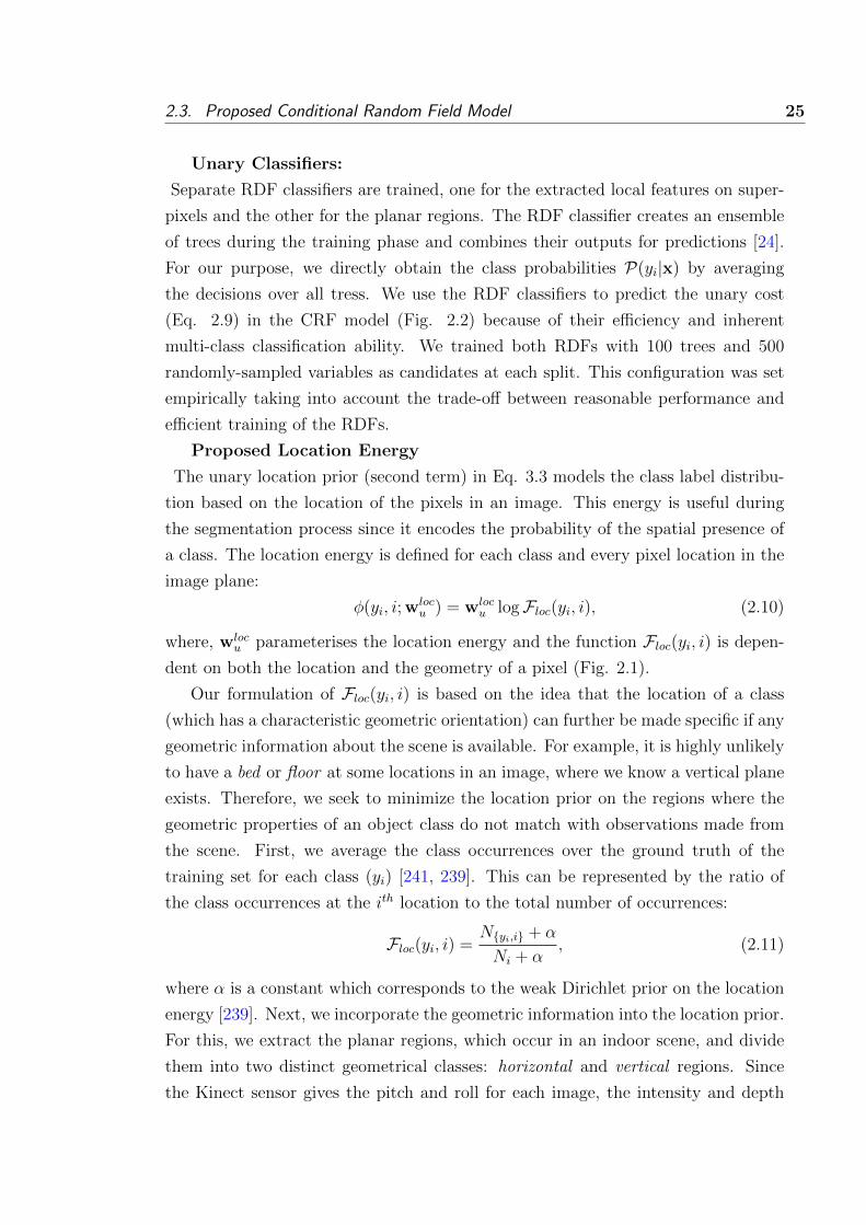
2.3. Proposed Conditional Random Field Model 25
Unary Classifiers:
Separate RDF classifiers are trained, one for the extracted local features on super-
pixels and the other for the planar regions. The RDF classifier creates an ensemble
of trees during the training phase and combines their outputs for predictions [24].
For our purpose, we directly obtain the class probabilities P(yi|x) by averaging
the decisions over all tress. We use the RDF classifiers to predict the unary cost
(Eq. 2.9) in the CRF model (Fig. 2.2) because of their efficiency and inherent
multi-class classification ability. We trained both RDFs with 100 trees and 500
randomly-sampled variables as candidates at each split. This configuration was set
empirically taking into account the trade-off between reasonable performance and
efficient training of the RDFs.
Proposed Location Energy
The unary location prior (second term) in Eq. 3.3 models the class label distribu-
tion based on the location of the pixels in an image. This energy is useful during
the segmentation process since it encodes the probability of the spatial presence of
a class. The location energy is defined for each class and every pixel location in the
image plane:
φ(yi, i; wlocu ) = wloc
u logFloc(yi, i), (2.10)
where, wlocu parameterises the location energy and the function Floc(yi, i) is depen-
dent on both the location and the geometry of a pixel (Fig. 2.1).
Our formulation of Floc(yi, i) is based on the idea that the location of a class
(which has a characteristic geometric orientation) can further be made specific if any
geometric information about the scene is available. For example, it is highly unlikely
to have a bed or floor at some locations in an image, where we know a vertical plane
exists. Therefore, we seek to minimize the location prior on the regions where the
geometric properties of an object class do not match with observations made from
the scene. First, we average the class occurrences over the ground truth of the
training set for each class (yi) [241, 239]. This can be represented by the ratio of
the class occurrences at the ith location to the total number of occurrences:
Floc(yi, i) =N{yi,i} + α
Ni + α, (2.11)
where α is a constant which corresponds to the weak Dirichlet prior on the location
energy [239]. Next, we incorporate the geometric information into the location prior.
For this, we extract the planar regions, which occur in an indoor scene, and divide
them into two distinct geometrical classes: horizontal and vertical regions. Since
the Kinect sensor gives the pitch and roll for each image, the intensity and depth

26 Chapter 2. Geometry Driven Semantic Labeling of Indoor Scenes
Figure 2.4: Learning Location Prior using Geometrical Context: (a) Original image.
(b) The normal location prior for wall is shown. (c) It shows how the prior (b) is
combined with the planar information to channelize the general location information
of a class by considering the scene geometry. Note that white color in (b) and (c)
shows high probability.
images in the NYU-Depth dataset are rotated appropriately to remove any affine
transformations. This positions the horizon (estimated using the accelerometer)
horizontally at the center of each image. We use this horizon to split the horizontal
geometric class into two subclasses, the ‘above-horizon’ and ‘below-horizon’ regions.
For each planar object class, we retain the 2D location prior in the regions where
the geometric properties of the class match with those of the planar region, and
decrease its value by a constant factor in the regions where that class cannot be
located. For example, the roof cannot lie on a horizontal plane in the below-horizon
region or a vertical region. This effectively reduces the class location prior to only
those regions which are consistent with the geometrical context. It must be noted
that this elimination procedure is only carried out for planar classes e,g., roof, floor,
bed and blinds. After that, the location prior is smoothed using a Gaussian filter and
the actual prior distribution is normalized in such a way that a uniform distribution
across different classes is obtained. The prior distribution is normalized to give∑iFloc(yi, i) = 1/L, where L is the total number of classes. Examples of the
resulting location priors are shown in Fig. 2.4.
2.3.2 Pairwise Energies
The pairwise energy in Eq. 3.2 is defined on the edges E (Fig. 2.2). This energy
is defined in terms of an edge-sensitive Potts model [23],
ψp(yij,x; wp) = wTp φp1(yi, yj)φp2(x). (2.12)

2.3. Proposed Conditional Random Field Model 27
The first function (φp1) is a class transition energy and the second one (φp2) is
the spatial discontinuation energy. These functions are defined in the following
subsections (Sec. 2.3.2 and 2.3.2 respectively).
Class Transition Energy
The class transition energy in Eq. 3.5 is a simple zero-one indicator function which
enforces a consistent labeling. The function is defined as:
φp1(yi, yj) = a1yi 6=yj =
{0 if yi = yj
a otherwise
For this work we used a = 10. This parameter selection was based on the validation
set (Sec. 7.5.3).
Proposed Spatial Discontinuation Energy
The spatial discontinuation energy in Eq. 3.5 encourages label transitions at nat-
ural boundaries in the image [239, 227]. It is defined as a combination of edges
from the intensity image, depth image and the super-pixel edges extracted using
Mean-shift [64] and Felzenswalb [57] segmentation: φp2(x) = wTp2φedges(x). Weights
assigned to each edge-based energy are learned using a quadratic program (see Sec.
2.4.1). In simple terms, edges which match with the manual annotations to a large
extent contribute more in the energy φp2 . The edge-based energy is given by:
φedges(x) =[βx exp(− σij〈σij〉
), βd exp(−σdij〈σdij〉
),
βsp-fwFsp-fw(x), βsp-msFsp-ms(x), α]T, (2.13)
where, σij = ‖xi − xj‖2, σdij = ‖xdi − xdj‖2 and 〈.〉 denotes the average contrast in
an image. xi and xdi shows the color and depth image pixels respectively. Fsp-ms
and Fsp-fw are indicator functions which give all zeros except at the boundaries of
the Mean-shift [64] or Felzenswalb [57] super-pixels respectively. The output is a
binary image containing ones at the super-pixel boundaries. The inclusion of a
constant α = 1 allows a bias to be learned to remove small isolated parts during the
segmentation process. For our case, we set βx = βd = 150 and βsp-ms = βsp-fw = 5
based on the validation set (see Sec. 7.5.3).
2.3.3 Proposed Higher-Order Energies
A useful strategy to enhance the representational power of a CRF model is to
introduce high-order energies (Eq. 2.1). These energies are dependent on a relatively
large number of dimensions of the output labeling vector y and therefore incorporate
long-range interactions (Fig. 2.2). HOEs try to eliminate inconsistent variables in a

28 Chapter 2. Geometry Driven Semantic Labeling of Indoor Scenes
0
Figure 2.5: Robust Higher-Order Energy: When the number of inconsistent nodes in
a clique increases, the penalty term defined over the clique increases in a logarithmic
fashion.
clique. On the other hand, these energies try to encourage all the variables in a clique
to take the dominant label. The robust P n model [131] poses this encouragement
in a soft manner while the P n Potts model [130] presents this requirement in a
hard fashion. In the robust P n model some pixels in a clique may retain different
labelings. Hence, it is a linear truncated function of the number of inconsistent
variables in a clique. We define our proposed HOE which works in a similar manner
as the robust HOE [131]:
ψc(yc,x; wc) = wc min`∈LFc(τc), (2.14)
where, Fc(.) is a function which takes the number of inconsistent pixels τc = #c −n`(yc) as its argument. Here, n` is a function which computes the number of pixels
in clique c taking the label `. The non-decreasing concave function Fc is defined
as: Fc(τc) = λmax − (λmax − λ`)exp(−ητc), where η = η0/Q` and η0 = 5 (Fig. 2.5).
Here η0 is the slope parameter which decides the rate of increase of the penalty,
with the increase in the number of pixels disagreeing with the dominant label. The
parameters λmax and λ` define the penalty range which is typically set to 1.5 and
0.15 respectively. Q` is the truncation parameter which provides the bound for
the maximum number of disagreements in a clique. The higher-order cliques are
formed using the depth-based segmentation method (Sec. 2.5). Details about the
disintegration of the HOE (Eq. 2.14) are given in Appendix A to describe how the
graph cuts algorithm can be applied.

2.4. Structured Learning and Inference 29
2.4 Structured Learning and Inference
The task of indoor scene labeling involves making joint predictions over many
complex yet correlated and structured outputs. The CRF model defined in the
previous section (Sec. 2.3) explicitly models the correlations over the output space
and performs approximate inference at test time. However, the CRF model con-
tains a number of energies, parametrized by weights which we learn using a S-SVM
formulation. The learning procedure is outlined as follows.
2.4.1 Learning Parameters
Unary, pairwise and high order terms (Eq. 3.2 and Fig. 2.1, 2.2) in the CRF
model introduce many parameters which need a more principled tuning procedure
rather than simple hand-picked values, cross validation learning or a piecewise train-
ing mechanism. In this work, we use a structured large-margin learning method
(S-SVM) to efficiently adjust the probabilistic model parameters. Instead of using
an n-slack formulation of the cost function, we use a single slack formulation, which
results in more efficient learning [117]. Given N training images, the training set
can be represented in the form of ordered pairs of image data x and labelings y:
T = {(xn,yn), n ∈ [1, . . . , N ]}. If ξ ∈ R+ is a single slack variable, the following
margin re-scaled cost function is solved to compute the parameter vector w∗:
(w∗, ξ∗) = argminw,ξ
1
2‖w‖2 + Cξ (2.15)
subject to;
1
N
N∑n=1
[E(y,xn; w)− E(yn,xn; w)] ≥ 1
N
N∑n=1
∆(y,yn)− ξ (2.16)
∀n ∈ [1..N ],∀y ∈ L : y 6= yn, C > 0,
wi ≥ 0 : ∀wi ∈ {w}\wu ,
where, C is the regularization constant, ∆(y,yn) is the Hamming loss function
and the parameter vector w consists of the appearance energy weight (wappu ), the
location energy weight (wlocu ), the pairwise energy weight (wp) and the weight for
HOE (wc). Due to the large number of constraints in Eq. 2.16, a cutting plane
algorithm ([117], Algorithm 4) is used for training which only considers the most
violated constraints to solve our optimization problem. It can be proved that the
algorithm converges after O(1/ε) steps with the guarantee that the objective value

30 Chapter 2. Geometry Driven Semantic Labeling of Indoor Scenes
(once the final solution is reached) differs by at most ε from the global minimum
[262]. The two major steps in this algorithm are the quadratic optimization step,
which is solvable by off-the-shelf convex optimization problem solvers and the loss-
augmented prediction step, which can be solved by graph cuts.
Once suitable parameters for the CRF are learned, the parameters for the edge-
based energies are learned which results in a balanced representation of each edge
in the pairwise energy. In our approach, instead of a simple contrast-based energy,
we define a weighted combination of various possible edge-based energies (such as
based on depth edges, contrast-based edges, super-pixels edges) to accommodate
information from all these sources (see Sec. 2.3.2 and Eq. 2.13). We start with a
heuristic-based initialization and iterate over the training samples to learn a more
balanced representation between the different edge-based energies. The weights for
edges are restrained to be non-negative so that the energy remains sub-modular.
This condition is necessary because the graph cuts based exact inference methods
can be applied only to sub-modular energy minimization problems.
We use structured learning to learn weights for the spatial discontinuation energy
(Sec. 2.3.2). The corresponding quadratic program is given as follows:
argmax‖wp2‖=1
γ (2.17)
s.t.; {Econ, Edep, Efel-sp, Ems-sp} − Egrd ≥ γ, {wp2} ≥ 0,
where, Egrd is the energy when the spatial discontinuation energy is based on the
manually identified edges from the training images. Energies for the case when the
spatial discontinuation energy is based on image contrast, image depth, Felzenswalb
or mean-shift super-pixels are represented as Econ, Edep, Efel-sp or Ems-sp respectively.
The cost function given in Eq. 3.7 is optimized in a similar way to that described in
([117], Algorithm 4). After learning, it turns out that the contrast and depth-based
edge energies are more reliable and therefore play a dominant role in the spatial
discontinuation energy.
2.4.2 Inference in CRF
Once the CRF energies have been learned along with their parameters, the next
step is to find the most probable labeling. As discussed earlier in Sec. 2.3, this turns
out to be an energy minimization problem (Eq. 3.8). Since our energy function is
sub-modular, this energy minimization problem can be solved via the expansion
move algorithms (alpha-expansion or alpha-beta swap graph cuts algorithm) of [22].
The main idea is to decompose the energy minimization problem into a series of

2.5. Planar Surface Detection 31
binary minimization problems which can themselves be solved efficiently. The al-
gorithm starts with an arbitrary initial labeling and at each step the move is only
made if it results in an overall minimization of the cost function [23, 22].
2.5 Planar Surface Detection
Indoor environments are predominantly composed of structures which can be
decomposed into planar regions, such as walls, ceilings, cupboards and blinds. These
flat surfaces are easier to manufacture and thus appear frequently in man-made
environments (Sec. 2.6.2). We extract the dominant planes which best fit the
sparse point clouds of indoor images (obtained from RGBD data) and use them in
our model-based representation (Fig. 2.1). It must be noted that the depth images
produced by a Kinect contain many missing values e.g., along the outer boundaries
of an image or when the scene contains a black or a specular surface. Traditional
plane detection algorithms (e.g. [242, 221]) either make use of dense 3D point clouds
or simply ignore the missing depth regions. In contrast, we propose an efficient
plane detection algorithm which is robust to missing depth values (often termed as
holes) in the Kinect depth map. We expect that the inference made on the improved
planar regions will help us achieve a better semantic labeling performance (see Sec.
2.6.2).
Our method3 first aligns the 3D points with the principal directions of the room.
Next, surface normals are computed at each point. Contiguous points in space are
then clustered by a region growing algorithm (Algorithm 1) which groups the 3D
points in a way to maintain their continuity and smoothness. It is robust to erro-
neous normal orientations caused due to big holes mostly present along the borders
of the depth image acquired via Kinect sensor (Fig. 2.7). The basic idea is to make
use of appearance-based cues when the depth information is not reliable. The algo-
rithm begins with a seed point and at each step, a region is grown by including the
points in the current region with normals pointing in the same direction. Iteratively,
the region is extended and the newly included points are treated as seeds in the sub-
sequent iteration. To deal with erroneous sensor measurements along the border
and any other regions with missing depth measurements, we relax the smoothness
constraint and use major line segments present in the image to decide about the
region continuity.
3Plane detection code is available at author’s webpage: http://www.csse.uwa.edu.au/
~salman
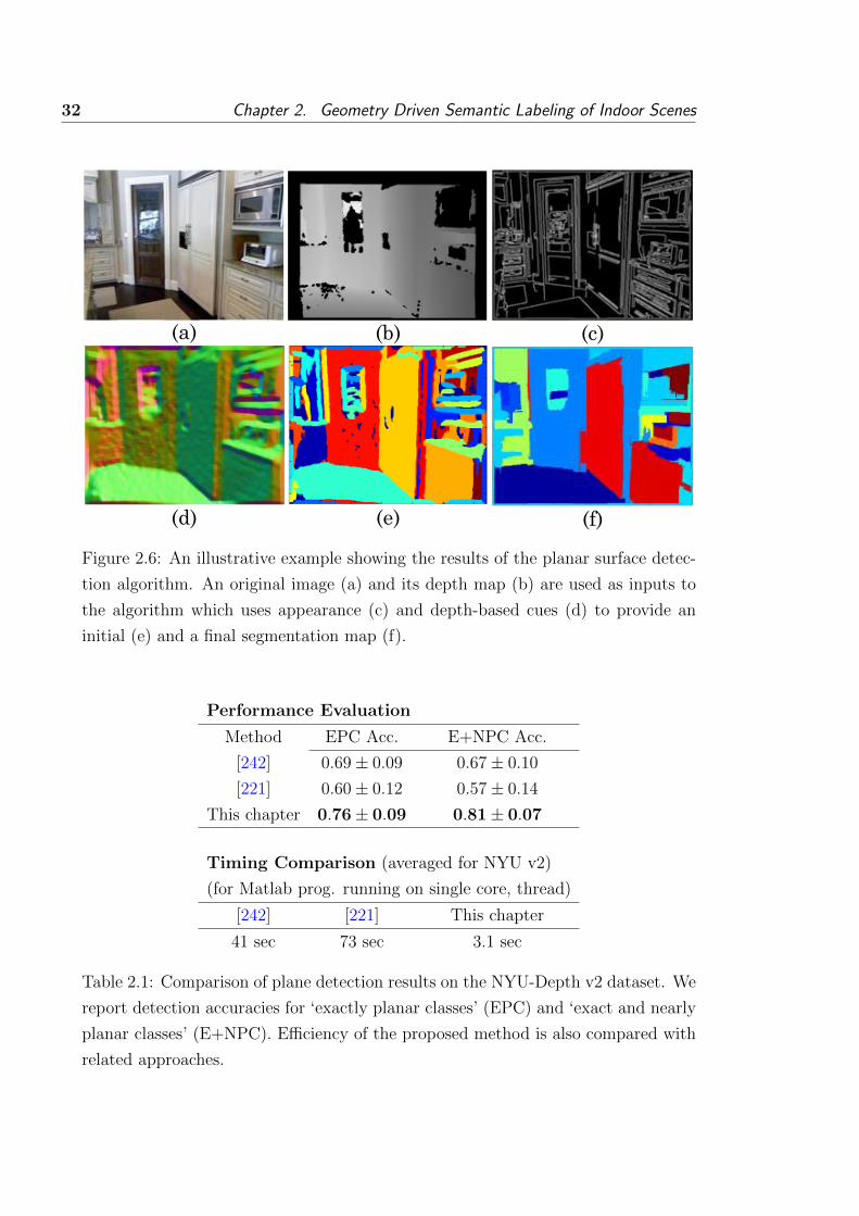
32 Chapter 2. Geometry Driven Semantic Labeling of Indoor Scenes
(a) (b) (c)
(f)(e)(d)
Figure 2.6: An illustrative example showing the results of the planar surface detec-
tion algorithm. An original image (a) and its depth map (b) are used as inputs to
the algorithm which uses appearance (c) and depth-based cues (d) to provide an
initial (e) and a final segmentation map (f).
Performance Evaluation
Method EPC Acc. E+NPC Acc.
[242] 0.69± 0.09 0.67± 0.10
[221] 0.60± 0.12 0.57± 0.14
This chapter 0.76± 0.09 0.81± 0.07
Timing Comparison (averaged for NYU v2)
(for Matlab prog. running on single core, thread)
[242] [221] This chapter
41 sec 73 sec 3.1 sec
Table 2.1: Comparison of plane detection results on the NYU-Depth v2 dataset. We
report detection accuracies for ‘exactly planar classes’ (EPC) and ‘exact and nearly
planar classes’ (E+NPC). Efficiency of the proposed method is also compared with
related approaches.

2.5. Planar Surface Detection 33
Algorithm 1 Region Growing Algorithm for Depth-Based Segmentation
Input: Point cloud = {P}, Depth map = {D}, RGB image = {I}, Edge matching
threshold eth, Normalized boundary matching threshold bth
Output: Labeled planar regions = {R}1: Calculate point normals: {N} ← Fnormal(D)
2: Remove inconsistencies by low-pass filtering: {Nsm} ← N ∗ ksm // ksm is the
smoothing kernel
3: Cluster 3D points with similar normal orientations: {Nclu} ← Fk−means(Nsm)
4: Initialize: R← Nclu
5: Line segment detector: {L} ← FLSD(I)
6: Diffused line map: {Lsm} ← L ∗ k′sm7: Identify planar regions with missing depth values: {M} ← Fholes(Nclu,D)
8: Find adjacency links for each cluster in Nclu: Aclu
9: Identify all unique neighbors of clusters in M: Unb
10: From Unb, separate correct and faulty clusters into Ncor and Ninc respectively
11: Initialize available cluster list: Lavl ← Ncor
12: Initialize label propagation list: Lprp ← ∅13: while list Lavl is not empty do
14: Randomly draw a cluster from available Ncor: ridx
15: Identify ridx neighbors (Nr−idx) with faulty depth values using Aclu and M
16: for each neighbor nr−idx in Nr−idx do
17: Find mutual boundary (bm) of ridx and nr−idx
18: Calculate edge strength at bm using Lsm: estr
19: Calculate normalized boundary matching cost: bstr = bm/ Area of nr−idx
20: if estr < eth ∧ bstr > bth then
21: nr−idxadd−−→ Ncor, nr−idx
add−−→ Lavl
22: ridxrem−−→ Lavl, nr−idx
rem−−→ Ninc
23: Update Lprp with ridx and nr−idx. If nr−idx was previously replaced,
use the updated value.
24: ridxrem−−→ Lavl
25: for any leftover clusters in Ninc do
26: Randomly draw a cluster from available Ninc: r′idx
27: Execute similar steps (from line 15 to 24) for r′idx
28: Update R according to Lprp
29: return {R}

34 Chapter 2. Geometry Driven Semantic Labeling of Indoor Scenes
Fig
ure
2.7:
Com
par
ison
ofou
ral
gori
thm
(las
tro
w)
wit
h[2
42]
(mid
dle
row
)is
show
n.
Not
eth
atth
ew
hite
colo
rin
mid
dle
row
show
sn
on-p
lan
arre
gion
s.T
he
last
row
show
sdet
ecte
dpla
nes
aver
aged
over
sup
er-p
ixel
s.R
esult
ssh
owth
atou
ral
gori
thm
is
mor
eac
cura
tees
pec
ially
nea
rth
eou
ter
bou
ndar
ies
ofth
esc
ene.
(Bes
tvi
ewed
inco
lor)
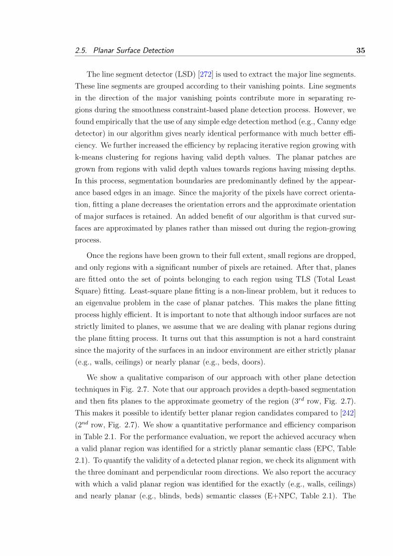
2.5. Planar Surface Detection 35
The line segment detector (LSD) [272] is used to extract the major line segments.
These line segments are grouped according to their vanishing points. Line segments
in the direction of the major vanishing points contribute more in separating re-
gions during the smoothness constraint-based plane detection process. However, we
found empirically that the use of any simple edge detection method (e.g., Canny edge
detector) in our algorithm gives nearly identical performance with much better effi-
ciency. We further increased the efficiency by replacing iterative region growing with
k-means clustering for regions having valid depth values. The planar patches are
grown from regions with valid depth values towards regions having missing depths.
In this process, segmentation boundaries are predominantly defined by the appear-
ance based edges in an image. Since the majority of the pixels have correct orienta-
tion, fitting a plane decreases the orientation errors and the approximate orientation
of major surfaces is retained. An added benefit of our algorithm is that curved sur-
faces are approximated by planes rather than missed out during the region-growing
process.
Once the regions have been grown to their full extent, small regions are dropped,
and only regions with a significant number of pixels are retained. After that, planes
are fitted onto the set of points belonging to each region using TLS (Total Least
Square) fitting. Least-square plane fitting is a non-linear problem, but it reduces to
an eigenvalue problem in the case of planar patches. This makes the plane fitting
process highly efficient. It is important to note that although indoor surfaces are not
strictly limited to planes, we assume that we are dealing with planar regions during
the plane fitting process. It turns out that this assumption is not a hard constraint
since the majority of the surfaces in an indoor environment are either strictly planar
(e.g., walls, ceilings) or nearly planar (e.g., beds, doors).
We show a qualitative comparison of our approach with other plane detection
techniques in Fig. 2.7. Note that our approach provides a depth-based segmentation
and then fits planes to the approximate geometry of the region (3rd row, Fig. 2.7).
This makes it possible to identify better planar region candidates compared to [242]
(2nd row, Fig. 2.7). We show a quantitative performance and efficiency comparison
in Table 2.1. For the performance evaluation, we report the achieved accuracy when
a valid planar region was identified for a strictly planar semantic class (EPC, Table
2.1). To quantify the validity of a detected planar region, we check its alignment with
the three dominant and perpendicular room directions. We also report the accuracy
with which a valid planar region was identified for the exactly (e.g., walls, ceilings)
and nearly planar (e.g., blinds, beds) semantic classes (E+NPC, Table 2.1). The

36 Chapter 2. Geometry Driven Semantic Labeling of Indoor Scenes
results demonstrate that our algorithm is superior to other region growing algorithms
(e.g., [221]) which are suitable for the segmentation of dense point clouds and fail
to deal with erroneous depth measurements from the Kinect sensor (Table 2.1).
2.6 Experiments and Analysis
2.6.1 Datasets
We evaluated our framework on the NYU-Depth datasets (v1 and v2) and the
SUN3D dataset. All these are recent RGBD datasets for indoor scenes acquired
using the Microsoft Kinect structured light sensor. The NYU-Depth dataset is
the only one of its kind and comes with manual annotations acquired via Amazon
Mechanical Turk. The dataset comes in two releases. The first version (v1) of
NYU-Depth [241] consists of 64 different indoor scenes categorized into 7 major
scene types and contains 2284 labeled frames. The second version (v2) of NYU-
Depth [242] consists of 464 different indoor scenes classified into 26 major scene
types and contains 1449 labeled frames. SUN3D is a large-scale indoor RGBD video
dataset [291]; however, it is still under development and only a small portion has
been labeled. We extracted labeled key-frames from the SUN3D database which
amounted to 83 images. We evaluated our method on the labeled portions of the
NYU v1, v2 and SUN3D datasets.
2.6.2 Results
In the NYU-Depth v1 dataset, around 1400 different object classes are present
in all indoor scenes. Since not all object classes have a sufficient representation, we
follow the procedure in [241] to cluster the existing annotations into the 13 most
frequently occurring classes. This clustering is performed using the Wordnet Natural
Language Toolkit (NLTK). In the NYU-Depth v2 dataset, around 900 different
object classes are present overall. We used a similar procedure to cluster existing
annotations into the 22 most frequently occurring classes. Moreover, we report
results on 40 classes to show how our performance compares when the number of
semantic classes is increased. For the SUN3D dataset, 32 classes are present
in the labeled images we acquired. We clustered them into 13 major classes using
Wordnet. In all three datasets, a supplementary class labeled ‘other ’ is also included
to model rarely-occurring objects. In our evaluations, we exclude all unlabeled
regions. For all the three datasets, roughly a train/test split of 60%/40% was used.
A relatively small validation set consisting of 50 random images was extracted from
each dataset (except for SUN3D where we used the parameters of NYU-Depth v1).

2.6. Experiments and Analysis 37
Fig
ure
2.8:
Exam
ple
sof
the
sem
anti
cla
bel
ing
resu
lts
onth
eN
YU
-Dep
thv1
dat
aset
.T
he
top
row
show
sth
ein
tensi
tyim
ages
,
the
bot
tom
row
are
the
grou
nd
truth
san
dth
em
iddle
row
are
our
lab
elin
gre
sult
s.T
he
repre
senta
tive
colo
rsar
esh
own
inth
e
figu
rele
gend
atth
eb
otto
m.
Our
fram
ewor
kp
erfo
rms
wel
lin
cludin
gth
eca
seof
som
eunla
bel
edre
gion
s.(B
est
view
edin
colo
r)

38 Chapter 2. Geometry Driven Semantic Labeling of Indoor Scenes
Tab
le2.
2:R
esult
son
the
NY
U-D
epth
v1,
v2
and
the
SU
N3D
Dat
aset
s:W
ere
por
tth
ere
sult
sof
our
pro
pos
edfr
amew
ork
when
only
the
unar
yen
ergy
was
use
d(t
op3
row
s)an
dre
por
tth
eim
pro
vem
ents
obse
rved
when
mor
eso
phis
tica
ted
pri
ors
and
HO
Es
(las
tro
w)
wer
ead
ded
.A
ccura
cies
are
rep
orte
dfo
r13
,22
and
13cl
ass
sem
anti
cla
bel
ings
for
NY
Uv1,
v2
and
SU
N3D
dat
aset
s,
resp
ecti
vely
.T
he
bes
tp
erfo
rman
ceis
achie
ved
by
com
bin
ing
unar
y,pai
rwis
ean
dH
OE
sin
the
CR
Ffr
amew
ork.
Var
iants
ofO
ur
Met
hod
NY
U-D
epth
v1
NY
U-D
epth
v2
SU
N3D
Glo
bal
Acc
ura
cyC
lass
Acc
.G
lob
alA
ccu
racy
Cla
ssA
cc.
Glo
bal
Acc
ura
cyC
lass
Acc
.
Fea
ture
En
sem
ble
(FE
)52.8±
13.3
%53
.4%
44.4±
15.8
%39
.2%
41.9±
11.1
%40.0
%
FE
+P
AM
(sin
gle
opin
ion
)60.9±
13.3
%60.2
%51.1±
15.6
%41.5
%47.6±
11.3
%41.8
%
FE
+P
lan
arA
pp
eara
nce
Mod
el(P
AM
)63.3±
13.1
%62.7
%52.5±
15.5
%42.4
%48.3±
11.5
%42.6
%
FE
+P
AM
+L
oca
tion
Pri
or(2
D)
65.2±
13.4
%63.5
%53.6±
15.6
%42.8
%48.9±
11.7
%42.8
%
FE
+P
AM
+P
lan
arL
oca
tion
Pri
or(P
LP
)68.6±
13.8
%65
.0%
55.3±
15.8
%43.1
%51.5±
11.9
%43.3
%
FE
+P
AM
+P
LP
+C
RF
70.5±
13.8
%66.5
%58.0±
16.0
%44.9
%53.7±
12.1
%44.4
%
FE
+P
AM
+P
LP
+C
RF
(HO
E)
70.6±
13.8
%66.5
%58.3±
15.9
%45.1
%54.2±
12.2
%44.7
%

2.6. Experiments and Analysis 39
Tab
le2.
3:C
lass
-wis
eA
ccura
cies
onN
YU
-Dep
thv1:
Mea
ncl
ass
and
glob
alac
cura
cies
are
also
rep
orte
d.
Our
pro
pos
edfr
amew
ork
per
form
sve
ryw
ell
onth
epla
nar
clas
ses
(e.g
.,‘w
all’
,‘t
elev
isio
n’,
‘cei
lin
g’)
.
Cla
ssBed
Blind
Bookshelf
Cabinet
Ceiling
Floor
Picture
Sofa
Table
Television
Wall
Window
Other
Unlabeled
Mean
Class
Accuracy
Mean
Pixel
Accuracy
Cla
ssF
req.
1.3
3.7
13.4
7.7
3.7
11.3
4.7
2.5
4.6
0.6
262.
10.
2418
.1-
-
Th
isch
apte
r66
.867
.747
.572
.679
.267
.853
.475
.169
.378
.686
.262
.038
.1-
66.5
70.6
Tab
le2.
4:C
lass
-wis
eA
ccura
cies
onN
YU
-Dep
thv2
(22
clas
ses)
:M
ean
clas
san
dgl
obal
accu
raci
esar
eal
sore
por
ted.
Our
pro
pos
edfr
amew
ork
per
form
sve
ryw
ell
onth
epla
nar
clas
ses
(e.g
.,‘w
all’
,‘d
oor’,
‘floo
r’)
.
Cla
ss
Bed
Blind
Bookshelf
Cabinet
Ceiling
Floor
Picture
Sofa
Table
Television
Wall
Window
Counter
Person
Books
Door
Clothes
Sink
Bag
Box
Utensils
Other
Unlabeled
Mean
Class
AccuracyMean
Pixel
Accuracy
Cla
ssF
req.
4.7
2.0
4.2
10.7
1.4
10.8
2.2
6.2
2.6
0.5
22.8
2.3
2.7
1.7
0.9
2.3
1.7
0.3
1.7
0.8
0.2
0.1
17.4
--
Th
isch
apte
r32
.356
.938
.345
.664
.775
.843
.658
.647
.945
.777
.554
.043
.838
.834
.058
.337
.223
.128
.435
.722
.629
.9-
45.1
58.3

40 Chapter 2. Geometry Driven Semantic Labeling of Indoor Scenes
Tab
le2.
5:C
lass
-wis
eA
ccura
cies
onth
eN
YU
-Dep
thv2
(40
clas
ses)
:M
ean
clas
san
dgl
obal
accu
raci
esar
eal
sore
por
ted.
Our
pro
pos
edfr
amew
ork
per
form
sve
ryw
ell
onth
epla
nar
clas
ses
(e.g
.,‘w
all’
,‘c
eili
ng’,
‘whi
tebo
ard
’).
Cla
ss
Wall
Floor
Cabinet
Bed
Chair
Sofa
Table
Door
Window
Bookshelf
Picture
Counter
Blinds
Desk
Shelves
Curtain
Dresser
Pillow
Mirror
Floormat
Clothes
Ceiling
Cla
ssF
req.
21.4
9.1
6.2
3.8
3.3
2.7
2.1
2.2
2.1
1.9
2.1
1.4
1.7
1.1
1.0
1.1
0.9
0.8
1.0
0.7
0.7
1.4
Th
isch
apte
r65
.762
.540
.132
.144
.550
.843
.551
.649
.236
.341
.439
.255
.848
.045
.253
.155
.350
.546
.154
.135
.450
.6
Cla
ss
Books
Refrigerator
Television
Paper
Towel
Shower
curtain
Box
Whiteboard
Person
Nightstand
Toilet
Sink
Lamp
Bathtub
Bag
Other
structureOther
furniture
Otherprops
Unlabeled
Mean
Class
AccuracyMean
Pixel
Accuracy
Cla
ssF
req.
0.6
0.6
0.5
0.4
0.4
0.4
0.3
0.3
0.3
0.3
0.3
0.3
0.3
0.3
0.2
3.8
2.5
2.2
17.4
--
Th
isch
apte
r39
.153
.650
.135
.439
.941
.836
.360
.635
.632
.531
.822
.526
.338
.537
.345
.724
.929
.1-
43.9
50.7

2.6. Experiments and Analysis 41
Fig
ure
2.9:
Exam
ple
sof
sem
anti
cla
bel
ing
resu
lts
onth
eN
YU
-Dep
thv2
dat
aset
.T
he
top
row
show
sth
ein
tensi
tyim
ages
,th
e
bot
tom
row
are
the
grou
nd
truth
san
dth
em
iddle
row
are
our
lab
elin
gre
sult
s.T
he
repre
senta
tive
colo
rsar
esh
own
inth
efigu
re
lege
nd
atth
eb
otto
m.
Our
fram
ewor
kp
erfo
rms
wel
lin
cludin
gth
eca
seof
som
eunla
bel
edre
gion
s.(B
est
view
edin
colo
r)

42 Chapter 2. Geometry Driven Semantic Labeling of Indoor Scenes
This validation set was used with the genetic search algorithm (Sec. 2.3.1) for
the selection of useful features and for the choice of the initial estimates of the
parameters which give the best performance. Afterwards, these parameters were
optimized during the learning process as described in Sec. 2.4.1.
We use two popular evaluation metrics to assess our results, ‘global accuracy ’
and ‘class accuracy ’ (see Table 2.2). Global accuracy measures the average number
of super-pixels which are correctly classified in the test set. Class accuracy measures
the average of the correct class predictions which is essentially equal to the mean of
the values occurring along the diagonal of the confusion matrix. We extensively
evaluated our approach on both versions of the NYU-Depth dataset and on the
SUN3D dataset. Our experimental results are reported in Tables 2.2, 2.3, 2.4 and
2.5. Comparisons with state-of-the-art techniques are reported in Tables 2.6, 2.7,
2.8 , 2.9 and 2.10. Sample labelings for NYU-Depth v1 and v2 and SUN3D are
presented in Figs. 2.8, 2.9 and 2.10 respectively. Although the unlabeled portions
in the annotated images are not considered during our evaluations, we observed that
the labeling scheme mostly predicts accurate class labels (see Figs. 2.8 and 2.9).
Ablation Study
We report our results in terms of average pixel and class accuracies in Table 2.2.
The first row shows the performance when a simple unary energy defined on pixels
using an ensemble of features is used. We achieve pixel and class accuracies of
52.8% and 53.4% respectively on NYU-Depth v1. The corresponding accuracies
for NYU-Depth v2 and SUN3D are 44.4%, 39.2% and 41.9%, 40.0% respectively.
Starting from this baseline, we were able to obtain significant improvements. Upon
the introduction of the planar appearance model, the pixel and class accuracies
increased by 10.5% and 9.3% from their previous values for NYU-Depth v1 (row
3, Table 2.2). Similarly for NYU-Depth v2, an increase of 8.1% and 3.2% is noted
for pixel and class accuracies respectively. Finally for the SUN3D database, we
achieve an increase of 6.4% and 2.6% in pixel and class accuracies respectively.
Note that a simple averaging operation on the pixel and planar appearance energies
(equivalently an LOP with weights [12, 1
2]) gives less accurate results (row 2, Table
2.2). The addition of the CRF and the proposed location energy enforce a better
label consistency which results in an improvement of 7.2% and 3.8% for NYU-Depth
v1, 5.5% and 2.5% for NYU-Depth v2, 5.4% and 2.1% for SUN3D datasets. The
introduction of HOEs gives a slight boost in accuracy. This is logical since the
introduction of cardinality-based HOEs improves segmentation accuracies for porous
and fine structures such as trees and cat fur, respectively. The classes which are

2.6. Experiments and Analysis 43
considered in this work usually have solid structures with definite and well-defined
boundaries. However, when we consider the segmentation performance around the
boundary regions, the HOEs give a significant increase in accuracy (Fig. 2.11).
Comparisons
For NYU-Depth v1, we compare our framework with [241] (Table 2.6). With the
same set of classes used in [241], we achieved a 13.2% improvement in terms of
average class accuracy. We also report the average global accuracy which gives a
better absolute measurement of performance. The class-wise accuracies for NYU-
Depth v1 are shown in Table 2.3 and the complete confusion matrix is presented in
Fig. 2.12. It can be seen that we perform really well on planar classes such as wall,
ceiling, blinds and table.
For the case of NYU-Depth v2, we compare our framework with recent multi-
scale convolutional network based techniques [53, 39]. Whereas in [53, 39] evalu-
ations were performed on just 13 classes, we use a broader range of 22 classes to
report our results (see Table 2.4). To compare with the class sofa, we report the
mean accuracies of the sofa and chair classes for a fair comparison (if we sum up
the class occurrences of the chair and sofa which are reported in [39], the combined
class frequency supports such a comparison). We compare the furniture class in [39]
with our cabinet class based on the details given in [39]. Overall, we get superior
performance compared to [53, 39] and also achieve best class accuracies for 19/22
classes.
On the NYU-Depth v2 dataset, [242] defined just four semantic classes: furniture,
ground, structure and props. The choice of these classes was based on the need to
infer the support relationships between objects. We evaluate our method on the
4-class segmentation task as well. As shown in Table 2.8, we achieved the best
performance overall. In particular, we performed well on planar classes such as floor
and structures. In terms of pixel and class accuracies, we noted an improvement of
2.2% and 1.3% respectively. We also compare our results with [80] in terms of the
weighted average Jaccard index (WAJI). Our system’s performance is lower than
that of [80], which is based on a very strong but computationally-expensive contour
detection technique called gPb [6] (Table 2.9). Finally, we compare our results on
a 40-class semantic labelling task (Table 2.10). We note that the RGBD version of
the R-CNN model proposed in [81] performs best. Their approach however, uses
external data (Imagenet) for pre-training and uses synthetic 3D CAD models from
the Internet to generate training data.
One may wonder why the incorporation of geometrical context in the CRF model

44 Chapter 2. Geometry Driven Semantic Labeling of Indoor Scenes
Figure 2.10: Examples of the semantic labeling results on the SUN3D dataset. The
top row shows the intensity images, the bottom row are the ground truths and the
middle row are our labeling results. The representative colors are shown in the figure
legend at the bottom. (Best viewed in color)
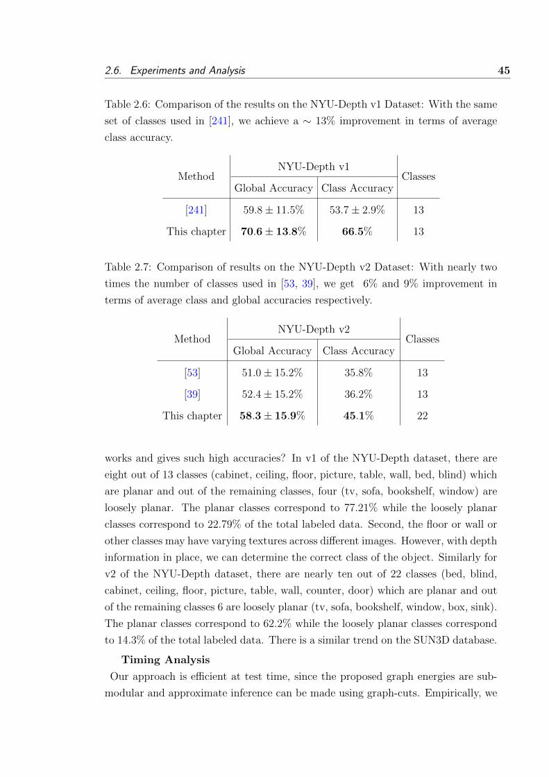
2.6. Experiments and Analysis 45
Table 2.6: Comparison of the results on the NYU-Depth v1 Dataset: With the same
set of classes used in [241], we achieve a ∼ 13% improvement in terms of average
class accuracy.
MethodNYU-Depth v1
ClassesGlobal Accuracy Class Accuracy
[241] 59.8± 11.5% 53.7± 2.9% 13
This chapter 70.6± 13.8% 66.5% 13
Table 2.7: Comparison of results on the NYU-Depth v2 Dataset: With nearly two
times the number of classes used in [53, 39], we get 6% and 9% improvement in
terms of average class and global accuracies respectively.
MethodNYU-Depth v2
ClassesGlobal Accuracy Class Accuracy
[53] 51.0± 15.2% 35.8% 13
[39] 52.4± 15.2% 36.2% 13
This chapter 58.3± 15.9% 45.1% 22
works and gives such high accuracies? In v1 of the NYU-Depth dataset, there are
eight out of 13 classes (cabinet, ceiling, floor, picture, table, wall, bed, blind) which
are planar and out of the remaining classes, four (tv, sofa, bookshelf, window) are
loosely planar. The planar classes correspond to 77.21% while the loosely planar
classes correspond to 22.79% of the total labeled data. Second, the floor or wall or
other classes may have varying textures across different images. However, with depth
information in place, we can determine the correct class of the object. Similarly for
v2 of the NYU-Depth dataset, there are nearly ten out of 22 classes (bed, blind,
cabinet, ceiling, floor, picture, table, wall, counter, door) which are planar and out
of the remaining classes 6 are loosely planar (tv, sofa, bookshelf, window, box, sink).
The planar classes correspond to 62.2% while the loosely planar classes correspond
to 14.3% of the total labeled data. There is a similar trend on the SUN3D database.
Timing Analysis
Our approach is efficient at test time, since the proposed graph energies are sub-
modular and approximate inference can be made using graph-cuts. Empirically, we

46 Chapter 2. Geometry Driven Semantic Labeling of Indoor Scenes
Table 2.8: Comparison of results on the NYU-Depth v2 Dataset (4-class labeling
task): Our method achieved best performance in terms of average pixel and class
accuracies for the 4-class segmentation task. We also get the best classification
performance on structure class.
MethodSemantic Classes Pixel Class
Floor Struct. Furn. Prop. Acc. Acc.
[242] 68 59 70 42 58.6 59.6
[53] 68.1 87.8 51.1 29.9 63 59.2
[39] 87.3 86.1 45.3 35.5 64.5 63.5
[26] 87.9 79.7 63.8 27.1 67.0 64.3
This chapter 87.1 88.2 54.7 32.6 69.2 65.6
0 5 10 15 2050
55
60
65
70
75
80
Width of Area Surrounding the Boundaries (Pixels)
Labe
ling
Err
or (
%ag
e)
FEFE+PAMFE+PAM+PLPFE+PAM+PLP+Grid CRFFE+PAM+PLP+CRF(HOP)
Figure 2.11: The error rate decreases as more area surrounding the class boundaries
is considered. The introduction of HOE improves the segmentation accuracy around
the boundaries.

2.6. Experiments and Analysis 47
Table 2.9: Comparison of results on the NYU-Depth v2 Dataset (4-class labeling
task): Our method achieved the second best performance in terms of weighted
average Jaccard index (WAJI).
Perf. SC-[242] LP-[242] [226] SVM-[80] This chapter
WAJI 56.31 53.4 59.19 64.81 62.66
Table 2.10: Comparison of results on the NYU-Depth v2 Dataset (40-class labeling
task): Our method achieved second best performance in terms of weighted average
Jaccard index (WAJI).
Perf. SC-[242] [226] SVM-[80] CNN-[81] This chapter
WAJI 38.2 37.6 43.9 47.0 42.1

48 Chapter 2. Geometry Driven Semantic Labeling of Indoor Scenes
(a)
NY
U-D
epth
v1
(b)
NY
U-D
epth
v2
(c)
SU
N3D
Fig
ure
2.12
:C
onfu
sion
Mat
rice
sfo
rN
YU
-Dep
than
dSU
N3D
Dat
aset
s:T
he
accu
raci
esin
each
confu
sion
mat
rix
sum
up
to
100%
alon
gea
chro
w.
All
the
clas
sac
cura
cies
show
non
the
dia
gonal
are
rounded
toth
ecl
oses
tin
tege
rfo
rcl
arit
y.(B
est
view
ed
inco
lor)

2.6. Experiments and Analysis 49
found average testing time per image to be ∼ 1.6 sec for NYU-Depth v1, ∼ 1.7 sec
for NYU-Depth v2 and ∼ 1.4 sec for the SUN3D database. For parameter learning
on the training set, it took ∼ 17 hrs for NYU-Depth v1, ∼ 12 hrs for NYU-Depth
v2 and ∼ 45 min for the SUN3D database. The RDF training took ∼ 4 hrs, ∼ 2
hrs and ∼ 7 mins on the NYU-Depth v1, v2 and SUN3D databases respectively.
2.6.3 Discussion
It may be of interest to know why we used a hierarchical ensemble learning
scheme to combine posteriors defined on pixels and planar regions. We prefer to
use the proposed scheme because it combines the posteriors on the fly and thus saves
a reasonable amount of training time. Alternate ensemble learning methods such
as Boosting and Bagging require considerable training data and take much time. It
must be noted that we used graph-cuts for making approximate inference during
the S-SVM training. This method is not always precisely accurate. Moreover, only
a limited set of constraints (the working set) from the original infinite number of
constraints are used during training. These approximations can sometimes lead to
unsatisfactory performance. However, we minimized this behavior by initializing
the parameters with values that gave the best performance on the validation set.
This heuristic worked well for our case and enhanced the labeling accuracy.
It can be seen that indoor scene labeling is a challenging problem due to the
diverse nature of the scenes. The major reason for the low reported scene labeling
accuracies (see Table 2.2) is the presence of a large number of objects with varying
textures and layouts across different images. These varied appearances of objects
cause many ambiguities. Also there are many bland regions in the scenes, which
introduce an additional challenge for a correct segmentation. Many times class errors
are due to the confusion between two similar classes e.g., as evident in the confusion
matrices (Fig. 2.12), door is usually confused with wall, blind with window, sink with
counter and sofa with bed. Despite the incorporation of the geometrical context,
an unusual confusion occurs between ceiling and wall. The reason is that the depth
estimates in the regions close to the upper boundary of the scenes were not accurate
and this is the typical location where the ceiling normally occurs in the majority of
the scenes. The planes extracted in this region give a horizontal orientation (instead
of vertical) which contributes to this misclassification, aided by the fact that the
walls and ceilings usually have similar appearances.
The NYU corpus captures natural indoor scene conditions which are common
in everyday life scenarios. As an example, the dataset contains large illumination

50 Chapter 2. Geometry Driven Semantic Labeling of Indoor Scenes
variations (e.g., for scenes of offices, stores) which correctly capture the indoor con-
ditions. Some misclassifications are possibly due to these illumination variations
and specular surfaces e.g., the window or the reflecting mirror was confused with
the light source. Another major challenge relates to the long-tail distribution of
object categories, where a small number of categories appear frequently in indoor
scenes while others are rare. For example, the top ten most frequent classes out
of a total of 894 classes in the NYU v2 dataset constitutes over 65% of the total
labelled data. This translates into a somewhat unbalanced dataset with an insuffi-
cient representation of many semantic classes in the training set [226]. The labeled
portion of the SUN3D database was insufficient for training (because the database
is under development). This explains why the achieved accuracies for this database
are on the low side (see Table 2.2, Fig. 2.12). The availability of more and higher
quality training data for each class will certainly improve the performance of scene
labeling frameworks. The removal of unwanted artifacts such as illumination varia-
tions and shadows can also help in improving the segmentation accuracy [124]. In
short, the challenging indoor scene classification task is far from being solved and
requires further investigation both in terms of new techniques and data for testing
and bench-marking.
2.7 Conclusion
This chapter presented a novel CRF model for semantic labeling of indoor scenes.
The proposed model uses both appearance and geometry information. The geometry
of indoor planar surfaces was approximated using a proposed robust region grow-
ing algorithm for segmentation. The approximate geometry was combined with
appearance-based information and a location prior in the unary term. A learned
combination of boundaries was used to define the spatial discontinuity across an im-
age. The proposed model also captured long-range interactions by defining cliques
on the dominant planar surfaces. The parameters of our model were learned using
a single slack formulation of the rescaled margin cutting plane algorithm. We ex-
tensively evaluated our scheme on both versions of the NYU-Depth and the recent
SUN3D database and reported comparisons and improvements over existing works.
As a future work, we will extend the proposed model to holistically reason about
indoor scenes and to understand the rich interactions between scene elements.

51CHAPTER 3
Automatic Shadow Detection and Removal from
a Single Photograph1
Everything that we see is a shadow cast by that which we do not see.
Martin Luther King, Jr.(1929-1968)
Abstract
We present a framework to automatically detect and remove shadows in real
world scenes from a single image. Previous works on shadow detection put a lot
of effort in designing shadow variant and invariant hand-crafted features. In con-
trast, our framework automatically learns the most relevant features in a supervised
manner using multiple convolutional deep neural networks (ConvNets). The fea-
tures are learned at the super-pixel level and along the dominant boundaries in the
image. The predicted posteriors based on the learned features are fed to a condi-
tional random field model to generate smooth shadow masks. Using the detected
shadow masks, we propose a Bayesian formulation to accurately extract shadow
matte and subsequently remove shadows. The Bayesian formulation is based on a
novel model which accurately models the shadow generation process in the umbra
and penumbra regions. The model parameters are efficiently estimated using an
iterative optimization procedure. Our proposed framework consistently performed
better than the state-of-the-art on all major shadow databases collected under a
variety of conditions.
Keywords : Feature Learning; Bayesian shadow removal; Conditional Random
Field; ConvNets; Shadow detection; Shadow matting
3.1 Introduction
Shadows are a frequently occurring natural phenomenon, whose detection and
manipulation are important in many computer vision (e.g., visual scene understand-
ing) and computer graphics applications. As early as the time of Da Vinci, the prop-
erties of shadows were well studied [42]. Recently, shadows have been used for tasks
1Published in IEEE Transactions on Pattern Analysis and Machine Intelligence (TPAMI),
IEEE, vol.38, no. 3, pp. 431-446, March 2016, doi:10.1109/TPAMI.2015.2462355. A preliminary
version of this research was published in the Proceedings of the IEEE Conference on Computer
Vision and Pattern Recognition (CVPR), pp. 1939-1946, IEEE, 2014.
52 Chapter 3. Automatic Shadow Detection and Removal from a Single Photograph
related to object shape [189, 198], size, movement [123], number of light sources and
illumination conditions [234]. Shadows have a particular practical importance in
augmented reality applications, where the illumination conditions in a scene can be
used to seamlessly render virtual objects and their casted shadows. Contrary to the
above mentioned assistive roles, shadows can also cause complications in many fun-
damental computer vision tasks. For instance, they can degrade the performance of
object recognition, stereo, shape reconstruction, image segmentation and scene anal-
ysis. In digital photography, information about shadows and their removal can help
to improve the visual quality of photographs. Shadows are also a serious concern
for aerial imaging and object tracking in video sequences [216].
Despite the ambiguities generated by shadows, the Human Visual System (HVS)
does not face any real difficulty in filtering out the degradations caused by shadows.
We need to equip machines with such visual comprehension abilities. Inspired by
the hierarchical architecture of the human visual cortex, many deep representation
learning architectures have been proposed in the last decade. We draw our moti-
vation from the recent successes of these deep learning methods in many computer
vision tasks where learned features out-performed hand-crafted features [86]. On
that basis, we propose to use multiple convolutional neural networks (ConvNets) to
learn useful feature representations for the task of shadow detection. ConvNets are
biologically inspired deep network architectures based on Hubel and Wiesel’s [99]
work on the cat’s primary visual cortex. Once shadows are detected, an automatic
shadow removal algorithm is proposed which encodes the detected information in
the likelihood and prior terms of the proposed Bayesian formulation. Our formu-
lation is based on a generalized shadow generation model which models both the
umbra and penumbra regions. To the best of our knowledge, we are the first to use
‘learned features’ in the context of shadow detection, as opposed to the common
carefully designed and hand-crafted features. Moreover, the proposed approach
detects and removes shadows automatically without any human input (Fig. 3.1).
Our proposed shadow detection approach combines local information at image
patches with the local information across boundaries (Fig. 3.1). Since the regions
and the boundaries exhibit different types of features, we split the detection proce-
dure into two respective portions. Separate ConvNets are consequently trained for
patches extracted around the scene boundaries and the super-pixels. Predictions
made by the ConvNets are local and we therefore need to exploit the higher level
interactions between the neighboring pixels. For this purpose, we incorporate local
beliefs in a Conditional Random Field (CRF) model which enforces the labeling

3.1. Introduction 53
Fig
ure
3.1:
Fro
mle
ftto
righ
t:O
rigi
nal
imag
e(a
).O
ur
fram
ewor
kfirs
tdet
ects
shad
ows
(c)
usi
ng
the
lear
ned
feat
ure
sal
ong
the
bou
ndar
ies
(top
imag
ein
(b))
and
the
regi
ons
(bot
tom
imag
ein
(b))
.It
then
extr
acts
the
shad
owm
atte
(e)
and
rem
oves
itto
pro
duce
ash
adow
free
imag
e(d
).

54 Chapter 3. Automatic Shadow Detection and Removal from a Single Photograph
consistency over the nodes of a grid graph defined on an image (Sec. 3.3). This
removes isolated and spurious labeling outcomes and encourages neighboring pixels
to adopt the same label.
Using the detected shadow mask, we identify the umbra (Latin meaning shadow),
penumbra (Latin meaning almost-shadow) and shadow-less regions and propose a
Bayesian formulation to automatically remove shadows. We introduce a generalized
shadow generation model which separately defines the umbra and penumbra gener-
ation process. The resulting optimization problem has a relatively large number
of unknown parameters, whose MAP estimates are efficiently computed by alter-
natively solving for the parameters (Eq. 3.26). The shadow removal process also
extracts smooth shadow matte that can be used in applications such as shadow
compositing and editing (Sec. 3.4).
A preliminary version of this research (which solely focuses on shadow detection)
appeared in [127]. In addition, the current study includes: (1) a new approach to
estimate shadow statistics, (2) automatic shadow removal and shadow matte extrac-
tion, (3) a substantial number of additional experiments, analysis and limitations,
(4) possible applications in many computer vision and graphics tasks.
3.2 Related Work and Contributions
Shadow Detection: One of the most popular methods to detect shadows is
to use a variety of shadow variant and invariant cues to capture the statistical
and deterministic characteristics of shadows [312, 144, 111, 78, 233]. The extracted
features model the chromatic, textural [312, 144, 78, 233] and illumination [111, 204]
properties of shadows to determine the illumination conditions in the scene. Some
works give more importance to features computed across image boundaries, such as
intensity and color ratios across boundaries and the computation of texton features
on both sides of the edges [265, 144]. Although these feature representations are
useful, they are based on assumptions that may not hold true in all cases. As an
example, chromatic cues assume that the texture of the image regions remains the
same across shadow boundaries and only the illumination is different. This approach
fails when the image regions under shadows are barely visible. Moreover, all of
these methods involve a considerable effort in the design of hand-crafted features for
shadow detection and feature selection (e.g., the use of ensemble learning methods
to rank the best features [312, 144]). Our data-driven framework is different and
unique: we propose to use deep feature learning methods to ‘learn the most relevant
features’ for shadow detection.

3.2. Related Work and Contributions 55
Owing to the challenging nature of the shadow detection problem, many simplis-
tic assumptions are commonly adopted. Previous works made assumptions related
to the illumination sources [234], the geometry of the objects casting shadows and
the material properties of the surfaces on which shadows are cast. For example,
Salvador et al. [233] consider object cast shadows while Lalonde et al. [144] only
detect shadows that lie on the ground. Some methods use synthetically generated
training data to detect shadows [203]. Techniques targeted for video surveillance ap-
plications take advantage of multiple images [58] or time-lapse sequences [119, 101]
to detect shadows. User assistance is also required by many proposed techniques
to achieve their attained performances [238, 21]. In contrast, our shadow detection
method makes absolutely ‘no prior assumptions’ about the scene, the shadow prop-
erties, the shape of objects, the image capturing conditions and the surrounding
environments. Based on this premise, we tested our proposed framework on all of
the publicly available databases for shadow detection from single images. These
databases contain common real world scenes with artifacts such as noise, compres-
sion and color balancing effects.
Shadow Removal and Matting: Almost all approaches that are employed to
either edit or remove shadows are based on models that are derived from the image
formation process. A popular choice is to physically model the image into a de-
composition of its intrinsic images along with some parameters that are responsible
for the generation of shadows. As a result, the shadow removal process is reduced
to the estimation of the model parameters. Finlayson et al. [61, 60] addressed this
problem by nullifying the shadow edges and reintegrating the image, which results
in the estimation of the additive scaling factor. Since such global integration (which
requires the solution of a 2D Poisson equation [61, 59]) causes artifacts, the integra-
tion along a 1D Hamiltonian path [63] is proposed for shadow removal. However,
these and other gradient based methods (such as [172, 191]) do not account for the
shadow variations inside the umbra region. To address this shortcoming, Arbel and
Hel-Or [5] treat the illumination recovery problem as a 3D surface reconstruction
and use a thin plate model to successfully remove shadows lying on curved surfaces.
Alternatively, information theory based techniques are proposed in [139, 59] and a
bilateral filtering based approach is recently proposed in [297] to recover intrinsic
(illumination and reflectance) images. However, these approaches either require user
assistance, calibrated imaging sensors, careful parameter selection or considerable
processing times. To overcome these shortcomings, some reasonably fast and accu-
rate approaches have been proposed which aim to transfer the color statistics from

56 Chapter 3. Automatic Shadow Detection and Removal from a Single Photograph
the non-shadow regions to the shadow regions (‘color transfer based approaches’ e.g.,
[225, 285, 238, 286, 290]). Our proposed shadow removal algorithm also belongs to
the category of color transfer based approaches. However, in contrast to previous
related works, we propose a generalized image formation model which enables us
to deal with non-uniform umbra regions as well as soft shadows. Color transfer is
also made at multiple spatial levels , which helps in the reduction of noise and color
artifacts. An added advantage of our approach is our ability to separate smooth
shadow matte from the actual image.
Several assumptions are made in the shadow removal literature due to the ill-
posed nature of recovering the model parameters for each pixel. The camera sensor
parameters are needed in [297, 61]. Multiple narrow-band sensor outputs for each
scene are required in [297], while [189] employs a sequence of images to recover the
intrinsic components. Lambertian surface and Planckian lightening assumptions are
made in [297]. Though several approaches work just on a single image, they require
considerable user interaction to identify either tri-maps [35], quad-maps [285, 286],
gradients [156] or exact shadow boundaries [172, 191]. Su and Chen [251] tried
to minimize the user effort by specifying the complete shadow boundary from the
user provided strokes. In contrast, our framework does not require any form of
user interaction and makes no assumption regarding the camera or scene properties
(except that the object surfaces are assumed to be Lambertian).
The key contributions of our work are outlined below:
� We propose a new approach for robust shadow detection combining both re-
gional and across-boundary learned features in a probabilistic framework in-
volving CRFs (Sec. 3.3).
� Our proposed method automatically learns the most relevant feature repre-
sentations from raw pixel values using multiple ConvNets (Sec. 3.3).
� We propose a generalized shadow formation model along with automatic color
statistics modeling using only detected shadow masks (Sec. 3.4.1 and 3.4.2).
� Our proposed Bayesian formulation for the shadow removal problem integrates
multi-level color transfer and the resulting cost function is efficiently optimized
to give superior results (Sec. 3.4.3 and 3.4.4).
� We performed extensive quantitative evaluation to prove that the proposed
framework is robust, less-constrained and generalisable across different types
of scenes (Sec. 4.6).

3.3. Proposed Shadow Detection Framework 57
Pre
pro
cess
ing
(Sec
. 3.1
)
Sup
erp
ixel
s(S
LIC
)
Bila
tera
l Filt
erin
g
Bo
und
ary
Extr
acti
on
(g
Pb)
[40
]W
ind
ow
Ext
ract
ion
at
Bo
und
ary
Po
ints
Win
do
w E
xtra
ctio
n at
C
entr
oid
s o
f Su
per
pix
els
Imba
lan
ce R
emov
al(S
MO
TE)
(Sec
. 3.1
)Fe
atur
e Le
arn
ing
(Co
nvN
et-1
) (S
ec. 3
.1)
Feat
ure
Lear
nin
g (C
onv
Net
-2)
(Sec
. 3.1
)
Shad
ow
Loc
aliz
atio
n/
Pos
teri
or
on
UC
Ms
(Sec
. 3.1
)
Una
ry T
erm
(S
ec. 3
.1, E
q. 3
)
Pai
rwis
e T
erm
(S
ec. 3
.2, E
q. 5
)
CR
F M
od
el(S
ec. 3
.3)
Edge
Map
(Sec
. 3.2
, Eq
. 7)
Inpu
t Im
age
Shad
ow M
ap
Fig
ure
3.2:
The
pro
pos
edsh
adow
det
ecti
onfr
amew
ork.
(Bes
tvi
ewed
inco
lor)

58 Chapter 3. Automatic Shadow Detection and Removal from a Single Photograph
3.3 Proposed Shadow Detection Framework
Given a single color image, we aim to detect and localize shadows precisely at
the pixel level (see block diagram in Fig. 3.2). If y denotes the desired binary
mask encoding class relationships, we can model the shadow detection problem as
a conditional distribution:
P(y|x; w) =1
Z(w)exp(−E(y,x; w)) (3.1)
where, the parameter vector w includes the weights of the model, the manifest
variables are represented by x where xi denotes the intensity of pixel i ∈ {pi}1×N
and Z(w) denotes the partition function. The energy function is composed of two
potentials; the unary potential ψi and the pairwise potential ψij:
E(y,x; w) =∑i∈V
ψi(yi,x; wi) +∑
(i,j)∈E
ψij(yij,x; wij) (3.2)
In the following discussion, we will explain how we model these potentials in a CRF
framework.
3.3.1 Feature Learning for Unary Predictions
The unary potential in Eq. 3.2 considers the shadow properties both at the
regions and at the boundaries inside an image.
ψi(yi,x; wi) =
region︷ ︸︸ ︷φri (yi,x; wr
i ) +
boundary︷ ︸︸ ︷φbi(yi,x; wb
i ) (3.3)
We define each of the boundary and regional potentials, φr and φb respectively, in
terms of probability estimates from the two separate ConvNets,
φri (yi,x; wri ) = −wr
i logPcnn1(yi|xr)
φbi(yi,x; wbi ) = −wb
i logPcnn2(yi|xb)(3.4)
This is logical because the features to be estimated at the boundaries are likely to
be different from the ones estimated inside the shadowed regions. Therefore, we
train two separate ConvNets, one for the regional potentials and the other for the
boundary potentials.
The ConvNet architecture used for feature learning consists of alternating con-
volution and sub-sampling layers (Fig. 3.3). Each convolutional layer in a ConvNet
consists of filter banks which are convolved with the input feature maps. The sub-
sampling layers pool the incoming features to derive invariant representations. This

3.3. Proposed Shadow Detection Framework 59
Figure 3.3: ConvNet Architecture used for Automatic Feature Learning to Detect
Shadows.
layered structure enables ConvNets to learn multilevel hierarchies of features. The
final layer of the network is fully connected and comes just before the output layer.
This layer works as a traditional MLP with one hidden layer followed by a logistic
regression output layer which provides a distribution over the classes. Overall, after
the network has been trained, it takes an RGB patch as an input and processes it
to give a posterior distribution over binary classes.
ConvNets operate on equi-sized windows, so it is required to extract patches
around desired points of interest. For the case of regional potentials, we extract
super-pixels by clustering the homogeneous pixels2. Afterwards, a patch (Ir) is
extracted by centering a τs×τs window at the centroid of each superpixel. Similarly
for boundary potentials, we first apply a Bilateral filter and then extract boundaries
using the gPb technique [6]. We traverse each boundary with a stride λb and extract
a τs × τs patch at each step to incorporate local context3. Therefore, ConvNets
operate on sets of boundary and super-pixel patches, xr = {Ir(i, j)}1×|Fslic(x)| and
xb = {Ib(i, j)}1×|FgPb(x)|
λb
respectively, where |.| is the cardinality operator. Note
that we include synthetic data (generated by artificial linear transformations [32])
during the training process. This data augmentation is important not only because
it removes the skewed class distribution of the shadowed regions but it also results
2In our implementation we used SLIC [2], due to its efficiency.3the step size is λb = τs/4 to get partially overlapping windows.

60 Chapter 3. Automatic Shadow Detection and Removal from a Single Photograph
in an enhanced performance. Moreover, data augmentation helps to reduce the
overfitting problem in ConvNets (e.g., in [36]) which results in the learning of more
robust feature representations.
During the training process, we use stochastic gradient descent to automatically
learn feature representations in a supervised manner. The gradients are computed
using back-propagation to minimize the cross entropy loss function [147]. We set
the training parameters (e.g., momentum and weight decay) using a cross valida-
tion process. The training samples are shuffled randomly before training since the
network can learn faster from unexpected samples. The weights of the ConvNet
were initialized with randomly drawn samples from a Gaussian distribution of zero
mean and a variance that is inversely proportional to the fan-in measure of neurons.
The number of epochs during the training of ConvNets is set by an early stopping
criterion based on a small validation set. The initial learning rate is heuristically
chosen by selecting the largest rate which resulted in the convergence of the training
error. This rate is decremented by a factor of υ = 0.5 after every 20 epochs.
The ConvNet trained on boundary patches learn to separate shadow and re-
flectance edges while the ConvNet trained on regions can differentiate between
shadow and non-shadow patches. For the case of the regions, the posteriors pre-
dicted by ConvNet are assigned to each super pixel in an image. However, for the
boundaries, we first localize the probable shadow location using the local contrast
and then average the predicted probabilities over each contour generated by the
Ultra-metric Contour Maps (UCM) [6].
3.3.2 Contrast Sensitive Pairwise Potential
The pairwise potential in Eq. 3.2 is defined as a combination of the class tran-
sition potential φp1 and the spatial transition potential φp2 :
ψij(yij,x; wij) = wijφp1(yi, yj)φp2(x). (3.5)
The class transition potential takes the form of an Ising prior:
φp1(yi, yj) = α1yi 6=yj =
{0 if yi = yj
α otherwise(3.6)
The spatial transition potential captures the differences in the adjacent pixel inten-
sities:
φp2(x) = [exp(− ‖xi − xj‖2
βx〈‖xi − xj‖2〉)] (3.7)
where, 〈·〉 denotes the average contrast in an image. The parameters α and βx were
derived using cross validation on each database.

3.3. Proposed Shadow Detection Framework 61
Fig
ure
3.4:
The
Pro
pos
edShad
owR
emov
alF
ram
ewor
k:
Aft
erth
edet
ecti
onof
the
shad
ows
inth
eim
age,
we
esti
mat
eth
eum
bra
,
pen
um
bra
and
obje
ct-s
had
owb
oundar
y.G
iven
this
info
rmat
ion,
am
ult
i-le
velco
lor
tran
sfer
isap
plied
toob
tain
acr
ude
esti
mat
e
ofsh
adow
-les
sim
age.
This
rough
esti
mat
eis
furt
her
impro
ved
usi
ng
the
pro
pos
edB
ayes
ian
form
ula
tion
whic
hes
tim
ates
the
opti
mal
shad
ow-l
ess
imag
eal
ong
wit
hth
esh
adow
model
par
amet
ers.

62 Chapter 3. Automatic Shadow Detection and Removal from a Single Photograph
3.3.3 Shadow Contour Generation using CRF Model
We model the shadow contour generation in the form of a two-class scene parsing
problem where each pixel is labeled either as a shadow or a non-shadow. This
binary classification problem takes probability estimates from the supervised feature
learning algorithm and incorporates them in a CRF model. The CRF model is
defined on a grid structured graph topology, where graph nodes correspond to image
pixels (Eq. 3.2). When making an inference, the most likely labeling is found using
the Maximum a Posteriori (MAP) estimate (y∗) upon a set of random variables
y ∈ LN . This estimation turns out to be an energy minimization problem since the
partition function Z(w) does not depend on y:
y∗ = argmaxy∈LN
P(y|x; w) = argminy∈LN
E(y,x; w) (3.8)
The CRF model proved to be an elegant source to enforce label consistency and the
local smoothness over the pixels. However, the size of the training space (labeled
images) makes it intractable to compute the gradient of the likelihood. Therefore
the parameters of the CRF cannot be found by simply maximizing the likelihood
of the hand labeled shadows. Hence, we use the ‘margin rescaled algorithm’ to
learn the parameters (w in Eq. 3.8) of our proposed CRF model (see Fig 3 in [253]
for details). Because our proposed energies are sub-modular, we use graph-cuts for
making efficient inferences [22]. In the next section, we describe the details of our
shadow removal and matting framework.
3.4 Proposed Shadow Removal and Matting Framework
Based on the detected shadows in the image, we propose a novel automatic
shadow removal approach. A block diagram of the proposed approach is presented
in Fig. 3.4. The first step is to identify the umbra, penumbra and the corresponding
non-shadowed regions in an image. We also need to identify the boundary where
the actual object and its shadow meet. This identification helps to avoid any errors
during the estimation of shadow/non-shadow statistics (e.g., color distribution). In
previous works (such as [286, 5, 238]), this process has been carried out manually
through human interaction. We, however, propose a simple procedure to automati-
cally estimate the umbra, penumbra regions and the object-shadow boundary.
Heuristically, the object-shadow boundary is relatively darker compared to other
shadow boundaries where differences in light intensity are significant. Therefore,
given a shadow mask, we calculate the boundary normals at each point. We

3.4. Proposed Shadow Removal and Matting Framework 63
Figure 3.5: Detection of Object and Shadow Boundary: We use the gradient profile
along the direction perpendicular to a boundary point (four sample profiles are
plotted on the anti-diagonal of above figure) to separate the object-shadow boundary
(shown in red in lower right image).

64 Chapter 3. Automatic Shadow Detection and Removal from a Single Photograph
Fig
ure
3.6:
Det
ecti
onof
Um
bra
and
Pen
um
bra
Reg
ions:
Wit
hth
edet
ecte
dsh
adow
map
(2nd
imag
efr
omle
ft),
we
esti
mat
eth
e
um
bra
and
pen
um
bra
regi
ons
(rig
htm
ost
imag
e)
by
anal
yzi
ng
the
grad
ient
pro
file
(4th
imag
efr
omle
ft)
atth
eb
oundar
yp
oints
.

3.4. Proposed Shadow Removal and Matting Framework 65
cluster the boundary points according to the direction of their normals. This results
in separate boundary segments which join to form the boundary contour around
the shadow. Then, the boundary segments in the shadow contour with a minimum
relative change in intensity are classified to represent the object-shadow boundary.
If %cb denotes the mean intensity change along the normal direction at a boundary
segment b of the shadow contour c, all boundary segments s.t. %cb/%cmax ≤ 0.5
are considered to correspond to the segments which separate the object and its
cast shadow. This simple procedure performs reasonably well for most of our test
examples (Fig. 3.5). In the case where the object shadow boundary is not visible,
no boundary portion is classified as an object shadow boundary and the shadow-less
statistics are taken from all around the shadow region. In most cases, this does not
affect the removal performance as long as the object-shadow boundary is not very
large compared to the total shadow boundary.
To estimate the umbra and penumbra regions, the boundary is estimated at each
point of the shadow contour by fitting a curve and finding the corresponding normal
direction. This procedure is adopted to extract accurate boundary estimates instead
of local normals which can result in erroneous outputs at times. We propagate the
boundaries along the estimated normal directions until the intensity change becomes
insignificant (Fig. 3.6). This results in an approximation of the penumbra region.
We then exclude this region from the shadow mask and the remaining region is
considered as the umbra region. The region immediately adjacent to the shadow
region, with twice the width of the penumbra region is treated as the non-shadow
region. Note that our approach is based on the assumption that the texture remains
approximately the same across the shadow boundary.
3.4.1 Rough Estimation of Shadow-less Image by Color-transfer
The rough shadow-less image estimation process is based on the one adopted by
the color transfer techniques in [225] and [286]. As opposed to [225, 286], we perform
a multilevel color transfer and our method does not require any user input. The
color statistics of the shadowed as well as the non-shadowed regions are modeled
using a Gaussian mixture model (GMM). For this purpose, a continuous probability
distribution function is estimated from the histograms of both regions using the
Expectation-Maximization (EM) algorithm. The EM algorithm is initialized using
an unsupervised clustering algorithm (k-means in our implementation) and the EM
iterations are carried out until convergence. We treat each of the R, G and B
channels separately and fit mixture models to each of the respective histograms. It

66 Chapter 3. Automatic Shadow Detection and Removal from a Single Photograph
Algorithm 2
RoughEstimation(S, N)
1: hS, hN ← Get histogram of color distribution
in S,N
2: gS, gN ← Fit GMM on hS, hN using EM algorithm
3: for each j ∈ [0, J ]
do
Channel wise color transfer between corresponding
Gaussians using Eqs. 3.9, 3.10.
Get probability of a pixel/super-pixel to belong to
a Gaussian component using Eq. 3.11.
Calculate overall transfer for each color channel
using Eq. 3.12.4: Combine multiple transfers:
C∗(x, y) = 1J+1
∑j Cj(x, y)
5: Calculate probability of a pixel to be shadow
or non-shadow:
pS(x, y) =∑K
k=1 ωkS
|DkN(x,y)||DkS (x,y)|+|DkN(x,y)|
6: Modify color transfer using Eq. 3.13
7: Improve result from above step using Eq. 3.14
return (I(x, y))
is considered that the estimated Gaussians, in the shadow and non-shadow regions,
correspond to each other when arranged according to their means. Therefore, the
color transfer is computed among the corresponding Gaussians using the following
pair of equations:
DkS(x, y) =I(x, y)− µkS
σkS(3.9)
Ck(x, y) = µkN + σkNDS(x, y) (3.10)
where D(·) measures the normalized deviation for each pixel, S and N denote the
shadow and non-shadow regions respectively. The index k is in range [1, K], where
K denotes the total number of Gaussians used to approximate the histogram of S.
The probability that a pixel (with coordinates x, y) belongs to a certain Gaussian
component can be represented in terms of its normalized deviation:
pkG(x, y) =
(|DkS(x, y)|
K∑k=1
1
|DkS(x, y)|+ ε
)−1
(3.11)

3.4. Proposed Shadow Removal and Matting Framework 67
The overall transfer is calculated by taking the weighted sum of transfers for all
Gaussian components:
Cj=0(x, y) =K∑k=1
pkG(x, y)Ck(x, y). (3.12)
The color transfer performed at each pixel location (i.e. at level j = 0) using
Eq. 3.12 is local, and it thus, does not accurately restore the image contrast in
the shadowed regions. Moreover, this local color transfer is prone to noise and
discontinuities in illumination. We therefore resort to a hierarchical strategy which
restores color at multiple levels and combines all transfers which results in a better
estimation of the shadow-less image. A graph based segmentation procedure [57]
is used to group the pixels. This clustering is performed at J levels, which we
set to 4 in the current work based on the performance on a small validation set,
where we noted an over-smoothing and a low computational efficiency when J ≥ 5.
Since, the segment size is kept quite small, it is highly unlikely that the differently
colored pixels will be grouped together. At each level j ∈ [1, J ], the mean of each
cluster is used in the color transfer process (using Eqs. 3.9, 3.10) and the resulting
estimate (Eq. 3.12) is distributed to all pixels in the cluster. This gives multiple
color transfers Cj(x, y) at J different resolutions plus the local color transfer i.e.
Cj=0(x, y). At each level, a pixel or a super-pixel is treated as a discrete unit during
the color transfer process. The resulting transfers are integrated to produce the final
outcome: C∗(x, y) = 1J+1
∑Jj=0 Cj(x, y). This process helps in reducing the noise. It
also restores a better texture and improves the quality of the restored image. It
should be noted that our hierarchical strategy helps in successfully retaining the self
shading patterns in the recovered image compared to previous works (Sec. 3.5.3).
To avoid possible errors due to the small non-shadow regions that may be present
in the selected shadow region S, we calculate the probability of a pixel to be shadowed
using: pS(x, y) =∑K
k=1 ωkSp
kS(x, y), where ωkS is the weight of Gaussians (learned by
the EM algorithm) and pkS(x, y) = |DkN|/(|DkS|+ |DkN|). The color transfer is modified
as:
C ′(x, y) = (1− pS(x, y))IS(x, y) + pS(x, y)C∗(x, y) (3.13)
However, the penumbra region pixels will not get accurate intensity values. To
correct this anomaly, we define a relation which measures the probability (in a
naive sense) of a pixel to belong to the penumbra region. Since the penumbra
region occurs around the shadow boundary, we define it as: bS(x, y) = d(x, y)/dmax.
The penumbra region is recovered using the exemplar based inpainting approach

68 Chapter 3. Automatic Shadow Detection and Removal from a Single Photograph
of Criminisi et al. [40]. The resulting improved approximation of the shadow-less
image is,
I(x, y) = (1− bS(x, y))E(x, y) + bS(x, y)C ′(x, y) (3.14)
where, E is the inpainted image.
In our approach, the crude estimate of a shadow-less image (Eq. 3.14) is further
improved using Bayesian estimation (Sec. 3.4.3). But first we need to introduce the
proposed shadow generation model used in our Bayesian formulation (Sec. 3.4.2).
3.4.2 Generalised Shadow Generation Model
Unlike previous works (such as [238, 290, 78, 286, 172]), which do not differentiate
between the umbra and the penumbra regions during the shadow formation process,
we propose a model which treats both types of shadow regions separately. It is
important to make such distinction because the umbra and penumbra regions exhibit
distinct illumination characteristics and have a different influence from the direct
and indirect light (Fig. 3.6).
Let us suppose that we have a scene with illuminated and shadowed regions.
A normal illuminated image can be represented in terms of two intrinsic images
according to the image formation model of Barrow et al. [10]:
I(x, y) = L(x, y)R(x, y) (3.15)
where L and R are the illumination and reflectance respectively and x, y denote the
pixel coordinates. The illumination intrinsic image takes into account the illumi-
nation differences such as shadows and shading. We assume that a single source
of light is casting the shadows. The ambient light is assumed to be uniformly dis-
tributed in the environment due to the indirect illumination caused by reflections.
Therefore,
I(x, y) = (Ld(x, y) + Li(x, y))R(x, y) (3.16)
A cast shadow is formed when the direct illumination is blocked by some obstructing
object resulting in an occlusion. A cast shadow can be described as the combination
of two regions created by two distinct phenomena, umbra (U) and penumbra (P).
Umbra is surrounded by the penumbra region where the light intensity changes
sharply from dark to illuminated. The occlusion which casts the shadow block all
of the direct illumination and parts of the indirect illumination to create the umbra
region. We can represent this as;
Iu(x, y) = β′(x, y)Li(x, y)R(x, y) ∀x, y ∈ U (3.17)

3.4. Proposed Shadow Removal and Matting Framework 69
(a)
(b)
Original Image with a
Selected Patch
Shadow Patch
Crude Estimate of Shadow-less Patch using Wu et al. [34]
Crude Estimate of Shadow-less Patch with
Local Color Transfer (Sec. 4.1, Eq. 12)
Crude Estimate of Shadow-less Patch with
Multi-level Color Transfer (Sec. 4.1, Eq. 14)
(i) (ii) (iii) (iv)
(i) (ii) (iii) (iv)
Figure 3.7: Multi-level Color Transfer: (from left to right) (i) Two example images
(a and b), with selected shadow regions. (ii) The recovered shadow-less patch using
the technique of Wu et al. [33]. To highlight the difference with the original patch,
we also show the difference image in color. (iii) The result of the local color transfer
and its difference with the original patch. (iv) The result of the multi-level color
transfer. Note that the multi-level transfer removes noise and preserves the local
texture.

70 Chapter 3. Automatic Shadow Detection and Removal from a Single Photograph
Fig
ure
3.8:
Shad
owR
emov
alSte
ps:
(fro
mle
ftto
righ
t)(i
)A
nor
igin
alim
age
wit
hsh
adow
.(i
i)A
nin
itia
les
tim
ate
ofth
e
shad
ow-l
ess
imag
eusi
ng
am
ult
i-le
vel
colo
rtr
ansf
erst
rate
gy.
(iii)
Impro
ved
esti
mat
eal
ong
the
bou
ndar
ies
usi
ng
in-p
ainti
ng.
(iv,
van
dvi)
The
Bay
esia
nfo
rmula
tion
isop
tim
ized
toso
lve
forα
(iv)
andβ
mat
te(v
i)an
dth
efinal
shad
ow-l
ess
imag
e(v
).

3.4. Proposed Shadow Removal and Matting Framework 71
∵ Ld(x, y) ≈ 0 ∀x, y ∈ U
where, β′(x, y) is the scaling factor for the U region. Using Eq. 3.16 and 3.17, we
have;
I(x, y) =Iu(x, y)
β′(x, y)+ α(x, y) (3.18)
Iu = I(x, y)β′(x, y)− α(x, y)β′(x, y) (3.19)
where, α(x, y) = Ld(x, y)R(x, y).
For the case of the penumbra region, all direct light is not blocked, rather its
intensity decreases from a fully lit region towards the umbra region. Since the
major source of change is the direct light, we can neglect the variation caused by
the indirect illumination in the penumbra region. Therefore,
Ip(x, y) = (β′′(x, y)Ld(x, y) + Li(x, y))R(x, y) (3.20)
∵ ∆Li(x, y) ≈ 0 ∀x, y ∈ P
where, β′′(x, y) is the scaling factor for the P region. Using Eq. 3.16 and 3.20, we
have:
Ip(x, y) = I(x, y)− α(x, y)(1− β′′(x, y)). (3.21)
3.4.3 Bayesian Shadow Removal and Matting
Having formulated the shadow generation model, we can now describe the esti-
mation procedure of the model parameters in probabilistic terms. We represent our
problem in a well-defined Bayesian formulation and estimate the required parame-
ters using maximum a posteriori estimate (MAP):
{α∗, β∗} = argmaxα,β
P(α, β |U,P,N) (3.22)
= argmaxα,β
P(U,P,N|α, β)P(α)P(β)
P(U,P,N)(3.23)
= argmaxα,β
P`(U,P,N|α, β) + P`(α) + P`(β)− P`(U,P,N) (3.24)
where, P` = logP(·) is the log likelihood and U,P and N represent the umbra,
penumbra and non-shadow regions respectively. The last term in the above equa-
tion can be neglected during optimization because it is independent of the model
parameters. Therefore:
= argmaxα,β
P`(U,P,N|α, β) + P`(α) + P`(β) (3.25)

72 Chapter 3. Automatic Shadow Detection and Removal from a Single Photograph
Let Is(x, y) ∀x, y ∈ {U ∪ P} represent the complete shadow region. Then, the first
term in Eq. 3.25 can be written as a function of Is since the parameters α and β
do not affect the region N, therefore:
= argmaxα,β
P`(Is|α, β) + P`(α) + P`(β) (3.26)
The first term in Eq. 3.26 can be modeled by the difference between the current
pixel values and the estimated pixel values, as follows:
P`(Is|α, β) = −∑{x,y}∈S
|Is(x, y)− Is(x, y)|2
2σ2Is
−∑{x,y}∈S
π(x, y)η(x, y)|I(x, y)− I(x, y)|2
2σ2I
(3.27)
where, η(x, y) = 1− λ(x,y)λmax
and π is an indicator function which switches on for the
penumbra region pixels. λ(·) is the distance metric which quantifies the shortest
distance between a valid shadow boundary (i.e., excluding the object-shadow bound-
ary). The estimated shadowed image (Is) can be decomposed as follows using Eqs.
3.19 and 3.21.
Is(x, y) =
(I(x, y)− α(x, y))β′(x, y) ∀{x, y} ∈ U ⊂ S
I(x, y)− α(x, y)(1− β′′(x, y)) ∀{x, y} ∈ P ⊂ S
It can be noted that P`(Is|α, β) models the error caused by the estimated parameters
and encourages the recovered pixel values (Is(x, y)) to lie close to (Is(x, y)) with
variance σ2I following a Gaussian distribution. However, in the above formulation,
there are nine unknowns for each pixel located inside the shadowed region. If we
had a smaller scale problem (e.g., finding the precise shadow matte in the penumbra
region by Chuang et al. [35]), we could have directly solved for the unknowns. But
in our case, the large number of variables makes the likelihood calculation rather
difficult and time consuming, especially when the number of shadowed pixels is large.
We therefore resort to optimize the crude shadow-less image (I(x, y)) calculated in
Sec. 4.1, Eq. 14.
The prior P`(β) can be modeled as a Gaussian probability distribution centered
at the mean (β) of the neighboring pixels. This helps in estimating a smoothly
varying beta mask. So,
P`(β) = −∑{x,y}
|β(x, y)− β(x′, y′)|2
2σ2β
, (x′, y′) ∈ N (x, y) (3.28)

3.4. Proposed Shadow Removal and Matting Framework 73
The prior P`(α) can also be modeled in a similar fashion. However, we require α to
model the variations in the penumbra region as well. Therefore, an additional term
(called the ‘image consistency term’) is introduced in the prior P`(α) to smooth the
estimated shadow-less image along the boundaries and to incorporate feedback from
the previously estimated crude shadowless image. Therefore,
P`(α) = −∑{x,y}
|α(x, y)− α(x′, y′)|2
2σ2α
− 1
2σ2I∑
{x,y}∈S
(1− λ(x, y)
λmax)|I(x, y)− I(x, y)|2, (x′, y′) ∈ N (x, y) (3.29)
In the image consistency term (second term in Eq. 3.29), I(x, y) will take different
values according to Eqs. 3.19 and 3.21:
I(x, y) =
Iu/β′(x, y) + α(x, y) ∀{x, y} ∈ U
Ip(x, y) + α(x, y)(1− β′′(x, y)) ∀{x, y} ∈ P
3.4.4 Parameter Estimation
In spite of the crude shadow image estimation, it can be seen from Eq. 3.27
that the objective function is not linear or quadratic in term of the unknowns. To
apply the gradient based energy optimization procedure, we simplify our problem
by breaking it into two sub-optimization problems and apply an iterative joint op-
timization as follows:
For the umbra region,
β′(x, y) =γ2ββ(x′, y′)− γ2
I [α(x, y)Is(x, y)− I(x, y)Is(x, y)]
γ2β − γ2
I [2 I(x, y)α(x, y)− α2(x, y)− I2(x, y)](3.30)
For the penumbra:
β′′(x, y) =αγ2Is [∆(x, y) + α] + γ2
ββ′′ + αγ2
Iη(x, y)[∆(x, y) + α]
α2γ2Is + γ2
β + α2γ2Iη(x, y)
(3.31)
where, γ = σ−1. To optimize α, the parameter β is held constant and the first
order partial derivative is taken with respect to α and is set to zero. We get the
following set of equations:
For the umbra region:
α(x, y) =γ2αα(x′, y′)− γ2
I [β′(x, y)Is(x, y)− I(x, y)β′2(x, y)]
γ2α + γ2
Iβ′2(x, y)
(3.32)

74 Chapter 3. Automatic Shadow Detection and Removal from a Single Photograph
Algorithm 3
BayesianRemoval(U,P,N, I)
β ← 1, α← 0, ε0 ← 10−3
while δ > ε0
do
for each {x, y} ∈ S
do
if {x, y} ∈ U
then
{Approximate β∗ using Eq. 3.30
Approximate α∗ using Eq. 3.32
else if {x, y} ∈ P
then
{Approximate β∗ using Eq. 3.31
Approximate α∗ using Eq. 3.33
δ ← α∗ − α + β∗ − βreturn (α, β)
For the penumbra:
α(x, y) =−γ2Is(1− β
′′)∆(x, y) + γ2αα− γ2
I(1− β′′)η(x, y)∆(x, y)
γ2Is(1− β′′)2 + γ2
α + γ2I(1− β′′)2η(x, y)
(3.33)
where, ∆(x, y) = Is(x, y) − I(x, y). We iteratively perform this procedure on each
pixel in the shadow region until convergence.
3.4.5 Boundary Enhancement in a Shadow-less Image
The resulting shadow-less image exhibits traces of shadow boundaries in some
cases. To remove these artifacts, we divide the shadow boundary into a group of
segments, where each segment contains nearly similar colored pixels. The boundary
segments which belong to the object shadow boundary are excluded from further
processing. For each non-object shadow boundary segment, we perform Poisson
smoothing [210] to conceal the shadow boundary artifacts.
3.5 Experiments and Analysis
We evaluated our technique on three widely used and publicly available datasets.
For the qualitative comparison of shadow removal, we also evaluate our technique
on a set of commonly used images in the literature.

3.5. Experiments and Analysis 75
Met
hods
UC
FD
atas
etC
MU
Dat
aset
UIU
CD
atas
et
BD
T-B
CR
F(Z
hu
etal
.[3
12])
88.7
0%−
−B
DT
-CR
F-S
cene
Lay
out
(Lal
onde
etal
.[1
44])
−84.8
0%−
Unar
ySV
M-P
airw
ise
(Guo
etal
.[7
8])
90.2
0%−
89.1
0%
This chapter
{Brig
ht
Chan
nel
-MR
F(P
anag
opou
los
etal
.[2
04])
85.9
0%−
−Il
lum
inat
ion
Map
s-B
DT
-CR
F(J
iang
etal
.[1
11])
83.5
0%84.9
8%−
Con
vN
et(B
oundar
y+
Reg
ion)
89.3
1%87.0
2%92.3
1%
Con
vN
et(B
oundar
y+
Reg
ion)-
CR
F90.6
5%
88.7
9%
93.1
6%
Tab
le3.
1:E
valu
atio
nof
the
pro
pos
edsh
adow
det
ecti
onsc
hem
e;A
llp
erfo
rman
ces
are
rep
orte
din
term
sof
pix
el-w
ise
accu
raci
es.

76 Chapter 3. Automatic Shadow Detection and Removal from a Single Photograph
3.5.1 Datasets
UCF Shadow Dataset is a collection of 355 images together with their man-
ually labeled ground truths. Zhu et al. have used a subset of 255/355 images for
shadow detection [312].
CMU Shadow Dataset consists of 135 consumer grade images with labels for only
those shadow edges which lie on the ground plane [144]. Since our algorithm is not
restricted to ground shadows, we tested our approach on the more challenging cri-
terion of full shadow detection which required the generation of new ground truths.
UIUC Shadow Dataset contains 108 images each of which is paired with its cor-
responding shadow-free image to generate a ground truth shadow mask [78].
Test/Train Split: For UCF and UIUC databases, we used the split mentioned
in [312, 78]. Since CMU database [144] did not report the split, we therefore used
even/odd images for training/testing (following the procedure in Jiang et al. [111]).
3.5.2 Evaluation of Shadow Detection
Results
We assessed our approach both quantitatively and qualitatively on all the major
datasets for single image shadow detection. We demonstrate the success of our
shadow detection framework on different types of scenes including beaches, forests,
street views, aerial images, road scenes and buildings. The databases also contain
shadows under a variety of illumination conditions such as sunny, cloudy and dark
environments. For quantitative evaluation, we report the performance of our frame-
work when only the unary term (Eq. 3.3) was used for shadow detection. Further,
we also report the per-pixel accuracy achieved using the CRF model on all the
datasets. This means that labels are predicted for every pixel in each test image
and are compared with the ground-truth shadow masks. For the UCF and CMU
datasets, the initial learning rate of η0 = 0.1 was used, for the UIUC dataset we set
η0 = 0.01 based on the performance on a small validation set. After every 20 epochs
the learning rate was decreased by a small factor β = 0.5 which resulted in a best
performance.
Table 3.1 summarizes the overall results of our framework and shows a compar-
ison with several state-of-the-art methods in shadow detection. It must be noted
that the accuracy of Jiang’s method [111] (on the CMU database) is given by the
Equal Error Rate (EER). All other accuracies represent the highest detection rate
achieved, which may not necessarily be an EER. Using the ConvNets and the CRF,
we were able to get the best performance on the UCF, CMU and UIUC databases

3.5. Experiments and Analysis 77
with a respective increase of 0.50%, 4.48% and 4.55% compared to the previous
best results4. For the case of the UCF dataset, a gain of 0.5% accuracy may
look modest. But it should be noted that the previous best methods of Zhu et al.
[312] and Guo et al. [78] were only evaluated on a subset (255/355 images). In
contrast, we report results on the complete dataset because the exact subset used
in [312, 78] is not known. Compared to Jiang et al. [111], which is evaluated on
the complete dataset, we achieved a relative accuracy gain of 8.56%. On five sets
of 255 randomly selected images from the UCF dataset, our method resulted in an
accuracy of 91.4± 4.2% which is a relative gain of 1.3% over Guo et al. [78].
Table 3.2 shows the comparison of class-wise accuracies. The true positives
(correctly classified shadows) are reported as the number of predicted shadow pixels
which match with the ground-truth shadow mask. True negative (correctly classified
non-shadows) are reported as the number of predicted non-shadow pixels which
match with the ground-truth non-shadow mask. It is interesting to see that our
framework has the highest shadow detection performance on the UCF, CMU and
UIUC datasets. For the case of CMU dataset, our approach got a relatively lower
non-shadow region detection accuracy of 90.9% compared to 96.4% of Lalonde et
al. [144]. This is due to the reason that [144] only consider ground shadows and
thus ignore many false negatives. In contrast, our method is evaluated on more
challenging case of general shadow detection i.e. all types of shadows. The ROC
curve comparisons are shown in Fig. 3.9. The plotted ROC curves represent the
performance of the unary detector since we cannot generate ROC curves from the
outcome of the CRF model. Our approach achieves the highest AUC measures for
all datasets (Fig. 3.9).
Some representative qualitative results are shown in Fig. 3.10 and Fig. 3.11.
The proposed framework successfully detects shadows in dark environments (Fig.
3.10: 1st row, middle image) and distinguishes between dark non-shadow regions and
shadow regions (Fig. 3.10: 2nd row, 2nd and 5th image from left). It performs equally
well on satellite images (Fig. 3.10: last column) and outdoor scenes with street views
(Fig. 3.10: 1st row, 3rd and 5th images; 2nd row, middle image), buildings (Fig. 3.10:
1st column) and shadows of animals and humans (Fig. 3.10: 2nd column).
Discussion
The previously proposed methods (e.g., Zhu et al. [312], Lalonde et al. [144]) that
use a large number of hand-crafted features, not only require a lot of effort in their
4Relative increase in performance is calculated by: 100×(our accuracy − previous
best)/previous best.

78 Chapter 3. Automatic Shadow Detection and Removal from a Single Photograph
(a) UCF Shadow Dataset (b) CMU Shadow Dataset
(c) UIUC Shadow Dataset
Figure 3.9: ROC curve comparisons of proposed framework with previous works.
Tested onTrained on
UCF CMU UIUC
UCF − 80.3% 80.5%
CMU 77.7% − 76.8%
UIUC 82.8% 81.5% −
Table 3.3: Results when ConvNets were trained and tested across different datasets.

3.5. Experiments and Analysis 79
Methods/Datasets Shadows Non-Shadows
UCF Dataset
− BDT-BCRF (Zhu et al. [312]) 63.9% 93.4%
− Unary-Pairwise (Guo et al. [78]) 73.3% 93.7%
− Bright Channel-MRF 68.3% 89.4%
(Panagopoulos et al. [204])
− ConvNet(Boundary+Region) 72.5% 92.1%
− ConvNet(Boundary+Region)-CRF 78.0% 92.6%
CMU Dataset
− BDT-CRF-Scene Layout 73.1% 96.4%
(Lalonde et al. [144])
− ConvNet(Boundary+Region) 81.5% 90.5%
− ConvNet(Boundary+Region)-CRF 83.3% 90.9%
UIUC Dataset
− Unary-Pairwise (Guo et al. [78]) 71.6% 95.2%
− ConvNet(Boundary+Region) 83.6% 94.7%
− ConvNet(Boundary+Region)-CRF 84.7% 95.5%
Table 3.2: Class-wise accuracies of our proposed framework in comparison with the
state-of-the-art techniques. Our approach gives the highest accuracy for the class
‘shadows’.
design but also require long training times when ensemble learning methods are used
for feature selection. As an example, Zhu et al. [312] extracted different shadow
variant and invariant features alongside an additional 40 classification results from
the Boosted Decision Tree (BDT) for each pixel as their features. Their approach
required a huge amount of memory (∼9GB for 125 training images of average size
of approximately 480 × 320). Even after parallelization and training on multiple
processors, they reported 10 hours of training with 125 images. Lalonde et al.
[144] used 48 dimensional feature vectors extracted at each pixel and fed these to a
boosted decision tree in a similar manner as Zhu et al. [312]. Jiang et al. included
illumination features on top of the features that are used by Lalonde et al. [144].
Although, enriching the feature set in this manner improves the performance, it
not only takes much more effort to design such features but it also slows down the
detection procedure. In contrast, our feature learning procedure is fully automatic
and requires only ∼1GB memory and approximately one hour training for each of

80 Chapter 3. Automatic Shadow Detection and Removal from a Single Photograph
Fig
ure
3.10
:E
xam
ple
sof
our
resu
lts;
Imag
es(1st,3
rd
row
)an
dsh
adow
mas
ks
(2nd,4
thro
w);
Shad
ows
are
inw
hit
e.

3.5. Experiments and Analysis 81
the UCF, CMU and UIUC databases. The proposed approach is also efficient at
test time because the ConvNet feature extraction and unary potential computation
take an average of 1.3±0.35 sec per image on the UCF, CMU and UIUC databases.
The graph-cut inference step used for the CRF energy minimization is also fast and
takes 0.21± 0.03 sec per image on average. Overall, our technique takes 2.8± 0.81
sec per image for shadow detection. In comparison, the method by Guo et al. [78]
takes 40.05± 10 sec per image for shadow detection.
Figure 3.11: Examples of Ambiguous Cases: (From left to right) Our framework
misclassified a dark non-shadow region, texture-less black window glass, very thin
shadow region and trees due to complex self shading patterns. (Best viewed in color)
We extensively evaluated our approach on all available databases and our pro-
posed framework turned out to be fairly generic and robust to variations. It achieved
the best results on all the single image shadow databases known to us. In con-
trast, previous techniques were only tested on a portion of database [144], one [312]
or at most two databases [78]. Another interesting observation was that the pro-
posed framework performed reasonably well when our ConvNets were trained on one
dataset and tested on another dataset. Table 3.3 summarizes the results of cross-
dataset evaluation experiments. These performance levels show that the feature
representations learned by the ConvNets across the different datasets were com-
mon to a large extent. This observation further supports our claim regarding the
generalization ability of the proposed framework.
In our experiments, objects with dark albedo turned out to be a difficult case
for shadow detection. Moreover, some ambiguities were caused by the complex self
shading patterns created by tree leaves. There were some inconsistencies in the
manually labeled ground-truths, in which a shadow mask was sometimes missing
for an attached shadow. Narrow shadowy regions caused by structures like poles

82 Chapter 3. Automatic Shadow Detection and Removal from a Single Photograph
Fig
ure
3.12
:Q
ual
itat
ive
Eva
luat
ion:
Shad
owre
cove
ryon
sam
ple
imag
esfr
omU
IUC
,U
CF
dat
abas
esan
dot
her
imag
esuse
din
lite
ratu
re.
Giv
ena
orig
inal
imag
ew
ith
shad
owm
ask
(firs
tro
w),
our
met
hod
isab
leto
extr
act
exac
tsh
adow
s(s
econ
dro
w)
and
toau
tom
atic
ally
reco
ver
the
shad
ow-l
ess
imag
es(t
hird
row
).(B
est
view
edin
colo
r)

3.5. Experiments and Analysis 83
and pipes also proved to be a challenging case for shadow detection. Examples of
the above mentioned failure cases are shown in Fig. 3.11.
3.5.3 Evaluation of Shadow Removal
For a quantitative evaluation of our shadow removal framework, we used all
images from the UIUC Shadow dataset which come with their corresponding shadow-
free ground truths [78]. The qualitative results of our method are evaluated against
the common evaluation images used in the literature for a fair comparison. To
further illustrate the performance of our algorithm, we also included qualitative
results on some example images from UIUC, UCF and CMU shadow datasets.
Quantitative Evaluation
Table 3.4 presents the per pixel root mean square error (RMSE) for the UIUC
dataset, calculated in LAB color space [78]. The first row gives the actual error
between the same image, with and without shadow. The difference between the two
versions of the same image is calculated for both the shadow and the lit regions.
Note that the error is large for the shadowed region (as expected), but it is not zero
for the lit regions for two reasons: the shadow masks are not perfect and there is a
little difference in the light intensity due to the change in the ambient light for the lit
regions when the object casting shadow is present. We achieved an average RMSE
error of 6.8 compared to 7.4 and 12.6 achieved by the methods of Guo et al. [78] and
Wu et al. [286], respectively. Following Guo et al. [78], we also include the removal
performance when the ground truth (GT) shadow masks are used for removal. This
gives a more precise estimate of the performance of the recovery algorithm. When
we evaluated our method using GT masks, our method achieved an error of 6.1
compared to 6.4 and 9.7 reported by [78] and [286] respectively. We also tested
the removal results without the Bayesian optimization, which resulted in an RMSE
error of 7.9. This is high compared to the results achieved after optimization. In
summary, our method achieved a reduction in error of 8.1% (removal using the
detected masks) and 4.6% (removal using ground truths) compared to the approach
of Guo et al. in [78].
Qualitative Evaluation
For the qualitative evaluation, we show some example images and their correspond-
ing recovered images along with the shadow masks in Fig. 3.12. It can be seen that
our method works well under different settings e.g., outdoor images (first five images
from the left) and indoor images (first two images from the right). The complex
texture in the shadow regions is preserved and the arbitrary shadow matte are pre-

84 Chapter 3. Automatic Shadow Detection and Removal from a Single Photograph
Methods Shadow Lit All
Reg. Reg. Reg.
− Actual Error 42.0 4.6 13.7
1a. Removal (Wu et al. [286]) with 28.2 7.6 12.6
Automatic Shadow Detection
1b. Removal (Wu et al. [286]) using GT 21.3 5.9 9.7
2a. Removal (Guo et al. [78]) 13.9 5.4 7.4
Th
isch
ap
ter
2b. Removal using GT (Guo et al. [78]) 11.8 4.7 6.4
3a. Removal without Bayesian Refinement 15.2 5.5 7.9
3b. Removal with Bayesian Refinement 12.1 5.1 6.8
3c. Removal using GT 10.5 4.7 6.1
Table 3.4: Quantitative Evaluation: RMSE per pixel for the UIUC Subset of Images.
(The smaller RMSE the better)

3.5. Experiments and Analysis 85
Fig
ure
3.13
:C
ompar
ison
wit
hA
uto
mat
ic/S
emi-
Auto
mat
icM
ethods:
Rec
over
edsh
adow
-les
sim
ages
are
com
par
edw
ith
the
stat
e-of
-the-
art
shad
owre
mov
alm
ethods
whic
har
eei
ther
auto
mat
ic[7
8,61
]or
requir
em
inim
aluse
rin
put
[238
,29
0].
We
com
par
eou
rw
ork
wit
h:
(fro
mle
ftto
righ
t)F
inla
yso
net
al.
[61]
,Shor
and
Lis
chin
ski
[238
],X
iao
etal
.[2
90]
and
Guo
etal
.
[78]
resp
ecti
vely
.T
he
resu
lts
achie
ved
usi
ng
our
met
hod
(sec
ond
colu
mn
from
righ
t)ar
eco
mpar
able
orb
ette
rth
anth
epre
vio
us
bes
tre
sult
s(c
olu
mn
s1-
5fr
omle
ft).
Addit
ional
ly,
our
met
hod
wor
ks
wit
hou
tan
yuse
rin
put
and
pro
vid
essh
adow
mat
te(l
ast
colu
mn
)w
hic
hca
nb
euse
dto
gener
ate
com
pos
ite
imag
es.
(Bes
tvi
ewed
inco
lor
and
enla
rged
)

86 Chapter 3. Automatic Shadow Detection and Removal from a Single Photograph
cisely recovered. Note that while our method can remove hard and smooth shadows
(e.g., 1st, 5th and 6th image from left), it also works well for the soft and variable
shadows (e.g., 2nd, 3rd and 4th image from left). Overall, the results are visually
pleasing and the extracted shadow matte are smooth and accurate.
Comparisons
We provide a qualitative comparison with two distinct categories of shadow removal
methods. First, we show comparisons (see Fig. 3.13) with the state-of-the-art
shadow removal methods which are either fully automatic (e.g., [78, 61]) or require
minimal user input (e.g., [238, 290]). From left to right we show the original image
along with the results from Finlayson et al. [61], Shor and Lischinski [238], Xiao et
al. [290], Guo et al. [78] and our technique. In comparison to the previous automatic
and semi-automatic (requiring minimal user input) methods, our approach produces
cleaner recovered images (second column from the right) along with an accurate
shadow matte (right most column).
Since, there are only very few automatic shadow removal methods in the liter-
ature, we also compare our approach with the most popular approaches but which
require user input (see Fig. 3.14). From left to right, we show our recovered images
(bottom row) along with the results from Wu et al. [286], Liu and Gleicher [172],
Arbel and Hel-Or [5], Vicente and Samaras [270], Fredembach and Finlayson [63]
and Kwatra et al. [139]. For the ’puzzled child ’ image, it can be seen that the
contrast of the recovered region is much better than the one recovered by Wu et
al. [286]. The shadow-less image has no trace of strong shadow boundaries and the
recovery in the penumbra region is smooth due to introduction of α in the model
and the exclusion of the spatial affinity term [286] or boundary nullification [285]
during the rough shadow-less image estimation process. Similar effects can be seen
with the other images; e.g., in 3rd image from the left, the result of Arbel and Hel-Or
[5] has a high contrast while our result is smooth and successfully retains texture.
Similarly, for the case of the 4th, 5th and 6th images from the left, our shadow removal
result is visually pleasing and considerably better than the recent state-of-the-art
methods. Note however that the recovery result of the 2nd image from the left has
an over-smoothing effect, probably because the color distributions of differently col-
ored shadowed regions could not be separated during the Gaussian fitting process.
Overall, the results are quite reasonable considering that the algorithm does not
require any user assistance and it does not make any prior assumptions such as a
Planckian light source or a narrow-band camera.
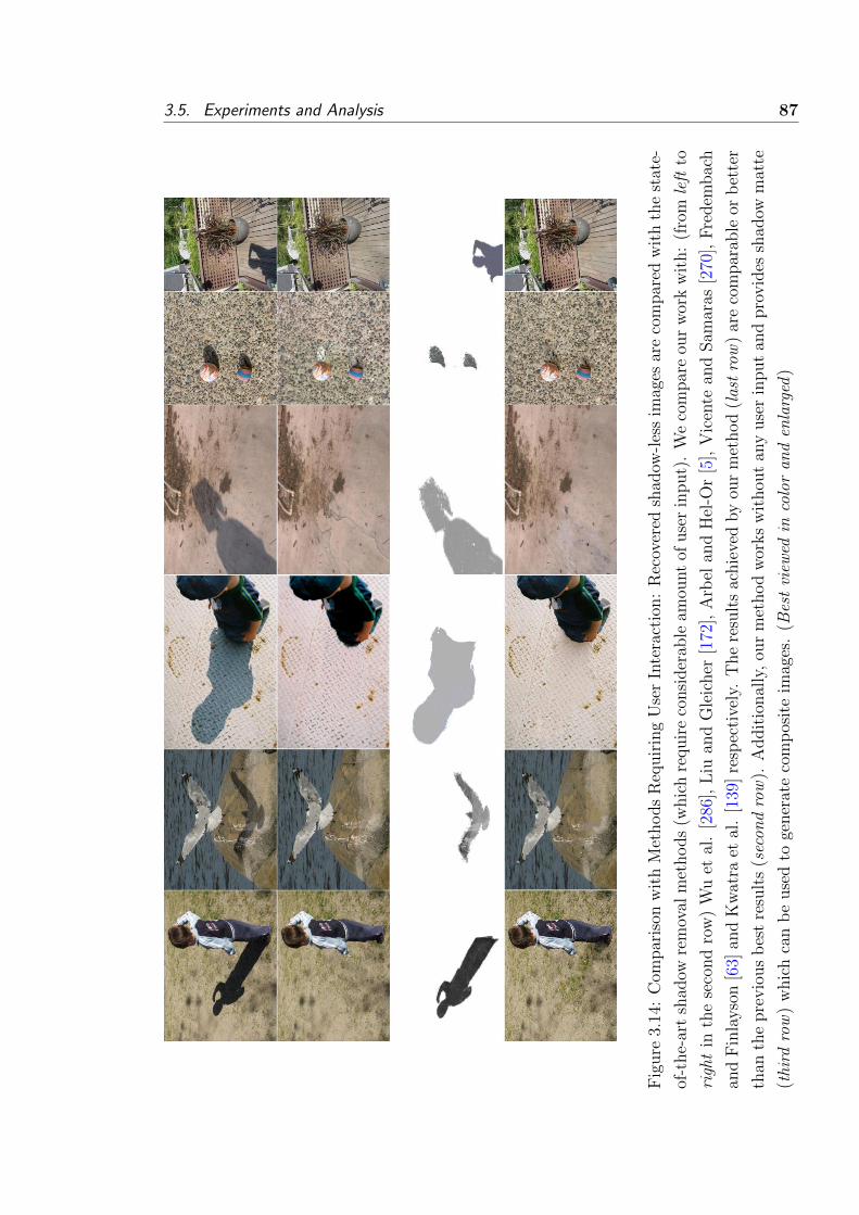
3.5. Experiments and Analysis 87
Fig
ure
3.14
:C
ompar
ison
wit
hM
ethods
Req
uir
ing
Use
rIn
tera
ctio
n:
Rec
over
edsh
adow
-les
sim
ages
are
com
par
edw
ith
the
stat
e-
of-t
he-
art
shad
owre
mov
alm
ethods
(whic
hre
quir
eco
nsi
der
able
amou
nt
ofuse
rin
put)
.W
eco
mpar
eou
rw
ork
wit
h:
(fro
mle
ftto
righ
tin
the
seco
nd
row
)W
uet
al.
[286
],L
iuan
dG
leic
her
[172
],A
rbel
and
Hel
-Or
[5],
Vic
ente
and
Sam
aras
[270
],F
redem
bac
h
and
Fin
layso
n[6
3]an
dK
wat
raet
al.
[139
]re
spec
tive
ly.
The
resu
lts
achie
ved
by
our
met
hod
(las
tro
w)
are
com
par
able
orb
ette
r
than
the
pre
vio
us
bes
tre
sult
s(s
econ
dro
w).
Addit
ional
ly,
our
met
hod
wor
ks
wit
hou
tan
yuse
rin
put
and
pro
vid
essh
adow
mat
te
(thi
rdro
w)
whic
hca
nb
euse
dto
gener
ate
com
pos
ite
imag
es.
(Bes
tvi
ewed
inco
lor
and
enla
rged
)

88 Chapter 3. Automatic Shadow Detection and Removal from a Single Photograph
Failure Cases and Limitations
Our shadow removal technique does not perform well on curved surfaces and in the
case of highly non-uniform shadows (e.g., Fig. 3.15: 1st and 3rd image from left).
Since, we apply a multi-level color transfer scheme, very fine texture details of image
regions with similar appearance can be removed during this transfer process (e.g.,
Fig. 3.15: 2nd image from left). For the cases of shadows in dark environments, our
method appears to increase the contrast of the recovered region. These limitations
are due to the constraints imposed on the shadow generation model, where the
higher order statistics are ignored during the shadow generation process (Eqs. 3.19
and 3.21).
Discussion
Our method does not require any user input and it automatically removes shadow
after its detection. The proposed shadow removal approach makes comparatively
fewer assumptions about the scene type, the type of light source or camera. The
only assumptions are that of Lambertian surfaces and the correspondence between
the shadow and the non-shadow region color distributions. The shadow removal
method of [285, 286] cannot separate the shadow from shading. With the inclusion
of the image consistency term in P`(Is|α, β), we are able to deal with the shading
by introducing a penalty on the distribution of the shadow effect through the pa-
rameters β and α. The proposed shadow removal approach takes 82.2 ± 25 sec for
each image on the UIUC database. The main overhead during the shadow removal
process is the Bayesian refinement step (which is required mainly for shadow mat-
ting). It takes 73.6±20 sec out of 82.2±25 sec per image on the UIUC database. In
comparison, the method by Guo et al. [78] takes 104.7± 18 sec for shadow removal.
The main overhead in their removal process is also due to Levin et al.’s matting
algorithm [155] which takes around 91.4± 11 sec per image.
3.5.4 Applications
Shadow detection, removal and matting have a number of applications. A direct
application is the generation of visually appealing photographs and the removal of
unwanted shadows. Some other applications include:
Shadow Compositing: Fig. 3.16a shows examples of shadow compositing.
The extracted shadow matte can be used to depict a realistic image compositing.
For example, the first image from the left did not originally contain the flying bird
and its shadow. If we had added just the bird, it would have looked unrealistic.
With the addition of a texture-free shadow matte, the photograph looks natural

3.5. Experiments and Analysis 89
Figure 3.15: Examples of Failure Cases: Our technique does not perfectly remove
shadows on curved surfaces, highly non-uniform shadows and shadows in dark en-
vironments. (Best viewed in color and enlarged)
and realistic. In the remaining three images, we combine extracted shadows with
the original images to create fake effects.
Image Editing: Fig. 3.16b shows how a detected shadow can be edited to
create fake effects. For example, shadow direction/length can be modified to give a
fake impression of illumination source or time of day.
Image Parsing: Fig. 3.16c shows how shadow removal can increase the accu-
racy of segmentation methods (e.g., [129, 125]). The segmentations are computed
using the graph based technique of [57] (we used a minimum region size of 600).
It can be seen that shadows change the appearance of a class (e.g., ground in this
case) and thus can introduce errors in the segmentation process.
Boundary Detection: We tested a recently proposed boundary detector [46]
on the original and recovered image (Fig. 3.16d). The boundaries identified in the
recovered image are more accurate. Since shadows do not constitute an object class,
the recovered image can help in achieving more accurate object detection proposals
and consequently a higher recognition performance.

90 Chapter 3. Automatic Shadow Detection and Removal from a Single Photograph
(a) Shadow Compositing
(b) Image Editing
(c) Image Parsing
(d) Boundary Detection
Figure 3.16: Different Applications of Shadow Detection, Removal and Matting.
(Best viewed in color and enlarged)

3.6. Conclusion 91
3.6 Conclusion
We presented a data-driven approach to learn the most relevant features for the
detection of shadows from a single image. We demonstrated that our framework
performs the best on a number of databases regardless of the shape of objects casting
shadows, the environment and the type of scene. We also proposed a shadow re-
moval framework which extracts the shadow matte along with the recovered image.
A Bayesian formulation constitutes the basis of our shadow removal procedure and
thereby makes use of an improved shadow generation model. Our shadow detection
results show that a combination of boundary and region ConvNets incorporated in
the CRF model provides the best performance. For shadow removal, the multi-level
color transfer followed by the Bayesian refinement performs well on unconstrained
images. The proposed framework has a number of applications including image edit-
ing and enhancement tasks. In our future work, we will use the proposed shadow
detection framework together with the scene geometry (as in [144]) and object prop-
erties to reason about high-level scene understanding tasks (as in [203]). The use
of our proposed framework for shadow detection in video sequences will also be
explored to take advantage of the spatio-temporal properties of moving shadows.

92 Chapter 3. Automatic Shadow Detection and Removal from a Single Photograph

93CHAPTER 4
Separating Objects and Clutter in Indoor Scenes
via Joint Reasoning1
Out of clutter, find simplicity.
Albert Einstein (1879-1955)
Abstract
Objects’ spatial layout estimation and clutter identification are two important
tasks to understand indoor scenes. We propose to solve both of these problems in
a joint framework using RGBD images of indoor scenes. In contrast to recent ap-
proaches which focus on either one of these two problems, we perform ‘fine grained
structure categorization’ by predicting all the major objects and simultaneously
labeling the cluttered regions. A conditional random field model is proposed to in-
corporate a rich set of local appearance, geometric features and interactions between
the scene elements. We take a structural learning approach with a loss of 3D lo-
calisation to estimate the model parameters from a large annotated RGBD dataset,
and a mixed integer linear programming formulation for inference. We demonstrate
that our approach is able to detect cuboids and estimate cluttered regions across
many different object and scene categories in the presence of occlusion, illumination
and appearance variations.
4.1 Introduction
We live in a three dimensional world where objects interact with each other
according to a rich set of physical and geometrical constraints. Therefore, merely
recognizing objects or segmenting an image into a set of semantic classes does not
always provide a meaningful interpretation of the scene and its properties. A better
understanding of real-world scenes requires a holistic perspective, exploring both
semantic and 3D structures of objects as well as the rich relationship among them
[79, 275, 129, 309]. To this end, one fundamental task is that of the volumetric
reasoning about generic 3D objects and their 3D spatial layout.
1Published in Proceedings of the IEEE Conference on Computer Vision and Pattern Recognition
(CVPR), pp. 4603-4611. IEEE, 2015.

94 Chapter 4. Separating Objects and Clutter in Indoor Scenes via Joint Reasoning
Figure 4.1: With a given RGBD image (left column), our method explores the
3D structures in an indoor scene and estimates their geometry using cuboids (right
image). It also identifies cluttered/unorganized regions in a scene (shown in orange)
which can be of interest for tasks such as robot grasping.
Among different approaches to tackle the generic 3D object reasoning problem,
much progress has been made based on representing objects as 3D geometric prim-
itives, such as cuboids. Some of the first efforts focus on the 3D spatial layout and
cuboid-like objects in indoor scenes from monocular imagery [150, 92, 293]. Owing
to the complex structure of the scenes, additional depth information has recently
been introduced to obtain more robust estimation [167, 110, 87, 236]. However,
real-world scenes are composed of not only large regular-shaped structures and ob-
jects (such as walls, floor, furniture), but also irregular shaped objects and cluttered
regions which cannot be represented well by object-level primitives. The overlay of
different types of scene elements makes the procedure of localizing 3D objects fragile
and prone to misalignment.
Most previous work has focused on clutter reasoning in the scene layout estima-
tion problem [92, 275, 306]. Such object clutter is usually defined at a coarse-level,
including everything other than the global layout, which is insufficient for object-

4.1. Introduction 95
level parsing. To tackle the problem of 3D object cuboid estimation, we attempt
to use clutter in a more fine-grained sense, referring to any unordered region other
than the main structures and major cuboid-like objects in the scene, as shown in
Fig. 4.1.
We aim to address the problem of 3D object cuboid detection in a cluttered
scene. In this work, we propose to jointly localize generic 3D objects (represented
by cuboids) and label cluttered regions from an RGBD image. Unlike the recent
cuboid detection techniques, which consider such regions as background, our method
explicitly models the appearance and geometric property of the fine-grained clut-
tered regions. We incorporate scene context (in the form of object and clutter) to
better model the regular-shaped objects and their interaction with other types of
regions in a scene.
We adopt the approach in [110] for representing an indoor scene, which models a
room as a set of hypothesized cuboids and local surfaces defined by superpixels. To
cope with clutters, we formulate the joint detection task using a higher-order Condi-
tional Random Field model (CRF) on superpixels and cuboid hypotheses generated
by a bottom-up grouping process. Our CRF approach extends the linear model
of [110] in several aspects. First, we introduce a random field of local surfaces (su-
perpixels) that captures the local appearance and spatial smoothness of cluttered
and noncluttered regions. In addition, we improve the cuboid representation by
generating two types of cuboid hypotheses, one of which corresponds to regular ob-
jects inside a scene and the other is for the main structures of a scene, such as floor
and walls. Furthermore, we incorporate both the consistency between superpixel
labels and cuboid hypotheses and the occlusion relation between cluttered regions
and cuboid objects.
More importantly, we take a structural learning approach to estimate the CRF
parameters from an annotated indoor dataset, which enables us to systematically
incorporate more features into our model and to avoid tedious manual tuning. We
use a max-margin based objective function that minimizes a loss defined on cuboid
detection. Similar to [110], the (loss-augmented) MAP inference of our CRF model
can be formulated as a mixed integer linear programming (MILP) formulation. We
empirically show that the MILP can be globally optimized with the Branch-and-
Bound method within a time of seconds to find a solution in most cases. During
testing, the MAP estimate of our CRF not only detects cuboid objects but also
identifies the cluttered regions. We evaluate our method on the NYU Kinect v2
dataset with augmented cuboid and clutter annotations, and demonstrate that the
96 Chapter 4. Separating Objects and Clutter in Indoor Scenes via Joint Reasoning
proposed approach achieves superior performance to the state of the art.
4.2 Related Work
Localizing and predicting the geometry of generic objects using cuboids is a
challenging problem in highly cluttered indoor scenes. A number of approaches
extend 2D appearance-based methods to the task of predicting the 3D cuboids.
Variants of the Deformable Parts based Model (DPM) [56] have been used for 3D
cuboid prediction [209, 236, 289]. However, they do not consider clutter and heavy
occlusion in the scene. In [167], the Constrained Parametric Min-cut (CPMC) [27]
was extended from 2D to RGBD to generate a cuboid hypotheses set. In contrast,
we directly generate two types of cuboid proposals in a bottom-up fashion [110],
thus providing a simpler and efficient procedure which is better suited for indoor
RGBD data.
Based on the physical and geometrical constraints, a number of approaches have
been proposed for 3D object and scene parsing, e.g., [309, 128, 15]. The basic idea
is to incorporate contextual relationships at a higher level to avoid false detection.
Silberman et al. [242] predict the support surfaces and semantic object classes in an
indoor scene. Geometric and semantic relationships between different object classes
are modeled in works such as [132, 242, 68]. Gupta et al. [79] use a parse graph to
consider mechanical and geometric relationships amongst objects represented by 3D
boxes. For indoor scenes, volumetric reasoning is performed for 2D [150] and RGBD
images [110] to detect cuboids. However, none of these works estimate cuboids and
clutter jointly using relevant constraints.
The joint estimation of clutter along with the room layouts has previously been
shown to enhance performance. Wang et al. [275] predict clutter and layouts in
a discriminative setting where clutter is modeled using hidden variables. Recently,
Zhang et al. [306] employed RGBD data for joint layout and clutter estimation and
efficiently perform inference by potential decomposition. However, these works are
limited to only scene layout estimation and label everything else as clutter. Recently,
Schwing et al. [236] used monocular imagery to jointly estimate room layout along
with one major object present in a bedroom scene. In this work, we estimate the
scene bounding structures as well as ‘all’ of the major objects using 3D cuboids.
4.3 Our Approach
Indoor scenes contain material structures (e.g., ceiling, walls) and the regular-
shaped objects which we term as non-cluttered regions. In contrast, cluttered regions

4.3. Our Approach 97
Figure 4.2: Graph structure representation for the potentials defined on the object
cuboids and the cluttered/non-cluttered regions. (Best viewed in color)
consist of small, indistinguishable objects (e.g., stationery on an office table) or
jumbled regions in a scene (e.g., clothes piled on a bed). We represent an indoor
scene as an overlay of the cluttered regions (modeled as local surfaces) and the non-
cluttered regions (modeled using 3D cuboids). Our goal is to describe an RGBD
image with an optimal set of cuboids and pixel-level labeling of cluttered regions.
Our approach first generates a set of cuboid hypotheses based on image and
depth cues, which aims to cover the majority of true object locations. Taking them
as the potential object candidates, we can significantly reduce the search space of 3D
cuboids and construct a CRF on the image/depth superpixels and these candidates.
We will first introduce our CRF formulation assuming the cuboid hypotheses are
given, and refer the reader to Sec. 4.4 for details on the cuboid extraction procedure.
4.3.1 CRF Formulation
Given an RGBD image, denoted by I, we decompose it into a number of contigu-
ous partitions, i.e., superpixels: S = {s1, · · · , sJ}, where J is the total number of
superpixels. We associate a binary membership variable mj with each superpixel sj
to indicate whether it belongs to the cluttered or non-cluttered regions, and denote
m = {m1, · · · ,mJ}. The set of cuboid hypotheses is denoted by O = {o1, · · · , oK},where K is the total number of cuboid hypotheses. For each cuboid, we introduce
a binary variable ck to indicate whether the kth cuboid hypothesis is active or not,
and denote c = {c1, · · · , cK}.Note that for indoor scenes, the room structures such as walls and floor bound
the scene and therefore appear as planar regions, which have different geometric
properties from the ordinary object cuboids. To encode such different constraints,
we define two types of cuboids in the hypotheses set, namely the scene bounding
cuboids (Osbc) and the object cuboids (Ooc). The cuboid extraction procedure for
both types of cuboids is described in Sec. 4.4.

98 Chapter 4. Separating Objects and Clutter in Indoor Scenes via Joint Reasoning
We build a CRF model on the superpixel clutter variables m and the object
variables c to describe the properties of clutter, objects and their relationship in the
scene. Formally, we define the Gibbs energy of the CRF as follows,
E(m, c|I) = Eobj(c) + Esp(m) + Ecom(m, c), (4.1)
where Eobj(c), Esp(m) captures the object level and the superpixel level properties
respectively, and Ecom(m, c) models the interactions between them.
More specifically, the first term, Eobj(c), is defined as a combination of three
potential functions:
Eobj(c) =K∑k=1
[ψuobj(ck) + ψhobj(ck)
]+∑i<j
ψpobj(ci, cj), (4.2)
where the unary potential ψuobj(ck) expresses the data likelihood of kth object hy-
pothesis, ψhobj(ck) encodes a MDL prior on the number of active cuboids, and the
pairwise potential ψpobj(ci, cj) models the physical and geometrical relationships be-
tween cuboids.
Similarly at the superpixel level, the second term, Esp, consists of two potential
functions:
Esp(m) =J∑j=1
ψusp(mj) +∑
(i,j)∈Ns
ψpsp(mi,mj), (4.3)
where the unary potential ψusp(mj) is the data likelihood of a superpixel’s label, and
the pairwise potential ψpsp(mi,mj) encodes the spatial smoothness between neigh-
boring superpixels, denoted by Ns.
The third term in Eq. (4.1), is the compatibility constraint which enforces the
consistency of the cuboid activations and the superpixel labeling:
Ecom(m, c) =J∑j=1
ψcom(mj, c). (4.4)
In the following discussion, we will explain the different costs which constitute the
energies defined in Eqs. (4.2), (4.3) and (4.4).
4.3.2 Potentials on Cuboids
Unary Potential on Cuboids
The unary potential of a cuboid hypothesis ψuobj measures the likelihood of a cuboid
hypothesis being active based on its appearance, physical and geometrical properties.
Instead of specifying local matching costs manually, we extract a set of informative

4.3. Our Approach 99
multi-modal features from image/depth and each cuboid, and take a learning ap-
proach to predict the local matching quality. Specifically, we generate seven different
types of cuboid features (fobjk ) as follows.
Volumetric occupancy feature f occk measures the portion of the kth cuboid
occupied by the 3D point data. We define f occk as the ratio between the empty
volume inside a cuboid (vke ) to the total volume of a cuboid (vkb ): f occk = vke/vkb . The
volumes are estimated by discretizing the 3D space into voxels and counting the
number of voxels that are occupied by 3D points or not. All invisible voxels behind
occupied voxels are also treated as occupied.
Color consistency feature f colk encodes the color variation of the kth cuboid.
Object instances normally have consistent appearance while cluttered regions tend to
have a skewed color distribution (Fig. 4.3). We fit a GMM with three components
on the color distribution of pixels enclosed in a cuboid and measure the average
deviation. Specifically, the feature is defined as: f colk =∑∀p∈ok ωu‖vp − σu‖, where
vp denotes the color of a pixel p, σu is the mean of the closest component (u) and
ωu is the mixture proportion.
Normal consistency feature fnork measures the normal variation of the kth
cuboid. The distribution of 3D point normals inside the cluttered regions has a
larger variance (Fig. 4.3). In contrast, the normal directions of regular objects are
usually aligned with the three perpendicular faces of the cuboid. Similar to the color
feature, we calculate the variation of 3D point normals with respect to the closest
dominant direction.
Tightness feature f tigk describes how loosely the 3D points fit the cuboid pro-
posals. For each visible face of a cuboid, we calculate the ratio between the area
of minimum bounding rectangle tightly enclosing all points (Afrec) to the area of the
face (Af ). We take the weighted average of the tightness ratios of the cuboid faces
to define f tigk = 1∑f JAfrec 6=0K
∑∀f∈Faces
AfrecAf
.
Support feature f supk measures how likely each cuboid is supported either by
another cuboid or clutter. We estimate the support by calculating the number
of 3D points that fall in the space surrounding the cuboid (τ%2 additional space
along each dimension). The feature is defined as: f supk =eo′k−eokeok
, where, eo′k and
eok denote the number of points enclosed by the extended cuboid and the original
cuboid respectively.
Geometric plausibility feature f geok measures the likelihood that a cuboid
has a plausible 3D object shape. Using 3D geometrical features (sizes and aspect
2Based on empirical tests, τ is set to 2.5% in this work.

100 Chapter 4. Separating Objects and Clutter in Indoor Scenes via Joint Reasoning
Figure 4.3: The distribution of variation in color for cluttered and non-cluttered
regions in the RMRC training set is compared in the top row. Comparison for
variation in normals is shown in the bottom row. The plots in the right column
show the cumulative distributions.
ratios), we train a Random Forest (RF) classifier to score the geometric plausibility.
The score is used to define f geok , which filters out the less likely cuboid candidates
e.g., very thin cuboids or those with irregular aspect ratio.
Cuboid size feature f ochk measures the relative size of a cuboid w.r.t the av-
erage object size in the dataset. Let `ldl denote the maximum diagonal length of a
cuboid and ¯ldl is the mean length of objects. We define f ochk = `ldl/¯
ldl, which helps
control the number of valid cuboids by removing small ones.
Given the feature descriptor fobjk , we train a RF classifier on fobj and define the
unary potential based on the output of the RF, P (ck = 1|fobjk ):
ψuobj(ck) = λbbuµbbuk ck, (4.5)
where λbbu is the weighting coefficient and
µbbuk = − logP (ck = 1|fobjk )
1− P (ck = 1|fobjk ).

4.3. Our Approach 101
Note that those features are automatically weighted and combined by the RF for
predicting the local matching cost.
Cuboid MDL Potential
The MDL principle prefers to explain a given image compactly in terms of a small
number of cuboids, instead of a complex representation consisting of an unnecessarily
large number of cuboids [15, 110]. We define the MDL potential ψhobj in Eq. (4.2)
as: ψhobj(ck) = λmdlck, where λmdl > 0 is the weighting parameter.
Pairwise Potentials on Cuboids
We follow [110] and the pairwise energy in Eq. (4.2) decomposes in to view ob-
struction and box intersection potentials:
ψpobj(ci, cj) = ψpobs(ci, cj) + ψpint(ci, cj). (4.6)
As we have two types of cuboids, our pairwise potentials on cuboids are parametrized
according to the configuration of each cuboid pair.
View obstruction potential (ψpobs) encodes the visibility constraint between
a pair of cuboids, and is expressed as follows:
ψpobs(ci, cj) = λobsµobsi,j cicj = λobsµ
obsi,j yi,j (4.7)
where, µobsi,j is the view obstruction cost, λobs is a weighting parameter and yi,j is an
auxiliary boolean variable introduced to linearize the pairwise term [110]. The view
obstruction cost µobsi,j computes the intersection of 2D projections of two cuboids and
induces a penalty when a larger cuboid lies in front of a smaller but farther cuboid.
Let µobsi,j = (Aci ∩ Acj)/Aci where, Aci and Acj are the areas of the 2D projections
of cuboid hypotheses ci and cj on the image plane respectively and ci is the farther
cuboid w.r.t the viewer. The cost µobsi,j = µobsi,j if µobsi,j < αobs and infinity otherwise.
This allows partial occlusion with a penalty but avoids heavy occlusion. We use
αobs = 60% for object cuboids (Ooc). For the case of scene bounding cuboids (Osbc),we relax the obstruction cost by a factor of 0.1 in Eq. (4.7) and set α′obs = 80%.
Cuboid intersection potential (ψpint) penalizes volumetric overlaps between
cuboid pairs as two objects cannot penetrate each other, and is defined as:
ψpint(ci, cj) = λintµinti,j cicj = λintµ
inti,j xi,j (4.8)
where, µinti,j is the cuboid intersection cost, λint is a weighting parameter and xi,j is
an auxiliary boolean variable introduced to linearize the pairwise cost. The cuboid
intersection cost induces a soft penalty as long as the intersection is smaller than
a threshold. Let µinti,j be the normalized intersection, and we define µinti,j = µinti,j if
102 Chapter 4. Separating Objects and Clutter in Indoor Scenes via Joint Reasoning
0 ≤ µinti,j < αint and infinity otherwise. We set αint = 10% for the case of object
cuboids and α′obs = 50% for all scene bounding cuboids.
4.3.3 Potentials on Superpixels
We decompose an input image into superpixels based on the hierarchical image
segmentation [6]. The unary potential on each superpixel captures the appearance
and texture properties of cluttered and non-cluttered regions. We employ the kernel
descriptor framework of [16, 17] to convert pixel attributes to rich patch level feature
representations. Kernel descriptors provide a continuous pixel attribute represen-
tation by employing a kernel view of patch similarity. These higher dimensional
representations are then transformed to a low dimensional representation which are
then aggregated on a superpixel level using Efficient Match Kernel (EMK) to im-
prove efficiency. We extract several cues including image and depth gradient, color,
surface normal, LBP and self similarity. A RF classifier is trained on these dense
features, which predicts the probability of a region being a clutter or non-clutter.
We use the negative log odds ratio as a cost µappj , weighted by the parameter λapp
and define the unary in Eq. (4.3) as ψusp(mj) = λappµappj mj.
For the superpixel pairwise term, we define a contrast-sensitive Potts model on
spatially neighboring superpixels, which encourages the smoothness of the clutter
and non-clutter regions:
ψpsp(mi,mj) = λsmoµsmoi,j (mi +mj −mi ·mj), (4.9)
where, µsmoi,j = exp(−‖vi− vj‖2/σ2c ), vi, vj are the mean color of superpixel si and sj.
We use wi,j as an auxiliary boolean variable to linearize the quadratic term mi ·mj
(see Sec. 4.5).
4.3.4 Superpixel-Cuboid Compatibility
The compatibility term links the superpixels labeling to the cuboid selection
task, which enforces consistency between the lower level and the higher level of the
scene representation. Our compatibility potential consists of two terms, one for
superpixel membership ψmem and the other for occlusion relation ψocc:
ψcom(mj, c) = ψmem(mj, c) +∑k
ψocc(mj, ck), (4.10)
Superpixel membership potential (ψmem) defines a constraint that a super-
pixel is associated with at least one active cuboid if it is not a cluttered region:

4.4. Cuboid Hypothesis Generation 103
mj ≤∑
k:sj∈okck. Equivalently, the corresponding potential function is a higher-order
term (Fig. 4.2):
ψmem(mj, c) = λ∞Jmj 6= maxk:sj∈ok
ckK, (4.11)
where λ∞ is an infinite (very large) penalty cost.
Superpixel-cuboid occlusion potential (ψocc) encodes that a cuboid should
not appear in front of a superpixel which is classified as clutter, i.e., a detected cuboid
cannot completely occlude a superpixel on the 2D plane which takes a clutter label.
ψocc(mj, ck) = λoccµoccjk mjck = λoccµ
occjk zjk (4.12)
where, mj = 1−mj, and zjk is the auxiliary variable for linearization. The cost µoccjk =(Amj∩Ack )
Aand A is the area of the further element (either cuboid or superpixel). The
cost µoccjk and parameter αocc are defined similar to the view obstruction potential in
Sec. 4.3.2.
4.4 Cuboid Hypothesis Generation
Our method for initial cuboid hypothesis generation is based on a bottom-up
clustering-and-fitting procedure, which generates both object cuboids and scene
bounding cuboids. Specifically, we first extract homogeneous regions from a nor-
mal image using SLIC [2]. Gaussian smoothing is performed to remove isolated
regions and similar regions are merged using the DBSCAN clustering algorithm
[51]. The neighborhood of each resulting region is found and the inlier points in
each region are estimated using the RANSAC algorithm. We then estimate three
major perpendicular directions of a room as in [242], denoted as x, z (horizontal)
and y (vertical).
For object cuboids, we adopt a fitting method similar to [110]. The cuboids
identified using this procedure usually capture objects whose two or more sides are
visible, but cannot capture the room structure. To propose scene bounding cuboids,
we also generate cuboids which cover only one planar region. Among all the planar
regions, we first remove the smaller ones (< 5% of the image size) and those not
aligned with the three dominant directions. We then select the planar regions which
are farthest from the camera view point. The cuboids enclosing these planar regions
are included in the hypotheses set as the scene bounding cuboids. The detected
cuboid proposals are ranked using the cuboid unary potential (Eq. (4.5)) and the
top 60 cuboids are selected for our CRF inference.

104 Chapter 4. Separating Objects and Clutter in Indoor Scenes via Joint Reasoning
4.5 Model Inference and Learning
4.5.1 Inference as MILP
Given an RGBD image I, we parse the input into a set of cuboids and clut-
tered/noncluttered regions by inferring the most likely configuration of clutter label
variables m and the cuboid hypotheses labels c. Equivalently, we minimize the CRF
energy:
{m∗, c∗} = argminm,c
E(m, c|I). (4.13)
We adopt the relaxation method in [110, 72] and transform the minimization in
Eq. (4.13) into a Mixed Integer Linear Program (MILP) with linear constraints.
The MILP formulation can be solved much faster compared to the original ILP,
using the branch and bound method.
Specifically, for the pairwise view obstruction cost in Eq. (4.7), we introduce yi,j
for ci ·cj with constraints: ci ≥ yi,j, cj ≥ yi,j, yi,j ≥ ci+cj−1. Similarly, we introduce
xi,j for the pairwise cuboid intersection cost. Also, we use an inequality ci + cj ≤ 1
for the infinity cost constraint of µobsi,j and µinti,j . These equivalent transforms can
also be applied to wi,j for mi · mj in the superpixel pairwise potential, and zj,k
for mjck in the superpixel-cuboid potential. For clarity, we denote the complete
set of linear inequality constraints for c and m as LC and include the details in
the supplementary material. The complete MILP formulation with linear objective
function and constraints is given by:
minm,c,x,y,w,z
E(m, c,x,y,w, z|I) (4.14)
s.t. linear inequality constraints in LC,
mj, ck ∈ {0, 1}, ∀j, k (4.15)
wi,j, xi,j, yi,j, zj,k ≥ 0, ∀i, j, k (4.16)
We solve the MILP problem in Eqs. (4.14) - (4.16) by the Branch and Bound method
in the GLPK solver [145].
Algorithmic Efficiency: We empirically evaluate the efficiency of the Branch
and Bound algorithm on the scene parsing problem introduced in Sec. 4.6. Tab. 4.1
lists the average time it takes to reach the optimal solution on a 3.4GHz machine.
On average, 819± 48% variables are involved in each inference and the final MILP
gap is zero for 98.5% of the cases on the whole dataset. In this work, we use a
MILP gap tolerance of 0.001, however, it turns out that increasing the MILP gap

4.6. Experiments and Analysis 105
Small gap Large gap Cuts LP relax.
Time (sec) 1.84± 31% 1.31± 24% 0.45± 13% 0.001± 0.4%
Det. Rate 26.8% 26.1% 24.4% 19.9%
Table 4.1: Inference running time comparisons for variants of MILP formulation.
by a factor of 100 causes a minute performance drop and a more efficient inference.
Including cuts (cover cuts, Gomory mixed cuts, mixed integer rounding cuts, clique
cuts) results in a much faster convergence at the expense of an average of 8%
performance degradation and a 5% increase in memory requirements. When c and
m are relaxed to get the corresponding LP which has a polynomial time convergence
guarantee, the performance on the detection task decreases by 26% compared to
the MILP formulation. These performance comparisons are computed at the 40%
Jaccard Index (JI) threshold for cuboid detection.
4.5.2 Parameter Learning
We take a structural learning approach to estimate the model parameters from
a fully annotated training dataset. We denote the model outputs (m, c) as t, and
the model parameters (λbbu, λmdl, λobs, λint, λapp, λsmo, λocc) as λ. The training set
consists of a set of annotated images T = {(tn, In}1×N .
We apply the structured SVM framework with margin re-scaling [257], which
uses the cutting plane algorithm [117] to search the optimal parameter setting (see
the supplementary materials for details of the learning algorithm). We use the IOU
loss function on cuboid matching as our loss function in learning, which is defined
as
∆(t(n), t) =∑i
(1− |o
(n)i ∩ oi||o(n)i ∪ oi|
)and oi is the 3D cuboid associated with ci. The algorithm efficiently adds low
energy labelings to the active constraints set and updates the parameters such that
the ground-truth has the lowest energy.
4.6 Experiments and Analysis
4.6.1 Dataset and Setup
We evaluate our method on the 3D detection dataset released as part of the Re-
construction Meets Recognition Challenge (RMRC), 2013. It contains 1074 RGBD

106 Chapter 4. Separating Objects and Clutter in Indoor Scenes via Joint Reasoning
images taken from the NYU Depth v2 dataset. Each image comes with 3D bound-
ing box annotations. There are 7701 annotated 3D bounded boxes in total, which
roughly equals to 7 labeled cuboids per image. We performed experiments on the
complete dataset using 3-fold cross validation. Specifically, for each fold, training is
done on 716 images and the testing is performed on the remaining 358 images.
We evaluate the performance on three tasks, including the cuboid detection,
clutter/non-clutter estimation and the foreground/background segmentation. The
weighting parameters involved in the energy function (Eq. (4.1)) are learned (details
in Sec. 4.5.2). Other parameters which are involved in shaping the constraints (e.g.,
αobs, αint) are set to achieve the best performance on a small validation set. This
validation set consists of 10 randomly sampled training images in each iteration of
3-fold cross validation.
4.6.2 Cuboid Detection Task
We first evaluate the cuboid detection task, in which we compute the intersection
over union of volumes (Jaccard Index-JI) for the quantitative evaluation. Fig. 4.4
shows the cuboid detection rate as the threshold for JI is increased from 0 to 1. The
overall low detection rate is partially due to the fact that many cuboids for scene
structures and major objects (e.g., cupboard) are quite thin and the volumetric
overlap measure can be sensitive in such cases. We compare our method with a
baseline approach and the state of the art techniques by Jiang et al. [110], Huebner
et al. [100] and Truax et al. [260]. The baseline method uses only the unary cuboid
costs for detection. Random initializations are chosen for the parameters involved
in [100, 260]. We use the projected area of a cuboid as its saliency measure to rank
the ground-truth objects. The results (Fig. 4.4, Tab. 4.2) show that the global
optimization performs better than the unary scores and the local search techniques
[100, 260]. At the 40% JI threshold mark in Fig. 4.4, we have 31.1%, 26.8%, 38.0%
and 89.4% better performances compared to [110] for top one, top two, top three
and all cuboids detection tasks respectively. The ablative analysis in Tab. 4.2
indicates that both the newly introduced features and the joint modeling contribute
to the overall improvement in detection accuracy.
Qualitative comparisons are shown in Fig. 4.5. Our method gives good results
on many difficult indoor scenes involving clutter, partial occlusions, appearance and
illumination variations. In some cases, ground-truth cuboids are not available for
some major objects/structures in the scene, but our technique is able to detect
them correctly. We also compare qualitatively with the Jiang et al’s method [110],

4.6. Experiments and Analysis 107
0 0.2 0.4 0.6 0.8 10
0.2
0.4
0.6
0.8
1
Jaccard Index Threshold
Det
ectio
n R
ate
This PaperJiang et al. [14]Truax et al. [22]Huebner et al. [13]Baseline
[16][28]
[15]
0 0.2 0.4 0.6 0.8 10
0.2
0.4
0.6
0.8
1
Jaccard Index Threshold
Det
ectio
n R
ate
This PaperJiang et al. [14]Truax et al. [22]Huebner et al. [13]Baseline
[16][28]
[15]
0 0.2 0.4 0.6 0.8 10
0.2
0.4
0.6
0.8
1
Jaccard Index Threshold
Det
ectio
n R
ate
This PaperJiang et al. [14]Truax et al. [22]Huebner et al. [13]Baseline
[16][28]
[15]
0 0.2 0.4 0.6 0.8 10
0.2
0.4
0.6
0.8
1
Jaccard Index Threshold
Det
ectio
n R
ate
This PaperJiang et al. [14]Truax et al. [22]Huebner et al. [13]Baseline
[16][28]
[15]
Figure 4.4: Jaccard Index comparisons for all annotated cuboids (top left), for the
most salient cuboid (top right), for top two salient cuboids (bottom left) and top
three salient cuboids (bottom right).

108 Chapter 4. Separating Objects and Clutter in Indoor Scenes via Joint Reasoning

4.6. Experiments and Analysis 109
Figure 4.5: Comparison of our results (right-most column) with the state of the art
technique[110] (middle column) and Ground Truth (right column). (Best viewed in
color and enlarged)
Method Accuracy
Unary cuboid cost of Jiang [110] 6.5%
Our unary cuboid cost only 8.8%
Our unary + pairwise cuboid cost only 19.4%
Our full model 26.1%
Table 4.2: An ablation study on the model potentials/features for the cuboid detec-
tion task at the 40% JI threshold.
for which the results are generated using the code provided by the authors. It can
be seen that our approach performs better in most of the cases.
4.6.3 Clutter/Non-Clutter Segmentation Task
To evaluate the clutter segmentation task, we generate the ground-truth clut-
ter labeling based on the cuboid annotation. Specifically, we project the 3D points
inside the ground-truth cuboids onto the image plane, and label them as the non-
clutter regions while the rest of the regions are clutter. As a baseline, we report the
performance when only superpixel unary cost was used for segmentation. The addi-
tion of the pairwise cost and the joint modeling results in significant improvement
(Tab. 4.3). We also consider only the object cuboids and compare the performance
when scene structure cuboids are excluded from the evaluations.

110 Chapter 4. Separating Objects and Clutter in Indoor Scenes via Joint Reasoning
Method Precision Recall F-Score
Superpixel unary only 0.43± 13% 0.45± 11% 0.44± 16%
Unary + pairwise 0.46± 12% 0.48± 10% 0.47± 16%
Full model (all classes) 0.65± 9% 0.68± 8% 0.66± 12%
Full model (only object classes) 0.75± 6% 0.71± 8% 0.73± 10%
Table 4.3: Evaluation on Clutter/Non-Clutter Segmentation Task. Precision signi-
fies the accuracy of clutter classification.
Eval. Criterion CPMC [27] This chapter
Pre. Rec. Pre. Rec.
Most salient obj. 0.83± 11% 0.79± 12 0.85± 15% 0.82± 15%
Top 2 salient obj. 0.77± 12% 0.73± 14 0.81± 16% 0.79± 16%
Top 3 salient obj. 0.69± 15% 0.66± 17 0.79± 21% 0.76± 19%
All objects 0.54± 17% 0.51± 20 0.73± 23% 0.69± 21%
Table 4.4: Evaluation on Foreground/Background Segmentation Task. Precision
signifies the accuracy of foreground detection.

4.6. Experiments and Analysis 111

112 Chapter 4. Separating Objects and Clutter in Indoor Scenes via Joint Reasoning
Figure 4.6: Qualitative Results: Our method is able to accurately detect cuboids
in the case of cluttered indoor scenes (left column). The right-most two rows show
our clutter labelling and the ground-truth labelling on superpixels, respectively. In
the right-most two rows, red color represents non-clutter while blue color represents
clutter. (Figure best viewed in color and enlarged)
4.6.4 Foreground Segmentation Task
We compare our results with the CPMC framework [27] on the foreground/background
segmentation task. The objects which are labeled in the dataset are treated as fore-
ground, while the cuboids which model the structures and the unlabeled regions
are treated as background. Tab. 4.4 shows the comparisons for the cases when top
most, top two, top three and all object cuboids are detected as foreground. For the
case of all detected object cuboids, the top ten foreground masks from the CPMC
framework are considered.
4.6.5 Discussion
The proposed approach can find wide applications in personal robotics, especially
for tasks such as indoor navigation and manipulation. A limitation of our approach is
its reliance on the initial cuboid generation. Some of the imperfect cuboid detection
examples are shown in Fig. 4.7. For example, our method is not able to propose
cuboids for objects when only one side was visible. For the clutter estimation task,
our method confuses specular surfaces with cluttered regions due to missing depth
values. Also we did not explicitly use constraints such as Manhattan world [62],
which may improve the quality of the cuboids aligned with room.

4.7. Conclusion 113
Figure 4.7: Ambiguous Cases: Examples of detection errors. (Figure best viewed in
color and enlarged)
In order to confirm that the detected cluttered regions satisfy our definition
(Sec. 4.3), we report some statistics on the RMRC dataset (Tab. 4.5). On each
detected cluttered region, we fit a cuboid whose base is aligned with the room
coordinates. It turns out that the mean volume occupancy and face coverage of all
such cuboids is quite low (36% and 44% respectively).
We summarize the run-time statistics of each step involved in our approach. The
cuboid hypothesis generation takes 21 ± 18% sec/img. The feature extraction on
cuboids and superpixels take 8± 25% and 97± 33% sec/img respectively. The RF
classifier training for terms f geok , f objk and ψspu take 6.5 sec, 11.2 sec and 2.8 min
respectively. The parameter learning algorithm takes ∼ 7 hours. The proposed
approach is also efficient at test time i.e., ∼ 1 sec/image (Tab. 4.1).
4.7 Conclusion
We have studied the problem of cuboid detection and clutter estimation for
developing a better holistic understanding of indoor scenes from RGBD images. Our
approach jointly models 3D generic objects as cuboids and cluttered regions as local
surfaces defined by superpixels. We build a CRF model for all the relevant scene
elements, and learn the model parameters based on a structural learning framework.
This enables us to incorporate a rich set of appearance and geometric features, as
well as meaningful physical and spatial relationships between generic objects. We
also derive an efficient inference based on the MILP formulation, and show superior
results on cuboid detection and foreground segmentation. In future, we will extend
the current work to incorporate useful relationships between semantic classes.

114 Chapter 4. Separating Objects and Clutter in Indoor Scenes via Joint Reasoning
Evaluation Criterion Statistics on RMRC Database
Mean Volume Occupied 0.36± 19%
Mean Coverage along Cuboid Faces 0.44± 20%
Table 4.5: Statistics for cuboids fitted on cluttered regions.
4.8 Supplementary Material:
“Separating Objects and Clutter in Indoor Scenes”
4.8.1 Inference as MILP
The complete set of linear inequality constraints for c and m is as follows:
ci ≥ yi,j, cj ≥ yi,j, yi,j ≥ ci + cj − 1, (4.17)
∀i, j : oi and oj ∈ Ooc, 0 ≤ µobsi,j < αobs,
∀i, j : oi or oj ∈ Osbc, 0 ≤ µobsi,j < α′obs.
(4.18)
ci ≥ xi,j, cj ≥ xi,j, xi,j ≥ ci + cj − 1, (4.19)
∀i, j : oi and oj ∈ Ooc, 0 ≤ µinti,j < αint,
∀i, j : oi or oj ∈ Osbc, 0 ≤ µinti,j < α′int.
(4.20)
ci + cj ≤ 1, (4.21)
∀i, j : oi and oj ∈ Ooc, µinti,j ≥ αint ∨ µobsi,j ≥ αobs,
∀i, j : oi or oj ∈ Osbc, µinti,j ≥ α′int ∨ µobsi,j ≥ α′obs.
(4.22)
mi ≥ wi,j, mj ≥ wi,j, wi,j ≥ mi +mj − 1, ∀i, j (4.23)
mj ≤∑
k:sj∈ok
ck. ∀j (4.24)
(4.25)
ck ≥ zj,k,mj ≤ 1− zj,k, zj,k ≥ ck −mj, (4.26)
∀k : ok ∈ Ooc, 0 ≤ µoccj,k < αint,
∀k : ok ∈ Osbc, 0 ≤ µoccj,k < α′int.

4.8. Supplementary Material:“Separating Objects and Clutter in Indoor Scenes” 115
Algorithm 4 Parameter Learning using the Structured SVM Formulation
Input: Training set: T = {(yn,xn)}1×N ; ε convergence threshold; initial parame-
ters λ0
Output: Learned parameters λ∗
1: S← ∅ // initialize working set of low energy labelings which will be used as
active constraints
2: λ← λ0 // initialize the parameter vector
3: while ∆λ ≥ ε do
4: for n = 1 . . . N do
5: y∗ ← argminy∈Y
E(y,x(n);λ)−∆(y(n),y)
6: if y∗ 6= y(n) then
7: S(n) ← S(n) ∪ {y∗}
8: λ∗ ← argminλ
12‖λ‖2 + C
N
∑n
ξn
9: s.t. λ ≥ 0 , ξn ≥ 0 , // update the parameters such that
10: E(y,xn;λ)− E(yn,xn;λ) ≥ ∆(y(n),y)− ξn ∀y ∈ S(n) ∀n //
ground truth has lowest energy
4.8.2 Parameter Learning
The training set consists of input image (x) and annotation (y) pairs. The
annotations y have labeled cluttered/non-cluttered regions as well as the ground
truth cuboids. The energy minimization step in Algorithm 4 (line 5) is solved using
the branch and bound method. The weight update step in Algorithm 4 (lines 8 -
10) can be solved using any standard quadratic program solver.
We use the re-scaled margin energy function formulation of Taskar et al. [257] in
the above algorithm. The re-scaled margin cutting plane algorithm efficiently adds
low energy labelings to the active constraints set and updates the parameters such
that the ground-truth has lowest energy. ∆(·) is the IOU loss function for cuboid
matching, defined as :
∆(y(n),y) =∑i
(1− |y
(n)i ∩ yi||y(n)i ∪ yi|
).
In our case, the initial parameters (λ0) are estimated using the piece-wise training
method described in [239]. Reasonable estimates of initial parameters make the
parameter learning process efficient and less prone to stucking into local minima.

116 Chapter 4. Separating Objects and Clutter in Indoor Scenes via Joint Reasoning