Under review as a conference paper at ICLR 2019

DEEP PROCESSING OF STRUCTURED DATA

Anonymous authorsPaper under double-blind review

ABSTRACT

We construct a general unified framework for learning representation of structureddata, i.e. data which cannot be represented as the fixed-length vectors (e.g. sets,graphs, texts or images of varying sizes). The key factor is played by an interme-diate network called SAN (Set Aggregating Network), which maps a structuredobject to a fixed length vector in a high dimensional latent space. Our main theo-retical result shows that for sufficiently large dimension of the latent space, SAN iscapable of learning a unique representation for every input example. Experimentsdemonstrate that replacing pooling operation by SAN in convolutional networksleads to better results in classifying images with different sizes. Moreover, its di-rect application to text and graph data allows to obtain results close to SOTA, bysimpler networks with smaller number of parameters than competitive models.

1 INTRODUCTION

Neural networks are one of the most powerful machine learning tools. However, in its basic form,neural networks can only process data represented as vectors with fixed size. Since very often thereal data cannot be directly represented in this form (e.g. graphs, sequences, sets), one needs toconstruct a data specific architecture to process them.

In natural language processing (NLP), documents are represented as sequences with differentlengths. Typical approach relies on embedding words into a vector space (Mikolov et al., 2013;Pennington et al., 2014) and processing them with use of recurrent (Bahdanau et al., 2014) or con-volutional neural network (Kim, 2014). Since the number of words in a document varies, it isimpossible to directly apply fully connected layers afterwards, e.g. for classification of machinetranslation (Sundermeyer et al., 2012; Cho et al., 2014). To do so, an intermediate pooling operator(sum or max) or zero padding are used to produce a fixed-length vectors (Kalchbrenner & Blunsom,2013; Sutskever et al., 2014). Alternatively, one may sum all word embeddings before applyingrecurrent network to make inputs equally sized, which is a basis of typical bag-of-words representa-tion. Both approaches have difficulties in handling context of long documents, which was the reasonof introducing attention models (Bahdanau et al., 2014).

Analogically, in computer vision, fully convolutional networks can process inputs of arbitraryshapes, but produced outputs have different sizes as well (Ciresan et al., 2011; Karpathy & Fei-Fei,2015). This is acceptable for image segmentation (Ronneberger et al., 2015) or inpainting (Iizukaet al., 2017), but to classify such images, we need to produce fixed-length output vectors. This canbe obtained by scaling images at preprocessing stage (He et al., 2015) or by applying pooling layerat the top of the network (Long et al., 2015; Maggiori et al., 2016).

Clearly, every new data type causes nontrivial problems when processed with neural network. Thisis observed in the case of graphs (Brin & Page, 1998; Frasconi et al., 1998). One option is toextract predefined features, e.g. fingerprints in cheminformatics (Klekota & Roth, 2008; Ewinget al., 2006), which however requires extensive domain knowledge. Alternatively, graph recurrentor convolutional networks can be used, but then we need to deal again with outputs of different sizes(Scarselli et al., 2009; Li et al., 2015; Hagenbuchner et al., 2003; Tsoi et al., 2003).

The aim of this paper is to construct a general approach for learning representation of structuredobjects. We replace pooling operation by our set aggregation network (SAN), which maps an inputset (our representation of structured object) to a fixed-length vector in high dimensional latent space,see Figure 1. Our main theoretical result (Theorem 3.1) shows that for latent space of sufficientlylarge dimension, SAN can learn a unique representation of every input set, which justifies this ap-

1

Under review as a conference paper at ICLR 2019

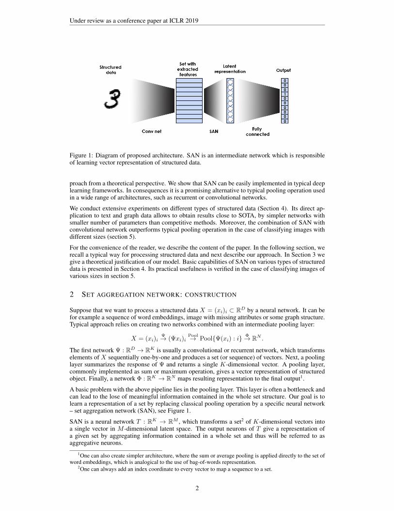
Figure 1: Diagram of proposed architecture. SAN is an intermediate network which is responsibleof learning vector representation of structured data.

proach from a theoretical perspective. We show that SAN can be easily implemented in typical deeplearning frameworks. In consequences it is a promising alternative to typical pooling operation usedin a wide range of architectures, such as recurrent or convolutional networks.

We conduct extensive experiments on different types of structured data (Section 4). Its direct ap-plication to text and graph data allows to obtain results close to SOTA, by simpler networks withsmaller number of parameters than competitive methods. Moreover, the combination of SAN withconvolutional network outperforms typical pooling operation in the case of classifying images withdifferent sizes (section 5).

For the convenience of the reader, we describe the content of the paper. In the following section, werecall a typical way for processing structured data and next describe our approach. In Section 3 wegive a theoretical justification of our model. Basic capabilities of SAN on various types of structureddata is presented in Section 4. Its practical usefulness is verified in the case of classifying images ofvarious sizes in section 5.

2 SET AGGREGATION NETWORK: CONSTRUCTION

Suppose that we want to process a structured data X = (xi)i ⊂ RD by a neural network. It can befor example a sequence of word embeddings, image with missing attributes or some graph structure.Typical approach relies on creating two networks combined with an intermediate pooling layer:

X = (xi)iΨ→ (Ψxi)i

Pool→ Pool{Ψ(xi) : i} Φ→ RN .

The first network Ψ : RD → RK is usually a convolutional or recurrent network, which transformselements of X sequentially one-by-one and produces a set (or sequence) of vectors. Next, a poolinglayer summarizes the response of Ψ and returns a single K-dimensional vector. A pooling layer,commonly implemented as sum or maximum operation, gives a vector representation of structuredobject. Finally, a network Φ : RK → RN maps resulting representation to the final output1.

A basic problem with the above pipeline lies in the pooling layer. This layer is often a bottleneck andcan lead to the lose of meaningful information contained in the whole set structure. Our goal is tolearn a representation of a set by replacing classical pooling operation by a specific neural network– set aggregation network (SAN), see Figure 1.

SAN is a neural network T : RK → RM , which transforms a set2 of K-dimensional vectors intoa single vector in M -dimensional latent space. The output neurons of T give a representation ofa given set by aggregating information contained in a whole set and thus will be referred to asaggregative neurons.

1One can also create simpler architecture, where the sum or average pooling is applied directly to the set ofword embeddings, which is analogical to the use of bag-of-words representation.

2One can always add an index coordinate to every vector to map a sequence to a set.

2

Under review as a conference paper at ICLR 2019

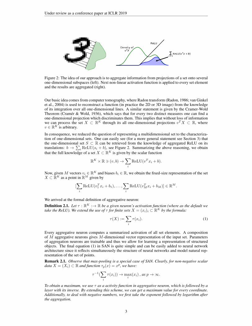
Figure 2: The idea of our approach is to aggregate information from projections of a set onto severalone-dimensional subspaces (left). Next non-linear activation function is applied to every set elementand the results are aggregated (right).

Our basic idea comes from computer tomography, where Radon transform (Radon, 1986; van Ginkelet al., 2004) is used to reconstruct a function (in practice the 2D or 3D image) from the knowledgeof its integration over all one-dimensional lines. A similar statement is given by the Cramer-WoldTheorem (Cramér & Wold, 1936), which says that for every two distinct measures one can find aone-dimensional projection which discriminates them. This implies that without loss of informationwe can process the set X ⊂ RK through its all one-dimensional projections vTX ⊂ R, wherev ∈ RK is arbitrary.

In consequence, we reduced the question of representing a multidimensional set to the characteriza-tion of one-dimensional sets. One can easily see (for a more general statement see Section 3) thatthe one-dimensional set S ⊂ R can be retrieved from the knowledge of aggregated ReLU on itstranslations: b →

∑i ReLU(si + b), see Figure 2. Summarizing the above reasoning, we obtain

that the full knowledge of a set X ⊂ RK is given by the scalar function

RK × R 3 (v, b)→∑i

ReLU(vTxi + b).

Now, given M vectors vi ∈ RK and biases bi ∈ R, we obtain the fixed-size representation of the setX ⊂ RK as a point in RM given by

[∑i

ReLU(vT1 xi + b1), . . . ,∑i

ReLU(vTMxi + bM )] ∈ RM .

We arrived at the formal definition of aggregative neuron:Definition 2.1. Let τ : RK :→ R be a given neuron’s activation function (where as the default wetake the ReLU). We extend the use of τ for finite sets X = (xi)i ⊂ RK by the formula:

τ(X) :=∑i

τ(xi). (1)

Every aggregative neuron computes a summarized activation of all set elements. A compositionof M aggregative neurons gives M -dimensional vector representation of the input set. Parametersof aggregation neurons are trainable and thus we allow for learning a representation of structuredobjects. The final equation (1) in SAN is quite simple and can be easily added to neural networkarchitecture since it reflects simultaneously the structure of neural networks and model natural rep-resentation of the set of points.Remark 2.1. Observe that max-pooling is a special case of SAN. Clearly, for non-negative scalardata X = (Xi) ⊂ R and function τp(x) = xp, we have:

τ−1(∑i

τ(xi))→ maxi

(xi) , as p→∞.

To obtain a maximum, we use τ as a activity function in aggregative neuron, which is followed by alayer with its inverse. By extending this scheme, we can get a maximum value for every coordinate.Additionally, to deal with negative numbers, we first take the exponent followed by logarithm afterthe aggregation.

3

Under review as a conference paper at ICLR 2019

We explain how to implement SAN in typical deep learning frameworks. Let X = {X1, . . . , Xn}be a batch, which consists of finite sets Xi ⊂ RK . While typical networks process vector by vector,SAN needs to compute a summary activation over all elements of Xi before passing the output tothe subsequent network.

To deal with sets of different sizes in one batch, we first transform every set Xi to the set of tuplesTi = {(x, 1) : x ∈ Xi}. Next, we complement every Ti to have the same sizes by adding zerotuples (x, 0), where x ∈ RK can be an arbitrary vector. The second element of each tuple indicateswhether a vector appears in a set or is a dummy vector. The set of tuples Ti can be understood as auniform discrete measure with a support defined on a given set Xi.

After the above operation every element from a batch is represented as a matrix of the same size.To compute the value of aggregative neuron of Xi, we apply 1D convolution to the first element ofeach tuple from Ti and multiply the outputs by their weights. Taking a sum, we get the activation ofaggregative neuron τ for Xi:

τ(Xi) =∑x∈Xi

1 · τ(xi) =∑

(x,f)∈Ti

f · τ(x).

These operations are applied to every element Xi of a batch. Summarizing, adding SAN to existingnetwork can be implemented in a few lines of codes.

3 THEORETICAL ANALYSIS

Our main theoretical result shows that SAN is able to uniquely identify every input set, whichjustifies our approach from theoretical perspective.

To prove this fact, we will use the UAP (universal approximation property). We say that a familyof neurons N has UAP if for every compact set K ⊂ RD and a continuous function f : K → Rthe function f can be arbitrarily close approximated with respect to supremum norm by span(N )(linear combinations of elements of N ).

We show that if a given family of neurons satisfies UAP, then corresponding aggregation neuronsallows to distinguish any two finite sets:Theorem 3.1. Let X,Y be two discrete sets in RD. Let N be a family of functions having UAP.

Ifτ(X) = τ(Y ) for every τ ∈ N , (2)

then X = Y .

Proof. Let µ and ν be two measures representing sets X and Y , respectively, i.e. µ = 1X andν = 1Y . We show that if τ(X) = τ(Y ) then µ and ν are equal.

Let R > 1 be such that X ∪ Y ⊂ B(0, R − 1), where B(a, r) denotes the closed ball centered at aand with radius r. To prove that measures µ, ν are equal it is sufficient to prove that they coincideon each ball B(a, r) with arbitrary a ∈ B(0, R− 1) and radius r < 1.

Let φn be defined byφn(x) = 1− n · d(x,B(a, r)) for x ∈ RD,

where d(x, U) denotes the distance of point x from the set U . Observe that φn is a continuousfunction which is one onB(a, r) an and zero on RD \B(a, r+1/n), and therefore φn is a uniformlybounded sequence of functions which converges pointwise to the characteristic funtion 1B(a,r) ofthe set B(a, r).

By the UAP property we choose ψn ∈ span(N ) such thatsupp

x∈B(0,R)

|φn(x)− ψn(x)| ≤ 1/n.

Thus ψn restricted to B(0, R) is also a uniformly bounded sequence of functions which convergespointwise to 1B(a,r). Since ψn ∈ N , by (2) we get∑

x∈Xµ(x)ψn(x) =

∑y∈Y

ν(y)ψn(y).

4

Under review as a conference paper at ICLR 2019

Table 1: AUC scores for classifying active chemical compounds .

ECFP4 KlekFP Mordred JTVAE set of atoms

Random Forest 0.726 0.604 0.493 0.527 -Extra Trees 0.713 0.667 0.501 0.470 -k-NN 0.532 0.569 0.546 0.521 -Dense network 0.702 0.574 0.593 0.560 -SAN - - - - 0.643

Now by the Lebesgue dominated convergence theorem we trivially get∑x∈X

µ(x)ψn(x) =

∫B(0,R)

ψn(x)dµ(x)→ µ(B(a, r)),∑y∈Y

ν(y)ψn(y) =

∫B(0,R)

ψn(x)dν(x)→ ν(B(a, r)),

which completes proof.

One could generalize the formula of aggregation neurons (1) to the case of arbitrary finite measuresµ by

τ(µ) =

∫τ(x)dµ(x).

For example, it can be used to process data with missing or uncertain attributes (Smieja et al., 2018;Dick et al., 2008; Williams et al., 2005). Although analogical theoretical result holds in this case,analytical formulas for aggregative neurons can be obtained only for special cases. Smieja et al.(2018) calculated analytical formulas for measures represented by the mixture of Gaussians andaggregative neurons parametrized by ReLU or RBF placed at the first hidden layer.

4 EXPERIMENTS: PROOF OF CONCEPT

In this section, as a proof of concept, we show that SAN is capable of processing various types ofstructured data: graphs, text and images. We are more interested here in demonstrating its wideapplicability than obtaining state-of-the-art performance on particular problem.

4.1 DETECTING ACTIVE CHEMICAL COMPOUNDS FROM GRAPH STRUCTURES

Figure 3: Example of a chemical compound repre-sented by graph and its lossy conversion to fingerprint.

Finding biologically active compounds isone of basic problems in medical chem-istry. Since the laboratory verificationof every molecule is very time and re-source consuming, the current trend is toanalyze its activity with machine learn-ing approaches. For this purpose, a graphof chemical compound is typically repre-sented as a fingerprint, which encodes pre-defined chemical patterns in a binary vec-tor (Figure 3). Since a multitude of chemi-cal features can be taken into account, var-ious types of fingerprints have been cre-ated.

As a simple alternative to chemical finger-prints, we encoded a molecule by a set ofits atoms in 2D space. More precisely, avector representing the atom contains its

5

Under review as a conference paper at ICLR 2019

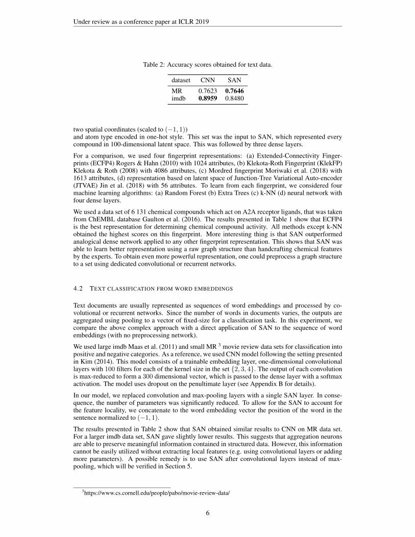
Table 2: Accuracy scores obtained for text data.

dataset CNN SAN

MR 0.7623 0.7646imdb 0.8959 0.8480

two spatial coordinates (scaled to (−1, 1))and atom type encoded in one-hot style. This set was the input to SAN, which represented everycompound in 100-dimensional latent space. This was followed by three dense layers.

For a comparison, we used four fingerprint representations: (a) Extended-Connectivity Finger-prints (ECFP4) Rogers & Hahn (2010) with 1024 attributes, (b) Klekota-Roth Fingerprint (KlekFP)Klekota & Roth (2008) with 4086 attributes, (c) Mordred fingerprint Moriwaki et al. (2018) with1613 attributes, (d) representation based on latent space of Junction-Tree Variational Auto-encoder(JTVAE) Jin et al. (2018) with 56 attributes. To learn from each fingerprint, we considered fourmachine learning algorithms: (a) Random Forest (b) Extra Trees (c) k-NN (d) neural network withfour dense layers.

We used a data set of 6 131 chemical compounds which act on A2A receptor ligands, that was takenfrom ChEMBL database Gaulton et al. (2016). The results presented in Table 1 show that ECFP4is the best representation for determining chemical compound activity. All methods except k-NNobtained the highest scores on this fingerprint. More interesting thing is that SAN outperformedanalogical dense network applied to any other fingerprint representation. This shows that SAN wasable to learn better representation using a raw graph structure than handcrafting chemical featuresby the experts. To obtain even more powerful representation, one could preprocess a graph structureto a set using dedicated convolutional or recurrent networks.

4.2 TEXT CLASSIFICATION FROM WORD EMBEDDINGS

Text documents are usually represented as sequences of word embeddings and processed by co-volutional or recurrent networks. Since the number of words in documents varies, the outputs areaggregated using pooling to a vector of fixed-size for a classification task. In this experiment, wecompare the above complex approach with a direct application of SAN to the sequence of wordembeddings (with no preprocessing network).

We used large imdb Maas et al. (2011) and small MR 3 movie review data sets for classification intopositive and negative categories. As a reference, we used CNN model following the setting presentedin Kim (2014). This model consists of a trainable embedding layer, one-dimensional convolutionallayers with 100 filters for each of the kernel size in the set {2, 3, 4}. The output of each convolutionis max-reduced to form a 300 dimensional vector, which is passed to the dense layer with a softmaxactivation. The model uses dropout on the penultimate layer (see Appendix B for details).

In our model, we replaced convolution and max-pooling layers with a single SAN layer. In conse-quence, the number of parameters was significantly reduced. To allow for the SAN to account forthe feature locality, we concatenate to the word embedding vector the position of the word in thesentence normalized to (−1, 1).

The results presented in Table 2 show that SAN obtained similar results to CNN on MR data set.For a larger imdb data set, SAN gave slightly lower results. This suggests that aggregation neuronsare able to preserve meaningful information contained in structured data. However, this informationcannot be easily utilized without extracting local features (e.g. using convolutional layers or addingmore parameters). A possible remedy is to use SAN after convolutional layers instead of max-pooling, which will be verified in Section 5.

3https://www.cs.cornell.edu/people/pabo/movie-review-data/

6

Under review as a conference paper at ICLR 2019

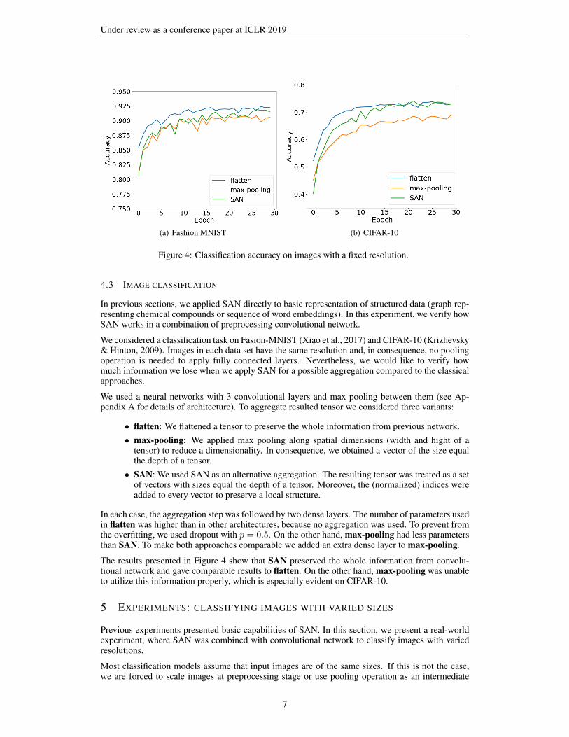
(a) Fashion MNIST (b) CIFAR-10

Figure 4: Classification accuracy on images with a fixed resolution.

4.3 IMAGE CLASSIFICATION

In previous sections, we applied SAN directly to basic representation of structured data (graph rep-resenting chemical compounds or sequence of word embeddings). In this experiment, we verify howSAN works in a combination of preprocessing convolutional network.

We considered a classification task on Fasion-MNIST (Xiao et al., 2017) and CIFAR-10 (Krizhevsky& Hinton, 2009). Images in each data set have the same resolution and, in consequence, no poolingoperation is needed to apply fully connected layers. Nevertheless, we would like to verify howmuch information we lose when we apply SAN for a possible aggregation compared to the classicalapproaches.

We used a neural networks with 3 convolutional layers and max pooling between them (see Ap-pendix A for details of architecture). To aggregate resulted tensor we considered three variants:

• flatten: We flattened a tensor to preserve the whole information from previous network.• max-pooling: We applied max pooling along spatial dimensions (width and hight of a

tensor) to reduce a dimensionality. In consequence, we obtained a vector of the size equalthe depth of a tensor.

• SAN: We used SAN as an alternative aggregation. The resulting tensor was treated as a setof vectors with sizes equal the depth of a tensor. Moreover, the (normalized) indices wereadded to every vector to preserve a local structure.

In each case, the aggregation step was followed by two dense layers. The number of parameters usedin flatten was higher than in other architectures, because no aggregation was used. To prevent fromthe overfitting, we used dropout with p = 0.5. On the other hand, max-pooling had less parametersthan SAN. To make both approaches comparable we added an extra dense layer to max-pooling.

The results presented in Figure 4 show that SAN preserved the whole information from convolu-tional network and gave comparable results to flatten. On the other hand, max-pooling was unableto utilize this information properly, which is especially evident on CIFAR-10.

5 EXPERIMENTS: CLASSIFYING IMAGES WITH VARIED SIZES

Previous experiments presented basic capabilities of SAN. In this section, we present a real-worldexperiment, where SAN was combined with convolutional network to classify images with variedresolutions.

Most classification models assume that input images are of the same sizes. If this is not the case,we are forced to scale images at preprocessing stage or use pooling operation as an intermediate

7

Under review as a conference paper at ICLR 2019

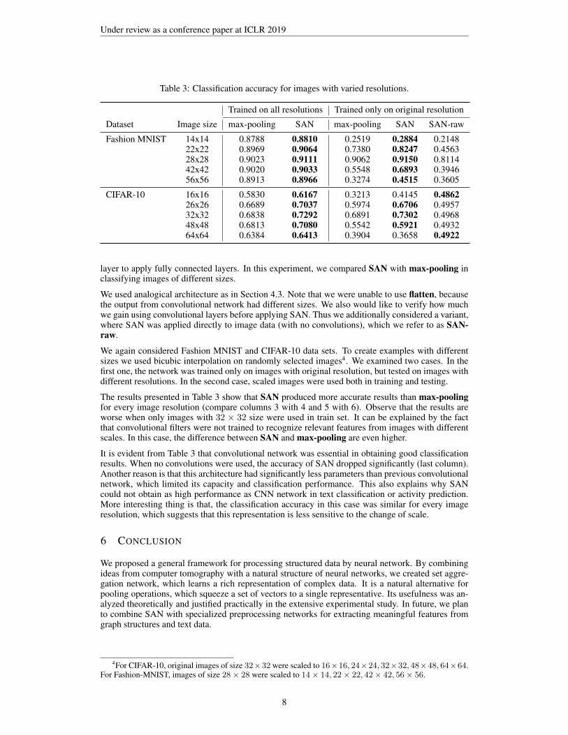
Table 3: Classification accuracy for images with varied resolutions.

Trained on all resolutions Trained only on original resolution

Dataset Image size max-pooling SAN max-pooling SAN SAN-raw

Fashion MNIST 14x14 0.8788 0.8810 0.2519 0.2884 0.214822x22 0.8969 0.9064 0.7380 0.8247 0.456328x28 0.9023 0.9111 0.9062 0.9150 0.811442x42 0.9020 0.9033 0.5548 0.6893 0.394656x56 0.8913 0.8966 0.3274 0.4515 0.3605

CIFAR-10 16x16 0.5830 0.6167 0.3213 0.4145 0.486226x26 0.6689 0.7037 0.5974 0.6706 0.495732x32 0.6838 0.7292 0.6891 0.7302 0.496848x48 0.6813 0.7080 0.5542 0.5921 0.493264x64 0.6384 0.6413 0.3904 0.3658 0.4922

layer to apply fully connected layers. In this experiment, we compared SAN with max-pooling inclassifying images of different sizes.

We used analogical architecture as in Section 4.3. Note that we were unable to use flatten, becausethe output from convolutional network had different sizes. We also would like to verify how muchwe gain using convolutional layers before applying SAN. Thus we additionally considered a variant,where SAN was applied directly to image data (with no convolutions), which we refer to as SAN-raw.

We again considered Fashion MNIST and CIFAR-10 data sets. To create examples with differentsizes we used bicubic interpolation on randomly selected images4. We examined two cases. In thefirst one, the network was trained only on images with original resolution, but tested on images withdifferent resolutions. In the second case, scaled images were used both in training and testing.

The results presented in Table 3 show that SAN produced more accurate results than max-poolingfor every image resolution (compare columns 3 with 4 and 5 with 6). Observe that the results areworse when only images with 32 × 32 size were used in train set. It can be explained by the factthat convolutional filters were not trained to recognize relevant features from images with differentscales. In this case, the difference between SAN and max-pooling are even higher.

It is evident from Table 3 that convolutional network was essential in obtaining good classificationresults. When no convolutions were used, the accuracy of SAN dropped significantly (last column).Another reason is that this architecture had significantly less parameters than previous convolutionalnetwork, which limited its capacity and classification performance. This also explains why SANcould not obtain as high performance as CNN network in text classification or activity prediction.More interesting thing is that, the classification accuracy in this case was similar for every imageresolution, which suggests that this representation is less sensitive to the change of scale.

6 CONCLUSION

We proposed a general framework for processing structured data by neural network. By combiningideas from computer tomography with a natural structure of neural networks, we created set aggre-gation network, which learns a rich representation of complex data. It is a natural alternative forpooling operations, which squeeze a set of vectors to a single representative. Its usefulness was an-alyzed theoretically and justified practically in the extensive experimental study. In future, we planto combine SAN with specialized preprocessing networks for extracting meaningful features fromgraph structures and text data.

4For CIFAR-10, original images of size 32×32 were scaled to 16×16, 24×24, 32×32, 48×48, 64×64.For Fashion-MNIST, images of size 28× 28 were scaled to 14× 14, 22× 22, 42× 42, 56× 56.

8

Under review as a conference paper at ICLR 2019

REFERENCES

Dzmitry Bahdanau, Kyunghyun Cho, and Yoshua Bengio. Neural machine translation by jointlylearning to align and translate. arXiv preprint arXiv:1409.0473, 2014.

Sergey Brin and Lawrence Page. The anatomy of a large-scale hypertextual web search engine.Computer networks and ISDN systems, 30(1-7):107–117, 1998.

Kyunghyun Cho, Bart Van Merriënboer, Dzmitry Bahdanau, and Yoshua Bengio. On the propertiesof neural machine translation: Encoder-decoder approaches. arXiv preprint arXiv:1409.1259,2014.

Dan C Ciresan, Ueli Meier, Jonathan Masci, Luca Maria Gambardella, and Jürgen Schmidhu-ber. Flexible, high performance convolutional neural networks for image classification. In IJ-CAI Proceedings-International Joint Conference on Artificial Intelligence, volume 22, pp. 1237.Barcelona, Spain, 2011.

Harald Cramér and Herman Wold. Some theorems on distribution functions. Journal of the LondonMathematical Society, 1(4):290–294, 1936.

Uwe Dick, Peter Haider, and Tobias Scheffer. Learning from incomplete data with infinite impu-tations. In Proceedings of the 25th international conference on Machine learning, pp. 232–239.ACM, 2008.

Todd Ewing, J Christian Baber, and Miklos Feher. Novel 2d fingerprints for ligand-based virtualscreening. Journal of chemical information and modeling, 46(6):2423–2431, 2006.

Paolo Frasconi, Marco Gori, and Alessandro Sperduti. A general framework for adaptive processingof data structures. IEEE transactions on Neural Networks, 9(5):768–786, 1998.

Anna Gaulton, Anne Hersey, Michał Nowotka, A Patrícia Bento, Jon Chambers, David Mendez,Prudence Mutowo, Francis Atkinson, Louisa J Bellis, Elena Cibrián-Uhalte, et al. The chembldatabase in 2017. Nucleic acids research, 45(D1):D945–D954, 2016.

Markus Hagenbuchner, Alessandro Sperduti, and Ah Chung Tsoi. A self-organizing map for adap-tive processing of structured data. IEEE transactions on Neural Networks, 14(3):491–505, 2003.

Kaiming He, Xiangyu Zhang, Shaoqing Ren, and Jian Sun. Spatial pyramid pooling in deep con-volutional networks for visual recognition. IEEE transactions on pattern analysis and machineintelligence, 37(9):1904–1916, 2015.

Satoshi Iizuka, Edgar Simo-Serra, and Hiroshi Ishikawa. Globally and locally consistent imagecompletion. ACM Transactions on Graphics (TOG), 36(4):107, 2017.

Wengong Jin, Regina Barzilay, and Tommi Jaakkola. Junction tree variational autoencoder formolecular graph generation. arXiv preprint arXiv:1802.04364, 2018.

Nal Kalchbrenner and Phil Blunsom. Recurrent continuous translation models. In Proceedings ofthe 2013 Conference on Empirical Methods in Natural Language Processing, pp. 1700–1709,2013.

Andrej Karpathy and Li Fei-Fei. Deep visual-semantic alignments for generating image descrip-tions. In Proceedings of the IEEE conference on computer vision and pattern recognition, pp.3128–3137, 2015.

Yoon Kim. Convolutional neural networks for sentence classification. arXiv preprintarXiv:1408.5882, 2014.

Justin Klekota and Frederick P Roth. Chemical substructures that enrich for biological activity.Bioinformatics, 24(21):2518–2525, 2008.

Alex Krizhevsky and Geoffrey Hinton. Learning multiple layers of features from tiny images. Tech-nical report, Citeseer, 2009.

9

Under review as a conference paper at ICLR 2019

Yujia Li, Daniel Tarlow, Marc Brockschmidt, and Richard Zemel. Gated graph sequence neuralnetworks. arXiv preprint arXiv:1511.05493, 2015.

Jonathan Long, Evan Shelhamer, and Trevor Darrell. Fully convolutional networks for semanticsegmentation. In Proceedings of the IEEE conference on computer vision and pattern recognition,pp. 3431–3440, 2015.

Andrew L. Maas, Raymond E. Daly, Peter T. Pham, Dan Huang, Andrew Y. Ng, and ChristopherPotts. Learning word vectors for sentiment analysis. In Proceedings of the 49th Annual Meetingof the Association for Computational Linguistics: Human Language Technologies, pp. 142–150,Portland, Oregon, USA, June 2011. Association for Computational Linguistics. URL http://www.aclweb.org/anthology/P11-1015.

Emmanuel Maggiori, Yuliya Tarabalka, Guillaume Charpiat, and Pierre Alliez. Fully convolutionalneural networks for remote sensing image classification. In Geoscience and Remote SensingSymposium (IGARSS), 2016 IEEE International, pp. 5071–5074. IEEE, 2016.

Tomas Mikolov, Kai Chen, Greg Corrado, and Jeffrey Dean. Efficient estimation of word represen-tations in vector space. arXiv preprint arXiv:1301.3781, 2013.

Hirotomo Moriwaki, Yu-Shi Tian, Norihito Kawashita, and Tatsuya Takagi. Mordred: a moleculardescriptor calculator. Journal of cheminformatics, 10(1):4, 2018.

Jeffrey Pennington, Richard Socher, and Christopher Manning. Glove: Global vectors for wordrepresentation. In Proceedings of the 2014 conference on empirical methods in natural languageprocessing (EMNLP), pp. 1532–1543, 2014.

Johann Radon. On the determination of functions from their integral values along certain manifolds.IEEE transactions on medical imaging, 5(4):170–176, 1986.

David Rogers and Mathew Hahn. Extended-connectivity fingerprints. Journal of chemical informa-tion and modeling, 50(5):742–754, 2010.

Olaf Ronneberger, Philipp Fischer, and Thomas Brox. U-net: Convolutional networks for biomedi-cal image segmentation. In International Conference on Medical image computing and computer-assisted intervention, pp. 234–241. Springer, 2015.

Franco Scarselli, Marco Gori, Ah Chung Tsoi, Markus Hagenbuchner, and Gabriele Monfardini.The graph neural network model. IEEE Transactions on Neural Networks, 20(1):61–80, 2009.

Marek Smieja, Łukasz Struski, Jacek Tabor, Bartosz Zielinski, and Przemysław Spurek. Processingof missing data by neural networks. accepted to NIPS, arXiv preprint arXiv:1805.07405, 2018.

Martin Sundermeyer, Ralf Schlüter, and Hermann Ney. Lstm neural networks for language model-ing. In Thirteenth Annual Conference of the International Speech Communication Association,2012.

Ilya Sutskever, Oriol Vinyals, and Quoc V Le. Sequence to sequence learning with neural networks.In Advances in neural information processing systems, pp. 3104–3112, 2014.

Ah Chung Tsoi, Gianni Morini, Franco Scarselli, Markus Hagenbuchner, and Marco Maggini.Adaptive ranking of web pages. In Proceedings of the 12th international conference on WorldWide Web, pp. 356–365. ACM, 2003.

Michael van Ginkel, CL Luengo Hendriks, and Lucas J van Vliet. A short introduction to the radonand hough transforms and how they relate to each other. Delft University of Technology, 2004.

David Williams, Xuejun Liao, Ya Xue, and Lawrence Carin. Incomplete-data classification usinglogistic regression. In Proceedings of the 22nd International Conference on Machine learning,pp. 972–979. ACM, 2005.

Han Xiao, Kashif Rasul, and Roland Vollgraf. Fashion-mnist: a novel image dataset for benchmark-ing machine learning algorithms, 2017.

10

Under review as a conference paper at ICLR 2019

Table 4: Architecture summary for image classification, where N is the size of input to the layer.Flatten Max-pooling SAN

Type Kernel Outputs Type Kernel Outputs Type Kernel Outputs

Conv 2d 5x5 32 Conv 2d 5x5 32 Conv 2d 5x5 32Max pooling 2x2 Max pooling 2x2 Max pooling 2x2

Conv 2d 5x5 32 Conv 2d 5x5 32 Conv 2d 5x5 32Max pooling 2x2 Max pooling 2x2 Max pooling 2x2

Conv 2d 3x3 32 Conv 2d 3x3 32 Conv 2d 3x3 32Flatten Max pooling NxN SAN 128Dense 128 Dense 128 Dense 128

Dropout (p=0.5) Dense 128 Dense 10Dense 10 Dense 10

A NETWORK ARCHITECTURE FOR IMAGE CLASSIFICATION

Table 4 presents the architecture used for image classification.

The CIFAR-10 dataset consists of 50000 train and 10000 test images of size 32x32 pixels, whereeach image belongs to one of 10 classes. The Fashion MNIST dataset contains 60000 train and10000 test images of size 28x28 pixels from 10 classes.

We used the categorical crossentropy as the loss function and trained the models using randombatches in adam optimization algorithm with the learning rate set to default 10−3. For the experi-ments where the network was trained only on images with original resolution and tested on imageswith different resolutions, we set the number of epochs to 30 with batches of 128 samples. Forthe experiments where scaled images were used both in training and testing, we set the number ofepochs to 50 with batches of 128 samples.

B NETWORK ARCHITECTURE FOR TEXT CLASSIFICATION

The architecture for text classfication models consists of an trainable embedding followed by model-specific layers which project the input onto 300-dimensional space. Then a finall dense layer isapplied. All models also include dropout with probability p = 0.5 on the penultimate layer. Thearchitecture is summamrized in 5. We used 10000 and 5000 most frequent words for the vocabularyfor the imdb and MR datasets, respectively.

The imdb dataset consists of 25000 test and 25000 train documents with the average length aftertokenization of 234.76. The MR datasets consists of 10664 documents, with an average length aftertokenization of 16.76. As the MR dataset does not include a pre-defined test set, we randomly select10% of the data as the test set.

We used the categorical crossentropy as the loss function and trained the models using randombatches in adam optimization algorithm. For the imdb dataset we set the number of epochs to30, the embedding dimension to 128, the batch size to 256 and we perform a grid search on thelearning rate in the set of {10−1, 10−2, 10−3, 10−4}. For the MR dataset we train for 20 epochs,with embedding dimension 32, learning rate 10−3 and we perform a grid search on the batch size inthe set of {32, 64, 128, 256}. For the smaller MR dataset we also incorporate a l2 regularization onthe weights with penalty 3.0.

11

Under review as a conference paper at ICLR 2019

Table 5: Architecture summary for text classification, where N is the length of the input sequenceand hdim is 128 for imdb and 32 for MR.

CNN SANType Kernel Outputs Type Kernel Outputs

Embedding hdim Embedding hdimConv 1d 3 100Conv 1d 4 100Conv 1d 5 100 SAN 300

Concatenate 300Max pooling N 300

Dropout (p=0.5) Dropout (p=0.5)Dense 2 Dense 2

12