Structured learning modulo theories - DISI UniTn
22
Artificial Intelligence 244 (2017) 166–187 Contents lists available at ScienceDirect Artificial Intelligence www.elsevier.com/locate/artint Structured learning modulo theories Stefano Teso a , Roberto Sebastiani b , Andrea Passerini b,∗ a DKM – Data & Knowledge Management Unit, Fondazione Bruno Kessler, Via Sommarive, 18, I38123 Povo, TN, Italy b DISI – Dipartimento di Ingegneria e Scienza dell’Informazione, Università degli Studi di Trento, Via Sommarive 5, I-38123 Povo, TN, Italy a r t i c l e i n f o a b s t r a c t Article history: Received in revised form 13 March 2015 Accepted 14 April 2015 Available online 29 April 2015 Keywords: Satisfiability modulo theory Structured-output support vector machines Optimization modulo theory Constructive machine learning Learning with constraints Modeling problems containing a mixture of Boolean and numerical variables is a long- standing interest of Artificial Intelligence. However, performing inference and learning in hybrid domains is a particularly daunting task. The ability to model these kinds of domains is crucial in “learning to design” tasks, that is, learning applications where the goal is to learn from examples how to perform automatic de novo design of novel objects. In this paper we present Structured Learning Modulo Theories, a max-margin approach for learning in hybrid domains based on Satisfiability Modulo Theories, which allows to combine Boolean reasoning and optimization over continuous linear arithmetical constraints. The main idea is to leverage a state-of-the-art generalized Satisfiability Modulo Theory solver for implementing the inference and separation oracles of Structured Output SVMs. We validate our method on artificial and real world scenarios. © 2015 Elsevier B.V. All rights reserved. 1. Introduction Research in machine learning has progressively widened its scope, from simple scalar classification and regression tasks to more complex problems involving multiple related variables. Methods developed in the related fields of statistical rela- tional learning (SRL) [1] and structured-output learning [2] allow to perform learning, reason and inferences about relational entities characterized by both hard and soft constraints. Most methods rely on some form of (finite) First-Order Logic (FOL) to encode the learning problem, and define the constraints as weighted logical formulae. One issue with these approaches is that First-Order Logic is not suited for efficient reasoning over hybrid domains, characterized by both continuous and dis- crete variables. The Booleanization of an n-bit integer variable requires 2 n distinct Boolean states, making naive translation impractical; for rational variables the situation is even worse. In addition, standard FOL automated reasoning techniques of- fer no mechanism to deal efficiently with operators among numerical variables, like comparisons (e.g. “less-than”, “equal-to”) and arithmetical operations (e.g. summation), limiting the range of realistically applicable constraints to those based solely on logical connectives. On the other hand, many real-world domains are inherently hybrid and require to reason over inter- related continuous and discrete variables. This is especially true in constructive machine learning tasks, where the focus is on the de-novo design of objects with certain characteristics to be learned from examples (e.g. a recipe for a dish, with ingredients, proportions, etc.). There is relatively little previous work on hybrid SRL methods. A number of approaches [3–6] focused on the feature representation perspective, in order to extend statistical relational learning algorithms to deal with continuous features as inputs. On the other hand, performing inference over joint continuous–discrete relational domains is still a challenge. The few existing attempts [7–12] aim at extending statistical relational learning methods to the hybrid domain. All these * Corresponding author. E-mail addresses: [email protected] (S. Teso), [email protected] (R. Sebastiani), [email protected] (A. Passerini). http://dx.doi.org/10.1016/j.artint.2015.04.002 0004-3702/© 2015 Elsevier B.V. All rights reserved.
-
Upload
khangminh22 -
Category
Documents
-
view
1 -
download
0
Transcript of Structured learning modulo theories - DISI UniTn

Artificial Intelligence 244 (2017) 166–187
Contents lists available at ScienceDirect
Artificial Intelligence
www.elsevier.com/locate/artint
Structured learning modulo theories
Stefano Teso a, Roberto Sebastiani b, Andrea Passerini b,∗a DKM – Data & Knowledge Management Unit, Fondazione Bruno Kessler, Via Sommarive, 18, I38123 Povo, TN, Italyb DISI – Dipartimento di Ingegneria e Scienza dell’Informazione, Università degli Studi di Trento, Via Sommarive 5, I-38123 Povo, TN, Italy
a r t i c l e i n f o a b s t r a c t
Article history:Received in revised form 13 March 2015Accepted 14 April 2015Available online 29 April 2015
Keywords:Satisfiability modulo theoryStructured-output support vector machinesOptimization modulo theoryConstructive machine learningLearning with constraints
Modeling problems containing a mixture of Boolean and numerical variables is a long-standing interest of Artificial Intelligence. However, performing inference and learning in hybrid domains is a particularly daunting task. The ability to model these kinds of domains is crucial in “learning to design” tasks, that is, learning applications where the goal is to learn from examples how to perform automatic de novo design of novel objects. In this paper we present Structured Learning Modulo Theories, a max-margin approach for learning in hybrid domains based on Satisfiability Modulo Theories, which allows to combine Boolean reasoning and optimization over continuous linear arithmetical constraints. The main idea is to leverage a state-of-the-art generalized Satisfiability Modulo Theory solver for implementing the inference and separation oracles of Structured Output SVMs. We validate our method on artificial and real world scenarios.
© 2015 Elsevier B.V. All rights reserved.
1. Introduction
Research in machine learning has progressively widened its scope, from simple scalar classification and regression tasks to more complex problems involving multiple related variables. Methods developed in the related fields of statistical rela-tional learning (SRL) [1] and structured-output learning [2] allow to perform learning, reason and inferences about relational entities characterized by both hard and soft constraints. Most methods rely on some form of (finite) First-Order Logic (FOL) to encode the learning problem, and define the constraints as weighted logical formulae. One issue with these approaches is that First-Order Logic is not suited for efficient reasoning over hybrid domains, characterized by both continuous and dis-crete variables. The Booleanization of an n-bit integer variable requires 2n distinct Boolean states, making naive translation impractical; for rational variables the situation is even worse. In addition, standard FOL automated reasoning techniques of-fer no mechanism to deal efficiently with operators among numerical variables, like comparisons (e.g. “less-than”, “equal-to”)and arithmetical operations (e.g. summation), limiting the range of realistically applicable constraints to those based solely on logical connectives. On the other hand, many real-world domains are inherently hybrid and require to reason over inter-related continuous and discrete variables. This is especially true in constructive machine learning tasks, where the focus is on the de-novo design of objects with certain characteristics to be learned from examples (e.g. a recipe for a dish, with ingredients, proportions, etc.).
There is relatively little previous work on hybrid SRL methods. A number of approaches [3–6] focused on the feature representation perspective, in order to extend statistical relational learning algorithms to deal with continuous features as inputs. On the other hand, performing inference over joint continuous–discrete relational domains is still a challenge. The few existing attempts [7–12] aim at extending statistical relational learning methods to the hybrid domain. All these
* Corresponding author.E-mail addresses: [email protected] (S. Teso), [email protected] (R. Sebastiani), [email protected] (A. Passerini).
http://dx.doi.org/10.1016/j.artint.2015.04.0020004-3702/© 2015 Elsevier B.V. All rights reserved.

S. Teso et al. / Artificial Intelligence 244 (2017) 166–187 167
approaches focus on modeling the probabilistic relationships between variables. While this allows to compute marginal probabilities in addition to most probable configurations, it imposes strong limitations on the type of constraints they can handle. Inference is typically run by approximate methods, based on variational approximations or sampling strategies. Exact inference, support for hard numeric (in addition to Boolean) constraints and combination of diverse theories, like linear algebra over rationals and integers, are out of the scope of these approaches. Hybrid Markov Logic networks [8] and Church [7] are the two formalisms which are closer to the scope of this paper. Hybrid Markov Logic networks [8] extend Markov Logic by including continuous variables, and allow to embed numerical comparison operators (namely �=, ≥ and ≤) into the constraints by defining an ad hoc translation of said operators to a continuous form amenable to numerical optimization. Inference relies on a stochastic local search procedure that interleaves calls to a MAX-SAT solver and to a numerical optimization procedure. This inference procedure is incapable of dealing with hard numeric constraints because of the lack of feedback from the continuous optimizer to the satisfiability module. Church [7] is a very expressive proba-bilistic programming language that can potentially represent arbitrary constraints on both continuous and discrete variables. Its focus is on modeling the generative process underlying the program, and inference is based on sampling techniques. This makes inference involving continuous optimization subtasks and hard constraints prohibitively expensive, as will be discussed in the experimental evaluation.
In order to overcome the limitations of existing approaches, we focused on the most recent advances in automated reasoning over hybrid domains. Researchers in automated reasoning and formal verification have developed logical languages and reasoning tools that allow for natively reasoning over mixtures of Boolean and numerical variables (or even more complex structures). These languages are grouped under the umbrella term of Satisfiability Modulo Theories (SMT) [13]. Each such language corresponds to a decidable fragment of First-Order Logic augmented with an additional background theory T . There are many such background theories, including those of linear arithmetic over the rationals LRA or over the integers LIA, among others [13]. In SMT, a formula can contain Boolean variables (i.e. 0-ary logical predicates) and connectives, mixed with symbols defined by the theory T , e.g. rational variables and arithmetical operators. For instance, the SMT(LRA) syntax allows to write formulas such as:
touching_i_j↔ ((xi + dxi = x j) ∨ (x j + dx j = xi))
where the variables are Boolean (touching_i_j) or rational (xi, x j, dxi, dx j).1 More specifically, SMT is a decision problem, which consists in finding an assignment to the variables of a quantifier-free formula, both Boolean and theory-specific ones, that makes the formula true, and it can be seen as an extension of SAT.
Recently, researchers have leveraged SMT from decision to optimization. In particular, MAX-SAT Modulo Theories (MAX-SMT) [14–16] generalizes MAX-SAT [17] to SMT formulae, and consists in finding a theory-consistent truth assignment to the atoms of the input SMT formula ϕ which maximizes the total weight of the satisfied clauses of ϕ . More generally, Optimization Modulo Theories (OMT) [14,18–22] consists in finding a model for ϕ which minimizes the value of some (arith-metical) term, and strictly subsumes MAX-SMT [19]. Most important for the scope of this paper is that there are high-quality OMT solvers which, at least for the LRA theory, can handle problems with thousands of hybrid variables.
In this paper we propose Learning Modulo Theories (LMT), a class of novel hybrid statistical relational learning methods. The main idea is to combine a solver able to deal with Boolean and rational variables with a structured output learning method. In particular, we rely on structured-output Support Vector Machines (SVM) [23,24], a very flexible max-margin structured prediction method. Structured-output SVMs are a generalization of binary SVM classifiers to predict structured outputs, like sequences or trees. They generalize the max-margin principle by learning to separate correct from incor-rect output structures with a large margin. Training structured-output SVMs requires a separation oracle for generating counter-examples and updating the parameters, while the prediction stage requires an inference oracle generating the high-est scoring candidate structure for a certain input. In order to implement the two oracles, we leverage a state-of-the-art OMT solver. This combination enables LMT to perform learning and inference in mixed Boolean-numerical domains. Thanks to the efficiency of the underlying OMT solver, and of the cutting plane algorithm we employ for weight learning, LMT is capable of addressing constructive learning problems which cannot be efficiently tackled with existing methods. Further-more, LMT is generic, and can in principle be applied to any of the existing background theories. This paper builds on a previous work in which MAX-SMT was used for interactive preference elicitation [25]. Here we focus on generating novel structures from a few prototypical examples, and cast the problem as supervised structured-output learning. Furthermore, we increase the expressive power from MAX-SMT to full OMT. This allows to model much richer cost functions, for instance by penalizing an unsatisfied constraint by a cost proportional to the distance from satisfaction.
The rest of the paper is organized as follows. In Section 2 we review the relevant related work, with an in-depth dis-cussion on all hybrid approaches and their relationships with our proposed framework. Section 3 provides an introduction to SMT and OMT technology. Section 4 reviews structured-output SVMs and shows how to cast LMT in this learning frame-work. Section 5 reports an experimental evaluation showing the potential of the approach. Finally, conclusions are drawn in Section 6.
1 Note that SMT solvers handle also formulas on combinations of theories, like e.g. (d ≥ 0) ∧ (d < 1) ∧ (( f (d) = f (0))→(read(write(V , i, x), i + d) =x + 1)), where d, i, x are integer variables, V is an array variable, f is an uninterpreted function symbol, read and write are functions of the theory of arrays [13]. However, for the scope of this paper it suffices to consider the LRA and LIA theories, and their combination.
168 S. Teso et al. / Artificial Intelligence 244 (2017) 166–187
2. Related work
There is a body of work concerning integration of relational and numerical data from a feature representation perspec-tive, in order to effectively incorporate numerical features into statistical relational learning models. Lippi and Frasconi [3]incorporate neural networks as feature generators within Markov Logic Networks, where neural networks act as numeri-cal functions complementing the Boolean formulae of standard MLNs. Semantic Based Regularization [6] is a framework for integrating logic constraints within kernel machines, by turning them into real-valued constraints using appropriate transfor-mations (T-norms). The resulting optimization problem is no longer convex in general, and they suggest a stepwise approach adding constraints in an incremental fashion, in order to solve progressively more complex problems. In Probabilistic Soft Logic [4], arbitrarily complex similarity measures between objects are combined with logic constraints, again using T-norms for the continuous relaxation of Boolean operators. In Gaussian Logic [5], numeric variables are modeled with multivariate Gaussian distributions. Their parameters are tied according to logic formulae defined over these variables, and combined with weighted first order formulae modeling the discrete part of the domain (as in standard MLNs). All these approaches aim at extending statistical relational learning algorithms to deal with continuous features as inputs. On the other hand, our framework aims at allowing learning and inference over hybrid continuous–discrete domains, where continuous and discrete variables are the output of the inference process.
While a number of efficient lifted-inference algorithms have been developed for Relational Continuous Models [26–28], performing inference over joint continuous–discrete relational domains is still a challenge. The few existing attempts aim at extending statistical relational learning methods to the hybrid domain.
Hybrid Probabilistic Relational Models [9] extend Probabilistic Relational Models (PRM) to deal with hybrid domains by specifying templates for hybrid distributions as standard PRM specify templates for discrete distributions. A template instantiation over a database defines a Hybrid Bayesian Network [29,30]. Inference in Hybrid BN is known to be hard, and restrictions are typically imposed on the allowed relational structure (e.g. in conditional Gaussian models, discrete nodes cannot have continuous parents). On the other hand, LMT can accommodate arbitrary combinations of predicates from the theories for which a solver is available. These currently include linear arithmetic over both rationals and integers as well as a number of other theories like strings, arrays and bit-vectors.
Relational Hybrid Models [11] (RHM) extend Relational Continuous Models to represent combinations of discrete and continuous distributions. The authors present a family of lifted variational algorithms for performing efficient inference, showing substantial improvements over their ground counterparts. As for most hybrid SRL approaches which will be discussed further on, the authors focus on efficiently computing probabilities rather than efficiently finding optimal con-figurations. Exact inference, hard constraints and theories like algebra over integers, which are naturally handled by our LMT framework, are all out of the scope of these approaches. Nonetheless, lifted inference is a powerful strategy to scale up inference and equipping OMT and SMT tools with lifting capabilities is a promising direction for future improvements.
The PRISM [31] system provides primitives for Gaussian distributions. However, inference is based on proof enumeration, which makes support for continuous variables very limited. Islam et al. [12] recently extended PRISM to perform inference over continuous random variables by a symbolic procedure which avoids the enumeration of individual proofs. The extension allows to encode models like Hybrid Bayesian Networks and Kalman Filters. Being built on top of the PRISM system, the approach assumes the exclusive explanation and independence property: no two different proofs for the same goal can be true simultaneously, and all random processes within a proof are independent (some research directions for lifting these restrictions have been suggested [32]). LMT has no assumptions on the relationships between proofs.
Hybrid Markov Logic Networks [8] extend Markov Logic Networks to deal with numeric variables. A Hybrid Markov Logic Network consists of both First Order Logic formulae and numeric terms. Most probable explanation (MPE) inference is per-formed by a hybrid version of MAXWalkSAT, where optimization of numeric variables is performed by a general-purpose global optimization algorithm (L-BFGS). This approach is extremely flexible and allows to encode arbitrary numeric con-straints, like soft equalities and inequalities with quadratic or exponential costs. A major drawback of this flexibility is the computational cost, as each single inference step on continuous variables requires to solve a global optimization problem, making the approach infeasible for addressing medium to large scale problems. Furthermore, this inference procedure is incapable of dealing with hard constraints involving numeric variables, as can be found for instance in layout problems (see e.g. the constraints on touching blocks or connected segments in the experimental evaluation). This is due to the lack of feedback from the continuous optimizer to the satisfiability module, which should inform about conflicting constraints and help guiding the search towards a more promising portion of the search space. Conversely, the OMT technology underlying LMT is built on top of SMT solvers and is hence specifically designed to tightly integrate theory-specific and SAT solvers [14,15,18–20]. Note that the tight interaction between theory-specific and modern CDCL SAT solvers, plus many techniques developed for maximizing their synergy, are widely recognized as one key reason of the success of SMT solvers [13]. Note also that previous attempts to substitute standard SAT solvers with WalkSAT inside an SMT solver have failed, producing dramatic worsening of performance [33].
Hybrid ProbLog [10] is an extension of the probabilistic logic language ProbLog [34] to deal with continuous variables. A ProbLog program consists of a set of probabilistic Boolean facts, and a set of deterministic first order logic formulae representing the background knowledge. Hybrid ProbLog introduces a set of probabilistic continuous facts, containing both discrete and continuous variables. Each continuous variable is associated with a probability density function. The authors show how to compute the probability of success of a query, by partitioning the continuous space into admissible intervals,

S. Teso et al. / Artificial Intelligence 244 (2017) 166–187 169
within which values are interchangeable with respect to the provability of the query. The drawback of this approach is that in order to make this computation feasible, severe limitations have to be imposed on the use of continuous variables. No algebraic operations or comparisons are allowed between continuous variables, which should remain uncoupled. Some of these limitations have been overcome in a recent approach [35] which performs inference by forward (i.e. from facts to rules) rather than backward reasoning, which is the typical inference process in (probabilistic) logic programming engines (SLD-resolution and its probabilistic extensions). Forward reasoning is more amenable to be adapted to sampling strategies for performing approximate inference and dealing with continuous variables. On the other hand, inference by sampling makes it prohibitively expensive to reason with hard continuous constraints.
Church [7] is a very expressive probabilistic programming language that can easily accommodate hybrid discrete–continuous distributions and arbitrary constraints. In order to deal with the resulting complexity, inference is again per-formed by sampling techniques, which result in the same aforementioned limitations. Indeed, our experimental evaluation shows that Church is incapable of solving in reasonable time the simple task of generating a pair of blocks conditioned on the fact that they touch somewhere.2
An advantage of these probabilistic inference approaches is that they allow to return marginal probabilities in addition to most probable explanations. This is actually the main focus of these approaches, and the reason why they are less suit-able for solving the latter problem when the search space becomes strongly disconnected. As with most structured-output approaches over which it builds, LMT is currently limited to the task of finding an optimal configuration, which in a prob-abilistic setting corresponds to generating the most probable explanation. We are planning to extend it to also perform probability computation, as discussed in the conclusions of the paper.
3. From satisfiability to optimization modulo theories
Propositional satisfiability (SAT), is the problem of deciding whether a logical formula over Boolean variables and logical connectives can be satisfied by some truth value assignment of the Boolean variables.3 In the last two decades we have witnessed an impressive advance in the efficiency of SAT solvers, which nowadays can handle industrially derived formulae in the order of up to 106–107 variables. Modern SAT solvers are based on the conflict-driven clause-learning (CDCL) schema [37], and adopt a variety of very-efficient search techniques [38].
In the contexts of automated reasoning (AR) and formal verification (FV), important decision problems are effectively encoded into and solved as Satisfiability Modulo Theories (SMT) problems [39]. SMT is the problem of deciding the satis-fiability of a (typically quantifier-free) first-order formula with respect to some decidable background theory T , which can also be a combination of theories
⋃i Ti . Theories of practical interest are, e.g., those of equality and uninterpreted functions
(EUF ), of linear arithmetic over the rationals (LRA) or over the integers (LIA), of non-linear arithmetic over the reals (NLA), of arrays (AR), of bit-vectors (BV), and their combinations.
In the last decade efficient SMT solvers have been developed following the so-called lazy approach, that combines the power of modern CDCL SAT solvers with the expressivity of dedicated decision procedures (T -solvers) for several first-order theories of interest. Modern lazy SMT solvers—like e.g. CVC4,4 MathSAT5,5 Yices,6 Z3
7—combine a variety of solving tech-niques coming from very heterogeneous domains. We refer the reader to [40,13] for an overview on lazy SMT solving, and to the URLs of the above solvers for a description of their supported theories and functionalities.
More recently, SMT has also been leveraged from decision to optimization. Optimization Modulo Theories (OMT) [14,18–20], is the problem of finding a model for an SMT formula ϕ which minimizes the value of some arithmetical cost function. References [18–20] present some general OMT procedure adding to SMT the capability of finding models min-imizing cost functions in LRA. This problem is denoted OMT(LRA) if only the LRA theory is involved in the SMT formula, OMT(LRA∪ T ) if some other theories are involved. Such procedures combine standard lazy SMT-solving with LP minimization techniques. OMT(LRA ∪ T ) procedures have been implemented into the OptiMathSAT tool,8 a sub-branch of MathSAT5.
Example 3.1. Consider the following toy LRA-formula ϕ:
(cost = x + y) ∧ (x ≥ 0) ∧ (y ≥ 0) ∧ (A ∨ (4x + y − 4 ≥ 0)) ∧ (¬A ∨ (2x + 3y − 6 ≥ 0))
2 The only publicly available version of Hybrid ProbLog is the original one by Gutmann, Jaeger and De Raedt [10] which does not support arithmetic over continuous variables. However we have no reason to expect the more recent version based on sampling should have a substantially different behavior with respect to what we observe with Church.
3 CDCL SAT-solving algorithms, and SMT-solving ones thereof, require the input formula to be in conjunctive normal form (CNF), i.e., a conjunction of clauses, each clause being a disjunction of propositions or of their negations. Since they very-effectively pre-convert input formulae into CNF [36], we assume wlog input formulae to have any form.
4 http://cvc4.cs.nyu.edu/.5 http://mathsat.fbk.eu/.6 http://yices.csl.sri.com/.7 http://research.microsoft.com/en-us/um/redmond/projects/z3/ml/z3.html.8 http://optimathsat.disi.unitn.it/.

170 S. Teso et al. / Artificial Intelligence 244 (2017) 166–187
and the OMT(LRA) problem of finding the model of ϕ (if any) which makes the value of cost minimum. In fact, depending on the truth value of A, there are two possible alternative sets of constraints to minimize:
{A, (cost = x + y), (x ≥ 0), (y ≥ 0), (2x + 3y − 6 ≥ 0)}{¬A, (cost = x + y), (x ≥ 0), (y ≥ 0), (4x + y − 4 ≥ 0)}
whose minimum-cost models are, respectively:
{A = True, x = 0.0, y = 2.0, cost = 2.0}{A = False, x = 1.0, y = 0.0, cost = 1.0}
from which we can conclude that the latter is a minimum-cost model for ϕ .
Overall, for the scope of this paper, it is important to highlight the fact that OMT solvers are available which, thanks to the underlying SAT and SMT technologies, can handle problems with a large number of hybrid variables (in the order of thousands, at least for the LRA theory).
To this extent, we notice that the underlying theories and T -solvers provide the meaning and the reasoning capabilities for specific predicates and function symbols (e.g., the LRA-specific symbols “≥” and “+”, or the AR-specific symbols “read(...)”, “write(...)”) that would otherwise be very difficult to describe, or to reason over, with logic-based automated reasoning tools—e.g., traditional first-order theorem provers cannot handle arithmetical reasoning efficiently—or with arithmetical ones—e.g., DLP, ILP, MILP, LGDP tools [41–43] or CLP tools [44–46] do not handle symbolic theory-reasoning on theories like EUF or AR. Also, the underlying CDCL SAT solver allows SMT solvers to handle a large amount of Boolean reasoning very efficiently, which is typically out of the reach of both first-order theorem provers and arithmetical tools.
These facts motivate our choice of using SMT/OMT technology, and hence the tool OptiMathSAT, as workhorse engines for reasoning in hybrid domains. Hereafter in the paper we consider only plain OMT(LRA).
Another prospective advantage of SMT technology is that modern SMT solvers (e.g., MathSAT5, Z3, . . . ) have an incremen-tal interface, which allows for solving sequences of “similar” formulae without restarting the search from scratch at each new formula, and instead reusing “common” parts of the search performed for previous formulae (see, e.g., [47]). This drastically improves overall performance on sequences of similar formulae. An incremental extension of OptiMathSAT, fully exploiting that of MathSAT5, is currently available.
Note that a current limitation of SMT solvers is that, unlike traditional theorem provers, they typically handle efficiently only quantifier-free formulae. Attempts at extending SMT to quantified formulae have been made in the literature [48–50], and a few SMT solvers (e.g., Z3) do provide some support for quantified formulae. However, the state of the art of these extensions is still far from being satisfactory. Nonetheless, the method we present in the paper can be easily adapted to deal with these types of extensions once they reach the required level of maturity.
4. Learning modulo theories using cutting planes
4.1. An introductory example
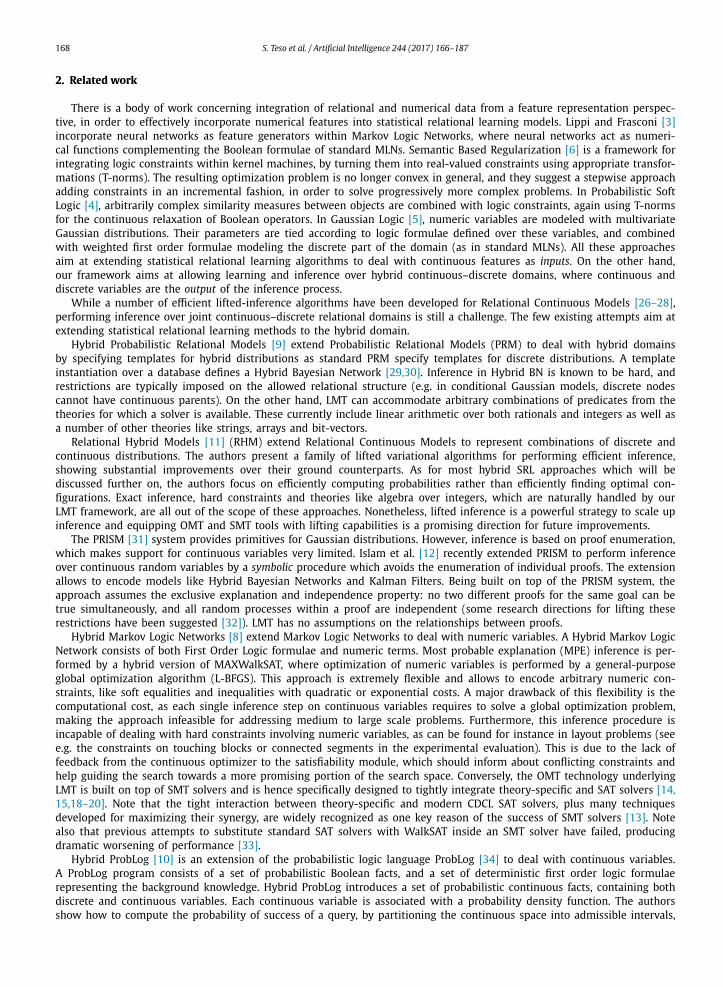
In order to introduce the LMT framework, we start with a toy learning example. We are given a unit-length bounding box, [0, 1] × [0, 1], that contains a given, fixed block (rectangle), as in Fig. 1(a). The block is identified by the four constants (x1, y1, dx1, dy1), where x1, y1 indicate the bottom-left corner of the rectangle, and dx1, dy1 its width and height, respec-tively. Now, suppose that we are assigned the task of fitting another block, identified by the variables (x2, y2, dx2, dy2), in the same bounding box, so as to minimize the following cost function:
cost := w1 × dx2 + w2 × dy2 (1)
with the additional requirements that (i) the two blocks “touch” either from above, below, or sideways, and (ii) the two blocks do not overlap.
It is easy to see that the weights w1 and w2 control the shape and location of the optimal solution. If both weights are positive, then the cost is minimized by any block of null size located along the perimeter of block 1. If both weights are negative and w1 � w2, then the optimal block will be placed so as to occupy as much horizontal space as possible, while if w1 � w2 it will prefer to occupy as much vertical space as possible, as in Fig. 1(b, c). If w1 and w2 are close, then the optimal solution depends on the relative amount of available vertical and horizontal space in the bounding box.
This toy example illustrates two key points. First, the problem involves a mixture of numerical variables (coordinates, sizes of block 2) and Boolean variables, along with hard rules that control the feasible space of the optimization procedure (conditions (i) and (ii)), and costs—or soft rules—which control the shape of the optimization landscape. This is the kind of problem that can be solved in terms of Optimization Modulo Linear Arithmetic, OMT(LRA). Second, it is possible to estimate the weights w1, w2 from data in order to learn what kind of blocks are to be considered optimal. The goal of our learning procedure is precisely to find a good set of weights from examples. In the following we will describe how such a learning task can be framed within the structured output SVMs framework.
S. Teso et al. / Artificial Intelligence 244 (2017) 166–187 171
Fig. 1. (a) Initial configuration. (b) Optimal configuration for w1 � w2. (c) Optimal configuration for w1 � w2.
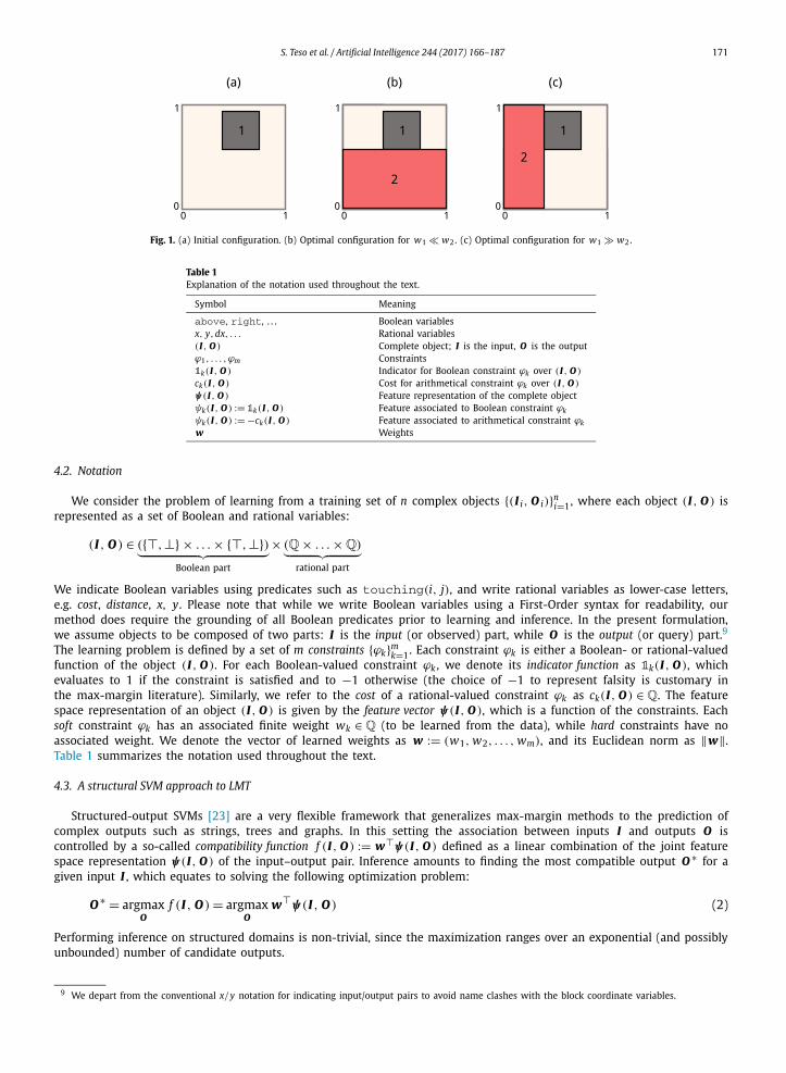
Table 1Explanation of the notation used throughout the text.
Symbol Meaning
above, right, . . . Boolean variablesx, y,dx, . . . Rational variables(I , O ) Complete object; I is the input, O is the outputϕ1, . . . ,ϕm Constraints1k(I , O ) Indicator for Boolean constraint ϕk over (I , O )
ck(I , O ) Cost for arithmetical constraint ϕk over (I , O )
ψ(I , O ) Feature representation of the complete objectψk(I , O ) := 1k(I , O ) Feature associated to Boolean constraint ϕk
ψk(I , O ) := −ck(I , O ) Feature associated to arithmetical constraint ϕk
w Weights
4.2. Notation
We consider the problem of learning from a training set of n complex objects {(I i, O i)}ni=1, where each object (I , O ) is
represented as a set of Boolean and rational variables:
(I , O ) ∈ ({�,⊥} × . . . × {�,⊥})︸ ︷︷ ︸Boolean part
× (Q× . . . ×Q)︸ ︷︷ ︸rational part
We indicate Boolean variables using predicates such as touching(i, j), and write rational variables as lower-case letters, e.g. cost, distance, x, y. Please note that while we write Boolean variables using a First-Order syntax for readability, our method does require the grounding of all Boolean predicates prior to learning and inference. In the present formulation, we assume objects to be composed of two parts: I is the input (or observed) part, while O is the output (or query) part.9
The learning problem is defined by a set of m constraints {ϕk}mk=1. Each constraint ϕk is either a Boolean- or rational-valued
function of the object (I , O ). For each Boolean-valued constraint ϕk , we denote its indicator function as 1k(I , O ), which evaluates to 1 if the constraint is satisfied and to −1 otherwise (the choice of −1 to represent falsity is customary in the max-margin literature). Similarly, we refer to the cost of a rational-valued constraint ϕk as ck(I , O ) ∈ Q. The feature space representation of an object (I , O ) is given by the feature vector ψ(I , O ), which is a function of the constraints. Each soft constraint ϕk has an associated finite weight wk ∈ Q (to be learned from the data), while hard constraints have no associated weight. We denote the vector of learned weights as w := (w1, w2, . . . , wm), and its Euclidean norm as ‖w‖. Table 1 summarizes the notation used throughout the text.
4.3. A structural SVM approach to LMT
Structured-output SVMs [23] are a very flexible framework that generalizes max-margin methods to the prediction of complex outputs such as strings, trees and graphs. In this setting the association between inputs I and outputs O is controlled by a so-called compatibility function f (I , O ) := w�ψ(I , O ) defined as a linear combination of the joint feature space representation ψ(I , O ) of the input–output pair. Inference amounts to finding the most compatible output O ∗ for a given input I , which equates to solving the following optimization problem:
O ∗ = argmaxO
f (I , O ) = argmaxO
w�ψ(I , O ) (2)
Performing inference on structured domains is non-trivial, since the maximization ranges over an exponential (and possibly unbounded) number of candidate outputs.
9 We depart from the conventional x/y notation for indicating input/output pairs to avoid name clashes with the block coordinate variables.

172 S. Teso et al. / Artificial Intelligence 244 (2017) 166–187
Data: Training instances {(I 1, O 1), . . . , (In, O n)}, parameters C , εResult: Learned weights w
1 Wi ← ∅, ξi ← 0 for all i = 1, . . . , n ;2 repeat3 for i = 1, . . . , n do4 O ′
i ← argmaxO ′[�(O i, O ′) − w� (
ψ(I i, O i) − ψ(I i, O ′))]
;5 if �(O i, O ′
i) − w� (ψ(I i, O i) − ψ(I i, O ′
i))> ξ i + ε then
6
Wi ← Wi ∪ {O ′i}
w, ξ ← argminw,ξ≥0
1
2w� w + C
n
n∑i=1
ξi
s.t. ∀O ′1 ∈ W1 : w� [
ψ(I 1, O 1) − ψ(I 1, O ′1)
] ≥�(O i, O ′
1) − ξ1
.
.
.
∀O ′n ∈ Wn : w� [
ψ(In, O n) − ψ(In, O ′n)
] ≥�(O i, O ′
n) − ξn
7 end8 end9 until no Wi has changed during iteration;
10 return w
Algorithm 1: Cutting-plane algorithm for training structural SVMs, according to the n-slack formulation presented in [51].
Learning is formulated within the regularized empirical risk minimization framework. In order to learn the weights from a training set of n examples, one needs to define a non-negative loss function �(I , O , O ′) that, for any given observation I , quantifies the penalty incurred when predicting O ′ instead of the correct output O . Learning can be expressed as the problem of finding the weights w that minimize the per-instance error ξi and the model complexity [23]:
argminw,ξ
1
2‖w‖2 + C
n
n∑i=1
ξi
s.t. w�(ψ(I i, O i) − ψ(I i, O ′)) ≥ �(I i, O i, O ′) − ξi ∀ i = 1, . . . ,n; O ′ �= O i (3)
Here the constraints require that the compatibility between any input I i and its corresponding correct output O i is always higher than that with all wrong outputs O ′ by a margin, with ξi playing the role of per-instance violations. This formulation is called n-slack margin rescaling and it is the original and most accessible formulation of structured-output SVMs. See [51]for an extensive exposition of alternative formulations.
Weight learning is a quadratic program, and can be solved very efficiently with a cutting-plane (CP) algorithm [23]. Since in Eq. (3) there is an exponential number of constraints, it is infeasible to naively account for all of them during learning. Based on the observations that the constraints obey a subsumption relation, the CP algorithm [51] sidesteps the issue by keeping a working set of active constraints W : at each iteration, it augments the working set with the most violated constraint, and then solves the corresponding reduced quadratic program using a standard SVM solver. This procedure is guaranteed to find an ε-approximate solution to the QP in a polynomial number of iterations, independently of the cardinality of the output space and of the number of examples n [23]. The n-slack margin rescaling version of the CP algorithm can be found in Algorithm 1 (adapted from [51]). Please note that in our experiments we make use of the faster, but otherwise equivalent, 1-slack margin rescaling variant [51]. We report the n-slack margin rescaling version here for ease of exposition.
The CP algorithm is generic, meaning that it can be adapted to any structured prediction problem as long as it is provided with: (i) a joint feature space representation ψ of input–output pairs (and consequently a compatibility function f ); (ii) an oracle to perform inference, i.e. to solve Eq. (2); and (iii) an oracle to retrieve the most violated constraint of the QP, i.e. to solve the separation problem:
argmax′
w T ψ(I i, O ′) + �(I i, O i, O ′) (4)
O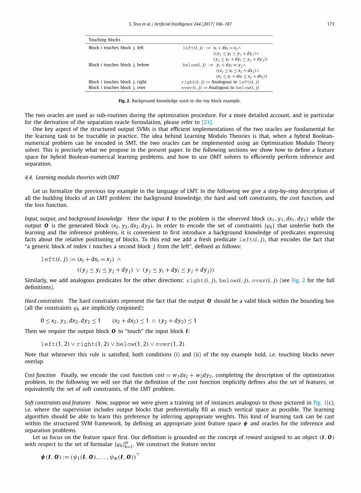
S. Teso et al. / Artificial Intelligence 244 (2017) 166–187 173
Touching blocks
Block i touches block j, left left(i, j) := xi + dxi = x j∧((y j ≤ yi ≤ y j + dy j)∨(y j ≤ yi + dyi ≤ y j + dy j))
Block i touches block j, below below(i, j) := yi + dyi = y j∧((x j ≤ xi ≤ x j + dx j)∨(x j ≤ xi + dxi ≤ x j + dx j))
Block i touches block j, right right(i, j) := Analogous to left(i, j)Block i touches block j, over over(i, j) := Analogous to below(i, j)
Fig. 2. Background knowledge used in the toy block example.
The two oracles are used as sub-routines during the optimization procedure. For a more detailed account, and in particular for the derivation of the separation oracle formulation, please refer to [23].
One key aspect of the structured output SVMs is that efficient implementations of the two oracles are fundamental for the learning task to be tractable in practice. The idea behind Learning Modulo Theories is that, when a hybrid Boolean-numerical problem can be encoded in SMT, the two oracles can be implemented using an Optimization Modulo Theory solver. This is precisely what we propose in the present paper. In the following sections we show how to define a feature space for hybrid Boolean-numerical learning problems, and how to use OMT solvers to efficiently perform inference and separation.
4.4. Learning modulo theories with OMT
Let us formalize the previous toy example in the language of LMT. In the following we give a step-by-step description of all the building blocks of an LMT problem: the background knowledge, the hard and soft constraints, the cost function, and the loss function.
Input, output, and background knowledge Here the input I to the problem is the observed block (x1, y1, dx1, dy1) while the output O is the generated block (x2, y2, dx2, dy2). In order to encode the set of constraints {ϕk} that underlie both the learning and the inference problems, it is convenient to first introduce a background knowledge of predicates expressing facts about the relative positioning of blocks. To this end we add a fresh predicate left(i, j), that encodes the fact that “a generic block of index i touches a second block j from the left”, defined as follows:
left(i, j) := (xi + dxi = x j) ∧((y j ≤ yi ≤ y j + dy j) ∨ (y j ≤ yi + dyi ≤ y j + dy j))
Similarly, we add analogous predicates for the other directions: right(i, j), below(i, j), over(i, j) (see Fig. 2 for the full definitions).
Hard constraints The hard constraints represent the fact that the output O should be a valid block within the bounding box (all the constraints ϕk are implicitly conjoined):
0 ≤ x2, y2,dx2,dy2 ≤ 1 (x2 + dx2) ≤ 1 ∧ (y2 + dy2) ≤ 1
Then we require the output block O to “touch” the input block I :
left(1,2) ∨ right(1,2) ∨ below(1,2) ∨ over(1,2)
Note that whenever this rule is satisfied, both conditions (i) and (ii) of the toy example hold, i.e. touching blocks never overlap.
Cost function Finally, we encode the cost function cost = w1dx2 + w2dy2, completing the description of the optimization problem. In the following we will see that the definition of the cost function implicitly defines also the set of features, or equivalently the set of soft constraints, of the LMT problem.
Soft constraints and features Now, suppose we were given a training set of instances analogous to those pictured in Fig. 1(c), i.e. where the supervision includes output blocks that preferentially fill as much vertical space as possible. The learning algorithm should be able to learn this preference by inferring appropriate weights. This kind of learning task can be cast within the structured SVM framework, by defining an appropriate joint feature space ψ and oracles for the inference and separation problems.
Let us focus on the feature space first. Our definition is grounded on the concept of reward assigned to an object (I , O )
with respect to the set of formulae {ϕk}mk=1. We construct the feature vector
ψ(I , O ) := (ψ1(I , O ), . . . ,ψm(I , O ))�
174 S. Teso et al. / Artificial Intelligence 244 (2017) 166–187
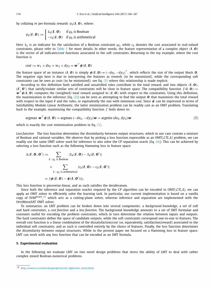
by collating m per-formula rewards ψk(I , O ), where:
ψk(I , O ) :={
1k(I , O ) if ϕk is Boolean
−ck(I , O ) if ϕk is arithmetical
Here 1k is an indicator for the satisfaction of a Boolean constraint ϕk , while ck denotes the cost associated to real-valued constraints, please refer to Table 1 for more details. In other words, the feature representation of a complex object (I , O )
is the vector of all indicator/cost functions associated to the soft constraints. Returning to the toy example, where the cost function is
cost := w1 × dx2 + w2 × dy2 = w�ψ(I , O )
the feature space of an instance (I , O ) is simply ψ(I , O ) = (−dx2,−dy2)� , which reflects the size of the output block O .
The negative sign here is due to interpreting the features as rewards (to be maximized), while the corresponding soft constraints can be seen as costs (to be minimized); see Eq. (5) where this relationship is made explicit.
According to this definition both satisfied and unsatisfied rules contribute to the total reward, and two objects (I , O ), (I ′, O ′) that satisfy/violate similar sets of constraints will be close in feature space. The compatibility function f (I , O ) :=w�ψ(I , O ) computes the (weighted) total reward assigned to (I , O ) with respect to the constraints. Using this definition, the maximization in the inference (Eq. (2)) can be seen as attempting to find the output O that maximizes the total reward with respect to the input I and the rules, or equivalently the one with minimum cost. Since ψ can be expressed in terms of Satisfiability Modulo Linear Arithmetic, the latter minimization problem can be readily cast as an OMT problem. Translating back to the example, maximizing the compatibility function f boils down to:
argmax w�ψ(I , O ) = argmax (−dx2,−dy2)w = argmin (dx2,dy2)w (5)
which is exactly the cost minimization problem in Eq. (1).
Loss function The loss function determines the dissimilarity between output structures, which in our case contain a mixture of Boolean and rational variables. We observe that by picking a loss function expressible as an OMT(LRA) problem, we can readily use the same OMT solver used for inference to also solve the CP separation oracle (Eq. (4)). This can be achieved by selecting a loss function such as the following Hamming loss in feature space:
�(I , O , O ′) :=∑
k : ϕk is Boolean
|1k(I , O ) − 1k(I , O ′)|
+∑
k : ϕk is arithmetical
|ck(I , O ) − ck(I , O ′)|
= ‖ψ(I , O ) − ψ(I , O ′)‖1
This loss function is piecewise-linear, and as such satisfies the desideratum.Since both the inference and separation oracles required by the CP algorithm can be encoded in OMT(LRA), we can
apply an OMT solver to efficiently solve the learning task. In particular, our current implementation is based on a vanilla copy of SVMstruct,10 which acts as a cutting-plane solver, whereas inference and separation are implemented with theOptiMathSAT OMT solver.
To summarize, an LMT problem can be broken down into several components: a background knowledge, a set of soft and hard constraints, a cost function and a loss function. The background knowledge amounts to a set of SMT formulae and constants useful for encoding the problem constraints, which in turn determine the relation between inputs and outputs. The hard constraints define the space of candidate outputs, while the soft constraints correspond one-to-one to features. The overall cost function is a linear combination of the dissatisfaction/cost (or, equivalently, satisfaction/reward) associated to the individual soft constraints, and as such is controlled entirely by the choice of features. Finally, the loss function determines the dissimilarity between output structures. While in the present paper we focused on a Hamming loss in feature space, LMT can work with any loss function that can be encoded as an SMT formula.
5. Experimental evaluation
In the following we evaluate LMT on two novel design problems that stress the ability of LMT to deal with rather complex mixed Boolean-numerical problems.
10 http://www.cs.cornell.edu/people/tj/svm_light/svm_struct.html.
S. Teso et al. / Artificial Intelligence 244 (2017) 166–187 175
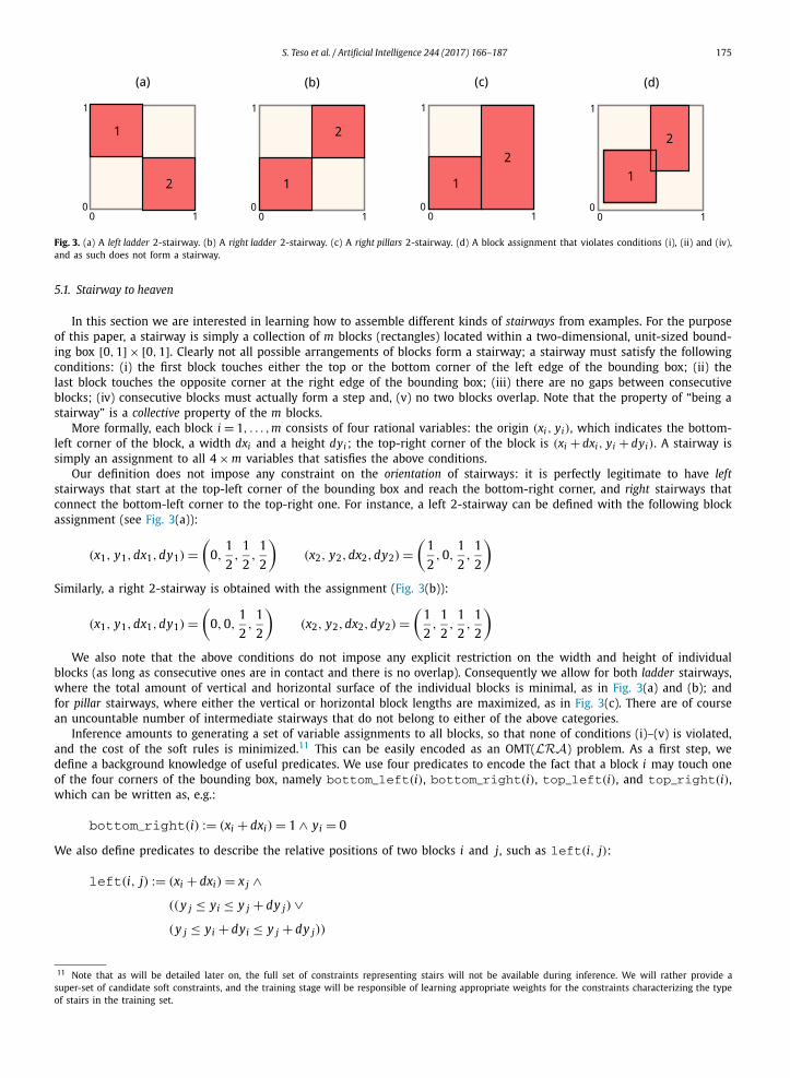
Fig. 3. (a) A left ladder 2-stairway. (b) A right ladder 2-stairway. (c) A right pillars 2-stairway. (d) A block assignment that violates conditions (i), (ii) and (iv), and as such does not form a stairway.
5.1. Stairway to heaven
In this section we are interested in learning how to assemble different kinds of stairways from examples. For the purpose of this paper, a stairway is simply a collection of m blocks (rectangles) located within a two-dimensional, unit-sized bound-ing box [0, 1] × [0, 1]. Clearly not all possible arrangements of blocks form a stairway; a stairway must satisfy the following conditions: (i) the first block touches either the top or the bottom corner of the left edge of the bounding box; (ii) the last block touches the opposite corner at the right edge of the bounding box; (iii) there are no gaps between consecutive blocks; (iv) consecutive blocks must actually form a step and, (v) no two blocks overlap. Note that the property of “being a stairway” is a collective property of the m blocks.
More formally, each block i = 1, . . . , m consists of four rational variables: the origin (xi, yi), which indicates the bottom-left corner of the block, a width dxi and a height dyi ; the top-right corner of the block is (xi + dxi, yi + dyi). A stairway is simply an assignment to all 4 × m variables that satisfies the above conditions.
Our definition does not impose any constraint on the orientation of stairways: it is perfectly legitimate to have leftstairways that start at the top-left corner of the bounding box and reach the bottom-right corner, and right stairways that connect the bottom-left corner to the top-right one. For instance, a left 2-stairway can be defined with the following block assignment (see Fig. 3(a)):
(x1, y1,dx1,dy1) =(
0,1
2,
1
2,
1
2
)(x2, y2,dx2,dy2) =
(1
2,0,
1
2,
1
2
)Similarly, a right 2-stairway is obtained with the assignment (Fig. 3(b)):
(x1, y1,dx1,dy1) =(
0,0,1
2,
1
2
)(x2, y2,dx2,dy2) =
(1
2,
1
2,
1
2,
1
2
)We also note that the above conditions do not impose any explicit restriction on the width and height of individual
blocks (as long as consecutive ones are in contact and there is no overlap). Consequently we allow for both ladder stairways, where the total amount of vertical and horizontal surface of the individual blocks is minimal, as in Fig. 3(a) and (b); and for pillar stairways, where either the vertical or horizontal block lengths are maximized, as in Fig. 3(c). There are of course an uncountable number of intermediate stairways that do not belong to either of the above categories.
Inference amounts to generating a set of variable assignments to all blocks, so that none of conditions (i)–(v) is violated, and the cost of the soft rules is minimized.11 This can be easily encoded as an OMT(LRA) problem. As a first step, we define a background knowledge of useful predicates. We use four predicates to encode the fact that a block i may touch one of the four corners of the bounding box, namely bottom_left(i), bottom_right(i), top_left(i), and top_right(i), which can be written as, e.g.:
bottom_right(i) := (xi + dxi) = 1 ∧ yi = 0
We also define predicates to describe the relative positions of two blocks i and j, such as left(i, j):
left(i, j) := (xi + dxi) = x j ∧((y j ≤ yi ≤ y j + dy j) ∨(y j ≤ yi + dyi ≤ y j + dy j))
11 Note that as will be detailed later on, the full set of constraints representing stairs will not be available during inference. We will rather provide a super-set of candidate soft constraints, and the training stage will be responsible of learning appropriate weights for the constraints characterizing the type of stairs in the training set.
176 S. Teso et al. / Artificial Intelligence 244 (2017) 166–187
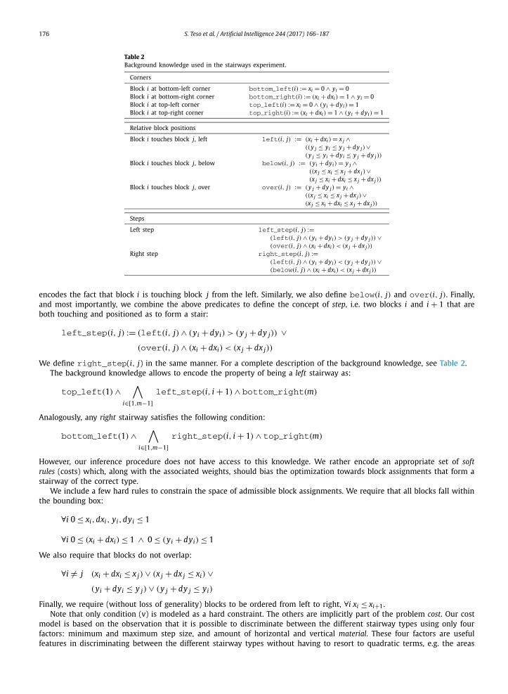
Table 2Background knowledge used in the stairways experiment.
Corners
Block i at bottom-left corner bottom_left(i) := xi = 0 ∧ yi = 0Block i at bottom-right corner bottom_right(i) := (xi + dxi) = 1 ∧ yi = 0Block i at top-left corner top_left(i) := xi = 0 ∧ (yi + dyi) = 1Block i at top-right corner top_right(i) := (xi + dxi) = 1 ∧ (yi + dyi) = 1
Relative block positions
Block i touches block j, left left(i, j) := (xi + dxi) = x j ∧((y j ≤ yi ≤ y j + dy j)∨(y j ≤ yi + dyi ≤ y j + dy j))
Block i touches block j, below below(i, j) := (yi + dyi) = y j ∧((x j ≤ xi ≤ x j + dx j)∨(x j ≤ xi + dxi ≤ x j + dx j))
Block i touches block j, over over(i, j) := (y j + dy j) = yi ∧((x j ≤ xi ≤ x j + dx j)∨(x j ≤ xi + dxi ≤ x j + dx j))
Steps
Left step left_step(i, j) :=(left(i, j) ∧ (yi + dyi) > (y j + dy j)) ∨(over(i, j) ∧ (xi + dxi) < (x j + dx j))
Right step right_step(i, j) :=(left(i, j) ∧ (yi + dyi) < (y j + dy j)) ∨(below(i, j) ∧ (xi + dxi) < (x j + dx j))
encodes the fact that block i is touching block j from the left. Similarly, we also define below(i, j) and over(i, j). Finally, and most importantly, we combine the above predicates to define the concept of step, i.e. two blocks i and i + 1 that are both touching and positioned as to form a stair:
left_step(i, j) := (left(i, j) ∧ (yi + dyi) > (y j + dy j)) ∨(over(i, j) ∧ (xi + dxi) < (x j + dx j))
We define right_step(i, j) in the same manner. For a complete description of the background knowledge, see Table 2.The background knowledge allows to encode the property of being a left stairway as:
top_left(1) ∧∧
i∈[1,m−1]left_step(i, i + 1) ∧ bottom_right(m)
Analogously, any right stairway satisfies the following condition:
bottom_left(1) ∧∧
i∈[1,m−1]right_step(i, i + 1) ∧ top_right(m)
However, our inference procedure does not have access to this knowledge. We rather encode an appropriate set of soft rules (costs) which, along with the associated weights, should bias the optimization towards block assignments that form a stairway of the correct type.
We include a few hard rules to constrain the space of admissible block assignments. We require that all blocks fall within the bounding box:
∀i 0 ≤ xi,dxi, yi,dyi ≤ 1
∀i 0 ≤ (xi + dxi) ≤ 1 ∧ 0 ≤ (yi + dyi) ≤ 1
We also require that blocks do not overlap:
∀i �= j (xi + dxi ≤ x j) ∨ (x j + dx j ≤ xi) ∨(yi + dyi ≤ y j) ∨ (y j + dy j ≤ yi)
Finally, we require (without loss of generality) blocks to be ordered from left to right, ∀i xi ≤ xi+1.Note that only condition (v) is modeled as a hard constraint. The others are implicitly part of the problem cost. Our cost
model is based on the observation that it is possible to discriminate between the different stairway types using only four factors: minimum and maximum step size, and amount of horizontal and vertical material. These four factors are useful features in discriminating between the different stairway types without having to resort to quadratic terms, e.g. the areas

S. Teso et al. / Artificial Intelligence 244 (2017) 166–187 177
Table 3List of all rules used in the stairway problem. Top, hard rules affect both the inference and separation procedures. Middle, soft rules (costs), whose weight is learned from data. Bottom, the total cost of a stairway instance is the weighted sum of all individual soft constraints.
(a) Hard constraints
Bounding box ∀i 0 ≤ xi + dxi ≤ 1 ∧0 ≤ yi + dyi ≤ 1
No overlap ∀i �= j (xi + dxi ≤ x j) ∨ (x j + dx j ≤ xi)∨(yi + dyi ≤ y j) ∨ (y j + dy j ≤ yi)
Blocks left to right ∀i xi ≤ xi+1
(b) Soft constraints (features)
Max step height left maxshl = m × maxi(yi + dyi) − (yi+1 + dyi+1)
Min step height left minshl = m × mini(yi + dyi) − (yi+1 + dyi+1)
Max step height right maxshr = m × maxi(yi+1 + dyi+1) − (yi + dyi)
Min step height right minshr = m × mini(yi+1 + dyi+1) − (yi + dyi)
Max step width left maxswl = m × maxi(xi+1 + dxi+1) − (xi + dxi)
Min step width left minswl = m × mini(xi+1 + dxi+1) − (xi + dxi)
Max step width right maxswr = m × maxi(xi + dxi) − (xi+1 + dxi+1)
Min step width right minswr = m × mini(xi + dxi) − (xi+1 + dxi+1)
Vertical material vmat = 1m
∑i dyi
Horizontal material hmat = 1m
∑i dxi
(c) Cost
cost := (maxshl,minshl,maxshr,minshr,maxswl,minswl,maxswr,minswr,vmat,hmat) w
of the individual blocks. For instance, in the cost we account for both the maximum step height of all left steps (a good stairway should not have too high steps):
maxshl = m × maxi∈[1,m−1]
{(yi + dyi) − (yi+1 + dyi+1) if i, i + 1 form a left step1 otherwise
and the minimum step width of all right steps (good stairways should have sufficiently large steps):
minswr = m × mini∈[1,m−1]
{(xi+1 + dxi+1) − (xi + dxi) if i, i + 1 form a right step0 otherwise
The value of these costs depends on whether a pair of blocks actually forms a left step, a right step, or no step at all. Note that these costs are multiplied by the number of blocks m. This allows to renormalize costs according to the number of steps; e.g. the step height of a stairway with m uniform steps is half that of a stairway with m/2 steps. Finally, we write the average amount of vertical material as vmat = 1
m
∑i dyi . All the other costs can be written similarly; see Table 3 for the
complete list. As we will see, the normalization of individual costs allows to learn weights which generalize to stairways with a larger number of blocks with respect to those seen during training.
Putting all the pieces together, the complete cost is:
cost := (maxshl,minshl,maxshr,minshr,
maxswl,minswl,maxswr,minswr,
vmat,hmat) w
Minimizing the weighted cost implicitly requires the inference engine to decide whether it is preferable to generate a left or a right stairway, thanks to the minshl, . . . , minswr components, and whether the stairway should be a ladder or pillar, due to vmat and hmat. The actual weights are learned, allowing the learnt model to reproduce whichever stairway type is present in the training data.
To test the stairway scenario, we focused on learning one model for each of six kinds of stairway: left ladder, right ladder, left pillar and right pillar with a preference for horizontal blocks, and left pillar and right pillar with vertical blocks. In this setting, the input I is empty, and the model should generate all m blocks as output O during test.
We generated “perfect” stairways of 2 to 6 blocks for each stairway type to be used as training instances. We then learned a model using all training instances up to a fixed number of blocks: a model using examples with up to 3 blocks, another with examples of up to 4, etc., for a total of 4 models per stairway type. Then we analyzed the generalization ability of the learnt models by generating stairways with a larger number of blocks (up to 10) than those in the training set. The results can be found in Fig. 4.

178 S. Teso et al. / Artificial Intelligence 244 (2017) 166–187
Fig. 4. Results for the stairway construction problem. From top to bottom: results for the ladder, horizontal pillar, and vertical pillar cases. Images in row labeled with N picture the stairways generated by a model learnt on a training set of perfect stairways made of 2, 3, . . . , N steps, with a varying number of generated blocks. (Best viewed in color.)
The experiment shows that LMT is able to solve the stairway construction problem, and can learn appropriate models for all stairway types, as expected. As can be seen in Fig. 4, the generated stairways can present some imperfections when the training set is too small (e.g., only two training examples; first row of each table), especially in the 10 output blocks case. However, the situation quickly improves when the training set increases: models learned with four training examples are always able to produce perfect 10-block stairways of the same kind. Note again that the learner has no explicit notion of what a stairway is, but just the values of step width, height and material for some training examples of stairways.
All in all, albeit simple, this experiment showcases the ability of LMT to handle learning in hybrid Boolean-numerical domains, whereas other formalisms are not particularly suited for the task. As previously mentioned, the Church [7] lan-guage allows to encode arbitrary constraints over both numeric and Boolean variables. The stairway problem can indeed be encoded in Church in a rather straightforward way. However, the sampling strategies used for inference are not conceived for performing optimization with hard continuous constraints. Even the simple task of generating two blocks, conditioned on the fact that they form a step, is prohibitively expensive.12
5.2. Learning to draw characters
In this section we are concerned with automatic character drawing, a novel structured-output learning problem that consists in learning to translate any input noisy hand-drawn character into its symbolic representation. More specifically, given an unlabeled black-and-white image of a handwritten letter or digit, the goal is to construct an equivalent vectorialrepresentation of the same character.
In this paper, we assume the character to be representable by a polyline made of a given number m of directed segments, i.e. segments identified by a starting point (xb, yb) and an ending point (xe, ye). The input image I is seen as the set P of coordinates of the pixels belonging to the character, while the output O is a set of m directed segments {(xb
i , ybi , x
ei , y
ei )}m
i=1. Just like in the previous section, we assume all coordinates to fall within the unit bounding box.
12 We interrupted the inference process after 24 hours of computation.
S. Teso et al. / Artificial Intelligence 244 (2017) 166–187 179
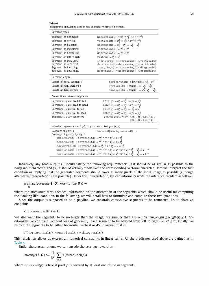
Table 4Background knowledge used in the character writing experiment.
Segment types
Segment i is horizontal horizontal(i) := (xbi �= xe
i ) ∧ (y = ybi )
Segment i is vertical vertical(i) := (xbi = xe
i ) ∧ (yei �= yb
i )
Segment i is diagonal diagonal(i) := |xei − xb
i | = |yei − yb
i |Segment i is increasing increasing(i) := ye
i > ybi
Segment i is decreasing decreasing(i) := yei < yb
i
Segment i is left-to-right right(i) := xei > xb
i
Segment i is incr. vert. incr_vert(i) := increasing(i) ∧ vertical(i)Segment i is decr. vert. decr_vert(i) := decreasing(i) ∧ vertical(i)Segment i is incr. diag. incr_diag(i) := increasing(i) ∧ diagonal(i)Segment i is decr. diag. decr_diag(i) := decreasing(i) ∧ diagonal(i)
Segment length
Length of horiz. segment i horizontal(i) → length(i) = |xei − xb
i |Length of vert. segment i vertical(i) → length(i) = |ye
i − ybi |
Length of diag. segment i diagonal(i) → length(i) = √2 |ye
i − ybi |
Connections between segments
Segments i, j are head-to-tail h2t(i, j) := (xei = xb
j ) ∧ (yei = yb
j )
Segments i, j are head-to-head h2h(i, j) := (xei = xe
j) ∧ (yei = ye
j)
Segments i, j are tail-to-tail t2t(i, j) := (xbi = xb
j ) ∧ (ybi = yb
j )
Segments i, j are tail-to-head t2h(i, j) := (xbi = xe
j) ∧ (ybi = ye
j)
Segments i, j are connected connected(i, j) := h2h(i, j) ∨ h2t(i, j)∨t2h(i, j) ∨ t2t(i, j)
Whether segment i = (xb, yb, xe, ye) covers pixel p = (x, y)
Coverage of pixel p covered(p) := ∨i covered(p, i)
Coverage of pixel p by seg. iincr_vert(i) → covered(p, i) := yb
i ≤ y ≤ yei ∧ x = xb
i
decr_vert(i) → covered(p, i) := yei ≤ y ≤ yb
i ∧ x = xbi
horizontal(i) → covered(p, i) := xbi ≤ x ≤ xe
i ∧ y = ybi
incr_diag(i) → covered(p, i) := ybi ≤ y ≤ ye
i ∧ xbi ≤ x ≤ xe
i ∧ xbi − yb
i = x − y
decr_diag(i) → covered(p, i) := yei ≤ y ≤ yb
i ∧ xbi ≤ x ≤ xe
i ∧ xbi + yb
i = x + y
Intuitively, any good output O should satisfy the following requirements: (i) it should be as similar as possible to the noisy input character; and (ii) it should actually “look like” the corresponding vectorial character. Here we interpret the first condition as implying that the generated segments should cover as many pixels of the input image as possible (although alternative interpretations are possible). Under this interpretation, we can informally write the inference problem as follows:
argmaxO
(coverage(I , O ),orientation(O )) w
where the orientation term encodes information on the orientation of the segments which should be useful for computing the “looking like” condition. In the following, we will detail how to formulate and compute these two quantities.
Since the output is supposed to be a polyline, we constrain consecutive segments to be connected, i.e. to share an endpoint:
∀i connected(i, i + 1)
We also want the segments to be no larger than the image, nor smaller than a pixel: ∀i min_length ≤ length(i) ≤ 1. Ad-ditionally, we constrain (without loss of generality) each segment to be ordered from left to right, i.e. xb
i ≤ xei . Finally, we
restrict the segments to be either horizontal, vertical or 45◦ diagonal, that is:
∀i horizontal(i) ∨ vertical(i) ∨ diagonal(i)
This restriction allows us express all numerical constraints in linear terms. All the predicates used above are defined as in Table 4.
Under these assumptions, we can encode the coverage reward as:
coverage(I , O ) := 1
|P |∑p∈P
1(covered(p))
where covered(p) is true if pixel p is covered by at least one of the m segments:
180 S. Teso et al. / Artificial Intelligence 244 (2017) 166–187
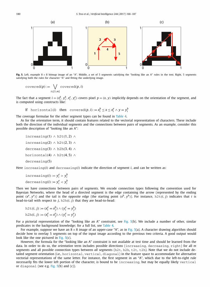
Fig. 5. Left, example 8 × 8 bitmap image of an “A”. Middle, a set of 5 segments satisfying the “looking like an A” rules in the text. Right, 5 segments satisfying both the rules for character “A” and fitting the underlying image.
covered(p) :=∨
i∈[1,m]covered(p, i)
The fact that a segment i = (xbi , y
bi , x
ei , y
ei ) covers pixel p = (x, y) implicitly depends on the orientation of the segment, and
is computed using constructs like:
If horizontal(i) then covered(p, i) := xbi ≤ x ≤ xe
i ∧ y = ybi
The coverage formulae for the other segment types can be found in Table 4.As for the orientation term, it should contain features related to the vectorial representation of characters. These include
both the direction of the individual segments and the connections between pairs of segments. As an example, consider this possible description of “looking like an A”:
increasing(1) ∧ h2t(1,2) ∧increasing(2) ∧ h2t(2,3) ∧decreasing(3) ∧ h2h(3,4) ∧horizontal(4) ∧ h2t(4,5) ∧decreasing(5)
Here increasing(i) and decreasing(i) indicate the direction of segment i, and can be written as:
increasing(i) := yei > yb
i
decreasing(i) := yei < yb
i
Then we have connections between pairs of segments. We encode connection types following the convention used for Bayesian Networks, where the head of a directed segment is the edge containing the arrow (represented by the ending point (xe, ye)) and the tail is the opposite edge (the starting point (xb, yb)). For instance, h2t(i, j) indicates that i is head-to-tail with respect to j, h2h(i, j) that they are head-to-head:
h2t(i, j) := (xei = xb
j ) ∧ (yei = yb
j )
h2h(i, j) := (xei = xe
j) ∧ (yei = ye
j)
For a pictorial representation of the “looking like an A” constraint, see Fig. 5(b). We include a number of other, similar predicates in the background knowledge; for a full list, see Table 4.
For example, suppose we have an 8 × 8 image of an upper-case “A”, as in Fig. 5(a). A character drawing algorithm should decide how to overlay 5 segments on top of the input image according to the previous two criteria. A good output would look like the one pictured in Fig. 5(c).
However, the formula for the “looking like an A” constraint is not available at test time and should be learned from the data. In order to do so, the orientation term includes possible directions (increasing, decreasing, right) for all msegments and all possible connection types between all segments (h2t, h2h, t2t, t2h). Note that we do not include de-tailed segment orientation (i.e., horizontal, vertical, diagonal) in the feature space to accommodate for alternative vectorial representations of the same letter. For instance, the first segment in an “A”, which due to the left-to-right rule necessarily fits the lower left portion of the character, is bound to be increasing, but may be equally likely verticalor diagonal (see e.g. Fig. 5(b) and (c)).
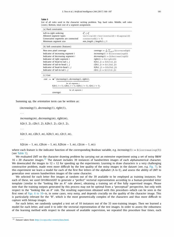
S. Teso et al. / Artificial Intelligence 244 (2017) 166–187 181
Table 5List of all rules used in the character writing problem. Top, hard rules. Middle, soft rules (costs). Bottom, total cost of a segment assignment.
(a) Hard constraints
Left-to-right ordering xbi ≤ xe
iAllowed segment types vertical(i) ∨ horizontal(i) ∨ diagonal(i)Consecutive segments are connected connected(i, i + 1)
Minimum segment size min_length ≤ length(i) ≤ 1
(b) Soft constraints (features)
Non-zero pixel coverage coverage := 1|P |
∑p∈P 1(covered(p))
Indicator of increasing segment i increasing(i) := 1(increasing(i))Indicator of decreasing segment i decreasing(i) := 1(decreasing(i))Indicator of right segment i right(i) := 1(right(i))Indicator of head-to-tail i, j h2t(i, j) := 1(h2t(i, j))Indicator of tail-to-head i, j t2h(i, j) := 1(t2h(i, j))Indicator of head-to-head i, j h2h(i, j) := 1(h2h(i, j))Indicator of tail-to-tail i, j t2t(i, j) := 1(t2t(i, j))
(c) Cost
cost := w�(increasing(i),decreasing(i), right(i)︸ ︷︷ ︸for all segments i
,
h2t(i, i + 1), t2h(i, i + 1),h2h(i, i + 1), t2t(i, i + 1)︸ ︷︷ ︸for all segments i
,
coverage)
Summing up, the orientation term can be written as:
(increasing(1),decreasing(1), right(1),
· · ·increasing(m),decreasing(m), right(m),
h2t(1,2), t2h(1,2),h2h(1,2), t2t(1,2),
· · ·h2t(1,m), t2h(1,m),h2h(1,m), t2t(1,m),
· · ·h2t(m − 1,m), t2h(m − 1,m),h2h(m − 1,m), t2t(m − 1,m))
where each feature is the indicator function of the corresponding Boolean variable, e.g. increasing(1) := 1(increasing(1))
(see Table 5).We evaluated LMT on the character drawing problem by carrying out an extensive experiment using a set of noisy B&W
16 × 20 character images.13 The dataset includes 39 instances of handwritten images of each alphanumerical character. We downscaled the images to 12 × 12 for speeding up the experiments. Learning to draw characters is a very challenging constructive problem, made even more difficult by the low quality of the noisy images in the dataset (see, e.g. Fig. 7). In this experiment we learn a model for each of the first five letters of the alphabet (A to E), and assess the ability of LMT to generalize over unseen handwritten images of the same character.
We selected for each letter five images at random out of the 39 available to be employed as training instances. For each of these, we used OptiMathSAT to generate a “perfect” vectorial representation according to a human-provided letter template (similar to the “looking like an A” rule above), obtaining a training set of five fully supervised images. Please note that the training outputs generated by this process may not be optimal from a “perceptual” perspective, but only with respect to the “looking like an A” rule. The resulting supervision obtained with this procedure—which can be seen in the first rows of Figs. 6 to 10—is, in some cases, very noisy, and depends crucially on the quality of the character image. This is particularly relevant for the “B”, which is the most geometrically complex of the characters and thus more difficult to capture with bitmap images.
For each letter, we randomly sampled a test set of 10 instances out of the 33 non-training images. Then we learned a model for each letter, and used it to infer the vectorial representation of the test images. In order to assess the robustness of the learning method with respect to the amount of available supervision, we repeated this procedure four times, each
13 Dataset taken from http://cs.nyu.edu/~roweis/data.html.
182 S. Teso et al. / Artificial Intelligence 244 (2017) 166–187
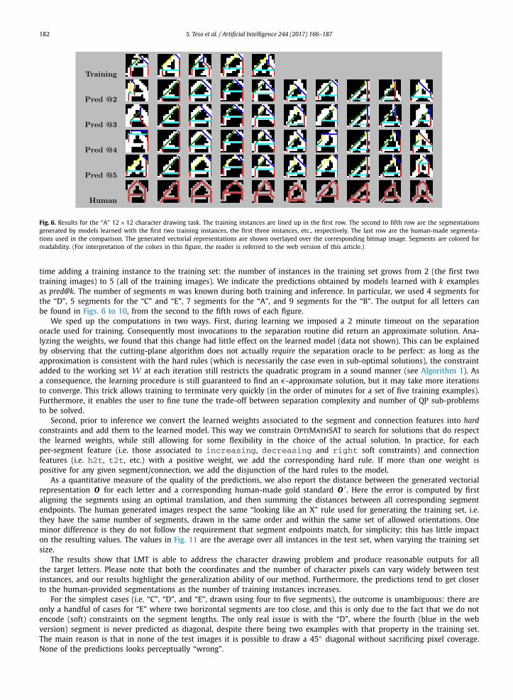
Fig. 6. Results for the “A” 12 × 12 character drawing task. The training instances are lined up in the first row. The second to fifth row are the segmentations generated by models learned with the first two training instances, the first three instances, etc., respectively. The last row are the human-made segmenta-tions used in the comparison. The generated vectorial representations are shown overlayed over the corresponding bitmap image. Segments are colored for readability. (For interpretation of the colors in this figure, the reader is referred to the web version of this article.)
time adding a training instance to the training set: the number of instances in the training set grows from 2 (the first two training images) to 5 (all of the training images). We indicate the predictions obtained by models learned with k examples as pred@k. The number of segments m was known during both training and inference. In particular, we used 4 segments for the “D”, 5 segments for the “C” and “E”, 7 segments for the “A”, and 9 segments for the “B”. The output for all letters can be found in Figs. 6 to 10, from the second to the fifth rows of each figure.
We sped up the computations in two ways. First, during learning we imposed a 2 minute timeout on the separation oracle used for training. Consequently most invocations to the separation routine did return an approximate solution. Ana-lyzing the weights, we found that this change had little effect on the learned model (data not shown). This can be explained by observing that the cutting-plane algorithm does not actually require the separation oracle to be perfect: as long as the approximation is consistent with the hard rules (which is necessarily the case even in sub-optimal solutions), the constraint added to the working set W at each iteration still restricts the quadratic program in a sound manner (see Algorithm 1). As a consequence, the learning procedure is still guaranteed to find an ε-approximate solution, but it may take more iterations to converge. This trick allows training to terminate very quickly (in the order of minutes for a set of five training examples). Furthermore, it enables the user to fine tune the trade-off between separation complexity and number of QP sub-problems to be solved.
Second, prior to inference we convert the learned weights associated to the segment and connection features into hardconstraints and add them to the learned model. This way we constrain OptiMathSAT to search for solutions that do respect the learned weights, while still allowing for some flexibility in the choice of the actual solution. In practice, for each per-segment feature (i.e. those associated to increasing, decreasing and right soft constraints) and connection features (i.e. h2t, t2t, etc.) with a positive weight, we add the corresponding hard rule. If more than one weight is positive for any given segment/connection, we add the disjunction of the hard rules to the model.
As a quantitative measure of the quality of the predictions, we also report the distance between the generated vectorial representation O for each letter and a corresponding human-made gold standard O ′ . Here the error is computed by first aligning the segments using an optimal translation, and then summing the distances between all corresponding segment endpoints. The human generated images respect the same “looking like an X” rule used for generating the training set, i.e. they have the same number of segments, drawn in the same order and within the same set of allowed orientations. One minor difference is they do not follow the requirement that segment endpoints match, for simplicity; this has little impact on the resulting values. The values in Fig. 11 are the average over all instances in the test set, when varying the training set size.
The results show that LMT is able to address the character drawing problem and produce reasonable outputs for all the target letters. Please note that both the coordinates and the number of character pixels can vary widely between test instances, and our results highlight the generalization ability of our method. Furthermore, the predictions tend to get closer to the human-provided segmentations as the number of training instances increases.
For the simplest cases (i.e. “C”, “D”, and “E”, drawn using four to five segments), the outcome is unambiguous: there are only a handful of cases for “E” where two horizontal segments are too close, and this is only due to the fact that we do not encode (soft) constraints on the segment lengths. The only real issue is with the “D”, where the fourth (blue in the web version) segment is never predicted as diagonal, despite there being two examples with that property in the training set. The main reason is that in none of the test images it is possible to draw a 45◦ diagonal without sacrificing pixel coverage. None of the predictions looks perceptually “wrong”.

S. Teso et al. / Artificial Intelligence 244 (2017) 166–187 183
Fig. 7. Results for the “B” 12 × 12 character drawing task.
Fig. 8. Results for the “C” 12 × 12 character drawing task.
Fig. 9. Results for the “D” 12 × 12 character drawing task.
184 S. Teso et al. / Artificial Intelligence 244 (2017) 166–187
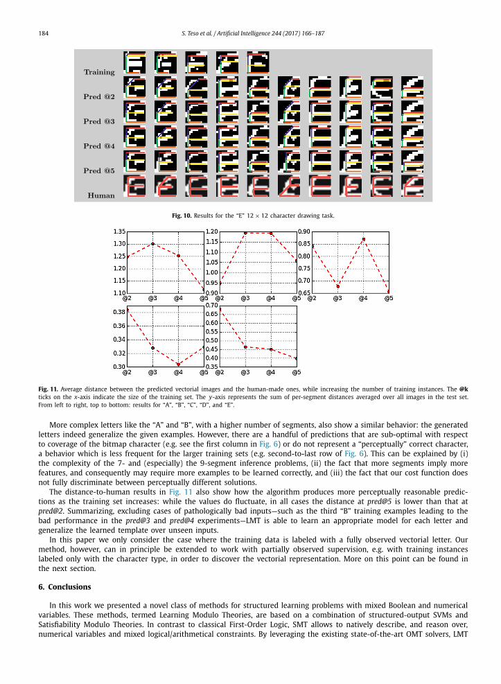
Fig. 10. Results for the “E” 12 × 12 character drawing task.
Fig. 11. Average distance between the predicted vectorial images and the human-made ones, while increasing the number of training instances. The @kticks on the x-axis indicate the size of the training set. The y-axis represents the sum of per-segment distances averaged over all images in the test set. From left to right, top to bottom: results for “A”, “B”, “C”, “D”, and “E”.
More complex letters like the “A” and “B”, with a higher number of segments, also show a similar behavior: the generated letters indeed generalize the given examples. However, there are a handful of predictions that are sub-optimal with respect to coverage of the bitmap character (e.g. see the first column in Fig. 6) or do not represent a “perceptually” correct character, a behavior which is less frequent for the larger training sets (e.g. second-to-last row of Fig. 6). This can be explained by (i) the complexity of the 7- and (especially) the 9-segment inference problems, (ii) the fact that more segments imply more features, and consequently may require more examples to be learned correctly, and (iii) the fact that our cost function does not fully discriminate between perceptually different solutions.
The distance-to-human results in Fig. 11 also show how the algorithm produces more perceptually reasonable predic-tions as the training set increases: while the values do fluctuate, in all cases the distance at pred@5 is lower than that at pred@2. Summarizing, excluding cases of pathologically bad inputs—such as the third “B” training examples leading to the bad performance in the pred@3 and pred@4 experiments—LMT is able to learn an appropriate model for each letter and generalize the learned template over unseen inputs.
In this paper we only consider the case where the training data is labeled with a fully observed vectorial letter. Our method, however, can in principle be extended to work with partially observed supervision, e.g. with training instances labeled only with the character type, in order to discover the vectorial representation. More on this point can be found in the next section.
6. Conclusions
In this work we presented a novel class of methods for structured learning problems with mixed Boolean and numerical variables. These methods, termed Learning Modulo Theories, are based on a combination of structured-output SVMs and Satisfiability Modulo Theories. In contrast to classical First-Order Logic, SMT allows to natively describe, and reason over, numerical variables and mixed logical/arithmetical constraints. By leveraging the existing state-of-the-art OMT solvers, LMT

S. Teso et al. / Artificial Intelligence 244 (2017) 166–187 185
is well-suited for dealing with hybrid constructive learning problems, avoiding the combinatorial explosion of the state space that would affect an equivalent FOL formulation.
Experimental results on both artificial and real world datasets show the potential of this approach. The stairway appli-cation is a simple instance of a layout problem, where the task is to find an optimal layout subject to a set of constraints. Automated or interactive layout synthesis has a broad range of potential applications, including urban pattern layout [52], decorative mosaics [53] and furniture arrangement [54–56]. Note that many spatial constraints can be encoded in terms of relationships between blocks [54]. Existing approaches typically design an energy function to be minimized by stochastic search. Our approach suggests how to automatically identify the relevant constraints and their respective weights, and can accommodate hard constraints and exact search. This is especially relevant for water-tight layouts [57], where the whole space needs to be filled (i.e. no gaps or overlaps) by deforming basic elements from a predetermined set of templates (as in residential building layout [58]). The character drawing application shows how to learn symbolic representations from a handful of very noisy training instances. Deep generative networks have been previously used for similar tasks, see for instance the work by Hinton [59] on generating images of digits with Deep Boltzmann Machines. However, these methods do not learn symbolic representations for characters and generate bitmaps rather than vectorial representations. Further-more, they require thousands of training examples to be learned. Recent extensions have been developed addressing the problem of learning from few [60] or even single [61] examples, but they focus on clean images of the target symbols. Gen-erally speaking, the LMT framework allows to introduce a learning stage in all application domains where SMT and OMT approaches have shown their potential, ranging, e.g., from hardware and software verification [62,63,39], to engineering of chemical reactions [64] and synthetic biology [65].
This work can be extended in a number of directions. First, the current formulation assumes knowledge of the desired output for training examples. This requirement can be loosened by introducting latent variables for the unobserved part of the output, to be maximized over during training [66]. Second, OMT is currently limited to quantifier free formulae and linear algebra for what concerns numeric theories. The former requires to ground all predicates before performing inference, while the latter prevents the formulation of non-linear constraints, e.g. on areas and Euclidean distances. Some attempts to extend SMT solvers to quantified formulae [48–50] and to non-linear arithmetic [67–69] have been presented in the litera-ture; although the state of the art of these extensions is not yet satisfactory in terms of efficiency, since they can currently handle problems which are much smaller—in terms of size, number of variables and of arithmetical operations—than the quantifier-free problems with linear constraints at the reach of current SMT solvers, these techniques are evolving rapidly and promise rapid improvements in terms of performances in the next few years; hence, we can rather easily extend our framework in these directions as soon as the underlying SMT technology is mature enough. Finally, LMT is currently focused on the task of finding the maximal configuration, and cannot compute marginal probabilities. We are planning to introduce support for probability computation by leveraging ideas from weighted model counting [70].
Acknowledgements
We would like to thank Luc De Raedt, Guy Van den Broeck and Bernd Gutmann for useful discussions, and Patrick Trentin for his support with the usage of OptiMathSAT. S. Teso has been partially supported by OKKAM srl as part of the S.I.C.Ra.S. project (Sistema Integrato di Conoscenza e Rappresentazione Semantica), Autonomous Province of Trento, Legge 6/1999, DD n. 251. R. Sebastiani is supported by Semiconductor Research Corporation (SRC) under GRC Research Project 2012-TJ-2266 WOLF.
References
[1] L. Getoor, B. Taskar, Introduction to Statistical Relational Learning, The MIT Press, 2007.[2] G.H. Bakir, T. Hofmann, B. Schölkopf, A.J. Smola, B. Taskar, S.V.N. Vishwanathan, Predicting Structured Data (Neural Information Processing), The MIT
Press, 2007.[3] M. Lippi, P. Frasconi, Prediction of protein-residue contacts by Markov logic networks with grounding-specific weights, Bioinformatics 25 (2009)
2326–2333.[4] M. Broecheler, L. Mihalkova, L. Getoor, Probabilistic similarity logic, in: Uncertainty in Artificial Intelligence, UAI, 2010, pp. 73–82.[5] O. Kuželka, A. Szabóvá, M. Holec, F. Železný, Gaussian logic for predictive classification, in: D. Gunopulos, T. Hofmann, D. Malerba, M. Vazirgiannis
(Eds.), Machine Learning and Knowledge Discovery in Databases, in: Lecture Notes in Computer Science, vol. 6912, Springer, Berlin, Heidelberg, 2011, pp. 277–292.
[6] M. Diligenti, M. Gori, M. Maggini, L. Rigutini, Bridging logic and kernel machines, Mach. Learn. 86 (2012) 57–88.[7] N.D. Goodman, V.K. Mansinghka, D.M. Roy, K. Bonawitz, J.B. Tenenbaum, Church: a language for generative models, in: D.A. McAllester, P. Myllymäki
(Eds.), UAI, AUAI Press, 2008, pp. 220–229.[8] J. Wang, P. Domingos, Hybrid Markov logic networks, in: Proceedings of the 23rd National Conference on Artificial Intelligence, vol. 2, AAAI’08, AAAI
Press, 2008, pp. 1106–1111.[9] P. Nrman, M. Buschle, J. Knig, P. Johnson, Hybrid probabilistic relational models for system quality analysis, in: EDOC, IEEE Computer Society, 2010,
pp. 57–66.[10] B. Gutmann, M. Jaeger, L. De Raedt, Extending ProbLog with continuous distributions, in: P. Frasconi, F. Lisi (Eds.), Inductive Logic Programming, in:
Lecture Notes in Computer Science, vol. 6489, Springer, Berlin, Heidelberg, 2011, pp. 76–91.[11] J. Choi, E. Amir, Lifted relational variational inference, in: N. de Freitas, K.P. Murphy (Eds.), Proceedings of the Twenty-Eighth Conference on Uncertainty
in Artificial Intelligence, UAI’12, AUAI Press, 2012, pp. 196–206.[12] M.A. Islam, C.R. Ramakrishnan, I.V. Ramakrishnan, Inference in probabilistic logic programs with continuous random variables, Theory Pract. Log.
Program. 12 (2012) 505–523.

186 S. Teso et al. / Artificial Intelligence 244 (2017) 166–187
[13] C. Barrett, R. Sebastiani, S.A. Seshia, C. Tinelli, Satisfiability modulo theories, in: [38], pp. 825–885.[14] R. Nieuwenhuis, A. Oliveras, On SAT modulo theories and optimization problems, in: Proc. Theory and Applications of Satisfiability Testing, SAT 2006,
in: Lecture Notes in Computer Science, vol. 4121, Springer, 2006.[15] A. Cimatti, A. Franzén, A. Griggio, R. Sebastiani, C. Stenico, Satisfiability modulo the theory of costs: foundations and applications, in: Proc. Tools and
Algorithms for the Construction and Analysis of Systems, TACAS, in: Lecture Notes in Computer Science, vol. 6015, Springer, 2010, pp. 99–113.[16] A. Cimatti, A. Griggio, B.J. Schaafsma, R. Sebastiani, A modular approach to MaxSAT modulo theories, in: International Conference on Theory and
Applications of Satisfiability Testing, SAT, in: Lecture Notes in Computer Science, vol. 7962, Springer, 2013.[17] C.M. Li, F. Manyà, MaxSAT, hard and soft constraints, in: [38], pp. 613–631.[18] R. Sebastiani, S. Tomasi, Optimization in SMT with LA(Q) cost functions, in: Proc. International Joint Conference on Automated Reasoning, IJCAR, in:
LNAI, vol. 7364, Springer, 2012, pp. 484–498.[19] R. Sebastiani, S. Tomasi, Optimization modulo theories with linear rational costs, ACM Trans. Comput. Log. 16 (2) (2015) 12.[20] Y. Li, A. Albarghouthi, Z. Kincad, A. Gurfinkel, M. Chechik, Symbolic optimization with SMT solvers, in: Proceedings of the 41st ACM SIGPLAN–SIGACT
Symposium on Principles of Programming Languages, POPL ’14, ACM, New York, NY, USA, 2014, pp. 607–618.[21] R. Sebastiani, P. Trentin, Pushing the envelope of optimization modulo theories with linear-arithmetic cost functions, in: Proc. Int. Conference on Tools
and Algorithms for the Construction and Analysis of Systems, TACAS’15, in: Lecture Notes in Computer Science, vol. 9035, Springer, 2015.[22] N. Bjorner, A.-D. Phan, ν Z – maximal satisfaction with Z3, in: Proc. International Symposium on Symbolic Computation in Software Science, EasyChair
Proceedings in Computing, EPiC, Gammart, Tunisia, 2014, http://www.easychair.org/publications/?page=862275542.[23] I. Tsochantaridis, T. Joachims, T. Hofmann, Y. Altun, Large margin methods for structured and interdependent output variables, J. Mach. Learn. Res. 6
(2005) 1453–1484.[24] T. Joachims, T. Hofmann, Y. Yue, C.-N. Yu, Predicting structured objects with support vector machines, Commun. ACM 52 (2009) 97–104.[25] P. Campigotto, A. Passerini, R. Battiti, Active learning of combinatorial features for interactive optimization, in: Proceedings of the 5th Learning and
Intelligent OptimizatioN Conference, LION V, Rome, Italy, Jan 17–21, 2011, in: Lecture Notes in Computer Science, Springer-Verlag, 2011.[26] J. Choi, D. Hill, E. Amir, Lifted inference for relational continuous models, in: Proceedings of the Twenty-Sixth Conference on Uncertainty in Artificial
Intelligence, UAI’10, 2010.[27] J. Choi, A. Guzmn-Rivera, E. Amir, Lifted relational Kalman filtering, in: Proceedings of IJCAI’11, 2011, pp. 2092–2099.[28] B. Ahmadi, K. Kersting, S. Sanner, Multi-evidence lifted message passing, with application to PageRank and the Kalman filter, in: Proceedings of IJCAI’11,
2011, pp. 1152–1158.[29] K.P. Murphy, Inference and learning in hybrid Bayesian networks, Technical report, Computer Science Division, University of California, Berkeley, 1998.[30] S.L. Lauritzen, Propagation of probabilities, means, and variances in mixed graphical association models, J. Am. Stat. Assoc. 87 (1992) 1098–1108.[31] T. Sato, A statistical learning method for logic programs with distribution semantics, in: L. Sterling (Ed.), ICLP, MIT Press, 1995, pp. 715–729.[32] M.A. Islam, Inference and learning in probabilistic logic programs with continuous random variables, Ph.D. thesis, Stony Brook University, 2012.[33] A. Griggio, Q.S. Phan, R. Sebastiani, S. Tomasi, Stochastic local search for SMT: combining theory solvers with WalkSAT, in: Frontiers of Combining
Systems, FroCoS’11, in: LNAI, vol. 6989, Springer, 2011.[34] L. De Raedt, A. Kimmig, H. Toivonen, ProbLog: a probabilistic Prolog and its application in link discovery, in: M.M. Veloso (Ed.), IJCAI, 2007,
pp. 2462–2467.[35] B. Gutmann, I. Thon, A. Kimmig, M. Bruynooghe, L. De Raedt, The magic of logical inference in probabilistic programming, Theory Pract. Log. Program.
11 (2011) 663–680.[36] S. Prestwich, CNF encodings, in: [38], pp. 75–97.[37] J.P. Marques-Silva, I. Lynce, S. Malik, Conflict-driven clause learning SAT solvers, in: [38], pp. 131–153.[38] A. Biere, M.J.H. Heule, H. van Maaren, T. Walsh (Eds.), Handbook of Satisfiability, Frontiers in Artificial Intelligence and Applications, IOS Press, 2009.[39] L. de Moura, N. Bjørner, Satisfiability modulo theories: introduction and applications, Commun. ACM 54 (2011) 69–77.[40] R. Sebastiani, Lazy satisfiability modulo theories, J. Satisf. Boolean Model. Comput. 3 (2007) 141–224.[41] E. Balas, Disjunctive programming, in: M. Junger, T.M. Liebling, D. Naddef, G.L. Nemhauser, W.R. Pulleyblank, G. Reinelt, G. Rinaldi, L.A. Wolsey (Eds.),
50 Years of Integer Programming 1958–2008, Springer, Berlin, Heidelberg, 2010, pp. 283–340.[42] A. Lodi, Mixed integer programming computation, in: 50 Years of Integer Programming 1958–2008, Springer-Verlag, 2009, pp. 619–645.[43] N.W. Sawaya, I.E. Grossmann, A hierarchy of relaxations for linear generalized disjunctive programming, Eur. J. Oper. Res. 216 (2012) 70–82.[44] J. Jaffar, M.J. Maher, Constraint logic programming: a survey, J. Log. Program. 19/20 (1994) 503–581.[45] P. Codognet, D. Diaz, Compiling constraints in clp(fd), J. Log. Program. 27 (1996) 185–226.[46] J. Jaffar, S. Michaylov, P.J. Stuckey, R.H.C. Yap, The clp(r) language and system, ACM Trans. Program. Lang. Syst. 14 (1992) 339–395.[47] A. Cimatti, A. Griggio, B.J. Schaafsma, R. Sebastiani, The MathSAT 5 SMT solver, in: Tools and Algorithms for the Construction and Analysis of Systems,
TACAS’13, in: Lecture Notes in Computer Science, vol. 7795, Springer, 2013, pp. 95–109.[48] P. Rümmer, A constraint sequent calculus for first-order logic with linear integer arithmetic, in: I. Cervesato, H. Veith, A. Voronkov (Eds.), Logic for
Programming, Artificial Intelligence, and Reasoning, in: Lecture Notes in Computer Science, vol. 5330, Springer, Berlin, Heidelberg, 2008, pp. 274–289.[49] P. Baumgartner, C. Tinelli, Model evolution with equality modulo built-in theories, in: N. Bjørner, V. Sofronie-Stokkermans (Eds.), Automated Deduction
CADE-23, in: Lecture Notes in Computer Science, vol. 6803, Springer, Berlin, Heidelberg, 2011, pp. 85–100.[50] E. Kruglov, Superposition modulo theory, Ph.D. thesis, Universität des Saarlandes, Postfach 151141, 66041 Saarbrücken, 2013.[51] T. Joachims, T. Finley, C.-N.J. Yu, Cutting-plane training of structural SVMs, Mach. Learn. 77 (2009) 27–59.[52] Y.-L. Yang, J. Wang, E. Vouga, P. Wonka, Urban pattern: layout design by hierarchical domain splitting, ACM Trans. Graph. 32 (2013) 181:1–181:12.[53] A. Hausner, Simulating decorative mosaics, in: Proceedings of the 28th Annual Conference on Computer Graphics and Interactive Techniques, SIGGRAPH
’01, ACM, New York, NY, USA, 2001, pp. 573–580.[54] L.-F. Yu, S.-K. Yeung, C.-K. Tang, D. Terzopoulos, T.F. Chan, S.J. Osher, Make it home: automatic optimization of furniture arrangement, ACM Trans.
Graph. 30 (2011) 86:1–86:12.[55] P. Merrell, E. Schkufza, Z. Li, M. Agrawala, V. Koltun, Interactive furniture layout using interior design guidelines, ACM Trans. Graph. 30 (2011)
87:1–87:10.[56] Y.-T. Yeh, L. Yang, M. Watson, N.D. Goodman, P. Hanrahan, Synthesizing open worlds with constraints using locally annealed reversible jump MCMC,
ACM Trans. Graph. 31 (2012) 56:1–56:11.[57] C.-H. Peng, Y.-L. Yang, P. Wonka, Computing layouts with deformable templates, ACM Trans. Graph. 33 (2014) 99:1–99:11.[58] P. Merrell, E. Schkufza, V. Koltun, Computer-generated residential building layouts, ACM Trans. Graph. 29 (2010) 181:1–181:12.[59] G.E. Hinton, To recognize shapes first learn to generate images, in: Computational Neuroscience: Theoretical Insights into Brain Function, Elsevier, 2007.[60] R. Salakhutdinov, J.B. Tenenbaum, A. Torralba, Learning with hierarchical-deep models, IEEE Trans. Pattern Anal. Mach. Intell. 35 (2013) 1958–1971.[61] B.M. Lake, R. Salakhutdinov, J.B. Tenenbaum, One-shot learning by inverting a compositional causal process, in: NIPS’13, 2013, pp. 2526–2534.[62] D. Beyer, A. Cimatti, A. Griggio, M.E. Keremoglu, R. Sebastiani, Software model checking via large-block encoding, in: FMCAD, IEEE, 2009, pp. 25–32.[63] A. Franzen, A. Cimatti, A. Nadel, R. Sebastiani, J. Shalev, Applying SMT in symbolic execution of microcode, in: Proc. Int. Conference on Formal Methods
in Computer Aided Design, FMCAD’10, IEEE, 2010.
http://refhub.elsevier.com/S0004-3702(15)00064-8/bib74736F6368616E74617269646973323030356C61726765s1

S. Teso et al. / Artificial Intelligence 244 (2017) 166–187 187
[64] R. Fagerberg, C. Flamm, D. Merkle, P. Peters, Exploring chemistry using SMT, in: Proceedings of the 18th International Conference on Principles and Practice of Constraint Programming, CP’12, Springer-Verlag, Berlin, Heidelberg, 2012, pp. 900–915.
[65] B. Yordanov, C.M. Wintersteiger, Y. Hamadi, H. Kugler, SMT-based analysis of biological computation, in: NASA Formal Methods Symposium 2013, in: Lecture Notes in Computer Science, vol. 7871, Springer-Verlag, 2013, pp. 78–92.
[66] C.-N.J. Yu, T. Joachims, Learning structural SVMs with latent variables, in: Proceedings of the 26th Annual International Conference on Machine Learning, ICML ’09, ACM, New York, NY, USA, 2009, pp. 1169–1176.
[67] M. Fränzle, C. Herde, T. Teige, S. Ratschan, T. Schubert, Efficient solving of large non-linear arithmetic constraint systems with complex boolean struc-ture, J. Satisf. Boolean Model. Comput. 1 (2007) 209–236.
[68] D. Jovanovic, L.M. de Moura, Solving non-linear arithmetic, in: B. Gramlich, D. Miller, U. Sattler (Eds.), IJCAR, in: Lecture Notes in Computer Science, vol. 7364, Springer, 2012, pp. 339–354.
[69] D. Larraz, A. Oliveras, E. Rodriguez-Carbonell, A. Rubio, Minimal-model-guided approaches to solving polynomial constraints and extensions, in: C. Sinz, U. Egly (Eds.), Theory and Applications of Satisfiability Testing, 17th International Conference, SAT’14, in: Lecture Notes in Computer Science, vol. 8561, Springer, 2014, pp. 333–350.
[70] M. Chavira, A. Darwiche, On probabilistic inference by weighted model counting, Artif. Intell. 172 (2008) 772–799.