MLP-Mixer: An all-MLP Architecture for Vision

Ilya Tolstikhin∗, Neil Houlsby∗, Alexander Kolesnikov∗, Lucas Beyer∗,

Xiaohua Zhai, Thomas Unterthiner, Jessica Yung, Andreas Steiner,

Daniel Keysers, Jakob Uszkoreit, Mario Lucic, Alexey Dosovitskiy∗equal contribution

Google Research, Brain Team

{tolstikhin, neilhoulsby, akolesnikov, lbeyer,xzhai, unterthiner, jessicayung†, andstein,

keysers, usz, lucic, adosovitskiy}@google.com†work done during Google AI Residency

Abstract

Convolutional Neural Networks (CNNs) are the go-to model for computer vision.Recently, attention-based networks, such as the Vision Transformer, have alsobecome popular. In this paper we show that while convolutions and attention areboth sufficient for good performance, neither of them are necessary. We presentMLP-Mixer, an architecture based exclusively on multi-layer perceptrons (MLPs).MLP-Mixer contains two types of layers: one with MLPs applied independently toimage patches (i.e. “mixing” the per-location features), and one with MLPs appliedacross patches (i.e. “mixing” spatial information). When trained on large datasets,or with modern regularization schemes, MLP-Mixer attains competitive scores onimage classification benchmarks, with pre-training and inference cost comparableto state-of-the-art models. We hope that these results spark further research beyondthe realms of well established CNNs and Transformers.1

1 Introduction

As the history of computer vision demonstrates, the availability of larger datasets coupled with in-creased computational capacity often leads to a paradigm shift. While Convolutional Neural Networks(CNNs) have been the de-facto standard for computer vision, recently Vision Transformers [14] (ViT),an alternative based on self-attention layers, attained state-of-the-art performance. ViT continues thelong-lasting trend of removing hand-crafted visual features and inductive biases from models andrelies further on learning from raw data.

We propose the MLP-Mixer architecture (or “Mixer” for short), a competitive but conceptually andtechnically simple alternative, that does not use convolutions or self-attention. Instead, Mixer’sarchitecture is based entirely on multi-layer perceptrons (MLPs) that are repeatedly applied acrosseither spatial locations or feature channels. Mixer relies only on basic matrix multiplication routines,changes to data layout (reshapes and transpositions), and scalar nonlinearities.

Figure 1 depicts the macro-structure of Mixer. It accepts a sequence of linearly projected imagepatches (also referred to as tokens) shaped as a “patches× channels” table as an input, and maintainsthis dimensionality. Mixer makes use of two types of MLP layers: channel-mixing MLPs andtoken-mixing MLPs. The channel-mixing MLPs allow communication between different channels;

1MLP-Mixer code is available at https://github.com/google-research/vision_transformer

35th Conference on Neural Information Processing Systems (NeurIPS 2021).

Patches

Mixer Layer

MLP

Fully-connected

GELU

Fully-connected

Patches

Cha

nnel

s

N x (Mixer Layer)

Global Average Pooling

Per-patch Fully-connected

Channels

Class

Lay

er N

orm

Fully-connected

MLP 1MLP 1MLP 1MLP 1

MLP 2MLP 2MLP 2MLP 2MLP 2MLP 2

Skip-connections Skip-connections

T T

Lay

er N

ormFigure 1: MLP-Mixer consists of per-patch linear embeddings, Mixer layers, and a classifier head.

Mixer layers contain one token-mixing MLP and one channel-mixing MLP, each consisting of twofully-connected layers and a GELU nonlinearity. Other components include: skip-connections,dropout, and layer norm on the channels.

they operate on each token independently and take individual rows of the table as inputs. Thetoken-mixing MLPs allow communication between different spatial locations (tokens); they operateon each channel independently and take individual columns of the table as inputs. These two types oflayers are interleaved to enable interaction of both input dimensions.

In the extreme case, our architecture can be seen as a very special CNN, which uses 1×1 convolutionsfor channel mixing, and single-channel depth-wise convolutions of a full receptive field and parametersharing for token mixing. However, the converse is not true as typical CNNs are not special cases ofMixer. Furthermore, a convolution is more complex than the plain matrix multiplication in MLPs asit requires an additional costly reduction to matrix multiplication and/or specialized implementation.

Despite its simplicity, Mixer attains competitive results. When pre-trained on large datasets (i.e.,∼100M images), it reaches near state-of-the-art performance, previously claimed by CNNs andTransformers, in terms of the accuracy/cost trade-off. This includes 87.94% top-1 validation accuracyon ILSVRC2012 “ImageNet” [13]. When pre-trained on data of more modest scale (i.e., ∼1–10M images), coupled with modern regularization techniques [49, 54], Mixer also achieves strongperformance. However, similar to ViT, it falls slightly short of specialized CNN architectures.

2 Mixer Architecture

Modern deep vision architectures consist of layers that mix features (i) at a given spatial location,(ii) between different spatial locations, or both at once. In CNNs, (ii) is implemented with N ×Nconvolutions (for N > 1) and pooling. Neurons in deeper layers have a larger receptive field [1, 29].At the same time, 1×1 convolutions also perform (i), and larger kernels perform both (i) and (ii).In Vision Transformers and other attention-based architectures, self-attention layers allow both (i)and (ii) and the MLP-blocks perform (i). The idea behind the Mixer architecture is to clearly separatethe per-location (channel-mixing) operations (i) and cross-location (token-mixing) operations (ii).Both operations are implemented with MLPs. Figure 1 summarizes the architecture.

Mixer takes as input a sequence of S non-overlapping image patches, each one projected to a desiredhidden dimension C. This results in a two-dimensional real-valued input table, X ∈ RS×C . If theoriginal input image has resolution (H,W ), and each patch has resolution (P, P ), then the number ofpatches is S = HW/P 2. All patches are linearly projected with the same projection matrix. Mixerconsists of multiple layers of identical size, and each layer consists of two MLP blocks. The first oneis the token-mixing MLP: it acts on columns of X (i.e. it is applied to a transposed input table X>),maps RS 7→ RS , and is shared across all columns. The second one is the channel-mixing MLP: itacts on rows of X, maps RC 7→ RC , and is shared across all rows. Each MLP block contains two

2

fully-connected layers and a nonlinearity applied independently to each row of its input data tensor.Mixer layers can be written as follows (omitting layer indices):

U∗,i = X∗,i +W2 σ(W1 LayerNorm(X)∗,i

), for i = 1 . . . C, (1)

Yj,∗ = Uj,∗ +W4 σ(W3 LayerNorm(U)j,∗

), for j = 1 . . . S.

Here σ is an element-wise nonlinearity (GELU [16]). DS and DC are tunable hidden widths in thetoken-mixing and channel-mixing MLPs, respectively. Note that DS is selected independently of thenumber of input patches. Therefore, the computational complexity of the network is linear in thenumber of input patches, unlike ViT whose complexity is quadratic. Since DC is independent of thepatch size, the overall complexity is linear in the number of pixels in the image, as for a typical CNN.

As mentioned above, the same channel-mixing MLP (token-mixing MLP) is applied to every row(column) of X. Tying the parameters of the channel-mixing MLPs (within each layer) is a naturalchoice—it provides positional invariance, a prominent feature of convolutions. However, tyingparameters across channels is much less common. For example, separable convolutions [9, 40], usedin some CNNs, apply convolutions to each channel independently of the other channels. However,in separable convolutions, a different convolutional kernel is applied to each channel unlike thetoken-mixing MLPs in Mixer that share the same kernel (of full receptive field) for all of the channels.The parameter tying prevents the architecture from growing too fast when increasing the hiddendimension C or the sequence length S and leads to significant memory savings. Surprisingly, thischoice does not affect the empirical performance, see Supplementary A.1.

Each layer in Mixer (except for the initial patch projection layer) takes an input of the same size. This“isotropic” design is most similar to Transformers, or deep RNNs in other domains, that also use afixed width. This is unlike most CNNs, which have a pyramidal structure: deeper layers have a lowerresolution input, but more channels. Note that while these are the typical designs, other combinationsexist, such as isotropic ResNets [38] and pyramidal ViTs [52].

Aside from the MLP layers, Mixer uses other standard architectural components: skip-connec-tions [15] and layer normalization [2]. Unlike ViTs, Mixer does not use position embeddings becausethe token-mixing MLPs are sensitive to the order of the input tokens. Finally, Mixer uses a standardclassification head with the global average pooling layer followed by a linear classifier. Overall, thearchitecture can be written compactly in JAX/Flax, the code is given in Supplementary F.

3 Experiments

We evaluate the performance of MLP-Mixer models, pre-trained with medium- to large-scale datasets,on a range of small and mid-sized downstream classification tasks. We are interested in three primaryquantities: (1) Accuracy on the downstream task; (2) Total computational cost of pre-training, whichis important when training the model from scratch on the upstream dataset; (3) Test-time throughput,which is important to the practitioner. Our goal is not to demonstrate state-of-the-art results, but toshow that, remarkably, a simple MLP-based model is competitive with today’s best convolutional andattention-based models.

Downstream tasks We use popular downstream tasks such as ILSVRC2012 “ImageNet” (1.3Mtraining examples, 1k classes) with the original validation labels [13] and cleaned-up ReaL labels [5],CIFAR-10/100 (50k examples, 10/100 classes) [23], Oxford-IIIT Pets (3.7k examples, 36 classes) [33],and Oxford Flowers-102 (2k examples, 102 classes) [32]. We also use the Visual Task AdaptationBenchmark (VTAB-1k), which consists of 19 diverse datasets, each with 1k training examples [58].

Pre-training We follow the standard transfer learning setup: pre-training followed by fine-tuningon the downstream tasks. We pre-train our models on two public datasets: ILSVRC2021 ImageNet,and ImageNet-21k, a superset of ILSVRC2012 that contains 21k classes and 14M images [13]. Toassess performance at larger scale, we also train on JFT-300M, a proprietary dataset with 300Mexamples and 18k classes [44]. We de-duplicate all pre-training datasets with respect to the test setsof the downstream tasks as done in Dosovitskiy et al. [14], Kolesnikov et al. [22]. We pre-train allmodels at resolution 224 using Adam with β1 = 0.9, β2 = 0.999, linear learning rate warmup of 10ksteps and linear decay, batch size 4 096, weight decay, and gradient clipping at global norm 1. ForJFT-300M, we pre-process images by applying the cropping technique from Szegedy et al. [45] inaddition to random horizontal flipping. For ImageNet and ImageNet-21k, we employ additional dataaugmentation and regularization techniques. In particular, we use RandAugment [12], mixup [60],

3

Table 1: Specifications of the Mixer architectures. The “B”, “L”, and “H” (base, large, and huge)model scales follow Dosovitskiy et al. [14]. A brief notation “B/16” means the model of base scalewith patches of resolution 16×16. The number of parameters is reported for an input resolution of224 and does not include the weights of the classifier head.

Specification S/32 S/16 B/32 B/16 L/32 L/16 H/14

Number of layers 8 8 12 12 24 24 32Patch resolution P×P 32×32 16×16 32×32 16×16 32×32 16×16 14×14Hidden size C 512 512 768 768 1024 1024 1280Sequence length S 49 196 49 196 49 196 256MLP dimension DC 2048 2048 3072 3072 4096 4096 5120MLP dimension DS 256 256 384 384 512 512 640Parameters (M) 19 18 60 59 206 207 431

dropout [43], and stochastic depth [19]. This set of techniques was inspired by the timm library [54]and Touvron et al. [48]. More details on these hyperparameters are provided in Supplementary B.

Fine-tuning We fine-tune using momentum SGD, batch size 512, gradient clipping at global norm 1,and a cosine learning rate schedule with a linear warmup. We do not use weight decay when fine-tuning. Following common practice [22, 48], we also fine-tune at higher resolutions with respect tothose used during pre-training. Since we keep the patch resolution fixed, this increases the numberof input patches (say from S to S′) and thus requires modifying the shape of Mixer’s token-mixingMLP blocks. Formally, the input in Eq. (1) is left-multiplied by a weight matrix W1 ∈ RDS×S andthis operation has to be adjusted when changing the input dimension S. For this, we increase thehidden layer width from DS to DS′ in proportion to the number of patches and initialize the (nowlarger) weight matrix W′

2 ∈ RDS′×S′with a block-diagonal matrix containing copies of W2 on its

diagonal. This particular scheme only allows for S′ = K2S with K ∈ N. See Supplementary C forfurther details. On the VTAB-1k benchmark we follow the BiT-HyperRule [22] and fine-tune Mixermodels at resolution 224 and 448 on the datasets with small and large input images respectively.

Metrics We evaluate the trade-off between the model’s computational cost and quality. For theformer we compute two metrics: (1) Total pre-training time on TPU-v3 accelerators, which combinesthree relevant factors: the theoretical FLOPs for each training setup, the computational efficiency onthe relevant training hardware, and the data efficiency. (2) Throughput in images/sec/core on TPU-v3.Since models of different sizes may benefit from different batch sizes, we sweep the batch sizes andreport the highest throughput for each model. For model quality, we focus on top-1 downstreamaccuracy after fine-tuning. On two occasions (Figure 3, right and Figure 4), where fine-tuning all ofthe models is too costly, we report the few-shot accuracies obtained by solving the `2-regularizedlinear regression problem between the frozen learned representations of images and the labels.

Models We compare various configurations of Mixer, summarized in Table 1, to the most recent,state-of-the-art, CNNs and attention-based models. In all the figures and tables, the MLP-based Mixermodels are marked with pink ( ), convolution-based models with yellow ( ), and attention-basedmodels with blue ( ). The Vision Transformers (ViTs) have model scales and patch resolutionssimilar to Mixer. HaloNets are attention-based models that use a ResNet-like structure with local self-attention layers instead of 3×3 convolutions [51]. We focus on the particularly efficient “HaloNet-H4(base 128, Conv-12)” model, which is a hybrid variant of the wider HaloNet-H4 architecture withsome of the self-attention layers replaced by convolutions. Note, we mark HaloNets with bothattention and convolutions with blue ( ). Big Transfer (BiT) [22] models are ResNets optimized fortransfer learning. NFNets [7] are normalizer-free ResNets with several optimizations for ImageNetclassification. We consider the NFNet-F4+ model variant. We consider MPL [35] and ALIGN [21]for EfficientNet architectures. MPL is pre-trained at very large-scale on JFT-300M images, usingmeta-pseudo labelling from ImageNet instead of the original labels. We compare to the EfficientNet-B6-Wide model variant. ALIGN pre-train image encoder and language encoder on noisy web imagetext pairs in a contrastive way. We compare to their best EfficientNet-L2 image encoder.

3.1 Main results

Table 2 presents comparison of the largest Mixer models to state-of-the-art models from the literature.“ImNet” and “ReaL” columns refer to the original ImageNet validation [13] and cleaned-up ReaL [5]

4

Table 2: Transfer performance, inference throughput, and training cost. The rows are sorted byinference throughput (fifth column). Mixer has comparable transfer accuracy to state-of-the-artmodels with similar cost. The Mixer models are fine-tuned at resolution 448. Mixer performancenumbers are averaged over three fine-tuning runs and standard deviations are smaller than 0.1.

ImNet ReaL Avg 5 VTAB-1k Throughput TPUv3top-1 top-1 top-1 19 tasks img/sec/core core-days

Pre-trained on ImageNet-21k (public)

HaloNet [51] 85.8 — — — 120 0.10kMixer-L/16 84.15 87.86 93.91 74.95 105 0.41kViT-L/16 [14] 85.30 88.62 94.39 72.72 32 0.18kBiT-R152x4 [22] 85.39 — 94.04 70.64 26 0.94k

Pre-trained on JFT-300M (proprietary)

NFNet-F4+ [7] 89.2 — — — 46 1.86kMixer-H/14 87.94 90.18 95.71 75.33 40 1.01kBiT-R152x4 [22] 87.54 90.54 95.33 76.29 26 9.90kViT-H/14 [14] 88.55 90.72 95.97 77.63 15 2.30k

Pre-trained on unlabelled or weakly labelled data (proprietary)

MPL [35] 90.0 91.12 — — — 20.48kALIGN [21] 88.64 — — 79.99 15 14.82k

labels. “Avg. 5” stands for the average performance across all five downstream tasks (ImageNet,CIFAR-10, CIFAR-100, Pets, Flowers). Figure 2 (left) visualizes the accuracy-compute frontier.When pre-trained on ImageNet-21k with additional regularization, Mixer achieves an overall strongperformance (84.15% top-1 on ImageNet), although slightly inferior to other models2. Regularizationin this scenario is necessary and Mixer overfits without it, which is consistent with similar observationsfor ViT [14]. The same conclusion holds when training Mixer from random initialization on ImageNet(see Section 3.2): Mixer-B/16 attains a reasonable score of 76.4% at resolution 224, but tends tooverfit. This score is similar to a vanilla ResNet50, but behind state-of-the-art CNNs/hybrids for theImageNet “from scratch” setting, e.g. 84.7% BotNet [42] and 86.5% NFNet [7].

When the size of the upstream dataset increases, Mixer’s performance improves significantly. In par-ticular, Mixer-H/14 achieves 87.94% top-1 accuracy on ImageNet, which is 0.5% better than BiT-ResNet152x4 and only 0.5% lower than ViT-H/14. Remarkably, Mixer-H/14 runs 2.5 times fasterthan ViT-H/14 and almost twice as fast as BiT. Overall, Figure 2 (left) supports our main claim that interms of the accuracy-compute trade-off Mixer is competitive with more conventional neural networkarchitectures. The figure also demonstrates a clear correlation between the total pre-training cost andthe downstream accuracy, even across architecture classes.

BiT-ResNet152x4 in the table are pre-trained using SGD with momentum and a long schedule. SinceAdam tends to converge faster, we complete the picture in Figure 2 (left) with the BiT-R200x3 modelfrom Dosovitskiy et al. [14] pre-trained on JFT-300M using Adam. This ResNet has a slightly loweraccuracy, but considerably lower pre-training compute. Finally, the results of smaller ViT-L/16 andMixer-L/16 models are also reported in this figure.

3.2 The role of the model scale

The results outlined in the previous section focus on (large) models at the upper end of the computespectrum. We now turn our attention to smaller Mixer models.

We may scale the model in two independent ways: (1) Increasing the model size (number of layers,hidden dimension, MLP widths) when pre-training; (2) Increasing the input image resolution when

2In Table 2 we consider the highest accuracy models in each class for each pre-training dataset. These alluse the large resolutions (448 and above). However, fine-tuning at smaller resolution can lead to substantialimprovements in the test-time throughput, with often only a small accuracy penalty. For instance, when pre-training on ImageNet-21k, the Mixer-L/16 model fine-tuned at 224 resolution achieves 82.84% ImageNet top-1accuracy at throughput 420 img/sec/core; the ViT-L/16 model fine-tuned at 384 resolution achieves 85.15% at80 img/sec/core [14]; and HaloNet fine-tuned at 384 resolution achieves 85.5% at 258 img/sec/core [51].

5

10 1 100 101

Total pre-training kilo-TPUv3-core-days

84

86

88

90

92

Imag

eNet

tran

sfer

acc

urac

y [%

]

Mixer (i21k | JFT)ViT (i21k | JFT)HaloNet (i21k)BiT (i21k | JFT)

NFNet (JFT)MPL (JFT)ALIGN (web)

10 M 30 M 100 M 300 MTraining Size

30

40

50

60

70

Linea

r 5-s

hot I

mag

eNet

Top

-1 [%

]

~3B

Mixer-B/32Mixer-L/32Mixer-L/16BiT-R152x2

ViT-B/32ViT-L/32ViT-L/16

Figure 2: Left: ImageNet accuracy/training cost Pareto frontier (dashed line) for the SOTA models inTable 2. Models are pre-trained on ImageNet-21k, or JFT (labelled, or pseudo-labelled for MPL), orweb image text pairs. Mixer is as good as these extremely performant ResNets, ViTs, and hybridmodels, and sits on frontier with HaloNet, ViT, NFNet, and MPL. Right: Mixer (solid) catches orexceeds BiT (dotted) and ViT (dashed) as the data size grows. Every point on a curve uses the samepre-training compute; they correspond to pre-training on 3%, 10%, 30%, and 100% of JFT-300M for233, 70, 23, and 7 epochs, respectively. Additional points at ∼3B correspond to pre-training on aneven larger JFT-3B dataset for the same number of total steps. Mixer improves more rapidly withdata than ResNets, or even ViT. The gap between large Mixer and ViT models shrinks.

102 103

TPUv3-core-days

65

70

75

80

85

90

Imag

eNet

trans

fer a

ccur

acy

MixerTransformer (ViT)ResNet (Adam, BiT)

102 103 104

Throughput (img/sec/core)

65

70

75

80

85

90

Figure 3: The role of the model scale. ImageNet validation top-1 accuracy vs. total pre-trainingcompute (left) and throughput (right) of ViT, BiT, and Mixer models at various scales. All modelsare pre-trained on JFT-300M and fine-tuned at resolution 224, which is lower than in Figure 2 (left).

fine-tuning. While the former affects both pre-training compute and test-time throughput, the latteronly affects the throughput. Unless stated otherwise, we fine-tune at resolution 224.

We compare various configurations of Mixer (see Table 1) to ViT models of similar scales and BiTmodels pre-trained with Adam. The results are summarized in Table 3 and Figure 3. When trainedfrom scratch on ImageNet, Mixer-B/16 achieves a reasonable top-1 accuracy of 76.44%. This is 3%behind the ViT-B/16 model. The training curves (not reported) reveal that both models achieve verysimilar values of the training loss. In other words, Mixer-B/16 overfits more than ViT-B/16. For theMixer-L/16 and ViT-L/16 models this difference is even more pronounced.

As the pre-training dataset grows, Mixer’s performance steadily improves. Remarkably, Mixer-H/14pre-trained on JFT-300M and fine-tuned at 224 resolution is only 0.3% behind ViT-H/14 on ImageNetwhilst running 2.2 times faster. Figure 3 clearly demonstrates that although Mixer is slightly belowthe frontier on the lower end of model scales, it sits confidently on the frontier at the high end.

3.3 The role of the pre-training dataset size

The results presented thus far demonstrate that pre-training on larger datasets significantly improvesMixer’s performance. Here, we study this effect in more detail.

To study Mixer’s ability to make use of the growing number of training examples we pre-trainMixer-B/32, Mixer-L/32, and Mixer-L/16 models on random subsets of JFT-300M containing 3%,10%, 30% and 100% of all the training examples for 233, 70, 23, and 7 epochs. Thus, every model ispre-trained for the same number of total steps. We also pre-train Mixer-L/16 model on an even largerJFT-3B dataset [59] containing roughly 3B images with 30k classes for the same number of total steps.

6

Table 3: Performance of Mixer and other models from the literature across various model andpre-training dataset scales. “Avg. 5” denotes the average performance across five downstream tasks.Mixer and ViT models are averaged over three fine-tuning runs, standard deviations are smallerthan 0.15. (‡) Extrapolated from the numbers reported for the same models pre-trained on JFT-300Mwithout extra regularization. (T) Numbers provided by authors of Dosovitskiy et al. [14] throughpersonal communication. Rows are sorted by throughput.

Image Pre-Train ImNet ReaL Avg. 5 Throughput TPUv3size Epochs top-1 top-1 top-1 (img/sec/core) core-days

Pre-trained on ImageNet (with extra regularization)

Mixer-B/16 224 300 76.44 82.36 88.33 1384 0.01k(‡)

ViT-B/16 (T) 224 300 79.67 84.97 90.79 861 0.02k(‡)

Mixer-L/16 224 300 71.76 77.08 87.25 419 0.04k(‡)

ViT-L/16 (T) 224 300 76.11 80.93 89.66 280 0.05k(‡)

Pre-trained on ImageNet-21k (with extra regularization)

Mixer-B/16 224 300 80.64 85.80 92.50 1384 0.15k(‡)

ViT-B/16 (T) 224 300 84.59 88.93 94.16 861 0.18k(‡)

Mixer-L/16 224 300 82.89 87.54 93.63 419 0.41k(‡)

ViT-L/16 (T) 224 300 84.46 88.35 94.49 280 0.55k(‡)

Mixer-L/16 448 300 83.91 87.75 93.86 105 0.41k(‡)

Pre-trained on JFT-300M

Mixer-S/32 224 5 68.70 75.83 87.13 11489 0.01kMixer-B/32 224 7 75.53 81.94 90.99 4208 0.05kMixer-S/16 224 5 73.83 80.60 89.50 3994 0.03kBiT-R50x1 224 7 73.69 81.92 — 2159 0.08kMixer-B/16 224 7 80.00 85.56 92.60 1384 0.08kMixer-L/32 224 7 80.67 85.62 93.24 1314 0.12kBiT-R152x1 224 7 79.12 86.12 — 932 0.14kBiT-R50x2 224 7 78.92 86.06 — 890 0.14kBiT-R152x2 224 14 83.34 88.90 — 356 0.58kMixer-L/16 224 7 84.05 88.14 94.51 419 0.23kMixer-L/16 224 14 84.82 88.48 94.77 419 0.45kViT-L/16 224 14 85.63 89.16 95.21 280 0.65kMixer-H/14 224 14 86.32 89.14 95.49 194 1.01kBiT-R200x3 224 14 84.73 89.58 — 141 1.78kMixer-L/16 448 14 86.78 89.72 95.13 105 0.45kViT-H/14 224 14 86.65 89.56 95.57 87 2.30kViT-L/16 [14] 512 14 87.76 90.54 95.63 32 0.65k

While not strictly comparable, this allows us to further extrapolate the effect of scale. We use thelinear 5-shot top-1 accuracy on ImageNet as a proxy for transfer quality. For every pre-training runwe perform early stopping based on the best upstream validation performance. Results are reportedin Figure 2 (right), where we also include ViT-B/32, ViT-L/32, ViT-L/16, and BiT-R152x2 models.

When pre-trained on the smallest subset of JFT-300M, all Mixer models strongly overfit. BiT modelsalso overfit, but to a lesser extent, possibly due to the strong inductive biases associated with theconvolutions. As the dataset increases, the performance of both Mixer-L/32 and Mixer-L/16 growsfaster than BiT; Mixer-L/16 keeps improving, while the BiT model plateaus.

The same conclusions hold for ViT, consistent with Dosovitskiy et al. [14]. However, the relativeimprovement of larger Mixer models are even more pronounced. The performance gap betweenMixer-L/16 and ViT-L/16 shrinks with data scale. It appears that Mixer benefits from the growingdataset size even more than ViT. One could speculate and explain it again with the difference ininductive biases: self-attention layers in ViT lead to certain properties of the learned functions that areless compatible with the true underlying distribution than those discovered with Mixer architecture.

3.4 Invariance to input permutations

In this section, we study the difference between inductive biases of Mixer and CNN architectures.Specifically, we train Mixer-B/16 and ResNet50x1 models on JFT-300M following the pre-training

7

Original Patch + pixel shuffling Global shuffling

0 100 k 200 k 300 k 400 k 500 kTraining steps

0

20

40

60

Line

ar 5

-shot

Imag

eNet Mixer-B/16

0 100 k 200 k 300 k 400 k 500 kTraining steps

0

20

40

60 ResNet50x1

original global shuffling patch + pixel shuffling

Figure 4: Top: Input examples from ImageNet before permuting the contents (left); after shufflingthe 16 × 16 patches and pixels within the patches (center); after shuffling pixels globally (right).Bottom: Mixer-B/16 (left) and ResNet50x1 (right) trained with three corresponding input pipelines.

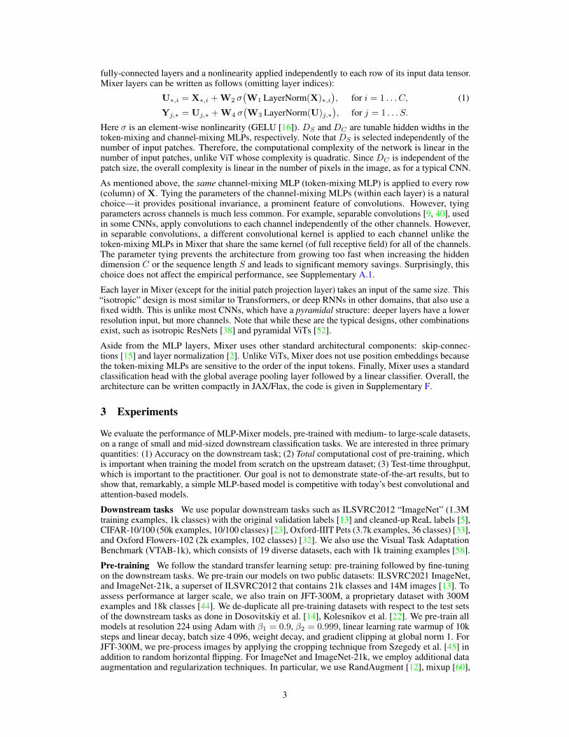
Figure 5: Hidden units in the first (left), second (center), and third (right) token-mixing MLPs ofa Mixer-B/16 model trained on JFT-300M. Each unit has 196 weights, one for each of the 14× 14incoming patches. We pair the units to highlight the emergence of kernels of opposing phase. Pairsare sorted by filter frequency. In contrast to the kernels of convolutional filters, where each weightcorresponds to one pixel in the input image, one weight in any plot from the left column correspondsto a particular 16× 16 patch of the input image. Complete plots in Supplementary D.

setup described in Section 3 and using one of two different input transformations: (1) Shuffle theorder of 16×16 patches and permute pixels within each patch with a shared permutation; (2) Permutethe pixels globally in the entire image. Same permutation is used across all images. We report thelinear 5-shot top-1 accuracy of the trained models on ImageNet in Figure 4 (bottom). Some originalimages along with their two transformed versions appear in Figure 4 (top). As could be expected,Mixer is invariant to the order of patches and pixels within the patches (the blue and green curvesmatch perfectly). On the other hand, ResNet’s strong inductive bias relies on a particular orderof pixels within an image and its performance drops significantly when the patches are permuted.Remarkably, when globally permuting the pixels, Mixer’s performance drops much less (∼45% drop)compared to the ResNet (∼75% drop).

3.5 Visualization

It is commonly observed that the first layers of CNNs tend to learn Gabor-like detectors that act onpixels in local regions of the image. In contrast, Mixer allows for global information exchange in thetoken-mixing MLPs, which begs the question whether it processes information in a similar fashion.Figure 5 shows hidden units of the first three token-mixing MLPs of Mixer trained on JFT-300M.Recall that the token-mixing MLPs allow global communication between different spatial locations.Some of the learned features operate on the entire image, while others operate on smaller regions.Deeper layers appear to have no clearly identifiable structure. Similar to CNNs, we observe manypairs of feature detectors with opposite phases [39]. The structure of learned units depends on thehyperparameters. Plots for the first embedding layer appear in Figure 2 of Supplementary D.

8

4 Related work

MLP-Mixer is a new architecture for computer vision that differs from previous successful architec-tures because it uses neither convolutional nor self-attention layers. Nevertheless, the design choicescan be traced back to ideas from the literature on CNNs [24, 25] and Transformers [50].

CNNs have been the de-facto standard in computer vision since the AlexNet model [24] surpassedprevailing approaches based on hand-crafted image features [36]. Many works focused on improvingthe design of CNNs. Simonyan and Zisserman [41] demonstrated that one can train state-of-the-artmodels using only convolutions with small 3×3 kernels. He et al. [15] introduced skip-connectionstogether with the batch normalization [20], which enabled training of very deep neural networksand further improved performance. A prominent line of research has investigated the benefits ofusing sparse convolutions, such as grouped [57] or depth-wise [9, 17] variants. In a similar spirit toour token-mixing MLPs, Wu et al. [55] share parameters in the depth-wise convolutions for naturallanguage processing. Hu et al. [18] and Wang et al. [53] propose to augment convolutional networkswith non-local operations to partially alleviate the constraint of local processing from CNNs. Mixertakes the idea of using convolutions with small kernels to the extreme: by reducing the kernel size to1×1 it turns convolutions into standard dense matrix multiplications applied independently to eachspatial location (channel-mixing MLPs). This alone does not allow aggregation of spatial informationand to compensate we apply dense matrix multiplications that are applied to every feature acrossall spatial locations (token-mixing MLPs). In Mixer, matrix multiplications are applied row-wiseor column-wise on the “patches×features” input table, which is also closely related to the work onsparse convolutions. Mixer uses skip-connections [15] and normalization layers [2, 20].

In computer vision, self-attention based Transformer architectures were initially applied for generativemodeling [8, 34]. Their value for image recognition was demonstrated later, albeit in combinationwith a convolution-like locality bias [37], or on low-resolution images [10]. Dosovitskiy et al.[14] introduced ViT, a pure transformer model that has fewer locality biases, but scales well tolarge data. ViT achieves state-of-the-art performance on popular vision benchmarks while retainingthe robustness of CNNs [6]. Touvron et al. [49] trained ViT effectively on smaller datasets usingextensive regularization. Mixer borrows design choices from recent transformer-based architectures.The design of Mixer’s MLP-blocks originates in [27, 50]. Converting images to a sequence of patchesand directly processing embeddings of these patches originates in Dosovitskiy et al. [14].

Many recent works strive to design more effective architectures for vision. Srinivas et al. [42] replace3×3 convolutions in ResNets by self-attention layers. Ramachandran et al. [37], Tay et al. [47], Liet al. [26], and Bello [3] design networks with new attention-like mechanisms. Mixer can be seen asa step in an orthogonal direction, without reliance on locality bias and attention mechanisms.

The work of Lin et al. [28] is closely related. It attains reasonable performance on CIFAR-10 usingfully connected networks, heavy data augmentation, and pre-training with an auto-encoder. Neyshabur[31] devises custom regularization and optimization algorithms and trains a fully-connected network,attaining impressive performance on small-scale tasks. Instead we rely on token and channel-mixingMLPs, use standard regularization and optimization techniques, and scale to large data effectively.

Traditionally, networks evaluated on ImageNet [13] are trained from random initialization usingInception-style pre-processing [46]. For smaller datasets, transfer of ImageNet models is popular.However, modern state-of-the-art models typically use either weights pre-trained on larger datasets,or more recent data-augmentation and training strategies. For example, Dosovitskiy et al. [14],Kolesnikov et al. [22], Mahajan et al. [30], Pham et al. [35], Xie et al. [56] all advance state-of-the-artin image classification using large-scale pre-training. Examples of improvements due to augmentationor regularization changes include Cubuk et al. [11], who attain excellent classification performancewith learned data augmentation, and Bello et al. [4], who show that canonical ResNets are still nearstate-of-the-art, if one uses recent training and augmentation strategies.

5 Conclusions

We describe a very simple architecture for vision. Our experiments demonstrate that it is as goodas existing state-of-the-art methods in terms of the trade-off between accuracy and computationalresources required for training and inference. We believe these results open many questions. Onthe practical side, it may be useful to study the features learned by the model and identify the main

9

differences (if any) from those learned by CNNs and Transformers. On the theoretical side, we wouldlike to understand the inductive biases hidden in these various features and eventually their role ingeneralization. Most of all, we hope that our results spark further research, beyond the realms ofestablished models based on convolutions and self-attention. It would be particularly interesting tosee whether such a design works in NLP or other domains.

Acknowledgments and Disclosure of Funding

The work was performed in the Brain teams in Berlin and Zürich. We thank Josip Djolonga forfeedback on the initial version of the paper; Preetum Nakkiran for proposing to train MLP-Mixer oninput images with shuffled pixels; Olivier Bousquet, Yann Dauphin, and Dirk Weissenborn for usefuldiscussions.

References[1] A. Araujo, W. Norris, and J. Sim. Computing receptive fields of convolutional neural net-

works. Distill, 2019. doi: 10.23915/distill.00021. URL https://distill.pub/2019/computing-receptive-fields.

[2] J. L. Ba, J. R. Kiros, and G. E. Hinton. Layer normalization. arXiv preprint arXiv:1607.06450,2016.

[3] I. Bello. LambdaNetworks: Modeling long-range interactions without attention. arXiv preprintarXiv:2102.08602, 2021.

[4] I. Bello, W. Fedus, X. Du, E. D. Cubuk, A. Srinivas, T.-Y. Lin, J. Shlens, and B. Zoph. RevisitingResNets: Improved training and scaling strategies. arXiv preprint arXiv:2103.07579, 2021.

[5] L. Beyer, O. J. Hénaff, A. Kolesnikov, X. Zhai, and A. van den Oord. Are we done withImageNet? arXiv preprint arXiv:2006.07159, 2020.

[6] S. Bhojanapalli, A. Chakrabarti, D. Glasner, D. Li, T. Unterthiner, and A. Veit. Understandingrobustness of transformers for image classification. arXiv preprint arXiv:2103.14586, 2021.

[7] A. Brock, S. De, S. L. Smith, and K. Simonyan. High-performance large-scale image recognitionwithout normalization. arXiv preprint arXiv:2102.06171, 2021.

[8] R. Child, S. Gray, A. Radford, and I. Sutskever. Generating long sequences with sparsetransformers. arXiv preprint arXiv:1904.10509, 2019.

[9] F. Chollet. Xception: Deep learning with depthwise separable convolutions. In CVPR, 2017.

[10] J.-B. Cordonnier, A. Loukas, and M. Jaggi. On the relationship between self-attention andconvolutional layers. In ICLR, 2020.

[11] E. D. Cubuk, B. Zoph, D. Mane, V. Vasudevan, and Q. V. Le. AutoAugment: Learningaugmentation policies from data. In CVPR, 2019.

[12] E. D. Cubuk, B. Zoph, J. Shlens, and Q. V. Le. RandAugment: Practical automated dataaugmentation with a reduced search space. In CVPR Workshops, 2020.

[13] J. Deng, W. Dong, R. Socher, L. Li, Kai Li, and Li Fei-Fei. ImageNet: A large-scale hierarchicalimage database. In CVPR, 2009.

[14] A. Dosovitskiy, L. Beyer, A. Kolesnikov, D. Weissenborn, X. Zhai, T. Unterthiner, M. Dehghani,M. Minderer, G. Heigold, S. Gelly, J. Uszkoreit, and N. Houlsby. An image is worth 16x16words: Transformers for image recognition at scale. In ICLR, 2021.

[15] K. He, X. Zhang, S. Ren, and J. Sun. Deep residual learning for image recognition. In CVPR,2016.

[16] D. Hendrycks and K. Gimpel. Gaussian error linear units (GELUs). arXiv preprintarXiv:1606.08415, 2016.

[17] A. G. Howard, M. Zhu, B. Chen, D. Kalenichenko, W. Wang, T. Weyand, M. Andreetto, andH. Adam. Mobilenets: Efficient convolutional neural networks for mobile vision applications.arXiv preprint arXiv:1704.04861, 2017.

[18] J. Hu, L. Shen, and G. Sun. Squeeze-and-excitation networks. In CVPR, 2018.

10

[19] G. Huang, Y. Sun, Z. Liu, D. Sedra, and K. Q. Weinberger. Deep networks with stochasticdepth. In ECCV, 2016.

[20] S. Ioffe and C. Szegedy. Batch normalization: Accelerating deep network training by reducinginternal covariate shift. In ICML, 2015.

[21] C. Jia, Y. Yang, Y. Xia, Y.-T. Chen, Z. Parekh, H. Pham, Q. V. Le, Y. Sung, Z. Li, and T. Duerig.Scaling up visual and vision-language representation learning with noisy text supervision. arXivpreprint arXiv:2102.05918, 2021.

[22] A. Kolesnikov, L. Beyer, X. Zhai, J. Puigcerver, J. Yung, S. Gelly, and N. Houlsby. Big transfer(BiT): General visual representation learning. In ECCV, 2020.

[23] A. Krizhevsky. Learning multiple layers of features from tiny images. Technical report,University of Toronto, 2009.

[24] A. Krizhevsky, I. Sutskever, and G. E. Hinton. ImageNet classification with deep convolutionalneural networks. In NeurIPS, 2012.

[25] Y. LeCun, B. Boser, J. Denker, D. Henderson, R. Howard, W. Hubbard, and L. Jackel. Back-propagation applied to handwritten zip code recognition. Neural Computation, 1:541–551,1989.

[26] D. Li, J. Hu, C. Wang, X. Li, Q. She, L. Zhu, T. Zhang, and Q. Chen. Involution: Inverting theinherence of convolution for visual recognition. CVPR, 2021.

[27] M. Lin, Q. Chen, and S. Yan. Network in network. In ICLR, 2014.[28] Z. Lin, R. Memisevic, and K. Konda. How far can we go without convolution: Improving

fullyconnected networks. In ICLR, Workshop Track, 2016.[29] W. Luo, Y. Li, R. Urtasun, and R. Zemel. Understanding the effective receptive field in deep

convolutional neural networks. In NeurIPS, 2016.[30] D. Mahajan, R. Girshick, V. Ramanathan, K. He, M. Paluri, Y. Li, A. Bharambe, and L. van der

Maaten. Exploring the limits of weakly supervised pretraining. In ECCV, 2018.[31] B. Neyshabur. Towards learning convolutions from scratch. In NeurIPS, 2020.[32] M. Nilsback and A. Zisserman. Automated flower classification over a large number of classes.

In ICVGIP, 2008.[33] O. M. Parkhi, A. Vedaldi, A. Zisserman, and C. V. Jawahar. Cats and dogs. In CVPR, 2012.[34] N. Parmar, A. Vaswani, J. Uszkoreit, L. Kaiser, N. Shazeer, A. Ku, and D. Tran. Image

transformer. In ICML, 2018.[35] H. Pham, Z. Dai, Q. Xie, M.-T. Luong, and Q. V. Le. Meta pseudo labels. In CVPR, 2021.[36] A. Pinz. Object categorization. Foundations and Trends in Computer Graphics and Vision, 1(4),

2006.[37] P. Ramachandran, N. Parmar, A. Vaswani, I. Bello, A. Levskaya, and J. Shlens. Stand-alone

self-attention in vision models. In NeurIPS, 2019.[38] M. Sandler, J. Baccash, A. Zhmoginov, and Howard. Non-discriminative data or weak model?

On the relative importance of data and model resolution. In ICCV Workshop on Real-WorldRecognition from Low-Quality Images and Videos, 2019.

[39] W. Shang, K. Sohn, D. Almeida, and H. Lee. Understanding and improving convolutionalneural networks via concatenated rectified linear units. In ICML, 2016.

[40] L. Sifre. Rigid-Motion Scattering For Image Classification. PhD thesis, Ecole Polytechnique,2014.

[41] K. Simonyan and A. Zisserman. Very deep convolutional networks for large-scale imagerecognition. In ICLR, 2015.

[42] A. Srinivas, T.-Y. Lin, N. Parmar, J. Shlens, P. Abbeel, and A. Vaswani. Bottleneck transformersfor visual recognition. arXiv preprint arXiv:2101.11605, 2021.

[43] N. Srivastava, G. Hinton, A. Krizhevsky, I. Sutskever, and R. Salakhutdinov. Dropout: A simpleway to prevent neural networks from overfitting. JMLR, 15(56), 2014.

[44] C. Sun, A. Shrivastava, S. Singh, and A. Gupta. Revisiting unreasonable effectiveness of data indeep learning era. In ICCV, 2017.

11

[45] C. Szegedy, W. Liu, Y. Jia, P. Sermanet, S. Reed, D. Anguelov, D. Erhan, V. Vanhoucke, andA. Rabinovich. Going deeper with convolutions. In CVPR, 2015.

[46] C. Szegedy, V. Vanhoucke, S. Ioffe, J. Shlens, and Z. Wojna. Rethinking the inception architec-ture for computer vision. In CVPR, 2016.

[47] Y. Tay, D. Bahri, D. Metzler, D.-C. Juan, Z. Zhao, and C. Zheng. Synthesizer: Rethinkingself-attention in transformer models. arXiv, 2020.

[48] H. Touvron, A. Vedaldi, M. Douze, and H. Jegou. Fixing the train-test resolution discrepancy.In NeurIPS, 2019.

[49] H. Touvron, M. Cord, M. Douze, F. Massa, A. Sablayrolles, and H. Jégou. Training data-efficientimage transformers & distillation through attention. arXiv preprint arXiv:2012.12877, 2020.

[50] A. Vaswani, N. Shazeer, N. Parmar, J. Uszkoreit, L. Jones, A. N. Gomez, Ł. Kaiser, andI. Polosukhin. Attention is all you need. In NeurIPS, 2017.

[51] A. Vaswani, P. Ramachandran, A. Srinivas, N. Parmar, B. Hechtman, and J. Shlens. Scalinglocal self-attention for parameter efficient visual backbones. arXiv preprint arXiv:2103.12731,2021.

[52] W. Wang, E. Xie, X. Li, D.-P. Fan, K. Song, D. Liang, T. Lu, P. Luo, and L. Shao. Pyramidvision transformer: A versatile backbone for dense prediction without convolutions. arXivpreprint arXiv:2102.12122, 2021.

[53] X. Wang, R. Girshick, A. Gupta, and K. He. Non-local neural networks. In CVPR, 2018.[54] R. Wightman. Pytorch image models. https://github.com/rwightman/

pytorch-image-models, 2019.[55] F. Wu, A. Fan, A. Baevski, Y. Dauphin, and M. Auli. Pay less attention with lightweight and

dynamic convolutions. In ICLR, 2019.[56] Q. Xie, M.-T. Luong, E. Hovy, and Q. V. Le. Self-training with noisy student improves imagenet

classification. In CVPR, 2020.[57] S. Xie, R. Girshick, P. Dollár, Z. Tu, and K. He. Aggregated residual transformations for deep

neural networks. arXiv preprint arXiv:1611.05431, 2016.[58] X. Zhai, J. Puigcerver, A. Kolesnikov, P. Ruyssen, C. Riquelme, M. Lucic, J. Djolonga, A. S.

Pinto, M. Neumann, A. Dosovitskiy, et al. A large-scale study of representation learning withthe visual task adaptation benchmark. arXiv preprint arXiv:1910.04867, 2019.

[59] X. Zhai, A. Kolesnikov, N. Houlsby, and L. Beyer. Scaling vision transformers. arXiv preprintarXiv:2106.04560, 2021.

[60] H. Zhang, M. Cisse, Y. N. Dauphin, and D. Lopez-Paz. mixup: Beyond empirical risk mini-mization. In ICLR, 2018.

12