LIQUID/LIQUID VISCOUS DISPERSIONSWITHA SMX STATIC MIXER

L. Fradette1, P. Tanguy1, H. -Z. Li2 and L. Choplin2

1Department of Chemical Engineering, Ecole Polytechnique, Montreal, Canada2Gemico-ENSIC, Institut National Polytechnique de Lorraine, Nancy, France

Abstract: A SMX static mixer was used to disperse highly viscous Newtonian liquids into lessviscous, Newtonian and non-Newtonian fluids without surfactants. The investigation coveredthe effect of the dispersed phase volume fraction, the viscosity ratio between the phases, themixer length and the power draw. The flow regime was kept laminar in all the experimentswith a dispersed phase content up to 25% and viscosity ratios ranging from 1 to 400. The exper-imental conditions allowed neglecting the affect of coalescence mainly because of the highviscosity of the continuous phase. The effect of the dispersed phase viscosity and volumefraction on the average drop size was quantified. The size distributions were obtained byimage analysis. Using the ‘process viscosity’ concept, it was possible to collapse all the averagediameters on a single master curve by using the energy consumption in the mixer as the shiftvariable between the experiments. A performance comparison against the Kenics mixer wasmade using literature results. The results showed that the SMX mixer is much better adaptedto the dispersion task mainly due to its internal structure.

Keywords: SMX static mixer; multiphase flow; liquid–liquid dispersion; laminar flow; Newtonian;non-Newtonian.

INTRODUCTION

Most inline liquid–liquid mixers are eithercolloidal mills or rotor stators, and thechoice between these two technologies ismainly based on the required dispersedphase droplet size to achieve. With viscousor highly viscous fluids, these mixers arealmost impossible to use because of theirintrinsic design and operating mode that gen-erate either excessive torque or significantviscous dissipation yielding local heatingeffects. One suitable alternative is to usestatic mixers, especially the designs welladapted to laminar flows. In the case ofliquid–liquid dispersions, the knowledgerequired to select a particular model orsimply determine the specification of afuture installation is poorly documented.Most of the available investigations havefocused on describing process debottleneck-ing, ways of getting higher yields in particularapplications, and other types of processimprovements (e.g., Craik et al., 2003;Benz et al., 2001).The work of Grace (1982) is considered as

the seminal contribution for liquid–liquiddispersions in static mixers in the laminarregime. According to Grace’s work, theeffect of the flow field type on a single dropover a wide range of viscosity ratio can be

expressed by means of the capillarynumber, namely

Ca ¼hu

s¼

t

(s=L)(1)

where t is the viscous stresses on the dropand (s/L) is the drop resistance to ruptureby surface tension (capillary) forces. The criti-cal capillary number is defined as the valuethat must be reached in a flowing fluidphase in order to break up a dispersed dropof a given viscosity. Following this work, itwas further shown that breaking drops of vis-cosity four times that of the continuous phaseand submitted to a simple shear field requiredlonger times but not higher Capillary numbers(Bentley and Leal, 1986). This observation isimportant since it demonstrates that it isalways possible to break a drop providedthe deformation or the deformation time islong enough (Stone, 1994).Time effects are of prime importance in

dispersion and even more in static mixerswhere the geometry generates chaotic flowperturbations (Li et al., 1996). The timerequired for rupture of a given drop at equili-brium deformation can be estimated with

trupture ¼hc

(s=Ddrop)(2)

395 Vol 85 (A3) 395–405

�Correspondence to:Dr L. Fradette, Department ofChemical Engineering, EcolePolytechnique, Montreal,Canada, H3T 1J7.E-mail: louis.fradette@polymtl.ca

DOI: 10.1205/cherd06206

0263–8762/07/$30.00þ 0.00

Chemical EngineeringResearch and Design

Trans IChemE,Part A, March 2007

# 2007 Institutionof Chemical Engineers

At very high viscosity ratios, trupture can reach very highvalues (Grace, 1982; Bentley and Leal, 1986). Time hasthen a major influence on the final dispersion and its effectsmust be considered at the early stages of process design.The flow type, defined as the ratio of the deformation (D)

to the rotational component (V) of the flow field (Manas-Zloczower, 1994), is also known as an important parametergoverning the breaking mechanism:

a ¼jDj

jDj þ jVjwhere DþV ¼

1

2rv þ rvT� ��

þ rv � rvT� ��

(3)

The value of a is well suited for representing the type of two-dimensional flow used: 0 ¼ pure rotational; 0.5 ¼ simpleshear; 1 ¼ pure extensional. Depending on the mixer geome-try, any intermediate value between 1.0 and 0.0 is possible.While this parameter cannot be used to compare completelydifferent geometries like an agitated tank and a static mixer(Astarita, 1979), it is still useful to compare similar geometriesand various operating conditions in the same mixer. Usingnumerical simulations, such a comparison has been estab-lished successfully for different static mixer models (e.g.,Rauline et al., 1998, 2000) and mixing tanks (De la Villeonet al., 1998).It was experimentally demonstrated that a constant defor-

mation flow (a constant) combined to a decreasing shear ratecould lead to the breakup of the dispersed phase. The samesize reduction effect was also demonstrated by varying theflow type (a) and the shear rate at the same time, again high-lighting the importance of the transient conditions as the onesfound in static mixers. From the fundamental contributions ofGrace, the conclusions are (Stone and Leal, 1989a, b):

. For a given stretching-sudden relaxation process, themaximum stretching required to rupture the drop at relax-ation is widely superior to the maximum stable deformationobserved in the critical capillary number experiments. Thisrequired stretching at breakup is an increasing function ofthe viscosity ratio.

. Steps in shear rates during a drop deformation experimentlead to the drop rupture without any important stretching.The breakup is attributed to surface tension effects.

. To allow for capillary instabilities effects to play a role in afilament rupture, the ratio Lfilament/Rfilament must be largerthan 20.

. Combining and alternating flow types (different a) can leadto drop rupture even though the same flow in stable con-ditions would not result in such a breakup. This latterobservation is of prime importance. It allows for a simpleshear flow to break up high viscosity droplets whilestable conditions would not.

These conclusions, while having been obtained with singledrop experiments, can be directly related to static mixersand their application to dispersion processes. They alsopartly explain why this type of mixers can effectively reachlow average sizes without the typical high shear generatedin rotating equipment such as colloidal mills and rotorstators.The reality of liquid–liquid dispersion is so that millions not to

say billions of drops are involved at the same time. The simul-taneous rupturing, colliding and coalescence generate a

tremendously complex hydrodynamic flow process from anengineering standpoint. Using a large amount of energy in tur-bulent regime is usually seen as the easiest (and probably themost intuitive) solution provided that the viscosity is sufficientlylow (Legrand et al., 2001). The laminar regime is not usuallyconsidered as an efficient means for a size reduction process,although Grace (1982) did carry interesting experiments withthe Kenics mixer. His ideas were to put in evidence the factthat transient conditions generated in the static mixers couldbe modeled with abrupt changes in flow conditions. Withoutever reaching the critical capillary number, the variations inshear rate effectively led to droplet breakup.The SMX mixer geometry is very different from that of the

Kenics. The SMX shape was used in a dispersion work byMutsakis et al. (1986) who clearly showed that this mixer geo-metry exhibits both effective shear and elongation to effi-ciently rupture drops of oil dispersed in a water phase. Themajor limitation of this research was the restriction of theviscosity ratios to values below 1.An analogy can be drawn between static mixers and impel-

ler-based mixing in stirred vessels, where equivalence can bederived between the mixer length (or alternatively the numberof elements) and the processing time in tanks. The longer themixer, the better the mixing provided. It has been known for awhile that the effect of the number of mixing elements can bemodelled with (Middleman, 1974):

D32

D32(Nmax )¼ C1 þ C2e

(�N � C3) (4)

Here, the value of D32(Nmax) is simply the minimum sizeachieved with the maximum number of elements used inthe experiments. The values of constants C1 to C3 obtainedwith a Kenics (Middleman, 1974) and an in-liner mixer fromLightnin (Al-Taweel and Walker, 1983) are presented inTable 1.In parallel with equation (4), the behaviour of the size

reduction in the mixer can be explained by a kinetic phenom-enon. With the dispersed phase flowing across the staticelements, the drops break in a repetitive fashion until equili-brium is reached between the flow forces needed to rupturethe drops and the drops resistance due to Laplace pressure.The point where this equilibrium is reached is a function ofthe dissipated energy and the liquid system involved. Thedistance to establish the equilibrium can be directly com-pared to the mixing time in tanks. During the design of anew process application, it is hence of prime importance toevaluate the required number of elements properly.

Table 1. Experimental values of constants C1, C2 and C3 [equation(4) from Middleman, 1974] with conditions.

Middleman(1974)

Al-Taweel(Al-Taweel and Walker, 1983)

C1 0.95 1.0C2 5.1 4.9C3 0.40 0.19Mixers 3, 6, 21

Kenics4, 8, 12, 16, 24, 36 in-liner

Fluids Benzene inwater

Kerosene in water

Volume fraction 0.5–1% 1%Interfacial tension 4 mN m21 —

Trans IChemE, Part A, Chemical Engineering Research and Design, 2007, 85(A3): 395–405

396 FRADETTE et al.

In a Kenics mixer under laminar flow conditions and a vis-cosity ratio of 0.001 Grace (1982) obtained a linear relationbetween the average drop size and the volume fraction inthe range 5–20%. These experiments were more represen-tative of a gas dispersed in the liquid phase. The increasein size of the dispersed phase was explained by the augmen-tation of the dispersed phase flow rate. The higher velocitiesout of the injection tip generated larger drops. With an identi-cal mixing length, the average size normally increases withthe volume fraction.In order to characterize the dispersion capacity in the lami-

nar regime, the effective or characteristic shear rate can becalculated following Grace (1982):

geff ¼ Cacrits

(Dd=2)

1

hc(5)

It is important to note that the characteristic shear rate is amixer property calculated from the dispersion results ratherthan a design parameter. It is however useful to assess theefficiency of a given mixer and it can be used for comparisonpurposes between different mixing geometries.In a Kenics mixer, Grace (1982) was able to relate the Sauter

mean diameter to the nominal wall shear rate expressed bymeans of the average velocity in the empty tube, namely

D32 ¼C1

gcw

(6)

In this expression, the exponent c was 1.0 with small viscosityratios and 0.5 in the case p . 1. It also appeared to be influ-enced by the continuous phase viscosity. The constant C1

was mentioned to be a function of the number of elements,the size of the tube, and the dispersed phase volume fraction.Obviously, it is also a strong function of the geometry of themixer but was never presented as such.Trying to put in evidence what he presented as capillary

instabilities, Grace used relaxation zones between theKenics mixing sections. The average diameters with this con-figuration were smaller than with straight length of mixers andhence, the specific power (DP * Qt) was lower. These resultswere attributed to the effectiveness of the stress relaxation ona deformed drop to break it and also to variations in the flowtype (a) (Stone, 1994; Stegeman et al., 2002). The timerequired for rupture would have been too long when com-pared to the available experimental results on capillaryinstabilities (Tjahjadi et al., 1992). By nature, the flow charac-ter (a) is constantly changing along the length of the elementin a SMX (Rauline et al., 1998). It was clearly demonstratedby numerical means (trajectory length distributions) thatthose variations in the flow character are very importantand can be very different from one mixer type to the next(Fradette, 1999). The SMX mixer creates many more andlarger fluctuations along its flow axis while, in a Kenicsmixer, the variations are mostly triggered at the inlet andoutlet of each element when the flow is split in two parts bythe element lamellae. Similar results were obtained numeri-cally in Kenics mixers by following the deformation of mass-less and dimensionless particles launched from a planelocated at the entrance of the mixer (Avalosse and Crochet,1997a,b). A second numerical study puts in evidence theimportant role of the entrance and exit effects on the dis-persion capability of a SMX and a new competing type of

static mixer known as the KMX mixer (Heniche et al.,2003). Moreover, the blade shapes used to build the mixerare the most important elements having an influence on theflow character (a) inside the mixer and consequently on itscapacity to disperse a second phase effectively (Henicheet al., 2005).In a recent and complete review on static mixing technol-

ogy, the lack of knowledge about the dispersion in the laminarregime was clearly identified (Thakur et al., 2003). Whilebeing more often the subject of dispersion studies theKenics mixer has been used in the turbulent regime andvery little is known about its capacity to disperse in the lami-nar regime.Although very few investigations have been published on

laminar dispersion, many valuable characterization elementshave been found in the literature to scale the dispersioncapacity of a mixer (capillary number, effective shear, kineticsof rupture, power draw, energy, and so on). In line with thepublished results, the objective of this work is to experimen-tally characterize the SMX dispersion performance in thelaminar regime when Newtonian liquids are dispersed intoNewtonian and non-Newtonian continuous phases. Thevery few results available about the Kenics mixer will beused for comparison purposes.

EXPERIMENTAL

The experimental setup has been fully described else-where and the reader is referred to (Fradette et al., 2006)for details. The additional element required for this part ofthe work was a second pump to inject the dispersed phase.The injected phase flow rate was determined from therotation speed of the progressive cavity pump. The pumpshaft entrained a speed encoder allowing the determinationof the flowrate from a calibration curve at any rotationalspeed of the pump. The mixers diameter was 12 mm andeach cell of six elements was 0.122 m.During the liquid–liquid dispersion investigations, silicone

oils formed the dispersed phase in all the experiments andthe continuous phases were either a mixture of glycerol ora polymer solution. The rheological properties of the fluidsused in the experiments are listed in Table 2. The parameterspresented are from the Cross viscosity model used to fit theviscosity curve of the experimental fluids:

h(g) ¼h0

1þ (jg j=C1)1�n

(7)

Fitting the Xanthan gum solution with this model led tosome unusual parameter values, mostly due to the fact that

Table 2. Rheological properties of the experimental fluids used in thiswork.

Fluid Ingredient (s) Conc. (% wt) h0 (Pa s) C1 n

Oil 1 Silicone — 1.1 — —Oil 2 Silicone — 16.3 — —Oil 3 Silicone — 48.0 — —Polymer Water 98 4.6 2.0 0.7phase 1 CMC 2Polymer Water 50 6714 4.38 � 1025 0.31phase 2 Glucose 49

Xanthan gum 1

Trans IChemE, Part A, Chemical Engineering Research and Design, 2007, 85(A3): 395–405

LIQUID/LIQUID VISCOUS DISPERSIONS WITH SMX STATIC MIXER 397

such solutions do not exhibit a viscosity plateau at low shear.In the range of shear rates of our experiments, the viscosityfrom the model was in excellent agreement with the exper-imental one. Details of the base fluids are provided in Table 3.The experimental plan of the investigation is summarized

on Figure 1 with its three major axes. The maximumvolume fraction of dispersed phase was set at 25% after aseries of preliminary tests clearly indicating that abnormaldispersion (w/o/w) occurred above 30% of dispersedphase. A coalescence time estimation by means of the inter-stitial film drainage time led to a drainage value in the order ofa few minutes. Observations of collected samples confirmedthis order of magnitude. On the other hand, the residencetime and the time required for the size measurement duringthe experiments was in the order of a few seconds. Theassumption of no significant coalescence effects that wouldbe included in the measured diameters is then justified.Appendix 1 presents the detailed calculation.The number of elements was varied from 6 to 18. The

measurements consisted in the pressure difference acrossthe elements, the temperature, and the flow rate of eachphase. The dispersed phase size distribution was obtainedafter performing image analysis of the recorded experiments,in the same manner as for bubbles in Fradette et al. (2006).The average size and the standard deviation are obtainedafter fitting the experimental size distribution with alog-normal function by means of the maximum likelihoodtechnique. This mathematical fitting method is much moreappropriate for finding regression parameters than a standardleast square minimization (Hogg and Craig, 1978) since itmaximizes the probability of finding the experimental valuesall at once. In this context, the log-normal model counts twoparameters, a and b and is expressed following

f (x,a,b) ¼1

xbffiffiffiffiffiffi2p

p e�(( ln x�a)2=2b2) (8)

The parameters a and b can be explicitly calculated with

a ¼

Pni¼1 ln xin

and b2 ¼

Pni¼1 ( ln xi � a)2

n(9)

RESULTS

A summary of the conditions and the fluids used in allthe dispersion is shown in Table 4. The raw diameterresults and their associated standard deviation are pre-sented along with the conditions. The first 15 experimentscorrespond to the experimental plan illustrated on Figure 1.The results from these experiments allowed for the effectof the vavg/D ratio and the number of elements to be cap-tured directly. In all the experiments, the Reynolds numberwas conservatively set below 15 to ensure operation in thelaminar regime (Li et al., 1996). Indeed, the onset of thetransition regime for this mixer geometry has beendetected at Re values around 100 in other research work(Hiresh et al., 2003). Every experiment was preceded bypressure drop measurements that were used to back-calculate the Reynolds number by means of the apparentviscosity concept. It has been shown previously that thismethod eliminates the need for rheological measurementson standard rheometers (Arzate et al., 2004). It alsoexplains why we do not present the results with Xanthangum and CMC separately despite their different rheologicalbehaviour.Figure 2 presents a typical size distribution curve obtained

after fitting the size categories with a log-normal model. Theraw numbers of the 40 size categories are also presented.The maximum likelihood technique used here is known tobe a very well suited minimizing method when discretevalues from experimental measurements have to be fittedwith a continuous model. On the graph, it is also obviousthat the resulting fit agrees very well with the measurements.Based on the observations made when the measurementswere fitted, it was noted that the standard least square tech-nique lead to unstable fits and the models were lesssatisfactory.The effect of the volume fraction on the raw average drop

size is shown on Figure 3. This graph is essentially thegraphic representation of Table 4. The curves were obtained

Table 3. Physical and rheological properties of the base fluids.

NameProducer/distributor Product Properties

Oil 1 RhodiaSilicones

Rhodorsil47 V 1 000

† Silicon (PDMS†)

† h ffi 1 Pa s @ 258Oil 2 Rhodia

SiliconesRhodorsil

48 V 14 000† Silicon (PDMS)

† h ffi 14 Pa s @ 258Oil 3 Rhodia

SiliconesRhodorsil

48 V 50 000† Silicon (PDMS)

† h ffi 50 Pa s @ 258CMC‡

mv SigmaChemicalsCo.

— † Unspecified mol. Wt.

Xanthangum

Kelco Inc.(Monsanto)

— † Food grade

† Unspecified mol. Wt.Glycerol Lambert et

Riviere— † Synthetic Glycerol

† 99.5%† h99.5% ¼ 0.95 Pa s

Glucose Cerestar,France

Glucose syrupMS 01424

† h ffi 115 Pa s @ 208

†PDMS: Polydimethyl-siloxane‡CMCmv: Carboxymethyl-cellulose, intermediate viscosity

Figure 1. Experimental plan used for the liquid–liquid dispersions.

Trans IChemE, Part A, Chemical Engineering Research and Design, 2007, 85(A3): 395–405

398 FRADETTE et al.

for respectively 6, 15 and 22% of dispersed phase and a vis-cosity ratio of 5. At a given dispersed phase fraction, all thediameters collapse on a single curve when the total energydrawn in the mixer is used as the common variable betweenthe experiments. 6, 12 and 18 static mixer elements wereused and combined to multiple formulations in order to gen-erate the results shown here. Similar tests were performedfor viscosity ratios in the range of 60 and 200 and, asexpected, similar plots were obtained. The overall energy(ET) is expressed according to Karbstein and Schubert(1995):

ET ¼ DP � Vmix (10)

The presence of a dispersed viscous second phase has beenknown to increase the bulk viscostity (Taylor, 1932; Sherman,

1959). Figure 4 presents this effect by using all the exper-imental results available from this work. The abscissascales the ratio of the observed viscosity, obtained from themeasured pressure drop, to the expected viscosity at thetotal flow rate with the continuous phase viscosity only. Aregular and non negligible increase of 40% in viscosity isseen when the dispersed phase fraction reaches 25%.The combined effect of the volume fraction and the vis-

cosity ratio can be plotted on a single graph and is presentedin Figure 5. On this graph, each point on a curve representsthe average diameter obtained at a given dispersed phasefraction and a chosen energy value of 1 Joule. Each one ofthese points can be assimilated to ordinates extrapolatedon a regular xy graph and are expected to be slightly morescattered than straight measurements. The same effect isfound when calculating derivatives from experimental differ-ences. As in Grace’s analysis, we forced a single slope

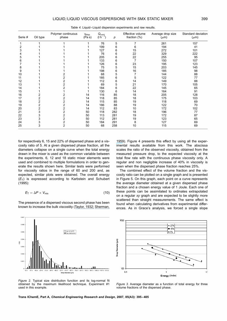
Table 4. Liquid–Liquid dispersion experiments and raw results.

Serie # Oil typePolymer continuous

phasehdisp

(Pa s)Qcont

(l h21) pEffective volume

fraction (%)Average drop size

(mm)Standard deviation

(mm)

1 1 1 1 76 5 7 261 1572 1 1 1 199 6 6 194 413 1 1 1 127 6 15 272 1014 1 1 1 76 6 22 329 2225 1 1 1 205 6 22 255 956 1 1 1 133 6 7 150 1077 1 1 1 126 6 23 195 1238 1 1 1 75 5 15 203 1459 1 1 1 198 6 16 185 9810 1 2 1 68 5 7 144 8811 1 2 1 185 6 5 122 7712 1 2 1 112 6 14 149 8813 1 2 1 69 5 21 170 10514 1 2 1 184 6 22 145 6515 1 1 1 130 6 14 164 9116 2 2 14 116 85 18 205 12817 2 2 14 118 85 18 175 10318 2 2 14 115 85 19 118 6919 2 2 14 186 88 19 122 7020 2 2 14 112 83 10 172 10221 3 2 50 118 282 18 196 7722 3 2 50 113 281 19 172 8723 3 2 50 112 281 19 123 6524 3 2 50 184 291 8 127 6925 3 2 50 68 258 10 115 69

Figure 2. Typical size distribution function and its log-normal fitobtained by the maximum likelihood technique. Experiment #1used in this example.

Figure 3. Average diameter as a function of total energy for threevolume fractions of the dispersed phase.

Trans IChemE, Part A, Chemical Engineering Research and Design, 2007, 85(A3): 395–405

LIQUID/LIQUID VISCOUS DISPERSIONS WITH SMX STATIC MIXER 399

value for the three curves. There is no theoretical reason todo otherwise. Moreover, the objective here is simply tocatch the drop size evolution as a function of the variationsin dispersed phase fraction. We used relative least squaresto determine the parameters value that best fitted all thepoints at once. The plot shows an exponential increase indiameter with an exponent 2.3 times the dispersed phasefraction. The results are expressed in the exponential formby similitude with the work of Grace:

Dd ¼ Ae2:3f (11)

The effects of the viscosity ratio on the average diameter canbe obtained in the same fashion as for the dispersed phase.At a given energy value, a plot of the average diameter vs.the viscosity ratio can be generated. The resulting graph isshown on Figure 6. As for the dispersed phase fractionresults, a reasonable scatter is observed and it can beexplained by the same reasons as above. It can be observedthat the decrease in diameter is strongly related to theincrease in the viscosity ratio. This result is easily explainedby the fact that the flow field in the SMX is chaotic (Liet al., 1996). Theoretical work on the stretching of a fluidthread of higher viscosity in a lower viscosity matrix flowingchaotically leads to a very high stretching ratio before rupture.At break-up time, the resulting droplets are hence of smallerdiameter (Tjahjadi and Ottino, 1991).

We now try to collapse all the average diameters on asingle curve using our previous interpretation of the averagediameters versus the experimental conditions. The energyconsumption in the mixer is used as the common variablebetween the experiments. The shift factors are extractedfrom Figures 5 and 6, for which we arbitrarily select referenceconditions of p ¼ 100 and f ¼ 15%, and calculate the corre-sponding average diameter. In Table 5, we present theanalytical expressions of the equations used to correct forthe viscosity ratio and the volume fraction, respectively. Theresults of the translation of all the average diameters fromall the experiments are presented in Figure 7. The averagediameters align on a smooth curve and decrease with theenergy consumption to the power 1

4. The envelope shown isset at +10% of the average diameter and reflects the verygood alignment of the corrected diameters. This very goodalignment of the experimental measurements can be inter-preted as a clear indication that the effects captured aboutthe viscosity ratio as well as for the dispersed phasevolume fraction (respectively Figures 5 and 6) are very repre-sentative of the reality despite the limited number of exper-imental values. The clearest indication of their quality is theuniformity of the curve on Figure 7. The use of Figure 7, com-bined to the relations presented in Table 5, can help in theinterpolation of the average size of a given dispersion. Dueto the very smooth behaviour observed here, we are confi-dent that these results express a general behaviour. This isleft for demonstration in future work.In order to compare the performance of the SMX used here

with results previously published in the literature, it is con-venient to use the effective Capillary number as the refer-ence. Figure 8 presents the effective capillary number as afunction of the viscosity ratio experimented. On the samegraph, the results from Grace (1982) for simple shear aswell as from Bentley and Leal (1986) for pure elongational

Figure 4. Effect of the dispersed phase fraction on the observedviscosity.

Figure 5. Effect of the dispersed phase volume fraction on theaverage diameter taken at constant energy value.

Figure 6. Effect of the phase viscosity ratio on the average diametertaken at constant energy value.

Table 5. Effect of the volume fraction and viscosity ratio on theaverage drop size.

Variation Diameter correction

Effect of f e 2.3f Dref ¼ Dini * e2.3(fref2fini)

Effect of p p20.063 Dref ¼ Dini (pref/pini)20.06

Trans IChemE, Part A, Chemical Engineering Research and Design, 2007, 85(A3): 395–405

400 FRADETTE et al.

flow are shown. On top of these, the results obtained at lowviscosity ratio (Mutsakis et al., 1986) with the same SMXmixer are also presented. Obviously, the results obtained inour experiments align reasonably well with the ones fromMustakis and are very close to a strong elongational com-ponent with a a value of 0.6 (Bently and Leal, 1986). Theexperimental results agree well with the numerical simu-lations that revealed a strong elongational flow field withinthe SMX with the same value of 0.6 (Rauline et al., 2000).It has been discussed above that times effects can have a

tremendous influence on dispersion results. The relationbetween residence time and time required to rupture a dropat constant deformation is hence of interest when workingwith static mixers. When studying the deformation of asingle drop in elongation or shear, it is possible to recordthe time at which the drop will break after a stable defor-mation has been reached. It is called the required time forbreak-up (trb). The most favourable dispersion conditionsare found when the process allows for a residence time ofthe same order of magnitude as the required time forbreak-up. The most favourable value for this ratio has beenfound as 0.5 (Grace, 1982). Here, the required time forbreakup was normalized by the residence time in order tosimplify the results interpretation. Figure 9 presents the

average diameters as a function of this time ratio. Threecurves are presented combining the volume fractions (5–25%) and the viscosity ratios (5–300), respectively. Thegraph shows a ratio of tbreakup/tresidence in the range 100–10 000. This graph scales the very unfavourable conditionsof dispersion existing within the mixers with only 1/100 oreven less of the time required to reach equilibrium defor-mation. According to the literature, this ‘lack of time for reach-ing favourable dispersing conditions’ must be compensatedby much larger stresses than the one required at equilibriumdeformation (Meijer and Jansen, 1994). However, the dis-persion process is not known to be hampered by theunsteady conditions. It has been shown that transition con-ditions lead to smaller average drop sizes with the drawbackthat the resulting distribution is wider than the one generatedat equilibrium (Meijer and Jansen, 1994). The curves onFigure 9 all show an increase in average size with a lowerresidence time perfectly reflecting a higher ratio of tbreakup/tresidence. The slope of all the curves is 0.33, which reflectsthe importance of the processing time on the resulting aver-age diameter of the drop distributions. The time for break-up correlation developed by Grace (1982) with the Kenicsrelates the time to the power 0.38 of the viscosity ratio andcan be considered very close to the experimental resultsseen here. On the graph shown, the exponent is in therange of 0.32–0.35. It is also important to note that, becauseof the design for inline use, static mixers can hardly achievethe optimum time ratio of 0.5 at which the minimum drop sizecan be achieved unless the flowrate is very low or the diam-eter of the mixer is rather large. This effect is much moredeveloped in the next section of this paper when all the par-ameters affecting the drop size are all considered at once.As it has been said, the time ratio (tbreakup/tresidence) is dif-

ficult to lower because of its direct relationship with the vis-cosity ratio. The major conclusion from this relation is thatthe rupture time is therefore a function of p, hc, the inletdrop diameter, the injection jet diameter, and the interfacialtension. The resulting effect is that a viscosity increase inthe continuous phase (as it could be tempting to use as afavourable factor in reducing the dispersed phase dropsize) does not necessarily generate a smaller drop as itwould be expected. The continuous phase viscosity plays arole in almost all the size reduction factors: dissipatedenergy, viscosity ratio, required time for break-up, and so

Figure 7. Master curve for average drop diameter as a function ofdissipated energy.

Figure 9. Time effects in the SMX mixer—average drop diameter as afunction of the rupture time.

Figure 8. Effective Capillary number obtained for viscosity ratios .1compared to Bentley and Leal (1986), Grace results (1982) andMutsakis (1986).

Trans IChemE, Part A, Chemical Engineering Research and Design, 2007, 85(A3): 395–405

LIQUID/LIQUID VISCOUS DISPERSIONS WITH SMX STATIC MIXER 401

on. A map of size reduction is proposed in order to appreciatewhich factor really has the strongest influence on the finalsize of the dispersion. This map is shown in Figure 10.To generate the map we use the previously introduced

relations for the energy consumption, required time forbreak-up, average residence time and Capillary number.The abscissa is the variation of one parameter compared toa reference state of 1 for this variable. The variations con-sidered in the calculations range from 0.1 to 10. When look-ing for the best conditions for a maximum size reduction, thezone below an ordinate value of 1.0 must be considered. Inorder to help in the appreciation of this zone, a magnified ver-sion is presented in the upper right corner of the map. In thisenlarged section, it is clear that, with all the other factorsremaining constant, it is the mixer diameter that has thestrongest influence on the final drop diameter as expectedfrom industrial experiments. The adverse effect of thereduction in residence time, with its direct influence onthe ratio tbreakup/tresidence, can also be appreciated andshould not be neglected.In order to provide an additional characterization means,

we turn towards the effective shear rate. It is a calculationbased on the Capillary number chart of Grace and representsthe shear rate required to disperse the same fluids at thesame average diameter. With the viscosity ratios used, weconsidered a constant capillary number of 0.15. The viscosityfunction f (p), first introduced by Taylor (1932), is also takeninto account for the capillary number calculation. This vis-cosity function takes values between 1.0 and 1.2 when theviscosity ratio goes from 0 to infinity. The resulting effectiveshear rate is shown in Figure 11 as a function of theenergy. The calculation steps are presented in Table 6. Thecorresponding relation is expressed as

geff ¼ A� E0:28T (12)

The value of constant A was found at 20 and the calculationwas based on elongation only. The simple shearing case hasbeen eliminated as the size reduction mechanism followingour previous work with gas dispersion in this mixer (Fradetteet al., 2006) and in which the value of A was found to be 25times larger. An envelope of +25% was added to the calcu-lated points. The values shown include a total of 30 individualexperiments with a viscosity ratio covering three orders of

magnitude, 0–25% in dispersed phase, six to 18 mixingelements, and a flow rate ranging within a factor of 10. Con-sidering all the factors affecting the dispersed phase diam-eter, the exponent of 0.28 is not far from the 0.2 obtainedwith a gas dispersed phase. As a consequence, in theseexperiments, the difference in the exponent values is notlarge enough to be considered as significantly different.Let us now conclude by comparing the performance or the

Kenics and the SMX mixers on two different bases: effectiveshear rate and size reduction capability. The reference frame isthe total energy in the elements rather than the wall shear rateas in Grace (1982). Figure 12 shows the resulting effectiveshear rates for a constant capillary number of 0.15 asper Bentleyand Leal (1986). The curves generated with the SMX wereextended in the low v/Dt values, typical of the Kenics mixer.The two curves shown for the SMX on this figure are for sixand 18 mixing elements, respectively. They represent the aver-age of the experimental results with all the volume fractions ofthe dispersed phase as well as all the viscosity ratios. Thisfigure simply puts in evidence in a quantitative way the factthat theSMXdesign ismuchbetter at dispersing fluids in adverseconditions such as an unfavourable viscosity ratio (.1). Whencomparing the two mixer geometries, at equal flow rates (equalwall shear rates), a similar number of elements will generateeffective shear rates an order of magnitude greater in the SMX.Figure 13 presents the same experiments and the same

values of effective shear rate and compares them on thebasis of the total energy in the mixer. Based on Grace’spressure drop values, it is possible to back calculate the

Figure 11. Effective shear rate as a function of the dissipated energywhen the viscosity ratio is .1.0.

Table 6. Non-Newtonian effective shear calculation.

Newtonian Non-Newtonian

Interfacial tension s (mN m21) 4 4hc 0.80 0.65P 2.3 � 1025 1.1 � 1025

s2/s1 — 1.0h1/h2 — 1.2(p1/p2)

20.536 — 1.2g2/g2:Calculated: — 1.4Exp. 6: 1.3Exp. 12: 1.0Exp. 18: 2.2Figure 10. Relative influence of the factors ruling the average drop

size.

Trans IChemE, Part A, Chemical Engineering Research and Design, 2007, 85(A3): 395–405

402 FRADETTE et al.

energy drawn in themixers from some of his experiments. Theysum to a total of seven configurations of mixers, combinebetween 21 and 63 elements of two diameters, and make useof two different continuous phases offering three viscosityratios. Here again, the total energy reasonably collapses allthe points on a single exponential curve with an exponent of0.3; an exponent very similar to the one obtained with theSMX (0.28). However, the effective shear rate is roughly 30times lower with the Kenics at a comparable energy value.These calculations represent a second method to predict thefinal size of the dispersions in the SMX mixer; actually, theuse ofCa versus p combined to the abovementioned figure pro-vides the mean to predict the average dispersion size.With the geometrical characterization of the static mixers in

mind, Figure 14 shows the evolution of the average diameterwith the number of mixing elements. The figure also showssome results obtained with the Kenics mixer (Grace, 1982).We use a kinetic equation of the following form to fit thesize reduction over the length of the mixer:

D

DNmax¼ C1 þ C2e

�NC3 (13)

The parameter C3 represents the efficiency of each element

to effectively reduce the size of the dispersed phase. Thecomparison between the Kenics and the SMX is based onvery similar experimental conditions: pSMX ¼ 5, pKenics ¼ 8;the volume fraction of the dispersed phase is 6% in bothcases. Table 7 summarizes the various values obtained forthe constants of equation (13) for both mixing systems. Inthe case of the SMX mixer, the value of constant C3 is iden-tically the same as previously obtained for the case p , 1,that is 0.61. For the Kenics, the value is a little lower at0.16 (compared to 0.21 with p , 1). Considering the difficultyto analyse Grace’s results, it is justified to see this value of0.16 satisfactorily close to 0.21.

CONCLUSION

The aim of this paper was to evaluate the liquid dispersioncapacity of the SMX mixer in laminar regime. It was clearlydemonstrated that:

. The size reduction process is presented as a kinetic pro-cess for which the general kinetic expression encom-passes parameters that can be taken as a directcharacterization of the mixer geometry.

. Size reduction is achieved three times faster (one-third thelength) in the SMX than in the Kenics mixer.

. The rheology is taken care of by means of the total energyin the mixer and is efficient to collapse on a single curve allthe diameters for all the conditions used.

. Based on the effective shear rate characterization, thebehaviour of the SMX is the same whenever the viscosityratio is below or above zero. This finding demonstratesthe ‘robustness’ of the SMX mixer when faced with difficultdispersive tasks or processes with large variations in theirconditions.

Figure 12. Comparison of the SMX and Kenics mixers on the base ofthe effective extensional shear rate as a function of the wall shear rate.

Figure 13. Comparison of the SMX mixer and the Kenics mixers onthe base of the effective shear rate as a function of the dissipatedenergy.

Figure 14. Comparison of the Kenics and SMX mixers on the base ofthe decrease in size of the dispersed phase as a function of thenumber of elements.

Table 7. Kinetic parameters for three dispersions in theSMX mixer and comparison with the Kenics mixer.

1 2 3 Grace (1982)

SMX SMX SMX Kenicsv/D 7 13 17 1.5C1 1 1 1 1C2 25 29 34 30C3 0.58 0.59 0.68 0.16

Trans IChemE, Part A, Chemical Engineering Research and Design, 2007, 85(A3): 395–405

LIQUID/LIQUID VISCOUS DISPERSIONS WITH SMX STATIC MIXER 403

. The size reduction process in the SMX static mixer, and inany other static mixer, is favoured by the minimum diam-eter that can be used in the application. This conclusionis of prime importance when scaling-up mixing applicationssince shear and elongation of a given mixing change withthe scaling.

A fairly large set of experiments provided results for the dis-persion of fluids in the SMX mixer and tried to quantify awell-known practical capability that had never been evaluatedsystematically. The cases presented here for liquids allowedfor a reasonable range of viscosity ratios to be covered andsize distributions to be measured.

NOMENCLATUREa, b parameters of the log-normal distribution in the

likelihood functionC1, 2 and 3 constants in the kinetic equation for size reductionCa capillary numberDdrop drop diameter, mDj jet diameter out of the injection port, mDp, Db port diameter used for the dispersed phase

injection, mD32 sauter mean diameter, mDP pressure drop, PaE energy, Joulek consistency index of the power law viscosity model,

Pa sn

L reference length, mn power law indexN number of mixing elementtrupture time for rupture of a liquid thread, su average velocity, m s21

v velocity, m s21

Vmix volume of the static mixer, m3

a flow typef dispersed phase fractiong shear rate, s21

h viscosity, Pa sr density, mN m21 kg m23

s surface tensiont stress, PajDj deformation component of the tensorjVj rotational component of the tensor

Subscriptsc continuous phased dispersed phase or drop, contextualt tubecrit critical valuew wall valueeff effectiveT total

REFERENCESAl-Taweel, A.M. and Walker, L.D., 1983, Liquid dispersion in static in-line mixers, Can J Chem Eng, 61: 527–533.

Arzate, A., Reglat, O. and Tanguy, P.A., 2004, Determination of in-lineprocess viscosity using static mixers, Flow Measurement andInstrumentation, 15(2): 77–85.

Astarita, G., 1979, Objective and generally applicable criteria for flowclassification, J Non-Newt Fl Mech, 6: 69–76.

Avalosse, T. and Crochet, M.J., 1997a, Finite element simulation ofmixing: 1. Two-dimensional flow in periodic geometry, AIChE J,43(3): 577–576.

Avalosse, T. and Crochet, M.J., 1997b, Finite element simulation ofmixing: 2. Three-dimensional flow through a Kenics mixer, AIChEJ, 43(3): 588–597.

Bentley, B.J. and Leal, L.G., 1986, An experimental investigation ofdrops deformation and break-up in steady two-dimensional linearflows, J Fluid Mech, 167: 241–283.

Benz, K., Jaeckel, K.-P., Regenauer, K.-J., Schiewe, J., Drese, K.,Ehrfeld, W., Hessel, V. and Loewe, H., 2001, Utilization of micro-mixers for extraction processes, Chem Eng and Technol, 24(1):11–17.

Craik, S.A., Smith, D.W., Chandrakanth, M. and Belosevic, M., 2003,Effect of turbulent gas-liquid contact in a static mixer on Cryptos-poridium parvum oocyst inactivation by ozone, Water Res.,37(15): 3622–3631.

De la Villeon, J., Bertrand, F., Tanguy, P.A., Labrie, R., Bousquet, J.and Lebouvier, D., 1998, Numerical investigation of mixing effi-ciency of helical ribbons, AIChE J, 44(4): 972–977.

Fradete, L., 1999, Etude de dispersion dans un melangeur statiqueSMX, PhD thesis, Ecole Polytechnique de Montreal.

Fradette, L., Li, H.-Z., Tanguy, P.A. and Choplin, L., 2006, Gas/liquiddispersions with a SMX static mixer in the laminar regime, ChemEng Sci, 61: 3506–3518.

Ghosh, P., 2004, A comparative study of the film-drainage models forcoalescence of drops and bubbles at flat interface, Chem EngTechnol, 27(11): 1200–1205.

Grace, H.P., 1982, Dispersion phenomena in high viscosity immisci-ble fluid systems and application of static mixers as dispersiondevices in such systems, Chem Eng Comm, 14: 225–277 (1971,3rd Engng Found Res Conf Mixing, Andover, NH).

Heniche, M., Reeder, M.F. and Tanguy, P.A., 2003, CFD analysis of alaminar flow through KMX static mixer, NLGI Spokesman, 67(1):10–18.

Heniche, M., Reeder, M.F., Tanguy, P.A. and Fasano, J., 2005,Numerical comparison of blade shape in static mixing, AIChE J.,51(1): 44–58.

Hiresh, K., Harhaliass, A. and Legrand, J., 2003, Experimental inves-tigation of flow regime in a SMX static mixer, Ind Eng Chem Res,42: 1478–1484.

Hogg, V.R. and Craig, T.A., 1978, Introduction to Mathematical Stat-istics, 4th edition (Macmillan Publishing, New York, USA).

Karbstein, H. and Schubert, H., 1995, Developments in the continu-ous mechanical production of oil-in-water macro-emulsions, ChemEng Proc, 34: 205–211.

Legrand, J., Morancais, P. and Carnelle, G., 2001, Liquid-liquid dis-persion in an SMX-Sulzer static mixer, Trans IChemE, 70(PartA): 949–956.

Li, H.Z., Fasol, C. and Choplin, L., 1996, Hydrodynamics and heattransfer of theologically complex fluids in a sulzer smx staticmixer, Chem Eng Sci, 51: 1947–1955.

Manas-Zloczower, I., 1994, Studies of mixing efficiency in batch andcontinuous mixers, Rubber Chem Technol, 67: 504–528.

Meijer, H.E.H. and Jansen, J.M.H., 1994, Mixing of immiscible liquid,in Manas-Zloczower and Tadmor (eds). Mixing and Compoundingof Polymers—Theory and Practice (Hanser Publishers, New York,USA).

Middleman, S., 1974, Drop size distributions produced by turbulentpipe flow of immiscible fluids through a static mixer, I&EC ProcessDesign and Developments, 13(1): 78–83.

Mutsakis, M., Streiff, F.A. and Scheneider, G., 1986, Advances instatic mixing technology, Chem Eng Prog, July: 42–48.

Rauline, D., Tanguy, P.A., LeBlevec, J.M. and Bousquet, J., 1998,Numerical investigation of the performance of several staticmixers, Can J Chem Eng, 76: 527–535.

Rauline, D., LeBlevec, J.M., Bousquet, J. and Tanguy, P.A., 2000, Acomparative assessment of the performance of the Kenics andSMX static mixers, Trans IChemE, 78: 527–535.

Shaw, D.J., 1992, Introduction to Colloid and Surface Chemistry, 4thedition (Butterworth-Heinemann, Massachussetts, USA).

Sherman, P., 1959, The influence of emulsifying agent concentrationon emulsion viscosity, 165(2): 156–161.

Stegeman, Y.W., Van de Vosse, F.N. and Meijer, E.H., 2002, On theapplicability of the Grace curve in practical mixing operations, CanJ Chem Eng, 80: 632–637.

Stone, H.A., 1994, Dynamics of drop deformation and breakup inviscous fluids, Ann Rev Fluid Mech, 26: 65–102.

Stone, H.A. and Leal, L.G., 1989a, Relaxation and breakup of aninitially extended drop in an otherwise quiescent fluid, J FluidMech, 198: 399–427.

Stone, H.A. and Leal, L.G., 1989b, The influence on initial defor-mation and drop breakup in sub-critical time-dependent flows atlow Reynolds number, J Fluid Mech, 206: 223–263.

Taylor, G.I., 1932, The viscosity of a fluid containing small drops ofanother fluid, Proc Roy Soc London, Serie A, 138: 41–48.

Trans IChemE, Part A, Chemical Engineering Research and Design, 2007, 85(A3): 395–405

404 FRADETTE et al.

Thakur, R.K., Vial, Ch., Nigam, K.D.P., Nauman, E.B. and Djelveh,G., 2003, Static mixers in the process industries—a review,Trans IChemE, 81(Part A): 787–826.

Tjahjadi, M. and Ottino, J.M., 1991, Stretching and breakup ofdroplets in chaotic flows, J Fluid Mech, 232: 191–219.

Tjahjadi, M., Stone, H.A. and Ottino, J.M., 1992, Satellite andsub-satellite formation in capillary breakup, J Fluid Mech, 243:297–317.

Van de Ven, T.G.M., 1989, Colloidal Hydrodynamics, 582 p.(Academic Press, San Diego, California).

ACKNOWLEDGEMENTSThe financial support of NSERC is also gratefully acknowledged.

The manuscript was received 2 August 2005 and accepted forpublication after revision 23 November 2006.

APPENDIX 1: CALCULATION OF THE INTERSTITIALFILM DRAINAGE TIME

At 25% dispersed phase (vol/vol), the average distancebetween drops is evaluated at 6 � 1025 m (h0). We supposea constant viscosity of the continuous phase (mc) of 1 Pa s, adrop diameter of 200 microns (2R0). Average velocities rangebetween 0.1 and 0.3 m s21with shear rates evaluated in therange 50 and 150 s21 (g). The drainage time (Van de Ven,1989) is calculated using

tdrain ¼ 3pmcR0

2Fln

h0hcrit

� �

Here, mc is the continuous phase viscosity, R0 the initial dropradius, h0 the initial distance separating the drops and hcrit,the distance at which the coalesce. F is the force leading tothe drops collision and can be evaluated by means of

F ¼ 6pmcgR20

in which the shear rate leading to collisions is expressed in g.The critical distance before coalescence is calculated with

hcrit ¼AR0

8ps

� �1=3

Here, A is the Hammaker constant, typically in the range10219–10221 for such systems (Shaw, 1991). Using4 mN m21 as the surface tension (s) value we end-up witha critical distance equal to 4.6 � 1028 m. The resulting drai-nage time is 120 s, or 2 min. This time is well above thetime spent in the mixer at the same velocity (4 s, in theworse conditions) and the time required to reach the dropsize measurement location (,1 s). It has also been estab-lished that the drainage times calculated by means of typicaldrainage models are most of the time too small because theydo not include repulsive forces that are present in waterbased dispersions (Ghosh, 2004). The time calculatedabove is then a very conservative one.

Trans IChemE, Part A, Chemical Engineering Research and Design, 2007, 85(A3): 395–405

LIQUID/LIQUID VISCOUS DISPERSIONS WITH SMX STATIC MIXER 405