Repulsive Particle Swarm Method on Some Difficult Test Problems of Global Optimization

MPRAMunich Personal RePEc Archive

Repulsive Particle Swarm Method onSome Difficult Test Problems of GlobalOptimization

Mishra, SK

North-Eastern Hill University, Shillong (India)

05 October 2006

Online at http://mpra.ub.uni-muenchen.de/1742/

MPRA Paper No. 1742, posted 07. November 2007 / 01:57

http://mpra.ub.uni-muenchen.de/

http://mpra.ub.uni-muenchen.de/1742/

Repulsive Particle Swarm Method on

Some Difficult Test Problems of Global Optimization

SK Mishra

Dept. of Economics

North-Eastern Hill University

Shillong (India)

I. Introduction: Optimization of non-convex (multi-modal) functions is the subject

matter of research in global optimization. During the 1970’s or before only little work

was done in this field, but in the 1980’s it attracted the attention of many researchers.

Since then, a number of methods have been proposed to find the global optima of non-

convex (multi-modal) problems of combinatorial as well as continuous types. Among

these methods, genetic algorithms, simulated annealing, particle swarm, ants colony,

tunneling, taboo search, etc. have been quite successful as well as popular.

It may be noted that no method can guarantee that it would surely find the global

optimum of an arbitrary function in a finite number of attempts, howsoever large. There

is one more point to be noted. A particular method might be quite effective in solving

some (class of) problems, but it may cut a sorry figure at the others. Next, each of these

methods operates with a number of parameters that may be changed at choice to make it

more effective. This choice is often problem oriented. A particular choice may be

extremely effective in a few cases, but it might be ineffective (or counterproductive) in

certain other cases. Additionally, there is a relation of trade-off among those parameters.

These features make all these methods a subject of trial and error exercises.

There is another feature of these methods (and the literature regarding them) that

deserves a mention here. Each method of global optimization has quite many variants.

The proponents of those variants introduce some changes into the original algorithm, test

their variants on a few (popularly used) benchmark functions (often of too small

dimensions) and haste to suggest that the proposed variant(s) performs better than the

original (or other variants of the) method. There is no harm in introducing a variant of

any method that functions well or better than the others. In a field of research, which is

attractive as well as alive, this is expected and welcome. However, the observed tendency

to test those variants on a couple of popular (and easy!) benchmark problems and push

the method into the market does not augur well. The extant literature on the subject

matter shows how some benchmark problems are in frequent use - Ackley, Griewank,

Himmelblau, Levy, Michalewicz, Rastrigin, Rosenbrock, Schwefel and a couple of

others, but much less frequently; so much so that some authors churn out ‘literature’

profusely with the test problems like Himmelblau’s, Griewank’s and Rastrigin’s

functions alone. This is not to say that these test problems are simple or trivial. Intended

is only to point out that frequent use of these functions introduces a specific bias into the

research efforts and keeps us away from many harder problems that characterize the

challenging task of global optimization research.

II. The Objectives: The objectives of this paper are plain and simple: to test a particular

variant of the (Repulsive) Particle Swarm method on some rather difficult problems. A

2

number of such problems are collected from the extant literature and a few of them are

newly introduced. First, we introduce the Particle Swarm (PS) method of global

optimization and its variant called the ‘Repulsive Particle Swarm’ (RPS) method. Then

we endow the particles with some stronger local search abilities – much like tunneling –

so that each particle can make a search in its neighborhood to optimize itself. Next, we

introduce the test problems, the existing as well as the new ones. We also give plots of

some of these functions to help appreciation of the optimization problem. Finally, we

present the results of the optimization exercise. We append the (Fortran) computer

program that we have developed and used in this exercise. En passant we may add that

this program has been used to optimize a large (over 60) number of benchmark problems

(see Mishra, 2006 (c), (d)).

III. The Particle Swarm Method of Global Optimization: As it is well known, the

problems of the existence of global order, its integrity, stability, efficiency, etc. emerging

at a collective level from the selfish nature of individual human beings have been long

standing. The laws of development of institutions, formal or informal that characterize

‘the settle habits of thinking and acting at a collective level’, have been sought in this

order. Thomas Hobbes, George Berkeley, David Hume, John Locke and Adam Smith

visualized the global system arising out of individual selfish actions. In particular, Adam

Smith (1759) postulated the role of invisible hand in establishing the harmony that led to

the said global order. The neo-classical economists applied the tools of equilibrium

analysis to show how this grand synthesis and order is established while each individual

is rational and selfish. The postulate of perfect competition was felt to be a necessary one

in demonstrating that. However, Alfred Marshall limited himself to partial equilibrium

analysis and, thus, indirectly allowed for the role of the invisible hand (while general

equilibrium economists - Leon Walras, Kenneth Arrow, Gerard Debreu and John Nash,

etc - have held that the establishment of order can be explained by their approach). Yet,

Thorstein Veblen (1898, 1899) never believed in the mechanistic view and pleaded for

economics as an evolutionary science. Friedrich von Hayek (1944) believed in a similar

philosophy and held that locally optimal decisions give rise to the global order and

efficiency. Later, Herbert Simon (1982) postulated the ‘bounded rationality’ hypothesis

and argued that the hypothesis of perfect competition is not necessary for explaining the

emergent harmony and order at the global level. Elsewhere, Ilya Prigogine (1984)

demonstrated how ‘order’ emerges from ‘chaos’.

The PS method is an instance of successful application of the philosophy of

Simon’s bounded rationality and decentralized decision-making to solve the global

optimization problems (Simon, 1982; Bauer, 2002; Fleischer, 2005). It allows for limited

knowledge, memory, habit formation, social learning, etc, not entertained before. In the

animal world we observe that a swarm of birds or insects or a school of fish searches for

food, protection, etc. in a very typical manner (Sumper, 2006). If one of the members of

the swarm sees a desirable path to go, the rest of the swarm will follow quickly. Every

member of the swarm searches for the best in its locality - learns from its own

experience. Additionally, each member learns from the others, typically from the best

performer among them. The PS method mimics this behavior (Wikipedia:

http://en.wikipedia.org/wiki/Particle_swarm_optimization). Every individual of the

swarm is considered as a particle in a multidimensional space that has a position and a

3

velocity. These particles fly through hyperspace and remember the best position that they

have seen. Members of a swarm communicate good positions to each other and adjust

their own position and velocity based on these good positions. There are two main ways

this communication is done: (i) “swarm best” that is known to all (ii) “local bests” are

known in neighborhoods of particles. Updating of the position and velocity are done in

each iteration as follows:

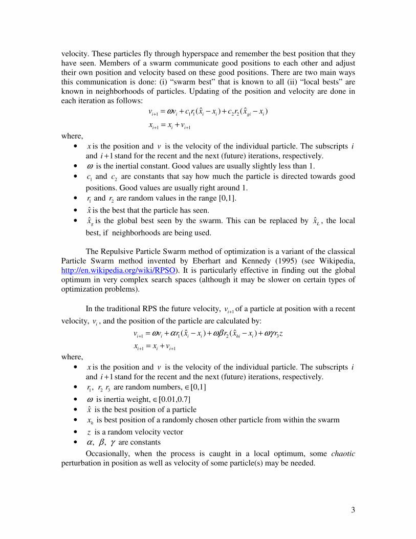
1 1 1 2 2

1 1

ˆ ˆ( ) ( )i i i i gi i

i i i

v v c r x x c r x x

x x v

ω+

+ +

= + − + −

= +

where,

• x is the position and v is the velocity of the individual particle. The subscripts i

and 1i + stand for the recent and the next (future) iterations, respectively.

• ω is the inertial constant. Good values are usually slightly less than 1.

• 1c and 2c are constants that say how much the particle is directed towards good

positions. Good values are usually right around 1.

• 1r and 2r are random values in the range [0,1].

• x̂ is the best that the particle has seen.

• ˆg

x is the global best seen by the swarm. This can be replaced by ˆL

x , the local

best, if neighborhoods are being used.

The Repulsive Particle Swarm method of optimization is a variant of the classical

Particle Swarm method invented by Eberhart and Kennedy (1995) (see Wikipedia,

http://en.wikipedia.org/wiki/RPSO). It is particularly effective in finding out the global

optimum in very complex search spaces (although it may be slower on certain types of

optimization problems).

In the traditional RPS the future velocity, 1iv + of a particle at position with a recent

velocity, i

v , and the position of the particle are calculated by:

1 1 2 3

1 1

ˆ ˆ( ) ( )i i i i hi i

i i i

v v r x x r x x r z

x x v

ω α ωβ ωγ+

+ +

= + − + − +

= +

where,

• x is the position and v is the velocity of the individual particle. The subscripts i

and 1i + stand for the recent and the next (future) iterations, respectively.

• 1 2 3,r r r are random numbers, ∈[0,1]

• ω is inertia weight, ∈[0.01,0.7]

• x̂ is the best position of a particle

• h

x is best position of a randomly chosen other particle from within the swarm

• z is a random velocity vector

• , ,α β γ are constants

Occasionally, when the process is caught in a local optimum, some chaotic

perturbation in position as well as velocity of some particle(s) may be needed.

4

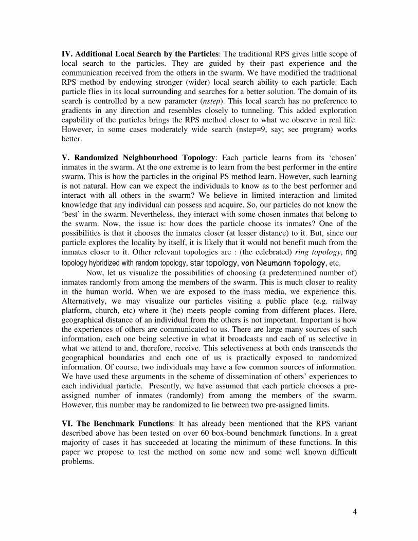
IV. Additional Local Search by the Particles: The traditional RPS gives little scope of

local search to the particles. They are guided by their past experience and the

communication received from the others in the swarm. We have modified the traditional

RPS method by endowing stronger (wider) local search ability to each particle. Each

particle flies in its local surrounding and searches for a better solution. The domain of its

search is controlled by a new parameter (nstep). This local search has no preference to

gradients in any direction and resembles closely to tunneling. This added exploration

capability of the particles brings the RPS method closer to what we observe in real life.

However, in some cases moderately wide search (nstep=9, say; see program) works

better.

V. Randomized Neighbourhood Topology: Each particle learns from its ‘chosen’

inmates in the swarm. At the one extreme is to learn from the best performer in the entire

swarm. This is how the particles in the original PS method learn. However, such learning

is not natural. How can we expect the individuals to know as to the best performer and

interact with all others in the swarm? We believe in limited interaction and limited

knowledge that any individual can possess and acquire. So, our particles do not know the

‘best’ in the swarm. Nevertheless, they interact with some chosen inmates that belong to

the swarm. Now, the issue is: how does the particle choose its inmates? One of the

possibilities is that it chooses the inmates closer (at lesser distance) to it. But, since our

particle explores the locality by itself, it is likely that it would not benefit much from the

inmates closer to it. Other relevant topologies are : (the celebrated) ring topology, ring

topology hybridized with random topology, star topology, von Neumann topology, etc.

Now, let us visualize the possibilities of choosing (a predetermined number of)

inmates randomly from among the members of the swarm. This is much closer to reality

in the human world. When we are exposed to the mass media, we experience this.

Alternatively, we may visualize our particles visiting a public place (e.g. railway

platform, church, etc) where it (he) meets people coming from different places. Here,

geographical distance of an individual from the others is not important. Important is how

the experiences of others are communicated to us. There are large many sources of such

information, each one being selective in what it broadcasts and each of us selective in

what we attend to and, therefore, receive. This selectiveness at both ends transcends the

geographical boundaries and each one of us is practically exposed to randomized

information. Of course, two individuals may have a few common sources of information.

We have used these arguments in the scheme of dissemination of others’ experiences to

each individual particle. Presently, we have assumed that each particle chooses a pre-

assigned number of inmates (randomly) from among the members of the swarm.

However, this number may be randomized to lie between two pre-assigned limits.

VI. The Benchmark Functions: It has already been mentioned that the RPS variant

described above has been tested on over 60 box-bound benchmark functions. In a great

majority of cases it has succeeded at locating the minimum of these functions. In this

paper we propose to test the method on some new and some well known difficult

problems.

5

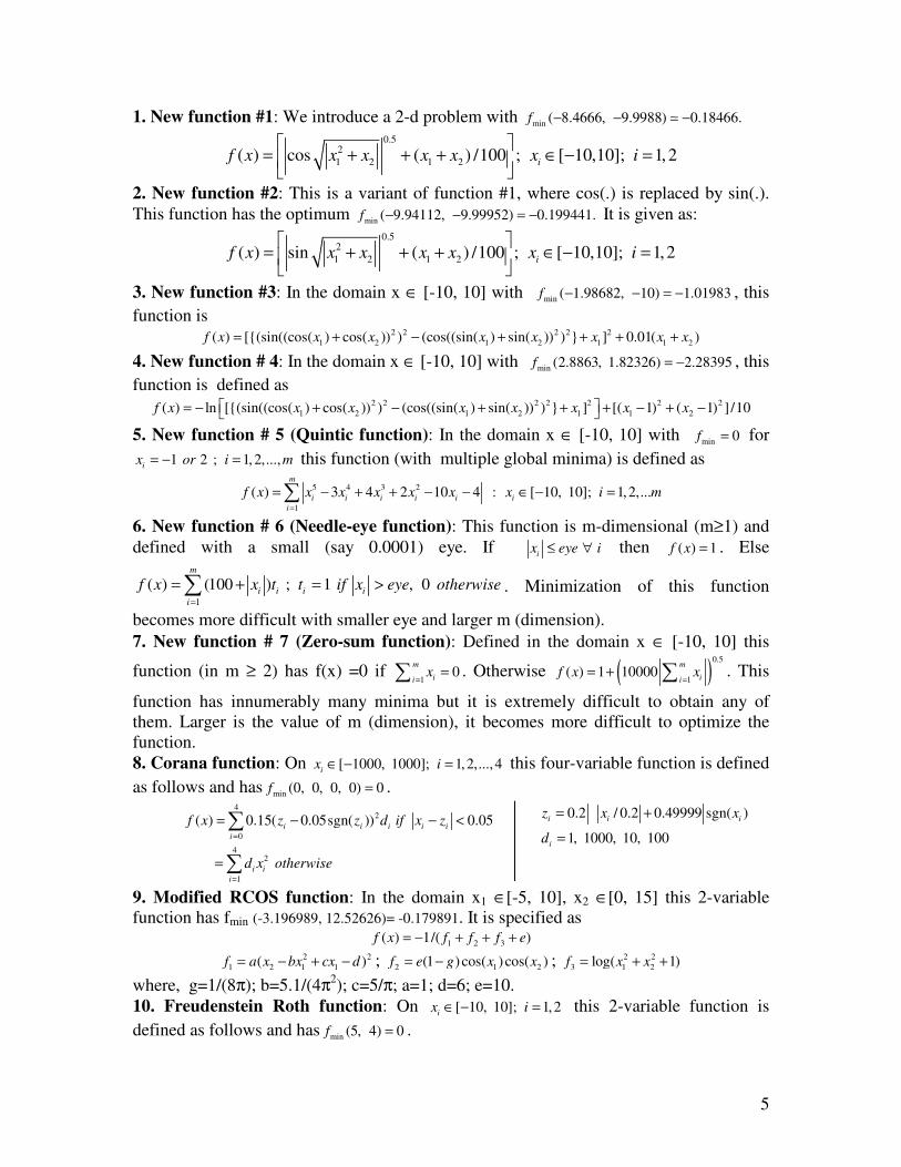
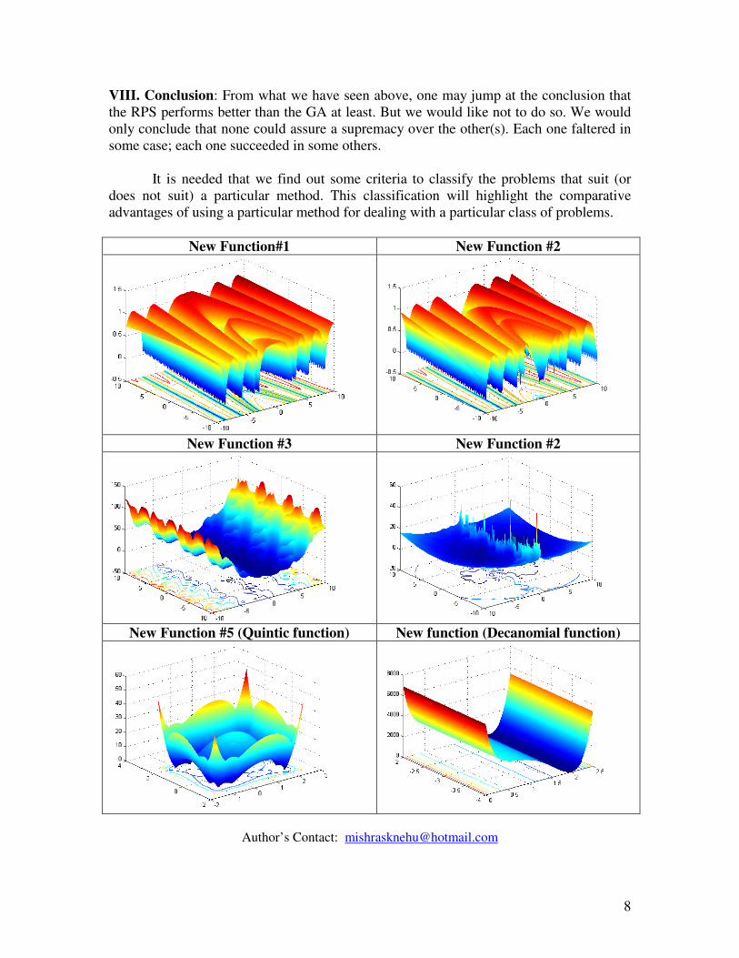
1. New function #1: We introduce a 2-d problem with min

( 8.4666, 9.9988) 0.18466.f − − −�

0.52

1 2 1 2( ) cos ( ) /100 ; [ 10,10]; 1, 2i

f x x x x x x i

= + + + ∈ − =

2. New function #2: This is a variant of function #1, where cos(.) is replaced by sin(.).

This function has the optimum min

( 9.94112, 9.99952) 0.199441.f − − = − It is given as:

0.52

1 2 1 2( ) sin ( ) /100 ; [ 10,10]; 1,2i

f x x x x x x i

= + + + ∈ − =

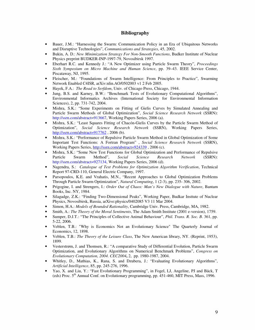
3. New function #3: In the domain x ∈ [-10, 10] with min

( 1.98682, 10) 1.01983f − − = − , this

function is 2 2 2 2 2

1 2 1 2 1 1 2( ) [{(sin((cos( ) cos( )) ) (cos((sin( ) sin( )) ) } ] 0.01( )f x x x x x x x x= + − + + + +

4. New function # 4: In the domain x ∈ [-10, 10] with min

(2.8863, 1.82326) 2.28395f = − , this

function is defined as 2 2 2 2 2 2 2

1 2 1 2 1 1 2( ) ln [{(sin((cos( ) cos( )) ) (cos((sin( ) sin( )) ) } ] [( 1) ( 1) ] /10f x x x x x x x x = − + − + + + − + −

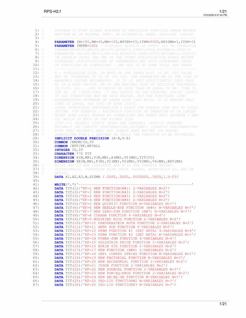
5. New function # 5 (Quintic function): In the domain x ∈ [-10, 10] with min

0f = for

1 2 ; 1,2,...,i

x or i m= − = this function (with multiple global minima) is defined as

5 4 3 2

1

( ) 3 4 2 10 4 : [ 10, 10]; 1,2,...m

i i i i i i

i

f x x x x x x x i m=

= − + + − − ∈ − =∑

6. New function # 6 (Needle-eye function): This function is m-dimensional (m≥1) and

defined with a small (say 0.0001) eye. If i

x eye i≤ ∀ then ( ) 1f x = . Else

1

( ) (100 ) ; 1 , 0m

i i i i

i

f x x t t if x eye otherwise=

= + = >∑ . Minimization of this function

becomes more difficult with smaller eye and larger m (dimension).

7. New function # 7 (Zero-sum function): Defined in the domain x ∈ [-10, 10] this

function (in m ≥ 2) has f(x) =0 if 1

0m

iix

==∑ . Otherwise ( )

0.5

1( ) 1 10000

m

iif x x

== + ∑ . This

function has innumerably many minima but it is extremely difficult to obtain any of

them. Larger is the value of m (dimension), it becomes more difficult to optimize the

function.

8. Corana function: On [ 1000, 1000]; 1,2,..., 4i

x i∈ − = this four-variable function is defined

as follows and hasmin

(0, 0, 0, 0) 0f = . 4

2

0

( ) 0.15( 0.05sgn( )) 0.05i i i i i

i

f x z z d if x z=

= − − <∑

4

2

1

i i

i

d x otherwise=

=∑

0.2 / 0.2 0.49999 sgn( )i i iz x x= +

1, 1000, 10, 100i

d =

9. Modified RCOS function: In the domain x1 ∈[-5, 10], x2 ∈[0, 15] this 2-variable

function has fmin (-3.196989, 12.52626)= -0.179891. It is specified as

1 2 3( ) 1/( )f x f f f e= − + + +

2 2

1 2 1 1( )f a x bx cx d= − + − ;

2 1 2(1 )cos( ) cos( )f e g x x= − ; 2 2

3 1 2log( 1)f x x= + +

where, g=1/(8π); b=5.1/(4π2); c=5/π; a=1; d=6; e=10.

10. Freudenstein Roth function: On [ 10, 10]; 1,2i

x i∈ − = this 2-variable function is

defined as follows and hasmin

(5, 4) 0f = .

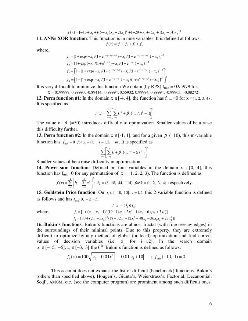
6

2 2

1 2 2 2 1 2 2 2( ) [ 13 ((5 ) 2) ] [ 29 (( 1) 14) ]f x x x x x x x x x= − + + − − + − + + + −

11. ANNs XOR function: This function is in nine variables. It is defined at follows.

1 2 3 4( )f x f f f f= + + +

where, 1 2 5 3 4 6( ) ( ) 2

1 7 8 9[1 exp{ /(1 e ) /(1 e ) }]

x x x x x xf x x x

− − − − − − −= + − + − + −

5 6( ) ( ) 2

2 7 8 9[1 exp{ /(1 e ) /(1 e ) }]

x xf x x x

− − −= + − + − + −

1 5 3 62

( ) ( ) 1

3 7 8 91 [1 exp{ /(1 e ) /(1 e ) }]x x x x

f x x x− − − − − = − + − + − + −

2 5 4 62

( ) ( ) 1

4 7 8 91 [1 exp{ /(1 e ) /(1 e ) }]x x x x

f x x x− − − − − = − + − + − + −

It is very difficult to minimize this function We obtain (by RPS) fmin = 0.95979 for:

x = (0.99999, 0.99993, -0.89414, 0.99994, 0.55932, 0.99994, 0.99994, -0.99963, -0.08272).

12. Perm function #1: In the domain x ∈[-4, 4], the function has fmin =0 for x =(1, 2, 3, 4) .

It is specified as 2

4 4

1 1

( ) ( ){( / ) 1}k k

i

k i

f x i x iβ= =

= + −

∑ ∑

The value of β (=50) introduces difficulty to optimization. Smaller values of beta raise

this difficulty further.

13. Perm function #2: In the domain x ∈[-1, 1], and for a given β (=10), this m-variable

function has 1;

min0 ( ) 1,2,...,

if for x i i m−= = = . It is specified as

24 4

1 1

( ){( ) ( ) }k k

i

k i

i x iβ −

= =

+ −

∑ ∑

Smaller values of beta raise difficulty in optimization.

14. Power-sum function: Defined on four variables in the domain x ∈[0, 4], this

function has fmin=0 for any permutation of x = (1, 2, 2, 3). The function is defined as 2

4 4

1 1

( ) ; (8, 18, 44, 114) (1, 2, 3, 4)k

k i k

k i

f x b x b for k= =

= − = =

∑ ∑ respectively.

15. Goldstein Price function: On [ 10, 10]; 1,2i

x i∈ − = this 2-variable function is defined

as follows and hasmin

(0, 1) 3f − = .

1 2( ) ( )( )f x f f=

where, 2 2 2

1 1 2 1 1 2 1 2 2[1 ( 1) (19 14 3 14 6 3 )]f x x x x x x x x= + + + − + − + +

2 2 2

1 1 2 1 1 2 1 2 2[30 (2 3 ) (18 32 12 48 36 27 )]f x x x x x x x x= + − − + + − +

16. Bukin’s functions: Bukin’s functions are almost fractal (with fine seesaw edges) in

the surroundings of their minimal points. Due to this property, they are extremely

difficult to optimize by any method of global (or local) optimization and find correct

values of decision variables (i.e. xi for i=1,2). In the search domain

1 2[ 15, 5], [ 3, 3]x x∈ − − ∈ − the 6th

Bukin’s function is defined as follows.

2

6 2 1 1( ) 100 0.01 0.01 10f x x x x= − + + ; min ( 10, 1) 0f − =

This account does not exhaust the list of difficult (benchmark) functions. Bukin’s

(others than specified above), Hougen’s, Giunta’s, Weierstrass’s, Factorial, Decanomial,

SeqP, AMGM, etc. (see the computer program) are prominent among such difficult ones.

7

Elsewhere (Mishra, 2006 (a) and (b)) also we faced difficult global optimization

problems.

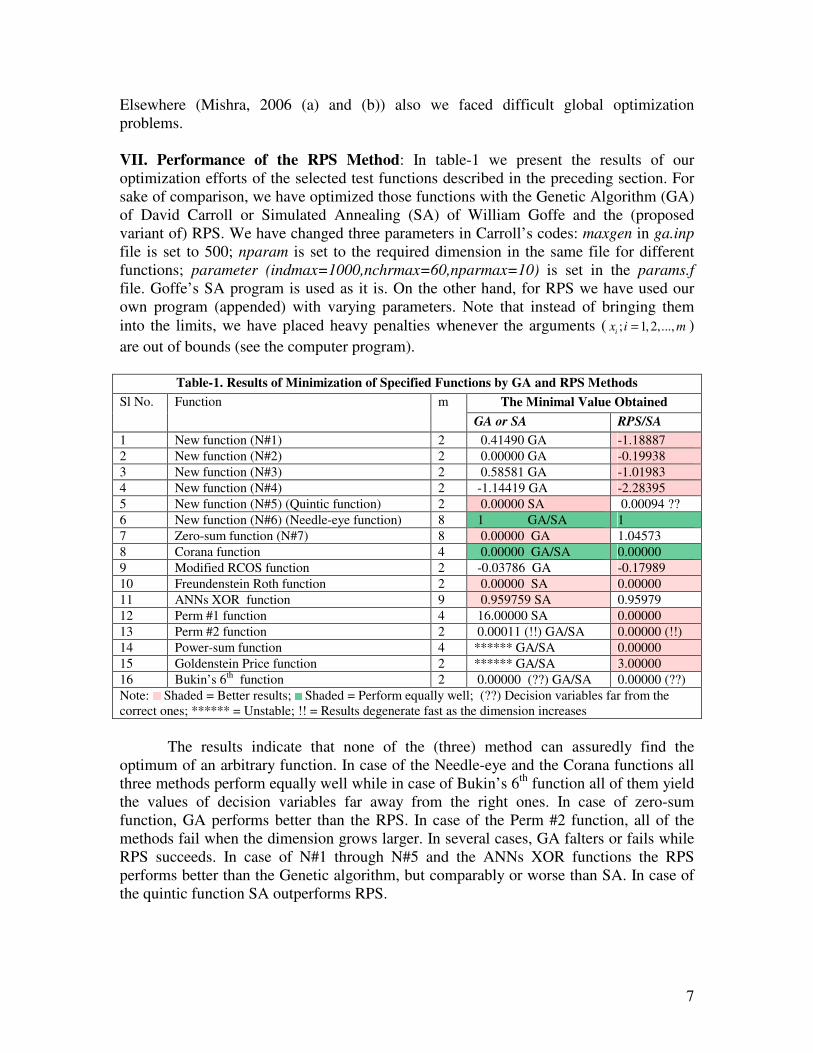
VII. Performance of the RPS Method: In table-1 we present the results of our

optimization efforts of the selected test functions described in the preceding section. For

sake of comparison, we have optimized those functions with the Genetic Algorithm (GA)

of David Carroll or Simulated Annealing (SA) of William Goffe and the (proposed

variant of) RPS. We have changed three parameters in Carroll’s codes: maxgen in ga.inp

file is set to 500; nparam is set to the required dimension in the same file for different

functions; parameter (indmax=1000,nchrmax=60,nparmax=10) is set in the params.f

file. Goffe’s SA program is used as it is. On the other hand, for RPS we have used our

own program (appended) with varying parameters. Note that instead of bringing them

into the limits, we have placed heavy penalties whenever the arguments ( ; 1,2,...,i

x i m= )

are out of bounds (see the computer program).

Table-1. Results of Minimization of Specified Functions by GA and RPS Methods

The Minimal Value Obtained Sl No. Function m

GA or SA RPS/SA

1 New function (N#1) 2 0.41490 GA -1.18887

2 New function (N#2) 2 0.00000 GA -0.19938

3 New function (N#3) 2 0.58581 GA -1.01983

4 New function (N#4) 2 -1.14419 GA -2.28395

5 New function (N#5) (Quintic function) 2 0.00000 SA 0.00094 ??

6 New function (N#6) (Needle-eye function) 8 1 GA/SA 1

7 Zero-sum function (N#7) 8 0.00000 GA 1.04573

8 Corana function 4 0.00000 GA/SA 0.00000

9 Modified RCOS function 2 -0.03786 GA -0.17989

10 Freundenstein Roth function 2 0.00000 SA 0.00000

11 ANNs XOR function 9 0.959759 SA 0.95979

12 Perm #1 function 4 16.00000 SA 0.00000

13 Perm #2 function 2 0.00011 (!!) GA/SA 0.00000 (!!)

14 Power-sum function 4 ****** GA/SA 0.00000

15 Goldenstein Price function 2 ****** GA/SA 3.00000

16 Bukin’s 6th

function 2 0.00000 (??) GA/SA 0.00000 (??)

Note: Shaded = Better results; Shaded = Perform equally well; (??) Decision variables far from the

correct ones; ****** = Unstable; !! = Results degenerate fast as the dimension increases

The results indicate that none of the (three) method can assuredly find the

optimum of an arbitrary function. In case of the Needle-eye and the Corana functions all

three methods perform equally well while in case of Bukin’s 6th

function all of them yield

the values of decision variables far away from the right ones. In case of zero-sum

function, GA performs better than the RPS. In case of the Perm #2 function, all of the

methods fail when the dimension grows larger. In several cases, GA falters or fails while

RPS succeeds. In case of N#1 through N#5 and the ANNs XOR functions the RPS

performs better than the Genetic algorithm, but comparably or worse than SA. In case of

the quintic function SA outperforms RPS.

8

VIII. Conclusion: From what we have seen above, one may jump at the conclusion that

the RPS performs better than the GA at least. But we would like not to do so. We would

only conclude that none could assure a supremacy over the other(s). Each one faltered in

some case; each one succeeded in some others.

It is needed that we find out some criteria to classify the problems that suit (or

does not suit) a particular method. This classification will highlight the comparative

advantages of using a particular method for dealing with a particular class of problems.

New Function#1 New Function #2

New Function #3 New Function #2

New Function #5 (Quintic function) New function (Decanomial function)

Author’s Contact: [email protected]

9

Bibliography

• Bauer, J.M.: “Harnessing the Swarm: Communication Policy in an Era of Ubiquitous Networks

and Disruptive Technologies”, Communications and Strategies, 45, 2002.

• Bukin, A. D.: New Minimization Strategy For Non-Smooth Functions, Budker Institute of Nuclear

Physics preprint BUDKER-INP-1997-79, Novosibirsk 1997.

• Eberhart R.C. and Kennedy J.: “A New Optimizer using Particle Swarm Theory”, Proceedings

Sixth Symposium on Micro Machine and Human Science, pp. 39–43. IEEE Service Center,

Piscataway, NJ, 1995.

• Fleischer, M.: “Foundations of Swarm Intelligence: From Principles to Practice”, Swarming

Network Enabled C4ISR, arXiv:nlin.AO/0502003 v1 2 Feb 2005.

• Hayek, F.A.: The Road to Serfdom, Univ. of Chicago Press, Chicago, 1944.

• Jung, B.S. and Karney, B.W.: “Benchmark Tests of Evolutionary Computational Algorithms”,

Environmental Informatics Archives (International Society for Environmental Information

Sciences), 2, pp. 731-742, 2004.

• Mishra, S.K.: “Some Experiments on Fitting of Gielis Curves by Simulated Annealing and

Particle Swarm Methods of Global Optimization”, Social Science Research Network (SSRN):

http://ssrn.com/abstract=913667, Working Papers Series, 2006 (a).

• Mishra, S.K.: “Least Squares Fitting of Chacón-Gielis Curves by the Particle Swarm Method of

Optimization”, Social Science Research Network (SSRN), Working Papers Series,

http://ssrn.com/abstract=917762 , 2006 (b).

• Mishra, S.K.: “Performance of Repulsive Particle Swarm Method in Global Optimization of Some

Important Test Functions: A Fortran Program” , Social Science Research Network (SSRN),

Working Papers Series, http://ssrn.com/abstract=924339 , 2006 (c).

• Mishra, S.K.: “Some New Test Functions for Global Optimization and Performance of Repulsive

Particle Swarm Method”, Social Science Research Network (SSRN):

http://ssrn.com/abstract=927134, Working Papers Series, 2006 (d).

• Nagendra, S.: Catalogue of Test Problems for Optimization Algorithm Verification, Technical

Report 97-CRD-110, General Electric Company, 1997.

• Parsopoulos, K.E. and Vrahatis, M.N., “Recent Approaches to Global Optimization Problems

Through Particle Swarm Optimization”, Natural Computing, 1 (2-3), pp. 235- 306, 2002.

• Prigogine, I. and Strengers, I.: Order Out of Chaos: Man’s New Dialogue with Nature, Bantam

Books, Inc. NY, 1984.

• Silagadge, Z.K.: “Finding Two-Dimensional Peaks”, Working Paper, Budkar Insttute of Nuclear

Physics, Novosibirsk, Russia, arXive:physics/0402085 V3 11 Mar 2004.

• Simon, H.A.: Models of Bounded Rationality, Cambridge Univ. Press, Cambridge, MA, 1982.

• Smith, A.: The Theory of the Moral Sentiments, The Adam Smith Institute (2001 e-version), 1759.

• Sumper, D.J.T.: “The Principles of Collective Animal Behaviour”, Phil. Trans. R. Soc. B. 361, pp.

5-22, 2006.

• Veblen, T.B.: "Why is Economics Not an Evolutionary Science" The Quarterly Journal of

Economics, 12, 1898.

• Veblen, T.B.: The Theory of the Leisure Class, The New American library, NY. (Reprint, 1953),

1899.

• Vesterstrøm, J. and Thomsen, R.: “A comparative Study of Differential Evolution, Particle Swarm

Optimization, and Evolutionary Algorithms on Numerical Benchmark Problems”, Congress on

Evolutionary Computation, 2004. CEC2004, 2, pp. 1980-1987, 2004.

• Whitley, D., Mathias, K., Rana, S. and Dzubera, J.: “Evaluating Evolutionary Algorithms”,

Artificial Intelligence, 85, pp. 245-276, 1996.

• Yao, X. and Liu, Y.: “Fast Evolutionary Programming”, in Fogel, LJ, Angeline, PJ and Bäck, T

(eds) Proc. 5th

Annual Conf. on Evolutionary programming, pp. 451-460, MIT Press, Mass, 1996.

RPS-H2.f 1/2110/5/2006 6:47:40 PM

1: C PROGRAM TO FIND GLOBAL MINIMUM BY REPULSIVE PARTICLE SWARM METHOD2: C WRITTEN BY SK MISHRA, DEPT. OF ECONOMICS, NEHU, SHILLONG (INDIA)3: C -----------------------------------------------------------------4: PARAMETER (N=100,NN=40,MX=100,NSTEP=15,ITRN=5000,NSIGMA=1,ITOP=3)

5: PARAMETER (NPRN=100) ! DISPLAYS RESULTS AT EVERY 100 TH ITERATION6: C PARAMETER(N=50,NN=25,MX=100,NSTEP=9,ITRN=10000,NSIGMA=1,ITOP=3)7: C PARAMETER (N=100,NN=15,MX=100,NSTEP=9,ITRN=10000,NSIGMA=1,ITOP=3)8: C IN CERTAIN CASES THE ONE OR THE OTHER SPECIFICATION WORKS BETTER9: C DIFFERENT SPECIFICATIONS OF PARAMETERS MAY SUIT DIFFERENT TYPES10: C OF FUNCTIONS OR DIMENSIONS - ONE HAS TO DO SOME TRIAL AND ERROR11: C -----------------------------------------------------------------12: C N = POPULATION SIZE. IN MOST OF THE CASES N=30 IS OK. ITS VALUE13: C MAY BE INCREASED TO 50 OR 100 TOO. THE PARAMETER NN IS THE SIZE OF14: C RANDOMLY CHOSEN NEIGHBOURS. 15 TO 25 (BUT SUFFICIENTLY LESS THAN15: C N) IS A GOOD CHOICE. MX IS THE MAXIMAL SIZE OF DECISION VARIABLES.16: C IN F(X1, X2,...,XM) M SHOULD BE LESS THAN OR EQUAL TO MX. ITRN IS17: C THE NO. OF ITERATIONS. IT MAY DEPEND ON THE PROBLEM. 200(AT LEAST)18: C TO 500 ITERATIONS MAY BE GOOD ENOUGH. BUT FOR FUNCTIONS LIKE19: C ROSENBROCKOR GRIEWANK OF LARGE SIZE (SAY M=30) IT IS NEEDED THAT20: C ITRN IS LARGE, SAY 5000 OR EVEN 10000.21: C SIGMA INTRODUCES PERTURBATION & HELPS THE SEARCH JUMP OUT OF LOCAL22: C OPTIMA. FOR EXAMPLE : RASTRIGIN FUNCTION OF DMENSION 3O OR LARGER23: C NSTEP DOES LOCAL SEARCH BY TUNNELLING AND WORKS WELL BETWEEN 5 AND24: C 15, WHICH IS MUCH ON THE HIGHER SIDE.25: C ITOP <=1 (RING); ITOP=2 (RING AND RANDOM); ITOP=>3 (RANDOM)26: C NSIGMA=0 (NO CHAOTIC PERTURBATION);NSIGMA=1 (CHAOTIC PERTURBATION)27: C NOTE THAT NSIGMA=1 NEED NOT ALWAYS WORK BETTER (OR WORSE)28: C SUBROUTINE FUNC( ) DEFINES OR CALLS THE FUNCTION TO BE OPTIMIZED.29: IMPLICIT DOUBLE PRECISION (A-H,O-Z)

30: COMMON /RNDM/IU,IV

31: COMMON /KFF/KF,NFCALL

32: INTEGER IU,IV

33: CHARACTER *70 TIT

34: DIMENSION X(N,MX),V(N,MX),A(MX),VI(MX),TIT(50)

35: DIMENSION XX(N,MX),F(N),V1(MX),V2(MX),V3(MX),V4(MX),BST(MX)

36: C A1 A2 AND A3 ARE CONSTANTS AND W IS THE INERTIA WEIGHT.37: C OCCASIONALLY, TINKERING WITH THESE VALUES, ESPECIALLY A3, MAY BE38: C NEEDED.39: DATA A1,A2,A3,W,SIGMA /.5D00,.5D00,.0005D00,.5D00,1.D-03/

40:

41: WRITE(*,*)'----------------------------------------------------'

42: DATA TIT(1)/'KF=1 NEW FUNCTION(N#1) 2-VARIABLES M=2'/




46: DATA TIT(5)/'KF=5 NEW QUINTIC FUNCTION M-VARIABLES M=?'/

47: DATA TIT(6)/'KF=6 NEW NEEDLE-EYE FUNCTION (N#6) M-VARIABLES M=?'/

48: DATA TIT(7)/'KF=7 NEW ZERO-SUM FUNCTION (N#7) M-VARIABLES M=?'/

49: DATA TIT(8)/'KF=8 CORANA FUNCTION 4-VARIABLES M=4'/

50: DATA TIT(9)/'KF=9 MODIFIED RCOS FUNCTION 2-VARIABLES M=2'/

51: DATA TIT(10)/'KF=10 FREUDENSTEIN ROTH FUNCTION 2-VARIABLES M=2'/

52: DATA TIT(11)/'KF=11 ANNS XOR FUNCTION 9-VARIABLES M=9'/

53: DATA TIT(12)/'KF=12 PERM FUNCTION #1 (SET BETA) 4-VARIABLES M=4'/

54: DATA TIT(13)/'KF=13 PERM FUNCTION #2 (SET BETA) M-VARIABLES M=?'/

55: DATA TIT(14)/'KF=14 POWER-SUM FUNCTION 4-VARIABLES M=4'/

56: DATA TIT(15)/'KF=15 GOLDSTEIN PRICE FUNCTION 2-VARIABLES M=2'/

57: DATA TIT(16)/'KF=16 BUKIN 6TH FUNCTION 2-VARIABLES M=2'/

58: DATA TIT(17)/'KF=17 NEW FUNCTION (N#8) 2-VARIABLES M=2'/

59: DATA TIT(18)/'KF=18 DEFL CORRUG SPRING FUNCTION M-VARIABLES M=?'/

60: DATA TIT(19)/'KF=19 NEW FACTORIAL FUNCTION M-VARIABLES M=?'/

61: DATA TIT(20)/'KF=20 NEW DECANOMIAL FUNCTION 2-VARIABLES M=2'/

62: DATA TIT(21)/'KF=21 JUDGE FUNCTION 2-VARIABLES M=2'/

63: DATA TIT(22)/'KF=22 NEW DODECAL FUNCTION 3-VARIABLES M=3'/

64: DATA TIT(23)/'KF=23 NEW SUM-EQ-PROD FUNCTION 2-VARIABLES M=2'/

65: DATA TIT(24)/'KF=24 NEW AM-EQ-GM FUNCTION M-VARIABLES M=?'/

66: DATA TIT(25)/'KF=25 YAO-LIU FUNCTION#2 M-VARIABLES M=?'/


1/21

RPS-H2.f 2/2110/5/2006 6:47:40 PM






73: DATA TIT(32)/'KF=32 YAO-LIU FUNCTION#14 2-VARIABLES M=2'/

74: DATA TIT(33)/'KF=33 YAO-LIU FUNCTION#15 4-VARIABLES M=4'/

75: DATA TIT(34)/'KF=34 LINEAR PROGRAMMING-I : 2-VARIABLES M=2'/

76: DATA TIT(35)/'KF=35 LINEAR PROGRAMMING-II : 3-VARIABLES M=3'/

77: DATA TIT(36)/'KF=36 TRIGON FUNCTION : M-VARIABLES M=?'/

78: C -----------------------------------------------------------------79: DO I=1,36

80: WRITE(*,*)TIT(I)

81: ENDDO

82: WRITE(*,*)'----------------------------------------------------'

83: WRITE(*,*)'CHOOSE FUNCTION CODE [KF] AND NO. OF VARIABLES [M]'

84: READ(*,*) KF,M

85:

86: LCOUNT=0

87: NFCALL=0

88: WRITE(*,*)'4-DIGITS SEED FOR RANDOM NUMBER GENERATION'

89: READ(*,*) IU

90: DATA FMIN /1.0E30/

91: C GENERATE N-SIZE POPULATION OF M-TUPLE PARAMETERS X(I,J) RANDOMLY92: DO I=1,N

93: DO J=1,M

94: CALL RANDOM(RAND)

95: X(I,J)=(RAND-0.5D00)*10

96: C WE GENERATE RANDOM(-5,5). HERE MULTIPLIER IS 10. TINKERING IN SOME97: C CASES MAY BE NEEDED98: ENDDO

99: F(I)=1.0D30

100: ENDDO

101: C INITIALISE VELOCITIES V(I) FOR EACH INDIVIDUAL IN THE POPULATION102: DO I=1,N

103: DO J=1,M


105: V(I,J)=(RAND-0.5D+00)

106: C V(I,J)=RAND107: ENDDO

108: ENDDO

109: DO 100 ITER=1,ITRN

110: C LET EACH INDIVIDUAL SEARCH FOR THE BEST IN ITS NEIGHBOURHOOD111: DO I=1,N

112: DO J=1,M

113: A(J)=X(I,J)

114: VI(J)=V(I,J)

115: ENDDO

116: CALL LSRCH(A,M,VI,NSTEP,FI)

117: IF(FI.LT.F(I)) THEN

118: F(I)=FI

119: DO IN=1,M

120: BST(IN)=A(IN)

121: ENDDO

122: C F(I) CONTAINS THE LOCAL BEST VALUE OF FUNCTION FOR ITH INDIVIDUAL123: C XX(I,J) IS THE M-TUPLE VALUE OF X ASSOCIATED WITH LOCAL BEST F(I)124: DO J=1,M

125: XX(I,J)=A(J)

126: ENDDO

127: ENDIF

128: ENDDO

129: C NOW LET EVERY INDIVIDUAL RANDOMLY COSULT NN(<<N) COLLEAGUES AND130: C FIND THE BEST AMONG THEM131: DO I=1,N

132: C ------------------------------------------------------------------133: IF(ITOP.GE.3) THEN

134: C RANDOM TOPOLOGY ******************************************

2/21

RPS-H2.f 3/2110/5/2006 6:47:40 PM

135: C CHOOSE NN COLLEAGUES RANDOMLY AND FIND THE BEST AMONG THEM136: BEST=1.0D30

137: DO II=1,NN


139: NF=INT(RAND*N)+1

140: IF(BEST.GT.F(NF)) THEN

141: BEST=F(NF)

142: NFBEST=NF

143: ENDIF

144: ENDDO

145: ENDIF

146: C----------------------------------------------------------------------147: IF(ITOP.EQ.2) THEN

148: C RING + RANDOM TOPOLOGY ******************************************149: C REQUIRES THAT THE SUBROUTINE NEIGHBOR IS TURNED ALIVE150: BEST=1.0D30

151: CALL NEIGHBOR(I,N,I1,I3)

152: DO II=1,NN

153: IF(II.EQ.1) NF=I1

154: IF(II.EQ.2) NF=I


156: IF(II.GT.3) THEN


158: NF=INT(RAND*N)+1

159: ENDIF


161: BEST=F(NF)

162: NFBEST=NF

163: ENDIF

164: ENDDO

165: ENDIF

166: C---------------------------------------------------------------------167: IF(ITOP.LE.1) THEN

168: C RING TOPOLOGY **************************************************169: C REQUIRES THAT THE SUBROUTINE NEIGHBOR IS TURNED ALIVE170: BEST=1.0D30

171: CALL NEIGHBOR(I,N,I1,I3)

172: DO II=1,3

173: IF (II.NE.I) THEN




177: BEST=F(NF)

178: NFBEST=NF

179: ENDIF

180: ENDIF

181: ENDDO

182: ENDIF

183: C---------------------------------------------------------------------184: C IN THE LIGHT OF HIS OWN AND HIS BEST COLLEAGUES EXPERIENCE, THE185: C INDIVIDUAL I WILL MODIFY HIS MOVE AS PER THE FOLLOWING CRITERION186: C FIRST, ADJUSTMENT BASED ON ONES OWN EXPERIENCE187: C AND OWN BEST EXPERIENCE IN THE PAST (XX(I))188: DO J=1,M


190: V1(J)=A1*RAND*(XX(I,J)-X(I,J))

191: C THEN BASED ON THE OTHER COLLEAGUES BEST EXPERIENCE WITH WEIGHT W192: C HERE W IS CALLED AN INERTIA WEIGHT 0.01< W < 0.7193: C A2 IS THE CONSTANT NEAR BUT LESS THAN UNITY194: CALL RANDOM(RAND)

195: V2(J)=V(I,J)

196: IF(F(NFBEST).LT.F(I)) THEN

197: V2(J)=A2*W*RAND*(XX(NFBEST,J)-X(I,J))

198: ENDIF

199: C THEN SOME RANDOMNESS AND A CONSTANT A3 CLOSE TO BUT LESS THAN UNITY200: CALL RANDOM(RAND)

201: RND1=RAND

3/21

RPS-H2.f 4/2110/5/2006 6:47:40 PM


203: V3(J)=A3*RAND*W*RND1

204: C V3(J)=A3*RAND*W205: C THEN ON PAST VELOCITY WITH INERTIA WEIGHT W206: V4(J)=W*V(I,J)

207: C FINALLY A SUM OF THEM208: V(I,J)= V1(J)+V2(J)+V3(J)+V4(J)

209: ENDDO

210: ENDDO

211: C CHANGE X212: DO I=1,N

213: DO J=1,M

214: RANDS=0.D00

215: C ------------------------------------------------------------------216: IF(NSIGMA.EQ.1) THEN

217: CALL RANDOM(RAND) ! FOR CHAOTIC PERTURBATION218: IF(DABS(RAND-.5D00).LT.SIGMA) RANDS=RAND-0.5D00

219: C SIGMA CONDITIONED RANDS INTRODUCES CHAOTIC ELEMENT IN TO LOCATION220: C IN SOME CASES THIS PERTURBATION HAS WORKED VERY EFFECTIVELY WITH221: C PARAMETER (N=100,NN=15,MX=100,NSTEP=9,ITRN=100000,NSIGMA=1,ITOP=2)222: ENDIF

223: C -----------------------------------------------------------------224: X(I,J)=X(I,J)+V(I,J)*(1.D00+RANDS)

225: ENDDO

226: ENDDO

227: DO I=1,N

228: IF(F(I).LT.FMIN) THEN

229: FMIN=F(I)

230: II=I

231: DO J=1,M

232: BST(J)=XX(II,J)

233: ENDDO

234: ENDIF

235: ENDDO

236: IF(LCOUNT.EQ.NPRN) THEN

237: LCOUNT=0

238: WRITE(*,*)'OPTIMAL SOLUTION UPTO THIS (FUNCTION CALLS=',NFCALL,')'

239: WRITE(*,*)'X = ',(BST(J),J=1,M),' MIN F = ',FMIN

240: C WRITE(*,*)'NO. OF FUNCTION CALLS = ',NFCALL241: ENDIF

242: LCOUNT=LCOUNT+1

243: 100 CONTINUE

244: WRITE(*,*)'COMPUTATION OVER:',TIT(KF)

245:

246: END

247: C ----------------------------------------------------------------248: SUBROUTINE LSRCH(A,M,VI,NSTEP,FI)

249: IMPLICIT DOUBLE PRECISION (A-H,O-Z)



252: INTEGER IU,IV

253: DIMENSION A(*),B(100),VI(*)

254: AMN=1.0D30

255: DO J=1,NSTEP

256: DO JJ=1,M

257: B(JJ)=A(JJ)+(J-(NSTEP/2)-1)*VI(JJ)

258: ENDDO

259: CALL FUNC(B,M,FI)

260: IF(FI.LT.AMN) THEN

261: AMN=FI

262: DO JJ=1,M

263: A(JJ)=B(JJ)

264: ENDDO

265: ENDIF

266: ENDDO

267: FI=AMN

268: RETURN

4/21

RPS-H2.f 5/2110/5/2006 6:47:40 PM

269: END

270: C -----------------------------------------------------------------271: C THIS SUBROUTINE IS NEEDED IF THE NEIGHBOURHOOD HAS RING TOPOLOGY272: C EITHER PURE OR HYBRIDIZED273: SUBROUTINE NEIGHBOR(I,N,J,K)

274: IF(I-1.GE.1 .AND. I.LT.N) THEN

275: J=I-1

276: K=I+1

277: ELSE

278: IF(I-1.LT.1) THEN

279: J=N-I+1

280: K=I+1

281: ENDIF

282: IF(I.EQ.N) THEN

283: J=I-1

284: K=1

285: ENDIF

286: ENDIF

287: RETURN

288: END

289: C -----------------------------------------------------------------290: SUBROUTINE RANDOM(RAND1)

291: DOUBLE PRECISION RAND1


293: INTEGER IU,IV

294: RAND=REAL(RAND1)

295: IV=IU*65539

296: IF(IV.LT.0) THEN

297: IV=IV+2147483647+1

298: ENDIF

299: RAND=IV

300: IU=IV

301: RAND=RAND*0.4656613E-09

302: RAND1=DBLE(RAND)

303: RETURN

304: END

305: C -----------------------------------------------------------------306: SUBROUTINE FUNC(X,M,F)

307: C TEST FUNCTIONS FOR GLOBAL OPTIMIZATION PROGRAM308: IMPLICIT DOUBLE PRECISION (A-H,O-Z)



311: INTEGER IU,IV

312: DIMENSION X(*)

313:

314: PI=4.D+00*DATAN(1.D+00)

315: NFCALL=NFCALL+1

316: C -----------------------------------------------------------------317: IF(KF.EQ.1) THEN

318: C FUNCTION #1 MIN AT -0.18467 APPROX AT (-8.4666, -9.9988) APPROX319: F=0.D00

320: FP=0.D00

321: DO I=1,M

322: IF(DABS(X(I)).GT.10.D00) FP=FP+DEXP(DABS(X(I)))

323: ENDDO

324: IF(FP.NE.0.D00) THEN

325: F=FP

326: RETURN

327: ELSE

328: F=DABS(DCOS(DSQRT(DABS(X(1)**2+X(2)))))**0.5 +0.01*X(1)+.01*X(2)

329: RETURN

330: ENDIF

331: ENDIF

332: C ----------------------------------------------------------------333: IF(KF.EQ.2) THEN

334: C FUNCTION #2 MIN = -0.199409 APPROX AT (-9.94112, -9.99952) APPROX335: F=0.D00

5/21

RPS-H2.f 6/2110/5/2006 6:47:40 PM

336: FP=0.D00

337: DO I=1,M


339: ENDDO


341: F=FP

342: RETURN

343: ELSE

344: F=DABS(DSIN(DSQRT(DABS(X(1)**2+X(2)))))**0.5 +0.01*X(1)+.01*X(2)

345: RETURN

346: ENDIF

347: ENDIF

348: C ----------------------------------------------------------------349: IF(KF.EQ.3) THEN

350: C FUNCTION #3 MIN = -1.01983 APPROX AT (-1.98682, -10.00000) APPROX351: F=0.D00

352: FP=0.D00

353: DO I=1,M


355: ENDDO


357: F=FP

358: RETURN

359: ELSE

360: F1=DSIN(( DCOS(X(1))+DCOS(X(2)) )**2)**2

361: F2=DCOS(( DSIN(X(1))+DSIN(X(2)) )**2)**2

362: F=(F1+F2+X(1))**2 ! IS MULTIMODAL363: F=F+ 0.01*X(1)+0.1*X(2) ! MAKES UNIMODAL364: RETURN

365: ENDIF

366: ENDIF

367: C ----------------------------------------------------------------368: IF(KF.EQ.4) THEN

369: C FUNCTION #4 MIN = -2.28395 APPROX AT (2.88631, 1.82326) APPROX370: F=0.D00

371: FP=0.D00

372: DO I=1,M


374: ENDDO


376: F=FP

377: RETURN

378: ELSE

379: F1=DSIN((DCOS(X(1))+DCOS(X(2)))**2)**2

380: F2=DCOS((DSIN(X(1))+DSIN(X(2)))**2)**2

381: F3=-DLOG((F1-F2+X(1))**2 )

382: F=F3+0.1D00*(X(1)-1.D00)**2+0.1D00*(X(2)-1.D00)**2

383: RETURN

384: ENDIF

385: ENDIF

386: C ----------------------------------------------------------------387: IF(KF.EQ.5) THEN

388: C QUINTIC FUNCTION:GLOBAL MINIMA,EXTREMELY DIFFICULT TO OPTIMIZE389: C MIN VALUE = 0 AT PERMUTATION OF (2, 2,..., 2, -1, -1, ......., -1)390:

391: C CHECK FOR OPTIMUM SOLUTION : SET X(I) = -1 OR 2 SUCH AS X=(-1,-1)392: C X=(2,2) OR X=(2,-1) OR X= (-1,2) OR TURN ALIVE THE FOLLOWING BY393: C REMOVING C FROM THE FIRST COLUMN ----------------------------394: C X(1)=? ! SET IT TO -1 OR 2395: C X(2)=? ! SET IT TO -1 OR 2396: C OR FOR M => 1 TURN THE FOLLOWING ALIVE BY REMOVING C IN THE FIRST397: C COLUMN OF THE LINE ---------------------------------------------398: C DO I=1,M ! TURN IT ALIVE399: C CALL RANDOM(RAND) ! TURN IT ALIVE400: C IF(RAND.LT.0.5D00) THEN ! TURN IT ALIVE401: C X(I)=-1.D00 ! TURN IT ALIVE402: C ELSE ! TURN IT ALIVE

6/21

RPS-H2.f 7/2110/5/2006 6:47:40 PM

403: C X(I)=2 ! TURN IT ALIVE404: C ENDIF ! TURN IT ALIVE405: C ENDDO ! TURN IT ALIVE406: C TEST OVER ------------------------------------------------------407:

408: FP=0.D00

409: F=0.D00

410: DO I=1,M


412: ENDDO


414: F=FP

415: RETURN

416: ELSE

417: CALL QUINTIC(M,F,X)

418: RETURN

419: ENDIF

420: ENDIF

421: C ----------------------------------------------------------------422: IF(KF.EQ.6) THEN

423: C NEEDLE-EYE FUNCTION M=>1;424: C MIN = 1 IF ALL ABS(X) ARE SMALLER THAN THE EYE425: C SMALLER THE VALUE OF ZZ, MORE DIFFICULT TO ENTER THE EYE426: C LARGER THE VALUE OF M, MORE DIFFICULT TO FIND THE OPTIMUM427: F=0.D00

428: EYE=0.0001D00

429: FP=0.D00

430: DO I=1,M

431: IF(DABS(X(I)).GT.EYE) THEN

432: FP=1.D00

433: F=F+100.D00+DABS(X(I))

434: ELSE

435: F=F+1.D00

436: ENDIF

437: ENDDO

438: IF(FP.EQ.0.D00) F=F/M

439: RETURN

440: ENDIF

441: C -----------------------------------------------------------------442: IF(KF.EQ.7) THEN

443: C ZERO SUM FUNCTION444: C MIN = 0 AT SUM(X(I))=0445: F=0.D00

446: FP=0.D00

447: DO I=1,M


449: ENDDO


451: F=FP

452: RETURN

453: ELSE

454: SUM=0.D00

455: DO I=1,M

456: SUM=SUM+X(I)

457: ENDDO

458: IF(SUM.NE.0.D00) F=1.D00+(10000*DABS(SUM))**0.5

459: RETURN

460: ENDIF

461: ENDIF

462: C -----------------------------------------------------------------463: IF(KF.EQ.8) THEN

464: C CORANA FUNCTION465: C MIN = 0 AT (0, 0, 0, 0) APPROX466: F=0.D00

467: FP=0.D00

468: C -1000 TO 1000 M=4469: DO I=1,4

7/21

RPS-H2.f 8/2110/5/2006 6:47:40 PM

470: IF(DABS(X(I)).GT.1000.D00) FP=FP+X(I)**2

471: ENDDO

472: IF(FP.GT.0.D00) THEN

473: F=FP

474: ELSE

475: DO J=1,4

476: IF(J.EQ.1) DJ=1.D00

477: IF(J.EQ.2) DJ=1000.D00

478: IF(J.EQ.3) DJ=10.D00

479: IF(J.EQ.4) DJ=100.D00

480: ISGNXJ=1

481: IF(X(J).LT.0.D00) ISGNXJ=-1

482: ZJ=(DABS(X(J)/0.2D00)+0.49999)*ISGNXJ*0.2D00

483: ISGNZJ=1

484: IF(ZJ.LT.0.D00) ISGNZJ=-1

485: IF(DABS(X(J)-ZJ).LT.0.05D00) THEN

486: F=F+0.15D00*(ZJ-0.05D00*ISGNZJ)**2 * DJ

487: ELSE

488: F=F+DJ*X(J)**2

489: ENDIF

490: ENDDO

491: ENDIF

492: RETURN

493: ENDIF

494: C -----------------------------------------------------------------495: IF(KF.EQ.9) THEN

496: C MODIFIED RCOS FUNCTION MIN=-0.179891 AT (-3.196989, 12.52626)APPRX497: F=0.D00

498: FP=0.D00

499: IF(X(1).LT.-5.D00 .OR. X(1).GT.10.D00) FP=FP+DEXP(DABS(X(1)))

500: IF(X(2).LT.-0.D00 .OR. X(2).GT.15.D00) FP=FP+DEXP(DABS(X(2)))


502: F=FP

503: RETURN

504: ELSE

505: CA=1.D00

506: CB=5.1/(4*PI**2)

507: CC=5.D00/PI

508: CD=6.D00

509: CE=10.D00

510: CF=1.0/(8*PI)

511: F1=CA*(X(2)-CB*X(1)**2+CC*X(1)-CD)**2

512: F2=CE*(1.D00-CF)*DCOS(X(1))*DCOS(X(2))

513: F3=DLOG(X(1)**2+X(2)**2+1.D00)

514: F=-1.0/(F1+F2+F3+CE)

515: RETURN

516: ENDIF

517: ENDIF

518: C ----------------------------------------------------------------519: IF(KF.EQ.10) THEN

520: C FREUDENSTEIN ROTH FUNCTION521: C MIN = 0 AT (5, 4)522: F=0.D00

523: FP=0.D00

524: DO I=1,M


526: ENDDO


528: F=FP

529: RETURN

530: ELSE

531: F1=(-13.D00+X(1)+((5.D00-X(2))*X(2)-2)*X(2))**2

532: F2=(-29.D00+X(1)+((X(2)+1.D00)*X(2)-14.D00)*X(2))**2

533: F=F1+F2

534: RETURN

535: ENDIF

536: ENDIF

8/21

RPS-H2.f 9/2110/5/2006 6:47:40 PM

537: C -----------------------------------------------------------------538: IF(KF.EQ.11) THEN

539: C ANNS XOR FUNCTION (PARSOPOULOS, KE, PLAGIANAKOS, VP, MAGOULAS, GD540: C AND VRAHATIS, MN "STRETCHING TECHNIQUE FOR OBTAINING GLOBAL541: C MINIMIZERS THROUGH PARTICLE SWARM OPTIMIZATION")542: C MIN = 0.959789 AT X = (0.99999, 0.99993, -0.89414, 0.99994,543: C 0.55932, 0.99994, 0.99994, -0.99963, -0.08272).544: F=0.D00

545: FP=0.D00

546: DO I=1,M

547: IF(DABS(X(I)).GT.1.D00) FP=FP+DEXP(10.D00+DABS(X(I)))

548: ENDDO


550: F=FP

551: RETURN

552: ELSE

553: F11=X(7)/(1.D00+DEXP(-X(1)-X(2)-X(5)))

554: F12=X(8)/(1.D00+DEXP(-X(3)-X(4)-X(6)))

555: F1=(1.D00+DEXP(-F11-F12-X(9)))**(-2)

556: F21=X(7)/(1.D00+DEXP(-X(5)))

557: F22=X(8)/(1.D00+DEXP(-X(6)))

558: F2=(1.D00+DEXP(-F21-F22-X(9)))**(-2)

559: F31=X(7)/(1.D00+DEXP(-X(1)-X(5)))

560: F32=X(8)/(1.D00+DEXP(-X(3)-X(6)))

561: F3=(1.D00-(1.D00+DEXP(-F31-F32-X(9)))**(-1))**2

562: F41=X(7)/(1.D00+DEXP(-X(2)-X(5)))

563: F42=X(8)/(1.D00+DEXP(-X(4)-X(6)))

564: F4=(1.D00-(1.D00+DEXP(-F41-F42-X(9)))**(-1))**2

565: F=F1+F2+F3+F4

566: RETURN

567: ENDIF

568: ENDIF

569: C -----------------------------------------------------------------570: IF(KF.EQ.12) THEN

571: C PERM FUNCTION #1 MIN = 0 AT (1, 2, 3, 4)572: C BETA => 0. CHANGE IF NEEDED. SMALLER BETA RAISES DIFFICULY573: C FOR BETA=0, EVERY PERMUTED SOLUTION IS A GLOBAL MINIMUM574: BETA=50.D00

575: F=0.D00

576: FP=0.D00

577: DO I=1,M

578: IF(DABS(X(I)).GT.M) FP=FP+X(I)**2

579: ENDDO


581: F=FP

582: RETURN

583: ELSE

584: DO K=1,M

585: SUM=0.D00

586: DO I=1,M

587: SUM=SUM+(I**K+BETA)*((X(I)/I)**K-1.D00)

588: ENDDO

589: F=F+SUM**2

590: ENDDO

591: RETURN

592: ENDIF

593: ENDIF

594: C -----------------------------------------------------------------595: IF(KF.EQ.13) THEN

596: C PERM FUNCTION #2 MIN = 0 AT (1/1, 1/2, 1/3, 1/4,..., 1/M)597: C BETA => 0. CHANGE IF NEEDED. SMALLER BETA RAISES DIFFICULY598: C FOR BETA=0, EVERY PERMUTED SOLUTION IS A GLOBAL MINIMUM599: BETA=10.D00

600: F=0.D00

601: FP=0.D00

602: DO I=1,M

603: C TO CHECK MIN=0, TURN THE FOLLOWING STATEMENT [(X(I)=1.D00/I] ALIVE

9/21

RPS-H2.f 10/2110/5/2006 6:47:40 PM

604: C X(I)=1.D00/I ! TURN IT ALIVE605: IF(DABS(X(I)).GT.1.D00) FP=FP+(1.D0+DABS(X(I)))**2

606: ENDDO


608: F=FP

609: RETURN

610: ELSE

611: DO K=1,M

612: SUM=0.D00

613: DO I=1,M

614: SUM=SUM+(I+BETA)*(X(I)**K-(1.D00/I)**K)

615: ENDDO

616: F=F+SUM**2

617: ENDDO

618: RETURN

619: ENDIF

620: ENDIF

621: C -----------------------------------------------------------------622: IF(KF.EQ.14) THEN

623: C POWER SUM FUNCTION; MIN = 0 AT PERM(1,2,2,3) FOR B=(8,18,44,114)624: C 0 =< X <=4625: F=0.D00

626: FP=0.D00

627: DO I=1,M

628: C TURN THE FOLLOWING STATEMENTS ALIVE TO CHECK SOLUTION FOR ANY629: C PERMULATION OF X=(1,2,2,3), FOR EXAMPLE630: C IF(I.EQ.1) X(I)=3.D00 ! TURN IT ALIVE631: C IF(I.EQ.2) X(I)=1.D00 ! TURN IT ALIVE632: C IF(I.EQ.3) X(I)=2.D00 ! TURN IT ALIVE633: C IF(I.EQ.4) X(I)=2.D00 ! TURN IT ALIVE634: C ANY PERMUTATION OF (1,2,2,3) WILL GIVE MIN = ZERO635: IF(X(I).LT.0.D00 .OR. X(I).GT.4.D00) FP=FP+(10.D0+DABS(X(I)))**2

636: ENDDO


638: F=FP

639: RETURN

640: ELSE

641: DO K=1,M

642: SUM=0.D00

643: DO I=1,M

644: SUM=SUM+X(I)**K

645: ENDDO

646: IF(K.EQ.1) B=8.D00

647: IF(K.EQ.2) B=18.D00

648: IF(K.EQ.3) B=44.D00

649: IF(K.EQ.4) B=114.D00

650: F=F+(SUM-B)**2

651: ENDDO

652: RETURN

653: ENDIF

654: ENDIF

655: C -----------------------------------------------------------------656: IF(KF.EQ.15) THEN

657: C GOLDSTEIN PRICE FUNCTION658: C MIN VALUE = 3 AT (0, -1)659: F=0.D00

660: FP=0.D00

661: DO I=1,M


663: ENDDO


665: F=FP

666: RETURN

667: ELSE

668: F11=(X(1)+X(2)+1.D00)**2

669: F12=(19.D00-14*X(1)+ 3*X(1)**2-14*X(2)+ 6*X(1)*X(2)+ 3*X(2)**2)

670: F1=1.00+F11*F12

10/21

RPS-H2.f 11/2110/5/2006 6:47:40 PM

671: F21=(2*X(1)-3*X(2))**2

672: F22=(18.D00-32*X(1)+12*X(1)**2+48*X(2)-36*X(1)*X(2)+27*X(2)**2)

673: F2=30.D00+F21*F22

674: F= (F1*F2)

675: RETURN

676: ENDIF

677: ENDIF

678: C -----------------------------------------------------------------679: IF(KF.EQ.16) THEN

680: C BUKIN'S 6TH FUNCTION MIN = 0 FOR (-10, 1)681: FP=0.D00

682: C -15. LE. X(1) .LE. -5 AND -3 .LE. X(2) .LE. 3683: IF(X(1).LT. -15.D00 .OR. X(1) .GT. -5.D00) FP=FP+X(1)**2

684: IF(DABS(X(2)).GT.3.D00) FP=FP+X(2)**2


686: F=FP

687: ELSE

688: F=100*DSQRT(DABS(X(2)-0.01D00*X(1)**2))+ 0.01*DABS(X(1)+10.D0)

689: ENDIF

690: RETURN

691: ENDIF

692: C -----------------------------------------------------------------693: IF(KF.EQ.17) THEN

694: C NEW N#8 FUNCTION (MULTIPLE GLOBAL MINIMA)695: C MIN VALUE = -1 AT (AROUND .7 AROUND, 0.785 APPROX)696: F=0.D00

697: FP=0.D00

698: DO I=1,M

699: IF(X(I).LT.0.5D00 .OR. X(I).GT.1.D00) FP=FP+DEXP(2.D00+DABS(X(I)))

700: ENDDO


702: F=FP

703: RETURN

704: ELSE

705: F=-DEXP(-DABS(DLOG(.001D00+DABS((DSIN(X(1)+X(2))+DSIN(X(1)-X(2))+

706: & (DCOS(X(1)+X(2))*DCOS(X(1)-X(2))+.001))**2)+

707: & .01D00*(X(2)-X(1))**2)))

708: ENDIF

709: RETURN

710: ENDIF

711: C -----------------------------------------------------------------712: IF(KF.EQ.18) THEN

713: C DEFLECTED CORRUGATED SPRING FUNCTION714: C MIN VALUE = -1 AT (5, 5, ..., 5) FOR ANY K AND ALPHA=5; M VARIABLE715: CALL DCS(M,F,X)

716: RETURN

717: ENDIF

718: C -----------------------------------------------------------------719: IF(KF.EQ.19) THEN

720: C FACTORIAL FUNCTION, MIN =0 AT X=(1,2,3,...,M)721: CALL FACTOR1(M,F,X)

722: RETURN

723: ENDIF

724: C -----------------------------------------------------------------725: IF(KF.EQ.20) THEN

726: C DECANOMIAL FUNCTION, MIN =0 AT X=(2, -3)727: FP=0.D00

728: IF(X(1).LT.-4.D00.OR. X(1).GT.4.D00) FP=FP+(100+DABS(X(1)))**2

729: IF(X(2).LT.-4.D00.OR. X(2).GT.4.D00) FP=FP+(100+DABS(X(2)))**2


731: F=FP

732: ELSE

733: CALL DECANOM(M,F,X)

734: ENDIF

735: RETURN

736: ENDIF

737: C -----------------------------------------------------------------

11/21

RPS-H2.f 12/2110/5/2006 6:47:40 PM

738: IF(KF.EQ.21) THEN

739: C JUDGE'S FUNCTION F(0.864, 1.23) = 16.0817; M=2740: CALL JUDGE(M,X,F)

741: RETURN

742: ENDIF

743: C -----------------------------------------------------------------744: IF(KF.EQ.22) THEN

745: C DODECAL FUNCTION746: CALL DODECAL(M,F,X)

747: RETURN

748: ENDIF

749: C -----------------------------------------------------------------750: IF(KF.EQ.23) THEN

751: C WHEN X(1)*X(2)=X(1)*X(2) ? M=2752: CALL SEQP(M,F,X)

753: RETURN

754: ENDIF

755: C -----------------------------------------------------------------756: IF(KF.EQ.24) THEN

757: C WHEN ARITHMETIC MEAN = GEOMETRIC MEAN ?758: C M =>1759: CALL AMGM(M,F,X)

760: RETURN

761: ENDIF

762: C -----------------------------------------------------------------763: IF(KF.EQ.25) THEN

764: C M =>2765: CALL FUNCT2(M,F,X)

766: RETURN

767: ENDIF

768: C -----------------------------------------------------------------769: IF(KF.EQ.26) THEN


772: RETURN

773: ENDIF

774: C -----------------------------------------------------------------775: IF(KF.EQ.27) THEN


778: RETURN

779: ENDIF

780: C -----------------------------------------------------------------781: IF(KF.EQ.28) THEN


784: RETURN

785: ENDIF

786: C -----------------------------------------------------------------787: IF(KF.EQ.29) THEN


790: RETURN

791: ENDIF

792: C -----------------------------------------------------------------793: IF(KF.EQ.30) THEN

794: C M =>2795: CALL FUNCT12(M,F,X)

796: RETURN

797: ENDIF

798: C -----------------------------------------------------------------799: IF(KF.EQ.31) THEN

800: C M =>2801: CALL FUNCT13(M,F,X)

802: RETURN

803: ENDIF

804: C -----------------------------------------------------------------

12/21

RPS-H2.f 13/2110/5/2006 6:47:40 PM

805: IF(KF.EQ.32) THEN

806: C M =2807: CALL FUNCT14(M,F,X)

808: RETURN

809: ENDIF

810: C -----------------------------------------------------------------811: IF(KF.EQ.33) THEN

812: C M =4813: CALL FUNCT15(M,F,X)

814: RETURN

815: ENDIF

816: C -----------------------------------------------------------------817: IF(KF.EQ.34) THEN

818: C LINEAR PROGRAMMING : MINIMIZATION PROBLEM819: C M =2820: CALL LINPROG1(M,F,X)

821: RETURN

822: ENDIF

823: C -----------------------------------------------------------------824: IF(KF.EQ.35) THEN

825: C LINEAR PROGRAMMING : MINIMIZATION PROBLEM826: C M =3827: CALL LINPROG2(M,F,X)

828: RETURN

829: ENDIF

830: C -----------------------------------------------------------------831: IF(KF.EQ.36) THEN

832: C TRIGONOMETRIC FUNCTION F(0, 0, ..., 0) = 0833: CALL TRIGON(M,F,X)

834: RETURN

835: ENDIF

836: C =================================================================837: WRITE(*,*)'FUNCTION NOT DEFINED. PROGRAM ABORTED'

838: STOP

839: END

840: C >>>>>>>>>>>>>>>>>>>>>>>>>>>>>>>>>>>>>>>>>>>>>>>>>>>>>>>>>>>>>>>>>841: SUBROUTINE DCS(M,F,X)

842: C FOR DEFLECTED CORRUGATED SPRING FUNCTION843: IMPLICIT DOUBLE PRECISION (A-H, O-Z)

844: DIMENSION X(*),C(100)

845: C OPTIMAL VALUES OF (ALL) X ARE ALPHA , AND K IS ONLY FOR SCALING846: C OPTIMAL VALUE OF F IS -1. DIFFICULT TO OPTIMIZE FOR LARGER M.847: DATA K,ALPHA/5,5.D00/ ! K AND ALPHA COULD TAKE ON ANY OTHER VALUES848: R2=0.D00

849: DO I=1,M

850: C(I)=ALPHA

851: R2=R2+(X(I)-C(I))**2

852: ENDDO

853: R=DSQRT(R2)

854: F=-DCOS(K*R)+0.1D00*R2

855: RETURN

856: END

857: C -----------------------------------------------------------------858: SUBROUTINE QUINTIC(M,F,X)

859: C QUINTIC FUNCTION: GLOBAL MINIMA,EXTREMELY DIFFICULT TO OPTIMIZE860: C MIN VALUE = 0 AT PERM( -1, -1, ......., -1, 2, 2,..., 2)861: IMPLICIT DOUBLE PRECISION (A-H, O-Z)

862: DIMENSION X(*)

863: F=0.D00

864: DO I=1,M

865: F=F+DABS(X(I)**5-3*X(I)**4+4*X(I)**3+2*X(I)**2-10*X(I)-4.D00)

866: ENDDO

867: F=1000*F

868: RETURN

869: END

870: C -----------------------------------------------------------------871: SUBROUTINE FACTOR1(M,F,X)

13/21

RPS-H2.f 14/2110/5/2006 6:47:40 PM

872: C FACTORIAL FUNCTION; MIN (1, 2, 3, ...., M) = 0873: C FACT = FACTORIAL(M) = 1 X 2 X 3 X 4 X .... X M874: C FIND X(I), I=1,2,...,M SUCH THAT THEIR PRODUCT IS EQUAL TO FACT.875: C LARGER THE VALUE OF M (=>8) OR SO, HARDER IS THE PROBLEM876: IMPLICIT DOUBLE PRECISION (A-H, O-Z)

877: DIMENSION X(*)

878: F=0.D00

879: FACT=1.D00

880: P=1.D00

881: DO I=1,M

882: FACT=FACT*I

883: P=P*X(I)

884: F=F+DABS(P-FACT)**2

885: ENDDO

886: RETURN

887: END

888: C -----------------------------------------------------------------889: SUBROUTINE DECANOM(M,F,X)

890: C DECANOMIAL FUNCTION; MIN (2, -3) = 0891: IMPLICIT DOUBLE PRECISION (A-H, O-Z)

892: DIMENSION X(*)

893: C X(1)=2 ! TO CHECK TURN IT ALIVE - REMOVE C FROM IST COLUMN894: C X(2)=-3 ! TO CHECK TURN IT ALIVE - REMOVE C FROM IST COLUMN895: F1= DABS(X(1)**10-20*X(1)**9+180*X(1)**8-960*X(1)**7+

896: & 3360*X(1)**6-8064*X(1)**5+13340*X(1)**4-15360*X(1)**3+

897: & 11520*X(1)**2-5120*X(1)+2624.D00)

898: F2= DABS(X(2)**4+12*X(2)**3+54*X(2)**2+108*X(2)+81.D00)

899: F=0.001D00*(F1+F2)**2

900: RETURN

901: END

902: C ----------------------------------------------------------------903: SUBROUTINE JUDGE(M,X,F)

904: PARAMETER (N=20)

905: C THIS SUBROUTINE IS FROM THE EXAMPLE IN JUDGE ET AL., THE THEORY906: C AND PRACTICE OF ECONOMETRICS, 2ND ED., PP. 956-7. THERE ARE TWO907: C OPTIMA: F(0.86479,1.2357)=16.0817307 (WHICH IS THE GLOBAL MINUMUM)908: C AND F(2.35,-0.319)=20.9805 (WHICH IS LOCAL). ADAPTED FROM BILL909: C GOFFE'S SIMMAN (SIMULATED ANNEALING) PROGRAM910: IMPLICIT DOUBLE PRECISION (A-H, O-Z)

911: DIMENSION Y(N), X2(N), X3(N), X(*)

912: DATA (Y(I),I=1,N)/4.284,4.149,3.877,0.533,2.211,2.389,2.145,

913: & 3.231,1.998,1.379,2.106,1.428,1.011,2.179,2.858,1.388,1.651,

914: & 1.593,1.046,2.152/

915: DATA (X2(I),I=1,N)/.286,.973,.384,.276,.973,.543,.957,.948,.543,

916: & .797,.936,.889,.006,.828,.399,.617,.939,.784,.072,.889/

917: DATA (X3(I),I=1,N)/.645,.585,.310,.058,.455,.779,.259,.202,.028,

918: & .099,.142,.296,.175,.180,.842,.039,.103,.620,.158,.704/

919:

920: F=0.D00

921: DO I=1,N

922: F=F+(X(1) + X(2)*X2(I) + (X(2)**2)*X3(I) - Y(I))**2

923: ENDDO

924: RETURN

925: END

926: C -----------------------------------------------------------------927: SUBROUTINE DODECAL(M,F,X)

928: IMPLICIT DOUBLE PRECISION (A-H, O-Z)

929: DIMENSION X(*)

930: C DODECAL POLYNOMIAL MIN F(1,2,3)=0931: C CHECK TURN THESE VALUES ALIVE932: C X(1)=1 !TURN ALIVE PY REMOVING C FROM THE FIRST COLUMN933: C X(2)=2 !TURN ALIVE PY REMOVING C FROM THE FIRST COLUMN934: C X(3)=3 !TURN ALIVE PY REMOVING C FROM THE FIRST COLUMN935: F=0.D00

936: F1=2*X(1)**3+5*X(1)*X(2)+4*X(3)-2*X(1)**2*X(3)-18.D00

937: F2=X(1)+X(2)**3+X(1)*X(2)**2+X(1)*X(3)**2-22.D00

938: F3=8*X(1)**2+2*X(2)*X(3)+2*X(2)**2+3*X(2)**3-52.D00

14/21

RPS-H2.f 15/2110/5/2006 6:47:40 PM

939: F=(F1*F3*F2**2+F1*F2*F3**2+F2**2+(X(1)+X(2)-X(3))**2)**2

940: RETURN

941: END

942: C ----------------------------------------------------------------943: SUBROUTINE SEQP(M,F,X)


945: DIMENSION X(*)

946: C FOR WHAT VALUES X(1)+X(2)=X(1)*X(2) ? ANSWER: FOR (0,0) AND (2,2)947: C CHECK THE ANSWER FMIN = 0 FOR X=(0, 0) OR X=(2, 2)948: C X(1)=2 !SET X(1) TO 0 OR 2949: C X(2)=2 !SET X(2) TO X(1) ------------------------------------950: C X(1)=DABS(X(1)) ! ONLY NON-NEGATIVE VALUES951: C X(2)=DABS(X(2)) ! ONLY NON-NEGATIVE VALUES952: F1=X(1)+X(2)

953: F2=X(1)*X(2)

954: C SET EITHER OF THE TWO ALIVE BY REMOVING C FROM THE FIRST COLUMN955: F=(F1-F2)**2 ! TURN ALIVE THIS XOR956: C F=DABS(F1-F2) ! TURN ALIVE THIS - BUT NOT BOTH --------------957: RETURN

958: END

959: C -----------------------------------------------------------------960: SUBROUTINE AMGM(M,F,X)


962: DIMENSION X(*)

963: C FOR WHAT VALUES ARITHMETIC MEAN = GEOMETRIC MEAN ? THE ANSWER IS:964: C IF X(1)=X(2)=....=X(M) AND ALL X ARE NON-NEGATIVE965: C TAKE ONLY THE ABSOLUTE VALUES OF X966: SUM=0.D00

967: DO I=1,M

968: X(I)=DABS(X(I))

969: ENDDO

970: C SET SUM = SOME POSITIVE NUMBER. THIS MAKES THE FUNCTION UNIMODAL971: SUM= 100.D00 ! TURNED ALIVE FOR UNIQUE MINIMUM AND SET SUM TO972: C SOME POSITIVE NUMBER. HERE IT IS 100; IT COULD BE ANYTHING ELSE.973: F1=0.D00

974: F2=1.D00

975: DO I=1,M

976: F1=F1+X(I)

977: F2=F2*X(I)

978: ENDDO

979: XSUM=F1

980: F1=F1/M ! SUM DIVIDED BY M = ARITHMETIC MEAN981: F2=F2**(1.D00/M) ! MTH ROOT OF THE PRODUCT = GEOMETRIC MEAN982: F=(F1-F2)**2

983: IF(SUM.GT.0.D00) F=F+(SUM-XSUM)**2

984: RETURN

985: END

986: C -----------------------------------------------------------------987: SUBROUTINE FUNCT2(M,F,X)

988: C REF: YAO, X. AND LIU, Y. (1996): FAST EVOLUTIONARY PROGRAMMING989: C IN FOGEL, L.J., ANGELIN, P.J. AND BACK, T. (ED) PROCEEDINGS OF THE990: C FIFTH ANNUAL CONFERENCE ON EVOLUTIONARY PROGRAMMING, PP. 451-460,991: C MIT PRESS, CAMBRIDGE, MASS.992: C MIN F (0, 0, ..., 0) = 0993: IMPLICIT DOUBLE PRECISION (A-H, O-Z)

994: DIMENSION X(*)

995: F=0.D00

996: F1=1.D00

997: FP=0.D00

998: DO I=1,M

999: IF(DABS(X(I)).GT.10.D00) FP=FP+(100.D00+DABS(X(I)))**2

1000: ENDDO


1002: F=FP

1003: RETURN

1004: ELSE

1005: DO I=1,M

15/21

RPS-H2.f 16/2110/5/2006 6:47:40 PM

1006: F=F+DABS(X(I))

1007: F1=F1*DABS(X(I))

1008: ENDDO

1009: F=F+F1

1010: RETURN

1011: ENDIF

1012: END


1015: C REF: YAO, X. AND LIU, Y. (1996): FAST EVOLUTIONARY PROGRAMMING1016: C MIN F (0, 0, ... , 0) = 01017: IMPLICIT DOUBLE PRECISION (A-H, O-Z)

1018: DIMENSION X(*)

1019: F=0.D00

1020: F1=0.D00

1021: FP=0.D00

1022: DO I=1,M


1024: ENDDO


1026: F=FP

1027: RETURN

1028: ELSE

1029: DO I=1,M

1030: F1=0.D00

1031: DO J=1,I

1032: F1=F1+X(J)**2

1033: ENDDO

1034: F=F+F1

1035: ENDDO

1036: RETURN

1037: ENDIF

1038: END


1041: C REF: YAO, X. AND LIU, Y. (1996): FAST EVOLUTIONARY PROGRAMMING1042: C MIN F (0, 0, ..., 0) = 01043: IMPLICIT DOUBLE PRECISION (A-H, O-Z)


1045: F=0.D00

1046: FP=0.D00

1047: DO I=1,M

1048: IF(X(I).LT.0.D00 .OR. X(I).GE.M) FP=FP+(100.D00+DABS(X(I)))**2

1049: ENDDO


1051: F=FP

1052: RETURN

1053: ELSE

1054: C FIND MAX(X(I))=MAX(ABS(X(I))) NOTE: HERE X(I) CAN BE ONLY POSITIVE1055: XMAX=X(1)

1056: DO I=1,M

1057: IF(XMAX.LT.X(I)) XMAX=X(I)

1058: ENDDO

1059: F=XMAX

1060: RETURN

1061: ENDIF

1062: END

1063: C ----------------------------------------------------------------1064: SUBROUTINE FUNCT6(M,F,X)

1065: C REF: YAO, X. AND LIU, Y. (1996): FAST EVOLUTIONARY PROGRAMMING1066: C MIN F (-.5, -.5, ..., -.5) = 01067: IMPLICIT DOUBLE PRECISION (A-H, O-Z)


1069: F=0.D00

1070: FP=0.D00

1071: DO I=1,M


16/21

RPS-H2.f 17/2110/5/2006 6:47:40 PM

1073: ENDDO


1075: F=FP

1076: RETURN

1077: ELSE

1078: DO I=1,M

1079: F=F+(X(I)+0.5D00)**2

1080: ENDDO

1081: RETURN

1082: ENDIF

1083: END


1086: C REF: YAO, X. AND LIU, Y. (1996): FAST EVOLUTIONARY PROGRAMMING1087: C MIN F(0, 0, ..., 0) = 01088: IMPLICIT DOUBLE PRECISION (A-H, O-Z)


1090: INTEGER IU,IV


1092: F=0.D00

1093: FP=0.D00

1094: DO I=1,M

1095: IF(DABS(X(I)).GT.1.28D00) FP=FP+(100.D00+DABS(X(I)))**2

1096: ENDDO


1098: F=FP

1099: RETURN

1100: ELSE

1101: F=0.D00

1102: DO I=1,M


1104: F=F+(I*X(I)**4)

1105: ENDDO


1107: F=F+RAND

1108: RETURN

1109: ENDIF

1110: END

1111: C ---------------------------------------------------------------1112: SUBROUTINE FUNCT12(M,F,X)

1113: C REF: YAO, X. AND LIU, Y. (1996): FAST EVOLUTIONARY PROGRAMMING1114: IMPLICIT DOUBLE PRECISION (A-H, O-Z)

1115: DIMENSION X(100),Y(100)

1116: DATA A,B,C /10.D00,100.D00,4.D00/

1117: PI=4.d00*DATAN(1.D00)

1118: F=0.D00

1119: FP=0.D00

1120: DO I=1,M

1121: C MIN F (-1, -1, -1, ..., -1) = 01122: C X(I)=-1.D00 ! TO CHECK, TURN IT ALIVE1123: IF(DABS(X(I)).GT.50.D00) FP=FP+(DABS(X(I)))**2

1124: ENDDO


1126: F=FP

1127: RETURN

1128: ELSE

1129: F1=0.D00

1130: DO I=1,M

1131: XX=DABS(X(I))

1132: U=0.D00

1133: IF(XX.GT.A) U=B*(XX-A)**C

1134: F1=F1+U

1135: ENDDO

1136: F2=0.D00

1137: DO I=1,M-1

1138: Y(I)=1.D00+.25D00*(X(I)+1.D00)

1139: F2=F2+ (Y(I)-1.D00)**2 * (1.D00+10.d00*(DSIN(PI*X(I+1))**2))

17/21

RPS-H2.f 18/2110/5/2006 6:47:40 PM

1140: ENDDO

1141: Y(M)=1.D00+.25D00*(X(M)+1.D00)

1142: F3=(Y(M)-1.D00)**2

1143: Y(1)=1.D00+.25D00*(X(1)+1.D00)

1144: F4=10.d00*(DSIN(PI*Y(1)))**2

1145: F=(PI/M)*(F4+F2+F3)+F1

1146: RETURN

1147: ENDIF

1148: END

1149: C ---------------------------------------------------------------1150: SUBROUTINE FUNCT13(M,F,X)

1151: C REF: YAO, X. AND LIU, Y. (1996): FAST EVOLUTIONARY PROGRAMMING1152: IMPLICIT DOUBLE PRECISION (A-H, O-Z)

1153: DIMENSION X(100)

1154: DATA A,B,C /5.D00,100.D00,4.D00/

1155: PI=4*DATAN(1.D00)

1156: F=0.D00

1157: FP=0.D00

1158: DO I=1,M

1159: C MIN F (1, 1, 1, ..., 4.7544 APPROX) = -1.15044 APPROX1160: C X(I)=1.D00 ! TO CHECK, TURN IT ALIVE1161: C X(M)=-4.7544 ! TO CHECK, TURN IT ALIVE1162: IF(DABS(X(I)).GT.50.D00) FP=FP+(DABS(X(I)))**2

1163: ENDDO


1165: F=FP

1166: RETURN

1167: ELSE

1168: F1=0.D00

1169: DO I=1,M

1170: XX=DABS(X(I))

1171: U=0.D00

1172: IF(XX.GT.A) U=B*(XX-A)**C

1173: F1=F1+U

1174: ENDDO

1175: F2=0.D00

1176: DO I=1,M-1

1177: F2=F2+ (X(I)-1.D00)**2 * (1.D00+(DSIN(3*PI*X(I+1))**2))

1178: ENDDO

1179: F3=(X(M)-1.D00)* (1.D00+(DSIN(2*PI*X(M)))**2)

1180: F4=(DSIN(3*PI*X(1)))**2

1181: F=0.1*(F4+F2+F3)+F1

1182: RETURN

1183: ENDIF

1184: END


1187: C REF: YAO, X. AND LIU, Y. (1996): FAST EVOLUTIONARY PROGRAMMING1188: C MIN F (-31.98, 31.98) = 0.9981189: PARAMETER (N=25,NN=2)


1191: DIMENSION X(2), A(NN,N)

1192: DATA (A(1,J),J=1,N) /-32.D00,-16.D00,0.D00,16.D00,32.D00,-32.D00,

1193: & -16.D00,0.D00,16.D00,32.D00,-32.D00,-16.D00,0.D00,16.D00,32.D00,

1194: & -32.D0,-16.D0,0.D0,16.D0,32.D0,-32.D0,-16.D0,0.D0,16.D0,32.D0/

1195: DATA (A(2,J),J=1,N) /-32.D00,-32.D00,-32.D00,-32.D00,-32.D00,

1196: & -16.D00,-16.D00,-16.D00,-16.D00,-16.D00,0.D00,0.D00,0.D00,0.D00,

1197: & 0.D00,16.D00,16.D00,16.D00,16.D00,16.D00,32.D00,32.D00,

1198: & 32.D00,32.D00,32.D00/

1199: C FOR TEST TURN VALUES OF X(1) AND X(2) BELOW ALIVE1200: C X(1)=-31.98 ! TURN ALIVE1201: C X(2)=-31.98 ! TURN ALIVE1202: F=0.D00

1203: FP=0.D00

1204: DO I=1,M

1205: IF(DABS(X(I)).GT.100.D00) FP=FP+(DABS(X(I)))**2

1206: ENDDO

18/21

RPS-H2.f 19/2110/5/2006 6:47:40 PM


1208: F=FP

1209: RETURN

1210: ELSE

1211: F1=0.D00

1212: DO J=1,N

1213: F2=0.D00

1214: DO I=1,2

1215: F2=F2+(X(I)-A(I,J))**6

1216: ENDDO

1217: F2=1.D00/(J+F2)

1218: F1=F1+F2

1219: ENDDO

1220: F=1.D00/(0.002D00+F1)

1221: RETURN

1222: ENDIF

1223: END


1226: C REF: YAO, X. AND LIU, Y. (1996): FAST EVOLUTIONARY PROGRAMMING1227: C MIN F(.19, .19, .12, .14) = 0.30751228: PARAMETER (N=11)


1230: DIMENSION X(*), A(N),B(N)

1231: DATA (A(I),I=1,N) /.1957D00,.1947D00,.1735D00,.16D00,.0844D00,

1232: & .0627D00,.0456D00,.0342D00,.0323D00,.0235D00,.0246D00/

1233: DATA (B(I),I=1,N) /0.25D00,0.5D00,1.D00,2.D00,4.D00,6.D00,8.D00,

1234: & 10.D00,12.D00,14.D00,16.D00/

1235: DO I=1,N

1236: B(I)=1.D00/B(I)

1237: ENDDO

1238: F=0.D00

1239: FP=0.D00

1240: DO I=1,M


1242: ENDDO


1244: F=FP

1245: RETURN

1246: ELSE

1247: DO I=1,N

1248: F1=X(1)*(B(I)**2+B(I)*X(2))

1249: F2=B(I)**2+B(I)*X(3)+X(4)

1250: F=F+(A(I)-F1/F2)**2

1251: ENDDO

1252: F=F*1000

1253: RETURN

1254: ENDIF

1255: END

1256: C ----------------------------------------------------------------1257: SUBROUTINE LINPROG1(M,F,X)

1258: C LINEAR PROGRAMMING : MINIMIZATION PROBLEM1259: C IN THIS PROBLEM : M = NO. OF DECISION VARIABLES = 21260: C MIN F (2.390, 2.033) = -19.7253 APPROX1261: C MIN F = OVER J=1, M : DO SUM(A(1,J)*X(J)) SUBJECT TO CONSTRAINTS1262: C OVER J=1, M : DO SUM(A(I,J)*X(J)) <= C(I) ; I=21263: C . . . . . . . . . . . .1264: C OVER J=1, M : DO SUM(A(I,J)*X(J)) <= C(I) ; I=N1265: C ALL X(I) => 01266: PARAMETER (N=3) ! N IS THE NO. OF CONSTRAINTS + 11267: IMPLICIT DOUBLE PRECISION (A-H, O-Z)

1268: DIMENSION X(*),A(20,10),C(20),FF(20)

1269: DATA (A(1,J),J=1,2),C(1)/4.D0,5.D0,0.0D0/!COEFF OF OBJ FUNCTION1270: DATA (A(2,J),J=1,2),C(2)/10.D0,3.D0,30D0/!COEFF OF 1ST CONSTRAINT1271: DATA (A(3,J),J=1,2),C(3)/6.D0,20.D0,55.D0/!COEFF OF 2ND CONSTRAINT1272: C ------------------------------------------------------------------1273: C USING ONLY NON-NEGATIVE VALUES OF X(I)

19/21

RPS-H2.f 20/2110/5/2006 6:47:40 PM

1274: DO I=1,M

1275: X(I)=DABS(X(I))

1276: ENDDO

1277: C EVALUATION OF OBJ FUNCTION AND CONSTRAINTS1278: DO I=1,N

1279: FF(I)=0.D00

1280: DO J=1,M

1281: FF(I)=FF(I)+A(I,J)*X(J)

1282: ENDDO

1283: ENDDO

1284: F=-FF(1) ! CHANGE OF SIGN FOR MINIMIZATION1285: C CHECK FOR SATISFYING OR VIOLATING THE CONSTRAINTS1286: DO I=2,N

1287: FF(I)=FF(I)-C(I) ! SLACK1288: C PENALTY FOR CROSSING LIMITS1289: IF(FF(I).GT.0) F=F+(10+FF(I))**2

1290: ENDDO

1291: RETURN

1292: END

1293: C ----------------------------------------------------------------1294: SUBROUTINE LINPROG2(M,F,X)

1295: C LINEAR PROGRAMMING : MINIMIZATION PROBLEM1296: C IN THIS PROBLEM : M = NO. OF DECISION VARIABLES = 31297: C MIN F (250, 625, 0) = -32501298: C MIN F = OVER J=1, M : DO SUM(A(1,J)*X(J)) SUBJECT TO CONSTRAINTS1299: C OVER J=1, M : DO SUM(A(I,J)*X(J)) <= C(I) ; I=21300: C . . . . . . . . . . . .1301: C OVER J=1, M : DO SUM(A(I,J)*X(J)) <= C(I) ; I=N1302: C ALL X(I) => 01303: PARAMETER (N=4) ! N IS THE NO. OF CONSTRAINTS + 11304: IMPLICIT DOUBLE PRECISION (A-H, O-Z)

1305: DIMENSION X(*),A(20,10),C(20),FF(20)

1306: DATA (A(1,J),J=1,3),C(1)/30.D0,40.D0,20.D0,0.0D0/! COEFF OF OBJ FUNCTION1307: DATA (A(2,J),J=1,3),C(2)/10.D0,12.D0,7.D0,10000.0D0/!COEFF OF 1ST CONSTRAINT1308: DATA (A(3,J),J=1,3),C(3)/7.D0,10.D0,8.D0,8000.D0/! COEFF OF 2ND CONSTRAINT1309: DATA (A(4,J),J=1,3),C(4)/1.D0,1.D0,1.D0,1000.D0/! COEFF OF 3RD CONSTRAINT1310: C ------------------------------------------------------------------1311: C USING ONLY NON-NEGATIVE VALUES OF X(I)1312: DO I=1,M

1313: X(I)=DABS(X(I))

1314: ENDDO

1315: C EVALUATION OF OBJ FUNCTION AND CONSTRAINTS1316: DO I=1,N

1317: FF(I)=0.D00

1318: DO J=1,M

1319: FF(I)=FF(I)+A(I,J)*X(J)

1320: ENDDO

1321: ENDDO

1322: F=-FF(1) ! CHANGE OF SIGN FOR MINIMIZATION1323: C CHECK FOR SATISFYING OR VIOLATING THE CONSTRAINTS1324: DO I=2,N

1325: FF(I)=FF(I)-C(I) ! SLACK1326: C PENALTY FOR CROSSING LIMITS1327: IF(FF(I).GT.0.D00) F=F+(100.D00+FF(I))**2

1328: ENDDO

1329: RETURN

1330: END

1331: C -----------------------------------------------------------------1332: SUBROUTINE TRIGON(M,F,X)



1335: C F MIN (0, 0, 0,..., 0) OR (PI, 0, 0, ...,0) =01336: PI=4*DATAN(1.D00)

1337: F=0.D00

1338: DO I=1,M

1339: IF(x(i).lt.0.d00 .or. X(I).GT.PI) THEN

1340: F=F+(DABS(X(I))+10.D00)**2

20/21

RPS-H2.f 21/2110/5/2006 6:47:40 PM

1341: ENDIF

1342: ENDDO

1343: DO I=2,M

1344: F=F+(dcos(I+0.D00)*DSIN(X(I)-X(I-1))**2 +

1345: & (i-1.D00)*(1.D0-DCOS(X(I))))**2

1346: ENDDO

1347: RETURN

1348: END

1349: C =================================================================

21/21

Repulsive Particle Swarm Method on Some Difficult Test Problems of Global Optimization

Documents

Transcript of Repulsive Particle Swarm Method on Some Difficult Test Problems of Global Optimization