Coverage Probability Analysis for WirelessNetworks Using Repulsive Point Processes

Abdelrahman M. Ibrahim, Tamer ElBatt2 , Amr El-KeyiWireless Intelligent Networks Center (WINC), Nile University, Giza, Egypt.

Email: abdelrahman.ibrahim@nileu.edu.eg , {telbatt, aelkeyi}@nileuniversity.edu.eg

Abstract—The recent witnessed evolution of cellular networksfrom a carefully planned deployment to more irregular,heterogeneous deployments of Macro, Pico and Femto-BSsmotivates new analysis and design approaches. In this paper, weanalyze the coverage probability in cellular networks assumingrepulsive point processes for the base station deployment.In particular, we characterize, analytically using stochasticgeometry, the downlink probability of coverage under a Maternhardcore point process to ensure minimum distance betweenthe randomly located base stations. Assuming a mobile userconnects to the nearest base station and Rayleigh fading,we derive two lower bounds expressions on the downlinkprobability of coverage that is within 4% from the simulatedscenario. To validate our model, we compare the probabilityof coverage of the Matern hardcore topology against an actualbase station deployment obtained from a public database. Thecomparison shows that the actual base station deployment canbe fitted by setting the appropriate Matern point process density.

Index Terms—Coverage probability, Matern point process,stochastic geometry, lower bounds, numerical results.

I. INTRODUCTION

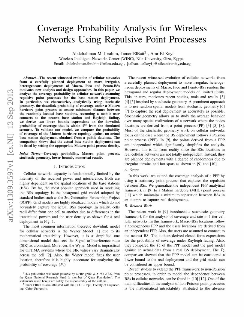
Cellular networks capacity is fundamentally limited by theintensity of the received power and interference. Both arehighly dependent on the spatial locations of the base stations(BSs). By far, the most popular approach used in modelingthe BSs topology is the hexagonal grid model adopted bystandard bodies such as the 3rd Generation Partnership Project(3GPP). Grid models are highly idealized models which do notaccurately capture the actual BSs topology. In reality, cellsradii differ from one cell to another due to differences in thetransmitted powers and the user density as shown for a realdeployment in Fig. 1.

The most common information theoretic downlink modelfor cellular networks is the Wyner Model [1] due to itsmathematical tractability. However, it is a simplified onedimensional model that sets the Signal-to-Interference ratio(SIR) as a constant. Moreover, the Wyner Model is impracticalfor OFDMA systems where the SIR values vary dramaticallyacross the cell [2]. Also, the Wyner model fixes the userlocation, therefore it is highly inaccurate for analyzing theprobability of coverage (Pc).

1This publication was made possible by NPRP grant # 5-782-2-322 fromthe Qatar National Research Fund (a member of Qatar Foundation). Thestatements made herein are solely the responsibility of the authors.

2Tamer ElBatt is also affiliated with the EECE Dept., Faculty of Engineer-ing, Cairo University.

The recent witnessed evolution of cellular networks froma carefully planned deployment to more irregular, heteroge-neous deployments of Macro, Pico and Femto-BSs renders thehexagonal and regular deployment models of limited utility.This, in turn, motivates recent studies, tools and results [3][4] [5] inspired by stochastic geometry. A prominent approachis to use random spatial models from stochastic geometry [6][7] to capture the real deployment as accurately as possible.Stochastic geometry allows us to study the average behaviorover many spatial realizations of a network where the nodeslocations are derived from a point process (PP) [3] [5] [8].Most of the stochastic geometry work on cellular networksfocus on the case where the BS deployment follows a Poissonpoint process (PPP). In [9], the points derived from a PPPare independent which significantly simplifies the analysis.However, this is far from reality since the BSs locations inreal cellular networks are not totally independent. Instead, theyare planned deployments with a degree of randomness due toirregular terrains and hot-spots as shown in [9] and [10].A. Scope

In this work, we extend the coverage analysis of a PPP byusing a stationary point process that captures the repulsionbetween BSs. We generalize the independent PPP analyticalframework in [9] to a Matern hardcore (MHC) point process[11] which maintains a minimum separation between BSs inan attempt to capture real deployments.B. Related Work

The recent work in [9] introduced a stochastic geometryframework for the analysis of coverage and rate in 1-tier cel-lular networks. In this framework, Macro-BSs locations followa homogeneous PPP and the users locations are derived froman independent PPP. Also, the users are assumed to connect tothe nearest BS. The authors derived closed form expressionsfor the probability of coverage under Rayleigh fading. Also,they compared the Pc of the PPP model and the grid modelagainst an actual data from a real BS deployment. The Pccomparison showed that the PPP model can be considered alower bound to the real deployment and the grid model canbe considered an upper bound.

Recent studies to extend the PPP framework to non-Poissonpoint processes, in order to model the dependence betweenBSs in cellular networks, can be found in [10] [12]. One of themain difficulties in the analysis of non-Poisson point processesis the mathematical intractability attributed to the absence

arX

iv:1

309.

3597

v1 [

cs.N

I] 1

3 Se

p 20

13

−5 −4 −3 −2 −1 0 1 2 3 4 5−5

−4

−3

−2

−1

0

1

2

3

Fig. 1: Actual BS deployment from a rural area [15]

of a closed form expression for the probability generatingfunctional (PGFL) of the underlying node distribution. Analternative approach is presented in [13] to overcome thePGFL hurdle by using Weierstrass inequality [14]. The authorsderived bounds on the probability of coverage utilizing thesecond order density of the underlying node distribution.However, these bounds are suggested for very small densitiesless than 0.04 and diverge as the SINR threshold increases.Therefore, we overcome the shortcomings of this approach byproposing a general framework based on the Matern hardcorepoint process [11] in order to find a lower bound on theprobability of coverage.

C. Contributions

Our contribution in this paper is multi-fold. First, we extendthe stochastic geometry framework presented in [9] to modelthe BSs locations using a MHC point process, incorporatingdependence between deployment points as encountered inpractice. Second, we derive the MHC empty space distribution.Third, we overcome the PGFL hurdle by applying Jensen’sinequality and the inequality proposed in Conjecture 1 toestablish tight lower bounds on the MHC coverage probability.Finally, we compare the coverage probability of PPP, squaregrid and MHC deployments to an actual BS deployment from arural area [15]. We also compare the simulated MHC coverageprobability to the analytical lower bounds which confirm theirtightness, especially for the Conjecture 1 inequality-basedbound.

The rest of this paper is organized as follows. In Section II,we present a background on the stochastic geometry tools andthe point processes used in this paper. Afterwards, we presentthe system model in Section III. In Section IV, we presentour main analytical results and establish lower bounds onthe coverage probability. In Section V, we provide numericalresults to support our analytical findings. Finally, conclusionsare drawn and potential directions for future research arepointed out in Section VI.

II. BACKGROUND: STOCHASTIC GEOMETRY

A. Spatial Point Processes

A spatial point process (PP) Φ is a random collection ofpoints in space. A PP is simple if no two points are at the samelocation, i.e. x 6= y for any x, y ∈ Φ. A random set of pointsin Φ can be represented as a countable set of {xı} randomvariables that take values in R2. The intensity measure of Φis Λ(B) = E[Φ(B)], where E[Φ(B)] is the expected numberof points in B ⊂ R2. A simple PP Φ is determined by its voidprobabilities over all compact sets, i.e. P(Φ(B) = 0) for acompact set B ⊂ R2. A point process is said to be stationaryif its distribution is invariant with respect to translation (shiftsin space) [8] [6].A stationary Poisson point process (PPP) of intensity λp ischaracterized by the following two properties:

• The number of points in any set B ⊂ R2 is a Poissonrandom variable with mean λ|B|, i.e.

P (Φ(B) = k) = e−λ|B|(λ|B|)k

k!(1)

• The number of points in disjoint sets are independentrandom variables [7].

Campbell’s Theorem. Let f(x) : R2 → [0,∞] be a measur-able integrable function. Then, the average sum of a functionevaluated at the points of Φ is given by:

E

[∑x∈Φ

f(x)

]=

∫R2

f(x)Λ(dx)

For a stationary PP Φ, the average number of points in a setB ⊂ R2 conditioning on having a point at the origin ”o” butexcluding that point is denoted as E!o[

∑x∈Φ 1B(x)], where

1B(.) is the indicator function [5].If f(x) : R2 → [0,∞] is an integrable function, then

E!o

[∑x∈Φ

f(x)

]= λ−1

∫R2

ρ(2)(x)f(x)dx (2)

where ρ(2)(x) is the second order product density of thestationary PP Φ.The conditional probability generating functional (PGFL) of aPP Φ is given by

G [f(x)] = E!o

[∏x∈Φ

f(x)

]B. The Matern Point Process

A Matern Hard-core (MHC) point process Φm is generatedby a dependent thinning of a stationary Poisson point processas follows [11]:

1) Generate a PPP Φp with density λp.2) For each point x ∈ Φp associate a mark mx ∼ U [0, 1]

independent of any other point.3) A point x is retained in Φm if it has the lowest mark

compared to all points in B(x, d), i.e. a circle centeredat x with radius d.

−5 −4 −3 −2 −1 0 1 2 3 4 5−5

−4

−3

−2

−1

0

1

2

3

4

5

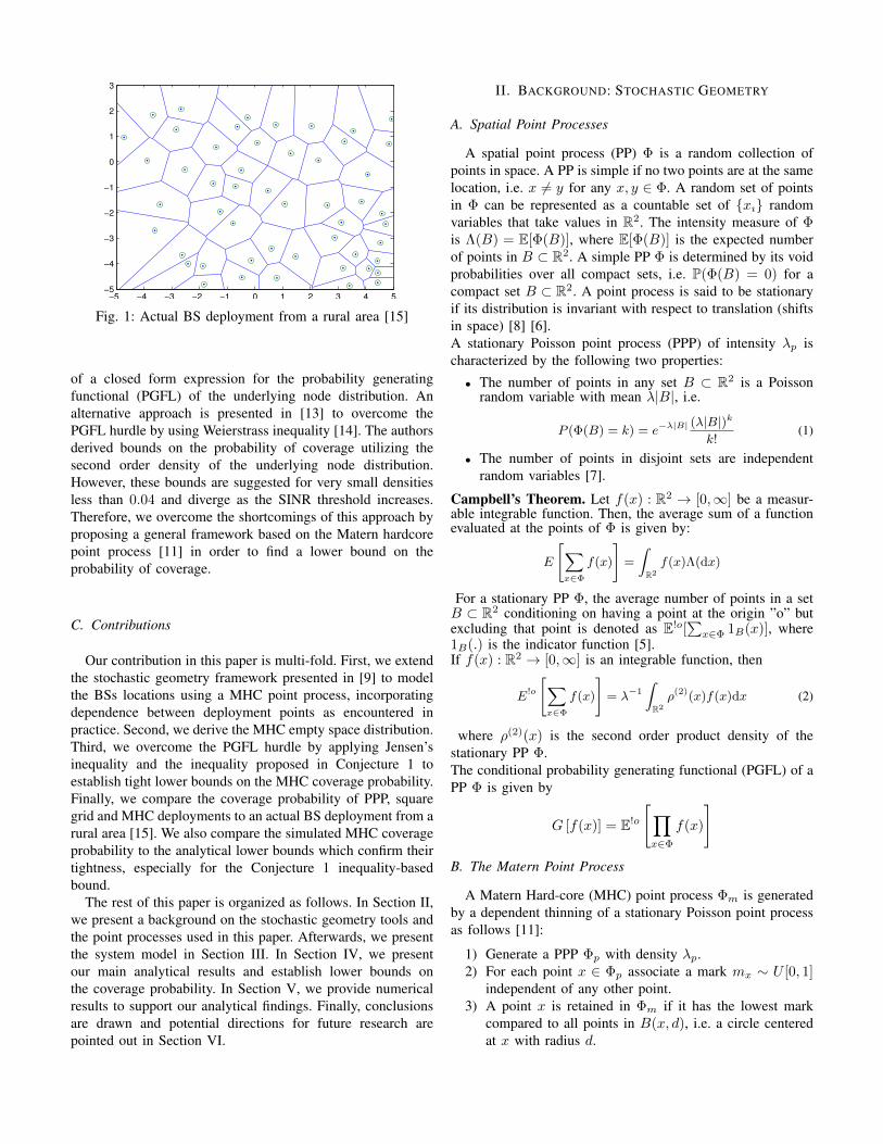
Fig. 2: A realization of MHC PP with λp = 1, d = 0.5

The probability of an arbitrary point x is retained in Φm isgiven by:

p =1− exp(−λpπd2)

λpπd2(3)

The density of the MHC PP Φm is λm = pλp, i.e.

λm =1− exp(−λpπd2)

πd2

The second order product density of the MHC PP Φm is givenby [16]

ρ(2)(υ) =

λ2m, if υ ≥ 2d

2V (υ)[1− exp(−λpπd2)]

πd2V (υ)[V (υ)− πd2]if 2d > υ > d

−2πd2[1− exp(−λpV (υ))]

πd2V (υ)[V (υ)− πd2]

0, otherwise(4)

where V (υ) is the union area of two discs of radius d andinter-center distance υ, centered at any two points of the MHCpoint process Φm, and V (υ) is defined as

V (υ) = 2πd2 − 2d2 cos−1( υ

2d

)+ υ

√d2 − υ2

4

III. SYSTEM MODEL

We model the downlink of a cellular network where the BSdeployment is based on a repulsive point process which is avariation of the independent PPP. A repulsive point processguarantees min distance d between BS deployment locations.In this paper, we consider a mathematically tractable type ofthe repulsive point processes, namely the Matern hardcore(MHC) point process Φm of intensity λm and a minimumdistance d between BSs. We assume that the mobile usersspatial distribution follows an independent homogeneous PPP.We assume that a mobile user is connected to the nearestBS. Hence, the base stations downlink coverage areas areVoronoi tessellations on the plane as shown in Fig. 2. Weadopt the standard path loss propagation model with path lossexponent α and assume that the channel between the mobileuser and the attached BS varies according to Rayleigh fading

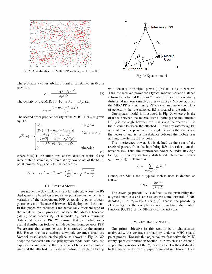
Fig. 3: System model

with constant transmitted power (1/γ) and noise power σ2.Thus, the received power for a typical mobile user at a distancer from the attached BS is hr−α, where h is an exponentiallydistributed random variable, i.e. h ∼ exp(γ). Moreover, sincethe MHC PP is a stationary PP we can assume without lossof generality that the attached BS is located at the origin.

Our system model is illustrated in Fig. 3, where r is thedistance between the mobile user at point y and the attachedBS, ϕ is the angle between the x-axis and the vector r, υ isthe distance between the attached BS and any interfering BSat point x on the plane, θ is the angle between the x-axis andthe vector υ, and Rx is the distance between the mobile userand any interfering BS at point x.

The interference power, Ir, is defined as the sum of thereceived powers from the interfering BSs, i.e. other than theattached BS. Thus, the interference power Ir under Rayleighfading, i.e. (an exponentially distributed interference powergx ∼ exp(γ)) is defined as

Ir =∑

x∈φm\{o}

gxR−αx

Hence, the SINR for a typical mobile user is defined asfollows:

SINR =hr−α

σ2 + Ir

The coverage probability is defined as the probability thata typical mobile user is able to achieve some threshold SINR,denoted β, i.e. Pc = P[SINR ≥ β]. That is, the probabilityof coverage is the complementary cumulative distributionfunction (CCDF) of the SINRs over the network.

IV. COVERAGE ANALYSIS

Our prime objective in this section is to characterize,analytically, the coverage probability under a MHC spatialpoint process. Towards this objective, we first derive the MHCempty space distribution in Section IV.A which is an essentialstep in the derivation of the Pc. Section IV.B is then dedicatedto the major results of this paper presented in Theorem 1 and

Proposition 1 which establish lower bounds on the probabilityof coverage under the MHC spatial point process.

A. MHC empty space distribution

In our model, we assume that a mobile user connects tothe nearest BS. Thus, if a mobile user is at a distance r fromthe attached BS, then there is no interfering BS that is closerthan r to the mobile user. The probability density function(pdf) of r is the empty space distribution of the underlyingMHC point process which is approximated in the followinglemma.

Lemma 1. Given that the mobile user is at a distance rfrom the attached BS, the approximated MHC empty spacedistribution f(r) is given by:

f(r) = 2πλmr e(−πλmr2) (5)

Proof: See Appendix A.

B. Probability of Coverage

This section hosts the main analytical findings of thispaper presented in Theorem 1 and Proposition 1. First, weestablish a lower bound on Pc using Jensen’s inequality inTheorem 1. Next, we establish a tighter lower bound on Pcin Proposition 1 using the inequality proposed in Conjecture 1.

Theorem 1. A lower bound on the coverage probability fora mobile user in a cellular network deployed using a MHCPP is given by

Pc ≥∫ 2π

ϕ=0

∫ ∞r=0

f(r)

2πe−γβσ

2rαe−(µ1+µ2)dr dϕ (6)

where

µ1 = λ−1m

∫ 2π

θ=0

∫ max[2d,|2r cos(θ−ϕ)|]

υ=max[d,|2r cos(θ−ϕ)|]∆(r, υ, θ, ϕ) ρ

(2)1 (υ) υ dυ dθ,

µ2 = λ−1m

∫ 2π

θ=0

∫ ∞υ=max[2d,|2r cos(θ−ϕ)|]

∆(r, υ, θ, ϕ) ρ(2)2 (υ) υ dυ dθ

(7)

and

∆(r, υ, θ, ϕ) = ln

(1 + β

(r2

υ2 + r2 − 2rυ cos(θ − ϕ)

)α/2)

ρ(2)(υ) =

ρ(2)1 (υ) ,if d < υ ≤ 2d

ρ(2)2 (υ) ,if υ > 2d

(8)

Proof: See Appendix B.Next, we propose an inequality in Conjecture 1 based onour numerical observations, by which we develop a lowerbound in Proposition 1 tighter than Theorem 1.

Conjecture 1. For d small enough, the followinginequality holds for a MHC PP

E!oφm

∏x∈φm

1−∆x

≥ e−E!oφm

[ ∑x∈φm

∆x

](9)

where∆x =

1

1 + β−1(rRx

)−α (10)

The inequality proposed in Conjecture 1 is motivated bythe fact that for d small enough, the probability of coverageof a MHC PP ≥ the probability of coverage of a PPP and thePGFL of PPP is given by

E!oφp

∏x∈φp

1−∆x

= exp

−E!oφp

∑x∈φp

∆x

Thus, applying the PPP PGFL definition on a MHC PP

results in a lower bound on MHC Pc which is characterizedby the inequality in Conjecture 1.

Proposition 1. A lower bound on the coverage probabilityfor a mobile user in a cellular network deployed using aMHC PP is given by

Pc ≥∫ 2π

ϕ=0

∫ ∞r=0

f(r)

2πe−γβσ

2rαe−(µ1+µ2)dr dϕ

with

∆(r, υ, θ, ϕ) =

(1 + β−1

(r2

υ2 + r2 − 2rυ cos(θ − ϕ)

)−α/2)−1

and µ1, µ2, ρ(2)(υ) are the same as (7) and (8).

Proof: See Appendix D.

V. NUMERICAL RESULTS

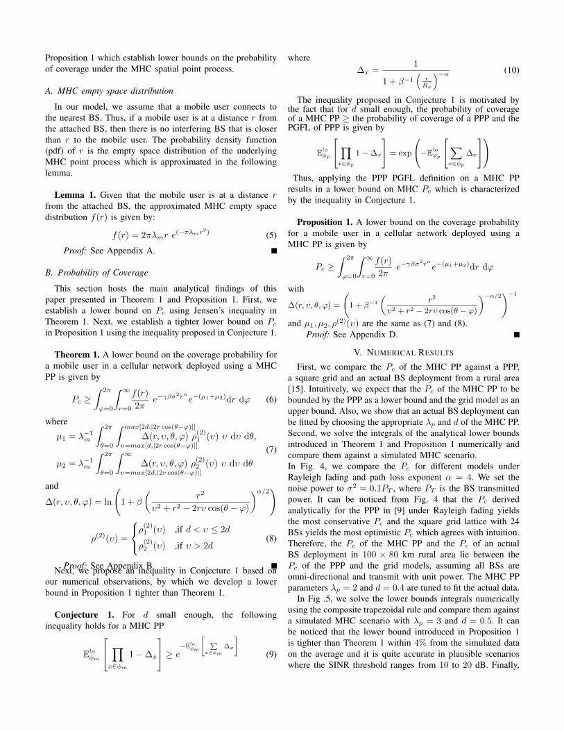
First, we compare the Pc of the MHC PP against a PPP,a square grid and an actual BS deployment from a rural area[15]. Intuitively, we expect that the Pc of the MHC PP to bebounded by the PPP as a lower bound and the grid model as anupper bound. Also, we show that an actual BS deployment canbe fitted by choosing the appropriate λp and d of the MHC PP.Second, we solve the integrals of the analytical lower boundsintroduced in Theorem 1 and Proposition 1 numerically andcompare them against a simulated MHC scenario.In Fig. 4, we compare the Pc for different models underRayleigh fading and path loss exponent α = 4. We set thenoise power to σ2 = 0.1PT , where PT is the BS transmittedpower. It can be noticed from Fig. 4 that the Pc derivedanalytically for the PPP in [9] under Rayleigh fading yieldsthe most conservative Pc and the square grid lattice with 24BSs yields the most optimistic Pc which agrees with intuition.Therefore, the Pc of the MHC PP and the Pc of an actualBS deployment in 100 × 80 km rural area lie between thePc of the PPP and the grid models, assuming all BSs areomni-directional and transmit with unit power. The MHC PPparameters λp = 2 and d = 0.4 are tuned to fit the actual data.

In Fig .5, we solve the lower bounds integrals numericallyusing the composite trapezoidal rule and compare them againsta simulated MHC scenario with λp = 3 and d = 0.5. It canbe noticed that the lower bound introduced in Proposition 1is tighter than Theorem 1 within 4% from the simulated dataon the average and it is quite accurate in plausible scenarioswhere the SINR threshold ranges from 10 to 20 dB. Finally,

−10 −5 0 5 10 15 200

0.1

0.2

0.3

0.4

0.5

0.6

0.7

0.8

0.9

1

SINR Threshold (dB)

Pro

ba

bili

ty o

f C

ove

rag

e

PPP, Analytical

Actual data

MHC PP ( λp=2 , d=0.4)

Square Grid, N=24

Fig. 4: Comparison of the coverage probability for a PPP, aMHC with λp = 2, d = 0.4, a square grid and actual data

−10 −5 0 5 10 15 200

0.1

0.2

0.3

0.4

0.5

0.6

0.7

0.8

0.9

1

SINR Threshold (dB)

Pro

ba

bili

ty o

f C

ove

rag

e

MHC (λp=3, d=0.5) simulation

Analytical lower bound (Theorem 1)

Analytical lower bound (Proposition 1)

Analytical lower bound (Weierstrass) [13]

Fig. 5: Analytical lower bounds for a MHC scenario withλp = 3 and d = 0.5

we replace Conjecture 1 by the Weierstrass inequality in [13]and we notice that the Pc diverges significantly as we increasethe SINR threshold.

VI. CONCLUSIONS

We presented a stochastic geometry formulation using theMatern hardcore spatial point process to model the BS de-ployment in cellular networks. Nevertheless, the presentedanalysis can be employed to study other wireless networks,e.g. ad hoc networks. This paper constitutes a departurefrom the recent literature on studying and analyzing coverageprobability using independent Poisson point processes. Weestablished, analytically, two lower bounds for the coverageprobability which constitutes our major analytical findings andconstitutes an important step towards deriving closed formexpressions. We compared our model to actual BSs locationsfrom a rural area and showed that the actual data can by fittedby using the appropriate MHC density λm via appropriately

260 280 300 320 340 360 380 400 420 4400

0.005

0.01

0.015

0.02

Number of eliminated points (n)

Density

Simulation (λp=4,d=0.75)

Approx Expression

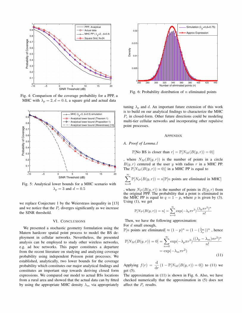
Fig. 6: Probability distribution of n eliminated points

tuning λp and d. An important future extension of this workis to build on our analytical findings to characterize the MHCPc in closed-form. Other future directions could be modelingmulti-tier cellular networks and incorporating other repulsivepoint processes.

APPENDIX

A. Proof of Lemma.1

P[No BS is closer than r] = P[NM (B(y, r)) = 0)]

, where NM (B(y, r)) is the number of points in a circleB(y, r) centered at the user y with radius r in a MHC PP.The P[NM (B(y, r)) = 0)] in a MHC PP is equal to∞∑n=0

P[NP (B(y, r)) = n]P[n points are eliminated in MHC]

, where NP (B(y, r)) is the number of points in B(y, r) fromthe original PPP. The probability that a point is eliminated inthe MHC PP is equal to q = 1 − p, where p is given by (3).Using (1), we get

P[NP (B(y, r)) = n] =

∞∑n=0

exp(−λpπr2)(λpπr

2)n

n!

Then, we have the following approximation:For d small enough,P[n points are eliminated] ≈ (1− p)n = (1− (λmλp ))n , hence

P[NM (B(y, r)) = 0] =

∞∑n=0

exp(−λpπr2)((λp − λm)πr2)n

n!

= exp(−λmπr2)(11)

Applying f(r) =d

dr(1− P[NM (B(y, r)) = 0]) to (11) we

get (5).The approximation in (11) is shown in Fig. 6. Also, we havechecked numerically that the approximation in (5) does notaffect the Pc results.

B. Proof of Theorem 1

The probability of coverage (Pc) is equal to

Pc = Er,ϕ[P(SINR > β|r, ϕ)]

=

∫ 2π

ϕ=0

∫ ∞r=0

f(r)

2πP(SINR > β|r, ϕ) drdϕ

P(SINR > β|r, ϕ) = P(h > β(σ2 + Ir)rα|r, ϕ)

(a)= E!o

Ir

[e−γ(β(σ2+Ir)rα)|r, ϕ

]step (a) assuming Rayleigh fading, i.e. h ∼ exp(γ)

Pc =

∫ 2π

ϕ=0

∫ ∞r=0

f(r)

2πe−γβσ

2rα E!oIr

[e−βγr

αIr |r, ϕ]

drdϕ

(12)where

E!oIr

[e−βγr

αIr |r, ϕ]

= E!oφm,gx

[e−βγrα

∑x∈φm

gxR−αx

](a)= E!o

φm

∏x∈φm

Egx[e−βγr

αgxR−αx

](b)= E!o

φm

∏x∈φm

1

1 + β(rRx

)α

= E!oφm

[e−

∑x∈φm

ln(1+β( rRx

)α)]

(c)

≥ eE!oφm

[−

∑x∈φm

ln(1+β( rRx

)α)

](13)

Steps (b) from gx ∼ exp(γ) and step (c) using Jensen’sinequality, let

µ = E!oφm

− ∑x∈φm

∆x

, where ∆x = ln

(1 + β

(r

Rx

)α)hence,

Pc ≥∫ 2π

ϕ=0

∫ ∞r=0

f(r)

2πe−γβσ

2rα e−µ drdϕ

From trigonometry of Fig .3, Rx can be substituted by

Rx =√υ2 + r2 − 2rυ cos(θ − ϕ)

hence, ∆(r, υ, θ, ϕ) = ln

(1 + β

(r2

υ2+r2−2rυ cos(θ−ϕ)

)α/2)From (2) , µ is equal to

µ = λ−1m

∫ 2π

θ=0

∫ ∞υ=max[d,|2r cos(θ−ϕ)|]

ρ(2)(υ) ∆(r, υ, θ, ϕ) υdυdθ

Using the definition of ρ(2)(υ) in (4), then µ = µ1+µ2, where

µ1(a)= λ−1

m

∫ 2π

θ=0

∫ max[2d,|2r cos(θ−ϕ)|]

υ=max[d,|2r cos(θ−ϕ)|]∆(r, υ, θ, ϕ) ρ

(2)1 (υ) υ dυ dθ

µ2(b)= λ−1

m

∫ 2π

θ=0

∫ ∞υ=max[2d,|2r cos(θ−ϕ)|]

∆(r, υ, θ, ϕ) ρ(2)2 (υ) υ dυ dθ

ρ(2)(υ) =

ρ(2)1 (υ) ,if d < υ ≤ 2d

ρ(2)2 (υ) ,if υ > 2d

From trigonometry of Fig. 3, υ = 2r cos(θ − ϕ) for Rx = r.Thus, the integral limits of υ is from max[d, |2r cos(θ − ϕ)|]to ∞, since the closest interfering BS is at least at distance rand ρ(2)(υ) = 0 for υ < d.

C. Proof of Proposition 1Same as proof of Theorem 1 till (13-b), then proceed with

E!oφm

∏x∈φm

1

1 + β(

rRx

)α = E!o

φm

∏x∈φm

1−∆x

(a)

≥ exp

−E!oφm

∑x∈φm

∆x

step (a) by using Conjecture 1.

REFERENCES

[1] A. D. Wyner, “Shannon-theoretic approach to a gaussian cellularmultiple-access channel,” IEEE Transactions on Information Theory,vol. 40, no. 6, pp. 1713–1727, 1994.

[2] J. Xu, J. Zhang, and J. G. Andrews, “On the accuracy of the wyner modelin cellular networks,” IEEE Transactions on Wireless Communications,vol. 10, no. 9, pp. 3098–3109, 2011.

[3] J. G. Andrews, R. K. Ganti, M. Haenggi, N. Jindal, and S. Weber, “Aprimer on spatial modeling and analysis in wireless networks,” IEEECommunications Magazine, vol. 48, no. 11, pp. 156–163, 2010.

[4] H. S. Dhillon, R. K. Ganti, F. Baccelli, and J. G. Andrews, “Modelingand analysis of k-tier downlink heterogeneous cellular networks,” IEEEJournal on Selected Areas in Communications, vol. 30, no. 3, pp. 550–560, 2012.

[5] M. Haenggi and R. K. Ganti, Interference in large wireless networks.Now Publishers Inc, 2009, vol. 3, no. 2.

[6] A. Baddeley, I. Barany, R. Schneider, and W. Weil, Stochastic Geometry:Lectures Given at the CIME Summer School, Held in Martina Franca,Italy, September 13-18, 2004. Springer, 2007.

[7] R. Serfozo, Basics of applied stochastic processes. Springer, 2009.[8] M. Haenggi, J. G. Andrews, F. Baccelli, O. Dousse, and

M. Franceschetti, “Stochastic geometry and random graphs forthe analysis and design of wireless networks,” IEEE Journal onSelected Areas in Communications, vol. 27, no. 7, pp. 1029–1046,2009.

[9] J. G. Andrews, F. Baccelli, and R. K. Ganti, “A tractable approachto coverage and rate in cellular networks,” IEEE Transactions onCommunications, vol. 59, no. 11, pp. 3122–3134, 2011.

[10] D. B. Taylor, H. S. Dhillon, T. D. Novlan, and J. G. Andrews, “Pairwiseinteraction processes for modeling cellular network topology,” in Proc.IEEE Global Telecomm. Conference, Anaheim, CA, 2012.

[11] D. Stoyan and H. Stoyan, “On one of matern’s hard-core point processmodels,” Mathematische Nachrichten, vol. 122, no. 1, pp. 205–214,1985.

[12] A. Busson, G. Chelius, J.-M. Gorce et al., “Interference modeling incsma multi-hop wireless networks,” 2009.

[13] R. K. Ganti and J. G. Andrews, “A new method for computing thetransmission capacity of non-poisson wireless networks,” in IEEE Inter-national Symposium on Information Theory Proceedings (ISIT), 2010,pp. 1693–1697.

[14] M. Klamkin and D. Newman, “Extensions of the weierstrass productinequalities,” Mathematics Magazine, vol. 43, no. 3, pp. 137–141, 1970.

[15] “Sitefinder dataset hosted by ofcom,” http://stakeholders.ofcom.org.uk/sitefinder/sitefinder-dataset/, accessed: 1/4/2013.

[16] J. Illian, A. Penttinen, H. Stoyan, and D. Stoyan, Statistical analysis andmodelling of spatial point patterns. Wiley-Interscience, 2008.