Physics of a magnetic barrier in low-temperature bounded plasmas: insight from particle-in-

cell simulations

This content has been downloaded from IOPscience. Please scroll down to see the full text.

Download details:

IP Address: 41.78.26.154

This content was downloaded on 30/09/2013 at 20:21

Please note that terms and conditions apply.

2012 Plasma Sources Sci. Technol. 21 025002

(http://iopscience.iop.org/0963-0252/21/2/025002)

View the table of contents for this issue, or go to the journal homepage for more

Home Search Collections Journals About Contact us My IOPscience

IOP PUBLISHING PLASMA SOURCES SCIENCE AND TECHNOLOGY

Plasma Sources Sci. Technol. 21 (2012) 025002 (14pp) doi:10.1088/0963-0252/21/2/025002

Physics of a magnetic barrier inlow-temperature bounded plasmas:insight from particle-in-cell simulationsSt Kolev1, G J M Hagelaar2, G Fubiani2 and J-P Boeuf2

1 Faculty of Physics, Sofia University, 5, J. Bourchier Blvd., BG-1164 Sofia, Bulgaria2 LAboratoire PLAsma et Conversion d’Energie (LAPLACE), Universite de Toulouse, Bt. 3R2,118 Route de Narbonne, F-31062 Toulouse Cedex 9, France

E-mail: skolev@phys.uni-sofia.bg

Received 14 August 2011, in final form 6 December 2011Published 1 March 2012Online at stacks.iop.org/PSST/21/025002

AbstractThe use of magnetic fields is quite common in low-pressure, low-temperature, gas-dischargedevices for industrial applications. However, transport in such devices is still not very wellclarified, mainly due to the presence of walls playing a crucial role and to the variety ofconfigurations studied. The latter often obstruct the underlying basic physical phenomena andmake the different studies valid only for very specific configurations. This work presents anumerical study of particle transport in low-pressure (0.3 Pa) plasmas across a localizedtransverse magnetic field (magnetic barrier) by means of the 2D3V particle-in-cell with MonteCarlo collisions method. The problem is treated as generally as possible while trying to revealthe basic physics, using very simplified chemistry and considering a simple rectangularconfiguration. The conditions chosen for the magnetic field are common to manyapplications—magnetized electrons and almost unmagnetized ions. Two basic configurationswith different magnetic field directions are analyzed in detail: magnetic field perpendicular tothe simulation plane and along the simulation plane. An extensive parametric study is carriedout in order to obtain the main trends and scaling laws for particle transport with respect todifferent parameters: plasma density, magnetic barrier size and magnetic field magnitude. Thetotal current of electrons crossing the barrier is found to scale linearly with the plasma density,which extends the validity of the obtained results to a wide range of plasma density values.

(Some figures may appear in colour only in the online journal)

1. Introduction

The problem of electron transport across a transverse magneticfield is rather old and has been studied for many yearswith respect to nuclear fusion devices based on magneticconfinement, probe diagnostics, particle beams, etc. In thelast few decades, low-temperature plasma sources (LTPS)have found numerous applications and become an importantpart of the whole industry. There are several low-pressureplasma sources operating with magnetic fields (such asmagnetron discharges, electron cyclotron resonance (ECR)plasma sources, Hall effect thrusters, end-hall sources andnegative ion sources) and for them the problem of magnetizedplasma transport is essential. While the magnetic field in theseplasma sources is usually much lower compared with fusion

devices and thus the ions are weakly magnetized, becauseof the relatively low gas pressure (below a few Pa), theelectrons are still strongly magnetized and transport in thedirection perpendicular to the magnetic field lines may poseproblems similar to fusion plasmas. An important differencebetween LTPS and fusion devices however is that in most LTPSthe vacuum chamber and geometry determine the dischargeoperation. The walls cause the formation of wall sheets whichmay interact with the magnetic field and produce additionaltransport. This effect appears to be especially important indevices where the magnetic field is used to reduce the electrontransport in a certain direction.

The purpose of this work is to study electron transportacross a localized magnetic field (also called magneticbarrier, MB) in the presence of chamber walls by means

0963-0252/12/025002+14$33.00 1 © 2012 IOP Publishing Ltd Printed in the UK & the USA

Plasma Sources Sci. Technol. 21 (2012) 025002 St Kolev et al

of particle-in-cell (PIC) kinetic modeling. This work aimsto give a better understanding of the influence of the wallson the electron transport in low-pressure LTPS and givesthe trends in the scaling of electron transport with respectto different parameters such as the magnetic field strength,electron density, MB width (MB length which is to be traversedby the electrons) and the distance between the walls. Theseresults are part of the authors’ efforts [1–3] devoted to modelingnegative hydrogen ion sources used in the neutral beaminjection systems of fusion devices [4]. In these sourcesa magnetic field (magnetic filter) is used [5–7] to reducethe electron temperature and electron transport toward theextraction grid in order to increase the negative ion productionand to allow their extraction.

Over the last two decades these sources have beenextensively studied both theoretically and numerically.Although there are numerous works studying the problemof MB (also called magnetic filter) and the negative ionextraction system, none of them considers in detail the effectof cross-field transport caused by the chamber walls. In [8]the extraction physics is studied under realistic conditionsusing the 2D3V particle-in-cell with Monte Carlo collisions(PIC-MCC) method, but due to the high density only asingle aperture is considered and the side walls of the realsource are replaced by periodic boundary conditions. In [9]again the 2D3V PIC method is used to describe a boundeddomain (including side walls); however, the magnetic fieldis chosen to have components only in the simulation plane,and thus the authors exclude any cross-field transport causedby the combined effect of the wall sheath/presheath and themagnetic field (E × B drift). Several works address theproblem using the fluid approach [2, 10, 11]. While carefulconstruction of fluid models could provide reasonable andqualitatively accurate results, they face serious difficultiesrelated to boundary conditions and nonlocalities of low-pressure discharges. Therefore, this work presents an extendedstudy of the MB problem and uses an explicit PIC-MCCmethod for the modeling.

While negative ion sources are the main motivation forthis work, the results obtained are not limited to negativeion sources and might be useful for a broad range of plasmasources using magnetic fields. The problem is treated in arather general way by considering the MB in very simplifiedgeometry and plasma chemistry in order to exclude anyeffects specific to certain complex geometry or chemistry.Although geometry/chemistry effects may sometimes play asignificant role, we think that the basic physics should bewell understood first and should then be analyzed with respectto any specific configuration and additional effects should beadded. Therefore, the geometry used here is a simple rectangle,the MB has an idealized Gaussian shape and the discharge issustained by artificial charged particle injection and electronMaxwellization in a limited region.

This paper has the following structure. In the next sectionwe recall some basic laws which are well known from theclassical textbooks on plasma physics but we add them hereexplicitly to make the paper easier for reading. Next we brieflypresent the numerical model based on the PIC-MCC method

and the conditions used in the simulations. In section 4 ofthe paper we present and analyze four simple configurationswith different directions of magnetic field perpendicular tothe plasma flow and different boundary conditions at the sidewalls—dielectric and grounded side walls. Here, we analyzethe MB performance for reducing the electron flow toward thedownstream region (to be defined precisely in section 4) wherewe apply certain attracting (extraction) positive potential.Section 5 includes several parametric studies of the plasmaand MB characteristics with respect to different parameters:the plasma density, filter width and magnetic field strength.In section 6 we present the results of the variation of plasmaparameters as a function of the transverse size of the domain(here in the ‘y’ direction) and their convergence to the 1Dsolution (where the side wall influence is neglected). Herewe will also briefly comment on the excitation of instabilitiesleading to the so-called anomalous transport across the MB.

2. Basic laws

In the presence of a magnetic field the motion of a singlecharged particle (between collisions with other particles orwalls) is described by the Newton equation:

dv

dt= q

m(E + v × B), (1)

where v is the particle velocity, q is the particle charge, m is theparticle mass, E is the electric field and B is the magnetic fieldinduction. Although precise (for single collisionless particletrajectory), the Newton equation is not convenient for thedescription of overall particle motion. For example, if theparticle is gyrating in the magnetic field it could happen thaton average it is not moving at all. Therefore, particle motionin a magnetic field (for weakly varying electric and magneticfields) is usually considered as a sum of two components—fast gyration of the particle in a cyclotron orbit xL(t), vL(t)

and slow drift (xgc(t), vgc(t)) of the guiding center obtainedafter averaging out the cyclotron motion: x(t) = xgc(t)+xL(t),v(t) = vgc(t)+vL(t). With respect to the MB problem, we aremainly interested in the particle’s guiding center motion, i.e.the particle drifts. In most of the plasma physics introductorytextbooks one can find a detailed explanation of the differentparticle drifts (see for example [12, 13]). Here we will mentionjust those appearing for the field and geometry configurationsconsidered in this work (assuming weakly varying fields):

vE×B = E × B

B2E × B drift, (2)

v∇B = q

|q|1

2v⊥rL

B × ∇B

B2∇B drift, (3)

where rL is the Larmor radius and v⊥ is the magnitude ofthe velocity component perpendicular to the magnetic field.Of course one should remember that single particle motionhas one more very important feature: collisions. This effect,however, is difficult to write using a simple formula for a singleparticle due to its random nature. Therefore, the phenomenon

2

Plasma Sources Sci. Technol. 21 (2012) 025002 St Kolev et al

is usually described with a statistical approach considering theaveraged (collective) motion of many particles.

The collective motion of particles in a plasma is fullycharacterized by the Boltzmann equation or its moments.Within the drift–diffusion approximation the steady-statemomentum equation is

nsus + Ωs × (nsus) = qs

|qs |µsnsE − ∇(Dsns) ≡ Gs (4)

where Gs is the drift–diffusion particle flux without a magneticfield for the species ‘s’, us is the mean velocity, ns is the speciesdensity,

Ωs = qs

|qs |µsB = qs

|qs |e

msνm,s

B

is a Hall parameter vector which represents the Hall parameter(|Ωs | = s = qs

|qs |µs |B| = ωc,s

νm,s) along the different space

dimensions, ωc, s = (|qs |B)/ms is the cyclotron frequency ofspecies ‘s’, µs is the species mobility without a magnetic field,Ds is the diffusion coefficient without a magnetic field and νm,s

is the momentum transfer collision frequency of species ‘s’.By applying cross and dot products with Ω to equation (4) weobtain the drift–diffusion expression for charged particle fluxin a plasma with a magnetic field [2]:

Γs ≡ nsus = 1

1 + 2s

(Gs + Ωs(Ωs · Gs) − Ωs × Gs). (5)

3. Numerical model and simulation conditions

The numerical model used here is an explicit PIC-MCC model[14–16]. The model is 2D in the configuration space and 3Din the velocity space (2D3V). The method used is based onthe classical leap-frog Buneman–Boris algorithm scheme [14].The PIC-MCC numerical technique provides the solution ofthe Boltzmann equation for the considered species and thusprovides an accurate distribution function and resolves thefull plasma dynamics. The major drawback of the explicitPIC-MCC method compared with the fluid approach is theconsiderable computational resources required for plasmaswith high density in two and three spatial dimensions. Inpractice, this limits the modeling to plasmas with electrondensities (ne) in the order of ne = 1014–1015 m−3 if we wantto use a regular computer workstation. A further increase inthe density would require a large-scale computer cluster or asupercomputer for the domain size considered in this work. Atfirst glance, it appears that the PIC-MCC method would notbe suitable for numerical modeling of most of the plasmas ofpractical interest, with densities usually from ne = 1015 m−3

up to ne = 1019 m−3 (the latter is the maximum value for high-power negative ion sources [4, 7]). However, one importantobservation found here allows us to use the PIC-MCC methodat low densities and claim the validity of the obtained results forhigher densities as well; the electron transport characteristicsacross the MB discussed in this work appear to scale linearlywith the electron density. This will be shown in detail insection 5, subsection 5.1.

The species considered in the simulations are electrons(e), positive hydrogen ions (H+) and hydrogen atoms (H).

Table 1. Collision processes.

Reactionnumber Process Reference

(1) e + H → e + H (elastic) [17, 18](2) e + H → e + H∗ [19]

(five energy levelsincluding the ionizationprocess taken as an excitation)

(3) H+ + H → H+ + H (elastic) [20](4) H+ + H → H + H+ (charge exchange) [20]

Table 2. Common external simulation parameters.

Description Symbol Value

Gas pressure p 0.3 PaGas temperature TH 1000 KMaxwellization temperature TM 6 eVGas density NH 2.17 × 1019 m−3

Upstream wall potential (x = 0) 1 0 VDownstream wall potential 2 25 V

(x = xmax)Standard deviation σB 1 cm

The last of these are assumed to have a homogeneous density(NH) which is calculated from NH = p/κTH, where p is thegas pressure, κ is the Boltzmann constant and TH is the gastemperature in ‘K’. The species composition is intentionallysimplified in order to omit any additional effects due to morecomplex plasma chemistry. The processes taken into accountand the sources for the cross-sections are summarized intable 1.

The main external parameters (discharge conditions) usedwithin the simulations are denoted in table 2. The gas pressureis relatively low (0.3 Pa) and corresponds to the typical valuesin high-power negative hydrogen ion sources [7]. The low gaspressure leads to a mean free path of the electrons in the orderof 20–50 cm, and 5–10 cm for the ions. The low pressure andthe relatively small MB width considered here (around 2 cmfor most of the simulations) mean that for a magnetic fieldof 5 mT the electrons are highly magnetized (Larmor radius0.1–0.2 cm) and the ions are weakly magnetized (Larmorradius 2–4 cm).

The geometry considered in the simulations is a 2Drectangle (see figure 1). Most of the real sources withmagnetic field are 3D systems and often without any symmetryaxis/plane. Therefore, 2D modeling of such devices is anapproximation assuming that along a certain dimension the sizeof the device will be very long. Here we consider two basiccases corresponding to two extreme cases—that the device isvery long along the magnetic field direction and very long inthe direction perpendicular to both the magnetic field and theplasma flow. The reality will be somewhere in between andwill be an interplay of both.

In addition, usually in negative ion sources there isa plasma grid [7] (or here, the downstream wall), thefirst electrode of which is biased at the plasma potentialor slightly higher in order to allow optimal negative ionextraction. Although negative ions are not included here, weuse ‘extraction’ in order to have similar conditions and to obtain

3

Plasma Sources Sci. Technol. 21 (2012) 025002 St Kolev et al

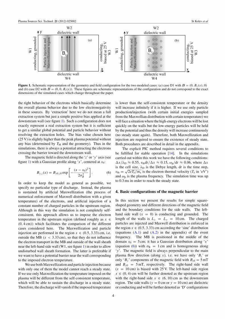
Figure 1. Schematic representation of the geometry and field configuration for the two modeled cases: (a) case D1 with B = (0, By(x), 0)and (b) case D2 with B = (0, 0, Bz(x)). These figures are schematic representations of the configuration and do not correspond to the exactdimensions of the simulated cases which change throughout the paper.

the right behavior of the electrons which basically determinethe overall plasma behavior due to the low electronegativityin these sources. By ‘extraction’ here we do not mean a fullextraction system but just a simple positive bias applied at thedownstream wall (see figure 1). Such a configuration does notexactly represent a real extraction system but it is sufficientto get a similar global potential and particle behavior withoutresolving the extraction holes. The bias value chosen here(25 V) is slightly higher than the peak plasma potential withoutany bias (determined by TM and the geometry). Thus in thesimulations, there is always a potential attracting the electronscrossing the barrier toward the downstream wall.

The magnetic field is directed along the ‘z’ or ‘y’ axis (seefigure 1) with a Gaussian profile along ‘x’, centered at x0:

By,z(x) = By0,z0 exp

[− (x − x0)

2

2σ 2B

]. (6)

In order to keep the model as general as possible, wespecify no particular type of discharge. Instead, the plasmais sustained by artificial Maxwellization (the process ofnumerical enforcement of Maxwell distribution with a giventemperature) of the electrons, and artificial injection of aconstant number of charged particles in the upstream region.Although in this way the simulation is not completely self-consistent, this approach allows us to impose the electrontemperature in the upstream region (defined roughly as x ∈(0, 4 cm)) which facilitates the comparison of the differentcases considered here. The Maxwellization and particleinjection are performed in the region x ∈ (0.5, 3.33) cm, i.e.outside the MB (x < 3.33 cm), so that they do not influencethe electron transport in the MB and outside of the wall sheathnear the left-hand side wall (W1, see figure 1) in order to allowundisturbed wall sheath formation. The latter is preferable ifwe want to have a potential barrier near the wall correspondingto the imposed electron temperature.

We use both Maxwellization and particle injection becausewith only one of them the model cannot reach a steady state.If we use only Maxwellization the temperature imposed on theplasma will be different from the self-consistent temperature,which will be able to sustain the discharge in a steady state.Therefore, the discharge will vanish if the imposed temperature

is lower than the self-consistent temperature or the densitywill increase infinitely if it is higher. If we use only particleproduction/injection (with certain initial energies sampledfrom the Maxwellian distribution with certain temperature) wewill face a situation where the high-energy electrons will be lostquickly on the walls but the low-energy particles will be heldby the potential and thus the density will increase continuously(no steady state again). Therefore, both Maxwellization andinjection are required to ensure the existence of steady state.Both procedures are described in detail in the appendix.

The explicit PIC method requires several conditions tobe fulfilled for stable operation [14]. In the simulationscarried out within this work we have the following conditions:x/λD ≈ 0.55, vthdt/x ≈ 0.15, ωp/dt ≈ 0.06, where x

is the cell size, λD is the Debye length, dt is the time step,vth = √

2eTe/me is the electron thermal velocity (Te in ‘eV’)and ωp is the plasma frequency. The simulation time was upto 0.3 ms in order to reach the steady state.

4. Basic configurations of the magnetic barrier

In this section we present the results for simple square-shaped geometry and different directions of the magnetic fieldand the boundary conditions for the side walls. The left-hand side wall (x = 0) is conducting and grounded. Thelength of the walls is Lx = Ly = 10 cm. The chargedparticles are injected and Maxwell distribution is enforced inthe region x ∈ (0.5, 3.33) cm according the ‘sine’ distribution(equations (A.1) and (A.2) in the appendix) of the eventfrequency. The MB is positioned in the middle of thedomain x0 = 5 cm; it has a Gaussian distribution along ‘x’(equation (6)) with σB = 1 cm and is homogeneous along‘y’. The magnetic field is always perpendicular to the mainplasma flow direction (along x), i.e. we have only ‘Bz’ oronly ‘By’ components of the magnetic field with Bz0 = 5 mTand By0 = 5 mT, respectively. The right-hand side wall(x = 10 cm) is biased with 25 V. The left-hand side regionx ∈ (0, 4) cm will be further denoted as the upstream regionwith the right-hand side x ∈ (6, 10) cm as the downstreamregion. The side walls (y = 0 cm or y = 10 cm) are dielectricor conducting and will be further denoted as ‘D’ configurations

4

Plasma Sources Sci. Technol. 21 (2012) 025002 St Kolev et al

(for dielectric) and ‘C’ configurations (for conducting). TheD1 and C1 cases will correspond to the magnetic field directedalong the ‘y’ axis and D2 and C2 cases will correspond tothe magnetic field directed along the ‘z’ (perpendicular to thesimulation plane).

4.1. Dielectric side walls

In this subsection we analyze two basic cases: with themagnetic field directed toward the side walls (figure 1(a))B = (0, By(x), 0), denoted as configuration D1, and themagnetic field directed perpendicular to the plane of simulation(figure 1(b)), i.e. B = (0, 0, Bz(x)), which will be denoted asconfiguration D2.

Configuration D1: bounded plasma infinite in ‘z’ (figure 1(a)).The magnetic field hasBy component only: B = (0, By(x), 0),E = (Ex, Ey, 0), domain: Lx = Ly = 10 cm.

For this configuration we have the following drifts allowedin the system

Single particle drifts (equations (2) and (3)):

vE×B = (0, 0, Ex/By) ‘z’ component only, (7)

v∇B =(

0, 0, − q

|q|1

2v⊥rL

∇xBy

By

)‘z’ component only. (8)

The guiding center particle drifts are in the ‘z’ direction onlywhere we have assumed infinity. This means that there are noparticle drifts along ‘x’ and thus we should not expect any othertype of transport across the barrier except due to collisions.

Collective motion drifts (equation (5)):

x = Gx

1 + 2, y = Gy, z =

1 + 2Gx. (9)

As with the separate particle drifts, the collective particle driftsalong ‘x’ are due to ‘classical’ collisional particle diffusion inthe magnetic field [12, 13]. The particle flux is reduced due tothe magnetic field as 1/(1 + 2) and the MB is characterizedby high stopping power for the electrons. We recall thatthis configuration approximately corresponds to the 1D caseconsidering the transport across the barrier while the otherdimensions are assumed to be infinite [3].

Configuration D2: bounded plasma infinite in ‘z’ (figure 1(b)).The magnetic field has Bz component only: B = (0, 0, Bz(x)),E = (Ex, Ey, 0), domain: Lx = Ly = 10 cm.

Single particle drifts (equations (2) and (3)):

vE×B = (Ey/Bz, −Ex/Bz, 0) ‘x’ and ‘y’ components,

(10)

v∇B =(

0,q

|q|1

2v⊥rL

∇xBz

Bz

, 0

)‘y’ component only. (11)

Here the E × B particle drift (Ey/Bz) allows transport acrossthe barrier.

Collective motion drifts (equation (5)):

x = 1

1 + 2(Gx + Gy), y = 1

1 + 2(Gy − Gx),

z = 0. (12)

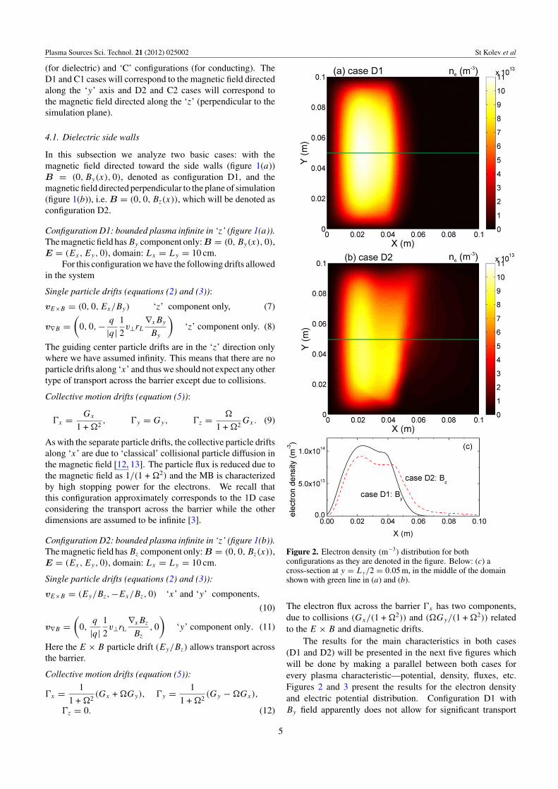
Figure 2. Electron density (m−3) distribution for bothconfigurations as they are denoted in the figure. Below: (c) across-section at y = Ly/2 = 0.05 m, in the middle of the domainshown with green line in (a) and (b).

The electron flux across the barrier x has two components,due to collisions (Gx/(1 + 2)) and (Gy/(1 + 2)) relatedto the E × B and diamagnetic drifts.

The results for the main characteristics in both cases(D1 and D2) will be presented in the next five figures whichwill be done by making a parallel between both cases forevery plasma characteristic—potential, density, fluxes, etc.Figures 2 and 3 present the results for the electron densityand electric potential distribution. Configuration D1 withBy field apparently does not allow for significant transport

5

Plasma Sources Sci. Technol. 21 (2012) 025002 St Kolev et al

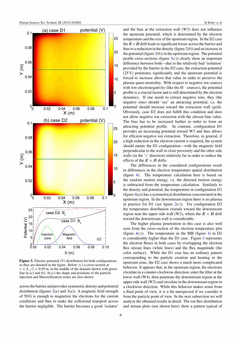
Figure 3. Electric potential (V) distribution for both configurationsas they are denoted in the figure. Below: (c) a cross-section aty = Ly/2 = 0.05 m, in the middle of the domain shown with greenline in (a) and (b). In (c) the shape and positions of the particleinjection and Maxwellization zones are also shown.

across the barrier and provides symmetric density and potentialdistribution (figures 2(a) and 3(a)). A magnetic field strengthof 50 G is enough to magnetize the electrons for the currentconditions and thus to make the collisional transport acrossthe barrier negligible. The barrier becomes a good ‘isolator’

and the bias at the extraction wall (W3) does not influencethe upstream potential, which is determined by the electrontemperature and the size of the upstream region. In the D2 casethe E×B drift leads to significant losses across the barrier andthus to a reduction in the density (figure 2(b)) and an increase inthe potential (figure 3(b)) in the upstream region. The potentialprofile cross-sections (figure 3(c)) clearly show an importantdifference between both—due to the relatively bad ‘isolation’provided by the barrier in the D2 case, the extraction potential(25 V) penetrates significantly and the upstream potential isforced to increase above that value in order to preserve theplasma quasi-neutrality. With respect to negative ion sourceswith low electronegativity (like the H− sources), the potentialprofile is a crucial factor and is still determined by the electrondynamics. If one needs to extract negative ions, they (thenegative ions) should ‘see’ an attracting potential, i.e. thepotential should increase toward the extraction wall (grid).Obviously, case D2 does not fulfill this condition and doesnot allow negative ion extraction with the chosen bias value.The bias has to be increased further in order to form anattracting potential profile. In contrast, configuration D1provides an increasing potential toward W3 and thus allowsfor efficient negative ion extraction. Therefore, in general, ifa high reduction in the electron current is required, the systemshould mimic the D1 configuration—with the magnetic fieldperpendicular to the wall in close proximity and the other sidewalls (in the ‘z’ direction) relatively far in order to reduce theeffects of the E × B drifts.

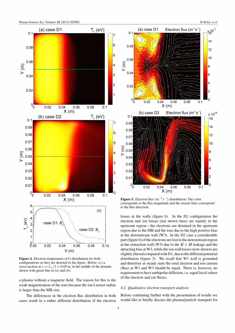
The differences in the considered configurations resultin differences in the electron temperature spatial distribution(figure 4). The temperature calculation here is based onthe random motion energy, i.e. the directed motion energyis subtracted from the temperature calculation. Similarly tothe density and potential, the temperature in configuration D1(figure 4(a)) has a symmetrical distribution concentrated in theupstream region. In the downstream region there is no plasmain practice for D1 (see figure 2(c)). For configuration D2the temperature distribution extends toward the downstreamregion near the upper side wall (W2), where the E × B drifttoward the downstream wall is considerable.

The higher plasma penetration in this case is also wellseen from the cross-section of the electron temperature plot(figure 4(c)). The temperature in the MB (figure 4) in D2is considerably higher than the D1 case. Figure 5 representsthe electron fluxes in both cases by overlapping the electronflux stream lines (white lines) and the flux magnitude (thecolor surface). While the D1 case has an ordinary patterncorresponding to the particle creation and heating in theupstream zone, the D2 case shows a much more complicatedbehavior. It appears that, in the upstream region, the electronscirculate in a counter-clockwise direction, enter the filter at thelower wall (W4), then penetrate the downstream region at theupper side wall (W2) and circulate in the downstream region ina clockwise direction. While this behavior makes sense froma fluid point of view, it is a bit unexpected if we consider itfrom the particle point of view. In the next subsection we willanalyze the obtained results in detail. The ion flux distributionand stream plots (not shown here) show a pattern typical of

6

Plasma Sources Sci. Technol. 21 (2012) 025002 St Kolev et al

Figure 4. Electron temperature (eV) distribution for bothconfigurations as they are denoted in the figure. Below: (c) across-section at y = Ly/2 = 0.05 m, in the middle of the domainshown with green line in (a) and (b).

a plasma without a magnetic field. The reason for this is theweak magnetization of the ions because the ion Larmor radiusis larger than the MB size.

The differences in the electron flux distribution in bothcases result in a rather different distribution of the electron

Figure 5. Electron flux (m−2 s−1) distribution: The colorcorresponds to the flux magnitude and the stream lines correspondto the flux direction.

losses at the walls (figure 6). In the D1 configuration theelectron and ion losses (not shown here) are mainly in theupstream region—the electrons are detained in the upstreamregion due to the MB and the ions due to the high positive biasat the downstream wall (W3). In the D2 case a considerablepart (figure 6) of the electrons are lost in the downstream regionat the extraction wall (W3) due to the E × B leakage and theattracting bias at W3, while the ion wall losses (now shown) areslightly altered compared with D1, due to the different potentialdistribution (figure 3). We recall that W1 wall is groundedand therefore at steady state the total electron and ion current(flux) at W1 and W3 should be equal. There is, however, norequirement to have ambipolar diffusion, i.e. equal local valuesof the electron and ion fluxes.

4.2. Qualitative electron transport analysis

Before continuing further with the presentation of results wewould like to briefly discuss the plasma/particle transport for

7

Plasma Sources Sci. Technol. 21 (2012) 025002 St Kolev et al

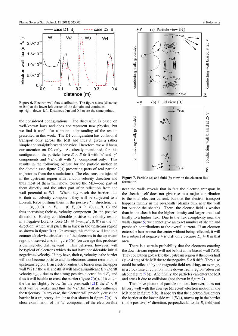
Figure 6. Electron wall flux distribution. The figure starts (distance= 0 m) at the lower left corner of the domain and continuesup–right–down–left. Distances 0 m and 0.4 m are the same points.

the considered configurations. The discussion is based onwell-known laws and does not represent new physics, butwe find it useful for a better understanding of the resultspresented in this work. The D1 configuration has collisionaltransport only across the MB and thus it gives a rathersimple and straightforward behavior. Therefore, we will focusour attention on D2 only. As already mentioned, for thisconfiguration the particles have E × B drift with ‘x’ and ‘y’components and ∇B drift with ‘y’ component only. Thisresults in the following picture for the particle motion inthe domain (see figure 7(a) presenting parts of real particletrajectories from the simulations). The electrons are injectedin the upstream region with random velocity direction andthus most of them will move toward the MB—one part ofthem directly and the other part after reflection from thewall potential at W1. When they reach the barrier, dueto their vx velocity component they will be subjected to aLorentz force pushing them in the positive ‘y’ direction, i.e.v = (vx, 0, 0) ⇒ FL = (0, Fy, 0) ∼= (0, evxBz, 0) andthus increasing their vy velocity component (in the positivedirection). Having considerable positive vy velocity resultsin a negative Lorentz force (FL

∼= (−evyBz, 0, 0)) in the ‘x’direction, which will push them back in the upstream regionas shown in figure 7(a). On average this motion will lead to acounter-clockwise circulation of the electrons in the upstreamregion, observed also in figure 5(b) (on average this producesa diamagnetic drift upward). This behavior, however, willbe typical of electrons which do not have considerable initialnegative vy velocity. If they have, their vy velocity in the barrierwill not become positive and the electrons cannot return to theupstream region. If an electron enters the barrier near the upperwall W2 (in the wall sheath) it will have a significant E×B driftvelocity vE×B due to the strong positive electric field Ey andthus it will be able to cross the barrier (figure 7(a)). If it entersthe barrier slightly below (in the presheath [21]) the E × B

drift will be weaker and thus the ∇B drift will also influencethe trajectory. In any case, the electron will probably cross thebarrier in a trajectory similar to that shown in figure 7(a). Aclose examination of the ‘x’ component of the electron flux

Figure 7. Particle (a) and fluid (b) view on the electron fluxformation.

near the walls reveals that in fact the electron transport inthe sheath itself does not give rise to a major contributionto the total electron current, but that the electron transporthappens mainly in the presheath (plasma bulk near the wallbut outside the sheath). There, the electric field is weakerthan in the sheath but the higher density and larger area leadfinally to a higher flux. Due to the flux complexity near thewalls (figure 5) we cannot give an exact number of sheath andpresheath contributions to the overall current. If an electronenters the barrier near the center without being reflected, it willbe a subject of negative ∇B drift only because Ey ≈ 0 in thatarea.

There is a certain probability that the electrons enteringthe downstream region will not be lost at the biased wall (W3).They could then go back to the upstream region at the lower half(y < 4 cm)of the MB due to the negativeE×B drift. They alsocould be reflected by the magnetic field resulting, on average,in a clockwise circulation in the downstream region (observedalso in figure 5(b)). And finally, the particles can enter the MBand cross it due to collisions (not shown in figure 7).

The above picture of particle motion, however, does notfit very well with the average (directed) electron motion in theMB seen in figure 5(b). It appears that the electron flux entersthe barrier at the lower side wall (W4), moves up in the barrier(in the positive ‘y’ direction, perpendicular to the Bz field) and

8

Plasma Sources Sci. Technol. 21 (2012) 025002 St Kolev et al

then goes out of the barrier and enters the downstream regionat the upper side wall (W2). Both ‘points of view’ (particle andcollective) agree that the electrons will enter in the upstreamzone at W2 but disagree as to where the electrons will enter thebarrier. To understand why, we need to analyze the electronflux components (equations (12)).

In addition to the collisional transport (diffusion), thereare two more components: E × B and diamagnetic drifts(figure 7(b)). The first one (E × B drift velocity, uE×B ∝(E × B)) is a direct result of the averaging of the E × B

drift of the separate particles. The diamagnetic drift, however,(diamagnetic velocity, uD ∝ −(∇p × B), where p is thepressure) has no particle analog and is a fluid-only drift(i.e. it is a result of averaging). This is a result of thedensity and temperature gradients (i.e. pressure gradient).The diamagnetic drift is not necessarily due to real drifts ofparticles (see [12, 13]). Even if there are no guiding centerdrifts of the particles, but there is a gradient of the densityor temperature, the diamagnetic drift will be present. Sothe high value of the flux (directed velocity) magnitude inthe MB (see figure 5(b)) may not correspond to real particledrifts! This is partially the case here. Figure 5(b) showspeak electron flux around the point y = 0.02 m, x = 0.047 m(the lower end of the barrier) directed upward (positive ‘y’).However, the allowed particle drifts at this point are ∇B andE×B pushing the particles together downward and toward theupstream region (see figure 7(a)). The particles are allowedto move upward only due to collisions, but this effect isrelatively weak. So despite the fact that the real drifts aredirected toward the upstream zone and downward, the flux isdirected upward (uD,y > 0, uD,x ≈ 0). This is due to thedominant diamagnetic drift at that point as a result of the largedensity (see figure 2(b)) and electron temperature (figure 4(b))gradients. Thus, the obtained flux pattern in the MB doesnot exactly represent the real particle drifts, but a flux due toaveraging. The above picture is verified by close trajectoryexamination at the considered point. This, however, doesnot mean that the diamagnetic flux is spurious. As alreadymentioned, the particles coming from the upstream region andfacing the magnetic field also contribute to the diamagneticdrift. The ∇B drift of separate particles is missing [12, 13]in the fluid plasma representation and does not have a directfluid analog. However, as shown in [22], the diamagneticdrift and pressure gradient of charged particles are relatedto the magnetic field inhomogeneity and particularly to ∇B2,which leads to a relation between the particle pressure and themagnetic pressure (proportional to B2).

Apparently, the E × B drift in configuration D2compromises the electron-stopping ability of the barrier. Thecurrent (mainly due to E × B drift) in D2 is three orders ofmagnitude higher than the drift due to collisions (12.2 mA forD2 against 0.0105 mA for D1, ratio = 1160). To fix this, weneed to make the plasma configuration closer to D1, i.e. to buildD2 with very large Ly . In this way the E × B current couldbecome comparable to and even smaller than the collisionalcurrent across the barrier. This is studied in section 6 of thispaper. However, this is usually not a practical method dueto the unacceptable length of the device. Another popular

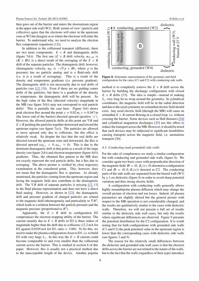
Figure 8. Schematic representation of the geometry and fieldconfiguration for the cases (C1 and C2) with conducting side walls.

method is to completely remove the E × B drift across thebarrier by building the discharge configuration with closedE × B drifts [23]. The idea is simple—instead of makingLy very long let us wrap around the geometry. In cylindricalcoordinates, the magnetic field will be in the radial directionand due to the axial symmetry no azimuthal electric field shouldexist. Any axial electric field (through the MB) will cause anazimuthal E × B current flowing in a closed loop, i.e. withoutcrossing the barrier. Some devices such as Hall thrusters [24]and cylindrical magnetron discharges [25] use this effect toreduce the transport across the MB. However, it should be notedthat such devices may be subjected to significant instabilitiescausing transport across the magnetic field, i.e. anomaloustransport [26].

4.3. Conducting (and grounded) side walls

For the sake of completeness we study a similar configurationbut with conducting and grounded side walls (figure 8). Weconsider again two basic cases with perpendicular direction ofthe magnetic field: B = (0, By(x), 0) denoted as configurationC1 and B = (0, 0, Bz(x)) denoted as C2. The conductingparts of the side walls are separated from the biased wall (W3)by a 1 cm dielectric (figure 8) in order to avoid sharp potentialvariation and thus strong electric fields.

A configuration with conducting walls generally allowshighly nonambipolar plasma diffusion which may change theoverall picture of electron and ion losses. Indeed, all plasmaparameters are slightly altered but the general picture withrespect to the MB operation is not considerably changed, andthe results are qualitatively similar to the cases with dielectricwalls. Therefore, we will not present a full set of resultssimilar to the dielectric side wall cases, but only the resultswhere significant differences are observed. Figure 9 presentsthe potential distribution for the C2 configuration. It is worthnoting that for both configurations with grounded side walls(C1 and C2) the peak potential value in the upstream region islower than the corresponding cases with dielectric side walls(see figures 3 and 9).

The reason for the relatively small differences betweenthe dielectric and grounded side wall cases is that the electrondrifts across the barrier are not related to the nature of the walls,but to the fact that the walls (regardless of their type) introduce

9

Plasma Sources Sci. Technol. 21 (2012) 025002 St Kolev et al

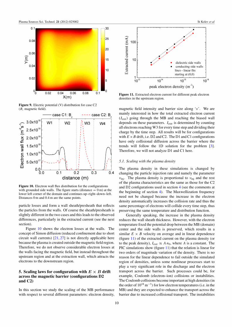
Figure 9. Electric potential (V) distribution for case C2(Bz magnetic field).

Figure 10. Electron wall flux distribution for the configurationswith grounded side walls. The figure starts (distance = 0 m) at thelower left corner of the domain and continues up–right–down–left.Distances 0 m and 0.4 m are the same points.

particle losses and form a wall sheath/presheath that reflectsthe particles from the walls. Of course the sheath/presheath isslightly different in the two cases and this leads to the observeddifferences, particularly in the extracted current (see the nextsection).

Figure 10 shows the electron losses at the walls. Theconcept of Simon diffusion (reduced confinement due to shortcircuit wall currents) [21, 27] is not directly applicable herebecause the plasma is created outside the magnetic field region.Therefore, we do not observe considerable electron losses atthe walls facing the magnetic field, but instead throughout theupstream region and at the extraction wall, which attracts theelectrons to the downstream region.

5. Scaling laws for configuration with E × B driftacross the magnetic barrier (configurations D2and C2)

In this section we study the scaling of the MB performancewith respect to several different parameters: electron density,

Figure 11. Extracted electron current for different peak electrondensities in the upstream region.

magnetic field intensity and barrier size along ‘x’. We aremainly interested in how the total extracted electron current(Iextr) going through the MB and reaching the biased walldepends on these parameters. Iextr is determined by countingall electrons reaching W3 for every time step and dividing theircharge by the time step. All results will be for configurationswith E×B drift, i.e. D2 and C2. The D1 and C1 configurationshave only collisional diffusion across the barrier where thetrends will follow the 1D solution for the problem [3].Therefore, we will not analyze D1 and C1 here.

5.1. Scaling with the plasma density

The plasma density in these simulations is changed bychanging the particle injection rate and namely the parameterνinj. The plasma density is proportional to νinj and the restof the plasma characteristics are the same as those for the C2and D2 configurations used in section 4 (see the comments atthe beginning of section 4). The Maxwellization frequencyneed not be changed because the increase in the electrondensity automatically increases the collision rate and thus thesame percentage of electrons will collide every time step, thuspreserving the same temperature and distribution function.

Generally speaking, the increase in the plasma densityreduces the wall sheath thickness. However, with the electrontemperature fixed the potential drop between the MB (domain)center and the side walls is preserved, which results in asimilar E × B velocity on average and in linear dependence(figure 11) of the extracted current on the plasma density (orto the peak density), Iextr ∝ A n0, where A is a constant. ThePIC simulations show (figure 11) that the relation is linear fortwo orders of magnitude variation of the density. There is noreason for the linear dependence to fail outside the simulatedregion of densities, unless some nonlinear processes start toplay a very significant role in the discharge and the electrontransport across the barrier. Such processes could be, forexample, Coulomb (electron–ion) collisions or instabilities.The Coulomb collisions become important at high densities (inthe order of 1018 m−3) for low electron temperatures (i.e. in theMB) and they are expected to enhance the transport across thebarrier due to increased collisional transport. The instabilities

10

Plasma Sources Sci. Technol. 21 (2012) 025002 St Kolev et al

are relatively weak for the considered configurations and theyseem to give a small contribution (see section 6). In general,the instabilities are nonlinear phenomena and if they determinethe electron transport across the barrier, it is not clear how theextracted current will scale with the plasma density.

Another possible issue related to the density scaling isthe ratio between the Larmor radius and the sheath size. Thequestion that arises is what will happen to the electron transportif the Larmor radius becomes larger than the Debye length,or even the sheath size (rL > λD)? For a magnetic fieldof 5 mT the electron Larmor radius is in the order of 1 mm,and for the highest density case simulated here (peak electrondensity 3 × 1015 m−3) the Debye length is in the order of0.5 mm, i.e. rL > λD. The linear dependence is apparently stillsatisfied. The reason for this is probably the following: (1) theelectron transport in the sheath itself does not provide themajor contribution to the total electron current, but the electrontransport happens mainly in the presheath (see section 4.2).(2) Even if the transport in the sheath becomes significant andpredominant under certain conditions, the rL/λD ratio wouldstill not affect the electron transport because what is importantis whether or not the electrons are reflected by the sheath. Ifthe particles are reflected they will contribute to the E×B drifthaving trajectories similar to those shown in figure 7(a) near theside walls. In the extreme case of a very thin sheath (rL λD ata very high density) the reflection becomes a ‘point’ reflectionfrom the wall, and trajectory becomes cycloid-like giving riseto the so-called ‘paramagnetic drift’ [22]. This gives the sameeffect as the E × B drift, forcing the particle to drift alongthe wall and to cross the MB. In fact any process (not onlyelectrostatic) causing electron-wall reflection (change in thevy velocity sign) will produce a paramagnetic drift.

The observed linear scaling of the extracted current withdensity is very important for our study, because it makes theresults obtained in this work applicable to conditions withdensities outside the simulated region, and thus applicable toa wider range of plasma devices.

5.2. Scaling with the magnetic field magnitude

In the current set of simulations, the magnetic field distributionremains Gaussian (equation (6)) and we change Bz0 only.The rest of the simulation conditions remain the same as inconfigurations C2 and D2 used in section 4 (see the commentsat the beginning of section 4).

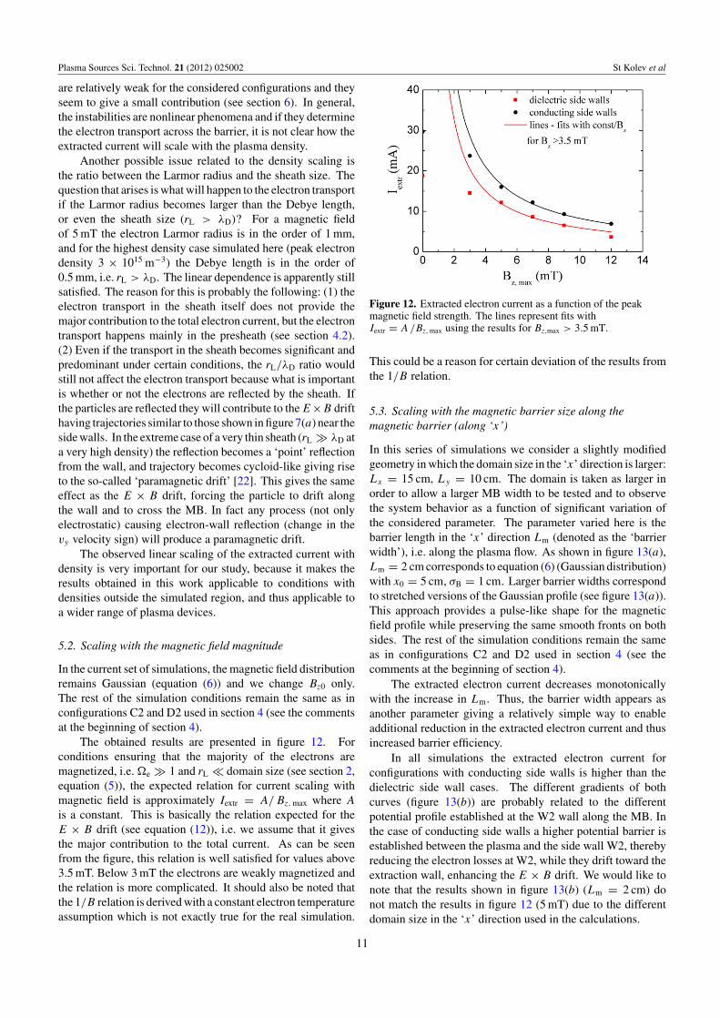
The obtained results are presented in figure 12. Forconditions ensuring that the majority of the electrons aremagnetized, i.e. e 1 and rL domain size (see section 2,equation (5)), the expected relation for current scaling withmagnetic field is approximately Iextr = A/ Bz, max where A

is a constant. This is basically the relation expected for theE × B drift (see equation (12)), i.e. we assume that it givesthe major contribution to the total current. As can be seenfrom the figure, this relation is well satisfied for values above3.5 mT. Below 3 mT the electrons are weakly magnetized andthe relation is more complicated. It should also be noted thatthe 1/B relation is derived with a constant electron temperatureassumption which is not exactly true for the real simulation.

Figure 12. Extracted electron current as a function of the peakmagnetic field strength. The lines represent fits withIextr = A /Bz, max using the results for Bz,max > 3.5 mT.

This could be a reason for certain deviation of the results fromthe 1/B relation.

5.3. Scaling with the magnetic barrier size along themagnetic barrier (along ‘x’)

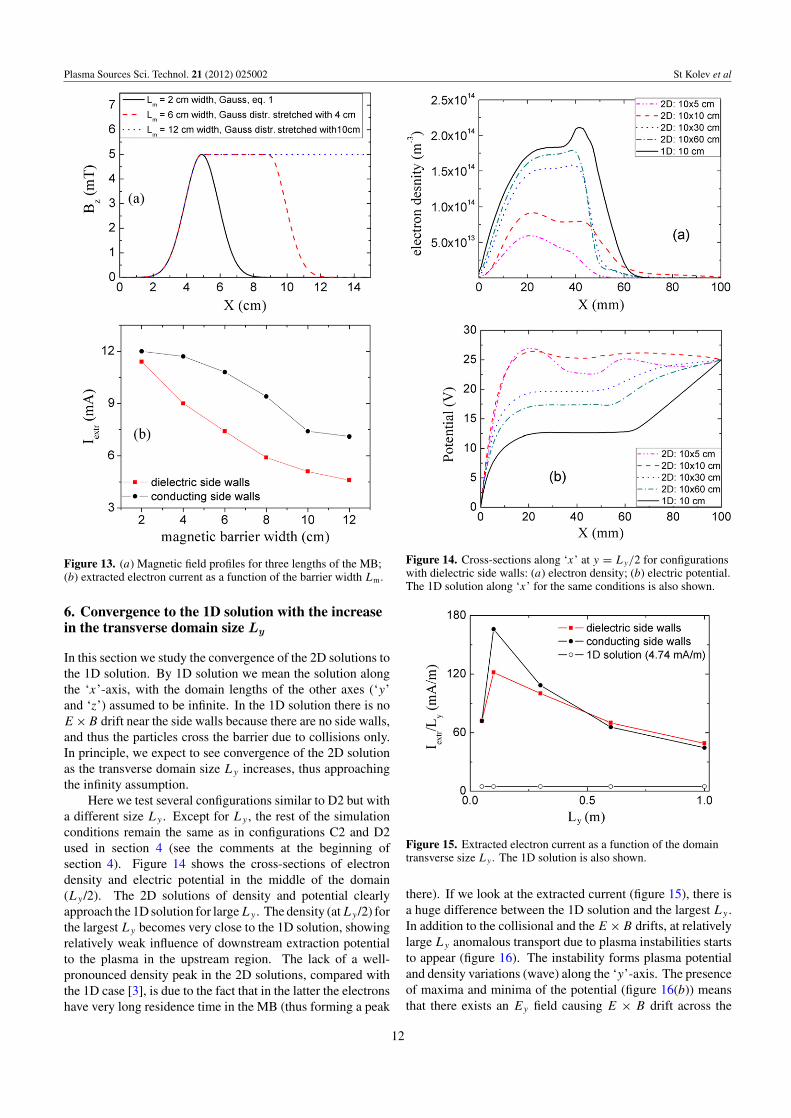
In this series of simulations we consider a slightly modifiedgeometry in which the domain size in the ‘x’ direction is larger:Lx = 15 cm, Ly = 10 cm. The domain is taken as larger inorder to allow a larger MB width to be tested and to observethe system behavior as a function of significant variation ofthe considered parameter. The parameter varied here is thebarrier length in the ‘x’ direction Lm (denoted as the ‘barrierwidth’), i.e. along the plasma flow. As shown in figure 13(a),Lm = 2 cm corresponds to equation (6) (Gaussian distribution)with x0 = 5 cm, σB = 1 cm. Larger barrier widths correspondto stretched versions of the Gaussian profile (see figure 13(a)).This approach provides a pulse-like shape for the magneticfield profile while preserving the same smooth fronts on bothsides. The rest of the simulation conditions remain the sameas in configurations C2 and D2 used in section 4 (see thecomments at the beginning of section 4).

The extracted electron current decreases monotonicallywith the increase in Lm. Thus, the barrier width appears asanother parameter giving a relatively simple way to enableadditional reduction in the extracted electron current and thusincreased barrier efficiency.

In all simulations the extracted electron current forconfigurations with conducting side walls is higher than thedielectric side wall cases. The different gradients of bothcurves (figure 13(b)) are probably related to the differentpotential profile established at the W2 wall along the MB. Inthe case of conducting side walls a higher potential barrier isestablished between the plasma and the side wall W2, therebyreducing the electron losses at W2, while they drift toward theextraction wall, enhancing the E × B drift. We would like tonote that the results shown in figure 13(b) (Lm = 2 cm) donot match the results in figure 12 (5 mT) due to the differentdomain size in the ‘x’ direction used in the calculations.

11

Plasma Sources Sci. Technol. 21 (2012) 025002 St Kolev et al

Figure 13. (a) Magnetic field profiles for three lengths of the MB;(b) extracted electron current as a function of the barrier width Lm.

6. Convergence to the 1D solution with the increasein the transverse domain size Ly

In this section we study the convergence of the 2D solutions tothe 1D solution. By 1D solution we mean the solution alongthe ‘x’-axis, with the domain lengths of the other axes (‘y’and ‘z’) assumed to be infinite. In the 1D solution there is noE ×B drift near the side walls because there are no side walls,and thus the particles cross the barrier due to collisions only.In principle, we expect to see convergence of the 2D solutionas the transverse domain size Ly increases, thus approachingthe infinity assumption.

Here we test several configurations similar to D2 but witha different size Ly . Except for Ly , the rest of the simulationconditions remain the same as in configurations C2 and D2used in section 4 (see the comments at the beginning ofsection 4). Figure 14 shows the cross-sections of electrondensity and electric potential in the middle of the domain(Ly /2). The 2D solutions of density and potential clearlyapproach the 1D solution for large Ly . The density (at Ly /2) forthe largest Ly becomes very close to the 1D solution, showingrelatively weak influence of downstream extraction potentialto the plasma in the upstream region. The lack of a well-pronounced density peak in the 2D solutions, compared withthe 1D case [3], is due to the fact that in the latter the electronshave very long residence time in the MB (thus forming a peak

Figure 14. Cross-sections along ‘x’ at y = Ly/2 for configurationswith dielectric side walls: (a) electron density; (b) electric potential.The 1D solution along ‘x’ for the same conditions is also shown.

Figure 15. Extracted electron current as a function of the domaintransverse size Ly . The 1D solution is also shown.

there). If we look at the extracted current (figure 15), there isa huge difference between the 1D solution and the largest Ly .In addition to the collisional and the E ×B drifts, at relativelylarge Ly anomalous transport due to plasma instabilities startsto appear (figure 16). The instability forms plasma potentialand density variations (wave) along the ‘y’-axis. The presenceof maxima and minima of the potential (figure 16(b)) meansthat there exists an Ey field causing E × B drift across the

12

Plasma Sources Sci. Technol. 21 (2012) 025002 St Kolev et al

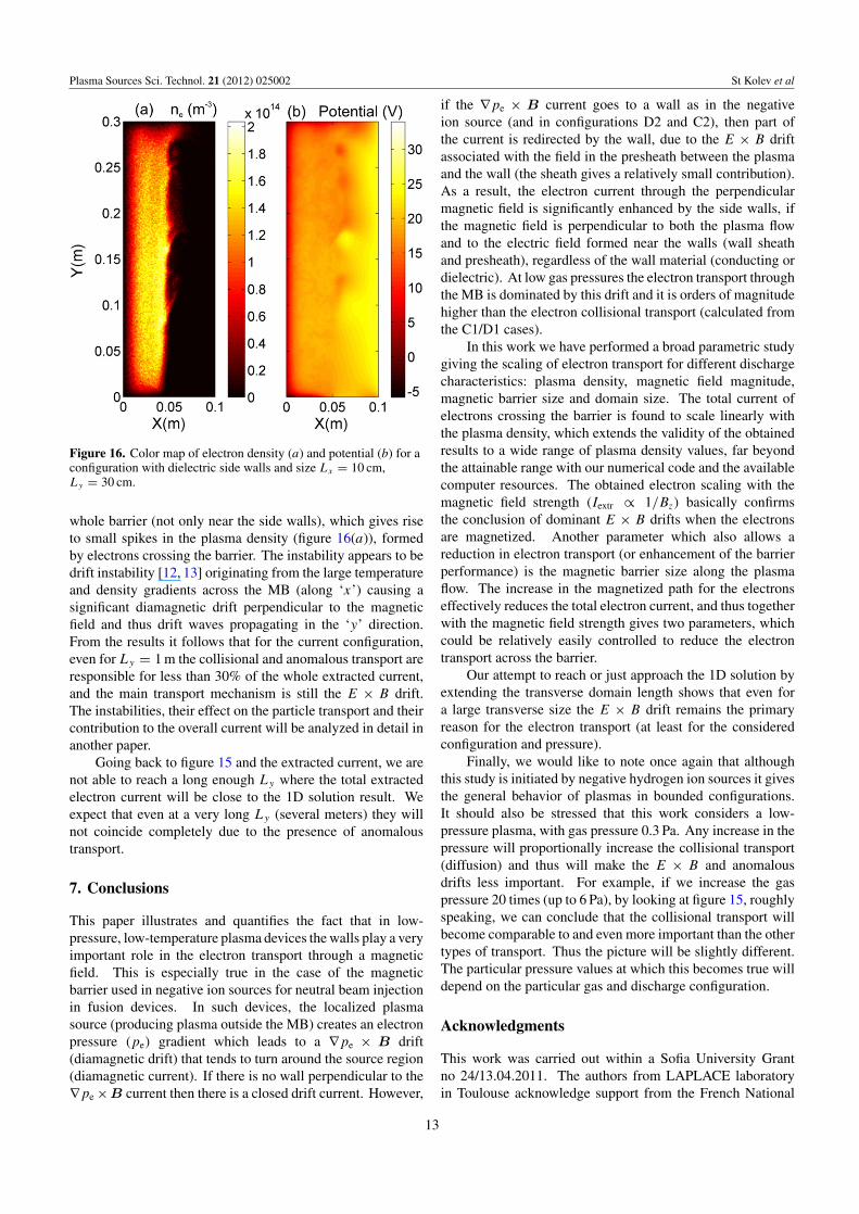
Figure 16. Color map of electron density (a) and potential (b) for aconfiguration with dielectric side walls and size Lx = 10 cm,Ly = 30 cm.

whole barrier (not only near the side walls), which gives riseto small spikes in the plasma density (figure 16(a)), formedby electrons crossing the barrier. The instability appears to bedrift instability [12, 13] originating from the large temperatureand density gradients across the MB (along ‘x’) causing asignificant diamagnetic drift perpendicular to the magneticfield and thus drift waves propagating in the ‘y’ direction.From the results it follows that for the current configuration,even for Ly = 1 m the collisional and anomalous transport areresponsible for less than 30% of the whole extracted current,and the main transport mechanism is still the E × B drift.The instabilities, their effect on the particle transport and theircontribution to the overall current will be analyzed in detail inanother paper.

Going back to figure 15 and the extracted current, we arenot able to reach a long enough Ly where the total extractedelectron current will be close to the 1D solution result. Weexpect that even at a very long Ly (several meters) they willnot coincide completely due to the presence of anomaloustransport.

7. Conclusions

This paper illustrates and quantifies the fact that in low-pressure, low-temperature plasma devices the walls play a veryimportant role in the electron transport through a magneticfield. This is especially true in the case of the magneticbarrier used in negative ion sources for neutral beam injectionin fusion devices. In such devices, the localized plasmasource (producing plasma outside the MB) creates an electronpressure (pe) gradient which leads to a ∇pe × B drift(diamagnetic drift) that tends to turn around the source region(diamagnetic current). If there is no wall perpendicular to the∇pe ×B current then there is a closed drift current. However,

if the ∇pe × B current goes to a wall as in the negativeion source (and in configurations D2 and C2), then part ofthe current is redirected by the wall, due to the E × B driftassociated with the field in the presheath between the plasmaand the wall (the sheath gives a relatively small contribution).As a result, the electron current through the perpendicularmagnetic field is significantly enhanced by the side walls, ifthe magnetic field is perpendicular to both the plasma flowand to the electric field formed near the walls (wall sheathand presheath), regardless of the wall material (conducting ordielectric). At low gas pressures the electron transport throughthe MB is dominated by this drift and it is orders of magnitudehigher than the electron collisional transport (calculated fromthe C1/D1 cases).

In this work we have performed a broad parametric studygiving the scaling of electron transport for different dischargecharacteristics: plasma density, magnetic field magnitude,magnetic barrier size and domain size. The total current ofelectrons crossing the barrier is found to scale linearly withthe plasma density, which extends the validity of the obtainedresults to a wide range of plasma density values, far beyondthe attainable range with our numerical code and the availablecomputer resources. The obtained electron scaling with themagnetic field strength (Iextr ∝ 1/Bz) basically confirmsthe conclusion of dominant E × B drifts when the electronsare magnetized. Another parameter which also allows areduction in electron transport (or enhancement of the barrierperformance) is the magnetic barrier size along the plasmaflow. The increase in the magnetized path for the electronseffectively reduces the total electron current, and thus togetherwith the magnetic field strength gives two parameters, whichcould be relatively easily controlled to reduce the electrontransport across the barrier.

Our attempt to reach or just approach the 1D solution byextending the transverse domain length shows that even fora large transverse size the E × B drift remains the primaryreason for the electron transport (at least for the consideredconfiguration and pressure).

Finally, we would like to note once again that althoughthis study is initiated by negative hydrogen ion sources it givesthe general behavior of plasmas in bounded configurations.It should also be stressed that this work considers a low-pressure plasma, with gas pressure 0.3 Pa. Any increase in thepressure will proportionally increase the collisional transport(diffusion) and thus will make the E × B and anomalousdrifts less important. For example, if we increase the gaspressure 20 times (up to 6 Pa), by looking at figure 15, roughlyspeaking, we can conclude that the collisional transport willbecome comparable to and even more important than the othertypes of transport. Thus the picture will be slightly different.The particular pressure values at which this becomes true willdepend on the particular gas and discharge configuration.

Acknowledgments

This work was carried out within a Sofia University Grantno 24/13.04.2011. The authors from LAPLACE laboratoryin Toulouse acknowledge support from the French National

13

Plasma Sources Sci. Technol. 21 (2012) 025002 St Kolev et al

Research Agency (ANR ITER-NIS, BLAN08-2 310122) andfrom EFDA, CEA and the French ‘Federation de Recherchesur la Fusion’.

Appendix. Maxwellization and particle injectionprocedures

The electron Maxwellization of electrons is done by virtual‘Maxwellizing collisions’. Every time step a certain numberof electrons are picked up depending on the spatial profileof the collision probability we impose, and their velocity ischanged by randomly sampling from isotropic Maxwelliandistribution with temperature TM. Therefore, the electrontemperature in the upstream region never becomes exactlyTM, but slightly lower because there are always particleswhich are not Maxwellized in several time steps. Even if wesignificantly increase the rate of ‘Maxwellizing collisions’ theonly consequence will be the fact that the electron temperaturein the upstream region will be even closer to TM.

Here we impose as an external parameter the ‘Maxwelliz-ing collision frequency’ νh(x, y). Once having the collisionfrequency spatial distribution we use the null collision method[16] to do the ‘collisions’. Obviously, these are not real colli-sions but virtual collisions giving the electrons new velocities.The procedure is done in this way to be compatible with therest of the Monte Carlo procedures.

The profile of the ‘Maxwellizing collision frequency’ istaken to have a half-period sine shape, i.e.

νh(x, y) =

1 × 107 π2 sin

(π x−xa

xb−xa

), if x ∈ (xa, xb),

0, if x /∈ (xa, xb),(A.1)

where xa = 5 × 10−3 m and xb = 3.333 × 10−2 m.The particle injection is done in a similar way. We impose

as external parameters the ‘injection collision frequency’νinj(x, y) with a similar profile:

νinj(x, y) =

νinj0π2 sin

(π x−xa

xb−xa

), if x ∈ (xa, xb),

0, if x /∈ (xa, xb),(A.2)

and certain ‘target density’ ninj. Here νinj0 = 7 × 105 s−1,xa = 5 × 10−3 m and xb = 3.333 × 10−2 m. The changein the electron (and ion) density due to injection is simplydn/dt |injection = ninjνinj(x, y) and thus every time step we injecta constant number of particles in the domain, regardless of thereal density of the different particle species. Both νinj(x, y)

and νh(x, y) are uniform along the ‘y’ direction.

References

[1] Boeuf J P, Hagelaar G J M, Sarrailh P, Fubiani G and Kohen N2011 Plasma Sources Sci. Technol. 20 015002

[2] Hagelaar G J M, Fubiani G and Boeuf J P 2011 PlasmaSources Sci. Technol. 20 015001

[3] Kolev St, Hagelaar G J M and Boeuf J P 2009 Phys. Plasmas16 042318

[4] Hemsworth R S and Inoue T 2005 IEEE Trans. Plasma Sci.33 1799

[5] Leung K N, Ehlers K W and Bacal M 1983 Rev. Sci. Instrum.54 56

[6] Bacal M 2006 Nucl. Fusion 46 S250[7] Fantz U et al 2008 Rev. Sci. Instrum. 79 02A511[8] Taccogna F, Minelli P, Longo S, Capitelli M and Schneider R

2010 Phys. Plasmas 17 063502[9] Kuppel S, Matsushita D, Hatayama A and Bacal M 2011

J. Appl. Phys. 109 013305[10] Kolev St, Lishev St, Shivarova A, Tarnev Kh and Wilhelm R

2007 Plasma Phys. Control. Fusion 49 1349[11] Lishev St, Shivarova A and Tarnev Kh 2010 J. Phys.: Conf.

Ser. 223 012003[12] Chen F 1984 Introduction to Plasma Physics and Controlled

Fusion (New York: Plenum)[13] Bellan P M 2008 Fundamentals of Plasma Physics

(Cambridge: Cambridge University Press)[14] Birdsall C K and Langdon A B 1985 Plasma Physics via

Computer Simulation (New York: McGraw-Hill)[15] Hockney R W and Eastwood J W 1989 Computer Simulation

Using Particles (London: Taylor and Francis)[16] Vahedi V and Surendra M 1995 Comput. Phys. Commun.

87 179[17] Itikawa Y 1974 At. Data Nucl. Data Tables 14 1[18] Trajmar S and Kanik I 1995 Atomic and Molecular Processes

in Fusion Edge Plasmas ed R K Janev (New York: Plenum)p 40

[19] Janev R K, Reiter D and Samm U 2003 Collision processes inlow-temperature hydrogen plasmas FZ-Julich Report No4105, http://www.eirene.de/report 4105.pdf

[20] Krstiæ P S and Schultz D R 1998 Atomic and Plasma–MaterialInteraction Data for Fusion vol 8 (Vienna: IAEA)

[21] Lieberman M A and Lichtenberg A J 1994 Principles ofPlasma Discharges and Materials Processing (New York:Wiley)

[22] Golant V E, Zhilinsky A P and Sakharov I E 1980Fundamentals of Plasma Physics (New York: Wiley)chapter 8.6

[23] Keidar M and Beilis I I 2006 IEEE Trans. Plasma Sci.34 804

[24] Goebel D M and Katz I 2008 Fundamentals of ElectricPropulsion: Ion and Hall Thrusters (New York: Wiley)

[25] Levchenko I, Romanov M, Keidar M and Beilis I I 2004 Appl.Phys. Lett. 85 2202–5

[26] Adam J C et al 2008 Plasma Phys. Control. Fusion50 124041

[27] Simon A 1955 Phys. Rev. 98 317–8

14