Understanding the Dynamics of Inflation Volatility in Nigeria: A GARCH Perspective

CBN Journal of Applied Statistics Vol. 3 No. 2 51

Understanding the Dynamics of Inflation Volatility

in Nigeria: A GARCH Perspective

Babatunde S. Omotosho and Sani I. Doguwa1

The estimation of inflation volatility is important to Central Banks as it guides their

policy initiatives for achieving and maintaining price stability. This paper employs

three models from the Generalized Autoregressive Conditional Heteroscedasticity

(GARCH) family with a view to providing a parsimonious approximation to the

dynamics of Nigeria’s inflation volatility between 1996 and 2011. Of the competing

models, the asymmetric TGARCH (1,1) provides an appropriate paradigm for

explaining the dynamics of headline and core CPI volatilities in Nigeria, while the

symmetric GARCH (1,1) was found to be adequate for food CPI. The results are quite

revealing. Firstly, model outcomes indicate high persistence parameters for the core

and food CPI, implying that the impacts of inflation shocks on their volatilities die

away very slowly. However, the impact of inflation shocks on headline volatility die

out rather quickly. Secondly, substantial evidence of asymmetric effect was found for

both headline and core inflation types while the contrary was confirmed for food

inflation. Thirdly, positive inflationary shocks yielded higher volatilities in headline

and core inflation than negative innovations, implying the absence of leverage effect

in them. The paper finds that periods of high inflation volatility are associated with

periods of specific government policy changes, shocks to food prices and lack of

coordination between monetary and fiscal policies.

JEL Classification: C22, C51, C52, E31

Keywords: Inflation volatility, Conditional heteroscedasticity, GARCH

models, Asymmetric effects, Volatility persistence

1.0 Introduction

In statistical terms, volatility is often regarded as variance and it is a measure

of the dispersion of a random variable from its mean value. Thus, inflation

volatility relates to the fluctuations (or instability) in a chosen measure of

inflation (for further discussion, see Judson and Orphanides, 1999; Kontonikas,

2004; Samimi and Shahryar, 2009 and Pourgerami and Maskus, 1987). In

Nigeria, for instance, monthly headline inflation is measured in terms of the

year-on-year percentage change in the all-items Consumer Price Index (CPI)

compiled by the National Bureau of Statistics (NBS) and fluctuations in such a

measure characterizes inflation volatility in the country.

1Statistics Department, Central Bank of Nigeria, Abuja

52 Understanding the Dynamics of Inflation Volatility in Nigeria:

A GARCH Perspective Omotosho & Doguwa

The adverse effects of inflation volatility on the economy have been widely

documented in countries of diverse economic structures and monetary policy

frameworks. For example, it has been found to cause higher risk premia,

hedging costs, unforeseen redistribution of wealth and ultimately a reduction in

overall economic growth. This is in line with Friedman’s (1977) conjecture

that the harmful effect of inflation on growth is driven principally by inflation

volatility. Additional evidences in this direction are provided by Judson and

Orphanides (1999), Elder (2004), Byme and Davis (2004) and Elder (2005),

Brunner and Hess (1993), Ungar and Zilberforb (1993), Baillie et al. (1996),

Grier and Perry (1998), Rother (2004) and Caporale et al. (2010).

Internationally, the evidence for ARCH effects in inflation series is mixed, but

there is strong evidence that countries with high inflation have significantly

higher levels of volatility on average and such volatilities ultimately impacts on

growth negatively. It is in recognition of this fact that most Central Banks of

the world have incorporated price stability as part of their core mandates

thereby mainstreaming policies that are capable of arresting the domestic

drivers of high and unstable prices as well as anchoring inflation expectations

at levels consistent with price stability. However, a crucial step in the

achievement of this mandate or any serious price stabilization strategy for that

matter involves proper estimation of inflation volatility as well as a firm

understanding of its dynamics.

Over the years, the Generalized Autoregressive Conditional Heteroscedasticity

(GARCH) methodology has become quite useful in modeling volatility of

economic time series, including consumer price indices. As posited by Engle

(1982), this methodology allows a conventional regression specification for the

mean function with a variance which is permitted to change stochastically over

the sample period. Within this framework, heteroscedasticity is seen as a

variance that should be modeled in a time series perspective. Thus, the

application of ARCH model introduced by Engle (1982) and its generalized

extension (GARCH) proposed by Bollerslev (1986) in financial modeling have

become very popular. An account of the variations and extensions to the

GARCH model can be found in Hentschel (1995), Pagan (1996), Brooks

(2008) and Xekalaki and Degiannakis (2010), among others. This study seeks

to leverage on this area of methodology to understand the dynamics of inflation

volatility in Nigeria in the last one and a half decades.

In Nigeria, some studies have been carried out in the area of modeling inflation

volatility using GARCH methodology, most of which focused on estimating


the conditional variance of the country’s headline CPI series and investigating

its impacts on other macro-economic variables. These studies include that of

Idowu and Hassan (2010) who explore the relationship between headline

inflation uncertainty and economic growth using quarterly headline CPI for the

period 1970 to 2007. Also, Udoh and Egwaikhide (2008) employed the

GARCH model to estimate headline inflation volatility and examined its

impacts on foreign direct investment between 1970 and 2005, using annual

data. Others include Adamgbe (2003) who fitted a symmetric GARCH (1,1)

model to provide volatility estimates for Nigeria’s headline CPI using annual

data for the period 1970-2001. These studies assumed symmetric response of

inflation volatility to positive and negative shocks as implied by the basic

GARCH model. However, such a symmetric restriction in the GARCH model

has been rejected by several empirical studies as inflation volatility was found

to be more sensitive to positive inflation shocks than to negative shocks

(Brunner and Hess, 1993).

A major implication of ignoring asymmetric considerations when modeling

inflation volatility relates to either over-prediction or under-prediction of

volatility levels depending on the nature of prevailing inflationary shocks.

Also, the studies employed a rather low-frequency data for their analysis of

headline inflation volatility. However, it has been argued in Natalia (2010) that

using high frequency data increases the efficiency of extracting model-based

estimates of volatility from economic time series. Finally, Idowu and Hassan

(2010) obtain volatility estimates up to 2007 for headline inflation and this pre-

dates the 2008 global financial crises.

In order to address the concerns highlighted above, this paper examines the

volatility dynamics of not only headline CPI, but also food and core CPI series

using monthly data. Also, the presence of volatility persistence and leverage

effects in the three components of inflation are investigated. Thus, the broad

objective of this paper is to model the time-varying volatility ( ) of Nigeria’s

inflation types between 1996 and 2011 using monthly data as well as explore

its characteristics. To achieve this objective, a symmetric GARCH model and

two asymmetric TGARCH and EGARCH models are fitted to each of the three

inflation types and the best model for each type is selected based on selected

information criterion2.

2 Akaike Information Criterion



For ease of exposition, the paper is structured into five sections; with section

one as the introduction. Section two provides some historical perspective on

Nigeria’s inflation episodes. Section three discusses the analytical framework

for the study as well as data sources. Section four presents the empirical

analysis, while the final section concludes the paper.

2.0 Nigeria’s Inflationary Episodes: Some Stylized Facts

Nigeria has had four major episodes of inflation in excess of 30 per cent since

1970. The first of these episodes was 1975, with an inflation rate of 33.7 per

cent (tagged IE 1 in Fig. 1). The factors responsible for this development

included drought in Northern Nigeria, which pushed up food prices as well as

the excessive monetization of the large inflow of dollars that accrued from the

crude oil boom. This period was also associated with high volatility as

measured by the moving standard deviation of the year on year headline

inflation rates (tagged VE 1 in Fig. 2). Some of the measures adopted to curb

the situation included the reduction in import duties on a relatively large

number of goods and raw materials, a conscious monetary policy targeted at

encouraging banks to lend more to the productive sectors of the economy and

the setting up of the Anti-Inflation Task Force, which recommended the

establishment of the Productivity, Prices and Incomes Board. These explain the

gradual decline in both the average inflation rate and its volatility during the

period 1976 – 1983 (Fig. 1 & 2).

Also, 1984 represented another remarkable episode as inflation rate settled at a

higher level of about 41.2 per cent, owing to the expectations of imminent

devaluation of the domestic currency and monetary expansion. This period also

witnessed increased inflation volatility as the computed 12 months moving

standard deviation rose above 10.0 in 1984 and above 15.0 in 1985 (Fig. 2). In

response, the military regime embarked on another round of price control,

which led to a decline in the inflation rate to 5.5 per cent) in 1985 and 5.4 per

cent in1986 and a decline in its standard deviation to less than 5 (Fig. 1 & 2).

The third episode of high inflation occurred during 1988 and 1989 caused by

fiscal expansion of the 1988 budget, which was financed by credit from the

CBN. Fig. 2 shows that the standard deviation of the headline inflation rate

stood at 25 in 1988 before falling to about 7 in 1990, a period tagged VE3.

Increased agricultural production helped to moderate inflationary pressures in

1990 as the inflation rate fell to 8.2 per cent.


The fourth inflationary episode was the most turbulent in Nigeria’s inflationary

experience as it lasted about five years starting from 1992 and reaching an all-

time high of over 80.0 per cent in 1995. The moving standard deviation was

also relatively high, at about 15. Largely responsible for this development were

monetary growth and fiscal expansion. As a response to the inflationary

pressures of the period, the government strengthened its stabilization measures

in the economy as it entrenched effective monetary policy, fiscal discipline as

well as exchange rate stability.

These measures resulted in a systematic decline in inflation rate from over 80.0

per cent in 1995 to 7.1 per cent in 2000. However, the last episode of inflation

volatility was in 1996-97. From the foregoing analysis, we could infer that

periods of high inflation are associated with periods of high inflation volatility.

3.0 Methodology

In developing the basic ARCH model, three distinct specifications are required,

and these are for the: conditional mean equation, conditional variance equation,

-20

0

20

40

60

80

100

Mon

th

Jan-

71

Feb-

72

Mar

-73

Apr-

74

May

-75

Jun-

76

Jul-7

7

Aug-

78

Sep-

79

Oct

-80

Nov

-81

Dec-

82

Jan-

84

Feb-

85

Mar

-86

Apr-

87

May

-88

Jun-

89

Jul-9

0

Aug-

91

Sep-

92

Oct

-93

Nov

-94

Dec-

95

Jan-

97

Feb-

98

Mar

-99

Apr-

00

May

-01

Jun-

02

Jul-0

3

Aug-

04

Sep-

05

Oct

-06

Nov

-07

Dec-

08

Jan-

10

Feb-

11

Mar

-12

Hea

dlin

e Y

on Y

Infla

tion

Rat

e (%

)

Fig 1: Plot of Nigeria's Y/Y Headline Inflation Rate

IE1

IE2 IE3

IE4

0.0

5.0

10.0

15.0

20.0

25.0

30.0

Jan-

70

Mar

-71

May

-72

Jul-7

3

Sep-

74

Nov

-75

Jan-

77

Mar

-78

May

-79

Jul-8

0

Sep-

81

Nov

-82

Jan-

84

Mar

-85

May

-86

Jul-8

7

Sep-

88

Nov

-89

Jan-

91

Mar

-92

May

-93

Jul-9

4

Sep-

95

Nov

-96

Jan-

98

Mar

-99

May

-00

Jul-0

1

Sep-

02

Nov

-03

Jan-

05

Mar

-06

May

-07

Jul-0

8

Sep-

09

Nov

-10

Jan-

12

12

Mo

nth

s M

ovin

g ơ

of H

ead

lin

e In

flat

ion

Rat

es

Fig 2: Plot of Headline Inflation Volatility

VE 1 VE 2

VE 3

VE 5

VE 4



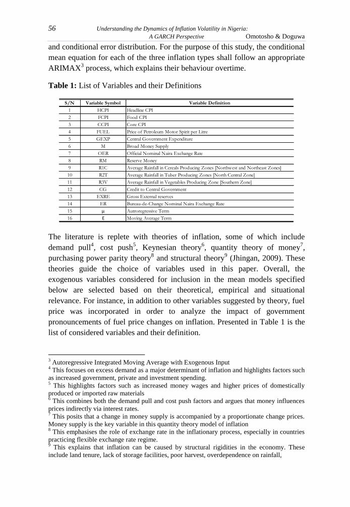
and conditional error distribution. For the purpose of this study, the conditional

mean equation for each of the three inflation types shall follow an appropriate

ARIMAX3 process, which explains their behaviour overtime.

Table 1: List of Variables and their Definitions

The literature is replete with theories of inflation, some of which include

demand pull4, cost push

5, Keynesian theory

6, quantity theory of money

7,

purchasing power parity theory8 and structural theory

9 (Jhingan, 2009). These

theories guide the choice of variables used in this paper. Overall, the

exogenous variables considered for inclusion in the mean models specified

below are selected based on their theoretical, empirical and situational

relevance. For instance, in addition to other variables suggested by theory, fuel

price was incorporated in order to analyze the impact of government

pronouncements of fuel price changes on inflation. Presented in Table 1 is the

list of considered variables and their definition.

3 Autoregressive Integrated Moving Average with Exogenous Input

4 This focuses on excess demand as a major determinant of inflation and highlights factors such

as increased government, private and investment spending. 5 This highlights factors such as increased money wages and higher prices of domestically

produced or imported raw materials 6 This combines both the demand pull and cost push factors and argues that money influences

prices indirectly via interest rates. 7 This posits that a change in money supply is accompanied by a proportionate change prices.

Money supply is the key variable in this quantity theory model of inflation 8 This emphasises the role of exchange rate in the inflationary process, especially in countries

practicing flexible exchange rate regime. 9 This explains that inflation can be caused by structural rigidities in the economy. These

include land tenure, lack of storage facilities, poor harvest, overdependence on rainfall,

S/N Variable Symbol Variable Definition

1 HCPI Headline CPI

2 FCPI Food CPI

3 CCPI Core CPI

4 FUEL Price of Petroleum Motor Spirit per Litre

5 GEXP Central Government Expenditure

6 M Broad Money Supply

7 OER Official Nominal Naira Exchange Rate

8 RM Reserve Money

9 R1C Average Rainfall in Cereals Producing Zones [Northwest and Northeast Zones]

10 R2T Average Rainfall in Tuber Producing Zones [North Central Zone]

11 R3V Average Rainfall in Vegetables Producing Zone [Southern Zone]

12 CG Credit to Central Government

13 EXRE Gross External reserves

14 ER Bureau-de-Change Nominal Naira Exchange Rate

15 µ Autroregressive Term

16 Ɛ Moving Average Term


Thus, the mean equations for the headline (HCPI), food (FCPI) and core

(CCPI) inflation types are specified respectively as:

∑

∑

∑

∑

∑

∑

∑

∑

∑

∑

∑

∑

∑

∑

∑

∑

∑

∑

∑

∑

∑

and,

∑

∑

∑

∑

∑

∑

∑

∑

where is assumed to be white noise [ ], is a constant, ωi’s are

the autoregressive terms (for i=1, 2, 3, …, p) and θi’s are the moving average

terms (for i=1, 2, 3, ..., q). The residuals ( ) from equations (1), (2) and (3) are

said to follow an ARCH (p) process if the conditional distribution of given

its past values has zero mean and conditional variance σ2

t. The coefficients of

the exogenous variables are

with the subscript on each of the parameters ranging from zero

to their respective limits. The endogenous and exogenous variables are listed

and defined in Table 1.

The conditional variance equations estimated in this study are broadly divided

into two groups, namely: the symmetric model (GARCH)10

and the asymmetric

models (TGARCH and EGARCH)11

. Starting with the symmetric model, Engle

10

GARCH means Generalized Autoregressive Conditional Heteroscedasticity 11

TGARCH means Threshold Generalized Autoregressive Conditional Heteroscedasticity and

EGARCH means Exponential Generalized Autoregressive Conditional Heteroscedasticity.



(1982) introduced the ARCH (q) model to estimate the time-varying volatility

of a series by expressing the conditional variance of the prediction error term

as a function of the recent past values of the squared error as follows:

∑

(4)

Such that ≥ 0 and ≥ 0 for i = 0, 1, 2, ...,q. σ2

t denotes the conditional

variance at time t, is a constant, αi are the parameters of the ARCH terms of

order q and ɛt-i2 represent the lagged values of the squared prediction error for

i= 1, 2, 3, ..., q. In order to provide solution to the problem of how many lags

of the squared innovations should be included in the ARCH model, Bollerslev

(1986) introduced a generalized version of the ARCH model by modeling the

conditional variance as a function of its own lagged values as well as the

lagged values of the squared innovations as follows:

(5)

where , , α and

are as previously defined in equation (4), β is the

GARCH coefficient and represents the one period lag of the fitted

variance from the model. To guarantee a well-defined GARCH (1,1) model, it

is required that α ≥ 0 and β ≥ 0, while α + β < 1 suffices for covariance

stationarity.

The TGARCH model introduced by Glosten et al. (1993) allows for

asymmetric effects in volatility modeling. They extended the GARCH model

by including an additional term γ, to capture possible asymmetries in the data.

The TGARCH specification is given as:

where is an indicator function that takes the value of 1 if - and 0

otherwise, γ is the asymmetric parameter and , α and β are as defined in

equation (5). Good news (positive shock) is obtained when Ɛt-1 > 0, while bad

news (negative shocks) is obtained when Ɛt-1 < 0. Good news has an impact of

α while bad news has an impact of α + γ on the conditional variance. If γ ≠ 0,

news impact is asymmetric and if γ > 0, there is leverage effect as negative

shocks increase volatility more compared with an equivalent amount of

positive shocks. The TGARCH model reduces to the basic GARCH model if

the asymmetric term (γ) is zero.


Nelson (1991) extends the GARCH model to efficiently capture volatility

clustering and asymmetric effect. This model is known as the EGARCH is

specified as:

(|

√

|) (

)

(7)

where , α, β and γ are as defined in equation (6). The fact that the left-hand

side of equation (7) is the log of the conditional variance implies that the

leverage effect is exponential, rather than quadratic. Therefore, the forecasts of

the conditional variance should be non-negative. The asymmetric effect of past

shocks is captured by the γ. If the asymmetric term is γ ≠ 0, news impact is

asymmetric and if γ < 0, there is leverage effect. The impact of conditional

shocks on the conditional variance is measured by α. A positive shock in

period has an effect of α + γ on the conditional variance whereas a

negative shock has an effect of α – γ. Usually ARCH/GARCH models are

estimated under specific assumption about the conditional distribution of the

error term. The normal distribution is assumed in this study12

.

There are various criteria for model selection in the literature. This paper

employs the Akaike Information Criterion (AIC) as it helps to balance the

trade-off between model-fit and complexity. It is defined as:

( ) (

) (8)

where L is the value of the log-likelihood function, K is the number of

estimated parameters and N is the number of observations. In each class of

model, different models are fitted and the one with the lowest AIC value is

selected as the best for that class.

4.0 Data, Results and Discussions

This empirical study uses headline, food and core Consumer Price Indices

(CPIs)13

, covering the period January 1996 to December 2011 as the dependent

variables for the class of mean models estimated in this paper. Data on the

other exogenous variables (listed in Table 1) for the same period are sourced

from the Central Bank of Nigeria database.

12

Estimation based on the student’s t-distribution and generalized error distribution assumption

of the prediction error term did not improve model results substantially. 13

Downloadable from www.nigerianstat.gov.ng



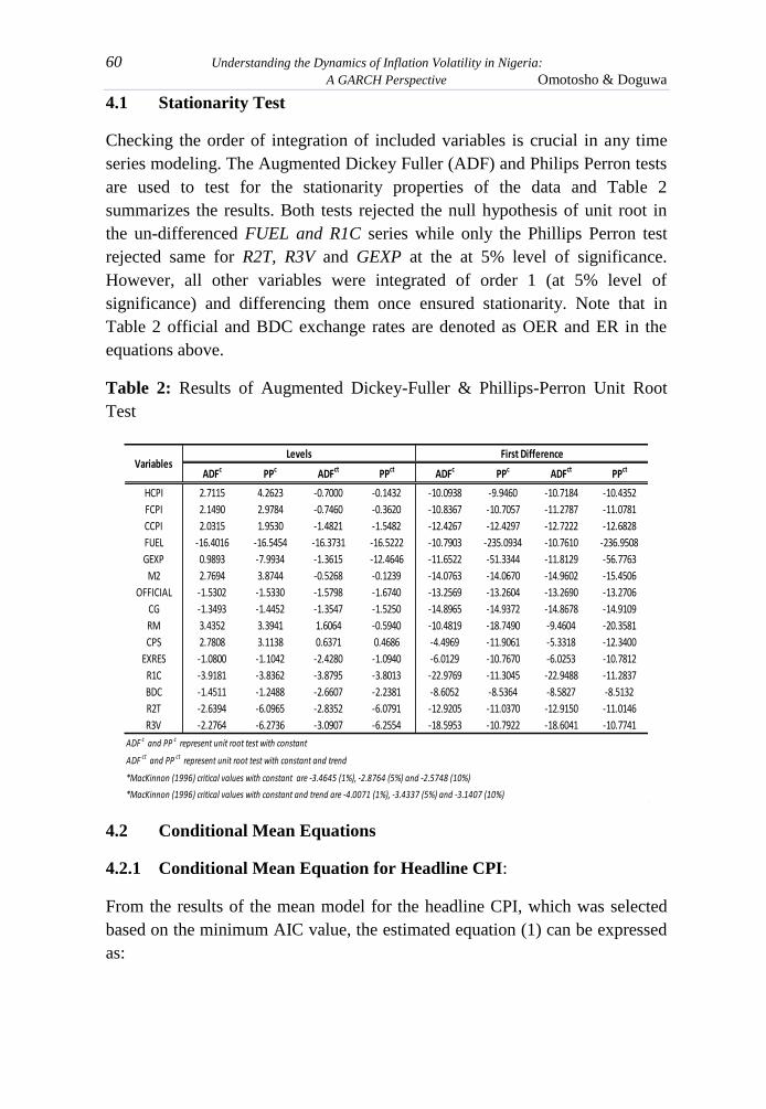
4.1 Stationarity Test

Checking the order of integration of included variables is crucial in any time

series modeling. The Augmented Dickey Fuller (ADF) and Philips Perron tests

are used to test for the stationarity properties of the data and Table 2

summarizes the results. Both tests rejected the null hypothesis of unit root in

the un-differenced FUEL and R1C series while only the Phillips Perron test

rejected same for R2T, R3V and GEXP at the at 5% level of significance.

However, all other variables were integrated of order 1 (at 5% level of

significance) and differencing them once ensured stationarity. Note that in

Table 2 official and BDC exchange rates are denoted as OER and ER in the

equations above.

Table 2: Results of Augmented Dickey-Fuller & Phillips-Perron Unit Root

Test

4.2 Conditional Mean Equations

4.2.1 Conditional Mean Equation for Headline CPI:

From the results of the mean model for the headline CPI, which was selected

based on the minimum AIC value, the estimated equation (1) can be expressed

as:

ADFc PPc ADFct PPct ADFc PPc ADFct PPct

HCPI 2.7115 4.2623 -0.7000 -0.1432 -10.0938 -9.9460 -10.7184 -10.4352

FCPI 2.1490 2.9784 -0.7460 -0.3620 -10.8367 -10.7057 -11.2787 -11.0781

CCPI 2.0315 1.9530 -1.4821 -1.5482 -12.4267 -12.4297 -12.7222 -12.6828

FUEL -16.4016 -16.5454 -16.3731 -16.5222 -10.7903 -235.0934 -10.7610 -236.9508

GEXP 0.9893 -7.9934 -1.3615 -12.4646 -11.6522 -51.3344 -11.8129 -56.7763

M2 2.7694 3.8744 -0.5268 -0.1239 -14.0763 -14.0670 -14.9602 -15.4506

OFFICIAL -1.5302 -1.5330 -1.5798 -1.6740 -13.2569 -13.2604 -13.2690 -13.2706

CG -1.3493 -1.4452 -1.3547 -1.5250 -14.8965 -14.9372 -14.8678 -14.9109

RM 3.4352 3.3941 1.6064 -0.5940 -10.4819 -18.7490 -9.4604 -20.3581

CPS 2.7808 3.1138 0.6371 0.4686 -4.4969 -11.9061 -5.3318 -12.3400

EXRES -1.0800 -1.1042 -2.4280 -1.0940 -6.0129 -10.7670 -6.0253 -10.7812

R1C -3.9181 -3.8362 -3.8795 -3.8013 -22.9769 -11.3045 -22.9488 -11.2837

BDC -1.4511 -1.2488 -2.6607 -2.2381 -8.6052 -8.5364 -8.5827 -8.5132

R2T -2.6394 -6.0965 -2.8352 -6.0791 -12.9205 -11.0370 -12.9150 -11.0146

R3V -2.2764 -6.2736 -3.0907 -6.2554 -18.5953 -10.7922 -18.6041 -10.7741

ADF c and PP c represent unit root test with constant

ADF ct and PP ct represent unit root test with constant and trend

*MacKinnon (1996) critical values with constant are -3.4645 (1%), -2.8764 (5%) and -2.5748 (10%)

*MacKinnon (1996) critical values with constant and trend are -4.0071 (1%), -3.4337 (5%) and -3.1407 (10%)

VariablesLevels First Difference


All the coefficients are statistically significant at the 1 per cent level. Equation

(9) is well fitted and suggests that the monthly increase in headline CPI at time

t is influenced by the monthly increases of food CPI and core CPI at the same

period, a depreciation of the parallel market exchange rate at the same period, a

depreciation of official exchange rate a year ago and increased money supply

five months earlier.

4.2.2 Conditional Mean Equation for Food CPI

From the results of the mean model for the food CPI, which was based on the

minimum AIC value, the estimated equation (2) can be expressed as:

All the coefficients are statistically significant at the 5 per cent level. Equation

(10) is well fitted and suggests that monthly increase in food CPI in period t is

largely explained by the expansion of reserve money in period t, increased

credit to government in period t and government expenditure in period t-1.

Also, increased gross external reserves in period t-2, and increased broad

money supply in period t-9. Surprisingly, appreciation of both the official

exchange rate and the parallel market exchange rate in periods t-12 and t-14

increase the food CPI in period t.

4.2.3 Conditional Mean Equation for Core CPI

From the results of the mean model for the core CPI, which was selected based

on the minimum AIC value, the estimated equation (3) can be expressed as:

All the coefficients except the constant are significant at the 5 per cent level.

Equation (11) is well fitted and suggests that an increase in core CPI in period t

is determined by the price of petroleum motor spirit in period t, increase in



broad money supply in period t, appreciation in parallel market exchange rate

in period t-4 and a decline in the food index in period . It is also affected

by rainfall data and some of the autoregressive and moving average terms.

Table 3: Breusch-Godfrey Serial Correlation LM Test on the Residuals of the

Mean Models

The Breusch-Godfrey Lagrange Multiplier test for Serial Correlation was used

to test for reliability of the estimated mean models in equations (9), (10) and

(11). The test presented in Table 6 failed to reject the null hypothesis of no

serial correlation in the residuals of the models. With the absence of serial

correlation in the residuals, these estimated models could be used to forecast

the CPI series.

4.3 Estimating the Volatility Models

The squared residuals in equations (9), (10) and (11) are tested for ARCH

effect. The null hypothesis of homoscedasticity in the squared residuals of

headline, food and core CPIs mean models was rejected at the 5 per cent level,

implying the presence of ARCH effect. The result of the ARCH LM test

presented in Table 4 leads to the conclusion that the headline, food and core

models of equations (9), (10) and (11) possess time varying volatilities. Also,

the plots of the autocorrelation function (ACF) and partial autocorrelation

function (PACF) provided additional evidence for significant autoregressive

conditional heteroscedasticity in the squared residuals as they revealed

significant spikes at specific lags. Therefore, these mean models are

subsequently used for the estimation of their volatilities.

Table 4: ARCH LM Test for Heteroscedasticity in the Squared Residuals of

the Mean Models

F-Statistic Prob. Obs*R-squared Prob. Chi-Square

Headline Inflation 0.3054 0.7372 0.6409 0.7258

Food Inflation 0.9937 0.3725 2.1603 0.3395

Core Inflation 0.1297 0.8785 0.2810 0.8689

ModelF-Statistic Test Chi-Square Test


Headline CPI 10.8077 0.0012 10.3140 0.0013

Food CPI 3.6721 0.0275 7.1642 0.0278

Core CPI 6.0852 0.0029 11.5029 0.0032



4.3.1 Volatility Model for Headline CPI

The volatility models defined in equations (5), (6) and (7), namely the

GARCH, TGARCH and EGARCH were estimated for the headline CPI.

However, the model selection criterion indicates that the TGARCH (1,1)

recorded the minimum AIC value and represents the best volatility model for

headline CPI. The summary of the volatility models and their characteristics is

presented in Table 5.

Table 5: Summary of the Headline CPI Volatility Models and their

Characteristics

From the results of the fitted TGARCH(1,1) model for the headline CPI, which

was selected based on the minimum AIC value, the re-estimated equation (9)

can be expressed as:

Equation (12) is well fitted and the coefficients are statistically significant at

the 1 per cent level. The corresponding estimated volatility model is:

where , and 0 otherwise. Equation (13) shows that the

ARCH and GARCH terms are significant at the 5% and 10% significant level,

respectively. The persistence parameter is about 0.8361, which is much less

than unity. This suffices for covariance stationarity and also indicates that

impacts of shocks on headline volatility do die away rather quickly. The news

impact is asymmetric and there is no leverage effect. Also, the asymmetric

GARCH TGARCH EGARCH

ω (Constant) 0.0267a 0.0310a -1.8199a

α (ARCH) 0.2549a

0.4518a

0.8411a

β (GARCH) 0.4110a 0.3843c 0.5570a

γ (Asymmetry) - -0.4293a 0.0683ns

Impact of +ve Shocks - 0.4518 0.9094

Impact of -ve Shocks - 0.0225 0.7728

Persistence (α + β) 0.6659 0.8361 1.3981

AIC 0.3800 0.3705* 0.4031

P values are in Italics

a = Significant at 5% level, c = Significant at 10% level, ns = Not significant



term is negative (-0.4293) and significantly different from zero. This indicates

that positive inflation shocks, that is, news capable of inducing higher inflation,

increases headline volatility than news capable of dampening inflation. For

instance, positive inflation shocks increases headline inflation volatility by

0.4518, while negative shocks of the same magnitude transmit smaller

volatility (0.0025).

4.3.2 Volatility Model for Food CPI

The volatility models estimated for the food CPI presented in Table 6 indicate

that GARCH (1,1) model recorded the smallest AIC value, and is therefore

more suitable for food CPI than the other two competing models.

Table 6: Summary of the Food CPI Volatility Models and their Characteristics

From the results of the fitted GARCH(1,1) model for the food CPI, which was

selected based on the minimum AIC value, the re-estimated equation (10) can

be expressed as:


the 1 per cent level, except the rainfall coefficient. The corresponding

estimated volatility model is:

(15)

GARCH TGARCH EGARCH

ω (Constant) 0.0024ns 0.0021ns -0.7339a

α (ARCH) 1.9910a

2.0906a

1.0100a

β (GARCH) 0.1819a 0.1873a 0.6878a

γ (Asymmetry) - -0.2524ns 0.0123ns

Impact of +ve Shocks - 2.0906 1.0223

Impact of -ve Shocks - 1.8382 0.9977

Persistence (α + β) 2.1729 2.2779 1.6978

AIC 3.0473* 3.0569 3.0854




The volatility model of the food CPI suggests that both positive and negative

inflation shocks confer similar effect on its volatility. However, there is

evidence of volatility persistence, implying that the impacts of shocks to food

inflation volatility die away very slowly.

4.3.3 Volatility Model for Core CPI

The volatility models estimated for core CPI and presented in Table 7 indicated

that the TGARCH (1,1) is the best model for core CPI.

Table 7: Summary of the Core CPI Volatility Models and their Characteristics

From the results of the fitted TGARCH (1,1) model for the core CPI, which

was selected based on the minimum AIC value, the re-estimated equation (11)

can be expressed as:


the 5 per cent level, except the AR (15). The corresponding estimated volatility

model is:

(17)

where . The model defined in

equation (17) confirms strong asymmetric response of core inflation volatility

to inflation shocks as the asymmetric term is highly significant and negative.

The negative coefficient of the asymmetric term connotes the absence of

leverage effect and shows that the impact of positive innovations on core

inflation volatility exceeds that of negative innovations. The ARCH and

GARCH variables are also highly significant justifying their inclusion in the

GARCH TGARCH EGARCH

ω (Constant) 0.1521ns 0.0256ns -0.3428a

α (ARCH) 0.2049a

0.1097a

0.5524a

β (GARCH) 0.7055a 0.9934a 0.7016a

γ (Asymmetry) - -0.2342a 0.1067ns

Impact of +ve Shocks 0.1097 0.6591

Impact of -ve Shocks -0.1245 0.4457

Persistence (α + β) 0.9104 1.1031 1.2540

AIC 3.2961 3.1846* 3.3030





model. As in the other inflation types, the persistence parameter for core

inflation volatility is high at 1.1031, indicating that the impact of shocks do die

away very slowly.

For correctly specified variance models, the standardized residuals should

contain no significant ARCH. The results of the ARCH LM test for ARCH in

the residuals presented in Table 8 show that there is no remaining ARCH in the

chosen variance equations and that the volatility models are adequate.

Table 8: ARCH LM Test for Remaining ARCH Effect in the Variance Models

4.4 Dynamics of Inflation Volatility

The time series plot of estimated volatilities for headline, food and core CPI

during the study period is presented in Fig. 3. It shows that food was the most

volatile of the three inflation types, followed by core CPI and headline CPI in

that order. In the case of headline CPI, the TGARCH variance estimates were

low and stable between 1997 and the first half of 1998 (Fig. 4). This was

brought about by successful measures put in place by the government against

high and unstable prices. In addition, improved harvest of staples and exchange

rate stability created an enabling environment for moderate and stable prices

during the period. However, there were major volatility spikes in headline CPI

during the third quarter of 1998 and core CPI during the fourth quarter,

coinciding with a period of domestic and external imbalances in the economy

(CBN, 1998). Sources of positive shocks to inflation during the period included

the announcement effect of an upward review of the salary structure in the

public sector, the continued scarcity of petroleum products and deteriorating

infrastructures. However, proactive monetary policy interventions and

favorable harvest of staples provided some dampening effects.

Following the volatility spikes of the second half of 1998, there was relative

calm in headline, food and core CPIs during 1999 reflecting the moderation in

inflationary pressure during the year (Fig. 3). This coincided with a period of

favorable agricultural harvest and effective harmonization of monetary and

fiscal policies. Also, interest rate policy (anchored on the Minimum Rediscount


Headline Inflation (GJR-GARCH) 0.1459 0.7030 0.1474 0.7011

Food Inflation (GARCH) 0.3230 0.5706 0.3261 0.5680

Core Inflation (GJR-GARCH) 0.0059 0.9387 0.0060 0.9382



Rate - MRR) was market based and responsive to market conditions thereby

engendering some stability in the year.

The relative stability in prices witnessed in 1999 continued in first half of

2000. However, moderate increase in volatility was experienced during the

third quarter of the year following the announcement of a hike in the price of

fuel from N20/litre to N22/litre in June 2000 and the monetization of enhanced

oil receipts. The instability in prices caused by these policy actions is reflected

moderately in the volatility of headline CPI (Fig. 4) and noticeably in core CPI

volatility (Fig. 5), while food CPI volatility remained quite low and stable (Fig.

6).

There were volatility spikes in the second quarter of 2001 in headline, food and

core CPIs. This was followed by a period of relative stability, enabled by

favorable agricultural harvest and tight fiscal and monetary policies. The

TGARCH variance estimates for headline and core CPIs remained at low and

moderate levels from the third quarter of 2001 to the beginning of 2003, with

the exception of some spikes in August 2002 following the introduction of the

RDAS in July, which saw the exchange rate depreciating from N118.49 per US

dollar to about N123.72. Also, the monetization of US$1.5 billion external

reserves in the last quarter of 2002 paved way for the inflationary pressure and

turbulence recorded in the latter part of 2003.

The headline CPI variance estimate rose sharply in October 2003 (Fig. 4).

Also, core CPI volatility reached its second highest point in August 2003 (Fig.

5) while food CPI volatility was relatively moderate (Fig. 6). The identified

spikes in headline and core CPIs closely followed the announcement of an

0.0

0.5

1.0

1.5

2.0

2.5

3.0

3.5

4.0

4.5

5.0

0

10

20

30

40

50

60

70

80

90

Co

re a

nd

He

ad

lin

e I

nfl

ati

on

Vo

lati

liti

es

Fo

od

In

fla

tio

n V

ola

tili

ty

Fig. 3: Volatility Estimates for Headline, Food and Core CPI

Food Inflation Volatility Headline Inflation Volatility Core Inflation Volatility



increase in pump price of petroleum products from N26/liter to N40/liter in

June 2003.

In 2004, headline, food and core inflation volatility decreased steadily during

the first two quarters of the year. During the year, inflationary pressure

moderated due to fiscal prudence as the government adhered to the fiscal rule

of the US$25.0/barrel oil benchmark price on which the budget was based.

Also, tight monetary policy was implemented, anchored on continuous

mopping up of excess liquidity and expansion of non-oil output.

In August 2005, however, food price volatility rose to its highest level during

the study period. This coincided with the period of increased food export from

the country and the restocking of the strategic grains reserves following food

aid to Niger and Chad. These factors mounted inflationary pressure on food

prices owing to limited supply. While core CPI volatility remained at high

levels during the year, headline CPI volatility was low.

The volatility of headline and food CPIs remained at low levels in 2006. This

was due to a number of factors, which included good harvests for most

agricultural commodities, the appreciation and relative stability of the naira

exchange rate and the implementation of sound monetary and fiscal policies.

However, core CPI witnessed a sharp increase in its volatility in June 2006, the

highest it ever got during the study period. In order to further maintain price

and overall economic stability, a new monetary policy implementation

framework (Monetary Policy Rate) was thus introduced in December 2006.

In 2007, there was less volatility in both headline, food and core inflation series

as inflationary pressures were effectively contained due to sound monetary and

0

0.1

0.2

0.3

0.4

0.5

0.6

0.7

0.8

0.9

1

Head

line

Infla

tion

Vola

tility

Fig 4: Volatility Estimate of Headline CPI

95th Percentile Volatility Threshold


fiscal policies, good agricultural harvest, stability in the prices and supply of

petroleum products, as well as the relative stability in the naira exchange rate.

The variance estimates for core inflation volatility declined steadily during the

year probably due to the continued use of MPR as an anchor interest rate for

moderating volatility in the interbank rates and improving monetary policy

actions (Fig. 5). During the year, the MPR was reviewed appropriately to

reflect monetary conditions. For instance, the MPR was reviewed downwards

by 200 basis points in June, upwards by 100 basis points in October and

upwards by 50 basis points in December, 2007.

The regime of low volatility of headline, food and core inflation continued in

2008, except for a spike recorded by food CPI in April reflecting the effect of

the global food crisis that peaked in 2008 (Fig. 6). In response to the crisis, 64,

984.76 tonnes of grains were released from the strategic grains reserves to

mitigate the effects of the food crisis during the year (CBN, 2008). Also, the

0

0.5

1

1.5

2

2.5

3

3.5

4

4.5

Core

Infla

tion

Vola

tility

Fig 5: Volatility Estimate of Core CPI


0

10

20

30

40

50

60

70

80

Food

Infla

tion

Vola

tility

Fig 6: Volatility Estimate for Food CPI




MPR was reviewed upwards by 50 basis points and 25 basis points in April

and June and downwards by 50 basis points in September as a proactive and

quick response to the contagion effect of the 2008 global financial crisis.

The impact of the 2008 crisis and other inflationary shocks were mitigated in

2009 through the proactive use of sound monetary and fiscal policies. Thus,

headline, food and core inflation volatilities remained at low levels during the

year (Fig. 3). However, moderate increase in volatility was recorded in the

third quarter following some inflationary shocks, such as a surge in the prices

of staples and the increase in price of petroleum products from N40/liter to

N70/liter, which was later reduced back to N65/liter in June of the same year.

In 2010, the volatility of headline, food and core inflation remained at

relatively low levels. During this period, inflationary pressures moderated due

to increased agricultural production, relative stability in the supply and prices

of petroleum products and very proactive and effective monetary policy

decisions. Thus, there was relative calm in the first half of 2010. However,

there was an increase in the volatility of food CPI in July, a period associated

with increased demand for food by agro-processors, industrial users and

neighboring countries (CBN, 2010). Headline CPI volatility got to its peak

during the first quarter of 2011 reflecting inflationary pressures and

instabilities preceding the April 2011 presidential elections. Food inflation also

reached its peak for the year during the first quarter.

5.0 Summary and Conclusion

The study modeled inflation volatility in Nigeria’s headline, food and core CPI

series in order to understand the dynamics of inflation volatility between 1996

and 2011, using monthly data sourced from the National Bureau of Statistics

(NBS) and the Central Bank of Nigeria (CBN). Most of the similar attempts

made by different authors in the recent past employed the symmetric GARCH

model using low frequency data. This paper however accommodates

asymmetric considerations in its modeling approach, using recent and high

frequency data set. Having modeled the conditional mean of the headline, food

and core CPI individually as an ARIMAX process, the obtained residuals were

tested for serial correlation and ARCH effects.

While no evidence of serial correlation was found, the squared residuals of the

conditional mean models showed significant Autoregressive Conditional

Heteroscedastic (ARCH) effect. For series with significant ARCH effects, the

three inflation types were modeled as zero-mean, serially uncorrelated process


with non-constant variances conditional upon the past. In this regard, a

symmetric GARCH model and two asymmetric GARCH models were fitted to

each of the three inflation types with a view to coming up with the best model

for obtaining reliable estimates of their conditional variances. Based on AIC

model selection procedure, the TGARCH (1,1) model was found appropriate

for headline and core CPI, while the symmetric GARCH was selected for food

CPI.

The variance models confirmed the presence of volatility persistence in

headline, food and core CPI, implying that while the effect of inflation shocks

on headline do die away rapidly, the effects on food and core do die away

rather slowly. However, a higher persistence parameter was recorded for food

CPI (2.2) compared with core CPI (1.1) and headline CPI (0.8). Also, the

asymmetric term for the headline and core CPI variance models were

significant, confirming the asymmetric response of their volatilities to inflation

shocks. However, no evidence of leverage effect was found for the two series

as their conditional volatility are more responsive to positive shocks than

negative innovations. In the case of food CPI, the asymmetric term was

insignificant and the symmetric GARCH was found appropriate. Thus, positive

and negative inflation shocks confer similar effects on food CPI volatility.

Based on the 95th

percentile point of the variance estimates during the study

period, episodes of high inflation volatilities in headline, food and core

inflation were identified. Thus, three major periods of high volatility of

headline CPI were identified and these are August 1998, October 2003 and

February 2011 (Fig. 4). In the case of food inflation volatility, six episodes

were identified during the periods May 2001, November 2002, August-

November 2005, November 2007, April 2008 and June-August 2010 (Fig. 6).

August-November 2005 represented the peak of food inflation volatility and

this coincided with the period of the global food crisis. Lastly, three episodes

of high core inflation volatility were found corresponding to the periods July-

August 2003, October 2003 - March 2004 and May-June, 2006 (Fig. 5). Of the

three inflation types, food inflation was found most volatile followed by core

and headline inflation, respectively.

Economic developments surrounding the periods of high inflation volatility

were discussed in the paper. However, major positive inflationary shocks

during the study period include, among others, announcement of fuel price

hikes, announcement of an upward review in the wages of public sector

workers, food crisis and exchange rate instability. An analysis of the volatility



dynamics of the series in a time series perspective showed that periods of high

inflation volatility were associated with periods of specific government policy

changes, shocks to food prices and lack of coordination between monetary and

fiscal policies. The study therefore recommends the strengthening of the

current market-based interest rate regime, strategic intervention for improved

agricultural productivity and effective harmonization of monetary and fiscal

policies as a way of maintaining price stability in the country.

References

Adamgbe, E.T. (2003). Price Volatility, Expectations and Monetary Policy in

Nigeria. Paper presented at the 33rd

Australian Conference of

Economists, 2004.

Baillie, R.T.; Chung, C.F. and Tieslau, M. (1996). Analyzing Inflation by the

Fractionally Integrated ARFIMA-GARCH Model. Journal of Applied

Econometrics 11: 23-40.

Bollerslev, T. (1986). Generalized Autoregressive Conditional

Heteroscedasticity. Journal of Econometrics, 31: 307-326.

Brooks, C. (1996). Testing for Non-Linearity in Daily Sterling Exchange

Rates. Applied Financial Economics, 6: 307–17.

Brooks, C. (2008). Introductory Econometrics for Finance. Cambridge

University Press, United Kingdom.

Brunner, A. and Hess, G. (1993). Are Higher Levels of Inflation Less

Predictable? A State-dependent Conditional Heteroscedasticity

Approach. Journal of Business and Economic Statistics, 11: 197-197.

Byrne, J.P. and Davies, E.P. (2004). Permanent and Transitory Inflation

Uncertainty and Investment in the US. Economic Letters, 271-277.

Caporale, G.M., Onorante, L. and Paesani, P. (2010). Inflation and Inflation

Uncertainty in the Euro Area. European Central Bank Working Paper

Series, No. 1229.

Ding, Z., Granger, C.W.J. and Engle, R.F. (1993). A Long Memory Property of

Stock Market Returns and a New Model. Journal of Empirical Finance,

1:83-106.


Elder, J. (2004). Another Perspective on the Effects of Inflation Uncertainty.

Journal of Money, Credit and Banking, 911-928.

Elder, J. (2005). Some Empirical Evidence on the Real Effects of Nominal

Volatility. Journal of Economics and Finance

Engle, R. (1982). Autoregressive Conditional Heteroscedasticity with estimates

of the variance of United Kingdom Inflation. Econometrica, 50 (1):987-

1007

Eviews 7 (2009). User‘s Guide. Quantitative Micro Software, LLC. 4521

Campus Drive, No. 336, Irvine CA, USA. ISBN: 978-1-880411-40-7

Friedman, M. (1977). Nobel Lecture: Inflation and Unemployment. Journal of

political Economy, University of Chicago Press, 85(3): 451-72

Glosten, L.R., Jaganathan, R. and Runkle, D.E. (1993). On the Relation

between the Expected Value and the Volatility of the Nominal Excess

Returns on Stocks. Journal of Finance, 48: 1779- 1801

Grier, K. and Perry M. (1998). On Inflation and Inflation Uncertainty in the G7

Countries. Journal of International Money and Finance, 17: 671–689.

Hentschel, L. (1995). All in the Family: Nesting Symmetric and Asymmetric

GARCH Models. Journal of Financial Economics, 39: 71–104.

Idowu, K.O. And Hassan, Y. (2010). Inflation Volatility and Economic Growth

in Nigeria: A Preliminary Investigation. Journal of Economic Theory,

4(2): 44-49.

Judson, R. and Orphanides, A. (1999). Inflation Volatility and Growth. Journal

of International Finance, 117-138.

Kontonikas, A. (2004). Inflation and inflation uncertainty in the United

Kingdom: Evidence from GARCH modelling. Journal of Economic

Modelling, 21:525-543.

Natalia, S. (2010). Integrated Variance Forecasting: Model-Based vs. Reduced

Form.

Nelson, D.B. (1991). Conditional Heteroscedasticity in Asset Returns: A New

Approach. Econometrica 59: 347-370.



Pagan, A.R. (1996). The Econometrics of Financial Markets. Journal of

Empirical Finance, 3:15–102.

Pourgerami, A. and Maskus, K. (1987). The Effects of Inflation on the

Predictability of Price Changes in Latin America: Some Estimates and

Policy Implications. Journal of International Development, 15(2):287–

290.

Rother, P.C. (2004). Fiscal Policy and Inflation Volatility. European Central

Bank Working Paper Series, 317.

Samimi, A.J. and Shahryar, B. (2009). Inflation Uncertainty and Economic

Growth in Iran. Australian Journal of Basic and Applied Sciences,

3(3):2919-2925.

Udoh, E. and Egwaikhide, F.O. (2008). Exchange Rate Volatility, Inflation

Uncertainty and Foreign Direct Investment in Nigeria. Botswana Journal

of Economics, 5 (7):14-31.

Ungar, M. and Zilberforb, B. (1993). Inflation and its Unpredictability: Theory

and Empirical Evidence. Journal of Money, Credit and Banking, 25:709-

720.

Xekalaki, E. and Degiannakis, S. (2010). ARCH Models for Financial

Applications. 1st Edition, Chichester: John Wiley & Sons Ltd

Understanding the Dynamics of Inflation Volatility in Nigeria: A GARCH Perspective

Documents

Transcript of Understanding the Dynamics of Inflation Volatility in Nigeria: A GARCH Perspective