Inflation and stabilization in Argentina

r • U T T E R W O R T t t [ ~ E I N E M A N N

Economic Modelling, Vol. 12, No. 4, pp. 391-413, 1995 Copyright © 1995 Elsevier Science Ltd

Printed in Great Britain. All rights reserved 0264-9993/95 $10.00 + 0.00

0264-9993(95)00027-5

Inflation and stabilization in Argentina

Baotai Wang, Erwin Klein and U L Gouranga Rao

This paper reports the results of simulation experiments which were conducted by using a CGE model of Argentina. The results suggest that: the economy could not have been stabilized by using the preannouneed devaluation rate during 1978-81; economic performance could have improved in 1985-89 under a modified Austral plan but, with the altered structure, there would still be a severe currency appreciation; and the Convertibility Law based programme is very successful in arresting inflation and eliminating a budget deficit, though it is not free from side effects such as money supply shortages and high interest rates. Keywords: CGE model; Inflation mechanism; Preannounced devaluation rate

Dur ing the per iod be tween the mid- 1970s and the early 1990s, the Argent ine economy exper ienced instability and recurrent high inflation. The average annual inflation rates for the years 1976-80, 1981-85 and 1986-90, measu red in te rms of CPI, were 211%, 382% and 1192% respectively. There were even a few instances of hyperinflat ion within this period. For example, the monthly inflation rate was 197% in July 1989 and 96% in D e c e m b e r 1990 (see Klein et al. [24]). In order to res tore stability and comba t

The authors are with the Department of Economics, Dal- housie University, Halifax, Nova Scotia, Canada B3H 3J5.

The authors are grateful to Dr Tomson Ogwang of University of Northern British Columbia for his help in writing the computer programmes for policy simulations, and to Dr A M Sinclair of Dalhousie University for his helpful comments. Any remaining errors are ours.

Final manuscript received April 1995.

high inflation, several stabilization p rog rammes were successively put in place in these two decades but the success was limited; and even that l imited success did not last for long. 1

In this study, a short- run computab le general equil ibrium ( C G E ) mode l is constructed to describe the functioning of the Argent ine economy, with focus on the inflationary process. In addition, the es t imated structure is used to simulate the impacts of al ternative stabilization policies under some postulated structural changes. T o this end, an effort is

1The major stabilization programmes adopted during these two decades include the programme of expectations management (1976-81), the Austral plan (1985-87), the Primavera plan (1988), the BB plan (1989) and finally the Convertibility Law based stabilization programme which started in 1991 and is still in effect. For details of these stabilization programmes and their acutai effects, see, for example, Fernandez [15], Dornbusch and Fisher [13], Canavese and Di Tella [6], Canavese [5] and Wang [42].

391

Inflation and stabilization in Argentina: B Wang et al.

made to found the model on theoretical grounds while capturing the essential traits of the Argentine economy.

The model developed in this study is based on the contribution of Klein et al [24]. In specifying the model, special attention is given to the interrelation- ships between important macroeconomic variables, especially to the interaction between the general price level and the exchange rate, which is viewed as one of the key relationships responsible for inflation and instability. An important limitation of the model consists in not taking explicitly into account the relationship between inflation and/or stabilization policies on the one hand, and capital accumulation and growth on the other. Hence, issues related to long-run economic stabilization and policies are not discussed in here. 2

In the next section, we discuss the theoretical underpinnings of some equations of the model. The complete CGE model and its estimated numerical structure are presented in the appendix. In the third section, we discuss the inflationary mechanisms embodied in the model. Two types of inflation mechanisms are identified and described, namely, the non-accelerating mechanism, which transmits exogenous shocks into inflation, and the accelerating mechanism, which sustains and magnifies (or dam- pens in some cases) the inflationary pressure. The results of model validation are then presented and discussed. In the fifth section, the results of policy simulation experiments are reported and discussed. Finally, some concluding remarks are given.

The model

In specifying the CGE model, the Argentine economy is viewed as a small open economy with its own special characteristics. The model consists of six sectors; the supply sector, expenditure, the external sector, the fiscal sector, financial sector and prices, wages and expectations. In the following discussions, real variables are denoted by a string of lower case letters, while the corresponding string of upper case letters denotes the same variable in nominal terms. Asterisked variables represent foreign variables which are all exogenous. Variables which are sub- scripted by t-1 denote one-period lagged values of the corresponding variables.

2Since data on net investment or capital depreciation are not available, we could not extend the model to simulate the long-run effects of various stabilization policies.

Supply sector

In modelling the supply sector, all goods and services produced in Argentina are aggregated into two categories: tradables and non-tradables. The produc- tive resources include capital, labour and imported inputs which, in the Argentine case, constitute an important component of production costs.

Producers in the tradables sector are assumed to operate in a flex-price market. Accordingly, the domestic price of tradables is formed by converting the foreign price using the exchange rate plus taxes. The supply function of tradables is derived from profit maximization based on price-taking behaviour and Cobb-Douglas technology. The latter is described by a short-run variable cost function:

oct = a12YtSa~wra'pza'nkta15(1 + a16ir) (1)

where oct, yts, wr pz, kt and ir denote respectively short-run costs, supply of tradables, real wage rate, domestic relative price of imported inputs, fixed capital stock in real value in the tradables sector and real interest rate.

The parameter a16 , where 0 < a16 < 1, measures the proportion of total working capital that is financed by borrowing and is subject to the real interest rate, which can be viewed as a weighted average of free and regulated interest rates in some periods. The borrowing cost of working capital is incorporated in the cost function in order to account for the state of development of the capital market and financial intermediation in Argentina and their consequences for financing production.

The parameter all measures returns to scale. For values of all > 1, 0 < all < 1 and all = 1, the technology exhibits decreasing returns to scale, increasing returns to scale and constant returns to scale respectively. In short-run analysis, decreasing returns to scale are more realistic, hence all should be greater than one. The parameter al2 is a shift parameter and should be positive. In general, this variable cost function is consistent with theory if and only if a l l >_ 0, a13 _> 0, a14 >_ 0, a13 + a14 = 1, and a~s _< 0. These conditions guarantee that the variable cost function is non-decreasing in prices of variable factors, non-increasing in fixed capital stock, non-decreasing in output and homogeneous of degree one in variable factor prices) Detailed discussions regarding variable cost functions can be found in Lau [25], McFadden [29], Brown and Christensen [2] and Hazilla and Kopp [19].

Given this variable cost function, the supply function of tradables can be directly derived from profit maximization, and the demand function for im-

392 Economic Modelling 1995 Volume 12 Number 4

ported inputs of the tradables sector can be derived by using Shephard's lemma--see Equations (A1) and (A2) in the appendix.

Producers in the non-tradables sector are assumed to operate in a fix-price market where direct external competition is absent and oligopolistic ele- ments are present. Hence, the supply of non-tradables is assumed to adjust to changes in the excess demand for non-tradables, i.e.,

ynst = ynst- l( yndt - l / yns t - 1 ) a2, (2)

where yns and ynd denote supply of and demand for non-tradables respectively. Clearly, modelling yns in this manner conforms to a Leontief production technology and an average cost pricing rule, i.e. mark-up rule. The following average cost ( V C N ) equation of non-tradables serves as the base for the mark up process:

V C N = (1 + a a l l R ) ( W R • L / y n s

+ P Z • z n d / y n s + K N / y n s ) (3)

where IR, WR, PZ, L and KN denote respectively the nominal interest rate, the nominal wage rate, the domestic price level of imported inputs, units of labour employment and the capital stock in the non-tradables sector. As in Equation (1), the borrowing cost is also involved in the non-tradables sector. Moreover, since there is no factor substitution in Leontief technology, the demand for imported inputs in the non-tradables sector is assumed to be proportional to output.

Finally, with the supply of tradables yts and the supply of non-tradables yns, the aggregate supply yys in the Argentine economy is given by the following accounting identity:

yys = p t • yts + pn • yns (4)

where pt and pn denote domestic relative prices of tradables and non-tradables respectively.

3A variable cost function can be written as: VC = VC(Pi, Qj, Y ) where Pi are variable factor prices, Q~ are the fixed factor stocks and Y is output. For the properties of the variable cost function: non-decreasing in P~, non-increasing in Qj, non-decreasing in Y, homogeneous of degree of one in Pi, variable factor symmetry, fixed factor symmetry, concave in Pi, and convex in Qj, it is required that OVC/c~P, >_ O, 3VC/~Q: <_ O, c~VC/OY >_ O, ~ . i ( ~ V C / O P i ) P i = VC, e) 2VC/cTPidPj ~ c) 2VC/OPjOPi ,

2 2 0 vC/aQiOQj = o vC/OQ,dQi , the matrix of second-order partial derivatwes of VC witl~ respect to P ' s be negative semidefinite and the matrix of second-order partial derivatives of VC with respect to Q's be positive semidefinite. These properties are satisfied in our variable cost function if a u > 0, al3 ~ 0, al4 > 0, a~5 _< 0 and a~3 + a~4 = 1.


Expenditures

Domestic private consumption and government consumption include tradables, non-tradables and imported goods and services. It is assumed that government also behaves in the same manner as its private counterpart does in allocating its expenditures among the various goods and services. However, the government does not have to balance its budget within a period due to its ability to print money or to borrow from domestic residents. Borrowing from foreign countries to finance the government deficit will not be considered in specifying the model since external credit disappeared at the beginning of the 1980s.

The modelling of demand behaviour in Argentina consists of two steps. We first explain determination of total private expenditure and aggregate expenditure, and then we explain how aggregate expenditure is allocated between tradables and non-tradables.

The level of total real private expenditure is a function of disposable income, real money balances held by the residents, and real domestic interest rate. The inclusion of the real interest rate is consistent with standard consumption and investment the- ories and also reflects its importance in the in- tertemporal allocation of expenditures. Accordingly, the real private expenditure function is specified as

y p d = ydb31md b32 e x p ( b33ir ) (5)

where ypd, yd and m d denote respectively the levels of real private expenditure, real disposable income, real money balances held by residents.

The definition of disposable income follows the practice standard in macroeconomic literature with, perhaps, the exception of the term [r//(1 + r i )](Ms/P) , which represents the inflation tax in real terms, where r/ stands for the inflation rate while Ms and P are the nominal money supply and the general price level respectively. 4 Accordingly, disposable income is defined as follows:

yd = yys - ( ta + ty + tz + tx ) + J r . bs t_

+ trs - [r/f(1 + r i ) ] ( M s / e ) (6)

4In general, ri(Ms/P) is considered as an approximate inflation tax on money creation - see, for example, Turnovsky [41]. This approximation, however, may not be appropriate in the case of Argentina with hyperinflation in the late 1980s because it implies that the real inflation tax will exceed the real money stock if the inflation rate is over 100%. Accordingly (n'/(1 + ri))(Ms/P) is used to account for the inflation tax.

Economic Modelling 1995 Volume 12 Number 4 393


where ta, ty, tz, tx, bs and trs denote respectively, real autonomous taxes, real output dependent taxes, real import taxes, real export taxes, real government bonds held by residents, and real government transfer payments to the private sector. Aggregate expenditure yyd is the sum of ypd and the real government expenditure ged, i.e. yyd = ypd + ged. Given yyd, a system of aggregate demand equations is required to model the corresponding allocation mechanism. This is achieved by specifying a system of two demand share equations along the lines suggested by Christensen et al. [7] and particularly by Jorgenson and Lau [22], Conrad and Jorgenson [8] and Lau [26].

The indirect translog system of Christensen et al. [7] satisfies all the theoretical properties of the inte- grable demand functions of the theory of individual consumer behaviour. However, as is documented in the literature - - see Sonnenschein [37, 38], Debreu [9], Mas-Colell [28] and Sharer and Sonnenschein [36] - - there are no compelling reasons why market demand functions such as those used in this study should satisfy the properties of individual demand functions other than homogeneity and summability. Hence, the motivation for choosing a well-known 'demand system' as a description of the allocation of aggregate expenditure within this model should be understood in the spirit of Conrad and Jorgenson's [8] suggestions regarding the possible methodological advantages of 'applying micro-theory to derive restrictions on the system of aggregate demand functions', rather than as an 'attempt to approximate the demand of a "representative consumer", which exists only under the very restrictive assumptions that are necessary for the integrability of aggregate demand functions' - - see Theil ([40], p 178). Of course, readers are free to assume the existence of such a 'representative consumer' or of some 'community utility functions'. Equations (7) and (8) below describe the allocation mechanism for aggregate expenditure yyd:

(pt/yyd)-l[ba + bll log(pt/yyd) + b12 log(pn/yyd)]

ytd = - 1 + (bll + b21) log(pt/yyd) (7)

+ (b12 + b22) log(pn/yyd)

(pn/yyd)-l[b2 + b21 log(pt/yyd) + b22 log(pn/yyd)]

ynd = (8) - 1 + (bll + b21) log(pt/yyd)

+ (b12 + b22) log(pn/yyd)

where ytd and ynd denote the demand for tradables and demand for non-tradables respectively. Clearly,

demand functions in this system satisfy the properties of summability, symmetry and homogeneity if b~ + b 2 = - 1 , b12 = b21 , and bl~ + b12 + b21 + b22 = 0 .

External sector

The external sector consists of equations of the balance of payments account, the risk premium and the nominal exchange rate.

Consider that the tradables are composed of both exportables and importables and the difference between supply of and demand for exportables can be viewed as approximately equal to exports, while the difference between demand for and supply of importables can be treated as approximately equal to imports. Net exports (i.e. the balance of trade) in this model are defined as the difference between supply of tradables, yts, and demand for tradables, ytd. Total imports are considered as the sum of the demand for imported inputs of both tradables and non-tradables sectors plus other imports which account for imported consumption goods and services. Given net exports and total imports, total exports can be derived.

In Argentina, the capital movements were subject to different policies in the 1970s and 1980s. In some periods, capital movements were almost totally liber- alized, while in other periods severe restrictions were imposed. Thus, the capital account recorded only those capital flows which were observed and reported by the government. There were no records for those induced but unreported capital flows. Un- der these circumstances, the capital account is modelled in a slightly different way from its treatment in standard macroeconomics. First, the reported capital flows are linearly determined by the interest rate differential adjusted by taking into account the risk premium rp and the expected devaluation rate 7r e. This is because in an unstable and highly inflationary economy both rp and 77" e play important roles in determining capital flows. Second, the unreported capital flows are assumed to be totally induced by the adjusted interest rate differential and to move in the same direction as the reported capital flows do. Finally, the total capital flows equal the sum of the reported and unreported capital flows.

The risk premium, an unobserved variable, is assumed to be proportional to the ratio of total foreign debt to the aggregate supply of output. The rational for this is as follows: foreign investors will consider this ratio when they make decisions to invest in Argentina. The larger the ratio, the weaker the ability of the Argentine economy to repay the debt


plus interest, and hence the higher will be the risk in investing in Argentina. This translates into the following equation for the risk premium:

rp = c31(ER • D E ) / ( P • yys) (9)

where E R and D E denote the nominal exchange rate and the total nominal foreign debt in terms of foreign currency respectively.

The nominal exchange rate is defined as the number of units of domestic currency per unit of foreign currency. Thus a rise in the exchange rate represents a devaluation of domestic currency. A large number of articles and books were published regarding the exchange rate determination and its dynamics. See, for instance, Bruno [3,4], Dornbusch [10-12], Frankel [16], Frankel and Mussa [17, 18], Lucas [27], Mussa [30,31], Obstfeld and Stockman [32], Ro- driguez [35] and many others. For Argentina, which experienced high inflation for more than half a century, prices play a paramount role in exchange rate determination. However, it is still difficult to model the institutional set-up of the exchange rate-price relationship for the Argentine economy during 1975-91 because Argentina experimented with all imaginable exchange rate regimes during this period - - single, double, fixed, floating etc rates. The exchange rate-price relationship specified in Equation (10) is chosen because of its strong empirical support, and in addition, it is consistent with the naive but realistic assumption, that in a highly inflationary environment the exchange rate and the inflation rate cannot diverge fundamentally, even in the short run. Hence the equation for exchange rate determination is specified as

E R r ~ E R r _ ~ = ( P t / P t 1 )c41 (10)

Fiscal sector

In addition to autonomous taxes, ta, the model also includes three other endogenously determined taxes, namely output dependent taxes, ty, import taxes tz,

and export taxes ix. The associated tax rates together with government expenditure serve as fiscal policy instruments in this model.

The real government deficit d f is defined as the difference between government real expenditure including real servicing of both domestic and foreign debts and real tax revenues adjusted for the Oliv- era-Tanzi effect, which is linearly approximated by dHr/, where r/represents the inflation rate. 5

d f = ged + ( i r t _ l b S t _ l ) + ( I R * I D E t _ I E R ) / P

- ( ta + ty + tz + tx) + dNri (11)


where IR* is the foreign nominal interest rate. This budget deficit is financed by seigniorage (i.e. print- ing money by the central bank) and/or by borrowing from residents (i.e. issuing government bonds).

Financial sector

Two interrelated asset markets constitute the financial sector. They are the money market and the bond market. 6

The nominal money supply is equal to the stock of money in the last period plus its change, A M s t, in the current period. That is, Mst = M s t_ 1 + AMs t"

The change in money supply, AMst , depends on the size of the money multiplier a and the change in the monetary base A M B t. Formally, we have diMs t =

o t A M B t. Further, A M B t is determined partially by the need for financing the budget deficit and partially by the change in the foreign reserves (i.e. the balance of payments). Thus, we have dXMB t = B P t +

/31M~ +/32(df~Pt), where BPt is the nominal balance of payments in domestic currency, M t is a monetary aggregate representing an "active' monetary policy component, and (df~P t) is the nominal deficit. Clearly, both 131 and /32 are positive while /32 measures the proportion of the budget deficit that is financed by money creation. We can write d i M s t =

M s t - Mst_ 1 = o~AMB t = ol[BP t + f l lMt +/32(df tPt)]

or M s t = M s t _ 1 + a b e t + a / 3 1 M t + o t / 3 2 ( d f t P t ) .

Since data on M t are not available, we assume that

5The Olivera-Tanzi effect refers to the effect of high inflation and fiscal lags on tax collection. High inflation, combined with lags in tax collection, imply that the real value of government tax receipts will be lower the higher the inflation rate. For example, if income taxes were to be paid one year later and the annual inflation rate were 100% in the year, then the government would find itself with half of the real value of taxes it would receive without inflation and fiscal lags. For detailed analysis, see Olivera [33] and Tanzi [39]. There is another market in the financial sector, namely, the

foreign assets market. Demand for foreign asset in real terms, fd, can be explained by the following equation which is similar to Equations (13) and (15):

fd = wwt~l I • yys e62 • exp[ e63( ir + r/")

+ e ~ ( I R * - trf)]

where ( IR* - trf) denotes the net foreign interest rate, and trf is the tax rate on income earned from holding foreign assets. However, as noted earlier, residents purchasing and holding foreign assets (including foreign currency) in Argentina were severely restricted for most periods during the 1970s and 1980s. Hence, for such periods in which purchasing and holding foreign assets were not allowed, this equation is not applicable. In addition, data on fd are unavailable. For these reasons, the equation of foreign assets market is eliminated from the model with the conviction that this equation would only play a minor role, if at all, in the determination of the overall behaviour of the model. It is assumed that only money and government bonds form the residents' financial asset portfolios.



a[31Mt + Ms t_ 1 is approximately equal t o e l l M S t _ 1

whereas a l 3 z ( d f t P t) = e l 3 ( d f t e t ) . O n this basis, we have

M s = e l l M s t _ 1 + e l e B P + e13(d f • P ) (12)

Demand for money in real terms is a function of real wealth ww, real income yys, and the nominal interest rate ( ir + rie), i.e.

m d = w w e21 vYs e22 exp[e23( ir + rie)] t - 1.ry (13)

where m d and rie denote demand for real money balances and the expected inflation rate respectively. In Equation (13) the variables ww and yys account for the transaction demand for money, whereas the other variables explain the opportunity cost of holding money and account for the possibility of substitution between financial assets.

In the bond market, nominal supply of government bonds, Bs, is equal to supply of bonds in the last period plus net change in the current period, i.e. n s t = ns t 1 "j- A nS t" T h e net change in Bs is determined partially by the need for financing the deficit and partially by the need for open market operations. Assuming that the quantity of bonds used in open market operations is proportional to Bs t -1 , we specify the equation for the supply of government bonds as:

Bs = e 3 1 n s t _ l + e32(d f • P ) (14)

where the parameter e32 is related to e13 in Equa- tion (12). Since the budget deficit is financed by both money creation and bonds, we have e32 = 1 - e l 3 / o t ,

where ~ (= e12) is the money multiplier. The demand for government bonds in real terms,

bd, is a function of the same variables as those in the demand for money equation. This implies inter- dependence between these two financial markets,

bd = w w t 4 _ l l y y s e 4 2 exp[e43( ir + rie)] (15)

These two financial assets, together with the capital stock, form the total wealth ww. The equilibrium condition, i.e. the quantity supplied equals the quantity demanded, is assumed to hold in both money and bonds markets for every period.

Two equations next describe the real interest rate ir and the adjustment process of the nominal interest rate IR . Following Klein et al [24] the relation between the real interest rate, the nominal interest rate and the inflation rate is self-explanatory. The usual approximation, ir = I R - ri where ri is the inflation rate, may not be useful in the Argentine case because of frequent occurrences of high inflation coupled with high nominal interest rates. Ac-

cordingly, the real domestic interest rate is defined as

ir = ( I R - r i) /(1 + ri) (16)

and the adjustment process of the nominal domestic interest rate is specified as

I R - I R t _ 1 = e51(IR* + 7r e + rp - I R t _ l )

+ e52( logMs - log Mst_ 1) (17)

That is, the adjustment of the nominal interest rate depends on the gap between the expected foreign nominal rate of return and the one-period lagged domestic nominal interest rate, and the change in nominal money supply. The former is consistent with the doctrine of interest rate parity and the latter explains short-run deviations of the nominal interest rate from its equilibrium value.

Prices, wages and expectat ions

Since the model contains only two types of com- modities, the general price level is explained by the following Divisia index:

P = P T / , 1 P N (1 fi~) (18)

where P T and P N are the price levels of tradables and non-tradables respectively. The law of one price is assumed to prevail in the case of tradables, where Argentina is a price taker. So the domestic tradables price is assumed to adjust instantaneously to the foreign tradables price P T * and the foreign price of imported inputs P Z * ,

P T = [ f 32 P T *

+(1 - f z l ) P Z * ] E R [ 1 + ( t r z - trx)] (19)

where trz and trx denotes the import tax rate and the export tax rate respectively. Both trx and trz are involved in Equation (19), since tradables contain both exportables and importables. In view of the assumption of the presence of oligopolistic power in the non-tradables market, the price of non-tradables is determined by the mark-up rule based on the average cost. Hence, the price of non-tradables is given by the product of the mark-up factor qf and the average cost of the non-tradables sector V C N ,

P N = q f . V C N (20)

Similar to the determination of the tradables price, the law of one price is also assumed to prevail in the case of imported goods, i.e.

P Z = P Z * E R ( 1 + trz) (21)


The relative prices of tradables, non-tradables and imported goods in this model follow the usual defini- tions.

As mentioned above, the Argentine economy was quite unstable in the last two decades, although various stabilization policies were successively implemented. For purposes of strengthening the policy effects, all government policies were highly transpar- ent to the public. Given this situation, it is reason- able to assume that the economic agents form their expectations on price levels, the inflation rate, and the devaluation rate rationally, i.e. the rational expectations hypothesis is assumed to hold.

The nominal wage is one of the components in the average variable cost VCN and also plays a crucial role in the inflationary process. Following a standard viewpoint, the nominal wage rate is speci-


fled as a function of the expected price pe and the excess aggregate demand. Thus, we have

W R = per6, exp{f62[(yy d _ yys)/yysl} (22)

We have discussed the theoretical underpinnings of some equations in this non-linear CGE model. In order to simulate the impacts of various stabilization policies, we require a numerical structure within the specified model.

This is achieved by using the ordinary least squares (OLS) method when the equation is linear or can be linearized by applying appropriate transformations, such as the logarithmic transformation. When the equation to be estimated is non-linear, the non-linear least squares (NLS) method is used. Occasion- ally, the parameters cannot be estimated for want of

[ t

1 t, , t t ~ 1 - - - - ( ~ :) - . 4 - - (vcu 1 - - - - [ Im ) - - - - - ( ,1~ ) / - ( r:t ]

- - ( : t d ]..----[yts ] 2 [y'~S ] ( )c,k

.--( : t ]... (~a ] - - . - [ :~1 ] - - - - (ylxt ]~

. - - . [ ~ ] . .

t ( c a l -

t t

I

. '-'•[

I~c ] (ged)

[~bp ] J ( DZ ) - - . . . ( rp ]

t

Figure I

Note that only major relationships among the variables are shown in this figure. Endogenous variables are identified by enclosing them in square- brackets whereas exogenous variables are identified by enclosing them in ordinary parentheses.

Major Relationships in the CGE Model.



relevant data; in such cases, we conjecture the size of the parameters based on available information. The complete CGE model and its estimated numerical structure are given in the appendix. Detailed discussions about the estimation and the procedures adopted in data construction can be found in Wang [42].

Inflation mechanisms

Although the ultimate purpose of constructing this CGE model is to explain the functioning of the whole economy, the inflation mechanisms are specifically described in the model. Some of these mechanisms, through which various shocks are translated into inflation, are called the non-accelerating mechanisms in this study. On the other hand, those mechanisms, represented by the interactions between prices and the exchange rate and between prices and wages, are termed as the accelerating mechanisms through which an initial inflationary pressure can be sustained and even magnified. Fig- ure 1 reveals the major relationships among variables from which a few salient features of the model regarding these mechanisms can be discerned.

First the monetary shock is directly transmitted into inflation through expectations and wage determination i.e.

M s ~ 7r e ~ Fie ~ p e ~ 14,rR ~ V C N ~ P N ~ P

In this way, the monetary shock, initially a demand- pull factor, also induces the cost-push effects through expectations. The pure demand-pull effects resulting from monetary shocks are implicitly modelled through the general equilibrium conditions i.e.

M s ---, y p d ~ y y d (together with yys) ~ P

Second, the fiscal shocks are directly transmitted into inflationary process through different mechanisms. For the budget deficit shock, the generated inflationary pressure passes through money creation (financing the deficit) to expectations and wage mechanisms. This transmission is similar to the effects of the monetary shock described above. For the tax shocks, the generated inflationary pressure passes through the prices of tradables and imported goods i.e.

trx and trz ~ P Z and P T ~ P

(See Equations (18) and (19).) Third, external shocks, say, changes in foreign

prices, are directly transmitted into the inflationary process through the mechanisms of the exchange

rate and tax rates on imports and exports. It is important that not only price of tradables but also the price of non-tradables are directly affected by the external shocks, although the mechanisms are different i.e.

P T * and P Z * (through E R , trz , and trx)

( P T and P Z ) ~ P

P Z * (through E R and t rz ) ~ P Z ~ V C N

~ P N ~ P

In view of the above discussion, it is clear that the price of non-tradables cannot be completely isolated from the outside economy and from the interaction between the exchange rate and prices.

Fourth, the interest plays an important role in the model. Not only does it affect the external sector by determining capital flows, but more importantly, it influences both production and consumption. Inter- est rates (either normal or real) enter cost equations on the supply side, and also enter the private expenditure equation on the demand side. Even though investment behaviour is not considered explicitly in this short-run model, the role of the interest rate in the inflationary process is still clear:

Fi t -1 ~ 77"e ----) I R ~ ir ~ ( yys and yyd) ~ P ~ Fi

Let us now consider the price-exchange rate spiral and the price-wage spiral, the mechanisms which produce inertial effects on inflation within the es- tablished economic structure. Intuitively, we can find from Figure 1 that

E R ~ ( P T and P N ) --* P ~ E R

p ~ p e ~ W R ~ V C N ~ P N ~ P

However, further discussions are needed in order to explain the conditions under which the intertial effects are either magnified or reduced.

Consider first the nominal wage equation which is now written in the logarithm form:

log WR = L1 log Pe + f62[(YY d - y y s ) / y y s ] (23)

The parameter f61 = 0 log WR/0 logP e measures the degree of wage indexation to the expected prices. If f61 is equal to one, then wages are fully indexed to expected prices. The estimate of the parameter f61 was equal to 0.99304, which is not significantly different from unity, while excess aggregate demand was not a significant variable in wage determination for the period between 1970s and the 1980s in Argentina (see Equation (A47) in the appendix). Given a full wage indexation, together with p e =

Pt- j(1 + Fie), it can be concluded that once inflation


occurs, the inflation pressure will be approximately fully sustained through the price-wage spiral.

Now we consider the price-exchange rate spiral. The relevant equations are reproduced below in order to facilitate discussion:

E R / E R t - 1 = ( p / l e t - 1 )c41 ( 2 4 )

p = pTf , , pN(1 -fH) (25)

P T = [ f 21PT*

+(1 - f 2 1 ) P Z * ] E R [ 1 + (trz - trx)] (26)

P N = qf . VCN

= qf(1 + a31IR)(WR • L / y n s

+ PZ • znd /yns + K N / y n s ) (27)

PZ = PZ*ER(1 + trz) (28)

The interaction between prices and the exchange rate is represented by the forward effect (from prices to the exchange rate) and the feedback effect (from the exchange rate to prices). The forward effect is explicitly described in Equation (24). If c41 > 1, an initial rise in price will lead to a larger increase in the exchange rate. Given the same feedback effect from the exchange rate to prices, c41 > 1 will continuously push up both prices and the exchange rate. Hence, c41 > 1 represents a strong forward effect. If 0 < c41 < 1, the forward effect is weak and inflation will dampen eventually, provided that the feedback effect remains the same. The estimate of c41 was 1.04 in Argentina for the period between the 1970s and 1980s (see Equation (A20) in the appendix).

We now turn to discuss the feedback effect. For convenience, we assume that foreign prices, PT* and PZ*, are both equal to one, and that no bor- rowed working capital is involved in the nominal variable cost equation of the non-tradables sector so that the term a31IR c a n be eliminated from Equa- tion (27). Further, we set m = L / y n s (labour-output ratio), n = z n d / y n s (input-output ratio for imported inputs) and k = K N / y n s (capital-output ratio) in the non-tradables sector. Finally, we substi- tute Equation (28) into Equation (27) and obtain thereby the following simplified equations:

PT = ER(1 + trz - trx) (29)

P N = ER • q f . n(1 + trz) + qf(WR • m + k) (30)

It is obvious from Equation (29) that A P T = AER(1 + trz - trx) and that A P T > h E R if trz > trx, i.e. if the import tax rate is larger than the export tax rate. However, percentage changes in P T and ER will be the same regardless of the values of trz and trx.


Therefore, if there is a percentage shock to ER, P T will reflect the same percentage change.

Special attention should be given to Equation (30). We find that a change in ER also affects the price of non-tradables P N through imported inputs. Specifically, A P N = AER[q f • n(1 + trz)] i.e. the effect of changes in ER on P N depends on the mark-up factor qf, the input-output ratio for imported inputs n, and the import tax rate trz. Since all these variables are positive, an increase in ER will lead to an increase in PN, and A P N > A E R if [qf • n(1 + trz)] > 1. Given this positive relationship between P N and ER, two arguments can be made regarding the relationship between A P N / P N (the inflation rate of non-tradables prices)and A E R / E R (the devaluation rate). First, since the relationship between P N and ER is positive, A P N / P N and A E R / E R are also positively related; and second, unlike the relationship between A P T / P T and A E R / E R discussed above, A P N / P N and h E R / ER need not be equal or even proportional because P N is determined differently from PT. Based on these arguments, we postulate a linear relationship between A P N / P N and A E R / E R which satisfies the above two conditions: i.e.

A P N / P N = h o + h l ( A E R / E R ) (31)

where h 0 = 0 if A E R = 0, 7 and h I > 0. If the percentage changes in P N and ER are equal, h 0 = 0, h I = 1; if they are proportional, then h 0 = 0, h 1 > 0. Set A P N / P N = A E R / E R = cv, and call cv the 'critical value' of the inflationary process; we obtain cv = h0/(1 - hi). The interpretation of this critical value is clear: given h 0 and h l, A E R / E R = A P N / P N if and only if the initial A E R / E R = cv. If A E R / E R is smaller (greater) than cv, then the associated A P N / P N will be greater (smaller) than the initial A E R / E R .

It is important to note that in the theoretical analysis, the values or the ranges of h 0 and hi are not the most important issues since they are functions of the variables that determine them. Most important issues in the analysis are the character- ized relationship between the percentage changes in ER and PN, and the role played by cv in the inflationary process.

In summary, a given initial A E R / E R (assuming A E R > 0) generates the same A P T / P T and, perhaps, a larger A P N / P N if the critical value cv is larger than the A E R / E R . The combined effect of

7Equation (31) describes the relationship between APN/PN and AER/ER. Hence, if hER = 0, this relationship does not exist, so h 0 is zero.



APT/PT and APN/PN will, through Equation (25) above, lead to a AP/P which is larger than the initial AER/ER, i.e. the feedback effect from ER to P is strong. If, at the same time, the parameter c41 in Equation (24) is greater than unity, ceteris paribus, an expansionary process is initiated and the inflation rate will accelerate continuously through both the forward effect, P-* ER, and the feedback effect, ER ~ P, until the percentage change in ER hits the critical value.

This price-exchange rate spiral also explains oscil- lations of domestic relative prices. If the initial AER/ER > cv, PT will increase faster than PN; if the initial AER/ER < cv, PN will increase faster than PT. It is clear that since the percentage change in ER varies over time and so does the critical value cv, and hence, relative prices PT/P and PN/P also oscillate. The oscillation of the relative prices may produce another shock to the economy and fuel the inflationary process. ~

Validation of the model

In comparison with a single-equation model, the multi-equation model is more complicated to vali- date and assess. In the case of a single-equation model, there are statistical measures and tests, such as R 2, F-test, t-test, DW statistic etc. which can be

SThe authors hope to address these issues in a separate research project.

used to judge the significance of the model as well as the estimates of parameters. However, in a multi-equation model, it is quite possible that each individual equation has a very good statistical fit, but the model as a whole does a poor job in tracking the historical trends in the observed data. It is also possible that some equations have a poor statistical fit but perform well in simulation while some have a good fit but perform poorly. All these problems are generated from the dynamic structure of the model as a whole, which is richer than that of any one of its individual equations.

Various statistical criteria can be used to assess the significance and forecasting ability of multi- equation models. The frequently used criteria for model validation are the MAPE (mean absolute percentage error) and the RMSPE (root mean square percentage error). See Klein ([23], p. 242) and Pindyck and Rubinfeld ([34], p. 338) for more details. These two statistics are defined below:

] T

M_APE = -~ ~ (IYt' - Yt°]/Y, ~) t = l

R M S P E ~-- [(Yt s - Yta) /Yta] 2

t

(32)

(33)

where Y' and ya denote the simulated and the actual Y values respectively, and T is the number of simulation periods. MAPE is used to circumvent the problem of positive and negative errors cancelling

Table 1 MAPE and R M S P E a

Variable M A l E RMSPE Variable MAPE RMSPE

y~ 12.5413 14.8975 ms = m d 12.2921 14.5975 yns 3.2447 4.2966 Ms 8.4214 11.4831 yys 4.7483 5.8533 bs = bd 17.0642 20.5950 ztd 12.5113 14.8975 Bs 8.1553 13.0947 znd 3.2447 4.2966 ww 1.6456 2.2179 VCN 12.6931 17.0266 IR 30.1627 41.7697 ypd 6.3529 7.7032 ~ 54.0173 97.0399 yd 4.3813 5.8160 qf 5.9391 7.2737 yyd 6.2767 7.6123 P N 8.0195 10.3280 ytd 14.0920 17.204 PT 26.0078 33.1480 ynd 4.6451 5.6923 P 12.7811 15.8480 xt 26.5255 38.9013 PZ 27.6346 31.8442 zt 10.6053 13.2541 n 54.2937 72.7870 ca 173.6792 502.5624 pC 13.7858 18.4563 kar 331.7739 973.3319 d e 62.8285 127.0430 bp 133.2655 180.9395 ~e 78.9474 119.2333 rp 12.0672 16.5757 pn 10.9818 13.3407 ER 13.9921 19.6662 pt 14.7476 18.3596

10.6054 13.2541 pz 18.0610 21.1323 26.5261 38.9010 WR 13.7436 16.9132 4.7489 5.8530 wr 14.5255 17.8748

df 7.0796 11.1975

aNote that, in model validation, unreported capital flows kau was assumed to be zero, so that ka = kar. Therefore, there are no separate MAPE and RMSPE for kau and ka.


each other, so that it yields a measure of systematic bias. The greater is the magnitude of MAPE, the larger is the systematic bias. On the other hand, RMSPE is used even more often in practice. Clearly, the smaller is the RMSPE, the better is the overall performance of the model in simulation. Table 1 shows the values of MAPE and RMSPE for each variable.

According to the values of MAPE and RMSPE in Table 1, it can be concluded that the model has basically tracked the historical paths of key endogenous variables and captured the essential traits of the Argentine economy in this period. We use it now to simulate impacts of various stabilization policies.

Policy simulations Policy analysis and economic forecasting form the major tasks of model simulations. The general method of policy simulations includes changing values of parameters or assigning some desired values to exogenous policy variables. By so doing, we are able to examine what might have been the effects of adopting assumed alternative policies. In addition, we can forecast the future economic path in the dynamic simulation if plausible values are assigned to the exogenous variables in the post-sample periods. Based on the results generated from policy simulations and forecasting, we can address economic issues in a coherent manner and prescribe appropriate counter measures to overcome economic maladies.

In this study, however, policy simulations are conducted in a different way. The actual effects of different stabilization policies, which were implemented by the Argentine government in the past, have already been absorbed into the observed time series data, so it is unnecessary to simulate the effects of these policies. But these stabilization policies did not produce the expected medium-term effects on the economy. These policies failed soon after they were implemented and reasons for their failure were widely debated among economists and policy analysts. This situation has raised an interest- ing question: what would the Argentine economic performance have been during these periods if the conditions which were considered to be responsible for the failure of stabilization policies had been completely removed? For example, the existence of a large budget deficit was considered as a direct cause of the failure of expectations management policies between 1976 and 1981 - - see Fernandez [15]. Could expectations management policies be


successful in the long term if there had not been fiscal deficits at the time of their implementation? In order to answer this question, we may introduce this policy into the model together with the assumption that all deficits were eliminated, and then simulate the policy effects. For this purpose, we are required not only to modify values of some parameters but also to change a part of the model structure i.e. change the specification of some equations. By following this procedure, we can assess the effects of different policies as well as the theoretical arguments made to explain the failure of economic stabilization policies in Argentina. In addition, although the data are available only up to 1989, this procedure allows us to assess impacts of the convertibility policy which was introduced in 1991 and is still in place now. We may imagine that the Argen- tine government imposed this policy at some time in the past, for instance, at the beginning of the third quarter of 1985. Then we use the simulation results as references to assess this stabilization programme.

The objectives of policy simulations in this study are: to evaluate some common arguments and explanations regarding the inflationary process and the failures of stabilization programmes in Argentina in the past; to answer the question whether ways ex- isted to improve economic performance under different stabilization policies during the period between 1978 and 1989; and to assess the stabilization programme which is now in place.

Policy simulation experiment 1: an expectations management approach with budgetary consistency

The first policy simulation experiment is designed for the period between 1978 and 1982 during which the policies of expectations management were implemented but failed to stabilize the economy. The purpose of this experiment is to examine what might have happened if the policies had been implemented under the postulated condition that all budget deficits were removed.

In this experiment it was assumed that the government had successfully and completely removed all of the deficit in the beginning of 1978 and maintained zero deficit afterwards, so that the government's credibility would be strong enough to ensure that public's expectations would follow the exact pattern desired by the government i.e. the expected devaluation rate was the same as the preannounced devaluation rate. Thus, the exchange rate became an exogenous variable and was given by

E R = E R t i(1 + 7r e) (34)


Inflation and stabilization m Argentina: B Wang et al.

where 7r e denotes the expected devaluation rate, but it was assumed to be equal to the actual preannounced devaluation rate. 9 With the balanced budget, the government expenditure ged was equal to tax revenue and aggregate demand yyd would equal the sum of total private expenditure ypd plus government tax revenue, i.e.

yyd = ypd + ( ta + ty + tx + tz) (35)

Since all deficits were removed, the deficit equation would disappear from the model. Moreover, without a deficit, both money and bonds supply equations were replaced by demand equations. 1° In addition, the price expectation was related to the preannounced devaluation rate which was exogenous, i.e.

pt ~ = Pt_l(1 + 77" e)

Fi~ = ( P t e - - P t e l ) / / P t e _ l

(36)

(37)

Finally, the risk premium, rp, was assumed to be reduced by 50% to reflect an increase in confidence among foreign investors since the Argentine government possessed more power to stabilize the economy and manage foreign debt in this postulated situation.

The results generated from this experiment were not satisfactory from an economic policy point of view. The inflation rate was indeed reduced, but the average quarterly rate still remained at a level higher than 10%. The balance of payments situation improved due to a large increase in net exports, although there was no substantial positive change in the capital account. However, the increase in net exports was generated from a substantial reduction in domestic demand for tradables ytd. It is useful here to recall the specification of demand equations. First, private expenditure ypd is determined by real income, real money balances and real interest rate.

9The actual devaluation rate was 22% in the first quarter of 1978 according to our statistics. For the purpose of policy simulation, a set of values was assigned to the devaluation rate for the following quarters up to the end of 1982 i.e. 20%, 18%, 16%, 14%, 12%, 10%, 9%, 8%, 7%, 6%, 5%, 4%, 3%, 2.7%, 2.4%, 2%, 1.7%, 1.4%, 1%. These were assumed to be the preannounced quarterly devaluation rates for this period. 10in this CGE model, demand for and supply of real money balances are assumed to be equal in every period. A similar equilibrium condition also holds for the bonds market. We note that once these equilibrium conditions are imposed, to avoid overdetermination, only one equation in each demand-supply pair can be used in computing the equilibrium solution. The supply equations were used in model validation since OLS estimation of demand for real money balances was unsatisfactory for the period between 1978-89. However, it was assumed in policy simulations that once no deficits needed to be financed by money creation and bonds in some periods, the money balances and the stock of bonds were determined by the demand-side factors. In this case, both demand equations were reestimated by using data relevant only for those periods (see Wang [42]).

Second, aggregate expenditure, yyd, is obtained by adding government expenditure ged to ypd. Third, yyd is allocated between tradables, ytd, and non- tradables, ynd. Therefore, when ged was cut down to eliminate deficits, i.e. yyd = ypd + ged was replaced by yyd = ypd + ( ta + ty + tx + tz), yyd decreased in each period and so did ytd. Moreover, since in this model, the quantity of net exports is the difference between supply of and demand for tradables, large net exports were generated when demand for tradables decreased substantially. The nominal interest rate fell dramatically and the average quarterly rate settled around the 10% level during the period, which still resulted, on average, in a negative real interest rate. The most serious problem in this simulation was that aggregate supply, yys, fell dramatically during the period except for 1982. This implies that a deep recession would occur from 1978 to 1981 under the postulated structural changes and expectations management policies. Figures 2 to 5 show, respectively, the performances of aggregate supply, balance of payments account, inflation rate and nominal interest rate in this experiment. In each figure, three time series data of the variable were plotted for purposes of comparison. For yys, for example, the observed yys is referred to as actual yys, the generated yys from model validation as validated yys, and the generated yys from the policy simulation as policy simulated yys. The same distinc- tion is also used in presenting the results from other policy simulations.

It has been widely accepted that, on the whole, the Argentine government was unable to manage the economic agents' expectations in the presence of a large deficit which needed to be financed by money creation during the period 1978-82. With reference to the simulated results in this experiment, we may further argue that even if there had been no deficit

6 ~ x ~ r

6"4x10 ~

6.0xlO'

cO

5"6x10 t 0 ~E

5~x10 t

4.8x101

." ". AI.

0 ~" 'O"

O ' / K

" 2\, Poicy szrt/ated Y!~/ '.. l "

: : Vaidated yys / "'b" =--...-o Actual Y3'S |

Figure 2

1978 1979 1980 1981

QUARTERS

Policy Simulation 1: yys.

1983


2x)0'

Z

<

lXZ

Ixi0'

0

2xW*

~ , /,4 /~\

• . ~ ~ V

~ ' " - I I : , I I

e 'b/ : ~ .

~b-.---~ Poicy sz~a ted bp | e . • : : VarKiated bp J e Q---.--o Actual bD

1978 1979 1980 1981 1982 1983

QUARTERS

Figure 3 Policy Simulation 1: bp.

. <

2 rY-

i ..---i Potty simulated n - __ -" --Vaidatedri ~ A o

t ' ~ " ' ~ \ * ". / ..- ~ " " . /

0 1978 1979 1980 1981 1982

QUARTERS

Figure 4 Policy Simulation 1: r/.

1983

.3

r~

• ----'aPokcy smJ, ated R A -- --va~ted~ J \ o----. • o Actual,,~_,,~.~R f../~.\

'~ ':\ •

\ I ...:r - . - - . .

.1 1978 1979 1980 1981 1982 1983

OUARTERS

Figure 5 Policy Simulation 2: IR.

and expectations had been completely managed by the government, the policies initiated in this period were still unable to stabilize the economy. Removing all deficits by cutting government expenditures was equivalent to adopting a contractionary fiscal policy which indeed reduced the inflation rate but also


created a recession. In addition, although the devaluation rate was coninuously decreasing, the inflation rate still fluctuated and remained, on average, at a level higher than 10%. This result may be taken as evidence for what was discussed above, the effect that decreasing devaluation rate may or may not reduce the inflation rate; the result depends on the relationship between the percentage increase in the exchange rate and the critical value, cu, which is determined by economic conditions prevailing in the non-tradables sector.

Policy simulation experiment 2: a modified Austral plan with fiscal discipline

The second policy simulation experiment is designed for the period between 1985 and 1989 during which the Austral plan and other stabilization programmes were implemented. Economic responses to stabilization programmes in this period were very impressive in the first nine months, but then economic instability and high inflation reoccurred - - see Canavese and Di Tella [6] and Wang [42].

The policy simulation experiment is designed to capture some very general arguments embodied in some of the proposed explanations. To this end, we maintained the assumption that fiscal deficits were completely removed in this period, with the consequences that Equation (35) was maintained in this simulation experiment and supply equations of money and of bonds were replaced by corresponding demand equations.

In addition to these structural changes, three more policy changes were introduced into the simulation experiment. The first change relates to the exchange rate. The exchange rate was frozen for nine months immediately after the Austral plan was launched, and it was later allowed to float in response to various diverse pressures, such as demand for higher nominal wages, the needs in relation to fiscal deficit financing, as well as the requirement to improve the balance of trade. In the policy simulation, we assumed that the exchange rate was fixed at a constant level for the entire period from the third quarter of 1985 to 1989. The possibility of freezing the exchange rate was founded upon the assumptions that the budget deficits had been completely removed, the price and wage freeze had been abandoned, and the nominal interest rate had been regulated during the whole period. Once the exchange rate is fixed for the entire period, the expected devaluation rate equation is no longer needed in the model because the expected devaluation rate is zero in this case. Moreover, since the exchange rate is fixed and the



expected devaluation rate is zero, the formation of the expected inflation rate needs to be modified. In this situation, the expected inflation rate is assumed to follow an adaptive pattern i.e.

riet= Tit-1 + kl(r i t 1 - r / t - l ) (38)

where k 1 is the correction parameter which can be estimated. On the other hand, the expected price level retains the form of p e = pt_l(1 + rie), the same as in the original model.

The second modification concerns prices and wages. Historically, prices and wages were also frozen during the first nine months of the Austral plan and the freeze was ended afterwards under the same pressures mentioned above. In the policy simulation, we give up the price and wage freeze for the period. With flexible prices and a frozen exchange rate, the balance of trade would totally depend on the com- petitiveness of the domestic tradables sector within a world economy. The tradables sector has to compete directly with foreign producers, while the non-tradables sector has to compete with the tradables sector to the extent that substitution between the two composite goods is allowed within the model. In addition, since prices and wages were flexible, there is no need to be concerned with the problem of higher nominal wage being demanded. Given the assumption of flexible price and wage, it is unnecessary to modify the specifications of the price and wage equations in the model.

The third modification relates to the nominal interest rate. In the period 1985-89, the nominal interest rate was sometimes regulated by the government and sometimes determined in the financial market. In addition, regulated and free nominal interest rates coexisted, for example, in late 1985 and early 1986. In the policy simulation experiment, it was assumed that the nominal interest rate was regulated at the quarterly rate of 10% for the whole period, u Exogenizing the nominal interest rate can also be viewed as a condition for freezing the exchange rate. In addition to these changes, we assumed a decrease in the risk premium by 50% to reflect an increase in foreign investors' confidence.

From the viewpoint of examining the economic policies, results of this simulation experiment are quite good. Figures 6 to 9 show the performance of four important variables during this period. Simu-

UThe regulated monthly nominal interest rate was around 4.5% for the first nine months after the Austral plan was initiated - see the appendix in Canavese and Di Tella ([6], pp 186-187). Given the 4.5% monthly rate, the associated quarterly rate is about 14%. In the simulation, we assumed a 10% quarterly rate which is lower than the actual regulated nominal interest rate.

lated aggregate supply yys moved along an upward trend from 1985 to the second quarter of 1988, and then fell slightly afterwards although it remained at a higher level than the actual yys and the validated yys for the rest of 1988 and early 1989. The balance of payments improved due to an improvement in the balance of trade. However, this time the improvement in the balance of trade resulted not only from a reduction in demand - - with the assumption of a zero deficit, simulated aggregate demand and demand for tradables were still less than the actual values - - but also from an increase in the supply of tradables. Inflation declined substantially at the beginning of the period and then fluctuated in the range between 1.1% and 4.6%, with an average of 3.1%, for the rest of the period. Real money balances increased quickly in the first two quarters and remained at a steady level afterwards.

According to the simulation results, the Argentine economy could have performed better in this period under the condition that all postulated structural changes had really occurred and that a set of different policies had really been implemented. It is very clear in comparison with other experiments which are not reported here for want of space, that the fixed exchange rate played the most important role in stabilizing the economy. This can be explained as follows. Given a fixed exchange rate, the price-exchange rate spiral is completely removed and the mechanism which involves the non-tradables price in generating an accelerating effect on inflation also disappears.

However, one question regarding the policy of fixing the exchange rate in this period needs to be asked. With a fixed exchange rate, was there a real appreciation problem? The answer is yes. The simulated quarterly inflation rate was, on average, around 3.1% which was still much higher than the US

6.6x10 t

6"3xtO I

6.0x10' <

S'7xlO t <

~ 5.4x~ s

5.1x10;

9

./'". a : :, .. ,

; o----o. ..' " .-'~

" ,¢, ~ . d, x

.' / ".." / - ' "

~ / f [ ~ ' - ' ~ Poky smJiated yys ~; X / ] - : Vaklateayys

" ~ I . . . . . . Actua, yys

Figure 6

1985 1986 1987

OUARTERS

Policy Simulation 2: yys.


2x~

Z

o

t Ix'K)', !

-2x~'

..A /~

~X.5\ /~ .

, - ' , ~ i . / , , .

.-\ / \.

: : Vaidaled bp I ° " "M t o- ----o Actual bo J

198,5 1986 1987 1988 1989

QUARTERS


1.4

<

<

1.11

.2

'P,-"--"* Poicy simulated ri - -- : Vaidated ri i i e-.....o Actual ti

.~'

i. g/ )t ~ fl,, / ~',

-.2 1985 1986 1987 1988 1989

QUARTERS

Figure 8 Policy Simulation 2: r/.

1.50x107

1.25x10 r

. l"00xt0t

0.75xi0'

0.50x10;

..!

6' ..41.

/ 4 ¢ / ~ : ~ 0 " O/''0"" "" , t - ~ - ~ . . '

/ / / / : /

6-- . -~ Poicy srnulatecl ms : -- Vaidated ms o..-..-o Actual ms

Figure 9

1985 1986 1987

QUARTERS

Policy Simulation 2: ms.

1988 1989

inflation rate for the same period. The higher domestic inflation rate led to a real appreciation of the domestic currency when the nominal exchange rate was fixed and this would eventually cause the balance of trade to deteriorate.


Policy simulation experiment 3: an antedated

con vertibility based stabilization programme

The third policy simulation is designed to experiment with the current stabilization programme based upon the Convertibility Law of 1991 but in a different historical context. The available data on economic variables are not adequate for a contem- porary analysis since this programme was put in place as recently as March 1991. As an alternative, we have chosen to simulate the effects of this programme not in terms of actual economic conditions, but we assume instead that the programme was initiated at the end of the second quarter of 1985, i.e. we suppose that the Argentine government implemented the convertibility programme, not the Austral plan, after June 1985. The simulated results are expected to shed some light on the properties and perhaps the prospects of this stabilization programme.

According to the Convertibility Law, the monetary base must be fully backed by foreign reserves at a fixed exchange rate. The modelling of this requirement and of other policies which were implemented together with the Convertibility Law makes some modifications to the basic model indispensable.

First, both the supply of money and the supply of bonds equations are modified. Under the Convert- ibility Law, money supply is directly related to changes in foreign reserves and bonds supply is directly related to the budget deficit. Since the change in foreign reserves is equivalent to the balance of payments, we have

ms = m s t_l + a A m b = m s , t + abp (39)

bs = bs, 1 + d f (40)

where A m b denotes change in the real monetary base which must be fully backed by changes in foreign reserves; the parameter o~ is the money multiplier. Nominal supply of money and supply of bonds are obtained by multiplying ms and bs by the general price level.

Second, since the exchange rate is fixed by law, the expected devaluation rate equation is not required. However, insofar as inflation is not completely stopped the expected inflation rate equation is still valid and is specified as in the second policy simulation experiment i.e. as Equation (38). In other words, the adaptive expectations hypothesis is assumed to hold.

The third modification hinges upon taxes. Export taxes are removed. (This should not be viewed as an assumption because export taxes were actually elimi-



nated when the Convertibility Law based programme was in effect.) Autonomous taxes are assumed to have doubled and the output-dependent tax rate is assumed to increase by 50% - meaning that the tax rate was increased from 1%, for example, to 1.5%. 12 These changes in taxes reflect the policies of opening markets and improving tax collection.

From a policy evaluation perspective, the simulated results (based on the data in the period 1985-89) for some of these variables were consistent with the actual economic responses to the convertibility programme during 1991-93, while others were not. In particular, the aggregate supply, yys, and the real balance of payments account, bp, did not perform well. Figures 10 to 15 show the performance of some selected major variables in this policy simulation.

The simulated aggregate supply, yys, increased at the beginning of the simulation period and then slightly fluctuated, but tended to decrease during the rest of the period (see Figure 10). The actual situation in 1991 to 1993 in Argentina, on the other hand, was that real GDP was continuously increasing. The stagnation of yys in the policy simulation can be explained in two ways. First, and very importantly, the model is a short-run model and, as such, does not incorporate technological progress, capital accumulation, and resource reallocation. Consequently, if growth of real GDP in 1991 to 1993 was caused mainly by a more efficient allocation of resources and technological progress after opening Argentine markets to the rest of the world, then the model

6.6x~ ~

>- 8.3x10 r

N 6"0x10~' < O

5,7x10~,

I¥ 5.4x~ ~

5.lxlO ~

G. ,i ' " e . . P

/ •d :~ ..'.. ,=

...* ,./~...~_ \ . ~/~:-, /

~ . / : : ValUated yyS " ~ o-....-o Actua l yyS

1985 1986 1987

QUARTERS

Figure 10 Policy Simulation 3: yys.

~a9

12The constructed output-dependent tax rate, based on the data given in DATAFIEL - a data bank of the Fundaction de Investi- gaciones Economicas Latinoamericanas in Buenos Aries, is very low, so this assumption on the output-dependent tax rate is not unreasonable. See Appendix 4 in Wang [42].

2x10"

Z

ao

d.,

Ix'lO'

0

- I x ~

-2x106

~ . e /~ a----,n Poicy smulaled I~ / ~ : --" Vaidated bp

A . o------o Actual b T . o / . ~

0"*" Q I ' . . ~ <~

~,--.'~ X

1985 1986 1987 1988 1989

QUARTERS


125x~

i 8

W=

0.75x106

0.25x~

025x106

~ ' , ' - '-~ Poicy simuited dl : : Vaidated df o......o Actual (:If

" / ) 8 " ~ . . ,

~.,.~d I V \,1/"" 1985 1986 1987 1988

QUARTERS

~a9

Figure 12 Policy Simulation 3: dr.

=<

1.0

.2

~985

Figure 13

Q ~ - - ' , * Policy sm~ted ri I : t * ""4 VaCated ri [ ~ I~..o ,==,,i I

" ~ b _ . . ~ ~ . -

1986 1987 1988 1989

OUARTERS

Policy S imula t ion 3: r/.

would not appropriately simulate such a sustained growth of real GDP. Second, the decreasing ten- dency of yys in the policy simulation is due to the high real interest rate. Given a very low inflation rate, the simulated real interest rate is considerably high. It can be seen from Figure 14 that the simu-


.2

.1

7, o

.2

r "X

/ "'-., . ,.,,--,.-*,l • I

o. ~' b-- . - . . Policy simulated r " " '~ ~ Vaidated ~r '.;

o-,..--o Actual f

.3 1985 1986 1987 1988 1989

OUARTERS

Figure 14 Policy Simulation 3: ir.

lated quarterly real interest rate ~s around 12%, on average, for the entire simulation period. The real interest rate is a part of production costs and enters the supply equation of tradables, and hence the higher the real interest rate, the smaller is the supply of tradable goods, which, in turn, makes aggregate supply smaller.

The simulated real balance of payments, bp, im- proves in comparison with bp generated from model validation for the simulation period. This improvement is consistent with actual performance of bp in the period between 1991 and 1993. However, there is an important difference. The actual situation during 1991-93 was that a large trade deficit was created by a substantial increase in imports which were brought about by rapid economic growth. This trade deficit was compensated by very large capital inflows with the result that the overall balance of payments still signalled an improvement during the period. In the policy simulation, a surplus does appear in the real capital account, though not very large, while a deficit is also recorded in the real current account. However, this trade deficit is not generated by an

1.~0X10'

1.25x I0 ~

O./5xlO'

O.SOx ~0'

='--'-'= Po~y s~ulated ms : = Valdated ms ! o . o Actual n~ ~ 6

o . . . . . . . . " - f

~985 ~986 1987

OUARTERS

Figure 15 Policy Simulation 3: ms.

1988 1989


increase in imports, but it is caused, instead, by a decrease in the supply of tradables, which leads to a decrease in exports.

In contrast to the simulated yys and bp, the simulated budget deficit, df and the inflation rate, n, are very close to the actual df and r/ for the period 1991-93. Given the improvement in tax collection, the real budget deficit is almost completely removed and a budget surplus is generated for some periods. The simulated inflation rate is dramatically and quickly reduced during the first four quarters and then fluctuates between -0.6% and 2.7%, with an average of 1.9% for the rest of the period. This simulated inflation rate is, on average, only slightly higher than the US inflation rate for the same period. Consequently, the problem of real appreciation of the domestic currency is not severe in the fixed exchange rate regime.

Real money balances, ms, grew in the policy simulation at the beginning of the period but quickly returned to their initial level and then remained in a constant range with a few fluctuations during the rest of the period. In comparison with the validated ms for the simulation period, the simulated values are smaller.

The serious problem regarding the convertibility based programme, suggested by the simulation experiment, is as follows. Since the expansion of the monetary base is directly related to the balance of payments and since the size of the money multiplier a is constant - whenever the required reserve ratio remains unchanged - the shortage of money in the economy is a distinct possibility when high inflation is defeated and the demand for money increases. The shortage of money will drive up the interest rate and the high interest rate will have negative effects on production, investment and consumption. In the short run during which no technological progress and reallocation of resources take place, a large trade deficit may be created since high interest rates hurt production of tradables and consequently lead to a decrease in exports. Although high interest rates induce capital inflows, the trade deficit may not be totally offset by increases in capital inflows. This result is apparent in the policy simulation experiment. In the long run, though the model is unable to simulate, it may be the case that the negative effect of high interest rates on production is offset by technological progress and reallocation of resources. But as the economy grows, a substantial increase in imports occurs, which also leads to a trade deficit if the increase in exports cannot catch up with the increase in imports. The large trade deficit may cancel out net capital inflows and cause an overall deficit in the balance of payments. The



deficit in the balance of payments, in turn, limits monetary expansion and leads to another cycle to begin all over again. Something of this sort in fact happened in Argentina between 1991 and 1993.

Conclusions

In this study, we have specified a short-run CGE model for the Argentine economy. The model has been used to describe the functioning of the economy, with focus on the inflationary process, between the late 1970s and the early 1990s. In addition, the estimated structure of the model has been used to simulate the impacts of alternative stabilization policies either under some postulated structural changes or under a totally different historical context. Some of these 'policy games' may be thought of as counterfactual experiments whose methodological role is to contribute to our knowledge of the properties of the studied structure.

Three policy simulation packages have been designed and experimented with. As stated before, the scope of the experiments and their significance are restricted by the short-run nature of the model. However, it seems plausible to draw the following three conclusions from the results of simulation experiments. First, a zero fiscal deficit was not a precondition for success of the expectations management policy followed between 1978 and 1981; instead, the simulations suggest that the economy could not have been stabilized by using the preannounced devaluation rate. Second, economic performance could have improved in 1985-89 during the Austral plan if the fiscal deficit had been completely removed and if the exchange rate and the nominal interest rate had been fixed at some constant levels. This notwithstanding, an important problem remains, namely, the fact that with the modified structure, the real appreciation is still severe. Third, the Convertibility Law based programme is very successful in arresting inflation and eliminating the budget deficit, but it is by no means free from side effects, such as inducing shortages of the money supply in the economy followed by high interest rates.

In conclusion, we present a few policy implica- tions which could be drawn from the policy simulation results.

In fighting inflation, the policy of fixing the exchange rate is, in general, very effective. This has been proved by the second and the third policy simulation experiments in which the assumption of the fixed exchange rate was invoked. As discussed above, an increase in the exchange rate (meaning a devaluation in domestic currency) is likely to generate spiralling inflation through both tradables and

non-tradables prices. When the exchange rate is fixed at a constant level during a certain period, this inflation mechanism stops operating automatically. The important problem generated by the policy of fixing the exchange rate, however, is that it may lead to a real appreciation of domestic currency if domestic inflation is still higher than that of a country's major trade partners. A policy dilemma appears in this context: the fixed exchange rate arrests inflation but may also produce real appreciation; devaluation solves the real appreciation problem but may lead to an accelerating inflation. In other words, there is a trade off between inflation and real appreciation of the domestic currency. This policy dilemma implies that the policy of fixing the exchange rate at some chosen level cannot last in the long run unless inflation is fully brought under control. If there is no internal inflationary pressure, then fixing the exchange rate is an attractive policy option to stabilize the economy.

The price-wage spiral is one of the most important mechanisms to generate inertial inflation. How- ever, the simulation experiments in this study have shown that the price-wage spiral was not as strong as the price-exchange rate spiral in the Argentine economy during the study period. In all three policy simulation experiments, the fixed wage (and prices) hypothesis was not imposed, but the experimental results showed that once the inflation rate was successfully brought under control by removing the price-exchange rate spiral, the mechanism of prices and wages did not yield the accelerating effects on inflation. This implies that an incomes policy of freezing wages and prices should be, if necessary, implemented only if the inflation rate is very high.

The 100% backing requirement in the convertibility policy is useful to constrain government spending as it eventually helps to reduce or remove fiscal deficits. In addition, the requirement is successful for restoring public confidence in the domestic currency, and hence, to stabilize the economy. How- ever, this requirement has also created some problems. As revealed in the policy simulation experiments, directly linking money supply with balance of payments constrains monetary expansions. In the short run, once high inflation is successfully defeated, demand for domestic currency increases. Given the 100% backing requirement, the increase in demand for money will drive up the nominal interest rate which leads to an increase in capital inflows on the one hand, and a decrease in production of tradables and consequently a decrease in exports on the other. This short-run equilibrium, simulated by the model, is not fully desirable because production is negatively affected. The problem of the shortage of money supply, to a certain extend,


can be solved in the short run by changing the reserve requirements, i.e. increasing the size of the money multiplier; or even by expanding open market operations. But this problem may become severe in the long run.

Special attention should also be given to fiscal instruments. It has been widely accepted that a large deficit financed by money creation is one of the direct causes responsible for inflation in Argentina. However, acceptance of this argument does not imply that a zero budget deficit is an ideal target worth achieving. The zero deficit hypothesis was imposed in the first and the second policy simulation experiments while in the third experiment an improvement in tax collection was imposed and government was allowed to overspend as long as this overspending (deficit) could be financed by borrowing. The lowest inflation rate was not generated in either the first or the second experiment. The average quarterly inflation rates were around 10% and 3.1% for the first and second experiments respectively. The lowest average quarterly inflation rate of 2% was generated in the third experiment. These results imply that deficits alone do not cause high inflation. They cause high inflation only if they are financed by money creation. To this end, government expenditure, as a fiscal instrument, should not be completely neglected in stabilization policies.

According to the results of simulation experiments, policies of expectations management are not recommended. The government generally cannot manage economic agents' expectations, but even if it could, the preannouncement of the future exchange rate is a highly risky policy because, on the one hand, the accelerating mechanism of the price-exchange rate spiral still operates, so that high inflation cannot be defeated, and, on the other hand, maintaining the preannounced rate for a long period may conflict with other economic goals and may delay quick corrections of other policy mistakes.

References

1 Analysis y Proyeccions del Desarrollo Economico Vol V: Desarrolllo Economico de la Argentina Parte 1, CEPAL (1959)

2 Brown, R S and Christensen L R 'Estimating elastici- ties of substitution in a model of partial static equilibrium: an application to US agriculture' in Berndt E R and Field B C (eds) Measuring and Modelling Natural Resources MIT Press, Cambridge, MA (1981)

3 Bruno, M 'The two-sector open economy and the real exchange rate' American Economic Review 1976 66 566-403

4 Bruno, M 'Exchange rates, import cost, and wage- price dynamics' Journal of Political Economy 1978 86 379-403


5 Canavese, A J 'Hyperinflation and convertibility-based stabilization in Argentina' in Zini, Alvero (ed.) The Market and the State in Economic Development in the 1990s North Holland (1992)

6 Canavese, A J and Di Tella, Guido 'Inflation stabilization or hyperinflation avoidance? The case of the Austral plan in Argentina: 1985-1987 in Bruno, Michael, Di Tella, Guido, Dornbusch, Rudiger and Fisher, Stanley (eds) Inflation Stabilization: The Expe- rience of Israel, Argentina, Brazil, Bolivia, and Mexico MIT Press, Cambridge, MA (1988)

7 Christensen, L, Jorgenson, D W and Lau, L J 'Tran- scendental logarithmic utility functions' American Economic ReL~ew 1975 65 367-383

8 Conrad, K and Jorgenson, D W 'Testing integrability of consumer demand functions: Federal Republic of Germany, 1950-1973' European Economic Review 1979 12 149-69

9 Debreu, G 'Excess demand functions' Journal of Mathematical Economics 1974 1 15-23

10 Dornbusch, R 'The theory of flexible exchange rate regimes and macroeconomic policy' Scandinat~an Journal of Economics 1976 78 255-275

11 Dornbusch, R 'Expectations and exchange rate dynamics' Journal of Political Economy 1976 84 1161 1176

12 Dornbusch, R Exchange Rates and Inflation MIT Press, Cambridge, MA (1988)

13 Dornbusch, R and Fischer, S 'Stopping Hyperinfla- tions Past and Present' Weltwirtschaftliches Archit~ Review of World Economics 1986 122

14 Federal Reserve Bulletin; Statistical Journal (various issues.)

15 Fernandez, Roque B 'The expectations management approach to stabilization in Argentina during 1976-82' The World Development 1985 13

16 Frankel, J A (1976) 'A monetary approach to the exchange rate: doctrinal aspects and empirical evidence' Scandinavian Journal of Economics 78 200-224

17 Frankel, J A and Mussa, M 'The efficiency of foreign exchange markets and measures of turbulence' Amer- ican Economic Review 1980 70 374-381

18 Frankel, J A and Mussa, M "Asset market, exchange rates, and the balance of payment' in Jones, R W and Kenen, P B (eds) Handbook oflnternational Economics 2 North-Holland (1985)

19 Hazilla, M and Kopp R J 'Testing for functional structure' Journal of Econometrics 1986 33

20 lndicadores de Coyuntura (FIEL) Monthly Statistical Journal, Argentina (various issues)

21 International Financial Statistics Monthly Statistical Journal, IMF (various issues)

22 Jorgenson, D W and Lau, L 'The integrability of consumer demand functions' European Economic Re- t~ew 1979 12 115-147

23 Klein, k R A Textbook of Econometrics 2nd edn, Prentice-Hall

24 Klein, E, Ortiz, J and Rao, U L G 'Inflation and stabilization in Argentina after 1975, Part 1: a Com- putable General Equilibrium Model' Working Paper Series No 91-07, Department of Economics, Dal- housie University, Canada (1991)

25 Lau, L J 'A characterization of the normalized restricted profit function' Journal of Economic Theory 1976 12 131-163

26 Lau, L J 'Functional forms in econometric model



building' Handbook of Econometrics Vol 3, North- Holland, Amsterdam (1986)

27 Lucas, R E Jr 'Interest rates and currency prices in a two-country world' Journal of Monetary Economics 1982 10 335-359

28 Mas-Colell, A 'On the equilibrium price set of an exchange economy' Journal of Mathematical Economics 4 117-126

29 McFadden, D 'Cost, revenue and profit functions' in Fuss, M and McFadden, D (eds) Production Economics: A Dual Approach to Theory and Applica- tions Vol 1, The Theory of Production North-Holland, Amsterdam (1978)

30 Mussa, M 'A model of exchange rate dynamics' Jour- nal of Political Economy 1982 90 74-10

31 Mussa, M 'The theory of exchange rate determination' in Bilson, J F O and Marston, R C (eds) Ex- change Rate Theory and Practice University of Chicago Press (1984)

32 Obstfeld, M and Stockman, A C 'Exchange-rate dynamics' in Jones, R W and Kenen P W (eds) Hand- book of International Economics North-Holland (1985)

33 Olivera, J H G 'Money, prices and fiscal lags: a note on the dynamics of inflation' Banca Nazionale del Latoro Quarterly Ret~ew 1967 September

34 Pindyck, R S and Rubinfeld, D L Econometric Models and Economic Forecasts (3rd edn) McGraw-Hill (1991)

35 Rodriguez, CA 'The role of trade flows in exchange rate determination: a rational expectations approach' Journal of Political Economy 1980 88 1148-1158

36 Shafer, W and Sonnenschein H, 'Market demand and excess demand functions' in Arrow, K J and Intriliga- tor, M D (eds) Handbook of Mathematical Economics Vol 2 North-Holland (1982)

37 Sonnenschein, H 'Do Walras' identity and continuity characterize the class of community excess demand functions' Journal of Economic Theory 1973 6 345-354

38 Sonnenschein, H 'The utility hypothesis and market demand theory' Western Economic Journal 1973 11 404-410

39 Tanzi, V Inflation lags in collection and the Real Value of Tax Retenue IMF Staff Paper (1977)

40 Theil, Henri The System-Wide Approach to Mi- croeconomics University of Chicago Press (1980)

41 Turnovsky, S J Macroeconomic Analysis and Stabiliza- tion Polic&s, Cambridge Unviversity Press, Cambridge (1977)

42 Wang, Baotai Exchange Rate and Price Stability in Argentina: A General Equilibrium Approach PhD Dis- sertation, Department of Economics, Dalhousie Uni- versity, Canada (1994)

Appendix The model and its numerical structure

The main sources of data for this study consist of:

(i) DATAFIEL, a data bank of the Fundacion de Investigaciones Economicas Latinoamericanas in Buenos Aries;

(ii) statistical monthly journal Indicadores de Coyuntura ;

(iii) Analisis y Proyeccions del Desarrollo Economico, Vol V, El Desarrollo Economico de la Ar- gentina, Parte 1, CEPAL 1959;

(iv) various issues of IMF International Financial Statistics;

(v) various issues of the Federal Reserve Bulletin of the USA

Quarterly data are used in estimating the numerical structure of the model. The sample size is of 48 observations, starting from the first quarter of 1978 to the last quarter of 1989. A hat is placed to denote an estimated coefficient. The figures in parentheses are the t-ratios and the signs of *, **, and *** after the t-ratios indicate significance of the estimates at the levels of 0.01, 0.05, and 0.10 respectively.

Supply of tradables (A1)

( pt ) X/(a,,- 1) yts = a11alzwr.~3pz.,4kt.,5( 1 + a16ir)

811 = 2.7697 (63.951)*

81= = 0.74127 × 10 5 (5.3899)*

813 = 0.46601 (9.3397)*

814 = 1 - 813 = 0.53399

a15 = - 1.0727 ( - 32.843)*

816 = 0.1 (conjectured)

Demand for imported inputs of the tradables sector (A2)

al4al2wr a13 kt",~ yts"H(1 + al6ir) z t d = pz( 1 at4)

Supply of non-tradables (A3)

yns t = yns, l( yndt_ 1/ynst_ 1) "='

821 = 0.99511 (6.8698)*

R= (adjusted) = 0.5862

Nominal variable cost of the non-tradables sector (A4)

VCN = (1 + a31IR)(WR • L / yn s

+PZ . znd/yns + KN/yns)

831 = 0.1 (conjectured, 831 plays the same role as 816)

Demand for imported inputs by the non-tradables sector (A5)

znd = a41 yns



a41 = 0.026 (conjectured according to the input- out ratio)

Aggregate supply (A6)

yys = p t • yts + pn • yns

Priuate expenditures (A7)

ypd = yd b~ m d b~2 exp( b33ir )

/931 = 0.84787 (30.508)*

/932 = 0.16688 (5.4913)*

/933 = - 0 . 1 7 3 0 × 10 2 ( -1 .3125)

R 2 (adjusted) = 0.8121

Aggregate demand (A8)

yyd = ypd + ged

Disposable income (A9)

yd = yys - ( ta + ty + tz + tx ) + Jr. bs t_ 1

+ trs - [r / / (1 + r i ) ] ( m s / P )

Demand for tradables (A10 and A11)

( p t / y y d ) - l I b 1 + bl l log( p t / y y d )

+b121og( p n / y y d ) ] y t d =

- 1 + (b H + bz1 ) log (p t / y yd )

+ (b12 + b z 2 ) l o g ( p n / y y d )

( p n / y y d ) l[b 2 + b z l l o g ( p t / y y d )

+ b22 log( p n / y y d ) ] ynd =

- 1 + (bl! + b z l ) l o g ( p t / y y d )

+ ( b 1 2 + b22) log (pn / yyd )

/91 = 2.9540 (4.0944)*

/92 = - 1 -/91 = -3-9540

/911 = - 0.33623 (-5.2713)*

/912 = 0.52124 (7.0740)*

/921 = - - 0.08771 ( - 1.7097)***

/922 = /911 - - /912 - - /921 = -0 .0973

Exports (A12)

xt = yts - ytd + zt

Imports (A 13)

zt = ztd + znd + zrd

Current account (A14 )

ca = xt - zt - ( E R "DE " IR* ) / P

Reported capital f lows (A15)

kar, = cll + c l z X , + c13Xt_ l + c14XtZ l

Economic Modelling 1995 Volume 12 Number 4

+ c15Xt3 i + c16dum

where X t = ( I R - IR* - rp - rre), and dum denotes the dummy variable.

cll = 0.54562 × 106 (5.0247)*

c12 = 0.36561 × 106 (4.8710)*

cl3 = -0.91640 × 106 (-2.3279)**

C14 = - - 0.14761 × 107 ( - 6.9005)*

cl5 = -0.25326 × 106 (-8.5334)*

c16 = 8509.6 (6.3108)*

R 2 (adjusted) = 0.8322

Unreported capital f lows (A16)

kau = c21(IR - IR* - rp - 7r e)

~21 will be assigned some plausible values for the purpose of policy simulations

Capital account (A17)

ka = kar + kau

Balance o f payments account (A18)

bp = ca + ka

Risk premium (A 19)

rp = c31(ER • D E ) / ( P • yys)

c31 = 1.0 (conjectured)

Nominal exchange rate (A20)

ERr~ERr ~ = ( p t / P t _ l ) C4~

c41 = 1.040 (20.690)*

R 2 (adjusted) = 0.8223

Output-dependent taxes (A21)

ty = try "yys

Import taxes (A22)

tz = trz • zt

Export taxes (A23)

tx = trx • xt

Government budget deficit (A24)

d f = g e d + ( ir t_lbs t l ) + ( I R * - I D E t 1 E R ) / P

- (ta + ty + tz + tx) + dNri

Different avlues will be assigned to dll in policy simulations.

Nominal money supply (A25)

Ms = ejl Mst_ 1 + e l z B P + e13(d f • P )

411


811 = 1.3957 (13.584)*

el2 = 1.1557 (7.8454)*

813 = 0 .90889 (1 .3184)

R 2 ( ad jus t ed ) = 0.7876

Demand for real money balances (A26)

md = wwt2_ll yys~:2 exp[ e23( ir + r iO]

821 = 0.024589 (3.5108)*

822 = 0.88290 (106.80)*

e23 = - 0.014405 ( - 1.67542)

R 2 ( ad jus t ed ) = 0.3058

Supply of nominal bonds (A27)

Bs = e31Bst_ 1 + e32(d f • P )

831 = 1.0217 (80.886)*

832 = 1 - (813/812) = 1 - ( 0 . 9 0 8 8 9 / 1 . 5 5 7 )

= 0.21356

R 2 ( ad jus t ed ) = 0.9648

Demand for real bonds (A28)

bd = wwt411yyse42 exp[e43(ir + rie)]

~'41 = 0.42294 (3.0560)*

842 = 0 . 6 0 9 7 7 (3.7505)* e43 = 1 . 1 4 2 5 (1.9116)*** R 2 (ad jus t ed ) = 0.1987

Equilibrium condition in the money markets (A29)

ms = Ms / P = md

Equilibrium condition in the bonds market (A30)

bs = B s / P = bd

Total wealth (A31)

ww = (Ms + B s ) / P + kk

Nominal interest rate (A32)

IR t - I R t _ 1 = e S l ( I R * + ,'B "e + r e - I R t _ 1)

+ esz( log Ms t - log Mst_ 1)

+ es3dum

w h e r e dum d e n o t e s a d u m m y va r i ab le which ac- coun t s fo r g o v e r n m e n t r egu la t ions on in te res t ra tes in s o m e per iods .

851 = 0.40804 (7.5219)*

852 = - 2.4869 ( - 7.2904)*

853 = 0 .43749 (4.7461)*

R 2 ( ad jus t ed ) = 0.5611

Real interest rate (A33)

ir = ( IR - r i ) / ( 1 + r /)

General price level (A34)

p = p T f . P N o-f11)

J~l = 0.42 ( c o m p u t e d - see W a n g [42])

Price of tradables (A35)

P T = [fz, PT* + (1 - f z l )PZ*]ER[1

+ (trz - t rx)]

f21 = 0.63005 (9.4839)*

R 2 ( ad jus t ed ) = 0.2373

Relative price of tradables (A36)

pt = P T / P

Price of non-tradables (A37)

P N = qf . VCN

Relative price of non-tradables (A38)

pn = P N / P

Domestic price of imported goods (A39)

PZ = PZ*ER(1 + trz)

Relative price of imported goods (A40)

pz = P Z / P

Mark-up factor (A41)

log q f = f31 + f32 log Pe + f33[ (yyd - yys)/yys]

J~l = 0 .43467 (21.868)*

/32 = 0.0043433 (1.8853)***

)~a3 = 0.70945 (3.8974)*

R 2 ( ad jus t ed ) = 0.2125

Expected inflation rate (A42)

r ie = f l l T r e

)~1 = 0.97291 (19.196)*

R 2 ( ad jus t ed ) = 0.8667

Expected devaluation rate (A43)

~rt e = f s l ( log Ms t - log M s t_ 1 )

-4- f 5 2 ( r i t _ 1 - F/t 1 )

J~l = 2.4062 (6.9497)*


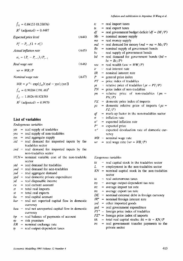
)~2 = 0 . 0 4 1 5 3 (0.33076)

R 2 (adjusted) = 0.4487

Expected price level (A44)

P f = P t 1( 1 +r i~)

A c t u a l inflation rate (A45)

ri, = (P, - Pt , ) / P t l

Rea l wage rate (A46)

wr = W R / P

N o m i n a l wage rate (A47)

W R = pef~l exp{f62[(yy d - yys ) / y y s ]}

f.1 = 0.99304 (191.48)*

)~2 = 1.0026 (0.92158)

R 2 (adjusted) = 0.9970

List of variables Endogenous variables

yts = real supply of tradables yns = real supply of non-tradables yys = real aggregate supply ztd = real demand for imported inputs by the

tradables sector znd = real demand for imported inputs by the

non-tradables sector V C N = nominal variable cost of the non-tradable

sector ytd = real demand for tradables y n d = real demand for non-tradables yyd = real aggregate demand ypd = real domestic private expenditure yd = real disposable income ca = real current account zt = total real imports xt = total real exports ka = real capital account kar = real net reported capital flow in domestic

currency kau = real net unreported capital flow in domestic

currency bp = real balance of payments of account rp = risk premium E R = nominal exchange rate ty = real output-dependent taxes

t~

Oc =

d f =

M s =

m s =

m d =

Bs =

b s =

bd =

W W =

ir =

I R =

P =

P T =

p t =

P N =

p n =

P Z =

p z =

f =

ri = ri e =

p e =

,W e =

W R =

w r =


real import taxes real export taxes real government budget deficit (d r = D F / P )

nominal money supply real money supply real demand for money ( m d = m s = M s ~ P )

nominal supply of government bonds real supply of government bonds real demand for government bonds (bd =

bs = B s / P )

real wealth ( w w = W W / P )

real interest rate nominal interest rate general price index price index of tradables relative price of tradables ( p t = P T / P )

price index of non-tradables relative price of non-tradables ( p n =

P N / P )

domestic price index of imports domestic relative price of imports ( p z =

P Z / P )

mark-up factor in the non-tradables sector inflation rate expected inflation rate expected price expected devaluation rate of domestic currency nominal wage rate real wage rate (wr = W R / P )

Exogenous variables

k t

L

K N

t~

try = trZ =

t rx =

D E =

I R * =

z r d =

ged =

P T * =

P Z * =

k k =

trs =

real capital stock in the tradables sector employment in the non-tradables sector nominal capital stock in the non-tradables sector real autonomous taxes average output-dependent tax rate average import tax rate average export tax rate nominal external debt in foreign currency nominal foreign interest rate other imported goods real government expenditure foreign price index of tradables foreign price index of imports total real capital stocks: k k = kt + K N / P

real government transfer payments to the private sector

Economic Modelling 1995 Volume 12 N u m b e r 4 413

Inflation and stabilization in Argentina

Documents

Transcript of Inflation and stabilization in Argentina