Housing Price Volatility and its Determinants

Chyi Lin Lee School of Economics and Finance, University of Western Sydney, Locked Bag 1797,

Penrith South D.C. 1797, Australia. Email: chyilin.lee@uws.edu.au

Paper submission for presentation at

The 15th Pacific Rim Real Estate Society Conference

Sydney, Australia

18th -21st January 2009

Housing Price Volatility and its Determinants

Abstract Many studies have been sought to understand the volatility patterns of real estate, whereas the study of housing price volatility is relatively little. This study aims to examine the determinants of housing price volatility for 8 capital cities in Australia. This study utilises quarterly data of 8 capital cities in Australia from 1987:Q4 to 2007:Q4. An Exponential-Generalised Autoregressive Conditional Heteoskedasticity (EGARCH) model is employed to analyse the volatility series of housing prices. Its determinants are also investigated. The results show that the volatility clustering effects (ARCH effects) are found in many capital cities. The importance of estimating each individual city’s EGARCH model is also demonstrated in which the determinants of housing volatility vary from a city to another city. These findings provide some important insights into the volatility of housing price. Keywords: Housing, Volatility Spillover, EGARCH, Australia.

2

1.0 INTRODUCTION

Housing is an important asset and it made a significant contribution to the total asset

of many households. In Australia, almost 55% of the total of Australian household

assets is in the housing form (Headay et al., 2005). Australia is also being one of the

countries with high homeownership rate at around 70% (IBISWorld, 2007). Given

the significance of housing market, housing has drawn a lot of attention from the

investors and researchers. Extensive studies have also been placed on the

determinants of housing prices such as Case and Shiller (1990), Bourassa and

Hendershott (1995) and Abelson et al. (2005).

It should be noted that these studies emphasis on the first moment (return), while the

volatility (the second moment) should also contain some important information. In

financial markets, the volatility has become an increasing concern for investors

(Brailsford et al., 2004). Extensive studies in financial markets also confirm that the

volatility clustering and volatility spillover (volatility linkages) effects in stock,

interest rate and exchange rate returns series (Bollerslev et al., 1992, a review). As

highlighted by Miles (2008) and Wong et al. (2006), failure to incorporate volatility

clustering may lead to inaccurate modelling results and sub-optimal allocation. Most

importantly, the volatility of housing price in Australia has increased dramatically in

recent years. As depicted in Figure 1, the 5-year rolling risk of Australia housing

prices has increased significantly from below 2% in 2001 to 4% in 2007.

(Insert Figure 1)

3

The recent global financial crisis has also further increased the volatility of housing

and drawn the attention of policy makers and investors towards the importance of

housing price volatility. Despite the volatilities of financial assets have been

extensively researched in the financial literature, few studies have been undertaken on

the volatility of housing market.

This study aims to extend the current literature by examining the volatility of house

price and its determinants in Australia over the study period 1987-2007. The

contributions of this study are twofold. Firstly, unlike previous studies, this study

employs an Exponential-Generalised Autoregressive Conditional Heteoskedasticity

(EGARCH) model to examine the spillover effects of numerous variables on housing

price volatility. As discussed by Nelson (1991), the EGARCH model allows for

testing the asymmetric and determinants of a volatility series simultaneously.

Importantly, the empirical support in favourite of EGARCH is also found by Engle

and Ng (1993) and Stevenson (2002). Second, this study is probably the first study of

volatility spillover in the Australian housing context. Importantly, the Australian

housing market offers an excellent dataset for examining the housing volatility

clustering and spillover effects in light of high transparency of this property market

(JLL, 2008).

The remainder of this study is organised as follows. Section 2 reviews the previous

literature on the determinants of housing price. The data and methodology are

discussed in Section 3. The results are reported and discussed in Section 4. The last

section concludes the paper.

4

2.0 LITERATURE REVIEW

The strong evidence of linkages between housing price and macroeconomic

fundamental factors has already appeared in the literature. Case and Shiller (1990)

demonstrated that population, real income and a change in house prices itself have

influence on the United States (U.S.) house prices. Stern (1992) found that the

disposable income is the most important variable affecting the United Kingdom

(U.K.) housing market. Munro and Tu (1996) examined the dynamics of U.K. housing

market with using Johansen co-integration technique and found that the U.K. housing

market is influenced by the household income, real mortgage rate and housing

completions at the national level.

The significance of mortgage rates in the U.S. housing market in a long-run is also

presented by McGibany and Nourzad (2004), while no similar evidence is available in

a short-run. Although Painter and Redfearn (2002) found little evidence of direct role

of interest rates on homeownership rates, it would affect the timing of changes in

tenure status. Stevenson (2000) presented strong evidence of housing and inflation is

cointegrated in a long run by utilising cointegration tests, whereas the conventional

ordinary least squares (OLS) model provides less conclusive results. Jud and Winkler

(2002) have also showed that real changes in income, construction costs and interest

rate, as well as the growth of population are significant factors for the real U.S.

housing price appreciation.

5

Similarly to Australia, Bourassa and Hendershott (1995) found that Australian capital

city real house prices are driven by the real wage income and the growth in

population. A more recent study, Abelson et al. (2005) also offered the evidence of

unemployment rate, mortgage rate, equity prices and the housing stock are negatively

related to Australian house prices, while positive relationships are demonstrated for

the disposable income and Consumer Price Index (CPI) in the long run. Stubbs (2005)

also described that interest rate is the prime concern of property investors in Australia,

implying that it is the main factor in driving the housing prices.

Tu (2000) also showed that the real weekly earnings, nominal mortgage rates,

unemployment rates and housing construction activities are the key factors affecting

the Australian housing market. More importantly, this study has also highlighted the

importance of analysing the regional housing markets in which the Australian housing

markets at subnational level are highly segmented. In other words, a national housing

price model would fail to represent the housing price dynamics of regional cities.

Few regional housing studies are available in Australia. Luo et al. (2007) examined

the causality linkages between Victorian residential price and macroeconomic

variables. They found that the housing price in Victoria is Granger caused by the

mortgage rate, weekly earning and unemployment rate. However, the sub-period

analysis also reveals that the relationships are instable and varied from time to time.

On the other hand, Karantonis and Ge (2007) focuses on the Sydney housing market

and demonstrated that the real household income, dwelling completions, speculative

investment and real interest rate are the driving forces of housing price in Sydney.

6

However, until recently, the determinants of housing price volatility have become the

growing concern research areas. Few studies have examined the issue of housing price

volatility. Baffoe-Bonnie (1998) conducted a variance decompose analysis in the U.S.

housing price. The results showed that the unemployment growth and mortgage rate

are driving factors for the U.S. housing market. However, the influence of a shock to

economic fundamentals (inflation, mortgage rates, employment growth and money

supply) are varied in different regions.

Dolde and Tirtiroglu (1997) examined the housing price volatility and found the time

varying volatility evidence in the Connecticut and San Francisco housing markets.

The persistence of time-varying volatility is also documented by Crawford and

Fratantoni (2003) and Wong et al. (2006) for the U.S. and Hong Kong housing

markets respectively. Similar strong linear dependency and heteroskedascity

(volatility clustering) is also exhibited in the Spanish housing markets by Guirguis et

al. (2007). Miles (2008) also demonstrated that volatility clustering effects are evident

in over half of the states in the U.S. His additional results also demonstrated that there

is volatility spillover effect (volatility linkage) of hosing conditional volatility on the

U.S. housing returns. In addition, the study has also presented the evidence of

asymmetric effect that housing prices are more sensitive to negative shocks.

Miller and Peng (2006) also found that about 17% of the Metropolitan Statistical

Areas (MSA) in the U.S. exhibit volatility clustering effect. Additionally, the

estimated volatility series with a GARCH model is Granger-caused by the home

appreciation rate and Gross Metropolitan Product (GMP) growth rate. More recently,

Hossain and Latif (2007) have also offered the evidence of time varying housing price

7

volatility in the Canadian housing market. The results also demonstrated that the gross

domestic product growth rate, house price appreciation rate and inflation are the

determinants of house price volatility with using an impulse responses analysis.

In summary, while there has been a multitude of literature in the housing literature

concerned with the housing price determinants, little attention has been on the

determinants of housing price volatility. The evidence of volatility clustering effect in

the housing market also reveals that an EGARCH model is appropriate to be applied

into housing volatility study.

3.0 DATA AND METHODOLOGY

Data

To assess the determinants of housing price volatility, the quarterly housing price

returns over 1987:Q4 to 2007:Q4 from the Australian Bureau of Statistics was

utilised1. The consumer price index (CPI), income, population and unemployment

rate were also extracted from the Australian Bureau of Statistics. The mortgage

lending rate was collected from the Reserve Bank of Australia.2

As discussed by Miller and Peng (2006), MSA data rather than national data are more

appropriate for analysing the metropolitan housing price volatility. Hence, in this 1 It should be noted that slight changes were proposed in the methodology of housing price index construction in 2005. This is one of the limitations of this study that should be borne in mind. 2 As highlighted by Luo et al. (2007), the selection of independent variables is subject to the availability of data.

8

study, all variables for 8 different state capital cities are at the state level, excepting

the mortgage lending rate. It must be noted that the differences in terms of mortgage

lending rate across different regions in Australia are insignificant. More importantly,

Richert (1990) found that regional housing prices only react uniformly to mortgage

rates. In this respect, the national level of mortgage rate was employed in this study.

(Inset Table 1)

Table 1 provides the summary statistics of housing prices and 5 independent

variables. Over the study period, Perth provided the highest average returns (2.35%

per quarter) with regard to the boom of housing market in recent years. It is followed

by Brisbane with 2.3% per quarter. Surprisingly, the largest city in Australia, Sydney

did not provide remarkable high returns. It could be attributed to the high outward

migration of residents (PRD, 2008). Turning our attention to volatility dimension

(standard deviation), Perth also recorded the highest risk level. However, housing

markets in Canberra, Darwin and Adelaide emerge as less volatile capital cities with

the lowest risk level, implying that volatility clustering effect would be less significant

in these housing markets.

Methodology

As demonstrated by previous studies, volatility clustering or ARCH effect is

commonly found in many financial and real estate assets (Cotter and Stevenson, 2006,

Asteriou and Hall, 2007, Lee, 2008). In this study, the presence of volatility clustering

9

effect in Australian housing markets was examined by the Engle (1982) LM test for

ARCH. The Engle (1982) LM test is computed as follows:

2222

2110

2 .... ptpttt −−− ++++= εφεφεφφε (1)

where is the squared residuals, and LM test is performed by 2tε

2* RTLM = (2)

T is the sample size

2R is derived from the Equation (1)

Thereafter, EGARCH models were computed to give an indication of housing price

volatility determinants on the series that exhibit volatility clustering. More

specifically, the CPI, income, population and unemployment rate were introduced into

the conditional variance equation as exogenous variables in order to determine the

volatility spillover of these variables on housing prices. The model of EGARCH (1,1)

for housing markets can be estimated as follows:

Mean Equation:

ttt RaaR μ++= −110 (3)

where is the return of housing at the time t ,tR tμ is the residual.

Variance Equation:

10

27

2int6

25

24

213

1

12

1

110

2 )log()log( populationerestincomecpitt

t

t

tt h

hhh μγμγμγμγγ

μγ

μγβ +++++++= −

−

−

−

−

(4) 28 ntunemploymeμγ+

where 0β is the constant term of variance equation, represents the lag of the

squared residual from the mean equation, is the lagged term,

21−tμ

2th th 2γ examines

leverage effect (asymmetric) in which if the asymmetric is presented, then the 02 <γ .

Statistics significant values for 4γ , 5γ , 6γ , 7γ and 8γ suggest that past volatility

shocks in inflation, income, interest, population and unemployment rate influence

current volatility in the housing market.

Unlike Miles (2008), this study employs an EGARCH model to assess the volatility of

housing prices and the volatility linkages between these factors and housing prices.

The EGARCH model has several theoretically superiority than a GARCH model in

which it allows an investigation of asymmetries and the conditional variance is always

positive (Asteriou and Hall, 2007). Moreover, the asymmetric volatility is also

demonstrated by Michayluk et al. (2006) and Lee (2008) in real estate and Miles

(2008) in housing. Most importantly, Engle and Ng (1993) and Stevenson (2002) have

found evidence that EGARCH models offer more intuitively appealing results and

perform surprisingly well in stock and real estate markets.

11

4.0 RESULTS AND DISCUSSION

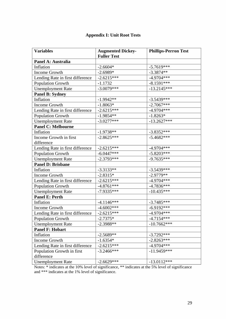
Stationary Tests

Unit root tests were first performed for examining the stationary of these data in

respect to the non-stationary would has profound implications for modelling. Two

standard procedures, the Augmented Dickey-Fuller test and Phillips-Perron tests were

employed in this study. The results are exhibited in Table 2.

(Inset Table 2)

It can be seen from the Table 2 that all housing price series are stationary. The

Augmented Dickey-Fuller tests reveal that all return series are statistically significant

at least at the 5% level. The only exception is Canberra in which it is statistically

significant at 6%. Similar strong stationary results are presented by the Phillips-Perron

test where all series are statistically significant at least at 5% level. Overall, these time

series data are stationary; indicating that shocks to the series are temporary and the

effects will disappear and revert to its long run mean. Importantly, no evidence is

found to support that the mean and autocovariance of the series depend on time (non-

stationary).

Similar tests were also performed to independent variables. The results show that

majority of variables is stationary. The exception is the lending rate, which the

variable is integrated in the first difference. Income growth in Melbourne and

population growth in Hobart exhibit comparable results, suggesting that these

12

variables are stationary after the first difference. The results are displayed in

Appendix I.

ARCH Effects

Thereafter, the ARCH LM test of Equations (1) and (2) was undertaken to investigate

whether there is volatility clustering in the housing price series. It is important to

perform a formal LM test prior to employing an EGARCH model. The results of LM

tests and p-value are depicted in Table 3.

(Inset Table 3)

Apparently, positive and statistic significant LM values are observed for Australia,

Sydney, Melbourne, Brisbane, Perth and Hobart series. This clearly suggests rejecting

the null hypothesis of homoskedascity, indicating that volatility clustering effects are

evident in these series. The strong evidence of volatility clustering also denotes the

appropriateness of employing an EGARCH model in analysing the volatility spillover

in these housing markets. Importantly, the ARCH effects also signify the potential

underestimation of actual risk by a constant variance risk measure (unconditional

variance).

However, no similar evidence is found for the series of Canberra, Adelaide and

Darwin. One of the possible explanations for these homoskedasticity series is the

housing prices of these cities are less active and less volatile. As shown in Table 1,

these cities reveal the lowest standard deviation levels in comparison to other cities.

13

Therefore, it is not surprisingly that the time series do not exhibit periods of unusually

high volatility and followed by calm periods of low volatility (the pattern of volatility

clustering).

In brief, over half Australian state capital cities exhibit volatility clustering effects.

These results also support the findings from Miles (2008) in the U.S., suggesting that

the ARCH effect is not only available in financial and real estate assets, but also in the

housing market. This finding also highlights the importance of estimating a separate

EGARCH model for each city.

Model Specifications

Once the ARCH effects are determined, an analysis of the housing volatility

determinants is conducted for each market that exhibits volatility clustering.

Specifically, the housing volatility determinants of Australia, Sydney, Melbourne,

Brisbane, Perth and Hobart are determined by using separate EGARCH models.

In should be noted that the optimal specification for an EGARCH model should be

determined prior to the construction of the model. Even though there is consensus that

GARCH (1,1) model is the most convenient specification in the financial literature

(Bollerslev et al., 1992), no similar agreement is available for EGARCH models. As a

result, the EGARCH(1,1) model is compared to various higher-order models based on

Akaike Information Criterion and Schwarz Information Criterion. The results are

displayed in Table 4.

14

(Insert Table 4)

Panel A of Table 4 illustrates that EGARCH(3,2) is the best specification for the

Australian housing price series. Both Akaike and Schwarz information criteria

confirm that this specification has the lowest value for this series, which in turn the

EGARCH(3,2) is employed in estimating the volatility spillover in Australian housing

prices. Similar estimating procedure is repeated for Sydney, Melbourne, Brisbane,

Perth and Hobart series respectively. Undoubtedly, EGARCH(1,3), EGARCH(1,2),

EGARCH(3,3) emerge the most appropriate specification for Sydney, Brisbane and

Hobart housing price series. More specifically, both criteria show the smallest value

of each criterion for these series.

Interestingly, the Akaike information criterion exhibits that the EGARCH(3,3)

specification is preferred model specification for the Melbourne series, whereas the

Schwarz information criterion shows that the EGARCH(1,1) specification is the most

optimal specification. Similar divergence results are also obtained from different

criteria for the Perth housing price series. As discussed by Brooks and Tsolacos

(2003), Schwarz criterion is a more prudent selection criteria than Akaike criterion. In

other words, the Schwarz criterion is preferred; EGARCH(1,1) and EGARCH(2,3)

were selected for Melbourne and Perth housing price series.

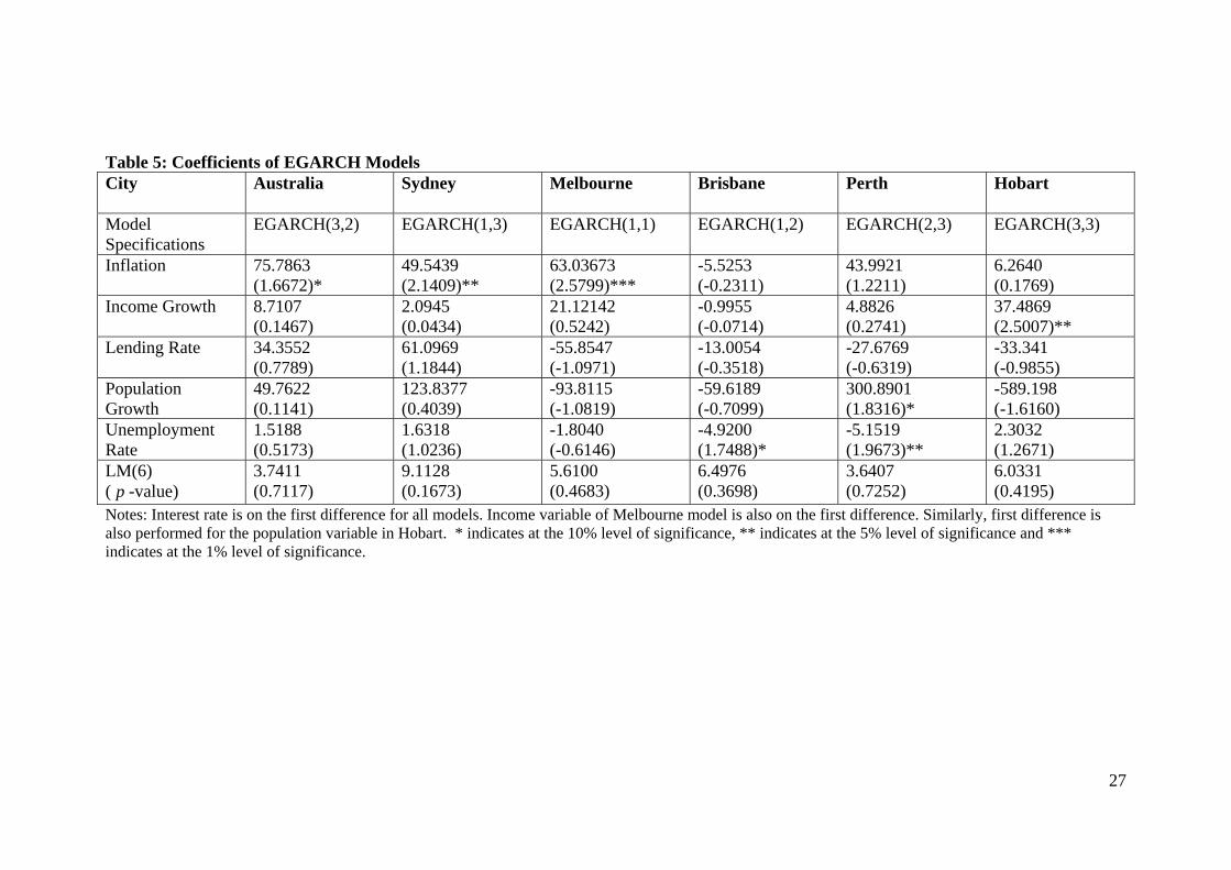
Volatility Determinants

Table 5 presents the results of EGARCH models based on the identified model

specifications in the above section. The parameters of interest in an EGARCH model

15

are the coefficients on shocks to housing price returns, thus only the coefficients of

inflation, income, interest, population and unemployment rate are reported in Table

53.

(Insert Table 5)

At the national level, a positive and significance coefficient is evident for inflation,

suggesting that a shock to inflation rate does produce dynamic responses in Australian

housing prices. Similar results are also evident in Sydney and Melbourne. The results

also support some studies in housing price volatility that inflation is one of the

determinants of housing price volatility, and the volatility of inflation will pushes up

the housing prices volatility (Hossain and Latif, 2007). Importantly, Fama and

Schwert (1977) have also offered the evidence of housing market hedging the

expected inflation and unexpected inflation.

On the other hand, the unemployment rate coefficients of Brisbane and Perth are

negatively and statistically at least at 10% level, showing that past volatility of

unemployment rates determines current volatility of housing prices in Brisbane and

Perth. The Perth residential market provides a higher significance level at 5%. This

result is intuitively appealing in which a lower unemployment rate will increase the

housing prices. Similar findings are also documented by Miller and Peng (2006) in the

U.S. housing price volatility.

3 The full results are depicted in Appendix II.

16

Strong volatility spillover evidence is also observed between income growth and

housing prices in Hobart. The positive and statistic significant coefficient shows the

transmission of past volatility of income growth to current volatility of Hobart

housing price, reflecting that the volatility of Hobart residential market will response

to the shock in income growth. Interestingly, this factor has influenced on the Hobart

housing market, but it does not have any effect on other cities. This could be

explained by the widening disparities in terms of state per capita incomes. This point

has also been pointed out by Cashin and Strappazzon (1998). Additionally, Tasmania

is the state with the lowest average annual income growth rate. Therefore, it is

reasonable to understand that the housing price volatility of Hobart is more sensitive

to the shock of income than other cities.

The volatility of population would appear to be influential in affecting the volatility of

housing market in Perth, which the coefficient of population is positive and

statistically significant at 10%. This means that there is a volatility spillover effect of

population on Perth housing prices and higher past volatility of population will

magnify the current volatility of housing prices.

Interestingly, the past volatility of mortgage rate is insignificant in explaining the

current volatility of housing price. In other words, the lending rate has little influence

on the housing price. This is inconsistent with the findings of Abelson et al. (2005) in

the first moment studies. However, McGibany and Nourzad (2004) also found little

evidence of short-run influence from mortgage rates to housing price based on a

variance decomposition analysis. Besides, the results also suggested that the housing

price is inelastic response to changes in mortgage rates in the U.S. Similarly to

17

Australia, no noticeable effect was observed in housing prices despite 7 consecutive

increases in interest rate by the Reserve Bank of Australia from March 2006 to March

2008.

Another important observation emerges from the Table 4 is these variables have

different impact on the dynamic behaviour of housing prices volatility in different

cities. There is little evidence to support that uniform reaction to any variable from

different capital city housing prices. Indeed, the determinants of housing price

volatility are varied from city to city. This result seems to agree with the findings of

Tu (2000) in Australia based on the first moment. This implies that the national

housing price is unable to represent the state capital housing price models and

highlighting the importance of constructing different models for different cities.

Moreover, the diagnostic test results support that there is no misspecification in the

model with regard to the insignificant LM statistics for ARCH, indicating that the

EGARCH models are sufficient representations. This also suggests that the EGARCH

models are sufficient to remove any residual heteroskedasticity effects. Overall,

volatility spillover effects of inflation on national housing prices are evident in Table

5. Nevertheless, the factors have different impact on the dynamic behaviour of

housing prices volatility in different cities.

Asymmetric Effects

Importantly, one of the important features of EGARCH models is the models are able

to capture and examine the asymmetric effect of a volatility series. This section

18

emphasises on the asymmetric effects in Australian housing prices. Table 6 reports the

results of testing for asymmetric EGARCH effects from the Equation (4).

(Insert Table 6)

The results signify that Melbourne, Brisbane and Hobart with time-varying volatility

also have significant asymmetric effects, where the coefficients on asymmetric shocks

( 2γ ) are positive and statistically significant at 10%. Stronger significance levels are

manifested for Melbourne and Brisbane, reflecting that housing prices are asymmetric

in the news, and bad news has larger impacts on the volatility of these series than

good news. In other words, a negative shock would raise the uncertainty and volatility

of these markets dramatically. These results are also consistent with Miles (2008) in

the U.S. housing market and Hossain and Latif (2007) in the Canada market,

suggesting that the EGARCH model could be a favouring model than a conventional

GARCH model.

Generally the results in Table 6 shows that asymmetric effects are demonstrated in

several capital cities, indicating positive shocks in the market generate less volatility

than negative shocks.

5.0 CONCLUSIONS

Existing literature on the determinants of housing prices is predominantly in the first

moment, and there is little study has been placed on the determinants of housing

19

prices volatility. This study aims to examine the volatility of Australian housing prices

and its determinants over 1987-2007.

Several important findings have been found in this study. Firstly, volatility clustering

has been demonstrated in over half of the 8 state capital cities. This indicates that the

Australian housing market is consistent with other markets in which its volatility is

time varying and clustering. Secondly, asymmetric shocks are also found in numerous

Australian capital cities, suggesting that the volatility raises more in response to the

bad news than good news. Thirdly, inflation appears as the determinant of housing

price volatility at the national level, while the linkages of housing volatility are varied

from one city to another city. This suggests that sub-national factors should be

considered in formulating the national housing policy.

Overall, this study has provided several important insights into the volatility of

housing prices. An in-depth understanding of house price volatility is essential for

housing investors and policy makers. More specifically, housing investors should

estimate the conditional variance (EGARCH process) of a housing market in respect

to the potential underestimation of the actual risk level of the market by using a

constant variance risk measure. Furthermore, policy makers should also address the

importance of considering the sub-national factors in formulating the national housing

policy.

20

References Abelson, P., Joyeux, R., Milunovich, G. & Chung, D. (2005) Explaining House Prices in

Australia: 1970–2003. The Economic Record, 81 (S1), S96-S103. Asteriou, D. & Hall, S. G. (2007) Applied Econometrics: A Modern Approach Using Eviews

and Microfit: Revised Edition, Hampshire, Palgrave Macmillan. Baffoe-Bonnie, J. (1998) The Dynamic Impact of Macroeconomic Aggregates on Housing

Prices and Stock of Houses: A National and Regional Analysis. Journal of Real Estate Finance and Economics, 17 (2), 179-197.

Bollerslev, T., Chou, R. Y. & Kroner, K. F. (1992) ARCH Modeling in Finance: A Review of the Theory and Empirical Evidence. Journal of Econometrics, 52 (1-2), 5-59.

Bourassa, S. C. & Hendershott, P. H. (1995) Australian Capital City Real House Prices, 1979-1993. The Australian Economic Review, 28 (3), 16-26.

Brailsford, T., Heaney, R. & Bilson, C. (2004) Investments: Concepts and Applications: Second Edition, Melbourne, Thomson.

Brooks, C. & Tsolacos, S. (2003) International Evidence on the Predictability of Returns to Securitised Real Estate Assets: Econometric Models versus Neural Networks. Journal of Property Research, 20 (2), 133-155.

Case, K. E. & Shiller, R. J. (1990) Forecasting Prices and Excess Returns in the Housing Market. Journal of the American Real Estate & Urban Economics Association, 18 (3), 253-273.

Cashin, P. & Strappazzon, L. (1998) Disparities in Australian Regional Incomes: Are They Widening or Narrowing? Australian Economic Review, 31 (3), 3-26.

Cotter, J. & Stevenson, S. (2006) Multivariate Modeling of Daily REIT Volatility. Journal of Real Estate Finance and Economics, 32 (3), 305-325.

Crawford, G. W. & Fratantoni, M. C. (2003) Assessing the Forecasting Performance of Regime-Switching, ARIMA and GARCH Models of House Prices. Real Estate Economics, 31 (2), 223-243.

Dolde, W. & Tirtiroglu, D. (1997) Temporal and Spatial Information Diffusion in Real Estate Price Changes and Variances. Real Estate Economics, 25 (4), 539-565.

Engle, R. F. (1982) Autoregressive Conditional Heteroscedasticity with Estimates of the Variance of United Kingdom Inflation. Econometrica, 50 (4), 987-1008.

Engle, R. F. & Ng, V. K. (1993) Measuring and Testing the Impact of News on Volatility. Journal of Finance, 48 (5), 1749-1778.

Fama, E. F. & Schwert, G. W. (1977) Asset Returns and Inflation. Journal of Financial Economics, 5 (2), 115-146.

Guirguis, H. S., Gianniko, C. I. & Garcia, L. G. (2007) Price and Volatility Spillovers between Large and Small Cities: A Study of the Spanish Market. Journal of Real Estate Portfolio Management, 13 (4), 311-316.

Headay, B., Marks, G. & Wooden, M. (2005) The Structure and Distribution of Household Wealth in Australia. Australian Economic Review, 38 (2), 159-175.

Hossain, B. & Latif, E. (2007) Determinants of Housing Price Volatility in Canada: A Dynamic Analysis. Applied Economics, 1-11.

IBISWorld (2007) Home Ownership Versus Leasing: Point to Ponder. Sydney, IBISWorld Pty Ltd, 1-10.

JLL (2008) From Opacity to Transparency: The Diverse World of Commercial Real Estate. Chicago, Jones Lang LaSalle, 1-20.

Jud, G. D. & Winkler, D. T. (2002) The Dynamics of Metropolitan Housing Prices. Journal of Real Estate Research, 23 (1/2), 29-45.

Karantonis, A. & Ge, X. J. (2007) An Empirical Study of the Determinants of Sydney's Dwelling Price. Pacific Rim Property Research Journal, 13 (4), 493-509.

Lee, C. L. (2008) Volatility Spillover in Australian Commercial Property. Pacific Rim Property Research Journal (in press).

21

Luo, Z., Liu, C. & Picken, D. (2007) Granger Causality among House Price and Macroeconomic Variables in Victoria. Pacific Rim Property Research Journal, 13 (2), 234-256.

McGibany, J. M. & Nourzad, F. (2004) Do Lower Mortgage Rates Mean Higher Housing Prices? Applied Economics, 36 (4), 305-313.

Michayluk, D., Wilson, P. J. & Zurbruegg, R. (2006) Asymmetric Volatility, Correlation and Returns Dynamics Between the U.S. and U.K. Securitized Real Estate Markets. Real Estate Economics, 34 (1), 109-131.

Miles, W. (2008) Volatility Clustering in U.S. Home Prices. Journal of Real Estate Research, 30 (1), 73-90.

Miller, N. & Peng, L. (2006) Exploring Metropolitan House Price Volatility. Journal of Real Estate Finance and Economics, 33 (5), 5-18.

Munro, M. & Tu, Y. (1996) The Dynamics of UK National and Regional House Prices. Review of Urban and Regional Development Studies, 8 (2), 186-201.

Nelson, D. B. (1991) Conditional Heteroskedasticity in Asset Returns: A New Approach. Econometrica, 59 (2), 347-370.

Painter, G. & Redfearn, C. L. (2002) The Role of Interest Rates in Influencing Long-Run Homeownership Rates. Journal of Real Estate Finance and Economics, 25 (2/3), 243-267.

PRD (2008) Quaterly Economic and Porperty Report Australia. Sydney, PRDnationwide Research,

Richert, A. K. (1990) The Impact of Interest Rate, Income, and Employment upon Regional housing Prices. Journal of Real Estate Finance and Economics, 3 (4), 373-391.

Stern, D. (1992) Explaining UK House Price Inflation 1971-89. Applied Economics, 24 (12), 1327-1333.

Stevenson, S. (2000) A Long Term Analysis of Housing and Inflation. Journal of Housing Economics, 9 (1-2), 24-39.

Stevenson, S. (2002) An Examination of Volatility Spillovers in REIT Returns. Journal of Real Estate Portfolio Management, 8 (3), 229-238.

Stubbs, D. (2005) Australia's Housing Boom Ends- Is a Crash around the Corner? Australian Property Journal, 38 (7), 523-529.

Tu, Y. (2000) Segmentation of Australian Housing Markets: 1989-98. Journal of Property Research, 17 (4), 311-327.

Wong, S. K., Yiu, C. Y., Tse, M. K. S. & Chau, K. W. (2006) Do the Forward Sales of Real Estate Stabilize Spot Prices? Journal of Real Estate Finance and Economics, 32 (3), 289-304.

22

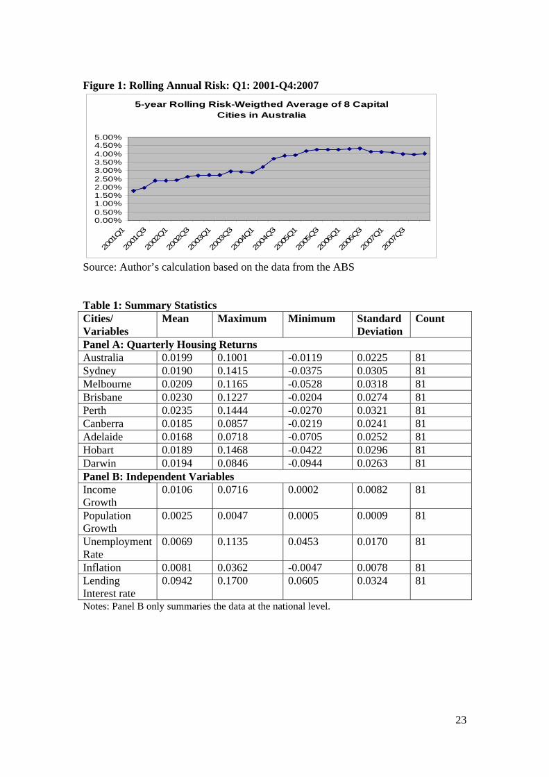
Figure 1: Rolling Annual Risk: Q1: 2001-Q4:2007

5-year Rolling Risk-Weigthed Average of 8 Capital Cities in Australia

0.00%0.50%1.00%1.50%2.00%2.50%3.00%3.50%4.00%4.50%5.00%

2001

Q1

2001

Q3

2002

Q1

2002

Q3

2003

Q1

2003

Q3

2004

Q1

2004

Q3

2005

Q1

2005

Q3

2006

Q1

2006

Q3

2007

Q1

2007

Q3

Source: Author’s calculation based on the data from the ABS Table 1: Summary Statistics Cities/ Variables

Mean Maximum Minimum Standard Deviation

Count

Panel A: Quarterly Housing Returns Australia 0.0199 0.1001 -0.0119 0.0225 81 Sydney 0.0190 0.1415 -0.0375 0.0305 81 Melbourne 0.0209 0.1165 -0.0528 0.0318 81 Brisbane 0.0230 0.1227 -0.0204 0.0274 81 Perth 0.0235 0.1444 -0.0270 0.0321 81 Canberra 0.0185 0.0857 -0.0219 0.0241 81 Adelaide 0.0168 0.0718 -0.0705 0.0252 81 Hobart 0.0189 0.1468 -0.0422 0.0296 81 Darwin 0.0194 0.0846 -0.0944 0.0263 81 Panel B: Independent Variables Income Growth

0.0106 0.0716 0.0002 0.0082 81

Population Growth

0.0025 0.0047 0.0005 0.0009 81

Unemployment Rate

0.0069 0.1135 0.0453 0.0170 81

Inflation 0.0081 0.0362 -0.0047 0.0078 81 Lending Interest rate

0.0942 0.1700 0.0605 0.0324 81

Notes: Panel B only summaries the data at the national level.

23

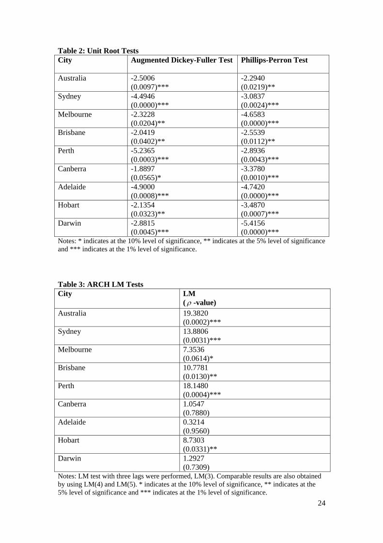
Table 2: Unit Root Tests City Augmented Dickey-Fuller Test Phillips-Perron Test

Australia -2.5006

(0.0097)*** -2.2940 (0.0219)**

Sydney -4.4946 (0.0000)***

-3.0837 (0.0024)***

Melbourne -2.3228 (0.0204)**

-4.6583 (0.0000)***

Brisbane -2.0419 (0.0402)**

-2.5539 (0.0112)**

Perth -5.2365 (0.0003)***

-2.8936 (0.0043)***

Canberra -1.8897 (0.0565)*

-3.3780 (0.0010)***

Adelaide -4.9000 (0.0008)***

-4.7420 (0.0000)***

Hobart -2.1354 (0.0323)**

-3.4870 (0.0007)***

Darwin -2.8815 (0.0045)***

-5.4156 (0.0000)***

Notes: * indicates at the 10% level of significance, ** indicates at the 5% level of significance and *** indicates at the 1% level of significance. Table 3: ARCH LM Tests City LM

( ρ -value) Australia 19.3820

(0.0002)*** Sydney 13.8806

(0.0031)*** Melbourne 7.3536

(0.0614)* Brisbane 10.7781

(0.0130)** Perth 18.1480

(0.0004)*** Canberra 1.0547

(0.7880) Adelaide 0.3214

(0.9560) Hobart 8.7303

(0.0331)** Darwin 1.2927

(0.7309) Notes: LM test with three lags were performed, LM(3). Comparable results are also obtained by using LM(4) and LM(5). * indicates at the 10% level of significance, ** indicates at the 5% level of significance and *** indicates at the 1% level of significance.

24

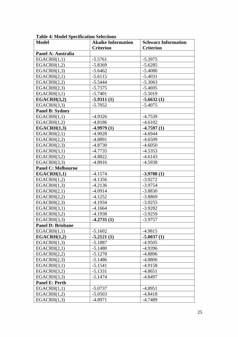
Table 4: Model Specification Selections Model Akaike Information

Criterion Schwarz Information Criterion

Panel A: Australia EGACRH(1,1) -5.5761 -5.3975 EGACRH(1,2) -5.8369 -5.6285 EGACRH(1,3) -5.6462 -5.4080 EGACRH(2,1) -5.6115 -5.4031 EGACRH(2,2) -5.5444 -5.3063 EGACRH(2,3) -5.7375 -5.4695 EGACRH(3,1) -5.7401 -5.5019 EGACRH(3,2) -5.9311 (1) -5.6632 (1) EGACRH(3,3) -5.7052 -5.4075 Panel B: Sydney EGACRH(1,1) -4.9326 -4.7539 EGACRH(1,2) -4.8186 -4.6102 EGACRH(1,3) -4.9979 (1) -4.7597 (1) EGACRH(2,1) -4.9028 -4.6944 EGACRH(2,2) -4.8891 -4.6509 EGACRH(2,3) -4.8730 -4.6050 EGACRH(3,1) -4.7735 -4.5353 EGACRH(3,2) -4.8822 -4.6143 EGACRH(3,3) -4.8916 -4.5938 Panel C: Melbourne EGACRH(1,1) -4.1574 -3.9788 (1) EGACRH(1,2) -4.1356 -3.9272 EGACRH(1,3) -4.2136 -3.9754 EGACRH(2,1) -4.0914 -3.8830 EGACRH(2,2) -4.1252 -3.8869 EGACRH(2,3) -4.1934 -3.9255 EGACRH(3,1) -4.1664 -3.9282 EGACRH(3,2) -4.1938 -3.9259 EGACRH(3,3) -4.2735 (1) -3.9757 Panel D: Brisbane EGACRH(1,1) -5.1602 -4.9815 EGACRH(1,2) -5.2121 (1) -5.0037 (1) EGACRH(1,3) -5.1887 -4.9505 EGACRH(2,1) -5.1480 -4.9396 EGACRH(2,2) -5.1278 -4.8896 EGACRH(2,3) -5.1486 -4.8806 EGACRH(3,1) -5.1541 -4.9158 EGACRH(3,2) -5.1331 -4.8651 EGACRH(3,3) -5.1474 -4.8497 Panel E: Perth EGACRH(1,1) -5.0737 -4.8951 EGACRH(1,2) -5.0503 -4.8418 EGACRH(1,3) -4.8971 -4.7489

25

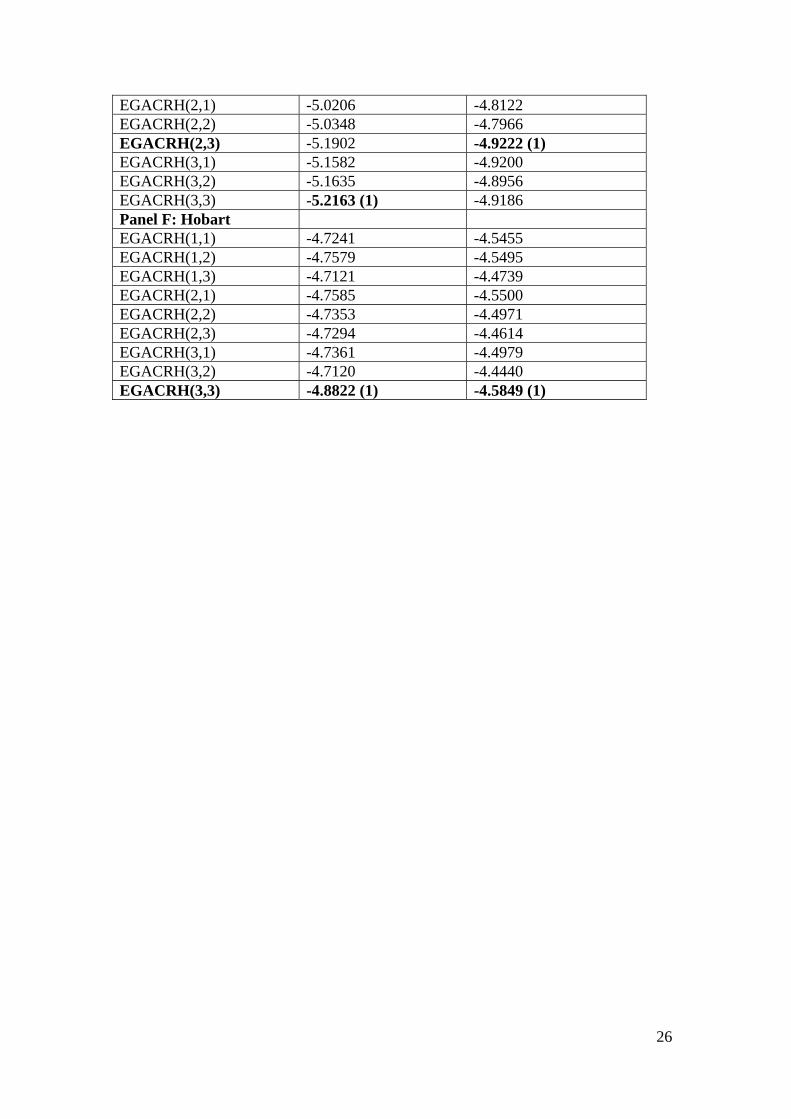
26

EGACRH(2,1) -5.0206 -4.8122 EGACRH(2,2) -5.0348 -4.7966 EGACRH(2,3) -5.1902 -4.9222 (1) EGACRH(3,1) -5.1582 -4.9200 EGACRH(3,2) -5.1635 -4.8956 EGACRH(3,3) -5.2163 (1) -4.9186 Panel F: Hobart EGACRH(1,1) -4.7241 -4.5455 EGACRH(1,2) -4.7579 -4.5495 EGACRH(1,3) -4.7121 -4.4739 EGACRH(2,1) -4.7585 -4.5500 EGACRH(2,2) -4.7353 -4.4971 EGACRH(2,3) -4.7294 -4.4614 EGACRH(3,1) -4.7361 -4.4979 EGACRH(3,2) -4.7120 -4.4440 EGACRH(3,3) -4.8822 (1) -4.5849 (1)

27

Table 5: Coefficients of EGARCH Models City

Australia Sydney Melbourne Brisbane Perth Hobart

Model Specifications

EGARCH(3,2) EGARCH(1,3) EGARCH(1,1) EGARCH(1,2) EGARCH(2,3) EGARCH(3,3)

Inflation

75.7863 (1.6672)*

49.5439 (2.1409)**

63.03673 (2.5799)***

-5.5253 (-0.2311)

43.9921 (1.2211)

6.2640 (0.1769)

Income Growth

8.7107 (0.1467)

2.0945 (0.0434)

21.12142 (0.5242)

-0.9955 (-0.0714)

4.8826 (0.2741)

37.4869 (2.5007)**

Lending Rate

34.3552 (0.7789)

61.0969 (1.1844)

-55.8547 (-1.0971)

-13.0054 (-0.3518)

-27.6769 (-0.6319)

-33.341 (-0.9855)

Population Growth

49.7622 (0.1141)

123.8377 (0.4039)

-93.8115 (-1.0819)

-59.6189 (-0.7099)

300.8901 (1.8316)*

-589.198 (-1.6160)

Unemployment Rate

1.5188 (0.5173)

1.6318 (1.0236)

-1.8040 (-0.6146)

-4.9200 (1.7488)*

-5.1519 (1.9673)**

2.3032 (1.2671)

LM(6) p( -value)

3.7411 (0.7117)

9.1128 (0.1673)

5.6100 (0.4683)

6.4976 (0.3698)

3.6407 (0.7252)

6.0331 (0.4195)

Notes: Interest rate is on the first difference for all models. Income variable of Melbourne model is also on the first difference. Similarly, first difference is also performed for the population variable in Hobart. * indicates at the 10% level of significance, ** indicates at the 5% level of significance and *** indicates at the 1% level of significance.

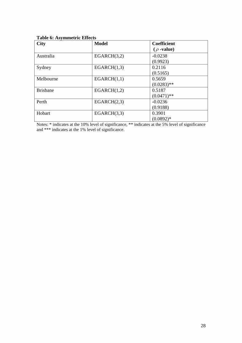
Table 6: Asymmetric Effects City Model Coefficient

( ρ -value) Australia EGARCH(3,2) -0.0238

(0.9923) Sydney EGARCH(1,3) 0.2116

(0.5165) Melbourne EGARCH(1,1) 0.5659

(0.0283)** Brisbane EGARCH(1,2) 0.5187

(0.0471)** Perth EGARCH(2,3) -0.0236

(0.9188) Hobart EGARCH(3,3) 0.3901

(0.0892)* Notes: * indicates at the 10% level of significance, ** indicates at the 5% level of significance and *** indicates at the 1% level of significance.

28

29

Appendix I: Unit Root Tests

Variables Augmented Dickey-

Fuller Test Phillips-Perron Test

Panel A: Australia Inflation -2.6604* -5.7619*** Income Growth -2.6989* -3.3874** Lending Rate in first difference -2.6215*** -4.9704*** Population Growth -1.1732 -8.1591*** Unemployment Rate -3.0079*** -13.2145*** Panel B: Sydney Inflation -1.9942** -3.5439*** Income Growth -1.8063* -2.7067*** Lending Rate in first difference -2.6215*** -4.9704*** Population Growth -1.9854** -1.8263* Unemployment Rate -3.0277*** -13.2627*** Panel C: Melbourne Inflation -1.9738** -3.8352*** Income Growth in first difference

-2.8625*** -5.4682***

Lending Rate in first difference -2.6215*** -4.9704*** Population Growth -6.0447*** -5.8203*** Unemployment Rate -2.3793*** -9.7635*** Panel D: Brisbane Inflation -3.3133** -3.5439*** Income Growth -2.8315* -2.9779** Lending Rate in first difference -2.6215*** -4.9704*** Population Growth -4.8761*** -4.7836*** Unemployment Rate -7.9335*** -10.435*** Panel E: Perth Inflation -4.1146*** -3.7485*** Income Growth -4.6002*** -6.9192*** Lending Rate in first difference -2.6215*** -4.9704*** Population Growth -2.7375* -4.7154*** Unemployment Rate -2.3988** -10.7662*** Panel F: Hobart Inflation -2.5689** -3.7292*** Income Growth -1.6354* -2.8263*** Lending Rate in first difference -2.6215*** -4.9704*** Population Growth in first difference

-3.2466*** -11.9459***

Unemployment Rate -2.6629*** -13.0112*** Notes: * indicates at the 10% level of significance, ** indicates at the 5% level of significance and *** indicates at the 1% level of significance.

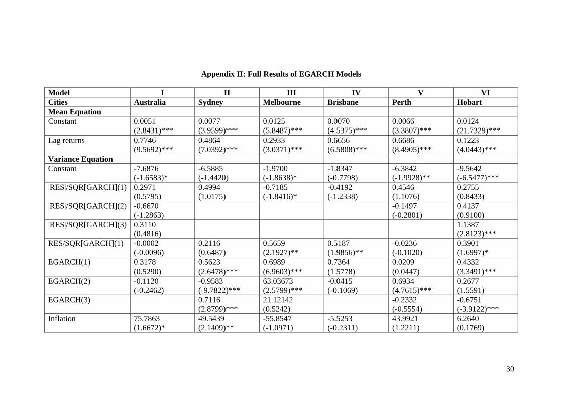
Appendix II: Full Results of EGARCH Models

Model I II III IV V VI Cities Australia Sydney Melbourne Brisbane Perth Hobart Mean Equation Constant 0.0051

(2.8431)*** 0.0077 (3.9599)***

0.0125 (5.8487)***

0.0070 (4.5375)***

0.0066 (3.3807)***

0.0124 (21.7329)***

Lag returns 0.7746 (9.5692)***

0.4864 (7.0392)***

0.2933 (3.0371)***

0.6656 (6.5808)***

0.6686 (8.4905)***

0.1223 (4.0443)***

Variance Equation Constant -7.6876

(-1.6583)* -6.5885 (-1.4420)

-1.9700 (-1.8638)*

-1.8347 (-0.7798)

-6.3842 (-1.9928)**

-9.5642 (-6.5477)***

|RES|/SQR[GARCH](1) 0.2971 (0.5795)

0.4994 (1.0175)

-0.7185 (-1.8416)*

-0.4192 (-1.2338)

0.4546 (1.1076)

0.2755 (0.8433)

|RES|/SQR[GARCH](2) -0.6670 (-1.2863)

-0.1497 (-0.2801)

0.4137 (0.9100)

|RES|/SQR[GARCH](3) 0.3110 (0.4816)

1.1387 (2.8123)***

RES/SQR[GARCH](1) -0.0002 (-0.0096)

0.2116 (0.6487)

0.5659 (2.1927)**

0.5187 (1.9856)**

-0.0236 (-0.1020)

0.3901 (1.6997)*

EGARCH(1) 0.3178 (0.5290)

0.5623 (2.6478)***

0.6989 (6.9603)***

0.7364 (1.5778)

0.0209 (0.0447)

0.4332 (3.3491)***

EGARCH(2) -0.1120 (-0.2462)

-0.9583 (-9.7822)***

63.03673 (2.5799)***

-0.0415 (-0.1069)

0.6934 (4.7615)***

0.2677 (1.5591)

EGARCH(3) 0.7116 (2.8799)***

21.12142 (0.5242)

-0.2332 (-0.5554)

-0.6751 (-3.9122)***

Inflation 75.7863 (1.6672)*

49.5439 (2.1409)**

-55.8547 (-1.0971)

-5.5253 (-0.2311)

43.9921 (1.2211)

6.2640 (0.1769)

30

Income Growth 8.7107 (0.1467)

2.0945 (0.0434)

-93.8115 (-1.0819)

-0.9955 (-0.0714)

4.8826 (0.2741)

37.4869 (2.5007)**

Interest 34.3552 (0.7789)

61.0969 (1.1844)

-1.8040 (-0.6146)

-13.0054 (-0.3518)

-27.6769 (-0.6319)

-33.341 (-0.9855)

Population 49.7622 (0.1141)

123.8377 (0.4039)

63.03673 (2.5799)***

-59.6189 (-0.7099)

300.8901 (1.8316)*

-589.198 (-1.6160)

Unemployment 1.5188 (0.5173)

1.6318 (1.0236)

21.12142 (0.5242)

-4.9200 (1.7488)*

-5.1519 (1.9673)**

2.3032 (1.2671)

31

Notes: * indicates at the 10% level of significance, ** indicates at the 5% level of significance and *** indicates at the 1% level of significance.