Actively Managed Volatility Strategies - CBS Research Portal

Copenhagen Business SchoolCopenhagen, Spring 2019

Actively Managed Volatility StrategiesIs it Possible to Disarm Ticking Time Bombs?

Atle Alkelin and Olivia Bergkvist

Supervisor: Fabrice Tourre

Master thesis

Advanced Economics and Finance

(Cand.Oecon.)

Copenhagen Business School

This page has intentionally been left blank

i

Acknowledgements

This thesis represents the tangible results of our master studies at Copenhagen Business

School. Several people deserve our gratitude for their contributions to this thesis. First

and foremost, we would like to thank our supervisor Fabrice Tourre for many fruitful

discussions, encouragement, helpful comments and guidance. We would also like to thank

Ing-Haw Cheng, Associate Professor at Tuck School of Business, Dartmouth College, and

author of "The VIX Premium"1, for helpful guidance in regards to the methodology of

the thesis.

During our studies, we have had the privilege to be surrounded by many great fellow

students and friends. We are grateful to all of them for providing a fantastic academic

and social environment. Finally, we would also like to thank our friends and family for

their support and patience.

Copenhagen Business School

Copenhagen, May 2019

Atle Alkelin Olivia Bergkvist

1See Cheng (2018) to read his interesting article in the Review of Financial Studies.

ii

Abstract

The popularity of short volatility strategies on the VIX has increased significantly over the

past decade. However, the recent increase in volatility of volatility has cannibalized returns

associated with these strategies, culminating during the "Volmageddon" of February 5th

2018 when the VIX saw its most significant daily increase ever recorded. The thesis

builds upon the methodology of Cheng (2018) by applying ex-ante estimated volatility

premiums as a signal in volatility futures strategies in the U.S. and Europe. The findings

confirm that trading volatility actively based on premiums embedded in volatility futures

significantly improves upon passive volatility strategies and deliver high risk-adjusted

returns, both on the U.S. and European markets. Actively trading volatility not only

improves upon performance but also reduces strategy drawdowns. Increasing trading

frequency improves strategy performance more on the European than on the U.S. market,

despite relatively large transaction costs.

Keywords – VIX, VSTOXX, futures, volatility, premiums, trading strategies

Contents iii

Contents

1 Introduction 1

2 Volatility Indexes 52.1 Volatility Indexes . . . . . . . . . . . . . . . . . . . . . . . . . . . . . . . 52.2 Investor Fear Gauges . . . . . . . . . . . . . . . . . . . . . . . . . . . . . 9

2.2.1 The VIX and VSTOXX Time Series . . . . . . . . . . . . . . . . . 112.2.2 Alternative Volatility Indexes . . . . . . . . . . . . . . . . . . . . 15

2.3 Volatility Index Futures . . . . . . . . . . . . . . . . . . . . . . . . . . . 152.3.1 Prices and Liquidity . . . . . . . . . . . . . . . . . . . . . . . . . 18

3 Volatility Premiums 203.1 Volatility Risk Premiums . . . . . . . . . . . . . . . . . . . . . . . . . . . 203.2 Modeling Volatility Indexes . . . . . . . . . . . . . . . . . . . . . . . . . 22

3.2.1 Alternative Models . . . . . . . . . . . . . . . . . . . . . . . . . . 233.2.2 Model Selection . . . . . . . . . . . . . . . . . . . . . . . . . . . . 233.2.3 Model Performance . . . . . . . . . . . . . . . . . . . . . . . . . . 24

3.3 Calculating Premiums . . . . . . . . . . . . . . . . . . . . . . . . . . . . 25

4 Exploiting the Volatility Premium 284.1 Common Features of the Futures Strategies . . . . . . . . . . . . . . . . 28

4.1.1 Transaction Costs . . . . . . . . . . . . . . . . . . . . . . . . . . . 294.1.2 Calculating Returns and Performance Measures . . . . . . . . . . 30

4.2 Monthly Futures Strategies . . . . . . . . . . . . . . . . . . . . . . . . . . 324.2.1 VIX Monthly Futures Strategies (1) . . . . . . . . . . . . . . . . . 334.2.2 VSTOXX Monthly Futures Strategies . . . . . . . . . . . . . . . . 36

4.3 Daily Futures Strategies . . . . . . . . . . . . . . . . . . . . . . . . . . . 394.3.1 VIX Daily Futures Strategies (1) . . . . . . . . . . . . . . . . . . 404.3.2 VSTOXX Daily Futures Strategies . . . . . . . . . . . . . . . . . 42

4.4 Same Period Performance . . . . . . . . . . . . . . . . . . . . . . . . . . 454.4.1 VIX Monthly Futures Strategies (2) . . . . . . . . . . . . . . . . . 464.4.2 VIX Daily Futures Strategies (2) . . . . . . . . . . . . . . . . . . 50

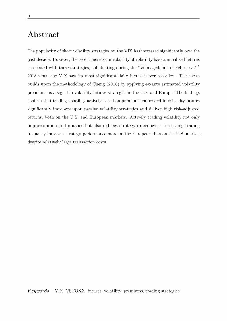
5 Discussion 555.1 Assumptions and Applicability . . . . . . . . . . . . . . . . . . . . . . . . 555.2 Value of the Volatility Premium . . . . . . . . . . . . . . . . . . . . . . . 565.3 Avoiding Drawdowns . . . . . . . . . . . . . . . . . . . . . . . . . . . . . 62

6 Conclusion 646.1 Suggestions for Future Research . . . . . . . . . . . . . . . . . . . . . . . 65

References 66

Appendix 69A1 Derivation of Equation 2.1 . . . . . . . . . . . . . . . . . . . . . . . . . . 69A2 Descriptive Statistics . . . . . . . . . . . . . . . . . . . . . . . . . . . . . 72A3 Properties of ARMA Models . . . . . . . . . . . . . . . . . . . . . . . . . 73

iv Contents

A4 Model Selection . . . . . . . . . . . . . . . . . . . . . . . . . . . . . . . . 74A5 Factor Loadings . . . . . . . . . . . . . . . . . . . . . . . . . . . . . . . . 76A6 L/S/C strategies - Sharpe Ratio Tables . . . . . . . . . . . . . . . . . . . 77A7 VHSI and VXJ . . . . . . . . . . . . . . . . . . . . . . . . . . . . . . . . 80

List of Figures v

List of Figures1.1 SVXY and VVIX . . . . . . . . . . . . . . . . . . . . . . . . . . . . . . . 32.1 Implied vs realized volatility of SPXT and SX5T . . . . . . . . . . . . . 82.2 Daily closing prices and the empirical distribution of VIX . . . . . . . . . . 112.3 Daily closing prices and the empirical distribution of VSTOXX . . . . . . 122.4 The level of VIX vs VSTOXX . . . . . . . . . . . . . . . . . . . . . . . . 132.5 The spread of VIX vs VSTOXX . . . . . . . . . . . . . . . . . . . . . . . 132.6 Scatter plots of VIX vs VSTOXX . . . . . . . . . . . . . . . . . . . . . . 142.7 Futures term structure in contango and backwardation. . . . . . . . . . . 172.8 Traded vega of VIX and VSTOXX futures . . . . . . . . . . . . . . . . . 193.1 Empirical distribution of VIX and VSTOXX premiums . . . . . . . . . . 263.2 Volatility premiums for VIX and VSTOXX . . . . . . . . . . . . . . . . . 274.1 Historical bid-ask spreads for futures on VIX and VSTOXX . . . . . . . 294.2 Log margin account growth for monthly strategies on VIX and SPXT (1) 354.3 Log margin account growth for monthly strategies on VSTOXX and SX5T 384.4 Log margin account growth for daily strategies on VIX and SPXT (1) . . . 414.5 Log margin account growth for daily strategies on VSTOXX and SX5T . 444.6 Log margin account growth for monthly strategies on VIX and SPXT (2) 484.7 Log margin account growth for daily strategies on VIX (2) . . . . . . . . 525.1 Log margin account growth for C/S strategies on VIX (2016-2018) . . . . 585.2 Log margin account growth for strategies on VIX and VSTOXX (unweighted) 63A4.1 ACF and PACF of VIX . . . . . . . . . . . . . . . . . . . . . . . . . . . 74A4.2 ACF and PACF of VSTOXX . . . . . . . . . . . . . . . . . . . . . . . . 75A7.1 Daily closing prices and the empirical distribution of VHSI . . . . . . . . 80A7.2 Daily closing prices and the empirical distribution of VXJ . . . . . . . . 80A7.3 Historical bid-ask spreads for futures on VHSI and VXJ . . . . . . . . . . 82A7.4 Traded vega of VHSI and VXJ futures . . . . . . . . . . . . . . . . . . . 82

vi List of Tables

List of Tables2.1 Examples of volatility indexes and their level on February 5th 2018 . . . . 72.2 Contract summary of volatility futures . . . . . . . . . . . . . . . . . . . 183.1 Model accuracy . . . . . . . . . . . . . . . . . . . . . . . . . . . . . . . . 243.2 Summary of estimated volatility premiums . . . . . . . . . . . . . . . . . 264.1 Performance of monthly trading strategies on VIX (1) . . . . . . . . . . . 344.2 Factor loadings for monthly strategies on VIX . . . . . . . . . . . . . . . 364.3 Performance of monthly trading strategies on VSTOXX . . . . . . . . . . 374.4 Factor loadings for monthly strategies on VSTOXX . . . . . . . . . . . . 394.5 Performance of daily trading strategies on VIX (1) . . . . . . . . . . . . . 404.6 Factor loadings for daily strategies on VIX (1) . . . . . . . . . . . . . . . 424.7 Performance of daily trading strategies on VSTOXX . . . . . . . . . . . 434.8 Factor loadings for daily strategies on VSTOXX . . . . . . . . . . . . . . 454.9 Performance of monthly strategies on VIX (2) . . . . . . . . . . . . . . . 474.10 Factor loadings for monthly strategies on VIX (2) . . . . . . . . . . . . . 494.11 Daily correlation of monthly trading strategies . . . . . . . . . . . . . . . 504.12 Performance of daily strategies on VIX (2) . . . . . . . . . . . . . . . . . . 514.13 Factor loadings for daily strategies on VIX (2) . . . . . . . . . . . . . . . 534.14 Daily correlation of daily trading strategies . . . . . . . . . . . . . . . . . 54A2.1 Descriptive statistics of VIX . . . . . . . . . . . . . . . . . . . . . . . . . 72A2.2 Descriptive statistics of VSTOXX . . . . . . . . . . . . . . . . . . . . . 72A4.1 VIX ARMA forecast models . . . . . . . . . . . . . . . . . . . . . . . . . 74A4.2 VSTOXX ARMA forecast models . . . . . . . . . . . . . . . . . . . . . 75A6.1 Sharpe ratios for monthly L/S/C strategies on VIX (full sample) . . . . . 77A6.2 Sharpe ratios for monthly L/S/C strategies on VSTOXX . . . . . . . . . 77A6.3 Sharpe ratios for daily L/S/C strategies on VIX (full sample) . . . . . . . 78A6.4 Sharpe ratios for daily L/S/C strategies on VSTOXX . . . . . . . . . . . 78A6.5 Sharpe ratios for monthly L/S/C strategies on VIX (Jun 2009 - Dec 2018) 78A6.6 Sharpe ratios for daily L/S/C strategies on VIX (Jun 2009 - Dec 2018) . 79A7.1 Descriptive statistics of VHSI and VXJ . . . . . . . . . . . . . . . . . . . 81A7.2 Correlation matrix of volatility indexes and underlying stock indexes . . . 81A7.3 Contract summary of volatility futures (VHSI & VXJ) . . . . . . . . . . . 81

1

1 Introduction

Up until the last decade, it was only possible to trade volatility by holding portfolios of

options, or by entering into variance swaps traded in over the counter (OTC) markets

(Alexander et al., 2015). This changed with the introduction of volatility indexes. The

VIX index, introduced by Chicago Board Options Exchange (CBOE) in 1993, measures

the expected future volatility of S&P500 (SPXT2) and is recognized as an indicator of

investor sentiment. Following Whaley (2000) it is often referred to as the "investor fear

gauge." In the last few years, a wide range of volatility indexes has been constructed

using prices of European style options (Alexander et al., 2015). A benefit of volatility

indexes is that they can serve as an underlying risk-factor for derivative instruments. Since

investors wanting to hedge their portfolios primarily dominate the stock options markets,

derivatives on volatility indexes are known to produce returns negatively correlated to

the stock market (Bollen and Whaley, 2004). Thus, providing a hedging alternative to

derivatives issued directly on the stock market (Dash and Moran, 2007).

A growing body of research shows that investors are ready to pay sizable sums for

protecting their stock portfolios (see e.g. Coval and Shumway (2018), Bakshi and Kapdia

(2003) and Bollerslev and Todorov (2011)). Bollerslev et al. (2009) and Bekaert and

Hoerova (2014) research the behavior of variance risk premiums, calculated as the difference

between implied and realized variance. The premiums paid by investors contain a puzzling

behavior in periods of market turmoil; sharp increases in realized variance drive premiums

downward, sometimes to negative levels, before they rebound (Bekaert and Hoerova, 2014).

It is counter-intuitive that premiums fall during periods of market turmoil. However,

as Bekaert and Hoerova (2014) points out, the behavior is persistent across multiple of

leading forecast models.

A ground rule in derivatives pricing is that the premium paid by investors is equal

to the expected risk-neutral return of the derivative. Speculators, often hedge funds,

who sell this insurance should therefore expect premiums to increase when risk goes

up. However, as pointed out, the opposite seems to be true. Cheng (2018) resorts to a

2In this thesis the underlying stock indexes are consistently referred to by their respective total returnticker on Bloomberg.

2

newly established method of estimating premiums paid by investors. Namely, the "VIX

premium". Embedded in VIX futures prices, the VIX premium can be economically

interpreted as the expected return of selling a VIX futures contract. Cheng (2018)

demonstrates that falling ex-ante estimated premiums reliably predict increases in ex-post

market and investment risk.

Investor hedging demand3 drives volatility futures to trade at a sizable premium relative

to the volatility index spot level. As a result, the VIX futures term structure is most often

upward sloping (Alexander et al., 2015), implying that short volatility futures strategies

are highly profitable on average. However, since volatility tends to spike (Avellanda and

Papanicolaou, 2017) and since they are known for destroying several years of profit in a

few hours (Brøgger, 2018) these strategies can be referred to as ticking time bombs. On

February 5th 2018 the VIX index experienced the largest daily increase ever recorded.

On this Monday the VIX closed at a value of 37.3, an increase of 116% compared to

the previous day’s closing price. Exchange traded products (ETPs) that tracked the

inverse of VIX futures performance, such as ProShares Short Term VIX Futures (SVXY),

suffered massive losses and some even had to liquidate (Brøgger, 2018). These ETPs

are, in the context of this thesis, considered equivalent to passive volatility strategies, as

they do not actively trade on any signal. Instead, they roll futures contracts to resemble

a constant maturity horizon of the traded futures, typically trading the two shortest

contracts (Eriksen, 2018).

To consistently earn the premium embedded in volatility futures’ term structure an investor

needs to disarm the ticking time bomb before volatility spikes. February 5th has been

referred to as "the Volpocalypse" (DGV Solutions, 2018) or "Volmageddon" (Kawa, 2019),

after which anecdotal evidence suggests that the popularity of short volatility strategies

have decreased significantly4. Kawa (2019) at Bloomberg News described Volmaggedon

as a collapse of one of the most pervasive and popular trades in financial market history.

If investors are not able to de-risk their positions before volatility spikes, it is likely that

Kawa (2019) is correct. However, Bollerslev et al. (2009), Bekaert and Hoerova (2014),

and most recently Cheng (2018) have shown that the returns of volatility strategies might

3Dash and Moran (2007), Ratner and Chiu (2017) and Warren (2012) evaluate portfolio performancewhen including long VIX futures and finds that investing in volatility can serve as portfolio diversificationor as a hedge.

4Aligning with news media coverage following the event. See e.g. Ahmed (2018) and Kawa (2019)

3

be (at least partially) predictable.

Cheng (2018) shows that trading on the information embedded in the VIX premium is

profitable, yielding higher returns than a passive short volatility strategy. The thesis seeks

to prolong the study by Cheng (2018). His sample covers the period up until 2015, which

means that the unprecedented spike in volatility during the Volmageddon of February 5th

2018 is not included. Extending the sample of Cheng (2018) will test the signal, i.e. the

ex-ante estimated volatility premium, over a period where volatility strategies suffered

their most substantial drawdowns and when the volatility of volatility has been higher5

(see Figure 1.1).

Figure 1.1: SVXY and VVIXNote: (Left) Cumulative return of ProShares Short VIX Short Term Futures ETF (SVXY) between 2012 and 2018. The

ETF suffered a massive loss of 90% on February 5th 2018 after which it reduced its leverage to -0.5 (Brøgger, 2018).(Right) Implied volatility of the VIX (VVIX) between 2007 and 2018. The average VVIX level was 87.12 between 2007and 2015, and 95.03 between 2016 and 2018. The highest spike of 180.61 occurred in conjunction with Volmageddon.

Source: Nasdaq and Yahoo Finance.

Since previous research on variance and volatility premiums is primarily focused on the

U.S. market, the thesis transfers the concept of VIX premium to the European market by

constructing a VSTOXX6 premium using the methodology of Cheng (2018). To the best

knowledge of the authors, no previous study has sought to transfer the concept of trading

on volatility premiums to the European market. Transferring the same methodology from

the VIX to the VSTOXX allows for a comparative study that might cast further light

on puzzling premium behavior, and provide insights to whether there exist profitable5E.g. Drimus and Farkas (2013) show that volatility futures strategies are sensitive to the volatility

of volatility.6The VSTOXX index measures the 30-day implied volatility of Euro Stoxx 50 (SX5T) (EUREX,

2019).

4

volatility trading opportunities on the European market.

The thesis focus on the short end of the volatility futures term structure and volatility

premiums associated with specific strategies rolling one month ahead futures contracts.

Trading strategies on the short end of the term structure is a preferable approach for

several reasons. First, it is the short end of the futures term structure that is the steepest

(Alexander et al., 2015). Thus, volatility premiums are largest on the short end. Second,

the short end of the term structure is the most liquid (Brøgger, 2018), improving upon

both transaction costs and the informational value of the signal. Third, focusing on the

short end of the term structure implies a shorter forecasting horizon, rendering more

precise model forecasts. Finally, a strategy focused approach allows for comparison of

VIX and VSTOXX findings.

The thesis confirms that active volatility strategies trading on the ex-ante estimated

volatility premium substantially outperform passive volatility strategies and the underlying

stock index on both investigated markets. Trading volatility actively not only improves

upon performance, it also reduces strategy drawdowns. Both when trading monthly and

daily. Surprisingly, daily trading strategies on VSTOXX futures outperform their VIX

equivalents over the same sample period even though the transaction costs are substantially

higher.

The structure of the thesis is as follows. Chapter 2 introduces the concept of volatility

indexes, more specifically the VIX and VSTOXX, their features, construction, and how

they are used for hedging and speculative purposes. Chapter 3 contains a theoretical

review of variance and volatility premiums and how they can be estimated. This chapter

also includes calculations of ex-ante volatility premiums for VIX and VSTOXX. These

premiums are used as a trading signal for the strategies tested in Chapter 4 which

outlines the main findings by documenting the result obtained from strategies on VIX and

VSTOXX futures. Chapter 5 discusses the findings of Chapter 4 and Chapter 6 concludes

the thesis by summarizing the empirical findings and providing suggestions for future

research.

5

2 Volatility Indexes

Uncertainty and risk of financial markets have always captured the interest of both

academic researchers and practitioners. One way of quantifying uncertainty, or risk, is to

consider the volatility of financial asset markets. Since volatility can serve as a simple proxy

of risk, it has become a key element in modern asset pricing theory. With transmission of

risk being a primary function of financial markets, the interest in understanding volatility

is well motivated and has resulted in the extensive literature on the subject.

Realized volatility can be used by investors as a parameter when making investment

decisions. The problem with such an approach is that it is based on historical rather than

current market information. A forward-looking approach is to use the market expectation

of future volatility implied through prices of options. The implied volatility is exactly

what volatility indexes, such as the VIX and VSTOXX, reflect. This chapter outlays

an in-depth presentation of volatility indexes and volatility futures, which provides the

foundation necessary for the estimation of ex-ante volatility premiums paid by investors

for transfer of risk.

2.1 Volatility Indexes

The birth of the volatility index is analogous to the birth of the VIX. The VIX index was

first introduced by John Whaley in 1993 and had two purposes at the time. First, to

provide a benchmark for short-term market implied volatility which facilitates a comparison

of historical volatility levels. Second, to create a risk factor on which derivatives can be

traded (Whaley, 1993).

It is essential to realize that the VIX is forward-looking and presents the volatility implied

trough prices of traded options. The pricing of options is based on the expectation of the

underlying stock index’s volatility from the time of purchase to the time of expiration. The

implied volatility, much like the implied yield of a bond, is not directly observable in the

market. By inverting an option pricing formula like the Black and Scholes formula, one can

obtain the market’s expectation of future volatility, i.e. the implied volatility. However,

this is an inconsiderate method since the validity of the approach is dependent on accurate

6 2.1 Volatility Indexes

model assumptions. The issue can be avoided by using a result from mathematical finance.

Namely, that the knowledge of all (or in practice many) options prices across different

strikes determines an underlying probability distribution of the underlying stock return

up until maturity. An application of this method can be found in e.g. Breeden and

Litzenberger (1978). The methodology for calculating the VIX was presented by Whaley

(1993) and is now implemented by CBOE.

In essence, the implied market volatility is estimated by taking the average weighted

price of a wide range of out-of-the-money call and put options with different strikes and

maturities. The maturities correspond to an average maturity that resembles the future

horizon of interest. In the case of the VIX, which seeks to estimate the 30-day implied

volatility, the targeted maturity is achieved by interpolating options with more than 23

days and less than 37 days to expiration (CBOE, 2018).

The formula used to calculate the volatility index is

σ2Tj

=2

Tj+∑i

∆Ki

K2i

erTQ(Ki)−1

Tj

[F

K0

− 1

]2(2.1)

, where T j is time to expiration, F is the forward level of the underlying index derived from

option prices, K0 is the first strike below F , Ki is the strike of the i−th7 out-of-the-money

option (a put option if Ki < K0, correspondingly a call option if Ki > K0 and both

a put and call option if Ki = K0), ∆Ki is the interval between strikes calculated as

∆Ki = Ki+1−Ki−1

2, r is the risk free interest rate until expiration and Q(Ki) is the bid-ask

midpoint for each option with strike Ki. The last term is an adjustment that compensates

for the fact that the underlying option portfolio is not necessarily centered around a strike

that is precisely at-the-money. (CBOE, 2018)

Equation 2.1 is a discrete time approximation of the expected risk-neutral value of future

realized variance as derived in Demeterfi et al. (1999). The result is obtained by finding a

7The included options are centered near the strike K0 and i represents the included options. TheVIX methodology only uses options with non-zero bid prices in the estimation of the implied volatility(CBOE, 2018).

2.1 Volatility Indexes 7

strike KV AR so that the 30-day variance swap8 with payoff

σ2R −KV AR (2.2)

has an initial value of zero, where σ2R is the realized variance of the underlying stock index

over the life of the contract. For a complete derivation of the continuous time formula

used to determine the level of a volatility index, see Appendix A1.

The implied volatility is presented as an annualized standard deviation which is attained

by applying 2.1 to the expiration dates T1 and T2 which yields σ2T1

and σ2T2. The final step

is to interpolate in between these two expiration dates according to

V IX = 100×√

[w × σ2T1

+ (1− w)× σ2T2

]× 365

30(2.3)

, where w = (T1−30)T2−T1 . For more details on the VIX calculations see e.g. CBOE (2018) or

Arnold and Earl (2018).

Equation 2.1 is not limited to a specific index or time horizon. It can be applied to other

markets, assets and maturities. CBOE calculates the implied future volatility for a 9-day

horizon (VX9D), a 90-day horizon (VIX3M) and on a 180-day horizon (VX6M). The same

methodology is used to derive the VSTOXX index which represents the 30-day implied

volatility of Euro Stoxx 50 (SX5T). It is because of historical reasons and liquidity that

the VIX has become the most common measure of market risk (Brøgger, 2018). Table 2.1

outlines a selection of different volatility indexes, their level on February 5th 2018 and

their maturity horizon.

Table 2.1: Examples of volatility indexes and their level on February 5th 2018

Stock Index Volatility Index Maturity LevelS&P500 VIX9D 9 days 59.34S&P500 VIX 30 days 37.32S&P500 VIX3M 90 days 28.13S&P500 VIX6M 180 days 24.55Euro Stoxx 50 VSTOXX 30 days 18.86Hang Seng VHSI 30 days 18.93Nikkei 225 VXJ 30 days 20.46

8A Variance swap can be understood as a forward contract where the payoff is linked to realizedvolatility. See further under Chapter 3.

8 2.1 Volatility Indexes

As can be seen in Table 2.1, a volatility index can be calculated using options traded on

any stock index with a liquid options market.

A volatility index refers to the volatility of yearly returns. However, market participants

might be more interested in the distribution of daily returns. It takes a quick calculation to

translate a volatility index, like the VIX, to an intuitively useful number. Since volatility

increases with the square root of time, the daily volatility is obtained by dividing the

index value by the square root of the number of trading days in a year. For example, a

VIX level of 37.32 corresponds to a daily stock market volatility of 37.32√252≈ 2.35% over the

next month.

Figure 2.1: Implied vs realized volatility of SPXT and SX5TNote: The figure illustrates the implied and realized volatility for the VIX (Left) and VSTOXX (Right) throughout Jan

2006 to Dec 2018 for both indexes on a 30-day horizon.

Source: Bloomberg.

Even though a volatility index measures the expected future volatility, it can be explained

by the realized volatility plus an insurance premium (Brøgger, 2018). Figure 2.1 plots

the VIX and the VSTOXX together with the realized volatility of the underlying stock

indexes, SPXT and SX5T. Figure 2.1 shows that a volatility index to a large extent is

realized volatility pushed upward. This connection can also be made when examining the

VIX as done in Cheng (2018):

V IXt =

√EQt [RV art,t+30] (2.4)

, where RV art,t+30 is the 30-day realized variance of two interpolated option maturities on

SPXT starting at date t9. This is a simpler way of reiterating the somewhat cumbersome

9Equation 2.4 refers to quadratic variation, for which realized variance is a consistent estimator, seee.g. Andersen and Benzoni. (2009). The equation presented has been modified by Cheng (2018) forexpositional simplicity following Carr and Wu (2006) equations 8 and 17.

2.2 Investor Fear Gauges 9

calculations presented above.

An essential feature of volatility indexes is that they cannot be traded. Although a

volatility index is based on market prices of options, it is not a financial asset or a portfolio

of assets. The explanation is two-folded. First, the options underlying the index today

are not necessarily the same as the options underlying it tomorrow. Second, the precise

strike retrieved from the forward level is not known until after the time of settlement.

This means that market participants are unable to hedge their derivative exposure by

trading the underlying volatility index.

2.2 Investor Fear Gauges

The VIX has earned the epithet of “the investor fear gauge.” While implied volatility per

definition is affected by both up and down movements, the options market on SPXT is

dominated by investors wanting to hedge their stock portfolios. Bollen and Whaley (2004)

show that the demand for at-the-money and out-of-the-money puts is a crucial driver of

the VIX, which explains its tendency to spike in times of market turmoil.

The proposition presented by Bollen and Whaley (2004), that investors hedging their

portfolios is the primary driver of a volatility index, is tested following Whaley (2008)

who finds that the VIX spikes higher in downturns10. The model to test this relationship,

with VIX as an example, is outlined as

∆V IXt = β0 + β1∆SPXTt + β2∆SPXT−t + εt (2.5)

, where ∆V IXt is the daily change in VIX, ∆SPXTt the daily change in SPXT and

∆SPXT−t is the daily change in SPXT times a dummy variable taking the value 1 if

∆SPXTt < 0 and 0 otherwise. If the proposition presented in Bollen and Whaley (2004)

is true, the slope coefficients should be negative and statistically different from zero. The

10Whaley (2008) tests this proposition for a sample of the VIX covering its inception up until andincluding the financial crisis in 2008.

10 2.2 Investor Fear Gauges

equations below present the results from the regressions:

∆V IXt = −0.00− 3.22∆SPXTt − 2.10∆SPXT−t + εt (2.6)

∆V STOXXt = −0.01− 2.21∆SX5Tt − 1.71∆SX5T−t + εt (2.7)

The relationship turns out to be accurate as the coefficients are negative and significantly

different from zero11. The regressions should be interpreted as: if the SX5T rises by 100

basis points, the VSTOXX will fall by 221 basis points. Conversely, if the SX5T falls by

100 basis points, VSTOXX will increase by 221 + 171 = 392 basis points. Both regressions

exhibit the same asymmetric relationship between the underlying index and the implied

volatility index.

It is the feature of spiking when the stock market falls that has assigned the epithet of “fear

gauge” to the VIX. There are two driving forces behind the negative correlation between

the VIX and the underlying stock index. The first relates to returns as compensation

for risk. If the expected risk rises (falls) investors will demand higher (lower) returns,

causing the underlying stock index to fall (rise). Only accounting for the first of the two

forces, the relationship between changes in the stock index and changes in the VIX should

be proportional. But, the relationship is more complicated. The second relates to, as

previously established, the options market being dominated by investors seeking to hedge

their portfolios.

Investor hedging demand establishes a link to a traditional view of asset pricing and

insurances. If a dollar in a "bad state" of the world is perceived as more valuable to an

investor than a dollar in a "good state", investors are willing to pay insurance premiums

to keep the dollar in the "bad state". If insurances are in high demand, their prices go up.

Assuming risk aversion, volatility indexes are expected to increase to a higher absolute

level when the markets fall.

11Using Newey and West (1987) standard errors with a 5% inference level.


2.2.1 The VIX and VSTOXX Time Series

Figure 2.2 plots the VIX from January 1990 to December 2018 and its empirical distribution.

As argued by Fernandes et al. (2013), the VIX displays long-run mean reversion but is

characterized by periods in which the index significantly deviates from the mean. The

mean of the VIX during this period was 19.27 while its median was 17.40.

Figure 2.2: Daily closing prices and the empirical distribution of VIXNote: Daily closing price (Left) and distribution (Right) of the VIX throughout Jan 1990 to Dec 2018.

Source: Bloomberg.

The all-time high for the VIX index was recorded on November 20th, 2008, following the

fall of Lehman Brothers and the financial crisis, when the VIX closed at 80.86. After this,

the VIX index followed a decreasing trajectory until the Greek debt crisis took off in April

of 2010. Other noticeable spikes have occurred in more recent years. In August 2011 the

VIX increased in conjunction with the U.S. downgrade by Standard and Poor’s, in August

2015 on the back of the Renminbi devaluation (Avellanda and Papanicolaou, 2017), and

most recently on February 5th 2018 when the VIX spiked following a correction in the

U.S. stock market (Brøgger, 2018). The lowest value of the VIX corresponds to November

3rd 2017 when it closed at 9.14. See Table A2.1 in the Appendix for descriptive statistics

of the VIX.

Previous empirical research has found that the VIX behaves like a stationary process (see

e.g. Avellanda and Papanicolaou (2017) and Fernandes et al. (2013)). Two tests are used

to evaluate the persistence of the VIX, the Augmented Dickey-Fuller (ADF) test and the

Phillips-Perron (PP) test. Both the ADF test and the PP test suggests that the VIX is


stationary. The p-value of the Jarque-Bera test is significant which means that the null

hypothesis, of a normal distribution, is rejected. Non-normality is also reflected in high

values for skewness and kurtosis. Indicating that VIX is leptokurtic and not Gaussian.

As already established, the VSTOXX has SX5T as its underlying stock index. SX5T has

50 constituents from 11 eurozone countries including Austria, Belgium, Finland, France,

Germany, Ireland, Italy, Luxembourg, the Netherlands, Portugal, and Spain. Constituents

are selected based on the largest companies by free-float market capitalization included in

the 19 Euro Stoxx Supersector Indexes.

Both SX5T and the VSTOXX index are owned by the Eurex Exchange Group (EUREX).

Since the inception of VSTOXX in 2009, it has had an average level of 22.23. However,

VSTOXX data can be retrieved from 1999 and onwards since it has been back-dated using

historical option prices. For the entire back-dated period, the mean of VSTOXX is 24.16.

The all-time high for VSTOXX occurred on October 16, 2008, when it reached 87.51. The

most substantial daily increase was in conjunction with the Volmageddon of February 5th

2018.

Figure 2.3: Daily closing prices and the empirical distribution of VSTOXXNote: Daily closing price (Left) and distribution (Right) throughout Jan 1999 to Dec 2018.

Source: Bloomberg.

Figure 2.3 illustrates the daily close of the VSTOXX time series since 1999 and its

empirical distribution. The same test for stationary and normality are performed on the

VSTOXX index which indicates that the VSTOXX, like the VIX, is a stationary process

with a leptokurtic distribution. See Table A2.2 in the Appendix for descriptive statistics

on the VSTOXX.


Because of international equity market integration, there is a high correlation between

the volatility indexes. The correlation between VIX and VSTOXX between 2001 and

2018 was 0.52. While the correlation is persistent, region-specific events cause volatility

to spike in individual markets, resulting in the correlation breaking down. This can be

seen in Figure 2.4.

Figure 2.4: The level of VIX vs VSTOXXNote: The graph plots the daily close of VIX (Blue) and VSTOXX (Red) for the entire backdated samples.

Source: Bloomberg

Figure 2.5 illustrates the spread between the VIX and the VSTOXX, making the

relationship described above more evident. Large negative numbers illustrate spikes

in VSTOXX, reversely spikes in VIX are illustrated by large positive numbers. For

example, when the U.K. voted in favor of "Brexit" in June 2016, the VSTOXX spiked

and the spread went down to -20.53. Overall, the spread seems to follow a mean-reverting

process.

Figure 2.5: The spread of VIX vs VSTOXXNote: The graph illustrates the spread between the VIX and of VSTOXX from Jan 2008 throughout Dec 2018.

Source: Bloomberg

Figure 2.6 illustrates the level of VIX against the level of VSTOXX and the change in


VIX versus the change in VSTOXX. The slope coefficient related to the scatter plot in

level is 1.01 while the one related to the change is 0.46.

Figure 2.6: Scatter plots of VIX vs VSTOXXNote: (Left) Level of VIX and VSTOXX. (Right) Daily changes of VIX and VSTOXX.

Source: Bloomberg

Turning to the descriptive statistics of VIX and VSTOXX in Appendix A2 it is clear that

the mean of VSTOXX is higher than the mean of VIX. This is true for the entire period

as well as the presented subsamples. To explain this difference, it is convenient to turn

to portfolio theory and start by examining the standard deviation of a portfolio with n

stocks:

σp =

√√√√√√n∑i=1

w2i σ

2i +

n∑i=1

n∑j=1︸︷︷︸

i 6= j

wiwjσiσiρij (2.8)

, where wi refers to the portfolio weight of a single stock i, σi to the standard deviation of

that the same stock i and ρij is the pairwise correlation between stocks i and j.

As seen in Equation 2.8, two components are driving the standard deviation of a portfolio

of stocks; the volatility of stock i and the pairwise correlations between all stocks included.

The non-linear transformation of portfolio weights, ceteris paribus, result in decreasing

portfolio standard deviation as the number of stocks, n, increases. When n becomes

large, the first component becomes very small while the second component gets closer

to the average variance of all pairs of stocks. Going back to SPXT and SX5T, they

can be thought of as stock portfolios that consist of (approximately) 500 and 50 stocks

2.3 Volatility Index Futures 15

respectively. A substantial difference, yielding SX5T to trade at higher volatility than

SPXT.

2.2.2 Alternative Volatility Indexes

The thesis set out to investigate alternative volatility indexes to VIX and VSTOXX.

However, the futures markets for VIX and VSTOXX are the only of the initially investigated

futures markets that are liquid enough to evaluate volatility premiums. In Appendix A7

the interested reader can find some additional information about two alternative indexes,

the VHSI, and the VXJ, which reflects the implied volatility of Hang Seng and Nikkei

225 respectively. Table A7.2 in the Appendix reports the correlation between all four

volatility indexes and their respective stock indexes.

2.3 Volatility Index Futures

As mentioned previously, a volatility index in itself cannot be traded. However, in 2004

the first derivatives using a volatility index as underlying risk-factor were launched; these

were futures on the VIX index. Two years later, in 2006, CBOE launched options with

VIX as an underlying risk-factor. Their popularity has risen over the years, and in 2015

over 800,000 derivatives contracts (options and futures) were traded daily (CBOE, 2018).

Futures on VSTOXX were introduced in 2005 but were withdrawn in 2009 due to low

trading volumes (Alexander et al., 2015). The replacement, VSTOXX mini-futures, has a

contract size corresponding to 10% of the initial VSTOXX futures contract.

Just like any other future, a volatility index future can be seen as a prediction of the

volatility index on a specific date. Thus, volatility futures reflect the market participants’

best guess of where the volatility index will be on a specific date and can be used for

speculative and hedging purposes. If an investor sells (buys) a futures contract the investor

bet that the value of the underlying index will be lower (higher) than the current value

of the underlying risk-factor. For example, an investor selling a VIX future at a value

of 14, with the VIX subsequently rising to 16 at settlement, will have incurred a loss of

(14− 16) ∗ $1000 = $− 2000, where $1000 is the contract multiplier. The investor buying

16 2.3 Volatility Index Futures

the VIX future at the same value would have made a profit corresponding to the seller’s

loss.

A fundamental difference of futures on a volatility index and futures on an underlying

stock index is that an investor can not replicate a futures contract using the underlying

risk-factor and the risk-free rate. This is because, as discussed briefly in Section 2.1,

volatility indexes are non-tradable assets. The index can (in theory) be replicated by

trading a weighted portfolio of options on the underlying stock index. However, this

would be impossible to do in practice as the number of options included is large and

the exact weights are unknown before the settlement date. The consequence is that

the usual cost-of-carry relationship12 between the price of the future and the spot level

cannot be established for volatility index futures in the same way as for futures with

a tradable underlying risk-factor. Put differently, a relationship between the spot and

futures price cannot be established since there never exists a carry arbitrage. However,

the price of volatility index futures still represents the risk-neutral expectation of the

volatility index (Cheng, 2018) and they offer a volatility exposure that is highly correlated

to the underlying volatility index. Albeit being highly correlated, the differences between

the movements in the futures price and the movements in the volatility index can at times

be sizable, as pointed out by Alexander et al. (2015).

Since volatility index futures are the markets best guess of implied volatility on any

given expiration date, one can refer to the volatility futures’ term structure. The terms

structure, or the forward curve, can be interpreted as futures prices as a function of time

to maturity. The futures term structure is most often in contango, i.e. rising13. A falling

term structure is a term structure in backwardation. Figure 2.7 illustrates these two types

of terms structures, taken from actual volatility futures on the VIX at two points in time.

The VIX term structure is the richest, with nine tradable maturities.

12The cost-of-carry relationship is central in pricing of futures and refers to the fact that the differencebetween the underlying asset (spot price) and the futures price can be explained by the difference in theinterest earned when investing in a risk-free asset rather than purchasing the underlying asset and thedividends received when owning the underlying asset. If one seeks to "carry" a volatility index one wouldhave to trade dynamically, or roll, a basket of options on the stock index underlying the volatility index.A strategy, if implementable, that is likely to be extremely costly in light of transaction costs.

13Simon (2016) and Avellanda and Papanicolaou (2017) show that the VIX futures curve has been incontango roughly 75% of the time since its introduction, which is the main reason behind the appeal ofshort volatility strategies. Since 2011 the VSTOXX futures curve has been in contango roughly 70% ofthe time (Morgan, 2018)


Figure 2.7: Futures term structure in contango and backwardation.Note: (Left) A term structure in contango. (Right) A term structure in backwardation.

Source: CBOE

The few periods of backwardation can be explained by increased trading volumes and the

front-running of the hedging of volatility ETPs. The term structure of the VIX is more

convex than that of VSTOXX, meaning that it is steeper in the short end of the curve.

This implies that the loss of long VIX futures should be more significant in the short end

of the curve than for long VSTOXX futures. The VSTOXX term structure is relatively

steeper in the long end. (Alexander et al., 2015)

When trading futures, the investor "rolls" up (down) the term structure when entering a

long (short) position, assuming a term structure in contango. Since the term structure

most often is in contango, it follows that a long (short) strategy will lose (accumulate)

value over time. However, if the term structure switches from contango to backwardation

the long (short) position will gain (loose) value. The short end of the futures curve is the

most susceptible to changes in the underlying, and thus, it is the most volatile. The short

end is also the most liquid part of the term structure (Brøgger, 2018), which is why the

first two contracts are the focus of the thesis.

Brøgger (2019) and Eriksen (2018) show that the price of volatility futures and the shape of

the term structure is a crucial determinant of the performance of ETPs tracking volatility

futures. These ETPs can be considered passive volatility strategies providing exposure

to a particular volatility index. Their popularity has risen since their introduction as

they provide access to volatility exposure, which was previously available exclusively for

sophisticated investors (Eriksen, 2018).

Table 2.2 presents details on the futures contracts used in this thesis.

18 2.3 Volatility Index Futures

Table 2.2: Contract summary of volatility futures

VIX VSTOXXFuture UX FVSUnderlying VIX Index VSTOXX Index#Maturities 9 8Stock Index S&P500 Euro Stoxx 50Contract Size $1,000 * Index €100 * IndexTick Size 0.05 0.05Tick Value $50 € 5

Expiration

30 calendar daysbefore the 3rdFriday of next

month

30 calendar daysbefore the 3rdFriday of next

month

Last Trading Day Expiration minus1 business day

Expiration minus1 business day

Convention Preceding PrecedingDaily Traded Volume (million USD)

Max 380.83 8.49Min 0.07 0.00Average 73.11 2.29Note: All strategies are modified to fit the specific maturities,see more under Section 3.3. Daily traded volume is for thefirst two contract maturities relevant for this thesis during theperiod the contracts have been traded.Source: (CBOE, 2019), (EUREX, 2019) and Bloomberg.

2.3.1 Prices and Liquidity

Grossman (1995) defines informational efficiency as a situation where prices aggregate and

convey all current information about future assets returns. This requires that markets are

perfectly efficient and that information is not costly. If prices were informationally efficient,

there would be no reason to trade, and passive investing would be optimal. Grossman

and Stiglitz (1980) argue that markets are not informationally efficient and that there

must be an "equilibrium level of disequilibrium", i.e., an equilibrium level of illiquidity,

which means that markets need to be illiquid enough to compensate for liquidity providers.

Derivative pricing theory relies on the assumption of no arbitrage. The premise of no

arbitrage does not only entail the absence of arbitrage, but it also assumes frictionless

markets. In the presence of frictions, prices will depend on the liquidity of the specific

security as well as the liquidity of other securities (Amihud et al., 2005). Market liquidity

can be measured by, e.g., bid-ask spreads, traded volumes or trading frequency.

The investigated indexes differ a lot in terms of liquidity as measured by both bid-ask

spreads and traded volumes. Since illiquidity increases frictions and implies a higher

degree of informational inefficiencies, it has implications on trading strategies. Market

inefficiencies will presumably affect the informational value of the premiums estimated in

Chapter 3 and cannibalize returns through high cost of trading.


Figure 2.8 illustrates the 21-day rolling average of traded volumes by index. The number

represents the total value of the near- and next-term futures contracts converted to USD.

Both futures on the VIX and the VSTOXX have gained popularity over the years, reflected

in a steadily increasing traded volumes.

Figure 2.8: Traded vega of VIX and VSTOXX futuresNote: Daily traded vega of the one and two month ahead futures contracts on the VIX (Left) and VSTOXX (Right).The traded vega has been plotted using a 21-day moving average to smooth the graphs. All reported volumes are in

million USD. On any given day the number of traded contracts have been multiplied by the respective contract multiplieras reported in Table 2.2.

Source: Bloomberg and FRED Economic Data.

Eriksen (2018) documents that the introduction of ETPs linked to the VIX through

VIX futures has increased significantly from November 2010 through December 2018.

A majority of this increase has occurred over the last five years of this sample and is

attributable to the introduction of inverse and leveraged ETPs tracking VIX in 2011. In

2015, both leveraged ETPs and inverse ETPs had reached billions of dollars in assets

under management (AUM). Both Brøgger (2019) and Eriksen (2018) documents that this

has a positive effect on liquidity, and that trading activity is concentrated on the first two

expiring contracts. While there exists a large selection of ETPs on the VIX, the universe

ETPs linked to VSTOXX is younger and smaller (Macroption, 2019). The first ETP on

VSTOXX was launched in 2010 by Barclays (ETF World, 2010), and the first U.S.-listed

VSTOXX ETP was launched in May 2017 by VelocityShares (Macroption, 2019).

20

3 Volatility Premiums

This chapter opens with a review of premiums paid by investors to hedge their portfolios,

and continues with a presentation of the volatility premium following the VIX premium

methodology as defined in Cheng (2018). The chapter then presents different approaches

of modeling volatility, model selection and model performance. The chapter concludes by

calculating and presenting the premiums used as trading signals in Chapter 4.

3.1 Volatility Risk Premiums

As established there is a growing body of research documenting that investors are willing

to pay substantial premiums to hedge stock market fluctuations. There are different

methodologies to estimate these premiums. Bekaert and Hoerova (2014) considers the

variance premium, calculated as the squared VIX minus the expected realized variance

measured over the next month. Thus, the variance premium is the expected return

from selling a variance swap contract. In contrast, Cheng (2018) considers the volatility

premium, calculated as the difference between the risk-neutral minus physical expectation

of the VIX. Under assumptions of no arbitrage the risk-neutral expectation is analogous

to the futures price. The physical expectation is a forecast of the VIX.

There are essential differences between the premiums calculated by Cheng (2018) and,

e.g. Bekaert and Hoerova (2014). First, the volatility premium relates to the expected

standard deviation while the variance premium relates to the expected variance. Second,

the variance premium relates to the payoff of a variance swap contract, settled against

realized volatility. Finally, the non-linear transformation of the VIX in the variance

premium makes it more volatile, and the payoffs will be different from that of the volatility

premium for equivalent moves (Warren, 2012).

Research shows that premiums are positive on average14 and contains a puzzle where market

turmoil drives premiums downwards. The natural explanation of this puzzling behavior

14A word of caution for the reader is in place here as the premiums can be defined differently. Carrand Wu (2009) defines the variance risk premium as EPt [.]− E

Qt [.], resulting in a variance premium that

is negative on average. In the thesis, as in Cheng (2018), the premium is defined as EQt [.]−EPt [.] (seeequation 2.4), thus positive on average and consistent with the findings of Carr and Wu (2009).

3.1 Volatility Risk Premiums 21

has been that estimates of variance risk premium contain errors from misspecifications of

variance forecasts (Cheng, 2018).

In the thesis the VIX premium, the VSTOXX premium and the volatility premium are

analogous. The VIX and VSTOXX premiums refer to the volatility premiums calculated

on the VIX and the VSTOXX index respectively, and the volatility premium refers to

both. There is no theoretical difference between the VIX and VSTOXX premium. In

order not to present analogous equations twice, the VIX is the example in the following

equations.

The volatility premium is the foundation of this thesis, and it eradicates the suspicion

of anomalous premium behavior being due to variance forecast misspecifications (Cheng,

2018). It can be economically interpreted as the price that investors are willing to pay

in order to hedge market volatility (Cheng (2018), Coval and Shumway (2018), Bakshi

and Kapdia (2003)). Cheng (2018) defines the premium as the risk-neutral (Q) minus the

physical (P ) expectation of the VIX at date t with a horizon T − t. The VIX premium

under risk-neutral forward measure is per definition

V IXP Tt = EQ

t [V IXT ]− EPt [V IXT ] (3.1)

, where EQt [.] and EP

t [.] are the risk-neutral and physical expectation respectively. The

VIX premium is positive on average and can be interpreted as the expected dollar loss for

a long position. Correspondingly it is the expected dollar gain for a short position. The

main contribution of Cheng (2018) is the creation of a direct measure of premiums that

makes it possible to study the forecasting power of volatility premiums and relate it to

anomalous market behavior. Cheng (2018) does so by using VIX futures prices under the

assumption of no arbitrage as the risk-neutral expectation while forecasting the VIX spot

to get the physical expectation. With these assumptions the VIX Premium equals

V IXPT (t)t = F

T (t)t − V̂ IX

T (t)t (3.2)

, where F T (t)t is the futures price with maturity T (t) at time t and V̂ IX

T (t)t is the forecasted

value of the VIX for the corresponding maturity, T (t), at time t. Since the premium is

22 3.2 Modeling Volatility Indexes

used as a signal that assumes that trading will occur the same day, the opening price of

the future at time t is used to avoid forward-looking bias. If the opening price does not

exist, the closing price of the previous day is used. Eriksen (2018) reports that the bulk of

the trading activity in VIX futures occurs at the end of the day, more specifically during

the last two hours. But, in the absence of sufficient intra-day data, the thesis resort to

the opening price.

The VIX premium fluctuates heavily over time, and there seems to be a pattern in which

the premium goes down before episodes of realized market risk. Cheng (2018) calls this

pattern “the low premium response puzzle” and he shows that it is stable across model

choice and the removal of the financial crisis from the subsample. In his study, Cheng

(2018) manages to accurately predict realized premiums with a coefficient of 0.92 and

a standard error of 0.2915. He also finds that falling premiums predict ensued realized

risk both in VIX futures and stock markets. Thus, creating opportunities for trading

strategies to profitably exploit the volatility premium as a signal.

3.2 Modeling Volatility Indexes

While prices of VIX futures are used as a proxy for the risk-neutral expectation of the VIX,

the physical expectation of the VIX is estimated using an out-of-sample autoregressive

moving average (ARMA) model. ARMA models are highly relevant in volatility modeling

and are applied on the VIX by, e.g. Mencia and Sentana (2013). They argue that ARMA

models are suitable due to the high persistence and the presence of partial autocorrelation

in the VIX time series. Another benefit of ARMA models is that they conveniently

produce multiperiod forecasts.

ARMA models combine the idea of auto-regressive (AR) and moving average (MA) models

into a compact form which allows the number of parameters to be kept small, resulting in

a more parsimonious model in terms of parameterization. For forecasting with ARMA

models to be possible, the data needs to be stationary. Since strict stationarity is difficult

to prove empirically, weak stationarity is often assumed. Weak stationary means that the

mean and the covariance of a time series is independent of time. The ARMA model is

15Cheng (2018) converts the premium into an estimated return and runs a regression. If ex-anteestimated premiums predict ex-post returns, they will do so with a coefficient close to one.

3.2 Modeling Volatility Indexes 23

explained further in Appendix A3.

3.2.1 Alternative Models

Previous academic literature has resorted to other statistical models to forecast volatility.

Fernandes et al. (2013) and Corsi (2009) argue that heterogeneous autoregressive (HAR)

processes are particularly suitable to forecast both realized and implied volatility because

they capture the long-run memory arising between asymmetric transmission of volatility

between long and short horizons. Mencia and Sentana (2013) analyze the presence

of generalized autoregressive conditional heteroskedasticity (GARCH) effects in the

residuals of an ARMA(2,1) model estimated on the VIX and finds supporting evidence

for an ARMA(2,1)-GARCH(1,1) model. However, as pointed out by Corsi (2009), when

aggregated over extended periods, GARCH models tend to appear as white noise. Cheng

(2018) estimates a battery of alternative models and evaluates the result using several

accuracy measures focusing on the 34-trading day forecast horizon. The difference in

the root-mean-squared error (RMSE), mean absolute error (MAE) and mean absolute

percentage error (MAPE) for the top performing models were economically small and

statistically indistinguishable. Further, the correlations between the ARMA forecast and

the forecast of these models were 99%.

3.2.2 Model Selection

In line with Cheng (2018), this study resorts to ARMA models to forecast each volatility

index. All models are estimated out-of-sample using the index data available up until the

introduction of volatility futures on each respective index. The smallest training sample

is on VSTOXX with 2,648 observations, which is considered sufficient. Lag lengths are

chosen based on the Akaike information criterion (AIC) and the Bayesian information

criterion (BIC). The thesis tests a wide variety of models, all of which are outlined in

the Appendix A4. Both the BIC and the AIC are estimators of the relative quality

of statistical models for a specific set of data and attempt to resolve the problem of

over-fitting by introducing a penalty term related to the number of parameters in the

model. Model accuracy tests are also performed. To ensure that the selected models

24 3.2 Modeling Volatility Indexes

produce white noise residuals, the residual ACF is plotted and a formal Box-Jenkins test

is conducted. Details on model selection and the tests for white noise residuals can be

found in Appendix A4.

The model choice for the VIX is an ARMA(2,2) and the estimated process is:

V IXt = 19.423 + 1.669(V IXt−1 − 19.423)− 0.671(V IXt−2 − 19.423)

−0.749εt−1 − 0.059εt−2 + εt

(3.3)

The model choice for the VSTOXX is an ARMA(2,3) and the estimated process is:

V STOXXt = 25.942 + 0.188(V STOXXt−1 − 25.942)

+0.795(V STOXXt−2 − 25.942) + 0.769εt−1 − 0.124εt−2 − 0.160εt−3 + εt

(3.4)

3.2.3 Model Performance

Model performance is evaluated using RMSE, MAE, MAPE and R2. By construction,

the RMSE gives higher weights to large errors while the MAE is less sensitive to outliers.

The MAPE is normalized by true observations and has the benefit of scale-independency.

The accuracy of each model is considered both on the 34-day horizon and on the daily

horizon. The daily horizon rolls forecasts from a median forecast horizon of 34 through 14

days which corresponds to the time to expiration of the futures contracts. The rationale

of the roll is discussed further in Section 3.3.

Table 3.1: Model accuracy

RMSE MAE MAPE R^2VIX Rolling 1.989 1.357 0.074 0.99VIX 34 day 6.364 3.959 0.199 0.53VSTOXX Rolling 1.754 1.415 0.075 0.99VSTOXX 34 day 5.509 4.175 0.199 0.40Note: The table presents model forecast accuracy. The"Rolling" forecast is equivalent to the forecasts on a rollinghorizon following the dynamically changing forecast horizonand the "34 day" to the accuracy on a constant horizonof 34 days.

Naturally, the model performance deteriorates with the forecasting horizon. On the daily

rolling forecasts, the estimated model for the VIX delivers the most accurate results in

3.3 Calculating Premiums 25

terms of MAE, MAPE, and R-squared while the model for the VSTOXX delivers the

most accurate results in terms of RMSE. Results are similar on the 34-day horizon.

3.3 Calculating Premiums

A daily time series of premiums is calculated using a specific investment strategy. On

the last day of the month, the strategy invests in a two-month ahead futures contract,

which becomes the one-month ahead futures contract, with a median time to expiration

of 34 trading days. The position is held for one month and liquidated with a median of

14 days before expiration. As argued by both Cheng (2018) and Mencia and Sentana

(2013), rolling contracts ahead of expiration avoids illiquidity as contracts near expiration.

Liquidating contracts ahead of expiration is also supported by Simon (2016) explaining

that futures contracts that are in contango (backwardation) tend to roll down (up) the

VIX futures curve to a lower (higher) VIX at settlement and lose (gain) value.

To calculate the futures contract roll for each index, the same methodology as in Cheng

(2018) is applied. Both the VIX futures contracts and the VSTOXX futures contracts

are rolled the last day of the month as these two have the same expiration date16. The

expiration date for VIX and VSTOXX futures usually falls somewhere between the 16th

and the 22nd day of the month. See Table 2.2 for details. Following the futures convention,

the previous business day is chosen for futures on both VIX and VSTOXX if the desired

day of the contract roll falls on a non-business day.

The premiums are calculated daily and scaled to one month. With the VIX as an example,

the volatility premium is expressed as:

V IXPT (t)t =

21

T (t)− t[F

T (t)t − V̂ IX

T (t)t ] (3.5)

Daily VIX and VSTOXX premiums correlated with a coefficient of 0.56. Table 3.2 presents

a summary of the ex-ante estimated premiums. The volatility premium is positive on 73%

and 45% of the trading days for the VIX and VSTOXX respectively.

16The VIX and VSTOXX futures follow the same maturity conventions. The only difference is interms of business calendars between the U.S. and Europe. Differences in business day calendars havebeen accounted for when calculating the premiums.

26 3.3 Calculating Premiums

Table 3.2: Summary of estimated volatility premiums

VIX VSTOXXMean 0.84 -0.11% Positive 73% 45%Positive Mean 1.58 1.57%Negative 27% 55%Negative Mean -1.16 -1.43

Max 12.06 10.19Min -14.44 -8.51Median 0.7 -0.2Standard deviation 1.95 2.02Skewness -1 0.14Kurtosis 9.53 2.37

T 3,271 2,447Note: The top section of the table presentsthe mean of the estimated premium scaled toone month, the percentage of time they arenegative/postive and their means conditionalon these states. The bottom part of the tablepresents general statistical properties.

Figure 3.1 illustrates the empirical distribution of premiums over the investigated samples.

As can be seen, the premiums on VSTOXX are centered around zero to a greater extent

than premiums on the VIX which exhibits a negative skew and higher kurtosis.

Figure 3.1: Empirical distribution of VIX and VSTOXX premiumsNote: The graph illustrates the empirical distribution of daily premiums scaled to one month for VIX (left) and

VSTOXX (right)

Figure 3.2 illustrates the expected monthly premium the last day of the month for each

index as well as the daily time series of premiums. Region-specific events causing market

turbulence are reflected, not only in the underlying volatility index but in the premium

3.3 Calculating Premiums 27

as well. For example, the most pronounced negative premium for VSTOXX was in

conjunction with Brexit in 2016. The largest positive premium was in conjunction with

the fear of "Frexit" in 2017 when the subsequent relief of the election results caused

VSTOXX to plunge. The most pronounced negative premium for VIX was in conjunction

with the financial crisis in 2008.

Figure 3.2: Volatility premiums for VIX and VSTOXXNote: The top graphs plot the estimated monthly premium at the day of the contract roll for the VIX (Left) and

VSTOXX (Right). The bottom graphs plot the daily premium time series of VIX (Left) and VSTOXX (Right). Daily

premiums are scaled to one month.

28

4 Exploiting the Volatility Premium

Using the ex-ante estimated volatility premium as a decision rule have the benefit of not

needing any in-sample data to estimate the trading rule. In Cheng (2018) five strategies

are considered: long/long (L/L), short/short (S/S), long/cash (L/C), cash/short (C/S),

and long/short (L/C). The first term specifies the desired position when the premium

is negative. Active strategies are those using the volatility premium as a signal, whilst

passive strategies roll long or short contracts once a month.

To validate the approach of this thesis the same sample as in Cheng (2018) is investigated

yielding the same results for the same period. The results in this chapter give insight to

whether it is possible to avoid unprecedented drawdowns such as those during Volmageddon

of February 5th 2018 and whether it is possible to exploit the volatility premium in other

markets than the U.S.

This chapter starts by covering the standard features of the strategies and calculations

of performance measures. It continues with monthly and daily strategies on VIX and

VSTOXX futures before concluding in the performance of VIX futures strategies since

the inception of VSTOXX futures.

4.1 Common Features of the Futures Strategies

The strategy positions considered are S/S, C/S, L/L, and L/S. In addition, a strategy

with imposed premium thresholds is tested, referred to as a long/short/cash (L/S/C)

strategy. In the L/S/C strategy a cash position is entered whenever the premium is in

between the imposed negative and positive thresholds.

The L/S/C strategy is tested to investigate whether it is possible to improve upon a

strategy that purely bases decisions on the premium being positive or negative. When

maximizing the strategies’ Sharpe ratios ex-post, one runs the risk of data mining results.

Here the purpose of doing so is to see whether it gives any additional information about

signal behavior on the two different markets. A large number of different thresholds are

tested, and their Sharpe ratios can be found in Appendix A6.

4.1 Common Features of the Futures Strategies 29

As mentioned in Section 3.1, the premiums are calculated using the opening price at time

t. All trades, and consequently transaction costs, are made on the closing price to avoid

forward-looking bias. A trade is defined as any time a position is changed or a contract

is rolled. All data except the risk-free rate and factor loadings have been retrieved from

Bloomberg17.

4.1.1 Transaction Costs

Because liquidity is time-varying, the modeled transaction costs are time-dependent and

related to the bid-ask spread at time t. As can be seen in Figure 4.1 liquidity is time-

varying both for the VIX and VSTOXX futures. The average bid-ask spread is 40 and 122

basis points for VIX and VSTOXX respectively. An alternative approach would have been

to penalize the strategy with the average bid-ask spread, but the actual time t spread

approach is chosen since it is a more realistic approach.

The plotted values in Figure 4.1 are for the contracts corresponding to the roll and forecast

horizon described in Section 3.3, meaning that they reflect either the bid-ask spread of

the near- or next-term futures contract depending on the time of the month.

Figure 4.1: Historical bid-ask spreads for futures on VIX and VSTOXXNote: The graph plots the used transaction costs for the VIX (Left) and VSTOXX (Right). Reported spreads are for thecontracts used as defined in Section 3.3. Plotted bid-ask spreads are in percentages calculated over the daily closing price.

Source: Bloomberg.

17The used proxy for the risk-free rate is the U.S. Federal Funds Rate (FED fund) and Euro InterbankOffered Rate (EONIA) for strategies on the VIX and VSTOXX respectively. FED fund is retrieved fromFRED Economic Data and EONIA from ECB. See French (2019) for details on factor loadings data.

30 4.1 Common Features of the Futures Strategies

There are a few cases when the bid-ask spread had to be modified due to being negative.

Since bid-ask spreads should be non-negative per definition, these observations have been

altered. There are 2 observations for both VIX (0, 06%) and VSTOXX (0, 08%) where the

bid-ask spread had to be altered. In these cases, the previous day’s bid-ask spread is used.

Since the strategy uses two different futures maturities, it creates some modeling issues

when contracts are rolled. For modelling simplicity, the bid-ask spreads for the next-term

contract has been used as a proxy for the transaction cost both for the liquidated near-term

contract and newly acquired next-term contract. The approach should not affect the

transaction costs significantly since the roll is performed ahead of expiration.

Each strategy is tested with transaction costs equal to zero and with a multiplier of two

relative to the base case. Factors that transaction costs can be multiplied with and still

maintain a higher Sharpe ratio than that of the underlying stock index are reported in

connection to the strategies.

When the thesis refers to the base case of transaction costs it should be understood as

the following: each time a position is entered, closed or a futures contract is rolled the

strategy is penalized with a transaction cost. If a strategy moves in or out of cash, it is

penalized with a transaction cost equal to half the bid-ask. If a contract is rolled, or if

the strategy changes position from short (long) to long (short), the strategy is penalized

with the entire bid-ask spread.

4.1.2 Calculating Returns and Performance Measures

For a short position the return for any day, t, is

RAt = F

T (t)t−1 − F

T (t)t − TCt (4.1)

, where RAt is the return at t. F T (t)

t and TCt are the corresponding futures price and

transaction cost as described in the previous section.

To get the return as a percentage for the same corresponding date the following

4.1 Common Features of the Futures Strategies 31

transformation is made:

rt =RAt

FT (t)t−i

(4.2)

, where F T (t)t−i is the futures contract price at the time when the current position was

entered. Thus, i ∈ [0, h], where h is the number of days to the next contract roll as defined

in Section 3.3. This operation reflects the feature of leverage moving away from the initial

margin requirement when trading futures18.

Whenever a position is changed, returns are calculated over the newly entered futures

price at time t, F T (t)t . The operation presents a problem to the strategies that hold

cash, as there is no futures price F T (t)t to calculate the return over whenever the strategy

liquidates a futures position and enters a cash position. There is a slight modification

of this calculation for strategies holding cash. Since these strategies can enter a cash

position at any day t, RAt is calculated over the liquidated contract, F T (t)

t−i . The slight

modification is made for modeling simplicity and should not affect the outcome of the

strategies significantly. Whenever these strategies hold cash, they earn the risk-free rate.

The daily percentage returns are used to calculate the return, alpha and standard deviation

of a specific strategy. All performance measures are presented on an annualized basis and

are benchmarked against their respective stock index19 and the passive strategies that

hold a fixed position for the entire period, i.e., the L/L and S/S strategies. The stock

index returns are calculated daily as

rt =StSt−1

− 1 (4.3)

, where St is the stock index level at time t. All figures plot cumulative returns and not

cumulative excess returns20.

Strategies are evaluated on their Sharpe ratio as well as on CAPM, Fama and French

18In the thesis the initial margin is 1. No margin calls, no stop loss features, and no funding constraintsare assumed.

19For stock indexes, the thesis uses a total return index in order to account for returns attributable tostock dividends.

20Excess returns, rt− rf , are used for calculating the strategies Sharpe ratios (SR) where SR =rt−rfσ .

32 4.2 Monthly Futures Strategies

(1993) three-factor and Carhart (1997) four-factor alphas. Alphas are calculated using

market specific factor loadings. For strategies on VIX futures, these include all firms

incorporated in the U.S. and listed on the NYSE, AMEX or NASDAQ French (2019).

SPXT covers about 80% of this market. For the European strategies on VSTOXX futures,

there is a higher discrepancy between the underlying stock index and the factor loadings

data. There are only 50 constituents in SX5T while all listed stocks in 16 European

countries are included in the factor loadings data (French, 2019). See Fama and French

(1993) and Carhart (1997) for a complete description of the factor loadings. A general

discussion centered around factor loading models and what they test for can be found in

the Appendix A5.

Since Sharpe ratios and alphas do not fully reflect the performance of nonlinear strategies,

the result tables also report daily skewness, kurtosis and maximum drawdowns of the

strategies (Brodie et al., 2007). The strategy’s drawdown is calculated as

DDt =HWMt −RCum

t

HWMt

(4.4)

, where RCumt =

∏Tt=1(1 + rt) and represents the cumulative return, HWMt is the all

time high at time t and is calculated as max[RCum1 , RCum

2 , ...RCumt ]. Calculations are done

daily for all t ∈ [1, T ], where T equals the number of trading days in the sample. Details

on the different samples can be found in Appendix A2.

In result tables and plots, the results have been retroactively weighted to have the same

standard deviation as their underlying stock index to ease comparability. The performance

measures affected by this transformation are reported separately in the result table.

4.2 Monthly Futures Strategies

In this section, the trading signal is evaluated monthly, and contracts are held until the

date of the roll as defined in Section 3.3. The active strategies are benchmarked against

the passive strategies, S/S and L/L, along with their respective stock index.

4.2 Monthly Futures Strategies 33

4.2.1 VIX Monthly Futures Strategies (1)

The monthly strategies on VIX futures between 2006 and 2018 delivered lower Sharpe

ratios than the same strategies did during the sample period of Cheng (2018). The S/S

strategy produced a Sharpe ratio of 0.38, compared to 0.57 during the 2004 to 2015 sample

of Cheng (2018).

The C/S and L/S strategies also perform slightly worse than under the period investigated

by Cheng (2018). In the sample period of the thesis they delivered Sharpe ratios of 0.78

and 0.64 respectively while in the sample period of Cheng (2018) they delivered Sharpe

ratios of 0.87 and 0.79 respectively. As an additional benchmark, SPXT delivered a

Sharpe ratio of 0.41 between 2006 and 2018, which means that the passive S/S strategy

performed weaker than the market for the sample period ending in 2018.

The L/L strategy produced better returns than over the sample investigated by Cheng

(2018)21, which is expected considering the S/S strategy. However, it is still in the negative

territory. All results are outlined in Table 4.1.

21In Cheng (2018) the L/L strategy produces a Sharpe ratio of -0.78 over the period 2004-2015.


Table 4.1: Performance of monthly trading strategies on VIX (1)

VIXJan 2006 - Dec 2018

Base case SPXT S/S L/L C/S L/S L/S/CMean excess return 8% 7% -10% 15% 12% 24%Standard deviation 19% 19% 19% 19% 19% 19%Sharpe 0.41 0.38 -0.53 0.78 0.64 1.26Max drawdown 55% 44% 85% 37% 38% 35%Weight 1 0.24 0.24 0.33 0.24 0.73Daily skewness -0.12 -1.92 1.93 -0.63 1.31 0.89Daily excess kurtosis 11.47 51.97 52.16 13.41 51.74 33.89Number of trades 157 157 130 157 40Number of days long/short/cash 0/3,271/0 3,271/0/0 0/2,352/919 919/2,352/0 42/548/2,681Number of trading days 3,271 3,271 3,271 3,271 3,271 3,271Average transaction costs 0.15% 0.15% 0.09% 0.09% 0.14%

Mean 8% 31% -42% 46% 51% 33%Standard deviation 19% 80% 80% 59% 80% 36%Max drawdown 55% 97% 100% 80% 93% 42%Average transaction costs 0.38% 0.38% 0.27% 0.38% 0.19%

W/O Transaction Costs SPXT S/S L/L C/S L/S L/S/CMean excess return 8% 8% -10% 16% 13% 24%Standard deviation 19% 19% 19% 19% 19% 19%Sharpe 0.41 0.44 -0.05 0.83 0.70 1.27Max drawdown 55% 43% 84% 37% 38% 35%Weight 1 0.24 0.24 0.33 0.24 0.73Daily skewness -0.12 -1.93 1.93 -0.64 1.31 0.90Daily excess kurtosis 11.47 52.12 52.12 13.45 51.79 33.91Average transaction costs 0.00% 0.00% 0.00% 0.00% 0.00%


2x Transaction Costs SPXT S/S L/L C/S L/S L/S/CMean excess return 8% 6% -12% 14% 11% 24%Standard deviation 19% 19% 19% 19% 19% 19%Sharpe 0.41 0.33 -0.63 0.74 0.58 1.24Max drawdown 55% 46% 86% 37% 39% 35%Weight 1 0.24 0.24 0.33 0.24 0.73Daily skewness -0.12 -1.91 1.95 -0.64 1.31 0.89Daily excess kurtosis 11.47 51.72 52.09 13.37 51.57 33.82Average transaction costs 0.25% 0.25% 0.18% 0.18% 0.28%

Mean 8% 26% -47% 43% 46% 33%Standard deviation 19% 80% 80% 59% 80% 26%Max drawdown 55% 97% 100% 80% 94% 45%Average transaction costs 0.76% 0.76% 0.55% 0.76% 0.38%Note: The table presents the strategies with different transaction costs in the different sections. All strategieshave been retroactively weighted to have the same standard deviation as the underlying stock index. Allaffected performance measures have been reported separately in the bottom of each table section with a weightequal to 1. Imposed signal thresholds for the L/S/C strategy to go short/long are 3.4/-2.0.

The results are robust to increases in transaction costs. The active strategies, C/S, L/S,

and L/S/C, are stressed until they reach the same Sharpe ratio as SPXT. Transaction

costs for C/S, L/S and L/S/C can be multiplied by a factor of 9.02, 4.95 and 36.48

respectively. As seen in Table 4.1 and Figure 4.2, increasing transaction costs do not have

a significant effect on the results. The lower average transaction cost for the C/S and

the L/S/C strategies is explained by it being penalized "only" by half the bid-ask spread

when it moves in and out of cash.


Figure 4.2 plots the log margin account growth for each strategy. It shows that the S/S

strategy suffers from large drawdowns in times of market turmoil. The active strategies

avoid some of the losses by keeping the investment in long futures positions or in cash.

The turbulent period following Volmageddon causes the L/S strategy to initially gain

value, and subsequently loose value of the same magnitude. The retroactively optimized

L/S/C strategy is long VIX futures for a total of two months, both during the financial

crisis. The strategy gains a lot of value during this time compared to the other strategies.

The imposed thresholds for the L/S/C are 3.4 and -2.0 for the positive and negative

premium signal respectively22.

Figure 4.2: Log margin account growth for monthly strategies on VIX and SPXT (1)Note: Figure illustrates the strategies with different a base case of transaction costs (Top), w/o transaction cost (Middle)

and double transaction costs (Bottom). All strategies have been retroactively scaled to have the same standard deviation

as the underlying stock index to improve comparability. Imposed signal thresholds for the L/S/C strategy to go

short/long are 3.4/-2.0.

Table 4.2 reports factor loadings of the monthly strategies. The C/S, L/S, and L/S/C

strategies earn significant four-factor annualized alphas of 9.9%, 10.8%, and 24.4%

22See Table A6.1 in the Appendix for all tested signal thresholds


respectively. The passive S/S strategy has high a market loading and delivers worse alpha

compared to the active strategies. Further, the active strategies remove the significance of

the momentum factor present in the two passive strategies.

Table 4.2: Factor loadings for monthly strategies on VIX

VIX Monthly Trading Strategies

S/S L/L C/S L/S L/S/CCAPMConstant 0.012 -0.055 0.099 0.102 0.236

0.029 0.029 0.034 0.043 0.074Excess market 0.634 -0.634 0.528 0.156 0.074

0.055 0.054 0.078 0.087 0.157R2 0.406 0.405 0.281 0.024 0.005Fama French 3-FactorConstant 0.009 -0.052 0.100 0.107 0.244

0.000 0.002 0.002 0.003 0.075Excess market 0.661 -0.660 0.516 0.112 -0.003

0.064 0.064 0.086 0.092 0.158SMB -0.015 0.015 0.092 0.130 0.271

0.652 0.648 0.069 0.078 0.108HML -0.137 0.136 0.030 0.185 0.301

0.052 0.055 0.060 0.058 0.104R2 0.410 0.410 0.283 0.035 0.038Carhart 4-FactorConstant 0.006 -0.049 0.099 0.108 0.244

0.002 0.002 0.002 0.003 0.075Excess market 0.683 -0.682 0.526 0.105 -0.006

0.060 0.060 0.084 0.095 0.152SMB -0.018 0.017 0.091 0.131 0.271

0.063 0.063 0.071 0.078 0.108HML -0.008 0.007 0.087 0.145 0.285

0.054 0.054 0.071 0.069 0.106Momentum 0.172 -0.172 0.077 -0.053 -0.021

0.030 0.030 0.050 0.067 0.086R2 0.423 0.422 0.285 0.036 0.038

T 3,271 3,271 3,271 3,271 3,271Note: The table presents the strategies factor loadings for three regressionson the market, high minus low (HML), small minus big (SMB) andmomentum. Units for alphas are annualized in percent/100.Newey and West (1987) standard errors with 20 lags are reported undereach coefficient. Bold coefficient indicates those that are reliably differentfrom 0 on the 5% level. Transaction costs are calculated according to thebase case. Imposed signal thresholds for the L/S/C strategy to go short/longare 3.4/-2.0

4.2.2 VSTOXX Monthly Futures Strategies

Table 4.3 outlines the result for the monthly strategies on VSTOXX futures. The only

strategy, apart from the L/S/C23 which has been optimized retroactively, performing

better than the stock index is the C/S strategy. The result is robust to transaction costs

as the strategy can be multiplied by a factor of 2.56 and maintain a higher Sharpe ratio

than that of SX5T. The L/S/C strategy can be multiplied by a factor of 5.27. The

23See Table A6.2 in the Appendix where Sharpe ratios for all tested thresholds are presented.


L/C/S strategy never goes long, thus holding cash until the premiums are larger than

the threshold of 1.0. The strategy enters a short position 37 times compared to the C/S

strategy that enters a short position 47 times.

Table 4.3: Performance of monthly trading strategies on VSTOXX

VSTOXXFeb 2009 - Dec 2018

Base case SX5T S/S L/L C/S L/S L/S/CMean excess return 6% 3% -12% 10% 3% 16%Standard deviation 20% 20% 20% 20% 20% 20%Sharpe 0.30 0.17 -0.61 0.51 0.15 0.78Max drawdown 33% 40% 78% 26% 39% 22%Weight 1 0.25 0.25 0.40 0.25 0.62Daily skewness -0.02 -0.35 0.37 -0.06 0.25 0.30Daily excess kurtosis 4.22 8.26 8.42 30.05 8.25 76.47Number of trades 115 115 47 115 37Number of days long/short/cash 0/2447/0 2447/0/0 0/1001/1446 1446/1001/0 0/520/1927Number of trading days 2,447 2,447 2,447 2,447 2,447Average transaction costs 0.36% 0.36% 0.47% 0.36% 0.54%


W/O Transaction Costs SX5T S/S L/L C/S L/S L/S/CMean excess return 6% 8% -8% 13% 7% 18%Standard deviation 20% 20% 20% 20% 20% 20%Sharpe 0.30 0.39 -0.39 0.64 0.37 0.88Max drawdown 33% 31% 68% 26% 29% 22%Weight 1 0.25 0.25 0.40 0.25 0.62Daily skewness -0.02 -0.35 0.35 -0.05 24.00 0.30Daily excess kurtosis 4.22 8.51 8.51 30.89 8.46 77.54Average transaction costs 0.00% 0.00% 0.00% 0.00% 0.00%


2x Transaction Costs SX5T S/S L/L C/S L/S L/S/CMean excess return 6% -1% -16% 8% -1% 14%Standard deviation 20% 20% 20% 20% 20% 20%Sharpe 0.30 -0.03 -0.80 0.38 -0.05 0.67Max drawdown 33% 48% 85% 27% 52% 22%Weight 1 0.25 0.25 0.39 0.25 0.61Daily skewness -0.02 -0.47 0.29 -0.15 0.16 0.25Daily excess kurtosis 4.22 8.52 8.28 28.64 8.03 74.10Average transaction costs 0.71% 0.71% 0.93% 0.71% 1.08%

Mean 6% -3% -65% 19% -4% 22%Standard deviation 20% 82% 81% 51% 82% 33%Max drawdown 33% 97% 100% 59% 99% 36%Average transaction costs 2.89% 2.89% 2.35% 2.89% 1.77%Note: The table presents the strategies with different transaction costs in the different sections. All strategieshave been retroactively weighted to have the same standard deviation as the underlying stock index. Allaffected performance measures have been reported separately in the bottom of each table section with a weightequal to 1. Imposed signal thresholds for the L/S/C strategy to go short/long are 1.0/-3.6.

Figure 4.3 plots the log margin account growth for each strategy. It can be seen, especially

by examining the S/S strategy, that the transaction costs of trading VSTOXX futures

have a large impact on the strategy returns.


Figure 4.3: Log margin account growth for monthly strategies on VSTOXX and SX5TNote: The figure illustrates the strategies with different a base case of transaction costs (Top), w/o transaction cost

(Middle) and double transaction costs (Bottom). All strategies have been retroactively scaled to have the same standard

deviation as the underlying stock index to improve comparability. Imposed signal thresholds for the L/S/C strategy to go


Table 4.4 reports factor loadings for the strategies. The L/S/C strategy is the only strategy

with a significant positive CAPM alpha. Both the C/S and L/C/S strategy produces

positive and significant four-factor alphas of 9.3%, and 13.4% respectively.

4.3 Daily Futures Strategies 39

Table 4.4: Factor loadings for monthly strategies on VSTOXX

VSTOXX Monthly Trading Strategies

S/S L/L C/S L/S L/C/SCAPMConstant -0.006 -0.084 0.072 0.031 0.119

0.044 0.027 0.033 0.042 0.036Excess market 0.576 -0.573 0.421 -0.033 0.205

0.030 0.029 0.051 0.067 0.050R2 0.266 0.263 0.142 0.000 0.033Fama French 3-FactorConstant 0.006 -0.095 0.083 0.036 0.131

0.029 0.027 0.033 0.042 0.037Excess Market 0.463 -0.478 0.319 -0.064 0.103

0.038 0.038 0.055 0.071 0.051SMB -0.452 0.388 -0.323 -0.008 -0.275

0.073 0.069 0.085 0.104 0.084HML -0.053 0.058 0.064 0.144 0.132

0.058 0.058 0.064 0.094 0.071R2 0.280 0.273 0.149 0.002 0.040Carhart 4 - FactorConstant -0.011 -0.077 0.093 0.065 0.134

0.029 0.027 0.033 0.042 0.038Excess Market 0.467 -0.483 0.316 -0.072 0.102

0.038 0.038 0.052 0.065 0.049SMB -0.467 0.404 -0.314 0.019 -0.273

0.071 0.067 0.086 0.102 0.084HML 0.031 -0.032 0.014 -0.010 0.118

0.061 0.062 0.781 0.110 0.090Momentum 0.189 -0.202 -0.112 -0.342 -0.031

0.045 0.045 0.069 0.082 0.070R2 0.287 0.281 0.151 0.024 0.040

T 2,447 2,447 2,447 2,447 2,447T 3,271 3,271 3,271 3,271 3,271Note: The table presents the strategies factor loadings for three regressionson the market, high minus low (HML), small minus big (SMB) andmomentum. Units for alphas are annualized in percent/100.Newey and West (1987) standard errors with 20 lags are reported undereach coefficient. Bold coefficient indicates those that are reliably differentfrom 0 on the 5% level. Transaction costs are calculated according to thebase case. Imposed signal thresholds for the L/S/C strategy to go short/longare 1.0/-3.6

4.3 Daily Futures Strategies

This section presents the result of the strategies where daily decisions are made based on

the ex-ante estimated volatility premium. Just as for the monthly strategies, contracts

are rolled ahead of expiration to avoid illiquidity. There is no reevaluation of the S/S and

L/L strategies since they do not include trading on any signal and because returns are

calculated daily also for monthly strategies. The S/S strategy is included as an additional

benchmark.

40 4.3 Daily Futures Strategies

4.3.1 VIX Daily Futures Strategies (1)

Implementing active daily strategies yields higher returns than the same strategies with

monthly decisions. The daily strategies perform in line with the monthly strategies up

until 2015 after which the daily strategies exhibit stronger performance. Cheng (2018)

finds that his results are robust to trading on a daily and monthly basis, and the thesis

finds the same results for the same period. The results are outlined in table 4.5.

Table 4.5: Performance of daily trading strategies on VIX (1)

VIXJan 2006 - Dec 2018

Base Case SPXT S/S C/S L/S L/S/CMean excess return 8% 7% 18% 18% 26%Standard deviation 19% 19% 19% 19% 19%Sharpe 0.41 0.38 0.93 0.96 1.35Max drawdown 55% 44% 28% 33% 26%Weight 1 0.24 0.36 0.24 0.39Daily skewness -0.12 -1.92 -0.26 2.27 0.53Daily excess kurtosis 11.47 51.97 12.31 49.77 20.96Number of trades 157 679 709 722Number of days L/S/C 0/3,271/0 0/2,385/886 886/2,385/0 85/1,603/1,583Number of trading days 3,271 3,271 3,271 3,271 3,271Average transaction costs 0.09% 0.08% 0.10% 0.78%

Mean 8% 31% 49% 75% 66%Standard deviation 19% 80% 53% 78% 49%Max drawdown 55% 97% 64% 83% 57%Average transaction costs 0.38% 0.23% 0.42% 0.20%

W/O Transaction Costs SPXT S/S C/S L/S L/S/CMean excess return 8% 8% 22% 24% 30%Standard deviation 19% 19% 19% 19% 19%Sharpe 0.41 0.44 1.15 1.26 1.56Max drawdown 55% 43% 26% 30% 16%Weight 1 0.24 0.36 0.25 0.39Daily skewness -0.12 -1.93 -0.22 2.40 0.60Daily excess kurtosis 11.47 52.12 12.54 51.49 21.20Average transaction costs 0.00% 0.00% 0.00% 0.00%


2 x Transaction costs SPXT S/S C/S L/S L/S/CMean excess return 8% 6% 13% 13% 22%Standard deviation 19% 19% 19% 19% 19%Sharpe 0.41 0.33 0.70 0.66 1.14Max drawdown 55% 46% 32% 38% 36%Weight 1 0.24 0.36 0.24 0.39Daily skewness -0.12 -1.91 -0.31 2.06 0.46Daily excess kurtosis 11.47 51.72 12.01 47.84 20.62Average transaction costs 0.18% 0.16% 0.20% 0.15%

Mean 8% 26% 37% 52% 56%Standard deviation 19% 80% 54% 79% 49%Max drawdown 55% 97% 70% 91% 70%Average transaction costs 0.76% 0.45% 0.83% 0.38%Note: The table presents the strategies with different transaction costs in the different sections.All strategies have been retroactively weighted to have the same standard deviation as theunderlying stock index. All affected performance measures have been reported separately in thebottom of each table section with a weight equal to 1. Imposed signal thresholds for the L/S/Cstrategy to go short/long are 0.8/-2.6.


As can be seen in Table 4.5 the daily strategies trade a lot more than the monthly. The

ex-ante estimated signal can change the sign on any day t, and when it does the C/S and

L/S strategies change position. The strategy with the highest number of trades over the

period is the L/S/C strategy where the Sharpe ratio has been retroactively maximized,

resulting in thresholds of -2.6 and 0.8.24

The C/S, L/S, and L/S/C strategies on VIX futures can be multiplied by a factor of 3.28,

2.85 and 5.51 respectively while maintaining a higher Sharpe ratio than the benchmark,

SPXT. As expected the daily strategies are more sensitive to transaction costs. This can

also be seen in Figure 4.4 below.

Figure 4.4: Log margin account growth for daily strategies on VIX and SPXT (1)Note: The figure illustrates the strategies with different a base case of transaction costs (Top), w/o transaction cost




24See Table A6.3 in the Appendix.


Table 4.6 reports factor loadings for the daily VIX strategies. The C/S, L/S, and L/S/C


respectively. As seen by both Table 4.2 and Table 4.6, trading more frequently improves

not only Sharpe ratios and drawdowns but also generate higher alphas than monthly

strategies on the same index futures.

Table 4.6: Factor loadings for daily strategies on VIX (1)

VIX Daily Trading Strategies

S/S C/S L/S L/S/CCAPMConstant 0.012 0.128 0.169 0.229

0.029 0.046 0.060 0.057Excess market 0.634 0.515 0.073 0.272

0.055 0.078 0.077 0.113R2 0.406 0.268 0.005 0.075Fama French 3-FactorConstant 0.009 0.129 0.175 0.234

0.037 0.046 0.060 0.058Excess market 0.661 0.491 0.014 0.215

0.064 0.080 0.075 0.115SMB -0.015 0.198 0.277 0.325

0.652 0.063 0.065 0.086HML -0.137 0.050 0.203 0.171

0.052 0.057 0.051 0.072R2 0.410 0.276 0.028 0.101Carhart 4-FactorConstant 0.006 0.129 0.177 0.235

0.029 0.046 0.061 0.058Excess market 0.683 0.495 -0.002 0.207

0.060 0.079 0.077 0.115SMB -0.018 0.198 0.279 0.326

0.063 0.063 0.064 0.087HML -0.008 0.077 0.111 0.124

0.054 0.067 0.058 0.088Momentum 0.172 0.036 -0.122 -0.063

0.030 0.041 0.051 0.052R2 0.423 0.276 0.034 0.102

T 3,271 3,271 3,271 3,271Note: The table present the strategies factor loadings for three regressionson the market, high minus low (HML), small minus big (SMB) andmomentum. Units for alphas are annualized in percent/100.Newey and West (1987) standard errors with 20 lags are reported undereach coefficient. Bold coefficient indicate those that are reliably differentfrom 0 on the 5% level. Transaction costs are calculated according with thebase case. Imposed signal thresholds for the L/S/C strategy to go short/longare 0.8/-2.6.

4.3.2 VSTOXX Daily Futures Strategies

Daily trading strategies on VSTOXX futures yield significantly better returns than

monthly despite higher transaction costs. Among the monthly strategies, it was only

the C/S strategy that performed better than the SX5T while all active daily strategies

outperformed the benchmark. Table 4.7 outlines the result of daily trading strategies.


Table 4.7: Performance of daily trading strategies on VSTOXX

VSTOXXFeb 2009 - Dec 2018

Base Case SX5T S/S C/S L/S L/S/CMean excess return 6% 3% 30% 31% 38%Standard deviation 20% 20% 20% 20% 20%Sharpe 0.30 0.17 1.50 1.54 1.86Max drawdown 33% 40% 15% 24% 15%Weight 1 0.25 0.44 0.25 0.26Daily skewness -0.02 -0.35 2.20 1.84 2.38Daily excess kurtosis 4.22 8.26 21.59 14.13 18.71Number of trades 115 461 516 754Number of days L/S/C 0/2,447/0 0/1,105/1,342 1,342/1,105/0 887/1,105/455Number of trading days 2,447 2,447 2,447 2,447Average transaction costs 0.36% 0.28% 0.30% 0.20%


W/O Transaction Costs SX5T S/S C/S L/S L/S/CMean excess return 6% 8% 44% 47% 54%Standard deviation 20% 20% 20% 20% 20%Sharpe 0.30 0.39 2.18 2.32 2.66Max drawdown 33% 31% 12% 15% 13%Weight 1 0.25 0.45 0.25 0.26Daily skewness -0.02 -0.35 2.61 2.06 2.61Daily excess kurtosis 4.22 8.51 23.61 15.55 20.24Average transaction costs 0.00% 0.00% 0.00% 0.00%


2 x Transaction Costs SX5T S/S C/S L/S L/S/CMean excess return 6% -1% 16% 15% 21%Standard deviation 20% 20% 20% 20% 20%Sharpe 0.30 -0.03 0.82 0.73 1.04Max drawdown 33% 48% 30% 34% 21%Weight 1 0.25 0.43 0.24 0.25Daily skewness -0.02 -0.47 1.55 1.35 1.89Daily excess kurtosis 4.22 8.52 190.10 12.01 16.24Average transaction costs 0.72% 0.55% 0.58% 0.39%

Mean 6% -3% 39% 63% 83%Standard deviation 20% 82% 47% 85% 79%Max drawdown 33% 97% 61% 73% 71%Average transaction costs 2.89% 1.28% 2.42% 1.56%Note: The table presents the strategies with different transaction costs in the different sections.All strategies have been retroactively weighted to have the same standard deviation as theunderlying stock index. All affected performance measures have been reported separately in thebottom of each table section with a weight equal to 1. Imposed signal thresholds for the L/S/Cstrategy to go short/long are 0.0/-0.8.

In the L/S/C strategy, the Sharpe ratio is maximized when the negative signal is -0.8 and

the positive is 0.025. The L/S/C strategy trades significantly more than both the C/S

and the L/S strategy and is nearly as volatile as the L/S strategy but does not experience

as sizable drawdowns.

The daily strategies perform vastly better than the monthly strategies. As reported in

25See Table A6.4 in the Appendix


Section 4.1.1, the transaction costs are relatively large for futures strategies on VSTOXX.

The daily C/S, L/S, and L/S/C strategies on VSTOXX futures can be multiplied by a

factor of 2.78, 2.55 and 2.96 respectively while maintaining a higher Sharpe ratio than the

benchmark, SX5T.

Figure 4.5 plots the log margin account growth for the daily strategies on VSTOXX

futures.

Figure 4.5: Log margin account growth for daily strategies on VSTOXX and SX5TNote: The figure illustrates the strategies with different a base case of transaction costs (Top), w/o transaction cost




Factor loadings for the strategies are reported in Table 4.8. The C/S, L/S, and L/S/C


respectively. Thus, trading on a daily horizon significantly improves, not only Sharpe ratios

and drawdowns, but alphas as well. The strategy with retroactively chosen thresholds,

4.4 Same Period Performance 45

i.e., L/S/C, produces smaller alphas than the C/S and L/S strategies and have higher

loadings on the HML factor.

Table 4.8: Factor loadings for daily strategies on VSTOXX

VSTOXX Daily Trading Strategies

S/S C/S L/S L/S/CCAPMConstant -0.006 0.274 0.314 0.209

0.044 0.051 0.064 0.063Excess market 0.576 0.398 -0.104 -0.008

0.030 0.042 0.049 0.049R2 0.266 0.127 0.008 0.000Fama French 3-FactorConstant 0.006 0.289 0.320 0.220

0.029 0.052 0.064 0.063Excess Market 0.463 0.265 -0.146 -0.087

0.038 0.047 0.051 0.050SMB -0.452 -0.366 0.013 -0.085

0.073 0.089 0.095 0.092HML -0.053 0.160 0.225 0.274

0.058 0.071 0.074 0.077R2 0.280 0.139 0.012 0.000Carhart 4 - FactorConstant -0.011 0.296 0.346 0.239

0.029 0.052 0.064 0.064Excess Market 0.467 0.264 -0.153 -0.092

0.038 0.047 0.050 0.050SMB -0.467 -0.360 0.036 -0.067

0.071 0.090 0.092 0.094HML 0.031 0.126 0.095 0.173

0.061 0.079 0.087 0.088Momentum 0.189 -0.075 -0.290 -0.224

0.045 0.060 0.069 0.067R2 0.287 0.140 0.029 0.017

T 2,447 2,447 2,447 2,447Note: The table present the strategies factor loadings for three regressionson the market, high minus low (HML), small minus big (SMB) andmomentum. Units for alphas are annualized in percent/100.Newey and West (1987) standard errors with 20 lags are reported undereach coefficient. Bold coefficient indicate those that are reliably differentfrom0 on the 5% level. Transaction costs are calculated according with thebase case. Imposed signal thresholds for the L/S/C strategy to go short/longare 0.0/-0.8.

4.4 Same Period Performance

The full sample of strategies on the VIX is subject to the financial crisis, possibly distorting

a comparison of results obtained from VSTOXX strategies. Therefore, VIX strategies are

tested for the period corresponding to that of VSTOXX. This section reports correlations

between strategies on the VIX and the VSTOXX.

46 4.4 Same Period Performance

4.4.1 VIX Monthly Futures Strategies (2)

The results from the monthly trading strategies are reported in Table 4.9. Comparing the

shorter sample with the results from the sample starting 2006 (see Section 4.1) it can be

seen that removing the financial crisis improves the result of the S/S, C/S and L/S/C but

the L/S and the L/L perform worse in terms of Sharpe ratio. Furthermore, the SPXT

index improves significantly and delivers a Sharpe ratio of 0.86. While the S/S strategy

performs better in the post-2009 regime, it is still subject to a significant drawdown of

97% in connection with Volmageddon of February 5th 2018.

The Sharpe ratio of the L/S/C strategy is maximized when the positive signal is at 3.4

and the negative at -2.0, resulting in a strategy that never goes long VIX futures. The

L/S/C strategy26 is essentially a C/S strategy but with a larger threshold to enter a

short position. The retroactively optimized L/S/C strategy is the only one performing

significantly better than the benchmark stock index, SPXT, over this investigated period.

With the base case of transaction costs, the C/S strategy performs slightly better than

SPXT, but when transaction costs are doubled it performs slightly worse. For the L/S/C

transaction costs can be multiplied by a factor of 27.62 while still maintaining a higher

Sharpe ratio than the market.

26See Table A6.5 in the Appendix for Sharpe ration of all tested thresholds.


Table 4.9: Performance of monthly strategies on VIX (2)

VIXJun 2009 - Dec 2018

Base Case SPXT S/S L/L C/S L/S L/S/CMean excess return 13% 9% -11% 13% 9% 17%Standard deviation 15% 15% 15% 15% 15% 11%Sharpe 0.86 0.61 -0.73 0.88 0.57 1.53Max drawdown 19% 22% 72% 28% 29% 9%Weight 1 0.18 0.18 0.24 0.18 0.73Daily skewness -0.39 -2.05 2.06 -0.62 1.41 0.02Daily excess kurtosis 4.11 53.93 54.05 12.58 53.38 17.66Number of trades 116 116 103 116 29Number of days L/S/C 0/2,413/0 2413/0/0 0/1873/540 540/1873/0 0/444/1971Number of trading days 2,413 2,413 2,413 2,413 2,413 2,413Average transaction costs 0.05% 0.05% 0.06% 0.05% 0.12%


W/O Transaction Costs SPXT S/S L/L C/S L/S L/S/CMean excess return 13% 10% -10% 14% 9% 24%Standard deviation 15% 15% 15% 15% 15% 15%Sharpe 0.86 0.65 -0.69 0.92 0.62 1.56Max drawdown 19% 22% 70% 28% 29% 12%Weight 1 0.18 0.18 0.24 0.18 0.73Daily skewness -0.39 -2.05 2.05 -0.62 1.41 0.05Daily excess kurtosis 4.11 54.01 54.01 12.61 53.43 17.66Average transaction costs 0.00% 0.00% 0.00% 0.00% 0.00%


2x Transaction Costs SPXT S/S L/L C/S L/S L/S/CMean excess return 13% 9% -12% 13% 8% 23%Standard deviation 15% 15% 15% 15% 15% 15%Sharpe 0.86 0.57 -0.77 0.84 0.53 1.51Max drawdown 19% 22% 73% 28% 30% 12%Weight 1 0.18 0.18 0.24 0.18 0.73Daily skewness -0.39 -2.04 2.06 -0.62 1.42 0.01Daily excess kurtosis 4.11 53.82 54.05 12.54 53.29 17.65Average transaction costs 0.11% 0.11% 0.11% 0.11% 0.22%

Mean 13% 48% -63% 53% 45% 31%Standard deviation 15% 85% 85% 64% 85% 21%Max drawdown 19% 97% 100% 80% 94% 16%Average transaction costs 0.60% 0.60% 0.49% 0.60% 0.31%Note: The table presents the strategies with different transaction costs in the different sections. All strategieshave been retroactively weighted to have the same standard deviation as the underlying stock index. Allaffected performance measures have been reported separately in the bottom of each table section with a weightequal to 1. Imposed signal thresholds for the L/S/C strategy to go short/long are 3.4/-2.0.

Figure 4.6 illustrates the log margin account growth for monthly strategies on VIX futures.

The L/S/C strategy holds cash from September 2009 and onwards.


Figure 4.6: Log margin account growth for monthly strategies on VIX and SPXT (2)Note: The figure illustrates the strategies with different a base case of transaction costs (Top), w/o transaction cost




As can be seen from Table 4.10, no strategy, expect the L/S/C, deliver significant alphas

over this period. Both the S/S and C/S have high market loadings.


Table 4.10: Factor loadings for monthly strategies on VIX (2)

VIX Monthly Trading Strategies

S/S L/L C/S L/S L/S/CCAPMConstant 0.000 -0.032 0.051 0.050 0.188

0.025 0.024 0.031 0.039 0.048Excess market 0.633 -0.633 0.557 0.213 0.322

0.040 0.040 0.063 0.094 0.071R2 0.423 0.423 0.327 0.048 0.109Fama French 3-FactorConstant -0.005 -0.027 0.051 0.054 0.194

0.025 0.025 0.031 0.040 0.049Excess market 0.668 -0.668 0.561 0.186 0.283

0.049 0.049 0.068 0.105 0.066SMB -0.153 0.153 -0.042 0.076 0.092

0.058 0.054 0.052 0.092 0.048HML -0.074 0.077 0.032 0.130 0.228

0.037 0.037 0.044 0.130 0.062R2 0.430 0.429 0.327 0.055 0.124Carhart 4-FactorConstant -0.006 -0.026 0.051 0.055 0.197

0.025 0.025 0.031 0.040 0.049Excess market 0.665 -0.665 0.561 0.189 0.287

0.049 0.049 0.067 0.104 0.066SMB -0.150 0.150 -0.042 0.073 0.086

0.058 0.058 0.053 0.092 0.049HML -0.053 0.056 0.030 0.106 0.190

0.038 0.038 0.052 0.063 0.075Momentum 0.044 -0.042 -0.003 -0.047 -0.077

0.029 0.029 0.058 0.054 0.064R2 0.430 0.430 0.327 0.053 0.127

T 2,413 2,413 2,413 2,413 2,413Note: The table presents the strategies factor loadings for three regressionson the market, high minus low (HML), small minus big (SMB) andmomentum. Units for alphas are annualized in percent/100.Newey and West (1987) standard errors with 20 lags are reported undereach coefficient. Bold coefficient indicates those that are reliably differentfrom0 on the 5% level. Transaction costs are calculated according to thebase case. Imposed signal thresholds for the L/S/C strategy to go short/longare 3.4/-2.0

Table 4.11 reports the daily correlation between monthly strategies. As expected, all

strategies on the VIX have a positive correlation with the corresponding strategy on

VSTOXX. Introducing a long component naturally removes some of the correlation with

underlying stock indexes. The L/S has the smallest correlation between strategy pairs at

0.07 while the strongest correlation, when the benchmark indexes are excluded, is between

the passive S/S strategies.


Table 4.11: Daily correlation of monthly trading strategies

VSTOXX VIXSX5T S/S L/L C/S L/S L/S/C SPXT S/S L/L C/S L/S L/S/C

SX5T 1.00 0.57 -0.57 0.36 -0.11 0.00 0.64 0.42 -0.42 0.42 0.22 -0.01S/S 0.57 1.00 -0.98 0.63 -0.19 0.01 0.37 0.45 -0.44 0.44 0.23 0.00L/L -0.57 -0.98 1.00 -0.62 0.21 0.00 -0.36 -0.44 0.44 -0.44 -0.22 0.01C/S 0.36 0.63 -0.62 1.00 0.63 0.00 0.26 0.24 -0.24 0.31 0.23 -0.01L/S -0.11 -0.19 0.21 0.63 1.00 -0.01 -0.03 -0.13 0.13 -0.04 0.07 -0.01L/S/C 0.00 0.01 0.00 0.00 -0.01 1.00 -0.01 -0.01 0.01 -0.02 -0.01 0.94

SPXT 0.64 0.37 -0.36 0.26 -0.03 -0.01 1.00 0.65 -0.65 0.58 0.22 -0.01S/S 0.42 0.45 -0.44 0.24 -0.13 -0.01 0.65 1.00 -1.00 0.75 0.14 -0.01L/L -0.42 -0.44 0.44 -0.24 0.13 0.01 -0.65 -1.00 1.00 -0.75 -0.13 0.01C/S 0.42 0.44 -0.44 0.31 -0.04 -0.02 0.58 0.75 -0.75 1.00 0.75 -0.02L/S 0.22 0.23 -0.22 0.23 0.07 -0.01 0.22 0.14 -0.13 0.75 1.00 -0.02L/S/C -0.01 0.00 0.01 -0.01 -0.01 0.94 -0.01 -0.01 0.01 -0.02 -0.02 1.00Note: Reported correlations are calculated with complete sets method based on trading days according toVSTOXX futures trading days. Correlations are calculated according to base case transaction costs.

4.4.2 VIX Daily Futures Strategies (2)

Table 4.12 outlines the results of daily strategies on VIX for the same period as the

strategies on VSTOXX. All active strategies perform better in terms of Sharpe ratio in

the sample starting in 2009. Much of the improvement in the Sharpe ratio can be traced

back to lower standard deviations rather than higher mean excess returns. In light of the

vastly better performance of the benchmark, the daily strategies in the shorter sample do

not improve considerably.


Table 4.12: Performance of daily strategies on VIX (2)

VIXJun 2009 - Dec 2018

Base case SPXT S/S C/S L/S L/S/CMean excess return 13% 9% 17% 17% 25%Standard deviation 15% 15% 15% 15% 15%Sharpe 0.86 0.61 1.16 1.13 1.64Max drawdown 19% 22% 21% 25% 13%Weight 1 0.18 0.26 0.18 0.30Daily skewness -0.39 -2.05 -0.24 2.47 0.55Daily excess kurtosis 4.11 53.93 11.83 51.95 23.26Number of trades 116 532 548 555Number of days L/S/C 0/2,413/0 0/1,908/505 505/1,908/0 41/1,278/1,094Number of trading days 2,413 2,413 2,413 2,413 2,413Average transaction costs 0.05% 0.05% 0.09% 0.09%


Without transaction costs SPXT S/S C/S L/S L/S/CMean excess return 13% 10% 20% 21% 27%Standard deviation 15% 15% 15% 15% 15%Sharpe 0.86 0.65 1.36 1.38 1.81Max drawdown 19% 22% 19% 23% 12%Weight 1 0.18 0.26 0.18 0.30Daily skewness -0.39 -2.05 -0.20 2.60 0.63Daily excess kurtosis 4.11 54.01 12.02 53.31 23.37Average transaction costs 0.00% 0.00% 0.00% 0.00%


Transaction costs x 2 SPXT S/S C/S L/S L/S/CMean excess return 13% 9% 14% 13% 22%Standard deviation 15% 15% 15% 15% 15%Sharpe 0.86 0.57 0.96 0.87 1.46Max drawdown 19% 22% 23% 30% 14%Weight 1 0.18 0.26 0.18 0.30Daily skewness -0.39 -2.04 -0.29 2.27 0.46Daily excess kurtosis 4.11 53.82 11.60 50.43 23.12Average transaction costs 0.11% 0.10% 0.13% 0.15%

Mean 13% 48% 55% 73% 73%Standard deviation 15% 85% 58% 84% 50%Max drawdown 19% 97% 96% 91% 41%Average transaction costs 0.60% 0.40% 0.73% 0.32%Note: The table presents the strategies with different transaction costs in the different sections.All strategies have been retroactively weighted to have the same standard deviation as theunderlying stock index. All affected performance measures have been reported separately in thebottom of each table section with a weight equal to 1. Imposed signal thresholds for the L/S/Cstrategy to go short/long are 0.8/-2.6.

Removing the financial crisis does not change the imposed thresholds for the L/S/C

strategy. For the new shorter sample, the maximized Sharpe thresholds are 0.8 and -2.8 for

the positive and negative signal respectively. See details in Table A6.6 in the Appendix.

The daily C/S, L/S, and L/S/C strategies on VIX futures can be multiplied by a factor

of 2.50, 2.06, and 5.38 respectively while maintaining a higher Sharpe ratio than the

benchmark, SPXT. The strategies display somewhat lower sensitivity to increases in


transaction costs than those in the sample starting 2006 (see Section 4.3.1).

Figure 4.7 plots the log margin account growth for the different strategies. It is clear that

the active L/S strategy performs worse than the S/S strategy during extended parts of

the sample.

Figure 4.7: Log margin account growth for daily strategies on VIX (2)Note: The figure illustrates the strategies with different a base case of transaction costs (Top), w/o transaction cost




Table 4.13 present the alphas and factor loading for the daily strategies over the shorter

sample. Trading daily improves upon the results presented in the previous section. A

difference from the full sample is that the C/S strategy does not produce a significant

CAPM alpha. Alphas are however significant when more factors are included. All

strategies produce lower alphas than those on the full sample.


Table 4.13: Factor loadings for daily strategies on VIX (2)

VIX Daily Trading Strategies

S/S C/S L/S L/S/CCAPMConstant 0.000 0.099 0.149 0.195

0.025 0.041 0.055 0.044Excess market 0.633 0.556 0.138 0.379

0.040 0.054 0.077 0.077R2 0.423 0.326 0.020 0.151Fama French 3-FactorConstant -0.005 0.102 0.157 0.201

0.025 0.042 0.057 0.044Excess market 0.668 0.539 0.082 0.334

0.049 0.059 0.087 0.081SMB -0.153 0.053 0.215 0.149

0.058 0.049 0.087 0.057HML -0.074 0.071 0.172 0.173

0.037 0.046 0.048 0.046R2 0.430 0.327 0.037 0.163Carhart 4-FactorConstant -0.006 0.103 0.160 0.205

0.025 0.042 0.057 0.044Excess market 0.665 0.542 0.089 0.343

0.049 0.059 0.086 0.079SMB -0.150 0.049 0.207 0.139

0.058 0.050 0.087 0.058HML -0.053 0.048 0.119 0.108

0.038 0.051 0.056 0.056Momentum 0.044 -0.047 -0.109 -0.133

0.029 0.043 0.046 0.053R2 0.430 0.328 0.043 0.171

T 2,413 2,413 2,413 2,413Note: The table present the strategies factor loadings for three regressionson the market, high minus low (HML), small minus big (SMB) andmomentum. Units for alphas are annualized in percent/100.Newey and West (1987) standard errors with 20 lags are reported undereach coefficient. Bold coefficient indicate those that are reliably differentfrom 0 on the 5% level. Transaction costs are calculated according with thebase case. Imposed signal thresholds for the L/S/C strategy to go short/longare 0.8/-2.6.

Table 4.14 outlines the correlations of the daily strategies on VIX and VSTOXX futures.

The active strategies are less correlated than the stock indexes and passive strategies. The

C/S strategies have a higher correlation compared to the active strategies with a long leg.

Table 4.11 and Table 4.14 shows that trading on a daily basis further removes correlation

of actively traded strategies.


Table 4.14: Daily correlation of daily trading strategies

VSTOXX VIXSX5T S/S C/S L/S L/S/C SPXT S/S C/S L/S L/S/C

SX5T 1.00 0.57 0.37 -0.14 -0.06 0.64 0.42 0.44 0.19 0.33S/S 0.57 1.00 0.60 -0.31 -0.21 0.37 0.45 0.41 0.13 0.31C/S 0.37 0.60 1.00 0.55 0.58 0.25 0.29 0.36 0.22 0.36L/S -0.14 -0.31 0.55 1.00 0.93 -0.07 -0.10 0.02 0.14 0.12L/S/C -0.06 -0.21 0.58 0.93 1.00 -0.01 -0.04 0.09 0.19 0.17

SPXT 0.64 0.37 0.25 -0.07 -0.01 1.00 0.65 0.57 0.14 0.39S/S 0.42 0.45 0.29 -0.10 -0.04 0.65 1.00 0.70 -0.01 0.41C/S 0.44 0.41 0.36 0.02 0.09 0.57 0.70 1.00 0.69 0.74L/S 0.19 0.13 0.22 0.14 0.19 0.14 -0.01 0.69 1.00 0.62L/S/C 0.33 0.31 0.36 0.12 0.17 0.39 0.41 0.74 0.62 1.00Note: Reported correlations are calculated with complete sets method based on trading daysaccording to VSTOXX futures trading days. Correlations are calculated according to base casetransaction costs.

55

5 Discussion

As mentioned in the introduction, the thesis set out to investigate whether it is (1) possible

to avoid large drawdowns of short volatility strategies in a regime of higher volatility of

volatility using ex-ante estimated volatility premiums and (2) whether it is possible to use

them as a trading signal in other markets than the U.S. market. This section discusses

the findings of Chapters 3 and Chapter 4 and provides answers to these questions.

The chapter starts with a discussion about the assumptions and the applicability of the

findings before continuing with a discussion on the value of using the volatility premium

as a signal. The final part provides a discussion about whether it is possible to disarm

the ticking time bombs and avoid large drawdowns like those experienced on February 5th

2018.

5.1 Assumptions and Applicability

In the thesis, a L/S/C strategy is considered where premium thresholds are implemented.

Moving the thresholds away from zero should increase the certainty of the premium

accurately predicting the signs of realized returns. The size of the thresholds are chosen

retroactively to maximize the strategy’s Sharpe ratio, meaning that these strategies suffer

from forward-looking bias and are not implementable in practice. If a L/S/C strategy

were to be implemented in reality, it could be done by using a rolling window on past

returns.

In the result tables and plots of Chapter 4, the strategies have been given weights so

that their standard deviation equals that of the underlying stock index. Weights are

retroactively chosen to ease comparability between strategies and stock index returns. In

practice, portfolio weights are likely chosen in line with traditional portfolio theory, e.g., by

diversifying using a wide variety of asset classes and choosing portfolio weights according

to rolling correlations. Several studies27 have shown that trading volatility can improve

portfolio performance following the asymmetric outcome driven by investors willing to

pay hefty premiums to hedge their stock portfolios. The findings of the thesis show that

27See, e.g., Warren (2012)

56 5.2 Value of the Volatility Premium

implementing actively traded volatility strategies produces attractive risk-adjusted returns,

significant alphas and lowers market loadings in comparison to both stock indexes and

passive volatility strategies. Trading daily increases performance across all performance

measures and also reduces the strategies internecine correlations.

To avoid forward-looking bias when backtesting strategies, the opening prices are used to

calculate the premium. Per assumption, trades are executed on the same day’s closing

price, which is likely to affect the performance of the premium. Eriksen (2018) documents

that most of the trading activity in the VIX futures market occurs during the latter part

of the trading day, mostly concentrated to the 2 hours before close. This suggest that the

signal could be improved if evaluated closer to the assumed time of trade. Arguably, the

chosen methodology does not exacerbate the results of the strategies. If anything, the

results should improve if the premiums were to be calculated using a futures price closer

to the market’s closing price.

When discussing the applicability of the findings in this thesis, it is important to consider

to what extent it is possible to scale up these strategies without moving the market.

Futures on the VIX index are more liquid and traded in much larger volumes than futures

on VSTOXX. The volumes in Section 2.3 reveals that it might be challenging to scale

the strategies on VSTOXX futures and still gain a Sharpe ratio of the same magnitude.

Although liquidity has improved over the sample period, the VSTOXX futures market

is far from the size of the VIX futures market. With an average daily traded vega of

approximately 4 million USD for VSTOXX futures over the past three years and closer

to 200 million USD for the corresponding contracts on VIX futures, it suggests that

VSTOXX strategies are perhaps most suitable for boutique hedge funds and sophisticated

family offices.

5.2 Value of the Volatility Premium

For the sample period 2006 through 2018, monthly trading strategies on the VIX performed

worse than for the sample period of Cheng (2018). Nevertheless, strategies actively trading

on the volatility premium avoid some of the most significant drawdowns and delivers

high Sharpe ratios. The C/S strategy is the best performing strategy in terms of the

5.2 Value of the Volatility Premium 57

Sharpe ratio, which aligns with the findings of Cheng (2018). For the period investigated

in the thesis, the S/S strategy underperformed the market in terms of Sharpe ratio.

When examining the factor loadings, all monthly strategies deliver significant CAPM,

three-factor and four-factor alphas.

Among the daily VIX strategies, the L/S strategy delivered the highest Sharpe ratio28.

The finding differs from Cheng (2018) who found that the C/S was the best performing

strategy in terms of Sharpe ratio. The result is, however, almost entirely attributable

to being long in the somewhat turbulent period of the latter half of 2018. Thus, this

finding seems hard to generalize over other periods, mainly because the strategy performed

worse than a C/S strategy during most of the sample period. Generally, as Cheng (2018)

explains, going long instead of entering a cash position when premiums are negative does

not improve Sharpe ratios much because the subsequent investment volatility is high.

Cheng (2018) finds that the outcome of VIX futures strategies between 2004 and 2015 are

stable to trading on a daily and monthly basis, which has been confirmed by testing the

strategies on his sample. Implying that between 2004 and 2015, the trade-off between

higher transaction costs and higher signal value associated with a shorter forecasting

horizon was close to zero. One of the findings in the thesis is that trading daily is

worthwhile in a the post-2015 regime. The result is not attributable to lower transaction

costs, suggesting that the explanatory power of the premium increases with daily trading

decisions on the post-2015 data. It could be attributable to the increase in hedging

requirements of ETPs, as reported by Eriksen (2018) and Brøgger (2019). Brøgger

(2019) finds that ETP hedging requirements sometimes distorts the VIX futures term

structure. The distortion, driven by sudden changes in ETP hedging demand, could be

better reflected on a shorter forecasting horizon; possibly explaining why daily strategies

perform better in a post-2015 regime. Another possible explanation is, as mentioned in

the introduction, that the volatility of volatility has been higher during 2016 and onwards.

Figure 5.1 plots the daily and monthly C/S strategies starting in 2016.

28The L/S/C strategies are discussed separately further down in this section.


Figure 5.1: Log margin account growth for C/S strategies on VIX (2016-2018)Note: The figure illustrates both the monthly and the daily C/S strategies from 2016 onwards and presents the period

where making daily decisions outperforms making monthly decisions. Transaction costs as per the base case.

Differences in volatility and intra-month sign changes of the premium over the different

subsamples are investigated. The differences in the number of intra-month sign changes

are small, and the volatility of the premium is lower during the subsample starting in 2016.

Hence, these tests do not provide an explanation of the daily strategies’ outperformance.

As mentioned, increased ETP hedging requirements and higher volatility of volatility are

possible explanations; but they stand to be empirically proven.

For monthly strategies on VSTOXX futures, the only strategy that outperforms SX5T is

the C/S, which holds cash for nearly half of the sample period. When evaluating SX5T

as a benchmark one should bear in mind that is has performed considerably worse than

its U.S. counterpart, SPXT. All other strategies performed worse than the market in

terms of Sharpe ratio. The active L/S strategy delivers slightly worse returns than that

of a passive S/S strategy which implies that either the signaling value of the VSTOXX

premium is weak on monthly strategies, that going long VSTOXX futures is not profitable

when premiums are negative or a combination of both. None of the strategies delivered

significant CAPM or three-factor alphas, and the C/S strategy was the only one delivering

a significant four-factor alpha. The S/S strategy loads negatively on the SMB factor. A

possible explanation is that the strategy is essentially long SX5T, on which only large

European stocks are listed and the SMB factor has the opposite exposure. But, as there is

a significant discrepancy between the SX5T and the companies included in the European

factor loadings data, a definite conclusion cannot be made.

Daily strategies using VSTOXX futures deliver higher Sharpe ratios than monthly


strategies on VSTOXX. The L/S strategy is the best performing strategy, but it suffers

from large drawdowns. Just as for the VIX futures strategies, the L/S only surpassed the

C/S strategy in the latter part of 2018, and it is difficult to generalize the result. The

Sharpe ratios of the active strategies are far better than the benchmark despite relatively

high transaction costs. The unweighted C/S strategy has a smaller maximum drawdown

than the market during this sample period. Both the C/S and L/S deliver large significant

CAPM, three-factor and four-factor alphas.

To facilitate a comparison between futures strategies on VIX and VSTOXX, the VIX

strategies were tested on a sample period starting from the inception of VSTOXX futures.

In general, monthly strategies on the VIX outperformed monthly strategies on VSTOXX

while daily strategies on VSTOXX outperformed daily strategies on VIX. For this sample

period, it can be seen that the strategies on VIX futures improve compared to the sample

period starting 2006, much attributable to the removal of the financial crisis. The monthly

active strategies on the VIX for the shorter sample barely outperform the market due to

the strong performance of SPXT.

As the factor loading tables in Chapter 4 describe, the alphas produced by the active

strategies are larger than a passive S/S strategy, both on a monthly and daily basis and

for both the VIX and VSTOXX. Introducing a long leg in the strategy reduces the market

loading, which is consistent with the reported correlations and the fact that going long

volatility index futures is essentially going short the market.

As can be seen in Table 4.14, which displays daily correlation of daily strategies for the

post-2009 sample, all strategy pairs are somewhat positively correlated. The presence

of a long component in either market reduces correlations. As established, the long leg

functions as a hedge. The lowest reported correlation is between the C/S strategy on

VIX futures and the L/S strategy on VSTOXX futures, and it amounts to 0.02. Since

both strategies deliver high Sharpe ratios over the period, it indicates that portfolio

performance can be improved not only by trading volatility actively, but trading volatility

actively on both the U.S. and European markets.

One significant difference between the strategies on VSTOXX compared to VIX is that

making daily trading decisions based on the premium outperforms a monthly strategy

from inception. As mentioned earlier, the daily VIX strategies only exceed the monthly


strategies from 2016 and onwards. It seems that the VIX premium has better predictive

power over a longer horizon than the VSTOXX premium. Not only is the difference

in performance between monthly and daily strategies on the VIX is smaller than for

VSTOXX, the monthly strategies on VSTOXX also delivered Sharpe ratios that were

generally low. The VSTOXX premium has a mean that is closer to zero than the VIX

premium, and it has a slightly higher standard deviation. However, when examining the

number of intra-month sign changes on the two different premiums the VIX premiums

changes signs as many times as the VSTOXX premiums29 on average. Consequently,

intra-month sign changes of the premium does not seem to provide an answer to why

monthly strategies on the VSTOXX performed poorly. The finding is surprising in light

of the substantially higher transaction costs for VSTOXX futures.

When increasing the frequency of trading, there is a trade-off between the increased

value of the signal and increased trading costs. Given the transaction costs reported in

Section 4.1.1 this trade-off comes at a relatively lower price for strategies on VIX futures.

However, transaction costs are not the only factor affecting the performance of strategies

on volatility futures.

Section 2.2 reports regressions of changes in the volatility indexes as responses to changes

in the underlying stock index. As can be seen by Equations 2.6 and 2.7, VIX falls more

when SPXT goes up than VSTOXX does when SX5T goes up, naturally affecting the

strategies over time. Since the parameter that is conditional on the stock index moving

downwards is larger for the VIX compared to VSTOXX, there is more asymmetry in the

behavior of the VIX w.r.t. its underlying, possibly playing a part in the payoff profiles of

the strategies. The relatively worse performance of S/S strategies on VSTOXX futures

might relate to the difference in the steepness of the volatility futures term structure as

reported by Alexander et al. (2015). In perfectly efficient markets this would already be

priced. However, perfectly efficient markets requires liquid markets for the prices to reflect

all available information.

The volatility premiums consist of two parts: the risk-neutral expectation of the volatility

index, i.e., the futures price, and the physical expectation of the volatility index, i.e., the

forecasted spot value. Breaking down the two parts of the volatility premium might shed

29The VIX/VSTOXX Premium changes its sign on average 17.8%/17.4% of the trading days.


some light onto conclusions to be drawn.

The model performance of the chosen ARMA models for the two volatility indexes is

shown in Table 3.1 in Section 3.2.3. The VSTOXX model performs in line with the VIX

model, both on the 34-day horizon and the rolling forecast horizon, indicating that the

physical measure of the premium is similar on the VIX and VSTOXX.

The other part of the premium, the futures price, is equally essential when examining

the value of the premium. When considering a monthly trading strategy, the VSTOXX

premium seems to have relatively worse signaling value compared to the VIX premium.

Breaking down the premium into its two individual parts shows that the strength of the

signal on longer forecast horizons depends on the liquidity of the futures market rather

than the forecasting ability of the two models. Liquidity also has an other effect on

strategy performance. If more investors trade, the premium is more exploited, and it will

provide lower returns.

The best performing active strategy across both futures markets and on both sample

periods is the L/S/C strategy. A finding that is of no surprise as the thresholds are

chosen in order to maximize performance as measured by Sharpe ratio. These strategies,

as discussed previously, can not be implemented in practice as they suffer from forward-

looking bias. The purpose of investigating the L/S/C strategy is not to see if it is

implementable in reality but rather to test whether strategy performance can be improved

upon by imposing premium thresholds. Looking at the tables presenting the Sharpe ratio

with different thresholds in Appendix A6, there seems to be a pattern where moving the

threshold away from zero increases the Sharpe ratio. This relationship is especially evident

for VIX strategies where the two sample periods maximize the Sharpe ratio over the same

thresholds. For the full period, the monthly L/S/C strategy on VIX futures only goes

long volatility futures for two months during the financial crisis. For the sample starting

in 2009, the monthly L/S/C strategy never goes long, neither on VIX or VSTOXX.

The L/S/C strategies show that daily performance improves when choosing a signal

threshold. In terms of Sharpe ratios of the daily strategies, the VSTOXX strategy

improved 19% while the VIX strategy improved 40%30. Examining the tables under

Section in the Appendix, the Sharpe ratio for strategies on the VIX increases with a larger

3045% for the sample period sample starting 2009

62 5.3 Avoiding Drawdowns

threshold. The same pattern is not seen for the VSTOXX, where increasing the positive

threshold results in a lower Sharpe ratio.

5.3 Avoiding Drawdowns

As shown in Chapter 4, it is possible to avoid drawdowns to some extent and investors

can significantly improve upon a passive investment strategy. The active strategies are

still volatile, and adding a long component when the ex-ante estimated volatility premium

is negative, rather than holding cash, increases both the volatility and the maximum

drawdowns. Since volatility indexes spike during periods of uncertainty, this is to be

expected. As shown in Figure 3.2 illustrating the time series of premiums, they exhibit

erratic behavior during these periods. The ex-ante signal does not correctly estimate the

sign of ex-post realized returns with complete accuracy. For strategies on both indexes,

there are however differences between the drawdowns of the passive strategies compared

to the drawdown experienced by the actively traded ones. While the active strategies

suffer from drawdowns, they are not sudden and of the same magnitude. For example, the

S/S strategy on the VIX experienced a 97% drawdown in the aftermath of Volmageddon

on February 5th 2018. Trading daily rather than monthly also reduces the drawdowns on

both markets.

The results show that trading volatility actively improves passive strategies significantly.

However, since volatility strategies are highly volatile they will suffer from drawdowns.

Active futures strategies on VIX and VSTOXX have performed better than their respective

stock indexes. Figure 5.2 illustrates the unweighted plots of the daily active C/S strategies

compared to the passive S/S strategy as well as the underlying stock index. The massive

drawdown of 97% for the S/S strategy on the VIX is illustrated clearly in the top graph.

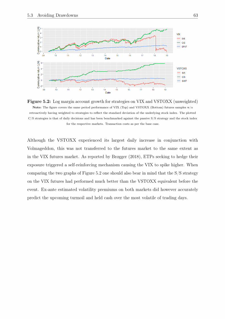
5.3 Avoiding Drawdowns 63

Figure 5.2: Log margin account growth for strategies on VIX and VSTOXX (unweighted)Note: The figure covers the same period performance of VIX (Top) and VSTOXX (Bottom) futures samples w/o

retroactively having weighted to strategies to reflect the standard deviation of the underlying stock index. The plotted

C/S strategies is that of daily decisions and has been benchmarked against the passive S/S strategy and the stock index

for the respective markets. Transaction costs as per the base case.

Although the VSTOXX experienced its largest daily increase in conjunction with

Volmageddon, this was not transferred to the futures market to the same extent as

in the VIX futures market. As reported by Brøgger (2018), ETPs seeking to hedge their

exposure triggered a self-reinforcing mechanism causing the VIX to spike higher. When

comparing the two graphs of Figure 5.2 one should also bear in mind that the S/S strategy

on the VIX futures had performed much better than the VSTOXX equivalent before the

event. Ex-ante estimated volatility premiums on both markets did however accurately

predict the upcoming turmoil and held cash over the most volatile of trading days.

64

6 Conclusion

The introduction of volatility indexes and their role as underlying risk-factors in derivative

instruments have undoubtedly provided the financial markets with efficient tools for

hedging market risk. It is the demand from investors seeking to hedge their portfolios that

drives the volatility futures term structure to most often be in contango, which makes

it possible to profit from short positions. However, in of era when volatility has been

low, small changes in the underlying stock index causes volatility of volatility to increase

which makes short strategies more susceptible to large drawdowns. The thesis answers

the question of whether it is possible to trade on the volatility premium actively and

thereby avoid losses associated with an event such as February 5th. It is demonstrated that

passively trading either long or short positions in volatility futures is not a sustainable

source of profit and that actively trading the on the volatility premium can generate

profitable returns on both the U.S. and European market.

Since the volatility futures term structure can suddenly move from contango to

backwardation, accurately predicting these swings can serve as an additional source

of returns for strategies trading both long and short positions. However, because there

are fewer and shorter periods of backwardation than contango and that the subsequent

investment environment is volatile, strategies with a long component suffer from drawdowns

to a more considerable extent than those holding cash when the estimated premium is

negative. Due to longer holding periods, this is especially true for monthly strategies.

The estimated volatility premium consists of both a forecast of the volatility index and

the futures price which means that the volatility premium requires both accurate model

performance and futures prices that are informationally efficient. For the futures prices to

reflect all relevant information it requires actively traded markets. Thus, liquidity also

affects the ex-ante estimated premium. The result suggests that the VIX premium serves

as a better prediction of realized returns over longer horizons compared to the VSTOXX

premium and that the less liquid European market might be an explanation.

Trading more frequently introduces a trade-off between the informational value of the

volatility premium and transaction costs. While the trade-off comes at a lower price in

terms of transaction costs in the U.S. market, the relative improvement in the informational

6.1 Suggestions for Future Research 65

value of the estimated premiums is larger in the European market, rendering strategies on

VSTOXX futures to be the most profitable and attractive over the investigated sample.

However, it should be mentioned that these strategies, due to the much lower traded

volumes, are more sensitive to the trading activity which questions whether it is possible

to scale up volatility futures strategies on the European market.

Although active volatility strategies are very volatile, they provide attractive risk-adjusted

returns in both U.S. and European markets. The ex-ante estimated volatility premiums

allows active strategies to avoid much of the larger drawdowns. An era of passively

investing in volatility might be over, but trading volatility actively still seems to be a

source of portfolio alpha.

6.1 Suggestions for Future Research

The thesis establishes that there most likely is a link between the signaling value of the

ex-ante estimated volatility premium and market liquidity. However, this stands to be

proven empirically, which provides an interesting research question for future studies.

That is, empirically investigating the finding of the VIX premium having relatively more

informational value than that of the VSTOXX premium when trading monthly.

When estimating the volatility premium, the thesis uses static ARMA(p,q) models that

have been estimated out of sample. An alternative approach would be to reestimate the

models by using a rolling window sample which might increase model performance and

better capture the seasonal components in volatility indexes as mentioned in Mencia and

Sentana (2013) for the VIX. Cheng (2018) reports that a rolling window approach has

been tested for the sample period 2004 through 2015 and it does not affect the forecast

performance significantly. However, this still stands to be tested for a more extended

sample period and for forecasting the VSTOXX time series.

66 References

References

Ahmed, S. (2018). Short volatility trading losses a cautionary tale for using leverage.Reuters. Available Online: https://reut.rs/2WclThj [Accessed: 16 January 2019].

Alexander, C., Kapraun, J., and Korovilas, D. (2015). Trading and investing in volatilityproducts. Financial Markets, Institutions and Instruments, 24(4):313–347.

Amihud, Y., Mendelson, H., and Pedersen, H. L. (2005). Liquidity and asset prices.Foundations and Trends in Finance, 1:269–364.

Andersen, T. and Benzoni., L. (2009). Handbook of Financial Time Series. Berlin:Springer-Verlag.

Arnold, T. and Earl, J. (2018). Calculating the vix in excel. Working Paper. AvailableOnline: https://bit.ly/2XTB54e [Accessed: 16 January 2019].

Avellanda, M. and Papanicolaou, A. (2017). Statistics of futures and applications totrading volatility exchange-traded products. The Journal of Investment Strategies,7(2):1–33.

Bakshi, G. and Kapdia, N. (2003). Delta-hedged gains and the negative market volatilityrisk premium. The Review of Financial Studies, 16(2):527–566.

Bekaert, G. and Hoerova, M. (2014). The vix, the variance premium and stock marketvolatility. Journal of Econometrics, 183(2):181–192.

Bollen, N. and Whaley, R. (2004). Does net buying pressure affect the shape of impliedvolatility functions? Journal of Finance, 59:475–495.

Bollerslev, T., Tauchen, G., and Zhou, H. (2009). Expected stock returns and variancerisk premia. Review of Financial Studies, 22:4463–4492.

Bollerslev, T. and Todorov, V. (2011). Tails, fears, and risk premia. Journal of Finance,66:2165–2211.

Breeden, D. T. and Litzenberger, R. (1978). Prices of state-contingent claims implicit inoption prices. The Journal of Business, 51:621–651.

Brodie, M., Chernov, M., and Johannes, M. (2007). Model specification and risk premia:Evidence from futures options. Journal of Finance, 62:1453–1490.

Brøgger, S. B. (2018). Afledte vix produkter: Logrer halen med hunden? Finans/Invest,3:28–35.

Brøgger, S. B. (2019). Leveraged etps and the vix futures market. Working Paper.

Carhart, M. (1997). On persistence in mutual fund performance. The Journal of Finance,52:57–82.

Carr, P. and Madan, D. (2001). Optimal positioning in derivative securities. QuantatativeFinance, 1:19–37.

Carr, P. and Wu, L. (2006). A tale of two indices. Journal of Derivatives, 13:13–29.

https://reut.rs/2WclThj

https://bit.ly/2XTB54e

References 67

Carr, P. and Wu, L. (2009). Variance risk premiums. The Review of Financial Studies,22(3):1312–1341.

CBOE (2018). White paper cboe volatility index (pdf). CBOE Exchange Inc. AvailableOnline: https://bit.ly/2u5Y7Yf [Accessed: 16 January 2019].

CBOE (2019). Settlement information for vix derivatives. CBOE Exchange Inc. AvailableOnline: https://bit.ly/2EXNb3K [Accessed: 17 January 2019].

Cheng, I. H. (2018). The vix premium. The Review of Financial Studies, 32(1):180–227.

Corsi, F. (2009). A simple approximate long memory model of realized volatility. Journalof Financial Econometrics, 7:174–196.

Coval, J. D. and Shumway, T. (2018). Expected option returns. Journal of Finance,56:983–1009.

Dash, S. and Moran, M. (2007). Vix futures and options: Pricing and using volatilityproducts to manage downside risk and improve efficiency in equity portfolios. Journalof Trading, 2(3):96–105.

Demeterfi, K., Derman, E., Kamel, M., and Zou, J. (1999). More than you ever wanted toknow about volatility swaps. Goldman Sachs Quantitative Strategies Research Notes.Available Online: https://bit.ly/2EXRADL [Accessed: 23 January 2019].

DGV Solutions (2018). Market observation: After the volpocalypse. DGV Solutions LP.Available Online: https://bit.ly/2CIK1Qt [Accessed: 15 February 2019].

Drimus, G. and Farkas, W. (2013). Local volatility of volatility for the vix market. Reviewof Derivatives Research, 16:267–293.

Eriksen, K. K. (2018). Betting against vix – magic money tree or ticking time bomb.Master Thesis.

ETF World (2010). First etn launched on euro stoxx 50 volatility index on xetra. AvailableOnline: https://bit.ly/2Lrus7p [Accessed: 30 April 2019].

EUREX (2019). Volatility derivatives on eurex exchange: Vstoxx (pdf). Eurex ExchangeGroup. Available Online: https://bit.ly/2FRzqW4 [Accessed: 18 February 2019].

Fama, E. F. and French, K. (1993). Common risk factors in the returns on stocks andbonds. Journal of Financial Economics, 33:3–56.

Fernandes, M., Medeiros, M., and Scharth, M. (2013). Modeling and predicting the cboemarket volatility index. Journal of Banking and Finance, 40:1–10.

French, K. (2019). Description of fama/french factors. (Data Source). Available Online:https://bit.ly/2VDltUu [Accessed: 1 April 2019].

Grossman, S. J. (1995). Dynamic asset allocation and the informational efficiency ofmarkets. Journal of Finance, 3:773–787.

Grossman, S. J. and Stiglitz, J. E. (1980). On the impossibility of informationally efficientmarkets. American Economic Review, 70:393–408.

https://bit.ly/2u5Y7Yf

https://bit.ly/2EXNb3K

https://bit.ly/2EXRADL

https://bit.ly/2CIK1Qt

https://bit.ly/2Lrus7p

https://bit.ly/2FRzqW4

https://bit.ly/2VDltUu

68 References

HKEX (2019). Hsi volatility index futures - vhsi info sheet (pdf). Hong Kong Exchangesand Clearing Limited. Available Online: https://bit.ly/2FFBn6K [Accessed: 1 April2019].

JPX (2019). Nikkei 225 vi futures. Japan Exchange Group. Available Online: https://bit.ly/2uHvcdc [Accessed: 1 April 2019].

Kawa, L. (2019). The day the vix doubled: Tales of ‘volmageddon’. Bloomberg MarketNews. Available Online: https://bloom.bg/2V5n59L [Accessed: 23 March 2019].

Macroption (2019). Vstoxx etf and etn list. Available Online: https://bit.ly/2XUMfoA[Accessed: 30 April 2019].

Mencia, J. and Sentana, E. (2013). Valuation of vix derivatives. Journal of FinancialEconomics, 108:367–391.

Morgan, M. (2018). Evolution of behavior of european volatility: Vstoxx® (pdf). AvailableOnline: https://bit.ly/2ISLV6B [Accessed: 2 May 2019].

Munk, C. (2010). Financial Asset Pricing Theory. Oxford University Press.

Newey, W. and West, K. (1987). A simple, positive semi-definite, heteroskedasticity andautocorrelation consistent covariance matrix. Econometrica, 55:703–708.

Ratner, M. and Chiu, C. (2017). Portfolio effects of vix futures index. QuantitativeFinance and Economics, 1(3):288–299.

Simon, D. (2016). Trading the vix futures roll and volatility premiums with vix options.The Journal of Futures Markets, 37(2):184–208.

Tsay, R. (2010). Analysis of Financial Time Series, volume 3. New Jersey, John Wileyand Sons.

Warren, G. (2012). Can investing in volatility help meet your portfolio objectives? Journalof Portfolio Management, 38(2):82–98.

Whaley, R. (1993). Derivatives on market volatility: Hedging tools long overdue. Journalof Derivatives, 1:71–84.

Whaley, R. (2000). The investor fear gauge. Journal of Portfolio Management, 26:12–17.

Whaley, R. (2008). Understanding vix (pdf). Available Online: https://bit.ly/2XZbuaq[Accessed: 25 January 2019].

https://bit.ly/2FFBn6K

https://bit.ly/2uHvcdc

https://bit.ly/2uHvcdc

https://bloom.bg/2V5n59L

https://bit.ly/2XUMfoA

https://bit.ly/2ISLV6B

https://bit.ly/2XZbuaq

69

Appendix

A1 Derivation of Equation 2.1

As mentioned in Section 2.1, Equation 2.1 is a discrete time approximation of Equation

2.2. This continuous time derivation uses results from Carr and Madan (2001) and largely

builds upon that presented in Eriksen (2018).

To find the fair variance swap rate, KV ARt , that equates the initial value of a variance

swap spanning the interval [0, T ] with payoff σ2RV −KV AR to 0 the realized variance over

the same interval is a function of the daily returns squared

σ2R =

1

T

T−1∑i=o

(Si+1 − Si

Si

)2

(.1)

, where Si denotes the underlying index level at every period i = 0, 1, 2, ..., T which in

the following should be interpreted as daily closing prices. Assuming that the underlying

follows a geometric Brownian motion Equation .1 is a consistent estimator of the variance

of the underlying security.

A 2nd-order Taylor approximation of the logarithm of the underlying index level gives

log(Si+1) ≈ log(Si) +1

Si(Si+1 − Si)−

1

2S2i

(Si+1 − Si)2(Si+1 − Si

Si

)2

≈ −2log

(Si+1

Si

)+ 2

(Si+1 − Si

Si

) (.2)

Summing both sides of Equation .2 over the periods i = 0, 1, 2, ..., T yields

T−1∑i=o

(Si+1 − Si

Si

)2

≈ −2log

(STS0

)+ 2

T−1∑i=0

(Si+1 − Si

Si

)(.3)

The left side of Equation .3 is the floating leg of the swap31 and can be replicated by

going short 2 log-contracts and dynamically trade long forward contracts spanning the

31That is σ2RV in Equation .1

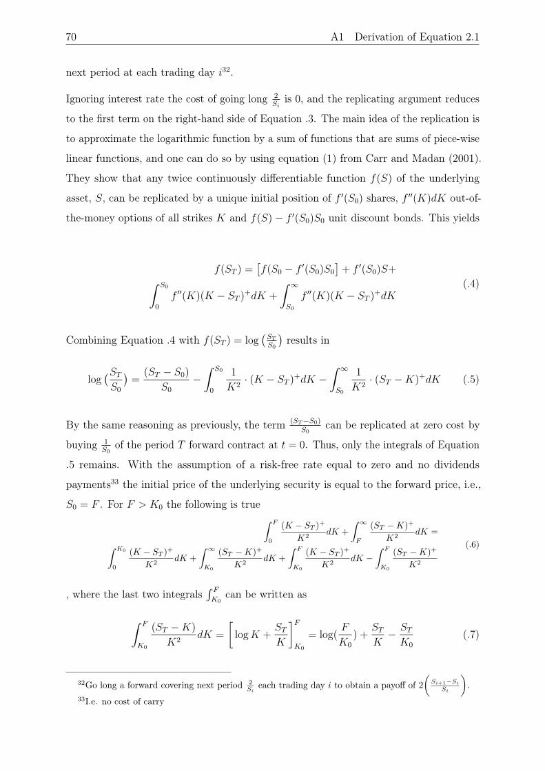
70 A1 Derivation of Equation 2.1

next period at each trading day i32.

Ignoring interest rate the cost of going long 2Si

is 0, and the replicating argument reduces

to the first term on the right-hand side of Equation .3. The main idea of the replication is

to approximate the logarithmic function by a sum of functions that are sums of piece-wise

linear functions, and one can do so by using equation (1) from Carr and Madan (2001).

They show that any twice continuously differentiable function f(S) of the underlying

asset, S, can be replicated by a unique initial position of f ′(S0) shares, f ′′(K)dK out-of-

the-money options of all strikes K and f(S)− f ′(S0)S0 unit discount bonds. This yields

f(ST ) =[f(S0 − f ′(S0)S0

]+ f ′(S0)S+∫ S0

0

f ′′(K)(K − ST )+dK +

∫ ∞S0

f ′′(K)(K − ST )+dK(.4)

Combining Equation .4 with f(ST ) = log(ST

S0

)results in

log(STS0

)=

(ST − S0)

S0

−∫ S0

0

1

K2· (K − ST )+dK −

∫ ∞S0

1

K2· (ST −K)+dK (.5)

By the same reasoning as previously, the term (ST−S0)S0

can be replicated at zero cost by

buying 1S0

of the period T forward contract at t = 0. Thus, only the integrals of Equation

.5 remains. With the assumption of a risk-free rate equal to zero and no dividends

payments33 the initial price of the underlying security is equal to the forward price, i.e.,

S0 = F . For F > K0 the following is true ∫ F

0

(K − ST )+

K2dK +

∫ ∞F

(ST −K)+

K2dK =∫ K0

0

(K − ST )+

K2dK +

∫ ∞K0

(ST −K)+

K2dK +

∫ F

K0

(K − ST )+

K2dK −

∫ F

K0

(ST −K)+

K2

(.6)

, where the last two integrals∫ FK0

can be written as

∫ F

K0

(ST −K)

K2dK =

[logK +

STK

]FK0

= log(F

K0

) +STK− STK0

(.7)

32Go long a forward covering next period 2Si

each trading day i to obtain a payoff of 2(Si+1−Si

Si

).

33I.e. no cost of carry

A1 Derivation of Equation 2.1 71

and put-call-parity was used to obtain (K-ST )+-(ST -K)+=(K-ST ).

So far it has been shown that the realized variance over the time interval [0, T ] can be

replicated by a portfolio that is constructed of call and put options with the same maturity

T and different strikes.

Defining the time to maturity of the options measured in years as T one can get to the fair

value of a variance swap by combining Equations .1, .3 and .5 to get KV AR = EQ[σ2RV ] as

2

T

(∫ F

0

EQ[K-ST )+]K2

dK+∫ ∞F

EQ[ST -K)+]

K2dK+ log

(EQ[ST ]

K0

)+EQ[ST ]

F-EQ[ST ]

K0

)

=2

TerT

(∫ F

0

P (K,T )

K2dK+

∫ ∞F

C(K,T )

K2dK

)+

2

T

(log

(F

K0

)+(1− F

K0

)) (.8)

, where the final term 2T

(·) ≈ − 1T

( FK0− 1)2, C(K,T ) and P (K,T ) are European style call

and put options respectively maturing in T years with strike K. Equation .8 also uses

the risk-neutral assumption of EQ[ST ] = F and a 2nd order Taylor expansion of log( FK0

)

around 1.

Now, defining Q(Ki) as the price of an out of the money option with strike Ki and writing

the expression in discrete time we get

σ2Tj

=2

Tj+∑i

∆Ki

K2i

erTQ(Ki)−1

Tj

[F

K0

− 1

]2(.9)

, which is the same as Equation 2.1.

72 A2 Descriptive Statistics

A2 Descriptive Statistics

Table A2.1: Descriptive statistics of VIX

Training data1990-01-02/2005-12-31

Test data2006-01-01/2018-12-31

Full sample1990-01-02/2018-12-31

Nr. of observations 4,033 3,271 7,304Mean 19.44 19.064 19.27Median 18.40 16.35 17.40Minimum 9.31 9.14 9.14Maximum 45.74 80.86 80.86Standard deviation 6.40 9.25 7.81Skewness 0.949 2.46 2.09Kurtosis 0.749 8.27 7.70

Jarque-Bera 0.00 0.00 0.00ADF (AIC/BIC) 0.00/0.00 0.00/0.00 0.00/0.00PP 0.00 0.00 0.00Note: Test Sample for the VIX starts in 2006 due to irregular maturities of VIX futures between2004-2006.

Table A2.2: Descriptive statistics of VSTOXX

Training data1999-01-04/2009-06-01

Test data2009-06-02/2018-12-28

Full sample1991-01-04/2018-12-28

Nr. of observations 2,648 2,441 5,089Mean 25.93 22.23 24.16Median 23.52 21.12 22.28Minimum 11.6 10.68 10.68Maximum 87.51 53.55 87.51Standard devation 11.09 6.91 9.50Skewness 1.43 1.11 1.63Kurtosis 2.27 1.70 3.64

Jarque-Bera 0.00 0.00 0.00ADF (AIC/BIC) 0.05/0.05 0.00/0.00 0.00/0.00PP 0.015 0.00/0.00 0.00Note: Test data since the inception of VSTOXX futures in June 2009.

A3 Properties of ARMA Models 73

A3 Properties of ARMA Models

ARMA models combine the ideas of AR and MA models into a compact form keeping

the number of parameters small, which allows for a more parsimonious model in terms of

parameterization. A time series, Yt, follows an ARMA(1,1) process if it satisfies

Yt − βtYt−1 = β0 + εt − δ1εt−1 (.10)

, where the right-hand side represents the AR(1) process, and the left-hand side represents

the MA(1) process. εt is a white noise series. For the model to be relevant, β1 6= δ1 must

hold. (Tsay, 2010)

The data needs to be stationary in order to apply an ARMA model. A process Yt is

strictly stationary if the distribution of a subset of Yt(Yt1, ..., Ytk) is identical to that of

(Yt1+t, ..., Ytk+t) for all t, where k is an arbitrary positive integer. However, this condition

is hard to prove empirically, and weak stationarity is often assumed. Weak stationarity,

or covariance stationarity, essentially means that both the mean of Yt and the covariance

of Yt and Ytk are independent of time. Consider the case of a general ARMA(p,q) model

of the form

Yt = β0 +

p∑i=1

βiYt−i + εt −q∑i=1

δiεi (.11)

, where εt is a white noise series, and p and q are positive integers. With lag-operators,

the model can be written as

(1− β1L− ...− βpLp)Yt = β0 + (1− δ1L− ...− δqLq)εt (.12)

The left-hand side polynomial represents the AR process, and the right-hand side

polynomial represents the MA process. Y is weakly stationary if all roots on the inverse

characteristic equation lie outside the unit circle, i.e., the solutions of the Equation .12

are larger than one. If the parameter β in Equation .11 is larger than one, the process will

not decay over time and the time series would suffer from non-stationarity in the form

of a deterministic trend. In the case when the parameter is equal to one, we have the

problem with a stochastic trend, also known as a random walk. (Tsay, 2010)

74 A4 Model Selection

A4 Model Selection

All table reports the results from estimated ARMA models for the respective implied

volatility indexes at the daily frequency for each respective sample period. µ denotes

the estimated mean, βi denotes the i-th order estimated AR term, and δi the i-th order

estimated MA term. Bold coefficients indicate those that are significantly different from

zero at the 5% level.

To give a visual indication of the appropriateness of an ARMA model, the ACF and PACF

of each index is graphed together with the ACF of the chosen model:s residuals.

Table A4.1: VIX ARMA forecast models

(1) (2) (3) (4) (5) (6) (7) (8) (9) (10)ARMA (1,0) (1,1) (1,2) (1,3) (2,0) (2,1) (2,2) (2,3) (3,0) (3,1)µ 19.444 19.444 19.443 19.443 19.444 19.351 19.423 19.399 19.444 19.418

1.041 1.084 1.215 1.318 1.075 1.607 1.556 1.547 1.164 1.547β1 0.982 0.983 0.987 0.989 0.949 1.766 1.669 1.683 0.946 1.734

0.003 0.003 0.003 0.002 0.016 0.039 0.671 0.088 0.016 0.048β2 0.034 -0.768 -0.671 -0.685 -0.045 -0.787

0.016 0.038 0.060 0.087 0.022 0.046β3 0.083 0.051

0.016 0.018δ1 -0.041 -0.053 -0.055 -0.861 -0.735 0.749 -0.800

0.014 0.016 0.016 0.032 0.062 0.090 0.046δ2 -0.097 -0.099 -0.058 -0.059

0.017 0.017 0.020 0.020δ3 -0.068 -0.006

0.017 0.024Log Lh -6,490.3 -6,487.5 -6,471.1 -6,462.9 -6,488.0 -6,458.9 -6,455.0 -6,454.9 -6,474.2 -6,455.1BIC 13,005.4 13,008.3 12,983.7 12,975.7 13,009.2 12,959.8 12,959.3 12,968.0 12,990.0 12,959.9AIC 12,986.5 12,983.1 12,952.2 12,937.9 12,984.0 12,927.8 12,922.0 12,923.9 12,958.4 12,922.1T 4,033 4,033 4,033 4,033 4,033 4,033 4,033 4,033 4,033 4,033Note: The chosen model for the expectation of the VIX under the physical measure is ARMA(2,2).

Figure A4.1: ACF and PACF of VIXNote: The ARMA(2,2) reduces the level of the serial correlation since there are only a few significant lags in the ACF.

This is also formally tested in a Box-Jenkins test.

A4 Model Selection 75

Table A4.2: VSTOXX ARMA forecast models

(1) (2) (3) (4) (5) (6) (7) (8) (9) (10)ARMA (1,0) (1,1) (1,2) (1,3) (2,0) (2,1) (2,2) (2,3) (3,0) (3,1)µ 25.934 25.9335 25.94 25.937 25.933 25.928 25.962 25.942 25.934 25.959

2.486 2.574 2.843 3.095 2.55 2.561 3.045 2.976 2.776 2.986β1 0.986 0.987 0.990 0.992 0.956 0.034 1.402 0.188 0.954 1.418

0.003 0.003 0.003 0.003 0.020 0.062 0.127 0.055 0.020 0.137β2 0.030 0.940 -0.407 0.795 -0.058 -0.508

0.020 0.061 0.126 0.054 0.027 0.126β3 0.091 0.084

0.020 0.023δ1 -0.038 -0.052 -0.032 0.930 -0.458 0.769 -0.470

0.022 0.019 0.020 0.075 0.126 0.057 0.138δ2 -0.087 -0.094 -0.077 -0.124

0.019 0.018 0.022 0.025δ3 -0.097 -0.160

0.021 0.020Log Lh -5,359.9 -5,358.4 -5,347.5 -5,336.5 -5,358.7 -5,352.6 -5,343.4 -5,323.0 -5,347.8 -5,342.36BIC 10,743.4 10,748.3 10,734.5 10,720 10,748.9 10,744.6 10,733.4 10,701.1 10,734.9 10,732.0AIC 10,725.8 10,724.8 10,705.1 10,685.0 10,725.4 10,715.1 10,698.1 10,659.9 10,705.5 10,696.7T 2,648 2,648 2,648 2,648 2,648 2,648 2,648 2,648 2,648 2,648Note: The chosen model for the expectation of the VIX under the physical measure is ARMA(2,3).

Figure A4.2: ACF and PACF of VSTOXXNote: The ARMA(2,3) reduces the level of the serial correlation since there are only a few significant lags in the ACF.

This is also formally tested in a Box-Jenkins test.

76 A5 Factor Loadings

A5 Factor Loadings

Portfolio factors are used to test the presence of pricing errors or performance not

attributable to tradable portfolios and are central in both asset pricing and portfolio

management. This section outlines a brief summary. For an in depth presentation see e.g.

Munk (2010).

If a factor xit is the return of a traded portfolio i at time t, like those presented in Fama

and French (1993) and Carhart (1997), the intercept, or α, is interpreted as a presence of

pricing errors or asset manager skills. For expositional simplicity, the section lays out a

one-factor model as an example. Tested in a time series regressions expressed as

Rit −R

ft = α + bi(x

it −R

ft ) + εt (.13)

, where Rit is the return of some asset (or strategy) i at time t, Rf

t is the risk-free rate (here

assumed to be constant), α the model intercept and bi the slope coefficient of factor i, and

εt a well-behaved error term. The OLS procedure yields an estimate of bi as b̂i = Cov(Ri,xi)V ar(xi)

.

The estimate of the slope coefficient, b̂i, is the exposure of Ri to a given risk-factor xi.

Under the condition that the risk factor, xi , is a traded portfolio like those presented by

Fama and French (1993) and Carhart (1997) it must be possible to price the factor itself

by the model. Thus, it can be put on the r.h.s. of the model as

xit −Rft = α + bi(x

it −R

ft ) + εt t = 1, 2, ..., T (.14)

, which, as any variable regressed on itself, will result in α = 0 and b̂i = 1. Consequently,

per the nature of OLS, if the unconditional expectation E[.] of .14 applied to any asset

(or strategy) return, Rit will result in

E[Rit −R

ft ] = α̂ + b̂iE[xit −R

ft ] + εt (.15)

If the estimated intercept α̂ 6= 0 and coefficient b̂i 6= 1, it serves as an indication of either

pricing errors or asset manager skills.

A6 L/S/C strategies - Sharpe Ratio Tables 77

A6 L/S/C strategies - Sharpe Ratio Tables

This thesis retroactively chose signal thresholds to maximize the performance of L/S/C

strategies. The evaluated performance is in terms of Sharpe ratios. Several different signal

threshold combinations are tested, all of which are reported in the tables below.

Table A6.1: Sharpe ratios for monthly L/S/C strategies on VIX (full sample)

0.0 0.2 0.4 0.6 0.8 1.0 1.2 1.4 1.6 1.8 2.00.0 0.64 0.59 0.58 0.61 0.59 0.59 0.51 0.62 0.61 0.54 0.540.2 0.70 0.65 0.64 0.67 0.66 0.66 0.58 0.70 0.69 0.62 0.620.4 0.79 0.75 0.74 0.79 0.78 0.78 0.69 0.87 0.87 0.78 0.780.6 0.75 0.71 0.70 0.75 0.73 0.73 0.64 0.83 0.83 0.74 0.740.8 0.79 0.74 0.74 0.79 0.78 0.78 0.69 0.89 0.89 0.80 0.801.0 0.81 0.76 0.76 0.81 0.80 0.80 0.71 0.92 0.92 0.84 0.831.2 0.81 0.76 0.76 0.81 0.80 0.80 0.71 0.93 0.94 0.85 0.851.4 0.84 0.80 0.80 0.85 0.84 0.84 0.76 0.98 0.99 0.90 0.901.6 0.83 0.79 0.79 0.84 0.83 0.83 0.74 0.97 0.98 0.89 0.891.8 0.83 0.79 0.79 0.84 0.83 0.83 0.74 0.97 0.98 0.89 0.892.0 0.84 0.80 0.80 0.85 0.84 0.85 0.76 0.99 1.00 0.91 0.912.2 0.84 0.80 0.80 0.85 0.84 0.85 0.76 0.99 1.00 0.91 0.912.4 0.74 0.69 0.69 0.74 0.73 0.73 0.63 0.87 0.88 0.78 0.782.6 0.74 0.69 0.69 0.74 0.73 0.73 0.63 0.87 0.88 0.78 0.782.8 0.74 0.69 0.69 0.74 0.73 0.73 0.63 0.87 0.88 0.78 0.783.0 0.74 0.69 0.69 0.74 0.73 0.73 0.63 0.87 0.88 0.78 0.78

2.2 2.4 2.6 2.8 3.0 3.2 3.4 3.6 3.8 4.00.0 0.55 0.55 0.59 0.60 0.56 0.56 0.56 0.51 0.50 0.480.2 0.63 0.63 0.68 0.69 0.65 0.65 0.65 0.60 0.59 0.570.4 0.84 0.86 0.93 0.95 0.91 0.91 0.92 0.85 0.84 0.810.6 0.81 0.83 0.91 0.93 0.89 0.88 0.90 0.82 0.81 0.780.8 0.88 0.91 0.99 1.02 0.98 0.98 0.99 0.91 0.91 0.881.0 0.93 0.96 1.05 1.08 1.04 1.04 1.06 0.98 0.98 0.941.2 0.95 0.99 1.09 1.12 1.09 1.09 1.11 1.03 1.03 0.991.4 1.02 1.07 1.18 1.20 1.18 1.18 1.20 1.12 1.12 1.091.6 1.01 1.06 1.17 1.20 1.17 1.17 1.20 1.11 1.12 1.091.8 1.01 1.06 1.17 1.20 1.17 1.17 1.20 1.11 1.12 1.092.0 1.05 1.10 1.22 1.25 1.23 1.23 1.26 1.17 1.18 1.152.2 1.05 1.10 1.22 1.25 1.23 1.23 1.26 1.17 1.18 1.152.4 0.90 0.96 1.09 1.13 1.11 1.11 1.15 1.04 1.05 1.032.6 0.90 0.96 1.09 1.13 1.11 1.11 1.15 1.04 1.05 1.032.8 0.90 0.96 1.09 1.13 1.11 1.11 1.15 1.04 1.05 1.033.0 0.90 0.96 1.09 1.13 1.11 1.11 1.15 1.04 1.05 1.03Note: The horizontal (vertical) table header is the imposed positive (negative) signal.Transaction costs as per the base case.

Table A6.2: Sharpe ratios for monthly L/S/C strategies on VSTOXX

0.0 0.2 0.4 0.6 0.8 1.0 1.2 1.4 1.6 1.8 2.0 2.2 2.4 2.6 2.8 3.00.0 0.16 0.18 0.23 0.15 0.17 0.21 0.15 0.12 -0.02 -0.02 -0.02 -0.09 -0.10 -0.10 -0.10 -0.130.2 0.18 0.20 0.26 0.18 0.19 0.23 0.18 0.14 0.00 0.00 0.00 -0.07 -0.08 -0.08 -0.09 -0.120.4 0.25 0.28 0.35 0.26 0.28 0.32 0.26 0.23 0.09 0.09 0.08 0.01 0.00 0.00 0.00 -0.030.6 0.27 0.30 0.37 0.29 0.30 0.35 0.29 0.26 0.11 0.11 0.10 0.03 0.02 0.02 0.01 -0.020.8 0.28 0.31 0.39 0.30 0.31 0.37 0.30 0.27 0.11 0.11 0.10 0.03 0.01 0.01 0.01 -0.031.0 0.25 0.29 0.37 0.27 0.29 0.35 0.28 0.24 0.06 0.06 0.05 -0.04 -0.05 -0.05 -0.06 -0.101.2 0.19 0.22 0.31 0.20 0.22 0.28 0.20 0.16 -0.04 -0.04 -0.05 -0.16 -0.18 -0.18 -0.18 -0.231.4 0.22 0.25 0.34 0.23 0.25 0.32 0.24 0.19 -0.01 -0.01 -0.02 -0.13 -0.15 -0.15 -0.16 -0.211.6 0.27 0.31 0.41 0.30 0.33 0.40 0.32 0.27 0.06 0.06 0.05 -0.05 -0.07 -0.07 -0.08 -0.131.8 0.37 0.43 0.55 0.44 0.48 0.58 0.49 0.45 0.19 0.19 0.18 0.04 0.02 0.02 0.01 -0.072.0 0.24 0.45 0.58 0.47 0.50 0.62 0.52 0.49 0.22 0.22 0.21 0.06 0.04 0.04 0.03 -0.052.2 0.39 0.46 0.59 0.48 0.52 0.63 0.53 0.51 0.23 0.23 0.23 0.08 0.06 0.06 0.05 -0.032.4 0.41 0.48 0.62 0.51 0.55 0.67 0.57 0.55 0.27 0.27 0.27 0.13 0.11 0.11 0.11 0.022.6 0.42 0.49 0.63 0.52 0.56 0.69 0.59 0.56 0.28 0.28 0.28 0.13 0.11 0.11 0.10 0.012.8 0.42 0.49 0.64 0.53 0.57 0.70 0.60 0.58 0.29 0.29 0.29 0.14 0.12 0.12 0.12 0.023.0 0.42 0.49 0.64 0.53 0.57 0.70 0.60 0.58 0.29 0.29 0.29 0.14 0.12 0.12 0.12 0.023.2 0.42 0.49 0.64 0.53 0.57 0.70 0.60 0.58 0.29 0.29 0.29 0.14 0.12 0.12 0.12 0.023.4 0.42 0.49 0.64 0.53 0.57 0.70 0.60 0.58 0.29 0.29 0.29 0.14 0.12 0.12 0.12 0.023.6 0.47 0.55 0.70 0.60 0.64 0.78 0.68 0.67 0.39 0.39 0.39 0.26 0.25 0.25 0.26 0.163.8 0.47 0.55 0.70 0.60 0.64 0.78 0.68 0.67 0.39 0.39 0.39 0.26 0.25 0.25 0.26 0.164.0 0.47 0.55 0.70 0.60 0.64 0.78 0.68 0.67 0.39 0.39 0.39 0.26 0.25 0.25 0.26 0.16Note: The horizontal (vertical) table header is the imposed positive (negative) signal. Transaction costs as per the base case.

78 A6 L/S/C strategies - Sharpe Ratio Tables

Table A6.3: Sharpe ratios for daily L/S/C strategies on VIX (full sample)

0.0 0.2 0.4 0.6 0.8 1.0 1.2 1.4 1.6 1.8 2.0 2.2 2.4 2.6 2.8 3.00.0 0.96 1.01 1.02 1.05 1.13 1.02 0.94 0.85 0.84 0.83 0.85 0.85 0.87 0.88 0.90 0.860.2 1.08 1.13 1.15 1.18 1.27 1.16 1.08 0.99 0.98 0.97 0.99 1.00 1.02 1.03 1.05 1.010.4 1.11 1.17 1.19 1.22 1.31 1.20 1.12 1.03 1.03 1.01 1.04 1.05 1.07 1.08 1.10 1.060.6 1.04 1.10 1.11 1.14 1.24 1.13 1.04 0.95 0.94 0.93 0.96 0.97 0.98 0.99 1.02 0.980.8 1.06 1.12 1.14 1.17 1.27 1.16 1.07 0.97 0.97 0.96 0.99 1.00 1.02 1.03 1.06 1.021.0 1.05 1.11 1.13 1.16 1.26 1.15 1.06 0.96 0.96 0.94 0.97 0.98 1.00 1.02 1.05 1.011.2 1.05 1.12 1.14 1.17 1.28 1.16 1.07 0.97 0.97 0.96 0.99 1.00 1.02 1.03 1.07 1.021.4 0.93 1.00 1.02 1.05 1.16 1.03 0.93 0.83 0.83 0.81 0.84 0.85 0.87 0.89 0.92 0.871.6 1.00 1.07 1.09 1.13 1.24 1.12 1.02 0.91 0.92 0.90 0.93 0.95 0.97 0.99 1.03 0.981.8 1.03 1.11 1.13 1.17 1.28 1.16 1.06 0.95 0.96 0.95 0.98 1.00 1.02 1.04 1.08 1.042.0 1.01 1.08 1.10 1.14 1.26 1.12 1.03 0.92 0.92 0.91 0.94 0.96 0.99 1.00 1.04 1.002.2 0.98 1.06 1.09 1.14 1.28 1.14 1.03 0.91 0.92 0.92 0.96 0.99 1.03 1.06 1.13 1.082.4 0.99 1.07 1.10 1.15 1.30 1.15 1.05 0.92 0.94 0.93 0.98 1.01 1.05 1.09 1.15 1.112.6 1.03 1.12 1.14 1.20 1.35 1.20 1.10 0.97 1.00 0.99 1.04 1.08 1.12 1.16 1.23 1.202.8 1.01 1.09 1.12 1.17 1.32 1.18 1.07 0.94 0.96 0.96 1.01 1.04 1.09 1.13 1.20 1.163.0 1.02 1.10 1.13 1.19 1.34 1.19 1.09 0.96 0.98 0.98 1.03 1.07 1.11 1.16 1.23 1.19Note: The horizontal (vertical) table header is the imposed positive (negative) signal. Transaction costs as per the base case.

Table A6.4: Sharpe ratios for daily L/S/C strategies on VSTOXX

0.0 0.2 0.4 0.6 0.8 1.0 1.2 1.4 1.6 1.8 2.0 2.2 2.4 2.6 2.8 3.00.0 1.54 1.52 1.46 1.38 1.27 1.32 1.25 1.31 1.30 1.27 1.25 1.20 1.13 1.11 1.09 1.000.2 1.65 1.63 1.58 1.49 1.39 1.44 1.37 1.43 1.42 1.39 1.37 1.32 1.25 1.24 1.21 1.130.4 1.80 1.78 1.72 1.64 1.53 1.58 1.51 1.58 1.57 1.54 1.52 1.47 1.41 1.39 1.37 1.280.6 1.76 1.74 1.68 1.60 1.49 1.55 1.47 1.54 1.54 1.51 1.48 1.43 1.37 1.35 1.32 1.240.8 1.86 1.84 1.78 1.69 1.58 1.64 1.57 1.64 1.63 1.61 1.59 1.53 1.47 1.45 1.42 1.341.0 1.75 1.73 1.67 1.58 1.47 1.53 1.45 1.52 1.52 1.49 1.47 1.41 1.34 1.33 1.30 1.211.2 1.84 1.32 1.76 1.67 1.56 1.62 1.54 1.62 1.61 1.59 1.56 1.51 1.45 1.43 1.40 1.311.4 1.82 1.80 1.73 1.65 1.53 1.59 1.51 1.59 1.58 1.56 1.54 1.48 1.41 1.39 1.36 1.281.6 1.73 1.71 1.64 1.55 1.43 1.49 1.41 1.49 1.48 1.45 1.43 1.37 1.30 1.28 1.25 1.161.8 1.73 1.71 1.64 1.55 1.42 1.49 1.40 1.48 1.48 1.45 1.43 1.37 1.30 1.28 1.25 1.152.0 1.76 1.73 1.67 1.57 1.44 1.51 1.43 1.51 1.51 1.48 1.46 1.40 1.33 1.31 1.28 1.182.2 1.54 1.66 1.59 1.49 1.36 1.43 1.34 1.43 1.43 1.40 1.37 1.31 1.23 1.21 1.18 1.072.4 1.54 1.52 1.44 1.33 1.18 1.26 1.17 1.26 1.26 1.22 1.20 1.12 1.04 1.01 0.97 0.852.6 1.42 1.39 1.31 1.19 1.03 1.12 1.01 1.11 1.11 1.07 1.04 0.96 0.86 0.83 0.78 0.642.8 1.40 1.37 1.28 1.17 1.01 1.09 0.99 1.09 1.08 1.04 1.01 0.93 0.83 0.80 0.75 0.603.0 1.32 1.30 1.21 1.09 0.92 1.01 0.89 1.00 0.99 0.95 0.91 0.82 0.71 0.68 0.63 0.47Note: The horizontal (vertical) table header is the imposed positive (negative) signal. Transaction costs as per the base case.

Table A6.5: Sharpe ratios for monthly L/S/C strategies on VIX (Jun 2009 - Dec 2018)

0.0 0.2 0.4 0.6 0.8 1.0 1.2 1.4 1.6 1.8 2.00.0 0.57 0.54 0.54 0.57 0.56 0.58 0.50 0.64 0.61 0.58 0.580.2 0.64 0.61 0.61 0.65 0.64 0.67 0.58 0.73 0.71 0.68 0.680.4 0.76 0.74 0.64 0.80 0.79 0.84 0.74 1.00 0.98 0.95 0.950.6 0.70 0.68 0.69 0.75 0.73 0.78 0.68 0.95 0.94 0.90 0.900.8 0.74 0.72 0.73 0.79 0.77 0.83 0.73 1.01 1.00 0.96 0.961.0 0.75 0.72 0.73 0.80 0.78 0.84 0.74 1.03 1.02 0.98 0.981.2 0.75 0.73 0.74 0.81 0.79 0.85 0.75 1.06 1.05 1.01 1.011.4 0.79 0.78 0.79 0.86 0.84 0.91 0.81 1.13 1.13 1.09 1.101.6 0.78 0.76 0.78 0.85 0.83 0.89 0.79 1.12 1.12 1.08 1.081.8 0.78 0.76 0.78 0.85 0.83 0.89 0.79 1.12 1.12 1.08 1.082.0 0.79 0.78 0.79 0.86 0.85 0.91 0.79 1.12 1.12 1.12 1.122.2 0.79 0.78 0.79 0.86 0.85 0.91 0.79 1.12 1.12 1.12 1.122.4 0.79 0.78 0.79 0.86 0.85 0.91 0.79 1.12 1.12 1.12 1.122.6 0.79 0.78 0.79 0.86 0.85 0.91 0.79 1.12 1.12 1.12 1.122.8 0.79 0.78 0.79 0.86 0.85 0.91 0.79 1.12 1.12 1.12 1.123.0 0.79 0.78 0.79 0.86 0.85 0.91 0.79 1.12 1.12 1.12 1.12

2.2 2.4 2.6 2.8 3.0 3.2 3.4 3.6 3.8 4.00.0 0.56 0.49 0.54 0.54 0.49 0.48 0.49 0.46 0.42 0.380.2 0.66 0.59 0.65 0.65 0.60 0.59 0.60 0.57 0.53 0.490.4 1.00 0.91 1.03 1.03 0.98 0.97 0.99 0.94 0.88 0.830.6 0.96 0.87 1.00 1.00 0.95 0.94 0.97 0.90 0.84 0.790.8 1.03 0.95 1.08 1.08 1.04 1.04 1.07 1.00 0.94 0.891.0 1.08 0.99 1.14 1.14 1.10 1.10 1.14 1.07 1.00 0.961.2 1.13 1.04 1.20 1.20 1.18 1.18 1.22 1.15 1.08 1.041.4 1.23 1.16 1.34 1.34 1.32 1.33 1.38 1.31 1.25 1.221.6 1.23 1.15 1.33 1.33 1.33 1.34 1.39 1.31 1.25 1.231.8 1.23 1.15 1.33 1.33 1.33 1.34 1.39 1.31 1.25 1.232.0 1.30 1.23 1.44 1.44 1.45 1.47 1.54 1.45 1.40 1.392.2 1.30 1.23 1.44 1.44 1.45 1.47 1.54 1.45 1.40 1.392.4 1.30 1.23 1.44 1.44 1.45 1.47 1.54 1.45 1.40 1.392.6 1.30 1.23 1.44 1.44 1.45 1.47 1.54 1.45 1.40 1.392.8 1.30 1.23 1.44 1.44 1.45 1.47 1.54 1.45 1.40 1.393.0 1.30 1.23 1.44 1.44 1.45 1.47 1.54 1.45 1.40 1.39Note: The horizontal (vertical) table header is the imposed positive (negative) signal.Transaction costs as per the base case.

A6 L/S/C strategies - Sharpe Ratio Tables 79

Table A6.6: Sharpe ratios for daily L/S/C strategies on VIX (Jun 2009 - Dec 2018)

0.0 0.2 0.4 0.6 0.8 1.0 1.2 1.4 1.6 1.8 2.0 2.2 2.4 2.6 2.8 3.00.0 1.13 1.18 1.20 1.26 1.39 1.22 1.13 1.03 1.04 1.02 1.04 1.01 1.00 1.03 1.06 1.020.2 1.28 1.34 1.36 1.43 1.56 1.39 1.30 1.20 1.21 1.20 1.22 1.20 1.19 1.22 1.25 1.220.4 1.30 1.36 1.39 1.46 1.59 1.42 1.33 1.23 1.25 1.23 1.26 1.23 1.22 1.25 1.29 1.260.6 1.22 1.28 1.31 1.38 1.52 1.34 1.24 1.14 1.15 1.14 1.16 1.14 1.13 1.16 1.20 1.170.8 1.25 1.31 1.34 1.41 1.56 1.38 1.28 1.17 1.19 1.18 1.21 1.18 1.17 1.21 1.25 1.221.0 1.23 1.30 1.32 1.40 1.55 1.37 1.27 1.15 1.18 1.17 1.19 1.17 1.16 1.19 1.23 1.201.2 1.21 1.28 1.30 1.38 1.54 1.35 1.24 1.13 1.15 1.14 1.17 1.14 1.13 1.17 1.21 1.201.4 1.05 1.12 1.14 1.22 1.38 1.18 1.07 0.94 0.96 0.95 0.97 0.94 0.93 0.97 1.01 0,971.6 1.08 1.15 1.18 1.26 1.43 1.23 1.11 0.99 1.01 1.00 1.03 1.00 0.99 1.03 1.01 1.031.8 1.12 1.20 1.22 1.31 1.48 1.28 1.16 1.04 1.07 1.06 1.08 1.06 1.05 1.09 1.14 1.102.0 1.09 1.17 1.19 1.28 1.45 1.24 1.13 1.00 1.03 1.02 1.05 1.02 1.01 1.05 1.10 1.062.2 1.11 1.20 1.23 1.34 1.56 1.33 1.20 1.06 1.11 1.12 1.16 1.14 1.14 1.22 1.31 1.292.4 1.14 1.23 1.28 1.39 1.61 1.38 1.26 1.11 1.17 1.18 1.23 1.22 1.22 1.30 1.40 1.402.6 1.16 1.26 1.30 1.41 1.64 1.41 1.28 1.14 1.20 1.21 1.26 1.25 1.26 1.34 1.45 1.442.8 1.15 1.24 1.28 1.39 1.62 1.39 1.26 1.11 1.18 1.19 1.24 1.23 1.23 1.31 1.42 1.413.0 1.16 1.25 1.30 1.41 1.63 1.40 1.28 1.13 1.20 1.21 1.26 1.25 1.26 1.34 1.44 1.44Note: The horizontal (vertical) table header is the imposed positive (negative) signal. Transaction costs as per the base case.

80 A7 VHSI and VXJ

A7 VHSI and VXJ

The thesis set out to investigate strategies on multiple indexes, but as only VIX and

VSTOXX futures are liquid enough to implement volatility futures strategies on VHSI

and VXJ have been excluded.

In this section of the Appendix statistics for VHSI and VXJ, the data underlying the

decision to exclude these indexes and the indexes correlations with VIX, VSTOXX together

with all underlying stock indexes are presented.

Figure A7.1: Daily closing prices and the empirical distribution of VHSINote: Daily closing price (Left) and distribution (Right) throughout Jan 2001 to Dec 2018.

Source: Bloomberg.

Figure A7.2: Daily closing prices and the empirical distribution of VXJNote: Daily closing price (Left) and distribution (Right) throughout Jan 1998 to Dec 2018.

Source: Bloomberg.

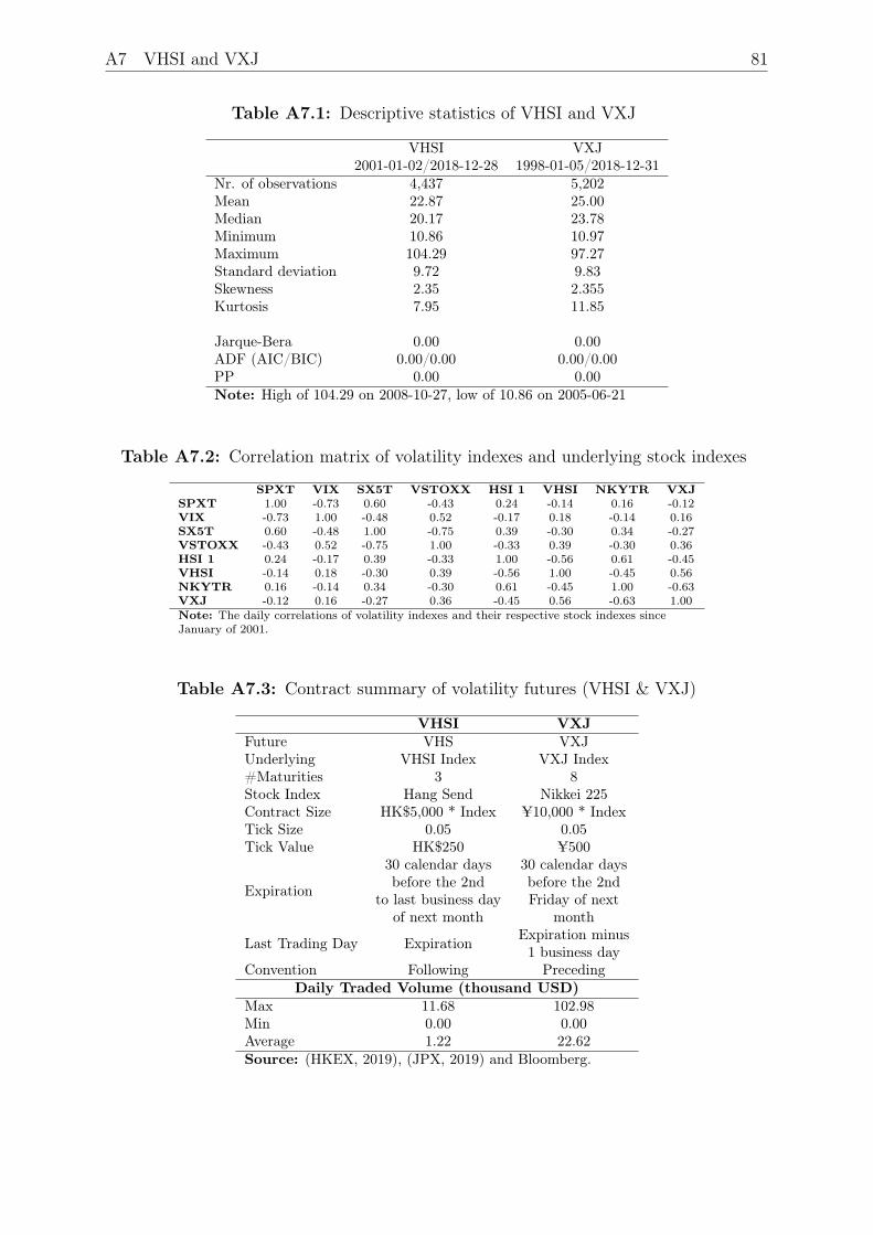
A7 VHSI and VXJ 81

Table A7.1: Descriptive statistics of VHSI and VXJ

VHSI2001-01-02/2018-12-28

VXJ1998-01-05/2018-12-31

Nr. of observations 4,437 5,202Mean 22.87 25.00Median 20.17 23.78Minimum 10.86 10.97Maximum 104.29 97.27Standard deviation 9.72 9.83Skewness 2.35 2.355Kurtosis 7.95 11.85

Jarque-Bera 0.00 0.00ADF (AIC/BIC) 0.00/0.00 0.00/0.00PP 0.00 0.00Note: High of 104.29 on 2008-10-27, low of 10.86 on 2005-06-21

Table A7.2: Correlation matrix of volatility indexes and underlying stock indexes

SPXT VIX SX5T VSTOXX HSI 1 VHSI NKYTR VXJSPXT 1.00 -0.73 0.60 -0.43 0.24 -0.14 0.16 -0.12VIX -0.73 1.00 -0.48 0.52 -0.17 0.18 -0.14 0.16SX5T 0.60 -0.48 1.00 -0.75 0.39 -0.30 0.34 -0.27VSTOXX -0.43 0.52 -0.75 1.00 -0.33 0.39 -0.30 0.36HSI 1 0.24 -0.17 0.39 -0.33 1.00 -0.56 0.61 -0.45VHSI -0.14 0.18 -0.30 0.39 -0.56 1.00 -0.45 0.56NKYTR 0.16 -0.14 0.34 -0.30 0.61 -0.45 1.00 -0.63VXJ -0.12 0.16 -0.27 0.36 -0.45 0.56 -0.63 1.00Note: The daily correlations of volatility indexes and their respective stock indexes sinceJanuary of 2001.

Table A7.3: Contract summary of volatility futures (VHSI & VXJ)

VHSI VXJFuture VHS VXJUnderlying VHSI Index VXJ Index#Maturities 3 8Stock Index Hang Send Nikkei 225Contract Size HK$5,000 * Index ¥10,000 * IndexTick Size 0.05 0.05Tick Value HK$250 ¥500

Expiration

30 calendar daysbefore the 2nd

to last business dayof next month

30 calendar daysbefore the 2ndFriday of next

month

Last Trading Day Expiration Expiration minus1 business day

Convention Following PrecedingDaily Traded Volume (thousand USD)

Max 11.68 102.98Min 0.00 0.00Average 1.22 22.62Source: (HKEX, 2019), (JPX, 2019) and Bloomberg.

82 A7 VHSI and VXJ

Figure A7.3: Historical bid-ask spreads for futures on VHSI and VXJNote: The figure covers the respective VHSI and VXJ futures samples. Reported spreads are in percentages and for thenear-term and next-term contracts. Due to illiquidity and high transaction costs the Cheng (2018) methodology is not

applicable to these indexes.

Source: Bloomberg.

Figure A7.4: Traded vega of VHSI and VXJ futuresNote: Daily traded vega of the one and two month ahead futures contracts on the VIX (Left) and VSTOXX (Right).The traded vega has been plotted using a 21-day moving average to smooth the graphs. All reported volumes are in

million USD. On any given day the number of traded contracts have been multiplied by the respective contract multiplieras reported in Table A7.3. Due to illiquidity and high transaction costs the Cheng (2018) methodology is not applicable

to these indexes

Source: Bloomberg and FRED Economic Data.

Actively Managed Volatility Strategies - CBS Research Portal

Documents

Transcript of Actively Managed Volatility Strategies - CBS Research Portal