Electronic copy available at: http://ssrn.com/abstract=1524222

CREATES Research Paper 2009-59

Modelling the Volatility-Return Trade-off when Volatility may be Nonstationary

Christian M. Dahl and Emma M. Iglesias

School of Economics and Management Aarhus University

Bartholins Allé 10, Building 1322, DK-8000 Aarhus C Denmark

Electronic copy available at: http://ssrn.com/abstract=1524222

Modelling the Volatility-Return Trade-off when Volatility

may be Nonstationary∗

Christian M. Dahl†

CREATES, School of Economics and Management

University of Aarhus

Emma M. Iglesias

Department of Economics

Michigan State University and University of Essex

October 2, 2009

Abstract

In this paper a new GARCH–M type model, denoted the GARCH-AR, is proposed.

In particular, it is shown that it is possible to generate a volatility-return trade-off in

a regression model simply by introducing dynamics in the standardized disturbance

process. Importantly, the volatility in the GARCH-AR model enters the return func-

tion in terms of relative volatility, implying that the risk term can be stationary even

if the volatility process is nonstationary. We provide a complete characterization of

the stationarity properties of the GARCH-AR process by generalizing the results of

Bougerol and Picard (1992b). Furthermore, allowing for nonstationary volatility, the

∗Comments from Tim Bollerslev, Lynda Khalaf, Nour Meddahi, Jeffrey Wooldridge and participants

at seminars at University of Aarhus and at the conferences: 2005 Symposium on Econometric Theory

and Applications (Taipei, Taiwan); the 2006 North American Summer meeting of the Econometric Soci-

ety (Minnesota), 2006 IMS Annual Meeting in Statistics (Rio de Janeiro), 2006 Canadian Econometrics

Group (Niagara Falls, Canada), 2006 European Meeting of the Econometric Society (Vienna) and at the

2009 Conference on Periodicity, Non-stationarity and Forecasting of Economic and Financial Time Series

(Aarhus) are gratefully acknowledged. The first author acknowledges the research support of CREATES

(funded by the Danish National Research Foundation). The second author acknowledges support from the

MSU Intramural Research Grants Program.†Corresponding author. Address: School of Economics and Management, Room 225, Building 1326.

Phone: +45 8942 1559. E-mail: cdahl@creates.au.dk.

1

asymptotic properties of the estimated parameters by quasi-maximum likelihood in

the GARCH-AR process are established. Finally, we stress the importance of being

able to choose correctly between AR-GARCH and GARCH-AR processes: First, it is

shown, by a small simulation study, that the estimators for the parameters in an AR-

GARCH model will be seriously inconsistent if the data generating process actually

is a GARCH-AR process. Second, we provide an LM test for neglected GARCH-AR

effects and discuss its finite sample size properties. Third, we provide an empiri-

cal illustration showing the empirical relevance of the GARCH-AR model based on

modelling a wide range of leading US stock return series.

Key words: Quasi-Maximum Likelihood; GARCH-M Model; Asymptotic Proper-

ties; Risk-return Relation.

JEL Codes: C12, C13; C22, G12.

1 Introduction

Since Merton’s (1973) pathbreaking article deriving the intertemporal Capital Asset Pric-

ing Model, the idea that higher risk assets must have higher expected returns to attract

investors has been a foundation of modern finance theory. The GARCH-M (Generalized

Autoregressive Conditional Heteroskedastic-in-mean) model proposed by Engle, Lilien and

Robins (1987) allows for the direct effect of volatility changes on asset prices through re-

quired returns in a short memory GARCH-type model, by introducing the conditional

volatility function into the conditional mean return equation. Numerous empirical studies

have explored this volatility-return trade-off in attempts to estimate the magnitude of

the trade-off itself. Perhaps surprisingly, both statistical significance and even the sign

of the linear relation between expected return and variance of return have proved elu-

sive in empirical work. Just naming a few studies and confining the listing to studies

using some form of GARCH-in-mean models, for example, confirmation of the positive

volatility-return trade-off is supported by French, Schwert, and Stambaugh (1987), Chou

(1988), Baillie and DeGennaro (1990), and Campbell and Hentschel (1992), while evidence

of a negative risk-return trade-off was found by Nelson (1991) and Glosten, Jagannathan,

and Runkle (1993). Indeed, Campbell and Hentschel (1992) argue that an alternative

source of a negative volatility-return relation is the volatility feedback mechanism, that

is, if volatility is increased, then so is the risk premium, in case of a positive trade-off

between risk and conditional expected return. Hence, the discount rate is also increased,

which in turn, for an unchanged dividend yield, lowers the stock price. Negative premia is

2

also found in recent work in asset pricing focussing on volatility innovations that examines

cross-sectional risk premia induced by covariance between volatility changes and stock

returns, e.g., Ang, Hodrick, Xing, and Zhang (2006). The idea is that since innovations in

volatility are higher during recessions, stocks which co-vary with volatility pay off in bad

states, and so they should require smaller risk premia. For a survey of these and related

studies, see Lettau and Ludvigson (forthcoming).

One possible source of the disagreement is misspecification of the way in which condi-

tional variance enters the conditional mean return equation. Considerations and debates

of this type have lead to the interest in specifying a more flexible model encompassing

these and other alternative volatility-return relations. Flexibility, however, comes at the

cost of more complicated statistical properties and typically also more restrictive assump-

tions on the data generating process. Hodgson and Vorkink (2003) estimate the density

function of a multivariate GARCH-M model in a semiparametric fashion. Linton and Per-

ron (2003), Sun and Stengos (2006), Conrad and Mammen (2008) and Christensen, Dahl

and Iglesias (2008) all propose to use a mean equation given by yt = µ(σ2

t

)+εtσt where yt

is the daily return, E(ε2t σ

2t |It−1

)= σ2

t is the conditional return variance, It−1 denotes the

sigma field generated by the information available up to time t − 1, εt ∼ i.i.d. (0, 1) , and

µ (·) is a smooth mean function determining the functional form of the volatility-return

relation. Common for all these papers is that the specification is estimated semiparamet-

rically, assuming stationary GARCH or exponential GARCH processes for the conditional

variance. Indeed, based on this approach and using CRSP excess return data, a hump

shaped (nonlinear) pattern of the risk premium is generally supported.

However, as pointed out by Christensen, Nielsen and Zhu (2009), a potential statistical

problem with the traditional GARCH-M specification is that possible nonstationarity or

long memory properties of the volatility process may not balance well with the short

memory properties of the return series in the regression model. Whether estimating the

GARCH-M parametrically or semiparametrically, this might give unwanted and spurious

results. The empirical evidence supporting the long memory properties of the volatility

is extensive and includes studies by Robinson (1991), Crato and de Lima (1994), Baillie

et al (1996), Ding and Granger (1996), Breidt, Crato and de Lima (1998), Robinson

(2001), Andersen, Bollerslev, Diebold and Labys (2003) and Christensen et al (2009).

Consequently, in the recent literature, see, e.g., Ang et al (2006), Christensen and Nielsen

(2007) and Christensen et al (2009), it has been suggested to use changes of volatility as

the M-term in the GARCH-M type return equations.

3

In this paper, we propose a new GARCH-M model which allows for an alternative

parametric relation across conditional means and variances relative to the traditional

GARCH-M of Engle et al (1987). In particular, we show that by introducing simple

dynamics in the standardized disturbance process of the return series (described in details

later), it is possible to generate a volatility-return trade-off in a regression model setting.

Importantly, the volatility will enter the return function in terms of relative volatility,

implying that even if the volatility process is nonstationary, the risk term will maintain

stationarity as required. For reasons that will be obvious later, and to differentiate our

model from the traditional GARCH-M of Engle, Lilien and Robins (1987), we will refer

to the new GARCH-M type model as the GARCH-AR model.

One unfortunate and potentially serious problem associated with all parametric GARCH-

M models (with or without stationary volatility) and with semiparametric GARCH-M

models (with nonstationary volatility) is the lack of asymptotic theory associated with

the estimated parameters. Lending on the techniques of Jensen and Rahbek (2004a,

2004b), we are able to establish the asymptotic normality of the Quasi Maximum Like-

lihood Estimator (QMLE) in the proposed GARCH-M type specification, allowing for

possible explosive and nonstationary behavior of the GARCH process. We provide a gen-

eral asymptotic theory that holds both in the stationary and the nonstationary regions of

the parameter space. We hereby fill in an important gap in the literature by facilitating

simple quasi-likelihood based inference in presence of risk premiums.

Finally, we provide some empirical illustrations. First, it is shown, by a small sim-

ulation study, that the estimators for the parameters in an AR-GARCH model will be

seriously inconsistent if the data generating process actually is a GARCH-AR process.

Second, we propose an LM test for neglected GARCH-AR effects and discuss its finite

sample size properties. Third, we provide an empirical illustration showing the empirical

relevance of the GARCH-AR model based on modelling a wide range of leading US stock

return series.

An important final remark is that the asymptotic theory applies to the stationary

as well as the nonstationary regions of the parameter space. In financial data it is very

common to be very close to the boundary of the stationary region and to have Integrated

GARCH type effects. In this paper we show that regardless if we are in the stationary or

the nonstationary region, the researcher can use the asymptotic normality of the QMLE

in the new model.

The plan of the paper is as follows. Section 2 motivates our new GARCH-M type

4

model in the risk-return trade-off literature. Section 3 establishes the strict stationarity

of a GARCH(1,1) model with ergodic and strictly stationary standardized disturbances.

Section 4 presents the simplest version of new GARCH-M type model and it provides

results on consistency and asymptotic normality of the QML estimator. Section 5 gener-

alizes Section 3. Section 6 presents some illustrations of our approach: first we provide

a Monte Carlo simulation study on the consequences of dynamic misspecification of the

GARCH model; second, we propose and illustrate an LM test, and third, we present an

empirical application based on modelling US riskless rate of return series. Finally, Section

7 concludes. The proofs are collected in Appendices 1-3.

2 The new GARCH-M type representation

For illustrative purposes consider initially the process yt, with the representation

yt = σtǫt, (1)

ǫt = µ + ρǫt−1 + υt, (2)

υt ∼ i.i.d.(0, 1), (3)

where σ2t has, say, a GARCH(1,1) specification. Relative to the existing literature, this

model contains one new term given by ρǫt−1. The contribution of this term and the link

to the traditional GARCH-M model can be seen more explicitly if we rewrite (1)-(3) as

yt = µσt︸︷︷︸Term 1

+ ρσt

σt−1yt−1

︸ ︷︷ ︸Term 2

+ σtυt︸︷︷︸,Term 3

(4)

Note that Terms 1 and 3 sum up to the standard GARCH-M model. However, when

ρ 6= 0, Term 2 becomes relevant. Some of the implications on the risk-return relationship

of this new term can be seen from the following derivative

E

(∂yt

∂σt|It−1

)= µ +

ρ

σt−1yt−1.

In the standard GARCH-M model, if volatility increases by one unit we would expect the

mean return (or excess return) to increase by µ. However from (4), in addition, we would

expect the return to change by an additional amount as a result of the new term, namelyρ

σt−1yt−1. In summary, the risk-return relationship becomes state dependent. Furthermore,

notice that this expected change (E(

∂yt

∂σt|It−1

)) would be larger if the increase in volatility

5

came from a low level at t-1, i.e., σt−1 is small when considering a change in σt. Another,

important implication from Term 2 is that a negative (excess) return in the previous period

(yt−1 < 0) could cause the risk premium to be smaller than µ and may even be negative

if the negative return comes at a time where the volatility level in the market is low.

Equation (4) also illustrates that it is critical how to model the dynamics. Traditionally,

lagged values of the return series have been included in the conditional mean equation as

in the traditional Autoregresive-GARCH (AR-GARCH) model . However, if the dynamics

should enter the process for ǫt, then the AR-GARCH will be misspecified. It is well known

that misspecification of the conditional mean function can have very serious effects on the

estimates in GARCH-type models. In the empirical section, we will analyze the effects of

this type of dynamic misspecification further.

Finally, it is clear from equation (4) that if volatility is nonstationary, for example

if σt → ∞ as in Jensen and Rahbek (2004a, 2004b), then the risk-return relationship

becomes unbalanced in the standard GARCH-M model due to Term 1. However, if we

restrict µ = 0, then as long as the ratio σt

σt−1is stationary, the risk-return relationship

maintains a balance. In what follows, this scenario where σt may be nonstationary will

serve as one of the main focus points of the theoretical and empirical analysis. We name

the model that allows for Terms 2 and 3 in (4), the GARCH-AR(1) model.

3 Strict stationarity and weak-GARCH(1,1) processes

Following Drost and Nijman (1993), GARCH models can be classified into three categories:

strong GARCH (where the innovation process ǫt is i.i.d. with zero mean and unit variance);

the semi-strong form (where the innovation process is a martingale difference sequence),

and finally the weak form, where also the martingale difference sequence assumption is

relaxed.

Asymptotic normality of the QMLE has been established under a wide range of alter-

native assumptions for strong-GARCH models (see e.g. Lumsdaine (1996) and Berkes and

Horvath (2004)). One of the most recent contribution is by Jensen and Rahbek (2004a,

2004b), who show that the QMLE is asymptotically normal both in the stationary and

the nonstationary region of the parameter space. Lee and Hansen (1994) show asymp-

totic normality of the QMLE for the semi-strong form. In relation to weak-form GARCH

models, the asymptotic normality of the QML estimator has not yet been established, see,

e.g., Linton and Mammen (2005, see page 787). Indeed Franqc and Zakoıan (2000) con-

6

sider a weak-GARCH type model where the squared of the errors are modelled explicitly

with ARMA (Autoregressive Moving Average) processes, but they show the properties of

estimating such a model with two-stage least squares instead of with QML.

GARCH processes where the innovation is not i.i.d. have mainly been treated semi-

parametrically in the literature, see, e.g., Meddahi and Renault (2004), Linton and Mam-

men (2005) and Dahl and Levine (2006). However, common for the semiparametric ap-

proaches, they do not permit nonstationary and explosive GARCH processes. The first

main contribution of this paper is to analyze a fully parametrically specified GARCH pro-

cess, where the standardized disturbances are neither i.i.d. nor a martingale difference

sequence and by allowing for explosive and nonstationary behavior of the GARCH pro-

cess. Papers such as Francq and Zakoıan (2000), Meddahi and Renault (2004), Linton

and Mammen (2005) and Dahl and Levine (2006) provide evidence that allowing for a

structure in ǫt that is non-i.i.d. is relevant in Economics and Finance. We are hereby ex-

tending the work of Jensen and Rahbek (2004a, 2004b) from strong-GARCH processes to

GARCH with serially dependent standardized disturbances. Linton and Mammen (2005)

argue that one of the important challenges in relation to modelling weak-form GARCH

processes parametrically is to avoid higher order moment restrictions on the dependent

variable. That is the reason of why all GARCH processes with non i.i.d.-noise have been

treated so far only semiparametrically or nonparametrically. Franqc and Zakoıan (2000)

are an exception, but they use two-stage least squares as the estimation method instead

of QML. Importantly, we show the moment restrictions needed for asymptotic normality

of the QMLE are not stronger for the GARCH process with serially dependent standard-

ized disturbances we consider relative to the strong-GARCH specification in Jensen and

Rahbek (2004a, 2004b).

It should be emphasized that the GARCH representation with non-i.i.d. noise we

consider in this paper is not new in the literature. It has been used previously, for example,

by Goncalves and White (2004, page 208). Kristensen and Rahbek (2005) also note the

relevance of this model. However, the asymptotic properties of this model and its GARCH-

M type representations has not previously been explored under the best of our knowledge.

One of the key elements in the derivation of the asymptotic results for GARCH pro-

cesses, including the new GARCH-M type representation, is strict stationarity of yt. To

7

keep a high level of generality, we therefore consider the following representation

yt = σt (θ∗) ǫt, (5)

σ2t (θ∗) = w + αy2

t−1 + βσ2t−1 (θ∗) , (6)

for t = 1, 2, ..., T, where we allow ǫt to be a dependent process. Following Jensen and Rah-

bek (2004b) as to the initial values, the analysis is conditional on the observed value y0 and

if expressions involved in (5)-(6) are well defined, we assume that the initial value of ǫt is

drawn from the strictly stationary distribution and the unobserved variance is parameter-

ized by γ = σ20 . The vector of parameters of interest is then given as θ

∗ = (w,α, β, γ)′ ∈ Θ∗,

where the true parameter vector is defined as θ0. In establishing strict stationarity, we will

work under the following set of general assumptions which are maintained throughout the

paper

Assumption A

A1 Θ∗ ⊂ R4+ is a compact set.

A2 ǫt is an ergodic and strictly stationary process.

For simplicity of notation we write σ2t = σ2

t (θ0) . We can now establish the following

result regarding strict stationarity of yt, which is an extension of the results of Bougerol

and Picard (1992a, 1992b).

Lemma 1 Let Assumption A hold. A necessary and sufficient condition for strict sta-

tionarity of yt generated by (5)-(6) is given by

E log(α0ǫ

2t + β0

)< 0.

Proof of Lemma 1 Given in Appendix 1.

An additional and important new result (extending the results in Nelson (1990)), under

the broad definition of ǫt in Assumption A,can now be formulated as follows

Lemma 2 Let Assumption A hold. If E log(α0ǫ

2t + β0

)≥ 0 as t → ∞, then σ2

ta.s.→ ∞.

8

Proof of Lemma 2 Given in Appendix 1.

Lemmas 1 and 2 generalize the well known conditions for strict stationarity of strong-

GARCH processes, to include weak-GARCH processes. The results presented in Lemmas

1 and 2 on strict stationarity also apply directly to the new GARCH-M type model, i.e.,

the GARCH-AR specification.

4 The GARCH(1,1)-AR(1) model and its properties

To obtain quasi-likelihood based estimators of the unknown parameters in θ∗, we pro-

ceed by parameterizing the process generating ǫt. We will begin under the simplifying

assumption that ǫt follows a strictly stationary and ergodic AR(1) process. Later we will

generalize all the results to the AR(p) case. In order to be precise about the dynamic

order of the new GARCH-M type model we will, for the remainder of the paper, mostly

refer to it as the GARCH(1,1)-AR(p) representation. To keep matters simple, however,

we begin considering the GARCH(1,1)-AR(1) representation given as

yt = σt (θ) ǫt (θ) , (7)

ǫt (θ) = ρǫt−1 (θ) + vt, (8)

σ2t (θ) = w + αy2

t−1 + βσ2t−1 (θ) , (9)

where the parameter vector is redefined as θ∗ = (w,α, β, γ, ρ)´ ∈ Θ with true values

θ0 = (w0, α0, β0, γ0, ρ0) and where vt is a white noise process defined by Assumption B

below. We write(ǫt, σ

2t

)=(ǫt (θ0) , σ2

t (θ0)).

To illustrate a potential and important difference, we will first consider the uncon-

ditional variance of the process given by (7) - (9) and compare it to the unconditional

variance generated from the strong-GARCH process. For illustration only, let us restrict

attention to the case where the unconditional variance is bounded and σ2t is a strictly

stationary and ergodic process. We immediately have that

E(σ2

t

)= w0 + α0 E

(σ2

t−1ǫ2t−1

)+ β0 E

(σ2

t−1

),

where

E(σ2

t−1ǫ2t−1

)= E

(σ2

t−1 (ρ0ǫt−2 + vt−1)2)

,

= ρ20 E(σ2

t−1ǫ2t−2

)+ E

(σ2

t−1

),

9

such that,

E(σ2

t

)=

w0 + α0ρ20 E(σ2

t−1ǫ2t−2

)

(1 − α0 − β0).

Consequently, the difference between the unconditional variance of the standard GARCH(1,1)

process and the GARCH(1,1)-AR(1) generated from (7) - (9) is equal to α0ρ20 E(σ2

t−1ǫ2t−2

)/ (1 − α0 − β0)

and the GARCH(1,1)-AR(1) model will be able to generate relative larger (smaller) un-

conditional variance depending on the magnitude of this term. Again we would like to

emphasize that stationarity of σ2t is not required in the estimation framework presented

below, so the unconditional variance may not exist in the GARCH(1,1)-AR(1) setting.

This feature introduces additional flexibility in the conditional volatility process mod-

elling relative to the traditional GARCH(1,1) model (since when ρ0 = 0 we are back in

the traditional GARCH(1,1)).

A second important issue is how to interpret the conditional variance function σ2t (θ∗)

in the representation given by (7) - (9). In what follows, let ηt = σt (θ∗) vt and define the

information set at time t − 1 as It−1 = yt−1, yt−2, .... To help the understanding, let

us compare to the traditional AR(1)-ARCH(1) model, see e.g., Ling and McAleer (2003,

page 283), where

yt − φyt−1 = ηt, (10)

σ2t (θ∗) = w + αη2

t−1. (11)

Here the interpretation is that σ2t (θ∗) is the conditional variance (conditional on informa-

tion up to and including t − 1) since σ2t (θ∗) = E

((yt − φyt−1)

2 |It−1

)= vart (ηt) , where

vart (ηt) is the conditional variance of ηt. Note, that in (10)- (11), σ2t (θ∗) is a function

of η2t−1 which is the original idea of Engle (1982). Alternatively, consider the double

autoregressive model of Ling (2004), where

yt − φyt−1 = ηt,

σ2t (θ∗) = w + αy2

t−1.

Again the interpretation is that σ2t (θ∗) = E

((yt − φyt−1)

2 |It−1

)= vart (ηt). It does not

change this interpretation that σ2t (θ∗) is a function of y2

t−1 which is different from η2t−1 in

(11) whenever φ 6= 0. Regarding the interpretation of σ2t (θ∗) in the model given by (7) -

(9), note that it can be re-represented as

yt − ρσt (θ∗) σ−1t−1 (θ∗) yt−1 = ηt, (12)

σ2t (θ∗) = w + αy2

t−1 + βσ2t−1 (θ∗) , (13)

10

since the model allows the standardized disturbances as defined in the traditional GARCH

model to be partially predicted through an autoregressive process. Note that with (12),

we have returned to traditional context of having an i.i.d. innovation term ηt (there-

fore vart (ηt) = var (ηt)). Also, this emphasizes the differences between a traditional

AR-GARCH model with a constant AR coefficient given by φ in the mean equation

versus the GARCH-AR having variable AR coefficients in the mean equation given by

ρσt (θ∗) σ−1t−1 (θ∗). However, because of the properties of ηt we again have that

E((

yt − ρσt (θ∗)σ−1t−1 (θ∗) yt−1

)2 |It−1

)= σ2

t (θ∗) ,

= vart (ηt) .

In conclusion, the interpretation of σ2t (θ∗) as the conditional variance still holds in the

GARCH(1,1)-AR(1) model and this result easily generalizes to any GARCH(1,1)-AR(p)

model. This result is not surprising as the GARCH(1,1) with serially dependent stan-

dardized disturbances given by (7) - (9) is a generalization of a Ling’s (2004) double

autoregressive model with a function of the volatility in the mean equation (i.e. allowing

for a risk premium effect).

From (12), it also becomes clear how by specifying an AR(1) process for the standard-

ized disturbance, a measure of the volatility is introduced into the mean equation of the

process yt. Interestingly, this gives an easy test for the presence of risk effects in the mean

equation: if the hypothesis that ρ = 0 cannot be rejected, then data supports the tradi-

tional GARCH(1,1) process without risk effects in the mean . Furthermore, as pointed

out by Dufour, Khalaf, Bernard and Genest (2004), it is difficult to test for GARCH

effects within the traditional GARCH-M framework due to the presence of identification

problems. These problems are not present in the GARCH-AR specification. To see this

let us define ρt = ρσt (θ∗) σ−1t−1 (θ∗) . A test for no GARCH effects would reduce to a test

of the null hypothesis ρt = ρ for all t, i.e., a test whether ρt is a constant versus a time

varying parameter. This test is particular simple since under the null hypothesis as the

standardized disturbance term will be i.i.d..

4.1 Estimation and the Asymptotics

In order to derive the asymptotic properties of the QMLE, in addition, we need to modify

the set of assumptions we will be work under.

Assumption B

11

B1 Θ ⊂ R4+ × R is a compact set, θ0 ∈ interior (Θ) and |ρ0| < 1.

B2 E log(α0ǫ

2t + β0

)≥ 0.

B3 vt ∼ i.i.d. (0, 1) with E(v4t − 1

)= ζ < ∞.

Note that we impose Assumption B2 to explicitly focus first on the nonstationarity

region for the GARCH process given by (5).

We now present the result of the asymptotic behavior of the QMLE in this setting.

The QML estimators will maximize the quasi log-likelihood (with θ = (w0, α, β, γ0, ρ) )

given as

lT (θ) = −1

2

T∑

t=1

(log(w0 + αy2

t−1 + βσ2t−1 (θ)

)+

(yt − ρσt (θ)σ−1

t−1 (θ) yt−1

)2

σ2t (θ)

). (14)

We then have,

Theorem 1 Let Assumption B hold with (w, γ) fixed at their true values, (w0, γ0) , and

assume that yt is generated from (7) - (9). Then there exists a fixed open neighborhood

U = U (α0, β0, ρ0) of (α0, β0, ρ0) such that with probability tending to one as T −→ ∞,

lT (θ) given by (14) has a unique maximum point(α, β, ρ

)´ in U. In addition, the QML

estimator(α, β, ρ

)´is consistent and asymptotically normal, i.e.,

√T[(

α, β, ρ)− (α0, β0, ρ0)

]´

d−→ N(0,Ω−1

),

with µi = E(β0/

(α0ǫ

2t + β0

))i, i = 1, 2 and where

Ω =

1ζα2

0

µ1

ζα0β0(1−µ1) 0

µ1

ζα0β0(1−µ1)(1+µ1)µ2

ζβ2

0(1−µ1)(1−µ2)

0

0 0 1

(1−ρ2

0)

.

Proof of Theorem 1 Given in Appendix 1.

Three remarks in relation to Theorem 1:

Remark 1: Note that Theorem 1 relies on the nonstationary case and later Theorem 5

will focus on the stationary case. Since in this paper our proofs consider both the stationary

and the nonstationary cases, that means that we do not need to estimate GARCH-AR

models by QML constrained to the restriction of stationarity.

12

Remark 2: Note that Theorem 1 involves to deal with µi = E(β0/

(α0ǫ

2t + β0

))i, i =

1, 2 where we use ǫt instead of the i.i.d. innovation process in Jensen and Rahbek (2004b).

Also E(v4t − 1

)= ζ.

Remark 3: When ρ = 0, The results in Theorem 1 match with the results in Jensen

and Rahbek (2004b).

Furthermore,

Theorem 2 If E log(α0ǫ

2t + β0

)> 0, under the conditions given in Theorem 1, then the

results in Theorem 1 hold for any arbitrary value of w > 0 and γ > 0.

Proof of Theorem 2 Theorem 2 is proved by a direct application of Theorem 2 of

Jensen and Rahbek (2004b).

In order to make the proofs easier to follow, we have structured the derivatives in the

Appendix such that comparisons to the results of Jensen and Rahbek (2004a, 2004b) are

straightforward to make.

5 Asymptotics of the QMLE for the GARCH(1,1)-AR(p)

process

We now generalize the results in Theorems 1 and 2 to the AR(p) case. Consider now the

GARCH(1,1)-AR(p) model given as

yt = σt (θ) ǫt (θ) , (15)

ρ (L) ǫt (θ) = vt, (16)

σ2t (θ) = w + αy2

t−1 + βσ2t−1 (θ) , (17)

where ρ (L) = 1−∑pi=1 ρiL

i and θ = (w0, α, β, γ0, ρ1, ..., ρp)′ ∈ Θ with its true value at θ0.

Again we write ǫt, σ2t = ǫt (θ0) , σ2

t (θ0). As in the previous section it can be shown

that the unconditional volatility of this process relative to the unconditional volatility

(provided that they exists) will depend on θ0, in particular, on the term

α0

(1 − α0 − β0)

(∑

i

ρ2i0 E

(σ2

t−1ǫ2t−i−1

)+ 2

∑

i

ρi−10ρi0 E(σ2

t−1ǫt−iǫt−i−1

))

.

13

It is again clear that there are some new extra-terms in the unconditional volatility that

would not be present given that the data was generated from the traditional GARCH(1,1)

process. Hence, more flexibility is introduced in the conditional variance of the GARCH(1,1)-

AR(p) versus the GARCH(1,1).

For estimation purpose we next impose the following set of assumptions

Assumption C

C1 Θ ⊂ R4+ ×R

p is a compact set, θ0 ∈ interior (Θ) and the roots of ρ (z) are all outside

the unit circle.

C2 E log(α0ǫ

2t + β0

)≥ 0.

C3 vt ∼ i.i.d. (0, 1) with E(v4t − 1

)= ζ < ∞

As Assumption C is more restrictive than Assumption A, Lemmas 1 and 2 still hold

when data under this assumption is generated from (15)-(17). In order to deriving the

limiting properties of the QML estimators, we represent (15)-(17) as

yt −p∑

i=1

ρiσt (θ)σ−1t−i (θ) yt−i = σt (θ) vt,

σ2t (θ) = w + αy2

t−1 + βσ2t−1 (θ) .

As in the previous section, we note that the AR(p) structure in the innovation process

generates a measure of risk premium in the mean equation. With (w, γ) fixed at their true

values, (w0, γ0) ,the quasi log-likelihood function associated with (15)-(17) then writes

lT (θ) = −1

2

T∑

t=1

(log(w + αy2

t−1 + βσ2t−1 (θ)

)+

(yt −

∑pi=1 ρiσt (θ) σ−1

t−i (θ) yt−i

)2

σ2t (θ)

).

(18)

We can now state the most important results of the paper.

Theorem 3 Let Assumption C hold and let data be generated according to the GARCH(1,1)-

AR(p) process given by (15)-(17) Then the results of Theorem 1 hold. The variance-

covariance matrix Ω will be block diagonal. The upper block will be unchanged while

the lower block will consist of the information matrix of the AR(p) process as given in

Hamilton (1994, page 125) using the Galbraith and Galbraith (1974) equation.

14

Proof of Theorem 3 Given in Appendix 2.

As in the GARCH(1,1)-AR(1) case we have the following companion result to Theorem 3.

Theorem 4 If E log(α0ǫ

2t + β0

)> 0, then the results in Theorem 3 hold for any arbitrary

value of w > 0 and γ > 0.

Proof of Theorem 4 Theorem 4 is proved by a direct application of Theorem 2 of

Jensen and Rahbek (2004b).

Very importantly, it is straightforward to show that, using similar techniques as in Jensen

and Rahbek (2004b), the results in Theorem 1 and 3 carry over to the stationary case by

the ergodic theorem. This important result can be summarized as follows

Theorem 5 Let Assumptions C1 and C3 hold and assume that E log(α0ǫ

2t + β0

)< 0.

Furthermore, let data be generated according to the GARCH(1,1)-AR(p) process given by

(15)-(17). Then the results of Theorem 3 hold.

Proof of Theorem 5 Given in Appendix 3.

By Theorems 3, 4 and 5, we have generalized the main results of Lumsdaine (1996)

and Jensen and Rahbek (2004a, 2004b) to a much richer class of volatility models. In the

next section we will turn to the subject of the empirical relevance of the new approach.

6 Illustrations

In this section we illustrate the importance and need of carefully considering whether to

specify the dynamics of the GARCH process in the conditional mean function (i.e., by

choosing the AR-GARCH specification), a GARCH-M model or to specify the dynamics

in the standardized disturbance by working with the GARCH-AR specification. We begin

by analyzing the effects on the estimated parameters in the conditional mean function if

it is misspecified, i.e., if the researcher estimates an AR-GARCH model when the true

data generating process is GARCH-AR. We derive the relative inconsistency theoretically

and we quantify it under various distributional assumptions by conducting simulations.

Second, we present an LM test for neglected serially dependent standardized disturbances

in GARCH models and we analyze its size properties in finite samples. Third, we provide

15

−4 −3 −2 −1 0 1 2 3 4

0.2

0.4 DensityN(0,1)

−15.0 −12.5 −10.0 −7.5 −5.0 −2.5 0.0 2.5 5.0 7.5 10.0 12.5 15.0 17.5 20.0 22.5

0.1

0.2

0.3

0.4 Densityt(5)

−10 −8 −6 −4 −2 0 2 4 6 8

0.2

0.4 DensityMixN(−1.5,1.5,4,0.25)

Figure 1: Alternative densities for vt.

an empirical illustration showing that the GARCH-AR model, in some cases, may be a

better alternative relative to the AR-GARCH model when fitting leading stock return

series.

6.1 Effects of misspecification: A simple illustration

Consider the time series of interest yt being generated according to the following GARCH(1,1)-

AR(1) process parameterized as

yt = σtǫt, (19)

ǫt = φ0ǫt−1 + vt, (20)

where vt is white noise and σ2t = 1 + αy2

t−1 + βσ2t−1. Assume, for simplicity that a) the

researchers primary interest is in estimating φ0 and b) that she can observe the conditional

variance function perfectly. However, the researcher “wrongly” assumes that the model is

given by an AR(1)-GARCH(1,1), hence uses the representation in the mean given as

yt = φyt−1 + σtvt, (21)

for estimation of the parameter φ0. The main interest is to analyze the consequences of

using the wrong model and to establish the asymptotic properties of the estimator of φ

based on (21) given that σt is known and data is generated from (19). When σt is known,

16

0.0 0.1 0.2 0.3 0.4 0.5 0.6 0.7 0.8 0.9

0.2

0.4

0.6 GARCH: (α ,β) =(0.4,0.6) and v t ~ N(0,1)

p0

|plim ( p −p 0)/ p 0|

0.0 0.1 0.2 0.3 0.4 0.5 0.6 0.7 0.8 0.9

0.25

0.50

0.75

GARCH: (α ,β) =(0.4,0.6) and v t ~ t(5)

p0

|plim ( p −p 0)/ p 0|

0.0 0.1 0.2 0.3 0.4 0.5 0.6 0.7 0.8 0.9

0.5

1.0

1.5

GARCH: (α ,β) =(0.4,0.6) and v t ~ MixN(−1.5,1.5,4,0.25)

p0

|plim ( p −p 0)/ p 0|

Figure 2: Measures of absolute relative inconsistency for alternative values of |φ0| and

alternative distributional assumptions.

a proper estimator of φ0 is the WLS (Weighted Least Squares) estimator φ given as

φ =1T

∑σ−2

t ytyt−1

1T

∑σ−2

t y2t−1

, (22)

= φ0

1T

∑(σ2

t /σ2t−1

)1/2 (σ−2

t y2t−1

)

1T

∑σ−2

t y2t−1

+ op(1),

For simplicity assume that y2t

a.s.→ ∞. Then from straightforward calculations we have

σ−2t y2

t−1 → 1/α, and σ2t /σ

2t−1 = 1/σ2

t−1 + αǫ2t−1+ β. By inserting in (22) it follows that

∣∣∣∣∣∣

plim(φ − φ0

)

φ0

∣∣∣∣∣∣=

∣∣∣∣plim

(1

T

∑(αǫ2

t−1 + β)1/2

)− 1

∣∣∣∣ . (23)

We will denote∣∣∣plim

(φ − φ0

)/φ0

∣∣∣ as the measure of absolute relative inconsistency. From

(23) it can be seen that estimating φ0 based on (21) when (19) is the actual data generating

process generally leads to relative inconsistency except in the trivial case when φ0 = 0. In

general plim 1T

∑(αǫ2

t−1 + β)1/2

can be far away from unity in particular for larger values

of |φ0| that will generate a large variance of ǫ2t−1.

To quantify the measure of absolute relative inconsistency under different distributional

assumptions on vt and for alternative values of |φ0| , we next conduct a small simulation

17

study. We consider vt being generated from three alternative densities depicted in Figure

1. As we expect the relative inconsistency to grow with the variance of vt, we include the

standard Gaussian density as well as a student−t density with 5 degrees of freedom and

a Gaussian mixture density.

In Figure 2 we have depicted the measure of absolute relative asymptotic inconsistency

for alternative values of |φ0| when (α, β) = (0.4, 0.6). Not surprisingly, the inconsistencies

become more severe as the variance of ǫt−1 increases. Note that var(ǫt−1) increases with

φ0 and when the density of vt goes from the normal to densities with fatter tails such as the

student−t and Gaussian mixture. Such fat-tailed distributions are common in financial

time series. In general, the inconsistencies seem significant even for very small values of |φ0|ranging from 5% in the Gaussian case to about 45% for the Gaussian mixture. This simple

example stresses that careful model evaluation is needed to determine whether to model the

dynamics in the standardized disturbance or in the conditional mean function, particularly

when the density of the data exhibit fat-tail behavior. This evidence emphasizes again

that the choice between the traditional AR-GARCH model with constant AR coefficients

in the mean equation versus the GARCH-AR with variable AR coefficients potentially is

of great importance.

6.2 Empirical illustration

In this section we provide an empirical motivation for the GARCH-AR specification. First,

we suggest a simple testing procedure for the presence of the new GARCH-M type risk-

return trade-off in AR-GARCH models. Secondly we illustrate the advantages of the

GARCH-AR specification versus other traditional GARCH-type models in terms of model

fitting leading US stock returns.

6.2.1 Testing

In order to test for the presence of serially correlated standardized disturbances in GARCH

models, we propose an extension of the LM test of Lundbergh and Terasvirta (2002). In

the model given by equations (15)-(17), the null hypothesis corresponds to the case where

H0 : ρi = 0, ∀i = 1, ...p. The LM test can therefore be computed according to the following

3-step procedure:

Step 1: (Estimating the model under the null) Estimate the parameters of the conditional

variance model using a traditional GARCH model under H0 : ρi = 0, ∀i = 1, ...p.

18

Compute the standardized residuals ǫt and the residual sum of squares under the

null hypothesis SSR0 =∑T

t=1 ǫ2t .

Step 2: (Estimating the auxiliary regression) Regress ǫt from Step 1 on p lags of ǫt, i.e.

(ǫt−1, ..., ǫt−p)′ , and compute the sum of squared residuals SSR1 associated with

this regression.

Step 3: (Form the LM test statistic) Compute the χ2 version of the test statistic as

LMχ2 = T (SSR0 − SSR1) /SSR0 ∼ χ2 (p) ,

or the F−version as

LMF =(SSR0 − SSR1) /p

SSR1/ (T − 3 − p)∼ F (p, T − 3 − p) .

In Table 1, the extent to which the asymptotic distribution of the LM statistic approx-

imates its distribution in finite samples is illustrated. We use two models for simulations

under the null; the GARCH(1,1) and an AR(5)-GARCH(1,1) with population parameters

fixed at the QML estimated parameters using IBM stock return series (to secure empirical

relevance of the simulations). From inspection of Table 1 it is apparent that the nominal

size is quite well matched by the simulated small sample distribution of the LMχ2 distri-

bution. The test seems to be only slightly oversized, even when the AR(5) mean function

has to be estimated.

[Table 1 about here]

6.2.2 Estimation

Based on 11 leading US Stock returns series1, we have reported results from estimation

of the simple GARCH(1,1) model in Table 2.2 A few stylized facts are confirmed: First,

the estimated sum of α and β is close to unity, and secondly, dynamic misspecification

in the conditional mean is often observed across the columns of the table. Specifically,

1Data corresponds to the following 11 companies: IBM, Intel, Microsoft, General Motors (GM), Ford,

General Electric (GE), Boing, Walmart, McDonald’s, TimeWarner and Sony.2Data on the individual stock are collected from Yahoo Finance and are closing prices. Returns are

computed as daily log returns. The last observation for all stock are 9.10.2007. Information on the dates

for the first observation are given in Tables 2-4.

19

the GARCH(1,1) is rejected for GM, Ford, GE, Walmart, McDonald’s, Time Warner and

Sony at 5% significance level based on the LM test described in the previous section.3

[Table 2 about here]

In Table 3, we have augmented the GARCH(1,1) model by including dynamics in the

conditional mean function. Indeed, this is the common practice when the GARCH(1,1)

model appears dynamically misspecified. The effect of including dynamics on the esti-

mated values of α and β is negligible. In all the models where the GARCH(1,1) model

was dynamically misspecified according to the LM test in Table 2, one or more of the

lagged dependent variables are significant in Table 3 (except for Intel, Microsoft, and Bo-

ing). However, only in the model for Ford and Sony, the inclusion of lagged dependent

variables matters in terms of dynamic misspecification according to the LM test at the

5% significance level. In summary, the LM test indicates that the AR-GARCH models

for GM, GE, Walmart, McDonald’s and Time Warner still appear misspecified after the

inclusion of lagged dependent variables in the conditional mean function.4

[Table 3 about here]

In Table 4, the results based on the GARCH(1,1)-AR(1) model are presented. For

all the models where the GARCH(1,1) specification is misspecified, the dynamic term,

represented by ǫt−1, becomes significant. Secondly, simply by including only a single

additional term/coefficient in the model, the null hypothesis of a dynamically well specified

model cannot be rejected for any of the return series considered, which is remarkable.

Finally, it should be noticed that the estimates of ρ take positive as well as negative

values depending on the return series considered.5 Moreover, it is exactly for the series

of GM, GE, Walmart, McDonald’s and Time Warner (the ones where the AR-ARCH is

not dynamically correctly specified in Table 3) where the estimate of ρ is statistically

significant even at the 1% in Table 4.

3The LM tests in Tables 2-4 are all testing for serial correlation of order 1. The results, however, do

not change when testing for serial correlation of higher order.4Although not reported here, we estimated and tested a wide range of alternative dynamic specifications

including up to 20 lags of the dependent variable. However, at large, this did not matter for the outcome

of the LM test. Typically, higher order lagged terms were highly insignificant.5We also estimated various versions of the classical GARCH-M model. The M-terms never turned up

significant in any of the US stock return series.

20

[Table 4 about here]

7 Conclusion

In this paper we introduce a new parametric volatility model. One of the key features

of the new model is that it can generate a volatility-return trade-off even when volatility

is nonstationary and returns have short memory. A second important feature is that the

model can be specified sufficiently simple facilitating a complete characterization of its

stationarity properties and the asymptotics of the estimated parameters. Finally, we pro-

vide evidence of the usefulness of the new representation in a Monte Carlo experiment and

in practical applications. We first show the consequences of dynamically misspecifying the

GARCH model when the actual data generating mechanism is an GARCH-AR specifica-

tion. We provide evidence of the large inconsistencies that this type of misspecification

can generate. Next, we propose an LM test for neglected serially dependent standardized

disturbances in AR-GARCH models. And finally, we provide an application based on a

broad range of leading US stock return series where we show the empirical relevance of

our new model.

21

Appendix 1

Appendix 1 provides the proof of Theorem 1. We need for that the use of Lemmas 1-5.

The proof of Lemmas 1-5 are in the technical appendix which is available upon request

from the authors.

Proof of Theorem 1 In order to allow for nonstationarity in the GARCH along the

lines of Jensen and Rahbek (2004a, 2004b), we first find the expressions for the first,

second and third order derivatives that are given in Results 1, 2 and 3. Lemmas 1 and 2

are used in our results. Later, Lemmas 3, 4 and 5 establish the Cramer type conditions.

As in Jensen and Rahbek (2004a, 2004b) we also use the central limit theorem in Brown

(1971). In order to make our results clear, we order the terms of the derivatives to find a

similar structure as in Jensen and Rahbek (2004a, 2004b), in all those cases where this is

possible. We also use Lemma 1 of Jensen and Rahbek (2004b) to prove uniqueness and

the existence of the consistent and asymptotically Gaussian estimator.

Result 1: First order derivatives The first order derivatives are given by

∂

∂zlT (θ) = −1

2

T∑

t=1

(

1 −(yt − ρσt (θ) σ−1

t−1 (θ) yt−1

)2

σ2t (θ)

)∂σ2

t (θ)∂z

σ2t (θ)

+

∂(yt−ρσt(θ)σ−1

t−1(θ)yt−1)

2

∂z

σ2t (θ)

;∀z = α, β,

with

∂

∂αlT (θ) =

T∑

t=1

s1t (θ) ,

∂

∂βlT (θ) =

T∑

t=1

s2t (θ) ,

∂

∂ρlT (θ) =

T∑

t=1

s3t (θ) =T∑

t=1

(yt − ρσt (θ) σ−1

t−1 (θ) yt−1

)σ−1

t−1 (θ) yt−1

σt (θ),

22

where

∂σ2t (θ)∂α

σ2t (θ)

=

∑tj=1 βj−1y2

t−j

σ2t (θ)

,

∂σ2t (θ)∂β

σ2t (θ)

=

t∑

j=1

βj−1σ2

t−j (θ)

σ2t (θ)

,

∂(yt − ρσt (θ) σ−1

t−1 (θ) yt−1

)2

∂z=

−(yt − ρσt (θ) σ−1

t−1 (θ) yt−1

)ρyt−1

(w + αy2

t−2 + βσ2t−2 (θ)

)3/2 (w + αy2

t−1 + βσ2t−1 (θ)

)1/2

×((

w + αy2t−2 + βσ2

t−2 (θ)) ∂σ2

t (θ)

∂z−(w + αy2

t−1 + βσ2t−1 (θ)

) ∂σ2t−1 (θ)

∂z

),

for ∀z = α, β. Then

Lemma 3 Let Assumption B hold. Define sit = sit (θ0) , ∀i = 1, 2, 3 where sit (θ0) is

defined in Result 1. Then

1√T

T∑

t=1

s1td−→ N

(0,

ζ

4α20

),

1√T

T∑

t=1

s2td−→ N

(0,

ζ (1 + µ1)µ2

4β20 (1 − µ1) (1 − µ2)

),

1√T

T∑

t=1

s3td−→ N

(0,

1(1 − ρ2

0

))

,

with µi = E(β0/

(α0ǫ

2t + β0

))i, i = 1, 2 as T −→ ∞.

Result 2: Second order derivatives We have,

∂2

∂z1∂z2lT (θ) =

1

2

T∑

t=1

(

1 −2(yt − ρσtσ

−1t−1yt−1

)2

σ2t (θ)

) ∂σ2t

∂z1

∂σ2t

∂z2

σ4t (θ)

+

((yt − ρσtσ

−1t−1yt−1

)2

σ2t (θ)

− 1

) ∂2σ2t

∂z1∂z2

σ2t (θ)

+1

2

T∑

t=1

−

∂2(yt−ρσtσ−1

t−1yt−1)

2

∂z1∂z2

σ2t

+

(∂σ2

t

∂z1

∂(yt−ρσtσ−1

t−1yt−1)

2

∂z2+

∂σ2t

∂z2

∂(yt−ρσtσ−1

t−1yt−1)

2

∂z1

)

σ4t

,

∂2

∂ρ2lT (θ) = −

T∑

t=1

σ−2t−1y

2t−1,

∂2

∂z∂ρlT (θ) =

T∑

t=1

∂[(yt−ρσtσ−1

t−1yt−1)σtσ

−1

t−1yt−1]

∂z

σ2t

−(yt − ρσtσ

−1t−1yt−1

)σ−1

t−1yt−1∂σ2

t

∂z

σ3t

,

23

where

∂2σ2t

∂α2

σ2t

= 2

∑tj=1 (j − 1) βj−2y2

t−j

σ2t

,

∂2σ2t

∂β2

σ2t

= 2

t∑

j=1

(j − 1) βj−2σ2

t−j

σ2t

,

∂[(

yt − ρσtσ−1t−1yt−1

)σtσ

−1t−1yt−1

]

∂z=

ytyt−1

2σtσt−1

∂σ2

t

∂z− σ2

t∂σ2

t−1

∂z

σ2t−1

− ρy2

t−1

∂σ2t

∂z

σ2t−1

− σ2t

∂σ2

t−1

∂z

σ4t−1

,

and

∂2(yt − ρσtσ

−1t−1yt−1

)2

∂z1∂z2=

(yt − ρσtσ

−1t−1yt−1

)(−ρyt−1)

∂σ2

t−1

∂z2

∂σ2t

∂z1+ σ2

t−1∂2σ2

t

∂z1∂z2− ∂σ2

t

∂z2

∂σ2

t−1

∂z1− σ2

t∂2σ2

t−1

∂z1∂z2

σ3t−1σt

+(yt − ρσtσ

−1t−1yt−1

)(ρyt−1)

(σ2

t−1∂σ2

t

∂z1− σ2

t∂σ2

t−1

∂z1

)(3

∂σ2

t−1

∂z2σt + σ2

t−1∂σ2

t

∂z2σ−1

t

)

2σ5t−1σ

2t

+ρ2y2t−1

[σ2

t−1∂σ2

t

∂z1− σ2

t∂σ2

t−1

∂z1

] [σ2

t−1∂σ2

t

∂z2− σ2

t∂σ2

t−1

∂z2

]

2σ6t−1σ

2t

,

for ∀z, z1, z2 = α, β. Then

Lemma 4 Under Assumption B, with the expressions of the second order derivatives

from Result 2 evaluated at θ0

(a) 1T

(− ∂2

∂α2 lT (θ) |θ=θ0

)p−→ 1

2α2

0

> 0,

(b) 1T

(− ∂2

∂β2 lT (θ) |θ=θ0

)p−→ (1+µ1)µ2

2β2

0(1−µ1)(1−µ2)

> 0,

(c) 1T

(− ∂2

∂α∂β lT (θ) |θ=θ0

)p−→ µ1

2α0β0(1−µ1) ,

(d) 1T

(− ∂2

∂α∂ρ lT (θ) |θ=θ0

)p−→ 0,

(e) 1T

(− ∂2

∂β∂ρ lT (θ) |θ=θ0

)p−→ 0,

(f) 1T

(− ∂2

∂ρ2 lT (θ) |θ=θ0

)p−→ 1

(1−ρ2

0)> 0,

as T −→ ∞.

24

Result 3: Third order derivatives We have,

∂3

∂z21∂z2

lT (θ) = −1

2

T∑

t=1

(1 −

(yt − ρσtσ

−1t−1yt−1

)2

σ2t

) ∂3σ2t

∂z2

1∂z2

σ2t

−T∑

t=1

(1 − 3

(yt − ρσtσ

−1t−1yt−1

)2

σ2t

) (∂σ2t

∂z1

)2 ∂σ2t

∂z2

σ6t

+

T∑

t=1

12

(∂2(yt−ρσtσ

−1

t−1yt−1)

2

∂z2

1

∂σ2t

∂z2+

∂2σ2t

∂z2

1

∂(yt−ρσtσ−1

t−1yt−1)

2

∂z2

)

σ4t

+

T∑

t=1

(∂2(yt−ρσtσ

−1

t−1yt−1)

2

∂z1∂z2

∂σ2t

∂z1+

∂2σ2t

∂z1∂z2

∂(yt−ρσtσ−1

t−1yt−1)

2

∂z1

)

σ4t

−T∑

t=1

(2

(yt − ρσtσ

−1t−1yt−1

)2

σ2t

− 1

) ( ∂2σ2t

∂z1∂z2

∂σ2t

∂z1+ 1

2∂2σ2

t

∂z2

1

∂σ2t

∂z2

)

σ4t

− 1

2

T∑

t=1

∂3(yt−ρσtσ−1

t−1yt−1)

2

∂z2

1∂z2

σ2t

−T∑

t=1

(∂(yt−ρσtσ

−1

t−1yt−1)

2

∂z2

(∂σ2

t

∂z1

)2+ 2

∂(yt−ρσtσ−1

t−1yt−1)

2

∂z1

∂σ2t

∂z1

∂σ2t

∂z2

)

σ6t

,

∂3

∂ρ3lT (θ) = 0,

∂3

∂z1∂z2∂ρlT (θ) =

T∑

t=1

2(yt − ρσtσ

−1t−1yt−1

)σtσ

−1t−1yt−1

∂σ2t

∂z1

∂σ2t

∂z2

σ6t

+

T∑

t=1

(yt − ρσtσ

−1t−1yt−1

)σtσ

−1t−1yt−1

∂2σ2t

∂z1∂z2

σ4t

+1

2

T∑

t=1

−

∂3(yt−ρσtσ−1

t−1yt−1)

2

∂z1∂z2∂ρ

σ2t

+

(∂σ2

t

∂z1

∂2(yt−ρσtσ−1

t−1yt−1)

2

∂z2∂ρ +∂σ2

t

∂z2

∂2(yt−ρσtσ−1

t−1yt−1)

2

∂z1∂ρ

)

σ4t

,

and

∂3

∂z∂ρ2lT (θ) =

T∑

t=1

y2t−1

∂σ2

t−1

∂z

σ4t−1

,

∂3σ2t

∂α3

σ2t

= 3

∑Tj=1 (j − 1) (j − 2) βj−3y2

t−j

σ2t

,

∂3σ2t

∂β3

σ2t

= 3t∑

j=1

(j − 1) (j − 2) βj−3σ2

t−j

σ2t

,

25

for ∀z, z1, z2 = α, β where

∂3(yt − ρσtσ

−1t−1yt−1

)2

∂z21∂z2

= −ρyt−1

(yt − ρσtσ

−1t−1yt−1

)[

(∂σ2

t−1

∂z2

∂2σ2t

∂z2

1

+∂3σ2

t−1

∂z2

1∂z2

σ2t−1 −

∂σ2t

∂z2

∂2σ2

t−1

∂z2

1

− σ2t

∂3σ2

t−1

∂z2

1∂z2

)

σ3t−1σt

−

(σ2

t−1∂2σ2

t

∂z2

1

− σ2t

∂2σ2

t−1

∂z2

1

)(3σt−1σt

∂σ2

t−1

∂z2+ σ−1

t σ3t−1

∂σ2t

∂z2

)

2σ6t−1σ

2t

−

(∂σ2

t−1

∂z1

∂2σ2t

∂z1∂z2+

∂σ2t

∂z1

∂2σ2

t−1

∂z1∂z2

)

σ4t−1σt

+

(∂σ2

t

∂z1

∂σ2

t−1

∂z1

)(2σ2

t−1σt∂σ2

t−1

∂z2+ 1

2σ−1t σ4

t−1∂σ2

t

∂z2

)

σ8t−1σ

2t

−

(∂σ2

t

∂z1

∂2σ2t

∂z1∂z2

)

σ2t−1σ

3t

+3(

∂σ2

t−1

∂z1

∂2σ2

t−1

∂z1∂z2

)

σ6t−1σ

−1t

+

(∂σ2

t

∂z1

)2 (σ3t

2

∂σ2

t−1

∂z2+ σtσ

2t−1

34

∂σ2t

∂z2

)

σ4t−1σ

6t

−32

(∂σ2

t−1

∂z1

)2 (3σ4

t−1σ−1t

∂σ2

t−1

∂z2− σ−3

t σ6t−1

12

∂σ2t

∂z2

)

σ12t−1σ

−2t

]

−ρ2y2t−1

2[

(σ2

t−1∂σ2

t

∂z2− σ2

t∂σ2

t−1

∂z2

)

σ3t−1σt

(2

∂σ2t

∂z1

∂σ2

t−1

∂z1

)

σ4t−1σt

+

(∂σ2

t

∂z1

)2

σ2t−1σ

3t

−3(

∂σ2

t−1

∂z1

)2

σ6t−1σ

−1t

−2(σ2

t−1∂σ2

t

∂z1− σ2

t∂σ2

t−1

∂z1

)(∂σ2

t

∂z1

∂σ2

t−1

∂z2+ σ2

t−1∂2σ2

t

∂z1∂z2− ∂σ2

t

∂z2

∂σ2

t−1

∂z1− σ2

t∂2σ2

t−1

∂z1∂z2

)

σ6t−1σ

2t

+

(σ2

t−1∂σ2

t

∂z1− σ2

t∂σ2

t−1

∂z1

)(3σ4

t−1σ2t

∂σ2

t−1

∂z2+ σ6

t−1∂σ2

t

∂z2

)

σ12t−1σ

4t

−

(σ2

t−1∂2σ2

t

∂z2

1

− σ2t

∂2σ2

t−1

∂z2

1

)(σ2

t−1∂σ2

t

∂z2− σ2

t∂σ2

t−1

∂z2

)

σ6t−1σ

2t

],

26

∂2(yt − ρσtσ

−1t−1yt−1

)2

∂z∂ρ=

[(yt − ρσtσ

−1t−1yt−1

)yt−1 − ρσtσ

−1t−1y

2t−1

]σt

∂σ2

t−1

∂z

σ3t−1

−∂σ2

t

∂z

σtσt−1

,

∂3(yt − ρσtσ

−1t−1yt−1

)2

∂z1∂z2∂ρ=

∂σ2

t−1

∂z2

∂σ2t

∂z1+ σ2

t−1∂2σ2

t

∂z1∂z2− ∂σ2

t

∂z2

∂σ2

t−1

∂z1− σ2

t∂2σ2

t−1

∂z1∂z2

σ3t−1σt

×[ρσtσ

−1t−1y

2t−1 −

(yt − ρσtσ

−1t−1yt−1

)yt−1

]

+

(σ2

t∂σ2

t−1

∂z1− σ2

t−1∂σ2

t

∂z1

)(3σt−1

∂σ2

t−1

∂z2σt + σ3

t−1∂σ2

t

∂z2σ−1

t

)

2σ6t−1σ

2t

×[ρσtσ

−1t−1y

2t−1 −

(yt − ρσtσ

−1t−1yt−1

)yt−1

]

+2ρy2t−1

[σ2

t−1∂σ2

t

∂z1− σ2

t∂σ2

t−1

∂z1

] [σ2

t−1∂σ2

t

∂z2− σ2

t∂σ2

t−1

∂z2

]

2σ6t−1σ

2t

,

again for ∀z, z1, z2 = α, β.

Definition 1 Following Jensen and Rahbek (2004b), we introduce the following lower

and upper bounds on each parameter in θ0 as

wL < w0 < wU ; αL < α0 < αU ,

βL < β0 < βU ; γL < γ0 < γU ; ρL < ρ0 < ρU ,

and we define the neighborhood N (θ0) around θ0 as

N (θ0) = θ\wL ≤ w ≤ wU , αL ≤ α ≤ αU , βL ≤ β ≤ βU , γL < γ < γU and ρL ≤ ρ ≤ ρU .

(24)

Lemma 5 Under Assumption B, there exists a neighborhood N (θ0) given by (24) in

Definition 1 for which(a) supθ∈N(θ0)

∣∣∣ ∂3

∂α3 lT (θ)∣∣∣ ≤ 1

T

∑Tt=1 w1t, (b) supθ∈N(θ0)

∣∣∣ ∂3

∂β3 lT (θ)∣∣∣ ≤ 1

T

∑Tt=1 w2t,

(c) supθ∈N(θ0)

∣∣∣ 1T

∂3

∂ρ3 lT (θ)∣∣∣ ≤ 1

T

∑Tt=1 w3t, (d) supθ∈N(θ0)

∣∣∣ 1T

∂3

∂α2∂βlT (θ)

∣∣∣ ≤ 1T

∑Tt=1 w4t,

(e) supθ∈N(θ0)

∣∣∣ 1T

∂3

∂α2∂ρlT (θ)

∣∣∣ ≤ 1T

∑Tt=1 w5t, (f) supθ∈N(θ0)

∣∣∣ 1T

∂3

∂β2∂ρlT (θ)

∣∣∣ ≤ 1T

∑Tt=1 w6t,

(g) supθ∈N(θ0)

∣∣∣ 1T

∂3

∂α∂β2 lT (θ)∣∣∣ ≤ 1

T

∑Tt=1 w7t, (h) supθ∈N(θ0)

∣∣∣ 1T

∂3

∂α∂ρ2 lT (θ)∣∣∣ ≤ 1

T

∑Tt=1 w8t,

(i) supθ∈N(θ0)

∣∣∣ 1T

∂3

∂β∂ρ2 lT (θ)∣∣∣ ≤ 1

T

∑Tt=1 w9t , (j) supθ∈N(θ0)

∣∣∣ 1T

∂3

∂α∂β∂ρ lT (θ)∣∣∣ ≤ 1

T

∑Tt=1 w10t,

where w1t, ..., w9t and w10t are stationary and have finite moments, E (wit) = Mi < ∞,∀i =

1, ..., 10. Furthermore 1T

∑Tt=1 wit

a.s.−→ Mi,∀i = 1, ..., 10.

27

Appendix 2

Proof of Theorem 3 We begin again with the first order derivatives (Lemma 6). Later,

we move to the second and third order derivatives (Lemmas 7 and 8). Brown (1971)

provides the type of central limit theorem we need. Lemmas 1 and 2 also hold for the

AR(p), and they are used in our proofs. The first, second and third order derivatives

are given in Results 4-6. The proof of Lemmas 6-8 are in the technical appendix that is

available upon request from the authors.

Result 4: First order derivatives The first order derivatives associated with (18) are

given by (∀z = α, β)

∂

∂zlT (θ) = −1

2

T∑

t=1

(

1 − (σt (θ) vt)2

σ2t (θ)

)∂σ2

t (θ)∂z

σ2t (θ)

+

∂(yt−∑p

i=1ρiσt(θ)σ−1

t−i(θ)yt−i)2

∂z

σ2t (θ)

,

with

∂

∂αlT (θ) =

T∑

t=1

s1t (θ) ,

∂

∂βlT (θ) =

T∑

t=1

s2t (θ) ,

and

∂

∂ρilT (θ) =

T∑

t=1

s(2+i)t (θ) =T∑

t=1

(σt (θ) vt)σ−1t−i (θ) yt−i

σt (θ);∀i = 1, ..., p,

where

∂σ2t (θ)∂α

σ2t (θ)

=

∑tj=1 βj−1y2

t−j

σ2t (θ)

,

∂σ2t (θ)∂β

σ2t (θ)

=

t∑

j=1

βj−1σ2

t−j (θ)

σ2t (θ)

,

∂(yt −

∑pi=1 ρiσt (θ)σ−1

t−i (θ) yt−i

)2

∂z= − (σt (θ) vt)

p∑

i=1

(σ2

t−i (θ)∂σ2

t (θ)∂z − σ2

t (θ)∂σ2

t−i(θ)

∂z

)ρiyt−i

σ3t−i (θ) σt (θ)

,

28

Lemma 6 Let Assumption C hold and write the scores associated with (18), derived in

Result 4, as slt = slt (θ0) . Then

1√T

T∑

t=1

s1td−→ N

(0,

ζ

4α20

),

1√T

T∑

t=1

s2td−→ N

(0,

ζ (1 + µ1)µ2

4β20 (1 − µ1) (1 − µ2)

),

1√T

T∑

t=1

s(2+i)td−→ N

(0,

1(1 − ρ2

i0

))

,

for ∀i = 1, ..., p, with µj = E(β0/

(α0ǫ

2t + β0

))j, j = 1, 2 as T −→ ∞.

Result 4: Second order derivatives The second order derivatives associated with

(18) are given by

∂2

∂z1∂z2lT (θ) =

1

2

T∑

t=1

(

1 − 2 (σtvt)2

σ2t

) ∂σ2t

∂z1

∂σ2t

∂z2

σ4t

+

((σtvt)

2

σ2t

− 1

) ∂2σ2t

∂z1∂z2

σ2t

−∂2(yt−

∑pi=1

ρiσt(θ)σ−1

t−i(θ)yt−i)2

∂z1∂z2

σ2t

+1

2

T∑

t=1

∂σ2t

∂z1

∂(yt−∑p

i=1ρiσt(θ)σ−1

t−i(θ)yt−i)2

∂z2+

∂σ2t

∂z2

∂(yt−∑p

i=1ρiσt(θ)σ−1

t−i(θ)yt−i)2

∂z1

σ4t

,

∂2

∂ρi∂ρjlT (θ) = −

T∑

t=1

σ−1t−iyt−iσ

−1t−jyt−j ,

∂2

∂z∂ρilT (θ) =

T∑

t=1

∂[(yt−∑p

i=1ρiσt(θ)σ−1

t−i(θ)yt−i)σtσ−1

t−iyt−i]∂z

σ2t

−T∑

t=1

(σtvt) σ−1t−iyt−i

∂σ2t

∂z

σ3t

,

29

for ∀i, j = 1, ..., p,and ∀z, z1, z2 = α, β, where

∂2σ2t

∂α2

σ2t

= 2

∑tj=1 (j − 1) βj−2y2

t−j

σ2t

,

∂2σ2t

∂β2

σ2t

= 2

t∑

j=1

(j − 1) βj−2σ2

t−j

σ2t

,

∂2 (σtvt)2

∂z1∂z2= − (σtvt)

(ρ1yt−1)

∂σ2

t−1

∂z2

∂σ2t

∂z1+ σ2

t−1∂2σ2

t

∂z1∂z2− ∂σ2

t

∂z2

∂σ2

t−1

∂z1− σ2

t∂2σ2

t−1

∂z1∂z2

σ3t−1σt

−... − (σtvt)

(ρpyt−p)

∂σ2

t−p

∂z2

∂σ2t

∂z1+ σ2

t−p∂2σ2

t

∂z1∂z2− ∂σ2

t

∂z2

∂σ2

t−p

∂z1− σ2

t∂2σ2

t−p

∂z1∂z2

σ3t−pσt

+ (σtvt)

(ρ1yt−1)

(σ2

t−1∂σ2

t

∂z1− σ2

t∂σ2

t−1

∂z1

)(3

∂σ2

t−1

∂z2σt + σ2

t−1∂σ2

t

∂z2σ−1

t

)

2σ5t−1σ

2t

+... + (σtvt)

(ρpyt−p)

(σ2

t−p∂σ2

t

∂z1− σ2

t∂σ2

t−p

∂z1

)(3

∂σ2

t−p

∂z2σt + σ2

t−p∂σ2

t

∂z2σ−1

t

)

2σ5t−pσ

2t

+ρ21y

2t−1

[σ2

t−1∂σ2

t

∂z1− σ2

t∂σ2

t−1

∂z1

] [σ2

t−1∂σ2

t

∂z2− σ2

t∂σ2

t−1

∂z2

]

2σ6t−1σ

2t

+... + ρ2py

2t−p

[σ2

t−p∂σ2

t

∂z1− σ2

t∂σ2

t−p

∂z1

] [σ2

t−p∂σ2

t

∂z2− σ2

t∂σ2

t−p

∂z2

]

2σ6t−pσ

2t

,

and

∂[(

yt −∑p

i=1 ρiσt (θ)σ−1t−i (θ) yt−i

)σtσ

−1t−iyt−i

]

∂z= −ytyt−i

2

[σtσ

−3t−i

∂σ2t−i

∂z− σ−1

t σ−1t−i

∂σ2t

∂z

]

− ρ1yt−1yt−i

[σ−1

t−1σ−1t−i

∂σ2t

∂z− σ2

t

2

[σ3

t−1σ−1t−i

∂σ2t−1

∂z+ σ−1

t−1σ−3t−i

∂σ2t−i

∂z

]]

− ... − ρpyt−pyt−i

[σ−1

t−pσ−1t−i

∂σ2t

∂z− σ2

t

2

[σ3

t−pσ−1t−i

∂σ2t−p

∂z+ σ−1

t−pσ−3t−i

∂σ2t−i

∂z

]].

Lemma 7 Under Assumption C, with the expressions of the second order derivatives

given by Result 5 and evaluated at θ0

30

(a) 1T

(− ∂2

∂α2 lT (θ) |θ=θ0

)p−→ 1

2α2

0

> 0,

(b) 1T

(− ∂2

∂β2 lT (θ) |θ=θ0

)p−→ (1+µ1)µ2

2β2

0(1−µ1)(1−µ2)

> 0,

(c) 1T

(− ∂2

∂α∂β lT (θ) |θ=θ0

)p−→ µ1

2α0β0(1−µ1) ,

(d) 1T

(− ∂2

∂α∂ρilT (θ) |θ=θ0

)p−→ 0, ∀i = 1, ..., p,

(e) 1T

(− ∂2

∂β∂ρilT (θ) |θ=θ0

)p−→ 0, ∀i = 1, ..., p,

(f) 1T

(− ∂2

∂ρ2

i

lT (θ) |θ=θ0

)p−→ 1

(1−ρ2

i0)> 0, ∀i = 1, ..., p,

with µj = E(β0/

(α0ǫ

2t + β0

))j, j = 1, 2 as T −→ ∞.

31

Result 6: Third order derivatives The third order derivatives associated with (18)

are given by

∂3

∂z21∂z2

lT (θ) = −1

2

T∑

t=1

(1 − (σtvt)

2

σ2t

) ∂3σ2t

∂z2

1∂z2

σ2t

−T∑

t=1

(2(σtvt)

2

σ2t

− 1

) ( ∂2σ2t

∂z1∂z2

∂σ2t

∂z1+ 1

2∂2σ2

t

∂z2

1

∂σ2t

∂z2

)

σ4t

−T∑

t=1

(1 − 3 (σtvt)

2

σ2t

) (∂σ2t

∂z1

)2 ∂σ2t

∂z2

σ6t

− 1

2

T∑

t=1

∂3(yt−∑p

i=1ρiσt(θ)σ−1

t−i(θ)yt−i)2

∂z2

1∂z2

σ2t

+T∑

t=1

(12

∂2(yt−∑p

i=1ρiσt(θ)σ−1

t−i(θ)yt−i)2

∂z2

1

∂σ2t

∂z2+

∂2(yt−∑p

i=1ρiσt(θ)σ−1

t−i(θ)yt−i)2

∂z1∂z2

∂σ2t

∂z1

)

σ4t

+

T∑

t=1

(12

∂2σ2t

∂z2

1

∂(yt−∑p

i=1ρiσt(θ)σ−1

t−i(θ)yt−i)2

∂z2+

∂2σ2t

∂z1∂z2

∂(yt−∑p

i=1ρiσt(θ)σ−1

t−i(θ)yt−i)2

∂z1

)

σ4t

−T∑

t=1

(∂(yt−

∑pi=1

ρiσt(θ)σ−1

t−i(θ)yt−i)2

∂z2

(∂σ2

t

∂z1

)2+ 2

∂(yt−∑p

i=1ρiσt(θ)σ−1

t−i(θ)yt−i)2

∂z1

∂σ2t

∂z1

∂σ2t

∂z2

)

σ6t

,

∂3

∂z1∂z2∂ρilT (θ) =

T∑

t=1

2 (σtvt) σtyt−i∂σ2

t

∂z1

∂σ2t

∂z2

σt−iσ6t

+

T∑

t=1

(σtvt) σtyt−i∂2σ2

t

∂z1∂z2

σt−iσ4t

−T∑

t=1

∂3(yt−∑p

i=1ρiσt(θ)σ−1

t−i(θ)yt−i)2

∂z1∂z2∂ρi

2σ2t

+1

2

T∑

t=1

(∂σ2

t

∂z1

∂2(yt−∑p

i=1ρiσt(θ)σ−1

t−i(θ)yt−i)2

∂z2∂ρi+

∂σ2t

∂z2

∂2(yt−∑p

i=1ρiσt(θ)σ−1

t−i(θ)yt−i)2

∂z1∂ρi

)

σ4t

,

∂3

∂z∂ρi∂ρjlT (θ) =

T∑

t=1

yt−iyt−j

(σt−i

∂σt−j

∂z + σt−j∂σt−i

∂z

)

σ2t−iσ

2t−j

,

∂3

∂ρi∂ρj∂ρklT (θ) = 0,

for ∀z1, z2 = α, β and ∀i, j, k = 1, ..., p where

∂3σ2t

∂α3

σ2t

= 3

∑tj=1 (j − 1) (j − 2) βj−3y2

t−j

σ2t

,

∂3σ2t

∂β3

σ2t

= 3t∑

j=1

(j − 1) (j − 2) βj−3σ2

t−j

σ2t

,

32

and

∂3(yt −

∑pi=1 ρiσt (θ) σ−1

t−i (θ) yt−i

)2

∂z21∂z2

= −ρ1yt−1 (σtvt) [

(∂σ2

t−1

∂z2

∂2σ2t

∂z2

1

+∂3σ2

t−1

∂z2

1∂z2

σ2t−1 −

∂σ2t

∂z2

∂2σ2

t−1

∂z2

1

− σ2t

∂3σ2

t−1

∂z2

1∂z2

)

σ3t−1σt

−

(σ2

t−1∂2σ2

t

∂z2

1

− σ2t

∂2σ2

t−1

∂z2

1

)(3σt−1σt

∂σ2

t−1

∂z2+ σ−1

t σ3t−1

∂σ2t

∂z2

)

2σ6t−1σ

2t

−

(∂σ2

t−1

∂z1

∂2σ2t

∂z1∂z2+

∂σ2t

∂z1

∂2σ2

t−1

∂z1∂z2

)

σ4t−1σt

+

(∂σ2

t

∂z1

∂σ2

t−1

∂z1

)(2σ2

t−1σt∂σ2

t−1

∂z2+ 1

2σ−1t σ4

t−1∂σ2

t

∂z2

)

σ8t−1σ

2t

−

(∂σ2

t

∂z1

∂2σ2t

∂z1∂z2

)

σ2t−1σ

3t

+3(

∂σ2

t−1

∂z1

∂2σ2

t−1

∂z1∂z2

)

σ6t−1σ

−1t

+

(∂σ2

t

∂z1

)2 (σ3t

2

∂σ2

t−1

∂z2+ σtσ

2t−1

34

∂σ2t

∂z2

)

σ4t−1σ

6t

−32

(∂σ2

t−1

∂z1

)2 (3σ4

t−1σ−1t

∂σ2

t−1

∂z2− σ−3

t σ6t−1

12

∂σ2t

∂z2

)

σ12t−1σ

−2t

]

−... − ρpyt−p (σtvt) [

(∂σ2

t−p

∂z2

∂2σ2t

∂z2

1

+∂3σ2

t−p

∂z2

1∂z2

σ2t−p −

∂σ2t

∂z2

∂2σ2t−p

∂z2

1

− σ2t

∂3σ2t−p

∂z2

1∂z2

)

σ3t−pσt

−

(σ2

t−p∂2σ2

t

∂z2

1

− σ2t

∂2σ2

t−p

∂z2

1

)(3σt−pσt

∂σ2

t−p

∂z2+ σ−1

t σ3t−p

∂σ2t

∂z2

)

2σ6t−pσ

2t

−

(∂σ2

t−p

∂z1

∂2σ2t

∂z1∂z2+

∂σ2t

∂z1

∂2σ2

t−p

∂z1∂z2

)

σ4t−pσt

+

(∂σ2

t

∂z1

∂σ2

t−p

∂z1

)(2σ2

t−pσt∂σ2

t−p

∂z2+ 1

2σ−1t σ4

t−p∂σ2

t

∂z2

)

σ8t−pσ

2t

−

(∂σ2

t

∂z1

∂2σ2t

∂z1∂z2

)

σ2t−pσ

3t

+

3

(∂σ2

t−p

∂z1

∂2σ2

t−p

∂z1∂z2

)

σ6t−pσ

−1t

+

(∂σ2

t

∂z1

)2(

σ3t

2

∂σ2

t−p

∂z2+ σtσ

2t−p

34

∂σ2t

∂z2

)

σ4t−pσ

6t

−32

(∂σ2

t−p

∂z1

)2(3σ4

t−pσ−1t

∂σ2

t−p

∂z2− σ−3

t σ6t−p

12

∂σ2t

∂z2

)

σ12t−pσ

−2t

]

−ρ21y

2t−1

2[

(σ2

t−1∂σ2

t

∂z2− σ2

t∂σ2

t−1

∂z2

)

σ3t−1σt

(2

∂σ2t

∂z1

∂σ2

t−1

∂z1

)

σ4t−1σt

+

(∂σ2

t

∂z1

)2

σ2t−1σ

3t

−3(

∂σ2

t−1

∂z1

)2

σ6t−1σ

−1t

−2(σ2

t−1∂σ2

t

∂z1− σ2

t∂σ2

t−1

∂z1

)(∂σ2

t

∂z1

∂σ2

t−1

∂z2+ σ2

t−1∂2σ2

t

∂z1∂z2− ∂σ2

t

∂z2

∂σ2

t−1

∂z1− σ2

t∂2σ2

t−1

∂z1∂z2

)

σ6t−1σ

2t

+

(σ2

t−1∂σ2

t

∂z1− σ2

t∂σ2

t−1

∂z1

)(3σ4

t−1σ2t

∂σ2

t−1

∂z2+ σ6

t−1∂σ2

t

∂z2

)

σ12t−1σ

4t

−

(σ2

t−1∂2σ2

t

∂z2

1

− σ2t

∂2σ2

t−1

∂z2

1

)(σ2

t−1∂σ2

t

∂z2− σ2

t∂σ2

t−1

∂z2

)

σ6t−1σ

2t

]

−... −ρ2

py2t−p

2[

(σ2

t−p∂σ2

t

∂z2− σ2

t∂σ2

t−p

∂z2

)

σ3t−pσt

(2

∂σ2t

∂z1

∂σ2

t−p

∂z1

)

σ4t−pσt

+

(∂σ2

t

∂z1

)2

σ2t−pσ

3t

−3

(∂σ2

t−p

∂z1

)2

σ6t−pσ

−1t

−2

(σ2

t−p∂σ2

t

∂z1− σ2

t∂σ2

t−p

∂z1

)(∂σ2

t

∂z1

∂σ2t−p

∂z2+ σ2

t−p∂2σ2

t

∂z1∂z2− ∂σ2

t

∂z2

∂σ2t−p

∂z1− σ2

t∂2σ2

t−p

∂z1∂z2

)

σ6t−1σ

2t

+

(σ2

t−p1∂σ2

t

∂z1− σ2

t∂σ2

t−p

∂z1

)(3σ4

t−pσ2t

∂σ2t−p

∂z2+ σ6

t−p∂σ2

t

∂z2

)

σ12t−pσ

4t

+

(σ2

t−p∂2σ2

t

∂z2

1

− σ2t

∂2σ2t−p

∂z2

1

)(σ2

t−p∂σ2

t

∂z2− σ2

t∂σ2

t−p

∂z2

)

σ6t−pσ

2t

],

33

for ∀z1, z2 = α, β. Furthermore,

∂2(yt −

∑pi=1 ρiσt (θ) σ−1

t−i (θ) yt−i

)2

∂z∂ρ=

[(σtvt) yt−1 − ρ1σtσ

−1t−1y

2t−1

]σt

∂σ2

t−1

∂z

σ3t−1

−∂σ2

t

∂z

σtσt−1

+... +[(σtvt) yt−p − ρpσtσ

−1t−py

2t−p

]σt

∂σ2t−p

∂z

σ3t−p

−∂σ2

t

∂z

σtσt−p

,

∂3 (σtvt)2

∂z1∂z2∂ρ=

∂σ2

t−1

∂z2

∂σ2t

∂z1+ σ2

t−1∂2σ2

t

∂z1∂z2− ∂σ2

t

∂z2

∂σ2

t−1

∂z1− σ2

t∂2σ2

t−1

∂z1∂z2

σ3t−1σt

×[ρ1σtσ

−1t−1y

2t−1 − (σtvt) yt−1

]

+... +

∂σ2

t−p

∂z2

∂σ2t

∂z1+ σ2

t−p∂2σ2

t

∂z1∂z2− ∂σ2

t

∂z2

∂σ2

t−p

∂z1− σ2

t∂2σ2

t−p

∂z1∂z2

σ3t−pσt

×[ρpσtσ

−1t−py

2t−p − (σtvt) yt−p

]

+

(σ2

t∂σ2

t−1

∂z1− σ2

t−1∂σ2

t

∂z1

)(3σt−1

∂σ2

t−1

∂z2σt + σ3

t−1∂σ2

t

∂z2σ−1

t

)

2σ6t−1σ

2t

×[ρ1σtσ

−1t−1y

2t−1 − (σtvt) yt−1

]

+... +

(σ2

t∂σ2

t−p

∂z1− σ2

t−p∂σ2

t

∂z1

)(3σt−p

∂σ2

t−p

∂z2σt + σ3

t−p∂σ2

t

∂z2σ−1

t

)

2σ6t−pσ

2t

×[ρpσtσ

−1t−py

2t−p − (σtvt) yt−p

]

+2ρ1y2t−1

[σ2

t−1∂σ2

t

∂z1− σ2

t∂σ2

t−1

∂z1

] [σ2

t−1∂σ2

t

∂z2− σ2

t∂σ2

t−1

∂z2

]

2σ6t−1σ

2t

+... + 2ρpy2t−p

[σ2

t−p∂σ2

t

∂z1− σ2

t∂σ2

t−p

∂z1

] [σ2

t−p∂σ2

t

∂z2− σ2

t∂σ2

t−p

∂z2

]

2σ6t−pσ

2t

,

for ∀z, z1, z2 = α, β.

Definition 2 Similar to Definition 1 we introduce lower and upper values for each pa-

rameter in θ0 as

wL < w0 < wU ; αL < α0 < αU ; βL < β0 < βU ,

γL < γ0 < γU ; ρL < ρ10 < ρU ; ...; ρL < ρp0 < ρU ,

34

and we define the neighborhood N (θ0) around θ0 as

N (θ0) = θ\wL ≤ w ≤ wU , αL ≤ α ≤ αU , βL ≤ β ≤ βU , γL < γ < γU , ρL < ρ1 < ρU , ρL ≤ ρp ≤ ρU ,

(25)

Lemma 8 Under Assumption C, there exists a neighborhood N (θ0) given (25) in Defi-

nition 2 for which(a) supθ∈N(θ0)

∣∣∣ ∂3

∂α3 lT (θ)∣∣∣ ≤ 1

T

∑Tt=1 w1t, (b) supθ∈N(θ0)

∣∣∣ ∂3

∂β3 lT (θ)∣∣∣ ≤ 1

T

∑Tt=1 w2t,

(c) supθ∈N(θ0)

∣∣∣ 1T

∂3

∂ρi∂ρj∂ρklT (θ)

∣∣∣ ≤ 1T

∑Tt=1 w3t, (d) supθ∈N(θ0)

∣∣∣ 1T

∂3

∂α2∂βlT (θ)

∣∣∣ ≤ 1T

∑Tt=1 w4t,

(e) supθ∈N(θ0)

∣∣∣ 1T

∂3

∂α2∂ρilT (θ)

∣∣∣ ≤ 1T

∑Tt=1 w5t, (f) supθ∈N(θ0)

∣∣∣ 1T

∂3

∂β2∂ρilT (θ)

∣∣∣ ≤ 1T

∑Tt=1 w6t,

(g) supθ∈N(θ0)

∣∣∣ 1T

∂3

∂α∂β2 lT (θ)∣∣∣ ≤ 1

T

∑Tt=1 w7t, (h) supθ∈N(θ0)

∣∣∣ 1T

∂3

∂α∂ρi∂ρjlT (θ)

∣∣∣ ≤ 1T

∑Tt=1 w8t,

(i) supθ∈N(θ0)

∣∣∣ 1T

∂3

∂β∂∂ρi∂ρjlT (θ)

∣∣∣ ≤ 1T

∑Tt=1 w9t, (j) supθ∈N(θ0)

∣∣∣ 1T

∂3

∂α∂β∂ρilT (θ)

∣∣∣ ≤ 1T

∑Tt=1 w10t,

with i, j, k = 1, ...p, where w1t, ..., w9t and w10t are stationary and have finite moments,

Ewlt = Ml < ∞,∀l = 1, ..., 10. Furthermore 1T

∑Tt=1 wlt

a.s.−→ Ml,∀l = 1, ..., 10.

35

Appendix 3

Proof of Theorem 5 The proof of Theorem 5 uses the same expressions of the first,

second and third order derivatives of Theorem 3. Lemmas 6 and 7 apply directly to the

stationary region by using the ergodic theorem for the observed information as in Jensen

and Rahbek (2004a , page 641 and 2004b, Remark 4, page 1212). Lemma 8 does not use

the nonstationary condition and therefore it applies directly both in the stationary and the

nonstationary case (see Jensen and Rahbek (2004b, page 1216 and Remark 5 page 1218).

Brown (1971) provides the type of central limit theorem we need. We also use Lemma 1

of Jensen and Rahbek (2004b) to prove uniqueness and the existence of the consistent and

asymptotically Gaussian estimator.

36

REFERENCES

Andersen, T. G., T. Bollerslev, F. X. Diebold and P. Labys (2003), Modelling and Fore-

casting Realized Volatility, Econometrica 71, 579–625.

Ang, A., R. J. Hodrick, Y. Xing, and X. Zhang (2006), The Cross-Section of Volatility

and Expected Returns, Journal of Finance 61, 259-299.

Baillie, R. T., T. Bollerslev and H. O. Mikkelsen (1996), Fractionally Integrated Gener-

alized Autoregressive Conditional Heteroskedasticity, Journal of Econometrics 74,

3–30.

Baillie, R. T. and R. P. DeGennaro (1990), Stock Returns and Volatility, Journal of

Financial and Quantitative Analysis 25, 2, 203-214.

Berkes, I. and L. Horvath (2004), The Efficiency of the Estimators of the Parameters in

GARCH Processes, The Annals of Statistics 32, 2, 633-655.

Bougerol P. and N. Picard (1992a), Strict Stationarity of Generalized Autoregressive

Processes, The Annals of Probability 20, 4, 1714-1730.

Bougerol P. and N. Picard (1992b), Stationarity of GARCH Processes and of some non-

negative time series, Journal of Econometrics 52, 115-127.

Breidt, F. J., N. Crato and P. de Lima (1998), The Detection and Estimation of Long-

Memory in Stochastic Volatility, Journal of Econometrics 83, 325–348.

Brown, B. M. (1971), Martingale Central Limit Theorems, Annals of Mathematical Statis-

tics 42, 59-66.

Campbell, J. Y. and L. Hentschel (1992), No News Is Good News: An Asymmetric

Model of Changing Volatility in Stock Returns, Journal of Financial Economics 31,

281-318.

Chou, R. Y. (1988), Volatility Persistence and Stock Valuations: Some Empirical Evi-

dence Using GARCH, Journal of Applied Econometrics 3, 279-294.

Christensen, B. J., C. M. Dahl and E. M. Iglesias (2008), A Class of Semiparametric

GARCH in Mean Models and its Semiparametric Efficiency Bound, CREATES Re-

search Papers, number 2008-46.

37

Christensen, B. J. and M. Ø. Nielsen (2007), The Effect of Long Memory in Volatility

on Stock Market Fluctuations, Review of Economics and Statistics 89, 4, 684-700.

Christensen, B. J., M. Ø. Nielsen and J. Zhu (2009), Long Memory in Stock Market

Volatility and the Volatility-in-mean Effect: the FIEGARCH-M Model, CREATES

Research Papers, number 2009-1207.

Conrad, C. and E. Mammen (2008), Nonparametric Regression on Latent Covariates

with an Application to Semiparametric GARCH-in-Mean Models, Working paper,

University of Mannheim.

Crato, N. and de Lima, P. (1994), Long-Range Dependence in the Conditional Variance

of Stock Returns, Economics Letters 45, 281–285.

Dahl, C. M., and M. Levine (2006), Nonparametric estimation of volatility models with

serially dependent innovations, Statistics and Probability Letters 76, 2007-2016.

Ding, Z. and C. W. J. Granger (1996), Modelling Volatility Persistence of Speculative

Returns: A new approach, Journal of Econometrics 73, 185–215.

Drost, F. C. and T. E. Nijman (1993), Temporal Aggregation of GARCH Processes,

Econometrica 61, 909-927.

Dufour, J. M., L. Khalaf, J.-T.- Bernard and I. Genest (2004), Simulation-Based Finite-

Sample Tests for Heteroscedasticity and ARCH Effects, Journal of Econometrics,

122, 2, 317-347.

Engle, R. F. (1982), Autoregressive Conditional Heteroscedasticity with Estimates of the

Variance of United Kingdom Inflation, Econometrica 50, 987-1007.

Engle, R. F., D. M. Lilien and R. P. Robins (1987), Estimating Time Varying Risk Premia

in the Term Structure: The ARCH-M Model, Econometrica 55, 2, 391-407.

Franqc, C. and J.-M. Zakoıan (2000), Estimating Weak-GARCH Representations, Econo-

metric Theory 16, 692-728.

French, K. R., G. W. Schwert, and R. F. Stambaugh (1987), Expected Stock Returns

and Volatility, Journal of Financial Economics 19, 3-29.

38

Galbraith, R. F. and J. I. Galbraith (1974), On the Inverses of Some Patterned Matrices

Arising in the Theory of Stationary Time Series, Journal of Applied Probability 11,

63-71.

Glosten, L. R., R. Jagannathan and D. E. Runkle (1993), On the Relation Between the

Expected Value and the Volatility of the Nominal Excess Return on Stocks, Journal

of Finance 48, 1779-1801.

Goncalves, S. and H. White (2004), Maximum Likelihood and the Bootstrap for Nonlinear

Dynamic Models, Journal of Econometrics 119, 199-219.

Hamilton, J. D. (1994), Time Series Analysis. Princeton University Press, Princeton.

Hodgson, D. J. and K. P. Vorkink (2003), Efficient Estimation of Conditional Asset

Pricing Models, Journal of Business and Economic Statistics 21, 2, 269-283.

Jensen, S. T. and A. Rahbek (2004a), Asymptotic Normality of the QML Estimator of

ARCH in the Nonstationary Case, Econometrica, 72, 2, 641-646.

Jensen, S. T. and A. Rahbek (2004b), Asymptotic Inference for Nonstationary GARCH,

Econometric Theory 20, 6, 1203-1226.

Kristensen, D. and A. Rahbek (2005), Asymptotics of the QMLE for a Class of ARCH(q)

Models, Econometric Theory 21, 946-961.

Lee, S. and B. Hansen (1994), Asymptotic Theory for the GARCH(1,1) Quasi-Maximum

Likelihood Estimator, Econometric Theory 10, 29-52.

Lettau, M. and S. C. Ludvigson (forthcoming), Measuring and Modeling Variation in

the Risk-Return Tradeoff, in Y. Ait-Sahalia and L. P. Hansen (Eds.), Handbook of

Financial Econometrics (Amsterdam: North-Holland).

Ling, S. and McAleer, M. (2003), Asymptotic theory for a vector ARMA-GARCH model,

Econometric Theory 19, 280-310.

Ling, S. (2004), Estimation and Testing Stationarity for Double-Autoregressive Models,

Journal of the Royal Statistical Society Series B 66, 1, 63-78.

Linton, O. and E. Mammen (2005), Estimating Semiparametric ARCH(∞) Models by

Kernel Smoothing Methods, Econometrica 73, 3, 771-836.

39

Lumsdaine, R. L. (1996), Consistency and Asymptotic Normality of the Quasi Maximum

Likelihood Estimator in IGARCH(1,1) and Covariance Stationary GARCH(1,1) Mod-

els, Econometrica 64, 3, 575-596.

Linton, O. and B. Perron (2003), The Shape of the Risk Premium: Evidence from a

Semiparametric GARCH Model, Journal of Business and Economic Statistics 21, 3,

354-367.

Lundbergh, S. and T. Terasvirta (2002), Evaluating GARCH Models, Journal of Econo-

metrics 110, 417-435.

Meddahi, N. and E. Renault (2004), Temporal Aggregation of Volatility Models, Journal

of Econometrics 119, 355-379.

Merton, R. (1973), An Intertemporal Capital Asset Pricing Model, Econometrica 41,

867-887.

Nelson, D. B. (1990), Stationarity and Persistence in the GARCH(1,1) Model, Econo-

metric Theory 6, 318-334.

Nelson, D. B. (1991), Conditional Heteroskedasticity in Asset Returns: A New Approach,

Econometrica 59, 347-370.

Robinson, P. M. (1991), Testing for strong serial correlation and dynamic conditional

heteroskedasticity in multiple regressions, Journal of Econometrics 47, 67–84.

Robinson, P. M. (2001), The Memory of Stochastic Volatility Models, Journal of Econo-

metrics 101, 195–218.

Sun, Y. and T. Stengos (2006), Semiparametric Efficient Adaptive Estimation of Asym-

metric GARCH Models, Journal of Econometrics 133, 373-386.

White, H. (1984), Asymptotic Theory for Econometricians. New York: Academic Press.

40

Table 1: Size results of the LMχ2 test statistic. Rejection frequencies reported

Nominal size: 50% 40% 30% 20% 15% 10% 5% 1%GARCH(1,1)500 0.57090 0.45040 0.33420 0.21670 0.16750 0.11520 0.056800 0.0123002000 0.56360 0.44360 0.33120 0.21500 0.16050 0.10930 0.055600 0.009200010000 0.54730 0.43310 0.31930 0.21580 0.16010 0.10770 0.054600 0.010100

AR(5)-GARCH(1,1)500 0.58380 0.46550 0.35270 0.23640 0.17880 0.12320 0.063700 0.0129002000 0.58010 0.45590 0.33910 0.22680 0.17100 0.11330 0.059000 0.01430010000 0.55780 0.44380 0.33450 0.22480 0.17430 0.11890 0.061600 0.012000Simulations based on 10000 Monte Carlo replications.The parameters values used in the GARCH(1,1) and AR(5)-GARCH(1,1) models are based on the IBM data.

Table 2: Estimation results based on the model yt = c+ σtεt, σ2t = w + αy2

t−1 + βσ2t−1, εt ∼iid(0, 1).

IBM Intel Microsoft GM Ford GE Boing Walmart McDonalds TimeWarner Sonyω 0.026** 0.086* 0.032 0.028** 0.034** 0.008*** 0.023** 0.001 0.025*** 0.004 0.105*

(0.011) (0.052) (0.022) (0.011) (0.013) (0.003) (0.010) (0.002) (0.006) (0.004) (0.057)α 0.068*** 0.055*** 0.051*** 0.057*** 0.048*** 0.032*** 0.032*** 0.020*** 0.047*** 0.042*** 0.073***

(0.020) (0.019) (0.015) (0.013) (0.011) (0.005) (0.007) (0.004) (0.007) (0.014) (0.023)β 0.925*** 0.935*** 0.945*** 0.935*** 0.945*** 0.966*** 0.964*** 0.980*** 0.946*** 0.959*** 0.903***

(0.021) (0.023) (0.015) (0.015) (0.012) (0.005) (0.009) (0.004) (0.007) (0.012) (0.035)c 0.022* 0.085*** 0.080*** 0.018 0.022 0.049*** 0.053*** 0.055*** 0.060*** 0.041 0.034

(0.012) (0.032) (0.025) (0.013) (0.021) (0.013) (0.018) (0.020) (0.016) (0.031) (0.024)LMTest 3.674 2.652 1.638 21.225 5.208 47.566 0.643 13.789 13.767 9.808 10.944

pval 0.055 0.103 0.201 0.000 0.022 0.000 0.423 0.000 0.000 0.002 0.001

logL -0.869 -1.434 -1.285 -0.947 -1.170 -0.949 -1.210 -1.387 -1.024 -1.546 -1.140

BIC 1.741 2.874 2.575 1.898 2.344 1.902 2.423 2.778 2.053 3.100 2.286

First obs. 1.3.62 7.10.86 3.14.86 1.3.62 1.3.62 1.3.62 1.3.62 8.28.70 1.5.70 3.20.92 4.7.83

Standard errors in parenthesis. The last observation for all stocks are dated 9.10.2007. * Significant at 10%;** Significant at 5%; *** Significant at 1%. LM test: denotes the test statistics for neglected serial correlation.pval: is the p-value associated with the LM test:. LogL: denotes the value of the log likelihood function evaluated atthe estimated parameters. BIC: is the Bayesian Information Criterion.

Table 3: Estimation results based on the model yt = c+∑5i=1 δiyt−i + σtεt, σ

2t = w + αy2

t−1 + βσ2t−1, εt ∼iid(0, 1).

IBM Intel Microsoft GM Ford GE Boing Walmart McDonalds TimeWarner Sonyω 0.026** 0.087* 0.032 0.028** 0.035*** 0.008*** 0.023** 0.002 0.025*** 0.004 0.106*

(0.011) (0.053) (0.022) (0.011) (0.013) (0.003) (0.010) (0.002) (0.006) (0.004) (0.055)α 0.069*** 0.056*** 0.050*** 0.058*** 0.047*** 0.031*** 0.032*** 0.019*** 0.047*** 0.043*** 0.074***

(0.020) (0.020) (0.015) (0.013) (0.011) (0.005) (0.007) (0.004) (0.007) (0.014) (0.023)β 0.924*** 0.934*** 0.946*** 0.934*** 0.946*** 0.967*** 0.964*** 0.981*** 0.945*** 0.958*** 0.902***

(0.021) (0.023) (0.015) (0.015) (0.012) (0.005) (0.009) (0.004) (0.008) (0.013) (0.034)c 0.021* 0.088*** 0.086*** 0.018 0.023 0.055*** 0.055*** 0.064*** 0.062*** 0.039 0.033

(0.012) (0.033) (0.026) (0.013) (0.021) (0.014) (0.018) (0.020) (0.016) (0.031) (0.023)δ1 0.023* 0.023 -0.019 0.053*** -0.027** -0.069*** -0.007 -0.042*** 0.043*** 0.058*** 0.046***

(0.012) (0.015) (0.016) (0.012) (0.013) (0.010) (0.011) (0.013) (0.012) (0.020) (0.016)δ2 -0.009 -0.011 -0.024 -0.018* -0.000 -0.037*** -0.015 -0.050*** -0.022** -0.023 0.006

(0.011) (0.015) (0.015) (0.010) (0.012) (0.011) (0.011) (0.013) (0.011) (0.018) (0.014)δ3 0.003 -0.016 -0.017 -0.014 -0.005 -0.017* -0.004 -0.035*** -0.022** 0.007 0.003

(0.010) (0.016) (0.016) (0.010) (0.012) (0.010) (0.010) (0.012) (0.011) (0.018) (0.014)δ4 -0.001 -0.012 -0.014 0.007 -0.003 -0.017* -0.015 -0.009 -0.022** 0.022 -0.033**

(0.011) (0.015) (0.015) (0.010) (0.012) (0.010) (0.010) (0.012) (0.011) (0.018) (0.014)δ5 0.011 -0.015 -0.002 -0.007 -0.012 -0.003 -0.006 -0.024** -0.006 -0.019 0.006

(0.010) (0.015) (0.015) (0.010) (0.012) (0.010) (0.010) (0.012) (0.011) (0.018) (0.014)LMTest 2.002 0.136 0.372 11.345 0.613 13.984 3.641 6.171 7.475 9.357 0.652

pval 0.157 0.712 0.542 0.001 0.434 0.000 0.056 0.013 0.006 0.002 0.419

logL -0.869 -1.433 -1.284 -0.946 -1.169 -0.946 -1.210 -1.385 -1.023 -1.544 -1.139

BIC 1.745 2.881 2.582 1.899 2.349 1.900 2.427 2.778 2.054 3.107 2.291

First obs. 1.3.62 7.10.86 3.14.86 1.3.62 1.3.62 1.3.62 1.3.62 8.28.70 1.5.70 3.20.92 4.7.83

Standard errors in parenthesis. The last observation for all stocks are dated 9.10.2007. * Significant at 10%;** Significant at 5%; *** Significant at 1%. LM test: denotes the test statistics for neglected serial correlation.pval: is the p-value associated with the LM test:. LogL: denotes the value of the log likelihood function evaluated atthe estimated parameters. BIC: is the Bayesian Information Criterion.

Table 4: Estimation results based on the model yt = c+ σtεt, σ2t = w + αy2

t−1 + βσ2t−1, εt = ρεt−1 + υt, υt ∼iid(0, 1).

IBM Intel Microsoft GM Ford GE Boing Walmart McDonalds TimeWarner Sonyω 0.026** 0.085 0.032 0.028** 0.035*** 0.008*** 0.023** 0.002 0.025*** 0.004 0.106*

(0.011) (0.052) (0.022) (0.011) (0.013) (0.003) (0.010) (0.002) (0.006) (0.004) (0.056)α 0.069*** 0.055*** 0.051*** 0.058*** 0.047*** 0.031*** 0.032*** 0.020*** 0.048*** 0.044*** 0.074***

(0.020) (0.019) (0.015) (0.013) (0.011) (0.005) (0.007) (0.004) (0.007) (0.015) (0.023)β 0.924*** 0.935*** 0.945*** 0.934*** 0.946*** 0.967*** 0.964*** 0.980*** 0.945*** 0.957*** 0.902***

(0.021) (0.023) (0.015) (0.015) (0.012) (0.005) (0.009) (0.004) (0.007) (0.013) (0.034)ρ 0.018* 0.022 -0.016 0.043*** -0.026** -0.065*** -0.007 -0.039*** 0.038*** 0.049*** 0.042***

(0.010) (0.014) (0.014) (0.011) (0.012) (0.010) (0.011) (0.013) (0.011) (0.018) (0.014)c 0.022* 0.085** 0.079*** 0.018 0.022 0.048*** 0.053*** 0.055*** 0.060*** 0.040 0.034

(0.013) (0.033) (0.025) (0.014) (0.020) (0.013) (0.018) (0.019) (0.017) (0.033) (0.024)LMTest 0.087 0.006 0.260 0.027 0.078 0.066 0.002 0.399 0.030 0.777 0.004

pval 0.769 0.939 0.610 0.870 0.780 0.798 0.963 0.528 0.863 0.378 0.950

logL -0.869 -1.434 -1.282 -0.946 -1.169 -0.947 -1.210 -1.386 -1.024 -1.544 -1.139

BIC 1.742 2.875 2.573 1.897 2.345 1.898 2.424 2.778 2.052 3.099 2.286

First obs. 1.3.62 7.10.86 3.14.86 1.3.62 1.3.62 1.3.62 1.3.62 8.28.70 1.5.70 3.20.92 4.7.83

Standard errors in parenthesis. The last observation for all stocks are dated 9.10.2007. * Significant at 10%;** Significant at 5%; *** Significant at 1%. LM test: denotes the test statistics for neglected serial correlation.pval: is the p-value associated with the LM test:. LogL: denotes the value of the log likelihood function evaluated atthe estimated parameters. BIC: is the Bayesian Information Criterion.

Supplementary Technical Appendix for “Modelling the Volatility-Return

Trade-off when Volatility may be Nonstationary”, by Christian M. Dahl

and Emma M. Iglesias.

In this Appendix, we provide a detailed proof of Lemmas 1-8. Also we show the expressions of the first (given in

Result 1), second (given in Result 2) and third order derivatives (given in Result 3) for the proof of Theorem 1, and

of the first (given in Result 4), second (given in Result 5) and third (shown in Result 6) order derivatives that are

needed for the proof of Theorem 3 in the paper: “Modelling the Volatility-Return Trade-off when Volatility may be

Nonstationary”, by Christian M. Dahl and Emma M. Iglesias.

Proof of Lemma 1 Let Assumption A hold and write the process

σ2t = w0 +

(α0ǫ

2t−1 + β0

)σ2

t−1 = Bt + Atσ2t−1,

where At =(α0ǫ

2t−1 + β0

)and Bt = w0. Then, applying Theorem 1.1 of Bougerol and Picard (1992a, page 1715)

with || being an operator norm, we verify the conditions that E (log (max |1, A0|)) < ∞, E (log (max |1, B0|)) < ∞(since by Assumption A w0, α0, β0 > 0), and also σ2

t is strictly stationary if the Lyapunov exponent τ

τ = inf

E

(1

T + 1log |A0···AT |

)< 0.

In the case of one-dimensional recurrence equations

1

T + 1E (log |A0···AT |) =

1

T + 1

T∑

i=0

E log |Ai| = E log |A0| < 0.

Therefore, σ2t is strictly stationary if

E log |A0| = E log(α0ǫ

2t + β0

)< 0.

This provides the conditions under which σ2t is strictly stationary. Since the pair

(yt, σ

2t

)´ =

(σtǫt, σ

2t

)´ is a fixed

function of(σ2

t , ǫt

)´which is ergodic and strictly stationary, then it follows that if

(σ2

t , ǫt

)´is strictly stationary, then

(σtǫt, σ

2t

)´is also strictly stationary.

We note that this is the same sufficient and necessary condition when we have and i.i.d. process in ǫt. Since we

have shown that the sufficient condition is the same regardless if ǫt is i.i.d. or ergodic and strictly stationary, then

we also prove that this is not only a sufficient but also a necessary condition since this is also a necessary condition

when ǫt is i.i.d. as proved in Bougerol and Picard (1992a). Therefore, we prove that the results carry over from the

i.i.d. case to the ergodic and strictly stationary framework. This is not a trivial result, since almost all theory in the

literature is developed only for strong GARCH processes.

1

Proof of Lemma 2 Let Assumption A hold. By recursions,

σ2t = w0 +

(α0ǫ

2t−1 + β0

)σ2

t−1, (1)

= Bt + Atσ2t−1,

= At···A1σ20 +

t−1∑

i=0

At···At−i+1Bt−i,

= σ21t + σ2

2t,

where σ21t = At···A1σ

20 and σ2

2t =∑t−1

i=0 At···At−i+1Bt−i. Since σ22t is always positive (and β0 and w0 are always positive

by Assumption A), it suffices to show thatlog σ2

1t

t

a.s.−→ E log(α0ǫ

2t + β0

)≥ 0. After taking logarithms and dividing by

t in the expression for σ21t in (1) we obtain

log σ21t

t=

∑t−1i=0 log

(α0ǫ

2t−i + β0

)+ log σ2

0

t,

and by the strong law of large numbers for ergodic and strictly stationary processes, when E log At ≥ 0, and as t → ∞,log σ2

1t

t

a.s.−→ E log(α0ǫ

2t + β0

)≥ 0, since

log σ2

0

t

a.s.−→ 0.

Proof of Lemma 3 Define It−1 = yt−1, yt−2, ....As in Jensen and Rahbek (2004b, Lemma 5 and its extension to

the α parameter), using the law of iterated expectations and the properties of vt, we have E (s1t|It−1) = E (s2t|It−1) =

E (s3t|It−1) = 0. Also, the proof of Lemma 3 requires that

E |s1t| < ∞, E |s2t| < ∞, E |s3t| < ∞. (2)

We prove now (2). For the first two scores, we have evaluated at θ0 (note that the second term of the score∂(yt−ρσtσ−1

t−1yt−1)

2

∂z is divided by σ2t )

1

2

(

1 −(yt − ρσtσ

−1t−1yt−1

)2

σ2t

)∂σ2

t

∂z

σ2t

+

∂(yt−ρσtσ−1

t−1yt−1)

2

∂z

σ2t

=1

2

(1 − v2

t

) ∂σ2

t

∂z

σ2t

+ρ0σtvtyt−1

2σ3t σ3

t−1

(σ2

t−1

∂σ2t

∂z− σ2

t

∂σ2t−1

∂z

)

=1

2

(1 − v2

t

) ∂σ2

t

∂z

σ2t

+ρ0

2

vtyt−1(σ2t−1

∂σ2

t

∂z − σ2t

∂σ2

t−1

∂z )

σ2t σ3

t−1

=

1

2

(1 − v2

t

) ∂σ2

t

∂z

σ2t

+ρ0

2vtǫt−1

∂σ2

t

∂z

σ2t

−∂σ2

t−1

∂z

σ2t−1

, ∀z = α, β,

where the first term follows from Lemma 5 in Jensen and Rahbek (2004b), and for the second term, note that

∣∣∣∣∣∣ρ0

2vtǫt−1

∂σ2

t

∂z

σ2t

−∂σ2

t−1

∂z

σ2t−1

∣∣∣∣∣∣≤∣∣∣ρ0

2vtǫt−1

∣∣∣

∂σ2

t

∂z

σ2t

−∂σ2

t−1

∂z

σ2t−1

.

2

In addition

|vtǫt−1| =

∣∣∣∣∣∣

∞∑

j=0

ρj0vtvt−1−j

∣∣∣∣∣∣(3)

≤∞∑

j=0

∣∣∣ρj0

∣∣∣ |vtvt−1−j | , (4)

and from Holder’s inequality

E |vtvt−1−j | ≤√

E(v2t )√

E(v2t−1−j) (5)

= E(v2t ) (6)

= 1. (7)

Finally, E |vtǫt−1| < ∞ (as∑

∞

j=0

∣∣∣ρj0

∣∣∣ < ∞), and hence E |s1t| < ∞ and E |s2t| < ∞. For the third score, we have

s3t = vtǫt−1,

and from the previous results for the first and second score, it follows directly that

E |s3t| = E |vtǫt−1| < ∞.

Besides

1

T

T∑

t=1

E(s21t|It−1

)=

1

T

T∑

t=1

ζ

4

(∂σ2

t

∂z

σ2t

)2

+1

T

T∑

t=1

ρ20y

2t−1

((w0 + α0y

2t−2 + β0σ

2t−2

) ∂σ2

t

∂z −(w0 + α0y

2t−1 + β0σ

2t−1

) ∂σ2

t−1

∂z

)2

4(1 + α0y2

t−2

)3 (1 + α0y2

t−1

)2

p−→ ζ

4α20

,

using Lemmas 4-6 in Jensen and Rahbek (2004b) and its extension to the α parameter, since

1

T

T∑

t=1

ζ

4

(∂σ2

t

∂α

σ2t

)2

p−→ ζ

4α20

, (8)

and

ρ20

4T

T∑

t=1

ǫ2t−1

∂σ2

t

∂z

σ2t

−∂σ2

t−1

∂z

σ2t−1

2

p−→ 0. (9)

We now prove (8) and (9). The proof of (8) requires (see Lemmas 3-6 in Jensen and Rahbek (2004b) to show that

Ejk=1

(β

αǫ2t−k + β

)p

is exponentially decreasing in j for each p ≥ 1, and it follows since ǫt is stationary and ergodic.

3

The proof of (9), for example for z = α, follows from first using Slutsky’s theorem and noting that 1T

∑Tt=1

(∂σ2

t∂α

σ2

t

)2p−→

1α2

0

and also that 1T

∑Tt=1

(∂σ2

t−1

∂α

σ2

t−1

)2

p−→ 1α2

0

. We also use the fact that ǫt is stationary and ergodic and therefore

1

T

T∑

t=1

ǫ2t−1p−→ 1

(1 − ρ20)

.

For the second score and the outer product

1

T

T∑

t=1

E(s22t|It−1

) p−→ ζ (1 + µ1)µ2

4β20 (1 − µ1) (1 − µ2)

,

1

T

T∑

t=1

E (s1ts2t|It−1)p−→ ζµ1

4α0β0 (1 − µ1),

since

1

T

T∑

t=1

ζ

4

∂σ2

t

∂β

σ2t

2

p−→ ζ (1 + µ1)µ2

4β20 (1 − µ1) (1 − µ2)

,

following Jensen and Rahbek (2004b), Lemmas 3, 4 and 5. For the last score

1

T

T∑

t=1

E(s23t|It−1

)=

1

T

T∑

t=1

y2t−1(

1 + α0y2t−2

) ,

p−→ 1

(1 − ρ20)

,

under Assumption B. Finally, we can derive a Lindeberg type condition as in Jensen and Rahbek (2004a), where we

have

1

4

(1 − v2

t

) ∂σ2

t

∂z

σ2t

+ ρ0

vtyt−1((w0 + α0y

2t−1 + β0σ

2t−1

) ∂σ2

t−1

∂z −(w0 + α0y

2t−2 + β0σ

2t−2

) ∂σ2

t

∂z )

σ2t σ3

t−1

2

=1

4[(1 − v2

t

)2(

∂σ2

t

∂z

σ2t

)2

+ ρ20

v2t y2

t−1((w0 + α0y

2t−1 + β0σ

2t−1

) ∂σ2

t−1

∂z −(w0 + α0y

2t−2 + β0σ

2t−2

) ∂σ2

t

∂z )2

σ4t σ6

t−1

+2ρ0vt

(1 − v2

t

) ∂σ2

t

∂z yt−1((w0 + α0y

2t−1 + β0σ

2t−1

) ∂σ2

t−1

∂z −(w0 + α0y

2t−2 + β0σ

2t−2

) ∂σ2

t

∂z )

σ4t σ3

t−1

],

=1

4

(1 − v2

t

)2(

∂σ2

t

∂z

σ2t

)2

+1

4ρ20 (vtǫt−1)

2

∂σ2

t−1

∂z

σ2t σ4

t−1

−∂σ2

t

∂z

σ4t σ2

t−1

+1

2ρ0 (vtǫt−1)

(1 − v2

t

)(

∂σ2

t

∂z

σ2t

)

∂σ2

t−1

∂z

σ2t−1

−∂σ2

t

∂z

σ2t

,

and

s23t = v2

t ǫ2t−1,

4

with the following bounds for s21t (for s2

2t, it would follow the same argument) and s23t

s21t ≤ µ2

1t ≡1

4α20

(1 − v2

t

)2+ ρ2

0 (vtǫt−1)2

+ |ρ0| |(vtǫt−1)|∣∣(1 − v2

t

)∣∣ , (10)

s23t ≤ µ2

3t ≡ v2t ǫ2t−1(1 + γ0) for 0 ≤ γ0 < ∞ . (11)

Since vt and ǫt−1 are stationary and ergodic, then also any measurable mapping of vt and ǫt−1 will be stationary and

ergodic, see, e.g., White (1984, Th. 3.35). Consequently, µ21t and µ2

3t are stationary and ergodic and it follows that

limT→∞

1

T

T∑

t=1

E(s2

itI(|sit| >

√T∂))

≤ limT→∞

1

T

T∑

t=1

E(µ2

itI(|µit| >

√T∂))

= limT→∞

E(µ2

i1I(|µi1| >

√T∂))

(12)

→ 0.

for i = 1, 2, 3. This establishes the Lindeberg type condition as in Jensen and Rahbek (2004a, 2004b).

Proof of Lemma 4 For expressions (a), (b) and (c)

− 1

2T

T∑

t=1

(

1 − 2(yt − ρ0σtσ

−1t−1yt−1

)2

σ2t

)∂σ2

t

∂z1

∂σ2

t

∂z2

σ4t

+

((yt − ρ0σtσ

−1t−1yt−1

)2

σ2t

− 1

)∂2σ2

t

∂z1∂z2

σ2t

p−→ 1

2α20

, with z1 = z2 = α,

p−→ (1 + µ1)µ2

2β20 (1 − µ1) (1 − µ2)

, with z1 = z2 = β,

p−→ µ1

2α0β0 (1 − µ1), with z1 = α and z2 = β,

because of Lemma 6 in Jensen and Rahbek (2004b), and its extension to α and the cross products of α and β. Also

− 1

2T

T∑

t=1

−

∂2(yt−ρ0σtσ−1

t−1yt−1)

2

∂z1∂z2

σ2t

+

(∂σ2

t

∂z1

∂(yt−ρ0σtσ−1

t−1yt−1)

2

∂z2

+∂σ2

t

∂z2

∂(yt−ρ0σtσ−1

t−1yt−1)

2

∂z1

)

σ4t

p−→ 0; ∀z1, z2 = α, β,

by using again Lemmas 3 and 4 in Jensen and Rahbek (2004b) and the same results as in Lemma 3 for our score. An

expression of the most complicated term in the previous expression is

ρ20

4T

T∑

t=1

y2t−1

σ2t−1

∂σ2

t

∂z1

∂σ2

t

∂z2

σ4t

−

(∂σ2

t

∂z1

∂σ2

t−1

∂z2

+∂σ2

t

∂z2

∂σ2

t−1

∂z1

)

σ2t−1σ

2t

−∂σ2

t−1

∂z1

∂σ2

t−1

∂z2

σ4t−1

p−→ 0; ∀z1, z2 = α, β.

For expressions (d) and (e)

− 1

T

T∑

t=1

∂[(yt−ρ0σtσ−1

t−1yt−1)σtσ−1

t−1yt−1]

∂z

σ2t

−(yt − ρ0σtσ

−1t−1yt−1

)σ−1

t−1yt−1∂σ2

t

∂z

σ3t

p−→ 0; ∀z = α, β,

5

since

1

T

T∑

t=1

ρ0y2t−1

σ2t−1

∂σ2

t

∂z

σ2t

−∂σ2

t−1

∂z

σ2t−1

− ytyt−1

2σtσt−1

∂σ2

t

∂z

σ2t

−∂σ2

t−1

∂z

σ2t−1

p−→ 0; ∀z = α, β,

and by a simple application again of Lemmas 3 and 4 in Jensen and Rahbek (2004b). Finally, expression (f)

1

T

T∑

t=1

σ−2t−1y

2t−1 =

1

T

T∑

t=1

ǫ2t−1

p−→ 1

(1 − ρ20)

,

by Assumption B.

Proof of Lemma 5 In this proof we change the notation slightly. We first define σ2t when the conditional variance

is evaluated at θ, and σ2t (θ0) when it is evaluated at the true parameter. By definition

(yt − ρσt (θ0)σ−1

t−1 (θ0) yt−1

)2

σ2t (θ0)

= v2t .

For expressions (a), (b), (d) and (g), then w1t (θ) , w2t (θ) , w4t (θ) and w7t (θ) are given by

−1

2

T∑

t=1

(1 −

(yt − ρσtσ

−1t−1yt−1

)2

σ2t

) ∂3σ2

t

∂z2

1∂z2

σ2t

−T∑

t=1

(1 − 3

(yt − ρσtσ

−1t−1yt−1

)2

σ2t

) (∂σ2

t

∂z1

)2∂σ2

t

∂z2

σ6t

−T∑

t=1

(2

(yt − ρσtσ

−1t−1yt−1

)2

σ2t

− 1

) ( ∂2σ2

t

∂z1∂z2

∂σ2

t

∂z1

+ 12

∂2σ2

t

∂z2

1

∂σ2

t

∂z2

)

σ4t

,

with z1 and z2 being the corresponding α and β that are needed. If in all the three previous ratios we replace(yt−ρσtσ−1

t−1yt−1)

2

σ2

t

by

σ2t (θ0)

σ2t

(yt − ρσtσ

−1t−1yt−1

)2(yt − ρσt (θ0) σ−1

t−1 (θ0) yt−1

)2 v2t ,

then, using Lemmas 3 and 9 of Jensen and Rahbek (2004b) as in their Lemma 10, and knowing that

σ2t (θ0)

σ2t

≤ R1 < ∞;σ2

t

σ2t (θ0)

≤ R2 < ∞ ,

therefore

(yt − ρσtσ

−1t−1yt−1

)2(yt − ρ0σt (θ0)σ−1

t−1 (θ0) yt−1

)2 v2t =

(y2

t + ρ2σ2t σ−2

t−1σ2t−1 (θ0) ǫ2t−1 − 2ρσtσ

−1t−1yt−1yt

)

σ2t (θ0)

,

≤ ǫ2t + ρ2 σ2t

σ2t (θ0)

σ2t−1 (θ0)

σ2t−1

ǫ2t−1 +σ2

t

σ2t (θ0)

√σ2

t−1 (θ0)

σ2t−1

2 |ρ| |ǫt−1ǫt| ,

≤ ǫ2t + ρ2R1R2ǫ2t−1 + 2 |ρ|R2

√R1 |ǫt−1ǫt| ,

6

and, for example, for the second of the previous ratios

D1 ≡(

3σ2

t (θ0)

σ2t

(yt − ρσtσ

−1t−1yt−1

)2(yt − ρσt (θ0)σ−1

t−1 (θ0) yt−1

)2 v2t − 1

) (∂σ2

t

∂z1

)2∂σ2

t

∂z2

σ6t

,

≤(

3σ2

t (θ0)

σ2t

(yt − ρσtσ

−1t−1yt−1

)2(yt − ρσt (θ0)σ−1

t−1 (θ0) yt−1

)2 v2t + 1

) (∂σ2

t

∂z1

)2∂σ2

t

∂z2

σ6t

,

≤ 3A(R1ǫ

2t + max

(ρ2

L, ρ2U

)R2

1R2ǫ2t−1 + 2 max (|ρL| , |ρU |)R2R1 |ǫt−1ǫt| + 1/3

),

≡ w∗

1t,

where A is the lower bound that is obtained in Lemma 9 of Jensen and Rahbek (2004b). Finally E (w∗

it) < ∞,

∀i = 1, 2, 4, 7 as E(ǫ2t ) < ∞, E(ǫ2t−1) < ∞ and E(|ǫt−1ǫt|) < ∞ provided that |ρ0| < 1 and E(v2t ) < ∞. For the

remaining ratios (and using the results of Lemma 4 with the same type of ratios that have been already analyzed), it

is enough to deal with the extra expression

∂3(yt − ρσtσ

−1t−1yt−1

)2

∂z21∂z2

.

The most complicated terms of the previous expression are the terms

−ρ2y2t−1

2σ2t−1

[

(σ2

t−1∂σ2

t

∂z2

− σ2t

∂σ2

t−1

∂z2

)

σt−1σ3t

(β + αǫ2t−1

) (2

∂σ2

t

∂z1

∂σ2

t−1

∂z1

)

σ2t−1σt (σ2

t − 1)+

(β + αǫ2t−1

) (∂σ2

t

∂z1

)2

(σ2t − 1)σ3

t

−3(

∂σ2

t−1

∂z1

)2

σ6t−1σ

−1t

−2(σ2

t−1∂σ2

t

∂z1

− σ2t

∂σ2

t−1

∂z1

)(∂σ2

t

∂z1

∂σ2

t−1

∂z2

+ σ2t−1

∂2σ2

t

∂z1∂z2

− ∂σ2

t

∂z2

∂σ2

t−1

∂z1

− σ2t

∂2σ2

t−1

∂z1∂z2

)

σ6t−1σ

4t

+

(σ2

t−1∂σ2

t

∂z1

− σ2t

∂σ2

t−1

∂z1

)(3σ4

t−1σ2t

∂σ2

t−1

∂z2

+ σ6t−1

∂σ2

t

∂z2

)

σ12t−1σ

6t

−

(σ2

t−1∂2σ2

t

∂z2

1

− σ2t

∂2σ2

t−1

∂z2

1

)(σ2

t−1∂σ2

t

∂z2

− σ2t

∂σ2

t−1

∂z2

)

σ6t−1σ

4t

],

for ∀z1, z2 = α, β, where we have re-arranged the terms and used the fact that σ2t−1 =

(σ2

t −1)(β+αǫ2t−1)

. Applying Lemma 9 of

Jensen and Rahbek (2004b) directly again, we get that the previous expectation is bounded. The proof for expression

(c) is trivial. For the proof of expressions (e) (f) and (j), we need to consider the extra ratios

∂3(yt−ρσtσ−1

t−1yt−1)

2

∂z1∂z2∂ρ

σ2t

, and

∂2(yt−ρσtσ−1

t−1yt−1)

2

∂z∂ρ

σ2t

.

For the first term, we use the law of iterated expectations and the fact that

∂σ2

t−1

∂z2

∂σ2

t

∂z1

+ σ2t−1

∂2σ2

t

∂z1∂z2

− ∂σ2

t

∂z2

∂σ2

t−1

∂z1

− σ2t

∂2σ2

t−1

∂z1∂z2

σ2t−1σ

2t

[ρy2

t−1

σ2t−1

],

7

and

(σ2

t∂σ2

t−1

∂z1

− σ2t−1

∂σ2

t

∂z1

)(3σt−1

∂σ2

t−1

∂z2

σt + σ3t−1

∂σ2

t

∂z2

σ−1t

)

2σ5t−1σ

3t

[ρy2

t−1

σ2t−1

],

as well as

2ρy2t−1

σ2t−1

[σ2

t−1∂σ2

t

∂z1

− σ2t

∂σ2

t−1

∂z1

] [σ2

t−1∂σ2

t

∂z2

− σ2t

∂σ2

t−1

∂z2

]

2σ4t−1σ

4t

,

for ∀z1, z2 = α, β are all bounded. For the second term we need

[ρy2

t−1

σ2t−1

]

∂σ2

t−1

∂z

σ2t−1

−∂σ2

t

∂z

σ2t

,

which is also bounded. For the proof of expressions (h) and (i), we have

wit (θ) = ǫ2t−1

∂σ2

t−1

∂z

σ2t−1

; ∀z = α, β; i = 8, 9.

and due to Assumption 1, E (wit) < ∞, i = 8, 9.

Proof of Lemma 6 The proof follows the same type of argument as Lemma 3 and the proof in Jensen and Rahbek

(2004b). Note that Lemma 6 is the same as Lemma 3, but with i = 1, ..., p. Define again It−1 = yt−1, yt−2, .... Using

the law of iterated expectations and the properties of vt, then E (s1t|It−1) = E (s2t|It−1) = E(s(2+i)t|It−1

)= 0. Also,

by the same argument as in Lemma 3

E |s1t| < ∞; E |s2t| < ∞; E∣∣s(2+i)t

∣∣ < ∞; ∀i = 1, ..., p.

In addition,

1

T

T∑

t=1

E(s21t|It−1

) p−→ ζ

4α20

,

1

T

T∑

t=1

E(s22t|It−1

) p−→ ζ (1 + µ1)µ2

4β20 (1 − µ1) (1 − µ2)

,

1

T

T∑

t=1

E (s1ts2t|It−1)p−→ ζµ1

4α0β0 (1 − µ1),

1

T

T∑

t=1

E(s2(2+i)t|It−1

)p−→ 1

(1 − ρ2i0)

.

Proof of Lemma 7 The proof follows the same type of arguments as in Lemma 4. Note that Lemma 7 is the same

as Lemma 4, but for i = 1, ..., p. All the results of the proof of Lemma 4 apply here directly.

8

Proof of Lemma 8 The proof follows the same argument as Lemma 5. Note that Lemma 8 is the same as Lemma

5, but instead for i = 1, ..., p. All the results of the proof of Lemma 5 apply here directly.

Result 1: First order derivatives The first order derivatives are given by

∂

∂zlT (θ) = −1

2

T∑

t=1

(

1 −(yt − ρσt (θ)σ−1

t−1 (θ) yt−1

)2

σ2t (θ)

)∂σ2

t (θ)∂z

σ2t (θ)

+

∂(yt−ρσt(θ)σ−1

t−1(θ)yt−1)

2

∂z

σ2t (θ)

; ∀z = α, β,

with

∂

∂αlT (θ) =

T∑

t=1

s1t (θ) ,

∂

∂βlT (θ) =

T∑

t=1

s2t (θ) ,

∂

∂ρlT (θ) =

T∑

t=1

s3t (θ) =

T∑

t=1

(yt − ρσt (θ)σ−1

t−1 (θ) yt−1

)σ−1

t−1 (θ) yt−1

σt (θ),

where

∂σ2

t (θ)∂α

σ2t (θ)

=

∑tj=1 βj−1y2

t−j

σ2t (θ)

,

∂σ2

t (θ)∂β

σ2t (θ)

=

t∑

j=1

βj−1σ2

t−j (θ)

σ2t (θ)

,

∂(yt − ρσt (θ)σ−1

t−1 (θ) yt−1

)2

∂z=

−(yt − ρσt (θ)σ−1

t−1 (θ) yt−1

)ρyt−1

(w + αy2

t−2 + βσ2t−2 (θ)

)3/2 (w + αy2

t−1 + βσ2t−1 (θ)

)1/2

×((

w + αy2t−2 + βσ2

t−2 (θ)) ∂σ2

t (θ)

∂z−(w + αy2

t−1 + βσ2t−1 (θ)

) ∂σ2t−1 (θ)

∂z

),

for ∀z = α, β.

Result 2: Second order derivatives We have,

∂2

∂z1∂z2lT (θ) =

1

2

T∑

t=1

(

1 − 2(yt − ρσtσ

−1t−1yt−1

)2

σ2t (θ)

)∂σ2

t

∂z1

∂σ2

t

∂z2

σ4t (θ)

+

((yt − ρσtσ

−1t−1yt−1

)2

σ2t (θ)

− 1

)∂2σ2

t

∂z1∂z2

σ2t (θ)

+1

2

T∑

t=1

−

∂2(yt−ρσtσ−1

t−1yt−1)

2

∂z1∂z2

σ2t

+

(∂σ2

t

∂z1

∂(yt−ρσtσ−1

t−1yt−1)

2

∂z2

+∂σ2

t

∂z2

∂(yt−ρσtσ−1

t−1yt−1)

2

∂z1

)

σ4t

,

∂2

∂ρ2lT (θ) = −

T∑

t=1

σ−2t−1y

2t−1,

∂2

∂z∂ρlT (θ) =

T∑

t=1

∂[(yt−ρσtσ−1

t−1yt−1)σtσ−1

t−1yt−1]

∂z

σ2t

−(yt − ρσtσ

−1t−1yt−1

)σ−1

t−1yt−1∂σ2

t

∂z

σ3t

,

9

where

∂2σ2

t

∂α2

σ2t

= 2

∑tj=1 (j − 1)βj−2y2

t−j

σ2t

,

∂2σ2

t

∂β2

σ2t

= 2

t∑

j=1

(j − 1)βj−2σ2

t−j

σ2t

,

∂[(

yt − ρσtσ−1t−1yt−1

)σtσ

−1t−1yt−1

]

∂z=

ytyt−1

2σtσt−1

∂σ2

t

∂z− σ2

t∂σ2

t−1

∂z

σ2t−1

− ρy2

t−1

∂σ2

t

∂z

σ2t−1

− σ2t

∂σ2

t−1

∂z

σ4t−1

,

and

∂2(yt − ρσtσ

−1t−1yt−1

)2

∂z1∂z2=

(yt − ρσtσ

−1t−1yt−1

)(−ρyt−1)

∂σ2

t−1

∂z2

∂σ2

t

∂z1

+ σ2t−1

∂2σ2

t

∂z1∂z2

− ∂σ2

t

∂z2

∂σ2

t−1

∂z1

− σ2t

∂2σ2

t−1

∂z1∂z2

σ3t−1σt

+(yt − ρσtσ

−1t−1yt−1

)(ρyt−1)

(σ2

t−1∂σ2

t

∂z1

− σ2t

∂σ2

t−1

∂z1

)(3

∂σ2

t−1

∂z2

σt + σ2t−1

∂σ2

t

∂z2

σ−1t

)

2σ5t−1σ

2t

+ρ2y2t−1

[σ2

t−1∂σ2

t

∂z1

− σ2t

∂σ2

t−1

∂z1

] [σ2

t−1∂σ2

t

∂z2

− σ2t

∂σ2

t−1

∂z2

]

2σ6t−1σ

2t

,

for ∀z, z1, z2 = α, β.

10

Result 3: Third order derivatives We have,

∂3

∂z21∂z2

lT (θ) = −1

2

T∑

t=1

(1 −

(yt − ρσtσ

−1t−1yt−1

)2

σ2t

) ∂3σ2

t

∂z2

1∂z2

σ2t

−T∑

t=1

(1 − 3

(yt − ρσtσ

−1t−1yt−1

)2

σ2t

) (∂σ2

t

∂z1

)2∂σ2

t

∂z2

σ6t

+T∑

t=1

12

(∂2(yt−ρσtσ−1

t−1yt−1)

2

∂z2

1

∂σ2

t

∂z2

+∂2σ2

t

∂z2

1

∂(yt−ρσtσ−1

t−1yt−1)

2

∂z2

)

σ4t

+T∑

t=1

(∂2(yt−ρσtσ−1

t−1yt−1)

2

∂z1∂z2

∂σ2

t

∂z1

+∂2σ2

t

∂z1∂z2

∂(yt−ρσtσ−1

t−1yt−1)

2

∂z1

)

σ4t

−T∑

t=1

(2

(yt − ρσtσ

−1t−1yt−1

)2

σ2t

− 1

) ( ∂2σ2

t

∂z1∂z2

∂σ2

t

∂z1

+ 12

∂2σ2

t

∂z2

1

∂σ2

t

∂z2

)

σ4t

− 1

2

T∑

t=1

∂3(yt−ρσtσ−1

t−1yt−1)

2

∂z2

1∂z2

σ2t

−T∑

t=1

(∂(yt−ρσtσ−1

t−1yt−1)

2

∂z2

(∂σ2

t

∂z1

)2

+ 2∂(yt−ρσtσ−1

t−1yt−1)

2

∂z1

∂σ2

t

∂z1

∂σ2

t

∂z2

)

σ6t

,

∂3

∂ρ3lT (θ) = 0,

∂3

∂z1∂z2∂ρlT (θ) =

T∑

t=1

2(yt − ρσtσ

−1t−1yt−1

)σtσ

−1t−1yt−1

∂σ2

t

∂z1

∂σ2

t

∂z2

σ6t

+T∑

t=1

(yt − ρσtσ

−1t−1yt−1

)σtσ

−1t−1yt−1

∂2σ2

t

∂z1∂z2

σ4t

+1

2

T∑

t=1

−

∂3(yt−ρσtσ−1

t−1yt−1)

2

∂z1∂z2∂ρ

σ2t

+

(∂σ2

t

∂z1

∂2(yt−ρσtσ−1

t−1yt−1)

2

∂z2∂ρ +∂σ2

t

∂z2

∂2(yt−ρσtσ−1

t−1yt−1)

2

∂z1∂ρ

)

σ4t

,

and

∂3

∂z∂ρ2lT (θ) =

T∑

t=1

y2t−1

∂σ2

t−1

∂z

σ4t−1

,

∂3σ2

t

∂α3

σ2t

= 3

∑Tj=1 (j − 1) (j − 2)βj−3y2

t−j

σ2t

,

∂3σ2

t

∂β3

σ2t

= 3

t∑

j=1

(j − 1) (j − 2)βj−3σ2

t−j

σ2t

,

11

for ∀z, z1, z2 = α, β where

∂3(yt − ρσtσ

−1t−1yt−1

)2

∂z21∂z2

= −ρyt−1

(yt − ρσtσ

−1t−1yt−1

)[

(∂σ2

t−1

∂z2

∂2σ2

t

∂z2

1

+∂3σ2

t−1

∂z2

1∂z2

σ2t−1 −

∂σ2

t

∂z2

∂2σ2

t−1

∂z2

1

− σ2t

∂3σ2

t−1

∂z2

1∂z2

)

σ3t−1σt

−

(σ2

t−1∂2σ2

t

∂z2

1

− σ2t

∂2σ2

t−1

∂z2

1

)(3σt−1σt

∂σ2

t−1

∂z2

+ σ−1t σ3

t−1∂σ2

t

∂z2

)

2σ6t−1σ

2t

−

(∂σ2

t−1

∂z1

∂2σ2

t

∂z1∂z2

+∂σ2

t

∂z1

∂2σ2

t−1

∂z1∂z2

)

σ4t−1σt

+

(∂σ2

t

∂z1

∂σ2

t−1

∂z1

)(2σ2

t−1σt∂σ2

t−1

∂z2

+ 12σ−1

t σ4t−1

∂σ2

t

∂z2

)

σ8t−1σ

2t

−

(∂σ2

t

∂z1

∂2σ2

t

∂z1∂z2

)

σ2t−1σ

3t

+3(

∂σ2

t−1

∂z1

∂2σ2

t−1

∂z1∂z2

)

σ6t−1σ

−1t

+

(∂σ2

t

∂z1

)2 (σ3

t

2

∂σ2

t−1

∂z2

+ σtσ2t−1

34

∂σ2

t

∂z2

)

σ4t−1σ

6t

−32

(∂σ2

t−1

∂z1

)2 (3σ4

t−1σ−1t

∂σ2

t−1

∂z2

− σ−3t σ6

t−112

∂σ2

t

∂z2

)

σ12t−1σ

−2t

]

−ρ2y2t−1

2[

(σ2

t−1∂σ2

t

∂z2

− σ2t

∂σ2

t−1

∂z2

)

σ3t−1σt

(2

∂σ2

t

∂z1

∂σ2

t−1

∂z1

)

σ4t−1σt

+

(∂σ2

t

∂z1

)2

σ2t−1σ

3t

−3(

∂σ2

t−1

∂z1

)2

σ6t−1σ

−1t

−2(σ2

t−1∂σ2

t

∂z1

− σ2t

∂σ2

t−1

∂z1

)(∂σ2

t

∂z1

∂σ2

t−1

∂z2

+ σ2t−1

∂2σ2

t

∂z1∂z2

− ∂σ2

t

∂z2

∂σ2

t−1

∂z1

− σ2t

∂2σ2

t−1

∂z1∂z2

)

σ6t−1σ

2t

+

(σ2

t−1∂σ2

t

∂z1

− σ2t

∂σ2

t−1

∂z1

)(3σ4

t−1σ2t

∂σ2

t−1

∂z2

+ σ6t−1

∂σ2

t

∂z2

)

σ12t−1σ

4t

−

(σ2

t−1∂2σ2

t

∂z2

1

− σ2t

∂2σ2

t−1

∂z2

1

)(σ2

t−1∂σ2

t

∂z2

− σ2t

∂σ2

t−1

∂z2

)

σ6t−1σ

2t

],

∂2(yt − ρσtσ

−1t−1yt−1

)2

∂z∂ρ=

[(yt − ρσtσ

−1t−1yt−1

)yt−1 − ρσtσ

−1t−1y

2t−1

]

σt∂σ2

t−1

∂z

σ3t−1

−∂σ2

t

∂z

σtσt−1

,

∂3(yt − ρσtσ

−1t−1yt−1

)2

∂z1∂z2∂ρ=

∂σ2

t−1

∂z2

∂σ2

t

∂z1

+ σ2t−1

∂2σ2

t

∂z1∂z2

− ∂σ2

t

∂z2

∂σ2

t−1

∂z1

− σ2t

∂2σ2

t−1

∂z1∂z2

σ3t−1σt

×[ρσtσ

−1t−1y

2t−1 −

(yt − ρσtσ

−1t−1yt−1

)yt−1

]

+

(σ2

t∂σ2

t−1

∂z1

− σ2t−1

∂σ2

t

∂z1

)(3σt−1

∂σ2

t−1

∂z2

σt + σ3t−1

∂σ2

t

∂z2

σ−1t

)

2σ6t−1σ

2t

×[ρσtσ

−1t−1y

2t−1 −

(yt − ρσtσ

−1t−1yt−1

)yt−1

]

+2ρy2t−1

[σ2

t−1∂σ2

t

∂z1

− σ2t

∂σ2

t−1

∂z1

] [σ2

t−1∂σ2

t

∂z2

− σ2t

∂σ2

t−1

∂z2

]

2σ6t−1σ

2t

,

12

again for ∀z, z1, z2 = α, β.

Result 4: First order derivatives The first order derivatives are given by (∀z = α, β)

∂

∂zlT (θ) = −1

2

T∑

t=1

(

1 − (σt (θ) vt)2

σ2t (θ)

)∂σ2

t (θ)∂z

σ2t (θ)

+

∂(yt−∑p

i=1ρiσt(θ)σ−1

t−i(θ)yt−i)2

∂z

σ2t (θ)

,

with

∂

∂αlT (θ) =

T∑

t=1

s1t (θ) ,

∂

∂βlT (θ) =

T∑

t=1

s2t (θ) ,

and

∂

∂ρilT (θ) =

T∑

t=1

s(2+i)t (θ) =

T∑

t=1

(σt (θ) vt) σ−1t−i (θ) yt−i

σt (θ); ∀i = 1, ..., p,

where

∂σ2

t (θ)∂α

σ2t (θ)

=

∑tj=1 βj−1y2

t−j

σ2t (θ)

,

∂σ2

t (θ)∂β

σ2t (θ)

=

t∑

j=1

βj−1σ2

t−j (θ)

σ2t (θ)

,

∂(yt −

∑pi=1 ρiσt (θ)σ−1

t−i (θ) yt−i

)2

∂z= − (σt (θ) vt)

p∑

i=1

(σ2

t−i (θ)∂σ2

t (θ)∂z − σ2

t (θ)∂σ2

t−i(θ)

∂z

)ρiyt−i

σ3t−i (θ)σt (θ)

.

Result 5: Second order derivatives The second order derivatives are given by

∂2

∂z1∂z2lT (θ) =

1

2

T∑

t=1

(

1 − 2 (σtvt)2

σ2t

)∂σ2

t

∂z1

∂σ2

t

∂z2

σ4t

+

((σtvt)

2

σ2t

− 1

)∂2σ2

t

∂z1∂z2

σ2t

−∂2(yt−

∑pi=1

ρiσt(θ)σ−1

t−i(θ)yt−i)2

∂z1∂z2

σ2t

+1

2

T∑

t=1

∂σ2

t

∂z1

∂(yt−∑p

i=1ρiσt(θ)σ−1

t−i(θ)yt−i)2

∂z2

+∂σ2

t

∂z2

∂(yt−∑p

i=1ρiσt(θ)σ−1

t−i(θ)yt−i)2

∂z1

σ4t

,

∂2

∂ρi∂ρjlT (θ) = −

T∑

t=1

σ−1t−iyt−iσ

−1t−jyt−j ,

∂2

∂z∂ρilT (θ) =

T∑

t=1

∂[(yt−∑p

i=1ρiσt(θ)σ−1

t−i(θ)yt−i)σtσ−1

t−iyt−i]∂z

σ2t

−T∑

t=1

(σtvt)σ−1t−iyt−i

∂σ2

t

∂z

σ3t

,

13

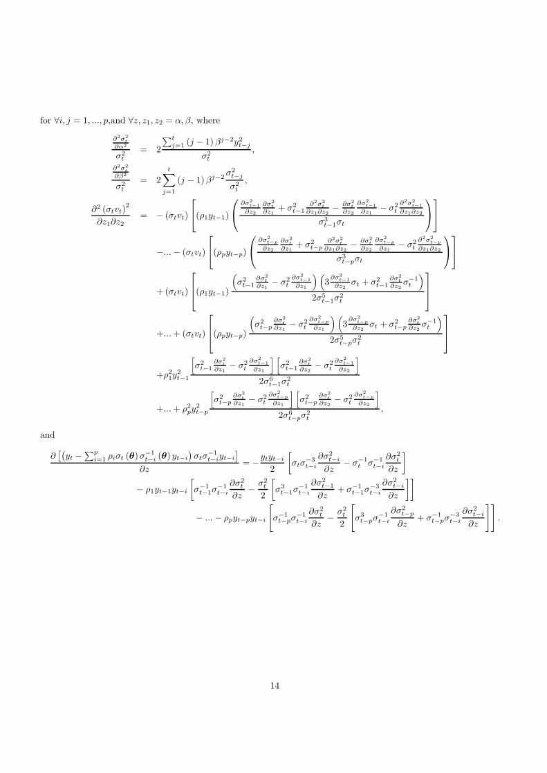
for ∀i, j = 1, ..., p,and ∀z, z1, z2 = α, β, where

∂2σ2

t

∂α2

σ2t

= 2

∑tj=1 (j − 1)βj−2y2

t−j

σ2t

,

∂2σ2

t

∂β2

σ2t

= 2

t∑

j=1

(j − 1)βj−2σ2

t−j

σ2t

,

∂2 (σtvt)2

∂z1∂z2= − (σtvt)

(ρ1yt−1)

∂σ2

t−1

∂z2

∂σ2

t

∂z1

+ σ2t−1

∂2σ2

t

∂z1∂z2

− ∂σ2

t

∂z2

∂σ2

t−1

∂z1

− σ2t

∂2σ2

t−1

∂z1∂z2

σ3t−1σt

−... − (σtvt)

(ρpyt−p)

∂σ2

t−p

∂z2

∂σ2

t

∂z1

+ σ2t−p

∂2σ2

t

∂z1∂z2

− ∂σ2

t

∂z2

∂σ2

t−p

∂z1

− σ2t

∂2σ2

t−p

∂z1∂z2

σ3t−pσt

+ (σtvt)

(ρ1yt−1)

(σ2

t−1∂σ2

t

∂z1

− σ2t

∂σ2

t−1

∂z1

)(3

∂σ2

t−1

∂z2

σt + σ2t−1

∂σ2

t

∂z2

σ−1t

)

2σ5t−1σ

2t

+... + (σtvt)

(ρpyt−p)

(σ2

t−p∂σ2

t

∂z1

− σ2t

∂σ2

t−p

∂z1

)(3

∂σ2

t−p

∂z2

σt + σ2t−p

∂σ2

t

∂z2

σ−1t

)

2σ5t−pσ

2t

+ρ21y

2t−1

[σ2

t−1∂σ2

t

∂z1

− σ2t

∂σ2

t−1

∂z1

] [σ2

t−1∂σ2

t

∂z2

− σ2t

∂σ2

t−1

∂z2

]

2σ6t−1σ

2t

+... + ρ2py

2t−p

[σ2

t−p∂σ2

t

∂z1

− σ2t

∂σ2

t−p

∂z1

] [σ2

t−p∂σ2

t

∂z2

− σ2t

∂σ2

t−p

∂z2

]

2σ6t−pσ

2t

,

and

∂[(

yt −∑p

i=1 ρiσt (θ)σ−1t−i (θ) yt−i

)σtσ

−1t−iyt−i

]

∂z= −ytyt−i

2

[σtσ

−3t−i

∂σ2t−i

∂z− σ−1

t σ−1t−i

∂σ2t

∂z

]

− ρ1yt−1yt−i

[σ−1

t−1σ−1t−i

∂σ2t

∂z− σ2

t

2

[σ3

t−1σ−1t−i

∂σ2t−1

∂z+ σ−1

t−1σ−3t−i

∂σ2t−i

∂z

]]

− ... − ρpyt−pyt−i

[σ−1

t−pσ−1t−i

∂σ2t

∂z− σ2

t

2

[σ3

t−pσ−1t−i

∂σ2t−p

∂z+ σ−1

t−pσ−3t−i

∂σ2t−i

∂z

]].

14

Result 6: Third order derivatives The third order derivatives are given by

∂3

∂z21∂z2

lT (θ) = −1

2

T∑

t=1

(1 − (σtvt)

2

σ2t

) ∂3σ2

t

∂z2

1∂z2

σ2t

−T∑

t=1

(2(σtvt)

2

σ2t

− 1

) ( ∂2σ2

t

∂z1∂z2

∂σ2

t

∂z1

+ 12

∂2σ2

t

∂z2

1

∂σ2

t

∂z2

)

σ4t

−T∑

t=1

(1 − 3 (σtvt)

2

σ2t

) (∂σ2

t

∂z1

)2∂σ2

t

∂z2

σ6t

− 1

2

T∑

t=1

∂3(yt−∑p

i=1ρiσt(θ)σ−1

t−i(θ)yt−i)2

∂z2

1∂z2

σ2t

+

T∑

t=1

(12

∂2(yt−∑p

i=1ρiσt(θ)σ−1

t−i(θ)yt−i)2

∂z2

1

∂σ2

t

∂z2

+∂2(yt−

∑pi=1

ρiσt(θ)σ−1

t−i(θ)yt−i)2

∂z1∂z2

∂σ2

t

∂z1

)

σ4t

+

T∑

t=1

(12

∂2σ2

t

∂z2

1

∂(yt−∑p

i=1ρiσt(θ)σ−1

t−i(θ)yt−i)2

∂z2

+∂2σ2

t

∂z1∂z2

∂(yt−∑p

i=1ρiσt(θ)σ−1

t−i(θ)yt−i)2

∂z1

)

σ4t

−T∑

t=1

(∂(yt−

∑pi=1

ρiσt(θ)σ−1

t−i(θ)yt−i)2

∂z2

(∂σ2

t

∂z1

)2

+ 2∂(yt−

∑pi=1

ρiσt(θ)σ−1

t−i(θ)yt−i)2

∂z1

∂σ2

t

∂z1

∂σ2

t

∂z2

)

σ6t

,

∂3

∂z1∂z2∂ρilT (θ) =

T∑

t=1

2 (σtvt)σtyt−i∂σ2

t

∂z1

∂σ2

t

∂z2

σt−iσ6t

+

T∑

t=1

(σtvt)σtyt−i∂2σ2

t

∂z1∂z2

σt−iσ4t

−T∑

t=1

∂3(yt−∑p

i=1ρiσt(θ)σ−1

t−i(θ)yt−i)2

∂z1∂z2∂ρi

2σ2t

+1

2

T∑

t=1

(∂σ2

t

∂z1

∂2(yt−∑p

i=1ρiσt(θ)σ−1

t−i(θ)yt−i)2

∂z2∂ρi+

∂σ2

t

∂z2

∂2(yt−∑p

i=1ρiσt(θ)σ−1

t−i(θ)yt−i)2

∂z1∂ρi

)

σ4t

,

∂3

∂z∂ρi∂ρjlT (θ) =

T∑

t=1

yt−iyt−j

(σt−i

∂σt−j

∂z + σt−j∂σt−i

∂z

)

σ2t−iσ

2t−j

,

∂3

∂ρi∂ρj∂ρklT (θ) = 0,

for ∀z1, z2 = α, β and ∀i, j, k = 1, ..., p where

∂3σ2

t

∂α3

σ2t

= 3

∑tj=1 (j − 1) (j − 2)βj−3y2

t−j

σ2t

,

∂3σ2

t

∂β3

σ2t

= 3

t∑

j=1

(j − 1) (j − 2)βj−3σ2

t−j

σ2t

,

15

and

∂3(yt −

∑pi=1 ρiσt (θ)σ−1

t−i (θ) yt−i

)2

∂z21∂z2

= −ρ1yt−1 (σtvt) [

(∂σ2

t−1

∂z2

∂2σ2

t

∂z2

1

+∂3σ2

t−1

∂z2

1∂z2

σ2t−1 −

∂σ2

t

∂z2

∂2σ2

t−1

∂z2

1

− σ2t

∂3σ2

t−1

∂z2

1∂z2

)

σ3t−1σt

−

(σ2

t−1∂2σ2

t

∂z2

1

− σ2t

∂2σ2

t−1

∂z2

1

)(3σt−1σt

∂σ2

t−1

∂z2

+ σ−1t σ3

t−1∂σ2

t

∂z2

)

2σ6t−1σ

2t

−

(∂σ2

t−1

∂z1

∂2σ2

t

∂z1∂z2

+∂σ2

t

∂z1

∂2σ2

t−1

∂z1∂z2

)

σ4t−1σt

+

(∂σ2

t

∂z1

∂σ2

t−1

∂z1

)(2σ2

t−1σt∂σ2

t−1

∂z2

+ 12σ−1

t σ4t−1

∂σ2

t

∂z2

)

σ8t−1σ

2t

−

(∂σ2

t

∂z1

∂2σ2

t

∂z1∂z2

)

σ2t−1σ

3t

+3(

∂σ2

t−1

∂z1

∂2σ2

t−1

∂z1∂z2

)

σ6t−1σ

−1t

+

(∂σ2

t

∂z1

)2 (σ3

t

2

∂σ2

t−1

∂z2

+ σtσ2t−1

34

∂σ2

t

∂z2

)

σ4t−1σ

6t

−32

(∂σ2

t−1

∂z1

)2 (3σ4

t−1σ−1t

∂σ2

t−1

∂z2

− σ−3t σ6

t−112

∂σ2

t

∂z2

)

σ12t−1σ

−2t

]

−... − ρpyt−p (σtvt) [

(∂σ2

t−p

∂z2

∂2σ2

t

∂z2

1

+∂3σ2

t−p

∂z2

1∂z2

σ2t−p − ∂σ2

t

∂z2

∂2σ2

t−p

∂z2

1

− σ2t

∂3σ2

t−p

∂z2

1∂z2

)

σ3t−pσt

−

(σ2

t−p∂2σ2

t

∂z2

1

− σ2t

∂2σ2

t−p

∂z2

1

)(3σt−pσt

∂σ2

t−p

∂z2

+ σ−1t σ3

t−p∂σ2

t

∂z2

)

2σ6t−pσ

2t

−

(∂σ2

t−p

∂z1

∂2σ2

t

∂z1∂z2

+∂σ2

t

∂z1

∂2σ2

t−p

∂z1∂z2

)

σ4t−pσt

+

(∂σ2

t

∂z1

∂σ2

t−p

∂z1

)(2σ2

t−pσt∂σ2

t−p

∂z2

+ 12σ−1

t σ4t−p

∂σ2

t

∂z2

)

σ8t−pσ

2t

−

(∂σ2

t

∂z1

∂2σ2

t

∂z1∂z2

)

σ2t−pσ

3t

+3(

∂σ2

t−p

∂z1

∂2σ2

t−p

∂z1∂z2

)

σ6t−pσ

−1t

+

(∂σ2

t

∂z1

)2 (σ3

t

2

∂σ2

t−p

∂z2

+ σtσ2t−p

34

∂σ2

t

∂z2

)

σ4t−pσ

6t

−32

(∂σ2

t−p

∂z1

)2 (3σ4

t−pσ−1t

∂σ2

t−p

∂z2

− σ−3t σ6

t−p12

∂σ2

t

∂z2

)

σ12t−pσ

−2t

]

−ρ21y

2t−1

2[

(σ2

t−1∂σ2

t

∂z2

− σ2t

∂σ2

t−1

∂z2

)

σ3t−1σt

(2

∂σ2

t

∂z1

∂σ2

t−1

∂z1

)

σ4t−1σt

+

(∂σ2

t

∂z1

)2

σ2t−1σ

3t

−3(

∂σ2

t−1

∂z1

)2

σ6t−1σ

−1t

−2(σ2

t−1∂σ2

t

∂z1

− σ2t

∂σ2

t−1

∂z1

)(∂σ2

t

∂z1

∂σ2

t−1

∂z2

+ σ2t−1

∂2σ2

t

∂z1∂z2

− ∂σ2

t

∂z2

∂σ2

t−1

∂z1

− σ2t

∂2σ2

t−1

∂z1∂z2

)

σ6t−1σ

2t

+

(σ2

t−1∂σ2

t

∂z1

− σ2t

∂σ2

t−1

∂z1

)(3σ4

t−1σ2t

∂σ2

t−1

∂z2

+ σ6t−1

∂σ2

t

∂z2

)

σ12t−1σ

4t

−

(σ2

t−1∂2σ2

t

∂z2

1

− σ2t

∂2σ2

t−1

∂z2

1

)(σ2

t−1∂σ2

t

∂z2

− σ2t

∂σ2

t−1

∂z2

)

σ6t−1σ

2t

]

−... −ρ2

py2t−p

2[

(σ2

t−p∂σ2

t

∂z2

− σ2t

∂σ2

t−p

∂z2

)

σ3t−pσt

(2

∂σ2

t

∂z1

∂σ2

t−p

∂z1

)

σ4t−pσt

+

(∂σ2

t

∂z1

)2

σ2t−pσ

3t

−3(

∂σ2

t−p

∂z1

)2

σ6t−pσ

−1t

−2(σ2

t−p∂σ2

t

∂z1

− σ2t

∂σ2

t−p

∂z1

)(∂σ2

t

∂z1

∂σ2

t−p

∂z2

+ σ2t−p

∂2σ2

t

∂z1∂z2

− ∂σ2

t

∂z2

∂σ2

t−p

∂z1

− σ2t

∂2σ2

t−p

∂z1∂z2

)

σ6t−1σ

2t

+

(σ2

t−p1∂σ2

t

∂z1

− σ2t

∂σ2

t−p

∂z1

)(3σ4

t−pσ2t

∂σ2

t−p

∂z2

+ σ6t−p

∂σ2

t

∂z2

)

σ12t−pσ

4t

+

(σ2

t−p∂2σ2

t

∂z2

1

− σ2t

∂2σ2

t−p

∂z2

1

)(σ2

t−p∂σ2

t

∂z2

− σ2t

∂σ2

t−p

∂z2

)

σ6t−pσ

2t

],

16

for ∀z1, z2 = α, β. Furthermore,

∂2(yt −

∑pi=1 ρiσt (θ)σ−1

t−i (θ) yt−i

)2

∂z∂ρ=

[(σtvt) yt−1 − ρ1σtσ

−1t−1y

2t−1

]σt

∂σ2

t−1

∂z

σ3t−1

−∂σ2

t

∂z

σtσt−1

+... +[(σtvt) yt−p − ρpσtσ

−1t−py

2t−p

]σt

∂σ2

t−p

∂z

σ3t−p

−∂σ2

t

∂z

σtσt−p

,

∂3 (σtvt)2

∂z1∂z2∂ρ=

∂σ2

t−1

∂z2

∂σ2

t

∂z1

+ σ2t−1

∂2σ2

t

∂z1∂z2

− ∂σ2

t

∂z2

∂σ2

t−1

∂z1

− σ2t

∂2σ2

t−1

∂z1∂z2

σ3t−1σt

×[ρ1σtσ

−1t−1y

2t−1 − (σtvt) yt−1

]

+... +

∂σ2

t−p

∂z2

∂σ2

t

∂z1

+ σ2t−p

∂2σ2

t

∂z1∂z2

− ∂σ2

t

∂z2

∂σ2

t−p

∂z1

− σ2t

∂2σ2

t−p

∂z1∂z2

σ3t−pσt

×[ρpσtσ

−1t−py

2t−p − (σtvt) yt−p

]

+

(σ2

t∂σ2

t−1

∂z1

− σ2t−1

∂σ2

t

∂z1

)(3σt−1

∂σ2

t−1

∂z2

σt + σ3t−1

∂σ2

t

∂z2

σ−1t

)

2σ6t−1σ

2t

×[ρ1σtσ

−1t−1y

2t−1 − (σtvt) yt−1

]

+... +

(σ2

t∂σ2

t−p

∂z1

− σ2t−p

∂σ2

t

∂z1

)(3σt−p

∂σ2

t−p

∂z2

σt + σ3t−p

∂σ2

t

∂z2

σ−1t

)

2σ6t−pσ

2t

×[ρpσtσ

−1t−py

2t−p − (σtvt) yt−p

]

+2ρ1y2t−1

[σ2

t−1∂σ2

t

∂z1

− σ2t

∂σ2

t−1

∂z1

] [σ2

t−1∂σ2

t

∂z2

− σ2t

∂σ2

t−1

∂z2

]

2σ6t−1σ

2t

+... + 2ρpy2t−p

[σ2

t−p∂σ2

t

∂z1

− σ2t

∂σ2

t−p

∂z1

] [σ2

t−p∂σ2

t

∂z2

− σ2t

∂σ2

t−p

∂z2

]

2σ6t−pσ

2t

,

for ∀z, z1, z2 = α, β.

17

Research Papers 2009

2009-45: Kim Christensen, Silja Kinnebrock and Mark Podolskij: Pre-averaging

estimators of the ex-post covariance matrix

2009-46: Matias D. Cattaneo, Richard K. Crump and Michael Jansson: Robust Data-Driven Inference for Density-Weighted Average Derivatives

2009-47: Mark Podolskij and Mathias Vetter: Understanding limit theorems for semimartingales: a short survey

2009-48: Isabel Casas and Irene Gijbels: Unstable volatility functions: the break preserving local linear estimator

2009-49: Torben G. Andersen and Viktor Todorov: Realized Volatility and Multipower Variation

2009-50: Robinson Kruse, Michael Frömmel, Lukas Menkhoff and Philipp Sibbertsen: What do we know about real exchange rate non-linearities?

2009-51: Tue Gørgens, Christopher L. Skeels and Allan H. Würtz: Efficient Estimation of Non-Linear Dynamic Panel Data Models with Application to Smooth Transition Models

2009-52: Torben G. Andersen, Dobrislav Dobrev and Ernst Schaumburg: Jump-Robust Volatility Estimation using Nearest Neighbor Truncation

2009-53: Florian Heinen, Philipp Sibbertsen and Robinson Kruse: Forecasting long memory time series under a break in persistence

2009-54: Tue Gørgens and Allan Würtz: Testing a parametric function against a nonparametric alternative in IV and GMM settings

2009-55: Michael Jansson and Morten Ørregaard Nielsen: Nearly Efficient Likelihood Ratio Tests for Seasonal Unit Roots

2009-56: Valeri Voev: On the Economic Evaluation of Volatility Forecasts

2009-57: Jesper Rangvid, Maik Schmeling and Andreas Schrimpf: Global Asset Pricing: Is There a Role for Long-run Consumption Risk?

2009-58: Olaf Posch: Risk premia in general equilibrium

2009-59: Christian M. Dahl and Emma M. Iglesias: Modelling the Volatility-Return Trade-off when Volatility may be Nonstationary