Electronic copy available at: http://ssrn.com/abstract=2141546Electronic copy available at: http://ssrn.com/abstract=2141546Electronic copy available at: http://ssrn.com/abstract=2109200

Semiparametric Autoregressive Conditional Duration Model:

Theory and Practice

Patrick W. Saart,a, Jiti Gaob, David E. Allenc

aThe University of CanterburybMonash University

cEdith Cowan University

Abstract

Many existing extensions of the Engle and Russell’s (1998) Autoregressive Conditional Duration(ACD) model in the literature are aimed at providing additional flexibility either on the dynamicsof the conditional duration model or the allowed shape of the hazard function, i.e. its two mostessential components. This paper introduces an alternative semiparametric regression approachto a nonlinear ACD model; the use of a semiparametric functional form on the dynamics of theduration process suggests the model being called the Semiparametric ACD (SEMI–ACD) model.Unlike existing alternatives, the SEMI–ACD model allows simultaneous generalizations on bothof the above–mentioned components of the ACD framework. To estimate the model, we establishan alternative use of the existing Buhlmann and McNeil’s (2002) iterative estimation algorithmin the semiparametric setting and provide the mathematical proof of its statistical consistency inour context. Furthermore, we investigate the asymptotic properties of the semiparametric esti-mators employed in order to ensure the statistical rigor of the SEMI–ACD estimation procedure.These asymptotic results are presented in conjunction with simulated examples, which providean empirical evidence of the SEMI–ACD model’s robust finite–sample performance. Finally, weapply the proposed model to study price duration process in the foreign exchange market toillustrate its usefulness in practice.

JEL Classification: C14, C41, F31.

Key words: Dependent point process, duration, hazard rate and random measure, irregularly

spaced high frequency data, semiparametric time series

1. Introduction

An important feature that leads to a statistically challenging property of high–frequency

data in finance is the fact that market events are clustered over time. This suggests; in

effects, that financial durations follow positively autocorrelated processes with strong per-

sistence. This feature may be captured in various ways through different dynamic models

which may be based either on duration, intensity or counting representations of a point

process. Engle and Russell (1998) develop the ACD model in which transaction arrival

times are treated as random variables, which follow a self–exciting point process.

Preprint submitted to - July 25, 2012

Electronic copy available at: http://ssrn.com/abstract=2141546Electronic copy available at: http://ssrn.com/abstract=2141546Electronic copy available at: http://ssrn.com/abstract=2109200

The ACD model considers a stochastic process that is simply a sequence of times

t0, t1, . . . , tn, . . . with t0 < t1 < · · · < tn . . . . The interval between two arrival times,

i.e. xi = ti − ti−1, measures the length of times commonly known as the durations such

that xi is a nonnegative stationary process adapted to the filtration Fi, i ∈ Z with

Fi = σ((xs, ψs) : s ≤ i) representing the previous history.

Furthermore, the ACD class of models assumes a multiplicative model for xi of the

form

xi = ψiεi, (1.1)

where εi is an independent and identically distributed (i.i.d.) innovation series with

non–negative support density p(ε;φ), in which φ is a vector of parameters whose values

satisfy a set of restrictions for a corresponding distribution, and E[ε1] = 1. Moreover,

ψi ≡ ϑ(xi−1, . . . , xi−p, ψi−1, . . . , ψi−q) (1.2)

and ϑ : Rp+×R

q+ → R+ is a strictly positive–valued function. Since ϑ(·) is Fi−1-measurable,

it can be shown that ψi ≡ E(xi|Fi−1), i.e. ψi denotes the expected value of xi given the

previous history generated by Fi−1.

It is apparent that we now have a host of potential specifications for the ACD model

where each is defined by different specifications for the expected duration and the distri-

bution of ε. The model assumes that the intertemporal dependence of the duration process

can be summarized by the former, while the importance of the later can be appreciated

most obviously by considering the baseline hazard, given by

λ0(t) =p(ε;φ)

S(ε;φ), (1.3)

where S(ε;φ) =∫∞εp(u;φ)du is the survivor function.

The intensity function for an ACD model is then given by

λ(t|N(t), t1, . . . , tN(t)) = λ0

(t− tN(t)

ψN(t)+1

)1

ψN(t)+1

, (1.4)

so that the past history influences the conditional intensity by both a multiplicative effect

and a shift in the baseline hazard, which signify the so–called accelerated failure time

model.

The First generation ACD model, which is proposed by Engle and Russell (1998) and

is often treated as a baseline model in a more recent study, relies on a linear parameteri-

zation of ϑ(·) such that

ψi ≡ ω +

p∑j=1

αjxi−j +

q∑k=1

βkψi−k, (1.5)

2

Electronic copy available at: http://ssrn.com/abstract=2141546Electronic copy available at: http://ssrn.com/abstract=2141546

while assuming that the durations are conditionally exponential. In this case, the baseline

hazard is simply one so that the conditional intensity is

λ(t|N(t), t1, . . . , tN(t)) =1

ψN(t)+1

. (1.6)

In the literature, this is often referred to as an Exponential ACD or EACD(p,q) model in

which a number of conditions are needed to ensure the positivity of ψi are ω > 0, αj ≥ 0

for ∀j = 1, . . . , p and βk ≥ 0 for ∀k = 1, . . . , q.

In practice, the EACD model as specified by (1.5) and (1.6) is clearly too restrictive. A

significant number of recent studies focus their attention on various parametric extensions

to the Engle and Russell’s baseline model. These extensions, which may be classed as the

Second generation models, are aimed at providing additional flexibility on the dynamic

specification of the conditional duration model and/or the shape of the hazard function.

Some well known examples are the Logarithmic ACD model of Bauwens and Giot (2000);

Box-Cox ACD model of Dufour and Engle (2000); Threshold ACD model of Zhang et al.

(2001); and the Augmented ACD model of Fernandes and Grammig (2006). Furthermore,

Grammig and Maurer (2000) question the assumption of monotonicity of the hazard

function implied by the weibull and advocate the use of the Burr distribution, which

contains the exponential, weibull and the log-logistic distributions as special cases.

More recently, researchers have begun to consider nonparametric and semiparametric

methods with hope of establishing the Third generation models, which may be able to

provide a more useful generalization to the ACD procedure. A well–known example of

these studies is Drost and Werker (2004), who argue against the i.i.d. assumption in

(1.1) in favor of a semiparametric alternative that allows the distribution function of the

innovations to be dependent on the past. The resulting model relies heavily on the linear

parameterization in (1.5) and the assumption that it is correctly specified.

In the meantime, Cosma and Galli (2006) initiate the use of a nonparametric regression

approach in dealing with nonlinearity in the ACD models. Their so–called Nonparametric

ACD (N–ACD) model is developed based on the use of Buhlmann and McNiel’s iterative

estimation algorithm; see Buhlmann and McNeil (2002) for details. Under the assumption

that ϑ in (1.2) is a strictly positive function, the N–ACD model allows for a relatively

flexible estimation of the nonlinearity in the conditional mean equation.

However, in order to take into account an existing set of information about linearity, we

propose using an alternative semiparametric regression approach to the above mentioned

parametric and nonparametric models. The semiparametric functional form specifica-

tion of the conditional mean equation suggests that the model be called the SEMI–ACD

model. The SEMI–ACD model consists of two important components. Firstly, it is a

semiparametric time series process that models the dynamics of the duration process.

For the various reasons, which will be discussed in detail later, we believe that a suitable

3

alternative in this case is a partially linear additive autoregressive process; see, for exam-

ple, Robinson (1988), Hardle et al. (2000) and Gao (2007). Secondly, it is an estimation

algorithm required in order to address a latency problem which arises because of the fact

that the conditional durations are not observable in practice.

The SEMI–ACD model follows a similar estimation strategy to the N–ACD model in

the sense that it too relies on the Buhlmann and McNeil’s type of iterative estimation

algorithm in order to address the above–mentioned latency problem in the ACD estima-

tion. Therefore, it is not surprising that the implications of the assumptions required in

this paper to derive the consistency of such the algorithm are in line with those employed

in Buhlmann and McNeil (2002), and Cosma and Galli (2006).

Nonetheless, this paper focuses instead on a separable semiparametric functional form.

Even though it might be considered by many to be a simpler model than the N–ACD, we

will show in this paper that this enables us to derive mathematical results that do not

only found a solid theoretical justification of the above–mentioned required assumptions

but also provide some low level conditions for them to hold. These issues were not the

main focus of the previous studies. Moreover, since they are essential, we present their

discussion in detail in Remark 3.1 below.

In addition, the research in this paper complements the works of the previous stud-

ies by providing a detailed investigation on the impacts of such numerically estimated

regressor on the asymptotic properties and inferences of the semiparametric estimation

involved. Similar to Robinson (1988), we establish not only T−1/2 consistency but also

the asymptotic normality of the kernel based estimator of the parametric component of

our model. Furthermore, although it is ensured that the theoretically optimum value

hoptimal = CT−1/5 can be included, our theoretical analysis suggests that the asymptotic

cost of such the algorithm–based estimation is on the narrower set of admissible band-

widths compared to other more standard studies; see also a similar finding in the generated

regressor literature, for example Li and Wooldridge (2002). Neither Buhlmann and Mc-

Neil (2002) and Cosma and Galli (2006) nor other existing studies have investigated these

issues.

The current paper is organized as follows. Section 2 explains the basic construction of

the SEMI-ACD model. Section 3 presents the above–mentioned computational algorithm

and then investigates its statistical consistency and other asymptotic properties. Section

4 considers various experimental examples in order to illustrate how well the SEMI–ACD

model preforms in practice. Section 5 applies the model to a thinned series of quotes

arrival times for the $US/$EUR exchange rate series. Section 6 summarizes the main

results and offers some remarks about further research. Note that while the appendix

presents a number of required mathematical assumptions, proofs of the main results are

given in the additional appendices, which are collected in the supplemental document of

this paper, see page 34 of this paper for details.

4

2. The SEMI–ACD Model

We introduce in this section the main idea about the SEMI–ACD model and its

estimation method. To do so without an unnecessary complication in our discussion, in

the current section we proceed under the assumption that the conditional expectation of

the ith duration is observable. The above–mentioned latency problem will be formally

discussed and dealt with in the next section.

Despite an overwhelming evidence of nonlinearity, which has been reported in previous

studies; see, for example, Dufour and Engle (2000) and Zhang et al. (2001), the question

about the most appropriate nonlinear specification of the conditional mean equation for

an ACD model has not been satisfactorily answered in the literature. We propose in this

paper the SEMI–ACD(p,q) model that relies on a semiparametric regression model

ψi ≡p∑j=1

γjxi−j +

q∑k=1

gk (ψi−k) , (2.1)

where γj are unknown parameters and gk(·) are unknown functions on the real line.

An advantage of such the partially linear autoregressive specification is the additional

flexibility by which the Engle and Russell’s ARMA type function form and a few other

parametric ones are nested as special cases. Statistically, this can be proven to be partic-

ularly useful given the fact that we have quite a limited knowledge about the unobserved

conditional expectation process. In this case, a functional form specification that allows

the data to speak more for themselves is less prone to mis–specification errors and there-

fore should be preferred. A real data example presented in Section 5 below will provide

not only a realistic illustration, but also an empirical evidence in support of such autore-

gressive nonlinearity. This is all in spite of the fact that the history of similar models in

the GARCH literature suggests that the first order source of nonlinearity is in the news

impact curve, i.e. on the lagged duration in the dynamic specification. The objective of

our work is to establish an alternative method that preserves its root as an ACD model

while being better in the sense that a number of its initial shortfalls can be systematically

addressed.

In this paper, our attention will be restricted only to a special case of (2.1) with p = 1,

q = 1, γ1 = γ and g1 = g, i.e. the SEMI–ACD(1,1) specification of the form

ψi ≡ γxi−1 + g (ψi−1) . (2.2)

We opt for the SEMI–ACD(1,1) model partly for convenience and clarity in introducing

the main idea of the new semiparametric method and its statistical properties. More

importantly, a number of existing empirical studies have found that an ACD(1,1) model

is often sufficient to remove the intertemporal dependence in the duration process; see,

for example, Engle and Russell (1998).

5

To derive the estimators of γ and g, observe that the multiplicative model in (1.1)

can be written in terms of an additive noise of the form

xi = γxi−1 + g (ψi−1) + ηi, (2.3)

where ηi = ψi (εi − 1) and εi is a sequence of positive and stationary errors satisfying

E [ε1] = 1 and E[ε2+δ

1

]<∞ for some δ > 0, and εi and ψi are mutually independent.

Thus

g (ψi−1) = E [xi|ψi−1]− γE [xi−1|ψi−1] = g1 (ψi−1)− γg2 (ψi−1) (2.4)

due to

E[ηi|ψi−1] = E [E (ψi(εi − 1)|xi−1, ψi−1) |ψi−1] = E [ψiE (εi − 1) |ψi−1] = 0.

Therefore, the natural estimates of gj (j = 1, 2) and g for a given γ are

gj,h (ψi−1) =T∑s=2

Ws,h (ψi−1)xs+1−j and gh(ψi−1) = g1,h (ψi−1)− γg2,h (ψi−1) , (2.5)

where Ws,h (·) is a probability weight function. This paper considers the case where Ws,h

is a kernel weight function

Ws,h(y) =Kh (y − ψs−1)∑Ti=2Kh (y − ψi−1)

, (2.6)

where Kh (·) = h−1K (·/h), K is a real-valued kernel function satisfying Assumption A.3

and h = hT ∈ HT , in which HT is an interval of possible bandwidth values.

As suggested in Assumption A.3(i), an optimal bandwidth h can be chosen propor-

tional to T−15 . Thus, throughout this paper, we choose HT =

[a T−1/5−c, b T−1/5+c

], in

which 0 < a < b < ∞ and 0 < c < 120

. As discussed in Hardle, Hall and Marron (1988),

one may also use a bandwidth interval wider than HT in practice.

For the gh defined as in (2.5), the kernel weighted least squares estimator (WLSE) of

γ can be found by minimizing

T∑i=2

xi − γxi−1 − gh(ψi−1)2 ω(ψi−1), (2.7)

where ω(·) is a known non–negative weight function satisfying Assumption A.3(ii); see

also an additional discussion in Remark 2.1 below. Hence, the WLSE of γ is

γψ(h) =

T∑i=2

u2iω(ψi−1)

−1 T∑i=2

uiviω(ψi−1)

, (2.8)

where vi = xi − g1,h(ψi−1) and ui = xi−1 − g2,h(ψi−1).

6

Furthermore, σ2 = Eη2i = E

ψ2i (εi − 1)2 = Eψ2

1σ21, where σ2

1 = Eε1 − 12,

which can be estimated by

σ2ψ(h) =

1

T − 1

T∑i=2

xi − γψ(h)xi−1 − g1,h(ψi−1) + γψ(h)g2,h(ψi−1)2ω(ψi−1). (2.9)

Finally, the quality of the proposed estimators can be measured by the average squared

error (ASE) of the form

Dψ(h) =1

T

T∑i=2

[γψ(h)xi−1 + g∗h(ψi−1) − γxi−1 + g(ψi−1)]2 ω(ψi−1), (2.10)

where g∗h(ψi−1) = g1,h(ψi−1)− γψ(h)g2,h(ψi−1).

Remark 2.1. In equation (2.7), we do not use a truncated method to “trim out” small

values of f(ψi−1) = 1Th

∑Tj=2K

(ψi−1−ψj−1

h

)as has been done in the literature; see, for

example, Robinson (1988). As an alternative, equation (2.7) involves a non–negative

weight function to help address this kind of random denominator issue.

3. The Computational Algorithm

Hereafter, we take into account the fact that ψ is not observable and discuss the above–

mentioned recursive computational algorithm. While Section 3.1 presents the algorithm’s

basic construction, Sections 3.2 and 3.3 discuss its theoretical justification that involves

two fundamental issues, namely its statistical consistency and the asymptotic properties

of the resulting semiparametric and nonparametric estimators in Section 2.

3.1. Basic Construction

Assume that we have a set of sample xi; 1 ≤ i ≤ T, ideally from the data gen-

erating process described by (1.1). Hereafter, let us denote the number of iterations by

m ≥ 1 and let i = m+1,m+2, . . . , T . The SEMI–ACD procedure discussed in the earlier

section suggests that the estimate of the ith conditional duration at the mth iteration

can be defined as ψi,m ≡ γm(h)xi−1 + gh,m(ψi−1,m−1), where γm(h) is the kernel WLS

estimate of γ at the mth iteration, gh,m(ψi−1,m−1) = g1,h(ψi−1,m−1)− γm(h) g2,h(ψi−1,m−1),

gj,h(ψi−1,m−1) =∑T

s=m+ιWs,h(ψi−1,m−1)xs−j+1 for j = 1, 2, ι ∈ N and Ws,h(·) is the proba-

bility kernel function. The estimation algorithm is constructed to include four important

steps as follows:

Step 3.1: Choose the starting values for the vector of the T conditional durations.

Index these values by a zero. Let ψi,0; 1 ≤ i ≤ T satisfy ψi,0 = ψi,0 and the stationarity

condition as stated in Assumption 3.1 below. Set m = 1.

7

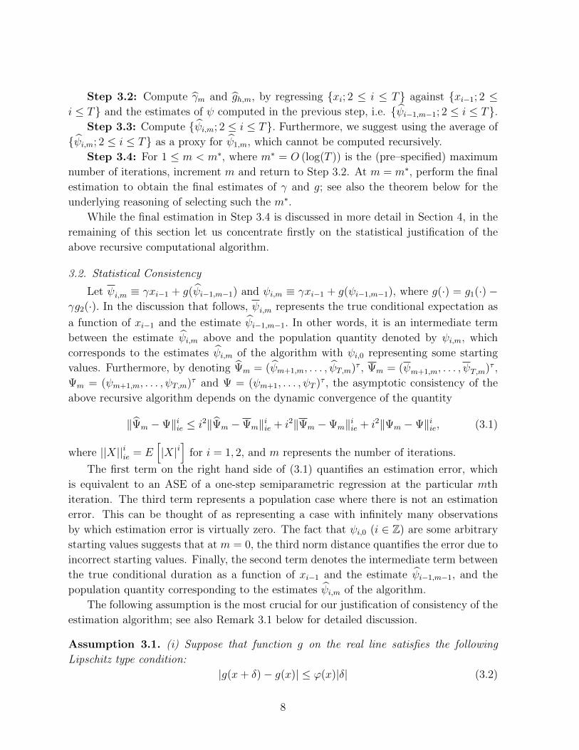
Step 3.2: Compute γm and gh,m, by regressing xi; 2 ≤ i ≤ T against xi−1; 2 ≤i ≤ T and the estimates of ψ computed in the previous step, i.e. ψi−1,m−1; 2 ≤ i ≤ T.

Step 3.3: Compute ψi,m; 2 ≤ i ≤ T. Furthermore, we suggest using the average of

ψi,m; 2 ≤ i ≤ T as a proxy for ψ1,m, which cannot be computed recursively.

Step 3.4: For 1 ≤ m < m∗, where m∗ = O (log(T )) is the (pre–specified) maximum

number of iterations, increment m and return to Step 3.2. At m = m∗, perform the final

estimation to obtain the final estimates of γ and g; see also the theorem below for the

underlying reasoning of selecting such the m∗.

While the final estimation in Step 3.4 is discussed in more detail in Section 4, in the

remaining of this section let us concentrate firstly on the statistical justification of the

above recursive computational algorithm.

3.2. Statistical Consistency

Let ψi,m ≡ γxi−1 + g(ψi−1,m−1) and ψi,m ≡ γxi−1 + g(ψi−1,m−1), where g(·) = g1(·)−γg2(·). In the discussion that follows, ψi,m represents the true conditional expectation as

a function of xi−1 and the estimate ψi−1,m−1. In other words, it is an intermediate term

between the estimate ψi,m above and the population quantity denoted by ψi,m, which

corresponds to the estimates ψi,m of the algorithm with ψi,0 representing some starting

values. Furthermore, by denoting Ψm = (ψm+1,m, . . . , ψT,m)τ , Ψm = (ψm+1,m, . . . , ψT,m)τ ,

Ψm = (ψm+1,m, . . . , ψT,m)τ and Ψ = (ψm+1, . . . , ψT )τ , the asymptotic consistency of the

above recursive algorithm depends on the dynamic convergence of the quantity

‖Ψm −Ψ‖iie ≤ i2‖Ψm −Ψm‖iie + i2‖Ψm −Ψm‖iie + i2‖Ψm −Ψ‖iie, (3.1)

where ||X||iie = E[|X|i

]for i = 1, 2, and m represents the number of iterations.

The first term on the right hand side of (3.1) quantifies an estimation error, which

is equivalent to an ASE of a one-step semiparametric regression at the particular mth

iteration. The third term represents a population case where there is not an estimation

error. This can be thought of as representing a case with infinitely many observations

by which estimation error is virtually zero. The fact that ψi,0 (i ∈ Z) are some arbitrary

starting values suggests that at m = 0, the third norm distance quantifies the error due to

incorrect starting values. Finally, the second term denotes the intermediate term between

the true conditional duration as a function of xi−1 and the estimate ψi−1,m−1, and the

population quantity corresponding to the estimates ψi,m of the algorithm.

The following assumption is the most crucial for our justification of consistency of the

estimation algorithm; see also Remark 3.1 below for detailed discussion.

Assumption 3.1. (i) Suppose that function g on the real line satisfies the following

Lipschitz type condition:

|g(x+ δ)− g(x)| ≤ ϕ(x)|δ| (3.2)

8

for each given x ∈ Sω, where Sω is the compact support of the weight function ω(·).Furthermore, ϕ(·) is a nonnegative measurable function such that with probability one,

maxi≥1

E[ϕ2(ψi)|(ψi−1, · · · , ψ1)

]≤ G2 and max

i≥1E[ϕ2(ψi,m)|(ψi−1,m−1, · · · , ψ1,1)

]≤ G2

(3.3)

for some 0 < G < 1.

(ii) Let ∆1T (ψ) = maxi,m≥1E12

[∣∣∣ψi,m − ψi,m∣∣∣2]→ 0 as T →∞

(iii) There exists a stationary sequence ψi,0 : 1 ≤ i ≤ T with E[ψ2

1,0

]<∞. In addition,

suppose that there exists ψi,0 such that ∆2T (ψ) = maxi≥1E12

[∣∣ψi,0 − ψi,0∣∣2] < ∞. Let

ψi,0 = ψi,0 for all i ≥ 1.

Remark 3.1. Assumption 3.1(i) imposes a Lipschitz type contraction property on the

function g with respect to the unobserved variable. It is quite common in a study of the

partially linear model to assume that the model’s unknown function satisfies some kind

of lipschitz type conditions; see, for example, Assumption C1(iii) of Li and Wooldridge

(2002). Furthermore, a similar property to (A.1) can also be frequently found in non-

parametric literature; for example Gao (2007). This assumption plays a similar role in

our paper to Assumption A1 of Buhlmann and McNeil (2002). The strict stationarity

and ergodicity assumed in Engle and Russell (1998) implies that Assumption 3.1 holds

for the ACD(1,1) model. Furthermore, we conducted a small simulation exercise and

have found that Assumption 3.1(i) holds for such a nonlinear model as the Mackey–Glass

ACD; see Section 4 below for details, and the logistic smooth–transition model of Meitz

and Terasvirta (2006). An example of a nonlinear model by which the above–mentioned

Lipschitz type condition might be violated is g(ψ) = sin(πψ), which is considered in

Hardle et al. (2000).

Assumption 3.1(ii) suggests the convergence of ∆1T (ψ) to zero as T → ∞. Even

though this asymptotic convergence is stated here as an assumption, it is only for the

sake of convenience in deriving the consistency of the estimation algorithm under the

norm distance that is in line with Buhlmann and McNeil (2002) and Cosma and Galli

(2006). To establish the asymptotic properties of the semiparametric estimators involved,

we also derive in Appendix C of the supplemental document of this paper a set of results,

especially those in Lemmas C.5 and C.6, which do not only show that Assumption 3.1(ii) is

in fact a theoretically justifiable result, but can also be used to provide low level conditions

for it to hold. Particularly, we define the sample version of ∆1T (ψ), namely

∆21T (ψ) =

1

N

N∑n=m

ψn+1,m − ψn+1,m

2

ω(ψn,m−1), (3.4)

and show in Lemma C.6 that ∆1T (ψ)→ 0 as T →∞.

9

Although the details are given in the above–mentioned Appendix C, here let us note

that the derivation of such result requires only the consistency of γm(h), which is equiv-

alent to the WLSE of γ in a standard one step partially linear estimation, and other

existing asymptotic results established in the immense semiparametric and nonparamet-

ric estimation literature; for example Gyorfi et al. (1989), Hardle et al. (2000) and Hansen

(2008).

Finally, Assumption 3.1(iii) requires the boundedness of the norm distance between

ψi,0 and ψi,0, whose zero subscripts indicate that they are related to the initial value

used in the earliest stage of the estimation algorithm. It is clearly shown in Appendix

B that this condition is required only for the sake of notational convenience in the proof

of Theorem 3.1 and does not play an important role that drives the convergence of the

estimation algorithm.

Let us recall the following norm: ||X||iie = E[|X|i

]for i = 1, 2 throughout this paper.

We now have the following theorem, whose mathematical proof is presented in Appendix

B; see the above–mentioned supplemental document for details.

Theorem 3.1. (i) Let Assumptions 3.1 above and Assumptions A.3 to A.4 in the appendix

hold. Then, at the mth iteration–step,∣∣∣∣∣∣Ψm −Ψ∣∣∣∣∣∣

1e≤ ∆1T (ψ) Cm(G) +Gm ∆2T (ψ) (3.5)

uniformly over h ∈ HT , where Cm(G) =(1−G(m+1))

1−G , ∆1T (ψ) = maxt,m≥1E12

[∣∣∣ψt,m − ψt,m∣∣∣2]and ∆2T (ψ) = maxt≥1E

12

[∣∣ψt,0 − ψt,0∣∣2].(ii) Let Assumptions 3.1 above and Assumptions A.3 to A.4 in the appendix hold.

Then ∣∣∣∣∣∣Ψm∗ −Ψ∣∣∣∣∣∣

1e= O

(∆1T (ψ)

)(3.6)

uniformly over h ∈ HT , where m∗ is defined by m∗ = CG ·⌊log(

∆−11T (ψ)

)⌋for some CG

satisfying CG ≥ max

(1

log(G−1), 1

log(∆−12T )

); bxc ≤ x denotes the largest integer part of x.

In contrast to Buhlmann and McNeil (2002), expressions (A.3) and (A.4) show that

in this paper we establish the L1–norm convergence with a possible rate. Note that a

practical determination of a choice of m∗ is quite difficult. In our implementation in

Sections 4 and 5 below, we select m∗ when the (m∗+1)th iteration may no longer provide

further improvement or change to the modeling outcomes, even though m∗ → ∞ in

theory. Further discussion about such an issue requires an estimated version for CG and

is therefore left in future research.

10

3.3. Asymptotic Properties

Let us begin this section with the discussion of an adaptive data–driven estimation

method for γ and σ. We will begin with the usual one–step nonparametric case.

For 1 ≤ n ≤ N = T − 1, the leave-one-out estimators of gj can be defined as

gj,n(ψn) =1

N − 1

N∑s=1,6=n

Kh(ψn − ψs)xn+2−j

fh,n(ψn)(3.7)

such that gh,n(ψn) = g1,n(ψn)− γg2,n(ψn) and fh,n(ψn) = 1N−1

∑Ns=1,6=nKh(ψn − ψs). The

leave–out estimate γψ(h) of γ can now be defined in a similar manner to that of (2.8), i.e.

by minimizing∑N

n=1 xn+1 − γxn − gj,n(ψn)2 ω(ψn). Furthermore, the cross–validation

(CV) function in this case can be written as

CVψ(h) =1

N

N∑n=1

xn+1 − γψ(h)xn − g1,n(ψn) + γψ(h)g2,n(ψn)2ω(ψn). (3.8)

An optimal value hC of h is chosen such that CVψ(hC) = infh∈HN CVψ(h). The discussion

in Hardle and Vieu (1992), and Gao and Yee (2000) shows that the above nonparametric

prediction algorithm is asymptotically optimal in the sense thatDψ(h)

infh∈HN Dψ(h)

P−→ 1, where

Dψ is as defined in (2.10).

Remark 3.2. For the sake of notational consistency, in the rest of this paper we use

n = i − 1 and N = T − 1 in places of i and T , respectively. Also for simplicity, let

ψn,m∗ ≡ ψn,m.

We begin our discussion on the asymptotic theory by re–writing the kernel WLS

estimators γψ(h) and σ2ψ(h) of the above section using the estimate ψn,m. The kernel–

weighted estimators of gj (for j = 1, 2) in this case can be rewritten as

gj,h(ψn,m) =1

N

N∑s=1

Kh[ψn,m − ψs,m]xs+2−j

fh(ψn,m)(3.9)

where fh(ψn,m) = 1N

∑Ns=1Kh[ψn,m − ψs,m]. The ψ–based versions of γψ(h) and σ2

ψ(h) are

then written as

γψ(h) =

N∑n=1

u2n+1ω(ψn,m)

−1 N∑n=1

un+1 ·(xn+1 − g1,h(ψn,m)

)ω(ψn,m)

,

σ2ψ(h) =

1

N

N∑n=1

xn+1 − γψ(h)xn − g1,h(ψn,m) + γψ(h)g2,h(ψn,m)2ω(ψn,m)

11

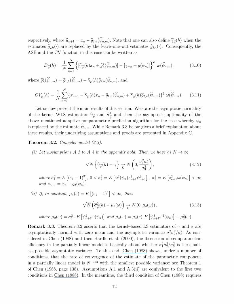
respectively, where un+1 = xn − g2,h(ψn,m). Note that one can also define γψ(h) when the

estimates gj,h(·) are replaced by the leave–one–out estimates gj,n(·). Consequently, the

ASE and the CV function in this case can be written as

Dψ(h) =1

N

N∑n=1

[γψ(h)xn + g∗h(ψn,m)]− [γxn + g(ψn)]

2

ω(ψn,m), (3.10)

where g∗h(ψn,m) = g1,h(ψn,m)− γψ(h)g2,h(ψn,m), and

CVψ(h) =1

N

N∑n=1

xn+1 − γψ(h)xn − g1,n(ψn,m) + γψ(h)g2,n(ψn,m)2 ω(ψn,m). (3.11)

Let us now present the main results of this section. We state the asymptotic normality

of the kernel WLS estimators γψ and σ2ψ

and then the asymptotic optimality of the

above–mentioned adaptive nonparametric prediction algorithm for the case whereby ψnis replaced by the estimate ψn,m. While Remark 3.3 below gives a brief explanation about

these results, their underlying assumptions and proofs are presented in Appendix C.

Theorem 3.2. Consider model (2.3).

(i) Let Assumptions A.1 to A.4 in the appendix hold. Then we have as N →∞

√Nγψ(h)− γ

→DN

(0,σ2

1σ22

σ23

), (3.12)

where σ21 = E

[(ε1 − 1)2], 0 < σ2

2 = E[ω2(ψn)z2

n+1ψ2n+1

], σ2

3 = E[z2n+1ω(ψn)

]<∞

and zn+1 = xn − g2(ψn).

(ii) If, in addition, µ4(ε) = E[(ε1 − 1)4] <∞, then

√N(σ2ψ(h)− µ2(ω)

)→DN (0, µ4(ω)) , (3.13)

where µ2(ω) = σ21 · E

[ψ2n+1ω(ψn)

]and µ4(ω) = µ4(ε) E

[ψ4n+1ω

2(ψn)]− µ2

2(ω).

Remark 3.3. Theorem 3.2 asserts that the kernel–based LS estimators of γ and σ are

asymptotically normal with zero mean and the asymptotic variance σ21σ

22/σ

23. As con-

sidered in Chen (1988) and then Hardle et al. (2000), the discussion of semiparametric

efficiency in the partially linear model is basically about whether σ21σ

22/σ

23 is the small-

est possible asymptotic variance. To this end, Chen (1988) shows, under a number of

conditions, that the rate of convergence of the estimate of the parametric component

in a partially linear model is N−1/2 with the smallest possible variance; see Theorem 1

of Chen (1988, page 138). Assumptions A.1 and A.3(ii) are equivalent to the first two

conditions in Chen (1988). In the meantime, the third condition of Chen (1988) requires

12

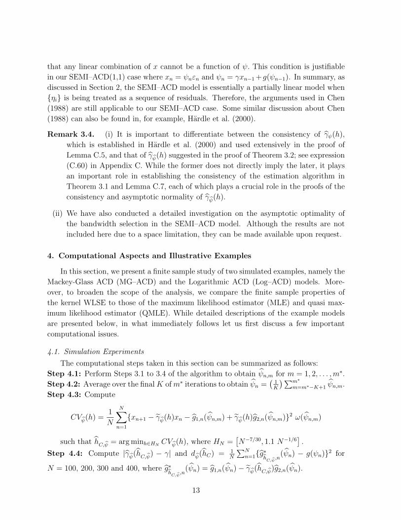
that any linear combination of x cannot be a function of ψ. This condition is justifiable

in our SEMI–ACD(1,1) case where xn = ψnεn and ψn = γxn−1 +g(ψn−1). In summary, as

discussed in Section 2, the SEMI–ACD model is essentially a partially linear model when

ηi is being treated as a sequence of residuals. Therefore, the arguments used in Chen

(1988) are still applicable to our SEMI–ACD case. Some similar discussion about Chen

(1988) can also be found in, for example, Hardle et al. (2000).

Remark 3.4. (i) It is important to differentiate between the consistency of γψ(h),

which is established in Hardle et al. (2000) and used extensively in the proof of

Lemma C.5, and that of γψ(h) suggested in the proof of Theorem 3.2; see expression

(C.60) in Appendix C. While the former does not directly imply the later, it plays

an important role in establishing the consistency of the estimation algorithm in

Theorem 3.1 and Lemma C.7, each of which plays a crucial role in the proofs of the

consistency and asymptotic normality of γψ(h).

(ii) We have also conducted a detailed investigation on the asymptotic optimality of

the bandwidth selection in the SEMI–ACD model. Although the results are not

included here due to a space limitation, they can be made available upon request.

4. Computational Aspects and Illustrative Examples

In this section, we present a finite sample study of two simulated examples, namely the

Mackey-Glass ACD (MG–ACD) and the Logarithmic ACD (Log–ACD) models. More-

over, to broaden the scope of the analysis, we compare the finite sample properties of

the kernel WLSE to those of the maximum likelihood estimator (MLE) and quasi max-

imum likelihood estimator (QMLE). While detailed descriptions of the example models

are presented below, in what immediately follows let us first discuss a few important

computational issues.

4.1. Simulation Experiments

The computational steps taken in this section can be summarized as follows:

Step 4.1: Perform Steps 3.1 to 3.4 of the algorithm to obtain ψn,m for m = 1, 2, . . . ,m∗.

Step 4.2: Average over the finalK ofm∗ iterations to obtain ψn =(

1K

)∑m∗

m=m∗−K+1 ψn,m.

Step 4.3: Compute

CVψ(h) =1

N

N∑n=1

xn+1 − γψ(h)xn − g1,n(ψn,m) + γψ(h)g2,n(ψn,m)2 ω(ψn,m)

such that hC,ψ = arg minh∈HN CVψ(h), where HN =[N−7/30, 1.1 N−1/6

].

Step 4.4: Compute |γψ(hC,ψ) − γ| and dψ(hC) = 1N

∑Nn=1g∗h

C,ψ,n

(ψn) − g(ψn)2 for

N = 100, 200, 300 and 400, where g∗hC,ψ

,n(ψn) = g1,n(ψn)− γψ(hC,ψ)g2,n(ψn).

13

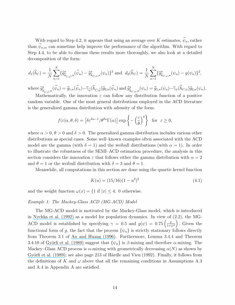
With regard to Step 4.2, it appears that using an average over K estimates, ψn, rather

than ψn,m can sometime help improve the performance of the algorithm. With regard to

Step 4.4, to be able to discuss these results more thoroughly, we also look at a detailed

decomposition of the form:

d1(hC) =1

N

N∑n=1

g∗hC,ψ

,n(ψn)− g∗

hC,ψ ,n(ψn)2 and d2(hC) =

1

N

N∑n=1

g∗hC,ψ ,n

(ψn)− g(ψn)2,

where g∗hC,ψ

,n(ψn) = g1,n(ψn)−γψ(hC,ψ)g2,n(ψn) and g∗

hC,ψ ,n(ψn) = g1,n(ψn)−γψ(hC,ψ)g2,n(ψn).

Mathematically, the innovation ε can follow any distribution function of a positive

random variable. One of the most general distributions employed in the ACD literature

is the generalized gamma distribution with adensity of the form:

f(ε|α, θ, δ) =[δεδα−1/θδαΓ(α)

]exp

−(εθ

)δfor ε ≥ 0,

where α > 0, θ > 0 and δ > 0. The generalized gamma distribution includes various other

distributions as special cases. Some well–known examples often associated with the ACD

model are the gamma (with δ = 1) and the weibull distributions (with α = 1). In order

to illustrate the robustness of the SEMI–ACD estimation procedure, the analysis in this

section considers the innovation ε that follows either the gamma distribution with α = 2

and θ = 1 or the weibull distribution with δ = 3 and θ = 1.

Meanwhile, all computations in this section are done using the quartic kernel function

K(u) = (15/16)(1− u2)2 (4.1)

and the weight function ω(x) = 1 if |x| ≤ 4; 0 otherwise.

Example 1: The Mackey-Glass ACD (MG-ACD) Model

The MG-ACD model is motivated by the Mackey-Glass model, which is introduced

in Nychka et al. (1992) as a model for population dynamics. In view of (2.2), the MG-

ACD model is established by specifying γ = 0.5 and g(ψ) = 0.75(

ψ1+ψ2

). Given the

functional form of g, the fact that the process ψn is strictly stationary follows directly

from Theorem 3.1 of An and Huang (1996). Furthermore, Lemma 3.4.4 and Theorem

3.4.10 of Gyorfi et al. (1989) suggest that ψn is β-mixing and therefore α-mixing. The

Mackey–Glass ACD process is α-mixing with geometrically decreasing α(N) as shown by

Gyorfi et al. (1989); see also page 213 of Hardle and Vieu (1992). Finally, it follows from

the definitions of K and ω above that all the remaining conditions in Assumptions A.3

and A.4 in Appendix A are satisfied.

14

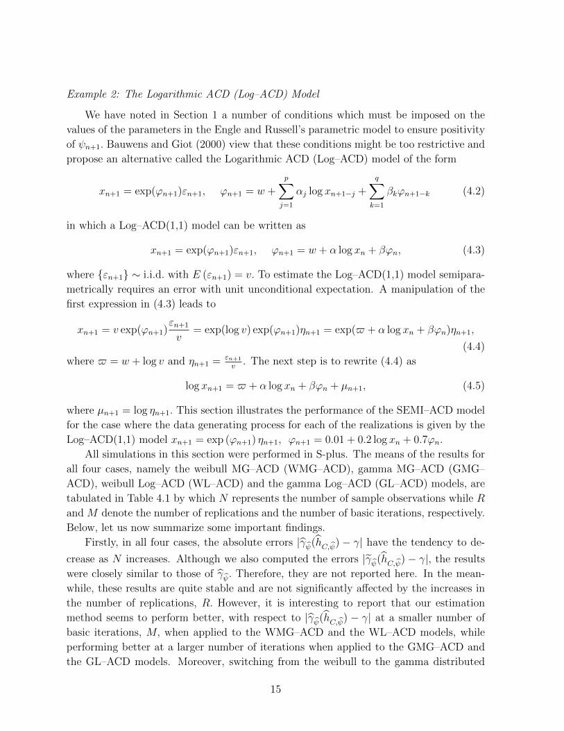
Example 2: The Logarithmic ACD (Log–ACD) Model

We have noted in Section 1 a number of conditions which must be imposed on the

values of the parameters in the Engle and Russell’s parametric model to ensure positivity

of ψn+1. Bauwens and Giot (2000) view that these conditions might be too restrictive and

propose an alternative called the Logarithmic ACD (Log–ACD) model of the form

xn+1 = exp(ϕn+1)εn+1, ϕn+1 = w +

p∑j=1

αj log xn+1−j +

q∑k=1

βkϕn+1−k (4.2)

in which a Log–ACD(1,1) model can be written as

xn+1 = exp(ϕn+1)εn+1, ϕn+1 = w + α log xn + βϕn, (4.3)

where εn+1 ∼ i.i.d. with E (εn+1) = v. To estimate the Log–ACD(1,1) model semipara-

metrically requires an error with unit unconditional expectation. A manipulation of the

first expression in (4.3) leads to

xn+1 = v exp(ϕn+1)εn+1

v= exp(log v) exp(ϕn+1)ηn+1 = exp($ + α log xn + βϕn)ηn+1,

(4.4)

where $ = w + log v and ηn+1 = εn+1

v. The next step is to rewrite (4.4) as

log xn+1 = $ + α log xn + βϕn + µn+1, (4.5)

where µn+1 = log ηn+1. This section illustrates the performance of the SEMI–ACD model

for the case where the data generating process for each of the realizations is given by the

Log–ACD(1,1) model xn+1 = exp (ϕn+1) ηn+1, ϕn+1 = 0.01 + 0.2 log xn + 0.7ϕn.

All simulations in this section were performed in S-plus. The means of the results for

all four cases, namely the weibull MG–ACD (WMG–ACD), gamma MG–ACD (GMG–

ACD), weibull Log–ACD (WL–ACD) and the gamma Log–ACD (GL–ACD) models, are

tabulated in Table 4.1 by which N represents the number of sample observations while R

and M denote the number of replications and the number of basic iterations, respectively.

Below, let us now summarize some important findings.

Firstly, in all four cases, the absolute errors |γψ(hC,ψ) − γ| have the tendency to de-

crease as N increases. Although we also computed the errors |γψ(hC,ψ) − γ|, the results

were closely similar to those of γψ. Therefore, they are not reported here. In the mean-

while, these results are quite stable and are not significantly affected by the increases in

the number of replications, R. However, it is interesting to report that our estimation

method seems to perform better, with respect to |γψ(hC,ψ) − γ| at a smaller number of

basic iterations, M, when applied to the WMG–ACD and the WL–ACD models, while

performing better at a larger number of iterations when applied to the GMG–ACD and

the GL–ACD models. Moreover, switching from the weibull to the gamma distributed

15

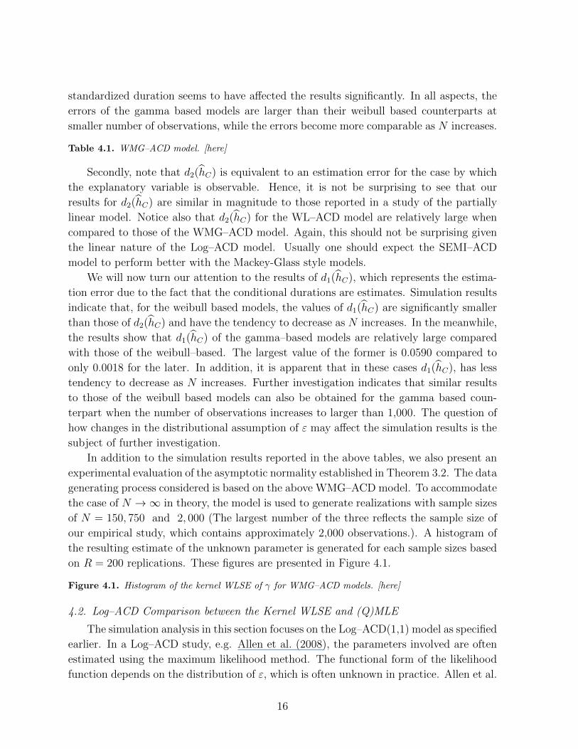
standardized duration seems to have affected the results significantly. In all aspects, the

errors of the gamma based models are larger than their weibull based counterparts at

smaller number of observations, while the errors become more comparable as N increases.

Table 4.1. WMG–ACD model. [here]

Secondly, note that d2(hC) is equivalent to an estimation error for the case by which

the explanatory variable is observable. Hence, it is not be surprising to see that our

results for d2(hC) are similar in magnitude to those reported in a study of the partially

linear model. Notice also that d2(hC) for the WL–ACD model are relatively large when

compared to those of the WMG–ACD model. Again, this should not be surprising given

the linear nature of the Log–ACD model. Usually one should expect the SEMI–ACD

model to perform better with the Mackey-Glass style models.

We will now turn our attention to the results of d1(hC), which represents the estima-

tion error due to the fact that the conditional durations are estimates. Simulation results

indicate that, for the weibull based models, the values of d1(hC) are significantly smaller

than those of d2(hC) and have the tendency to decrease as N increases. In the meanwhile,

the results show that d1(hC) of the gamma–based models are relatively large compared

with those of the weibull–based. The largest value of the former is 0.0590 compared to

only 0.0018 for the later. In addition, it is apparent that in these cases d1(hC), has less

tendency to decrease as N increases. Further investigation indicates that similar results

to those of the weibull based models can also be obtained for the gamma based coun-

terpart when the number of observations increases to larger than 1,000. The question of

how changes in the distributional assumption of ε may affect the simulation results is the

subject of further investigation.

In addition to the simulation results reported in the above tables, we also present an

experimental evaluation of the asymptotic normality established in Theorem 3.2. The data

generating process considered is based on the above WMG–ACD model. To accommodate

the case of N →∞ in theory, the model is used to generate realizations with sample sizes

of N = 150, 750 and 2, 000 (The largest number of the three reflects the sample size of

our empirical study, which contains approximately 2,000 observations.). A histogram of

the resulting estimate of the unknown parameter is generated for each sample sizes based

on R = 200 replications. These figures are presented in Figure 4.1.

Figure 4.1. Histogram of the kernel WLSE of γ for WMG–ACD models. [here]

4.2. Log–ACD Comparison between the Kernel WLSE and (Q)MLE

The simulation analysis in this section focuses on the Log–ACD(1,1) model as specified

earlier. In a Log–ACD study, e.g. Allen et al. (2008), the parameters involved are often

estimated using the maximum likelihood method. The functional form of the likelihood

function depends on the distribution of ε, which is often unknown in practice. Allen et al.

16

(2008) empirically study the finite sample properties of the MLE and QMLE for the Log–

ACD(1,1) model based on various probability distributions. An objective of the analysis in

this section is to observe how well the SEMI–ACD model performs numerically compared

to the MLE and QMLE given that the true data generating process is the Log–ACD(1,1)

model.

Due to the involvement of the nonlinearity in the SEMI–ACD model, our comparison

will focus mainly on the parametric component, i.e. the estimates of the unknown pa-

rameter associated with the lag value of duration. Even though such a comparison may

offer the MLE and QMLE some unfair advantages as the functional form of the condi-

tional mean equation is known in these cases, we expect the kernel WLSE to perform

competitively. However, instead of recalculating all the required results, we feel that it is

efficient and not unreasonable to use the ML and QML results already available in Allen

et al. (2008).

Table 4.2. Weibull based Log–ACD model. [here]

Table 4.3. Generalized gamma based Log–ACD model. [here]

Tables 4.2 and 4.3 present simulation results of the kernel WLSE, MLE and the QMLE

as applied to the Log–ACD(1,1) model generated based on the weibull and the generalized

gamma errors. The second column of the tables presents descriptive statistics of the

estimate γψ(h), which is computed using similar computational steps to those discussed

in Section 4.1, but with N = 500 and 1, 000, R = 500 and M = 3. Our experience shows

that changes in R and M do not have significant effect on the results. While the third

column shows the finite sample properties of the MLE for each of the distributions, the

forth (the fifth) columns show those of QMLE1 (QMLE2), whose sample mean is closest

to (furthest from) the true value of the parameter as reported in Allen et al. (2008).

As predicted, in all four cases the MLE seems to give the most accurate estimators

on average among the three estimators in question. However, the maximum likelihood

estimates for the generalized gamma based Log–ACD model seems to be leptokurtic

as evidenced by a relatively high kurtosis of 4.849 and 5.670 at N = 500 and 1, 000,

respectively. Allen et al. (2008) suggest that the problem with the generalized gamma

distribution could be caused by the difficulty of obtaining robust and accurate numerical

derivatives of the likelihood functions for the purpose of maximization.

Like the QMLE, the kernel WLSE seems to have suffered from a similar problem,

but at a much less extent. Overall, the average squared error suggests that when the

sample size is finite and the true distribution of the innovation is unknown, the kernel

WLSE should be preferred to the QMLE. Simulation results in the above tables show that

on average the SEMI–ACD method tends to overestimate the value of the parameter γ.

Although increasing the number of observations from 500 to 1,000 improves the accuracy

of the estimation only slightly, its precision increases quite significantly as evidenced by

17

the decline in the estimation standard deviation in Tables 4.2 and 4.3 from 0.057 to 0.040

and from 0.062 to 0.037, respectively. Also, as N increases, both the skewness and kurtosis

of our estimates converge to those of normal distribution.

5. An Analysis of the Intensity of Changes in Quoted Foreign Exchange Prices

This section applies the SEMI–ACD model to foreign exchange quotes arrival times

published over the Reuters’ network. The foreign exchange market is massive with in-

ternational participants trading billions of dollars 24 hours a day and a large number of

transactions carried out in split seconds between parties across the globe. Generally, when

foreign exchange data are examined, it is clear that many of the price quotes are simply

noisy repeats of the previous quote. By systematically thinning the sample, a measure of

the time between price changes is developed. In the following, these price durations are

analyzed with the SEMI–ACD model to obtain estimates of the instantaneous intensity

of price change. The empirical analysis in this paper considers the $US/$EU quotes data.

The complete data set is one whole week covering March 11 through to March 17, 2001.

However, it is assumed that that the business week is periodic, i.e. 5 days, beginning

Sunday 22:00 GMT to Friday 22:00 GMT and the weekend observations data are filtered

out. To eliminate the problem of bid-ask bounce, the current price is defined as the mid-

point of the bid-ask spread, i.e. the midprice of the form pn = (bidn+askn)2

, where bidn and

askn are the current bid and ask prices associated with transaction at time tn.

To construct the price duration process, the so–called dependent thinning is per-

formed. In essence only the points at which the price has changed significantly since the

occurrence of the last price change is kept. In order to to minimize the effects of errant

quotes two consecutive points were required to have changed more than a threshold value,

c, since the last price change. Hence, errant quote will not trigger a price change. In the

current study, we set c = 0.0003, i.e. three pips, to minimize the the impact of an asym-

metric quote setting due to portfolio adjustments by individual banks. This choice of c

yields a sample size of 2,732 or 2.15% of the original sample. The second column of Table

5.1 presents the summary statistics of the resulting price duration process. The average

price duration for the sample is 158 seconds, while the minimum and the maximum are

1 and 5,833 seconds, respectively. Additionally, the Ljung–Box test statistic indicates

significant autocorrelation, which is consistent with what is often reported in existing

studies.

For currency trading, the fact that there are clear periods of high and low activity

as markets around the world open and close leads us to believe that the intraday dura-

tions may comprise of both the stochastic component, which models the dynamics of the

process, and the deterministic component that accounts for any existing intraday trading

pattern. To model the price durations within the context of the SEMI–ACD model, let

18

us write

xn+1 = φ(tn) νn+1, (5.1)

where xn+1 is the price duration (in seconds) of the (n + 1)th price change, φ(·) denotes

the diurnal factor of the calendar time tn at which the (n + 1)th duration begins and

νn+1 represents a sequence of stationary time series errors.

Table 5.1. Descriptive statistics. [here]

By assuming that the diurnal function of time is multiplicatively separable from the

stochastic component, the latter can be incorporated into the model by defining νn+1 =xn+1

φ(tn)= ψn+1εn+1, where ψn+1 is the series of the conditional expectation of the price

durations as defined in Section 1. Similar to Engle and Russell (1997, 1998), in this paper

we interpret E[xn+1|Fn]φ(tn) ≡ ψn+1φ(tn) and εn+1 = xn+1

φ(tn)ψn+1as the one–step forecast

of price durations and the standardized price durations, respectively.

The modeling procedure employed in this section consists of three important steps,

namely i) diurnal adjustment, ii) SEMI–ACD model of the diurnal adjusted price dura-

tions and iii) empirical estimation of the baseline intensity function. Let us now proceed

with each of these steps in detail.

With regard to the first step, the most restrictive method, which was introduced by

Engle and Russell (1998), is to assume that the deterministic and stochastic components

both belong to some parametric families of functions. The two sets of parameters can

then be jointly estimated using maximum likelihood techniques. By contrast, our semi-

parametric estimation proposes using a more general method. We begin with a simple

transformation of (5.1) into an additive model of the form xn+1 = φ(tn) + ξn+1, where

ξn+1 = φ(tn)(νn+1 − 1) is a martingale difference series. This makes possible an alter-

native two–step approach that is to compute a consistent estimate of φ(tn), for example

φ(tn), using a nonparametric smoother, and then model the ratio of actual to fitted value

νn+1 = xn+1

φ(tn)as a SEMI–ACD model of the diurnally adjusted series of price durations.

To estimate the diurnal factor, the current paper employs the kernel regression smooth-

ing technique with the smoother defined as

φh (tn) =N∑s=1

Ws,h(tn)xs, (5.2)

whereWs,h(y) = Kh(y−ts)∑Nn=1Kh(y−tn)

is a kernel weight function. In our calculation, an asymptot-

ically optimal bandwidth is selected using the leave–one–out cross validation selection cri-

terion over a sequence of bandwidth values HN =h = hmaxa

k : h ≥ hmin, k = 0, 1, 2, . . .,

where 0 < hmin < hmax and 0 < a < 1 and letting JN ≤ log1/a(hmax/hmin) denotes the

number of elements of HN . The nonparametric kernel estimation of φ(tn) in (5.2) is advan-

tageous given the fact that it allows a more flexible dependence structure of the residual

19

error process. Since νn+1 in (5.1) represents the remaining dynamics not captured by

φ(·), the SEMI–ACD model allows it to be a stationary α-mixing process, which is the

assumption we made when constructing the SEMI–ACD model; see Appendix A for detail.

Figure 5.1. Expected price duration on hour of day, where 0 denotes 24:00GMT. [here]

Figure 5.1 presents the kernel estimates of the diurnal factors of the price durations.

There is enough evidence in the figure to suggest that price movements change charac-

teristics as business activities of major currency markets around the world fluctuate. A

moderate fluctuation, which occurs between hours 00:00GMT and 06:00GMT, marks the

beginning and the end of a business period in Tokyo, while the sudden slow down during

hours 03:00GMT and 04:00GMT belongs to the Japanese lunch hours. Furthermore, there

are two periods of high price intensity. While the first occurs between hours 07:00GMT

and 10:00GMT, which is the period by which European, Japanese and other Asian mar-

kets are active, the second one takes place between hours 14:00GMT and 17:00GMT, i.e.

the period during which European and New York business hours are overlapped. Finally,

it is clear that price changes occur much less frequently between hours 21:00GMT and

22:00GMT, which is 2:00PM to 4:00PM in New York, before the intensity begins to pick

up as the business day comes to a close and Japanese market becomes active. Engle

and Russell (1997) report similar intraday seasonal pattern in their study on the price

intensity of USD/Deutschmark exchange rate.

As the ACD model is proposed as a model for intertemporally correlated event arrival

times, it is a good idea to first examine the dynamic dependence of the diurnally adjusted

price duration, νn+1, before carrying out the second modeling step. Despite the fact that

the Ljung–Box test statistic shown in the third column of Table 5.1 reduces to 276.47

compared to 2,157.93 reported in the first column, the null hypothesis is still rejected at

the 5% significance level. This suggests that the large Ljung–Box statistic observed for

the raw price durations is not a result of the diurnal factor alone.

We now apply the SEMI-ACD(1,1) model to the diurnally adjusted price durations.

A number of previous studies in the field of nonparametric models have suggested that the

choice of the kernel function is much less critical than bandwidth choice; see, for example,

Gao and Yee (2000). To study the current problem, we employ the normal kernel function

of the form K(z) = 1√2πe−z

2/2. The cross–validation criterion is employed in order to select

an asymptotically optimal bandwidth with the CV function for the mth iteration

CVm(h) =1

N

N∑n=1

xn+1 − γm(h)xn − g1,n(ψn,m) + γm(h)g2,n(ψn,m)2 ω(ψn). (5.3)

To specify the most appropriate bandwidth interval for the mth iteration, we follow a

similar procedure to that suggested in Hardle et al. (1988). The first step is to compute

the score for each of the CV functions among one hundred sample values of h drawn

20

sequentially from the set H0 =hs : 0.01 < hs ≤ 4

, where s = 1, 2, . . . , 100. The results

show that the interval HN = [0.0320, 0.5486] is the smallest possible bandwidth interval

in which CVm(h) can attain their smallest values. The above step is then repeated, except

that each hs is now drawn sequentially among HN . With regard to the maximum number

of basic iterations, initially, it is set at m∗ = 15. However, it is found that no further

improvement can be obtained at m∗ ≥ 6. Therefore, the analysis in this paper is based

on m∗ = 5.

Table 5.2. SEMI-ACD(1,1) and EACD(1,1) price models. [here]

Table 5.2 shows the estimation results of γm(hC,m), hC,m, γψ(hC,ψ) and hC,ψ for

the SEMI-ACD(1,1) model. For the sake of comparison, we also present results of an

EACD(1,1) model based on the above–mentioned (Q)ML technique. Note that our para-

metric estimate of the unknown parameter γ of 0.1167 is slightly larger than what sug-

gested in Engle and Russell (1997), who report an estimate of 0.07315 in their study on

the price intensity of $USD/Deutschmark exchange rate. However, both parametric esti-

mates are smaller than our semiparametric estimates of 0.1332 and 0.1346. Furthermore,

the EACD model provide the estimate with a slightly smaller standard error of 0.0201

compared to 0.0257 for the SEMI–ACD estimate.

Figure 5.2. Empirical estimate of the unknown real valued function g(·). [here]

To obtain a more complete picture, let us now examine empirically the intertemporal

importance of the conditional duration on the ACD process. Recall firstly that, in a SEMI–

ACD(1,1) model, the intertemporal relationship is described by g(ψn) = E[xn+1|ψn] −γE[xn|ψn] ≡ g1(ψn)− γg2(ψn). To construct the confidence bands about gh, let us make

use of the following transformed version of the SEMI–ACD(1,1,) model

xn+1 = g(ψn) + ηn+1, (5.4)

where xn+1 = xn+1 − γxn and E[xn+1|ψn]− γE[xn|ψn] = E[xn+1|ψn] ≡ g(ψn+1). We then

propose the following procedure.

Step 5.1: Follow the SEMI–ACD estimation procedure discussed earlier to obtain

γψ(h) and ψn,m∗ .

Step 5.2: Compute xn+1 = xn+1 − γψ(h)xn, then perform regression of (5.4).

Step 5.3: Compute the bias–corrected confidence bands about g(ψn,m∗) using the

procedure introduced in Xia (1998).

Remark 5.1. In this paper, the regressors in the kernel regression are estimated them-

selves. Therefore, an interesting question, which warrant further investigation, is how

this might affect Xia’s procedure. To investigate the issue, we conduct a small simulation

exercise following Steps 5.1 to 5.3 above with a similar style of generated regressor as in

21

Li and Wooldridge (2002). We have found that in this case the estimation of regressors

result in wider confidence bands. Although a more detailed investigation is required, we

conjecture that such outcome is also applicable to our SEMI–ACD model.

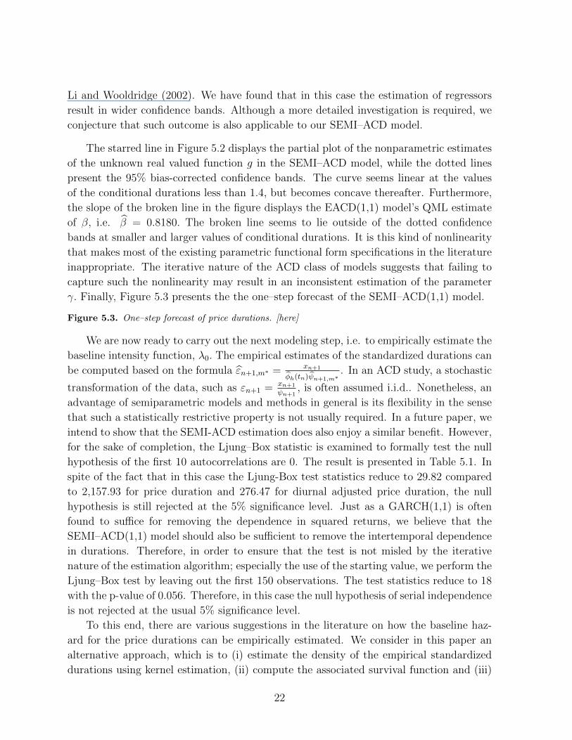
The starred line in Figure 5.2 displays the partial plot of the nonparametric estimates

of the unknown real valued function g in the SEMI–ACD model, while the dotted lines

present the 95% bias-corrected confidence bands. The curve seems linear at the values

of the conditional durations less than 1.4, but becomes concave thereafter. Furthermore,

the slope of the broken line in the figure displays the EACD(1,1) model’s QML estimate

of β, i.e. β = 0.8180. The broken line seems to lie outside of the dotted confidence

bands at smaller and larger values of conditional durations. It is this kind of nonlinearity

that makes most of the existing parametric functional form specifications in the literature

inappropriate. The iterative nature of the ACD class of models suggests that failing to

capture such the nonlinearity may result in an inconsistent estimation of the parameter

γ. Finally, Figure 5.3 presents the the one–step forecast of the SEMI–ACD(1,1) model.

Figure 5.3. One–step forecast of price durations. [here]

We are now ready to carry out the next modeling step, i.e. to empirically estimate the

baseline intensity function, λ0. The empirical estimates of the standardized durations can

be computed based on the formula εn+1,m∗ = xn+1

φh(tn)ψn+1,m∗. In an ACD study, a stochastic

transformation of the data, such as εn+1 = xn+1

ψn+1, is often assumed i.i.d.. Nonetheless, an

advantage of semiparametric models and methods in general is its flexibility in the sense

that such a statistically restrictive property is not usually required. In a future paper, we

intend to show that the SEMI-ACD estimation does also enjoy a similar benefit. However,

for the sake of completion, the Ljung–Box statistic is examined to formally test the null

hypothesis of the first 10 autocorrelations are 0. The result is presented in Table 5.1. In

spite of the fact that in this case the Ljung-Box test statistics reduce to 29.82 compared

to 2,157.93 for price duration and 276.47 for diurnal adjusted price duration, the null

hypothesis is still rejected at the 5% significance level. Just as a GARCH(1,1) is often

found to suffice for removing the dependence in squared returns, we believe that the

SEMI–ACD(1,1) model should also be sufficient to remove the intertemporal dependence

in durations. Therefore, in order to ensure that the test is not misled by the iterative

nature of the estimation algorithm; especially the use of the starting value, we perform the

Ljung–Box test by leaving out the first 150 observations. The test statistics reduce to 18

with the p-value of 0.056. Therefore, in this case the null hypothesis of serial independence

is not rejected at the usual 5% significance level.

To this end, there are various suggestions in the literature on how the baseline haz-

ard for the price durations can be empirically estimated. We consider in this paper an

alternative approach, which is to (i) estimate the density of the empirical standardized

durations using kernel estimation, (ii) compute the associated survival function and (iii)

22

take the quotient of the two to obtain the baseline hazard. In the following, we explain

the first two steps in more detail. The survival function of ε is the function Sε defined by

Sε(e) = Pr(ε > e) for all e. If the cumulative distribution function Fε is known, then Sεcan be computed as Sε(e) = 1− Fε(e). Otherwise, Fε can be estimated by

Fε(e) =

∫ e

−∞pε(y)dy, (5.5)

where pε(y) is the nonparametric kernel density estimate of the form

pε(y) =1

Nh

N∑n=1

K

(en+1 − y

h

), (5.6)

in which h is the bandwidth parameter. We can now write (5.5) using the estimate in

(5.6) as Fε(e) = 1Nh

∑Nn=1

∫ e−∞K

(en+1−y

h

)dy, which becomes

Fε(e) =1

N

N∑n=1

−∫ en+1−e

h

−∞K(z)dz =

1

N

N∑n=1

∫ ∞en+1−e

h

K(z)dz. (5.7)

If K(z) is the normal kernel function,furthermore, we then immediately have

Fε(e) =1

N

N∑n=1

[Φ(∞)− Φ

(en+1 − e

h

)]=

1

N

N∑n=1

[1− Φ

(en+1 − e

h

)], (5.8)

which implies

Sε(e) =1

N

N∑n=1

Φ

(en+1 − e

h

), (5.9)

where Φ(u) = 1√2π

∫ u−∞ exp−u

2/2 du. Now, in order to estimate and implement (5.6) and

(5.9), we need to replace en+1 by εn+1 and then compute the bandwidth parameter h0

based on the following rule of thumb h0 = 1.06 min(σε,

R1.34

)N−1/5, where R is the

inter–quartile range defined as R = ε0.75N − ε0.25N .

Figure 5.4. Kernel density estimates of pε. [here]

Figure 5.5. Kernel density estimates of pε. [here]

Figure 5.6. Empirical estimates of the survival function Sε. [here]

Figure 5.7. Empirical estimates of the baseline hazard of price durations. [here]

Figure 5.4 presents the kernel density estimator pε of p. At first glance, one may

conjecture that a gamma distribution with suitable parameter values may imply such a

density function. To give some idea about the kind of distribution ε may follow, the

23

figure compares the estimate with that of a Gamma(1.2,0.5) distribution, whose param-

eter values were selected using the maximum likelihood estimation. However, a more

careful consideration suggests that there is clear evidence of an applicability of a mix-

ture distribution in Figure 5.4. Clearly, there is a turning point between the values of

the standardized durations at above and below 2 seconds. Nonetheless, a formal testing

is required in order to obtain more conclusive information about the distribution of the

standardized duration. In addition, Figure 5.5 presents the kernel density estimator pεof p and its 95% confidence bands, which are computed based on the biased correction

approach discussed in Hall (1992). Figure 5.6 presents the SEMI–ACD based empirical

estimates of the survival function Sε (top panel) and the baseline hazard (bottom panel),

which is essentially U-shaped and close to that of a generalized hazard function. Finally,

note that confidence bands are not drawn for Figure 5.6 since the empirical survival func-

tion and baseline hazard are both the immediate transformation of the kernel density

estimate in Figure 5.4.

6. Conclusions and Discussions

We introduce in this paper a new alternative semiparametric regression approach to

the ACD model. The newly developed SEMI–ACD model enables an analysis of a richer

dynamics of the duration process when compared to its parametric counterpart, while

retaining the linear structure involved in the phenomena being modeled. To estimate

the SEMI–ACD model, we remodified an existing estimation algorithm in the literature

to suit our autoregressive semiparametric specification, while providing a rigorous proof

of its statistical consistency. Unlike in the existing studies, the autoregressive semipara-

metric functional form set up in this paper enables the establishment of mathematical

results which provide low level conditions for the underlying assumptions of the con-

sistency to hold. Furthermore, we study in detail the impacts of such the numerical

estimation method on both the asymptotic theory and its practical implementation of

the proposed semiparametric estimation. We provide experimental evidence which show

that the SEMI–ACD procedure possesses sound asymptotic properties with a robust per-

formance across various data generating processes. Finally, to illustrate the usefulness of

the model in practice, we apply it to model a thinned series of quotes arrival times for

the $US/$EU exchange rate.

There are various extensions that may be discussed. A potential extension beyond

the SEMI–ACD(1,1) may concentrate on approximating the conditional mean function

Ψ(Xn,Ψn) = E[Yn|Xn,Ψn] by a semiparametric function of the form Ψ(Xn,Ψn) = µ +

Xτnγ + g(Ψn), where µ is an unknown parameter, γ = (γ1, γ2, . . . , γq)

τ is a vector of

unknown parameters, g(·) is an unknown function on Rq, Xn = (Xn1, Xn2, . . . , Xnq)τ and

Ψn = (Ψn1,Ψn2, . . . ,Ψnp)τ . The mean squared error, E[Xt − Ψ(Xn,Ψn)]2, is minimized

subject to E[g(Ψn)] = 0 to ensure the identifiability of Ψ(Xn,Ψn). Estimation of g(·) may

24

suffer from the curse of dimensionality when g(·) is not necessarily additive and p ≥ 3.

Gao (2007) proposes a number of different estimation methods to address such an issue.

When g(·) itself is additive, the functional form of Ψ(Xn,Ψn) can be written as

Ψ(Xn,Ψn) = µ+Xτnγ+

∑pi=1 gi(Ψni) subject to E[gi(Ψni)] = 0 for all 1 ≤ i ≤ p to ensure

the identifiability of each gi(·), where all gi(·)’s for 1 ≤ i ≤ p are unknown one–dimensional

functions over R1. The semiparametric kernel estimation method is then based on mini-

mization of E[Xt−Ψ(Xn,Ψn)]2 = E[Yn−µ−Xτnγ−g(Ψn)]2. Such a minimization problem

is equivalent to minimizingE[Yn−µ−Xτnγ−g(Ψn)]2 = E [E (Yn − µ−Xτ

nγ − g(Ψn))2|Ψn]over some (µ, γ, g). This implies that g(Ψn) = E[(Yn−µ−Xτ

nγ)|Ψn] and µ = E[Yn−Xτnγ]

with γ given by γ = Σ−1E[(Xn − E[Xn|Ψn])(Xn − E[Xn|Ψn])] provided that the inverse

Σ−1 = (E[(Xn − E[Xn|Ψn])(Xn − E[Xn|Ψn])τ ])−1 exists.

The estimation procedure is then an extended version of the one proposed in this

paper. As suggested in Gao (2007), this may involve three important steps. Firstly, it is

to estimate µ and g(·) using the standard local linear estimation by treating γ as if it were

known. The second step is to employ marginal integration to obtain g1, . . . , gp under the

assumption that E[gi(Ψni)] = 0. The third and final step is to estimate γ. Under a number

of suitable conditions, including the above–mentioned identification condition and the

assumption that Ψn are observable, Gao (2007) establishes the asymptotic theory of the

marginal integration estimators for both the parametric and nonparametric components.

As the required assumptions and derivations are highly technical, we leave the discussion

of such an extension to a future paper.

7. Acknowledgments

The authors would also like to acknowledge the financial support from the Australian Re-

search Council Discovery Grants Program under Grant Number: DP1096374.

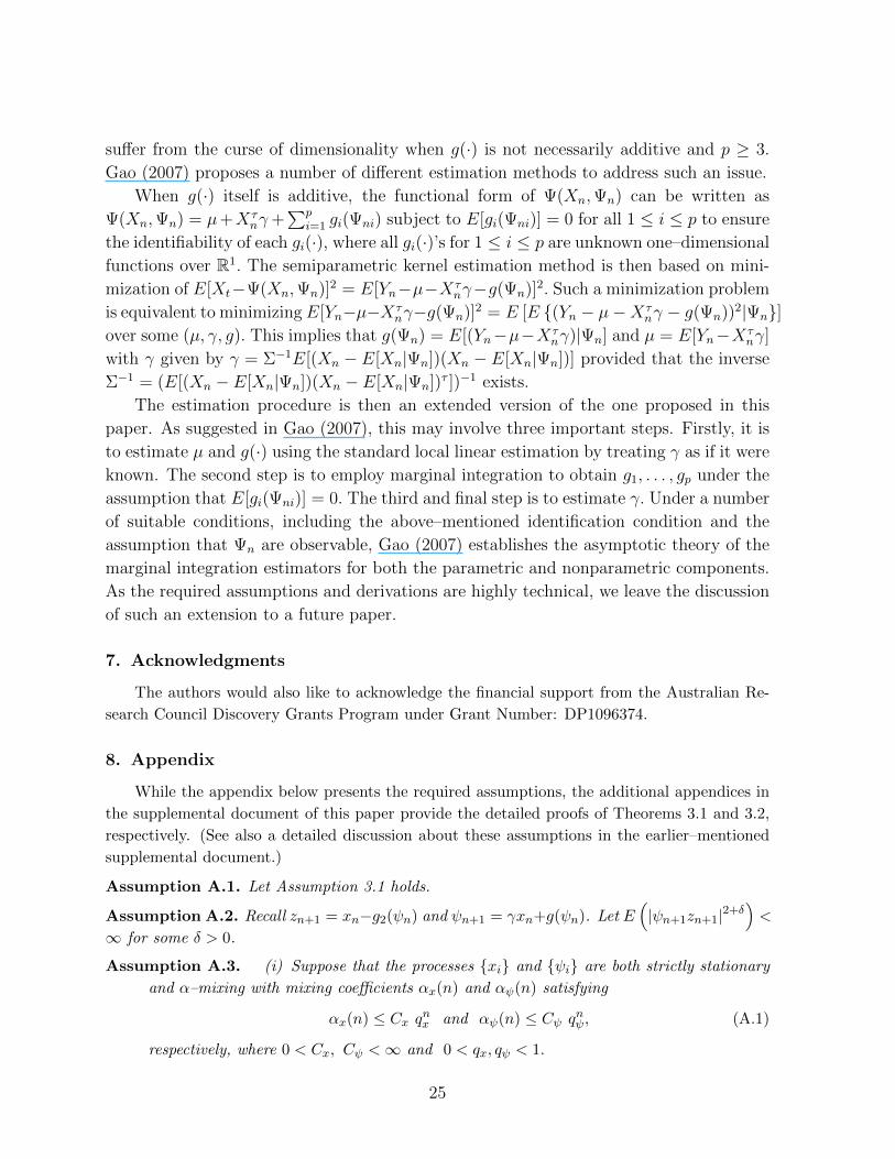
8. Appendix

While the appendix below presents the required assumptions, the additional appendices in

the supplemental document of this paper provide the detailed proofs of Theorems 3.1 and 3.2,

respectively. (See also a detailed discussion about these assumptions in the earlier–mentioned

supplemental document.)

Assumption A.1. Let Assumption 3.1 holds.

Assumption A.2. Recall zn+1 = xn−g2(ψn) and ψn+1 = γxn+g(ψn). Let E(|ψn+1zn+1|2+δ

)<

∞ for some δ > 0.

Assumption A.3. (i) Suppose that the processes xi and ψi are both strictly stationary

and α–mixing with mixing coefficients αx(n) and αψ(n) satisfying

αx(n) ≤ Cx qnx and αψ(n) ≤ Cψ qnψ, (A.1)

respectively, where 0 < Cx, Cψ <∞ and 0 < qx, qψ < 1.

25

(ii) Assume that ψi has a common marginal density f(·) and that g1, g2 and f have con-

tinuous derivatives of up to the second order and are all bounded on the interior of Sω,

where Sω is the compact support of the weight function ω(·) as assumed in Assumption

A.4 below. In addition, infψ∈Sω f(ψ) > 0.

(iii) There are constants 0 < B1 such that supψ(ψ2E[|ψi||ψi−1 = ψ]f(ψ)

)≤ B1 <∞.

(iv) Let Pψi > 0 = 1 for all i ≥ 1 and E[|xi|k

]<∞ for any k ≥ 1.

Assumption A.4. (i) Suppose that the kernel function satisfies:

a) K is symmetric, twice differentiable and the second derivative, K(2)(u), is continuous. In

addition, K has an absolutely integrable Fourier transform with∫K (u) du = 1, K (·) ≥ 0

and∫∞−∞ u

2K (u) du <∞.

b) The bandwidth h satisfies limT→∞ h = 0, limT→∞ Th2 =∞ and limT→∞ Th

5 <∞.(ii) Assume that the nonnegative weight function ω(·) is continuous and bounded. In addition,

the support Sω is compact.

References

Allen, D., Chan, F., McAleer, M., Peiris, S., 2008. Finite sample properties of the QMLE for the log-ACD

model: application to Australian stocks. Journal of Econometrics 147, 163–185.

An, H., Huang, F., 1996. The geometrical ergodicity of nonlinear autoregressive models. Statistica Sinica

6, 943–956.

Bauwens, L., Giot, P., 2000. The logarithmic ACD model: an application to the bid-ask quote process of

three NYSE stocks. Annales d’Economie et de Statistique 60, 117–149.

Buhlmann, P., McNeil, A., 2002. An algorithm for nonparametric GARCH modelling. Computational

Statistics & Data Analysis 40, 665–683.

Chen, H., 1988. Convergence rates for parametric components in a partly linear model. The Annals of

Statistics, 136–146.

Cosma, A., Galli, F., 2006. A nonparametric ACD model. CORE Discussion Paper (Paper No. 2006/67).

Drost, F. C., Werker, B., 2004. Semiparametric duration models. Journal of Business & Economic Statis-

tics 22, 40–50.

Dufour, A., Engle, R., 2000. Time and the price impact of a trade. Journal of Finance 55, 2467–2498.

Engle, R., Russell, J., 1997. Forecasting the frequency of changes in quoted foreign exchange prices with

the autoregressive conditional duration model. Journal of Empirical Finance (2-3), 187–212.

Engle, R., Russell, J., 1998. Autoregressive conditional duration: a new model for irregularly spaced

transaction data. Econometrica 66, 1127–1162.

Fernandes, M., Grammig, J., 2006. A family of autoregressive conditional duration models. Journal of

Econometrics 130, 1–23.

26

Gao, J., 2007. Nonlinear Time Series: Semiparametric and Nonparametric Methods. Chapman &

Hall/CRC, London.

Gao, J., King, M. L., 2004. Adaptive testing in continuous-time diffusion models. Econometric Theory

20 (5), 844–882.

Gao, J., Yee, T., 2000. Adaptive estimation in partially linear autoregressive models. Canadian Journal

of Statistics 28, 571–586.

Grammig, J., Maurer, K., 2000. Non-monotonic hazard functions and the autoregressive conditional

duration model. The Econometrics Journal 3, 16–38.

Gyorfi, L., Hardle, W., Sarda, P., Vieu, P., 1989. Nonparametric Curve Estimation from Time Series.

Vol. 60 of Lecture Notes in Statistics. Springer-Verlag, Berlin.

Hall, P., 1992. Effect of bias estimation on coverage accuracy of bootstrap confidence intervals for a

probability density. The Annals of Statistics 20 (2), 675–694.

Hansen, B., 2008. Uniform convergence rates for kernel estimation with dependent data. Econometric

Theory 24, 726–748.

Hardle, W., Hall, P., Marron, S., 1988. How far are automatically chosen regression smoothing parameter

from their optimum? Journal of the American Statistical Association 83, 86–101.

Hardle, W., Liang, H., Gao, J., 2000. Partially Linear Models. Physica Verlag, New York.

Hardle, W., Vieu, P., 1992. Kernel regression smoothing of time series. Journal of Time Series Analysis

13, 209–232.

Li, Q., Wooldridge, J., 2002. Semiparametric estimation of partially linear models for dependent data

with generated regressors. Econometric Theory 18, 625–645.

Meitz, M., Terasvirta, T., 2006. Evaluating models of autoregressive conditional duration. Journal of

Business & Economic Statistics 24, 104–124.

Nychka, D., Ellner, S., McCaffrey, D., Gallant, A., 1992. Finding chaos in noisy systems. Journal of the

Royal Statistical Society, Series B 54, 399–426.

Pagan, A., Ullah, A., 1999. Nonparametric Econometrics. Cambridge University Press, Cambridge.

Pollard, D., 1984. Convergence of Stochastic Processes. Springer, New York.

Robinson, P., 1988. Root-N-consistent semiparametric regression. Econometrica 56, 931–954.

Xia, Y., 1998. Bias-corrected confidence bands in nonparametric regression. Journal of the Royal Statis-

tical Society, Series B 60, 797–811.

Zhang, M. Y., Russell, J. R., Tsay, R., 2001. A nonlinear autoregressive conditional duration model with

applications to financial transaction data. Journal of Econometrics 104, 179–207.

27

Table 4.1. WMG–ACD, GMG–ACD, WL–ACD and GL–ACD models.

WMG–ACD N 100 200R 100 500 100 500M 3 8 3 8 3 8 3 8

|γψ(hC,ψ)− γ| 0.0774 0.0770 0.0809 0.0814 0.0706 0.0706 0.0636 0.0633

d1(hC) 0.0009 0.0011 0.0008 0.0009 0.0006 0.0005 0.0005 0.0004

d2(hC) 0.0065 0.0070 0.0066 0.0065 0.0046 0.0046 0.0045 0.0045

dψ(hC) 0.0056 0.0054 0.0055 0.0055 0.0033 0.0033 0.0035 0.0034

N 300 400

|γψ(hC,ψ)− γ| 0.0602 0.0608 0.0561 0.0561 0.0539 0.0540 0.0513 0.0511

d1(hC) 0.0006 0.0004 0.0004 0.0004 0.0004 0.0004 0.0004 0.0004

d2(hC) 0.0038 0.0038 0.0041 0.0041 0.0041 0.0041 0.0036 0.0036

dψ(hC) 0.0030 0.0029 0.0029 0.0030 0.0030 0.0030 0.0026 0.0026

GMG–ACD N 100 200

|γψ(hC,ψ)− γ| 0.1320 0.1300 0.1280 0.1235 0.1057 0.0959 0.1111 0.1017

d1(hC) 0.0099 0.0115 0.0100 0.0127 0.0179 0.0236 0.0148 0.0199

d2(hC) 0.0152 0.0150 0.0117 0.0117 0.0096 0.0092 0.0111 0.0118

dψ(hC) 0.0174 0.0181 0.0156 0.0180 0.0178 0.0203 0.0175 0.0223

N 300 400

|γψ(hC,ψ)− γ| 0.0938 0.0888 0.1083 0.0991 0.0839 0.0781 0.0818 0.0735

d1(hC) 0.0137 0.0170 0.0155 0.0211 0.0191 0.0195 0.0206 0.0206

d2(hC) 0.0087 0.0087 0.0078 0.0095 0.0079 0.0079 0.0044 0.0044

dψ(hC) 0.0142 0.0160 0.0146 0.0208 0.0191 0.0186 0.0148 0.0136

WL–ACD N 100 200

|γψ(hC,ψ)− γ| 0.0981 0.1031 0.1049 0.1093 0.0790 0.0828 0.0800 0.0832

d1(hC) 0.0018 0.0017 0.0020 0.0018 0.0007 0.0006 0.0004 0.0006

d2(hC) 0.0113 0.0113 0.0152 0.0152 0.0144 0.0144 0.0120 0.0120

dψ(hC) 0.0159 0.0156 0.0213 0.0206 0.0178 0.0175 0.0152 0.0152

N 300 400

|γψ(hC,ψ)− γ| 0.0688 0.0712 0.0702 0.0727 0.0621 0.0647 0.0577 0.0597

d1(hC) 0.0006 0.0005 0.0007 0.0007 0.0007 0.0005 0.0007 0.0005

d2(hC) 0.0117 0.0120 0.0131 0.0131 0.0125 0.0125 0.0116 0.0116

dψ(hC) 0.0158 0.0155 0.0172 0.0170 0.0163 0.0163 0.0146 0.0143

GL–ACD N 100 200

|γψ(hC,ψ)− γ| 0.0970 0.0963 0.0972 0.0970 0.0776 0.0785 0.0709 0.0733

d1(hC) 0.0430 0.0430 0.0351 0.0351 0.0232 0.0329 0.0348 0.0348

d2(hC) 0.0064 0.0049 0.0060 0.0053 0.0043 0.0019 0.0034 0.0036

dψ(hC) 0.0624 0.0586 0.0502 0.0487 0.0372 0.0446 0.0486 0.0477

N 300 400

|γψ(hC,ψ)− γ| 0.0685 0.0656 0.0593 0.0600 0.0584 0.0591 0.0544 0.0935

d1(hC) 0.0590 0.0509 0.0405 0.0405 0.0312 0.0312 0.0420 0.0420

d2(hC) 0.0030 0.0025 0.0028 0.0025 0.0021 0.0017 0.0028 0.0028

dψ(hC) 0.0616 0.0535 0.0500 0.0491 0.0429 0.0416 0.0595 0.0334

28

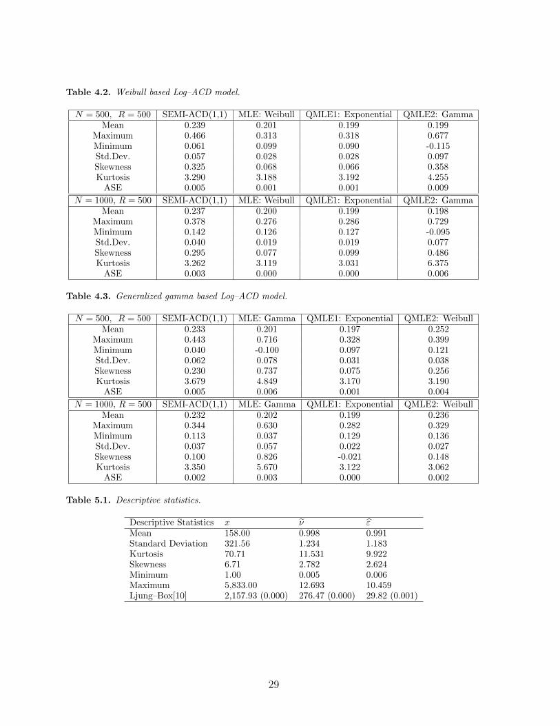
Table 4.2. Weibull based Log–ACD model.

N = 500, R = 500 SEMI-ACD(1,1) MLE: Weibull QMLE1: Exponential QMLE2: GammaMean 0.239 0.201 0.199 0.199

Maximum 0.466 0.313 0.318 0.677Minimum 0.061 0.099 0.090 -0.115Std.Dev. 0.057 0.028 0.028 0.097Skewness 0.325 0.068 0.066 0.358Kurtosis 3.290 3.188 3.192 4.255

ASE 0.005 0.001 0.001 0.009

N = 1000, R = 500 SEMI-ACD(1,1) MLE: Weibull QMLE1: Exponential QMLE2: GammaMean 0.237 0.200 0.199 0.198

Maximum 0.378 0.276 0.286 0.729Minimum 0.142 0.126 0.127 -0.095Std.Dev. 0.040 0.019 0.019 0.077Skewness 0.295 0.077 0.099 0.486Kurtosis 3.262 3.119 3.031 6.375

ASE 0.003 0.000 0.000 0.006

Table 4.3. Generalized gamma based Log–ACD model.

N = 500, R = 500 SEMI-ACD(1,1) MLE: Gamma QMLE1: Exponential QMLE2: WeibullMean 0.233 0.201 0.197 0.252

Maximum 0.443 0.716 0.328 0.399Minimum 0.040 -0.100 0.097 0.121Std.Dev. 0.062 0.078 0.031 0.038Skewness 0.230 0.737 0.075 0.256Kurtosis 3.679 4.849 3.170 3.190

ASE 0.005 0.006 0.001 0.004

N = 1000, R = 500 SEMI-ACD(1,1) MLE: Gamma QMLE1: Exponential QMLE2: WeibullMean 0.232 0.202 0.199 0.236

Maximum 0.344 0.630 0.282 0.329Minimum 0.113 0.037 0.129 0.136Std.Dev. 0.037 0.057 0.022 0.027Skewness 0.100 0.826 -0.021 0.148Kurtosis 3.350 5.670 3.122 3.062

ASE 0.002 0.003 0.000 0.002

Table 5.1. Descriptive statistics.

Descriptive Statistics x ν εMean 158.00 0.998 0.991Standard Deviation 321.56 1.234 1.183Kurtosis 70.71 11.531 9.922Skewness 6.71 2.782 2.624Minimum 1.00 0.005 0.006Maximum 5,833.00 12.693 10.459Ljung–Box[10] 2,157.93 (0.000) 276.47 (0.000) 29.82 (0.001)

29

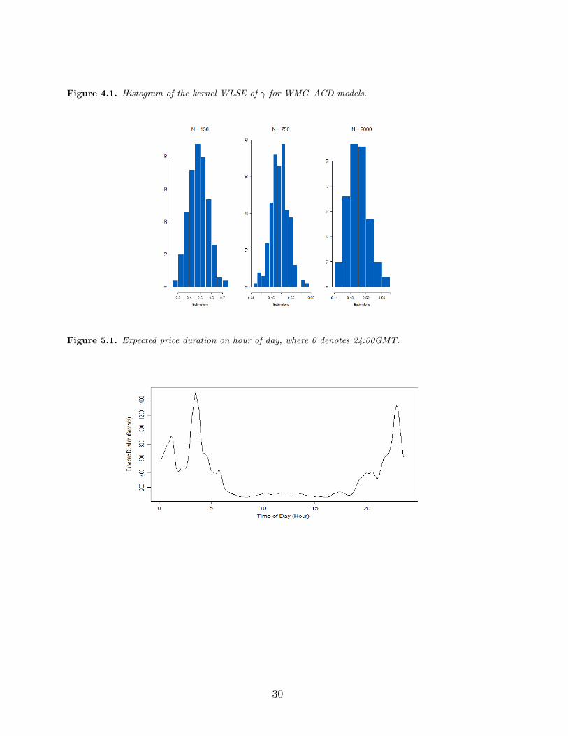
Figure 4.1. Histogram of the kernel WLSE of γ for WMG–ACD models.

Figure 5.1. Expected price duration on hour of day, where 0 denotes 24:00GMT.

30

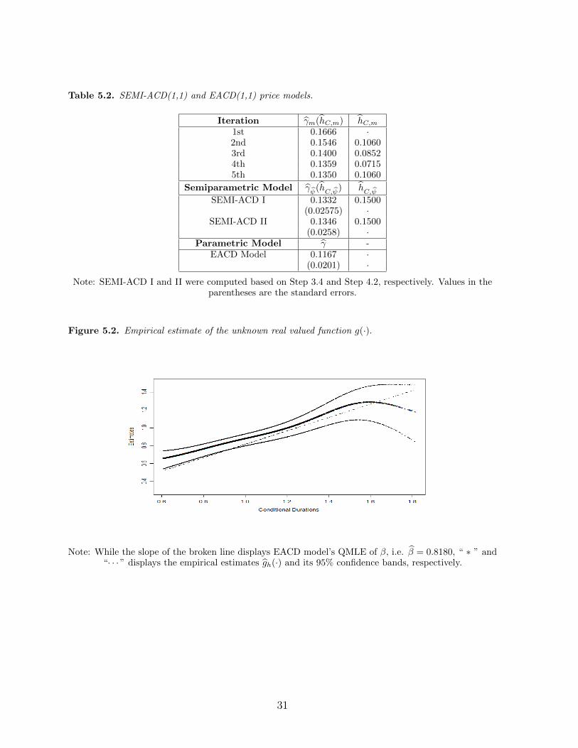
Table 5.2. SEMI-ACD(1,1) and EACD(1,1) price models.

Iteration γm(hC,m) hC,m1st 0.1666 ·2nd 0.1546 0.10603rd 0.1400 0.08524th 0.1359 0.07155th 0.1350 0.1060

Semiparametric Model γψ(hC,ψ) hC,ψSEMI-ACD I 0.1332 0.1500

(0.02575) ·SEMI-ACD II 0.1346 0.1500

(0.0258) ·Parametric Model γ -

EACD Model 0.1167 ·(0.0201) ·

Note: SEMI-ACD I and II were computed based on Step 3.4 and Step 4.2, respectively. Values in theparentheses are the standard errors.

Figure 5.2. Empirical estimate of the unknown real valued function g(·).

Note: While the slope of the broken line displays EACD model’s QMLE of β, i.e. β = 0.8180, “ ∗ ” and“· · · ” displays the empirical estimates gh(·) and its 95% confidence bands, respectively.

31

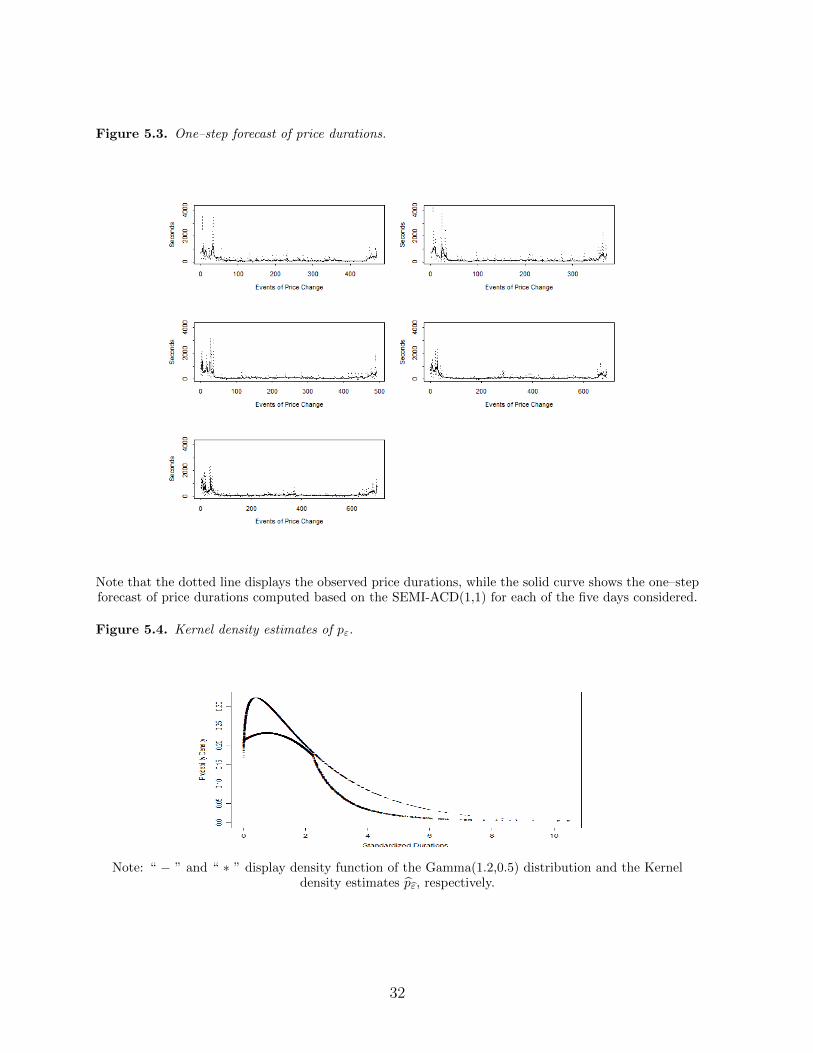
Figure 5.3. One–step forecast of price durations.

Note that the dotted line displays the observed price durations, while the solid curve shows the one–stepforecast of price durations computed based on the SEMI-ACD(1,1) for each of the five days considered.

Figure 5.4. Kernel density estimates of pε.

Note: “ − ” and “ ∗ ” display density function of the Gamma(1.2,0.5) distribution and the Kerneldensity estimates pε, respectively.

32

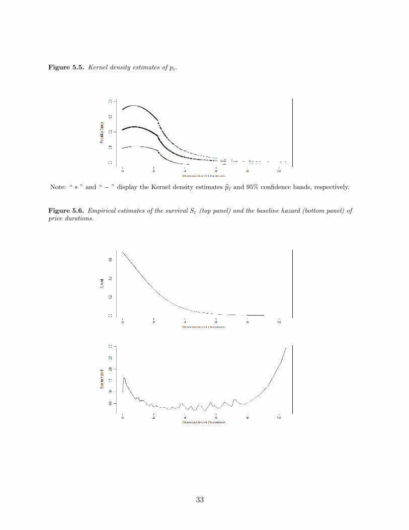
Figure 5.5. Kernel density estimates of pε.

Note: “ ∗ ” and “ − ” display the Kernel density estimates pε and 95% confidence bands, respectively.

Figure 5.6. Empirical estimates of the survival Sε (top panel) and the baseline hazard (bottom panel) ofprice durations.

33

Supplemental Document for

Semiparametric Autoregressive Conditional DurationModel: Theory and Practice

This is the supplemental document for the submitted paper entitled “Semiparametric Au-toregressive Conditional Duration Model: Theory and Practice”. For convenience, we first recallAssumption 3.1, and Theorems 3.1 and 3.2 of the main paper. Then Appendix A presents therequired assumptions (as shown in the main paper), Appendices B and C provide the detailedproofs of Theorems 3.1 and 3.2, respectively.

Assumption 3.1. (i) Suppose that function g on the real line satisfies the following Lipschitztype condition:

|g(x+ δ)− g(x)| ≤ ϕ(x)|δ| (A.1)

for each given x ∈ Sω, where Sω is the compact support of the weight function ω(·). Furthermore,ϕ(·) is a nonnegative measurable function such that with probability one,

maxi≥1

E[ϕ2(ψi)|(ψi−1, · · · , ψ1)

]≤ G2 and max

i≥1E[ϕ2(ψi,m)|(ψi−1,m−1, · · · , ψ1,1)

]≤ G2 (A.2)

for some 0 < G < 1.

(ii) Let ∆1T (ψ) = maxi,m≥1E12

[∣∣∣ψi,m − ψi,m∣∣∣2]→ 0 as T →∞

(iii) There exists a stationary sequence ψi,0 : 1 ≤ i ≤ T with E[ψ2

1,0

]< ∞. In addition,

suppose that there exists ψi,0 such that ∆2T (ψ) = maxi≥1E12

[∣∣ψi,0 − ψi,0∣∣2] < ∞. Let ψi,0 =

ψi,0 for all i ≥ 1.

Theorem 3.1. (i) Let Assumptions 3.1 above and Assumptions A.3 to A.4 in the appendixhold. Then, at the mth iteration–step,∣∣∣∣∣∣Ψm −Ψ

∣∣∣∣∣∣1e≤ ∆1T (ψ) Cm(G) +Gm ∆2T (ψ) (A.3)

uniformly over h ∈ HT , where Cm(G) =(1−G(m+1))

1−G , ∆1T (ψ) = maxt,m≥1E12

[∣∣∣ψt,m − ψt,m∣∣∣2]and ∆2T (ψ) = maxt≥1E

12

[∣∣ψt,0 − ψt,0∣∣2].(ii) Let Assumptions 3.1 above and Assumptions A.3 to A.4 in appendix hold. Then∣∣∣∣∣∣Ψm∗ −Ψ

∣∣∣∣∣∣1e

= O(

∆1T (ψ))

(A.4)

uniformly over h ∈ HT , where m∗ is defined by m∗ = CG·⌊log(

∆−11T (ψ)

)⌋for some CG satisfying

CG ≥ max

(1

log(G−1), 1

log(∆−12T )

); bxc ≤ x denotes the largest integer part of x.

34

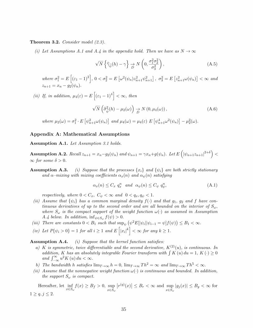
Theorem 3.2. Consider model (2.3).

(i) Let Assumptions A.1 and A.4 in the appendix hold. Then we have as N →∞

√Nγψ

(h)− γ→DN

(0,σ2

1σ22

σ23

), (A.5)

where σ21 = E

[(ε1 − 1)2

], 0 < σ2

2 = E[ω2(ψn)z2

n+1ψ2n+1

], σ2

3 = E[z2n+1ω(ψn)

]<∞ and

zn+1 = xn − g2(ψn).

(ii) If, in addition, µ4(ε) = E[(ε1 − 1)4

]<∞, then

√N(σ2ψ

(h)− µ2(ω))→DN (0, µ4(ω)) , (A.6)

where µ2(ω) = σ21 · E

[ψ2n+1ω(ψn)

]and µ4(ω) = µ4(ε) E

[ψ4n+1ω

2(ψn)]− µ2

2(ω).

Appendix A: Mathematical Assumptions

Assumption A.1. Let Assumption 3.1 holds.

Assumption A.2. Recall zn+1 = xn−g2(ψn) and ψn+1 = γxn+g(ψn). Let E(|ψn+1zn+1|2+δ

)<

∞ for some δ > 0.

Assumption A.3. (i) Suppose that the processes xi and ψi are both strictly stationaryand α–mixing with mixing coefficients αx(n) and αψ(n) satisfying

αx(n) ≤ Cx qnx and αψ(n) ≤ Cψ qnψ, (A.1)

respectively, where 0 < Cx, Cψ <∞ and 0 < qx, qψ < 1.

(ii) Assume that ψi has a common marginal density f(·) and that g1, g2 and f have con-tinuous derivatives of up to the second order and are all bounded on the interior of Sω,where Sω is the compact support of the weight function ω(·) as assumed in AssumptionA.4 below. In addition, infψ∈Sω f(ψ) > 0.

(iii) There are constants 0 < B1 such that supψ(ψ2E[|ψi||ψi−1 = ψ]f(ψ)

)≤ B1 <∞.

(iv) Let Pψi > 0 = 1 for all i ≥ 1 and E[|xi|k

]<∞ for any k ≥ 1.

Assumption A.4. (i) Suppose that the kernel function satisfies:

a) K is symmetric, twice differentiable and the second derivative, K(2)(u), is continuous. Inaddition, K has an absolutely integrable Fourier transform with

∫K (u) du = 1, K (·) ≥ 0

and∫∞−∞ u

2K (u) du <∞.

b) The bandwidth h satisfies limT→∞ h = 0, limT→∞ Th2 =∞ and limT→∞ Th

5 <∞.(ii) Assume that the nonnegative weight function ω(·) is continuous and bounded. In addition,

the support Sω is compact.

Hereafter, let infx∈Sω

f(x) ≥ Bf > 0, supx∈Sω

∣∣r(q)(x)∣∣ ≤ Br < ∞ and sup

x∈Sω|gj(x)| ≤ Bg < ∞ for

1 ≥ q, j ≤ 2.

35

Remark A.1. (i) Assumption 3.1 is discussed in detail in Section 3 above.

(ii) While the assumption of a geometrically decaying mixing coefficient is quite common inthe literature (see, for example, Hardle and Vieu (1992) and Gao and Yee (2000)), itmay be relaxed with the involvement of a slower rate of convergence. Nonetheless, such achange involves much more technicalities. Since this is not essential, we use AssumptionA.2 throughout the proofs of the main theorems of this paper.

(iii) Assumptions A.3(ii) and A.4(ii) involve a non–negative weight function to help address the

random denominator problem that may arise due to small values of fh(ψn). Meanwhile,it is quite common to assume the remaining of Assumption A.3(ii) due to the stationarityof the process ψi.

(iv) Assumption A.3(iii) imposes certain conditions on the tail behavior of f(ψ). AssumptionA.3(iv) is included to ensure the positivity of the duration process and the finiteness of themoments.

(v) Assumptions A.4(i) and A.4(ii) are similar to those assumed in, for example, Hardle andVieu (1992). This particular set of admissible bandwidths is at least as large as thoseallowed in related studies; see, for example Li and Wooldridge (2002) and Gao and King(2004). Furthermore, it ensures that the theoretically optimum value of hoptimal = CT−1/5

can be included.

Appendix B: Proof of Theorem 3.1

B.1 Proof of Theorem 3.1(i)We begin with Assumption A.1, which suggests

|ψi,m − ψi,m| = |g(ψi−1,m−1)− g(ψi−1,m−1)| ≤ ϕ(ψi−1,m−1)|ψi−1,m−1 − ψi−1,m−1|,

∣∣∣ψi−1,m−1 − ψi−1,m−1

∣∣∣ ≤ ∣∣∣ψi−1,m−1 − ψi−1,m−1

∣∣∣+∣∣ψi−1,m−1 − ψi−1,m−1

∣∣≤∣∣∣ψi−1,m−1 − ψi−1,m−1

∣∣∣+ ϕ(ψi−2,m−2)∣∣∣ψi−2,m−2 − ψi−2,m−2

∣∣∣ . (B.1)

and recursively∣∣ψi,m − ψi,m∣∣ ≤ ϕ(ψi−1,m−1)∣∣∣ψi−1,m−1 − ψi−1,m−1

∣∣∣+ ϕ(ψi−1,m−1)ϕ(ψi−2,m−2)

∣∣∣ψi−2,m−2 − ψi−2,m−2

∣∣∣ ≤ · · · · · ·≤

m∑j=1

(j∏c=1

ϕ(ψi−c,m−c)

)∣∣∣ψi−j,m−j − ψi−j,m−j∣∣∣+

(m∏d=1

ϕ(ψi−d,m−d)

)∣∣ψi−m,0 − ψi−m,0∣∣ ,

36

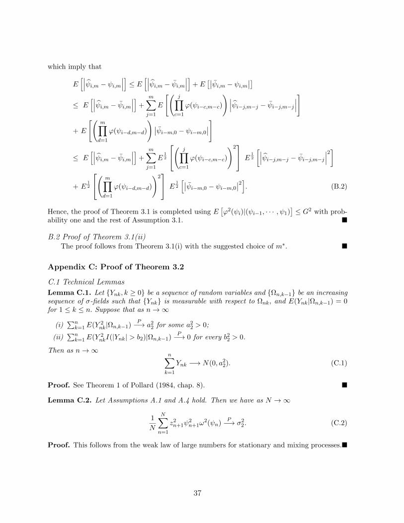
which imply that

E[∣∣∣ψi,m − ψi,m∣∣∣] ≤ E [∣∣∣ψi,m − ψi,m∣∣∣]+ E

[∣∣ψi,m − ψi,m∣∣]≤ E

[∣∣∣ψi,m − ψi,m∣∣∣]+m∑j=1

E

[(j∏c=1

ϕ(ψi−c,m−c)

)∣∣∣ψi−j,m−j − ψi−j,m−j∣∣∣]

+ E

[(m∏d=1

ϕ(ψi−d,m−d)

)∣∣ψi−m,0 − ψi−m,0∣∣]

≤ E[∣∣∣ψi,m − ψi,m∣∣∣]+

m∑j=1

E12

( j∏c=1

ϕ(ψi−c,m−c)

)2 E

12

[∣∣∣ψi−j,m−j − ψi−j,m−j∣∣∣2]

+ E12

( m∏d=1

ϕ(ψi−d,m−d)

)2 E

12

[∣∣ψi−m,0 − ψi−m,0∣∣2]. (B.2)

Hence, the proof of Theorem 3.1 is completed using E[ϕ2(ψi)|(ψi−1, · · · , ψ1)

]≤ G2 with prob-

ability one and the rest of Assumption 3.1.

B.2 Proof of Theorem 3.1(ii)The proof follows from Theorem 3.1(i) with the suggested choice of m∗.

Appendix C: Proof of Theorem 3.2

C.1 Technical Lemmas

Lemma C.1. Let Ynk, k ≥ 0 be a sequence of random variables and Ωn,k−1 be an increasingsequence of σ-fields such that Ynk is measurable with respect to Ωnk, and E(Ynk|Ωn,k−1) = 0for 1 ≤ k ≤ n. Suppose that as n→∞

(i)∑n

k=1E(Y 2nk|Ωn,k−1)

P−→ a22 for some a2

2 > 0;

(ii)∑n

k=1E(Y 2nkI(|Ynk| > b2)|Ωn,k−1)

P−→ 0 for every b22 > 0.

Then as n→∞n∑k=1

Ynk −→ N(0, a22). (C.1)

Proof. See Theorem 1 of Pollard (1984, chap. 8).

Lemma C.2. Let Assumptions A.1 and A.4 hold. Then we have as N →∞

1

N

N∑n=1

z2n+1ψ

2n+1ω

2(ψn)P−→ σ2

2. (C.2)

Proof. This follows from the weak law of large numbers for stationary and mixing processes.

37

Lemma C.3. Assume that Assumptions A.1 and A.4 hold. Then we have for j = 1, 2

supx∈R1

suph∈HN

|gj,h(x)− gj(x)| = oP N−1/4, (C.3)

supx∈R1

suph∈HN

∣∣∣fh(x)− f(x)∣∣∣ = oP N−1/4, (C.4)

where gj,h(x) are as defined in (2.5) and fh(x) = 1N

∑Ts=1Kh (x− xs) .

Proof. Lemma C.3 is a strong version of Theorems 3.3.6 and 5.3.3 of Gyorfi et al. (1989). Seealso Lemma 1 of Hardle and Vieu (1992) for some weak results.

Lemma C.4. Let Assumptions A.1 and A.4 hold. Then for j = 1, 2

1

N

N∑n=1

gj,h(ψn)− gj(ψn)2ω(ψn) = oP N−1/2 (C.5)

and

1

N

N∑n=1

gj,h(ψn)− gj(ψn)zn+1ω(ψn) = oP N−1/2 (C.6)

uniformly over h ∈ HN .

Proof. See Lemma A.2 of Gao and Yee (2000).

Lemma C.5. Let Assumptions A.1 and A.4 hold. Then

∆21T (ψ) = ‖Ψm − Ψm‖22 = oP

N−

12

uniformly over h ∈ HN . (C.7)

Proof. In order to prove Lemma C.5, observe firstly that

‖Ψm − Ψm‖22 =1

N

N∑n=m

ψn+1,m − ψn+1,m2ω(ψn,m−1)

=1

N

N∑n=m

[γm(h)xn + g∗h(ψn,m−1)]− [γxn + g(ψn,m−1)]2 ω(ψn,m−1), (C.8)

where g∗h(ψn,m−1) = g1,h(ψn,m−1)− γm(h)g2,h(ψn,m−1).Equation (C.8) suggests that the asymptotic convergence of the quantity of interest depends

on the following terms:

d1(h) = γm(h)− γ2 1

N

N∑n=m

z2n+1ω(ψn,m−1),

d2(h) =1

N

N∑n=m

g1,h(ψn,m−1)− g1(ψn,m−1)2 ω(ψn,m−1),

d3(h) = γ2m(h)

1

N

N∑n=m

g2,h(ψn,m−1)− g2(ψn,m−1)2 ω(ψn,m−1),

38

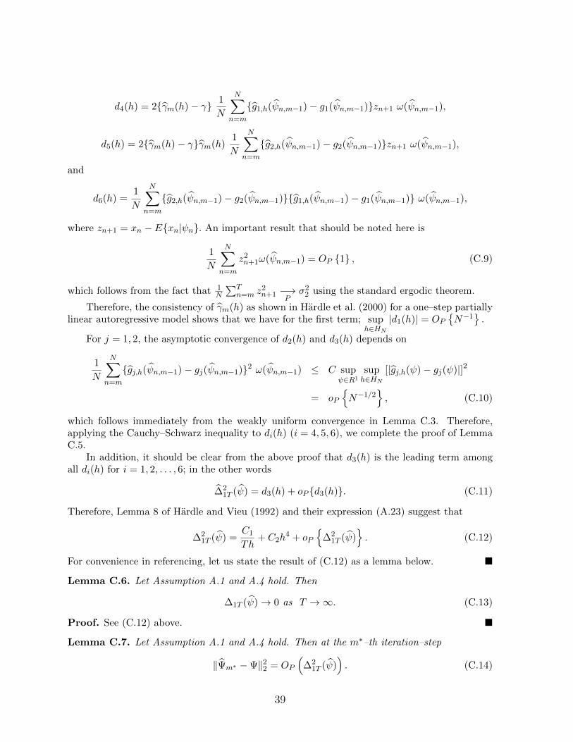
d4(h) = 2γm(h)− γ 1

N

N∑n=m

g1,h(ψn,m−1)− g1(ψn,m−1)zn+1 ω(ψn,m−1),

d5(h) = 2γm(h)− γγm(h)1

N

N∑n=m

g2,h(ψn,m−1)− g2(ψn,m−1)zn+1 ω(ψn,m−1),

and

d6(h) =1

N

N∑n=m

g2,h(ψn,m−1)− g2(ψn,m−1)g1,h(ψn,m−1)− g1(ψn,m−1) ω(ψn,m−1),

where zn+1 = xn − Exn|ψn. An important result that should be noted here is

1

N

N∑n=m

z2n+1ω(ψn,m−1) = OP 1 , (C.9)

which follows from the fact that 1N

∑Tn=m z

2n+1 −→

Pσ2

2 using the standard ergodic theorem.

Therefore, the consistency of γm(h) as shown in Hardle et al. (2000) for a one–step partiallylinear autoregressive model shows that we have for the first term; sup

h∈HN|d1(h)| = OP

N−1

.

For j = 1, 2, the asymptotic convergence of d2(h) and d3(h) depends on

1

N

N∑n=m

gj,h(ψn,m−1)− gj(ψn,m−1)2 ω(ψn,m−1) ≤ C supψ∈R1

suph∈HN

[|gj,h(ψ)− gj(ψ)|]2

= oP

N−1/2

, (C.10)

which follows immediately from the weakly uniform convergence in Lemma C.3. Therefore,applying the Cauchy–Schwarz inequality to di(h) (i = 4, 5, 6), we complete the proof of LemmaC.5.

In addition, it should be clear from the above proof that d3(h) is the leading term amongall di(h) for i = 1, 2, . . . , 6; in the other words

∆21T (ψ) = d3(h) + oP d3(h). (C.11)

Therefore, Lemma 8 of Hardle and Vieu (1992) and their expression (A.23) suggest that

∆21T (ψ) =

C1

Th+ C2h

4 + oP

∆2

1T (ψ). (C.12)

For convenience in referencing, let us state the result of (C.12) as a lemma below.

Lemma C.6. Let Assumption A.1 and A.4 hold. Then

∆1T (ψ)→ 0 as T →∞. (C.13)

Proof. See (C.12) above.

Lemma C.7. Let Assumption A.1 and A.4 hold. Then at the m∗–th iteration–step

‖Ψm∗ −Ψ‖22 = OP

(∆2

1T (ψ)). (C.14)

39

Proof. Applying Markov inequality, the proof of Lemma C.7 follows from the proof of Theorem3.1 with the particular choice of m∗.

Lemma C.8. Let Assumptions A.1 and A.4 hold. Then the followings hold for j = 1, 2

1

N

N∑n=1

gj,h(ψn,m)− gj(ψn)2ω(ψn) = oP N−1/2 (C.15)

and

1

N

N∑n=1

gj,h(ψn,m)− gj(ψn)zn+1ω(ψn) = oP N−1/2. (C.16)

Proof. Firstly, let us write gj,h(ψn,m)− gj(ψn) as

gj,h(ψn,m)− gj(ψn) fh(ψn)

f(ψn)−gj,h(ψn,m)− gj(ψn)f(ψn)− f(ψn)

f(ψn). (C.17)

Lemma C.3 suggests that the second term is negligible. The first can be decomposed as

gj,h(ψn,m)− gj(ψn) fh(ψn)

f(ψn)= gj,h(ψn,m)− gj,h(ψn) fh(ψn)

f(ψn)

+gj,h(ψn)− gj(ψn) fh(ψn)

f(ψn). (C.18)

By letting

gj,h(ψn,m) =1N

∑Ns=1Kh[ψn,m − ψs,m]xs+2−j

1N

∑Ns=1Kh[ψn,m − ψs,m]

≡rj,h(ψn,m)

fh(ψn,m)(C.19)

and

gj,h(ψn) =1N

∑Ns=1Kh[ψn − ψs]xs+2−j

1N

∑Ns=1Kh[ψn − ψs]

≡rj,h(ψn)

fh(ψn), (C.20)

the quantity gj,h(ψn,m)− gj,h(ψn) can be rewritten asrj,h(ψn,m)− rj,h(ψn)

fh(ψn)

− rj,h(ψn,m)

fh(ψn,m)− fh(ψn)

fh(ψn,m)fh(ψn)

. (C.21)

The two numerators in (C.21) can be written as

rj,h(ψn,m)− rj,h(ψn) =1

N

N∑s=1

Kh[ψn,m − ψs,m]−Kh[ψn − ψs]

xs+2−j (C.22)

and

fh(ψn,m)− fh(ψn) =1

N

N∑s=1

Kh[ψn,m − ψs,m]−Kh[ψn − ψs]

, (C.23)

40

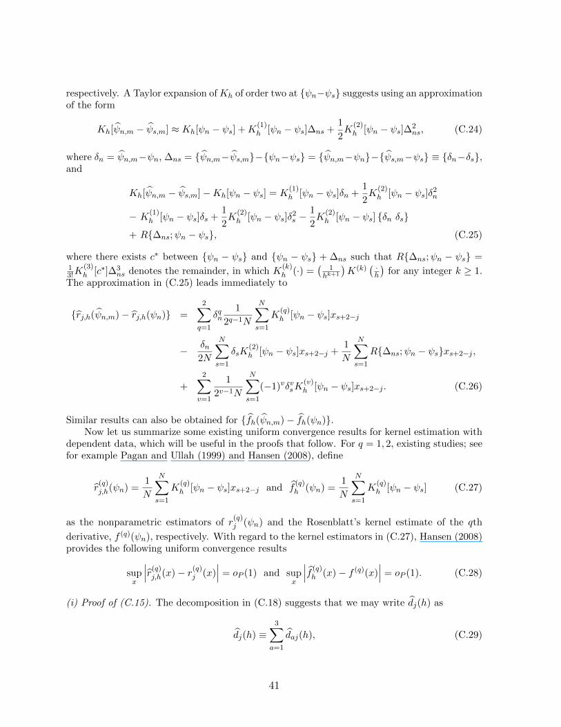
respectively. A Taylor expansion ofKh of order two at ψn−ψs suggests using an approximationof the form

Kh[ψn,m − ψs,m] ≈ Kh[ψn − ψs] +K(1)h [ψn − ψs]∆ns +

1

2K

(2)h [ψn − ψs]∆2

ns, (C.24)

where δn = ψn,m−ψn, ∆ns = ψn,m−ψs,m−ψn−ψs = ψn,m−ψn−ψs,m−ψs ≡ δn−δs,and

Kh[ψn,m − ψs,m]−Kh[ψn − ψs] = K(1)h [ψn − ψs]δn +

1

2K

(2)h [ψn − ψs]δ2

n

− K(1)h [ψn − ψs]δs +

1

2K

(2)h [ψn − ψs]δ2

s −1

2K

(2)h [ψn − ψs] δn δs

+ R∆ns;ψn − ψs, (C.25)

where there exists c∗ between ψn − ψs and ψn − ψs + ∆ns such that R∆ns;ψn − ψs =13!K

(3)h [c∗]∆3

ns denotes the remainder, in which K(k)h (·) =

(1

hk+1

)K(k)

( ·h

)for any integer k ≥ 1.

The approximation in (C.25) leads immediately to

rj,h(ψn,m)− rj,h(ψn) =2∑q=1

δqn1

2q−1N

N∑s=1

K(q)h [ψn − ψs]xs+2−j

− δn2N

N∑s=1

δsK(2)h [ψn − ψs]xs+2−j +

1

N

N∑s=1

R∆ns;ψn − ψsxs+2−j ,

+

2∑v=1

1

2v−1N

N∑s=1

(−1)vδvsK(v)h [ψn − ψs]xs+2−j . (C.26)

Similar results can also be obtained for fh(ψn,m)− fh(ψn).Now let us summarize some existing uniform convergence results for kernel estimation with

dependent data, which will be useful in the proofs that follow. For q = 1, 2, existing studies; seefor example Pagan and Ullah (1999) and Hansen (2008), define

r(q)j,h(ψn) =

1

N

N∑s=1

K(q)h [ψn − ψs]xs+2−j and f

(q)h (ψn) =

1

N

N∑s=1

K(q)h [ψn − ψs] (C.27)

as the nonparametric estimators of r(q)j (ψn) and the Rosenblatt’s kernel estimate of the qth

derivative, f (q)(ψn), respectively. With regard to the kernel estimators in (C.27), Hansen (2008)provides the following uniform convergence results

supx

∣∣∣r(q)j,h(x)− r(q)

j (x)∣∣∣ = oP (1) and sup

x

∣∣∣f (q)h (x)− f (q)(x)

∣∣∣ = oP (1). (C.28)

(i) Proof of (C.15). The decomposition in (C.18) suggests that we may write dj(h) as

dj(h) ≡3∑

a=1

daj(h), (C.29)

41

where

d1j(h) =1

N

N∑n=1

gj,h(ψn,m)− gj,h(ψn)2fh(ψn)

f(ψn)

2

ω(ψn), (C.30)

d2j(h) =1

N

N∑n=1

gj,h(ψn)− gj(ψn)2fh(ψn)

f(ψn)

2

ω(ψn), (C.31)

d3j(h) =2

N

N∑n=1

gj,h(ψn,m)− gj,h(ψn)gj,h(ψn)− gj(ψn)

fh(ψn)

f(ψn)

2

ω(ψn). (C.32)

Clearly, the required results can be immediately obtained for d2j(h) using Lemma C.4. With

regard to d1j(h), equation (C.21) suggests that we can write

d1j(h) =1

N

N∑n=1

gj,h(ψn,m)− gj,h(ψn)2fh(ψn)

f(ψn)

2

ω(ψn) ≡ aj(h) + bj(h)− 2cj(h),

where

aj(h) =1

N

N∑n=1

rj,h(ψn,m)− rj,h(ψn)

fh(ψn)

2fh(ψn)

f(ψn)

2

ω(ψn),

bj(h) =1

N

N∑n=1

rj,h(ψn,m)

fh(ψn,m)

fh(ψn,m)− fh(ψn)

fh(ψn)

2fh(ψn)

f(ψn)

2

ω(ψn),

cj(h) =1

N

N∑n=1

rj,h(ψn,m)

fh(ψn,m)

rj,h(ψn,m)− rj,h(ψn)fh(ψn,m)− fh(ψn)

fh(ψn)2

fh(ψn)

f(ψn)

2

ω(ψn).

We now consider each of these terms in more detail. The approximation in (C.26) impliesthat aj(h) can be written as the summation of a number of additional terms. Firstly, we havefor q = 1, 2

a1qj(h) =1

N

N∑n=1

δ2qn

1

N

N∑s=1

K(q)h [ψn − ψs]xs+2−j

f(ψn)

2

ω(ψn)

≤ B2r

1

N

N∑n=1

δ2qn

r(q)j,h(ψn)

r(q)(ψn)

2

1

Bf

2

ω(ψn)

= (1 + oP 1)BrBf

2 1

N

N∑n=1

δ2qn ω(ψn) ≤ oP N−1/2, (C.33)

using the uniform convergence in (C.28) and Theorem 3.1. Note that the inequality holds for

q = 2 using the fact that δ2qn ≤ δ2

n at a sufficiently large N, i.e. δn is asymptotically negligibleat m = m∗.

A similar result can be obtained for the remaining terms by noting that for v = 1, 2

1

N

N∑s=1

K(v)h [ψn − ψs]xs+2−jδ

vs ≤ oP N−1/4, (C.34)

42

which are direct results of (C.28). Hence, we have for v = 1, 2

a2vj(h) =1

N

N∑n=1

1

N

N∑s=1

K(v)h [ψn − ψs]xs+2−jδ

vs

21

f(ψn)

2

ω(ψn) ≤ oP N−1/2 (C.35)

and

a3j(h) =1

N

N∑n=1

δn

1

2N

N∑s=1

K(2)h [ψn − ψs]xs+2−jδs

21

f(ψn)

2

ω(ψn) ≤ oP N−1/2. (C.36)

An analogous treatment to aj(h) leads to the decomposition of bj(h) into a number ofquantities that are to be discussed below. For q = 1, 2, Theorem 3.1 lead to

b1qj(h) =1

N

N∑n=1

δ2qn

gj,h(ψn,m)f

(q)h (ψn)

2

1

f(ψn)

2

ω(ψn)

≤

1

Bf

2 1

N

N∑n=1

δ2qn

gj,h(ψn,m)

gj,h(ψn)· gj,h(ψn)f

(q)h (ψn)

2

ω(ψn)

≤ (1 + oP 1)

1

Bf

2 1

N

N∑n=1

δ2qn

gj,h(ψn)f

(q)h (ψn)

2ω(ψn)

= b11qj + b12qj + 2b13qj ,

where

b11qj = (1 + oP 1)

1

Bf

2 1

N

N∑n=1

δ2qn

gj,h(ψn)f

(q)h (ψn)− gj(ψn)f (q)(ψn)

2ω(ψn)

≤ oP N−1/2 (C.37)

due to the uniform convergence rates in (C.28) and Lemma C.3, and

b12qj = (1 + oP 1)

1

Bf

2 1

N

N∑n=1

δ2qn

gj(ψn)f (q)(ψn)

2ω(ψn) ≤ oP N−1/2 (C.38)

using the boundedness of gj(ψn)f (q)(ψn). A similar result can then be obtained for the crossterm b13qj(h) through the use of Cauchy–Schwarz inequality.

Furthermore, for v = 1, 2 the boundedness of gj(ψn) as implied by Assumptions A.1 to A.4and a similar set of arguments to that of a2vj(h) lead to

b2vj =1

N

N∑n=1

gj,h(ψn,m)

1

N

N∑s=1

K(v)h [ψn − ψs]δvs

21

f(ψn)

2

ω(ψn)

≤

1

Bf

2 1

N

N∑n=1

gj,h(ψn,m)

gj,h(ψn)· gj,h(ψn)

21

N

N∑s=1

K(v)h [ψn − ψs]δvs

2

ω(ψn)

≤ (1 + oP 1)

1

Bf

2

b21vj + b22vj + 2b23vj ,

43

where

b21vj =1

N

N∑n=1

gj(ψn)2

1

N

N∑s=1

K(v)h [ψn − ψs]δvs

2

ω(ψn) ≤ oP N−1/42vB2g ≤ oP N−1/2

and

b22vj =1

N

N∑n=1

gj,h(ψn)− gj(ψn)2

1

N

N∑s=1

K(v)h [ψn − ψs]δvs

2

ω(ψn) ≤ oP N−1/2

using the differentiability of K. It can similarly be shown that the final term is

b3j =1

N

N∑n=1

gj,h(ψn,m)

δn2N

N∑s=1

K(2)h [ψn − ψs]δs

21

f(ψn)

2

ω(ψn)

≤

1

Bf

2 1

N

N∑n=1

δ2n

gj,h(ψn,m)

gj,h(ψn)· gj,h(ψn)

21

2N

N∑s=1

K(2)h [ψn − ψs]δs

2

ω(ψn)

≤ (1 + oP 1)

1

Bf

2

b31j + b32j + 2b33j ,

in which

b31j =1

N

N∑n=1

δ2n

gj(ψn)

1

2N

N∑s=1

K(2)h [ψn − ψs]δs

2

ω(ψn) ≤ oP N−1/42B2g ≤ oP N−1/2

and

b32j =1

N

N∑n=1

δ2n gj,h(ψn)− gj(ψn)2

1

2N

N∑s=1

K(2)h [ψn − ψs]δs

2

ω(ψn) = oP N−1/2.

Cauchy–Schwarz inequality is a useful tool for the proof of the cross terms in the decom-positions of aj(h) and bj(h). For instance, the required asymptotic result can be obtained im-mediately for cj(h) by applying Cauchy–Schwarz inequality and the results of aj(h) and bj(h).

A similar use of Cauchy–schwarz inequality, together with the asymptotic results of d1j(h) and

d2j(h), leads ultimately to d3j(h) ≤ oPN−1/2

. Finally, it is important to note that the re-

quired rate of convergence for the terms that involve the remainder, denoted by R∆ns;ψn−ψs,can also be obtained using similar arguments to those involved in the above discussion.

(ii) Proof of (C.16). The decomposition of gj,h(ψn,m)−gjψn in a similar manner to the abovediscussion suggests that in order to prove (C.16) we only have to consider the quantities

m1j(h) =1

N

N∑n=1

zn+1gj,h(ψn,m)− gj,h(ψn)

fh(ψn)

f(ψn)

ω(ψn)

and

m2j(h) =1

N

N∑n=1

zn+1gj,h(ψn)− gj(ψn)

fh(ψn)

f(ψn)

ω(ψn).

44

The fact that m2j(h) = oP N−1/2 follows immediately from Lemma C.4. To complete theproof we only have to consider m1j(h). In view of (C.21), m1j(h) can be further decomposed as

m1j(h) = m1j(h) + m2j(h), (C.39)

where

m1j(h) =1

N

N∑n=1

zn+1

rj,h(ψn,m)− rj,h(ψn)

fh(ψn)

fh(ψn)

f(ψn)

ω(ψn) (C.40)

m2j(h) =1

N

N∑n=1

zn+1

rj,h(ψn,m)

fh(ψn,m)

[fh(ψn,m)− fh(ψn)

fh(ψn)

]fh(ψn)

f(ψn)

ω(ψn). (C.41)

To proceed, let us consider for the moment the decomposition of δn = ψn,m−ψn. The proof

of Theorem3.1 suggests that the second and third components of ψn,m − ψn are asymptoticallynegligible. Therefore, to make our proof concise, hereafter we assume without loss of generalitythat δn consists only of γ

ψ(h)− γzn. Also, we have by Assumption A.2

E

[1√N

N∑n=1

znzn+1ω(ψn)

]2

=1

NE

[N∑n=1

znzn+1ω(ψn)

]2

=1

N

N∑n=1

E[z2nz

2n+1ω

2(ψn)] +2

N

N∑n=2

N−1∑m=1

E [znzn+1zmzm+1ω(ψn)] = O1 (C.42)

using the fact that E[znzn+1] = 0 and that E[znzmzm+1ω(ψn)E[zn+1|Ωn]] = 0.For 1 ≤ q, v ≥ 2, the approximation in (C.25) suggests that m1j(h) can be written as the

summation of the following quantities. Firstly, it is

a1qj(h) =1

N

N∑n=1

δqnzn+1

1

N

N∑s=1

K(q)h [ψn − ψs]xs+2−j

fh(ψn)

fh(ψn)

f(ψn)

ω(ψn)

≤ 1

N

N∑n=1

δqnzn+1

r(q)

j,h(ψn)

f(ψn)−r

(q)j (ψn)

f(ψn)

+r

(q)j (ψn)

f(ψn)

ω(ψn) = a11qj + a12qj ,

where, for τ1q,n(ψn) =r(q)j (ψn)

f(ψn) and τ2q,n(ψn) =

[r(q)j,h(ψn)−r(q)j (ψn)

]f(ψn) = oP 1,

a11qj =1

N

N∑n=1

δqnzn+1

r

(q)j (ψn)

f(ψn)

ω(ψn)

= γψ

(h)− γq 1√N

1√N

N∑n=1

zqnzn+1τ1q,n(ψn)ω(ψn)

≤ oP N−q,

a12qj =1

N

N∑n=1

δqnzn+1

r(q)j,h(ψn)− r(q)

j (ψn)

f(ψn)

ω(ψn)

= γψ

(h)− γq 1√N

1√N

N∑n=1

zqnzn+1τ2q,n(ψn)ω(ψn)

≤ oP N−q (C.43)

45

using the uniform convergence of (C.28), the partially linear autoregressive version of Theorem3.2, Assumption A.2 and the fact that for k = 1, 2

1

N

N∑n=1

|zqnzn+1τkq,n(ψn)ω(ψn)|2 = OP 1. (C.44)

Secondly, we have for v = 1, 2

a2vj(h) =1

N

N∑n=1

zn+1

1

N

N∑s=1

δvsK

(v)h [ψn − ψs]xs+2−j

fh(ψn)

fh(ψn)

f(ψn)

ω(ψn)

= γψ

(h)− γv 1

N

N∑n=1

zn+1

1

N

N∑s=1

K(v)h [ψn − ψs]x∗v,s

fh(ψn)

fh(ψn)

f(ψn)

ω(ψn)

= γψ

(h)− γv 1√N

1√N

N∑n=1

zn+1

r∗(v)j,h (ψn)

f(ψn)

ω(ψn)

(C.45)

where x∗v,s = xs+2−jzvs . Given the simplification in (C.45), a similar set of arguments to that of

(C.43) and the fact that 1N

∑Nn=1 |zn+1τ

∗kv,n(ψn)ω(ψn)|2 = OP 1, where τ∗1v,n(ψn) =

r∗(v)j (ψn)

f(ψn)

and τ∗2v,n(ψn) =

[r∗(v)j,h (ψn)−r∗(v)j (ψn)

]f(ψn) = oP 1 that follows from (C.42), lead immediately to

a2vj(h) ≤ oPN−1

v. The final term is

a3j(h) =1

2N

N∑n=1

zn+1δn1

N

N∑s=1

δsK(2)h [ψn − ψs]xs+2−jω(ψn)

= γψ

(h)− γ2 1√N

1√N

N∑n=1

znzn+1r∗(2)j,h (ψn)ω(ψn)

≤ oP N−1, (C.46)

where r∗(2)j,h (ψn) = 1

N

∑Ns=1K

(2)h [ψn − ψs]x∗2,s and x∗2,s = xs+2−jz

2s .

Let us now consider the various components of m2j(h). Firstly, we have for 1 ≤ q ≥ 2

b1qj(h) =1

N

N∑n=1

δqnzn+1

rj,h(ψn,m)

fh(ψn,m)

[1

N

N∑s=1

K(q)h [ψn − ψs]fh(ψn)

]fh(ψn)

f(ψn)

ω(ψn)

= γψ

(ψn)− γq 1

N

N∑n=1

zqnzn+1

gj,h(ψn)

gj,h(ψn)·gj,h(ψn) f

(q)h (ψn)

f(ψn)

ω(ψn) =

2∑k=1

b1kqj(ψn),

where

b1kqj(ψn) = γψ

(ψn)− γq 1√N

1√N

N∑n=1

zqnzn+1[1 + oP 1]τkq,n(ψn)ω(ψn)

with τ1q,n(ψn) =gj(ψn)r

(q)j (ψn)

f(ψn) and τ2q,n(ψn) =

[gj,h(ψn)r

(q)j,h(ψn)−gj(ψn)r

(q)j (ψn)

]f(ψn) = oP 1.

46

The fact that b1kqj(ψn) ≤ oPN−1

qcan be proved using the same arguments as in the

proof of (C.42). We also have for 1 ≤ v ≤ 2

b2vj(h) =1

N

N∑n=1

zn+1

rj,h(ψn,m)

fh(ψn,m)

[1

N

N∑s=1

δvsK

(v)h [ψn − ψs]fh(ψn)

]fh(ψn)

f(ψn)

ω(ψn)

=1

N

N∑n=1

zn+1

gj,h(ψn,m)

[1

N

N∑s=1

K(v)h [ψn − ψs]zvs

]1

f(ψn)

ω(ψn)

= γψ

(ψn)− γv 1

N

N∑n=1

zn+1

gj,h(ψn)

gj,h(ψn)·gj,h(ψn) f

∗(v)h (ψn)

f(ψn)

ω(ψn)

=2∑

k=1

b2kvj(ψn), (C.47)

where

b2kvj(ψn) = γψ

(ψn)− γv 1√N

1√N

N∑n=1

zn+1[1 + oP 1]τ∗kv,n(ψn)ω(ψn)

with τ∗1v,n(ψn) =gj(ψn)f

∗(v)j (ψn)

f(ψn) and τ∗2v,n(ψn) =

[gj,h(ψn)f

∗(v)j,h (ψn)−gj(ψn)f

∗(v)j (ψn)

]f(ψn) = oP 1, in

which f∗(v)h (ψn) = 1

N

∑Ns=1K

(v)h [ψn − ψs]zvs .

Note that using a similar set of arguments to that of b1qj(h), it can be proved that

b2kvj(ψn) ≤ oP N−v. The third term is

b3j(h) =1

2N

N∑n=1

zn+1δn

rj,h(ψn,m)

fh(ψn,m)

[1

N

N∑s=1

δsK

(v)h [ψn − ψs]fh(ψn)

]fh(ψn)

f(ψn)

ω(ψn)

= γψ

(h)− γ2 1√N

1√N

N∑n=1

znzn+1f∗(2)j,h (ψn)ω(ψn)

≤ oP

N−1/2

. (C.48)

Finally, though the formal steps are not included here, it is important to note that the re-quired convergence rate for each of these terms, which concern the remainder denotedR∆ns;ψn−ψs can also be obtained using similar procedures to those in the above discussion.

Lemma C.9. Under Assumptions A.1 and A.4, we have as N →∞

1

N

N∑n=1

u2n+1ω(ψn,m)

P−→ σ23, (C.49)

where un+1 = xn − g2,h(ψn,m) and σ23 is a positive constant.

Proof. Boundedness of the weighted function ω(·) and a standard ergodic theorem suggest that

1

N

N∑n=1

z2n+1ω(ψn)

P−→ σ23, (C.50)

47

where σ23 = E

[z2n+1ω(ψn)

]. Observe further that

1

N

N∑n=1

u2n+1ω(ψn,m) =

1

N

N∑n=1

xn − g2,h(ψn,m)2ω(ψn,m)

=1

N

N∑n=1

z2n+1 ω(ψn) + oP 1+

1

N

N∑n=1

g2,h(ψn,m)− g2,h(ψn)2 ω(ψn) + oP 1

+1

N

N∑n=1

zn+1g2,h(ψn,m)− g2(ψn) ω(ψn) + oP 1

≡ 1

N

N∑n=1

z2n+1 ω(ψn) + oP 1+RN (h), (C.51)

where second equality is due to the fact that ω(ψn,m) = ω(ψn) + oP 1. Lemma C.8 shows that

RN (h) = oP N−1/2. Hence, the result of (C.49) is immediately obtained using (C.50).

C.2 Proof of Theorem 3.2(i) Proof of Theorem 3.2(i): Let us first recall the kernel–weighted LS estimator γ

ψ(h) of γ as

γψ

(h)− γ =1N

∑Nn=1 un+1 · ηn+1ω(ψn,m) +

∑Nn=1 un+1 · gh(ψn,m)ω(ψn,m)

1N

∑Nn=1 u

2n+1ω(ψn,m)

, (C.52)

where gh(ψn,m) = g1,h(ψn,m)−γg2,h(ψn,m), gh = g(ψn)− gh(ψn,m) and un+1 = xn− g2,h(ψn,m).Defining

AN =1

N

N∑n=1

un+1(ηn+1 − gh(ψn,m)− g(ψn))ω(ψn,m), (C.53)

then the fact that we can also write un+1 = zn+1 − g2,h(ψn,m)− g2(ψn) suggests that

AN =1

N

N∑n=1

zn+1ηn+1ω(ψn,m)− a2(h)− a3(h) + a4(h), (C.54)

where

a2(h) =1

N

N∑n=1

gh(ψn,m)− g(ψn)zn+1ω(ψn,m) = opN−1/2, (C.55)

a3(h) =1

N

N∑n=1

g2,h(ψn,m)− g2(ψn)ηn+1ω(ψn,m) = opN−1/2, (C.56)

a4(h) =1

N

N∑n=1

g2,h(ψn,m)− g2(ψn)gh(ψn,m)− gh(ψn)ω(ψn,m) = opN−1/2. (C.57)

(C.55) and (C.56) follows immediately from Lemma C.8 and the fact that ω(ψn,m) = ω(ψn)+oP (1). To prove (C.57), observe that

g2,h(ψn,m)− g2(ψn)gh(ψn,m)− g(ψn)

= g2,h(ψn,m)− g2(ψn)[g1,h(ψn,m)− g1(ψn) − γg2,h(ψn,m)− g2(ψn)

].

48

Therefore, the required result can be obtained using the Cauchy-Schwarz inequality and (C.15).In order to prove Theorem 3.2, we need only to show that as N →∞

1

N1/2

N∑n=1

zn+1ηn+1ω(ψn)D→ N

(0, σ2

2σ21

),

where ηn+1 = ψn+1 (εn+1 − 1), zn+1 = xn − g2(ψn) and ψn+1 = γxn + g(ψn). The remainingproof is to verify that the conditions of Lemma C.1 are satisfied. By letting Bn denote a sequenceof σ–fields generated by (xi, ψi) : 1 ≤ i ≤ n, Lemma C.2 implies that we have as N →∞

1

N

N∑n=1

E(zn+1ηn+1)2ω2(ψn)|Bn =1

N

N∑n=1

ψ2n+1z

2n+1ω

2(ψn)E(εn+1 − 1)2 |BnP→ σ2

2σ21,

(C.58)

where σ21 = E

[(ε1 − 1)2

]. Observe also that for every given b > 0 and some δ > 0

1

N

N∑n=1

E(zn+1ηn+1ω(ψn))2 I(|zn+1ηn+1ω(ψn)| > bN δ)|Bn

≤ C

N1+δ

N∑n=1

E|zn+1ηn+1ω(ψn)|2+δ |Bn

=C

N1+δ

N∑n=1

|zn+1ψn+1ω(ψn)|2+δ E[|(εn − 1)|2+δ |Bn

]≤ C

N1+δ

N∑n=1

|zn+1ψn+1ω(ψn)|2+δ = oP (1), (C.59)

which follows from Assumption A.2 and the fact that 1N

∑Nn=1 |zn+1ψn+1ω(ψn)|2+δ = OP (1).

Furthermore, the consistency of γψ

(h) is proved by using (C.55) to (C.57) and the fact that

1

N

N∑n=1

zn+1ηn+1ω(ψn,m) =1

N

N∑n=1

zn+1ω(ψn,m) · 1

N

N∑n=1

ηn+1 = 0. (C.60)

(ii) Proof of Theorem 3.2(ii): Observe that

σ2ψ

(h) =1

N

N∑n=2

xn+1 − γψ(h)xn − g1,h(ψn,m) + γψ

(h)g2,h(ψn,m)2ω(ψn,m)

can be rewritten as a summation of the following terms

v1(h) =1

N

N∑n=1

η2n+1ω(ψn), v2(h) = γ − γ

ψ(h)2 1

N

N∑n=1

u2n+1ω(ψn),

v3(h) =1

N

N∑n=1

g1(ψn)− g1,h(ψn,m)2ω(ψn), v4(h) = γ1

N

N∑n=1

g2(ψn)− g2,h(ψn,m)2ω(ψn),

49

v5(h) =2

N

N∑n=1

ηn+1g1(ψn)− g1,h(ψn,m)ω(ψn),

v6(h) = γ − γψ

(h)γ 2

N

N∑n=1

un+1g2(ψn)− g2,h(ψn,m)ω(ψn),

v7(h) = γ−γψ

(h) 2

N

N∑n=2

ηn+1un+1ω(ψn), v8(h) = γ−γψ

(h) 2

N

N∑n=2

un+1g1(ψn)−g1,h(ψn,m)ω(ψn),

v9(h) = γ2

N

N∑n=2

g1(ψn)− g1,h(ψn,m)g2(ψn)− g2,h(ψn,m)ω(ψn),

v10(h) = γ2

N

N∑n=2

ηn+1g2(ψn)− g2,h(ψn,m)ω(ψn).

Lemmas C.8 and C.9 lead immediately to vs(h) = oP N−1/2, for s = 2, 3, 4. Furthermore,similar arguments to those in the proof of Lemma C.8, while replacing z with η, suggest thatvs(h) = oP N−1/2 for s = 5, 10. With regard to the sixth term, the decomposition

v6(h) = γ − γψ

(h)2γ

N

N∑n=1

(zn+1g2(ψn)− g2,h(ψn,m)+ g2(ψn)− g2,h(ψn,m)2

)ω(ψn)

(C.61)shows that the required result for v6(h) can be obtained using Lemma C.8. With regard tov7(h), observe that

γ − γψ

(h) 2

N

N∑n=2

(ηn+1zn+1 + ηn+1g2(ψn)− g2,h(ψn,m)

)ω(ψn)

= γ − γψ

(h)

2

N

N∑n=2

(ηn+1zn+1)ω(ψn) +2

N

N∑n=2

(ηn+1g2(ψn)− g2,h(ψn,m)

)ω(ψn)

.

While the the second term is oP N−1/2 by using similar reasoning to v5(h) and v10(h), the

first term is so due to the central limit theorem, which implies that 1√N

∑Nn=1 ηn+1zn+1ω(ψn) =

OP (1). Finally, the proof of v8(h) is similar to that of v6(h). Hence, the proof of Theorem 3.2(ii)is completed by noting that as N →∞

√N v1(h)− µ2(ω) D−→ N (0, µ4(ω)) , (C.62)

where µ2(ω) = E[η2n+1ω(ψn)

]and µ4(ω) = E

[η4n+1ω

2(ψn)]− µ2

2(ω).

50