Journal of Statistical Planning and Inference 139 (2009) 3 -- 15

Contents lists available at ScienceDirect

Journal of Statistical Planning and Inference

journal homepage: www.e lsev ier .com/ locate / jsp i

Robust designs for misspecified logistic models

Adeniyi J. Adewalea, Douglas P. Wiensb,∗

aMerck Research Laboratories, North Wales, Pennsylvania 19454, United StatesbDepartment of Mathematical and Statistical Sciences, University of Alberta, Edmonton, Alberta, Canada T6G 2G1

A R T I C L E I N F O A B S T R A C T

Available online 24 May 2008MSC:primary 62K05;62F35secondary 62J05

Keywords:Fisher informationLogistic regressionLinear predictorMonte Carlo samplePolynomialRandom walkSimulated annealing

We develop criteria that generate robust designs and use such criteria for the construction ofdesigns that insure against possible misspecifications in logistic regressionmodels. The designcriteria we propose are different from the classical in that we do not focus on sampling erroralone. Instead we use design criteria that account as well for error due to bias engenderedby the model misspecification. Our robust designs optimize the average of a function of thesampling error and bias error over a specified misspecification neighbourhood. Examples ofrobust designs for logistic models are presented, including a case study implementing themethodologies using beetle mortality data.

© 2008 Elsevier B.V. All rights reserved.

1. Introduction

Experimental designs have been treated extensively in the statistical literature, starting with designs for linear models andextending to nonlinear models. A large volume of literature is devoted to designs assuming the exact correctness of the relation-ship between the response variable and the design (explanatory) variables. Box and Draper (1959) added another dimension tothe theory by investigating the impact of model misspecification. Following the work of Box and Draper the literature has sincebeen repletewith regression designswhich are robust against violations of variousmodel assumptions—linearity of the response,independence and homoscedasticity of the errors, etc. Authors who have considered designs with an eye on the approximatenature of the assumed linear models include Marcus and Sacks (1976), Li and Notz (1982), Wiens (1992) and Wiens and Zhou(1999), to mention but a few.

For nonlinear designs, Fedorov (1972), Ford and Silvey (1980), Chaloner and Larntz (1989) and Chaudhuri andMykland (1993)have explored the construction of optimal designs while assuming that the nonlinear model of interest is correctly specified.Still others have investigated designs for generalized linear models, a class of possibly nonlinear models in which the responsefollows a distribution from the exponential family such as the normal, binomial, Poisson or gamma (McCullagh and Nelder,1989). The expository article (Ford et al., 1989) hinted that in the context of nonlinear models, as in the case of linear models, themisspecification of the model itself is of serious concern. They asserted that “indeed, if the model is seriously in doubt, the formsof design that we have considered may be completely inappropriate.” Sinha and Wiens (2002) have explored some designs fornonlinear models with due consideration for the approximate nature of the assumedmodel. In this work we consider designs formisspecified logistic regression models.

For the logistic model, the mean response E(Y) = � depends on the parameters, b, and the vector of explanatory variables, x,through the nonlinear function � = e�/(1 + e�), where � = zT(x)b. The function � is termed the linear predictor, with regressorsz1(x), . . . , zp(x) depending on the q-dimensional independent variable x. The variance of the response, written var(Y|x), is a

∗ Corresponding author. Tel.: +17804924406; fax: +17804926826.E-mail addresses: adeniyiadewale@hotmail.com (A.J. Adewale), doug.wiens@ualberta.ca (D.P. Wiens).

0378-3758/$ - see front matter © 2008 Elsevier B.V. All rights reserved.doi:10.1016/j.jspi.2008.05.022

4 A.J. Adewale, D.P. Wiens / Journal of Statistical Planning and Inference 139 (2009) 3 -- 15

nonlinear function of the linear predictor. Abdelbasit and Plackett (1983), Minkin (1987), Ford et al. (1992), Chaudhuri andMykland (1993), Burridge and Sebastiani (1994), Atkinson and Haines (1996) and King and Wong (2000) have investigateddesigns for binary data, and in particular for logistic regression. As illustrated in these papers, the general approach to optimaldesign is to seek a design that optimizes certain functions of the information matrix of the model parameters. The informationmatrix for b from a design consisting of the points x1, . . . ,xn is given by

n∑i=1

w(xi,b)z(xi)zT(xi) = ZTWZ, (1)

where Z = (z(x1), z(x2), . . . , z(xn))T and

W = diag(w(x1,b),w(x2,b), . . . ,w(xn,b))

for weights w(xi,b) = (d�/d�i)2/var(Y|xi). Thus, as with nonlinear experiments the information matrix depends on the unknown

parameters b. Designing an experiment for the estimation of these parameters would then seem to require that these parametersbe known. The following are some of the approaches that have been explored in the literature for handling the dependency ofthe information matrix on b.

(1) Locally optimal designs: A traditional approach in designing a nonlinear experiment is to aim for maximum efficiency at abest guess (initial estimate) of the parameter values (Chernoff, 1953). Designs that are optimal for given parameter valuesare dubbed locally optimal designs. These designs may be stable over a range of parameter values. However, if unstable, adesign which is optimal for a best guess may not be efficient for parameter values in even a small neighbourhood of thisguess.

(2) Bayesian optimal designs: A natural generalization of locally optimal designs is to use a prior distribution on the unknownparameters rather than a single guess. The approach which assumes such a prior and incorporates this distribution into theappropriate design criteria is termed Bayesian optimal design—see Chaloner and Larntz (1989) and Dette andWong (1996).

(3) Minimax optimal designs: Rather than assume a prior distribution, this approach assumes a range of plausible values for theparameters. Theminimax optimal design is the designwith the least loss when the parameters take theworst possible valuewithin their respective ranges. These least favourable parameter values are those that maximize the loss (King and Wong,2000; Dette et al., 2003).

(4) Sequential designs: In sequential designs, the experiment is done in stages. Parameter estimates from a previous stage areused as initial estimates in the current stage. The process continues until optimal designs are obtained (Abdelbasit andPlackett, 1983; Sinha and Wiens, 2002).

Suppose an experimenter is faced with a set S = {xi}Ni=1 of possible design points from which he is interested in choosing n,not necessarily distinct, points at which to observe a binary response Y. The experimenter makes ni�0 observations at xi suchthat

∑Ni=1 ni = n. The design problem is to choose n1, . . . ,nN in an optimal manner. The objective then is to choose a probability

distribution {pi}Ni=1, with pi = ni/n, on the design space S. The commonalities in the work of the authors who have consideredlogistic design is the salient assumption that the assumedmodel form is exactly correct. In thiswork, we propose the constructionof robust designs for logistic models with due consideration for possible misspecification in the assumed form of the systematiccomponent—the linear predictor. The linear predictor could be said to be misspecified when it does not reflect the influence ofthe covariates correctly, possibly due to omitted covariates or to omission of some transformation of existing covariates in themodel. In this section we formalize our notion of model misspecification.

We suppose that the experimenter fits a logistic model with the mean response

�i = �(�i), i = 1, . . . ,n, (2)

for �i = zT(xi)b0 when in fact the true mean response is represented by

�T,i = �(�i + f (xi)). (3)

The target parameter b0 is defined by

b0 = arg min�

1N

N∑i=1

{E(Y|xi) − �(zT(xi)b)}2.

Thus the target parameter is that which guarantees the least sum of squares of discrepancies, over all points in the design space,between the assumedmean response and the true mean response. The contamination function f (x) may or may not be known. Itwould be known, for example, when an experimenter decides to fit the more parsimonious model (2) despite the knowledge of amore appropriate model (3) with a specified f (x). For instance, the simplified model might be required if the number of support

A.J. Adewale, D.P. Wiens / Journal of Statistical Planning and Inference 139 (2009) 3 -- 15 5

points is not sufficient to handle a more complicated but more appropriate model. Knowing that the parsimonious model mightresult in an inferior analysis, the experimenter may seek a design that remedies the anticipated model inadequacy.

The contamination function would be unknown in a situation where the experimenter is aware of the possible uncertaintiesin the assumedmodel form andmight have clues about the properties of the possiblemisspecification, without knowing its exactstructure. When f (x) is unknown, some knowledge about its properties or conditions it satisfies would be required to constructany appropriate design. This is so because no single design which takes a finite number of observations can protect against allpossible forms of bias. Thus, we must impose some conditions on the contamination function when its precise form is unknown.

To bound the bias of an estimator �, we assume that

1N

N∑i=1

f2(xi)��2, (4)

with �2 =O(n−1). This latter requirement is analogous to the notion of contiguity in the asymptotic theory of hypothesis testing,and is justified in the same manner. The choice of � is discussed following Theorem 3 in the next section. In order to ensureidentifiability of the model parameters b and the contamination function f (x) we require that the vector of regressors and thecontamination be orthogonal. That is,

1N

N∑i=1

z(xi)f (xi) = 0. (5)

LetF denote the class of contamination functions f (x) satisfying (4) and (5).

2. Loss functions: estimated and averaged mean squared errors of prediction

The basis for the construction of classical designs for logistic regression models has typically been the minimization of(a function of) the inverse of Fisher's information matrix (1)—see Atkinson and Haines (1996). However, in the face of modelmisspecification the asymptotic covariance, cov(b), of the maximum likelihood estimator of the model parameters no longerequals the inverse of Fisher information—see White (1982) and also Fahrmeir (1990), who discusses the asymptotic propertiesof MLEs under a misspecified likelihood.

Suppose that data {xi, yi} are given, where the xi are the design points chosen from S with ni observations at xi such that∑Ni=1 ni = n, and yi is the proportion of successes at location xi. The asymptotic bias and covariance of the MLE b are given in

Theorem 1; see the Appendix for details of this and other proofs. The expressions for the asymptotic bias and covariance of theMLE b are used in the derivation of the loss function in Corollary 2.

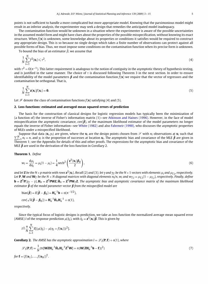
Theorem 1. Define

wi = d�id�i

= �i(1 − �i) = 14sech2

(zT(xi)b0

2

), (6)

and let Z be the N×pmatrix with rows zT(xi). Recall (2) and (3); let c and cT be the N×1 vectors with elements �i and �T,i, respectively.Let P,W andWT be the N ×N diagonal matrices with diagonal elements ni/n, wi and wT,i = �T,i(1− �T,i), respectively. Finally, defineb = ZTP(cT − c),Hn = ZTPWZ, Hn = ZTPWTZ. The asymptotic bias and asymptotic covariance matrix of the maximum likelihoodestimator b of the model parameter vector b from the misspecified model are

bias(b) = E(b− b0) = H−1n b + o(n−1/2),

cov(√n(b− b0)) = H−1

n HnH−1n + o(1),

respectively.

Since the typical focus of logistic designs is prediction, we take as loss function the normalized average mean squared error(AMSE) I of the response prediction �(�i), with �i = zT(xi)b. This is given by

I� nN

N∑i=1

E[{�(�i) − �(�i + f (xi))}2].

Corollary 2. The AMSE has the asymptotic approximation I =LI(P, f) + o(1), where

LI(P, f) = 1N

{tr[WZH−1n HnH−1

n ZTW] + n‖W(ZH−1n b − f)‖2} (7)

for f = (f (x1), . . . , f (xN))T.

6 A.J. Adewale, D.P. Wiens / Journal of Statistical Planning and Inference 139 (2009) 3 -- 15

By using the expressions for asymptotic bias and covariance given in Theorem 1, Corollary 2 expresses the AMSE as anexplicit function of the design matrix Z and contamination vector f. The first term in the loss function LI corresponds to theaverage variance of the predictions and it depends on the contamination function f (x) through the matrix Hn. The second termin the expression for LI is the average squared bias of the predictions, which depends on the contamination f (x) throughthe contamination vector f and implicitly through the vector b. Thus a design cannot minimize (7) directly without certainassumptions about the contamination f (x).

Fang and Wiens (2000) constructed integer-valued designs for linear models, in the case of an unknown f, using a minimaxapproach. Their minimax criterion minimizes the maximum value of the loss function over f. They solve the design problem byminimizing the loss when the misspecification is the worst possible in the neighbourhood of interest.

Here, we take one of the two approaches depending on whether or not there are initial data. If we have initial data werepresent the discrepancy between the true response and the assumed response, at a sampled location x, by

d(x) = �(zT(x)b0 + f (x)) − �(zT(x)b0),

and estimate this by the residual d(x) = y(x) − �(zT(x)b). A first order approximation is d(x) ≈ (d�/d�)f (x), leading to f (x) =d(x)/(d�/d�|b=b). We smooth this estimated contamination over the entire design space—see Example 3 of Section 5 for an

illustration. The resulting estimate f, together with b, is then substituted into the terms in (7), and we compute a designminimizingLI(P, f) using the techniques outlined in Section 3.

If there are no initial data we propose to instead average LI over F defined by (4) and (5). Our optimal design minimizesthis average value. This criterion is in the spirit of Lauter (1974, 1976). Lauter's criterion optimizes the weighted average of theloss of a finite set of plausible models. Here we are instead faced with an infinite set of models indexed by f ∈ F.

To carry out the averaging we begin as in Fang and Wiens (2000), with the singular value decomposition

Z = UN×pKp×pVTp×p, (8)

with UTU = VTV = Ip and K diagonal and invertible. We augment U by UN×(N−p) such that [U...U]N×N is orthogonal. Then by (4)

and (5), we have that there is an (N − p) × 1 vector t, with ‖t‖�1, satisfying

f(=ft) = �√NUt. (9)

The average loss is taken to be the expected value of (7), as a function of t, with respect to the uniform measure on the unitsphere and its interior in RN−p. This measure has density p(t) = (1/�N,p)I(‖t‖�1), where �N,p = �(N−p)/2/�((N − p)/2 + 1) is thevolume of the unit sphere. Theorem 3 handles the averaging of LI . The importance of this theorem is in its elimination of thedependency of our design criterion on the unknown contamination function.

Theorem 3. The average loss over the misspecification neighbourhoodF is, apart from terms which are o(1), given by

LI,ave(P,)�∫

LI(P, ft)p(t) dt

= 1Ntr[(UTPWU)−1(UTW2U)] +

N − p + 2tr[W(R − IN)(R

T − IN)W], (10)

where = n�2 and RN×N = U(UTPWU)−1UTPW. For numerical work it is more efficient to compute the second trace in (10) as

tr[W(R − IN)(RT − IN)W] =

N∑i=1

w2i ‖ri‖2,

where rTi is the ith row of R − IN .

The dependency of the design criterion on the unknown contamination has now been represented by a design parameter ,which can be chosen by the experimenter. This parameter can be interpreted as a measure of departure of the true model fromthe fitted model. In other words, it is a measure of the experimenter's lack of confidence in the validity of the model that he fits.If he believes that this assumed model is exactly correct, he chooses = 0 corresponding to the classical I-optimal design. On theother hand, if the experimenter believes that the assumed model is highly uncertain, he chooses a large value of for his design.Designs corresponding to a large value of are dominated by the bias component of the loss.

Our design criterion (10) remains dependent on the model parameter vector b0, as is the case in the general nonlinear designproblems, through the weights, as at (6). In the examples of the next section we handle this dependency by either taking a guess(locally optimal designs) or assuming a prior distribution, say�(b0), onb0 (Bayesian designs). The loss functionLI,ave ismodifiedas∫LI,ave(b)�(b) db in the case of a Bayesian construction.

A.J. Adewale, D.P. Wiens / Journal of Statistical Planning and Inference 139 (2009) 3 -- 15 7

3. Designs—algorithm and examples

3.1. Simulated annealing

Weconsider problemswith polynomial predictors, viz. �=zT(x)bwith z(x)=(1, x, x2, . . . , xp−1)T.We take equally spaced designpoints {xi}Ni=1 in the intervalS. Our design minimizes the relevant loss function through the matrix P=diag(n1/n, . . . ,nN/n). Thisis a nonlinear integer optimization problem for which there is no analytic solution, and for whichwe employ simulated annealingto search for the optimal design.

The simulated annealing algorithm is a direct search random walk optimization algorithm which has been quite successfulat finding global extrema of non-smooth functions and/or functions with many local extrema. The algorithm consists of threesteps, each of which must be well adapted to the problem of interest for the algorithm to be successful. The first step is aspecification of the initial state of the process. In this step an initial design has to be specified, say P0. The second is a specificationof a scheme by which a new design P1 is chosen from the optimization space. The last step is a prescription of the basisof acceptance or rejection: an acceptance with probability 1 if LI,ave(P1) <LI,ave(P0), otherwise acceptance with probabilityexp{−(LI,ave(P1) − LI,ave(P0))/T}, where T is a tuning parameter. The tuning parameter is usually decreased as the iterationsproceed. After a large number of iterations between the second and third steps the loss function is expected to converge to its(near) minimum value. Simulated annealing has been used for design problems by, among others, Meyer and Nachtsheim (1988),Fang and Wiens (2000) and Adewale and Wiens (2006).

A very simple and general approach that we considered for choosing the initial design is to randomly select p points from{xi}Ni=1 and randomly allocate the observations to these points such that the total number of observations is n. Fang and Wiens(2000) used a different approachwhich assumes that one of (n,N) is amultiple of the other. For any (n,N) combination they chosethe initial design to be as uniform as possible. We applied this approach as well but found that the two approaches are equallyefficient. For generating a new design we adopted the perturbation scheme of Fang and Wiens (2000). The turning parameter inthe third step was chosen initially such that the acceptance rate is in the range 70% and 95%. We decrease T by a factor of .95 aftereach 20 iterations. In the examples below we run the algorithm several times with varying turning parameter specification andreduction rate in order to satisfy ourselves that the resulting design has the least loss possible under the relevant circumstancesof each example. In Fig. 1 we present the simulated annealing trajectory for one of the cases presented in Example 1. It took83 s for the algorithm to complete the preset maximum number of iterations (12000, for this case) and the minimum loss wasattained just before the 9000th iteration.

3.2. Examples

Example 1 (No contamination). As a benchmark we first consider the logistic regression model with a single predictor: p = 2,z(x) = (1, x)T, x ∈ S = [−1, 1],b = (1, 3)T, and no contamination: = 0. We initially took n = 20, N = 40 and considered designsminimizing LI . The annealing algorithm converged to the design placing 10 of the 20 observations at each of the points −.744and .128. This design is therefore the classical I-optimal design minimizing the integrated variance of the predictions over S.There is evidently no previous theory that applies to this case. However, using a model that is a reparameterization of ours, anda continuous design space [−1, 1], King and Wong (2000) showed the locally D-optimal design to be the design that is equallysupported at −.848 and .181. For the sake of comparison, we sought an equivalent design using our finite design space and thealgorithm described above. The resulting design places 10 of 20 observations at each of −.846 and .180. Thus, our algorithmattains the closest approximation to King andWong's solution in that the points −.846 and .180 are nearest, in our design space,to −.848 and .181. Unlike designs for linear models, the optimal designs in this case do not necessarily place observations at theextreme points of the design space. This phenomenon is due to the curvature introduced by the link function and the resultingnonlinear relationship between the mean response and x.

0 2000 4000 6000 8000 10000 12000 14000

0.26

0.28

0.3

0.32

Iteration number

Loss

Fig. 1. Simulated annealing trajectory for logistic design with � = 1 + 3x, x ∈ S= [−1, 1], = 0 and (N = 40,n = 200).

8 A.J. Adewale, D.P. Wiens / Journal of Statistical Planning and Inference 139 (2009) 3 -- 15

-1 0 10

2

4

6

8

10

Num

ber o

f obs

erva

tions

loss = 0.2496

-0.7

89-0

.684

0.05

260.

158

-1 0 10

20

40

60

80

100

loss = 0.2491

-0.7

89

0.05

260.

158

-1 0 10

2

4

6

8

10

12

loss = 0.2527

-0.7

44

0.12

8

-1 0 10

20

40

60

80

loss = 0.2524

-0.7

95-0

.744

0.07

690.

128

Fig. 2. Locally optimal designs minimizingLI,ave when =0 (no contamination) with (a) N=20,n=20; (b) N=20,n=200; (c) N=40,n=20; (d) N=40,n=200.

Table 1Comparing restricted designs with unrestricted design; = 0

(N,n) Restricted design (two-point) Unrestricted design

Design points Loss Design pointsa Loss

(20, 20) −.789(9), .053(11) .250 −.789(7),−.684(3), .250.0526(2), .158(8)

(20, 200) −.789(94), .053(106) .250 −.789(95), .0526(63), .158(42) .249(40, 20) −.744(10), .128(10) .2527 −.744(10), .128(10) .2527(40, 200) −.744(97), .128(103) .2525 −.795(49),−.744(47), .2524

.0769(39), .128(65)

aNumber of observations in parentheses.

Our numerical results further revealed that the designs depend on the number of points in the design space and the numberof observations the experimenter is willing to take. For this “no-contamination” case, we investigated designs for variouscombinations of N and n. Some of these designs are presented in Fig. 2. The number of distinct design points varies from 2to 4. We found this somewhat surprising, in light of the fact that all D-optimum designs for the two parameter logistic modelin the literature are two-point designs. Presumably this is explained through our use of a finite design space, and/or our use ofaverage loss rather than that based on the determinant of the information matrix.

To check that this phenomenon was not merely an artefact due to a lack of convergence, we modified our algorithm to obtain“restricted” designs—restricted to two support points only. The results for the same values of N and n as in Fig. 2 are presentedin Table 1. The loss for the unrestricted design is less than or equal to that for the corresponding restricted design in all casesconsidered.

In the examples that follow we limit discussion to the case N = 40, n = 200.

Example 2 (Example 1 continued). In this example, which we include largely for illustrative purposes, the form of the con-tamination is known. Suppose that the experimenter anticipates fitting a simple logistic model, while wishing protectionagainst a range of logistic models with quadratic predictor: �(x) = zT(x)b + f (x), where zT(x) and b are as in Example 1, and

f (x) = �2(x2 − �2)/

√�4 − �2

2, for �k = N−1∑ xki (=0 if k is odd). The contaminant f (x) is an omitted quadratic term, translatedand scaled to ensure the orthogonality condition (5); (4) becomes |�2|��. We obtained optimal designs for various values of thequadratic coefficient �2. The resulting designs and the corresponding values of the loss function are presented in Table 2. In therange of values of �2 considered, we found that the number of distinct points varied from 3 to 6. The spread of the design overthe design space tended to increase as the magnitude of the omitted quadratic term increases. We computed the premium paidfor robustness and the gain due to robustness for each design presented as

Premium =(

LI(Popt, f = 0)LI(Pclassical, f = 0)

− 1

)× 100% (11)

and

Gain =(1 − LI(Popt, f)

LI(Pclassical, f)

)× 100%. (12)

A.J. Adewale, D.P. Wiens / Journal of Statistical Planning and Inference 139 (2009) 3 -- 15 9

Table 2Designs for simple logistic model when the true model has a quadratic term

�2 Design points (number of observations) LI(P, f) Premium Gain

−10 −1(42),−.180(42),−.128(96), 3.500 35.0% 34.8%−.077(12),−.026(2), .077(6)

−3 −1(48),−.282(26),−.231(64), .282(62) .5020 10.9% 17.0%−1 −.949(42),−.590(34),−.539(29), .128(95) .2756 2.1% .5%0 −.795(49),−.744(47), .077(39), .128(65) .2524 0 01 −.641(100), .128(22), .180(78) .3080 1.9% 4.0%3 −.692(57),−.641(29),−.077(39), .6073 11.9% 19.9%

−.026(44), .795(31)10 −1(11),−.590(51),−.539(27), 3.679 39.0% 42.9%

−.231(30),−.180(40), .949(41)

Table 3Experimental design and response values

Design point .−1 − 79 − 5

9 − 39 − 1

919

39

59

79 1

No. of observations 20 20 20 20 20 20 20 20 20 20No. of successes 8 6 7 13 17 18 18 19 20 20

The gain measure is the percentage reduction in loss due to the use of a robust design as opposed to a (non-robust) classicaldesign which assumes the fitted model to be exactly correct. The premiummeasure is the percentage increase in loss as a resultof not using the classical design if in actual fact the assumed model is correct. The application of the premium and/or gainmeasure depends on the amount of confidence the experimenter has in his knowledge of the true model. In this example, sincethe assumption is that the experimenter knows that the model with a linear predictor involving the quadratic term is a moreappropriate model, the relevant measure would be the gain. Nevertheless, both measures are reported in Table 2. The value ofa design from our robust procedure increases with increasing magnitude of the quadratic parameter. On the other hand, theexperimenter has to be aware of the increasing premium when his knowledge of the true model is not accurate. The premiumpaid for robustness also increases with the magnitude of the quadratic parameter.

Of course this example is artificial, assuming as it does that the true form of the predictor is known to be quadratic, withparameter �2 = 3, say. If one did indeed possess this knowledge then the classically optimal—i.e., variance minimizing—designwould be−1(49),−.282(2),−.231(91), .436(9), .487(49). The premium figures in Table 2would rise appreciably—to typical valuesof 100% or more—since the robust design would be protecting against bias, known not to be present.

Example 3 (Designing when there are initial data to estimate contamination). Table 3 shows simulated data (“# of successes”) froma logistic regression model with the predictor �(x) = 1 + 3x + f (x), the model of the previous example; the quadratic parameterwas �2 = 3. The data were simulated using a uniform design over equally spaced points in [−1, 1]. Having simulated the data, wesuppose the contamination function f (x) to be unknown. We proceed using the procedure described in Section 2 for estimationand eventual smoothing of the contamination. A plot of the estimated contamination with its loess smooth f (x) over the designspace is presented in Fig. 3.

We plugged the smoothed contamination values into the loss function (7), and used simulated annealing to obtain the design.Our design places 34, 82, and 84 of the 200 observations at −.641,−.590, and .180, respectively. For this design the premium forrobustness is 5.0% and the gain is 60.0%. This example indicates that when there are initial data, it is expedient to incorporate theinformation from the data into the design procedure. The resulting design can lead to substantial gain at a reduced premium.

Example 4 (Unknown contamination). Consider the logistic model with predictor

�(x) = �0 + �1x + f (x). (13)

In this example—as in Example 3—we assume that f is an unknown member of the class F defined by (4) and (5). In Fig. 4 weexhibit designs minimizing the averaged loss (10) for various values of , �0 and �1. We observed a progression of the dispersionof the design points over the design space with increasing . The pattern of the dispersion is, however, modified by the curvatureindexed by �0 and �1 through the nonlinear mean response. For small our robust designs can be described as taking clustersof observations at neighbouring locations rather than replications at only a few distinct sites; this was noticed for linear modelsby Fang and Wiens (2000). However, here there is always a pattern to the clusters of observation to be taken depending on thevalues of the model parameters. Large values of denote large departures from the assumed model and an extremely large value corresponds to the all-bias design. Even though the all-bias design is spread over the entire design space the frequenciesof observations are different and these frequencies are prescribed by the curvature of the mean response as determined by the

10 A.J. Adewale, D.P. Wiens / Journal of Statistical Planning and Inference 139 (2009) 3 -- 15

-1.0x [Design Space]

0.0

0.5

1.0

1.5

2.0

2.5

Con

tam

inat

ion

Estimated Contamination with its LoessSmooth Superimposed

-0.5 0.0 0.5 1.0

Fig. 3. Estimated contamination plot for Example 3. True (but unknown) form of contamination is quadratic.

-1 0 10

50

100

#Obs

erva

tions

ρ = 0, loss = 0.29

-1 0 10

10

20ρ = 10, loss = 0.68

-1 0 10

5

10ρ = 100, loss = 3.98

-1 0 10

5

10ρ = 10000, loss = 363.19

-1 0 10

50

100

#Obs

erva

tions

ρ = 0, loss = 0.25

-1 0 10

5

10ρ = 10, loss = 0.51

-1 0 10

5

10ρ = 100, loss = 2.72

-1 0 10

5

10ρ = 10000, loss = 244.75

-1 0 10

50

100

#Obs

erva

tions

ρ = 0, loss = 0.08

-1 0 10

20

40ρ = 10, loss = 0.11

-1 0 10

10

20ρ = 100, loss = 0.39

-1 0 10

5

10ρ = 10000, loss = 30.15

-1 0 10

50

100

#Obs

erva

tions

ρ = 0, loss = 0.14

-1 0 10

20

40ρ = 10, loss = 0.28

-1 0 10

10

20ρ = 100, loss = 1.42

-1 0 10

10

20ρ = 10000, loss = 125.88

Fig. 4. Locally optimal designs in Example 4: (a)–(d) (�0,�1) = (1, 1); (e)–(h) (�0,�1) = (1, 3); (i)–(l) (�0,�1) = (3, 1); (m)–(p) (�0,�1) = (3, 3).

A.J. Adewale, D.P. Wiens / Journal of Statistical Planning and Inference 139 (2009) 3 -- 15 11

Table 4Design for unknown contamination with �0 = 1 and �1 = 3

LI,ave(P,) Premium Gain

0 .2524 0 01 .2809 .62% 2.01%

10 .5090 3.06% 14.33%100 2.7204 7.44% 25.87%

1000 24.7294 11.29% 28.16%10 000 244.7545 11.97% 28.43%

-1 0 10

10

20

30

Num

ber o

f obs

erva

tions

loss = 0.2630

-1 0 10

10

20

30

loss = 0.2836

-1 0 10

10

20

loss = 0.2748

-1 0 10

10

20

loss = 0.2840

Fig. 5. Robust Bayesian optimal design in Example 5 with = .25 and parameters �0 and �1 having independent uniform priors over (a) [.5, 1.5] × [2.5, 3.5],(b) [.5, 1.5] × [1, 5], (c) [−1, 3] × [2.5, 3.5], (d) [−1, 3] × [1, 5].

model parameters. In Table 4 we present the values of the premium paid and the gain in robustness for designs correspondingto different values of for the particular case of (�0,�1)= (1, 3). The gain in robustness, measured by (12), exceeds the premiumpaid, as measured by (11), for each design. Increasing robustness, however, comes with increasing premium; the experimenterwould thus have to choose his level of comfort.

Thus far, the examples we have presented have been locally optimal, hence have assumed good parameter guesses forunknownmodel parameters. In the absence of a reliable best guess formodel parameters, Sitter (1992) and King andWong (2000)considered minimax D-optimality, a procedure which assumes the knowledge of a prior range for each of the parameters. Weconsider a Bayesian paradigm to be in the same spirit as averaging the contamination function over the specifiedmisspecificationneighbourhood, and take independent uniform prior distributions over the range of each model parameter. Our design criteriathen becomes the expected loss, E(LI,ave(P,)), with the expectation taken with respect to these priors. The dependency of ourdesign criteria on the model parameters is through the weights wi, and we do not have analytic expressions for the resultingintegrals. In the examples that follow we employ number-theoretic methods for numerical evaluation of multiple integrals asdiscussed in Fang andWang (1994). This approach is based on generating quasi-random points in the domain of definition of theintegrand, and averaging the values of the loss over the sample of points.

Example 5 (Robust Bayesian design). In this examplewe consider the following ranges of parameter values: (a) [.5, 1.5]×[2.5, 3.5],(b) [.5, 1.5] × [1, 5], (c) [−1, 3] × [2.5, 3.5], (d) [−1, 3] × [1, 5], all with centre point (1, 3) but with coverage areas 1, 4, 4, and 16,respectively. As described above, the robust design for each range of parameter values is the design that minimizes the expectedaverage loss with respect to uniform distributions on the specified ranges of parameter values. For each of the designs—seeFig. 5—we take = .25.We observed an increasing spread over the design spacewith increasing uncertainty inmodel parameters,as measured by the coverage area of the priors. This is consistent with previous work in optimal Bayesian design—see, forexample, Chaloner and Larntz (1989)—which suggests increasing number of distinct design points with increasing uncertaintyin the specified prior distributions. Comparing the design plots in panels (b) and (c) of Fig. 5, we see that there is more sensitivityto uncertainty in the intercept parameter than the slope parameter.

4. Case study: beetle mortality data

Bliss (1935) reported the numbers of beetles dead after 5h exposure to gaseous carbon disulphide at various concentrations.The doses are given in Table 5; to facilitate our discussion we have linearly transformed these to the range [0, 1]. Note that theoriginal design is then very nearly uniform on the eight equally spaced points 0( 17 )1.

12 A.J. Adewale, D.P. Wiens / Journal of Statistical Planning and Inference 139 (2009) 3 -- 15

Table 5Beetle mortality data

Dose, xi (log10 CS2 mg l−1) 1.69 1.72 1.75 1.78 1.81 1.84 1.86 1.88Number of beetles, ni 59 60 62 56 63 59 62 60Number killed, niyi 6 13 18 28 52 53 61 60

0 0.5 10

50

100

Num

ber o

f obs

erva

tions

0 0.5 10

10

20

30

Fig. 6. (a) Prediction design when contamination is estimated from initial data. (b) Robust Bayesian prediction design with multivariate normal prior and = 5.

We first fitted the logistic model with the linear predictor �(1) = �(1)0 + �(1)

1 x, and obtained the estimates �(1)0 = −2.777 and

�(1)1 = 6.621 with the estimated variance–covariance matrix

(1) =(

.082 −.144−.144 .317

)

and deviance =11.232 (df = 6). The corresponding estimates for the logistic model with the linear predictor �(2) =�(2)0 +�(2)

1 x+�(2)2 x2 are �(2)

0 = −2.00, �(2)1 = 1.60, �(2)

2 = 5.84 and

(2) =⎛⎝ .124 −.522 .489

−.522 3.252 −3.690.489 −3.690 4.665

⎞⎠

with deviance =3.195 (df = 5). The deviances and a plot (not presented here) of proportions of beetles killed against dose levelswith the estimated proportions from each model superimposed suggest that the model with the quadratic term is a significantlybetter fit for these data. Suppose the experimenter is inclined to use the simple logistic fit for future data for ease of interpretationand model simplicity or that the adequacy of the model with the quadratic term is itself in doubt. We proceed by estimatingthe contamination and then smoothing over the design space as discussed in Section 2. The resulting design, obtained using theparameter estimates �(1)

0 and �(1)1 as initial guesses, with total number of observations n = 481 over an equally spaced grid of

N = 40 points in [0, 1] is presented in panel (a) of Fig. 6. This would be the design of choice if the experimenter were interested inprediction but contemplated the superiority of themodel with quadratic term. However, the experimenter can ensure robustnessagainst a broader set of alternatives by taking the contamination to belong to the classFwhile assuming an initial multivariatenormal prior on the parameter, with mean vector (�(1)

0 , �(1)1 )T and variance–covariance matrix (1), and then using the Bayesian

paradigm as in Example 5. The loss function becomes the expected value of (10), with expectation taken with respect to themultivariate normal prior. The numerical implementation of expectation is done using a quasi-Monte Carlo sampling approach.The design plot is given in Fig. 6(b).

5. Conclusions

We have investigated integer-valued designs for logistic regressionmodels, using polynomial predictors as specific examples.Our designs are robust against misspecification in the predictor. We have addressed both known and unknown contamination.Previous robustness work done for logistic models has concentrated on the uncertainty of model parameters; in this contributionwe have gone further to investigate specific violations in the form of the assumed linear (in the parameters) predictor.

Designs for a specific alternative, for example quadratic versus linear in the independent variable, are quite different fromthose for broad classes of alternatives. The number of distinct design points is usually not as large in the former case as in thelatter. In fact, when the magnitude of the misspecification is minimal the resulting robust design could have about the samenumber of distinct observation points as its classical counterpart. Nevertheless, the gain in robustness often exceeds the premiumpaid for robustness—see Table 1.

A.J. Adewale, D.P. Wiens / Journal of Statistical Planning and Inference 139 (2009) 3 -- 15 13

Designs for a very specific alternative may, however, suffer the same fate as designs assuming the correctness of the fittedmodel when the alternative itself is not valid. Both take replicates of observations at only a few distinct points, especially whenthe magnitude of the departure is small. However, when there is a higher degree of certainty in the alternative, these designscould result in substantial gain in robustness. An example of this would bewhen the experimenter is aware of amore appropriatemodel but seeks a design that allows for the fitting of a more parsimonious model. Also, designs when there are data to estimatemodel contamination are quite similar to designs when the exact form of the contamination is known (single alternative). Whenthe information in the initial data is incorporated into the design procedure, as seen in Example 3 above, the robustness of theresulting design could come at a very reduced premium.

In general, we have found there to be increasing numbers of distinct observation sites with increasing model uncertainty. Theoverall message is consistent with that reported in the model robust design literature for linear models—robust designs can beapproximated by placing clusters of observations about the support points for classical designs. However, the nonlinearity of themean response in logistic design adds a slight twist to the overall message, in that the clusters of observation comewith patternsthat are determined by the curvature prescribed by the model parameters. More striking is the fact that the all-bias design isnon-uniform in logistic regressionmodels—even though the recommended design points are spread over the entire design space,the frequencies of observations vary due to the curvature.

Overall, the design that protects against uncertainty in model parameters (via a Bayesian paradigm) and that which protectsagainst uncertainty in assumed model form could be described as taking observations in clusters. These clusters often come ininteresting patterns of curvature prescribed by the nonlinearity of themodel—see examples in the previous section. Further workwould be required to obtain analytic descriptions of the effect of curvature in this robust approach, or even for the all-bias designsfor logisticmodels.While the focus of themodelmisspecification reported here is exclusively on linear predictormisspecification,we are currently investigating other forms of misspecification in designing for the broader class of generalized linear models, ofwhich the logistic model is but a special case.

Acknowledgements

The research of both authors is supported by the Natural Sciences and Engineering Research Council of Canada.We appreciatehelpful comments from an anonymous referee.

Appendix A. Derivations

Proof of Theorem 1. Under conditions as in Fahrmeir (1990) the maximum likelihood estimate b exists and is consistent, and�l(b)/�b is op(n−1/2). The log-likelihood l, the score function and −1 times the second derivative according to the assumedmodelare

l(b) =N∑i=1

{ni

[yi log

(�i

1 − �i

)+ log(1 − �i)

]+ log

(niniyi

)},

�l(b)�b

=N∑i=1

ni(yi − �i)z(xi), − �2l(b)

�b�bT=

N∑i=1

niwiz(xi)zT(xi).

An expansion of �l(b)/��j around b0 gives

�l(b)��j

= �l(b0)��j

+∑k

(�k − �0,k)�2l(b0)��j��k

+ 12

∑k

∑l

(�k − �0,k)(�l − �0,l)�3l(b∗)

��j��k��l,

where �j and �0,j are the jth terms of the vectors b and b0, respectively, and b∗ is a point on the line segment connecting b and

b0. If we replace b by b in this expansion, we obtain

√n∑k

(�k − �0,k)

⎡⎣1n

�2l(b0)��j��k

+ 12n

∑l

(�l − �0,l)�3l(b∗)

��j��k��l

⎤⎦= − 1√

n�l(b0)��j

.

For the logistic likelihood the �3l(b∗)/��j��k��l are bounded, and so, using the consistency of b, we have that[1n

�2l(b0)��j��k

+ 12n

∑(�l − �0,l)

�3l(b∗)��j��k��l

]p−→ −Hjk,

where Hjk is the (j, k)th element of the matrix Hn = −(1/n)�2l(b0)/�b�bT = ZTPWZ. Thus the limit distribution of

√n(b − b0) is

that of the solution of the equations∑

Hjk√n(�k − �0,k) = (1/

√n)�l(b0)/��j, i.e., is the limit distribution of H−1

n (1/√n)�l(b0)/�b.

14 A.J. Adewale, D.P. Wiens / Journal of Statistical Planning and Inference 139 (2009) 3 -- 15

Using the central limit theorem for independent not identically distributed random variables we have that (1/√n)�l(b0)/�b has a

multivariate normal limit distribution with asymptotic mean (1/√n)∑N

i=1 niE[yi − �i(b0)]z(xi)= √nb and asymptotic covariance

matrix Hn = ZTPWTZ. From this it follows that√n(b− b0) is AN(

√nH−1

n b,H−1n HnH−1

n ), as required. �

Proof of Corollary 2. First write

I = 1N

N∑i=1

var[√n�(�i)] + 1

N

N∑i=1

{E[√n�(�i)] − √n�(�i + f (xi))}2.

By the �-method, the first sum is, up to terms which are o(1),

1N

N∑i=1

(d�id�i

)2var[

√n�i] = 1

N

N∑i=1

(d�d�i

)2zT(xi)H−1

n HnH−1n z(xi)

= 1Ntr[WZH−1

n HnH−1n ZTW].

Also, on expanding �(�i) and �(�i + f (xi)) around �i, we have

E[√n�(�i)] = √

n�(�i) + E[√

nd�d�i

(�i − �i) + o(√n(�i − �i))

],

and

√n�(�i + f (xi)) = √

n�(�i) + √nd�d�i

f (xi) + o(√nf (xi)).

Using an argument similar to that in the proof of Theorem 1, we have

E[√n�(�i)] = √

n�(�i) + √nd�d�i

E(�i − �i) + o(1).

Thus, the second sum in the expression of I is, up to terms which are o(1),

1N

N∑i=1

{E[√n�(�i)] − √n�(�i + f (xi))}2

= 1N

N∑i=1

(d�d�i

)2{n · biasT(b)z(xi)zT(xi) bias(b) + nf2(xi)}

= 1N

{n · bTH−1n ZTW2ZH−1

n b − 2nfTW2ZH−1n b + n · fTW2f},

reducing to (n/N)‖W(ZH−1n b − f)‖2. �

Proof of Theorem 3. Here and elsewhere, in the averaging we will use the identity∫tTtp(t) dt = (N − p)/(N − p + 2), which

implies that∫ttTp(t) dt = 1

N − p + 2IN−p.

First use (8) and (9) to write (7) explicitly in terms of t:

LI(P, f) = 1N

{tr[(UTPWU)−1(UTPWT (t)U)(UTPWU)−1UTW2U]

+n‖W(U(UTPWU)−1UTP(cT (t) − c) − �√NUt)‖2

}. (A.1)

Using (9) again we have WT (t) = W + W�√NUt + O(�2), where W = diag(w′(�1), . . . ,w′(�N)). Since �2 = O(n−1) we obtain∫

WT (t)p(t) dt = W + O(n−1), and so∫tr[(UTPWU)−1(UTPWT (t)U)(U

TPWU)−1UTW2U]p(t) dt = tr[(UTPWU)−1(UTW2U)].

Similarly, we have cT (t) − c= �√NWUt + O(�2), and so

n‖W(U(UTPWU)−1UTP(cT (t) − c) − �√NUt)‖2 = n�2N‖W(R − I)Ut‖2 + O(n−1/2),

A.J. Adewale, D.P. Wiens / Journal of Statistical Planning and Inference 139 (2009) 3 -- 15 15

with∫

n‖W(U(UTPWU)−1UTP(cT (t) − c) − �√NUt)‖2p(t) dt = n�2N · tr[W(R − I)UUT(R − I)TW]

N − p + 2.

The result follows upon noting that UUT = I − UUT and (R − I)U = 0, and then substituting these integrals into (A.1) andsimplifying. �

References

Abdelbasit, K.M., Plackett, R.L., 1983. Experimental design for binary data. J. Amer. Statist. Assoc. 8, 90–98.Adewale, A., Wiens, D.P., 2006. New criteria for robust integer-valued designs in linear models. Comput. Statist. Data Anal. 51, 723–736.Atkinson, A.C., Haines, L.M., 1996. Designs for nonlinear and generalized linear models. In: Ghosh, S., Rao, C.R. (Eds.), Handbook of Statistics, vol. 13. pp. 437–475.Bliss, C.I., 1935. The calculation of the dose-mortality curve. Ann. Appl. Biol. 22, 134–167.Box, G.E.P., Draper, N.R., 1959. A basis for the selection of a response surface design. J. Amer. Statist. Assoc. 54, 622–654.Burridge, J., Sebastiani, P., 1994. D-optimal designs for generalized linear models with variance proportional to the square of the mean. Biometrika 81, 295–304.Chaloner, K., Larntz, K., 1989. Optimal Bayesian design applied to logistic regression experiments. J. Statist. Plann. Inference 21, 191–208.Chaudhuri, P., Mykland, P., 1993. Nonlinear experiments: optimal design and inference based on likelihood. J. Amer. Statist. Assoc. 88, 538–546.Chernoff, H., 1953. Locally optimal designs for estimating parameters. Ann. Math. Statist. 24, 586–602.Dette, H., Wong, W.K., 1996. Optimal Bayesian designs for models with partially specified heteroscedastic structure. Ann. Statist. 24, 2108–2127.Dette, H., Haines, L., Imhof, L., 2003. Bayesian and maximin optimal designs for heteroscedastic regression models. Canad. J. Statist. 33, 221–241.Fahrmeir, L., 1990. Maximum likelihood estimation in misspecified generalized linear models. Statistics 21, 487–502.Fang, K.-T., Wang, Y., 1994. Number-Theoretic Methods in Statistics. Chapman & Hall, London.Fang, Z., Wiens, D.P., 2000. Integer-valued, minimax robust designs for estimation and extrapolation in heteroscedastic, approximately linear models. J. Amer.

Statist. Assoc. 95, 807–818.Fedorov, V.V., 1972. Theory of Optimal Experiments. Academic Press, New York.Ford, I., Silvey, S.D., 1980. A sequentially constructed design for estimating a nonlinear parametric function. Biometrika 67, 381–388.Ford, I., Titterington, D.M., Kitsos, C.P., 1989. Recent advances in nonlinear experimental design. Technometrics 31, 49–60.Ford, I., Torsney, B., Wu, C.F.J., 1992. The use of a canonical form in the construction of locally optimal designs for nonlinear problems. J. Roy. Statist. Soc. B 54,

569–583.King, J., Wong, W.-K., 2000. Minimax D-Optimal designs for the logistic model. Biometrics 56, 1263–1267.Lauter, E., 1974. Experimental design in a class of models. Math. Operationsforschung Statist. 5, 379–396.Lauter, E., 1976. Optimal multipurpose designs for regression models. Math. Operationsforschung Statist. 7, 51–68.Li, K.C., Notz, W., 1982. Robust designs for nearly linear regression. J. Statist. Plann. Inference 6, 135–151.Marcus, M.B., Sacks, J., 1976. Robust designs for regression problems. In: Gupta, S.S., Moore, D.S. (Eds.), Statistical Theory and Related Topics II. Academic Press,

New York, pp. 245–268.McCullagh, P., Nelder, J.A., 1989. Generalized Linear Models. Chapman & Hall, CRC, London, Boca Raton, FL.Meyer, R.K., Nachtsheim, C.J., 1988. Constructing exact D-optimal experimental designs by simulated annealing. Amer. J. Math. Management Sci. 3 & 4, 329–359.Minkin, S., 1987. Optimal design for binary data. J. Amer. Statist. Assoc. 82, 1098–1103.Sinha, S., Wiens, D.P., 2002. Robust sequential designs for nonlinear regression. Canad. J. Statist. 30, 601–618.Sitter, R.R., 1992. Robust designs for binary data. Biometrics 48, 1145–1155.White, H., 1982. Maximum likelihood estimation of misspecified models. Econometrica 50, 1–25.Wiens, D.P., 1992. Minimax designs for approximately linear regression. J. Statist. Plann. Inference 31, 353–371.Wiens, D.P., Zhou, J., 1999. Minimax designs for approximately linear models with AR(1) errors. Canad. J. Statist. 27, 781–794.