The LOGISTIC Procedure - SAS Support
270
SAS/STAT ® 15.1 User’s Guide The LOGISTIC Procedure
-
Upload
khangminh22 -
Category
Documents
-
view
0 -
download
0
Transcript of The LOGISTIC Procedure - SAS Support

SAS/STAT® 15.1User’s GuideThe LOGISTIC Procedure

This document is an individual chapter from SAS/STAT® 15.1 User’s Guide.
The correct bibliographic citation for this manual is as follows: SAS Institute Inc. 2018. SAS/STAT® 15.1 User’s Guide. Cary, NC:SAS Institute Inc.
SAS/STAT® 15.1 User’s Guide
Copyright © 2018, SAS Institute Inc., Cary, NC, USA
All Rights Reserved. Produced in the United States of America.
For a hard-copy book: No part of this publication may be reproduced, stored in a retrieval system, or transmitted, in any form or byany means, electronic, mechanical, photocopying, or otherwise, without the prior written permission of the publisher, SAS InstituteInc.
For a web download or e-book: Your use of this publication shall be governed by the terms established by the vendor at the timeyou acquire this publication.
The scanning, uploading, and distribution of this book via the Internet or any other means without the permission of the publisher isillegal and punishable by law. Please purchase only authorized electronic editions and do not participate in or encourage electronicpiracy of copyrighted materials. Your support of others’ rights is appreciated.
U.S. Government License Rights; Restricted Rights: The Software and its documentation is commercial computer softwaredeveloped at private expense and is provided with RESTRICTED RIGHTS to the United States Government. Use, duplication, ordisclosure of the Software by the United States Government is subject to the license terms of this Agreement pursuant to, asapplicable, FAR 12.212, DFAR 227.7202-1(a), DFAR 227.7202-3(a), and DFAR 227.7202-4, and, to the extent required under U.S.federal law, the minimum restricted rights as set out in FAR 52.227-19 (DEC 2007). If FAR 52.227-19 is applicable, this provisionserves as notice under clause (c) thereof and no other notice is required to be affixed to the Software or documentation. TheGovernment’s rights in Software and documentation shall be only those set forth in this Agreement.
SAS Institute Inc., SAS Campus Drive, Cary, NC 27513-2414
November 2018
SAS® and all other SAS Institute Inc. product or service names are registered trademarks or trademarks of SAS Institute Inc. in theUSA and other countries. ® indicates USA registration.
Other brand and product names are trademarks of their respective companies.
SAS software may be provided with certain third-party software, including but not limited to open-source software, which islicensed under its applicable third-party software license agreement. For license information about third-party software distributedwith SAS software, refer to http://support.sas.com/thirdpartylicenses.

Chapter 76
The LOGISTIC Procedure
ContentsOverview: LOGISTIC Procedure . . . . . . . . . . . . . . . . . . . . . . . . . . . . . . . . 5751Getting Started: LOGISTIC Procedure . . . . . . . . . . . . . . . . . . . . . . . . . . . . . 5754Syntax: LOGISTIC Procedure . . . . . . . . . . . . . . . . . . . . . . . . . . . . . . . . . 5761
PROC LOGISTIC Statement . . . . . . . . . . . . . . . . . . . . . . . . . . . . . . 5762BY Statement . . . . . . . . . . . . . . . . . . . . . . . . . . . . . . . . . . . . . . 5776CLASS Statement . . . . . . . . . . . . . . . . . . . . . . . . . . . . . . . . . . . . 5777CODE Statement . . . . . . . . . . . . . . . . . . . . . . . . . . . . . . . . . . . . . 5780CONTRAST Statement . . . . . . . . . . . . . . . . . . . . . . . . . . . . . . . . . 5781EFFECT Statement . . . . . . . . . . . . . . . . . . . . . . . . . . . . . . . . . . . 5783EFFECTPLOT Statement . . . . . . . . . . . . . . . . . . . . . . . . . . . . . . . . 5785ESTIMATE Statement . . . . . . . . . . . . . . . . . . . . . . . . . . . . . . . . . . 5786EXACT Statement . . . . . . . . . . . . . . . . . . . . . . . . . . . . . . . . . . . . 5787EXACTOPTIONS Statement . . . . . . . . . . . . . . . . . . . . . . . . . . . . . . 5789FREQ Statement . . . . . . . . . . . . . . . . . . . . . . . . . . . . . . . . . . . . . 5793ID Statement . . . . . . . . . . . . . . . . . . . . . . . . . . . . . . . . . . . . . . . 5793LSMEANS Statement . . . . . . . . . . . . . . . . . . . . . . . . . . . . . . . . . . 5794LSMESTIMATE Statement . . . . . . . . . . . . . . . . . . . . . . . . . . . . . . . 5795MODEL Statement . . . . . . . . . . . . . . . . . . . . . . . . . . . . . . . . . . . . 5796NLOPTIONS Statement . . . . . . . . . . . . . . . . . . . . . . . . . . . . . . . . . 5815ODDSRATIO Statement . . . . . . . . . . . . . . . . . . . . . . . . . . . . . . . . . 5816OUTPUT Statement . . . . . . . . . . . . . . . . . . . . . . . . . . . . . . . . . . . 5817ROC Statement . . . . . . . . . . . . . . . . . . . . . . . . . . . . . . . . . . . . . . 5822ROCCONTRAST Statement . . . . . . . . . . . . . . . . . . . . . . . . . . . . . . . 5823SCORE Statement . . . . . . . . . . . . . . . . . . . . . . . . . . . . . . . . . . . . 5824SLICE Statement . . . . . . . . . . . . . . . . . . . . . . . . . . . . . . . . . . . . . 5827STORE Statement . . . . . . . . . . . . . . . . . . . . . . . . . . . . . . . . . . . . 5827STRATA Statement . . . . . . . . . . . . . . . . . . . . . . . . . . . . . . . . . . . 5827TEST Statement . . . . . . . . . . . . . . . . . . . . . . . . . . . . . . . . . . . . . 5828UNITS Statement . . . . . . . . . . . . . . . . . . . . . . . . . . . . . . . . . . . . 5829WEIGHT Statement . . . . . . . . . . . . . . . . . . . . . . . . . . . . . . . . . . . 5830
Details: LOGISTIC Procedure . . . . . . . . . . . . . . . . . . . . . . . . . . . . . . . . . 5831Missing Values . . . . . . . . . . . . . . . . . . . . . . . . . . . . . . . . . . . . . . 5831Response Level Ordering . . . . . . . . . . . . . . . . . . . . . . . . . . . . . . . . 5831Link Functions and the Corresponding Distributions . . . . . . . . . . . . . . . . . . 5833Determining Observations for Likelihood Contributions . . . . . . . . . . . . . . . . 5834Iterative Algorithms for Model Fitting . . . . . . . . . . . . . . . . . . . . . . . . . . 5835

5750 F Chapter 76: The LOGISTIC Procedure
Convergence Criteria . . . . . . . . . . . . . . . . . . . . . . . . . . . . . . . . . . . 5837Existence of Maximum Likelihood Estimates . . . . . . . . . . . . . . . . . . . . . . 5837Effect-Selection Methods . . . . . . . . . . . . . . . . . . . . . . . . . . . . . . . . 5839Model Fitting Information . . . . . . . . . . . . . . . . . . . . . . . . . . . . . . . . 5840Score Statistics and Tests . . . . . . . . . . . . . . . . . . . . . . . . . . . . . . . . 5845Confidence Intervals for Parameters . . . . . . . . . . . . . . . . . . . . . . . . . . . 5847Odds Ratio Estimation . . . . . . . . . . . . . . . . . . . . . . . . . . . . . . . . . . 5848Linear Predictor, Predicted Probability, and Confidence Limits . . . . . . . . . . . . . 5851Classification Table . . . . . . . . . . . . . . . . . . . . . . . . . . . . . . . . . . . 5852Goodness-of-Fit Tests . . . . . . . . . . . . . . . . . . . . . . . . . . . . . . . . . . 5855Overdispersion . . . . . . . . . . . . . . . . . . . . . . . . . . . . . . . . . . . . . . 5858Receiver Operating Characteristic Curves . . . . . . . . . . . . . . . . . . . . . . . . 5860Testing Linear Hypotheses about the Regression Coefficients . . . . . . . . . . . . . 5863Joint Tests and Type 3 Tests . . . . . . . . . . . . . . . . . . . . . . . . . . . . . . . 5863Regression Diagnostics . . . . . . . . . . . . . . . . . . . . . . . . . . . . . . . . . 5864Scoring Data Sets . . . . . . . . . . . . . . . . . . . . . . . . . . . . . . . . . . . . 5867Conditional Logistic Regression . . . . . . . . . . . . . . . . . . . . . . . . . . . . . 5872Exact Conditional Logistic Regression . . . . . . . . . . . . . . . . . . . . . . . . . 5875Input and Output Data Sets . . . . . . . . . . . . . . . . . . . . . . . . . . . . . . . 5879Computational Resources . . . . . . . . . . . . . . . . . . . . . . . . . . . . . . . . 5885Displayed Output . . . . . . . . . . . . . . . . . . . . . . . . . . . . . . . . . . . . . 5888ODS Table Names . . . . . . . . . . . . . . . . . . . . . . . . . . . . . . . . . . . . 5893ODS Graphics . . . . . . . . . . . . . . . . . . . . . . . . . . . . . . . . . . . . . . 5896
Examples: LOGISTIC Procedure . . . . . . . . . . . . . . . . . . . . . . . . . . . . . . . 5898Example 76.1: Stepwise Logistic Regression and Predicted Values . . . . . . . . . . . 5898Example 76.2: Logistic Modeling with Categorical Predictors . . . . . . . . . . . . . 5910Example 76.3: Ordinal Logistic Regression . . . . . . . . . . . . . . . . . . . . . . . 5919Example 76.4: Nominal Response Data: Generalized Logits Model . . . . . . . . . . 5926Example 76.5: Stratified Sampling . . . . . . . . . . . . . . . . . . . . . . . . . . . . 5933Example 76.6: Logistic Regression Diagnostics . . . . . . . . . . . . . . . . . . . . . 5935Example 76.7: ROC Curve, Customized Odds Ratios, Goodness-of-Fit Statistics, R-
Square, and Confidence Limits . . . . . . . . . . . . . . . . . . . . . . . . . 5943Example 76.8: Comparing Receiver Operating Characteristic Curves . . . . . . . . . 5946Example 76.9: Goodness-of-Fit Tests and Subpopulations . . . . . . . . . . . . . . . 5954Example 76.10: Overdispersion . . . . . . . . . . . . . . . . . . . . . . . . . . . . . 5956Example 76.11: Conditional Logistic Regression for Matched Pairs Data . . . . . . . 5960Example 76.12: Exact Conditional Logistic Regression . . . . . . . . . . . . . . . . . 5964Example 76.13: Firth’s Penalized Likelihood Compared with Other Approaches . . . 5968Example 76.14: Complementary Log-Log Model for Infection Rates . . . . . . . . . 5972Example 76.15: Complementary Log-Log Model for Interval-Censored Survival Times 5976Example 76.16: Scoring Data Sets . . . . . . . . . . . . . . . . . . . . . . . . . . . . 5981Example 76.17: Using the LSMEANS Statement . . . . . . . . . . . . . . . . . . . . 5986Example 76.18: Partial Proportional Odds Model . . . . . . . . . . . . . . . . . . . . 5991Example 76.19: Goodness-of-Fit Tests and Calibration . . . . . . . . . . . . . . . . . 5996
References . . . . . . . . . . . . . . . . . . . . . . . . . . . . . . . . . . . . . . . . . . . 6000

Overview: LOGISTIC Procedure F 5751
Overview: LOGISTIC ProcedureBinary responses (for example, success and failure), ordinal responses (for example, normal, mild, andsevere), and nominal responses (for example, major TV networks viewed at a certain hour) arise in manyfields of study. Logistic regression analysis is often used to investigate the relationship between these discreteresponses and a set of explanatory variables. Texts that discuss logistic regression include Agresti (2013);Allison (2012); Collett (2003); Cox and Snell (1989); Hosmer and Lemeshow (2013); Stokes, Davis, andKoch (2012).
For binary response models, the response, Y, of an individual or an experimental unit can take on one of twopossible values, denoted for convenience by 1 and 2 (for example, Y = 1 if a disease is present, otherwise Y =2). Suppose x is a vector of explanatory variables and � D Pr.Y D 1 j x/ is the response probability to bemodeled. The linear logistic model has the form
logit.�/ � log� �
1 � �
�D ˛ C ˇ0x
where ˛ is the intercept parameter and ˇ D .ˇ1; : : : ; ˇs/0 is the vector of s slope parameters. Notice that theLOGISTIC procedure, by default, models the probability of the lower response levels.
The logistic model shares a common feature with a more general class of linear models: a function g D g.�/of the mean of the response variable is assumed to be linearly related to the explanatory variables. Becausethe mean � implicitly depends on the stochastic behavior of the response, and the explanatory variables areassumed to be fixed, the function g provides the link between the random (stochastic) component and thesystematic (deterministic) component of the response variable Y. For this reason, Nelder and Wedderburn(1972) refer to g.�/ as a link function. One advantage of the logit function over other link functions is thatdifferences on the logistic scale are interpretable regardless of whether the data are sampled prospectivelyor retrospectively (McCullagh and Nelder 1989, Chapter 4). Other link functions that are widely used inpractice are the probit function and the complementary log-log function. The LOGISTIC procedure enablesyou to choose one of these link functions, resulting in fitting a broader class of binary response models of theform
g.�/ D ˛ C ˇ0x
For ordinal response models, the response, Y, of an individual or an experimental unit might be restricted toone of a (usually small) number of ordered values, denoted for convenience by 1; : : : ; k; k C 1. For example,the severity of coronary disease can be classified into three response categories as 1 = no disease, 2 = anginapectoris, and 3 = myocardial infarction. The LOGISTIC procedure fits a common slopes cumulative model,which is a parallel lines regression model based on the cumulative probabilities of the response categoriesrather than on their individual probabilities. The cumulative model defines k response functions of the form
g.Pr.Y � i j x// D ˛i C ˇ0x; i D 1; : : : ; k
where ˛1; : : : ; ˛k are k intercept parameters and ˇ is a common vector of slope parameters. You can specifycumulative logit, cumulative probit, and cumulative complementary log-log links. These models have beenconsidered by many researchers. Aitchison and Silvey (1957) and Ashford (1959) employ a probit scaleand provide a maximum likelihood analysis; Walker and Duncan (1967) and Cox and Snell (1989) discussthe use of the log odds scale. For the log odds scale, the cumulative logit model is often referred to as theproportional odds model.

5752 F Chapter 76: The LOGISTIC Procedure
Besides the three preceding cumulative response models, the LOGISTIC procedure provides a fourth ordinalresponse model, the common slopes adjacent-category logit model. This model uses the adjacent-categorylogit link function, which is based on the individual probabilities of the response categories and has the form
log�
Pr.Y D i j x/Pr.Y D i C 1 j x/
�D ˛i C ˇ
0x; i D 1; : : : ; k
You can use this model when you want to interpret results in terms of the individual response categoriesinstead of cumulative categories.
For nominal response logistic models, where the k C 1 possible responses have no natural ordering, the logitmodel can be extended to a multinomial model known as a generalized or baseline-category logit model,which has the form
log�
Pr.Y D i j x/Pr.Y D k C 1 j x/
�D ˛i C ˇ
0ix; i D 1; : : : ; k
where the ˛1; : : : ; ˛k are k intercept parameters and the ˇ1; : : : ;ˇk are k vectors of slope parameters. Thesemodels are a special case of the discrete choice or conditional logit models introduced by McFadden (1974).
The LOGISTIC procedure enables you to relax the parallel lines assumption in ordinal response models, andapply the parallel lines assumption to nominal response models, by specifying parallel line, constrained, andunconstrained parameters as in Peterson and Harrell (1990) and Agresti (2010). The linear predictors forthese models have the form
˛i C ˇ01x1 C ˇ
02ix2 C .�iˇ3/
0x3; i D 1; : : : ; k
where the ˇ1 are the parallel line (equal slope) parameters, the ˇ21; : : : ;ˇ2k are k vectors of unequal slope(unconstrained) parameters, and the ˇ3 are the constrained slope parameters whose constraints are providedby the diagonal �i matrix. To fit these models, you specify the EQUALSLOPES and UNEQUALSLOPESoptions in the MODEL statement. Models that have cumulative logits and both equal and unequal slopesparameters are called partial proportional odds models, and models that have only unequal slope parametersare called general models.
The LOGISTIC procedure fits linear logistic regression models for discrete response data by the method ofmaximum likelihood. It can also perform conditional logistic regression for binary response data and exactlogistic regression for binary and nominal response data. The maximum likelihood estimation is carriedout with either the Fisher scoring algorithm or the Newton-Raphson algorithm, and you can perform thebias-reducing penalized likelihood optimization as discussed by Firth (1993) and Heinze and Schemper(2002). You can specify starting values for the parameter estimates.
Any term specified in the model is referred to as an effect. The LOGISTIC procedure enables you tospecify categorical variables (also known as classification or CLASS variables) and continuous variables asexplanatory effects. You can also specify more complex model terms such as interactions and nested termsin the same way as in the GLM procedure. You can create complex constructed effects with the EFFECTstatement. An effect in the model that is not an interaction or a nested term or a constructed effect is referredto as a main effect.
The LOGISTIC procedure allows either a full-rank parameterization or a less-than-full-rank parameterizationof the CLASS variables. The full-rank parameterization offers eight coding methods: effect, reference,ordinal, polynomial, and orthogonalizations of these. The effect coding is the same method that is used bydefault in the CATMOD procedure. The less-than-full-rank parameterization, often called dummy coding,

Overview: LOGISTIC Procedure F 5753
is the same coding as that used by default in the GENMOD, GLIMMIX, GLM, HPGENSELECT, andHPLOGISTIC procedures.
The LOGISTIC procedure provides four effect selection methods: forward selection, backward elimination,stepwise selection, and best subset selection. The best subset selection is based on the score statistic. Thismethod identifies a specified number of best models containing one, two, three effects, and so on, up to asingle model containing effects for all the explanatory variables.
The LOGISTIC procedure has some additional options to control how to move effects in and out of a modelwith the forward selection, backward elimination, or stepwise selection model-building strategies. When thereare no interaction terms, a main effect can enter or leave a model in a single step based on the p-value of thescore or Wald statistic. When there are interaction terms, the selection process also depends on whether youwant to preserve model hierarchy. These additional options enable you to specify whether model hierarchy isto be preserved, how model hierarchy is applied, and whether a single effect or multiple effects can be movedin a single step.
Odds ratio estimates are displayed along with parameter estimates. You can also specify the change in thecontinuous explanatory main effects for which odds ratio estimates are desired. Confidence intervals for theregression parameters and odds ratios can be computed based either on the profile-likelihood function or onthe asymptotic normality of the parameter estimators. You can also produce odds ratios for effects that areinvolved in interactions or nestings, and for any type of parameterization of the CLASS variables.
Various methods to correct for overdispersion are provided, including Williams’ method for grouped binaryresponse data. The adequacy of the fitted model can be evaluated by various goodness-of-fit tests, includingthe Hosmer-Lemeshow test for binary response data.
Like many procedures in SAS/STAT software that enable the specification of CLASS variables, the LOGIS-TIC procedure provides a CONTRAST statement for specifying customized hypothesis tests concerningthe model parameters. The CONTRAST statement also provides estimation of individual rows of contrasts,which is particularly useful for obtaining odds ratio estimates for various levels of the CLASS variables.The LOGISTIC procedure also provides testing capability through the ESTIMATE and TEST statements.Analyses of LS-means are enabled with the LSMEANS, LSMESTIMATE, and SLICE statements.
You can perform a conditional logistic regression on binary response data by specifying the STRATAstatement. This enables you to perform matched-set and case-control analyses. The number of events andnonevents can vary across the strata. Many of the features available with the unconditional analysis are alsoavailable with a conditional analysis.
The LOGISTIC procedure enables you to perform exact logistic regression, also known as exact conditionallogistic regression, by specifying one or more EXACT statements. You can test individual parameters orconduct a joint test for several parameters. The procedure computes two exact tests: the exact conditionalscore test and the exact conditional probability test. You can request exact estimation of specific parametersand corresponding odds ratios where appropriate. Point estimates, standard errors, and confidence intervalsare provided. You can perform stratified exact logistic regression by specifying the STRATA statement.

5754 F Chapter 76: The LOGISTIC Procedure
Further features of the LOGISTIC procedure enable you to do the following:
� control the ordering of the response categories� compute a generalized R-square measure for the fitted model� reclassify binary response observations according to their predicted response probabilities� test linear hypotheses about the regression parameters� create a data set for producing a receiver operating characteristic (ROC) curve for each fitted model� specify contrasts to compare several receiver operating characteristic curves� create a data set containing the estimated response probabilities, residuals, and influence diagnostics� score a data set by using a previously fitted model� store the model for input to the PLM procedure
The LOGISTIC procedure uses ODS Graphics to create graphs as part of its output. For general informationabout ODS Graphics, see Chapter 21, “Statistical Graphics Using ODS.” For more information about theplots implemented in PROC LOGISTIC, see the section “ODS Graphics” on page 5896.
The remaining sections of this chapter describe how to use PROC LOGISTIC and discuss the underlyingstatistical methodology. The section “Getting Started: LOGISTIC Procedure” on page 5754 introducesPROC LOGISTIC with an example for binary response data. The section “Syntax: LOGISTIC Procedure” onpage 5761 describes the syntax of the procedure. The section “Details: LOGISTIC Procedure” on page 5831summarizes the statistical technique employed by PROC LOGISTIC. The section “Examples: LOGISTICProcedure” on page 5898 illustrates the use of the LOGISTIC procedure.
For more examples and discussion on the use of PROC LOGISTIC, see Stokes, Davis, and Koch (2012);Allison (1999); SAS Institute Inc. (1995).
Getting Started: LOGISTIC ProcedureThe LOGISTIC procedure is similar in use to the other regression procedures in the SAS System. Todemonstrate the similarity, suppose the response variable y is binary or ordinal, and x1 and x2 are twoexplanatory variables of interest. To fit a logistic regression model, you can specify a MODEL statementsimilar to that used in the REG procedure. For example:
proc logistic;model y=x1 x2;
run;
The response variable y can be either character or numeric. PROC LOGISTIC enumerates the total numberof response categories and orders the response levels according to the response variable option ORDER= inthe MODEL statement.
You can also input binary response data that are grouped. In the following statements, n represents thenumber of trials and r represents the number of events:
proc logistic;model r/n=x1 x2;
run;

Getting Started: LOGISTIC Procedure F 5755
The following example illustrates the use of PROC LOGISTIC. The data, taken from Cox and Snell (1989, pp.10–11), consist of the number, r, of ingots not ready for rolling, out of n tested, for a number of combinationsof heating time and soaking time.
data ingots;input Heat Soak r n @@;datalines;
7 1.0 0 10 14 1.0 0 31 27 1.0 1 56 51 1.0 3 137 1.7 0 17 14 1.7 0 43 27 1.7 4 44 51 1.7 0 17 2.2 0 7 14 2.2 2 33 27 2.2 0 21 51 2.2 0 17 2.8 0 12 14 2.8 0 31 27 2.8 1 22 51 4.0 0 17 4.0 0 9 14 4.0 0 19 27 4.0 1 16;
The following invocation of PROC LOGISTIC fits the binary logit model to the grouped data. The continuouscovariates Heat and Soak are specified as predictors, and the bar notation (“|”) includes their interaction,Heat*Soak. The ODDSRATIO statement produces odds ratios in the presence of interactions, and a graphicaldisplay of the requested odds ratios is produced when ODS Graphics is enabled.
ods graphics on;proc logistic data=ingots;
model r/n = Heat | Soak;oddsratio Heat / at(Soak=1 2 3 4);
run;
The results of this analysis are shown in the following figures. PROC LOGISTIC first lists backgroundinformation in Figure 76.1 about the fitting of the model. Included are the name of the input data set, theresponse variable(s) used, the number of observations used, and the link function used.
Figure 76.1 Binary Logit Model
The LOGISTIC Procedure
Model Information
Data Set WORK.INGOTS
Response Variable (Events) r
Response Variable (Trials) n
Model binary logit
Optimization Technique Fisher's scoring
Number of Observations Read 19
Number of Observations Used 19
Sum of Frequencies Read 387
Sum of Frequencies Used 387
The “Response Profile” table (Figure 76.2) lists the response categories (which are Event and Nonevent whengrouped data are input), their ordered values, and their total frequencies for the given data.

5756 F Chapter 76: The LOGISTIC Procedure
Figure 76.2 Response Profile for Grouped Data with Events/Trials Syntax
Response Profile
OrderedValue
BinaryOutcome
TotalFrequency
1 Event 12
2 Nonevent 375
Model Convergence Status
Convergence criterion (GCONV=1E-8) satisfied.
The “Model Fit Statistics” table (Figure 76.3) contains Akaike’s information criterion (AIC), the Schwarzcriterion (SC), and the negative of twice the log likelihood (–2 Log L) for the intercept-only model and thefitted model. AIC and SC can be used to compare different models, and the ones with smaller values arepreferred. Results of the likelihood ratio test and the efficient score test for testing the joint significance of theexplanatory variables (Soak, Heat, and their interaction) are included in the “Testing Global Null Hypothesis:BETA=0” table (Figure 76.3); the small p-values reject the hypothesis that all slope parameters are equal tozero.
Figure 76.3 Fit Statistics and Hypothesis Tests
Model Fit Statistics
Intercept andCovariates
CriterionIntercept
OnlyLog
LikelihoodFull Log
Likelihood
AIC 108.988 103.222 35.957
SC 112.947 119.056 51.791
-2 Log L 106.988 95.222 27.957
Testing Global Null Hypothesis: BETA=0
Test Chi-Square DF Pr > ChiSq
Likelihood Ratio 11.7663 3 0.0082
Score 16.5417 3 0.0009
Wald 13.4588 3 0.0037
The “Analysis of Maximum Likelihood Estimates” table in Figure 76.4 lists the parameter estimates, theirstandard errors, and the results of the Wald test for individual parameters. Note that the Heat*Soak parameteris not significantly different from zero (p=0.727), nor is the Soak variable (p=0.6916).
Figure 76.4 Parameter Estimates
Analysis of Maximum Likelihood Estimates
Parameter DF EstimateStandard
ErrorWald
Chi-Square Pr > ChiSq
Intercept 1 -5.9901 1.6666 12.9182 0.0003
Heat 1 0.0963 0.0471 4.1895 0.0407
Soak 1 0.2996 0.7551 0.1574 0.6916
Heat*Soak 1 -0.00884 0.0253 0.1219 0.7270

Getting Started: LOGISTIC Procedure F 5757
The “Association of Predicted Probabilities and Observed Responses” table (Figure 76.5) contains fourmeasures of association for assessing the predictive ability of a model. They are based on the number of pairsof observations with different response values, the number of concordant pairs, and the number of discordantpairs, which are also displayed. Formulas for these statistics are given in the section “Rank Correlation ofObserved Responses and Predicted Probabilities” on page 5844.
Figure 76.5 Association Table
Association of Predicted Probabilities andObserved Responses
Percent Concordant 73.2 Somers' D 0.541
Percent Discordant 19.1 Gamma 0.586
Percent Tied 7.6 Tau-a 0.033
Pairs 4500 c 0.771
The ODDSRATIO statement produces the “Odds Ratio Estimates and Wald Confidence Intervals” table(Figure 76.6), and a graphical display of these estimates is shown in Figure 76.7. The differences betweenthe odds ratios are small compared to the variability shown by their confidence intervals, which confirms theprevious conclusion that the Heat*Soak parameter is not significantly different from zero.
Figure 76.6 Odds Ratios of Heat at Several Values of Soak
Odds Ratio Estimates and Wald ConfidenceIntervals
Odds Ratio Estimate 95% Confidence Limits
Heat at Soak=1 1.091 1.032 1.154
Heat at Soak=2 1.082 1.028 1.139
Heat at Soak=3 1.072 0.986 1.166
Heat at Soak=4 1.063 0.935 1.208

5758 F Chapter 76: The LOGISTIC Procedure
Figure 76.7 Plot of Odds Ratios of Heat at Several Values of Soak
Because the Heat*Soak interaction is nonsignificant, the following statements fit a main-effects model:
proc logistic data=ingots;model r/n = Heat Soak;
run;
The results of this analysis are shown in the following figures. The model information and response profilesare the same as those in Figure 76.1 and Figure 76.2 for the saturated model. The “Model Fit Statistics” tablein Figure 76.8 shows that the AIC and SC for the main-effects model are smaller than for the saturated model,indicating that the main-effects model might be the preferred model. As in the preceding model, the “TestingGlobal Null Hypothesis: BETA=0” table indicates that the parameters are significantly different from zero.

Getting Started: LOGISTIC Procedure F 5759
Figure 76.8 Fit Statistics and Hypothesis Tests
The LOGISTIC Procedure
Model Fit Statistics
Intercept andCovariates
CriterionIntercept
OnlyLog
LikelihoodFull Log
Likelihood
AIC 108.988 101.346 34.080
SC 112.947 113.221 45.956
-2 Log L 106.988 95.346 28.080
Testing Global Null Hypothesis: BETA=0
Test Chi-Square DF Pr > ChiSq
Likelihood Ratio 11.6428 2 0.0030
Score 15.1091 2 0.0005
Wald 13.0315 2 0.0015
The “Analysis of Maximum Likelihood Estimates” table in Figure 76.9 again shows that the Soak parameteris not significantly different from zero (p=0.8639). The odds ratio for each effect parameter, estimatedby exponentiating the corresponding parameter estimate, is shown in the “Odds Ratios Estimates” table(Figure 76.9), along with 95% Wald confidence intervals. The confidence interval for the Soak parametercontains the value 1, which also indicates that this effect is not significant.
Figure 76.9 Parameter Estimates and Odds Ratios
Analysis of Maximum Likelihood Estimates
Parameter DF EstimateStandard
ErrorWald
Chi-Square Pr > ChiSq
Intercept 1 -5.5592 1.1197 24.6503 <.0001
Heat 1 0.0820 0.0237 11.9454 0.0005
Soak 1 0.0568 0.3312 0.0294 0.8639
Odds Ratio Estimates
EffectPoint
Estimate95% Wald
Confidence Limits
Heat 1.085 1.036 1.137
Soak 1.058 0.553 2.026
Association of Predicted Probabilities andObserved Responses
Percent Concordant 73.0 Somers' D 0.537
Percent Discordant 19.3 Gamma 0.581
Percent Tied 7.6 Tau-a 0.032
Pairs 4500 c 0.769
Using these parameter estimates, you can calculate the estimated logit of � as
�5:5592C 0:082 � HeatC 0:0568 � Soak

5760 F Chapter 76: The LOGISTIC Procedure
For example, if Heat=7 and Soak=1, then logit.b�/ D �4:9284. Using this logit estimate, you can calculateb� as follows:
b� D 1=.1C e4:9284/ D 0:0072
This gives the predicted probability of the event (ingot not ready for rolling) for Heat=7 and Soak=1. Note thatPROC LOGISTIC can calculate these statistics for you; use the OUTPUT statement with the PREDICTED=option, or use the SCORE statement.
To illustrate the use of an alternative form of input data, the following program creates the ingots data setwith the new variables NotReady and Freq instead of n and r. The variable NotReady represents the responseof individual units; it has a value of 1 for units not ready for rolling (event) and a value of 0 for units readyfor rolling (nonevent). The variable Freq represents the frequency of occurrence of each combination ofHeat, Soak, and NotReady. Note that, compared to the previous data set, NotReady=1 implies Freq=r, andNotReady=0 implies Freq=n–r.
data ingots;input Heat Soak NotReady Freq @@;datalines;
7 1.0 0 10 14 1.0 0 31 14 4.0 0 19 27 2.2 0 21 51 1.0 1 37 1.7 0 17 14 1.7 0 43 27 1.0 1 1 27 2.8 1 1 51 1.0 0 107 2.2 0 7 14 2.2 1 2 27 1.0 0 55 27 2.8 0 21 51 1.7 0 17 2.8 0 12 14 2.2 0 31 27 1.7 1 4 27 4.0 1 1 51 2.2 0 17 4.0 0 9 14 2.8 0 31 27 1.7 0 40 27 4.0 0 15 51 4.0 0 1;
The following statements invoke PROC LOGISTIC to fit the main-effects model by using the alternativeform of the input data set:
proc logistic data=ingots;model NotReady(event='1') = Heat Soak;freq Freq;
run;
Results of this analysis are the same as the preceding grouped main-effects analysis. The displayed output forthe two runs are identical except for the background information of the model fit and the “Response Profile”table shown in Figure 76.10.
Figure 76.10 Response Profile with Single-Trial Syntax
The LOGISTIC Procedure
Response Profile
OrderedValue NotReady
TotalFrequency
1 0 375
2 1 12
Probability modeled is NotReady=1.
By default, Ordered Values are assigned to the sorted response values in ascending order, and PROCLOGISTIC models the probability of the response level that corresponds to the Ordered Value 1. Thereare several methods to change these defaults; the preceding statements specify the response variable optionEVENT= to model the probability of NotReady=1 as displayed in Figure 76.10. For more information, seethe section “Response Level Ordering” on page 5831.

Syntax: LOGISTIC Procedure F 5761
Syntax: LOGISTIC ProcedureThe following statements are available in the LOGISTIC procedure:
PROC LOGISTIC < options > ;BY variables ;CLASS variable < (options) > < variable < (options) > . . . > < / options > ;CODE < options > ;CONTRAST 'label ' effect values< , effect values, . . . > < / options > ;EFFECT name=effect-type(variables < / options >) ;EFFECTPLOT < plot-type < (plot-definition-options) > > < / options > ;ESTIMATE < 'label ' > estimate-specification < / options > ;EXACT < 'label ' > < INTERCEPT > < effects > < / options > ;EXACTOPTIONS options ;FREQ variable ;ID variables ;LSMEANS < model-effects > < / options > ;LSMESTIMATE model-effect lsmestimate-specification < / options > ;< label: > MODEL variable < (variable_options) > = < effects > < / options > ;< label: > MODEL events/trials = < effects > < / options > ;NLOPTIONS options ;ODDSRATIO < 'label ' > variable < / options > ;OUTPUT < OUT=SAS-data-set > < keyword=name < keyword=name . . . > > < / option > ;ROC < 'label ' > < specification > < / options > ;ROCCONTRAST < 'label ' > < contrast > < / options > ;SCORE < options > ;SLICE model-effect < / options > ;STORE < OUT= >item-store-name < / LABEL='label ' > ;STRATA effects < / options > ;< label: > TEST equation1 < ,equation2, . . . > < / option > ;UNITS < independent1=list1 < independent2=list2 . . . > > < / option > ;WEIGHT variable < / option > ;
The PROC LOGISTIC and MODEL statements are required. The CLASS and EFFECT statements (ifspecified) must precede the MODEL statement, and the CONTRAST, EXACT, and ROC statements (ifspecified) must follow the MODEL statement.
The PROC LOGISTIC, MODEL, and ROCCONTRAST statements can be specified at most once. If a FREQor WEIGHT statement is specified more than once, the variable specified in the first instance is used. If a BY,OUTPUT, or UNITS statement is specified more than once, the last instance is used.
The rest of this section provides detailed syntax information for each of the preceding statements, beginningwith the PROC LOGISTIC statement. The remaining statements are covered in alphabetical order. The CODE,EFFECT, EFFECTPLOT, ESTIMATE, LSMEANS, LSMESTIMATE, SLICE, and STORE statements arealso available in many other procedures. Summary descriptions of functionality and syntax for thesestatements are provided, but you can find full documentation on them in the corresponding sections ofChapter 19, “Shared Concepts and Topics.”

5762 F Chapter 76: The LOGISTIC Procedure
PROC LOGISTIC StatementPROC LOGISTIC < options > ;
The PROC LOGISTIC statement invokes the LOGISTIC procedure. Optionally, it identifies input and outputdata sets, suppresses the display of results, and controls the ordering of the response levels. Table 76.1summarizes the options available in the PROC LOGISTIC statement.
Table 76.1 PROC LOGISTIC Statement Options
Option Description
Input/Output Data Set OptionsCOVOUT Displays the estimated covariance matrix in the OUTEST= data setDATA= Names the input SAS data setINEST= Specifies the initial estimates SAS data setINMODEL= Specifies the model information SAS data setNOCOV Does not save covariance matrix in the OUTMODEL= data setOUTDESIGN= Specifies the design matrix output SAS data setOUTDESIGNONLY Outputs the design matrix onlyOUTEST= Specifies the parameter estimates output SAS data setOUTMODEL= Specifies the model output data set for scoringResponse and CLASS Variable OptionsDESCENDING Reverses the sort order of the response variableMAXRESPONSELEVELS= Specifies the maximum number of response levels allowedNAMELEN= Specifies the maximum length of effect namesORDER= Specifies the sort order of the response variableTRUNCATE Truncates class level namesDisplayed Output OptionsALPHA= Specifies the significance level for confidence intervalsNOPRINT Suppresses all displayed outputPLOTS Specifies options for plotsSIMPLE Displays descriptive statisticsLarge Data Set OptionMULTIPASS Does not copy the input SAS data set for internal computationsControl of Other Statement OptionsEXACTONLY Performs exact analysis onlyEXACTOPTIONS Specifies global options for EXACT statementsROCOPTIONS Specifies global options for ROC statements

PROC LOGISTIC Statement F 5763
ALPHA=numberspecifies the level of significance ˛ for 100.1 � ˛/% confidence intervals. The value number must bebetween 0 and 1; the default value is 0.05, which results in 95% intervals. This value is used as thedefault confidence level for limits computed by the following options:
Statement Options
CONTRAST ESTIMATE=EXACT ESTIMATE=MODEL CLODDS= CLPARM=ODDSRATIO CL=OUTPUT LOWER= UPPER=PROC LOGISTIC PLOTS=EFFECT(CLBAR CLBAND)ROCCONTRAST ESTIMATE=SCORE CLM
You can override the default in most of these cases by specifying the ALPHA= option in the separatestatements.
COVOUTadds the estimated covariance matrix to the OUTEST= data set. For the COVOUT option to havean effect, the OUTEST= option must be specified. See the section “OUTEST= Output Data Set” onpage 5879 for more information.
DATA=SAS-data-setnames the SAS data set containing the data to be analyzed. If you omit the DATA= option, theprocedure uses the most recently created SAS data set. The INMODEL= option cannot be specifiedwith this option.
DESCENDING
DESCreverses the sort order for the levels of the response variable. If both the DESCENDING and ORDER=options are specified, PROC LOGISTIC orders the levels according to the ORDER= option and thenreverses that order. This option has the same effect as the response variable option DESCENDING inthe MODEL statement. See the section “Response Level Ordering” on page 5831 for more detail.
EXACTONLYrequests only the exact analyses. The asymptotic analysis that PROC LOGISTIC usually performs issuppressed.

5764 F Chapter 76: The LOGISTIC Procedure
EXACTOPTIONS (options)specifies options that apply to every EXACT statement in the program. The available options aresummarized here, and full descriptions are available in the EXACTOPTIONS statement.
Option Description
ABSFCONV Specifies the absolute function convergence criterionADDTOBS Adds the observed sufficient statistic to the sampled exact distributionBUILDSUBSETS Builds every distribution for samplingEPSILON= Specifies the comparison fuzz for partial sums of sufficient statisticsFCONV Specifies the relative function convergence criterionMAXTIME= Specifies the maximum time allowed in secondsMETHOD= Specifies the DIRECT, NETWORK, NETWORKMC, or MCMC algorithmN= Specifies the number of Monte Carlo samplesONDISK Uses disk spaceSEED= Specifies the initial seed for samplingSTATUSN= Specifies the sampling interval for printing a status lineSTATUSTIME= Specifies the time interval for printing a status lineXCONV Specifies the relative parameter convergence criterion
INEST=SAS-data-setnames the SAS data set that contains initial estimates for all the parameters in the model. If BY-groupprocessing is used, it must be accommodated in setting up the INEST= data set. See the section“INEST= Input Data Set” on page 5881 for more information.
INMODEL=SAS-data-setspecifies the name of the SAS data set that contains the model information needed for scoring newdata. This INMODEL= data set is the OUTMODEL= data set saved in a previous PROC LOGISTICcall. The OUTMODEL= data set should not be modified before its use as an INMODEL= data set.
The DATA= option cannot be specified with this option; instead, specify the data sets to be scoredin the SCORE statements. FORMAT statements are not allowed when the INMODEL= data set isspecified; variables in the DATA= and PRIOR= data sets in the SCORE statement should be formattedwithin the data sets.
You can specify the BY statement provided that the INMODEL= data set is created under the sameBY-group processing.
The CLASS, EFFECT, EFFECTPLOT, ESTIMATE, EXACT, LSMEANS, LSMESTIMATE, MODEL,OUTPUT, ROC, ROCCONTRAST, SLICE, STORE, TEST, and UNIT statements are not availablewith the INMODEL= option.
MAXRESPONSELEVELS=numberspecifies the maximum number of response levels that are allowed in your data set. If you have moreresponse levels than the maximum number allowed, then a message is displayed in the SAS log thatprovides the value of number that is required in order to continue the analysis, and the procedure stops.By default, MAXRESPONSELEVELS=100.
MULTIPASSforces the procedure to reread the DATA= data set as needed rather than require its storage in memoryor in a temporary file on disk. By default, the data set is cleaned up and stored in memory or in a

PROC LOGISTIC Statement F 5765
temporary file. This option can be useful for large data sets. All exact analyses are ignored in thepresence of the MULTIPASS option. If a STRATA statement is specified, then the data set must firstbe grouped or sorted by the strata variables.
NAMELEN=numberspecifies the maximum length of effect names in tables and output data sets to be number characters,where number is a value between 20 and 200. The default length is 20 characters.
NOCOVspecifies that the covariance matrix not be saved in the OUTMODEL= data set. The covariance matrixis needed for computing the confidence intervals for the posterior probabilities in the OUT= data set inthe SCORE statement. Specifying this option will reduce the size of the OUTMODEL= data set.
NOPRINTsuppresses all displayed output. Note that this option temporarily disables the Output Delivery System(ODS); see Chapter 20, “Using the Output Delivery System,” for more information.
ORDER=DATA | FORMATTED | FREQ | INTERNAL
RORDER=DATA | FORMATTED | INTERNALspecifies the sort order for the levels of the response variable. See the response variable optionORDER= in the MODEL statement for more information. For ordering of CLASS variable levels, seethe ORDER= option in the CLASS statement.
OUTDESIGN=SAS-data-setspecifies the name of the data set that contains the design matrix for the model. The data set containsthe same number of observations as the corresponding DATA= data set and includes the responsevariable (with the same format as in the DATA= data set), the FREQ variable, the WEIGHT variable,the OFFSET= variable, and the design variables for the covariates, including the Intercept variable ofconstant value 1 unless the NOINT option in the MODEL statement is specified.
OUTDESIGNONLYsuppresses the model fitting and creates only the OUTDESIGN= data set. This option is ignored if theOUTDESIGN= option is not specified.
OUTEST=SAS-data-setcreates an output SAS data set that contains the final parameter estimates and, optionally, their estimatedcovariances (see the preceding COVOUT option). The output data set also includes a variable named_LNLIKE_, which contains the log likelihood. See the section “OUTEST= Output Data Set” onpage 5879 for more information.
OUTMODEL=SAS-data-setspecifies the name of the SAS data set that contains the information about the fitted model. This dataset contains sufficient information to score new data without having to refit the model. It is solely usedas the input to the INMODEL= option in a subsequent PROC LOGISTIC call. The OUTMODEL=option is not available with the STRATA statement. Information in this data set is stored in a verycompact form, so you should not modify it manually.
NOTE: The STORE statement can also be used to save your model. See the section “STORE Statement”on page 5827 for more information.

5766 F Chapter 76: The LOGISTIC Procedure
PLOTS < (global-plot-options) > < =plot-request < (options) > >
PLOTS < (global-plot-options) > =(plot-request < (options) > < . . . plot-request < (options) > >)controls the plots produced through ODS Graphics. When you specify only one plot-request , you canomit the parentheses from around the plot-request . For example:
PLOTS = ALLPLOTS = (ROC EFFECT INFLUENCE(UNPACK))PLOTS(ONLY) = EFFECT(CLBAR SHOWOBS)
ODS Graphics must be enabled before plots can be requested. For example:
ods graphics on;proc logistic plots=all;
model y=x;run;
For more information about enabling and disabling ODS Graphics, see the section “Enabling andDisabling ODS Graphics” on page 623 in Chapter 21, “Statistical Graphics Using ODS.”
If the PLOTS option is not specified or is specified with no plot-requests, then graphics are producedby default in the following situations:
� If the INFLUENCE or IPLOTS option is specified in the MODEL statement, then the INFLU-ENCE plots are produced unless the MAXPOINTS= cutoff is exceeded.
� If you specify the OUTROC= option in the MODEL statement, then ROC curves are produced.If you also specify a SELECTION= method, then an overlaid plot of all the ROC curves for eachstep of the selection process is displayed.
� If the OUTROC= option is specified in a SCORE statement, then the ROC curve for the scoreddata set is displayed.
� If you specify ROC statements, then an overlaid plot of the ROC curves for the model (or theselected model if a SELECTION= method is specified) and for all the ROC statement models isdisplayed.
� If you specify the CLODDS= option in the MODEL statement or if you specify the ODDSRATIOstatement, then a plot of the odds ratios and their confidence limits is displayed.
For general information about ODS Graphics, see Chapter 21, “Statistical Graphics Using ODS.”
The following global-plot-options are available:
LABELdisplays a label on diagnostic plots to aid in identifying the outlying observations. This optionenhances the plots produced by the DFBETAS, DPC, INFLUENCE, LEVERAGE, and PHAToptions. If an ID statement is specified, then the plots are labeled with the ID variables. Otherwise,the observation number is displayed.

PROC LOGISTIC Statement F 5767
MAXPOINTS=NONE | numbersuppresses the plots produced by the DFBETAS, DPC, INFLUENCE, LEVERAGE, and PHAToptions if there are more than number observations. Also, observations are not displayed on theEFFECT plots when the cutoff is exceeded. The default is MAXPOINTS=5000. The cutoff isignored if you specify MAXPOINTS=NONE.
ONLYdisplays only specifically requested plot-requests.
UNPACKPANELS
UNPACKsuppresses paneling. By default, multiple plots can appear in some output panels. SpecifyUNPACKPANEL to display each plot separately.
The following plot-requests are available:
ALLproduces all appropriate plots. You can specify other options with ALL. For example, to displayall plots and unpack the DFBETAS plots, you can specify plots=(all dfbetas(unpack)).
CALIBRATION< (calibration-options) >displays calibration plots for the fitted model. For binomial response data, a loess curve is fit tothe observed events/trials ratios versus the predicted probabilities. For binary data, an indicatorvariable is set to 1 if the response is an event and set to 0 otherwise, and a loess curve is fit to thisindicator versus the predicted probabilities. For polytomous response data, a panel of plots isproduced that displays one plot for each response level as follows: an indicator variable is set to 1if the observed response equals that level and set to 0 otherwise, and a loess curve is fit to thisindicator versus the predicted probability of that level. See Output 76.19.4 for an example of thisplot.
You can specify the following calibration-options:
ALPHA=numberspecifies the significance level for constructing two-sided 100(1–number )% confidenceintervals of the mean predicted values. The value of number must be between 0 and 1. TheALPHA= value that you specify in the PROC LOGISTIC statement is the default. If neitherALPHA= value is specified, the default value of 0.05 results in 95% intervals.
CLMdisplays confidence limits of the mean predicted values. By default, 95% limits are computed.You can use the ALPHA= option to change the significance level.
RANGE=(min,max) | CLIPspecifies the range of the axes. The axes might extend beyond your specified values. You canspecify min and max as numbers between 0 and 1; by default, RANGE=(0,1). Specifyingthe RANGE=CLIP option chooses the smallest range that displays the full loess curve andconfidence intervals.

5768 F Chapter 76: The LOGISTIC Procedure
SHOWOBSdisplays a bar chart of the predicted probabilities in the upper and lower margins of theplot; the predicted probability axis is divided into 200 bins of equal width. For binary andbinomial response data, the upper chart displays frequencies of events, and the lower chartdisplays frequencies of nonevents. For polytomous response data, for each response level,the upper chart displays frequencies of observations that have an observed response equalto that response level, and the lower chart displays frequencies of observations that have adifferent observed response from that response level. This option is ignored when a panel ofplots is produced.
SMOOTH=numberspecifies the smoothing parameter, which is the fraction of the data in each local neighbor-hood for the loess fit. You can specify a value between 0 and 1. By default, SMOOTH=0,which means that the value is chosen automatically.
UNPACKPANELS
UNPACKdisplays the plots separately.
DFBETAS < (UNPACK) >displays plots of DFBETAS versus the case (observation) number. This option is available onlyfor binary and binomial response models. This displays the statistics that are generated by theDFBETAS=_ALL_ option in the OUTPUT statement. The UNPACK option displays the plotsseparately. See Output 76.6.5 for an example of this plot.
DPC< (dpc-options) >displays plots of DIFCHISQ and DIFDEV versus the predicted event probability, and displaysthe markers according to the value of the confidence interval displacement C. This option isavailable only for binary and binomial response models. See Output 76.6.8 for an example ofthis plot. You can specify the following dpc-options:
MAXSIZE=Smaxspecifies the maximum size when TYPE=BUBBLE or TYPE=LABEL. ForTYPE=BUBBLE, the size is the bubble radius and MAXSIZE=21 by default; forTYPE=LABEL, the size is the font size and MAXSIZE=20 by default. This dpc-option isignored if TYPE=GRADIENT.
MAXVALUE=Cmaxdisplays all observations for which C � Cmax at the value of the MAXSIZE= option whenTYPE=BUBBLE or TYPE=LABEL. By default, Cmax=maxi .Ci /. This dpc-option isignored if TYPE=GRADIENT.
MINSIZE=Sminspecifies the minimum size when TYPE=BUBBLE or TYPE=LABEL. Any observationthat maps to a smaller size is displayed at this size. For TYPE=BUBBLE, the size is thebubble radius and MINSIZE=3.5 by default; for TYPE=LABEL, the size is the font size andMINSIZE=2 by default. This dpc-option is ignored if TYPE=GRADIENT.

PROC LOGISTIC Statement F 5769
TYPE=BUBBLE | GRADIENT | LABELspecifies how the C statistic is displayed. You can specify the following values:
BUBBLE displays circular markers whose areas are proportional to C and whose colorsare determined by their response.
GRADIENT colors the markers according to the value of C.
LABEL displays the ID variables (if an ID statement is specified) or the observationnumber. The colors of the ID variable or observation numbers are determinedby their response, and their font sizes are proportional to Ci
maxi .Ci /.
By default, TYPE=GRADIENT.
UNPACKPANELSUNPACK
displays the plots separately.
EFFECT< (effect-options) >displays and enhances the effect plots for the model. For more information about effect plots andthe available effect-options, see the section “PLOTS=EFFECT Plots” on page 5772.
NOTE: The EFFECTPLOT statement provides much of the same functionality and more optionsfor creating effect plots. See Outputs 76.2.11, 76.3.5, 76.4.8, 76.7.4, and 76.16.4 for examples ofeffect plots.
INFLUENCE< (UNPACK | STDRES) >displays index plots of RESCHI, RESDEV, leverage, confidence interval displacements Cand CBar, DIFCHISQ, and DIFDEV. This option is available only for binary and binomialresponse models. These plots are produced by default when any plot-request is specified and theMAXPOINTS= cutoff is not exceeded. The UNPACK option displays the plots separately. TheSTDRES option also displays index plots of STDRESCHI, STDRESDEV, and RESLIK. SeeOutputs 76.6.3 and 76.6.4 for examples of these plots.
LEVERAGE< (UNPACK) >displays plots of DIFCHISQ, DIFDEV, confidence interval displacement C, and the predictedprobability versus the leverage. This option is available only for binary and binomial responsemodels. The UNPACK option displays the plots separately. See Output 76.6.7 for an example ofthis plot.
NONEsuppresses all plots.
ODDSRATIO < (oddsratio-options) >displays and enhances the odds ratio plots for the model. For more information about odds ratioplots and the available oddsratio-options, see the section “Odds Ratio Plots” on page 5775. SeeOutputs 76.7,76.2.9, 76.3.3, and 76.4.5 for examples of this plot.
PHAT< (UNPACK) >displays plots of DIFCHISQ, DIFDEV, confidence interval displacement C, and leverage versusthe predicted event probability. This option is available only for binary and binomial responsemodels. The UNPACK option displays the plots separately. See Output 76.6.6 for an example ofthis plot.

5770 F Chapter 76: The LOGISTIC Procedure
ROC< (ID< =keyword >) >displays the ROC curve. This option is available only for binary and binomial response models.If you also specify a SELECTION= method, then an overlaid plot of all the ROC curves for eachstep of the selection process is displayed. If you specify ROC statements, then an overlaid plot ofthe model (or the selected model if a SELECTION= method is specified) and the ROC statementmodels is displayed. If the OUTROC= option is specified in a SCORE statement, then the ROCcurve for the scored data set is displayed.
The ID= option labels certain points on the ROC curve. Typically, the labeled points are closestto the upper left corner of the plot, and points directly below or to the right of a labeled point aresuppressed. This option is identical to, and has the same keywords as, the ID= suboption of theROCOPTIONS option.
You can define the following macro variables to modify the labels and titles on the graphic:
_ROC_ENTRY_ID sets the note for the ID= option on the ROC plot._ROC_ENTRYTITLE sets the first title line on the ROC plot._ROC_ENTRYTITLE2 sets the second title line on the ROC plot._ROC_XAXISOPTS_LABEL sets the X-axis label on the ROC and overlaid ROC plots._ROC_YAXISOPTS_LABEL sets the Y-axis label on the ROC and overlaid ROC plots._ROCOVERLAY_ENTRYTITLE sets the title on the overlaid ROC plot.
To revert to the default labels and titles, you can specify the macro variables in a %SYMDELstatement. For example:
%let _ROC_ENTRYTITLE=New Title;Submit PROC LOGISTIC statement%symdel _ROC_ENTRYTITLE;
See Output 76.8.3 and Example 76.8 for examples of these ROC plots.
ROCOPTIONS (options)specifies options that apply to every model specified in a ROC statement. Some of these options alsoapply to the SCORE statement. This option is available only for binary and binomial response models.The following options are available:
ALPHA=numbersets the significance level for creating confidence limits of the areas and the pairwise differences.The ALPHA= value specified in the PROC LOGISTIC statement is the default. If neitherALPHA= value is specified, then ALPHA=0.05 by default.
CROSSVALIDATE
Xuses cross validated predicted probabilities instead of the model-predicted probabilities forall ROC and area under the ROC curve (AUC) computations; for more information, see thesection “Classification Table” on page 5852. The cross validated probabilities are also used incomputations for the “Association of Predicted Probabilities and Observed Responses” table.If you use a SCORE statement, then the OUTROC= data set and the AUC statistic from theFITSTAT option use the cross validated probabilities only when you score the original data set;otherwise, the model-predicted probabilities are used.

PROC LOGISTIC Statement F 5771
EPS=valueis an alias for the ROCEPS= option in the MODEL statement. This value is used to determinewhich predicted probabilities are equal. The default value is the square root of the machineepsilon, which is about 1E–8.
ID< =keyword >displays labels on certain points on the individual ROC curves and also on the SCORE statement’sROC curve. This option overrides the ID= suboption of the PLOTS=ROC option. If severalobservations lie at the same place on the ROC curve, the value for the last observation is displayed.If you specify the ID option with no keyword , any variables that are listed in the ID statementare used. If no ID statement is specified, the observation number is displayed. The followingkeywords are available:
PROB displays the model predicted probability.OBS displays the (last) observation number.SENSIT displays the true positive fraction (sensitivity).1MSPEC displays the false positive fraction (1–specificity).FALPOS displays the fraction of falsely predicted event responses.FALNEG displays the fraction of falsely predicted nonevent responses.POSPRED displays the positive predictive value (1–FALPOS).NEGPRED displays the negative predictive value (1–FALNEG).MISCLASS displays the misclassification rate.ID displays the ID variables.
The SENSIT, 1MSPEC, POSPRED, and NEGPRED statistics are defined in the section “ReceiverOperating Characteristic Curves” on page 5860. The misclassification rate is the number ofevents that are predicted as nonevents and the number of nonevents that are predicted as eventsas calculated by using the given cutpoint (predicted probability) divided by the number ofobservations. If the PEVENT= option is also specified, then POSPRED and NEGPRED arecomputed using the first PEVENT= value and Bayes’ theorem, as discussed in the section“Positive Predictive Values, Negative Predictive Values, and Correct Classification Rates UsingBayes’ Theorem” on page 5854.
NODETAILSsuppresses the display of the model fitting information for the models specified in the ROCstatements.
OUT=SAS-data-set-nameis an alias for the OUTROC= option in the MODEL statement.
WEIGHTEDuses frequency�weight in the ROC computations (Izrael et al. 2002) instead of just frequency.Typically, weights are considered in the fit of the model only, and hence are accounted for in theparameter estimates. The “Association of Predicted Probabilities and Observed Responses” tableuses frequency (unless the BINWIDTH=0 option is also specified on the MODEL statement), andis suppressed when ROC comparisons are performed. This option also affects SCORE statementROC and area under the ROC curve (AUC) computations.

5772 F Chapter 76: The LOGISTIC Procedure
SIMPLEdisplays simple descriptive statistics (mean, standard deviation, minimum, and maximum) for eachcontinuous explanatory variable. For each CLASS variable involved in the modeling, the frequencycounts of the classification levels are displayed. The SIMPLE option generates a breakdown of thesimple descriptive statistics or frequency counts for the entire data set and also for individual responsecategories.
TRUNCATEdetermines class levels by using no more than the first 16 characters of the formatted values of CLASS,response, and strata variables. When formatted values are longer than 16 characters, you can use thisoption to revert to the levels as determined in releases previous to SAS 9.0. This option invokes thesame option in the CLASS statement.
PLOTS=EFFECT Plots
Only one PLOTS=EFFECT plot is produced by default; you must specify other effect-options to producemultiple plots. For binary response models, the following plots are produced when an EFFECT option isspecified with no effect-options:
� If you have only continuous covariates in the model, then a plot is displayed of the predicted probabilityversus the first continuous covariate, fixing all other continuous covariates at their means. SeeOutput 76.7.4 for an example with one continuous covariate.
� If you have only classification covariates in the model, then a plot is displayed of the predictedprobability versus the first CLASS covariate at each level of the second CLASS covariate, if any,holding all other CLASS covariates at their reference levels. If you have exactly two CLASS covariates,and one is nested in the other, then the nested covariate is clustered within the levels of the othercovariate.
� If you have both classification and continuous covariates in the model, then a plot is displayed ofthe predicted probability versus the first continuous covariate at up to 10 cross-classifications of theCLASS covariate levels, fixing all other continuous covariates at their means and all other CLASScovariates at their reference levels. For example, if your model has four binary covariates, there are 16cross-classifications of the CLASS covariate levels. The plot displays the 8 cross-classifications of thelevels of the first three covariates, and the fourth covariate is fixed at its reference level.
For polytomous response models, similar plots are produced by default, except that the response levels areused in place of the CLASS covariate levels. Plots for polytomous response models involving OFFSET=variables with multiple values are not available.
The following effect-options specify the type of graphic to produce:
AT(variable=value-list | ALL< . . . variable=value-list | ALL >)specifies fixed values for a covariate. For continuous covariates, you can specify one or more numbersin the value-list . For classification covariates, you can specify one or more formatted levels of thecovariate enclosed in single quotes (for example, A=’cat’ ’dog’), or you can specify the keywordALL to select all levels of the classification variable. You can specify a variable at most once in theAT option. By default, continuous covariates are set to their means when they are not used on anaxis, while classification covariates are set to their reference level when they are not used as an X=,

PROC LOGISTIC Statement F 5773
SLICEBY=, or PLOTBY= effect. For example, for a model that includes a classification variableA={cat,dog} and a continuous covariate X, specifying AT(A=’cat’ X=7 9) will set A to ‘cat’ when Adoes not appear in the plot. When X does not define an axis it first produces plots setting X = 7 andthen produces plots setting X = 9. Note in this example that specifying AT( A=ALL ) is the same asspecifying the PLOTBY=A option.
FITOBSONLYcomputes the predicted values only at the observed data. If the FITOBSONLY option is omitted and theX-axis variable is continuous, the predicted values are computed at a grid of points extending slightlybeyond the range of the data (see the EXTEND= option for more information). If the FITOBSONLYoption is omitted and the X-axis effect is categorical, the predicted values are computed at all possiblecategories.
INDIVIDUALdisplays the individual probabilities instead of the cumulative probabilities. This option is availableonly with cumulative models, and it is not available with the LINK option.
LINKdisplays the linear predictors instead of the probabilities on the Y axis. For example, for a binarylogistic regression, the Y axis will be displayed on the logit scale. The INDIVIDUAL and POLYBARoptions are not available with the LINK option.
PLOTBY=effectdisplays an effect plot at each unique level of the PLOTBY= effect. You can specify effect as oneCLASS variable or as an interaction of classification covariates. For polytomous response models, youcan also specify the response variable as the lone PLOTBY= effect. For nonsingular parameterizations,the complete cross-classification of the CLASS variables specified in the effect define the differentPLOTBY= levels. When the GLM parameterization is used, the PLOTBY= levels can depend on themodel and the data.
SLICEBY=effectdisplays predicted probabilities at each unique level of the SLICEBY= effect. You can specify effectas one CLASS variable or as an interaction of classification covariates. For polytomous responsemodels, you can also specify the response variable as the lone SLICEBY= effect. For nonsingularparameterizations, the complete cross-classification of the CLASS variables specified in the effectdefine the different SLICEBY= levels. When the GLM parameterization is used, the SLICEBY= levelscan depend on the model and the data.
X=effect
X=(effect. . . effect)specifies effects to be used on the X axis of the effect plots. You can specify several different X axes:continuous variables must be specified as main effects, while CLASS variables can be crossed. Fornonsingular parameterizations, the complete cross-classification of the CLASS variables specified inthe effect define the axes. When the GLM parameterization is used, the X= levels can depend on themodel and the data.
NOTE: Any variable not specified in a SLICEBY= or PLOTBY= option is available to be displayed on the Xaxis. A variable can be specified in at most one of the SLICEBY=, PLOTBY=, and X= options.
The following effect-options enhance the graphical output:
5774 F Chapter 76: The LOGISTIC Procedure
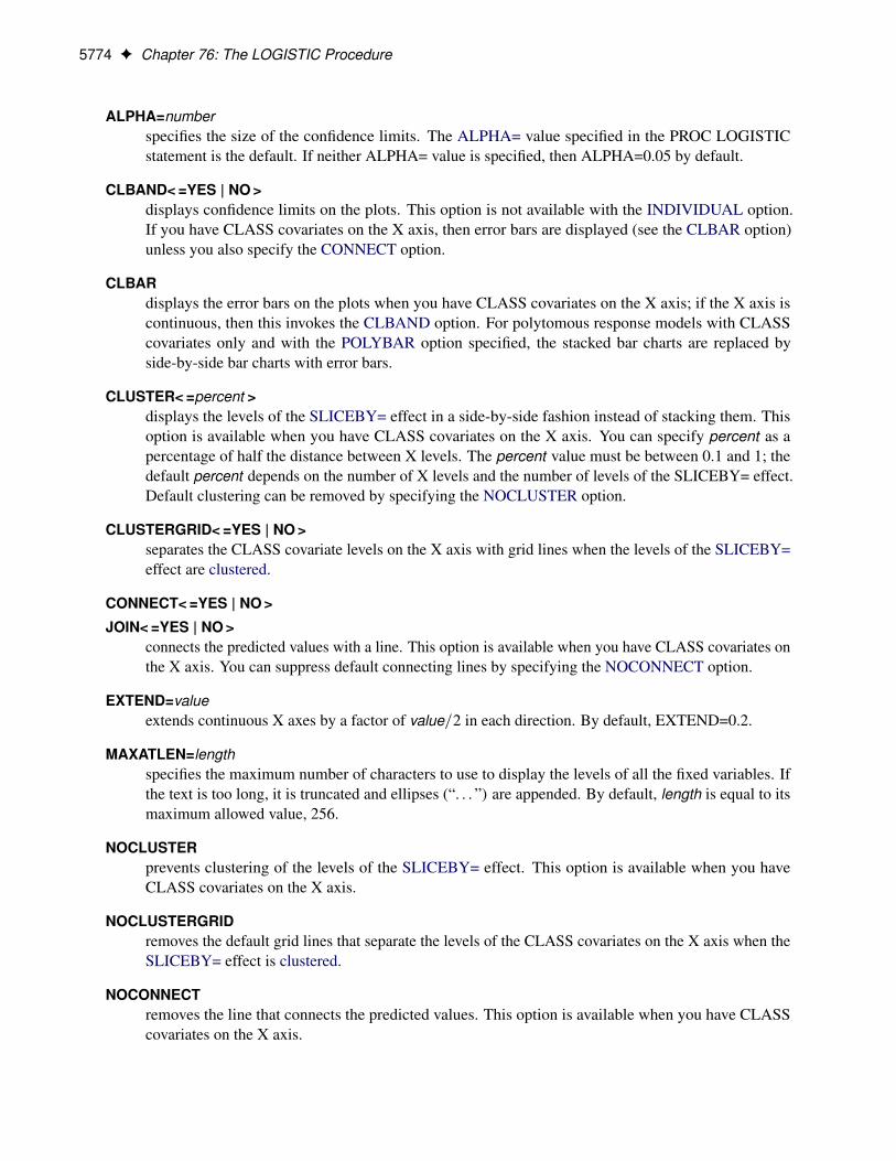
ALPHA=numberspecifies the size of the confidence limits. The ALPHA= value specified in the PROC LOGISTICstatement is the default. If neither ALPHA= value is specified, then ALPHA=0.05 by default.
CLBAND< =YES | NO >displays confidence limits on the plots. This option is not available with the INDIVIDUAL option.If you have CLASS covariates on the X axis, then error bars are displayed (see the CLBAR option)unless you also specify the CONNECT option.
CLBARdisplays the error bars on the plots when you have CLASS covariates on the X axis; if the X axis iscontinuous, then this invokes the CLBAND option. For polytomous response models with CLASScovariates only and with the POLYBAR option specified, the stacked bar charts are replaced byside-by-side bar charts with error bars.
CLUSTER< =percent >displays the levels of the SLICEBY= effect in a side-by-side fashion instead of stacking them. Thisoption is available when you have CLASS covariates on the X axis. You can specify percent as apercentage of half the distance between X levels. The percent value must be between 0.1 and 1; thedefault percent depends on the number of X levels and the number of levels of the SLICEBY= effect.Default clustering can be removed by specifying the NOCLUSTER option.
CLUSTERGRID< =YES | NO >separates the CLASS covariate levels on the X axis with grid lines when the levels of the SLICEBY=effect are clustered.
CONNECT< =YES | NO >
JOIN< =YES | NO >connects the predicted values with a line. This option is available when you have CLASS covariates onthe X axis. You can suppress default connecting lines by specifying the NOCONNECT option.
EXTEND=valueextends continuous X axes by a factor of value=2 in each direction. By default, EXTEND=0.2.
MAXATLEN=lengthspecifies the maximum number of characters to use to display the levels of all the fixed variables. Ifthe text is too long, it is truncated and ellipses (“. . . ”) are appended. By default, length is equal to itsmaximum allowed value, 256.
NOCLUSTERprevents clustering of the levels of the SLICEBY= effect. This option is available when you haveCLASS covariates on the X axis.
NOCLUSTERGRIDremoves the default grid lines that separate the levels of the CLASS covariates on the X axis when theSLICEBY= effect is clustered.
NOCONNECTremoves the line that connects the predicted values. This option is available when you have CLASScovariates on the X axis.

PROC LOGISTIC Statement F 5775
POLYBARreplaces scatter plots of polytomous response models with bar charts. This option has no effect onbinary-response models, and it is overridden by the CONNECT option. By default, the X axis is chosento be a crossing of available classification variables so that there are no more than 16 levels; if no suchcrossing is possible then the first available classification variable is used. You can override this defaultby specifying the X= option.
SHOWOBS< =YES | NO >displays observations on the plot when the MAXPOINTS= cutoff is not exceeded. For events/trialsnotation, the observed proportions are displayed; for single-trial binary-response models, the observedevents are displayed at Op D 1 and the observed nonevents are displayed at Op D 0. For polytomousresponse models the predicted probabilities at the observed values of the covariate are computed anddisplayed.
YRANGE=(< min >< ,max >)displays the Y axis as [min,max]. Note that the axis might extend beyond your specified values. Bydefault, the entire Y axis, [0,1], is displayed for the predicted probabilities. This option is useful ifyour predicted probabilities are all contained in some subset of this range.
Odds Ratio Plots
The odds ratios and confidence limits from the default “Odds Ratio Estimates” table and from the tablesproduced by the CLODDS= option or the ODDSRATIO statement can be displayed in a graphic. If you havemany odds ratios, you can produce multiple graphics, or panels, by displaying subsets of the odds ratios.Odds ratios that have duplicate labels are not displayed. See Outputs 76.2.9 and 76.3.3 for examples of oddsratio plots.
The following oddsratio-options modify the default odds ratio plot:
CLDISPLAY=SERIF | SERIFARROW | LINE | LINEARROW | BAR< width >controls the look of the confidence limit error bars. The default CLDISPLAY=SERIF displays theconfidence limits as lines with serifs, and the CLDISPLAY=LINE option removes the serifs fromthe error bars. The CLDISPLAY=SERIFARROW and CLDISPLAY=LINEARROW options displayarrowheads on any error bars that are clipped by the RANGE= option; if the entire error bar is cut fromthe graphic, then an arrowhead is displayed that points toward the odds ratio. The CLDISPLAY=BAR< width > option displays the limits along with a bar whose width is equal to the size of the marker.You can control the width of the bars and the size of the marker by specifying the width value as apercentage of the distance between the bars, 0 < width � 1.
NOTE: Your bar might disappear if you have small values of width.
DOTPLOTdisplays dotted gridlines on the plot.
GROUPdisplays the odds ratios in panels that are defined by the ODDSRATIO statements. The NPANELPOS=option is ignored when this option is specified.

5776 F Chapter 76: The LOGISTIC Procedure
LOGBASE=2 | E | 10displays the odds ratio axis on the specified log scale.
NPANELPOS=numberbreaks the plot into multiple graphics that have at most |number | odds ratios per graphic. If numberis positive, then the number of odds ratios per graphic is balanced; if number is negative, then nobalancing of the number of odds ratios takes place. By default, number = 0 and all odds ratios aredisplayed in a single plot. For example, suppose you want to display 21 odds ratios. Then specifyingNPANELPOS=20 displays two plots, the first with 11 odds ratios and the second with 10; but specifyingNPANELPOS=-20 displays 20 odds ratios in the first plot and only 1 odds ratio in the second plot.
ORDER=ASCENDING | DESCENDINGdisplays the odds ratios in sorted order. By default the odds ratios are displayed in the order in whichthey appear in the corresponding table.
RANGE=(< min >< ,max >) | CLIPspecifies the range of the displayed odds ratio axis. Specifying the RANGE=CLIP option has the sameeffect as specifying the minimum odds ratio as min and the maximum odds ratio as max . By default,all odds ratio confidence intervals are displayed.
TYPE=HORIZONTAL | HORIZONTALSTAT | VERTICAL | VERTICALBLOCKcontrols the look of the graphic. The default TYPE=HORIZONTAL option places the odds ratio valueson the X axis, while the TYPE=HORIZONTALSTAT option also displays the values of the odds ratiosand their confidence limits on the right side of the graphic. The TYPE=VERTICAL option places theodds ratio values on the Y axis, while the TYPE=VERTICALBLOCK option (available only with theCLODDS= option) places the odds ratio values on the Y axis and puts boxes around the labels.
BY StatementBY variables ;
You can specify a BY statement in PROC LOGISTIC to obtain separate analyses of observations in groupsthat are defined by the BY variables. When a BY statement appears, the procedure expects the input dataset to be sorted in order of the BY variables. If you specify more than one BY statement, only the last onespecified is used.
If your input data set is not sorted in ascending order, use one of the following alternatives:
� Sort the data by using the SORT procedure with a similar BY statement.
� Specify the NOTSORTED or DESCENDING option in the BY statement in the LOGISTIC procedure.The NOTSORTED option does not mean that the data are unsorted but rather that the data are arrangedin groups (according to values of the BY variables) and that these groups are not necessarily inalphabetical or increasing numeric order.
� Create an index on the BY variables by using the DATASETS procedure (in Base SAS software).
If a SCORE statement is specified, then define the training data set to be the DATA= data set or theINMODEL= data set in the PROC LOGISTIC statement, and define the scoring data set to be the DATA=

CLASS Statement F 5777
data set and PRIOR= data set in the SCORE statement. The training data set contains all of the BY variables,and the scoring data set must contain either all of them or none of them. If the scoring data set contains allthe BY variables, matching is carried out between the training and scoring data sets. If the scoring data setdoes not contain any of the BY variables, the entire scoring data set is used for every BY group in the trainingdata set and the BY variables are added to the output data sets that are specified in the SCORE statement.
CAUTION: The order of the levels in the response and classification variables is determined from all the dataregardless of BY groups. However, different sets of levels might appear in different BY groups. This mightaffect the value of the reference level for these variables, and hence your interpretation of the model and theparameters.
For more information about BY-group processing, see the discussion in SAS Language Reference: Concepts.For more information about the DATASETS procedure, see the discussion in the Base SAS Procedures Guide.
CLASS StatementCLASS variable < (options) > . . . < variable < (options) > > < / global-options > ;
The CLASS statement names the classification variables to be used as explanatory variables in the analysis.Response variables do not need to be specified in the CLASS statement.
The CLASS statement must precede the MODEL statement. Most options can be specified either as individualvariable options or as global-options. You can specify options for each variable by enclosing the optionsin parentheses after the variable name. You can also specify global-options for the CLASS statement byplacing them after a slash (/). Global-options are applied to all the variables that are specified in the CLASSstatement. If you specify more than one CLASS statement, the global-options that are specified in any oneCLASS statement apply to all CLASS statements. However, individual CLASS variable options override theglobal-options. You can specify the following values for either an option or a global-option:
CPREFIX=nspecifies that, at most, the first n characters of a CLASS variable name be used in creating names forthe corresponding design variables. The default is 32 �min.32;max.2; f //, where f is the formattedlength of the CLASS variable.
DESCENDING
DESCreverses the sort order of the classification variable. If you specify both the DESCENDING andORDER= options, PROC LOGISTIC orders the categories according to the ORDER= option and thenreverses that order.
LPREFIX=nspecifies that, at most, the first n characters of a CLASS variable label be used in creating labels for thecorresponding design variables. The default is 256 �min.256;max.2; f //, where f is the formattedlength of the CLASS variable.
MISSINGtreats missing values (., ._, .A, . . . , .Z for numeric variables and blanks for character variables) as validvalues of the CLASS variable.

5778 F Chapter 76: The LOGISTIC Procedure
ORDER=DATA | FORMATTED | FREQ | INTERNALspecifies the sort order for the levels of classification variables. This ordering determines whichparameters in the model correspond to each level in the data, so this option can be useful when youuse the CONTRAST statement. By default, ORDER=FORMATTED. For ORDER=FORMATTEDand ORDER=INTERNAL, the sort order is machine-dependent. When ORDER=FORMATTED is ineffect for numeric variables for which you have supplied no explicit format, the levels are ordered bytheir internal values.
The following table shows how PROC LOGISTIC interprets values of the ORDER= option:
Value of ORDER= Levels Sorted By
DATA Order of appearance in the input data setFORMATTED External formatted values, except for numeric
variables with no explicit format, which are sortedby their unformatted (internal) values
FREQ Descending frequency count; levels with moreobservations come earlier in the order
INTERNAL Unformatted value
For more information about sort order, see the chapter on the SORT procedure in the Base SASProcedures Guide and the discussion of BY-group processing in SAS Language Reference: Concepts.
PARAM=keywordspecifies the parameterization method for the classification variable or variables. You can specifyany of the keywords shown in the following table. The default is PARAM=EFFECT. Design matrixcolumns are created from CLASS variables according to the corresponding coding schemes.
Value of PARAM= Coding
EFFECT Effect coding
GLM Less-than-full-rank reference cell coding (thiskeyword can be used only in a global option)
ORDINALTHERMOMETER
Cumulative parameterization for an ordinalCLASS variable
POLYNOMIALPOLY
Polynomial coding
REFERENCEREF
Reference cell coding
ORTHEFFECT Orthogonalizes PARAM=EFFECT coding
ORTHORDINALORTHOTHERM
Orthogonalizes PARAM=ORDINAL coding
ORTHPOLY Orthogonalizes PARAM=POLYNOMIAL coding
ORTHREF Orthogonalizes PARAM=REFERENCE coding
All parameterizations are full rank, except for the GLM parameterization. The REF= option in theCLASS statement determines the reference level for EFFECT and REFERENCE coding and for their

CLASS Statement F 5779
orthogonal parameterizations. It also indirectly determines the reference level for a singular GLMparameterization through the order of levels.
If a PARAM= option is specified as a variable option for some variables, then any variables for whichPARAM= is not specified use either the EFFECT parameterization if the global PARAM= option isnot specified, or the full-rank parameterization indicated in the global PARAM= option if specified. Ifthe global PARAM=GLM option is specified and PARAM= is also specified for some variables, GLMparameterization is used for all variables.
If PARAM=ORTHPOLY or PARAM=POLY and the classification variable is numeric, then theORDER= option in the CLASS statement is ignored, and the internal unformatted values are used.For more information, see the section “Other Parameterizations” on page 397 in Chapter 19, “SharedConcepts and Topics.”
REF=’level’ | keywordspecifies the reference level for PARAM=EFFECT, PARAM=REFERENCE, and their orthogonaliza-tions. For PARAM=GLM, the REF= option specifies a level of the classification variable to be put atthe end of the list of levels. This level thus corresponds to the reference level in the usual interpretationof the linear estimates with a singular parameterization.
For an individual variable REF= option (but not for a global REF= option), you can specify the levelof the variable to use as the reference level. Specify the formatted value of the variable if a format isassigned. For a global or individual variable REF= option, you can use one of the following keywords:
FIRST designates the first ordered level as reference.
LAST designates the last ordered level as reference.
By default, REF=LAST.
TRUNCATE< =n >specifies the length n of CLASS variable values to use in determining CLASS variable levels. Thedefault is to use the full formatted length of the CLASS variable. If you specify TRUNCATE withoutthe length n, the first 16 characters of the formatted values are used. When formatted values are longerthan 16 characters, you can use this option to revert to the levels as determined in releases before SAS9. The TRUNCATE option is available only as a global option.
Class Variable Naming Convention
Parameter names for a CLASS predictor variable are constructed by concatenating the CLASS variable namewith the CLASS levels. However, for the POLYNOMIAL and orthogonal parameterizations, parameternames are formed by concatenating the CLASS variable name and keywords that reflect the parameterization.For examples and more information, see the section “Other Parameterizations” on page 397 in Chapter 19,“Shared Concepts and Topics.”
Class Variable Parameterization with Unbalanced Designs
PROC LOGISTIC initially parameterizes the CLASS variables by looking at the levels of the variables acrossthe complete data set. If you have an unbalanced replication of levels across variables or BY groups, thenthe design matrix and the parameter interpretation might be different from what you expect. For example,suppose you have a model that has one CLASS variable A with three levels (1, 2, and 3) and another CLASS

5780 F Chapter 76: The LOGISTIC Procedure
variable B with two levels (1 and 2). If the third level of A occurs only with the first level of B, if you use theEFFECT parameterization, and if your model contains the effect A(B) and an intercept, then the design for Awithin the second level of B is not a differential effect. In particular, the design looks like the following:
Design MatrixA(B=1) A(B=2)
B A A1 A2 A1 A2
1 1 1 0 0 01 2 0 1 0 01 3 –1 –1 0 02 1 0 0 1 02 2 0 0 0 1
PROC LOGISTIC detects linear dependency among the last two design variables and sets the parameter forA2(B=2) to zero, resulting in an interpretation of these parameters as if they were reference- or dummy-coded.The REFERENCE or GLM parameterization might be more appropriate for such problems.
CODE StatementCODE < options > ;
The CODE statement writes SAS DATA step code for computing predicted values of the fitted model eitherto a file or to a catalog entry. This code can then be included in a DATA step to score new data.
Table 76.2 summarizes the options available in the CODE statement.
Table 76.2 CODE Statement Options
Option Description
CATALOG= Names the catalog entry where the generated code is savedDUMMIES Retains the dummy variables in the data setERROR Computes the error functionFILE= Names the file where the generated code is savedFORMAT= Specifies the numeric format for the regression coefficientsGROUP= Specifies the group identifier for array names and statement labelsIMPUTE Imputes predicted values for observations with missing or invalid
covariatesLINESIZE= Specifies the line size of the generated codeLOOKUP= Specifies the algorithm for looking up CLASS levelsRESIDUAL Computes residuals
For details about the syntax of the CODE statement, see the section “CODE Statement” on page 400 inChapter 19, “Shared Concepts and Topics.”

CONTRAST Statement F 5781
CONTRAST StatementCONTRAST 'label ' row-description< , . . . , row-description > < / options > ;
where a row-description is defined as follows:
effect values< , . . . , effect values >
The CONTRAST statement provides a mechanism for obtaining customized hypothesis tests. It is similar tothe CONTRAST and ESTIMATE statements in other modeling procedures.
The CONTRAST statement enables you to specify a matrix, L, for testing the hypothesis Lˇ D 0, whereˇ is the vector of intercept and slope parameters. You must be familiar with the details of the modelparameterization that PROC LOGISTIC uses (for more information, see the PARAM= option in the section“CLASS Statement” on page 5777). Optionally, the CONTRAST statement enables you to estimate eachrow, l 0iˇ, of Lˇ and test the hypothesis l 0iˇ D 0. Computed statistics are based on the asymptotic chi-squaredistribution of the Wald statistic.
There is no limit to the number of CONTRAST statements that you can specify, but they must appear afterthe MODEL statement.
The following parameters are specified in the CONTRAST statement:
label identifies the contrast in the displayed output. A label is required for every contrast specified, andit must be enclosed in quotation marks.
effect identifies an effect that appears in the MODEL statement. The name INTERCEPT can be used asan effect when one or more intercepts are included in the model. You do not need to include alleffects that are included in the MODEL statement.
values are constants that are elements of the L matrix associated with the effect. To correctly specifyyour contrast, it is crucial to know the ordering of parameters within each effect and the variablelevels associated with any parameter. The “Class Level Information” table shows the orderingof levels within variables. The E option, described later in this section, enables you to verify theproper correspondence of values to parameters. If too many values are specified for an effect, theextra ones are ignored. If too few values are specified, the remaining ones are set to 0.
Multiple degree-of-freedom hypotheses can be tested by specifying multiple row-descriptions; the rows ofL are specified in order and are separated by commas. The degrees of freedom is the number of linearlyindependent constraints implied by the CONTRAST statement—that is, the rank of L.
More details for specifying contrasts involving effects with full-rank parameterizations are given in thesection “Full-Rank Parameterized Effects” on page 5782, while details for less-than-full-rank parameterizedeffects are given in the section “Less-Than-Full-Rank Parameterized Effects” on page 5783.
You can specify the following options after a slash (/):
ALPHA=numberspecifies the level of significance ˛ for the 100.1� ˛/% confidence interval for each contrast when theESTIMATE option is specified. The value of number must be between 0 and 1. By default, number isequal to the value of the ALPHA= option in the PROC LOGISTIC statement, or 0.05 if that option isnot specified.

5782 F Chapter 76: The LOGISTIC Procedure
Edisplays the L matrix.
ESTIMATE=keywordestimates and tests each individual contrast (that is, each row, l 0iˇ, of Lˇ), exponentiated contrast(el0iˇ), or predicted probability for the contrast (g�1.l 0iˇ/). PROC LOGISTIC displays the point
estimate, its standard error, a Wald confidence interval, and a Wald chi-square test. The significancelevel of the confidence interval is controlled by the ALPHA= option. You can estimate the individualcontrast, the exponentiated contrast, or the predicted probability for the contrast by specifying one ofthe following keywords:
PARM estimates the individual contrast.EXP estimates the exponentiated contrast.BOTH estimates both the individual contrast and the exponentiated contrast.PROB estimates the predicted probability of the contrast.ALL estimates the individual contrast, the exponentiated contrast, and the predicted probability
of the contrast.
For more information about the computations of the standard errors and confidence limits, see thesection “Linear Predictor, Predicted Probability, and Confidence Limits” on page 5851.
SINGULAR=numbertunes the estimability check. This option is ignored when a full-rank parameterization is specified. Ifv is a vector, define ABS.v/ to be the largest absolute value of the elements of v. For a row vectorl 0 of the contrast matrix L, define c D ABS.l/ if ABS.l/ is greater than 0; otherwise, c = 1. IfABS.l 0� l 0T/ is greater than c�number , then l is declared nonestimable. The T matrix is the Hermiteform matrix I�0 I0, where I�0 represents a generalized inverse of the (observed or expected) informationmatrix I0 of the null model. The value for number must be between 0 and 1; the default value is 1E–4.
Full-Rank Parameterized Effects
If an effect involving a CLASS variable with a full-rank parameterization does not appear in the CONTRASTstatement, then all of its coefficients in the L matrix are set to 0.
If you use effect coding by default or by specifying PARAM=EFFECT in the CLASS statement, then allparameters are directly estimable and involve no other parameters. For example, suppose an effect-codedCLASS variable A has four levels. Then there are three parameters (ˇ1; ˇ2; ˇ3) representing the first threelevels, and the fourth parameter is represented by
�ˇ1 � ˇ2 � ˇ3
To test the first versus the fourth level of A, you would test
ˇ1 D �ˇ1 � ˇ2 � ˇ3
or, equivalently,
2ˇ1 C ˇ2 C ˇ3 D 0

EFFECT Statement F 5783
which, in the form Lˇ D 0, is
�2 1 1
�24 ˇ1ˇ2ˇ3
35 D 0Therefore, you would use the following CONTRAST statement:
contrast '1 vs. 4' A 2 1 1;
To contrast the third level with the average of the first two levels, you would testˇ1 C ˇ2
2D ˇ3
or, equivalently,
ˇ1 C ˇ2 � 2ˇ3 D 0
Therefore, you would use the following CONTRAST statement:
contrast '1&2 vs. 3' A 1 1 -2;
Other CONTRAST statements are constructed similarly. For example:
contrast '1 vs. 2 ' A 1 -1 0;contrast '1&2 vs. 4 ' A 3 3 2;contrast '1&2 vs. 3&4' A 2 2 0;contrast 'Main Effect' A 1 0 0,
A 0 1 0,A 0 0 1;
Less-Than-Full-Rank Parameterized Effects
When you use the less-than-full-rank parameterization (by specifying PARAM=GLM in the CLASS state-ment), each row is checked for estimability; see the section “Estimable Functions” on page 59 in Chapter 3,“Introduction to Statistical Modeling with SAS/STAT Software,” for more information. If PROC LOGISTICfinds a contrast to be nonestimable, it displays missing values in corresponding rows in the results. PROCLOGISTIC handles missing level combinations of classification variables in the same manner as PROC GLM:parameters corresponding to missing level combinations are not included in the model. This conventioncan affect the way in which you specify the L matrix in your CONTRAST statement. If the elements of Lare not specified for an effect that contains a specified effect, then the elements of the specified effect aredistributed over the levels of the higher-order effect just as the GLM procedure does for its CONTRAST andESTIMATE statements. For example, suppose that the model contains effects A and B and their interactionA*B. If you specify a CONTRAST statement involving A alone, the L matrix contains nonzero terms forboth A and A*B, because A*B contains A. For more information, see rule 4 in the section “Construction ofLeast Squares Means” on page 4056 in Chapter 50, “The GLM Procedure.”
EFFECT StatementEFFECT name=effect-type (variables < / options >) ;
The EFFECT statement enables you to construct special collections of columns for design matrices. Thesecollections are referred to as constructed effects to distinguish them from the usual model effects that areformed from continuous or classification variables, as discussed in the section “GLM Parameterization ofClassification Variables and Effects” on page 393 in Chapter 19, “Shared Concepts and Topics.”
You can specify the following effect-types:

5784 F Chapter 76: The LOGISTIC Procedure
COLLECTION specifies a collection effect that defines one or more variables as a singleeffect with multiple degrees of freedom. The variables in a collection areconsidered as a unit for estimation and inference.
LAG specifies a classification effect in which the level that is used for a particularperiod corresponds to the level in the preceding period.
MULTIMEMBER | MM specifies a multimember classification effect whose levels are determined byone or more variables that appear in a CLASS statement.
POLYNOMIAL | POLY specifies a multivariate polynomial effect in the specified numeric variables.
SPLINE specifies a regression spline effect whose columns are univariate spline ex-pansions of one or more variables. A spline expansion replaces the originalvariable with an expanded or larger set of new variables.
Table 76.3 summarizes the options available in the EFFECT statement.
Table 76.3 EFFECT Statement Options
Option Description
Collection Effects OptionsDETAILS Displays the constituents of the collection effect
Lag Effects OptionsDESIGNROLE= Names a variable that controls to which lag design an observation
is assigned
DETAILS Displays the lag design of the lag effect
NLAG= Specifies the number of periods in the lag
PERIOD= Names the variable that defines the period. This option is required.
WITHIN= Names the variable or variables that define the group within whicheach period is defined. This option is required.
Multimember Effects OptionsNOEFFECT Specifies that observations with all missing levels for the
multimember variables should have zero values in thecorresponding design matrix columns
WEIGHT= Specifies the weight variable for the contributions of each of theclassification effects
Polynomial Effects OptionsDEGREE= Specifies the degree of the polynomialMDEGREE= Specifies the maximum degree of any variable in a term of the
polynomialSTANDARDIZE= Specifies centering and scaling suboptions for the variables that
define the polynomial
Spline Effects OptionsBASIS= Specifies the type of basis (B-spline basis or truncated power
function basis) for the spline effect

EFFECTPLOT Statement F 5785
Table 76.3 continued
Option Description
DEGREE= Specifies the degree of the spline effectKNOTMETHOD= Specifies how to construct the knots for the spline effect
For more information about the syntax of these effect-types and how columns of constructed effects arecomputed, see the section “EFFECT Statement” on page 403 in Chapter 19, “Shared Concepts and Topics.”
EFFECTPLOT StatementEFFECTPLOT < plot-type < (plot-definition-options) > > < / options > ;
The EFFECTPLOT statement produces a display of the fitted model and provides options for changing andenhancing the displays. Table 76.4 describes the available plot-types and their plot-definition-options.
Table 76.4 Plot-Types and Plot-Definition-Options
Plot-Type and Description Plot-Definition-Options
BOXDisplays a box plot of continuous response data at eachlevel of a CLASS effect, with predicted valuessuperimposed and connected by a line. This is analternative to the INTERACTION plot-type.
PLOTBY= variable or CLASS effectX= CLASS variable or effect
CONTOURDisplays a contour plot of predicted values against twocontinuous covariates.
PLOTBY= variable or CLASS effectX= continuous variableY= continuous variable
FITDisplays a curve of predicted values versus acontinuous variable.
PLOTBY= variable or CLASS effectX= continuous variable
INTERACTIONDisplays a plot of predicted values (possibly with errorbars) versus the levels of a CLASS effect. Thepredicted values are connected with lines and can begrouped by the levels of another CLASS effect.
PLOTBY= variable or CLASS effectSLICEBY= variable or CLASS effectX= CLASS variable or effect
MOSAICDisplays a mosaic plot of predicted values using up tothree CLASS effects.
PLOTBY= variable or CLASS effectX= CLASS effects
SLICEFITDisplays a curve of predicted values versus acontinuous variable grouped by the levels of aCLASS effect.
PLOTBY= variable or CLASS effectSLICEBY= variable or CLASS effectX= continuous variable

5786 F Chapter 76: The LOGISTIC Procedure
For full details about the syntax and options of the EFFECTPLOT statement, see the section “EFFECTPLOTStatement” on page 423 in Chapter 19, “Shared Concepts and Topics.”
See Outputs 76.2.11, 76.2.12, 76.3.5, 76.4.8, 76.7.4, and 76.16.4 for examples of plots produced by thisstatement.
ESTIMATE StatementESTIMATE < 'label ' > estimate-specification < (divisor=n) >
< , . . . < 'label ' > estimate-specification < (divisor=n) > >< / options > ;
The ESTIMATE statement provides a mechanism for obtaining custom hypothesis tests. Estimates areformed as linear estimable functions of the form Lˇ. You can perform hypothesis tests for the estimablefunctions, construct confidence limits, and obtain specific nonlinear transformations.
Table 76.5 summarizes the options available in the ESTIMATE statement.
Table 76.5 ESTIMATE Statement Options
Option Description
Construction and Computation of Estimable FunctionsDIVISOR= Specifies a list of values to divide the coefficientsNOFILL Suppresses the automatic fill-in of coefficients for higher-order
effectsSINGULAR= Tunes the estimability checking difference
Degrees of Freedom and p-ValuesADJUST= Determines the method of multiple comparison adjustment of
estimatesALPHA=˛ Determines the confidence level (1 � ˛)LOWER Performs one-sided, lower-tailed inferenceSTEPDOWN Adjusts multiplicity-corrected p-values further in a step-down
fashionTESTVALUE= Specifies values under the null hypothesis for testsUPPER Performs one-sided, upper-tailed inference
Statistical OutputCL Constructs confidence limitsCORR Displays the correlation matrix of estimatesCOV Displays the covariance matrix of estimatesE Prints the L matrixJOINT Produces a joint F or chi-square test for the estimable functionsPLOTS= Produces ODS statistical graphics if the analysis is sampling-basedSEED= Specifies the seed for computations that depend on random
numbers

EXACT Statement F 5787
Table 76.5 continued
Option Description
Generalized Linear ModelingCATEGORY= Specifies how to construct estimable functions for multinomial dataEXP Exponentiates and displays estimatesILINK Computes and displays estimates and standard errors on the inverse
linked scale
For more information about the syntax of the ESTIMATE statement, see the section “ESTIMATE Statement”on page 451 in Chapter 19, “Shared Concepts and Topics.”
EXACT StatementEXACT < 'label ' > < INTERCEPT > < effects > < / options > ;
The EXACT statement performs exact tests of the parameters for the specified effects and optionally estimatesthe parameters and outputs the exact conditional distributions. You can specify the keyword INTERCEPTand any effects in the MODEL statement. Inference on the parameters of the specified effects is performedby conditioning on the sufficient statistics of all the other model parameters (possibly including the intercept).
You can specify several EXACT statements, but they must follow the MODEL statement. Each statement canoptionally include an identifying label . If several EXACT statements are specified, any statement withouta label is assigned a label of the form “Exactn,” where n indicates the nth EXACT statement. The label isincluded in the headers of the displayed exact analysis tables.
If a STRATA statement is also specified, then a stratified exact logistic regression is performed. The modelcontains a different intercept for each stratum, and these intercepts are conditioned out of the model alongwith any other nuisance parameters (parameters for effects specified in the MODEL statement that are not inthe EXACT statement).
If the LINK=GLOGIT option is specified in the MODEL statement, then the METHOD=DIRECT option isinvoked in the EXACTOPTIONS statement by default and a generalized logit model is fit. Since each effectspecified in the MODEL statement adds k parameters to the model (where k + 1 is the number of responselevels), exact analysis of the generalized logit model by using this method is limited to rather small problems.
The CONTRAST, ESTIMATE, LSMEANS, LSMESTIMATE, ODDSRATIO, OUTPUT, ROC, ROCCON-TRAST, SCORE, SLICE, STORE, TEST, and UNITS statements are not available with an exact analysis;results from these statements are based on the asymptotic results. Exact analyses are not performed when youspecify a WEIGHT statement, a link other than LINK=LOGIT or LINK=GLOGIT, an offset variable, theNOFIT option, or a model selection method. Exact estimation is not available for ordinal response models.
For classification variables, use of the reference parameterization is recommended.
The following options can be specified in each EXACT statement after a slash (/):

5788 F Chapter 76: The LOGISTIC Procedure
ALPHA=numberspecifies the level of significance ˛ for 100.1 � ˛/% confidence limits for the parameters or oddsratios. The value of number must be between 0 and 1. By default, number is equal to the value of theALPHA= option in the PROC LOGISTIC statement, or 0.05 if that option is not specified.
CLTYPE=EXACT | MIDPrequests either the exact or mid-p confidence intervals for the parameter estimates. By default, the exactintervals are produced. The confidence coefficient can be specified with the ALPHA= option. Themid-p interval can be modified with the MIDPFACTOR= option. See the section “Exact ConditionalLogistic Regression” on page 5875 for details.
ESTIMATE < =keyword >estimates the individual parameters (conditioned on all other parameters) for the effects specified in theEXACT statement. For each parameter, a point estimate, a standard error, a confidence interval, and ap-value for a two-sided test that the parameter is zero are displayed. Note that the two-sided p-value istwice the one-sided p-value. You can optionally specify one of the following keywords:
PARM specifies that the parameters be estimated. This is the default.
ODDS specifies that the odds ratios be estimated. If you have classification variables, then youmust also specify the PARAM=REF option in the CLASS statement.
BOTH specifies that both the parameters and odds ratios be estimated.
JOINTperforms the joint test that all of the parameters are simultaneously equal to zero, performs individualhypothesis tests for the parameter of each continuous variable, and performs joint tests for the parame-ters of each classification variable. The joint test is indicated in the “Conditional Exact Tests” table bythe label “Joint.”
JOINTONLYperforms only the joint test of the parameters. The test is indicated in the “Conditional Exact Tests”table by the label “Joint.” When this option is specified, individual tests for the parameters of eachcontinuous variable and joint tests for the parameters of the classification variables are not performed.
MIDPFACTOR=ı1 | (ı1; ı2)sets the tie factors used to produce the mid-p hypothesis statistics and the mid-p confidence intervals.ı1 modifies both the hypothesis tests and confidence intervals, while ı2 affects only the hypothesistests. By default, ı1 D 0:5 and ı2 D 1:0. See the section “Exact Conditional Logistic Regression” onpage 5875 for details.
ONESIDEDrequests one-sided confidence intervals and p-values for the individual parameter estimates and oddsratios. The one-sided p-value is the smaller of the left- and right-tail probabilities for the observedsufficient statistic of the parameter under the null hypothesis that the parameter is zero. The two-sidedp-values (default) are twice the one-sided p-values. See the section “Exact Conditional LogisticRegression” on page 5875 for more details.

EXACTOPTIONS Statement F 5789
OUTDIST=SAS-data-setnames the SAS data set that contains the exact conditional distributions. This data set contains all ofthe exact conditional distributions that are required to process the corresponding EXACT statement.This data set contains the possible sufficient statistics for the parameters of the effects specifiedin the EXACT statement, the counts, and, when hypothesis tests are performed on the parameters,the probability of occurrence and the score value for each sufficient statistic. When you request anOUTDIST= data set, the observed sufficient statistics are displayed in the “Sufficient Statistics” table.See the section “OUTDIST= Output Data Set” on page 5883 for more information.
EXACT Statement Examples
In the following example, two exact tests are computed: one for x1 and the other for x2. The test for x1 isbased on the exact conditional distribution of the sufficient statistic for the x1 parameter given the observedvalues of the sufficient statistics for the intercept, x2, and x3 parameters; likewise, the test for x2 is conditionalon the observed sufficient statistics for the intercept, x1, and x3.
proc logistic;model y= x1 x2 x3;exact x1 x2;
run;
PROC LOGISTIC determines, from all the specified EXACT statements, the distinct conditional distributionsthat need to be evaluated. For example, there is only one exact conditional distribution for the following twoEXACT statements:
exact 'One' x1 / estimate=parm;exact 'Two' x1 / estimate=parm onesided;
For each EXACT statement, individual tests for the parameters of the specified effects are computed unlessthe JOINTONLY option is specified. Consider the following EXACT statements:
exact 'E12' x1 x2 / estimate;exact 'E1' x1 / estimate;exact 'E2' x2 / estimate;exact 'J12' x1 x2 / joint;
In the E12 statement, the parameters for x1 and x2 are estimated and tested separately. Specifying the E12statement is equivalent to specifying both the E1 and E2 statements. In the J12 statement, the joint test forthe parameters of x1 and x2 is computed in addition to the individual tests for x1 and x2.
EXACTOPTIONS StatementEXACTOPTIONS options ;
The EXACTOPTIONS statement specifies options that apply to every EXACT statement in the program.The following options are available:

5790 F Chapter 76: The LOGISTIC Procedure
ABSFCONV=valuespecifies the absolute function convergence criterion. Convergence requires a small change in thelog-likelihood function in subsequent iterations,
jli � li�1j < value
where li is the value of the log-likelihood function at iteration i.
By default, ABSFCONV=1E–12. You can also specify the FCONV= and XCONV= criteria; optimiza-tions are terminated as soon as one criterion is satisfied.
ADDTOBSadds the observed sufficient statistic to the sampled exact distribution if the statistic was not sampled.This option has no effect unless the METHOD=NETWORKMC or METHOD=MCMC option isspecified and the ESTIMATE option is specified in the EXACT statement. If the observed statistichas not been sampled, then the parameter estimate does not exist; by specifying this option, you canproduce (biased) estimates.
BUILDSUBSETSbuilds every distribution for sampling. By default, some exact distributions are created by takinga subset of a previously generated exact distribution. When the METHOD=NETWORKMC orMETHOD=MCMC option is invoked, this subsetting behavior has the effect of using fewer than thedesired n samples; see the N= option for more details. Use the BUILDSUBSETS option to suppressthis subsetting.
EPSILON=valuecontrols how the partial sums
PjiD1 yixi are compared. value must be between 0 and 1; by default,
value=1E–8.
FCONV=valuespecifies the relative function convergence criterion. Convergence requires a small relative change inthe log-likelihood function in subsequent iterations,
jli � li�1j
jli�1j C 1E–6< value
where li is the value of the log likelihood at iteration i.
By default, FCONV=1E–8. You can also specify the ABSFCONV= and XCONV= criteria; if youspecify more than one criterion, then optimizations are terminated as soon as one criterion is satisfied.
MAXSWAP=n
MAXR=nspecifies the maximum number of swaps for each sample that PROC LOGISTIC makes when youspecify the METHOD=MCMC option. If an intercept or a stratum is conditioned out, then n swaps areperformed: one event is changed to a nonevent, and one nonevent is changed to an event. Althoughyou might need large values of n in order to transition between any two points in the exact distribution,such values quickly increase computation time. By default, MAXSWAP=2.

EXACTOPTIONS Statement F 5791
MAXTIME=secondsspecifies the maximum clock time (in seconds) that PROC LOGISTIC can use to calculate the exactdistributions. If the limit is exceeded, the procedure halts all computations and prints a note to the SASlog. The default maximum clock time is seven days.
METHOD=keywordspecifies which exact conditional algorithm to use for every EXACT statement specified. You canspecify one of the following keywords:
DIRECT invokes the multivariate shift algorithm of Hirji, Mehta, and Patel (1987). This methoddirectly builds the exact distribution, but it can require an excessive amount of memory in itsintermediate stages. METHOD=DIRECT is invoked by default when you are conditioningout at most the intercept, or when the LINK=GLOGIT option is specified in the MODELstatement.
NETWORK invokes an algorithm described in Mehta, Patel, and Senchaudhuri (1992). This methodbuilds a network for each parameter that you are conditioning out, combines the networks,then uses the multivariate shift algorithm to create the exact distribution. The NETWORKmethod can be faster and require less memory than the DIRECT method. The NETWORKmethod is invoked by default for most analyses.
NETWORKMC invokes the hybrid network and Monte Carlo algorithm of Mehta, Patel, and Sen-chaudhuri (1992). This method creates a network, then samples from that network; thismethod does not reject any of the samples at the cost of using a large amount of memoryto create the network. METHOD=NETWORKMC is most useful for producing parameterestimates for problems that are too large for the DIRECT and NETWORK methods tohandle and for which asymptotic methods are invalid—for example, for sparse data on alarge grid.
MCMC invokes the Markov chain Monte Carlo (MCMC) algorithm of Forster, McDonald, andSmith (2003). This method uses a Metropolis-Hastings algorithm to generate samples fromthe exact distribution by repeatedly perturbing the response vector to obtain a new responsevector while maintaining the sufficient statistics for the nuisance parameters. You mustalso condition out the intercept or the strata. (Using notation from Zamar et al. 2007, thecurrent implementation samples from VA, does not explicitly sample for v = 0, allowscandidates v and –v, allows d < 0, and limits r by the number of observations.) The samplingis divided into parallel threads, where the number of threads is the value of the SAS systemoption CPUCOUNT=. The MCMC method is most useful for problems for which theNETWORKMC method has difficulty generating the network and for which asymptoticresults are suspect; however, to make sure you are sampling from the equilibrium distribution,you should run your program multiple times and increase the N= and MAXSWAP= valuesuntil you believe that your results are stable. The MCMC method can take a large amountof time, depending on the number of observations in your data set, the number of samples,and the number of swaps.
N=nspecifies the number of Monte Carlo samples to take when you specify the METHOD=NETWORKMCor METHOD=MCMC option. By default, n = 10,000. If PROC LOGISTIC cannot obtain n samplesbecause of a lack of memory, then a note is printed in the SAS log (the number of valid samples is alsoreported in the listing) and the analysis continues.

5792 F Chapter 76: The LOGISTIC Procedure
The number of samples used to produce any particular statistic might be smaller than n. For example,let X1 and X2 be continuous variables, denote their joint distribution by f (X1,X2), and let f (X1 | X2 =x2) denote the marginal distribution of X1 conditioned on the observed value of X2. If you requestthe JOINT test of X1 and X2, then n samples are used to generate the estimate Of (X1,X2) of f (X1,X2),from which the test is computed. However, the parameter estimate for X1 is computed from the subsetof Of (X1,X2) that has X2 = x2, and this subset need not contain n samples. Similarly, the distributionfor each level of a classification variable is created by extracting the appropriate subset from the jointdistribution for the CLASS variable.
In some cases, the marginal sample size can be too small to admit accurate estimation of a particularstatistic; a note is printed in the SAS log when a marginal sample size is less than 100. Increasing nincreases the number of samples used in a marginal distribution; however, if you want to control thesample size exactly, you can either specify the BUILDSUBSETS option or do both of the following:
� Remove the JOINT option from the EXACT statement.
� Create dummy variables in a DATA step to represent the levels of a CLASS variable, and specifythem as independent variables in the MODEL statement.
NBI=n
BURNIN=nspecifies the number of burn-in samples that are discarded when you specify the METHOD=MCMCoption. By default, NBI=0.
NOLOGSCALEspecifies that computations for the exact conditional models be computed by using normal scaling.Log scaling can handle numerically larger problems than normal scaling; however, computations in thelog scale are slower than computations in normal scale.
NTHIN=ncontrols the thinning rate of the sampling when you specify the METHOD=MCMC option. Every nthsample is kept and the rest are discarded. By default, NTHIN=1.
ONDISKuses disk space instead of random access memory to build the exact conditional distribution. Use thisoption to handle larger problems at the cost of slower processing.
SEED=seedspecifies the initial seed for the random number generator used to take the Monte Carlo samples whenyou specify the METHOD=NETWORKMC or METHOD=MCMC option. The value of the SEED=option must be an integer. If you do not specify a seed, or if you specify a value less than or equal to 0,then PROC LOGISTIC uses the time of day from the computer’s clock to generate an initial seed.
STATUSN=numberprints a status line in the SAS log after every number of Monte Carlo samples when you specify theMETHOD=NETWORKMC or METHOD=MCMC option. When you specify METHOD=MCMC, theactual number that is used depends on the number of threads used in the computations. The numberof samples that are taken and the current exact p-value for testing the significance of the model aredisplayed. You can use this status line to track the progress of the computation of the exact conditionaldistributions.

FREQ Statement F 5793
STATUSTIME=secondsspecifies the time interval (in seconds) for printing a status line in the SAS log. You can use thisstatus line to track the progress of the computation of the exact conditional distributions. The timeinterval that you specify is approximate; the actual time interval varies. By default, no status reportsare produced.
XCONV=valuespecifies the relative parameter convergence criterion. Convergence requires a small relative parameterchange in subsequent iterations,
maxjjı.i/j j < value
where
ı.i/j D
8<: ˇ.i/j � ˇ
.i�1/j jˇ
.i�1/j j < 0:01
ˇ.i/
j�ˇ
.i�1/
j
ˇ.i�1/
j
otherwise
and ˇ.i/j is the estimate of the jth parameter at iteration i.
By default, XCONV=1E–4. You can also specify the ABSFCONV= and FCONV= criteria; if morethan one criterion is specified, then optimizations are terminated as soon as one criterion is satisfied.
FREQ StatementFREQ variable ;
The FREQ statement identifies a variable that contains the frequency of occurrence of each observation.PROC LOGISTIC treats each observation as if it appears n times, where n is the value of the FREQ variablefor the observation. If it is not an integer, the frequency value is truncated to an integer. If the frequencyvalue is less than 1 or missing, the observation is not used in the model fitting. When the FREQ statement isnot specified, each observation is assigned a frequency of 1. If you specify more than one FREQ statement,then the first statement is used.
If a SCORE statement is specified, then the FREQ variable is used for computing fit statistics and the ROCcurve, but they are not required for scoring. If the DATA= data set in the SCORE statement does not containthe FREQ variable, the frequency values are assumed to be 1 and a warning message is issued in the LOG.If you fit a model and perform the scoring in the same run, the same FREQ variable is used for fitting andscoring. If you fit a model in a previous run and input it with the INMODEL= option in the current run, thenthe FREQ variable can be different from the one used in the previous run. However, if a FREQ variable wasnot specified in the previous run, you can still specify a FREQ variable in the current run.
ID StatementID variable< variable,. . . > ;
The ID statement specifies variables in the DATA= data set that are used for labeling ROC curves and influencediagnostic plots. If more than one ID variable is specified, then the plots are labeled by concatenating the ID

5794 F Chapter 76: The LOGISTIC Procedure
variable values together. For more information, see the PLOTS(LABEL) and ROCOPTIONS(ID) options inthe PROC LOGISTIC statement.
LSMEANS StatementLSMEANS < model-effects > < / options > ;
The LSMEANS statement computes and compares least squares means (LS-means) of fixed effects. LS-meansare predicted population margins—that is, they estimate the marginal means over a balanced population. In asense, LS-means are to unbalanced designs as class and subclass arithmetic means are to balanced designs.
Table 76.6 summarizes the options available in the LSMEANS statement.
Table 76.6 LSMEANS Statement Options
Option Description
Construction and Computation of LS-MeansAT Modifies the covariate value in computing LS-meansBYLEVEL Computes separate marginsDIFF Computes differences of LS-meansOM= Specifies the weighting scheme for LS-means computation as
determined by the input data setSINGULAR= Tunes estimability checking
Degrees of Freedom and p-ValuesADJUST= Determines the method of multiple-comparison adjustment of
LS-means differencesALPHA=˛ Determines the confidence level (1 � ˛)STEPDOWN Adjusts multiple-comparison p-values further in a step-down
fashion
Statistical OutputCL Constructs confidence limits for means and mean differencesCORR Displays the correlation matrix of LS-meansCOV Displays the covariance matrix of LS-meansE Prints the L matrixLINES Uses connecting lines to indicate nonsignificantly different subsets
of LS-meansLINESTABLE Displays the results of the LINES option as a tableMEANS Prints the LS-meansPLOTS= Produces graphs of means and mean comparisonsSEED= Specifies the seed for computations that depend on random
numbers

LSMESTIMATE Statement F 5795
Table 76.6 continued
Option Description
Generalized Linear ModelingEXP Exponentiates and displays estimates of LS-means or LS-means
differencesILINK Computes and displays estimates and standard errors of LS-means
(but not differences) on the inverse linked scaleODDSRATIO Reports (simple) differences of least squares means in terms of
odds ratios if permitted by the link function
For more information about the syntax of the LSMEANS statement, see the section “LSMEANS Statement”on page 467 in Chapter 19, “Shared Concepts and Topics.”
NOTE: If you have classification variables in your model, then the LSMEANS statement is allowed only ifyou also specify the PARAM=GLM option.
LSMESTIMATE StatementLSMESTIMATE model-effect < 'label ' > values < divisor=n >
< , . . . < 'label ' > values < divisor=n > >< / options > ;
The LSMESTIMATE statement provides a mechanism for obtaining custom hypothesis tests among leastsquares means.
Table 76.7 summarizes the options available in the LSMESTIMATE statement.
Table 76.7 LSMESTIMATE Statement Options
Option Description
Construction and Computation of LS-MeansAT Modifies covariate values in computing LS-meansBYLEVEL Computes separate marginsDIVISOR= Specifies a list of values to divide the coefficientsOM= Specifies the weighting scheme for LS-means computation as
determined by a data setSINGULAR= Tunes estimability checking
Degrees of Freedom and p-ValuesADJUST= Determines the method of multiple-comparison adjustment of
LS-means differencesALPHA=˛ Determines the confidence level (1 � ˛)LOWER Performs one-sided, lower-tailed inferenceSTEPDOWN Adjusts multiple-comparison p-values further in a step-down
fashion

5796 F Chapter 76: The LOGISTIC Procedure
Table 76.7 continued
Option Description
TESTVALUE= Specifies values under the null hypothesis for testsUPPER Performs one-sided, upper-tailed inference
Statistical OutputCL Constructs confidence limits for means and mean differencesCORR Displays the correlation matrix of LS-meansCOV Displays the covariance matrix of LS-meansE Prints the L matrixELSM Prints the K matrixJOINT Produces a joint F or chi-square test for the LS-means and
LS-means differencesPLOTS= Produces graphs of means and mean comparisonsSEED= Specifies the seed for computations that depend on random
numbers
Generalized Linear ModelingCATEGORY= Specifies how to construct estimable functions for multinomial dataEXP Exponentiates and displays LS-means estimatesILINK Computes and displays estimates and standard errors of LS-means
(but not differences) on the inverse linked scale
For more information about the syntax of the LSMESTIMATE statement, see the section “LSMESTIMATEStatement” on page 487 in Chapter 19, “Shared Concepts and Topics.”
NOTE: If you have classification variables in your model, then the LSMESTIMATE statement is allowedonly if you also specify the PARAM=GLM option.
MODEL Statement< label: > MODEL variable< (variable_options) > = < effects > < / options > ;
< label: > MODEL events/trials = < effects > < / options > ;
The MODEL statement names the response variable and the explanatory effects, including covariates, maineffects, interactions, and nested effects; see the section “Specification of Effects” on page 4020 in Chapter 50,“The GLM Procedure,” for more information. If you omit the explanatory effects, PROC LOGISTIC fits anintercept-only model. You must specify exactly one MODEL statement. The optional label must be a validSAS name; it is used to identify the resulting output when you specify the ROC statement or the ROCCIoption.
Two forms of the MODEL statement can be specified. The first form, referred to as single-trial syntax, isapplicable to binary, ordinal, and nominal response data. The second form, referred to as events/trials syntax,is restricted to the case of binary response data. The single-trial syntax is used when each observation inthe DATA= data set contains information about only a single trial, such as a single subject in an experiment.

MODEL Statement F 5797
When each observation contains information about multiple binary-response trials, such as the counts of thenumber of subjects observed and the number responding, then events/trials syntax can be used.
In the events/trials syntax, you specify two variables that contain count data for a binomial experiment. Thesetwo variables are separated by a slash. The value of the first variable, events, is the number of positiveresponses (or events). The value of the second variable, trials, is the number of trials. The values of bothevents and (trials–events) must be nonnegative and the value of trials must be positive for the response to bevalid.
In the single-trial syntax, you specify one variable (on the left side of the equal sign) as the response variable.This variable can be character or numeric. Variable_options specific to the response variable can be specifiedimmediately after the response variable with parentheses around them.
For both forms of the MODEL statement, explanatory effects follow the equal sign. Variables can be eithercontinuous or classification variables. Classification variables can be character or numeric, and they must bedeclared in the CLASS statement. When an effect is a classification variable, the procedure inserts a set ofcoded columns into the design matrix instead of directly entering a single column containing the values ofthe variable.
Response Variable Options
DESCENDING
DESCreverses the order of the response categories. If both the DESCENDING and ORDER= options arespecified, PROC LOGISTIC orders the response categories according to the ORDER= option and thenreverses that order. See the section “Response Level Ordering” on page 5831 for more detail.
EVENT=’category ’ | keywordspecifies the event category for the binary response model. PROC LOGISTIC models the probabilityof the event category. The EVENT= option has no effect when there are more than two responsecategories. You can specify the value (formatted if a format is applied) of the event category inquotation marks, or you can specify one of the following keywords:
FIRST designates the first ordered category as the event. This is the default.LAST designates the last ordered category as the event.
One of the most common sets of response levels is {0,1}, with 1 representing the event for which theprobability is to be modeled. Consider the example where Y takes the values 1 and 0 for event andnonevent, respectively, and Exposure is the explanatory variable. To specify the value 1 as the eventcategory, use the following MODEL statement:
model Y(event='1') = Exposure;
ORDER= DATA | FORMATTED | FREQ | INTERNALspecifies the sort order for the levels of the response variable. The following table displays the availableORDER= options:

5798 F Chapter 76: The LOGISTIC Procedure
ORDER= Levels Sorted By
DATA Order of appearance in the input data setFORMATTED External formatted value, except for numeric
variables with no explicit format, which are sortedby their unformatted (internal) value
FREQ Descending frequency count; levels with the mostobservations come first in the order
INTERNAL Unformatted value
By default, ORDER=FORMATTED. For ORDER=FORMATTED and ORDER=INTERNAL, thesort order is machine-dependent. When ORDER=FORMATTED is in effect for numeric variables forwhich you have supplied no explicit format, the levels are ordered by their internal values.
For more information about sort order, see the chapter on the SORT procedure in the Base SASProcedures Guide and the discussion of BY-group processing in SAS Language Reference: Concepts.
REFERENCE=’category ’ | keyword
REF=’category ’ | keywordspecifies the reference category for the generalized logit model and the binary response model. For thegeneralized logit model, each logit contrasts a nonreference category with the reference category. Forthe binary response model, specifying one response category as the reference is the same as specifyingthe other response category as the event category. You can specify the value (formatted if a formatis applied) of the reference category in quotation marks, or you can specify one of the followingkeywords:
FIRST designates the first ordered category as the reference.LAST designates the last ordered category as the reference. This is the default.
Model Options
Table 76.8 summarizes the options available in the MODEL statement. These options can be specified after aslash (/).
Table 76.8 Model Statement Options
Option Description
Model Specification OptionsEQUALSLOPES Specifies equal slope parametersLINK= Specifies the link functionNOFIT Suppresses model fittingNOINT Suppresses the interceptOFFSET= Specifies the offset variableSELECTION= Specifies the effect selection methodUNEQUALSLOPES Specifies unequal slope parameters
Effect Selection OptionsBEST= Controls the number of models displayed for SCORE
selection

MODEL Statement F 5799
Table 76.8 continued
Option Description
DETAILS Requests detailed results at each stepFAST Uses the fast elimination methodHIERARCHY= Specifies whether and how hierarchy is maintained and
whether a single effect or multiple effects are allowed toenter or leave the model per step
INCLUDE= Specifies the number of effects included in every modelMAXSTEP= Specifies the maximum number of steps for STEPWISE
selectionSEQUENTIAL Adds or deletes effects in sequential orderSLENTRY= Specifies the significance level for entering effectsSLSTAY= Specifies the significance level for removing effectsSTART= Specifies the number of variables in the first modelSTOP= Specifies the number of variables in the final modelSTOPRES Adds or deletes variables by the residual chi-square
criterion
Model-Fitting Specification OptionsABSFCONV= Specifies the absolute function convergence criterionFCONV= Specifies the relative function convergence criterionFIRTH Specifies Firth’s penalized likelihood methodGCONV= Specifies the relative gradient convergence criterionMAXFUNCTION= Specifies the maximum number of function calls for the
conditional analysisMAXITER= Specifies the maximum number of iterationsNOCHECK Suppresses checking for infinite parametersRIDGING= Specifies the technique used to improve the log-likelihood
function when its value is worse than that of the previousstep
SINGULAR= Specifies the tolerance for testing singularityTECHNIQUE= Specifies the iterative algorithm for maximizationXCONV= Specifies the relative parameter convergence criterion
Confidence Interval OptionsALPHA= Specifies ˛ for the 100.1 � ˛/% confidence intervalsCLODDS= Computes confidence intervals for odds ratiosCLPARM= Computes confidence intervals for parametersPLCONV= Specifies the profile-likelihood convergence criterion
Classification OptionsCTABLE Displays the classification tablePEVENT= Specifies prior event probabilitiesPPROB= Specifies probability cutpoints for classification
Overdispersion and Goodness-of-Fit Test OptionsAGGREGATE= Determines subpopulations for Pearson chi-square and
devianceGOF Computes goodness-of-fit tests and statistics

5800 F Chapter 76: The LOGISTIC Procedure
Table 76.8 continued
Option Description
LACKFIT Requests the Hosmer and Lemeshow goodness-of-fit testSCALE= Specifies the method to correct overdispersion
ROC Curve OptionsOUTROC= Names the output ROC data setROCCI Computes confidence intervals for the AUC
ROCEPS= Specifies the probability grouping criterion
Regression Diagnostics OptionsINFLUENCE Displays influence statisticsIPLOTS Displays influence statistics
Display OptionsCORRB Displays the correlation matrixCOVB Displays the covariance matrixEXPB Displays exponentiated values of the estimatesITPRINT Displays the iteration historyNODUMMYPRINT Suppresses the “Class Level Information” tableNOODDSRATIO Suppresses the default “Odds Ratio” tableORPVALUE Displays p-values in tables produced by the CLODDS=
option and ODDSRATIO statementPARMLABEL Displays parameter labelsPCORR Displays the partial correlation statisticRSQUARE Displays the generalized R-squareSTB Displays standardized estimatesComputational OptionsBINWIDTH= Specifies the bin size for estimating association statisticsNOLOGSCALE Performs calculations by using normal scaling
The following list describes these options.
ABSFCONV=valuespecifies the absolute function convergence criterion. Convergence requires a small change in thelog-likelihood function in subsequent iterations,
jli � li�1j < value
where li is the value of the log-likelihood function at iteration i. See the section “Convergence Criteria”on page 5837 for more information.
AGGREGATE< =(variable-list) >specifies the subpopulations on which the Pearson chi-square test statistic and the likelihood ratiochi-square test statistic (deviance) are calculated. Observations with common values in the givenlist of variables are regarded as coming from the same subpopulation. Variables in the list can beany variables in the input data set. Specifying the AGGREGATE option is equivalent to specifyingthe AGGREGATE= option with a variable list that includes all explanatory variables in the MODELstatement. The deviance and Pearson goodness-of-fit statistics are calculated only when the SCALE=

MODEL Statement F 5801
option is specified. Thus, the AGGREGATE (or AGGREGATE=) option has no effect if the SCALE=option is not specified.
See the section “Rescaling the Covariance Matrix” on page 5859 for more information.
ALPHA=numbersets the level of significance ˛ for 100.1 � ˛/% confidence intervals for regression parameters or oddsratios. The value of number must be between 0 and 1. By default, number is equal to the value ofthe ALPHA= option in the PROC LOGISTIC statement, or 0.05 if the option is not specified. Thisoption has no effect unless confidence limits for the parameters (CLPARM= option) or odds ratios(CLODDS= option or ODDSRATIO statement) are requested.
BEST=numberspecifies that number models with the highest score chi-square statistics are to be displayed for eachmodel size. It is used exclusively with the SCORE model selection method. If the BEST= optionis omitted and there are no more than 10 explanatory variables, then all possible models are listedfor each model size. If the option is omitted and there are more than 10 explanatory variables, thenthe number of models selected for each model size is, at most, equal to the number of explanatoryvariables listed in the MODEL statement.
BINWIDTH=widthspecifies the size of the bins used for estimating the association statistics. For more information, seethe section “Rank Correlation of Observed Responses and Predicted Probabilities” on page 5844.Valid values are 0 � width < 1 (for polytomous response models, 0 < width < 1). In releases beforeSAS/STAT 14.1, the default width is 0.002. Beginning in SAS/STAT 14.1, if you have a binary responseand fewer than 5,000,000 observations, the default is BINWIDTH=0; this means that no binning isperformed and the exact values of the statistics are computed using the trapezoidal area described inthe section “ROC Computations” on page 5862. This method is a bit slower and might require morememory than the binning approach.
If a nonzero width does not evenly divide the unit interval, it is reduced to a valid value and a messageis displayed in the SAS log. The number of bins is also constrained by the amount of memory availableon your machine; if a nonzero width is so small that you cannot allocate 8=width bytes of memory forthe bins, then width is adjusted to a value for which memory can be allocated and a note is displayed inthe SAS log.
The BINWIDTH= option is ignored and no binning is performed when a ROC statement is specified,when ROC graphics are produced, or when the SCORE statement computes an ROC area.
CLODDS=PL | WALD | BOTHproduces confidence intervals for odds ratios of main effects not involved in interactions or nestings.Computation of these confidence intervals is based on the profile likelihood (CLODDS=PL) or based onindividual Wald tests (CLODDS=WALD). By specifying CLODDS=BOTH, the procedure computestwo sets of confidence intervals for the odds ratios, one based on the profile likelihood and the otherbased on the Wald tests. The confidence coefficient can be specified with the ALPHA= option. TheCLODDS=PL option is not available with the STRATA statement. Classification main effects thatuse parameterizations other than REF, EFFECT, or GLM are ignored. If you need to compute oddsratios for an effect involved in interactions or nestings, or using some other parameterization, then youshould specify an ODDSRATIO statement for that effect.

5802 F Chapter 76: The LOGISTIC Procedure
CLPARM=PL | WALD | BOTHrequests confidence intervals for the parameters. Computation of these confidence intervals is basedon the profile likelihood (CLPARM=PL) or individual Wald tests (CLPARM=WALD). If you specifyCLPARM=BOTH, the procedure computes two sets of confidence intervals for the parameters, onebased on the profile likelihood and the other based on individual Wald tests. The confidence coefficientcan be specified with the ALPHA= option. The CLPARM=PL option is not available with the STRATAstatement.
See the section “Confidence Intervals for Parameters” on page 5847 for more information.
CORRBdisplays the correlation matrix of the parameter estimates.
COVBdisplays the covariance matrix of the parameter estimates.
CTABLEclassifies the input binary response observations according to whether the predicted event probabilitiesare above or below some cutpoint value z in the range .0; 1/. An observation is predicted as an event ifthe predicted event probability exceeds or equals z. You can supply a list of cutpoints other than thedefault list by specifying the PPROB= option (page 5809). Also, you can compute positive and negativepredictive values as posterior probabilities by using Bayes’ theorem. You can use the PEVENT= optionto specify prior probabilities for computing these statistics. The CTABLE option is ignored if the datahave more than two response levels. This option is not available with the STRATA statement.
For more information, see the section “Classification Table” on page 5852.
DETAILSproduces a summary of computational details for each step of the effect selection process. It producesthe “Analysis of Effects Eligible for Entry” table before displaying the effect selected for entry forforward or stepwise selection. For each model fitted, it produces the “Joint Tests” or “Type 3 Analysisof Effects” table if the fitted model involves CLASS variables, the “Analysis of Maximum LikelihoodEstimates” table, and measures of association between predicted probabilities and observed responses.For the statistics included in these tables, see the section “Displayed Output” on page 5888. TheDETAILS option has no effect when SELECTION=NONE.
EQUALSLOPES< =effect | (effect-list) >specifies one or more effects that have the same parameters for each response function in a polytomousresponse model. If you specify more than one effect, enclose the effects in parentheses. The effectsmust be explanatory effects that are specified in the MODEL statement.
If you do not specify this option, the generalized logit model (LINK=GLOGIT) makes the unequalslopes assumption, g.Pr.Y D i// D ˛i C x0ˇi , where the response functions have different slopeparameters ˇi . If you specify this option without an effect or effect-list , all slope parameters areshared across the response functions, resulting in the model g.Pr.Y D i// D ˛i C x0ˇ. Specifying aneffect or effect-list enables you to choose which effects have the same parameters across the responsefunctions. For any specified selection method, equal slope parameters can contain and be contained inonly other equal slope parameters; for more information, see the HIERARCHY= option.
You can specify the EQUALSLOPES option along with the UNEQUALSLOPES option to create aneffect that has both equal and unequal slopes. In this case, the parameters that have equal slopes model

MODEL Statement F 5803
the mean effect across the response functions, whereas the parameters that have unequal slopes modeldeviations from the mean. For more information, see the UNEQUALSLOPES option.
For an example that uses this option, see Example 76.18. If you specify the EQUALSLOPES option,you cannot specify any of the EFFECTPLOT, ESTIMATE, EXACT, LSMEANS, LSMESTIMATE,ROC, ROCCONTRAST, SLICE, STORE, and STRATA statements, and you cannot specify the follow-ing options: CTABLE, FIRTH, OUTROC=, PEVENT=, PPROB=, RIDGING=, and TECHNIQUE=.
EXPBEXPEST
displays the exponentiated values (eb̌i ) of the parameter estimates b̌i in the “Analysis of MaximumLikelihood Estimates” table for the logit model. These exponentiated values are the estimated oddsratios for parameters corresponding to the continuous explanatory variables, and for CLASS effectsthat use reference or GLM parameterizations.
FASTuses a computational algorithm of Lawless and Singhal (1978) to compute a first-order approximationto the remaining slope estimates for each subsequent elimination of a variable from the model. Variablesare removed from the model on the basis of these approximate estimates. This option is extremelyefficient because the model is not refitted for every variable removed. The FAST option is used whenSELECTION=BACKWARD and in the backward elimination steps when SELECTION=STEPWISE.The FAST option is ignored when SELECTION=FORWARD or SELECTION=NONE.
FCONV=valuespecifies the relative function convergence criterion. Convergence requires a small relative change inthe log-likelihood function in subsequent iterations,
jli � li�1j
jli�1j C 1E�6< value
where li is the value of the log likelihood at iteration i. See the section “Convergence Criteria” onpage 5837 for more information.
FIRTHperforms Firth’s penalized maximum likelihood estimation to reduce bias in the parameter estimates(Heinze and Schemper 2002; Firth 1993). This method is useful in cases of separability, as often occurswhen the event is rare, and is an alternative to performing an exact logistic regression. See the section“Firth’s Bias-Reducing Penalized Likelihood” on page 5837 for more information.
NOTE: The intercept-only log likelihood is modified by using the full-model Hessian, computed withthe slope parameters equal to zero. When fitting a model and scoring a data set in the same PROCLOGISTIC step, the model is fit using Firth’s penalty for parameter estimation purposes, but thepenalty is not applied to the scored log likelihood.
GCONV=valuespecifies the relative gradient convergence criterion. Convergence requires that the normalized predic-tion function reduction is small,
g0iH�1i gi
jli j C 1E�6< value
where li is the value of the log-likelihood function, gi is the gradient vector, and Hi is the (expected)Hessian matrix, all at iteration i. This is the default convergence criterion, and the default value is1E–8. See the section “Convergence Criteria” on page 5837 for more information.

5804 F Chapter 76: The LOGISTIC Procedure
GOF< (gof-options) >performs goodness-of-fit tests for specified or selected binary response models and displays more fitstatistics. This option is not available for polytomous response models or for a link function otherthan the logit. This option is also ignored if the optimization fails, if your data are separable, or if thespecified or selected model has no covariates.
It is usually recommended that you have at least five observations for every combination of yourexplanatory variables in order to compute valid Pearson chi-square and deviance goodness-of-fit tests.However, when you have sparse data, particularly when you have continuous variables in your model,this condition is not met and these two tests are not appropriate. The GOF option computes additionaltests that are valid in these situations, and the “Deviance and Pearson Goodness-of-Fit Statistics” tableis replaced by the “Goodness-of-Fit Statistics” table. These tests are described in detail in the section“Goodness-of-Fit Tests” on page 5855.
This option modifies the standard “Model Fit Statistics” table by displaying one column of the statisticsthat are discussed in the section “Model Fitting Information” on page 5840.
By default, specifying this option also sets the SCALE=NONE, AGGREGATE, LACKFIT, andPLOTS=CALIBRATION options. You can override these options, except for SCALE=NONE, byexplicitly specifying them or by specifying certain gof-options.
The LACKFIT option is enabled in a manner that is recommended by Paul, Pennell, and Lemeshow(2013), where the number of groups is chosen to maintain the same power as grouping 1,000 observa-tions into 10 groups. If you have fewer than 1,000 observations, then the LACKFIT(NGROUPS=10)option is used. If you have 1,000 to 25,000 observations, then the following number of groups isformed,
max�10;min
�ne
2;nn
2; 2C 8
� n
1000
�2��where n D ne C nn is the number of observations, ne is the number of events, and nn is the number ofnonevents. If you have more than 25,000 observations, then the LACKFIT option is disabled; however,you can still specify the LACKFIT option in the MODEL statement.
You can specify the following gof-options:
CUTPOINT=numberspecifies a value between 0 and 1 for which observations that have a larger predicted prob-ability are classified as events and observations that have a smaller predicted probability areclassified as nonevents. This value is used in computing the misclassification rate. By default,CUTPOINT=0.5.
NOLACKFITsuppresses the LACKFIT computations.
NOPLOTsuppresses the calibration plots.
NOSTATdisplays the standard “Model Fit Statistics” table.
The GOF option is not available when you specify the EXACT and STRATA statements. The GOFoption is ignored when you specify the SELECTION=SCORE option.

MODEL Statement F 5805
HIERARCHY=keyword
HIER=keywordspecifies whether and how the model hierarchy requirement is applied and whether a single effect ormultiple effects are allowed to enter or leave the model in one step. You can specify that only CLASS ef-fects, or both CLASS and interval effects, be subject to the hierarchy requirement. The HIERARCHY=option is ignored unless you also specify one of the following options: SELECTION=FORWARD,SELECTION=BACKWARD, or SELECTION=STEPWISE.
Model hierarchy refers to the requirement that, for any term to be in the model, all effects containedin the term must be present in the model. For example, in order for the interaction A*B to enter themodel, the main effects A and B must be in the model. Likewise, neither effect A nor B can leave themodel while the interaction A*B is in the model.
The keywords you can specify in the HIERARCHY= option are as follows:
NONE indicates that the model hierarchy is not maintained. Any single effect can enter or leavethe model at any given step of the selection process.
SINGLE indicates that only one effect can enter or leave the model at one time, subject to the modelhierarchy requirement. For example, suppose that you specify the main effects A and Band the interaction A*B in the model. In the first step of the selection process, either Aor B can enter the model. In the second step, the other main effect can enter the model.The interaction effect can enter the model only when both main effects have already beenentered. Also, before A or B can be removed from the model, the A*B interaction must firstbe removed. All effects (CLASS and interval) are subject to the hierarchy requirement.
SINGLECLASS is the same as HIERARCHY=SINGLE except that only CLASS effects are subjectto the hierarchy requirement.
MULTIPLE indicates that more than one effect can enter or leave the model at one time, subjectto the model hierarchy requirement. In a forward selection step, a single main effect canenter the model, or an interaction can enter the model together with all the effects that arecontained in the interaction. In a backward elimination step, an interaction itself, or theinteraction together with all the effects that the interaction contains, can be removed. Alleffects (CLASS and continuous) are subject to the hierarchy requirement.
MULTIPLECLASS is the same as HIERARCHY=MULTIPLE except that only CLASS effects aresubject to the hierarchy requirement.
The default value is HIERARCHY=SINGLE, which means that model hierarchy is to be maintainedfor all effects (that is, both CLASS and continuous effects) and that only a single effect can enter orleave the model at each step.
INCLUDE=number | EQUALSLOPESspecifies effects in the MODEL statement to include in every model during model selection. You canspecify the following values:
number requests that the first number effects be included in every model.
EQUALSLOPES enables you to include all the equal slope effects in every model and perform theselection process on the unequal slope effects.

5806 F Chapter 76: The LOGISTIC Procedure
By default, INCLUDE=0. The INCLUDE= option has no effect when SELECTION=NONE. Youcannot specify the INCLUDE=EQUALSLOPES option if you specify SELECTION=SCORE.
If you specify the same effect in both the EQUALSLOPES and UNEQUALSLOPES options, thenthat effect is treated as two separate effects. For example, suppose you specify the following MODELstatement:
model Y=X1 X2 / equalslopes unequalslopes selection=forward;
The X1 and X2 variables both generate an equal slope effect and an unequal slope effect. Specifying IN-CLUDE=1 includes the equal slope effect for X1 in every model; specifying INCLUDE=2 includes boththe equal and unequal slope effects for X1 in every model; specifying INCLUDE=EQUALSLOPESincludes the equal slope effects for X1 and for X2 in every model.
Note that the INCLUDE= and START= options perform different tasks: the INCLUDE= optionincludes effects in every model, whereas the START= option requires only that the effects appear inthe first model.
INFLUENCE< (STDRES) >displays diagnostic measures for identifying influential observations in the case of a binary or binomialresponse model. For each observation, the INFLUENCE option displays the case number (which isthe sequence number of the observation), the values of the explanatory variables included in the finalmodel, and the regression diagnostic measures developed by Pregibon (1981). The STDRES optionincludes standardized and likelihood residuals in the display. See Example 76.6 for an illustration.
For a discussion of these diagnostic measures, see the section “Regression Diagnostics” on page 5864.When a STRATA statement is specified, the diagnostics are computed following Storer and Crowley(1985); for more information, see the section “Regression Diagnostic Details” on page 5873.
IPLOTSproduces an index plot for the regression diagnostic statistics developed by Pregibon (1981) for binaryor binomial response models. An index plot is a scatter plot with the regression diagnostic statisticrepresented on the Y axis and the case number on the X axis. See Example 76.6 for an illustration.
ITPRINTdisplays the iteration history of the maximum-likelihood model fitting. The ITPRINT option alsodisplays the last evaluation of the gradient vector and the final change in the –2 Log Likelihood.
LACKFIT< (DF=df DFREDUCE=r NGROUPS=G) >performs the Hosmer and Lemeshow goodness-of-fit test for binary and polytomous response models(Hosmer and Lemeshow 2000; Fagerland, Hosmer, and Bofin 2008; Fagerland and Hosmer 2013, 2016).The subjects are divided into at most G groups of approximately the same size. You can specify Gas any integer greater than or equal to 5; by default, G=10. The discrepancies between the observedand expected number of observations in these groups are summarized by the Pearson chi-squarestatistic, which is then compared to a chi-square distribution. The number of degrees of freedom thatPROC LOGISTIC uses for this test depends on the specified model; you can override this number byspecifying a nonnegative integer df and by modifying the reduction r . For more information, see thesection “The Hosmer-Lemeshow Goodness-of-Fit Test” on page 5855.
A small p-value suggests that the fitted model is not an adequate model. The LACKFIT option is notavailable with the STRATA statement.

MODEL Statement F 5807
LINK=keyword
L=keywordspecifies the link function linking the response probabilities to the linear predictors. You can specifyone of the following keywords. The default is LINK=LOGIT.
ALOGIT is the adjacent-category logit function for polytomous response models. PROC LOGIS-TIC fits the adjacent-category logit model, in which each category is contrasted with thefollowing category.
CLOGLOG is the complementary log-log function. PROC LOGISTIC fits the binary complementarylog-log model when there are two response categories and fits the cumulative complemen-tary log-log model when there are more than two response categories. The aliases areCCLOGLOG, CCLL, and CUMCLOGLOG.
GLOGIT is the generalized logit function for polytomous response models. PROC LOGISTIC fitsthe generalized logit model, in which each nonreference category is contrasted with thereference category. You can use the response variable option REF= to specify the referencecategory.
LOGIT is the log odds function. PROC LOGISTIC fits the binary logit model when there aretwo response categories and fits the cumulative logit model when there are more than tworesponse categories. The aliases are CLOGIT and CUMLOGIT.
PROBIT is the inverse standard normal distribution function. PROC LOGISTIC fits the binary probitmodel when there are two response categories and fits the cumulative probit model whenthere are more than two response categories. The aliases are NORMIT, CPROBIT, andCUMPROBIT.
The LINK= option is not available with the STRATA statement.
For more information, see the section “Link Functions and the Corresponding Distributions” onpage 5833.
MAXFUNCTION=numberspecifies the maximum number of function calls to perform when you are maximizing the likelihood.This option is valid only when you specify an EQUALSLOPES or UNEQUALSLOPES option, orwhen you specify a STRATA statement. The default values are as follows:
� 125 when the number of parameters p < 40� 500 when 40 � p < 400� 1,000 when p � 400
Because the optimization is terminated only after a full iteration is completed, the number of functioncalls that are actually performed can exceed number . If convergence is not attained, the displayedoutput and all output data sets that PROC LOGISTIC creates contain results that are based on the lastmaximum likelihood iteration.
MAXITER=numberspecifies the maximum number of iterations to perform. By default, MAXITER=25. If convergence isnot attained in number iterations, the displayed output and all output data sets created by the procedurecontain results that are based on the last maximum likelihood iteration.

5808 F Chapter 76: The LOGISTIC Procedure
MAXSTEP=numberspecifies the maximum number of times any explanatory variable is added to or removed from themodel when SELECTION=STEPWISE. The default number is twice the number of explanatoryvariables in the MODEL statement. When the MAXSTEP= limit is reached, the stepwise selectionprocess is terminated. All statistics that are displayed by the procedure (and included in output data sets)are based on the last model fitted. The MAXSTEP= option has no effect when SELECTION=NONE,FORWARD, or BACKWARD.
NOCHECKdisables the checking process to determine whether maximum likelihood estimates of the regressionparameters exist. If you are sure that the estimates are finite, this option can reduce the execution timeif the estimation takes more than eight iterations. For more information, see the section “Existence ofMaximum Likelihood Estimates” on page 5837.
NODUMMYPRINT
NODESIGNPRINT
NODPsuppresses the “Class Level Information” table, which shows how the design matrix columns for theCLASS variables are coded.
NOINTsuppresses the intercept for the binary response model, the first intercept for the ordinal response model(which forces all intercepts to be nonnegative), or all intercepts for the generalized logit model. Thiscan be particularly useful in conditional logistic analysis; see Example 76.11.
NOFITperforms the global score test without fitting the model. The global score test evaluates the jointsignificance of the effects in the MODEL statement. No further analyses are performed. If the NOFIToption is specified along with other MODEL statement options, NOFIT takes effect and all otheroptions except FIRTH, LINK=, NOINT, OFFSET=, and TECHNIQUE= are ignored. The NOFIToption is not available with the STRATA statement.
NOLOGSCALEspecifies that computations for the conditional and exact logistic regression models should be computedby using normal scaling. Log scaling can handle numerically larger problems than normal scaling;however, computations in the log scale are slower than computations in normal scale.
NOODDSRATIO
NOORsuppresses the default “Odds Ratio” table.
OFFSET=namenames the offset variable. The regression coefficient for this variable will be fixed at 1. For an examplethat uses this option, see Example 76.14. You can also use the OFFSET= option to restrict parameters toa fixed value. For example, if you want to restrict the parameter for variable X1 to 1 and the parameterfor X2 to 2, compute RestrictD X1C 2 �X2 in a DATA step, specify the option offset=Restrict,and leave X1 and X2 out of the model.

MODEL Statement F 5809
ORPVALUEdisplays p-values in tables produced by the CLODDS= option and the ODDSRATIO statement. A p-value for an odds ratio corresponds to the significance level such that the two-sided confidence intervalfor the odds ratio has “1” as one of its endpoints. Computing profile-likelihood p-values requiresoptimizing restricted log-likelihood equations; for more information, see the section “ConfidenceIntervals for Parameters” on page 5847. This option is not available with the FIRTH option.
OUTROC=SAS-data-set
OUTR=SAS-data-setcreates, for binary response models, an output SAS data set that contains the data necessary to producethe receiver operating characteristic (ROC) curve. The OUTROC= option is not available with theSTRATA statement. See the section “OUTROC= Output Data Set” on page 5885 for the list of variablesin this data set.
PARMLABELdisplays the labels of the parameters in the “Analysis of Maximum Likelihood Estimates” table.
PCORR
computes the partial correlation statistic sign.ˇi /
r�2i�2
�2 logL0for each parameter i, where �2i is the
Wald chi-square statistic for the parameter and logL0 is the log-likelihood of the intercept-only model(Hilbe 2009, p. 101). If �2i < 2 then the partial correlation is set to 0. The partial correlation for theintercept terms is set to missing.
PEVENT=value | (list)specifies one prior probability or a list of prior probabilities for the event of interest. This option isavailable only for binary and binomial response models. The positive and negative predictive valuesare then computed as posterior probabilities by Bayes’ theorem. The prior probability is also used incomputing the rate of correct prediction. For each prior probability in the given list, a classificationtable of all observations is computed. By default, the prior probability is the total sample proportion ofevents. The PEVENT= option is useful for stratified samples. It has no effect if the CTABLE option isnot specified. For more information, see the section “Positive Predictive Values, Negative PredictiveValues, and Correct Classification Rates Using Bayes’ Theorem” on page 5854. Also see the PPROB=option for information about how the list is specified.
PLCLis the same as specifying CLPARM=PL.
PLCONV=valuecontrols the convergence criterion for confidence intervals based on the profile-likelihood function.The quantity value must be a positive number, with a default value of 1E–4. The PLCONV= optionhas no effect if profile-likelihood confidence intervals (CLPARM=PL) are not requested.
PLRLis the same as specifying CLODDS=PL.
PPROB=value | (list)specifies one critical probability value (or cutpoint) or a list of critical probability values for classifyingobservations with the CTABLE option. This option is available only for binary and binomial responsemodels. Each value must be between 0 and 1. A response that has a cross validated predicted

5810 F Chapter 76: The LOGISTIC Procedure
probability greater than or equal to the current PPROB= value is classified as an event response. ThePPROB= option is ignored if the CTABLE option is not specified.
A classification table for each of several cutpoints can be requested by specifying a list. For example,the following statement requests a classification of the observations for each of the cutpoints 0.3, 0.5,0.6, 0.7, and 0.8:
pprob= (0.3, 0.5 to 0.8 by 0.1)
If the PPROB= option is not specified, the default is to display the classification for a range ofprobabilities from the smallest estimated probability (rounded down to the nearest 0.02) to the highestestimated probability (rounded up to the nearest 0.02) with 0.02 increments.
RIDGING=ABSOLUTE | RELATIVE | NONEspecifies the technique used to improve the log-likelihood function when its value in the currentiteration is less than that in the previous iteration. If you specify the RIDGING=ABSOLUTE option,the diagonal elements of the negative (expected) Hessian are inflated by adding the ridge value. If youspecify the RIDGING=RELATIVE option, the diagonal elements are inflated by a factor of 1 plus theridge value. If you specify the RIDGING=NONE option, the crude line search method of taking half astep is used instead of ridging. By default, RIDGING=RELATIVE.
RISKLIMITS
RL
WALDRLis the same as specifying CLODDS=WALD.
ROCCIdisplays standard errors and confidence limits for the area under the ROC curve (AUC) statistic whenyou have a binary response variable. This option replaces the “Association of Predicted Probabilitiesand Observed Responses” table with the “ROC Association Statistics” table.
ROCEPS=numberspecifies a criterion for the ROC curve used for grouping estimated event probabilities that are closeto each other. This option is available only for binary and binomial response models. In each group,the difference between the largest and the smallest estimated event probabilities does not exceed thegiven value. The value for number must be between 0 and 1; the default value is the square rootof the machine epsilon, which is about 1E–8 (in releases prior to 9.2, the default was 1E–4). Thesmallest estimated probability in each group serves as a cutpoint for predicting an event response. TheROCEPS= option has no effect unless the OUTROC= option, the BINWIDTH=0 option, or a ROCstatement is specified.
RSQUARE
RSQrequests a generalized R-square measure for binary and polytomous response models. For moreinformation, see the section “Generalized Coefficient of Determination” on page 5841.

MODEL Statement F 5811
SCALE=scaleenables you to supply the value of the dispersion parameter or to specify the method for estimatingthe dispersion parameter. It also enables you to display the “Deviance and Pearson Goodness-of-FitStatistics” table. To correct for overdispersion or underdispersion, the covariance matrix is multipliedby the estimate of the dispersion parameter. Valid values for scale are as follows:
D | DEVIANCE specifies that the dispersion parameter be estimated by the deviance divided by itsdegrees of freedom.
P | PEARSON specifies that the dispersion parameter be estimated by the Pearson chi-squarestatistic divided by its degrees of freedom.
WILLIAMS < (constant) > specifies that Williams’ method be used to model overdispersion. Thisoption can be used only with the events/trials syntax. An optional constant can be specifiedas the scale parameter; otherwise, a scale parameter is estimated under the full model. Aset of weights is created based on this scale parameter estimate. These weights can then beused in fitting subsequent models of fewer terms than the full model. When fitting thesesubmodels, specify the computed scale parameter as constant . See Example 76.10 for anillustration.
N | NONE specifies that no correction is needed for the dispersion parameter; that is, the dispersionparameter remains as 1. This specification is used for requesting the deviance and thePearson chi-square statistic without adjusting for overdispersion.
constant sets the estimate of the dispersion parameter to be the square of the given constant . Forexample, SCALE=2 sets the dispersion parameter to 4. The value constant must be apositive number.
You can use the AGGREGATE (or AGGREGATE=) option to define the subpopulations for calcu-lating the Pearson chi-square statistic and the deviance. In the absence of the AGGREGATE (orAGGREGATE=) option, each observation is regarded as coming from a different subpopulation. Forthe events/trials syntax, each observation consists of n Bernoulli trials, where n is the value of the trialsvariable. For single-trial syntax, each observation consists of a single response, and for this setting it isnot appropriate to carry out the Pearson or deviance goodness-of-fit analysis. Thus, PROC LOGISTICignores specifications SCALE=P, SCALE=D, and SCALE=N when single-trial syntax is specifiedwithout the AGGREGATE (or AGGREGATE=) option.
The “Deviance and Pearson Goodness-of-Fit Statistics” table includes the Pearson chi-square statistic,the deviance, the degrees of freedom, the ratio of each statistic divided by its degrees of freedom, andthe corresponding p-value. The SCALE= option is not available with the STRATA statement. Formore information, see the section “Overdispersion” on page 5858.
SELECTION=BACKWARD | B
| FORWARD | F
| NONE | N
| STEPWISE | S
| SCOREspecifies the method used to select the variables in the model. BACKWARD requests backwardelimination, FORWARD requests forward selection, NONE fits the complete model specified inthe MODEL statement, and STEPWISE requests stepwise selection. SCORE requests best subset

5812 F Chapter 76: The LOGISTIC Procedure
selection. By default, SELECTION=NONE. SCORE selection is not available when you also specifyLINK=GLOGIT.
For more information, see the section “Effect-Selection Methods” on page 5839.
SEQUENTIALSEQ
forces effects to be added to the model in the order specified in the MODEL statement or eliminatedfrom the model in the reverse order of that specified in the MODEL statement. The model-buildingprocess continues until the next effect to be added has an insignificant adjusted chi-square statistic oruntil the next effect to be deleted has a significant Wald chi-square statistic. The SEQUENTIAL optionhas no effect when SELECTION=NONE.
SINGULAR=valuespecifies the tolerance for testing the singularity of the Hessian matrix (Newton-Raphson algorithm) orthe expected value of the Hessian matrix (Fisher scoring algorithm). The Hessian matrix is the matrixof second partial derivatives of the log-likelihood function. The test requires that a pivot for sweepingthis matrix be at least this number times a norm of the matrix. Values of the SINGULAR= option mustbe numeric. By default, value is the machine epsilon times 1E7, which is approximately 1E–9.
SLENTRY=value
SLE=valuespecifies the significance level of the score chi-square for entering an effect into the model in the FOR-WARD or STEPWISE method. Values of the SLENTRY= option should be between 0 and 1, inclusive.By default, SLENTRY=0.05. The SLENTRY= option has no effect when SELECTION=NONE,SELECTION=BACKWARD, or SELECTION=SCORE.
SLSTAY=value
SLS=valuespecifies the significance level of the Wald chi-square for an effect to stay in the model in a back-ward elimination step. Values of the SLSTAY= option should be between 0 and 1, inclusive. Bydefault, SLSTAY=0.05. The SLSTAY= option has no effect when SELECTION=NONE, SELEC-TION=FORWARD, or SELECTION=SCORE.
START=number | EQUALSLOPESspecifies which effects in the MODEL statement are included in the initial model. You can specify thefollowing values:
number requests that the first number effects be included in the initial model. Thevalue of number ranges from 0 to s, where s is the total number of effectsthat are specified in the MODEL statement. The default value of number iss when SELECTION=BACKWARD and 0 when SELECTION=FORWARDor SELECTION=STEPWISE. When SELECTION=SCORE, START=numberspecifies that the smallest models contain number effects, where number rangesfrom 1 to s; the default value is 1.
EQUALSLOPES enables you to begin the model selection process with all the equal slope effectsin the model.
The START= option has no effect when SELECTION=NONE. You cannot specify theSTART=EQUALSLOPES option if you specify SELECTION=SCORE.

MODEL Statement F 5813
If you specify the same effect in both the EQUALSLOPES and UNEQUALSLOPES options, thenthat effect is treated as two separate effects. For example, suppose you specify the following MODELstatement:
model Y=X1 X2 / equalslopes unequalslopes selection=forward;
The X1 and X2 variables both generate an equal slope effect and an unequal slope effect. SpecifyingSTART=1 includes the equal slope effect for X1 in the initial model; specifying START=2 includes boththe equal and unequal slope effects for X1 in the initial model; specifying START=EQUALSLOPESincludes the equal slope effects for X1 and for X2 in the initial model.
Note that the INCLUDE= and START= options perform different tasks: the INCLUDE= optionincludes effects in every model, whereas the START= option requires only that the effects appear inthe first model.
STBdisplays the standardized estimates for the parameters in the “Analysis of Maximum LikelihoodEstimates” table. The standardized estimate of ˇi is given by b̌i=.s=si /, where si is the total samplestandard deviation for the ith explanatory variable and
s D
8<:�=p3 Logistic
1 Normal�=p6 Extreme-value
The sample standard deviations for parameters associated with CLASS and EFFECT variables arecomputed using their codings. For the intercept parameters, the standardized estimates are set tomissing.
STOP=numberspecifies the maximum (SELECTION=FORWARD) or minimum (SELECTION=BACKWARD)number of effects to be included in the final model. The effect selection process is stopped whennumber effects are found. The value of number ranges from 0 to s, where s is the total number ofeffects in the MODEL statement. The default value of number is s for the FORWARD method and0 for the BACKWARD method. For the SCORE method, STOP=number specifies that the largestmodels contain number effects, where number ranges from 1 to s; the default value of number is s.The STOP= option has no effect when SELECTION=NONE or STEPWISE.
STOPRES
SRspecifies that the removal or entry of effects be based on the value of the residual chi-square. IfSELECTION=FORWARD, then the STOPRES option adds the effects into the model one at a timeuntil the residual chi-square becomes insignificant (until the p-value of the residual chi-square exceedsthe SLENTRY= value). If SELECTION=BACKWARD, then the STOPRES option removes effectsfrom the model one at a time until the residual chi-square becomes significant (until the p-value of theresidual chi-square becomes less than the SLSTAY= value). The STOPRES option has no effect whenSELECTION=NONE or SELECTION=STEPWISE.

5814 F Chapter 76: The LOGISTIC Procedure
TECHNIQUE=FISHER | NEWTONTECH=FISHER | NEWTON
specifies the optimization technique for estimating the regression parameters. NEWTON (or NR) isthe Newton-Raphson algorithm and FISHER (or FS) is the Fisher scoring algorithm. Both techniquesyield the same estimates, but the estimated covariance matrices are slightly different except for the casewhen the LOGIT link is specified for binary response data. By default, TECHNIQUE=FISHER. Ifyou specify the LINK=GLOGIT or LINK=ALOGIT option, then Newton-Raphson is the default andonly available method. The TECHNIQUE= option is not applied to conditional and exact conditionalanalyses. This option is not available when the EQUALSLOPES or UNEQUALSLOPES option isspecified. For more information, see the section “Iterative Algorithms for Model Fitting” on page 5835.
UNEQUALSLOPES< =effect >UNEQUALSLOPES< =(effect-list) >
specifies one or more effects in a model for which you want a different set of parameters for eachresponse function in a polytomous response model. If you specify more than one effect, enclosethe effects in parentheses. The effects must be explanatory effects that are specified in the MODELstatement. Each member of the effect-list can have one of the following forms:
effecteffect=numberlist_C_=numberlist
where the numberlist enables you to specify constrained parameters (Peterson and Harrell 1990). Toassign a default numberlist for all the explanatory effects in this option, specify the _C_=numberlistform.
For example, suppose your ordinal response variable Y has three levels, {0, 1, 2}, so that you have twocumulative response functions. Let the CLASS variable A have three levels, {a, b, c}, with referencecoding. The following table shows how the numberlist is distributed across the models:
If You Specify Then You Fit This Model
unequalslopes=(A=1 2 3 4) g.Pr.Y D 0// D ˛0 C 1.A D ’a’/ˇ1 C 3.A D ’b’/ˇ2g.Pr.Y � 1// D ˛1 C 2.A D ’a’/ˇ1 C 4.A D ’b’/ˇ2
unequalslopes=(_C_=1 2) g.Pr.Y D 0// D ˛0 C 1.A D ’a’/ˇ1 C 1.A D ’b’/ˇ2g.Pr.Y � 1// D ˛1 C 2.A D ’a’/ˇ1 C 2.A D ’b’/ˇ2
If you do not specify this option, the cumulative response models (and the adjacent-category logitmodel) make the parallel lines assumption, g.Pr.Y � i// D ˛i C x0ˇ, where each response functionhas the same slope parameters ˇ. If you specify this option without an effect or effect-list , all slopeparameters vary across the response functions, resulting in the model g.Pr.Y � i// D ˛i C x0ˇi .Specifying an effect or effect-list enables you to choose which effects have different parametersacross the response functions, and whether the parameters are constrained or unconstrained. Forany specified selection method, unconstrained parameters can contain and be contained in only otherunconstrained parameters, and constrained parameters can contain and be contained in only otherconstrained parameters; for more information, see the HIERARCHY= option. If you select the first x1parameters to have equal slopes and the remaining x2 parameters to have unequal slopes, the modelcan be written as g.Pr.Y � i// D ˛i C x01ˇ1 C x02ˇ2i . Such a model that uses the CLOGIT link iscalled a partial proportional odds model (Peterson and Harrell 1990).
You can specify this option along with the EQUALSLOPES option to create an effect that has bothequal and unequal slopes. In this case, the parameters that have equal slopes model the mean effect

NLOPTIONS Statement F 5815
across the response functions, whereas the parameters that have unequal slopes model deviations fromthe mean. To distinguish between these two types of parameters, the unconstrained unequal slopeparameters are prefixed with “U_” and the constrained parameters are prefixed with “C_”. You can usethe “Joint Tests” or “Type 3 Analysis of Effects” table to test whether the unequal slope parameters arezero.
For an example that uses this option, see Example 76.18. If you specify the UNEQUALSLOPES option,you cannot specify any of the EFFECTPLOT, ESTIMATE, EXACT, LSMEANS, LSMESTIMATE,ROC, ROCCONTRAST, SLICE, STORE, and STRATA statements, and you cannot specify the follow-ing options: CTABLE, FIRTH, OUTROC=, PEVENT=, PPROB=, RIDGING=, and TECHNIQUE=.
WALDCL
CLis the same as specifying CLPARM=WALD.
XCONV=valuespecifies the relative parameter convergence criterion. Convergence requires a small relative parameterchange in subsequent iterations,
maxjjı.i/j j < value
where
ı.i/j D
8<: ˇ.i/j � ˇ
.i�1/j jˇ
.i�1/j j < 0:01
ˇ.i/
j�ˇ
.i�1/
j
ˇ.i�1/
j
otherwise
and ˇ.i/j is the estimate of the jth parameter at iteration i. See the section “Convergence Criteria” onpage 5837 for more information.
NLOPTIONS StatementNLOPTIONS < options > ;
The NLOPTIONS statement controls the optimization process for conditional analyses (which result fromspecifying a STRATA statement) and for partial parallel slope models (which result from specifying theEQUALSLOPES or UNEQUALSLOPES option in the MODEL statement). An option that is specified in theNLOPTIONS statement takes precedence over the same option specified in the MODEL statement.
The default optimization techniques are chosen according to the number of parameters, p, as follows:
� Newton-Raphson with ridging when p < 40� quasi-Newton when 40 � p < 400� conjugate gradient when p � 400
The available options are described in the section “NLOPTIONS Statement” on page 499 in Chapter 19,“Shared Concepts and Topics.”

5816 F Chapter 76: The LOGISTIC Procedure
ODDSRATIO StatementODDSRATIO < 'label ' > variable < / options > ;
The ODDSRATIO statement produces odds ratios for variable even when the variable is involved in inter-actions with other covariates, and for classification variables that use any parameterization. You can alsospecify variables on which constructed effects are based, in addition to the names of COLLECTION orMULTIMEMBER effects. You can specify several ODDSRATIO statements.
If variable is continuous, then the odds ratios honor any values specified in the UNITS statement. If variableis a classification variable, then odds ratios comparing each pairwise difference between the levels of variableare produced. If variable interacts with a continuous variable, then the odds ratios are produced at the meanof the interacting covariate by default. If variable interacts with a classification variable, then the odds ratiosare produced at each level of the interacting covariate by default. The computed odds ratios are independentof the parameterization of any classification variable.
The odds ratios are uniquely labeled by concatenating the following terms to variable:
1. If this is a polytomous response model, then prefix the response variable and the level describing thelogit followed by a colon; for example, “Y 0:”.
2. If variable is continuous and the UNITS statement provides a value that is not equal to 1, then append“Units=value”; otherwise, if variable is a classification variable, then append the levels being contrasted;for example, “cat vs dog”.
3. Append all interacting covariates preceded by “At”; for example, “At X=1.2 A=cat”.
If you are also creating odds ratio plots, then this label is displayed on the plots (see the PLOTS option formore information). If you specify a 'label' in the ODDSRATIO statement, then the odds ratios produced bythis statement are also labeled: 'label', 'label 2', 'label 3',. . . , and these are the labels used in the plots. If thereare any duplicated labels across all ODDSRATIO statements, then the corresponding odds ratios are notdisplayed on the plots.
The following options are available:
AT(covariate=value-list | REF | ALL< . . . covariate=value-list | REF | ALL >)specifies fixed levels for covariates. These levels are used in the odds ratio computation when thecovariate interacts with variable. The specified levels for variable are used when variable constructs aSPLINE or POLYNOMIAL effect.
For continuous covariates, you can specify one or more numbers in the value-list . For classificationcovariates, you can specify one or more formatted levels of the covariate enclosed in single quotes(for example, A=’cat’ ’dog’), you can specify the keyword REF to select the reference-level, or youcan specify the keyword ALL to select all levels of the classification variable. By default, continuouscovariates are set to their means, while CLASS covariates are set to ALL. For a model that includesa classification variable A={cat,dog} and a continuous covariate X, specifying AT(A=’cat’ X=7 9)
will set A to ’cat’, and X to 7 and then 9.

OUTPUT Statement F 5817
CL=WALD | PL | BOTHspecifies whether to create Wald or profile-likelihood confidence limits, or both. By default, Waldconfidence limits are produced.
DIFF=REF | ALLspecifies whether the odds ratios for a classification variable are computed against the reference level,or all pairs of variable are compared. By default, DIFF=ALL. The DIFF= option is ignored whenvariable is continuous.
PLCONV=valuecontrols the convergence criterion for confidence intervals based on the profile-likelihood function.The quantity value must be a positive number, with a default value of 1E–4. The PLCONV= optionhas no effect if profile-likelihood confidence intervals (CL=PL) are not requested.
PLMAXITER=numberspecifies the maximum number of iterations to perform. By default, PLMAXITER=25. If conver-gence is not attained in number iterations, the odds ratio or the confidence limits are set to missing.The PLMAXITER= option has no effect if profile-likelihood confidence intervals (CL=PL) are notrequested.
PLSINGULAR=valuespecifies the tolerance for testing the singularity of the Hessian matrix (Newton-Raphson algorithm) orthe expected value of the Hessian matrix (Fisher scoring algorithm). The test requires that a pivot forsweeping this matrix be at least this number times a norm of the matrix. Values of the PLSINGULAR=option must be numeric. By default, value is the machine epsilon times 1E7, which is approximately1E–9. The PLSINGULAR= option has no effect if profile-likelihood confidence intervals (CL=PL) arenot requested.
OUTPUT StatementOUTPUT < OUT=SAS-data-set > < keyword-options > / < option > ;
The OUTPUT statement creates a new SAS data set that contains all the variables in the input data set and,optionally, the estimated linear predictors and their standard error estimates, the estimates of the cumulativeor individual response probabilities, and the confidence limits for the cumulative probabilities. Regressiondiagnostic statistics and estimates of cross validated response probabilities are also available for binaryresponse models. If you specify more than one OUTPUT statement, only the last one is used. Formulas forthe statistics are given in the sections “Linear Predictor, Predicted Probability, and Confidence Limits” onpage 5851 and “Regression Diagnostics” on page 5864, and, for conditional logistic regression, in the section“Conditional Logistic Regression” on page 5872.
If you use the single-trial syntax, the data set also contains a variable named _LEVEL_, which indicates thelevel of the response that the given row of output is referring to. For instance, the value of the cumulativeprobability variable is the probability that the response variable is as large as the corresponding value of_LEVEL_. For more information, see the section “OUT= Output Data Set in the OUTPUT Statement” onpage 5881.
The estimated linear predictor, its standard error estimate, all predicted probabilities, and the confidencelimits for the cumulative probabilities are computed for all observations in which the explanatory variables

5818 F Chapter 76: The LOGISTIC Procedure
have no missing values, even if the response is missing. By adding observations with missing response valuesto the input data set, you can compute these statistics for new observations or for settings of the explanatoryvariables not present in the data without affecting the model fit. Alternatively, the SCORE statement can beused to compute predicted probabilities and confidence intervals for new observations.
Table 76.9 summarizes the options available in the OUTPUT statement. The statistic and diagnostic keyword-options specify the statistics to be included in the output data set and name the new variables that containthe statistics. If a STRATA statement is specified, only the PREDICTED=, RESCHI=, STDRESCHI=,DFBETAS=, and H= options are available; for more information, see the section “Regression DiagnosticDetails” on page 5873.
Table 76.9 OUTPUT Statement Options
Option Description
ALPHA= Specifies ˛ for the 100.1 � ˛/% confidence intervalsOUT= Names the output data setStatistic keyword-optionsLOWER= Names the lower confidence limitPREDICTED= Names the predicted probabilitiesPREDPROBS= Requests the individual, cumulative, or cross validated predicted probabili-
tiesSTDXBETA= Names the standard error estimate of the linear predictorUPPER= Names the upper confidence limitXBETA= Names the linear predictorDiagnostic keyword-options for binary responseC= Names the confidence interval displacementCBAR= Names the confidence interval displacementDFBETAS= Names the standardized deletion parameter differencesDIFCHISQ= Names the deletion chi-square goodness-of-fit changeDIFDEV= Names the deletion deviance changeH= Names the leverageRESCHI= Names the Pearson chi-square residualRESDEV= Names the deviance residualRESLIK= Names the likelihood residualSTDRESCHI= Names the standardized Pearson chi-square residualSTDRESDEV= Names the standardized deviance residual
Details on the specifications in the OUTPUT statement follow.
OUT=SAS-data-setnames the output data set. If you omit the OUT= option, the output data set is created and given adefault name by using the DATAn convention.
keyword-optionsspecifies the statistics to include in the output data set and provides names for the new variables thatcontain the statistics. The keyword-options have the following form:
keyword=name | name-list | option

OUTPUT Statement F 5819
The keyword designates the desired statistic (see the following list of keywords), name provides thename of the new variable that contains the statistic, name-list is a list of such names, and optiongenerates the statistics using default names.
The keywords allowed and the statistics they represent are as follows:
C=namespecifies the confidence interval displacement diagnostic that measures the influence of individualobservations on the regression estimates.
CBAR=namespecifies the confidence interval displacement diagnostic that measures the overall change in theglobal regression estimates due to deleting an individual observation.
DFBETAS=_ALL_ | name-listspecifies the standardized differences in the regression estimates for assessing the effects ofindividual observations on the estimated regression parameters in the fitted model. You canspecify a list of up to s C 1 variable names, where s is the number of explanatory variables in theMODEL statement, or you can specify just the keyword _ALL_. In the former specification, thefirst variable contains the standardized differences in the intercept estimate, the second variablecontains the standardized differences in the parameter estimate for the first explanatory variable inthe MODEL statement, and so on. In the latter specification, the DFBETAS statistics are namedDFBETA_xxx, where xxx is the name of the regression parameter. For example, if the modelcontains two variables X1 and X2, the specification DFBETAS=_ALL_ produces three DFBETASstatistics: DFBETA_Intercept, DFBETA_X1, and DFBETA_X2. If an explanatory variable isnot included in the final model, the corresponding output variable named in DFBETAS=var-listcontains missing values.
DIFCHISQ=namespecifies the change in the chi-square goodness-of-fit statistic attributable to deleting the individualobservation.
DIFDEV=namespecifies the change in the deviance attributable to deleting the individual observation.
H=namespecifies the diagonal element of the hat matrix for detecting extreme points in the design space.
LOWER=name
L=namenames the variable containing the lower confidence limits for � , where � is the probability of theevent response if events/trials syntax or single-trial syntax with binary response is specified; for acumulative model, � is the cumulative probability (that is, the probability that the response isless than or equal to the value of _LEVEL_); for the generalized logit model, it is the individualprobability (that is, the probability that the response category is represented by the value of_LEVEL_). See the ALPHA= option to set the confidence level.

5820 F Chapter 76: The LOGISTIC Procedure
PREDICTED=name
PRED=name
PROB=name
P=namenames the variable containing the predicted probabilities. For the events/trials syntax or single-trial syntax with binary response, it is the predicted event probability. For a cumulative model, itis the predicted cumulative probability (that is, the probability that the response variable is lessthan or equal to the value of _LEVEL_); and for the generalized logit model, it is the predictedindividual probability (that is, the probability of the response category represented by the valueof _LEVEL_).
PREDPROBS=(options)requests individual, cumulative, or cross validated predicted probabilities. Descriptions of theoptions are as follows.
INDIVIDUAL | I requests the predicted probability of each response level. For a responsevariable Y with three levels, 1, 2, and 3, the individual probabilities are Pr(Y=1),Pr(Y=2), and Pr(Y=3).
CUMULATIVE | C requests the cumulative predicted probability of each response level. Fora response variable Y with three levels, 1, 2, and 3, the cumulative probabilities arePr(Y�1), Pr(Y�2), and Pr(Y�3). The cumulative probability for the last responselevel always has the constant value of 1. For generalized logit models, the cumulativepredicted probabilities are not computed and are set to missing.
CROSSVALIDATE | XVALIDATE | X requests the cross validated individual predicted proba-bility of each response level. These probabilities are derived from the leave-one-outprinciple—that is, dropping the data of one subject and reestimating the parameterestimates. PROC LOGISTIC uses a less expensive one-step approximation to computethe parameter estimates. This option is valid only for binary response models; fornominal and ordinal models, the cross validated probabilities are not computed andare set to missing.
For more information, see the section “Details of the PREDPROBS= Option” on page 5821 atthe end of this section.
RESCHI=namespecifies the Pearson (chi-square) residual for identifying observations that are poorly accountedfor by the model.
RESDEV=namespecifies the deviance residual for identifying poorly fitted observations.
RESLIK=namespecifies the likelihood residual for identifying poorly fitted observations.
STDRESCHI=namespecifies the standardized Pearson (chi-square) residual for identifying observations that arepoorly accounted for by the model.

OUTPUT Statement F 5821
STDRESDEV=namespecifies the standardized deviance residual for identifying poorly fitted observations.
STDXBETA=namenames the variable containing the standard error estimates of XBETA. For more information, seethe section “Linear Predictor, Predicted Probability, and Confidence Limits” on page 5851.
UPPER=name
U=namenames the variable containing the upper confidence limits for � , where � is the probability ofthe event response if events/trials syntax or single-trial syntax with binary response is specified;for a cumulative model, � is cumulative probability (that is, the probability that the response isless than or equal to the value of _LEVEL_); for the generalized logit model, it is the individualprobability (that is, the probability that the response category is represented by the value of_LEVEL_). See the ALPHA= option to set the confidence level.
XBETA=namenames the variable containing the estimates of the linear predictor ˛i C ˇ0x, where i is thecorresponding ordered value of _LEVEL_.
The following option is available in the OUTPUT statement and is specified after a slash (/):
ALPHA=numbersets the level of significance ˛ for 100.1 � ˛/% confidence limits for the appropriate responseprobabilities. The value of number must be between 0 and 1. By default, number is equal to the valueof the ALPHA= option in the PROC LOGISTIC statement, or 0.05 if that option is not specified. Youcan specify this option after a slash(/).
Details of the PREDPROBS= Option
You can request any of the three types of predicted probabilities. For example, you can request both theindividual predicted probabilities and the cross validated probabilities by specifying PREDPROBS=(I X).
When you specify the PREDPROBS= option, two automatic variables, _FROM_ and _INTO_, are includedfor the single-trial syntax and only one variable, _INTO_, is included for the events/trials syntax. The variable_FROM_ contains the formatted value of the observed response. The variable _INTO_ contains the formattedvalue of the response level with the largest individual predicted probability.
If you specify PREDPROBS=INDIVIDUAL, the OUT= data set contains k additional variables representingthe individual probabilities, one for each response level, where k is the maximum number of response levelsacross all BY groups. The names of these variables have the form IP_xxx, where xxx represents the particularlevel. The representation depends on the following situations:
� If you specify events/trials syntax, xxx is either ‘Event’ or ‘Nonevent’. Thus, the variable containingthe event probabilities is named IP_Event and the variable containing the nonevent probabilities isnamed IP_Nonevent.
� If you specify the single-trial syntax with more than one BY group, xxx is 1 for the first ordered levelof the response, 2 for the second ordered level of the response, and so forth, as given in the “ResponseProfile” table. The variable containing the predicted probabilities Pr(Y=1) is named IP_1, where Y is

5822 F Chapter 76: The LOGISTIC Procedure
the response variable. Similarly, IP_2 is the name of the variable containing the predicted probabilitiesPr(Y=2), and so on.
� If you specify the single-trial syntax with no BY-group processing, xxx is the left-justified formattedvalue of the response level (the value might be truncated so that IP_xxx does not exceed 32 characters).For example, if Y is the response variable with response levels ‘None’, ‘Mild’, and ‘Severe’, thevariables representing individual probabilities Pr(Y=’None’), P(Y=’Mild’), and P(Y=’Severe’) arenamed IP_None, IP_Mild, and IP_Severe, respectively.
If you specify PREDPROBS=CUMULATIVE, the OUT= data set contains k additional variables representingthe cumulative probabilities, one for each response level, where k is the maximum number of responselevels across all BY groups. The names of these variables have the form CP_xxx, where xxx represents theparticular response level. The naming convention is similar to that given by PREDPROBS=INDIVIDUAL.The PREDPROBS=CUMULATIVE values are the same as those output by the PREDICT= option, but arearranged in variables on each output observation rather than in multiple output observations.
If you specify PREDPROBS=CROSSVALIDATE, the OUT= data set contains k additional variables repre-senting the cross validated predicted probabilities of the k response levels, where k is the maximum numberof response levels across all BY groups. The names of these variables have the form XP_xxx, where xxxrepresents the particular level. The representation is the same as that given by PREDPROBS=INDIVIDUALexcept that for the events/trials syntax there are four variables for the cross validated predicted probabilitiesinstead of two:
XP_EVENT_R1E is the cross validated predicted probability of an event when a single event is removedfrom the current observation.
XP_NONEVENT_R1E is the cross validated predicted probability of a nonevent when a single event isremoved from the current observation.
XP_EVENT_R1N is the cross validated predicted probability of an event when a single nonevent is removedfrom the current observation.
XP_NONEVENT_R1N is the cross validated predicted probability of a nonevent when a single nonevent isremoved from the current observation.
The cross validated predicted probabilities are precisely those used in the CTABLE option. For moreinformation about the computation, see the section “Predicted Probability of an Event for Classification” onpage 5854.
ROC StatementROC < 'label ' > < specification > < / options > ;
The ROC statements specify models to be used in the ROC comparisons. This statement is available only forbinary and binomial response models. You can specify more than one ROC statement. ROC statements areidentified by their label—if you do not specify a label , the ith ROC statement is labeled “ROCi”. Additionally,the specified or selected model is labeled with the MODEL statement label or “Model” if the MODEL label isnot present. The specification can be either a list of effects that have previously been specified in the MODELstatement, or PRED=variable, where the variable does not have to be specified in the MODEL statement. ThePRED= option enables you to input a criterion produced outside PROC LOGISTIC; for example, you can fit

ROCCONTRAST Statement F 5823
a random-intercept model by using PROC GLIMMIX or use survey weights in PROC SURVEYLOGISTIC,then use the predicted values from those models to produce an ROC curve for the comparisons. If you do notmake a specification, then an intercept-only model is fit to the data, resulting in a noninformative ROC curvethat can be used for comparing the area under another ROC curve to 0.5.
You can specify a ROCCONTRAST statement and a ROCOPTIONS option in the PROC LOGISTICstatement to control how the models are compared, while the PLOTS=ROC option controls the ODS Graphicsdisplays. See Example 76.8 for an example that uses the ROC statement.
If you specify any options, then a “ROC Model Information” table summarizing the new ROC model isdisplayed. The options are ignored for the PRED= specification. The following options are available:
NOINTsuppresses the intercept for the model. Note that specifying the NOINT option in the MODELstatement does not affect the ROC model.
NOOFFSETdoes not include an offset variable if the OFFSET= option is specified in the MODEL statement.A constant offset has no effect on the ROC curve, although the cutpoints might be different, but anonconstant offset can affect the parameter estimates and hence the ROC curve.
LINK=keywordspecifies the link function to be used in the model. The available keywords are LOGIT, NORMIT, andCLOGLOG. The logit link is the default. Note that the LINK= option in the MODEL statement isignored.
ROCCONTRAST StatementROCCONTRAST < 'label ' > < contrast > < / options > ;
The ROCCONTRAST statement compares the different ROC models. This statement is available onlyfor binary and binomial response models. You can specify only one ROCCONTRAST statement. TheROCOPTIONS options in the PROC LOGISTIC statement control how the models are compared. You canspecify one of the following contrast specifications:
REFERENCE< (MODEL | ’roc-label’) >produces a contrast matrix of differences between each ROC curve and a reference curve. The MODELkeyword specifies that the reference curve is that produced from the MODEL statement; the roc-labelspecifies the label of the ROC curve that is to be used as the reference curve. If neither the MODELkeyword nor the roc-label label is specified, then the reference ROC curve is either the curve producedfrom the MODEL statement, the selected model if a selection method is specified, or the model fromthe first ROC statement if the NOFIT option is specified.
ADJACENTPAIRSproduces a contrast matrix of each ROC curve minus the succeeding curve.
matrixspecifies the contrast in the form row1,row2,..., where each row contains the coefficients used tocompare the ROC curves. Each row must contain the same number of entries as there are ROC curvesbeing compared. The elements of each row refer to the ROC statements in the order in which they are

5824 F Chapter 76: The LOGISTIC Procedure
specified. However, the first element of each row refers either to the fitted model, the selected modelif a SELECTION= method is specified, or the first specified ROC statement if the NOFIT option isspecified.
If no contrast is specified, then the REFERENCE contrast with the default reference curve is used. See thesection “Comparing ROC Curves” on page 5861 for more information about comparing ROC curves, and seeExample 76.8 for an example.
The following options are available:
Edisplays the contrast.
ESTIMATE < = ROWS | ALLPAIRS >produces estimates of each row of the contrast when ESTIMATE or ESTIMATE=ROWS is specified.If the ESTIMATE=ALLPAIRS option is specified, then estimates of every pairwise difference of ROCcurves are produced.
The row contrasts are labeled “ModelLabel1 – ModelLabel2”, where the model labels are as describedin the ROC statement; in particular, for the REFERENCE contrast, ModelLabel2 is the reference modellabel. If you specify your own contrast matrix, then the ith contrast row estimate is labeled “Rowi”.
COVdisplays covariance matrices used in the computations.
SCORE StatementSCORE < options > ;
The SCORE statement creates a data set that contains all the data in the DATA= data set together withposterior probabilities and, optionally, prediction confidence intervals. Fit statistics are displayed on request.If you have binary response data, the SCORE statement can be used to create a data set containing data forthe ROC curve. You can specify several SCORE statements. FREQ, WEIGHT, and BY statements can beused with the SCORE statements. Weights do not affect the computation of predicted probabilities, theirconfidence limits, or the predicted response level. Weights affect some fit statistics as described in “FitStatistics for Scored Data Sets” on page 5868. The SCORE statement is not available with the STRATAstatement.
If a SCORE statement is specified in the same run as fitting the model, FORMAT statements should bespecified after the SCORE statement in order for the formats to apply to all the DATA= and PRIOR= datasets in the SCORE statement.
See the section “Scoring Data Sets” on page 5867 for more information, and see Example 76.16 for anillustration of how to use this statement.
Table 76.10 summarizes the options available in the SCORE statement.

SCORE Statement F 5825
Table 76.10 SCORE Statement Options
Option Description
ALPHA= Specifies the significance levelCLM Outputs the Wald-test-based confidence limitsCUMULATIVE Outputs the cumulative predicted probabilitiesDATA= Names the SAS data that you want to scoreFITSTAT Displays fit statisticsOUT= Names the SAS data set that contains the predicted informationOUTROC= Names the SAS data set that contains the ROC curvePRIOR= Names the SAS data set that contains the priors of the response categoriesPRIOREVENT= Specifies the prior event probabilityROCEPS= Specifies the criterion for grouping estimated event probabilities
You can specify the following options:
ALPHA=numberspecifies the significance level ˛ for 100.1 � ˛/% confidence intervals. By default, the value ofnumber is equal to the ALPHA= option in the PROC LOGISTIC statement, or 0.05 if that option isnot specified. This option has no effect unless the CLM option in the SCORE statement is requested.
CLMoutputs the Wald-test-based confidence limits for the predicted probabilities. This option is not availablewhen the INMODEL= data set is created with the NOCOV option.
CUMULATIVEoutputs the cumulative predicted probabilities Pr.Y � i/; i D 1; : : : ; k C 1, to the OUT= data set.This option is valid only when you have more than two response levels; otherwise, the option is ignoredand a note is printed in the SAS log. These probabilities are named CP_level_i, where level_i is the ithresponse level.
If the CLM option is also specified in the SCORE statement, then the Wald-based confidence limits forthe cumulative predicted probabilities are also output. The confidence limits are named CLCL_level_iand CUCL_level_i. In particular, for the lowest response level, the cumulative values (CP, CLCL,CUCL) should be identical to the individual values (P, LCL, UCL), and for the highest response levelCP=CLCL=CUCL=1.
DATA=SAS-data-setnames the SAS data set that you want to score. If you omit the DATA= option in the SCORE statement,then scoring is performed on the DATA= input data set in the PROC LOGISTIC statement, if specified;otherwise, the DATA=_LAST_ data set is used.
It is not necessary for the DATA= data set in the SCORE statement to contain the response variableunless you are specifying the FITSTAT or OUTROC= option.
Only those variables involved in the fitted model effects are required in the DATA= data set in theSCORE statement. For example, the following statements use forward selection to select effects:

5826 F Chapter 76: The LOGISTIC Procedure
proc logistic data=Neuralgia outmodel=sasuser.Model;class Treatment Sex;model Pain(event='Yes')= Treatment|Sex Age
/ selection=forward sle=.01;run;
Suppose Treatment and Age are the effects selected for the final model. You can score a data set thatdoes not contain the variable Sex because the effect Sex is not in the model that the scoring is basedon. For example, the following statements score the Neuralgia data set after dropping the Sex variable:
proc logistic inmodel=sasuser.Model;score data=Neuralgia(drop=Sex);
run;
FITSTATdisplays fit statistics for the data set you are scoring. The data set must contain the response variable.For more information, see the section “Fit Statistics for Scored Data Sets” on page 5868.
OUT=SAS-data-setnames the SAS data set that contains the predicted information. If you omit the OUT= option, theoutput data set is created and given a default name by using the DATAn convention.
OUTROC=SAS-data-setnames the SAS data set that contains the ROC curve for the DATA= data set. The ROC curve iscomputed only for binary response data. See the section “OUTROC= Output Data Set” on page 5885for the list of variables in this data set.
PRIOR=SAS-data-setnames the SAS data set that contains the priors of the response categories. The priors can be valuesproportional to the prior probabilities; thus, they do not necessarily sum to one. This data set shouldinclude a variable named _PRIOR_ that contains the prior probabilities. For events/trials MODELstatement syntax, this data set should also include an _OUTCOME_ variable that contains the valuesEVENT and NONEVENT; for single-trial syntax, this data set should include the response variablethat contains the unformatted response categories. See Example 76.16 for an example.
PRIOREVENT=valuespecifies the prior event probability for a binary response model. If both PRIOR= and PRIOREVENT=options are specified, the PRIOR= option takes precedence.
ROCEPS=valuespecifies the criterion for grouping estimated event probabilities that are close to each other for the ROCcurve. In each group, the difference between the largest and the smallest estimated event probabilitydoes not exceed the given value. The value must be between 0 and 1; the default value is the squareroot of the machine epsilon, which is about 1E–8 (in releases prior to 9.2, the default was 1E–4). Thesmallest estimated probability in each group serves as a cutpoint for predicting an event response. TheROCEPS= option has no effect if the OUTROC= option is not specified in the SCORE statement.

SLICE Statement F 5827
SLICE StatementSLICE model-effect < / options > ;
The SLICE statement provides a general mechanism for performing a partitioned analysis of the LS-meansfor an interaction. This analysis is also known as an analysis of simple effects.
This statement uses the same options as the LSMEANS statement, which are summarized in Table 19.23 inChapter 19, “Shared Concepts and Topics.” For more information about the syntax of the SLICE statement,see the section “SLICE Statement” on page 516 in Chapter 19, “Shared Concepts and Topics.”
NOTE: If you have classification variables in your model, then the SLICE statement is allowed only if youalso specify the PARAM=GLM option.
STORE StatementSTORE < OUT= >item-store-name < / LABEL='label ' > ;
The STORE statement saves the context and results of the statistical analysis. The resulting item store hasa binary file format that cannot be modified. The contents of the item store can be processed using thePLM procedure. For more information about the syntax of the STORE statement, see the section “STOREStatement” on page 520 in Chapter 19, “Shared Concepts and Topics.”
The STORE statement is not available for models created with the LINK=ALOGIT option, the EQUAL-SLOPES or UNEQUALSLOPES options, a STRATA statement, or an EXACT statement.
STRATA StatementSTRATA variable < (option) > . . . < variable < (option) > > < / options > ;
The STRATA statement names the variables that define strata or matched sets to use in stratified logisticregression of binary response data.
Observations that have the same variable values are in the same matched set. For a stratified logistic model,you can analyze 1:1, 1:n, m:n, and general mi :ni matched sets where the number of cases and controlsvaries across strata. At least one variable must be specified to invoke the stratified analysis, and the usualunconditional asymptotic analysis is not performed. The stratified logistic model has the form
logit.�hi / D ˛h C x0hiˇ
where �hi is the event probability for the ith observation in stratum h with covariates xhi and where thestratum-specific intercepts ˛h are the nuisance parameters that are to be conditioned out.
STRATA variables can also be specified in the MODEL statement as classification or continuous covariates;however, the effects are nondegenerate only when crossed with a nonstratification variable. Specifying severalSTRATA statements is the same as specifying one STRATA statement that contains all the strata variables.The STRATA variables can be either character or numeric, and the formatted values of the STRATA variablesdetermine the levels. Thus, you can also use formats to group values into levels; see the discussion of theFORMAT procedure in the Base SAS Procedures Guide.

5828 F Chapter 76: The LOGISTIC Procedure
The “Strata Summary” table is displayed by default. For an exact logistic regression, it displays the numberof strata that have a specific number of events and non-events. For example, if you are analyzing a 1:5matched study, this table enables you to verify that every stratum in the analysis has exactly one event andfive non-events. Strata that contain only events or only non-events are reported in this table, but such strataare uninformative and are not used in the analysis.
If an EXACT statement is also specified, then a stratified exact logistic regression is performed.
The EFFECTPLOT, SCORE, and WEIGHT statements are not available with a STRATA statement. Thefollowing MODEL options are also not supported with a STRATA statement: CLPARM=PL, CLODDS=PL,CTABLE, FIRTH, LACKFIT, LINK=, NOFIT, OUTMODEL=, OUTROC=, ROC, and SCALE=.
The following option can be specified for a stratification variable by enclosing the option in parentheses afterthe variable name, or it can be specified globally for all STRATA variables after a slash (/).
MISSINGtreats missing values (‘.’, ._, .A, . . . , .Z for numeric variables and blanks for character variables) asvalid STRATA variable values.
The following strata options are also available after the slash:
CHECKDEPENDENCY=keyword
CHECK=keywordspecifies which variables are to be tested for dependency before the analysis is performed. The availablekeywords are as follows:
NONE performs no dependence checking. Typically, a message about a singular information matrixis displayed if you have dependent variables. Dependent variables can be identified after theanalysis by noting any missing parameter estimates.
COVARIATES checks dependence between covariates and an added intercept. Dependent covariatesare removed from the analysis. However, covariates that are linear functions of the stratavariable might not be removed, which results in a singular information matrix messagebeing displayed in the SAS log. This is the default.
ALL checks dependence between all the strata and covariates. This option can adversely affectperformance if you have a large number of strata.
NOSUMMARYsuppresses the display of the “Strata Summary” table.
INFOdisplays the “Strata Information” table, which includes the stratum number, levels of the STRATAvariables that define the stratum, the number of events, the number of non-events, and the totalfrequency for each stratum. Since the number of strata can be very large, this table is displayed onlyby request.
TEST Statement< label: > TEST equation1 < , equation2, . . . > < / option > ;

UNITS Statement F 5829
The TEST statement tests linear hypotheses about the regression coefficients. The Wald test is used toperform a joint test of the null hypotheses H0WLˇ D c specified in a single TEST statement, where ˇ is thevector of intercept and slope parameters. When c D 0 you should specify a CONTRAST statement instead.
Each equation specifies a linear hypothesis (a row of the L matrix and the corresponding element of the cvector). Multiple equations are separated by commas. The label , which must be a valid SAS name, is usedto identify the resulting output and should always be included. You can submit multiple TEST statements.
The form of an equation is as follows:
term<˙ term : : :> <D ˙term <˙term: : :> >
where term is a parameter of the model, or a constant, or a constant times a parameter. Intercept and CLASSvariable parameter names should be specified as described in the section “Parameter Names in the OUTEST=Data Set” on page 5880. For multinomial response models, this form enables you to construct tests ofparameters from specific logits. When no equal sign appears, the expression is set to 0. The followingstatements illustrate possible uses of the TEST statement:
proc logistic;model y= a1 a2 a3 a4;test1: test intercept + .5 * a2 = 0;test2: test intercept + .5 * a2;test3: test a1=a2=a3;test4: test a1=a2, a2=a3;
run;
Note that the first and second TEST statements are equivalent, as are the third and fourth TEST statements.
You can specify the following option in the TEST statement after a slash(/):
PRINTdisplays intermediate calculations in the testing of the null hypothesis H0WLˇ D c. These calculationsinclude LbV.b̌/L0 bordered by .Lb̌� c/ and ŒLbV.b̌/L0��1 bordered by ŒLbV.b̌/L0��1.Lb̌� c/, whereb̌ is the maximum likelihood estimator of ˇ and bV.b̌/ is the estimated covariance matrix of b̌.
For more information, see the section “Testing Linear Hypotheses about the Regression Coefficients”on page 5863.
UNITS StatementUNITS < independent1=list1 < independent2=list2: : : > > < / option > ;
The UNITS statement enables you to specify units of change for the continuous explanatory variables sothat customized odds ratios can be estimated. If you specify more than one UNITS statement, only the lastone is used. An estimate of the corresponding odds ratio is produced for each unit of change specified foran explanatory variable. The UNITS statement is ignored for CLASS variables. Odds ratios are computedonly for main effects that are not involved in interactions or nestings, unless an ODDSRATIO statement isalso specified. If the CLODDS= option is specified in the MODEL statement, the corresponding confidencelimits for the odds ratios are also displayed, as are odds ratios and confidence limits for any CLASS maineffects that are not involved in interactions or nestings. The CLASS effects must use the GLM, reference, oreffect coding.

5830 F Chapter 76: The LOGISTIC Procedure
The UNITS statement also enables you to customize the odds ratios for effects specified in ODDSRATIOstatements, in which case interactions and nestings are allowed, and CLASS variables can be specified withany parameterization.
The term independent is the name of an explanatory variable and list represents a list of units of change,separated by spaces, that are of interest for that variable. Each unit of change in a list has one of the followingforms:
� number� SD or –SD� number * SD
where number is any nonzero number, and SD is the sample standard deviation of the correspondingindependent variable. For example, X D �2 requests an odds ratio that represents the change in the oddswhen the variable X is decreased by two units. X D 2�SD requests an estimate of the change in the oddswhen X is increased by two sample standard deviations.
You can specify the following option in the UNITS statement after a slash(/):
DEFAULT=listgives a list of units of change for all explanatory variables that are not specified in the UNITS statement.Each unit of change can be in any of the forms described previously. If the DEFAULT= option is notspecified, PROC LOGISTIC does not produce customized odds ratio estimates for any continuousexplanatory variable that is not listed in the UNITS statement. For more information, see the section“Odds Ratio Estimation” on page 5848.
WEIGHT StatementWEIGHT variable < / option > ;
When a WEIGHT statement appears, each observation in the input data set is weighted by the value of theWEIGHT variable. Unlike a FREQ variable, the values of the WEIGHT variable can be nonintegral and arenot truncated. Observations with negative, zero, or missing values for the WEIGHT variable are not usedin the model fitting. When the WEIGHT statement is not specified, each observation is assigned a weightof 1. The WEIGHT statement is not available with the STRATA statement. If you specify more than oneWEIGHT statement, then the first WEIGHT variable is used.
If a SCORE statement is specified, then the WEIGHT variable is used for computing fit statistics (see thesection “Fit Statistics for Scored Data Sets” on page 5868) and the ROC curve (see the WEIGHTED optionof the ROCOPTIONS option), but it is not required for scoring. Weights do not affect the computation ofpredicted probabilities, their confidence limits, or the predicted response level. If the DATA= data set in theSCORE statement does not contain the WEIGHT variable, the weights are assumed to be 1 and a warningmessage is issued in the SAS log. If you fit a model and perform the scoring in the same run, the sameWEIGHT variable is used for fitting and scoring. If you fit a model in a previous run and input it with theINMODEL= option in the current run, then the WEIGHT variable can be different from the one used in theprevious run; however, if a WEIGHT variable was not specified in the previous run, you can still specify aWEIGHT variable in the current run.

Details: LOGISTIC Procedure F 5831
CAUTION: PROC LOGISTIC does not compute the proper variance estimators if you are analyzing surveydata and specifying the sampling weights through the WEIGHT statement. The SURVEYLOGISTICprocedure is designed to perform the necessary, and correct, computations.
The following option can be added to the WEIGHT statement after a slash (/):
NORMALIZE
NORMcauses the weights specified by the WEIGHT variable to be normalized so that they add up to theactual sample size. Weights wi are normalized by multiplying them by nPn
iD1wi, where n is the sample
size. With this option, the estimated covariance matrix of the parameter estimators is invariant to thescale of the WEIGHT variable.
If an INMODEL= option is specified, then this option is ignored. If a SCORE statement is specified,then this option is ignored unless you score the same data set that you fit.
Details: LOGISTIC Procedure
Missing ValuesAny observation with missing values for the response, offset, strata, or explanatory variables is excludedfrom the analysis; however, missing values are valid for variables specified with the MISSING option in theCLASS or STRATA statement. Observations with a nonpositive or missing weight or with a frequency lessthan 1 are also excluded. The estimated linear predictor and its standard error estimate, the fitted probabilitiesand confidence limits, and the regression diagnostic statistics are not computed for any observation withmissing offset or explanatory variable values. However, if only the response value is missing, the linearpredictor, its standard error, the fitted individual and cumulative probabilities, and confidence limits for thecumulative probabilities can be computed and output to a data set by using the OUTPUT statement.
Response Level OrderingResponse level ordering is important because, by default, PROC LOGISTIC models the probability ofresponse levels with lower Ordered Value. Ordered Values are assigned to response levels in ascending sortedorder (that is, the lowest response level is assigned Ordered Value 1, the next lowest is assigned OrderedValue 2, and so on) and are displayed in the “Response Profiles” table. If your response variable Y takesvalues in f1; : : : ; k C 1g, then, by default, the functions modeled with the binary or cumulative model are
logit.Pr.Y � i jx//; i D 1; : : : ; k
and for the generalized logit model the functions modeled are
log�
Pr.Y D i jx/Pr.Y D k C 1jx/
�; i D 1; : : : ; k

5832 F Chapter 76: The LOGISTIC Procedure
where the highest Ordered Value Y D k C 1 is the reference level. You can change which probabilities aremodeled by specifying the EVENT=, REF=, DESCENDING, or ORDER= response variable options in theMODEL statement.
For binary response data with event and nonevent categories, if your event category has a higher OrderedValue, then by default the nonevent is modeled. Because the default response function modeled is
logit.�/ D log� �
1 � �
�where � is the probability of the response level assigned Ordered Value 1, and because
logit.�/ D �logit.1 � �/
the effect of modeling the nonevent is to change the signs of ˛ and ˇ in the model for the event, logit.�/ D˛ C ˇ0x.
For example, suppose the binary response variable Y takes the values 1 and 0 for event and nonevent,respectively, and Exposure is the explanatory variable. By default, PROC LOGISTIC assigns Ordered Value1 to response level Y=0, and Ordered Value 2 to response level Y=1. As a result, PROC LOGISTIC modelsthe probability of the nonevent (Ordered Value=1) category, and your parameter estimates have the oppositesign from those in the model for the event. To model the event without using a DATA step to change thevalues of the variable Y, you can control the ordering of the response levels or select the event or referencelevel, as shown in the following list:
� Explicitly state which response level is to be modeled by using the response variable option EVENT=in the MODEL statement:
model Y(event='1') = Exposure;
� Specify the nonevent category for the response variable in the response variable option REF= in theMODEL statement. This option is most useful for generalized logit models where the EVENT= optioncannot be used.
model Y(ref='0') = Exposure;
� Specify the response variable option DESCENDING in the MODEL statement to assign the lowestOrdered Value to Y=1:
model Y(descending)=Exposure;
� Assign a format to Y such that the first formatted value (when the formatted values are put in sortedorder) corresponds to the event. In the following example, Y=1 is assigned the formatted value ‘event’and Y=0 is assigned the formatted value ‘nonevent’. Because ORDER=FORMATTED by default,Ordered Value 1 is assigned to response level Y=1, so the procedure models the event.

Link Functions and the Corresponding Distributions F 5833
proc format;value Disease 1='event' 0='nonevent';
run;proc logistic;
format Y Disease.;model Y=Exposure;
run;
Link Functions and the Corresponding DistributionsFive link functions are available in the LOGISTIC procedure. The logit function is the default. To specifya different link function, use the LINK= option in the MODEL statement. The link functions and thecorresponding distributions are as follows:
� The logit function
g.p/ D log.p=.1 � p//
is the inverse of the cumulative logistic distribution function, which is
F.x/ D 1=.1C exp.�x// D exp.x/=.1C exp.x//
� The probit (or normit) function
g.p/ D ˆ�1.p/
is the inverse of the cumulative standard normal distribution function, which is
F.x/ D ˆ.x/ D .2�/�1=2Z x
�1
exp.�z2=2/dz
Traditionally, the probit function contains the additive constant 5, but throughout PROC LOGISTIC,the terms probit and normit are used interchangeably.
� The complementary log-log function
g.p/ D log.� log.1 � p//
is the inverse of the cumulative extreme-value function (also called the Gompertz distribution), whichis
F.x/ D 1 � exp.� exp.x//
� The generalized logit function extends the binary logit link to a vector of levels .p1; : : : ; pkC1/ bycontrasting each level with a fixed level:
g.pi / D log.pi=pkC1/ i D 1; : : : ; k

5834 F Chapter 76: The LOGISTIC Procedure
� The adjacent-category logit function extends the binary logit link to a vector of levels .p1; : : : ; pkC1/by contrasting each level with the following level:
g.pi / D log.pi=piC1/ i D 1; : : : ; k
The variances of the normal, logistic, and extreme-value distributions are not the same. Their respectivemeans and variances are shown in the following table:
Distribution Mean Variance
Normal 0 1Logistic 0 �2=3
Extreme-value � �2=6
Here is the Euler constant. In comparing parameter estimates from different link functions, you need totake into account the different scalings of the corresponding distributions and, for the complementary log-logfunction, a possible shift in location. For example, if the fitted probabilities are in the neighborhood of 0.1 to0.9, then the parameter estimates from the logit link function should be about �=
p3 larger than the estimates
from the probit link function.
Determining Observations for Likelihood ContributionsIf you use events/trials MODEL statement syntax, split each observation into two observations. One hasresponse value 1 with a frequency equal to the frequency of the original observation (which is 1 if the FREQstatement is not used) times the value of the events variable. The other observation has response value 2 anda frequency equal to the frequency of the original observation times the value of (trials–events). These twoobservations will have the same explanatory variable values and the same FREQ and WEIGHT values as theoriginal observation.
For either single-trial or events/trials syntax, let j index all observations. In other words, for single-trial syntax,j indexes the actual observations. And, for events/trials syntax, j indexes the observations after splitting (asdescribed in the preceding paragraph). If your data set has 30 observations and you use single-trial syntax, jhas values from 1 to 30; if you use events/trials syntax, j has values from 1 to 60.
Suppose the response variable in a cumulative response model can take on the ordered values 1; : : : ; k; kC 1,where k is an integer � 1. The likelihood for the jth observation with ordered response value yj andexplanatory variables vector xj is given by
Lj D
8<:F.˛1 C ˇ
0xj / yj D 1
F.˛i C ˇ0xj / � F.˛i�1 C ˇ0xj / 1 < yj D i � k
1 � F.˛k C ˇ0xj / yj D k C 1
where F.�/ is the logistic, normal, or extreme-value distribution function, ˛1; : : : ; ˛k are ordered interceptparameters, and ˇ is the common slope parameter vector.

Iterative Algorithms for Model Fitting F 5835
For the adjacent-category logit model, the likelihood for the jth observation with ordered response value yjand explanatory variables vector xj is given by
Lj D Pr.Y D yj jxj / D
8̂̂̂̂<̂ˆ̂̂:
ePkiDyj
˛iCx0jˇ
1CPkmD1 e
PkiDm ˛iCx0
jˇ
1 � yj � k
1
1CPkmD1 e
PkiDm ˛iCx0
jˇ
yj D k C 1
where the ˛1; : : : ; ˛k are not necessarily ordered.
For the generalized logit model, letting the k C 1st level be the reference level, the intercepts ˛1; : : : ; ˛k areunordered and the slope vector ˇi varies with each logit. The likelihood for the jth observation with responsevalue yj and explanatory variables vector xj is given by
Lj D Pr.Y D yj jxj / D
8̂̂̂<̂ˆ̂:
e˛iCx0jˇi
1CPkmD1 e
˛mCx0jˇm
1 � yj D i � k
1
1CPkmD1 e
˛mCx0jˇm
yj D k C 1
Iterative Algorithms for Model FittingThis section describes the two iterative maximum likelihood algorithms that are available in PROC LOGISTICfor fitting an unconditional logistic regression. For information about available optimization techniques forconditional logistic regression and models that specify the EQUALSLOPES or UNEQUALSLOPES options,see the section “NLOPTIONS Statement” on page 5815. Exact logistic regression uses a special algorithm,which is described in the section “Exact Conditional Logistic Regression” on page 5875.
The default maximum likelihood algorithm is the Fisher scoring method, which is equivalent to fittingby iteratively reweighted least squares. The alternative algorithm is the Newton-Raphson method. Forgeneralized logit models, adjacent-category logit models, and models that specify the EQUALSLOPES orUNEQUALSLOPES options, only the Newton-Raphson technique is available. Both algorithms produce thesame parameter estimates. However, the estimated covariance matrix of the parameter estimators can differslightly because Fisher scoring is based on the expected information matrix whereas the Newton-Raphsonmethod is based on the observed information matrix. For a binary logit model, the observed and expectedinformation matrices are identical, resulting in identical estimated covariance matrices for both algorithms.You can specify the TECHNIQUE= option to select a fitting algorithm, and you can specify the FIRTH optionto perform a bias-reducing penalized maximum likelihood fit.
Iteratively Reweighted Least Squares Algorithm (Fisher Scoring)
Consider the multinomial variable Zj D .Z1j ; : : : ; ZkC1;j /0 such that
Zij D
�1 if Yj D i0 otherwise
With �ij denoting the probability that the jth observation has response value i, the expected value of Zjis �j D .�1j ; : : : ; �kC1;j /0 where �kC1;j D 1 �
PkiD1 �ij . The covariance matrix of Zj is Vj , which is

5836 F Chapter 76: The LOGISTIC Procedure
the covariance matrix of a multinomial random variable for one trial with parameter vector �j . Let ˇ bethe vector of regression parameters; in other words, ˇ D .˛1; : : : ; ˛k; ˇ1; : : : ; ˇs/0. Let Dj be the matrix ofpartial derivatives of �j with respect to ˇ. The estimating equation for the regression parameters isX
j
D0jWj .Zj � �j / D 0
where Wj D wjfjV�j , wj and fj are the weight and frequency of the jth observation, and V�j is ageneralized inverse of Vj . PROC LOGISTIC chooses V�j as the inverse of the diagonal matrix with �j asthe diagonal.
With a starting value of ˇ.0/, the maximum likelihood estimate of ˇ is obtained iteratively as
ˇ.mC1/ D ˇ.m/ C .Xj
D0jWjDj /�1Xj
D0jWj .Zj � �j /
where Dj , Wj , and �j are evaluated at ˇ.m/. The expression after the plus sign is the step size. If thelikelihood evaluated at ˇ.mC1/ is less than that evaluated at ˇ.m/, then ˇ.mC1/ is recomputed by step-halvingor ridging as determined by the value of the RIDGING= option. The iterative scheme continues untilconvergence is obtained—that is, until ˇ.mC1/ is sufficiently close to ˇ.m/. Then the maximum likelihoodestimate of ˇ is b̌D ˇ.mC1/.The covariance matrix of b̌ is estimated by
bCov.b̌/ D .Xj
bD0j bWjbDj /�1 DbI�1
where bDj and bWj are, respectively, Dj and Wj evaluated at b̌.bI is the information matrix, or the negativeexpected Hessian matrix, evaluated at b̌.
By default, starting values are zero for the slope parameters, and for the intercept parameters, startingvalues are the observed cumulative logits (that is, logits of the observed cumulative proportions of response).Alternatively, the starting values can be specified with the INEST= option.
Newton-Raphson Algorithm
For cumulative models, let the parameter vector be ˇ D .˛1; : : : ; ˛k; ˇ1; : : : ; ˇs/0, and for the generalizedlogit model let ˇ D .˛1; : : : ; ˛k;ˇ
01; : : : ;ˇ
0k/0. The gradient vector and the Hessian matrix are given,
respectively, by
g D
Xj
wjfj@lj
@ˇ
H D
Xj
wjfj@2lj
@ˇ2
where lj D logLj is the log likelihood for the jth observation. With a starting value of ˇ.0/, the maximumlikelihood estimate b̌ of ˇ is obtained iteratively until convergence is obtained:
ˇ.mC1/ D ˇ.m/ �H�1g

Convergence Criteria F 5837
where H and g are evaluated at ˇ.m/. If the likelihood evaluated at ˇ.mC1/ is less than that evaluated at ˇ.m/,then ˇ.mC1/ is recomputed by step-halving or ridging.
The covariance matrix of b̌ is estimated by
bCov.b̌/ DbI�1where the observed information matrixbI D �bH is computed by evaluating H at b̌.
Firth’s Bias-Reducing Penalized Likelihood
Firth’s bias-reducing penalized likelihood method is available for binary response models. The log likelihoodl.ˇ/ is penalized by the determinant of the information matrix I,
l.ˇ/C1
2jI.ˇ/j
and the components of the gradient g.ˇ/ are computed as
g.ˇj /C1
2trace
�I.ˇ/�1
@I.ˇ/@ˇj
�The Hessian matrix is not modified by this penalty, and the optimization is performed in the usual manner.
Note that for the probit and complementary log-log links, the penalty for the Fisher scoring method is basedon the expected information matrix, but the penalty for the Newton-Raphson algorithm is based on theobserved information matrix. Because these are noncanonical links, the resulting parameter estimates will bedifferent.
Convergence CriteriaFour convergence criteria are available: ABSFCONV=, FCONV=, GCONV=, and XCONV=. If you specifymore than one convergence criterion, the optimization is terminated as soon as one of the criteria is satisfied.If none of the criteria is specified, the default is GCONV=1E–8.
If you specify a STRATA statement or the EQUALSLOPES or UNEQUALSLOPES options in the MODELstatement, all unspecified (or nondefault) criteria are also compared to zero. For example, specifying only thecriterion XCONV=1E–8 but attaining FCONV=0 terminates the optimization even if the XCONV= criterionis not satisfied, because the log likelihood has reached its maximum. More convergence criteria are alsoavailable; for more information, see the section “NLOPTIONS Statement” on page 5815.
Existence of Maximum Likelihood EstimatesThe likelihood equation for a logistic regression model does not always have a finite solution. Sometimesthere is a nonunique maximum on the boundary of the parameter space, at infinity. The existence, finiteness,and uniqueness of maximum likelihood estimates for the logistic regression model depend on the patterns ofdata points in the observation space (Albert and Anderson 1984; Santner and Duffy 1986). Existence checksare not performed for conditional logistic regression.

5838 F Chapter 76: The LOGISTIC Procedure
Consider a binary response model. Let Yj be the response of the jth subject, and let xj be the vector ofexplanatory variables (including the constant 1 associated with the intercept). There are three mutuallyexclusive and exhaustive types of data configurations: complete separation, quasi-complete separation, andoverlap.
Complete Separation There is a complete separation of data points if there exists a vector b that correctlyallocates all observations to their response groups; that is,�
b0xj > 0 Yj D 1
b0xj < 0 Yj D 2
This configuration gives nonunique infinite estimates. If the iterative process of maximizing thelikelihood function is allowed to continue, the log likelihood diminishes to zero, and the dispersionmatrix becomes unbounded.
Quasi-complete Separation The data are not completely separable, but there is a vector b such that�b0xj � 0 Yj D 1
b0xj � 0 Yj D 2
and equality holds for at least one subject in each response group. This configuration also yieldsnonunique infinite estimates. If the iterative process of maximizing the likelihood function isallowed to continue, the dispersion matrix becomes unbounded and the log likelihood diminishesto a nonzero constant.
Overlap If neither complete nor quasi-complete separation exists in the sample points, there is an overlapof sample points. In this configuration, the maximum likelihood estimates exist and are unique.
Complete separation and quasi-complete separation are problems typically encountered with small data sets.Although complete separation can occur with any type of data, quasi-complete separation is not likely withtruly continuous explanatory variables.
The LOGISTIC procedure uses a simple empirical approach to recognize the data configurations that leadto infinite parameter estimates. The basis of this approach is that any convergence method of maximizingthe log likelihood must yield a solution giving complete separation, if such a solution exists. In maximizingthe log likelihood, there is no checking for complete or quasi-complete separation if convergence is attainedin eight or fewer iterations. Subsequent to the eighth iteration, the probability of the observed response iscomputed for each observation. If the predicted response equals the observed response for every observation,there is a complete separation of data points and the iteration process is stopped. If the complete separation ofdata has not been determined and an observation is identified to have an extremely large probability (�0.95)of predicting the observed response, there are two possible situations. First, there is overlap in the data set,and the observation is an atypical observation of its own group. The iterative process, if allowed to continue,will stop when a maximum is reached. Second, there is quasi-complete separation in the data set, and theasymptotic dispersion matrix is unbounded. If any of the diagonal elements of the dispersion matrix for thestandardized observations vectors (all explanatory variables standardized to zero mean and unit variance)exceeds 5000, quasi-complete separation is declared and the iterative process is stopped. If either completeseparation or quasi-complete separation is detected, a warning message is displayed in the procedure output.
Checking for quasi-complete separation is less foolproof than checking for complete separation. TheNOCHECK option in the MODEL statement turns off the process of checking for infinite parameterestimates. In cases of complete or quasi-complete separation, turning off the checking process typicallyresults in the procedure failing to converge.

Effect-Selection Methods F 5839
To address the separation issue, you can change your model, specify the FIRTH option to use Firth’s penalizedlikelihood method, or for small data sets specify an EXACT statement to perform an exact logistic regression.
Effect-Selection MethodsFive effect-selection methods are available by specifying the SELECTION= option in the MODEL statement.The simplest method (and the default) is SELECTION=NONE, for which PROC LOGISTIC fits the completemodel as specified in the MODEL statement. The other four methods are FORWARD for forward selection,BACKWARD for backward elimination, STEPWISE for stepwise selection, and SCORE for best subsetsselection. Intercept parameters are forced to stay in the model unless the NOINT option is specified.
When SELECTION=FORWARD, PROC LOGISTIC first estimates parameters for effects forced into themodel. These effects are the intercepts and the first n explanatory effects in the MODEL statement, where nis the number specified by the START= or INCLUDE= option in the MODEL statement (n is zero by default).Next, the procedure computes the score chi-square statistic for each effect not in the model and examines thelargest of these statistics. If it is significant at the SLENTRY= level, the corresponding effect is added to themodel. Once an effect is entered in the model, it is never removed from the model. The process is repeateduntil none of the remaining effects meet the specified level for entry or until the STOP= value is reached. Formore information, see the section “Score Statistics and Tests” on page 5845.
When SELECTION=BACKWARD, parameters for the complete model as specified in the MODEL statementare estimated unless the START= option is specified. In that case, only the parameters for the intercepts andthe first n explanatory effects in the MODEL statement are estimated, where n is the number specified bythe START= option. Results of the Wald test for individual parameters are examined. The least significanteffect that does not meet the SLSTAY= level for staying in the model is removed. Once an effect is removedfrom the model, it remains excluded. The process is repeated until no other effect in the model meets thespecified level for removal or until the STOP= value is reached. Backward selection is often less successfulthan forward or stepwise selection because the full model fit in the first step is the model most likely toresult in a complete or quasi-complete separation of response values as described in the section “Existenceof Maximum Likelihood Estimates” on page 5837. For more information, see the section “Testing LinearHypotheses about the Regression Coefficients” on page 5863.
The SELECTION=STEPWISE option is similar to the SELECTION=FORWARD option except that effectsalready in the model do not necessarily remain. Effects are entered into and removed from the model in sucha way that each forward selection step can be followed by one or more backward elimination steps. Thestepwise selection process terminates if no further effect can be added to the model or if the current model isidentical to a previously visited model.
For SELECTION=SCORE, PROC LOGISTIC uses the branch-and-bound algorithm of Furnival and Wilson(1974) adapted to find a specified number of models with the highest score chi-square statistic for all possiblemodel sizes, from 1, 2, 3 effect models, and so on, up to the single model containing all of the explanatoryeffects. The number of models displayed for each model size is controlled by the BEST= option. You canuse the START= option to impose a minimum model size, and you can use the STOP= option to impose amaximum model size. For instance, with BEST=3, START=2, and STOP=5, the SCORE selection methoddisplays the three best models (that is, the three models with the highest score chi-square statistics) containing2, 3, 4, and 5 effects. The SELECTION=SCORE option is not available for models that contain CLASSvariables or when you also specify LINK=GLOGIT. For more information, see the section “Score Statisticsand Tests” on page 5845.

5840 F Chapter 76: The LOGISTIC Procedure
The options FAST, SEQUENTIAL, and STOPRES can alter the default criteria for entering or removingeffects from the model when they are used with the FORWARD, BACKWARD, or STEPWISE selectionmethod.
Model Fitting InformationThe statistics that this section discusses are useful for comparing competing models that are not necessarilynested. They are different measures of how well your model is fitted to your data.
Let N be the number of observations in your data. For the jth observation, let rj be the number of events andnj be the number of trials when events/trials syntax is specified or nj D 1 for single-trial syntax. Let wjand fj be the weight and frequency values, respectively, and denote F D
Pj fj and W D
Pj fjwj . The
total sample size is n DPj fjnj .
Let p denote the number of parameters in the model, including the intercept parameters. Let s be the numberof explanatory effects—that is, the number of slope parameters. Let k be the total number of responsefunctions; this is the same as the number of intercepts in the model unless you specify the NOINT optionin the MODEL statement. For this section, assume that the NOINT option is not specified. For binary andcumulative response models, p D k C s. For the generalized logit model, p D k.s C 1/.
Information Criteria
For the jth observation, let b�obsj be the estimated probability of the observed response. The criteria that the
LOGISTIC procedure displays are calculated as follows:
� –2 log likelihood:
�2 logL D �2Xj
wj
�2fj log.b�obs
j /
where �2 is the dispersion parameter, which equals 1 unless the SCALE= option is specified. Forbinary response models that use events/trials MODEL statement syntax, this is
�2 logL D �2Xj
wj
�2fj Œlog
nj
rj
!C rj log.b�j /C .nj � rj / log.1 �b�j /�
where b�j denotes the estimated event probability. This statistic is reported both with and without theconstant term.
� Akaike’s information criterion:
AIC D �2 logLC 2p
� Schwarz (Bayesian information) criterion:
SC D �2 logLC p log
0@Xj
fjnj
1A

Model Fitting Information F 5841
� Akaike’s corrected information criterion:
AICC D��2 logLC 2pF=.F � p � 1/ when F > p C 2
�2 logLC 2p.p C 2/ otherwise
The AIC and SC statistics give two different ways of adjusting the –2 log-likelihood statistic for the numberof terms in the model and the number of observations used. You can use these statistics to compare differentmodels for the same data (for example, when you use the SELECTION=STEPWISE option in the MODELstatement). The models that you are comparing do not have to be nested; lower values of the statistics indicatea more desirable model.
The AICC is a small-sample, bias-corrected version of Akaike’s information criterion, as promoted in Hurvichand Tsai (1989) and Burnham and Anderson (1998), for example. The AICC is displayed in the “Model FitStatistics” table for the selected model when you specify the GOF option in the MODEL statement, and inthe “Fit Statistics for SCORE Data” table when you specify the FITSTAT option in the SCORE statement.
The difference in the –2 log-likelihood statistics between the intercepts-only model and the specified modelhas a p � k degree-of-freedom chi-square distribution under the null hypothesis that all the explanatoryeffects in the model are zero. The likelihood ratio test in the “Testing Global Null Hypothesis: BETA=0”table displays this difference and the associated p-value for this statistic. The score and Wald tests in thattable test the same hypothesis and are asymptotically equivalent; for more information, see the sections“Residual Chi-Square” on page 5845 and “Testing Linear Hypotheses about the Regression Coefficients” onpage 5863.
Generalized Coefficient of Determination
Like the AIC and SC statistics that are described in the section “Information Criteria” on page 5840, R-squarestatistics are most useful for comparing competing models that are not necessarily nested—larger valuesindicate better models. The statistics that are discussed in this section are based on the likelihood of the fittedmodel. Specifying the NORMALIZE option in the WEIGHT statement makes these coefficients invariant tothe scale of the weights.
Let L0 denote the likelihood of the intercept-only model, and let L denote the likelihood of the specifiedmodel.
Maddala (1983) and Cox and Snell (1989, pp. 208–209) propose the following generalization of thecoefficient of determination to a more general linear model:
R2 D 1 �
�L0
L
�2=WThe quantity R2 achieves a maximum of less than one for discrete models, where the maximum is given by
R2max D 1 � .L0/2=W
Cragg and Uhler (1970), Maddala (1983), and Nagelkerke (1991) propose the following adjusted coefficient,which can achieve a maximum value of 1:
R2N DR2
R2max
The RSQUARE option in the MODEL statement displays R2, labeled as “R-Square,” and R2N, labeled as“Max-rescaled R-Square,” in the “RSquare” table. The GOF option in the MODEL statement displays these

5842 F Chapter 76: The LOGISTIC Procedure
two statistics in the “Model Fit Statistics” table. The FITSTAT option in the SCORE statement displays themin the “Fit Statistics for SCORE Data” table.
You produce the remaining statistics in this section by specifying the GOF option when you have a binarylogistic regression model. These statistics are displayed in the “Model Fit Statistics” table.
McFadden (1974) suggests a measure analogous to the R-square in the linear regression model, labeled as“McFadden’s R-Square,” also called the likelihood ratio index or the deviance R-square:
R2M D 1 �logLlogL0
Estrella (1998) devised an R-square measure, labeled “Estrella’s R-Square,” which satisfies a requirementthat its derivative equal 1 when its value is 0:
R2E D 1 �
�1 �
2.logL � logL0/�2 logL0
��2 log.L0/=W
Estrella also adjusts R2E, in a measure labeled “Estrella’s Adjusted R-Square,” by imposing a penalty for thenumber of parameters in the model in the same fashion as the AIC:
R2EA D 1 �
�logL � p
logL0
��2 log.L0/=W
Aldrich and Nelson (1984) based another measure on the model chi-square statistic that compares the fullmodel to the intercept-only model:
R2AN D2.logL � logL0/
2.logL � logL0/CW
Veall and Zimmermann (1996) adjust R2AN to obtain an upper limit of 1:
R2VZ D2.logL � logL0/.�2 logL0 CW /�2 logL0.2.logL � logL0/CW /
Discussions of these and other pseudo-R2 measures can also be found in Allison (2014), Menard (2000),Smith and McKenna (2013), and Windmeijer (1995).
Probability- and Residual-Based Model Fitting Criteria
Measures that are discussed in this section use residuals and predicted probabilities to evaluate the strengthof the fit.
For binary response models, let b�j denote the estimated event probability for observation j. For polytomousresponse models, let b� ij denote the predicted probability of response level i, 1 � i � k C 1. Let ej bethe residual, which for binomial models is yj =nj � b�j , for binary response models is yj � b�j , and forpolytomous response models is
Pj yij �b� ij .

Model Fitting Information F 5843
Average Square Error and Brier ScoreThe average square error is computed as
ASE D1
F
Xfj e
2j
If you have specified a WEIGHT statement, then the weighted average square error is
WASE D1
W
Xfjwj e
2j
If you specify the FITSTAT option in the SCORE statement, then these statistics are displayed in the “FitStatistics for SCORE Data” table, and they are labeled as “Brier Score” or “Brier Reliability,” as discussed inthe section “Fit Statistics for Scored Data Sets” on page 5868. If you specify the GOF option and are fitting abinary logistic regression model, then these statistics are displayed in the “Model Fit Statistics” table.
Misclassification RateThe misclassification rate, or error rate, is the proportion of observations that are incorrectly classified. Bydefault, observations for whichb�j >D 0:5 are classified as events; otherwise they are classified as nonevents.
If you specify the FITSTAT option in the SCORE statement, then the error rate is displayed in the “FitStatistics for SCORE Data” table. You can change the cutpoint from 0.5 by specifying the PEVENT= optionin the MODEL statement; the first value that you specify in that option is used.
If you specify the GOF option in the MODEL statement and are fitting a binary logistic regression model,then the misclassification rate is displayed in the “Model Fit Statistics” table. You can change the cutpointfrom 0.5 by specifying the GOF(CUTPOINT=) option.
Lave and Efron’s OLS R-SquareLave (1970) and Efron and Hinkley (1978) propose a statistic that is analogous to the general linear modelR2,
R2E D 1 �
Pfjwj e
2j
W1.1 �W1=W /
whereW1 is the total frequency*weight of the events. If you specify the GOF option in the MODEL statementand are fitting a binary logistic regression model, then this statistic is displayed in the “Model Fit Statistics”table.
Tjur’s R-SquareFor a binary response model, write the mean of the model-predicted probabilities of event (Y=1) observationsas
b�1 D 1
F1
NXjD1
fjb�j I.yj D 1/and of the nonevent (Y=2) observations as
b�2 D 1
F2
NXjD1
fjb�j I.yj D 2/

5844 F Chapter 76: The LOGISTIC Procedure
where F1 is the total frequency of events, F2 is the total frequency of nonevents, and I.�/ is the indicatorfunction. Tjur (2009) defines the statistic
R2T D b�1 �b�2and relates it to other R-square measures. If you specify the GOF option in the MODEL statement and arefitting a binary logistic regression model, then this statistic is displayed in the “Model Fit Statistics” tableand labeled “Tjur’s R-Square.” Tjur calls it the coefficient of discrimination because it is a measure of themodel’s ability to distinguish between the event and nonevent distributions; it is called the “Mean Difference”and the “Difference of Means” in other SAS procedures. This statistic is the same as the d 0 or �m statistic(with unit standard error) that is discussed in the signal detection literature (McNicol 2005).
Rank Correlation of Observed Responses and Predicted Probabilities
The predicted mean score of an observation is the sum of the Ordered Values (shown in the “ResponseProfile” table) minus one, weighted by the corresponding predicted probabilities for that observation; that is,the predicted means score D
PkC1iD1 .i � 1/b� i , where k C 1 is the number of response levels and b� i is the
predicted probability of the ith (ordered) response.
A pair of observations with different observed responses is said to be concordant if the observation with thelower ordered response value has a lower predicted mean score than the observation with the higher orderedresponse value. If the observation with the lower ordered response value has a higher predicted mean scorethan the observation with the higher ordered response value, then the pair is discordant. If the pair is neitherconcordant nor discordant, it is a tie. If you have more than two response levels, enumeration of the totalnumbers of concordant and discordant pairs is carried out by categorizing the predicted mean score intointervals of length k=500 and accumulating the corresponding frequencies of observations. You can changethe length of these intervals by specifying the BINWIDTH= option in the MODEL statement.
Let N be the sum of observation frequencies in the data. Suppose there are a total of t pairs with differentresponses: nc of them are concordant, nd of them are discordant, and t � nc � nd of them are tied. PROCLOGISTIC computes the following four indices of rank correlation for assessing the predictive ability of amodel:
c D .nc C 0:5.t � nc � nd //=t
Somers’ D(Gini coefficient) D .nc � nd /=t
Goodman-Kruskal gamma D .nc � nd /=.nc C nd /
Kendall’s tau-a D .nc � nd /=.0:5N.N � 1//
If there are no ties, then Somers’ D (Gini’s coefficient)D 2c � 1. Note that the concordance index, c, alsogives an estimate of the area under the receiver operating characteristic (ROC) curve when the response isbinary (Hanley and McNeil 1982). See the section “ROC Computations” on page 5862 for more informationabout this area.
For binary responses, the predicted mean score is equal to the predicted probability for Ordered Value 2. Assuch, the preceding definition of concordance is consistent with the definition used in previous releases forthe binary response model.
These statistics are not available when the STRATA statement is specified.

Score Statistics and Tests F 5845
Score Statistics and TestsTo understand the general form of the score statistics, let g.ˇ/ be the vector of first partial derivatives of thelog likelihood with respect to the parameter vector ˇ, and let H.ˇ/ be the matrix of second partial derivativesof the log likelihood with respect to ˇ. That is, g.ˇ/ is the gradient vector, and H.ˇ/ is the Hessian matrix.Let I.ˇ/ be either �H.ˇ/ or the expected value of �H.ˇ/. Consider a null hypothesis H0. Let b̌H0 be theMLE of ˇ under H0. The chi-square score statistic for testing H0 is defined by
g0.b̌H0/I�1.b̌H0/g.b̌H0/and it has an asymptotic �2 distribution with r degrees of freedom under H0, where r is the number ofrestrictions imposed on ˇ by H0.
Score statistics are used when performing forward, stepwise and score selection; for more information seethe section “Effect-Selection Methods” on page 5839.
Residual Chi-Square
When you use SELECTION=FORWARD, BACKWARD, or STEPWISE, the procedure calculates a residualchi-square score statistic and reports the statistic, its degrees of freedom, and the p-value. This sectiondescribes how the statistic is calculated.
Suppose there are s explanatory effects of interest. The full cumulative response model has a parametervector
ˇ D .˛1; : : : ; ˛k; ˇ1; : : : ; ˇs/0
where ˛1; : : : ; ˛k are intercept parameters, and ˇ1; : : : ; ˇs are the common slope parameters for the sexplanatory effects. The full generalized logit model has a parameter vector
ˇ D .˛1; : : : ; ˛k;ˇ01; : : : ;ˇ
0k/0 with
ˇ0i D .ˇi1; : : : ; ˇis/; i D 1; : : : ; k
where ˇij is the slope parameter for the jth effect in the ith logit.
Consider the null hypothesisH0WˇtC1 D � � � D ˇs D 0, where t < s for the cumulative response model, andH0Wˇi;tC1 D � � � D ˇis D 0; t < s; i D 1; : : : ; k, for the generalized logit model. For the reduced modelwith t explanatory effects, let b̨1; : : : ;b̨k be the MLEs of the unknown intercept parameters, let b̌1; : : : ; b̌tbe the MLEs of the unknown slope parameters, and let b̌0
i.t/D .b̌i1; : : : ; b̌it /; i D 1; : : : ; k, be those for the
generalized logit model. The residual chi-square is the chi-square score statistic testing the null hypothesisH0; that is, the residual chi-square is
g0.b̌H0/I�1.b̌H0/g.b̌H0/where for the cumulative response model b̌H0 D .b̨1; : : : ;b̨k; b̌1; : : : ; b̌t ; 0; : : : ; 0/0, and for the generalized
logit model b̌H0 D .b̨1; : : : ;b̨k; b̌1.t/0; 00.s�t/; : : : b̌k.t/0; 00.s�t//0, where 0.s�t/ denotes a vector of s � tzeros.
The residual chi-square has an asymptotic chi-square distribution with s � t degrees of freedom (k.s � t / forthe generalized logit model). A special case is the global score chi-square, where the reduced model consistsof the k intercepts and no explanatory effects. The global score statistic is displayed in the “Testing GlobalNull Hypothesis: BETA=0” table. The table is not produced when the NOFIT option is used, but the globalscore statistic is displayed.

5846 F Chapter 76: The LOGISTIC Procedure
Testing Individual Effects Not in the Model
These tests are performed when you specify SELECTION=FORWARD or STEPWISE, and are displayedwhen the DETAILS option is specified. In the displayed output, the tests are labeled “Score Chi-Square” inthe “Analysis of Effects Eligible for Entry” table and in the “Summary of Stepwise (Forward) Selection”table. This section describes how the tests are calculated.
Suppose that k intercepts and t explanatory variables (say v1; : : : ; vt ) have been fit to a model and that vtC1is another explanatory variable of interest. Consider a full model with the k intercepts and t C 1 explanatoryvariables (v1; : : : ; vt ; vtC1) and a reduced model with vtC1 excluded. The significance of vtC1 adjustedfor v1; : : : ; vt can be determined by comparing the corresponding residual chi-square with a chi-squaredistribution with one degree of freedom (k degrees of freedom for the generalized logit model).
Testing the Parallel Lines Assumption
For an ordinal response, PROC LOGISTIC performs a test of the parallel lines assumption. In the displayedoutput, this test is labeled “Score Test for the Equal Slopes Assumption” when the LINK= option is NORMITor CLOGLOG. When LINK=LOGIT, the test is labeled as “Score Test for the Proportional Odds Assumption”in the output. For small sample sizes, this test might be too liberal (Stokes, Davis, and Koch 2000, p. 249).This section describes the methods used to calculate the test.
For this test the number of response levels, k C 1, is assumed to be strictly greater than 2. Let Y be theresponse variable taking values 1; : : : ; k; k C 1. Suppose there are s explanatory variables. Consider thegeneral cumulative model without making the parallel lines assumption
g.Pr.Y � i j x// D .1; x0/ˇi ; 1 � i � k
where g.�/ is the link function, and ˇi D .˛i ; ˇi1; : : : ; ˇis/0 is a vector of unknown parameters consisting ofan intercept ˛i and s slope parameters ˇi1; : : : ; ˇis . The parameter vector for this general cumulative modelis
ˇ D .ˇ01; : : : ;ˇ0k/0
Under the null hypothesis of parallelism H0Wˇ1m D ˇ2m D � � � D ˇkm; 1 � m � s, there is a singlecommon slope parameter for each of the s explanatory variables. Let ˇ1; : : : ; ˇs be the common slopeparameters. Let b̨1; : : : ;b̨k and b̌1; : : : ; b̌s be the MLEs of the intercept parameters and the common slopeparameters. Then, under H0, the MLE of ˇ is
b̌H0 D .
b̌01; : : : ;
b̌0k/0 with b̌
i D .b̨i ; b̌1; : : : ; b̌s/0 1 � i � k
and the chi-square score statistic g0.b̌H0/I�1.b̌H0/g.b̌H0/ has an asymptotic chi-square distribution withs.k � 1/ degrees of freedom. This tests the parallel lines assumption by testing the equality of separate slopeparameters simultaneously for all explanatory variables.

Confidence Intervals for Parameters F 5847
Confidence Intervals for ParametersThere are two methods of computing confidence intervals for the regression parameters. One is based on theprofile-likelihood function, and the other is based on the asymptotic normality of the parameter estimators.The latter is not as time-consuming as the former, because it does not involve an iterative scheme; however, itis not thought to be as accurate as the former, especially with small sample size. You use the CLPARM=option to request confidence intervals for the parameters.
Likelihood Ratio-Based Confidence Intervals
The likelihood ratio-based confidence interval is also known as the profile-likelihood confidence interval.The construction of this interval is derived from the asymptotic �2 distribution of the generalized likelihoodratio test (Venzon and Moolgavkar 1988). Suppose that the parameter vector is ˇ D .ˇ0; ˇ1; : : : ; ˇs/0 andyou want to compute a confidence interval for ˇj . The profile-likelihood function for ˇj D is defined as
l�j . / D maxˇ2Bj . /
l.ˇ/
where Bj . / is the set of all ˇ with the jth element fixed at , and l.ˇ/ is the log-likelihood function for ˇ.(The penalized log-likelihood function is used when you specify the FIRTH option in the MODEL statement.)If lmax D l.b̌/ is the log likelihood evaluated at the maximum likelihood estimate b̌, then 2.lmax � l
�j .ˇj //
has a limiting chi-square distribution with one degree of freedom if ˇj is the true parameter value. Letl0 D lmax � 0:5�
21.1� ˛/, where �21.1� ˛/ is the 100.1� ˛/th percentile of the chi-square distribution with
one degree of freedom. A 100.1 � ˛/% confidence interval for ˇj is
f W l�j . / � l0g
The endpoints of the confidence interval are found by solving numerically for values of ˇj that satisfyequality in the preceding relation. To obtain an iterative algorithm for computing the confidence limits, thelog-likelihood function in a neighborhood of ˇ is approximated by the quadratic function
Ql.ˇ C ı/ D l.ˇ/C ı0gC1
2ı0Vı
where g D g.ˇ/ is the gradient vector and V D V.ˇ/ is the Hessian matrix. The increment ı for the nextiteration is obtained by solving the likelihood equations
d
dıfQl.ˇ C ı/C �.e0j ı � /g D 0
where � is the Lagrange multiplier, ej is the jth unit vector, and is an unknown constant. The solution is
ı D �V�1.gC �ej /
By substituting this ı into the equation Ql.ˇ C ı/ D l0, you can estimate � as
� D ˙
�2.l0 � l.ˇ/C
12g0V�1g/
e0jV�1ej
� 12
The upper confidence limit for ˇj is computed by starting at the maximum likelihood estimate of ˇ anditerating with positive values of � until convergence is attained. The process is repeated for the lowerconfidence limit by using negative values of �.

5848 F Chapter 76: The LOGISTIC Procedure
Convergence is controlled by the value � specified with the PLCONV= option in the MODEL statement (thedefault value of � is 1E–4). Convergence is declared on the current iteration if the following two conditionsare satisfied:
jl.ˇ/ � l0j � �
and
.gC �ej /0V�1.gC �ej / � �
Wald Confidence Intervals
Wald confidence intervals are sometimes called the normal confidence intervals. They are based on theasymptotic normality of the parameter estimators. The 100.1� ˛/% Wald confidence interval for ˇj is givenby
b̌j ˙ z1�˛=2b�j
where zp is the 100pth percentile of the standard normal distribution, b̌j is the maximum likelihood estimateof ˇj , andb�j is the standard error estimate of b̌j .
Odds Ratio EstimationConsider a dichotomous response variable with outcomes event and nonevent. Consider a dichotomous riskfactor variable X that takes the value 1 if the risk factor is present and 0 if the risk factor is absent. Accordingto the logistic model, the log odds function, logit.X/, is given by
logit.X/ � log�
Pr.event j X/Pr.nonevent j X/
�D ˛ CXˇ
The odds ratio is defined as the ratio of the odds for those with the risk factor (X = 1) to the odds for thosewithout the risk factor (X = 0). The log of the odds ratio is given by
log. / � log. .X D 1;X D 0// D logit.X D 1/� logit.X D 0/ D .˛C 1 � ˇ/� .˛C 0 � ˇ/ D ˇ
In general, the odds ratio can be computed by exponentiating the difference of the logits between any twopopulation profiles. This is the approach taken by the ODDSRATIO statement, so the computations areavailable regardless of parameterization, interactions, and nestings. However, as shown in the precedingequation for log. /, odds ratios of main effects can be computed as functions of the parameter estimates,and the remainder of this section is concerned with this methodology.
The parameter, ˇ, associated with X represents the change in the log odds from X D 0 to X D 1. So theodds ratio is obtained by simply exponentiating the value of the parameter associated with the risk factor.The odds ratio indicates how the odds of the event change as you change X from 0 to 1. For instance, D 2means that the odds of an event when X = 1 are twice the odds of an event when X = 0. You can also expressthis as follows: the percent change in the odds of an event from X = 0 to X = 1 is . � 1/100% D 100%.

Odds Ratio Estimation F 5849
Suppose the values of the dichotomous risk factor are coded as constants a and b instead of 0 and 1. Theodds when X D a become exp.˛ C aˇ/, and the odds when X D b become exp.˛ C bˇ/. The odds ratiocorresponding to an increase in X from a to b is
D expŒ.b � a/ˇ� D Œexp.ˇ/�b�a � Œexp.ˇ/�c
Note that for any a and b such that c D b � a D 1; D exp.ˇ/. So the odds ratio can be interpreted as thechange in the odds for any increase of one unit in the corresponding risk factor. However, the change inodds for some amount other than one unit is often of greater interest. For example, a change of one pound inbody weight might be too small to be considered important, while a change of 10 pounds might be moremeaningful. The odds ratio for a change in X from a to b is estimated by raising the odds ratio estimate for aunit change in X to the power of c D b � a as shown previously.
For a polytomous risk factor, the computation of odds ratios depends on how the risk factor is parameterized.For illustration, suppose that Race is a risk factor with four categories: White, Black, Hispanic, and Other.
For the effect parameterization scheme (PARAM=EFFECT) with White as the reference group(REF=’White’), the design variables for Race are as follows:
Design VariablesRace X1 X2 X3
Black 1 0 0Hispanic 0 1 0
Other 0 0 1White –1 –1 –1
The log odds for Black is
logit.Black/ D ˛ C .X1 D 1/ˇ1 C .X2 D 0/ˇ2 C .X3 D 0/ˇ3
D ˛ C ˇ1
The log odds for White is
logit.White/ D ˛ C .X1 D �1/ˇ1 C .X2 D �1/ˇ2 C .X3 D �1/ˇ3
D ˛ � ˇ1 � ˇ2 � ˇ3
Therefore, the log odds ratio of Black versus White becomes
log. .Black;White// D logit.Black/ � logit.White/
D 2ˇ1 C ˇ2 C ˇ3
For the reference cell parameterization scheme (PARAM=REF) with White as the reference cell, the designvariables for race are as follows:
Design VariablesRace X1 X2 X3
Black 1 0 0Hispanic 0 1 0
Other 0 0 1White 0 0 0

5850 F Chapter 76: The LOGISTIC Procedure
The log odds ratio of Black versus White is given by
log. .Black;White// D logit.Black/ � logit.White/
D .˛ C .X1 D 1/ˇ1 C .X2 D 0/ˇ2 C .X3 D 0/ˇ3/ �
.˛ C .X1 D 0/ˇ1 C .X2 D 0/ˇ2 C .X3 D 0/ˇ3/
D ˇ1
For the GLM parameterization scheme (PARAM=GLM), the design variables are as follows:
Design VariablesRace X1 X2 X3 X4
Black 1 0 0 0Hispanic 0 1 0 0
Other 0 0 1 0White 0 0 0 1
The log odds ratio of Black versus White is
log. .Black;White// D logit.Black/ � logit.White/
D .˛ C .X1 D 1/ˇ1 C .X2 D 0/ˇ2 C .X3 D 0/ˇ3 C .X4 D 0/ˇ4/ �
.˛ C .X1 D 0/ˇ1 C .X2 D 0/ˇ2 C .X3 D 0/ˇ3 C .X4 D 1/ˇ4/
D ˇ1 � ˇ4
Consider the hypothetical example of heart disease among race in Hosmer and Lemeshow (2000, p. 56). Theentries in the following contingency table represent counts:
RaceDisease Status White Black Hispanic Other
Present 5 20 15 10Absent 20 10 10 10
The computation of odds ratio of Black versus White for various parameterization schemes is tabulated inTable 76.11.
Table 76.11 Odds Ratio of Heart Disease Comparing Black to White
Parameter EstimatesPARAM= b̌
1b̌2
b̌3
b̌4 Odds Ratio Estimates
EFFECT 0.7651 0.4774 0.0719 exp.2 � 0:7651C 0:4774C 0:0719/ D 8REF 2.0794 1.7917 1.3863 exp.2:0794/ D 8GLM 2.0794 1.7917 1.3863 0.0000 exp.2:0794/ D 8
Because the log odds ratio (log. /) is a linear function of the parameters, the Wald confidence intervalfor log. / can be derived from the parameter estimates and the estimated covariance matrix. Confidence

Linear Predictor, Predicted Probability, and Confidence Limits F 5851
intervals for the odds ratios are obtained by exponentiating the corresponding confidence limits for the logodd ratios. In the displayed output of PROC LOGISTIC, the “Odds Ratio Estimates” table contains the oddsratio estimates and the corresponding 95% Wald confidence intervals. For continuous explanatory variables,these odds ratios correspond to a unit increase in the risk factors.
To customize odds ratios for specific units of change for a continuous risk factor, you can use the UNITSstatement to specify a list of relevant units for each explanatory variable in the model. Estimates of thesecustomized odds ratios are given in a separate table. Let .Lj ; Uj / be a confidence interval for log. /. Thecorresponding lower and upper confidence limits for the customized odds ratio exp.cˇj / are exp.cLj /and exp.cUj /, respectively (for c > 0), or exp.cUj / and exp.cLj /, respectively (for c < 0). You use theCLODDS= option or ODDSRATIO statement to request the confidence intervals for the odds ratios.
For a generalized logit model, odds ratios are computed similarly, except k odds ratios are computed for eacheffect, corresponding to the k logits in the model.
Linear Predictor, Predicted Probability, and Confidence LimitsThis section describes how predicted probabilities and confidence limits are calculated by using the maximumlikelihood estimates (MLEs) obtained from PROC LOGISTIC. For a specific example, see the section“Getting Started: LOGISTIC Procedure” on page 5754. Predicted probabilities and confidence limits can beoutput to a data set with the OUTPUT statement.
Binary and Cumulative Response Models
For a vector of explanatory variables x, the linear predictor
�i D g.Pr.Y � i j x// D ˛i C x0ˇ 1 � i � k
is estimated by
O�i D b̨i C x0b̌where b̨i and b̌ are the MLEs of ˛i and ˇ. The estimated standard error of �i is O�. O�i /, which can becomputed as the square root of the quadratic form .1; x0/bVb.1; x0/0, where bVb is the estimated covariancematrix of the parameter estimates. The asymptotic 100.1 � ˛/% confidence interval for �i is given by
O�i ˙ z˛=2 O�. O�i /
where z˛=2 is the 100.1 � ˛=2/th percentile point of a standard normal distribution.
The predicted probability and the 100.1 � ˛/% confidence limits for �i D Pr.Y � i j x/ are obtained byback-transforming the corresponding measures for the linear predictor, as shown in the following table:
Link Predicted Probability 100(1–˛)% Confidence Limits
LOGIT 1=.1C exp.�O�i // 1=.1C exp.�O�i ˙ z˛=2 O�. O�i ///PROBIT ˆ. O�i / ˆ. O�i ˙ z˛=2 O�. O�i //
CLOGLOG 1 � exp.� exp. O�i // 1� exp.� exp. O�i ˙ z˛=2 O�. O�i ///
The CONTRAST statement also enables you to estimate the exponentiated contrast, e O�i . The correspondingstandard error is e O�i O�. O�i /, and the confidence limits are computed by exponentiating those for the linearpredictor: expf O�i ˙ z˛=2 O�. O�i /g.

5852 F Chapter 76: The LOGISTIC Procedure
Generalized Logit Model
For a vector of explanatory variables x, define the linear predictors �i D ˛i C x0ˇi , and let �i denote theprobability of obtaining the response value i:
�i D
8<:�kC1e
�i 1 � i � k1
1CPkjD1 e
�ji D k C 1
By the delta method,
�2.�i / D
�@�i
@ˇ
�0V.ˇ/
@�i
@ˇ
A 100(1�˛)% confidence level for �i is given by
b� i ˙ z˛=2 O�.b� i /where b� i is the estimated expected probability of response i, and O�.b� i / is obtained by evaluating �.�i / atˇ D b̌.
Note that the contrast O�i and exponentiated contrast e O�i , their standard errors, and their confidence intervalsare computed in the same fashion as for the cumulative response models, replacing ˇ with ˇi .
Classification TableFor binary response data, the response is either an event or a nonevent. In PROC LOGISTIC, the responsewith Ordered Value 1 is regarded as the event, and the response with Ordered Value 2 is the nonevent. PROCLOGISTIC models the probability of the event. From the fitted model, a predicted event probability can becomputed for each observation. A method to compute a reduced-bias estimate of the predicted probability isgiven in the section “Predicted Probability of an Event for Classification” on page 5854. If the (reduced-bias)predicted event probability exceeds or equals some cutpoint value z 2 Œ0; 1�, the observation is predicted tobe an event observation; otherwise, it is predicted to be a nonevent observation.
Suppose that n1 of n individuals experience an event, such as a disease, and the remaining n2 D n � n1individuals do not experience that event (that is, they have a nonevent response). The 2 � 2 frequency(classification, confusion, decision, error) table in Table 76.12 is obtained by cross-classifying the observedand predicted responses, where nij is the total number of observations that are observed to have Y = i and areclassified into j. In this table, let Y = 1 denote an observed event and Y = 2 denote a nonevent, and let thedecision rule, D, classify an observation as an event when O� � z; D = 1 indicates that the observation isclassified as an event, and D = 2 indicates that the observation is classified as a nonevent.
Table 76.12 Classification Matrix
DD1 ( O� � z) DD2 ( O� < z) Total
Y D1 (event) n11 n12 n1Y D2 (nonevent) n21 n22 n2

Classification Table F 5853
The CTABLE option produces this table, and the PPROB= option selects one or more cutpoints z. Eachcutpoint generates a classification table. If the PEVENT= option is also specified, a classification table isproduced for each combination of PEVENT= and PPROB= values.
The cells of the classification matrix in Table 76.12 have the following interpretations:
n11 the number of true positives, which is the number of event observations thatare correctly classified as events
n21 the number of false positives, which is the number of noneventobservations that are incorrectly classified as events
n12 the number of false negatives, which is the number of event observationsthat are incorrectly classified as nonevents
n22 the number of true negatives, which is the number of nonevent observationsthat are correctly classified as nonevents
n1 the total number of actual eventsn2 the total number of actual nonevents
The statistics in Table 76.13 are computed from the classification table in Table 76.12.
Table 76.13 Statistics from the Classification Matrix with Cutpoint z
Statistic Equation Value
Sensitivity Pr.DD1jY D1/ n11=n11–specificity Pr.DD1jY D2/ n21=n2Correct classification rate Pr.Y D1&DD1/C Pr.Y D2&DD2/ .n11 C n22/=n
Misclassification rate Pr.Y D1&DD2/C Pr.Y D2&DD1/ .n12 C n21/=n
Positive predictive value Pr.Y D1jDD1/ n11=.n11 C n21/
Negative predictive value Pr.Y D2jDD2/ n22=.n12 C n22/
The accuracy of the classification is measured by its ability to predict events and nonevents correctly.Sensitivity (true positive fraction, TPF, or recall) is the proportion of event responses that are predicted to beevents. Specificity (true negative fraction, 1–FPF) is the proportion of nonevent responses that are predictedto be nonevents.
You can also measure accuracy by how well the classification predicts the response. The positive predictivevalue (precision, PPV) is the proportion of observations classified as events that are correctly classified. Thenegative predictive value (NPV) is the proportion of observations classified as nonevents that are correctlyclassified. The correct classification rate (accuracy, PC) is the proportion of observations that are correctlyclassified, and the misclassification rate (error rate) is the proportion of observations that are incorrectlyclassified. Given prior probabilities (prevalence, Pr.Y D1/) that are specified by the PEVENT= option, youcan compute these conditional probabilities as posterior probabilities by using Bayes’ theorem, as shown inthe following section.
NOTE: In previous releases, PROC LOGISTIC followed Fleiss (1981) and defined the false positive rate as1–PPV and the false negative rate as 1–NPV. However, current literature defines the false positive fraction asFPFD n21=n2 and the false negative fraction as FNFD n12=n1, and 1–PPV is called the false discovery rateand 1–NPV is called the false omission rate.

5854 F Chapter 76: The LOGISTIC Procedure
Positive Predictive Values, Negative Predictive Values, and Correct Classification RatesUsing Bayes’ Theorem
If the prevalence of the disease in the population Pr.Y D1/ is provided by the value of the PEVENT= option,then PROC LOGISTIC uses Bayes’ theorem to modify the PPV, NPV, and PC as follows (Fleiss, Levin, andPaik 2003):
PPV D Pr.Y D1jDD1/ DPr.DD1jY D1/Pr.Y D1/
Pr.DD1jY D2/C Pr.Y D1/ŒPr.DD1jY D1/ � Pr.DD1jY D2/�
NPV D Pr.Y D2jDD2/ DPr.DD2jY D2/.1 � Pr.Y D1//
Pr.DD2jY D2/C Pr.Y D1/ŒPr.DD2jY D1/ � Pr.DD2jY D2/�PC D Pr.Y D1&DD1/C Pr.Y D2&DD2/D Pr.DD1jY D1/Pr.Y D1/C Pr.DD2jY D2/Œ1 � Pr.Y D1/�
If you do not specify the PEVENT= option, then PROC LOGISTIC uses the sample proportion of diseasedindividuals; that is, Pr.Y D1/ D n1=n. In such a case, the preceding values reduce to those in Table 76.13.Note that for a stratified sampling or case-control situation in which n1 and n2 are chosen a priori, n1=n isnot a desirable estimate of Pr.Y D1/, so you should specify the PEVENT= option.
Predicted Probability of an Event for Classification
When you classify a set of binary data, if the same observations used to fit the model are also used to estimatethe classification error, the resulting error-count estimate is biased. One way of reducing the bias is toremove the binary observation to be classified from the data, reestimate the parameters of the model, andthen classify the observation based on the new parameter estimates. However, it would be costly to fit themodel by leaving out each observation one at a time. The LOGISTIC procedure provides a less expensiveone-step approximation to the preceding parameter estimates. Let b̌ be the MLE of the parameter vector.˛; ˇ1; : : : ; ˇs/
0 based on all observations. Let b̌.j / denote the MLE computed without the jth observation.The one-step estimate of b̌.j / is given by
b̌1.j / D
b̌� wj .yj �b�j /1 � hj
bV.b̌/� 1
xj
�where
yj is 1 for an observed event response and 0 otherwise
wj is the weight of the observationb�j is the predicted event probability based on b̌hj is the hat diagonal element (defined on page 5865) with nj D 1 and rj D yjbV.b̌/ is the estimated covariance matrix of b̌

Goodness-of-Fit Tests F 5855
Goodness-of-Fit TestsThe following subsection describes the standard Pearson and deviance goodness-of-fit tests. To be valid,these two tests require sufficient replication within subpopulations. When there are continuous predictors inthe model, the data are often too sparse to use these statistics. The remaining subsections describe tests thatare all designed to be valid in such situations.
Let N be the number of observations in your data, and let m denote the number of subpopulation profiles. Youcan use the AGGREGATE (or AGGREGATE=) option in the MODEL statement to define the subpopulationprofiles. If you omit this option, each observation is regarded as coming from a separate subpopulation, andm=N.
Let k C 1 be the number of response levels and p be the number of parameters that are estimated. For thejth profile (or observation) and the ith response level, let wij be the total weight (sum of the product of thefrequencies and the weights of the observations within that profile), let wj D
PkC1iD1 wij , and let b� ij be the
fitted probability. Let rij be the number of responses with level i, and let nj DPi rij be the number of
trials. Let b� ij denote the predicted probability of response level i, 1 � i � k C 1.
Pearson and Deviance Goodness-of-Fit Test
The Pearson chi-square statistic �2P and the deviance �2D are given by
�2P D
mXjD1
kC1XiD1
.rij � njb� ij /2njb� ij
�2D D 2
mXjD1
kC1XiD1
rij log�
rij
njb� ij�
Each of these chi-square statistics has mk � p degrees of freedom
A large difference between the Pearson statistic and the deviance provides some evidence that the data aretoo sparse to use either statistic.
Without the AGGREGATE (or AGGREGATE=) option, the Pearson chi-square statistic and the deviance arecalculated only for events/trials syntax.
The Hosmer-Lemeshow Goodness-of-Fit Test
Sufficient replication within subpopulations is required to make the Pearson and deviance goodness-of-fittests valid. When there are one or more continuous predictors in the model, the data are often too sparse touse these statistics. Hosmer and Lemeshow (2000) proposed a statistic that they show, through simulation, isdistributed as chi-square when there is no replication in any of the subpopulations. Fagerland, Hosmer, andBofin (2008) and Fagerland and Hosmer (2013, 2016) extend this test to polytomous response models.
The observations are sorted in increasing order of a scored value. For binary response variables, the scoredvalue of an observation is its estimated event probability. The event is the response level specified in theresponse variable option EVENT=, the response level that is not specified in the REF= option, or, if neitherof these options was specified, the response level identified in the “Response Profiles” table as “OrderedValue 1.” For nominal response variables (LINK=GLOGIT), the scored value of an observation is 1 minus

5856 F Chapter 76: The LOGISTIC Procedure
the estimated probability of the reference level (specified using the REF= option). For ordinal responsevariables, the scored value of an observation is
PKiD1 ib� i , where K is the number of response levels and b� i
is the predicted probability of the ith ordered response.
The observations (and frequencies) are then combined into G groups. By default G = 10, but you can specifyG � 5 with the NGROUPS= suboption of the LACKFIT option in the MODEL statement. For single-trialsyntax, observations with identical scored values are combined and are placed in the same group. Let F bethe total frequency. The target frequency for each group is T D bF=G C 0:5c, which is the integer part ofF=G C 0:5. Load the first group (gj ; j D 1) with the observation that has the smallest scored value andwith frequency f1, and let the next-smallest observation have a frequency of f. PROC LOGISTIC performsthe following steps for each observation to create the groups:
1. If j D G, then add this observation to group gj .2. Otherwise, if fj < T and fj C bf=2c � T , then add this observation to group gj .3. Otherwise, start loading the next group (gjC1) with fjC1 D f , and set j D j C 1.
If the final group gj has frequency fj < F2G
, then add these observations to the preceding group. The totalnumber of groups actually created, g, can be less than G. There must be at least three groups in order for theHosmer-Lemeshow statistic to be computed.
For binary response variables, the Hosmer-Lemeshow goodness-of-fit statistic is obtained by calculating thePearson chi-square statistic from the 2� g table of observed and expected frequencies, where g is the numberof groups. The statistic is written
�2HL D
gXjD1
.Oj � Fj N�j /2
Fj N�j .1 � N�j /
where Fj is the total frequency of subjects in the jth group, Oj is the total frequency of event outcomes in thejth group, and N�j is the average estimated predicted probability of an event outcome for the jth group. (Notethat the predicted probabilities are computed as shown in the section “Linear Predictor, Predicted Probability,and Confidence Limits” on page 5851 and are not the cross validated estimates discussed in the section“Classification Table” on page 5852.) The Hosmer-Lemeshow statistic is then compared to a chi-squaredistribution with .g � r/ degrees of freedom, where the value of r can be specified in the DFREDUCE=suboption of the LACKFIT option in the MODEL statement. The default is r = 2.
For polytomous response variables, the Pearson chi-square statistic is computed from a 2K � g table ofobserved and expected frequencies,
�2HL D
gXjD1
KXkD1
.Ojk �Ejk/2
Ejk
where Ojk is the sum of the observed frequencies and Ejk is the sum of the model predicted probabilitiesof the observations in group j with response k. The Hosmer-Lemeshow statistic is then compared to achi-square distribution. The number of degrees of freedom for this test of cumulative and adjacent-categorylogit models with the equal-slopes assumption is given by Fagerland and Hosmer (2013) and Fagerlandand Hosmer (2016) as (g–r )(K–1)+(K–2); PROC LOGISTIC uses this number for all models that make theequal-slopes assumption. The number of degrees of freedom for this test of the generalized logit model isgiven by Fagerland, Hosmer, and Bofin (2008) as (g–r )(K–1), where K is the number of response levels;PROC LOGISTIC uses this number for all models that do not make the equal-slopes assumption. The degreesof freedom can also be specified using the DF= suboption of the LACKFIT option in the MODEL statement.
Large values of �2HL (and small p-values) indicate a lack of fit of the model.

Goodness-of-Fit Tests F 5857
Goodness-of-Fit Tests with Sparse Data
The tests in this section are valid even when the data are sparse and there is very little or no replication in thedata. These tests are currently available only for binary logistic regression models, and they are reportedin the “Goodness-of-Fit Tests” table when you specify the GOF option in the MODEL statement. Let b�jdenote the predicted event probability, and let bV be the covariance matrix for the fitted model.
Information Matrix TestThe general misspecification test of White (1982) is applied by Orme (1988) to binary response data. Thedesign vector xj for observation j is expanded by the upper triangular matrix of xjx0j ; that is, by vech.xj /.The xj are scaled by
pO�j .1 � O�j /, the vech.xj / values are scaled by
pO�j .1 � O�j /.1 � 2 O�j /, and new
response values are created by using the binary form of the residual ej D yj � O�j :
Y � Dejp
O�j .1 � O�j /
The model sum of squares from a linear regression of Y � against the expanded set of covariates has achi-square distribution with degrees of freedom equal to the number of scaled vech.xj / covariates that arenondegenerate. This test is labeled “Information Matrix” in the “Goodness-of-Fit Tests” table.
Kuss (2002) modifies this test by expanding the design matrix using only the diagonal values of xjx0j . Thistest is labeled “Information Matrix Diagonal” in the “Goodness-of-Fit Tests” table.
Osius-Rojek TestOsius and Rojek (1992) use fixed-cells asymptotics to derive the mean and variance of the Pearson chi-squarestatistic. The mean is m, the number of subpopulation profiles, and the variance is as follows:
�2 D 2mC
mXjD1
1
wjnj
�1
O�j .1 � O�j /� 6
�� c0bVc where c D
mXjD1
.1 � 2 O�j /xj
Standardize the Pearson statistic,�2P �m
�, then square it to obtain a �21 test.
Unweighted Residual Sum-of-Squares TestCopas (1989) bases a test on the asymptotic normal distribution of the numerator of the Pearson chi-squarestatistic
S D
NXjD1
2XiD1
wij .rij � njb� ij /2which has mean E.S/ D trace.bV/. Hosmer et al. (1997) simplify the distribution of S � trace.bV/ for binaryresponse models, so that its variance, �2, is the residual sum of squares of a regression of a vector with
entries .1� 2b�j / on X with weights bV. Standardize the statistic,S � trace.bV/
�, then square it to obtain a �21
test.
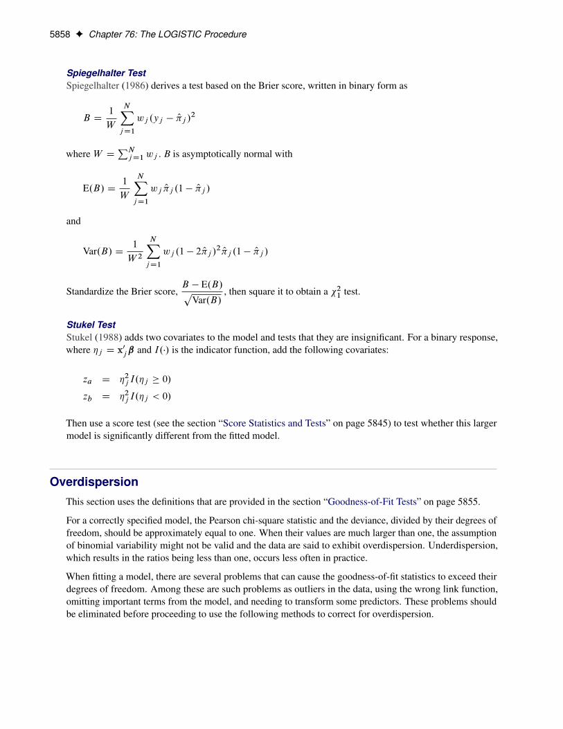
5858 F Chapter 76: The LOGISTIC Procedure
Spiegelhalter TestSpiegelhalter (1986) derives a test based on the Brier score, written in binary form as
B D1
W
NXjD1
wj .yj � O�j /2
where W DPNjD1wj . B is asymptotically normal with
E.B/ D1
W
NXjD1
wj O�j .1 � O�j /
and
Var.B/ D1
W 2
NXjD1
wj .1 � 2 O�j /2O�j .1 � O�j /
Standardize the Brier score,B � E.B/p
Var.B/, then square it to obtain a �21 test.
Stukel TestStukel (1988) adds two covariates to the model and tests that they are insignificant. For a binary response,where �j D x0jˇ and I.�/ is the indicator function, add the following covariates:
za D �2j I.�j � 0/
zb D �2j I.�j < 0/
Then use a score test (see the section “Score Statistics and Tests” on page 5845) to test whether this largermodel is significantly different from the fitted model.
OverdispersionThis section uses the definitions that are provided in the section “Goodness-of-Fit Tests” on page 5855.
For a correctly specified model, the Pearson chi-square statistic and the deviance, divided by their degrees offreedom, should be approximately equal to one. When their values are much larger than one, the assumptionof binomial variability might not be valid and the data are said to exhibit overdispersion. Underdispersion,which results in the ratios being less than one, occurs less often in practice.
When fitting a model, there are several problems that can cause the goodness-of-fit statistics to exceed theirdegrees of freedom. Among these are such problems as outliers in the data, using the wrong link function,omitting important terms from the model, and needing to transform some predictors. These problems shouldbe eliminated before proceeding to use the following methods to correct for overdispersion.

Overdispersion F 5859
Rescaling the Covariance Matrix
One way of correcting overdispersion is to multiply the covariance matrix by a dispersion parameter. Thismethod assumes that the sample sizes in each subpopulation are approximately equal. You can supply thevalue of the dispersion parameter directly, or you can estimate the dispersion parameter based on either thePearson chi-square statistic or the deviance for the fitted model.
The dispersion parameter is estimated by
c�2 D8<:�2P =.mk � p/ SCALE=PEARSON�2D=.mk � p/ SCALE=DEVIANCE.constant/2 SCALE=constant
In order for the Pearson statistic and the deviance to be distributed as chi-square, there must be sufficientreplication within the subpopulations. When this is not true, the data are sparse, and the p-values for thesestatistics are not valid and should be ignored. Similarly, these statistics, divided by their degrees of freedom,cannot serve as indicators of overdispersion. A large difference between the Pearson statistic and the devianceprovides some evidence that the data are too sparse to use either statistic.
Note that the parameter estimates are not changed by this method. However, their standard errors are adjustedfor overdispersion, affecting their significance tests.
Williams’ Method
Suppose that the data consist of n binomial observations. For the jth observation, let rj =nj be the observedproportion and let xj be the associated vector of explanatory variables. Suppose that the response probabilityfor the jth observation is a random variable Pj with mean and variance
E.Pj / D �j and V.Pj / D ��j .1 � �j /
where pj is the probability of the event, and � is a nonnegative but otherwise unknown scale parameter.Then the mean and variance of rj are
E.rj / D nj�j and V.rj / D nij�j .1 � �j /Œ1C .nj � 1/��
Williams (1982) estimates the unknown parameter � by equating the value of Pearson’s chi-square statisticfor the full model to its approximate expected value. Suppose w�j is the weight associated with the jthobservation. The Pearson chi-square statistic is given by
�2 D
nXjD1
w�j .rj � njb�j /2njb�j .1 �b�j /
Let g0.�/ be the first derivative of the link function g.�/. The approximate expected value of �2 is
E�2 D
nXjD1
w�j .1 � w�j vjdj /Œ1C �.nj � 1/�
where vj D nj =.�j .1 � �j /Œg0.�j /�2/ and dj is the variance of the linear predictor b̨j C x0j b̌. The scaleparameter � is estimated by the following iterative procedure.

5860 F Chapter 76: The LOGISTIC Procedure
At the start, let w�j D 1 and let �j be approximated by rj =nj , j D 1; 2; : : : ; n. If you apply these weightsand approximated probabilities to �2 and E�2 and then equate them, an initial estimate of � is
O�0 D�2 � .n � p/P
j .nj � 1/.1 � vjdj /
where p is the total number of parameters. The initial estimates of the weights become Ow�j0 D Œ1C .nj �
1/ O�0��1. After a weighted fit of the model, the b̨j and b̌ are recalculated, and so is �2. Then a revised
estimate of � is given by
O�1 D�2 �
Pj w�j .1 � w
�j vjdj /
w�j .nj � 1/.1 � w�j vjdj /
The iterative procedure is repeated until �2 is very close to its degrees of freedom.
Once � has been estimated by O� under the full model, weights of .1C .nj �1/ O�/�1 can be used to fit modelsthat have fewer terms than the full model. See Example 76.10 for an illustration.
NOTE: If the WEIGHT statement is specified with the NORMALIZE option, then the initial w�j values areset to the normalized weights, and the weights resulting from Williams’ method will not add up to the actualsample size. However, the estimated covariance matrix of the parameter estimates remains invariant to thescale of the WEIGHT variable.
Receiver Operating Characteristic CurvesReceiver operating characteristic (ROC) curves are used to evaluate and compare the performance ofdiagnostic tests; they can also be used to evaluate model fit. An ROC curve is just a plot of the proportion oftrue positives (events predicted to be events) versus the proportion of false positives (nonevents predicted tobe events).
In a sample of n individuals, suppose that n1 individuals are observed to have a certain condition or event,indicated by Y = 1; denote this group as C1. Let the remaining n2 D n � n1 individuals who do not have thecondition be indicated by Y = 2, and denote this group as C2. Risk factors are identified for the sample, and alogistic regression model is fitted to the data. For the jth individual, an estimated probability b�j of the eventof interest is calculated. By default, theb�j are computed as shown in the section “Linear Predictor, PredictedProbability, and Confidence Limits” on page 5851; you can use the cross validated probabilities (discussedin the section “Classification Table” on page 5852) by specifying the CROSSVALIDATE suboption of theROCOPTIONS option.
Suppose that the n individuals undergo a test for predicting the event and that the test is based on the estimatedprobability of the event. Higher values of this estimated probability are assumed to be associated with theevent. Define this test as a decision rule, D, which classifies an observation as an event when O� � z; D = 1indicates that the observation is classified as an event, and D = 2 indicates that the observation is classified asa nonevent. You can construct an ROC curve by varying the cutpoint z that determines which estimated eventprobabilities are considered to predict the event. For a given cutpoint, the resulting 2 � 2 classification tableis shown in Table 76.14, where nij is the total number of observations that are observed to have Y = i and areclassified into D = j.

Receiver Operating Characteristic Curves F 5861
Table 76.14 Classification Matrix for Cutpoint z
O� � z (DD1) O� < z (DD2) Total
C1.Y D1/ (event) n11 n12 n1C2.Y D2/ (nonevent) n21 n22 n2
For each cutpoint z, you can output the measures in Table 76.15 to a data set by specifying the OUTROC=option in the MODEL statement or the OUTROC= option in the SCORE statement.
Table 76.15 Statistics from the Classification Matrix with Cutpoint z
Statistic Equation Description
_PROB_ z Cutpoint_POS_ n11 Number of correctly predicted event responses_NEG_ n22 Number of correctly predicted nonevent responses_FALPOS_ n12 Number of falsely predicted event responses_FALNEG_ n21 Number of falsely predicted nonevent responses_SENSIT_ n11
n1Sensitivity of the test
_1MSPEC_ n21n2
One minus the specificity of the test
The ROC curve is a plot of sensitivity (_SENSIT_) against 1–specificity (_1MSPEC_). The plot can beproduced by using the PLOTS option or by using the GPLOT or SGPLOT procedure with the OUTROC= dataset. See Example 76.7 for an illustration. The area under the ROC curve, as determined by the trapezoidalrule, is estimated by the concordance index, c, in the “Association of Predicted Probabilities and ObservedResponses” table.
Comparing ROC Curves
ROC curves can be created from each model fit in a selection routine, from the specified model in the MODELstatement, from specified models in ROC statements, or from input variables which act as b� in the precedingdiscussion. Association statistics are computed for these models, and the models are compared when theROCCONTRAST statement is specified. The ROC comparisons are performed by using a contrast matrix totake differences of the areas under the empirical ROC curves (DeLong, DeLong, and Clarke-Pearson 1988).For example, if you have three curves and the second curve is the reference, the contrast used for the overalltest is
L1 D�l 01l 02
�D
�1 �1 0
0 �1 1
�and you can optionally estimate and test each row of this contrast, in order to test the difference betweenthe reference curve and each of the other curves. If you do not want to use a reference curve, the global testoptionally uses the following contrast:
L2 D�l 01l 02
�D
�1 �1 0
0 1 �1
�You can also specify your own contrast matrix. Instead of estimating the rows of these contrasts, you canrequest that the difference between every pair of ROC curves be estimated and tested. Demler, Pencina, and

5862 F Chapter 76: The LOGISTIC Procedure
D’Agostino (2012) caution that testing the difference in the AUC between two nested models is not a validapproach if the added predictor is not significantly associated with the response; in any case, if you use thisapproach, you are more likely to fail to reject the null.
By default for the reference contrast, the specified or selected model is used as the reference unless theNOFIT option is specified in the MODEL statement, in which case the first ROC model is the reference.
In order to label the contrasts, a name is attached to every model. The name for the specified or selectedmodel is the MODEL statement label, or “Model” if the MODEL label is not present. The ROC statementmodels are named with their labels, or as “ROCi” for the ith ROC statement if a label is not specified.The contrast L1 is labeled as “Reference = ModelName”, where ModelName is the reference model name,while L2 is labeled “Adjacent Pairwise Differences”. The estimated rows of the contrast matrix are labeled“ModelName1 – ModelName2”. In particular, for the rows of L1, ModelName2 is the reference model name.If you specify your own contrast matrix, then the contrast is labeled “Specified” and the ith contrast rowestimates are labeled “Rowi”.
If ODS Graphics is enabled, then all ROC curves are displayed individually and are also overlaid in a finaldisplay. If a selection method is specified, then the curves produced in each step of the model selectionprocess are overlaid onto a single plot and are labeled “Stepi”, and the selected model is displayed on aseparate plot and on a plot with curves from specified ROC statements. See Example 76.8 for an example.
ROC Computations
The trapezoidal area under an empirical ROC curve is equal to the Mann-Whitney two-sample rank measureof association statistic (a generalized U-statistic) applied to two samples, fXig; i D 1; : : : ; n1, in C1 andfYig; i D 1; : : : ; n2, in C2. PROC LOGISTIC uses the predicted probabilities in place of X and Y; however,in general any criterion could be used. Denote the frequency of observation i in Ck as fki , and denote thetotal frequency in Ck as Fk . The WEIGHTED option replaces fki with fkiwki , where wki is the weight ofobservation i in group Ck . The trapezoidal area under the curve is computed as
Oc D1
F1F2
n1XiD1
n2XjD1
.Xi ; Yj /f1if2j
.X; Y / D
8<:1 Y < X12
Y D X
0 Y > X
so that E. Oc/ D Pr.Y < X/C 12
Pr.Y D X/. Note that the concordance index, c, in the “Association ofPredicted Probabilities and Observed Responses” table does not use weights unless both the WEIGHTEDand BINWIDTH=0 options are in effect.
To compare K empirical ROC curves, first compute the trapezoidal areas. Asymptotic normality of theestimated area follows from U-statistic theory, and a covariance matrix S can be computed; For moreinformation, see DeLong, DeLong, and Clarke-Pearson (1988). A Wald confidence interval for the rth area,1 � r � K, can be constructed as
Ocr ˙ z1�˛2sr;r
where sr;r is the rth diagonal of S.

Testing Linear Hypotheses about the Regression Coefficients F 5863
For a contrast of ROC curve areas, Lc, the statistic
.Oc � c/0L0�LSL0
��1 L.Oc � c/
has a chi-square distribution with df=rank(LSL0). For a row of the contrast, l 0c,
l 0 Oc � l 0c
Œl 0Sl �1=2
has a standard normal distribution. The corresponding confidence interval is
l 0 Oc˙ z1�˛2
�l 0Sl
�1=2
Testing Linear Hypotheses about the Regression CoefficientsLinear hypotheses for ˇ are expressed in matrix form as
H0WLˇ D c
where L is a matrix of coefficients for the linear hypotheses, and c is a vector of constants. The vector ofregression coefficients ˇ includes slope parameters as well as intercept parameters. The Wald chi-squarestatistic for testing H0 is computed as
�2W D .Lb̌� c/0ŒLbV.b̌/L0��1.Lb̌� c/
where bV.b̌/ is the estimated covariance matrix. Under H0, �2W has an asymptotic chi-square distributionwith r degrees of freedom, where r is the rank of L.
Joint Tests and Type 3 TestsFor models that use less-than-full-rank parameterization (as specified by the PARAM=GLM option in theCLASS statement), a Type 3 test of an effect of interest (main effect or interaction) is a test of the Type IIIestimable functions that are defined for that effect. When the model contains no missing cells, performingthe Type 3 test of a main effect corresponds to testing the hypothesis of equal marginal means. For moreinformation about Type III estimable functions, see Chapter 50, “The GLM Procedure,” and Chapter 15,“The Four Types of Estimable Functions.” Also see Littell, Freund, and Spector (1991).
For models that use full-rank parameterization, all parameters are estimable when there are no missing cells,so it is unnecessary to define estimable functions. The standard test of an effect of interest in this case isthe joint test that the values of the parameters associated with that effect are zero. For a model that useseffects parameterization (as specified by the PARAM=EFFECT option in the CLASS statement), performingthe joint test for a main effect is equivalent to testing the equality of marginal means. For a model that usesreference parameterization (as specified by the PARAM=REF option in the CLASS statement), performingthe joint test is equivalent to testing the equality of cell means at the reference level of the other model effects.For more information about the coding scheme and the associated interpretation of results, see Muller andFetterman (2002, Chapter 14).

5864 F Chapter 76: The LOGISTIC Procedure
If there is no interaction term, the Type 3 test of an effect for a model that uses GLM parameterization is thesame as the joint test of the effect for the model that uses full-rank parameterization. In this situation, thejoint test is also called the Type 3 test. For a model that contains an interaction term and no missing cells,the Type 3 test of a component main effect under GLM parameterization is the same as the joint test of thecomponent main effect under effect parameterization. Both test the equality of cell means. But this Type 3test differs from the joint test under reference parameterization, which tests the equality of cell means at thereference level of the other component main effect. If some cells are missing, you can obtain meaningfultests only by testing a Type III estimable function, so in this case you should use GLM parameterization.
The results of a Type 3 test or a joint test do not depend on the order in which you specify the terms in theMODEL statement.
Regression DiagnosticsFor binary response data, regression diagnostics developed by Pregibon (1981) can be requested by specifyingthe INFLUENCE option. For diagnostics available with conditional logistic regression, see the section“Regression Diagnostic Details” on page 5873. These diagnostics can also be obtained from the OUTPUTstatement.
This section uses the following notation:
rj ; nj rj is the number of event responses out of nj trials for the jth observation. If events/trials syntaxis used, rj is the value of events and nj is the value of trials. For single-trial syntax, nj D 1, andrj D 1 if the ordered response is 1, and rj D 0 if the ordered response is 2.
wj is the weight of the jth observation.
�j is the probability of an event response for the jth observation given by �j D F.˛ C ˇ0xj /, whereF.�/ is the inverse link function defined on page 5833.b̌ is the maximum likelihood estimate (MLE) of .˛; ˇ1; : : : ; ˇs/0.bV.b̌/ is the estimated covariance matrix of b̌.
Opj ; Oqj Opj is the estimate of �j evaluated at b̌, and Oqj D 1 � Opj .
Pregibon (1981) suggests using the index plots of several diagnostic statistics to identify influential ob-servations and to quantify the effects on various aspects of the maximum likelihood fit. In an index plot,the diagnostic statistic is plotted against the observation number. In general, the distributions of thesediagnostic statistics are not known, so cutoff values cannot be given for determining when the values arelarge. However, the IPLOTS and INFLUENCE options in the MODEL statement and the PLOTS option inthe PROC LOGISTIC statement provide displays of the diagnostic values, allowing visual inspection andcomparison of the values across observations. In these plots, if the model is correctly specified and fits allobservations well, then no extreme points should appear.
The next five sections give formulas for these diagnostic statistics.

Regression Diagnostics F 5865
Hat Matrix Diagonal (Leverage)
The diagonal elements of the hat matrix are useful in detecting extreme points in the design space where theytend to have larger values. The jth diagonal element is
hj D
( ewj .1; x0j /bV.b̌/.1; x0j /0 Fisher scoringbwj .1; x0j /bV.b̌/.1; x0j /0 Newton-Raphson
where
ewj D wjnj
Opj Oqj Œg0. Opj /�2
bwj D ewj C wj .rj � nj Opj /Œ Opj Oqjg00. Opj /C . Oqj � Opj /g
0. Opj /�
. Opj Oqj /2Œg0. Opj /�3
and g0.�/ and g00.�/ are the first and second derivatives of the link function g.�/, respectively.
For a binary response logit model, the hat matrix diagonal elements are
hj D wjnj Opj Oqj .1; x0j /bV.b̌/� 1
xj
�If the estimated probability is extreme (less than 0.1 or greater than 0.9, approximately), then the hat diagonalmight be greatly reduced in value. Consequently, when an observation has a very large or very small estimatedprobability, its hat diagonal value is not a good indicator of the observation’s distance from the design space(Hosmer and Lemeshow 2000, p. 171).
Residuals
Residuals are useful in identifying observations that are not explained well by the model. Pearson residualsare components of the Pearson chi-square statistic and deviance residuals are components of the deviance.The Pearson residual for the jth observation is
�j D
pwj .rj � nj Opj /p
nj Opj Oqj
The Pearson chi-square statistic is the sum of squares of the Pearson residuals.
The deviance residual for the jth observation is
dj D
8̂<̂:�p�2wjnj log. Oqj / if rj D 0
˙
q2wj Œrj log. rj
nj Opj/C .nj � rj / log.nj�rj
nj Oqj/� if 0 < rj < njp
�2wjnj log. Opj / if rj D nj
where the plus (minus) in˙ is used if rj =nj is greater (less) than Opj . The deviance is the sum of squares ofthe deviance residuals.

5866 F Chapter 76: The LOGISTIC Procedure
The STDRES option in the INFLUENCE and PLOTS=INFLUENCE options computes three more residuals(Collett 2003). The Pearson and deviance residuals are standardized to have approximately unit variance:
epj D�jp1 � hj
edj Ddjp1 � hj
The likelihood residuals, which estimate components of a likelihood ratio test of deleting an individualobservation, are a weighted combination of the standardized Pearson and deviance residuals
elj D sign.rj � nj Opj /qhj e2pj C .1 � hj /e
2dj
DFBETAS
For each parameter estimate, the procedure calculates a DFBETAS diagnostic for each observation. TheDFBETAS diagnostic for an observation is the standardized difference in the parameter estimate due todeleting the observation, and it can be used to assess the effect of an individual observation on each estimatedparameter of the fitted model. Instead of reestimating the parameter every time an observation is deleted,PROC LOGISTIC uses the one-step estimate. See the section “Predicted Probability of an Event forClassification” on page 5854. For the jth observation, the DFBETAS are given by
DFBETASij D �ib̌1j = O�iwhere i D 0; 1; : : : ; s; O�i is the standard error of the ith component of b̌, and�ib̌1j is the ith component ofthe one-step difference
�b̌1j D wj .rj � nj Opj /
1 � hjbV.b̌/� 1
xj
��b̌1j is the approximate change (b̌� b̌1j ) in the vector of parameter estimates due to the omission of the jthobservation. The DFBETAS are useful in detecting observations that are causing instability in the selectedcoefficients.
C and CBAR
C and CBAR are confidence interval displacement diagnostics that provide scalar measures of the influenceof individual observations on b̌. These diagnostics are based on the same idea as the Cook distance inlinear regression theory (Cook and Weisberg 1982), but use the one-step estimate. C and CBAR for the jthobservation are computed as
Cj D �2jhj =.1 � hj /
2
and
C j D �2jhj =.1 � hj /
respectively.
Typically, to use these statistics, you plot them against an index and look for outliers.

Scoring Data Sets F 5867
DIFDEV and DIFCHISQ
DIFDEV and DIFCHISQ are diagnostics for detecting ill-fitted observations; in other words, observationsthat contribute heavily to the disagreement between the data and the predicted values of the fitted model.DIFDEV is the change in the deviance due to deleting an individual observation while DIFCHISQ is thechange in the Pearson chi-square statistic for the same deletion. By using the one-step estimate, DIFDEVand DIFCHISQ for the jth observation are computed as
DIFDEV D d2j C C j
and
DIFCHISQ D C j =hj
Scoring Data SetsScoring a data set, which is especially important for predictive modeling, means applying a previously fittedmodel to a new data set in order to compute the conditional, or posterior, probabilities of each responsecategory given the values of the explanatory variables in each observation.
The SCORE statement enables you to score new data sets and output the scored values and, optionally, thecorresponding confidence limits into a SAS data set. If the response variable is included in the new data set,then you can request fit statistics for the data, which is especially useful for test or validation data. If theresponse is binary, you can also create a SAS data set containing the receiver operating characteristic (ROC)curve. You can specify multiple SCORE statements in the same invocation of PROC LOGISTIC.
By default, the posterior probabilities are based on implicit prior probabilities that are proportional to thefrequencies of the response categories in the training data (the data used to fit the model). Explicit priorprobabilities should be specified with the PRIOR= or PRIOREVENT= option when the sample proportionsof the response categories in the training data differ substantially from the operational data to be scored. Forexample, to detect a rare category, it is common practice to use a training set in which the rare categoriesare overrepresented; without prior probabilities that reflect the true incidence rate, the predicted posteriorprobabilities for the rare category will be too high. By specifying the correct priors, the posterior probabilitiesare adjusted appropriately.
The model fit to the DATA= data set in the PROC LOGISTIC statement is the default model used for thescoring. Alternatively, you can save a model fit in one run of PROC LOGISTIC and use it to score newdata in a subsequent run. The OUTMODEL= option in the PROC LOGISTIC statement saves the modelinformation in a SAS data set. Specifying this data set in the INMODEL= option of a new PROC LOGISTICrun will score the DATA= data set in the SCORE statement without refitting the model.
The STORE statement can also be used to save your model. The PLM procedure can use this model to scorenew data sets; see Chapter 91, “The PLM Procedure,” for more information. You cannot specify priors inPROC PLM.

5868 F Chapter 76: The LOGISTIC Procedure
Fit Statistics for Scored Data Sets
Specifying the FITSTAT option displays the following fit statistics when the data set being scored includesthe response variable:
Statistic Description
Total frequency F DPi fini
Total weight W DPi fiwini
Log likelihood logL DPi fiwi log.b� i /
Full log likelihood logLf D constantC logL
Misclassification (error) ratePi 1fF_Yi ¤ I_Yigfini
FAIC �2 logLf C 2p
AICC �2 logLf C2pn
n � p � 1BIC �2 logLf C p log.n/SC �2 logLf C p log.F /
R-square R2 D 1 �
�L0
L
�2=FMaximum-rescaled R-square
R2
1 � L2=F0
AUC Area under the ROC curveBrier score (polytomous response) 1
W
Pi fiwi
Pj .yij �b� ij /2
Brier score (binary response) 1W
Pi fiwi .ri .1 �b� i /2 C .ni � ri /b�2i /
Brier reliability (events/trials syntax) 1W
Pi fiwi .ri=ni �b� i /2
In the preceding table, fi is the frequency of the ith observation in the data set being scored, wi is the weightof the observation, and n D
Pi fi . The number of trials when events/trials syntax is specified is ni , and
with single-trial syntax ni D 1. The values F_Yi and I_Yi are described in the section “OUT= Output DataSet in a SCORE Statement” on page 5882. The indicator function 1fAg is 1 if A is true and 0 otherwise. Thelikelihood of the model is L, and L0 denotes the likelihood of the intercept-only model. For polytomousresponse models, yi is the observed polytomous response level, b� ij is the predicted probability of the jthresponse level for observation i, and yij D 1fyi D j g. For binary response models, b� i is the predictedprobability of the observation, ri is the number of events when you specify events/trials syntax, and ri D yiwhen you specify single-trial syntax.
The log likelihood, Akaike’s information criterion (AIC), and Schwarz criterion (SC) are described in thesection “Model Fitting Information” on page 5840. The full log likelihood is displayed for models specifiedwith events/trials syntax, and the constant term is described in the section “Model Fitting Information”on page 5840. The AICC is a small-sample bias-corrected version of the AIC (Hurvich and Tsai 1993;Burnham and Anderson 1998). The Bayesian information criterion (BIC) is the same as the SC except whenevents/trials syntax is specified. The area under the ROC curve for binary response models is defined inthe section “ROC Computations” on page 5862. The R-square and maximum-rescaled R-square statistics,defined in “Generalized Coefficient of Determination” on page 5841, are not computed when you specifyboth an OFFSET= variable and the INMODEL= data set. The Brier score (Brier 1950) is the weightedsquared difference between the predicted probabilities and their observed response levels. For events/trialssyntax, the Brier reliability is the weighted squared difference between the predicted probabilities and theobserved proportions (Murphy 1973).

Scoring Data Sets F 5869
Posterior Probabilities and Confidence Limits
Let F be the inverse link function. That is,
F.t/ D
8<:1
1Cexp.�t/ logisticˆ.t/ normal1 � exp.� exp.t// complementary log-log
The first derivative of F is given by
F 0.t/ D
8̂<̂:
exp.�t/.1Cexp.�t//2 logistic�.t/ normalexp.t/ exp.� exp.t// complementary log-log
Suppose there are k C 1 response categories. Let Y be the response variable with levels 1; : : : ; k C 1. Letx D .x0; x1; : : : ; xs/0 be a .s C 1/-vector of covariates, with x0 � 1. Let ˇ be the vector of intercept andslope regression parameters.
Posterior probabilities are given by
p.Y D i jx/ Dpo.Y D i jx/pn.YDi/po.YDi/Pj po.Y D j jx/
pn.YDj /po.YDj /
i D 1; : : : ; k C 1
where the old posterior probabilities (po.Y D i jx/; i D 1; : : : ; k C 1) are the conditional probabilities ofthe response categories given x, the old priors (po.Y D i/; i D 1; : : : ; k C 1) are the sample proportions ofresponse categories of the training data, and the new priors (pn.Y D i/; i D 1; : : : ; k C 1) are specified inthe PRIOR= or PRIOREVENT= option. To simplify notation, absorb the old priors into the new priors; thatis
p.Y D i/ Dpn.Y D i/
po.Y D i/i D 1; : : : ; k C 1
Note if the PRIOR= and PRIOREVENT= options are not specified, then p.Y D i/ D 1.
The posterior probabilities are functions of ˇ and their estimates are obtained by substituting ˇ by its MLEb̌. The variances of the estimated posterior probabilities are given by the delta method as follows:
Var.bp.Y D i jx// D �@p.Y D i jx/@ˇ
�0Var.b̌/�@p.Y D i jx/
@ˇ
�where
@p.Y D i jx/@ˇ
D
@po.YDi jx/@ˇ
p.Y D i/Pj po.Y D j jx/p.Y D j /
�
po.Y D i jx/p.Y D i/[email protected] jx/
@ˇp.Y D j /
ŒPj po.Y D j jx/p.Y D j /�2
and the old posterior probabilities po.Y D i jx/ are described in the following sections.
A 100(1 � ˛)% confidence interval for p.Y D i jx/ is
bp.Y D i jx/˙ z1�˛=2qcVar.bp.Y D i jx//where z� is the upper 100� th percentile of the standard normal distribution.

5870 F Chapter 76: The LOGISTIC Procedure
Binary and Cumulative Response ModelsLet ˛1; : : : ; ˛k be the intercept parameters and let ˇs be the vector of slope parameters. Denote ˇ D.˛1; : : : ; ˛k;ˇ
0s/0. Let
�i D �i .ˇ/ D ˛i C x0ˇs; i D 1; : : : ; k
Estimates of �1; : : : ; �k are obtained by substituting the maximum likelihood estimate b̌ for ˇ.
The predicted probabilities of the responses are
cpo.Y D i jx/ D bPr.Y D i/ D
8<:F. O�1/ i D 1
F. O�i / � F. O�i�1/ i D 2; : : : ; k
1 � F. O�k/ i D k C 1
For i D 1; : : : ; k, let ıi .x/ be a (k + 1) column vector with ith entry equal to 1, k + 1 entry equal to x, and allother entries 0. The derivative of po.Y D i jx/ with respect to ˇ are
@po.Y D i jx/@ˇ
D
8<:F 0.˛1 C x0ˇs/ı1.x/ i D 1
F 0.˛i C x0ˇs/ıi .x/ � F 0.˛i�1 C x0ˇs/ıi�1.x/ i D 2; : : : ; k
�F 0.˛k C x0ˇs/ık.x/ i D k C 1
The cumulative posterior probabilities are
p.Y � i jx/ D
PijD1 po.Y D j jx/p.Y D j /PkC1jD1 po.Y D j jx/p.Y D j /
D
iXjD1
p.Y D j jx/ i D 1; : : : ; k C 1
Their derivatives are
@p.Y � i jx/@ˇ
D
iXjD1
@p.Y D j jx/@ˇ
i D 1; : : : ; k C 1
In the delta-method equation for the variance, replace p.Y D �jx/ with p.Y � �jx/.
Finally, for the cumulative response model, use
cpo.Y � i jx/ D F. O�i / i D 1; : : : ; kcpo.Y � k C 1jx/ D 1
@po.Y � i jx/@ˇ
D F 0.˛i C x0ˇs/ıi .x/ i D 1; : : : ; k
@po.Y � k C 1jx/@ˇ
D 0

Scoring Data Sets F 5871
Generalized Logit ModelConsider the last response level (Y=k+1) as the reference. Let ˇ1; : : : ;ˇk be the (intercept and slope)parameter vectors for the first k logits, respectively. Denote ˇ D .ˇ01; : : : ;ˇ
0k/0. Let � D .�1; : : : ; �k/0 with
�i D �i .ˇ/ D x0ˇi i D 1; : : : ; k
Estimates of �1; : : : ; �k are obtained by substituting the maximum likelihood estimate b̌ for ˇ.
The predicted probabilities are
cpo.Y D k C 1jx/ � Pr.Y D k C 1jx/ D1
1CPklD1 exp. O�l/cpo.Y D i jx/ � Pr.Y D i jx/ D cpo.Y D k C 1jx/ exp.�i /; i D 1; : : : ; k
The derivative of po.Y D i jx/ with respect to ˇ are
@po.Y D i jx/@ˇ
D@�
@ˇ
@po.Y D i jx/@�
D .Ik ˝ x/�@po.Y D i jx/
@�1; � � � ;
@po.Y D i jx/@�k
�0where
@po.Y D i jx/@�j
D
�po.Y D i jx/.1 � po.Y D i jx// j D i
�po.Y D i jx/po.Y D j jx/ otherwise
Special Case of Binary Response Model with No PriorsLet ˇ be the vector of regression parameters. Let
� D �.ˇ/ D x0ˇ
The variance of O� is given by
Var. O�/ D x0Var.b̌/xA 100(1 � ˛) percent confidence interval for � is
O�˙ z1�˛=2
qcVar. O�/
Estimates of po.Y D 1jx/ and confidence intervals for the po.Y D 1jx/ are obtained by back-transformingO� and the confidence intervals for �, respectively. That is,
cpo.Y D 1jx/ D F. O�/and the confidence intervals are
F
�O�˙ z1�˛=2
qcVar. O�/�

5872 F Chapter 76: The LOGISTIC Procedure
Conditional Logistic RegressionThe method of maximum likelihood described in the preceding sections relies on large-sample asymptoticnormality for the validity of estimates and especially of their standard errors. When you do not have a largesample size compared to the number of parameters, this approach might be inappropriate and might resultin biased inferences. This situation typically arises when your data are stratified and you fit intercepts toeach stratum so that the number of parameters is of the same order as the sample size. For example, ina 1:1 matched pairs study with n pairs and p covariates, you would estimate n � 1 intercept parametersand p slope parameters. Taking the stratification into account by “conditioning out” (and not estimating)the stratum-specific intercepts gives consistent and asymptotically normal MLEs for the slope coefficients.See Breslow and Day (1980) and Stokes, Davis, and Koch (2012) for more information. If your nuisanceparameters are not just stratum-specific intercepts, you can perform an exact conditional logistic regression.
Computational Details
For each stratum h, h D 1; : : : ;H , number the observations as i D 1; : : : ; nh so that hi indexes the ithobservation in stratum h. Denote the p covariates for the hith observation as xhi and its binary responseas yhi , and let y D .y11; : : : ; y1n1 ; : : : ; yH1; : : : ; yHnH /
0, Xh D .xh1 : : : xhnh/0, and X D .X01 : : :X
0H /0.
Let the dummy variables zh; h D 1; : : : ;H , be indicator functions for the strata (zh D 1 if the observationis in stratum h), and denote zhi D .z1; : : : ; zH / for the hith observation, Zh D .zh1 : : : zhnh/
0, and Z D.Z01 : : :Z
0H /0. Denote X
�
D .ZjX) and x�hiD .z0
hijx0hi/0. Arrange the observations in each stratum h so
that yhi D 1 for i D 1; : : : ; mh, and yhi D 0 for i D mhC1; : : : ; nh. Suppose all observations have unitfrequency.
Consider the binary logistic regression model on page 5751 written as
logit.�/ D X�
�
where the parameter vector � D .˛0;ˇ0/0 consists of ˛ D .˛1; : : : ; ˛H /0, ˛h is the intercept for stratum
h; h D 1; : : : ;H , and ˇ is the parameter vector for the p covariates.
From the section “Determining Observations for Likelihood Contributions” on page 5834, you can write thelikelihood contribution of observation hi; i D 1; : : : ; nh; h D 1; : : : ;H; as
Lhi .�/ Deyhix
�hi
0�
1C ex�hi
0�
where yhi D 1 when the response takes Ordered Value 1, and yhi D 0 otherwise.
The full likelihood is
L.�/ D
HYhD1
nhYiD1
Lhi .�/ Dey0X�
�QHhD1
QnhiD1
�1C ex
�hi
0��
Unconditional likelihood inference is based on maximizing this likelihood function.
When your nuisance parameters are the stratum-specific intercepts .˛1; : : : ; ˛H /0, and the slopes ˇ areyour parameters of interest, “conditioning out” the nuisance parameters produces the conditional likelihood(Lachin 2000)
L.ˇ/ D
HYhD1
Lh.ˇ/ D
HYhD1
QmhiD1 exp.x0
hiˇ/PQjmh
jDj1exp.x0
hjˇ/

Conditional Logistic Regression F 5873
where the summation is over all�nhmh
�subsets fj1; : : : ; jmhg of mh observations chosen from the nh observa-
tions in stratum h. Note that the nuisance parameters have been factored out of this equation.
For conditional asymptotic inference, maximum likelihood estimates b̌ of the regression parameters areobtained by maximizing the conditional likelihood, and asymptotic results are applied to the conditionallikelihood function and the maximum likelihood estimators. A relatively fast method of computing thisconditional likelihood and its derivatives is given by Gail, Lubin, and Rubinstein (1981) and Howard (1972).The optimization techniques can be controlled by specifying the NLOPTIONS statement.
Sometimes the log likelihood converges but the estimates diverge. This condition is flagged by havinginordinately large standard errors for some of your parameter estimates, and can be monitored by specifyingthe ITPRINT option. Unfortunately, broad existence criteria such as those discussed in the section “Existenceof Maximum Likelihood Estimates” on page 5837 do not exist for this model. It might be possible tocircumvent such a problem by standardizing your independent variables before fitting the model.
Regression Diagnostic Details
Diagnostics are used to indicate observations that might have undue influence on the model fit or that mightbe outliers. Further investigation should be performed before removing such an observation from the data set.
The derivations in this section use an augmentation method described by Storer and Crowley (1985), whichprovides an estimate of the “one-step” DFBETAS estimates advocated by Pregibon (1984). The methodalso provides estimates of conditional stratum-specific predicted values, residuals, and leverage for eachobservation. The augmentation method can take a lot of time and memory.
Following Storer and Crowley (1985), the log-likelihood contribution can be written as
lh D log.Lh/ D y0h h � a. h/ where
a. h/ D log
24X jmhYjDj1
exp. hj /
35and the h subscript on matrices indicates the submatrix for the stratum, h D . h1; : : : ; hnh/
0, and hi Dx0hiˇ. Then the gradient and information matrix are
g.ˇ/ D�@lh
@ˇ
�HhD1
D X0.y � �/
ƒ.ˇ/ D
�@2lh
@ˇ2
�HhD1
D X0diag.U1; : : : ;UH /X

5874 F Chapter 76: The LOGISTIC Procedure
where
�hi D@a. h/
@ hiD
Pj.i/
QjmhjDj1
exp. hj /PQjmhjDj1
exp. hj /�h D .�h1; : : : ; �hnh/
Uh D@2a. h/
@ 2h
D
�@2a. h/@ hi@ hj
�D faij g
aij D
Pk.i;j /
QkmhkDk1
exp. hk/PQkmhkDk1
exp. hk/�@a. h/
@ hi
@a. h/
@ hjD �hij � �hi�hj
and where �hi is the conditional stratum-specific probability that subject i in stratum h is a case, thesummation on j.i/ is over all subsets from f1; : : : ; nhg of sizemh that contain the index i, and the summationon k.i; j / is over all subsets from f1; : : : ; nhg of size mh that contain the indices i and j.
To produce the true one-step estimate ˇ1hi
, start at the MLE b̌, delete the hith observation, and use thisreduced data set to compute the next Newton-Raphson step. Note that if there is only one event or onenonevent in a stratum, deletion of that single observation is equivalent to deletion of the entire stratum. Theaugmentation method does not take this into account.
The augmented model is
logit.Pr.yhi D 1jxhi // D x0hiˇ C z0hi
where zhi D .0; : : : ; 0; 1; 0; : : : ; 0/0 has a 1 in the hith coordinate, and use ˇ0 D .b̌0; 0/0 as the initial estimatefor .ˇ0; /0. The gradient and information matrix before the step are
g.ˇ0/ D�
X0
z0hi
�.y � �/ D
�0
yhi � �hi
�ƒ.ˇ0/ D
�X0
z0hi
�U ŒX zhi � D
�ƒ.ˇ/ X0Uzhiz0hi
UX z0hi
Uzhi
�Inserting the ˇ0 and .X0; z0
hi/0 into the Gail, Lubin, and Rubinstein (1981) algorithm provides the appropriate
estimates of g.ˇ0/ and ƒ.ˇ0/. Indicate these estimates with b� D �.b̌/, bU D U.b̌/,bg, and bƒ.
DFBETA is computed from the information matrix as
�hiˇ D ˇ0 � ˇ1hi
D �bƒ�1.ˇ0/bg.ˇ0/D �bƒ�1.b̌/.X0bUzhi /M�1z0hi .y �b�/
where
M D .z0hibUzhi / � .z0hibUX/bƒ�1.b̌/.X0bUzhi /
For each observation in the data set, a DFBETA statistic is computed for each parameter ˇj , 1 � j � p, andstandardized by the standard error of ˇj from the full data set to produce the estimate of DFBETAS.

Exact Conditional Logistic Regression F 5875
The estimated leverage is defined as
hhi Dtracef.z0
hibUX/bƒ�1.b̌/.X0bUzhi /g
tracefz0hibUzhig
This definition of leverage produces different values from those defined by Pregibon (1984); Moolgavkar,Lustbader, and Venzon (1985); Hosmer and Lemeshow (2000); however, it has the advantage that no extracomputations beyond those for the DFBETAS are required.
The estimated residuals ehi D yhi �b�hi are obtained frombg.ˇ0/, and the weights, or predicted probabilities,are then b�hi D yhi � ehi . The residuals are standardized and reported as (estimated) Pearson residuals:
rhi � nhib�hipnhib�hi .1 �b�hi /
where rhi is the number of events in the observation and nhi is the number of trials.
The STDRES option in the INFLUENCE option computes the standardized Pearson residual:
es;hi Dehip1 � hhi
For events/trials MODEL statement syntax, treat each observation as two observations (the first for thenonevents and the second for the events) with frequencies fh;2i�1 D nhi �rhi and fh;2i D rhi , and augmentthe model with a matrix Zhi D Œzh;2i�1zh;2i � instead of a single zhi vector. Writing hi D x0
hiˇfhi in the
preceding section results in the following gradient and information matrix:
g.ˇ0/ D
24 0
fh;2i�1.yh;2i�1 � �h;2i�1/
fh;2i .yh;2i � �h;2i /
35ƒ.ˇ0/ D
�ƒ.ˇ/ X0diag.f/Udiag.f/Zhi
Z0hidiag.f/Udiag.f/X Z0hidiag.f/Udiag.f/Zhi
�The predicted probabilities are then b�hi D yh;2i � eh;2i=rh;2i , while the leverage and the DFBETAS areproduced from ƒ.ˇ0/ in a fashion similar to that for the preceding single-trial equations.
Exact Conditional Logistic RegressionThe theory of exact logistic regression, also known as exact conditional logistic regression, was originallylaid out by Cox (1970), and the computational methods employed in PROC LOGISTIC are described in Hirji,Mehta, and Patel (1987); Hirji (1992); Mehta, Patel, and Senchaudhuri (1992). Other useful references forthe derivations include Cox and Snell (1989); Agresti (1990); Mehta and Patel (1995).
Exact conditional inference is based on generating the conditional distribution for the sufficient statistics ofthe parameters of interest. This distribution is called the permutation or exact conditional distribution. Usingthe notation in the section “Computational Details” on page 5872, follow Mehta and Patel (1995) and firstnote that the sufficient statistics T D .T1; : : : ; Tp/ for the parameter vector of intercepts and slopes, ˇ, are
Tj D
nXiD1
yixij ; j D 1; : : : ; p

5876 F Chapter 76: The LOGISTIC Procedure
Denote a vector of observable sufficient statistics as t D .t1; : : : ; tp/0.
The probability density function (PDF) for T can be created by summing over all binary sequences y thatgenerate an observable t and letting C.t/ D jjfy W y0X D t0gjj denote the number of sequences y thatgenerate t
Pr.T D t/ DC.t/ exp.t0ˇ/QniD1Œ1C exp.x0iˇ/�
In order to condition out the nuisance parameters, partition the parameter vector ˇ D .ˇ0N;ˇ0I/0, where ˇN is
a pN � 1 vector of the nuisance parameters, and ˇI is the parameter vector for the remaining pI D p � pNparameters of interest. Likewise, partition X into XN and XI, T into TN and TI, and t into tN and tI. Thenuisance parameters can be removed from the analysis by conditioning on their sufficient statistics to createthe conditional likelihood of TI given TN D tN,
Pr.TI D tIjTN D tN/ DPr.T D t/
Pr.TN D tN/
D fˇI.tIjtN/ DC.tN; tI/ exp.t0IˇI/Pu C.tN; u/ exp.u0ˇI/
where C.tN; u/ is the number of vectors y such that y0XN D tN and y0XI D u. Note that the nuisanceparameters have factored out of this equation, and that C.tN; tI/ is a constant.
The goal of the exact conditional analysis is to determine how likely the observed response y0 is with respectto all 2n possible responses y D .y1; : : : ; yn/0. One way to proceed is to generate every y vector for whichy0XN D tN, and count the number of vectors y for which y0XI is equal to each unique tI. Generating theconditional distribution from complete enumeration of the joint distribution is conceptually simple; however,this method becomes computationally infeasible very quickly. For example, if you had only 30 observations,you would have to scan through 230 different y vectors.
Several algorithms are available in PROC LOGISTIC to generate the exact distribution. All of the algorithmsare based on the following observation. Given any y D .y1; : : : ; yn/
0 and a design X D .x1; : : : ; xn/0, lety.i/ D .y1; : : : ; yi /0 and X.i/ D .x1; : : : ; xi /0 be the first i rows of each matrix. Write the sufficient statisticbased on these i rows as t0
.i/D y0
.i/X.i/. A recursion relation results: t.iC1/ D t.i/ C yiC1xiC1.
The following methods are available:
� The multivariate shift algorithm developed by Hirji, Mehta, and Patel (1987), which steps through therecursion relation by adding one observation at a time and building an intermediate distribution at eachstep. If it determines that t.i/ for the nuisance parameters could eventually equal t, then t.i/ is addedto the intermediate distribution.
� An extension of the multivariate shift algorithm to generalized logit models by Hirji (1992). Becausethe generalized logit model fits a new set of parameters to each logit, the number of parameters in themodel can easily get too large for this algorithm to handle. Note for these models that the hypothesistests for each effect are computed across the logit functions, while individual parameters are estimatedfor each logit function.
� A network algorithm described in Mehta, Patel, and Senchaudhuri (1992), which builds a network foreach parameter that you are conditioning out in order to identify feasible yi for the y vector. These

Exact Conditional Logistic Regression F 5877
networks are combined and the set of feasible yi is further reduced, and then the multivariate shiftalgorithm uses this knowledge to build the exact distribution without adding as many intermediatet.iC1/ as the multivariate shift algorithm does.
� A hybrid Monte Carlo and network algorithm described by Mehta, Patel, and Senchaudhuri (2000),which extends their 1992 algorithm by sampling from the combined network to build the exactdistribution.
� A Markov chain Monte Carlo algorithm described by Forster, McDonald, and Smith (2003), whichgenerates the exact distribution by repeatedly perturbing the response vector to obtain a new responsevector while maintaining the sufficient statistics for the nuisance parameters, and the resulting t areadded to the exact distribution.
The bulk of the computation time and memory for these algorithms is consumed by the creation of thenetworks and the exact joint distribution. After the joint distribution for a set of effects is created, thecomputational effort required to produce hypothesis tests and parameter estimates for any subset of the effectsis (relatively) trivial. See the section “Computational Resources for Exact Logistic Regression” on page 5886for more computational notes about exact analyses.
NOTE: An alternative to using these exact conditional methods is to perform Firth’s bias-reducing penalizedlikelihood method (see the FIRTH option in the MODEL statement); this method has the advantage of beingmuch faster and less memory intensive than exact algorithms, but it might not converge to a solution.
Hypothesis Tests
Consider testing the null hypothesis H0WˇI D 0 against the alternative HAWˇI ¤ 0, conditional on TN D tN.Under the null hypothesis, the test statistic for the exact probability test is just fˇID0.tIjtN/, while thecorresponding p-value is the probability of getting a less likely (more extreme) statistic,
p.tIjtN/ DXu2�p
f0.ujtN/
where �p D fuW there exist y with y0XI D u, y0XN D tN, and f0.ujtN/ � f0.tIjtN/g.
The exact probability test is not necessarily a sum of tail areas and can be inflated if the distribution is skewed.The more robust exact conditional scores test is a sum of tail areas and is usually preferred to the exactprobability test. To compute the exact conditional scores test, the conditional mean �I and variance matrix†I of the TI (conditional on TN D tN) are calculated, and the score statistic for the observed value,
s D .tI � �I/0†�1I .tI � �I/
is compared to the score for each member of the distribution
S.TI/ D .TI � �I/0†�1I .TI � �I/
The resulting p-value is
p.tIjtN/ D Pr.S � s/ DXu2�s
f0.ujtN/
where �s D fuW there exist y with y0XI D u, y0XN D tN, and S.u/ � sg.

5878 F Chapter 76: The LOGISTIC Procedure
The mid-p statistic, defined as
p.tIjtN/ �1
2f0.tIjtN/
was proposed by Lancaster (1961) to compensate for the discreteness of a distribution. See Agresti (1992) formore information. However, to allow for more flexibility in handling ties, you can write the mid-p statistic as(based on a suggestion by LaMotte (2002) and generalizing Vollset, Hirji, and Afifi (1991))X
u2�<
f0.ujtN/C ı1f0.tIjtN/C ı2Xu2�D
f0.ujtN/
where, for i 2 fp; sg, �< is �i using strict inequalities, and �D is �i using equalities with the addedrestriction that u ¤ tI. Letting .ı1; ı2/ D .0:5; 1:0/ yields Lancaster’s mid-p.
CAUTION: When the exact distribution has ties and you specify METHOD=NETWORKMC orMETHOD=MCMC, the sampling algorithm estimates p.tjtN/ with error, and hence it cannot determineprecisely which values contribute to the reported p-values. For example, if the exact distribution has densitiesf0:2; 0:2; 0:2; 0:4g and if the observed statistic has probability 0.2, then the exact probability p-value isexactly 0.6. Under Monte Carlo sampling, if the densities after N samples are f0:18; 0:21; 0:23; 0:38g and theobserved probability is 0.21, then the resulting p-value is 0.39. Therefore, the exact probability test p-valuefor this example fluctuates between 0.2, 0.4, and 0.6, and the reported p-values are actually lower boundsfor the true p-values. If you need more precise values, you can specify the OUTDIST= option, determineappropriate cutoff values for the observed probability and score, and then construct p-value estimates fromthe OUTDIST= data set and display them in the SAS log by using the following statements:
data _null_;set outdist end=end;retain pvalueProb 0 pvalueScore 0;if prob < ProbCutOff then pvalueProb+prob;if score > ScoreCutOff then pvalueScore+prob;if end then put pvalueProb= pvalueScore=;
run;
Because the METHOD=MCMC samples are correlated, the covariance that is computed for the exactconditional scores test is biased. Specifying the NTHIN= option might reduce this bias.
Inference for a Single Parameter
Exact parameter estimates are derived for a single parameter ˇi by regarding all the other parametersˇN D .ˇ1; : : : ; ˇi�1; ˇiC1; : : : ; ˇpNCpI/
0 as nuisance parameters. The appropriate sufficient statistics areTI D Ti and TN D .T1; : : : ; Ti�1; TiC1; : : : ; TpNCpI/
0, with their observed values denoted by the lowercaset. Hence, the conditional PDF used to create the parameter estimate for ˇi is
fˇi .ti jtN/ DC.tN; ti / exp.tiˇi /Pu2� C.tN; u/ exp.uˇi /
for � D fuW there exist y with Ti D u and TN D tNg.
The maximum exact conditional likelihood estimate is the quantity b̌i , which maximizes the conditionalPDF. A Newton-Raphson algorithm is used to perform this search. However, if the observed ti attainseither its maximum or minimum value in the exact distribution (that is, either ti D minfu W u 2 �g orti D maxfu W u 2 �g), then the conditional PDF is monotonically increasing in ˇi and cannot be maximized.

Input and Output Data Sets F 5879
In this case, a median unbiased estimate (Hirji, Tsiatis, and Mehta 1989) b̌i is produced that satisfiesfb̌i .ti jtN/ D 0:5, and a Newton-Raphson algorithm is used to perform the search.
The standard error of the exact conditional likelihood estimate is just the negative of the inverse of the secondderivative of the exact conditional log likelihood (Agresti 2002).
Likelihood ratio tests based on the conditional PDF are used to test the nullH0Wˇi D 0 against the alternativeHAWˇi > 0. The critical region for this UMP test consists of the upper tail of values for Ti in the exactdistribution. Thus, the p-value pC.ti I 0/ for a one-tailed test is
pC.ti I 0/ DXu�ti
f0.ujtN/
Similarly, the p-value p�.ti I 0/ for the one-tailed test of H0 against HAWˇi < 0 is
p�.ti I 0/ DXu�ti
f0.ujtN/
The p-value p.ti I 0/ for a two-tailed test of H0 against HAWˇi ¤ 0 is
p.ti I 0/ D 2minŒp�.ti I 0/; pC.ti I 0/�
By default, the p-value that is reported for a single parameter in the “Exact Parameter Estimates” table is forthe two-tailed test. For median unbiased estimates, the p-value for a one-tailed test is always reported.
An upper 100.1� 2�/% exact confidence limit for b̌i corresponding to the observed ti is the solution ˇU .ti /of � D p�.ti ; ˇU .ti //, while the lower exact confidence limit is the solution ˇL.ti / of � D pC.ti ; ˇL.ti //.Again, a Newton-Raphson procedure is used to search for the solutions. Note that one of the confidencelimits for a median unbiased estimate is set to infinity and the other is computed at 2�, which results in thedisplay of a one-sided 100.1 � 2�/% confidence interval.
Specifying the ONESIDED option displays only one p-value and one confidence interval, because smallvalues of pC.ti I 0/ and p�.ti I 0/ support different alternative hypotheses and only one of these p-values canbe less than 0.50.
The mid-p confidence limits are the solutions to minfp�.ti ; ˇ.ti //; pC.ti ; ˇ.ti //g�.1�ı1/fˇ.ti /.ti jtN/ D �for � D ˛=2; 1� ˛=2 (Vollset, Hirji, and Afifi 1991). ı1 D 1 produces the usual exact (or max-p) confidenceinterval, ı1 D 0:5 yields the mid-p interval, and ı1 D 0 gives the min-p interval. The mean of the endpointsof the max-p and min-p intervals provides the mean-p interval as defined by Hirji, Mehta, and Patel (1988).
Estimates and confidence intervals for the odds ratios are produced by exponentiating the estimates andinterval endpoints for the parameters.
Input and Output Data Sets
OUTEST= Output Data Set
The OUTEST= data set contains one observation for each BY group containing the maximum likelihoodestimates of the regression coefficients. If you also use the COVOUT option in the PROC LOGISTICstatement, there are additional observations containing the rows of the estimated covariance matrix. If youspecify SELECTION=FORWARD, BACKWARD, or STEPWISE, only the estimates of the parameters andcovariance matrix for the final model are output to the OUTEST= data set.
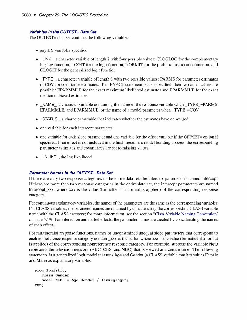
5880 F Chapter 76: The LOGISTIC Procedure
Variables in the OUTEST= Data SetThe OUTEST= data set contains the following variables:
� any BY variables specified
� _LINK_, a character variable of length 8 with four possible values: CLOGLOG for the complementarylog-log function, LOGIT for the logit function, NORMIT for the probit (alias normit) function, andGLOGIT for the generalized logit function
� _TYPE_, a character variable of length 8 with two possible values: PARMS for parameter estimatesor COV for covariance estimates. If an EXACT statement is also specified, then two other values arepossible: EPARMMLE for the exact maximum likelihood estimates and EPARMMUE for the exactmedian unbiased estimates.
� _NAME_, a character variable containing the name of the response variable when _TYPE_=PARMS,EPARMMLE, and EPARMMUE, or the name of a model parameter when _TYPE_=COV
� _STATUS_, a character variable that indicates whether the estimates have converged
� one variable for each intercept parameter
� one variable for each slope parameter and one variable for the offset variable if the OFFSET= option ifspecified. If an effect is not included in the final model in a model building process, the correspondingparameter estimates and covariances are set to missing values.
� _LNLIKE_, the log likelihood
Parameter Names in the OUTEST= Data SetIf there are only two response categories in the entire data set, the intercept parameter is named Intercept.If there are more than two response categories in the entire data set, the intercept parameters are namedIntercept_xxx, where xxx is the value (formatted if a format is applied) of the corresponding responsecategory.
For continuous explanatory variables, the names of the parameters are the same as the corresponding variables.For CLASS variables, the parameter names are obtained by concatenating the corresponding CLASS variablename with the CLASS category; for more information, see the section “Class Variable Naming Convention”on page 5779. For interaction and nested effects, the parameter names are created by concatenating the namesof each effect.
For multinomial response functions, names of unconstrained unequal slope parameters that correspond toeach nonreference response category contain _xxx as the suffix, where xxx is the value (formatted if a formatis applied) of the corresponding nonreference response category. For example, suppose the variable Net3represents the television network (ABC, CBS, and NBC) that is viewed at a certain time. The followingstatements fit a generalized logit model that uses Age and Gender (a CLASS variable that has values Femaleand Male) as explanatory variables:
proc logistic;class Gender;model Net3 = Age Gender / link=glogit;
run;

Input and Output Data Sets F 5881
There are two logit functions, one that contrasts ABC with NBC and one that contrasts CBS with NBC.For each logit, there are three parameters: an intercept parameter, a slope parameter for Age, and a slopeparameter for Gender (because there are only two gender levels and the EFFECT parameterization is used bydefault). The names of the parameters and their descriptions are as follows:
Intercept_ABC intercept parameter for the logit that contrasts ABC with NBC
Intercept_CBS intercept parameter for the logit that contrasts CBS with NBC
Age_ABC Age slope parameter for the logit that contrasts ABC with NBC
Age_CBS Age slope parameter for the logit that contrasts CBS with NBC
GenderFemale_ABC Gender=Female slope parameter for the logit that contrasts ABC with NBC
GenderFemale_CBS Gender=Female slope parameter for the logit that contrasts CBS with NBC
In a polytomous response model, if you specify an effect in both the EQUALSLOPES and UNEQUAL-SLOPES options, then its unequal slope parameter names are prefixed with “U_” if they are unconstrained or“C_” if they are constrained.
INEST= Input Data Set
You can specify starting values for the iterative algorithm in the INEST= data set. The INEST= data set hasthe same structure as the OUTEST= data set but is not required to have all the variables or observations thatappear in the OUTEST= data set. A previous OUTEST= data set can be used as, or modified for use as, anINEST= data set.
The INEST= data set must contain the intercept variables (named Intercept for binary response models andIntercept, Intercept_2, Intercept_3, and so forth, for ordinal and nominal response models) and all explanatoryvariables in the MODEL statement. If BY processing is used, the INEST= data set should also include theBY variables, and there must be one observation for each BY group. If the INEST= data set also contains the_TYPE_ variable, only observations with _TYPE_ value ’PARMS’ are used as starting values.
OUT= Output Data Set in the OUTPUT Statement
The OUT= data set in the OUTPUT statement contains all the variables in the input data set along withstatistics you request by specifying keyword=name options or the PREDPROBS= option in the OUTPUTstatement. In addition, if you use the single-trial syntax and you request any of the XBETA=, STDXBETA=,PREDICTED=, LCL=, and UCL= options, the OUT= data set contains the automatic variable _LEVEL_.The value of _LEVEL_ identifies the response category upon which the computed values of XBETA=,STDXBETA=, PREDICTED=, LCL=, and UCL= are based.
When there are more than two response levels, only variables named by the XBETA=, STDXBETA=,PREDICTED=, LOWER=, and UPPER= options and the variables given by PREDPROBS=(INDIVIDUALCUMULATIVE) have their values computed; the other variables have missing values. If you fit a generalizedlogit model, the cumulative predicted probabilities are not computed.
When there are only two response categories, each input observation produces one observation in the OUT=data set.
If there are more than two response categories and you specify only the PREDPROBS= option, then eachinput observation produces one observation in the OUT= data set. However, if you fit an ordinal (cumulative)model and specify options other than the PREDPROBS= options, each input observation generates as many

5882 F Chapter 76: The LOGISTIC Procedure
output observations as one fewer than the number of response levels, and the predicted probabilities and theirconfidence limits correspond to the cumulative predicted probabilities. If you fit a generalized logit modeland specify options other than the PREDPROBS= options, each input observation generates as many outputobservations as the number of response categories; the predicted probabilities and their confidence limitscorrespond to the probabilities of individual response categories.
For observations in which only the response variable is missing, values of the XBETA=, STDXBETA=,PREDICTED=, UPPER=, LOWER=, and the PREDPROBS= options are computed even though theseobservations do not affect the model fit. This enables, for instance, predicted probabilities to be computed fornew observations.
OUT= Output Data Set in a SCORE Statement
The OUT= data set in a SCORE statement contains all the variables in the data set being scored. The dataset being scored can be either the input DATA= data set in the PROC LOGISTIC statement or the DATA=data set in the SCORE statement. The DATA= data set in the SCORE statement does not need to contain theresponse variable.
If the data set being scored contains the response variable, then denote the normalized levels (left-justified,formatted values of 16 characters or less) of your response variable Y by Y1; : : : ; YkC1. For each responselevel, the OUT= data set also contains the following:
� F_Y, the normalized levels of the response variable Y in the data set being scored. If the events/trialssyntax is used, the F_Y variable is not created.
� I_Y, the normalized levels that the observations are classified into. Note that an observation is classifiedinto the level with the largest probability. If the events/trials syntax is used, the _INTO_ variable iscreated instead, and it contains the values EVENT and NONEVENT.
� P_Yi , the posterior probabilities of the normalized response level Yi
� If the CLM option is specified in the SCORE statement, the OUT= data set also includes the following:
– LCL_Yi , the lower 100(1 � ˛)% confidence limits for P_Yi– UCL_Yi , the upper 100(1 � ˛)% confidence limits for P_Yi

Input and Output Data Sets F 5883
OUTDESIGN= Output Data Set
The OUTDESIGN= data set contains the same number of observations as the corresponding DATA= data setand includes the response variable (with the same format as in the DATA= data set), the FREQ variable, theWEIGHT variable, the OFFSET= variable, and the design variables for the covariates, including an Interceptvariable of constant value 1 unless the NOINT option in the MODEL statement is specified. This data setdoes not contain the full design matrix because the covariate columns are not distinguished by responsefunction.
OUTDIST= Output Data Set
The OUTDIST= data set contains every exact conditional distribution necessary to process the correspondingEXACT statement. For example, the following statements create one distribution for the x1 parameter andanother for the x2 parameters, and produce the data set dist shown in Table 76.16:
data test;input y x1 x2 count;datalines;
0 0 0 11 0 0 10 1 1 21 1 1 11 0 2 31 1 2 11 2 0 31 2 1 21 2 2 1;
proc logistic data=test exactonly;class x2 / param=ref;model y=x1 x2;exact x1 x2/ outdist=dist;
run;proc print data=dist;run;

5884 F Chapter 76: The LOGISTIC Procedure
Table 76.16 OUTDIST= Data Set
Obs x1 x20 x21 Count Score Prob
1 . 0 0 3 5.81151 0.033332 . 0 1 15 1.66031 0.166673 . 0 2 9 3.12728 0.100004 . 1 0 15 1.46523 0.166675 . 1 1 18 0.21675 0.200006 . 1 2 6 4.58644 0.066677 . 2 0 19 1.61869 0.211118 . 2 1 2 3.27293 0.022229 . 3 0 3 6.27189 0.03333
10 2 . . 6 3.03030 0.1200011 3 . . 12 0.75758 0.2400012 4 . . 11 0.00000 0.2200013 5 . . 18 0.75758 0.3600014 6 . . 3 3.03030 0.06000
The first nine observations in the dist data set contain an exact distribution for the parameters of the x2effect (hence the values for the x1 parameter are missing), and the remaining five observations are for thex1 parameter. If a joint distribution was created, there would be observations with values for both the x1and x2 parameters. For CLASS variables, the corresponding parameters in the dist data set are identified byconcatenating the variable name with the appropriate classification level.
The data set contains the possible sufficient statistics of the parameters for the effects specified in the EXACTstatement, and the Count variable contains the number of different responses that yield these statistics. Inparticular, there are six possible response vectors y for which the dot product y0x1 was equal to 2, and forwhich y0x20, y0x21, and y01 were equal to their actual observed values (displayed in the “Sufficient Statistics”table).
When hypothesis tests are performed on the parameters, the Prob variable contains the probability of obtainingthat statistic (which is just the count divided by the total count), and the Score variable contains the score forthat statistic.
The OUTDIST= data set can contain a different exact conditional distribution for each specified EXACTstatement. For example, consider the following EXACT statements:
exact 'O1' x1 / outdist=o1;exact 'OJ12' x1 x2 / jointonly outdist=oj12;exact 'OA12' x1 x2 / joint outdist=oa12;exact 'OE12' x1 x2 / estimate outdist=oe12;
The O1 statement outputs a single exact conditional distribution. The OJ12 statement outputs only the jointdistribution for x1 and x2. The OA12 statement outputs three conditional distributions: one for x1, one for x2,and one jointly for x1 and x2. The OE12 statement outputs two conditional distributions: one for x1 and theother for x2. Data set oe12 contains both the x1 and x2 variables; the distribution for x1 has missing valuesin the x2 column while the distribution for x2 has missing values in the x1 column.

Computational Resources F 5885
OUTROC= Output Data Set
The OUTROC= data set contains data necessary for producing the ROC curve, and can be created byspecifying the OUTROC= option in the MODEL statement or the OUTROC= option in the SCORE statement:It has the following variables:
� any BY variables specified
� _STEP_, the model step number. This variable is not included if model selection is not requested.
� _PROB_, the estimated probability of an event. These estimated probabilities serve as cutpoints forpredicting the response. Any observation with an estimated event probability that exceeds or equals_PROB_ is predicted to be an event; otherwise, it is predicted to be a nonevent. Predicted probabilitiesthat are close to each other are grouped together, with the maximum allowable difference between thelargest and smallest values less than a constant that is specified by the ROCEPS= option. The smallestestimated probability is used to represent the group.
� _POS_, the number of correctly predicted event responses
� _NEG_, the number of correctly predicted nonevent responses
� _FALPOS_, the number of falsely predicted event responses
� _FALNEG_, the number of falsely predicted nonevent responses
� _SENSIT_, the sensitivity, which is the proportion of event observations that were predicted to have anevent response
� _1MSPEC_, one minus specificity, which is the proportion of nonevent observations that were predictedto have an event response
Note that none of these statistics are affected by the bias-correction method discussed in the section “Classifi-cation Table” on page 5852. An ROC curve is obtained by plotting _SENSIT_ against _1MSPEC_.
For more information, see the section “Receiver Operating Characteristic Curves” on page 5860.
Computational ResourcesThe memory needed to fit an unconditional model is approximately 8n.p C 2/C 24.p C 2/2 bytes, where pis the number of parameters estimated and n is the number of observations in the data set. For cumulativeresponse models with more than two response levels, a test of the parallel lines assumption requires anadditional memory of approximately 4k2.mC 1/2 C 24.mC 2/2 bytes, where k is the number of responselevels and m is the number of slope parameters. However, if this additional memory is not available, theprocedure skips the test and finishes the other computations. You might need more memory if you use theSELECTION= option for model building.
The data that consist of relevant variables (including the design variables for model effects) and observationsfor fitting the model are stored in a temporary utility file. If sufficient memory is available, such data will alsobe kept in memory; otherwise, the data are reread from the utility file for each evaluation of the likelihoodfunction and its derivatives, with the resulting execution time of the procedure substantially increased.

5886 F Chapter 76: The LOGISTIC Procedure
Specifying the MULTIPASS option in the MODEL statement avoids creating this utility file and also doesnot store the data in memory; instead, the DATA= data set is reread when needed. This saves approximately8n.p C 2/ bytes of memory but increases the execution time.
If a conditional logistic regression is performed, then approximately 4.m2 CmC 4/maxh.mh/C .8sH C36/H C 12sH additional bytes of memory are needed, where mh is the number of events in stratumh, H is the total number of strata, and sH is the number of variables used to define the strata. If theCHECKDEPENDENCY=ALL option is specified in the STRATA statement, then an extra 4.mCH/.mCH C 1/ bytes are required, and the resulting execution time of the procedure might be substantially increased.
Computational Resources for Exact Logistic Regression
Many problems require a prohibitive amount of time and memory for exact computations, depending on thespeed and memory available on your computer. For such problems, consider whether exact methods arereally necessary. Stokes, Davis, and Koch (2012) suggest looking at exact p-values when the sample size issmall and the approximate p-values from the unconditional analysis are less than 0.10, and they provide rulesof thumb for determining when various models are valid.
A formula does not exist that can predict the amount of time and memory necessary to generate the exactconditional distributions for a particular problem. The time and memory required depends on severalfactors, including the total sample size, the number of parameters of interest, the number of nuisanceparameters, and the order in which the parameters are processed. To provide a feel for how these factorsaffect performance, data sets containing Nobs 2 f10; : : : ; 500g observations with up to 10 independentuniform binary covariates (X1,. . . ,XN) and a binary response variable (Y) are generated, and the followingstatements create exact conditional distributions for X1 conditional on the other covariates by using thedefault METHOD=NETWORK. Figure 76.11 displays results that were obtained on a 64-bit, 3.4GHz PCwith 16GB RAM running Microsoft Windows 7.
data one;do obs=1 to HalfNobs;
do Y=0 to 1;X1=round(ranuni(0));...XN=round(ranuni(0));output;
end;end;
options fullstimer;proc logistic exactonly;
exactoptions method=network maxtime=1200;class X: / param=ref;model Y=X:;exact X1 / outdist=dist;
run;

Computational Resources F 5887
Figure 76.11 Mean Time and Memory Required
At any time while PROC LOGISTIC is deriving the distributions, you can terminate the computations bypressing the system interrupt key sequence (see the SAS Companion for your system) and choosing to stopcomputations. If you run out of memory, see the SAS Companion for your system to see how to allocatemore.
You can use the EXACTOPTIONS option MAXTIME= to limit the total amount of time PROC LOGISTICuses to derive all of the exact distributions. If PROC LOGISTIC does not finish within that time, the procedureterminates.
Frequency calculation is performed in the log scale by default. This reduces the need to check for excessivelylarge frequencies but can be slower than not scaling. You can turn off the log scaling by specifying theNOLOGSCALE option in the EXACTOPTIONS statement. If a frequency in the exact distribution is largerthan the largest integer that can be held in double precision, a warning is printed to the SAS log. Becauseinaccuracies due to adding small numbers to these large frequencies might have little or no effect on thestatistics, the exact computations continue.
You can monitor the progress of the procedure by submitting your program with the EXACTOPTIONS optionSTATUSTIME=. If the procedure is too slow, you can try another method by specifying the EXACTOPTIONSoption METHOD=, you can try reordering the variables in the MODEL statement (note that CLASS variablesare always processed before continuous covariates), or you can try reparameterizing your classificationvariables as in the following statement:
class class-variables / param=ref ref=first order=freq;
If you condition out CLASS variables that use reference or GLM coding but you are not using the STRATAstatement, then you can speed up the analysis by specifying one of the nuisance CLASS variables in the

5888 F Chapter 76: The LOGISTIC Procedure
STRATA statement. This performance gain occurs because STRATA variables partition your data set intosmaller pieces. However, moving two (or more) nuisance CLASS variables into the STRATA statementresults in a different model, because the sufficient statistics for the second CLASS variable are actuallycomputed across the levels of the first CLASS variable.
Displayed OutputIf you use the NOPRINT option in the PROC LOGISTIC statement, the procedure does not display anyoutput. Otherwise, the tables displayed by the LOGISTIC procedure are discussed in the following sectionin the order in which they appear in the output. Some of the tables appear only in conjunction with certainoptions or statements; for more information, see the section “ODS Table Names” on page 5893.
NOTE: The EFFECT, ESTIMATE, LSMEANS, LSMESTIMATE, and SLICE statements also create tables,which are not listed in this section. For information about these tables, see the corresponding sections ofChapter 19, “Shared Concepts and Topics.”
Table Summary
Model Information and the Number of ObservationsSee the section “Missing Values” on page 5831 for information about missing-value handling, and thesections “FREQ Statement” on page 5793 and “WEIGHT Statement” on page 5830 for information aboutvalid frequencies and weights.
Response ProfileDisplays the Ordered Value assigned to each response level. For more information, see the section “ResponseLevel Ordering” on page 5831.
Class Level InformationDisplays the design values for each CLASS explanatory variable. For more information, see the section“Other Parameterizations” on page 397 in Chapter 19, “Shared Concepts and Topics.”
Simple Statistics TablesThe following tables are displayed if you specify the SIMPLE option in the PROC LOGISTIC statement:
� Descriptive Statistics for Continuous Explanatory Variables
� Frequency Distribution of Class Variables
� Weight Distribution of Class VariablesDisplays if you also specify a WEIGHT statement.
Strata Tables for (Exact) Conditional Logistic RegressionThe following tables are displayed if you specify a STRATA statement:
� Strata SummaryShows the pattern of the number of events and the number of nonevents in a stratum. See the section“STRATA Statement” on page 5827 for more information.

Displayed Output F 5889
� Strata InformationDisplays if you specify the INFO option in a STRATA statement.
Maximum Likelihood Iteration HistoryDisplays if you specify the ITPRINT option in the MODEL statement. For more information, see the sections“Iterative Algorithms for Model Fitting” on page 5835, “Convergence Criteria” on page 5837, and “Existenceof Maximum Likelihood Estimates” on page 5837.
Deviance and Pearson Goodness-of-Fit StatisticsDisplays if you specify the SCALE= option in the MODEL statement. Small p-values reject the nullhypotheses that the fitted model is adequate. For more information, see the sections “Pearson and DevianceGoodness-of-Fit Test” on page 5855 and “Overdispersion” on page 5858.
Goodness-of-Fit StatisticsDisplays if you specify the GOF option in the MODEL statement and you fit a binary logistic regressionmodel. Small p-values reject the null hypotheses that the fitted model is adequate. For more information, seethe section “Goodness-of-Fit Tests” on page 5855.
Score Test for the Equal Slopes (Proportional Odds) AssumptionTests the parallel lines assumption if you fit an ordinal response model with the LINK=CLOGLOG orLINK=PROBIT options. If you specify LINK=LOGIT, this is called the “Proportional Odds” assumption.The table is not displayed if you specify the EQUALSLOPES or UNEQUALSLOPES option in the MODELstatement. Small p-values reject the null hypothesis that the slope parameters for each explanatory variableare constant across all the response functions. For more information, see the section “Testing the ParallelLines Assumption” on page 5846.
Model Fit StatisticsComputes various fit criteria based on a model with intercepts only and a model with intercepts andexplanatory variables. If you specify the NOINT option in the MODEL statement, these statistics arecalculated without considering the intercept parameters. If you specify the GOF option in the MODELstatement, then more criteria are displayed in a single column. For more information, see the section “ModelFitting Information” on page 5840.
If you also specify the RSQUARE option in the MODEL statement (without specifying the GOF option), twogeneralized R-square measures are displayed; for more information, see the section “Generalized Coefficientof Determination” on page 5841.
Testing Global Null Hypothesis: BETA=0Tests the joint effect of the explanatory variables included in the model. Small p-values reject the nullhypothesis that all slope parameters are equal to zero, H0Wˇ D 0. For more information, see the sections“Model Fitting Information” on page 5840, “Residual Chi-Square” on page 5845, and “Testing LinearHypotheses about the Regression Coefficients” on page 5863.
Score Test for Global Null HypothesisDisplays instead of the “Testing Global Null Hypothesis: BETA=0” table if the NOFIT option is specified inthe MODEL statement. The global score test evaluates the joint significance of the effects in the MODEL

5890 F Chapter 76: The LOGISTIC Procedure
statement. Small p-values reject the null hypothesis that all slope parameters are equal to zero, H0Wˇ D 0.For more information, see the section “Residual Chi-Square” on page 5845.
Model Selection TablesThe tables in this section are produced when the SELECTION= option is specified in the MODEL statement.See the section “Effect-Selection Methods” on page 5839 for more information.
� Residual Chi-Square TestDisplays if you specify SELECTION=FORWARD, BACKWARD, or STEPWISE in the MODELstatement. Small p-values reject the null hypothesis that the reduced model is adequate. For moreinformation, see the section “Residual Chi-Square” on page 5845.
� Analysis of Effects Eligible for EntryDisplays if you specify the DETAILS option and the SELECTION=FORWARD or STEPWISE optionin the MODEL statement. Small p-values rejectH0Wˇi ¤ 0. The score chi-square is used to determineentry; for more information, see the section “Testing Individual Effects Not in the Model” on page 5846.
� Analysis of Effects Eligible for RemovalDisplays if you specify the SELECTION=BACKWARD or STEPWISE option in the MODEL state-ment. Small p-values reject H0Wˇi D 0. The Wald chi-square is used to determine removal; formore information, see the section “Testing Linear Hypotheses about the Regression Coefficients” onpage 5863.
� Analysis of Effects Removed by Fast Backward EliminationDisplays if you specify the FAST option and the SELECTION=BACKWARD or STEPWISE option inthe MODEL statement. This table gives the approximate chi-square statistic for the variable removed,the corresponding p-value with respect to a chi-square distribution with one degree of freedom, theresidual chi-square statistic for testing the joint significance of the variable and the preceding ones, thedegrees of freedom, and the p-value of the residual chi-square with respect to a chi-square distributionwith the corresponding degrees of freedom.
� Summary of Forward, Backward, and Stepwise SelectionDisplays if you specify SELECTION=FORWARD, BACKWARD, or STEPWISE in the MODELstatement. The score chi-square is used to determine entry; for more information, see the section“Testing Individual Effects Not in the Model” on page 5846. The Wald chi-square is used to determineremoval; for more information, see the section “Testing Linear Hypotheses about the RegressionCoefficients” on page 5863.
� Regression Models Selected by Score CriterionDisplays the score chi-square for all models if you specify the SELECTION=SCORE option in theMODEL statement. Small p-values reject the null hypothesis that the fitted model is adequate. Formore information, see the sections “Effect-Selection Methods” on page 5839 and “Score Statistics andTests” on page 5845.
Joint Tests or Type 3 Analysis of EffectsDisplays if the model contains a CLASS variable and performs Wald chi-square tests of the joint effect of theparameters for each CLASS variable in the model. Small p-values reject H0Wˇi D 0. The title of this tablefor main-effects models or models that use GLM parameterization is “Type 3 Analysis of Effects”; for all

Displayed Output F 5891
other models the title is “Joint Tests.” For more information, see the sections “Testing Linear Hypothesesabout the Regression Coefficients” on page 5863 and “Joint Tests and Type 3 Tests” on page 5863.
Analysis of Maximum Likelihood EstimatesCLASS effects are identified by their (nonreference) level. For generalized logit models, a response variablecolumn displays the nonreference level of the logit. The table includes the following:
� the estimated standard error of the parameter estimate, computed as the square root of the correspondingdiagonal element of the estimated covariance matrix
� the Wald chi-square statistic, computed by squaring the ratio of the parameter estimate divided by itsstandard error estimate. For more information, see the section “Testing Linear Hypotheses about theRegression Coefficients” on page 5863.
� the p-value tests the null hypothesis H0Wˇi D 0; small values reject the null.
� the standardized estimate for the slope parameter, if you specify the STB option in the MODELstatement. For more information, see the STB option on page 5813.
� exponentiated values of the estimates of the slope parameters, if you specify the EXPB option in theMODEL statement. For more information, see the EXPB option on page 5803.
� the label of the variable, if you specify the PARMLABEL option in the MODEL statement and ifspace permits. Due to constraints on the line size, the variable label might be suppressed in order todisplay the table in one panel. Use the SAS system option LINESIZE= to specify a larger line size toaccommodate variable labels. A shorter line size can break the table into two panels allowing labels tobe displayed.
Odds Ratio EstimatesDisplays the odds ratio estimates and the corresponding 95% Wald confidence intervals for variables that arenot involved in nestings or interactions. For continuous explanatory variables, these odds ratios correspondto a unit increase in the risk factors. For more information, see the section “Odds Ratio Estimation” onpage 5848.
Association of Predicted Probabilities and Observed ResponsesFor more information, see the section “Rank Correlation of Observed Responses and Predicted Probabilities”on page 5844.
Parameter Estimates and Profile-Likelihood or Wald Confidence IntervalsDisplays if you specify the CLPARM= option in the MODEL statement. For more information, see thesection “Confidence Intervals for Parameters” on page 5847.
Odds Ratio Estimates and Profile-Likelihood or Wald Confidence IntervalsDisplays if you specify the ODDSRATIO statement for any effects with any class parameterizations. Alsodisplays if you specify the CLODDS= option in the MODEL statement, except odds ratios are computedonly for main effects not involved in interactions or nestings, and if the main effect is a CLASS variable, theparameterization must be EFFECT, REFERENCE, or GLM. For more information, see the section “OddsRatio Estimation” on page 5848.

5892 F Chapter 76: The LOGISTIC Procedure
Estimated Covariance or Correlation MatrixDisplays if you specify the COVB or CORRB option in the MODEL statement. For more information, seethe section “Iterative Algorithms for Model Fitting” on page 5835.
Contrast Test ResultsDisplays the Wald test for each specified CONTRAST statement. Small p-values reject H0WLˇ D 0. The“Coefficients of Contrast” table displays the contrast matrix if you specify the E option, and the “ContrastEstimation and Testing Results by Row” table displays estimates and Wald tests for each row of the contrastmatrix if you specify the ESTIMATE= option. For more information, see the sections “CONTRASTStatement” on page 5781, “Testing Linear Hypotheses about the Regression Coefficients” on page 5863, and“Linear Predictor, Predicted Probability, and Confidence Limits” on page 5851.
Linear Hypotheses Testing ResultsDisplays the Wald test for each specified TEST statement. For more information, see the sections “TestingLinear Hypotheses about the Regression Coefficients” on page 5863 and “TEST Statement” on page 5828.
Hosmer and Lemeshow Goodness-of-Fit TestDisplays if you specify the LACKFIT or GOF option in the MODEL statement. Small p-values reject the nullhypothesis that the fitted model is adequate. If you have 50 or fewer groups, the “Partition for the Hosmerand Lemeshow Test” table displays the grouping that is used in the test. However, if you have more than 50groups, this table is not displayed, but you can instead use the ODS OUTPUT statement to save this table toan output data set. For more information, see the section “The Hosmer-Lemeshow Goodness-of-Fit Test” onpage 5855.
Classification TableDisplays if you use the CTABLE option in the MODEL statement. If you specify a list of cutpoints with thePPROB= option, then the cutpoints are displayed in the Prob Level column. If you specify the prior eventprobabilities with the PEVENT= option, then the probabilities are displayed in the Prob Event column. TheCorrect column displays the number of correctly classified events and nonevents, the Incorrect Event columndisplays the number of nonevents incorrectly classified as events, and the Incorrect Nonevent column givesthe number of events incorrectly classified as nonevents. For more information, see the section “ClassificationTable” on page 5852.
Regression DiagnosticsDisplays if you specify the INFLUENCE option in the MODEL statement. See the section “RegressionDiagnostics” on page 5864 for more information about diagnostics from an unconditional analysis, and thesection “Regression Diagnostic Details” on page 5873 for information about diagnostics from a conditionalanalysis.
Fit Statistics for SCORE DataDisplays if you specify the FITSTAT option in the SCORE statement. For more information, see the section“Scoring Data Sets” on page 5867.
ROC Association Statistic and Contrast TablesDisplayed if a ROC statement, a ROCCONTRAST statement, or the ROCCI option is specified. For moreinformation, about the Mann-Whitney statistics and the test and estimation computations, see the section

ODS Table Names F 5893
“ROC Computations” on page 5862. For more information about the other statistics, see the section “RankCorrelation of Observed Responses and Predicted Probabilities” on page 5844.
Exact Conditional Logistic Regression TablesThe tables in this section are produced when the EXACT statement is specified. If theMETHOD=NETWORKMC option is specified, the test and estimate tables are renamed “Monte Carlo”tables and a Monte Carlo standard error column (
pp.1 � p/=n) is displayed.
� Sufficient StatisticsDisplays if you request an OUTDIST= data set in an EXACT statement. The table lists the parametersand their observed sufficient statistics.
� (Monte Carlo) Conditional Exact TestsFor more information, see the section “Hypothesis Tests” on page 5877.
� (Monte Carlo) Exact Parameter EstimatesDisplays if you specify the ESTIMATE option in the EXACT statement. This table gives individualparameter estimates for each variable (conditional on the values of all the other parameters in themodel), confidence limits, and a two-sided p-value (twice the one-sided p-value) for testing thatthe parameter is zero. For more information, see the section “Inference for a Single Parameter” onpage 5878.
� (Monte Carlo) Exact Odds RatiosDisplays if you specify the ESTIMATE=ODDS or ESTIMATE=BOTH option in the EXACT statement.For more information, see the section “Inference for a Single Parameter” on page 5878.
ODS Table NamesPROC LOGISTIC assigns a name to each table it creates. You can use these names to reference the tablewhen using the Output Delivery System (ODS) to select tables and create output data sets. These names arelisted in Table 76.17. For more information about ODS, see Chapter 20, “Using the Output Delivery System.”
The EFFECT, ESTIMATE, LSMEANS, LSMESTIMATE, and SLICE statements also create tables, whichare not listed in Table 76.17. For information about these tables, see the corresponding sections of Chapter 19,“Shared Concepts and Topics.”
Table 76.17 ODS Tables Produced by PROC LOGISTIC
ODS Table Name Description Statements Options
Association Association of predictedprobabilities and observedresponses
MODEL(without STRATA)
Default
BestSubsets Best subset selection MODEL SELECTION=SCOREClassFreq Frequency breakdown of
CLASS variablesPROC LOGISTIC SIMPLE (with CLASS
variables)

5894 F Chapter 76: The LOGISTIC Procedure
Table 76.17 continued
ODS Table Name Description Statements Options
Classification Classification table MODEL CTABLEClassLevelInfo CLASS variable levels and
design variablesMODEL Default (with CLASS
variables)ClassWgt Weight breakdown of
CLASS variablesPROC LOGISTIC,WEIGHT
SIMPLE (with CLASSvariables)
CLOddsPL Odds ratio estimates andprofile-likelihood confidenceintervals
MODEL CLODDS=PL
CLOddsWald Odds ratio estimates andWald confidence intervals
MODEL CLODDS=WALD
CLParmPL Parameter estimates andprofile-likelihood confidenceintervals
MODEL CLPARM=PL
CLParmWald Parameter estimates andWald confidence intervals
MODEL CLPARM=WALD
ContrastCoeff L matrix from CONTRAST CONTRAST EContrastEstimate Estimates from CONTRAST CONTRAST ESTIMATE=ContrastTest Wald test for CONTRAST CONTRAST DefaultConvergenceStatus Convergence status MODEL DefaultCorrB Estimated correlation matrix
of parameter estimatorsMODEL CORRB
CovB Estimated covariance matrixof parameter estimators
MODEL COVB
CumulativeModelTest Test of the cumulative modelassumption
MODEL Default with cumulativeresponse
EffectInModel Test effects in model MODEL SELECTION=S | BEffectNotInModel Test for effects not in model MODEL SELECTION=S | FExactOddsRatio Exact odds ratios EXACT ESTIMATE=ODDS,
ESTIMATE=BOTHExactParmEst Parameter estimates EXACT ESTIMATE,
ESTIMATE=PARM,ESTIMATE=BOTH
ExactTests Conditional exact tests EXACT DefaultFastElimination Fast backward elimination MODEL SELECTION=B, FASTFitStatistics Model fit statistics MODEL DefaultGlobalScore Global score test MODEL NOFITGlobalTests Test for global null
hypothesisMODEL Default
GoodnessOfFit Pearson and deviancegoodness-of-fit tests
MODEL SCALE, GOF
IndexPlots Batch capture of the indexplots
MODEL IPLOTS
Influence Regression diagnostics MODEL INFLUENCEIterHistory Iteration history MODEL ITPRINT

ODS Table Names F 5895
Table 76.17 continued
ODS Table Name Description Statements Options
LackFitChiSq Hosmer-Lemeshowchi-square test results
MODEL LACKFIT, GOF
LackFitPartition Partition for the Hosmer-Lemeshow test
MODEL LACKFIT, GOF
LastGradient Last evaluation of gradient MODEL ITPRINTLinear Linear combination PROC LOGISTIC DefaultLogLikeChange Final change in the log
likelihoodMODEL ITPRINT
ModelANOVA Joint or Type 3 tests ofeffects
MODEL Default (withCLASS variables)
ModelBuildingSummary Summary of model building MODEL SELECTION=B | F | SModelInfo Model information PROC LOGISTIC DefaultNObs Number of observations PROC LOGISTIC DefaultOddsEst Adjusted odds ratios UNITS DefaultOddsRatios Odds ratio estimates MODEL DefaultOddsRatiosPL Odds ratio estimates and PL
confidence intervalsODDSRATIOS CL=PL
OddsRatiosWald Odds ratio estimates andWald confidence intervals
ODDSRATIOS CL=WALD
ParameterEstimates Maximum likelihoodestimates of modelparameters
MODEL Default
ResidualChiSq Residual chi-square MODEL SELECTION=F | BResponseProfile Response profile PROC LOGISTIC DefaultROCAssociation Association table for ROC
modelsROCMODEL
DefaultROCCI
ROCContrastCoeff L matrix fromROCCONTRAST
ROCCONTRAST E
ROCContrastCov Covariance ofROCCONTRAST rows
ROCCONTRAST COV
ROCContrastEstimate Estimates fromROCCONTRAST
ROCCONTRAST ESTIMATE=
ROCContrastTest Wald test fromROCCONTRAST
ROCCONTRAST Default
ROCCov Covariance between ROCcurves
ROCCONTRAST COV
RSquare R-square MODEL RSQUAREScoreFitStat Fit statistics for scored data SCORE FITSTATSimpleStatistics Summary statistics for
explanatory variablesPROC LOGISTIC SIMPLE
StrataInfo Event and noneventfrequencies for each stratum
STRATA INFO
StrataSummary Number of strata withspecific response frequencies
STRATA Default

5896 F Chapter 76: The LOGISTIC Procedure
Table 76.17 continued
ODS Table Name Description Statements Options
SuffStats Sufficient statistics EXACT OUTDIST=TestPrint1 L[Cov(b)]L’ and Lb-c TEST PRINTTestPrint2 Ginv(L[Cov(b)]L’) and
Ginv(L[Cov(b)]L’)(Lb-c)TEST PRINT
TestStmts Linear hypotheses testingresults
TEST Default
ODS GraphicsStatistical procedures use ODS Graphics to create graphs as part of their output. ODS Graphics is describedin detail in Chapter 21, “Statistical Graphics Using ODS.”
Before you create graphs, ODS Graphics must be enabled (for example, by specifying the ODS GRAPH-ICS ON statement). For more information about enabling and disabling ODS Graphics, see the section“Enabling and Disabling ODS Graphics” on page 623 in Chapter 21, “Statistical Graphics Using ODS.”
The overall appearance of graphs is controlled by ODS styles. Styles and other aspects of using ODSGraphics are discussed in the section “A Primer on ODS Statistical Graphics” on page 622 in Chapter 21,“Statistical Graphics Using ODS.”
You must also specify the options in the PROC LOGISTIC statement that are indicated in Table 76.18.
When ODS Graphics is enabled, then the EFFECT, EFFECTPLOT, ESTIMATE, LSMEANS, LSMESTI-MATE, and SLICE statements can produce plots that are associated with their analyses. For informationabout these plots, see the corresponding sections of Chapter 19, “Shared Concepts and Topics.”
PROC LOGISTIC assigns a name to each graph it creates using ODS. You can use these names to referencethe graphs when using ODS. The names are listed in Table 76.18.
Table 76.18 Graphs Produced by PROC LOGISTIC
ODS Graph Name Plot Description Statement or Option
CalibrationPlot Panel of calibration plots forpolytomous response
PLOTS=CALIBRATIONor MODEL / GOF
Calibration plot for a singlepolytomous response level
PLOTS=CALIBRATION(UNPACK)
Calibration plot for binary response PLOTS=CALIBRATIONor MODEL / GOF
DfBetasPlot Panel of dfbetas by case number PLOTS=DFBETASor MODEL / INFLUENCE or IPLOTS
Effect dfbetas by case number PLOTS=DFBETAS(UNPACK)DPCPlot Difchisq and/or difdev by predicted
probability by CI displacement CPLOTS=DPC

ODS Graphics F 5897
Table 76.18 continued
ODS Graph Name Plot Description Statement or Option
EffectPlot Predicted probability PLOTS=EFFECTInfluencePlots Panel of influence statistics by case
numberPLOTS=INFLUENCEor MODEL / INFLUENCE or IPLOTS
CBarPlot CI displacement Cbar by casenumber
PLOTS=INFLUENCE(UNPACK)
CPlot CI displacement C by case number PLOTS=INFLUENCE(UNPACK)DevianceResidualPlot Deviance residual by case number PLOTS=INFLUENCE(UNPACK)DifChisqPlot Difchisq by case number PLOTS=INFLUENCE(UNPACK)DifDeviancePlot Difdev by case number PLOTS=INFLUENCE(UNPACK)LeveragePlot Hat diagonal by case number PLOTS=INFLUENCE(UNPACK)LikelihoodResidualPlot Likelihood residual by case number PLOTS=INFLUENCE(UNPACK
STDRES)PearsonResidualPlot Pearson chi-square residual by case
numberPLOTS=INFLUENCE(UNPACK)
StdDevianceResidualPlot Standardized deviance residual bycase number
PLOTS=INFLUENCE(UNPACKSTDRES)
StdPearsonResidualPlot Standardized Pearson chi-squareresidual by case number
PLOTS=INFLUENCE(UNPACKSTDRES)
LeveragePlots Panel of influence statistics byleverage
PLOTS=LEVERAGE
LeverageCPlot CI displacement C by leverage PLOTS=LEVERAGE(UNPACK)LeverageDifChisqPlot Difchisq by leverage PLOTS=LEVERAGE(UNPACK)LeverageDifDevPlot Difdev by leverage PLOTS=LEVERAGE(UNPACK)LeveragePhatPlot Predicted probability by leverage PLOTS=LEVERAGE(UNPACK)
ORPlot Odds ratios Default orPLOTS=ODDSRATIO andMODEL / CLODDS=or ODDSRATIO
PhatPlots Panel of influence by predictedprobability
PLOTS=PHAT
PhatCPlot CI displacement C by predictedprobability
PLOTS=PHAT(UNPACK)
PhatDifChisqPlot Difchisq by predicted probability PLOTS=PHAT(UNPACK)PhatDifDevPlot Difdev by predicted probability PLOTS=PHAT(UNPACK)PhatLeveragePlot Leverage by predicted probability PLOTS=PHAT(UNPACK)
ROCCurve Receiver operating characteristicscurve
PLOTS=ROCor MODEL / OUTROC=or SCORE OUTROC=or ROC
ROCOverlay ROC curves for comparisons PLOTS=ROC andMODEL / SELECTION=or ROC
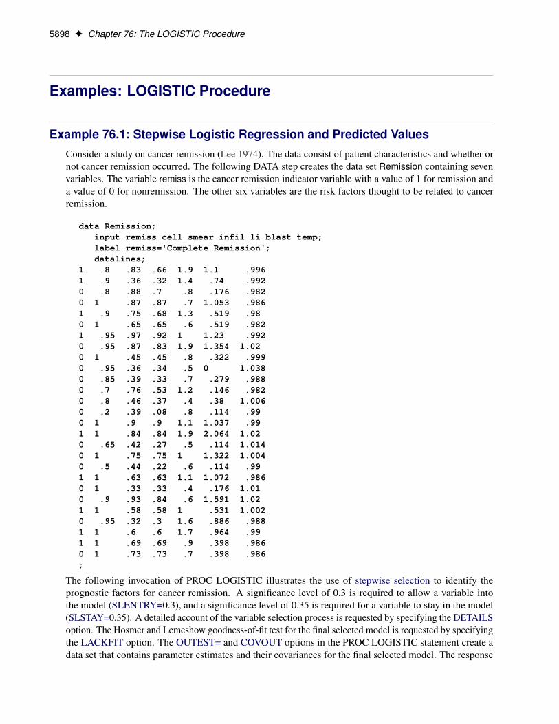
5898 F Chapter 76: The LOGISTIC Procedure
Examples: LOGISTIC Procedure
Example 76.1: Stepwise Logistic Regression and Predicted ValuesConsider a study on cancer remission (Lee 1974). The data consist of patient characteristics and whether ornot cancer remission occurred. The following DATA step creates the data set Remission containing sevenvariables. The variable remiss is the cancer remission indicator variable with a value of 1 for remission anda value of 0 for nonremission. The other six variables are the risk factors thought to be related to cancerremission.
data Remission;input remiss cell smear infil li blast temp;label remiss='Complete Remission';datalines;
1 .8 .83 .66 1.9 1.1 .9961 .9 .36 .32 1.4 .74 .9920 .8 .88 .7 .8 .176 .9820 1 .87 .87 .7 1.053 .9861 .9 .75 .68 1.3 .519 .980 1 .65 .65 .6 .519 .9821 .95 .97 .92 1 1.23 .9920 .95 .87 .83 1.9 1.354 1.020 1 .45 .45 .8 .322 .9990 .95 .36 .34 .5 0 1.0380 .85 .39 .33 .7 .279 .9880 .7 .76 .53 1.2 .146 .9820 .8 .46 .37 .4 .38 1.0060 .2 .39 .08 .8 .114 .990 1 .9 .9 1.1 1.037 .991 1 .84 .84 1.9 2.064 1.020 .65 .42 .27 .5 .114 1.0140 1 .75 .75 1 1.322 1.0040 .5 .44 .22 .6 .114 .991 1 .63 .63 1.1 1.072 .9860 1 .33 .33 .4 .176 1.010 .9 .93 .84 .6 1.591 1.021 1 .58 .58 1 .531 1.0020 .95 .32 .3 1.6 .886 .9881 1 .6 .6 1.7 .964 .991 1 .69 .69 .9 .398 .9860 1 .73 .73 .7 .398 .986;
The following invocation of PROC LOGISTIC illustrates the use of stepwise selection to identify theprognostic factors for cancer remission. A significance level of 0.3 is required to allow a variable intothe model (SLENTRY=0.3), and a significance level of 0.35 is required for a variable to stay in the model(SLSTAY=0.35). A detailed account of the variable selection process is requested by specifying the DETAILSoption. The Hosmer and Lemeshow goodness-of-fit test for the final selected model is requested by specifyingthe LACKFIT option. The OUTEST= and COVOUT options in the PROC LOGISTIC statement create adata set that contains parameter estimates and their covariances for the final selected model. The response

Example 76.1: Stepwise Logistic Regression and Predicted Values F 5899
variable option EVENT= chooses remiss=1 (remission) as the event so that the probability of remission ismodeled. The OUTPUT statement creates a data set that contains the cumulative predicted probabilities andthe corresponding confidence limits, and the individual and cross validated predicted probabilities for eachobservation. The ODS OUTPUT statement writes the “Association” table from each selection step to a SASdata set.
title 'Stepwise Regression on Cancer Remission Data';proc logistic data=Remission outest=betas covout;
model remiss(event='1')=cell smear infil li blast temp/ selection=stepwise
slentry=0.3slstay=0.35detailslackfit;
output out=pred p=phat lower=lcl upper=uclpredprob=(individual crossvalidate);
ods output Association=Association;run;
proc print data=betas;title2 'Parameter Estimates and Covariance Matrix';
run;
proc print data=pred;title2 'Predicted Probabilities and 95% Confidence Limits';
run;
In stepwise selection, an attempt is made to remove any insignificant variables from the model before addinga significant variable to the model. Each addition or deletion of a variable to or from a model is listed as aseparate step in the displayed output, and at each step a new model is fitted. Details of the model selectionsteps are shown in Outputs 76.1.1 through 76.1.5.
Prior to the first step, the intercept-only model is fit and individual score statistics for the potential variablesare evaluated (Output 76.1.1).
Output 76.1.1 Startup Model
Stepwise Regression on Cancer Remission Data
The LOGISTIC Procedure
Step 0. Intercept entered:
Model Convergence Status
Convergence criterion (GCONV=1E-8) satisfied.
-2 Log L = 34.372
Analysis of Maximum Likelihood Estimates
Parameter DF EstimateStandard
ErrorWald
Chi-Square Pr > ChiSq
Intercept 1 -0.6931 0.4082 2.8827 0.0895

5900 F Chapter 76: The LOGISTIC Procedure
Output 76.1.1 continued
Residual Chi-Square Test
Chi-Square DF Pr > ChiSq
9.4609 6 0.1493
Analysis of Effects Eligible forEntry
Effect DFScore
Chi-Square Pr > ChiSq
cell 1 1.8893 0.1693
smear 1 1.0745 0.2999
infil 1 1.8817 0.1701
li 1 7.9311 0.0049
blast 1 3.5258 0.0604
temp 1 0.6591 0.4169
In Step 1 (Output 76.1.2), the variable li is selected into the model because it is the most significant variableamong those to be chosen (p D 0:0049 < 0:3). The intermediate model that contains an intercept and li isthen fitted. li remains significant (p D 0:0146 < 0:35) and is not removed.
Output 76.1.2 Step 1 of the Stepwise Analysis
Step 1. Effect li entered:
Model Convergence Status
Convergence criterion (GCONV=1E-8) satisfied.
Model Fit Statistics
CriterionIntercept
Only
Interceptand
Covariates
AIC 36.372 30.073
SC 37.668 32.665
-2 Log L 34.372 26.073
Testing Global Null Hypothesis: BETA=0
Test Chi-Square DF Pr > ChiSq
Likelihood Ratio 8.2988 1 0.0040
Score 7.9311 1 0.0049
Wald 5.9594 1 0.0146
Analysis of Maximum Likelihood Estimates
Parameter DF EstimateStandard
ErrorWald
Chi-Square Pr > ChiSq
Intercept 1 -3.7771 1.3786 7.5064 0.0061
li 1 2.8973 1.1868 5.9594 0.0146
Odds Ratio Estimates
EffectPoint
Estimate95% Wald
Confidence Limits
li 18.124 1.770 185.563

Example 76.1: Stepwise Logistic Regression and Predicted Values F 5901
Output 76.1.2 continued
Association of Predicted Probabilities andObserved Responses
Percent Concordant 84.0 Somers' D 0.710
Percent Discordant 13.0 Gamma 0.732
Percent Tied 3.1 Tau-a 0.328
Pairs 162 c 0.855
Residual Chi-Square Test
Chi-Square DF Pr > ChiSq
3.1174 5 0.6819
Analysis of Effects Eligible forRemoval
Effect DFWald
Chi-Square Pr > ChiSq
li 1 5.9594 0.0146
Note: No effects for the model in Step 1 are removed.
Analysis of Effects Eligible forEntry
Effect DFScore
Chi-Square Pr > ChiSq
cell 1 1.1183 0.2903
smear 1 0.1369 0.7114
infil 1 0.5715 0.4497
blast 1 0.0932 0.7601
temp 1 1.2591 0.2618
In Step 2 (Output 76.1.3), the variable temp is added to the model. The model then contains an intercept andthe variables li and temp. Both li and temp remain significant at 0.35 level; therefore, neither li nor temp isremoved from the model.
Output 76.1.3 Step 2 of the Stepwise Analysis
Step 2. Effect temp entered:
Model Convergence Status
Convergence criterion (GCONV=1E-8) satisfied.
Model Fit Statistics
CriterionIntercept
Only
Interceptand
Covariates
AIC 36.372 30.648
SC 37.668 34.535
-2 Log L 34.372 24.648

5902 F Chapter 76: The LOGISTIC Procedure
Output 76.1.3 continued
Testing Global Null Hypothesis: BETA=0
Test Chi-Square DF Pr > ChiSq
Likelihood Ratio 9.7239 2 0.0077
Score 8.3648 2 0.0153
Wald 5.9052 2 0.0522
Analysis of Maximum Likelihood Estimates
Parameter DF EstimateStandard
ErrorWald
Chi-Square Pr > ChiSq
Intercept 1 47.8448 46.4381 1.0615 0.3029
li 1 3.3017 1.3593 5.9002 0.0151
temp 1 -52.4214 47.4897 1.2185 0.2697
Odds Ratio Estimates
EffectPoint
Estimate95% Wald
Confidence Limits
li 27.158 1.892 389.856
temp <0.001 <0.001 >999.999
Association of Predicted Probabilities andObserved Responses
Percent Concordant 87.0 Somers' D 0.747
Percent Discordant 12.3 Gamma 0.752
Percent Tied 0.6 Tau-a 0.345
Pairs 162 c 0.873
Residual Chi-Square Test
Chi-Square DF Pr > ChiSq
2.1429 4 0.7095
Analysis of Effects Eligible forRemoval
Effect DFWald
Chi-Square Pr > ChiSq
li 1 5.9002 0.0151
temp 1 1.2185 0.2697
Note: No effects for the model in Step 2 are removed.
Analysis of Effects Eligible forEntry
Effect DFScore
Chi-Square Pr > ChiSq
cell 1 1.4700 0.2254
smear 1 0.1730 0.6775
infil 1 0.8274 0.3630
blast 1 1.1013 0.2940
In Step 3 (Output 76.1.4), the variable cell is added to the model. The model then contains an intercept andthe variables li, temp, and cell. None of these variables are removed from the model because all are significantat the 0.35 level.

Example 76.1: Stepwise Logistic Regression and Predicted Values F 5903
Output 76.1.4 Step 3 of the Stepwise Analysis
Step 3. Effect cell entered:
Model Convergence Status
Convergence criterion (GCONV=1E-8) satisfied.
Model Fit Statistics
CriterionIntercept
Only
Interceptand
Covariates
AIC 36.372 29.953
SC 37.668 35.137
-2 Log L 34.372 21.953
Testing Global Null Hypothesis: BETA=0
Test Chi-Square DF Pr > ChiSq
Likelihood Ratio 12.4184 3 0.0061
Score 9.2502 3 0.0261
Wald 4.8281 3 0.1848
Analysis of Maximum Likelihood Estimates
Parameter DF EstimateStandard
ErrorWald
Chi-Square Pr > ChiSq
Intercept 1 67.6339 56.8875 1.4135 0.2345
cell 1 9.6521 7.7511 1.5507 0.2130
li 1 3.8671 1.7783 4.7290 0.0297
temp 1 -82.0737 61.7124 1.7687 0.1835
Odds Ratio Estimates
EffectPoint
Estimate95% Wald
Confidence Limits
cell >999.999 0.004 >999.999
li 47.804 1.465 >999.999
temp <0.001 <0.001 >999.999
Association of Predicted Probabilities andObserved Responses
Percent Concordant 88.9 Somers' D 0.778
Percent Discordant 11.1 Gamma 0.778
Percent Tied 0.0 Tau-a 0.359
Pairs 162 c 0.889
Residual Chi-Square Test
Chi-Square DF Pr > ChiSq
0.1831 3 0.9803

5904 F Chapter 76: The LOGISTIC Procedure
Output 76.1.4 continued
Analysis of Effects Eligible forRemoval
Effect DFWald
Chi-Square Pr > ChiSq
cell 1 1.5507 0.2130
li 1 4.7290 0.0297
temp 1 1.7687 0.1835
Note: No effects for the model in Step 3 are removed.
Analysis of Effects Eligible forEntry
Effect DFScore
Chi-Square Pr > ChiSq
smear 1 0.0956 0.7572
infil 1 0.0844 0.7714
blast 1 0.0208 0.8852
Finally, none of the remaining variables outside the model meet the entry criterion, and the stepwise selectionis terminated. A summary of the stepwise selection is displayed in Output 76.1.5.
Output 76.1.5 Summary of the Stepwise Selection
Summary of Stepwise Selection
Effect
Step Entered Removed DFNumber
InScore
Chi-SquareWald
Chi-Square Pr > ChiSq
1 li 1 1 7.9311 0.0049
2 temp 1 2 1.2591 0.2618
3 cell 1 3 1.4700 0.2254

Example 76.1: Stepwise Logistic Regression and Predicted Values F 5905
Results of the Hosmer and Lemeshow test are shown in Output 76.1.6. There is no evidence of a lack of fit inthe selected model .p D 0:5054/.
Output 76.1.6 Display of the LACKFIT Option
Partition for the Hosmer and Lemeshow Test
remiss = 1 remiss = 0
Group Total Observed Expected Observed Expected
1 3 0 0.00 3 3.00
2 3 0 0.01 3 2.99
3 3 0 0.19 3 2.81
4 3 0 0.56 3 2.44
5 4 1 1.09 3 2.91
6 3 2 1.35 1 1.65
7 3 2 1.84 1 1.16
8 3 3 2.15 0 0.85
9 2 1 1.80 1 0.20
Hosmer and LemeshowGoodness-of-Fit Test
Chi-Square DF Pr > ChiSq
6.2983 7 0.5054
The data set betas created by the OUTEST= and COVOUT options is displayed in Output 76.1.7. Thedata set contains parameter estimates and the covariance matrix for the final selected model. Note that allexplanatory variables listed in the MODEL statement are included in this data set; however, variables that arenot included in the final model have all missing values.
Output 76.1.7 Data Set of Estimates and Covariances
Stepwise Regression on Cancer Remission DataParameter Estimates and Covariance Matrix
Obs _LINK_ _TYPE_ _STATUS_ _NAME_ Intercept cell smear infil li blast temp _LNLIKE_ _ESTTYPE_
1 LOGIT PARMS 0 Converged remiss 67.63 9.652 . . 3.8671 . -82.07 -10.9767 MLE
2 LOGIT COV 0 Converged Intercept 3236.19 157.097 . . 64.5726 . -3483.23 -10.9767 MLE
3 LOGIT COV 0 Converged cell 157.10 60.079 . . 6.9454 . -223.67 -10.9767 MLE
4 LOGIT COV 0 Converged smear . . . . . . . -10.9767 MLE
5 LOGIT COV 0 Converged infil . . . . . . . -10.9767 MLE
6 LOGIT COV 0 Converged li 64.57 6.945 . . 3.1623 . -75.35 -10.9767 MLE
7 LOGIT COV 0 Converged blast . . . . . . . -10.9767 MLE
8 LOGIT COV 0 Converged temp -3483.23 -223.669 . . -75.3513 . 3808.42 -10.9767 MLE
The data set pred created by the OUTPUT statement is displayed in Output 76.1.8. It contains all the variablesin the input data set, the variable phat for the (cumulative) predicted probability, the variables lcl and uclfor the lower and upper confidence limits for the probability, and four other variables (IP_1, IP_0, XP_1,and XP_0) for the PREDPROBS= option. The data set also contains the variable _LEVEL_, indicatingthe response value to which phat, lcl, and ucl refer. For instance, for the first row of the OUTPUT dataset, the values of _LEVEL_ and phat, lcl, and ucl are 1, 0.72265, 0.16892, and 0.97093, respectively; thismeans that the estimated probability that remiss=1 is 0.723 for the given explanatory variable values, and

5906 F Chapter 76: The LOGISTIC Procedure
the corresponding 95% confidence interval is (0.16892, 0.97093). The variables IP_1 and IP_0 contain thepredicted probabilities that remiss=1 and remiss=0, respectively. Note that values of phat and IP_1 areidentical because they both contain the probabilities that remiss=1. The variables XP_1 and XP_0 containthe cross validated predicted probabilities that remiss=1 and remiss=0, respectively.
Output 76.1.8 Predicted Probabilities and Confidence Intervals
Stepwise Regression on Cancer Remission DataPredicted Probabilities and 95% Confidence Limits
Obs remiss cell smear infil li blast temp _FROM_ _INTO_ IP_0 IP_1 XP_0 XP_1 _LEVEL_ phat lcl ucl
1 1 0.80 0.83 0.66 1.9 1.100 0.996 1 1 0.27735 0.72265 0.43873 0.56127 1 0.72265 0.16892 0.97093
2 1 0.90 0.36 0.32 1.4 0.740 0.992 1 1 0.42126 0.57874 0.47461 0.52539 1 0.57874 0.26788 0.83762
3 0 0.80 0.88 0.70 0.8 0.176 0.982 0 0 0.89540 0.10460 0.87060 0.12940 1 0.10460 0.00781 0.63419
4 0 1.00 0.87 0.87 0.7 1.053 0.986 0 0 0.71742 0.28258 0.67259 0.32741 1 0.28258 0.07498 0.65683
5 1 0.90 0.75 0.68 1.3 0.519 0.980 1 1 0.28582 0.71418 0.36901 0.63099 1 0.71418 0.25218 0.94876
6 0 1.00 0.65 0.65 0.6 0.519 0.982 0 0 0.72911 0.27089 0.67269 0.32731 1 0.27089 0.05852 0.68951
7 1 0.95 0.97 0.92 1.0 1.230 0.992 1 0 0.67844 0.32156 0.72923 0.27077 1 0.32156 0.13255 0.59516
8 0 0.95 0.87 0.83 1.9 1.354 1.020 0 1 0.39277 0.60723 0.09906 0.90094 1 0.60723 0.10572 0.95287
9 0 1.00 0.45 0.45 0.8 0.322 0.999 0 0 0.83368 0.16632 0.80864 0.19136 1 0.16632 0.03018 0.56123
10 0 0.95 0.36 0.34 0.5 0.000 1.038 0 0 0.99843 0.00157 0.99840 0.00160 1 0.00157 0.00000 0.68962
11 0 0.85 0.39 0.33 0.7 0.279 0.988 0 0 0.92715 0.07285 0.91723 0.08277 1 0.07285 0.00614 0.49982
12 0 0.70 0.76 0.53 1.2 0.146 0.982 0 0 0.82714 0.17286 0.63838 0.36162 1 0.17286 0.00637 0.87206
13 0 0.80 0.46 0.37 0.4 0.380 1.006 0 0 0.99654 0.00346 0.99644 0.00356 1 0.00346 0.00001 0.46530
14 0 0.20 0.39 0.08 0.8 0.114 0.990 0 0 0.99982 0.00018 0.99981 0.00019 1 0.00018 0.00000 0.96482
15 0 1.00 0.90 0.90 1.1 1.037 0.990 0 1 0.42878 0.57122 0.35354 0.64646 1 0.57122 0.25303 0.83973
16 1 1.00 0.84 0.84 1.9 2.064 1.020 1 1 0.28530 0.71470 0.47213 0.52787 1 0.71470 0.15362 0.97189
17 0 0.65 0.42 0.27 0.5 0.114 1.014 0 0 0.99938 0.00062 0.99937 0.00063 1 0.00062 0.00000 0.62665
18 0 1.00 0.75 0.75 1.0 1.322 1.004 0 0 0.77711 0.22289 0.73612 0.26388 1 0.22289 0.04483 0.63670
19 0 0.50 0.44 0.22 0.6 0.114 0.990 0 0 0.99846 0.00154 0.99842 0.00158 1 0.00154 0.00000 0.79644
20 1 1.00 0.63 0.63 1.1 1.072 0.986 1 1 0.35089 0.64911 0.42053 0.57947 1 0.64911 0.26305 0.90555
21 0 1.00 0.33 0.33 0.4 0.176 1.010 0 0 0.98307 0.01693 0.98170 0.01830 1 0.01693 0.00029 0.50475
22 0 0.90 0.93 0.84 0.6 1.591 1.020 0 0 0.99378 0.00622 0.99348 0.00652 1 0.00622 0.00003 0.56062
23 1 1.00 0.58 0.58 1.0 0.531 1.002 1 0 0.74739 0.25261 0.84423 0.15577 1 0.25261 0.06137 0.63597
24 0 0.95 0.32 0.30 1.6 0.886 0.988 0 1 0.12989 0.87011 0.03637 0.96363 1 0.87011 0.40910 0.98481
25 1 1.00 0.60 0.60 1.7 0.964 0.990 1 1 0.06868 0.93132 0.08017 0.91983 1 0.93132 0.44114 0.99573
26 1 1.00 0.69 0.69 0.9 0.398 0.986 1 0 0.53949 0.46051 0.62312 0.37688 1 0.46051 0.16612 0.78529
27 0 1.00 0.73 0.73 0.7 0.398 0.986 0 0 0.71742 0.28258 0.67259 0.32741 1 0.28258 0.07498 0.65683
If you want to order the selected models based on a statistic such as the AIC, R-square, or area under theROC curve (AUC), you can use the ODS OUTPUT statement to save the appropriate table to a data set andthen display the statistic along with the step number. For example, the following program orders the stepsaccording to the “c” statistic from the Association data set:
data Association(rename=(Label2=Statistic nValue2=Value));set Association;if (Label2='c');keep Step Label2 nValue2;
proc sort data=Association;by Value;
title;proc print data=Association;run;

Example 76.1: Stepwise Logistic Regression and Predicted Values F 5907
The results, displayed in Output 76.1.9, show that the model that has the largest AUC (0.889) is the finalmodel selected by the stepwise method. You can also perform this analysis by using the %SELECT macro(SAS Institute Inc. 2015).
Output 76.1.9 Selection Steps Ordered by AUC
Obs Step Statistic Value
1 1 c 0.854938
2 2 c 0.873457
3 3 c 0.888889
Next, a different variable selection method is used to select prognostic factors for cancer remission, and anefficient algorithm is employed to eliminate insignificant variables from a model. The following statementsinvoke PROC LOGISTIC to perform the backward elimination analysis:
title 'Backward Elimination on Cancer Remission Data';proc logistic data=Remission;
model remiss(event='1')=temp cell li smear blast/ selection=backward fast slstay=0.2ctable pprob=(0 to 1 by 0.05);
run;
The backward elimination analysis (SELECTION=BACKWARD) starts with a model that contains allexplanatory variables given in the MODEL statement. By specifying the FAST option, PROC LOGISTICeliminates insignificant variables without refitting the model repeatedly. This analysis uses a significance levelof 0.2 to retain variables in the model (SLSTAY=0.2), which is different from the previous stepwise analysiswhere SLSTAY=.35. The CTABLE option is specified to produce classifications of input observations onthe basis of the final selected model, and the PPROB= option lists the cutpoints that are used to create theclassification table.
Results of the fast elimination analysis are shown in Output 76.1.10 and Output 76.1.11. Initially, a fullmodel that contains all six risk factors is fit to the data (Output 76.1.10). In the next step (Output 76.1.11),PROC LOGISTIC removes blast, smear, cell, and temp from the model all at once. This leaves li and theintercept as the only variables in the final model. Note that in this analysis, only parameter estimates for thefinal model are displayed because the DETAILS option has not been specified.
Output 76.1.10 Initial Step in Backward Elimination
Backward Elimination on Cancer Remission Data
The LOGISTIC Procedure
Model Information
Data Set WORK.REMISSION
Response Variable remiss Complete Remission
Number of Response Levels 2
Model binary logit
Optimization Technique Fisher's scoring
Number of Observations Read 27
Number of Observations Used 27

5908 F Chapter 76: The LOGISTIC Procedure
Output 76.1.10 continued
Response Profile
OrderedValue remiss
TotalFrequency
1 0 18
2 1 9
Probability modeled is remiss=1.
Backward Elimination Procedure
Step 0. The following effects were entered:
Intercept temp cell li smear blast
Model Convergence Status
Convergence criterion (GCONV=1E-8) satisfied.
Model Fit Statistics
CriterionIntercept
Only
Interceptand
Covariates
AIC 36.372 33.857
SC 37.668 41.632
-2 Log L 34.372 21.857
Testing Global Null Hypothesis: BETA=0
Test Chi-Square DF Pr > ChiSq
Likelihood Ratio 12.5146 5 0.0284
Score 9.3295 5 0.0966
Wald 4.7284 5 0.4499
Output 76.1.11 Fast Elimination Step
Step 1. Fast Backward Elimination:
Analysis of Effects Removed by Fast Backward Elimination
EffectRemoved Chi-Square DF Pr > ChiSq
ResidualChi-Square DF
Pr >Residual
ChiSq
blast 0.0008 1 0.9768 0.0008 1 0.9768
smear 0.0951 1 0.7578 0.0959 2 0.9532
cell 1.5134 1 0.2186 1.6094 3 0.6573
temp 0.6535 1 0.4189 2.2628 4 0.6875
Model Convergence Status
Convergence criterion (GCONV=1E-8) satisfied.

Example 76.1: Stepwise Logistic Regression and Predicted Values F 5909
Output 76.1.11 continued
Model Fit Statistics
CriterionIntercept
Only
Interceptand
Covariates
AIC 36.372 30.073
SC 37.668 32.665
-2 Log L 34.372 26.073
Testing Global Null Hypothesis: BETA=0
Test Chi-Square DF Pr > ChiSq
Likelihood Ratio 8.2988 1 0.0040
Score 7.9311 1 0.0049
Wald 5.9594 1 0.0146
Residual Chi-Square Test
Chi-Square DF Pr > ChiSq
2.8530 4 0.5827
Summary of Backward Elimination
StepEffectRemoved DF
NumberIn
WaldChi-Square Pr > ChiSq
1 blast 1 4 0.0008 0.9768
1 smear 1 3 0.0951 0.7578
1 cell 1 2 1.5134 0.2186
1 temp 1 1 0.6535 0.4189
Analysis of Maximum Likelihood Estimates
Parameter DF EstimateStandard
ErrorWald
Chi-Square Pr > ChiSq
Intercept 1 -3.7771 1.3786 7.5064 0.0061
li 1 2.8973 1.1868 5.9594 0.0146
Odds Ratio Estimates
EffectPoint
Estimate95% Wald
Confidence Limits
li 18.124 1.770 185.563
Association of Predicted Probabilities andObserved Responses
Percent Concordant 84.0 Somers' D 0.710
Percent Discordant 13.0 Gamma 0.732
Percent Tied 3.1 Tau-a 0.328
Pairs 162 c 0.855
Note that you can also use the FAST option when SELECTION=STEPWISE. However, the FAST optionoperates only on backward elimination steps. In this example, the stepwise process only adds variables, sothe FAST option would not be useful.
Results of the CTABLE option are shown in Output 76.1.12.

5910 F Chapter 76: The LOGISTIC Procedure
Output 76.1.12 Classifying Input Observations
Classification Table
Correct Incorrect Percentages
ProbLevel Event
Non-Event Event
Non-Event Correct
Sensi-tivity
Speci-ficity
PosPred
NegPred
0.000 9 0 18 0 33.3 100.0 0.0 33.3 .
0.050 9 0 18 0 33.3 100.0 0.0 33.3 .
0.100 9 4 14 0 48.1 100.0 22.2 39.1 100.0
0.150 9 7 11 0 59.3 100.0 38.9 45.0 100.0
0.200 8 13 5 1 77.8 88.9 72.2 61.5 92.9
0.250 8 13 5 1 77.8 88.9 72.2 61.5 92.9
0.300 6 13 5 3 70.4 66.7 72.2 54.5 81.3
0.350 5 14 4 4 70.4 55.6 77.8 55.6 77.8
0.400 5 15 3 4 74.1 55.6 83.3 62.5 78.9
0.450 5 15 3 4 74.1 55.6 83.3 62.5 78.9
0.500 4 16 2 5 74.1 44.4 88.9 66.7 76.2
0.550 3 16 2 6 70.4 33.3 88.9 60.0 72.7
0.600 3 16 2 6 70.4 33.3 88.9 60.0 72.7
0.650 3 16 2 6 70.4 33.3 88.9 60.0 72.7
0.700 3 16 2 6 70.4 33.3 88.9 60.0 72.7
0.750 2 16 2 7 66.7 22.2 88.9 50.0 69.6
0.800 2 17 1 7 70.4 22.2 94.4 66.7 70.8
0.850 0 17 1 9 63.0 0.0 94.4 0.0 65.4
0.900 0 17 1 9 63.0 0.0 94.4 0.0 65.4
0.950 0 18 0 9 66.7 0.0 100.0 . 66.7
1.000 0 18 0 9 66.7 0.0 100.0 . 66.7
Each row of the “Classification Table” corresponds to a cutpoint applied to the predicted probabilities, whichis given in the Prob Level column. The 2 � 2 frequency tables of observed and predicted responses are givenby the next four columns. For example, with a cutpoint of 0.5, 4 events and 16 nonevents were classifiedcorrectly. On the other hand, 2 nonevents were incorrectly classified as events and 5 events were incorrectlyclassified as nonevents. For this cutpoint, the correct classification rate is 20/27 (=74.1%), which is given inthe sixth column. Accuracy of the classification is summarized by the sensitivity, specificity, and positiveand negative predictive values, which are displayed in the last four columns. You can control the number ofcutpoints used, and their values, by using the PPROB= option.
Example 76.2: Logistic Modeling with Categorical PredictorsConsider a study of the analgesic effects of treatments on elderly patients with neuralgia. Two test treatmentsand a placebo are compared. The response variable is whether the patient reported pain or not. Researchersrecorded the age and gender of 60 patients and the duration of complaint before the treatment began. Thefollowing DATA step creates the data set Neuralgia:
data Neuralgia;input Treatment $ Sex $ Age Duration Pain $ @@;datalines;
P F 68 1 No B M 74 16 No P F 67 30 No

Example 76.2: Logistic Modeling with Categorical Predictors F 5911
P M 66 26 Yes B F 67 28 No B F 77 16 NoA F 71 12 No B F 72 50 No B F 76 9 YesA M 71 17 Yes A F 63 27 No A F 69 18 YesB F 66 12 No A M 62 42 No P F 64 1 YesA F 64 17 No P M 74 4 No A F 72 25 NoP M 70 1 Yes B M 66 19 No B M 59 29 NoA F 64 30 No A M 70 28 No A M 69 1 NoB F 78 1 No P M 83 1 Yes B F 69 42 NoB M 75 30 Yes P M 77 29 Yes P F 79 20 YesA M 70 12 No A F 69 12 No B F 65 14 NoB M 70 1 No B M 67 23 No A M 76 25 YesP M 78 12 Yes B M 77 1 Yes B F 69 24 NoP M 66 4 Yes P F 65 29 No P M 60 26 YesA M 78 15 Yes B M 75 21 Yes A F 67 11 NoP F 72 27 No P F 70 13 Yes A M 75 6 YesB F 65 7 No P F 68 27 Yes P M 68 11 YesP M 67 17 Yes B M 70 22 No A M 65 15 NoP F 67 1 Yes A M 67 10 No P F 72 11 YesA F 74 1 No B M 80 21 Yes A F 69 3 No;
The data set Neuralgia contains five variables: Treatment, Sex, Age, Duration, and Pain. The last variable,Pain, is the response variable. A specification of Pain=Yes indicates there was pain, and Pain=No indicatesno pain. The variable Treatment is a categorical variable with three levels: A and B represent the two testtreatments, and P represents the placebo treatment. The gender of the patients is given by the categoricalvariable Sex. The variable Age is the age of the patients, in years, when treatment began. The duration ofcomplaint, in months, before the treatment began is given by the variable Duration.
The following statements use the LOGISTIC procedure to fit a two-way logit with interaction model for theeffect of Treatment and Sex, with Age and Duration as covariates. The categorical variables Treatment andSex are declared in the CLASS statement.
proc logistic data=Neuralgia;class Treatment Sex;model Pain= Treatment Sex Treatment*Sex Age Duration / expb;
run;
In this analysis, PROC LOGISTIC models the probability of no pain (Pain=No). By default, effect coding isused to represent the CLASS variables. Two design variables are created for Treatment and one for Sex, asshown in Output 76.2.1.
Output 76.2.1 Effect Coding of CLASS Variables
The LOGISTIC Procedure
Class Level Information
Class ValueDesign
Variables
Treatment A 1 0
B 0 1
P -1 -1
Sex F 1
M -1

5912 F Chapter 76: The LOGISTIC Procedure
PROC LOGISTIC displays a table of the Type 3 analysis of effects based on the Wald test (Output 76.2.2).Note that the Treatment*Sex interaction and the duration of complaint are not statistically significant (p =0.9318 and p = 0.8752, respectively). This indicates that there is no evidence that the treatments affect paindifferently in men and women, and no evidence that the pain outcome is related to the duration of pain.
Output 76.2.2 Wald Tests of Individual Effects
Joint Tests
Effect DFWald
Chi-Square Pr > ChiSq
Treatment 2 11.9886 0.0025
Sex 1 5.3104 0.0212
Treatment*Sex 2 0.1412 0.9318
Age 1 7.2744 0.0070
Duration 1 0.0247 0.8752
Note: Under full-rank parameterizations, Type 3 effect tests are replaced by joint tests. The joint test for an effect is a test that all theparameters associated with that effect are zero. Such joint tests might not be equivalent to Type 3 effect tests under GLMparameterization.
Parameter estimates are displayed in Output 76.2.3. The Exp(Est) column contains the exponentiatedparameter estimates requested with the EXPB option. These values can, but do not necessarily, represent oddsratios for the corresponding variables. For continuous explanatory variables, the Exp(Est) value correspondsto the odds ratio for a unit increase of the corresponding variable. For CLASS variables that use effect coding,the Exp(Est) values have no direct interpretation as a comparison of levels. However, when the referencecoding is used, the Exp(Est) values represent the odds ratio between the corresponding level and the referencelevel. Following the parameter estimates table, PROC LOGISTIC displays the odds ratio estimates for thosevariables that are not involved in any interaction terms. If the variable is a CLASS variable, the odds ratioestimate comparing each level with the reference level is computed regardless of the coding scheme. In thisanalysis, because the model contains the Treatment*Sex interaction term, the odds ratios for Treatment andSex were not computed. The odds ratio estimates for Age and Duration are precisely the values given in theExp(Est) column in the parameter estimates table.
Output 76.2.3 Parameter Estimates with Effect Coding
Analysis of Maximum Likelihood Estimates
Parameter DF EstimateStandard
ErrorWald
Chi-Square Pr > ChiSq Exp(Est)
Intercept 1 19.2236 7.1315 7.2661 0.0070 2.232E8
Treatment A 1 0.8483 0.5502 2.3773 0.1231 2.336
Treatment B 1 1.4949 0.6622 5.0956 0.0240 4.459
Sex F 1 0.9173 0.3981 5.3104 0.0212 2.503
Treatment*Sex A F 1 -0.2010 0.5568 0.1304 0.7180 0.818
Treatment*Sex B F 1 0.0487 0.5563 0.0077 0.9302 1.050
Age 1 -0.2688 0.0996 7.2744 0.0070 0.764
Duration 1 0.00523 0.0333 0.0247 0.8752 1.005
Odds Ratio Estimates
EffectPoint
Estimate95% Wald
Confidence Limits
Age 0.764 0.629 0.929
Duration 1.005 0.942 1.073

Example 76.2: Logistic Modeling with Categorical Predictors F 5913
The following PROC LOGISTIC statements illustrate the use of forward selection on the data set Neuralgiato identify the effects that differentiate the two Pain responses. The option SELECTION=FORWARD isspecified to carry out the forward selection. The term Treatment|Sex@2 illustrates another way to specifymain effects and two-way interactions. (Note that, in this case, the “@2” is unnecessary because nointeractions besides the two-way interaction are possible).
proc logistic data=Neuralgia;class Treatment Sex;model Pain=Treatment|Sex@2 Age Duration
/selection=forward expb;run;
Results of the forward selection process are summarized in Output 76.2.4. The variable Treatment is selectedfirst, followed by Age and then Sex. The results are consistent with the previous analysis (Output 76.2.2) inwhich the Treatment*Sex interaction and Duration are not statistically significant.
Output 76.2.4 Effects Selected into the Model
The LOGISTIC Procedure
Summary of Forward Selection
StepEffectEntered DF
NumberIn
ScoreChi-Square Pr > ChiSq
1 Treatment 2 1 13.7143 0.0011
2 Age 1 2 10.6038 0.0011
3 Sex 1 3 5.9959 0.0143
Output 76.2.5 shows the Type 3 analysis of effects, the parameter estimates, and the odds ratio estimatesfor the selected model. All three variables, Treatment, Age, and Sex, are statistically significant at the 0.05level (p=0.0018, p=0.0213, and p=0.0057, respectively). Because the selected model does not contain theTreatment*Sex interaction, odds ratios for Treatment and Sex are computed. The estimated odds ratio is24.022 for treatment A versus placebo, 41.528 for Treatment B versus placebo, and 6.194 for female patientsversus male patients. Note that these odds ratio estimates are not the same as the corresponding values in theExp(Est) column in the parameter estimates table because effect coding was used. From Output 76.2.5, it isevident that both Treatment A and Treatment B are better than the placebo in reducing pain; females tend tohave better improvement than males; and younger patients are faring better than older patients.
Output 76.2.5 Type 3 Effects and Parameter Estimates with Effect Coding
Type 3 Analysis of Effects
Effect DFWald
Chi-Square Pr > ChiSq
Treatment 2 12.6928 0.0018
Sex 1 5.3013 0.0213
Age 1 7.6314 0.0057

5914 F Chapter 76: The LOGISTIC Procedure
Output 76.2.5 continued
Analysis of Maximum Likelihood Estimates
Parameter DF EstimateStandard
ErrorWald
Chi-Square Pr > ChiSq Exp(Est)
Intercept 1 19.0804 6.7882 7.9007 0.0049 1.9343E8
Treatment A 1 0.8772 0.5274 2.7662 0.0963 2.404
Treatment B 1 1.4246 0.6036 5.5711 0.0183 4.156
Sex F 1 0.9118 0.3960 5.3013 0.0213 2.489
Age 1 -0.2650 0.0959 7.6314 0.0057 0.767
Odds Ratio Estimates
EffectPoint
Estimate95% Wald
Confidence Limits
Treatment A vs P 24.022 3.295 175.121
Treatment B vs P 41.528 4.500 383.262
Sex F vs M 6.194 1.312 29.248
Age 0.767 0.636 0.926
Finally, the following statements refit the previously selected model, except that reference coding is used forthe CLASS variables instead of effect coding:
ods graphics on;proc logistic data=Neuralgia plots(only)=(oddsratio(range=clip));
class Treatment Sex /param=ref;model Pain= Treatment Sex Age / noor;oddsratio Treatment;oddsratio Sex;oddsratio Age;contrast 'Pairwise A vs P' Treatment 1 0 / estimate=exp;contrast 'Pairwise B vs P' Treatment 0 1 / estimate=exp;contrast 'Pairwise A vs B' Treatment 1 -1 / estimate=exp;contrast 'Female vs Male' Sex 1 / estimate=exp;effectplot / at(Sex=all) noobs;effectplot slicefit(sliceby=Sex plotby=Treatment) / noobs;
run;
The ODDSRATIO statements compute the odds ratios for the covariates, and the NOOR option suppressesthe default odds ratio table. Four CONTRAST statements are specified; they provide another method ofproducing the odds ratios. The three contrasts labeled ‘Pairwise’ specify a contrast vector, L, for each ofthe pairwise comparisons between the three levels of Treatment. The contrast labeled ‘Female vs Male’compares female to male patients. The option ESTIMATE=EXP is specified in all CONTRAST statementsto exponentiate the estimates of L0ˇ. With the given specification of contrast coefficients, the first of the‘Pairwise’ CONTRAST statements corresponds to the odds ratio of A versus P, the second corresponds to Bversus P, and the third corresponds to A versus B. You can also specify the ‘Pairwise’ contrasts in a singlecontrast statement with three rows. The ‘Female vs Male’ CONTRAST statement corresponds to the oddsratio that compares female to male patients.
The PLOTS(ONLY)= option displays only the requested odds ratio plot when ODS Graphics is enabled.The EFFECTPLOT statements do not honor the ONLY option, and display the fitted model. The firstEFFECTPLOT statement by default produces a plot of the predicted values against the continuous Agevariable, grouped by the Treatment levels. The AT option produces one plot for males and another for females;

Example 76.2: Logistic Modeling with Categorical Predictors F 5915
the NOOBS option suppresses the display of the observations. In the second EFFECTPLOT statement, aSLICEFIT plot is specified to display the Age variable on the X axis, the fits are grouped by the Sex levels,and the PLOTBY= option produces a panel of plots that displays each level of the Treatment variable.
The reference coding is shown in Output 76.2.6. The Type 3 analysis of effects and the parameter estimates forthe reference coding are displayed in Output 76.2.7. Although the parameter estimates are different becauseof the different parameterizations, the “Type 3 Analysis of Effects” table remains the same as in Output 76.2.5.With effect coding, the treatment A parameter estimate (0.8772) estimates the effect of treatment A comparedto the average effect of treatments A, B, and placebo. The treatment A estimate (3.1790) under the referencecoding estimates the difference in effect of treatment A and the placebo treatment.
Output 76.2.6 Reference Coding of CLASS Variables
The LOGISTIC Procedure
Class Level Information
Class ValueDesign
Variables
Treatment A 1 0
B 0 1
P 0 0
Sex F 1
M 0
Output 76.2.7 Type 3 Effects and Parameter Estimates with Reference Coding
Type 3 Analysis of Effects
Effect DFWald
Chi-Square Pr > ChiSq
Treatment 2 12.6928 0.0018
Sex 1 5.3013 0.0213
Age 1 7.6314 0.0057
Analysis of Maximum Likelihood Estimates
Parameter DF EstimateStandard
ErrorWald
Chi-Square Pr > ChiSq
Intercept 1 15.8669 6.4056 6.1357 0.0132
Treatment A 1 3.1790 1.0135 9.8375 0.0017
Treatment B 1 3.7264 1.1339 10.8006 0.0010
Sex F 1 1.8235 0.7920 5.3013 0.0213
Age 1 -0.2650 0.0959 7.6314 0.0057
The ODDSRATIO statement results are shown in Output 76.2.8, and the resulting plot is displayed inOutput 76.2.9. Note in Output 76.2.9 that the odds ratio confidence limits are truncated due to specifying theRANGE=CLIP option; this enables you to see which intervals contain “1” more clearly. The odds ratios areidentical to those shown in the “Odds Ratio Estimates” table in Output 76.2.5 with the addition of the oddsratio for “Treatment A vs B”. Both treatments A and B are highly effective over placebo in reducing pain, ascan be seen from the odds ratios comparing treatment A against P and treatment B against P (the secondand third rows in the table). However, the 95% confidence interval for the odds ratio comparing treatment Ato B is (0.0932, 3.5889), indicating that the pain reduction effects of these two test treatments are not very

5916 F Chapter 76: The LOGISTIC Procedure
different. Again, the ’Sex F vs M’ odds ratio shows that female patients fared better in obtaining relief frompain than male patients. The odds ratio for Age shows that a patient one year older is 0.77 times as likely toshow no pain; that is, younger patients have more improvement than older patients.
Output 76.2.8 Results from the ODDSRATIO Statements
Odds Ratio Estimates and Wald ConfidenceIntervals
Odds Ratio Estimate 95% Confidence Limits
Treatment A vs B 0.578 0.093 3.589
Treatment A vs P 24.022 3.295 175.121
Treatment B vs P 41.528 4.500 383.262
Sex F vs M 6.194 1.312 29.248
Age 0.767 0.636 0.926
Output 76.2.9 Plot of the ODDSRATIO Statement Results

Example 76.2: Logistic Modeling with Categorical Predictors F 5917
Output 76.2.10 contains two tables: the “Contrast Test Results” table and the “Contrast Estimation andTesting Results by Row” table. The former contains the overall Wald test for each CONTRAST statement.The latter table contains estimates and tests of individual contrast rows. The estimates for the first two rowsof the ’Pairwise’ CONTRAST statements are the same as those given in the two preceding odds ratio tables(Output 76.2.5 and Output 76.2.8). The third row estimates the odds ratio comparing A to B, agreeing withOutput 76.2.8, and the last row computes the odds ratio comparing pain relief for females to that for males.
Output 76.2.10 Results of CONTRAST Statements
Contrast Test Results
Contrast DFWald
Chi-Square Pr > ChiSq
Pairwise A vs P 1 9.8375 0.0017
Pairwise B vs P 1 10.8006 0.0010
Pairwise A vs B 1 0.3455 0.5567
Female vs Male 1 5.3013 0.0213
Contrast Estimation and Testing Results by Row
Contrast Type Row EstimateStandard
Error AlphaConfidence
LimitsWald
Chi-Square Pr > ChiSq
Pairwise A vs P EXP 1 24.0218 24.3473 0.05 3.2951 175.1 9.8375 0.0017
Pairwise B vs P EXP 1 41.5284 47.0877 0.05 4.4998 383.3 10.8006 0.0010
Pairwise A vs B EXP 1 0.5784 0.5387 0.05 0.0932 3.5889 0.3455 0.5567
Female vs Male EXP 1 6.1937 4.9053 0.05 1.3116 29.2476 5.3013 0.0213
ANCOVA-style plots of the model-predicted probabilities against the Age variable for each combination ofTreatment and Sex are displayed in Output 76.2.11 and Output 76.2.12. These plots confirm that femalesalways have a higher probability of pain reduction in each treatment group, the placebo treatment has a lowerprobability of success than the other treatments, and younger patients respond to treatment better than olderpatients.

5918 F Chapter 76: The LOGISTIC Procedure
Output 76.2.11 Model-Predicted Probabilities by Sex

Example 76.3: Ordinal Logistic Regression F 5919
Output 76.2.12 Model-Predicted Probabilities by Treatment
Example 76.3: Ordinal Logistic RegressionConsider a study of the effects on taste of various cheese additives. Researchers tested four cheese additivesand obtained 52 response ratings for each additive. Each response was measured on a scale of nine categoriesranging from strong dislike (1) to excellent taste (9). The data, given in McCullagh and Nelder (1989, p. 175)in the form of a two-way frequency table of additive by rating, are saved in the data set Cheese by using thefollowing program. The variable y contains the response rating. The variable Additive specifies the cheeseadditive (1, 2, 3, or 4). The variable freq gives the frequency with which each additive received each rating.
data Cheese;do Additive = 1 to 4;
do y = 1 to 9;input freq @@;output;
end;end;label y='Taste Rating';datalines;
0 0 1 7 8 8 19 8 1

5920 F Chapter 76: The LOGISTIC Procedure
6 9 12 11 7 6 1 0 01 1 6 8 23 7 5 1 00 0 0 1 3 7 14 16 11;
The response variable y is ordinally scaled. A cumulative logit model is used to investigate the effects ofthe cheese additives on taste. The following statements invoke PROC LOGISTIC to fit this model withy as the response variable and three indicator variables as explanatory variables, with the fourth additiveas the reference level. With this parameterization, each Additive parameter compares an additive to thefourth additive. The COVB option displays the estimated covariance matrix, and the NOODDSRATIOoption suppresses the default odds ratio table. The ODDSRATIO statement computes odds ratios for allcombinations of the Additive levels. The PLOTS option produces a graphical display of the odds ratios, andthe EFFECTPLOT statement displays the predicted probabilities.
ods graphics on;proc logistic data=Cheese plots(only)=oddsratio(range=clip);
freq freq;class Additive (param=ref ref='4');model y=Additive / covb nooddsratio;oddsratio Additive;effectplot / polybar;title 'Multiple Response Cheese Tasting Experiment';
run;
The “Response Profile” table in Output 76.3.1 shows that the strong dislike (y=1) end of the rating scale isassociated with lower Ordered Values in the “Response Profile” table; hence the probability of disliking theadditives is modeled.
The score chi-square for testing the proportional odds assumption is 17.287, which is not significant withrespect to a chi-square distribution with 21 degrees of freedom .p D 0:694/. This indicates that theproportional odds assumption is reasonable. The positive value (1.6128) for the parameter estimate forAdditive1 indicates a tendency toward the lower-numbered categories of the first cheese additive relativeto the fourth. In other words, the fourth additive tastes better than the first additive. The second and thirdadditives are both less favorable than the fourth additive. The relative magnitudes of these slope estimatesimply the preference ordering: fourth, first, third, second.
Output 76.3.1 Proportional Odds Model Regression Analysis
Multiple Response Cheese Tasting Experiment
The LOGISTIC Procedure
Model Information
Data Set WORK.CHEESE
Response Variable y Taste Rating
Number of Response Levels 9
Frequency Variable freq
Model cumulative logit
Optimization Technique Fisher's scoring

Example 76.3: Ordinal Logistic Regression F 5921
Output 76.3.1 continued
Number of Observations Read 36
Number of Observations Used 28
Sum of Frequencies Read 208
Sum of Frequencies Used 208
Response Profile
OrderedValue y
TotalFrequency
1 1 7
2 2 10
3 3 19
4 4 27
5 5 41
6 6 28
7 7 39
8 8 25
9 9 12
Probabilities modeled are cumulated over the lower Ordered Values.
Note: 8 observations having nonpositive frequencies or weights were excluded since they do not contribute to theanalysis.
Class Level Information
Class ValueDesign
Variables
Additive 1 1 0 0
2 0 1 0
3 0 0 1
4 0 0 0
Model Convergence Status
Convergence criterion (GCONV=1E-8) satisfied.
Score Test for theProportional Odds
Assumption
Chi-Square DF Pr > ChiSq
17.2866 21 0.6936
Model Fit Statistics
CriterionIntercept
Only
Interceptand
Covariates
AIC 875.802 733.348
SC 902.502 770.061
-2 Log L 859.802 711.348

5922 F Chapter 76: The LOGISTIC Procedure
Output 76.3.1 continued
Testing Global Null Hypothesis: BETA=0
Test Chi-Square DF Pr > ChiSq
Likelihood Ratio 148.4539 3 <.0001
Score 111.2670 3 <.0001
Wald 115.1504 3 <.0001
Type 3 Analysis of Effects
Effect DFWald
Chi-Square Pr > ChiSq
Additive 3 115.1504 <.0001
Analysis of Maximum Likelihood Estimates
Parameter DF EstimateStandard
ErrorWald
Chi-Square Pr > ChiSq
Intercept 1 1 -7.0801 0.5624 158.4851 <.0001
Intercept 2 1 -6.0249 0.4755 160.5500 <.0001
Intercept 3 1 -4.9254 0.4272 132.9484 <.0001
Intercept 4 1 -3.8568 0.3902 97.7087 <.0001
Intercept 5 1 -2.5205 0.3431 53.9704 <.0001
Intercept 6 1 -1.5685 0.3086 25.8374 <.0001
Intercept 7 1 -0.0669 0.2658 0.0633 0.8013
Intercept 8 1 1.4930 0.3310 20.3439 <.0001
Additive 1 1 1.6128 0.3778 18.2265 <.0001
Additive 2 1 4.9645 0.4741 109.6427 <.0001
Additive 3 1 3.3227 0.4251 61.0931 <.0001
Association of Predicted Probabilities andObserved Responses
Percent Concordant 67.6 Somers' D 0.578
Percent Discordant 9.8 Gamma 0.746
Percent Tied 22.6 Tau-a 0.500
Pairs 18635 c 0.789
The odds ratio results in Output 76.3.2 show the preferences more clearly. For example, the “Additive 1 vs4” odds ratio says that the first additive has 5.017 times the odds of receiving a lower score than the fourthadditive; that is, the first additive is 5.017 times more likely than the fourth additive to receive a lower score.Output 76.3.3 displays the odds ratios graphically; the range of the confidence limits is truncated by theRANGE=CLIP option, so you can see that “1” is not contained in any of the intervals.

Example 76.3: Ordinal Logistic Regression F 5923
Output 76.3.2 Odds Ratios of All Pairs of Additive Levels
Odds Ratio Estimates and Wald ConfidenceIntervals
Odds Ratio Estimate 95% Confidence Limits
Additive 1 vs 2 0.035 0.015 0.080
Additive 1 vs 3 0.181 0.087 0.376
Additive 1 vs 4 5.017 2.393 10.520
Additive 2 vs 3 5.165 2.482 10.746
Additive 2 vs 4 143.241 56.558 362.777
Additive 3 vs 4 27.734 12.055 63.805
Output 76.3.3 Plot of Odds Ratios for Additive
The estimated covariance matrix of the parameters is displayed in Output 76.3.4.

5924 F Chapter 76: The LOGISTIC Procedure
Output 76.3.4 Estimated Covariance Matrix
Estimated Covariance Matrix
Parameter Intercept_1 Intercept_2 Intercept_3 Intercept_4 Intercept_5 Intercept_6 Intercept_7 Intercept_8 Additive1 Additive2 Additive3
Intercept_1 0.316291 0.219581 0.176278 0.147694 0.114024 0.091085 0.057814 0.041304 -0.09419 -0.18686 -0.13565
Intercept_2 0.219581 0.226095 0.177806 0.147933 0.11403 0.091081 0.057813 0.041304 -0.09421 -0.18161 -0.13569
Intercept_3 0.176278 0.177806 0.182473 0.148844 0.114092 0.091074 0.057807 0.0413 -0.09427 -0.1687 -0.1352
Intercept_4 0.147694 0.147933 0.148844 0.152235 0.114512 0.091109 0.05778 0.041277 -0.09428 -0.14717 -0.13118
Intercept_5 0.114024 0.11403 0.114092 0.114512 0.117713 0.091821 0.057721 0.041162 -0.09246 -0.11415 -0.11207
Intercept_6 0.091085 0.091081 0.091074 0.091109 0.091821 0.09522 0.058312 0.041324 -0.08521 -0.09113 -0.09122
Intercept_7 0.057814 0.057813 0.057807 0.05778 0.057721 0.058312 0.07064 0.04878 -0.06041 -0.05781 -0.05802
Intercept_8 0.041304 0.041304 0.0413 0.041277 0.041162 0.041324 0.04878 0.109562 -0.04436 -0.0413 -0.04143
Additive1 -0.09419 -0.09421 -0.09427 -0.09428 -0.09246 -0.08521 -0.06041 -0.04436 0.142715 0.094072 0.092128
Additive2 -0.18686 -0.18161 -0.1687 -0.14717 -0.11415 -0.09113 -0.05781 -0.0413 0.094072 0.22479 0.132877
Additive3 -0.13565 -0.13569 -0.1352 -0.13118 -0.11207 -0.09122 -0.05802 -0.04143 0.092128 0.132877 0.180709
Output 76.3.5 displays the probability of each taste rating y within each additive. You can see that Additive=1mostly receives ratings of 5 to 7, Additive=2 mostly receives ratings of 2 to 5, Additive=3 mostly receivesratings of 4 to 6, and Additive=4 mostly receives ratings of 7 to 9, which also confirms the previouslydiscussed preference orderings.
Output 76.3.5 Model-Predicted Probabilities

Example 76.3: Ordinal Logistic Regression F 5925
Alternatively, you can use an adjacent-category logit model. The following statements invoke PROCLOGISTIC to fit this model:
proc logistic data=Cheeseplots(only)=effect(x=y sliceby=additive connect yrange=(0,0.4));freq freq;class Additive (param=ref ref='4');model y=Additive / nooddsratio link=alogit;oddsratio Additive;title 'Multiple Response Cheese Tasting Experiment';
run;
You can see that the parameter estimates for the intercepts in Output 76.3.6 are no longer strictly increasing,as they are for the cumulative model in Output 76.3.1.
Output 76.3.6 Adjacent-Category Logistic Regression Analysis
Multiple Response Cheese Tasting Experiment
The LOGISTIC Procedure
Analysis of Maximum Likelihood Estimates
Parameter DF EstimateStandard
ErrorWald
Chi-Square Pr > ChiSq
Intercept 1 1 -2.2262 0.5542 16.1350 <.0001
Intercept 2 1 -2.4238 0.4620 27.5216 <.0001
Intercept 3 1 -1.9852 0.3800 27.2909 <.0001
Intercept 4 1 -1.8164 0.3294 30.4096 <.0001
Intercept 5 1 -0.6908 0.3097 4.9737 0.0257
Intercept 6 1 -1.0433 0.2841 13.4902 0.0002
Intercept 7 1 0.0322 0.2667 0.0146 0.9040
Intercept 8 1 0.5160 0.3527 2.1402 0.1435
Additive 1 1 0.7172 0.1783 16.1776 <.0001
Additive 2 1 1.9838 0.2463 64.8748 <.0001
Additive 3 1 1.3826 0.2122 42.4478 <.0001
The odds ratio results in Output 76.3.7 show the same preferences that you obtain from the proportional oddsmodel. Output 76.3.8 displays the probability of each additive according to the taste rating.
Output 76.3.7 Odds Ratios of All Pairs of Additive Levels
Odds Ratio Estimates and Wald ConfidenceIntervals
Odds Ratio Estimate 95% Confidence Limits
Additive 1 vs 2 0.282 0.192 0.414
Additive 1 vs 3 0.514 0.377 0.700
Additive 1 vs 4 2.049 1.444 2.906
Additive 2 vs 3 1.824 1.355 2.456
Additive 2 vs 4 7.271 4.487 11.782
Additive 3 vs 4 3.985 2.629 6.040

5926 F Chapter 76: The LOGISTIC Procedure
Output 76.3.8 Model-Predicted Probabilities
Example 76.4: Nominal Response Data: Generalized Logits ModelOver the course of one school year, third graders from three different schools are exposed to three differentstyles of mathematics instruction: a self-paced computer-learning style, a team approach, and a traditionalclass approach. The students are asked which style they prefer and their responses, classified by the typeof program they are in (a regular school day versus a regular day supplemented with an afternoon schoolprogram), are displayed in Table 76.19. The data set is from Stokes, Davis, and Koch (2012), and is alsoanalyzed in the section “Generalized Logits Model” on page 2130 in Chapter 33, “The CATMOD Procedure.”

Example 76.4: Nominal Response Data: Generalized Logits Model F 5927
Table 76.19 School Program Data
Learning Style PreferenceSchool Program Self Team Class
1 Regular 10 17 261 Afternoon 5 12 502 Regular 21 17 262 Afternoon 16 12 363 Regular 15 15 163 Afternoon 12 12 20
The levels of the response variable (self, team, and class) have no essential ordering, so a logistic regressionis performed on the generalized logits. The model to be fit is
log��hij
�hir
�D ˛j C x0hiˇj
where �hij is the probability that a student in school h and program i prefers teaching style j, j ¤ r , and styler is the baseline style (in this case, class). There are separate sets of intercept parameters ˛j and regressionparameters ˇj for each logit, and the vector xhi is the set of explanatory variables for the hith population.Thus, two logits are modeled for each school and program combination: the logit comparing self to class andthe logit comparing team to class.
The following statements create the data set school and request the analysis. The LINK=GLOGIT optionforms the generalized logits. The response variable option ORDER=DATA means that the response variablelevels are ordered as they exist in the data set: self, team, and class; thus, the logits are formed by comparingself to class and by comparing team to class. The ODDSRATIO statement produces odds ratios in thepresence of interactions, and a graphical display of the requested odds ratios is produced when ODS Graphicsis enabled.
data school;length Program $ 9;input School Program $ Style $ Count @@;datalines;
1 regular self 10 1 regular team 17 1 regular class 261 afternoon self 5 1 afternoon team 12 1 afternoon class 502 regular self 21 2 regular team 17 2 regular class 262 afternoon self 16 2 afternoon team 12 2 afternoon class 363 regular self 15 3 regular team 15 3 regular class 163 afternoon self 12 3 afternoon team 12 3 afternoon class 20;
ods graphics on;proc logistic data=school;
freq Count;class School Program(ref=first);model Style(order=data)=School Program School*Program / link=glogit;oddsratio program;
run;

5928 F Chapter 76: The LOGISTIC Procedure
Summary information about the model, the response variable, and the classification variables are displayed inOutput 76.4.1.
Output 76.4.1 Analysis of Saturated Model
The LOGISTIC Procedure
Model Information
Data Set WORK.SCHOOL
Response Variable Style
Number of Response Levels 3
Frequency Variable Count
Model generalized logit
Optimization Technique Newton-Raphson
Number of Observations Read 18
Number of Observations Used 18
Sum of Frequencies Read 338
Sum of Frequencies Used 338
Response Profile
OrderedValue Style
TotalFrequency
1 self 79
2 team 85
3 class 174
Logits modeled use Style='class' as the reference category.
Class Level Information
Class ValueDesign
Variables
School 1 1 0
2 0 1
3 -1 -1
Program afternoon -1
regular 1
Model Convergence Status
Convergence criterion (GCONV=1E-8) satisfied.
The “Testing Global Null Hypothesis: BETA=0” table in Output 76.4.2 shows that the parameters aresignificantly different from zero.
Output 76.4.2 Analysis of Saturated Model
Model Fit Statistics
CriterionIntercept
Only
Interceptand
Covariates
AIC 699.404 689.156
SC 707.050 735.033
-2 Log L 695.404 665.156

Example 76.4: Nominal Response Data: Generalized Logits Model F 5929
Output 76.4.2 continued
Testing Global Null Hypothesis: BETA=0
Test Chi-Square DF Pr > ChiSq
Likelihood Ratio 30.2480 10 0.0008
Score 28.3738 10 0.0016
Wald 25.6828 10 0.0042
However, the “Type 3 Analysis of Effects” table in Output 76.4.3 shows that the interaction effect is clearlynonsignificant.
Output 76.4.3 Analysis of Saturated Model
Joint Tests
Effect DFWald
Chi-Square Pr > ChiSq
School 4 14.5522 0.0057
Program 2 10.4815 0.0053
School*Program 4 1.7439 0.7827
Note: Under full-rank parameterizations, Type 3 effect tests are replaced by joint tests. The joint test for an effect is a test that all theparameters associated with that effect are zero. Such joint tests might not be equivalent to Type 3 effect tests under GLMparameterization.
Analysis of Maximum Likelihood Estimates
Parameter Style DF EstimateStandard
ErrorWald
Chi-Square Pr > ChiSq
Intercept self 1 -0.8097 0.1488 29.5989 <.0001
Intercept team 1 -0.6585 0.1366 23.2449 <.0001
School 1 self 1 -0.8194 0.2281 12.9066 0.0003
School 1 team 1 -0.2675 0.1881 2.0233 0.1549
School 2 self 1 0.2974 0.1919 2.4007 0.1213
School 2 team 1 -0.1033 0.1898 0.2961 0.5863
Program regular self 1 0.3985 0.1488 7.1684 0.0074
Program regular team 1 0.3537 0.1366 6.7071 0.0096
School*Program 1 regular self 1 0.2751 0.2281 1.4547 0.2278
School*Program 1 regular team 1 0.1474 0.1881 0.6143 0.4332
School*Program 2 regular self 1 -0.0998 0.1919 0.2702 0.6032
School*Program 2 regular team 1 -0.0168 0.1898 0.0079 0.9293
The table produced by the ODDSRATIO statement is displayed in Output 76.4.4. The differences betweenthe program preferences are small across all the styles (logits) compared to their variability as displayed bythe confidence limits in Output 76.4.5, confirming that the interaction effect is nonsignificant.
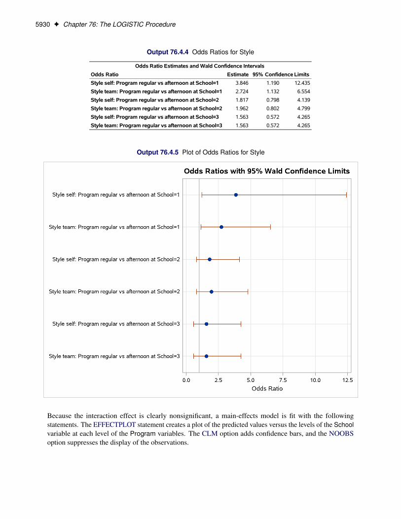
5930 F Chapter 76: The LOGISTIC Procedure
Output 76.4.4 Odds Ratios for Style
Odds Ratio Estimates and Wald Confidence Intervals
Odds Ratio Estimate 95% Confidence Limits
Style self: Program regular vs afternoon at School=1 3.846 1.190 12.435
Style team: Program regular vs afternoon at School=1 2.724 1.132 6.554
Style self: Program regular vs afternoon at School=2 1.817 0.798 4.139
Style team: Program regular vs afternoon at School=2 1.962 0.802 4.799
Style self: Program regular vs afternoon at School=3 1.563 0.572 4.265
Style team: Program regular vs afternoon at School=3 1.563 0.572 4.265
Output 76.4.5 Plot of Odds Ratios for Style
Because the interaction effect is clearly nonsignificant, a main-effects model is fit with the followingstatements. The EFFECTPLOT statement creates a plot of the predicted values versus the levels of the Schoolvariable at each level of the Program variables. The CLM option adds confidence bars, and the NOOBSoption suppresses the display of the observations.

Example 76.4: Nominal Response Data: Generalized Logits Model F 5931
proc logistic data=school;freq Count;class School Program(ref=first);model Style(order=data)=School Program / link=glogit;effectplot interaction(plotby=Program) / clm noobs;
run;
All of the global fit tests in Output 76.4.6 suggest the model is significant, and the Type 3 tests show that theschool and program effects are also significant.
Output 76.4.6 Analysis of Main-Effects Model
The LOGISTIC Procedure
Model Convergence Status
Convergence criterion (GCONV=1E-8) satisfied.
Model Fit Statistics
CriterionIntercept
Only
Interceptand
Covariates
AIC 699.404 682.934
SC 707.050 713.518
-2 Log L 695.404 666.934
Testing Global Null Hypothesis: BETA=0
Test Chi-Square DF Pr > ChiSq
Likelihood Ratio 28.4704 6 <.0001
Score 27.1190 6 0.0001
Wald 25.5881 6 0.0003
Type 3 Analysis of Effects
Effect DFWald
Chi-Square Pr > ChiSq
School 4 14.8424 0.0050
Program 2 10.9160 0.0043
The parameter estimates, tests for individual parameters, and odds ratios are displayed in Output 76.4.7. TheProgram variable has nearly the same effect on both logits, while School=1 has the largest effect of theschools.

5932 F Chapter 76: The LOGISTIC Procedure
Output 76.4.7 Estimates
Analysis of Maximum Likelihood Estimates
Parameter Style DF EstimateStandard
ErrorWald
Chi-Square Pr > ChiSq
Intercept self 1 -0.7978 0.1465 29.6502 <.0001
Intercept team 1 -0.6589 0.1367 23.2300 <.0001
School 1 self 1 -0.7992 0.2198 13.2241 0.0003
School 1 team 1 -0.2786 0.1867 2.2269 0.1356
School 2 self 1 0.2836 0.1899 2.2316 0.1352
School 2 team 1 -0.0985 0.1892 0.2708 0.6028
Program regular self 1 0.3737 0.1410 7.0272 0.0080
Program regular team 1 0.3713 0.1353 7.5332 0.0061
Odds Ratio Estimates
Effect StylePoint
Estimate95% Wald
Confidence Limits
School 1 vs 3 self 0.269 0.127 0.570
School 1 vs 3 team 0.519 0.267 1.010
School 2 vs 3 self 0.793 0.413 1.522
School 2 vs 3 team 0.622 0.317 1.219
Program regular vs afternoon self 2.112 1.215 3.670
Program regular vs afternoon team 2.101 1.237 3.571
The interaction plots in Output 76.4.8 show that School=1 and Program=afternoon have a preference forthe traditional classroom style. Of course, because these are not simultaneous confidence intervals, thenonoverlapping 95% confidence limits do not take the place of an actual test.

Example 76.5: Stratified Sampling F 5933
Output 76.4.8 Model-Predicted Probabilities
Example 76.5: Stratified SamplingConsider the hypothetical example in Fleiss (1981, pp. 6–7), in which a test is applied to a sample of 1,000people known to have a disease and to another sample of 1,000 people known not to have the same disease.In the diseased sample, 950 test positive; in the nondiseased sample, only 10 test positive. If the true diseaserate in the population is 1 in 100, specifying PEVENT=0.01 results in the correct positive and negativepredictive values for the stratified sampling scheme. Omitting the PEVENT= option is equivalent to usingthe overall sample disease rate (1000/2000 = 0.5) as the value of the PEVENT= option, which would ignorethe stratified sampling.

5934 F Chapter 76: The LOGISTIC Procedure
The statements to create the data set and perform the analysis are as follows:
data Screen;do Disease='Present','Absent';
do Test=1,0;input Count @@;output;
end;end;datalines;
950 5010 990
;
proc logistic data=Screen;freq Count;model Disease(event='Present')=Test
/ pevent=.5 .01 ctable pprob=.5;run;
The response variable option EVENT= indicates that Disease=’Present’ is the event. The CTABLE option isspecified to produce a classification table. Specifying PPROB=0.5 indicates a cutoff probability of 0.5. Alist of two probabilities, 0.5 and 0.01, is specified for the PEVENT= option; 0.5 corresponds to the overallsample disease rate, and 0.01 corresponds to a true disease rate of 1 in 100.
The classification table is shown in Output 76.5.1.
Output 76.5.1 Positive and Negative Predictive Values
The LOGISTIC Procedure
Classification Table
Correct Incorrect Percentages
ProbEvent
ProbLevel Event
Non-Event Event
Non-Event Correct
Sensi-tivity
Speci-ficity
PosPred
NegPred
0.500 0.500 950 990 10 50 97.0 95.0 99.0 99.0 95.2
0.010 0.500 950 990 10 50 99.0 95.0 99.0 49.0 99.9
In the classification table, the column “Prob Level” represents the cutoff values (the settings of the PPROB=option) for predicting whether an observation is an event. The “Correct” columns list the numbers of subjectsthat are correctly predicted as events and nonevents, respectively, and the “Incorrect” columns list the numberof nonevents incorrectly predicted as events and the number of events incorrectly predicted as nonevents,respectively. For PEVENT=0.5, the positive predictive value is 99% and the negative predictive value is95.2%. These results ignore the fact that the samples were stratified and incorrectly assume that the overallsample proportion of disease (which is 0.5) estimates the true disease rate. For a true disease rate of 0.01, thepositive and negative predictive values are 49% and 99.9%, respectively, as shown in the second line of theclassification table.

Example 76.6: Logistic Regression Diagnostics F 5935
Example 76.6: Logistic Regression DiagnosticsIn a controlled experiment to study the effect of the rate and volume of air intake on a transient reflexvasoconstriction in the skin of the digits, 39 tests under various combinations of rate and volume of airintake were obtained (Finney 1947). The endpoint of each test is whether or not vasoconstriction occurred.Pregibon (1981) uses this set of data to illustrate the diagnostic measures he proposes for detecting influentialobservations and to quantify their effects on various aspects of the maximum likelihood fit.
The vasoconstriction data are saved in the data set vaso:
data vaso;length Response $12;input Volume Rate Response @@;LogVolume=log(Volume);LogRate=log(Rate);datalines;
3.70 0.825 constrict 3.50 1.09 constrict1.25 2.50 constrict 0.75 1.50 constrict0.80 3.20 constrict 0.70 3.50 constrict0.60 0.75 no_constrict 1.10 1.70 no_constrict0.90 0.75 no_constrict 0.90 0.45 no_constrict0.80 0.57 no_constrict 0.55 2.75 no_constrict0.60 3.00 no_constrict 1.40 2.33 constrict0.75 3.75 constrict 2.30 1.64 constrict3.20 1.60 constrict 0.85 1.415 constrict1.70 1.06 no_constrict 1.80 1.80 constrict0.40 2.00 no_constrict 0.95 1.36 no_constrict1.35 1.35 no_constrict 1.50 1.36 no_constrict1.60 1.78 constrict 0.60 1.50 no_constrict1.80 1.50 constrict 0.95 1.90 no_constrict1.90 0.95 constrict 1.60 0.40 no_constrict2.70 0.75 constrict 2.35 0.03 no_constrict1.10 1.83 no_constrict 1.10 2.20 constrict1.20 2.00 constrict 0.80 3.33 constrict0.95 1.90 no_constrict 0.75 1.90 no_constrict1.30 1.625 constrict;
In the data set vaso, the variable Response represents the outcome of a test. The variable LogVolumerepresents the log of the volume of air intake, and the variable LogRate represents the log of the rate of airintake.
The following statements invoke PROC LOGISTIC to fit a logistic regression model to the vasoconstrictiondata, where Response is the response variable, and LogRate and LogVolume are the explanatory variables.Regression diagnostics are displayed when ODS Graphics is enabled, and the INFLUENCE option is specifiedto display a table of the regression diagnostics.
ods graphics on;title 'Occurrence of Vasoconstriction';proc logistic data=vaso;
model Response=LogRate LogVolume/influence;run;

5936 F Chapter 76: The LOGISTIC Procedure
Results of the model fit are shown in Output 76.6.1. Both LogRate and LogVolume are statistically significantto the occurrence of vasoconstriction (p = 0.0131 and p = 0.0055, respectively). Their positive parameterestimates indicate that a higher inspiration rate or a larger volume of air intake is likely to increase theprobability of vasoconstriction.
Output 76.6.1 Logistic Regression Analysis for Vasoconstriction Data
Occurrence of Vasoconstriction
The LOGISTIC Procedure
Model Information
Data Set WORK.VASO
Response Variable Response
Number of Response Levels 2
Model binary logit
Optimization Technique Fisher's scoring
Number of Observations Read 39
Number of Observations Used 39
Response Profile
OrderedValue Response
TotalFrequency
1 constrict 20
2 no_constrict 19
Probability modeled is Response='constrict'.
Model Convergence Status
Convergence criterion (GCONV=1E-8) satisfied.
Model Fit Statistics
CriterionIntercept
Only
Interceptand
Covariates
AIC 56.040 35.227
SC 57.703 40.218
-2 Log L 54.040 29.227
Testing Global Null Hypothesis: BETA=0
Test Chi-Square DF Pr > ChiSq
Likelihood Ratio 24.8125 2 <.0001
Score 16.6324 2 0.0002
Wald 7.8876 2 0.0194
Analysis of Maximum Likelihood Estimates
Parameter DF EstimateStandard
ErrorWald
Chi-Square Pr > ChiSq
Intercept 1 -2.8754 1.3208 4.7395 0.0295
LogRate 1 4.5617 1.8380 6.1597 0.0131
LogVolume 1 5.1793 1.8648 7.7136 0.0055

Example 76.6: Logistic Regression Diagnostics F 5937
Output 76.6.1 continued
Odds Ratio Estimates
EffectPoint
Estimate95% Wald
Confidence Limits
LogRate 95.744 2.610 >999.999
LogVolume 177.562 4.592 >999.999
Association of Predicted Probabilities andObserved Responses
Percent Concordant 93.7 Somers' D 0.874
Percent Discordant 6.3 Gamma 0.874
Percent Tied 0.0 Tau-a 0.448
Pairs 380 c 0.937
The INFLUENCE option displays the values of the explanatory variables (LogRate and LogVolume) foreach observation, a column for each diagnostic produced, and the case number that represents the sequencenumber of the observation (Output 76.6.2).

5938 F Chapter 76: The LOGISTIC Procedure
Output 76.6.2 Regression Diagnostics from the INFLUENCE Option
Regression Diagnostics
Covariates
CaseNumber LogRate LogVolume
PearsonResidual
DevianceResidual
HatMatrix
DiagonalIntercept
DfBetaLogRate
DfBetaLogVolume
DfBeta
ConfidenceInterval
DisplacementC
ConfidenceInterval
DisplacementCBar
DeltaDeviance
DeltaChi-Square
1 -0.1924 1.3083 0.2205 0.3082 0.0927 -0.0165 0.0193 0.0556 0.00548 0.00497 0.1000 0.0536
2 0.0862 1.2528 0.1349 0.1899 0.0429 -0.0134 0.0151 0.0261 0.000853 0.000816 0.0369 0.0190
3 0.9163 0.2231 0.2923 0.4049 0.0612 -0.0492 0.0660 0.0589 0.00593 0.00557 0.1695 0.0910
4 0.4055 -0.2877 3.5181 2.2775 0.0867 1.0734 -0.9302 -1.0180 1.2873 1.1756 6.3626 13.5523
5 1.1632 -0.2231 0.5287 0.7021 0.1158 -0.0832 0.1411 0.0583 0.0414 0.0366 0.5296 0.3161
6 1.2528 -0.3567 0.6090 0.7943 0.1524 -0.0922 0.1710 0.0381 0.0787 0.0667 0.6976 0.4376
7 -0.2877 -0.5108 -0.0328 -0.0464 0.00761 -0.00280 0.00274 0.00265 8.321E-6 8.258E-6 0.00216 0.00109
8 0.5306 0.0953 -1.0196 -1.1939 0.0559 -0.1444 0.0613 0.0570 0.0652 0.0616 1.4870 1.1011
9 -0.2877 -0.1054 -0.0938 -0.1323 0.0342 -0.0178 0.0173 0.0153 0.000322 0.000311 0.0178 0.00911
10 -0.7985 -0.1054 -0.0293 -0.0414 0.00721 -0.00245 0.00246 0.00211 6.256E-6 6.211E-6 0.00172 0.000862
11 -0.5621 -0.2231 -0.0370 -0.0523 0.00969 -0.00361 0.00358 0.00319 0.000014 0.000013 0.00274 0.00138
12 1.0116 -0.5978 -0.5073 -0.6768 0.1481 -0.1173 0.0647 0.1651 0.0525 0.0447 0.5028 0.3021
13 1.0986 -0.5108 -0.7751 -0.9700 0.1628 -0.0931 -0.00946 0.1775 0.1395 0.1168 1.0577 0.7175
14 0.8459 0.3365 0.2559 0.3562 0.0551 -0.0414 0.0538 0.0527 0.00404 0.00382 0.1307 0.0693
15 1.3218 -0.2877 0.4352 0.5890 0.1336 -0.0940 0.1408 0.0643 0.0337 0.0292 0.3761 0.2186
16 0.4947 0.8329 0.1576 0.2215 0.0402 -0.0198 0.0234 0.0307 0.00108 0.00104 0.0501 0.0259
17 0.4700 1.1632 0.0709 0.1001 0.0172 -0.00630 0.00701 0.00914 0.000089 0.000088 0.0101 0.00511
18 0.3471 -0.1625 2.9062 2.1192 0.0954 0.9595 -0.8279 -0.8477 0.9845 0.8906 5.3817 9.3363
19 0.0583 0.5306 -1.0718 -1.2368 0.1315 -0.2591 0.2024 -0.00488 0.2003 0.1740 1.7037 1.3227
20 0.5878 0.5878 0.2405 0.3353 0.0525 -0.0331 0.0421 0.0518 0.00338 0.00320 0.1156 0.0610
21 0.6931 -0.9163 -0.1076 -0.1517 0.0373 -0.0180 0.0158 0.0208 0.000465 0.000448 0.0235 0.0120
22 0.3075 -0.0513 -0.4193 -0.5691 0.1015 -0.1449 0.1237 0.1179 0.0221 0.0199 0.3437 0.1956
23 0.3001 0.3001 -1.0242 -1.1978 0.0761 -0.1961 0.1275 0.0357 0.0935 0.0864 1.5212 1.1355
24 0.3075 0.4055 -1.3684 -1.4527 0.0717 -0.1281 0.0410 -0.1004 0.1558 0.1447 2.2550 2.0171
25 0.5766 0.4700 0.3347 0.4608 0.0587 -0.0403 0.0570 0.0708 0.00741 0.00698 0.2193 0.1190
26 0.4055 -0.5108 -0.1595 -0.2241 0.0548 -0.0366 0.0329 0.0373 0.00156 0.00147 0.0517 0.0269
27 0.4055 0.5878 0.3645 0.4995 0.0661 -0.0327 0.0496 0.0788 0.0101 0.00941 0.2589 0.1423
28 0.6419 -0.0513 -0.8989 -1.0883 0.0647 -0.1423 0.0617 0.1025 0.0597 0.0559 1.2404 0.8639
29 -0.0513 0.6419 0.8981 1.0876 0.1682 0.2367 -0.1950 0.0286 0.1961 0.1631 1.3460 0.9697
30 -0.9163 0.4700 -0.0992 -0.1400 0.0507 -0.0224 0.0227 0.0159 0.000554 0.000526 0.0201 0.0104
31 -0.2877 0.9933 0.6198 0.8064 0.2459 0.1165 -0.0996 0.1322 0.1661 0.1253 0.7755 0.5095
32 -3.5066 0.8544 -0.00073 -0.00103 0.000022 -3.22E-6 3.405E-6 2.48E-6 1.18E-11 1.18E-11 1.065E-6 5.324E-7
33 0.6043 0.0953 -1.2062 -1.3402 0.0510 -0.0882 -0.0137 -0.00216 0.0824 0.0782 1.8744 1.5331
34 0.7885 0.0953 0.5447 0.7209 0.0601 -0.0425 0.0877 0.0671 0.0202 0.0190 0.5387 0.3157
35 0.6931 0.1823 0.5404 0.7159 0.0552 -0.0340 0.0755 0.0711 0.0180 0.0170 0.5295 0.3091
36 1.2030 -0.2231 0.4828 0.6473 0.1177 -0.0867 0.1381 0.0631 0.0352 0.0311 0.4501 0.2641
37 0.6419 -0.0513 -0.8989 -1.0883 0.0647 -0.1423 0.0617 0.1025 0.0597 0.0559 1.2404 0.8639
38 0.6419 -0.2877 -0.4874 -0.6529 0.1000 -0.1395 0.1032 0.1397 0.0293 0.0264 0.4526 0.2639
39 0.4855 0.2624 0.7053 0.8987 0.0531 0.0326 0.0190 0.0489 0.0295 0.0279 0.8355 0.5254

Example 76.6: Logistic Regression Diagnostics F 5939
Because ODS Graphics is enabled, influence plots are displayed in Outputs 76.6.3 through 76.6.5. For generalinformation about ODS Graphics, see Chapter 21, “Statistical Graphics Using ODS.” For specific informationabout the graphics available in the LOGISTIC procedure, see the section “ODS Graphics” on page 5896.The vertical axis of an index plot represents the value of the diagnostic, and the horizontal axis represents thesequence (case number) of the observation. The index plots are useful for identification of extreme values.
The index plots of the Pearson residuals and the deviance residuals (Output 76.6.3) indicate that case 4 andcase 18 are poorly accounted for by the model. The index plot of the diagonal elements of the hat matrix(Output 76.6.3) suggests that case 31 is an extreme point in the design space. The index plots of DFBETAS(Output 76.6.5) indicate that case 4 and case 18 are causing instability in all three parameter estimates. Theother four index plots in Outputs 76.6.3 and 76.6.4 also point to these two cases as having a large impact onthe coefficients and goodness of fit.
Output 76.6.3 Residuals, Hat Matrix, and CI Displacement C

5940 F Chapter 76: The LOGISTIC Procedure
Output 76.6.4 CI Displacement CBar, Change in Deviance and Pearson Chi-Square
Output 76.6.5 DFBETAS Plots

Example 76.6: Logistic Regression Diagnostics F 5941
Other versions of diagnostic plots can be requested by specifying the appropriate options in the PLOTS=option. For example, the following statements produce three other sets of influence diagnostic plots: thePHAT option plots several diagnostics against the predicted probabilities (Output 76.6.6), the LEVERAGEoption plots several diagnostics against the leverage (Output 76.6.7), and the DPC option plots the deletiondiagnostics against the predicted probabilities and colors the observations according to the confidence intervaldisplacement diagnostic (Output 76.6.8). The LABEL option displays the observation numbers on the plots.In all plots, you are looking for the outlying observations, and again cases 4 and 18 are noted.
proc logistic data=vaso plots(only label)=(phat leverage dpc);model Response=LogRate LogVolume;
run;
Output 76.6.6 Diagnostics versus Predicted Probability

5942 F Chapter 76: The LOGISTIC Procedure
Output 76.6.7 Diagnostics versus Leverage
Output 76.6.8 Three Diagnostics

Example 76.7: ROC Curve . . . and Confidence Limits F 5943
Example 76.7: ROC Curve, Customized Odds Ratios, Goodness-of-FitStatistics, R-Square, and Confidence Limits
This example plots an ROC curve, estimates a customized odds ratio, produces the traditional goodness-of-fitanalysis, displays the generalized R-square measures for the fitted model, calculates the normal confidenceintervals for the regression parameters, and produces a display of the probability function and predictioncurves for the fitted model. The data consist of three variables: n (number of subjects in the sample), disease(number of diseased subjects in the sample), and age (age for the sample). A linear logistic regression modelis used to study the effect of age on the probability of contracting the disease. The statements to produce thedata set and perform the analysis are as follows:
data Data1;input disease n age;datalines;
0 14 250 20 350 19 457 18 556 12 65
17 17 75;
ods graphics on;%let _ROC_XAXISOPTS_LABEL=False Positive Fraction;%let _ROC_YAXISOPTS_LABEL=True Positive Fraction;proc logistic data=Data1 plots(only)=roc(id=obs);
model disease/n=age / scale=noneclparm=waldclodds=plrsquare;
units age=10;effectplot;
run;%symdel _ROC_XAXISOPTS_LABEL _ROC_YAXISOPTS_LABEL;
The option SCALE=NONE is specified to produce the deviance and Pearson goodness-of-fit analysis withoutadjusting for overdispersion. The RSQUARE option is specified to produce generalized R-square measuresof the fitted model. The CLPARM=WALD option is specified to produce the Wald confidence intervals forthe regression parameters. The UNITS statement is specified to produce customized odds ratio estimates for achange of 10 years in the age variable, and the CLODDS=PL option is specified to produce profile-likelihoodconfidence limits for the odds ratio. The PLOTS= option with ODS Graphics enabled produces a graphicaldisplay of the ROC curve, the two macro variables modify the ROC axis labels, and the EFFECTPLOTstatement displays the model fit.
The results in Output 76.7.1 show that the deviance and Pearson statistics indicate no lack of fit in the model.

5944 F Chapter 76: The LOGISTIC Procedure
Output 76.7.1 Deviance and Pearson Goodness-of-Fit Analysis
The LOGISTIC Procedure
Deviance and Pearson Goodness-of-FitStatistics
Criterion Value DF Value/DF Pr > ChiSq
Deviance 7.7756 4 1.9439 0.1002
Pearson 6.6020 4 1.6505 0.1585
Number of events/trials observations: 6
Output 76.7.2 shows that the R-square for the model is 0.74. The odds of an event increases by a factor of7.9 for each 10-year increase in age.
Output 76.7.2 R-Square, Confidence Intervals, and Customized Odds Ratio
Model Fit Statistics
Intercept andCovariates
CriterionIntercept
OnlyLog
LikelihoodFull Log
Likelihood
AIC 124.173 52.468 18.075
SC 126.778 57.678 23.285
-2 Log L 122.173 48.468 14.075
R-Square 0.5215 Max-rescaled R-Square 0.8925
Testing Global Null Hypothesis: BETA=0
Test Chi-Square DF Pr > ChiSq
Likelihood Ratio 73.7048 1 <.0001
Score 55.3274 1 <.0001
Wald 23.3475 1 <.0001
Analysis of Maximum Likelihood Estimates
Parameter DF EstimateStandard
ErrorWald
Chi-Square Pr > ChiSq
Intercept 1 -12.5016 2.5555 23.9317 <.0001
age 1 0.2066 0.0428 23.3475 <.0001
Association of Predicted Probabilities andObserved Responses
Percent Concordant 92.6 Somers' D 0.906
Percent Discordant 2.0 Gamma 0.958
Percent Tied 5.4 Tau-a 0.384
Pairs 2100 c 0.953
Parameter Estimates and Wald ConfidenceIntervals
Parameter Estimate 95% Confidence Limits
Intercept -12.5016 -17.5104 -7.4929
age 0.2066 0.1228 0.2904

Example 76.7: ROC Curve . . . and Confidence Limits F 5945
Output 76.7.2 continued
Odds Ratio Estimates and Profile-LikelihoodConfidence Intervals
Effect Unit Estimate 95% Confidence Limits
age 10.0000 7.892 3.881 21.406
Because ODS Graphics is enabled, a graphical display of the ROC curve is produced as shown in Out-put 76.7.3.
Output 76.7.3 Receiver Operating Characteristic Curve
Note that the area under the ROC curve is estimated by the statistic c in the “Association of PredictedProbabilities and Observed Responses” table. In this example, the area under the ROC curve is 0.953. Bydefault, the Y axis is labeled “Sensitivity” and the X axis is labeled “1–Specificity”.
Because there is only one continuous covariate and because ODS Graphics is enabled, the EFFECTPLOTstatement produces a graphical display of the predicted probability curve with bounding 95% confidencelimits as shown in Output 76.7.4.

5946 F Chapter 76: The LOGISTIC Procedure
Output 76.7.4 Predicted Probability and 95% Prediction Limits
Example 76.8: Comparing Receiver Operating Characteristic CurvesDeLong, DeLong, and Clarke-Pearson (1988) report on 49 patients with ovarian cancer who also suffer froman intestinal obstruction. Three (correlated) screening tests are measured to determine whether a patient willbenefit from surgery. The three tests are the K-G score and two measures of nutritional status: total proteinand albumin. The data are as follows:
data roc;input alb tp totscore popind @@;totscore = 10 - totscore;datalines;
3.0 5.8 10 0 3.2 6.3 5 1 3.9 6.8 3 1 2.8 4.8 6 03.2 5.8 3 1 0.9 4.0 5 0 2.5 5.7 8 0 1.6 5.6 5 13.8 5.7 5 1 3.7 6.7 6 1 3.2 5.4 4 1 3.8 6.6 6 14.1 6.6 5 1 3.6 5.7 5 1 4.3 7.0 4 1 3.6 6.7 4 02.3 4.4 6 1 4.2 7.6 4 0 4.0 6.6 6 0 3.5 5.8 6 13.8 6.8 7 1 3.0 4.7 8 0 4.5 7.4 5 1 3.7 7.4 5 13.1 6.6 6 1 4.1 8.2 6 1 4.3 7.0 5 1 4.3 6.5 4 13.2 5.1 5 1 2.6 4.7 6 1 3.3 6.8 6 0 1.7 4.0 7 0

Example 76.8: Comparing Receiver Operating Characteristic Curves F 5947
3.7 6.1 5 1 3.3 6.3 7 1 4.2 7.7 6 1 3.5 6.2 5 12.9 5.7 9 0 2.1 4.8 7 1 2.8 6.2 8 0 4.0 7.0 7 13.3 5.7 6 1 3.7 6.9 5 1 3.6 6.6 5 1;
In the following statements, the NOFIT option is specified in the MODEL statement to prevent PROCLOGISTIC from fitting the model with three covariates. Each ROC statement lists one of the covariates, andPROC LOGISTIC then fits the model with that single covariate. Note that the original data set contains sixmore records with missing values for one of the tests, but PROC LOGISTIC ignores all records with missingvalues; hence there is a common sample size for each of the three models. The ROCCONTRAST statementimplements the nonparametric approach of DeLong, DeLong, and Clarke-Pearson (1988) to compare thethree ROC curves, the REFERENCE option specifies that the K-G Score curve is used as the reference curvein the contrast, the E option displays the contrast coefficients, and the ESTIMATE option computes andtests each comparison. With ODS Graphics enabled, the plots=roc(id=prob) specification in the PROCLOGISTIC statement displays several plots, and the plots of individual ROC curves have certain pointslabeled with their predicted probabilities.
ods graphics on;proc logistic data=roc plots=roc(id=prob);
model popind(event='0') = alb tp totscore / nofit;roc 'Albumin' alb;roc 'K-G Score' totscore;roc 'Total Protein' tp;roccontrast reference('K-G Score') / estimate e;
run;
The initial model information is displayed in Output 76.8.1.
Output 76.8.1 Initial LOGISTIC Output
The LOGISTIC Procedure
Model Information
Data Set WORK.ROC
Response Variable popind
Number of Response Levels 2
Model binary logit
Optimization Technique Fisher's scoring
Number of Observations Read 43
Number of Observations Used 43
Response Profile
OrderedValue popind
TotalFrequency
1 0 12
2 1 31
Probability modeled is popind=0.
Score Test for Global NullHypothesis
Chi-Square DF Pr > ChiSq
10.7939 3 0.0129

5948 F Chapter 76: The LOGISTIC Procedure
For each ROC model, the model fitting details in Outputs 76.8.2, 76.8.4, and 76.8.6 can be suppressed withthe ROCOPTIONS(NODETAILS) option; however, the convergence status is always displayed.
The ROC curves for the three models are displayed in Outputs 76.8.3, 76.8.5, and 76.8.7. Note that the labelson the ROC curve are produced by specifying the ID=PROB option, and are the predicted probabilities forthe cutpoints.
Output 76.8.2 Fit Tables for Popind=Alb
Model Convergence Status
Convergence criterion (GCONV=1E-8) satisfied.
Model Fit Statistics
CriterionIntercept
Only
Interceptand
Covariates
AIC 52.918 49.384
SC 54.679 52.907
-2 Log L 50.918 45.384
Testing Global Null Hypothesis: BETA=0
Test Chi-Square DF Pr > ChiSq
Likelihood Ratio 5.5339 1 0.0187
Score 5.6893 1 0.0171
Wald 4.6869 1 0.0304
Analysis of Maximum Likelihood Estimates
Parameter DF EstimateStandard
ErrorWald
Chi-Square Pr > ChiSq
Intercept 1 2.4646 1.5913 2.3988 0.1214
alb 1 -1.0520 0.4859 4.6869 0.0304
Odds Ratio Estimates
EffectPoint
Estimate95% Wald
Confidence Limits
alb 0.349 0.135 0.905

Example 76.8: Comparing Receiver Operating Characteristic Curves F 5949
Output 76.8.3 ROC Curve for Popind=Alb
Output 76.8.4 Fit Tables for Popind=Totscore
Model Convergence Status
Convergence criterion (GCONV=1E-8) satisfied.
Model Fit Statistics
CriterionIntercept
Only
Interceptand
Covariates
AIC 52.918 46.262
SC 54.679 49.784
-2 Log L 50.918 42.262
Testing Global Null Hypothesis: BETA=0
Test Chi-Square DF Pr > ChiSq
Likelihood Ratio 8.6567 1 0.0033
Score 8.3613 1 0.0038
Wald 6.3845 1 0.0115

5950 F Chapter 76: The LOGISTIC Procedure
Output 76.8.4 continued
Analysis of Maximum Likelihood Estimates
Parameter DF EstimateStandard
ErrorWald
Chi-Square Pr > ChiSq
Intercept 1 2.1542 1.2477 2.9808 0.0843
totscore 1 -0.7696 0.3046 6.3845 0.0115
Odds Ratio Estimates
EffectPoint
Estimate95% Wald
Confidence Limits
totscore 0.463 0.255 0.841
Output 76.8.5 ROC Curve for Popind=Totscore

Example 76.8: Comparing Receiver Operating Characteristic Curves F 5951
Output 76.8.6 Fit Tables for Popind=Tp
Model Convergence Status
Convergence criterion (GCONV=1E-8) satisfied.
Model Fit Statistics
CriterionIntercept
Only
Interceptand
Covariates
AIC 52.918 51.794
SC 54.679 55.316
-2 Log L 50.918 47.794
Testing Global Null Hypothesis: BETA=0
Test Chi-Square DF Pr > ChiSq
Likelihood Ratio 3.1244 1 0.0771
Score 3.1123 1 0.0777
Wald 2.9059 1 0.0883
Analysis of Maximum Likelihood Estimates
Parameter DF EstimateStandard
ErrorWald
Chi-Square Pr > ChiSq
Intercept 1 2.8295 2.2065 1.6445 0.1997
tp 1 -0.6279 0.3683 2.9059 0.0883
Odds Ratio Estimates
EffectPoint
Estimate95% Wald
Confidence Limits
tp 0.534 0.259 1.099

5952 F Chapter 76: The LOGISTIC Procedure
Output 76.8.7 ROC Curve for Popind=Tp
All ROC curves being compared are also overlaid on the same plot, as shown in Output 76.8.8.

Example 76.8: Comparing Receiver Operating Characteristic Curves F 5953
Output 76.8.8 Overlay of All Models Being Compared
Output 76.8.9 displays the association statistics, and displays the area under the ROC curve along with itsstandard error and a confidence interval for each model in the comparison. The confidence interval for TotalProtein contains 0.50; hence it is not significantly different from random guessing, which is represented bythe diagonal line in the preceding ROC plots.
Output 76.8.9 ROC Association Table
ROC Association Statistics
Mann-Whitney
ROC Model AreaStandard
Error95% Wald
Confidence Limits Somers' D Gamma Tau-a
Albumin 0.7366 0.0927 0.5549 0.9182 0.4731 0.4809 0.1949
K-G Score 0.7258 0.1028 0.5243 0.9273 0.4516 0.5217 0.1860
Total Protein 0.6478 0.1000 0.4518 0.8439 0.2957 0.3107 0.1218
Output 76.8.10 shows that the contrast used ’K-G Score’ as the reference level. This table is produced byspecifying the E option in the ROCCONTRAST statement.

5954 F Chapter 76: The LOGISTIC Procedure
Output 76.8.10 ROC Contrast Coefficients
ROC ContrastCoefficients
ROC Model Row1 Row2
Albumin 1 0
K-G Score -1 -1
Total Protein 0 1
Output 76.8.11 shows that the 2-degrees-of-freedom test that the ’K-G Score’ is different from at least oneother test is not significant at the 0.05 level.
Output 76.8.11 ROC Test Results (2 Degrees of Freedom)
ROC Contrast Test Results
Contrast DF Chi-Square Pr > ChiSq
Reference = K-G Score 2 2.5340 0.2817
Output 76.8.12 is produced by specifying the ESTIMATE option in the ROCCONTRAST statement. Eachrow shows that the curves are not significantly different.
Output 76.8.12 ROC Contrast Row Estimates (1-Degree-of-Freedom Tests)
ROC Contrast Estimation and Testing Results by Row
Contrast EstimateStandard
Error95% Wald
Confidence Limits Chi-Square Pr > ChiSq
Albumin - K-G Score 0.0108 0.0953 -0.1761 0.1976 0.0127 0.9102
Total Protein - K-G Score -0.0780 0.1046 -0.2830 0.1271 0.5554 0.4561
Example 76.9: Goodness-of-Fit Tests and SubpopulationsA study is done to investigate the effects of two binary factors, A and B, on a binary response, Y. Subjects arerandomly selected from subpopulations defined by the four possible combinations of levels of A and B. Thenumber of subjects responding with each level of Y is recorded, and the following DATA step creates the dataset One:
data One;do A=0,1;
do B=0,1;do Y=1,2;
input F @@;output;
end;end;
end;datalines;
23 63 31 70 67 100 70 104;

Example 76.9: Goodness-of-Fit Tests and Subpopulations F 5955
The following statements fit a full model to examine the main effects of A and B as well as the interactioneffect of A and B:
proc logistic data=One;freq F;model Y=A B A*B;
run;
Results of the model fit are shown in Output 76.9.1. Notice that neither the A*B interaction nor the B maineffect is significant.
Output 76.9.1 Full Model Fit
The LOGISTIC Procedure
Model Information
Data Set WORK.ONE
Response Variable Y
Number of Response Levels 2
Frequency Variable F
Model binary logit
Optimization Technique Fisher's scoring
Number of Observations Read 8
Number of Observations Used 8
Sum of Frequencies Read 528
Sum of Frequencies Used 528
Response Profile
OrderedValue Y
TotalFrequency
1 1 191
2 2 337
Probability modeled is Y=1.
Model Convergence Status
Convergence criterion (GCONV=1E-8) satisfied.
Model Fit Statistics
CriterionIntercept
Only
Interceptand
Covariates
AIC 693.061 691.914
SC 697.330 708.990
-2 Log L 691.061 683.914
Testing Global Null Hypothesis: BETA=0
Test Chi-Square DF Pr > ChiSq
Likelihood Ratio 7.1478 3 0.0673
Score 6.9921 3 0.0721
Wald 6.9118 3 0.0748

5956 F Chapter 76: The LOGISTIC Procedure
Output 76.9.1 continued
Analysis of Maximum Likelihood Estimates
Parameter DF EstimateStandard
ErrorWald
Chi-Square Pr > ChiSq
Intercept 1 -1.0074 0.2436 17.1015 <.0001
A 1 0.6069 0.2903 4.3714 0.0365
B 1 0.1929 0.3254 0.3515 0.5533
A*B 1 -0.1883 0.3933 0.2293 0.6321
Pearson and deviance goodness-of-fit tests cannot be obtained for this model because a full model containingfour parameters is fit, leaving no residual degrees of freedom. For a binary response model, the goodness-of-fit tests have m � q degrees of freedom, where m is the number of subpopulations and q is the number ofmodel parameters. In the preceding model, m D q D 4, resulting in zero degrees of freedom for the tests.
The following statements fit a reduced model containing only the A effect, so two degrees of freedom becomeavailable for testing goodness of fit. Specifying the SCALE=NONE option requests the Pearson and deviancestatistics. With single-trial syntax, the AGGREGATE= option is needed to define the subpopulations in thestudy. Specifying AGGREGATE=(A B) creates subpopulations of the four combinations of levels of A and B.Although the B effect is being dropped from the model, it is still needed to define the original subpopulationsin the study. If AGGREGATE=(A) were specified, only two subpopulations would be created from the levelsof A, resulting in m D q D 2 and zero degrees of freedom for the tests.
proc logistic data=One;freq F;model Y=A / scale=none aggregate=(A B);
run;
The goodness-of-fit tests in Output 76.9.2 show that dropping the B main effect and the A*B interactionsimultaneously does not result in significant lack of fit of the model. The tests’ large p-values indicateinsufficient evidence for rejecting the null hypothesis that the model fits.
Output 76.9.2 Reduced Model Fit
The LOGISTIC Procedure
Deviance and Pearson Goodness-of-FitStatistics
Criterion Value DF Value/DF Pr > ChiSq
Deviance 0.3541 2 0.1770 0.8377
Pearson 0.3531 2 0.1765 0.8382
Number of unique profiles: 4
Example 76.10: OverdispersionIn a seed germination test, seeds of two cultivars were planted in pots of two soil conditions. The followingstatements create the data set seeds, which contains the observed proportion of seeds that germinated forvarious combinations of cultivar and soil condition. The variable n represents the number of seeds planted ina pot, and the variable r represents the number germinated. The indicator variables cult and soil represent thecultivar and soil condition, respectively.

Example 76.10: Overdispersion F 5957
data seeds;input pot n r cult soil;datalines;
1 16 8 0 02 51 26 0 03 45 23 0 04 39 10 0 05 36 9 0 06 81 23 1 07 30 10 1 08 39 17 1 09 28 8 1 0
10 62 23 1 011 51 32 0 112 72 55 0 113 41 22 0 114 12 3 0 115 13 10 0 116 79 46 1 117 30 15 1 118 51 32 1 119 74 53 1 120 56 12 1 1;
PROC LOGISTIC is used as follows to fit a logit model to the data, with cult, soil, and cult � soil interactionas explanatory variables. The option SCALE=NONE is specified to display goodness-of-fit statistics.
proc logistic data=seeds;model r/n=cult soil cult*soil/scale=none;title 'Full Model With SCALE=NONE';
run;
Results of fitting the full factorial model are shown in Output 76.10.1. Both Pearson �2 and deviance arehighly significant (p < 0:0001), suggesting that the model does not fit well.
Output 76.10.1 Results of the Model Fit for the Two-Way Layout
Full Model With SCALE=NONE
The LOGISTIC Procedure
Deviance and Pearson Goodness-of-FitStatistics
Criterion Value DF Value/DF Pr > ChiSq
Deviance 68.3465 16 4.2717 <.0001
Pearson 66.7617 16 4.1726 <.0001
Number of events/trials observations: 20

5958 F Chapter 76: The LOGISTIC Procedure
Output 76.10.1 continued
Model Fit Statistics
Intercept andCovariates
CriterionIntercept
OnlyLog
LikelihoodFull Log
Likelihood
AIC 1256.852 1213.003 156.533
SC 1261.661 1232.240 175.769
-2 Log L 1254.852 1205.003 148.533
Testing Global Null Hypothesis: BETA=0
Test Chi-Square DF Pr > ChiSq
Likelihood Ratio 49.8488 3 <.0001
Score 49.1682 3 <.0001
Wald 47.7623 3 <.0001
Analysis of Maximum Likelihood Estimates
Parameter DF EstimateStandard
ErrorWald
Chi-Square Pr > ChiSq
Intercept 1 -0.3788 0.1489 6.4730 0.0110
cult 1 -0.2956 0.2020 2.1412 0.1434
soil 1 0.9781 0.2128 21.1234 <.0001
cult*soil 1 -0.1239 0.2790 0.1973 0.6569
If the link function and the model specification are correct and if there are no outliers, then the lackof fit might be due to overdispersion. Without adjusting for the overdispersion, the standard errors arelikely to be underestimated, causing the Wald tests to be too sensitive. In PROC LOGISTIC, there arethree SCALE= options to accommodate overdispersion. With unequal sample sizes for the observations,SCALE=WILLIAMS is preferred. The Williams model estimates a scale parameter � by equating the valueof Pearson �2 for the full model to its approximate expected value. The full model considered in the followingstatements is the model with cultivar, soil condition, and their interaction. Using a full model reduces the riskof contaminating � with lack of fit due to incorrect model specification.
proc logistic data=seeds;model r/n=cult soil cult*soil / scale=williams;title 'Full Model With SCALE=WILLIAMS';
run;
Results of using Williams’ method are shown in Output 76.10.2. The estimate of � is 0.075941 and is givenin the formula for the Weight Variable at the beginning of the displayed output.

Example 76.10: Overdispersion F 5959
Output 76.10.2 Williams’ Model for Overdispersion
Full Model With SCALE=WILLIAMS
The LOGISTIC Procedure
Model Information
Data Set WORK.SEEDS
Response Variable (Events) r
Response Variable (Trials) n
Weight Variable 1 / ( 1 + 0.075941 * (n - 1) )
Model binary logit
Optimization Technique Fisher's scoring
Number of Observations Read 20
Number of Observations Used 20
Sum of Frequencies Read 906
Sum of Frequencies Used 906
Sum of Weights Read 198.3216
Sum of Weights Used 198.3216
Response Profile
OrderedValue
BinaryOutcome
TotalFrequency
TotalWeight
1 Event 437 92.95346
2 Nonevent 469 105.36819
Model Convergence Status
Convergence criterion (GCONV=1E-8) satisfied.
Deviance and Pearson Goodness-of-FitStatistics
Criterion Value DF Value/DF Pr > ChiSq
Deviance 16.4402 16 1.0275 0.4227
Pearson 16.0000 16 1.0000 0.4530
Number of events/trials observations: 20
Note: Since the Williams method was used to accommodate overdispersion, the Pearson chi-squared statistic and the deviance canno longer be used to assess the goodness of fit of the model.
Model Fit Statistics
Intercept andCovariates
CriterionIntercept
OnlyLog
LikelihoodFull Log
Likelihood
AIC 276.155 273.586 44.579
SC 280.964 292.822 63.815
-2 Log L 274.155 265.586 36.579

5960 F Chapter 76: The LOGISTIC Procedure
Output 76.10.2 continued
Testing Global Null Hypothesis: BETA=0
Test Chi-Square DF Pr > ChiSq
Likelihood Ratio 8.5687 3 0.0356
Score 8.4856 3 0.0370
Wald 8.3069 3 0.0401
Analysis of Maximum Likelihood Estimates
Parameter DF EstimateStandard
ErrorWald
Chi-Square Pr > ChiSq
Intercept 1 -0.3926 0.2932 1.7932 0.1805
cult 1 -0.2618 0.4160 0.3963 0.5290
soil 1 0.8309 0.4223 3.8704 0.0491
cult*soil 1 -0.0532 0.5835 0.0083 0.9274
Because neither cult nor cult � soil is statistically significant (p = 0.5290 and p = 0.9274, respectively),a reduced model that contains only the soil condition factor is fitted, with the observations weighted by1=.1 C 0:075941.N � 1//. This can be done conveniently in PROC LOGISTIC by including the scaleestimate in the SCALE=WILLIAMS option as follows:
proc logistic data=seeds;model r/n=soil / scale=williams(0.075941);title 'Reduced Model With SCALE=WILLIAMS(0.075941)';
run;
Results of the reduced model fit are shown in Output 76.10.3. Soil condition remains a significant factor (p =0.0064) for the seed germination.
Output 76.10.3 Reduced Model with Overdispersion Controlled
Reduced Model With SCALE=WILLIAMS(0.075941)
The LOGISTIC Procedure
Analysis of Maximum Likelihood Estimates
Parameter DF EstimateStandard
ErrorWald
Chi-Square Pr > ChiSq
Intercept 1 -0.5249 0.2076 6.3949 0.0114
soil 1 0.7910 0.2902 7.4284 0.0064
Example 76.11: Conditional Logistic Regression for Matched Pairs DataIn matched pairs, or case-control, studies, conditional logistic regression is used to investigate the relationshipbetween an outcome of being an event (case) or a nonevent (control) and a set of prognostic factors.
The following data are a subset of the data from the Los Angeles Study of the Endometrial Cancer Datain Breslow and Day (1980). There are 63 matched pairs, each consisting of a case of endometrial cancer(Outcome=1) and a control (Outcome=0). The case and corresponding control have the same ID. Twoprognostic factors are included: Gall (an indicator variable for gall bladder disease) and Hyper (an indicatorvariable for hypertension). The goal of the case-control analysis is to determine the relative risk for gallbladder disease, controlling for the effect of hypertension.

Example 76.11: Conditional Logistic Regression for Matched Pairs Data F 5961
data Data1;do ID=1 to 63;
do Outcome = 1 to 0 by -1;input Gall Hyper @@;output;
end;end;datalines;
0 0 0 0 0 0 0 0 0 1 0 1 0 0 1 0 1 0 0 10 1 0 0 1 0 0 0 1 1 0 1 0 0 0 0 0 0 0 01 0 0 0 0 0 0 1 1 0 0 1 1 0 1 0 1 0 0 10 1 0 0 0 0 1 1 0 0 1 1 0 0 0 1 0 1 0 00 0 1 1 0 1 0 1 0 1 0 0 0 0 0 0 0 0 0 00 0 0 1 1 0 0 1 0 0 0 1 1 0 0 0 0 1 0 00 1 0 0 0 1 0 0 0 1 0 0 0 0 0 0 1 1 1 10 0 0 1 0 1 0 0 0 1 0 1 0 1 0 1 0 1 0 00 0 0 0 0 1 1 0 0 0 0 1 0 0 0 0 1 0 0 00 0 0 0 1 1 0 0 0 1 0 0 0 0 0 0 0 1 0 10 0 0 0 0 1 0 1 0 1 0 0 0 1 0 0 1 0 0 00 0 0 0 1 1 1 0 0 0 0 0 0 0 0 0 1 1 0 01 0 1 0 0 1 0 0 1 0 0 0;
There are several ways to approach this problem with PROC LOGISTIC:
� Specify the STRATA statement to perform a conditional logistic regression.
� Specify EXACT and STRATA statements to perform an exact logistic regression on the original dataset, if you believe the data set is too small or too sparse for the usual asymptotics to hold.
� Transform each matched pair into a single observation, and then specify a PROC LOGISTIC statementon this transformed data without a STRATA statement; this also performs a conditional logisticregression and produces essentially the same results.
� Specify an EXACT statement on the transformed data.
SAS statements and selected results for the first two approaches are given in the remainder of this example.
Conditional Analysis Using the STRATA Statement
In the following statements, PROC LOGISTIC is invoked with the ID variable declared in the STRATAstatement to obtain the conditional logistic model estimates for a model containing Gall as the only predictorvariable:
proc logistic data=Data1;strata ID;model outcome(event='1')=Gall;
run;
Results from the conditional logistic analysis are shown in Output 76.11.1. Note that there is no interceptterm in the “Analysis of Maximum Likelihood Estimates” tables.

5962 F Chapter 76: The LOGISTIC Procedure
The odds ratio estimate for Gall is 2.60, which is marginally significant (p = 0.0694) and which is an estimateof the relative risk for gall bladder disease. A 95% confidence interval for this relative risk is (0.927, 7.293).
Output 76.11.1 Conditional Logistic Regression (Gall as Risk Factor)
The LOGISTIC Procedure
Conditional Analysis
Model Information
Data Set WORK.DATA1
Response Variable Outcome
Number of Response Levels 2
Number of Strata 63
Model binary logit
Optimization Technique Newton-Raphson ridge
Number of Observations Read 126
Number of Observations Used 126
Number of Observations Informative 126
Response Profile
OrderedValue Outcome
TotalFrequency
1 0 63
2 1 63
Probability modeled is Outcome=1.
Strata Summary
Outcome
ResponsePattern 0 1
Number ofStrata Frequency
1 1 1 63 126
Newton-Raphson Ridge Optimization
Without Parameter Scaling
Convergence criterion (GCONV=1E-8) satisfied.
Model Fit Statistics
CriterionWithout
CovariatesWith
Covariates
AIC 87.337 85.654
SC 87.337 88.490
-2 Log L 87.337 83.654
Testing Global Null Hypothesis: BETA=0
Test Chi-Square DF Pr > ChiSq
Likelihood Ratio 3.6830 1 0.0550
Score 3.5556 1 0.0593
Wald 3.2970 1 0.0694

Example 76.11: Conditional Logistic Regression for Matched Pairs Data F 5963
Output 76.11.1 continued
Analysis of Conditional Maximum Likelihood Estimates
Parameter DF EstimateStandard
ErrorWald
Chi-Square Pr > ChiSq
Gall 1 0.9555 0.5262 3.2970 0.0694
Odds Ratio Estimates
EffectPoint
Estimate95% Wald
Confidence Limits
Gall 2.600 0.927 7.293
Exact Analysis Using the STRATA Statement
When you believe there are not enough data or that the data are too sparse, you can perform a stratified exactlogistic regression. The following statements perform stratified exact logistic regressions on the original dataset by specifying both the STRATA and EXACT statements:
proc logistic data=Data1 exactonly;strata ID;model outcome(event='1')=Gall;exact Gall / estimate=both;
run;
Output 76.11.2 Exact Logistic Regression (Gall as Risk Factor)
The LOGISTIC Procedure
Exact Conditional Analysis
Exact Conditional Tests
p-Value
Effect Test Statistic Exact Mid
Gall Score 3.5556 0.0963 0.0799
Probability 0.0327 0.0963 0.0799
Exact Parameter Estimates
Parameter EstimateStandard
Error
95%Confidence
Limits p-Value
Gall 0.9555 0.5262 -0.1394 2.2316 0.0963
Exact Odds Ratios
Parameter Estimate
95%Confidence
Limits p-Value
Gall 2.600 0.870 9.315 0.0963
Note that the score statistic in the “Conditional Exact Tests” table in Output 76.11.2 is identical to the scorestatistic in Output 76.11.1 from the conditional analysis. The exact odds ratio confidence interval is muchwider than its conditional analysis counterpart, but the parameter estimates are similar. The exact analysisconfirms the marginal significance of Gall as a predictor variable.

5964 F Chapter 76: The LOGISTIC Procedure
Example 76.12: Exact Conditional Logistic RegressionThe following data, from Hand et al. (1994), contain the results of a study of 49 anxious or depressed children.The Diagnosis variable indicates whether the child was anxious or depressed when the study began, theFriendships variable indicates whether the child has good friendships, the Total variable represents the totalnumber of children in the study who exhibit the specified values for Diagnosis and Friendships, and theRecovered variable represents the number of children whose mothers believe that their child has recovered atthe end of the study.
data one;length Diagnosis $ 9;input Diagnosis $ Friendships $ Recovered Total @@;datalines;
Anxious Poor 0 0 Anxious Good 13 21Depressed Poor 0 8 Depressed Good 15 20;
Notice that no children in the study are both anxious and have poor friendships and that no children who aredepressed and have poor friendships have recovered. The following statements fit an unconditional logisticregression model to these data.
proc logistic data=one;class Diagnosis Friendships / param=ref;model Recovered/Total = Diagnosis Friendships;
run;
Because the data set has quasi-complete separation, the unconditional logistic regression results are notreliable and Output 76.12.1 is displayed.
Output 76.12.1 Unconditional Logistic Regression Results
The LOGISTIC Procedure
Model Convergence Status
Quasi-complete separation of data points detected.
The sparseness of the data and the separability of the data set make this a good candidate for an exact logisticregression. In the following code, the EXACTONLY option suppresses the unconditional logistic regressionresults, the EXACT statement requests an exact analysis of the two covariates, the OUTDIST= option outputsthe exact distribution into a SAS data set, the JOINT option computes a joint test for the significance of thetwo covariates in the model, and the ESTIMATE option produces parameter estimates for the two covariates.

Example 76.12: Exact Conditional Logistic Regression F 5965
proc logistic data=one exactonly;class Diagnosis Friendships / param=ref;model Recovered/Total = Diagnosis Friendships;exact Diagnosis Friendships
/ outdist=dist joint estimate;run;
proc print data=dist(obs=10);run;
proc print data=dist(firstobs=162 obs=175);run;
proc print data=dist(firstobs=176 obs=184);run;
Tests for the joint significance of the Diagnosis and Friendships covariates are labeled “Joint” in Out-put 76.12.2. Both of these tests reject the null hypothesis that all the parameters are identically zero.
Output 76.12.2 Exact Tests
The LOGISTIC Procedure
Exact Conditional Analysis
Exact Conditional Tests
p-Value
Effect Test Statistic Exact Mid
Joint Score 13.1905 0.0008 0.0008
Probability 0.000081 0.0007 0.0007
Diagnosis Score 0.7915 0.5055 0.4159
Probability 0.1791 0.5055 0.4159
Friendships Score 12.4615 0.0004 0.0002
Probability 0.000414 0.0004 0.0002
In Output 76.12.2, the joint probability statistic (0.000081) is the probability of the observed sufficientstatistics (Friendships=28 and Diagnosis=13) in the joint exact distribution (part of which is displayed inOutput 76.12.3). Note that the joint exact distribution has sufficient statistics displayed for both covariates;the marginal distributions have sufficient statistics displayed for only one covariate. The associated exactp-value (0.0007) in Output 76.12.2 is the sum of the probabilities of all sufficient statistics in the joint exactdistribution that have probabilities less than or equal to 0.000081. The mid-p-value (0.0007) adjusts theexact p-value for the discreteness of the exact distribution by subtracting half the probability of the observedsufficient statistic (Hirji 2006). The score statistic (13.1905) is a weighted distance of the observed sufficientstatistics from the mean sufficient statistics, and the score p-value (0.0008) is the sum of all probabilities inthe Dist data set for sufficient statistics that are no closer to the mean.

5966 F Chapter 76: The LOGISTIC Procedure
Output 76.12.3 First 10 Observations in the Joint Exact Distribution
Obs DiagnosisAnxious FriendshipsGood Count Score Prob
1 0 20 1 48.0000 2.5608E-14
2 1 20 420 40.3905 1.0755E-11
3 1 21 168 40.6905 4.3022E-12
4 2 20 39900 33.5619 1.02177E-9
5 2 21 33600 33.4619 8.6044E-10
6 2 22 5880 34.7619 1.5058E-10
7 3 20 1516200 27.5143 3.88272E-8
8 3 21 2021600 27.0143 5.17696E-8
9 3 22 744800 27.9143 1.9073E-8
10 3 23 74480 30.2143 1.9073E-9
For the univariate tests of the Diagnosis variable, PROC LOGISTIC extracts the part of the joint exactdistribution for which Friendships=28; this is displayed in Output 76.12.4. In addition, PROC LOGISTICcomputes the probability and score tests in Output 76.12.2 in the same fashion as the joint tests. Both of thetests do not reject the null hypothesis that the parameter is zero.
Output 76.12.4 Marginal Exact Distribution for Diagnosis
Obs DiagnosisAnxious FriendshipsGood Count Score Prob
162 8 . 203490 17.6871 0.00001
163 9 . 5878600 12.5487 0.00033
164 10 . 67016040 8.2899 0.00380
165 11 . 402096240 4.9108 0.02282
166 12 . 1424090850 2.4113 0.08082
167 13 . 3154908960 0.7915 0.17905
168 14 . 4507012800 0.0513 0.25579
169 15 . 4206545280 0.1907 0.23874
170 16 . 2563363530 1.2098 0.14548
171 17 . 1005240600 3.1086 0.05705
172 18 . 245725480 5.8870 0.01395
173 19 . 35271600 9.5450 0.00200
174 20 . 2645370 14.0827 0.00015
175 21 . 77520 19.5000 0.00000
For the univariate tests of the Friendships variable, PROC LOGISTIC extracts the part of the exact distributionfor which Diagnosis=13; this is displayed in Output 76.12.5. Both tests in Output 76.12.2 reject the nullhypothesis that the parameter is zero.

Example 76.12: Exact Conditional Logistic Regression F 5967
Output 76.12.5 Marginal Exact Distribution for Friendships
Obs DiagnosisAnxious FriendshipsGood Count Score Prob
176 . 20 15774544800 9.3600 0.00207
177 . 21 205069082400 4.9985 0.02692
178 . 22 956989051200 1.9938 0.12560
179 . 23 2.1053759E12 0.3462 0.27633
180 . 24 2.3924726E12 0.0554 0.31401
181 . 25 1.4354836E12 1.1215 0.18841
182 . 26 441687254400 3.5446 0.05797
183 . 27 63098179200 7.3246 0.00828
184 . 28 3154908960 12.4615 0.00041
The parameter estimates are displayed in Output 76.12.6. Similar to the univariate tests, the parameterestimates are derived from the marginal exact distributions.
The Diagnosis parameter estimate (–0.5981) is computed by an iterative search for the parameter thatmaximizes the univariate conditional probability density function, as described in the section “Inference for aSingle Parameter” on page 5878. The Diagnosis parameter is not significantly different from zero.
Because the observed sufficient statistic for the Friendships parameter is on the edge of its distribution, theFriendships parameter estimate is the value for which the univariate conditional probability density functionis equal to 0.5. In a similar fashion, the confidence limits for both the Diagnosis and Friendships parametersare created by finding values to make the two tail probabilities equal to 0.025.
Output 76.12.6 Exact Parameter Estimates
Exact Parameter Estimates
Parameter EstimateStandard
Error
95%Confidence
Limits p-Value
Diagnosis Anxious -0.5981 0.6760 -2.1970 0.9103 0.5737
Friendships Good 3.2612 * . 1.4948 Infinity 0.0004
Note: * indicates a median unbiased estimate and a one-sided p-value.
To conclude, you find that the Friendships variable is a significant effect for explaining how mothers perceivethe recovery of their children.
You can also use the exact parameter estimates to compute predicted probabilities for any data. This facilityis not built into PROC LOGISTIC for exact logistic regression, because exact methods can be very expensiveand the computations can fail. But this example is well behaved, so you can use the following statements toscore the data:
proc logistic data=one exactonly outest=est;class Diagnosis Friendships / param=ref;model Recovered/Total = Diagnosis Friendships;exact Intercept Diagnosis Friendships / estimate;
run;proc means data=est noprint;
output out=out;run;data out; set out; if _STAT_='MEAN'; drop _TYPE_; run;data est(type=est); set out; _TYPE_='PARMS'; run;

5968 F Chapter 76: The LOGISTIC Procedure
You specify the INTERCEPT keyword in the EXACT statement to compute an exact estimate for theintercept in addition to the other parameters. The parameter estimates are stored in the OUTEST= data set.Because there are both maximum-likelihood and median-unbiased estimates, the PROC MEANS statementaccumulates the estimates into one observation, and then a TYPE=EST data set is formed.
The following program uses the scoring facility for unconditional logistic regression to score the originaldata set by using the exact parameter estimates:
proc logistic data=one inest=est;class Diagnosis Friendships / param=ref;model Recovered/Total = Diagnosis Friendships / maxiter=0;score out=score;
run;
proc print data=score;var Diagnosis Friendships P_Event;
run;
Output 76.12.7 shows that good friendships correspond to high recovery probabilities.
Output 76.12.7 Data Scored by Using Exact Parameter Estimates
Obs Diagnosis Friendships P_Event
1 Anxious Poor 0.04741
2 Anxious Good 0.56484
3 Depressed Poor 0.08300
4 Depressed Good 0.70243
Example 76.13: Firth’s Penalized Likelihood Compared with OtherApproaches
Firth’s penalized likelihood approach is a method of addressing issues of separability, small sample sizes,and bias of the parameter estimates. This example performs some comparisons between results from usingthe FIRTH option to results from the usual unconditional, conditional, and exact logistic regression analyses.When the sample size is large enough, the unconditional estimates and the Firth penalized-likelihoodestimates should be nearly the same. These examples show that Firth’s penalized likelihood approachcompares favorably with unconditional, conditional, and exact logistic regression; however, this is not anexhaustive analysis of Firth’s method. For more detailed analyses with separable data sets, see Heinze(2006, 1999) and Heinze and Schemper (2002).
Comparison on 2x2 Tables with One Zero Cell
A 2�2 table with one cell having zero frequency, where the rows of the table are the levels of a covariatewhile the columns are the levels of the response variable, is an example of a quasi-completely separateddata set. The parameter estimate for the covariate under unconditional logistic regression will move off toinfinity, although PROC LOGISTIC will stop the iterations at an earlier point in the process. An exact logisticregression is sometimes performed to determine the importance of the covariate in describing the variation inthe data, but the median-unbiased parameter estimate, while finite, might not be near the true value, and oneconfidence limit (for this example, the upper) is always infinite.

Example 76.13: Firth’s Penalized Likelihood Compared with Other Approaches F 5969
The following DATA step produces 1000 different 2�2 tables, all following an underlying probabilitystructure, with one cell having a near zero probability of being observed:
%let beta0=-15;%let beta1=16;data one;
keep sample X y pry;do sample=1 to 1000;
do i=1 to 100;X=rantbl(987987,.4,.6)-1;xb= &beta0 + X*&beta1;exb=exp(xb);pry= exb/(1+exb);cut= ranuni(393993);if (pry < cut) then y=1; else y=0;output;
end;end;
run;
The following statements perform the bias-corrected and exact logistic regression on each of the 1000different data sets, output the odds ratio tables by using the ODS OUTPUT statement, and compute variousstatistics across the data sets by using the MEANS procedure:
ods exclude all;proc logistic data=one;
by sample;class X(param=ref);model y(event='1')=X / firth clodds=pl;ods output cloddspl=firth;
run;proc logistic data=one exactonly;
by sample;class X(param=ref);model y(event='1')=X;exact X / estimate=odds;ods output exactoddsratio=exact;
run;ods select all;proc means data=firth;
var LowerCL OddsRatioEst UpperCL;run;proc means data=exact;
var LowerCL Estimate UpperCL;run;
The results of the PROC MEANS statements are summarized in Table 76.20. You can see that the odds ratiosare all quite large; the confidence limits on every table suggest that the covariate X is a significant factor inexplaining the variability in the data.

5970 F Chapter 76: The LOGISTIC Procedure
Table 76.20 Odds Ratio Results
Method Mean Estimate Standard Error Minimum Lower CL Maximum Upper CL
Firth 231.59 83.57 10.40 111317Exact 152.02 52.30 11.16 1
Comparison on Case-Control Data
Case-control models contain an intercept term for every case-control pair in the data set. This means thatthere are a large number of parameters compared to the number of observations. Breslow and Day (1980)note that the estimates from unconditional logistic regression are biased with the corresponding odds ratiosoff by a power of 2 from the true value; conditional logistic regression was developed to remedy this.
The following DATA step produces 1000 case-control data sets, with pair indicating the strata:
%let beta0=1;%let beta1=2;data one;
do sample=1 to 1000;do pair=1 to 20;
ran=ranuni(939393);a=3*ranuni(9384984)-1;pdf0= pdf('NORMAL',a,.4,1);pdf1= pdf('NORMAL',a,1,1);pry0= pdf0/(pdf0+pdf1);pry1= 1-pry0;xb= log(pry0/pry1);x= (xb-&beta0*pair/100) / &beta1;y=0;output;x= (-xb-&beta0*pair/100) / &beta1;y=1;output;
end;end;
run;
Unconditional, conditional, exact, and Firth-adjusted analyses are performed on the data sets, and the mean,minimum, and maximum odds ratios and the mean upper and lower limits for the odds ratios are displayed inTable 76.21. CAUTION: Due to the exact analyses, this program takes a long time and a lot of resources torun. You might want to reduce the number of samples generated.

Example 76.13: Firth’s Penalized Likelihood Compared with Other Approaches F 5971
ods exclude all;proc logistic data=one;
by sample;class pair / param=ref;model y=x pair / clodds=pl;ods output cloddspl=oru;
run;data oru;
set oru;if Effect='x';rename lowercl=lclu uppercl=uclu oddsratioest=orestu;
run;proc logistic data=one;
by sample;strata pair;model y=x / clodds=wald;ods output cloddswald=orc;
run;data orc;
set orc;if Effect='x';rename lowercl=lclc uppercl=uclc oddsratioest=orestc;
run;proc logistic data=one exactonly;
by sample;strata pair;model y=x;exact x / estimate=both;ods output ExactOddsRatio=ore;
run;proc logistic data=one;
by sample;class pair / param=ref;model y=x pair / firth clodds=pl;ods output cloddspl=orf;
run;data orf;
set orf;if Effect='x';rename lowercl=lclf uppercl=uclf oddsratioest=orestf;
run;data all;
merge oru orc ore orf;run;ods select all;proc means data=all;run;
You can see from Table 76.21 that the conditional, exact, and Firth-adjusted results are all comparable, whilethe unconditional results are several orders of magnitude different.

5972 F Chapter 76: The LOGISTIC Procedure
Table 76.21 Odds Ratio Estimates
Method N Minimum Mean Maximum
Unconditional 1000 0.00045 112.09 38038Conditional 1000 0.021 4.20 195Exact 1000 0.021 4.20 195Firth 1000 0.018 4.89 71
Further examination of the data set all shows that the differences between the square root of the unconditionalodds ratio estimates and the conditional estimates have mean –0.00019 and standard deviation 0.0008,verifying that the unconditional odds ratio is about the square of the conditional odds ratio. The conditionaland exact conditional odds ratios are also nearly equal, with their differences having mean 3E–7 and standarddeviation 6E–6. The differences between the Firth and the conditional odds ratios can be large (mean 0.69,
standard deviation 5.40), but their relative differences,Firth � Conditional
Conditional, have mean 0.20 with standard
deviation 0.19, so the largest differences occur with the larger estimates.
Example 76.14: Complementary Log-Log Model for Infection RatesAntibodies produced in response to an infectious disease like malaria remain in the body after the individualhas recovered from the disease. A serological test detects the presence or absence of such antibodies. Anindividual with such antibodies is called seropositive. In geographic areas where the disease is endemic, theinhabitants are at fairly constant risk of infection. The probability of an individual never having been infectedin Y years is exp.��Y /, where � is the mean number of infections per year (see the appendix of Draper,Voller, and Carpenter 1972). Rather than estimating the unknown �, epidemiologists want to estimate theprobability of a person living in the area being infected in one year. This infection rate is given by
D 1 � e��
The following statements create the data set sero, which contains the results of a serological survey of malarialinfection. Individuals of nine age groups (Group) were tested. The variable A represents the midpoint of theage range for each age group. The variable N represents the number of individuals tested in each age group,and the variable R represents the number of individuals that are seropositive.
data sero;input Group A N R;X=log(A);label X='Log of Midpoint of Age Range';datalines;
1 1.5 123 82 4.0 132 63 7.5 182 184 12.5 140 145 17.5 138 20

Example 76.14: Complementary Log-Log Model for Infection Rates F 5973
6 25.0 161 397 35.0 133 198 47.0 92 259 60.0 74 44;
For the ith group with the age midpoint Ai , the probability of being seropositive is pi D 1 � exp.��Ai /. Itfollows that
log.� log.1 � pi // D log.�/C log.Ai /
By fitting a binomial model with a complementary log-log link function and by using X=log(A) as an offsetterm, you can estimate ˛ D log.�/ as an intercept parameter. The following statements invoke PROCLOGISTIC to compute the maximum likelihood estimate of ˛. The LINK=CLOGLOG option is specified torequest the complementary log-log link function. Also specified is the CLPARM=PL option, which requeststhe profile-likelihood confidence limits for ˛.
proc logistic data=sero;model R/N= / offset=X
link=cloglogclparm=plscale=none;
title 'Constant Risk of Infection';run;
Results of fitting this constant risk model are shown in Output 76.14.1.
Output 76.14.1 Modeling Constant Risk of Infection
Constant Risk of Infection
The LOGISTIC Procedure
Model Information
Data Set WORK.SERO
Response Variable (Events) R
Response Variable (Trials) N
Offset Variable X Log of Midpoint of Age Range
Model binary cloglog
Optimization Technique Fisher's scoring
Number of Observations Read 9
Number of Observations Used 9
Sum of Frequencies Read 1175
Sum of Frequencies Used 1175
Response Profile
OrderedValue
BinaryOutcome
TotalFrequency
1 Event 193
2 Nonevent 982

5974 F Chapter 76: The LOGISTIC Procedure
Output 76.14.1 continued
Intercept-Only Model Convergence Status
Convergence criterion (GCONV=1E-8) satisfied.
-2 Log L = 967.1158
Deviance and Pearson Goodness-of-FitStatistics
Criterion Value DF Value/DF Pr > ChiSq
Deviance 41.5032 8 5.1879 <.0001
Pearson 50.6883 8 6.3360 <.0001
Number of events/trials observations: 9
Analysis of Maximum Likelihood Estimates
Parameter DF EstimateStandard
ErrorWald
Chi-Square Pr > ChiSq
Intercept 1 -4.6605 0.0725 4133.5626 <.0001
X 0 1.0000 0 . .
Parameter Estimates and Profile-LikelihoodConfidence Intervals
Parameter Estimate 95% Confidence Limits
Intercept -4.6605 -4.8057 -4.5219
Output 76.14.1 shows that the maximum likelihood estimate of ˛ D log.�/ and its estimated standard errorare b̨D �4:6605 andb�b̨D 0:0725, respectively. The infection rate is estimated as
b D 1 � e�b� D 1 � e�eb̌0 D 1 � e�e�4:6605 D 0:00942The 95% confidence interval for , obtained by back-transforming the 95% confidence interval for ˛, is(0.0082, 0.0108); that is, there is a 95% chance that, in repeated sampling, the interval of 8 to 11 infectionsper thousand individuals contains the true infection rate.
The goodness-of-fit statistics for the constant risk model are statistically significant (p < 0:0001), indicatingthat the assumption of constant risk of infection is not correct. You can fit a more extensive model byallowing a separate risk of infection for each age group. Suppose �i is the mean number of infections peryear for the ith age group. The probability of seropositive for the ith group with the age midpoint Ai ispi D 1 � exp.��iAi /, so that
log.� log.1 � pi // D log.�i /C log.Ai /
In the following statements, a complementary log-log model is fit containing Group as an explanatoryclassification variable with the GLM coding (so that a dummy variable is created for each age group), nointercept term, and X=log(A) as an offset term. The ODS OUTPUT statement saves the estimates andtheir 95% profile-likelihood confidence limits to the ClparmPL data set. Note that log.�i / is the regressionparameter associated with GroupD i .
proc logistic data=sero;ods output ClparmPL=ClparmPL;class Group / param=glm;model R/N=Group / noint

Example 76.14: Complementary Log-Log Model for Infection Rates F 5975
offset=Xlink=cloglogclparm=pl;
title 'Infectious Rates and 95% Confidence Intervals';run;
Results of fitting the model with a separate risk of infection are shown in Output 76.14.2.
Output 76.14.2 Modeling Separate Risk of Infection
Infectious Rates and 95% Confidence Intervals
The LOGISTIC Procedure
Analysis of Maximum Likelihood Estimates
Parameter DF EstimateStandard
ErrorWald
Chi-Square Pr > ChiSq
Group 1 1 -3.1048 0.3536 77.0877 <.0001
Group 2 1 -4.4542 0.4083 119.0164 <.0001
Group 3 1 -4.2769 0.2358 328.9593 <.0001
Group 4 1 -4.7761 0.2674 319.0600 <.0001
Group 5 1 -4.7165 0.2238 443.9920 <.0001
Group 6 1 -4.5012 0.1606 785.1350 <.0001
Group 7 1 -5.4252 0.2296 558.1114 <.0001
Group 8 1 -4.9987 0.2008 619.4666 <.0001
Group 9 0 0 . . .
X 0 1.0000 0 . .
Parameter Estimates and Profile-LikelihoodConfidence Intervals
Parameter Estimate 95% Confidence Limits
Group 1 -3.1048 -3.8880 -2.4833
Group 2 -4.4542 -5.3769 -3.7478
Group 3 -4.2769 -4.7775 -3.8477
Group 4 -4.7761 -5.3501 -4.2940
Group 5 -4.7165 -5.1896 -4.3075
Group 6 -4.5012 -4.8333 -4.2019
Group 7 -5.4252 -5.9116 -5.0063
Group 8 -4.9987 -5.4195 -4.6289
For the first age group (Group=1), the point estimate of log.�1/ is –3.1048, which transforms into an infectionrate of 1 � exp.� exp.�3:1048// D 0:0438. A 95% confidence interval for this infection rate is obtained bytransforming the 95% confidence interval for log.�1/. For the first age group, the lower and upper confidencelimits are 1� exp.� exp.�3:8880/ D 0:0203 and 1� exp.� exp.�2:4833// D 0:0801, respectively; that is,there is a 95% chance that, in repeated sampling, the interval of 20 to 80 infections per thousand individualscontains the true infection rate. The following statements perform this transformation on the estimates andconfidence limits saved in the ClparmPL data set; the resulting estimated infection rates in one year’s timefor each age group are displayed in Table 76.22. Note that the infection rate for the first age group is highcompared to that of the other age groups.
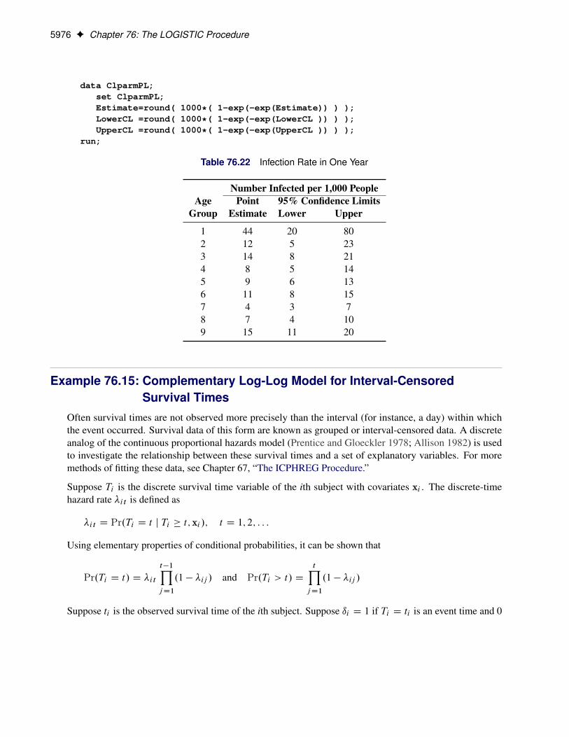
5976 F Chapter 76: The LOGISTIC Procedure
data ClparmPL;set ClparmPL;Estimate=round( 1000*( 1-exp(-exp(Estimate)) ) );LowerCL =round( 1000*( 1-exp(-exp(LowerCL )) ) );UpperCL =round( 1000*( 1-exp(-exp(UpperCL )) ) );
run;
Table 76.22 Infection Rate in One Year
Number Infected per 1,000 PeopleAge Point 95% Confidence Limits
Group Estimate Lower Upper
1 44 20 802 12 5 233 14 8 214 8 5 145 9 6 136 11 8 157 4 3 78 7 4 109 15 11 20
Example 76.15: Complementary Log-Log Model for Interval-CensoredSurvival Times
Often survival times are not observed more precisely than the interval (for instance, a day) within whichthe event occurred. Survival data of this form are known as grouped or interval-censored data. A discreteanalog of the continuous proportional hazards model (Prentice and Gloeckler 1978; Allison 1982) is usedto investigate the relationship between these survival times and a set of explanatory variables. For moremethods of fitting these data, see Chapter 67, “The ICPHREG Procedure.”
Suppose Ti is the discrete survival time variable of the ith subject with covariates xi . The discrete-timehazard rate �it is defined as
�it D Pr.Ti D t j Ti � t; xi /; t D 1; 2; : : :
Using elementary properties of conditional probabilities, it can be shown that
Pr.Ti D t / D �itt�1YjD1
.1 � �ij / and Pr.Ti > t/ DtY
jD1
.1 � �ij /
Suppose ti is the observed survival time of the ith subject. Suppose ıi D 1 if Ti D ti is an event time and 0

Example 76.15: Complementary Log-Log Model for Interval-Censored Survival Times F 5977
otherwise. The likelihood for the grouped survival data is given by
L D
Yi
ŒPr.Ti D ti /�ıi ŒPr.Ti > ti /�1�ıi
D
Yi
��iti
1 � �iti
�ıi tiYjD1
.1 � �ij /
D
Yi
tiYjD1
��ij
1 � �ij
�yij.1 � �ij /
where yij D 1 if the ith subject experienced an event at time Ti D j and 0 otherwise.
Note that the likelihood L for the grouped survival data is the same as the likelihood of a binary responsemodel with event probabilities �ij . If the data are generated by a continuous-time proportional hazardsmodel, Prentice and Gloeckler (1978) have shown that
�ij D 1 � exp.� exp.˛j C ˇ0xi //
which can be rewritten as
log.� log.1 � �ij // D ˛j C ˇ0xi
where the coefficient vector ˇ is identical to that of the continuous-time proportional hazards model, and˛j is a constant related to the conditional survival probability in the interval defined by Ti D j at xi D 0.The grouped data survival model is therefore equivalent to the binary response model with complementarylog-log link function. To fit the grouped survival model by using PROC LOGISTIC, you must treat eachdiscrete time unit for each subject as a separate observation. For each of these observations, the response isdichotomous, corresponding to whether or not the subject died in the time unit.
Consider a study of the effect of insecticide on flour beetles. Four different concentrations of an insecticidewere sprayed on separate groups of flour beetles. The following DATA step saves the number of male andfemale flour beetles dying in successive intervals in the data set Beetles:
data Beetles(keep=time sex conc freq);input time m20 f20 m32 f32 m50 f50 m80 f80;conc=.20; freq= m20; sex=1; output;
freq= f20; sex=2; output;conc=.32; freq= m32; sex=1; output;
freq= f32; sex=2; output;conc=.50; freq= m50; sex=1; output;
freq= f50; sex=2; output;conc=.80; freq= m80; sex=1; output;
freq= f80; sex=2; output;datalines;
1 3 0 7 1 5 0 4 22 11 2 10 5 8 4 10 73 10 4 11 11 11 6 8 154 7 8 16 10 15 6 14 95 4 9 3 5 4 3 8 36 3 3 2 1 2 1 2 47 2 0 1 0 1 1 1 1

5978 F Chapter 76: The LOGISTIC Procedure
8 1 0 0 1 1 4 0 19 0 0 1 1 0 0 0 0
10 0 0 0 0 0 0 1 111 0 0 0 0 1 1 0 012 1 0 0 0 0 1 0 013 1 0 0 0 0 1 0 014 101 126 19 47 7 17 2 4;
The data set Beetles contains four variables: time, sex, conc, and freq. The variable time represents theinterval death time; for example, time=2 is the interval between day 1 and day 2. Insects surviving theduration (13 days) of the experiment are given a time value of 14. The variable sex represents the sex ofthe insects (1=male, 2=female), conc represents the concentration of the insecticide (mg/cm2), and freqrepresents the frequency of the observations.
To use PROC LOGISTIC with the grouped survival data, you must expand the data so that each beetle has aseparate record for each day of survival. A beetle that died in the third day (time=3) would contribute threeobservations to the analysis, one for each day it was alive at the beginning of the day. A beetle that survivesthe 13-day duration of the experiment (time=14) would contribute 13 observations.
The following DATA step creates a new data set named Days containing the beetle-day observations from thedata set Beetles. In addition to the variables sex, conc, and freq, the data set contains an outcome variable yand a classification variable day. The variable y has a value of 1 if the observation corresponds to the day thatthe beetle died, and it has a value of 0 otherwise. An observation for the first day will have a value of 1 forday; an observation for the second day will have a value of 2 for day, and so on. For instance, Output 76.15.1shows an observation in the Beetles data set with time=3, and Output 76.15.2 shows the correspondingbeetle-day observations in the data set Days.
data Days;set Beetles;do day=1 to time;
if (day < 14) then do;y= (day=time);output;
end;end;
run;
Output 76.15.1 An Observation with Time=3 in Beetles Data Set
Obs time conc freq sex
17 3 0.2 10 1
Output 76.15.2 Corresponding Beetle-Day Observations in Days
Obs time conc freq sex day y
25 3 0.2 10 1 1 0
26 3 0.2 10 1 2 0
27 3 0.2 10 1 3 1

Example 76.15: Complementary Log-Log Model for Interval-Censored Survival Times F 5979
The following statements invoke PROC LOGISTIC to fit a complementary log-log model for binary data withthe response variable Y and the explanatory variables day, sex, and Variableconc. Specifying the EVENT=option ensures that the event (y=1) probability is modeled. The GLM coding in the CLASS statement createsan indicator column in the design matrix for each level of day. The coefficients of the indicator effects forday can be used to estimate the baseline survival function. The NOINT option is specified to prevent anyredundancy in estimating the coefficients of day. The Newton-Raphson algorithm is used for the maximumlikelihood estimation of the parameters.
proc logistic data=Days outest=est1;class day / param=glm;model y(event='1')= day sex conc
/ noint link=cloglog technique=newton;freq freq;
run;
Results of the model fit are given in Output 76.15.3. Both sex and conc are statistically significant for thesurvival of beetles sprayed by the insecticide. Female beetles are more resilient to the chemical than malebeetles, and increased concentration of the insecticide increases its effectiveness.
Output 76.15.3 Parameter Estimates for the Grouped Proportional Hazards Model
Analysis of Maximum Likelihood Estimates
Parameter DF EstimateStandard
ErrorWald
Chi-Square Pr > ChiSq
day 1 1 -3.9314 0.2934 179.5602 <.0001
day 2 1 -2.8751 0.2412 142.0596 <.0001
day 3 1 -2.3985 0.2299 108.8833 <.0001
day 4 1 -1.9953 0.2239 79.3960 <.0001
day 5 1 -2.4920 0.2515 98.1470 <.0001
day 6 1 -3.1060 0.3037 104.5799 <.0001
day 7 1 -3.9704 0.4230 88.1107 <.0001
day 8 1 -3.7917 0.4007 89.5233 <.0001
day 9 1 -5.1540 0.7316 49.6329 <.0001
day 10 1 -5.1350 0.7315 49.2805 <.0001
day 11 1 -5.1131 0.7313 48.8834 <.0001
day 12 1 -5.1029 0.7313 48.6920 <.0001
day 13 1 -5.0951 0.7313 48.5467 <.0001
sex 1 -0.5651 0.1141 24.5477 <.0001
conc 1 3.0918 0.2288 182.5665 <.0001
The coefficients of parameters for the day variable are the maximum likelihood estimates of ˛1; : : : ; ˛13,respectively. The baseline survivor function S0.t/ is estimated by
OS0.t/ D bPr.T > t/ DYj�t
exp.� exp.b̨j //and the survivor function for a given covariate pattern (sex=x1 and conc=x2) is estimated by
OS.t/ D Œ OS0.t/�exp.�0:5651x1C3:0918x2/

5980 F Chapter 76: The LOGISTIC Procedure
The following statements compute the survival curves for male and female flour beetles exposed to theinsecticide in concentrations of 0.20 mg/cm2 and 0.80 mg/cm2:
data one (keep=day survival element s_m20 s_f20 s_m80 s_f80);array dd[13] day1-day13;array sc[4] m20 f20 m80 f80;array s_sc[4] s_m20 s_f20 s_m80 s_f80 (1 1 1 1);set est1;m20= exp(sex + .20 * conc);f20= exp(2 * sex + .20 * conc);m80= exp(sex + .80 * conc);f80= exp(2 * sex + .80 * conc);survival=1;day=0;output;do day=1 to 13;
element= exp(-exp(dd[day]));survival= survival * element;do i=1 to 4;
s_sc[i] = survival ** sc[i];end;output;
end;run;
Instead of plotting the curves as step functions, the following statements use the PBSPLINE statement inthe SGPLOT procedure to smooth the curves with a penalized B-spline. For more information about theimplementation of the penalized B-spline method, see Chapter 123, “The TRANSREG Procedure.” The SASautocall macro %MODSTYLE is specified to change the marker symbols for the plot. For more informationabout the %MODSTYLE macro, see the section “ODS Style Template Modification Macro” on page 701 inChapter 21, “Statistical Graphics Using ODS.” The smoothed survival curves are displayed in Output 76.15.4.
%modstyle(name=LogiStyle,parent=htmlblue,markers=circlefilled);ods listing style=LogiStyle;proc sgplot data=one;
title 'Flour Beetles Sprayed with Insecticide';xaxis grid integer;yaxis grid label='Survival Function';pbspline y=s_m20 x=day /
legendlabel = "Male at 0.20 conc." name="pred1";pbspline y=s_m80 x=day /
legendlabel = "Male at 0.80 conc." name="pred2";pbspline y=s_f20 x=day /
legendlabel = "Female at 0.20 conc." name="pred3";pbspline y=s_f80 x=day /
legendlabel = "Female at 0.80 conc." name="pred4";discretelegend "pred1" "pred2" "pred3" "pred4" / across=2;
run;

Example 76.16: Scoring Data Sets F 5981
Output 76.15.4 Predicted Survival at Insecticide Concentrations of 0.20 and 0.80 mg/cm2
The probability of survival is displayed on the vertical axis. Notice that most of the insecticide effect occursby day 6 for both the high and low concentrations.
Example 76.16: Scoring Data SetsThis example first illustrates the syntax used for scoring data sets, then uses a previously scored data setto score a new data set. A generalized logit model is fit to the remote-sensing data set used in the section“Example 39.4: Linear Discriminant Analysis of Remote-Sensing Data on Crops” on page 2660 in Chapter 39,“The DISCRIM Procedure,” to illustrate discrimination and classification methods. In the following DATAstep, the response variable is Crop and the prognostic factors are x1 through x4:
data Crops;length Crop $ 10;infile datalines truncover;input Crop $ @@;do i=1 to 3;
input x1-x4 @@;if (x1 ^= .) then output;

5982 F Chapter 76: The LOGISTIC Procedure
end;input;datalines;
Corn 16 27 31 33 15 23 30 30 16 27 27 26Corn 18 20 25 23 15 15 31 32 15 32 32 15Corn 12 15 16 73Soybeans 20 23 23 25 24 24 25 32 21 25 23 24Soybeans 27 45 24 12 12 13 15 42 22 32 31 43Cotton 31 32 33 34 29 24 26 28 34 32 28 45Cotton 26 25 23 24 53 48 75 26 34 35 25 78Sugarbeets 22 23 25 42 25 25 24 26 34 25 16 52Sugarbeets 54 23 21 54 25 43 32 15 26 54 2 54Clover 12 45 32 54 24 58 25 34 87 54 61 21Clover 51 31 31 16 96 48 54 62 31 31 11 11Clover 56 13 13 71 32 13 27 32 36 26 54 32Clover 53 08 06 54 32 32 62 16;
In the following statements, you specify a SCORE statement to use the fitted model to score the Cropsdata. The data together with the predicted values are saved in the data set Score1. The output from theEFFECTPLOT statement is discussed at the end of this section.
ods graphics on;proc logistic data=Crops;
model Crop=x1-x4 / link=glogit;score out=Score1;effectplot slicefit(x=x3);
run;
In the following statements, the model is fit again, and the data and the predicted values are saved into thedata set Score2. The OUTMODEL= option saves the fitted model information in the permanent SAS dataset sasuser.CropModel, and the STORE statement saves the fitted model information into the SAS data setCropModel2. Both the OUTMODEL= option and the STORE statement are specified to illustrate their use;you would usually specify only one of these model-storing methods.
proc logistic data=Crops outmodel=sasuser.CropModel;model Crop=x1-x4 / link=glogit;score data=Crops out=Score2;store CropModel2;
run;
To score data without refitting the model, specify the INMODEL= option to identify a previously saved SASdata set of model information. In the following statements, the model is read from the sasuser.CropModeldata set, and the data and the predicted values are saved in the data set Score3. Note that the data set beingscored does not have to include the response variable.
proc logistic inmodel=sasuser.CropModel;score data=Crops out=Score3;
run;
Another method available to score the data without refitting the model is to invoke the PLM procedure. Inthe following statements, the stored model is named in the SOURCE= option. The PREDICTED= optioncomputes the linear predictors, and the ILINK option transforms the linear predictors to the probability scale.The SCORE statement scores the Crops data set, and the predicted probabilities are saved in the data setScorePLM. See Chapter 91, “The PLM Procedure,” for more information.

Example 76.16: Scoring Data Sets F 5983
proc plm source=CropModel2;score data=Crops out=ScorePLM predicted=p / ilink;
run;
For each observation in the Crops data set, the ScorePLM data set contains 5 observations—one for eachlevel of the response variable. The following statements transform this data set into a form that is similar tothe other scored data sets in this example:
proc transpose data=ScorePLM out=Score4 prefix=P_ let;id _LEVEL_;var p;by x1-x4 notsorted;
run;data Score4(drop=_NAME_ _LABEL_);
merge Score4 Crops(keep=Crop x1-x4);F_Crop=Crop;
run;proc summary data=ScorePLM nway;
by x1-x4 notsorted;var p;output out=into maxid(p(_LEVEL_))=I_Crop;
run;data Score4;
merge Score4 into(keep=I_Crop);run;
To set prior probabilities on the responses, specify the PRIOR= option to identify a SAS data set containingthe response levels and their priors. In the following statements, the Prior data set contains the values of theresponse variable (because this example uses single-trial MODEL statement syntax) and a _PRIOR_ variablecontaining values proportional to the default priors. The data and the predicted values are saved in the dataset Score5.
data Prior;length Crop $10.;input Crop _PRIOR_;datalines;
Clover 11Corn 7Cotton 6Soybeans 6Sugarbeets 6;
proc logistic inmodel=sasuser.CropModel;score data=Crops prior=prior out=Score5 fitstat;
run;
The “Fit Statistics for SCORE Data” table displayed in Output 76.16.1 shows that 47.22% of the observationsare misclassified.

5984 F Chapter 76: The LOGISTIC Procedure
Output 76.16.1 Fit Statistics for Data Set Prior
Fit Statistics for SCORE Data
Data SetTotal
FrequencyLog
LikelihoodErrorRate AIC AICC BIC SC R-Square
Max-RescaledR-Square AUC
BrierScore
WORK.CROPS 36 -32.2247 0.4722 104.4493 160.4493 136.1197 136.1197 0.744081 0.777285 . 0.492712
The data sets Score1, Score2, Score3, Score4, and Score5 are identical. The following statements displaythe scoring results in Output 76.16.2:
proc freq data=Score1;table F_Crop*I_Crop / nocol nocum nopercent;
run;
Output 76.16.2 Classification of Data Used for Scoring
FrequencyRow Pct
Table of F_Crop by I_Crop
F_Crop(From:Crop)
I_Crop(Into: Crop)
Clover Corn Cotton Soybeans Sugarbeets Total
Clover 654.55
00.00
218.18
218.18
19.09
11
Corn 00.00
7100.00
00.00
00.00
00.00
7
Cotton 466.67
00.00
116.67
116.67
00.00
6
Soybeans 116.67
116.67
116.67
350.00
00.00
6
Sugarbeets 233.33
00.00
00.00
233.33
233.33
6
Total 13 8 4 8 3 36
The following statements use the previously fitted and saved model in the sasuser.CropModel data set toscore the observations in a new data set, Test. The results of scoring the test data are saved in the ScoredTestdata set and displayed in Output 76.16.3.
data Test;input Crop $ 1-10 x1-x4;datalines;
Corn 16 27 31 33Soybeans 21 25 23 24Cotton 29 24 26 28Sugarbeets 54 23 21 54Clover 32 32 62 16;
proc logistic noprint inmodel=sasuser.CropModel;score data=Test out=ScoredTest;
run;
proc print data=ScoredTest label noobs;var F_Crop I_Crop P_Clover P_Corn P_Cotton P_Soybeans P_Sugarbeets;
run;

Example 76.16: Scoring Data Sets F 5985
Output 76.16.3 Classification of Test Data
From: CropInto:Crop
PredictedProbability:
Crop=Clover
PredictedProbability:Crop=Corn
PredictedProbability:
Crop=Cotton
PredictedProbability:
Crop=Soybeans
PredictedProbability:
Crop=Sugarbeets
Corn Corn 0.00342 0.90067 0.00500 0.08675 0.00416
Soybeans Soybeans 0.04801 0.03157 0.02865 0.82933 0.06243
Cotton Clover 0.43180 0.00015 0.21267 0.07623 0.27914
Sugarbeets Clover 0.66681 0.00000 0.17364 0.00000 0.15955
Clover Cotton 0.41301 0.13386 0.43649 0.00033 0.01631
The EFFECTPLOT statement that is specified in the first PROC LOGISTIC invocation produces a plotof the model-predicted probabilities versus X3 while holding the other three covariates at their means(Output 76.16.4). This plot shows how the value of X3 affects the probabilities of the various crops whenthe other prognostic factors are fixed at their means. If you are interested in the effect of X3 when the othercovariates are fixed at a certain level—say, 10—specify the following EFFECTPLOT statement.
effectplot slicefit(x=x3) / at(x1=10 x2=10 x4=10)
Output 76.16.4 Model-Predicted Probabilities

5986 F Chapter 76: The LOGISTIC Procedure
Example 76.17: Using the LSMEANS StatementRecall the main-effects model fit to the Neuralgia data set in Example 76.2. The Treatment*Sex interaction,which was previously shown to be nonsignificant, is added back into the model for this discussion.
In the following statements, the ODDSRATIO statement is specified to produce odds ratios of pairwisedifferences of the Treatment parameters in the presence of the Sex interaction. The LSMEANS statement isspecified with several options: the E option displays the coefficients that are used to compute the LS-meansfor each Treatment level, the DIFF option takes all pairwise differences of the LS-means for the levels ofthe Treatment variable, the ODDSRATIO option computes odds ratios of these differences, the CL optionproduces confidence intervals for the differences and odds ratios, and the ADJUST=BON option performs avery conservative adjustment of the p-values and confidence intervals.
proc logistic data=Neuralgia;class Treatment Sex / param=glm;model Pain= Treatment|Sex Age;oddsratio Treatment;lsmeans Treatment / e diff oddsratio cl adjust=bon;
run;
The results from the ODDSRATIO statement are displayed in Output 76.17.1. All pairwise differences oflevels of the Treatment effect are compared. However, because of the interaction between the Treatment andSex variables, each difference is computed at each of the two levels of the Sex variable. These results showthat the difference between Treatment levels A and B is insignificant for both genders.
To compute these odds ratios, you must first construct a linear combination of the parameters, l 0ˇ, for eachlevel that is compared with all other levels fixed at some value. For example, to compare Treatment=A withB for Sex=F, you fix the Age variable at its mean, 70.05, and construct the following l vectors:
Treatment Sex Treatment*SexIntercept A B P F M AF AM BF BM PF PM Age
l 0A 1 1 0 0 1 0 1 0 0 0 0 0 70.05l 0B 1 0 1 0 1 0 0 0 1 0 0 0 70.05l 0A � l
0B 0 1 –1 0 0 0 1 0 –1 0 0 0 0
Then the odds ratio for Treatment A versus B at Sex=F is computed as exp..l 0A � l0B/ˇ/. Different l vectors
must be similarly constructed when Sex=M because the resulting odds ratio will be different due to theinteraction.
Output 76.17.1 Odds Ratios from the ODDSRATIO Statement
Odds Ratio Estimates and Wald Confidence Intervals
Odds Ratio Estimate 95% Confidence Limits
Treatment A vs B at Sex=F 0.398 0.016 9.722
Treatment A vs P at Sex=F 16.892 1.269 224.838
Treatment B vs P at Sex=F 42.492 2.276 793.254
Treatment A vs B at Sex=M 0.663 0.078 5.623
Treatment A vs P at Sex=M 34.766 1.807 668.724
Treatment B vs P at Sex=M 52.458 2.258 >999.999

Example 76.17: Using the LSMEANS Statement F 5987
The results from the LSMEANS statement are displayed in Output 76.17.2 through Output 76.17.4.
The LS-means are computed by constructing each of the l coefficient vectors shown in Output 76.17.2,and then computing l 0ˇ. The LS-means are not estimates of the event probabilities; they are estimatesof the linear predictors on the logit scale and therefore are estimated log odds. In order to obtain eventprobabilities, you need to apply the inverse-link transformation by specifying the ILINK option in theLSMEANS statement. Notice in Output 76.17.2 that the Sex rows of the coefficient vectors do not selecteither Sex=F or Sex=M. Instead, the LS-means are computed at an average of these two levels, so onlyone result needs to be reported. For more information about the construction of LS-means, see the section“Construction of Least Squares Means” on page 4056 in Chapter 50, “The GLM Procedure.”
Output 76.17.2 Treatment LS-Means Coefficients
Coefficients for Treatment Least Squares Means
Parameter Treatment Sex Row1 Row2 Row3
Intercept: Pain=No 1 1 1
Treatment A A 1
Treatment B B 1
Treatment P P 1
Sex F F 0.5 0.5 0.5
Sex M M 0.5 0.5 0.5
Treatment A * Sex F A F 0.5
Treatment A * Sex M A M 0.5
Treatment B * Sex F B F 0.5
Treatment B * Sex M B M 0.5
Treatment P * Sex F P F 0.5
Treatment P * Sex M P M 0.5
Age 70.05 70.05 70.05
The Treatment LS-means shown in Output 76.17.3 are all significantly nonzero at the 0.05 level. TheseLS-means are predicted population margins of the logits; that is, they estimate the marginal means over abalanced population, and they are effectively the within-Treatment means appropriately adjusted for the othereffects in the model. The LS-means are not event probabilities; in order to obtain event probabilities, youneed to apply the inverse-link transformation by specifying the ILINK option in the LSMEANS statement.For more information about LS-means, see the section “LSMEANS Statement” on page 467 in Chapter 19,“Shared Concepts and Topics.”
Output 76.17.3 Treatment LS-Means
Treatment Least Squares Means
Treatment EstimateStandard
Error z Value Pr > |z| Alpha Lower Upper
A 1.3195 0.6664 1.98 0.0477 0.05 0.01331 2.6257
B 1.9864 0.7874 2.52 0.0116 0.05 0.4431 3.5297
P -1.8682 0.7620 -2.45 0.0142 0.05 -3.3618 -0.3747
Pairwise differences between the Treatment LS-means, requested with the DIFF option, are displayed inOutput 76.17.4. The LS-mean for the level that is displayed in the _Treatment column is subtracted from theLS-mean for the level in the Treatment column, so the first row displays the LS-mean for Treatment level Aminus the LS-mean for Treatment level B. The difference (–0.6669) is the estimated difference in log odds,

5988 F Chapter 76: The LOGISTIC Procedure
or equivalently the log odds ratio of the two treatments. The Pr > |z| column indicates that the A and B levelsare not significantly different; however, both of these levels are significantly different from level P. If theinverse-link transformation is specified by the ILINK option, then these differences do not transform back todifferences in probabilities.
There are two odds ratios for Treatment level A versus B in Output 76.17.1; these are constructed at eachlevel of the interacting covariate Sex. In contrast, there is only one LS-means odds ratio for Treatmentlevel A versus B in Output 76.17.4. This odds ratio is computed at an average of the interacting effects bycreating the l vectors shown in Output 76.17.2 (the Row1 column corresponds to lA, and the Row2 columncorresponds to lB ) and computing exp.l 0Aˇ � l
0Bˇ/.
Because multiple tests are performed, you can protect yourself from falsely significant results by adjustingyour p-values for multiplicity. The ADJUST=BON option performs the very conservative Bonferroniadjustment, and adds the columns labeled with ‘Adj’ to Output 76.17.4. By comparing the Pr > |z| column tothe Adj P column, you can see that the p-values are adjusted upwards; in this case, there is no change in yourconclusions. The confidence intervals are also adjusted for multiplicity—all adjusted intervals are wider thanthe unadjusted intervals, but again your conclusions in this example are unchanged. You can specify otheradjustment methods by using the ADJUST= option.
Output 76.17.4 Differences and Odds Ratios for the Treatment LS-Means
Differences of Treatment Least Squares MeansAdjustment for Multiple Comparisons: Bonferroni
Treatment _Treatment EstimateStandard
Error z Value Pr > |z| Adj P Alpha Lower UpperAdj
LowerAdj
UpperOddsRatio
A B -0.6669 1.0026 -0.67 0.5059 1.0000 0.05 -2.6321 1.2982 -3.0672 1.7334 0.513
A P 3.1877 1.0376 3.07 0.0021 0.0064 0.05 1.1541 5.2214 0.7037 5.6717 24.234
B P 3.8547 1.2126 3.18 0.0015 0.0044 0.05 1.4780 6.2313 0.9517 6.7576 47.213
Differences of Treatment Least Squares MeansAdjustment for Multiple Comparisons: Bonferroni
Treatment _Treatment
LowerConfidence
Limit forOdds Ratio
UpperConfidence
Limit forOdds Ratio
Adj LowerOdds Ratio
Adj UpperOdds Ratio
A B 0.072 3.663 0.047 5.660
A P 3.171 185.195 2.021 290.542
B P 4.384 508.441 2.590 860.612
If you want to jointly test whether the active treatments are different from the placebo, you can specifya custom hypothesis test among LS-means by using the LSMESTIMATE statement. In the followingstatements, the LS-means for the two treatments are contrasted against the LS-mean of the placebo, and theJOINT option performs a joint test that the two treatments are not different from placebo.
proc logistic data=Neuralgia;class Treatment Sex / param=glm;model Pain= Treatment|Sex Age;lsmestimate treatment 1 0 -1, 0 1 -1 / joint;
run;

Example 76.17: Using the LSMEANS Statement F 5989
Output 76.17.5 displays the results from the LSMESTIMATE statement. The “Least Squares Means Estimates”table displays the differences of the two active treatments against the placebo, and the results are identicalto the second and third rows of Output 76.17.4. The “Chi-Square Test for Least Squares Means Estimates”table displays the joint test. In all of these tests, you reject the null hypothesis that the treatment has the sameeffect as the placebo.
Output 76.17.5 Custom LS-Mean Tests
Least Squares Means Estimates
Effect Label EstimateStandard
Error z Value Pr > |z|
Treatment Row 1 3.1877 1.0376 3.07 0.0021
Treatment Row 2 3.8547 1.2126 3.18 0.0015
Chi-Square Test for Least SquaresMeans Estimates
EffectNum
DF Chi-Square Pr > ChiSq
Treatment 2 12.13 0.0023
If you want to work with LS-means but you prefer to compute the Treatment odds ratios within the Sexlevels in the same fashion as the ODDSRATIO statement does, you can specify the SLICE statement. Inthe following statements, you specify the same options in the SLICE statement as you do in the LSMEANSstatement, except that you also specify the SLICEBY= option to perform an LS-means analysis partitionedinto sets that are defined by the Sex variable:
proc logistic data=Neuralgia;class Treatment Sex / param=glm;model Pain= Treatment|Sex Age;slice Treatment*Sex / sliceby=Sex diff oddsratio cl adjust=bon;
run;
The results for Sex=F are displayed in Output 76.17.6 and Output 76.17.7. The joint test in Output 76.17.6tests the equality of the LS-means of the levels of Treatment for Sex=F, and rejects equality at level 0.05. InOutput 76.17.7, the odds ratios and confidence intervals match those reported for Sex=F in Output 76.17.1,and multiplicity adjustments are performed.
Output 76.17.6 Joint Test of Treatment Equality for Females
Chi-Square Test for Treatment*SexLeast Squares Means Slice
SliceNum
DF Chi-Square Pr > ChiSq
Sex F 2 8.22 0.0164

5990 F Chapter 76: The LOGISTIC Procedure
Output 76.17.7 Differences of the Treatment LS-Means for Females
Simple Differences of Treatment*Sex Least Squares MeansAdjustment for Multiple Comparisons: Bonferroni
Slice Treatment _Treatment EstimateStandard
Error z Value Pr > |z| Adj P Alpha Lower UpperAdj
LowerAdj
UpperOddsRatio
Sex F A B -0.9224 1.6311 -0.57 0.5717 1.0000 0.05 -4.1193 2.2744 -4.8272 2.9824 0.398
Sex F A P 2.8269 1.3207 2.14 0.0323 0.0970 0.05 0.2384 5.4154 -0.3348 5.9886 16.892
Sex F B P 3.7493 1.4933 2.51 0.0120 0.0361 0.05 0.8225 6.6761 0.1744 7.3243 42.492
Simple Differences of Treatment*Sex Least Squares MeansAdjustment for Multiple Comparisons: Bonferroni
Slice Treatment _Treatment
LowerConfidence
Limit forOdds Ratio
UpperConfidence
Limit forOdds Ratio
Adj LowerOdds Ratio
Adj UpperOdds Ratio
Sex F A B 0.016 9.722 0.008 19.734
Sex F A P 1.269 224.838 0.715 398.848
Sex F B P 2.276 793.254 1.190 >999.999
Similarly, the results for Sex=M are shown in Output 76.17.8 and Output 76.17.9.
Output 76.17.8 Joint Test of Treatment Equality for Males
Chi-Square Test for Treatment*SexLeast Squares Means Slice
SliceNum
DF Chi-Square Pr > ChiSq
Sex M 2 6.64 0.0361
Output 76.17.9 Differences of the Treatment LS-Means for Males
Simple Differences of Treatment*Sex Least Squares MeansAdjustment for Multiple Comparisons: Bonferroni
Slice Treatment _Treatment EstimateStandard
Error z Value Pr > |z| Adj P Alpha Lower UpperAdj
LowerAdj
UpperOddsRatio
Sex M A B -0.4114 1.0910 -0.38 0.7061 1.0000 0.05 -2.5496 1.7268 -3.0231 2.2003 0.663
Sex M A P 3.5486 1.5086 2.35 0.0187 0.0560 0.05 0.5919 6.5054 -0.06286 7.1601 34.766
Sex M B P 3.9600 1.6049 2.47 0.0136 0.0408 0.05 0.8145 7.1055 0.1180 7.8021 52.458
Simple Differences of Treatment*Sex Least Squares MeansAdjustment for Multiple Comparisons: Bonferroni
Slice Treatment _Treatment
LowerConfidence
Limit forOdds Ratio
UpperConfidence
Limit forOdds Ratio
Adj LowerOdds Ratio
Adj UpperOdds Ratio
Sex M A B 0.078 5.623 0.049 9.028
Sex M A P 1.807 668.724 0.939 >999.999
Sex M B P 2.258 >999.999 1.125 >999.999

Example 76.18: Partial Proportional Odds Model F 5991
Example 76.18: Partial Proportional Odds ModelCameron and Trivedi (1998, p. 68) studied the number of doctor visits from the Australian Health Survey1977–78. The data set contains a dependent variable, dvisits, which contains the number of doctor visitsin the past two weeks (0, 1, or 2, where 2 represents two or more visits) and the following explanatoryvariables: sex, which indicates whether the patient is female; age, which contains the patient’s age in yearsdivided by 100; income, which contains the patient’s annual income (in units of $10,000); levyplus, whichindicates whether the patient has private health insurance; freepoor, which indicates that the patient hasfree government health insurance due to low income; freerepa, which indicates that the patient has freegovernment health insurance for other reasons; illness, which contains the number of illnesses in the past twoweeks; actdays, which contains the number of days the illness caused reduced activity; hscore, which is aquestionnaire score; chcond1, which indicates a chronic condition that does not limit activity; and chcond2,which indicates a chronic condition that limits activity.
data docvisit;input sex age agesq income levyplus freepoor freerepa
illness actdays hscore chcond1 chcond2 dvisits;if ( dvisits > 2) then dvisits = 2;datalines;
1 0.19 0.0361 0.55 1 0 0 1 4 1 0 0 11 0.19 0.0361 0.45 1 0 0 1 2 1 0 0 10 0.19 0.0361 0.90 0 0 0 3 0 0 0 0 1
... more lines ...
1 0.37 0.1369 0.25 0 0 1 1 0 1 0 0 01 0.52 0.2704 0.65 0 0 0 0 0 0 0 0 00 0.72 0.5184 0.25 0 0 1 0 0 0 0 0 0;
Because the response variable dvisits has three levels, the proportional odds model constructs two responsefunctions. There is an intercept parameter for each of the two response functions, ˛1 < ˛2, and commonslope parameters ˇ D .ˇ1; : : : ; ˇ12/ across the functions. The model can be written as
logit.Pr.Y � i j x// D ˛i C ˇ0x; i D 1; 2
The following statements fit a proportional odds model to this data:
proc logistic data=docvisit;model dvisits = sex age agesq income levyplus
freepoor freerepa illness actdays hscorechcond1 chcond2;
run;
Selected results are displayed in Output 76.18.1.

5992 F Chapter 76: The LOGISTIC Procedure
Output 76.18.1 Test of Proportional Odds Assumption
Score Test for theProportional Odds
Assumption
Chi-Square DF Pr > ChiSq
27.4256 12 0.0067
Testing Global Null Hypothesis: BETA=0
Test Chi-Square DF Pr > ChiSq
Likelihood Ratio 734.2971 12 <.0001
Score 811.8964 12 <.0001
Wald 690.7156 12 <.0001
The test of the proportional odds assumption in Output 76.18.1 rejects the null hypothesis that all the slopesare equal across the two response functions. This test is very anticonservative; that is, it tends to reject thenull hypothesis even when the proportional odds assumption is reasonable.
The proportional odds assumption for ordinal response models can be relaxed by specifying theUNEQUALSLOPES option in the MODEL statement. A general (nonproportional odds) model has differentslope parameters ˇi D .ˇ1;i ; : : : ; ˇ12;i / for every logit i:
logit.Pr.Y � i j x// D ˛i C ˇ0ix; i D 1; 2
The following statements fit the general model:
proc logistic data=docvisit;model dvisits = sex age agesq income levyplus
freepoor freerepa illness actdays hscorechcond1 chcond2 / unequalslopes;
sex: test sex_0 =sex_1;age: test age_0 =age_1;agesq: test agesq_0 =agesq_1;income: test income_0 =income_1;levyplus: test levyplus_0=levyplus_1;freepoor: test freepoor_0=freepoor_1;freerepa: test freerepa_0=freerepa_1;illness: test illness_0 =illness_1;actdays: test actdays_0 =actdays_1;hscore: test hscore_0 =hscore_1;chcond1: test chcond1_0 =chcond1_1;chcond2: test chcond2_0 =chcond2_1;
run;
The TEST statements test the proportional odds assumption for each of the covariates in the model. Theparameter names are constructed by appending the response level that identifies the response function, asdescribed in the section “Parameter Names in the OUTEST= Data Set” on page 5880. Selected results fromfitting the general model to the data are displayed in Output 76.18.2.

Example 76.18: Partial Proportional Odds Model F 5993
Output 76.18.2 Results for the General Model
Testing Global Null Hypothesis: BETA=0
Test Chi-Square DF Pr > ChiSq
Likelihood Ratio 761.4797 24 <.0001
Score 957.6793 24 <.0001
Wald 688.2306 24 <.0001
Analysis of Maximum Likelihood Estimates
Parameter dvisits DF EstimateStandard
ErrorWald
Chi-Square Pr > ChiSq
Intercept 0 1 2.3238 0.2754 71.2018 <.0001
Intercept 1 1 4.2862 0.4890 76.8368 <.0001
sex 0 1 -0.2637 0.0818 10.3909 0.0013
sex 1 1 -0.1232 0.1451 0.7210 0.3958
age 0 1 1.7489 1.5115 1.3389 0.2472
age 1 1 -2.0974 2.6003 0.6506 0.4199
agesq 0 1 -2.4718 1.6636 2.2076 0.1373
agesq 1 1 2.6883 2.8398 0.8961 0.3438
income 0 1 -0.00857 0.1266 0.0046 0.9460
income 1 1 0.6464 0.2375 7.4075 0.0065
levyplus 0 1 -0.2658 0.0997 7.0999 0.0077
levyplus 1 1 -0.2869 0.1820 2.4848 0.1150
freepoor 0 1 0.6773 0.2601 6.7811 0.0092
freepoor 1 1 0.9020 0.4911 3.3730 0.0663
freerepa 0 1 -0.4044 0.1382 8.5637 0.0034
freerepa 1 1 -0.0958 0.2361 0.1648 0.6848
illness 0 1 -0.2645 0.0287 84.6792 <.0001
illness 1 1 -0.3083 0.0499 38.1652 <.0001
actdays 0 1 -0.1521 0.0116 172.2764 <.0001
actdays 1 1 -0.1863 0.0134 193.7700 <.0001
hscore 0 1 -0.0620 0.0172 12.9996 0.0003
hscore 1 1 -0.0568 0.0252 5.0940 0.0240
chcond1 0 1 -0.1140 0.0909 1.5721 0.2099
chcond1 1 1 -0.2478 0.1743 2.0201 0.1552
chcond2 0 1 -0.2660 0.1255 4.4918 0.0341
chcond2 1 1 -0.3146 0.2116 2.2106 0.1371

5994 F Chapter 76: The LOGISTIC Procedure
Output 76.18.2 continued
Linear Hypotheses Testing Results
LabelWald
Chi-Square DF Pr > ChiSq
sex 1.0981 1 0.2947
age 2.5658 1 0.1092
agesq 3.8309 1 0.0503
income 8.8006 1 0.0030
levyplus 0.0162 1 0.8989
freepoor 0.2569 1 0.6122
freerepa 2.0099 1 0.1563
illness 0.8630 1 0.3529
actdays 6.9407 1 0.0084
hscore 0.0476 1 0.8273
chcond1 0.6906 1 0.4060
chcond2 0.0615 1 0.8042
The preceding general model fits 12 � 2 D 24 slope parameters, and according to the “Linear HypothesesTesting Results” table in Output 76.18.2, several variables are unnecessarily allowing nonproportional odds.You can obtain a more parsimonious model by specifying a subset of the parameters to have nonproportionalodds. The following statements allow the parameters for the variables in the “Linear Hypotheses TestingResults” table that have p-values less than 0.1 (actdays, agesq, and income) to vary across the responsefunctions:
proc logistic data=docvisit;model dvisits= sex age agesq income levyplus freepoor
freerepa illness actdays hscore chcond1 chcond2/ unequalslopes=(actdays agesq income);
run;
Selected results from fitting this partial proportional odds model are displayed in Output 76.18.3.
Output 76.18.3 Results for Partial Proportional Odds Model
Testing Global Null Hypothesis: BETA=0
Test Chi-Square DF Pr > ChiSq
Likelihood Ratio 752.5512 15 <.0001
Score 947.3269 15 <.0001
Wald 683.4719 15 <.0001

Example 76.18: Partial Proportional Odds Model F 5995
Output 76.18.3 continued
Analysis of Maximum Likelihood Estimates
Parameter dvisits DF EstimateStandard
ErrorWald
Chi-Square Pr > ChiSq
Intercept 0 1 2.3882 0.2716 77.2988 <.0001
Intercept 1 1 3.7597 0.3138 143.5386 <.0001
sex 1 -0.2485 0.0807 9.4789 0.0021
age 1 1.3000 1.4864 0.7649 0.3818
agesq 0 1 -2.0110 1.6345 1.5139 0.2186
agesq 1 1 -0.8789 1.6512 0.2833 0.5945
income 0 1 0.0209 0.1261 0.0275 0.8683
income 1 1 0.4283 0.2221 3.7190 0.0538
levyplus 1 -0.2703 0.0989 7.4735 0.0063
freepoor 1 0.6936 0.2589 7.1785 0.0074
freerepa 1 -0.3648 0.1358 7.2155 0.0072
illness 1 -0.2707 0.0281 92.7123 <.0001
actdays 0 1 -0.1522 0.0115 173.5696 <.0001
actdays 1 1 -0.1868 0.0129 209.7134 <.0001
hscore 1 -0.0609 0.0166 13.5137 0.0002
chcond1 1 -0.1200 0.0901 1.7756 0.1827
chcond2 1 -0.2628 0.1227 4.5849 0.0323
You can also specify the following code to let stepwise selection determine which parameters have unequalslopes:
proc logistic data=docvisit;model dvisits= sex age agesq income levyplus freepoor
freerepa illness actdays hscore chcond1 chcond2/ equalslopes unequalslopes selection=stepwise details;
run;
This selection process chooses sex, freepoor, illness, and hscore as the proportional odds effects and choosesU_actdays and U_agesq as the unconstrained general effects. For more information about model selectionfor partial proportional odds models, see Derr (2013).
The partial proportional odds model can be written in the same form as the general model by lettingx D .x1; : : : ; xq; xqC1; : : : ; x12/ and ˇi D .ˇ1; : : : ; ˇq; ˇqC1;i ; : : : ; ˇ12;i /. So the first q parameters haveproportional odds and the remaining parameters do not. The last 12 – q parameters can be rewritten to have acommon slope plus an increment from the common slope: ˇqCj C qCj;i ; j D 1; : : : ; 12 � q, where thenew parameters i contain the increments from the common slopes. The model in this form makes it obviousthat the proportional odds model is a submodel of the partial proportional odds model, and both of these aresubmodels of the general model. This means that you can use likelihood ratio tests to compare models.
You can use the following statements to compute the likelihood ratio tests from the Likelihood Ratio row ofthe “Testing Global Null hypothesis: BETA=0” tables in the preceding outputs:
data a;label p='Pr>ChiSq';format p 8.6;input Test $10. ChiSq1 DF1 ChiSq2 DF2;ChiSq= ChiSq1-ChiSq2;

5996 F Chapter 76: The LOGISTIC Procedure
DF= DF1-DF2;p=1-probchi(ChiSq,DF);keep Test Chisq DF p;datalines;
Gen vs PO 761.4797 24 734.2971 12PPO vs PO 752.5512 15 734.2971 12Gen vs PPO 761.4797 24 752.5512 15;
proc print data=a label noobs;var Test ChiSq DF p;
run;
Output 76.18.4 Likelihood Ratio Tests
Test ChiSq DF Pr>ChiSq
Gen vs PO 27.1826 12 0.007273
PPO vs PO 18.2541 3 0.000390
Gen vs PPO 8.9285 9 0.443900
Therefore, you reject the proportional odds model in favor of both the general model and the partialproportional odds model, and the partial proportional odds model fits as well as the general model. Thelikelihood ratio test of the general model versus the proportional odds model is very similar to the score testof the proportional odds assumption in Output 76.18.1 because of the large sample size (Stokes, Davis, andKoch 2000, p. 249).
NOTE: The proportional odds model has increasing intercepts, which ensures the increasing nature ofthe cumulative response functions. However, none of the parameters in the partial proportional odds orgeneral models are constrained. Because of this, sometimes during the optimization process a predictedindividual probability can be negative; the optimization continues because it might recover from this situation.Sometimes your final model will predict negative individual probabilities for some of the observations; inthis case a message is displayed, and you should check your data for outliers and possibly redefine yourmodel. Other times the model fits your data well, but if you try to score new data you can get negativeindividual probabilities. This means the model is not appropriate for the data you are trying to score, amessage is displayed, and the estimates are set to missing. These optimization issues do not arise when youfit an adjacent-category or generalized logit model that has equal and unequal slope effects.
Example 76.19: Goodness-of-Fit Tests and CalibrationThe following data were originally published by Mroz (1987) and downloaded from Wooldridge (2002). Thisdata set is based on a sample of 753 married white women. The dependent variable is a discrete variable oflabor force participation (InLaborForce). Explanatory variables are the number of children age 5 or younger(KidsLt6); the number of children ages 6 to 18 (KidsGe6); the woman’s age (Age); the woman’s years ofschooling (Education); the wife’s labor experience (Experience); the square of experience (SqExperience);and the family income, excluding the wife’s wages (IncomeExcl).
data Mroz;input InLaborForce IncomeExcl Education Experience
SqExperience Age KidsLt6 KidsGe6 lWage;

Example 76.19: Goodness-of-Fit Tests and Calibration F 5997
datalines;1 10.91006 12 14 196 32 1 0 1.2101541 19.49998 12 5 25 30 0 2 0.3285121
... more lines ...
0 9.952 12 4 16 43 0 0 .0 24.984 12 15 225 60 0 0 .0 28.363 9 12 144 39 0 3 .;
The following program sets aside about 30% of the data set to be used for testing the model. To do this, anew response variable, InLaborForce2, is set to missing for the test data; otherwise it is set to the originalvalue of InLaborForce.
data Mroz;set Mroz;if (ranuni(3939)<.3) then InLaborForce2=.;else InLaborForce2=InLaborForce;
run;
In the following statements, the GOF option modifies the “Model Fitting Statistics” table by displaying asingle column with more statistics in Output 76.19.1, displays more tests in the “Goodness-of-Fit” table,displays the results of the Hosmer-Lemeshow test, and displays a calibration plot because ODS Graphics isenabled. The SHOWOBS option modifies the calibration plot by displaying a bar chart of the events in theupper margin of the plot and a bar chart of the nonevents in the bottom margin. The CLM option displaysconfidence intervals for the mean loess fit as a band around the loess curve. The OUTPUT statement createsa data set that contains the linear predictors and the original InLaborForce variable.
ods graphics on;proc logistic data=Mroz plots=calibration(clm showobs);
model InLaborForce2 = IncomeExcl Education ExperienceSqExperience Age KidsLt6 KidsGe6 / gof;
id InLaborForce;output out=Scored xbeta=XBeta;
run;
Because of the continuous predictors, the Pearson and deviance tests in Output 76.19.1 cannot be trusted.However, all the other tests remain valid and do not reject the null hypothesis that the fit is adequate.
Output 76.19.1 Goodness-of-Fit Tests
Goodness-of-Fit Tests
Criterion Value DF Pr > ChiSq
Deviance 606.5035 544 0.0324
Pearson 538.4877 544 0.5586
Information Matrix 38.2455 35 0.3243
Information Matrix Diagonal 11.4027 8 0.1799
Osius and Rojek 0.8412 1 0.3590
Residual Sum of Squares 1.3502 1 0.2453
Spiegelhalter 0.0201 1 0.8871
Stukel 2.2581 2 0.3233
Number of unique profiles: 552

5998 F Chapter 76: The LOGISTIC Procedure
The “Model Fit Statistics” table displays an assortment of statistics in Output 76.19.2 that are most usefulwhen you compare this model to other models. The misclassification rate and the average square error are ofmoderate size.
Output 76.19.2 Model Fit Statistics
Model Fit Statistics
Criterion Value
AIC 622.5035
AICC 622.7687
SC 657.0119
-2 Log L 606.5035
-2 Log L (Intercept-Only) 755.2843
Misclassification Rate 0.2754
Average Square Error 0.1862
R-Square 0.2363
Max-rescaled R-Square 0.3169
Aldrich-Nelson's R-Square 0.2123
Efron's R-Square 0.2417
Estrella's R-Square 0.2593
Estrella's Adjusted R-Square 0.2324
McFadden's R-Square 0.1970
Tjur's R-Square 0.2440
Veall-Zimmerman's R-Square 0.3675
The Hosmer-Lemeshow test is computed using 10 groups for an 8-degrees-of-freedom chi-square test, andyou do not reject the null hypothesis that the fit is adequate. The results are shown in Output 76.19.3.
Output 76.19.3 Hosmer-Lemeshow Test
Partition for the Hosmer and Lemeshow Test
InLaborForce2 = 0 InLaborForce2 = 1
Group Total Observed Expected Observed Expected
1 55 3 5.22 52 49.78
2 55 10 9.12 45 45.88
3 55 10 12.24 45 42.76
4 55 20 15.85 35 39.15
5 55 24 19.39 31 35.61
6 55 17 23.44 38 31.56
7 55 36 28.84 19 26.16
8 55 30 34.31 25 20.69
9 55 40 41.02 15 13.98
10 57 49 49.58 8 7.42
Hosmer and LemeshowGoodness-of-Fit Test
Chi-Square DF Pr > ChiSq
13.2967 8 0.1020

Example 76.19: Goodness-of-Fit Tests and Calibration F 5999
The calibration plot in Output 76.19.4 shows you how well the predicted probabilities align with the observedresponses. The smoothing parameter that the procedure selects seems rather small; you can change thesmoothing parameter for the loess fit by specifying the PLOTS=CALIBRATION(SMOOTH=) option. Theconfidence band is not a simultaneous band, so you cannot use the fact that the band does or does not containthe diagonal line as a calibration test. The displayed Spiegelhalter z statistic is a standard normal; its squaredvalue is reported in Output 76.19.1.
Output 76.19.4 Calibration Plot for Training Model
Now that the model has been fit to the training data, refit the testing data by using the original responsevariable versus the linear predictor (Harrell 2015). Ideally, the intercept parameter should be near 0, and theslope parameter should be near 1. In the following statements, the WHERE data set option extracts the testdata from the Scored data set, and the TEST statement performs a Wald test of this joint hypothesis. Thecalibration plot of this fit should also be close to the diagonal.
proc logistic data=Scored(where=(InLaborForce2=.))plots=calibration(clm showobs);
model InLaborForce = XBeta;test intercept = 0, XBeta = 1;
run;

6000 F Chapter 76: The LOGISTIC Procedure
The TEST result in Output 76.19.5 shows that you do not reject the null that the intercept parameter is 0 andthe slope parameter is 1.
Output 76.19.5 Calibration Test for Test Data
Linear Hypotheses TestingResults
LabelWald
Chi-Square DF Pr > ChiSq
Test 1 2.7568 2 0.2520
The calibration plot displayed in Output 76.19.6 follows the diagonal quite well.
Output 76.19.6 Calibration Plot for Test Data
References
Agresti, A. (1990). Categorical Data Analysis. New York: John Wiley & Sons.
Agresti, A. (1992). “A Survey of Exact Inference for Contingency Tables.” Statistical Science 7:131–177.

References F 6001
Agresti, A. (2002). Categorical Data Analysis. 2nd ed. New York: John Wiley & Sons.
Agresti, A. (2010). Analysis of Ordinal Categorical Data. 2nd ed. New York: John Wiley & Sons.
Agresti, A. (2013). Categorical Data Analysis. 3rd ed. Hoboken, NJ: John Wiley & Sons.
Aitchison, J., and Silvey, S. (1957). “The Generalization of Probit Analysis to the Case of Multiple Responses.”Biometrika 44:131–140.
Albert, A., and Anderson, J. A. (1984). “On the Existence of Maximum Likelihood Estimates in LogisticRegression Models.” Biometrika 71:1–10.
Aldrich, J. H., and Nelson, F. D. (1984). Linear Probability, Logit, and Probit Models, vol. 45 of SageUniversity Paper Series on Quantitative Applications in the Social Sciences. Newbury Park, CA: SagePublications.
Allison, P. D. (1982). “Discrete-Time Methods for the Analysis of Event Histories.” In Sociological Methodsand Research, edited by S. Leinhardt, 61–98. San Francisco: Jossey-Bass.
Allison, P. D. (1999). Logistic Regression Using the SAS System: Theory and Application. Cary, NC: SASInstitute Inc.
Allison, P. D. (2012). Logistic Regression Using SAS: Theory and Application. 2nd ed. Cary, NC: SASInstitute Inc.
Allison, P. D. (2014). “Measures of Fit for Logistic Regression.” In Proceedings of the SAS Global Forum2014 Conference, 1–12. Cary, NC: SAS Institute Inc.
Ashford, J. R. (1959). “An Approach to the Analysis of Data for Semi-quantal Responses in BiologyResponse.” Biometrics 15:573–581.
Bartolucci, A. A., and Fraser, M. D. (1977). “Comparative Step-Up and Composite Test for SelectingPrognostic Indicator Associated with Survival.” Biometrical Journal 19:437–448.
Breslow, N. E., and Day, N. E. (1980). The Analysis of Case-Control Studies. Statistical Methods in CancerResearch, IARC Scientific Publications, vol. 1, no. 32. Lyon: International Agency for Research onCancer.
Brier, G. W. (1950). “Verification of Forecasts Expressed in Terms of Probability.” Monthly Weather Review78:1–3.
Burnham, K. P., and Anderson, D. R. (1998). Model Selection and Inference: A Practical Information-Theoretic Approach. New York: Springer-Verlag.
Cameron, A. C., and Trivedi, P. K. (1998). Regression Analysis of Count Data. Cambridge: CambridgeUniversity Press.
Collett, D. (2003). Modelling Binary Data. 2nd ed. London: Chapman & Hall.
Cook, R. D., and Weisberg, S. (1982). Residuals and Influence in Regression. New York: Chapman & Hall.
Copas, J. B. (1989). “Unweighted Sum of Squares Test for Proportions.” Journal of the Royal StatisticalSociety, Series C 38:71–80.

6002 F Chapter 76: The LOGISTIC Procedure
Cox, D. R. (1970). The Analysis of Binary Data. New York: Chapman & Hall.
Cox, D. R. (1972). “Regression Models and Life-Tables.” Journal of the Royal Statistical Society, Series B34:187–220. With discussion.
Cox, D. R., and Snell, E. J. (1989). The Analysis of Binary Data. 2nd ed. London: Chapman & Hall.
Cragg, J. G., and Uhler, R. S. (1970). “The Demand for Automobiles.” Canadian Journal of Economics3:386–406.
DeLong, E. R., DeLong, D. M., and Clarke-Pearson, D. L. (1988). “Comparing the Areas under Two orMore Correlated Receiver Operating Characteristic Curves: A Nonparametric Approach.” Biometrics44:837–845.
Demler, O. V., Pencina, M. J., and D’Agostino, R. B. (2012). “Misuse of DeLong Test to Compare AUCs forNested Models.” Statistics in Medicine 31:2577–2587.
Derr, B. (2013). “Ordinal Response Modeling with the LOGISTIC Procedure.” In Proceedings of theSAS Global Forum 2013 Conference. Cary, NC: SAS Institute Inc. https://support.sas.com/resources/papers/proceedings13/446-2013.pdf.
Draper, C. C., Voller, A., and Carpenter, R. G. (1972). “The Epidemiologic Interpretation of Serologic Datain Malaria.” American Journal of Tropical Medicine and Hygiene 21:696–703.
Efron, B., and Hinkley, D. V. (1978). “Assessing the Accuracy of the Maximum Likelihood Estimator:Observed versus Expected Fisher Information.” Biometrika 65:457–483.
Estrella, A. (1998). “A New Measure of Fit for Equations with Dichotomous Dependent Variables.” Journalof Business and Economic Statistics 16:198–205.
Fagerland, M. W., and Hosmer, D. W. (2013). “A Goodness-of-Fit Test for the Proportional Odds RegressionModel.” Statistics in Medicine 32:2235–2249.
Fagerland, M. W., and Hosmer, D. W. (2016). “Tests for Goodness of Fit in Ordinal Logistic RegressionModels.” Journal of Statistical Computation and Simulation 86:3398–3418.
Fagerland, M. W., Hosmer, D. W., and Bofin, A. M. (2008). “Multinomial Goodness-of-Fit Tests for LogisticRegression Models.” Statistics in Medicine 27:4238–4253.
Finney, D. J. (1947). “The Estimation from Individual Records of the Relationship between Dose and QuantalResponse.” Biometrika 34:320–334.
Firth, D. (1993). “Bias Reduction of Maximum Likelihood Estimates.” Biometrika 80:27–38.
Fleiss, J. L. (1981). Statistical Methods for Rates and Proportions. 2nd ed. New York: John Wiley & Sons.
Fleiss, J. L., Levin, B., and Paik, M. C. (2003). Statistical Methods for Rates and Proportions. 3rd ed.Hoboken, NJ: John Wiley & Sons.
Forster, J. J., McDonald, J. W., and Smith, P. W. F. (2003). “Markov Chain Monte Carlo Exact Inference forBinomial and Multinomial Logistic Regression Models.” Statistics and Computing 13:169–177.
Freeman, D. H., Jr. (1987). Applied Categorical Data Analysis. New York: Marcel Dekker.

References F 6003
Furnival, G. M., and Wilson, R. W. (1974). “Regression by Leaps and Bounds.” Technometrics 16:499–511.
Gail, M. H., Lubin, J. H., and Rubinstein, L. V. (1981). “Likelihood Calculations for Matched Case-ControlStudies and Survival Studies with Tied Death Times.” Biometrika 68:703–707.
Hand, D. J., Daly, F., Lunn, A. D., McConway, K. J., and Ostrowski, E. (1994). A Handbook of Small DataSets. London: Chapman & Hall.
Hanley, J. A., and McNeil, B. J. (1982). “The Meaning and Use of the Area under a Receiver OperatingCharacteristic (ROC) Curve.” Radiology 143:29–36.
Harrell, F. E. (1986). “The LOGIST Procedure.” In SUGI Supplemental Library Guide, Version 5 Edition.Cary, NC: SAS Institute Inc.
Harrell, F. E., Jr. (2015). Regression Modeling Strategies: With Applications to Linear Models, LogisticRegression, and Survival Analysis. 2nd ed. New York: Springer.
Heinze, G. (1999). The Application of Firth’s Procedure to Cox and Logistic Regression. Technical Report10, updated January 2001, Department of Medical Computer Sciences, Section of Clinical Biometrics,University of Vienna.
Heinze, G. (2006). “A Comparative Investigation of Methods for Logistic Regression with Separated orNearly Separated Data.” Statistics in Medicine 25:4216–4226.
Heinze, G., and Schemper, M. (2002). “A Solution to the Problem of Separation in Logistic Regression.”Statistics in Medicine 21:2409–2419.
Hilbe, J. M. (2009). Logistic Regression Models. London: Chapman & Hall/CRC.
Hirji, K. F. (1992). “Computing Exact Distributions for Polytomous Response Data.” Journal of the AmericanStatistical Association 87:487–492.
Hirji, K. F. (2006). Exact Analysis of Discrete Data. Boca Raton, FL: Chapman & Hall/CRC.
Hirji, K. F., Mehta, C. R., and Patel, N. R. (1987). “Computing Distributions for Exact Logistic Regression.”Journal of the American Statistical Association 82:1110–1117.
Hirji, K. F., Mehta, C. R., and Patel, N. R. (1988). “Exact Inference for Matched Case-Control Studies.”Biometrics 44:803–814.
Hirji, K. F., Tsiatis, A. A., and Mehta, C. R. (1989). “Median Unbiased Estimation for Binary Data.”American Statistician 43:7–11.
Hosmer, D. W., Hosmer, T., Le Cessie, S., and Lemeshow, S. (1997). “A Comparison of Goodness-of-FitTests for the Logistic Regression Model.” Statistics in Medicine 16:965–980.
Hosmer, D. W., Jr., and Lemeshow, S. (2000). Applied Logistic Regression. 2nd ed. New York: John Wiley& Sons.
Hosmer, D. W., Jr., and Lemeshow, S. (2013). Applied Logistic Regression. 3rd ed. New York: John Wiley &Sons.
Howard, S. (1972). “Remark on the Paper by Cox (‘Regression Methods and Life Tables’).” Journal of theRoyal Statistical Society, Series B 34:187–220.

6004 F Chapter 76: The LOGISTIC Procedure
Hurvich, C. M., and Tsai, C.-L. (1989). “Regression and Time Series Model Selection in Small Samples.”Biometrika 76:297–307.
Hurvich, C. M., and Tsai, C.-L. (1993). “A Corrected Akaike Information Criterion for Vector AutoregressiveModel Selection.” Journal of Time Series Analysis 14:271–279.
Izrael, D., Battaglia, A. A., Hoaglin, D. C., and Battaglia, M. P. (2002). “Use of the ROC Curve and theBootstrap in Comparing Weighted Logistic Regression Models.” In Proceedings of the Twenty-SeventhAnnual SAS Users Group International Conference. Cary, NC: SAS Institute Inc. http://www2.sas.com/proceedings/sugi27/p248-27.pdf.
Kuss, O. (2002). “Global Goodness-of-Fit Tests in Logistic Regression with Sparse Data.” Statistics inMedicine 21:3789–3801.
Lachin, J. M. (2000). Biostatistical Methods: The Assessment of Relative Risks. New York: John Wiley &Sons.
LaMotte, L. R. (2002). Personal communication, June.
Lancaster, H. O. (1961). “Significance Tests in Discrete Distributions.” Journal of the American StatisticalAssociation 56:223–234.
Lave, C. A. (1970). “The Demand for Urban Mass Transportation.” Review of Economics and Statistics52:320–323.
Lawless, J. F., and Singhal, K. (1978). “Efficient Screening of Nonnormal Regression Models.” Biometrics34:318–327.
Lee, E. T. (1974). “A Computer Program for Linear Logistic Regression Analysis.” Computer Programs inBiomedicine 4:80–92.
Littell, R. C., Freund, R. J., and Spector, P. C. (1991). SAS System for Linear Models. 3rd ed. Cary, NC: SASInstitute Inc.
Maddala, G. S. (1983). Limited-Dependent and Qualitative Variables in Econometrics. New York: CambridgeUniversity Press.
McCullagh, P., and Nelder, J. A. (1989). Generalized Linear Models. 2nd ed. London: Chapman & Hall.
McFadden, D. (1974). “Conditional Logit Analysis of Qualitative Choice Behavior.” In Frontiers inEconometrics, edited by P. Zarembka, 105–142. New York: Academic Press.
McNicol, D. (2005). A Primer of Signal Detection Theory. Mahwah, NJ: Lawrence Erlbaum Associates.
Mehta, C. R., and Patel, N. R. (1995). “Exact Logistic Regression: Theory and Examples.” Statistics inMedicine 14:2143–2160.
Mehta, C. R., Patel, N. R., and Senchaudhuri, P. (1992). “Exact Stratified Linear Rank Tests for OrderedCategorical and Binary Data.” Journal of Computational and Graphical Statistics 1:21–40.
Mehta, C. R., Patel, N. R., and Senchaudhuri, P. (2000). “Efficient Monte Carlo Methods for ConditionalLogistic Regression.” Journal of the American Statistical Association 95:99–108.

References F 6005
Menard, S. (2000). “Coefficients of Determination for Multiple Logistic Regression Analysis.” AmericanStatistician 54:17–24.
Moolgavkar, S. H., Lustbader, E. D., and Venzon, D. J. (1985). “Assessing the Adequacy of the LogisticRegression Model for Matched Case-Control Studies.” Statistics in Medicine 4:425–435.
Mroz, T. A. (1987). “The Sensitivity of an Empirical Model of Married Women’s Work to Economic andStatistical Assumptions.” Econometrica 55:765–799.
Muller, K. E., and Fetterman, B. A. (2002). Regression and ANOVA: An Integrated Approach Using SASSoftware. Cary, NC: SAS Institute Inc.
Murphy, A. H. (1973). “A New Vector Partition of the Probability Score.” Journal of Applied Meteorology12:595–600.
Naessens, J. M., Offord, K. P., Scott, W. F., and Daood, S. L. (1986). “The MCSTRAT Procedure.” In SUGISupplemental Library User’s Guide, Version 5 Edition, 307–328. Cary, NC: SAS Institute Inc.
Nagelkerke, N. J. D. (1991). “A Note on a General Definition of the Coefficient of Determination.” Biometrika78:691–692.
Nelder, J. A., and Wedderburn, R. W. M. (1972). “Generalized Linear Models.” Journal of the RoyalStatistical Society, Series A 135:370–384.
Orme, C. (1988). “The Calculation of the Information Matrix Test for Binary Data Models.” The ManchesterSchool 56:370–376.
Osius, G., and Rojek, D. (1992). “Normal Goodness-of-Fit Tests for Multinomial Models with Large Degreesof Freedom.” Journal of the American Statistical Association 87:1145–1152.
Paul, P., Pennell, M. L., and Lemeshow, S. (2013). “Standardizing the Power of the Hosmer-LemeshowGoodness of Fit Test in Large Data Sets.” Statistics in Medicine 32:67–80.
Peterson, B. L., and Harrell, F. E. (1990). “Partial Proportional Odds Models for Ordinal Response Variables.”Journal of the Royal Statistical Society, Series B 39:205–217.
Pregibon, D. (1981). “Logistic Regression Diagnostics.” Annals of Statistics 9:705–724.
Pregibon, D. (1984). “Data Analytic Methods for Matched Case-Control Studies.” Biometrics 40:639–651.
Prentice, R. L., and Gloeckler, L. A. (1978). “Regression Analysis of Grouped Survival Data with Applica-tions to Breast Cancer Data.” Biometrics 34:57–67.
Press, S. J., and Wilson, S. (1978). “Choosing between Logistic Regression and Discriminant Analysis.”Journal of the American Statistical Association 73:699–705.
Santner, T. J., and Duffy, D. E. (1986). “A Note on A. Albert and J. A. Anderson’s Conditions for theExistence of Maximum Likelihood Estimates in Logistic Regression Models.” Biometrika 73:755–758.
SAS Institute Inc. (1995). Logistic Regression Examples Using the SAS System. Cary, NC: SAS Institute Inc.
SAS Institute Inc. (2015). “Sample 54866: Logistic Model Selection Using Area under Curve (AUC) orR-Square Selection Criteria.” SAS Institute Inc., Cary, NC. http://support.sas.com/kb/54/866.html.

6006 F Chapter 76: The LOGISTIC Procedure
Smith, T. J., and McKenna, C. M. (2013). “A Comparison of Logistic Regression Pseudo R2 Indices.”Multiple Linear Regression Viewpoints 39:17–26.
Spiegelhalter, D. J. (1986). “Probabilistic Prediction in Patient Management and Clinical Trials.” Statistics inMedicine 5:421–433.
Stokes, M. E., Davis, C. S., and Koch, G. G. (2000). Categorical Data Analysis Using the SAS System. 2nded. Cary, NC: SAS Institute Inc.
Stokes, M. E., Davis, C. S., and Koch, G. G. (2012). Categorical Data Analysis Using SAS. 3rd ed. Cary,NC: SAS Institute Inc.
Storer, B. E., and Crowley, J. (1985). “A Diagnostic for Cox Regression and General Conditional Likelihoods.”Journal of the American Statistical Association 80:139–147.
Stukel, T. A. (1988). “Generalized Logistic Models.” Journal of the American Statistical Association83:426–431.
Tjur, T. (2009). “Coefficients of Determination in Logistic Regression Models—a New Proposal: TheCoefficient of Discrimination.” American Statistician 63:366–372.
Veall, M. R., and Zimmermann, K. F. (1996). “Pseudo-R2 Measures for Some Common Limited DependentVariable Models.” Journal of Economic Surveys 10:241–259.
Venzon, D. J., and Moolgavkar, S. H. (1988). “A Method for Computing Profile-Likelihood-Based ConfidenceIntervals.” Journal of the Royal Statistical Society, Series C 37:87–94.
Vollset, S. E., Hirji, K. F., and Afifi, A. A. (1991). “Evaluation of Exact and Asymptotic Interval Estimatorsin Logistic Analysis of Matched Case-Control Studies.” Biometrics 47:1311–1325.
Walker, S. H., and Duncan, D. B. (1967). “Estimation of the Probability of an Event as a Function of SeveralIndependent Variables.” Biometrika 54:167–179.
White, H. (1982). “Maximum Likelihood Estimation of Misspecified Models.” Econometrica 50:1–25.
Williams, D. A. (1982). “Extra-binomial Variation in Logistic Linear Models.” Journal of the Royal StatisticalSociety, Series C 31:144–148.
Windmeijer, F. A. G. (1995). “Goodness-of-Fit Measures in Binary Choice Models.” Econometric Reviews14:101–116.
Wooldridge, J. M. (2002). Econometric Analysis of Cross Section and Panel Data. Cambridge, MA: MITPress.
Zamar, D., McNeney, B., , and Graham, J. (2007). “elrm: Software Implementing Exact-Like Inference forLogistic Regression Models.” Journal of Statistical Software 21:1–18.

Subject Index
AICLOGISTIC procedure, 5840
AICCLOGISTIC procedure, 5840
Akaike’s corrected information criterionLOGISTIC procedure, 5840
Akaike’s information criterionLOGISTIC procedure, 5840
backward eliminationLOGISTIC procedure, 5811, 5839
Bayes’ theoremLOGISTIC procedure, 5809
best subset selectionLOGISTIC procedure, 5801, 5811, 5839
BICLOGISTIC procedure, 5840
branch-and-bound algorithmLOGISTIC procedure, 5839
classification tableLOGISTIC procedure, 5809, 5852, 5934
complete separationLOGISTIC procedure, 5838
conditional logistic regressionLOGISTIC procedure, 5827, 5872
confidence intervalsprofile likelihood (LOGISTIC), 5809, 5847Wald (LOGISTIC), 5815, 5848
confidence limitsLOGISTIC procedure, 5851
convergence criterionprofile likelihood (LOGISTIC), 5809
correct classification rateLOGISTIC procedure, 5854
descriptive statisticsLOGISTIC procedure, 5772
devianceLOGISTIC procedure, 5800, 5811, 5855
deviance residualsLOGISTIC procedure, 5865
DFBETAS statisticsLOGISTIC procedure, 5866
dispersion parameterLOGISTIC procedure, 5859
estimability checkingLOGISTIC procedure, 5782
exact conditional logistic regression, see exact logisticregression
exact logistic regressionLOGISTIC procedure, 5787, 5875
Firth’s penalized likelihoodLOGISTIC procedure, 5837
Fisher scoring algorithmLOGISTIC procedure, 5812, 5814, 5835
forward selectionLOGISTIC procedure, 5811, 5839
frequency variableLOGISTIC procedure, 5793
Goodness-of-fit testLOGISTIC procedure, 5855
gradientLOGISTIC procedure, 5845
hat matrixLOGISTIC procedure, 5865
Hessian matrixLOGISTIC procedure, 5812, 5845
hierarchyLOGISTIC procedure, 5805
Hosmer-Lemeshow testLOGISTIC procedure, 5806, 5855test statistic (LOGISTIC), 5856
infinite parameter estimatesLOGISTIC procedure, 5808, 5837
initial valuesLOGISTIC procedure, 5881
leverageLOGISTIC procedure, 5865
likelihood residualsLOGISTIC procedure, 5865
link functionLOGISTIC procedure, 5751, 5807, 5833, 5846
log likelihoodoutput data sets (LOGISTIC), 5765
log oddsLOGISTIC procedure, 5848
LOGISTIC procedureAIC, 5840AICC, 5840Akaike’s corrected information criterion, 5840Akaike’s information criterion, 5840

Bayes’ theorem, 5809best subset selection, 5801BIC, 5840branch-and-bound algorithm, 5839classification table, 5809, 5852, 5934conditional logistic regression, 5827, 5872confidence intervals, 5809, 5815, 5847, 5848confidence limits, 5851convergence criterion, 5790, 5800customized odds ratio, 5829descriptive statistics, 5772deviance, 5800, 5811, 5855DFBETAS diagnostic, 5866dispersion parameter, 5859displayed output, 5888estimability checking, 5782exact logistic regression, 5787, 5875existence of MLEs, 5837Firth’s penalized likelihood, 5837Fisher scoring algorithm, 5812, 5814, 5835frequency variable, 5793goodness of fit, 5800, 5811Goodness-of-fit test, 5855gradient, 5845hat matrix, 5865Hessian matrix, 5812, 5845hierarchy, 5805Hosmer-Lemeshow test, 5806, 5855, 5856infinite parameter estimates, 5808initial values, 5881introductory example, 5754leverage, 5865link function, 5751, 5807, 5833, 5846log odds, 5848maximum likelihood algorithms, 5835missing values, 5831model fitting criteria, 5840model hierarchy, 5753, 5805model selection, 5798, 5811, 5839multiple classifications, 5810Newton-Raphson algorithm, 5812, 5814, 5835,
5836odds ratio confidence limits, 5801, 5810odds ratio estimation, 5848odds ratios with interactions, 5816ODS graph names, 5896ODS table names, 5893optimization, 5815output data sets, 5765, 5879, 5881–5883, 5885overdispersion, 5811, 5858, 5859parallel lines assumption, 5802, 5814, 5991partial proportional odds model, 5802, 5814, 5991Pearson’s chi-square, 5800, 5811, 5855predicted probabilities, 5851
prior event probability, 5809, 5934profile-likelihood convergence criterion, 5809rank correlation, 5844regression diagnostics, 5864residuals, 5865response level ordering, 5763, 5797, 5831ROC curve, 5809, 5822, 5860, 5885ROC curve, comparing, 5823, 5861SBC, 5840Schwarz criterion, 5840score statistics, 5845scoring data sets, 5824, 5867selection methods, 5798, 5811, 5839singular contrast matrix, 5782stratified exact logistic regression, 5827subpopulation, 5800, 5811, 5855testing linear hypotheses, 5828, 5863Williams’ method, 5859
logistic regression, see also LOGISTIC procedure
maximum likelihoodalgorithms (LOGISTIC), 5835estimates (LOGISTIC), 5837
missing valuesLOGISTIC procedure, 5831
modelfitting criteria (LOGISTIC), 5840hierarchy (LOGISTIC), 5753, 5805
model selectionLOGISTIC procedure, 5798, 5811, 5839
multiple classificationscutpoints (LOGISTIC), 5810
negative predictive valueLOGISTIC procedure, 5809, 5854
Newton-Raphson algorithmLOGISTIC procedure, 5812, 5814, 5835, 5836
odds ratioconfidence limits (LOGISTIC), 5801, 5810customized (LOGISTIC), 5829estimation (LOGISTIC), 5848with interactions (LOGISTIC), 5816
ODS graph namesLOGISTIC procedure, 5896
optimizationLOGISTIC procedure, 5815
options summaryEFFECT statement, 5784ESTIMATE statement, 5786
output data setsLOGISTIC procedure, 5879, 5881–5883, 5885
overdispersionLOGISTIC procedure, 5811, 5858, 5859
overlap of data points

LOGISTIC procedure, 5838
parallel lines assumptionLOGISTIC procedure, 5802, 5814, 5991
partial proportional odds modelLOGISTIC procedure, 5802, 5814, 5991
Pearson residualsLOGISTIC procedure, 5865
Pearson’s chi-squareLOGISTIC procedure, 5800, 5811, 5855
positive predictive valueLOGISTIC procedure, 5809, 5854
predicted probabilitiesLOGISTIC procedure, 5851
prior event probabilityLOGISTIC procedure, 5809, 5934
quasi-complete separationLOGISTIC procedure, 5838
R-square statisticLOGISTIC procedure, 5810, 5841
rank correlationLOGISTIC procedure, 5844
receiver operating characteristic, see ROC curveregression diagnostics
LOGISTIC procedure, 5864residuals
LOGISTIC procedure, 5865response level ordering
LOGISTIC procedure, 5763, 5797, 5831reverse response level ordering
LOGISTIC procedure, 5831ROC curve
comparing (LOGISTIC), 5823, 5861LOGISTIC procedure, 5809, 5822, 5860, 5885
SBCLOGISTIC procedure, 5840
Schwarz criterionLOGISTIC procedure, 5840
score statisticsLOGISTIC procedure, 5845
selection methods, see model selectionsingularity criterion
contrast matrix (LOGISTIC), 5782standardized deviance residuals
LOGISTIC procedure, 5865standardized Pearson residuals
LOGISTIC procedure, 5865stepwise selection
LOGISTIC procedure, 5811, 5839, 5898stratified exact logistic regression
LOGISTIC procedure, 5827subpopulation
LOGISTIC procedure, 5811survivor function
estimates (LOGISTIC), 5979
testing linear hypothesesLOGISTIC procedure, 5828, 5863
Williams’ methodoverdispersion (LOGISTIC), 5859


Syntax Index
ABSFCONV optionMODEL statement (LOGISTIC), 5790, 5800
ADJACENTPAIRS optionROCCONTRAST statement (LOGISTIC), 5823
AGGREGATE= optionMODEL statement (LOGISTIC), 5800
ALPHA= optionCONTRAST statement (LOGISTIC), 5781EXACT statement (LOGISTIC), 5788MODEL statement (LOGISTIC), 5801OUTPUT statement (LOGISTIC), 5821PROC LOGISTIC statement, 5763SCORE statement (LOGISTIC), 5825
AT optionODDSRATIO statement (LOGISTIC), 5816
BEST= optionMODEL statement (LOGISTIC), 5801
BINWIDTH= optionMODEL statement (LOGISTIC), 5801
BY statementLOGISTIC procedure, 5776
C= optionOUTPUT statement (LOGISTIC), 5819
CBAR= optionOUTPUT statement (LOGISTIC), 5819
CHECKDEPENDENCY= optionSTRATA statement (LOGISTIC), 5828
CL optionMODEL statement (LOGISTIC), 5815
CL= optionODDSRATIO statement (LOGISTIC), 5817
CLASS statementLOGISTIC procedure, 5777
CLM optionSCORE statement (LOGISTIC), 5825
CLODDS= optionMODEL statement (LOGISTIC), 5801
CLPARM= optionMODEL statement (LOGISTIC), 5802
CLTYPE= optionEXACT statement (LOGISTIC), 5788
CODE statementLOGISTIC procedure, 5780
CONTRAST statementLOGISTIC procedure, 5781
CORRB optionMODEL statement (LOGISTIC), 5802
COV optionROCCONTRAST statement (LOGISTIC), 5824
COVB optionMODEL statement (LOGISTIC), 5802
COVOUT optionPROC LOGISTIC statement, 5763
CPREFIX= optionCLASS statement (LOGISTIC), 5777
CTABLE optionMODEL statement (LOGISTIC), 5802
CUMULATIVE optionSCORE statement (LOGISTIC), 5825
DATA= optionPROC LOGISTIC statement, 5763SCORE statement (LOGISTIC), 5825
DEFAULT= optionUNITS statement (LOGISTIC), 5830
DESCENDING optionCLASS statement (LOGISTIC), 5777MODEL statement, 5797PROC LOGISTIC statement, 5763
DETAILS optionMODEL statement (LOGISTIC), 5802
DFBETAS= optionOUTPUT statement (LOGISTIC), 5819
DIFCHISQ= optionOUTPUT statement (LOGISTIC), 5819
DIFDEV= optionOUTPUT statement (LOGISTIC), 5819
DIFF= optionODDSRATIO statement (LOGISTIC), 5817
E optionCONTRAST statement (LOGISTIC), 5782ROCCONTRAST statement (LOGISTIC), 5824
EFFECT statementLOGISTIC procedure, 5783
EFFECTPLOT statementLOGISTIC procedure, 5785
EQUALSLOPES optionMODEL statement (LOGISTIC), 5802
ESTIMATE optionEXACT statement (LOGISTIC), 5788ROCCONTRAST statement (LOGISTIC), 5824
ESTIMATE statementLOGISTIC procedure, 5786
ESTIMATE= optionCONTRAST statement (LOGISTIC), 5782

EVENT= optionMODEL statement, 5797
EXACT statementLOGISTIC procedure, 5787
EXACTONLY optionPROC LOGISTIC statement, 5763
EXACTOPTIONS optionPROC LOGISTIC statement, 5764
EXACTOPTIONS statementLOGISTIC procedure, 5789
EXPEST optionMODEL statement (LOGISTIC), 5803
FAST optionMODEL statement (LOGISTIC), 5803
FCONV= optionMODEL statement (LOGISTIC), 5790, 5803
FIRTH optionMODEL statement (LOGISTIC), 5803
FITSTAT optionSCORE statement (LOGISTIC), 5826
FREQ statementLOGISTIC procedure, 5793
GCONV= optionMODEL statement (LOGISTIC), 5803
GOF optionMODEL statement (LOGISTIC), 5804
H= optionOUTPUT statement (LOGISTIC), 5819
HIERARCHY= optionMODEL statement (LOGISTIC), 5805
ID statementLOGISTIC procedure, 5793
INCLUDE= optionMODEL statement (LOGISTIC), 5805
INEST= optionPROC LOGISTIC statement, 5764
INFLUENCE optionMODEL statement (LOGISTIC), 5806
INFO optionSTRATA statement (LOGISTIC), 5828
INMODEL= optionPROC LOGISTIC statement, 5764
IPLOTS optionMODEL statement (LOGISTIC), 5806
ITPRINT optionMODEL statement (LOGISTIC), 5806
JOINT optionEXACT statement (LOGISTIC), 5788
JOINTONLY optionEXACT statement (LOGISTIC), 5788
keyword= optionOUTPUT statement (LOGISTIC), 5818
LACKFIT optionMODEL statement (LOGISTIC), 5806
LINK= optionMODEL statement (LOGISTIC), 5807ROC statement (LOGISTIC), 5823
LOGISTIC procedure, 5761ID statement, 5793NLOPTIONS statement, 5815syntax, 5761
LOGISTIC procedure, BY statement, 5776LOGISTIC procedure, CLASS statement, 5777
CPREFIX= option, 5777DESCENDING option, 5777LPREFIX= option, 5777MISSING option, 5777ORDER= option, 5778PARAM= option, 5778REF= option, 5779TRUNCATE option, 5779
LOGISTIC procedure, CODE statement, 5780LOGISTIC procedure, CONTRAST statement, 5781
ALPHA= option, 5781E option, 5782ESTIMATE= option, 5782SINGULAR= option, 5782
LOGISTIC procedure, EFFECT statement, 5783LOGISTIC procedure, EFFECTPLOT statement, 5785LOGISTIC procedure, ESTIMATE statement, 5786LOGISTIC procedure, EXACT statement, 5787
ALPHA= option, 5788CLTYPE= option, 5788ESTIMATE option, 5788JOINT option, 5788JOINTONLY option, 5788MIDPFACTOR= option, 5788ONESIDED option, 5788OUTDIST= option, 5789
LOGISTIC procedure, EXACTOPTIONS statement,5789
LOGISTIC procedure, FREQ statement, 5793LOGISTIC procedure, LSMEANS statement, 5794LOGISTIC procedure, LSMESTIMATE statement,
5795LOGISTIC procedure, MODEL statement, 5796
ABSFCONV option, 5790, 5800AGGREGATE= option, 5800ALPHA= option, 5801BEST= option, 5801BINWIDTH= option, 5801CL option, 5815CLODDS= option, 5801

CLPARM= option, 5802CORRB option, 5802COVB option, 5802CTABLE option, 5802DESCENDING option, 5797DETAILS option, 5802EQUALSLOPES option, 5802EVENT= option, 5797EXPEST option, 5803FAST option, 5803FCONV= option, 5790, 5803FIRTH option, 5803GCONV= option, 5803GOF option, 5804HIERARCHY= option, 5805INCLUDE= option, 5805INFLUENCE option, 5806IPLOTS option, 5806ITPRINT option, 5806LACKFIT option, 5806LINK= option, 5807MAXFUNCTION= option, 5807MAXITER= option, 5807MAXSTEP= option, 5808NOCHECK option, 5808NODESIGNPRINT= option, 5808NODUMMYPRINT= option, 5808NOFIT option, 5808NOINT option, 5808NOLOGSCALE option, 5792, 5808NOODDSRATIO option, 5808NOOR option, 5808OFFSET= option, 5808ORDER= option, 5797ORPVALUE option, 5809OUTROC= option, 5809PARMLABEL option, 5809PCORR option, 5809PEVENT= option, 5809PLCL option, 5809PLCONV= option, 5809PLRL option, 5809PPROB= option, 5809REFERENCE= option, 5798RIDGING= option, 5810RISKLIMITS option, 5810ROCCI option, 5810ROCEPS= option, 5810RSQUARE option, 5810SCALE= option, 5811SELECTION= option, 5811SEQUENTIAL option, 5812SINGULAR= option, 5812SLENTRY= option, 5812
SLSTAY= option, 5812START= option, 5812STB option, 5813STOP= option, 5813STOPRES option, 5813TECHNIQUE= option, 5814UNEQUALSLOPES option, 5814WALDCL option, 5815WALDRL option, 5810XCONV= option, 5793, 5815
LOGISTIC procedure, ODDSRATIO statement, 5816AT option, 5816CL= option, 5817DIFF= option, 5817PLCONV= option, 5817PLMAXITER= option, 5817PLSINGULAR= option, 5817
LOGISTIC procedure, OUTPUT statement, 5817ALPHA= option, 5821C= option, 5819CBAR= option, 5819DFBETAS= option, 5819DIFCHISQ= option, 5819DIFDEV= option, 5819H= option, 5819keyword= option, 5818LOWER= option, 5819OUT= option, 5818PREDICTED= option, 5820PREDPROBS= option, 5820RESCHI= option, 5820RESDEV= option, 5820RESLIK= option, 5820STDRESCHI= option, 5820STDRESDEV= option, 5821STDXBETA = option, 5821UPPER= option, 5821XBETA= option, 5821
LOGISTIC procedure, PROC LOGISTIC statement,5762
ALPHA= option, 5763COVOUT option, 5763DATA= option, 5763DESCENDING option, 5763EXACTONLY option, 5763EXACTOPTIONS option, 5764INEST= option, 5764INMODEL= option, 5764MAXRESPONSELEVELS= option, 5764MULTIPASS option, 5764NAMELEN= option, 5765NOCOV option, 5765NOPRINT option, 5765ORDER= option, 5765

OUTDESIGN= option, 5765OUTDESIGNONLY option, 5765OUTEST= option, 5765OUTMODEL= option, 5765PLOTS option, 5766ROCOPTIONS option, 5770SIMPLE option, 5772TRUNCATE option, 5772
LOGISTIC procedure, ROC statement, 5822LINK= option, 5823NOINT option, 5823NOOFFSET option, 5823
LOGISTIC procedure, ROCCONTRAST statement,5823
ADJACENTPAIRS option, 5823COV option, 5824E option, 5824ESTIMATE option, 5824REFERENCE option, 5823
LOGISTIC procedure, SCORE statement, 5824ALPHA= option, 5825CLM option, 5825CUMULATIVE option, 5825DATA= option, 5825FITSTAT option, 5826OUT= option, 5826OUTROC= option, 5826PRIOR= option, 5826PRIOREVENT= option, 5826ROCEPS= option, 5826
LOGISTIC procedure, SLICE statement, 5827LOGISTIC procedure, STORE statement, 5827LOGISTIC procedure, STRATA statement, 5827
CHECKDEPENDENCY= option, 5828INFO option, 5828MISSING option, 5828NOSUMMARY option, 5828
LOGISTIC procedure, TEST statement, 5828PRINT option, 5829
LOGISTIC procedure, UNITS statement, 5829DEFAULT= option, 5830
LOGISTIC procedure, WEIGHT statement, 5830NORMALIZE option, 5831
LOWER= optionOUTPUT statement (LOGISTIC), 5819
LPREFIX= optionCLASS statement (LOGISTIC), 5777
LSMEANS statementLOGISTIC procedure, 5794
LSMESTIMATE statementLOGISTIC procedure, 5795
MARESPONSELEVELS= optionPROC LOGISTIC statement (LOGISTIC), 5764
MAXFUNCTION= optionMODEL statement (LOGISTIC), 5807
MAXITER= optionMODEL statement (LOGISTIC), 5807
MAXSTEP= optionMODEL statement (LOGISTIC), 5808
MIDPFACTOR= optionEXACT statement (LOGISTIC), 5788
MISSING optionCLASS statement (LOGISTIC), 5777STRATA statement (LOGISTIC), 5828
MODEL statementLOGISTIC procedure, 5796
MULTIPASS optionPROC LOGISTIC statement, 5764
NAMELEN= optionPROC LOGISTIC statement, 5765
NLOPTIONS statementLOGISTIC procedure, 5815
NOCHECK optionMODEL statement (LOGISTIC), 5808
NOCOV optionPROC LOGISTIC statement, 5765
NODESIGNPRINT= optionMODEL statement (LOGISTIC), 5808
NODUMMYPRINT= optionMODEL statement (LOGISTIC), 5808
NOFIT optionMODEL statement (LOGISTIC), 5808
NOINT optionMODEL statement (LOGISTIC), 5808ROC statement (LOGISTIC), 5823
NOLOGSCALE optionMODEL statement (LOGISTIC), 5792, 5808
NOODDSRATIO optionMODEL statement (LOGISTIC), 5808
NOOFFSET optionROC statement (LOGISTIC), 5823
NOOR optionMODEL statement (LOGISTIC), 5808
NOPRINT optionPROC LOGISTIC statement, 5765
NORMALIZE optionWEIGHT statement (LOGISTIC), 5831
NOSUMMARY optionSTRATA statement (LOGISTIC), 5828
ODDSRATIO statementLOGISTIC procedure, 5816
OFFSET= optionMODEL statement (LOGISTIC), 5808
ONESIDED optionEXACT statement (LOGISTIC), 5788

ORDER= optionCLASS statement (LOGISTIC), 5778MODEL statement, 5797PROC LOGISTIC statement, 5765
ORPVALUE optionMODEL statement (LOGISTIC), 5809
OUT= optionOUTPUT statement (LOGISTIC), 5818SCORE statement (LOGISTIC), 5826
OUTDESIGN= optionPROC LOGISTIC statement, 5765
OUTDESIGNONLY optionPROC LOGISTIC statement, 5765
OUTDIST= optionEXACT statement (LOGISTIC), 5789
OUTEST= optionPROC LOGISTIC statement, 5765
OUTMODEL= optionPROC LOGISTIC statement, 5765
OUTPUT statementLOGISTIC procedure, 5817
OUTROC= optionMODEL statement (LOGISTIC), 5809SCORE statement (LOGISTIC), 5826
PARAM= optionCLASS statement (LOGISTIC), 5778
PARMLABEL optionMODEL statement (LOGISTIC), 5809
PCORR optionMODEL statement (LOGISTIC), 5809
PEVENT= optionMODEL statement (LOGISTIC), 5809
PLCL optionMODEL statement (LOGISTIC), 5809
PLCONV= optionMODEL statement (LOGISTIC), 5809ODDSRATIO statement (LOGISTIC), 5817
PLMAXITER= optionODDSRATIO statement (LOGISTIC), 5817
PLOTS optionPROC LOGISTIC statement, 5766
PLRL optionMODEL statement (LOGISTIC), 5809
PLSINGULAR= optionODDSRATIO statement (LOGISTIC), 5817
PPROB= optionMODEL statement (LOGISTIC), 5809
PREDICTED= optionOUTPUT statement (LOGISTIC), 5820
PREDPROBS= optionOUTPUT statement (LOGISTIC), 5820
PRINT optionTEST statement (LOGISTIC), 5829
PRIOR= optionSCORE statement (LOGISTIC), 5826
PRIOREVENT= optionSCORE statement (LOGISTIC), 5826
PROC LOGISTIC statement, see LOGISTICprocedure
REF= optionCLASS statement (LOGISTIC), 5779
REFERENCE optionROCCONTRAST statement (LOGISTIC), 5823
REFERENCE= optionMODEL statement, 5798
RESCHI= optionOUTPUT statement (LOGISTIC), 5820
RESDEV= optionOUTPUT statement (LOGISTIC), 5820
RESLIK= optionOUTPUT statement (LOGISTIC), 5820
RIDGING= optionMODEL statement (LOGISTIC), 5810
RISKLIMITS optionMODEL statement (LOGISTIC), 5810
ROC statementLOGISTIC procedure, 5822
ROCCI optionMODEL statement (LOGISTIC), 5810
ROCCONTRAST statementLOGISTIC procedure, 5823
ROCEPS= optionMODEL statement (LOGISTIC), 5810SCORE statement (LOGISTIC), 5826
ROCOPTIONS optionPROC LOGISTIC statement, 5770
RSQUARE optionMODEL statement (LOGISTIC), 5810
SCALE= optionMODEL statement (LOGISTIC), 5811
SCORE statementLOGISTIC procedure, 5824
SELECTION= optionMODEL statement (LOGISTIC), 5811
SEQUENTIAL optionMODEL statement (LOGISTIC), 5812
SIMPLE optionPROC LOGISTIC statement, 5772
SINGULAR= optionCONTRAST statement (LOGISTIC), 5782MODEL statement (LOGISTIC), 5812
SLENTRY= optionMODEL statement (LOGISTIC), 5812
SLICE statementLOGISTIC procedure, 5827

SLSTAY= optionMODEL statement (LOGISTIC), 5812
START= optionMODEL statement (LOGISTIC), 5812
STB optionMODEL statement (LOGISTIC), 5813
STDRESCHI= optionOUTPUT statement (LOGISTIC), 5820
STDRESDEV= optionOUTPUT statement (LOGISTIC), 5821
STDXBETA= optionOUTPUT statement (LOGISTIC), 5821
STOP= optionMODEL statement (LOGISTIC), 5813
STOPRES optionMODEL statement (LOGISTIC), 5813
STORE statementLOGISTIC procedure, 5827
STRATA statementLOGISTIC procedure, 5827
TECHNIQUE= optionMODEL statement (LOGISTIC), 5814
TEST statementLOGISTIC procedure, 5828
TRUNCATE optionCLASS statement (LOGISTIC), 5779PROC LOGISTIC statement, 5772
UNEQUALSLOPES optionMODEL statement (LOGISTIC), 5814
UNITS statement, LOGISTIC procedure, 5829UPPER= option
OUTPUT statement (LOGISTIC), 5821
WALDCL optionMODEL statement (LOGISTIC), 5815
WALDRL optionMODEL statement (LOGISTIC), 5810
WEIGHT statementLOGISTIC procedure, 5830
XBETA= optionOUTPUT statement (LOGISTIC), 5821
XCONV= optionMODEL statement (LOGISTIC), 5793, 5815