Base SAS 9.3 Procedures Guide
536
Base SAS ® 9.3 Procedures Guide Statistical Procedures SAS ® Documentation
-
Upload
khangminh22 -
Category
Documents
-
view
1 -
download
0
Transcript of Base SAS 9.3 Procedures Guide

Base SAS® 9.3Procedures GuideStatistical Procedures
SAS® Documentation

The correct bibliographic citation for this manual is as follows: SAS Institute Inc. 2011. Base SAS® 9.3 Procedures Guide:Statistical Procedures. Cary, NC: SAS Institute Inc.
Base SAS® 9.3 Procedures Guide: Statistical Procedures
Copyright © 2011, SAS Institute Inc., Cary, NC, USA
ISBN 978-1-60764-896-3
All rights reserved. Produced in the United States of America.
For a hard-copy book: No part of this publication may be reproduced, stored in a retrieval system, or transmitted, in any form orby any means, electronic, mechanical, photocopying, or otherwise, without the prior written permission of the publisher, SASInstitute Inc.
For a Web download or e-book: Your use of this publication shall be governed by the terms established by the vendor at the timeyou acquire this publication.
The scanning, uploading, and distribution of this book via the Internet or any other means without the permission of the publisheris illegal and punishable by law. Please purchase only authorized electronic editions and do not participate in or encourageelectronic piracy of copyrighted materials. Your support of others’ rights is appreciated.
U.S. Government Restricted Rights Notice: Use, duplication, or disclosure of this software and related documentation by theU.S. government is subject to the Agreement with SAS Institute and the restrictions set forth in FAR 52.227-19, CommercialComputer Software-Restricted Rights (June 1987).
SAS Institute Inc., SAS Campus Drive, Cary, North Carolina 27513.
1st electronic book, July 2011
1st printing, July 2011
SAS® Publishing provides a complete selection of books and electronic products to help customers use SAS software to its fullestpotential. For more information about our e-books, e-learning products, CDs, and hard-copy books, visit the SAS Publishing Website at support.sas.com/publishing or call 1-800-727-3228.
SAS® and all other SAS Institute Inc. product or service names are registered trademarks or trademarks of SAS Institute Inc. inthe USA and other countries. ® indicates USA registration.
Other brand and product names are registered trademarks or trademarks of their respective companies.

ContentsChapter 1. What’s New in the Base SAS Statistical Procedures . . . . . . . . . . . . 1Chapter 2. The CORR Procedure . . . . . . . . . . . . . . . . . . . . . . . 3Chapter 3. The FREQ Procedure . . . . . . . . . . . . . . . . . . . . . . . . 71Chapter 4. The UNIVARIATE Procedure . . . . . . . . . . . . . . . . . . . . 239
Subject Index 505
Syntax Index 515

iv

Chapter 1
What’s New in the Base SAS StatisticalProcedures
Enhancements
The following are enhancements to the Base SAS statistical procedures for SAS 9.3.
CORR Procedure
The POLYSERIAL option has been added to the PROC CORR statement. The POLYSERIAL option re-quests a table of polyserial correlation coefficients. Polyserial correlation measures the correlation betweentwo continuous variables with a bivariate normal distribution, where only one variable is observed directly.Information about the unobserved variable is obtained through an observed ordinal variable that is derivedfrom the unobserved variable by classifying its values into a finite set of discrete, ordered values.
FREQ Procedure
The FREQ procedure now produces agreement plots when the AGREE option is specified and ODS Graph-ics is enabled. It also provides exact unconditional confidence limits for the relative risk and the risk differ-ence.
UNIVARIATE Procedure
The UNIVARIATE procedure supports five new fitted distributions for SAS 9.3:
� Gumbel distribution
� inverse Gaussian distribution
� generalized Pareto distribution
� power function distribution

2 F Chapter 1: What’s New in the Base SAS Statistical Procedures
� Rayleigh distribution
These new distributions are available in the CDFPLOT, HISTOGRAM, PROBPLOT, PPPLOT, and QQ-PLOT statements.
What’s Changed
What follows are changes in software behavior from SAS 9.2 to SAS 9.3.
FREQ Procedure
Frequency plots and cumulative frequency plots are no longer produced by default when ODS Graphics isenabled. You can request these plots with the PLOTS=FREQPLOT and PLOTS=CUMFREQPLOT optionsin the TABLES statement.

Chapter 2
The CORR Procedure
ContentsOverview: CORR Procedure . . . . . . . . . . . . . . . . . . . . . . . . . . . . . . . . . . 4Getting Started: CORR Procedure . . . . . . . . . . . . . . . . . . . . . . . . . . . . . . . 5Syntax: CORR Procedure . . . . . . . . . . . . . . . . . . . . . . . . . . . . . . . . . . . 9
PROC CORR Statement . . . . . . . . . . . . . . . . . . . . . . . . . . . . . . . . . 9BY Statement . . . . . . . . . . . . . . . . . . . . . . . . . . . . . . . . . . . . . . 16FREQ Statement . . . . . . . . . . . . . . . . . . . . . . . . . . . . . . . . . . . . . 17ID Statement . . . . . . . . . . . . . . . . . . . . . . . . . . . . . . . . . . . . . . . 17PARTIAL Statement . . . . . . . . . . . . . . . . . . . . . . . . . . . . . . . . . . . 17VAR Statement . . . . . . . . . . . . . . . . . . . . . . . . . . . . . . . . . . . . . . 17WEIGHT Statement . . . . . . . . . . . . . . . . . . . . . . . . . . . . . . . . . . . 18WITH Statement . . . . . . . . . . . . . . . . . . . . . . . . . . . . . . . . . . . . . 18
Details: CORR Procedure . . . . . . . . . . . . . . . . . . . . . . . . . . . . . . . . . . . 19Pearson Product-Moment Correlation . . . . . . . . . . . . . . . . . . . . . . . . . . 19Spearman Rank-Order Correlation . . . . . . . . . . . . . . . . . . . . . . . . . . . . 21Kendall’s Tau-b Correlation Coefficient . . . . . . . . . . . . . . . . . . . . . . . . . 22Hoeffding Dependence Coefficient . . . . . . . . . . . . . . . . . . . . . . . . . . . 23Partial Correlation . . . . . . . . . . . . . . . . . . . . . . . . . . . . . . . . . . . . 24Fisher’s z Transformation . . . . . . . . . . . . . . . . . . . . . . . . . . . . . . . . 26Polyserial Correlation . . . . . . . . . . . . . . . . . . . . . . . . . . . . . . . . . . 28Cronbach’s Coefficient Alpha . . . . . . . . . . . . . . . . . . . . . . . . . . . . . . 30Confidence and Prediction Ellipses . . . . . . . . . . . . . . . . . . . . . . . . . . . 32Missing Values . . . . . . . . . . . . . . . . . . . . . . . . . . . . . . . . . . . . . . 33In-Database Computation . . . . . . . . . . . . . . . . . . . . . . . . . . . . . . . . 34Output Tables . . . . . . . . . . . . . . . . . . . . . . . . . . . . . . . . . . . . . . 35Output Data Sets . . . . . . . . . . . . . . . . . . . . . . . . . . . . . . . . . . . . . 35ODS Table Names . . . . . . . . . . . . . . . . . . . . . . . . . . . . . . . . . . . . 37ODS Graphics . . . . . . . . . . . . . . . . . . . . . . . . . . . . . . . . . . . . . . 38
Examples: CORR Procedure . . . . . . . . . . . . . . . . . . . . . . . . . . . . . . . . . . 38Example 2.1: Computing Four Measures of Association . . . . . . . . . . . . . . . . 38Example 2.2: Computing Correlations between Two Sets of Variables . . . . . . . . . 43Example 2.3: Analysis Using Fisher’s z Transformation . . . . . . . . . . . . . . . . 48Example 2.4: Applications of Fisher’s z Transformation . . . . . . . . . . . . . . . . 50Example 2.5: Computing Polyserial Correlations . . . . . . . . . . . . . . . . . . . . 54Example 2.6: Computing Cronbach’s Coefficient Alpha . . . . . . . . . . . . . . . . 56

4 F Chapter 2: The CORR Procedure
Example 2.7: Saving Correlations in an Output Data Set . . . . . . . . . . . . . . . . 59Example 2.8: Creating Scatter Plots . . . . . . . . . . . . . . . . . . . . . . . . . . . 60Example 2.9: Computing Partial Correlations . . . . . . . . . . . . . . . . . . . . . 65
References . . . . . . . . . . . . . . . . . . . . . . . . . . . . . . . . . . . . . . . . . . . 68
Overview: CORR Procedure
The CORR procedure computes Pearson correlation coefficients, three nonparametric measures of associa-tion, polyserial correlation coefficients, and the probabilities associated with these statistics. The correlationstatistics include the following:
� Pearson product-moment correlation
� Spearman rank-order correlation
� Kendall’s tau-b coefficient
� Hoeffding’s measure of dependence, D
� Pearson, Spearman, and Kendall partial correlation
� polyserial correlation
Pearson product-moment correlation is a parametric measure of a linear relationship between two vari-ables. For nonparametric measures of association, Spearman rank-order correlation uses the ranks of thedata values and Kendall’s tau-b uses the number of concordances and discordances in paired observations.Hoeffding’s measure of dependence is another nonparametric measure of association that detects more gen-eral departures from independence. A partial correlation provides a measure of the correlation between twovariables after controlling the effects of other variables.
Polyserial correlation measures the correlation between two continuous variables with a bivariate normaldistribution, where only one variable is observed directly. Information about the unobserved variable isobtained through an observed ordinal variable that is derived from the unobserved variable by classifyingits values into a finite set of discrete, ordered values.
A related type of correlation, polychoric correlation, measures the correlation between two unobservedvariables with a bivariate normal distribution. Information about these variables is obtained through twocorresponding observed ordinal variables that are derived from the unobserved variables by classifying theirvalues into finite sets of discrete, ordered values. Polychoric correlation is not available in the CORRprocedure, but it is available in the FREQ procedure.
When only one set of analysis variables is specified, the default correlation analysis includes descriptivestatistics for each analysis variable and pairwise Pearson correlation statistics for these variables. You canalso compute Cronbach’s coefficient alpha for estimating reliability.

Getting Started: CORR Procedure F 5
When two sets of analysis variables are specified, the default correlation analysis includes descriptive statis-tics for each analysis variable and pairwise Pearson correlation statistics between the two sets of variables.
For a Pearson or Spearman correlation, the Fisher’s z transformation can be used to derive its confidencelimits and a p-value under a specified null hypothesis H0W � D �0. Either a one-sided or a two-sidedalternative is used for these statistics.
When the relationship between two variables is nonlinear or when outliers are present, the correlation co-efficient might incorrectly estimate the strength of the relationship. Plotting the data enables you to verifythe linear relationship and to identify the potential outliers. If ODS Graphics is enabled, scatter plots and ascatter plot matrix can be created via the Output Delivery System (ODS). Confidence and prediction ellipsescan also be added to the scatter plot. See the section “Confidence and Prediction Ellipses” on page 32 for adetailed description of the ellipses.
You can save the correlation statistics in a SAS data set for use with other statistical and reporting proce-dures.
Getting Started: CORR Procedure
The following statements create the data set Fitness, which has been altered to contain some missing values:
*----------------- Data on Physical Fitness -----------------*| These measurements were made on men involved in a physical || fitness course at N.C. State University. || The variables are Age (years), Weight (kg), || Runtime (time to run 1.5 miles in minutes), and || Oxygen (oxygen intake, ml per kg body weight per minute) || Certain values were changed to missing for the analysis. |
*------------------------------------------------------------*;data Fitness;
input Age Weight Oxygen RunTime @@;datalines;
44 89.47 44.609 11.37 40 75.07 45.313 10.0744 85.84 54.297 8.65 42 68.15 59.571 8.1738 89.02 49.874 . 47 77.45 44.811 11.6340 75.98 45.681 11.95 43 81.19 49.091 10.8544 81.42 39.442 13.08 38 81.87 60.055 8.6344 73.03 50.541 10.13 45 87.66 37.388 14.0345 66.45 44.754 11.12 47 79.15 47.273 10.6054 83.12 51.855 10.33 49 81.42 49.156 8.9551 69.63 40.836 10.95 51 77.91 46.672 10.0048 91.63 46.774 10.25 49 73.37 . 10.0857 73.37 39.407 12.63 54 79.38 46.080 11.1752 76.32 45.441 9.63 50 70.87 54.625 8.9251 67.25 45.118 11.08 54 91.63 39.203 12.8851 73.71 45.790 10.47 57 59.08 50.545 9.9349 76.32 . . 48 61.24 47.920 11.5052 82.78 47.467 10.50;

6 F Chapter 2: The CORR Procedure
The following statements invoke the CORR procedure and request a correlation analysis:
ods graphics on;proc corr data=Fitness plots=matrix(histogram);run;ods graphics off;
The “Simple Statistics” table in Figure 2.1 displays univariate statistics for the analysis variables.
Figure 2.1 Univariate Statistics
The CORR Procedure
4 Variables: Age Weight Oxygen RunTime
Simple Statistics
Variable N Mean Std Dev Sum Minimum Maximum
Age 31 47.67742 5.21144 1478 38.00000 57.00000Weight 31 77.44452 8.32857 2401 59.08000 91.63000Oxygen 29 47.22721 5.47718 1370 37.38800 60.05500RunTime 29 10.67414 1.39194 309.55000 8.17000 14.03000
By default, all numeric variables not listed in other statements are used in the analysis. Observations withnonmissing values for each variable are used to derive the univariate statistics for that variable.
The “Pearson Correlation Coefficients” table in Figure 2.2 displays the Pearson correlation, the p-valueunder the null hypothesis of zero correlation, and the number of nonmissing observations for each pair ofvariables.
Figure 2.2 Pearson Correlation Coefficients
Pearson Correlation CoefficientsProb > |r| under H0: Rho=0Number of Observations
Age Weight Oxygen RunTime
Age 1.00000 -0.23354 -0.31474 0.144780.2061 0.0963 0.4536
31 31 29 29
Weight -0.23354 1.00000 -0.15358 0.200720.2061 0.4264 0.2965
31 31 29 29
Oxygen -0.31474 -0.15358 1.00000 -0.868430.0963 0.4264 <.0001
29 29 29 28
RunTime 0.14478 0.20072 -0.86843 1.000000.4536 0.2965 <.0001
29 29 28 29

Getting Started: CORR Procedure F 7
By default, Pearson correlation statistics are computed from observations with nonmissing values for eachpair of analysis variables. Figure 2.2 displays a correlation of �0.86843 between Runtime and Oxygen,which is significant with a p-value less than 0.0001. That is, there exists an inverse linear relationshipbetween these two variables. As Runtime (time to run 1.5 miles in minutes) increases, Oxygen (oxygenintake, ml per kg body weight per minute) decreases.
When you use the PLOTS=MATRIX(HISTOGRAM) option, the CORR procedure displays a symmetricmatrix plot for the analysis variables in Figure 2.3. The histograms for these analysis variables are alsodisplayed on the diagonal of the matrix plot. This inverse linear relationship between the two variables,Oxygen and Runtime, is also shown in the plot.
Note that ODS Graphics must be enabled and you must specify the PLOTS= option to produce graphs.For more information about ODS Graphics, see Chapter 21, “Statistical Graphics Using ODS” (SAS/STATUser’s Guide).

8 F Chapter 2: The CORR Procedure
Figure 2.3 Symmetric Matrix Plot

Syntax: CORR Procedure F 9
Syntax: CORR Procedure
The following statements are available in PROC CORR:
PROC CORR < options > ;BY variables ;FREQ variable ;ID variables ;PARTIAL variables ;VAR variables ;WEIGHT variable ;WITH variables ;
The BY statement specifies groups in which separate correlation analyses are performed.
The FREQ statement specifies the variable that represents the frequency of occurrence for other values inthe observation.
The ID statement specifies one or more additional tip variables to identify observations in scatter plots andscatter plot matrices.
The PARTIAL statement identifies controlling variables to compute Pearson, Spearman, or Kendall partial-correlation coefficients.
The VAR statement lists the numeric variables to be analyzed and their order in the correlation matrix. Ifyou omit the VAR statement, all numeric variables not listed in other statements are used.
The WEIGHT statement identifies the variable whose values weight each observation to compute Pearsonproduct-moment correlation.
The WITH statement lists the numeric variables with which correlations are to be computed.
The PROC CORR statement is the only required statement for the CORR procedure. The rest of thissection provides detailed syntax information for each of these statements, beginning with the PROC CORRstatement. The remaining statements are presented in alphabetical order.
PROC CORR Statement
PROC CORR < options > ;
Table 2.1 summarizes the options available in the PROC CORR statement.
Table 2.1 Summary of PROC CORR Options
Option Description
Data SetsDATA= Specifies the input data setOUTH= Specifies the output data set with Hoeffding’s D statistics

10 F Chapter 2: The CORR Procedure
Table 2.1 continued
Option Description
OUTK= Specifies the output data set with Kendall correlation statisticsOUTP= Specifies the output data set with Pearson correlation statisticsOUTS= Specifies the output data set with Spearman correlation statistics
Statistical AnalysisEXCLNPWGT Excludes observations with nonpositive weight values from the analysisFISHER Requests correlation statistics using Fisher’s z transformationHOEFFDING Requests Hoeffding’s measure of dependence, DKENDALL Requests Kendall’s tau-bNOMISS Excludes observations with missing analysis values from the analysisPEARSON Requests Pearson product-moment correlationPOLYSERIAL Requests polyserial correlationSPEARMAN Requests Spearman rank-order correlation
Pearson Correlation StatisticsALPHA Computes Cronbach’s coefficient alphaCOV Computes covariancesCSSCP Computes corrected sums of squares and crossproductsFISHER Computes correlation statistics based on Fisher’s z transformationSINGULAR= Specifies the singularity criterionSSCP Computes sums of squares and crossproductsVARDEF= Specifies the divisor for variance calculations
ODS Output GraphicsPLOTS=MATRIX Displays the scatter plot matrixPLOTS=SCATTER Displays scatter plots for pairs of variables
Printed OutputBEST= Displays the specified number of ordered correlation coefficientsNOCORR Suppresses Pearson correlationsNOPRINT Suppresses all printed outputNOPROB Suppresses p-valuesNOSIMPLE Suppresses descriptive statisticsRANK Displays ordered correlation coefficients
The following options can be used in the PROC CORR statement. They are listed in alphabetical order.
ALPHAcalculates and prints Cronbach’s coefficient alpha. PROC CORR computes separate coefficients usingraw and standardized values (scaling the variables to a unit variance of 1). For each VAR statementvariable, PROC CORR computes the correlation between the variable and the total of the remainingvariables. It also computes Cronbach’s coefficient alpha by using only the remaining variables.
If a WITH statement is specified, the ALPHA option is invalid. When you specify the ALPHA option,the Pearson correlations will also be displayed. If you specify the OUTP= option, the output data setalso contains observations with Cronbach’s coefficient alpha. If you use the PARTIAL statement,

PROC CORR Statement F 11
PROC CORR calculates Cronbach’s coefficient alpha for partialled variables. See the section “PartialCorrelation” on page 24 for details.
BEST=nprints the n highest correlation coefficients for each variable, n � 1. Correlations are ordered fromhighest to lowest in absolute value. Otherwise, PROC CORR prints correlations in a rectangular table,using the variable names as row and column labels.
If you specify the HOEFFDING option, PROC CORR displays the D statistics in order from highestto lowest.
COVdisplays the variance and covariance matrix. When you specify the COV option, the Pearson corre-lations will also be displayed. If you specify the OUTP= option, the output data set also contains thecovariance matrix with the corresponding _TYPE_ variable value ‘COV.’ If you use the PARTIALstatement, PROC CORR computes a partial covariance matrix.
CSSCPdisplays a table of the corrected sums of squares and crossproducts. When you specify the CSSCPoption, the Pearson correlations will also be displayed. If you specify the OUTP= option, the outputdata set also contains a CSSCP matrix with the corresponding _TYPE_ variable value ‘CSSCP.’ Ifyou use a PARTIAL statement, PROC CORR prints both an unpartial and a partial CSSCP matrix,and the output data set contains a partial CSSCP matrix.
DATA=SAS-data-setnames the SAS data set to be analyzed by PROC CORR. By default, the procedure uses the mostrecently created SAS data set.
EXCLNPWGT
EXCLNPWGTSexcludes observations with nonpositive weight values from the analysis. By default, PROC CORRtreats observations with negative weights like those with zero weights and counts them in the totalnumber of observations.
FISHER < ( fisher-options ) >requests confidence limits and p-values under a specified null hypothesis,H0W � D �0, for correlationcoefficients by using Fisher’s z transformation. These correlations include the Pearson correlationsand Spearman correlations.
The following fisher-options are available:
ALPHA=˛specifies the level of the confidence limits for the correlation, 100.1 � ˛/%. The value of theALPHA= option must be between 0 and 1, and the default is ALPHA=0.05.
BIASADJ=YES | NOspecifies whether or not the bias adjustment is used in constructing confidence limits. TheBIASADJ=YES option also produces a new correlation estimate that uses the bias adjustment.By default, BIASADJ=YES.

12 F Chapter 2: The CORR Procedure
RHO0=�0specifies the value �0 in the null hypothesis H0W � D �0, where �1 < �0 < 1. By default,RHO0=0.
TYPE=LOWER | UPPER | TWOSIDEDspecifies the type of confidence limits. The TYPE=LOWER option requests a lower confidencelimit from the lower alternativeH1W � < �0, the TYPE=UPPER option requests an upper confi-dence limit from the upper alternative H1W � > �0, and the default TYPE=TWOSIDED optionrequests two-sided confidence limits from the two-sided alternative H1W � ¤ �0.
HOEFFDINGrequests a table of Hoeffding’sD statistics. ThisD statistic is 30 times larger than the usual definitionand scales the range between �0.5 and 1 so that large positive values indicate dependence. TheHOEFFDING option is invalid if a WEIGHT or PARTIAL statement is used.
KENDALLrequests a table of Kendall’s tau-b coefficients based on the number of concordant and discordantpairs of observations. Kendall’s tau-b ranges from �1 to 1.
The KENDALL option is invalid if a WEIGHT statement is used. If you use a PARTIAL statement,probability values for Kendall’s partial tau-b are not available.
NOCORRsuppresses displaying of Pearson correlations. If you specify the OUTP= option, the data set typeremains CORR. To change the data set type to COV, CSSCP, or SSCP, use the TYPE= data set option.
NOMISSexcludes observations with missing values from the analysis. Otherwise, PROC CORR computescorrelation statistics by using all of the nonmissing pairs of variables. Using the NOMISS option iscomputationally more efficient.
NOPRINTsuppresses all displayed output, which also includes output produced with ODS Graphics. Use theNOPRINT option if you want to create an output data set only.
NOPROBsuppresses displaying the probabilities associated with each correlation coefficient.
NOSIMPLEsuppresses printing simple descriptive statistics for each variable. However, if you request an outputdata set, the output data set still contains simple descriptive statistics for the variables.
OUTH=output-data-setcreates an output data set that contains Hoeffding’s D statistics. The contents of the output data setare similar to those of the OUTP= data set. When you specify the OUTH= option, the Hoeffding’s Dstatistics will be displayed.
OUTK=output-data-setcreates an output data set that contains Kendall correlation statistics. The contents of the output dataset are similar to those of the OUTP= data set. When you specify the OUTK= option, the Kendallcorrelation statistics will be displayed.

PROC CORR Statement F 13
OUTP=output-data-set
OUT=output-data-setcreates an output data set that contains Pearson correlation statistics. This data set also includesmeans, standard deviations, and the number of observations. The value of the _TYPE_ variable is‘CORR.’ When you specify the OUTP= option, the Pearson correlations will also be displayed. Ifyou specify the ALPHA option, the output data set also contains six observations with Cronbach’scoefficient alpha.
OUTS=SAS-data-setcreates an output data set that contains Spearman correlation coefficients. The contents of the out-put data set are similar to those of the OUTP= data set. When you specify the OUTS= option, theSpearman correlation coefficients will be displayed.
PEARSONrequests a table of Pearson product-moment correlations. The correlations range from �1 to 1. If youdo not specify the HOEFFDING, KENDALL, SPEARMAN, OUTH=, OUTK=, or OUTS= option,the CORR procedure produces Pearson product-moment correlations by default. Otherwise, you mustspecify the PEARSON, ALPHA, COV, CSSCP, SSCP, or OUT= option for Pearson correlations. Also,if a scatter plot or a scatter plot matrix is requested, the Pearson correlations will be displayed.
PLOTS < ( MAXPOINTS=NONE | n ) > = plot-request
PLOTS < ( MAXPOINTS=NONE | n ) > = ( plot-request < . . . plot-request )requests statistical graphics via the Output Delivery System (ODS).
ODS Graphics must be enabled before requesting plots. For example:
ods graphics on;proc corr data=Fitness plots=matrix(histogram);run;ods graphics off;
For more information about enabling and disabling ODS Graphics, see the section “Enabling and Dis-abling ODS Graphics” in Chapter 21, “Statistical Graphics Using ODS” (SAS/STAT User’s Guide).
The global plot option MAXPOINTS= specifies that plots with elements that require processing morethan n points be suppressed. The default is MAXPOINTS=5000. This limit is ignored if you specifyMAXPOINTS=NONE. The plot request options include the following:
ALLproduces all appropriate plots.
MATRIX < ( matrix-options ) >requests a scatter plot matrix for variables. That is, the procedure displays a symmetric matrixplot with variables in the VAR list if a WITH statement is not specified. Otherwise, the proce-dure displays a rectangular matrix plot with the WITH variables appearing down the side andthe VAR variables appearing across the top.
NONEsuppresses all plots.

14 F Chapter 2: The CORR Procedure
SCATTER < ( scatter-options ) >requests scatter plots for pairs of variables. That is, the procedure displays a scatter plot foreach applicable pair of distinct variables from the VAR list if a WITH statement is not specified.Otherwise, the procedure displays a scatter plot for each applicable pair of variables, one fromthe WITH list and the other from the VAR list.
When a scatter plot or a scatter plot matrix is requested, the Pearson correlations will also be displayed.
The available matrix-options are as follows:
HIST | HISTOGRAMdisplays histograms of variables in the VAR list (specified in the VAR statement) in the sym-metric matrix plot.
NVAR=ALL | nspecifies the maximum number of variables in the VAR list to be displayed in the matrix plot,where n > 0. The NVAR=ALL option uses all variables in the VAR list. By default, NVAR=5.
NWITH=ALL | nspecifies the maximum number of variables in the WITH list (specified in the WITH statement)to be displayed in the matrix plot, where n > 0. The NWITH=ALL option uses all variables inthe WITH list. By default, NWITH=5.
If the resulting maximum number of variables in the VAR or WITH list is greater than 10, only thefirst 10 variables in the list are displayed in the scatter plot matrix.
The available scatter-options are as follows:
ALPHA=˛specifies the ˛ values for the confidence or prediction ellipses to be displayed in the scatterplots, where 0 < ˛ < 1. For each ˛ value specified, a (1 � ˛) confidence or prediction ellipseis created. By default, ˛ D 0:05.
ELLIPSE=PREDICTION | CONFIDENCE | NONErequests prediction ellipses for new observations (ELLIPSE=PREDICTION), confidence el-lipses for the mean (ELLIPSE=CONFIDENCE), or no ellipses (ELLIPSE=NONE) to be cre-ated in the scatter plots. By default, ELLIPSE=PREDICTION.
NOINSETsuppresses the default inset of summary information for the scatter plot. The inset table containsthe number of observations (Observations) and correlation.
NVAR=ALL | nspecifies the maximum number of variables in the VAR list (specified in the VAR statement) tobe displayed in the plots, where n > 0. The NVAR=ALL option uses all variables in the VARlist. By default, NVAR=5.
NWITH=ALL | nspecifies the maximum number of variables in the WITH list (specified in the WITH statement)to be displayed in the plots, where n > 0. The NWITH=ALL option uses all variables in theWITH list. By default, NWITH=5.

PROC CORR Statement F 15
If the resulting maximum number of variables in the VAR or WITH list is greater than 10, only thefirst 10 variables in the list are displayed in the scatter plots.
POLYSERIAL < ( options ) >requests a table of polyserial correlation coefficients. A polyserial correlation measures the corre- Experimentallation between two continuous variables with a bivariate normal distribution, where one variable isobserved and the other is unobserved. Information about the unobserved variable is obtained throughan observed ordinal variable that is derived from the unobserved variable by classifying its values intoa finite set of discrete, ordered values. If you specify a WEIGHT statement, the POLYSERIAL optionis not applicable.
The following options are available for computing polyserial correlation:
CONVERGE=pspecifies the convergence criterion. The value p must be between 0 and 1. The iterations areconsidered to have converged when the absolute change in the parameter estimates betweeniteration steps is less than p for each parameter—that is, for the correlation and the thresholdsfor the unobserved continuous variable that define the categories for the ordinal variable. Bydefault, CONVERGE=0.0001.
MAXITER=numberspecifies the maximum number of iterations. The iterations stop when the number of iterationsexceeds the MAXITER= value. By default, MAXITER=200.
NGROUPS=ALL | nspecifies the maximum number of groups allowed for each ordinal variable, where n > 1.The NGROUPS=ALL option allows an unlimited number of groups in each ordinal variable.Otherwise, if the number of groups exceeds the specified number n, polyserial correlations arenot computed for the affected pairs of variables. By default, NGROUPS=10.
ORDINAL=WITH | VARspecifies the ordinal variable list. The ORDINAL=WITH option specifies that the ordinal vari-ables are provided in the WITH statement, and the continuous variables are provided in theVAR statement. The ORDINAL=VAR option specifies that the ordinal variables are providedin the VAR statement, and the continuous variables are provided in the WITH statement. Bydefault, ORDINAL=WITH.
RANKdisplays the ordered correlation coefficients for each variable. Correlations are ordered from highestto lowest in absolute value. If you specify the HOEFFDING option, the D statistics are displayed inorder from highest to lowest.
SINGULAR=pspecifies the criterion for determining the singularity of a variable if you use a PARTIAL statement.A variable is considered singular if its corresponding diagonal element after Cholesky decompo-sition has a value less than p times the original unpartialled value of that variable. By default,SINGULAR=1E�8. The range of p is between 0 and 1.
SPEARMANrequests a table of Spearman correlation coefficients based on the ranks of the variables. The correla-tions range from �1 to 1. If you specify a WEIGHT statement, the SPEARMAN option is invalid.

16 F Chapter 2: The CORR Procedure
SSCPdisplays a table of the sums of squares and crossproducts. When you specify the SSCP option, thePearson correlations are also displayed. If you specify the OUTP= option, the output data set containsa SSCP matrix and the corresponding _TYPE_ variable value is ‘SSCP.’ If you use a PARTIALstatement, the unpartial SSCP matrix is displayed, and the output data set does not contain an SSCPmatrix.
VARDEF=DF | N | WDF | WEIGHT | WGTspecifies the variance divisor in the calculation of variances and covariances. The default isVARDEF=DF.
Table 2.2 displays available values and associated divisors for the VARDEF= option, where n is thenumber of nonmissing observations, k is the number of variables specified in the PARTIAL statement,and wj is the weight associated with the j th nonmissing observation.
Table 2.2 Possible Values for the VARDEF= Option
Value Description Divisor
DF Degrees of freedom n � k � 1
N Number of observations n
WDF Sum of weights minus onePnj wj � k � 1
WEIGHT | WGT Sum of weightsPnj wj
BY Statement
BY variables ;
You can specify a BY statement with PROC CORR to obtain separate analyses on observations in groupsthat are defined by the BY variables. When a BY statement appears, the procedure expects the input dataset to be sorted in order of the BY variables. If you specify more than one BY statement, only the last onespecified is used.
If your input data set is not sorted in ascending order, use one of the following alternatives:
� Sort the data by using the SORT procedure with a similar BY statement.
� Specify the NOTSORTED or DESCENDING option in the BY statement for the CORR procedure.The NOTSORTED option does not mean that the data are unsorted but rather that the data are ar-ranged in groups (according to values of the BY variables) and that these groups are not necessarilyin alphabetical or increasing numeric order.
� Create an index on the BY variables by using the DATASETS procedure (in Base SAS software).
For more information about BY-group processing, see the discussion in SAS Language Reference: Concepts.For more information about the DATASETS procedure, see the discussion in the Base SAS ProceduresGuide.

FREQ Statement F 17
FREQ Statement
FREQ variable ;
The FREQ statement lists a numeric variable whose value represents the frequency of the observation. Ifyou use the FREQ statement, the procedure assumes that each observation represents n observations, wheren is the value of the FREQ variable. If n is not an integer, SAS truncates it. If n is less than 1 or is missing,the observation is excluded from the analysis. The sum of the frequency variable represents the total numberof observations.
The effects of the FREQ and WEIGHT statements are similar except when calculating degrees of freedom.
ID Statement
ID variables ;
The ID statement specifies one or more additional tip variables to identify observations in scatter plots andscatter plot matrix. For each plot, the tip variables include the X-axis variable, the Y-axis variable, and thevariable for observation numbers. The ID statement names additional variables to identify observations inscatter plots and scatter plot matrices.
PARTIAL Statement
PARTIAL variables ;
The PARTIAL statement lists variables to use in the calculation of partial correlation statistics. Only thePearson partial correlation, Spearman partial rank-order correlation, and Kendall’s partial tau-b can be com-puted. When you use the PARTIAL statement, observations with missing values are excluded.
With a PARTIAL statement, PROC CORR also displays the partial variance and standard deviation for eachanalysis variable if the PEARSON option is specified.
VAR Statement
VAR variables ;
The VAR statement lists variables for which to compute correlation coefficients. If the VAR statement isnot specified, PROC CORR computes correlations for all numeric variables not listed in other statements.

18 F Chapter 2: The CORR Procedure
WEIGHT Statement
WEIGHT variable ;
The WEIGHT statement lists weights to use in the calculation of Pearson weighted product-moment correla-tion. The HOEFFDING, KENDALL, and SPEARMAN options are not valid with the WEIGHT statement.
The observations with missing weights are excluded from the analysis. By default, for observations withnonpositive weights, weights are set to zero and the observations are included in the analysis. You can usethe EXCLNPWGT option to exclude observations with negative or zero weights from the analysis.
WITH Statement
WITH variables ;
The WITH statement lists variables with which correlations of the VAR statement variables are to be com-puted. The WITH statement requests correlations of the form r.Xi ; Yj /, where X1; : : : ; Xm are analysisvariables specified in the VAR statement, and Y1; : : : ; Yn are variables specified in the WITH statement.The correlation matrix has a rectangular structure of the form264 r.Y1; X1/ � � � r.Y1; Xm/
:::: : :
:::
r.Yn; X1/ � � � r.Yn; Xm/
375For example, the statements
proc corr;var x1 x2;with y1 y2 y3;
run;
produce correlations for the following combinations:
24 r.Y1;X1/ r.Y1;X2/
r.Y 2;X1/ r.Y 2;X2/
r.Y 3;X1/ r.Y 3;X2/
35

Details: CORR Procedure F 19
Details: CORR Procedure
Pearson Product-Moment Correlation
The Pearson product-moment correlation is a parametric measure of association for two variables. It mea-sures both the strength and the direction of a linear relationship. If one variable X is an exact linear functionof another variable Y, a positive relationship exists if the correlation is 1 and a negative relationship existsif the correlation is �1. If there is no linear predictability between the two variables, the correlation is 0. Ifthe two variables are normal with a correlation 0, the two variables are independent. However, correlationdoes not imply causality because, in some cases, an underlying causal relationship might not exist.
The scatter plot matrix in Figure 2.4 displays the relationship between two numeric random variables invarious situations.

20 F Chapter 2: The CORR Procedure
Figure 2.4 Correlations between Two Variables
The scatter plot matrix shows a positive correlation between variables Y1 and X1, a negative correlationbetween Y1 and X2, and no clear correlation between Y2 and X1. The plot also shows no clear linearcorrelation between Y2 and X2, even though Y2 is dependent on X2.
The formula for the population Pearson product-moment correlation, denoted �xy , is
�xy DCov.x; y/pV.x/V.y/
DE. .x � E.x//.y � E.y// /pE.x � E.x//2 E.y � E.y//2
Spearman Rank-Order Correlation F 21
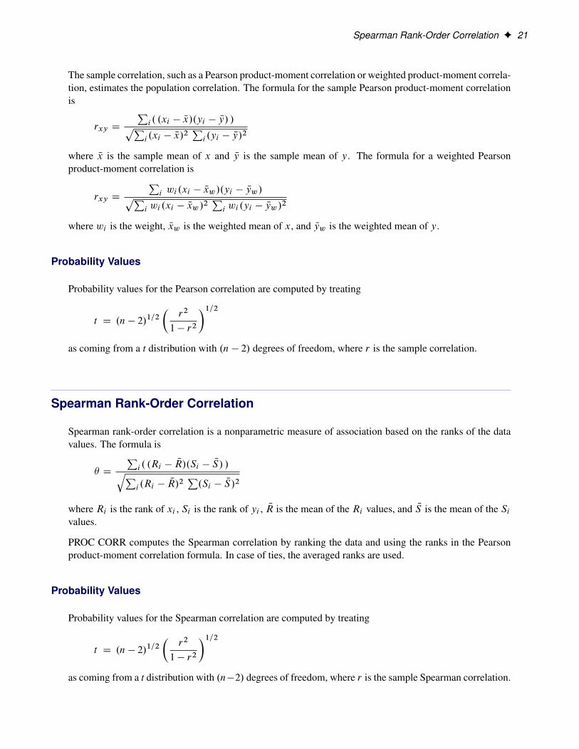
The sample correlation, such as a Pearson product-moment correlation or weighted product-moment correla-tion, estimates the population correlation. The formula for the sample Pearson product-moment correlationis
rxy D
Pi . .xi � Nx/.yi � Ny/ /pPi .xi � Nx/
2Pi .yi � Ny/
2
where Nx is the sample mean of x and Ny is the sample mean of y. The formula for a weighted Pearsonproduct-moment correlation is
rxy D
Pi wi .xi � Nxw/.yi � Nyw/pP
i wi .xi � Nxw/2Pi wi .yi � Nyw/
2
where wi is the weight, Nxw is the weighted mean of x, and Nyw is the weighted mean of y.
Probability Values
Probability values for the Pearson correlation are computed by treating
t D .n � 2/1=2�
r2
1 � r2
�1=2as coming from a t distribution with .n � 2/ degrees of freedom, where r is the sample correlation.
Spearman Rank-Order Correlation
Spearman rank-order correlation is a nonparametric measure of association based on the ranks of the datavalues. The formula is
� D
Pi . .Ri �
NR/.Si � NS/ /qPi .Ri �
NR/2P.Si � NS/2
where Ri is the rank of xi , Si is the rank of yi , NR is the mean of the Ri values, and NS is the mean of the Sivalues.
PROC CORR computes the Spearman correlation by ranking the data and using the ranks in the Pearsonproduct-moment correlation formula. In case of ties, the averaged ranks are used.
Probability Values
Probability values for the Spearman correlation are computed by treating
t D .n � 2/1=2�
r2
1 � r2
�1=2as coming from a t distribution with .n�2/ degrees of freedom, where r is the sample Spearman correlation.

22 F Chapter 2: The CORR Procedure
Kendall’s Tau-b Correlation Coefficient
Kendall’s tau-b is a nonparametric measure of association based on the number of concordances and discor-dances in paired observations. Concordance occurs when paired observations vary together, and discordanceoccurs when paired observations vary differently. The formula for Kendall’s tau-b is
� D
Pi<j .sgn.xi � xj /sgn.yi � yj //p
.T0 � T1/.T0 � T2/
where T0 D n.n � 1/=2, T1 DPk tk.tk � 1/=2, and T2 D
Pl ul.ul � 1/=2. The tk is the number of
tied x values in the kth group of tied x values, ul is the number of tied y values in the l th group of tied yvalues, n is the number of observations, and sgn.z/ is defined as
sgn.z/ D
8<:1 if z > 00 if z D 0�1 if z < 0
PROC CORR computes Kendall’s tau-b by ranking the data and using a method similar to Knight (1966).The data are double sorted by ranking observations according to values of the first variable and rerankingthe observations according to values of the second variable. PROC CORR computes Kendall’s tau-b fromthe number of interchanges of the first variable and corrects for tied pairs (pairs of observations with equalvalues of X or equal values of Y).
Probability Values
Probability values for Kendall’s tau-b are computed by treating
spV.s/
as coming from a standard normal distribution where
s DXi<j
.sgn.xi � xj /sgn.yi � yj //
and V.s/, the variance of s, is computed as
V.s/ Dv0 � vt � vu
18C
v1
2n.n � 1/C
v2
9n.n � 1/.n � 2/
where
v0 D n.n � 1/.2nC 5/
vt DPk tk.tk � 1/.2tk C 5/
vu DPl ul.ul � 1/.2ul C 5/
v1 D .Pk tk.tk � 1// .
Pui .ul � 1//

Hoeffding Dependence Coefficient F 23
v2 D .Pl ti .tk � 1/.tk � 2// .
Pul.ul � 1/.ul � 2//
The sums are over tied groups of values where ti is the number of tied x values and ui is the number of tiedy values (Noether 1967). The sampling distribution of Kendall’s partial tau-b is unknown; therefore, theprobability values are not available.
Hoeffding Dependence Coefficient
Hoeffding’s measure of dependence,D, is a nonparametric measure of association that detects more generaldepartures from independence. The statistic approximates a weighted sum over observations of chi-squarestatistics for two-by-two classification tables (Hoeffding 1948). Each set of .x; y/ values are cut points forthe classification. The formula for Hoeffding’s D is
D D 30.n � 2/.n � 3/D1 CD2 � 2.n � 2/D3
n.n � 1/.n � 2/.n � 3/.n � 4/
where D1 DPi .Qi � 1/.Qi � 2/, D2 D
Pi .Ri � 1/.Ri � 2/.Si � 1/.Si � 2/, and D3 D
Pi .Ri �
2/.Si � 2/.Qi � 1/. Ri is the rank of xi , Si is the rank of yi , and Qi (also called the bivariate rank) is 1plus the number of points with both x and y values less than the i th point.
A point that is tied on only the x value or y value contributes 1/2 to Qi if the other value is less than thecorresponding value for the i th point.
A point that is tied on both x and y contributes 1/4 to Qi . PROC CORR obtains the Qi values by firstranking the data. The data are then double sorted by ranking observations according to values of the firstvariable and reranking the observations according to values of the second variable. Hoeffding’s D statisticis computed using the number of interchanges of the first variable. When no ties occur among data set ob-servations, theD statistic values are between �0.5 and 1, with 1 indicating complete dependence. However,when ties occur, the D statistic might result in a smaller value. That is, for a pair of variables with identicalvalues, the Hoeffding’s D statistic might be less than 1. With a large number of ties in a small data set, theD statistic might be less than �0.5. For more information about Hoeffding’s D, see Hollander and Wolfe(1999).
Probability Values
The probability values for Hoeffding’sD statistic are computed using the asymptotic distribution computedby Blum, Kiefer, and Rosenblatt (1961). The formula is
.n � 1/�4
60D C
�4
72
which comes from the asymptotic distribution. If the sample size is less than 10, refer to the tables for thedistribution of D in Hollander and Wolfe (1999).

24 F Chapter 2: The CORR Procedure
Partial Correlation
A partial correlation measures the strength of a relationship between two variables, while controlling theeffect of other variables. The Pearson partial correlation between two variables, after controlling for vari-ables in the PARTIAL statement, is equivalent to the Pearson correlation between the residuals of the twovariables after regression on the controlling variables.
Let y D .y1; y2; : : : ; yv/ be the set of variables to correlate and z D .z1; z2; : : : ; zp/ be the set of controllingvariables. The population Pearson partial correlation between the i th and the j th variables of y given z isthe correlation between errors .yi � E.yi // and .yj � E.yj //, where
E.yi / D ˛i C zˇi and E.yj / D ˛j C zˇj
are the regression models for variables yi and yj given the set of controlling variables z, respectively.
For a given sample of observations, a sample Pearson partial correlation between yi and yj given z isderived from the residuals yi � Oyi and yj � Oyj , where
Oyi D O i C z Oi and Oyj D Oj C z Oj
are fitted values from regression models for variables yi and yj given z.
The partial corrected sums of squares and crossproducts (CSSCP) of y given z are the corrected sumsof squares and crossproducts of the residuals y � Oy. Using these partial corrected sums of squares andcrossproducts, you can calculate the partial covariances and partial correlations.
PROC CORR derives the partial corrected sums of squares and crossproducts matrix by applying theCholesky decomposition algorithm to the CSSCP matrix. For Pearson partial correlations, let S be thepartitioned CSSCP matrix between two sets of variables, z and y:
S D
�Szz SzyS0zy Syy
�
PROC CORR calculates Syy:z , the partial CSSCP matrix of y after controlling for z, by applying theCholesky decomposition algorithm sequentially on the rows associated with z, the variables being partialledout.
After applying the Cholesky decomposition algorithm to each row associated with variables z, PROC CORRchecks all higher-numbered diagonal elements associated with z for singularity. A variable is consideredsingular if the value of the corresponding diagonal element is less than " times the original unpartialledcorrected sum of squares of that variable. You can specify the singularity criterion " by using the SINGU-LAR= option. For Pearson partial correlations, a controlling variable z is considered singular if the R2 forpredicting this variable from the variables that are already partialled out exceeds 1 � ". When this happens,PROC CORR excludes the variable from the analysis. Similarly, a variable is considered singular if the R2
for predicting this variable from the controlling variables exceeds 1 � ". When this happens, its associateddiagonal element and all higher-numbered elements in this row or column are set to zero.
After the Cholesky decomposition algorithm is applied to all rows associated with z, the resulting matrixhas the form

Partial Correlation F 25
T D
�Tzz Tzy0 Syy:z
�
where Tzz is an upper triangular matrix with T 0zzTzz D S0zz , T 0zzTzy D S
0zy , and Syy:z D Syy � T 0zyTzy .
If Szz is positive definite, then Tzy D T 0zz�1S 0zy and the partial CSSCP matrix Syy:z is identical to the
matrix derived from the formula
Syy:z D Syy � S0zyS0�1zz Szy
The partial variance-covariance matrix is calculated with the variance divisor (VARDEF= option). PROCCORR then uses the standard Pearson correlation formula on the partial variance-covariance matrix to cal-culate the Pearson partial correlation matrix.
When a correlation matrix is positive definite, the resulting partial correlation between variables x and y afteradjusting for a single variable z is identical to that obtained from the first-order partial correlation formula
rxy:z Drxy � rxzryzq.1 � r2xz/.1 � r
2yz/
where rxy , rxz , and ryz are the appropriate correlations.
The formula for higher-order partial correlations is a straightforward extension of the preceding first-orderformula. For example, when the correlation matrix is positive definite, the partial correlation between x andy controlling for both z_1 and z_2 is identical to the second-order partial correlation formula
rxy:z1z2 Drxy:z1 � rxz2:z1ryz2:z1q.1 � r2xz2:z1/.1 � r
2yz2:z1
/
where rxy:z1 , rxz2:z1 , and ryz2:z1 are first-order partial correlations among variables x, y, and z_2 givenz_1.
To derive the corresponding Spearman partial rank-order correlations and Kendall partial tau-b correlations,PROC CORR applies the Cholesky decomposition algorithm to the Spearman rank-order correlation matrixand Kendall’s tau-b correlation matrix and uses the correlation formula. That is, the Spearman partialcorrelation is equivalent to the Pearson correlation between the residuals of the linear regression of theranks of the two variables on the ranks of the partialled variables. Thus, if a PARTIAL statement is specifiedwith the CORR=SPEARMAN option, the residuals of the ranks of the two variables are displayed in theplot. The partial tau-b correlations range from –1 to 1. However, the sampling distribution of this partialtau-b is unknown; therefore, the probability values are not available.
Probability Values
Probability values for the Pearson and Spearman partial correlations are computed by treating
.n � k � 2/1=2r
.1 � r2/1=2
as coming from a t distribution with .n � k � 2/ degrees of freedom, where r is the partial correlation andk is the number of variables being partialled out.

26 F Chapter 2: The CORR Procedure
Fisher’s z Transformation
For a sample correlation r that uses a sample from a bivariate normal distribution with correlation � D 0,the statistic
tr D .n � 2/1=2�
r2
1 � r2
�1=2has a Student’s t distribution with (n � 2) degrees of freedom.
With the monotone transformation of the correlation r (Fisher 1921)
zr D tanh�1.r/ D1
2log
�1C r
1 � r
�the statistic z has an approximate normal distribution with mean and variance
E.zr/ D � C�
2.n � 1/
V .zr/ D1
n � 3
where � D tanh�1.�/.
For the transformed zr , the approximate variance V.zr/ D 1=.n � 3/ is independent of the correlation �.Furthermore, even the distribution of zr is not strictly normal, it tends to normality rapidly as the samplesize increases for any values of � (Fisher 1970, pp. 200–201).
For the null hypothesis H0W � D �0, the p-values are computed by treating
zr � �0 ��0
2.n � 1/
as a normal random variable with mean zero and variance 1=.n� 3/, where �0 D tanh�1.�0/ (Fisher 1970,p. 207; Anderson 1984, p. 123).
Note that the bias adjustment, �0=.2.n � 1//, is always used when computing p-values under the nullhypothesis H0W � D �0 in the CORR procedure.
The ALPHA= option in the FISHER option specifies the value ˛ for the confidence level 1�˛, the RHO0=option specifies the value �0 in the hypothesisH0W � D �0, and the BIASADJ= option specifies whether thebias adjustment is to be used for the confidence limits.
The TYPE= option specifies the type of confidence limits. The TYPE=TWOSIDED option requests two-sided confidence limits and a p-value under the hypothesis H0W � D �0. For a one-sided confidence limit,the TYPE=LOWER option requests a lower confidence limit and a p-value under the hypothesisH0W � <D�0, and the TYPE=UPPER option requests an upper confidence limit and a p-value under the hypothesisH0W � >D �0.

Fisher’s z Transformation F 27
Confidence Limits for the Correlation
The confidence limits for the correlation � are derived through the confidence limits for the parameter �,with or without the bias adjustment.
Without a bias adjustment, confidence limits for � are computed by treating
zr � �
as having a normal distribution with mean zero and variance 1=.n � 3/.
That is, the two-sided confidence limits for � are computed as
�l D zr � z.1�˛=2/
r1
n � 3
�u D zr C z.1�˛=2/
r1
n � 3
where z.1�˛=2/ is the 100.1 � ˛=2/ percentage point of the standard normal distribution.
With a bias adjustment, confidence limits for � are computed by treating
zr � � � bias.r/
as having a normal distribution with mean zero and variance 1=.n � 3/, where the bias adjustment function(Keeping 1962, p. 308) is
bias.rr/ Dr
2.n � 1/
That is, the two-sided confidence limits for � are computed as
�l D zr � bias.r/ � z.1�˛=2/
r1
n � 3
�u D zr � bias.r/C z.1�˛=2/
r1
n � 3
These computed confidence limits of �l and �u are then transformed back to derive the confidence limits forthe correlation �:
rl D tanh.�l/ Dexp.2�l/ � 1exp.2�l/C 1
ru D tanh.�u/ Dexp.2�u/ � 1exp.2�u/C 1
Note that with a bias adjustment, the CORR procedure also displays the following correlation estimate:
radj D tanh.zr � bias.r//

28 F Chapter 2: The CORR Procedure
Applications of Fisher’s z Transformation
Fisher (1970, p. 199) describes the following practical applications of the z transformation:
� testing whether a population correlation is equal to a given value
� testing for equality of two population correlations
� combining correlation estimates from different samples
To test if a population correlation �1 from a sample of n1 observations with sample correlation r1 is equalto a given �0, first apply the z transformation to r1 and �0: z1 D tanh�1.r1/ and �0 D tanh�1.�0/.
The p-value is then computed by treating
z1 � �0 ��0
2.n1 � 1/
as a normal random variable with mean zero and variance 1=.n1 � 3/.
Assume that sample correlations r1 and r2 are computed from two independent samples of n1 and n2 obser-vations, respectively. To test whether the two corresponding population correlations, �1 and �2, are equal,first apply the z transformation to the two sample correlations: z1 D tanh�1.r1/ and z2 D tanh�1.r2/.
The p-value is derived under the null hypothesis of equal correlation. That is, the difference z1 � z2 isdistributed as a normal random variable with mean zero and variance 1=.n1 � 3/C 1=.n2 � 3/.
Assuming further that the two samples are from populations with identical correlation, a combined correla-tion estimate can be computed. The weighted average of the corresponding z values is
Nz D.n1 � 3/z1 C .n2 � 3/z2
n1 C n2 � 6
where the weights are inversely proportional to their variances.
Thus, a combined correlation estimate is Nr D tanh. Nz/ and V. Nz/ D 1=.n1 C n2 � 6/. See Example 2.4 forfurther illustrations of these applications.
Note that this approach can be extended to include more than two samples.
Polyserial Correlation
Polyserial correlation measures the correlation between two continuous variables with a bivariate normaldistribution, where one variable is observed directly, and the other is unobserved. Information about theunobserved variable is obtained through an observed ordinal variable that is derived from the unobservedvariable by classifying its values into a finite set of discrete, ordered values (Olsson, Drasgow, and Dorans1982).

Polyserial Correlation F 29
Let X be the observed continuous variable from a normal distribution with mean � and variance �2, let Ybe the unobserved continuous variable, and let � be the Pearson correlation between X and Y. Furthermore,assume that an observed ordinal variable D is derived from Y as follows:
D D
8<:d.1/ if Y < �1d.k/ if �k�1 � Y < �k; k D 2; 3; : : : ; K � 1d.K/ if Y � �K�1
where d.1/ < d.2/ < : : : < d.K/ are ordered observed values, and �1 < �2 < : : : < �K�1 are orderedunknown threshold values.
The likelihood function for the joint distribution (X, D) from a sample of N observations .xj ; dj / is
L D
NYjD1
f .xj ; dj / D
NYjD1
f .xj / P.D D dj j xj /
where f .xj / is the normal density function with mean � and standard deviation � (Drasgow 1986).
The conditional distribution of Y given X D xj is normal with mean �zj and variance 1 � �2, wherezj D .xj � �/=� is a standard normal variate. Without loss of generality, assume the variable Y has astandard normal distribution. Then if dj D d.k/, the kth ordered value in D, the resulting conditionaldensity is
P.D D d.k/ j xj / D
8ˆ<ˆ:
ˆ
��1��zjp1��2
�if k D 1
ˆ
��k��zjp1��2
��ˆ
��k�1��zjp
1��2
�if k D 2; 3; : : : ; K � 1
1 �ˆ
��K�1��zjp
1��2
�if k D K
where ˆ is the cumulative normal distribution function.
Cox (1972) derives the maximum likelihood estimates for all parameters �, � , � and �1, . . . , �k�1. Themaximum likelihood estimates for � and �2 can be derived explicitly. The maximum likelihood estimatefor � is the sample mean and the maximum likelihood estimate for �2 is the sample variancePN
jD1.xj � Nx/2
N
The maximum likelihood estimates for the remaining parameters, including the polyserial correlation �and thresholds �1, . . . , �k�1, can be computed by an iterative process, as described by Cox (1972). Theasymptotic standard error of the maximum likelihood estimate of � can also be computed after this process.
For a vector of parameters, the information matrix is the negative of the Hessian matrix (the matrix of secondpartial derivatives of the log likelihood function), and is used in the computation of the maximum likelihoodestimates of these parameters. The CORR procedure uses the observed information matrix (the informationmatrix evaluated at the current parameter estimates) in the computation. After the maximum likelihoodestimates are derived, the asymptotic covariance matrix for these parameter estimates is computed as theinverse of the observed information matrix (the information matrix evaluated at the maximum likelihoodestimates).

30 F Chapter 2: The CORR Procedure
Probability Values
The CORR procedure computes two types of testing for the zero polyserial correlation: the Wald test andthe likelihood ratio (LR) test.
Given the maximum likelihood estimate of the polyserial correlation O�, and its asymptotic standard errorStdErr. O�/, the Wald chi-square test statistic is computed as�
O�
StdErr. O�/
�2The Wald statistic has an asymptotic chi-square distribution with one degree of freedom.
For the LR test, the maximum likelihood function assuming zero polyserial correlation is also needed. If� D 0, the likelihood function is reduced to
L D
NYjD1
f .xj ; dj / D
NYjD1
f .xj /
NYjD1
P.D D dj /
In this case, the maximum likelihood estimates for all parameters can be derived explicitly. The maximumlikelihood estimates for � is the sample mean and the maximum likelihood estimate for �2 is the samplevariancePN
jD1.xj � Nx/2
N
In addition, the maximum likelihood estimate for the threshold �k , k D 1; : : : ; K � 1, is
ˆ�1
PkgD1 ng
N
!
where ng is the number of observations in the gth ordered group of the ordinal variable D, and N DPKgD1 ng is the total number of observations.
The LR test statistic is computed as
�2 log�L0
L1
�where L1 is the likelihood function with the maximum likelihood estimates for all parameters, and L0is the likelihood function with the maximum likelihood estimates for all parameters except the polyserialcorrelation, which is set to zero. The LR statistic also has an asymptotic chi-square distribution with onedegree of freedom.
Cronbach’s Coefficient Alpha
Analyzing latent constructs such as job satisfaction, motor ability, sensory recognition, or customer satisfac-tion requires instruments to accurately measure the constructs. Interrelated items can be summed to obtain

Cronbach’s Coefficient Alpha F 31
an overall score for each participant. Cronbach’s coefficient alpha estimates the reliability of this type ofscale by determining the internal consistency of the test or the average correlation of items within the test(Cronbach 1951).
When a value is recorded, the observed value contains some degree of measurement error. Two sets ofmeasurements on the same variable for the same individual might not have identical values. However,repeated measurements for a series of individuals will show some consistency. Reliability measures internalconsistency from one set of measurements to another. The observed value Y is divided into two components,a true value T and a measurement error E. The measurement error is assumed to be independent of the truevalue; that is,
Y D T CE Cov.T;E/ D 0
The reliability coefficient of a measurement test is defined as the squared correlation between the observedvalue Y and the true value T ; that is,
r2.Y; T / DCov.Y; T /2
V.Y /V.T /D
V.T /2
V.Y /V.T /D
V.T /V.Y /
which is the proportion of the observed variance due to true differences among individuals in the sample. IfY is the sum of several observed variables measuring the same feature, you can estimate V.T /. Cronbach’scoefficient alpha, based on a lower bound for V.T /, is an estimate of the reliability coefficient.
Suppose p variables are used with Yj D Tj C Ej for j D 1; 2; : : : ; p, where Yj is the observed value,Tj is the true value, and Ej is the measurement error. The measurement errors (Ej ) are independent of thetrue values (Tj ) and are also independent of each other. Let Y0 D
Pj Yj be the total observed score and
let T0 DPj Tj be the total true score. Because
.p � 1/Xj
V.Tj / �Xi¤j
Cov.Ti ; Tj /
a lower bound for V.T0/ is given by
p
p � 1
Xi¤j
Cov.Ti ; Tj /
With Cov.Yi ; Yj / D Cov.Ti ; Tj / for i ¤ j , a lower bound for the reliability coefficient, V.T0/=V .Y0/, isthen given by the Cronbach’s coefficient alpha:
˛ D
�p
p � 1
� Pi¤j Cov.Yi ; Yj /
V .Y0/D
�p
p � 1
� 1 �
Pj V.Yj /
V .Y0/
!
If the variances of the items vary widely, you can standardize the items to a standard deviation of 1 beforecomputing the coefficient alpha. If the variables are dichotomous (0,1), the coefficient alpha is equivalent tothe Kuder-Richardson 20 (KR-20) reliability measure.
When the correlation between each pair of variables is 1, the coefficient alpha has a maximum value of 1.With negative correlations between some variables, the coefficient alpha can have a value less than zero.The larger the overall alpha coefficient, the more likely that items contribute to a reliable scale. Nunnally

32 F Chapter 2: The CORR Procedure
and Bernstein (1994) suggests 0.70 as an acceptable reliability coefficient; smaller reliability coefficientsare seen as inadequate. However, this varies by discipline.
To determine how each item reflects the reliability of the scale, you calculate a coefficient alpha after deletingeach variable independently from the scale. Cronbach’s coefficient alpha from all variables except the kthvariable is given by
˛k D
�p � 1
p � 2
� 1 �
Pi¤k V.Yi /
V .Pi¤k Yi /
!
If the reliability coefficient increases after an item is deleted from the scale, you can assume that the item isnot correlated highly with other items in the scale. Conversely, if the reliability coefficient decreases, youcan assume that the item is highly correlated with other items in the scale. Refer to Yu (2001) for moreinformation about how to interpret Cronbach’s coefficient alpha.
Listwise deletion of observations with missing values is necessary to correctly calculate Cronbach’s coeffi-cient alpha. PROC CORR does not automatically use listwise deletion if you specify the ALPHA option.Therefore, you should use the NOMISS option if the data set contains missing values. Otherwise, PROCCORR prints a warning message indicating the need to use the NOMISS option with the ALPHA option.
Confidence and Prediction Ellipses
When the relationship between two variables is nonlinear or when outliers are present, the correlation coef-ficient might incorrectly estimate the strength of the relationship. Plotting the data enables you to verify thelinear relationship and to identify the potential outliers.
The partial correlation between two variables, after controlling for variables in the PARTIAL statement, isthe correlation between the residuals of the linear regression of the two variables on the partialled variables.Thus, if a PARTIAL statement is also specified, the residuals of the analysis variables are displayed in thescatter plot matrix and scatter plots.
The CORR procedure optionally provides two types of ellipses for each pair of variables in a scatter plot.One is a confidence ellipse for the population mean, and the other is a prediction ellipse for a new observa-tion. Both assume a bivariate normal distribution.
Let NZ and S be the sample mean and sample covariance matrix of a random sample of size n from a bivariatenormal distribution with mean � and covariance matrix †. The variable NZ � � is distributed as a bivariatenormal variate with mean zero and covariance .1=n/†, and it is independent of S. Using Hotelling’s T 2
statistic, which is defined as
T 2 D n. NZ � �/0S�1. NZ � �/
a 100.1 � ˛/% confidence ellipse for � is computed from the equation
n
n � 1. NZ � �/0S�1. NZ � �/ D
2
n � 2F2;n�2.1 � ˛/
where F2;n�2.1� ˛/ is the .1� ˛/ critical value of an F distribution with degrees of freedom 2 and n� 2.

Missing Values F 33
A prediction ellipse is a region for predicting a new observation in the population. It also approximates aregion that contains a specified percentage of the population.
Denote a new observation as the bivariate random variable Znew. The variable
Znew � NZ D .Znew � �/ � . NZ � �/
is distributed as a bivariate normal variate with mean zero (the zero vector) and covariance .1C1=n/†, andit is independent of S. A 100.1 � ˛/% prediction ellipse is then given by the equation
n
n � 1. NZ � �/0S�1. NZ � �/ D
2.nC 1/
n � 2F2;n�2.1 � ˛/
The family of ellipses generated by different critical values of the F distribution has a common center (thesample mean) and common major and minor axis directions.
The shape of an ellipse depends on the aspect ratio of the plot. The ellipse indicates the correlation betweenthe two variables if the variables are standardized (by dividing the variables by their respective standarddeviations). In this situation, the ratio between the major and minor axis lengths iss
1C jr j
1 � jr j
In particular, if r D 0, the ratio is 1, which corresponds to a circular confidence contour and indicates thatthe variables are uncorrelated. A larger value of the ratio indicates a larger positive or negative correlationbetween the variables.
Missing Values
PROC CORR excludes observations with missing values in the WEIGHT and FREQ variables. By default,PROC CORR uses pairwise deletion when observations contain missing values. PROC CORR includesall nonmissing pairs of values for each pair of variables in the statistical computations. Therefore, thecorrelation statistics might be based on different numbers of observations.
If you specify the NOMISS option, PROC CORR uses listwise deletion when a value of the VAR or WITHstatement variable is missing. PROC CORR excludes all observations with missing values from the analysis.Therefore, the number of observations for each pair of variables is identical.
The PARTIAL statement always excludes the observations with missing values by automatically invokingthe NOMISS option. With the NOMISS option, the data are processed more efficiently because fewerresources are needed. Also, the resulting correlation matrix is nonnegative definite.
In contrast, if the data set contains missing values for the analysis variables and the NOMISS option is notspecified, the resulting correlation matrix might not be nonnegative definite. This leads to several statisticaldifficulties if you use the correlations as input to regression or other statistical procedures.

34 F Chapter 2: The CORR Procedure
In-Database Computation
The CORR procedure can use in-database computation to compute univariate statistics and the SSCP matrixif the DATA= input data set is stored as a table in a database management system (DBMS). When the CORRprocedure performs in-database computation for the DATA= data set, the procedure generates an SQL querythat computes summary tables of univariate statistics and the SSCP matrix. The query is passed to the DBMSand executed in-database. The results of the query are then passed back to the SAS System and transmittedto PROC CORR. The CORR procedure then uses these summary tables to perform the remaining tasks(such as producing the correlation and covariance matrices) in the usual way (out of the database).
In-database computation can provide the advantages of faster processing and reduced data transfer be-tween the database and SAS software. For information about in-database computation, see the section“In-Database Procedures” in SAS/ACCESS 9.2 for Relational Databases: Reference. Instead of transferringthe entire data set over the network between the database and SAS software, the in-database method trans-fers only the summary tables. This can substantially reduce processing time when the dimensions of thesummary tables (in terms of rows and columns) are much smaller than the dimensions of the entire databasetable (in terms of individual observations). Additionally, in-database summarization uses efficient parallelprocessing, which can also provide performance advantages.
By default, PROC CORR uses in-database computation when possible. If in-database computation is used,the EXCLNPWGT option is activated to exclude observations with nonpositive weights. The ID state-ment requires row-level access and therefore cannot be used in-database. In addition, the HOEFFDING,KENDALL, SPEARMAN, OUTH=, OUTK=, OUTS=, and PLOTS= options also require row-level accessand cannot be used in-database.
In-database computation is controlled by the SQLGENERATION option, which you can specify in either aLIBNAME statement or an OPTIONS statement. See the section “In-Database Procedures” in SAS/ACCESS9.2 for Relational Databases: Reference for details about the SQLGENERATION option and other optionsthat affect in-database computation. There are no CORR procedure options that control in-database compu-tation.
The order of observations is not inherently defined for DBMS tables. The following options relate to theorder of observations and therefore should not be specified for PROC CORR in-database computation:
� If you specify the FIRSTOBS= or OBS= data set option, PROC CORR does not perform in-databasecomputation.
� If you specify the NOTSORTED option in the BY statement, PROC CORR in-database computationignores it and uses the default ASCENDING order for BY variables.
NOTE: In-database computing in the CORR procedure requires installation of the SAS Analytics Acceler-ator.

Output Tables F 35
Output Tables
By default, PROC CORR prints a report that includes descriptive statistics and correlation statistics for eachvariable. The descriptive statistics include the number of observations with nonmissing values, the mean,the standard deviation, the minimum, and the maximum.
If a nonparametric measure of association is requested, the descriptive statistics include the median. Other-wise, the sample sum is included. If a Pearson partial correlation is requested, the descriptive statistics alsoinclude the partial variance and partial standard deviation.
If variable labels are available, PROC CORR labels the variables. If you specify the CSSCP, SSCP, orCOV option, the appropriate sums of squares and crossproducts and covariance matrix appear at the top ofthe correlation report. If the data set contains missing values, PROC CORR prints additional statistics foreach pair of variables. These statistics, calculated from the observations with nonmissing row and columnvariable values, might include the following:
� SSCP(’W’,’V’), uncorrected sums of squares and crossproducts
� USS(’W’), uncorrected sums of squares for the row variable
� USS(’V’), uncorrected sums of squares for the column variable
� CSSCP(’W’,’V’), corrected sums of squares and crossproducts
� CSS(’W’), corrected sums of squares for the row variable
� CSS(’V’), corrected sums of squares for the column variable
� COV(’W’,’V’), covariance
� VAR(’W’), variance for the row variable
� VAR(’V’), variance for the column variable
� DF(’W’,’V’), divisor for calculating covariance and variances
For each pair of variables, PROC CORR prints the correlation coefficients, the number of observations usedto calculate the coefficient, and the p-value.
If you specify the ALPHA option, PROC CORR prints Cronbach’s coefficient alpha, the correlation betweenthe variable and the total of the remaining variables, and Cronbach’s coefficient alpha by using the remainingvariables for the raw variables and the standardized variables.
Output Data Sets
If you specify the OUTP=, OUTS=, OUTK=, or OUTH= option, PROC CORR creates an output data setthat contains statistics for Pearson correlation, Spearman correlation, Kendall’s tau-b, or Hoeffding’s D,

36 F Chapter 2: The CORR Procedure
respectively. By default, the output data set is a special data set type (TYPE=CORR) that many SAS/STATprocedures recognize, including PROC REG and PROC FACTOR. When you specify the NOCORR optionand the COV, CSSCP, or SSCP option, use the TYPE= data set option to change the data set type to COV,CSSCP, or SSCP.
The output data set includes the following variables:
� BY variables, which identify the BY group when using a BY statement
� _TYPE_ variable, which identifies the type of observation
� _NAME_ variable, which identifies the variable that corresponds to a given row of the correlationmatrix
� INTERCEPT variable, which identifies variable sums when specifying the SSCP option
� VAR variables, which identify the variables listed in the VAR statement
You can use a combination of the _TYPE_ and _NAME_ variables to identify the contents of an observation.The _NAME_ variable indicates which row of the correlation matrix the observation corresponds to. Thevalues of the _TYPE_ variable are as follows:
� SSCP, uncorrected sums of squares and crossproducts
� CSSCP, corrected sums of squares and crossproducts
� COV, covariances
� MEAN, mean of each variable
� STD, standard deviation of each variable
� N, number of nonmissing observations for each variable
� SUMWGT, sum of the weights for each variable when using a WEIGHT statement
� CORR, correlation statistics for each variable
If you specify the SSCP option, the OUTP= data set includes an additional observation that contains in-tercept values. If you specify the ALPHA option, the OUTP= data set also includes observations with thefollowing _TYPE_ values:
� RAWALPHA, Cronbach’s coefficient alpha for raw variables
� STDALPHA, Cronbach’s coefficient alpha for standardized variables
� RAWALDEL, Cronbach’s coefficient alpha for raw variables after deleting one variable
� STDALDEL, Cronbach’s coefficient alpha for standardized variables after deleting one variable
� RAWCTDEL, the correlation between a raw variable and the total of the remaining raw variables

ODS Table Names F 37
� STDCTDEL, the correlation between a standardized variable and the total of the remaining standard-ized variables
If you use a PARTIAL statement, the statistics are calculated after the variables are partialled. If PROCCORR computes Pearson correlation statistics, MEAN equals zero and STD equals the partial standarddeviation associated with the partial variance for the OUTP=, OUTK=, and OUTS= data sets. Otherwise,PROC CORR assigns missing values to MEAN and STD.
ODS Table Names
PROC CORR assigns a name to each table it creates. You must use these names to reference tables whenusing the Output Delivery System (ODS). These names are listed in Table 2.3 and Table 2.4. For moreinformation about ODS, see Chapter 20, “Using the Output Delivery System” (SAS/STAT User’s Guide).
Table 2.3 ODS Tables Produced by PROC CPRR
ODS Table Name Description Option
Cov Covariances COVCronbachAlpha Coefficient alpha ALPHACronbachAlphaDel Coefficient alpha with deleted variable ALPHACsscp Corrected sums of squares and crossproducts CSSCPFisherPearsonCorr Pearson correlation statistics using FISHER
Fisher’s z transformationFisherSpearmanCorr Spearman correlation statistics using FISHER SPEARMAN
Fisher’s z transformationHoeffdingCorr Hoeffding’s D statistics HOEFFDINGKendallCorr Kendall’s tau-b coefficients KENDALLPearsonCorr Pearson correlations PEARSONPolyserialCorr Polyserial correlations POLYSERIALSimpleStats Simple descriptive statisticsSpearmanCorr Spearman correlations SPEARMANSscp Sums of squares and crossproducts SSCPVarInformation Variable information
Table 2.4 ODS Tables Produced with the PARTIAL Statement
ODS Table Name Description Option
FisherPearsonPartialCorr Pearson partial correlation statistics FISHERusing Fisher’s z transformation
FisherSpearmanPartialCorr Spearman partial correlation statistics FISHER SPEARMANusing Fisher’s z transformation
PartialCsscp Partial corrected sums of squares CSSCPand crossproducts
PartialCov Partial covariances COV
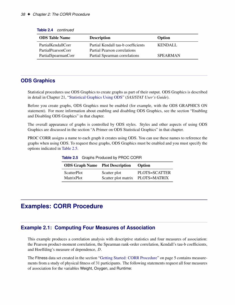
38 F Chapter 2: The CORR Procedure
Table 2.4 continued
ODS Table Name Description Option
PartialKendallCorr Partial Kendall tau-b coefficients KENDALLPartialPearsonCorr Partial Pearson correlationsPartialSpearmanCorr Partial Spearman correlations SPEARMAN
ODS Graphics
Statistical procedures use ODS Graphics to create graphs as part of their output. ODS Graphics is describedin detail in Chapter 21, “Statistical Graphics Using ODS” (SAS/STAT User’s Guide).
Before you create graphs, ODS Graphics must be enabled (for example, with the ODS GRAPHICS ONstatement). For more information about enabling and disabling ODS Graphics, see the section “Enablingand Disabling ODS Graphics” in that chapter.
The overall appearance of graphs is controlled by ODS styles. Styles and other aspects of using ODSGraphics are discussed in the section “A Primer on ODS Statistical Graphics” in that chapter.
PROC CORR assigns a name to each graph it creates using ODS. You can use these names to reference thegraphs when using ODS. To request these graphs, ODS Graphics must be enabled and you must specify theoptions indicated in Table 2.5.
Table 2.5 Graphs Produced by PROC CORR
ODS Graph Name Plot Description Option
ScatterPlot Scatter plot PLOTS=SCATTERMatrixPlot Scatter plot matrix PLOTS=MATRIX
Examples: CORR Procedure
Example 2.1: Computing Four Measures of Association
This example produces a correlation analysis with descriptive statistics and four measures of association:the Pearson product-moment correlation, the Spearman rank-order correlation, Kendall’s tau-b coefficients,and Hoeffding’s measure of dependence, D.
The Fitness data set created in the section “Getting Started: CORR Procedure” on page 5 contains measure-ments from a study of physical fitness of 31 participants. The following statements request all four measuresof association for the variables Weight, Oxygen, and Runtime:

Example 2.1: Computing Four Measures of Association F 39
ods graphics on;title 'Measures of Association for a Physical Fitness Study';proc corr data=Fitness pearson spearman kendall hoeffding
plots=matrix(histogram);var Weight Oxygen RunTime;
run;ods graphics off;
Note that Pearson correlations are computed by default only if all three nonparametric correlations (SPEAR-MAN, KENDALL, and HOEFFDING) are not specified. Otherwise, you need to specify the PEARSONoption explicitly to compute Pearson correlations.
The “Simple Statistics” table in Output 2.1.1 displays univariate descriptive statistics for analysis variables.By default, observations with nonmissing values for each variable are used to derive the univariate statisticsfor that variable. When nonparametric measures of association are specified, the procedure displays themedian instead of the sum as an additional descriptive measure.
Output 2.1.1 Simple Statistics
Measures of Association for a Physical Fitness Study
The CORR Procedure
3 Variables: Weight Oxygen RunTime
Simple Statistics
Variable N Mean Std Dev Median Minimum Maximum
Weight 31 77.44452 8.32857 77.45000 59.08000 91.63000Oxygen 29 47.22721 5.47718 46.67200 37.38800 60.05500RunTime 29 10.67414 1.39194 10.50000 8.17000 14.03000
The “Pearson Correlation Coefficients” table in Output 2.1.2 displays Pearson correlation statistics for pairsof analysis variables. The Pearson correlation is a parametric measure of association for two continuousrandom variables. When there are missing data, the number of observations used to calculate the correlationcan vary.

40 F Chapter 2: The CORR Procedure
Output 2.1.2 Pearson Correlation Coefficients
Pearson Correlation CoefficientsProb > |r| under H0: Rho=0Number of Observations
Weight Oxygen RunTime
Weight 1.00000 -0.15358 0.200720.4264 0.2965
31 29 29
Oxygen -0.15358 1.00000 -0.868430.4264 <.0001
29 29 28
RunTime 0.20072 -0.86843 1.000000.2965 <.0001
29 28 29
The table shows that the Pearson correlation between Runtime and Oxygen is�0.86843, which is significantwith a p-value less than 0.0001. This indicates a strong negative linear relationship between these twovariables. As Runtime increases, Oxygen decreases linearly.
The Spearman rank-order correlation is a nonparametric measure of association based on the ranks of thedata values. The “Spearman Correlation Coefficients” table in Output 2.1.3 displays results similar to thoseof the “Pearson Correlation Coefficients” table in Output 2.1.2.
Output 2.1.3 Spearman Correlation Coefficients
Spearman Correlation CoefficientsProb > |r| under H0: Rho=0Number of Observations
Weight Oxygen RunTime
Weight 1.00000 -0.06824 0.137490.7250 0.4769
31 29 29
Oxygen -0.06824 1.00000 -0.801310.7250 <.0001
29 29 28
RunTime 0.13749 -0.80131 1.000000.4769 <.0001
29 28 29
Kendall’s tau-b is a nonparametric measure of association based on the number of concordances and discor-dances in paired observations. The “Kendall Tau b Correlation Coefficients” table in Output 2.1.4 displaysresults similar to those of the “Pearson Correlation Coefficients” table in Output 2.1.2.

Example 2.1: Computing Four Measures of Association F 41
Output 2.1.4 Kendall’s Tau-b Correlation Coefficients
Kendall Tau b Correlation CoefficientsProb > |tau| under H0: Tau=0
Number of Observations
Weight Oxygen RunTime
Weight 1.00000 -0.00988 0.066750.9402 0.6123
31 29 29
Oxygen -0.00988 1.00000 -0.624340.9402 <.0001
29 29 28
RunTime 0.06675 -0.62434 1.000000.6123 <.0001
29 28 29
Hoeffding’s measure of dependence,D, is a nonparametric measure of association that detects more generaldepartures from independence. Without ties in the variables, the values of the D statistic can vary between�0:5 and 1, with 1 indicating complete dependence. Otherwise, theD statistic can result in a smaller value.The “Hoeffding Dependence Coefficients” table in Output 2.1.5 displays Hoeffding dependence coefficients.Since ties occur in the variable Weight, the D statistic for the Weight variable is less than 1.
Output 2.1.5 Hoeffding’s Dependence Coefficients
Hoeffding Dependence CoefficientsProb > D under H0: D=0Number of Observations
Weight Oxygen RunTime
Weight 0.97690 -0.00497 -0.02355<.0001 0.5101 1.0000
31 29 29
Oxygen -0.00497 1.00000 0.234490.5101 <.0001
29 29 28
RunTime -0.02355 0.23449 1.000001.0000 <.0001
29 28 29
When you use the PLOTS=MATRIX(HISTOGRAM) option, the CORR procedure displays a symmetricmatrix plot for the analysis variables listed in the VAR statement (Output 2.1.6).

42 F Chapter 2: The CORR Procedure
Output 2.1.6 Symmetric Scatter Plot Matrix
The strong negative linear relationship between Oxygen and Runtime is evident in Output 2.1.6.
Note that this graphical display is requested by enabling ODS Graphics and by specifying the PLOTS=option. For more information about ODS Graphics, see Chapter 21, “Statistical Graphics Using ODS”(SAS/STAT User’s Guide).
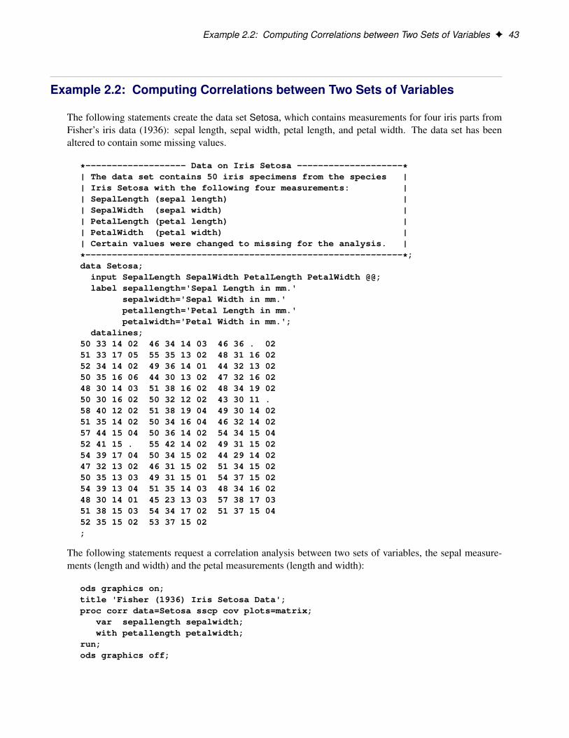
Example 2.2: Computing Correlations between Two Sets of Variables F 43
Example 2.2: Computing Correlations between Two Sets of Variables
The following statements create the data set Setosa, which contains measurements for four iris parts fromFisher’s iris data (1936): sepal length, sepal width, petal length, and petal width. The data set has beenaltered to contain some missing values.
*------------------- Data on Iris Setosa --------------------*| The data set contains 50 iris specimens from the species || Iris Setosa with the following four measurements: || SepalLength (sepal length) || SepalWidth (sepal width) || PetalLength (petal length) || PetalWidth (petal width) || Certain values were changed to missing for the analysis. |
*------------------------------------------------------------*;data Setosa;
input SepalLength SepalWidth PetalLength PetalWidth @@;label sepallength='Sepal Length in mm.'
sepalwidth='Sepal Width in mm.'petallength='Petal Length in mm.'petalwidth='Petal Width in mm.';
datalines;50 33 14 02 46 34 14 03 46 36 . 0251 33 17 05 55 35 13 02 48 31 16 0252 34 14 02 49 36 14 01 44 32 13 0250 35 16 06 44 30 13 02 47 32 16 0248 30 14 03 51 38 16 02 48 34 19 0250 30 16 02 50 32 12 02 43 30 11 .58 40 12 02 51 38 19 04 49 30 14 0251 35 14 02 50 34 16 04 46 32 14 0257 44 15 04 50 36 14 02 54 34 15 0452 41 15 . 55 42 14 02 49 31 15 0254 39 17 04 50 34 15 02 44 29 14 0247 32 13 02 46 31 15 02 51 34 15 0250 35 13 03 49 31 15 01 54 37 15 0254 39 13 04 51 35 14 03 48 34 16 0248 30 14 01 45 23 13 03 57 38 17 0351 38 15 03 54 34 17 02 51 37 15 0452 35 15 02 53 37 15 02;
The following statements request a correlation analysis between two sets of variables, the sepal measure-ments (length and width) and the petal measurements (length and width):
ods graphics on;title 'Fisher (1936) Iris Setosa Data';proc corr data=Setosa sscp cov plots=matrix;
var sepallength sepalwidth;with petallength petalwidth;
run;ods graphics off;

44 F Chapter 2: The CORR Procedure
The “Simple Statistics” table in Output 2.2.1 displays univariate statistics for variables in the VAR andWITH statements.
Output 2.2.1 Simple Statistics
Fisher (1936) Iris Setosa Data
The CORR Procedure
2 With Variables: PetalLength PetalWidth2 Variables: SepalLength SepalWidth
Simple Statistics
Variable N Mean Std Dev Sum
PetalLength 49 14.71429 1.62019 721.00000PetalWidth 48 2.52083 1.03121 121.00000SepalLength 50 50.06000 3.52490 2503SepalWidth 50 34.28000 3.79064 1714
Simple Statistics
Variable Minimum Maximum Label
PetalLength 11.00000 19.00000 Petal Length in mm.PetalWidth 1.00000 6.00000 Petal Width in mm.SepalLength 43.00000 58.00000 Sepal Length in mm.SepalWidth 23.00000 44.00000 Sepal Width in mm.
When the WITH statement is specified together with the VAR statement, the CORR procedure producesrectangular matrices for statistics such as covariances and correlations. The matrix rows correspond to theWITH variables (PetalLength and PetalWidth), while the matrix columns correspond to the VAR variables(SepalLength and SepalWidth). The CORR procedure uses the WITH variable labels to label the matrixrows.
The SSCP option requests a table of the uncorrected sum-of-squares and crossproducts matrix, and the COVoption requests a table of the covariance matrix. The SSCP and COV options also produce a table of thePearson correlations.
The sum-of-squares and crossproducts statistics for each pair of variables are computed by using observa-tions with nonmissing row and column variable values. The “Sums of Squares and Crossproducts” tablein Output 2.2.2 displays the crossproduct, sum of squares for the row variable, and sum of squares for thecolumn variable for each pair of variables.

Example 2.2: Computing Correlations between Two Sets of Variables F 45
Output 2.2.2 Sums of Squares and Crossproducts
Sums of Squares and CrossproductsSSCP / Row Var SS / Col Var SS
SepalLength SepalWidth
PetalLength 36214.00000 24756.00000Petal Length in mm. 10735.00000 10735.00000
123793.0000 58164.0000
PetalWidth 6113.00000 4191.00000Petal Width in mm. 355.00000 355.00000
121356.0000 56879.0000
The variances are computed by using observations with nonmissing row and column variable values. The“Variances and Covariances” table in Output 2.2.3 displays the covariance, variance for the row variable,variance for the column variable, and associated degrees of freedom for each pair of variables.
Output 2.2.3 Variances and Covariances
Variances and CovariancesCovariance / Row Var Variance / Col Var Variance / DF
SepalLength SepalWidth
PetalLength 1.270833333 1.363095238Petal Length in mm. 2.625000000 2.625000000
12.33333333 14.6054421848 48
PetalWidth 0.911347518 1.048315603Petal Width in mm. 1.063386525 1.063386525
11.80141844 13.6272163147 47
When there are missing values in the analysis variables, the “Pearson Correlation Coefficients” table inOutput 2.2.4 displays the correlation, the p-value under the null hypothesis of zero correlation, and thenumber of observations for each pair of variables. Only the correlation between PetalWidth and SepalLengthand the correlation between PetalWidth and SepalWidth are slightly positive.

46 F Chapter 2: The CORR Procedure
Output 2.2.4 Pearson Correlation Coefficients
Pearson Correlation CoefficientsProb > |r| under H0: Rho=0Number of Observations
Sepal SepalLength Width
PetalLength 0.22335 0.22014Petal Length in mm. 0.1229 0.1285
49 49
PetalWidth 0.25726 0.27539Petal Width in mm. 0.0775 0.0582
48 48
When ODS Graphics is enabled, the PLOTS= option displays a scatter matrix plot by default. Output 2.2.5displays a rectangular scatter plot matrix for the two sets of variables: the VAR variables SepalLength andSepalWidth are listed across the top of the matrix, and the WITH variables PetalLength and PetalWidth arelisted down the side of the matrix. As measured in Output 2.2.4, the plot for PetalWidth and SepalLengthand the plot for PetalWidth and SepalWidth also show slight positive correlations.

Example 2.2: Computing Correlations between Two Sets of Variables F 47
Output 2.2.5 Rectangular Matrix Plot
Note that this graphical display is requested by enabling ODS Graphics and by specifying the PLOTS=option. For more information about ODS Graphics, see Chapter 21, “Statistical Graphics Using ODS”(SAS/STAT User’s Guide).

48 F Chapter 2: The CORR Procedure
Example 2.3: Analysis Using Fisher’s z Transformation
The following statements request Pearson correlation statistics by using Fisher’s z transformation for thedata set Fitness:
proc corr data=Fitness nosimple fisher;var weight oxygen runtime;
run;
The NOSIMPLE option suppresses the table of univariate descriptive statistics. By default, PROC CORRdisplays the “Pearson Correlation Coefficients” table in Output 2.3.1.
Output 2.3.1 Pearson Correlations
The CORR Procedure
Pearson Correlation CoefficientsProb > |r| under H0: Rho=0Number of Observations
Weight Oxygen RunTime
Weight 1.00000 -0.15358 0.200720.4264 0.2965
31 29 29
Oxygen -0.15358 1.00000 -0.868430.4264 <.0001
29 29 28
RunTime 0.20072 -0.86843 1.000000.2965 <.0001
29 28 29
Using the FISHER option, the CORR procedure displays correlation statistics by using Fisher’s z transfor-mation in Output 2.3.2.

Example 2.3: Analysis Using Fisher’s z Transformation F 49
Output 2.3.2 Correlation Statistics Using Fisher’s z Transformation
Pearson Correlation Statistics (Fisher's z Transformation)
With Sample Bias CorrelationVariable Variable N Correlation Fisher's z Adjustment Estimate
Weight Oxygen 29 -0.15358 -0.15480 -0.00274 -0.15090Weight RunTime 29 0.20072 0.20348 0.00358 0.19727Oxygen RunTime 28 -0.86843 -1.32665 -0.01608 -0.86442
Pearson Correlation Statistics (Fisher's z Transformation)
With p Value forVariable Variable 95% Confidence Limits H0:Rho=0
Weight Oxygen -0.490289 0.228229 0.4299Weight RunTime -0.182422 0.525765 0.2995Oxygen RunTime -0.935728 -0.725221 <.0001
The table also displays confidence limits and a p-value for the default null hypothesis H0W � D �0. See thesection “Fisher’s z Transformation” on page 26 for details on Fisher’s z transformation.
The following statements request one-sided hypothesis tests and confidence limits for the correlations usingFisher’s z transformation:
proc corr data=Fitness nosimple nocorr fisher (type=lower);var weight oxygen runtime;
run;
The NOSIMPLE option suppresses the “Simple Statistics” table, and the NOCORR option suppresses the“Pearson Correlation Coefficients” table.

50 F Chapter 2: The CORR Procedure
Output 2.3.3 displays correlation statistics by using Fisher’s z transformation.
Output 2.3.3 One-Sided Correlation Analysis Using Fisher’s z Transformation
The CORR Procedure
Pearson Correlation Statistics (Fisher's z Transformation)
With Sample Bias CorrelationVariable Variable N Correlation Fisher's z Adjustment Estimate
Weight Oxygen 29 -0.15358 -0.15480 -0.00274 -0.15090Weight RunTime 29 0.20072 0.20348 0.00358 0.19727Oxygen RunTime 28 -0.86843 -1.32665 -0.01608 -0.86442
Pearson Correlation Statistics (Fisher's z Transformation)
With p Value forVariable Variable Lower 95% CL H0:Rho<=0
Weight Oxygen -0.441943 0.7850Weight RunTime -0.122077 0.1497Oxygen RunTime -0.927408 1.0000
The FISHER(TYPE=LOWER) option requests a lower confidence limit and a p-value for the test of theone-sided hypothesis H0W � � 0 against the alternative hypothesis H1W � > 0. Here Fisher’s z, the biasadjustment, and the estimate of the correlation are the same as for the two-sided alternative. However,because TYPE=LOWER is specified, only a lower confidence limit is computed for each correlation, andone-sided p-values are computed.
Example 2.4: Applications of Fisher’s z Transformation
This example illustrates some applications of Fisher’s z transformation. For details, see the section “Fisher’sz Transformation” on page 26.
The following statements simulate independent samples of variables X and Y from a bivariate normal distri-bution. The first batch of 150 observations is sampled using a known correlation of 0.3, the second batch of150 observations is sampled using a known correlation of 0.25, and the third batch of 100 observations issampled using a known correlation of 0.3.
data Sim (drop=i);do i=1 to 400;
X = rannor(135791);Batch = 1 + (i>150) + (i>300);if Batch = 1 then Y = 0.3*X + 0.9*rannor(246791);if Batch = 2 then Y = 0.25*X + sqrt(.8375)*rannor(246791);if Batch = 3 then Y = 0.3*X + 0.9*rannor(246791);output;
end;run;

Example 2.4: Applications of Fisher’s z Transformation F 51
This data set will be used to illustrate the following applications of Fisher’s z transformation:
� testing whether a population correlation is equal to a given value
� testing for equality of two population correlations
� combining correlation estimates from different samples
Testing Whether a Population Correlation Is Equal to a Given Value �0
You can use the following statements to test the null hypothesis H0W � D 0:5 against a two-sided alternativeH1W � ¤ 0:5. The test is requested with the option FISHER(RHO0=0.5).
title 'Analysis for Batch 1';proc corr data=Sim (where=(Batch=1)) fisher(rho0=.5);
var X Y;run;
Output 2.4.1 displays the results based on Fisher’s transformation. The null hypothesis is rejected since thep-value is less than 0:0001.
Output 2.4.1 Fisher’s Test for H0 W � D �0
Analysis for Batch 1
The CORR Procedure
Pearson Correlation Statistics (Fisher's z Transformation)
With Sample Bias CorrelationVariable Variable N Correlation Fisher's z Adjustment Estimate
X Y 150 0.22081 0.22451 0.0007410 0.22011
Pearson Correlation Statistics (Fisher's z Transformation)
With ------H0:Rho=Rho0-----Variable Variable 95% Confidence Limits Rho0 p Value
X Y 0.062034 0.367409 0.50000 <.0001
Testing for Equality of Two Population Correlations
You can use the following statements to test for equality of two population correlations, �1 and �2. Here,the null hypothesis H0W �1 D �2 is tested against the alternative H1W �1 ¤ �2.
ods output FisherPearsonCorr=SimCorr;title 'Testing Equality of Population Correlations';proc corr data=Sim (where=(Batch=1 or Batch=2)) fisher;
var X Y;by Batch;
run;

52 F Chapter 2: The CORR Procedure
The ODS OUTPUT statement saves the “FisherPearsonCorr” table into an output data set in the CORRprocedure. The output data set SimCorr contains Fisher’s z statistics for both batches.
The following statements display (in Figure 2.4.2) the output data set SimCorr:proc print data=SimCorr;run;
Output 2.4.2 Fisher’s Correlation Statistics
WithObs Batch Var Var NObs Corr ZVal BiasAdj
1 1 X Y 150 0.22081 0.22451 0.00074102 2 X Y 150 0.33694 0.35064 0.00113
Obs CorrEst Lcl Ucl pValue
1 0.22011 0.062034 0.367409 0.00652 0.33594 0.185676 0.470853 <.0001
The p-value for testing H0 is derived by treating the difference z1 � z2 as a normal random variable withmean zero and variance 1=.n1 � 3/ C 1=.n2 � 3/, where z1 and z2 are Fisher’s z transformation of thesample correlations r1 and r2, respectively, and where n1 and n2 are the corresponding sample sizes.
The following statements compute the p-value in Output 2.4.3:data SimTest (drop=Batch);
merge SimCorr (where=(Batch=1) keep=Nobs ZVal Batchrename=(Nobs=n1 ZVal=z1))
SimCorr (where=(Batch=2) keep=Nobs ZVal Batchrename=(Nobs=n2 ZVal=z2));
variance = 1/(n1-3) + 1/(n2-3);z = (z1 - z2) / sqrt( variance );pval = probnorm(z);if (pval > 0.5) then pval = 1 - pval;pval = 2*pval;
run;
proc print data=SimTest noobs;run;
Output 2.4.3 Test of Equality of Observed Correlations
n1 z1 n2 z2 variance z pval
150 0.22451 150 0.35064 0.013605 -1.08135 0.27954
In Output 2.4.3, the p-value of 0.2795 does not provide evidence to reject the null hypothesis that �1 D �2.The sample sizes n1 D 150 and n2 D 150 are not large enough to detect the difference �1 � �2 D 0:05 at asignificance level of ˛ D 0:05.

Example 2.4: Applications of Fisher’s z Transformation F 53
Combining Correlation Estimates from Different Samples
Assume that sample correlations r1 and r2 are computed from two independent samples of n1 and n2 ob-servations, respectively. A combined correlation estimate is given by Nr D tanh. Nz/, where Nz is the weightedaverage of the z transformations of r1 and r2:
Nz D.n1 � 3/z1 C .n2 � 3/z2
n1 C n2 � 6
The following statements compute a combined estimate of � by using Batch 1 and Batch 3:
ods output FisherPearsonCorr=SimCorr2;proc corr data=Sim (where=(Batch=1 or Batch=3)) fisher;
var X Y;by Batch;
run;
data SimComb (drop=Batch);merge SimCorr2 (where=(Batch=1) keep=Nobs ZVal Batch
rename=(Nobs=n1 ZVal=z1))SimCorr2 (where=(Batch=3) keep=Nobs ZVal Batch
rename=(Nobs=n2 ZVal=z2));z = ((n1-3)*z1 + (n2-3)*z2) / (n1+n2-6);corr = tanh(z);var = 1/(n1+n2-6);zlcl = z - probit(0.975)*sqrt(var);zucl = z + probit(0.975)*sqrt(var);lcl= tanh(zlcl);ucl= tanh(zucl);pval= probnorm( z/sqrt(var));if (pval > .5) then pval= 1 - pval;pval= 2*pval;
run;
proc print data=SimComb noobs;var n1 z1 n2 z2 corr lcl ucl pval;
run;
Output 2.4.4 displays the combined estimate of �. The table shows that a correlation estimate from thecombined samples is r D 0:2264. The 95% confidence interval is .0:10453; 0:34156/, using the variance ofthe combined estimate. Note that this interval contains the population correlation 0:3.
Output 2.4.4 Combined Correlation Estimate
n1 z1 n2 z2 corr lcl ucl pval
150 0.22451 100 0.23929 0.22640 0.10453 0.34156 .000319748

54 F Chapter 2: The CORR Procedure
Example 2.5: Computing Polyserial Correlations
The following statements create the data set Fitness1. This data set contains an ordinal variable Oxygenthat is derived from a continuous measurement of oxygen intake which is not directly observed.
*----------------- Data on Physical Fitness -----------------*| These measurements were made on men involved in a physical || fitness course at N.C. State University. || The variables are Age (years), Weight (kg), || Runtime (time to run 1.5 miles in minutes), and || Oxygen (an ordinal variable based on oxygen intake, || ml per kg body weight per minute) || Certain values were changed to missing for the analysis. |
*------------------------------------------------------------*;data Fitness1;
input Age Weight RunTime Oxygen @@;datalines;
44 89.47 11.37 8 40 75.07 10.07 944 85.84 8.65 10 42 68.15 8.17 1138 89.02 . 9 47 77.45 11.63 840 75.98 11.95 9 43 81.19 10.85 944 81.42 13.08 7 38 81.87 8.63 1244 73.03 10.13 10 45 87.66 14.03 745 66.45 11.12 8 47 79.15 10.60 954 83.12 10.33 10 49 81.42 8.95 951 69.63 10.95 8 51 77.91 10.00 948 91.63 10.25 9 49 73.37 10.08 .57 73.37 12.63 7 54 79.38 11.17 952 76.32 9.63 9 50 70.87 8.92 1051 67.25 11.08 9 54 91.63 12.88 751 73.71 10.47 9 57 59.08 9.93 1049 76.32 . . 48 61.24 11.50 952 82.78 10.50 9;
The following statements compute Pearson correlations and polyserial correlations:
proc corr data=Fitness1 pearson polyserial;with Oxygen;var Age Weight RunTime;
run;
For the purpose of computing Pearson correlations, the variables in the WITH and VAR statements aretreated as continuous variables. For the purpose of computing polyserial correlations, the variables in theWITH statement are treated as ordinal variables by default, and the variables in the VAR statement aretreated as continuous variables.

Example 2.5: Computing Polyserial Correlations F 55
The “Simple Statistics” table in Output 2.5.1 displays univariate descriptive statistics for each analysisvariable.
Output 2.5.1 Simple Statistics
The CORR Procedure
1 With Variables: Oxygen3 Variables: Age Weight RunTime
Simple Statistics
Variable N Mean Std Dev Median Minimum Maximum
Oxygen 29 8.93103 1.16285 9.00000 7.00000 12.00000Age 31 47.67742 5.21144 48.00000 38.00000 57.00000Weight 31 77.44452 8.32857 77.45000 59.08000 91.63000RunTime 29 10.67414 1.39194 10.50000 8.17000 14.03000
The “Pearson Correlation Coefficients” table in Output 2.5.2 displays Pearson correlation statistics betweenOxygen and the other three variables. The table shows a strong correlation between variables Oxygen andRunTime.
Output 2.5.2 Pearson Correlation Coefficients
Pearson Correlation CoefficientsProb > |r| under H0: Rho=0
Number of Observations
Age Weight RunTime
Oxygen -0.25581 -0.22211 -0.857500.1804 0.2469 <.0001
29 29 28
The “Polyserial Correlations” table in Output 2.5.3 displays polyserial correlation statistics between Oxygenand the three continuous variables. The variable Oxygen is treated as an ordinal variable derived fromoxygen intake (the underlying continuous variable), assuming a bivariate normal distribution for oxygenintake and each of the three continuous variables Age, Weight, and RunTime. The CORR procedure providestwo tests for a zero polyserial correlation: the Wald test and the likelihood ratio test. The table shows a strongpolyserial correlation between RunTime and the underlying continuous variable of Oxygen from both tests.
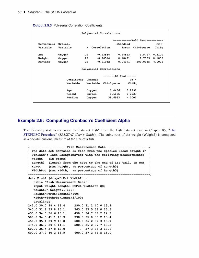
56 F Chapter 2: The CORR Procedure
Output 2.5.3 Polyserial Correlation Coefficients
Polyserial Correlations
-----------Wald Test----------Continuous Ordinal Standard Pr >Variable Variable N Correlation Error Chi-Square ChiSq
Age Oxygen 29 -0.23586 0.18813 1.5717 0.2100Weight Oxygen 29 -0.24514 0.18421 1.7709 0.1833RunTime Oxygen 28 -0.91042 0.04071 500.0345 <.0001
Polyserial Correlations
-------LR Test------Continuous Ordinal Pr >Variable Variable Chi-Square ChiSq
Age Oxygen 1.4466 0.2291Weight Oxygen 1.6185 0.2033RunTime Oxygen 38.6963 <.0001
Example 2.6: Computing Cronbach’s Coefficient Alpha
The following statements create the data set Fish1 from the Fish data set used in Chapter 85, “TheSTEPDISC Procedure” (SAS/STAT User’s Guide). The cubic root of the weight (Weight3) is computedas a one-dimensional measure of the size of a fish.
*------------------- Fish Measurement Data ----------------------*| The data set contains 35 fish from the species Bream caught in || Finland's lake Laengelmavesi with the following measurements: || Weight (in grams) || Length3 (length from the nose to the end of its tail, in cm) || HtPct (max height, as percentage of Length3) || WidthPct (max width, as percentage of Length3) |
*----------------------------------------------------------------*;data Fish1 (drop=HtPct WidthPct);
title 'Fish Measurement Data';input Weight Length3 HtPct WidthPct @@;Weight3= Weight**(1/3);Height=HtPct*Length3/100;Width=WidthPct*Length3/100;datalines;
242.0 30.0 38.4 13.4 290.0 31.2 40.0 13.8340.0 31.1 39.8 15.1 363.0 33.5 38.0 13.3430.0 34.0 36.6 15.1 450.0 34.7 39.2 14.2500.0 34.5 41.1 15.3 390.0 35.0 36.2 13.4450.0 35.1 39.9 13.8 500.0 36.2 39.3 13.7475.0 36.2 39.4 14.1 500.0 36.2 39.7 13.3500.0 36.4 37.8 12.0 . 37.3 37.3 13.6600.0 37.2 40.2 13.9 600.0 37.2 41.5 15.0

Example 2.6: Computing Cronbach’s Coefficient Alpha F 57
700.0 38.3 38.8 13.8 700.0 38.5 38.8 13.5610.0 38.6 40.5 13.3 650.0 38.7 37.4 14.8575.0 39.5 38.3 14.1 685.0 39.2 40.8 13.7620.0 39.7 39.1 13.3 680.0 40.6 38.1 15.1700.0 40.5 40.1 13.8 725.0 40.9 40.0 14.8720.0 40.6 40.3 15.0 714.0 41.5 39.8 14.1850.0 41.6 40.6 14.9 1000.0 42.6 44.5 15.5920.0 44.1 40.9 14.3 955.0 44.0 41.1 14.3925.0 45.3 41.4 14.9 975.0 45.9 40.6 14.7950.0 46.5 37.9 13.7;
The following statements request a correlation analysis and compute Cronbach’s coefficient alpha for thevariables Weight3, Length3, Height, and Width:
ods graphics on;title 'Fish Measurement Data';proc corr data=fish1 nomiss alpha plots=matrix;
var Weight3 Length3 Height Width;run;ods graphics off;
The ALPHA option computes Cronbach’s coefficient alpha for the analysis variables.
The “Simple Statistics” table in Output 2.6.1 displays univariate descriptive statistics for each analysisvariable.
Output 2.6.1 Simple Statistics
Fish Measurement Data
The CORR Procedure
4 Variables: Weight3 Length3 Height Width
Simple Statistics
Variable N Mean Std Dev Sum Minimum Maximum
Weight3 34 8.44751 0.97574 287.21524 6.23168 10.00000Length3 34 38.38529 4.21628 1305 30.00000 46.50000Height 34 15.22057 1.98159 517.49950 11.52000 18.95700Width 34 5.43805 0.72967 184.89370 4.02000 6.74970

58 F Chapter 2: The CORR Procedure
The “Pearson Correlation Coefficients” table in Output 2.6.2 displays Pearson correlation statistics for pairsof analysis variables.
Output 2.6.2 Pearson Correlation Coefficients
Pearson Correlation Coefficients, N = 34Prob > |r| under H0: Rho=0
Weight3 Length3 Height Width
Weight3 1.00000 0.96523 0.96261 0.92789<.0001 <.0001 <.0001
Length3 0.96523 1.00000 0.95492 0.92171<.0001 <.0001 <.0001
Height 0.96261 0.95492 1.00000 0.92632<.0001 <.0001 <.0001
Width 0.92789 0.92171 0.92632 1.00000<.0001 <.0001 <.0001
Since the data set contains only one species of fish, all the variables are highly correlated. Using the AL-PHA option, the CORR procedure computes Cronbach’s coefficient alpha in Output 2.6.3. The Cronbach’scoefficient alpha is a lower bound for the reliability coefficient for the raw variables and the standardizedvariables. Positive correlation is needed for the alpha coefficient because variables measure a commonentity.
Output 2.6.3 Cronbach’s Coefficient Alpha
Cronbach Coefficient Alpha
Variables Alpha----------------------------Raw 0.822134Standardized 0.985145
Because the variances of some variables vary widely, you should use the standardized score to estimatereliability. The overall standardized Cronbach’s coefficient alpha of 0.985145 provides an acceptable lowerbound for the reliability coefficient. This is much greater than the suggested value of 0.70 given by Nunnallyand Bernstein (1994).
The standardized alpha coefficient provides information about how each variable reflects the reliability ofthe scale with standardized variables. If the standardized alpha decreases after removing a variable from theconstruct, then this variable is strongly correlated with other variables in the scale. On the other hand, if thestandardized alpha increases after removing a variable from the construct, then removing this variable fromthe scale makes the construct more reliable. The “Cronbach Coefficient Alpha with Deleted Variables” tablein Output 2.6.4 does not show significant increase or decrease in the standardized alpha coefficients. Seethe section “Cronbach’s Coefficient Alpha” on page 30 for more information about Cronbach’s alpha.

Example 2.7: Saving Correlations in an Output Data Set F 59
Output 2.6.4 Cronbach’s Coefficient Alpha with Deleted Variables
Cronbach Coefficient Alpha with Deleted Variable
Raw Variables Standardized Variables
Deleted Correlation CorrelationVariable with Total Alpha with Total Alpha------------------------------------------------------------------------Weight3 0.975379 0.783365 0.973464 0.977103Length3 0.967602 0.881987 0.967177 0.978783Height 0.964715 0.655098 0.968079 0.978542Width 0.934635 0.824069 0.937599 0.986626
Example 2.7: Saving Correlations in an Output Data Set
The following statements compute Pearson correlations:
title 'Correlations for a Fitness and Exercise Study';proc corr data=Fitness nomiss outp=CorrOutp;
var weight oxygen runtime;run;
The NOMISS option excludes observations with missing values of the VAR statement variables from theanalysis—that is, the same set of 28 observations is used to compute the correlation for each pair of vari-ables. The OUTP= option creates an output data set named CorrOutp that contains the Pearson correlationstatistics.
“Pearson Correlation Coefficients” table in Output 2.7.1 displays the correlation and the p-value under thenull hypothesis of zero correlation.
Output 2.7.1 Pearson Correlation Coefficients
Correlations for a Fitness and Exercise Study
The CORR Procedure
Pearson Correlation Coefficients, N = 28Prob > |r| under H0: Rho=0
Weight Oxygen RunTime
Weight 1.00000 -0.18419 0.195050.3481 0.3199
Oxygen -0.18419 1.00000 -0.868430.3481 <.0001
RunTime 0.19505 -0.86843 1.000000.3199 <.0001

60 F Chapter 2: The CORR Procedure
The following statements display (in Output 2.7.2) the output data set:title 'Output Data Set from PROC CORR';proc print data=CorrOutp noobs;run;
Output 2.7.2 OUTP= Data Set with Pearson Correlations
Output Data Set from PROC CORR
_TYPE_ _NAME_ Weight Oxygen RunTime
MEAN 77.2168 47.1327 10.6954STD 8.4495 5.5535 1.4127N 28.0000 28.0000 28.0000CORR Weight 1.0000 -0.1842 0.1950CORR Oxygen -0.1842 1.0000 -0.8684CORR RunTime 0.1950 -0.8684 1.0000
The output data set has the default type CORR and can be used as an input data set for regression or otherstatistical procedures. For example, the following statements request a regression analysis using CorrOutp,without reading the original data in the REG procedure:
title 'Input Type CORR Data Set from PROC REG';proc reg data=CorrOutp;
model runtime= weight oxygen;run;
The following statements generate the same results as the preceding statements:
proc reg data=Fitness;model runtime= weight oxygen;
run;
Example 2.8: Creating Scatter Plots
The following statements request a correlation analysis and a scatter plot matrix for the variables in the dataset Fish1, which was created in Example 2.6.
ods graphics on;title 'Fish Measurement Data';proc corr data=fish1 nomiss plots=matrix(histogram);
var Height Width Length3 Weight3;run;ods graphics off;

Example 2.8: Creating Scatter Plots F 61
The “Simple Statistics” table in Output 2.8.1 displays univariate descriptive statistics for analysis variables.
Output 2.8.1 Simple Statistics
Fish Measurement Data
The CORR Procedure
4 Variables: Height Width Length3 Weight3
Simple Statistics
Variable N Mean Std Dev Sum Minimum Maximum
Height 34 15.22057 1.98159 517.49950 11.52000 18.95700Width 34 5.43805 0.72967 184.89370 4.02000 6.74970Length3 34 38.38529 4.21628 1305 30.00000 46.50000Weight3 34 8.44751 0.97574 287.21524 6.23168 10.00000
The “Pearson Correlation Coefficients” table in Output 2.8.2 displays Pearson correlation statistics for pairsof analysis variables.
Output 2.8.2 Pearson Correlation Coefficients
Pearson Correlation Coefficients, N = 34Prob > |r| under H0: Rho=0
Height Width Length3 Weight3
Height 1.00000 0.92632 0.95492 0.96261<.0001 <.0001 <.0001
Width 0.92632 1.00000 0.92171 0.92789<.0001 <.0001 <.0001
Length3 0.95492 0.92171 1.00000 0.96523<.0001 <.0001 <.0001
Weight3 0.96261 0.92789 0.96523 1.00000<.0001 <.0001 <.0001
The variables are highly correlated. For example, the correlation between Height and Width is 0.92632.

62 F Chapter 2: The CORR Procedure
The PLOTS=MATRIX(HISTOGRAM) option requests a scatter plot matrix for the VAR statement variablesin Output 2.8.3.
Output 2.8.3 Scatter Plot Matrix
Note that this graphical display is requested by enabling ODS Graphics and by specifying the PLOTS=option. For more information about ODS Graphics, see Chapter 21, “Statistical Graphics Using ODS”(SAS/STAT User’s Guide).
To explore the correlation between Height and Width, the following statements display (in Output 2.8.4) ascatter plot with prediction ellipses for the two variables:

Example 2.8: Creating Scatter Plots F 63
ods graphics on;proc corr data=fish1 nomiss
plots=scatter(nvar=2 alpha=.20 .30);var Height Width Length3 Weight3;
run;ods graphics off;
The PLOTS=SCATTER(NVAR=2) option requests a scatter plot for the first two variables in the VAR list.The ALPHA=.20 .30 suboption requests 80% and 70% prediction ellipses, respectively.
Output 2.8.4 Scatter Plot with Prediction Ellipses
A prediction ellipse is a region for predicting a new observation from the population, assuming bivariatenormality. It also approximates a region that contains a specified percentage of the population. The dis-played prediction ellipse is centered at the means . Nx; Ny/. For further details, see the section “Confidenceand Prediction Ellipses” on page 32.

64 F Chapter 2: The CORR Procedure
Note that the following statements also display (in Output 2.8.5) a scatter plot for Height and Width:
ods graphics on;proc corr data=fish1
plots=scatter(alpha=.20 .30);var Height Width;
run;ods graphics off;
Output 2.8.5 Scatter Plot with Prediction Ellipses
Output 2.8.5 includes the point .13:9; 5:1/, which was excluded from Output 2.8.4 because the observationhad a missing value for Weight3. The prediction ellipses in Output 2.8.5 also reflect the inclusion of thisobservation.
The following statements display (in Output 2.8.6) a scatter plot with confidence ellipses for the mean:
ods graphics on;title 'Fish Measurement Data';proc corr data=fish1 nomiss
plots=scatter(ellipse=confidence nvar=2 alpha=.05 .01);var Height Width Length3 Weight3;
run;ods graphics off;

Example 2.9: Computing Partial Correlations F 65
The NVAR=2 suboption within the PLOTS= option restricts the number of plots created to the first twovariables in the VAR statement, and the ELLIPSE=CONFIDENCE suboption requests confidence ellipsesfor the mean. The ALPHA=.05 .01 suboption requests 95% and 99% confidence ellipses, respectively.
Output 2.8.6 Scatter Plot with Confidence Ellipses
The confidence ellipse for the mean is centered at the means . Nx; Ny/. For further details, see the section“Confidence and Prediction Ellipses” on page 32.
Example 2.9: Computing Partial Correlations
A partial correlation measures the strength of the linear relationship between two variables, while adjustingfor the effect of other variables.
The following statements request a partial correlation analysis of variables Height and Width while adjustingfor the variables Length3 and Weight. The latter variables, which are said to be “partialled out” of theanalysis, are specified with the PARTIAL statement.

66 F Chapter 2: The CORR Procedure
ods graphics on;title 'Fish Measurement Data';proc corr data=fish1 plots=scatter(alpha=.20 .30);
var Height Width;partial Length3 Weight3;
run;ods graphics off;
Output 2.9.1 displays descriptive statistics for all the variables. The partial variance and partial standarddeviation for the variables in the VAR statement are also displayed.
Output 2.9.1 Descriptive Statistics
Fish Measurement Data
The CORR Procedure
2 Partial Variables: Length3 Weight32 Variables: Height Width
Simple Statistics
Variable N Mean Std Dev Sum Minimum Maximum
Length3 34 38.38529 4.21628 1305 30.00000 46.50000Weight3 34 8.44751 0.97574 287.21524 6.23168 10.00000Height 34 15.22057 1.98159 517.49950 11.52000 18.95700Width 34 5.43805 0.72967 184.89370 4.02000 6.74970
Simple Statistics
Partial PartialVariable Variance Std Dev
Length3Weight3Height 0.26607 0.51582Width 0.07315 0.27047
When you specify a PARTIAL statement, observations with missing values are excluded from the analysis.Output 2.9.2 displays partial correlations for the variables in the VAR statement.
Output 2.9.2 Pearson Partial Correlation Coefficients
Pearson Partial Correlation Coefficients, N = 34Prob > |r| under H0: Partial Rho=0
Height Width
Height 1.00000 0.256920.1558
Width 0.25692 1.000000.1558

Example 2.9: Computing Partial Correlations F 67
The partial correlation between the variables Height and Width is 0.25692, which is much less than theunpartialled correlation, 0.92632 (in Output 2.9.2). The p-value for the partial correlation is 0.1558.
The PLOTS=SCATTER option displays (in Output 2.9.3) a scatter plot of the residuals for the variablesHeight and Width after controlling for the effect of variables Length3 and Weight. The ALPHA=.20 .30suboption requests 80% and 70% prediction ellipses, respectively.
Output 2.9.3 Partial Residual Scatter Plot
In Output 2.9.3, a standard deviation of Height has roughly the same length on the X axis as a standarddeviation of Width on the Y axis. The major axis length is not significantly larger than the minor axislength, indicating a weak partial correlation between Height and Width.

68 F Chapter 2: The CORR Procedure
References
Anderson, T. W. (1984), An Introduction to Multivariate Statistical Analysis, Second Edition, New York:John Wiley & Sons.
Blum, J. R., Kiefer, J., and Rosenblatt, M. (1961), “Distribution Free Tests of Independence Based on theSample Distribution Function,” Annals of Mathematical Statistics, 32, 485–498.
Conover, W. J. (1998), Practical Nonparametric Statistics, Third Edition, New York: John Wiley & Sons.
Cox, N. R. (1974), “Estimation of the Correlation between a Continuous and a Discrete Variable,” Biomet-rics, 30, 171–178.
Cronbach, L. J. (1951), “Coefficient Alpha and the Internal Structure of Tests,” Psychometrika, 16, 297–334.
Drasgow, F. (1986), “Polychoric and Polyserial Correlations” in Encyclopedia of Statistical Sciences, vol.7, ed. S. Kotz and N. L. Johnson, New York: John Wiley & Sons, 68–74.
Fisher, R. A. (1915), “Frequency Distribution of the Values of the Correlation Coefficient in Samples froman Indefinitely Large Population,” Biometrika, 10, 507–521.
Fisher, R. A. (1921), “On the “Probable Error” of a Coefficient of Correlation Deduced from a Small Sam-ple,” Metron, 1, 3–32.
Fisher, R. A. (1936), “The Use of Multiple Measurements in Taxonomic Problems,” Annals of Eugenics, 7,179–188.
Fisher, R. A. (1970), Statistical Methods for Research Workers, Fourteenth Edition, Davien, CT: HafnerPublishing Company.
Hoeffding, W. (1948), “A Non-parametric Test of Independence,” Annals of Mathematical Statistics, 19,546–557.
Hollander, M. and Wolfe, D. (1999), Nonparametric Statistical Methods, Second Edition, New York: JohnWiley & Sons.
Keeping, E. S. (1962), Introduction to Statistical Inference, New York: D. Van Nostrand.
Knight, W. E. (1966), “A Computer Method for Calculating Kendall’s Tau with Ungrouped Data,” Journalof the American Statistical Association, 61, 436–439.
Moore, D. S. (2000), Statistics: Concepts and Controversies, Fifth Edition, New York: W. H. Freeman.
Mudholkar, G. S. (1983), “Fisher’s z-Transformation,” Encyclopedia of Statistical Sciences, 3, 130–135.
Noether, G. E. (1967), Elements of Nonparametric Statistics, New York: John Wiley & Sons.
Novick, M. R. (1967), “Coefficient Alpha and the Reliability of Composite Measurements,” Psychometrika,32, 1–13.

References F 69
Nunnally, J. C. and Bernstein, I. H. (1994), Psychometric Theory, Third Edition, New York: McGraw-Hill.
Olsson, U., Drasgow, F., and Dorans, N. J. (1982), “The Polyserial Correlation Coefficient,” Biometrika, 47,337–347.
Ott, R. L. and Longnecker, M. T. (2000), An Introduction to Statistical Methods and Data Analysis, FifthEdition, Belmont, CA: Wadsworth.
Spector, P. E. (1992), Summated Rating Scale Construction: An Introduction, Newbury Park, CA: Sage.
Yu, C. H. (2001) “An introduction to computing and interpreting Cronbach Coefficient Alpha in SAS,”Proceedings of the Twenty-Six Annual SAS Users Group International Conference, Cary, NC: SAS Institute,Inc., paper 246.

70

Chapter 3
The FREQ Procedure
ContentsOverview: FREQ Procedure . . . . . . . . . . . . . . . . . . . . . . . . . . . . . . . . . . 72Getting Started: FREQ Procedure . . . . . . . . . . . . . . . . . . . . . . . . . . . . . . . 74
Frequency Tables and Statistics . . . . . . . . . . . . . . . . . . . . . . . . . . . . . 74Agreement Study . . . . . . . . . . . . . . . . . . . . . . . . . . . . . . . . . . . . . 81
Syntax: FREQ Procedure . . . . . . . . . . . . . . . . . . . . . . . . . . . . . . . . . . . . 84PROC FREQ Statement . . . . . . . . . . . . . . . . . . . . . . . . . . . . . . . . . 84BY Statement . . . . . . . . . . . . . . . . . . . . . . . . . . . . . . . . . . . . . . 87EXACT Statement . . . . . . . . . . . . . . . . . . . . . . . . . . . . . . . . . . . . 87OUTPUT Statement . . . . . . . . . . . . . . . . . . . . . . . . . . . . . . . . . . . 91TABLES Statement . . . . . . . . . . . . . . . . . . . . . . . . . . . . . . . . . . . 95TEST Statement . . . . . . . . . . . . . . . . . . . . . . . . . . . . . . . . . . . . . 124WEIGHT Statement . . . . . . . . . . . . . . . . . . . . . . . . . . . . . . . . . . . 125
Details: FREQ Procedure . . . . . . . . . . . . . . . . . . . . . . . . . . . . . . . . . . . . 126Inputting Frequency Counts . . . . . . . . . . . . . . . . . . . . . . . . . . . . . . . 126Grouping with Formats . . . . . . . . . . . . . . . . . . . . . . . . . . . . . . . . . 127Missing Values . . . . . . . . . . . . . . . . . . . . . . . . . . . . . . . . . . . . . . 128In-Database Computation . . . . . . . . . . . . . . . . . . . . . . . . . . . . . . . . 131Statistical Computations . . . . . . . . . . . . . . . . . . . . . . . . . . . . . . . . . 132
Definitions and Notation . . . . . . . . . . . . . . . . . . . . . . . . . . . . 132Chi-Square Tests and Statistics . . . . . . . . . . . . . . . . . . . . . . . . . 133Measures of Association . . . . . . . . . . . . . . . . . . . . . . . . . . . . 138Binomial Proportion . . . . . . . . . . . . . . . . . . . . . . . . . . . . . . 147Risks and Risk Differences . . . . . . . . . . . . . . . . . . . . . . . . . . . 154Odds Ratio and Relative Risks for 2 x 2 Tables . . . . . . . . . . . . . . . . 164Cochran-Armitage Test for Trend . . . . . . . . . . . . . . . . . . . . . . . 167Jonckheere-Terpstra Test . . . . . . . . . . . . . . . . . . . . . . . . . . . . 168Tests and Measures of Agreement . . . . . . . . . . . . . . . . . . . . . . . 170Cochran-Mantel-Haenszel Statistics . . . . . . . . . . . . . . . . . . . . . . 175Gail-Simon Test for Qualitative Interactions . . . . . . . . . . . . . . . . . . 183Exact Statistics . . . . . . . . . . . . . . . . . . . . . . . . . . . . . . . . . 184
Computational Resources . . . . . . . . . . . . . . . . . . . . . . . . . . . . . . . . 189Output Data Sets . . . . . . . . . . . . . . . . . . . . . . . . . . . . . . . . . . . . . 189Displayed Output . . . . . . . . . . . . . . . . . . . . . . . . . . . . . . . . . . . . . 192ODS Table Names . . . . . . . . . . . . . . . . . . . . . . . . . . . . . . . . . . . . 200
72 F Chapter 3: The FREQ Procedure
ODS Graphics . . . . . . . . . . . . . . . . . . . . . . . . . . . . . . . . . . . . . . 204Examples: FREQ Procedure . . . . . . . . . . . . . . . . . . . . . . . . . . . . . . . . . . 205
Example 3.1: Output Data Set of Frequencies . . . . . . . . . . . . . . . . . . . . . 205Example 3.2: Frequency Dot Plots . . . . . . . . . . . . . . . . . . . . . . . . . . . 208Example 3.3: Chi-Square Goodness-of-Fit Tests . . . . . . . . . . . . . . . . . . . . 211Example 3.4: Binomial Proportions . . . . . . . . . . . . . . . . . . . . . . . . . . . 215Example 3.5: Analysis of a 2x2 Contingency Table . . . . . . . . . . . . . . . . . . 218Example 3.6: Output Data Set of Chi-Square Statistics . . . . . . . . . . . . . . . . . 221Example 3.7: Cochran-Mantel-Haenszel Statistics . . . . . . . . . . . . . . . . . . . 223Example 3.8: Cochran-Armitage Trend Test . . . . . . . . . . . . . . . . . . . . . . 225Example 3.9: Friedman’s Chi-Square Test . . . . . . . . . . . . . . . . . . . . . . . 229Example 3.10: Cochran’s Q Test . . . . . . . . . . . . . . . . . . . . . . . . . . . . 230
References . . . . . . . . . . . . . . . . . . . . . . . . . . . . . . . . . . . . . . . . . . . 233
Overview: FREQ Procedure
The FREQ procedure produces one-way to n-way frequency and contingency (crosstabulation) tables. Fortwo-way tables, PROC FREQ computes tests and measures of association. For n-way tables, PROC FREQprovides stratified analysis by computing statistics across, as well as within, strata.
For one-way frequency tables, PROC FREQ computes goodness-of-fit tests for equal proportions or speci-fied null proportions. For one-way tables, PROC FREQ also provides confidence limits and tests for bino-mial proportions, including tests for noninferiority and equivalence.
For contingency tables, PROC FREQ can compute various statistics to examine the relationships betweentwo classification variables. For some pairs of variables, you might want to examine the existence or strengthof any association between the variables. To determine if an association exists, chi-square tests are com-puted. To estimate the strength of an association, PROC FREQ computes measures of association that tendto be close to zero when there is no association and close to the maximum (or minimum) value when thereis perfect association. The statistics for contingency tables include the following:
� chi-square tests and measures
� measures of association
� risks (binomial proportions) and risk differences for 2 � 2 tables
� odds ratios and relative risks for 2 � 2 tables
� tests for trend
� tests and measures of agreement
� Cochran-Mantel-Haenszel statistics

Overview: FREQ Procedure F 73
PROC FREQ computes asymptotic standard errors, confidence intervals, and tests for measures of associa-tion and measures of agreement. Exact p-values and confidence intervals are available for many test statisticsand measures. PROC FREQ also performs analyses that adjust for any stratification variables by computingstatistics across, as well as within, strata for n-way tables. These statistics include Cochran-Mantel-Haenszelstatistics and measures of agreement.
In choosing measures of association to use in analyzing a two-way table, you should consider the studydesign (which indicates whether the row and column variables are dependent or independent), the mea-surement scale of the variables (nominal, ordinal, or interval), the type of association that each measure isdesigned to detect, and any assumptions required for valid interpretation of a measure. You should exercisecare in selecting measures that are appropriate for your data.
Similar comments apply to the choice and interpretation of test statistics. For example, the Mantel-Haenszelchi-square statistic requires an ordinal scale for both variables and is designed to detect a linear association.The Pearson chi-square, on the other hand, is appropriate for all variables and can detect any kind of asso-ciation, but it is less powerful for detecting a linear association because its power is dispersed over a greaternumber of degrees of freedom (except for 2 � 2 tables).
For more information about selecting the appropriate statistical analyses, see Agresti (2007) or Stokes,Davis, and Koch (2000).
Several SAS procedures produce frequency counts; only PROC FREQ computes chi-square tests for one-way to n-way tables and measures of association and agreement for contingency tables. Other proceduresto consider for counting include the TABULATE and UNIVARIATE procedures. When you want to pro-duce contingency tables and tests of association for sample survey data, use PROC SURVEYFREQ. SeeChapter 14, “Introduction to Survey Procedures” (SAS/STAT User’s Guide), for more information. Whenyou want to fit models to categorical data, use a procedure such as CATMOD, GENMOD, GLIMMIX,LOGISTIC, PROBIT, or SURVEYLOGISTIC. See Chapter 8, “Introduction to Categorical Data AnalysisProcedures” (SAS/STAT User’s Guide), for more information.
PROC FREQ uses the Output Delivery System (ODS), a SAS subsystem that provides capabilities for dis-playing and controlling the output from SAS procedures. ODS enables you to convert any of the output fromPROC FREQ into a SAS data set. See the section “ODS Table Names” on page 200 for more information.
PROC FREQ uses ODS Graphics to create graphs as part of its output. For general information aboutODS Graphics, see Chapter 21, “Statistical Graphics Using ODS” (SAS/STAT User’s Guide). For specificinformation about the statistical graphics available with the FREQ procedure, see the PLOTS= option in theTABLES statement and the section “ODS Graphics” on page 204.

74 F Chapter 3: The FREQ Procedure
Getting Started: FREQ Procedure
Frequency Tables and Statistics
The FREQ procedure provides easy access to statistics for testing for association in a crosstabulation table.
In this example, high school students applied for courses in a summer enrichment program; these coursesincluded journalism, art history, statistics, graphic arts, and computer programming. The students acceptedwere randomly assigned to classes with and without internships in local companies. Table 3.1 containscounts of the students who enrolled in the summer program by gender and whether they were assigned aninternship slot.
Table 3.1 Summer Enrichment Data
EnrollmentGender Internship Yes No Total
boys yes 35 29 64boys no 14 27 41girls yes 32 10 42girls no 53 23 76
The SAS data set SummerSchool is created by inputting the summer enrichment data as cell count data, orproviding the frequency count for each combination of variable values. The following DATA step statementscreate the SAS data set SummerSchool:
data SummerSchool;input Gender $ Internship $ Enrollment $ Count @@;datalines;
boys yes yes 35 boys yes no 29boys no yes 14 boys no no 27girls yes yes 32 girls yes no 10girls no yes 53 girls no no 23;
The variable Gender takes the values ‘boys’ or ‘girls,’ the variable Internship takes the values ‘yes’ and‘no,’ and the variable Enrollment takes the values ‘yes’ and ‘no.’ The variable Count contains the number ofstudents that correspond to each combination of data values. The double at sign (@@) indicates that morethan one observation is included on a single data line. In this DATA step, two observations are included oneach line.
Researchers are interested in whether there is an association between internship status and summer pro-gram enrollment. The Pearson chi-square statistic is an appropriate statistic to assess the association in thecorresponding 2 � 2 table. The following PROC FREQ statements specify this analysis.

Frequency Tables and Statistics F 75
You specify the table for which you want to compute statistics with the TABLES statement. You specify thestatistics you want to compute with options after a slash (/) in the TABLES statement.
proc freq data=SummerSchool order=data;tables Internship*Enrollment / chisq;weight Count;
run;
The ORDER= option controls the order in which variable values are displayed in the rows and columnsof the table. By default, the values are arranged according to the alphanumeric order of their unformattedvalues. If you specify ORDER=DATA, the data are displayed in the same order as they occur in the inputdata set. Here, because ‘yes’ appears before ‘no’ in the data, ‘yes’ appears first in any table. Other optionsfor controlling order include ORDER=FORMATTED, which orders according to the formatted values, andORDER=FREQUENCY, which orders by descending frequency count.
In the TABLES statement, Internship*Enrollment specifies a table where the rows are internship statusand the columns are program enrollment. The CHISQ option requests chi-square statistics for assessingassociation between these two variables. Because the input data are in cell count form, the WEIGHTstatement is required. The WEIGHT statement names the variable Count, which provides the frequency ofeach combination of data values.
Figure 3.1 presents the crosstabulation of Internship and Enrollment. In each cell, the values printed underthe cell count are the table percentage, row percentage, and column percentage, respectively. For example,in the first cell, 63.21 percent of the students offered courses with internships accepted them and 36.79percent did not.
Figure 3.1 Crosstabulation Table
The FREQ Procedure
Table of Internship by Enrollment
Internship Enrollment
Frequency|Percent |Row Pct |Col Pct |yes |no | Total---------+--------+--------+yes | 67 | 39 | 106
| 30.04 | 17.49 | 47.53| 63.21 | 36.79 || 50.00 | 43.82 |
---------+--------+--------+no | 67 | 50 | 117
| 30.04 | 22.42 | 52.47| 57.26 | 42.74 || 50.00 | 56.18 |
---------+--------+--------+Total 134 89 223
60.09 39.91 100.00

76 F Chapter 3: The FREQ Procedure
Figure 3.2 displays the statistics produced by the CHISQ option. The Pearson chi-square statistic is la-beled ‘Chi-Square’ and has a value of 0.8189 with 1 degree of freedom. The associated p-value is 0.3655,which means that there is no significant evidence of an association between internship status and programenrollment. The other chi-square statistics have similar values and are asymptotically equivalent. The otherstatistics (phi coefficient, contingency coefficient, and Cramer’s V ) are measures of association derivedfrom the Pearson chi-square. For Fisher’s exact test, the two-sided p-value is 0.4122, which also shows noassociation between internship status and program enrollment.
Figure 3.2 Statistics Produced with the CHISQ Option
Statistic DF Value Prob------------------------------------------------------Chi-Square 1 0.8189 0.3655Likelihood Ratio Chi-Square 1 0.8202 0.3651Continuity Adj. Chi-Square 1 0.5899 0.4425Mantel-Haenszel Chi-Square 1 0.8153 0.3666Phi Coefficient 0.0606Contingency Coefficient 0.0605Cramer's V 0.0606
Fisher's Exact Test----------------------------------Cell (1,1) Frequency (F) 67Left-sided Pr <= F 0.8513Right-sided Pr >= F 0.2213
Table Probability (P) 0.0726Two-sided Pr <= P 0.4122
The analysis, so far, has ignored gender. However, it might be of interest to ask whether program enrollmentis associated with internship status after adjusting for gender. You can address this question by doing ananalysis of a set of tables (in this case, by analyzing the set consisting of one for boys and one for girls). TheCochran-Mantel-Haenszel (CMH) statistic is appropriate for this situation: it addresses whether rows andcolumns are associated after controlling for the stratification variable. In this case, you would be stratifyingby gender.
The PROC FREQ statements for this analysis are very similar to those for the first analysis, except thatthere is a third variable, Gender, in the TABLES statement. When you cross more than two variables, thetwo rightmost variables construct the rows and columns of the table, respectively, and the leftmost variablesdetermine the stratification.
The following PROC FREQ statements also request frequency plots for the crosstabulation tables. PROCFREQ produces these plots by using ODS Graphics to create graphs as part of the procedure output. ODSGraphics must be enabled before producing plots.
ods graphics on;proc freq data=SummerSchool;
tables Gender*Internship*Enrollment /chisq cmh plots(only)=freqplot;
weight Count;run;ods graphics off;

Frequency Tables and Statistics F 77
This execution of PROC FREQ first produces two individual crosstabulation tables of Internship by En-rollment: one for boys and one for girls. Frequency plots and chi-square statistics are produced for eachindividual table. Figure 3.3, Figure 3.4, and Figure 3.5 show the results for boys. Note that the chi-squarestatistic for boys is significant at the ˛ D 0:05 level of significance. Boys offered a course with an internshipare more likely to enroll than boys who are not.
Figure 3.4 displays the frequency plot of Internship by Enrollment for boys. By default, the frequency plot isdisplayed as a bar chart with vertical grouping by the row variable Internship. You can use PLOTS= optionsto request a dot plot instead of a bar chart or to change the orientation of the bars from vertical to horizontal.You can also use PLOTS= options to specify other two-way layouts such as stacked or horizontal grouping.
Figure 3.6, Figure 3.7, and Figure 3.8 display the crosstabulation table, frequency plot, and chi-squarestatistics for girls. You can see that there is no evidence of association between internship offers and programenrollment for girls.
Figure 3.3 Crosstabulation Table for Boys
The FREQ Procedure
Table 1 of Internship by EnrollmentControlling for Gender=boys
Internship Enrollment
Frequency|Percent |Row Pct |Col Pct |no |yes | Total---------+--------+--------+no | 27 | 14 | 41
| 25.71 | 13.33 | 39.05| 65.85 | 34.15 || 48.21 | 28.57 |
---------+--------+--------+yes | 29 | 35 | 64
| 27.62 | 33.33 | 60.95| 45.31 | 54.69 || 51.79 | 71.43 |
---------+--------+--------+Total 56 49 105
53.33 46.67 100.00

78 F Chapter 3: The FREQ Procedure
Figure 3.4 Frequency Plot for Boys
Figure 3.5 Chi-Square Statistics for Boys
Statistic DF Value Prob------------------------------------------------------Chi-Square 1 4.2366 0.0396Likelihood Ratio Chi-Square 1 4.2903 0.0383Continuity Adj. Chi-Square 1 3.4515 0.0632Mantel-Haenszel Chi-Square 1 4.1963 0.0405Phi Coefficient 0.2009Contingency Coefficient 0.1969Cramer's V 0.2009
Fisher's Exact Test----------------------------------Cell (1,1) Frequency (F) 27Left-sided Pr <= F 0.9885Right-sided Pr >= F 0.0311
Table Probability (P) 0.0196Two-sided Pr <= P 0.0467

Frequency Tables and Statistics F 79
Figure 3.6 Crosstabulation Table for Girls
Table 2 of Internship by EnrollmentControlling for Gender=girls
Internship Enrollment
Frequency|Percent |Row Pct |Col Pct |no |yes | Total---------+--------+--------+no | 23 | 53 | 76
| 19.49 | 44.92 | 64.41| 30.26 | 69.74 || 69.70 | 62.35 |
---------+--------+--------+yes | 10 | 32 | 42
| 8.47 | 27.12 | 35.59| 23.81 | 76.19 || 30.30 | 37.65 |
---------+--------+--------+Total 33 85 118
27.97 72.03 100.00
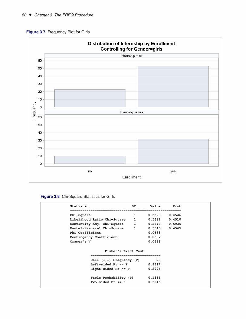
80 F Chapter 3: The FREQ Procedure
Figure 3.7 Frequency Plot for Girls
Figure 3.8 Chi-Square Statistics for Girls
Statistic DF Value Prob------------------------------------------------------Chi-Square 1 0.5593 0.4546Likelihood Ratio Chi-Square 1 0.5681 0.4510Continuity Adj. Chi-Square 1 0.2848 0.5936Mantel-Haenszel Chi-Square 1 0.5545 0.4565Phi Coefficient 0.0688Contingency Coefficient 0.0687Cramer's V 0.0688
Fisher's Exact Test----------------------------------Cell (1,1) Frequency (F) 23Left-sided Pr <= F 0.8317Right-sided Pr >= F 0.2994
Table Probability (P) 0.1311Two-sided Pr <= P 0.5245

Agreement Study F 81
These individual table results demonstrate the occasional problems with combining information into onetable and not accounting for information in other variables such as Gender. Figure 3.9 contains the CMHresults. There are three summary (CMH) statistics; which one you use depends on whether your rows and/orcolumns have an order in r � c tables. However, in the case of 2 � 2 tables, ordering does not matter andall three statistics take the same value. The CMH statistic follows the chi-square distribution under thehypothesis of no association, and here, it takes the value 4.0186 with 1 degree of freedom. The associatedp-value is 0.0450, which indicates a significant association at the ˛ D 0:05 level.
Thus, when you adjust for the effect of gender in these data, there is an association between internship andprogram enrollment. But, if you ignore gender, no association is found. Note that the CMH option alsoproduces other statistics, including estimates and confidence limits for relative risk and odds ratios for 2� 2tables and the Breslow-Day Test. These results are not displayed here.
Figure 3.9 Test for the Hypothesis of No Association
Cochran-Mantel-Haenszel Statistics (Based on Table Scores)
Statistic Alternative Hypothesis DF Value Prob---------------------------------------------------------------
1 Nonzero Correlation 1 4.0186 0.04502 Row Mean Scores Differ 1 4.0186 0.04503 General Association 1 4.0186 0.0450
Agreement Study
Medical researchers are interested in evaluating the efficacy of a new treatment for a skin condition. Der-matologists from participating clinics were trained to conduct the study and to evaluate the condition. Afterthe training, two dermatologists examined patients with the skin condition from a pilot study and rated thesame patients. The possible evaluations are terrible, poor, marginal, and clear. Table 3.2 contains the data.
Table 3.2 Skin Condition Data
Dermatologist 2Dermatologist 1 Terrible Poor Marginal Clear
Terrible 10 4 1 0Poor 5 10 12 2Marginal 2 4 12 5Clear 0 2 6 13

82 F Chapter 3: The FREQ Procedure
The following DATA step statements create the SAS dataset SkinCondition. The dermatologists’ evaluationsof the patients are contained in the variables Derm1 and Derm2; the variable Count is the number of patientsgiven a particular pair of ratings.
data SkinCondition;input Derm1 $ Derm2 $ Count;datalines;
terrible terrible 10terrible poor 4terrible marginal 1terrible clear 0poor terrible 5poor poor 10poor marginal 12poor clear 2marginal terrible 2marginal poor 4marginal marginal 12marginal clear 5clear terrible 0clear poor 2clear marginal 6clear clear 13;
The following PROC FREQ statements request an agreement analysis of the skin condition data. In orderto evaluate the agreement of the diagnoses (a possible contribution to measurement error in the study), thekappa coefficient is computed.
The TABLES statement requests a crosstabulation of the variables Derm1 and Derm2. The AGREE optionin the TABLES statement requests the kappa coefficient, together with its standard error and confidencelimits. The KAPPA option in the TEST statement requests a test for the null hypothesis that kappa equalszero, or that the agreement is purely by chance. The NOPRINT option in the TABLES statement suppressesthe display of the two-way table. The PLOTS= option requests an agreement plot for the two dermatologists.ODS Graphics must be enabled before producing plots.
ods graphics on;proc freq data=SkinCondition order=data;
tables Derm1*Derm2 /agree noprint plots=agreeplot;
test kappa;weight Count;
run;ods graphics off;
Figure 3.10 and Figure 3.11 show the results. The kappa coefficient has the value 0.3449, which indicatessome agreement between the dermatologists, and the hypothesis test confirms that you can reject the nullhypothesis of no agreement. This conclusion is further supported by the confidence interval of (0.2030,0.4868), which suggests that the true kappa is greater than zero. The AGREE option also produces Bowker’stest for symmetry and the weighted kappa coefficient, but that output is not shown here. Figure 3.11 displaysthe agreement plot for the ratings of the two dermatologists.

Agreement Study F 83
Figure 3.10 Agreement Study
The FREQ Procedure
Statistics for Table of Derm1 by Derm2
Simple Kappa Coefficient--------------------------------Kappa 0.3449ASE 0.072495% Lower Conf Limit 0.203095% Upper Conf Limit 0.4868
Test of H0: Kappa = 0
ASE under H0 0.0612Z 5.6366One-sided Pr > Z <.0001Two-sided Pr > |Z| <.0001
Figure 3.11 Agreement Plot

84 F Chapter 3: The FREQ Procedure
Syntax: FREQ Procedure
The following statements are available in PROC FREQ:
PROC FREQ < options > ;BY variables ;EXACT statistic-options < / computation-options > ;OUTPUT < OUT=SAS-data-set > options ;TABLES requests < / options > ;TEST options ;WEIGHT variable < / option > ;
The PROC FREQ statement is the only required statement for the FREQ procedure. If you specify the fol-lowing statements, PROC FREQ produces a one-way frequency table for each variable in the most recentlycreated data set.
proc freq;run;
The rest of this section gives detailed syntax information for the BY, EXACT, OUTPUT, TABLES, TEST,and WEIGHT statements in alphabetical order after the description of the PROC FREQ statement. Table 3.3summarizes the basic function of each PROC FREQ statement.
Table 3.3 Summary of PROC FREQ Statements
Statement Description
BY Provides separate analyses for each BY groupEXACT Requests exact testsOUTPUT Requests an output data setTABLES Specifies tables and requests analysesTEST Requests tests for measures of association and agreementWEIGHT Identifies a weight variable
PROC FREQ Statement
PROC FREQ < options > ;
The PROC FREQ statement invokes the procedure and optionally identifies the input data set. By default,the procedure uses the most recently created SAS data set.
Table 3.4 lists the options available in the PROC FREQ statement. Descriptions of the options follow inalphabetical order.

PROC FREQ Statement F 85
Table 3.4 PROC FREQ Statement Options
Option Description
COMPRESS Begins the next one-way table on the current pageDATA= Names the input data setFORMCHAR= Specifies the outline and cell divider characters for crosstabulation tablesNLEVELS Displays the number of levels for all TABLES variablesNOPRINT Suppresses all displayed outputORDER= Specifies the order for reporting variable valuesPAGE Displays one table per page
You can specify the following options in the PROC FREQ statement.
COMPRESSbegins display of the next one-way frequency table on the same page as the preceding one-way tableif there is enough space to begin the table. By default, the next one-way table begins on the currentpage only if the entire table fits on that page. The COMPRESS option is not valid with the PAGEoption.
DATA=SAS-data-setnames the SAS data set to be analyzed by PROC FREQ. If you omit the DATA= option, the procedureuses the most recently created SAS data set.
FORMCHAR(1,2,7)=‘formchar-string’defines the characters to be used for constructing the outlines and dividers for the cells of crosstabu-lation table displays. The formchar-string should be three characters long. The characters are used todraw the vertical separators (1), the horizontal separators (2), and the vertical-horizontal intersections(7). If you do not specify the FORMCHAR= option, PROC FREQ uses FORMCHAR(1,2,7)=‘|-+’by default. Table 3.5 summarizes the formatting characters used by PROC FREQ.
Table 3.5 Formatting Characters Used by PROC FREQ
Position Default Used to Draw
1 | Vertical separators2 - Horizontal separators7 + Intersections of vertical and horizontal separators
The FORMCHAR= option can specify 20 different SAS formatting characters used to display output;however, PROC FREQ uses only the first, second, and seventh formatting characters. Therefore, theproper specification for PROC FREQ is FORMCHAR(1,2,7)= ‘formchar-string’.
Specifying all blanks for formchar-string produces crosstabulation tables with no outlines ordividers—for example, FORMCHAR(1,2,7)=‘ ’. You can use any character in formchar-string, in-cluding hexadecimal characters. If you use hexadecimal characters, you must put an x after the closing

86 F Chapter 3: The FREQ Procedure
quote. For information about which hexadecimal codes to use for which characters, see the documen-tation for your hardware.
See the CALENDAR, PLOT, and TABULATE procedures in the Base SAS Procedures Guide formore information about form characters.
NLEVELSdisplays the “Number of Variable Levels” table, which provides the number of levels for each variablenamed in the TABLES statements. See the section “Number of Variable Levels Table” on page 192 fordetails. PROC FREQ determines the variable levels from the formatted variable values, as describedin the section “Grouping with Formats” on page 127.
NOPRINTsuppresses the display of all output. You can use the NOPRINT option when you only want to createan output data set. See the section “Output Data Sets” on page 189 for information about the outputdata sets produced by PROC FREQ. Note that the NOPRINT option temporarily disables the OutputDelivery System (ODS). For more information, see Chapter 20, “Using the Output Delivery System”(SAS/STAT User’s Guide).
NOTE: A NOPRINT option is also available in the TABLES statement. It suppresses display of thecrosstabulation tables but allows display of the requested statistics.
ORDER=DATA | FORMATTED | FREQ | INTERNALspecifies the order of the variable levels in the frequency and crosstabulation tables, which you requestin the TABLES statement.
The ORDER= option can take the following values:
Value of ORDER= Levels Ordered By
DATA Order of appearance in the input data set
FORMATTED External formatted value, except for numeric variableswith no explicit format, which are sorted by their unfor-matted (internal) value
FREQ Descending frequency count; levels with the most obser-vations come first in the order
INTERNAL Unformatted value
By default, ORDER=INTERNAL. The FORMATTED and INTERNAL orders are machine-dependent. The ORDER= option does not apply to missing values, which are always ordered first.
For more information about sorting order, see the chapter on the SORT procedure in the Base SASProcedures Guide and the discussion of BY-group processing in SAS Language Reference: Concepts.
PAGEdisplays only one table per page. Otherwise, PROC FREQ displays multiple tables per page as spacepermits. The PAGE option is not valid with the COMPRESS option.

BY Statement F 87
BY Statement
BY variables ;
You can specify a BY statement with PROC FREQ to obtain separate analyses on observations in groupsdefined by the BY variables. When a BY statement appears, the procedure expects the input data set to besorted in order of the BY variables.
If your input data set is not sorted in ascending order, use one of the following alternatives:
� Sort the data by using the SORT procedure with a similar BY statement.
� Specify the BY statement option NOTSORTED or DESCENDING in the BY statement for the FREQprocedure. The NOTSORTED option does not mean that the data are unsorted but rather that thedata are arranged in groups (according to values of the BY variables) and that these groups are notnecessarily in alphabetical or increasing numeric order.
� Create an index on the BY variables by using the DATASETS procedure.
For more information about the BY statement, see SAS Language Reference: Concepts. For more informa-tion about the DATASETS procedure, see the Base SAS Procedures Guide.
EXACT Statement
EXACT statistic-options < / computation-options > ;
The EXACT statement requests exact tests or confidence limits for the specified statistics. Optionally, PROCFREQ computes Monte Carlo estimates of the exact p-values. The statistic-options specify the statistics toprovide exact tests or confidence limits for. The computation-options specify options for the computationof exact statistics. See the section “Exact Statistics” on page 184 for details.
NOTE: PROC FREQ computes exact tests with fast and efficient algorithms that are superior to directenumeration. Exact tests are appropriate when a data set is small, sparse, skewed, or heavily tied. Forsome large problems, computation of exact tests might require a considerable amount of time and memory.Consider using asymptotic tests for such problems. Alternatively, when asymptotic methods might not besufficient for such large problems, consider using Monte Carlo estimation of exact p-values. You can requestMonte Carlo estimation by specifying the MC computation-option in the EXACT statement. See the section“Computational Resources” on page 187 for more information.
Statistic Options
The statistic-options specify the statistics to provide exact tests or confidence limits for.
For one-way tables, exact p-values are available for the binomial proportion tests and the chi-squaregoodness-of-fit test. Exact (Clopper-Pearson) confidence limits are available for the binomial proportion.

88 F Chapter 3: The FREQ Procedure
For two-way tables, exact p-values are available for the following tests: Pearson chi-square test, likelihood-ratio chi-square test, Mantel-Haenszel chi-square test, Fisher’s exact test, Jonckheere-Terpstra test, andCochran-Armitage test for trend. Exact p-values are also available for tests of the following statistics:Pearson correlation coefficient, Spearman correlation coefficient, Kendall’s tau-b, Stuart’s tau-c, Somers’D.C jR/, Somers’ D.RjC/, simple kappa coefficient, and weighted kappa coefficient.
For 2�2 tables, PROC FREQ provides McNemar’s exact test and exact confidence limits for the odds ratio.PROC FREQ also provides exact unconditional confidence limits for the risk (proportion) difference and forthe relative risk (ratio of proportions). For stratified 2 � 2 tables, PROC FREQ provides Zelen’s exact testfor equal odds ratios, exact confidence limits for the common odds ratio, and an exact test for the commonodds ratio.
Table 3.6 lists the available statistic-options and the exact statistics computed. For more information aboutthese statistics, see the TABLES statement and the section “Statistical Computations” on page 132. Formore information about exact computations, see the section “Exact Statistics” on page 184.
Most of the option names listed in Table 3.6 are identical to the corresponding option names in the TABLESand OUTPUT statements. You can request exact computations for groups of statistics by using options thatare identical to the following TABLES statement options: CHISQ, MEASURES, and AGREE. For example,when you specify the CHISQ option in the EXACT statement, PROC FREQ computes exact p-values forthe Pearson chi-square, likelihood-ratio chi-square, and Mantel-Haenszel chi-square tests. You can requestexact computations for an individual statistic by specifying the corresponding statistic-option from the listin Table 3.6.
Table 3.6 EXACT Statement Statistic Options
Statistic Option Exact Statistics
AGREE McNemar’s test (for 2 � 2 tables), simple kappa test,weighted kappa test
BINOMIAL Binomial proportion tests for one-way tablesCHISQ Chi-square goodness-of-fit test for one-way tables;
Pearson chi-square, likelihood-ratio chi-square, andMantel-Haenszel chi-square tests for two-way tables
COMOR Confidence limits for the common odds ratio,common odds ratio test (for h � 2 � 2 tables)
EQOR | ZELEN Zelen’s test for equal odds ratios (for h � 2 � 2 tables)FISHER Fisher’s exact testJT Jonckheere-Terpstra testKAPPA Test for the simple kappa coefficientKENTB Test for Kendall’s tau-bLRCHI Likelihood-ratio chi-square testMCNEM McNemar’s test (for 2 � 2 tables)MEASURES Tests for the Pearson correlation and Spearman correlation,
confidence limits for the odds ratio (for 2 � 2 tables)MHCHI Mantel-Haenszel chi-square testOR Confidence limits for the odds ratio (for 2 � 2 tables)PCHI Pearson chi-square testPCORR Test for the Pearson correlation coefficient

EXACT Statement F 89
Table 3.6 continued
Statistic Option Exact Statistics
RELRISK Confidence limits for the relative risk (for 2 � 2 tables)RISKDIFF Confidence limits for the proportion difference (for 2�2 tables)SCORR Test for the Spearman correlation coefficientSMDCR Test for Somers’ D.C jR/SMDRC Test for Somers’ D.RjC/STUTC Test for Stuart’s tau-cTREND Cochran-Armitage test for trendWTKAP Test for the weighted kappa coefficient
You can specify options for the following two EXACT statement statistic-options:
RELRISK < (options) >requests exact unconditional confidence limits for the relative risk for 2 � 2 tables. PROC FREQcomputes the confidence limits by inverting two separate one-sided exact tests (Santner and Snell1980). By default, this computation uses the unstandardized relative risk as the test statistic. If youspecify the RELRISK(METHOD=FMSCORE) option, PROC FREQ uses the Farrington-Manningscore statistic (Chan and Zhang 1999). See the section “Exact Unconditional Confidence Limits forthe Relative Risk” on page 166 for more information.
You can set the confidence level by using the ALPHA= option in the TABLES statement. The defaultof ALPHA=0.5 produces 95% confidence limits.
You can specify the following options inside parentheses after the RELRISK statistic-option:
COLUMN=1 | 2 | BOTHspecifies the 2 � 2 table column for which to compute the relative risk. The default is COL-UMN=1, which provides exact confidence limits for the column 1 relative risk. If you specifyCOLUMN=BOTH, PROC FREQ provides exact confidence limits for both column 1 and col-umn 2 relative risks.
METHOD=FMSCORE | SCORErequests exact unconditional confidence limits that are based on the Farrington-Manningscore statistic (Chan and Zhang 1999). See the section “Exact Unconditional ConfidenceLimits for the Relative Risk” on page 166 for more information. If you do not specifyMETHOD=FMSCORE, by default PROC FREQ uses the unstandardized relative risk in theexact confidence limit computations.
RISKDIFF < (options) >requests exact unconditional confidence limits for the risk difference for 2 � 2 tables. PROC FREQcomputes the confidence limits by inverting two separate one-sided exact tests (Santner and Snell1980). By default, this computation uses the unstandardized risk difference as the test statistic. If youspecify the RISKDIFF(METHOD=FMSCORE) option, PROC FREQ uses the Farrington-Manningscore statistic (Chan and Zhang 1999). See the section “Exact Unconditional Confidence Limits forthe Risk Difference” on page 163 for more information.

90 F Chapter 3: The FREQ Procedure
You can set the confidence level by using the ALPHA= option in the TABLES statement. The defaultof ALPHA=0.5 produces 95% confidence limits.
You can specify the following options inside parentheses after the RISKDIFF statistic-option:
COLUMN=1 | 2 | BOTHspecifies the 2 � 2 table column for which to compute the risk difference. The default is COL-UMN=BOTH, which provides exact confidence limits for both column 1 and column 2 riskdifferences.
METHOD=FMSCORE | SCORErequests exact unconditional confidence limits that are based on the Farrington-Manning scorestatistic (Chan and Zhang 1999). See the section “Exact Unconditional Confidence Lim-its for the Risk Difference” on page 163 for more information. If you do not specifyMETHOD=FMSCORE, by default PROC FREQ uses the unstandardized risk difference inthe exact confidence limit computations.
Using TABLES Statement Options with the EXACT Statement
If you use only one TABLES statement, you do not need to specify the same options in both the TABLESand EXACT statements; when you specify a statistic-option in the EXACT statement, PROC FREQ auto-matically invokes the corresponding TABLES statement option. However, when you use multiple TABLESstatements and want exact computations, you must specify options in the TABLES statements to request thedesired statistics. PROC FREQ then performs exact computations for all statistics that you also specify inthe EXACT statement.
The TABLES statement group option CHISQ includes tests that correspond to the following EXACT state-ment individual statistic-options: LRCHI, MHCHI, and PCHI. The MEASURES option in the TABLESstatement includes statistics that correspond to the following EXACT statement statistic-options: KENTB,OR, PCORR, SCORR, SMDCR, SMDRC, and STUTC. The AGREE option in the TABLES statementproduces analyses that correspond to the KAPPA, MCNEM, and WTKAP statistic-options in the EXACTstatement. The CMH option in the TABLES statement produces analyses that correspond to the COMORand EQOR (ZELEN) statistic-options in the EXACT statement.
Computation Options
The computation-options specify options for computation of exact statistics. You can specify the followingcomputation-options in the EXACT statement after a slash (/).
ALPHA=˛specifies the level of the confidence limits for Monte Carlo p-value estimates. The value of ˛ must bebetween 0 and 1, and the default is 0.01. A confidence level of ˛ produces 100.1 � ˛/% confidencelimits. The default of ALPHA=.01 produces 99% confidence limits for the Monte Carlo estimates.
The ALPHA= option invokes the MC option.
MAXTIME=valuespecifies the maximum clock time (in seconds) that PROC FREQ can use to compute an exact p-value. If the procedure does not complete the computation within the specified time, the computation

OUTPUT Statement F 91
terminates. The value of MAXTIME= must be a positive number. The MAXTIME= option is validfor Monte Carlo estimation of exact p-values, as well as for direct exact p-value computation. See thesection “Computational Resources” on page 187 for more information.
MCrequests Monte Carlo estimation of exact p-values instead of direct exact p-value computation. MonteCarlo estimation can be useful for large problems that require a considerable amount of time andmemory for exact computations but for which asymptotic approximations might not be sufficient. Seethe section “Monte Carlo Estimation” on page 187 for more information.
The MC option is available for all EXACT statistic-options except the BINOMIAL option and thefollowing options that apply only to 2 � 2 or h � 2 � 2 tables: COMOR, EQOR, MCNEM, OR,RELRISK, and RISKDIFF. PROC FREQ computes only exact tests or confidence limits for thesestatistics.
The ALPHA=, N=, and SEED= options also invoke the MC option.
N=nspecifies the number of samples for Monte Carlo estimation. The value of n must be a positiveinteger, and the default is 10,000. Larger values of n produce more precise estimates of exact p-values. Because larger values of n generate more samples, the computation time increases.
The N= option invokes the MC option.
POINTrequests exact point probabilities for the test statistics.
The POINT option is available for all the EXACT statement statistic-options except the OR. REL-RISK, and RISKDIFF options, which provide exact confidence limits. The POINT option is notavailable with the MC option.
SEED=numberspecifies the initial seed for random number generation for Monte Carlo estimation. The value of theSEED= option must be an integer. If you do not specify the SEED= option or if the SEED= valueis negative or zero, PROC FREQ uses the time of day from the computer’s clock to obtain the initialseed.
The SEED= option invokes the MC option.
OUTPUT Statement
OUTPUT < OUT= SAS-data-set > options ;
The OUTPUT statement creates a SAS data set that contains statistics computed by PROC FREQ. Youspecify which statistics to store in the output data set with the OUTPUT statement options. The output dataset contains one observation for each two-way table or stratum, and one observation for summary statisticsacross all strata. For more information about the contents of the output data set, see the section “Contentsof the OUTPUT Statement Output Data Set” on page 191.

92 F Chapter 3: The FREQ Procedure
Only one OUTPUT statement is allowed for each execution of PROC FREQ. You must specify a TABLESstatement with the OUTPUT statement. If you use multiple TABLES statements, the contents of the OUT-PUT data set correspond to the last TABLES statement. If you use multiple table requests in a TABLESstatement, the contents of the OUTPUT data set correspond to the last table request.
Note that you can use the Output Delivery System (ODS) to create a SAS data set from any piece of PROCFREQ output. For more information, see the section “ODS Table Names” on page 200.
Also note that the output data set created by the OUTPUT statement is not the same as the output data setcreated by the OUT= option in the TABLES statement. The OUTPUT statement creates a data set thatcontains statistics (such as the Pearson chi-square and its p-value), and the OUT= option in the TABLESstatement creates a data set that contains frequency table counts and percentages. See the section “OutputData Sets” on page 189 for more information.
You can specify the following options in the OUTPUT statement:
OUT=SAS-data-setnames the output data set. If you omit the OUT= option, the data set is named DATAn, where n is thesmallest integer that makes the name unique.
optionsspecify the statistics you want in the output data set. Table 3.7 lists the available options, together withthe TABLES statement options needed to produce the statistics. You can output groups of statistics byusing group options identical to those available in the TABLES statement, which include the AGREE,ALL, CHISQ, CMH, and MEASURES options. Or you can request statistics individually.
When you specify an option in the OUTPUT statement, the output data set contains all statistics fromthat analysis—the estimate or test statistic plus any associated standard error, confidence limits, p-values, and degrees of freedom. See the section “Contents of the OUTPUT Statement Output DataSet” on page 191 for details.
If you want to store a statistic in the output data set, you must also request computation of thatstatistic with the appropriate TABLES or EXACT statement option. For example, you cannot specifythe option PCHI (Pearson chi-square) in the OUTPUT statement without also specifying a TABLESor EXACT statement option to compute the Pearson chi-square test. The TABLES statement optionALL or CHISQ requests the Pearson chi-square test. If you have only one TABLES statement, theEXACT statement option CHISQ or PCHI also requests the Pearson chi-square test. Table 3.7 liststhe TABLES statement options required to produce the OUTPUT data set statistics. Note that theALL option in the TABLES statement invokes the CHISQ, MEASURES, and CMH options.
Table 3.7 OUTPUT Statement Options
Option Output Data Set Statistics Required TABLESStatement Option
AGREE McNemar’s test, Bowker’s test, simple and AGREEweighted kappas; for multiple strata, overallsimple and weighted kappas, tests for equalkappas, and Cochran’s Q
AJCHI Continuity-adjusted chi-square (2 � 2 tables) CHISQALL CHISQ, MEASURES, and CMH statistics; N ALL

OUTPUT Statement F 93
Table 3.7 continued
Option Output Data Set Statistics Required TABLESStatement Option
BDCHI Breslow-Day test (h � 2 � 2 tables) CMH, CMH1, or CMH2BINOMIAL Binomial statistics for one-way tables BINOMIALCHISQ For one-way tables, goodness-of-fit test; CHISQ
for two-way tables, Pearson, likelihood-ratio,continuity-adjusted, and Mantel-Haenszelchi-squares, Fisher’s exact test (2 � 2 tables),phi and contingency coefficients, Cramer’s V
CMH Cochran-Mantel-Haenszel (CMH) correlation, CMHrow mean scores (ANOVA), and generalassociation statistics; for 2 � 2 tables, logit andMantel-Haenszel adjusted odds ratios andrelative risks, Breslow-Day test
CMH1 CMH output, except row mean scores (ANOVA) CMH or CMH1and general association statistics
CMH2 CMH output, except general association statistic CMH or CMH2CMHCOR CMH correlation statistic CMH, CMH1, or CMH2CMHGA CMH general association statistic CMHCMHRMS CMH row mean scores (ANOVA) statistic CMH or CMH2COCHQ Cochran’s Q (h � 2 � 2 tables) AGREECONTGY Contingency coefficient CHISQCRAMV Cramer’s V CHISQEQKAP Test for equal simple kappas AGREEEQOR | ZELEN Zelen’s test for equal odds ratios (h � 2 � 2 tables) CMH and EXACT EQOREQWKP Test for equal weighted kappas AGREEFISHER Fisher’s exact test CHISQ or FISHER 1
GAILSIMON Gail-Simon test GAILSIMONGAMMA Gamma MEASURESJT Jonckheere-Terpstra test JTKAPPA Simple kappa coefficient AGREEKENTB Kendall’s tau-b MEASURESLAMCR Lambda asymmetric .C jR/ MEASURESLAMDAS Lambda symmetric MEASURESLAMRC Lambda asymmetric .RjC/ MEASURESLGOR Adjusted logit odds ratio (h � 2 � 2 tables) CMH, CMH1, or CMH2LGRRC1 Adjusted column 1 logit relative risk CMH, CMH1, or CMH2LGRRC2 Adjusted column 2 logit relative risk CMH, CMH1, or CMH2LRCHI Likelihood-ratio chi-square CHISQMCNEM McNemar’s test (2 � 2 tables) AGREE
1CHISQ computes Fisher’s exact test for 2� 2 tables. Use the FISHER option to compute Fisher’s exact test for general r � ctables.

94 F Chapter 3: The FREQ Procedure
Table 3.7 continued
Option Output Data Set Statistics Required TABLESStatement Option
MEASURES Gamma, Kendall’s tau-b, Stuart’s tau-c, MEASURESSomers’ D.C jR/ and D.RjC/, Pearson andSpearman correlations, lambda asymmetric.C jR/ and .RjC/, lambda symmetric,uncertainty coefficients .C jR/ and .RjC/,symmetric uncertainty coefficient;odds ratio and relative risks (2 � 2 tables)
MHCHI Mantel-Haenszel chi-square CHISQMHOR | COMOR Adjusted Mantel-Haenszel odds ratio CMH, CMH1, or CMH2
(h � 2 � 2 tables)MHRRC1 Adjusted column 1 Mantel-Haenszel relative risk CMH, CMH1, or CMH2MHRRC2 Adjusted column 2 Mantel-Haenszel relative risk CMH, CMH1, or CMH2N Number of nonmissing observationsNMISS Number of missing observationsOR Odds ratio (2 � 2 tables) MEASURES or RELRISKPCHI Chi-square goodness-of-fit test for one-way tables, CHISQ
Pearson chi-square for two-way tablesPCORR Pearson correlation coefficient MEASURESPHI Phi coefficient CHISQPLCORR Polychoric correlation coefficient PLCORRRDIF1 Column 1 risk difference (row 1 - row 2) RISKDIFFRDIF2 Column 2 risk difference (row 1 - row 2) RISKDIFFRELRISK Odds ratio and relative risks (2 � 2 tables) MEASURES or RELRISKRISKDIFF Risks and risk differences (2 � 2 tables) RISKDIFFRISKDIFF1 Column 1 risks and risk difference RISKDIFFRISKDIFF2 Column 2 risks and risk difference RISKDIFFRRC1 Column 1 relative risk MEASURES or RELRISKRRC2 Column 2 relative risk MEASURES or RELRISKRSK1 Column 1 risk, overall RISKDIFFRSK11 Column 1 risk, for row 1 RISKDIFFRSK12 Column 2 risk, for row 1 RISKDIFFRSK2 Column 2 risk, overall RISKDIFFRSK21 Column 1 risk, for row 2 RISKDIFFRSK22 Column 2 risk, for row 2 RISKDIFFSCORR Spearman correlation coefficient MEASURESSMDCR Somers’ D.C jR/ MEASURESSMDRC Somers’ D.RjC/ MEASURESSTUTC Stuart’s tau-c MEASURESTREND Cochran-Armitage test for trend TRENDTSYMM Bowker’s test of symmetry AGREEU Symmetric uncertainty coefficient MEASURESUCR Uncertainty coefficient .C jR/ MEASURESURC Uncertainty coefficient .RjC/ MEASURESWTKAP Weighted kappa coefficient AGREE

TABLES Statement F 95
TABLES Statement
TABLES requests < / options > ;
The TABLES statement requests one-way to n-way frequency and crosstabulation tables and statistics forthose tables.
If you omit the TABLES statement, PROC FREQ generates one-way frequency tables for all data set vari-ables that are not listed in the other statements.
The following argument is required in the TABLES statement.
requestsspecify the frequency and crosstabulation tables to produce. A request is composed of one variablename or several variable names separated by asterisks. To request a one-way frequency table, use asingle variable. To request a two-way crosstabulation table, use an asterisk between two variables. Torequest a multiway table (an n-way table, where n>2), separate the desired variables with asterisks.The unique values of these variables form the rows, columns, and strata of the table. You can includeup to 50 variables in a single multiway table request.
For two-way to multiway tables, the values of the last variable form the crosstabulation table columns,while the values of the next-to-last variable form the rows. Each level (or combination of levels) ofthe other variables forms one stratum. PROC FREQ produces a separate crosstabulation table for eachstratum. For example, a specification of A*B*C*D in a TABLES statement produces k tables, wherek is the number of different combinations of values for A and B. Each table lists the values for C downthe side and the values for D across the top.
You can use multiple TABLES statements in the PROC FREQ step. PROC FREQ builds all thetable requests in one pass of the data, so that there is essentially no loss of efficiency. You canalso specify any number of table requests in a single TABLES statement. To specify multiple tablerequests quickly, use a grouping syntax by placing parentheses around several variables and joiningother variables or variable combinations. For example, the statements shown in Table 3.8 illustrategrouping syntax.
Table 3.8 Grouping Syntax
TABLES Request Equivalent to
A*(B C) A*B A*C(A B)*(C D) A*C B*C A*D B*D(A B C)*D A*D B*D C*DA – – C A B C(A – – C)*D A*D B*D C*D
The TABLES statement variables are one or more variables from the DATA= input data set. Thesevariables can be either character or numeric, but the procedure treats them as categorical variables.PROC FREQ uses the formatted values of the TABLES variable to determine the categorical variablelevels. So if you assign a format to a variable with a FORMAT statement, PROC FREQ formats thevalues before dividing observations into the levels of a frequency or crosstabulation table. See thediscussion of the FORMAT procedure in the Base SAS Procedures Guide and the discussions of theFORMAT statement and SAS formats in SAS Language Reference: Dictionary.

96 F Chapter 3: The FREQ Procedure
If you use PROC FORMAT to create a user-written format that combines missing and nonmissingvalues into one category, PROC FREQ treats the entire category of formatted values as missing. Seethe discussion in the section “Grouping with Formats” on page 127 for more information.
By default, the frequency or crosstabulation table lists the values of both character and numeric vari-ables in ascending order based on internal (unformatted) variable values. You can change the order ofthe values in the table by specifying the ORDER= option in the PROC FREQ statement. To list thevalues in ascending order by formatted value, use ORDER=FORMATTED.
Without Options
If you request a one-way frequency table for a variable without specifying options, PROC FREQ producesfrequencies, cumulative frequencies, percentages of the total frequency, and cumulative percentages foreach value of the variable. If you request a two-way or an n-way crosstabulation table without specifyingoptions, PROC FREQ produces crosstabulation tables that include cell frequencies, cell percentages ofthe total frequency, cell percentages of row frequencies, and cell percentages of column frequencies. Theprocedure excludes observations with missing values from the table but displays the total frequency ofmissing observations below each table.
Options
Table 3.9 lists the options available in the TABLES statement. Descriptions of the options follow in alpha-betical order.
Table 3.9 TABLES Statement Options
Option Description
Control Statistical AnalysisAGREE Requests tests and measures of classification agreementALL Requests tests and measures of association produced by CHISQ,
MEASURES, and CMHALPHA= Sets the confidence level for confidence limitsBDT Requests Tarone’s adjustment for the Breslow-Day testBINOMIAL Requests binomial proportion, confidence limits, and tests
for one-way tablesBINOMIALC Requests BINOMIAL statistics with a continuity correctionCHISQ Requests chi-square tests and measures based on chi-squareCL Requests confidence limits for the MEASURES statisticsCMH Requests all Cochran-Mantel-Haenszel statisticsCMH1 Requests CMH correlation statistic, adjusted odds ratios,
and adjusted relative risksCMH2 Requests CMH correlation and row mean scores (ANOVA)
statistics, adjusted odds ratios, and adjusted relative risksCONVERGE= Specifies convergence criterion for polychoric correlationFISHER Requests Fisher’s exact test for tables larger than 2 � 2GAILSIMON Requests Gail-Simon test for qualitative interactionsJT Requests Jonckheere-Terpstra testMAXITER= Specifies maximum number of iterations for polychoric correlationMEASURES Requests measures of association

TABLES Statement F 97
Table 3.9 continued
Option Description
MISSING Treats missing values as nonmissingPLCORR Requests polychoric correlationRELRISK Requests relative risk measures for 2 � 2 tablesRISKDIFF Requests risks and risk differences for 2 � 2 tablesSCORES= Specifies the type of row and column scoresTESTF= Specifies expected frequencies for one-way chi-square testTESTP= Specifies expected proportions for one-way chi-square testTREND Requests Cochran-Armitage test for trend
Control Additional Table InformationCELLCHI2 Displays cell contributions to the Pearson chi-square statisticCUMCOL Displays cumulative column percentagesDEVIATION Displays deviations of cell frequencies from expected valuesEXPECTED Displays expected cell frequenciesMISSPRINT Displays missing value frequenciesSPARSE Includes all possible combinations of variable levels
in LIST and OUT=TOTPCT Displays percentages of total frequency for n-way tables (n > 2)
Control Displayed OutputCONTENTS= Specifies the contents label for crosstabulation tablesCROSSLIST Displays crosstabulation tables in ODS column formatFORMAT= Formats the frequencies in crosstabulation tablesLIST Displays two-way to n-way tables in list formatNOCOL Suppresses display of column percentagesNOCUM Suppresses display of cumulative frequencies and percentagesNOFREQ Suppresses display of frequenciesNOPERCENT Suppresses display of percentagesNOPRINT Suppresses display of crosstabulation tables but displays statisticsNOROW Suppresses display of row percentagesNOSPARSE Suppresses zero frequency levels in CROSSLIST, LIST and OUT=NOWARN Suppresses log warning message for the chi-square testPRINTKWT Displays kappa coefficient weightsSCOROUT Displays row and column scores
Produce Statistical GraphicsPLOTS= Requests plots from ODS Graphics
Create an Output Data SetOUT= Names an output data set to contain frequency countsOUTCUM Includes cumulative frequencies and percentages
in the output data set for one-way tablesOUTEXPECT Includes expected frequencies in the output data setOUTPCT Includes row, column, and two-way table percentages
in the output data set

98 F Chapter 3: The FREQ Procedure
You can specify the following options in a TABLES statement.
AGREE < (WT=FC) >requests tests and measures of classification agreement for square tables. The AGREE option pro-vides McNemar’s test for 2 � 2 tables and Bowker’s test of symmetry for square tables with morethan two response categories. The AGREE option also produces the simple kappa coefficient, theweighted kappa coefficient, their asymptotic standard errors, and their confidence limits. When thereare multiple strata, the AGREE option provides overall simple and weighted kappas as well as testsfor equal kappas among strata. When there are multiple strata and two response categories, PROCFREQ computes Cochran’s Q test. See the section “Tests and Measures of Agreement” on page 170for details about these statistics.
If you specify the WT=FC option in parentheses following the AGREE option, PROC FREQ usesFleiss-Cohen weights to compute the weighted kappa coefficient. By default, PROC FREQ usesCicchetti-Allison weights. See the section “Weighted Kappa Coefficient” on page 172 for details.You can specify the PRINTKWT option to display the kappa coefficient weights.
AGREE statistics are computed only for square tables, where the number of rows equals the numberof columns. If your table is not square due to observations with zero weights, you can specify theZEROS option in the WEIGHT statement to include these observations. For more details, see thesection “Tables with Zero Rows and Columns” on page 174.
You can use the TEST statement to request asymptotic tests for the simple and weighted kappa coef-ficients. You can request exact p-values for the simple and weighted kappa coefficient tests, as wellas for McNemar’s test, by specifying the corresponding options in the EXACT statement. See thesection “Exact Statistics” on page 184 for more information.
ALLrequests all of the tests and measures that are computed by the CHISQ, MEASURES, and CMHoptions. The number of CMH statistics computed can be controlled by the CMH1 and CMH2 options.
ALPHA=˛specifies the level of confidence limits. The value of ˛ must be between 0 and 1, and the default is0.05. A confidence level of ˛ produces 100.1� ˛/% confidence limits. The default of ALPHA=0.05produces 95% confidence limits.
ALPHA= applies to confidence limits requested by TABLES statement options. There is a separateALPHA= option in the EXACT statement that sets the level of confidence limits for Monte Carloestimates of exact p-values, which are requested in the EXACT statement.
BDTrequests Tarone’s adjustment in the Breslow-Day test for homogeneity of odds ratios. (You mustspecify the CMH option to compute the Breslow-Day test.) See the section “Breslow-Day Test forHomogeneity of the Odds Ratios” on page 181 for more information.
BINOMIAL < (binomial-options) >requests the binomial proportion for one-way tables. When you specify the BINOMIAL option,by default PROC FREQ also provides the asymptotic standard error, asymptotic (Wald) and exact(Clopper-Pearson) confidence limits, and the asymptotic equality test for the binomial proportion.

TABLES Statement F 99
You can specify binomial-options inside parentheses following the BINOMIAL option. The LEVEL=binomial-option identifies the variable level for which to compute the proportion. If you do not specifyLEVEL=, PROC FREQ computes the proportion for the first level that appears in the output. The P=binomial-option specifies the null proportion for the binomial tests. If you do not specify P=, PROCFREQ uses P=0.5 by default.
You can also specify binomial-options to request additional tests and confidence limits for the bi-nomial proportion. The EQUIV, NONINF, and SUP binomial-options request tests of equivalence,noninferiority, and superiority, respectively. Table 3.10 summarizes the binomial-options.
Available confidence limits for the binomial proportion include Agresti-Coull, exact (Clopper-Pearson), Jeffreys, Wald, and Wilson (score) confidence limits. You can specify more than one typeof binomial confidence limits in the same analysis. If you do not specify any confidence limit requestswith binomial-options, PROC FREQ computes Wald asymptotic confidence limits and exact (Clopper-Pearson) confidence limits by default. The ALPHA= option determines the confidence level, and thedefault of ALPHA=0.05 produces 95% confidence limits for the binomial proportion.
As part of the noninferiority, superiority, and equivalence analyses, PROC FREQ provides test-basedconfidence limits that have a confidence coefficient of 100.1 � 2˛/% (Schuirmann 1999). TheALPHA= option determines the confidence level, and the default of ALPHA=0.05 produces 90%confidence limits. See the sections “Noninferiority Test” on page 151 and “Equivalence Test” onpage 153 for details.
To request exact tests for the binomial proportion, specify the BINOMIAL option in the EXACTstatement. PROC FREQ then computes exact p-values for all binomial tests that you request withbinomial-options, which can include tests of noninferiority, superiority, and equivalence, in additionto the test of equality.
See the section “Binomial Proportion” on page 147 for details.
Table 3.10 BINOMIAL Options
Option Description
LEVEL= Specifies the variable levelP= Specifies the null proportionCORRECT Requests continuity correction
Request Confidence LimitsAGRESTICOULL | AC Requests Agresti-Coull confidence limitsALL Requests all confidence limitsEXACT | CLOPPERPEARSON Requests Clopper-Pearson confidence limitsJEFFREYS | J Requests Jeffreys confidence limitsWALD Requests Wald confidence limitsWILSON | W Requests Wilson (score) confidence limits
Request TestsEQUIV | EQUIVALENCE Requests an equivalence testNONINF | NONINFERIORITY Requests a noninferiority testSUP | SUPERIORITY Requests a superiority testMARGIN= Specifies the test marginVAR=SAMPLE | NULL Specifies the test variance

100 F Chapter 3: The FREQ Procedure
You can specify the following binomial-options inside parentheses following the BINOMIAL option:
AGRESTICOULL | ACrequests Agresti-Coull confidence limits for the binomial proportion. See the section “Agresti-Coull Confidence Limits” on page 148 for details.
ALLrequests all available types of confidence limits for the binomial proportion. These include thefollowing: Agresti-Coull, exact (Clopper-Pearson), Jeffreys, Wald, and Wilson (score) confi-dence limits.
CORRECTincludes a continuity correction in the Wald confidence limits and tests. The BINO-MIAL(CORRECT) option is equivalent to the BINOMIALC option.
EQUIV | EQUIVALENCErequests a test of equivalence for the binomial proportion. See the section “Equivalence Test”on page 153 for details. You can specify the equivalence test margins, the null proportion, andthe variance type with the MARGIN=, P=, and VAR= binomial-options, respectively.
EXACT | CLOPPERPEARSONrequests exact (Clopper-Pearson) confidence limits for the binomial proportion. See the section“Exact (Clopper-Pearson) Confidence Limits” on page 149 for details. If you do not request anybinomial confidence limits by specifying binomial-options, PROC FREQ produces Wald andexact (Clopper-Pearson) confidence limits by default. To request exact tests for the binomialproportion, specify the BINOMIAL option in the EXACT statement.
JEFFREYS | Jrequests Jeffreys confidence limits for the binomial proportion. See the section “Jeffreys Con-fidence Limits” on page 148 for details.
LEVEL=level-number | ‘level-value’specifies the variable level for the binomial proportion. By default, PROC FREQ computesthe proportion of observations for the first variable level that appears in the output. To requesta different level, use LEVEL=level-number or LEVEL=‘level-value’, where level-number isthe variable level’s number or order in the output, and level-value is the formatted value ofthe variable level. The value of level-number must be a positive integer. You must encloselevel-value in single quotes.
MARGIN=value | (lower,upper )specifies the margin for the noninferiority, superiority, and equivalence tests, which you requestwith the NONINF, SUP, and EQUIV binomial-options, respectively. If you do not specifyMARGIN=, PROC FREQ uses a margin of 0.2 by default.
For noninferiority and superiority tests, specify a single value for the MARGIN= option. TheMARGIN= value must be a positive number. You can specify value as a number between 0and 1. Or you can specify value in percentage form as a number between 1 and 100, and PROCFREQ converts that number to a proportion. The procedure treats the value 1 as 1%.
For noninferiority and superiority tests, the test limits must be between 0 and 1. The limits aredetermined by the null proportion value (which you can specify with the P= binomial-option)

TABLES Statement F 101
and by the margin value. The noninferiority limit equals the null proportion minus the margin.By default, the null proportion equals 0.5 and the margin equals 0.2, which gives a noninferi-ority limit of 0.3. The superiority limit equals the null proportion plus the margin, which is 0.7by default.
For an equivalence test, you can specify a single MARGIN= value, or you can specify bothlower and upper values. If you specify a single MARGIN= value, it must be a positive number,as described previously. If you specify a single MARGIN= value for an equivalence test, PROCFREQ uses –value as the lower margin and value as the upper margin for the test. If you specifyboth lower and upper values for an equivalence test, you can specify them in proportion formas numbers between –1 or 1. Or you can specify them in percentage form as numbers between–100 and 100, and PROC FREQ converts the numbers to proportions. The value of lower mustbe less than the value of upper.
The equivalence limits must be between 0 and 1. The equivalence limits are determined by thenull proportion value (which you can specify with the P= binomial-option) and by the marginvalues. The lower equivalence limit equals the null proportion plus the lower margin. Bydefault, the null proportion equals 0.5 and the lower margin equals –0.2, which gives a lowerequivalence limit of 0.3. The upper equivalence limit equals the null proportion plus the uppermargin, which is 0.7 by default.
See the sections “Noninferiority Test” on page 151 and “Equivalence Test” on page 153 fordetails.
NONINF | NONINFERIORITYrequests a test of noninferiority for the binomial proportion. See the section “NoninferiorityTest” on page 151 for details. You can specify the noninferiority test margin, the null proportion,and the variance type with the MARGIN=, P=, and VAR= binomial-options, respectively.
P=valuespecifies the null hypothesis proportion for the binomial tests. If you omit the P= option, PROCFREQ uses 0.5 as the null proportion. The null proportion value must be a positive number.You can specify value as a number between 0 and 1. Or you can specify value in percentageform as a number between 1 and 100, and PROC FREQ converts that number to a proportion.The procedure treats the value 1 as 1%.
SUP | SUPERIORITYrequests a test of superiority for the binomial proportion. See the section “Superiority Test” onpage 152 for details. You can specify the superiority test margin, the null proportion, and thevariance type with the MARGIN=, P=, and VAR= binomial-options, respectively.
VAR=SAMPLE | NULLspecifies the type of variance estimate to use in the Wald tests of noninferiority, superiority,and equivalence. The default is VAR=SAMPLE, which estimates the variance from the sampleproportion. VAR=NULL uses a test-based variance that is computed from the null hypothesisproportion (which is specified by the P= binomial-option). See the sections “NoninferiorityTest” on page 151 and “Equivalence Test” on page 153 for details.

102 F Chapter 3: The FREQ Procedure
WALDrequests Wald confidence limits for the binomial proportion. See the section “Wald ConfidenceLimits” on page 148 for details. If you specify the CORRECT binomial-option, the Wald confi-dence limits include a continuity correction. If you do not request any binomial confidence lim-its by specifying binomial-options, PROC FREQ produces Wald and exact (Clopper-Pearson)confidence limits by default.
WILSON | W | SCORErequests Wilson confidence limits for the binomial proportion. These are also known as scoreconfidence limits. See the section “Wilson (Score) Confidence Limits” on page 149 for details.
BINOMIALC < (binomial-options) >requests the BINOMIAL statistics for one-way tables and includes a continuity correction in theWald confidence limits and tests. Specifying BINOMIALC is equivalent to specifying the BINO-MIAL(CORRECT) option.
The BINOMIAL statistics include the binomial proportion, its asymptotic standard error, Wald andexact (Clopper-Pearson) confidence limits, and the asymptotic equality test for the binomial propor-tion by default. You can request exact binomial tests by specifying the BINOMIAL option in theEXACT statement.
You can specify binomial-options inside parentheses following BINOMIALC to request additionaltests and confidence limits for the binomial proportion. The binomial-options are the same as thoseavailable with the BINOMIAL option (Table 3.10). See the description of the BINOMIAL option andthe section “Binomial Proportion” on page 147 for details.
CELLCHI2displays each crosstabulation table cell’s contribution to the total Pearson chi-square statistic. The cellcontribution is computed as
.frequency � expected/2
expected
where frequency is the table cell frequency or count and expected is the expected cell frequency,which is computed under the null hypothesis that the row and column variables are independent. Seethe section “Pearson Chi-Square Test for Two-Way Tables” on page 134 for details.
The CELLCHI2 option has no effect for one-way tables or for tables that are displayed with the LISToption.
CHISQ < (option) >requests chi-square tests of homogeneity or independence and measures of association based on thechi-square statistic. The tests include the Pearson chi-square, likelihood-ratio chi-square, and Mantel-Haenszel chi-square. The measures include the phi coefficient, the contingency coefficient, andCramer’s V . For 2 � 2 tables, the CHISQ option also provides Fisher’s exact test and the continuity-adjusted chi-square. See the section “Chi-Square Tests and Statistics” on page 133 for details.
For one-way tables, the CHISQ option provides a chi-square goodness-of-fit test for equal proportions.If you specify the null hypothesis proportions with the TESTP= option, PROC FREQ computes a chi-square goodness-of-fit test for the specified proportions. If you specify null hypothesis frequencies

TABLES Statement F 103
with the TESTF= option, PROC FREQ computes a chi-square goodness-of-fit test for the specifiedfrequencies. See the section “Chi-Square Test for One-Way Tables” on page 134 for more information.
To request Fisher’s exact test for tables larger than 2 � 2, use the FISHER option in the EXACTstatement. Exact tests are also available for other CHISQ statistics, including the Pearson, likelihood-ratio, and Mantel-Haenszel chi-square, and the chi-square goodness-of-fit test for one-way tables. Youcan use the EXACT statement to request these tests. See the section “Exact Statistics” on page 184for details.
You can specify the following option in parentheses following the CHISQ option:
WARN=value | (values)controls the warning message about the validity of the asymptotic Pearson chi-square test. Bydefault, PROC FREQ displays a warning when more than 20% of the table cells have expectedfrequencies that are less than 5. If you specify the NOPRINT option in the PROC FREQstatement, this warning is included in the log; otherwise, the warning is displayed as a footnotein the chi-square table. You can use the WARN= option to suppress the warning and to includea warning indicator in the output data set.
The WARN= option can take one or more of the following values. If you specifymore than one value, enclose the values in parentheses following WARN=. For example,warn = (output noprint).
Value of WARN= Description
OUTPUT Adds a warning indicator variable to the output data setNOLOG Suppresses the chi-square warning message in the logNOPRINT Suppresses the chi-square warning message in the dis-
playNONE Suppresses the chi-square warning message entirely
If you specify the WARN=OUTPUT option, the chi-square ODS output data set contains avariable named Warning that equals 1 for the Pearson chi-square when more than 20% of thetable cells have expected frequencies that are less than 5 and equals 0 otherwise. If you specifyWARN=OUTPUT and also specify the CHISQ option in the OUTPUT statement, then thestatistics output data set contains a variable named WARN_PCHI that indicates the warning.
The WARN=NOLOG option has the same effect as the NOWARN option in the TABLES state-ment.
CLrequests confidence limits for the MEASURES statistics. If you omit the MEASURES option, theCL option invokes MEASURES. You can set the level of the confidence limits by using the ALPHA=option. The default of ALPHA=0.5 produces 95% confidence limits. See the sections “Measures ofAssociation” on page 138 and “Confidence Limits” on page 138 for more information.
CMH < (cmh-options) >requests Cochran-Mantel-Haenszel statistics, which test for association between the row and col-umn variables after adjusting for the remaining variables in a multiway table. The Cochran-Mantel-Haenszel statistics include the nonzero correlation statistic, the row mean scores (ANOVA) statistic,

104 F Chapter 3: The FREQ Procedure
and the general association statistic. In addition, for 2�2 tables, the CMH option provides the adjustedMantel-Haenszel and logit estimates of the odds ratio and relative risks, together with their confidencelimits. For stratified 2 � 2 tables, the CMH option provides the Breslow-Day test for homogeneity ofodds ratios. (To request Tarone’s adjustment for the Breslow-Day test, specify the BDT cmh-option.)See the section “Cochran-Mantel-Haenszel Statistics” on page 175 for details.
You can use the CMH1 or CMH2 option to control the number of CMH statistics that PROC FREQcomputes.
For stratified 2 � 2 tables, you can request Zelen’s exact test for equal odds ratios by specifying theEQOR option in the EXACT statement. See the section “Zelen’s Exact Test for Equal Odds Ratios” onpage 181 for details. You can request exact confidence limits for the common odds ratio by specifyingthe COMOR option in the EXACT statement. This option also provides a common odds ratio test.See the section “Exact Confidence Limits for the Common Odds Ratio” on page 181 for details.
You can specify the following cmh-options in parentheses following the CMH option. These cmh-options, which apply to stratified 2 � 2 tables, are also available with the CMH1 or CMH2 option.
BDTrequests Tarone’s adjustment in the Breslow-Day test for homogeneity of odds ratios. See thesection “Breslow-Day Test for Homogeneity of the Odds Ratios” on page 181 for details. TheBDT cmh-option has the same effect as the BDT option in the TABLES statement.
GAILSIMON | GS < (COLUMN=1 | 2) >requests the Gail-Simon test for qualitative interaction, which applies to stratified 2 � 2 tables.See the section “Gail-Simon Test for Qualitative Interactions” on page 183 for details.
The COLUMN= option specifies the column of the risk differences to use in computing theGail-Simon test. By default, PROC FREQ uses column 1 risk differences. If you specifyCOLUMN=2, PROC FREQ uses column 2 risk differences.
The GAILSIMON cmh-option has the same effect as the GAILSIMON option in the TABLESstatement.
MANTELFLEISS | MFrequests the Mantel-Fleiss criterion for the Mantel-Haenszel statistic for stratified 2 � 2 tables.See the section “Mantel-Fleiss Criterion” on page 178 for details.
CMH1 < (cmh-options) >requests the Cochran-Mantel-Haenszel correlation statistic. This option does not provide the CMHrow mean scores (ANOVA) statistic or the general association statistic, which are provided by theCMH option. For tables larger than 2 � 2, the CMH1 option requires less memory than the CMHoption, which can require an enormous amount of memory for large tables.
For 2 � 2 tables, the CMH1 option also provides the adjusted Mantel-Haenszel and logit estimates ofthe odds ratio and relative risks, together with their confidence limits. For stratified 2 � 2 tables, theCMH1 option provides the Breslow-Day test for homogeneity of odds ratios.
The cmh-options available with the CMH1 option are the same as those available with the CMHoption. See the description of the CMH option for details.

TABLES Statement F 105
CMH2 < (cmh-options) >requests the Cochran-Mantel-Haenszel correlation statistic and the row mean scores (ANOVA) statis-tic. This option does not provide the CMH general association statistic, which is provided by theCMH option. For tables larger than 2 � 2, the CMH2 option requires less memory than the CMHoption, which can require an enormous amount of memory for large tables.
For 2 � 2 tables, the CMH1 option also provides the adjusted Mantel-Haenszel and logit estimates ofthe odds ratio and relative risks, together with their confidence limits. For stratified 2 � 2 tables, theCMH1 option provides the Breslow-Day test for homogeneity of odds ratios.
The cmh-options available with the CMH2 option are the same as those available with the CMHoption. See the description of the CMH option for details.
CONTENTS=‘string’specifies the label to use for crosstabulation tables in the contents file, the Results window, and thetrace record. For information about output presentation, see the SAS Output Delivery System: User’sGuide.
If you omit the CONTENTS= option, the contents label for crosstabulation tables is “Cross-TabularFreq Table” by default.
Note that contents labels for all crosstabulation tables that are produced by a single TABLES statementuse the same text. To specify different contents labels for different crosstabulation tables, request thetables in separate TABLES statements and use the CONTENTS= option in each TABLES statement.
To remove the crosstabulation table entry from the contents file, you can specify a null label withCONTENTS=‘’.
The CONTENTS= option affects only contents labels for crosstabulation tables. It does not affectcontents labels for other PROC FREQ tables.
To specify the contents label for any PROC FREQ table, you can use PROC TEMPLATE to createa customized table definition. The CONTENTS_LABEL attribute in the DEFINE TABLE statementof PROC TEMPLATE specifies the contents label for the table. See the chapter “The TEMPLATEProcedure” in the SAS Output Delivery System: User’s Guide for more information.
CONVERGE=valuespecifies the convergence criterion for computing the polychoric correlation, which you request withthe PLCORR option. The CONVERGE= value must be a positive number. By default CON-VERGE=0.0001. Iterative computation of the polychoric correlation stops when the convergencemeasure falls below the value of CONVERGE= or when the number of iterations exceeds the valuespecified in the MAXITER= option, whichever happens first. See the section “Polychoric Correla-tion” on page 144 for details.
CROSSLISTdisplays crosstabulation tables in ODS column format instead of the default crosstabulation cell for-mat. In a CROSSLIST table display, the rows correspond to the crosstabulation table cells, and thecolumns correspond to descriptive statistics such as Frequency and Percent. The CROSSLIST tabledisplays the same information as the default crosstabulation table, but uses an ODS column formatinstead of the table cell format. See the section “Multiway Tables” on page 194 for details about thecontents of the CROSSLIST table.

106 F Chapter 3: The FREQ Procedure
You can control the contents of a CROSSLIST table with the same options available for the defaultcrosstabulation table. These include the NOFREQ, NOPERCENT, NOROW, and NOCOL options.You can request additional information in a CROSSLIST table with the CELLCHI2, DEVIATION,EXPECTED, MISSPRINT, and TOTPCT options.
The FORMAT= option and the CUMCOL option have no effect for CROSSLIST tables. You cannotspecify both the LIST option and the CROSSLIST option in the same TABLES statement.
You can use the NOSPARSE option to suppress display of variable levels with zero frequency inCROSSLIST tables. By default for CROSSLIST tables, PROC FREQ displays all levels of the col-umn variable within each level of the row variable, including any column variable levels with zerofrequency for that row. And for multiway tables displayed with the CROSSLIST option, the proce-dure displays all levels of the row variable for each stratum of the table by default, including any rowvariable levels with zero frequency for the stratum.
CUMCOLdisplays the cumulative column percentages in the cells of the crosstabulation table. The CUMCOLoption does not apply to crosstabulation tables produced with the LIST or CROSSLIST option.
DEVIATIONdisplays the deviation of the frequency from the expected frequency for each cell of the crosstabulationtable. See the section “Pearson Chi-Square Test for Two-Way Tables” on page 134 for details. TheDEVIATION option does not apply to crosstabulation tables produced with the LIST option.
EXPECTEDdisplays the expected cell frequencies under the hypothesis of independence (or homogeneity) forcrosstabulation tables. See the section “Pearson Chi-Square Test for Two-Way Tables” on page 134for details. The EXPECTED option does not apply to tables produced with the LIST option.
FISHER | EXACTrequests Fisher’s exact test for tables that are larger than 2 � 2. (For 2 � 2 tables, the CHISQ optionprovides Fisher’s exact test.) This test is also known as the Freeman-Halton test. See the sections“Fisher’s Exact Test” on page 136 and “Exact Statistics” on page 184 for more information.
If you omit the CHISQ option in the TABLES statement, the FISHER option invokes CHISQ. Youcan also request Fisher’s exact test by specifying the FISHER option in the EXACT statement.
NOTE: PROC FREQ computes exact tests with fast and efficient algorithms that are superior to directenumeration. Exact tests are appropriate when a data set is small, sparse, skewed, or heavily tied.For some large problems, computation of exact tests might require a considerable amount of timeand memory. Consider using asymptotic tests for such problems. Alternatively, when asymptoticmethods might not be sufficient for such large problems, consider using Monte Carlo estimation ofexact p-values. See the section “Computational Resources” on page 187 for more information.
FORMAT=format-namespecifies a format for the following crosstabulation table cell values: frequency, expected frequency,and deviation. PROC FREQ also uses the specified format to display the row and column total fre-quencies and the overall total frequency in crosstabulation tables.
You can specify any standard SAS numeric format or a numeric format defined with the FORMATprocedure. The format length must not exceed 24. If you omit the FORMAT= option, by default

TABLES Statement F 107
PROC FREQ uses the BEST6. format to display frequencies less than 1E6, and the BEST7. formatotherwise.
The FORMAT= option applies only to crosstabulation tables displayed in the default format. It doesnot apply to crosstabulation tables produced with the LIST or CROSSLIST option.
To change display formats in any FREQ table, you can use PROC TEMPLATE. See the chapter “TheTEMPLATE Procedure” in the SAS Output Delivery System: User’s Guide for more information.
GAILSIMON | GS < (COLUMN=1 | 2) >requests the Gail-Simon test for qualitative interaction, which applies to stratified 2 � 2 tables. Seethe section “Gail-Simon Test for Qualitative Interactions” on page 183 for details.
The COLUMN= option specifies the column of the risk differences to use in computing the Gail-Simon test. By default, PROC FREQ uses column 1 risk differences. If you specify COLUMN=2,PROC FREQ uses column 2 risk differences.
JTrequests the Jonckheere-Terpstra test. See the section “Jonckheere-Terpstra Test” on page 168 fordetails.
LISTdisplays two-way to n-way crosstabulation tables in a list format instead of the default crosstabulationcell format. The LIST option displays the entire multiway table in one table, instead of displaying aseparate two-way table for each stratum. See the section “Multiway Tables” on page 194 for details.
The LIST option is not available when you also specify statistical options. You must use the stan-dard crosstabulation table display or the CROSSLIST display when you request statistical tests ormeasures.
MAXITER=numberspecifies the maximum number of iterations for computing the polychoric correlation, which yourequest with the PLCORR option. The value of the MAXITER= option must be a positive integer. Bydefault MAXITER=20. Iterative computation of the polychoric correlation stops when the numberof iterations exceeds the MAXITER= value or when the convergence measures falls below the valueof the CONVERGE= option, whichever happens first. See the section “Polychoric Correlation” onpage 144 for details.
MEASURESrequests several measures of association and their asymptotic standard errors. The MEASURESoption provides the following statistics: gamma, Kendall’s tau-b, Stuart’s tau-c, Somers’ D.C jR/,Somers’ D.RjC/, the Pearson and Spearman correlation coefficients, lambda (symmetric and asym-metric), and uncertainty coefficients (symmetric and asymmetric). To request confidence limits forthese measures of association, you can specify the CL option.
For 2 � 2 tables, the MEASURES option also provides the odds ratio, column 1 relative risk, column2 relative risk, and the corresponding confidence limits. Alternatively, you can obtain the odds ratioand relative risks, without the other measures of association, by specifying the RELRISK option.
See the section “Measures of Association” on page 138 for details.
You can use the TEST statement to request asymptotic tests for the following measures of association:gamma, Kendall’s tau-b, Stuart’s tau-c, Somers’ D.C jR/, Somers’ D.RjC/, and the Pearson and

108 F Chapter 3: The FREQ Procedure
Spearman correlation coefficients. You can use the EXACT statement to request exact confidencelimits for the odds ratio, exact unconditional confidence limits for the relative risks, and exact tests forthe following measures of association: Kendall’s tau-b, Stuart’s tau-c, Somers’D.C jR/ andD.RjC/,and the Pearson and Spearman correlation coefficients. See the section “Exact Statistics” on page 184for more information.
MISSINGtreats missing values as a valid nonmissing level for all TABLES variables. The MISSING option dis-plays the missing levels in frequency and crosstabulation tables and includes them in all calculationsof percentages, tests, and measures.
By default, if you do not specify the MISSING or MISSPRINT option, an observation is excludedfrom a table if it has a missing value for any of the variables in the TABLES request. When PROCFREQ excludes observations with missing values, it displays the total frequency of missing observa-tions below the table. See the section “Missing Values” on page 128 for more information.
MISSPRINTdisplays missing value frequencies in frequency and crosstabulation tables but does not include themissing value frequencies in any computations of percentages, tests, or measures.
By default, if you do not specify the MISSING or MISSPRINT option, an observation is excludedfrom a table if it has a missing value for any of the variables in the TABLES request. When PROCFREQ excludes observations with missing values, it displays the total frequency of missing observa-tions below the table. See the section “Missing Values” on page 128 for more information.
NOCOLsuppresses the display of column percentages in crosstabulation table cells.
NOCUMsuppresses the display of cumulative frequencies and percentages in one-way frequency tables. TheNOCUM option also suppresses the display of cumulative frequencies and percentages in crosstabu-lation tables in list format, which you request with the LIST option.
NOFREQsuppresses the display of cell frequencies in crosstabulation tables. The NOFREQ option also sup-presses row total frequencies. This option has no effect for one-way tables or for crosstabulationtables in list format, which you request with the LIST option.
NOPERCENTsuppresses the display of overall percentages in crosstabulation tables. These percentages include thecell percentages of the total (two-way) table frequency, as well as the row and column percentages ofthe total table frequency. To suppress the display of cell percentages of row or column totals, use theNOROW or NOCOL option, respectively.
For one-way frequency tables and crosstabulation tables in list format, the NOPERCENT optionsuppresses the display of percentages and cumulative percentages.
NOPRINTsuppresses the display of frequency and crosstabulation tables but displays all requested tests andstatistics. To suppress the display of all output, including tests and statistics, use the NOPRINToption in the PROC FREQ statement.

TABLES Statement F 109
NOROWsuppresses the display of row percentages in crosstabulation table cells.
NOSPARSEsuppresses the display of cells with a zero frequency count in LIST output and omits them fromthe OUT= data set. The NOSPARSE option applies when you specify the ZEROS option in theWEIGHT statement to include observations with zero weights. By default, the ZEROS option invokesthe SPARSE option, which displays table cells with a zero frequency count in the LIST output andincludes them in the OUT= data set. See the description of the ZEROS option for more information.
The NOSPARSE option also suppresses the display of variable levels with zero frequency inCROSSLIST tables. By default for CROSSLIST tables, PROC FREQ displays all levels of the col-umn variable within each level of the row variable, including any column variable levels with zerofrequency for that row. For multiway tables displayed with the CROSSLIST option, the proceduredisplays all levels of the row variable for each stratum of the table by default, including any rowvariable levels with zero frequency for the stratum.
NOWARNsuppresses the log warning message about the validity of the asymptotic Pearson chi-square test. Bydefault, PROC FREQ provides a warning about the validity of the asymptotic Pearson chi-square testwhen more than 20cells have expected frequencies that are less than 5. This warning message appearsin the log if you specify the NOPRINT option in the PROC FREQ statement,
The NOWARN option is equivalent to the CHISQ(WARN=NOLOG) option. You can also use theCHISQ(WARN=) option to suppress the warning message in the display and to request a warningvariable in the chi-square ODS output data set or in the OUTPUT data set.
OUT=SAS-data-setnames an output data set that contains frequency or crosstabulation table counts and percentages. Ifmore than one table request appears in the TABLES statement, the contents of the OUT= data setcorrespond to the last table request in the TABLES statement. The OUT= data set variable COUNTcontains the frequencies and the variable PERCENT contains the percentages. See the section “OutputData Sets” on page 189 for details. You can specify the following options to include additionalinformation in the OUT= data set: OUTCUM, OUTEXPECT, and OUTPCT.
OUTCUMincludes cumulative frequencies and cumulative percentages in the OUT= data set for one-way ta-bles. The variable CUM_FREQ contains the cumulative frequencies, and the variable CUM_PCTcontains the cumulative percentages. See the section “Output Data Sets” on page 189 for details. TheOUTCUM option has no effect for two-way or multiway tables.
OUTEXPECTincludes expected cell frequencies in the OUT= data set for crosstabulation tables. The variableEXPECTED contains the expected cell frequencies. See the section “Output Data Sets” on page 189for details. The EXPECTED option has no effect for one-way tables.

110 F Chapter 3: The FREQ Procedure
OUTPCTincludes the following additional variables in the OUT= data set for crosstabulation tables:
PCT_COL percentage of column frequency
PCT_ROW percentage of row frequency
PCT_TABL percentage of stratum (two-way table) frequency, for n-way tables where n > 2
See the section “Output Data Sets” on page 189 for details. The OUTPCT option has no effect forone-way tables.
PLCORRrequests the polychoric correlation coefficient. For 2 � 2 tables, this statistic is more commonlyknown as the tetrachoric correlation coefficient, and it is labeled as such in the displayed output.See the section “Polychoric Correlation” on page 144 for details. Also see the descriptions of theCONVERGE= and MAXITER= options, which you can specify to control the iterative computationof the polychoric correlation coefficient.
If you omit the MEASURES option, the PLCORR option invokes MEASURES.
PLOTS < ( global-plot-options ) > < = plot-request < ( plot-options ) > >
PLOTS < ( global-plot-options ) >
< = ( plot-request < (plot-options) > < . . . plot-request < (plot-options ) > > ) >controls the plots that are produced through ODS Graphics. Plot-requests identify the plots, and plot-options control the appearance and content of the plots. You can specify plot-options in parenthesesfollowing a plot-request. A global-plot-option applies to all plots for which it is available, unless itis altered by a specific plot-option. You can specify global-plot-options in parentheses following thePLOTS option.
When you specify only one plot-request, you can omit the parentheses around the request. For exam-ple:
plots=allplots=freqplotplots=(freqplot oddsratioplot)plots(only)=(cumfreqplot deviationplot)
ODS Graphics must be enabled before requesting plots. For example:
ods graphics on;proc freq;
tables treatment*response / chisq plots=freqplot;weight wt;
run;ods graphics off;
For more information about enabling and disabling ODS Graphics, see the section “Enabling and Dis-abling ODS Graphics” in Chapter 21, “Statistical Graphics Using ODS” (SAS/STAT User’s Guide).

TABLES Statement F 111
If ODS Graphics is enabled but you do not specify the PLOTS= option, PROC FREQ produces allplots that are associated with the analyses that you request with the exception of the frequency andcumulative frequency plots. To produce a frequency plot or cumulative frequency plot when ODSGraphics is enabled, you must specify the FREQPLOT or CUMFREQPLOT plot-request, respec-tively, in the PLOTS= option. PROC FREQ produces the remaining plots (listed in Table 3.11)by default when you request the corresponding TABLES statement options. You can suppress de-fault plots and request specific plots by using the PLOTS(ONLY)= option; PLOTS(ONLY)=(plot-requests) produces only the plots that are specified as plot-requests. You can suppress all plots withthe PLOTS=NONE option. The PLOTS= option has no effect when you specify the NOPRINT optionin the PROC FREQ statement.
Table 3.11 lists the available plot-requests, together with their plot-options and required TABLESstatement options.
Table 3.11 PLOTS= Options
Plot Request Plot Options Required TABLESStatement Option
AGREEPLOT LEGEND= AGREE (r � r table)PARTIAL=SHOWSCALE=STATS
CUMFREQPLOT ORIENT= One-way table requestSCALE=TYPE=
DEVIATIONPLOT NOSTAT CHISQ (one-way table)ORIENT=TYPE=
FREQPLOT ORIENT= Any table requestSCALE=TYPE=
FREQPLOT NPANELPOS= Two-way or multiway table requestTWOWAY=
KAPPAPLOT CLDISPLAY= AGREENPANELPOS= (h � r � r table)ORDER=RANGE=STATS
ODDSRATIOPLOT CLDISPLAY= MEASURES or RELRISKEXACT� (h � 2 � 2 table)LOGBASE=NPANELPOS=ORDER=RANGE=STATS
� Also requires EXACT statement

112 F Chapter 3: The FREQ Procedure
Table 3.11 continued
Plot Request Plot Options Required TABLESStatement Option
RELRISKPLOT CLDISPLAY= MEASURES or RELRISKCOLUMN= (h � 2 � 2 table)EXACT�
LOGBASE=NPANELPOS=ORDER=RANGE=STATS
RISKDIFFPLOT CLDISPLAY= RISKDIFFCOLUMN= (h � 2 � 2 table)EXACT�
NPANELPOS=ORDER=RANGE=STATS
WTKAPPAPLOT CLDISPLAY= AGREENPANELPOS= (h � r � r table, r > 2)ORDER=RANGE=STATS
Global Plot Options
A global-plot-option applies to all plots for which the option is available, unless it is altered by aspecific plot-option. You can specify global-plot-options in parentheses following the PLOTS option.
The following specific plot-options are available as global-plot-options: CLDISPLAY=, COLUMN=,EXACT, LOGBASE=, NPANELPOS=, ORDER=, ORIENT=, RANGE=, SCALE=, STATS, andTYPE=.
These plot-options are described in the section “Plot Options.” Additionally, you can specify thefollowing global-plot-option in parentheses following the PLOTS option:
ONLYsuppresses the default plots and requests only the plots that are specified as plot-requests.
Plot Requests
The following plot-requests are available with the PLOTS= option:
AGREEPLOTrequests an agreement plot (Bangdiwala and Bryan 1987). An agreement plot displays thestrength of agreement in a two-way table, where the row and column variables represent two

TABLES Statement F 113
independent ratings of n subjects. See Bangdiwala (1988), Bangdiwala et al. (2008), andFriendly (2000, Section 3.7.2) for information about agreement plots.
To produce an agreement plot, you must also specify the AGREE option in the TABLESstatement. Agreement statistics and plots are available for two-way square tables, where thenumber of rows equals the number of columns. The following plot-options are available forAGREEPLOT: LEGEND=, PARTIAL=, SHOWSCALE=, and STATS.
ALLrequests all plots that are associated with the specified analyses. This is the default if you donot specify the PLOTS(ONLY) option.
CUMFREQPLOT < (plot-options) >requests a plot of cumulative frequencies. Cumulative frequency plots are available for one-wayfrequency tables. The following plot-options are available for CUMFREQPLOT: ORIENT=,SCALE=, and TYPE=.
You must specify the CUMFREQPLOT plot-request in the PLOTS= option to produce a cu-mulative frequency plot. Cumulative frequency plots are not produced by default when yourequest frequency or crosstabulation tables.
DEVIATIONPLOT < (plot-options) >requests a plot of relative deviations from expected frequencies. Deviation plots are availablefor one-way frequency tables. To produce a deviation plot, you must also specify the CHISQoption in the TABLES statement. The following plot-options are available for DEVIATION-PLOT: NOSTAT, ORIENT=, and TYPE=.
FREQPLOT < (plot-options) >requests a frequency plot. Frequency plots are available for frequency and crosstabulation ta-bles. For multiway tables, PROC FREQ provides a two-way frequency plot for each stratum.
The following plot-options are available for FREQPLOT for all tables: ORIENT=, SCALE=,and TYPE=. Additionally, the TWOWAY= and NPANELPOS= plot-options are available fortwo-way and multiway tables. You can use the TWOWAY= plot-option to specify the lay-out of a two-way frequency plot. The NPANELPOS= plot-option is not available with theTWOWAY=STACKED layout.
You must specify the FREQPLOT plot-request in the PLOTS= option to produce a frequencyplot. Frequency plots are not produced by default when you request frequency or crosstabula-tion tables.
KAPPAPLOT < (plot-options) >requests a plot of kappa statistics and confidence limits. Kappa plots are available for multiwaysquare tables. To produce a kappa plot, you must also specify the AGREE option in the TA-BLES statement. The following plot-options are available for KAPPAPLOT: CLDISPLAY=,NPANELPOS=, ORDER=, RANGE=, and STATS.
NONEsuppresses all plots.

114 F Chapter 3: The FREQ Procedure
ODDSRATIOPLOT < (plot-options) >requests a plot of odds ratios with confidence limits. Odds ratio plots are available for mul-tiway 2 � 2 tables. To produce an odds ratio plot, you must also specify the MEASURES orRELRISK option in the TABLES statement. The following plot-options are available for ODD-SRATIOPLOT: CLDISPLAY=, EXACT, LOGBASE=, NPANELPOS=, ORDER=, RANGE=,and STATS. If you request a plot of exact confidence limits by specifying the EXACT plot-option, you must also request computation of exact confidence limits by specifying the ORoption in the EXACT statement.
RELRISKPLOT < (plot-options) >requests a plot of relative risks with confidence limits. Relative risk plots are available for mul-tiway 2 � 2 tables. To produce a relative risk plot, you must also specify the MEASURES orRELRISK option in the TABLES statement. The following plot-options are available for REL-RISKPLOT: CLDISPLAY=, COLUMN=, EXACT, LOGBASE=, NPANELPOS=, ORDER=,RANGE=, and STATS. If you request a plot of exact confidence limits by specifying the EX-ACT plot-option, you must also request computation of exact confidence limits by specifyingthe RELRISK option in the EXACT statement.
RISKDIFFPLOT < (plot-options) >requests a plot of risk (proportion) differences with confidence limits. Risk difference plotsare available for multiway 2 � 2 tables. To produce a risk difference plot, you must also spec-ify the RISKDIFF option in the TABLES statement. The following plot-options are avail-able for RISKDIFFPLOT: CLDISPLAY=, COLUMN=, EXACT, NPANELPOS=, ORDER=,RANGE=, and STATS.
If you request a plot of exact confidence limits by specifying the EXACT plot-option, you mustalso request computation of exact confidence limits by specifying the RISKDIFF option inthe EXACT statement. If you do not specify the EXACT plot-option, the risk difference plotdisplays the Wald confidence limits that are produced by the RISKDIFF option by default anddisplayed in the “Risk Estimates” table.
WTKAPPAPLOT < (plot-options) >requests a plot of weighted kappa statistics with confidence limits. Weighted kappa plots areavailable for multiway square tables. To produce a weighted kappa plot, you must also specifythe AGREE option in the TABLES statement. Note that simple kappa and weighted kappastatistics are the same for 2 � 2 tables; therefore, the procedure does not present weightedkappa statistics for 2� 2 tables. The following plot-options are available for WTKAPPAPLOT:CLDISPLAY=, NPANELPOS=, ORDER=, RANGE=, and STATS.
Plot Options
You can specify the following plot-options in parentheses after a plot-request:
CLDISPLAY=SERIF | LINE | BAR < width >controls the appearance of the confidence limit error bars. The CLDISPLAY= plot-optionis available for the following plots: KAPPAPLOT, ODDSRATIOPLOT, RELRISKPLOT,RISKDIFFPLOT, and WTKAPPAPLOT.

TABLES Statement F 115
The default value is CLDISPLAY=SERIF, which displays the confidence limits as lines withserifs. CLDISPLAY=LINE displays the confidence limits as plain lines without serifs. CLD-ISPLAY=BAR displays the confidence limits as bars. By default, the width of the bars equalsthe size of the marker for the estimate. You can control the width of the bars and the sizeof the marker by specifying the value of width as a percentage of the distance between bars,0 < width � 1. The bar might disappear when the value of width is very small.
COLUMN=1 | 2specifies the 2 � 2 table column to use to compute the risk (proportion). The COLUMN=plot-option is available for the relative risk plot (RELRISKPLOT) and the risk difference plot(RISKDIFFPLOT). If you specify COLUMN=1, the plot displays the column 1 risk differencesor the column 1 relative risks. Similarly, if you specify COLUMN=2, the plot displays thecolumn 2 risk differences or relative risks. The default is COLUMN=1.
EXACTrequests exact confidence limits instead of asymptotic confidence limits. The EXACT plot-option is available for the odds ratio plot (ODDSRATIOPLOT), the relative risk plot (REL-RISKPLOT), and the risk difference plot (RISKDIFFPLOT). If you specify the EXACT plot-option, you must also request computation of the exact confidence limits by specifying thecorresponding option in the EXACT statement.
LOGBASE=2 | E | 10applies to the odds ratio plot (ODDSRATIOPLOT) and the relative risk plot (RELRISKPLOT).LOGBASE= displays the odds ratio or relative risk axis on the specified log scale.
LEGEND=YES | NOapplies to the agreement plot (AGREEPLOT). LEGEND=NO suppresses the legend that iden-tifies the areas of exact and partial agreement. The default is LEGEND=YES.
NOSTATapplies to the deviation plot (DEVIATIONPLOT). NOSTAT suppresses the chi-square p-valuethat is displayed by default in the deviation plot.
NPANELPOS=napplies to the following plots: FREQPLOT (for two-way and multiway tables), KAPPAPLOT,ODDSRATIOPLOT, RELRISKPLOT, RISKDIFFPLOT, and WTKAPPAPLOT.
NPANELPOS= divides the plot into multiple panels that display at most jnj statistics per panel.If n is positive, the number of statistics per panel is balanced; but if n is negative, the numberof statistics per panel is not balanced. By default, n D 0 and all statistics are displayed in asingle plot. For example, suppose you want to display 21 odds ratios. Then NPANELPOS=20displays two panels, the first with 11 odds ratios and the second with 10; NPANELPOS=–20displays 20 odds ratios in the first panel but only one in the second.
For two-way frequency plots, NPANELPOS= divides the plot into multiple panels that dis-play at most jnj levels of the row variable per panel. The NPANELPOS= plot-option ap-plies to two-way plots that are displayed with grouped layout, which you specify withthe TWOWAY=GROUPVERTICAL or TWOWAY=GROUPHORIZONTAL plot-option. TheNPANELPOS= plot-option does not apply to the TWOWAY=STACKED layout.

116 F Chapter 3: The FREQ Procedure
ORDER=ASCENDING | DESCENDINGdisplays the statistics in sorted order. By default, the statistics are displayed in the order in whichthe corresponding strata appear in the multiway table display. The ORDER= plot-option appliesto the following plots: KAPPAPLOT, ODDSRATIOPLOT, RELRISKPLOT, RISKDIFFPLOT,and WTKAPPAPLOT.
ORIENT=HORIZONTAL | VERTICALcontrols the orientation of the plot. The ORIENT= plot-option applies to the following plots:CUMFREQPLOT, DEVIATIONPLOT, and FREQPLOT.
ORIENT=HORIZONTAL places the variable levels on the Y axis and the frequencies, percent-ages, or statistic-values on the X axis. ORIENT=VERTICAL places the variable levels on theX axis. The default orientation is ORIENT=VERTICAL for bar charts (TYPE=BARCHART)and ORIENT=HORIZONTAL for dot plots (TYPE=DOTPLOT).
PARTIAL=YES | NOcontrols the display of partial agreement in the agreement plot (AGREEPLOT). PARTIAL=NOsuppresses the display of partial agreement. When you specify PARTIAL=NO, the agreementplot displays only exact agreement. Exact agreement includes the diagonal cells of the squaretable, where the row and column variable levels are the same. Partial agreement includes theadjacent off-diagonal table cells, where the row and column values are within one level of exactagreement. The default is PARTIAL=YES.
RANGE=(< min > < ,max >) | CLIPspecifies the range of values to display. The RANGE= plot-option applies to the fol-lowing plots: KAPPAPLOT, ODDSRATIOPLOT, RELRISKPLOT, RISKDIFFPLOT, andWTKAPPAPLOT. If you specify RANGE=CLIP, the confidence limits are clipped and thedisplay range is determined by the minimum and maximum values of the estimates. By default,the display range includes all confidence limits.
SCALE=FREQ | LOG | PERCENT | SQRTspecifies the scale of the frequencies to display. The SCALE= plot-option applies to the fre-quency plot (FREQPLOT) and the cumulative frequency plot (CUMFREQPLOT).
The default is SCALE=FREQ, which displays unscaled frequencies. SCALE=LOG displayslog (base 10) frequencies. SCALE=PERCENT displays percentages (relative frequencies).SCALE=SQRT displays square roots of the frequencies, which produces a plot known as arootogram.
SHOWSCALE=YES | NOcontrols the display of the cumulative frequency scale on the right side of the agreementplot (AGREEPLOT). SHOWSCALE=NO suppresses the display of the scale. The default isSHOWSCALE=YES.
STATSdisplays statistic values in the plot. For the following plots, the STATS plot-option displays thestatistics and their confidence limits on the right side of the plot: KAPPAPLOT, ODDSRATIO-PLOT, RELRISKPLOT, RISKDIFFPLOT, and WTKAPPAPLOT.
For the agreement plot (AGREEPLOT), STATS displays the values of the kappa statistic, theweighted kappa statistic, and the Bn measure (Bangdiwala 1987).
If you do not request the STATS plot-option, these plots do not display the statistic values.

TABLES Statement F 117
TWOWAY=GROUPVERTICAL | GROUPHORIZONTAL | STACKEDspecifies the layout for a two-way frequency plot (FREQPLOT). The TWOWAY= plot-optionapplies to frequency plots for two-way and multiway table requests; PROC FREQ produces atwo-way frequency plot for each stratum of a multiway table request.
TWOWAY=GROUPVERTICAL produces a grouped plot with a vertical common baseline. Theplot is grouped by the row variable, which is the first variable that you specify in a two-waytable request. TWOWAY=GROUPHORIZONTAL produces a grouped plot with a horizontalcommon baseline.
TWOWAY=STACKED produces stacked frequency plots for two-way tables. In a stacked barchart, the bars correspond to the column variable values, and the row frequencies are stackedwithin each column. In a stacked dot plot, the dotted lines correspond to the columns, and therow frequencies within columns are plotted as data dots on the same column line.
The default two-way layout is TWOWAY=GROUPVERTICAL. The ORIENT=, SCALE=, andTYPE= plot-options are available for each TWOWAY= layout.
TYPE=BARCHART | DOTPLOTspecifies the plot type for frequency (FREQPLOT), cumulative frequency (CUMFREQPLOT),and deviation plots (DEVIATIONPLOT). TYPE=BARCHART produces a bar chart, andTYPE=DOTPLOT produces a dot plot. The default is TYPE=BARCHART.
PRINTKWTdisplays the weights that PROC FREQ uses to compute the weighted kappa coefficient. You must alsospecify the AGREE option to request the weighted kappa coefficient. You can specify (WT=FC) withthe AGREE option to request Fleiss-Cohen weights. By default, PROC FREQ uses Cicchetti-Allisonweights to compute the weighted kappa coefficient. See the section “Weighted Kappa Coefficient” onpage 172 for details.
RELRISK | ORrequests relative risk measures and their confidence limits for 2 � 2 tables. These measures includethe odds ratio and the column 1 and 2 relative risks. See the section “Odds Ratio and Relative Risksfor 2 x 2 Tables” on page 164 for details.
You can also obtain the RELRISK measures by specifying the MEASURES option, which producesother measures of association in addition to the relative risks.
You can request exact confidence limits for the odds ratio by specifying the OR option in the EXACTstatement. You can request exact unconditional confidence limits for the relative risks by specifyingthe RELRISK option in the EXACT statement. See the sections “Exact Confidence Limits for theOdds Ratio” on page 165 and “Exact Unconditional Confidence Limits for the Relative Risk” onpage 166 for more information.
RISKDIFF < (riskdiff-options) >requests risks (binomial proportions) and risk differences for 2 � 2 tables. When you specify theRISKDIFF option, PROC FREQ provides the row 1 risk, row 2 risk, total (overall) risk, and riskdifference (row 1 – row 2), together with their asymptotic standard errors and Wald confidence limits.PROC FREQ also provides exact (Clopper-Pearson) confidence limits for the row 1, row 2, and totalrisks by default. You can request exact unconditional confidence limits for the risk difference by spec-ifying the RISKDIFF option in the EXACT statement. See the section “Risks and Risk Differences”

118 F Chapter 3: The FREQ Procedure
on page 154 for details. PROC FREQ displays these results in the column 1 and column 2 “RiskEstimates” tables.
You can specify riskdiff-options inside parentheses following the RISKDIFF option to request testsand additional confidence limits for the risk difference. Table 3.12 summarizes the riskdiff-options.
The EQUIV, NONINF, and SUP riskdiff-options request tests of equivalence, noninferiority, and su-periority, respectively, for the risk difference. Available test methods include Farrington-Manning,Hauck-Anderson, and Newcombe score, in addition to the Wald test.
As part of the noninferiority, superiority, and equivalence analyses, PROC FREQ provides test-basedconfidence limits that have a confidence coefficient of 100.1 � 2˛/% (Schuirmann 1999). TheALPHA= option determines the confidence level, and the default of ALPHA=0.05 produces 90%confidence limits. See the sections “Noninferiority Tests” on page 159 and “Equivalence Tests” onpage 162 for details.
The CL= riskdiff-option requests confidence limits for the risk difference. Available confidence limittypes include exact unconditional, Farrington-Manning, Hauck-Anderson, Newcombe score, andWald. You can request more than one type of confidence limits in the same analysis. If you specify theCORRECT riskdiff-option, PROC FREQ includes continuity corrections in the Newcombe and Waldconfidence limits. PROC FREQ displays the confidence limits in the “Proportion (Risk) DifferenceConfidence Limits” table.
The ALPHA= option determines the level of the confidence limits that the CL= riskdiff-option pro-vides. The default of ALPHA=0.05 produces 95% confidence limits for the risk difference.
The CL=EXACT riskdiff-option displays exact unconditional confidence limits in the “Proportion(Risk) Difference Confidence Limits” table. When you use CL=EXACT, you must also request com-putation of the exact confidence limits by specifying the RISKDIFF option in the EXACT statement.
Table 3.12 RISKDIFF (Proportion Difference) Options
Option Description
COLUMN=1 | 2 Specifies the risk columnCORRECT Requests continuity correctionNORISKS Suppresses default risk tables
Request Confidence LimitsCL=EXACT Displays exact confidence limitsCL=FM Requests Farrington-Manning confidence limitsCL=HA Requests Hauck-Anderson confidence limitsCL=NEWCOMBE Requests Newcombe confidence limitsCL=WALD Requests Wald confidence limits
Request TestsEQUAL Requests an equality testEQUIV | EQUIVALENCE Requests an equivalence testNONINF | NONINFERIORITY Requests a noninferiority testSUP | SUPERIORITY Requests a superiority testMARGIN= Specifies the test marginMETHOD= Specifies the test methodVAR=SAMPLE | NULL Specifies the test variance

TABLES Statement F 119
You can specify the following riskdiff-options inside parentheses following the RISKDIFF option:
CL=type | (types)requests confidence limits for the risk difference. You can specify one or more types of confi-dence limits. PROC FREQ displays the confidence limits in the “Proportion (Risk) DifferenceConfidence Limits” table.
The ALPHA= option determines the confidence level, and the default of ALPHA=0.05 pro-duces 95% confidence limits for the risk difference. This differs from the test-based confidencelimits that are provided with the equivalence, noninferiority, and superiority tests (EQUIV,NONINF, and SUP), which have a confidence coefficient of 100.1�2˛/% (Schuirmann 1999).
You can specify CL= with or without requests for risk difference tests. The confidence limitsproduced by CL= do not depend on the tests that you request and do not use the value of thetest margin (which is specified by the MARGIN= riskdiff-option).
You can control the risk column for the confidence limits with the COLUMN= riskdiff-option.If you do not specify COLUMN=, PROC FREQ provides confidence limits for the column 1risk difference by default.
The following types of confidence limits are available:
EXACTdisplays exact unconditional confidence limits for the risk difference in the “Proportion(Risk) Difference Confidence Limits” table. You must also request computation of theexact confidence limits by specifying the RISKDIFF option in the EXACT statement.
PROC FREQ computes the confidence limits by inverting two separate one-sided exacttests (tail method), where the tests are based on the unstandardized risk difference by de-fault. If you specify the RISKDIFF(METHOD=FMSCORE) option in the EXACT state-ment, the tests are based on the Farrington-Manning score statistic. See the RISKDIFFoption in the EXACT statement and the section “Exact Unconditional Confidence Limitsfor the Risk Difference” on page 163 for more information.
By default, PROC FREQ also displays these exact confidence limits in the “Risk Esti-mates” table. You can suppress this table by specifying the NORISKS riskdiff-option.
FM < (NULL=value) >requests Farrington-Manning confidence limits for the risk difference. See the subsec-tion Farrington-Manning Confidence Limits in the section “Risk Difference ConfidenceLimits” on page 156 for details.
You can specify the null value of the risk difference for the Farrington-Manning compu-tations by including NULL=value in parentheses following FM. The null risk differencevalue must be between –1 and 1. If you do not specify NULL=, the computations usea null risk difference of 0 by default. This differs from the Farrington-Manning confi-dence limits that are provided with the equivalence, noninferiority, and superiority tests,which use a null value based on the test margin (which is specified by the MARGIN=riskdiff-option).

120 F Chapter 3: The FREQ Procedure
HArequests Hauck-Anderson confidence limits for the risk difference. See the subsectionHauck-Anderson Confidence Limits in the section “Risk Difference Confidence Limits”on page 156 for details.
NEWCOMBE | SCORE | WILSONrequests Newcombe score confidence limits for the risk difference. If you specify theCORRECT riskdiff-option, the Newcombe confidence limits include a continuity correc-tion. See the section “Risk Difference Confidence Limits” on page 156 for details.
WALD < (NULL< =value >) >requests Wald confidence limits for the risk difference. If you specify the CORRECTriskdiff-option, the Wald confidence limits include a continuity correction.
By default, the Wald confidence limits are computed by using a sample-based variance. Ifyou specify NULL=value in parentheses following WALD, the confidence limit compu-tations use a test-based variance with a null risk difference of value. The null value mustbe between –1 and 1. If you specify NULL but do not specify value, the computationsuse a test-based variance with a null value of 0.
See the subsection Wald Confidence Limits in the section “Risk Difference ConfidenceLimits” on page 156 for details.
COLUMN=1 | 2 | BOTHspecifies the table column for which to compute the risk difference tests (EQUAL, EQUIV,NONINF, and SUP) and the risk difference confidence limits (which are requested by the CL=riskdiff-option).
If you do not specify COLUMN=, PROC FREQ provides the risk difference tests and con-fidence limits for column 1 by default. The COLUMN= option has no effect on the “RiskEstimates” table, which is produced for both column 1 and column 2. You can suppress the“Risk Estimates” table by specifying the NORISKS riskdiff-option.
CORRECTincludes a continuity correction in the Wald confidence limits, Wald tests, and Newcombe scoreconfidence limits. See the section “Risks and Risk Differences” on page 154 for details. TheRISKDIFF(CORRECT) option is equivalent to the RISKDIFFC option.
EQUALrequests a test of the null hypothesis that the risk difference equals zero. PROC FREQ providesan asymptotic Wald test of equality. If you specify the CORRECT riskdiff-option, the Wald testincludes a continuity correction. If you specify the VAR=NULL riskdiff-option, the test uses thenull (test-based) variance instead of the sample-based variance. See the section “Equality Test”on page 158 for details.
EQUIV | EQUIVALENCErequests a test of equivalence for the risk difference. See the section “Equivalence Tests”on page 162 for details. You can specify the equivalence test margins with the MARGIN=riskdiff-option and the test method with the METHOD= riskdiff-option. PROC FREQ usesMETHOD=WALD by default.

TABLES Statement F 121
MARGIN=value | (lower,upper )specifies the margin for the noninferiority, superiority, and equivalence tests, which you re-quest with the NONINF, SUP, and EQUIV riskdiff-options, respectively. If you do not specifyMARGIN=, PROC FREQ uses a margin of 0.2 by default.
For noninferiority and superiority tests, specify a single value for MARGIN=. The MARGIN=value must be a positive number. You can specify value as a number between 0 and 1. Oryou can specify value in percentage form as a number between 1 and 100, and PROC FREQconverts that number to a proportion. The procedure treats the value 1 as 1%.
For an equivalence test, you can specify a single MARGIN= value, or you can specify bothlower and upper values. If you specify a single MARGIN= value, it must be a positive number,as described previously. If you specify a single MARGIN= value for an equivalence test, PROCFREQ uses –value as the lower margin and value as the upper margin for the test. If you specifyboth lower and upper values for an equivalence test, you can specify them in proportion formas numbers between –1 or 1. Or you can specify them in percentage form as numbers between–100 and 100, and PROC FREQ converts the numbers to proportions. The value of lower mustbe less than the value of upper.
METHOD=methodspecifies the method for the noninferiority, superiority, and equivalence analyses, which yourequest with the NONINF, SUP, and EQUIV riskdiff-options, respectively. If you do not specifythe METHOD= riskdiff-option, PROC FREQ uses METHOD=WALD by default.
The following methods are available:
FMrequests Farrington-Manning tests and test-based confidence limits for the equivalence,noninferiority, and superiority analyses. See the subsection Farrington-Manning Test inthe section “Noninferiority Tests” on page 159 for details.
HArequests Hauck-Anderson tests and confidence limits for the equivalence, noninferiority,and superiority analyses. See the subsection Hauck-Anderson Test in the section “Non-inferiority Tests” on page 159 for details.
NEWCOMBE | SCORE | WILSONrequests Newcombe score confidence limits for the equivalence, noninferiority, and supe-riority analyses. If you specify the CORRECT riskdiff-option, the Newcombe confidencelimits include a continuity correction. See the subsection Newcombe Score ConfidenceLimits in the section “Noninferiority Tests” on page 159 for details.
WALDrequests Wald tests and confidence limits for the equivalence, noninferiority, and superi-ority analyses. If you specify the CORRECT riskdiff-option, the Wald confidence limitsinclude a continuity correction. If you specify the VAR=NULL riskdiff-option, the testsand confidence limits use the null (test-based) variance instead of the sample-based vari-ance. See the subsection Wald Test in the section “Noninferiority Tests” on page 159 fordetails.

122 F Chapter 3: The FREQ Procedure
NONINF | NONINFERIORITYrequests a test of noninferiority for the risk difference. See the section “Noninferiority Tests”on page 159 for details. You can specify the test margin with the MARGIN= riskdiff-option andthe test method with the METHOD= riskdiff-option. PROC FREQ uses METHOD=WALD bydefault.
NORISKSsuppresses display of the “Risk Estimates” tables, which the RISKDIFF option produces bydefault for column 1 and column 2. The “Risk Estimates” tables contain the risks and riskdifferences, together with their asymptotic standard errors, Wald confidence limits, and exactconfidence limits.
SUP | SUPERIORITYrequests a test of superiority for the binomial proportion. See the section “Superiority Test” onpage 162 for details. You can specify the test margin with the MARGIN= riskdiff-option andthe test method with the METHOD= riskdiff-option. PROC FREQ uses METHOD=WALD bydefault.
VAR=SAMPLE | NULLspecifies the type of variance estimate to use in the Wald tests of noninferiority, superiority,equivalence, and equality. The default is VAR=SAMPLE, which uses the sample-based vari-ance. VAR=NULL uses a test-based variance that is computed from the null hypothesis riskdifference value. See the sections “Equality Test” on page 158 and “Noninferiority Tests” onpage 159 for details.
RISKDIFFC < (riskdiff-options) >requests the RISKDIFF statistics for 2 � 2 tables and includes continuity corrections in the Waldconfidence limits, Wald tests, and Newcombe confidence limits. Specifying RISKDIFFC is equivalentto specifying the RISKDIFF(CORRECT) option.
The RISKDIFF statistics include risks (binomial proportions) and risk differences for 2 � 2 tables.PROC FREQ provides the row 1 risk, row 2 risk, total risk, and risk difference (row 1 – row 2),together with their asymptotic standard errors and Wald confidence limits. PROC FREQ also providesexact (Clopper-Pearson) confidence limits for the row 1, row 2, and total risks by default. You canrequest exact unconditional confidence limits for the risk difference by specifying the RISKDIFFoption in the EXACT statement.
You can specify riskdiff-options inside parentheses following RISKDIFFC to request tests and addi-tional confidence limits for the risk difference. The riskdiff-options are the same as those availablewith the RISKDIFF option (Table 3.12). See the description of the RISKDIFF option and the section“Risks and Risk Differences” on page 154 for details.
SCORES=typespecifies the type of row and column scores that PROC FREQ uses to compute the following statistics:Mantel-Haenszel chi-square, Pearson correlation, Cochran-Armitage test for trend, weighted kappacoefficient, and Cochran-Mantel-Haenszel statistics. The value of type can be one of the following:
� MODRIDIT
� RANK

TABLES Statement F 123
� RIDIT
� TABLE
See the section “Scores” on page 132 for descriptions of these score types.
If you do not specify the SCORES= option, PROC FREQ uses SCORES=TABLE by default. Forcharacter variables, the row and column TABLE scores are the row and column numbers. That is,the TABLE score is 1 for row 1, 2 for row 2, and so on. For numeric variables, the row and columnTABLE scores equal the variable values. See the section “Scores” on page 132 for details. UsingMODRIDIT, RANK, or RIDIT scores yields nonparametric analyses.
You can use the SCOROUT option to display the row and column scores.
SCOROUTdisplays the row and column scores that PROC FREQ uses to compute score-based tests and statistics.You can specify the score type with the SCORES= option. See the section “Scores” on page 132 fordetails.
The scores are computed and displayed only when PROC FREQ computes statistics for two-waytables. You can use ODS to store the scores in an output data set. See the section “ODS TableNames” on page 200 for more information.
SPARSEreports all possible combinations of the variable values for an n-way table when n > 1, even if acombination does not occur in the data. The SPARSE option applies only to crosstabulation tablesdisplayed in LIST format and to the OUT= output data set. If you do not use the LIST or OUT=option, the SPARSE option has no effect.
When you specify the SPARSE and LIST options, PROC FREQ displays all combinations of variablevalues in the table listing, including those with a frequency count of zero. By default, without theSPARSE option, PROC FREQ does not display zero-frequency levels in LIST output. When you usethe SPARSE and OUT= options, PROC FREQ includes empty crosstabulation table cells in the outputdata set. By default, PROC FREQ does not include zero-frequency table cells in the output data set.
See the section “Missing Values” on page 128 for more information.
TESTF=(values)specifies the null hypothesis frequencies for a one-way chi-square goodness-of-fit test, which yourequest with the CHISQ option. See the section “Chi-Square Test for One-Way Tables” on page 134for details.
You can separate the TESTF= values with blanks or commas. The number of values must equal thenumber of variable levels in the one-way table. The sum of the values must equal the total frequencyfor the one-way table. List the values in the order in which the corresponding variable levels appearin the output. If you omit the CHISQ option, the TESTF= option invokes CHISQ.
TESTP=(values)specifies the null hypothesis proportions for a one-way chi-square goodness-of-fit test, which yourequest with the CHISQ option. See the section “Chi-Square Test for One-Way Tables” on page 134for details.

124 F Chapter 3: The FREQ Procedure
You can separate the TESTP= values with blanks or commas. The number of values must equal thenumber of variable levels in the one-way table. List the values in the order in which the correspondingvariable levels appear in the output. You can specify values in probability form as numbers between0 and 1, where the proportions sum to 1. Or you can specify values in percentage form as numbersbetween 0 and 100, where the percentages sum to 100. If you omit the CHISQ option, the TESTP=option invokes CHISQ.
TOTPCTdisplays the percentage of the total multiway table frequency in crosstabulation tables for n-waytables, where n > 2. By default, PROC FREQ displays the percentage of the individual two-waytable frequency but does not display the percentage of the total frequency for multiway crosstabulationtables. See the section “Multiway Tables” on page 194 for more information.
The percentage of total multiway table frequency is displayed by default when you specify the LISToption. It is also provided by default in the PERCENT variable in the OUT= output data set.
TRENDrequests the Cochran-Armitage test for trend. The table must be 2�C or R � 2 to compute the trendtest. See the section “Cochran-Armitage Test for Trend” on page 167 for details.
TEST Statement
TEST options ;
The TEST statement requests asymptotic tests for measures of association and measures of agreement. Youmust use a TABLES statement with the TEST statement.
optionsspecify the statistics for which to provide asymptotic tests. Table 3.13 lists the available statistics,which include measures of association and agreement. The option names are identical to those in theTABLES and OUTPUT statements. You can request all tests for groups of statistics by using groupoptions MEASURES or AGREE. Or you can request tests individually by using the options shown inTable 3.13.
For each measure of association or agreement that you specify, PROC FREQ provides an asymptotictest that the measure equals zero. PROC FREQ displays the asymptotic standard error under thenull hypothesis, the test statistic, and the p-values. Additionally, PROC FREQ reports the confidencelimits for the measure. The ALPHA= option in the TABLES statement determines the confidencelevel, which by default equals 0.05 and provides 95% confidence limits. See the sections “AsymptoticTests” on page 139 and “Confidence Limits” on page 138 for details. Also see the section “StatisticalComputations” on page 132 for information about individual measures.
You can request exact tests for selected measures of association and agreement by using the EXACTstatement. See the section “Exact Statistics” on page 184 for more information.
If you use only one TABLES statement, you do not need to specify the same options in both theTABLES and TEST statements; when you specify an option in the TEST statement, PROC FREQ au-tomatically invokes the corresponding TABLES statement option. However, when you use the TEST

WEIGHT Statement F 125
statement with multiple TABLES statements, you must specify options in the TABLES statements torequest the desired statistics. PROC FREQ then provides asymptotic tests for those statistics that youalso specify in the TEST statement.
Table 3.13 TEST Statement Options
Option Asymptotic Tests Required TABLESStatement Option
AGREE simple and weighted kappa coefficients AGREEGAMMA gamma ALL or MEASURESKAPPA simple kappa coefficient AGREEKENTB Kendall’s tau-b ALL or MEASURESMEASURES gamma, Kendall’s tau-b, Stuart’s tau-c, ALL or MEASURES
Somers’ D.C jR/, Somers’ D.RjC/,Pearson and Spearman correlations
PCORR Pearson correlation coefficient ALL or MEASURESSCORR Spearman correlation coefficient ALL or MEASURESSMDCR Somers’ D.C jR/ ALL or MEASURESSMDRC Somers’ D.RjC/ ALL or MEASURESSTUTC Stuart’s tau-c ALL or MEASURESWTKAP weighted kappa coefficient AGREE
WEIGHT Statement
WEIGHT variable < / option > ;
The WEIGHT statement names a numeric variable that provides a weight for each observation in the inputdata set. The WEIGHT statement is most commonly used to input cell count data. See the section “InputtingFrequency Counts” on page 126 for more information. If you use a WEIGHT statement, PROC FREQassumes that an observation represents n observations, where n is the value of variable. The value of theWEIGHT variable is not required to be an integer.
If the value of the WEIGHT variable is missing, PROC FREQ does not use that observation in the analysis.If the value of the WEIGHT variable is zero, PROC FREQ ignores the observation unless you specifythe ZEROS option, which includes observations with zero weights. If you do not specify a WEIGHTstatement, PROC FREQ assigns a weight of one to each observation. The sum of the WEIGHT variablevalues represents the total number of observations.
If any value of the WEIGHT variable is negative, PROC FREQ displays the frequencies computed fromthe weighted values but does not compute percentages and statistics. If you create an output data set byusing the OUT= option in the TABLES statement, PROC FREQ assigns missing values to the PERCENTvariable. PROC FREQ also assigns missing values to the variables that the OUTEXPECT and OUTPCToptions provide. If any value of the WEIGHT variable is negative, you cannot create an output data set byusing the OUTPUT statement because statistics are not computed when there are negative weights.

126 F Chapter 3: The FREQ Procedure
You can specify the following option in the WEIGHT statement:
ZEROSincludes observations with zero weight values. By default, PROC FREQ ignores observations withzero weights.
If you specify the ZEROS option, frequency and and crosstabulation tables display any levels cor-responding to observations with zero weights. Without the ZEROS option, PROC FREQ does notprocess observations with zero weights, and so does not display levels that contain only observationswith zero weights.
With the ZEROS option, PROC FREQ includes levels with zero weights in the chi-square goodness-of-fit test for one-way tables. Also, PROC FREQ includes any levels with zero weights in binomialcomputations for one-way tables. This makes it possible to compute binomial tests and estimateswhen the specified level contains no observations with positive weights.
For two-way tables, the ZEROS option enables computation of kappa statistics when there are levelsthat contain no observations with positive weight. For more information, see the section “Tables withZero Rows and Columns” on page 174.
Note that even with the ZEROS option, PROC FREQ does not compute the CHISQ or MEASURESstatistics for two-way tables when the table has a zero row or zero column because most of thesestatistics are undefined in this case.
The ZEROS option invokes the SPARSE option in the TABLES statement, which includes table cellswith a zero frequency count in the LIST output and in the OUT= data set. By default, without theSPARSE option, PROC FREQ does not include zero frequency cells in the LIST output or in theOUT= data set. If you specify the ZEROS option in the WEIGHT statement but do not want theSPARSE option, you can specify the NOSPARSE option in the TABLES statement.
Details: FREQ Procedure
Inputting Frequency Counts
PROC FREQ can use either raw data or cell count data to produce frequency and crosstabulation tables.Raw data, also known as case-record data, report the data as one record for each subject or sample member.Cell count data report the data as a table, listing all possible combinations of data values along with thefrequency counts. This way of presenting data often appears in published results.
The following DATA step statements store raw data in a SAS data set:
data Raw;input Subject $ R C @@;datalines;
01 1 1 02 1 1 03 1 1 04 1 1 05 1 106 1 2 07 1 2 08 1 2 09 2 1 10 2 111 2 1 12 2 1 13 2 2 14 2 2 14 2 2;
Grouping with Formats F 127
You can store the same data as cell counts by using the following DATA step statements:
data CellCounts;input R C Count @@;datalines;
1 1 5 1 2 32 1 4 2 2 3;
The variable R contains the values for the rows, and the variable C contains the values for the columns. Thevariable Count contains the cell count for each row and column combination.
Both the Raw data set and the CellCounts data set produce identical frequency counts, two-way tables, andstatistics. When using the CellCounts data set, you must include a WEIGHT statement to specify that thevariable Count contains cell counts. For example, the following PROC FREQ statements create a two-waycrosstabulation table by using the CellCounts data set:
proc freq data=CellCounts;tables R*C;weight Count;
run;
Grouping with Formats
PROC FREQ groups a variable’s values according to its formatted values. If you assign a format to avariable with a FORMAT statement, PROC FREQ formats the variable values before dividing observationsinto the levels of a frequency or crosstabulation table.
For example, suppose that variable X has the values 1.1, 1.4, 1.7, 2.1, and 2.3. Each of these values appearsas a level in the frequency table. If you decide to round each value to a single digit, include the followingstatement in the PROC FREQ step:
format X 1.;
Now the table lists the frequency count for formatted level 1 as two and for formatted level 2 as three.
PROC FREQ treats formatted character variables in the same way. The formatted values are used to groupthe observations into the levels of a frequency table or crosstabulation table. PROC FREQ uses the entirevalue of a character format to classify an observation.
You can also use the FORMAT statement to assign formats that were created with the FORMAT procedureto the variables. User-written formats determine the number of levels for a variable and provide labels for atable. If you use the same data with different formats, then you can produce frequency counts and statisticsfor different classifications of the variable values.
When you use PROC FORMAT to create a user-written format that combines missing and nonmissing valuesinto one category, PROC FREQ treats the entire category of formatted values as missing. For example, a

128 F Chapter 3: The FREQ Procedure
questionnaire codes 1 as yes, 2 as no, and 8 as a no answer. The following PROC FORMAT statementscreate a user-written format:
proc format;value Questfmt 1 ='Yes'
2 ='No'8,. ='Missing';
run;
When you use a FORMAT statement to assign Questfmt. to a variable, the variable’s frequency table nolonger includes a frequency count for the response of 8. You must use the MISSING or MISSPRINT optionin the TABLES statement to list the frequency for no answer. The frequency count for this level includesobservations with either a value of 8 or a missing value (.).
The frequency or crosstabulation table lists the values of both character and numeric variables in ascendingorder based on internal (unformatted) variable values unless you change the order with the ORDER= option.To list the values in ascending order by formatted values, use ORDER=FORMATTED in the PROC FREQstatement.
For more information about the FORMAT statement, see SAS Language Reference: Concepts.
Missing Values
When the value of the WEIGHT variable is missing, PROC FREQ does not include that observation in theanalysis.
PROC FREQ treats missing BY variable values like any other BY variable value. The missing values forma separate BY group.
If an observation has a missing value for a variable in a TABLES request, by default PROC FREQ does notinclude that observation in the frequency or crosstabulation table. Also by default, PROC FREQ does notinclude observations with missing values in the computation of percentages and statistics. The proceduredisplays the number of missing observations below each table.
PROC FREQ also reports the number of missing values in output data sets. The TABLES statement OUT=data set includes an observation that contains the missing value frequency. The NMISS option in the OUT-PUT statement provides an output data set variable that contains the missing value frequency.
The following options change the way in which PROC FREQ handles missing values of TABLES variables:
MISSPRINT displays missing value frequencies in frequency or crosstabulation tables but does not in-clude them in computations of percentages or statistics.
MISSING treats missing values as a valid nonmissing level for all TABLES variables. Displays miss-ing levels in frequency and crosstabulation tables and includes them in computations ofpercentages and statistics.

Missing Values F 129
This example shows the three ways that PROC FREQ can handle missing values of TABLES variables. Thefollowing DATA step statements create a data set with a missing value for the variable A:
data one;input A Freq;datalines;
1 22 2. 2;
The following PROC FREQ statements request a one-way frequency table for the variable A. The firstrequest does not specify a missing value option. The second request specifies the MISSPRINT option in theTABLES statement. The third request specifies the MISSING option in the TABLES statement.
proc freq data=one;tables A;weight Freq;title 'Default';
run;proc freq data=one;
tables A / missprint;weight Freq;title 'MISSPRINT Option';
run;proc freq data=one;
tables A / missing;weight Freq;title 'MISSING Option';
run;
Figure 3.12 displays the frequency tables produced by this example. The first table shows PROC FREQ’sdefault behavior for handling missing values. The observation with a missing value of the TABLES variableA is not included in the table, and the frequency of missing values is displayed below the table. The secondtable, for which the MISSPRINT option is specified, displays the missing observation but does not includeits frequency when computing the total frequency and percentages. The third table shows that PROC FREQtreats the missing level as a valid nonmissing level when the MISSING option is specified. The table displaysthe missing level, and PROC FREQ includes this level when computing frequencies and percentages.

130 F Chapter 3: The FREQ Procedure
Figure 3.12 Missing Values in Frequency Tables
Default
The FREQ Procedure
Cumulative CumulativeA Frequency Percent Frequency Percent------------------------------------------------------1 2 50.00 2 50.002 2 50.00 4 100.00
Frequency Missing = 2
MISSPRINT Option
The FREQ Procedure
Cumulative CumulativeA Frequency Percent Frequency Percent------------------------------------------------------. 2 . . .1 2 50.00 2 50.002 2 50.00 4 100.00
Frequency Missing = 2
MISSING Option
The FREQ Procedure
Cumulative CumulativeA Frequency Percent Frequency Percent------------------------------------------------------. 2 33.33 2 33.331 2 33.33 4 66.672 2 33.33 6 100.00
When a combination of variable values for a two-way table is missing, PROC FREQ assigns zero to thefrequency count for the table cell. By default, PROC FREQ does not display missing combinations in LISTformat. Also, PROC FREQ does not include missing combinations in the OUT= output data set by default.To include missing combinations, you can specify the SPARSE option with the LIST or OUT= option in theTABLES statement.

In-Database Computation F 131
In-Database Computation
The FREQ procedure can use in-database computation to construct frequency and crosstabulation tableswhen the DATA= input data set is stored as a table in a supported database management system (DBMS).Supported databases include Teradata, DB2 under UNIX, and Oracle. In-database computation can providethe advantages of faster processing and reduced data transfer between the database and SAS software. Forinformation about in-database computation, see the section “In-Database Procedures” in SAS/ACCESS 9.2for Relational Databases: Reference.
PROC FREQ performs in-database computation by using SQL implicit pass-through. The procedure gen-erates SQL queries that are based on the tables that you request in the TABLES statement. The databaseexecutes these SQL queries to construct initial summary tables, which are then transmitted to PROC FREQ.The procedure uses this summary information to perform the remaining analyses and tasks in the usual way(out of the database). So instead of transferring the entire data set over the network between the databaseand SAS software, the in-database method transfers only the summary tables. This can substantially re-duce processing time when the dimensions of the summary tables (in terms of rows and columns) are muchsmaller than the dimensions of the entire database table (in terms of individual observations). Additionally,in-database summarization uses efficient parallel processing, which can also provide performance advan-tages.
In-database computation is controlled by the SQLGENERATION option, which you can specify in either aLIBNAME statement or an OPTIONS statement. See the section “In-Database Procedures” in SAS/ACCESS9.2 for Relational Databases: Reference for details about the SQLGENERATION option and other optionsthat affect in-database computation. By default, PROC FREQ uses in-database computation when possible.There are no FREQ procedure options that control in-database computation.
PROC FREQ uses formatted values to group observations into the levels of frequency and crosstabulationtables. See the section “Grouping with Formats” on page 127 for more information. If formats are avail-able in the database, then in-database summarization uses the formats. If formats are not available in thedatabase, then in-database summarization is based on the raw data values, and PROC FREQ performs thefinal, formatted classification (out of the database). For more information, see the section “Deploying andUsing SAS Formats in Teradata” in SAS/ACCESS 9.2 for Relational Databases: Reference.
The order of observations is not inherently defined for DBMS tables. The following options relate to theorder of observations and therefore should not be specified for PROC FREQ in-database computation:
� If you specify the FIRSTOBS= or OBS= data set option, PROC FREQ does not perform in-databasecomputation.
� If you specify the NOTSORTED option in the BY statement, PROC FREQ in-database computationignores it and uses the default ASCENDING order for BY variables.
� If you specify the ORDER=DATA option for input data in a DBMS table, PROC FREQ computationmight produce different results for separate runs of the same analysis. In addition to determiningthe order of variable levels in crosstabulation table displays, the ORDER= option can also affect thevalues of many of the test statistics and measures that PROC FREQ computes.

132 F Chapter 3: The FREQ Procedure
Statistical Computations
Definitions and Notation
A two-way table represents the crosstabulation of row variable X and column variable Y. Let the table rowvalues or levels be denoted by Xi , i D 1; 2; : : : ; R, and the column values by Yj , j D 1; 2; : : : ; C . Let nijdenote the frequency of the table cell in the i th row and j th column and define the following notation:
ni � DXj
nij (row totals)
n�j DXi
nij (column totals)
n DXi
Xj
nij (overall total)
pij D nij =n (cell percentages)
pi � D ni �=n (row percentages of total)
p�j D n�j =n (column percentages of total)
Ri D score for row i
Cj D score for column j
NR DXi
ni �Ri=n (average row score)
NC DXj
n�jCj =n (average column score)
Aij DXk>i
Xl>j
nkl CXk<i
Xl<j
nkl
Dij DXk>i
Xl<j
nkl CXk<i
Xl>j
nkl
P DXi
Xj
nijAij (twice the number of concordances)
Q DXi
Xj
nijDij (twice the number of discordances)
Scores
PROC FREQ uses scores of the variable values to compute the Mantel-Haenszel chi-square, Pearson correla-tion, Cochran-Armitage test for trend, weighted kappa coefficient, and Cochran-Mantel-Haenszel statistics.The SCORES= option in the TABLES statement specifies the score type that PROC FREQ uses. The avail-able score types are TABLE, RANK, RIDIT, and MODRIDIT scores. The default score type is TABLE.Using MODRIDIT, RANK, or RIDIT scores yields nonparametric analyses.
Statistical Computations F 133
For numeric variables, table scores are the values of the row and column levels. If the row or columnvariable is formatted, then the table score is the internal numeric value corresponding to that level. If twoor more numeric values are classified into the same formatted level, then the internal numeric value for thatlevel is the smallest of these values. For character variables, table scores are defined as the row numbers andcolumn numbers (that is, 1 for the first row, 2 for the second row, and so on).
Rank scores, which you request with the SCORES=RANK option, are defined as
R1i DXk<i
nk� C .ni � C 1/=2 i D 1; 2; : : : ; R
C1j DXl<j
n�l C .n�j C 1/=2 j D 1; 2; : : : ; C
where R1i is the rank score of row i , and C1j is the rank score of column j . Note that rank scores yieldmidranks for tied values.
Ridit scores, which you request with the SCORES=RIDIT option, are defined as rank scores standardizedby the sample size (Bross 1958, Mack and Skillings 1980). Ridit scores are derived from the rank scores as
R2i D R1i=n i D 1; 2; : : : ; R
C2j D C1j =n j D 1; 2; : : : ; C
Modified ridit scores (SCORES=MODRIDIT) represent the expected values of the order statistics of theuniform distribution on (0,1) (van Elteren 1960, Lehmann 1975). Modified ridit scores are derived fromrank scores as
R3i D R1i=.nC 1/ i D 1; 2; : : : ; R
C3j D C1j =.nC 1/ j D 1; 2; : : : ; C
Chi-Square Tests and Statistics
The CHISQ option provides chi-square tests of homogeneity or independence and measures of associationbased on the chi-square statistic. When you specify the CHISQ option in the TABLES statement, PROCFREQ computes the following chi-square tests for each two-way table: the Pearson chi-square, likelihood-ratio chi-square, and Mantel-Haenszel chi-square. PROC FREQ provides the following measures of asso-ciation based on the Pearson chi-square statistic: the phi coefficient, contingency coefficient, and Cramer’sV . For 2 � 2 tables, the CHISQ option also provides Fisher’s exact test and the continuity-adjusted chi-square. You can request Fisher’s exact test for general R�C tables by specifying the FISHER option in theTABLES or EXACT statement.
For one-way frequency tables, the CHISQ option provides a chi-square goodness-of-fit test. The otherchi-square tests and statistics described in this section are computed only for two-way tables.
All of the two-way test statistics described in this section test the null hypothesis of no association betweenthe row variable and the column variable. When the sample size n is large, these test statistics have anasymptotic chi-square distribution when the null hypothesis is true. When the sample size is not large, exacttests might be useful. PROC FREQ provides exact tests for the Pearson chi-square, the likelihood-ratio chi-square, and the Mantel-Haenszel chi-square (in addition to Fisher’s exact test). PROC FREQ also providesan exact chi-square goodness-of-fit test for one-way tables. You can request these exact tests by specifying
134 F Chapter 3: The FREQ Procedure
the corresponding options in the EXACT statement. See the section “Exact Statistics” on page 184 for moreinformation.
Note that the Mantel-Haenszel chi-square statistic is appropriate only when both variables lie on an ordinalscale. The other chi-square tests and statistics in this section are appropriate for either nominal or ordinalvariables. The following sections give the formulas that PROC FREQ uses to compute the chi-square testsand statistics. See Agresti (2007), Stokes, Davis, and Koch (2000), and the other references cited for eachstatistic for more information.
Chi-Square Test for One-Way Tables
For one-way frequency tables, the CHISQ option in the TABLES statement provides a chi-square goodness-of-fit test. Let C denote the number of classes, or levels, in the one-way table. Let fi denote the frequencyof class i (or the number of observations in class i ) for i D 1; 2; : : : ; C . Then PROC FREQ computes theone-way chi-square statistic as
QP D
CXiD1
.fi � ei /2
ei
where ei is the expected frequency for class i under the null hypothesis.
In the test for equal proportions, which is the default for the CHISQ option, the null hypothesis specifiesequal proportions of the total sample size for each class. Under this null hypothesis, the expected frequencyfor each class equals the total sample size divided by the number of classes,
ei D n=C for i D 1; 2; : : : ; C
In the test for specified frequencies, which PROC FREQ computes when you input null hypothesis frequen-cies by using the TESTF= option, the expected frequencies are the TESTF= values that you specify. In thetest for specified proportions, which PROC FREQ computes when you input null hypothesis proportions byusing the TESTP= option, the expected frequencies are determined from the specified TESTP= proportionspi as
ei D pi � n for i D 1; 2; : : : ; C
Under the null hypothesis (of equal proportions, specified frequencies, or specified proportions), QP has anasymptotic chi-square distribution with C � 1 degrees of freedom.
In addition to the asymptotic test, you can request an exact one-way chi-square test by specifying the CHISQoption in the EXACT statement. See the section “Exact Statistics” on page 184 for more information.
Pearson Chi-Square Test for Two-Way Tables
The Pearson chi-square for two-way tables involves the differences between the observed and expectedfrequencies, where the expected frequencies are computed under the null hypothesis of independence. ThePearson chi-square statistic is computed as
QP DXi
Xj
.nij � eij /2
eij

Statistical Computations F 135
where nij is the observed frequency in table cell (i; j ) and eij is the expected frequency for table cell(i; j ). The expected frequency is computed under the null hypothesis that the row and column variables areindependent,
eij Dni � n�j
n
When the row and column variables are independent, QP has an asymptotic chi-square distribution with.R � 1/.C � 1/ degrees of freedom. For large values of QP, this test rejects the null hypothesis in favor ofthe alternative hypothesis of general association.
In addition to the asymptotic test, you can request an exact Pearson chi-square test by specifying the PCHIor CHISQ option in the EXACT statement. See the section “Exact Statistics” on page 184 for more infor-mation.
For 2 � 2 tables, the Pearson chi-square is also appropriate for testing the equality of two binomial propor-tions. ForR�2 and 2�C tables, the Pearson chi-square tests the homogeneity of proportions. See Fienberg(1980) for details.
Likelihood-Ratio Chi-Square Test
The likelihood-ratio chi-square involves the ratios between the observed and expected frequencies. Thelikelihood-ratio chi-square statistic is computed as
G2 D 2Xi
Xj
nij ln�nij
eij
�where nij is the observed frequency in table cell (i; j ) and eij is the expected frequency for table cell (i; j ).
When the row and column variables are independent, G2 has an asymptotic chi-square distribution with.R � 1/.C � 1/ degrees of freedom.
In addition to the asymptotic test, you can request an exact likelihood-ratio chi-square test by specifying theLRCHI or CHISQ option in the EXACT statement. See the section “Exact Statistics” on page 184 for moreinformation.
Continuity-Adjusted Chi-Square Test
The continuity-adjusted chi-square for 2 � 2 tables is similar to the Pearson chi-square, but it is adjustedfor the continuity of the chi-square distribution. The continuity-adjusted chi-square is most useful for smallsample sizes. The use of the continuity adjustment is somewhat controversial; this chi-square test is moreconservative (and more like Fisher’s exact test) when the sample size is small. As the sample size increases,the continuity-adjusted chi-square becomes more like the Pearson chi-square.
The continuity-adjusted chi-square statistic is computed as
QC DXi
Xj
�max.0; jnij � eij j � 0:5/
�2eij
Under the null hypothesis of independence,QC has an asymptotic chi-square distribution with .R�1/.C�1/degrees of freedom.

136 F Chapter 3: The FREQ Procedure
Mantel-Haenszel Chi-Square Test
The Mantel-Haenszel chi-square statistic tests the alternative hypothesis that there is a linear associationbetween the row variable and the column variable. Both variables must lie on an ordinal scale. The Mantel-Haenszel chi-square statistic is computed as
QMH D .n � 1/r2
where r2 is the Pearson correlation between the row variable and the column variable. For a descriptionof the Pearson correlation, see the “Pearson Correlation Coefficient” on page 142. The Pearson correlationand thus the Mantel-Haenszel chi-square statistic use the scores that you specify in the SCORES= option inthe TABLES statement. See Mantel and Haenszel (1959) and Landis, Heyman, and Koch (1978) for moreinformation.
Under the null hypothesis of no association,QMH has an asymptotic chi-square distribution with one degreeof freedom.
In addition to the asymptotic test, you can request an exact Mantel-Haenszel chi-square test by specifyingthe MHCHI or CHISQ option in the EXACT statement. See the section “Exact Statistics” on page 184 formore information.
Fisher’s Exact Test
Fisher’s exact test is another test of association between the row and column variables. This test assumes thatthe row and column totals are fixed, and then uses the hypergeometric distribution to compute probabilitiesof possible tables conditional on the observed row and column totals. Fisher’s exact test does not dependon any large-sample distribution assumptions, and so it is appropriate even for small sample sizes and forsparse tables.
2 � 2 Tables For 2 � 2 tables, PROC FREQ gives the following information for Fisher’s exact test: tableprobability, two-sided p-value, left-sided p-value, and right-sided p-value. The table probability equals thehypergeometric probability of the observed table, and is in fact the value of the test statistic for Fisher’sexact test.
Where p is the hypergeometric probability of a specific table with the observed row and column totals,Fisher’s exact p-values are computed by summing probabilities p over defined sets of tables,
PROB DXA
p
The two-sided p-value is the sum of all possible table probabilties (conditional on the observed row andcolumn totals) that are less than or equal to the observed table probability. For the two-sided p-value, theset A includes all possible tables with hypergeometric probabilities less than or equal to the probability ofthe observed table. A small two-sided p-value supports the alternative hypothesis of association betweenthe row and column variables.
For 2 � 2 tables, one-sided p-values for Fisher’s exact test are defined in terms of the frequency of the cellin the first row and first column of the table, the (1,1) cell. Denoting the observed (1,1) cell frequency byn11, the left-sided p-value for Fisher’s exact test is the probability that the (1,1) cell frequency is less thanor equal to n11. For the left-sided p-value, the set A includes those tables with a (1,1) cell frequency less

Statistical Computations F 137
than or equal to n11. A small left-sided p-value supports the alternative hypothesis that the probability ofan observation being in the first cell is actually less than expected under the null hypothesis of independentrow and column variables.
Similarly, for a right-sided alternative hypothesis, A is the set of tables where the frequency of the (1,1) cellis greater than or equal to that in the observed table. A small right-sided p-value supports the alternativethat the probability of the first cell is actually greater than that expected under the null hypothesis.
Because the (1,1) cell frequency completely determines the 2 � 2 table when the marginal row and columnsums are fixed, these one-sided alternatives can be stated equivalently in terms of other cell probabilities orratios of cell probabilities. The left-sided alternative is equivalent to an odds ratio less than 1, where theodds ratio equals (n11n22=n12n21). Additionally, the left-sided alternative is equivalent to the column 1risk for row 1 being less than the column 1 risk for row 2, p1j1 < p1j2. Similarly, the right-sided alternativeis equivalent to the column 1 risk for row 1 being greater than the column 1 risk for row 2, p1j1 > p1j2. SeeAgresti (2007) for details.
R � C Tables Fisher’s exact test was extended to general R � C tables by Freeman and Halton (1951),and this test is also known as the Freeman-Halton test. For R � C tables, the two-sided p-value definitionis the same as for 2 � 2 tables. The set A contains all tables with p less than or equal to the probability ofthe observed table. A small p-value supports the alternative hypothesis of association between the row andcolumn variables. For R � C tables, Fisher’s exact test is inherently two-sided. The alternative hypothesisis defined only in terms of general, and not linear, association. Therefore, Fisher’s exact test does not haveright-sided or left-sided p-values for general R � C tables.
For R � C tables, PROC FREQ computes Fisher’s exact test by using the network algorithm of Mehta andPatel (1983), which provides a faster and more efficient solution than direct enumeration. See the section“Exact Statistics” on page 184 for more details.
Phi Coefficient
The phi coefficient is a measure of association derived from the Pearson chi-square. The range of thephi coefficient is �1 � � � 1 for 2 � 2 tables. For tables larger than 2 � 2, the range is 0 � � �
min.pR � 1;
pC � 1/ (Liebetrau 1983). The phi coefficient is computed as
� D .n11n22 � n12n21/ =pn1�n2�n�1n�2 for 2 � 2 tables
� DpQP=n otherwise
See Fleiss, Levin, and Paik (2003, pp. 98–99) for more information.
Contingency Coefficient
The contingency coefficient is a measure of association derived from the Pearson chi-square. The rangeof the contingency coefficient is 0 � P �
p.m � 1/=m, where m D min.R; C / (Liebetrau 1983). The
contingency coefficient is computed as
P DpQP = .QP C n/
See Kendall and Stuart (1979, pp. 587–588) for more information.

138 F Chapter 3: The FREQ Procedure
Cramer’s V
Cramer’s V is a measure of association derived from the Pearson chi-square. It is designed so that theattainable upper bound is always 1. The range of Cramer’s V is �1 � V � 1 for 2 � 2 tables; for tableslarger than 2 � 2, the range is 0 � V � 1. Cramer’s V is computed as
V D � for 2 � 2tables
V D
sQP=n
min.R � 1; C � 1/otherwise
See Kendall and Stuart (1979, p. 588) for more information.
Measures of Association
When you specify the MEASURES option in the TABLES statement, PROC FREQ computes several statis-tics that describe the association between the row and column variables of the contingency table. The fol-lowing are measures of ordinal association that consider whether the column variable Y tends to increase asthe row variable X increases: gamma, Kendall’s tau-b, Stuart’s tau-c, and Somers’ D. These measures areappropriate for ordinal variables, and they classify pairs of observations as concordant or discordant. A pairis concordant if the observation with the larger value of X also has the larger value of Y. A pair is discordantif the observation with the larger value of X has the smaller value of Y. See Agresti (2007) and the otherreferences cited for the individual measures of association.
The Pearson correlation coefficient and the Spearman rank correlation coefficient are also appropriate forordinal variables. The Pearson correlation describes the strength of the linear association between the rowand column variables, and it is computed by using the row and column scores specified by the SCORES=option in the TABLES statement. The Spearman correlation is computed with rank scores. The polychoriccorrelation (requested by the PLCORR option) also requires ordinal variables and assumes that the variableshave an underlying bivariate normal distribution. The following measures of association do not requireordinal variables and are appropriate for nominal variables: lambda asymmetric, lambda symmetric, andthe uncertainty coefficients.
PROC FREQ computes estimates of the measures according to the formulas given in the following sections.For each measure, PROC FREQ computes an asymptotic standard error (ASE), which is the square root ofthe asymptotic variance denoted by var in the following sections.
Confidence Limits
If you specify the CL option in the TABLES statement, PROC FREQ computes asymptotic confidencelimits for all MEASURES statistics. The confidence coefficient is determined according to the value of theALPHA= option, which, by default, equals 0.05 and produces 95% confidence limits.
The confidence limits are computed as
est ˙ . z˛=2 � ASE /
where est is the estimate of the measure, z˛=2 is the 100.1 � ˛=2/th percentile of the standard normaldistribution, and ASE is the asymptotic standard error of the estimate.

Statistical Computations F 139
Asymptotic Tests
For each measure that you specify in the TEST statement, PROC FREQ computes an asymptotic test ofthe null hypothesis that the measure equals zero. Asymptotic tests are available for the following measuresof association: gamma, Kendall’s tau-b, Stuart’s tau-c, Somers’ D.C jR/, Somers’ D.RjC/, the Pearsoncorrelation coefficient, and the Spearman rank correlation coefficient. To compute an asymptotic test, PROCFREQ uses a standardized test statistic z, which has an asymptotic standard normal distribution under thenull hypothesis. The test statistic is computed as
z D est =p
var0.est/
where est is the estimate of the measure and var0.est/ is the variance of the estimate under the null hypoth-esis. Formulas for var0.est/ for the individual measures of association are given in the following sections.
Note that the ratio of est top
var0.est/ is the same for the following measures: gamma, Kendall’s tau-b,Stuart’s tau-c, Somers’D.C jR/, and Somers’D.RjC/. Therefore, the tests for these measures are identical.For example, the p-values for the test of H0W gamma D 0 equal the p-values for the test of H0W tau-b D 0.
PROC FREQ computes one-sided and two-sided p-values for each of these tests. When the test statistic z isgreater than its null hypothesis expected value of zero, PROC FREQ displays the right-sided p-value, whichis the probability of a larger value of the statistic occurring under the null hypothesis. A small right-sidedp-value supports the alternative hypothesis that the true value of the measure is greater than zero. Whenthe test statistic is less than or equal to zero, PROC FREQ displays the left-sided p-value, which is theprobability of a smaller value of the statistic occurring under the null hypothesis. A small left-sided p-valuesupports the alternative hypothesis that the true value of the measure is less than zero. The one-sided p-valueP1 can be expressed as
P1 D
(Prob.Z > z/ if z > 0
Prob.Z < z/ if z � 0
where Z has a standard normal distribution. The two-sided p-value P2 is computed as
P2 D Prob.jZj > jzj/
Exact Tests
Exact tests are available for the following measures of association: Kendall’s tau-b, Stuart’s tau-c, Somers’D.C jR/ and .RjC/, the Pearson correlation coefficient, and the Spearman rank correlation coefficient. Ifyou request an exact test for a measure of association in the EXACT statement, PROC FREQ computes theexact test of the hypothesis that the measure equals zero. See the section “Exact Statistics” on page 184 fordetails.
Gamma
The gamma (�) statistic is based only on the number of concordant and discordant pairs of observations. Itignores tied pairs (that is, pairs of observations that have equal values of X or equal values of Y ). Gammais appropriate only when both variables lie on an ordinal scale. The range of gamma is �1 � � � 1. If therow and column variables are independent, then gamma tends to be close to zero. Gamma is estimated by
G D .P �Q/ = .P CQ/

140 F Chapter 3: The FREQ Procedure
and the asymptotic variance is
var.G/ D16
.P CQ/4
Xi
Xj
nij .QAij � PDij /2
For 2 � 2 tables, gamma is equivalent to Yule’s Q. See Goodman and Kruskal (1979) and Agresti (2002)for more information.
The variance under the null hypothesis that gamma equals zero is computed as
var0.G/ D4
.P CQ/2
0@Xi
Xj
nij .Aij �Dij /2� .P �Q/2=n
1ASee Brown and Benedetti (1977) for details.
Kendall’s Tau-b
Kendall’s tau-b (�b) is similar to gamma except that tau-b uses a correction for ties. Tau-b is appropriateonly when both variables lie on an ordinal scale. The range of tau-b is �1 � �b � 1. Kendall’s tau-b isestimated by
tb D .P �Q/ =pwrwc
and the asymptotic variance is
var.tb/ D1
w4
0@Xi
Xj
nij .2wdij C tbvij /2� n3t2b .wr C wc/
2
1Awhere
w Dpwrwc
wr D n2 �Xi
n2i �
wc D n2 �Xj
n2�j
dij D Aij �Dij
vij D ni �wc C n�jwr
See Kendall (1955) for more information.
The variance under the null hypothesis that tau-b equals zero is computed as
var0.tb/ D4
wrwc
0@Xi
Xj
nij .Aij �Dij /2� .P �Q/2=n
1A

Statistical Computations F 141
See Brown and Benedetti (1977) for details.
PROC FREQ also provides an exact test for the Kendall’s tau-b. You can request this test by specifyingthe KENTB option in the EXACT statement. See the section “Exact Statistics” on page 184 for moreinformation.
Stuart’s Tau-c
Stuart’s tau-c (�c) makes an adjustment for table size in addition to a correction for ties. Tau-c is appropriateonly when both variables lie on an ordinal scale. The range of tau-c is �1 � �c � 1. Stuart’s tau-c isestimated by
tc D m.P �Q/ = n2.m � 1/
and the asymptotic variance is
var.tc/ D4m2
.m � 1/2n4
0@Xi
Xj
nijd2ij � .P �Q/
2=n
1Awhere m D min.R; C / and dij D Aij �Dij . The variance under the null hypothesis that tau-c equals zerois the same as the asymptotic variance var ,
var0.tc/ D var.tc/
See Brown and Benedetti (1977) for details.
PROC FREQ also provides an exact test for the Stuart’s tau-c. You can request this test by specifyingthe STUTC option in the EXACT statement. See the section “Exact Statistics” on page 184 for moreinformation.
Somers’ D
Somers’ D.C jR/ and Somers’ D.RjC/ are asymmetric modifications of tau-b. C jR indicates that therow variable X is regarded as the independent variable and the column variable Y is regarded as dependent.Similarly, RjC indicates that the column variable Y is regarded as the independent variable and the rowvariable X is regarded as dependent. Somers’ D differs from tau-b in that it uses a correction only for pairsthat are tied on the independent variable. Somers’ D is appropriate only when both variables lie on anordinal scale. The range of Somers’ D is �1 � D � 1. Somers’ D.C jR/ is computed as
D.C jR/ D .P �Q/ = wr
and its asymptotic variance is
var.D.C jR// D4
w4r
Xi
Xj
nij�wrdij � .P �Q/.n � ni �/
�2where dij D Aij �Dij and
wr D n2�
Xi
n2i �

142 F Chapter 3: The FREQ Procedure
See Somers (1962), Goodman and Kruskal (1979), and Liebetrau (1983) for more information.
The variance under the null hypothesis that D.C jR/ equals zero is computed as
var0.D.C jR// D4
w2r
0@Xi
Xj
nij .Aij �Dij /2� .P �Q/2=n
1ASee Brown and Benedetti (1977) for details.
Formulas for Somers’ D.RjC/ are obtained by interchanging the indices.
PROC FREQ also provides exact tests for Somers’ D.C jR/ and .RjC/. You can request these tests byspecifying the SMDCR and SMDCR options in the EXACT statement. See the section “Exact Statistics”on page 184 for more information.
Pearson Correlation Coefficient
The Pearson correlation coefficient (�) is computed by using the scores specified in the SCORES= option.This measure is appropriate only when both variables lie on an ordinal scale. The range of the Pearsoncorrelation is �1 � � � 1. The Pearson correlation coefficient is estimated by
r D v=w D ssrc=pssrssc
and its asymptotic variance is
var.r/ D1
w4
Xi
Xj
nij
�w.Ri � NR/.Cj � NC/ �
bij v
2w
�2where Ri and Cj are the row and column scores and
ssr DXi
Xj
nij .Ri � NR/2
ssc DXi
Xj
nij .Cj � NC/2
ssrc DXi
Xj
nij .Ri � NR/.Cj � NC/
bij D .Ri � NR/2ssc C .Cj � NC/
2ssr
v D ssrc
w Dpssrssc
See Snedecor and Cochran (1989) for more information.

Statistical Computations F 143
The SCORES= option in the TABLES statement determines the type of row and column scores used tocompute the Pearson correlation (and other score-based statistics). The default is SCORES=TABLE. Seethe section “Scores” on page 132 for details about the available score types and how they are computed.
The variance under the null hypothesis that the correlation equals zero is computed as
var0.r/ D
0@Xi
Xj
nij .Ri � NR/2.Cj � NC/
2� ss2rc=n
1A = ssrssc
Note that this expression for the variance is derived for multinomial sampling in a contingency table frame-work, and it differs from the form obtained under the assumption that both variables are continuous andnormally distributed. See Brown and Benedetti (1977) for details.
PROC FREQ also provides an exact test for the Pearson correlation coefficient. You can request this test byspecifying the PCORR option in the EXACT statement. See the section “Exact Statistics” on page 184 formore information.
Spearman Rank Correlation Coefficient
The Spearman correlation coefficient (�s) is computed by using rank scores, which are defined in the section“Scores” on page 132. This measure is appropriate only when both variables lie on an ordinal scale. Therange of the Spearman correlation is �1 � �s � 1. The Spearman correlation coefficient is estimated by
rs D v = w
and its asymptotic variance is
var.rs/ D1
n2w4
Xi
Xj
nij .zij � Nz/2
where R1i and C1j are the row and column rank scores and
v DXi
Xj
nijR.i/C.j /
w D1
12
pFG
F D n3 �Xi
n3i �
G D n3 �Xj
n3�j

144 F Chapter 3: The FREQ Procedure
R.i/ D R1i � n=2
C.j / D C1j � n=2
Nz D1
n
Xi
Xj
nij zij
zij D wvij � vwij
vij D n
R.i/C.j / C
1
2
Xl
nilC.l/ C1
2
Xk
nkjR.k/C
Xl
Xk>i
nklC.l/ CXk
Xl>j
nklR.k/
1Awij D
�n
96w
�Fn2�j CGn
2i �
�See Snedecor and Cochran (1989) for more information.
The variance under the null hypothesis that the correlation equals zero is computed as
var0.rs/ D1
n2w2
Xi
Xj
nij .vij � Nv/2
where
Nv DXi
Xj
nij vij =n
Note that the asymptotic variance is derived for multinomial sampling in a contingency table framework,and it differs from the form obtained under the assumption that both variables are continuous and normallydistributed. See Brown and Benedetti (1977) for details.
PROC FREQ also provides an exact test for the Spearman correlation coefficient. You can request this testby specifying the SCORR option in the EXACT statement. See the section “Exact Statistics” on page 184for more information.
Polychoric Correlation
When you specify the PLCORR option in the TABLES statement, PROC FREQ computes the polychoriccorrelation. This measure of association is based on the assumption that the ordered, categorical variablesof the frequency table have an underlying bivariate normal distribution. For 2� 2 tables, the polychoric cor-relation is also known as the tetrachoric correlation. See Drasgow (1986) for an overview of polychoric cor-relation. The polychoric correlation coefficient is the maximum likelihood estimate of the product-momentcorrelation between the normal variables, estimating thresholds from the observed table frequencies. Therange of the polychoric correlation is from –1 to 1. Olsson (1979) gives the likelihood equations and anasymptotic covariance matrix for the estimates.

Statistical Computations F 145
To estimate the polychoric correlation, PROC FREQ iteratively solves the likelihood equations by a Newton-Raphson algorithm that uses the Pearson correlation coefficient as the initial approximation. Iteration stopswhen the convergence measure falls below the convergence criterion or when the maximum number ofiterations is reached, whichever occurs first. The CONVERGE= option sets the convergence criterion, andthe default value is 0.0001. The MAXITER= option sets the maximum number of iterations, and the defaultvalue is 20.
Lambda (Asymmetric)
Asymmetric lambda, �.C jR/, is interpreted as the probable improvement in predicting the column variableY given knowledge of the row variable X. The range of asymmetric lambda is 0 � �.C jR/ � 1. Asymmetriclambda (C jR) is computed as
�.C jR/ D
Pi ri � r
n � r
and its asymptotic variance is
var.�.C jR// Dn �
Pi ri
.n � r/3
Xi
ri C r � 2Xi
.ri j li D l/
!
where
ri D maxj.nij /
r D maxj.n�j /
cj D maxi.nij /
c D maxi.ni �/
The values of li and l are determined as follows. Denote by li the unique value of j such that ri D nij ,and let l be the unique value of j such that r D n�j . Because of the uniqueness assumptions, ties in thefrequencies or in the marginal totals must be broken in an arbitrary but consistent manner. In case of ties, lis defined as the smallest value of j such that r D n�j .
For those columns containing a cell .i; j / for which nij D ri D cj , csj records the row in which cj isassumed to occur. Initially csj is set equal to –1 for all j . Beginning with i D 1, if there is at least onevalue j such that nij D ri D cj , and if csj D �1, then li is defined to be the smallest such value of j , andcsj is set equal to i . Otherwise, if nil D ri , then li is defined to be equal to l . If neither condition is true,then li is taken to be the smallest value of j such that nij D ri .
The formulas for lambda asymmetric .RjC/ can be obtained by interchanging the indices.
See Goodman and Kruskal (1979) for more information.
146 F Chapter 3: The FREQ Procedure
Lambda (Symmetric)
The nondirectional lambda is the average of the two asymmetric lambdas, �.C jR/ and �.RjC/. Its rangeis 0 � � � 1. Lambda symmetric is computed as
� D
Pi ri C
Pj cj � r � c
2n � r � cDw � v
w
and its asymptotic variance is computed as
var.�/ D1
w4
�wvy � 2w2
�n �
Xi
Xj
.nij j j D li ; i D kj /�� 2v2.n � nkl/
�where
ri D maxj.nij /
r D maxj.n�j /
cj D maxi.nij /
c D maxi.ni �/
w D 2n � r � c
v D 2n �Xi
ri �Xj
cj
x D
Xi
.ri j li D l/ CXj
.cj j kj D k/ C rk C cl
y D 8n � w � v � 2x
The definitions of li and l are given in the previous section. The values kj and k are defined in a similarway for lambda asymmetric (RjC ).
See Goodman and Kruskal (1979) for more information.
Uncertainty Coefficients (Asymmetric)
The uncertainty coefficient U.C jR/measures the proportion of uncertainty (entropy) in the column variableY that is explained by the row variable X. Its range is 0 � U.C jR/ � 1. The uncertainty coefficient iscomputed as
U.C jR/ D .H.X/CH.Y / �H.XY // = H.Y / D v=w
and its asymptotic variance is
var.U.C jR// D1
n2w4
Xi
Xj
nij�H.Y / ln
�nij
ni �
�C .H.X/ �H.XY // ln
�n�jn
��2

Statistical Computations F 147
where
v D H.X/CH.Y / �H.XY /
w D H.Y /
H.X/ D �
Xi
�ni �n
�ln�ni �n
�H.Y / D �
Xj
�n�jn
�ln�n�jn
�
H.XY / D �
Xi
Xj
�nijn
�ln�nijn
�
The formulas for the uncertainty coefficient U.RjC/ can be obtained by interchanging the indices.
See Theil (1972, pp. 115–120) and Goodman and Kruskal (1979) for more information.
Uncertainty Coefficient (Symmetric)
The uncertainty coefficient U is the symmetric version of the two asymmetric uncertainty coefficients. Itsrange is 0 � U � 1. The uncertainty coefficient is computed as
U D 2 .H.X/CH.Y / �H.XY // = .H.X/CH.Y //
and its asymptotic variance is
var.U / D 4Xi
Xj
nij
�H.XY / ln
�ni �n�jn2
�� .H.X/CH.Y // ln
�nijn
��2n2 .H.X/CH.Y //4
whereH.X/,H.Y /, andH.XY / are defined in the previous section. See Goodman and Kruskal (1979) formore information.
Binomial Proportion
If you specify the BINOMIAL option in the TABLES statement, PROC FREQ computes the binomialproportion for one-way tables. By default, this is the proportion of observations in the first variable levelthat appears in the output. (You can use the LEVEL= option to specify a different level for the proportion.)The binomial proportion is computed as
Op D n1 = n
where n1 is the frequency of the first (or designated) level and n is the total frequency of the one-way table.The standard error of the binomial proportion is computed as
se. Op/ DpOp .1 � Op/ = n
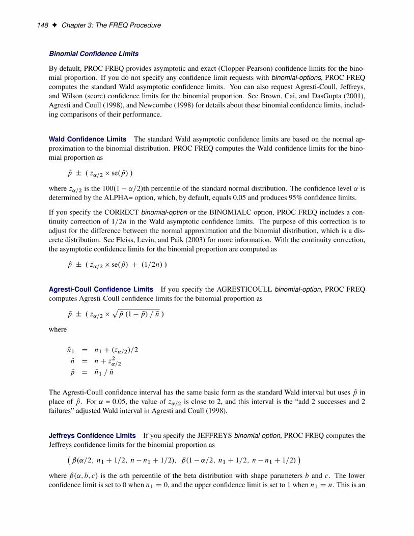
148 F Chapter 3: The FREQ Procedure
Binomial Confidence Limits
By default, PROC FREQ provides asymptotic and exact (Clopper-Pearson) confidence limits for the bino-mial proportion. If you do not specify any confidence limit requests with binomial-options, PROC FREQcomputes the standard Wald asymptotic confidence limits. You can also request Agresti-Coull, Jeffreys,and Wilson (score) confidence limits for the binomial proportion. See Brown, Cai, and DasGupta (2001),Agresti and Coull (1998), and Newcombe (1998) for details about these binomial confidence limits, includ-ing comparisons of their performance.
Wald Confidence Limits The standard Wald asymptotic confidence limits are based on the normal ap-proximation to the binomial distribution. PROC FREQ computes the Wald confidence limits for the bino-mial proportion as
Op ˙ . z˛=2 � se. Op/ /
where z˛=2 is the 100.1 � ˛=2/th percentile of the standard normal distribution. The confidence level ˛ isdetermined by the ALPHA= option, which, by default, equals 0.05 and produces 95% confidence limits.
If you specify the CORRECT binomial-option or the BINOMIALC option, PROC FREQ includes a con-tinuity correction of 1=2n in the Wald asymptotic confidence limits. The purpose of this correction is toadjust for the difference between the normal approximation and the binomial distribution, which is a dis-crete distribution. See Fleiss, Levin, and Paik (2003) for more information. With the continuity correction,the asymptotic confidence limits for the binomial proportion are computed as
Op ˙ . z˛=2 � se. Op/ C .1=2n/ /
Agresti-Coull Confidence Limits If you specify the AGRESTICOULL binomial-option, PROC FREQcomputes Agresti-Coull confidence limits for the binomial proportion as
Qp ˙ . z˛=2 �pQp .1 � Qp/ = Qn /
where
Qn1 D n1 C .z˛=2/=2
Qn D nC z2˛=2
Qp D Qn1 = Qn
The Agresti-Coull confidence interval has the same basic form as the standard Wald interval but uses Qp inplace of Op. For ˛ = 0.05, the value of z˛=2 is close to 2, and this interval is the “add 2 successes and 2failures” adjusted Wald interval in Agresti and Coull (1998).
Jeffreys Confidence Limits If you specify the JEFFREYS binomial-option, PROC FREQ computes theJeffreys confidence limits for the binomial proportion as�
ˇ.˛=2; n1 C 1=2; n � n1 C 1=2/; ˇ.1 � ˛=2; n1 C 1=2; n � n1 C 1=2/�
where ˇ.˛; b; c/ is the ˛th percentile of the beta distribution with shape parameters b and c. The lowerconfidence limit is set to 0 when n1 D 0, and the upper confidence limit is set to 1 when n1 D n. This is an

Statistical Computations F 149
equal-tailed interval based on the noninformative Jeffreys prior for a binomial proportion. See Brown, Cai,and DasGupta (2001) for details. See Berger (1985) for information about using beta priors for inference onthe binomial proportion.
Wilson (Score) Confidence Limits If you specify the WILSON binomial-option, PROC FREQ computesWilson confidence limits for the binomial proportion. These are also known as score confidence limits andare attributed to Wilson (1927). The confidence limits are based on inverting the normal test that uses thenull proportion in the variance (the score test). Wilson confidence limits are the roots of
jp � Opj D z˛=2pp.1 � p/=n
and are computed as Op C z2˛=2=2n ˙ z˛=2
r�Op.1 � Op/C z2
˛=2=4n
�=n
!=�1C z2˛=2=n
�
The Wilson interval has been shown to have better performance than the Wald interval and the exact(Clopper-Pearson) interval. See Agresti and Coull (1998), Brown, Cai, and DasGupta (2001), and New-combe (1998) for more information.
Exact (Clopper-Pearson) Confidence Limits Exact (Clopper-Pearson) confidence limits for the bino-mial proportion are constructed by inverting the equal-tailed test based on the binomial distribution. Thismethod is attributed to Clopper and Pearson (1934). The exact confidence limits pL and pU satisfy thefollowing equations, for n1 D 1; 2; : : : n � 1:
nXxDn1
n
x
!p x
L .1 � pL/n�x
D ˛=2
n1XxD0
n
x
!p x
U .1 � pU/n�x
D ˛=2
The lower confidence limit equals 0 when n1 D 0, and the upper confidence limit equals 1 when n1 D n.
PROC FREQ computes the exact (Clopper-Pearson) confidence limits by using the F distribution as
pL D
�1C
n � n1 C 1
n1 F.1 � ˛=2; 2n1; 2.n � n1 C 1/ /
��1
pU D
�1C
n � n1
.n1 C 1/ F. ˛=2; 2.n1 C 1/; 2.n � n1/ /
��1where F.˛; b; c/ is the ˛th percentile of the F distribution with b and c degrees of freedom. See Leemisand Trivedi (1996) for a derivation of this expression. Also see Collett (1991) for more information aboutexact binomial confidence limits.

150 F Chapter 3: The FREQ Procedure
Because this is a discrete problem, the confidence coefficient (or coverage probability) of the exact (Clopper-Pearson) interval is not exactly (1� ˛) but is at least (1� ˛). Thus, this confidence interval is conservative.Unless the sample size is large, the actual coverage probability can be much larger than the target value.See Agresti and Coull (1998), Brown, Cai, and DasGupta (2001), and Leemis and Trivedi (1996) for moreinformation about the performance of these confidence limits.
Binomial Tests
The BINOMIAL option provides an asymptotic equality test for the binomial proportion by default. You canalso specify binomial-options to request tests of noninferiority, superiority, and equivalence for the binomialproportion. If you specify the BINOMIAL option in the EXACT statement, PROC FREQ also computesexact p-values for the tests that you request with the binomial-options.
Equality Test PROC FREQ computes an asymptotic test of the hypothesis that the binomial proportionequals p0, where you can specify the value of p0 with the P= binomial-option. If you do not specify a nullvalue with P=, PROC FREQ uses p0 D 0:5 by default. The binomial test statistic is computed as
z D . Op � p0/=se
By default, the standard error is based on the null hypothesis proportion as
se Dpp0.1 � p0/=n
If you specify the VAR=SAMPLE binomial-option, the standard error is computed from the sample propor-tion as
se DpOp.1 � Op/=n
If you specify the CORRECT binomial-option or the BINOMIALC option, PROC FREQ includes a con-tinuity correction in the asymptotic test statistic, towards adjusting for the difference between the normalapproximation and the discrete binomial distribution. See Fleiss, Levin, and Paik (2003) for details. Thecontinuity correction of .1=2n/ is subtracted from the numerator of the test statistic if . Op � p0/ is positive;otherwise, the continuity correction is added to the numerator.
PROC FREQ computes one-sided and two-sided p-values for this test. When the test statistic z is greaterthan zero (its expected value under the null hypothesis), PROC FREQ computes the right-sided p-value,which is the probability of a larger value of the statistic occurring under the null hypothesis. A small right-sided p-value supports the alternative hypothesis that the true value of the proportion is greater than p0.When the test statistic is less than or equal to zero, PROC FREQ computes the left-sided p-value, which isthe probability of a smaller value of the statistic occurring under the null hypothesis. A small left-sided p-value supports the alternative hypothesis that the true value of the proportion is less than p0. The one-sidedp-value P1 can be expressed as
P1 D
(Prob.Z > z/ if z > 0
Prob.Z < z/ if z � 0
where Z has a standard normal distribution. The two-sided p-value is computed as P2 D 2 � P1.

Statistical Computations F 151
If you specify the BINOMIAL option in the EXACT statement, PROC FREQ also computes an exact testof the null hypothesis H0Wp D p0. To compute the exact test, PROC FREQ uses the binomial probabilityfunction,
Prob.X D x j p0/ D
n
x
!p x0 .1 � p0/
.n�x/ for x D 0; 1; 2; : : : ; n
where the variable X has a binomial distribution with parameters n and p0. To compute the left-sided p-value, Prob.X � n1/, PROC FREQ sums the binomial probabilities over x from zero to n1. To computethe right-sided p-value, Prob.X � n1/, PROC FREQ sums the binomial probabilities over x from n1 to n.The exact one-sided p-value is the minimum of the left-sided and right-sided p-values,
P1 D min . Prob.X � n1 j p0/; Prob.X � n1 j p0/ /
and the exact two-sided p-value is computed as P2 D 2 � P1.
Noninferiority Test If you specify the NONINF binomial-option, PROC FREQ provides a noninferioritytest for the binomial proportion. The null hypothesis for the noninferiority test is
H0Wp � p0 � �ı
versus the alternative
HaWp � p0 > �ı
where ı is the noninferiority margin and p0 is the null proportion. Rejection of the null hypothesis indicatesthat the binomial proportion is not inferior to the null value. See Chow, Shao, and Wang (2003) for moreinformation.
You can specify the value of ı with the MARGIN= binomial-option, and you can specify p0 with the P=binomial-option. By default, ı D 0:2 and p0 D 0:5.
PROC FREQ provides an asymptotic Wald test for noninferiority. The test statistic is computed as
z D . Op � p�0 / = se
where p�0 is the noninferiority limit,
p�0 D p0 � ı
By default, the standard error is computed from the sample proportion as
se DpOp.1 � Op/=n
If you specify the VAR=NULL binomial-option, the standard error is based on the noninferiority limit (de-termined by the null proportion and the margin) as
se D
qp�0 .1 � p
�0 /=n

152 F Chapter 3: The FREQ Procedure
If you specify the CORRECT binomial-option or the BINOMIALC option, PROC FREQ includes a con-tinuity correction in the asymptotic test statistic z. The continuity correction of .1=2n/ is subtracted fromthe numerator of the test statistic if . Op � p�0 / is positive; otherwise, the continuity correction is added to thenumerator.
The p-value for the noninferiority test is
Pz D Prob.Z > z/
where Z has a standard normal distribution.
As part of the noninferiority analysis, PROC FREQ provides asymptotic Wald confidence limits for thebinomial proportion. These confidence limits are computed as described in the section “Wald ConfidenceLimits” on page 148 but use the same standard error (VAR=NULL or VAR=SAMPLE) as the noninferioritytest statistic z. The confidence coefficient is 100.1 � 2˛/% (Schuirmann 1999). By default, if you donot specify the ALPHA= option, the noninferiority confidence limits are 90% confidence limits. You cancompare the confidence limits to the noninferiority limit, p�0 D p0 � ı.
If you specify the BINOMIAL option in the EXACT statement, PROC FREQ provides an exact noninfe-riority test for the binomial proportion. The exact p-value is computed by using the binomial probabilityfunction with parameters p�0 and n,
Px D
kDnXkDn1
n
k
!.p�0 /
k .1 � p�0 /.n�k/
See Chow, Shao, Wang (2003, p. 116) for details. If you request exact binomial statistics, PROC FREQ alsoincludes exact (Clopper-Pearson) confidence limits for the binomial proportion in the equivalence analysisdisplay. See the section “Exact (Clopper-Pearson) Confidence Limits” on page 149 for details.
Superiority Test If you specify the SUP binomial-option, PROC FREQ provides a superiority test for thebinomial proportion. The null hypothesis for the superiority test is
H0Wp � p0 � ı
versus the alternative
HaWp � p0 > ı
where ı is the superiority margin and p0 is the null proportion. Rejection of the null hypothesis indicatesthat the binomial proportion is superior to the null value. You can specify the value of ı with the MARGIN=binomial-option, and you can specify the value of p0 with the P= binomial-option. By default, ı D 0:2 andp0 D 0:5.
The superiority analysis is identical to the noninferiority analysis but uses a positive value of the margin ıin the null hypothesis. The superiority limit equals p0 C ı. The superiority computations follow those inthe section “Noninferiority Test” on page 151 but replace –ı with ı. See Chow, Shao, and Wang (2003) formore information.
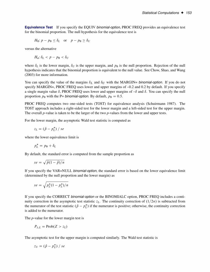
Statistical Computations F 153
Equivalence Test If you specify the EQUIV binomial-option, PROC FREQ provides an equivalence testfor the binomial proportion. The null hypothesis for the equivalence test is
H0Wp � p0 � ıL or p � p0 � ıU
versus the alternative
HaW ıL < p � p0 < ıU
where ıL is the lower margin, ıU is the upper margin, and p0 is the null proportion. Rejection of the nullhypothesis indicates that the binomial proportion is equivalent to the null value. See Chow, Shao, and Wang(2003) for more information.
You can specify the value of the margins ıL and ıU with the MARGIN= binomial-option. If you do notspecify MARGIN=, PROC FREQ uses lower and upper margins of –0.2 and 0.2 by default. If you specifya single margin value ı, PROC FREQ uses lower and upper margins of –ı and ı. You can specify the nullproportion p0 with the P= binomial-option. By default, p0 D 0:5.
PROC FREQ computes two one-sided tests (TOST) for equivalence analysis (Schuirmann 1987). TheTOST approach includes a right-sided test for the lower margin and a left-sided test for the upper margin.The overall p-value is taken to be the larger of the two p-values from the lower and upper tests.
For the lower margin, the asymptotic Wald test statistic is computed as
zL D . Op � p�L / = se
where the lower equivalence limit is
p�L D p0 C ıL
By default, the standard error is computed from the sample proportion as
se DpOp.1 � Op/=n
If you specify the VAR=NULL binomial-option, the standard error is based on the lower equivalence limit(determined by the null proportion and the lower margin) as
se D
qp�L .1 � p
�L /=n
If you specify the CORRECT binomial-option or the BINOMIALC option, PROC FREQ includes a conti-nuity correction in the asymptotic test statistic zL. The continuity correction of .1=2n/ is subtracted fromthe numerator of the test statistic . Op � p�L / if the numerator is positive; otherwise, the continuity correctionis added to the numerator.
The p-value for the lower margin test is
Pz;L D Prob.Z > zL/
The asymptotic test for the upper margin is computed similarly. The Wald test statistic is
zU D . Op � p�U/ = se

154 F Chapter 3: The FREQ Procedure
where the upper equivalence limit is
p�U D p0 C ıU
By default, the standard error is computed from the sample proportion. If you specify the VAR=NULLbinomial-option, the standard error is based on the upper equivalence limit as
se D
qp�U.1 � p
�U/=n
If you specify the CORRECT binomial-option or the BINOMIALC option, PROC FREQ includes a conti-nuity correction of .1=2n/ in the asymptotic test statistic zU .
The p-value for the upper margin test is
Pz;U D Prob.Z < zU/
Based on the two one-sided tests (TOST), the overall p-value for the test of equivalence equals the largerp-value from the lower and upper margin tests, which can be expressed as
Pz D max.Pz;L ; Pz;U/
As part of the equivalence analysis, PROC FREQ provides asymptotic Wald confidence limits for the bi-nomial proportion. These confidence limits are computed as described in the section “Wald ConfidenceLimits” on page 148, but use the same standard error (VAR=NULL or VAR=SAMPLE) as the equiva-lence test statistics and have a confidence coefficient of 100.1 � 2˛/% (Schuirmann 1999). By default, ifyou do not specify the ALPHA= option, the equivalence confidence limits are 90% limits. If you specifyVAR=NULL, separate standard errors are computed for the lower and upper margin tests, each based onthe null proportion and the corresponding (lower or upper) margin. The confidence limits are computed byusing the maximum of these two standard errors. You can compare the confidence limits to the equivalencelimits, .p0 C ıL; p0 C ıU/.
If you specify the BINOMIAL option in the EXACT statement, PROC FREQ also provides an exact equiv-alence test by using two one-sided exact tests (TOST). The procedure computes lower and upper marginexact tests by using the binomial probability function as described in the section “Noninferiority Test” onpage 151. The overall exact p-value for the equivalence test is taken to be the larger p-value from the lowerand upper margin exact tests. If you request exact statistics, PROC FREQ also includes exact (Clopper-Pearson) confidence limits in the equivalence analysis display. The confidence coefficient is 100.1 � 2˛/%(Schuirmann 1999). See the section “Exact (Clopper-Pearson) Confidence Limits” on page 149 for details.
Risks and Risk Differences
The RISKDIFF option in the TABLES statement provides estimates of risks (binomial proportions) andrisk differences for 2 � 2 tables. This analysis might be appropriate when comparing the proportion ofsome characteristic for two groups, where row 1 and row 2 correspond to the two groups, and the columnscorrespond to two possible characteristics or outcomes. For example, the row variable might be a treatmentor dose, and the column variable might be the response. See Collett (1991), Fleiss, Levin, and Paik (2003),and Stokes, Davis, and Koch (2000) for more information.

Statistical Computations F 155
Let the frequencies of the 2 � 2 table be represented as follows.
Column 1 Column 2 TotalRow 1 n11 n12 n1�Row 2 n21 n22 n2�Total n�1 n�2 n
For column 1 and column 2, PROC FREQ provides estimates of the row 1 risk (proportion), the row 2 risk,the overall risk, and the risk difference. The risk difference is defined as the row 1 risk minus the row 2 risk.The risks are binomial proportions of their rows (row 1, row 2, or overall), and the computation of theirstandard errors and confidence limits follow the binomial proportion computations, which are described inthe section “Binomial Proportion” on page 147.
The column 1 risk for row 1 is the proportion of row 1 observations classified in column 1,
p1 D n11 = n1�
This estimates the conditional probability of the column 1 response, given the first level of the row variable.
The column 1 risk for row 2 is the proportion of row 2 observations classified in column 1,
p2 D n21 = n2�
The overall column 1 risk is the proportion of all observations classified in column 1,
p D n�1 = n
The column 1 risk difference compares the risks for the two rows, and it is computed as the column 1 riskfor row 1 minus the column 1 risk for row 2,
d D p1 � p2
The risks and risk difference are defined similarly for column 2.
The standard error of the column 1 risk for row i is computed as
se.pi / Dppi .1 � pi / = n1�
The standard error of the overall column 1 risk is computed as
se.p/ Dpp .1 � p/ = n
If the two rows represent independent binomial samples, the standard error for the column 1 risk differenceis computed as
se.d/ Dpvar.p1/C var.p2/
The standard errors are computed in a similar manner for the column 2 risks and risk difference.

156 F Chapter 3: The FREQ Procedure
Confidence Limits
By default, the RISKDIFF option provides standard Wald asymptotic confidence limits for the risks (row 1,row 2, and overall) and the risk difference. The RISKDIFF option also provides other types of confidencelimits and tests for the risk difference. See the sections “Risk Difference Confidence Limits” on page 156and “Risk Difference Tests” on page 158 for details.
The risks are equivalent to binomial proportions of their corresponding rows. This section describes theWald confidence limits for risks that are provided by the RISKDIFF option. The BINOMIAL option pro-vides additional confidence limit types and tests for risks in the binomial proportion framework. See thesections “Binomial Confidence Limits” on page 148 and “Binomial Tests” on page 150 for details.
The Wald asymptotic confidence limits are based on the normal approximation to the binomial distribution.PROC FREQ computes the Wald confidence limits for the risks and risk differences as
est ˙ . z˛=2 � se.est/ /
where est is the estimate, z˛=2 is the 100.1 � ˛=2/th percentile of the standard normal distribution, andse.est/ is the standard error of the estimate. The confidence level ˛ is determined from the value of theALPHA= option, which, by default, equals 0.05 and produces 95% confidence limits.
If you specify the CORRECT riskdiff-option or the RISKDIFFC option, PROC FREQ includes continuitycorrections in the Wald asymptotic confidence limits for the risks and risk differences. The purpose of acontinuity correction is to adjust for the difference between the normal approximation and the binomialdistribution, which is discrete. See Fleiss, Levin, and Paik (2003) for more information. With the continuitycorrection, the asymptotic confidence limits are computed as
est ˙ . z˛=2 � se.est/C cc /
where cc is the continuity correction. For the row 1 risk, cc D .1=2n1�/; for the row 2 risk, cc D .1=2n2�/;for the overall risk, cc D .1=2n/; and for the risk difference, cc D ..1=n1�C 1=n2�/=2/. The column 1 andcolumn 2 risks use the same continuity corrections.
PROC FREQ also computes exact (Clopper-Pearson) confidence limits for the column 1, column 2, andoverall risks. These confidence limits are constructed by inverting the equal-tailed test based on the binomialdistribution. PROC FREQ uses the F distribution to compute the Clopper-Pearson confidence limits. Seethe section “Exact (Clopper-Pearson) Confidence Limits” on page 149 for details.
Risk Difference Confidence Limits You can request additional confidence limits for the risk differ-ence by specifying the CL= riskdiff-option. Available confidence limit types include exact unconditional,Farrington-Manning, Hauck-Anderson, Newcombe score, and Wald. Continuity-corrected versions of theNewcombe and Wald confidence limits are available. By default, the Wald confidence limits use a sample-based variance; alternatively, you can request a test-based variance and specify the null risk difference value.
The confidence coefficient for the confidence limits produced by the CL= riskdiff-option is 100.1 � ˛/%,where the value of ˛ is determined by the ALPHA= option. By default, ALPHA=0.05, which produces 95%confidence limits. This differs from the test-based confidence limits that are provided with the equivalence,noninferiority, and superiority tests, which have a confidence coefficient of 100.1 � 2˛/% (Schuirmann1999). See the section “Risk Difference Tests” on page 158 for details.
The section “Exact Unconditional Confidence Limits for the Risk Difference” on page 163 describes thecomputation of the exact confidence limits. The confidence limits are constructed by inverting two separate

Statistical Computations F 157
one-sided exact tests (tail method). By default, the tests are based on the unstandardized risk difference.If you specify the RISKDIFF(METHOD=FMSCORE) option, the Farrington-Manning score is used as thetest statistic.
PROC FREQ computes the Newcombe confidence limits for the risk difference as described in the sub-section Newcombe Score Confidence Limits in the section “Noninferiority Tests” on page 159, exceptthat the Newcombe confidence limits produced by the CL= riskdiff-option have a confidence coefficientof 100.1 � ˛/%.
The following sections describe the computation of the Farrington-Manning, Hauck-Anderson, and Waldconfidence limits for the risk difference.
Farrington-Manning Confidence Limits The Farrington-Manning confidence limits for the risk differenceare computed as
Od ˙ . z˛=2 � se. Od/ /
where Od D Op1 � Op2, z˛=2 is the 100.1 � ˛=2/th percentile of the standard normal distribution, and thestandard error is
se. Od/ DpQp1.1 � Qp1/=n1� C Qp2.1 � Qp2/=n2�
where Qp1 and Qp2 are the maximum likelihood estimators of p1 and p2 under the null hypothesis that therisk difference equals d0.
The subsection Farrington-Manning Test in the section “Noninferiority Tests” on page 159 describes thecomputation of the maximum likelihood estimators Qp1 and Qp2. See Farrington and Manning (1990) fordetails.
This computation uses a null hypothesis value of the risk difference, which you can specify in theCL=FM(NULL=value) riskdiff=option. By default, PROC FREQ uses a null value of 0. This differs fromthe Farrington-Manning confidence limits that are produced in the noninferiority analysis, where the nullvalue of the risk difference is based on the test margin (which is specified by the MARGIN= riskdiff-option).
Hauck-Anderson Confidence Limits The Hauck-Anderson confidence limits for the risk difference arecomputed as
Od ˙ . cc C z˛=2 � se. Od/ /
where Od D Op1 � Op2 and z˛=2 is the 100.1 � ˛=2/th percentile of the standard normal distribution. Thestandard error is computed from the sample proportions as
se. Od/ DpOp1.1 � Op1/=.n1� � 1/ C Op2.1 � Op2/=.n2� � 1/
The Hauck-Anderson continuity correction cc is computed as
cc D 1 =�2 min.n1�; n2�/
�See Hauck and Anderson (1986) for more information. The subsection Hauck-Anderson Test in the section“Noninferiority Tests” on page 159 describes the corresponding noninferiority test.
Wald Confidence Limits The Wald confidence limits for the risk difference are computed as
Od ˙ . z˛=2 � se. Od/ /

158 F Chapter 3: The FREQ Procedure
where Od D Op1 � Op2 and z˛=2 is the 100.1 � ˛=2/th percentile of the standard normal distribution. Bydefault, the standard error is computed from the sample proportions as
se. Od/ DpOp1.1 � Op1/=n1� C Op2.1 � Op2/=n2�
If you specify the CL=WALD(NULL=value) riskdiff-option, the standard error is based on the null hypoth-esis that the risk difference equals d0 D value (Dunnett and Gent 1977). The standard error is computedas
se. Od/ DpQp.1 � Qp/=n2� C . Qp C d0/.1 � Qp � d0/=n1�
where
Qp D .n11 C n21 C d0n1�/=n
If you specify the CORRECT riskdiff-option, the Wald confidence limits include a continuity correction cc,
Od ˙ . cc C z˛=2 � se. Od/ /
where cc D .1=n1� C 1=n2�/=2.
The subsection Wald Test in the section “Noninferiority Tests” on page 159 describes the correspondingnoninferiority test.
Risk Difference Tests
You can specify riskdiff-options to request tests of the risk (proportion) difference. You can request tests ofequality, noninferiority, superiority, and equivalence for the risk difference. The test of equality is a standardWald asymptotic test, available with or without a continuity correction. For noninferiority, superiority, andequivalence tests of the risk difference, the following test methods are provided: Wald (with and withoutcontinuity correction), Hauck-Anderson, Farrington-Manning, and Newcombe score (with and without con-tinuity correction). You can specify the test method with the METHOD= riskdiff-option. By default, PROCFREQ uses METHOD=WALD.
Equality Test If you specify the EQUAL riskdiff-option, PROC FREQ computes a test of equality, or atest of the null hypothesis that the risk difference equals zero. For the column 1 (or 2) risk difference, thistest can be expressed as H0W d D 0 versus the alternative HaW d ¤ 0, where d D p1 � p2 denotes thecolumn 1 (or 2) risk difference. PROC FREQ provides a Wald asymptotic test of equality. The test statisticis computed as
z D Od=se. Od/
By default, the standard error is computed from the sample proportions as
se. Od/ DpOp1.1 � Op1/=n1� C Op2.1 � Op2/=n2�
If you specify the VAR=NULL riskdiff-option, the standard error is based on the null hypothesis that the row1 and row 2 risks are equal,
se. Od/ DpOp.1 � Op/ � .1=n1� C 1=n2�/
where Op D n�1=n estimates the overall column 1 risk.

Statistical Computations F 159
If you specify the CORRECT riskdiff-option or the RISKDIFFC option, PROC FREQ includes a continuitycorrection in the test statistic. If Od > 0, the continuity correction is subtracted from Od in the numerator ofthe test statistic; otherwise, the continuity correction is added to the numerator. The value of the continuitycorrection is .1=n1� C 1=n2�/=2.
PROC FREQ computes one-sided and two-sided p-values for this test. When the test statistic z is greaterthan 0, PROC FREQ displays the right-sided p-value, which is the probability of a larger value occurringunder the null hypothesis. The one-sided p-value can be expressed as
P1 D
(Prob.Z > z/ if z > 0
Prob.Z < z/ if z � 0
where Z has a standard normal distribution. The two-sided p-value is computed as P2 D 2 � P1.
Noninferiority Tests If you specify the NONINF riskdiff-option, PROC FREQ provides a noninferioritytest for the risk difference, or the difference between two proportions. The null hypothesis for the noninfe-riority test is
H0Wp1 � p2 � �ı
versus the alternative
HaWp1 � p2 > �ı
where ı is the noninferiority margin. Rejection of the null hypothesis indicates that the row 1 risk is notinferior to the row 2 risk. See Chow, Shao, and Wang (2003) for more information.
You can specify the value of ı with the MARGIN= riskdiff-option. By default, ı D 0:2. You can specifythe test method with the METHOD= riskdiff-option. The following methods are available for the risk differ-ence noninferiority analysis: Wald (with and without continuity correction), Hauck-Anderson, Farrington-Manning, and Newcombe score (with and without continuity correction). The Wald, Hauck-Anderson, andFarrington-Manning methods provide tests and corresponding test-based confidence limits; the Newcombescore method provides only confidence limits. If you do not specify METHOD=, PROC FREQ uses theWald test by default.
The confidence coefficient for the test-based confidence limits is 100.1 � 2˛/% (Schuirmann 1999). Bydefault, if you do not specify the ALPHA= option, these are 90% confidence limits. You can compare theconfidence limits to the noninferiority limit, –ı.
The following sections describe the noninferiority analysis methods for the risk difference.
Wald Test If you specify the METHOD=WALD riskdiff-option, PROC FREQ provides an asymptotic Waldtest of noninferiority for the risk difference. This is also the default method. The Wald test statistic iscomputed as
z D . Od C ı/ = se. Od/
where ( Od D Op1 � Op2) estimates the risk difference and ı is the noninferiority margin.
By default, the standard error for the Wald test is computed from the sample proportions as
se. Od/ DpOp1.1 � Op1/=n1� C Op2.1 � Op2/=n2�

160 F Chapter 3: The FREQ Procedure
If you specify the VAR=NULL riskdiff-option, the standard error is based on the null hypothesis that the riskdifference equals –ı (Dunnett and Gent 1977). The standard error is computed as
se. Od/ DpQp.1 � Qp/=n2� C . Qp � ı/.1 � Qp C ı/=n1�
where
Qp D .n11 C n21 C ın1�/=n
If you specify the CORRECT riskdiff-option or the RISKDIFFC option, a continuity correction is includedin the test statistic. The continuity correction is subtracted from the numerator of the test statistic if thenumerator is greater than zero; otherwise, the continuity correction is added to the numerator. The value ofthe continuity correction is .1=n1� C 1=n2�/=2.
The p-value for the Wald noninferiority test is Pz D Prob.Z > z/, where Z has a standard normal distri-bution.
Hauck-Anderson Test If you specify the METHOD=HA riskdiff-option, PROC FREQ provides the Hauck-Anderson test for noninferiority. The Hauck-Anderson test statistic is computed as
z D . Od C ı ˙ cc/ = se. Od/
where Od D Op1 � Op2 and the standard error is computed from the sample proportions as
se. Od/ DpOp1.1 � Op1/=.n1� � 1/ C Op2.1 � Op2/=.n2� � 1/
The Hauck-Anderson continuity correction cc is computed as
cc D 1 =�2 min.n1�; n2�/
�The p-value for the Hauck-Anderson noninferiority test is Pz D Prob.Z > z/, where Z has a standardnormal distribution. See Hauck and Anderson (1986) and Schuirmann (1999) for more information.
Farrington-Manning Test If you specify the METHOD=FM riskdiff-option, PROC FREQ provides theFarrington-Manning test of noninferiority for the risk difference. The Farrington-Manning test statistic iscomputed as
z D . Od C ı/ = se. Od/
where Od D Op1 � Op2 and
se. Od/ DpQp1.1 � Qp1/=n1� C Qp2.1 � Qp2/=n2�
where Qp1 and Qp2 are the maximum likelihood estimators of p1 and p2 under the null hypothesis that the riskdifference equals –ı. The p-value for the Farrington-Manning noninferiority test is then Pz D Prob.Z > z/,where Z has a standard normal distribution.
From Farrington and Manning (1990), the solution to the maximum likelihood equation is
Qp1 D 2u cos.w/ � b=3a and Qp2 D Qp1 C ı

Statistical Computations F 161
where
w D .� C cos�1.v=u3//=3
v D b3=.3a/3 � bc=6a2 C d=2a
u D sign.v/qb2=.3a/2 � c=3a
a D 1C �
b D � .1C � C Op1 C � Op2 � ı.� C 2//
c D ı2 � ı.2 Op1 C � C 1/C Op1 C � Op2
d D Op1ı.1 � ı/
� D n2�=n1�
Newcombe Score Confidence Limits If you specify the METHOD=NEWCOMBE riskdiff-option, PROCFREQ provides the Newcombe hybrid score (Wilson) confidence limits for the risk difference. The confi-dence coefficient for the confidence limits is 100.1 � 2˛/% (Schuirmann 1999). By default, if you do notspecify the ALPHA= option, these are 90% confidence limits. You can compare the confidence limits withthe noninferiority limit, –ı.
The Newcombe score confidence limits for the risk difference are constructed from the Wilson score confi-dence limits for each of the two individual proportions. The confidence limits for the individual proportionsare used in the standard error terms of the Wald confidence limits for the proportion difference. See New-combe (1998) and Barker et al. (2001) for more information.
Wilson score confidence limits for p1 and p2 are the roots of
jpi � Opi j D z˛ppi .1 � pi /=ni �
for i D 1; 2. The confidence limits are computed as�Opi C z2˛=2ni � ˙ z˛
q�Opi .1 � Opi /C z2˛=4ni �
�=ni �
�=�1C z2˛=ni �
�See the section “Wilson (Score) Confidence Limits” on page 149 for details.
Denote the lower and upper Wilson score confidence limits for p1 as L1 and U1, and denote the lower andupper confidence limits for p2 as L2 and U2. The Newcombe score confidence limits for the proportiondifference (d D p1 � p2) are computed as
dL D . Op1 � Op2/ �
q. Op1 � L1/2 C .U2 � Op2/2
dU D . Op1 � Op2/ C
q.U1 � Op1/2 C . Op2 � L2/2
If you specify the CORRECT riskdiff-option, PROC FREQ provides continuity-corrected Newcombe scoreconfidence limits. By including a continuity correction of 1=2ni �, the Wilson score confidence limits for theindividual proportions are computed as the roots of
jpi � Opi j � 1=2ni � D z˛ppi .1 � pi /=ni �
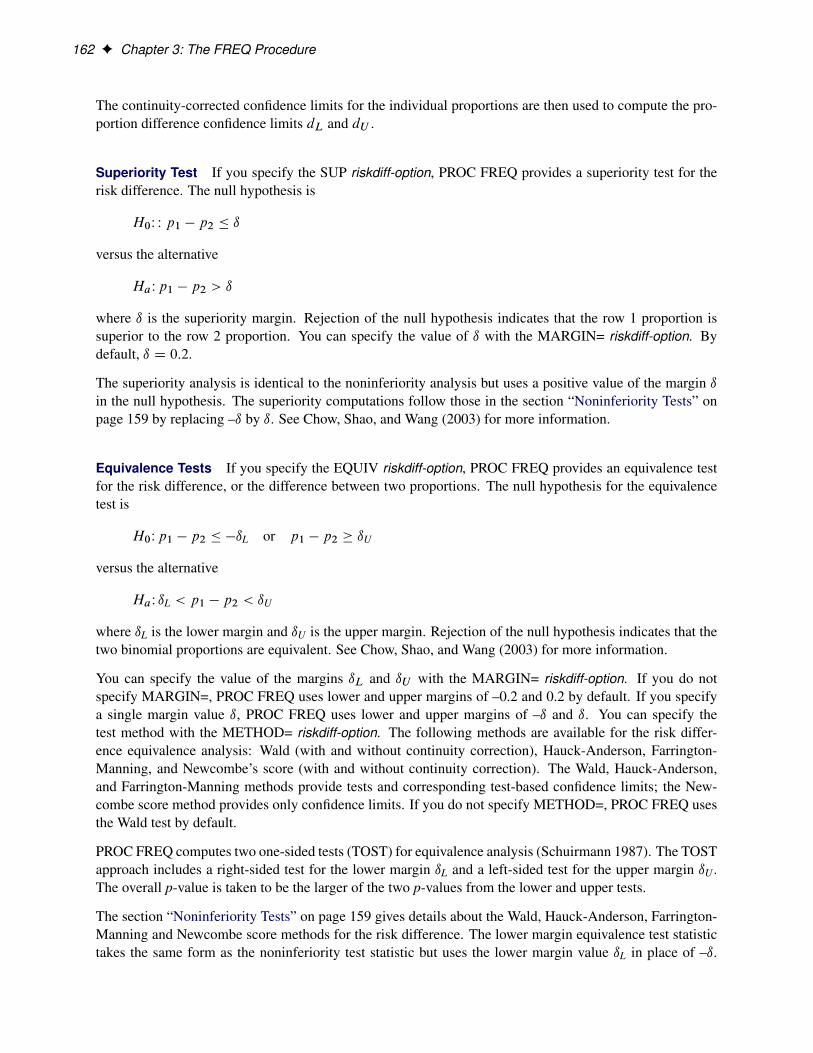
162 F Chapter 3: The FREQ Procedure
The continuity-corrected confidence limits for the individual proportions are then used to compute the pro-portion difference confidence limits dL and dU .
Superiority Test If you specify the SUP riskdiff-option, PROC FREQ provides a superiority test for therisk difference. The null hypothesis is
H0W W p1 � p2 � ı
versus the alternative
HaWp1 � p2 > ı
where ı is the superiority margin. Rejection of the null hypothesis indicates that the row 1 proportion issuperior to the row 2 proportion. You can specify the value of ı with the MARGIN= riskdiff-option. Bydefault, ı D 0:2.
The superiority analysis is identical to the noninferiority analysis but uses a positive value of the margin ıin the null hypothesis. The superiority computations follow those in the section “Noninferiority Tests” onpage 159 by replacing –ı by ı. See Chow, Shao, and Wang (2003) for more information.
Equivalence Tests If you specify the EQUIV riskdiff-option, PROC FREQ provides an equivalence testfor the risk difference, or the difference between two proportions. The null hypothesis for the equivalencetest is
H0Wp1 � p2 � �ıL or p1 � p2 � ıU
versus the alternative
HaW ıL < p1 � p2 < ıU
where ıL is the lower margin and ıU is the upper margin. Rejection of the null hypothesis indicates that thetwo binomial proportions are equivalent. See Chow, Shao, and Wang (2003) for more information.
You can specify the value of the margins ıL and ıU with the MARGIN= riskdiff-option. If you do notspecify MARGIN=, PROC FREQ uses lower and upper margins of –0.2 and 0.2 by default. If you specifya single margin value ı, PROC FREQ uses lower and upper margins of –ı and ı. You can specify thetest method with the METHOD= riskdiff-option. The following methods are available for the risk differ-ence equivalence analysis: Wald (with and without continuity correction), Hauck-Anderson, Farrington-Manning, and Newcombe’s score (with and without continuity correction). The Wald, Hauck-Anderson,and Farrington-Manning methods provide tests and corresponding test-based confidence limits; the New-combe score method provides only confidence limits. If you do not specify METHOD=, PROC FREQ usesthe Wald test by default.
PROC FREQ computes two one-sided tests (TOST) for equivalence analysis (Schuirmann 1987). The TOSTapproach includes a right-sided test for the lower margin ıL and a left-sided test for the upper margin ıU .The overall p-value is taken to be the larger of the two p-values from the lower and upper tests.
The section “Noninferiority Tests” on page 159 gives details about the Wald, Hauck-Anderson, Farrington-Manning and Newcombe score methods for the risk difference. The lower margin equivalence test statistictakes the same form as the noninferiority test statistic but uses the lower margin value ıL in place of –ı.

Statistical Computations F 163
The upper margin equivalence test statistic take the same form as the noninferiority test statistic but uses theupper margin value ıU in place of –ı.
The test-based confidence limits for the risk difference are computed according to the equivalence testmethod that you select. If you specify METHOD=WALD with VAR=NULL, or METHOD=FM, separatestandard errors are computed for the lower and upper margin tests. In this case, the test-based confidencelimits are computed by using the maximum of these two standard errors. The confidence limits have aconfidence coefficient of 100.1� 2˛/% (Schuirmann 1999). By default, if you do not specify the ALPHA=option, these are 90% confidence limits. You can compare the confidence limits to the equivalence limits,.ıL; ıU/.
Exact Unconditional Confidence Limits for the Risk Difference
If you specify the RISKDIFF option in the EXACT statement, PROC FREQ provides exact unconditionalconfidence limits for the risk difference. PROC FREQ computes the confidence limits by inverting two sep-arate one-sided tests (tail method), where the size of each test is at most ˛=2 and the confidence coefficientis at least .1 � ˛). Exact conditional methods, described in the section “Exact Statistics” on page 184, donot apply to the risk difference due to the presence of a nuisance parameter (Agresti 1992). The uncondi-tional approach eliminates the nuisance parameter by maximizing the p-value over all possible values of theparameter (Santner and Snell 1980).
By default, PROC FREQ uses the unstandardized risk difference as the test statistic in the confidencelimit computations. If you specify the RISKDIFF(METHOD=FMSCORE) option, the procedure uses theFarrington-Manning score statistic (Chan and Zhang 1999). The score statistic is a less discrete statisticthan the raw risk difference and produces less conservative confidence limits (Agresti and Min 2001). Seealso Santner et al. (2007) for comparisons of methods for computing exact confidence limits for the riskdifference.
PROC FREQ computes the confidence limits as follows. The risk difference is defined as the differencebetween the row 1 and row 2 risks (proportions), d D p1 � p2, and n1 and n2 denote the row totals of the2�2 table. The joint probability function for the table can be expressed in terms of the table cell frequencies,the risk difference, and the nuisance parameter p2 as
f .n11; n21In1; n2; d; p2/ D
n1
n11
!.d C p2/
n11.1 � d � p2/
n1�n11 �
n2
n21
!pn212 .1 � p2/
n2�n21
The 100.1 � ˛=2/% confidence limits for the risk difference are computed as
dL D sup .d� W PU .d�/ > ˛=2/
dU D inf .d� W PL.d�/ > ˛=2/
where
PU .d�/ D supp2
� XA;T .a/�t0
f .n11; n21In1; n2; d�; p2/�
PL.d�/ D supp2
� XA;T .a/�t0
f .n11; n21In1; n2; d�; p2/�

164 F Chapter 3: The FREQ Procedure
The set A includes all 2 � 2 tables with row sums equal to n1 and n2, and T .a/ denotes the value of thetest statistic for table a in A. To compute PU .d�/, the sum includes probabilities of those tables for which(T .a/ � t0), where t0 is the value of the test statistic for the observed table. For a fixed value of d�, PU .d�/is taken to be the maximum sum over all possible values of p2.
By default, PROC FREQ uses the unstandardized risk difference as the test statistic T . If you specifythe RISKDIFF(METHOD=FMSCORE) option, the procedure uses the Farrington-Manning risk differencescore statistic as the test statistic. The computation of the risk difference score statistic is described in thesubsection Farrington-Manning Test in the section “Noninferiority Tests” on page 159. See Farrington andManning (1990) and Miettinen and Nurminen (1985) for more information.
Odds Ratio and Relative Risks for 2 x 2 Tables
Odds Ratio (Case-Control Studies)
The odds ratio is a useful measure of association for a variety of study designs. For a retrospective designcalled a case-control study, the odds ratio can be used to estimate the relative risk when the probability ofpositive response is small (Agresti 2002). In a case-control study, two independent samples are identifiedbased on a binary (yes-no) response variable, and the conditional distribution of a binary explanatory vari-able is examined, within fixed levels of the response variable. See Stokes, Davis, and Koch (2000) andAgresti (2007).
The odds of a positive response (column 1) in row 1 is n11=n12. Similarly, the odds of a positive responsein row 2 is n21=n22. The odds ratio is formed as the ratio of the row 1 odds to the row 2 odds. The oddsratio for a 2 � 2 table is defined as
OR Dn11=n12
n21=n22Dn11 n22
n12 n21
The odds ratio can be any nonnegative number. When the row and column variables are independent, thetrue value of the odds ratio equals 1. An odds ratio greater than 1 indicates that the odds of a positiveresponse are higher in row 1 than in row 2. Values less than 1 indicate the odds of positive response arehigher in row 2. The strength of association increases with the deviation from 1.
The transformation G D .OR � 1/=.OR C 1/ transforms the odds ratio to the range .�1; 1/ with G D 0
when OR D 1; G D �1 when OR D 0; and G approaches 1 as OR approaches infinity. G is the gammastatistic, which PROC FREQ computes when you specify the MEASURES option.
The asymptotic 100.1 � ˛/% confidence limits for the odds ratio are�OR � exp.�z
pv/; OR � exp.z
pv/�
where
v D var.lnOR/ D1
n11C
1
n12C
1
n21C
1
n22
and z is the 100.1�˛=2/th percentile of the standard normal distribution. If any of the four cell frequenciesare zero, the estimates are not computed.

Statistical Computations F 165
Exact Confidence Limits for the Odds Ratio When you specify the OR option in the EXACT statement,PROC FREQ computes exact confidence limits for the odds ratio. Because this is a discrete problem, theconfidence coefficient for the exact confidence interval is not exactly (1 � ˛) but is at least (1 � ˛). Thus,these confidence limits are conservative. See Agresti (1992) for more information.
PROC FREQ computes exact confidence limits for the odds ratio by using an algorithm based on Thomas(1971). See also Gart (1971). The following two equations are solved iteratively to determine the lower andupper confidence limits, �1 and �2:
n�1XiDn11
n1�
i
! n2�
n�1 � i
!�i1 =
n�1XiD0
n1�
i
! n2�
n�1 � i
!�i1 D ˛=2
n11XiD0
n1�
i
! n2�
n�1 � i
!�i2 =
n�1XiD0
n1�
i
! n2�
n�1 � i
!�i2 D ˛=2
When the odds ratio equals zero, which occurs when either n11 D 0 or n22 D 0, PROC FREQ sets thelower exact confidence limit to zero and determines the upper limit with level ˛. Similarly, when the oddsratio equals infinity, which occurs when either n12 D 0 or n21 D 0, PROC FREQ sets the upper exactconfidence limit to infinity and determines the lower limit with level ˛.
Relative Risks (Cohort Studies)
These measures of relative risk are useful in cohort (prospective) study designs, where two samples areidentified based on the presence or absence of an explanatory factor. The two samples are observed infuture time for the binary (yes-no) response variable under study. Relative risk measures are also usefulin cross-sectional studies, where two variables are observed simultaneously. See Stokes, Davis, and Koch(2000) and Agresti (2007) for more information.
The column 1 relative risk is the ratio of the column 1 risk for row 1 to row 2. The column 1 risk for row 1is the proportion of the row 1 observations classified in column 1,
p1 D n11 = n1�
Similarly, the column 1 risk for row 2 is
p2 D n21 = n2�
The column 1 relative risk is then computed as
RR1 D p1 = p2
A relative risk greater than 1 indicates that the probability of positive response is greater in row 1 than inrow 2. Similarly, a relative risk less than 1 indicates that the probability of positive response is less in row 1than in row 2. The strength of association increases with the deviation from 1.
Asymptotic 100.1 � ˛/% confidence limits for the column 1 relative risk are computed as�RR1 � exp.�z
pv/; RR1 � exp.z
pv/�

166 F Chapter 3: The FREQ Procedure
where
v D var.lnRR1/ D�.1 � p1/=n11
�C�.1 � p2/=n21
�and z is the 100.1 � ˛=2/th percentile of the standard normal distribution. If either n11 or n21 is zero, theestimates are not computed.
PROC FREQ computes the column 2 relative risks in the same way.
Exact Unconditional Confidence Limits for the Relative Risk If you specify the RELRISK option inthe EXACT statement, PROC FREQ provides exact unconditional confidence limits for the relative risk.PROC FREQ computes the confidence limits by inverting two separate one-sided tests (tail method), wherethe size of each test is at most ˛=2 and the confidence coefficient is at least .1 � ˛). Exact conditionalmethods, described in the section “Exact Statistics” on page 184, do not apply to the relative risk due tothe presence of a nuisance parameter (Agresti 1992). The unconditional approach eliminates the nuisanceparameter by maximizing the p-value over all possible values of the parameter (Santner and Snell 1980).
By default, PROC FREQ uses the unstandardized relative risk as the test statistic in the confidence limit com-putations. If you specify the RELRISK(METHOD=FMSCORE) option, the procedure uses the Farrington-Manning relative risk score statistic (Chan and Zhang 1999). The score statistic is a less discrete statisticthan the raw relative risk and produces less conservative confidence limits (Agresti and Min 2001). See alsoSantner et al. (2007) for comparisons of methods for computing exact confidence limits.
See the section “Exact Unconditional Confidence Limits for the Risk Difference” on page 163 for a de-scription of the method that PROC FREQ uses to compute confidence limits for the relative risk. The teststatistic for the relative risk computation is either the unstandardized relative risk (by default) or the relativerisk score statistic (if you specify the RELRISK(METHOD=FMSCORE) option). PROC FREQ uses thefollowing form of the unstandardized relative risk, which adds 0.05 to each frequency, to ensure that thestatistic is defined when there are zero table cells (Gart and Nam 1988):
Orr D.n11 C 0:5/ = .n1� C 0:5/
.n21 C 0:5/ = .n2� C 0:5/
If you specify the RELRISK(METHOD=FMSCORE) option, PROC FREQ uses the relative risk scorestatistic (Farrington and Manning 1990; Miettinen and Nurminen 1985). This test statistic is computed as
z D . Op1 �R0 Op2/ = se. Orr/
where
se. Orr/ DqQp1.1 � Qp1/=n1� C R20 Qp2.1 � Qp2/=n2�
where Qp1 and Qp2 are the maximum likelihood estimators of p1 and p2 under the null hypothesis that therelative risk equals R0. From Farrington and Manning (1990), the maximum likelihood solution is
Qp1 D .�b �p
b2 � 4ac/=2a and Qp2 D Qp1=R0

Statistical Computations F 167
where
a D 1C �
b D � .R0.1C � Op2/C � C Op1/
c D R0. Op1 C � Op2/
� D n2�=n1�
Cochran-Armitage Test for Trend
The TREND option in the TABLES statement provides the Cochran-Armitage test for trend, which testsfor trend in binomial proportions across levels of a single factor or covariate. This test is appropriate for atwo-way table where one variable has two levels and the other variable is ordinal. The two-level variablerepresents the response, and the other variable represents an explanatory variable with ordered levels. Whenthe two-way has two columns and R rows, PROC FREQ tests for trend across the R levels of the rowvariable, and the binomial proportion is computed as the proportion of observations in the first column.When the table has two rows and C columns, PROC FREQ tests for trend across the C levels of the columnvariable, and the binomial proportion is computed as the proportion of observations in the first row.
The trend test is based on the regression coefficient for the weighted linear regression of the binomialproportions on the scores of the explanatory variable levels. See Margolin (1988) and Agresti (2002) fordetails. If the table has two columns and R rows, the trend test statistic is computed as
T D
RXiD1
ni1.Ri � NR/ =
qp�1 .1 � p�1/ s2
where Ri is the score of row i , NR is the average row score, and
s2 D
RXiD1
ni �.Ri � NR/2
The SCORES= option in the TABLES statement determines the type of row scores used in computing thetrend test (and other score-based statistics). The default is SCORES=TABLE. See the section “Scores” onpage 132 for details. For character variables, the table scores for the row variable are the row numbers (forexample, 1 for the first row, 2 for the second row, and so on). For numeric variables, the table score for eachrow is the numeric value of the row level. When you perform the trend test, the explanatory variable mightbe numeric (for example, dose of a test substance), and the variable values might be appropriate scores. Ifthe explanatory variable has ordinal levels that are not numeric, you can assign meaningful scores to thevariable levels. Sometimes equidistant scores, such as the table scores for a character variable, might beappropriate. For more information on choosing scores for the trend test, see Margolin (1988).
The null hypothesis for the Cochran-Armitage test is no trend, which means that the binomial proportionpi1 D ni1=ni � is the same for all levels of the explanatory variable. Under the null hypothesis, the trendstatistic has an asymptotic standard normal distribution.
PROC FREQ computes one-sided and two-sided p-values for the trend test. When the test statistic is greaterthan its null hypothesis expected value of zero, PROC FREQ displays the right-sided p-value, which is the

168 F Chapter 3: The FREQ Procedure
probability of a larger value of the statistic occurring under the null hypothesis. A small right-sided p-valuesupports the alternative hypothesis of increasing trend in proportions from row 1 to row R. When the teststatistic is less than or equal to zero, PROC FREQ displays the left-sided p-value. A small left-sided p-valuesupports the alternative of decreasing trend.
The one-sided p-value for the trend test is computed as
P1 D
(Prob.Z > T / if T > 0
Prob.Z < T / if T � 0
where Z has a standard normal distribution. The two-sided p-value is computed as
P2 D Prob.jZj > jT j/
PROC FREQ also provides exact p-values for the Cochran-Armitage trend test. You can request the ex-act test by specifying the TREND option in the EXACT statement. See the section “Exact Statistics” onpage 184 for more information.
Jonckheere-Terpstra Test
The JT option in the TABLES statement provides the Jonckheere-Terpstra test, which is a nonparametrictest for ordered differences among classes. It tests the null hypothesis that the distribution of the responsevariable does not differ among classes. It is designed to detect alternatives of ordered class differences,which can be expressed as �1 � �2 � � � � � �R (or �1 � �2 � � � � � �R), with at least one of the inequalitiesbeing strict, where �i denotes the effect of class i . For such ordered alternatives, the Jonckheere-Terpstratest can be preferable to tests of more general class difference alternatives, such as the Kruskal–Wallis test(produced by the WILCOXON option in the NPAR1WAY procedure). See Pirie (1983) and Hollander andWolfe (1999) for more information about the Jonckheere-Terpstra test.
The Jonckheere-Terpstra test is appropriate for a two-way table in which an ordinal column variable repre-sents the response. The row variable, which can be nominal or ordinal, represents the classification variable.The levels of the row variable should be ordered according to the ordering you want the test to detect. Theorder of variable levels is determined by the ORDER= option in the PROC FREQ statement. The default isORDER=INTERNAL, which orders by unformatted values. If you specify ORDER=DATA, PROC FREQorders values according to their order in the input data set. For more information about how to order variablelevels, see the ORDER= option.
The Jonckheere-Terpstra test statistic is computed by first formingR.R�1/=2Mann-Whitney countsMi;i 0 ,where i < i 0, for pairs of rows in the contingency table,
Mi;i 0 D f number of times Xi;j < Xi 0;j 0 ; j D 1; : : : ; ni:I j0D 1; : : : ; ni 0: g
C12f number of times Xi;j D Xi 0;j 0 ; j D 1; : : : ; ni:I j
0D 1; : : : ; ni 0: g
where Xi;j is response j in row i . The Jonckheere-Terpstra test statistic is computed as
J DX1�i<
Xi 0�R
Mi;i 0

Statistical Computations F 169
This test rejects the null hypothesis of no difference among classes for large values of J . Asymptotic p-values for the Jonckheere-Terpstra test are obtained by using the normal approximation for the distributionof the standardized test statistic. The standardized test statistic is computed as
J � D .J � E0.J // =p
var0.J /
where E0.J / and var0.J / are the expected value and variance of the test statistic under the null hypothesis,
E0.J / D
n2 �
Xi
n2i �
!=4
var0.J / D A=72C B= .36n.n � 1/.n � 2//C C= .8n.n � 1//
where
A D n.n � 1/.2nC 5/ �Xi
ni �.ni � � 1/.2ni � C 5/ �Xj
n�j .n�j � 1/.2n�j C 5/
B D
Xi
ni �.ni � � 1/.ni � � 2/
!0@Xj
n�j .n�j � 1/.n�j � 2/
1AC D
Xi
ni �.ni � � 1/
!0@Xj
n�j .n�j � 1/
1APROC FREQ computes one-sided and two-sided p-values for the Jonckheere-Terpstra test. When the stan-dardized test statistic is greater than its null hypothesis expected value of zero, PROC FREQ displays theright-sided p-value, which is the probability of a larger value of the statistic occurring under the null hy-pothesis. A small right-sided p-value supports the alternative hypothesis of increasing order from row 1 torow R. When the standardized test statistic is less than or equal to zero, PROC FREQ displays the left-sidedp-value. A small left-sided p-value supports the alternative of decreasing order from row 1 to row R.
The one-sided p-value for the Jonckheere-Terpstra test, P1, is computed as
P1 D
(Prob.Z > J �/ if J � > 0
Prob.Z < J �/ if J � � 0
where Z has a standard normal distribution. The two-sided p-value, P2, is computed as
P2 D Prob.jZj > jJ �j/
PROC FREQ also provides exact p-values for the Jonckheere-Terpstra test. You can request the exact testby specifying the JT option in the EXACT statement. See the section “Exact Statistics” on page 184 formore information.

170 F Chapter 3: The FREQ Procedure
Tests and Measures of Agreement
When you specify the AGREE option in the TABLES statement, PROC FREQ computes tests and measuresof agreement for square tables (that is, for tables where the number of rows equals the number of columns).For two-way tables, these tests and measures include McNemar’s test for 2 � 2 tables, Bowker’s test ofsymmetry, the simple kappa coefficient, and the weighted kappa coefficient. For multiple strata (n-waytables, where n > 2), PROC FREQ also computes the overall simple kappa coefficient and the overallweighted kappa coefficient, as well as tests for equal kappas (simple and weighted) among strata. Cochran’sQ is computed for multiway tables when each variable has two levels, that is, for h � 2 � 2 tables.
PROC FREQ computes the kappa coefficients (simple and weighted), their asymptotic standard errors, andtheir confidence limits when you specify the AGREE option in the TABLES statement. If you also specifythe KAPPA option in the TEST statement, then PROC FREQ computes the asymptotic test of the hypothesisthat simple kappa equals zero. Similarly, if you specify the WTKAP option in the TEST statement, PROCFREQ computes the asymptotic test for weighted kappa.
In addition to the asymptotic tests described in this section, PROC FREQ provides exact p-values for Mc-Nemar’s test, the simple kappa coefficient test, and the weighted kappa coefficient test. You can requestthese exact tests by specifying the corresponding options in the EXACT statement. See the section “ExactStatistics” on page 184 for more information.
The following sections provide the formulas that PROC FREQ uses to compute the AGREE statistics. Forinformation about the use and interpretation of these statistics, see Agresti (2002), Agresti (2007), Fleiss,Levin, and Paik (2003), and the other references cited for each statistic.
McNemar’s Test
PROC FREQ computes McNemar’s test for 2 � 2 tables when you specify the AGREE option. McNemar’stest is appropriate when you are analyzing data from matched pairs of subjects with a dichotomous (yes-no)response. It tests the null hypothesis of marginal homogeneity, or p1� D p�1. McNemar’s test is computedas
QM D .n12 � n21/2 = .n12 C n21/
Under the null hypothesis, QM has an asymptotic chi-square distribution with one degree of freedom. SeeMcNemar (1947), as well as the general references cited in the preceding section. In addition to the asymp-totic test, PROC FREQ also computes the exact p-value for McNemar’s test when you specify the MCNEMoption in the EXACT statement.
Bowker’s Test of Symmetry
For Bowker’s test of symmetry, the null hypothesis is that the cell proportions are symmetric, or that pij Dpj i for all pairs of table cells. For 2 � 2 tables, Bowker’s test is identical to McNemar’s test, and so PROCFREQ provides Bowker’s test for square tables larger than 2 � 2.

Statistical Computations F 171
Bowker’s test of symmetry is computed as
QB D
XXi<j
.nij � nj i /2 = .nij C nj i /
For large samples,QB has an asymptotic chi-square distribution with R.R�1/=2 degrees of freedom underthe null hypothesis of symmetry. See Bowker (1948) for details.
Simple Kappa Coefficient
The simple kappa coefficient, introduced by Cohen (1960), is a measure of interrater agreement. PROCFREQ computes the simple kappa coefficient as
O� D .Po � Pe/ = .1 � Pe/
where Po DPi pi i and Pe D
Pi pi:p:i . If the two response variables are viewed as two independent
ratings of the n subjects, the kappa coefficient equals +1 when there is complete agreement of the raters.When the observed agreement exceeds chance agreement, kappa is positive, with its magnitude reflecting thestrength of agreement. Although this is unusual in practice, kappa is negative when the observed agreementis less than chance agreement. The minimum value of kappa is between�1 and 0, depending on the marginalproportions.
The asymptotic variance of the simple kappa coefficient is computed as
var. O�/ D .AC B � C/ = .1 � Pe/2 n
where
A D
Xi
pi i .1 � .pi � C p�i /.1 � O�//2
B D .1 � O�/2XXi¤j
pij .p�i C pj �/2
C D . O� � Pe.1 � O�/ /2
See Fleiss, Cohen, and Everitt (1969) for details.
PROC FREQ computes confidence limits for the simple kappa coefficient as
O� ˙�z˛=2 �
pvar. O�/
�where z˛=2 is the 100.1�˛=2/th percentile of the standard normal distribution. The value of ˛ is determinedby the value of the ALPHA= option, which, by default, equals 0.05 and produces 95% confidence limits.
To compute an asymptotic test for the kappa coefficient, PROC FREQ uses the standardized test statisticO��, which has an asymptotic standard normal distribution under the null hypothesis that kappa equals zero.The standardized test statistic is computed as
O�� D O� =p
var0. O�/

172 F Chapter 3: The FREQ Procedure
where var0. O�/ is the variance of the kappa coefficient under the null hypothesis,
var0. O�/ D
Pe C P
2e �
Xi
pi �p�i .pi � C p�i /
!= .1 � Pe/
2 n
See Fleiss, Levin, and Paik (2003) for details.
PROC FREQ also provides an exact test for the simple kappa coefficient. You can request the exact test byspecifying the KAPPA or AGREE option in the EXACT statement. See the section “Exact Statistics” onpage 184 for more information.
Weighted Kappa Coefficient
The weighted kappa coefficient is a generalization of the simple kappa coefficient that uses weights toquantify the relative difference between categories. For 2 � 2 tables, the weighted kappa coefficient equalsthe simple kappa coefficient. PROC FREQ displays the weighted kappa coefficient only for tables largerthan 2 � 2. PROC FREQ computes the kappa weights from the column scores, by using either Cicchetti-Allison weights or Fleiss-Cohen weights, both of which are described in the following section. The weightswij are constructed so that 0 � wij < 1 for all i 6D j , wi i D 1 for all i , and wij D wj i . The weightedkappa coefficient is computed as
O�w D�Po.w/ � Pe.w/
�=�1 � Pe.w/
�where
Po.w/ DXi
Xj
wijpij
Pe.w/ DXi
Xj
wijpi �p�j
The asymptotic variance of the weighted kappa coefficient is
var. O�w/ D
0@Xi
Xj
pij�wij � .wi � C w�j /.1 � O�w/
�2��O�w � Pe.w/.1 � O�w/
�21A = .1�Pe.w//2 n
where
wi � DXj
p�jwij
w�j DXi
pi �wij
See Fleiss, Cohen, and Everitt (1969) for details.
PROC FREQ computes confidence limits for the weighted kappa coefficient as
O�w ˙�z˛=2 �
pvar. O�w/
�where z˛=2 is the 100.1�˛=2/th percentile of the standard normal distribution. The value of ˛ is determinedby the value of the ALPHA= option, which, by default, equals 0.05 and produces 95% confidence limits.

Statistical Computations F 173
To compute an asymptotic test for the weighted kappa coefficient, PROC FREQ uses the standardized teststatistic O��w , which has an asymptotic standard normal distribution under the null hypothesis that weightedkappa equals zero. The standardized test statistic is computed as
O��w D O�w =p
var0. O�w/
where var0. O�w/ is the variance of the weighted kappa coefficient under the null hypothesis,
var0. O�w/ D
0@Xi
Xj
pi �p�j�wij � .wi � C w�j /
�2� P 2e.w/
1A = .1 � Pe.w//2 n
See Fleiss, Levin, and Paik (2003) for details.
PROC FREQ also provides an exact test for the weighted kappa coefficient. You can request the exact testby specifying the WTKAPPA or AGREE option in the EXACT statement. See the section “Exact Statistics”on page 184 for more information.
Weights PROC FREQ computes kappa coefficient weights by using the column scores and one of thetwo available weight types. The column scores are determined by the SCORES= option in the TABLESstatement. The two available types of kappa weights are Cicchetti-Allison and Fleiss-Cohen weights. Bydefault, PROC FREQ uses Cicchetti-Allison weights. If you specify (WT=FC) with the AGREE option,then PROC FREQ uses Fleiss-Cohen weights to compute the weighted kappa coefficient.
PROC FREQ computes Cicchetti-Allison kappa coefficient weights as
wij D 1 �jCi � Cj j
CC � C1
where Ci is the score for column i and C is the number of categories or columns. See Cicchetti and Allison(1971) for details.
The SCORES= option in the TABLES statement determines the type of column scores used to compute thekappa weights (and other score-based statistics). The default is SCORES=TABLE. See the section “Scores”on page 132 for details. For numeric variables, table scores are the values of the variable levels. You canassign numeric values to the levels in a way that reflects their level of similarity. For example, suppose youhave four levels and order them according to similarity. If you assign them values of 0, 2, 4, and 10, theCicchetti-Allison kappa weights take the following values: w12 = 0.8, w13 = 0.6, w14 = 0, w23 = 0.8, w24= 0.2, and w34 = 0.4. Note that when there are only two categories (that is, C = 2), the weighted kappacoefficient is identical to the simple kappa coefficient.
If you specify (WT=FC) with the AGREE option in the TABLES statement, PROC FREQ computes Fleiss-Cohen kappa coefficient weights as
wij D 1 �.Ci � Cj /
2
.CC � C1/2
See Fleiss and Cohen (1973) for details.
For the preceding example, the Fleiss-Cohen kappa weights are: w12 = 0.96, w13 = 0.84, w14 = 0, w23 =0.96, w24 = 0.36, and w34 = 0.64.

174 F Chapter 3: The FREQ Procedure
Overall Kappa Coefficient
When there are multiple strata, PROC FREQ combines the stratum-level estimates of kappa into an overallestimate of the supposed common value of kappa. Assume there are q strata, indexed by h D 1; 2; : : : ; q,and let var. O�h/ denote the variance of O�h. The estimate of the overall kappa coefficient is computed as
O�T D
qXhD1
O�h
var. O�h/=
qXhD1
1
var. O�h/
See Fleiss, Levin, and Paik (2003) for details.
PROC FREQ computes an estimate of the overall weighted kappa in the same way.
Tests for Equal Kappa Coefficients
When there are multiple strata, the following chi-square statistic tests whether the stratum-level values ofkappa are equal:
QK D
qXhD1
. O�h � O�T/2 = var. O�h/
Under the null hypothesis of equal kappas for the q strata, QK has an asymptotic chi-square distributionwith q � 1 degrees of freedom. See Fleiss, Levin, and Paik (2003) for more information. PROC FREQcomputes a test for equal weighted kappa coefficients in the same way.
Cochran’s Q Test
Cochran’s Q is computed for multiway tables when each variable has two levels, that is, for 2 � 2 � � � � 2tables. Cochran’s Q statistic is used to test the homogeneity of the one-dimensional margins. Let m denotethe number of variables and N denote the total number of subjects. Cochran’s Q statistic is computed as
QC D m.m � 1/
0@ mXjD1
T 2j � T2
1A =
mT �
NXkD1
S2k
!
where Tj is the number of positive responses for variable j , T is the total number of positive responses overall variables, and Sk is the number of positive responses for subject k. Under the null hypothesis, Cochran’sQ has an asymptotic chi-square distribution withm�1 degrees of freedom. See Cochran (1950) for details.When there are only two binary response variables (m D 2), Cochran’s Q simplifies to McNemar’s test.When there are more than two response categories, you can test for marginal homogeneity by using therepeated measures capabilities of the CATMOD procedure.
Tables with Zero Rows and Columns
The AGREE statistics are defined only for square tables, where the number of rows equals the number ofcolumns. If the table is not square, PROC FREQ does not compute AGREE statistics. In the kappa statisticframework, where two independent raters assign ratings to each of n subjects, suppose one of the ratersdoes not use all possible r rating levels. If the corresponding table has r rows but only r � 1 columns, then

Statistical Computations F 175
the table is not square and PROC FREQ does not compute AGREE statistics. To create a square table inthis situation, use the ZEROS option in the WEIGHT statement, which requests that PROC FREQ includeobservations with zero weights in the analysis. Include zero-weight observations in the input data set torepresent any rating levels that are not used by a rater, so that the input data set has at least one observationfor each possible rater and rating combination. The analysis then includes all rating levels, even when alllevels are not actually assigned by both raters. The resulting table (of rater 1 by rater 2) is a square table,and AGREE statistics can be computed.
For more information, see the description of the ZEROS option. By default, PROC FREQ does not processobservations that have zero weights, because these observations do not contribute to the total frequencycount, and because any resulting zero-weight row or column causes many of the tests and measures ofassociation to be undefined. However, kappa statistics are defined for tables with a zero-weight row orcolumn, and the ZEROS option makes it possible to input zero-weight observations and construct the tablesneeded to compute kappas.
Cochran-Mantel-Haenszel Statistics
The CMH option in the TABLES statement gives a stratified statistical analysis of the relationship betweenthe row and column variables after controlling for the strata variables in a multiway table. For example, forthe table request A*B*C*D, the CMH option provides an analysis of the relationship between C and D, aftercontrolling for A and B. The stratified analysis provides a way to adjust for the possible confounding effectsof A and B without being forced to estimate parameters for them.
The CMH analysis produces Cochran-Mantel-Haenszel statistics, which include the correlation statistic, theANOVA (row mean scores) statistic, and the general association statistic. For 2 � 2 tables, the CMH optionalso provides Mantel-Haenszel and logit estimates of the common odds ratio and the common relative risks,as well as the Breslow-Day test for homogeneity of the odds ratios.
Exact statistics are also available for stratified 2 � 2 tables. If you specify the EQOR option in the EXACTstatement, PROC FREQ provides Zelen’s exact test for equal odds ratios. If you specify the COMOR optionin the EXACT statement, PROC FREQ provides exact confidence limits for the common odds ratio and anexact test that the common odds ratio equals one.
Let the number of strata be denoted by q, indexing the strata by h D 1; 2; : : : ; q. Each stratum contains acontingency table with X representing the row variable and Y representing the column variable. For tableh, denote the cell frequency in row i and column j by nhij , with corresponding row and column marginaltotals denoted by nhi: and nh:j , and the overall stratum total by nh.
Because the formulas for the Cochran-Mantel-Haenszel statistics are more easily defined in terms of matri-ces, the following notation is used. Vectors are presumed to be column vectors unless they are transposed.0/.
n0hi
D .nhi1; nhi2; : : : ; nhiC / .1 � C/
n0h
D .n0h1;n0h2; : : : ;n0
hR/ .1 �RC/
phi � D nhi � = nh .1 � 1/
ph�j D nh�j = nh .1 � 1/
P0h��
D .ph1�; ph2�; : : : ; phR�/ .1 �R/
P0h��
D .ph�1; ph�2; : : : ; ph�C / .1 � C/

176 F Chapter 3: The FREQ Procedure
Assume that the strata are independent and that the marginal totals of each stratum are fixed. The nullhypothesis, H0, is that there is no association between X and Y in any of the strata. The correspondingmodel is the multiple hypergeometric; this implies that, underH0, the expected value and covariance matrixof the frequencies are, respectively,
mh D EŒnh jH0� D nh.Ph�� ˝ Ph��/
varŒnh jH0� D c�.DPh�� � Ph��P0h��/˝ .DPh�� � Ph��P0h��/
�where
c D n2h = .nh � 1/
and where ˝ denotes Kronecker product multiplication and Da is a diagonal matrix with the elements of aon the main diagonal.
The generalized CMH statistic (Landis, Heyman, and Koch 1978) is defined as
QCMH D G0VG�1G
where
G D
Xh
Bh.nh �mh/
VG D
Xh
Bh .Var.nh jH0//B0h
and where
Bh D Ch ˝ Rh
is a matrix of fixed constants based on column scores Ch and row scores Rh. When the null hypothesis istrue, the CMH statistic has an asymptotic chi-square distribution with degrees of freedom equal to the rankof Bh. If VG is found to be singular, PROC FREQ prints a message and sets the value of the CMH statisticto missing.
PROC FREQ computes three CMH statistics by using this formula for the generalized CMH statistic, withdifferent row and column score definitions for each statistic. The CMH statistics that PROC FREQ computesare the correlation statistic, the ANOVA (row mean scores) statistic, and the general association statistic.These statistics test the null hypothesis of no association against different alternative hypotheses. The fol-lowing sections describe the computation of these CMH statistics.
CAUTION: The CMH statistics have low power for detecting an association in which the patterns of asso-ciation for some of the strata are in the opposite direction of the patterns displayed by other strata. Thus, anonsignificant CMH statistic suggests either that there is no association or that no pattern of association hasenough strength or consistency to dominate any other pattern.

Statistical Computations F 177
Correlation Statistic
The correlation statistic, popularized by Mantel and Haenszel (1959) and Mantel (1963), has one degree offreedom and is known as the Mantel-Haenszel statistic.
The alternative hypothesis for the correlation statistic is that there is a linear association between X and Yin at least one stratum. If either X or Y does not lie on an ordinal (or interval) scale, then this statistic is notmeaningful.
To compute the correlation statistic, PROC FREQ uses the formula for the generalized CMH statistic withthe row and column scores determined by the SCORES= option in the TABLES statement. See the section“Scores” on page 132 for more information about the available score types. The matrix of row scores Rhhas dimension 1 �R, and the matrix of column scores Ch has dimension 1 � C .
When there is only one stratum, this CMH statistic reduces to .n� 1/r2, where r is the Pearson correlationcoefficient between X and Y . When nonparametric (RANK or RIDIT) scores are specified, the statisticreduces to .n� 1/r2s , where rs is the Spearman rank correlation coefficient between X and Y. When there ismore than one stratum, this CMH statistic becomes a stratum-adjusted correlation statistic.
ANOVA (Row Mean Scores) Statistic
The ANOVA statistic can be used only when the column variable Y lies on an ordinal (or interval) scale sothat the mean score of Y is meaningful. For the ANOVA statistic, the mean score is computed for each rowof the table, and the alternative hypothesis is that, for at least one stratum, the mean scores of the R rowsare unequal. In other words, the statistic is sensitive to location differences among the R distributions of Y.
The matrix of column scores Ch has dimension 1 � C , and the column scores are determined by theSCORES= option.
The matrix of row scores Rh has dimension .R � 1/ �R and is created internally by PROC FREQ as
Rh D ŒIR�1;�JR�1�
where IR�1 is an identity matrix of rank R � 1 and JR�1 is an .R � 1/ � 1 vector of ones. This matrix hasthe effect of forming R � 1 independent contrasts of the R mean scores.
When there is only one stratum, this CMH statistic is essentially an analysis of variance (ANOVA) statisticin the sense that it is a function of the variance ratio F statistic that would be obtained from a one-wayANOVA on the dependent variable Y. If nonparametric scores are specified in this case, then the ANOVAstatistic is a Kruskal-Wallis test.
If there is more than one stratum, then this CMH statistic corresponds to a stratum-adjusted ANOVA orKruskal-Wallis test. In the special case where there is one subject per row and one subject per column in thecontingency table of each stratum, this CMH statistic is identical to Friedman’s chi-square. See Example 3.9for an illustration.
General Association Statistic
The alternative hypothesis for the general association statistic is that, for at least one stratum, there is somekind of association between X and Y. This statistic is always interpretable because it does not require anordinal scale for either X or Y.

178 F Chapter 3: The FREQ Procedure
For the general association statistic, the matrix Rh is the same as the one used for the ANOVA statistic. Thematrix Ch is defined similarly as
Ch D ŒIC�1;�JC�1�
PROC FREQ generates both score matrices internally. When there is only one stratum, then the generalassociation CMH statistic reduces to QP .n � 1/=n, where QP is the Pearson chi-square statistic. Whenthere is more than one stratum, then the CMH statistic becomes a stratum-adjusted Pearson chi-squarestatistic. Note that a similar adjustment can be made by summing the Pearson chi-squares across the strata.However, the latter statistic requires a large sample size in each stratum to support the resulting chi-squaredistribution with q.R � 1/.C � 1/ degrees of freedom. The CMH statistic requires only a large overallsample size because it has only .R � 1/.C � 1/ degrees of freedom.
See Cochran (1954); Mantel and Haenszel (1959); Mantel (1963); Birch (1965); and Landis, Heyman, andKoch (1978).
Mantel-Fleiss Criterion
If you specify the CMH(MANTELFLEISS) option in the TABLES statement, PROC FREQ computes theMantel-Fleiss criterion for stratified 2�2 tables. The Mantel-Fleiss criterion can be used to assess the valid-ity of the chi-square approximation for the distribution of the Mantel-Haenszel statistic for 2� 2 tables. SeeMantel and Fleiss (1980), Mantel and Haenszel (1959), Stokes, Davis, and Koch (2000), and Dimitrienkoet al. (2005) for details.
The Mantel-Fleiss criterion is computed as
MF D min
"Xh
mh11 �Xh
.nh11/L
#;
"Xh
.nh11/U �Xh
mh11
# !
where mh11 is the expected value of nh11 under the hypothesis of no association between the row andcolumn variables in table h, .nh11/L is the minimum possible value of the table cell frequency, and .nh11/Uis the maximum possible value,
mh11 D nh1� nh�1 = nh
.nh11/L D max . 0; nh1� � nh�2 /
.nh11/U D min . nh�1; nh1� /
The Mantel-Fleiss guideline accepts the validity of the Mantel-Haenszel approximation when the value ofthe criterion is at least 5. When the criterion is less than 5, PROC FREQ displays a warning.
Adjusted Odds Ratio and Relative Risk Estimates
The CMH option provides adjusted odds ratio and relative risk estimates for stratified 2 � 2 tables. Foreach of these measures, PROC FREQ computes a Mantel-Haenszel estimate and a logit estimate. Theseestimates apply to n-way table requests in the TABLES statement, when the row and column variables bothhave two levels.

Statistical Computations F 179
For example, for the table request A*B*C*D, if the row and column variables C and D both have two levels,PROC FREQ provides odds ratio and relative risk estimates, adjusting for the confounding variables A andB.
The choice of an appropriate measure depends on the study design. For case-control (retrospective) studies,the odds ratio is appropriate. For cohort (prospective) or cross-sectional studies, the relative risk is appro-priate. See the section “Odds Ratio and Relative Risks for 2 x 2 Tables” on page 164 for more informationon these measures.
Throughout this section, z denotes the 100.1 � ˛=2/th percentile of the standard normal distribution.
Odds Ratio, Case-Control Studies PROC FREQ provides Mantel-Haenszel and logit estimates for thecommon odds ratio for stratified 2 � 2 tables.
Mantel-Haenszel Estimator The Mantel-Haenszel estimate of the common odds ratio is computed as
ORMH D
Xh
nh11 nh22=nh
!=
Xh
nh12 nh21=nh
!It is always computed unless the denominator is zero. See Mantel and Haenszel (1959) and Agresti (2002)for details.
To compute confidence limits for the common odds ratio, PROC FREQ uses the Greenland and Robins(1985) variance estimate for ln.ORMH/. The 100.1� ˛=2/ confidence limits for the common odds ratio are�
ORMH � exp.�z O�/; ORMH � exp.z O�/�
where
O�2 D cvar. ln.ORMH/ /
D
Ph.nh11 C nh22/.nh11 nh22/=n
2h
2�P
h nh11 nh22=nh�2
C
PhŒ.nh11 C nh22/.nh12 nh21/C .nh12 C nh21/.nh11 nh22/�=n
2h
2�P
h nh11 nh22=nh� �P
h nh12 nh21=nh�
C
Ph.nh12 C nh21/.nh12 nh21/=n
2h
2�P
h nh12 nh21=nh�2
Note that the Mantel-Haenszel odds ratio estimator is less sensitive to small nh than the logit estimator.
Logit Estimator The adjusted logit estimate of the common odds ratio (Woolf 1955) is computed as
ORL D exp
Xh
wh ln.ORh/ =Xh
wh
!and the corresponding 100.1 � ˛/% confidence limits are0@ ORL � exp
0@�z=sXh
wh
1A ; ORL � exp
0@z=sXh
wh
1A 1A

180 F Chapter 3: The FREQ Procedure
where ORh is the odds ratio for stratum h, and
wh D 1=var.ln.ORh//
If any table cell frequency in a stratum h is zero, PROC FREQ adds 0:5 to each cell of the stratum beforecomputing ORh and wh (Haldane 1955) for the logit estimate. The procedure prints a warning when thisoccurs.
Relative Risks, Cohort Studies PROC FREQ provides Mantel-Haenszel and logit estimates of the com-mon relative risks for stratified 2 � 2 tables.
Mantel-Haenszel Estimator The Mantel-Haenszel estimate of the common relative risk for column 1 iscomputed as
RRMH D
Xh
nh11 nh2� = nh
!=
Xh
nh21 nh1� = nh
!
It is always computed unless the denominator is zero. See Mantel and Haenszel (1959) and Agresti (2002)for more information.
To compute confidence limits for the common relative risk, PROC FREQ uses the Greenland and Robins(1985) variance estimate for log.RRMH/. The 100.1 � ˛=2/ confidence limits for the common relative riskare �
RRMH � exp.�z O�/; RRMH � exp.z O�/�
where
O�2 D cvar. ln.RRMH/ / D
Ph.nh1� nh2� nh�1 � nh11 nh21 nh/=n
2h�P
h nh11 nh2�=nh� �P
h nh21 nh1�=nh�
Logit Estimator The adjusted logit estimate of the common relative risk for column 1 is computed as
RRL D exp
Xh
wh ln.RRh/ =X
wh
!
and the corresponding 100.1 � ˛/% confidence limits are0@ RRL � exp
0@�z =sXh
wh
1A ; RRL � exp
0@z =sXh
wh
1A 1Awhere RRh is the column 1 relative risk estimate for stratum h and
wh D 1 = var.ln.RRh//
If nh11 or nh21 is zero, then PROC FREQ adds 0:5 to each cell of the stratum before computing RRh andwh for the logit estimate. The procedure prints a warning when this occurs. See Kleinbaum, Kupper, andMorgenstern (1982, Sections 17.4 and 17.5) for details.

Statistical Computations F 181
Breslow-Day Test for Homogeneity of the Odds Ratios
When you specify the CMH option, PROC FREQ computes the Breslow-Day test for stratified 2� 2 tables.It tests the null hypothesis that the odds ratios for the q strata are equal. When the null hypothesis is true,the statistic has approximately a chi-square distribution with q � 1 degrees of freedom. See Breslow andDay (1980) and Agresti (2007) for more information.
The Breslow-Day statistic is computed as
QBD DXh
.nh11 � E.nh11 j ORMH//2 = var.nh11 j ORMH/
where E and var denote expected value and variance, respectively. The summation does not include anytable with a zero row or column. If ORMH equals zero or if it is undefined, then PROC FREQ does notcompute the statistic and prints a warning message.
For the Breslow-Day test to be valid, the sample size should be relatively large in each stratum, and at least80% of the expected cell counts should be greater than 5. Note that this is a stricter sample size requirementthan the requirement for the Cochran-Mantel-Haenszel test for q � 2� 2 tables, in that each stratum samplesize (not just the overall sample size) must be relatively large. Even when the Breslow-Day test is valid, itmight not be very powerful against certain alternatives, as discussed in Breslow and Day (1980).
If you specify the BDT option, PROC FREQ computes the Breslow-Day test with Tarone’s adjustment,which subtracts an adjustment factor from QBD to make the resulting statistic asymptotically chi-square.The Breslow-Day-Tarone statistic is computed as
QBDT D QBD �
Xh
.nh11 � E.nh11 j ORMH//
!2=Xh
var.nh11 j ORMH/
See Tarone (1985), Jones et al. (1989), and Breslow (1996) for more information.
Zelen’s Exact Test for Equal Odds Ratios
If you specify the EQOR option in the EXACT statement, PROC FREQ computes Zelen’s exact test forequal odds ratios for stratified 2�2 tables. Zelen’s test is an exact counterpart to the Breslow-Day asymptotictest for equal odds ratios. The reference set for Zelen’s test includes all possible q � 2 � 2 tables with thesame row, column, and stratum totals as the observed multiway table and with the same sum of cell .1; 1/frequencies as the observed table. The test statistic is the probability of the observed q � 2 � 2 tableconditional on the fixed margins, which is a product of hypergeometric probabilities.
The p-value for Zelen’s test is the sum of all table probabilities that are less than or equal to the observedtable probability, where the sum is computed over all tables in the reference set determined by the fixedmargins and the observed sum of cell .1; 1/ frequencies. This test is similar to Fisher’s exact test for two-waytables. See Zelen (1971), Hirji (2006), and Agresti (1992) for more information. PROC FREQ computesZelen’s exact test by using the polynomial multiplication algorithm of Hirji et al. (1996).
Exact Confidence Limits for the Common Odds Ratio
If you specify the COMOR option in the EXACT statement, PROC FREQ computes exact confidence limitsfor the common odds ratio for stratified 2�2 tables. This computation assumes that the odds ratio is constant

182 F Chapter 3: The FREQ Procedure
over all the 2 � 2 tables. Exact confidence limits are constructed from the distribution of S DPh nh11,
conditional on the marginal totals of the 2 � 2 tables.
Because this is a discrete problem, the confidence coefficient for these exact confidence limits is not exactly(1 � ˛) but is at least (1 � ˛). Thus, these confidence limits are conservative. See Agresti (1992) for moreinformation.
PROC FREQ computes exact confidence limits for the common odds ratio by using an algorithm based onVollset, Hirji, and Elashoff (1991). See also Mehta, Patel, and Gray (1985).
Conditional on the marginal totals of 2� 2 table h, let the random variable Sh denote the frequency of tablecell .1; 1/. Given the row totals nh1� and nh2� and column totals nh�1 and nh�2, the lower and upper boundsfor Sh are lh and uh,
lh D max . 0; nh1� � nh�2 /
uh D min . nh1�; nh�1 /
Let Csh denote the hypergeometric coefficient,
Csh D
nh�1
sh
! nh�2
nh1� � sh
!and let � denote the common odds ratio. Then the conditional distribution of Sh is
P. Sh D sh j n1�; n�1; n�2 / D Csh �sh =
x D uhXx D lh
Cx �x
Summing over all the 2 � 2 tables, S DPh Sh, and the lower and upper bounds of S are l and u,
l DXh
lh and u DXh
uh
The conditional distribution of the sum S is
P. S D s j nh1�; nh�1; nh�2I h D 1; : : : ; q / D Cs �s =
x D uXx D l
Cx �x
where
Cs DX
s1C::::Csq D s
Yh
Csh
!
Let s0 denote the observed sum of cell (1,1) frequencies over the q tables. The following two equations aresolved iteratively for lower and upper confidence limits for the common odds ratio, �1 and �2:
x D uXx D s0
Cx �x1 =
x D uXx D l
Cx �x1 D ˛=2
x D s0Xx D l
Cx �x2 =
x D uXx D l
Cx �x2 D ˛=2

Statistical Computations F 183
When the observed sum s0 equals the lower bound l , PROC FREQ sets the lower confidence limit to zeroand determines the upper limit with level ˛. Similarly, when the observed sum s0 equals the upper boundu, PROC FREQ sets the upper confidence limit to infinity and determines the lower limit with level ˛.
When you specify the COMOR option in the EXACT statement, PROC FREQ also computes the exact testthat the common odds ratio equals one. Setting � D 1, the conditional distribution of the sum S under thenull hypothesis becomes
P0. S D s j nh1�; nh�1; nh�2I h D 1; : : : ; q / D Cs =
x D uXx D l
Cx
The point probability for this exact test is the probability of the observed sum s0 under the null hypothesis,conditional on the marginals of the stratified 2 � 2 tables, and is denoted by P0.s0/. The expected value ofS under the null hypothesis is
E0.S/ Dx D uXx D l
x Cx =
x D uXx D l
Cx
The one-sided exact p-value is computed from the conditional distribution as P0.S >D s0/ or P0.S � s0/,depending on whether the observed sum s0 is greater or less than E0.S/,
P1 D P0. S >D s0 / D
x D uXx D s0
Cx =
x D uXx D l
Cx if s0 > E0.S/
P1 D P0. S <D s0 / D
x D s0Xx D l
Cx =
x D uXx D l
Cx if s0 � E0.S/
PROC FREQ computes two-sided p-values for this test according to three different definitions. A two-sidedp-value is computed as twice the one-sided p-value, setting the result equal to one if it exceeds one,
P a2 D 2 � P1
Additionally, a two-sided p-value is computed as the sum of all probabilities less than or equal to the pointprobability of the observed sum s0, summing over all possible values of s, l � s � u,
P b2 D
Xl�s�uWP0.s/�P0.s0/
P0.s/
Also, a two-sided p-value is computed as the sum of the one-sided p-value and the corresponding area inthe opposite tail of the distribution, equidistant from the expected value,
P c2 D P0 . jS � E0.S/j � js0 � E0.S/j /
Gail-Simon Test for Qualitative Interactions
The GAILSIMON option in the TABLES statement provides the Gail-Simon test for qualitative interactionfor stratified 2 � 2 tables. See Gail and Simon (1985), Silvapulle (2001), and Dimitrienko et al. (2005) fordetails.

184 F Chapter 3: The FREQ Procedure
The Gail-Simon test is based on the risk differences in stratified 2 � 2 tables, where the risk differenceis defined as the row 1 risk (proportion in column 1) minus the row 2 risk. See the section “Risks andRisk Differences” on page 154 for details. By default, the procedure uses column 1 risks to compute theGail-Simon test. If you specify the GAILSIMON(COLUMN=2) option, the procedure uses column 2 risks.
PROC FREQ computes the Gail-Simon test statistics as described in Gail and Simon (1985),
Q� D
Xh
.dh=sh/2 I.dh > 0/
QC D
Xh
.dh=sh/2 I.dh < 0/
Q D min .Q�; QC/
where dh is the risk difference in table h, sh is the standard error of the risk difference, and I.dh > 0/
equals 1 if dh > 0 and 0 otherwise. Similarly, I.dh < 0/ equals 1 if dh < 0 and 0 otherwise. The q 2 � 2tables (strata) are indexed by h D 1; 2; : : : ; q.
The p-values for the Gail-Simon statistics are computed as
p.Q�/ DXh
.1 � Fh.Q�// B.hIn D q; p D 0:5/
p.QC/ DXh
.1 � Fh.QC// B.hIn D q; p D 0:5/
p.Q/ D
q�1XhD1
.1 � Fh.Q// B.hIn D .q � 1/; p D 0:5/
where Fh.�/ is the cumulative chi-square distribution function with h degrees of freedom and B.hIn; p/is the binomial probability function with parameters n and p. The statistic Q tests the null hypothesis ofno qualitative interaction. The statistic Q� tests the null hypothesis of positive risk differences. A smallp-value for Q� indicates negative differences; similarly, a small p-value for QC indicates positive riskdifferences.
Exact Statistics
Exact statistics can be useful in situations where the asymptotic assumptions are not met, and so the asymp-totic p-values are not close approximations for the true p-values. Standard asymptotic methods involvethe assumption that the test statistic follows a particular distribution when the sample size is sufficientlylarge. When the sample size is not large, asymptotic results might not be valid, with the asymptotic p-valuesdiffering perhaps substantially from the exact p-values. Asymptotic results might also be unreliable whenthe distribution of the data is sparse, skewed, or heavily tied. See Agresti (2007) and Bishop, Fienberg,and Holland (1975) for more information. Exact computations are based on the statistical theory of exactconditional inference for contingency tables, reviewed by Agresti (1992).

Statistical Computations F 185
In addition to computation of exact p-values, PROC FREQ provides the option of estimating exact p-valuesby Monte Carlo simulation. This can be useful for problems that are so large that exact computations requirea great amount of time and memory, but for which asymptotic approximations might not be sufficient.
Exact statistics are available for many PROC FREQ tests. For one-way tables, PROC FREQ providesexact p-values for the binomial proportion tests and the chi-square goodness-of-fit test. Exact (Clopper-Pearson) confidence limits are available for the binomial proportion. For two-way tables, PROC FREQprovides exact p-values for the following tests: Pearson chi-square test, likelihood-ratio chi-square test,Mantel-Haenszel chi-square test, Fisher’s exact test, Jonckheere-Terpstra test, and Cochran-Armitage testfor trend. PROC FREQ also computes exact p-values for tests of the following statistics: Kendall’s tau-b,Stuart’s tau-c, Somers’ D.C jR/, Somers’ D.RjC/, Pearson correlation coefficient, Spearman correlationcoefficient, simple kappa coefficient, and weighted kappa coefficient. For 2�2 tables, PROC FREQ providesMcNemar’s exact test and exact confidence limits for the odds ratio. PROC FREQ also provides exactunconditional confidence limits for the proportion (risk) difference and for the relative risk. For stratified2 � 2 tables, PROC FREQ provides Zelen’s exact test for equal odds ratios, exact confidence limits for thecommon odds ratio, and an exact test for the common odds ratio.
The following sections summarize the exact computational algorithms, define the exact p-values that PROCFREQ computes, discuss the computational resource requirements, and describe the Monte Carlo estimationoption.
Computational Algorithms
PROC FREQ computes exact p-values for general R � C tables by using the network algorithm developedby Mehta and Patel (1983). This algorithm provides a substantial advantage over direct enumeration, whichcan be very time-consuming and feasible only for small problems. See Agresti (1992) for a review ofalgorithms for computation of exact p-values, and see Mehta, Patel, and Tsiatis (1984) and Mehta, Patel,and Senchaudhuri (1991) for information about the performance of the network algorithm.
The reference set for a given contingency table is the set of all contingency tables with the observed marginalrow and column sums. Corresponding to this reference set, the network algorithm forms a directed acyclicnetwork consisting of nodes in a number of stages. A path through the network corresponds to a distincttable in the reference set. The distances between nodes are defined so that the total distance of a paththrough the network is the corresponding value of the test statistic. At each node, the algorithm computesthe shortest and longest path distances for all the paths that pass through that node. For statistics that canbe expressed as a linear combination of cell frequencies multiplied by increasing row and column scores,PROC FREQ computes shortest and longest path distances by using the algorithm of Agresti, Mehta, andPatel (1990). For statistics of other forms, PROC FREQ computes an upper bound for the longest path anda lower bound for the shortest path by following the approach of Valz and Thompson (1994).
The longest and shortest path distances or bounds for a node are compared to the value of the test statisticto determine whether all paths through the node contribute to the p-value, none of the paths through thenode contribute to the p-value, or neither of these situations occurs. If all paths through the node contribute,the p-value is incremented accordingly, and these paths are eliminated from further analysis. If no pathscontribute, these paths are eliminated from the analysis. Otherwise, the algorithm continues, still processingthis node and the associated paths. The algorithm finishes when all nodes have been accounted for.
In applying the network algorithm, PROC FREQ uses full numerical precision to represent all statistics,row and column scores, and other quantities involved in the computations. Although it is possible to use

186 F Chapter 3: The FREQ Procedure
rounding to improve the speed and memory requirements of the algorithm, PROC FREQ does not do thisbecause it can result in reduced accuracy of the p-values.
For one-way tables, PROC FREQ computes the exact chi-square goodness-of-fit test by the method ofRadlow and Alf (1975). PROC FREQ generates all possible one-way tables with the observed total samplesize and number of categories. For each possible table, PROC FREQ compares its chi-square value withthe value for the observed table. If the table’s chi-square value is greater than or equal to the observedchi-square, PROC FREQ increments the exact p-value by the probability of that table, which is calculatedunder the null hypothesis by using the multinomial frequency distribution. By default, the null hypothesisstates that all categories have equal proportions. If you specify null hypothesis proportions or frequenciesby using the TESTP= or TESTF= option in the TABLES statement, then PROC FREQ calculates the exactchi-square test based on that null hypothesis.
Other exact computations are described in sections about the individual statistics. See the section “BinomialProportion” on page 147 for details about how PROC FREQ computes exact confidence limits and tests forthe binomial proportion. See the section “Odds Ratio and Relative Risks for 2 x 2 Tables” on page 164 forinformation about computation of exact confidence limits for the odds ratio for 2 � 2 tables. Also, see thesections “Exact Unconditional Confidence Limits for the Risk Difference” on page 163, “Exact ConfidenceLimits for the Common Odds Ratio” on page 181, and “Zelen’s Exact Test for Equal Odds Ratios” onpage 181.
Definition of p-Values
For several tests in PROC FREQ, the test statistic is nonnegative, and large values of the test statistic in-dicate a departure from the null hypothesis. Such nondirectional tests include the Pearson chi-square, thelikelihood-ratio chi-square, the Mantel-Haenszel chi-square, Fisher’s exact test for tables larger than 2 � 2,McNemar’s test, and the one-way chi-square goodness-of-fit test. The exact p-value for a nondirectionaltest is the sum of probabilities for those tables having a test statistic greater than or equal to the value of theobserved test statistic.
There are other tests where it might be appropriate to test against either a one-sided or a two-sided alter-native hypothesis. For example, when you test the null hypothesis that the true parameter value equals 0(T D 0), the alternative of interest might be one-sided (T � 0, or T � 0) or two-sided (T ¤ 0). Suchtests include the Pearson correlation coefficient, Spearman correlation coefficient, Jonckheere-Terpstra test,Cochran-Armitage test for trend, simple kappa coefficient, and weighted kappa coefficient. For these tests,PROC FREQ displays the right-sided p-value when the observed value of the test statistic is greater than itsexpected value. The right-sided p-value is the sum of probabilities for those tables for which the test statisticis greater than or equal to the observed test statistic. Otherwise, when the observed test statistic is less thanor equal to the expected value, PROC FREQ displays the left-sided p-value. The left-sided p-value is thesum of probabilities for those tables for which the test statistic is less than or equal to the one observed. Theone-sided p-value P1 can be expressed as
P1 D
(Prob. Test Statistic � t / if t > E0.T /Prob. Test Statistic � t / if t � E0.T /
where t is the observed value of the test statistic and E0.T / is the expected value of the test statistic underthe null hypothesis. PROC FREQ computes the two-sided p-value as the sum of the one-sided p-value andthe corresponding area in the opposite tail of the distribution of the statistic, equidistant from the expected
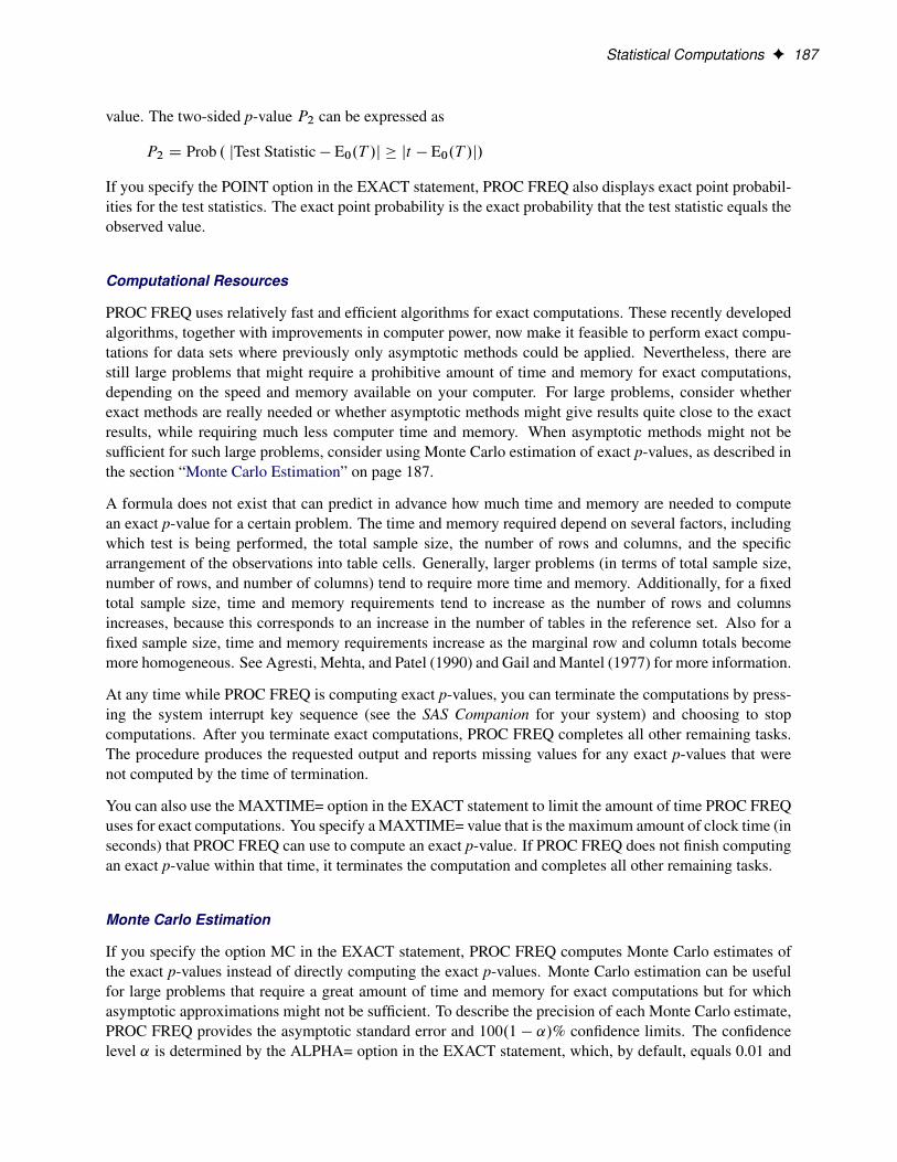
Statistical Computations F 187
value. The two-sided p-value P2 can be expressed as
P2 D Prob . jTest Statistic � E0.T /j � jt � E0.T /j/
If you specify the POINT option in the EXACT statement, PROC FREQ also displays exact point probabil-ities for the test statistics. The exact point probability is the exact probability that the test statistic equals theobserved value.
Computational Resources
PROC FREQ uses relatively fast and efficient algorithms for exact computations. These recently developedalgorithms, together with improvements in computer power, now make it feasible to perform exact compu-tations for data sets where previously only asymptotic methods could be applied. Nevertheless, there arestill large problems that might require a prohibitive amount of time and memory for exact computations,depending on the speed and memory available on your computer. For large problems, consider whetherexact methods are really needed or whether asymptotic methods might give results quite close to the exactresults, while requiring much less computer time and memory. When asymptotic methods might not besufficient for such large problems, consider using Monte Carlo estimation of exact p-values, as described inthe section “Monte Carlo Estimation” on page 187.
A formula does not exist that can predict in advance how much time and memory are needed to computean exact p-value for a certain problem. The time and memory required depend on several factors, includingwhich test is being performed, the total sample size, the number of rows and columns, and the specificarrangement of the observations into table cells. Generally, larger problems (in terms of total sample size,number of rows, and number of columns) tend to require more time and memory. Additionally, for a fixedtotal sample size, time and memory requirements tend to increase as the number of rows and columnsincreases, because this corresponds to an increase in the number of tables in the reference set. Also for afixed sample size, time and memory requirements increase as the marginal row and column totals becomemore homogeneous. See Agresti, Mehta, and Patel (1990) and Gail and Mantel (1977) for more information.
At any time while PROC FREQ is computing exact p-values, you can terminate the computations by press-ing the system interrupt key sequence (see the SAS Companion for your system) and choosing to stopcomputations. After you terminate exact computations, PROC FREQ completes all other remaining tasks.The procedure produces the requested output and reports missing values for any exact p-values that werenot computed by the time of termination.
You can also use the MAXTIME= option in the EXACT statement to limit the amount of time PROC FREQuses for exact computations. You specify a MAXTIME= value that is the maximum amount of clock time (inseconds) that PROC FREQ can use to compute an exact p-value. If PROC FREQ does not finish computingan exact p-value within that time, it terminates the computation and completes all other remaining tasks.
Monte Carlo Estimation
If you specify the option MC in the EXACT statement, PROC FREQ computes Monte Carlo estimates ofthe exact p-values instead of directly computing the exact p-values. Monte Carlo estimation can be usefulfor large problems that require a great amount of time and memory for exact computations but for whichasymptotic approximations might not be sufficient. To describe the precision of each Monte Carlo estimate,PROC FREQ provides the asymptotic standard error and 100.1 � ˛/% confidence limits. The confidencelevel ˛ is determined by the ALPHA= option in the EXACT statement, which, by default, equals 0.01 and

188 F Chapter 3: The FREQ Procedure
produces 99% confidence limits. The N=n option in the EXACT statement specifies the number of samplesthat PROC FREQ uses for Monte Carlo estimation; the default is 10000 samples. You can specify a largervalue for n to improve the precision of the Monte Carlo estimates. Because larger values of n generate moresamples, the computation time increases. Alternatively, you can specify a smaller value of n to reduce thecomputation time.
To compute a Monte Carlo estimate of an exact p-value, PROC FREQ generates a random sample of ta-bles with the same total sample size, row totals, and column totals as the observed table. PROC FREQuses the algorithm of Agresti, Wackerly, and Boyett (1979), which generates tables in proportion to theirhypergeometric probabilities conditional on the marginal frequencies. For each sample table, PROC FREQcomputes the value of the test statistic and compares it to the value for the observed table. When estimatinga right-sided p-value, PROC FREQ counts all sample tables for which the test statistic is greater than orequal to the observed test statistic. Then the p-value estimate equals the number of these tables divided bythe total number of tables sampled.
OPMC D M = N
M D number of samples with .Test Statistic � t /
N D total number of samples
t D observed Test Statistic
PROC FREQ computes left-sided and two-sided p-value estimates in a similar manner. For left-sided p-values, PROC FREQ evaluates whether the test statistic for each sampled table is less than or equal to theobserved test statistic. For two-sided p-values, PROC FREQ examines the sample test statistics accordingto the expression for P2 given in the section “Definition of p-Values” on page 186.
The variable M is a binomially distributed variable with N trials and success probability p. It follows thatthe asymptotic standard error of the Monte Carlo estimate is
se. OPMC/ D
qOPMC .1 � OPMC/ = .N � 1/
PROC FREQ constructs asymptotic confidence limits for the p-values according to
OPMC ˙
�z˛=2 � se. OPMC/
�where z˛=2 is the 100.1 � ˛=2/th percentile of the standard normal distribution and the confidence level ˛is determined by the ALPHA= option in the EXACT statement.
When the Monte Carlo estimate OPMC equals 0, PROC FREQ computes the confidence limits for the p-valueas
. 0; 1 � ˛.1=N/ /
When the Monte Carlo estimate OPMC equals 1, PROC FREQ computes the confidence limits as
. ˛.1=N/; 1 /

Computational Resources F 189
Computational Resources
For each variable in a table request, PROC FREQ stores all of the levels in memory. If all variables arenumeric and not formatted, this requires about 84 bytes for each variable level. When there are charactervariables or formatted numeric variables, the memory that is required depends on the formatted variablelengths, with longer formatted lengths requiring more memory. The number of levels for each variable islimited only by the largest integer that your operating environment can store.
For any single crosstabulation table requested, PROC FREQ builds the entire table in memory, regardlessof whether the table has zero cell counts. Thus, if the numeric variables A, B, and C each have 10 levels,PROC FREQ requires 2520 bytes to store the variable levels for the table request A*B*C, as follows:
3 variables * 10 levels/variable * 84 bytes/level
In addition, PROC FREQ requires 8000 bytes to store the table cell frequencies
1000 cells * 8 bytes/cell
even though there might be only 10 observations.
When the variables have many levels or when there are many multiway tables, your computer might nothave enough memory to construct the tables. If PROC FREQ runs out of memory while constructing tables,it stops collecting levels for the variable with the most levels and returns the memory that is used by thatvariable. The procedure then builds the tables that do not contain the disabled variables.
If there is not enough memory for your table request and if increasing the available memory is impractical,you can reduce the number of multiway tables or variable levels. If you are not using the CMH or AGREEoption in the TABLES statement to compute statistics across strata, reduce the number of multiway tablesby using PROC SORT to sort the data set by one or more of the variables or by using the DATA step tocreate an index for the variables. Then remove the sorted or indexed variables from the TABLES statementand include a BY statement that uses these variables. You can also reduce memory requirements by usinga FORMAT statement in the PROC FREQ step to reduce the number of levels. Additionally, reducing theformatted variable lengths reduces the amount of memory that is needed to store the variable levels. Formore information about using formats, see the section “Grouping with Formats” on page 127.
Output Data Sets
PROC FREQ produces two types of output data sets that you can use with other statistical and reportingprocedures. You can request these data sets as follows:
� Specify the OUT= option in a TABLES statement. This creates an output data set that containsfrequency or crosstabulation table counts and percentages
� Specify an OUTPUT statement. This creates an output data set that contains statistics.

190 F Chapter 3: The FREQ Procedure
PROC FREQ does not display the output data sets. Use PROC PRINT, PROC REPORT, or any other SASreporting tool to display an output data set.
In addition to these two output data sets, you can create a SAS data set from any piece of PROC FREQoutput by using the Output Delivery System. See the section “ODS Table Names” on page 200 for moreinformation.
Contents of the TABLES Statement Output Data Set
The OUT= option in the TABLES statement creates an output data set that contains one observation for eachcombination of variable values (or table cell) in the last table request. By default, each observation containsthe frequency and percentage for the table cell. When the input data set contains missing values, the outputdata set also contains an observation with the frequency of missing values. The output data set includes thefollowing variables:
� BY variables
� table request variables, such as A, B, C, and D in the table request A*B*C*D
� COUNT, which contains the table cell frequency
� PERCENT, which contains the table cell percentage
If you specify the OUTEXPECT option in the TABLES statement for a two-way or multiway table, theoutput data set also includes expected frequencies. If you specify the OUTPCT option for a two-wayor multiway table, the output data set also includes row, column, and table percentages. The additionalvariables are as follows:
� EXPECTED, which contains the expected frequency
� PCT_TABL, which contains the percentage of two-way table frequency, for n-way tables where n > 2
� PCT_ROW, which contains the percentage of row frequency
� PCT_COL, which contains the percentage of column frequency
If you specify the OUTCUM option in the TABLES statement for a one-way table, the output data set alsoincludes cumulative frequencies and cumulative percentages. The additional variables are as follows:
� CUM_FREQ, which contains the cumulative frequency
� CUM_PCT, which contains the cumulative percentage
The OUTCUM option has no effect for two-way or multiway tables.
The following PROC FREQ statements create an output data set of frequencies and percentages:
proc freq;tables A A*B / out=D;
run;

Output Data Sets F 191
The output data set D contains frequencies and percentages for the table of A by B, which is the last tablerequest listed in the TABLES statement. If A has two levels (1 and 2), B has three levels (1,2, and 3), andno table cell count is zero or missing, then the output data set D includes six observations, one for eachcombination of A and B levels. The first observation corresponds to A=1 and B=1; the second observationcorresponds to A=1 and B=2; and so on. The data set includes the variables COUNT and PERCENT. Thevalue of COUNT is the number of observations with the given combination of A and B levels. The value ofPERCENT is the percentage of the total number of observations with that A and B combination.
When PROC FREQ combines different variable values into the same formatted level, the output data setcontains the smallest internal value for the formatted level. For example, suppose a variable X has thevalues 1.1., 1.4, 1.7, 2.1, and 2.3. When you submit the statement
format X 1.;
in a PROC FREQ step, the formatted levels listed in the frequency table for X are 1 and 2. If you create anoutput data set with the frequency counts, the internal values of the levels of X are 1.1 and 1.7. To report theinternal values of X when you display the output data set, use a format of 3.1 for X.
Contents of the OUTPUT Statement Output Data Set
The OUTPUT statement creates a SAS data set that contains the statistics that PROC FREQ computes forthe last table request. You specify which statistics to store in the output data set. There is an observationwith the specified statistics for each stratum or two-way table. If PROC FREQ computes summary statisticsfor a stratified table, the output data set also contains a summary observation with those statistics.
The OUTPUT data set can include the following variables.
� BY variables
� variables that identify the stratum, such as A and B in the table request A*B*C*D
� variables that contain the specified statistics
The output data set also includes variables with the p-values and degrees of freedom, asymptotic standarderror (ASE), or confidence limits when PROC FREQ computes these values for a specified statistic.
The variable names for the specified statistics in the output data set are the names of the options enclosedin underscores. PROC FREQ forms variable names for the corresponding p-values, degrees of freedom, orconfidence limits by combining the name of the option with the appropriate prefix from the following list:
DF_ degrees of freedomE_ asymptotic standard error (ASE)L_ lower confidence limitU_ upper confidence limitE0_ ASE under the null hypothesisZ_ standardized value
P_ p-valueP2_ two-sided p-valuePL_ left-sided p-valuePR_ right-sided p-value

192 F Chapter 3: The FREQ Procedure
XP_ exact p-valueXP2_ exact two-sided p-valueXPL_ exact left-sided p-valueXPR_ exact right-sided p-valueXPT_ exact point probabilityXL_ exact lower confidence limitXU_ exact upper confidence limit
For example, variable names created for the Pearson chi-square, its degrees of freedom, and its p-values are_PCHI_, DF_PCHI, and P_PCHI, respectively.
If the length of the prefix plus the statistic option exceeds eight characters, PROC FREQ truncates the optionso that the name of the new variable is eight characters long.
Displayed Output
Number of Variable Levels Table
If you specify the NLEVELS option in the PROC FREQ statement, PROC FREQ displays the “Numberof Variable Levels” table. This table provides the number of levels for all variables named in the TABLESstatements. PROC FREQ determines the variable levels from the formatted variable values. See “Groupingwith Formats” on page 127 for details. The “Number of Variable Levels” table contains the followinginformation:
� Variable name
� Levels, which is the total number of levels of the variable
� Number of Nonmissing Levels, if there are missing levels for any of the variables
� Number of Missing Levels, if there are missing levels for any of the variables
One-Way Frequency Tables
PROC FREQ displays one-way frequency tables for all one-way table requests in the TABLES statements,unless you specify the NOPRINT option in the PROC statement or the NOPRINT option in the TABLESstatement. For a one-way table showing the frequency distribution of a single variable, PROC FREQ dis-plays the name of the variable and its values. For each variable value or level, PROC FREQ displays thefollowing information:
� Frequency count, which is the number of observations in the level
� Test Frequency count, if you specify the CHISQ and TESTF= options to request a chi-squaregoodness-of-fit test for specified frequencies
� Percent, which is the percentage of the total number of observations. (The NOPERCENT optionsuppresses this information.)

Displayed Output F 193
� Test Percent, if you specify the CHISQ and TESTP= options to request a chi-square goodness-of-fittest for specified percents. (The NOPERCENT option suppresses this information.)
� Cumulative Frequency count, which is the sum of the frequency counts for that level and all otherlevels listed above it in the table. The last cumulative frequency is the total number of nonmissingobservations. (The NOCUM option suppresses this information.)
� Cumulative Percent, which is the percentage of the total number of observations in that level and inall other levels listed above it in the table. (The NOCUM or the NOPERCENT option suppresses thisinformation.)
The one-way table also displays the Frequency Missing, which is the number of observations with missingvalues.
Statistics for One-Way Frequency Tables
For one-way tables, two statistical options are available in the TABLES statement. The CHISQ option pro-vides a chi-square goodness-of-fit test, and the BINOMIAL option provides binomial proportion statisticsand tests. PROC FREQ displays the following information, unless you specify the NOPRINT option in thePROC FREQ statement:
� If you specify the CHISQ option for a one-way table, PROC FREQ provides a chi-square goodness-of-fit test, displaying the Chi-Square statistic, the degrees of freedom (DF), and the probability value(Pr > ChiSq). If you specify the CHISQ option in the EXACT statement, PROC FREQ also displaysthe exact probability value for this test. If you specify the POINT option with the CHISQ option inthe EXACT statement, PROC FREQ displays the exact point probability for the test statistic.
� If you specify the BINOMIAL option for a one-way table, PROC FREQ displays the estimate of thebinomial Proportion, which is the proportion of observations in the first class listed in the one-waytable. PROC FREQ also displays the asymptotic standard error (ASE) and the asymptotic (Wald) andexact (Clopper-Pearson) confidence limits by default. For the binomial proportion test, PROC FREQdisplays the asymptotic standard error under the null hypothesis (ASE Under H0), the standardizedtest statistic (Z), and the one-sided and two-sided probability values.
If you specify the BINOMIAL option in the EXACT statement, PROC FREQ also displays the exactone-sided and two-sided probability values for this test. If you specify the POINT option with theBINOMIAL option in the EXACT statement, PROC FREQ displays the exact point probability forthe test.
� If you request additional binomial confidence limits by specifying binomial-options, PROC FREQprovides a table that displays the lower and upper confidence limits for each type that you request. Inaddition to the Wald and exact (Clopper-Pearson) confidence limits, you can request Agresti-Coull,Jeffreys, and Wilson (score) confidence limits for the binomial proportion.
� If you request a binomial noninferiority or superiority test by specifying the NONINF or SUPbinomial-option, PROC FREQ displays the following information: the binomial Proportion, the testASE (under H0 or Sample), the test statistic Z, the probability value, the noninferiority or superioritylimit, and the test confidence limits. If you specify the BINOMIAL option in the EXACT statement,PROC FREQ also provides the exact probability value for the test, and exact test confidence limits.

194 F Chapter 3: The FREQ Procedure
� If you request a binomial equivalence test by specifying the EQUIV binomial-option, PROC FREQdisplays the binomial Proportion and the test ASE (under H0 or Sample). PROC FREQ displays twoone-sided tests (TOST) for equivalence, which include test statistics (Z) and probability values for theLower and Upper tests, together with the Overall probability value. PROC FREQ also displays theequivalence limits and the test-based confidence limits. If you specify the BINOMIAL option in theEXACT statement, PROC FREQ provides exact probability values for the TOST and exact test-basedconfidence limits.
Multiway Tables
PROC FREQ displays all multiway table requests in the TABLES statements, unless you specify the NO-PRINT option in the PROC FREQ statement or the NOPRINT option in the TABLES statement.
For two-way to multiway crosstabulation tables, the values of the last variable in the table request form thetable columns. The values of the next-to-last variable form the rows. Each level (or combination of levels)of the other variables forms one stratum.
There are three ways to display multiway tables in PROC FREQ. By default, PROC FREQ displays mul-tiway tables as separate two-way crosstabulation tables for each stratum of the multiway table. Also bydefault, PROC FREQ displays these two-way crosstabulation tables in table cell format. Alternatively, ifyou specify the CROSSLIST option, PROC FREQ displays the two-way crosstabulation tables in ODS col-umn format. If you specify the LIST option, PROC FREQ displays multiway tables in list format, whichpresents the entire multiway crosstabulation in a single table.
Crosstabulation Tables
By default, PROC FREQ displays two-way crosstabulation tables in table cell format. The row variablevalues are listed down the side of the table, the column variable values are listed across the top of the table,and each row and column variable level combination forms a table cell.
Each cell of a crosstabulation table can contain the following information:
� Frequency, which is the number of observations in the table cell. (The NOFREQ option suppressesthis information.)
� Expected frequency under the hypothesis of independence, if you specify the EXPECTED option
� Deviation of the cell frequency from the expected value, if you specify the DEVIATION option
� Cell Chi-Square, which is the cell’s contribution to the total chi-square statistic, if you specify theCELLCHI2 option
� Tot Pct, which is the cell’s percentage of the total multiway table frequency, for n-way tables whenn > 2, if you specify the TOTPCT option
� Percent, which is the cell’s percentage of the total (two-way table) frequency. (The NOPERCENToption suppresses this information.)
� Row Pct, or the row percentage, which is the cell’s percentage of the total frequency for its row. (TheNOROW option suppresses this information.)

Displayed Output F 195
� Col Pct, or column percentage, which is the cell’s percentage of the total frequency for its column.(The NOCOL option suppresses this information.)
� Cumulative Col%, or cumulative column percentage, if you specify the CUMCOL option
The table also displays the Frequency Missing, which is the number of observations with missing values.
CROSSLIST Tables
If you specify the CROSSLIST option, PROC FREQ displays two-way crosstabulation tables in ODS col-umn format. The CROSSLIST column format is different from the default crosstabulation table cell format,but the CROSSLIST table provides the same information (frequencies, percentages, and other statistics) asthe default crosstabulation table.
In the CROSSLIST table format, the rows of the display correspond to the crosstabulation table cells, andthe columns of the display correspond to descriptive statistics such as frequencies and percentages. Eachtable cell is identified by the values of its TABLES row and column variable levels, with all column variablelevels listed within each row variable level. The CROSSLIST table also provides row totals, column totals,and overall table totals.
For a crosstabulation table in CROSSLIST format, PROC FREQ displays the following information:
� the row variable name and values
� the column variable name and values
� Frequency, which is the number of observations in the table cell. (The NOFREQ option suppressesthis information.)
� Expected cell frequency under the hypothesis of independence, if you specify the EXPECTED option
� Deviation of the cell frequency from the expected value, if you specify the DEVIATION option
� Cell Chi-Square, which is the cell’s contribution to the total chi-square statistic, if you specify theCELLCHI2 option
� Total Percent, which is the cell’s percentage of the total multiway table frequency, for n-way tableswhen n > 2, if you specify the TOTPCT option
� Percent, which is the cell’s percentage of the total (two-way table) frequency. (The NOPERCENToption suppresses this information.)
� Row Percent, which is the cell’s percentage of the total frequency for its row. (The NOROW optionsuppresses this information.)
� Column Percent, the cell’s percentage of the total frequency for its column. (The NOCOL optionsuppresses this information.)
The table also displays the Frequency Missing, which is the number of observations with missing values.

196 F Chapter 3: The FREQ Procedure
LIST Tables
If you specify the LIST option in the TABLES statement, PROC FREQ displays multiway tables in a listformat rather than as crosstabulation tables. The LIST option displays the entire multiway table in onetable, instead of displaying a separate two-way table for each stratum. The LIST option is not availablewhen you also request statistical options. Unlike the default crosstabulation output, the LIST output doesnot display row percentages, column percentages, and optional information such as expected frequenciesand cell chi-squares.
For a multiway table in list format, PROC FREQ displays the following information:
� the variable names and values
� Frequency, which is the number of observations in the level (with the indicated variable values)
� Percent, which is the level’s percentage of the total number of observations. (The NOPERCENToption suppresses this information.)
� Cumulative Frequency, which is the accumulated frequency of the level and all other levels listedabove it in the table. The last cumulative frequency in the table is the total number of nonmissingobservations. (The NOCUM option suppresses this information.)
� Cumulative Percent, which is the accumulated percentage of the level and all other levels listed aboveit in the table. (The NOCUM or the NOPERCENT option suppresses this information.)
The table also displays the Frequency Missing, which is the number of observations with missing values.
Statistics for Multiway Tables
PROC FREQ computes statistical tests and measures for crosstabulation tables, depending on which state-ments and options you specify. You can suppress the display of these results by specifying the NOPRINToption in the PROC FREQ statement. With any of the following information, PROC FREQ also displaysthe Sample Size and the Frequency Missing.
� If you specify the SCOROUT option in the TABLES statement, PROC FREQ displays the Row Scoresand Column Scores that it uses for statistical computations. The Row Scores table displays the rowvariable values and the Score corresponding to each value. The Column Scores table displays thecolumn variable values and the corresponding Scores. PROC FREQ also identifies the score typeused to compute the row and column scores. You can specify the score type with the SCORES=option in the TABLES statement.
� If you specify the CHISQ option, PROC FREQ displays the following statistics for each two-waytable: Pearson Chi-Square, Likelihood-Ratio Chi-Square, Continuity-Adjusted Chi-Square (for 2 � 2tables), Mantel-Haenszel Chi-Square, the Phi Coefficient, the Contingency Coefficient, and Cramer’sV . For each test statistic, PROC FREQ also displays the degrees of freedom (DF) and the probabilityvalue (Prob).
� If you specify the CHISQ option for 2 � 2 tables, PROC FREQ also displays Fisher’s exact test. Thetest output includes the cell (1,1) frequency (F), the exact left-sided and right-sided probability values,the table probability (P), and the exact two-sided probability value.

Displayed Output F 197
� If you specify the FISHER option in the TABLES statement (or, equivalently, the FISHER option inthe EXACT statement), PROC FREQ displays Fisher’s exact test for tables larger than 2� 2. The testoutput includes the table probability (P) and the probability value. In addition, PROC FREQ displaysthe CHISQ output listed earlier, even if you do not also specify the CHISQ option.
� If you specify the PCHI, LRCHI, or MHCHI option in the EXACT statement, PROC FREQ displaysthe corresponding exact test: Pearson Chi-Square, Likelihood-Ratio Chi-Square, or Mantel-HaenszelChi-Square, respectively. The test output includes the test statistic, the degrees of freedom (DF), andthe asymptotic and exact probability values. If you also specify the POINT option in the EXACTstatement, PROC FREQ displays the point probability for each exact test requested. If you specifythe CHISQ option in the EXACT statement, PROC FREQ displays exact probability values for allthree of these chi-square tests.
� If you specify the MEASURES option, PROC FREQ displays the following statistics and theirasymptotic standard errors (ASE) for each two-way table: Gamma, Kendall’s Tau-b, Stuart’s Tau-c,Somers’ D.C jR/, Somers’ D.RjC/, Pearson Correlation, Spearman Correlation, Lambda Asym-metric .C jR/, Lambda Asymmetric .RjC/, Lambda Symmetric, Uncertainty Coefficient .C jR/, Un-certainty Coefficient .RjC/, and Uncertainty Coefficient Symmetric. If you specify the CL option,PROC FREQ also displays confidence limits for these measures.
� If you specify the PLCORR option, PROC FREQ displays the tetrachoric correlation for 2 � 2 tablesor the polychoric correlation for larger tables. In addition, PROC FREQ displays the MEASURESoutput listed earlier, even if you do not also specify the MEASURES option.
� If you specify the GAMMA, KENTB, STUTC, SMDCR, SMDRC, PCORR, or SCORR option inthe TEST statement, PROC FREQ displays asymptotic tests for Gamma, Kendall’s Tau-b, Stuart’sTau-c, Somers’ D.C jR/, Somers’ D.RjC/, the Pearson Correlation, or the Spearman Correlation,respectively. If you specify the MEASURES option in the TEST statement, PROC FREQ displaysall these asymptotic tests. The test output includes the statistic, its asymptotic standard error (ASE),Confidence Limits, the ASE under the null hypothesis H0, the standardized test statistic (Z), and theone-sided and two-sided probability values.
� If you specify the KENTB, STUTC, SMDCR, SMDRC, PCORR, or SCORR option in the EXACTstatement, PROC FREQ displays asymptotic and exact tests for the corresponding measure of associ-ation: Kendall’s Tau-b, Stuart’s Tau-c, Somers’ D.C jR/, Somers’ D.RjC/, the Pearson Correlation,or the Spearman correlation, respectively. The test output includes the correlation, its asymptoticstandard error (ASE), Confidence Limits, the ASE under the null hypothesis H0, the standardized teststatistic (Z), and the asymptotic and exact one-sided and two-sided probability values. If you alsospecify the POINT option in the EXACT statement, PROC FREQ displays the point probability foreach exact test requested.
� If you specify the RISKDIFF option for 2�2 tables, PROC FREQ displays the Column 1 and Column2 Risk Estimates. For each column, PROC FREQ displays the Row 1 Risk, Row 2 Risk, Total Risk,and Risk Difference, together with their asymptotic standard errors (ASE) and Asymptotic ConfidenceLimits. PROC FREQ also displays Exact Confidence Limits for the Row 1 Risk, Row 2 Risk, andTotal Risk. If you specify the RISKDIFF option in the EXACT statement, PROC FREQ providesunconditional Exact Confidence Limits for the Risk Difference.
� If you specify the RISKDIFF(CL=) option for 2 � 2 tables, PROC FREQ displays the ProportionDifference Confidence Limits. For each confidence limit Type that you request (Exact, Farrington-

198 F Chapter 3: The FREQ Procedure
Manning, Hauck-Anderson, Newcombe Score, or Wald), PROC FREQ displays the Lower and UpperConfidence Limits.
� If you request a noninferiority or superiority test for the proportion difference (RISKDIFF) by spec-ifying the NONINF or SUP riskdiff-option, and if you specify METHOD=HA (Hauck-Anderson),METHOD=FM (Farrington-Manning), or METHOD=WALD (Wald), PROC FREQ displays the fol-lowing information: the Proportion Difference, the test ASE (H0, Sample, Sample H-A, or FM,depending on the method you specify), the test statistic Z, the probability value, the Noninferiorityor Superiority Limit, and the test-based Confidence Limits. If you specify METHOD=NEWCOMBE(Newcombe score), PROC FREQ displays the Proportion Difference, the Noninferiority or Superior-ity Limit, and the Newcombe Confidence Limits.
� If you request an equivalence test for the proportion difference (RISKDIFF) by specifying the EQUIVriskdiff-option, and if you specify METHOD=HA (Hauck-Anderson), METHOD=FM (Farrington-Manning), or METHOD=WALD (Wald), PROC FREQ displays the following information: the Pro-portion Difference and the test ASE (H0, Sample, Sample H-A, or FM, depending on the method youspecify). PROC FREQ displays a two one-sided test (TOST) for equivalence, which includes teststatistics (Z) and probability values for the Lower and Upper tests, together with the Overall proba-bility value. PROC FREQ also displays the Equivalence Limits and the test-based Confidence Limits.If you specify METHOD=NEWCOMBE (Newcombe score), PROC FREQ displays the ProportionDifference, the Equivalence Limits, and the score Confidence Limits.
� If you request an equality test for the proportion difference (RISKDIFF) by specifying the EQUALriskdiff-option, PROC FREQ displays the following information: the Proportion Difference and thetest ASE (H0 or Sample), the test statistic Z, the One-Sided probability value (Pr > Z or Pr < Z), andthe Two-Sided probability value, Pr > |Z|.
� If you specify the MEASURES option or the RELRISK option for 2�2 tables, PROC FREQ displaysEstimates of the Relative Risk for Case-Control and Cohort studies, together with their ConfidenceLimits. These measures are also known as the Odds Ratio and the Column 1 and 2 Relative Risks.If you specify the OR option in the EXACT statement, PROC FREQ also displays Exact ConfidenceLimits for the Odds Ratio. If you specify the RELRISK option in the EXACT statement, PROCFREQ displays unconditional Exact Confidence Limits for the Relative Risk.
� If you specify the TREND option, PROC FREQ displays the Cochran-Armitage Trend Test for tablesthat are 2 � C or R � 2. For this test, PROC FREQ gives the Statistic (Z) and the one-sided andtwo-sided probability values. If you specify the TREND option in the EXACT statement, PROCFREQ also displays the exact one-sided and two-sided probability values for this test. If you specifythe POINT option with the TREND option in the EXACT statement, PROC FREQ displays the exactpoint probability for the test statistic.
� If you specify the JT option, PROC FREQ displays the Jonckheere-Terpstra Test, showing the Statistic(JT), the standardized test statistic (Z), and the one-sided and two-sided probability values. If youspecify the JT option in the EXACT statement, PROC FREQ also displays the exact one-sided andtwo-sided probability values for this test. If you specify the POINT option with the JT option in theEXACT statement, PROC FREQ displays the exact point probability for the test statistic.
� If you specify the AGREE option and the PRINTKWT option, PROC FREQ displays the KappaCoefficient Weights for square tables larger than 2 � 2.

Displayed Output F 199
� If you specify the AGREE option, for two-way tables PROC FREQ displays McNemar’s Test and theSimple Kappa Coefficient for 2� 2 tables. For square tables larger than 2� 2, PROC FREQ displaysBowker’s Test of Symmetry, the Simple Kappa Coefficient, and the Weighted Kappa Coefficient. ForMcNemar’s Test and Bowker’s Test of Symmetry, PROC FREQ displays the Statistic (S), the degreesof freedom (DF), and the probability value (Pr > S). If you specify the MCNEM option in the EXACTstatement, PROC FREQ also displays the exact probability value for McNemar’s test. If you specifythe POINT option with the MCNEM option in the EXACT statement, PROC FREQ displays the exactpoint probability for the test statistic. For the simple and weighted kappa coefficients, PROC FREQdisplays the kappa values, asymptotic standard errors (ASE), and Confidence Limits.
� If you specify the KAPPA or WTKAP option in the TEST statement, PROC FREQ displays asymp-totic tests for the simple kappa coefficient or the weighted kappa coefficient, respectively. If youspecify the AGREE option in the TEST statement, PROC FREQ displays both these asymptotic tests.The test output includes the kappa coefficient, its asymptotic standard error (ASE), Confidence Lim-its, the ASE under the null hypothesis H0, the standardized test statistic (Z), and the one-sided andtwo-sided probability values.
� If you specify the KAPPA or WTKAP option in the EXACT statement, PROC FREQ displays asymp-totic and exact tests for the simple kappa coefficient or the weighted kappa coefficient, respectively.The test output includes the kappa coefficient, its asymptotic standard error (ASE), Confidence Lim-its, the ASE under the null hypothesis H0, the standardized test statistic (Z), and the asymptotic andexact one-sided and two-sided probability values. If you specify the POINT option in the EXACTstatement, PROC FREQ displays the point probability for each exact test requested.
� If you specify the MC option in the EXACT statement, PROC FREQ displays Monte Carlo estimatesfor all exact p-values requested by statistic-options in the EXACT statement. The Monte Carlo outputincludes the p-value Estimate, its Confidence Limits, the Number of Samples used to compute theMonte Carlo estimate, and the Initial Seed for random number generation.
� If you specify the AGREE option, for multiple strata PROC FREQ displays Overall Simple andWeighted Kappa Coefficients, with their asymptotic standard errors (ASE) and Confidence Limits.PROC FREQ also displays Tests for Equal Kappa Coefficients, giving the Chi-Squares, degrees offreedom (DF), and probability values (Pr > ChiSq) for the Simple Kappa and Weighted Kappa. Formultiple strata of 2�2 tables, PROC FREQ displays Cochran’sQ, giving the Statistic (Q), the degreesof freedom (DF), and the probability value (Pr > Q).
� If you specify the CMH option, PROC FREQ displays Cochran-Mantel-Haenszel Statistics for thefollowing three alternative hypotheses: Nonzero Correlation, Row Mean Scores Differ (ANOVAStatistic), and General Association. For each of these statistics, PROC FREQ gives the degrees offreedom (DF) and the probability value (Prob). If you specify the MANTELFLEISS option, PROCFREQ displays the Mantel-Fleiss Criterion for 2 � 2 tables. For 2 � 2 tables, PROC FREQ alsodisplays Estimates of the Common Relative Risk for Case-Control and Cohort studies, together withtheir confidence limits. These include both Mantel-Haenszel and Logit stratum-adjusted estimatesof the common Odds Ratio, Column 1 Relative Risk, and Column 2 Relative Risk. Also for 2 � 2tables, PROC FREQ displays the Breslow-Day Test for Homogeneity of the Odds Ratios. For thistest, PROC FREQ gives the Chi-Square, the degrees of freedom (DF), and the probability value (Pr >ChiSq).
� If you specify the CMH option in the TABLES statement and also specify the COMOR op-tion in the EXACT statement, PROC FREQ displays exact confidence limits for the Common

200 F Chapter 3: The FREQ Procedure
Odds Ratio for multiple strata of 2 � 2 tables. PROC FREQ also displays the Exact Test ofH0: Common Odds Ratio = 1. The test output includes the Cell (1,1) Sum (S), Mean of S Under H0,One-sided Pr <= S, and Point Pr = S. PROC FREQ also provides exact two-sided probability valuesfor the test, computed according to the following three methods: 2 * One-sided, Sum of probabilities<= Point probability, and Pr >= |S - Mean|.
� If you specify the CMH option in the TABLES statement and also specify the EQOR option in theEXACT statement, PROC FREQ computes Zelen’s exact test for equal odds ratios for h � 2 � 2tables. PROC FREQ displays Zelen’s test along with the asymptotic Breslow-Day test produced bythe CMH option. PROC FREQ displays the test statistic, Zelen’s Exact Test (P), and the probabilityvalue, Exact Pr <= P.
� If you specify the GAILSIMON option in the TABLES statement for a multiway 2 � 2 tables, PROCFREQ displays the Gail-Simon test for qualitative interactions. The display include the followingstatistics and their p-values: Q+ (Positive Risk Differences), Q- (Negative Risk Differences), and Q(Two-Sided).
ODS Table Names
PROC FREQ assigns a name to each table that it creates. You can use these names to refer to tables whenyou use the Output Delivery System (ODS) to select tables and create output data sets. For more informationabout ODS, see Chapter 20, “Using the Output Delivery System” (SAS/STAT User’s Guide).
Table 3.14 lists the ODS table names together with their descriptions and the options required to produce thetables. Note that the ALL option in the TABLES statement invokes the CHISQ, MEASURES, and CMHoptions.
Table 3.14 ODS Tables Produced by PROC FREQ
ODS Table Name Description Statement Option
BinomialCLs Binomial confidence limits TABLES BINOMIAL(AC | J | W)BinomialEquiv Binomial equivalence analysis TABLES BINOMIAL(EQUIV)BinomialEquivLimits Binomial equivalence limits TABLES BINOMIAL(EQUIV)BinomialEquivTest Binomial equivalence test TABLES BINOMIAL(EQUIV)BinomialNoninf Binomial noninferiority test TABLES BINOMIAL(NONINF)BinomialProp Binomial proportion TABLES BINOMIALBinomialPropTest Binomial proportion test TABLES BINOMIALBinomialSup Binomial superiority test TABLES BINOMIAL(SUP)BreslowDayTest Breslow-Day test TABLES CMH
(h � 2 � 2 table)CMH Cochran-Mantel-Haenszel TABLES CMH
statisticsChiSq Chi-square tests TABLES CHISQCochransQ Cochran’s Q TABLES AGREE
(h � 2 � 2 table)ColScores Column scores TABLES SCOROUTCommonOdds- Exact confidence limits EXACT COMORRatioCl for the common odds ratio (h � 2 � 2 table)

ODS Table Names F 201
Table 3.14 continued
ODS Table Name Description Statement Option
CommonOdds- Common odds ratio exact test EXACT COMORRatioTest (h � 2 � 2 table)CommonRelRisks Common relative risks TABLES CMH
(h � 2 � 2 table)CrossList Crosstabulation table TABLES CROSSLIST
in column format (n-way table, n > 1)CrossTabFreqs Crosstabulation table TABLES (n-way table, n > 1)EqualKappaTest Test for equal simple kappas TABLES AGREE
(h � 2 � 2 table)EqualKappaTests Tests for equal kappas TABLES AGREE
(h � r � r , r > 2)EqualOddsRatios Tests for equal odds ratios EXACT EQOR
(h � 2 � 2 table)GailSimon Gail-Simon test TABLES GAILSIMON
(h � 2 � 2 table)FishersExact Fisher’s exact test EXACT FISHER
or TA-BLES
FISHER or EXACT
or TA-BLES
CHISQ (2 � 2 table)
FishersExactMC Monte Carlo estimates EXACT FISHER / MCfor Fisher’s exact test
Gamma Gamma TEST GAMMAGammaTest Gamma test TEST GAMMAJTTest Jonckheere-Terpstra test TABLES JTJTTestMC Monte Carlo estimates for EXACT JT / MC
Jonckheere-Terpstra exact testKappaStatistics Kappa statistics TABLES AGREE,
no TEST or EXACT(r � r table, r > 2)
KappaWeights Kappa weights TABLES AGREEand PRINTKWT
List List format multiway table TABLES LISTLRChiSq Likelihood-ratio chi-square EXACT LRCHI
exact testLRChiSqMC Monte Carlo exact test for EXACT LRCHI / MC
likelihood-ratio chi-squareMantelFleiss Mantel-Fleiss criterion TABLES CMH(MF)
(h � 2 � 2 table)McNemarsTest McNemar’s test TABLES AGREE
(2 � 2 table)Measures Measures of association TABLES MEASURES

202 F Chapter 3: The FREQ Procedure
Table 3.14 continued
ODS Table Name Description Statement Option
MHChiSq Mantel-Haenszel chi-square EXACT MHCHIexact test
MHChiSqMC Monte Carlo exact test for EXACT MHCHI / MCMantel-Haenszel chi-square
NLevels Number of variable levels PROC NLEVELSOddsRatioCL Exact confidence limits EXACT OR (2 � 2 table)
for the odds ratioOneWayChiSq One-way chi-square test TABLES CHISQ
(one-way table)OneWayChiSqMC Monte Carlo exact test for EXACT CHISQ / MC
one-way chi-square (one-way table)OneWayFreqs One-way frequencies PROC (no TABLES stmt)
or TA-BLES
(one-way table)
OverallKappa Overall simple kappa TABLES AGREE(h � 2 � 2 table)
OverallKappas Overall kappa coefficients TABLES AGREE(h � r � r , r > 2)
PdiffCLs Proportion difference TABLES RISKDIFF(CL=)confidence limits (2 � 2 table)
PdiffEquiv Equivalence analysis TABLES RISKDIFF(EQUIV)for the proportion difference (2 � 2 table)
PdiffEquivLimits Equivalence limits TABLES RISKDIFF(EQUIV)for the proportion difference (2 � 2 table)
PdiffEquivTest Equivalence test TABLES RISKDIFF(EQUIV)for the proportion difference (2 � 2 table)
PdiffNoninf Noninferiority test TABLES RISKDIFF(NONINF)for the proportion difference (2 � 2 table)
PdiffSup Superiority test TABLES RISKDIFF(SUP)for the proportion difference (2 � 2 table)
PdiffTest Proportion difference test TABLES RISKDIFF(EQUAL)(2 � 2 table)
PearsonChiSq Pearson chi-square exact test EXACT PCHIPearsonChiSqMC Monte Carlo exact test for EXACT PCHI / MC
Pearson chi-squarePearsonCorr Pearson correlation TEST PCORR
or EXACT PCORRPearsonCorrMC Monte Carlo exact test for EXACT PCORR / MC
Pearson correlationPearsonCorrTest Pearson correlation test TEST PCORR
or EXACT PCORRRelativeRisks Relative risk estimates TABLES RELRISK
or MEASURES(2 � 2 table)

ODS Table Names F 203
Table 3.14 continued
ODS Table Name Description Statement Option
RelRisk1CL Exact confidence limits EXACT RELRISKfor column 1 relative risk (2 � 2 table)
RelRisk2CL Exact confidence limits EXACT RELRISKfor column 2 relative risk (2 � 2 table)
RiskDiffCol1 Column 1 risk estimates TABLES RISKDIFF(2 � 2 table)
RiskDiffCol2 Column 2 risk estimates TABLES RISKDIFF(2 � 2 table)
RowScores Row scores TABLES SCOROUTSimpleKappa Simple kappa coefficient TEST KAPPA
or EXACT KAPPASimpleKappaMC Monte Carlo exact test for EXACT KAPPA / MC
simple kappaSimpleKappaTest Simple kappa test TEST KAPPA
or EXACT KAPPASomersDCR Somers’ D.C jR/ TEST SMDCRSomersDCRTest Somers’ D.C jR/ test TEST SMDCRSomersDRC Somers’ D.RjC/ TEST SMDRCSomersDRCTest Somers’ D.RjC/ test TEST SMDRCSpearmanCorr Spearman correlation TEST SCORR
or EXACT SCORRSpearmanCorrMC Monte Carlo exact test for EXACT SCORR / MC
Spearman correlationSpearmanCorrTest Spearman correlation test TEST SCORR
or EXACT SCORRSymmetryTest Test of symmetry TABLES AGREETauB Kendall’s tau-b TEST KENTBTauBTest Kendall’s tau-b test TEST KENTBTauC Stuart’s tau-c TEST STUTCTauCTest Stuart’s tau-c test TEST STUTCTrendTest Cochran-Armitage trend test TABLES TRENDTrendTestMC Monte Carlo exact test EXACT TREND / MC
for trendWeightedKappa Weighted kappa TEST WTKAP
or EXACT WTKAPWeightedKappaMC Monte Carlo exact test for EXACT WTKAP / MC
weighted kappaWeightedKappaTest Weighted kappa test TEST WTKAP
or EXACT WTKAP

204 F Chapter 3: The FREQ Procedure
ODS Graphics
Statistical procedures use ODS Graphics to create graphs as part of their output. ODS Graphics is describedin detail in Chapter 21, “Statistical Graphics Using ODS” (SAS/STAT User’s Guide).
Before you create graphs, ODS Graphics must be enabled (for example, with the ODS GRAPHICS ONstatement). For more information about enabling and disabling ODS Graphics, see the section “Enablingand Disabling ODS Graphics” in that chapter.
The overall appearance of graphs is controlled by ODS styles. Styles and other aspects of using ODSGraphics are discussed in the section “A Primer on ODS Statistical Graphics” in that chapter.
When ODS Graphics is enabled, you can request specific plots with the PLOTS= option in the TABLESstatement. To produce a frequency plot or cumulative frequency plot, you must specify the FREQPLOT orCUMFREQPLOT plot-request, respectively, in the PLOTS= option. By default, PROC FREQ produces allother plots that are associated with the analyses that you request in the TABLES statement. You can suppressthe default plots and request specific plots by using the PLOTS(ONLY)= option. See the description of thePLOTS= option for details.
PROC FREQ assigns a name to each graph that it creates with ODS Graphics. You can use these names torefer to the graphs. Table 3.15 lists the names of the graphs that PROC FREQ generates together with theirdescriptions, their PLOTS= options (plot-requests), and the TABLES statement options that are required toproduce the graphs.
Table 3.15 Graphs Produced by PROC FREQ
ODS Graph Name Description PLOTS= Option TABLES Statement Option
AgreePlot Agreement plot AGREEPLOT AGREE (r � r table)CumFreqPlot Cumulative frequency plot CUMFREQPLOT One-way table requestDeviationPlot Deviation plot DEVIATIONPLOT CHISQ (one-way table)FreqPlot Frequency plot FREQPLOT Any table requestKappaPlot Kappa plot KAPPAPLOT AGREE (h � r � r table)ORPlot Odds ratio plot ODDSRATIOPLOT MEASURES or RELRISK
(h � 2 � 2 table)RelRiskPlot Relative risk plot RELRISKPLOT MEASURES or RELRISK
(h � 2 � 2 table)RiskDiffPlot Risk difference plot RISKDIFFPLOT RISKDIFF (h � 2 � 2 table)WtKappaPlot Weighted kappa plot WTKAPPAPLOT AGREE
(h � r � r table, r > 2)

Examples: FREQ Procedure F 205
Examples: FREQ Procedure
Example 3.1: Output Data Set of Frequencies
The eye and hair color of children from two different regions of Europe are recorded in the data set Color.Instead of recording one observation per child, the data are recorded as cell counts, where the variable Countcontains the number of children exhibiting each of the 15 eye and hair color combinations. The data set doesnot include missing combinations.
The following DATA step statements create the SAS data set Color:
data Color;input Region Eyes $ Hair $ Count @@;label Eyes ='Eye Color'
Hair ='Hair Color'Region='Geographic Region';
datalines;1 blue fair 23 1 blue red 7 1 blue medium 241 blue dark 11 1 green fair 19 1 green red 71 green medium 18 1 green dark 14 1 brown fair 341 brown red 5 1 brown medium 41 1 brown dark 401 brown black 3 2 blue fair 46 2 blue red 212 blue medium 44 2 blue dark 40 2 blue black 62 green fair 50 2 green red 31 2 green medium 372 green dark 23 2 brown fair 56 2 brown red 422 brown medium 53 2 brown dark 54 2 brown black 13;
The following PROC FREQ statements read the Color data set and create an output data set that contains thefrequencies, percentages, and expected cell frequencies of the two-way table of Eyes by Hair. The TABLESstatement requests three tables: a frequency table for Eyes, a frequency table for Hair, and a crosstabulationtable for Eyes by Hair. The OUT= option creates the FreqCount data set, which contains the crosstabulationtable frequencies. The OUTEXPECT option outputs the expected table cell frequencies to FreqCount, andthe SPARSE option includes zero cell frequencies in the output data set. The WEIGHT statement specifiesthat the variable Count contains the observation weights. These statements create Output 3.1.1 throughOutput 3.1.3.
proc freq data=Color;tables Eyes Hair Eyes*Hair / out=FreqCount outexpect sparse;weight Count;title 'Eye and Hair Color of European Children';
run;
proc print data=FreqCount noobs;title2 'Output Data Set from PROC FREQ';
run;

206 F Chapter 3: The FREQ Procedure
Output 3.1.1 displays the two frequency tables produced by PROC FREQ: one showing the distribution ofeye color, and one showing the distribution of hair color. By default, PROC FREQ lists the variables valuesin alphabetical order. The ‘Eyes*Hair’ specification produces a crosstabulation table, shown in Output 3.1.2,with eye color defining the table rows and hair color defining the table columns. A zero cell frequency forgreen eyes and black hair indicates that this eye and hair color combination does not occur in the data.
The output data set FreqCount (Output 3.1.3) contains frequency counts and percentages for the last tablerequested in the TABLES statement, Eyes by Hair. Because the SPARSE option is specified, the data setincludes the observation with a zero frequency. The variable Expected contains the expected frequencies,as requested by the OUTEXPECT option.
Output 3.1.1 Frequency Tables
Eye and Hair Color of European Children
The FREQ Procedure
Eye Color
Cumulative CumulativeEyes Frequency Percent Frequency Percent----------------------------------------------------------blue 222 29.13 222 29.13brown 341 44.75 563 73.88green 199 26.12 762 100.00
Hair Color
Cumulative CumulativeHair Frequency Percent Frequency Percent-----------------------------------------------------------black 22 2.89 22 2.89dark 182 23.88 204 26.77fair 228 29.92 432 56.69medium 217 28.48 649 85.17red 113 14.83 762 100.00

Example 3.1: Output Data Set of Frequencies F 207
Output 3.1.2 Crosstabulation Table
Table of Eyes by Hair
Eyes(Eye Color) Hair(Hair Color)
Frequency|Percent |Row Pct |Col Pct |black |dark |fair |medium |red | Total---------+--------+--------+--------+--------+--------+blue | 6 | 51 | 69 | 68 | 28 | 222
| 0.79 | 6.69 | 9.06 | 8.92 | 3.67 | 29.13| 2.70 | 22.97 | 31.08 | 30.63 | 12.61 || 27.27 | 28.02 | 30.26 | 31.34 | 24.78 |
---------+--------+--------+--------+--------+--------+brown | 16 | 94 | 90 | 94 | 47 | 341
| 2.10 | 12.34 | 11.81 | 12.34 | 6.17 | 44.75| 4.69 | 27.57 | 26.39 | 27.57 | 13.78 || 72.73 | 51.65 | 39.47 | 43.32 | 41.59 |
---------+--------+--------+--------+--------+--------+green | 0 | 37 | 69 | 55 | 38 | 199
| 0.00 | 4.86 | 9.06 | 7.22 | 4.99 | 26.12| 0.00 | 18.59 | 34.67 | 27.64 | 19.10 || 0.00 | 20.33 | 30.26 | 25.35 | 33.63 |
---------+--------+--------+--------+--------+--------+Total 22 182 228 217 113 762
2.89 23.88 29.92 28.48 14.83 100.00
Output 3.1.3 Output Data Set of Frequencies
Eye and Hair Color of European ChildrenOutput Data Set from PROC FREQ
Eyes Hair COUNT EXPECTED PERCENT
blue black 6 6.409 0.7874blue dark 51 53.024 6.6929blue fair 69 66.425 9.0551blue medium 68 63.220 8.9239blue red 28 32.921 3.6745brown black 16 9.845 2.0997brown dark 94 81.446 12.3360brown fair 90 102.031 11.8110brown medium 94 97.109 12.3360brown red 47 50.568 6.1680green black 0 5.745 0.0000green dark 37 47.530 4.8556green fair 69 59.543 9.0551green medium 55 56.671 7.2178green red 38 29.510 4.9869
208 F Chapter 3: The FREQ Procedure
Example 3.2: Frequency Dot Plots
This example produces frequency dot plots for the children’s eye and hair color data from Example 3.1.
PROC FREQ produces plots by using ODS Graphics to create graphs as part of the procedure output.Frequency plots are available for any frequency or crosstabulation table request. You can display frequencyplots as bar charts or dot plots. You can use plot-options to specify the orientation (vertical or horizontal),scale, and layout of the plots.
The following PROC FREQ statements request frequency tables and dot plots. The first TABLES statementrequests a one-way frequency table of Hair and a crosstabulation table of Eyes by Hair. The PLOTS= optionrequests frequency plots for the tables, and the TYPE=DOTPLOT plot-option specifies dot plots. By default,frequency plots are produced as bar charts. ODS Graphics must be enabled before producing plots.
The second TABLES statement requests a crosstabulation table of Region by Hair and a frequency dotplot for this table. The SCALE=PERCENT plot-option plots percentages instead of frequency counts.SCALE=LOG and SCALE=SQRT plot-options are also available to plot log frequencies and square rootsof frequencies, respectively.
The ORDER=FREQ option in the PROC FREQ statement orders the variable levels by frequency. Thisorder applies to the frequency and crosstabulation table displays and also to the corresponding frequencyplots.
ods graphics on;proc freq data=Color order=freq;
tables Hair Eyes*Hair / plots=freqplot(type=dotplot);tables Region*Hair / plots=freqplot(type=dotplot scale=percent);weight Count;title 'Eye and Hair Color of European Children';
run;ods graphics off;
Output 3.2.1, Output 3.2.2, and Output 3.2.3 display the dot plots produced by PROC FREQ. By default,the orientation of dot plots is horizontal, which places the variable levels on the Y axis. You can spec-ify the ORIENT=VERTICAL plot-option to request a vertical orientation. For two-way plots, you canuse the TWOWAY= plot-option to specify the plot layout. The default layout (shown in Output 3.2.2 andOutput 3.2.3) is GROUPVERTICAL. Two-way layouts STACKED and GROUPHORIZONTAL are alsoavailable.

Example 3.2: Frequency Dot Plots F 209
Output 3.2.1 One-Way Frequency Dot Plot
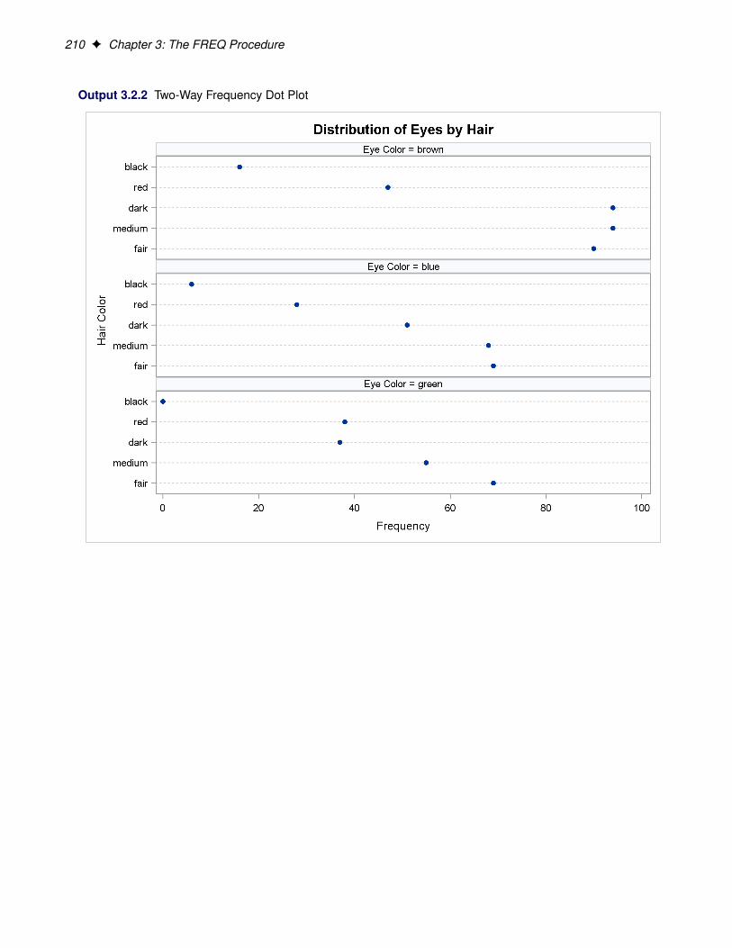
210 F Chapter 3: The FREQ Procedure
Output 3.2.2 Two-Way Frequency Dot Plot

Example 3.3: Chi-Square Goodness-of-Fit Tests F 211
Output 3.2.3 Two-Way Percent Dot Plot
Example 3.3: Chi-Square Goodness-of-Fit Tests
This example examines whether the children’s hair color (from Example 3.1) has a specified multinomialdistribution for the two geographical regions. The hypothesized distribution of hair color is 30% fair, 12%red, 30% medium, 25% dark, and 3% black.
In order to test the hypothesis for each region, the data are first sorted by Region. Then the FREQ procedureuses a BY statement to produce a separate table for each BY group (Region). The option ORDER=DATAorders the variable values (hair color) in the frequency table by their order in the input data set. The TABLESstatement requests a frequency table for hair color, and the option NOCUM suppresses the display of thecumulative frequencies and percentages.
The CHISQ option requests a chi-square goodness-of-fit test for the frequency table of Hair. The TESTP=option specifies the hypothesized (or test) percentages for the chi-square test; the number of percentageslisted equals the number of table levels, and the percentages sum to 100%. The TESTP= percentages arelisted in the same order as the corresponding variable levels appear in frequency table.

212 F Chapter 3: The FREQ Procedure
The PLOTS= option requests a deviation plot, which is associated with the CHISQ option and displays therelative deviations from the test frequencies. The TYPE=DOTPLOT plot-option requests a dot plot insteadof the default type, which is a bar chart. ODS Graphics must be enabled before producing plots. Thesestatements produce Output 3.3.1 through Output 3.3.4.
proc sort data=Color;by Region;
run;
ods graphics on;proc freq data=Color order=data;
tables Hair / nocum chisq testp=(30 12 30 25 3)plots(only)=deviationplot(type=dotplot);
weight Count;by Region;title 'Hair Color of European Children';
run;ods graphics off;
Output 3.3.1 Frequency Table and Chi-Square Test for Region 1
Hair Color of European Children
----------------------------- Geographic Region=1 ------------------------------
The FREQ Procedure
Hair Color
TestHair Frequency Percent Percent-------------------------------------------fair 76 30.89 30.00red 19 7.72 12.00medium 83 33.74 30.00dark 65 26.42 25.00black 3 1.22 3.00
----------------------------- Geographic Region=1 ------------------------------
Chi-Square Testfor Specified Proportions-------------------------Chi-Square 7.7602DF 4Pr > ChiSq 0.1008
Output 3.3.1 shows the frequency table and chi-square test for Region 1. The frequency table lists thevariable values (hair color) in the order in which they appear in the data set. The “Test Percent” columnlists the hypothesized percentages for the chi-square test. Always check that you have ordered the TESTP=percentages to correctly match the order of the variable levels.

Example 3.3: Chi-Square Goodness-of-Fit Tests F 213
Output 3.3.2 shows the deviation plot for Region 1, which displays the relative deviations from the hypoth-esized values. The relative deviation for a level is the difference between the observed and hypothesized(test) percentage divided by the test percentage. You can suppress the chi-square p-value that is displayedby default in the deviation plot by specifying the NOSTATS plot-option.
Output 3.3.2 Deviation Plot for Region 1

214 F Chapter 3: The FREQ Procedure
Output 3.3.3 and Output 3.3.4 show the results for Region 2. PROC FREQ computes a chi-square statisticfor each region. The chi-square statistic is significant at the 0.05 level for Region 2 (p=0.0003) but not forRegion 1. This indicates a significant departure from the hypothesized percentages in Region 2.
Output 3.3.3 Frequency Table and Chi-Square Test for Region 2
Hair Color of European Children
----------------------------- Geographic Region=2 ------------------------------
The FREQ Procedure
Hair Color
TestHair Frequency Percent Percent-------------------------------------------fair 152 29.46 30.00red 94 18.22 12.00medium 134 25.97 30.00dark 117 22.67 25.00black 19 3.68 3.00
----------------------------- Geographic Region=2 ------------------------------
Chi-Square Testfor Specified Proportions-------------------------Chi-Square 21.3824DF 4Pr > ChiSq 0.0003

Example 3.4: Binomial Proportions F 215
Output 3.3.4 Deviation Plot for Region 2
Example 3.4: Binomial Proportions
In this example, PROC FREQ computes binomial proportions, confidence limits, and tests. The exampleuses the eye and hair color data from Example 3.1. By default, PROC FREQ computes the binomial propor-tion as the proportion of observations in the first level of the one-way table. You can designate a differentlevel by using the LEVEL= binomial-option.
The following PROC FREQ statements compute the proportion of children with brown eyes (from the dataset in Example 3.1) and test the null hypothesis that the population proportion equals 50%. These statementsalso compute an equivalence for the proportion of children with fair hair.
The first TABLES statement requests a one-way frequency table for the variable Eyes. The BINOMIALoption requests the binomial proportion, confidence limits, and test. PROC FREQ computes the propor-tion with Eyes = ‘brown’, which is the first level displayed in the table. The AC, WILSON, and EXACTbinomial-options request the following confidence limits types: Agresti-Coull, Wilson (score), and exact(Clopper-Pearson). By default, PROC FREQ provides Wald and exact (Clopper-Pearson) confidence limitsfor the binomial proportion. The BINOMIAL option also produces an asymptotic Wald test that the propor-tion equals 0.5. You can specify a different test proportion with the P= binomial-option. The ALPHA=0.1option specifies that ˛ D 10%, which produces 90% confidence limits.

216 F Chapter 3: The FREQ Procedure
The second TABLES statement requests a one-way frequency table for the variable Hair. The BINOMIALoption requests the proportion for the first level, Hair = ‘fair’. The EQUIV binomial-option requests an equiv-alence test for the binomial proportion. The P=.28 option specifies 0.28 as the null hypothesis proportion,and the MARGIN=.1 option specifies 0.1 as the equivalence test margin.
proc freq data=Color order=freq;tables Eyes / binomial(ac wilson exact) alpha=.1;tables Hair / binomial(equiv p=.28 margin=.1);weight Count;title 'Hair and Eye Color of European Children';
run;
Output 3.4.1 displays the results for eye color, and Output 3.4.2 displays the results for hair color.
Output 3.4.1 Binomial Proportion for Eye Color
Hair and Eye Color of European Children
The FREQ Procedure
Eye Color
Cumulative CumulativeEyes Frequency Percent Frequency Percent----------------------------------------------------------brown 341 44.75 341 44.75blue 222 29.13 563 73.88green 199 26.12 762 100.00
Binomial Proportionfor Eyes = brown
----------------------Proportion 0.4475ASE 0.0180
Type 90% Confidence Limits
Wilson 0.4181 0.4773Agresti-Coull 0.4181 0.4773Clopper-Pearson (Exact) 0.4174 0.4779
Test of H0: Proportion = 0.5
ASE under H0 0.0181Z -2.8981One-sided Pr < Z 0.0019Two-sided Pr > |Z| 0.0038
The frequency table in Output 3.4.1 displays the values of Eyes in order of descending frequency count.PROC FREQ computes the proportion of children in the first level displayed in the frequency table, Eyes =‘brown’. Output 3.4.1 displays the binomial proportion confidence limits and test. The confidence limits are90% confidence limits. If you do not specify the ALPHA= option, PROC FREQ computes 95% confidencelimits by default. Because the value of Z is less than zero, PROC FREQ displays the a left-sided p-value

Example 3.4: Binomial Proportions F 217
(0.0019). This small p-value supports the alternative hypothesis that the true value of the proportion ofchildren with brown eyes is less than 50%.
Output 3.4.2 displays the equivalence test results produced by the second TABLES statement. The nullhypothesis proportion is 0.28 and the equivalence margins are –0.1 and 0.1, which yield equivalence limitsof 0.18 and 0.38. PROC FREQ provides two one-sided tests (TOST) for equivalence. The small p-valueindicates rejection of the null hypothesis in favor of the alternative that the proportion is equivalent to thenull value.
Output 3.4.2 Binomial Proportion for Hair Color
Hair Color
Cumulative CumulativeHair Frequency Percent Frequency Percent-----------------------------------------------------------fair 228 29.92 228 29.92medium 217 28.48 445 58.40dark 182 23.88 627 82.28red 113 14.83 740 97.11black 22 2.89 762 100.00
Equivalence Analysis
H0: P - p0 <= Lower Margin or >= Upper MarginHa: Lower Margin < P - p0 < Upper Margin
p0 = 0.28 Lower Margin = -0.1 Upper Margin = 0.1
Proportion ASE (Sample)
0.2992 0.0166
Two One-Sided Tests (TOST)
Test Z P-Value
Lower Margin 7.1865 Pr > Z <.0001Upper Margin -4.8701 Pr < Z <.0001Overall <.0001
Equivalence Limits 90% Confidence Limits
0.1800 0.3800 0.2719 0.3265

218 F Chapter 3: The FREQ Procedure
Example 3.5: Analysis of a 2x2 Contingency Table
This example computes chi-square tests and Fisher’s exact test to compare the probability of coronary heartdisease for two types of diet. It also estimates the relative risks and computes exact confidence limits for theodds ratio.
The data set FatComp contains hypothetical data for a case-control study of high fat diet and the risk ofcoronary heart disease. The data are recorded as cell counts, where the variable Count contains the fre-quencies for each exposure and response combination. The data set is sorted in descending order by thevariables Exposure and Response, so that the first cell of the 2 � 2 table contains the frequency of positiveexposure and positive response. The FORMAT procedure creates formats to identify the type of exposureand response with character values.
proc format;value ExpFmt 1='High Cholesterol Diet'
0='Low Cholesterol Diet';value RspFmt 1='Yes'
0='No';run;
data FatComp;input Exposure Response Count;label Response='Heart Disease';datalines;
0 0 60 1 21 0 41 1 11;
proc sort data=FatComp;by descending Exposure descending Response;
run;
In the following PROC FREQ statements, ORDER=DATA option orders the contingency table values bytheir order in the input data set. The TABLES statement requests a two-way table of Exposure by Response.The CHISQ option produces several chi-square tests, while the RELRISK option produces relative riskmeasures. The EXACT statement requests the exact Pearson chi-square test and exact confidence limits forthe odds ratio.
proc freq data=FatComp order=data;format Exposure ExpFmt. Response RspFmt.;tables Exposure*Response / chisq relrisk;exact pchi or;weight Count;title 'Case-Control Study of High Fat/Cholesterol Diet';
run;

Example 3.5: Analysis of a 2x2 Contingency Table F 219
The contingency table in Output 3.5.1 displays the variable values so that the first table cell contains thefrequency for the first cell in the data set (the frequency of positive exposure and positive response).
Output 3.5.1 Contingency Table
Case-Control Study of High Fat/Cholesterol Diet
The FREQ Procedure
Table of Exposure by Response
Exposure Response(Heart Disease)
Frequency |Percent |Row Pct |Col Pct |Yes |No | Total-----------------+--------+--------+High Cholesterol | 11 | 4 | 15Diet | 47.83 | 17.39 | 65.22
| 73.33 | 26.67 || 84.62 | 40.00 |
-----------------+--------+--------+Low Cholesterol | 2 | 6 | 8Diet | 8.70 | 26.09 | 34.78
| 25.00 | 75.00 || 15.38 | 60.00 |
-----------------+--------+--------+Total 13 10 23
56.52 43.48 100.00
Output 3.5.2 displays the chi-square statistics. Because the expected counts in some of the table cells aresmall, PROC FREQ gives a warning that the asymptotic chi-square tests might not be appropriate. In thiscase, the exact tests are appropriate. The alternative hypothesis for this analysis states that coronary heartdisease is more likely to be associated with a high fat diet, so a one-sided test is desired. Fisher’s exact right-sided test analyzes whether the probability of heart disease in the high fat group exceeds the probability ofheart disease in the low fat group; because this p-value is small, the alternative hypothesis is supported.
The odds ratio, displayed in Output 3.5.3, provides an estimate of the relative risk when an event is rare.This estimate indicates that the odds of heart disease is 8.25 times higher in the high fat diet group; however,the wide confidence limits indicate that this estimate has low precision.

220 F Chapter 3: The FREQ Procedure
Output 3.5.2 Chi-Square Statistics
Statistic DF Value Prob------------------------------------------------------Chi-Square 1 4.9597 0.0259Likelihood Ratio Chi-Square 1 5.0975 0.0240Continuity Adj. Chi-Square 1 3.1879 0.0742Mantel-Haenszel Chi-Square 1 4.7441 0.0294Phi Coefficient 0.4644Contingency Coefficient 0.4212Cramer's V 0.4644
WARNING: 50% of the cells have expected counts less than 5.(Asymptotic) Chi-Square may not be a valid test.
Pearson Chi-Square Test----------------------------------Chi-Square 4.9597DF 1Asymptotic Pr > ChiSq 0.0259Exact Pr >= ChiSq 0.0393
Fisher's Exact Test----------------------------------Cell (1,1) Frequency (F) 11Left-sided Pr <= F 0.9967Right-sided Pr >= F 0.0367
Table Probability (P) 0.0334Two-sided Pr <= P 0.0393
Output 3.5.3 Relative Risk
Estimates of the Relative Risk (Row1/Row2)
Type of Study Value 95% Confidence Limits-----------------------------------------------------------------Case-Control (Odds Ratio) 8.2500 1.1535 59.0029Cohort (Col1 Risk) 2.9333 0.8502 10.1204Cohort (Col2 Risk) 0.3556 0.1403 0.9009
Odds Ratio (Case-Control Study)-----------------------------------Odds Ratio 8.2500
Asymptotic Conf Limits95% Lower Conf Limit 1.153595% Upper Conf Limit 59.0029
Exact Conf Limits95% Lower Conf Limit 0.867795% Upper Conf Limit 105.5488

Example 3.6: Output Data Set of Chi-Square Statistics F 221
Example 3.6: Output Data Set of Chi-Square Statistics
This example uses the Color data from Example 3.1 to output the Pearson chi-square and the likelihood-ratiochi-square statistics to a SAS data set. The following PROC FREQ statements create a two-way table of eyecolor versus hair color.
proc freq data=Color order=data;tables Eyes*Hair / expected cellchi2 norow nocol chisq;output out=ChiSqData n nmiss pchi lrchi;weight Count;title 'Chi-Square Tests for 3 by 5 Table of Eye and Hair Color';
run;
proc print data=ChiSqData noobs;title1 'Chi-Square Statistics for Eye and Hair Color';title2 'Output Data Set from the FREQ Procedure';
run;
The EXPECTED option displays expected cell frequencies in the crosstabulation table, and the CELLCHI2option displays the cell contribution to the overall chi-square. The NOROW and NOCOL options suppressthe display of row and column percents in the crosstabulation table. The CHISQ option produces chi-squaretests.
The OUTPUT statement creates the ChiSqData output data set and specifies the statistics to include. TheN option requests the number of nonmissing observations, the NMISS option stores the number of missingobservations, and the PCHI and LRCHI options request Pearson and likelihood-ratio chi-square statistics,respectively, together with their degrees of freedom and p-values.
The preceding statements produce Output 3.6.1 and Output 3.6.2. The contingency table in Output 3.6.1displays eye and hair color in the order in which they appear in the Color data set. The Pearson chi-squarestatistic in Output 3.6.2 provides evidence of an association between eye and hair color (p=0.0073). Thecell chi-square values show that most of the association is due to more green-eyed children with fair or redhair and fewer with dark or black hair. The opposite occurs with the brown-eyed children.
Output 3.6.3 displays the output data set created by the OUTPUT statement. It includes one observationthat contains the sample size, the number of missing values, and the chi-square statistics and correspondingdegrees of freedom and p-values as in Output 3.6.2.

222 F Chapter 3: The FREQ Procedure
Output 3.6.1 Contingency Table
Chi-Square Tests for 3 by 5 Table of Eye and Hair Color
The FREQ Procedure
Table of Eyes by Hair
Eyes(Eye Color) Hair(Hair Color)
Frequency |Expected |Cell Chi-Square|Percent |fair |red |medium |dark |black | Total---------------+--------+--------+--------+--------+--------+blue | 69 | 28 | 68 | 51 | 6 | 222
| 66.425 | 32.921 | 63.22 | 53.024 | 6.4094 || 0.0998 | 0.7357 | 0.3613 | 0.0772 | 0.0262 || 9.06 | 3.67 | 8.92 | 6.69 | 0.79 | 29.13
---------------+--------+--------+--------+--------+--------+green | 69 | 38 | 55 | 37 | 0 | 199
| 59.543 | 29.51 | 56.671 | 47.53 | 5.7454 || 1.5019 | 2.4422 | 0.0492 | 2.3329 | 5.7454 || 9.06 | 4.99 | 7.22 | 4.86 | 0.00 | 26.12
---------------+--------+--------+--------+--------+--------+brown | 90 | 47 | 94 | 94 | 16 | 341
| 102.03 | 50.568 | 97.109 | 81.446 | 9.8451 || 1.4187 | 0.2518 | 0.0995 | 1.935 | 3.8478 || 11.81 | 6.17 | 12.34 | 12.34 | 2.10 | 44.75
---------------+--------+--------+--------+--------+--------+Total 228 113 217 182 22 762
29.92 14.83 28.48 23.88 2.89 100.00
Output 3.6.2 Chi-Square Statistics
Statistic DF Value Prob------------------------------------------------------Chi-Square 8 20.9248 0.0073Likelihood Ratio Chi-Square 8 25.9733 0.0011Mantel-Haenszel Chi-Square 1 3.7838 0.0518Phi Coefficient 0.1657Contingency Coefficient 0.1635Cramer's V 0.1172
Output 3.6.3 Output Data Set
Chi-Square Statistics for Eye and Hair ColorOutput Data Set from the FREQ Procedure
N NMISS _PCHI_ DF_PCHI P_PCHI _LRCHI_ DF_LRCHI P_LRCHI
762 0 20.9248 8 .007349898 25.9733 8 .001061424

Example 3.7: Cochran-Mantel-Haenszel Statistics F 223
Example 3.7: Cochran-Mantel-Haenszel Statistics
The data set Migraine contains hypothetical data for a clinical trial of migraine treatment. Subjects of bothgenders receive either a new drug therapy or a placebo. Their response to treatment is coded as ‘Better’ or‘Same’. The data are recorded as cell counts, and the number of subjects for each treatment and responsecombination is recorded in the variable Count.
data Migraine;input Gender $ Treatment $ Response $ Count @@;datalines;
female Active Better 16 female Active Same 11female Placebo Better 5 female Placebo Same 20male Active Better 12 male Active Same 16male Placebo Better 7 male Placebo Same 19;
The following PROC FREQ statements create a multiway table stratified by Gender, where Treatment formsthe rows and Response forms the columns. The RELRISK option in the TABLES statement requests theodds ratio and relative risks for the two-way tables of Treatment by Response. The PLOTS= option requestsa relative risk plot, which shows the relative risk and its confidence limits for each level of Gender. TheCMH option requests Cochran-Mantel-Haenszel statistics for the multiway table. For this stratified 2 � 2table, the CMH option also produces estimates of the common relative risk and the Breslow-Day test forhomogeneity of the odds ratios. The NOPRINT option suppresses the display of the crosstabulation tables.
ods graphics on;proc freq data=Migraine;
tables Gender*Treatment*Response /relrisk plots(only)=relriskplot(stats) cmh noprint;
weight Count;title 'Clinical Trial for Treatment of Migraine Headaches';
run;ods graphics off;
Output 3.7.1 through Output 3.7.4 show the results of the analysis. The relative risk plot (Output 3.7.1)displays the relative risks and confidence limits for the two levels of Gender. Output 3.7.2 displays theCMH statistics. For a stratified 2�2 table, the three CMH statistics test the same hypothesis. The significantp-value (0.004) indicates that the association between treatment and response remains strong after adjustingfor gender.
The CMH option also produces a table of overall relative risks, as shown in Output 3.7.3. Because this isa prospective study, the relative risk estimate assesses the effectiveness of the new drug; the “Cohort (Col1Risk)” values are the appropriate estimates for the first column (the risk of improvement). The probabilityof migraine improvement with the new drug is just over two times the probability of improvement with theplacebo.
The large p-value for the Breslow-Day test (0.2218) in Output 3.7.4 indicates no significant gender differ-ence in the odds ratios.

224 F Chapter 3: The FREQ Procedure
Output 3.7.1 Relative Risk Plot
Output 3.7.2 Cochran-Mantel-Haenszel Statistics
Cochran-Mantel-Haenszel Statistics (Based on Table Scores)
Statistic Alternative Hypothesis DF Value Prob---------------------------------------------------------------
1 Nonzero Correlation 1 8.3052 0.00402 Row Mean Scores Differ 1 8.3052 0.00403 General Association 1 8.3052 0.0040

Example 3.8: Cochran-Armitage Trend Test F 225
Output 3.7.3 CMH Option: Common Relative Risks
Estimates of the Common Relative Risk (Row1/Row2)
Type of Study Method Value 95% Confidence Limits-------------------------------------------------------------------------Case-Control Mantel-Haenszel 3.3132 1.4456 7.5934(Odds Ratio) Logit 3.2941 1.4182 7.6515
Cohort Mantel-Haenszel 2.1636 1.2336 3.7948(Col1 Risk) Logit 2.1059 1.1951 3.7108
Cohort Mantel-Haenszel 0.6420 0.4705 0.8761(Col2 Risk) Logit 0.6613 0.4852 0.9013
Output 3.7.4 CMH Option: Breslow-Day Test
Breslow-Day Test forHomogeneity of the Odds Ratios------------------------------Chi-Square 1.4929DF 1Pr > ChiSq 0.2218
Example 3.8: Cochran-Armitage Trend Test
The data set Pain contains hypothetical data for a clinical trial of a drug therapy to control pain. Theclinical trial investigates whether adverse responses increase with larger drug doses. Subjects receive eithera placebo or one of four drug doses. An adverse response is recorded as Adverse=‘Yes’; otherwise, itis recorded as Adverse=‘No’. The number of subjects for each drug dose and response combination iscontained in the variable Count.
data pain;input Dose Adverse $ Count @@;datalines;
0 No 26 0 Yes 61 No 26 1 Yes 72 No 23 2 Yes 93 No 18 3 Yes 144 No 9 4 Yes 23;
The following PROC FREQ statements provide a trend analysis. The TABLES statement requests a table ofAdverse by Dose. The MEASURES option produces measures of association, and the CL option producesconfidence limits for these measures. The TREND option tests for a trend across the ordinal values of thevariable Dose with the Cochran-Armitage test. The EXACT statement produces exact p-values for this test,and the MAXTIME= option terminates the exact computations if they do not complete within 60 seconds.The TEST statement computes an asymptotic test for Somers’ D.RjC/.

226 F Chapter 3: The FREQ Procedure
The PLOTS= option requests a frequency plot for the table of Adverse by Dose. By default, PROC FREQprovides a bar chart for the frequency plot. The TWOWAY=STACKED option requests a stacked layout,where the bars correspond to the column variable (Dose) values, and the row variable (Adverse) frequenciesare stacked within each bar.
ods graphics on;proc freq data=Pain;
tables Adverse*Dose / trend measures clplots=freqplot(twoway=stacked orient=horizontal scale=percent);
test smdrc;exact trend / maxtime=60;weight Count;title 'Clinical Trial for Treatment of Pain';
run;ods graphics off;
Output 3.8.1 through Output 3.8.4 display the results of the analysis. The “Col Pct” values in Output 3.8.1show the expected increasing trend in the proportion of adverse effects with the increasing dosage (from18.75% to 71.88%). The corresponding bar chart (Output 3.8.2) also shows this increasing trend.
Output 3.8.1 Contingency Table
Clinical Trial for Treatment of Pain
The FREQ Procedure
Table of Adverse by Dose
Adverse Dose
Frequency|Percent |Row Pct |Col Pct | 0| 1| 2| 3| 4| Total---------+--------+--------+--------+--------+--------+No | 26 | 26 | 23 | 18 | 9 | 102
| 16.15 | 16.15 | 14.29 | 11.18 | 5.59 | 63.35| 25.49 | 25.49 | 22.55 | 17.65 | 8.82 || 81.25 | 78.79 | 71.88 | 56.25 | 28.13 |
---------+--------+--------+--------+--------+--------+Yes | 6 | 7 | 9 | 14 | 23 | 59
| 3.73 | 4.35 | 5.59 | 8.70 | 14.29 | 36.65| 10.17 | 11.86 | 15.25 | 23.73 | 38.98 || 18.75 | 21.21 | 28.13 | 43.75 | 71.88 |
---------+--------+--------+--------+--------+--------+Total 32 33 32 32 32 161
19.88 20.50 19.88 19.88 19.88 100.00

Example 3.8: Cochran-Armitage Trend Test F 227
Output 3.8.2 Stacked Bar Chart of Percents
Output 3.8.3 displays the measures of association produced by the MEASURES option. Somers’ D.RjC/measures the association treating the row variable (Adverse) as the response and the column variable (Dose)as a predictor. Because the asymptotic 95% confidence limits do not contain zero, this indicates a strongpositive association. Similarly, the Pearson and Spearman correlation coefficients show evidence of a strongpositive association, as hypothesized.
The Cochran-Armitage test (Output 3.8.4) supports the trend hypothesis. The small left-sided p-valuesfor the Cochran-Armitage test indicate that the probability of the Row 1 level (Adverse=‘No’) decreasesas Dose increases or, equivalently, that the probability of the Row 2 level (Adverse=‘Yes’) increases asDose increases. The two-sided p-value tests against either an increasing or decreasing alternative. Thisis an appropriate hypothesis when you want to determine whether the drug has progressive effects on theprobability of adverse effects but the direction is unknown.

228 F Chapter 3: The FREQ Procedure
Output 3.8.3 Measures of Association
95%Statistic Value ASE Confidence Limits----------------------------------------------------------------------------Gamma 0.5313 0.0935 0.3480 0.7146Kendall's Tau-b 0.3373 0.0642 0.2114 0.4631Stuart's Tau-c 0.4111 0.0798 0.2547 0.5675
Somers' D C|R 0.4427 0.0837 0.2786 0.6068Somers' D R|C 0.2569 0.0499 0.1592 0.3547
Pearson Correlation 0.3776 0.0714 0.2378 0.5175Spearman Correlation 0.3771 0.0718 0.2363 0.5178
Lambda Asymmetric C|R 0.1250 0.0662 0.0000 0.2547Lambda Asymmetric R|C 0.2373 0.0837 0.0732 0.4014Lambda Symmetric 0.1604 0.0621 0.0388 0.2821
Uncertainty Coefficient C|R 0.0515 0.0191 0.0140 0.0890Uncertainty Coefficient R|C 0.1261 0.0467 0.0346 0.2175Uncertainty Coefficient Symmetric 0.0731 0.0271 0.0199 0.1262
Somers' D R|C--------------------------------Somers' D R|C 0.2569ASE 0.049995% Lower Conf Limit 0.159295% Upper Conf Limit 0.3547
Test of H0: Somers' D R|C = 0
ASE under H0 0.0499Z 5.1511One-sided Pr > Z <.0001Two-sided Pr > |Z| <.0001
Output 3.8.4 Trend Test
Cochran-Armitage Trend Test-------------------------------Statistic (Z) -4.7918
Asymptotic TestOne-sided Pr < Z <.0001Two-sided Pr > |Z| <.0001
Exact TestOne-sided Pr <= Z 7.237E-07Two-sided Pr >= |Z| 1.324E-06

Example 3.9: Friedman’s Chi-Square Test F 229
Example 3.9: Friedman’s Chi-Square Test
Friedman’s test is a nonparametric test for treatment differences in a randomized complete block design.Each block of the design might be a subject or a homogeneous group of subjects. If blocks are groupsof subjects, the number of subjects in each block must equal the number of treatments. Treatments arerandomly assigned to subjects within each block. If there is one subject per block, then the subjects arerepeatedly measured once under each treatment. The order of treatments is randomized for each subject.
In this setting, Friedman’s test is identical to the ANOVA (row means scores) CMH statistic when theanalysis uses rank scores (SCORES=RANK). The three-way table uses subject (or subject group) as thestratifying variable, treatment as the row variable, and response as the column variable. PROC FREQhandles ties by assigning midranks to tied response values. If there are multiple subjects per treatment ineach block, the ANOVA CMH statistic is a generalization of Friedman’s test.
The data set Hypnosis contains data from a study investigating whether hypnosis has the same effect onskin potential (measured in millivolts) for four emotions (Lehmann 1975, p. 264). Eight subjects are askedto display fear, joy, sadness, and calmness under hypnosis. The data are recorded as one observation persubject for each emotion.
data Hypnosis;length Emotion $ 10;input Subject Emotion $ SkinResponse @@;datalines;
1 fear 23.1 1 joy 22.7 1 sadness 22.5 1 calmness 22.62 fear 57.6 2 joy 53.2 2 sadness 53.7 2 calmness 53.13 fear 10.5 3 joy 9.7 3 sadness 10.8 3 calmness 8.34 fear 23.6 4 joy 19.6 4 sadness 21.1 4 calmness 21.65 fear 11.9 5 joy 13.8 5 sadness 13.7 5 calmness 13.36 fear 54.6 6 joy 47.1 6 sadness 39.2 6 calmness 37.07 fear 21.0 7 joy 13.6 7 sadness 13.7 7 calmness 14.88 fear 20.3 8 joy 23.6 8 sadness 16.3 8 calmness 14.8;
In the following PROC FREQ statements, the TABLES statement creates a three-way table stratified by Sub-ject and a two-way table; the variables Emotion and SkinResponse form the rows and columns of each table.The CMH2 option produces the first two Cochran-Mantel-Haenszel statistics, the option SCORES=RANKspecifies that rank scores are used to compute these statistics, and the NOPRINT option suppresses thecontingency tables. These statements produce Output 3.9.1 and Output 3.9.2.
proc freq data=Hypnosis;tables Subject*Emotion*SkinResponse /
cmh2 scores=rank noprint;run;
proc freq data=Hypnosis;tables Emotion*SkinResponse /
cmh2 scores=rank noprint;run;

230 F Chapter 3: The FREQ Procedure
Because the CMH statistics in Output 3.9.1 are based on rank scores, the Row Mean Scores Differ statisticis identical to Friedman’s chi-square (Q D 6:45). The p-value of 0.0917 indicates that differences in skinpotential response for different emotions are significant at the 10% level but not at the 5% level.
When you do not stratify by subject, the Row Mean Scores Differ CMH statistic is identical to a Kruskal-Wallis test and is not significant (p=0.9038 in Output 3.9.2). Thus, adjusting for subject is critical toreducing the background variation due to subject differences.
Output 3.9.1 CMH Statistics: Stratifying by Subject
Clinical Trial for Treatment of Pain
The FREQ Procedure
Summary Statistics for Emotion by SkinResponseControlling for Subject
Cochran-Mantel-Haenszel Statistics (Based on Rank Scores)
Statistic Alternative Hypothesis DF Value Prob---------------------------------------------------------------
1 Nonzero Correlation 1 0.2400 0.62422 Row Mean Scores Differ 3 6.4500 0.0917
Output 3.9.2 CMH Statistics: No Stratification
Clinical Trial for Treatment of Pain
The FREQ Procedure
Summary Statistics for Emotion by SkinResponse
Cochran-Mantel-Haenszel Statistics (Based on Rank Scores)
Statistic Alternative Hypothesis DF Value Prob---------------------------------------------------------------
1 Nonzero Correlation 1 0.0001 0.99332 Row Mean Scores Differ 3 0.5678 0.9038
Example 3.10: Cochran’s Q Test
When a binary response is measured several times or under different conditions, Cochran’s Q tests that themarginal probability of a positive response is unchanged across the times or conditions. When there aremore than two response categories, you can use the CATMOD procedure to fit a repeated-measures model.
The data set Drugs contains data for a study of three drugs to treat a chronic disease (Agresti 2002). Forty-six subjects receive drugs A, B, and C. The response to each drug is either favorable (‘F’) or unfavorable(‘U’).

Example 3.10: Cochran’s Q Test F 231
proc format;value $ResponseFmt 'F'='Favorable'
'U'='Unfavorable';run;
data drugs;input Drug_A $ Drug_B $ Drug_C $ Count @@;datalines;
F F F 6 U F F 2F F U 16 U F U 4F U F 2 U U F 6F U U 4 U U U 6;
The following statements create one-way frequency tables of the responses to each drug. The AGREEoption produces Cochran’s Q and other measures of agreement for the three-way table. These statementsproduce Output 3.10.1 through Output 3.10.5.
proc freq data=Drugs;tables Drug_A Drug_B Drug_C / nocum;tables Drug_A*Drug_B*Drug_C / agree noprint;format Drug_A Drug_B Drug_C $ResponseFmt.;weight Count;title 'Study of Three Drug Treatments for a Chronic Disease';
run;
The one-way frequency tables in Output 3.10.1 provide the marginal response for each drug. For drugs Aand B, 61% of the subjects reported a favorable response while 35% of the subjects reported a favorableresponse to drug C. Output 3.10.2 and Output 3.10.3 display measures of agreement for the ‘Favorable’ and‘Unfavorable’ levels of drug A, respectively. McNemar’s test shows a strong discordance between drugs Band C when the response to drug A is favorable.
Output 3.10.1 One-Way Frequency Tables
Study of Three Drug Treatments for a Chronic Disease
The FREQ Procedure
Drug_A Frequency Percent------------------------------------Favorable 28 60.87Unfavorable 18 39.13
Drug_B Frequency Percent------------------------------------Favorable 28 60.87Unfavorable 18 39.13
Drug_C Frequency Percent------------------------------------Favorable 16 34.78Unfavorable 30 65.22

232 F Chapter 3: The FREQ Procedure
Output 3.10.2 Measures of Agreement for Drug A Favorable
McNemar's Test------------------------Statistic (S) 10.8889DF 1Pr > S 0.0010
Simple Kappa Coefficient--------------------------------Kappa -0.0328ASE 0.116795% Lower Conf Limit -0.261595% Upper Conf Limit 0.1960
Output 3.10.3 Measures of Agreement for Drug A Unfavorable
McNemar's Test-----------------------Statistic (S) 0.4000DF 1Pr > S 0.5271
Simple Kappa Coefficient--------------------------------Kappa -0.1538ASE 0.223095% Lower Conf Limit -0.590995% Upper Conf Limit 0.2832
Output 3.10.4 displays the overall kappa coefficient. The small negative value of kappa indicates no agree-ment between drug B response and drug C response.
Cochran’s Q is statistically significant (p=0.0144 in Output 3.10.5), which leads to rejection of the hypoth-esis that the probability of favorable response is the same for the three drugs.
Output 3.10.4 Overall Measures of Agreement
Overall Kappa Coefficient--------------------------------Kappa -0.0588ASE 0.103495% Lower Conf Limit -0.261595% Upper Conf Limit 0.1439
Test for Equal KappaCoefficients
--------------------Chi-Square 0.2314DF 1Pr > ChiSq 0.6305

References F 233
Output 3.10.5 Cochran’s Q Test
Cochran's Q, for Drug_Aby Drug_B by Drug_C
-----------------------Statistic (Q) 8.4706DF 2Pr > Q 0.0145
References
Agresti, A. (1992), “A Survey of Exact Inference for Contingency Tables,” Statistical Science, 7(1), 131–177.
Agresti, A. (2002), Categorical Data Analysis, Second Edition, New York: John Wiley & Sons.
Agresti, A. (2007), An Introduction to Categorical Data Analysis, Second Edition, New York: John Wiley& Sons.
Agresti, A. and Coull, B. A. (1998), “Approximate is Better than “Exact” for Interval Estimation of BinomialProportions,” The American Statistician, 52, 119–126.
Agresti, A., Mehta, C. R., and Patel, N. R. (1990), “Exact Inference for Contingency Tables with OrderedCategories,” Journal of the American Statistical Association, 85, 453–458.
Agresti, A. and Min, Y. (2001), “On Small-Sample Confidence Intervals for Parameters in Discrete Distri-butions,” Biometrics, 57, 963–971.
Agresti, A., Wackerly, D., and Boyett, J. M. (1979), “Exact Conditional Tests for Cross-Classifications:Approximation of Attained Significance Levels,” Psychometrika, 44, 75–83.
Bangdiwala, S. I. (1988), “The Agreement Chart,” Institute of Statistics Mimeo Series No. 1859, Depart-ment of Biostatistics, University of North Carolina at Chapel Hill.
Bangdiwala, S. I. and Bryan, H. E. (1987), “Using SAS Software Graphical Procedures for the ObserverAgreement Chart,” in Proceedings of the Twelfth Annual SAS Users Group International Conference, Cary,NC: SAS Institute Inc., 1083–1088.
Bangdiwala, S. I., Haedo, A. S., Natal, M. L., and Villaveces, A. (2008), “The Agreement Chart as anAlternative to the Receiver-Operating Characteristic Curve for Diagnostic Tests,” Journal of Clinical Epi-demiology, 61, 866–874.
Barker, L., Rolka, H., Rolka, D., and Brown, C. (2001), “Equivalence Testing for Binomial Random Vari-ables: Which Test to Use?,” The American Statistician, 55, 279–287.
Berger, J. O. (1985), Statistical Decision Theory and Bayesian Analysis, Second Edition, New York:Springer-Verlag.

234 F Chapter 3: The FREQ Procedure
Birch, M. W. (1965), “The Detection of Partial Association, II: The General Case,” Journal of the RoyalStatistical Society, B, 27, 111–124.
Bishop, Y., Fienberg, S. E., and Holland, P. W. (1975), Discrete Multivariate Analysis: Theory and Practice,Cambridge, MA: MIT Press.
Bowker, A. H. (1948), “Bowker’s Test for Symmetry,” Journal of the American Statistical Association, 43,572–574.
Breslow, N. E. (1996), “Statistics in Epidemiology: The Case-Control Study,” Journal of the AmericanStatistical Association, 91, 14–26.
Breslow, N. E. and Day, N. E. (1980), Statistical Methods in Cancer Research, Volume I: The Analysisof Case-Control Studies, IARC Scientific Publications, No. 32, Lyon, France: International Agency forResearch on Cancer.
Breslow, N. E. and Day, N. E. (1987), Statistical Methods in Cancer Research, Volume II: The Design andAnalysis of Cohort Studies, IARC Scientific Publications, No. 82, Lyon, France: International Agency forResearch on Cancer.
Bross, I. D. J. (1958), “How to Use Ridit Analysis,” Biometrics, 14, 18–38.
Brown, L. D., Cai, T. T., and DasGupta, A. (2001), “Interval Estimation for a Binomial Proportion,” Statis-tical Science 16, 101–133.
Brown, M. B. and Benedetti, J. K. (1977), “Sampling Behavior of Tests for Correlation in Two-Way Con-tingency Tables,” Journal of the American Statistical Association, 72, 309–315.
Chan, I. S. F. (1998), “Exact Tests of Equivalence and Efficacy with a Non-Zero Lower Bound for Compar-ative Studies,” Statistics in Medicine, 17, 1403–1413.
Chan, I. S. F. (2003), “Proving Non-Inferiority or Equivalence of Two Treatments with Dichotomous End-points Using Exact Methods,” Statistical Methods in Medical Research, 12, 37–58.
Chan, I. S. F. and Zhang, Z. (1999), “Test-Based Exact Confidence Intervals for the Difference of TwoBinomial Proportions,” Biometrics, 55, 1202–1209.
Chow, S., Shao, J., and Wang, H. (2003), Sample Size Calculations in Clinical Research, Boca Raton, FL:CRC Press.
Cicchetti, D. V. and Allison, T. (1971), “A New Procedure for Assessing Reliability of Scoring EEG SleepRecordings,” American Journal of EEG Technology, 11, 101–109.
Clopper, C. J., and Pearson, E. S. (1934), “The Use of Confidence or Fiducial Limits Illustrated in the Caseof the Binomial,” Biometrika 26, 404–413.
Cochran, W. G. (1950), “The Comparison of Percentages in Matched Samples,” Biometrika, 37, 256–266.
Cochran, W. G. (1954), “Some Methods for Strengthening the Common �2 Tests,” Biometrics, 10, 417–451.
Collett, D. (1991), Modelling Binary Data, London: Chapman & Hall.

References F 235
Cohen, J. (1960), “A Coefficient of Agreement for Nominal Scales,” Educational and Psychological Mea-surement, 20, 37–46.
Dimitrienko, A., Molenberghs, G., Chuang-Stein, C., and Offen, W. (2005), Analysis of Clinical TrialsUsing SAS: A Practical Guide, Cary, NC: SAS Institute Inc.
Drasgow, F. (1986), “Polychoric and Polyserial Correlations” in Encyclopedia of Statistical Sciences, vol.7, ed. S. Kotz and N. L. Johnson, New York: John Wiley & Sons, 68–74.
Dunnett, C. W., and Gent, M. (1977), “Significance Testing to Establish Equivalence Between Treatments,with Special Reference to Data in the Form of 2 � 2 Tables,” Biometrics, 33, 593–602.
Farrington, C. P., and Manning, G. (1990), “Test Statistics and Sample Size Formulae for ComparativeBinomial Trials with Null Hypothesis of Non-Zero Risk Difference or Non-Unity Relative Risk,” Statisticsin Medicine, 9, 1447–1454.
Fienberg, S. E. (1980), The Analysis of Cross-Classified Data, Second Edition, Cambridge, MA: MIT Press.
Fleiss, J. L., Levin, B., and Paik, M. C. (2003), Statistical Methods for Rates and Proportions, Third Edition,New York: John Wiley & Sons.
Fleiss, J. L. and Cohen, J. (1973), “The Equivalence of Weighted Kappa and the Intraclass CorrelationCoefficient as Measures of Reliability,” Educational and Psychological Measurement, 33, 613–619.
Fleiss, J. L., Cohen, J., and Everitt, B. S. (1969), “Large-Sample Standard Errors of Kappa and WeightedKappa,” Psychological Bulletin, 72, 323–327.
Freeman, G. H. and Halton, J. H. (1951), “Note on an Exact Treatment of Contingency, Goodness of Fit andOther Problems of Significance,” Biometrika, 38, 141–149.
Friendly, M. (2000), Visualizing Categorical Data, Cary, NC: SAS Institute Inc.
Gail, M. and Mantel, N. (1977), “Counting the Number of r � c Contingency Tables with Fixed Margins,”Journal of the American Statistical Association, 72, 859–862.
Gail, M. and Simon, R. (1985), “Tests for Qualitative Interactions between Treatment Effects and PatientSubsets,” Biometrics, 41, 361–372.
Gart, J. J. (1971), “The Comparison of Proportions: A Review of Significance Tests, Confidence Intervals,and Adjustments for Stratification,” Review of the International Statistical Institute, 39(2), 148–169.
Gart, J. J. and Nam, J. (1988), “Approximate Interval Estimation of the Ratio of Binomial Parameters: AReview and Corrections for Skewness,” Biometrics, 44, 323–338.
Goodman, L. A. and Kruskal, W. H. (1979), Measures of Association for Cross Classification, New York:Springer-Verlag.
Greenland, S. and Robins, J. M. (1985), “Estimators of the Mantel-Haenszel Variance Consistent in BothSparse Data and Large-Strata Limiting Models,” Biometrics, 42, 311–323.
Haldane, J. B. S. (1955), “The Estimation and Significance of the Logarithm of a Ratio of Frequencies,”Annals of Human Genetics, 20, 309–314.

236 F Chapter 3: The FREQ Procedure
Hauck, W. W. and Anderson, S. (1986), “A Comparison of Large-Sample Confidence Interval Methods forthe Difference of Two Binomial Probabilities,” The American Statistician, 40, 318–322.
Hirji, K. F. (2006), Exact Analysis of Discrete Data, Boca Raton, FL: Chapman & Hall/CRC.
Hirji, K. F., Vollset, S. E., Reis, I. M., and Afifi, A. A. (1996), “Exact Tests for Interaction in Several 2 � 2Tables,” Journal of Computational and Graphical Statistics, 5, 209–224.
Hollander, M. and Wolfe, D. A. (1999), Nonparametric Statistical Methods, Second Edition, New York:John Wiley & Sons.
Jones, M. P., O’Gorman, T. W., Lemka, J. H., and Woolson, R. F. (1989), “A Monte Carlo Investigation ofHomogeneity Tests of the Odds Ratio Under Various Sample Size Configurations,” Biometrics, 45, 171–181.
Kendall, M. (1955), Rank Correlation Methods, Second Edition, London: Charles Griffin and Co.
Kendall, M. and Stuart, A. (1979), The Advanced Theory of Statistics, vol. 2, New York: Macmillan.
Kleinbaum, D. G., Kupper, L. L., and Morgenstern, H. (1982), Epidemiologic Research: Principles andQuantitative Methods, Research Methods Series, New York: Van Nostrand Reinhold.
Landis, R. J., Heyman, E. R., and Koch, G. G. (1978), “Average Partial Association in Three-way Contin-gency Tables: A Review and Discussion of Alternative Tests,” International Statistical Review, 46, 237–254.
Leemis, L. M. and Trivedi, K. S. (1996), “A Comparison of Approximate Interval Estimators for theBernoulli Parameter,” The American Statistician, 50, 63–68.
Lehmann, E. L. (1975), Nonparametrics: Statistical Methods Based on Ranks, San Francisco: Holden-Day.
Liebetrau, A. M. (1983), Measures of Association, Quantitative Application in the Social Sciences, vol. 32,Beverly Hills: Sage Publications.
Mack, G. A. and Skillings, J. H. (1980), “A Friedman-Type Rank Test for Main Effects in a Two-FactorANOVA,” Journal of the American Statistical Association, 75, 947–951.
Mantel, N. (1963), “Chi-square Tests with One Degree of Freedom: Extensions of the Mantel-HaenszelProcedure,” Journal of the American Statistical Association, 58, 690–700.
Mantel, N. and Fleiss, J. L. (1980), “Minimum Expected Cell Size Requirements for the Mantel-HaenszelOne-Degree-of-Freedom Chi-Square Test and a Related Rapid Procedure,” American Journal of Epidemi-ology, 112, 129–134.
Mantel, N. and Haenszel, W. (1959), “Statistical Aspects of the Analysis of Data from Retrospective Studiesof Disease,” Journal of the National Cancer Institute, 22, 719–748.
Margolin, B. H. (1988), “Test for Trend in Proportions,” in Encyclopedia of Statistical Sciences, vol. 9, ed.S. Kotz and N. L. Johnson, New York: John Wiley & Sons, 334–336.
McNemar, Q. (1947), “Note on the Sampling Error of the Difference Between Correlated Proportions orPercentages,” Psychometrika, 12, 153–157.

References F 237
Mehta, C. R. and Patel, N. R. (1983), “A Network Algorithm for Performing Fisher’s Exact Test in r � cContingency Tables,” Journal of the American Statistical Association, 78, 427–434.
Mehta, C. R., Patel, N. R., and Gray, R. (1985), “On Computing an Exact Confidence Interval for theCommon Odds Ratio in Several 2�2 Contingency Tables,” Journal of the American Statistical Association,80, 969–973.
Mehta, C. R., Patel, N. R., and Senchaudhuri, P. (1991), “Exact Stratified Linear Rank Tests for BinaryData,” Computing Science and Statistics: Proceedings of the 23rd Symposium on the Interface, ed. E.M.Keramidas, 200–207.
Mehta, C. R., Patel, N. R., and Tsiatis, A. A. (1984), “Exact Significance Testing to Establish TreatmentEquivalence with Ordered Categorical Data,” Biometrics, 40, 819–825.
Mietinnen, O. and Nurminen, M. (1985), “Comparative Analysis of Two Rates,” Statistics in Medicine, 4,213–226.
Narayanan, A. and Watts, D. (1996), “Exact Methods in the NPAR1WAY Procedure,” in Proceedings of theTwenty-First Annual SAS Users Group International Conference, Cary, NC: SAS Institute Inc., 1290–1294.
Newcombe, R. G. (1998), “Two-sided Confidence Intervals for the Single Proportion: Comparison of SevenMethods,” Statistics in Medicine, 17, 857–872.
Newcombe, R. G. (1998), “Interval Estimation for the Difference Between Independent Proportions: Com-parison of Eleven Methods,” Statistics in Medicine, 17, 873–890.
Olsson, U. (1979), “Maximum Likelihood Estimation of the Polychoric Correlation Coefficient,” Psychome-trika, 12, 443–460.
Pirie, W. (1983), “Jonckheere Tests for Ordered Alternatives,” in Encyclopedia of Statistical Sciences, vol.4, ed. S. Kotz and N. L. Johnson, New York: John Wiley & Sons, 315–318.
Radlow, R. and Alf, E. F. (1975), “An Alternate Multinomial Assessment of the Accuracy of the Chi-SquareTest of Goodness of Fit,” Journal of the American Statistical Association, 70, 811–813.
Robins, J. M., Breslow, N., and Greenland, S. (1986), “Estimators of the Mantel-Haenszel Variance Consis-tent in Both Sparse Data and Large-Strata Limiting Models,” Biometrics, 42, 311–323.
Santner, T. J., Pradhan, V., Senchaudhuri, P., Mehta, C. R., and Tamhane, A. (2007), “Small-Sample Com-parisons of Confidence Intervals for the Difference of Two Independent Binomial Proportions,” Computa-tional Statistics and Data Analysis, 51, 5791–5799.
Santner, T. J. and Snell, M. K. (1980), “Small-Sample Confidence Intervals for p1 �p2 and p1=p2 in 2� 2Contingency Tables,” Journal of the American Statistical Association, 75, 386–394.
Schuirmann, D. J. (1987), “A Comparison of the Two One-Sided Tests Procedure and the Power Approachfor Assessing the Equivalence of Average Bioavailability,” Journal of Pharmacokinetics and Biopharma-ceutics, 15, 657–680.
Schuirmann, D. J. (1999), “Confidence Interval Methods for Bioequivalence Testing with Binomial End-points,” Proceedings of the Biopharmaceutical Section, ASA, 227–232.

238 F Chapter 3: The FREQ Procedure
Silvapulle, M. J. (2001), “Tests Against Qualitative Interaction: Exact Critical Values and Robust Tests,”Biometrics, 57, 1157–1165.
Snedecor, G. W. and Cochran, W. G. (1989), Statistical Methods, Eighth Edition, Ames: Iowa State Univer-sity Press.
Somers, R. H. (1962), “A New Asymmetric Measure of Association for Ordinal Variables,” American Soci-ological Review, 27, 799–811.
Stokes, M. E., Davis, C. S., and Koch, G. G. (2000), Categorical Data Analysis Using the SAS System,Second Edition, Cary, NC: SAS Institute Inc.
Tarone, R. E. (1985), “On Heterogeneity Tests Based on Efficient Scores,” Biometrika, 72, 1, 91–95.
Theil, H. (1972), Statistical Decomposition Analysis, Amsterdam: North-Holland Publishing Company.
Thomas, D. G. (1971), “Algorithm AS-36. Exact Confidence Limits for the Odds Ratio in a 2 � 2 Table,”Applied Statistics, 20, 105–110.
Valz, P. D. and Thompson, M. E. (1994), “Exact Inference for Kendall’s S and Spearman’s Rho with Ex-tensions to Fisher’s Exact Test in r � c Contingency Tables,” Journal of Computational and GraphicalStatistics, 3(4), 459–472.
van Elteren, P. H. (1960), “On the Combination of Independent Two-Sample Tests of Wilcoxon,” Bulletinof the International Statistical Institute, 37, 351–361.
Vollset, S. E., Hirji, K. F., and Elashoff, R. M. (1991), “Fast Computation of Exact Confidence Limits forthe Common Odds Ratio in a Series of 2 � 2 Tables,” Journal of the American Statistical Association, 86,404–409.
Wilson, E. B. (1927), “Probable Inference, the Law of Succession, and Statistical Inference,” Journal of theAmerican Statistical Association, 22, 209–212.
Woolf, B. (1955), “On Estimating the Relationship Between Blood Group and Disease,” Annals of HumanGenetics, 19, 251–253.
Zelen, M. (1971), “The Analysis of Several 2 �2 Contingency Tables,” Biometrika, 58, 129–137.

Chapter 4
The UNIVARIATE Procedure
ContentsOverview: UNIVARIATE Procedure . . . . . . . . . . . . . . . . . . . . . . . . . . . . . . 241Getting Started: UNIVARIATE Procedure . . . . . . . . . . . . . . . . . . . . . . . . . . . 242
Capabilities of PROC UNIVARIATE . . . . . . . . . . . . . . . . . . . . . . . . . . 242Summarizing a Data Distribution . . . . . . . . . . . . . . . . . . . . . . . . . . . . 243Exploring a Data Distribution . . . . . . . . . . . . . . . . . . . . . . . . . . . . . . 244Modeling a Data Distribution . . . . . . . . . . . . . . . . . . . . . . . . . . . . . . 248
Syntax: UNIVARIATE Procedure . . . . . . . . . . . . . . . . . . . . . . . . . . . . . . . 251PROC UNIVARIATE Statement . . . . . . . . . . . . . . . . . . . . . . . . . . . . . 251BY Statement . . . . . . . . . . . . . . . . . . . . . . . . . . . . . . . . . . . . . . 258CDFPLOT Statement . . . . . . . . . . . . . . . . . . . . . . . . . . . . . . . . . . 259CLASS Statement . . . . . . . . . . . . . . . . . . . . . . . . . . . . . . . . . . . . 272FREQ Statement . . . . . . . . . . . . . . . . . . . . . . . . . . . . . . . . . . . . . 274HISTOGRAM Statement . . . . . . . . . . . . . . . . . . . . . . . . . . . . . . . . 274ID Statement . . . . . . . . . . . . . . . . . . . . . . . . . . . . . . . . . . . . . . . 293INSET Statement . . . . . . . . . . . . . . . . . . . . . . . . . . . . . . . . . . . . . 294OUTPUT Statement . . . . . . . . . . . . . . . . . . . . . . . . . . . . . . . . . . . 305PPPLOT Statement . . . . . . . . . . . . . . . . . . . . . . . . . . . . . . . . . . . . 310PROBPLOT Statement . . . . . . . . . . . . . . . . . . . . . . . . . . . . . . . . . . 324QQPLOT Statement . . . . . . . . . . . . . . . . . . . . . . . . . . . . . . . . . . . 336VAR Statement . . . . . . . . . . . . . . . . . . . . . . . . . . . . . . . . . . . . . . 348WEIGHT Statement . . . . . . . . . . . . . . . . . . . . . . . . . . . . . . . . . . . 349Dictionary of Common Options . . . . . . . . . . . . . . . . . . . . . . . . . . . . . 350
Details: UNIVARIATE Procedure . . . . . . . . . . . . . . . . . . . . . . . . . . . . . . . 356Missing Values . . . . . . . . . . . . . . . . . . . . . . . . . . . . . . . . . . . . . . 356Rounding . . . . . . . . . . . . . . . . . . . . . . . . . . . . . . . . . . . . . . . . . 357Descriptive Statistics . . . . . . . . . . . . . . . . . . . . . . . . . . . . . . . . . . . 357Calculating the Mode . . . . . . . . . . . . . . . . . . . . . . . . . . . . . . . . . . 361Calculating Percentiles . . . . . . . . . . . . . . . . . . . . . . . . . . . . . . . . . . 361Tests for Location . . . . . . . . . . . . . . . . . . . . . . . . . . . . . . . . . . . . 363Confidence Limits for Parameters of the Normal Distribution . . . . . . . . . . . . . 365Robust Estimators . . . . . . . . . . . . . . . . . . . . . . . . . . . . . . . . . . . . 366Creating Line Printer Plots . . . . . . . . . . . . . . . . . . . . . . . . . . . . . . . . 369Creating High-Resolution Graphics . . . . . . . . . . . . . . . . . . . . . . . . . . . 371Using the CLASS Statement to Create Comparative Plots . . . . . . . . . . . . . . . 375

240 F Chapter 4: The UNIVARIATE Procedure
Positioning Insets . . . . . . . . . . . . . . . . . . . . . . . . . . . . . . . . . . . . 376Formulas for Fitted Continuous Distributions . . . . . . . . . . . . . . . . . . . . . . 380Goodness-of-Fit Tests . . . . . . . . . . . . . . . . . . . . . . . . . . . . . . . . . . 393Kernel Density Estimates . . . . . . . . . . . . . . . . . . . . . . . . . . . . . . . . 398Construction of Quantile-Quantile and Probability Plots . . . . . . . . . . . . . . . . 400Interpretation of Quantile-Quantile and Probability Plots . . . . . . . . . . . . . . . . 401Distributions for Probability and Q-Q Plots . . . . . . . . . . . . . . . . . . . . . . . 402Estimating Shape Parameters Using Q-Q Plots . . . . . . . . . . . . . . . . . . . . . 408Estimating Location and Scale Parameters Using Q-Q Plots . . . . . . . . . . . . . . 408Estimating Percentiles Using Q-Q Plots . . . . . . . . . . . . . . . . . . . . . . . . . 409Input Data Sets . . . . . . . . . . . . . . . . . . . . . . . . . . . . . . . . . . . . . . 410OUT= Output Data Set in the OUTPUT Statement . . . . . . . . . . . . . . . . . . . 410OUTHISTOGRAM= Output Data Set . . . . . . . . . . . . . . . . . . . . . . . . . . 412OUTKERNEL= Output Data Set . . . . . . . . . . . . . . . . . . . . . . . . . . . . 413OUTTABLE= Output Data Set . . . . . . . . . . . . . . . . . . . . . . . . . . . . . 414Tables for Summary Statistics . . . . . . . . . . . . . . . . . . . . . . . . . . . . . . 416ODS Table Names . . . . . . . . . . . . . . . . . . . . . . . . . . . . . . . . . . . . 417ODS Tables for Fitted Distributions . . . . . . . . . . . . . . . . . . . . . . . . . . . 418ODS Graphics . . . . . . . . . . . . . . . . . . . . . . . . . . . . . . . . . . . . . . 418Computational Resources . . . . . . . . . . . . . . . . . . . . . . . . . . . . . . . . 419
Examples: UNIVARIATE Procedure . . . . . . . . . . . . . . . . . . . . . . . . . . . . . . 420Example 4.1: Computing Descriptive Statistics for Multiple Variables . . . . . . . . 420Example 4.2: Calculating Modes . . . . . . . . . . . . . . . . . . . . . . . . . . . . 422Example 4.3: Identifying Extreme Observations and Extreme Values . . . . . . . . . 424Example 4.4: Creating a Frequency Table . . . . . . . . . . . . . . . . . . . . . . . 426Example 4.5: Creating Plots for Line Printer Output . . . . . . . . . . . . . . . . . . 427Example 4.6: Analyzing a Data Set With a FREQ Variable . . . . . . . . . . . . . . 433Example 4.7: Saving Summary Statistics in an OUT= Output Data Set . . . . . . . . 434Example 4.8: Saving Percentiles in an Output Data Set . . . . . . . . . . . . . . . . 435Example 4.9: Computing Confidence Limits for the Mean, Standard Deviation, and
Variance . . . . . . . . . . . . . . . . . . . . . . . . . . . . . . . . . . . . . 436Example 4.10: Computing Confidence Limits for Quantiles and Percentiles . . . . . . 438Example 4.11: Computing Robust Estimates . . . . . . . . . . . . . . . . . . . . . . 441Example 4.12: Testing for Location . . . . . . . . . . . . . . . . . . . . . . . . . . . 443Example 4.13: Performing a Sign Test Using Paired Data . . . . . . . . . . . . . . . 444Example 4.14: Creating a Histogram . . . . . . . . . . . . . . . . . . . . . . . . . . 445Example 4.15: Creating a One-Way Comparative Histogram . . . . . . . . . . . . . 447Example 4.16: Creating a Two-Way Comparative Histogram . . . . . . . . . . . . . 449Example 4.17: Adding Insets with Descriptive Statistics . . . . . . . . . . . . . . . . 452Example 4.18: Binning a Histogram . . . . . . . . . . . . . . . . . . . . . . . . . . 453Example 4.19: Adding a Normal Curve to a Histogram . . . . . . . . . . . . . . . . 457Example 4.20: Adding Fitted Normal Curves to a Comparative Histogram . . . . . . 459Example 4.21: Fitting a Beta Curve . . . . . . . . . . . . . . . . . . . . . . . . . . . 461Example 4.22: Fitting Lognormal, Weibull, and Gamma Curves . . . . . . . . . . . . 463

Overview: UNIVARIATE Procedure F 241
Example 4.23: Computing Kernel Density Estimates . . . . . . . . . . . . . . . . . . 468Example 4.24: Fitting a Three-Parameter Lognormal Curve . . . . . . . . . . . . . . 469Example 4.25: Annotating a Folded Normal Curve . . . . . . . . . . . . . . . . . . . 471Example 4.26: Creating Lognormal Probability Plots . . . . . . . . . . . . . . . . . 477Example 4.27: Creating a Histogram to Display Lognormal Fit . . . . . . . . . . . . 481Example 4.28: Creating a Normal Quantile Plot . . . . . . . . . . . . . . . . . . . . 483Example 4.29: Adding a Distribution Reference Line . . . . . . . . . . . . . . . . . 485Example 4.30: Interpreting a Normal Quantile Plot . . . . . . . . . . . . . . . . . . 487Example 4.31: Estimating Three Parameters from Lognormal Quantile Plots . . . . . 488Example 4.32: Estimating Percentiles from Lognormal Quantile Plots . . . . . . . . 493Example 4.33: Estimating Parameters from Lognormal Quantile Plots . . . . . . . . 494Example 4.34: Comparing Weibull Quantile Plots . . . . . . . . . . . . . . . . . . . 496Example 4.35: Creating a Cumulative Distribution Plot . . . . . . . . . . . . . . . . 498Example 4.36: Creating a P-P Plot . . . . . . . . . . . . . . . . . . . . . . . . . . . 500
References . . . . . . . . . . . . . . . . . . . . . . . . . . . . . . . . . . . . . . . . . . . 501
Overview: UNIVARIATE Procedure
The UNIVARIATE procedure provides the following:
� descriptive statistics based on moments (including skewness and kurtosis), quantiles or percentiles(such as the median), frequency tables, and extreme values
� histograms that optionally can be fitted with probability density curves for various distributions andwith kernel density estimates
� cumulative distribution function plots (cdf plots). Optionally, these can be superimposed with proba-bility distribution curves for various distributions.
� quantile-quantile plots (Q-Q plots), probability plots, and probability-probability plots (P-P plots).These plots facilitate the comparison of a data distribution with various theoretical distributions.
� goodness-of-fit tests for a variety of distributions including the normal
� the ability to inset summary statistics on plots
� the ability to analyze data sets with a frequency variable
� the ability to create output data sets containing summary statistics, histogram intervals, and parametersof fitted curves
You can use the PROC UNIVARIATE statement, together with the VAR statement, to compute summarystatistics. See the section “Getting Started: UNIVARIATE Procedure” on page 242 for introductory exam-ples. In addition, you can use the following statements to request plots:

242 F Chapter 4: The UNIVARIATE Procedure
� the CDFPLOT statement for creating cdf plots
� the HISTOGRAM statement for creating histograms
� the PPPLOT statement for creating P-P plots
� the PROBPLOT statement for creating probability plots
� the QQPLOT statement for creating Q-Q plots
� the CLASS statement together with any of these plot statements for creating comparative plots
� the INSET statement with any of the plot statements for enhancing the plot with an inset table ofsummary statistics
The UNIVARIATE procedure produces two kinds of graphical output:
� ODS Statistical Graphics output, which is produced when ODS Graphics is enabled prior to yourprocedure statements
� traditional graphics, which are produced when ODS Graphics is not enabled
See the section “Creating High-Resolution Graphics” on page 371 for more information about producingtraditional graphics and ODS Graphics output.
Getting Started: UNIVARIATE Procedure
The following examples demonstrate how you can use the UNIVARIATE procedure to analyze the dis-tributions of variables through the use of descriptive statistical measures and graphical displays, such ashistograms.
Capabilities of PROC UNIVARIATE
The UNIVARIATE procedure provides a variety of descriptive measures, graphical displays, and statisticalmethods, which you can use to summarize, visualize, analyze, and model the statistical distributions ofnumeric variables. These tools are appropriate for a broad range of tasks and applications:
� Exploring the distributions of the variables in a data set is an important preliminary step in dataanalysis, data warehousing, and data mining. With the UNIVARIATE procedure you can use tablesand graphical displays, such as histograms and nonparametric density estimates, to find key features ofdistributions, identify outliers and extreme observations, determine the need for data transformations,and compare distributions.

Summarizing a Data Distribution F 243
� Modeling the distributions of data and validating distributional assumptions are basic steps in statis-tical analysis. You can use the UNIVARIATE procedure to fit parametric distributions (beta, expo-nential, gamma, Gumbel, inverse Gaussian, lognormal, normal, generalized Pareto, power function,Rayleigh, Johnson SB , Johnson SU , and Weibull) and to compute probabilities and percentiles fromthese models. You can assess goodness of fit with hypothesis tests and with graphical displays suchas probability plots and quantile-quantile plots. You can also use the UNIVARIATE procedure tovalidate distributional assumptions for other types of statistical analysis. When standard assumptionsare not met, you can use the UNIVARIATE procedure to perform nonparametric tests and computerobust estimates of location and scale.
� Summarizing the distribution of the data is often helpful for creating effective statistical reports andpresentations. You can use the UNIVARIATE procedure to create tables of summary measures, suchas means and percentiles, together with graphical displays, such as histograms and comparative his-tograms, which facilitate the interpretation of the report.
The following examples illustrate a few of the tasks that you can carry out with the UNIVARIATE procedure.
Summarizing a Data Distribution
Figure 4.1 shows a table of basic summary measures and a table of extreme observations for the loan-to-value ratios of 5,840 home mortgages. The ratios are saved as values of the variable LoanToValueRatio in adata set named HomeLoans. The following statements request a univariate analysis:
ods select BasicMeasures ExtremeObs;proc univariate data=HomeLoans;
var LoanToValueRatio;run;
The ODS SELECT statement restricts the default output to the tables for basic statistical measures andextreme observations.
Figure 4.1 Basic Measures and Extreme Observations
The UNIVARIATE ProcedureVariable: LoanToValueRatio (Loan to Value Ratio)
Basic Statistical Measures
Location Variability
Mean 0.292512 Std Deviation 0.16476Median 0.248050 Variance 0.02715Mode 0.250000 Range 1.24780
Interquartile Range 0.16419

244 F Chapter 4: The UNIVARIATE Procedure
Figure 4.1 continued
Extreme Observations
-------Lowest------ -----Highest-----
Value Obs Value Obs
0.0651786 1 1.13976 57760.0690157 3 1.14209 57910.0699755 59 1.14286 58010.0702412 84 1.17090 57990.0704787 4 1.31298 5811
The tables in Figure 4.1 show, in particular, that the average ratio is 0.2925 and the minimum and maximumratios are 0.06518 and 1.1398, respectively.
Exploring a Data Distribution
Figure 4.2 shows a histogram of the loan-to-value ratios. The histogram reveals features of the ratio distri-bution, such as its skewness and the peak at 0.175, which are not evident from the tables in the previousexample. The following statements create the histogram:
ods graphics off;title 'Home Loan Analysis';proc univariate data=HomeLoans noprint;
histogram LoanToValueRatio;inset n = 'Number of Homes' / position=ne;
run;
By default, PROC UNIVARIATE produces traditional graphics output, and the basic appearance of thehistogram is determined by the prevailing ODS style. The NOPRINT option suppresses the display ofsummary statistics. The INSET statement inserts the total number of analyzed home loans in the upper right(northeast) corner of the plot.

Exploring a Data Distribution F 245
Figure 4.2 Histogram for Loan-to-Value Ratio
The data set HomeLoans contains a variable named LoanType that classifies the loans into two types: Goldand Platinum. It is useful to compare the distributions of LoanToValueRatio for the two types. The fol-lowing statements request quantiles for each distribution and a comparative histogram, which are shown inFigure 4.3 and Figure 4.4.
title 'Comparison of Loan Types';options nogstyle;ods select Quantiles MyHist;proc univariate data=HomeLoans;
var LoanToValueRatio;class LoanType;histogram LoanToValueRatio / kernel(color=red)
cfill=ltgrayname='MyHist';
inset n='Number of Homes' median='Median Ratio' (5.3) / position=ne;label LoanType = 'Type of Loan';
run;options gstyle;

246 F Chapter 4: The UNIVARIATE Procedure
The ODS SELECT statement restricts the default output to the tables of quantiles and the graph produced bythe HISTOGRAM statement, which is identified by the value specified by the NAME= option. The CLASSstatement specifies LoanType as a classification variable for the quantile computations and comparative his-togram. The KERNEL option adds a smooth nonparametric estimate of the ratio density to each histogram.The INSET statement specifies summary statistics to be displayed directly in the graph.
The NOGSTYLE system option specifies that the ODS style not influence the appearance of the histogram.Instead, the CFILL= option determines the color of the histogram bars and the COLOR= option specifiesthe color of the kernel density curve.
Figure 4.3 Quantiles for Loan-to-Value Ratio
Comparison of Loan Types
The UNIVARIATE ProcedureVariable: LoanToValueRatio (Loan to Value Ratio)
LoanType = Gold
Quantiles (Definition 5)
Quantile Estimate
100% Max 1.061764799% 0.897457695% 0.638590890% 0.447136975% Q3 0.298509950% Median 0.221703325% Q1 0.173456810% 0.14111305% 0.12130791% 0.09421670% Min 0.0651786
Comparison of Loan Types
The UNIVARIATE ProcedureVariable: LoanToValueRatio (Loan to Value Ratio)
LoanType = Platinum
Quantiles (Definition 5)
Quantile Estimate
100% Max 1.31298199% 1.05000095% 0.69180390% 0.54927375% Q3 0.43016050% Median 0.36616825% Q1 0.31445210% 0.2736705% 0.2531241% 0.2311140% Min 0.215504

Exploring a Data Distribution F 247
The output in Figure 4.3 shows that the median ratio for Platinum loans (0.366) is greater than the medianratio for Gold loans (0.222). The comparative histogram in Figure 4.4 enables you to compare the twodistributions more easily. It shows that the ratio distributions are similar except for a shift of about 0.14.
Figure 4.4 Comparative Histogram for Loan-to-Value Ratio
A sample program for this example, univar1.sas, is available in the SAS Sample Library for Base SASsoftware.

248 F Chapter 4: The UNIVARIATE Procedure
Modeling a Data Distribution
In addition to summarizing a data distribution as in the preceding example, you can use PROC UNIVARI-ATE to statistically model a distribution based on a random sample of data. The following statements createa data set named Aircraft that contains the measurements of a position deviation for a sample of 30 aircraftcomponents.
data Aircraft;input Deviation @@;label Deviation = 'Position Deviation';datalines;
-.00653 0.00141 -.00702 -.00734 -.00649 -.00601-.00631 -.00148 -.00731 -.00764 -.00275 -.00497-.00741 -.00673 -.00573 -.00629 -.00671 -.00246-.00222 -.00807 -.00621 -.00785 -.00544 -.00511-.00138 -.00609 0.00038 -.00758 -.00731 -.00455;
An initial question in the analysis is whether the measurement distribution is normal. The following state-ments request a table of moments, the tests for normality, and a normal probability plot, which are shown inFigure 4.5 and Figure 4.6:
title 'Position Deviation Analysis';ods graphics on;ods select Moments TestsForNormality ProbPlot;proc univariate data=Aircraft normaltest;
var Deviation;probplot Deviation / normal (mu=est sigma=est)
square;label Deviation = 'Position Deviation';inset mean std / format=6.4;
run;
When ODS Graphics is enabled, the procedure produces ODS Graphics output rather than traditional graph-ics. (See the section “Alternatives for Producing Graphics” on page 371 for information about traditionalgraphics and ODS Graphics.) The INSET statement displays the sample mean and standard deviation onthe probability plot.

Modeling a Data Distribution F 249
Figure 4.5 Moments and Tests for Normality
Position Deviation Analysis
The UNIVARIATE ProcedureVariable: Deviation (Position Deviation)
Moments
N 30 Sum Weights 30Mean -0.0053067 Sum Observations -0.1592Std Deviation 0.00254362 Variance 6.47002E-6Skewness 1.2562507 Kurtosis 0.69790426Uncorrected SS 0.00103245 Corrected SS 0.00018763Coeff Variation -47.932613 Std Error Mean 0.0004644
Tests for Normality
Test --Statistic--- -----p Value------
Shapiro-Wilk W 0.845364 Pr < W 0.0005Kolmogorov-Smirnov D 0.208921 Pr > D <0.0100Cramer-von Mises W-Sq 0.329274 Pr > W-Sq <0.0050Anderson-Darling A-Sq 1.784881 Pr > A-Sq <0.0050
All four goodness-of-fit tests in Figure 4.5 reject the hypothesis that the measurements are normally dis-tributed.
Figure 4.6 shows a normal probability plot for the measurements. A linear pattern of points following thediagonal reference line would indicate that the measurements are normally distributed. Instead, the curvedpoint pattern suggests that a skewed distribution, such as the lognormal, is more appropriate than the normaldistribution.
A lognormal distribution for Deviation is fitted in Example 4.26.
A sample program for this example, univar2.sas, is available in the SAS Sample Library for Base SASsoftware.

250 F Chapter 4: The UNIVARIATE Procedure
Figure 4.6 Normal Probability Plot
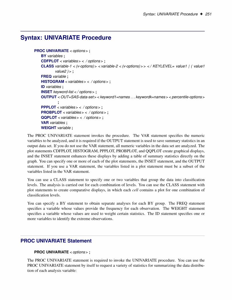
Syntax: UNIVARIATE Procedure F 251
Syntax: UNIVARIATE Procedure
PROC UNIVARIATE < options > ;BY variables ;CDFPLOT < variables > < / options > ;CLASS variable-1 < (v-options) > < variable-2 < (v-options) > > < / KEYLEVEL= value1 | ( value1
value2 ) > ;FREQ variable ;HISTOGRAM < variables > < / options > ;ID variables ;INSET keyword-list < / options > ;OUTPUT < OUT=SAS-data-set > < keyword1=names . . . keywordk=names > < percentile-options >
;PPPLOT < variables > < / options > ;PROBPLOT < variables > < / options > ;QQPLOT < variables > < / options > ;VAR variables ;WEIGHT variable ;
The PROC UNIVARIATE statement invokes the procedure. The VAR statement specifies the numericvariables to be analyzed, and it is required if the OUTPUT statement is used to save summary statistics in anoutput data set. If you do not use the VAR statement, all numeric variables in the data set are analyzed. Theplot statements CDFPLOT, HISTOGRAM, PPPLOT, PROBPLOT, and QQPLOT create graphical displays,and the INSET statement enhances these displays by adding a table of summary statistics directly on thegraph. You can specify one or more of each of the plot statements, the INSET statement, and the OUTPUTstatement. If you use a VAR statement, the variables listed in a plot statement must be a subset of thevariables listed in the VAR statement.
You can use a CLASS statement to specify one or two variables that group the data into classificationlevels. The analysis is carried out for each combination of levels. You can use the CLASS statement withplot statements to create comparative displays, in which each cell contains a plot for one combination ofclassification levels.
You can specify a BY statement to obtain separate analyses for each BY group. The FREQ statementspecifies a variable whose values provide the frequency for each observation. The WEIGHT statementspecifies a variable whose values are used to weight certain statistics. The ID statement specifies one ormore variables to identify the extreme observations.
PROC UNIVARIATE Statement
PROC UNIVARIATE < options > ;
The PROC UNIVARIATE statement is required to invoke the UNIVARIATE procedure. You can use thePROC UNIVARIATE statement by itself to request a variety of statistics for summarizing the data distribu-tion of each analysis variable:

252 F Chapter 4: The UNIVARIATE Procedure
� sample moments
� basic measures of location and variability
� confidence intervals for the mean, standard deviation, and variance
� tests for location
� tests for normality
� trimmed and Winsorized means
� robust estimates of scale
� quantiles and related confidence intervals
� extreme observations and extreme values
� frequency counts for observations
� missing values
In addition, you can use options in the PROC UNIVARIATE statement to do the following:
� specify the input data set to be analyzed
� specify a graphics catalog for saving traditional graphics output
� specify rounding units for variable values
� specify the definition used to calculate percentiles
� specify the divisor used to calculate variances and standard deviations
� request that plots be produced on line printers and define special printing characters used for features
� suppress tables
� save statistics in an output data set
The following are the options that can be used with the PROC UNIVARIATE statement:
ALLrequests all statistics and tables that the FREQ, MODES, NEXTRVAL=5, PLOT, and CIBASICoptions generate. If the analysis variables are not weighted, this option also requests the statis-tics and tables generated by the CIPCTLDF, CIPCTLNORMAL, LOCCOUNT, NORMAL, RO-BUSTSCALE, TRIMMED=.25, and WINSORIZED=.25 options. PROC UNIVARIATE also usesany values that you specify for ALPHA=, MU0=, NEXTRVAL=, CIBASIC, CIPCTLDF, CIPCTL-NORMAL, TRIMMED=, or WINSORIZED= to produce the output.

PROC UNIVARIATE Statement F 253
ALPHA=˛specifies the level of significance ˛ for 100.1 � ˛/% confidence intervals. The value ˛ must bebetween 0 and 1; the default value is 0.05, which results in 95% confidence intervals.
Note that specialized ALPHA= options are available for a number of confidence interval options. Forexample, you can specify CIBASIC(ALPHA=0.10) to request a table of basic confidence limits atthe 90% level. The default value of these options is the value of the ALPHA= option in the PROCstatement.
ANNOTATE=SAS-data-set
ANNO=SAS-data-setspecifies an input data set that contains annotate variables as described in SAS/GRAPH: Reference.You can use this data set to add features to your traditional graphics. PROC UNIVARIATE adds thefeatures in this data set to every graph that is produced in the procedure. PROC UNIVARIATE doesnot use the ANNOTATE= data set unless you create a traditional graph with a plot statement. Theoption does not apply to ODS Graphics output. Use the ANNOTATE= option in the plot statement ifyou want to add a feature to a specific graph produced by that statement.
CIBASIC < (< TYPE=keyword > < ALPHA=˛ >) >requests confidence limits for the mean, standard deviation, and variance based on the assumptionthat the data are normally distributed. If you use the CIBASIC option, you must use the default valueof VARDEF=, which is DF.
TYPE=keywordspecifies the type of confidence limit, where keyword is LOWER, UPPER, or TWOSIDED.The default value is TWOSIDED.
ALPHA=˛specifies the level of significance ˛ for 100.1 � ˛/% confidence intervals. The value ˛ mustbe between 0 and 1; the default value is 0.05, which results in 95% confidence intervals. Thedefault value is the value of ALPHA= given in the PROC statement.
CIPCTLDF < (< TYPE=keyword > < ALPHA=˛ >) >
CIQUANTDF < (< TYPE=keyword > < ALPHA=˛ >) >requests confidence limits for quantiles based on a method that is distribution-free. In other words,no specific parametric distribution such as the normal is assumed for the data. PROC UNIVARIATEuses order statistics (ranks) to compute the confidence limits as described by Hahn and Meeker (1991).This option does not apply if you use a WEIGHT statement.
TYPE=keywordspecifies the type of confidence limit, where keyword is LOWER, UPPER, SYMMETRIC, orASYMMETRIC. The default value is SYMMETRIC.
ALPHA=˛specifies the level of significance ˛ for 100.1 � ˛/% confidence intervals. The value ˛ mustbe between 0 and 1; the default value is 0.05, which results in 95% confidence intervals. Thedefault value is the value of ALPHA= given in the PROC statement.

254 F Chapter 4: The UNIVARIATE Procedure
CIPCTLNORMAL < (< TYPE=keyword > < ALPHA=˛ >) >
CIQUANTNORMAL < (< TYPE=keyword > < ALPHA=˛ >) >requests confidence limits for quantiles based on the assumption that the data are normally distributed.The computational method is described in Section 4.4.1 of Hahn and Meeker (1991) and uses thenoncentral t distribution as given by Odeh and Owen (1980). This option does not apply if you use aWEIGHT statement
TYPE=keywordspecifies the type of confidence limit, where keyword is LOWER, UPPER, or TWOSIDED.The default is TWOSIDED.
ALPHA=˛specifies the level of significance ˛ for 100.1 � ˛/% confidence intervals. The value ˛ mustbe between 0 and 1; the default value is 0.05, which results in 95% confidence intervals. Thedefault value is the value of ALPHA= given in the PROC statement.
DATA=SAS-data-setspecifies the input SAS data set to be analyzed. If the DATA= option is omitted, the procedure usesthe most recently created SAS data set.
EXCLNPWGT
EXCLNPWGTSexcludes observations with nonpositive weight values (zero or negative) from the analysis. By de-fault, PROC UNIVARIATE counts observations with negative or zero weights in the total number ofobservations. This option applies only when you use a WEIGHT statement.
FREQrequests a frequency table that consists of the variable values, frequencies, cell percentages, andcumulative percentages.
If you specify the WEIGHT statement, PROC UNIVARIATE includes the weighted count in the tableand uses this value to compute the percentages.
GOUT=graphics-catalogspecifies the SAS catalog that PROC UNIVARIATE uses to save traditional graphics output. If youomit the libref in the name of the graphics-catalog, PROC UNIVARIATE looks for the catalog in thetemporary library called WORK and creates the catalog if it does not exist. The option does not applyto ODS Graphics output.
IDOUTincludes ID variables in the output data set created by an OUTPUT statement. The value of an IDvariable in the output data set is its first value from the input data set or BY group. By default, IDvariables are not included in OUTPUT statement data sets.
LOCCOUNTrequests a table that shows the number of observations greater than, not equal to, and less than thevalue of MU0=. PROC UNIVARIATE uses these values to construct the sign test and the signed ranktest. This option does not apply if you use a WEIGHT statement.

PROC UNIVARIATE Statement F 255
MODES|MODErequests a table of all possible modes. By default, when the data contain multiple modes, PROCUNIVARIATE displays the lowest mode in the table of basic statistical measures. When all the valuesare unique, PROC UNIVARIATE does not produce a table of modes.
MU0=values
LOCATION=valuesspecifies the value of the mean or location parameter (�0) in the null hypothesis for tests of locationsummarized in the table labeled “Tests for Location: Mu0=value.” If you specify one value, PROCUNIVARIATE tests the same null hypothesis for all analysis variables. If you specify multiple values,a VAR statement is required, and PROC UNIVARIATE tests a different null hypothesis for eachanalysis variable, matching variables and location values by their order in the two lists. The defaultvalue is 0.
The following statement tests the hypothesis�0 D 0 for the first variable and the hypothesis�0 D 0:5for the second variable.
proc univariate mu0=0 0.5;
NEXTROBS=nspecifies the number of extreme observations that PROC UNIVARIATE lists in the table of extremeobservations. The table lists the n lowest observations and the n highest observations. The defaultvalue is 5. You can specify NEXTROBS=0 to suppress the table of extreme observations.
NEXTRVAL=nspecifies the number of extreme values that PROC UNIVARIATE lists in the table of extreme values.The table lists the n lowest unique values and the n highest unique values. By default, n D 0 and notable is displayed.
NOBYPLOTsuppresses side-by-side line printer box plots that are created by default when you use the BY state-ment and either the ALL option or the PLOT option in the PROC statement.
NOPRINTsuppresses all the tables of descriptive statistics that the PROC UNIVARIATE statement creates. NO-PRINT does not suppress the tables that the HISTOGRAM statement creates. You can use the NO-PRINT option in the HISTOGRAM statement to suppress the creation of its tables. Use NOPRINTwhen you want to create an OUT= or OUTTABLE= output data set only.
NORMAL
NORMALTESTrequests tests for normality that include a series of goodness-of-fit tests based on the empirical distri-bution function. The table provides test statistics and p-values for the Shapiro-Wilk test (provided thesample size is less than or equal to 2000), the Kolmogorov-Smirnov test, the Anderson-Darling test,and the Cramér-von Mises test. This option does not apply if you use a WEIGHT statement.
NOTABCONTENTSsuppresses the table of contents entries for tables of summary statistics produced by the PROC UNI-VARIATE statement.

256 F Chapter 4: The UNIVARIATE Procedure
NOVARCONTENTSsuppresses grouping entries associated with analysis variables in the table of contents. By default, thetable of contents lists results associated with an analysis variable in a group with the variable name.
OUTTABLE=SAS-data-setcreates an output data set that contains univariate statistics arranged in tabular form, with one ob-servation per analysis variable. See the section “OUTTABLE= Output Data Set” on page 414 fordetails.
PCTLDEF=value
DEF=valuespecifies the definition that PROC UNIVARIATE uses to calculate quantiles. The default value is 5.Values can be 1, 2, 3, 4, or 5. You cannot use PCTLDEF= when you compute weighted quantiles.See the section “Calculating Percentiles” on page 361 for details on quantile definitions.
PLOTS | PLOTproduces a stem-and-leaf plot (or a horizontal bar chart), a box plot, and a normal probability plotin line printer output. If you use a BY statement, side-by-side box plots that are labeled “SchematicPlots” appear after the univariate analysis for the last BY group.
PLOTSIZE=nspecifies the approximate number of rows used in line-printer plots requested with the PLOTS option.If n is larger than the value of the SAS system option PAGESIZE=, PROC UNIVARIATE uses thevalue of PAGESIZE=. If n is less than 8, PROC UNIVARIATE uses eight rows to draw the plots.
ROBUSTSCALEproduces a table with robust estimates of scale. The statistics include the interquartile range, Gini’smean difference, the median absolute deviation about the median (MAD), and two statistics proposedby Rousseeuw and Croux (1993), Qn, and Sn. See the section “Robust Estimates of Scale” onpage 368 for details. This option does not apply if you use a WEIGHT statement.
ROUND=unitsspecifies the units to use to round the analysis variables prior to computing statistics. If you specifyone unit, PROC UNIVARIATE uses this unit to round all analysis variables. If you specify multipleunits, a VAR statement is required, and each unit rounds the values of the corresponding analysisvariable. If ROUND=0, no rounding occurs. The ROUND= option reduces the number of uniquevariable values, thereby reducing memory requirements for the procedure. For example, to make therounding unit 1 for the first analysis variable and 0.5 for the second analysis variable, submit thestatement
proc univariate round=1 0.5;var Yieldstrength tenstren;
run;
When a variable value is midway between the two nearest rounded points, the value is rounded to thenearest even multiple of the roundoff value. For example, with a roundoff value of 1, the variablevalues of �2.5, �2.2, and �1.5 are rounded to �2; the values of �0.5, 0.2, and 0.5 are rounded to 0;and the values of 0.6, 1.2, and 1.4 are rounded to 1.

PROC UNIVARIATE Statement F 257
SUMMARYCONTENTS=’string’specifies the table of contents entry used for grouping the summary statistics produced by the PROCUNIVARIATE statement. You can specify SUMMARYCONTENTS=‘’ to suppress the groupingentry.
TRIMMED=values < (< TYPE=keyword > < ALPHA=˛ >) >
TRIM=values < (< TYPE=keyword > < ALPHA=˛ >) >requests a table of trimmed means, where value specifies the number or the proportion of observationsthat PROC UNIVARIATE trims. If the value is the number n of trimmed observations, n must bebetween 0 and half the number of nonmissing observations. If value is a proportion p between 0 and½, the number of observations that PROC UNIVARIATE trims is the smallest integer that is greaterthan or equal to np, where n is the number of observations. To include confidence limits for the meanand the Student’s t test in the table, you must use the default value of VARDEF=, which is DF. Fordetails concerning the computation of trimmed means, see the section “Trimmed Means” on page 367.The TRIMMED= option does not apply if you use a WEIGHT statement.
TYPE=keywordspecifies the type of confidence limit for the mean, where keyword is LOWER, UPPER, orTWOSIDED. The default value is TWOSIDED.
ALPHA=˛specifies the level of significance ˛ for 100.1� ˛/% confidence intervals. The value ˛ must bebetween 0 and 1; the default value is 0.05, which results in 95% confidence intervals.
VARDEF=divisorspecifies the divisor to use in the calculation of variances and standard deviation. By default,VARDEF=DF. Table 4.1 shows the possible values for divisor and associated divisors.
Table 4.1 Possible Values for VARDEF=
Value Divisor Formula for Divisor
DF degrees of freedom n � 1
N number of observations n
WDF sum of weights minus one .†iwi / � 1
WEIGHT | WGT sum of weights †iwi
The procedure computes the variance as CSSdivisor whereCSS is the corrected sums of squares and equalsPn
iD1.xi � Nx/2. When you weight the analysis variables, CSS D
PniD1.wixi � Nxw/
2 where Nxw isthe weighted mean.
The default value is DF. To compute the standard error of the mean, confidence limits, and Student’st test, use the default value of VARDEF=.
When you use the WEIGHT statement and VARDEF=DF, the variance is an estimate of s2 where thevariance of the i th observation is var.xi / D s2
wiand wi is the weight for the i th observation. This
yields an estimate of the variance of an observation with unit weight.

258 F Chapter 4: The UNIVARIATE Procedure
When you use the WEIGHT statement and VARDEF=WGT, the computed variance is asymptotically(for large n) an estimate of s
2
Nwwhere Nw is the average weight. This yields an asymptotic estimate of
the variance of an observation with average weight.
WINSORIZED=values < (< TYPE=keyword > < ALPHA=˛ >) >
WINSOR=values < (< TYPE=keyword > < ALPHA=˛ >) >requests of a table of Winsorized means, where value is the number or the proportion of observationsthat PROC UNIVARIATE uses to compute the Winsorized mean. If the value is the number n ofWinsorized observations, n must be between 0 and half the number of nonmissing observations. Ifvalue is a proportion p between 0 and ½, the number of observations that PROC UNIVARIATE uses isequal to the smallest integer that is greater than or equal to np, where n is the number of observations.To include confidence limits for the mean and the Student t test in the table, you must use the defaultvalue of VARDEF=, which is DF. For details concerning the computation of Winsorized means, seethe section “Winsorized Means” on page 366. The WINSORIZED= option does not apply if you usea WEIGHT statement.
TYPE=keywordspecifies the type of confidence limit for the mean, where keyword is LOWER, UPPER, orTWOSIDED. The default is TWOSIDED.
ALPHA=˛specifies the level of significance ˛ for 100.1� ˛/% confidence intervals. The value ˛ must bebetween 0 and 1; the default value is 0.05, which results in 95% confidence intervals.
BY Statement
BY variables ;
You can specify a BY statement with PROC UNIVARIATE to obtain separate analyses for each BY group.The BY statement specifies the variables that the procedure uses to form BY groups. You can specify morethan one variable. If you do not use the NOTSORTED option in the BY statement, the observations in thedata set must either be sorted by all the variables that you specify or be indexed appropriately.
DESCENDINGspecifies that the data set is sorted in descending order by the variable that immediately follows theword DESCENDING in the BY statement.
NOTSORTEDspecifies that observations are not necessarily sorted in alphabetic or numeric order. The data aregrouped in another way—for example, chronological order.
The requirement for ordering or indexing observations according to the values of BY variables issuspended for BY-group processing when you use the NOTSORTED option. In fact, the proceduredoes not use an index if you specify NOTSORTED. The procedure defines a BY group as a set ofcontiguous observations that have the same values for all BY variables. If observations with the samevalues for the BY variables are not contiguous, the procedure treats each contiguous set as a separateBY group.

CDFPLOT Statement F 259
CDFPLOT Statement
CDFPLOT < variables > < / options > ;
The CDFPLOT statement plots the observed cumulative distribution function (cdf) of a variable, defined as
FN .x/ D percent of nonmissing values � x
Dnumber of values � x
N� 100%
whereN is the number of nonmissing observations. The cdf is an increasing step function that has a verticaljump of 1
Nat each value of x equal to an observed value. The cdf is also referred to as the empirical
cumulative distribution function (ecdf).
You can use any number of CDFPLOT statements in the UNIVARIATE procedure. The components of theCDFPLOT statement are as follows.
variablesspecify variables for which to create cdf plots. If you specify a VAR statement, the variables mustalso be listed in the VAR statement. Otherwise, the variables can be any numeric variables in theinput data set. If you do not specify a list of variables, then by default the procedure creates a cdf plotfor each variable listed in the VAR statement, or for each numeric variable in the DATA= data set ifyou do not specify a VAR statement.
For example, suppose a data set named Steel contains exactly three numeric variables: Length, Width,and Height. The following statements create a cdf plot for each of the three variables:
proc univariate data=Steel;cdfplot;
run;
The following statements create a cdf plot for Length and a cdf plot for Width:
proc univariate data=Steel;var Length Width;cdfplot;
run;
The following statements create a cdf plot for Width:
proc univariate data=Steel;var Length Width;cdfplot Width;
run;
optionsspecify the theoretical distribution for the plot or add features to the plot. If you specify more thanone variable, the options apply equally to each variable. Specify all options after the slash (/) in theCDFPLOT statement. You can specify only one option that names a distribution in each CDFPLOT

260 F Chapter 4: The UNIVARIATE Procedure
statement, but you can specify any number of other options. The distributions available are listed inTable 4.2. By default, the procedure produces a plot for the normal distribution.
Table 4.2 through Table 4.15 list the CDFPLOT options by function. For complete descriptions, seethe sections “Dictionary of Options” on page 265 and “Dictionary of Common Options” on page 350.Options can be any of the following:
� primary options
� secondary options
� general options
Distribution Options
Table 4.2 lists primary options for requesting a theoretical distribution.
Table 4.2 Primary Options for Theoretical Distributions
Option Description
BETA(beta-options) plots two-parameter beta distributionfunction, parameters � and � as-sumed known
EXPONENTIAL(exponential-options) plots one-parameter exponential dis-tribution function, parameter � as-sumed known
GAMMA(gamma-options) plots two-parameter gamma distribu-tion function, parameter � assumedknown
GUMBEL(Gumbel-options) plots Gumbel distribution with loca-tion parameter � and scale parameter�
IGAUSS(iGauss-options) plots inverse Gaussian distributionwith mean � and shape parameter �
LOGNORMAL(lognormal-options) plots two-parameter lognormal dis-tribution function, parameter � as-sumed known
NORMAL(normal-options) plots normal distribution functionPARETO(Pareto-options) plots generalized Pareto distribution
with threshold parameter � , scale pa-rameter � , and shape parameter ˛
POWER(power-options) plots power function distributionwith threshold parameter � , scale pa-rameter � , and shape parameter ˛
RAYLEIGH(Rayleigh-options) plots Rayleigh distribution withthreshold parameter � and scaleparameter �
WEIBULL(Weibull-options) plots two-parameter Weibull distribu-tion function, parameter � assumedknown

CDFPLOT Statement F 261
Table 4.3 through Table 4.14 list secondary options that specify distribution parameters and control thedisplay of a theoretical distribution function. Specify these options in parentheses after the distributionkeyword. For example, you can request a normal probability plot with a distribution reference line byspecifying the NORMAL option as follows:
proc univariate;cdfplot / normal(mu=10 sigma=0.5 color=red);
run;
The COLOR= option specifies the color for the curve, and the normal-options MU= and SIGMA= specifythe parameters � D 10 and � D 0:5 for the distribution function. If you do not specify these parameters,maximum likelihood estimates are computed.
Table 4.3 Secondary Options Used with All Distributions
Option Description
COLOR= specifies color of theoretical distribution functionL= specifies line type of theoretical distribution functionW= specifies width of theoretical distribution function
Table 4.4 Secondary Beta-Options
Option Description
ALPHA= specifies first shape parameter ˛ for beta distribution functionBETA= specifies second shape parameter ˇ for beta distribution functionSIGMA= specifies scale parameter � for beta distribution functionTHETA= specifies lower threshold parameter � for beta distribution function
Table 4.5 Secondary Exponential-Options
Option Description
SIGMA= specifies scale parameter � for exponential distribution functionTHETA= specifies threshold parameter � for exponential distribution function

262 F Chapter 4: The UNIVARIATE Procedure
Table 4.6 Secondary Gamma-Options
Option Description
ALPHA= specifies shape parameter ˛ for gamma distribution functionALPHADELTA= specifies change in successive estimates of ˛ at which the Newton-
Raphson approximation of O terminatesALPHAINITIAL= specifies initial value for ˛ in the Newton-Raphson approximation of OMAXITER= specifies maximum number of iterations in the Newton-Raphson ap-
proximation of OSIGMA= specifies scale parameter � for gamma distribution functionTHETA= specifies threshold parameter � for gamma distribution function
Table 4.7 Secondary Gumbel-Options
Option Description
MU= specifies location parameter � for Gumbel distribution functionSIGMA= specifies scale parameter � for Gumbel distribution function
Table 4.8 Secondary IGauss-Options
Option Description
LAMBDA= specifies shape parameter � for inverse Gaussian distribution functionMU= specifies mean � for inverse Gaussian distribution function
Table 4.9 Secondary Lognormal-Options
Option Description
SIGMA= specifies shape parameter � for lognormal distribution functionTHETA= specifies threshold parameter � for lognormal distribution functionZETA= specifies scale parameter � for lognormal distribution function
Table 4.10 Secondary Normal-Options
Option Description
MU= specifies mean � for normal distribution functionSIGMA= specifies standard deviation � for normal distribution function

CDFPLOT Statement F 263
Table 4.11 Secondary Pareto-Options
Option Description
ALPHA= specifies shape parameter ˛ for generalized Pareto distribution functionSIGMA= specifies scale parameter � for generalized Pareto distribution functionTHETA= specifies threshold parameter � for generalized Pareto distribution func-
tion
Table 4.12 Secondary Power-Options
Option Description
ALPHA= specifies shape parameter ˛ for power function distributionSIGMA= specifies scale parameter � for power function distributionTHETA= specifies threshold parameter � for power function distribution
Table 4.13 Secondary Rayleigh-Options
Option Description
SIGMA= specifies scale parameter � for Rayleigh distribution functionTHETA= specifies threshold parameter � for Rayleigh distribution function
Table 4.14 Secondary Weibull-Options
Option Description
C= specifies shape parameter c for Weibull distribution functionCDELTA= specifies change in successive estimates of c at which the Newton-
Raphson approximation of Oc terminatesCINITIAL= specifies initial value for c in the Newton-Raphson approximation of OcMAXITER= specifies maximum number of iterations in the Newton-Raphson ap-
proximation of OcSIGMA= specifies scale parameter � for Weibull distribution functionTHETA= specifies threshold parameter � for Weibull distribution function

264 F Chapter 4: The UNIVARIATE Procedure
General Options
Table 4.15 summarizes general options for enhancing cdf plots.
Table 4.15 General Graphics Options
Option Description
ANNOKEY applies annotation requested in ANNOTATE= data set to key cell onlyANNOTATE= specifies annotate data setCAXIS= specifies color for axisCFRAME= specifies color for frameCFRAMESIDE= specifies color for filling row label framesCFRAMETOP= specifies color for filling column label framesCHREF= specifies color for HREF= linesCONTENTS= specifies table of contents entry for cdf plot groupingCPROP= specifies color for proportion of frequency barCTEXT= specifies color for textCTEXTSIDE= specifies color for row labelsCTEXTTOP= specifies color for column labelsCVREF= specifies color for VREF= linesDESCRIPTION= specifies description for graphics catalog memberFONT= specifies text fontHAXIS= specifies AXIS statement for horizontal axisHEIGHT= specifies height of text used outside framed areasHMINOR= specifies number of horizontal axis minor tick marksHREF= specifies reference lines perpendicular to the horizontal axisHREFLABELS= specifies labels for HREF= linesHREFLABPOS= specifies position for HREF= line labelsINFONT= specifies software font for text inside framed areasINHEIGHT= specifies height of text inside framed areasINTERTILE= specifies distance between tiles in comparative plotLHREF= specifies line style for HREF= linesLVREF= specifies line style for VREF= linesNAME= specifies name for plot in graphics catalogNCOLS= specifies number of columns in comparative plotNOECDF suppresses plot of empirical (observed) distribution functionNOFRAME suppresses frame around plotting areaNOHLABEL suppresses label for horizontal axisNOVLABEL suppresses label for vertical axisNOVTICK suppresses tick marks and tick mark labels for vertical axisNROWS= specifies number of rows in comparative plotOVERLAY overlays plots for different class levels (ODS Graphics only)TURNVLABELS turns and vertically strings out characters in labels for vertical axisVAXIS= specifies AXIS statement for vertical axisVAXISLABEL= specifies label for vertical axisVMINOR= specifies number of vertical axis minor tick marksVREF= specifies reference lines perpendicular to the vertical axisVREFLABELS= specifies labels for VREF= lines

CDFPLOT Statement F 265
Table 4.15 continued
Option Description
VREFLABPOS= specifies position for VREF= line labelsVSCALE= specifies scale for vertical axisWAXIS= specifies line thickness for axes and frame
Dictionary of Options
The following entries provide detailed descriptions of the options specific to the CDFPLOT statement. Seethe section “Dictionary of Common Options” on page 350 for detailed descriptions of options common toall plot statements.
ALPHA=valuespecifies the shape parameter ˛ for distribution functions requested with the BETA, GAMMA,PARETO, and POWER options. Enclose the ALPHA= option in parentheses after the distributionkeyword. If you do not specify a value for ˛, the procedure calculates a maximum likelihood esti-mate. For examples, see the entries for the BETA and GAMMA options.
BETA< (beta-options ) >displays a fitted beta distribution function on the cdf plot. The equation of the fitted cdf is
F.x/ D
8<:0 for x � �Ix��
�.˛; ˇ/ for � < x < � C �
1 for x � � C �
where Iy.˛; ˇ/ is the incomplete beta function and
� D lower threshold parameter (lower endpoint)
� D scale parameter .� > 0/
˛ D shape parameter .˛ > 0/
ˇ D shape parameter .ˇ > 0/
The beta distribution is bounded below by the parameter � and above by the value � C � . You canspecify � and � by using the THETA= and SIGMA= beta-options, as illustrated in the followingstatements, which fit a beta distribution bounded between 50 and 75. The default values for � and �are 0 and 1, respectively.
proc univariate;cdfplot / beta(theta=50 sigma=25);
run;
The beta distribution has two shape parameters: ˛ and ˇ. If these parameters are known, you canspecify their values with the ALPHA= and BETA= beta-options. If you do not specify values for ˛and ˇ, the procedure calculates maximum likelihood estimates.
The BETA option can appear only once in a CDFPLOT statement. Table 4.3 and Table 4.4 list optionsyou can specify with the BETA distribution option.

266 F Chapter 4: The UNIVARIATE Procedure
BETA=value
B=valuespecifies the second shape parameter ˇ for beta distribution functions requested by the BETA option.Enclose the BETA= option in parentheses after the BETA keyword. If you do not specify a value forˇ, the procedure calculates a maximum likelihood estimate. For examples, see the preceding entryfor the BETA option.
C=valuespecifies the shape parameter c for Weibull distribution functions requested with the WEIBULL op-tion. Enclose the C= option in parentheses after the WEIBULL keyword. If you do not specify avalue for c, the procedure calculates a maximum likelihood estimate. You can specify the SHAPE=option as an alias for the C= option.
EXPONENTIAL< (exponential-options ) >
EXP< (exponential-options ) >displays a fitted exponential distribution function on the cdf plot. The equation of the fitted cdf is
F.x/ D
(0 for x � �
1 � exp��x���
�for x > �
where
� D threshold parameter
� D scale parameter .� > 0/
The parameter � must be less than or equal to the minimum data value. You can specify � with theTHETA= exponential-option. The default value for � is 0. You can specify � with the SIGMA=exponential-option. By default, a maximum likelihood estimate is computed for � . For example, thefollowing statements fit an exponential distribution with � D 10 and a maximum likelihood estimatefor � :
proc univariate;cdfplot / exponential(theta=10 l=2 color=green);
run;
The exponential curve is green and has a line type of 2.
The EXPONENTIAL option can appear only once in a CDFPLOT statement. Table 4.3 and Table 4.5list the options you can specify with the EXPONENTIAL option.
GAMMA< (gamma-options) >displays a fitted gamma distribution function on the cdf plot. The equation of the fitted cdf is
F.x/ D
(0 for x � �1
�.˛/�
R x�
�t���
�˛�1exp
��t���
�dt for x > �
where
� D threshold parameter

CDFPLOT Statement F 267
� D scale parameter .� > 0/
˛ D shape parameter .˛ > 0/
The parameter � for the gamma distribution must be less than the minimum data value. You canspecify � with the THETA= gamma-option. The default value for � is 0. In addition, the gammadistribution has a shape parameter ˛ and a scale parameter � . You can specify these parameters withthe ALPHA= and SIGMA= gamma-options. By default, maximum likelihood estimates are computedfor ˛ and � . For example, the following statements fit a gamma distribution function with � D 4 andmaximum likelihood estimates for ˛ and � :
proc univariate;cdfplot / gamma(theta=4);
run;
Note that the maximum likelihood estimate of ˛ is calculated iteratively using the Newton-Raphsonapproximation. The gamma-options ALPHADELTA=, ALPHAINITIAL=, and MAXITER= controlthe approximation.
The GAMMA option can appear only once in a CDFPLOT statement. Table 4.3 and Table 4.6 list theoptions you can specify with the GAMMA option.
GUMBEL< (Gumbel-options) >displays a fitted Gumbel distribution (also known as Type 1 extreme value distribution) function onthe cdf plot. The equation of the fitted cdf is
F.x/ D exp��e�.x��/=�
�where
� D location parameter� D scale parameter .� > 0/
You can specify known values for � and � with the MU= and SIGMA= Gumbel-options. By default,maximum likelihood estimates are computed for � and � .
The GUMBEL option can appear only once in a CDFPLOT statement. Table 4.3 and Table 4.7 listsecondary options you can specify with the GUMBEL option.
IGAUSS< (iGauss-options) >displays a fitted inverse Gaussian distribution function on the cdf plot. The equation of the fitted cdfis
F.x/ D ˆ
(r�
x
�x
�� 1
�)C e2�=�ˆ
(�
r�
x
�x
�C 1
�)
where ˆ.�/ is the standard normal cumulative distribution function, and
� D mean parameter .� > 0/� D shape parameter .� > 0/

268 F Chapter 4: The UNIVARIATE Procedure
You can specify known values for� and �with the MU= and LAMBDA= iGauss-options. By default,maximum likelihood estimates are computed for � and �.
The IGAUSS option can appear only once in a CDFPLOT statement. Table 4.3 and Table 4.8 listsecondary options you can specify with the IGAUSS option.
LAMBDA=valuespecifies the shape parameter � for distribution functions requested with the IGAUSS option. Enclosethe LAMBDA= option in parentheses after the IGAUSS distribution keyword. If you do not specifya value for �, the procedure calculates a maximum likelihood estimate.
LOGNORMAL< (lognormal-options) >displays a fitted lognormal distribution function on the cdf plot. The equation of the fitted cdf is
F.x/ D
(0 for x � �
ˆ�
log.x��/���
�for x > �
where ˆ.�/ is the standard normal cumulative distribution function and
� D threshold parameter
� D scale parameter
� D shape parameter .� > 0/
The parameter � for the lognormal distribution must be less than the minimum data value. You canspecify � with the THETA= lognormal-option. The default value for � is 0. In addition, the lognormaldistribution has a shape parameter � and a scale parameter �. You can specify these parameterswith the SIGMA= and ZETA= lognormal-options. By default, maximum likelihood estimates arecomputed for � and �. For example, the following statements fit a lognormal distribution functionwith � D 10 and maximum likelihood estimates for � and �:
proc univariate;cdfplot / lognormal(theta = 10);
run;
The LOGNORMAL option can appear only once in a CDFPLOT statement. Table 4.3 and Table 4.9list options that you can specify with the LOGNORMAL option.
MU=valuespecifies the parameter � for theoretical cumulative distribution functions requested with the GUM-BEL, IGAUSS, and NORMAL option. Enclose the MU= option in parentheses after the distributionkeyword. For the inverse Gaussian and normal distributions, the default value is the sample mean. Ifyou do not specify a value for � for the Gumbel distribution, the procedure calculates a maximumlikelihood estimate. For an example, see the entry for the NORMAL option.
NOECDFsuppresses the observed distribution function (the empirical cumulative distribution function) of thevariable, which is drawn by default. This option enables you to create theoretical cdf plots withoutdisplaying the data distribution. The NOECDF option can be used only with a theoretical distribution(such as the NORMAL option).
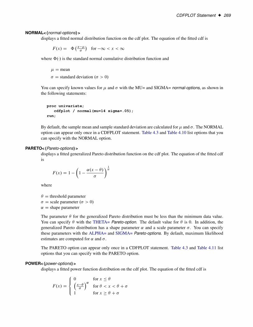
CDFPLOT Statement F 269
NORMAL< (normal-options) >displays a fitted normal distribution function on the cdf plot. The equation of the fitted cdf is
F.x/ D ˆ�x���
�for �1 < x <1
where ˆ.�/ is the standard normal cumulative distribution function and
� D mean
� D standard deviation .� > 0/
You can specify known values for � and � with the MU= and SIGMA= normal-options, as shown inthe following statements:
proc univariate;cdfplot / normal(mu=14 sigma=.05);
run;
By default, the sample mean and sample standard deviation are calculated for� and � . The NORMALoption can appear only once in a CDFPLOT statement. Table 4.3 and Table 4.10 list options that youcan specify with the NORMAL option.
PARETO< (Pareto-options) >displays a fitted generalized Pareto distribution function on the cdf plot. The equation of the fitted cdfis
F.x/ D 1 �
�1 �
˛.x � �/
�
� 1˛
where
� D threshold parameter� D scale parameter .� > 0/˛ D shape parameter
The parameter � for the generalized Pareto distribution must be less than the minimum data value.You can specify � with the THETA= Pareto-option. The default value for � is 0. In addition, thegeneralized Pareto distribution has a shape parameter ˛ and a scale parameter � . You can specifythese parameters with the ALPHA= and SIGMA= Pareto-options. By default, maximum likelihoodestimates are computed for ˛ and � .
The PARETO option can appear only once in a CDFPLOT statement. Table 4.3 and Table 4.11 listoptions that you can specify with the PARETO option.
POWER< (power-options) >displays a fitted power function distribution on the cdf plot. The equation of the fitted cdf is
F.x/ D
8<:0 for x � ��x���
�˛for � < x < � C �
1 for x � � C �
270 F Chapter 4: The UNIVARIATE Procedure
where
� D lower threshold parameter (lower endpoint)� D scale parameter .� > 0/˛ D shape parameter .˛ > 0/
The power function distribution is bounded below by the parameter � and above by the value � C � .You can specify � and � by using the THETA= and SIGMA= power-options. The default values for� and � are 0 and 1, respectively.
You can specify a value for the shape parameter, ˛, with the ALPHA= power-option. If you do notspecify a value for ˛, the procedure calculates a maximum likelihood estimate.
The power function distribution is a special case of the beta distribution with its second shape param-eter, ˇ D 1.
The POWER option can appear only once in a CDFPLOT statement. Table 4.3 and Table 4.12 listoptions that you can specify with the POWER option.
RAYLEIGH< (Rayleigh-options) >displays a fitted Rayleigh distribution function on the cdf plot. The equation of the fitted cdf is
F.x/ D 1 � e�.x��/2=.2�2/
where
� D threshold parameter� D scale parameter .� > 0/
The parameter � for the Rayleigh distribution must be less than the minimum data value. You canspecify � with the THETA= Rayleigh-option. The default value for � is 0. You can specify � with theSIGMA= Rayleigh-option. By default, a maximum likelihood estimate is computed for � .
The RAYLEIGH option can appear only once in a CDFPLOT statement. Table 4.3 and Table 4.13 listoptions that you can specify with the RAYLEIGH option.
SIGMA=value | ESTspecifies the parameter � for distribution functions requested by the BETA, EXPONENTIAL,GAMMA, LOGNORMAL, NORMAL, and WEIBULL options. Enclose the SIGMA= option inparentheses after the distribution keyword. The following table summarizes the use of the SIGMA=option:

CDFPLOT Statement F 271
Distribution Option SIGMA= Specifies Default Value AliasBETA scale parameter � 1 SCALE=EXPONENTIAL scale parameter � maximum likelihood estimate SCALE=GAMMA scale parameter � maximum likelihood estimate SCALE=GUMBEL scale parameter � maximum likelihood estimateLOGNORMAL shape parameter � maximum likelihood estimate SHAPE=NORMAL scale parameter � standard deviationPARETO scale parameter � maximum likelihood estimatePOWER scale parameter � 1RAYLEIGH scale parameter � maximum likelihood estimateWEIBULL scale parameter � maximum likelihood estimate SCALE=
THETA=value | EST
THRESHOLD=value | ESTspecifies the lower threshold parameter � for theoretical cumulative distribution functions requestedwith the BETA, EXPONENTIAL, GAMMA, LOGNORMAL, PARETO, POWER, RAYLEIGH, andWEIBULL options. Enclose the THETA= option in parentheses after the distribution keyword. Thedefault value is 0.
VSCALE=PERCENT | PROPORTIONspecifies the scale of the vertical axis. The value PERCENT scales the data in units of percent ofobservations per data unit. The value PROPORTION scales the data in units of proportion of obser-vations per data unit. The default is PERCENT.
WEIBULL< (Weibull-options) >displays a fitted Weibull distribution function on the cdf plot. The equation of the fitted cdf is
F.x/ D
(0 for x � �
1 � exp��
�x���
�c�for x > �
where
� D threshold parameter
� D scale parameter .� > 0/
c D shape parameter .c > 0/
The parameter � must be less than the minimum data value. You can specify � with the THETA=Weibull-option. The default value for � is 0. In addition, the Weibull distribution has a shape pa-rameter c and a scale parameter � . You can specify these parameters with the SIGMA= and C=Weibull-options. By default, maximum likelihood estimates are computed for c and � . For example,the following statements fit a Weibull distribution function with � D 15 and maximum likelihoodestimates for � and c:
proc univariate;cdfplot / weibull(theta=15);
run;

272 F Chapter 4: The UNIVARIATE Procedure
Note that the maximum likelihood estimate of c is calculated iteratively using the Newton-Raphsonapproximation. The Weibull-options CDELTA=, CINITIAL=, and MAXITER= control the approxi-mation.
The WEIBULL option can appear only once in a CDFPLOT statement. Table 4.3 and Table 4.14 listoptions that you can specify with the WEIBULL option.
ZETA=valuespecifies a value for the scale parameter � for a lognormal distribution function requested with theLOGNORMAL option. Enclose the ZETA= option in parentheses after the LOGNORMAL keyword.If you do not specify a value for �, a maximum likelihood estimate is computed. You can specify theSCALE= option as an alias for the ZETA= option.
CLASS Statement
CLASS variable-1 < (v-options) > < variable-2 < (v-options) > > < / KEYLEVEL= value1 | ( value1 value2) > ;
The CLASS statement specifies one or two variables used to group the data into classification levels. Vari-ables in a CLASS statement are referred to as CLASS variables. CLASS variables can be numeric orcharacter. Class variables can have floating point values, but they typically have a few discrete values thatdefine levels of the variable. You do not have to sort the data by CLASS variables. PROC UNIVARIATEuses the formatted values of the CLASS variables to determine the classification levels.
You can specify the following v-options enclosed in parentheses after the CLASS variable:
MISSINGspecifies that missing values for the CLASS variable are to be treated as valid classification levels.Special missing values that represent numeric values (‘.A’ through ‘.Z’ and ‘._’) are each consideredas a separate value. If you omit MISSING, PROC UNIVARIATE excludes the observations with amissing CLASS variable value from the analysis. Enclose this option in parentheses after the CLASSvariable.
ORDER=DATA | FORMATTED | FREQ | INTERNALspecifies the display order for the CLASS variable values. The default value is INTERNAL. You canspecify the following values with the ORDER=option:
DATA orders values according to their order in the input data set. When you use a plotstatement, PROC UNIVARIATE displays the rows (columns) of the comparativeplot from top to bottom (left to right) in the order that the CLASS variable valuesfirst appear in the input data set.
FORMATTED orders values by their ascending formatted values. This order might depend onyour operating environment. When you use a plot statement, PROC UNIVARIATEdisplays the rows (columns) of the comparative plot from top to bottom (left toright) in increasing order of the formatted CLASS variable values. For example,suppose a numeric CLASS variable DAY (with values 1, 2, and 3) has a user-defined format that assigns Wednesday to the value 1, Thursday to the value 2, and

CLASS Statement F 273
Friday to the value 3. The rows of the comparative plot will appear in alphabeticalorder (Friday, Thursday, Wednesday) from top to bottom.
If there are two or more distinct internal values with the same formatted value, thenPROC UNIVARIATE determines the order by the internal value that occurs first inthe input data set. For numeric variables without an explicit format, the levels areordered by their internal values.
FREQ orders values by descending frequency count so that levels with the most observa-tions are listed first. If two or more values have the same frequency count, PROCUNIVARIATE uses the formatted values to determine the order.
When you use a plot statement, PROC UNIVARIATE displays the rows (columns)of the comparative plot from top to bottom (left to right) in order of decreasingfrequency count for the CLASS variable values.
INTERNAL orders values by their unformatted values, which yields the same order as PROCSORT. This order may depend on your operating environment.
When you use a plot statement, PROC UNIVARIATE displays the rows (columns)of the comparative plot from top to bottom (left to right) in increasing order of theinternal (unformatted) values of the CLASS variable. The first CLASS variable isused to label the rows of the comparative plots (top to bottom). The second CLASSvariable is used to label the columns of the comparative plots (left to right). Forexample, suppose a numeric CLASS variable DAY (with values 1, 2, and 3) has auser-defined format that assigns Wednesday to the value 1, Thursday to the value2, and Friday to the value 3. The rows of the comparative plot will appear inday-of-the-week order (Wednesday, Thursday, Friday) from top to bottom.
You can specify the following option after the slash (/) in the CLASS statement.
KEYLEVEL=value | ( value1 value2 )specifies the key cells in comparative plots. For each plot, PROC UNIVARIATE first determines thehorizontal axis scaling for the key cell, and then extends the axis using the established tick interval toaccommodate the data ranges for the remaining cells, if necessary. Thus, the choice of the key celldetermines the uniform horizontal axis that PROC UNIVARIATE uses for all cells.
If you specify only one CLASS variable and use a plot statement, KEYLEVEL=value identifies thekey cell as the level for which the CLASS variable is equal to value. By default, PROC UNIVARIATEsorts the levels in the order determined by the ORDER= option, and the key cell is the first occurrenceof a level in this order. The cells display in order from top to bottom or left to right. Consequently,the key cell appears at the top (or left). When you specify a different key cell with the KEYLEVEL=option, this cell appears at the top (or left).
If you specify two CLASS variables, use KEYLEVEL= (value1 value2) to identify the key cell asthe level for which CLASS variable n is equal to valuen. By default, PROC UNIVARIATE sorts thelevels of the first CLASS variable in the order that is determined by its ORDER= option. Then, withineach of these levels, it sorts the levels of the second CLASS variable in the order that is determined byits ORDER= option. The default key cell is the first occurrence of a combination of levels for the twovariables in this order. The cells display in the order of the first CLASS variable from top to bottomand in the order of the second CLASS variable from left to right. Consequently, the default key cellappears at the upper left corner. When you specify a different key cell with the KEYLEVEL= option,this cell appears at the upper left corner.

274 F Chapter 4: The UNIVARIATE Procedure
The length of the KEYLEVEL= value cannot exceed 16 characters and you must specify a formattedvalue.
The KEYLEVEL= option has no effect unless you specify a plot statement.
NOKEYMOVEspecifies that the location of the key cell in a comparative plot be unchanged by the CLASS statementKEYLEVEL= option. By default, the key cell is positioned as the first cell in a comparative plot.
The NOKEYMOVE option has no effect unless you specify a plot statement.
FREQ Statement
FREQ variable ;
The FREQ statement specifies a numeric variable whose value represents the frequency of the observation.If you use the FREQ statement, the procedure assumes that each observation represents n observations,where n is the value of variable. If the variable is not an integer, the SAS System truncates it. If the variableis less than 1 or is missing, the procedure excludes that observation from the analysis. See Example 4.6.
NOTE: The FREQ statement affects the degrees of freedom, but the WEIGHT statement does not.
HISTOGRAM Statement
HISTOGRAM < variables > < / options > ;
The HISTOGRAM statement creates histograms and optionally superimposes estimated parametric andnonparametric probability density curves. You cannot use the WEIGHT statement with the HISTOGRAMstatement. You can use any number of HISTOGRAM statements after a PROC UNIVARIATE statement.The components of the HISTOGRAM statement are follows.
variablesare the variables for which histograms are to be created. If you specify a VAR statement, the variablesmust also be listed in the VAR statement. Otherwise, the variables can be any numeric variables in theinput data set. If you do not specify variables in a VAR statement or in the HISTOGRAM statement,then by default, a histogram is created for each numeric variable in the DATA= data set. If you usea VAR statement and do not specify any variables in the HISTOGRAM statement, then by default, ahistogram is created for each variable listed in the VAR statement.
For example, suppose a data set named Steel contains exactly two numeric variables named Lengthand Width. The following statements create two histograms, one for Length and one for Width:
proc univariate data=Steel;histogram;
run;

HISTOGRAM Statement F 275
Likewise, the following statements create histograms for Length and Width:
proc univariate data=Steel;var Length Width;histogram;
run;
The following statements create a histogram for Length only:
proc univariate data=Steel;var Length Width;histogram Length;
run;
optionsadd features to the histogram. Specify all options after the slash (/) in the HISTOGRAM statement.Options can be one of the following:
� primary options for fitted parametric distributions and kernel density estimates
� secondary options for fitted parametric distributions and kernel density estimates
� general options for graphics and output data sets
For example, in the following statements, the NORMAL option displays a fitted normal curve on thehistogram, the MIDPOINTS= option specifies midpoints for the histogram, and the CTEXT= optionspecifies the color of the text:
proc univariate data=Steel;histogram Length / normal
midpoints = 5.6 5.8 6.0 6.2 6.4ctext = blue;
run;
Table 4.16 through Table 4.33 list the HISTOGRAM options by function. For complete descrip-tions, see the sections “Dictionary of Options” on page 282 and “Dictionary of Common Options” onpage 350.
Parametric Density Estimation Options
Table 4.16 lists primary options that display parametric density estimates on the histogram. You can specifyeach primary option once in a given HISTOGRAM statement, and each primary option can display multiplecurves from its family on the histogram.

276 F Chapter 4: The UNIVARIATE Procedure
Table 4.16 Primary Options for Parametric Fitted Distributions
Option Description
BETA(beta-options) fits beta distribution with thresholdparameter � , scale parameter � , andshape parameters ˛ and ˇ
EXPONENTIAL(exponential-options) fits exponential distribution withthreshold parameter � and scale pa-rameter �
GAMMA(gamma-options) fits gamma distribution with thresh-old parameter � , scale parameter � ,and shape parameter ˛
GUMBEL(Gumbel-options) fits gumbel distribution with locationparameter �, and scale parameter �
IGAUSS(iGauss-options) fits inverse Gaussian distributionwith tlocation parameter �, andshape parameter �
LOGNORMAL(lognormal-options) fits lognormal distribution withthreshold parameter � , scale pa-rameter �, and shape parameter�
NORMAL(normal-options) fits normal distribution with mean �and standard deviation �
PARETO(Pareto-options) fits generalized Pareto distributionwith threshold parameter � , scale pa-rameter � , and shape parameter ˛
POWER(power-options) fits power function distribution withthreshold parameter � , scale parame-ter � , and shape parameter ˛
RAYLEIGH(Rayleigh-options) fits Rayleigh distribution with thresh-old parameter � , and scale parameter�
SB(SB -options) fits Johnson SB distribution withthreshold parameter � , scale param-eter � , and shape parameters ı and
SU(SU -options) fits Johnson SU distribution withthreshold parameter � , scale param-eter � , and shape parameters ı and
WEIBULL(Weibull-options) fits Weibull distribution with thresh-old parameter � , scale parameter � ,and shape parameter c
Table 4.17 through Table 4.30 list secondary options that specify parameters for fitted parametric distribu-tions and that control the display of fitted curves. Specify these secondary options in parentheses after theprimary distribution option. For example, you can fit a normal curve by specifying the NORMAL option asfollows:

HISTOGRAM Statement F 277
proc univariate;histogram / normal(color=red mu=10 sigma=0.5);
run;
The COLOR= normal-option draws the curve in red, and the MU= and SIGMA= normal-options specify theparameters � D 10 and � D 0:5 for the curve. Note that the sample mean and sample standard deviationare used to estimate � and � , respectively, when the MU= and SIGMA= normal-options are not specified.
You can specify lists of values for secondary options to display more than one fitted curve from the samedistribution family on a histogram. Option values are matched by list position. You can specify the valueEST in a list of distribution parameter values to use an estimate of the parameter.
For example, the following code displays two normal curves on a histogram:
proc univariate;histogram / normal(color=(red blue) mu=10 est sigma=0.5 est);
run;
The first curve is red, with � D 10 and � D 0:5. The second curve is blue, with � equal to the sample meanand � equal to the sample standard deviation.
See the section “Formulas for Fitted Continuous Distributions” on page 380 for detailed information aboutthe families of parametric distributions that you can fit with the HISTOGRAM statement.
Table 4.17 Secondary Options Used with All Parametric Distribution Options
Option Description
COLOR= specifies colors of density curvesCONTENTS= specifies table of contents entry for density curve groupingFILL fills area under density curveL= specifies line types of density curvesMIDPERCENTS prints table of midpoints of histogram intervalsNOPRINT suppresses tables summarizing curvesPERCENTS= lists percents for which quantiles calculated from data and quantiles
estimated from curves are tabulatedW= specifies widths of density curves
Table 4.18 Secondary Beta-Options
Option Description
ALPHA= specifies first shape parameter ˛ for beta curveBETA= specifies second shape parameter ˇ for beta curveSIGMA= specifies scale parameter � for beta curveTHETA= specifies lower threshold parameter � for beta curve

278 F Chapter 4: The UNIVARIATE Procedure
Table 4.19 Secondary Exponential-Options
Option Description
SIGMA= specifies scale parameter � for exponential curveTHETA= specifies threshold parameter � for exponential curve
Table 4.20 Secondary Gamma-Options
Option Description
ALPHA= specifies shape parameter ˛ for gamma curveALPHADELTA= specifies change in successive estimates of ˛ at which the Newton-
Raphson approximation of O terminatesALPHAINITIAL= specifies initial value for ˛ in the Newton-Raphson approximation of OMAXITER= specifies maximum number of iterations in the Newton-Raphson ap-
proximation of OSIGMA= specifies scale parameter � for gamma curveTHETA= specifies threshold parameter � for gamma curve
Table 4.21 Secondary Gumbel-Options
Option Description
EDFNSAMPLES= specifies number of samples for EDF goodness-of-fit simulationEDFSEED= specifies seed value for EDF goodness-of-fit simulationMU= specifies location parameter � for gumbel curveSIGMA= specifies scale parameter � for gumbel curve
Table 4.22 Secondary IGauss-Options
Option Description
EDFNSAMPLES= specifies number of samples for EDF goodness-of-fit simulationEDFSEED= specifies seed value for EDF goodness-of-fit simulationLAMBDA= specifies shape parameter � for inverse Gaussian curveMU= specifies location parameter � for inverse Gaussian curve
Table 4.23 Secondary Lognormal-Options
Option Description
SIGMA= specifies shape parameter � for lognormal curveTHETA= specifies threshold parameter � for lognormal curveZETA= specifies scale parameter � for lognormal curve

HISTOGRAM Statement F 279
Table 4.24 Secondary Normal-Options
Option Description
MU= specifies mean � for normal curveSIGMA= specifies standard deviation � for normal curve
Table 4.25 Secondary Pareto-Options
Option Description
EDFNSAMPLES= specifies number of samples for EDF goodness-of-fit simulationEDFSEED= specifies seed value for EDF goodness-of-fit simulationALPHA= specifies shape parameter ˛ for generalized Pareto curveSIGMA= specifies scale parameter � for generalized Pareto curveTHETA= specifies threshold parameter � for generalized Pareto curve
Table 4.26 Secondary Power-Options
Option Description
ALPHA= specifies shape parameter ˛ for power function curveSIGMA= specifies scale parameter � for power function curveTHETA= specifies threshold parameter � for power function curve
Table 4.27 Secondary Rayleigh-Options
Option Description
EDFNSAMPLES= specifies number of samples for EDF goodness-of-fit simulationEDFSEED= specifies seed value for EDF goodness-of-fit simulationSIGMA= specifies scale parameter � for Rayleigh curveTHETA= specifies threshold parameter � for Rayleigh curve
Table 4.28 Secondary Johnson SB -Options
Option Description
DELTA= specifies first shape parameter ı for Johnson SB curveFITINTERVAL= specifies z-value for method of percentilesFITMETHOD= specifies method of parameter estimationFITTOLERANCE= specifies tolerance for method of percentilesGAMMA= specifies second shape parameter for Johnson SB curveSIGMA= specifies scale parameter � for Johnson SB curveTHETA= specifies lower threshold parameter � for Johnson SB curve

280 F Chapter 4: The UNIVARIATE Procedure
Table 4.29 Secondary Johnson SU -Options
Option Description
DELTA= specifies first shape parameter ı for Johnson SU curveFITINTERVAL= specifies z-value for method of percentilesFITMETHOD= specifies method of parameter estimationFITTOLERANCE= specifies tolerance for method of percentilesGAMMA= specifies second shape parameter for Johnson SU curveSIGMA= specifies scale parameter � for Johnson SU curveTHETA= specifies lower threshold parameter � for Johnson SU curve
Table 4.30 Secondary Weibull-Options
Option Description
C= specifies shape parameter c for Weibull curveCDELTA= specifies change in successive estimates of c at which the Newton-
Raphson approximation of Oc terminatesCINITIAL= specifies initial value for c in the Newton-Raphson approximation of OcMAXITER= specifies maximum number of iterations in the Newton-Raphson ap-
proximation of OcSIGMA= specifies scale parameter � for Weibull curveTHETA= specifies threshold parameter � for Weibull curve
Nonparametric Density Estimation Options
Use the option KERNEL(kernel-options) to compute kernel density estimates. Specify the following sec-ondary options in parentheses after the KERNEL option to control features of density estimates requestedwith the KERNEL option.
Table 4.31 Kernel-Options
Option Description
C= specifies standardized bandwidth parameter cCOLOR= specifies color of the kernel density curveFILL fills area under kernel density curveK= specifies type of kernel functionL= specifies line type used for kernel density curveLOWER= specifies lower bound for kernel density curveUPPER= specifies upper bound for kernel density curveW= specifies line width for kernel density curve

HISTOGRAM Statement F 281
General Options
Table 4.32 summarizes options for enhancing histograms, and Table 4.33 summarizes options for requestingoutput data sets.
Table 4.32 General Graphics Options
Option Description
ANNOKEY applies annotation requested in ANNOTATE= data set to key cell onlyANNOTATE= specifies annotate data setBARLABEL= produces labels above histogram barsBARWIDTH= specifies width for the barsCAXIS= specifies color for axisCBARLINE= specifies color for outlines of histogram barsCFILL= specifies color for filling under curveCFRAME= specifies color for frameCFRAMESIDE= specifies color for filling frame for row labelsCFRAMETOP= specifies color for filling frame for column labelsCGRID= specifies color for grid linesCHREF= specifies color for HREF= linesCLIPREF draws reference lines behind histogram barsCONTENTS= specifies table of contents entry for histogram groupingCPROP= specifies color for proportion of frequency barCTEXT= specifies color for textCTEXTSIDE= specifies color for row labels of comparative histogramsCTEXTTOP= specifies color for column labels of comparative histogramsCVREF= specifies color for VREF= linesDESCRIPTION= specifies description for plot in graphics catalogENDPOINTS= lists endpoints for histogram intervalsFONT= specifies software font for textFRONTREF draws reference lines in front of histogram barsGRID creates a gridHANGING constructs hanging histogramHAXIS= specifies AXIS statement for horizontal axisHEIGHT= specifies height of text used outside framed areasHMINOR= specifies number of horizontal minor tick marksHOFFSET= specifies offset for horizontal axisHREF= specifies reference lines perpendicular to the horizontal axisHREFLABELS= specifies labels for HREF= linesHREFLABPOS= specifies vertical position of labels for HREF= linesINFONT= specifies software font for text inside framed areasINHEIGHT= specifies height of text inside framed areasINTERBAR= specifies space between histogram barsINTERTILE= specifies distance between tilesLGRID= specifies a line type for grid linesLHREF= specifies line style for HREF= linesLVREF= specifies line style for VREF= linesMAXNBIN= specifies maximum number of bins to display

282 F Chapter 4: The UNIVARIATE Procedure
Table 4.32 continued
Option Description
MAXSIGMAS= limits the number of bins that display to within a specified number ofstandard deviations above and below mean of data in key cell
MIDPOINTS= specifies midpoints for histogram intervalsNAME= specifies name for plot in graphics catalogNCOLS= specifies number of columns in comparative histogramNENDPOINTS= specifies number of histogram interval endpointsNMIDPOINTS= specifies number of histogram interval midpointsNOBARS suppresses histogram barsNOFRAME suppresses frame around plotting areaNOHLABEL suppresses label for horizontal axisNOPLOT suppresses plotNOTABCONTENTS suppresses table of contents entries for tables produced by HIS-
TOGRAM statementNOVLABEL suppresses label for vertical axisNOVTICK suppresses tick marks and tick mark labels for vertical axisNROWS= specifies number of rows in comparative histogramPFILL= specifies pattern for filling under curveRTINCLUDE includes right endpoint in intervalTURNVLABELS turns and vertically strings out characters in labels for vertical axisVAXIS= specifies AXIS statement or values for vertical axisVAXISLABEL= specifies label for vertical axisVMINOR= specifies number of vertical minor tick marksVOFFSET= specifies length of offset at upper end of vertical axisVREF= specifies reference lines perpendicular to the vertical axisVREFLABELS= specifies labels for VREF= linesVREFLABPOS= specifies horizontal position of labels for VREF= linesVSCALE= specifies scale for vertical axisWAXIS= specifies line thickness for axes and frameWBARLINE= specifies line thickness for bar outlinesWGRID= specifies line thickness for grid
Table 4.33 Options for Requesting Output Data Sets
Option Description
MIDPERCENTS creates table of histogram intervalsOUTHISTOGRAM= specifies information about histogram intervalsOUTKERNEL= creates a data set containing kernel density estimates
Dictionary of Options
The following entries provide detailed descriptions of options in the HISTOGRAM statement. Optionsmarked with † are applicable only when traditional graphics are produced. See the section “Dictionary of

HISTOGRAM Statement F 283
Common Options” on page 350 for detailed descriptions of options common to all plot statements.
ALPHA=value-listspecifies the shape parameter ˛ for fitted curves requested with the BETA, GAMMA, PARETO andPOWER options. Enclose the ALPHA= option in parentheses after the distribution keyword. Bydefault, or if you specify the value EST, the procedure calculates a maximum likelihood estimate for˛. You can specify A= as an alias for ALPHA= if you use it as a beta-option. You can specifySHAPE= as an alias for ALPHA= if you use it as a gamma-option.
BARLABEL=COUNT | PERCENT | PROPORTIONdisplays labels above the histogram bars. If you specify BARLABEL=COUNT, the label showsthe number of observations associated with a given bar. If you specify BARLABEL=PERCENT,the label shows the percentage of observations represented by that bar. If you specify BARLA-BEL=PROPORTION, the label displays the proportion of observations associated with the bar.
† BARWIDTH=valuespecifies the width of the histogram bars in percentage screen units. If both the BARWIDTH= andINTERBAR= options are specified, the INTERBAR= option takes precedence.
BETA < (beta-options) >displays fitted beta density curves on the histogram. The BETA option can occur only once in aHISTOGRAM statement, but it can request any number of beta curves. The beta distribution isbounded below by the parameter � and above by the value � C � . Use the THETA= and SIGMA=beta-options to specify these parameters. By default, THETA=0 and SIGMA=1. You can specifyTHETA=EST and SIGMA=EST to request maximum likelihood estimates for � and � .
The beta distribution has two shape parameters: ˛ and ˇ. If these parameters are known, you canspecify their values with the ALPHA= and BETA= beta-options. By default, the procedure computesmaximum likelihood estimates for ˛ and ˇ. NOTE: Three- and four-parameter maximum likelihoodestimation may not always converge.
Table 4.17 and Table 4.18 list secondary options you can specify with the BETA option. See thesection “Beta Distribution” on page 380 for details and Example 4.21 for an example that uses theBETA option.
BETA=value-list
B=value-listspecifies the second shape parameter ˇ for beta density curves requested with the BETA option.Enclose the BETA= option in parentheses after the BETA option. By default, or if you specify thevalue EST, the procedure calculates a maximum likelihood estimate for ˇ.
C=value-listspecifies the shape parameter c for Weibull density curves requested with the WEIBULL option.Enclose the C= Weibull-option in parentheses after the WEIBULL option. By default, or if you specifythe value EST, the procedure calculates a maximum likelihood estimate for c. You can specify theSHAPE= Weibull-option as an alias for the C= Weibull-option.
C=value-listspecifies the standardized bandwidth parameter c for kernel density estimates requested with the KER-NEL option. Enclose the C= kernel-option in parentheses after the KERNEL option. You can specify

284 F Chapter 4: The UNIVARIATE Procedure
a list of values to request multiple estimates. You can specify the value MISE to produce the estimatewith a bandwidth that minimizes the approximate mean integrated square error (MISE), or SJPI toselect the bandwidth by using the Sheather-Jones plug-in method.
You can also use the C= kernel-option with the K= kernel-option (which specifies the kernel function)to compute multiple estimates. If you specify more kernel functions than bandwidths, the last band-width in the list is repeated for the remaining estimates. Similarly, if you specify more bandwidthsthan kernel functions, the last kernel function is repeated for the remaining estimates. If you do notspecify the C= kernel-option, the bandwidth that minimizes the approximate MISE is used for all theestimates.
See the section “Kernel Density Estimates” on page 398 for more information about kernel densityestimates.
† CBARLINE=colorspecifies the color for the outline of the histogram bars when producing traditional graphics. Theoption does not apply to ODS Graphics output.
† CFILL=colorspecifies the color to fill the bars of the histogram (or the area under a fitted density curve if youalso specify the FILL option) when producing traditional graphics. See the entries for the FILL andPFILL= options for additional details. Refer to SAS/GRAPH: Reference for a list of colors. The optiondoes not apply to ODS Graphics output.
† CGRID=colorspecifies the color for grid lines when a grid displays on the histogram in traditional graphics. Thisoption also produces a grid if the GRID= option is not specified.
† CLIPREFdraws reference lines requested with the HREF= and VREF= options behind the histogram bars.When the GSTYLE system option is in effect for traditional graphics, reference lines are drawn infront of the bars by default.
CONTENTS=specifies the table of contents grouping entry for tables associated with a density curve. Enclose theCONTENTS= option in parentheses after the distribution option. You can specify CONTENTS=‘’ tosuppress the grouping entry.
DELTA=value-listspecifies the first shape parameter ı for Johnson SB and Johnson SU distribution functions requestedwith the SB and SU options. Enclose the DELTA= option in parentheses after the SB or SU option. Ifyou do not specify a value for ı, or if you specify the value EST, the procedure calculates an estimate.
EDFNSAMPLES=valuespecifies the number of simulation samples used to compute p-values for EDF goodness-of-fit statis-tics for density curves requested with the GUMBEL, IGAUSS, PARETO, and RAYLEIGH options.Enclose the EDFNSAMPLES= option in parentheses after the distribution option. The default valueis 500.

HISTOGRAM Statement F 285
EDFNSEED=valuespecifies an integer value used to start the pseudo-random number generator when creating simulationsamples for computing EDF goodness-of-fit statistic p-values for density curves requested with theGUMBEL, IGAUSS, PARETO, and RAYLEIGH options. Enclose the EDFNSEED= option in paren-theses after the distribution option. By default, the procedure uses a random number seed generatedfrom reading the time of day from the computer’s clock.
ENDPOINTS < =values | KEY | UNIFORM >uses histogram bin endpoints as the tick mark values for the horizontal axis and determines how tocompute the bin width of the histogram bars. The values specify both the left and right endpointof each histogram interval. The width of the histogram bars is the difference between consecutiveendpoints. The procedure uses the same values for all variables.
The range of endpoints must cover the range of the data. For example, if you specify
endpoints=2 to 10 by 2
then all of the observations must fall in the intervals [2,4) [4,6) [6,8) [8,10]. You also must use evenlyspaced endpoints which you list in increasing order.
KEY determines the endpoints for the data in the key cell. The initial number of end-points is based on the number of observations in the key cell by using the methodof Terrell and Scott (1985). The procedure extends the endpoint list for the keycell in either direction as necessary until it spans the data in the remaining cells.
UNIFORM determines the endpoints by using all the observations as if there were no cells. Inother words, the number of endpoints is based on the total sample size by usingthe method of Terrell and Scott (1985).
Neither KEY nor UNIFORM apply unless you use the CLASS statement.
If you omit ENDPOINTS, the procedure uses the histogram midpoints as horizontal axis tick values.If you specify ENDPOINTS, the procedure computes the endpoints by using an algorithm (Terrell andScott 1985) that is primarily applicable to continuous data that are approximately normally distributed.
If you specify both MIDPOINTS= and ENDPOINTS, the procedure issues a warning message anduses the endpoints.
If you specify RTINCLUDE, the procedure includes the right endpoint of each histogram interval inthat interval instead of including the left endpoint.
If you use a CLASS statement and specify ENDPOINTS, the procedure uses ENDPOINTS=KEY asthe default. However if the key cell is empty, then the procedure uses ENDPOINTS=UNIFORM.
EXPONENTIAL < (exponential-options) >
EXP < (exponential-options) >displays fitted exponential density curves on the histogram. The EXPONENTIAL option can occuronly once in a HISTOGRAM statement, but it can request any number of exponential curves. Theparameter � must be less than or equal to the minimum data value. Use the THETA= exponential-option to specify � . By default, THETA=0. You can specify THETA=EST to request the maximum

286 F Chapter 4: The UNIVARIATE Procedure
likelihood estimate for � . Use the SIGMA= exponential-option to specify � . By default, the procedurecomputes a maximum likelihood estimate for � . Table 4.17 and Table 4.19 list options you can specifywith the EXPONENTIAL option. See the section “Exponential Distribution” on page 382 for details.
FILLfills areas under the fitted density curve or the kernel density estimate with colors and patterns. TheFILL option can occur with only one fitted curve. Enclose the FILL option in parentheses after adensity curve option or the KERNEL option. The CFILL= and PFILL= options specify the color andpattern for the area under the curve when producing traditional graphics. For a list of available colorsand patterns, see SAS/GRAPH: Reference.
† FRONTREFdraws reference lines requested with the HREF= and VREF= options in front of the histogram bars.When the NOGSTYLE system option is in effect for traditional graphics, reference lines are drawnbehind the histogram bars by default, and they can be obscured by filled bars.
GAMMA < (gamma-options) >displays fitted gamma density curves on the histogram. The GAMMA option can occur only once ina HISTOGRAM statement, but it can request any number of gamma curves. The parameter � mustbe less than the minimum data value. Use the THETA= gamma-option to specify � . By default,THETA=0. You can specify THETA=EST to request the maximum likelihood estimate for � . Use theALPHA= and the SIGMA= gamma-options to specify the shape parameter ˛ and the scale parameter� . By default, PROC UNIVARIATE computes maximum likelihood estimates for ˛ and � . Theprocedure calculates the maximum likelihood estimate of ˛ iteratively by using the Newton-Raphsonapproximation. Table 4.17 and Table 4.20 list options you can specify with the GAMMA option. Seethe section “Gamma Distribution” on page 383 for details, and see Example 4.22 for an example thatuses the GAMMA option.
GAMMA=value-listspecifies the second shape parameter for Johnson SB and Johnson SU distribution functions re-quested with the SB and SU options. Enclose the GAMMA= option in parentheses after the SB or SUoption. If you do not specify a value for , or if you specify the value EST, the procedure calculatesan estimate.
GRIDdisplays a grid on the histogram. Grid lines are horizontal lines that are positioned at major tick markson the vertical axis.
GUMBEL < (Gumbel-options) >displays fitted Gumbel density curves on the histogram. The GUMBEL option can occur only oncein a HISTOGRAM statement, but it can request any number of Gumbel curves. Use the MU= andthe SIGMA= Gumbel-options to specify the location parameter � and the scale parameter � . Bydefault, PROC UNIVARIATE computes maximum likelihood estimates for � and � . Table 4.17and Table 4.21 list options you can specify with the GUMBEL option. See the section “GumbelDistribution” on page 384 for details about the Gumbel distribution.
HANGINGHANG
requests a hanging histogram, as illustrated in Figure 4.7.
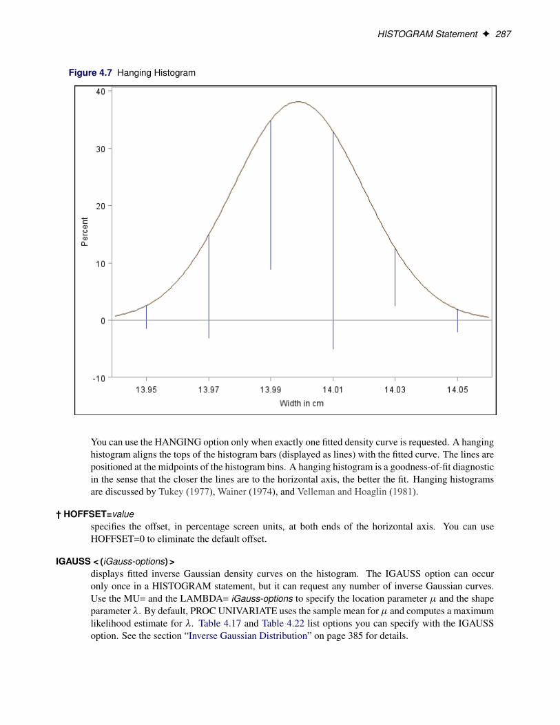
HISTOGRAM Statement F 287
Figure 4.7 Hanging Histogram
You can use the HANGING option only when exactly one fitted density curve is requested. A hanginghistogram aligns the tops of the histogram bars (displayed as lines) with the fitted curve. The lines arepositioned at the midpoints of the histogram bins. A hanging histogram is a goodness-of-fit diagnosticin the sense that the closer the lines are to the horizontal axis, the better the fit. Hanging histogramsare discussed by Tukey (1977), Wainer (1974), and Velleman and Hoaglin (1981).
† HOFFSET=valuespecifies the offset, in percentage screen units, at both ends of the horizontal axis. You can useHOFFSET=0 to eliminate the default offset.
IGAUSS < (iGauss-options) >displays fitted inverse Gaussian density curves on the histogram. The IGAUSS option can occuronly once in a HISTOGRAM statement, but it can request any number of inverse Gaussian curves.Use the MU= and the LAMBDA= iGauss-options to specify the location parameter � and the shapeparameter �. By default, PROC UNIVARIATE uses the sample mean for � and computes a maximumlikelihood estimate for �. Table 4.17 and Table 4.22 list options you can specify with the IGAUSSoption. See the section “Inverse Gaussian Distribution” on page 385 for details.
288 F Chapter 4: The UNIVARIATE Procedure
† INTERBAR=valuespecifies the space between histogram bars in percentage screen units. If both the INTERBAR= andBARWIDTH= options are specified, the INTERBAR= option takes precedence.
K=NORMAL | QUADRATIC | TRIANGULARspecifies the kernel function (normal, quadratic, or triangular) used to compute a kernel density es-timate. You can specify a list of values to request multiple estimates. You must enclose this optionin parentheses after the KERNEL option. You can also use the K= kernel-option with the C= kernel-option, which specifies standardized bandwidths. If you specify more kernel functions than band-widths, the procedure repeats the last bandwidth in the list for the remaining estimates. Similarly, ifyou specify more bandwidths than kernel functions, the procedure repeats the last kernel function forthe remaining estimates. By default, K=NORMAL.
KERNEL< (kernel-options) >superimposes kernel density estimates on the histogram. By default, the procedure uses the AMISEmethod to compute kernel density estimates. To request multiple kernel density estimates on thesame histogram, specify a list of values for the C= kernel-option or K= kernel-option. Table 4.31 listsoptions you can specify with the KERNEL option. See the section “Kernel Density Estimates” onpage 398 for more information about kernel density estimates, and see Example 4.23.
LAMBDA=valuespecifies the shape parameter � for fitted curves requested with the IGAUSS option. Enclose theLAMBDA= option in parentheses after the IGAUSS distribution keyword. If you do not specify avalue for �, the procedure calculates a maximum likelihood estimate.
† LGRID=linetypespecifies the line type for the grid when a grid displays on the histogram. This option also creates agrid if the GRID option is not specified.
LOGNORMAL< (lognormal-options) >displays fitted lognormal density curves on the histogram. The LOGNORMAL option can occur onlyonce in a HISTOGRAM statement, but it can request any number of lognormal curves. The parameter� must be less than the minimum data value. Use the THETA= lognormal-option to specify � . Bydefault, THETA=0. You can specify THETA=EST to request the maximum likelihood estimate for� . Use the SIGMA= and ZETA= lognormal-options to specify � and �. By default, the procedurecomputes maximum likelihood estimates for � and �. Table 4.17 and Table 4.23 list options you canspecify with the LOGNORMAL option. See the section “Lognormal Distribution” on page 385 fordetails, and see Example 4.22 and Example 4.24 for examples using the LOGNORMAL option.
LOWER=value-listspecifies lower bounds for kernel density estimates requested with the KERNEL option. Enclose theLOWER= option in parentheses after the KERNEL option. If you specify more kernel estimates thanlower bounds, the last lower bound is repeated for the remaining estimates. The default is a missingvalue, indicating no lower bounds for fitted kernel density curves.
MAXNBIN=nlimits the number of bins displayed in the comparative histogram. This option is useful when thescales or ranges of the data distributions differ greatly from cell to cell. By default, the bin size andmidpoints are determined for the key cell, and then the midpoint list is extended to accommodate

HISTOGRAM Statement F 289
the data ranges for the remaining cells. However, if the cell scales differ considerably, the resultingnumber of bins can be so great that each cell histogram is scaled into a narrow region. By usingMAXNBIN= to limit the number of bins, you can narrow the window about the data distribution inthe key cell. This option is not available unless you specify the CLASS statement. The MAXNBIN=option is an alternative to the MAXSIGMAS= option.
MAXSIGMAS=valuelimits the number of bins displayed in the comparative histogram to a range of value standard devia-tions (of the data in the key cell) above and below the mean of the data in the key cell. This option isuseful when the scales or ranges of the data distributions differ greatly from cell to cell. By default,the bin size and midpoints are determined for the key cell, and then the midpoint list is extended toaccommodate the data ranges for the remaining cells. However, if the cell scales differ considerably,the resulting number of bins can be so great that each cell histogram is scaled into a narrow region.By using MAXSIGMAS= to limit the number of bins, you can narrow the window that surrounds thedata distribution in the key cell. This option is not available unless you specify the CLASS statement.
MIDPERCENTSrequests a table listing the midpoints and percentage of observations in each histogram interval. Ifyou specify MIDPERCENTS in parentheses after a density estimate option, the procedure displays atable that lists the midpoints, the observed percentage of observations, and the estimated percentageof the population in each interval (estimated from the fitted distribution). See Example 4.18.
MIDPOINTS=values | KEY | UNIFORMspecifies how to determine the midpoints for the histogram intervals, where values determines thewidth of the histogram bars as the difference between consecutive midpoints. The procedure uses thesame values for all variables.
The range of midpoints, extended at each end by half of the bar width, must cover the range of thedata. For example, if you specify
midpoints=2 to 10 by 0.5
then all of the observations should fall between 1.75 and 10.25. You must use evenly spaced midpointslisted in increasing order.
KEY determines the midpoints for the data in the key cell. The initial number of mid-points is based on the number of observations in the key cell that use the methodof Terrell and Scott (1985). The procedure extends the midpoint list for the keycell in either direction as necessary until it spans the data in the remaining cells.
UNIFORM determines the midpoints by using all the observations as if there were no cells. Inother words, the number of midpoints is based on the total sample size by usingthe method of Terrell and Scott (1985).
Neither KEY nor UNIFORM apply unless you use the CLASS statement. By default, if youuse a CLASS statement, MIDPOINTS=KEY; however, if the key cell is empty then MID-POINTS=UNIFORM. Otherwise, the procedure computes the midpoints by using an algorithm (Ter-rell and Scott 1985) that is primarily applicable to continuous data that are approximately normallydistributed.

290 F Chapter 4: The UNIVARIATE Procedure
MU=value-listspecifies the parameter � for Gumbel, inverse Gaussian, and normal density curves requested with theGUMBEL, IGAUSS, and NORMAL options, respectively. Enclose the MU= option in parenthesesafter the distribution keyword. By default, or if you specify the value EST, the procedure uses thesample mean for� for normal and inverse Gaussian distributions and computes a maximum likelihoodestimate of � for the Gumbel distribution. For more detail please see “Inverse Gaussian Distribution”on page 385 and “Gumbel Distribution” on page 384.
NENDPOINTS=nuses histogram interval endpoints as the tick mark values for the horizontal axis and determines thenumber of bins.
NMIDPOINTS=nspecifies the number of histogram intervals.
NOBARSsuppresses drawing of histogram bars, which is useful for viewing fitted curves only.
NOPLOT
NOCHARTsuppresses the creation of a plot. Use this option when you only want to tabulate summary statisticsfor a fitted density or create an OUTHISTOGRAM= data set.
NOPRINTsuppresses tables summarizing the fitted curve. Enclose the NOPRINT option in parentheses follow-ing the distribution option.
NORMAL< (normal-options) >displays fitted normal density curves on the histogram. The NORMAL option can occur only oncein a HISTOGRAM statement, but it can request any number of normal curves. Use the MU= andSIGMA= normal-options to specify � and � . By default, the procedure uses the sample mean andsample standard deviation for � and � . Table 4.17 and Table 4.24 list options you can specify withthe NORMAL option. See the section “Normal Distribution” on page 386 for details, and see Exam-ple 4.19 for an example that uses the NORMAL option.
NOTABCONTENTSsuppresses the table of contents entries for tables produced by the HISTOGRAM statement.
OUTHISTOGRAM=SAS-data-set
OUTHIST=SAS-data-setcreates a SAS data set that contains information about histogram intervals. Specifically, the data setcontains the midpoints of the histogram intervals (or the lower endpoints of the intervals if you specifythe ENDPOINTS option), the observed percentage of observations in each interval, and the estimatedpercentage of observations in each interval (estimated from each of the specified fitted curves).
PARETO < (Pareto-options) >displays fitted generalized Pareto density curves on the histogram. The PARETO option can occuronly once in a HISTOGRAM statement, but it can request any number of generalized Pareto curves.The parameter � must be less than the minimum data value. Use the THETA= Pareto-option to

HISTOGRAM Statement F 291
specify � . By default, THETA=0. Use the SIGMA= and the ALPHA= Pareto-options to specify thescale parameter � and the shape parameter ˛. By default, PROC UNIVARIATE computes maximumlikelihood estimates for � and ˛. Table 4.17 and Table 4.25 list options you can specify with thePARETO option. See the section “Generalized Pareto Distribution” on page 387 for details.
PERCENTS=values
PERCENT=valuesspecifies a list of percents for which quantiles calculated from the data and quantiles estimated fromthe fitted curve are tabulated. The percents must be between 0 and 100. Enclose the PERCENTS=option in parentheses after the curve option. The default percents are 1, 5, 10, 25, 50, 75, 90, 95, and99.
† PFILL=patternspecifies a pattern used to fill the bars of the histograms (or the areas under a fitted curve if you alsospecify the FILL option) when producing traditional graphics. See the entries for the CFILL= andFILL options for additional details. Refer to SAS/GRAPH: Reference for a list of pattern values. Theoption does not apply to ODS Graphics output.
POWER < (power-options) >displays fitted power function density curves on the histogram. The POWER option can occur onlyonce in a HISTOGRAM statement, but it can request any number of power function curves. Theparameter � must be less than the minimum data value. Use the THETA= and SIGMA= power-optionsto specify � and � . The default values are 0 and 1, respectively. Use the ALPHA= power-option tospecify the and the shape parameter, ˛. By default, PROC UNIVARIATE computes a maximumlikelihood estimate for ˛. Table 4.17 and Table 4.26 list options you can specify with the POWERoption. See the section “Power Function Distribution” on page 388 for details.
RAYLEIGH < (Rayleigh-options) >displays fitted Rayleigh density curves on the histogram. The RAYLEIGH option can occur onlyonce in a HISTOGRAM statement, but it can request any number of Rayleigh curves. The parameter� must be less than the minimum data value. Use the THETA= Rayleigh-option to specify � . Bydefault, THETA=0. Use the SIGMA= Rayleigh-option to specify the scale parameter � . By default,PROC UNIVARIATE computes maximum likelihood estimates for � . Table 4.17 and Table 4.27 listoptions you can specify with the RAYLEIGH option. See the section “Rayleigh Distribution” onpage 389 for details.
RTINCLUDEincludes the right endpoint of each histogram interval in that interval. By default, the left endpoint isincluded in the histogram interval.
SB< (SB -options) >displays fitted Johnson SB density curves on the histogram. The SB option can occur only once ina HISTOGRAM statement, but it can request any number of Johnson SB curves. Use the THETA=and SIGMA= normal-options to specify � and � . By default, the procedure computes maximumlikelihood estimates of � and � . Table 4.17 and Table 4.28 list options you can specify with the SBoption. See the section “Johnson SB Distribution” on page 390 for details.

292 F Chapter 4: The UNIVARIATE Procedure
SIGMA=value-listspecifies the parameter � for the fitted density curve when you request the BETA, EXPONENTIAL,GAMMA, GUMBEL, LOGNORMAL, NORMAL, PARETO, POWER, RAYLEIGH, SB, SU, orWEIBULL options.
See Table 4.34 for a summary of how to use the SIGMA= option. You must enclose this option inparentheses after the density curve option. You can specify the value EST to request a maximumlikelihood estimate for � .
Table 4.34 Uses of the SIGMA= Option
Distribution Keyword SIGMA= Specifies Default Value Alias
BETA scale parameter � 1 SCALE=EXPONENTIAL scale parameter � maximum likelihood estimate SCALE=GAMMA scale parameter � maximum likelihood estimate SCALE=GUMBEL scale parameter � maximum likelihood estimateLOGNORMAL shape parameter � maximum likelihood estimate SHAPE=NORMAL scale parameter � standard deviationPARETO scale parameter � 1POWER scale parameter � maximum likelihood estimateRAYLEIGH scale parameter � maximum likelihood estimateSB scale parameter � 1 SCALE=SU scale parameter � percentile-based estimateWEIBULL scale parameter � maximum likelihood estimate SCALE=
SU< (SU -options) >displays fitted Johnson SU density curves on the histogram. The SU option can occur only once ina HISTOGRAM statement, but it can request any number of Johnson SU curves. Use the THETA=and SIGMA= normal-options to specify � and � . By default, the procedure computes maximumlikelihood estimates of � and � . Table 4.17 and Table 4.29 list options you can specify with the SUoption. See the section “Johnson SU Distribution” on page 391 for details.
THETA=value-list
THRESHOLD= value-listspecifies the lower threshold parameter � for curves requested with the BETA, EXPONENTIAL,GAMMA, LOGNORMAL, PARETO, POWER, RAYLEIGH, SB, SU, and WEIBULL options. En-close the THETA= option in parentheses after the curve option. By default, THETA=0. If you specifythe value EST, an estimate is computed for � .
UPPER=value-listspecifies upper bounds for kernel density estimates requested with the KERNEL option. Enclose theUPPER= option in parentheses after the KERNEL option. If you specify more kernel estimates thanupper bounds, the last upper bound is repeated for the remaining estimates. The default is a missingvalue, indicating no upper bounds for fitted kernel density curves.
† VOFFSET=valuespecifies the offset, in percentage screen units, at the upper end of the vertical axis.

ID Statement F 293
VSCALE=COUNT | PERCENT | PROPORTIONspecifies the scale of the vertical axis for a histogram. The value COUNT requests the data be scaledin units of the number of observations per data unit. The value PERCENT requests the data be scaledin units of percent of observations per data unit. The value PROPORTION requests the data be scaledin units of proportion of observations per data unit. The default is PERCENT.
† WBARLINE=nspecifies the width of bar outlines when producing traditional graphics. The option does not apply toODS Graphics output.
WEIBULL< (Weibull-options) >displays fitted Weibull density curves on the histogram. The WEIBULL option can occur only oncein a HISTOGRAM statement, but it can request any number of Weibull curves. The parameter �must be less than the minimum data value. Use the THETA= Weibull-option to specify � . By de-fault, THETA=0. You can specify THETA=EST to request the maximum likelihood estimate for � .Use the C= and SIGMA= Weibull-options to specify the shape parameter c and the scale parameter� . By default, the procedure computes the maximum likelihood estimates for c and � . Table 4.17and Table 4.30 list options you can specify with the WEIBULL option. See the section “WeibullDistribution” on page 392 for details, and see Example 4.22 for an example that uses the WEIBULLoption.
PROC UNIVARIATE calculates the maximum likelihood estimate of a iteratively by using theNewton-Raphson approximation. See also the C=, SIGMA=, and THETA= Weibull-options.
† WGRID=nspecifies the line thickness for the grid when producing traditional graphics. The option does notapply to ODS Graphics output.
ZETA= value-listspecifies a value for the scale parameter � for lognormal density curves requested with the LOGNOR-MAL option. Enclose the ZETA= lognormal-option in parentheses after the LOGNORMAL option.By default, or if you specify the value EST, the procedure calculates a maximum likelihood estimatefor �. You can specify the SCALE= option as an alias for the ZETA= option.
ID Statement
ID variables ;
The ID statement specifies one or more variables to include in the table of extreme observations. Thecorresponding values of the ID variables appear beside the n largest and n smallest observations, where n isthe value of NEXTROBS= option. See Example 4.3.
You can also include ID variables in the output data set created by an OUTPUT statement by specifying theIDOUT option in the PROC UNIVARIATE statement.

294 F Chapter 4: The UNIVARIATE Procedure
INSET Statement
INSET keywords < / options > ;
An INSET statement places a box or table of summary statistics, called an inset, directly in a graph createdwith a CDFPLOT, HISTOGRAM, PPPLOT, PROBPLOT, or QQPLOT statement. The INSET statementmust follow the plot statement that creates the plot that you want to augment. The inset appears in all thegraphs that the preceding plot statement produces.
You can use multiple INSET statements after a plot statement to add more than one inset to a plot. SeeExample 4.17.
In an INSET statement, you specify one or more keywords that identify the information to display in theinset. The information is displayed in the order that you request the keywords. Keywords can be any of thefollowing:
� statistical keywords
� primary keywords
� secondary keywords
The available statistical keywords are listed in Table 4.35 through Table 4.41.
Table 4.35 Descriptive Statistic Keywords
Keyword Description
CSS corrected sum of squaresCV coefficient of variationKURTOSIS | KURT kurtosisMAX largest valueMEAN sample meanMIN smallest valueMODE most frequent valueN sample sizeNEXCL number of observations excluded by MAXNBIN= or
MAXSIGMAS= optionNMISS number of missing valuesNOBS number of observationsRANGE rangeSKEWNESS | SKEW skewnessSTD | STDDEV standard deviationSTDMEAN | STDERR standard error of the meanSUM sum of the observationsSUMWGT sum of the weightsUSS uncorrected sum of squaresVAR variance

INSET Statement F 295
Table 4.36 Percentile Statistic Keywords
Keyword Description
P1 1st percentileP5 5th percentileP10 10th percentileQ1P25 lower quartile (25th percentile)MEDIANQ2P50 median (50th percentile)Q3P75 upper quartile (75th percentile)P90 90th percentileP95 95th percentileP99 99th percentileQRANGE interquartile range (Q3 - Q1)
Table 4.37 lists keywords for distribution-free confidence limits for percentiles requested with theCIPCTLDF option.

296 F Chapter 4: The UNIVARIATE Procedure
Table 4.37 Keywords for Distribution-Free Confidence Limits for Percentiles
Keyword Description
P1_LCL_DF 1st percentile lower confidence limitP1_UCL_DF 1st percentile upper confidence limitP5_LCL_DF 5th percentile lower confidence limitP5_UCL_DF 5th percentile upper confidence limitP10_LCL_DF 10th percentile lower confidence limitP10_UCL_DF 10th percentile upper confidence limitQ1_LCL_DFP25_LCL_DF lower quartile (25th percentile) lower confidence limitQ1_UCL_DFP25_UCL_DF lower quartile (25th percentile) upper confidence limitMEDIAN_LCL_DFQ2_LCL_DFP50_LCL_DF median (50th percentile) lower confidence limitMEDIAN_UCL_DFQ2_UCL_DFP50_UCL_DF median (50th percentile) upper confidence limitQ3_LCL_DFP75_LCL_DF upper quartile (75th percentile) lower confidence limitQ3_UCL_DFP75_UCL_DF upper quartile (75th percentile) upper confidence limitP90_LCL_DF 90th percentile lower confidence limitP90_UCL_DF 90th percentile upper confidence limitP95_LCL_DF 95th percentile lower confidence limitP95_UCL_DF 95th percentile upper confidence limitP99_LCL_DF 99th percentile lower confidence limitP99_UCL_DF 99th percentile upper confidence limit
Table 4.38 lists keywords for percentile confidence limits computed assuming normality requested with theCIPCTLNORMAL option.

INSET Statement F 297
Table 4.38 Keywords Percentile Confidence Limits Assuming Normality
Keyword Description
P1_LCL 1st percentile lower confidence limitP1_UCL 1st percentile upper confidence limitP5_LCL 5th percentile lower confidence limitP5_UCL 5th percentile upper confidence limitP10_LCL 10th percentile lower confidence limitP10_UCL 10th percentile upper confidence limitQ1_LCLP25_LCL lower quartile (25th percentile) lower confidence limitQ1_UCLP25_UCL lower quartile (25th percentile) upper confidence limitMEDIAN_LCLQ2_LCLP50_LCL median (50th percentile) lower confidence limitMEDIAN_UCLQ2_UCLP50_UCL median (50th percentile) upper confidence limitQ3_LCLP75_LCL upper quartile (75th percentile) lower confidence limitQ3_UCLP75_UCL upper quartile (75th percentile) upper confidence limitP90_LCL 90th percentile lower confidence limitP90_UCL 90th percentile upper confidence limitP95_LCL 95th percentile lower confidence limitP95_UCL 95th percentile upper confidence limitP99_LCL 99th percentile lower confidence limitP99_UCL 99th percentile upper confidence limit
Table 4.39 Robust Statistics Keywords
Keyword Description
GINI Gini’s mean differenceMAD median absolute difference about the medianQN Qn, alternative to MADSN Sn, alternative to MADSTD_GINI Gini’s standard deviationSTD_MAD MAD standard deviationSTD_QN Qn standard deviationSTD_QRANGE interquartile range standard deviationSTD_SN Sn standard deviation

298 F Chapter 4: The UNIVARIATE Procedure
Table 4.40 Hypothesis Testing Keywords
Keyword Description
MSIGN sign statisticNORMALTEST test statistic for normalityPNORMAL probability value for the test of normalitySIGNRANK signed rank statisticPROBM probability of greater absolute value for the sign statisticPROBN probability value for the test of normalityPROBS probability value for the signed rank testPROBT probability value for the Student’s t testT statistics for Student’s t test
Table 4.41 Keyword for Reading Input Data Set
Keyword Description
DATA= (label, value) pairs from input data set
To create a completely customized inset, use a DATA= data set.
DATA=SAS-data-setrequests that PROC UNIVARIATE display customized statistics from a SAS data set in the inset table.The data set must contain two variables:
_LABEL_ a character variable whose values provide labels for inset entries
_VALUE_ a variable that is either character or numeric and whose values provide values forinset entries
The label and value from each observation in the data set occupy one line in the inset. The position ofthe DATA= keyword in the keyword list determines the position of its lines in the inset.
A primary keyword enables you to specify secondary keywords in parentheses immediately after the pri-mary keyword. The primary keywords are listed in Table 4.42 and Table 4.43. If you specify a primarykeyword but omit a secondary keyword, the inset displays a colored line and the distribution name as a keyfor the density curve.
By default, PROC UNIVARIATE identifies inset statistics with appropriate labels and prints numeric valueswith appropriate formats. To customize the label, specify the keyword followed by an equal sign (=) and thedesired label in quotes. To customize the format, specify a numeric format in parentheses after the keyword.Labels can have up to 24 characters. If you specify both a label and a format for a statistic, the label mustappear before the format. For example,
inset n='Sample Size' std='Std Dev' (5.2);
requests customized labels for two statistics and displays the standard deviation with a field width of 5 andtwo decimal places.

INSET Statement F 299
Table 4.42 Parametric Density Primary Keywords
Keyword Distribution Plot Statement Availability
BETA beta all plot statementsEXPONENTIAL exponential all plot statementsGAMMA gamma all plot statementsGUMBEL Gumbel all plot statementsIGAUSS inverse Gaussian CDFPLOT, HISTOGRAM, PPPLOTLOGNORMAL lognormal all plot statementsNORMAL normal all plot statementsPARETO Pareto all plot statementsPOWER power function all plot statementsRAYLEIGH Rayleigh all plot statementsSB Johnson SB HISTOGRAMSU Johnson SU HISTOGRAMWEIBULL Weibull(3-parameter) all plot statementsWEIBULL2 Weibull(2-parameter) PROBPLOT, QQPLOT
Table 4.43 Kernel Density Estimate Primary Keywords
Keyword Description
KERNEL displays statistics for all kernel estimatesKERNELn displays statistics for only the nth kernel density estimate
n D 1; 2; 3; 4; or 5
Table 4.44 through Table 4.58 list the secondary keywords available with primary keywords in Table 4.42and Table 4.43.
Table 4.44 Secondary Keywords Available with the BETA Keyword
Secondary Keyword Alias Description
ALPHA SHAPE1 first shape parameter ˛BETA SHAPE2 second shape parameter ˇMEAN mean of the fitted distributionSIGMA SCALE scale parameter �STD standard deviation of the fitted distributionTHETA THRESHOLD lower threshold parameter �

300 F Chapter 4: The UNIVARIATE Procedure
Table 4.45 Secondary Keywords Available with the EXPONENTIAL Keyword
Secondary Keyword Alias Description
MEAN mean of the fitted distributionSIGMA SCALE scale parameter �STD standard deviation of the fitted distributionTHETA THRESHOLD threshold parameter �
Table 4.46 Secondary Keywords Available with the GAMMA Keyword
Secondary Keyword Alias Description
ALPHA SHAPE shape parameter ˛MEAN mean of the fitted distributionSIGMA SCALE scale parameter �STD standard deviation of the fitted distributionTHETA THRESHOLD threshold parameter �
Table 4.47 Secondary Keywords Available with the GUMBEL Keyword
Secondary Keyword Alias Description
MEAN mean of the fitted distributionMU location parameter �SIGMA SCALE scale parameter �STD standard deviation of the fitted distribution
Table 4.48 Secondary Keywords Available with the IGAUSS Keyword
Secondary Keyword Alias Description
LAMBDA shape parameter �MEAN mean of the fitted distributionMU mean parameter �STD standard deviation of the fitted distribution
Table 4.49 Secondary Keywords Available with the LOGNORMAL Keyword
Secondary Keyword Alias Description
MEAN mean of the fitted distributionSIGMA SHAPE shape parameter �STD standard deviation of the fitted distributionTHETA THRESHOLD threshold parameter �ZETA SCALE scale parameter �

INSET Statement F 301
Table 4.50 Secondary Keywords Available with the NORMAL Keyword
Secondary Keyword Alias Description
MU MEAN mean parameter �SIGMA STD scale parameter �
Table 4.51 Secondary Keywords Available with the PARETO Keyword
Secondary Keyword Alias Description
ALPHA shape parameter ˛MEAN mean of the fitted distributionSIGMA SCALE scale parameter �STD standard deviation of the fitted distributionTHETA THRESHOLD threshold parameter �
Table 4.52 Secondary Keywords Available with the POWER Keyword
Secondary Keyword Alias Description
ALPHA shape parameter ˛MEAN mean of the fitted distributionSIGMA SCALE scale parameter �STD standard deviation of the fitted distributionTHETA THRESHOLD threshold parameter �
Table 4.53 Secondary Keywords Available with the RAYLEIGH Keyword
Secondary Keyword Alias Description
MEAN mean of the fitted distributionSIGMA SCALE scale parameter �STD standard deviation of the fitted distributionTHETA THRESHOLD threshold parameter �
Table 4.54 Secondary Keywords Available with the SB and SU Keywords
Secondary Keyword Alias Description
DELTA SHAPE1 first shape parameter ıGAMMA SHAPE2 second shape parameter MEAN mean of the fitted distributionSIGMA SCALE scale parameter �STD standard deviation of the fitted distributionTHETA THRESHOLD lower threshold parameter �

302 F Chapter 4: The UNIVARIATE Procedure
Table 4.55 Secondary Keywords Available with the WEIBULL
Secondary Keyword Alias Description
C SHAPE shape parameter cMEAN mean of the fitted distributionSIGMA SCALE scale parameter �STD standard deviation of the fitted distributionTHETA THRESHOLD threshold parameter �
Table 4.56 Secondary Keywords Available with the WEIBULL2 Keyword
Secondary Keyword Alias Description
C SHAPE shape parameter cMEAN mean of the fitted distributionSIGMA SCALE scale parameter �STD standard deviation of the fitted distributionTHETA THRESHOLD known lower threshold �0
Table 4.57 Secondary Keywords Available with the KERNEL Keyword
Secondary Keyword Description
AMISE approximate mean integrated square error (MISE) for the kernel den-sity
BANDWIDTH bandwidth � for the density estimateBWIDTH alias for BANDWIDTHC standardized bandwidth c for the density estimate:
c D �Qn15 where n D sample size, � D bandwidth, and
Q D interquartile rangeTYPE kernel type: normal, quadratic, or triangular
Table 4.58 Goodness-of-Fit Statistics for Fitted Curves
Secondary Keyword Description
AD Anderson-Darling EDF test statisticADPVAL Anderson-Darling EDF test p-valueCVM Cramér-von Mises EDF test statisticCVMPVAL Cramér-von Mises EDF test p-valueKSD Kolmogorov-Smirnov EDF test statisticKSDPVAL Kolmogorov-Smirnov EDF test p-value

INSET Statement F 303
The inset statistics listed in Table 4.42 through Table 4.58 are not available unless you request a plot state-ment and options that calculate these statistics. For example, consider the following statements:
proc univariate data=score;histogram final / normal;inset mean std normal(ad adpval);
run;
The MEAN and STD keywords display the sample mean and standard deviation of final. The NORMALkeyword with the secondary keywords AD and ADPVAL display the Anderson-Darling goodness-of-fittest statistic and p-value. The statistics that are specified with the NORMAL keyword are available onlybecause the NORMAL option is requested in the HISTOGRAM statement.
The KERNEL or KERNELn keyword is available only if you request a kernel density estimate in a HIS-TOGRAM statement. The WEIBULL2 keyword is available only if you request a two-parameter Weibulldistribution in the PROBPLOT or QQPLOT statement.
If you specify multiple kernel density estimates, you can request inset statistics for all the estimates with theKERNEL keyword. Alternatively, you can display inset statistics for individual curves with the KERNELnkeyword, where n is the curve number between 1 and 5.
Summary of Options
Table 4.59 lists INSET statement options, which are specified after the slash (/) in the INSET statement. Forcomplete descriptions, see the section “Dictionary of Options” on page 304.
Table 4.59 INSET Options
Option Description
CFILL=color | BLANK specifies color of inset backgroundCFILLH=color specifies color of header backgroundCFRAME=color specifies color of frameCHEADER=color specifies color of header textCSHADOW=color specifies color of drop shadowCTEXT=color specifies color of inset textDATA specifies data units for POSITION=.x; y/ coordinatesFONT=font specifies font of textFORMAT=format specifies format of values in insetGUTTER=value specifies gutter width for inset in top or bottom marginHEADER=‘string’ specifies header textHEIGHT=value specifies height of inset textNCOLS= specifies number of columns for inset in top or bottom mar-
ginNOFRAME suppresses frame around insetPOSITION=position specifies position of insetREFPOINT=BR | BL | TR | TL specifies reference point of inset positioned with
POSITION=.x; y/ coordinates

304 F Chapter 4: The UNIVARIATE Procedure
Dictionary of Options
The following entries provide detailed descriptions of options for the INSET statement. Options markedwith † are applicable only when traditional graphics are produced.
† CFILL=color | BLANKspecifies the color of the background for traditional graphics. If you omit the CFILLH= option theheader background is included. By default, the background is empty, which causes items that overlapthe inset (such as curves or histogram bars) to show through the inset.
If you specify a value for CFILL= option, then overlapping items no longer show through the inset.Use CFILL=BLANK to leave the background uncolored and to prevent items from showing throughthe inset.
† CFILLH=colorspecifies the color of the header background for traditional graphics. The default value is the CFILL=color.
† CFRAME=colorspecifies the color of the frame for traditional graphics. The default value is the same color as the axisof the plot.
† CHEADER=colorspecifies the color of the header text for traditional graphics. The default value is the CTEXT= color.
† CSHADOW=colorspecifies the color of the drop shadow for traditional graphics. By default, if a CSHADOW= optionis not specified, a drop shadow is not displayed.
† CTEXT=colorspecifies the color of the text for traditional graphics. The default value is the same color as the othertext on the plot.
DATAspecifies that data coordinates are to be used in positioning the inset with the POSITION= option.The DATA option is available only when you specify POSITION=(x,y). You must place DATA im-mediately after the coordinates (x,y). NOTE: Positioning insets with coordinates is not supported forODS Graphics output.
† FONT=fontspecifies the font of the text for traditional graphics. By default, if you locate the inset in the interiorof the plot, then the font is SIMPLEX. If you locate the inset in the exterior of the plot, then the fontis the same as the other text on the plot.
FORMAT=formatspecifies a format for all the values in the inset. If you specify a format for a particular statistic, thenthat format overrides the one specified with the FORMAT= option. For more information about SASformats, see SAS Formats and Informats: Reference.
OUTPUT Statement F 305
GUTTER=valuespecifies the gutter width in percent screen units for an inset located in the top or bottom margin.The gutter is the space between columns of (label, value) pairs in an inset. The default value is four.NOTE: The GUTTER= option applies only when ODS Graphics is enabled.
HEADER=stringspecifies the header text. The string cannot exceed 40 characters. By default, no header line appearsin the inset. If all the keywords that you list in the INSET statement are secondary keywords thatcorrespond to a fitted curve on a histogram, PROC UNIVARIATE displays a default header thatindicates the distribution and identifies the curve.
† HEIGHT=valuespecifies the height of the text for traditional graphics.
NCOLS=nspecifies the number of columns of (label, value) pairs displayed in an inset located in the top orbottom margin. The default value is three. NOTE: The NCOLS= option applies only when ODSGraphics is enabled.
NOFRAMEsuppresses the frame drawn around the text.
POSITION=position
POS=positiondetermines the position of the inset. The position is a compass point keyword, a margin keyword, ora pair of coordinates (x,y). You can specify coordinates in axis percent units or axis data units. Thedefault value is NW, which positions the inset in the upper left (northwest) corner of the display. Seethe section “Positioning Insets” on page 376.
NOTE: Positioning insets with coordinates is not supported for ODS Graphics output.
† REFPOINT=BR | BL | TR | TLspecifies the reference point for an inset that PROC UNIVARIATE positions by a pair of coordinateswith the POSITION= option. The REFPOINT= option specifies which corner of the inset frame thatyou want to position at coordinates (x,y). The keywords are BL, BR, TL, and TR, which correspond tobottom left, bottom right, top left, and top right. The default value is BL. You must use REFPOINT=with POSITION=(x,y) coordinates. The option does not apply to ODS Graphics output.
OUTPUT Statement
OUTPUT < OUT=SAS-data-set < keyword1=names . . . keywordk=names > < percentile-options > > ;
The OUTPUT statement saves statistics and BY variables in an output data set. When you use a BYstatement, each observation in the OUT= data set corresponds to one of the BY groups. Otherwise, theOUT= data set contains only one observation.
You can use any number of OUTPUT statements in the UNIVARIATE procedure. Each OUTPUT state-ment creates a new data set containing the statistics specified in that statement. You must use the VAR

306 F Chapter 4: The UNIVARIATE Procedure
statement with the OUTPUT statement. The OUTPUT statement must contain a specification of the formkeyword=names or the PCTLPTS= and PCTLPRE= specifications. See Example 4.7 and Example 4.8.
OUT=SAS-data-setidentifies the output data set. If SAS-data-set does not exist, PROC UNIVARIATE creates it. If youomit OUT=, the data set is named DATAn, where n is the smallest integer that makes the name unique.
keyword=namesspecifies the statistics to include in the output data set and gives names to the new variables that containthe statistics. Specify a keyword for each desired statistic, followed by an equal sign, followed by thenames of the variables to contain the statistic. In the output data set, the first variable listed aftera keyword in the OUTPUT statement contains the statistic for the first variable listed in the VARstatement, the second variable contains the statistic for the second variable in the VAR statement, andso on. If the list of names following the equal sign is shorter than the list of variables in the VARstatement, the procedure uses the names in the order in which the variables are listed in the VARstatement. The available keywords are listed in the following tables:
Table 4.60 Descriptive Statistic Keywords
Keyword Description
CSS corrected sum of squaresCV coefficient of variationKURTOSIS | KURT kurtosisMAX largest valueMEAN sample meanMIN smallest valueMODE most frequent valueN sample sizeNMISS number of missing valuesNOBS number of observationsRANGE rangeSKEWNESS |SKEW
skewness
STD | STDDEV standard deviationSTDMEAN |STDERR
standard error of the mean
SUM sum of the observationsSUMWGT sum of the weightsUSS uncorrected sum of squaresVAR variance

OUTPUT Statement F 307
Table 4.61 Quantile Statistic Keywords
Keyword Description
P1 1st percentileP5 5th percentileP10 10th percentileQ1 | P25 lower quartile (25th percentile)MEDIAN | Q2 | P50 median (50th percentile)Q3 | P75 upper quartile (75th percentile)P90 90th percentileP95 95th percentileP99 99th percentileQRANGE interquartile range (Q3 - Q1)
Table 4.62 Robust Statistics Keywords
Keyword Description
GINI Gini’s mean differenceMAD median absolute difference about the medianQN Qn, alternative to MADSN Sn, alternative to MADSTD_GINI Gini’s standard deviationSTD_MAD MAD standard deviationSTD_QN Qn standard deviationSTD_QRANGE interquartile range standard deviationSTD_SN Sn standard deviation
Table 4.63 Hypothesis Testing Keywords
Keyword Description
MSIGN sign statisticNORMALTEST test statistic for normalitySIGNRANK signed rank statisticPROBM probability of a greater absolute value for the sign statisticPROBN probability value for the test of normalityPROBS probability value for the signed rank testPROBT probability value for the Student’s t testT statistic for the Student’s t test
The UNIVARIATE procedure automatically computes the 1st, 5th, 10th, 25th, 50th, 75th, 90th, 95th,and 99th percentiles for the data. These can be saved in an output data set by using keyword=namesspecifications. For additional percentiles, you can use the following percentile-options.

308 F Chapter 4: The UNIVARIATE Procedure
PCTLPTS=percentilesspecifies one or more percentiles that are not automatically computed by the UNIVARIATE procedure.The PCTLPRE= and PCTLPTS= options must be used together. You can specify percentiles with anexpression of the form start TO stop BY increment where start is a starting number, stop is an endingnumber, and increment is a number to increment by. The PCTLPTS= option generates additionalpercentiles and outputs them to a data set. These additional percentiles are not printed.
To compute the 50th, 95th, 97.5th, and 100th percentiles, submit the statement
output pctlpre=P_ pctlpts=50,95 to 100 by 2.5;
PROC UNIVARIATE computes the requested percentiles based on the method that you specify withthe PCTLDEF= option in the PROC UNIVARIATE statement. You must use PCTLPRE=, and op-tionally PCTLNAME=, to specify variable names for the percentiles. For example, the followingstatements create an output data set named Pctls that contains the 20th and 40th percentiles of theanalysis variables PreTest and PostTest:
proc univariate data=Score;var PreTest PostTest;output out=Pctls pctlpts=20 40 pctlpre=PreTest_ PostTest_
pctlname=P20 P40;run;
PROC UNIVARIATE saves the 20th and 40th percentiles for PreTest and PostTest in the variablesPreTest_P20, PostTest_P20, PreTest_P40, and PostTest_P40.
PCTLPRE=prefixesspecifies one or more prefixes to create the variable names for the variables that contain thePCTLPTS= percentiles. To save the same percentiles for more than one analysis variable, specifya list of prefixes. The order of the prefixes corresponds to the order of the analysis variables in theVAR statement. The PCTLPRE= and PCTLPTS= options must be used together.
The procedure generates new variable names by using the prefix and the percentile values. If thespecified percentile is an integer, the variable name is simply the prefix followed by the value. Ifthe specified value is not an integer, an underscore replaces the decimal point in the variable name,and decimal values are truncated to one decimal place. For example, the following statements createthe variables pwid20, pwid33_3, pwid66_6, and pwid80 for the 20th, 33.33rd, 66.67th, and 80thpercentiles of Width, respectively:
proc univariate noprint;var Width;output pctlpts=20 33.33 66.67 80 pctlpre=pwid;
run;
If you request percentiles for more than one variable, you should list prefixes in the same order inwhich the variables appear in the VAR statement. If combining the prefix and percentile value resultsin a name longer than 32 characters, the prefix is truncated so that the variable name is 32 characters.

OUTPUT Statement F 309
PCTLNAME=suffixesspecifies one or more suffixes to create the names for the variables that contain the PCTLPTS= per-centiles. PROC UNIVARIATE creates a variable name by combining the PCTLPRE= value and suffixname. Because the suffix names are associated with the percentiles that are requested, list the suffixnames in the same order as the PCTLPTS= percentiles. If you specify n suffixes with the PCTL-NAME= option and m percentile values with the PCTLPTS= option where m > n, the suffixes areused to name the first n percentiles and the default names are used for the remainingm�n percentiles.For example, consider the following statements:
proc univariate;var Length Width Height;output pctlpts = 20 40
pctlpre = pl pw phpctlname = twenty;
run;
The value twenty in the PCTLNAME= option is used for only the first percentile in the PCTLPTS=list. This suffix is appended to the values in the PCTLPRE= option to generate the new variablenames pltwenty, pwtwenty, and phtwenty, which contain the 20th percentiles for Length, Width, andHeight, respectively. Because a second PCTLNAME= suffix is not specified, variable names for the40th percentiles for Length, Width, and Height are generated using the prefixes and percentile values.Thus, the output data set contains the variables pltwenty, pl40, pwtwenty, pw40, phtwenty, and ph40.
You must specify PCTLPRE= to supply prefix names for the variables that contain the PCTLPTS=percentiles.
If the number of PCTLNAME= values is fewer than the number of percentiles or if you omit PCTL-NAME=, PROC UNIVARIATE uses the percentile as the suffix to create the name of the variable thatcontains the percentile. For an integer percentile, PROC UNIVARIATE uses the percentile. Other-wise, PROC UNIVARIATE truncates decimal values of percentiles to two decimal places and replacesthe decimal point with an underscore.
If either the prefix and suffix name combination or the prefix and percentile name combination islonger than 32 characters, PROC UNIVARIATE truncates the prefix name so that the variable nameis 32 characters.
PCTLNDEC=valuespecifies the number of decimal places in percentile values that are incorporated into percentile vari-able names. The default value is 2. For example, the following statements create two output data sets,each containing one percentile variable. The variable in data set short is named pwid85_12, while theone in data set long is named pwid85_125.
proc univariate;var width;output out=short pctlpts=85.125 pctlpre=pwid;output out=long pctlpts=85.125 pctlpre=pwid pctlndec=3;
run;

310 F Chapter 4: The UNIVARIATE Procedure
PPPLOT Statement
PPPLOT < variables > < / options > ;
The PPPLOT statement creates a probability-probability plot (also referred to as a P-P plot or percent plot),which compares the empirical cumulative distribution function (ecdf) of a variable with a specified theoret-ical cumulative distribution function such as the normal. If the two distributions match, the points on theplot form a linear pattern that passes through the origin and has unit slope. Thus, you can use a P-P plot todetermine how well a theoretical distribution models a set of measurements.
You can specify one of the following theoretical distributions with the PPPLOT statement:
� beta
� exponential
� gamma
� Gumbel
� generalized Pareto
� inverse Gaussian
� lognormal
� normal
� power function
� Rayleigh
� Weibull
NOTE: Probability-probability plots should not be confused with probability plots, which compare a set ofordered measurements with percentiles from a specified distribution. You can create probability plots withthe PROBPLOT statement.
You can use any number of PPPLOT statements in the UNIVARIATE procedure. The components of thePPPLOT statement are as follows.
variablesare the process variables for which P-P plots are created. If you specify a VAR statement, the variablesmust also be listed in the VAR statement. Otherwise, the variables can be any numeric variables inthe input data set. If you do not specify a list of variables, then by default, the procedure creates aP-P plot for each variable listed in the VAR statement or for each numeric variable in the input dataset if you do not specify a VAR statement. For example, if data set measures contains two numericvariables, length and width, the following two PPPLOT statements each produce a P-P plot for eachof those variables:

PPPLOT Statement F 311
proc univariate data=measures;var length width;ppplot;
run;
proc univariate data=measures;ppplot length width;
run;
optionsspecify the theoretical distribution for the plot or add features to the plot. If you specify more thanone variable, the options apply equally to each variable. Specify all options after the slash (/) in thePPPLOT statement. You can specify only one option that names a distribution, but you can specifyany number of other options. By default, the procedure produces a P-P plot based on the normaldistribution.
In the following example, the NORMAL, MU=, and SIGMA= options request a P-P plot based on thenormal distribution with mean 10 and standard deviation 0.3. The SQUARE option displays the plotin a square frame, and the CTEXT= option specifies the text color.
proc univariate data=measures;ppplot length width / normal(mu=10 sigma=0.3)
squarectext=blue;
run;
Table 4.64 through Table 4.77 list the PPPLOT options by function. For complete descriptions, seethe sections “Dictionary of Options” on page 316 and “Dictionary of Common Options” on page 350.Options can be any of the following:
� primary options
� secondary options
� general options

312 F Chapter 4: The UNIVARIATE Procedure
Distribution Options
Table 4.64 summarizes the options for requesting a specific theoretical distribution.
Table 4.64 Options for Specifying the Theoretical Distribution
Option Description
BETA(beta-options) specifies beta P-P plotEXPONENTIAL(exponential-options) specifies exponential P-P plotGAMMA(gamma-options) specifies gamma P-P plotGUMBEL(Gumbel-options) specifies Gumbel P-P plotPARETO(Pareto-options) specifies generalized Pareto P-P plotIGAUSS(iGauss-options) specifies inverse Gaussian P-P plotLOGNORMAL(lognormal-options) specifies lognormal P-P plotNORMAL(normal-options) specifies normal P-P plotPOWER(power-options) specifies power function P-P plotRAYLEIGH(Rayleigh-options) specifies Rayleigh P-P plotWEIBULL(Weibull-options) specifies Weibull P-P plot
Table 4.65 through Table 4.76 summarize options that specify distribution parameters and control the displayof the diagonal distribution reference line. Specify these options in parentheses after the distribution option.For example, the following statements use the NORMAL option to request a normal P-P plot:
proc univariate data=measures;ppplot length / normal(mu=10 sigma=0.3 color=red);
run;
The MU= and SIGMA= normal-options specify � and � for the normal distribution, and the COLOR=normal-option specifies the color for the line.
Table 4.65 Distribution Reference Line Options
Option Description
COLOR= specifies color of distribution reference lineL= specifies line type of distribution reference lineNOLINE suppresses the distribution reference lineW= specifies width of distribution reference line
Table 4.66 Secondary Beta-Options
Option Description
ALPHA= specifies shape parameter ˛BETA= specifies shape parameter ˇSIGMA= specifies scale parameter �THETA= specifies lower threshold parameter �

PPPLOT Statement F 313
Table 4.67 Secondary Exponential-Options
Option Description
SIGMA= specifies scale parameter �THETA= specifies threshold parameter �
Table 4.68 Secondary Gamma-Options
Option Description
ALPHA= specifies shape parameter ˛ALPHADELTA= specifies change in successive estimates of ˛ at which the Newton-
Raphson approximation of O terminatesALPHAINITIAL= specifies initial value for ˛ in the Newton-Raphson approximation of OMAXITER= specifies maximum number of iterations in the Newton-Raphson ap-
proximation of OSIGMA= specifies scale parameter �THETA= specifies threshold parameter �
Table 4.69 Secondary Gumbel-Options
Option Description
MU= specifies location parameter �SIGMA= specifies scale parameter �
Table 4.70 Secondary IGauss-Options
Option Description
LAMBDA= specifies shape parameter �MU= specifies mean �
Table 4.71 Secondary Lognormal-Options
Option Description
SIGMA= specifies shape parameter �THETA= specifies threshold parameter �ZETA= specifies scale parameter �

314 F Chapter 4: The UNIVARIATE Procedure
Table 4.72 Secondary Normal-Options
Option Description
MU= specifies mean �SIGMA= specifies standard deviation �
Table 4.73 Secondary Pareto-Options
Option Description
ALPHA= specifies shape parameter ˛SIGMA= specifies scale parameter �THETA= specifies threshold parameter �
Table 4.74 Secondary Power-Options
Option Description
ALPHA= specifies shape parameter ˛SIGMA= specifies scale parameter �THETA= specifies threshold parameter �
Table 4.75 Secondary Rayleigh-Options
Option Description
SIGMA= specifies scale parameter �THETA= specifies threshold parameter �
Table 4.76 Secondary Weibull-Options
Option Description
C= specifies shape parameter cCDELTA= specifies change in successive estimates of c at which the Newton-
Raphson approximation of Oc terminatesCINITIAL= specifies initial value for c in the Newton-Raphson approximation of OcMAXITER= specifies maximum number of iterations in the Newton-Raphson ap-
proximation of OcSIGMA= specifies scale parameter �THETA= specifies threshold parameter �

PPPLOT Statement F 315
General Options
Table 4.77 lists options that control the appearance of the plots. For complete descriptions, see the sections“Dictionary of Options” on page 316 and “Dictionary of Common Options” on page 350.
Table 4.77 General Graphics Options
Option Description
ANNOKEY applies annotation requested in ANNOTATE= data set to key cell onlyANNOTATE= provides an annotate data setCAXIS= specifies color for axisCFRAME= specifies color for frameCFRAMESIDE= specifies color for filling row label framesCFRAMETOP= specifies color for filling column label framesCHREF= specifies color for HREF= linesCONTENTS= specifies table of contents entry for P-P plot groupingCPROP= specifies color for proportion of frequency barCTEXT= specifies color for textCTEXTSIDE= specifies color for row labelsCTEXTTOP= specifies color for column labelsCVREF= specifies color for VREF= linesDESCRIPTION= specifies description for plot in graphics catalogFONT= specifies software font for textHAXIS= specifies AXIS statement for horizontal axisHEIGHT= specifies height of text used outside framed areasHMINOR= specifies number of minor tick marks on horizontal axisHREF= specifies reference lines perpendicular to the horizontal axisHREFLABELS= specifies line labels for HREF= linesHREFLABPOS= specifies position for HREF= line labelsINFONT= specifies software font for text inside framed areasINHEIGHT= specifies height of text inside framed areasINTERTILE= specifies distance between tiles in comparative plotLHREF= specifies line type for HREF= linesLVREF= specifies line type for VREF= linesNAME= specifies name for plot in graphics catalogNCOLS= specifies number of columns in comparative plotNOFRAME suppresses frame around plotting areaNOHLABEL suppresses label for horizontal axisNOVLABEL suppresses label for vertical axisNOVTICK suppresses tick marks and tick mark labels for vertical axisNROWS= specifies number of rows in comparative plotOVERLAY overlays plots for different class levels (ODS Graphics only)SQUARE displays P-P plot in square formatTURNVLABELS turns and vertically strings out characters in labels for vertical axisVAXIS= specifies AXIS statement for vertical axisVAXISLABEL= specifies label for vertical axisVMINOR= specifies number of minor tick marks on vertical axisVREF= specifies reference lines perpendicular to the vertical axis

316 F Chapter 4: The UNIVARIATE Procedure
Table 4.77 continued
Option Description
VREFLABELS= specifies line labels for VREF= linesVREFLABPOS= specifies position for VREF= line labelsWAXIS= specifies line thickness for axes and frame
Dictionary of Options
The following entries provide detailed descriptions of options for the PPPLOT statement. See the section“Dictionary of Common Options” on page 350 for detailed descriptions of options common to all plotstatements.
ALPHA=valuespecifies the shape parameter ˛ .˛ > 0/ for P-P plots requested with the BETA, GAMMA, PARETOand POWER options.
BETA< (beta-options) >creates a beta P-P plot. To create the plot, the n nonmissing observations are ordered from smallest tolargest:
x.1/ � x.2/ � � � � � x.n/
The y-coordinate of the i th point is the empirical cdf value in
. The x-coordinate is the theoretical betacdf value
B˛ˇ
�x.i/ � �
�
�D
Z x.i/
�
.t � �/˛�1.� C � � t /ˇ�1
B.˛; ˇ/� .˛Cˇ�1/dt
where B˛ˇ .�/ is the normalized incomplete beta function, B.˛; ˇ/ D �.˛/�.ˇ/�.˛Cˇ/
, and
� D lower threshold parameter
� D scale parameter .� > 0/
˛ D first shape parameter .˛ > 0/
ˇ D second shape parameter .ˇ > 0/
You can specify ˛, ˇ, � , and � with the ALPHA=, BETA=, SIGMA=, and THETA= beta-options, asillustrated in the following example:
proc univariate data=measures;ppplot width / beta(theta=1 sigma=2 alpha=3 beta=4);
run;
PPPLOT Statement F 317
If you do not specify values for these parameters, then by default, � D 0, � D 1, and maximumlikelihood estimates are calculated for ˛ and ˇ.
IMPORTANT: If the default unit interval (0,1) does not adequately describe the range of your data,then you should specify THETA=� and SIGMA=� so that your data fall in the interval .�; � C �/.
If the data are beta distributed with parameters ˛, ˇ, � , and � , then the points on the plot forALPHA=˛, BETA=ˇ, SIGMA=� , and THETA=� tend to fall on or near the diagonal line y D x,which is displayed by default. Agreement between the diagonal line and the point pattern is evidencethat the specified beta distribution is a good fit. You can specify the SCALE= option as an alias forthe SIGMA= option and the THRESHOLD= option as an alias for the THETA= option.
BETA=valuespecifies the shape parameter ˇ .ˇ > 0/ for P-P plots requested with the BETA distribution option.See the preceding entry for the BETA distribution option for an example.
C=valuespecifies the shape parameter c .c > 0/ for P-P plots requested with the WEIBULL option. See theentry for the WEIBULL option for examples.
EXPONENTIAL< (exponential-options) >
EXP< (exponential-options) >creates an exponential P-P plot. To create the plot, the n nonmissing observations are ordered fromsmallest to largest:
x.1/ � x.2/ � � � � � x.n/
The y-coordinate of the i th point is the empirical cdf value in
. The x-coordinate is the theoreticalexponential cdf value
F.x.i// D 1 � exp��x.i/ � �
�
�where
� D threshold parameter
� D scale parameter .� > 0/
You can specify � and � with the SIGMA= and THETA= exponential-options, as illustrated in thefollowing example:
proc univariate data=measures;ppplot width / exponential(theta=1 sigma=2);
run;
If you do not specify values for these parameters, then by default, � D 0 and a maximum likelihoodestimate is calculated for � .
IMPORTANT: Your data must be greater than or equal to the lower threshold � . If the default � D 0is not an adequate lower bound for your data, specify � with the THETA= option.

318 F Chapter 4: The UNIVARIATE Procedure
If the data are exponentially distributed with parameters � and � , the points on the plot for SIGMA=�and THETA=� tend to fall on or near the diagonal line y D x, which is displayed by default. Agree-ment between the diagonal line and the point pattern is evidence that the specified exponential distri-bution is a good fit. You can specify the SCALE= option as an alias for the SIGMA= option and theTHRESHOLD= option as an alias for the THETA= option.
GAMMA< (gamma-options) >creates a gamma P-P plot. To create the plot, the n nonmissing observations are ordered from smallestto largest:
x.1/ � x.2/ � � � � � x.n/
The y-coordinate of the i th point is the empirical cdf value in
. The x-coordinate is the theoreticalgamma cdf value
G˛
�x.i/ � �
�
�D
Z x.i/
�
1
��.˛/
�t � �
�
�˛�1exp
��t � �
�
�dt
where G˛.�/ is the normalized incomplete gamma function and
� D threshold parameter
� D scale parameter .� > 0/
˛ D shape parameter .˛ > 0/
You can specify ˛, � , and � with the ALPHA=, SIGMA=, and THETA= gamma-options, as illus-trated in the following example:
proc univariate data=measures;ppplot width / gamma(alpha=1 sigma=2 theta=3);
run;
If you do not specify values for these parameters, then by default, � D 0 and maximum likelihoodestimates are calculated for ˛ and � .
IMPORTANT: Your data must be greater than or equal to the lower threshold � . If the default � D 0is not an adequate lower bound for your data, specify � with the THETA= option.
If the data are gamma distributed with parameters ˛, � , and � , the points on the plot for ALPHA=˛,SIGMA=� , and THETA=� tend to fall on or near the diagonal line y D x, which is displayed bydefault. Agreement between the diagonal line and the point pattern is evidence that the specifiedgamma distribution is a good fit. You can specify the SHAPE= option as an alias for the ALPHA=option, the SCALE= option as an alias for the SIGMA= option, and the THRESHOLD= option as analias for the THETA= option.
GUMBEL< (Gumbel-options) >creates a Gumbel P-P plot. To create the plot, the n nonmissing observations are ordered from smallestto largest:
x.1/ � x.2/ � � � � � x.n/

PPPLOT Statement F 319
The y-coordinate of the i th point is the empirical cdf value in
. The x-coordinate is the theoreticalGumbel cdf value
F�x.i/
�D exp.�e�.x.i/��/=� /
where
� D location parameter
� D scale parameter .� > 0/
You can specify � and � with the MU= and SIGMA= Gumbel-options, as illustrated in the followingexample:
proc univariate data=measures;ppplot width / gumbel(mu=1 sigma=2);
run;
If you do not specify values for these parameters, then by default, the maximum likelihood estimatesare calculated for � and � .
If the data are Gumbel distributed with parameters � and � , the points on the plot for MU=� andSIGMA=� tend to fall on or near the diagonal line y D x, which is displayed by default. Agreementbetween the diagonal line and the point pattern is evidence that the specified Gumbel distribution is agood fit.
IGAUSS< (iGauss-options) >creates an inverse Gaussian P-P plot. To create the plot, the n nonmissing observations are orderedfrom smallest to largest:
x.1/ � x.2/ � � � � � x.n/
The y-coordinate of the i th point is the empirical cdf value in
. The x-coordinate is the theoreticalinverse Gaussian cdf value
F.x.i// D ˆ
(s�
x.i/
�x.i/
�� 1
�)C e2�=�ˆ
(�
s�
x.i/
�x.i/
�C 1
�)
where ˆ.�/ is the standard normal distribution function and
� D mean parameter .� > 0/
� D shape parameter .� > 0/
You can specify � and�with the LAMBDA= and MU= IGauss-options, as illustrated in the followingexample:
proc univariate data=measures;ppplot width / igauss(lambda=1 mu=2);
run;
320 F Chapter 4: The UNIVARIATE Procedure
If you do not specify values for these parameters, then by default, the maximum likelihood estimatesare calculated for � and �.
If the data are inverse Gaussian distributed with parameters � and �, the points on the plot forLAMBDA=� and MU=� tend to fall on or near the diagonal line y D x, which is displayed bydefault. Agreement between the diagonal line and the point pattern is evidence that the specifiedinverse Gaussian distribution is a good fit.
LAMBDA=valuespecifies the shape parameter � for fitted curves requested with the IGAUSS option. Enclose theLAMBDA= option in parentheses after the IGAUSS distribution keyword. If you do not specify avalue for �, the procedure calculates a maximum likelihood estimate.
LOGNORMAL< (lognormal-options) >LNORM< (lognormal-options) >
creates a lognormal P-P plot. To create the plot, the n nonmissing observations are ordered fromsmallest to largest:
x.1/ � x.2/ � � � � � x.n/
The y-coordinate of the i th point is the empirical cdf value in
. The x-coordinate is the theoreticallognormal cdf value
ˆ
�log.x.i/ � �/ � �
�
�where ˆ.�/ is the cumulative standard normal distribution function and
� D threshold parameter
� D scale parameter
� D shape parameter .� > 0/
You can specify � , �, and � with the THETA=, ZETA=, and SIGMA= lognormal-options, as illus-trated in the following example:
proc univariate data=measures;ppplot width / lognormal(theta=1 zeta=2);
run;
If you do not specify values for these parameters, then by default, � D 0 and maximum likelihoodestimates are calculated for � and �.
IMPORTANT: Your data must be greater than the lower threshold � . If the default � D 0 is not anadequate lower bound for your data, specify � with the THETA= option.
If the data are lognormally distributed with parameters � , � , and �, the points on the plot forSIGMA=� , THETA=� , and ZETA=� tend to fall on or near the diagonal line y D x, which isdisplayed by default. Agreement between the diagonal line and the point pattern is evidence that thespecified lognormal distribution is a good fit. You can specify the SHAPE= option as an alias forthe SIGMA=option, the SCALE= option as an alias for the ZETA= option, and the THRESHOLD=option as an alias for the THETA= option.

PPPLOT Statement F 321
MU=valuespecifies the parameter � for P-P plots requested with the GUMBEL, IGAUSS, and NORMAL op-tions. By default, the sample mean is used for � with inverse Gaussian and normal distributions.A maximum likelihood estimate is computed by default with the Gumbel distribution. See Exam-ple 4.36.
NOLINEsuppresses the diagonal reference line.
NORMAL< (normal-options ) >
NORM< (normal-options ) >creates a normal P-P plot. By default, if you do not specify a distribution option, the proceduredisplays a normal P-P plot. To create the plot, the n nonmissing observations are ordered from smallestto largest:
x.1/ � x.2/ � � � � � x.n/
The y-coordinate of the i th point is the empirical cdf value in
. The x-coordinate is the theoreticalnormal cdf value
ˆ�x.i/ � �
�
�D
Z x.i/
�1
1
�p2�
exp��.t � �/2
2�2
�dt
where ˆ.�/ is the cumulative standard normal distribution function and
� D location parameter or mean
� D scale parameter or standard deviation .� > 0/
You can specify � and � with the MU= and SIGMA= normal-options, as illustrated in the followingexample:
proc univariate data=measures;ppplot width / normal(mu=1 sigma=2);
run;
By default, the sample mean and sample standard deviation are used for � and � .
If the data are normally distributed with parameters � and � , the points on the plot for MU=� andSIGMA=� tend to fall on or near the diagonal line y D x, which is displayed by default. Agreementbetween the diagonal line and the point pattern is evidence that the specified normal distribution is agood fit. See Example 4.36.
PARETO< (Pareto-options) >creates a generalized Pareto P-P plot. To create the plot, the n nonmissing observations are orderedfrom smallest to largest:
x.1/ � x.2/ � � � � � x.n/

322 F Chapter 4: The UNIVARIATE Procedure
The y-coordinate of the i th point is the empirical cdf value in
. The x-coordinate is the theoreticalgeneralized Pareto cdf value
F.x.i// D 1 �
�1 �
˛.x.i/ � �/
�
� 1˛
where
� D threshold parameter� D scale parameter .� > 0/˛ D shape parameter
The parameter � for the generalized Pareto distribution must be less than the minimum data value.You can specify � with the THETA= Pareto-option. The default value for � is 0. In addition, thegeneralized Pareto distribution has a shape parameter ˛ and a scale parameter � . You can specifythese parameters with the ALPHA= and SIGMA= Pareto-options. By default, maximum likelihoodestimates are computed for ˛ and � .
If the data are generalized Pareto distributed with parameters � , � , and ˛, the points on the plot forTHETA=� , SIGMA=� , and ALPHA=˛ tend to fall on or near the diagonal line y D x, which isdisplayed by default. Agreement between the diagonal line and the point pattern is evidence that thespecified generalized Pareto distribution is a good fit.
POWER< (Power-options) >creates a power function P-P plot. To create the plot, the n nonmissing observations are ordered fromsmallest to largest:
x.1/ � x.2/ � � � � � x.n/
The y-coordinate of the i th point is the empirical cdf value in
. The x-coordinate is the theoreticalpower function cdf value
F.x.i// D
�x.i/ � �
�
�˛where
� D lower threshold parameter (lower endpoint)� D scale parameter .� > 0/˛ D shape parameter .˛ > 0/
The power function distribution is bounded below by the parameter � and above by the value � C � .You can specify � and � by using the THETA= and SIGMA= power-options. The default values for� and � are 0 and 1, respectively.
You can specify a value for the shape parameter, ˛, with the ALPHA= power-option. If you do notspecify a value for ˛, the procedure calculates a maximum likelihood estimate.
The power function distribution is a special case of the beta distribution with its second shape param-eter, ˇ D 1.

PPPLOT Statement F 323
If the data are power function distributed with parameters � , � , and ˛, the points on the plot forTHETA=� , SIGMA=� , and ALPHA=˛ tend to fall on or near the diagonal line y D x, which isdisplayed by default. Agreement between the diagonal line and the point pattern is evidence that thespecified power function distribution is a good fit.
RAYLEIGH< (Rayleigh-options) >creates a Rayleigh P-P plot. To create the plot, the n nonmissing observations are ordered fromsmallest to largest:
x.1/ � x.2/ � � � � � x.n/
The y-coordinate of the i th point is the empirical cdf value in
. The x-coordinate is the theoreticalRayleigh cdf value
F.x.i// D 1 � e�.x.i/��/
2=.2�2/
where
� D threshold parameter� D scale parameter .� > 0/
The parameter � for the Rayleigh distribution must be less than the minimum data value. You canspecify � with the THETA= Rayleigh-option. The default value for � is 0. You can specify � with theSIGMA= Rayleigh-option. By default, a maximum likelihood estimate is computed for � .
If the data are Rayleigh distributed with parameters � and � , the points on the plot for THETA=� andSIGMA=� tend to fall on or near the diagonal line y D x, which is displayed by default. Agreementbetween the diagonal line and the point pattern is evidence that the specified Rayleigh distribution isa good fit.
SIGMA=valuespecifies the parameter � , where � > 0. When used with the BETA, EXPONENTIAL, GAMMA,GUMBEL, NORMAL, PARETO, POWER, RAYLEIGH, and WEIBULL options, the SIGMA= op-tion specifies the scale parameter. When used with the LOGNORMAL option, the SIGMA= optionspecifies the shape parameter. See Example 4.36.
SQUAREdisplays the P-P plot in a square frame. The default is a rectangular frame. See Example 4.36.
THETA=value
THRESHOLD=valuespecifies the lower threshold parameter � for plots requested with the BETA, EXPONENTIAL,GAMMA, LOGNORMAL, PARETO, POWER, RAYLEIGH, and WEIBULL options.
WEIBULL< (Weibull-options) >
WEIB< (Weibull-options) >creates a Weibull P-P plot. To create the plot, the n nonmissing observations are ordered from smallestto largest:
x.1/ � x.2/ � � � � � x.n/

324 F Chapter 4: The UNIVARIATE Procedure
The y-coordinate of the i th point is the empirical cdf value in
. The x-coordinate is the theoreticalWeibull cdf value
F.x.i// D 1 � exp��
�x.i/ � �
�
�c�where
� D threshold parameter
� D scale parameter .� > 0/
c D shape parameter .c > 0/
You can specify c, � , and � with the C=, SIGMA=, and THETA= Weibull-options, as illustrated inthe following example:
proc univariate data=measures;ppplot width / weibull(theta=1 sigma=2);
run;
If you do not specify values for these parameters, then by default � D 0 and maximum likelihoodestimates are calculated for � and c.
IMPORTANT: Your data must be greater than or equal to the lower threshold � . If the default � D 0is not an adequate lower bound for your data, you should specify � with the THETA= option.
If the data are Weibull distributed with parameters c, � , and � , the points on the plot for C=c,SIGMA=� , and THETA=� tend to fall on or near the diagonal line y D x, which is displayed bydefault. Agreement between the diagonal line and the point pattern is evidence that the specifiedWeibull distribution is a good fit. You can specify the SHAPE= option as an alias for the C= option,the SCALE= option as an alias for the SIGMA= option, and the THRESHOLD= option as an aliasfor the THETA= option.
ZETA=valuespecifies a value for the scale parameter � for lognormal P-P plots requested with the LOGNORMALoption.
PROBPLOT Statement
PROBPLOT < variables > < / options > ;
The PROBPLOT statement creates a probability plot, which compares ordered variable values with thepercentiles of a specified theoretical distribution. If the data distribution matches the theoretical distribution,the points on the plot form a linear pattern. Consequently, you can use a probability plot to determine howwell a theoretical distribution models a set of measurements.
Probability plots are similar to Q-Q plots, which you can create with the QQPLOT statement. Probabilityplots are preferable for graphical estimation of percentiles, whereas Q-Q plots are preferable for graphicalestimation of distribution parameters.

PROBPLOT Statement F 325
You can use any number of PROBPLOT statements in the UNIVARIATE procedure. The components ofthe PROBPLOT statement are as follows.
variablesare the variables for which probability plots are created. If you specify a VAR statement, the variablesmust also be listed in the VAR statement. Otherwise, the variables can be any numeric variables in theinput data set. If you do not specify a list of variables, then by default the procedure creates a proba-bility plot for each variable listed in the VAR statement, or for each numeric variable in the DATA=data set if you do not specify a VAR statement. For example, each of the following PROBPLOTstatements produces two probability plots, one for Length and one for Width:
proc univariate data=Measures;var Length Width;probplot;
proc univariate data=Measures;probplot Length Width;
run;
optionsspecify the theoretical distribution for the plot or add features to the plot. If you specify more thanone variable, the options apply equally to each variable. Specify all options after the slash (/) in thePROBPLOT statement. You can specify only one option that names a distribution in each PROB-PLOT statement, but you can specify any number of other options. The distributions available are thebeta, exponential, gamma, generalized Pareto, Gumbel, lognormal, normal, Rayleigh, two-parameterWeibull, and three-parameter Weibull. By default, the procedure produces a plot for the normal dis-tribution.
In the following example, the NORMAL option requests a normal probability plot for each variable,while the MU= and SIGMA= normal-options request a distribution reference line corresponding tothe normal distribution with � D 10 and � D 0:3. The SQUARE option displays the plot in a squareframe, and the CTEXT= option specifies the text color.
proc univariate data=Measures;probplot Length1 Length2 / normal(mu=10 sigma=0.3)
square ctext=blue;run;
Table 4.78 through Table 4.91 list the PROBPLOT options by function. For complete descriptions, seethe sections “Dictionary of Options” on page 331 and “Dictionary of Common Options” on page 350.Options can be any of the following:
� primary options
� secondary options
� general options

326 F Chapter 4: The UNIVARIATE Procedure
Distribution Options
Table 4.78 lists options for requesting a theoretical distribution.
Table 4.78 Primary Options for Theoretical Distributions
Option Description
BETA(beta-options) specifies beta probability plot forshape parameters ˛ and ˇ speci-fied with mandatory ALPHA= andBETA= beta-options
EXPONENTIAL(exponential-options) specifies exponential probability plotGAMMA(gamma-options) specifies gamma probability plot for
shape parameter ˛ specified withmandatory ALPHA= gamma-option
GUMBEL(Gumbel-options) specifies Gumbel probability plotLOGNORMAL(lognormal-options) specifies lognormal probability plot
for shape parameter � specifiedwith mandatory SIGMA= lognormal-option
NORMAL(normal-options) specifies normal probability plotPARETO(Pareto-options) specifies generalized Pareto proba-
bility plot for shape parameter ˛
specified with mandatory ALPHA=Pareto-option
POWER(power-options) specifies power function probabilityplot for shape parameter ˛ specifiedwith mandatory ALPHA= power-option
RAYLEIGH(Rayleigh-options) specifies Rayleigh probability plotWEIBULL(Weibull-options) specifies three-parameter Weibull
probability plot for shape parameterc specified with mandatory C=Weibull-option
WEIBULL2(Weibull2-options) specifies two-parameter Weibullprobability plot
Table 4.79 through Table 4.90 list secondary options that specify distribution parameters and control thedisplay of a distribution reference line. Specify these options in parentheses after the distribution keyword.For example, you can request a normal probability plot with a distribution reference line by specifying theNORMAL option as follows:
proc univariate;probplot Length / normal(mu=10 sigma=0.3 color=red);
run;
The MU= and SIGMA= normal-options display a distribution reference line that corresponds to the normaldistribution with mean �0 D 10 and standard deviation �0 D 0:3, and the COLOR= normal-option specifiesthe color for the line.

PROBPLOT Statement F 327
Table 4.79 Secondary Reference Line Options Used with All Distributions
Option Description
COLOR= specifies color of distribution reference lineL= specifies line type of distribution reference lineW= specifies width of distribution reference line
Table 4.80 Secondary Beta-Options
Option Description
ALPHA= specifies mandatory shape parameter ˛BETA= specifies mandatory shape parameter ˇSIGMA= specifies �0 for distribution reference lineTHETA= specifies �0 for distribution reference line
Table 4.81 Secondary Exponential-Options
Option Description
SIGMA= specifies �0 for distribution reference lineTHETA= specifies �0 for distribution reference line
Table 4.82 Secondary Gamma-Options
Option Description
ALPHA= specifies mandatory shape parameter ˛ALPHADELTA= specifies change in successive estimates of ˛ at which the Newton-
Raphson approximation of O terminatesALPHAINITIAL= specifies initial value for ˛ in the Newton-Raphson approximation of OMAXITER= specifies maximum number of iterations in the Newton-Raphson ap-
proximation of OSIGMA= specifies �0 for distribution reference lineTHETA= specifies �0 for distribution reference line
Table 4.83 Secondary Gumbel-Options
Option Description
MU= specifies �0 for distribution reference lineSIGMA= specifies �0 for distribution reference line

328 F Chapter 4: The UNIVARIATE Procedure
Table 4.84 Secondary Lognormal-Options
Option Description
SIGMA= specifies mandatory shape parameter �SLOPE= specifies slope of distribution reference lineTHETA= specifies �0 for distribution reference lineZETA= specifies �0 for distribution reference line (slope is exp.�0/)
Table 4.85 Secondary Normal-Options
Option Description
MU= specifies �0 for distribution reference lineSIGMA= specifies �0 for distribution reference line
Table 4.86 Secondary Pareto-Options
Option Description
ALPHA= specifies mandatory shape parameter ˛SIGMA= specifies �0 for distribution reference lineTHETA= specifies �0 for distribution reference line
Table 4.87 Secondary Power-Options
Option Description
ALPHA= specifies mandatory shape parameter ˛SIGMA= specifies �0 for distribution reference lineTHETA= specifies �0 for distribution reference line
Table 4.88 Secondary Rayleigh-Options
Option Description
SIGMA= specifies �0 for distribution reference lineTHETA= specifies �0 for distribution reference line

PROBPLOT Statement F 329
Table 4.89 Secondary Weibull-Options
Option Description
C= specifies mandatory shape parameter cCDELTA= specifies change in successive estimates of c at which the Newton-
Raphson approximation of Oc terminatesCINITIAL= specifies initial value for c in the Newton-Raphson approximation of OcMAXITER= specifies maximum number of iterations in the Newton-Raphson ap-
proximation of OcSIGMA= specifies �0 for distribution reference lineTHETA= specifies �0 for distribution reference line
Table 4.90 Secondary Weibull2-Options
Option Description
C= specifies c0 for distribution reference line (slope is 1=c0)CDELTA= specifies change in successive estimates of c at which the Newton-
Raphson approximation of Oc terminatesCINITIAL= specifies initial value for c in the Newton-Raphson approximation of OcMAXITER= specifies maximum number of iterations in the Newton-Raphson ap-
proximation of OcSIGMA= specifies �0 for distribution reference line (intercept is log.�0/)SLOPE= specifies slope of distribution reference lineTHETA= specifies known lower threshold �0
General Graphics Options
Table 4.91 summarizes the general options for enhancing probability plots.
Table 4.91 General Graphics Options
Option Description
ANNOKEY applies annotation requested in ANNOTATE= data set to key cell onlyANNOTATE= specifies annotate data setCAXIS= specifies color for axisCFRAME= specifies color for frameCFRAMESIDE= specifies color for filling frame for row labelsCFRAMETOP= specifies color for filling frame for column labelsCGRID= specifies color for grid linesCHREF= specifies color for HREF= linesCONTENTS= specifies table of contents entry for probability plot groupingCPROP= specifies color for proportion of frequency barCTEXT= specifies color for text

330 F Chapter 4: The UNIVARIATE Procedure
Table 4.91 (continued)
Option Description
CTEXTSIDE= specifies color for row labelsCTEXTTOP= specifies color for column labelsCVREF= specifies color for VREF= linesDESCRIPTION= specifies description for plot in graphics catalogFONT= specifies software font for textGRID creates a gridHAXIS= specifies AXIS statement for horizontal axisHEIGHT= specifies height of text used outside framed areasHMINOR= specifies number of horizontal minor tick marksHREF= specifies reference lines perpendicular to the horizontal axisHREFLABELS= specifies labels for HREF= linesHREFLABPOS= specifies position for HREF= line labelsINFONT= specifies software font for text inside framed areasINHEIGHT= specifies height of text inside framed areasINTERTILE= specifies distance between tilesLGRID= specifies a line type for grid linesLHREF= specifies line style for HREF= linesLVREF= specifies line style for VREF= linesNADJ= adjusts sample size when computing percentilesNAME= specifies name for plot in graphics catalogNCOLS= specifies number of columns in comparative probability plotNOFRAME suppresses frame around plotting areaNOHLABEL suppresses label for horizontal axisNOVLABEL suppresses label for vertical axisNOVTICK suppresses tick marks and tick mark labels for vertical axisNROWS= specifies number of rows in comparative probability plotOVERLAY overlays plots for different class levels (ODS Graphics only)PCTLMINOR requests minor tick marks for percentile axisPCTLORDER= specifies tick mark labels for percentile axisRANKADJ= adjusts ranks when computing percentilesROTATE switches horizontal and vertical axesSQUARE displays plot in square formatTURNVLABELS turns and vertically strings out characters in labels for vertical axisVAXIS= specifies AXIS statement for vertical axisVAXISLABEL= specifies label for vertical axisVMINOR= specifies number of vertical minor tick marksVREF= specifies reference lines perpendicular to the vertical axisVREFLABELS= specifies labels for VREF= linesVREFLABPOS= specifies horizontal position of labels for VREF= linesWAXIS= specifies line thickness for axes and frameWGRID= specifies line thickness for grid

PROBPLOT Statement F 331
Dictionary of Options
The following entries provide detailed descriptions of options in the PROBPLOT statement. Options markedwith † are applicable only when traditional graphics are produced. See the section “Dictionary of CommonOptions” on page 350 for detailed descriptions of options common to all plot statements.
ALPHA=value-list | ESTspecifies the mandatory shape parameter ˛ for probability plots requested with the BETA, GAMMA,PARETO, and POWER options. Enclose the ALPHA= option in parentheses after the distributionkeyword. If you specify ALPHA=EST, a maximum likelihood estimate is computed for ˛.
BETA(ALPHA=value | EST BETA=value | EST < beta-options >)creates a beta probability plot for each combination of the required shape parameters ˛ and ˇ specifiedby the required ALPHA= and BETA= beta-options. If you specify ALPHA=EST and BETA=EST,the procedure creates a plot based on maximum likelihood estimates for ˛ and ˇ. You can specify theSCALE= beta-option as an alias for the SIGMA= beta-option and the THRESHOLD= beta-option asan alias for the THETA= beta-option. To create a plot that is based on maximum likelihood estimatesfor ˛ and ˇ, specify ALPHA=EST and BETA=EST.
To obtain graphical estimates of ˛ and ˇ, specify lists of values in the ALPHA= and BETA= beta-options, and select the combination of ˛ and ˇ that most nearly linearizes the point pattern. To assessthe point pattern, you can add a diagonal distribution reference line corresponding to lower thresholdparameter �0 and scale parameter �0 with the THETA= and SIGMA= beta-options. Alternatively, youcan add a line that corresponds to estimated values of �0 and �0 with the beta-options THETA=ESTand SIGMA=EST. Agreement between the reference line and the point pattern indicates that the betadistribution with parameters ˛, ˇ, �0, and �0 is a good fit.
BETA=value-list | EST
B=value-list | ESTspecifies the mandatory shape parameter ˇ for probability plots requested with the BETA option. En-close the BETA= option in parentheses after the BETA option. If you specify BETA=EST, a maximumlikelihood estimate is computed for ˇ.
C=value-list | ESTspecifies the shape parameter c for probability plots requested with the WEIBULL and WEIBULL2options. Enclose this option in parentheses after the WEIBULL or WEIBULL2 option. C= is arequired Weibull-option in the WEIBULL option; in this situation, it accepts a list of values, or ifyou specify C=EST, a maximum likelihood estimate is computed for c. You can optionally specifyC=value or C=EST as a Weibull2-option with the WEIBULL2 option to request a distribution refer-ence line; in this situation, you must also specify Weibull2-option SIGMA=value or SIGMA=EST.
† CGRID=colorspecifies the color for grid lines when a grid displays on the plot. This option also produces a grid.
EXPONENTIAL< (exponential-options) >
EXP< (exponential-options) >creates an exponential probability plot. To assess the point pattern, add a diagonal distribution ref-erence line corresponding to �0 and �0 with the THETA= and SIGMA= exponential-options. Al-ternatively, you can add a line corresponding to estimated values of the threshold parameter �0 and

332 F Chapter 4: The UNIVARIATE Procedure
the scale parameter � with the exponential-options THETA=EST and SIGMA=EST. Agreement be-tween the reference line and the point pattern indicates that the exponential distribution with param-eters �0 and �0 is a good fit. You can specify the SCALE= exponential-option as an alias for theSIGMA= exponential-option and the THRESHOLD= exponential-option as an alias for the THETA=exponential-option.
GAMMA(ALPHA=value | EST < gamma-options >)creates a gamma probability plot for each value of the shape parameter ˛ given by the mandatory AL-PHA= gamma-option. If you specify ALPHA=EST, the procedure creates a plot based on a maximumlikelihood estimate for ˛. To obtain a graphical estimate of ˛, specify a list of values for the ALPHA=gamma-option and select the value that most nearly linearizes the point pattern. To assess the pointpattern, add a diagonal distribution reference line corresponding to �0 and �0 with the THETA= andSIGMA= gamma-options. Alternatively, you can add a line corresponding to estimated values ofthe threshold parameter �0 and the scale parameter � with the gamma-options THETA=EST andSIGMA=EST. Agreement between the reference line and the point pattern indicates that the gammadistribution with parameters ˛, �0, and �0 is a good fit. You can specify the SCALE= gamma-optionas an alias for the SIGMA= gamma-option and the THRESHOLD= gamma-option as an alias for theTHETA= gamma-option.
GRIDdisplays a grid. Grid lines are reference lines that are perpendicular to the percentile axis at major tickmarks.
GUMBEL< (Gumbel-options) >creates a Gumbel probability plot. To assess the point pattern, add a diagonal distribution referenceline corresponding to �0 and �0 with the MU= and SIGMA= Gumbel-options. Alternatively, you canadd a line corresponding to estimated values of the location parameter �0 and the scale parameter �with the Gumbel-options MU=EST and SIGMA=EST. Agreement between the reference line and thepoint pattern indicates that the exponential distribution with parameters �0 and �0 is a good fit.
† LGRID=linetypespecifies the line type for the grid requested by the GRID= option. By default, LGRID=1, whichproduces a solid line.
LOGNORMAL(SIGMA=value | EST < lognormal-options >)
LNORM(SIGMA=value | EST < lognormal-options >)creates a lognormal probability plot for each value of the shape parameter � given by the mandatorySIGMA= lognormal-option. If you specify SIGMA=EST, the procedure creates a plot based on amaximum likelihood estimate for � . To obtain a graphical estimate of � , specify a list of valuesfor the SIGMA= lognormal-option and select the value that most nearly linearizes the point pattern.To assess the point pattern, add a diagonal distribution reference line corresponding to �0 and �0with the THETA= and ZETA= lognormal-options. Alternatively, you can add a line correspondingto estimated values of the threshold parameter �0 and the scale parameter �0 with the lognormal-options THETA=EST and ZETA=EST. Agreement between the reference line and the point patternindicates that the lognormal distribution with parameters � , �0, and �0 is a good fit. You can specifythe THRESHOLD= lognormal-option as an alias for the THETA= lognormal-option and the SCALE=lognormal-option as an alias for the ZETA= lognormal-option. See Example 4.26.

PROBPLOT Statement F 333
MU=value | ESTspecifies the mean �0 for a probability plot requested with the GUMBEL and NORMAL options.Enclose MU= in parentheses after the distribution keyword. You can specify MU=EST to request adistribution reference line with �0 equal to the sample mean with the normal distribution. If you spec-ify MU=EST for the Gumbel distribution, the procedure computes a maximum likelihood estimate.
NADJ=valuespecifies the adjustment value added to the sample size in the calculation of theoretical percentiles.By default, NADJ=1
4. Refer to Chambers et al. (1983).
NORMAL< (normal-options) >creates a normal probability plot. This is the default if you omit a distribution option. To assess thepoint pattern, you can add a diagonal distribution reference line corresponding to �0 and �0 withthe MU= and SIGMA= normal-options. Alternatively, you can add a line corresponding to estimatedvalues of �0 and �0 with the normal-options MU=EST and SIGMA=EST; the estimates of the mean�0 and the standard deviation �0 are the sample mean and sample standard deviation. Agreementbetween the reference line and the point pattern indicates that the normal distribution with parameters�0 and �0 is a good fit.
PARETO(ALPHA=value | EST < Pareto-options >)creates a generalized Pareto probability plot for each value of the shape parameter ˛ given by themandatory ALPHA= Pareto-option. If you specify ALPHA=EST, the procedure creates a plot basedon a maximum likelihood estimate for ˛. To obtain a graphical estimate of ˛, specify a list of valuesfor the ALPHA= Pareto-option and select the value that most nearly linearizes the point pattern. Toassess the point pattern, add a diagonal distribution reference line corresponding to �0 and �0 with theTHETA= and SIGMA= Pareto-options. Alternatively, you can add a line corresponding to estimatedvalues of the threshold parameter �0 and the scale parameter � with the Pareto-options THETA=ESTand SIGMA=EST. Agreement between the reference line and the point pattern indicates that thegeneralized Pareto distribution with parameters ˛, �0, and �0 is a good fit.
† PCTLMINORrequests minor tick marks for the percentile axis. The HMINOR option overrides the minor tick marksrequested by the PCTLMINOR option.
PCTLORDER=valuesspecifies the tick marks that are labeled on the theoretical percentile axis. Because the values arepercentiles, the labels must be between 0 and 100, exclusive. The values must be listed in increasingorder and must cover the plotted percentile range. Otherwise, the default values of 1, 5, 10, 25, 50,75, 90, 95, and 99 are used.
POWER(ALPHA=value | EST < power-options >)creates a power function probability plot for each value of the shape parameter ˛ given by the manda-tory ALPHA= power-option. If you specify ALPHA=EST, the procedure creates a plot based on amaximum likelihood estimate for ˛. To obtain a graphical estimate of ˛, specify a list of values for theALPHA= power-option and select the value that most nearly linearizes the point pattern. To assess thepoint pattern, add a diagonal distribution reference line corresponding to �0 and �0 with the THETA=and SIGMA= power-options. Alternatively, you can add a line corresponding to estimated valuesof the threshold parameter �0 and the scale parameter � with the power-options THETA=EST andSIGMA=EST. Agreement between the reference line and the point pattern indicates that the powerfunction distribution with parameters ˛, �0, and �0 is a good fit.

334 F Chapter 4: The UNIVARIATE Procedure
RANKADJ=valuespecifies the adjustment value added to the ranks in the calculation of theoretical percentiles. Bydefault, RANKADJ=�3
8, as recommended by Blom (1958). Refer to Chambers et al. (1983) for
additional information.
RAYLEIGH< (Rayleigh-options) >creates an Rayleigh probability plot. To assess the point pattern, add a diagonal distribution referenceline corresponding to �0 and �0 with the THETA= and SIGMA= Rayleigh-options. Alternatively, youcan add a line corresponding to estimated values of the threshold parameter �0 and the scale parameter� with the Rayleigh-options THETA=EST and SIGMA=EST. Agreement between the reference lineand the point pattern indicates that the exponential distribution with parameters �0 and �0 is a goodfit.
ROTATEswitches the horizontal and vertical axes so that the theoretical percentiles are plotted vertically whilethe data are plotted horizontally. Regardless of whether the plot has been rotated, horizontal axisoptions (such as HAXIS=) still refer to the horizontal axis, and vertical axis options (such as VAXIS=)still refer to the vertical axis. All other options that depend on axis placement adjust to the rotatedaxes.
SIGMA=value-list | ESTspecifies the parameter � , where � > 0. Alternatively, you can specify SIGMA=EST to request amaximum likelihood estimate for �0. The interpretation and use of the SIGMA= option depend onthe distribution option with which it is used. See Table 4.92 for a summary of how to use the SIGMA=option. You must enclose this option in parentheses after the distribution option.
Table 4.92 Uses of the SIGMA= Option
Distribution Option Use of the SIGMA= Option
BETAEXPONENTIALGAMMAPARETOPOWERRAYLEIGHWEIBULL
THETA=�0 and SIGMA=�0 request a distribution referenceline corresponding to �0 and �0.
GUMBEL MU=�0 and SIGMA=�0 request a distribution reference linecorresponding to �0 and �0.
LOGNORMAL SIGMA=�1 : : : �n requests n probability plots with shape pa-rameters �1 : : : �n. The SIGMA= option must be specified.
NORMAL MU=�0 and SIGMA=�0 request a distribution reference linecorresponding to�0 and �0. SIGMA=EST requests a line with�0 equal to the sample standard deviation.
WEIBULL2 SIGMA=�0 and C=c0 request a distribution reference line cor-responding to �0 and c0.

PROBPLOT Statement F 335
SLOPE=value | ESTspecifies the slope for a distribution reference line requested with the LOGNORMAL and WEIBULL2options. Enclose the SLOPE= option in parentheses after the distribution option. When you usethe SLOPE= lognormal-option with the LOGNORMAL option, you must also specify a thresholdparameter value �0 with the THETA= lognormal-option to request the line. The SLOPE= lognormal-option is an alternative to the ZETA= lognormal-option for specifying �0, because the slope is equalto exp.�0/.
When you use the SLOPE= Weibull2-option with the WEIBULL2 option, you must also specifya scale parameter value �0 with the SIGMA= Weibull2-option to request the line. The SLOPE=Weibull2-option is an alternative to the C= Weibull2-option for specifying c0, because the slope isequal to 1
c0.
For example, the first and second PROBPLOT statements produce the same probability plots and thethird and fourth PROBPLOT statements produce the same probability plots:
proc univariate data=Measures;probplot Width / lognormal(sigma=2 theta=0 zeta=0);probplot Width / lognormal(sigma=2 theta=0 slope=1);probplot Width / weibull2(sigma=2 theta=0 c=.25);probplot Width / weibull2(sigma=2 theta=0 slope=4);
run;
SQUAREdisplays the probability plot in a square frame. By default, the plot is in a rectangular frame.
THETA=value | EST
THRESHOLD=value | ESTspecifies the lower threshold parameter � for plots requested with the BETA, EXPONENTIAL,GAMMA, PARETO, POWER, RAYLEIGH, LOGNORMAL, WEIBULL, and WEIBULL2 op-tions. Enclose the THETA= option in parentheses after a distribution option. When used with theWEIBULL2 option, the THETA= option specifies the known lower threshold �0, for which the de-fault is 0. When used with the other distribution options, the THETA= option specifies �0 for adistribution reference line; alternatively in this situation, you can specify THETA=EST to request amaximum likelihood estimate for �0. To request the line, you must also specify a scale parameter.
WEIBULL(C=value | EST < Weibull-options >)
WEIB(C=value | EST < Weibull-options >)creates a three-parameter Weibull probability plot for each value of the required shape parameter cspecified by the mandatory C= Weibull-option. To create a plot that is based on a maximum likelihoodestimate for c, specify C=EST. To obtain a graphical estimate of c, specify a list of values in the C=Weibull-option and select the value that most nearly linearizes the point pattern. To assess the pointpattern, add a diagonal distribution reference line corresponding to �0 and �0 with the THETA= andSIGMA= Weibull-options. Alternatively, you can add a line corresponding to estimated values of �0and �0 with the Weibull-options THETA=EST and SIGMA=EST. Agreement between the referenceline and the point pattern indicates that the Weibull distribution with parameters c, �0, and �0 is agood fit. You can specify the SCALE= Weibull-option as an alias for the SIGMA= Weibull-option andthe THRESHOLD= Weibull-option as an alias for the THETA= Weibull-option.

336 F Chapter 4: The UNIVARIATE Procedure
WEIBULL2< (Weibull2-options) >
W2< (Weibull2-options) >creates a two-parameter Weibull probability plot. You should use the WEIBULL2 option when yourdata have a known lower threshold �0, which is 0 by default. To specify the threshold value �0, usethe THETA= Weibull2-option. By default, THETA=0. An advantage of the two-parameter Weibullplot over the three-parameter Weibull plot is that the parameters c and � can be estimated from theslope and intercept of the point pattern. A disadvantage is that the two-parameter Weibull distributionapplies only in situations where the threshold parameter is known. To obtain a graphical estimateof �0, specify a list of values for the THETA= Weibull2-option and select the value that most nearlylinearizes the point pattern. To assess the point pattern, add a diagonal distribution reference linecorresponding to �0 and c0 with the SIGMA= and C= Weibull2-options. Alternatively, you can add adistribution reference line corresponding to estimated values of �0 and c0 with the Weibull2-optionsSIGMA=EST and C=EST. Agreement between the reference line and the point pattern indicates thatthe Weibull distribution with parameters c0, �0, and �0 is a good fit. You can specify the SCALE=Weibull2-option as an alias for the SIGMA= Weibull2-option and the SHAPE= Weibull2-option as analias for the C= Weibull2-option.
† WGRID=nspecifies the line thickness for the grid when producing traditional graphics. The option does notapply to ODS Graphics output.
ZETA=value | ESTspecifies a value for the scale parameter � for the lognormal probability plots requested with theLOGNORMAL option. Enclose the ZETA= lognormal-option in parentheses after the LOGNOR-MAL option. To request a distribution reference line with intercept �0 and slope exp.�0/, specify theTHETA=�0 and ZETA=�0.
QQPLOT Statement
QQPLOT < variables > < / options > ;
The QQPLOT statement creates quantile-quantile plots (Q-Q plots) and compares ordered variable valueswith quantiles of a specified theoretical distribution. If the data distribution matches the theoretical distri-bution, the points on the plot form a linear pattern. Thus, you can use a Q-Q plot to determine how well atheoretical distribution models a set of measurements.
Q-Q plots are similar to probability plots, which you can create with the PROBPLOT statement. Q-Q plotsare preferable for graphical estimation of distribution parameters, whereas probability plots are preferablefor graphical estimation of percentiles.
You can use any number of QQPLOT statements in the UNIVARIATE procedure. The components of theQQPLOT statement are as follows.
variablesare the variables for which Q-Q plots are created. If you specify a VAR statement, the variables mustalso be listed in the VAR statement. Otherwise, the variables can be any numeric variables in theinput data set. If you do not specify a list of variables, then by default the procedure creates a Q-Q

QQPLOT Statement F 337
plot for each variable listed in the VAR statement, or for each numeric variable in the DATA= dataset if you do not specify a VAR statement. For example, each of the following QQPLOT statementsproduces two Q-Q plots, one for Length and one for Width:
proc univariate data=Measures;var Length Width;qqplot;
proc univariate data=Measures;qqplot Length Width;
run;
optionsspecify the theoretical distribution for the plot or add features to the plot. If you specify more thanone variable, the options apply equally to each variable. Specify all options after the slash (/) in theQQPLOT statement. You can specify only one option that names the distribution in each QQPLOTstatement, but you can specify any number of other options. The distributions available are the beta,exponential, gamma, lognormal, normal, two-parameter Weibull, and three-parameter Weibull. Bydefault, the procedure produces a plot for the normal distribution.
In the following example, the NORMAL option requests a normal Q-Q plot for each variable. TheMU= and SIGMA= normal-options request a distribution reference line with intercept 10 and slope0.3 for each plot, corresponding to a normal distribution with mean � D 10 and standard deviation� D 0:3. The SQUARE option displays the plot in a square frame, and the CTEXT= option specifiesthe text color.
proc univariate data=measures;qqplot length1 length2 / normal(mu=10 sigma=0.3)
square ctext=blue;run;
Table 4.93 through Table 4.106 list the QQPLOT options by function. For complete descriptions, seethe sections “Dictionary of Options” on page 342 and “Dictionary of Common Options” on page 350.
Options can be any of the following:
� primary options
� secondary options
� general options
Distribution Options
Table 4.93 lists primary options for requesting a theoretical distribution. See the section “Distributions forProbability and Q-Q Plots” on page 402 for detailed descriptions of these distributions.

338 F Chapter 4: The UNIVARIATE Procedure
Table 4.93 Primary Options for Theoretical Distributions
Option Description
BETA(beta-options) specifies beta Q-Q plot for shapeparameters ˛ and ˇ specified withmandatory ALPHA= and BETA=beta-options
EXPONENTIAL(exponential-options) specifies exponential Q-Q plotGAMMA(gamma-options) specifies gamma Q-Q plot for shape
parameter ˛ specified with manda-tory ALPHA= gamma-option
GUMBEL(Gumbel-options) specifies gumbel Q-Q plotLOGNORMAL(lognormal-options) specifies lognormal Q-Q plot for
shape parameter � specified withmandatory SIGMA= lognormal-option
NORMAL(normal-options) specifies normal Q-Q plotPARETO(Pareto-options) specifies generalized Pareto Q-Q plot
for shape parameter ˛ specified withmandatory ALPHA= Pareto-option
POWER(power-options) specifies power function Q-Q plotfor shape parameter ˛ specified withmandatory ALPHA= power-option
RAYLEIGH(Rayleigh-options) specifies Rayleigh Q-Q plotWEIBULL(Weibull-options) specifies three-parameter Weibull Q-
Q plot for shape parameter c spec-ified with mandatory C= Weibull-option
WEIBULL2(Weibull2-options) specifies two-parameter Weibull Q-Qplot
Table 4.94 through Table 4.105 list secondary options that specify distribution parameters and control thedisplay of a distribution reference line. Specify these options in parentheses after the distribution keyword.For example, you can request a normal Q-Q plot with a distribution reference line by specifying the NOR-MAL option as follows:
proc univariate;qqplot Length / normal(mu=10 sigma=0.3 color=red);
run;
The MU= and SIGMA= normal-options display a distribution reference line that corresponds to the normaldistribution with mean �0 D 10 and standard deviation �0 D 0:3, and the COLOR= normal-option specifiesthe color for the line.

QQPLOT Statement F 339
Table 4.94 Secondary Reference Line Options Used with All Distributions
Option Description
COLOR= specifies color of distribution reference lineL= specifies line type of distribution reference lineW= specifies width of distribution reference line
Table 4.95 Secondary Beta-Options
Option Description
ALPHA= specifies mandatory shape parameter ˛BETA= specifies mandatory shape parameter ˇSIGMA= specifies �0 for distribution reference lineTHETA= specifies �0 for distribution reference line
Table 4.96 Secondary Exponential-Options
Option Description
SIGMA= specifies �0 for distribution reference lineTHETA= specifies �0 for distribution reference line
Table 4.97 Secondary Gamma-Options
Option Description
ALPHA= specifies mandatory shape parameter ˛ALPHADELTA= specifies change in successive estimates of ˛ at which the Newton-
Raphson approximation of O terminatesALPHAINITIAL= specifies initial value for ˛ in the Newton-Raphson approximation of OMAXITER= specifies maximum number of iterations in the Newton-Raphson ap-
proximation of OSIGMA= specifies �0 for distribution reference lineTHETA= specifies �0 for distribution reference line
Table 4.98 Secondary Gumbel-Options
Option Description
MU= specifies �0 for distribution reference lineSIGMA= specifies �0 for distribution reference line

340 F Chapter 4: The UNIVARIATE Procedure
Table 4.99 Secondary Lognormal-Options
Option Description
SIGMA= specifies mandatory shape parameter �SLOPE= specifies slope of distribution reference lineTHETA= specifies �0 for distribution reference lineZETA= specifies �0 for distribution reference line (slope is exp.�0/)
Table 4.100 Secondary Normal-Options
Option Description
MU= specifies �0 for distribution reference lineSIGMA= specifies �0 for distribution reference line
Table 4.101 Secondary Pareto-Options
Option Description
ALPHA= specifies mandatory shape parameter ˛SIGMA= specifies �0 for distribution reference lineTHETA= specifies �0 for distribution reference line
Table 4.102 Secondary Power-Options
Option Description
ALPHA= specifies mandatory shape parameter ˛SIGMA= specifies �0 for distribution reference lineTHETA= specifies �0 for distribution reference line
Table 4.103 Secondary Rayleigh-Options
Option Description
SIGMA= specifies �0 for distribution reference lineTHETA= specifies �0 for distribution reference line
Table 4.104 Secondary Weibull-Options
Option Description
C= specifies mandatory shape parameter cSIGMA= specifies �0 for distribution reference lineTHETA= specifies �0 for distribution reference line

QQPLOT Statement F 341
Table 4.105 Secondary Weibull2-Options
Option Description
C= specifies c0 for distribution reference line (slope is 1=c0)SIGMA= specifies �0 for distribution reference line (intercept is log.�0/)SLOPE= specifies slope of distribution reference lineTHETA= specifies known lower threshold �0
General Options
Table 4.106 summarizes general options for enhancing Q-Q plots.
Table 4.106 General Graphics Options
Option Description
ANNOKEY applies annotation requested in ANNOTATE= data set to key cell onlyANNOTATE= specifies annotate data setCAXIS= specifies color for axisCFRAME= specifies color for frameCFRAMESIDE= specifies color for filling frame for row labelsCFRAMETOP= specifies color for filling frame for column labelsCGRID= specifies color for grid linesCHREF= specifies color for HREF= linesCONTENTS= specifies table of contents entry for Q-Q plot groupingCTEXT= specifies color for textCVREF= specifies color for VREF= linesDESCRIPTION= specifies description for plot in graphics catalogFONT= specifies software font for textGRID creates a gridHEIGHT= specifies height of text used outside framed areasHMINOR= specifies number of horizontal minor tick marksHREF= specifies reference lines perpendicular to the horizontal axisHREFLABELS= specifies labels for HREF= linesHREFLABPOS= specifies vertical position of labels for HREF= linesINFONT= specifies software font for text inside framed areasINHEIGHT= specifies height of text inside framed areasINTERTILE= specifies distance between tilesLGRID= specifies a line type for grid linesLHREF= specifies line style for HREF= linesLVREF= specifies line style for VREF= linesNADJ= adjusts sample size when computing percentilesNAME= specifies name for plot in graphics catalogNCOLS= specifies number of columns in comparative Q-Q plotNOFRAME suppresses frame around plotting areaNOHLABEL suppresses label for horizontal axis

342 F Chapter 4: The UNIVARIATE Procedure
Table 4.106 (continued)
Option Description
NOVLABEL suppresses label for vertical axisNOVTICK suppresses tick marks and tick mark labels for vertical axisNROWS= specifies number of rows in comparative Q-Q plotPCTLAXIS displays a nonlinear percentile axisPCTLMINOR requests minor tick marks for percentile axisPCTLSCALE replaces theoretical quantiles with percentilesRANKADJ= adjusts ranks when computing percentilesROTATE switches horizontal and vertical axesSQUARE displays plot in square formatVAXIS= specifies AXIS statement for vertical axisVAXISLABEL= specifies label for vertical axisVMINOR= specifies number of vertical minor tick marksVREF= specifies reference lines perpendicular to the vertical axisVREFLABELS= specifies labels for VREF= linesVREFLABPOS= specifies horizontal position of labels for VREF= linesWAXIS= specifies line thickness for axes and frameWGRID= specifies line thickness for grid
Dictionary of Options
The following entries provide detailed descriptions of options in the QQPLOT statement. Options markedwith † are applicable only when traditional graphics are produced. See the section “Dictionary of CommonOptions” on page 350 for detailed descriptions of options common to all plot statements.
ALPHA=value-list | ESTspecifies the mandatory shape parameter ˛ for quantile plots requested with the BETA, GAMMA,PARETO, and POWER options. Enclose the ALPHA= option in parentheses after the distributionkeyword. If you specify ALPHA=EST, a maximum likelihood estimate is computed for ˛.
BETA(ALPHA=value | EST BETA=value | EST < beta-options >)creates a beta quantile plot for each combination of the required shape parameters ˛ and ˇ specifiedby the required ALPHA= and BETA= beta-options. If you specify ALPHA=EST and BETA=EST,the procedure creates a plot based on maximum likelihood estimates for ˛ and ˇ. You can specify theSCALE= beta-option as an alias for the SIGMA= beta-option and the THRESHOLD= beta-option asan alias for the THETA= beta-option. To create a plot that is based on maximum likelihood estimatesfor ˛ and ˇ, specify ALPHA=EST and BETA=EST. See the section “Beta Distribution” on page 403for details.
To obtain graphical estimates of ˛ and ˇ, specify lists of values in the ALPHA= and BETA= beta-options and select the combination of ˛ and ˇ that most nearly linearizes the point pattern. To assessthe point pattern, you can add a diagonal distribution reference line corresponding to lower thresholdparameter �0 and scale parameter �0 with the THETA= and SIGMA= beta-options. Alternatively, youcan add a line that corresponds to estimated values of �0 and �0 with the beta-options THETA=EST

QQPLOT Statement F 343
and SIGMA=EST. Agreement between the reference line and the point pattern indicates that the betadistribution with parameters ˛, ˇ, �0, and �0 is a good fit.
BETA=value-list | EST
B=value | ESTspecifies the mandatory shape parameter ˇ for quantile plots requested with the BETA option. Enclosethe BETA= option in parentheses after the BETA option. If you specify BETA=EST, a maximumlikelihood estimate is computed for ˇ.
C=value-list | ESTspecifies the shape parameter c for quantile plots requested with the WEIBULL and WEIBULL2 op-tions. Enclose this option in parentheses after the WEIBULL or WEIBULL2 option. C= is a requiredWeibull-option in the WEIBULL option; in this situation, it accepts a list of values, or if you specifyC=EST, a maximum likelihood estimate is computed for c. You can optionally specify C=value orC=EST as a Weibull2-option with the WEIBULL2 option to request a distribution reference line; inthis situation, you must also specify Weibull2-option SIGMA=value or SIGMA=EST.
† CGRID=colorspecifies the color for grid lines when a grid displays on the plot. This option also produces a grid.
EXPONENTIAL< (exponential-options) >
EXP< (exponential-options) >creates an exponential quantile plot. To assess the point pattern, add a diagonal distribution refer-ence line corresponding to �0 and �0 with the THETA= and SIGMA= exponential-options. Alter-natively, you can add a line corresponding to estimated values of the threshold parameter �0 andthe scale parameter � with the exponential-options THETA=EST and SIGMA=EST. Agreement be-tween the reference line and the point pattern indicates that the exponential distribution with param-eters �0 and �0 is a good fit. You can specify the SCALE= exponential-option as an alias for theSIGMA= exponential-option and the THRESHOLD= exponential-option as an alias for the THETA=exponential-option. See the section “Exponential Distribution” on page 404 for details.
GAMMA(ALPHA=value | EST < gamma-options >)creates a gamma quantile plot for each value of the shape parameter ˛ given by the mandatory AL-PHA= gamma-option. If you specify ALPHA=EST, the procedure creates a plot based on a maximumlikelihood estimate for ˛. To obtain a graphical estimate of ˛, specify a list of values for the ALPHA=gamma-option and select the value that most nearly linearizes the point pattern. To assess the pointpattern, add a diagonal distribution reference line corresponding to �0 and �0 with the THETA= andSIGMA= gamma-options. Alternatively, you can add a line corresponding to estimated values ofthe threshold parameter �0 and the scale parameter � with the gamma-options THETA=EST andSIGMA=EST. Agreement between the reference line and the point pattern indicates that the gammadistribution with parameters ˛, �0, and �0 is a good fit. You can specify the SCALE= gamma-optionas an alias for the SIGMA= gamma-option and the THRESHOLD= gamma-option as an alias for theTHETA= gamma-option. See the section “Gamma Distribution” on page 404 for details.
GRIDdisplays a grid of horizontal lines positioned at major tick marks on the vertical axis.

344 F Chapter 4: The UNIVARIATE Procedure
GUMBEL< (Gumbel-options) >creates a Gumbel quantile plot. To assess the point pattern, add a diagonal distribution reference linecorresponding to �0 and �0 with the MU= and SIGMA= Gumbel-options. Alternatively, you canadd a line corresponding to estimated values of the location parameter �0 and the scale parameter �with the Gumbel-options MU=EST and SIGMA=EST. Agreement between the reference line and thepoint pattern indicates that the exponential distribution with parameters �0 and �0 is a good fit. Seethe section “Gumbel Distribution” on page 404 for details.
† LGRID=linetypespecifies the line type for the grid requested by the GRID option. By default, LGRID=1, whichproduces a solid line. The LGRID= option also produces a grid.
LOGNORMAL(SIGMA=value | EST < lognormal-options >)
LNORM(SIGMA=value | EST < lognormal-options >)creates a lognormal quantile plot for each value of the shape parameter � given by the mandatorySIGMA= lognormal-option. If you specify SIGMA=EST, the procedure creates a plot based on amaximum likelihood estimate for � . To obtain a graphical estimate of � , specify a list of values forthe SIGMA= lognormal-option and select the value that most nearly linearizes the point pattern. Toassess the point pattern, add a diagonal distribution reference line corresponding to �0 and �0 withthe THETA= and ZETA= lognormal-options. Alternatively, you can add a line corresponding to es-timated values of the threshold parameter �0 and the scale parameter �0 with the lognormal-optionsTHETA=EST and ZETA=EST. Agreement between the reference line and the point pattern indicatesthat the lognormal distribution with parameters � , �0, and �0 is a good fit. You can specify theTHRESHOLD= lognormal-option as an alias for the THETA= lognormal-option and the SCALE=lognormal-option as an alias for the ZETA= lognormal-option. See the section “Lognormal Distribu-tion” on page 405 for details, and see Example 4.31 through Example 4.33 for examples that use theLOGNORMAL option.
MU=value | ESTspecifies the mean �0 for a quantile plot requested with the GUMBEL and NORMAL options. En-close MU= in parentheses after the distribution keyword. You can specify MU=EST to request adistribution reference line with �0 equal to the sample mean with the normal distribution. If youspecify MU=EST for the Gumbel distribution, the procedure computes a maximum likelihood esti-mate.
NADJ=valuespecifies the adjustment value added to the sample size in the calculation of theoretical percentiles.By default, NADJ=1
4. Refer to Chambers et al. (1983) for additional information.
NORMAL< (normal-options) >creates a normal quantile plot. This is the default if you omit a distribution option. To assess the pointpattern, you can add a diagonal distribution reference line corresponding to �0 and �0 with the MU=and SIGMA= normal-options. Alternatively, you can add a line corresponding to estimated values of�0 and �0 with the normal-options MU=EST and SIGMA=EST; the estimates of the mean �0 andthe standard deviation �0 are the sample mean and sample standard deviation. Agreement betweenthe reference line and the point pattern indicates that the normal distribution with parameters �0 and�0 is a good fit. See the section “Normal Distribution” on page 405 for details, and see Example 4.28and Example 4.30 for examples that use the NORMAL option.

QQPLOT Statement F 345
PARETO(ALPHA=value | EST < Pareto-options >)creates a generalized Pareto quantile plot for each value of the shape parameter ˛ given by the manda-tory ALPHA= Pareto-option. If you specify ALPHA=EST, the procedure creates a plot based on amaximum likelihood estimate for ˛. To obtain a graphical estimate of ˛, specify a list of values forthe ALPHA= Pareto-option and select the value that most nearly linearizes the point pattern. To as-sess the point pattern, add a diagonal distribution reference line corresponding to �0 and �0 with theTHETA= and SIGMA= Pareto-options. Alternatively, you can add a line corresponding to estimatedvalues of the threshold parameter �0 and the scale parameter � with the Pareto-options THETA=ESTand SIGMA=EST. Agreement between the reference line and the point pattern indicates that the gen-eralized Pareto distribution with parameters ˛, �0, and �0 is a good fit. See the section “GeneralizedPareto Distribution” on page 405 for details.
PCTLAXIS< (axis-options) >adds a nonlinear percentile axis along the frame of the Q-Q plot opposite the theoretical quantile axis.The added axis is identical to the axis for probability plots produced with the PROBPLOT statement.When using the PCTLAXIS option, you must specify HREF= values in quantile units, and you cannotuse the NOFRAME option. You can specify the following axis-options:
Table 4.107 PCTLAXIS Axis Options
Option Description
CGRID= specifies color for grid linesGRID draws grid lines at major percentilesLABEL=‘string’ specifies label for percentile axisLGRID=linetype specifies line type for gridWGRID=n specifies line thickness for grid
† PCTLMINORrequests minor tick marks for the percentile axis when you specify PCTLAXIS. The HMINOR optionoverrides the PCTLMINOR option.
PCTLSCALErequests scale labels for the theoretical quantile axis in percentile units, resulting in a nonlinear axisscale. Tick marks are drawn uniformly across the axis based on the quantile scale. In all other respects,the plot remains the same, and you must specify HREF= values in quantile units. For a true nonlinearaxis, use the PCTLAXIS option or use the PROBPLOT statement.
POWER(ALPHA=value | EST < power-options >)creates a power function quantile plot for each value of the shape parameter ˛ given by the mandatoryALPHA= power-option. If you specify ALPHA=EST, the procedure creates a plot based on a max-imum likelihood estimate for ˛. To obtain a graphical estimate of ˛, specify a list of values for theALPHA= power-option and select the value that most nearly linearizes the point pattern. To assess thepoint pattern, add a diagonal distribution reference line corresponding to �0 and �0 with the THETA=and SIGMA= power-options. Alternatively, you can add a line corresponding to estimated valuesof the threshold parameter �0 and the scale parameter � with the power-options THETA=EST andSIGMA=EST. Agreement between the reference line and the point pattern indicates that the powerfunction distribution with parameters ˛, �0, and �0 is a good fit. See the section “Power FunctionDistribution” on page 406 for details.

346 F Chapter 4: The UNIVARIATE Procedure
RAYLEIGH< (Rayleigh-options) >creates a Rayleigh quantile plot. To assess the point pattern, add a diagonal distribution reference linecorresponding to �0 and �0 with the THETA= and SIGMA= Rayleigh-options. Alternatively, you canadd a line corresponding to estimated values of the threshold parameter �0 and the scale parameter� with the Rayleigh-options THETA=EST and SIGMA=EST. Agreement between the reference lineand the point pattern indicates that the exponential distribution with parameters �0 and �0 is a goodfit. See the section “Rayleigh Distribution” on page 406 for details.
RANKADJ=valuespecifies the adjustment value added to the ranks in the calculation of theoretical percentiles. Bydefault, RANKADJ=�3
8, as recommended by Blom (1958). Refer to Chambers et al. (1983) for
additional information.
ROTATEswitches the horizontal and vertical axes so that the theoretical quantiles are plotted vertically whilethe data are plotted horizontally. Regardless of whether the plot has been rotated, horizontal axisoptions (such as HAXIS=) still refer to the horizontal axis, and vertical axis options (such as VAXIS=)still refer to the vertical axis. All other options that depend on axis placement adjust to the rotatedaxes.
SIGMA=value | ESTspecifies the parameter � , where � > 0. Alternatively, you can specify SIGMA=EST to request amaximum likelihood estimate for �0. The interpretation and use of the SIGMA= option depend onthe distribution option with which it is used, as summarized in Table 4.108. Enclose this option inparentheses after the distribution option.
Table 4.108 Uses of the SIGMA= Option
Distribution Option Use of the SIGMA= Option
BETAEXPONENTIALGAMMAPARETOPOWERRAYLEIGHWEIBULL
THETA=�0 and SIGMA=�0 request a distribution referenceline corresponding to �0 and �0.
GUMBEL MU=�0 and SIGMA=�0 request a distribution reference linecorresponding to �0 and �0.
LOGNORMAL SIGMA=�1 : : : �n requests n quantile plots with shape param-eters �1 : : : �n. The SIGMA= option must be specified.
NORMAL MU=�0 and SIGMA=�0 request a distribution reference linecorresponding to�0 and �0. SIGMA=EST requests a line with�0 equal to the sample standard deviation.
WEIBULL2 SIGMA=�0 and C=c0 request a distribution reference line cor-responding to �0 and c0.

QQPLOT Statement F 347
SLOPE=value | ESTspecifies the slope for a distribution reference line requested with the LOGNORMAL and WEIBULL2options. Enclose the SLOPE= option in parentheses after the distribution option. When you usethe SLOPE= lognormal-option with the LOGNORMAL option, you must also specify a thresholdparameter value �0 with the THETA= lognormal-option to request the line. The SLOPE= lognormal-option is an alternative to the ZETA= lognormal-option for specifying �0, because the slope is equalto exp.�0/.
When you use the SLOPE= Weibull2-option with the WEIBULL2 option, you must also specifya scale parameter value �0 with the SIGMA= Weibull2-option to request the line. The SLOPE=Weibull2-option is an alternative to the C= Weibull2-option for specifying c0, because the slope isequal to 1
c0.
For example, the first and second QQPLOT statements produce the same quantile plots and the thirdand fourth QQPLOT statements produce the same quantile plots:
proc univariate data=Measures;qqplot Width / lognormal(sigma=2 theta=0 zeta=0);qqplot Width / lognormal(sigma=2 theta=0 slope=1);qqplot Width / weibull2(sigma=2 theta=0 c=.25);qqplot Width / weibull2(sigma=2 theta=0 slope=4);
SQUAREdisplays the quantile plot in a square frame. By default, the frame is rectangular.
THETA=value | EST
THRESHOLD=value | ESTspecifies the lower threshold parameter � for plots requested with the BETA, EXPONENTIAL,GAMMA, PARETO, POWER, RAYLEIGH, LOGNORMAL, WEIBULL, and WEIBULL2 op-tions. Enclose the THETA= option in parentheses after a distribution option. When used with theWEIBULL2 option, the THETA= option specifies the known lower threshold �0, for which the de-fault is 0. When used with the other distribution options, the THETA= option specifies �0 for adistribution reference line; alternatively in this situation, you can specify THETA=EST to request amaximum likelihood estimate for �0. To request the line, you must also specify a scale parameter.
WEIBULL(C=value | EST < Weibull-options >)
WEIB(C=value | EST < Weibull-options >)creates a three-parameter Weibull quantile plot for each value of the required shape parameter cspecified by the mandatory C= Weibull-option. To create a plot that is based on a maximum likelihoodestimate for c, specify C=EST. To obtain a graphical estimate of c, specify a list of values in the C=Weibull-option and select the value that most nearly linearizes the point pattern. To assess the pointpattern, add a diagonal distribution reference line corresponding to �0 and �0 with the THETA= andSIGMA= Weibull-options. Alternatively, you can add a line corresponding to estimated values of �0and �0 with the Weibull-options THETA=EST and SIGMA=EST. Agreement between the referenceline and the point pattern indicates that the Weibull distribution with parameters c, �0, and �0 is agood fit. You can specify the SCALE= Weibull-option as an alias for the SIGMA= Weibull-option andthe THRESHOLD= Weibull-option as an alias for the THETA= Weibull-option. See Example 4.34.

348 F Chapter 4: The UNIVARIATE Procedure
WEIBULL2< (Weibull2-options) >
W2< (Weibull2-options) >creates a two-parameter Weibull quantile plot. You should use the WEIBULL2 option when yourdata have a known lower threshold �0, which is 0 by default. To specify the threshold value �0, usethe THETA= Weibull2-option. By default, THETA=0. An advantage of the two-parameter Weibullplot over the three-parameter Weibull plot is that the parameters c and � can be estimated from theslope and intercept of the point pattern. A disadvantage is that the two-parameter Weibull distributionapplies only in situations where the threshold parameter is known. To obtain a graphical estimateof �0, specify a list of values for the THETA= Weibull2-option and select the value that most nearlylinearizes the point pattern. To assess the point pattern, add a diagonal distribution reference linecorresponding to �0 and c0 with the SIGMA= and C= Weibull2-options. Alternatively, you can add adistribution reference line corresponding to estimated values of �0 and c0 with the Weibull2-optionsSIGMA=EST and C=EST. Agreement between the reference line and the point pattern indicates thatthe Weibull distribution with parameters c0, �0, and �0 is a good fit. You can specify the SCALE=Weibull2-option as an alias for the SIGMA= Weibull2-option and the SHAPE= Weibull2-option as analias for the C= Weibull2-option. See Example 4.34.
† WGRID=nspecifies the line thickness for the grid when producing traditional graphics. The option does notapply to ODS Graphics output.
ZETA=value | ESTspecifies a value for the scale parameter � for the lognormal quantile plots requested with the LOG-NORMAL option. Enclose the ZETA= lognormal-option in parentheses after the LOGNORMALoption. To request a distribution reference line with intercept �0 and slope exp.�0/, specify theTHETA=�0 and ZETA=�0.
VAR Statement
VAR variables ;
The VAR statement specifies the analysis variables and their order in the results. By default, if you omitthe VAR statement, PROC UNIVARIATE analyzes all numeric variables that are not listed in the otherstatements.
Using the Output Statement with the VAR Statement
You must provide a VAR statement when you use an OUTPUT statement. To store the same statistic forseveral analysis variables in the OUT= data set, you specify a list of names in the OUTPUT statement.PROC UNIVARIATE makes a one-to-one correspondence between the order of the analysis variables in theVAR statement and the list of names that follow a statistic keyword.

WEIGHT Statement F 349
WEIGHT Statement
WEIGHT variable ;
The WEIGHT statement specifies numeric weights for analysis variables in the statistical calculations. TheUNIVARIATE procedure uses the values wi of the WEIGHT variable to modify the computation of anumber of summary statistics by assuming that the variance of the i th value xi of the analysis variable isequal to �2=wi , where � is an unknown parameter. The values of the WEIGHT variable do not have tobe integers and are typically positive. By default, observations with nonpositive or missing values of theWEIGHT variable are handled as follows:1
� If the value is zero, the observation is counted in the total number of observations.
� If the value is negative, it is converted to zero, and the observation is counted in the total number ofobservations.
� If the value is missing, the observation is excluded from the analysis.
To exclude observations that contain negative and zero weights from the analysis, use EXCLNPWGT. Notethat most SAS/STAT procedures, such as PROC GLM, exclude negative and zero weights by default. Theweight variable does not change how the procedure determines the range, mode, extreme values, extremeobservations, or number of missing values. When you specify a WEIGHT statement, the procedure alsocomputes a weighted standard error and a weighted version of Student’s t test. The Student’s t test is theonly test of location that PROC UNIVARIATE computes when you weight the analysis variables.
When you specify a WEIGHT variable, the procedure uses its values, wi , to compute weighted versions ofthe statistics2 provided in the Moments table. For example, the procedure computes a weighted mean xwand a weighted variance s2w as
xw D
Pi wixiPi wi
and
s2w D1
d
Xi
wi .xi � xw/2
where xi is the i th variable value. The divisor d is controlled by the VARDEF= option in the PROCUNIVARIATE statement.
The WEIGHT statement does not affect the determination of the mode, extreme values, extreme obser-vations, or the number of missing values of the analysis variables. However, the weights wi are used tocompute weighted percentiles.3 The WEIGHT variable has no effect on graphical displays produced withthe plot statements.
1In SAS 6.12 and earlier releases, observations were used in the analysis if and only if the WEIGHT variable value was greaterthan zero.
2In SAS 6.12 and earlier releases, weighted skewness and kurtosis were not computed.3In SAS 6.12 and earlier releases, the weights did not affect the computation of percentiles and the procedure did not exclude
the observations with missing weights from the count of observations.

350 F Chapter 4: The UNIVARIATE Procedure
The CIPCTLDF, CIPCTLNORMAL, LOCCOUNT, NORMAL, ROBUSTSCALE, TRIMMED=, andWINSORIZED= options are not available with the WEIGHT statement.
To compute weighted skewness or kurtosis, use VARDEF=DF or VARDEF=N in the PROC statement.
You cannot specify the HISTOGRAM, PROBPLOT, or QQPLOT statements with the WEIGHT statement.
When you use the WEIGHT statement, consider which value of the VARDEF= option is appropriate. SeeVARDEF= and the calculation of weighted statistics for more information.
Dictionary of Common Options
The following entries provide detailed descriptions of options that are common to all the plot statements:CDFPLOT, HISTOGRAM, PPPLOT, PROBPLOT, and QQPLOT. Options marked with † are applicableonly when traditional graphics are produced.
ALPHADELTA=valuespecifies the change in successive estimates of O at which iteration terminates in the Newton-Raphsonapproximation of the maximum likelihood estimate of ˛ for gamma distributions requested with theGAMMA option. Enclose the ALPHADELTA= option in parentheses after the GAMMA keyword.Iteration continues until the change in ˛ is less than the value specified or the number of iterationsexceeds the value of the MAXITER= option. The default value is 0.00001.
ALPHAINITIAL=valuespecifies the initial value for O in the Newton-Raphson approximation of the maximum likelihoodestimate of ˛ for gamma distributions requested with the GAMMA option. Enclose the ALPHAINI-TIAL= option in parentheses after the GAMMA keyword. The default value is Thom’s approximationof the estimate of ˛ (refer to Johnson, Kotz, and Balakrishnan (1995).
† ANNOKEYapplies the annotation requested with the ANNOTATE= option only to the key cell of a comparativeplot. By default, the procedure applies annotation to all of the cells. This option is not availableunless you use the CLASS statement. You can use the KEYLEVEL= option in the CLASS statementto specify the key cell.
† ANNOTATE=SAS-data-set
† ANNO=SAS-data-setspecifies an input data set that contains annotate variables as described in SAS/GRAPH: Reference.The ANNOTATE= data set you specify in the plot statement is used for all plots created by thestatement. You can also specify an ANNOTATE= data set in the PROC UNIVARIATE statement toenhance all plots created by the procedure (see the section “ANNOTATE= Data Sets” on page 410).
† CAXIS=color
† CAXES=color
† CA=colorspecifies the color for the axes and tick marks. This option overrides any COLOR= specifications inan AXIS statement.

Dictionary of Common Options F 351
CDELTA=valuespecifies the change in successive estimates of c at which iterations terminate in the Newton-Raphsonapproximation of the maximum likelihood estimate of c for Weibull distributions requested by theWEIBULL option. Enclose the CDELTA= option in parentheses after the WEIBULL keyword. Itera-tion continues until the change in c between consecutive steps is less than the value specified or untilthe number of iterations exceeds the value of the MAXITER= option. The default value is 0.00001.
† CFRAME=colorspecifies the color for the area that is enclosed by the axes and frame. The area is not filled by default.
† CFRAMESIDE=colorspecifies the color to fill the frame area for the row labels that display along the left side of a com-parative plot. This color also fills the frame area for the label of the corresponding CLASS variable(if you associate a label with the variable). By default, these areas are not filled. This option is notavailable unless you use the CLASS statement.
† CFRAMETOP=colorspecifies the color to fill the frame area for the column labels that display across the top of a compara-tive plot. This color also fills the frame area for the label of the corresponding CLASS variable (if youassociate a label with the variable). By default, these areas are not filled. This option is not availableunless you use the CLASS statement.
† CHREF=color
† CH=colorspecifies the color for horizontal axis reference lines requested by the HREF= option.
CINITIAL=valuespecifies the initial value for Oc in the Newton-Raphson approximation of the maximum likelihoodestimate of c for Weibull distributions requested with the WEIBULL or WEIBULL2 option. Thedefault value is 1.8 (see Johnson, Kotz, and Balakrishnan (1995).
† COLOR=color
† COLOR=color-listspecifies the color of the curve or reference line associated with a distribution or kernel density esti-mate. Enclose the COLOR= option in parentheses after a distribution option or the KERNEL option.In a HISTOGRAM statement, you can specify a list of colors in parentheses for multiple densitycurves.
CONTENTS=‘string’specifies the table of contents grouping entry for output produced by the plot statement. You canspecify CONTENTS=‘’ to suppress the grouping entry.
† CPROP=color | EMPTY
CPROPspecifies the color for a horizontal bar whose length (relative to the width of the tile) indicates theproportion of the total frequency that is represented by the corresponding cell in a comparative plot.By default, no proportion bars are displayed. This option is not available unless you use the CLASSstatement. You can specify the keyword EMPTY to display empty bars. See Example 4.20.

352 F Chapter 4: The UNIVARIATE Procedure
For ODS Graphics and traditional graphics with the GSTYLE system option in effect, you can specifyCPROP with no argument to produce proportion bars using an appropriate color from the ODS style.
† CTEXT=color
† CT=colorspecifies the color for tick mark values and axis labels. The default is the color specified for theCTEXT= option in the GOPTIONS statement.
† CTEXTSIDE=colorspecifies the color for the row labels that display along the left side of a comparative plot. By default,the color specified by the CTEXT= option is used. If you omit the CTEXT= option, the color specifiedin the GOPTIONS statement is used. This option is not available unless you use the CLASS statement.You can specify the CFRAMESIDE= option to change the background color for the row labels.
† CTEXTTOP=colorspecifies the color for the column labels that display along the left side of a comparative plot. Bydefault, the color specified by the CTEXT= option is used. If you omit the CTEXT= option, the colorspecified in the GOPTIONS statement is used. This option is not available unless you specify theCLASS statement. You can use the CFRAMETOP= option to change the background color for thecolumn labels.
† CVREF=color
† CV=colorspecifies the color for lines requested with the VREF= option.
† DESCRIPTION=‘string’
† DES=‘string’specifies a description, up to 256 characters long, that appears in the PROC GREPLAY master menufor a traditional graphics chart. The default value is the analysis variable name.
FITINTERVAL=valuespecifies the value of z for the method of percentiles when this method is used to fit a Johnson SB orJohnson SU distribution. The FITINTERVAL= option is specified in parentheses after the SB or SUoption. The default of z is 0.524.
FITMETHOD=PERCENTILE | MLE | MOMENTSspecifies the method used to estimate the parameters of a Johnson SB or Johnson SU distribution. TheFITMETHOD= option is specified in parentheses after the SB or SU option. By default, the methodof percentiles is used.
FITTOLERANCE=valuespecifies the tolerance value for the ratio criterion when the method of percentiles is used to fit aJohnson SB or Johnson SU distribution. The FITTOLERANCE= option is specified in parenthesesafter the SB or SU option. The default value is 0.01.
† FONT=fontspecifies a software font for reference line and axis labels. You can also specify fonts for axis labelsin an AXIS statement. The FONT= font takes precedence over the FTEXT= font specified in theGOPTIONS statement.

Dictionary of Common Options F 353
HAXIS=valuespecifies the name of an AXIS statement describing the horizontal axis.
† HEIGHT=valuespecifies the height, in percentage screen units, of text for axis labels, tick mark labels, and legends.This option takes precedence over the HTEXT= option in the GOPTIONS statement.
† HMINOR=n
† HM=nspecifies the number of minor tick marks between each major tick mark on the horizontal axis. Minortick marks are not labeled. By default, HMINOR=0.
HREF=valuesdraws reference lines that are perpendicular to the horizontal axis at the values that you specify. Alsosee the CHREF= and LHREF= options.
HREFLABELS=‘label1’ . . . ‘labeln’
HREFLABEL=‘label1’ . . . ‘labeln’
HREFLAB=‘label1’ . . . ‘labeln’specifies labels for the lines requested by the HREF= option. The number of labels must equal thenumber of lines. Enclose each label in quotes. Labels can have up to 16 characters.
HREFLABPOS=nspecifies the vertical position of HREFLABELS= labels, as described in the following table.
n Position
1 along top of plot2 staggered from top to bottom of plot3 along bottom of plot4 staggered from bottom to top of plot
By default, HREFLABPOS=1. NOTE: HREFLABPOS=2 and HREFLABPOS=4 are not supportedfor ODS Graphics output.
† INFONT=fontspecifies a software font to use for text inside the framed areas of the plot. The INFONT= optiontakes precedence over the FTEXT= option in the GOPTIONS statement. For a list of fonts, seeSAS/GRAPH: Reference.
† INHEIGHT=valuespecifies the height, in percentage screen units, of text used inside the framed areas of the histogram.By default, the height specified by the HEIGHT= option is used. If you do not specify the HEIGHT=option, the height specified with the HTEXT= option in the GOPTIONS statement is used.
† INTERTILE=valuespecifies the distance in horizontal percentage screen units between the framed areas, called tiles, of acomparative plot. By default, INTERTILE=0.75 percentage screen units. This option is not availableunless you use the CLASS statement. You can specify INTERTILE=0 to create contiguous tiles.

354 F Chapter 4: The UNIVARIATE Procedure
† L=linetype
† L=linetype-listspecifies the line type of the curve or reference line associated with a distribution or kernel densityestimate. Enclose the L= option in parentheses after the distribution option or the KERNEL option.In a HISTOGRAM statement, you can specify a list of line types in parentheses for multiple densitycurves.
† LHREF=linetype
† LH=linetypespecifies the line type for the reference lines that you request with the HREF= option. By default,LHREF=2, which produces a dashed line.
† LVREF=linetype
† LV=linetypespecifies the line type for lines requested with the VREF= option. By default, LVREF=2, whichproduces a dashed line.
MAXITER=nspecifies the maximum number of iterations in the Newton-Raphson approximation of the maximumlikelihood estimate of ˛ for gamma distributions requested with the GAMMA option and c for Weibulldistributions requested with the WEIBULL and WEIBULL2 options. Enclose the MAXITER= optionin parentheses after the GAMMA, WEIBULL, or WEIBULL2 keywords. The default value of n is20.
† NAME=‘string’specifies a name for the plot, up to eight characters long, that appears in the PROC GREPLAY mastermenu for a traditional graphics chart. The default value is ‘UNIVAR’.
NCOLS=n
NCOL=nspecifies the number of columns per panel in a comparative plot. This option is not available unlessyou use the CLASS statement. By default, NCOLS=1 if you specify only one CLASS variable, andNCOLS=2 if you specify two CLASS variables. If you specify two CLASS variables, you can usethe NCOLS= option with the NROWS= option.
NOFRAMEsuppresses the frame around the subplot area.
NOHLABELsuppresses the label for the horizontal axis. You can use this option to reduce clutter.
NOVLABELsuppresses the label for the vertical axis. You can use this option to reduce clutter.
NOVTICKsuppresses the tick marks and tick mark labels for the vertical axis. This option also suppresses thelabel for the vertical axis.

Dictionary of Common Options F 355
NROWS=n
NROW=nspecifies the number of rows per panel in a comparative plot. This option is not available unless youuse the CLASS statement. By default, NROWS=2. If you specify two CLASS variables, you can usethe NCOLS= option with the NROWS= option.
OVERLAYspecifies that plots associated with different levels of a CLASS variable be overlaid onto a single plot,rather than displayed as separate cells in a comparative plot. If you specify the OVERLAY optionwith one CLASS variable, the output associated with each level of the CLASS variable is overlaidon a single plot. If you specify the OVERLAY option with two CLASS variables, a comparative plotbased on the first CLASS variable’s levels is produced. Each cell in this comparative plot containsoverlaid output associated with the levels of the second CLASS variable.
The OVERLAY option applies only to ODS Graphics output and it is not available in the HIS-TOGRAM statement.
SCALE=valueis an alias for the SIGMA= option for distributions requested by the BETA, EXPONENTIAL,GAMMA, SB, SU, WEIBULL, and WEIBULL2 options and for the ZETA= option for distributionsrequested by the LOGNORMAL option.
SHAPE=valueis an alias for the ALPHA= option for distributions requested by the GAMMA option, for theSIGMA= option for distributions requested by the LOGNORMAL option, and for the C= optionfor distributions requested by the WEIBULL and WEIBULL2 options.
† TURNVLABELS
† TURNVLABELturns the characters in the vertical axis labels so that they display vertically. This happens by defaultwhen you use a hardware font.
VAXIS=name
VAXIS=value-listspecifies the name of an AXIS statement describing the vertical axis. In a HISTOGRAM statement,you can alternatively specify a value-list for the vertical axis.
VAXISLABEL=‘label ’specifies a label for the vertical axis. Labels can have up to 40 characters.
† VMINOR=n
† VM=nspecifies the number of minor tick marks between each major tick mark on the vertical axis. Minortick marks are not labeled. The default is zero.
VREF=value-listdraws reference lines perpendicular to the vertical axis at the values specified. Also see the CVREF=and LVREF= options.

356 F Chapter 4: The UNIVARIATE Procedure
VREFLABELS=‘label1’. . . ‘labeln’
VREFLABEL=‘label1’. . . ‘labeln’
VREFLAB=‘label1’. . . ‘labeln’specifies labels for the lines requested by the VREF= option. The number of labels must equal thenumber of lines. Enclose each label in quotes. Labels can have up to 16 characters.
VREFLABPOS=nspecifies the horizontal position of VREFLABELS= labels. If you specify VREFLABPOS=1, thelabels are positioned at the left of the plot. If you specify VREFLABPOS=2, the labels are positionedat the right of the plot. By default, VREFLABPOS=1.
† W=value
† W=value-listspecifies the width in pixels of the curve or reference line associated with a distribution or kerneldensity estimate. Enclose the W= option in parentheses after the distribution option or the KERNELoption. In a HISTOGRAM statement, you can specify a list of widths in parentheses for multipledensity curves.
† WAXIS=nspecifies the line thickness, in pixels, for the axes and frame.
Details: UNIVARIATE Procedure
Missing Values
PROC UNIVARIATE excludes missing values for an analysis variable before calculating statistics. Eachanalysis variable is treated individually; a missing value for an observation in one variable does not affectthe calculations for other variables. The statements handle missing values as follows:
� If a BY or an ID variable value is missing, PROC UNIVARIATE treats it like any other BY or IDvariable value. The missing values form a separate BY group.
� If the FREQ variable value is missing or nonpositive, PROC UNIVARIATE excludes the observationfrom the analysis.
� If the WEIGHT variable value is missing, PROC UNIVARIATE excludes the observation from theanalysis.
PROC UNIVARIATE tabulates the number of missing values and reports this information in the ODS tablenamed “Missing Values.” See the section “ODS Table Names” on page 417. Before the number of missingvalues is tabulated, PROC UNIVARIATE excludes observations when either of the following conditionsexist:

Rounding F 357
� you use the FREQ statement and the frequencies are nonpositive
� you use the WEIGHT statement and the weights are missing or nonpositive (you must specify theEXCLNPWGT option)
Rounding
When you specify ROUND=u, PROC UNIVARIATE rounds a variable by using the rounding unit to dividethe number line into intervals with midpoints of the form ui , where u is the nonnegative rounding unit andi is an integer. The interval width is u. Any variable value that falls in an interval is rounded to the midpointof that interval. A variable value that is midway between two midpoints, and is therefore on the boundary oftwo intervals, rounds to the even midpoint. Even midpoints occur when i is an even integer .0;˙2;˙4; : : :/.
When ROUND=1 and the analysis variable values are between �2.5 and 2.5, the intervals are as follows:
Table 4.109 Intervals for Rounding When ROUND=1
i Interval Midpoint Left endpt rounds to Right endpt rounds to
�2 [�2.5, �1.5] �2 �2 �2�1 [�1.5, �0.5] �1 �2 0
0 [�0.5, 0.5] 0 0 01 [0.5, 1.5] 1 0 22 [1.5, 2.5] 2 2 2
When ROUND=0.5 and the analysis variable values are between�1.25 and 1.25, the intervals are as follows:
Table 4.110 Intervals for Rounding When ROUND=0.5
i Interval Midpoint Left endpt rounds to Right endpt rounds to
�2 [�1.25, �0.75] �1.0 �1 �1�1 [�0.75, �0.25] �0.5 �1 0
0 [�0.25, 0.25] 0.0 0 01 [0.25, 0.75] 0.5 0 12 [0.75, 1.25] 1.0 1 1
As the rounding unit increases, the interval width also increases. This reduces the number of unique valuesand decreases the amount of memory that PROC UNIVARIATE needs.
Descriptive Statistics
This section provides computational details for the descriptive statistics that are computed with the PROCUNIVARIATE statement. These statistics can also be saved in the OUT= data set by specifying the keywords

358 F Chapter 4: The UNIVARIATE Procedure
listed in Table 4.60 in the OUTPUT statement.
Standard algorithms (Fisher 1973) are used to compute the moment statistics. The computational methodsused by the UNIVARIATE procedure are consistent with those used by other SAS procedures for calculatingdescriptive statistics.
The following sections give specific details on a number of statistics calculated by the UNIVARIATE pro-cedure.
Mean
The sample mean is calculated as
Nxw D
PniD1wixiPniD1wi
where n is the number of nonmissing values for a variable, xi is the i th value of the variable, and wi is theweight associated with the i th value of the variable. If there is no WEIGHT variable, the formula reduces to
Nx D1
n
nXiD1
xi
Sum
The sum is calculated asPniD1wixi , where n is the number of nonmissing values for a variable, xi is the
i th value of the variable, and wi is the weight associated with the i th value of the variable. If there is noWEIGHT variable, the formula reduces to
PniD1 xi .
Sum of the Weights
The sum of the weights is calculated asPniD1wi , where n is the number of nonmissing values for a variable
and wi is the weight associated with the i th value of the variable. If there is no WEIGHT variable, the sumof the weights is n.
Variance
The variance is calculated as
1
d
nXiD1
wi .xi � Nxw/2
where n is the number of nonmissing values for a variable, xi is the i th value of the variable, Nxw is theweighted mean, wi is the weight associated with the i th value of the variable, and d is the divisor controlled

Descriptive Statistics F 359
by the VARDEF= option in the PROC UNIVARIATE statement:
d D
8<:
n � 1 if VARDEF=DF (default)n if VARDEF=N
.Pi wi / � 1 if VARDEF=WDFPi wi if VARDEF=WEIGHT | WGT
If there is no WEIGHT variable, the formula reduces to
1
d
nXiD1
.xi � Nx/2
Standard Deviation
The standard deviation is calculated as
sw D
vuut 1
d
nXiD1
wi .xi � Nxw/2
where n is the number of nonmissing values for a variable, xi is the i th value of the variable, Nxw is theweighted mean, wi is the weight associated with the i th value of the variable, and d is the divisor controlledby the VARDEF= option in the PROC UNIVARIATE statement. If there is no WEIGHT variable, theformula reduces to
s D
vuut 1
d
nXiD1
.xi � Nx/2
Skewness
The sample skewness, which measures the tendency of the deviations to be larger in one direction than inthe other, is calculated as follows depending on the VARDEF= option:
Table 4.111 Formulas for Skewness
VARDEF Formula
DF (default)n
.n � 1/.n � 2/
nXiD1
w3=2i
�xi � Nxw
sw
�3
N1
n
nXiD1
w3=2i
�xi � Nxw
sw
�3WDF missing
WEIGHT | WGT missing

360 F Chapter 4: The UNIVARIATE Procedure
where n is the number of nonmissing values for a variable, xi is the i th value of the variable, Nxw is thesample average, s is the sample standard deviation, and wi is the weight associated with the i th value of thevariable. If VARDEF=DF, then n must be greater than 2. If there is no WEIGHT variable, then wi D 1 forall i D 1; : : : ; n.
The sample skewness can be positive or negative; it measures the asymmetry of the data distribution and
estimates the theoretical skewnesspˇ1 D �3�
� 32
2 , where �2 and �3 are the second and third centralmoments. Observations that are normally distributed should have a skewness near zero.
Kurtosis
The sample kurtosis, which measures the heaviness of tails, is calculated as follows depending on theVARDEF= option:
Table 4.112 Formulas for Kurtosis
VARDEF Formula
DF (default)n.nC 1/
.n � 1/.n � 2/.n � 3/
nXiD1
w2i
�xi � Nxw
sw
�4�
3.n � 1/2
.n � 2/.n � 3/
N1
n
nXiD1
w2i
�xi � Nxw
sw
�4� 3
WDF missing
WEIGHT | WGT missing
where n is the number of nonmissing values for a variable, xi is the i th value of the variable, Nxw is thesample average, sw is the sample standard deviation, and wi is the weight associated with the i th value ofthe variable. If VARDEF=DF, then n must be greater than 3. If there is no WEIGHT variable, then wi D 1for all i D 1; : : : ; n.
The sample kurtosis measures the heaviness of the tails of the data distribution. It estimates the adjustedtheoretical kurtosis denoted as ˇ2� 3, where ˇ2 D
�4�22
, and �4 is the fourth central moment. Observationsthat are normally distributed should have a kurtosis near zero.
Coefficient of Variation (CV)
The coefficient of variation is calculated as
CV D100 � sw
Nxw

Calculating the Mode F 361
Calculating the Mode
The mode is the value that occurs most often in the data. PROC UNIVARIATE counts repetitions of thevalues of the analysis variables or, if you specify the ROUND= option, the rounded values. If a tie occursfor the most frequent value, the procedure reports the lowest mode in the table labeled “Basic StatisticalMeasures” in the statistical output. To list all possible modes, use the MODES option in the PROC UNI-VARIATE statement. When no repetitions occur in the data (as with truly continuous data), the proceduredoes not report the mode. The WEIGHT statement has no effect on the mode. See Example 4.2.
Calculating Percentiles
The UNIVARIATE procedure automatically computes the 1st, 5th, 10th, 25th, 50th, 75th, 90th, 95th, and99th percentiles (quantiles), as well as the minimum and maximum of each analysis variable. To computepercentiles other than these default percentiles, use the PCTLPTS= and PCTLPRE= options in the OUTPUTstatement.
You can specify one of five definitions for computing the percentiles with the PCTLDEF= option. Let n bethe number of nonmissing values for a variable, and let x1; x2; : : : ; xn represent the ordered values of thevariable. Let the t th percentile be y, set p D t
100, and let
np D j C g when PCTLDEF=1, 2, 3, or 5.nC 1/p D j C g when PCTLDEF=4
where j is the integer part of np, and g is the fractional part of np. Then the PCTLDEF= option defines thet th percentile, y, as described in the following table.
Table 4.113 Percentile Definitions
PCTLDEF Description Formula
1 weighted average at xnp y D .1 � g/xj C gxjC1where x0 is taken to be x1
2 observation numberedclosest to np
y D xj if g < 12
y D xj if g D 12
and j is eveny D xjC1 if g D 1
2and j is odd
y D xjC1 if g > 12
3 empirical distribution functiony D xj if g D 0y D xjC1 if g > 0
4 weighted average aimed y D .1 � g/xj C gxjC1at x.nC1/p where xnC1 is taken to be xn
5 empirical distribution functionwith averaging
y D 12.xj C xjC1/ if g D 0
y D xjC1 if g > 0

362 F Chapter 4: The UNIVARIATE Procedure
Weighted Percentiles
When you use a WEIGHT statement, the percentiles are computed differently. The 100pth weighted per-centile y is computed from the empirical distribution function with averaging:
y D
8<:
x1 if w1 > pW12.xi C xiC1/ if
PijD1wj D pW
xiC1 ifPijD1wj < pW <
PiC1jD1wj
where wi is the weight associated with xi and W DPniD1wi is the sum of the weights.
Note that the PCTLDEF= option is not applicable when a WEIGHT statement is used. However, in thiscase, if all the weights are identical, the weighted percentiles are the same as the percentiles that would becomputed without a WEIGHT statement and with PCTLDEF=5.
Confidence Limits for Percentiles
You can use the CIPCTLNORMAL option to request confidence limits for percentiles, assuming the dataare normally distributed. These limits are described in Section 4.4.1 of Hahn and Meeker (1991). When0 < p < 1
2, the two-sided 100.1 � ˛/% confidence limits for the 100pth percentile are
lower limit D NX � g0.˛2I 1 � p; n/s
upper limit D NX � g0.1 � ˛2Ip; n/s
where n is the sample size. When 12� p < 1, the two-sided 100.1 � ˛/% confidence limits for the 100pth
percentile are
lower limit D NX C g0.˛2I 1 � p; n/s
upper limit D NX C g0.1 � ˛2Ip; n/s
One-sided 100.1� ˛/% confidence bounds are computed by replacing ˛2
by ˛ in the appropriate precedingequation. The factor g0. ; p; n/ is related to the noncentral t distribution and is described in Owen and Hua(1977) and Odeh and Owen (1980). See Example 4.10.
You can use the CIPCTLDF option to request distribution-free confidence limits for percentiles. In particu-lar, it is not necessary to assume that the data are normally distributed. These limits are described in Section5.2 of Hahn and Meeker (1991). The two-sided 100.1�˛/% confidence limits for the 100pth percentile are
lower limit D X.l/upper limit D X.u/
where X.j / is the j th order statistic when the data values are arranged in increasing order:
X.1/ � X.2/ � : : : � X.n/
The lower rank l and upper rank u are integers that are symmetric (or nearly symmetric) around Œnp�C 1,where Œnp� is the integer part of np and n is the sample size. Furthermore, l and u are chosen so that X.l/and X.u/ are as close to XŒnC1�p as possible while satisfying the coverage probability requirement,
Q.u � 1In; p/ �Q.l � 1In; p/ � 1 � ˛

Tests for Location F 363
where Q.kIn; p/ is the cumulative binomial probability,
Q.kIn; p/ D
kXiD0
�n
i
�pi .1 � p/n�i
In some cases, the coverage requirement cannot be met, particularly when n is small and p is near 0 or 1.To relax the requirement of symmetry, you can specify CIPCTLDF(TYPE = ASYMMETRIC). This optionrequests symmetric limits when the coverage requirement can be met, and asymmetric limits otherwise.
If you specify CIPCTLDF(TYPE = LOWER), a one-sided 100.1�˛/% lower confidence bound is computedas X.l/, where l is the largest integer that satisfies the inequality
1 �Q.l � 1In; p/ � 1 � ˛
with 0 < l � n. Likewise, if you specify CIPCTLDF(TYPE = UPPER), a one-sided 100.1 � ˛/% lowerconfidence bound is computed as X.u/, where u is the largest integer that satisfies the inequality
Q.u � 1In; p/ � 1 � ˛ where 0 < u � n
Note that confidence limits for percentiles are not computed when a WEIGHT statement is specified. SeeExample 4.10.
Tests for Location
PROC UNIVARIATE provides three tests for location: Student’s t test, the sign test, and the Wilcoxonsigned rank test. All three tests produce a test statistic for the null hypothesis that the mean or median isequal to a given value �0 against the two-sided alternative that the mean or median is not equal to �0.By default, PROC UNIVARIATE sets the value of �0 to zero. You can use the MU0= option in the PROCUNIVARIATE statement to specify the value of �0. Student’s t test is appropriate when the data are from anapproximately normal population; otherwise, use nonparametric tests such as the sign test or the signed ranktest. For large sample situations, the t test is asymptotically equivalent to a z test. If you use the WEIGHTstatement, PROC UNIVARIATE computes only one weighted test for location, the t test. You must use thedefault value for the VARDEF= option in the PROC statement (VARDEF=DF). See Example 4.12.
You can also use these tests to compare means or medians of paired data. Data are said to be paired whensubjects or units are matched in pairs according to one or more variables, such as pairs of subjects with thesame age and gender. Paired data also occur when each subject or unit is measured at two times or undertwo conditions. To compare the means or medians of the two times, create an analysis variable that is thedifference between the two measures. The test that the mean or the median difference of the variables equalszero is equivalent to the test that the means or medians of the two original variables are equal. Note thatyou can also carry out these tests by using the PAIRED statement in the TTEST procedure; see Chapter 95,“The TTEST Procedure” (SAS/STAT User’s Guide). Also see Example 4.13.

364 F Chapter 4: The UNIVARIATE Procedure
Student’s t Test
PROC UNIVARIATE calculates the t statistic as
t DNx � �0
s=pn
where Nx is the sample mean, n is the number of nonmissing values for a variable, and s is the samplestandard deviation. The null hypothesis is that the population mean equals �0. When the data valuesare approximately normally distributed, the probability under the null hypothesis of a t statistic that is asextreme, or more extreme, than the observed value (the p-value) is obtained from the t distribution withn � 1 degrees of freedom. For large n, the t statistic is asymptotically equivalent to a z test. When you usethe WEIGHT statement and the default value of VARDEF=, which is DF, the t statistic is calculated as
tw DNxw � �0
sw=
qPniD1wi
where Nxw is the weighted mean, sw is the weighted standard deviation, and wi is the weight for i th ob-servation. The tw statistic is treated as having a Student’s t distribution with n � 1 degrees of freedom. Ifyou specify the EXCLNPWGT option in the PROC statement, n is the number of nonmissing observationswhen the value of the WEIGHT variable is positive. By default, n is the number of nonmissing observationsfor the WEIGHT variable.
Sign Test
PROC UNIVARIATE calculates the sign test statistic as
M D .nC � n�/=2
where nC is the number of values that are greater than �0, and n� is the number of values that are less than�0. Values equal to �0 are discarded. Under the null hypothesis that the population median is equal to �0,the p-value for the observed statistic Mobs is
Pr.jMobsj � jM j/ D 0:5.nt�1/
min.nC;n�/XjD0
�nti
�
where nt D nC C n� is the number of xi values not equal to �0.
NOTE: If nC and n� are equal, the p-value is equal to one.
Wilcoxon Signed Rank Test
The signed rank statistic S is computed as
S DX
i Wjxi��0j>0
rCi �nt .nt C 1/
4

Confidence Limits for Parameters of the Normal Distribution F 365
where rCi is the rank of jxi � �0j after discarding values of xi D �0, and nt is the number of xi values notequal to �0. Average ranks are used for tied values.
If nt � 20, the significance of S is computed from the exact distribution of S , where the distribution is aconvolution of scaled binomial distributions. When nt > 20, the significance of S is computed by treating
S
snt � 1
ntV � S2
as a Student’s t variate with nt � 1 degrees of freedom. V is computed as
V D1
24nt .nt C 1/.2nt C 1/ �
1
48
Xti .ti C 1/.ti � 1/
where the sum is over groups tied in absolute value and where ti is the number of values in the i th group(Iman 1974; Conover 1999). The null hypothesis tested is that the mean (or median) is �0, assuming thatthe distribution is symmetric. Refer to Lehmann (1998).
Confidence Limits for Parameters of the Normal Distribution
The two-sided 100.1 � ˛/% confidence interval for the mean has upper and lower limits
Nx ˙ t1�˛2In�1
spn
where s2 D 1n�1
P.xi � Nx/
2 and t1�˛2In�1 is the .1� ˛
2/ percentile of the t distribution with n� 1 degrees
of freedom. The one-sided upper 100.1 � ˛/% confidence limit is computed as Nx C spnt1�˛In�1 and the
one-sided lower 100.1 � ˛/% confidence limit is computed as Nx � spnt1�˛In�1. See Example 4.9.
The two-sided 100.1 � ˛/% confidence interval for the standard deviation has lower and upper limits,
sr
n�1
�21�˛
2In�1
and sr
n�1
�2˛2In�1
respectively, where �21�˛
2In�1
and �2˛2In�1
are the .1 � ˛2/ and ˛
2percentiles of the chi-square distribution
with n � 1 degrees of freedom. A one-sided 100.1 � ˛/% confidence limit has lower and upper limits,
s
rn�1
�21�˛In�1and s
rn�1
�2˛In�1
respectively. The 100.1 � ˛/% confidence interval for the variance has upper and lower limits equal to thesquares of the corresponding upper and lower limits for the standard deviation. When you use the WEIGHTstatement and specify VARDEF=DF in the PROC statement, the 100.1 � ˛/% confidence interval for theweighted mean is
Nxw ˙ t1�˛2
swqPniD1wi
where Nxw is the weighted mean, sw is the weighted standard deviation, wi is the weight for i th observation,and t1�˛
2is the .1 � ˛
2/ percentile for the t distribution with n � 1 degrees of freedom.

366 F Chapter 4: The UNIVARIATE Procedure
Robust Estimators
A statistical method is robust if it is insensitive to moderate or even large departures from the assumptionsthat justify the method. PROC UNIVARIATE provides several methods for robust estimation of locationand scale. See Example 4.11.
Winsorized Means
The Winsorized mean is a robust estimator of the location that is relatively insensitive to outliers. Thek-times Winsorized mean is calculated as
Nxwk D1
n
[email protected] C 1/x.kC1/ C n�k�1XiDkC2
x.i/ C .k C 1/x.n�k/
1Awhere n is the number of observations and x.i/ is the i th order statistic when the observations are arrangedin increasing order:
x.1/ � x.2/ � : : : � x.n/
The Winsorized mean is computed as the ordinary mean after the k smallest observations are replaced bythe .k C 1/st smallest observation and the k largest observations are replaced by the .k C 1/st largestobservation.
For data from a symmetric distribution, the Winsorized mean is an unbiased estimate of the populationmean. However, the Winsorized mean does not have a normal distribution even if the data are from anormal population.
The Winsorized sum of squared deviations is defined as
s2wk D .k C 1/.x.kC1/ � Nxwk/2C
n�k�1XiDkC2
.x.i/ � Nxwk/2C .k C 1/.x.n�k/ � Nxwk/
2
The Winsorized t statistic is given by
twk DNxwk � �0
SE. Nxwk/
where �0 denotes the location under the null hypothesis and the standard error of the Winsorized mean is
SE. Nxwk/ Dn � 1
n � 2k � 1�
swkpn.n � 1/
When the data are from a symmetric distribution, the distribution of twk is approximated by a Student’s tdistribution with n � 2k � 1 degrees of freedom (Tukey and McLaughlin 1963; Dixon and Tukey 1968).

Robust Estimators F 367
The Winsorized 100.1 � ˛2/% confidence interval for the location parameter has upper and lower limits
Nxwk ˙ t1�˛2In�2k�1SE. Nxwk/
where t1�˛2In�2k�1 is the .1� ˛
2/100th percentile of the Student’s t distribution with n� 2k � 1 degrees of
freedom.
Trimmed Means
Like the Winsorized mean, the trimmed mean is a robust estimator of the location that is relatively insensitiveto outliers. The k-times trimmed mean is calculated as
Nxtk D1
n � 2k
n�kXiDkC1
x.i/
where n is the number of observations and x.i/ is the i th order statistic when the observations are arrangedin increasing order:
x.1/ � x.2/ � : : : � x.n/
The trimmed mean is computed after the k smallest and k largest observations are deleted from the sample.In other words, the observations are trimmed at each end.
For a symmetric distribution, the symmetrically trimmed mean is an unbiased estimate of the populationmean. However, the trimmed mean does not have a normal distribution even if the data are from a normalpopulation.
A robust estimate of the variance of the trimmed mean ttk can be based on the Winsorized sum of squareddeviations s2
wk, which is defined in the section “Winsorized Means” on page 366; see Tukey and McLaughlin
(1963). This can be used to compute a trimmed t test which is based on the test statistic
ttk D. Nxtk � �0/
SE. Nxtk/
where the standard error of the trimmed mean is
SE. Nxtk/ Dswkp
.n � 2k/.n � 2k � 1/
When the data are from a symmetric distribution, the distribution of ttk is approximated by a Student’s tdistribution with n � 2k � 1 degrees of freedom (Tukey and McLaughlin 1963; Dixon and Tukey 1968).
The “trimmed” 100.1 � ˛/% confidence interval for the location parameter has upper and lower limits
Nxtk ˙ t1�˛2In�2k�1SE. Nxtk/
where t1�˛2In�2k�1 is the .1� ˛
2/100th percentile of the Student’s t distribution with n� 2k � 1 degrees of
freedom.

368 F Chapter 4: The UNIVARIATE Procedure
Robust Estimates of Scale
The sample standard deviation, which is the most commonly used estimator of scale, is sensitive to outliers.Robust scale estimators, on the other hand, remain bounded when a single data value is replaced by anarbitrarily large or small value. The UNIVARIATE procedure computes several robust measures of scale,including the interquartile range, Gini’s mean differenceG, the median absolute deviation about the median(MAD), Qn, and Sn. In addition, the procedure computes estimates of the normal standard deviation �derived from each of these measures.
The interquartile range (IQR) is simply the difference between the upper and lower quartiles. For a normalpopulation, � can be estimated as IQR/1.34898.
Gini’s mean difference is computed as
G D1�n
2
�Xi<j
jxi � xj j
For a normal population, the expected value of G is 2�=p� . Thus G
p�=2 is a robust estimator of � when
the data are from a normal sample. For the normal distribution, this estimator has high efficiency relative tothe usual sample standard deviation, and it is also less sensitive to the presence of outliers.
A very robust scale estimator is the MAD, the median absolute deviation from the median (Hampel 1974),which is computed as
MAD D medi .jxi �medj .xj /j/
where the inner median, medj .xj /, is the median of the n observations, and the outer median (taken overi ) is the median of the n absolute values of the deviations about the inner median. For a normal population,1:4826 �MAD is an estimator of � .
The MAD has low efficiency for normal distributions, and it may not always be appropriate for symmetricdistributions. Rousseeuw and Croux (1993) proposed two statistics as alternatives to the MAD. The first is
Sn D 1:1926 �medi .medj .jxi � xj j//
where the outer median (taken over i ) is the median of the n medians of jxi � xj j, j D 1; 2; : : : ; n. Toreduce small-sample bias, csnSn is used to estimate � , where csn is a correction factor; see Croux andRousseeuw (1992).
The second statistic proposed by Rousseeuw and Croux (1993) is
Qn D 2:2219fjxi � xj jI i < j g.k/
where
k D
� �n2
�C 1
2
�
In other words, Qn is 2.2219 times the kth order statistic of the�n
2
�distances between the data points.
The bias-corrected statistic cqnQn is used to estimate � , where cqn is a correction factor; see Croux andRousseeuw (1992).

Creating Line Printer Plots F 369
Creating Line Printer Plots
The PLOTS option in the PROC UNIVARIATE statement provides up to four diagnostic line printer plotsto examine the data distribution. These plots are the stem-and-leaf plot or horizontal bar chart, the box plot,the normal probability plot, and the side-by-side box plots. If you specify the WEIGHT statement, PROCUNIVARIATE provides a weighted histogram, a weighted box plot based on the weighted quantiles, and aweighted normal probability plot.
Note that these plots are a legacy feature of the UNIVARIATE procedure in earlier versions of SAS. Theypredate the addition of the CDFPLOT, HISTOGRAM, PPPLOT, PROBPLOT, and QQPLOT statements,which provide high-resolution graphics displays. Also note that line printer plots requested with the PLOTSoption are mainly intended for use with the ODS LISTING destination. See Example 4.5.
Stem-and-Leaf Plot
The first plot in the output is either a stem-and-leaf plot (Tukey 1977) or a horizontal bar chart. If any singleinterval contains more than 49 observations, the horizontal bar chart appears. Otherwise, the stem-and-leafplot appears. The stem-and-leaf plot is like a horizontal bar chart in that both plots provide a method tovisualize the overall distribution of the data. The stem-and-leaf plot provides more detail because eachpoint in the plot represents an individual data value.
To change the number of stems that the plot displays, use PLOTSIZE= to increase or decrease the numberof rows. Instructions that appear below the plot explain how to determine the values of the variable. If noinstructions appear, you multiply Stem.Leaf by 1 to determine the values of the variable. For example, ifthe stem value is 10 and the leaf value is 1, then the variable value is approximately 10.1. For the stem-and-leaf plot, the procedure rounds a variable value to the nearest leaf. If the variable value is exactly halfwaybetween two leaves, the value rounds to the nearest leaf with an even integer value. For example, a variablevalue of 3.15 has a stem value of 3 and a leaf value of 2.
Box Plot
The box plot, also known as a schematic box plot, appears beside the stem-and-leaf plot. Both plots use thesame vertical scale. The box plot provides a visual summary of the data and identifies outliers. The bottomand top edges of the box correspond to the sample 25th (Q1) and 75th (Q3) percentiles. The box lengthis one interquartile range (Q3 – Q1). The center horizontal line with asterisk endpoints corresponds to thesample median. The central plus sign (+) corresponds to the sample mean. If the mean and median areequal, the plus sign falls on the line inside the box. The vertical lines that project out from the box, calledwhiskers, extend as far as the data extend, up to a distance of 1.5 interquartile ranges. Values farther awayare potential outliers. The procedure identifies the extreme values with a zero or an asterisk (*). If zeroappears, the value is between 1.5 and 3 interquartile ranges from the top or bottom edge of the box. If anasterisk appears, the value is more extreme.
NOTE: To produce box plots that use high-resolution graphics, use the BOXPLOT procedure in SAS/STATsoftware. See Chapter 25, “The BOXPLOT Procedure” (SAS/STAT User’s Guide).

370 F Chapter 4: The UNIVARIATE Procedure
Normal Probability Plot
The normal probability plot plots the empirical quantiles against the quantiles of a standard normal distribu-tion. Asterisks (*) indicate the data values. The plus signs (+) provide a straight reference line that is drawnby using the sample mean and standard deviation. If the data are from a normal distribution, the asteriskstend to fall along the reference line. The vertical coordinate is the data value, and the horizontal coordinateis ˆ�1.vi / where
vi Dri�
38
nC 14
ˆ�1.�/ D inverse of the standard normal distribution functionri D rank of the i th data value when ordered from smallest to largestn D number of nonmissing observations
For a weighted normal probability plot, the i th ordered observation is plotted against ˆ�1.vi / where
vi D.1� 3
8i/PijD1w.j/
.1C 14n/PniD1wi
w.j / D weight associated with the j th ordered observation
When each observation has an identical weight, wj D w, the formula for vi reduces to the expression forvi in the unweighted normal probability plot:
vi Di � 3
8
nC 14
When the value of VARDEF= is WDF or WEIGHT, a reference line with intercept O� and slope O� is addedto the plot. When the value of VARDEF= is DF or N, the slope is
OsigmapNw
where Nw DPniD1win
is the averageweight.
When each observation has an identical weight and the value of VARDEF= is DF, N, or WEIGHT, thereference line reduces to the usual reference line with intercept Omu and slope O� in the unweighted normalprobability plot.
If the data are normally distributed with mean � and standard deviation � , and each observation has anidentical weight w, then the points on the plot should lie approximately on a straight line. The intercept forthis line is �. The slope is � when VARDEF= is WDF or WEIGHT, and the slope is �p
wwhen VARDEF=
is DF or N.
NOTE: To produce high-resolution probability plots, use the PROBPLOT statement in PROC UNIVARI-ATE; see the section “PROBPLOT Statement” on page 324.
Side-by-Side Box Plots
When you use a BY statement with the PLOT option, PROC UNIVARIATE produces side-by-side box plots,one for each BY group. The box plots (also known as schematic plots) use a common scale that enables youto compare the data distribution across BY groups. This plot appears after the univariate analyses of all BYgroups. Use the NOBYPLOT option to suppress this plot.

Creating High-Resolution Graphics F 371
NOTE: To produce high-resolution side-by-side box plots, use the BOXPLOT procedure in SAS/STATsoftware. See Chapter 25, “The BOXPLOT Procedure” (SAS/STAT User’s Guide).
Creating High-Resolution Graphics
You can use the CDFPLOT, HISTOGRAM, PPPLOT, PROBPLOT, and QQPLOT statements to create high-resolution graphs.
The CDFPLOT statement plots the observed cumulative distribution function of a variable. You can option-ally superimpose a fitted theoretical distribution on the plot.
The HISTOGRAM statement creates histograms that enable you to examine the data distribution. You canoptionally fit families of density curves and superimpose kernel density estimates on the histograms. Foradditional information about the fitted distributions and kernel density estimates, see the sections “Formulasfor Fitted Continuous Distributions” on page 380 and “Kernel Density Estimates” on page 398.
The PPPLOT statement creates a probability-probability (P-P) plot, which compares the empirical cumula-tive distribution function (ecdf) of a variable with a specified theoretical cumulative distribution function.You can use a P-P plot to determine how well a theoretical distribution models a set of measurements.
The PROBPLOT statement creates a probability plot, which compares ordered values of a variable withpercentiles of a specified theoretical distribution. Probability plots are useful for graphical estimation ofpercentiles.
The QQPLOT statement creates a quantile-quantile plot, which compares ordered values of a variable withquantiles of a specified theoretical distribution. Q-Q plots are useful for graphical estimation of distributionparameters.
NOTE: You can use the CLASS statement with any of these plot statements to produce comparative versionsof the plots.
Alternatives for Producing Graphics
The UNIVARIATE procedure supports two kinds of graphical output.
� ODS Statistical Graphics output is produced if ODS Graphics is enabled, for example by specifyingthe ODS GRAPHICS ON statement prior to the PROC statement.
� Otherwise, traditional graphics are produced if SAS/GRAPH® is licensed.
Traditional graphics are saved in graphics catalogs. Their appearance is controlled by the SAS/GRAPHGOPTIONS, AXIS, and SYMBOL statements (as described in SAS/GRAPH: Reference) and numerousspecialized plot statement options.
ODS Statistical Graphics (or ODS Graphics for short) is an extension to the Output Delivery System (ODS)that can be enabled by specifying the ODS GRAPHICS statement prior to your procedure statements. AnODS graph is produced in ODS output (not a graphics catalog), and the details of its appearance and layout

372 F Chapter 4: The UNIVARIATE Procedure
are controlled by ODS styles and templates rather than by SAS/GRAPH statements and procedure options.See Chapter 21, “Statistical Graphics Using ODS” (SAS/STAT User’s Guide), for a thorough discussion ofODS Graphics.
Prior to SAS 9.2, the plots produced by PROC UNIVARIATE were extremely basic by default. Producingattractive graphical output required the careful selection of colors, fonts, and other elements, which werespecified via SAS/GRAPH statements and plot statement options. Beginning with SAS 9.2, the defaultappearance of traditional graphs is governed by the prevailing ODS style, which automatically producesattractive, consistent output. The SAS/GRAPH statements and procedure options for controlling graphappearance continue to be honored for traditional graphics. You can specify the NOGSTYLE system optionto prevent the ODS style from affecting the appearance of traditional graphs. This enables existing PROCUNIVARIATE programs to produce customized graphs that appear as they did under previous SAS releases.
The appearance of ODS Graphics output is also controlled by the ODS style, but it is not affected bySAS/GRAPH statements or plot statement options that govern traditional graphics, For example, theCAXIS= option used to specify the color of graph axes in traditional graphics is ignored when produc-ing ODS Graphics output. NOTE: Some features available with traditional graphics are not supported inODS Graphics by the UNIVARIATE procedure for SAS 9.2.
The traditional graphics system enables you to control every detail of a graph through convenient proceduresyntax. ODS Graphics provides the highest quality output with minimal syntax and full compatibility withgraphics produced by SAS/STAT and SAS/ETS procedures.
The following code produces a histogram with a fitted lognormal distribution of the LoanToValueRatio dataintroduced in the section “Summarizing a Data Distribution” on page 243:
options nogstyle;ods graphics off;proc univariate data=HomeLoans noprint;
histogram LoanToValueRatio / lognormal;inset lognormal(theta sigma zeta) / position=ne;
run;
The NOGSTYLE system option keeps the ODS style from influencing the output, and no SAS/GRAPHstatements or procedure options affecting the appearance of the plot are specified. Figure 4.8 shows theresulting histogram, which is essentially identical to the default output produced under releases prior toSAS 9.2.

Creating High-Resolution Graphics F 373
Figure 4.8 Traditional Graph with NOGSTYLE
Figure 4.9 shows the result of executing the same code with the GSTYLE system option turned on (thedefault). Note the influence of the ODS style on the histogram’s appearance. For example, the quality of thetext is improved and histogram bars are filled by default.

374 F Chapter 4: The UNIVARIATE Procedure
Figure 4.9 Traditional Graph with GSTYLE
Figure 4.10 shows the same histogram produced using ODS Graphics. The histogram’s appearance is gov-erned by the same style elements as in Figure 4.9, but the plots are not identical. Note, for example, the titleincorporated in the ODS Graphics output and the smoother appearance of the fitted curve.

Using the CLASS Statement to Create Comparative Plots F 375
Figure 4.10 ODS Graphics Output
Using the CLASS Statement to Create Comparative Plots
When you use the CLASS statement with the CDFPLOT, HISTOGRAM, PPPLOT, PROBPLOT, or QQ-PLOT statements, PROC UNIVARIATE creates comparative versions of the plots. You can use these plotstatements with the CLASS statement to create one-way and two-way comparative plots. When you useone CLASS variable, PROC UNIVARIATE displays an array of component plots (stacked or side-by-side),one for each level of the classification variable. When you use two CLASS variables, PROC UNIVARIATEdisplays a matrix of component plots, one for each combination of levels of the classification variables. Theobservations in a given level are referred to collectively as a cell.
When you create a one-way comparative plot, the observations in the input data set are sorted by the methodspecified in the ORDER= option. PROC UNIVARIATE creates a separate plot for the analysis variablevalues in each level and arranges these component plots in an array to form the comparative plot withuniform horizontal and vertical axes. See Example 4.15.
When you create a two-way comparative plot, the observations in the input data set are cross-classifiedaccording to the values (levels) of these variables. PROC UNIVARIATE creates a separate plot for the

376 F Chapter 4: The UNIVARIATE Procedure
analysis variable values in each cell of the cross-classification and arranges these component plots in amatrix to form the comparative plot with uniform horizontal and vertical axes. The levels of the first CLASSvariable are the labels for the rows of the matrix, and the levels of the second CLASS variable are the labelsfor the columns of the matrix. See Example 4.16.
PROC UNIVARIATE determines the layout of a two-way comparative plot by using the order for the firstCLASS variable to obtain the order of the rows from top to bottom. Then it applies the order for the secondCLASS variable to the observations that correspond to the first row to obtain the order of the columns fromleft to right. If any columns remain unordered (that is, the categories are unbalanced), PROC UNIVARIATEapplies the order for the second CLASS variable to the observations in the second row, and so on, until allthe columns have been ordered.
If you associate a label with a CLASS variable, PROC UNIVARIATE displays the variable label in thecomparative plot and this label is parallel to the column (or row) labels.
Use the MISSING option to treat missing values as valid levels.
To reduce the number of classification levels, use a FORMAT statement to combine variable values.
Positioning Insets
Positioning an Inset Using Compass Point Values
To position an inset by using a compass point position, specify the value N, NE, E, SE, S, SW, W, or NWwith the POSITION= option. The default position of the inset is NW. The following statements produce ahistogram to show the position of the inset for the eight compass points:
data Score;input Student $ PreTest PostTest @@;label ScoreChange = 'Change in Test Scores';ScoreChange = PostTest - PreTest;
datalines;Capalleti 94 91 Dubose 51 65Engles 95 97 Grant 63 75Krupski 80 75 Lundsford 92 55Mcbane 75 78 Mullen 89 82Nguyen 79 76 Patel 71 77Si 75 70 Tanaka 87 73;
title 'Test Scores for a College Course';ods graphics off;proc univariate data=Score noprint;
histogram PreTest / midpoints = 45 to 95 by 10;inset n / cfill=blank
header='Position = NW' pos=nw;inset mean / cfill=blank
header='Position = N ' pos=n ;inset sum / cfill=blank

Positioning Insets F 377
header='Position = NE' pos=ne;inset max / cfill=blank
header='Position = E ' pos=e ;inset min / cfill=blank
header='Position = SE' pos=se;inset nobs / cfill=blank
header='Position = S ' pos=s ;inset range / cfill=blank
header='Position = SW' pos=sw;inset mode / cfill=blank
header='Position = W ' pos=w ;label PreTest = 'Pretest Score';
run;
Figure 4.11 Compass Positions for Inset
Positioning Insets in the Margins
To position an inset in one of the four margins that surround the plot area, specify the value LM, RM, TM, orBM with the POSITION= option. Margin positions are recommended if you list a large number of statisticsin the INSET statement. If you attempt to display a lengthy inset in the interior of the plot, the inset is likely

378 F Chapter 4: The UNIVARIATE Procedure
to collide with the data display.
Positioning an Inset Using Coordinates
To position an inset with coordinates, use POSITION=(x,y). You specify the coordinates in axis data units orin axis percentage units (the default). NOTE: You cannot position an inset with coordinates when producingODS Graphics output.
If you specify the DATA option immediately following the coordinates, PROC UNIVARIATE positions theinset by using axis data units. For example, the following statements place the bottom left corner of the insetat 45 on the horizontal axis and 10 on the vertical axis:
title 'Test Scores for a College Course';ods graphics off;proc univariate data=Score noprint;
histogram PreTest / midpoints = 45 to 95 by 10;inset n / header = 'Position=(45,10)'
position = (45,10) data;run;
Figure 4.12 Coordinate Position for Inset

Positioning Insets F 379
By default, the specified coordinates determine the position of the bottom left corner of the inset. To changethis reference point, use the REFPOINT= option (see below).
If you omit the DATA option, PROC UNIVARIATE positions the inset by using axis percentage units. Thecoordinates in axis percentage units must be between 0 and 100. The coordinates of the bottom left cornerof the display are (0,0), while the upper right corner is (100, 100). For example, the following statementscreate a histogram and use coordinates in axis percentage units to position the two insets:
title 'Test Scores for a College Course';ods graphics off;proc univariate data=Score noprint;
histogram PreTest / midpoints = 45 to 95 by 10;inset min / position = (5,25)
header = 'Position=(5,25)'refpoint = tl;
inset max / position = (95,95)header = 'Position=(95,95)'refpoint = tr;
run;
The REFPOINT= option determines which corner of the inset to place at the coordinates that are specifiedwith the POSITION= option. The first inset uses REFPOINT=TL, so that the top left corner of the inset ispositioned 5% of the way across the horizontal axis and 25% of the way up the vertical axis. The secondinset uses REFPOINT=TR, so that the top right corner of the inset is positioned 95% of the way across thehorizontal axis and 95% of the way up the vertical axis.

380 F Chapter 4: The UNIVARIATE Procedure
Figure 4.13 Reference Point for Inset
A sample program for these examples, univar3.sas, is available in the SAS Sample Library for Base SASsoftware.
Formulas for Fitted Continuous Distributions
The following sections provide information about the families of parametric distributions that you can fitwith the HISTOGRAM statement. Properties of these distributions are discussed by Johnson, Kotz, andBalakrishnan (1994, 1995).
Beta Distribution
The fitted density function is
p.x/ D
(hv .x��/
˛�1.�C��x/ˇ�1
B.˛;ˇ/�.˛Cˇ�1/for � < x < � C �
0 for x � � or x � � C �

Formulas for Fitted Continuous Distributions F 381
where B.˛; ˇ/ D �.˛/�.ˇ/�.˛Cˇ/
and
� D lower threshold parameter (lower endpoint parameter)
� D scale parameter .� > 0/
˛ D shape parameter .˛ > 0/
ˇ D shape parameter .ˇ > 0/
h D width of histogram interval
v D vertical scaling factor
and
v D
8<:n the sample size, for VSCALE=COUNT100 for VSCALE=PERCENT1 for VSCALE=PROPORTION
NOTE: This notation is consistent with that of other distributions that you can fit with the HISTOGRAMstatement. However, many texts, including Johnson, Kotz, and Balakrishnan (1995), write the beta densityfunction as
p.x/ D
(.x�a/p�1.b�x/q�1
B.p;q/.b�a/pCq�1for a < x < b
0 for x � a or x � b

382 F Chapter 4: The UNIVARIATE Procedure
The two parameterizations are related as follows:
� D b � a
� D a
˛ D p
ˇ D q
The range of the beta distribution is bounded below by a threshold parameter � D a and above by �C� D b.If you specify a fitted beta curve by using the BETA option, � must be less than the minimum data valueand � C � must be greater than the maximum data value. You can specify � and � with the THETA= andSIGMA= beta-options in parentheses after the keyword BETA. By default, � D 1 and � D 0. If you specifyTHETA=EST and SIGMA=EST, maximum likelihood estimates are computed for � and � . However, three-and four-parameter maximum likelihood estimation does not always converge.
In addition, you can specify ˛ and ˇ with the ALPHA= and BETA= beta-options, respectively. By default,the procedure calculates maximum likelihood estimates for ˛ and ˇ. For example, to fit a beta density curveto a set of data bounded below by 32 and above by 212 with maximum likelihood estimates for ˛ and ˇ, usethe following statement:
histogram Length / beta(theta=32 sigma=180);
The beta distributions are also referred to as Pearson Type I or II distributions. These include the power func-tion distribution (ˇ D 1), the arc sine distribution (˛ D ˇ D 1
2), and the generalized arc sine distributions
(˛ C ˇ D 1, ˇ ¤ 12
).
You can use the DATA step function BETAINV to compute beta quantiles and the DATA step functionPROBBETA to compute beta probabilities.
Exponential Distribution
The fitted density function is
p.x/ D
�hv�
exp.�.x���// for x � �
0 for x < �
where
� D threshold parameter
� D scale parameter .� > 0/
h D width of histogram interval
v D vertical scaling factor

Formulas for Fitted Continuous Distributions F 383
and
v D
8<:n the sample size, for VSCALE=COUNT100 for VSCALE=PERCENT1 for VSCALE=PROPORTION
The threshold parameter � must be less than or equal to the minimum data value. You can specify � withthe THRESHOLD= exponential-option. By default, � D 0. If you specify THETA=EST, a maximumlikelihood estimate is computed for � . In addition, you can specify � with the SCALE= exponential-option.By default, the procedure calculates a maximum likelihood estimate for � . Note that some authors definethe scale parameter as 1
�.
The exponential distribution is a special case of both the gamma distribution (with ˛ D 1) and the Weibulldistribution (with c D 1). A related distribution is the extreme value distribution. If Y D exp.�X/ has anexponential distribution, then X has an extreme value distribution.
Gamma Distribution
The fitted density function is
p.x/ D
(hv
�.˛/�.x���/˛�1 exp.�.x��
�// for x > �
0 for x � �
where
� D threshold parameter
� D scale parameter .� > 0/
˛ D shape parameter .˛ > 0/
h D width of histogram interval
v D vertical scaling factor
and
v D
8<:n the sample size, for VSCALE=COUNT100 for VSCALE=PERCENT1 for VSCALE=PROPORTION
The threshold parameter � must be less than the minimum data value. You can specify � with the THRESH-OLD= gamma-option. By default, � D 0. If you specify THETA=EST, a maximum likelihood estimate iscomputed for � . In addition, you can specify � and ˛ with the SCALE= and ALPHA= gamma-options. Bydefault, the procedure calculates maximum likelihood estimates for � and ˛.
The gamma distributions are also referred to as Pearson Type III distributions, and they include the chi-square, exponential, and Erlang distributions. The probability density function for the chi-square distributionis

384 F Chapter 4: The UNIVARIATE Procedure
p.x/ D
(1
2�.�2/
�x2
��2�1 exp.�x
2/ for x > 0
0 for x � 0
Notice that this is a gamma distribution with ˛ D �2
, � D 2, and � D 0. The exponential distributionis a gamma distribution with ˛ D 1, and the Erlang distribution is a gamma distribution with ˛ being apositive integer. A related distribution is the Rayleigh distribution. If R D max.X1;:::;Xn/
min.X1;:::;Xn/where the Xi ’s
are independent �2� variables, then logR is distributed with a �� distribution having a probability densityfunction of
p.x/ D
( h2�2�1�.�
2/i�1
x��1 exp.�x2
2/ for x > 0
0 for x � 0
If � D 2, the preceding distribution is referred to as the Rayleigh distribution.
You can use the DATA step function GAMINV to compute gamma quantiles and the DATA step functionPROBGAM to compute gamma probabilities.
Gumbel Distribution
The fitted density function is
p.x/ Dhv
�e�.x��/=� exp
��e�.x��/=�
�where
� D location parameter
� D scale parameter .� > 0/
h D width of histogram interval
v D vertical scaling factor
and
v D
8<:n the sample size, for VSCALE=COUNT100 for VSCALE=PERCENT1 for VSCALE=PROPORTION
You can specify � and � with the MU= and SIGMA= Gumbel-options, respectively. By default, the proce-dure calculates maximum likelihood estimates for these parameters.
NOTE: The Gumbel distribution is also referred to as Type 1 extreme value distribution.
NOTE: The random variable X has Gumbel (Type 1 extreme value) distribution if and only if eX hasWeibull distribution and exp..X � �/=�/ has standard exponential distribution.

Formulas for Fitted Continuous Distributions F 385
Inverse Gaussian Distribution
The fitted density function is
p.x/ D
(hv�
�2�x3
�1=2exp.� �
2�2x.x � �/2/ for x > 0
0 for x � 0
where
� D location parameter .� > 0/
� D shape parameter .� > 0/
h D width of histogram interval
v D vertical scaling factor
and
v D
8<:n the sample size, for VSCALE=COUNT100 for VSCALE=PERCENT1 for VSCALE=PROPORTION
The location parameter � has to be greater then zero. You can specify � with the MU= iGauss-option. Inaddition, you can specify shape parameter � with LAMBDA= iGauss-option. By default, the procedurecalculates maximum likelihood estimates for � and �.
NOTE: The special case where � D 1 and � D � corresponds to the Wald distribution.
Lognormal Distribution
The fitted density function is
p.x/ D
(hv
�p2�.x��/
exp��.log.x��/��/2
2�2
�for x > �
0 for x � �
where
� D threshold parameter
� D scale parameter .�1 < � <1/
� D shape parameter .� > 0/
h D width of histogram interval
v D vertical scaling factor

386 F Chapter 4: The UNIVARIATE Procedure
and
v D
8<:n the sample size, for VSCALE=COUNT100 for VSCALE=PERCENT1 for VSCALE=PROPORTION
The threshold parameter � must be less than the minimum data value. You can specify � with the THRESH-OLD= lognormal-option. By default, � D 0. If you specify THETA=EST, a maximum likelihood estimate iscomputed for � . You can specify � and � with the SCALE= and SHAPE= lognormal-options, respectively.By default, the procedure calculates maximum likelihood estimates for these parameters.
NOTE: The lognormal distribution is also referred to as the SL distribution in the Johnson system of distri-butions.
NOTE: This book uses � to denote the shape parameter of the lognormal distribution, whereas � is used todenote the scale parameter of the other distributions. The use of � to denote the lognormal shape parameteris based on the fact that 1
�.log.X��/��/ has a standard normal distribution ifX is lognormally distributed.
Based on this relationship, you can use the DATA step function PROBIT to compute lognormal quantilesand the DATA step function PROBNORM to compute probabilities.
Normal Distribution
The fitted density function is
p.x/ Dhv
�p2�
exp��12.x���/2�
for �1 < x <1
where
� D mean
� D standard deviation .� > 0/
h D width of histogram interval
v D vertical scaling factor
and
v D
8<:n the sample size, for VSCALE=COUNT100 for VSCALE=PERCENT1 for VSCALE=PROPORTION
You can specify � and � with the MU= and SIGMA= normal-options, respectively. By default, the proce-dure estimates � with the sample mean and � with the sample standard deviation.
You can use the DATA step function PROBIT to compute normal quantiles and the DATA step functionPROBNORM to compute probabilities.
NOTE: The normal distribution is also referred to as the SN distribution in the Johnson system of distribu-tions.

Formulas for Fitted Continuous Distributions F 387
Generalized Pareto Distribution
The fitted density function is
p.x/ D
(hv�.1 � ˛.x � �/=�/1=˛�1 if ˛ ¤ 0
hv�
exp.�x=�/ if ˛ D 0
where
� D threshold parameter
˛ D shape parameter
� D shape parameter .� > 0/
h D width of histogram interval
v D vertical scaling factor
and
v D
8<:n the sample size, for VSCALE=COUNT100 for VSCALE=PERCENT1 for VSCALE=PROPORTION
The support of the distribution is x > 0 for ˛ � 0 and 0 < x < �=˛ for ˛ > 0.
NOTE: Special cases of Pareto distribution with ˛ D 0 and ˛ D 1 correspond respectively to the exponentialdistribution with mean � and uniform distribution on the interval .0; �/.
The threshold parameter � must be less than the minimum data value. You can specify � with the THETA=Pareto-option. By default, � D 0. You can also specify ˛ and � with the ALPHA= and SIGMA= Pareto-options,respectively. By default, the procedure calculates maximum likelihood estimates for these parame-ters.
NOTE: Maximum likelihood estimation of the parameters works well if ˛ < 12
, but not otherwise. Inthis case the estimators are asymptotically normal and asymptotically efficient. The asymptotic normaldistribution of the maximum likelihood estimates has mean .˛; �/ and variance-covariance matrix
1
n
�.1 � ˛/2 �.1 � ˛/
�.1 � ˛/ 2�2.1 � ˛/
�:
NOTE: If no local minimum found in the space
f˛ < 0; � > 0g [ f0 < ˛ � 1; �=˛ > max.Xi /g;
there is no maximum likelihood estimator. More details on how to find maximum likelihood estimators andsuggested algorithm can be found in Grimshaw(1993).

388 F Chapter 4: The UNIVARIATE Procedure
Power Function Distribution
The fitted density function is
p.x/ D
(hv ˛
�
�x���
�˛�1for � < x < � C �
0 for x � � or x � � C �
where
� D lower threshold parameter (lower endpoint parameter)
� D scale parameter .� > 0/
˛ D shape parameter .˛ > 0/
h D width of histogram interval
v D vertical scaling factor
and
v D
8<:n the sample size, for VSCALE=COUNT100 for VSCALE=PERCENT1 for VSCALE=PROPORTION
NOTE: This notation is consistent with that of other distributions that you can fit with the HISTOGRAMstatement. However, many texts, including Johnson, Kotz, and Balakrishnan (1995), write the densityfunction of power function distribution as
p.x/ D
(pb�a
�x�ab�a
�p�1 for a < x < b0 for x � a or x � b
The two parameterizations are related as follows:
� D b � a
� D a
˛ D p
NOTE: The family of power function distributions is subclass of beta distribution with density function
p.x/ D
(hv .x��/
˛�1.�C��x/ˇ�1
B.˛;ˇ/�.˛Cˇ�1/for � < x < � C �
0 for x � � or x � � C �
where B.˛; ˇ/ D �.˛/�.ˇ/�.˛Cˇ/
with parameter ˇ D 1. Therefore, all properties and estimation procedures ofbeta distribution apply.

Formulas for Fitted Continuous Distributions F 389
The range of the power function distribution is bounded below by a threshold parameter � D a and above by�C� D b. If you specify a fitted power function curve by using the POWER option, � must be less than theminimum data value and �C� must be greater than the maximum data value. You can specify � and � withthe THETA= and SIGMA= power-options in parentheses after the keyword POWER. By default, � D 1
and � D 0. If you specify THETA=EST and SIGMA=EST, maximum likelihood estimates are computedfor � and � . However, three-parameter maximum likelihood estimation does not always converge.
In addition, you can specify ˛ with the ALPHA= power-option. By default, the procedure calculates maxi-mum likelihood estimate for ˛. For example, to fit a power function density curve to a set of data boundedbelow by 32 and above by 212 with maximum likelihood estimate for ˛, use the following statement:
histogram Length / power(theta=32 sigma=180);
Rayleigh Distribution
The fitted density function is
p.x/ D
(hv x��
�2e�.x��/
2=.2�2/ for x � �0 for x < �
where
� D lower threshold parameter (lower endpoint parameter)
� D scale parameter .� > 0/
h D width of histogram interval
v D vertical scaling factor
and
v D
8<:n the sample size, for VSCALE=COUNT100 for VSCALE=PERCENT1 for VSCALE=PROPORTION
NOTE: The Rayleigh distribution is Weibull distribution with density function
p.x/ D
(hv k
�
�x���
�k�1exp.�.x��
�/k/ for x � �
0 for x < �
and with shape parameter k D 2 and scale parameter � Dp2� .
The threshold parameter � must be less than the minimum data value. You can specify � with the THETA=Rayleigh-option. By default, � D 0. In addition you can specify � with the SIGMA= Rayleigh-option. Bydefault, the procedure calculates maximum likelihood estimate for � .
For example, to fit a Rayleigh density curve to a set of data bounded below by 32 with maximum likelihoodestimate for � , use the following statement:
histogram Length / rayleigh(theta=32);

390 F Chapter 4: The UNIVARIATE Procedure
Johnson SB Distribution
The fitted density function is
p.x/ D
8<ˆ:
ıhv
�p2�
h�x���
� �1 � x��
�
�i�1�
exp��12
� C ı log. x��
�C��x/�2�
for � < x < � C �
0 for x � � or x � � C �
where
� D threshold parameter .�1 < � <1/
� D scale parameter .� > 0/
ı D shape parameter .ı > 0/
D shape parameter .�1 < <1/
h D width of histogram interval
v D vertical scaling factor
and
v D
8<:n the sample size, for VSCALE=COUNT100 for VSCALE=PERCENT1 for VSCALE=PROPORTION
The SB distribution is bounded below by the parameter � and above by the value � C � . The parameter� must be less than the minimum data value. You can specify � with the THETA= SB -option, or you canrequest that � be estimated with the THETA = EST SB -option. The default value for � is zero. The sum� C � must be greater than the maximum data value. The default value for � is one. You can specify � withthe SIGMA= SB -option, or you can request that � be estimated with the SIGMA = EST SB -option.
By default, the method of percentiles given by Slifker and Shapiro (1980) is used to estimate the parameters.This method is based on four data percentiles, denoted by x�3z , x�z , xz , and x3z , which correspond to thefour equally spaced percentiles of a standard normal distribution, denoted by �3z, �z, z, and 3z, under thetransformation
z D C ı log�
x � �
� C � � x
�The default value of z is 0.524. The results of the fit are dependent on the choice of z, and you can specifyother values with the FITINTERVAL= option (specified in parentheses after the SB option). If you use themethod of percentiles, you should select a value of z that corresponds to percentiles which are critical toyour application.
The following values are computed from the data percentiles:
m D x3z � xzn D x�z � x�3zp D xz � x�z

Formulas for Fitted Continuous Distributions F 391
It was demonstrated by Slifker and Shapiro (1980) that
mnp2
> 1 for any SU distributionmnp2
< 1 for any SB distributionmnp2D 1 for any SL (lognormal) distribution
A tolerance interval around one is used to discriminate among the three families with this ratio criterion.You can specify the tolerance with the FITTOLERANCE= option (specified in parentheses after the SBoption). The default tolerance is 0.01. Assuming that the criterion satisfies the inequality
mn
p2< 1 � tolerance
the parameters of the SB distribution are computed using the explicit formulas derived by Slifker andShapiro (1980).
If you specify FITMETHOD = MOMENTS (in parentheses after the SB option), the method of moments isused to estimate the parameters. If you specify FITMETHOD = MLE (in parentheses after the SB option),the method of maximum likelihood is used to estimate the parameters. Note that maximum likelihoodestimates may not always exist. Refer to Bowman and Shenton (1983) for discussion of methods for fittingJohnson distributions.
Johnson SU Distribution
The fitted density function is
p.x/ D
8<ˆ:
ıhv
�p2�
1p1C..x��/=�/2
�
exp��12
� C ı sinh�1
�x���
��2�for x > �
0 for x � �
where
� D location parameter .�1 < � <1/
� D scale parameter .� > 0/
ı D shape parameter .ı > 0/
D shape parameter .�1 < <1/
h D width of histogram interval
v D vertical scaling factor
and
v D
8<:n the sample size, for VSCALE=COUNT100 for VSCALE=PERCENT1 for VSCALE=PROPORTION

392 F Chapter 4: The UNIVARIATE Procedure
You can specify the parameters with the THETA=, SIGMA=, DELTA=, and GAMMA= SU -options, whichare enclosed in parentheses after the SU option. If you do not specify these parameters, they are estimated.
By default, the method of percentiles given by Slifker and Shapiro (1980) is used to estimate the parameters.This method is based on four data percentiles, denoted by x�3z , x�z , xz , and x3z , which correspond to thefour equally spaced percentiles of a standard normal distribution, denoted by �3z, �z, z, and 3z, under thetransformation
z D C ı sinh�1�x � �
�
�The default value of z is 0.524. The results of the fit are dependent on the choice of z, and you can specifyother values with the FITINTERVAL= option (specified in parentheses after the SB option). If you use themethod of percentiles, you should select a value of z that corresponds to percentiles that are critical to yourapplication. You can specify the value of z with the FITINTERVAL= option (specified in parentheses afterthe SU option).
The following values are computed from the data percentiles:
m D x3z � xzn D x�z � x�3zp D xz � x�z
It was demonstrated by Slifker and Shapiro (1980) that
mnp2
> 1 for any SU distributionmnp2
< 1 for any SB distributionmnp2D 1 for any SL (lognormal) distribution
A tolerance interval around one is used to discriminate among the three families with this ratio criterion.You can specify the tolerance with the FITTOLERANCE= option (specified in parentheses after the SUoption). The default tolerance is 0.01. Assuming that the criterion satisfies the inequality
mn
p2> 1C tolerance
the parameters of the SU distribution are computed using the explicit formulas derived by Slifker andShapiro (1980).
If you specify FITMETHOD = MOMENTS (in parentheses after the SU option), the method of moments isused to estimate the parameters. If you specify FITMETHOD = MLE (in parentheses after the SU option),the method of maximum likelihood is used to estimate the parameters. Note that maximum likelihoodestimates do not always exist. Refer to Bowman and Shenton (1983) for discussion of methods for fittingJohnson distributions.
Weibull Distribution
The fitted density function is
p.x/ D
�hv c
�.x���/c�1 exp.�.x��
�/c/ for x > �
0 for x � �

Goodness-of-Fit Tests F 393
where
� D threshold parameter
� D scale parameter .� > 0/
c D shape parameter .c > 0/
h D width of histogram interval
v D vertical scaling factor
and
v D
8<:n the sample size, for VSCALE=COUNT100 for VSCALE=PERCENT1 for VSCALE=PROPORTION
The threshold parameter � must be less than the minimum data value. You can specify � with the THRESH-OLD= Weibull-option. By default, � D 0. If you specify THETA=EST, a maximum likelihood estimate iscomputed for � . You can specify � and c with the SCALE= and SHAPE= Weibull-options, respectively. Bydefault, the procedure calculates maximum likelihood estimates for � and c.
The exponential distribution is a special case of the Weibull distribution where c D 1.
Goodness-of-Fit Tests
When you specify the NORMAL option in the PROC UNIVARIATE statement or you request a fittedparametric distribution in the HISTOGRAM statement, the procedure computes goodness-of-fit tests for thenull hypothesis that the values of the analysis variable are a random sample from the specified theoreticaldistribution. See Example 4.22.
When you specify the NORMAL option, these tests, which are summarized in the output table labeled“Tests for Normality,” include the following:
� Shapiro-Wilk test
� Kolmogorov-Smirnov test
� Anderson-Darling test
� Cramér-von Mises test
The Kolmogorov-Smirnov D statistic, the Anderson-Darling statistic, and the Cramér-von Mises statisticare based on the empirical distribution function (EDF). However, some EDF tests are not supported whencertain combinations of the parameters of a specified distribution are estimated. See Table 4.114 for a list ofthe EDF tests available. You determine whether to reject the null hypothesis by examining the p-value that
394 F Chapter 4: The UNIVARIATE Procedure
is associated with a goodness-of-fit statistic. When the p-value is less than the predetermined critical value(˛), you reject the null hypothesis and conclude that the data did not come from the specified distribution.
If you want to test the normality assumptions for analysis of variance methods, beware of using a statisticaltest for normality alone. A test’s ability to reject the null hypothesis (known as the power of the test)increases with the sample size. As the sample size becomes larger, increasingly smaller departures fromnormality can be detected. Because small deviations from normality do not severely affect the validity ofanalysis of variance tests, it is important to examine other statistics and plots to make a final assessment ofnormality. The skewness and kurtosis measures and the plots that are provided by the PLOTS option, theHISTOGRAM statement, the PROBPLOT statement, and the QQPLOT statement can be very helpful. Forsmall sample sizes, power is low for detecting larger departures from normality that may be important. Toincrease the test’s ability to detect such deviations, you may want to declare significance at higher levels,such as 0.15 or 0.20, rather than the often-used 0.05 level. Again, consulting plots and additional statisticscan help you assess the severity of the deviations from normality.
Shapiro-Wilk Statistic
If the sample size is less than or equal to 2000 and you specify the NORMAL option, PROC UNIVARIATEcomputes the Shapiro-Wilk statistic, W (also denoted as Wn to emphasize its dependence on the samplesize n). The W statistic is the ratio of the best estimator of the variance (based on the square of a linearcombination of the order statistics) to the usual corrected sum of squares estimator of the variance (Shapiroand Wilk 1965). When n is greater than three, the coefficients to compute the linear combination of theorder statistics are approximated by the method of Royston (1992). The statistic W is always greater thanzero and less than or equal to one .0 < W � 1/.
Small values of W lead to the rejection of the null hypothesis of normality. The distribution of W is highlyskewed. Seemingly large values of W (such as 0.90) may be considered small and lead you to reject thenull hypothesis. The method for computing the p-value (the probability of obtaining a W statistic less thanor equal to the observed value) depends on n. For n D 3, the probability distribution of W is known and isused to determine the p-value. For n > 4, a normalizing transformation is computed:
Zn D
�.� log. � log.1 �Wn// � �/=� if 4 � n � 11.log.1 �Wn/ � �/=� if 12 � n � 2000
The values of � , , and � are functions of n obtained from simulation results. Large values of Zn indicatedeparture from normality, and because the statistic Zn has an approximately standard normal distribution,this distribution is used to determine the p-values for n > 4.
EDF Goodness-of-Fit Tests
When you fit a parametric distribution, PROC UNIVARIATE provides a series of goodness-of-fit tests basedon the empirical distribution function (EDF). The EDF tests offer advantages over traditional chi-squaregoodness-of-fit test, including improved power and invariance with respect to the histogram midpoints. Fora thorough discussion, refer to D’Agostino and Stephens (1986).
Goodness-of-Fit Tests F 395
The empirical distribution function is defined for a set of n independent observations X1; : : : ; Xn witha common distribution function F.x/. Denote the observations ordered from smallest to largest asX.1/; : : : ; X.n/. The empirical distribution function, Fn.x/, is defined as
Fn.x/ D 0; x < X.1/Fn.x/ D
in; X.i/ � x < X.iC1/ i D 1; : : : ; n � 1
Fn.x/ D 1; X.n/ � x
Note that Fn.x/ is a step function that takes a step of height 1n
at each observation. This function estimatesthe distribution function F.x/. At any value x, Fn.x/ is the proportion of observations less than or equalto x, while F.x/ is the probability of an observation less than or equal to x. EDF statistics measure thediscrepancy between Fn.x/ and F.x/.
The computational formulas for the EDF statistics make use of the probability integral transformation U DF.X/. If F.X/ is the distribution function of X , the random variable U is uniformly distributed between 0and 1.
Given n observations X.1/; : : : ; X.n/, the values U.i/ D F.X.i// are computed by applying the transforma-tion, as discussed in the next three sections.
PROC UNIVARIATE provides three EDF tests:
� Kolmogorov-Smirnov
� Anderson-Darling
� Cramér-von Mises
The following sections provide formal definitions of these EDF statistics.
Kolmogorov D Statistic
The Kolmogorov-Smirnov statistic (D) is defined as
D D supxjFn.x/ � F.x/j
The Kolmogorov-Smirnov statistic belongs to the supremum class of EDF statistics. This class of statisticsis based on the largest vertical difference between F.x/ and Fn.x/.
The Kolmogorov-Smirnov statistic is computed as the maximum of DC and D�, where DC is the largestvertical distance between the EDF and the distribution function when the EDF is greater than the distributionfunction, and D� is the largest vertical distance when the EDF is less than the distribution function.
DC D maxi�in� U.i/
�D� D maxi
�U.i/ �
i�1n
�D D max
�DC;D�
�PROC UNIVARIATE uses a modified Kolmogorov D statistic to test the data against a normal distributionwith mean and variance equal to the sample mean and variance.
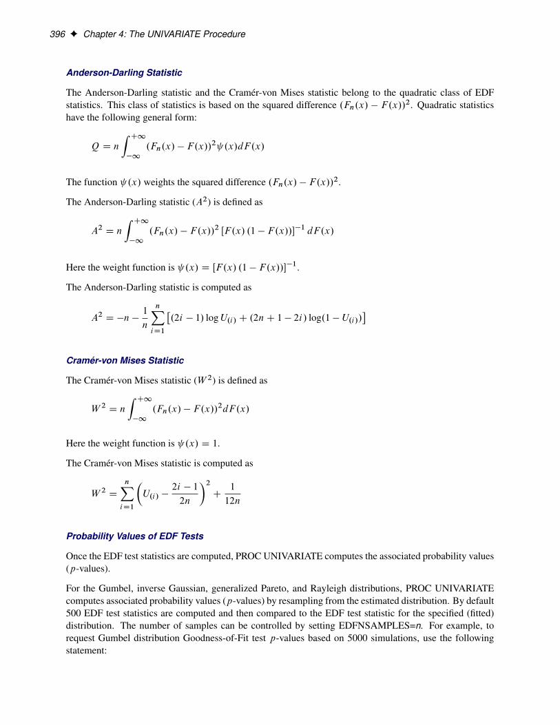
396 F Chapter 4: The UNIVARIATE Procedure
Anderson-Darling Statistic
The Anderson-Darling statistic and the Cramér-von Mises statistic belong to the quadratic class of EDFstatistics. This class of statistics is based on the squared difference .Fn.x/ � F.x//2. Quadratic statisticshave the following general form:
Q D n
Z C1�1
.Fn.x/ � F.x//2 .x/dF.x/
The function .x/ weights the squared difference .Fn.x/ � F.x//2.
The Anderson-Darling statistic (A2) is defined as
A2 D n
Z C1�1
.Fn.x/ � F.x//2 ŒF .x/ .1 � F.x//��1 dF.x/
Here the weight function is .x/ D ŒF .x/ .1 � F.x//��1.
The Anderson-Darling statistic is computed as
A2 D �n �1
n
nXiD1
�.2i � 1/ logU.i/ C .2nC 1 � 2i/ log.1 � U.i//
�
Cramér-von Mises Statistic
The Cramér-von Mises statistic (W 2) is defined as
W 2D n
Z C1�1
.Fn.x/ � F.x//2dF.x/
Here the weight function is .x/ D 1.
The Cramér-von Mises statistic is computed as
W 2D
nXiD1
�U.i/ �
2i � 1
2n
�2C
1
12n
Probability Values of EDF Tests
Once the EDF test statistics are computed, PROC UNIVARIATE computes the associated probability values(p-values).
For the Gumbel, inverse Gaussian, generalized Pareto, and Rayleigh distributions, PROC UNIVARIATEcomputes associated probability values (p-values) by resampling from the estimated distribution. By default500 EDF test statistics are computed and then compared to the EDF test statistic for the specified (fitted)distribution. The number of samples can be controlled by setting EDFNSAMPLES=n. For example, torequest Gumbel distribution Goodness-of-Fit test p-values based on 5000 simulations, use the followingstatement:

Goodness-of-Fit Tests F 397
proc univariate data=test;histogram / gumbel(edfnsamples=5000);
run;
For the beta, exponential, gamma, lognormal, normal, power function, and Weibull distributions the UNI-VARIATE procedure uses internal tables of probability levels similar to those given by D’Agostino andStephens (1986). If the value is between two probability levels, then linear interpolation is used to estimatethe probability value.
The probability value depends upon the parameters that are known and the parameters that are estimated forthe distribution. Table 4.114 summarizes different combinations fitted for which EDF tests are available.
Table 4.114 Availability of EDF Tests
Distribution Parameters Tests AvailableThreshold Scale Shape
beta � known � known ˛; ˇ known all� known � known ˛; ˇ < 5 unknown all
exponential � known, � known all� known � unknown all� unknown � known all� unknown � unknown all
gamma � known � known ˛ known all� known � unknown ˛ known all� known � known ˛ unknown all� known � unknown ˛ > 1 unknown all� unknown � known ˛ > 1 known all� unknown � unknown ˛ > 1 known all� unknown � known ˛ > 1 unknown all� unknown � unknown ˛ > 1 unknown all
lognormal � known � known � known all� known � known � unknown A2 and W 2
� known � unknown � known A2 and W 2
� known � unknown � unknown all� unknown � known � < 3 known all� unknown � known � < 3 unknown all� unknown � unknown � < 3 known all� unknown � unknown � < 3 unknown all
normal � known � known all� known � unknown A2 and W 2
� unknown � known A2 and W 2
� unknown � unknown all
power function � known � known ˛ known all� known � known ˛ < 5 unknown all
Weibull � known � known c known all� known � unknown c known A2 and W 2
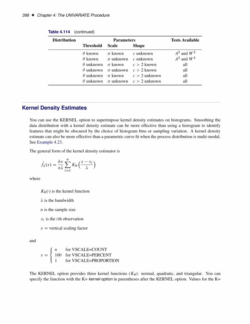
398 F Chapter 4: The UNIVARIATE Procedure
Table 4.114 (continued)
Distribution Parameters Tests AvailableThreshold Scale Shape
� known � known c unknown A2 and W 2
� known � unknown c unknown A2 and W 2
� unknown � known c > 2 known all� unknown � unknown c > 2 known all� unknown � known c > 2 unknown all� unknown � unknown c > 2 unknown all
Kernel Density Estimates
You can use the KERNEL option to superimpose kernel density estimates on histograms. Smoothing thedata distribution with a kernel density estimate can be more effective than using a histogram to identifyfeatures that might be obscured by the choice of histogram bins or sampling variation. A kernel densityestimate can also be more effective than a parametric curve fit when the process distribution is multi-modal.See Example 4.23.
The general form of the kernel density estimator is
Of�.x/ Dhv
n�
nXiD1
K0
�x � xi�
�where
K0.�/ is the kernel function
� is the bandwidth
n is the sample size
xi is the i th observation
v D vertical scaling factor
and
v D
8<:n for VSCALE=COUNT100 for VSCALE=PERCENT1 for VSCALE=PROPORTION
The KERNEL option provides three kernel functions (K0): normal, quadratic, and triangular. You canspecify the function with the K= kernel-option in parentheses after the KERNEL option. Values for the K=

Kernel Density Estimates F 399
option are NORMAL, QUADRATIC, and TRIANGULAR (with aliases of N, Q, and T, respectively). Bydefault, a normal kernel is used. The formulas for the kernel functions are
Normal K0.t/ D1p2�
exp.�12t2/ for �1 < t <1
Quadratic K0.t/ D34.1 � t2/ for jt j � 1
Triangular K0.t/ D 1 � jt j for jt j � 1
The value of �, referred to as the bandwidth parameter, determines the degree of smoothness in the estimateddensity function. You specify � indirectly by specifying a standardized bandwidth c with the C= kernel-option. If Q is the interquartile range and n is the sample size, then c is related to � by the formula
� D cQn�15
For a specific kernel function, the discrepancy between the density estimator Of�.x/ and the true densityf .x/ is measured by the mean integrated square error (MISE):
MISE.�/ DZx
fE. Of�.x// � f .x/g2dx C
Zx
var. Of�.x//dx
The MISE is the sum of the integrated squared bias and the variance. An approximate mean integratedsquare error (AMISE) is:
AMISE.�/ D1
4�4�Z
t
t2K.t/dt
�2 Zx
�f 00.x/
�2dx C
1
n�
Zt
K.t/2dt
A bandwidth that minimizes AMISE can be derived by treating f .x/ as the normal density that has param-eters � and � estimated by the sample mean and standard deviation. If you do not specify a bandwidthparameter or if you specify C=MISE, the bandwidth that minimizes AMISE is used. The value of AMISEcan be used to compare different density estimates. You can also specify C=SJPI to select the bandwidth byusing a plug-in formula of Sheather and Jones (Jones, Marron, and Sheather 1996). For each estimate, thebandwidth parameter c, the kernel function type, and the value of AMISE are reported in the SAS log.
The general kernel density estimates assume that the domain of the density to estimate can take on all valueson a real line. However, sometimes the domain of a density is an interval bounded on one or both sides. Forexample, if a variable Y is a measurement of only positive values, then the kernel density curve should bebounded so that is zero for negative Y values. You can use the LOWER= and UPPER= kernel-options tospecify the bounds.
The UNIVARIATE procedure uses a reflection technique to create the bounded kernel density curve, asdescribed in Silverman (1986, pp. 30-31). It adds the reflections of the kernel density that are outside theboundary to the bounded kernel estimates. The general form of the bounded kernel density estimator iscomputed by replacing K0
�x�xi�
�in the original equation with�
K0
�x � xi�
�CK0
�.x � xl/C .xi � xl/
�
�CK0
�.xu � x/C .xu � xi /
�
��
where xl is the lower bound and xu is the upper bound.

400 F Chapter 4: The UNIVARIATE Procedure
Without a lower bound, xl D �1 and K0�.x�xl /C.xi�xl /
�
�D 0. Similarly, without an upper bound,
xu D1 and K0�.xu�x/C.xu�xi /
�
�D 0.
When C=MISE is used with a bounded kernel density, the UNIVARIATE procedure uses a bandwidth thatminimizes the AMISE for its corresponding unbounded kernel.
Construction of Quantile-Quantile and Probability Plots
Figure 4.14 illustrates how a Q-Q plot is constructed for a specified theoretical distribution. First, the nnonmissing values of the variable are ordered from smallest to largest:
x.1/ � x.2/ � � � � � x.n/
Then the i th ordered value x.i/ is plotted as a point whose y-coordinate is x.i/ and whose x-coordinate is
F�1�i�0:375nC0:25
�, where F.�/ is the specified distribution with zero location parameter and unit scale param-
eter.
You can modify the adjustment constants �0.375 and 0.25 with the RANKADJ= and NADJ= options.This default combination is recommended by Blom (1958). For additional information, see Chamberset al. (1983). Because x.i/ is a quantile of the empirical cumulative distribution function (ecdf), a Q-Qplot compares quantiles of the ecdf with quantiles of a theoretical distribution. Probability plots (see thesection “PROBPLOT Statement” on page 324) are constructed the same way, except that the x-axis isscaled nonlinearly in percentiles.

Interpretation of Quantile-Quantile and Probability Plots F 401
Figure 4.14 Construction of a Q-Q Plot
Interpretation of Quantile-Quantile and Probability Plots
The following properties of Q-Q plots and probability plots make them useful diagnostics of how well aspecified theoretical distribution fits a set of measurements:
� If the quantiles of the theoretical and data distributions agree, the plotted points fall on or near the liney D x.
� If the theoretical and data distributions differ only in their location or scale, the points on the plot fallon or near the line y D ax C b. The slope a and intercept b are visual estimates of the scale andlocation parameters of the theoretical distribution.
Q-Q plots are more convenient than probability plots for graphical estimation of the location and scaleparameters because the x-axis of a Q-Q plot is scaled linearly. On the other hand, probability plots are moreconvenient for estimating percentiles or probabilities.
There are many reasons why the point pattern in a Q-Q plot may not be linear. Chambers et al. (1983) andFowlkes (1987) discuss the interpretations of commonly encountered departures from linearity, and theseare summarized in Table 4.115.
In some applications, a nonlinear pattern may be more revealing than a linear pattern. However, Chamberset al. (1983) note that departures from linearity can also be due to chance variation.

402 F Chapter 4: The UNIVARIATE Procedure
Table 4.115 Quantile-Quantile Plot Diagnostics
Description of Point Pattern Possible Interpretation
all but a few points fall on a line outliers in the dataleft end of pattern is below the line;right end of pattern is above the line
long tails at both ends of the data distri-bution
left end of pattern is above the line;right end of pattern is below the line
short tails at both ends of the data distri-bution
curved pattern with slope increasingfrom left to right
data distribution is skewed to the right
curved pattern with slope decreasingfrom left to right
data distribution is skewed to the left
staircase pattern (plateaus and gaps) data have been rounded or are discrete
When the pattern is linear, you can use Q-Q plots to estimate shape, location, and scale parameters and toestimate percentiles. See Example 4.26 through Example 4.34.
Distributions for Probability and Q-Q Plots
You can use the PROBPLOT and QQPLOT statements to request probability and Q-Q plots that are basedon the theoretical distributions summarized in Table 4.116.
Table 4.116 Distributions and Parameters
ParametersDistribution Density Function p.x/ Range Location Scale Shape
Beta .x��/˛�1.�C��x/ˇ�1
B.˛;ˇ/�.˛Cˇ�1/� < x < � C � � � ˛, ˇ
Exponential 1�
exp��x���
�x � � � �
Gamma 1��.˛/
�x���
�˛�1exp
��x���
�x > � � � ˛
Gumbel e�.x��/=�
�exp
��e�.x��/=�
�all x � �
Lognormal 1
�p2�.x��/
exp��.log.x��/��/2
2�2
�x > � � � �
(3-parameter)
Normal 1
�p2�
exp��.x��/2
2�2
�all x � �
Generalized ˛ ¤ 0 1�.1 � ˛.x � �/=�/1=˛�1 x > � � � ˛
Pareto ˛ D 0 1�
exp.�.x � �/=�/
Power Function ˛�
�x���
�˛�1x > � � � ˛

Distributions for Probability and Q-Q Plots F 403
Table 4.116 (continued)
ParametersDistribution Density Function p.x/ Range Location Scale Shape
Rayleigh x���2
exp.�.x � �/2=.2�2// x � � � �
Weibull c�
�x���
�c�1exp
��
�x���
�c�x > � � � c
(3-parameter)
Weibull c�
�x��0�
�c�1exp
��
�x��0�
�c�x > �0 �0 � c
(2-parameter) (known)
You can request these distributions with the BETA, EXPONENTIAL, GAMMA, PARETO, GUMBEL,LOGNORMAL, NORMAL, POWER, RAYLEIGH, WEIBULL, and WEIBULL2 options, respectively. Ifyou do not specify a distribution option, a normal probability plot or a normal Q-Q plot is created.
The following sections provide details for constructing Q-Q plots that are based on these distributions.Probability plots are constructed similarly except that the horizontal axis is scaled in percentile units.
Beta Distribution
To create the plot, the observations are ordered from smallest to largest, and the i th ordered observationis plotted against the quantile B�1
˛ˇ
�i�0:375nC0:25
�, where B�1
˛ˇ.�/ is the inverse normalized incomplete beta
function, n is the number of nonmissing observations, and ˛ and ˇ are the shape parameters of the betadistribution. In a probability plot, the horizontal axis is scaled in percentile units.
The pattern on the plot for ALPHA=˛ and BETA=ˇ tends to be linear with intercept � and slope � if thedata are beta distributed with the specific density function
p.x/ D
(.x��/˛�1.�C��x/ˇ�1
B.˛;ˇ/�.˛Cˇ�1/for � < x < � C �
0 for x � � or x � � C �
where B.˛; ˇ/ D �.˛/�.ˇ/�.˛Cˇ/
and
� D lower threshold parameter
� D scale parameter .� > 0/
˛ D first shape parameter .˛ > 0/
ˇ D second shape parameter .ˇ > 0/

404 F Chapter 4: The UNIVARIATE Procedure
Exponential Distribution
To create the plot, the observations are ordered from smallest to largest, and the i th ordered observation isplotted against the quantile � log
�1 � i�0:375
nC0:25
�, where n is the number of nonmissing observations. In a
probability plot, the horizontal axis is scaled in percentile units.
The pattern on the plot tends to be linear with intercept � and slope � if the data are exponentially distributedwith the specific density function
p.x/ D
(1�
exp��x���
�for x � �
0 for x < �
where � is a threshold parameter, and � is a positive scale parameter.
Gamma Distribution
To create the plot, the observations are ordered from smallest to largest, and the i th ordered observationis plotted against the quantile G�1˛
�i�0:375nC0:25
�, where G�1˛ .�/ is the inverse normalized incomplete gamma
function, n is the number of nonmissing observations, and ˛ is the shape parameter of the gamma distribu-tion. In a probability plot, the horizontal axis is scaled in percentile units.
The pattern on the plot for ALPHA=˛ tends to be linear with intercept � and slope � if the data are gammadistributed with the specific density function
p.x/ D
(1
��.˛/
�x���
�˛�1exp
��x���
�for x > �
0 for x � �
where
� D threshold parameter
� D scale parameter .� > 0/
˛ D shape parameter .˛ > 0/
Gumbel Distribution
To create the plot, the observations are ordered from smallest to largest, and the i th ordered observation isplotted against the quantile � log
�� log
�i�0:375nC0:25
��, where n is the number of nonmissing observations. In
a probability plot, the horizontal axis is scaled in percentile units.
The pattern on the plot tends to be linear with intercept � and slope � if the data are Gumbel distributedwith the specific density function
p.x/ De�.x��/=�
�exp
��e�.x��/=�
�

Distributions for Probability and Q-Q Plots F 405
� D location parameter
� D scale parameter .� > 0/
Lognormal Distribution
To create the plot, the observations are ordered from smallest to largest, and the i th ordered observation isplotted against the quantile exp
��ˆ�1
�i�0:375nC0:25
��, where ˆ�1.�/ is the inverse cumulative standard normal
distribution, n is the number of nonmissing observations, and � is the shape parameter of the lognormaldistribution. In a probability plot, the horizontal axis is scaled in percentile units.
The pattern on the plot for SIGMA=� tends to be linear with intercept � and slope exp.�/ if the data arelognormally distributed with the specific density function
p.x/ D
(1
�p2�.x��/
exp��.log.x��/��/2
2�2
�for x > �
0 for x � �
where
� D threshold parameter
� D scale parameter
� D shape parameter .� > 0/
See Example 4.26 and Example 4.33.
Normal Distribution
To create the plot, the observations are ordered from smallest to largest, and the i th ordered observation isplotted against the quantile ˆ�1
�i�0:375nC0:25
�, where ˆ�1.�/ is the inverse cumulative standard normal distri-
bution and n is the number of nonmissing observations. In a probability plot, the horizontal axis is scaled inpercentile units.
The point pattern on the plot tends to be linear with intercept � and slope � if the data are normally dis-tributed with the specific density function
p.x/ D 1
�p2�
exp��.x��/2
2�2
�for all x
where � is the mean and � is the standard deviation (� > 0).
Generalized Pareto Distribution
To create the plot, the observations are ordered from smallest to largest, and the i th ordered observation isplotted against the quantile .1 � .1 � i�0:375
nC0:25/˛/=˛ (˛ ¤ 0) or � log.1 � i�0:375
nC0:25/ (˛ D 0), where n is the

406 F Chapter 4: The UNIVARIATE Procedure
number of nonmissing observations and ˛ is the shape parameter of the generalized Pareto distribution. Thehorizontal axis is scaled in percentile units.
The point pattern on the plot for ALPHA=˛ tends to be linear with intercept � and slope � if the data aregeneralized Pareto distributed with the specific density function
p.x/ D
�1�.1 � ˛.x � �/=�/1=˛�1 if ˛ ¤ 01�
exp.�.x � �/=�/ if ˛ D 0
where
� D threshold parameter� D scale parameter .� > 0/˛ D shape parameter .˛ > 0/
Power Function Distribution
To create the plot, the observations are ordered from smallest to largest, and the i th ordered observationis plotted against the quantile B�1
˛.1/
�i�0:375nC0:25
�, where B�1
˛.1/.�/ is the inverse normalized incomplete beta
function, n is the number of nonmissing observations, ˛ is one shape parameter of the beta distribution, andthe second shape parameter, ˇ D 1. The horizontal axis is scaled in percentile units.
The point pattern on the plot for ALPHA=˛ tends to be linear with intercept � and slope � if the data arepower function distributed with the specific density function
p.x/ D
(˛�
�x���
�˛�1for � < x < � C �
0 for x � � or x � � C �
where
� D threshold parameter
� D shape parameter .� > 0/
˛ D shape parameter .˛ > 0/
Rayleigh Distribution
To create the plot, the observations are ordered from smallest to largest, and the i th ordered observation
is plotted against the quantiler�2 log
�1 � i�0:375
nC0:25
�, where n is the number of nonmissing observations.
The horizontal axis is scaled in percentile units.
The point pattern on the plot tends to be linear with intercept � and slope � if the data are Rayleigh dis-tributed with the specific density function
p.x/ D
�x���2
exp.�.x � �/2=.2�2// for x � �0 for x < �

Distributions for Probability and Q-Q Plots F 407
where � is a threshold parameter, and � is a positive scale parameter.
Three-Parameter Weibull Distribution
To create the plot, the observations are ordered from smallest to largest, and the i th ordered observation is
plotted against the quantile�� log
�1 � i�0:375
nC0:25
�� 1c
, where n is the number of nonmissing observations, andc is the Weibull distribution shape parameter. In a probability plot, the horizontal axis is scaled in percentileunits.
The pattern on the plot for C=c tends to be linear with intercept � and slope � if the data are Weibulldistributed with the specific density function
p.x/ D
(c�
�x���
�c�1exp
��
�x���
�c�for x > �
0 for x � �
where
� D threshold parameter
� D scale parameter .� > 0/
c D shape parameter .c > 0/
See Example 4.34.
Two-Parameter Weibull Distribution
To create the plot, the observations are ordered from smallest to largest, and the log of the shifted i th orderedobservation x.i/, denoted by log.x.i/ � �0/, is plotted against the quantile log
�� log
�1 � i�0:375
nC0:25
��, where
n is the number of nonmissing observations. In a probability plot, the horizontal axis is scaled in percentileunits.
Unlike the three-parameter Weibull quantile, the preceding expression is free of distribution parameters.Consequently, the C= shape parameter is not mandatory with the WEIBULL2 distribution option.
The pattern on the plot for THETA=�0 tends to be linear with intercept log.�/ and slope 1c
if the data areWeibull distributed with the specific density function
p.x/ D
(c�
�x��0�
�c�1exp
��
�x��0�
�c�for x > �0
0 for x � �0
where
�0 D known lower threshold
� D scale parameter .� > 0/
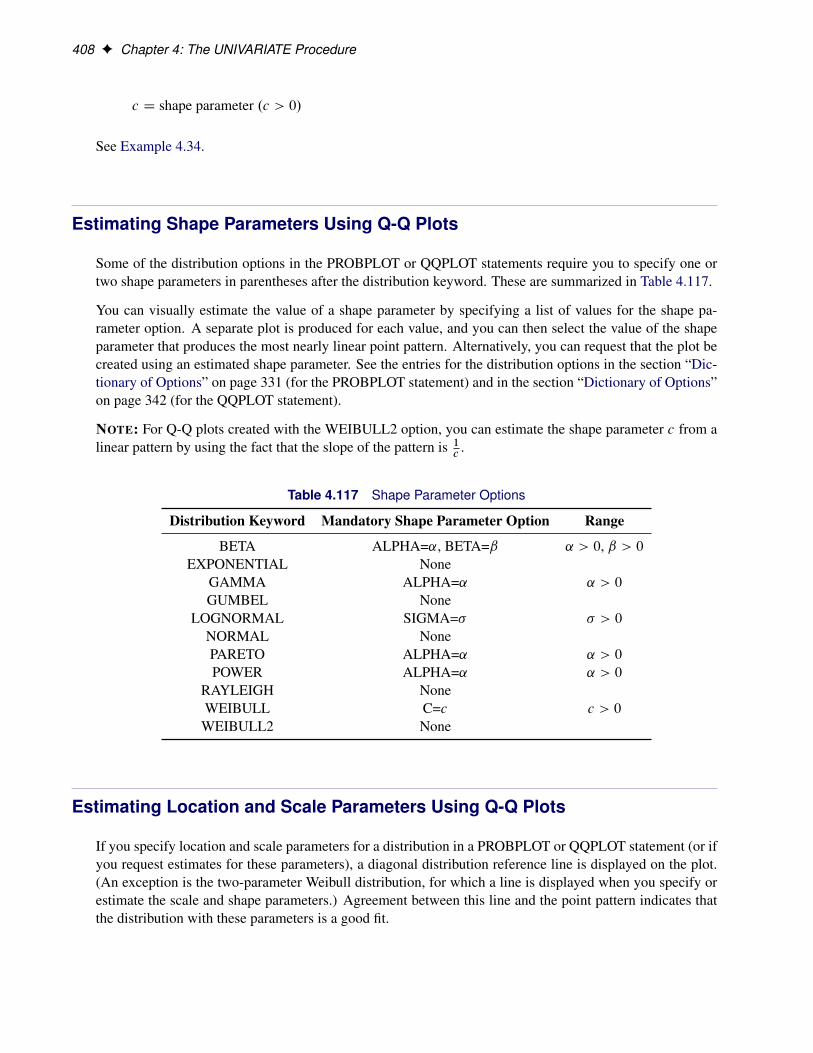
408 F Chapter 4: The UNIVARIATE Procedure
c D shape parameter .c > 0/
See Example 4.34.
Estimating Shape Parameters Using Q-Q Plots
Some of the distribution options in the PROBPLOT or QQPLOT statements require you to specify one ortwo shape parameters in parentheses after the distribution keyword. These are summarized in Table 4.117.
You can visually estimate the value of a shape parameter by specifying a list of values for the shape pa-rameter option. A separate plot is produced for each value, and you can then select the value of the shapeparameter that produces the most nearly linear point pattern. Alternatively, you can request that the plot becreated using an estimated shape parameter. See the entries for the distribution options in the section “Dic-tionary of Options” on page 331 (for the PROBPLOT statement) and in the section “Dictionary of Options”on page 342 (for the QQPLOT statement).
NOTE: For Q-Q plots created with the WEIBULL2 option, you can estimate the shape parameter c from alinear pattern by using the fact that the slope of the pattern is 1
c.
Table 4.117 Shape Parameter Options
Distribution Keyword Mandatory Shape Parameter Option Range
BETA ALPHA=˛, BETA=ˇ ˛ > 0, ˇ > 0EXPONENTIAL None
GAMMA ALPHA=˛ ˛ > 0
GUMBEL NoneLOGNORMAL SIGMA=� � > 0
NORMAL NonePARETO ALPHA=˛ ˛ > 0
POWER ALPHA=˛ ˛ > 0
RAYLEIGH NoneWEIBULL C=c c > 0
WEIBULL2 None
Estimating Location and Scale Parameters Using Q-Q Plots
If you specify location and scale parameters for a distribution in a PROBPLOT or QQPLOT statement (or ifyou request estimates for these parameters), a diagonal distribution reference line is displayed on the plot.(An exception is the two-parameter Weibull distribution, for which a line is displayed when you specify orestimate the scale and shape parameters.) Agreement between this line and the point pattern indicates thatthe distribution with these parameters is a good fit.

Estimating Percentiles Using Q-Q Plots F 409
When the point pattern on a Q-Q plot is linear, its intercept and slope provide estimates of the locationand scale parameters. (An exception to this rule is the two-parameter Weibull distribution, for which theintercept and slope are related to the scale and shape parameters.)
Table 4.118 shows how the specified parameters determine the intercept and slope of the line. The interceptand slope are based on the quantile scale for the horizontal axis, which is used in Q-Q plots.
Table 4.118 Intercept and Slope of Distribution Reference Line
Parameters Linear PatternDistribution Location Scale Shape Intercept Slope
Beta � � ˛ , ˇ � �
Exponential � � � �
Gamma � � ˛ � �
Gumbel � � � �
Lognormal � � � � exp.�/Normal � � � �
Generalized Pareto � � ˛ � �
Power Function � � ˛ � �
Rayleigh � � � �
Weibull (3-parameter) � � c � �
Weibull (2-parameter) �0 (known) � c log.�/ 1c
For instance, specifying MU=3 and SIGMA=2 with the NORMAL option requests a line with intercept3 and slope 2. Specifying SIGMA=1 and C=2 with the WEIBULL2 option requests a line with interceptlog.1/ D 0 and slope 1
2. On a probability plot with the LOGNORMAL and WEIBULL2 options, you
can specify the slope directly with the SLOPE= option. That is, for the LOGNORMAL option, specifyingTHETA= �0 and SLOPE=exp.�0/ displays the same line as specifying THETA= �0 and ZETA= �0. For theWEIBULL2 option, specifying SIGMA= �0 and SLOPE= 1
c0displays the same line as specifying SIGMA=
�0 and C= c0.
Estimating Percentiles Using Q-Q Plots
There are two ways to estimate percentiles from a Q-Q plot:
� Specify the PCTLAXIS option, which adds a percentile axis opposite the theoretical quantile axis.The scale for the percentile axis ranges between 0 and 100 with tick marks at percentile values suchas 1, 5, 10, 25, 50, 75, 90, 95, and 99.
� Specify the PCTLSCALE option, which relabels the horizontal axis tick marks with their percentileequivalents but does not alter their spacing. For example, on a normal Q-Q plot, the tick mark labeled“0” is relabeled as “50” because the 50th percentile corresponds to the zero quantile.
You can also estimate percentiles by using probability plots created with the PROBPLOT statement. SeeExample 4.32.
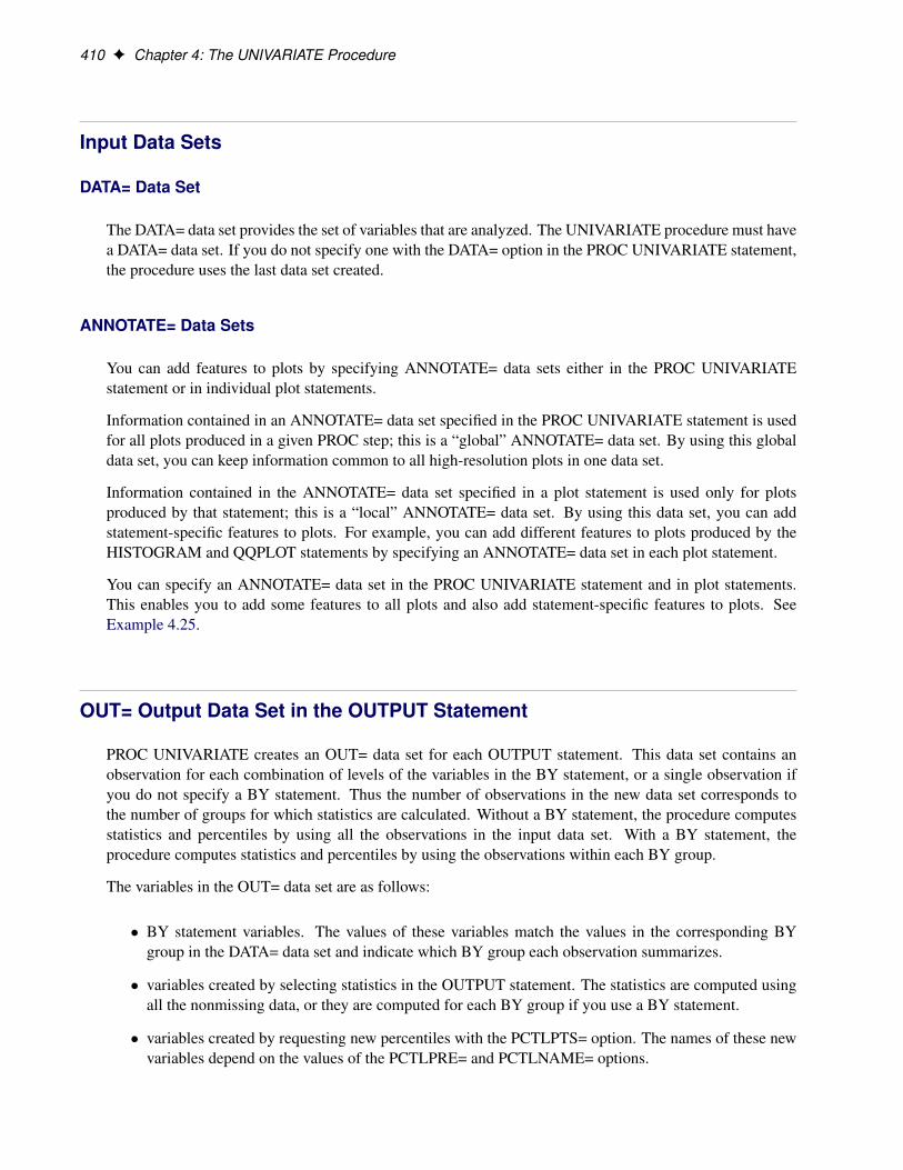
410 F Chapter 4: The UNIVARIATE Procedure
Input Data Sets
DATA= Data Set
The DATA= data set provides the set of variables that are analyzed. The UNIVARIATE procedure must havea DATA= data set. If you do not specify one with the DATA= option in the PROC UNIVARIATE statement,the procedure uses the last data set created.
ANNOTATE= Data Sets
You can add features to plots by specifying ANNOTATE= data sets either in the PROC UNIVARIATEstatement or in individual plot statements.
Information contained in an ANNOTATE= data set specified in the PROC UNIVARIATE statement is usedfor all plots produced in a given PROC step; this is a “global” ANNOTATE= data set. By using this globaldata set, you can keep information common to all high-resolution plots in one data set.
Information contained in the ANNOTATE= data set specified in a plot statement is used only for plotsproduced by that statement; this is a “local” ANNOTATE= data set. By using this data set, you can addstatement-specific features to plots. For example, you can add different features to plots produced by theHISTOGRAM and QQPLOT statements by specifying an ANNOTATE= data set in each plot statement.
You can specify an ANNOTATE= data set in the PROC UNIVARIATE statement and in plot statements.This enables you to add some features to all plots and also add statement-specific features to plots. SeeExample 4.25.
OUT= Output Data Set in the OUTPUT Statement
PROC UNIVARIATE creates an OUT= data set for each OUTPUT statement. This data set contains anobservation for each combination of levels of the variables in the BY statement, or a single observation ifyou do not specify a BY statement. Thus the number of observations in the new data set corresponds tothe number of groups for which statistics are calculated. Without a BY statement, the procedure computesstatistics and percentiles by using all the observations in the input data set. With a BY statement, theprocedure computes statistics and percentiles by using the observations within each BY group.
The variables in the OUT= data set are as follows:
� BY statement variables. The values of these variables match the values in the corresponding BYgroup in the DATA= data set and indicate which BY group each observation summarizes.
� variables created by selecting statistics in the OUTPUT statement. The statistics are computed usingall the nonmissing data, or they are computed for each BY group if you use a BY statement.
� variables created by requesting new percentiles with the PCTLPTS= option. The names of these newvariables depend on the values of the PCTLPRE= and PCTLNAME= options.

OUT= Output Data Set in the OUTPUT Statement F 411
If the output data set contains a percentile variable or a quartile variable, the percentile definition assignedwith the PCTLDEF= option in the PROC UNIVARIATE statement is recorded in the output data set label.See Example 4.8.
The following table lists variables available in the OUT= data set.
Table 4.119 Variables Available in the OUT= Data Set
Variable Name Description
Descriptive StatisticsCSS sum of squares corrected for the meanCV percent coefficient of variationKURTOSIS | KURT measurement of the heaviness of tailsMAX largest (maximum) valueMEAN arithmetic meanMIN smallest (minimum) valueMODE most frequent value (if not unique, the smallest mode)N number of observations on which calculations are basedNMISS number of missing observationsNOBS total number of observationsRANGE difference between the maximum and minimum valuesSKEWNESS | SKEW measurement of the tendency of the deviations to be larger in one di-
rection than in the otherSTD | STDDEV standard deviationSTDMEAN | STDERR standard error of the meanSUM sumSUMWGT sum of the weightsUSS uncorrected sum of squaresVAR varianceQuantile StatisticsMEDIAN | Q2 | P50 middle value (50th percentile)P1 1st percentileP5 5th percentileP10 10th percentileP90 90th percentileP95 95th percentileP99 99th percentileQ1 | P25 lower quartile (25th percentile)Q3 | P75 upper quartile (75th percentile)QRANGE difference between the upper and lower quartiles (also known as the
inner quartile range)Robust StatisticsGINI Gini’s mean differenceMAD median absolute differenceQN 2nd variation of median absolute differenceSN 1st variation of median absolute differenceSTD_GINI standard deviation for Gini’s mean differenceSTD_MAD standard deviation for median absolute difference

412 F Chapter 4: The UNIVARIATE Procedure
Table 4.119 (continued)
Variable Name Description
STD_QN standard deviation for the second variation of the median absolute dif-ference
STD_QRANGE estimate of the standard deviation, based on interquartile rangeSTD_SN standard deviation for the first variation of the median absolute differ-
enceHypothesis Test StatisticsMSIGN sign statisticNORMAL test statistic for normality. If the sample size is less than or equal to
2000, this is the Shapiro-Wilk W statistic. Otherwise, it is the Kol-mogorov D statistic.
PROBM probability of a greater absolute value for the sign statisticPROBN probability that the data came from a normal distributionPROBS probability of a greater absolute value for the signed rank statisticPROBT two-tailed p-value for Student’s t statistic with n � 1 degrees of free-
domSIGNRANK signed rank statisticT Student’s t statistic to test the null hypothesis that the population mean
is equal to �0
OUTHISTOGRAM= Output Data Set
You can create an OUTHISTOGRAM= data set with the HISTOGRAM statement. This data set containsinformation about histogram intervals. Because you can specify multiple HISTOGRAM statements withthe UNIVARIATE procedure, you can create multiple OUTHISTOGRAM= data sets.
An OUTHISTOGRAM= data set contains a group of observations for each variable in the HISTOGRAMstatement. The group contains an observation for each interval of the histogram, beginning with the leftmostinterval that contains a value of the variable and ending with the rightmost interval that contains a valueof the variable. These intervals do not necessarily coincide with the intervals displayed in the histogrambecause the histogram might be padded with empty intervals at either end. If you superimpose one or morefitted curves on the histogram, the OUTHISTOGRAM= data set contains multiple groups of observationsfor each variable (one group for each curve). If you use a BY statement, the OUTHISTOGRAM= data setcontains groups of observations for each BY group. ID variables are not saved in an OUTHISTOGRAM=data set.
By default, an OUTHISTOGRAM= data set contains the _MIDPT_ variable, whose values identify his-togram intervals by their midpoints. When the ENDPOINTS= or NENDPOINTS option is specified, in-tervals are identified by endpoint values instead. If the RTINCLUDE option is specified, the _MAXPT_variable contains upper endpoint values. Otherwise, the _MINPT_ variable contains lower endpoint values.See Example 4.18.
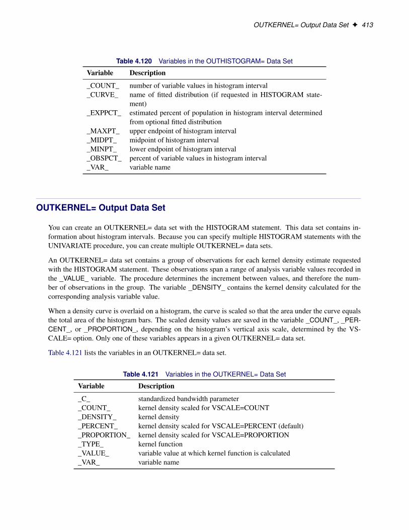
OUTKERNEL= Output Data Set F 413
Table 4.120 Variables in the OUTHISTOGRAM= Data Set
Variable Description
_COUNT_ number of variable values in histogram interval_CURVE_ name of fitted distribution (if requested in HISTOGRAM state-
ment)_EXPPCT_ estimated percent of population in histogram interval determined
from optional fitted distribution_MAXPT_ upper endpoint of histogram interval_MIDPT_ midpoint of histogram interval_MINPT_ lower endpoint of histogram interval_OBSPCT_ percent of variable values in histogram interval_VAR_ variable name
OUTKERNEL= Output Data Set
You can create an OUTKERNEL= data set with the HISTOGRAM statement. This data set contains in-formation about histogram intervals. Because you can specify multiple HISTOGRAM statements with theUNIVARIATE procedure, you can create multiple OUTKERNEL= data sets.
An OUTKERNEL= data set contains a group of observations for each kernel density estimate requestedwith the HISTOGRAM statement. These observations span a range of analysis variable values recorded inthe _VALUE_ variable. The procedure determines the increment between values, and therefore the num-ber of observations in the group. The variable _DENSITY_ contains the kernel density calculated for thecorresponding analysis variable value.
When a density curve is overlaid on a histogram, the curve is scaled so that the area under the curve equalsthe total area of the histogram bars. The scaled density values are saved in the variable _COUNT_, _PER-CENT_, or _PROPORTION_, depending on the histogram’s vertical axis scale, determined by the VS-CALE= option. Only one of these variables appears in a given OUTKERNEL= data set.
Table 4.121 lists the variables in an OUTKERNEL= data set.
Table 4.121 Variables in the OUTKERNEL= Data Set
Variable Description
_C_ standardized bandwidth parameter_COUNT_ kernel density scaled for VSCALE=COUNT_DENSITY_ kernel density_PERCENT_ kernel density scaled for VSCALE=PERCENT (default)_PROPORTION_ kernel density scaled for VSCALE=PROPORTION_TYPE_ kernel function_VALUE_ variable value at which kernel function is calculated_VAR_ variable name

414 F Chapter 4: The UNIVARIATE Procedure
OUTTABLE= Output Data Set
The OUTTABLE= data set saves univariate statistics in a data set that contains one observation per analysisvariable. The following variables are saved:
Table 4.122 Variables in the OUTTABLE= Data Set
Variable Description
_CSS_ corrected sum of squares_CV_ coefficient of variation_GINI_ Gini’s mean difference_KURT_ kurtosis_MAD_ median absolute difference about the median_MAX_ maximum_MEAN_ mean_MEDIAN_ median_MIN_ minimum_MODE_ mode_MSIGN_ sign statistic_NMISS_ number of missing observations_NOBS_ number of nonmissing observations_NORMAL_ test statistic for normality_P1_ 1st percentile_P5_ 5th percentile_P10_ 10th percentile_P90_ 90th percentile_P95_ 95th percentile_P99_ 99th percentile_PROBM_ p-value of sign statistic_PROBN_ p-value of test for normality_PROBS_ p-value of signed rank test_PROBT_ p-value of t statistic_Q1_ 25th percentile (lower quartile)_Q3_ 75th percentile (upper quartile)_QN_ Qn_QRANGE_ interquartile range (upper quartile minus lower quartile)_RANGE_ range_SGNRNK_ centered sign rank_SKEW_ skewness_SN_ Sn (see “Robust Estimates of Scale” on page 368)_STD_ standard deviation_STDGINI_ Gini’s standard deviation_STDMAD_ MAD standard deviation_STDMEAN_ standard error of the mean_STDQN_ Qn standard deviation_STDQRANGE_ interquartile range standard deviation

OUTTABLE= Output Data Set F 415
Table 4.122 (continued)
Variable Description
_STDSN_ Sn standard deviation_SUMWGT_ sum of the weights_SUM_ sum_T_ Student’s t statistic_USS_ uncorrected sum of squares_VARI_ variance_VAR_ variable name
The OUTTABLE= data set and the OUT= data set see the section “OUT= Output Data Set in the OUTPUTStatement” on page 410) contain essentially the same information. in the OUT= data set (see the section“OUT= Output Data Set in the OUTPUT Statement” on page 410). However, the structure of the OUT-TABLE= data set may be more appropriate when you are computing summary statistics for more than oneanalysis variable in the same invocation of the UNIVARIATE procedure. Each observation in the OUT-TABLE= data set corresponds to a different analysis variable, and the variables in the data set correspond tosummary statistics and indices.
For example, suppose you have 10 analysis variables (P1-P10). The following statements create an OUT-TABLE= data set named Table, which contains summary statistics for each of these variables:
data Analysis;input A1-A10;datalines;
72 223 332 138 110 145 23 293 353 45897 54 61 196 275 171 117 72 81 14156 170 140 400 371 72 60 20 484 138
124 6 332 493 214 43 125 55 372 30152 236 222 76 187 126 192 334 109 546
5 260 194 277 176 96 109 184 240 261161 253 153 300 37 156 282 293 451 299128 121 254 297 363 132 209 257 429 295116 152 331 27 442 103 80 393 383 9443 178 278 159 25 180 253 333 51 22534 128 182 415 524 112 13 186 145 131
142 236 234 255 211 80 281 135 179 11108 215 335 66 254 196 190 363 226 37962 232 219 474 31 139 15 56 429 298
177 218 275 171 457 146 163 18 155 1290 235 83 239 398 99 226 389 498 18
147 199 324 258 504 2 218 295 422 28739 161 156 198 214 58 238 19 231 548
120 42 372 420 232 112 157 79 197 166178 83 238 492 463 68 46 386 45 81161 267 372 296 501 96 11 288 330 7414 2 52 81 169 63 194 161 173 5422 181 92 272 417 94 188 180 367 34255 248 214 422 133 193 144 318 271 47956 83 169 30 379 5 296 320 396 597
;

416 F Chapter 4: The UNIVARIATE Procedure
proc univariate data=Analysis outtable=Table noprint;var A1-A10;
run;
The following statements create the table shown in Figure 4.15, which contains the mean, standard deviation,and so on, for each analysis variable:
proc print data=Table label noobs;var _VAR_ _MIN_ _MEAN_ _MAX_ _STD_;label _VAR_='Analysis';
run;
Figure 4.15 Tabulating Results for Multiple Process Variables
Test Scores for a College Course
StandardAnalysis Minimum Mean Maximum Deviation
A1 0 90.76 178 57.024A2 2 167.32 267 81.628A3 52 224.56 372 96.525A4 27 258.08 493 145.218A5 25 283.48 524 157.033A6 2 107.48 196 52.437A7 11 153.20 296 90.031A8 18 217.08 393 130.031A9 45 280.68 498 140.943A10 11 243.24 597 178.799
Tables for Summary Statistics
By default, PROC UNIVARIATE produces ODS tables of moments, basic statistical measures, tests forlocation, quantiles, and extreme observations. You must specify options in the PROC UNIVARIATE state-ment to request other statistics and tables. The CIBASIC option produces a table that displays confidencelimits for the mean, standard deviation, and variance. The CIPCTLDF and CIPCTLNORMAL options re-quest tables of confidence limits for the quantiles. The LOCCOUNT option requests a table that shows thenumber of values greater than, not equal to, and less than the value of MU0=. The FREQ option requests atable of frequencies counts. The NEXTRVAL= option requests a table of extreme values. The NORMALoption requests a table with tests for normality.
The TRIMMED=, WINSORIZED=, and ROBUSTSCALE options request tables with robust estimators.The table of trimmed or Winsorized means includes the percentage and the number of observations that aretrimmed or Winsorized at each end, the mean and standard error, confidence limits, and the Student’s t test.The table with robust measures of scale includes interquartile range, Gini’s mean difference G, MAD, Qn,and Sn, with their corresponding estimates of � .
See the section “ODS Table Names” on page 417 for the names of ODS tables created by PROC UNIVARI-ATE.

ODS Table Names F 417
ODS Table Names
PROC UNIVARIATE assigns a name to each table that it creates. You can use these names to reference thetable when you use the Output Delivery System (ODS) to select tables and create output data sets.
Table 4.123 ODS Tables Produced with the PROC UNIVARIATE Statement
ODS Table Name Description Option
BasicIntervals confidence intervals for mean,standard deviation, variance
CIBASIC
BasicMeasures measures of location and vari-ability
default
ExtremeObs extreme observations defaultExtremeValues extreme values NEXTRVAL=Frequencies frequencies FREQLocationCounts counts used for sign test and
signed rank testLOCCOUNT
MissingValues missing values default, if missing valuesexist
Modes modes MODESMoments sample moments defaultPlots line printer plots PLOTSQuantiles quantiles defaultRobustScale robust measures of scale ROBUSTSCALESSPlots line printer side-by-side box
plotsPLOTS (with BY state-ment)
TestsForLocation tests for location defaultTestsForNormality tests for normality NORMALTESTTrimmedMeans trimmed means TRIMMED=WinsorizedMeans Winsorized means WINSORIZED=
Table 4.124 ODS Tables Produced with the HISTOGRAM Statement
ODS Table Name Description Option
Bins histogram bins MIDPERCENTS sec-ondary option
FitQuantiles quantiles of fitted distribution any distribution optionGoodnessOfFit goodness-of-fit tests for fitted
distributionany distribution option
HistogramBins histogram bins MIDPERCENTS optionParameterEstimates parameter estimates for fitted
distributionany distribution option

418 F Chapter 4: The UNIVARIATE Procedure
ODS Tables for Fitted Distributions
If you request a fitted parametric distribution with a HISTOGRAM statement, PROC UNIVARIATE createsa summary that is organized into the ODS tables described in this section.
Parameters
The ParameterEstimates table lists the estimated (or specified) parameters for the fitted curve as well as theestimated mean and estimated standard deviation. See “Formulas for Fitted Continuous Distributions” onpage 380.
EDF Goodness-of-Fit Tests
When you fit a parametric distribution, the HISTOGRAM statement provides a series of goodness-of-fittests based on the empirical distribution function (EDF). See “EDF Goodness-of-Fit Tests” on page 394.These are displayed in the GoodnessOfFit table.
Histogram Intervals
The Bins table is included in the summary only if you specify the MIDPERCENTS option in parenthesesafter the distribution option. This table lists the midpoints for the histogram bins along with the observedand estimated percentages of the observations that lie in each bin. The estimated percentages are based onthe fitted distribution.
If you specify the MIDPERCENTS option without requesting a fitted distribution, the HistogramBins tableis included in the summary. This table lists the interval midpoints with the observed percent of observationsthat lie in the interval. See the entry for the MIDPERCENTS option on page 289.
Quantiles
The FitQuantiles table lists observed and estimated quantiles. You can use the PERCENTS= option tospecify the list of quantiles in this table. See the entry for the PERCENTS= option on page 291. By default,the table lists observed and estimated quantiles for the 1, 5, 10, 25, 50, 75, 90, 95, and 99 percent of a fittedparametric distribution.
ODS Graphics
Statistical procedures use ODS Graphics to create graphs as part of their output. ODS Graphics is describedin detail in Chapter 21, “Statistical Graphics Using ODS” (SAS/STAT User’s Guide).

Computational Resources F 419
Before you create graphs, ODS Graphics must be enabled (for example, with the ODS GRAPHICS ONstatement). For more information about enabling and disabling ODS Graphics, see the section “Enablingand Disabling ODS Graphics” in that chapter.
The overall appearance of graphs is controlled by ODS styles. Styles and other aspects of using ODSGraphics are discussed in the section “A Primer on ODS Statistical Graphics” in that chapter.
PROC UNIVARIATE assigns a name to each graph it creates by using ODS Graphics. You can use thesenames to reference the graphs when you use ODS. The names are listed in Table 4.125.
Table 4.125 ODS Graphics Produced by PROC UNIVARIATE
ODS Graph Name Plot Description Statement
CDFPlot cdf plot CDFPLOTHistogram histogram HISTOGRAMPPPlot P-P plot PPPLOTProbPlot probability plot PROBPLOTQQPlot Q-Q plot QQPLOT
Computational Resources
Because the UNIVARIATE procedure computes quantile statistics, it requires additional memory to storea copy of the data in memory. By default, the MEANS, SUMMARY, and TABULATE procedures requireless memory because they do not automatically compute quantiles. These procedures also provide an optionto use a new fixed-memory quantiles estimation method that is usually less memory-intensive.
In the UNIVARIATE procedure, the only factor that limits the number of variables that you can analyze isthe computer resources that are available. The amount of temporary storage and CPU time required dependson the statements and the options that you specify. To calculate the computer resources the procedure needs,let
N be the number of observations in the data setV be the number of variables in the VAR statementUi be the number of unique values for the i th variable
Then the minimum memory requirement in bytes to process all variables is M D 24Pi Ui . If M bytes are
not available, PROC UNIVARIATE must process the data multiple times to compute all the statistics. Thisreduces the minimum memory requirement to M D 24max.Ui /.
Using the ROUND= option reduces the number of unique values .Ui /, thereby reducing memory require-ments. The ROBUSTSCALE option requires 40Ui bytes of temporary storage.
Several factors affect the CPU time:
� The time to create V tree structures to internally store the observations is proportional toNV log.N /.
� The time to compute moments and quantiles for the i th variable is proportional to Ui .
� The time to compute the NORMAL option test statistics is proportional to N .

420 F Chapter 4: The UNIVARIATE Procedure
� The time to compute the ROBUSTSCALE option test statistics is proportional to Ui log.Ui /.
� The time to compute the exact significance level of the sign rank statistic can increase when thenumber of nonzero values is less than or equal to 20.
Each of these factors has a different constant of proportionality. For additional information about optimizingCPU performance and memory usage, see the SAS documentation for your operating environment.
Examples: UNIVARIATE Procedure
Example 4.1: Computing Descriptive Statistics for Multiple Variables
This example computes univariate statistics for two variables. The following statements create the data setBPressure, which contains the systolic (Systolic) and diastolic (Diastolic) blood pressure readings for 22patients:
data BPressure;length PatientID $2;input PatientID $ Systolic Diastolic @@;datalines;
CK 120 50 SS 96 60 FR 100 70CP 120 75 BL 140 90 ES 120 70CP 165 110 JI 110 40 MC 119 66FC 125 76 RW 133 60 KD 108 54DS 110 50 JW 130 80 BH 120 65JW 134 80 SB 118 76 NS 122 78GS 122 70 AB 122 78 EC 112 62HH 122 82;
The following statements produce descriptive statistics and quantiles for the variables Systolic and Diastolic:
title 'Systolic and Diastolic Blood Pressure';ods select BasicMeasures Quantiles;proc univariate data=BPressure;
var Systolic Diastolic;run;
The ODS SELECT statement restricts the output, which is shown in Output 4.1.1, to the “BasicMeasures”and “Quantiles” tables; see the section “ODS Table Names” on page 417. You use the PROC UNIVARIATEstatement to request univariate statistics for the variables listed in the VAR statement, which specifies theanalysis variables and their order in the output. Formulas for computing the statistics in the “BasicMeasures”table are provided in the section “Descriptive Statistics” on page 357. The quantiles are calculated usingDefinition 5, which is the default definition; see the section “Calculating Percentiles” on page 361.

Example 4.1: Computing Descriptive Statistics for Multiple Variables F 421
A sample program for this example, uniex01.sas, is available in the SAS Sample Library for Base SASsoftware.
Output 4.1.1 Display Basic Measures and Quantiles
Systolic and Diastolic Blood Pressure
The UNIVARIATE ProcedureVariable: Systolic
Basic Statistical Measures
Location Variability
Mean 121.2727 Std Deviation 14.28346Median 120.0000 Variance 204.01732Mode 120.0000 Range 69.00000
Interquartile Range 13.00000
Note: The mode displayed is the smallest of 2 modes with a count of 4.
Quantiles (Definition 5)
Quantile Estimate
100% Max 16599% 16595% 14090% 13475% Q3 12550% Median 12025% Q1 11210% 1085% 1001% 960% Min 96
Systolic and Diastolic Blood Pressure
The UNIVARIATE ProcedureVariable: Diastolic
Basic Statistical Measures
Location Variability
Mean 70.09091 Std Deviation 15.16547Median 70.00000 Variance 229.99134Mode 70.00000 Range 70.00000
Interquartile Range 18.00000

422 F Chapter 4: The UNIVARIATE Procedure
Output 4.1.1 continued
Quantiles (Definition 5)
Quantile Estimate
100% Max 11099% 11095% 9090% 8275% Q3 7850% Median 7025% Q1 6010% 505% 501% 400% Min 40
Example 4.2: Calculating Modes
An instructor is interested in calculating all the modes of the scores on a recent exam. The followingstatements create a data set named Exam, which contains the exam scores in the variable Score:
data Exam;label Score = 'Exam Score';input Score @@;datalines;
81 97 78 99 77 81 84 86 86 9785 86 94 76 75 42 91 90 88 8697 97 89 69 72 82 83 81 80 81;
The following statements use the MODES option to request a table of all possible modes:
title 'Table of Modes for Exam Scores';ods select Modes;proc univariate data=Exam modes;
var Score;run;
The ODS SELECT statement restricts the output to the “Modes” table; see the section “ODS Table Names”on page 417.

Example 4.2: Calculating Modes F 423
Output 4.2.1 Table of Modes Display
Table of Modes for Exam Scores
The UNIVARIATE ProcedureVariable: Score (Exam Score)
Modes
Mode Count
81 486 497 4
By default, when the MODES option is used and there is more than one mode, the lowest mode is displayedin the “BasicMeasures” table. The following statements illustrate the default behavior:
title 'Default Output';ods select BasicMeasures;proc univariate data=Exam;
var Score;run;
Output 4.2.2 Default Output (Without MODES Option)
Default Output
The UNIVARIATE ProcedureVariable: Score (Exam Score)
Basic Statistical Measures
Location Variability
Mean 83.66667 Std Deviation 11.08069Median 84.50000 Variance 122.78161Mode 81.00000 Range 57.00000
Interquartile Range 10.00000
Note: The mode displayed is the smallest of 3 modes with a count of 4.
The default output displays a mode of 81 and includes a note regarding the number of modes; the modes 86and 97 are not displayed. The ODS SELECT statement restricts the output to the “BasicMeasures” table;see the section “ODS Table Names” on page 417.
A sample program for this example, uniex02.sas, is available in the SAS Sample Library for Base SASsoftware.

424 F Chapter 4: The UNIVARIATE Procedure
Example 4.3: Identifying Extreme Observations and Extreme Values
This example, which uses the data set BPressure introduced in Example 4.1, illustrates how to produce atable of the extreme observations and a table of the extreme values in a data set. The following statementsgenerate the “Extreme Observations” tables for Systolic and Diastolic, which enable you to identify theextreme observations for each variable:
title 'Extreme Blood Pressure Observations';ods select ExtremeObs;proc univariate data=BPressure;
var Systolic Diastolic;id PatientID;
run;
The ODS SELECT statement restricts the output to the “ExtremeObs” table; see the section “ODS TableNames” on page 417. The ID statement requests that the extreme observations are to be identified usingthe value of PatientID as well as the observation number. By default, the five lowest and five highestobservations are displayed. You can use the NEXTROBS= option to request a different number of extremeobservations.
Output 4.3.1 shows that the patient identified as ‘CP’ (Observation 7) has the highest values for both Systolicand Diastolic. To visualize extreme observations, you can create histograms; see Example 4.14.
Output 4.3.1 Blood Pressure Extreme Observations
Extreme Blood Pressure Observations
The UNIVARIATE ProcedureVariable: Systolic
Extreme Observations
---------Lowest--------- ---------Highest--------
Patient PatientValue ID Obs Value ID Obs
96 SS 2 130 JW 14100 FR 3 133 RW 11108 KD 12 134 JW 16110 DS 13 140 BL 5110 JI 8 165 CP 7

Example 4.3: Identifying Extreme Observations and Extreme Values F 425
Output 4.3.1 continued
Extreme Blood Pressure Observations
The UNIVARIATE ProcedureVariable: Diastolic
Extreme Observations
---------Lowest--------- ---------Highest--------
Patient PatientValue ID Obs Value ID Obs
40 JI 8 80 JW 1450 DS 13 80 JW 1650 CK 1 82 HH 2254 KD 12 90 BL 560 RW 11 110 CP 7
The following statements generate the “Extreme Values” tables for Systolic and Diastolic, which tabulatethe tails of the distributions:
title 'Extreme Blood Pressure Values';ods select ExtremeValues;proc univariate data=BPressure nextrval=5;
var Systolic Diastolic;run;
The ODS SELECT statement restricts the output to the “ExtremeValues” table; see the section “ODS TableNames” on page 417. The NEXTRVAL= option specifies the number of extreme values at each end of thedistribution to be shown in the tables in Output 4.3.2.
Output 4.3.2 shows that the values 78 and 80 occurred twice for Diastolic and the maximum of Diastolic is110. Note that Output 4.3.1 displays the value of 80 twice for Diastolic because there are two observationswith that value. In Output 4.3.2, the value 80 is only displayed once.

426 F Chapter 4: The UNIVARIATE Procedure
Output 4.3.2 Blood Pressure Extreme Values
Extreme Blood Pressure Values
The UNIVARIATE ProcedureVariable: Systolic
Extreme Values
---------Lowest-------- --------Highest--------
Order Value Freq Order Value Freq
1 96 1 11 130 12 100 1 12 133 13 108 1 13 134 14 110 2 14 140 15 112 1 15 165 1
Extreme Blood Pressure Values
The UNIVARIATE ProcedureVariable: Diastolic
Extreme Values
---------Lowest-------- --------Highest--------
Order Value Freq Order Value Freq
1 40 1 11 78 22 50 2 12 80 23 54 1 13 82 14 60 2 14 90 15 62 1 15 110 1
A sample program for this example, uniex01.sas, is available in the SAS Sample Library for Base SASsoftware.
Example 4.4: Creating a Frequency Table
An instructor is interested in creating a frequency table of score changes between a pair of tests given inone of his college courses. The data set Score contains test scores for his students who took a pretest anda posttest on the same material. The variable ScoreChange contains the difference between the two testscores. The following statements create the data set:
data Score;input Student $ PreTest PostTest @@;label ScoreChange = 'Change in Test Scores';ScoreChange = PostTest - PreTest;datalines;

Example 4.5: Creating Plots for Line Printer Output F 427
Capalleti 94 91 Dubose 51 65Engles 95 97 Grant 63 75Krupski 80 75 Lundsford 92 55Mcbane 75 78 Mullen 89 82Nguyen 79 76 Patel 71 77Si 75 70 Tanaka 87 73;
The following statements produce a frequency table for the variable ScoreChange:
title 'Analysis of Score Changes';ods select Frequencies;proc univariate data=Score freq;
var ScoreChange;run;
The ODS SELECT statement restricts the output to the “Frequencies” table; see the section “ODS TableNames” on page 417. The FREQ option on the PROC UNIVARIATE statement requests the table of fre-quencies shown in Output 4.4.1.
Output 4.4.1 Table of Frequencies
Analysis of Score Changes
The UNIVARIATE ProcedureVariable: ScoreChange (Change in Test Scores)
Frequency Counts
Percents Percents PercentsValue Count Cell Cum Value Count Cell Cum Value Count Cell Cum
-37 1 8.3 8.3 -3 2 16.7 58.3 6 1 8.3 83.3-14 1 8.3 16.7 2 1 8.3 66.7 12 1 8.3 91.7-7 1 8.3 25.0 3 1 8.3 75.0 14 1 8.3 100.0-5 2 16.7 41.7
From Output 4.4.1, the instructor sees that only score changes of �3 and �5 occurred more than once.
A sample program for this example, uniex03.sas, is available in the SAS Sample Library for Base SASsoftware.
Example 4.5: Creating Plots for Line Printer Output
The PLOT option in the PROC UNIVARIATE statement requests several basic plots for display in lineprinter output. For more information about plots created by the PLOT option, see the section “Creating LinePrinter Plots” on page 369. This example illustrates the use of the PLOT option as well as BY processingin PROC UNIVARIATE.

428 F Chapter 4: The UNIVARIATE Procedure
A researcher is analyzing a data set consisting of air pollution data from three different measurement sites.The data set AirPoll, created by the following statements, contains the variables Site and Ozone, which arethe site number and ozone level, respectively.
data AirPoll (keep = Site Ozone);label Site = 'Site Number'
Ozone = 'Ozone level (in ppb)';do i = 1 to 3;
input Site @@;do j = 1 to 15;
input Ozone @@;output;
end;end;datalines;
102 4 6 3 4 7 8 2 3 4 1 3 8 9 5 6134 5 3 6 2 1 2 4 3 2 4 6 4 6 3 1137 8 9 7 8 6 7 6 7 9 8 9 8 7 8 5;
The following statements produce stem-and-leaf plots, box plots, and normal probability plots for each sitein the AirPoll data set:
ods select Plots SSPlots;proc univariate data=AirPoll plot;
by Site;var Ozone;
run;
The PLOT option produces a stem-and-leaf plot, a box plot, and a normal probability plot for the Ozonevariable at each site. Because the BY statement is used, a side-by-side box plot is also created to comparethe ozone levels across sites. Note that AirPoll is sorted by Site; in general, the data set should be sortedby the BY variable by using the SORT procedure. The ODS SELECT statement restricts the output to the“Plots” and “SSPlots” tables; see the section “ODS Table Names” on page 417. Optionally, you can specifythe PLOTSIZE=n option to control the approximate number of rows (between 8 and the page size) that theplots occupy.
Output 4.5.1 through Output 4.5.3 show the plots produced for each BY group. Output 4.5.4 shows theside-by-side box plot for comparing Ozone values across sites.

Example 4.5: Creating Plots for Line Printer Output F 429
Output 4.5.1 Ozone Plots for BY Group Site = 102
Analysis of Score Changes
------------------------------- Site Number=102 --------------------------------
The UNIVARIATE ProcedureVariable: Ozone (Ozone level (in ppb))
Stem Leaf # Boxplot9 0 1 |8 00 2 |7 0 1 +-----+6 00 2 | |5 0 1 | |4 000 3 *--+--*3 000 3 +-----+2 0 1 |1 0 1 |----+----+----+----+
Normal Probability Plot9.5+ *++++
| * * ++++| * +++++| * *+++
5.5+ +*++| **+*| * *+*+| *++++
1.5+ *+++++----+----+----+----+----+----+----+----+----+----+
-2 -1 0 +1 +2

430 F Chapter 4: The UNIVARIATE Procedure
Output 4.5.2 Ozone Plots for BY Group Site = 134
Analysis of Score Changes
------------------------------- Site Number=134 --------------------------------
The UNIVARIATE ProcedureVariable: Ozone (Ozone level (in ppb))
Stem Leaf # Boxplot6 000 3 |5 0 1 +-----+4 000 3 | |3 000 3 *--+--*2 000 3 +-----+1 00 2 |----+----+----+----+
Normal Probability Plot6.5+ * * ++*+++
| * ++++++| **+*+++| **+*+++| *+*+*++
1.5+ * ++*++++----+----+----+----+----+----+----+----+----+----+
-2 -1 0 +1 +2

Example 4.5: Creating Plots for Line Printer Output F 431
Output 4.5.3 Ozone Plots for BY Group Site = 137
Analysis of Score Changes
------------------------------- Site Number=137 --------------------------------
The UNIVARIATE ProcedureVariable: Ozone (Ozone level (in ppb))
Stem Leaf # Boxplot9 000 3 |8 00000 5 +-----+7 0000 4 +--+--+6 00 2 |5 0 1 0----+----+----+----+
Normal Probability Plot9.5+ * *++++*++++
| * ** *+*+++++7.5+ * * **++++++
| *++*+++++5.5+ +++*++++
+----+----+----+----+----+----+----+----+----+----+-2 -1 0 +1 +2

432 F Chapter 4: The UNIVARIATE Procedure
Output 4.5.4 Ozone Side-by-Side Boxplot for All BY Groups
Analysis of Score Changes
The UNIVARIATE ProcedureVariable: Ozone (Ozone level (in ppb))
Schematic Plots
|10 +
|| | || | |
8 + | *-----*| | | + || +-----+ +-----+| | | |
6 + | | | || | | || | + | +-----+ 0| | | | |
4 + *-----* | || | | | + || +-----+ *-----*| | | |
2 + | +-----+| | || | ||
0 +------------+-----------+-----------+-----------
Analysis of Score Changes
The UNIVARIATE ProcedureVariable: Ozone (Ozone level (in ppb))
Schematic Plots
Site 102 134 137
Note that you can use the PROBPLOT statement with the NORMAL option to produce high-resolutionnormal probability plots; see the section “Modeling a Data Distribution” on page 248.
Note that you can use the BOXPLOT procedure to produce box plots that use high-resolution graphics. SeeChapter 25, “The BOXPLOT Procedure” (SAS/STAT User’s Guide).
A sample program for this example, uniex04.sas, is available in the SAS Sample Library for Base SASsoftware.

Example 4.6: Analyzing a Data Set With a FREQ Variable F 433
Example 4.6: Analyzing a Data Set With a FREQ Variable
This example illustrates how to use PROC UNIVARIATE to analyze a data set with a variable that containsthe frequency of each observation. The data set Speeding contains data on the number of cars pulled overfor speeding on a stretch of highway with a 65 mile per hour speed limit. Speed is the speed at which thecars were traveling, and Number is the number of cars at each speed. The following statements create thedata set:
data Speeding;label Speed = 'Speed (in miles per hour)';do Speed = 66 to 85;
input Number @@;output;
end;datalines;
2 3 2 1 3 6 8 9 10 1312 14 6 2 0 0 1 1 0 1;
The following statements create a table of moments for the variable Speed:
title 'Analysis of Speeding Data';ods select Moments;proc univariate data=Speeding;
freq Number;var Speed;
run;
The ODS SELECT statement restricts the output, which is shown in Output 4.6.1, to the “Moments” table;see the section “ODS Table Names” on page 417. The FREQ statement specifies that the value of thevariable Number represents the frequency of each observation.
For the formulas used to compute these moments, see the section “Descriptive Statistics” on page 357.A sample program for this example, uniex05.sas, is available in the SAS Sample Library for Base SASsoftware.
Output 4.6.1 Table of Moments
Analysis of Speeding Data
The UNIVARIATE ProcedureVariable: Speed (Speed (in miles per hour))
Freq: Number
Moments
N 94 Sum Weights 94Mean 74.3404255 Sum Observations 6988Std Deviation 3.44403237 Variance 11.861359Skewness -0.1275543 Kurtosis 0.92002287Uncorrected SS 520594 Corrected SS 1103.10638Coeff Variation 4.63278538 Std Error Mean 0.35522482

434 F Chapter 4: The UNIVARIATE Procedure
Example 4.7: Saving Summary Statistics in an OUT= Output Data Set
This example illustrates how to save summary statistics in an output data set. The following statementscreate a data set named Belts, which contains the breaking strengths (Strength) and widths (Width) of asample of 50 automotive seat belts:
data Belts;label Strength = 'Breaking Strength (lb/in)'
Width = 'Width in Inches';input Strength Width @@;datalines;
1243.51 3.036 1221.95 2.995 1131.67 2.983 1129.70 3.0191198.08 3.106 1273.31 2.947 1250.24 3.018 1225.47 2.9801126.78 2.965 1174.62 3.033 1250.79 2.941 1216.75 3.0371285.30 2.893 1214.14 3.035 1270.24 2.957 1249.55 2.9581166.02 3.067 1278.85 3.037 1280.74 2.984 1201.96 3.0021101.73 2.961 1165.79 3.075 1186.19 3.058 1124.46 2.9291213.62 2.984 1213.93 3.029 1289.59 2.956 1208.27 3.0291247.48 3.027 1284.34 3.073 1209.09 3.004 1146.78 3.0611224.03 2.915 1200.43 2.974 1183.42 3.033 1195.66 2.9951258.31 2.958 1136.05 3.022 1177.44 3.090 1246.13 3.0221183.67 3.045 1206.50 3.024 1195.69 3.005 1223.49 2.9711147.47 2.944 1171.76 3.005 1207.28 3.065 1131.33 2.9841215.92 3.003 1202.17 3.058;
The following statements produce two output data sets containing summary statistics:
proc univariate data=Belts noprint;var Strength Width;output out=Means mean=StrengthMean WidthMean;output out=StrengthStats mean=StrengthMean std=StrengthSD
min=StrengthMin max=StrengthMax;run;
When you specify an OUTPUT statement, you must also specify a VAR statement. You can use multipleOUTPUT statements with a single procedure statement. Each OUTPUT statement creates a new data setwith the name specified by the OUT= option. In this example, two data sets, Means and StrengthStats, arecreated. See Output 4.7.1 for a listing of Means and Output 4.7.2 for a listing of StrengthStats.
Output 4.7.1 Listing of Output Data Set Means
Analysis of Speeding Data
Strength WidthObs Mean Mean
1 1205.75 3.00584

Example 4.8: Saving Percentiles in an Output Data Set F 435
Output 4.7.2 Listing of Output Data Set StrengthStats
Analysis of Speeding Data
Strength Strength Strength StrengthObs Mean SD Max Min
1 1205.75 48.3290 1289.59 1101.73
Summary statistics are saved in an output data set by specifying keyword=names after the OUT= option.In the preceding statements, the first OUTPUT statement specifies the keyword MEAN followed by thenames StrengthMean and WidthMean. The second OUTPUT statement specifies the keywords MEAN,STD, MAX, and MIN, for which the names StrengthMean, StrengthSD, StrengthMax, and StrengthMinare given.
The keyword specifies the statistic to be saved in the output data set, and the names determine the namesfor the new variables. The first name listed after a keyword contains that statistic for the first variable listedin the VAR statement; the second name contains that statistic for the second variable in the VAR statement,and so on.
The data set Means contains the mean of Strength in a variable named StrengthMean and the mean ofWidth in a variable named WidthMean. The data set StrengthStats contains the mean, standard deviation,maximum value, and minimum value of Strength in the variables StrengthMean, StrengthSD, StrengthMax,and StrengthMin, respectively.
See the section “OUT= Output Data Set in the OUTPUT Statement” on page 410 for more informationabout OUT= output data sets.
A sample program for this example, uniex06.sas, is available in the SAS Sample Library for Base SASsoftware.
Example 4.8: Saving Percentiles in an Output Data Set
This example, which uses the Belts data set from the previous example, illustrates how to save percentilesin an output data set. The UNIVARIATE procedure automatically computes the 1st, 5th, 10th, 25th, 75th,90th, 95th, and 99th percentiles for each variable. You can save these percentiles in an output data set byspecifying the appropriate keywords. For example, the following statements create an output data set namedPctlStrength, which contains the 5th and 95th percentiles of the variable Strength:
proc univariate data=Belts noprint;var Strength Width;output out=PctlStrength p5=p5str p95=p95str;
run;
The output data set PctlStrength is listed in Output 4.8.1.

436 F Chapter 4: The UNIVARIATE Procedure
Output 4.8.1 Listing of Output Data Set PctlStrength
Analysis of Speeding Data
Obs p95str p5str
1 1284.34 1126.78
You can use the PCTLPTS=, PCTLPRE=, and PCTLNAME= options to save percentiles not automaticallycomputed by the UNIVARIATE procedure. For example, the following statements create an output data setnamed Pctls, which contains the 20th and 40th percentiles of the variables Strength and Width:
proc univariate data=Belts noprint;var Strength Width;output out=Pctls pctlpts = 20 40
pctlpre = Strength Widthpctlname = pct20 pct40;
run;
The PCTLPTS= option specifies the percentiles to compute (in this case, the 20th and 40th percentiles). ThePCTLPRE= and PCTLNAME= options build the names for the variables containing the percentiles. ThePCTLPRE= option gives prefixes for the new variables, and the PCTLNAME= option gives a suffix to addto the prefix. When you use the PCTLPTS= specification, you must also use the PCTLPRE= specification.
The OUTPUT statement saves the 20th and 40th percentiles of Strength and Width in the variables Strength-pct20, Widthpct20, Strengthpct40, and Weightpct40. The output data set Pctls is listed in Output 4.8.2.
Output 4.8.2 Listing of Output Data Set Pctls
Analysis of Speeding Data
Obs Strengthpct20 Strengthpct40 Widthpct20 Widthpct40
1 1165.91 1199.26 2.9595 2.995
A sample program for this example, uniex06.sas, is available in the SAS Sample Library for Base SASsoftware.
Example 4.9: Computing Confidence Limits for the Mean, StandardDeviation, and Variance
This example illustrates how to compute confidence limits for the mean, standard deviation, and variance ofa population. A researcher is studying the heights of a certain population of adult females. She has collecteda random sample of heights of 75 females, which are saved in the data set Heights:

Example 4.9: Computing Confidence Limits for the Mean, Standard Deviation, and Variance F 437
data Heights;label Height = 'Height (in)';input Height @@;datalines;
64.1 60.9 64.1 64.7 66.7 65.0 63.7 67.4 64.9 63.764.0 67.5 62.8 63.9 65.9 62.3 64.1 60.6 68.6 68.663.7 63.0 64.7 68.2 66.7 62.8 64.0 64.1 62.1 62.962.7 60.9 61.6 64.6 65.7 66.6 66.7 66.0 68.5 64.460.5 63.0 60.0 61.6 64.3 60.2 63.5 64.7 66.0 65.163.6 62.0 63.6 65.8 66.0 65.4 63.5 66.3 66.2 67.565.8 63.1 65.8 64.4 64.0 64.9 65.7 61.0 64.1 65.568.6 66.6 65.7 65.1 70.0;
The following statements produce confidence limits for the mean, standard deviation, and variance of thepopulation of heights:
title 'Analysis of Female Heights';ods select BasicIntervals;proc univariate data=Heights cibasic;
var Height;run;
The CIBASIC option requests confidence limits for the mean, standard deviation, and variance. For ex-ample, Output 4.9.1 shows that the 95% confidence interval for the population mean is .64:06; 65:07/.The ODS SELECT statement restricts the output to the “BasicIntervals” table; see the section “ODS TableNames” on page 417.
The confidence limits in Output 4.9.1 assume that the heights are normally distributed, so you should checkthis assumption before using these confidence limits. See the section “Shapiro-Wilk Statistic” on page 394for information about the Shapiro-Wilk test for normality in PROC UNIVARIATE. See Example 4.19 foran example that uses the test for normality.
Output 4.9.1 Default 95% Confidence Limits
Analysis of Female Heights
The UNIVARIATE ProcedureVariable: Height (Height (in))
Basic Confidence Limits Assuming Normality
Parameter Estimate 95% Confidence Limits
Mean 64.56667 64.06302 65.07031Std Deviation 2.18900 1.88608 2.60874Variance 4.79171 3.55731 6.80552
By default, the confidence limits produced by the CIBASIC option produce 95% confidence intervals. Youcan request different level confidence limits by using the ALPHA= option in parentheses after the CIBASICoption. The following statements produce 90% confidence limits:

438 F Chapter 4: The UNIVARIATE Procedure
title 'Analysis of Female Heights';ods select BasicIntervals;proc univariate data=Heights cibasic(alpha=.1);
var Height;run;
The 90% confidence limits are displayed in Output 4.9.2.
Output 4.9.2 90% Confidence Limits
Analysis of Female Heights
The UNIVARIATE ProcedureVariable: Height (Height (in))
Basic Confidence Limits Assuming Normality
Parameter Estimate 90% Confidence Limits
Mean 64.56667 64.14564 64.98770Std Deviation 2.18900 1.93114 2.53474Variance 4.79171 3.72929 6.42492
For the formulas used to compute these limits, see the section “Confidence Limits for Parameters of theNormal Distribution” on page 365.
A sample program for this example, uniex07.sas, is available in the SAS Sample Library for Base SASsoftware.
Example 4.10: Computing Confidence Limits for Quantiles and Percentiles
This example, which is a continuation of Example 4.9, illustrates how to compute confidence limits forquantiles and percentiles. A second researcher is more interested in summarizing the heights with quantilesthan the mean and standard deviation. He is also interested in computing 90% confidence intervals for thequantiles. The following statements produce estimated quantiles and confidence limits for the populationquantiles:
title 'Analysis of Female Heights';ods select Quantiles;proc univariate data=Heights ciquantnormal(alpha=.1);
var Height;run;
The ODS SELECT statement restricts the output to the “Quantiles” table; see the section “ODS TableNames” on page 417. The CIQUANTNORMAL option produces confidence limits for the quantiles. Asnoted in Output 4.10.1, these limits assume that the data are normally distributed. You should check thisassumption before using these confidence limits. See the section “Shapiro-Wilk Statistic” on page 394 forinformation about the Shapiro-Wilk test for normality in PROC UNIVARIATE; see Example 4.19 for anexample that uses the test for normality.

Example 4.10: Computing Confidence Limits for Quantiles and Percentiles F 439
Output 4.10.1 Normal-Based Quantile Confidence Limits
Analysis of Female Heights
The UNIVARIATE ProcedureVariable: Height (Height (in))
Quantiles (Definition 5)
90% Confidence LimitsQuantile Estimate Assuming Normality
100% Max 70.099% 70.0 68.94553 70.5822895% 68.6 67.59184 68.8931190% 67.5 66.85981 68.0027375% Q3 66.0 65.60757 66.5426250% Median 64.4 64.14564 64.9877025% Q1 63.1 62.59071 63.5257610% 61.6 61.13060 62.273525% 60.6 60.24022 61.541491% 60.0 58.55106 60.187810% Min 60.0
It is also possible to use PROC UNIVARIATE to compute confidence limits for quantiles without assumingnormality. The following statements use the CIQUANTDF option to request distribution-free confidencelimits for the quantiles of the population of heights:
title 'Analysis of Female Heights';ods select Quantiles;proc univariate data=Heights ciquantdf(alpha=.1);
var Height;run;
The distribution-free confidence limits are shown in Output 4.10.2.

440 F Chapter 4: The UNIVARIATE Procedure
Output 4.10.2 Distribution-Free Quantile Confidence Limits
Analysis of Female Heights
The UNIVARIATE ProcedureVariable: Height (Height (in))
Quantiles (Definition 5)
Quantile Estimate
100% Max 70.099% 70.095% 68.690% 67.575% Q3 66.050% Median 64.425% Q1 63.110% 61.65% 60.61% 60.00% Min 60.0
Quantiles (Definition 5)
90% Confidence Limits -------Order Statistics-------Quantile Distribution Free LCL Rank UCL Rank Coverage
100% Max99% 68.6 70.0 73 75 48.9795% 67.5 70.0 68 75 94.5090% 66.6 68.6 63 72 91.5375% Q3 65.7 66.6 50 63 91.7750% Median 64.1 65.1 31 46 91.5425% Q1 62.7 63.7 13 26 91.7710% 60.6 62.7 4 13 91.535% 60.0 61.6 1 8 94.501% 60.0 60.5 1 3 48.970% Min
The table in Output 4.10.2 includes the ranks from which the confidence limits are computed. For moreinformation about how these confidence limits are calculated, see the section “Confidence Limits for Per-centiles” on page 362. Note that confidence limits for quantiles are not produced when the WEIGHTstatement is used.
A sample program for this example, uniex07.sas, is available in the SAS Sample Library for Base SASsoftware.

Example 4.11: Computing Robust Estimates F 441
Example 4.11: Computing Robust Estimates
This example illustrates how you can use the UNIVARIATE procedure to compute robust estimates oflocation and scale. The following statements compute these estimates for the variable Systolic in the dataset BPressure, which was introduced in Example 4.1:
title 'Robust Estimates for Blood Pressure Data';ods select TrimmedMeans WinsorizedMeans RobustScale;proc univariate data=BPressure trimmed=1 .1
winsorized=.1 robustscale;var Systolic;
run;
The ODS SELECT statement restricts the output to the “TrimmedMeans,” “WinsorizedMeans,” and “Ro-bustScale” tables; see the section “ODS Table Names” on page 417. The TRIMMED= option computestwo trimmed means, the first after removing one observation and the second after removing 10% of theobservations. If the value of TRIMMED= is greater than or equal to one, it is interpreted as the number ofobservations to be trimmed. The WINSORIZED= option computes a Winsorized mean that replaces threeobservations from the tails with the next closest observations. (Three observations are replaced becausenp D .22/.:1/ D 2:2, and three is the smallest integer greater than 2.2.) The trimmed and Winsorizedmeans for Systolic are displayed in Output 4.11.1.
Output 4.11.1 Computation of Trimmed and Winsorized Means
Robust Estimates for Blood Pressure Data
The UNIVARIATE ProcedureVariable: Systolic
Trimmed Means
Percent Number Std ErrorTrimmed Trimmed Trimmed Trimmed 95% Confidencein Tail in Tail Mean Mean Limits DF
4.55 1 120.3500 2.573536 114.9635 125.7365 1913.64 3 120.3125 2.395387 115.2069 125.4181 15
Trimmed Means
PercentTrimmed t for H0:in Tail Mu0=0.00 Pr > |t|
4.55 46.76446 <.000113.64 50.22675 <.0001

442 F Chapter 4: The UNIVARIATE Procedure
Output 4.11.1 continued
Winsorized Means
Percent Number Std ErrorWinsorized Winsorized Winsorized Winsorized 95% Confidence
in Tail in Tail Mean Mean Limits DF
13.64 3 120.6364 2.417065 115.4845 125.7882 15
Winsorized Means
PercentWinsorized t for H0:
in Tail Mu0=0.00 Pr > |t|
13.64 49.91027 <.0001
Output 4.11.1 shows the trimmed mean for Systolic is 120.35 after one observation has been trimmed,and 120.31 after 3 observations are trimmed. The Winsorized mean for Systolic is 120.64. For details ontrimmed and Winsorized means, see the section “Robust Estimators” on page 366. The trimmed meanscan be compared with the means shown in Output 4.1.1 (from Example 4.1), which displays the mean forSystolic as 121.273.
The ROBUSTSCALE option requests a table, displayed in Output 4.11.2, which includes the interquartilerange, Gini’s mean difference, the median absolute deviation about the median, Qn, and Sn.
Output 4.11.2 shows the robust estimates of scale for Systolic. For instance, the interquartile range is 13.The estimates of � range from 9.54 to 13.32. See the section “Robust Estimators” on page 366.
A sample program for this example, uniex01.sas, is available in the SAS Sample Library for Base SASsoftware.
Output 4.11.2 Computation of Robust Estimates of Scale
Robust Measures of Scale
EstimateMeasure Value of Sigma
Interquartile Range 13.00000 9.63691Gini's Mean Difference 15.03030 13.32026MAD 6.50000 9.63690Sn 9.54080 9.54080Qn 13.33140 11.36786

Example 4.12: Testing for Location F 443
Example 4.12: Testing for Location
This example, which is a continuation of Example 4.9, illustrates how to carry out three tests for location:the Student’s t test, the sign test, and the Wilcoxon signed rank test. These tests are discussed in the section“Tests for Location” on page 363.
The following statements demonstrate the tests for location by using the Heights data set introduced inExample 4.9. Because the data consists of adult female heights, the researchers are not interested in testingwhether the mean of the population is equal to zero inches, which is the default �0 value. Instead, theyare interested in testing whether the mean is equal to 66 inches. The following statements test the nullhypothesis H0W�0 D 66:
title 'Analysis of Female Height Data';ods select TestsForLocation LocationCounts;proc univariate data=Heights mu0=66 loccount;
var Height;run;
The ODS SELECT statement restricts the output to the “TestsForLocation” and “LocationCounts” tables;see the section “ODS Table Names” on page 417. The MU0= option specifies the null hypothesis value of�0 for the tests for location; by default, �0 D 0. The LOCCOUNT option produces the table of the numberof observations greater than, not equal to, and less than 66 inches.
Output 4.12.1 contains the results of the tests for location. All three tests are highly significant, causing theresearchers to reject the hypothesis that the mean is 66 inches.
A sample program for this example, uniex07.sas, is available in the SAS Sample Library for Base SASsoftware.
Output 4.12.1 Tests for Location with MU0=66 and LOCCOUNT
Analysis of Female Height Data
The UNIVARIATE ProcedureVariable: Height (Height (in))
Tests for Location: Mu0=66
Test -Statistic- -----p Value------
Student's t t -5.67065 Pr > |t| <.0001Sign M -20 Pr >= |M| <.0001Signed Rank S -849 Pr >= |S| <.0001
Location Counts: Mu0=66.00
Count Value
Num Obs > Mu0 16Num Obs ^= Mu0 72Num Obs < Mu0 56

444 F Chapter 4: The UNIVARIATE Procedure
Example 4.13: Performing a Sign Test Using Paired Data
This example demonstrates a sign test for paired data, which is a specific application of the tests for locationdiscussed in Example 4.12.
The instructor from Example 4.4 is now interested in performing a sign test for the pairs of test scores in hiscollege course. The following statements request basic statistical measures and tests for location:
title 'Test Scores for a College Course';ods select BasicMeasures TestsForLocation;proc univariate data=Score;
var ScoreChange;run;
The ODS SELECT statement restricts the output to the “BasicMeasures” and “TestsForLocation” tables; seethe section “ODS Table Names” on page 417. The instructor is not willing to assume that the ScoreChangevariable is normal or even symmetric, so he decides to examine the sign test. The large p-value (0.7744) ofthe sign test provides insufficient evidence of a difference in test score medians.
Output 4.13.1 Sign Test for ScoreChange
Test Scores for a College Course
The UNIVARIATE ProcedureVariable: ScoreChange (Change in Test Scores)
Basic Statistical Measures
Location Variability
Mean -3.08333 Std Deviation 13.33797Median -3.00000 Variance 177.90152Mode -5.00000 Range 51.00000
Interquartile Range 10.50000
Note: The mode displayed is the smallest of 2 modes with a count of 2.
Tests for Location: Mu0=0
Test -Statistic- -----p Value------
Student's t t -0.80079 Pr > |t| 0.4402Sign M -1 Pr >= |M| 0.7744Signed Rank S -8.5 Pr >= |S| 0.5278
A sample program for this example, uniex03.sas, is available in the SAS Sample Library for Base SASsoftware.

Example 4.14: Creating a Histogram F 445
Example 4.14: Creating a Histogram
This example illustrates how to create a histogram. A semiconductor manufacturer produces printed circuitboards that are sampled to determine the thickness of their copper plating. The following statements createa data set named Trans, which contains the plating thicknesses (Thick) of 100 boards:
data Trans;input Thick @@;label Thick = 'Plating Thickness (mils)';datalines;
3.468 3.428 3.509 3.516 3.461 3.492 3.478 3.556 3.482 3.5123.490 3.467 3.498 3.519 3.504 3.469 3.497 3.495 3.518 3.5233.458 3.478 3.443 3.500 3.449 3.525 3.461 3.489 3.514 3.4703.561 3.506 3.444 3.479 3.524 3.531 3.501 3.495 3.443 3.4583.481 3.497 3.461 3.513 3.528 3.496 3.533 3.450 3.516 3.4763.512 3.550 3.441 3.541 3.569 3.531 3.468 3.564 3.522 3.5203.505 3.523 3.475 3.470 3.457 3.536 3.528 3.477 3.536 3.4913.510 3.461 3.431 3.502 3.491 3.506 3.439 3.513 3.496 3.5393.469 3.481 3.515 3.535 3.460 3.575 3.488 3.515 3.484 3.4823.517 3.483 3.467 3.467 3.502 3.471 3.516 3.474 3.500 3.466;
The following statements create the histogram shown in Output 4.14.1.
title 'Analysis of Plating Thickness';ods graphics off;proc univariate data=Trans noprint;
histogram Thick;run;
The NOPRINT option in the PROC UNIVARIATE statement suppresses tables of summary statistics forthe variable Thick that would be displayed by default. A histogram is created for each variable listed in theHISTOGRAM statement.
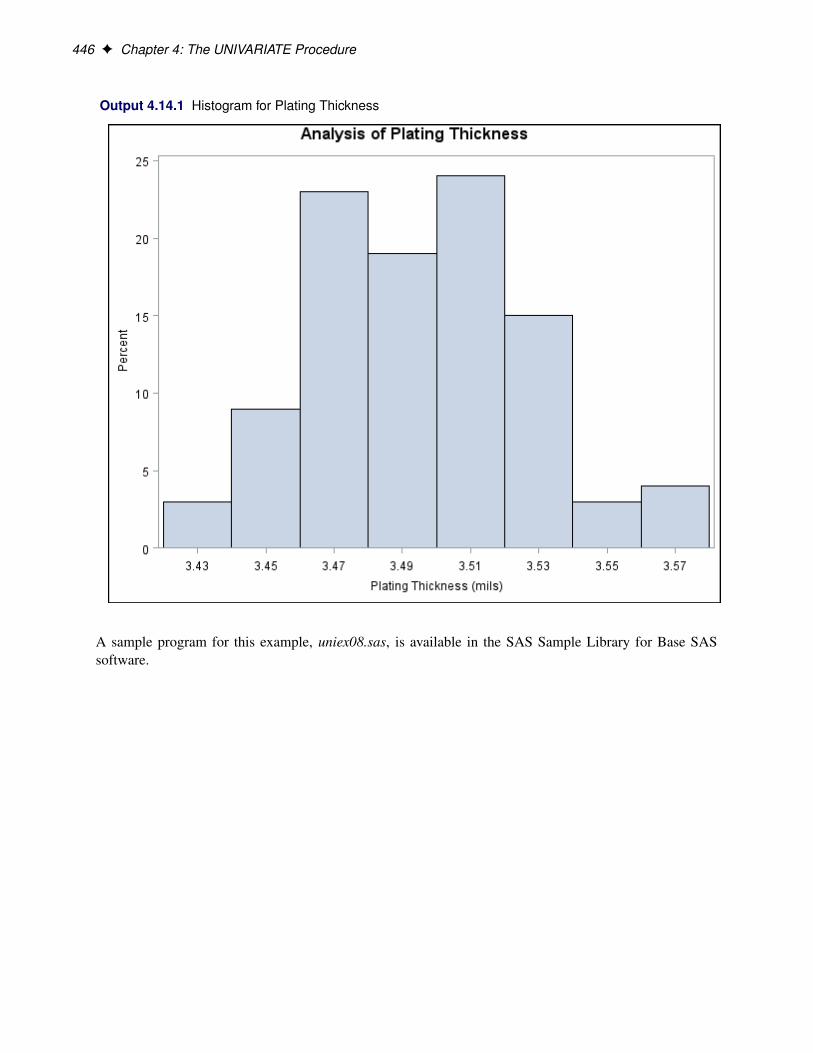
446 F Chapter 4: The UNIVARIATE Procedure
Output 4.14.1 Histogram for Plating Thickness
A sample program for this example, uniex08.sas, is available in the SAS Sample Library for Base SASsoftware.

Example 4.15: Creating a One-Way Comparative Histogram F 447
Example 4.15: Creating a One-Way Comparative Histogram
This example illustrates how to create a comparative histogram. The effective channel length (in microns)is measured for 1225 field effect transistors. The channel lengths (Length) are stored in a data set namedChannel, which is partially listed in Output 4.15.1:
Output 4.15.1 Partial Listing of Data Set Channel
The Data Set Channel
Lot Length
Lot 1 0.91. .
Lot 1 1.17Lot 2 1.47. .
Lot 2 1.39Lot 3 2.04. .
Lot 3 1.91
The following statements request a histogram of Length ignoring the lot source:
title 'Histogram of Length Ignoring Lot Source';ods graphics off;proc univariate data=Channel noprint;
histogram Length;run;
The resulting histogram is shown in Output 4.15.2.

448 F Chapter 4: The UNIVARIATE Procedure
Output 4.15.2 Histogram for Length Ignoring Lot Source
To investigate whether the peaks (modes) in Output 4.15.2 are related to the lot source, you can createa comparative histogram by using Lot as a classification variable. The following statements create thehistogram shown in Output 4.15.3:
title 'Comparative Analysis of Lot Source';ods graphics off;proc univariate data=Channel noprint;
class Lot;histogram Length / nrows = 3;
run;
The CLASS statement requests comparisons for each level (distinct value) of the classification variable Lot.The HISTOGRAM statement requests a comparative histogram for the variable Length. The NROWS=option specifies the number of rows per panel in the comparative histogram. By default, comparative his-tograms are displayed in two rows per panel.

Example 4.16: Creating a Two-Way Comparative Histogram F 449
Output 4.15.3 Comparison by Lot Source
Output 4.15.3 reveals that the distributions of Length are similarly distributed except for shifts in mean.
A sample program for this example, uniex09.sas, is available in the SAS Sample Library for Base SASsoftware.
Example 4.16: Creating a Two-Way Comparative Histogram
This example illustrates how to create a two-way comparative histogram. Two suppliers (A and B) pro-vide disk drives for a computer manufacturer. The manufacturer measures the disk drive opening width todetermine whether there has been a change in variability from 2002 to 2003 for each supplier.
The following statements save the measurements in a data set named Disk. There are two classificationvariables, Supplier and Year, and a user-defined format is associated with Year.

450 F Chapter 4: The UNIVARIATE Procedure
proc format ;value mytime 1 = '2002' 2 = '2003';
data Disk;input @1 Supplier $10. Year Width;label Width = 'Opening Width (inches)';format Year mytime.;
datalines;Supplier A 1 1.8932
. . .Supplier B 1 1.8986Supplier A 2 1.8978
. . .Supplier B 2 1.8997;
The following statements create the comparative histogram in Output 4.16.1:
title 'Results of Supplier Training Program';ods graphics off;proc univariate data=Disk noprint;
class Supplier Year / keylevel = ('Supplier A' '2003');histogram Width / intertile = 1.0
vaxis = 0 10 20 30ncols = 2nrows = 2;
run;
The KEYLEVEL= option specifies the key cell as the cell for which Supplier is equal to ‘SUPPLIER A’ andYear is equal to ‘2003.’ This cell determines the binning for the other cells, and the columns are arrangedso that this cell is displayed in the upper left corner. Without the KEYLEVEL= option, the default key cellwould be the cell for which Supplier is equal to ‘SUPPLIER A’ and Year is equal to ‘2002’; the columnlabeled ‘2002’ would be displayed to the left of the column labeled ‘2003.’
The VAXIS= option specifies the tick mark labels for the vertical axis. The NROWS=2 and NCOLS=2options specify a 2 � 2 arrangement for the tiles. Output 4.16.1 provides evidence that both suppliers havereduced variability from 2002 to 2003.
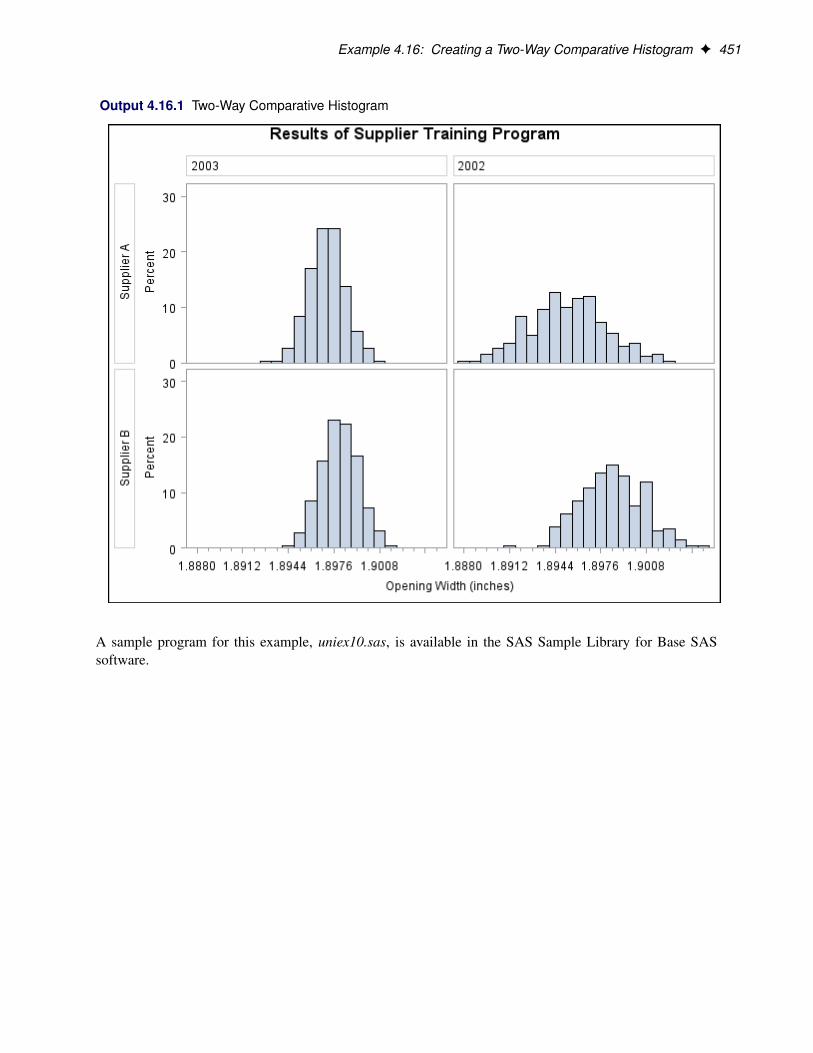
Example 4.16: Creating a Two-Way Comparative Histogram F 451
Output 4.16.1 Two-Way Comparative Histogram
A sample program for this example, uniex10.sas, is available in the SAS Sample Library for Base SASsoftware.

452 F Chapter 4: The UNIVARIATE Procedure
Example 4.17: Adding Insets with Descriptive Statistics
This example illustrates how to add insets with descriptive statistics to a comparative histogram; see Out-put 4.17.1. Three similar machines are used to attach a part to an assembly. One hundred assemblies aresampled from the output of each machine, and a part position is measured in millimeters. The followingstatements create the data set Machines, which contains the measurements in a variable named Position:
data Machines;input Position @@;label Position = 'Position in Millimeters';if (_n_ <= 100) then Machine = 'Machine 1';else if (_n_ <= 200) then Machine = 'Machine 2';else Machine = 'Machine 3';datalines;
-0.17 -0.19 -0.24 -0.24 -0.12 0.07 -0.61 0.22 1.91 -0.08-0.59 0.05 -0.38 0.82 -0.14 0.32 0.12 -0.02 0.26 0.19
... more lines ...
0.48 0.41 0.78 0.58 0.43 0.07 0.27 0.49 0.79 0.920.79 0.66 0.22 0.71 0.53 0.57 0.90 0.48 1.17 1.03
;
The following statements create the comparative histogram in Output 4.17.1:
title 'Machine Comparison Study';ods graphics off;proc univariate data=Machines noprint;
class Machine;histogram Position / nrows = 3
intertile = 1midpoints = -1.2 to 2.2 by 0.1vaxis = 0 to 16 by 4;
inset mean std="Std Dev" / pos = ne format = 6.3;run;
The INSET statement requests insets that contain the sample mean and standard deviation for each machinein the corresponding tile. The MIDPOINTS= option specifies the midpoints of the histogram bins.

Example 4.18: Binning a Histogram F 453
Output 4.17.1 Comparative Histograms
Output 4.17.1 shows that the average position for Machines 2 and 3 are similar and that the spread forMachine 1 is much larger than for Machines 2 and 3.
A sample program for this example, uniex11.sas, is available in the SAS Sample Library for Base SASsoftware.
Example 4.18: Binning a Histogram
This example, which is a continuation of Example 4.14, demonstrates various methods for binning a his-togram. This example also illustrates how to save bin percentages in an OUTHISTOGRAM= data set.
The manufacturer from Example 4.14 now wants to enhance the histogram by using the ENDPOINTS=option to change the endpoints of the bins. The following statements create a histogram with bins that haveend points 3.425 and 3.6 and width 0.025:

454 F Chapter 4: The UNIVARIATE Procedure
title 'Enhancing a Histogram';ods graphics off;ods select HistogramBins MyHist;proc univariate data=Trans;
histogram Thick / midpercents name='MyHist'endpoints = 3.425 to 3.6 by .025;
run;
The ODS SELECT statement restricts the output to the “HistogramBins” table and the “MyHist” histogram;see the section “ODS Table Names” on page 417. The ENDPOINTS= option specifies the endpoints for thehistogram bins. By default, if the ENDPOINTS= option is not specified, the automatic binning algorithmcomputes values for the midpoints of the bins. The MIDPERCENTS option requests a table of the midpointsof each histogram bin and the percent of the observations that fall in each bin. This table is displayed inOutput 4.18.1; the histogram is displayed in Output 4.18.2. The NAME= option specifies a name for thehistogram that can be used in the ODS SELECT statement.
Output 4.18.1 Table of Bin Percentages Requested with MIDPERCENTS Option
Enhancing a Histogram
The UNIVARIATE Procedure
Histogram Bins for Thick
BinMinimum ObservedPoint Percent
3.425 8.0003.450 21.0003.475 25.0003.500 29.0003.525 11.0003.550 5.0003.575 1.000

Example 4.18: Binning a Histogram F 455
Output 4.18.2 Histogram with ENDPOINTS= Option
The MIDPOINTS= option is an alternative to the ENDPOINTS= option for specifying histogram bins.The following statements create a histogram, shown in Output 4.18.3, which is similar to the one in Out-put 4.18.2:
title 'Enhancing a Histogram';ods graphics off;proc univariate data=Trans noprint;
histogram Thick / midpoints = 3.4375 to 3.5875 by .025rtincludeouthistogram = OutMdpts;
run;
Output 4.18.3 differs from Output 4.18.2 in two ways:
� The MIDPOINTS= option specifies the bins for the histogram by specifying the midpoints of the binsinstead of specifying the endpoints. Note that the histogram displays midpoints instead of endpoints.
� The RTINCLUDE option requests that the right endpoint of each bin be included in the histograminterval instead of the default, which is to include the left endpoint in the interval. This changes the

456 F Chapter 4: The UNIVARIATE Procedure
histogram slightly from Output 4.18.2. Six observations have a thickness equal to an endpoint of aninterval. For instance, there is one observation with a thickness of 3.45 mils. In Output 4.18.3, thisobservation is included in the bin from 3.425 to 3.45.
Output 4.18.3 Histogram with MIDPOINTS= and RTINCLUDE Options
The OUTHISTOGRAM= option produces an output data set named OutMdpts, displayed in Output 4.18.4.This data set provides information about the bins of the histogram. For more information, see the section“OUTHISTOGRAM= Output Data Set” on page 412.

Example 4.19: Adding a Normal Curve to a Histogram F 457
Output 4.18.4 The OUTHISTOGRAM= Data Set OutMdpts
Enhancing a Histogram
Obs _VAR_ _MIDPT_ _OBSPCT_ _COUNT_
1 Thick 3.4375 9 92 Thick 3.4625 21 213 Thick 3.4875 26 264 Thick 3.5125 28 285 Thick 3.5375 11 116 Thick 3.5625 5 5
A sample program for this example, uniex08.sas, is available in the SAS Sample Library for Base SASsoftware.
Example 4.19: Adding a Normal Curve to a Histogram
This example is a continuation of Example 4.14. The following statements fit a normal distribution to thethickness measurements in the Trans data set and superimpose the fitted density curve on the histogram:
title 'Analysis of Plating Thickness';ods graphics off;ods select ParameterEstimates GoodnessOfFit FitQuantiles Bins MyPlot;proc univariate data=Trans;
histogram Thick / normal(percents=20 40 60 80 midpercents)name='MyPlot';
inset n normal(ksdpval) / pos = ne format = 6.3;run;
The ODS SELECT statement restricts the output to the “ParameterEstimates,” “GoodnessOfFit,” “FitQuan-tiles,” and “Bins” tables; see the section “ODS Table Names” on page 417. The NORMAL option specifiesthat the normal curve be displayed on the histogram shown in Output 4.19.2. It also requests a summaryof the fitted distribution, which is shown in Output 4.19.1. goodness-of-fit tests, parameter estimates, andquantiles of the fitted distribution. (If you specify the NORMALTEST option in the PROC UNIVARIATEstatement, the Shapiro-Wilk test for normality is included in the tables of statistical output.)
Two secondary options are specified in parentheses after the NORMAL primary option. The PERCENTS=option specifies quantiles, which are to be displayed in the “FitQuantiles” table. The MIDPERCENTSoption requests a table that lists the midpoints, the observed percentage of observations, and the estimatedpercentage of the population in each interval (estimated from the fitted normal distribution). See Table 4.17and Table 4.24 for the secondary options that can be specified with after the NORMAL primary option.

458 F Chapter 4: The UNIVARIATE Procedure
Output 4.19.1 Summary of Fitted Normal Distribution
Analysis of Plating Thickness
The UNIVARIATE ProcedureFitted Normal Distribution for Thick (Plating Thickness (mils))
Parameters for Normal Distribution
Parameter Symbol Estimate
Mean Mu 3.49533Std Dev Sigma 0.032117
Goodness-of-Fit Tests for Normal Distribution
Test ----Statistic----- ------p Value------
Kolmogorov-Smirnov D 0.05563823 Pr > D >0.150Cramer-von Mises W-Sq 0.04307548 Pr > W-Sq >0.250Anderson-Darling A-Sq 0.27840748 Pr > A-Sq >0.250
Histogram Bin Percents for Normal Distribution
Bin -------Percent------Midpoint Observed Estimated
3.43 3.000 3.2963.45 9.000 9.3193.47 23.000 18.0913.49 19.000 24.1243.51 24.000 22.0993.53 15.000 13.9073.55 3.000 6.0113.57 4.000 1.784
Quantiles for Normal Distribution
------Quantile------Percent Observed Estimated
20.0 3.46700 3.4683040.0 3.48350 3.4871960.0 3.50450 3.5034780.0 3.52250 3.52236

Example 4.20: Adding Fitted Normal Curves to a Comparative Histogram F 459
Output 4.19.2 Histogram Superimposed with Normal Curve
The histogram of the variable Thick with a superimposed normal curve is shown in Output 4.19.2.
The estimated parameters for the normal curve ( Omu D 3:50 and O� D 0:03) are shown in Output 4.19.1.By default, the parameters are estimated unless you specify values with the MU= and SIGMA= secondaryoptions after the NORMAL primary option. The results of three goodness-of-fit tests based on the empiricaldistribution function (EDF) are displayed in Output 4.19.1. Because the p-values are all greater than 0.15,the hypothesis of normality is not rejected.
A sample program for this example, uniex08.sas, is available in the SAS Sample Library for Base SASsoftware.
Example 4.20: Adding Fitted Normal Curves to a Comparative Histogram
This example is a continuation of Example 4.15, which introduced the data set Channel on page 447.In Output 4.15.3, it appears that the channel lengths in each lot are normally distributed. The followingstatements use the NORMAL option to fit a normal distribution for each lot:

460 F Chapter 4: The UNIVARIATE Procedure
title 'Comparative Analysis of Lot Source';ods graphics off;proc univariate data=Channel noprint;
class Lot;histogram Length / nrows = 3
intertile = 1cpropnormal(noprint);
inset n = "N" / pos = nw;run;
The NOPRINT option in the PROC UNIVARIATE statement suppresses the tables of statistical outputproduced by default; the NOPRINT option in parentheses after the NORMAL option suppresses the tablesof statistical output related to the fit of the normal distribution. The normal parameters are estimated fromthe data for each lot, and the curves are superimposed on each component histogram. The INTERTILE=option specifies the space between the framed areas, which are referred to as tiles. The CPROP= optionrequests the shaded bars above each tile, which represent the relative frequencies of observations in eachlot. The comparative histogram is displayed in Output 4.20.1.
A sample program for this example, uniex09.sas, is available in the SAS Sample Library for Base SASsoftware.
Output 4.20.1 Fitting Normal Curves to a Comparative Histogram

Example 4.21: Fitting a Beta Curve F 461
Example 4.21: Fitting a Beta Curve
You can use a beta distribution to model the distribution of a variable that is known to vary between lowerand upper bounds. In this example, a manufacturing company uses a robotic arm to attach hinges on metalsheets. The attachment point should be offset 10.1 mm from the left edge of the sheet. The actual offsetvaries between 10.0 and 10.5 mm due to variation in the arm. The following statements save the offsets for50 attachment points as the values of the variable Length in the data set Robots:
data Robots;input Length @@;label Length = 'Attachment Point Offset (in mm)';datalines;
10.147 10.070 10.032 10.042 10.10210.034 10.143 10.278 10.114 10.12710.122 10.018 10.271 10.293 10.13610.240 10.205 10.186 10.186 10.08010.158 10.114 10.018 10.201 10.06510.061 10.133 10.153 10.201 10.10910.122 10.139 10.090 10.136 10.06610.074 10.175 10.052 10.059 10.07710.211 10.122 10.031 10.322 10.18710.094 10.067 10.094 10.051 10.174;
The following statements create a histogram with a fitted beta density curve, shown in Output 4.21.1:
title 'Fitted Beta Distribution of Offsets';ods graphics off;ods select ParameterEstimates FitQuantiles MyHist;proc univariate data=Robots;
histogram Length /beta(theta=10 scale=0.5 color=red fill)href = 10hreflabel = 'Lower Bound'lhref = 2vaxis = axis1name = 'MyHist';
axis1 label=(a=90 r=0);inset n = 'Sample Size'
beta / pos=ne cfill=blank;run;
The ODS SELECT statement restricts the output to the “ParameterEstimates” and “FitQuantiles” tables; seethe section “ODS Table Names” on page 417. The BETA primary option requests a fitted beta distribution.The THETA= secondary option specifies the lower threshold. The SCALE= secondary option specifies therange between the lower threshold and the upper threshold. Note that the default THETA= and SCALE=values are zero and one, respectively.

462 F Chapter 4: The UNIVARIATE Procedure
Output 4.21.1 Superimposing a Histogram with a Fitted Beta Curve
The FILL secondary option specifies that the area under the curve is to be filled with the CFILL= color. (IfFILL were omitted, the CFILL= color would be used to fill the histogram bars instead.)
The HREF= option draws a reference line at the lower bound, and the HREFLABEL= option adds the labelLower Bound. The LHREF= option specifies a dashed line type for the reference line. The INSET statementadds an inset with the sample size positioned in the northeast corner of the plot.
In addition to displaying the beta curve, the BETA option requests a summary of the curve fit. This summary,which includes parameters for the curve and the observed and estimated quantiles, is shown in Output 4.21.2.
A sample program for this example, uniex12.sas, is available in the SAS Sample Library for Base SASsoftware.

Example 4.22: Fitting Lognormal, Weibull, and Gamma Curves F 463
Output 4.21.2 Summary of Fitted Beta Distribution
Fitted Beta Distribution of Offsets
The UNIVARIATE ProcedureFitted Beta Distribution for Length (Attachment Point Offset (in mm))
Parameters for Beta Distribution
Parameter Symbol Estimate
Threshold Theta 10Scale Sigma 0.5Shape Alpha 2.06832Shape Beta 6.022479Mean 10.12782Std Dev 0.072339
Quantiles for Beta Distribution
------Quantile------Percent Observed Estimated
1.0 10.0180 10.01245.0 10.0310 10.0285
10.0 10.0380 10.041625.0 10.0670 10.071850.0 10.1220 10.117475.0 10.1750 10.173590.0 10.2255 10.229295.0 10.2780 10.263099.0 10.3220 10.3237
Example 4.22: Fitting Lognormal, Weibull, and Gamma Curves
To determine an appropriate model for a data distribution, you should consider curves from several distri-bution families. As shown in this example, you can use the HISTOGRAM statement to fit more than onedistribution and display the density curves on a histogram.
The gap between two plates is measured (in cm) for each of 50 welded assemblies selected at random fromthe output of a welding process. The following statements save the measurements (Gap) in a data set namedPlates:
data Plates;label Gap = 'Plate Gap in cm';input Gap @@;datalines;
0.746 0.357 0.376 0.327 0.485 1.741 0.241 0.777 0.768 0.4090.252 0.512 0.534 1.656 0.742 0.378 0.714 1.121 0.597 0.2310.541 0.805 0.682 0.418 0.506 0.501 0.247 0.922 0.880 0.3440.519 1.302 0.275 0.601 0.388 0.450 0.845 0.319 0.486 0.5291.547 0.690 0.676 0.314 0.736 0.643 0.483 0.352 0.636 1.080;

464 F Chapter 4: The UNIVARIATE Procedure
The following statements fit three distributions (lognormal, Weibull, and gamma) and display their densitycurves on a single histogram:
title 'Distribution of Plate Gaps';ods graphics off;ods select ParameterEstimates GoodnessOfFit FitQuantiles MyHist;proc univariate data=Plates;
var Gap;histogram / midpoints=0.2 to 1.8 by 0.2
lognormalweibullgammavaxis = axis1name = 'MyHist';
inset n mean(5.3) std='Std Dev'(5.3) skewness(5.3)/ pos = ne header = 'Summary Statistics';
axis1 label=(a=90 r=0);run;
The ODS SELECT statement restricts the output to the “ParameterEstimates,” “GoodnessOfFit,” and“FitQuantiles” tables; see the section “ODS Table Names” on page 417. The LOGNORMAL, WEIBULL,and GAMMA primary options request superimposed fitted curves on the histogram in Output 4.22.1. Notethat a threshold parameter � D 0 is assumed for each curve. In applications where the threshold is not zero,you can specify � with the THETA= secondary option.
The LOGNORMAL, WEIBULL, and GAMMA options also produce the summaries for the fitted distribu-tions shown in Output 4.22.2 through Output 4.22.4.
Output 4.22.2 provides three EDF goodness-of-fit tests for the lognormal distribution: the Anderson-Darling, the Cramér-von Mises, and the Kolmogorov-Smirnov tests. At the ˛ D 0:10 significance level, alltests support the conclusion that the two-parameter lognormal distribution with scale parameter O� D �0:58and shape parameter O� D 0:50 provides a good model for the distribution of plate gaps.

Example 4.22: Fitting Lognormal, Weibull, and Gamma Curves F 465
Output 4.22.1 Superimposing a Histogram with Fitted Curves
Output 4.22.2 Summary of Fitted Lognormal Distribution
Distribution of Plate Gaps
The UNIVARIATE ProcedureFitted Lognormal Distribution for Gap (Plate Gap in cm)
Parameters for Lognormal Distribution
Parameter Symbol Estimate
Threshold Theta 0Scale Zeta -0.58375Shape Sigma 0.499546Mean 0.631932Std Dev 0.336436

466 F Chapter 4: The UNIVARIATE Procedure
Output 4.22.2 continued
Goodness-of-Fit Tests for Lognormal Distribution
Test ----Statistic----- ------p Value------
Kolmogorov-Smirnov D 0.06441431 Pr > D >0.150Cramer-von Mises W-Sq 0.02823022 Pr > W-Sq >0.500Anderson-Darling A-Sq 0.24308402 Pr > A-Sq >0.500
Quantiles for Lognormal Distribution
------Quantile------Percent Observed Estimated
1.0 0.23100 0.174495.0 0.24700 0.24526
10.0 0.29450 0.2940725.0 0.37800 0.3982550.0 0.53150 0.5578075.0 0.74600 0.7812990.0 1.10050 1.0580795.0 1.54700 1.2686299.0 1.74100 1.78313
Output 4.22.3 Summary of Fitted Weibull Distribution
Distribution of Plate Gaps
The UNIVARIATE ProcedureFitted Weibull Distribution for Gap (Plate Gap in cm)
Parameters for Weibull Distribution
Parameter Symbol Estimate
Threshold Theta 0Scale Sigma 0.719208Shape C 1.961159Mean 0.637641Std Dev 0.339248
Goodness-of-Fit Tests for Weibull Distribution
Test ----Statistic----- ------p Value------
Cramer-von Mises W-Sq 0.15937281 Pr > W-Sq 0.016Anderson-Darling A-Sq 1.15693542 Pr > A-Sq <0.010

Example 4.22: Fitting Lognormal, Weibull, and Gamma Curves F 467
Output 4.22.3 continued
Quantiles for Weibull Distribution
------Quantile------Percent Observed Estimated
1.0 0.23100 0.068895.0 0.24700 0.15817
10.0 0.29450 0.2283125.0 0.37800 0.3810250.0 0.53150 0.5966175.0 0.74600 0.8495590.0 1.10050 1.1004095.0 1.54700 1.2584299.0 1.74100 1.56691
Output 4.22.3 provides two EDF goodness-of-fit tests for the Weibull distribution: the Anderson-Darlingand the Cramér-von Mises tests. The p-values for the EDF tests are all less than 0.10, indicating that thedata do not support a Weibull model.
Output 4.22.4 Summary of Fitted Gamma Distribution
Distribution of Plate Gaps
The UNIVARIATE ProcedureFitted Gamma Distribution for Gap (Plate Gap in cm)
Parameters for Gamma Distribution
Parameter Symbol Estimate
Threshold Theta 0Scale Sigma 0.155198Shape Alpha 4.082646Mean 0.63362Std Dev 0.313587
Goodness-of-Fit Tests for Gamma Distribution
Test ----Statistic----- ------p Value------
Kolmogorov-Smirnov D 0.09695325 Pr > D >0.250Cramer-von Mises W-Sq 0.07398467 Pr > W-Sq >0.250Anderson-Darling A-Sq 0.58106613 Pr > A-Sq 0.137

468 F Chapter 4: The UNIVARIATE Procedure
Output 4.22.4 continued
Quantiles for Gamma Distribution
------Quantile------Percent Observed Estimated
1.0 0.23100 0.133265.0 0.24700 0.21951
10.0 0.29450 0.2793825.0 0.37800 0.4040450.0 0.53150 0.5827175.0 0.74600 0.8080490.0 1.10050 1.0539295.0 1.54700 1.2216099.0 1.74100 1.57939
Output 4.22.4 provides three EDF goodness-of-fit tests for the gamma distribution: the Anderson-Darling,the Cramér-von Mises, and the Kolmogorov-Smirnov tests. At the ˛ D 0:10 significance level, all testssupport the conclusion that the gamma distribution with scale parameter � D 0:16 and shape parameter˛ D 4:08 provides a good model for the distribution of plate gaps.
Based on this analysis, the fitted lognormal distribution and the fitted gamma distribution are both goodmodels for the distribution of plate gaps.
A sample program for this example, uniex13.sas, is available in the SAS Sample Library for Base SASsoftware.
Example 4.23: Computing Kernel Density Estimates
This example illustrates the use of kernel density estimates to visualize a nonnormal data distribution. Thisexample uses the data set Channel, which is introduced in Example 4.15.
When you compute kernel density estimates, you should try several choices for the bandwidth parameterc because this determines the smoothness and closeness of the fit. You can specify a list of up to five C=values with the KERNEL option to request multiple density estimates, as shown in the following statements:
title 'FET Channel Length Analysis';ods graphics off;proc univariate data=Channel noprint;
histogram Length / kernel(c = 0.25 0.50 0.75 1.00l = 1 20 2 34noprint);
run;
The L= secondary option specifies distinct line types for the curves (the L= values are paired with the C=values in the order listed). Output 4.23.1 demonstrates the effect of c. In general, larger values of c yieldsmoother density estimates, and smaller values yield estimates that more closely fit the data distribution.

Example 4.24: Fitting a Three-Parameter Lognormal Curve F 469
Output 4.23.1 Multiple Kernel Density Estimates
Output 4.23.1 reveals strong trimodality in the data, which is displayed with comparative histograms inExample 4.15.
A sample program for this example, uniex09.sas, is available in the SAS Sample Library for Base SASsoftware.
Example 4.24: Fitting a Three-Parameter Lognormal Curve
If you request a lognormal fit with the LOGNORMAL primary option, a two-parameter lognormal distri-bution is assumed. This means that the shape parameter � and the scale parameter � are unknown (unlessspecified) and that the threshold � is known (it is either specified with the THETA= option or assumed to bezero).
If it is necessary to estimate � in addition to � and � , the distribution is referred to as a three-parameterlognormal distribution. This example shows how you can request a three-parameter lognormal distribution.

470 F Chapter 4: The UNIVARIATE Procedure
A manufacturing process produces a plastic laminate whose strength must exceed a minimum of 25 poundsper square inch (psi). Samples are tested, and a lognormal distribution is observed for the strengths. It isimportant to estimate � to determine whether the process meets the strength requirement. The followingstatements save the strengths for 49 samples in the data set Plastic:
data Plastic;label Strength = 'Strength in psi';input Strength @@;datalines;
30.26 31.23 71.96 47.39 33.93 76.15 42.2181.37 78.48 72.65 61.63 34.90 24.83 68.9343.27 41.76 57.24 23.80 34.03 33.38 21.8731.29 32.48 51.54 44.06 42.66 47.98 33.7325.80 29.95 60.89 55.33 39.44 34.50 73.5143.41 54.67 99.43 50.76 48.81 31.86 33.8835.57 60.41 54.92 35.66 59.30 41.96 45.32;
The following statements use the LOGNORMAL primary option in the HISTOGRAM statement to displaythe fitted three-parameter lognormal curve shown in Output 4.24.1:
title 'Three-Parameter Lognormal Fit';ods graphics off;proc univariate data=Plastic noprint;
histogram Strength / lognormal(fill theta = est noprint);inset lognormal / format=6.2 pos=ne;
run;
The NOPRINT option suppresses the tables of statistical output produced by default. SpecifyingTHETA=EST requests a local maximum likelihood estimate (LMLE) for � , as described by Cohen (1951).This estimate is then used to compute maximum likelihood estimates for � and �.
NOTE: You can also specify THETA=EST with the WEIBULL primary option to fit a three-parameterWeibull distribution.
A sample program for this example, uniex14.sas, is available in the SAS Sample Library for Base SASsoftware.

Example 4.25: Annotating a Folded Normal Curve F 471
Output 4.24.1 Three-Parameter Lognormal Fit
Example 4.25: Annotating a Folded Normal Curve
This example shows how to display a fitted curve that is not supported by the HISTOGRAM statement.The offset of an attachment point is measured (in mm) for a number of manufactured assemblies, and themeasurements (Offset) are saved in a data set named Assembly. The following statements create the dataset Assembly:
data Assembly;label Offset = 'Offset (in mm)';input Offset @@;datalines;
11.11 13.07 11.42 3.92 11.08 5.40 11.22 14.69 6.27 9.769.18 5.07 3.51 16.65 14.10 9.69 16.61 5.67 2.89 8.139.97 3.28 13.03 13.78 3.13 9.53 4.58 7.94 13.51 11.43
11.98 3.90 7.67 4.32 12.69 6.17 11.48 2.82 20.42 1.013.18 6.02 6.63 1.72 2.42 11.32 16.49 1.22 9.13 3.341.29 1.70 0.65 2.62 2.04 11.08 18.85 11.94 8.34 2.070.31 8.91 13.62 14.94 4.83 16.84 7.09 3.37 0.49 15.19

472 F Chapter 4: The UNIVARIATE Procedure
5.16 4.14 1.92 12.70 1.97 2.10 9.38 3.18 4.18 7.2215.84 10.85 2.35 1.93 9.19 1.39 11.40 12.20 16.07 9.230.05 2.15 1.95 4.39 0.48 10.16 4.81 8.28 5.68 22.810.23 0.38 12.71 0.06 10.11 18.38 5.53 9.36 9.32 3.63
12.93 10.39 2.05 15.49 8.12 9.52 7.77 10.70 6.37 1.918.60 22.22 1.74 5.84 12.90 13.06 5.08 2.09 6.41 1.40
15.60 2.36 3.97 6.17 0.62 8.56 9.36 10.19 7.16 2.3712.91 0.95 0.89 3.82 7.86 5.33 12.92 2.64 7.92 14.06;
It is decided to fit a folded normal distribution to the offset measurements. A variableX has a folded normaldistribution if X D jY j, where Y is distributed as N.�; �/. The fitted density is
h.x/ D1
p2��
�exp
��.x � �/2
2�2
�C exp
��.x C �/2
2�2
��where x � 0.
You can use SAS/IML to compute preliminary estimates of � and � based on a method of moments givenby Elandt (1961). These estimates are computed by solving equation (19) Elandt (1961), which is given by
f .�/ D
�2p2�e��
2=2 � � Œ1 � 2ˆ.�/��2
1C �2D A
where ˆ.�/ is the standard normal distribution function and
A DNx2
1n
PniD1 x
2i
Then the estimates of � and � are given by
O�0 D
r1n
PniD1 x
2i
1C O�2
Omu0 D O� � O�0
Begin by using PROC MEANS to compute the first and second moments and by using the following DATAstep to compute the constant A:
proc means data = Assembly noprint;var Offset;output out=stat mean=m1 var=var n=n min = min;
run;
* Compute constant A from equation (19) of Elandt (1961);data stat;
keep m2 a min;set stat;a = (m1*m1);m2 = ((n-1)/n)*var + a;a = a/m2;
run;

Example 4.25: Annotating a Folded Normal Curve F 473
Next, use the SAS/IML subroutine NLPDD to solve equation (19) by minimizing .f .�/�A/2, and computeOmu0 and O�0:
proc iml;use stat;read all var {m2} into m2;read all var {a} into a;read all var {min} into min;
* f(t) is the function in equation (19) of Elandt (1961);start f(t) global(a);
y = .39894*exp(-0.5*t*t);y = (2*y-(t*(1-2*probnorm(t))))**2/(1+t*t);y = (y-a)**2;return(y);
finish;
* Minimize (f(t)-A)**2 and estimate mu and sigma;if ( min < 0 ) then do;
print "Warning: Observations are not all nonnegative.";print " The folded normal is inappropriate.";stop;end;
if ( a < 0.637 ) then do;print "Warning: the folded normal may be inappropriate";end;
opt = { 0 0 };con = { 1e-6 };x0 = { 2.0 };tc = { . . . . . 1e-8 . . . . . . .};call nlpdd(rc,etheta0,"f",x0,opt,con,tc);esig0 = sqrt(m2/(1+etheta0*etheta0));emu0 = etheta0*esig0;
create prelim var {emu0 esig0 etheta0};append;close prelim;
* Define the log likelihood of the folded normal;start g(p) global(x);
y = 0.0;do i = 1 to nrow(x);
z = exp( (-0.5/p[2])*(x[i]-p[1])*(x[i]-p[1]) );z = z + exp( (-0.5/p[2])*(x[i]+p[1])*(x[i]+p[1]) );y = y + log(z);
end;y = y - nrow(x)*log( sqrt( p[2] ) );return(y);
finish;
* Maximize the log likelihood with subroutine NLPDD;use assembly;read all var {offset} into x;esig0sq = esig0*esig0;x0 = emu0||esig0sq;

474 F Chapter 4: The UNIVARIATE Procedure
opt = { 1 0 };con = { . 0.0, . . };call nlpdd(rc,xr,"g",x0,opt,con);emu = xr[1];esig = sqrt(xr[2]);etheta = emu/esig;create parmest var{emu esig etheta};append;close parmest;
quit;
The preliminary estimates are saved in the data set Prelim, as shown in Output 4.25.1.
Output 4.25.1 Preliminary Estimates of �, � , and �
Obs EMU0 ESIG0 ETHETA0
1 6.51735 6.54953 0.99509
Now, using Omu0 and O�0 as initial estimates, call the NLPDD subroutine to maximize the log likelihood,l.�; �/, of the folded normal distribution, where, up to a constant,
l.�; �/ D �n log � CnXiD1
log�
exp��.xi � �/
2
2�2
�C exp
��.xi C �/
2
2�2
��* Define the log likelihood of the folded normal;start g(p) global(x);
y = 0.0;do i = 1 to nrow(x);
z = exp( (-0.5/p[2])*(x[i]-p[1])*(x[i]-p[1]) );z = z + exp( (-0.5/p[2])*(x[i]+p[1])*(x[i]+p[1]) );y = y + log(z);
end;y = y - nrow(x)*log( sqrt( p[2] ) );return(y);
finish;
* Maximize the log likelihood with subroutine NLPDD;use assembly;read all var {offset} into x;esig0sq = esig0*esig0;x0 = emu0||esig0sq;opt = { 1 0 };con = { . 0.0, . . };call nlpdd(rc,xr,"g",x0,opt,con);emu = xr[1];esig = sqrt(xr[2]);etheta = emu/esig;create parmest var{emu esig etheta};append;close parmest;quit;
The data set ParmEst contains the maximum likelihood estimates Omu and O� (as well as Omu= O� ), as shownin Output 4.25.2.

Example 4.25: Annotating a Folded Normal Curve F 475
Output 4.25.2 Final Estimates of �, � , and �
Obs EMU ESIG ETHETA
1 6.66761 6.39650 1.04239
To annotate the curve on a histogram, begin by computing the width and endpoints of the histogram intervals.The following statements save these values in a data set called OutCalc. Note that a plot is not produced atthis point.
proc univariate data = Assembly noprint;histogram Offset / outhistogram = out normal(noprint) noplot;
run;
data OutCalc (drop = _MIDPT_);set out (keep = _MIDPT_) end = eof;retain _MIDPT1_ _WIDTH_;if _N_ = 1 then _MIDPT1_ = _MIDPT_;if eof then do;
_MIDPTN_ = _MIDPT_;_WIDTH_ = (_MIDPTN_ - _MIDPT1_) / (_N_ - 1);output;
end;run;
Output 4.25.3 provides a listing of the data set OutCalc. The width of the histogram bars is saved as thevalue of the variable _WIDTH_; the midpoints of the first and last histogram bars are saved as the values ofthe variables _MIDPT1_ and _MIDPTN_.
Output 4.25.3 The Data Set OutCalc
Obs _MIDPT1_ _WIDTH_ _MIDPTN_
1 1.5 3 22.5
The following statements create an annotate data set named Anno, which contains the coordinates of thefitted curve:
data Anno;merge ParmEst OutCalc;length function color $ 8;function = 'point';color = 'black';size = 2;xsys = '2';ysys = '2';when = 'a';constant = 39.894*_width_;;left = _midpt1_ - .5*_width_;right = _midptn_ + .5*_width_;inc = (right-left)/100;

476 F Chapter 4: The UNIVARIATE Procedure
do x = left to right by inc;z1 = (x-emu)/esig;z2 = (x+emu)/esig;y = (constant/esig)*(exp(-0.5*z1*z1)+exp(-0.5*z2*z2));output;function = 'draw';
end;run;
The following statements read the ANNOTATE= data set and display the histogram and fitted curve:
title 'Folded Normal Distribution';ods graphics off;proc univariate data=assembly noprint;
histogram Offset / annotate = anno;run;
Output 4.25.4 displays the histogram and fitted curve.
Output 4.25.4 Histogram with Annotated Folded Normal Curve
A sample program for this example, uniex15.sas, is available in the SAS Sample Library for Base SASsoftware.

Example 4.26: Creating Lognormal Probability Plots F 477
Example 4.26: Creating Lognormal Probability Plots
This example is a continuation of the example explored in the section “Modeling a Data Distribution” onpage 248.
In the normal probability plot shown in Output 4.6, the nonlinearity of the point pattern indicates a departurefrom normality in the distribution of Deviation. Because the point pattern is curved with slope increasingfrom left to right, a theoretical distribution that is skewed to the right, such as a lognormal distribution,should provide a better fit than the normal distribution. See the section “Interpretation of Quantile-Quantileand Probability Plots” on page 401.
You can explore the possibility of a lognormal fit with a lognormal probability plot. When you request sucha plot, you must specify the shape parameter � for the lognormal distribution. This value must be positive,and typical values of � range from 0.1 to 1.0. You can specify values for � with the SIGMA= secondaryoption in the LOGNORMAL primary option, or you can specify that � is to be estimated from the data.
The following statements illustrate the first approach by creating a series of three lognormal probabilityplots for the variable Deviation introduced in the section “Modeling a Data Distribution” on page 248:
symbol v=plus height=3.5pct;title 'Lognormal Probability Plot for Position Deviations';ods graphics off;proc univariate data=Aircraft noprint;
probplot Deviation /lognormal(theta=est zeta=est sigma=0.7 0.9 1.1)href = 95lhref = 1square;
run;
The LOGNORMAL primary option requests plots based on the lognormal family of distributions, andthe SIGMA= secondary option requests plots for � equal to 0.7, 0.9, and 1.1. These plots are displayedin Output 4.26.1, Output 4.26.2, and Output 4.26.3, respectively. Alternatively, you can specify � to beestimated using the sample standard deviation by using the option SIGMA=EST.
The SQUARE option displays the probability plot in a square format, the HREF= option requests a referenceline at the 95th percentile, and the LHREF= option specifies the line type for the reference line.

478 F Chapter 4: The UNIVARIATE Procedure
Output 4.26.1 Probability Plot Based on Lognormal Distribution with � =0.7

Example 4.26: Creating Lognormal Probability Plots F 479
Output 4.26.2 Probability Plot Based on Lognormal Distribution with � =0.9

480 F Chapter 4: The UNIVARIATE Procedure
Output 4.26.3 Probability Plot Based on Lognormal Distribution with � =1.1
The value � D 0:9 in Output 4.26.2 most nearly linearizes the point pattern. The 95th percentile of theposition deviation distribution seen in Output 4.26.2 is approximately 0.001, because this is the value cor-responding to the intersection of the point pattern with the reference line.
NOTE: After the � that produces the most linear fit is found, you can then estimate the threshold parameter� and the scale parameter �. See Example 4.31.
The following statements illustrate how you can create a lognormal probability plot for Deviation by usinga local maximum likelihood estimate for � .
symbol v=plus height=3.5pct;title 'Lognormal Probability Plot for Position Deviations';ods graphics off;proc univariate data=Aircraft noprint;
probplot Deviation / lognormal(theta=est zeta=est sigma=est)href = 95square;
run;
The plot is displayed in Output 4.26.4. Note that the maximum likelihood estimate of � (in this case, 0.882)does not necessarily produce the most linear point pattern.

Example 4.27: Creating a Histogram to Display Lognormal Fit F 481
Output 4.26.4 Probability Plot Based on Lognormal Distribution with Estimated �
A sample program for this example, uniex16.sas, is available in the SAS Sample Library for Base SASsoftware.
Example 4.27: Creating a Histogram to Display Lognormal Fit
This example uses the data set Aircraft from Example 4.26 to illustrate how to display a lognormal fit witha histogram. To determine whether the lognormal distribution is an appropriate model for a distribution,you should consider the graphical fit as well as conduct goodness-of-fit tests. The following statements fit alognormal distribution and display the density curve on a histogram:
title 'Distribution of Position Deviations';ods graphics off;ods select Lognormal.ParameterEstimates Lognormal.GoodnessOfFit MyPlot;proc univariate data=Aircraft;
var Deviation;histogram / lognormal(w=3 theta=est)
vaxis = axis1name = 'MyPlot';
inset n mean (5.3) std='Std Dev' (5.3) skewness (5.3) /pos = ne header = 'Summary Statistics';
axis1 label=(a=90 r=0);run;

482 F Chapter 4: The UNIVARIATE Procedure
The ODS SELECT statement restricts the output to the “ParameterEstimates” and “GoodnessOfFit” tables;see the section “ODS Table Names” on page 417. The LOGNORMAL primary option superimposes a fittedcurve on the histogram in Output 4.27.1. The W= option specifies the line width for the curve. The INSETstatement specifies that the mean, standard deviation, and skewness be displayed in an inset in the northeastcorner of the plot. Note that the default value of the threshold parameter � is zero. In applications where thethreshold is not zero, you can specify � with the THETA= option. The variable Deviation includes valuesthat are less than the default threshold; therefore, the option THETA= EST is used.
Output 4.27.1 Normal Probability Plot Created with Graphics Device
Output 4.27.2 provides three EDF goodness-of-fit tests for the lognormal distribution: the Anderson-Darling, the Cramér-von Mises, and the Kolmogorov-Smirnov tests. The null hypothesis for the three testsis that a lognormal distribution holds for the sample data.

Example 4.28: Creating a Normal Quantile Plot F 483
Output 4.27.2 Summary of Fitted Lognormal Distribution
Distribution of Position Deviations
The UNIVARIATE ProcedureFitted Lognormal Distribution for Deviation (Position Deviation)
Parameters for Lognormal Distribution
Parameter Symbol Estimate
Threshold Theta -0.00834Scale Zeta -6.14382Shape Sigma 0.882225Mean -0.00517Std Dev 0.003438
Goodness-of-Fit Tests for Lognormal Distribution
Test ----Statistic----- ------p Value------
Kolmogorov-Smirnov D 0.09419634 Pr > D >0.500Cramer-von Mises W-Sq 0.02919815 Pr > W-Sq >0.500Anderson-Darling A-Sq 0.21606642 Pr > A-Sq >0.500
The p-values for all three tests are greater than 0.5, so the null hypothesis is not rejected. The tests supportthe conclusion that the two-parameter lognormal distribution with scale parameter O� D �6:14 and shapeparameter O� D 0:88 provides a good model for the distribution of position deviations. For further discussionof goodness-of-fit interpretation, see the section “Goodness-of-Fit Tests” on page 393.
A sample program for this example, uniex16.sas, is available in the SAS Sample Library for Base SASsoftware.
Example 4.28: Creating a Normal Quantile Plot
This example illustrates how to create a normal quantile plot. An engineer is analyzing the distribution ofdistances between holes cut in steel sheets. The following statements save measurements of the distancebetween two holes cut into 50 steel sheets as values of the variable Distance in the data set Sheets:
data Sheets;input Distance @@;label Distance = 'Hole Distance (cm)';datalines;
9.80 10.20 10.27 9.70 9.7610.11 10.24 10.20 10.24 9.639.99 9.78 10.10 10.21 10.009.96 9.79 10.08 9.79 10.06
10.10 9.95 9.84 10.11 9.9310.56 10.47 9.42 10.44 10.1610.11 10.36 9.94 9.77 9.36

484 F Chapter 4: The UNIVARIATE Procedure
9.89 9.62 10.05 9.72 9.829.99 10.16 10.58 10.70 9.54
10.31 10.07 10.33 9.98 10.15;
The engineer decides to check whether the distribution of distances is normal. The following statementscreate a Q-Q plot for Distance, shown in Output 4.28.1:
symbol v=plus;title 'Normal Quantile-Quantile Plot for Hole Distance';ods graphics off;proc univariate data=Sheets noprint;
qqplot Distance;run;
The plot compares the ordered values of Distance with quantiles of the normal distribution. The linearity ofthe point pattern indicates that the measurements are normally distributed. Note that a normal Q-Q plot iscreated by default.
Output 4.28.1 Normal Quantile-Quantile Plot for Distance

Example 4.29: Adding a Distribution Reference Line F 485
A sample program for this example, uniex17.sas, is available in the SAS Sample Library for Base SASsoftware.
Example 4.29: Adding a Distribution Reference Line
This example, which is a continuation of Example 4.28, illustrates how to add a reference line to a normalQ-Q plot, which represents the normal distribution with mean �0 and standard deviation �0. The followingstatements reproduce the Q-Q plot in Output 4.28.1 and add the reference line:
symbol v=plus;title 'Normal Quantile-Quantile Plot for Hole Distance';ods graphics off;proc univariate data=Sheets noprint;
qqplot Distance / normal(mu=est sigma=est color=red l=2)square;
run;
The plot is displayed in Output 4.29.1.
Specifying MU=EST and SIGMA=EST with the NORMAL primary option requests the reference line forwhich �0 and �0 are estimated by the sample mean and standard deviation. Alternatively, you can specifynumeric values for�0 and �0 with the MU= and SIGMA= secondary options. The COLOR= and L= optionsspecify the color and type of the line, and the SQUARE option displays the plot in a square format. TheNOPRINT options in the PROC UNIVARIATE statement and after the NORMAL option suppress all thetables of statistical output produced by default.

486 F Chapter 4: The UNIVARIATE Procedure
Output 4.29.1 Adding a Distribution Reference Line to a Q-Q Plot
The data clearly follow the line, which indicates that the distribution of the distances is normal.
A sample program for this example, uniex17.sas, is available in the SAS Sample Library for Base SASsoftware.

Example 4.30: Interpreting a Normal Quantile Plot F 487
Example 4.30: Interpreting a Normal Quantile Plot
This example illustrates how to interpret a normal quantile plot when the data are from a non-normal dis-tribution. The following statements create the data set Measures, which contains the measurements of thediameters of 50 steel rods in the variable Diameter:
data Measures;input Diameter @@;label Diameter = 'Diameter (mm)';datalines;
5.501 5.251 5.404 5.366 5.445 5.576 5.6075.200 5.977 5.177 5.332 5.399 5.661 5.5125.252 5.404 5.739 5.525 5.160 5.410 5.8235.376 5.202 5.470 5.410 5.394 5.146 5.2445.309 5.480 5.388 5.399 5.360 5.368 5.3945.248 5.409 5.304 6.239 5.781 5.247 5.9075.208 5.143 5.304 5.603 5.164 5.209 5.4755.223;
The following statements request the normal Q-Q plot in Output 4.30.1:
symbol v=plus;title 'Normal Q-Q Plot for Diameters';ods graphics off;proc univariate data=Measures noprint;
qqplot Diameter / normalsquarevaxis=axis1;
axis1 label=(a=90 r=0);run;
The nonlinearity of the points in Output 4.30.1 indicates a departure from normality. Because the pointpattern is curved with slope increasing from left to right, a theoretical distribution that is skewed to theright, such as a lognormal distribution, should provide a better fit than the normal distribution. The mildcurvature suggests that you should examine the data with a series of lognormal Q-Q plots for small valuesof the shape parameter � , as illustrated in Example 4.31. For details on interpreting a Q-Q plot, see thesection “Interpretation of Quantile-Quantile and Probability Plots” on page 401.

488 F Chapter 4: The UNIVARIATE Procedure
Output 4.30.1 Normal Quantile-Quantile Plot of Nonnormal Data
A sample program for this example, uniex18.sas, is available in the SAS Sample Library for Base SASsoftware.
Example 4.31: Estimating Three Parameters from Lognormal Quantile Plots
This example, which is a continuation of Example 4.30, demonstrates techniques for estimating the shape,location, and scale parameters, and the theoretical percentiles for a three-parameter lognormal distribution.
The three-parameter lognormal distribution depends on a threshold parameter � , a scale parameter �, anda shape parameter � . You can estimate � from a series of lognormal Q-Q plots which use the SIGMA=secondary option to specify different values of � ; the estimate of � is the value that linearizes the pointpattern. You can then estimate the threshold and scale parameters from the intercept and slope of thepoint pattern. The following statements create the series of plots in Output 4.31.1, Output 4.31.2, andOutput 4.31.3 for � values of 0.2, 0.5, and 0.8, respectively:

Example 4.31: Estimating Three Parameters from Lognormal Quantile Plots F 489
symbol v=plus;title 'Lognormal Q-Q Plot for Diameters';ods graphics off;proc univariate data=Measures noprint;
qqplot Diameter / lognormal(sigma=0.2 0.5 0.8)square;
run;
NOTE: You must specify a value for the shape parameter � for a lognormal Q-Q plot with the SIGMA=option or its alias, the SHAPE= option.
Output 4.31.1 Lognormal Quantile-Quantile Plot (� =0.2)

490 F Chapter 4: The UNIVARIATE Procedure
Output 4.31.2 Lognormal Quantile-Quantile Plot (� =0.5)

Example 4.31: Estimating Three Parameters from Lognormal Quantile Plots F 491
Output 4.31.3 Lognormal Quantile-Quantile Plot (� =0.8)
The plot in Output 4.31.2 displays the most linear point pattern, indicating that the lognormal distributionwith � D 0:5 provides a reasonable fit for the data distribution.
Data with this particular lognormal distribution have the following density function:
p.x/ D
( p2
p�.x��/
exp��2.log.x � �/ � �/2
�for x > �
0 for x � �
The points in the plot fall on or near the line with intercept � and slope exp.�/. Based on Output 4.31.2,� � 5 and exp.�/ � 1:2
3D 0:4, giving � � log.0:4/ � �0:92.
You can also request a reference line by using the SIGMA=, THETA=, and ZETA= options together. Thefollowing statements produce the lognormal Q-Q plot in Output 4.31.4:

492 F Chapter 4: The UNIVARIATE Procedure
symbol v=plus;title 'Lognormal Q-Q Plot for Diameters';ods graphics off;proc univariate data=Measures noprint;
qqplot Diameter / lognormal(theta=5 zeta=est sigma=estcolor=black l=2)
square;run;
Output 4.31.1 through Output 4.31.3 show that the threshold parameter � is not equal to zero. SpecifyingTHETA=5 overrides the default value of zero. The SIGMA=EST and ZETA=EST secondary options requestestimates for � and exp � that use the sample mean and standard deviation.
Output 4.31.4 Lognormal Quantile-Quantile Plot (� =est, � =est, � =5)
From the plot in Output 4.31.2, � can be estimated as 0.51, which is consistent with the estimate of 0.5derived from the plot in Output 4.31.2. Example 4.32 illustrates how to estimate percentiles by usinglognormal Q-Q plots.
A sample program for this example, uniex18.sas, is available in the SAS Sample Library for Base SASsoftware.

Example 4.32: Estimating Percentiles from Lognormal Quantile Plots F 493
Example 4.32: Estimating Percentiles from Lognormal Quantile Plots
This example, which is a continuation of Example 4.31, shows how to use a Q-Q plot to estimate percentilessuch as the 95th percentile of the lognormal distribution. A probability plot can also be used for this purpose,as illustrated in Example 4.26.
The point pattern in Output 4.31.4 has a slope of approximately 0.39 and an intercept of 5. The followingstatements reproduce this plot, adding a lognormal reference line with this slope and intercept:
symbol v=plus;title 'Lognormal Q-Q Plot for Diameters';ods graphics off;proc univariate data=Measures noprint;
qqplot Diameter / lognormal(sigma=0.5 theta=5 slope=0.39)pctlaxis(grid)vref = 5.8 5.9 6.0square;
run;
The result is shown in Output 4.32.1:
Output 4.32.1 Lognormal Q-Q Plot Identifying Percentiles

494 F Chapter 4: The UNIVARIATE Procedure
The PCTLAXIS option labels the major percentiles, and the GRID option draws percentile axis referencelines. The 95th percentile is 5.9, because the intersection of the distribution reference line and the 95threference line occurs at this value on the vertical axis.
Alternatively, you can compute this percentile from the estimated lognormal parameters. The ˛th percentileof the lognormal distribution is
P˛ D exp.�ˆ�1.˛/C �/C �
where ˆ�1.�/ is the inverse cumulative standard normal distribution. Consequently,
OP0:95 D exp�12ˆ�1.0:95/C log.0:39/
�C 5 D 5:89
A sample program for this example, uniex18.sas, is available in the SAS Sample Library for Base SASsoftware.
Example 4.33: Estimating Parameters from Lognormal Quantile Plots
This example, which is a continuation of Example 4.31, demonstrates techniques for estimating the shape,location, and scale parameters, and the theoretical percentiles for a two-parameter lognormal distribution.
If the threshold parameter is known, you can construct a two-parameter lognormal Q-Q plot by subtractingthe threshold from the data values and making a normal Q-Q plot of the log-transformed differences, asillustrated in the following statements:
data ModifiedMeasures;set Measures;LogDiameter = log(Diameter-5);label LogDiameter = 'log(Diameter-5)';
run;
symbol v=plus;title 'Two-Parameter Lognormal Q-Q Plot for Diameters';ods graphics off;proc univariate data=ModifiedMeasures noprint;
qqplot LogDiameter / normal(mu=est sigma=est)squarevaxis=axis1;
inset n mean (5.3) std (5.3)/ pos = nw header = 'Summary Statistics';
axis1 label=(a=90 r=0);run;

Example 4.33: Estimating Parameters from Lognormal Quantile Plots F 495
Output 4.33.1 Two-Parameter Lognormal Q-Q Plot for Diameters
Because the point pattern in Output 4.33.1 is linear, you can estimate the lognormal parameters � and � asthe normal plot estimates of � and � , which are �0.99 and 0.51. These values correspond to the previousestimates of �0.92 for � and 0.5 for � from Example 4.31. A sample program for this example, uniex18.sas,is available in the SAS Sample Library for Base SAS software.

496 F Chapter 4: The UNIVARIATE Procedure
Example 4.34: Comparing Weibull Quantile Plots
This example compares the use of three-parameter and two-parameter Weibull Q-Q plots for the failuretimes in months for 48 integrated circuits. The times are assumed to follow a Weibull distribution. Thefollowing statements save the failure times as the values of the variable Time in the data set Failures:
data Failures;input Time @@;label Time = 'Time in Months';datalines;
29.42 32.14 30.58 27.50 26.08 29.06 25.10 31.3429.14 33.96 30.64 27.32 29.86 26.28 29.68 33.7629.32 30.82 27.26 27.92 30.92 24.64 32.90 35.4630.28 28.36 25.86 31.36 25.26 36.32 28.58 28.8826.72 27.42 29.02 27.54 31.60 33.46 26.78 27.8229.18 27.94 27.66 26.42 31.00 26.64 31.44 32.52;
If no assumption is made about the parameters of this distribution, you can use the WEIBULL option torequest a three-parameter Weibull plot. As in the previous example, you can visually estimate the shapeparameter c by requesting plots for different values of c and choosing the value of c that linearizes the pointpattern. Alternatively, you can request a maximum likelihood estimate for c, as illustrated in the followingstatements:
symbol v=plus;title 'Three-Parameter Weibull Q-Q Plot for Failure Times';ods graphics off;proc univariate data=Failures noprint;
qqplot Time / weibull(c=est theta=est sigma=est)squarehref=0.5 1 1.5 2vref=25 27.5 30 32.5 35lhref=4 lvref=4;
run;
NOTE: When using the WEIBULL option, you must either specify a list of values for the Weibull shapeparameter c with the C= option or specify C=EST.
Output 4.34.1 displays the plot for the estimated value Oc D 1:99. The reference line corresponds to theestimated values for the threshold and scale parameters of O� D 24:19 and O�0 D 5:83, respectively.
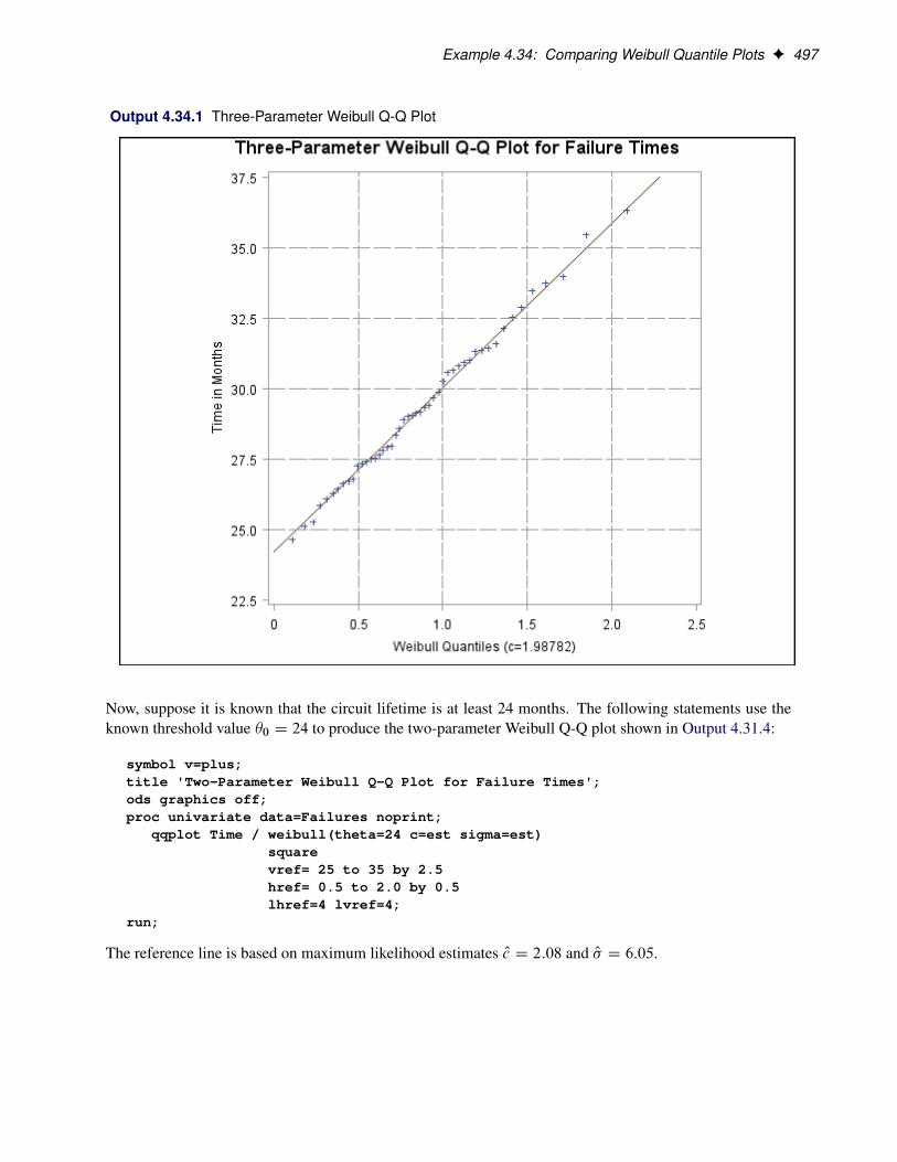
Example 4.34: Comparing Weibull Quantile Plots F 497
Output 4.34.1 Three-Parameter Weibull Q-Q Plot
Now, suppose it is known that the circuit lifetime is at least 24 months. The following statements use theknown threshold value �0 D 24 to produce the two-parameter Weibull Q-Q plot shown in Output 4.31.4:
symbol v=plus;title 'Two-Parameter Weibull Q-Q Plot for Failure Times';ods graphics off;proc univariate data=Failures noprint;
qqplot Time / weibull(theta=24 c=est sigma=est)squarevref= 25 to 35 by 2.5href= 0.5 to 2.0 by 0.5lhref=4 lvref=4;
run;
The reference line is based on maximum likelihood estimates Oc D 2:08 and O� D 6:05.
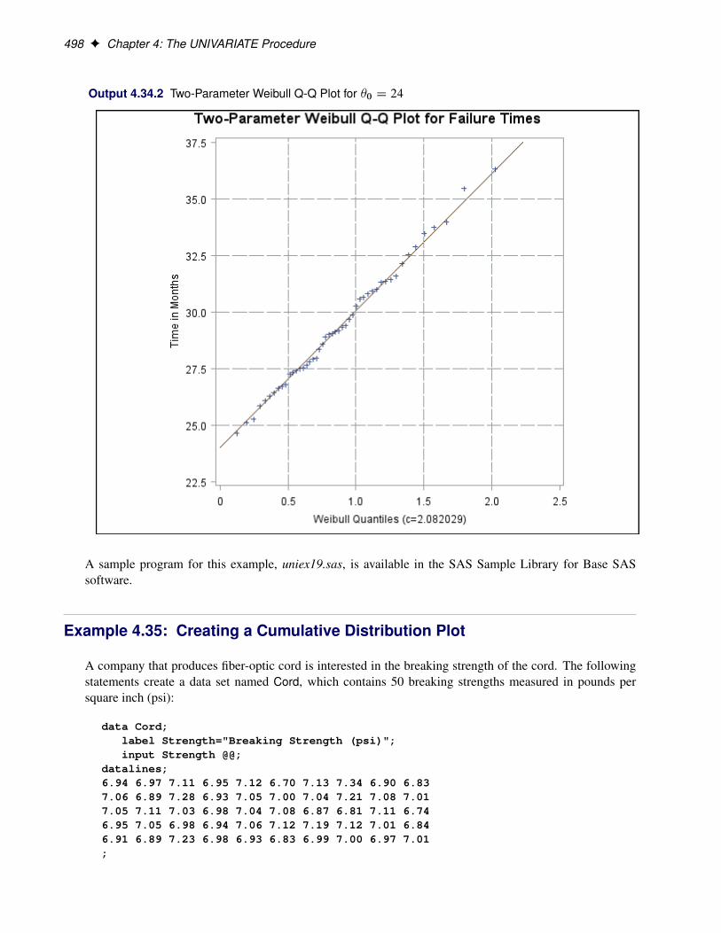
498 F Chapter 4: The UNIVARIATE Procedure
Output 4.34.2 Two-Parameter Weibull Q-Q Plot for �0 D 24
A sample program for this example, uniex19.sas, is available in the SAS Sample Library for Base SASsoftware.
Example 4.35: Creating a Cumulative Distribution Plot
A company that produces fiber-optic cord is interested in the breaking strength of the cord. The followingstatements create a data set named Cord, which contains 50 breaking strengths measured in pounds persquare inch (psi):
data Cord;label Strength="Breaking Strength (psi)";input Strength @@;
datalines;6.94 6.97 7.11 6.95 7.12 6.70 7.13 7.34 6.90 6.837.06 6.89 7.28 6.93 7.05 7.00 7.04 7.21 7.08 7.017.05 7.11 7.03 6.98 7.04 7.08 6.87 6.81 7.11 6.746.95 7.05 6.98 6.94 7.06 7.12 7.19 7.12 7.01 6.846.91 6.89 7.23 6.98 6.93 6.83 6.99 7.00 6.97 7.01;

Example 4.35: Creating a Cumulative Distribution Plot F 499
You can use the CDFPLOT statement to fit any of six theoretical distributions (beta, exponential, gamma,lognormal, normal, and Weibull) and superimpose them on the cdf plot. The following statements use theNORMAL option to display a fitted normal distribution function on a cdf plot of breaking strengths:
title 'Cumulative Distribution Function of Breaking Strength';ods graphics on;proc univariate data=Cord noprint;
cdf Strength / normal;inset normal(mu sigma);
run;
The NORMAL option requests the fitted curve. The INSET statement requests an inset containing the pa-rameters of the fitted curve, which are the sample mean and standard deviation. For more information aboutthe INSET statement, see “INSET Statement” on page 294. The resulting plot is shown in Output 4.35.1.
Output 4.35.1 Cumulative Distribution Function
The plot shows a symmetric distribution with observations concentrated 6.9 and 7.1. The agreement betweenthe empirical and the normal distribution functions in Output 4.35.1 is evidence that the normal distributionis an appropriate model for the distribution of breaking strengths.

500 F Chapter 4: The UNIVARIATE Procedure
Example 4.36: Creating a P-P Plot
The distances between two holes cut into 50 steel sheets are measured and saved as values of the variableDistance in the following data set:
data Sheets;input Distance @@;label Distance='Hole Distance in cm';datalines;
9.80 10.20 10.27 9.70 9.7610.11 10.24 10.20 10.24 9.639.99 9.78 10.10 10.21 10.009.96 9.79 10.08 9.79 10.06
10.10 9.95 9.84 10.11 9.9310.56 10.47 9.42 10.44 10.1610.11 10.36 9.94 9.77 9.369.89 9.62 10.05 9.72 9.829.99 10.16 10.58 10.70 9.54
10.31 10.07 10.33 9.98 10.15;
It is decided to check whether the distances are normally distributed. The following statements create a P-Pplot, shown in Output 4.36.1, which is based on the normal distribution with mean � D 10 and standarddeviation � D 0:3:
title 'Normal Probability-Probability Plot for Hole Distance';ods graphics on;proc univariate data=Sheets noprint;
ppplot Distance / normal(mu=10 sigma=0.3)square;
run;
The NORMAL option in the PPPLOT statement requests a P-P plot based on the normal cumulative distri-bution function, and the MU= and SIGMA= normal-options specify � and � . Note that a P-P plot is alwaysbased on a completely specified distribution—in other words, a distribution with specific parameters. Inthis example, if you did not specify the MU= and SIGMA= normal-options, the sample mean and samplestandard deviation would be used for � and � .

References F 501
Output 4.36.1 Normal P-P Plot with Diagonal Reference Line
The linearity of the pattern in Output 4.36.1 is evidence that the measurements are normally distributed withmean 10 and standard deviation 0.3. The SQUARE option displays the plot in a square format.
ReferencesBlom, G. (1958), Statistical Estimates and Transformed Beta Variables, New York: John Wiley & Sons.
Bowman, K. O. and Shenton, L. R. (1983), “Johnson’s System of Distributions,” in S. Kotz, N. L. Johnson,and C. B. Read, eds., Encyclopedia of Statistical Sciences, volume 4, 303–314, New York: John Wiley &Sons.
Chambers, J. M., Cleveland, W. S., Kleiner, B., and Tukey, P. A. (1983), Graphical Methods for DataAnalysis, Belmont, CA: Wadsworth International Group.
Cohen, A. C. (1951), “Estimating Parameters of Logarithmic-Normal Distributions by Maximum Likeli-hood,” Journal of the American Statistical Association, 46, 206–212.

502 F Chapter 4: The UNIVARIATE Procedure
Conover, W. J. (1999), Practical Nonparametric Statistics, Third Edition, New York: John Wiley & Sons.
Croux, C. and Rousseeuw, P. J. (1992), “Time-Efficient Algorithms for Two Highly Robust Estimators ofScale,” Computational Statistics, 1, 411–428.
D’Agostino, R. and Stephens, M. (1986), Goodness-of-Fit Techniques, New York: Marcel Dekker.
Dixon, W. J. and Tukey, J. W. (1968), “Approximate Behavior of the Distribution of Winsorized t (Trim-ming/Winsorization 2),” Technometrics, 10, 83–98.
Elandt, R. C. (1961), “The Folded Normal Distribution: Two Methods of Estimating Parameters from Mo-ments,” Technometrics, 3, 551–562.
Fisher, R. A. (1973), Statistical Methods for Research Workers, Fourteenth Edition, New York: HafnerPublishing.
Fowlkes, E. B. (1987), A Folio of Distributions: A Collection of Theoretical Quantile-Quantile Plots, NewYork: Marcel Dekker.
Hahn, G. J. and Meeker, W. Q. (1991), Statistical Intervals: A Guide for Practitioners, New York: JohnWiley & Sons.
Hampel, F. R. (1974), “The Influence Curve and Its Role in Robust Estimation,” Journal of the AmericanStatistical Association, 69, 383–393.
Iman, R. L. (1974), “Use of a t -Statistic as an Approximation to the Exact Distribution of the WilcoxonSigned Rank Statistic,” Communications in Statistics, 3, 795–806.
Johnson, N. L., Kotz, S., and Balakrishnan, N. (1994), Continuous Univariate Distributions-1, SecondEdition, New York: John Wiley & Sons.
Johnson, N. L., Kotz, S., and Balakrishnan, N. (1995), Continuous Univariate Distributions-2, SecondEdition, New York: John Wiley & Sons.
Jones, M. C., Marron, J. S., and Sheather, S. J. (1996), “A Brief Survey of Bandwidth Selection for DensityEstimation,” Journal of the American Statistical Association, 91, 401–407.
Lehmann, E. L. (1998), Nonparametrics: Statistical Methods Based on Ranks, San Francisco: Holden-Day.
Odeh, R. E. and Owen, D. B. (1980), Tables for Normal Tolerance Limits, Sampling Plans, and Screening,New York: Marcel Dekker.
Owen, D. B. and Hua, T. A. (1977), “Tables of Confidence Limits on the Tail Area of the Normal Distribu-tion,” Communication and Statistics, Part B—Simulation and Computation, 6, 285–311.
Rousseeuw, P. J. and Croux, C. (1993), “Alternatives to the Median Absolute Deviation,” Journal of theAmerican Statistical Association, 88, 1273–1283.
Royston, J. P. (1992), “Approximating the Shapiro-Wilk’s W Test for Nonnormality,” Statistics and Com-puting, 2, 117–119.
Shapiro, S. S. and Wilk, M. B. (1965), “An Analysis of Variance Test for Normality (Complete Samples),”Biometrika, 52, 591–611.
References F 503
Silverman, B. W. (1986), Density Estimation for Statistics and Data Analysis, New York: Chapman & Hall.
Slifker, J. F. and Shapiro, S. S. (1980), “The Johnson System: Selection and Parameter Estimation,” Tech-nometrics, 22, 239–246.
Terrell, G. R. and Scott, D. W. (1985), “Oversmoothed Nonparametric Density Estimates,” Journal of theAmerican Statistical Association, 80, 209–214.
Tukey, J. W. (1977), Exploratory Data Analysis, Reading, MA: Addison-Wesley.
Tukey, J. W. and McLaughlin, D. H. (1963), “Less Vulnerable Confidence and Significance Procedures forLocation Based on a Single Sample: Trimming/Winsorization 1,” Sankhya A, 25, 331–352.
Velleman, P. F. and Hoaglin, D. C. (1981), Applications, Basics, and Computing of Exploratory Data Anal-ysis, Boston, MA: Duxbury Press.
Wainer, H. (1974), “The Suspended Rootogram and Other Visual Displays: An Empirical Validation,” TheAmerican Statistician, 28, 143–145.

504
Subject Index
A
adjusted odds ratioFREQ procedure, 179
adjusted relative risksFREQ procedure, 180
agreement plotsFREQ procedure, 83, 111
agreement, measures ofFREQ procedure, 170
Agresti-Coull confidence limitsproportions (FREQ), 148
alpha levelFREQ procedure, 90, 98
Anderson-Darling statistic, 396Anderson-Darling test, 255annotating
histograms, 350ANOVA (row mean scores) statistic
Mantel-Haenszel (FREQ), 177association, measures of
FREQ procedure, 138
B
bar chartsFREQ procedure, 117
beta distribution, 380, 403cdf plots, 265deviation from theoretical distribution, 394EDF goodness-of-fit test, 394estimation of parameters, 283fitting, 283, 380formulas for, 380P-P plots, 316probability plots, 331, 403quantile plots, 342, 403
binomial proportionsClopper-Pearson test (FREQ), 151confidence limits (FREQ), 148equivalence tests (FREQ), 153exact test (FREQ), 151FREQ procedure, 147noninferiority tests (FREQ), 151superiority tests (FREQ), 152tests (FREQ), 150TOST (FREQ), 153
Bowker’s test of symmetry
FREQ procedure, 170box plots, line printer, 256, 369
side-by-side, 255, 370Breslow-Day test
FREQ procedure, 181Tarone’s adjustment (FREQ), 181
C
case-control studiesodds ratio (FREQ), 164
categorical data analysisFREQ procedure, 72
cdf plots, 259axes, specifying, 271beta distribution, 265creating, 498example, 498exponential distribution, 266gamma distribution, 266gumbel distribution, 267igauss distribution, 267lognormal distribution, 268normal distribution, 269normal distribution, example, 498options summarized by function, 261parameters for distributions, 261pareto distribution, 269power function distribution, 269rayleigh distribution, 270suppressing empirical cdf, 268Weibull distribution, 271
cell count dataexample (FREQ), 205FREQ procedure, 126
chi-square goodness-of-fit testsFREQ procedure, 134
chi-square testsFREQ procedure, 133
Cicchetti-Allison weightskappa coefficient (FREQ), 173
Clopper-Pearson confidence limitsproportions (FREQ), 149
Cochran’s Q testFREQ procedure, 170, 174
Cochran-Armitage test for trendFREQ procedure, 167
Cochran-Mantel-Haenszel statistics

506 F Subject Index
FREQ procedure, 175cohort studies
relative risks (FREQ), 165common odds ratio
exact confidence limits (FREQ), 181exact test (FREQ), 181logit (FREQ), 179Mantel-Haenszel (FREQ), 179
common relative riskslogit (FREQ), 180Mantel-Haenszel (FREQ), 180
comparative plots, 272, 273, 375histograms, 288, 289, 354, 355, 447, 449, 459
concordant observationsFREQ procedure, 138
confidence ellipse, 32confidence limits
exact (FREQ), 87for percentiles, 362means, for, 365measures of association (FREQ), 138parameters of normal distribution, for, 365proportions (FREQ), 148standard deviations, for, 365variances, for, 365
confidence limits for the correlationFisher’s z transformation, 27
contingency coefficientFREQ procedure, 137
contingency tablesFREQ procedure, 72, 95
continuity-adjusted chi-square testFREQ procedure, 135
CORR procedureconcepts, 19details, 19examples, 38missing values, 33ODS graph names, 38ODS table names, 37output, 35output data sets, 35overview, 4results, 33syntax, 9task tables, 9
corrected sums of squares and crossproducts, 10correlation coefficients, 4
limited combinations of, 18printing, for each variable, 10suppressing probabilities, 10
correlation statisticMantel-Haenszel (FREQ), 177
covariances, 10
Cramer’s V statisticFREQ procedure, 138
Cramér-von Mises statistic, 396Cramér-von Mises test, 255Cronbach’s coefficient alpha, 30
calculating and printing, 10example, 56for estimating reliability, 4
crosstabulation tablesFREQ procedure, 72, 95, 194
D
data summarization tools, 242density estimation, see kernel density estimationdescriptive statistics
computing, 357discordant observations
FREQ procedure, 138distribution of variables, 242dot plots
FREQ procedure, 117, 208
E
EDF, see empirical distribution functionEDF goodness-of-fit tests, 394
probability values of, 396empirical distribution function
definition of, 395EDF test statistics, 394, 395
equivalence testsbinomial proportions (FREQ), 153risk difference (FREQ), 162
exact confidence limitsodds ratio (FREQ), 165proportion difference (FREQ), 163proportions (FREQ), 149ratio of proportions (FREQ), 166relative risks (FREQ), 166risk difference (FREQ), 163
exact p-valuesFREQ procedure, 186
exact testscomputational algorithms (FREQ), 185computational resources (FREQ), 187FREQ procedure, 87, 184, 225network algorithm (FREQ), 185
exponential distribution, 382, 404cdf plots, 266deviation from theoretical distribution, 394EDF goodness-of-fit test, 394estimation of parameters, 285fitting, 382

Subject Index F 507
formulas for, 382P-P plots, 317, 318probability plots, 331, 404quantile plots, 343, 404
extreme observations, 293, 424extreme values, 424
F
Farrington-Manning confidence limitsrisk difference (FREQ), 157
Fisher’s exact testFREQ procedure, 136
Fisher’s z transformationapplications, 28
Fisher’s z transformation, 10, 26confidence limits for the correlation, 27
fitted parametric distributions, 380beta distribution, 380exponential distribution, 382folded normal distribution, 471gamma distribution, 383gumbel distribution, 384inverse Gaussian distribution, 385Johnson SB distribution, 390Johnson SU distribution, 391lognormal distribution, 385normal distribution, 386pareto distribution, 387power function distribution, 388rayleigh distribution, 389Weibull distribution, 392
Fleiss-Cohen weightskappa coefficient (FREQ), 173
folded normal distribution, 471Freeman-Halton test
FREQ procedure, 137FREQ procedure
adjusted odds ratio (Mantel-Haenszel), 179adjusted relative risks (Mantel-Haenszel), 180agreement plots, 111Agresti-Coull confidence limits, 148alpha level, 90, 98ANOVA (row mean scores) statistic, 177bar charts, 117binomial proportions, 147Bowker’s test of symmetry, 170Breslow-Day test, 181cell count data, 126chi-square goodness-of-fit tests, 134chi-square tests, 133Clopper-Pearson confidence limits, 149Cochran’s Q test, 170, 174Cochran-Armitage test for trend, 167
common odds ratio, 181computational resources, 189computational resources (exact tests), 187contingency coefficient, 137continuity-adjusted chi-square test, 135correlation statistic, 177Cramer’s V statistic, 138crosstabulation tables, 194default tables, 95displayed output, 192dot plots, 117, 208equivalence tests, 153, 162exact confidence limits, 87exact p-values, 186exact tests, 87, 184, 225exact unconditional confidence limits, 163Farrington-Manning confidence limits, 157Fisher’s exact test, 136Freeman-Halton test, 137frequency plots, 111Friedman’s chi-square test, 229Gail-Simon test, 183gamma statistic, 138, 139general association statistic, 177grouping with formats, 127Hauck-Anderson confidence limits, 157in-database computation, 131input data sets, 85, 126introductory examples, 74Jeffreys confidence limits, 148Jonckheere-Terpstra test, 168kappa coefficient, 170, 171kappa plots, 111Kendall’s tau-b statistic, 138, 140lambda asymmetric, 138, 145lambda symmetric, 138, 146likelihood-ratio chi-square test, 135Mantel-Fleiss criterion, 178Mantel-Haenszel chi-square test, 136Mantel-Haenszel statistics, 175maximum time (exact tests), 90McNemar’s test, 170measures of agreement, 170measures of association, 138missing values, 128Monte Carlo estimation (exact tests), 87, 187multiway tables, 194network algorithm, 185Newcombe score confidence limits, 161noninferiority tests, 151, 159odds ratio, 164odds ratio plots, 111ODS graph names, 204ODS table names, 200

508 F Subject Index
one-way frequency tables, 192ordering of levels, 86output data sets, 91, 189overall kappa coefficient, 174Pearson chi-square test, 134Pearson correlation coefficient, 138, 142phi coefficient, 137polychoric correlation coefficient, 138, 144relative risks, 165risk difference, 154risk difference plots, 112scores, 132Somers’ D statistics, 138, 141Spearman rank correlation coefficient, 138, 143Stuart’s tau-c statistic, 138, 141superiority tests, 152, 162tetrachoric correlation coefficient, 144uncertainty coefficients, 138, 146, 147weighted kappa coefficient, 170, 172Wilson confidence limits, 149Yule’s Q statistic, 139Zelen’s exact test, 181
frequency plotsFREQ procedure, 111
frequency tablescreating (UNIVARIATE), 426FREQ procedure, 72, 95one-way (FREQ), 192
Friedman’s chi-square testFREQ procedure, 229
G
Gail-Simon testFREQ procedure, 183
gamma distribution, 383, 404cdf plots, 266deviation from theoretical distribution, 394EDF goodness-of-fit test, 394estimation of parameters, 286fitting, 286, 383formulas for, 383P-P plots, 318probability plots, 332, 404quantile plots, 343, 404
gamma statisticFREQ procedure, 138, 139
general association statisticMantel-Haenszel (FREQ), 177
Gini’s mean difference, 368goodness-of-fit tests, 255, 393, see empirical
distribution function, 463Anderson-Darling, 396Cramér-von Mises, 396
EDF, 394, 396Kolmogorov D, 395Shapiro-Wilk, 394
graphics, 242annotating, 253descriptions, 352high-resolution, 242, 371insets, 294, 376–378line printer, 369naming, 354probability plots, 324quantile plots, 336saving, 254
Gumbel distribution, 404P-P plots, 318, 319probability plots, 404quantile plots, 404
gumbel distribution, 384cdf plots, 267estimation of parameters, 286fitting, 286, 384formulas for, 384probability plots, 332quantile plots, 344
H
Hauck-Anderson confidence limitsrisk difference (FREQ), 157
high-resolution graphics, 242, 371histograms, 274, 418
adding a grid, 286annotating, 350appearance, 283, 284, 287, 290–293, 350–356axis color, 350axis scaling, 293bar labels, 283bar width, 283, 289bars, suppressing, 290beta curve, superimposed, 283binning, 453color, options, 284, 351, 352comparative, 288, 289, 354, 355, 447, 449, 459creating, 445endpoints of intervals, 291exponential curve, superimposed, 285extreme observations, 424filling area under density curve, 286gamma curve, superimposed, 286gumbel curve, superimposed, 286hanging, 286insets, 452intervals, 290, 418inverse Gaussian curve, superimposed, 287

Subject Index F 509
Johnson SB curve, superimposed, 291Johnson SU curve, superimposed, 292kernel density estimation, options, 283, 288, 292kernel density estimation, superimposed, 398,
468line type, 354lognormal curve, superimposed, 288lognormal distribution, 481midpoints, 289multiple distributions, example, 463normal curve, superimposed, 290normal distribution, 289options summarized by function, 277output data sets, 412, 413parameters for fitted density curves, 283, 289,
292, 293pareto curve, superimposed, 290plots, suppressing, 290power curve, superimposed, 291quantiles, 418rayleigh curve, superimposed, 291reference lines, options, 286, 351–356saving histogram intervals, 290tables of statistical output, 418tables of statistical output, suppressing, 290three-parameter lognormal distribution,
superimposed, 469three-parameter Weibull distribution,
superimposed, 470tick marks on horizontal axis, 353tiles for comparative plots, 353Weibull curve, superimposed, 293
Hoeffding’s measure of dependence, 4, 23calculating and printing, 10example, 38output data set with, 10probability values, 23
hypothesis testsexact (FREQ), 87
I
igauss distributioncdf plots, 267
in-database computationFREQ procedure, 131
insets, 294, 452appearance, 304appearance, color, 304positioning, 304, 305, 376positioning in margins, 377positioning with compass point, 376positioning with coordinates, 378statistics associated with distributions, 299–302
insets for descriptive statistics, see insetsinterquartile range, 368inverse Gaussian distribution, 385
estimation of parameters, 287fitting, 287, 385formulas for, 385P-P plots, 319, 320
J
Jeffreys confidence limitsproportions (FREQ), 148
Johnson SB distribution, 390estimation of parameters, 291fitting, 291, 390formulas for, 390
Johnson SU distribution, 391estimation of parameters, 292fitting, 292, 391formulas for, 391
Jonckheere-Terpstra testFREQ procedure, 168
K
kappa coefficientFREQ procedure, 170, 171plots (FREQ), 111weights (FREQ), 173
Kendall correlation statistics, 10Kendall’s partial tau-b, 4, 17Kendall’s tau-b, 4, 22probability values, 22
Kendall’s tau-b statisticFREQ procedure, 138, 140
kernel density estimation, 398, 468adding density curve to histogram, 288bandwidth parameter, specifying, 283kernel function, specifying type of, 288line type for density curve, 354lower bound, specifying, 288upper bound, specifying, 292
kernel function, see kernel density estimationkey cell for comparative plots, 273Kolmogorov D statistic, 395Kolmogorov-Smirnov test, 255
L
lambda asymmetricFREQ procedure, 138, 145
lambda symmetricFREQ procedure, 138, 146
likelihood-ratio chi-square test

510 F Subject Index
FREQ procedure, 135line printer plots, 369
box plots, 369, 370normal probability plots, 370stem-and-leaf plots, 369
listwise deletion, 33location estimates
robust, 257, 258location parameters, 408
probability plots, estimation with, 408quantile plots, estimation with, 408
location, tests forUNIVARIATE procedure, 443
lognormal distribution, 385, 405cdf plots, 268deviation from theoretical distribution, 394EDF goodness-of-fit test, 394estimation of parameters, 288fitting, 288, 385formulas for, 385histograms, 469, 481P-P plots, 320probability plots, 332, 405, 477quantile plots, 344, 405, 494
M
Mantel-Fleiss criterionFREQ procedure, 178
Mantel-Haenszel chi-square testFREQ procedure, 136
Mantel-Haenszel statisticsANOVA (row mean scores) statistic (FREQ), 177correlation statistic (FREQ), 177FREQ procedure, 175general association statistic (FREQ), 177Mantel-Fleiss criterion (FREQ), 178
McNemar’s testFREQ procedure, 170
measures of association, 38nonparametric, 4
measures of locationmeans, 358modes, 361, 422trimmed means, 367Winsorized means, 366
median absolute deviation (MAD), 368Mehta-Patel network algorithm
exact tests (FREQ), 185missing values
FREQ procedure, 128UNIVARIATE procedure, 356
mode calculation, 361modified ridit scores
FREQ procedure, 133Monte Carlo estimation
exact tests (FREQ), 87, 187multiway tables
FREQ procedure, 72, 95, 194
N
network algorithmexact tests (FREQ), 185
Newcombe score confidence limitsrisk difference (FREQ), 161
Newton-Raphson approximationgamma shape parameter, 350Weibull shape parameter, 351
noninferiority testsbinomial proportions (FREQ), 151risk difference (FREQ), 159
nonparametric density estimation, see kernel densityestimation
nonparametric measures of association, 4normal distribution, 386, 405
cdf plots, 269cdf plots, example, 498deviation from theoretical distribution, 394EDF goodness-of-fit test, 394estimation of parameters, 290fitting, 290, 386formulas for, 386histograms, 289P-P plots, 321probability plots, 325, 333, 405quantile plots, 344, 405, 483
normal probability plots, see probability plotsline printer, 256, 370
O
odds ratioBreslow-Day test (FREQ), 181case-control studies (FREQ), 164exact confidence limits (FREQ), 165FREQ procedure, 164logit adjusted (FREQ), 179Mantel-Haenszel adjusted (FREQ), 179plots (FREQ), 111Zelen’s exact test (FREQ), 181
ODS (Output Delivery System)CORR procedure and, 37UNIVARIATE procedure table names, 417
ODS graph namesCORR procedure, 38FREQ procedure, 204
output data sets

Subject Index F 511
saving correlations in, 59
P
P-P plots, 310beta distribution, 316distribution options, 312, 314distribution reference line, 312, 501exponential distribution, 317gamma distribution, 318Gumbel distribution, 318gumbel distribution, 319inverse Gaussian distribution, 319lognormal distribution, 320normal distribution, 321options summarized by function, 314, 316Pareto distribution, 321plot layout, 315Power distribution, 322Rayleigh distribution, 323Weibull distribution, 323
paired data, 363, 444pairwise deletion, 33parameters for fitted density curves, 283, 289, 292,
293Pareto distribution, 405
P-P plots, 321probability plots, 405quantile plots, 405
pareto distribution, 387cdf plots, 269estimation of parameters, 290fitting, 290, 387formulas for, 387probability plots, 333quantile plots, 344
partial correlations, 24probability values, 25
Pearson chi-square testFREQ procedure, 134
Pearson correlation coefficientFREQ procedure, 138, 142
Pearson correlation statistics, 4example, 38in output data set, 10Pearson partial correlation, 4, 17Pearson product-moment correlation, 4, 10, 19,
38Pearson weighted product-moment correlation,
4, 18probability values, 21suppressing, 10
percent plots, see See P-P plotspercentiles
axes, quantile plots, 345, 409calculating, 361confidence limits for, 362, 438defining, 256, 361empirical distribution function, 361options, 307–309probability plots and, 324quantile plots and, 336saving to an output data set, 435visual estimates, probability plots, 409visual estimates, quantile plots, 409weighted, 362weighted average, 361
phi coefficientFREQ procedure, 137
plot statements, UNIVARIATE procedure, 241plots
box plots, 255, 256, 369, 370comparative, 272, 273, 375comparative histograms, 288, 289, 354, 355,
447, 449, 459line printer plots, 369normal probability plots, 256, 370probability plots, 324, 402quantile plots, 336, 402size of, 256stem-and-leaf, 256, 369suppressing, 290
polychoric correlation coefficientFREQ procedure, 138, 144
polyserial correlation, 28polyserial correlation statistics, 4, 10Power distribution
P-P plots, 322power function distribution, 388, 406
cdf plots, 269estimation of parameters, 291fitting, 291, 388formulas for, 388probability plots, 333, 406quantile plots, 345, 406
prediction ellipse, 32probability plots, 324
appearance, 331–333beta distribution, 331, 403distribution reference lines, 334distributions for, 402exponential distribution, 331, 404gamma distribution, 332, 404generalized Pareto distribution, 406Gumbel distribution, 404gumbel distribution, 332location parameters, estimation of, 408lognormal distribution, 332, 405, 477, 481

512 F Subject Index
normal distribution, 325, 333, 405options summarized by function, 327overview, 324parameters for distributions, 327, 331, 332,
334–336Pareto distribution, 405pareto distribution, 333percentile axis, 333percentiles, estimates of, 409power function distribution, 333, 406Rayleigh distribution, 406rayleigh distribution, 334reference lines, 332reference lines, options, 332scale parameters, estimation of, 408shape parameters, 408three-parameter Weibull distribution, 407threshold parameter, 335threshold parameters, estimation of, 408two-parameter Weibull distribution, 407Weibull distribution, 335, 336
proportion differenceFREQ procedure, 154
proportions, see binomial proportions (FREQ)
Q
Q-Q plots, see quantile plotsQn, 368quantile plots, 336
appearance, 343, 344, 347axes, percentile scale, 345, 409beta distribution, 342, 403creating, 400diagnostics, 401distribution reference lines, 346, 485distributions for, 402exponential distribution, 343, 404gamma distribution, 343, 404Gumbel distribution, 404gumbel distribution, 344interpreting, 401legends, suppressing (UNIVARIATE), 485location parameters, estimation of, 408lognormal distribution, 344, 405, 488, 494lognormal distribution, percentiles, 493nonnormal data, 487normal distribution, 344, 405, 483options summarized by function, 339, 340overview, 336parameters for distributions, 339, 340, 342–344,
346–348Pareto distribution, 405pareto distribution, 344
percentiles, estimates of, 409power function distribution, 345, 406Rayleigh distribution, 406rayleigh distribution, 345reference lines, 343, 345reference lines, options, 344scale parameters, estimation of, 408shape parameters, 408three-parameter Weibull distribution, 407threshold parameter, 347threshold parameters, estimation of, 408two-parameter Weibull distribution, 407Weibull distribution, 347, 348, 496
quantile-quantile plots, see quantile plotsquantiles
defining, 361empirical distribution function, 361histograms and, 418weighted average, 361
R
rank scoresFREQ procedure, 133
Rayleigh distribution, 406P-P plots, 323probability plots, 406quantile plots, 406
rayleigh distribution, 389cdf plots, 270estimation of parameters, 291fitting, 291, 389formulas for, 389probability plots, 334quantile plots, 345
relative riskscohort studies (FREQ), 165exact confidence limits (FREQ), 166FREQ procedure, 165logit adjusted (FREQ), 180Mantel-Haenszel adjusted (FREQ), 180plots (FREQ), 112
reliability estimation, 4ridit scores
FREQ procedure, 133risk difference
confidence limits (FREQ), 156equivalence tests (FREQ), 162exact confidence limits (FREQ), 163FREQ procedure, 154noninferiority tests (FREQ), 159plots (FREQ), 112superiority tests (FREQ), 162TOST (FREQ), 162

Subject Index F 513
risks, see also binomial proportions (FREQ)FREQ procedure, 154
robust estimates, 256–258robust estimators, 366, 441
Gini’s mean difference, 368interquartile range, 368median absolute deviation (MAD), 368Qn, 368Sn, 368trimmed means, 367Winsorized means, 366
robust measures of scale, 368rounding, 256, 357
UNIVARIATE procedure, 357row mean scores statistic
Mantel-Haenszel (FREQ), 177
S
saving correlationsexample, 59
scale estimatesrobust, 256
scale parameters, 408probability plots, 408quantile plots, 408
shape parameters, 408Shapiro-Wilk statistic, 394Shapiro-Wilk test, 255sign test, 363, 364
paired data and, 444signed rank statistic, computing, 364singularity of variables, 10smoothing data distribution, see kernel density
estimationSn, 368Somers’ D statistics
FREQ procedure, 138, 141Spearman correlation statistics, 10
probability values, 21Spearman partial correlation, 4, 17Spearman rank-order correlation, 4, 21, 38
Spearman rank correlation coefficientFREQ procedure, 138, 143
standard deviation, 10specifying, 269
stem-and-leaf plots, 256, 369stratified analysis
FREQ procedure, 72, 95Stuart’s tau-c statistic
FREQ procedure, 138, 141Student’s t test, 363, 364summary statistics
insets of, 294
saving, 256, 414sums of squares and crossproducts, 10superiority tests
binomial proportions (FREQ), 152risk difference (FREQ), 162
T
t testStudent’s, 363, 364
table scoresFREQ procedure, 133
tablescontingency (FREQ), 72crosstabulation (FREQ), 72, 194multiway (FREQ), 72, 194one-way frequency (FREQ), 72, 192
Tarone’s adjustmentBreslow-Day test (FREQ), 181
tests for location, 363, 443paired data, 363, 444sign test, 364Student’s t test, 364Wilcoxon signed rank test, 364
tetrachoric correlation coefficientFREQ procedure, 144
theoretical distributions, 402three-parameter Weibull distribution, 407
probability plots, 407quantile plots, 407
threshold parameterprobability plots, 335quantile plots, 347
threshold parametersprobability plots, 408quantile plots, 408
tiles for comparative plotshistograms, 353
TOSTequivalence tests (FREQ), 153, 162
trend testFREQ procedure, 167
trimmed means, 257, 367two-parameter Weibull distribution, 407
probability plots, 407quantile plots, 407
U
uncertainty coefficientsFREQ procedure, 138, 146, 147
univariate analysisfor multiple variables, 420
UNIVARIATE procedure

514 F Subject Index
calculating modes, 422classification levels, 272comparative plots, 272, 273, 375computational resources, 419concepts, 356confidence limits, 253, 365, 436descriptive statistics, 357, 420examples, 420extreme observations, 293, 424extreme values, 424fitted continuous distributions, 380frequency variables, 433goodness-of-fit tests, 393high-resolution graphics, 371histograms, 418, 424insets for descriptive statistics, 294keywords for insets, 294keywords for output data sets, 306line printer plots, 369, 427missing values, 272, 356mode calculation, 361normal probability plots, 370ODS graph names, 418ODS table names, 417output data sets, 305, 410, 434overview, 242percentiles, 324, 336, 361percentiles, confidence limits, 253, 254, 438plot statements, 241probability plots, 324, 402quantile plots, 336, 402quantiles, confidence limits, 253, 254results, 416robust estimates, 441robust estimators, 366robust location estimates, 257, 258robust scale estimates, 256rounding, 357sign test, 364, 444specifying analysis variables, 348task tables, 336testing for location, 443tests for location, 363weight variables, 349
UNIVARIATE procedure, OUTPUT statementoutput data set, 410
V
variances, 10
W
Weibull distribution, 392
cdf plots, 271deviation from theoretical distribution, 394EDF goodness-of-fit test, 394estimation of parameters, 293fitting, 293, 392formulas for, 392histograms, 470P-P plots, 323probability plots, 335, 336quantile plots, 347, 348, 496three-parameter, 407two-parameter, 407
weight values, 254weighted kappa coefficient
FREQ procedure, 170, 172weighted percentiles, 362Wilcoxon signed rank test, 363, 364Wilson confidence limits
proportions (FREQ), 149Winsorized means, 258, 366
Y
Yule’s Q statisticFREQ procedure, 139
Z
Zelen’s testequal odds ratios (FREQ), 181
zeros, structural and randomagreement statistics (FREQ), 174

Syntax Index
A
AGREE optionEXACT statement (FREQ), 88TABLES statement (FREQ), 98TEST statement (FREQ), 125
AGRESTICOULL option (BINOMIAL)TABLES statement (FREQ), 100
ALL optionPLOTS= option (CORR), 13PROC UNIVARIATE statement, 252TABLES statement (FREQ), 98
ALL option (BINOMIAL)TABLES statement (FREQ), 100
ALPHA optionPROC CORR statement, 10
ALPHA= optionEXACT statement (FREQ), 90HISTOGRAM statement (UNIVARIATE), 283,
382, 388PLOTS=SCATTER option (CORR), 14PROBPLOT statement (UNIVARIATE), 331PROC UNIVARIATE statement, 253QQPLOT statement (UNIVARIATE), 342TABLES statement (FREQ), 98
ALPHADELTA= optionplot statements (UNIVARIATE), 350
ALPHAINITIAL= optionplot statements (UNIVARIATE), 350
ANNOKEY optionplot statements (UNIVARIATE), 350
ANNOTATE= optionHISTOGRAM statement (UNIVARIATE), 471plot statements (UNIVARIATE), 350PROC UNIVARIATE statement, 253, 410
B
BARLABEL= optionHISTOGRAM statement (UNIVARIATE), 283
BARWIDTH= optionHISTOGRAM statement (UNIVARIATE), 283
BDT option (CMH)TABLES statement (FREQ), 104
BEST= optionPROC CORR statement, 11
BETA option
HISTOGRAM statement (UNIVARIATE), 283,380, 461
PROBPLOT statement (UNIVARIATE), 331,403
QQPLOT statement (UNIVARIATE), 342, 403BETA= option
HISTOGRAM statement (UNIVARIATE), 283,382
PROBPLOT statement (UNIVARIATE), 331QQPLOT statement (UNIVARIATE), 343
BINOMIAL optionEXACT statement (FREQ), 88TABLES statement (FREQ), 98
BY statementCORR procedure, 16FREQ procedure, 87UNIVARIATE procedure, 258
C
C= optionHISTOGRAM statement (UNIVARIATE), 283,
398, 399, 468PROBPLOT statement (UNIVARIATE), 331QQPLOT statement (UNIVARIATE), 343, 496
CAXIS= optionplot statements (UNIVARIATE), 350
CBARLINE= optionHISTOGRAM statement (UNIVARIATE), 284
CDFPLOT statementexamples, 498options summarized by function, 261UNIVARIATE procedure, 259
CELLCHI2 optionTABLES statement (FREQ), 102
CFILL= optionHISTOGRAM statement (UNIVARIATE), 284INSET statement (UNIVARIATE), 304
CFILLH= optionINSET statement (UNIVARIATE), 304
CFRAME= optionINSET statement (UNIVARIATE), 304plot statements (UNIVARIATE), 351
CFRAMESIDE= optionplot statements (UNIVARIATE), 351
CFRAMETOP= optionplot statements (UNIVARIATE), 351
CGRID= option

516 F Syntax Index
HISTOGRAM statement (UNIVARIATE), 284PROBPLOT statement (UNIVARIATE), 331QQPLOT statement (UNIVARIATE), 343
CHEADER= optionINSET statement (UNIVARIATE), 304
CHISQ optionEXACT statement (FREQ), 88, 218TABLES statement (FREQ), 102, 134, 218
CHREF= optionplot statements (UNIVARIATE), 351
CIBASIC optionPROC UNIVARIATE statement, 253, 436
CIPCTLDF optionPROC UNIVARIATE statement, 253
CIPCTLNORMAL optionPROC UNIVARIATE statement, 254
CIQUANTDF optionPROC UNIVARIATE statement, 438
CIQUANTNORMAL optionPROC UNIVARIATE statement, 254, 438
CL optionTABLES statement (FREQ), 103
CL= option (RISKDIFF)TABLES statement (FREQ), 119
CLASS statementUNIVARIATE procedure, 272
CLIPREF optionHISTOGRAM statement (UNIVARIATE), 284
CLOPPERPEARSON option (BINOMIAL)TABLES statement (FREQ), 100
CMH optionTABLES statement (FREQ), 103
CMH1 optionTABLES statement (FREQ), 104
CMH2 optionTABLES statement (FREQ), 105
COLUMN= option (RELRISK)EXACT statement (FREQ), 89
COLUMN= option (RISKDIFF)EXACT statement (FREQ), 90TABLES statement (FREQ), 120
COMOR optionEXACT statement (FREQ), 88
COMPRESS optionPROC FREQ statement, 85
CONTENTS= optionHISTOGRAM statement (UNIVARIATE), 284plot statements (UNIVARIATE), 351TABLES statement (FREQ), 105
CONVERGE optionPOLYSERIAL option (CORR), 15
CONVERGE= optionTABLES statement (FREQ), 105
CORR procedure
syntax, 9CORR procedure, BY statement, 16CORR procedure, FREQ statement, 17CORR procedure, ID statement, 17CORR procedure, PARTIAL statement, 17CORR procedure, PLOTS= option
ALL option, 13HISTOGRAM option, 14MATRIX option, 13MAXPOINTS= option, 13NONE option, 13NVAR= option, 14NWITH= option, 14SCATTER option, 14
CORR procedure, PLOTS=SCATTER optionALPHA=, 14ELLIPSE=, 14NOINSET, 14
CORR procedure, POLYSERIALCONVERGE option, 15MAXITER option, 15NGROUPS option, 15ORDINAL option, 15
CORR procedure, POLYSERIAL option, 15CORR procedure, PROC CORR statement, 9
ALPHA option, 10BEST= option, 11COV option, 11CSSCP option, 11DATA= option, 11EXCLNPWGT option, 11FISHER option, 11HOEFFDING option, 12KENDALL option, 12NOCORR option, 12NOMISS option, 12NOPRINT option, 12NOPROB option, 12NOSIMPLE option, 12OUT= option, 12OUTH= option, 12OUTK= option, 12OUTP= option, 12OUTS= option, 13PEARSON option, 13RANK option, 15SINGULAR= option, 15SPEARMAN option, 15SSCP option, 15VARDEF= option, 16
CORR procedure, VAR statement, 17CORR procedure, WEIGHT statement, 18CORR procedure, WITH statement, 18CORRECT option (BINOMIAL)

Syntax Index F 517
TABLES statement (FREQ), 100CORRECT option (RISKDIFF)
TABLES statement (FREQ), 120COV option
PROC CORR statement, 11CPROP= option
HISTOGRAM statement (UNIVARIATE), 459plot statements (UNIVARIATE), 351
CROSSLIST optionTABLES statement (FREQ), 105
CSHADOW= optionINSET statement (UNIVARIATE), 304
CSSCP optionPROC CORR statement, 11
CTEXT= optionINSET statement (UNIVARIATE), 304plot statements (UNIVARIATE), 352
CTEXTSIDE= optionplot statements (UNIVARIATE), 352
CTEXTTOP= optionplot statements (UNIVARIATE), 352
CUMCOL optionTABLES statement (FREQ), 106
CVREF= optionplot statements (UNIVARIATE), 352
D
DATA optionINSET statement (UNIVARIATE), 304
DATA= optionINSET statement (UNIVARIATE), 298PROC CORR statement, 11PROC FREQ statement, 85PROC UNIVARIATE statement, 254, 410
DESCENDING optionBY statement (UNIVARIATE), 258
DESCRIPTION= optionplot statements (UNIVARIATE), 352
DEVIATION optionTABLES statement (FREQ), 106
E
ELLIPSE= optionPLOTS=SCATTER option (CORR), 14
ENDPOINTS= optionHISTOGRAM statement (UNIVARIATE), 285,
453EQOR option
EXACT statement (FREQ), 88EQUAL option (RISKDIFF)
TABLES statement (FREQ), 120EQUIVALENCE option (BINOMIAL)
TABLES statement (FREQ), 100EQUIVALENCE option (RISKDIFF)
TABLES statement (FREQ), 120EXACT option (BINOMIAL)
TABLES statement (FREQ), 100EXACT statement
FREQ procedure, 87EXCLNPWGT option
PROC CORR statement, 11PROC UNIVARIATE statement, 254
EXPECTED optionTABLES statement (FREQ), 106
EXPONENTIAL optionHISTOGRAM statement (UNIVARIATE), 285,
382PROBPLOT statement (UNIVARIATE), 331,
404QQPLOT statement (UNIVARIATE), 343, 404
F
FILL optionHISTOGRAM statement (UNIVARIATE), 286
FISHER optionEXACT statement (FREQ), 88PROC CORR statement, 11TABLES statement (FREQ), 106
FITINTERVAL= optionplot statements (UNIVARIATE), 352
FITMETHOD= optionplot statements (UNIVARIATE), 352
FITTOLERANCE= optionplot statements (UNIVARIATE), 352
FONT= optionINSET statement (UNIVARIATE), 304plot statements (UNIVARIATE), 352
FORMAT= optionINSET statement (UNIVARIATE), 304TABLES statement (FREQ), 106
FORMCHAR= optionPROC FREQ statement, 85
FREQ optionPROC UNIVARIATE statement, 254, 426
FREQ proceduresyntax, 84
FREQ procedure, BY statement, 87FREQ procedure, EXACT statement, 87
AGREE option, 88ALPHA= option, 90BINOMIAL option, 88CHISQ option, 88, 218COLUMN= option (RELRISK), 89COLUMN= option (RISKDIFF), 90COMOR option, 88

518 F Syntax Index
EQOR option, 88FISHER option, 88JT option, 88KAPPA option, 88KENTB option, 88LRCHI option, 88MAXTIME= option, 90MC option, 91MCNEM option, 88MEASURES option, 88METHOD= option (RELRISK), 89METHOD= option (RISKDIFF), 90MHCHI option, 88N= option, 91OR option, 88, 218PCHI option, 88PCORR option, 88POINT option, 91RELRISK option, 89RISKDIFF option, 89SCORR option, 89SEED= option, 91SMDCR option, 89SMDRC option, 89STUTC option, 89TREND option, 89, 225WTKAP option, 89ZELEN option, 88
FREQ procedure, OUTPUT statement, 91OUT= option, 92
FREQ procedure, PROC FREQ statement, 84COMPRESS option, 85DATA= option, 85FORMCHAR= option, 85NLEVELS option, 86NOPRINT option, 86ORDER= option, 86PAGE option, 86
FREQ procedure, TABLES statement, 95AGREE option, 98AGRESTICOULL option (BINOMIAL), 100ALL option, 98ALL option (BINOMIAL), 100ALPHA= option, 98BDT option (CMH), 104BINOMIAL option, 98CELLCHI2 option, 102CHISQ option, 102, 134, 218CL option, 103CL= option (RISKDIFF), 119CLOPPERPEARSON option (BINOMIAL), 100CMH option, 103CMH1 option, 104CMH2 option, 105
COLUMN= option (RISKDIFF), 120CONTENTS= option, 105CONVERGE= option, 105CORRECT option (BINOMIAL), 100CORRECT option (RISKDIFF), 120CROSSLIST option, 105CUMCOL option, 106DEVIATION option, 106EQUAL option (RISKDIFF), 120EQUIVALENCE option (BINOMIAL), 100EQUIVALENCE option (RISKDIFF), 120EXACT option (BINOMIAL), 100EXPECTED option, 106FISHER option, 106FORMAT= option, 106GAILSIMON option, 107GAILSIMON option (CMH), 104JEFFREYS option (BINOMIAL), 100JT option, 107LEVEL= option (BINOMIAL), 100LIST option, 107MANTELFLEISS option (CMH), 104MARGIN= option (BINOMIAL), 100MARGIN= option (RISKDIFF), 121MAXITER= option, 107MEASURES option, 107METHOD= option (RISKDIFF), 121MISSING option, 108MISSPRINT option, 108NOCOL option, 108NOCUM option, 108NOFREQ option, 108NONINFERIORITY option (BINOMIAL), 101NONINFERIORITY option (RISKDIFF), 122NOPERCENT option, 108NOPRINT option, 108NORISKS option (RISKDIFF), 122NOROW option, 109NOSPARSE option, 109NOWARN option, 109OR option, 117OUT= option, 109OUTCUM option, 109OUTEXPECT option, 109, 205OUTPCT option, 110P= option (BINOMIAL), 101PLCORR option, 110PLOTS= option, 110PRINTKWT option, 117RELRISK option, 117, 218RISKDIFF option, 117SCORES= option, 122, 229SCOROUT option, 123SPARSE option, 123, 205

Syntax Index F 519
SUPERIORITY option (BINOMIAL), 101SUPERIORITY option (RISKDIFF), 122TESTF= option, 123, 134TESTP= option, 123, 134, 212TOTPCT option, 124TREND option, 124, 225VAR= option (BINOMIAL), 101VAR= option (RISKDIFF), 122WALD option (BINOMIAL), 102WARN= option (CHISQ), 103WILSON option (BINOMIAL), 102
FREQ procedure, TEST statement, 124AGREE option, 125GAMMA option, 125KAPPA option, 125KENTB option, 125MEASURES option, 125PCORR option, 125SCORR option, 125SMDCR option, 125, 225SMDRC option, 125STUTC option, 125WTKAP option, 125
FREQ procedure, WEIGHT statement, 125ZEROS option, 126
FREQ statementCORR procedure, 17UNIVARIATE procedure, 274
FRONTREF optionHISTOGRAM statement (UNIVARIATE), 286
G
GAILSIMON optionTABLES statement (FREQ), 107
GAILSIMON option (CMH)TABLES statement (FREQ), 104
GAMMA optionHISTOGRAM statement (UNIVARIATE), 286,
383, 390, 391, 463PROBPLOT statement (UNIVARIATE), 332,
404QQPLOT statement (UNIVARIATE), 343, 404TEST statement (FREQ), 125
GOUT= optionPROC UNIVARIATE statement, 254
GRID optionHISTOGRAM statement (UNIVARIATE), 286PROBPLOT statement (UNIVARIATE), 332QQPLOT statement (UNIVARIATE), 343, 345,
493GUMBEL option
HISTOGRAM statement (UNIVARIATE), 286,384
PROBPLOT statement (UNIVARIATE), 332QQPLOT statement (UNIVARIATE), 344
Gumbel optionPROBPLOT statement (UNIVARIATE), 404QQPLOT statement (UNIVARIATE), 404
GUTTER= optionINSET statement (UNIVARIATE), 304
H
HAXIS= optionplot statements (UNIVARIATE), 352
HEADER= optionINSET statement (UNIVARIATE), 305
HEIGHT= optionINSET statement (UNIVARIATE), 305plot statements (UNIVARIATE), 353
HISTOGRAMPLOTS= option (CORR), 14
HISTOGRAM statementUNIVARIATE procedure, 274
HMINOR= optionplot statements (UNIVARIATE), 353
HOEFFDING optionPROC CORR statement, 12
HOFFSET= optionHISTOGRAM statement (UNIVARIATE), 287
HREF= optionplot statements (UNIVARIATE), 353
HREFLABELS= optionplot statements (UNIVARIATE), 353
HREFLABPOS= optionplot statements (UNIVARIATE), 353
I
ID statementCORR procedure, 17UNIVARIATE procedure, 293
IDOUT optionPROC UNIVARIATE statement, 254
IGAUSS optionHISTOGRAM statement (UNIVARIATE), 287,
385INFONT= option
plot statements (UNIVARIATE), 353INHEIGHT= option
plot statements (UNIVARIATE), 353INSET statement
UNIVARIATE procedure, 294INTERBAR= option
HISTOGRAM statement (UNIVARIATE), 287INTERTILE= option
HISTOGRAM statement (UNIVARIATE), 459

520 F Syntax Index
plot statements (UNIVARIATE), 353
J
JEFFREYS option (BINOMIAL)TABLES statement (FREQ), 100
JT optionEXACT statement (FREQ), 88TABLES statement (FREQ), 107
K
K= optionHISTOGRAM statement (UNIVARIATE), 288,
398, 399KAPPA option
EXACT statement (FREQ), 88TEST statement (FREQ), 125
KENDALL optionPROC CORR statement, 12
KENTB optionEXACT statement (FREQ), 88TEST statement (FREQ), 125
KERNEL optionHISTOGRAM statement (UNIVARIATE), 288,
398, 399, 468KEYLEVEL= option
CLASS statement (UNIVARIATE), 273PROC UNIVARIATE statement, 449
L
L= optionplot statements (UNIVARIATE), 354
LABEL= optionQQPLOT statement (UNIVARIATE), 345
LAMBDA= optionHISTOGRAM statement (UNIVARIATE), 288PPPLOT statement (UNIVARIATE), 320
LEVEL= option (BINOMIAL)TABLES statement (FREQ), 100
LGRID= optionHISTOGRAM statement (UNIVARIATE), 288PROBPLOT statement (UNIVARIATE), 332QQPLOT statement (UNIVARIATE), 344, 345
LHREF= optionplot statements (UNIVARIATE), 354
LIST optionTABLES statement (FREQ), 107
LOCCOUNT optionPROC UNIVARIATE statement, 254, 443
LOGNORMAL optionHISTOGRAM statement (UNIVARIATE), 288,
385, 463, 469, 481
PROBPLOT statement (UNIVARIATE), 332,405, 477
QQPLOT statement (UNIVARIATE), 344, 405LOWER= option
HISTOGRAM statement (UNIVARIATE), 288LRCHI option
EXACT statement (FREQ), 88LVREF= option
plot statements (UNIVARIATE), 354
M
MANTELFLEISS option (CMH)TABLES statement (FREQ), 104
MARGIN= option (BINOMIAL)TABLES statement (FREQ), 100
MARGIN= option (RISKDIFF)TABLES statement (FREQ), 121
MATRIX optionPLOTS= option (CORR), 13
MAXITER optionPOLYSERIAL option (CORR), 15
MAXITER= optionplot statements (UNIVARIATE), 354TABLES statement (FREQ), 107
MAXNBIN= optionHISTOGRAM statement (UNIVARIATE), 288
MAXPOINTS= optionPLOTS= option (CORR), 13
MAXSIGMAS= optionHISTOGRAM statement (UNIVARIATE), 289
MAXTIME= optionEXACT statement (FREQ), 90
MC optionEXACT statement (FREQ), 91
MCNEM optionEXACT statement (FREQ), 88
MEASURES optionEXACT statement (FREQ), 88TABLES statement (FREQ), 107TEST statement (FREQ), 125
METHOD= option (RELRISK)EXACT statement (FREQ), 89
METHOD= option (RISKDIFF)EXACT statement (FREQ), 90TABLES statement (FREQ), 121
MHCHI optionEXACT statement (FREQ), 88
MIDPERCENTS optionHISTOGRAM statement (UNIVARIATE), 289,
457MIDPOINTS= option
HISTOGRAM statement (UNIVARIATE), 289,452, 453

Syntax Index F 521
MISSING optionCLASS statement (UNIVARIATE), 272TABLES statement (FREQ), 108
MISSPRINT optionTABLES statement (FREQ), 108
MODES optionPROC UNIVARIATE statement, 254, 422
MU0= optionPROC UNIVARIATE statement, 255
MU= optionHISTOGRAM statement (UNIVARIATE), 289,
457PROBPLOT statement (UNIVARIATE), 332QQPLOT statement (UNIVARIATE), 344, 485
N
N= optionEXACT statement (FREQ), 91
NADJ= optionPROBPLOT statement (UNIVARIATE), 333QQPLOT statement (UNIVARIATE), 344, 400
NAME= optionplot statements (UNIVARIATE), 354
NCOLS= optionINSET statement (UNIVARIATE), 305plot statements (UNIVARIATE), 354
NENDPOINTS= optionHISTOGRAM statement (UNIVARIATE), 290
NEXTROBS= optionPROC UNIVARIATE statement, 255, 424
NEXTRVAL= optionPROC UNIVARIATE statement, 255, 424
NGROUPS optionPOLYSERIAL option (CORR), 15
NLEVELS optionPROC FREQ statement, 86
NMIDPOINTS= optionHISTOGRAM statement (UNIVARIATE), 290
NOBARS optionHISTOGRAM statement (UNIVARIATE), 290
NOBYPLOT optionPROC UNIVARIATE statement, 255
NOCOL optionTABLES statement (FREQ), 108
NOCORR optionPROC CORR statement, 12
NOCUM optionTABLES statement (FREQ), 108
NOFRAME optionINSET statement (UNIVARIATE), 305plot statements (UNIVARIATE), 354
NOFREQ optionTABLES statement (FREQ), 108
NOHLABEL optionplot statements (UNIVARIATE), 354
NOINSET optionPLOTS=SCATTER option (CORR), 14
NOKEYMOVE optionCLASS statement (UNIVARIATE), 274
NOMISS optionPROC CORR statement, 12
NONE optionPLOTS= option (CORR), 13
NONINFERIORITY option (BINOMIAL)TABLES statement (FREQ), 101
NONINFERIORITY option (RISKDIFF)TABLES statement (FREQ), 122
NOPERCENT optionTABLES statement (FREQ), 108
NOPLOT optionHISTOGRAM statement (UNIVARIATE), 290
NOPRINT optionHISTOGRAM statement (UNIVARIATE), 290PROC CORR statement, 12PROC FREQ statement, 86PROC UNIVARIATE statement, 255TABLES statement (FREQ), 108
NOPROB optionPROC CORR statement, 12
NORISKS option (RISKDIFF)TABLES statement (FREQ), 122
NORMAL optionHISTOGRAM statement (UNIVARIATE), 290,
386, 457PROBPLOT statement (UNIVARIATE), 333,
405PROC UNIVARIATE statement, 255QQPLOT statement (UNIVARIATE), 344, 405
NORMALTEST optionPROC UNIVARIATE statement, 255
NOROW optionTABLES statement (FREQ), 109
NOSIMPLE optionPROC CORR statement, 12
NOSPARSE optionTABLES statement (FREQ), 109
NOTABCONTENTS optionHISTOGRAM statement (UNIVARIATE), 290PROC UNIVARIATE statement, 255
NOTSORTED optionBY statement (UNIVARIATE), 258
NOVARCONTENTS optionPROC UNIVARIATE statement, 255
NOVLABEL optionplot statements (UNIVARIATE), 354
NOVTICK optionplot statements (UNIVARIATE), 354

522 F Syntax Index
NOWARN optionTABLES statement (FREQ), 109
NROWS= optionHISTOGRAM statement (UNIVARIATE), 447plot statements (UNIVARIATE), 355
NVAR= optionPLOTS= option (CORR), 14
NWITH= optionPLOTS= option (CORR), 14
O
OR optionEXACT statement (FREQ), 88, 218TABLES statement (FREQ), 117
ORDER= optionCLASS statement (UNIVARIATE), 272PROC FREQ statement, 86
ORDINAL optionPOLYSERIAL option (CORR), 15
OUT= optionOUTPUT statement (FREQ), 92OUTPUT statement (UNIVARIATE), 306PROC CORR statement, 12TABLES statement (FREQ), 109
OUTCUM optionTABLES statement (FREQ), 109
OUTEXPECT optionTABLES statement (FREQ), 109, 205
OUTH= optionPROC CORR statement, 12
OUTHISTOGRAM= optionHISTOGRAM statement (UNIVARIATE), 290,
412, 453OUTK= option
PROC CORR statement, 12OUTKERNEL= option
HISTOGRAM statement (UNIVARIATE), 413OUTP= option
PROC CORR statement, 12OUTPCT option
TABLES statement (FREQ), 110OUTPUT statement
FREQ procedure, 91UNIVARIATE procedure, 305, 348
OUTS= optionPROC CORR statement, 13
OUTTABLE= optionPROC UNIVARIATE statement, 256, 414
OVERLAY optionplot statements (UNIVARIATE), 355
P
P= option (BINOMIAL)TABLES statement (FREQ), 101
PAGE optionPROC FREQ statement, 86
PARETO optionHISTOGRAM statement (UNIVARIATE), 290,
387PROBPLOT statement (UNIVARIATE), 333QQPLOT statement (UNIVARIATE), 344
Pareto optionPROBPLOT statement (UNIVARIATE), 405QQPLOT statement (UNIVARIATE), 405
PARTIAL statementCORR procedure, 17
PCHI optionEXACT statement (FREQ), 88
PCORR optionEXACT statement (FREQ), 88TEST statement (FREQ), 125
PCTLAXIS optionQQPLOT statement (UNIVARIATE), 345, 409,
493PCTLDEF= option
PROC UNIVARIATE statement, 256, 361PCTLMINOR option
PROBPLOT statement (UNIVARIATE), 333QQPLOT statement (UNIVARIATE), 345
PCTLNAME= optionOUTPUT statement (UNIVARIATE), 308
PCTLNDEC= optionOUTPUT statement (UNIVARIATE), 309
PCTLORDER= optionPROBPLOT statement (UNIVARIATE), 333
PCTLPRE= optionOUTPUT statement (UNIVARIATE), 308
PCTLPTS= optionOUTPUT statement (UNIVARIATE), 307
PCTLSCALE optionQQPLOT statement (UNIVARIATE), 345, 409
PEARSON optionPROC CORR statement, 13
PERCENTS= optionHISTOGRAM statement (UNIVARIATE), 291
PFILL= optionHISTOGRAM statement (UNIVARIATE), 291
PLCORR optionTABLES statement (FREQ), 110
PLOT optionPROC UNIVARIATE statement, 427
plot statementsUNIVARIATE procedure, 350
PLOTS optionPROC UNIVARIATE statement, 256
PLOTS= option

Syntax Index F 523
TABLES statement (FREQ), 110PLOTSIZE= option
PROC UNIVARIATE statement, 256POINT option
EXACT statement (FREQ), 91POSITION= option
INSET statement (UNIVARIATE), 305POWER option
HISTOGRAM statement (UNIVARIATE), 291,388
PROBPLOT statement (UNIVARIATE), 333QQPLOT statement (UNIVARIATE), 345
power optionPROBPLOT statement (UNIVARIATE), 406QQPLOT statement (UNIVARIATE), 406
PPPLOT statementoptions dictionary, 316options summarized by function, 314, 316UNIVARIATE procedure, 310
PRINTKWT optionTABLES statement (FREQ), 117
PROBPLOT statementUNIVARIATE procedure, 324
PROC CORR statement, 9, see CORR procedureCORR procedure, 9
PROC FREQ statement, see FREQ procedurePROC UNIVARIATE statement, 251, see
UNIVARIATE procedure
Q
QQPLOT statementUNIVARIATE procedure, 336
R
RANK optionPROC CORR statement, 15
RANKADJ= optionPROBPLOT statement (UNIVARIATE), 333QQPLOT statement (UNIVARIATE), 346, 400
RAYLEIGH optionHISTOGRAM statement (UNIVARIATE), 291,
389PROBPLOT statement (UNIVARIATE), 334QQPLOT statement (UNIVARIATE), 345
Rayleigh optionPROBPLOT statement (UNIVARIATE), 406QQPLOT statement (UNIVARIATE), 406
REFPOINT= optionINSET statement (UNIVARIATE), 305
RELRISK optionEXACT statement (FREQ), 89TABLES statement (FREQ), 117, 218
RISKDIFF optionEXACT statement (FREQ), 89TABLES statement (FREQ), 117
ROBUSTSCALE optionPROC UNIVARIATE statement, 256, 441
ROTATE optionPROBPLOT statement (UNIVARIATE), 334QQPLOT statement (UNIVARIATE), 346
ROUND= optionPROC UNIVARIATE statement, 256
RTINCLUDE optionHISTOGRAM statement (UNIVARIATE), 291,
453
S
SB optionHISTOGRAM statement (UNIVARIATE), 291
SCALE= optionHISTOGRAM statement (UNIVARIATE), 383,
385, 461SCATTER option
PLOTS= option (CORR), 14SCORES= option
TABLES statement (FREQ), 122, 229SCOROUT option
TABLES statement (FREQ), 123SCORR option
EXACT statement (FREQ), 89TEST statement (FREQ), 125
SEED= optionEXACT statement (FREQ), 91
SIGMA= optionHISTOGRAM statement (UNIVARIATE), 292,
382, 388, 389, 457PROBPLOT statement (UNIVARIATE), 334,
477QQPLOT statement (UNIVARIATE), 346, 485,
488SINGULAR= option
PROC CORR statement, 15SLOPE= option
PROBPLOT statement (UNIVARIATE), 334QQPLOT statement (UNIVARIATE), 346
SMDCR optionEXACT statement (FREQ), 89TEST statement (FREQ), 125, 225
SMDRC optionEXACT statement (FREQ), 89TEST statement (FREQ), 125
SPARSE optionTABLES statement (FREQ), 123, 205
SPEARMAN optionPROC CORR statement, 15
524 F Syntax Index
SQUARE optionPROBPLOT statement (UNIVARIATE), 335,
477QQPLOT statement, 485QQPLOT statement (UNIVARIATE), 347
SSCP optionPROC CORR statement, 15
STUTC optionEXACT statement (FREQ), 89TEST statement (FREQ), 125
SU optionHISTOGRAM statement (UNIVARIATE), 292
SUMMARYCONTENTS= optionPROC UNIVARIATE statement, 256
SUPERIORITY option (BINOMIAL)TABLES statement (FREQ), 101
SUPERIORITY option (RISKDIFF)TABLES statement (FREQ), 122
T
TABLES statementFREQ procedure, 95
TEST statementFREQ procedure, 124
TESTF= optionTABLES statement (FREQ), 123, 134
TESTP= optionTABLES statement (FREQ), 123, 134, 212
THETA= optionHISTOGRAM statement (UNIVARIATE), 292,
382, 388, 389, 461, 469, 481PROBPLOT statement (UNIVARIATE), 335QQPLOT statement (UNIVARIATE), 347
THRESHOLD= optionHISTOGRAM statement (UNIVARIATE), 292,
383PROBPLOT statement (UNIVARIATE), 335QQPLOT statement (UNIVARIATE), 347
TOTPCT optionTABLES statement (FREQ), 124
TREND optionEXACT statement (FREQ), 89, 225TABLES statement (FREQ), 124, 225
TRIMMED= optionPROC UNIVARIATE statement, 257, 441
TURNVLABELS optionplot statements (UNIVARIATE), 355
U
UNIVARIATE proceduresyntax, 250
UNIVARIATE procedure, BY statement, 258
DESCENDING option, 258NOTSORTED option, 258
UNIVARIATE procedure, CDFPLOT statement, 259ALPHA= beta-option, 265ALPHA= gamma-option, 265BETA beta-option, 265BETA= option, 266C= option, 266EXPONENTIAL option, 266GAMMA option, 266GAMMA= option, 286GUMBEL option, 267IGAUSS option, 267LAMBDA= option, 268LOGNORMAL option, 268MU= option, 268NOECDF option, 268NORMAL option, 269PARETO option, 269POWER option, 269RAYLEIGH option, 270SIGMA= option, 270THETA= option, 271THRESHOLD= option, 271VSCALE= option, 271WEIBULL Weibull-option, 271ZETA= option, 272
UNIVARIATE procedure, CLASS statement, 272KEYLEVEL= option, 273MISSING option, 272NOKEYMOVE option, 274ORDER= option, 272
UNIVARIATE procedure, FREQ statement, 274UNIVARIATE procedure, HISTOGRAM statement,
274ALPHA= option, 283, 382, 388ANNOTATE= option, 471BARLABEL= option, 283BARWIDTH= option, 283BETA option, 283, 380, 461BETA= option, 283, 382C= option, 283, 398, 399, 468CBARLINE= option, 284CFILL= option, 284CGRID= option, 284CLIPREF option, 284CONTENTS= option, 284CPROP= option, 459DELTA= option, 284EDFNSAMPLES= option, 284EDFSEED= option, 285ENDPOINTS= option, 285, 453EXPONENTIAL option, 285, 382FILL option, 286

Syntax Index F 525
FRONTREF option, 286GAMMA option, 286, 383, 463GRID option, 286GUMBEL option, 286, 384HANGING option, 286HOFFSET= option, 287IGAUSS option, 287, 385INTERBAR= option, 287INTERTILE= option, 459K= option, 288, 398, 399KERNEL option, 288, 398, 399, 468LAMBDA= option, 288, 320LGRID= option, 288LOGNORMAL option, 288, 385, 463, 469, 481LOWER= option, 288MAXNBIN= option, 288MAXSIGMAS= option, 289MIDPERCENTS option, 289, 457MIDPOINTS= option, 289, 452, 453MU= option, 289, 457NENDPOINTS= option, 290NMIDPOINTS= option, 290NOBARS option, 290NOPLOT option, 290NOPRINT option, 290NORMAL option, 290, 386, 457NOTABCONTENTS option, 290NROWS= option, 447OUTHISTOGRAM= option, 290, 412, 453OUTKERNEL= option, 413PARETO option, 290, 387PERCENTS= option, 291PFILL= option, 291POWER option, 291, 388RAYLEIGH option, 291, 389RTINCLUDE option, 291, 453SB option, 291, 390SCALE= option, 383, 385, 461SIGMA= option, 292, 382, 388, 389, 457SU option, 292, 391THETA= option, 292, 382, 388, 389, 461, 469,
481THRESHOLD= option, 292, 383UPPER= option, 292VOFFSET= option, 292VSCALE= option, 292WBARLINE= option, 293WEIBULL option, 293, 392, 463WGRID= option, 293ZETA= option, 293
UNIVARIATE procedure, ID statement, 293UNIVARIATE procedure, INSET statement, 294
CFILL= option, 304CFILLH= option, 304
CFRAME= option, 304CHEADER= option, 304CSHADOW= option, 304CTEXT= option, 304DATA option, 304DATA= option, 298FONT= option, 304FORMAT= option, 304GUTTER= option, 304HEADER= option, 305HEIGHT= option, 305NCOLS= option, 305NOFRAME option, 305POSITION= option, 305REFPOINT= option, 305
UNIVARIATE procedure, OUTPUT statement, 305,348
OUT= option, 306PCTLNAME= option, 308PCTLNDEC= option, 309PCTLPRE= option, 308PCTLPTS= option, 307
UNIVARIATE procedure, plot statements, 350ALPHADELTA= gamma-option, 350ALPHAINITIAL= gamma-option, 350ANNOKEY option, 350ANNOTATE= option, 350CAXIS= option, 350CDELTA= option, 351CFRAME= option, 351CFRAMESIDE= option, 351CFRAMETOP= option, 351CHREF= option, 351CINITIAL= option, 351COLOR= option, 351CONTENTS= option, 351CPROP= option, 351CTEXT= option, 352CTEXTSIDE= option, 352CTEXTTOP= option, 352CVREF= option, 352DESCRIPTION= option, 352FITINTERVAL= option, 352FITMETHOD= option, 352FITTOLERANCE= option, 352FONT= option, 352HAXIS= option, 352HEIGHT= option, 353HMINOR= option, 353HREF= option, 353HREFLABELS= option, 353HREFLABPOS= option, 353INFONT= option, 353INHEIGHT= option, 353
526 F Syntax Index
INTERTILE= option, 353L= option, 354LHREF= option, 354LVREF= option, 354MAXITER= option, 354NAME= option, 354NCOLS= option, 354NOFRAME option, 354NOHLABEL option, 354NOVLABEL option, 354NOVTICK option, 354NROWS= option, 355OVERLAY option, 355SCALE= option, 355SHAPE= option, 355TURNVLABELS option, 355VAXIS= option, 355VAXISLABEL= option, 355VMINOR= option, 355VREF= option, 355VREFLABELS= option, 356VREFLABPOS= option, 356W= option, 356WAXIS= option, 356
UNIVARIATE procedure, PPPLOT statement, 310ALPHA= option, 316, 318–320BETA option, 312, 316BETA= option, 317C= option, 317, 324EXPONENTIAL option, 312, 317GAMMA option, 313, 318GUMBEL option, 313, 318IGAUSS option, 313, 319LOGNORMAL option, 313, 320MU= option, 312, 320, 321NOLINE option, 321NORMAL option, 313, 321PARETO option, 314Pareto option, 321POWER option, 314Power option, 322RAYLEIGH option, 314Rayleigh option, 323SCALE= option, 318, 320SHAPE= option, 318, 320SIGMA= option, 312, 318–321, 323, 324SQUARE option, 323, 501THETA= option, 318–320, 323, 324THRESHOLD= option, 318, 320, 323WEIBULL option, 314, 323ZETA= option, 320, 324
UNIVARIATE procedure, PROBPLOT statement,324
ALPHA= option, 331
BETA option, 331, 403BETA= option, 331C= option, 331CGRID= option, 331EXPONENTIAL option, 331, 404GAMMA option, 332, 404GRID option, 332GUMBEL option, 332Gumbel option, 404LGRID= option, 332LOGNORMAL option, 332, 405, 477MU= option, 332NADJ= option, 333NORMAL option, 333, 405PARETO option, 333Pareto option, 405PCTLMINOR option, 333PCTORDER= option, 333POWER option, 333power option, 406RANKADJ= option, 333RAYLEIGH option, 334Rayleigh option, 406ROTATE option, 334SIGMA= option, 334, 477SLOPE= option, 334SQUARE option, 335, 477THETA= option, 335THRESHOLD= option, 335WEIBULL option, 335, 407WEIBULL2 option, 407WEIBULL2 statement, 336WGRID= option, 336ZETA= option, 336
UNIVARIATE procedure, PROC UNIVARIATEstatement, 251
ALL option, 252ALPHA= option, 253ANNOTATE= option, 253, 410CIBASIC option, 253, 436CIPCTLDF option, 253CIPCTLNORMAL option, 254CIQUANTDF option, 438CIQUANTNORMAL option, 254, 438DATA= option, 254, 410EXCLNPWGT option, 254FREQ option, 254, 426GOUT= option, 254IDOUT option, 254KEYLEVEL= option, 449LOCCOUNT option, 254, 443MODES option, 254, 422MU0= option, 255NEXTROBS= option, 255, 424

Syntax Index F 527
NEXTRVAL= option, 255, 424NOBYPLOT option, 255NOPRINT option, 255NORMAL option, 255NORMALTEST option, 255NOTABCONTENTS option, 255NOVARCONTENTS option, 255OUTTABLE= option, 256, 414PCTLDEF= option, 256, 361PLOT option, 427PLOTS option, 256PLOTSIZE= option, 256ROBUSTSCALE option, 256, 441ROUND= option, 256SUMMARYCONTENTS= option, 256TRIMMED= option, 257, 441VARDEF= option, 257WINSORIZED= option, 258, 441
UNIVARIATE procedure, QQPLOT statement, 336ALPHA= option, 342BETA option, 342, 403BETA= option, 343C= option, 343, 496CGRID= option, 343EXPONENTIAL option, 343, 404GAMMA option, 343, 404GRID option, 343, 345, 493GUMBEL option, 344Gumbel option, 404LABEL= option, 345LGRID= option, 344, 345LOGNORMAL option, 344, 405MU= option, 344, 485NADJ= option, 344, 400NORMAL option, 344, 405PARETO option, 344Pareto option, 405PCTLAXIS option, 345, 409, 493PCTLMINOR option, 345PCTLSCALE option, 345, 409POWER option, 345power option, 406RANKADJ= option, 346, 400RAYLEIGH option, 345Rayleigh option, 406ROTATE option, 346SIGMA= option, 346, 485, 488SLOPE= option, 346SQUARE option, 347, 485THETA= option, 347THRESHOLD= option, 347WEIBULL option, 347, 407, 496WEIBULL2 option, 407WEIBULL2 statement, 348
WGRID= option, 348ZETA= option, 348, 488
UNIVARIATE procedure, VAR statement, 348UNIVARIATE procedure, WEIGHT statement, 349UPPER= option
HISTOGRAM statement (UNIVARIATE), 292
V
VAR statementCORR procedure, 17UNIVARIATE procedure, 348
VAR= option (BINOMIAL)TABLES statement (FREQ), 101
VAR= option (RISKDIFF)TABLES statement (FREQ), 122
VARDEF= optionPROC CORR statement, 16PROC UNIVARIATE statement, 257
VAXISLABEL= optionplot statements (UNIVARIATE), 355
VMINOR= optionplot statements (UNIVARIATE), 355
VOFFSET= optionHISTOGRAM statement (UNIVARIATE), 292
VREF= optionplot statements (UNIVARIATE), 355
VREFLABELS= optionplot statements (UNIVARIATE), 356
VREFLABPOS= optionplot statements (UNIVARIATE), 356
VSCALE= optionHISTOGRAM statement (UNIVARIATE), 292
W
W= optionplot statements (UNIVARIATE), 356
WALD option (BINOMIAL)TABLES statement (FREQ), 102
WARN= option (CHISQ)TABLES statement (FREQ), 103
WAXIS= optionplot statements (UNIVARIATE), 356
WBARLINE= optionHISTOGRAM statement (UNIVARIATE), 293
WEIBULL optionHISTOGRAM statement (UNIVARIATE), 293,
392, 463PROBPLOT statement (UNIVARIATE), 335,
407QQPLOT statement (UNIVARIATE), 347, 407,
496WEIBULL2 option

528 F Syntax Index
PROBPLOT statement (UNIVARIATE), 336,407
QQPLOT statement (UNIVARIATE), 348, 407WEIGHT statement
CORR procedure, 18FREQ procedure, 125UNIVARIATE procedure, 349
WGRID= optionHISTOGRAM statement (UNIVARIATE), 293PROBPLOT statement (UNIVARIATE), 336QQPLOT statement (UNIVARIATE), 348
WILSON option (BINOMIAL)TABLES statement (FREQ), 102
WINSORIZED= optionPROC UNIVARIATE statement, 258, 441
WITH statementCORR procedure, 18
WTKAP optionEXACT statement (FREQ), 89TEST statement (FREQ), 125
Z
ZELEN optionEXACT statement (FREQ), 88
ZEROS optionWEIGHT statement (FREQ), 126
ZETA= optionHISTOGRAM statement (UNIVARIATE), 293PROBPLOT statement (UNIVARIATE), 336QQPLOT statement (UNIVARIATE), 348, 488

Your Turn
We welcome your feedback.
� If you have comments about this book, please send them [email protected]. Include the full title and page numbers (if applicable).
� If you have comments about the software, please send them [email protected].


SAS® Publishing Delivers!Whether you are new to the work force or an experienced professional, you need to distinguish yourself in this rapidly changing and competitive job market. SAS® Publishing provides you with a wide range of resources to help you set yourself apart. Visit us online at support.sas.com/bookstore.
SAS® Press Need to learn the basics? Struggling with a programming problem? You’ll find the expert answers that you need in example-rich books from SAS Press. Written by experienced SAS professionals from around the world, SAS Press books deliver real-world insights on a broad range of topics for all skill levels.
s u p p o r t . s a s . c o m / s a s p r e s sSAS® Documentation To successfully implement applications using SAS software, companies in every industry and on every continent all turn to the one source for accurate, timely, and reliable information: SAS documentation. We currently produce the following types of reference documentation to improve your work experience:
• Onlinehelpthatisbuiltintothesoftware.• Tutorialsthatareintegratedintotheproduct.• ReferencedocumentationdeliveredinHTMLandPDF– free on the Web. • Hard-copybooks.
s u p p o r t . s a s . c o m / p u b l i s h i n gSAS® Publishing News Subscribe to SAS Publishing News to receive up-to-date information about all new SAS titles, author podcasts, and new Web site features via e-mail. Complete instructions on how to subscribe, as well as access to past issues, are available at our Web site.
s u p p o r t . s a s . c o m / s p n
SAS and all other SAS Institute Inc. product or service names are registered trademarks or trademarks of SAS Institute Inc. in the USA and other countries. ® indicates USA registration. Otherbrandandproductnamesaretrademarksoftheirrespectivecompanies.©2009SASInstituteInc.Allrightsreserved.518177_1US.0109