IOSR Journal of Mathematics (IOSR-JM)

e-ISSN: 2278-5728, p-ISSN: 2319-765X. Volume 10, Issue 4 Ver. VI (Jul-Aug. 2014), PP 36-46 www.iosrjournals.org

www.iosrjournals.org 36 | Page

Alpha-Skew-Logistic Distribution

Partha Jyoti Hazarikaa and Subrata Chakraborty

b

a Department of Mathematics, NIT, Meghalaya, India b Department of Statistics, Dibrugarh University, Dibrugarh-786 004, Assam, India

Abstract: Alpha–skew–Logistic distribution is introduced following the same methodology as those of Alpha–

skew–normal distribution (Elal-Olivero, 2010) and Alpha–skew–Laplace distributions (Harandi and Alamatsaz,

2013). Cumulative distribution function (cdf), moment generating function (mgf), moments, skewness and

kurtosis of the new distribution is studied. Some related distributions are also investigated. Parameter estimation by method of moment and maximum likelihood are discussed. Closeness of the proposed distribution

with alpha-skew-normal distribution is studied. The suitability of the proposed distribution is tested by

conducting data fitting experiment and comparing the values of log likelihood, AIC, BIC. Likelihood ratio test

is used for discriminating between Alpha–skew–Logistic and logistic distributions.

Mathematics Subject Classification: 60E05; 62E15; 62H10

Keywords: Alpha-Skew normal distribution; Multimodal distribution; Alpha-skew normal; Alpha-skew

Laplace; Kullback Leibler (KL) distance.

I. Introduction Azzalini (1985) first introduced the path breaking skew-normal distribution, which is nothing but a

natural extension of normal distribution derived by adding an additional asymmetry parameter and the

probability density function (pdf) of the same is given by

RRzzzzfZ ,);()(2);( (1)

where and are the pdf and cdf of standard normal distribution respectively. Here, is the asymmetry

parameter. Following Azzalini‟s (1985) seminal paper, a lot of research work has so far been carried out to

present different skew normal distributions derived from the underlying symmetric one to model asymmetric

behavior of empirical data suitable under different situations (For a complete survey on univariate skew normal

distributions see Chakraborty and Hazarika (2011)).

Huang and Chen (2007), proposed the general formula for the construction of skew-symmetric

distributions starting from a symmetric (about 0) pdf h(.) by introducing the concept of skew function (.)G , a

Lebesgue measurable function such that, 1)(0 zG and 1)()( zGzG ; RZ , almost everywhere. A

random variable Z is said to be skew symmetric if the pdf is of the following form

)()(2)( zGzhzfZ ; Rz (2)

Choosing an appropriate skew function )(zG in the equation (2) one can construct different skew

distributions with both unimodal and multimodal behavior. Chakraborty et al., [2012, 2014a, and 2014b]

introduced new skew logistic, skew Laplace and skew normal distributions which are multimodal with peaks

occurring at intervals by considering a periodic skew function involving trigonometric “sine” function and

studied their different properties including parameter estimation and data fitting. Alpha–skew–normal

distribution was introduced by Elal-Olivero (2010) as a new class of skew normal distribution that includes both unimodal as well as bimodal normal distributions. Using exactly the similar approach Harandi and Alamatsaz

(2013) investigated a class of alpha–skew–Laplace distributions and very recently Gui (2014) introduced alpha

skew normal slash distribution and studied its properties.

The logistic distribution which very often is seen as a competitor of normal and Laplace distribution is

an important probability distribution which attracted wide attention from both theoretical and application point

of view (see Johnson et al., 2004 and Balakrishnan, 1992). Again, like other skewed distributions, the skewed

version of the logistic distribution also has wide range of applications in real life (for detail see Wahed and Ali

(2001); Nadarajah and Kotz, (2006 and 2007); Nadarajah (2009); Chakraborty et al., (2012)). In the present

study we have borrowed the idea from Elal-Olivero (2010) and Harandi and Alamatsaz (2013) to propose and

investigate an alpha-skew-logistic distribution which generalizes the logistic distribution and flexible enough

to adequately model both unimodal as well as bimodal data in the presence of positive or negative skewness.

Alpha-Skew-Logistic Distribution

www.iosrjournals.org 37 | Page

II. Alpha–Skew–Logistic Distribution In this section we introduce the proposed alpha skew logistic distribution and investigate its shape and

mode numerically.

Definition 1. If an r.v. Z has the density function

222

2

))exp(1()}(6{

)exp(}1)1{(3);(

z

zzzfZ

; Rz , R (3)

where, then we say Z is an alpha-skew-logistic r.v. with parameter and denote it by )(ASLG~ Z .

Particular cases:

i. for 0 , we get the standard Logistic distribution is given by

2))exp(1(

)exp()(

z

zzfZ

; Rz (4)

and is denoted by )1,0(L~Z .

ii. If the we get a bimodal logistic (BLG) distribution given by

22

2

))exp(1(

)exp(3)(

z

zzzfZ

; Rz (5)

and is denoted by BLGd

Z

iii. If )ASLG(~ Z then )ASLG(-~ Z .

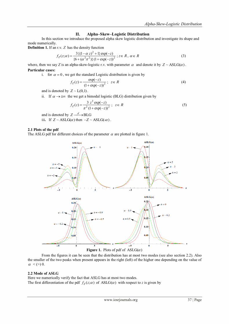
2.1 Plots of the pdf

The ASLG pdf for different choices of the parameter are plotted in figure 1.

Figure 1. Plots of pdf of )ASLG(

From the figures it can be seen that the distribution has at most two modes (see also section 2.2). Also

the smaller of the two peaks when present appears in the right (left) of the higher one depending on the value of

< (>) 0.

2.2 Mode of ASLG Here we numerically verify the fact that ASLG has at most two modes.

The first differentiation of the pdf );( zfZ of )(ASLG with respect to z is given by

Alpha-Skew-Logistic Distribution

www.iosrjournals.org 38 | Page

);( zDfZ 322 )1)(exp()6(

]2)exp(2}2)2)2(()2))2(2()({exp()[exp(3

z

zzzzzzz

(6)

In order to check that )ASLG( has at most two modes, the contour of the equation 0);( zDfZ is

drawn in figure 2. It can be seen that there is at most three zeros of );( zDfZ which establishes that

)(ASLG has at most two modes. Note that for – 0.8 < < 0.8 )(ASLG remains unimodal (see the second

plot in figure 2).

Figure 2. Contour plots of the equation 0);( zDfZ

III. Distributional Properties 3.1 Cumulative Distribution Function (cdf)

Theorem 1. The cdf of )ASLG( is given by

exp(z)]- [Li2)}exp(1log{)1(2

)exp(1

1)1(

)6(

3);( 2

22

22

zz

z

zzFZ (7)

Proof: dzz

zzzF

z

Z

2

2

22 ))exp(1(

)exp(}1)1{(

)6(

3);(

dzz

zzdz

z

zzdz

z

zzzz

2

22

2222 ))exp(1(

)exp(

))exp(1(

)exp(2

))exp(1(

)exp(2

)6(

3

))exp(1log(2

)exp(1

2

)exp(1

2

)6(

322

zz

z

z

exp(z)]- [Li 2))exp(1log(2

)exp(12

2222

zzz

z

exp(z)]- [Li2)}exp(1log{)1(2

)exp(1

1)1(

)6(

32

22

22

zz

z

z.

Where

1

n )(Li

kn

k

k

zz is the poly-logarithm function (see Prudnikov et al. (1986)).

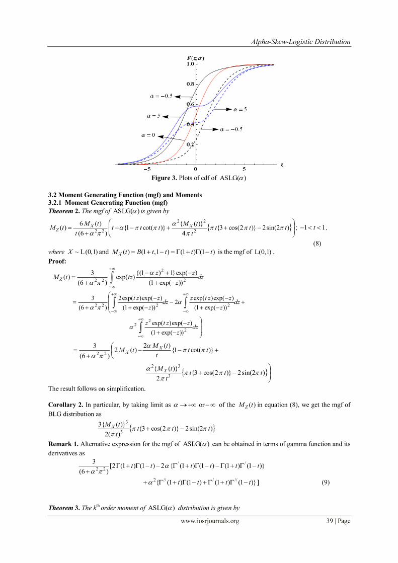
The cdf is plotted in figure 3 for studying variation in its shape with respect to the parameter .

Corollary 1. In particular by taking limit or the cdf of BLG distribution in equation (5) is

easily obtained from (7) as

22

))exp(1(

exp(z)] [Li))exp(1((6))}exp(1log(()exp(1(2){exp(3

z

zzzzz

Alpha-Skew-Logistic Distribution

www.iosrjournals.org 39 | Page

Figure 3. Plots of cdf of )ASLG(

3.2 Moment Generating Function (mgf) and Moments

3.2.1 Moment Generating Function (mgf)

Theorem 2. The mgf of )ASLG( is given by

)2sin(2)}2cos(3{

4

)}({)}cot(1{

)6(

)(6)(

2

22

22ttt

t

tMttt

t

tMtM XX

Z

; 11 t ,

(8)

where )1,0(L~X and )1()1()1,1()( ttttBtM X is the mgf of )1,0(L .

Proof:

dzz

zztztM Z

2

2

22 ))exp(1(

)exp(}1)1{()exp(

)6(

3)(

dzz

zztz

dzz

zztzdz

z

zzt

2

22

2222

))exp(1(

)exp()exp(

))exp(1(

)exp()exp(2

))exp(1(

)exp()exp(2

)6(

3

)}cot(1{

)(2)(2

)6(

322

ttt

tMtM X

X

)2sin(2)}2cos(3{

2

)}({3

32

tttt

tM X

The result follows on simplification.

Corollary 2. In particular, by taking limit as or of the )(tMZ in equation (8), we get the mgf of

BLG distribution as

)2sin(2)}2cos(3{)(2

)}({33

3

tttt

tM X

Remark 1. Alternative expression for the mgf of )ASLG( can be obtained in terms of gamma function and its

derivatives as

)}1()1()1()1({2)1()1(2[)6(

3 //

22tttttt

])}1()1()1()1({ /////2 tttt (9)

Theorem 3. The kth order moment of )(ASLG distribution is given by

Alpha-Skew-Logistic Distribution

www.iosrjournals.org 40 | Page

odd if);1()2()2

11(2

even if;)2()3()2

11()()1()

2

11(2

)6(

6)(E

1

2

1

22

kkk

kkkkk

Z

k

kkk

(10)

where

j

sjs)( is the Riemann zeta functions and dttts s

0

1 )exp()( .

Proof: Recall that, for )1,0(L~X i.e. for the standard logistic random variable X

.odd is if;0

even is if);()1())2/1(1(2)(E

1

k

kkkX

kk

(Balakrishnan, 1992)

Now,

dz

z

zzzzdzzfzZ kkk

2

22

22 ))exp(1(

)exp()22(

)6(

3);()(E

dzz

zzdz

z

zzdz

z

zz kkk

2

22

2

1

222 ))exp(1(

)exp(

))exp(1(

)exp(2

))exp(1(

)exp(2

)6(

3

Case I. when k is even

dzz

zzdz

z

zzZ

kkk

2

22

222 ))exp(1(

)exp(

))exp(1(

)exp(2

)6(

3)(E

)2()3()

2

11()()1()

2

11(2

)6(

61

2

122kkkk

kk

Case II. when k is odd

dzz

zzZ

kk

2

1

22 ))exp(1(

)exp(2

)6(

3)(E

)1()2()

2

11(2

)6(

622

kkk

The result (10) follows immediately.

3.2.2 Moments

From (10) using the following particular values of the Riemann zeta functions,

6/)2( 2 , 90/)4( 4 and 945/)6( 9 (Prudnikov et al. 1986), we get

22

2/1

6

2)(E

Z ,

Which is proportional to variance of standard logistic distribution and is positive (or negative) if 0)( .

)6(5

710)(E

22

422/2

2

Z

)6(5

14)(E

22

4/3

3

Z , is positive (or negative) if depending on whether 0)( .

)6(35

)15598()(E

22

224/4

4

Z

222

44222

2)6(5

)73260()(Var

Z

222

44222

)6(15

)2196180(

3

Since, 1)6(15

)2196180(222

4422

therefore, variance of )(ASLG is greater than or equal to that of

)1,0(L .

Alpha-Skew-Logistic Distribution

www.iosrjournals.org 41 | Page

Remark 2. From the compact formulas of the moments obtained above we can see that 213 4.1/

8286.13 , which means that the third moment is increasing (decreasing) function of the mean according as the

parameter 0)( . Further, 1

21

3 3001.0

)(217.0

and hence the pdf of in equation (3) can be written in

terms of 1 as

221

21

221

1))exp(1()8893.06(

)exp(})0901.0{(3);(

z

zzzfZ

; Rz , R

Bounds for mean and variance: The following bounds for mean, variance can be derived using numerically

optimizing )(E Z and )(Var Z with respect to .

i. 29.1)(E29.1 Z and

ii. 82.13)(Var29.3 Z

Plots of mean and variance: We have plotted the mean and the variance respectively in figure 4 and 5 to study

their behavior. Theses plots also verify the bounds presented above.

Figure 4. Plots of mean Figure 5 . Plots of variance

Remark 3. Moments of BLG Distribution can be derived easily by taking limit as or in the

moments of )(ASLG in section 3.2.2 as

,0)(E Z 82.135/7)(Var 2 Z

3.2.3 Skewness and Kurtosis

The skewness and Kurtosis of )(ASLG is given by:

Skewness,2/32

12

31213

1)(

23

2/322

4222

})2120(30{

})6340(9045{52

CC

CCC

Kurtosis, 3)(

36422

12

412

21314

2

222

22244

}30)2021({7

)107(1890}1120)1372465({45}800)8021(21{21

CC

CCCCCCC

where, 3/)6( 22C . Note that, for 0)( all odd order moments are positive (negative) while the even

order moments are always positive.

Bounds for skewness and kurtosis: The following bounds for skewness and kurtosis can be derived using

numerically optimizing 1 and 2 with respect to .

i. 62.162.1 1 and

ii. 17.274.0 2 .

Plots of skewness and kurtosis: We have plotted the skewness and kurtosis respectively in figure 6 and 7 to

study their behavior. Theses plots also verify the bounds presented above.

Remark 4. Skewness and Kurtosis of BLG Distribution can be derived easily by taking limit as or

in the results of )(ASLG in section 3.2.3 as 74.0,0 21

Alpha-Skew-Logistic Distribution

www.iosrjournals.org 42 | Page

Figure 6. Plots of skewness Figure 7. Plots of and kurtosis

IV. Truncated alpha-skew-logistic-distribution as a life time distribution Here we present alpha-Skew-logistic-distribution truncated below „0‟ as a potential life time

distribution. The pdf of the truncated-alpha-logistic-distribution )(TASLG truncated below „0‟ is given by

)616.4())exp(1(

)exp(}1)1{(6);(

222

2

t

tttfT ; 0t (11)

provided, 0616.422 .

The survival function );( tST and the hazard rate functions );( thT of )(TASLG can be easily

expressed in terms of the pdf );( tfZ and cdf ),( tFZ of )(ASLG as

),0(1

),(1);(

Z

ZT

F

tFtS

and

),(1

);(

);(

);();(

tF

tf

tS

tfth

Z

Z

T

TT

For admissible values of the parameter , we have plotted the );( thT in figure 8 to study its behavior

graphically.

Figure 8. Plots of hazard rate function )(TASLG

From the figure 8 it can be seen that for 0 the hazard rate is increasing always while for 7.0 it

assumes bathtub shape. For values of )7.0,0( the hazard rate takes different shapes. Thus depending on the

range of the values of the parameter , the hazard rate function of )(TASLG assumes different useful shapes

like the Weibull model and thus has the potential to be a flexible life time model.

Remark 5. Clearly, for 0 , )(TASLG reduces to standard half logistic distribution (Balakrishnan, 1992).

As such the present )(TASLG may be seen as a generalization of the standard half logistic distribution

(Balakrishnan, 1992).

V. Closeness of alpha skew normal and alpha skew logistic distributions Similarities of normal and logistic have been examined in the statistical literature (Johnson et al.

(2004), pp. 119,). Since the alpha skew logistic distribution proposed here has the same structure as that of the

alpha skew normal distribution of Elal-Olivero (2010), we present results of a brief numerical investigation

carried out to check their closeness. Accordingly, the difference of the pdfs of ),0,(ASN a and ),0,(ASLG ,

have been studied to find combinations of parameters such that the two pdfs almost coincide. This is achieved

by minimizing the sum of the squared difference of the pdfs over a finite set of equally spaced points in the

range of these two distributions with respect to one parameter while others are kept fixed. The KL distance

Alpha-Skew-Logistic Distribution

www.iosrjournals.org 43 | Page

(Burnham and Anderson, 2002) of these pairs are then checked to re-emphasize their closeness. We found many

close pairs, two such close pairs are

I. )2,0,2.5 (ASN and )1,0,1.656(ASLG :

Distance between the pdfs = 0.00265 and KL distance = 0.03275.

II. )6,0,3.8535 (ASN and )3,0,2.5 (ASLG :

Distance between the pdfs = 0.00896 and KL distance = 0.03572.

We have presented the graphs of the pdfs, cdfs and difference of cdfs of the first pair of distributions

respectively in Figure 9, 10 and 11 to depict their closeness.

Figure 9. Plots of pdf Figure 10. Plots of cdf Figure 11. Plots of differences of cdf

VI. Parameter estimation

We present the problem of parameter estimation of a location and scale extension of )(ASLG .

If )(ASLG~ Z , then ZY is said to be the location ( ) and scale extension ( ) of Z and

has the pdf

222

2

))/)(exp(1()6(

)/)(exp(}1)/)(1{(3),,;(

y

yyyfY ; Ry , R, , 0 (12)

We denote it by ),,(ASLG~ Y .

In particular, for or , BLG),,(ASLG .

6.1 Method of moments

Let 1m , 2m and 3m are respectively the first three sample raw moments for a given random sample

),,,( 21 nyyy of size n drawn from ),,(ASLG distribution in equ. (12). Then the moment estimates of

the three parameters , and are obtained by simultaneously solving the following equations derived by

equating first three population moments with corresponding sample moments.

122

2

22

2

16

2

6

2mm

(13)

)6(5

)710(2022

2222222

2

m (14)

)6(5

14)710(33022

342222223

3

m (15)

Substituting the value of from equ. (13) in equ. (14) and solving for 2 we get,

)73260(

)6)((544222

2222122

mm (16)

Finally, putting these values of and 2 in equ. (15), we get the following equ. in

2/3

4422

212

222

322

442242

1213

1373260

)()6(

)6(

)71636(54)(3

mmmmmmm

(17)

Alpha-Skew-Logistic Distribution

www.iosrjournals.org 44 | Page

While the exact solution of the equ. (17) is not tractable, it can be numerically solved to estimate .

Once is estimated rest of the two parameters namely, and can be directly estimated from equ. (13) and

(16) respectively.

Remark 6. It may be noted that the equ. (17) may return multiple solutions for and hence leading to more

than one set of feasible estimates for the parameters. This situation may be resolved by retaining the best set

(according to some criterion e.g., likelihood or entropy) among the feasible solutions.

6.2 Maximum likelihood estimation

For a random sample of size n ),,,( 21 nyyy drawn from ),,(ASLG distribution in equ. (12), the

likelihood function is given by

n

i

Y yfL

1

),,;(loglog

n

i

ii yyn

1

222

))]/)(exp(1log[(2]1)/)(1log[(3

)6(

n

i

iy

1

/)( (18)

The MLE‟s of and, are obtained by numerically maximizing Llog with respect

to and, .

The variance-covariance matrix of the MLEs can be derived by using the asymptotic distribution of

MLEs as, 1

2

222

2

2

22

22

2

2

logE

logE

logE

logE

logE

logE

logE

logE

logE

LLL

LLL

LLL

(19)

When the exact expressions for various expectations above are cumbersome, in practice they are estimated as

ˆ

2

2

2

2 loglogE

LL,

ˆ,ˆ

22 loglogE

LL etc.

VII. Real life applications: comparative data fitting Here we have considered data set of the heights of 100 Australian athletes (Cook and Weisberg, 1994)

and compared the proposed distribution ),,(ASLG with the logistic distribution ),( L , skew logistic

distribution ),,( SL of Wahed and Ali (2001), the new skew logistic distribution ),,,( SL of

Chakraborty et al. (2012), alpha-skew-normal distribution ),,(ASN of Elal-Olivero (2010), alpha-skew-

Laplace distribution ),,(ASL of Harandi and Alamatsaz (2013) and alpha skew normal slash distribution

),,,(ASNS q of Gui (2014) . The MLE of the parameters are obtained by using numerical optimization

routine. In the present work, the GenSA-package, Version-1.0.3, of the software R is used. Akaike Information

Criterion (AIC) and Beysian Information Criterion (BIC) are used for model comparison.

Further, since ),(L and ),,(ASLG are nested models the likelihood ratio (LR) test is used to

discriminate between them.

The LR test is carried out to test the following hypothesis

0:0 H , that is the sample is drawn from ),( L ,

against the alternative

0:1 H , that is the sample is drawn from ),,(ASLG .

From the Table 1 it is seen that the proposed alpha skew logistic distribution ),,(ASLG provides

best fit to the data set under consideration in terms of all the criteria, namely the log-likelihood, the AIC as well

Alpha-Skew-Logistic Distribution

www.iosrjournals.org 45 | Page

as the BIC. The plots of observed (in histogram) and expected densities (lines) presented in Figure 9, also

confirms our finding.

LR test result: The value of LR test statistic is 5.058 which exceed the 95% critical value, 3.84. Thus there is

evidence in favors of the alternative hypothesis that the sampled data comes from ),,(ASLG not from

),(L .

Table 1: MLE‟s, log-likelihood, AIC and BIC for heights (in cm)

of 100 Australian Athletes data Parameters

Distributions q

Log-

likelihood AIC BIC

),( L 175.001 4.410 -- -- -- -349.589 703.179 708.388

),,( SL 179.563 5.197 -0.901 -- -- -348.689 703.378 711.194

),,,( SL 172.909 4.620 1.646 2.037 -- -347.546 703.092 713.513

),,(ASN 169.465 7.280 -- -1.112 -- -348.000 701.994 709.810

),,(ASL 171.400 3.301 -- -1.091 -- -347.933 701.866 709.682

),,,(ASNS q

178.01 4.744 -- 0.550 2.548 -349.552 707.104 717.525

),,(ASLG 170.496 3.203 -- -0.747 -- -347.060 700.121 707.936

Figure 12. Plots of observed and expected densities for heights of 100 Australian athletes

Remark 7. The variance-covariance matrix of the MLEs of the parameters of ),,(ASLG is obtained by

using (19) as

0.02400.02090.0497

0.02090.09210.0646-

0.04970.0646-0.6841

)ˆ,ˆ,ˆ(CovranceVariace

VIII. Concluding remarks

In this article a new alpha skew logistic distribution which includes both unimodal as well as bimodal

logistic distributions is introduced and some of its basic properties are investigated. A truncated version of the

proposed distribution is seen to have bathtub shaped failure rate function. Closeness of the alpha skew normal

and alpha skew logistic distributions is briefly explored.

The numerical results of the modeling of a real life data set considered here has shown that the

proposed distribution provides better fitting in comparison to the logistic and skew logistic distribution of

Wahed and Ali (2001), alpha-skew-normal distribution ),,(ASN of Elal-Olivero (2010), alpha skew

logistic distribution ),,(ASL of Harandi and Alamatsaz (2013), the new multimodal skew logistic

distribution of Chakraborty et al. (2012) and alpha skew normal slash distribution of Gui (2014).

Alpha-Skew-Logistic Distribution

www.iosrjournals.org 46 | Page

References [1] Azzalini, A. (1985) A class of distributions which includes the normal ones. Scand. J. Stat. 12: 171 - 178.

[2] Balakrishnan, N. (1992) Handbook of Logistic Distribution. Marcel Dekker. New York.

[3] Burnham, K. P., Anderson, D. R. (2002) Model Selection and Multimodel Inference: A Practical Information Theoretic Approach.

2nd

edn. Springer.New York.

[4] Chakraborty, S., Hazarika, P. J. (2011) A survey of the theoretical developments in univariate skew normal distributions. Assam

Statist. Rev. 25(1): 41 - 63.

[5] Chakraborty, S. Hazarika, P. J., Ali, M. M. (2012) A new skew logistic distribution and its properties. Pak. J. Statist. 28(4): 513 -

524.

[6] Chakraborty, S. Hazarika, P. J., Ali, M. M. (2014a) A multimodal skewed extension of normal distribution: its properties and

applications. Statistics-A Journal of Theoretical and Applied Statistics, http://dx.doi.org/10.1080/ 02331888.2014.908880.

[7] Chakraborty, S. Hazarika, P. J., Ali, M. M. (2014b) A multimodal skew-Laplace distribution: its properties and applications. Pak. J.

Statist, 30(2): 253-264.

[8] Cook, R. D., Weisberg, S. (1994) An Introduction to Regression Analysis. Wiley. New York.

[9] Elal-Olivero, D. (2010) Alpha–skew–normal distribution. Proyecciones Journal of Mathematics. 29: 224 - 240.

[10] Gui, W. (2014) A generalization of the slashed distribution via alpha skew normal distribution. Stat Methods Appl. DOI

10.1007/s10260-014-0258-7.

[11] Harandi, S. S., Alamatsaz, M. H. (2013) Alpha-skew-Laplace distribution, Statist Probab Lett. 83(3):774 - 782.

[12] Huang, W. J., Chen, Y. H. (2007) Generalized skew Cauchy distribution, Statist Probab Lett. 77:1137 - 1147.

[13] Johnson, N. L., Kotz, S., Balakrishnan, N. (2004) Continuous Univariate Distributions (Volume 2). A Wiley-Interscience

Publication. John Wiley & Sons Inc. New York.

[14] Nadarajah, S. (2009) The skew logistic distribution. AStA Adv Stat Anal. 93: 187 - 203.

[15] Nadarajah, S., Kotz, S. (2006) Skew distributions generated from different families. Acta Appl Math. 91:1 - 37.

[16] Nadarajah, S., Kotz, S. (2007) Skew models I. Acta Appl Math. 98:1 - 28.

[17] Prudnikov, A. P., Brychkov, Y. A. and Marichev, Y. I. (1986) Integrals and Series, (Volume - 1), Gordon and Breach. Amsterdam.

[18] Wahed, A. S., Ali, M. M. (2001) The skew logistic distribution. J Stat. Res. 35:71 - 80.