
CHAPTER 28 Multiple and Logistic Regression
61
Baldi-4100190 psls January 16, 2014 14:46 IN THIS CHAPTER WE COVER... ■ Parallel regression lines ■ Estimating parameters ■ Using technology ■ Conditions for inference ■ Inference for multiple regression ■ Interaction ■ A case study for multiple regression ■ Logistic regression ■ Inference for logistic regression CHAPTER 28 Multiple and Logistic Regression Sinclair Stammers/Science Source W hen a scatterplot shows a linear relationship between a quantitative ex- planatory variable x and a quantitative response variable y , we fit a re- gression line to the data to describe the relationship. We can also use the line to predict the value of y for a given value of x . For example, Chapter 4 uses regression lines to describe relationships between ■ the gain in body fat y of overfed individuals and the amount of nonexercise activity x in their daily routine; ■ the mating-call frequency y of frogs and outside temperature x ; and ■ the number y of new adults that join a colony of birds and the percent x of adult birds that return from the previous year. In all these cases, other explanatory variables might improve our understanding of the response y and help us to better predict y . ■ The gain in body fat y of an overfed individual may depend on the amount of daily nonexercise activity x 1 and on the individual’s age x 2 and gender x 3 . ■ Mating-call frequency y may depend on outside temperature x 1 and also on the species x 2 of the frogs we study. 28-1
-
Upload
khangminh22 -
Category
Documents
-
view
2 -
download
0
Transcript of CHAPTER 28 Multiple and Logistic Regression

Baldi-4100190 psls January 16, 2014 14:46
IN THIS CHAPTERWE COVER.. .
■ Parallel regression lines
■ Estimating parameters
■ Using technology
■ Conditions for inference
■ Inference for multiple regression
■ Interaction
■ A case study for multiple
regression
■ Logistic regression
■ Inference for logistic regression
C H A P T E R 28 Multiple and LogisticRegression
Sinc
lair
Stam
mer
s/Sc
ienc
eSo
urce
When a scatterplot shows a linear relationship between a quantitative ex-planatory variable x and a quantitative response variable y, we fit a re-gression line to the data to describe the relationship. We can also use the
line to predict the value of y for a given value of x . For example, Chapter 4 usesregression lines to describe relationships between
■ the gain in body fat y of overfed individuals and the amount of nonexerciseactivity x in their daily routine;
■ the mating-call frequency y of frogs and outside temperature x ; and■ the number y of new adults that join a colony of birds and the percent x of
adult birds that return from the previous year.
In all these cases, other explanatory variables might improve our understanding ofthe response y and help us to better predict y.
■ The gain in body fat y of an overfed individual may depend on the amountof daily nonexercise activity x1 and on the individual’s age x2 and gender x3.
■ Mating-call frequency y may depend on outside temperature x1 and also onthe species x2 of the frogs we study.
28-1

Baldi-4100190 psls January 16, 2014 14:46
28-2 C H A P T E R 28 ■ Multiple and Logistic Regression
■ The number y of new adults in a bird colony may depend on the percent x1of returning adults and also on the species x2 of the birds we study.
We will now call regression with just one explanatory variable simple linear re-gression to remind us that this is a special case. This chapter introduces the moresimple linear regressiongeneral case of multiple regression, which allows several explanatory variablesmultiple regressionto combine in explaining a response variable. We start with the simplest case bycomparing two parallel regression lines and will gradually build up to increasinglycomplex models.
Parallel regression linesIn Chapter 3 we learned how to add a categorical variable to a scatterplot by usingdifferent colors or plot symbols to indicate the different values of the categoricalvariable. In Example 3.6 we examined the relationship between the longevity yand the thorax length of male fruit flies under two experimental conditions. Theconditions make-up a categorical variable (call it x2) that takes just two values.The scatterplot shows two parallel straight-line patterns linking the response y(longevity) to a quantitative explanatory variable x1 (thorax length), with onepattern for each value of x2 (experimental condition).
Yoav Levy/Phototake
EXAMPLE 28.1 Cost of reproduction in male fruit flies
STATE: Longevity in male fruit flies is positively associated with adult size. But repro-duction has a high physiological cost that could impact longevity. A study looks at theassociation between longevity and adult size in male fruit flies kept under one of twoconditions. One group is kept with sexually active females over the male’s life span. Theother group is cared for in the same way but kept with females that are not sexually ac-tive. Table 28.1 gives the longevity in days and thorax length in millimeters (mm) forthe male fruit flies given an opportunity to reproduce (IndReprod = 1) and for those de-prived of the opportunity (IndReprod = 0).1 Is there evidence that reproduction impactsmale fruit fly longevity?
PLAN: Make a scatterplot to display the relationship between longevity y and thoraxlength x1. Use different colors for the two reproductive conditions. (So reproduction isa categorical variable x2 that takes two values.) If both reproductive conditions showlinear patterns, fit two separate least-squares regression lines to describe them.
SOLVE: Figure 28.1 shows a scatterplot with two separate regression lines, one for eachexperimental group. The longevities for fruit flies that never reproduced are higher thanthe longevities of reproducing fruit flies of similar size. Both regression lines have a pos-itive slope, indicating that larger adult males live longer, but the males prevented fromreproducing clearly have greater longevity than reproducing males of similar size. Soft-ware gives the following regression lines:
For nonreproducing males: y = −52.381 + 143.504x1
For reproducing males: y = −59.816 + 123.370x1
We notice from the estimated regression lines and Figure 28.1 that the intercepts forthe two regression lines are clearly different, but the two regression lines are roughly

Baldi-4100190 psls January 16, 2014 14:46
■ Parallel regression lines 28-3
T A B L E 28.1 Thorax length (mm) and longevity (days) of reproducing andnonreproducing male fruit flies
Longevity ThxLength IndReprod Longevity ThxLength IndReprod
35 0.64 0 16 0.64 137 0.68 0 19 0.64 149 0.68 0 19 0.68 146 0.72 0 33 0.72 164 0.72 0 34 0.72 139 0.76 0 34 0.74 146 0.76 0 30 0.76 156 0.76 0 42 0.76 164 0.76 0 42 0.76 165 0.76 0 34 0.78 156 0.80 0 26 0.80 165 0.80 0 30 0.80 170 0.80 0 40 0.82 164 0.84 0 54 0.82 165 0.84 0 35 0.84 170 0.84 0 35 0.84 176 0.84 0 46 0.84 181 0.84 0 46 0.84 185 0.84 0 42 0.88 170 0.88 0 46 0.88 170 0.88 0 54 0.88 176 0.92 0 54 0.88 176 0.92 0 56 0.88 176 0.94 0 61 0.88 1
44 0.92 1
parallel. Therefore, the difference in the two intercepts indicates how much longer thenonreproducing males live after we take into account thorax length. We will soon learnhow to formally estimate parameters and make inferences for parallel regression lines.
CONCLUDE: Our preliminary analysis clearly shows that the nonreproducing male fruitflies live longer than reproducing males of similar size. We know that both groups of malefruit flies lived in similar conditions, except the nonreproducing males lived their livesin the company of females that were not fertile and could not reproduce, whereas thereproducing males lived with fertile females. So the physiological cost of reproducingwas the sole difference between the two groups. We will learn later in this chapter howto formally test if the difference observed is statistically significant. ■
We now think that the relationship between longevity and thorax length hasabout the same rate for both experimental conditions, but that the physiologicalcost of reproduction results in shorter life spans. This difference in life span appearsto be fairly constant for all thorax lengths. We would like to have a single regressionmodel that captures this insight.

Baldi-4100190 psls January 16, 2014 14:46
28-4 C H A P T E R 28 ■ Multiple and Logistic Regression
FIGURE 28.1 A scatterplot oflongevity of male fruit flies ofdifferent adult sizes, with twoseparate regression lines, forExample 28.1.
10
30
90
Thorax length (mm)
Long
evit
y (d
ays)
0.95
20
80
70
60
50
40
0.900.850.800.750.700.650.60
Regression line fornonreproducing flies
Regression line forreproducing flies
Nonreproducing Reproducing
To do this, introduce a second explanatory variable x2 for “reproductive sta-tus.” This is a categorical variable that takes the values “reproductive” and “non-reproductive.” To incorporate this categorical variable x2 into a regression model,we simply use values 0 and 1 to distinguish the two conditions. Now we have anindicator variable:
x2 = 0 for nonreproductive males
x2 = 1 for reproductive males
INDICATOR VARIABLE
An indicator variable places individuals into one of two categories, usuallycoded by the two values 0 and 1.
An indicator variable is like an indicator light on the dash of a car. If the fuelis above a certain level, the indicator light for fuel is off, but if the fuel drops belowa certain level, the light switches on to indicate that there is a low amount of fuelin the tank. An indicator variable for fuel, say x2, could be coded as x2 = 0 if thefuel is above a certain level and x2 = 1 if the fuel is below that level. Indicatorvariables are commonly used to indicate categorical characteristics such as gender(0 = male, 1 = female) or condition of patient (0 = good, 1 = poor). When a cate-gorical variable can take more than two values, it is necessary to use more than oneindicator variable to encode it. For instance, if we describe a patient’s condition as

Baldi-4100190 psls January 16, 2014 14:46
■ Parallel regression lines 28-5
stationary, improving, or deteriorating, we would need two indicator variables, sayx2 and x3, each taking only values 0 or 1; we could then use stationary = (1, 0),improving = (0, 1), and deteriorating = (0, 0) in the regression model.
The conditions for inference in simple linear regression (Chapter 23, page 563)describe the relationship between the explanatory variable x and the mean re-sponse μy in the population by a population regression line μy = α + βx . In thischapter we switch to the notation μy = β0 + β1x because it is easier to extend tothe multiple regression model. Now we add a second explanatory variable, so thatour regression model for the population becomes
μy = β0 + β1x1 + β2x2
The conditions for inference are the same as in the simple linear regression setting:For any fixed values of the explanatory variables, y varies about its mean accordingto a Normal distribution with unknown standard deviation σ , which is the samefor all values of x1 and x2. We will look in detail at conditions for inference inmultiple regression later on.
EXAMPLE 28.2 Interpreting a multiple regression model
Multiple regression models are no longer simple straight lines, so we must think a bitharder in order to interpret what they say. Consider our model
μy = β0 + β1x1 + β2x2
in which y is the longevity of male fruit flies in the lab, x1 is their thorax length, andx2 is an indicator variable for reproductive status. For nonreproducing males, x2 = 0, sothe model becomes
μy = β0 + β1x1
For reproducing males, x2 = 1, so the model is
μy = β0 + β1x1 + β2
= (β0 + β2) + β1x1
Look carefully: The slope that describes how the mean longevity changes as thoraxlength x1 varies is β1 in both groups. The intercepts differ: β0 for nonreproducing malesand (β0 +β2) for reproducing males. So β2 is of particular interest, because it is the fixedchange between nonreproducing and reproducing male fruit flies.
Figure 28.2 is a graph of this model with all three β ’s identified. We have succeededin giving a single model for two parallel straight lines. ■
A P P L Y Y O U R K N O W L E D G E
28.1 Bird colonies. Suppose that the number y of new birds that join a colony this yearhas the same straight-line relationship with the percent x1 of returning birds incolonies for two different bird species. An indicator variable shows which specieswe observe; x2 = 0 for one, and x2 = 1 for the other. Write a population regressionmodel that describes this setting. Explain in words what each β in your modelmeans.
■

Baldi-4100190 psls January 16, 2014 14:46
28-6 C H A P T E R 28 ■ Multiple and Logistic Regression
FIGURE 28.2 Multipleregression model with two parallelstraight lines, for Example 28.2.
10
90
Thorax length (mm)
Long
evit
y (d
ays)
0.950.60
0 is the y intercept ofthe regression line forX2 = 0 (nonreproducing).
1 is the slope of bothlines (when X2 = 0 andwhen X2 = 1).
my for X2 = 0(nonreproducing)
my for X2 = 1(reproducing)
2β
β
β
Estimating parametersHow shall we estimate the β ’s in the model μy = β0 + β1x1 + β2x2? Because wehope to predict y, we want to make the errors in the y direction small. We can’tcall this the vertical distance from the points to a line as we did for a simple linearregression model, because we now have two lines. But we still concentrate on theprediction of y and therefore on the deviations between the observed responses yand the responses predicted by the regression model. These deviations are residualerrors, similar to the residuals we first saw in simple linear regression:
residual = observed y − predicted y = y − y
The method of least squares estimates the β ’s in the model by choosing thevalues that minimize the sum of the squared residuals. Call b ’s the estimates of theβ ’s. Then the b ’s minimize∑
(residual)2 =∑
(observed y − predicted y)2
=∑
(y − y)2
=∑
(y − b0 − b1x1 − b2x2)2
The least-squares regression model y = b0 + b1x1 + b2x2 estimates the populationregression model μy = β0+β1x1+β2x2. Remember from Chapter 23 that the pop-ulation model describes the mean response μy for given values of the explanatoryvariable(s).
The remaining parameter to be estimated is the standard deviation σ , whichdescribes the variability of the response y about the mean μy given by the popu-lation regression model. Since the residuals estimate how much y varies about the

Baldi-4100190 psls January 16, 2014 14:46
■ Estimating parameters 28-7
mean of the regression model, the standard deviation s of the residuals is used toestimate σ . The value of s is also referred to as the regression standard error.
REGRESSION STANDARD ERROR
The regression standard error for the multiple regression model with twoparallel lines is
s =√
1n − 3
∑residual2 =
√1
n − 3
∑(y − y)2
where n is the number of observations in the data set. Use s to estimate thestandard deviation σ of the responses about the mean given by thepopulation regression model.
Notice that instead of dividing by (n − 2), as we did for the simple linearregression model in Chapter 23, we are now dividing by (n − 3). Since we areestimating three β parameters in our population regression model, the degrees offreedom must reflect this change. In general, the degrees of freedom for the re- degrees of freedomgression standard error will be the number of data points minus the number of β
parameters in the population regression model.Why do we prefer one regression model with parallel lines to the two separate
regression models? Simplicity is one reason—why use separate models with four β ’sif a single model with three β ’s describes the data well? Looking at the regressionstandard error provides another reason: The n in the formula for s includes all theobservations in both groups. As usual, more observations produce a more preciseestimate of σ . (Of course, using one model for both groups assumes that σ describesthe scatter about the line in both groups.)
EXAMPLE 28.3 Cost of reproduction in male fruit flies
We developed a single model with parallel straight lines in Example 28.2 for the longevi-ties in the two experimental groups shown in Figure 28.1. The mean longevity is μy =β0 + β1x1 + β2x2, where x1 is the individual thorax length (the value on the x axis inFigure 28.1) and x2 is an indicator variable to identify the experimental group (differ-ent symbols in Figure 28.1). The estimated regression model obtained from statisticalsoftware is
y = −44.285 + 133.395x1 − 23.551x2
By substituting the two values of the indicator variable into our estimated regressionequation, we can obtain a least-squares line for each group. The predicted longevitiesare
y = −67.836 + 133.395x1 for reproducing males (x2 = 1)
and
y = −44.285 + 133.395x1 for nonreproducing males (x2 = 0)
Comparing these estimated regression equations with the two separate regressionlines obtained in Example 28.1, we see that the intercept parameters are very close to one

Baldi-4100190 psls January 16, 2014 14:46
28-8 C H A P T E R 28 ■ Multiple and Logistic Regression
another (−67.836 is close to −59.816, and −44.285 is close to −52.381) for both groups.The big change, as intended, is that the slope 133.395 is now the same for both lines. Inother words, the estimated change in mean longevity for a 1-unit change in thorax lengthis now the same for both models, 133.395. A closer look reveals that 133.395 is roughlythe average of the two slope estimates (143.504 and 123.370) obtained in Example 28.1.
Finally, the regression standard error s = 7.846 indicates the size of the error be-tween the observations and the estimated model. ■
A P P L Y Y O U R K N O W L E D G E
28.2 LDL cholesterol. A study examined the change in blood LDL cholesterol level (inmillimoles per liter, mmol/l) as a function of baseline LDL cholesterol level whensubjects took either a placebo or the drug Pravastatin for two years.2 One modelof the results shows two parallel lines and gives a multiple linear regression modelμy = −1.875 + 0.4375x1 + 1.4x2, where x1 represents baseline cholesterol leveland x2 is an indicator variable for treatment that takes value 0 for the placebo groupand 1 for the Pravastatin group. Identify the parameter estimates in the model. Findthe straight-line equations for the placebo group and for the Pravastatin group, andthen make a graph that shows these two lines.
■
Using technologyTable 28.1 provides a compact way to display data in a textbook, but this is typicallynot the best way to enter your data into a statistical software package for analysis.The primary disadvantage to entering the data into a worksheet as it appears inTable 28.1 is that the response variable of interest, longevity, is entered in twoseparate columns, one for each experimental group.
As problems become more complex, we often collect information on morethan two variables. This means that data management becomes a much largerpart of our job. When fitting and analyzing models, it is usually best to have onecolumn for each variable and to use the rows to identify the individuals.
EXAMPLE 28.4 Organizing data
To fit the multiple regression model with equal slopes in Example 28.3, three columnswere created. The 49 longevities y for reproducing and nonreproducing males werestacked into a column labeled Longevity, values of the explanatory variable x1 were en-tered into a column labeled ThxLength, and values of the indicator variable x2 wereentered into a column labeled IndReprod. Here are the first five rows of the worksheet:
Row Longevity ThxLength IndReprod
1 35 0.64 02 37 0.68 03 49 0.68 04 46 0.72 05 64 0.72 0
■

Baldi-4100190 psls January 16, 2014 14:46
■ Using technology 28-9
Statistical software performs all the necessary computations after we identifythe response variable Longevity and the two explanatory variables ThxLength andIndReprod. Figure 28.3 shows the regression output from Excel, Minitab, R, andSPSS. The format of the output differs slightly, but each package provides param-eter estimates, standard errors, t statistics, and P -values, an analysis of variance(ANOVA) table, the regression standard error, and R2. We will digest this out-put one piece at a time: first describing the model, then looking at the conditionsneeded for inference, and finally interpreting the results of inference.
Microsoft Excel
Book1A B
1
2 0.900006132
3 0.810011038
4 0.801750649
5 7.845843899
6 49
7
8
9 df10 2
11
Regression statisticsMultiple R
R Square
Adjusted R Square
Standard Error
Observations
ANOVA
Regression
46Residual
C
SS12072.56982
D
MS6036.284912
E
F98.0596647
F G
2831.634258 61.55726649
Significance F2.57485E–17
12 48
13
14
15 –44.28543
16 133.3949179
17
Total
Intercept
ThxLength
–23.5505042IndReprod
Coefficients11.71411366
14.49005467
Standard Error–3.78051907
9.205963738
t Stat0.000449471
5.2827E–12
P-value
2.242169166 –10.5034467 8.33921E–14
–67.8646953
104.2279785
Lower 95%
–28.0637524
–20.7061648
162.5618572
Upper 95%
–19.0372561
14904.20408
Session
Minitab
Regression Analysis: Longevity versus ThxLength, IndReprod
The regression equation isLongevity = - 44.3 + 133 ThxLength - 23.6 Ind_Reprod
Predictor Coef SE Coef T PConstant -44.29 11.71 -3.78 0.000ThxLength 133.39 14.49 9.21 0.000IndReprod -23.551 2.242 -10.50 0.000
S = 7.84584 R-Sq = 81.0% R-Sq(adj) = 80.2%
Analysis of Variance
Source DF SS MS F PRegression 2 12072.6 6036.3 98.06 0.000Residual Error 46 2831.6 61.6Total 48 14904.2
FIGURE 28.3 Output fromExcel, Minitab, SPSS, and R for themodel with parallel regression linesin Example 28.3. (Continued on nextpage.)

Baldi-4100190 psls January 16, 2014 14:46
28-10 C H A P T E R 28 ■ Multiple and Logistic Regression
SPSSSession
Model Summaryb
.900a .810 .802 7.846Model1
R R SquareAdjustedR Square
Std. Error ofthe Estimate
Predictors: (Constant), IndReprod, ThxLengtha.
Dependent Variable: Longevityb.
ANOVAb
12072.570 2 6036.285 98.060 .000a
2831.634 46 61.55714904.204 48
RegressionResidualTotal
Model1
Sum ofSquares df Mean Square F Sig.
Predictors: (Constant), IndReprod, ThxLengtha.
Dependent Variable: Longevityb.
Coefficientsa
-44.285 11.714 -3.781 .000 -67.865 -20.706133.395 14.490 .592 9.206 .000 104.228 162.562-23.551 2.242 -.675 -10.503 .000 -28.064 -19.037
(Constant)ThxLengthIndReprod
Model1
B Std. Error
UnstandardizedCoefficients
Beta
StandardizedCoefficients
t Sig. Lower Bound Upper Bound95% Confidence Interval for B
Dependent Variable: Longevitya.
FIGURE 28.3 (Continued)
R
Im(formula = Longevity ~ ThxLength + IndReprod)
Residuals: Min 1Q Median 3Q Max -18.095 -5.106 -1.537 5.792 17.234
Coefficients: Estimate Std. Error t value Pr(>|t|)(Intercept) -44.285 11.714 -3.781 0.000449 ***ThxLength 133.395 14.490 9.206 5.28e-12 ***IndReprod -23.551 2.242 -10.503 8.34e-14 ***---Signif. codes: 0 ‘***’ 0.001 ‘***’0.01 ‘***’0.05 ’.‘ 0.1 ’’ 1
Residual standard error: 7.846 on 46 degrees of freedomMultiple R-squared: 0.81, Adjusted R-squared: 0.8018F-statistic: 98.06 on 2 and 46 DF, p-value: <2.2e-16
EXAMPLE 28.5 Parameter estimates on statistical output
On the Excel output in Figure 28.3, the parameter estimates b0 = −44.28543, b1 =133.3949179, and b2 = −23.5505042 are clearly labeled in a column. Thus, our multipleregression model for predicting longevity (after rounding) is y = −44.285+133.395x1−23.551x2. SPSS and R have a similar output format. Minitab provides the estimatedregression equation first and then gives more detailed estimates in a column labeled

Baldi-4100190 psls January 16, 2014 14:46
■ Using technology 28-11
“Coef” for coefficients. After rounding, all four sets of estimates match the estimatesprovided in Example 28.3.
Although the labels differ again, the regression standard error is provided by all fourpackages:
Excel: Standard Error = 7.845843899Minitab: S = 7.84584R: Residual standard error = 7.846SPSS: Std. Error of the Estimate = 7.846 ■
For simple linear regression models, the square of the correlation coefficientr 2 between y and x provides a statistic that can be used along with residual plotsand other techniques to assess the fit of the model. In particular, r 2 measures theproportion of variation in the response variable that is explained by using the ex-planatory variable. For our multiple regression model with parallel regression lines,we do not have one correlation coefficient. However, by squaring the correlationcoefficient between the observed responses y and the predicted responses y, weobtain the squared multiple correlation coefficient R2.
Alternative computation formulas based on values in the ANOVA table of theoutput help us interpret this new statistic. You may want to refer to Chapter 24 torefresh your memory about the details of the ANOVA procedure. The ANOVAtable breaks the total variability in the responses into two pieces. One piece sum-marizes the variation explained by the model, and the other piece summarizes theresidual variation traditionally labeled “error.” In short, we have
total variation = variation explained by model + residual variation
The value of R2 is the ratio of model to total variation, so R2 tells us how muchvariation in the response variable y we explained by using the set of explanatoryvariables in the multiple regression model.
SQUARED MULTIPLE CORRELATION COEFFICIENT
The squared multiple correlation coefficient R2 is the square of thecorrelation coefficient between the observed responses y and the predictedresponses y and can be computed as
R2 = variability explained by modeltotal variability in y
=∑
(y − y)2∑(y − y)2 = SSModel
SSTotal
The denominator measures the deviation of the observed responses abouttheir mean. Just as in simple linear regression, the predicted responses y havethe same mean y as the observed responses. So the numerator is thevariability we would see if the model fitted perfectly and there were nospread of the y’s about the model. We can think of this as the variabilityexplained by the model.

Baldi-4100190 psls January 16, 2014 14:46
28-12 C H A P T E R 28 ■ Multiple and Logistic Regression
EXAMPLE 28.6 Using R 2
The value of R2 = 0.810 for our multiple regression model with parallel lines in Ex-ample 28.3 can be found in the output for all four packages in Figure 28.3 (labeled asMultiple R-squared, R Square, or R-Sq). Thus, the proportion of variation in the re-sponse variable Longevity that is explained by the explanatory variable ThxLength andthe indicator variable IndReprod using the regression model with parallel lines is 0.810,or 81.0%. Converting R2 to the percent of variation explained by the explanatory vari-ables in a multiple regression model is a common practice. The value of R2 indicatesthat 81% of the variation in the longevity of male fruit flies in the lab is explainedby using multiple regression with an explanatory variable for their thorax length andan indicator variable for the experimental condition determining their reproductivestatus. ■
The squared multiple correlation coefficient takes only values between 0 and1 (0% and 100%) and is a very useful statistic to help us assess the fit of a multipleregression model.
A P P L Y Y O U R K N O W L E D G E
28.3 Heights and weights for boys and girls. Suppose you are designing a study to in-vestigate the relationship between height and weight for boys and girls.
(a) Specify a model with two regression lines that could be used to predict heightseparately for boys and for girls. Be sure to identify all variables and describeall parameters in your model.
(b) How many columns in a worksheet would be required to fit this model withstatistical software? Describe each column.
28.4 Nestling mass and nest humidity. Researchers investigated the relationship be-tween nestling mass, measured in grams, and nest humidity index, measured as the
Session
Minitab
Regression Analysis: Mass versus Humidity, Exposed
The regression equation isMass = 18.1 - 5.41 Humidity + 0.848 Exposed
Predictor Coef SE Coef T PConstant 18.0848 0.6592 27.43 0.000Humidity -5.411 1.377 -3.93 0.000Exposed 0.8484 0.3587 2.37 0.024
S = 1.01583 R-Sq = 47.7% R-Sq(adj) = 44.6%
Analysis of Variance
Source DF SS MS T PRegression 2 32.008 16.004 15.51 0.000Residual Error 34 35.085 1.032Total 36 67.092

Baldi-4100190 psls January 16, 2014 14:46
■ Conditions for inference 28-13
ratio of total mass of water in the nest divided by nest dry mass, for two differentgroups of great titmice parents.3 One group was exposed to fleas during egg laying,and the other was not. Exposed parents were coded as 1, and unexposed parentswere coded as 0. Use the output on the previous page, obtained by fitting a multipleregression model with parallel lines for the two groups of parents, to answer thefollowing questions.
(a) Identify the regression model for predicting nestling mass from nest humidityindex for the two groups of great titmice parents.
(b) Based on your model, do you think that nestling mass was higher in nests ofbirds exposed to fleas during egg laying? Explain.
(c) What is the value of the regression standard error? Interpret this value.
(d) What is the value of the squared multiple correlation coefficient? Interpretthis value.
■
Conditions for inferenceWe have seen in a simple but useful case how adding another explanatory variablecan fit patterns more complex than the single straight line of simple linear regres-sion. So far we have included two explanatory variables: a quantitative variable x1and an indicator variable x2. Multiple linear regression, however, can allow anynumber of explanatory variables, each of which can be either quantitative or in-dicator. You can also work with data from just one random sample, or you can pulltogether separate random samples represented by an indicator variable (as in thecase of the fruit fly data in Example 28.1). Here is a statement of the general modelthat includes the conditions needed for inference.
THE MULTIPLE LINEAR REGRESSION MODEL
We have n observations on k explanatory variables x1, x2, . . . , xk and aresponse variable y. Our goal is to study or predict the behavior of y for agiven set of the explanatory variables.
■ For any set of fixed values of the explanatory variables, the response yvaries according to a Normal distribution. Repeated responses y areindependent of each other.
■ The mean response μy has a linear relationship given by the populationregression model
μy = β0 + β1x1 + β2x2 + · · · + βk xk
The β ’s are unknown parameters.
■ The standard deviation of y (call it σ ) is the same for all values of theexplanatory variables. The value of σ is unknown.
This model has k + 2 parameters that we must estimate from data: the k + 1coefficients β0, β1, . . . , βk and the standard deviation σ .

Baldi-4100190 psls January 16, 2014 14:46
28-14 C H A P T E R 28 ■ Multiple and Logistic Regression
These conditions are similar to those we have described in Chapter 23 forsimple linear regression (page 563). However, the challenge in checking inferenceconditions for multiple regression is that there is no one simple plot that can givethe entire picture. We will present a few simple basics here because regressiondiagnostics is a subject that could be expanded to several chapters.
First, plot the response variable against each of the explanatory variables.These plots help you explore and understand potential relationships. Multiple re-gression models allow curvature and other interesting features that are not simpleto visually check, especially when we get beyond two explanatory variables. Forexample, if you see a quadratic pattern, you should consider adding a quadraticterm (x2) for that explanatory variable.
Then, plot the residuals against the predicted values and all of the explanatoryvariables in the model. These plots will allow you to check the condition that thestandard deviation of the response about the multiple regression model is thesame everywhere. They should show an unstructured horizontal band of pointscentered at 0. The mean of the residuals is always 0, just as in simple linear regres-sion. Funnel or cone shapes indicate that this condition is not met and that oneor more variables should be transformed to stabilize the standard deviation of theresiduals before doing inference.
Look for outliers and influential observations in all residual plots. To checkhow much influence a particular observation has, you can fit your model with andwithout this observation. If the estimates and statistics do not change much, youcan safely proceed. However, if there are substantial changes, you must begin amore careful investigation. Do not simply throw out observations to improve thefit and increase R2. (See Chapter 2, page 53, for an in-depth discussion of outliertreatment.)
Ideally, we would like all the explanatory variables to be independent and theobservations on the response variable to be independent. As you will see in thischapter, practical problems include explanatory variables that are not indepen-dent. Association between two or more explanatory variables can create seriousproblems in the model, so use correlations and scatterplots to check relationships.
The response should vary about the multiple regression model according to aNormal distribution. This condition is checked by making a histogram, stemplot,or Normal quantile plot of the residuals. Once again, we will rely on the robustnessof the regression methods when there is a slight departure from Normality, exceptfor prediction intervals. As we did with simple linear regression, we view predictionintervals from multiple regression models as rough approximations.
EXAMPLE 28.7 Checking the conditions
Four plots displaying the residuals for the multiple regression model with parallel linesin Example 28.3 are shown in Figure 28.4. The conditions for inference are linearity,Normality, constant variance, and independence. We will check these conditions oneat a time.
Linear trend: The scatterplot in Figure 28.1 shows parallel linear patterns for the twoexperimental groups, so the model is reasonable.

Baldi-4100190 psls January 16, 2014 14:46
■ Conditions for inference 28-15
Fitted value
Resi
dual
80604020
10
20
0
−10
−20
Resi
dual
4530 35 4015 20 251 5 10
10
20
0
−10
−20
Residual
Perc
ent
20100−10−20
99
90
50
10
1
Normal quantile plot of the residuals
Residual Plots for Longevity
Residual
Freq
uenc
y
1680−8−16
12
9
6
3
0
Histogram of the residuals Residuals versus the order of the data
Observation order
Residuals versus the fitted values
FIGURE 28.4 Residual plots to check the conditions for inference for the model with parallelregression lines in Example 28.3.
Normality: The normal quantile plot (upper left) and histogram (lower left) of themodel’s residuals in Figure 28.4 indicate that the residuals are symmetric about zero andapproximately Normal.
Constant variance: The residual plot (upper right, residuals versus y values) in Fig-ure 28.4 does not have any obvious pattern and shows a fairly constant amount of vari-ability. Note, though, that since there are fewer points at the edges of the plot, it isharder to assess variability for the fruit flies with the shortest and the longest life spans.Overall, this residual plot supports the model’s condition that a single σ describes thescatter about the reproducing and nonreproducing lines.
Independence: The male fruit flies were randomly assigned to the two experimentalconditions. The individuals should therefore be independent. In addition, the plot ofordered residuals (lower right, ordered as they appear in the data set) provides a quickcheck to see if there is a pattern in the residuals based on the order in which they wereentered into the worksheet. The lack of any obvious pattern in this last graph reinforcesour belief that the individuals used for this model are independent.
We conclude that a linear model provides a reasonable summary of the male fruitfly longevities and that the conditions for inference appear to be satisfied. We can nowproceed to inference for this model. ■

Baldi-4100190 psls January 16, 2014 14:46
28-16 C H A P T E R 28 ■ Multiple and Logistic Regression
FIGURE 28.5 Scatterplot andresidual plot to check the conditionsfor inference in Exercise 28.5.
Yeast amount (mg/vial)
Egg
prod
ucti
on (
per f
emal
e)76543210
90
80
70
60
50
40
30
20
10
0
Fitted value
Res
idua
l
806040200
20
10
0
−10
−20
0
1
Genotype
A P P L Y Y O U R K N O W L E D G E
28.5 Nutrition and reproduction. A research team looked at the relationship betweenprotein intake (in the form of yeast supplements) and reproductive output (meannumber of eggs per female) in wild-type versus mutant fruit flies with higherlongevity.4 Figure 28.5 shows the scatterplot and residual plot of this relation-ship. Do the plots suggest any potential problems with the conditions for inference?Explain your answer.
CDC/Dr. Gilda Jones
28.6 Evolution in bacteria. Biologists designed an experiment to test the theory of evolu-tion in E. coli bacteria. These bacteria can be grown for 2000 generations (“evolved”)in less than a year. Bacteria were evolved in either a neutral or an acidic pH (x1)and then compared with the ancestral line to compute a relative fitness score (y)in environments of various pH (x2).5 A multiple regression model with three vari-ables was found significant with R2 = 74.1% and equation y = 2.12 − 0.957x1 −0.166x2 + 0.147x1x2. The residual plot and a histogram of the residuals are shownin Figure 28.6. Do you see any reason for concern in making inferences from thismodel, which has a high R2-value? Comment on both plots.
■
FIGURE 28.6 Residual plot andhistogram of the residuals to checkthe conditions for inference inExercise 28.6.
Fitted value
Resi
dual
1.21.11.00.90.8
0.1
0.0
−0.1
−0.2
Residual
Freq
uenc
y
0.100.050.00−0.05−0.10−0.15−0.20−0.25
16
12
8
4
0

Baldi-4100190 psls January 16, 2014 14:46
■ Inference for multiple regression 28-17
Inference for multiple regressionTo this point, we have concentrated on understanding the model, estimating pa-rameters, and verifying the conditions for inference that are part of a regressionmodel. Inference in multiple regression begins with tests that help us to decide if amodel μy = β0 + β1x1 + β2x2 + · · · + βk xk adequately fits the data and to choosebetween several possible models.
The first inference for a multiple regression model examines the overall model.The ANOVA table summarizes the breakdown of the variability in the responsevariable when k explanatory variables are used. There is one row for each of thethree sources of variation: model, error, and total. Each source of variation has adegrees of freedom associated with it. The F statistic for the overall model is theratio of the model variation (MSM) over the error variation (MSE). Refer back toChapter 24 on ANOVA if you need to refresh your memory.
F STATISTIC FOR REGRESSION MODEL
The ANOVA F statistic for testing the null hypotheses that all theregression coefficients (β ’s) except β0 are equal to zero has the form
F = variation due to modelvariation due to error
= MSMMSE
This F statistic is used to compute the P -value and determine whether all thek regression coefficients (one for each of the k explanatory variables, but not theintercept) are significantly different from zero. The P -value is obtained by findingthe area to the right of F under the F (k, n−k −1) distribution. Software typicallyprovides the ANOVA table, which contains all the information you need.
null model
EXAMPLE 28.8 Overall F test for parallel lines
The mean longevity is μy = β0 + β1x1 + β2x2, where x1 is labeled as ThxLength and x2
is labeled as IndReprod on the output in Figure 28.3. The null and alternative hypothesesfor the overall F test are
H0: β1 = β2 = 0 (that is, μy = β0)
Ha : at least one of β1 and β2 is not 0
The null hypothesis H0 specifies a model, called the null model, where the responsevariable y is a constant (its mean) plus random variation. In other words, the null modelsays that x1 and x2 together do not help predict y.
The value of the F statistic reported in all four ANOVA tables in Figure 28.3 isF = 98.06 (up to rounding error). The P -value is obtained from an F distribution with2 degrees of freedom for the numerator and 46 degrees of freedom for the denominator.SPSS and Minitab report a P -value of 0.000, which does not mean that its value is zerobut that it is less than 0.0005. R shows that P < 2.2e-16, and Excel reports that theP -value is actually 2.57485E-17, which is extremely small. All four software packagesindicate that the P -value is extremely significant. Since the P -value is less than anyreasonable significance level, say, α = 0.01, we reject the null hypothesis and concludethat at least one of the x ’s helps explain the variation in the longevities y. ■

Baldi-4100190 psls January 16, 2014 14:46
28-18 C H A P T E R 28 ■ Multiple and Logistic Regression
Rejecting the null hypothesis with the F statistic tells us that at least one ofour β parameters (excluding β0) is not equal to zero, but it doesn’t tell us whichparameters are not equal to zero. We turn to individual tests for each parameter toanswer that question.
INDIVIDUAL t TESTS FOR COEFFICIENTS
To test the null hypothesis that one of the β ’s in a specific regression modelis zero, compute the t statistic
t = parameter estimatestandard error of estimate
= bSEb
When the conditions for inference are met, the t distribution with (n − k − 1)degrees of freedom can be used to compute confidence intervals and conduct hy-pothesis tests for each of the β ’s.
EXAMPLE 28.9 Individual t tests
The output in Figure 28.3 provides parameter estimates and standard errors for the coef-ficients β0, β1, and β2. The individual t statistic for x1 (ThxLength) tests the hypotheses
H0: β1 = 0 in this model (that is, μy = β0 + β2x2)
Ha : β1 �= 0 in this model
We must state the model explicitly in the null hypothesis because the bare statement H0:β1 = 0 can be misleading. The hypothesis of interest is that in this model the coefficientof x1 is 0. If the same x1 is used in a different model with different explanatory variables,the hypothesis H0: β1 = 0 has a different meaning even though we would write it thesame way. More on this later.
Using the Minitab output, we see that the test statistic is
t = 133.3914.49
= 9.21 for β1
The P -value is obtained by finding the area under a t distribution with 49−2−1 =46 degrees of freedom below –9.21 or above 9.21. Since this value is so small, Minitabsimply reports the P -value as being 0.000 (< 0.0005).
The test statistic for the other variable coefficient is
t = −23.5512.242
= −10.50 for β2
The P -value is again obtained using the t distribution with 46 degrees of freedom.It is so small that it is reported by Minitab as being 0.000 (< 0.0005).
We have very strong evidence that thorax length x1 (ThxLength) helps explainthe longevity y even after we allow the reproductive status x2 (IndReprod) to explainlongevity. Similarly, reproductive status x2 adds to our ability to explain longevity evenafter we take thorax length x1 into account. ■
Statistical software reports two-sided P -values for the individual t tests. If youhad an alternative hypothesis that would require a one-sided P -value, you can

Baldi-4100190 psls January 16, 2014 14:46
■ Inference for multiple regression 28-19
simply divide the P -value on the output by 2 if the effect is in the direction of thealternative.
Example 28.9 illustrates one of the easiest situations you will encounter. Theoverall F test tells us that at least one of the coefficients (except for β0) is not equalto zero; that is, both explanatory variables together help explain the response.Then the individual t tests indicate that both coefficients are significantly differentfrom zero. This means that each explanatory variable significantly improves theexplanation when added to a model that uses only the other explanatory variable.
Individual t tests are helpful in identifying the explanatory variables that areuseful predictors, but extreme caution is necessary when interpreting the results ofthese tests. Remember that an individual t assesses the contribution of its variablein the presence of the other variables in this specific model. That is, individualt ’s depend on the model in use, not just on the direct association between an ex-planatory variable and the response. The case study described later in this chapterillustrates some of these challenges.
CONFIDENCE INTERVALS FOR COEFFICIENTS
A level C confidence interval for β is b ± t∗SEb .The critical value t∗ is obtained from the t(n − k − 1) density curve, where kis the number of explanatory variables used in the multiple regression model.
EXAMPLE 28.10 Parameter confidence intervals when allpredictors are helpful
The individual t statistics and the corresponding P -values in Figure 28.3 indicate thatboth explanatory variables are useful predictors. Only Excel and SPSS provide a con-fidence interval for the regression coefficients. With 95% confidence, both programsdetermine that β1 is between 104.228 and 162.562 days per millimeter (mm) of thoraxlength and that β2 is within the interval −28.064 to −19.037. Interpretation is relativelysimple here because the model has only two parallel lines. We are 95% confident that,in this particular model, the longevity of male fruit flies in each group increases by about104 to 163 days per mm of thorax length (or, more practically, by 10 to 16 days per tenthof mm) and that reproducing males live about 19 to 28 days less than nonreproducingmales of similar size.
If the software you use does not provide confidence intervals for the regression co-efficients, you can compute them yourself from the parameter estimates provided. Theregression model for the cost of reproduction in male fruit flies has n−k−1 = 49−2−1 =46 degrees of freedom. Using Table C in the back of the textbook, we find that the t crit-ical value for degrees of freedom 40 (since 46 is not in the table) and confidence level95% is t∗ = 2.021. Thus, an approximate 95% confidence interval for β1 is
b1 ± t∗SEb1 = 133.395 ± (2.021)(14.490) = 133.395 ± 29.284, or 104.111 to 162.679
and an approximate 95% confidence interval for β2 is
b2 ± t∗SEb2 = −23.551± (2.021)(2.242) = −23.551±4.531, or−28.082 to−19.020
These approximate intervals are very close to those provided by software. ■

Baldi-4100190 psls January 16, 2014 14:46
28-20 C H A P T E R 28 ■ Multiple and Logistic Regression
Interpreting coefficients, beyond significance, can get very challenging in morecomplex models. We will see an example later in the chapter.
Beyond model building, prediction can also be an important objective of scien-tific studies. Construction of confidence intervals for a mean response and predictionintervals for a future observation with multiple regression models is similar to themethods we used for simple linear regression in Chapter 23. The main differenceis that we must now specify a list of values for all the explanatory variables inthe model. As we learned in simple linear regression, the additional uncertaintyin predicting future observations will result in prediction intervals that are widerthan confidence intervals.
CONFIDENCE AND PREDICTION INTERVALS FOR MULTIPLEREGRESSION RESPONSE
A level C confidence interval for the mean response μ y is y ± t∗SEμ.
A level C prediction interval for a single response y is y ± t∗SEy .
The critical value t∗ is obtained from the t(n − k − 1) density curve, where kis the number of explanatory variables used in the multiple regression model.
EXAMPLE 28.11 Predicting means and future values
Figure 28.7 provides the predicted values (“Fit”), 95% confidence limits for the meanlongevity (“95% CI”), and 95% prediction limits (“95% PI”) for two observations. Asyou can see, we had to specify a numerical value for both of the model’s explanatory vari-ables in order to get these intervals. Here we have obtained confidence and predictionintervals for male fruit flies with thorax lengths of 0.8 mm (whether allowed to repro-duce or not). As expected, the prediction limits for future fruit fly longevities are widerthan the corresponding confidence limits for the mean fruit fly longevities. ■
FIGURE 28.7 Predicted values,confidence limits for mean longevity,and prediction limits for futurelongevity for two fruit flyobservations, for Example 28.11.
MinitabSession
Predicted Values for New Observations
NewObs12
Values of Predictors for New Observations
NewObs
12
IndReprod0.000000
1.00
ThxLengt0.8000.800
95% CI 95% PI(59.21, 65.65)(35.72, 42.04)
(46.31, 78.55)(22.77, 54.99)
SE Fit1.601.57
Fit62.4338.88

Baldi-4100190 psls January 16, 2014 14:46
■ Inference for multiple regression 28-21
A P P L Y Y O U R K N O W L E D G E
28.7 Bone density in elderly men. Bone fractures are a substantial concern among theelderly. A study examined the impact of a number of variables on bone mineraldensity (BMD) assessed from the femur in a random sample of 43 elderly men hos-pitalized for hip fracture. The researchers found that BMD could be predicted fromserum albumin level and body weight according to the following multiple regres-sion model:6
b SE t P
Constant −8.14 1.00 −8.12 <0.001Albumin 0.098 0.026 3.71 <0.01Weight 0.042 0.01 3.69 <0.01
F = 15.19, (P < 0.001), R2 = 0.451
Use the information provided to answer the following questions.
(a) What is the multiple linear regression equation for this model? What is thenumber k of explanatory variables involved?
(b) What tells you that the overall model is significant?
(c) What percent of variation in BMD is explained by the model?
(d) What is a 95% confidence interval for the slope parameter for albumin level?
(e) What is a 95% confidence interval for the slope parameter for body weight?
28.8 Bone density in elderly women. Men and women age differently. The study de-scribed in the previous exercise also examined a random sample of 243 elderlywomen hospitalized for hip fracture. The researchers found that BMD in elderlywomen with hip fracture could be modeled from body weight, fracture type (cer-vical or trochanteric), age, and total lymphocyte count (TLC) according to thefollowing multiple regression model:
b SE t P
Constant −5.03 0.644 −7.82 <0.001Weight 0.055 0.005 10.01 <0.001Fracture −0.51 0.113 −4.56 <0.001Age 0.019 0.006 −3.00 <0.01TLC 3.1E-04 0.000 2.39 <0.05
F = 42.2, (P < 0.001), R2 = 0.422
Use the information provided to answer the following questions.
(a) What is the multiple linear regression equation for this model? What is thenumber k of explanatory variables involved?
(b) Which, if any, of the explanatory variables in the model is an indicatorvariable?
(c) What tells you that the overall model is significant?

Baldi-4100190 psls January 16, 2014 14:46
28-22 C H A P T E R 28 ■ Multiple and Logistic Regression
(d) What percent of variation in BMD in elderly women is explained by themodel?
(e) What is a 95% confidence interval for the slope parameter for body weight?
Sinclair Stammers/Science Source
28.9 Neural mechanism of nociception. The roundworm Caenorhabditis elegans is a widelystudied animal model, in part because of its small number of neurons and easilymanipulated genome. Nociception is the neural perception of an actually or po-tentially harmful stimulus. In C. elegans, it evokes a self-preserving withdrawal be-havior. However, repeated stimulation can result in reduced withdrawal response,or habituation. Researchers compared the withdrawal response to disturbing lightstimuli in wild-type C. elegans and a mutant C. elegans line that exhibits a slowerresponse of PVD sensory neurons. Failure to react indicates habituation. Here arethe percents of animals tested that exhibited a withdrawal reaction to a noxiousstimulus consisting of varying numbers of consecutive light pulses (IndMutant = 1for the mutant line, and 0 for the wild type):7
% Reacting Pulses IndMutant % Reacting Pulses IndMutant % Reacting Pulses IndMutant
93 1 1 54 15 1 91 9 081 2 1 56 16 1 82 10 073 3 1 50 17 1 86 11 064 4 1 42 18 1 82 12 073 5 1 42 19 1 91 13 068 6 1 29 20 1 85 14 064 7 1 96 1 0 83 15 065 8 1 100 2 0 70 16 050 9 1 92 3 0 74 17 068 10 1 96 4 0 64 18 057 11 1 92 5 0 68 19 050 12 1 92 6 0 78 20 062 13 1 84 7 044 14 1 96 8 0
(a) Make a scatterplot of the percent reacting as a function of the number of lightpulses with two separate lines representing the two subpopulations. Describethe shape of the relationship. What does it suggest about the pattern ofwithdrawal responses in the two subpopulations of C. elegans for increasingnumbers of light pulses? How does your answer fit in the context ofhabituation? Explain why these results suggest an involvement of PVDsensory neurons in nociception and habituation.
(b) Use software to obtain the statistical analysis of the linear regression of thepercent reacting (y) as a function of the number of light pulses (x1) and theindicator variable IndMutant (x2). What is the regression equation for thismodel?
(c) Is the overall model significant? What percent of variation in percent reactingis explained by the model?
(d) Are the regression coefficients for the two explanatory variables significant?

Baldi-4100190 psls January 16, 2014 14:46
■ Interaction 28-23
28.10 Neural mechanism of nociception: prediction. Minitab gives the following infor-mation for mutants exposed to 10 light pulses (x1 = 10, x2 = 1):
Predicted Values for New ObservationsNewObs Fit SE Fit 95% CI 95% PI1 60.18 1.47 (52.20, 63.17) (46.52, 73.84)
With 95% confidence, what is the average percent of mutants reacting to 10 lightpulses in similar experimental conditions? What range of percents reacting wouldwe predict for 95% of experiments in which mutant C. elegans are exposed to 10light pulses?
■
InteractionWe have first examined simple examples with two parallel linear patterns for twovalues of an indicator variable. We now turn to situations with two linear patternsthat are not parallel. To write a regression model for this setting, we need to con-sider the interaction between two explanatory variables. We first described the interactionconcept of interaction between two factors in Chapter 26 for two-way ANOVA.In multiple linear regression, interaction between variables x1 and x2 appears asa product term x1x2, making a new variable x3 in the model. The product termmeans that the relationship between the mean response and one explanatory variablex1 changes when we change the value of the other explanatory variable x2. Here is anexample.
EXAMPLE 28.12 Lung capacity in boys and girls
STATE: Children’s respiratory health has become a major concern due to the effects ofairborne pollution and secondhand smoke. To understand the impact of these negativefactors, however, it is important first to understand the respiratory system of healthy chil-dren. A common way to assess respiratory function is by measuring the forced expiratoryvolume (FEV), which represents the amount of air that can be actively exhaled in onesecond. A study recorded the FEV of a random sample of 589 boys and girls aged 3 to 19years to determine how FEV is related to age and gender in children.8
PLAN: Fit and evaluate a model with two regression lines for predicting FEV. ■
Since boys and girls have different growth patterns, it is likely that the patternof FEV over time will differ somewhat for boys and girls. The scatterplot in Fig-ure 28.8 confirms this suspicion. The pattern is linear for both boys and girls, butthe two lines are not parallel. Let’s see how adding an interaction term can helpus model the data. Consider the following model:
μy = β0 + β1x1 + β2x2 + β3x1x2

Baldi-4100190 psls January 16, 2014 14:46
28-24 C H A P T E R 28 ■ Multiple and Logistic Regression
FIGURE 28.8 Scatterplot of FEVversus age for male and femalechildren, for Example 28.12.
1
3
2
4
5
6
5 10 15 20
Age (years)
FEV
(l/
s)
0-F
1-M
Sex
Here y is the FEV value, x1 is the child’s age, x2 is an indicator variable that is1 if the child is a boy and 0 otherwise, and x1x2 is the interaction term. For girls,x2 = 0, so the model is
μy = β0 + β1x1
For boys, x2 = 1, so the model is
μy = β0 + β1x1 + β2 + β3x1
= (β0 + β2) + (β1 + β3)x1
A careful look allows us to interpret all four parameters: β0 and β1 are the interceptand slope, respectively, for girls; β2 and β3 indicate the fixed change in the inter-cept and slope, respectively, for boys. Be careful not to interpret β2 as the interceptand β3 as the slope for boys. The indicator variable allows us to change the inter-cept as we did before, and the new interaction term allows us to change the slope.Thus, if β3 is zero, the two lines are parallel. If β3 is nonzero, then the lines are notparallel. The test for H0: β3 = 0 is sometimes called the “test of parallelism.”
INTERACTION IN A MODEL WITH TWO REGRESSION LINES
We have n observations on an explanatory variable x1, an indicator variablex2 coded as 0 for some individuals and as 1 for other individuals, and aresponse variable y. The mean response μy is a linear function of the fourparameters β0, β1, β2, and β3:
μy = β0 + β1x1 + β2x2 + β3x1x2

Baldi-4100190 psls January 16, 2014 14:46
■ Interaction 28-25
EXAMPLE 28.13 Lung capacity in boys and girls
SOLVE: Figure 28.8 shows the two regression lines, one for girls and one for boys. Thefitted model, as shown by the two regression lines in this case, appears to provide a goodvisual summary for the two groups.
Figure 28.9 provides the regression output from Minitab. By substituting 0 and 1 forthe indicator variable x2, we can easily obtain the two estimated regression lines. Theestimated regression lines are
y = 0.674 + 0.182x1 for girls
and
y = (0.674 − 0.731) + (0.182 + 0.106)x1 = −0.057 + 0.288x1 for boys
The overall F statistic 389.61 and the corresponding P -value in the ANOVA tableclearly indicate that the model with the two variables and their interaction is helpful inpredicting FEV. Looking at the individual t tests for the coefficients, we notice that allare highly significant and the model explains 66.6% of variations in FEV (R2 = 66.6%).Therefore, all three variables are useful in explaining FEV, and the two regression lines(for boys and for girls) are not parallel. That is, the lung capacity of boys and girls doesnot develop similarly as children grow up. Lung capacity increases faster in boys.
The residual plots (not shown) indicate no major deviation from Normality or lin-earity, but possibly some minor concern with the assumption of constant variance.
CONCLUDE: The model with two regression lines, one for girls and one for boys, andinteraction between age and gender explains approximately 67% of the variation in FEVvalues. This model provides a better fit than the simple linear regression model predictingFEV from age alone (R2 = 61.1%, not shown). ■
MinitabSession
Regression Analysis: fev versus age, sex, Age*Sex
The regression equation isfev = 0.674 + 0.182 age - 0.731 sex + 0.106 age*sex
Predictor Coef SE Coef T PConstant 0.6739 0.1069 6.31 0.000age 0.18209 0.01097 16.60 0.000sex -0.7314 0.1475 -4.96 0.000age*sex 0.10613 0.01490 7.12 0.000
S = 0.492471 R-Sq = 66.6% R-Sq(adj) = 66.5%
Analysis of Variance
Source DF SS MS F PRegression 3 283.473 94.491 389.61 0.000Residual Error 585 141.879 0.243Total 588 425.351
FIGURE 28.9 Output fromMinitab for the model withtwo regression lines inExample 28.13.

Baldi-4100190 psls January 16, 2014 14:46
28-26 C H A P T E R 28 ■ Multiple and Logistic Regression
Even though, for simplicity, we have discussed models without interaction first, itis better in practice to consider models with interaction terms before going to the morerestrictive model with parallel regression lines. If you begin your model fitting with themore restrictive model with parallel regression lines, you are basically assuming that thereis no interaction. We won’t discuss model selection formally, but deciding whichmodel to use is an important skill.
The concept of interaction is fairly simple to visualize when there are onlytwo variables and one of them is an indicator variable because we can simply seewhether the two lines are parallel or not. But multiple regression models can in-clude any number of explanatory variables, and interaction need not necessarilyinvolve a simple indicator variable. In fact, the multiple linear regression modelcan even include squares or higher powers of quantitative explanatory variables,as long as the model is linear and each variable is multiplied by a constant β. Hereare some conceptual examples that illustrate the flexibility of multiple regressionmodels.
EXAMPLE 28.14 Two interacting explanatory variables
Suppose that we have n observations on two continuous explanatory variables x1 and x2
and a response variable y. Our goal is to predict the behavior of y for given values of x1
and x2 such that the mean response is given by
μy = β0 + β1x1 + β2x2 + β3x1x2
Because there are two explanatory variables x1 and x2, we can graph the relationshipof y with x1 and x2 in three dimensions. Figure 28.10 shows y vertically above a plane inwhich x1 and x2 take their values. The result is a surface in space. Figure 28.10(a) showsthe easiest extension of our simple linear regression model from Chapter 23. Insteadof fitting a line to the data, we are now fitting a plane. This figure shows the planeμy = x1 + x2. The plane is a population model, and when we collect data on ourexplanatory variables, we will see vertical deviations from the points to the plane. Thegoal of our least-squares regression model is to minimize the vertical distances from thepoints to the plane.
Figure 28.10(b) adds a slight twist created by the interaction term in the model.The mean response in Figure 28.10(b) is μy = 2x1 + 2x2 + 10x1x2. The coefficientsin front of the explanatory variables indicate part of the effect of a 1-unit change onthe mean response for each 1-unit change in one of the explanatory variables. But theinterpretation of the effect of a 1-unit change on the mean response for one variable alsodepends on the other variable. For example, if x2 = 1, the mean response increases by12 (μy = 2x1 + 2(1) + 10x1(1) = 2 + 12x1) for a 1-unit increase in x1. However, whenx2 = 2, the mean response increases by 22 (μy = 2x1 + 2(2) + 10x1(2) = 4 + 22x1)for a 1-unit increase in x1. To interpret the parameters in multiple regression models, we thinkabout the impact of one variable on the mean response while all the other variables are heldfixed.
Another way to think about possible changes in the mean response for differentpossible multiple regression models for two explanatory variables is to take a piece ofpaper and hold it as shown in Figure 28.10(a). Now begin moving the corners of thepaper to get different surfaces. You will discover that a wide variety of surfaces are possiblewith only two explanatory variables.

Baldi-4100190 psls January 16, 2014 14:46
■ Interaction 28-27
(a) (b)
(c)
x1
x1
x1
x2
x2
x2
Meanresponsely
Meanresponsely
Meanresponsely
FIGURE 28.10 Some possiblesurfaces for multiple regressionmodels, for Example 28.14. (a) Planeμy = x1 + x2. (b) Surfaceμy = 2x1 + 2x2 + 10x1x2.(c) Surface μy = 2000 − 20x2
1 −2x1 − 3x2
2 + 5x2 + 10x1x2.
Another possible response surface is shown in Figure 28.10(c). A quick inspectionof this figure reveals some curvature in the mean response. Multiple linear regressionmodels are linear in the parameters, so we can fit quadratic models by squaring theexplanatory variables, or higher-order polynomial models by considering higher-orderterms for the explanatory variables. However, these polynomial models require spe-cial care, beyond the scope of this textbook. The mean response in Figure 28.10(c) isμy = 2000 − 20x2
1 − 2x1 − 3x22 + 5x2 + 10x1x2. Notice that this mean response has
two linear terms, two quadratic terms, and one interaction term. Models of this form areknown as second-order polynomial regression models. ■
Software estimates the parameters just as before, finding the β ’s by the least-squares method and estimating σ by the regression standard error based on theresiduals. Nothing is new there except more complicated calculations that softwaredoes for us and, of course, much more challenging interpretations.
One of the greatest practical challenges lies with regression coefficients be-cause the relationship between the response y and any one explanatory variable canchange greatly, depending on what other explanatory variables are present in the model.In fact, when the explanatory variables are correlated, multiple regression modelscan produce some very odd and counterintuitive results, so it is important to checkcarefully for correlation among a potential set of explanatory variables. We shallsee a concrete example of this in the following case study.

Baldi-4100190 psls January 16, 2014 14:46
28-28 C H A P T E R 28 ■ Multiple and Logistic Regression
A P P L Y Y O U R K N O W L E D G E
28.11 Physiology of men and women. High blood pressure and arterial stiffness are riskfactors for cardiovascular disease, the leading cause of death worldwide. The sympa-thetic nervous system is known to affect vasoconstriction. Researchers investigatedthe relationship between sympathetic nerve activity (in number of bursts per 100heartbeats) and an indirect measure of arterial stiffness (augmented aortic pressure,in mm Hg) in 44 healthy young adults. The results are displayed in Table 28.2.9
(a) Plot arterial stiffness versus sympathetic nerve activity using different symbolsfor men and women. Does a multiple regression model with parallel slopes formen and women make sense? Explain.
(b) Create a new variable representing the interaction x1x2 between the twoexplanatory variables. Then fit a model that includes both explanatoryvariables and their interaction. What do you conclude?
(c) Are the conditions for inference met for your model in part (b)? Constructappropriate residual plots and comment.
28.12 Neural mechanism of nociception: interaction. You can add an interaction termto test whether the lines in a model with two lines are likely to be parallel.
T A B L E 28.2 Sympathetic nerve activity (bursts/100 heartbeats) and arterialstiffness (mm Hg) of men and women
IndMen Sympathetic Stiffness IndMen Sympathetic Stiffness
1 12.8 −2.0 0 17.5 10.01 14.2 −1.1 0 20.1 10.01 17.7 −1.0 0 18.8 8.31 19.9 0.0 0 18.1 7.01 31.1 0.5 0 16.9 4.91 34.6 2.0 0 14.3 4.51 35.9 2.0 0 9.9 4.01 37.9 2.0 0 9.6 3.41 45.0 8.0 0 17.3 0.01 46.1 2.7 0 17.9 2.01 66.7 7.5 0 22.5 2.51 63.8 0.0 0 23.4 3.51 47.2 −4.0 0 23.4 4.31 36.5 0.0 0 27.7 3.01 34.7 −4.0 0 27.1 2.01 33.3 −4.5 0 34.2 −0.51 28.2 −5.5 0 34.9 1.51 29.1 −2.9 0 36.9 4.01 29.8 −2.5 0 37.1 4.41 24.1 −3.0 0 37.5 8.01 18.4 −5.5 0 49.2 −3.01 5.3 9.0 0 52.7 −4.0

Baldi-4100190 psls January 16, 2014 14:46
■ A case study for multiple regression 28-29
Exercise 28.9 described the changes in percent reacting to light pulses in two sub-populations C. elegans. The scatterplot created for part (a) of that exercise showedtwo regression lines with negative slopes.
(a) Create a new variable equal to the product of Pulses and IndMutant. This isyour interaction term, Pulses*Mutant. Then use software to create a multiplelinear regression model of percent reacting as a function of Pulses, IndMutant,and Pulses*Mutant. Compare it with the Minitab output provided below andmake sure that your results are similar, up to rounding errors.
(b) Interpret the software output for the model with interaction. Is the modelsignificant overall? What percent of the variations in percent reacting isexplained by the model?
(c) Obtain the equation of the estimated regression line for each subpopulation.Are the slopes significantly different for the two subpopulations? Explain youranswers.
Session
P0.0000.0000.0000.027
P0.000
DF3
3639
F99.09
MS3838.4
38.7
SS11515.31394.5
12909.8
T34.78-6.09-4.30-2.31
SE Coef2.891
0.24134.089
0.3413
Coef100.542-1.4707-17.568-0.7887
Regression Analysis: Reacting versus Pulses, IndMutant, Pulses*Mutant
The regression equation isPercentReacting = 101 - 1.47 Pulses - 17.6 IndMutant - 0.789 Pulses*Mutant
PredictorConstantPulsesIndMutant Pulses*Mutant
S = 6.22379 R-Sq = 89.2% R-Sq(adj) = 88.3%
Analysis of Variance
SourceRegressionResidual ErrorTotal
■
A case study for multiple regressionWe will now illustrate step-by-step the process of arriving at a suitable multipleregression model from raw data. To build a multiple regression model, first exam-ine the data for outliers and other deviations that might unduly influence yourconclusions. Next, use descriptive statistics, especially correlations, to get an ideaof which explanatory variables may be most helpful in explaining the responseand to find out if some of the explanatory variables are also correlated. Fit severalmodels using combinations of these variables, paying attention to the individual tstatistics to see if any variables contribute little in this particular model.
Always think about the real-world setting of your data and use common senseas part of the process. When building a regression model, it is far more efficient

Baldi-4100190 psls January 16, 2014 14:46
28-30 C H A P T E R 28 ■ Multiple and Logistic Regression
to start with a selection of variables that make sense biologically, than to searchsystematically through a large number of variables in a blind fashion.
Tom Tracy Photography/Alamy
EXAMPLE 28.15 Energy cost of running: exploratory analysis
If you run on a computerized treadmill at the gym and check the calories you have justburned, chances are that the machine’s answer is based on the following 1963 study. Re-searchers asked athletes to run on a treadmill at various speeds and inclines and assessedthe athletes’ energy expenditure (computed indirectly via oxygen consumption and indi-vidual body measurements). Table 28.3 provides data from 25 measurements taken undervarious conditions of speed (in kilometers per hour) and treadmill incline (in percent).10
We want to find a model that can explain the variations in energy expenditure.The response variable y is energy expenditure. A careful examination of these values
reveals no outliers or skew. We plot the energy values against speed and against inclinein two separate scatterplots. They are shown in Figure 28.11(a) and (b), respectively.As expected, the treadmill’s incline influences energy expenditure. This relationship ispositive and linear. Surprisingly though, there is no direct relationship between energyexpenditure and running speed in the data set.
A correlation analysis gives the following correlation coefficients and associatedP -values:
Energy and Incline r = 0.726, P < 0.001Energy and Speed r = −0.022, P = 0.916Incline and Speed r = −0.686, P < 0.001
The correlation analysis confirms what we saw in the scatterplots, but it also revealsthat incline and speed are strongly correlated (r = –0.686). For the significant relation-ship between energy and incline, software gives the following simple linear regressionmodel:
y = 10.2 + 0.352 Incline ■
T A B L E 28.3 Energy expenditure while running at various speeds (km/h) andtreadmill inclines (%)
Speed Energy Incline Speed Energy Incline
8.7 3.0 −10 13.8 13.5 011.3 4.4 −10 18.9 18.1 013.8 6.2 −10 10.0 13.5 516.3 7.8 −10 8.8 12.2 518.8 8.4 −10 6.3 9.1 521.4 10.0 −10 5.0 10.6 10
6.2 3.7 −5 6.9 13.1 108.8 5.9 −5 7.5 14.3 10
13.8 9.1 −5 8.8 16.7 1016.3 12.0 −5 4.4 14.0 15
6.2 6.1 0 5.0 15.0 158.8 8.4 0 6.0 16.8 15
11.3 11.1 0

Baldi-4100190 psls January 16, 2014 14:46
■ A case study for multiple regression 28-31
5.0 7.5 10.0 12.5 15.0 17.5
(a)
20.0 22.5
Ener
gy (
Cal /
kg
h)
Speed (km/h)
20
15
10
5
−10 −5 0 5 10
(b)
15
Ener
gy (
Cal /
kg
h)
Incline (percent)
20
15
10
5
FIGURE 28.11 Scatterplots of energy expenditure against (a) speed and against (b) incline forExample 28.15.
The exploratory analysis shows that, in this particular context when both speedand incline are varied, speed alone cannot explain the observed variations in en-ergy expenditure. Incline alone, on the other hand, explains 53% (R2 = 0.527)of the variations in energy expenditure. Could we obtain an even better model?
The finding that speed and incline are correlated is also very important. It tellsus that the effect of one may be offset or modified by the other. Therefore, althoughthe relationship between energy and speed is not significant, we shouldn’t discountspeed in building a model of running energy expenditure. Also, if common senseor previous studies suggest that a variable may be influential, you should make sureto study it carefully. Common sense certainly points to some impact of runningspeed on energy expenditure.
EXAMPLE 28.16 Energy cost of running: displaying morecomplex relationships
One of the challenges of multiple regression is visualizing complex relationships. At thispoint, we would like to see how energy expenditure relates to both speed and incline.Figure 28.12(a) shows a 3D scatterplot of the three variables with a surface fit. The dotson this graph follow a clear pattern that depends on both speed and incline, supportingour suspicion that speed should impact energy expenditure in some way. If your softwareprogram creates 3D plots, try rotating the graph to better see the pattern.
In our case, incline is discrete, taking only 6 possible values. Therefore, we cancreate a scatterplot of energy against speed and color-code the dots for each inclinevalue. Figure 28.12(b) shows such a plot. The relationship between energy, speed, and

Baldi-4100190 psls January 16, 2014 14:46
28-32 C H A P T E R 28 ■ Multiple and Logistic Regression
Speed
Ener
gy
22.520.017.515.012.510.07.55.0
20
15
10
5
2015
Ener
gy
5
10
15
Speed
20
10−100 5
10Incline
Incline
−505
−10
1015
FIGURE 28.12 Scatterplots of energy expenditure against speed and incline using (a) a3D-surface plot or a (b) 2D plot with regression lines of different colors for various inclines.
incline is now much clearer. For any fixed incline value, energy expenditure increaseslinearly with speed. For similar speeds, energy expenditure is higher for higher inclines.We also notice that the lines corresponding to different inclines appear to be somewhatsteeper for higher inclines than for lower ones. ■
The more advanced graphing led us to expose the relationship between speedand energy in this experiment, even though we found that the correlation betweenthe two is not significant. Therefore, we definitely want to include both speed andincline to build a model of energy expenditure. Because the lines in Figure 28.12(b)are not all parallel, we will also check whether an interaction term between speedand incline helps predict energy.
EXAMPLE 28.17 Energy cost of running: comparing models
We create an interaction variable x1x2, Speed*Incline. Figure 28.13 shows the multipleregression output using Speed, Incline, and their interaction Speed*Incline. The overallmodel is significant (P -value of ANOVA test < 0.0005), and residual plots (not shown)give no reason to discard the model. All regression coefficients in the model are signif-icant too (P < 0.0005) and, together, they explain 98.2% of the variations in energyexpenditure. The fitted model using all three explanatory variables is
y = 1.25 + 0.471 Incline + 0.888 Speed + 0.0232 Speed*Incline
The model using speed, incline, and their interaction is outstanding and does amuch better job of explaining energy expenditure than the model using incline alone,discussed in Example 28.15. The next question is whether a simpler model could be

Baldi-4100190 psls January 16, 2014 14:46
■ A case study for multiple regression 28-33
MinitabSession
Regression Analysis: Energy versus Incline, Speed, Speed*Incline
The regression equation isEnergy = 1.25 + 0.471 Incline + 0.888 Speed + 0.0232 Speed*Incline
Predictor Coef SE Coef T PConstant 1.2475 0.4074 3.06 0.006Incline 0.47084 0.03647 12.91 0.000Speed 0.88848 0.03943 22.53 0.000Speed*Incline 0.023190 0.003975 5.83 0.000
S = 0.606371 R-Sq = 98.2% R-Sq(adj) = 98.0%
Analysis of Variance
Source DF SS MS F PRegression 3 424.36 141.45 384.71 0.000Residual Error 21 7.72 0.37Total 24 432.08
FIGURE 28.13 Output fromMinitab for the model with twovariables and their interaction termin Example 28.17.
almost as successful. (We know that removing an explanatory variable can onlyreduce R2.)
Energy versus Speed, Incline R2 = 95.3%Energy versus Speed, Speed*Incline R2 = 84.0%Energy versus Incline, Speed*Incline R2 = 55.0%
Two of the models have a drastically reduced squared multiple correlation coeffi-cient. However, the model with speed and incline but no interaction term comes quiteclose, with R2 = 95.3%. The fitted model using only speed and incline is
y = 1.77 + 0.782 Speed + 0.651 Incline
with significant regression coefficients for both speed and incline (P < 0.0005).While a model with only speed and incline is quite satisfactory, the full model with
incline, speed, and their interaction performs substantially better. The complete modelshows that, when both speed and incline are taken into account, the interaction of thesetwo variables plays a significant role in explaining variations in energy expenditure. Thisalso reflects our observation that the color-coded lines in Figure 28.12(b) are not allparallel. ■
Some statistical programs provide automated algorithms to choose regression automated algorithmsmodels. All possible regression algorithms are very useful. However, automatedprograms do not add interaction terms, create new variables, or notice curved pat-terns in the residuals. Automated algorithms that add or remove variables one at a timeoften miss good models. Try building models by considering and evaluating variouspossible subsets of models.
It is helpful to start with clear objectives, if you can. Choose variables thatfit these objectives, even in choosing the response variable. Notice that in

Baldi-4100190 psls January 16, 2014 14:46
28-34 C H A P T E R 28 ■ Multiple and Logistic Regression
Example 28.17, energy expenditure is measured in Calories per kilogram of bodyweight and per hour. The researchers could have used a simpler measure of Caloriesburned. However, the duration of the runs and the physiological characteristics ofthe runners would have added a lot of variability and made the model selection alot more challenging. The model we have created can be used quite successfully topredict the number of Calories burned per unit of time for a person with a givenweight.
A P P L Y Y O U R K N O W L E D G E
28.13 Fish sizes. Table 28.4 contains data on the size of perch caught in a lake in Finland.11
Use statistical software to help you analyze these data.
T A B L E 28.4 Measurements on 56 perch
Observation Weight Length Width Observation Weight Length Widthnumber (g) (cm) (cm) number (g) (cm) (cm)
104 5.9 8.8 1.4 132 197.0 27.0 4.2105 32.0 14.7 2.0 133 218.0 28.0 4.1106 40.0 16.0 2.4 134 300.0 28.7 5.1107 51.5 17.2 2.6 135 260.0 28.9 4.3108 70.0 18.5 2.9 136 265.0 28.9 4.3109 100.0 19.2 3.3 137 250.0 28.9 4.6110 78.0 19.4 3.1 138 250.0 29.4 4.2111 80.0 20.2 3.1 139 300.0 30.1 4.6112 85.0 20.8 3.0 140 320.0 31.6 4.8113 85.0 21.0 2.8 141 514.0 34.0 6.0114 110.0 22.5 3.6 142 556.0 36.5 6.4115 115.0 22.5 3.3 143 840.0 37.3 7.8116 125.0 22.5 3.7 144 685.0 39.0 6.9117 130.0 22.8 3.5 145 700.0 38.3 6.7118 120.0 23.5 3.4 146 700.0 39.4 6.3119 120.0 23.5 3.5 147 690.0 39.3 6.4120 130.0 23.5 3.5 148 900.0 41.4 7.5121 135.0 23.5 3.5 149 650.0 41.4 6.0122 110.0 23.5 4.0 150 820.0 41.3 7.4123 130.0 24.0 3.6 151 850.0 42.3 7.1124 150.0 24.0 3.6 152 900.0 42.5 7.2125 145.0 24.2 3.6 153 1015.0 42.4 7.5126 150.0 24.5 3.6 154 820.0 42.5 6.6127 170.0 25.0 3.7 155 1100.0 44.6 6.9128 225.0 25.5 3.7 156 1000.0 45.2 7.3129 145.0 25.5 3.8 157 1100.0 45.5 7.4130 188.0 26.2 4.2 158 1000.0 46.0 8.1131 180.0 26.5 3.7 159 1000.0 46.6 7.6

Baldi-4100190 psls January 16, 2014 14:46
■ A case study for multiple regression 28-35
(a) Use the multiple regression model with two explanatory variables, length andwidth, to predict the weight of a perch. Provide the estimated multipleregression equation.
Design Pics Inc./Alamy
(b) How much of the variation in the weight of perch is explained by the modelin part (a)?
(c) Does the ANOVA table indicate that at least one of the explanatory variablesis helpful in predicting the weight of perch? Explain.
(d) Do the individual t tests indicate that both β1 and β2 are significantlydifferent from zero? Explain.
(e) Create a new variable, called interaction, that is the product of lengthand width. Use the multiple regression model with three explanatoryvariables—length, width, and interaction—to predict the weight of a perch.Provide the estimated multiple regression equation.
(f) How much of the variation in the weight of perch is explained by the modelin part (e)?
(g) Does the ANOVA table indicate that at least one of the explanatory variablesis helpful in predicting the weight of perch? Explain.
(h) Describe how the individual t statistics changed when the interaction termwas added.
28.14 Tasting cheddar cheese. What determines the taste of cheddar cheese? Experi-menters assessed the concentration of lactic acid, acetic acid, and hydrogen sulfide(H2S) in 30 randomly chosen pieces of cheddar cheese that were also rated fortaste by a panel of food tasters (the higher the score, the tastier). Data from thestudy are shown in Table 28.5. “Acetic” and “H2S” are actually log-transformedconcentrations.12
T A B L E 28.5 Chemical composition and taste score of aged cheddar cheese
Taste Acetic H2S Lactic Taste Acetic H2S Lactic
12.3 4.543 3.135 0.86 40.9 6.365 9.588 1.7420.9 5.159 5.043 1.53 15.9 4.787 3.912 1.1639.0 5.366 5.438 1.57 6.4 5.412 4.700 1.4947.9 5.759 7.496 1.81 18.0 5.247 6.174 1.63
5.6 4.663 3.807 0.99 38.9 5.438 9.064 1.9925.9 5.697 7.601 1.09 14.0 4.564 4.949 1.1537.3 5.892 8.726 1.29 15.2 5.298 5.220 1.3321.9 6.078 7.966 1.78 32.0 5.455 9.242 1.4418.1 4.898 3.850 1.29 56.7 5.855 10.199 2.0121.0 5.242 4.174 1.58 16.8 5.366 3.664 1.3134.9 5.740 6.142 1.68 11.6 6.043 3.219 1.4657.2 6.446 7.908 1.90 26.5 6.458 6.962 1.72
0.7 4.477 2.996 1.06 0.7 5.328 3.912 1.2525.9 5.236 4.942 1.30 13.4 5.802 6.685 1.0854.9 6.151 6.752 1.52 5.5 6.176 4.787 1.25

Baldi-4100190 psls January 16, 2014 14:46
28-36 C H A P T E R 28 ■ Multiple and Logistic Regression
(a) For each of the three explanatory variables in turn, make a scatterplot withtaste on the y axis and find the correlation coefficient. Which relationshipsare linear? Which have the strongest correlation with taste?
(b) Use software to obtain the regression equation and run inference for aregression model that includes all three explanatory variables. Interpret thesoftware output, including the meaning of the value taken by R2.
(c) The model in (b) has one nonsignificant regression coefficient. Whichexplanatory variable does it describe? Now create a new regression model thatexcludes this explanatory variable. Interpret the software output and compareit with your findings in (b).
(d) Both regression coefficients in (c) are significant. Which explanatory variableof the two has the less significant (larger) P -value? Create a new regressionmodel that excludes this explanatory variable and keeps only the moresignificant one. How does this last model compare with the model in (c)?
(e) Which model best explains cheddar cheese taste? Check the conditions forinference for this model and conclude. The approach you have used here toselect a multiple linear regression model is called backward selection becausebackward selectionyou start with all reasonable explanatory variables and gradually prune themodel back until you get a satisfactory one.
■
Logistic regressionSo far, we have examined how a quantitative response variable can be expressedas a linear function of any number of either quantitative or categorical explana-tory variables. A simple linear regression model, for instance, represents the meanresponse μy for a given value of the explanatory variable x in the form of μy =β0 + β1x . Can we apply the same principles to a categorical response variable?
We have seen in Chapters 12 and 19 that when a variable y is categorical, wecan describe it in a binary fashion such that any outcome is either a success or afailure (arbitrarily defined). For example, we can ask whether a patient’s healthimproves after treatment (success) or not (failure). For any given value of an ex-planatory variable x , the mean response is the population proportion of successespy = p for that particular value of x . This is also the probability of randomlyobtaining a success when x takes this particular value.
If there is no relationship between x and y, the mean response is simply p forany value of x . But what if there is an association between x and y? Can we finda simple linear model that expresses p as a function of x? Unfortunately, this israther unlikely. Indeed, as a probability or a proportion, p can take only valuesbetween 0 and 1. On the other hand, a linear function of a quantitative variablex is likely to create values over a whole range of intervals, especially for extremevalues of x . So the relationship between p and a quantitative variable x is unlikelyto be truly linear.
A number of examples in this and other chapters on regression discussed rela-tionships that are not linear. It is sometimes possible to reveal a linear relationshipby using a simple mathematical transformation, such as computing the logarithm

Baldi-4100190 psls January 16, 2014 14:46
■ Logistic regression 28-37
of one or both quantitative variables. We now apply the same idea to describingrelationships in which the response variable is categorical.
In Chapter 9 we discussed the concept of odds in probability. Odds are theratio of two probabilities where the numerator is the probability p of an event andthe denominator is the complementary probability of that event not occurring.That is,
odds = p1 − p
Provided that neither probability is equal to zero, odds can take any strictlypositive value. In turn, the natural logarithm of odds can take any real value, pos-itive or negative. We can therefore hope to find a linear relationship between thenatural logarithm of odds (called log odds, logit, or L) and some relevant contin-uous random variable x .
LOGISTIC REGRESSION
The logistic regression model is
L = ln(
p1 − p
)= β0 + β1x
where p is the proportion or probability of a given outcome in a population,x is an explanatory variable, and L is the natural logarithm of the odds ofthat outcome in the population.The model can be extended to include k explanatory variables, such that
L = ln(
p1 − p
)= β0 + β1x + · · · + βk xk
As with the relationship between two quantitative variables, not all (L , x)pairs of variables studied will show a linear trend, but those that do can be modeledand studied with the tools of linear regression. Note also that the logistic modeldoes not represent values of p that are either 0 or 1. Instead, it provides models inwhich p can come arbitrarily close to 0 or 1.
Figure 28.14(a) illustrates how a linear relationship between L and x trans-lates when p is expressed as a function of x . Figure 28.14(b) shows that the lo-gistic regression model corresponds to a relationship between p and x that hasan “S,” or “sigmoidal,” shape. In practice, you may observe only a subset of thatsigmoidal curve if your explanatory variable x takes values over a limited intervalonly. We can derive the equation for that sigmoidal curve by using the antilogtransformation:
p1 − p
= e ln(p/(1−p)) = eβ0+β1x
p = eβ0+β1x
1 + eβ0+β1x

Baldi-4100190 psls January 16, 2014 14:46
28-38 C H A P T E R 28 ■ Multiple and Logistic Regression
0
1
x
p
x
L
(a) (b)
FIGURE 28.14 (a) Linear relationship between the logit L and an explanatory variable x and(b) its equivalent when L is untransformed to obtain p , the probability of a given outcome. Therelationship between p and x has a sigmoidal, or “S,” shape.
Therefore, there are three versions of the same model:
(1) L = ln(odds) = β0 + β1x
(2) odds = p1 − p
= eβ0+β1x
(3) p = eβ0+β1x
1 + eβ0+β1x
We are often more interested in the odds (2) or the probability p of success(3), but we first estimate the logit model (1) because of its linear property. Themathematical process needed to obtain parameter estimates for this linear modelis somewhat computationally intensive. Explaining these computations is beyondthe scope of an introductory statistics textbook, and we will rely solely on tech-nology to obtain these estimates.
EXAMPLE 28.18 Diagnosing meningitis
Meningitis is a generic term that describes an inflammation of the meninges, the outermembranes protecting the brain. The source of the inflammation is usually either a viralor a bacterial infection. Meningitis is potentially deadly and must be treated promptly.
Researchers examined the test results of 352 patients with acute meningitis thatwere later unambiguously identified as either a viral or a bacterial infection.13 They de-fined the variable abm (acute bacterial meningitis) as a binary response variable (y) thatequals 0 when the infection is viral and equals 1 when the infection is bacterial. To helpwith diagnosis, the immune system’s response to infection can be assessed by examin-ing the white cell count per cubic millimeter of cerebrospinal fluid filling the meninges.Does this white cell count, wcsf (x), help predict whether a case of acute meningitis isviral or bacterial?
Figure 28.15 shows dotplots of wcsf for viral (abm = 0) and for bacterial (abm = 1)meningitis cases. The two plots are stacked and share a common x axis, making thecomparison particularly easy. The two distributions overlap, but all individuals who hada high white cell count (wcsf > 500) had bacterial meningitis. On the other hand, all

Baldi-4100190 psls January 16, 2014 14:46
■ Logistic regression 28-39
White cell counts (per mm3 of cerebrospinal fiuid)
abm
100,00080,00060,00040,00020,0000
0
1
FIGURE 28.15 Dotplots of whitecell counts (per mm3 ofcerebrospinal fluid) in patientswith viral (abm = 0) or bacterial(abm = 1) meningitis, forExample 28.18. Note that each dotrepresents up to seven observations.
MinitabSession
Binary Logistic Regression: abm versus wcsf
Logistic Regression TableOdds 95% CI
Predictor Coef SE Coef Z P Ratio Lower UpperConstant -1.19627 0.170705 -7.01 0.000wcsf 0.0018239 0.0002824 6.46 0.000 1.00 1.00 1.00 FIGURE 28.16 Minitab output
for the simple logistic regressionmodel in Example 28.18.
patients with viral meningitis had relatively low white cell counts in the cerebrospinalfluid. Therefore, there is clearly some relationship between abm and wcsf.
Figure 28.16 shows part of Minitab’s output for the logistic regression of abm as afunction of wcsf. The estimates for β0 and β1 are −1.1963 and 0.0018, respectively, sothat the fitted logistic regression model is
L = ln(
p1 − p
)= −1.1963 + 0.0018x
If we convert this equation to express the estimated probability p that a given caseof acute meningitis is due to a bacterial infection as a function of the white cell countper cubic millimeter x , we find that
p = e−1.1963+0.0018x
1 + e−1.1963+0.0018x
The logistic regression model allows us to estimate the probability p that a given case isdue to bacterial infection for different test result values of x . Here are some results:
x(wcsf) 0 100 500 1000 10,000
p(bacterial) 0.2321 0.2657 0.4265 0.6465 0.99999995
Low white cell counts in the cerebrospinal fluid indicate that a viral infection is morelikely, whereas high counts indicate that a bacterial infection is more likely, and veryhigh counts indicate that a bacterial infection is almost certain. ■

Baldi-4100190 psls January 16, 2014 14:46
28-40 C H A P T E R 28 ■ Multiple and Logistic Regression
A P P L Y Y O U R K N O W L E D G E
28.15 Recurring bladder tumors. Why do some cancers come back after a period of re-mission while others don’t? Can we predict which cancers are more likely to recur?Researchers examined 86 patients with bladder cancer, looking for a relationshipbetween cancer recurrence y (0 no, 1 yes) and the number x of superficial blad-der tumors identified and removed right after the initial cancer diagnosis.14 Usethe Minitab output for the logistic regression analysis to find the linear equationlinking the estimated logit L to the response variable x .
James Cavallini/Science Source
Session
Binary Logistic Regression: recurrence versus number
Logistic Regression Table
P0.1130.018
OddsRatio
1.49
95%Lower
1.07
CIUpper
2.08
Z–1.582.37
SE Coef0.3763090.169022
Coef-0.5963020.400574
PredictorConstantnumber
28.16 Recurring bladder tumors, continued. Return to the previous exercise. We are in-terested in the probability p that a patient with x number of initial tumors willexperience a cancer recurrence. Convert the logistic equation so that you expressp as a function of x . Then use this equation to estimate the probability p of cancerrecurrence when x = 0, when x = 2, and when x = 6.
■
Inference for logistic regressionInference for logistic regression is very similar to inference for regression with acontinuous response variable, except that the actual computations are more com-plex. In particular, the sample statistic follows approximately a Normal distributiononly when the sample size is large enough.15 (This is again an issue related to thecentral limit theorem we first discussed in Chapter 13.) We will rely on softwarefor the computations and focus on interpreting the results.
INFERENCE FOR THE SLOPE OF THE LOGISTIC REGRESSION MODEL
To test the hypothesis H0: β1 = 0, compute the test statistic
z = parameter estimatestandard error of estimate
= b1
SEb1
Approximate P -values for this test come from the standard Normaldistribution.An approximate level C confidence interval for the slope β1 has the form
b1 ± z∗SEb1
where z∗ is the critical value for the standard Normal curve with area Cbetween −z∗ and z∗.

Baldi-4100190 psls January 16, 2014 14:46
■ Inference for logistic regression 28-41
EXAMPLE 28.19 Diagnosing meningitis
The output in Figure 28.16 provides parameter estimates and standard errors for theslope β1: b1 = 0.0018 and SEb1 = 0.00028. The test of H0: β1 = 0 indicates thatthe linear relationship between L and x is significant (“P 0.000” implies that P <
0.0005). Minitab does not provide a confidence interval for β1, but we can computeone very easily. A 95% confidence interval for the slope β1 is b1 ± z∗SEb1 = 0.0018 ±(1.96)(0.00028), or 0.0013 to 0.0023. That is, for every increase of 1 white cell per mm3,the logit L increases by 0.0013 to 0.0023, with 95% confidence. ■
The log of odds is not an intuitive concept, and we often prefer to translateit back into odds. In particular, the ratio of two odds, or odds ratio (OR), is a odds ratiocommonly used comparative measure of health risk in medical science. We firstdiscussed this concept in Chapter 20.
Suppose that the explanatory variable x increases by 1. In simple linear regres-sion, the corresponding change in y is the slope. In logistic regression, we measurethe impact of this change in the odds of success. This is the odds ratio of (x + 1)to x :
OR = oddsx+1
oddsx
Because ea/eb = ea−b and e ln(a) = a , it follows that
OR = oddsx+1
oddsx= eβ0+β1(x+1)
eβ0+β1x = eβ1
An odds ratio equal to 1 indicates no effect (same risk for x and x + 1) and isequivalent to β1 = 0.
CONFIDENCE INTERVALS FOR THE ODDS RATIO
A level C confidence interval for the odds ratio eβ1 can be obtained bytransforming the confidence interval for the slope, resulting in the interval
(eb1−z∗SEb1 , eb1+z∗SEb1)
where z∗ is the critical value for the standard Normal curve with area Cbetween −z∗ and z∗.
This particular odds ratio may or may not have a practical meaning. In themeningitis example, for instance, an increase of 1 white cell per mm3 is not med-ically relevant and brings us no further understanding. However, when the ex-planatory variable in a logistic regression model is categorical, the odds ratio iscommonly used to compare the odds between two conditions.

Baldi-4100190 psls January 16, 2014 14:46
28-42 C H A P T E R 28 ■ Multiple and Logistic Regression
EXAMPLE 28.20 Preventing blood clots in immobilized patients
Patients immobilized for a substantial amount of time can develop deep vein thrombosis(DVT), a blood clot in a leg or pelvis vein. DVT can have serious adverse health effectsand can be difficult to diagnose. On its website, drug manufacturer Pfizer reports the out-come of a study looking at the effectiveness of the drug Fragmin (dalteparin) comparedwith that of a placebo in preventing DVT in immobilized patients.
In a double-blind study, severely immobilized patients were randomly assigned toreceive daily subcutaneous injections of either Fragmin or a placebo for two weeks. Thenumber of patients experiencing a complication from DVT (including death) over thenext 90 days is shown in the following table:
Treatment Outcome
Complication No complication Sample size
Fragmin 42 1476 1518Placebo 73 1400 1473
The proportions of subjects experiencing DVT complications in the two samplesare
pFragmin = 42/1518 = 0.0277
pplacebo = 73/1473 = 0.0496
The odds of a subject’s experiencing DVT complications in the two samples are
oddsFragmin = 42/1476 ≈ 0.02846 and ln(oddsFragmin) ≈ −3.5594
oddsplacebo = 73/1400 ≈ 0.05214 and ln(oddsplacebo) ≈ −2.9538
If we set the indicator variable treatment, or x , equal to 0 for the placebo group and1 for the Fragmin group, we can derive from the above information the equation for thelogistic regression model:
L = ln(oddsDVT) = ln(oddsplacebo) + [ln(oddsFragmin) − ln(oddsplacebo)]x
L = ln(oddsDVT) = −2.9538 + (−3.5594 + 2.9538)x = −2.9538 − 0.6056x
Minitab gives the same result, up to rounding error, as can be seen from the outputshown here:
Session
Binary Logistic Regression: DVT, n versus treatment
Logistic Regression Table
P0.0000.002
OddsRatio
0.55
95%Lower
0.37
CIUpper
0.80
Z–24.60–3.07
SE Coef0.1200540.197231
Coef-2.95377–0.605653
PredictorConstanttreatment
The estimated odds ratio of DVT complication is
oddsx=1
oddsx=0= eb1 = e−0.6056 ≈ 0.546

Baldi-4100190 psls January 16, 2014 14:46
■ Inference for logistic regression 28-43
This estimate is also the observed ratio of the two experimental odds,oddsFragmin/oddsplacebo ≈ 0.02846/0.05214 ≈ 0.546. A 95% confidence interval forthe odds ratio can be calculated to be
(eb1−z∗SEb1 , eb1+z∗SEb1 ) = (e−0.6056−(1.96)(0.1972), e−0.6056+(1.96)(0.1972))
= (e−0.9921, e−0.2291) ≈ (0.371, 0.803)
Our calculations agree with the Minitab output, up to rounding error. Notice thatthe confidence interval for OR is not symmetric around the estimate. This is because theexponential function is nonlinear.
The OR confidence interval means that, with 95% confidence, the odds of DVTcomplication in the Fragmin group are somewhere between 0.37 and 0.80 times thecorresponding odds for the placebo group. Because we are 95% confident that OR isless than 1, we can conclude that the Fragmin treatment helps reduce the odds of DVTcomplication in immobilized patients. ■
A P P L Y Y O U R K N O W L E D G E
28.17 Recurring bladder tumors, continued. Go back to Exercise 28.15 and use Minitab’soutput in your answers. Is the slope of the logistic regression model significant?Give the 95% confidence interval for the slope of the logistic regression. Can youconclude with 95% confidence that the slope is positive? What does this mean interms of the impact of the number of initial tumors on the probability of cancerrecurrence?
28.18 Antibiotics in the ICU. Patients who are admitted to the intensive care unit (ICU)and require mechanical ventilation can develop fatal bacterial infections. A clini-cal trial randomly assigned to two groups 934 patients who were admitted to an ICUand required mechanical ventilation. The control group received a standard med-ical treatment, whereas the antibiotics group received antibiotics prophylacticallyin addition to standard treatment. The study found that 107 of the 468 patientsin the control group died, compared with 69 of the 466 patients in the antibioticsgroup.16
(a) What are the odds of dying in each of the two groups? Use this information tocompute the equation of the logistic regression model if the indicator variablex equals 0 for the control group and 1 for the antibiotics group.
(b) Below is Minitab’s logistic regression output for these data. Show how youwould compute the odds ratio for death and its 95% confidence interval.Check that your calculations agree with Minitab’s.
(c) Interpret your results in the context of the study.
Session
Binary Logistic Regression: death versus antibiotic
Logistic Regression Table
P0.0000.002
OddsRatio
0.59
95%Lower
0.42
CIUpper
0.82
Z–11.05–3.13
SE Coef0.1100720.170668
Coef-1.21605–0.533781
PredictorConstantantibiotic
■

Baldi-4100190 psls January 16, 2014 14:46
28-44 C H A P T E R 28 ■ Multiple and Logistic Regression
CHAPTER 28 SUMMARY■ An indicator variable x2 can be used to fit a regression model with two
parallel lines. The mean response is
μy = β0 + β1x1 + β2x2
where x1 is a continuous explanatory variable.■ A multiple regression model with two regression lines includes a continuous
variable x1, an indicator variable x2, and an interaction term x1x2. The meanresponse is
μy = β0 + β1x1 + β2x2 + β3x1x2
■ The mean response μy for a general multiple regression model based on kexplanatory variables x1, x2, . . . , xk is
μy = β0 + β1x1 + β2x2 + · · · + βk xk
■ The estimated regression model is
y = b0 + b1x1 + b2x2 + · · · + bk xk
where the b ’s are obtained by the method of least squares. Use software toobtain these estimates.
■ The regression standard error s has n − k − 1 degrees of freedom and is usedto estimate σ .
■ The analysis of variance (ANOVA) table breaks the total variability in theresponses into two pieces. One piece summarizes the variability due to themodel, and the other piece summarizes the variability due to error.
total variation = variation explained by model + residual (“error”) variation
■ The squared multiple correlation coefficient R2 represents the proportion ofvariability in the response variable y that is explained by the explanatoryvariables x1, x2, . . . , xk in a multiple regression model.
■ To test the hypothesis that all the regression coefficients (β ’s) except β0 areequal to zero, use the ANOVA F statistic. The null hypothesis says that thex ’s do not help predict y. The alternative is that at least one of theexplanatory variables is helpful in predicting y.
■ Individual t procedures in regression inference have n − k − 1 degrees offreedom. These individual t procedures are dependent on the otherexplanatory variables specified in a multiple regression model. Individual ttests assess the contribution of one explanatory variable in the presence of theother variables in a model. The null hypothesis is written as H0: β = 0 butinterpreted as “the coefficient of x is 0 in this particular model.”
■ Confidence intervals for the mean response μy have the form y ± t∗SEμ.■ Prediction intervals for an individual future response y have the form
y ± t∗SEy .

Baldi-4100190 psls January 16, 2014 14:46
■ Statistics in summary 28-45
■ When the response variable is categorical, it can be coded as y = 1 for a givenoutcome (often arbitrarily defined as “success”) and y = 0 otherwise(“failure”). The population mean response is the probability p of the givenoutcome (success) in the population. We use logistic regression methods todescribe the relationship between p and any set of explanatory variables.
■ The simple logistic regression model with one explanatory variable x is
L = ln(
p1 − p
)= β0 + β1x
where L is the natural logarithm of the odds of a given outcome in thepopulation. The estimated model is Lestimate = b0 + b1x , which can berewritten as
pestimate = eb0+b1x
1 + eb0+b1x
■ A Normal z procedure is used to test the hypothesis that the slope β1 is equalto zero and to compute an approximate level C confidence interval for theslope of the form b1 ± z∗SEb1.
■ Logistic regression models often report an approximate level C confidenceinterval for the odds ratio OR = eβ1 , which is obtained by transforming theconfidence interval for the slope, giving the interval
(eb1−z∗SEb1 , eb1+z∗SEb1)
STATISTICS IN SUMMARY
Here are the most important skills you should have acquired from reading thischapter.A. Preliminaries
1. Examine the data for outliers and other deviations that might influenceyour conclusions.
2. Use descriptive statistics, especially correlations, to get an idea of whichexplanatory variables may be most helpful in explaining the response.
3. Make scatterplots to examine the relationships between explanatoryvariables and a response variable.
4. Use software to compute a correlation matrix to explore the relationshipsbetween pairs of variables.
B. Recognition1. Recognize when a multiple regression model with parallel regression lines
is appropriate.2. Recognize when an interaction term needs to be added to fit a multiple
regression model with two separate regression lines.

Baldi-4100190 psls January 16, 2014 14:46
28-46 C H A P T E R 28 ■ Multiple and Logistic Regression
3. Recognize when a multiple regression model with several explanatoryvariables is appropriate.
4. Recognize the difference between the overall F test and the individual ttests.
5. Recognize when the explanatory variable is categorical, requiring the useof a logistic regression model.
6. Recognize that the parameter estimates, t statistics, and P -values for eachexplanatory variable depend on the specific model.
7. Inspect the data to recognize situations in which inference isn’t safe:influential observations, strongly skewed residuals in a small sample, ornonconstant variation of the data points about the regression model.
C. Doing Inference Using Computer Output1. Use software to find the estimated multiple regression model or logistic
model.2. Explain the meaning of the regression parameters (β ’s) in any specific
multiple regression model.3. Understand the software output for regression. Find the regression
standard error, the squared multiple correlation coefficient R2, and theoverall F test and P -value. Identify the parameter estimates, standarderrors, individual t tests, andP -values.
4. Use that information to carry out tests and calculate confidence intervalsfor the β ’s.
5. Use R2 and residual plots to assess the fit of a model.6. Choose a model by comparing R2-values, regression standard errors, and
individual t statistics.7. Explain the distinction between a confidence interval for the mean
response and a prediction interval for an individual response.8. Understand what the odds ratio represents in a logistic model, and use the
confidence interval to determine whether a change in condition results ina significant increase or decrease in odds.
THIS CHAPTER IN CONTEXT
Chapters 3 and 4 described the relationship between two quantitative variables. Weused scatterplots to visualize patterns and identify linear relationships in particular.We obtained the equation of the least-square regression line to model linear rela-tionships. In Chapter 23 we used statistical inference procedures to ask whetherthe linear pattern in the sample data would hold for the entire population and toestimate parameters such as the regression slope and the mean response.
In this chapter we expand the concept of simple linear regression to includemultiple explanatory variables used to describe and predict one response variable.We use inference procedures to determine which of these explanatory variables,

Baldi-4100190 psls January 16, 2014 14:46
■ Check your skills 28-47
alone or in sets, has a statistically significant effect on the response variable. Someof these statistical procedures are variants of the t procedures from Chapter 17 andANOVA from Chapter 24. In fact, in this chapter we find out how a categoricalvariable can be coded with zeros and ones to allow it into a linear regression model,instead of being used as a factor as in ANOVA.
A categorical response variable can also be coded with zeros and ones for thepurpose of regression, as we describe here in the context of logistic regression.Logistic regression relies on the concepts of odds and odds ratios, which were firstexamined in Chapters 9 and 20, respectively.
CHECK YOUR SKILLS
Many exercise bikes, elliptical trainers, and treadmills display basicinformation like distance, speed, Calories burned per hour (or totalCalories), and duration of the workout. The data in Table 28.6show the treadmill display’s claimed Calories per hour by speed(miles per hour) for a 175-pound male using a Cybex treadmillat inclines of 0%, 2%, and 4%.
The relationship between speed and Calories is different forwalking and running, so we need an indicator for slow/fast. Thevariables created from Table 28.6 are
Session
Minitab
Predictor Coef SE Coef T PConstant -80.41 18.99 -4.24 0.000MPH 145.841 2.570 56.74 0.000Ind_slow -50.01 16.04 -3.12 0.003Incline 36.264 2.829 12.82 0.000
S = 33.9422 R-Sq = 99.3% R-Sq(adj) = 99.3%
Analysis of Variance
Source Df SS MS F PRegression 3 8554241 2851414 2475.03 0.000Residual Error 50 57604 1152Total 53 8611845
Predicted Values for New ObservationsNewObs Fit SE Fit 95% CI 95% PI 1 940.09 5.28 (929.49, 950.69) (871.09, 1009.08)
Values of Predictors for New ObservationsNewObs MPH Ind_slow Incline 1 6.50 0.000000 2.00
Calories = Calories burned per hourMPH = speed of the treadmillIncline = the incline percent(0 , 2 , or 4 )Ind slow = 1 for MPH ≤ 3 andInd slow = 0 for MPH > 3 .0
Here is part of the Minitab output from fitting a multiple regressionmodel to predict Calories from MPH, Ind slow, and Incline for theCybex treadmill:

Baldi-4100190 psls January 16, 2014 14:46
28-48 C H A P T E R 28 ■ Multiple and Logistic Regression
T A B L E 28.6 Cybex treadmill display's claimed Calories per hour by speed andincline for a 175-lb man
Incline (%)
MPH 0 2 4
1.5 174 207 2402.0 205 249 2942.5 236 291 3473.0 267 333 4003.5 372 436 5034.0 482 542 6074.5 592 649 7095.0 701 756 8125.5 763 824 8856.0 825 892 9596.5 887 960 10327.0 949 1027 11057.5 1011 1094 11788.0 1073 1163 12528.5 1135 1230 13259.0 1197 1298 13989.5 1259 1365 1470
10.0 1321 1433 1544
Exercises 28.19 to 28.26 are based on this output.
28.19 The equation for predicting Calories from these ex-planatory variables is(a) Calories = −80.41 + 145.84MPH − 50.01Ind slow +
36.26Incline.(b) Calories = −4.24 + 56.74MPH − 3.12Ind slow +
12.82Incline.(c) Calories = 18.99 + 2.57MPH + 16.04Ind slow +
2.83Incline.
28.20 The regression standard error for these data is
(a) 0.993. (b) 33.94. (c) 1152.
28.21 To predict Calories when walking with no incline, usethe line(a) −80.41 + 145.84MPH.(b) (−80.41 − 50.01) + 145.84MPH.(c) [−80.41 + (2 × 36.26)] + 145.84MPH.
28.22 To predict Calories when running with no incline, usethe line(a) −80.41 + 145.84MPH.
(b) (−80.41 − 50.01) + 145.84MPH.(c) [−80.41 + (2 × 36.26)] + 145.84MPH.
28.23 To predict Calories when running on a 2% incline, usethe line(a) −80.41 + 145.84MPH.(b) (−80.41 − 50.01) + 145.84MPH.(c) [−80.41 + (2 × 36.26)] + 145.84MPH.
28.24 Is there significant evidence that more Calories areburned for higher speeds? To answer this question, you test thehypotheses(a) H0: β0 = 0 versus Ha : β0 > 0.(b) H0: β1 = 0 versus Ha : β1 > 0.(c) H0: β1 = 0 versus Ha : β1 �= 0.
28.25 Confidence intervals and tests for these data use the tdistribution with degrees of freedom
(a) 3. (b) 50. (c) 53.
28.26 Orlando, a 175-pound man, plans to run 6.5 mph for1 hour on a 2% incline. He can be 95% confident that he willburn between

Baldi-4100190 psls January 16, 2014 14:46
■ Chapter 28 Exercises 28-49
(a) 871 and 1009 Cal.(b) 929 and 950 Cal.(c) 906 and 974 Cal.
Physical and hormonal factors contribute to bone weakness in agingwomen. A study examined the number of bone fractures among arandom sample of 1469 elderly men and women. We set the re-sponse variable fracture to be equal to 1 for one or more fracturesand 0 for no fracture in the previous three years. In this context,p is the probability of having a bone fracture in the past three yearsfor an elderly person.17 Below is the Minitab output for the logisticregression of fracture as a function of gender (0 for men and 1 forwomen). Exercises 28.27 and 28.28 are based on this output.
Session
Logistic Regression Table
P0.0000.021
OddsRatio
2.97
95%Lower
1.18
CIUpper
7.48
Z–11.60
2.31
SE Coef0.4099970.471244
Coef-4.757891.08895
PredictorConstantgender
28.27 The estimated logistic regression equation is(a) L = −4.758 + 1.089gender.(b) L = 1.089 + 0.471gender.(c) p = −4.758 + 1.089gender.
28.28 Which of the following statements is true?(a) The odds of a fracture are not significantly different for
men and for women.(b) The odds of a fracture are significantly higher for women
than for men, about 3 to 7.5 times with 95% confidence.(c) The odds of a fracture are significantly higher for women
than for men, about 1.2 to 7.5 times with 95%confidence.
CHAPTER 28 EXERCISES28.29 Children’s feet. A mother was told by a shoe salesmanthat girls’ shoes are narrower than boys’ shoes because girlshave narrower feet. Table 28.7 shows foot measurements (incm) collected on 39 fourth-graders.18 Run a simple t test to de-termine whether there is a significant difference in foot widthbetween boys and girls in the fourth grade. Does your analysissupport the salesman’s assertion? Also use software to create aregression model of width using only sex B. Because boys andgirls have similar variability in this data set, you should findthat both analyses give very similar P-values.
28.30 Children’s feet, continued. Go back to the previous ex-ercise. Feet are always longer than they are wide, and we canexpect that foot width is somehow associated with foot length.(a) Make a scatterplot of width (y) against length and
describe the relationship. Use software to determinewhether this relationship is statistically significant.
(b) Now use software to obtain a multiple linear regressionmodel of width that includes both length and sex B asexplanatory variables. Create a scatterplot usingdifferent symbols for boys and girls. Discuss the resultsshown in the ANOVA table and individual t tests in the
context of your scatterplot. Check the conditions forinference. Does this analysis support the salesman’sassertion?
(c) Contrast the conclusions you reached here and inExercise 28.29. The conclusions are somewhat different.Explain why. This illustrates why regression coefficientsmust be interpreted in the context of the specific modelused.
28.31 Caterpillars. Scientists have long been interested inthe question of how body mass determines charac-teristics such as metabolic rate. Tobacco hornworm
caterpillars (Manduca sexta) were chosen to study this rela-tionship because they maintain their overall shape through-out the five stages of larval development. For theoretical rea-sons (explored in Exercises 28.44 and 28.45), researchers wereinterested more specifically in the relationship between thelog of metabolic rate y = log(MR) and the log of bodymass x1 = log(BM). The full data set for caterpillars at thefourth and fifth stages of development is available in the fileex28-31.dat available on the companion website.19 What isthe relationship between the log of metabolic rate and the log

Baldi-4100190 psls January 16, 2014 14:46
28-50 C H A P T E R 28 ■ Multiple and Logistic Regression
T A B L E 28.7 Foot width and length of fourth-graders (in cm)
Width Length Sex B Width Length Sex B
8.4 22.4 1 9.2 22.0 18.8 23.4 1 8.6 22.4 19.7 22.5 1 8.3 22.0 09.8 23.2 1 9.0 22.5 08.9 23.1 1 8.1 22.2 09.7 23.7 1 9.4 25.1 19.6 24.1 1 9.5 24.1 08.8 21.0 0 9.5 23.5 19.3 21.6 0 8.9 22.2 18.8 20.9 1 9.3 21.9 19.8 25.5 1 9.3 22.0 08.9 22.8 1 8.6 20.5 09.1 24.1 1 8.6 22.5 09.8 25.0 1 9.0 21.6 19.3 24.0 0 8.6 22.7 17.9 21.7 0 8.5 20.9 08.7 22.0 0 9.0 24.0 08.8 22.7 0 7.9 19.6 09.0 24.7 0 8.8 22.6 09.5 23.5 0
of body mass for tobacco hornworm caterpillars? Is the rela-tionship the same for the two different stages? Use the four-step process as in Examples 28.1, 28.12, and 28.13. Make sureto check the conditions for inference and to include a statisti-cal analysis.
28.32 Correlated explanatory variables. Suppose that x1 =2x2 − 4, so that x1 and x2 are positively correlated. Let y =3x2 + 4, so that y and x2 are positively correlated.(a) Use the relationship between x1 and x2 to find the linear
relationship between y and x1. Are y and x1 positivelycorrelated?
(b) Add the equations x1 = 2x2 − 4 and y = 3x2 + 4 andsolve for y to obtain an equation relating y to both x1
and x2. Are the coefficients of both x ’s positive?Combining explanatory variables that are correlated canproduce surprising results.
28.33 Body fat for men. You are interested in predicting theamount of body fat y of a man using the explanatory variableswaist size x1 and height x2.
(a) Do you think body fat y and waist size x1 are positivelycorrelated? Explain.
(b) For a fixed waist size, height x2 is negatively correlatedwith body fat y. Explain why.
(c) The slope of the simple linear regression line forpredicting body fat from height for a sample of men isalmost 0, say, 0.13. Knowing a man’s height does not tellyou much about his body fat. Do you think thisparameter estimate would become negative if a multipleregression model with height x2 and waist size x1 wasused to predict body fat? Explain.
28.34 Metabolic rate and body mass. Metabolic rate, the rateat which the body consumes energy, is important in studies ofweight gain, dieting, and exercise. The table below gives dataon the lean body mass and resting metabolic rate for 12 womenand 7 men who are subjects in a study of dieting. Lean bodymass, given in kilograms, is a person’s weight leaving out allfat. Metabolic rate is measured in kilocalories (Cal) burnedper 24 hours, the same calories used to describe the energy

Baldi-4100190 psls January 16, 2014 14:46
■ Chapter 28 Exercises 28-51
content of foods. The researchers believe that lean body massis an important influence on metabolic rate.
Subject Sex Mass Rate Subject Sex Mass Rate
1 M 62.0 1792 11 F 40.3 11892 M 62.9 1666 12 F 33.1 9133 F 36.1 995 13 M 51.9 14604 F 54.6 1425 14 F 42.4 11245 F 48.5 1396 15 F 34.5 10526 F 42.0 1418 16 F 51.1 13477 M 47.4 1362 17 F 41.2 12048 F 50.6 1502 18 M 51.9 18679 F 42.0 1256 19 M 46.9 1439
10 M 48.7 1614
(a) Make a scatterplot of the data, using different symbols orcolors for men and women. Summarize what you see inthe plot.
(b) Use the model with two regression lines to predictmetabolic rate from lean body mass for the differentgenders. Summarize the results.
(c) The parameter associated with the interaction term isoften used to decide if a model with parallel regressionlines can be used. Test the hypothesis that this parameteris equal to zero, and comment on whether you would bewilling to use the more restrictive model with parallelregression lines for these data.
28.35 World record running times. Table 28.8 shows theprogress of world record times (in seconds) for the 10,000-meter run for both men and women.(a) Make a scatterplot of world record time against year,
using separate symbols for men and women. Describe thepattern for each sex. Then compare the progress of menand women.
(b) Fit the model with two regression lines, one for womenand one for men, and identify the estimated regressionlines.
T A B L E 28.8 World record running times for men and women
Men Women
Record Time Record Time Record Timeyear (seconds) year (seconds) year (seconds)
1912 1880.8 1962 1698.2 1967 2286.41921 1840.2 1963 1695.6 1970 2130.51924 1835.4 1965 1659.3 1975 2100.41924 1823.2 1972 1658.4 1975 2041.41924 1806.2 1973 1650.8 1977 1995.11937 1805.6 1977 1650.5 1979 1972.51938 1802.0 1978 1642.4 1981 1950.81939 1792.6 1984 1633.8 1981 1937.21944 1775.4 1989 1628.2 1982 1895.21949 1768.2 1993 1627.9 1983 1895.01949 1767.2 1993 1618.4 1983 1887.61949 1761.2 1994 1612.2 1984 1873.81950 1742.6 1995 1603.5 1985 1859.41953 1741.6 1996 1598.1 1986 1813.71954 1734.2 1997 1591.3 1993 1771.81956 1722.8 1997 1587.81956 1710.4 1998 1582.71960 1698.8 2004 1580.3

Baldi-4100190 psls January 16, 2014 14:46
28-52 C H A P T E R 28 ■ Multiple and Logistic Regression
(c) Women began running this long distance later thanmen, so we might expect their improvement to be morerapid. Moreover, it is often said that men have littleadvantage over women in distance running as opposed tosprints, where muscular strength plays a greater role. Dothe data appear to support these claims?
28.36 World record running times, continued. The previousexercise shows the progress of world record times (in seconds)for the 10,000-meter run for both men and women.(a) Provide the ANOVA table for the regression model with
two regression lines, one for men and one for women.(b) Are all the individual coefficients significantly different
from zero? Set up the appropriate hypotheses, identifythe test statistics and P -values, and make conclusions inthe context of the problem.
28.37 Mycorrhizal colonies and plant nutrition. Mycorrhizalfungi are present in the roots of many plants. This is a symbi-otic relationship in which the plant supplies nutrition to thefungus and the fungus helps the plant absorb nutrients fromthe soil. An experiment compared the effects of adding vari-ous amounts of nitrogen fertilizer (in kilograms per hectare) totwo genotypes of tomato plants, a wild-type variety with my-corrhizal colonies and a mutant variety without the colonies.
The percent of phosphorus in the plant at harvest time wasthen assessed, and the results are shown in Table 28.9.20
(a) Produce a scatterplot of the amount of phosphorous inthe plant against the amount of fertilizer provided(nitrogen), and use different symbols for the two plantgenotypes. Does the graph suggest that a multiple linearregression might be appropriate? Explain.
(b) Use software to obtain the estimated multiple linearregression equation when the two explanatory variablesnitrogen and genotype are included. Create a residualplot for this model. Are the conditions for multiplelinear regression satisfied? Explain.
(c) Create a new variable called “Interaction” by multiplyingthe explanatory variables nitrogen and genotype. Addthis new variable to your regression model. Provide theestimated multiple linear regression equation. Create aresidual plot for this new model and discuss whether theconditions for multiple linear regression are met.
(d) Does the ANOVA table for the model with theinteraction term indicate that at least one of theexplanatory variables is helpful in predicting the amountof phosphorus in the plant? Do the individual t testsindicate that all coefficients are significantly differentfrom zero? Explain.
T A B L E 28.9 Percent of phosphorus in tomato plants
Phosphorus Nitrogen Genotype Phosphorus Nitrogen Genotype
0.29 0 0 0.64 0 10.25 0 0 0.54 0 10.27 0 0 0.53 0 10.24 0 0 0.52 0 10.24 0 0 0.41 0 10.2 0 0 0.43 0 10.21 28 0 0.41 28 10.24 28 0 0.37 28 10.21 28 0 0.5 28 10.22 28 0 0.43 28 10.19 28 0 0.39 28 10.17 28 0 0.44 28 10.18 160 0 0.34 160 10.20 160 0 0.31 160 10.19 160 0 0.36 160 10.19 160 0 0.37 160 10.16 160 0 0.26 160 10.17 160 0 0.27 160 1

Baldi-4100190 psls January 16, 2014 14:46
■ Chapter 28 Exercises 28-53
28.38 Mycorrhizal colonies and plant nutrition, continued. InChapter 26, we ran a two-way ANOVA on this same data set.Go back to Example 26.12 and read it carefully. Explain whywe can run either a two-way ANOVA or a multiple linear re-gression analysis on this data set. Compare your conclusionsfrom Exercise 28.37 with those reached in Example 26.12.What are the advantages and disadvantages of either method?
28.39 Reaction time. A learning system includes a test of skillin using the computer’s mouse. The software displays a circle ata random location on the computer screen. The subject clicksin the circle with the mouse as quickly as possible. A new circleappears as soon as the subject clicks the old one. Table 28.10gives data for one subject’s trials, 20 with each hand. Distanceis the distance from the cursor location to the center of thenew circle, in units whose actual size depends on the size ofthe screen. Time is the time required to click in the new cir-cle, in milliseconds.21
(a) Specify the population multiple regression model forpredicting time from distance separately for each hand.Make sure you include the interaction term that isnecessary to allow for the possibility of having different
slopes. Explain in words what each β in your modelmeans.
(b) Use statistical software to find the estimated multipleregression equation for predicting time from distanceseparately for each hand. What percent of variation inthe distances is explained by this multiple regressionmodel?
(c) Explain how to use the estimated multiple regressionequation in part (b) to obtain the least-squares line foreach hand. Draw these lines on a scatterplot of timeversus distance.
28.40 Reaction time, continued. Go back to the previous ex-ercise. Would you be willing to use your model to predict reac-tion times for individuals in the general population? Explainyour answer. A statistical model represents only the popula-tion from which the sample was taken.
28.41 Burning calories with exercise. Many exercise bikes,elliptical trainers, and treadmills display basic information likedistance, speed, Calories burned per hour (or total Calories),and duration of the workout. Let’s take another look at thedata in Table 28.6 that were used for the Check Your Skills
T A B L E 28.10 Reaction times (ms) in a computer game
Time Distance Hand Time Distance Hand
115 190.70 Right 240 190.70 Left96 138.52 Right 190 138.52 Left
110 165.08 Right 170 165.08 Left100 126.19 Right 125 126.19 Left111 163.19 Right 315 163.19 Left101 305.66 Right 240 305.66 Left111 176.15 Right 141 176.15 Left106 162.78 Right 210 162.78 Left
96 147.87 Right 200 147.87 Left96 271.46 Right 401 271.46 Left95 40.25 Right 320 40.25 Left96 24.76 Right 113 24.76 Left96 104.80 Right 176 104.80 Left
106 136.80 Right 211 136.80 Left100 308.60 Right 238 308.60 Left113 279.80 Right 316 279.80 Left123 125.51 Right 176 125.51 Left111 329.80 Right 173 329.80 Left
95 51.66 Right 210 51.66 Left108 201.95 Right 170 201.95 Left

Baldi-4100190 psls January 16, 2014 14:46
28-54 C H A P T E R 28 ■ Multiple and Logistic Regression
exercises. Scatterplots show different linear relationships foreach incline, one for slow speeds and another for faster speeds,so the following indicator variables were created:
Ind slow = 1 for MPH ≤ 3 and Ind slow = 0for MPH > 3.0
NonIncline = 1 for 0% incline and NonIncline = 0for other inclines
2%Incline = 1 for a 2% incline and 2%Incline = 0for other inclines
Figure 28.17 shows part of the Minitab output from fittinga multiple regression model to predict Calories from MPH,Ind slow, NoIncline, and 2%Incline for a 175-pound man usingthe Cybex machine.(a) Use the Minitab output to estimate each parameter in
this multiple regression model for predicting Caloriesburned with the Cybex machine. Don’t forget toestimate σ .
(b) How many separate lines are fitted with this model? Dothe lines all have the same slope? Identify each fitted line.
(c) Do you think that this model provides a good fit for thesedata? Explain.
(d) Is there significant evidence that more calories areburned for higher speeds? State the hypotheses, identifythe test statistic and P -value, and provide a conclusionin the context of this question.
28.42 Children’s perception of reading difficulty. Table 28.11contains measured and self-estimated reading ability data for
60 fifth-grade students randomly sampled from one elementaryschool.22 The variables are
Variable Description
OBS Observation number for each individualSEX Gender of the individualLSS Median grade level of student’s selection of
“best for me to read” (8 repetitions, each withfour choices at grades 3, 5, 7, and 9 level)
IQ IQ scoreREAD Score on reading subtest of the Metropolitan
Achievement TestEST Student’s own estimate of his or her reading
ability, scale 1 to 5 (1 = low)
(a) Is the relationship between measured (READ) andself-estimated (EST) reading ability the same for bothboys and girls? Create an indicator variable for genderand fit an appropriate multiple regression model toanswer the question.
(b) Fit a multiple regression model for predicting IQ fromthe explanatory variables LSS, READ, and EST. Are youhappy with the fit of this model? Explain.
(c) Use residual plots to check the appropriate conditions foryour model.
(d) Only two of the three explanatory variables in yourmodel in part (b) have parameters that are significantly
Session
Minitab
Regression Analysis: Calories versus MPH, Ind_slow, NoIncline, 2% Incline
Predictor Coef SE Coef T PConstant 64.75 19.46 3.33 0.002MPH 145.841 2.596 56.17 0.000Ind_slow −50.01 16.20 −3.09 0.003NoIncline −145.06 11.43 −12.69 0.0002%Incline −72.83 11.43 −6.37 0.000
S = 34.2865 R-Sq = 99.3% R-Sq(adj) = 99.3%
Analysis of Variance
Source Df SS MS F PRegression 4 8554242 2138561 1819.18 0.000Residual Error 49 57603 1176Total 53 8611845
FIGURE 28.17 Minitab output for Exercise 28.42.
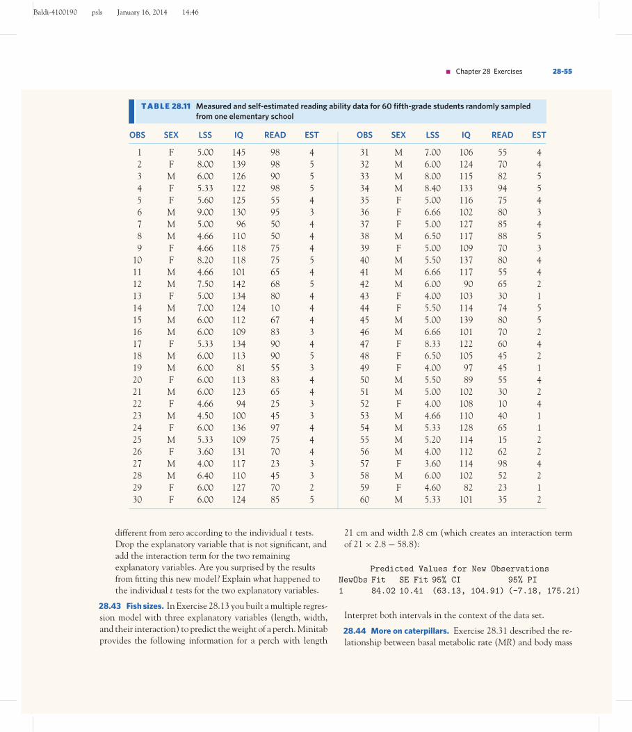
Baldi-4100190 psls January 16, 2014 14:46
■ Chapter 28 Exercises 28-55
T A B L E 28.11 Measured and self-estimated reading ability data for 60 fifth-grade students randomly sampledfrom one elementary school
OBS SEX LSS IQ READ EST OBS SEX LSS IQ READ EST
1 F 5.00 145 98 4 31 M 7.00 106 55 42 F 8.00 139 98 5 32 M 6.00 124 70 43 M 6.00 126 90 5 33 M 8.00 115 82 54 F 5.33 122 98 5 34 M 8.40 133 94 55 F 5.60 125 55 4 35 F 5.00 116 75 46 M 9.00 130 95 3 36 F 6.66 102 80 37 M 5.00 96 50 4 37 F 5.00 127 85 48 M 4.66 110 50 4 38 M 6.50 117 88 59 F 4.66 118 75 4 39 F 5.00 109 70 3
10 F 8.20 118 75 5 40 M 5.50 137 80 411 M 4.66 101 65 4 41 M 6.66 117 55 412 M 7.50 142 68 5 42 M 6.00 90 65 213 F 5.00 134 80 4 43 F 4.00 103 30 114 M 7.00 124 10 4 44 F 5.50 114 74 515 M 6.00 112 67 4 45 M 5.00 139 80 516 M 6.00 109 83 3 46 M 6.66 101 70 217 F 5.33 134 90 4 47 F 8.33 122 60 418 M 6.00 113 90 5 48 F 6.50 105 45 219 M 6.00 81 55 3 49 F 4.00 97 45 120 F 6.00 113 83 4 50 M 5.50 89 55 421 M 6.00 123 65 4 51 M 5.00 102 30 222 F 4.66 94 25 3 52 F 4.00 108 10 423 M 4.50 100 45 3 53 M 4.66 110 40 124 F 6.00 136 97 4 54 M 5.33 128 65 125 M 5.33 109 75 4 55 M 5.20 114 15 226 F 3.60 131 70 4 56 M 4.00 112 62 227 M 4.00 117 23 3 57 F 3.60 114 98 428 M 6.40 110 45 3 58 M 6.00 102 52 229 F 6.00 127 70 2 59 F 4.60 82 23 130 F 6.00 124 85 5 60 M 5.33 101 35 2
different from zero according to the individual t tests.Drop the explanatory variable that is not significant, andadd the interaction term for the two remainingexplanatory variables. Are you surprised by the resultsfrom fitting this new model? Explain what happened tothe individual t tests for the two explanatory variables.
28.43 Fish sizes. In Exercise 28.13 you built a multiple regres-sion model with three explanatory variables (length, width,and their interaction) to predict the weight of a perch. Minitabprovides the following information for a perch with length
21 cm and width 2.8 cm (which creates an interaction termof 21 × 2.8 − 58.8):
Predicted Values for New ObservationsNewObs Fit SE Fit 95% CI 95% PI1 84.02 10.41 (63.13, 104.91) (-7.18, 175.21)
Interpret both intervals in the context of the data set.
28.44 More on caterpillars. Exercise 28.31 described the re-lationship between basal metabolic rate (MR) and body mass

Baldi-4100190 psls January 16, 2014 14:46
28-56 C H A P T E R 28 ■ Multiple and Logistic Regression
(BM) in tobacco hornworm caterpillars, or, more specifically,the relationship between response variable y = log(MR) andexplanatory variable x1 = log(BM). Both experimental andtheoretical research have suggested the general relationshipMR = α(BM)β .23 However, there is still considerable de-bate on whether the scaling exponent is β = 2/3 orβ = 3/4.(a) Use software to estimate α and β in the general
relationship MR − α(BM)β , which is the same asμlog(MR) = log(α) + β log(BM). The predicted model isy = a + b log(B M), so that b0 estimates log(α) and b1
estimates β in the original model. What percent ofvariation in log(MR) is explained by using linearregression with the explanatory variable log(MR)?
(b) Find a 95% confidence interval for the slope parameterβ. Are the values β = 2/3 and β = 3/4 contained inyour confidence interval?
28.45 More on caterpillars, continued. Go back to the pre-vious exercise. This time, use the multiple regression modelwith two explanatory variables: the continuous variable x1 =log(BM) and an indicator variable reflecting instar stage (x2 =1 for instar 5, x2 = 0 for instar 4). This should reflect what youdid in Exercise 28.31.(a) Find a 95% confidence interval for the slope parameter β
for caterpillars during stage 4.(b) If you were asked to report a confidence interval for the
slope parameter β for caterpillars during stage 5, wouldyou report the same interval that you calculated in part(a)? Explain why or why not.
(c) Are the values β = 2/3 and β = 3/4 contained in yourconfidence interval from part (a)?
(d) How does your confidence interval in part (a) comparewith the confidence interval you computed in part (b) ofExercise 28.44?
28.46 Recurring bladder tumors, continued. Go back to Ex-ercises 28.15 and 28.16. You already computed the estimatedvalue of p when x is 0, 2, or 6. Complete your analysis for theother values of x (1, 3, 4, 5, 7, 8). Use your results to createa plot that shows how p changes as a function of x . Interpretthis plot.
28.47 FDA warning on insomnia prescriptions. In a January2013 safety announcement, the Food and Drug Administra-tion warned drug manufacturers that the recommended doseof the widely prescribed insomnia drug zolpidem should behalved for women. The warning came after pharmacokinetictrials found that 38 of 250 women and 8 of 250 men who
had taken the recommended dose of zolpidem still had enoughdrug in their blood 8 hours later to cause impairment.(a) What are the odds of impairment 8 hours after dosing for
women and for men? Use this information to computethe equation of the logistic regression model if theindicator variable x equals 0 for men and 1 for women.
(b) Minitab provides the standard error of the slope,SEb1 = 0.4002. Use this information to compute a 95%confidence interval for the slope of the logistic regressionmodel. Then compute a 95% confidence interval for theodds ratio for impairment 8 hours after dosing. Interpretyour results in the context of the FDA warning.
28.48 Treating AIDS. The drug AZT was the first drug thatseemed effective in delaying the onset of AIDS in people in-fected with HIV. A study randomly assigned 435 HIV-positivevolunteers who had not yet developed AIDS to take 500 mg ofAZT each day (AZT = 1) and another 435 to take a placebo(AZT = 0). At the end of the study, 38 of the placebo subjectsand 17 of the AZT subjects had developed AIDS.(a) What are the odds of developing AIDS in each of the
two groups? Use this information to compute theequation of the logistic regression model using theindicator variable AZT.
(b) Minitab provides the standard error of the slope,SEb1 = 0.3001. Use this information to compute a 95%confidence interval for the slope of the logistic regressionmodel. Then compute a 95% confidence interval for theodds ratio for developing AIDS. Do the data support theclaim that taking AZT lowers the odds of developingAIDS in HIV-positive patients? Explain.
A study screened a random sample of adult subjects for adult-onset, type 2 diabetes with the objective of identifying some of therisk factors associated with the disease. The file ex28-49.dat onthe companion website contains data about diabetes status, weight(in pounds), waist circumference (in inches), and cholesterol ratio(ratio of total cholesterol to HDL cholesterol in blood) for all 386subjects.24 Fifty-nine of the 386 were identified as having type 2diabetes (diabetes = 1). Exercises 28.49 to 28.51 are based onthis study.
28.49 Type 2 diabetes. Adult-onset, or type 2, diabetes hasbeen associated with obesity. The Minitab output in Figure28.18 shows the results of a logistic regression analysis with re-sponse variable diabetes and explanatory variable weight. Givethe equation of the logistic regression model. Is the coefficientfor the slope significantly different from zero? Does a higherweight appear to increase the odds of having type 2 diabetes?

Baldi-4100190 psls January 16, 2014 14:46
■ Chapter 28 Exercises 28-57
Session
Logistic Regression Table
P0.0000.002
OddsRatio
1.01
95%Lower
1.00
CIUpper
1.02
Z–5.543.04
SE Coef0.644311
0.0033247
Coef-3.569050.0101218
PredictorConstantweight
FIGURE 28.18 Minitab outputfor Exercises 28.49 to 28.51.
28.50 Type 2 diabetes, continued. Use software to obtain thelogistic regression analysis with response variable diabetes andexplanatory variable weight. Make sure that you obtain thesame results as those shown in the previous exercise, up torounding error.(a) Research suggests that where body fat is stored is an
important factor in predicting diabetes. Use software torun a model with both weight and waist as explanatoryvariables. What is the equation of this new logisticregression model? Do both variables contributesignificantly to the model? Explain how adding thevariable waist could change the relative contribution ofthe variable weight.
(b) Use software to fit a logistic regression model to predictdiabetes from waist. Interpret the output in the contextof the study. Which of the three models described inthis exercise would you favor and why?
28.51 Type 2 diabetes, continued. Among the list of poten-tial risk factors for type 2 diabetes is a person’s cholesterol ra-tio (cholratio), the ratio of total cholesterol to good, or HDL,cholesterol. Use software to fit a logistic regression model topredict diabetes from both waist and cholratio as explanatoryvariables. What is the equation of this new logistic regressionmodel? Are both coefficients significant? Explain in your ownwords what the two corresponding odds ratios mean in thecontext of this study.
28.52 Sleep apnea. Sleep apnea is a potentially dangerouscondition in which patients cease to breathe for at least 10seconds at a time while asleep. Researchers collected data on133 individuals in order to find risk factors for sleep apnea.(a) Neck size (measured in centimeters) may predict the risk
of sleep apnea because a larger neck size might constrictthe airway. Below is the software output for the logisticregression model explaining sleep apnea (y = 1 for sleepapnea, 0 otherwise) as a function of neck size. Is neck sizesignificant in predicting sleep apnea? Explain.
Odds 95% CI
Predictor Coef SE Coef Z P Ratio Lower Upper
Constant -8.15026 1.90008 -4.29 0.000
Neck Size 0.227170 0.0511498 4.44 0.000 1.26 1.14 1.39
(b) Being overweight has been linked to sleep apnea. Belowis the software output for the logistic regression modelexplaining sleep apnea as a function of an individual’sbody mass index (BMI, measured in kg/m2). Is BMIsignificant in predicting sleep apnea? Explain.
Odds 95% CI
Predictor Coef SE Coef Z P Ratio Lower Upper
Constant -8.37612 1.66623 -5.03 0.000
BMI 0.322748 0.0627380 5.14 0.000 1.38 1.22 1.56
(c) Based on the results obtained in (a) and (b), we also rana logistic regression model using both neck size and BMIas explanatory variables. The software output is givenbelow. Are both variables still significant when the otheris taken into consideration? What conclusions do youreach?
Odds 95% CI
Predictor Coef SE Coef Z P Ratio Lower Upper
Constant -9.31099 2.28744 -4.07 0.000
BMI 0.298216 0.0729842 4.09 0.000 1.35 1.17 1.55
Neck Size 0.0428161 0.0691903 0.62 0.536 1.04 0.91 1.20
LARGEDATASET
28.53 Student achievement and self-concept. In order todetermine if student achievement is related to self-concept, as measured by the Piers-Harris Children’s
Self-Concept Scale, data were collected on 78 seventh-gradestudents from a rural midwestern school. The large data fileLarge.SelfConcept available on the companion website con-tains data on the following variables for all 78 students:25

Baldi-4100190 psls January 16, 2014 14:46
28-58 C H A P T E R 28 ■ Multiple and Logistic Regression
Variable Description
OBS Observation number (n = 78, some gaps innumbers)
GPA GPA from school recordsIQ Test score from school recordsAGE Age in years, self-reportedGENDER 1 = F, 2 = M, self-reportedRAW Raw score on Piers-Harris Childrens’
Self-Concept ScaleC1 Cluster 1 within self-concept: behaviorC2 Cluster 2: school statusC3 Cluster 3: physicalC4 Cluster 4: anxietyC5 Cluster 5: popularityC6 Cluster 6: happiness
We will investigate the relationship between GPA and onlythree of the explanatory variables:■ IQ, the student’s score on a standard IQ test■ C2, the student’s self-assessment of his or her school
status■ C5, the student’s self-assessment of his or her popularityUse statistical software to analyze the relationship betweenstudents’ GPA and their IQ, self-assessed school status (C2),and self-assessed popularity (C5).(a) One observation is an extreme outlier when all three
explanatory variables are used. Which observation isthis? Give the observation number and explain how youfound it using regression output. Find this observation inthe data list. What is unusual about it?
(b) Software packages often identify unusual or influentialobservations. Have any observations been identified asunusual or influential? If so, identify these points on ascatterplot of GPA versus IQ.
(c) C2 (school status) is the aspect of self-concept mosthighly correlated to GPA. If we carried out the simplelinear regression of GPA on C2, what percent of thevariation in students’ GPAs would be explained by thestraight-line relationship between GPA and C2?
(d) You know that IQ is associated with GPA, and you arenot studying that relationship. Because C2 and IQ arepositively correlated (r = 0.547), a significantrelationship between C2 and GPA might occur justbecause C2 can “stand in” for IQ. Does C2 stillcontribute significantly to explaining GPA after we haveallowed for the relationship between GPA and IQ? (Givea test statistic, its P -value, and your conclusion.)
(e) A new student in this class has IQ 115 and C2 score 14.What do you predict this student’s GPA to be? (Just givea point prediction, not an interval.)
LARGEDATASET
28.54 Growth of pine trees. The Department of Biology atKenyon College conducted an experiment to study thegrowth of pine trees at a site located just south of
Gambier on a hill overlooking the Kokosing River. In April1990, student and faculty volunteers planted 1000 white pine(Pinus strobus) seedlings at the Brown Family Environmen-tal Center. These seedlings were planted in two grids, distin-guished by 10- and 15-foot spacings between the seedlings.A subset of the data collected by students at Kenyon Col-lege is available in the Large.PineTrees file on the companionwebsite.26 A description of the variables is provided below.
Variable Description
Row Row number in pine plantationCol Column number in pine plantationHgt90 Tree height at the time of planting (cm)Hgt96 Tree height in September 1996 (cm)Diam96 Tree trunk diameter in September 1996 (cm)Grow96 Leader growth during 1996 (cm)Hgt97 Tree height in September 1997 (cm)Diam97 Tree trunk diameter in September 1997 (cm)Spread97 Widest lateral spread in September 1997 (cm)Needles97 Needle length in September 1997 (mm)Deer95 Type of deer damage in September 1995:
1 = none, 2 = browsedDeer97 Type of deer damage in September 1997:
1 = none, 2 = browsedCover95 Amount of thorny cover in September 1995:
0 = none, 1 = <1/3, 2 = between 1/3 and 2/3,3 = >2/3
Fert Indicator for fertilizer: 0 = no, 1 = yesSpacing Distance (in feet) between trees (10 or 15)
(a) Use tree height at the time of planting (Hgt90) and theindicator variable for fertilizer (Fert) to fit a multipleregression model for predicting Hgt97. Specify theestimated regression model and the regression standarderror. Are you happy with the fit of this model?Comment on the value of R2 and the plot of theresiduals against the predicted values.
(b) Construct a correlation matrix with Hgt90, Hgt96,Diam96, Grow96, Hgt97, Diam97, Spread97, andNeedles97. Which variable is most strongly correlatedwith the response variable of interest (Hgt97)? Does thismake sense to you?

Baldi-4100190 psls January 16, 2014 14:46
■ Chapter 28 Exercises 28-59
(c) Add tree height in September 1996 (Hgt96) to themodel in part (a). Does this model do a better job ofpredicting tree height in 1997? Explain.
(d) What happened to the individual t statistic for Hgt90when Hgt96 was added to the model? Explain why thischange occurred.
(e) Fit a multiple regression model for predicting Hgt97based on the explanatory variables Diam97, Hgt96, andFert. Summarize the results of the individual t tests. Doesthis model provide a better fit than the previous models?
Explain by comparing the values of R2 and s for eachmodel.
(f) Does the parameter estimate for the variable indicatingwhether a tree was fertilized or not have the sign youexpected? Explain. (Experiments can produce surprisingresults!)
(g) Do you think that the model in part (e) should be usedfor predicting growth in other pine seedlings? Thinkcarefully about the conditions for inference.

Baldi-4100190 psls January 16, 2014 14:46
28-60 C H A P T E R 28 ■ Multiple and Logistic Regression
NOTES AND DATA SOURCES
1. Data were estimated from a scatterplot in L. Partridge and M. Farquhar,“Sexual activity reduces lifespan of male fruitflies,” Nature, 294 (1981),pp. 580–582.
2. Data were estimated from a scatterplot in T. J. Cleophas, “The sense andnonsense of regression modeling for increasing precision of clinical trials,”Clinical Pharmacology and Therapeutics, 74 (2003), pp. 295–297.
3. Data were estimated from a scatterplot in P. Heeb, M. Kolliker, and H.Richner, “Bird-ectoparasite interactions, nest humidity, and ectoparasitecommunity structure,” Ecology, 81 (2000), pp. 958–968.
4. F. H. Simmons, “Physiology of the trade-off between fecundity and survivalin Drosophila melanogaster, as revealed through dietary manipulation,” MSthesis, University of California at Irvine, 1996.
5. Data courtesy of Brad Hughes, Department of Ecology and EvolutionaryBiology, University of California, Irvine.
6. M. Di Monacoa et al., “Biochemical markers of nutrition and bone mineraldensity in the elderly,” Gerontology, 49 (2003), pp. 50–54.
7. S. J. Husson et al., “Optogenetic analysis of a nociceptor neuron and networkreveals ion channels acting downstream of primary sensors,” Current Biology,22 (2012), pp. 743–752, doi:10.1016/j.cub.2012.02.066.
8. This data set comes from the Journal of Statistics Education online dataarchive. It was originally submitted by M. J. Kahn of Wheaton College.
9. D. P. Casey et al., “Relationship between muscle sympathetic nerve activityand aortic wave reflection characteristics in young men and women,”Hypertension, 57 (2011), pp. 421–427.
10. R. Margaria et al., “Energy cost of running,” Journal of Applied Physiology, 18(1963), pp. 367–370.
11. The data in Table 28.4 are part of a larger data set in the Journal of StatisticsEducation online archive. The original source is P. Brofeldt, “Bidrag tillkaennedom on fiskbestondet i vaara sjoear. Laengelmaevesi,” in T. H. Jaervi,Finlands fiskeriet, vol. 4, Meddelanden utgivna av fiskerifoereningen i Finland,Helsinki, 1917. The data were contributed to the archive (with informationin English) by J. Puranen of the University of Helsinki.
12. These data come from the Data and Story Library online at lib.stat.cmu.edu/DASL. They were contributed by D. S. Moore and G. P. McCabe.
13. A. Spanos, F. E. Harrell, and D. T. Durack, “Differential diagnosis of acutemeningitis: an analysis of the predictive value of initial observations,” Journalof the American Medical Association, 262 (1989), pp. 2700–2707.
14. These data come from the Data and Story Library online atlib.stat.cmu.edu/DASL and were first published in L. J. Wei, D. Y. Lin,

Baldi-4100190 psls January 16, 2014 14:46
■ Notes and data sources 28-61
and L. Weissfeld, “Tumor recurrence data for patients with bladder cancer,”Journal of the American Statistical Association, 84 (1989), pp. 1065–1073.
15. The test statistic for logistic regression is z, not t (unlike for simple andmultiple linear regression). Interestingly, when z follows the standardNormal distribution, the value z2 actually follows a chi-square distributionwith df = 1. For this reason, inference for logistic regression sometimes usesthe chi-square statistic (such that X2 = z2) and the chi-square distributionwith df = 1. Both methods give the same P -value.
16. E. de Jonge et al., “Effects of selective decontamination of digestive tract onmortality and acquisition of resistant bacteria in intensive care: a randomisedcontrolled trial,” Lancet, 362 (2003), pp. 1011–1016.
17. A. M. Tromp et al., “Predictors for falls and fractures in the longitudinalaging study, Amsterdam,” Journal of Bone and Mineral Research, 13 (1998),pp. 1932–1939.
18. This data set comes from the Journal of Statistics Education online dataarchive. It was originally submitted by M. C. Meyer from the University ofGeorgia.
19. We thank Haruhiko Itagaki and his students Andrew Vreede and MarissaStearns for providing data on tobacco hornworm caterpillars (Manducasexta).
20. Data courtesy of David LeBauer, University of California at Irvine.21. P. Velleman, ActivStats 2.0, Addison-Wesley Interactive, 1997.22. J. T. Fleming, “The measurement of children’s perception of difficulty in
reading materials,” Research in the Teaching of English, 1 (1967), pp. 136–156.23. For more details, see H. Hoppeler and E. Weibel, “Scaling functions to
body size: theories and facts,” Journal of Experimental Biology, 208 (2005),pp. 1573–1574.
24. J. B. Schorling et al., “A trial of church-based smoking cessationinterventions for rural African Americans,” Preventive Medicine, 26 (1997),pp. 92–101. Data posted on the website of the Department of Biostatistics atVanderbilt University.
25. D. Gordon, “The relationships among academic self-concept, academicachievement, and persistence with academic self-attribution, study habits,and perceived school environment,” PhD thesis, Purdue University, 1997.
26. We thank Ray and Pat Heithaus for providing data on the pine seedlings atthe Brown Family Environmental Center.