Application of shrinkage techniques inlogistic regression analysis: a case study

E. W. Steyerberg�, M. J. C. Eijkemans, J. D. F. Habbema

Center for Clinical Decision Sciences, Department of Public Health,

Erasmus University, P.O. Box 1738, 3000 DR, Rotterdam,

The Netherlands

Logistic regression analysis may well be used to develop a predictivemodel for a dichotomous medical outcome, such as short-term mortality.When the data set is small compared to the number of covariablesstudied, shrinkage techniques may improve predictions. We comparedthe performance of three variants of shrinkage techniques: 1) a linearshrinkage factor, which shrinks all coef®cients with the same factor; 2)penalized maximum likelihood (or ridge regression), where a penaltyfactor is added to the likelihood function such that coef®cients are shrunkindividually according to the variance of each covariable; 3) the Lasso,which shrinks some coef®cients to zero by setting a constraint on thesum of the absolute values of the coef®cients of standardized covari-ables.

Logistic regression models were constructed to predict 30-day mortal-ity after acute myocardial infarction. Small data sets were created from alarge randomized controlled trial, half of which provided independentvalidation data. We found that all three shrinkage techniques improvedthe calibration of predictions compared to the standard maximum like-lihood estimates. This study illustrates that shrinkage is a valuable tool toovercome some of the problems of over®tting in medical data.

Key Words and Phrases: regression analysis, logistic models, bias,variable selection, prediction.

1 Introduction

Predictions from prognostic models may be used for a variety of reasons in medicine,

including diagnostic and therapeutic decision making, selection of patients for

randomized clinical trials, and informing patients and their families (see e.g.

HARRELL et al. 1996). The probability of a dichotomous medical outcome may well

be estimated with a logistic regression model. An important problem is that medical

data sets are often small compared to the number of covariables studied. Regression

models constructed in such small data sets provide overcon®dent predictions in

# VVS, 2001. Published by Blackwell Publishers, 108 Cowley Road, Oxford OX4 1JF, UK and 350 Main Street, Malden, MA 02148, USA.

76

Statistica Neerlandica (2001) Vol. 55, nr. 1, pp. 76±88

� steyerberg@mgz.fgg.eur.nlPart of this research was supported by a grant from the Netherlands Organization for Scienti®cResearch (NWO, S96ÿ156). Ewout Steyerberg is a fellow of the Royal Netherlands Academy ofArts and Sciences.

independent data: higher predictions will be found too high, and low predictions too

low. COPAS (1983) and VAN HOUWELINGEN and LE CESSIE (1990) have proposed

shrinkage techniques as a remedy against such extreme predictions.

In this study, we compare three shrinkage techniques for the estimation of logistic

regression coef®cients in small data sets: linear shrinkage, penalized maximum

likelihood (or ridge regression), and the Lasso. For a general theoretical background

of shrinkage, we refer to the paper of Van Houwelingen in this issue of Statistica

Neerlandica. We here describe the predictive performance of logistic regression

models which are constructed in small parts of a large data set of patients with an

acute myocardial infarction to predict 30-day mortality. We only consider pre-

speci®ed models. In another publication, we described the effects of shrinkage in

combination with various model speci®cation techniques, especially stepwise selec-

tion (STEYERBERG et al., 2000).

We will ®rst describe the three shrinkage techniques that we studied and their

implementation (section 2). The patient data are described in section 3. Evaluations

of predictive performance are presented in section 4. We discuss our ®ndings in

section 5.

2 Shrinkage techniques considered

We consider the usual logistic regression model logitfY � 1jXg � â0 �Óâi � X i � PI where Y is a binary outcome variable (0 or 1), â0 is an intercept, and

âi denotes the logistic regression coef®cients for the design matrix X of covariables

i. PI is the prognostic index, which is equivalent to the `linear predictor' in the

context of generalized linear models. Our aim is to estimate the logitfY � 1jXgaccurately for new patients; interpretation of regression coef®cients is secondary in

our analyses.

Linear shrinkage factor

A relatively straightforward approach is to apply a linear shrinkage factor, s, for the

regression coef®cients as estimated with standard maximum likelihood (ML).

According to COPAS (1983) and VAN HOUWELINGEN and LE CESSIE (1990), the

shrunken coef®cients (âs) are then estimated as: âs � s � â. We estimated s with a

bootstrap procedure:

1. Take a random bootstrap sample from the original sample, with the same size and

patient records drawn with replacement (see e.g. EFRON, 1993).

2. Estimate the logistic regression coef®cients in the bootstrap sample.

3. Calculate the PI for each patient in the original sample. The PI is the linear

combination of the regression coef®cients as estimated in the bootstrap sample

with the values of the covariables in the original sample.

4. Estimate the slope of the PI with logistic regression, using the outcomes of the

patients in the original sample and the PI as a single covariable.

Shrinkage in logistic regression 77

# VVS, 2001

The slope of the PI is by de®nition unity in step 3. In step 4 it will generally be

smaller than 1, re¯ecting that regression coef®cients are too extreme for predictive

purposes. Steps 1 to 4 were repeated 300 times to obtain a stable estimate of s, which

was calculated as the mean of the 300 slopes estimated in step 4 (s � mean(slope)).

Essentially, the expected miscalibration was estimated and used to correct the

initially estimated regression coef®cients. Linear shrinkage may be therefore referred

to as `shrinkage after ®tting'.

Penalized ML

Ridge regression was proposed HOERL and KENNARD already in 1970 as a method to

obtain less extreme regression coef®cients, and has also been applied by LE CESSIE

and VAN HOUWELINGEN (1992) with logistic regression. We use the more general

term penalized maximum likelihood estimation (see e.g. HARRELL et al., 1996). For

estimation of coef®cients, a penalty factor ë is included in the maximum likelihood

formula (see e.g. VERWEIJ and VAN HOUWELINGEN, 1994): log Lÿ 12ëâ9Pâ. Here L

denotes the usual likelihood function, ë is the (positive) penalty factor, â9 denotes the

transpose of the vector of estimated regression coef®cients â (excluding the

intercept), and P is a penalty matrix. In our analyses, the diagonal of P consisted of

the variances of the covariables and all other values of P were set to 0. This choice of

P makes the penalty to the log-likelihood unitless. This scaling was used both for

continuous and dichotomous covariables, although dichotomous variables might

generally not require scaling by their variance.

To determine the optimal value of ë, we varied ë over a grid e.g. 0, 0.5, 1, 1.5, 2, 3,

4, 6, 8, 12, 16, 24, 32, 48, 64 and evaluated a modi®ed Akaike Information Criterion

(AIC): AIC � [model ÷2 ÿ 2 � effective d.f.]. Here, model ÷2 is the likelihood ratio

÷2 of the model (i.e. compared to the null model with an intercept only), ignoring the

penalty function. The effective degrees of freedom are calculated according to GRAY

(1992): trace[I(â)cov(â)]. In the latter formula, I(â) is the information matrix as

computed without the penalty function, and cov(â) is the covariance matrix as

computed by inverting the information matrix calculated with the penalty function.

Note that if both the I(â) and the cov(â) are estimated without penalty, I(â) cov(â)

is the identity matrix and trace[I(â) cov(â)] is equal to the number of estimated

parameters in the model (excluding the intercept). With a positive penalty function,

the elements of cov(â) become smaller and the effective degrees of freedom

decrease. The ë with the highest AIC was used in the penalized estimation of the

coef®cients.

Note that although only a single shrinkage parameter is estimated (ë), a varying

degree of effective shrinkage (se) is attained for individual coef®cients. We may refer

to penalized ML or ridge regression as `shrinkage during ®tting'.

Lasso

Another form of a penalized ML procedure is the Lasso method (`Least Absolute

Shrinkage and Selection Operator') as proposed by TIBSHIRANI (1996). The Lasso

78 E. W. Steyerberg et al.

# VVS, 2001

combines shrinkage with selection of predictors, since some coef®cients are shrunk

to zero. It was developed in the same spirit as BREIMAN's Garotte (1995). We studied

the Lasso since it can readily be applied to linear regression models but also to

generalized linear models such as logistic regression or Cox proportional hazards

regression. The Lasso estimates the regression coef®cients â of standardized covari-

ables while the intercept is kept ®xed. The log-likelihood is minimized subject to

Ójâj < t, where the constraint t determines the shrinkage in the model. We varied

s � t=Ójâ0j over a grid from 0.5 to 0.95, where â0 indicates the standard ML

regression coef®cients and s may be interpreted as a standardized shrinkage factor.

When s � 1, â � â0 ful®lls the constraint and no shrinkage is attained. We estimated

â with the value of t that gave the lowest mean-squared error in a generalized cross-

validation procedure. We may refer to the Lasso as `shrinkage with selection'.

Estimation of required shrinkage

The described implementations of shrinkage techniques are available for S-plus

software (MathSoft Inc., Seattle WA), with functions for linear shrinkage and

penalized ML programmed by Harrell (http://lib.stat.cmu.edu/DOS/S/Harrell/) and

lasso functions by Tibshirani (http://lib.stat.cmu.edu/S/). A drawback of these

implementations is that the shrinkage parameters are estimated with rather different

techniques. One would anticipate that any shrinkage parameter could be estimated

with some form of cross-validation or bootstrapping. For the Lasso, ®vefold cross-

validation however gave poor results in TIBSHIRANI's simulation study (1996), but

one might hypothesize that other variants of cross-validation (e.g. 20 3 ®vefold)

might work well. AIC and effective degrees of freedom can be applied for linear

shrinkage and penalized ML. These two techniques are closely related; a linear

shrinkage factor s is estimated in the penalized ML procedure when the matrix P is

equal to the full matrix of second derivatives, with s � 1=(1� ë).

For our evaluation we used the most practical implementations of the shrinkage

techniques: linear shrinkage by bootstrap resampling, penalized ML by AIC and

effective degrees of freedom, and the Lasso by generalized cross-validation. The

linear shrinkage factor might however have been estimated even simpler with Van

Houwelingen and Le Cessie's heuristic formula: sheur �[model ÷2 ÿ (df ÿ 1)]=model

÷2, where df indicates the degrees of freedom of the covariables in the model and

model ÷2 is calculated on the log-likelihood scale. It is readily understood that sheur

approaches zero when larger numbers of predictors are considered (since the df

increase), or when the sample size is smaller (since model ÷2 decreases).

3 Empirical evaluation

Patients

For evaluation of the shrinkage techniques we used the data of 40,830 patients with

an acute myocardial infarction from the GUSTO-I study. LEE et al. (1995) decribed

the data in detail, which were previously analysed by ENNIS et al. (1998) and

Shrinkage in logistic regression 79

# VVS, 2001

STEYERBERG et al. (1999, 2000). Mortality at 30-days was studied, which occurred in

2,851 patients (7.0%). Within the total data set, we distinguished 16 regions: 8 in the

United States (US), 6 in Europe and 2 other (Canada and Australia/New Zealand).

The data set was split in a training and test part. These parts each consisted of eight

regions with geographical balance and a similar overall mortality (7.0%). Within

regions in the training part (n � 20, 512), `large' and `small' multicenter subsamples

were created by grouping hospitals together on a geographical basis. We note that

`small' and `large' are meant here in relation to the need for shrinkage, which is

higher in smaller samples. The `large' subsamples were created such that they each

contained at least 50 events. The subgrouping procedure was repeated to create small

subsamples with at least 20 events. In this way, 61 small and 23 large subsamples of

the training part were created, containing on average 336 and 892 patients of whom

23 and 62 died respectively. Logistic regression models were ®tted in the subsamples

and evaluated in the test part.

We note that the subsamples were not strictly random samples. Rather, it was

aimed to replicate the real-life situation that a small multicenter data set would be

available that contained patients from several nearby hospitals to construct a

prognostic model which should be applicable to the total patient population.

Predictors considered

We considered two prognostic models. First, we focused on evaluations of an 8-

predictor model, as de®ned by MUELLER et al. (1992) based for the TIMI-II study.

This model included as predictors: shock, age .65 years, anterior infarct location,

diabetes, hypotension, tachycardia, no relief of chest pain, and female gender. All 8

predictors were dichotomous, including age, where a continuous function would have

been more appropriate. Second, we considered a 17-predictor model in the larger

samples. This model consisted of the TIMI-II model plus nine other previously

studied covariables (see e.g. LEE et al., 1995).

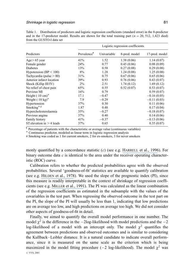
Table 1 shows the distribution of the 17 covariables and their uni- and multi-

variable logistic regression coef®cients in the 8 and in the 17-predictor model.

Results are shown for the training part only, since results for the test part were very

similar. We note that the dichotomous predictors `hypotension' and `shock' had a low

prevalence, but a strong effect in the multivariable models. Most multivariable

coef®cients were smaller (closer to zero) than the univariable coef®cients, re¯ecting

(modest) positive correlations between the predictors (r generally around 0.1±0.2).

All coef®cients in the 8-predictor model were signi®cant at the p , 0:001 level. The

17-predictor model contained covariables with relatively small coef®cients, such as

sex, hypertension, previous angina and family history.

Evaluation

For the evaluation of model performance we considered discrimination, calibration,

and overall performance. Discrimination refers to the ability to distinguish high risk

patients from low risk patients. In medical studies, discriminative ability is com-

80 E. W. Steyerberg et al.

# VVS, 2001

monly quanti®ed by a concordance statistic (c) (see e.g. HARRELL et al., 1996). For

binary outcome data c is identical to the area under the receiver operating character-

istic (ROC) curve.

Calibration refers to whether the predicted probabilities agree with the observed

probabilities. Several `goodness-of-®t' statistics are available to quantify calibration

(see e.g. HILDEN et al., 1978). We used the slope of the prognostic index (PI), since

this measure is readily interpretable in the context of shrinkage of regression coef®-

cients (see e.g. MILLER et al., 1991). The PI was calculated as the linear combination

of the regression coef®cients as estimated in the subsample with the values of the

covariables in the test part. When regressing the observed outcome in the test part on

the PI, the slope of the PI will usually be less than 1, indicating that low predictions

are on average too low, and high predictions on average too high. We did not consider

other aspects of goodness-of-®t in detail.

Finally, we aimed to quantify the overall model performance in one number. The

model ÷2 is the difference in the ÿ2log-likelihood with model predictions and the ÿ2

log-likelihood of a model with an intercept only. The model ÷2 quanti®es the

agreement between predictions and observed outcomes and is similar to considering

the Kullback±Leibler distance. It is a natural candidate to indicate overall perform-

ance, since it is measured on the same scale as the criterion which is being

maximized in the model ®tting procedure (ÿ2 log-likelihood). The model ÷2 was

Table 1. Distribution of predictors and logistic regression coef®cients (standard error) in the 8-predictor

and in the 17-predictor model. Results are shown for the total training part (n � 20, 512, 1,423 died)

from the GUSTO-I data set

Logistic regression coef®cients

Predictors Prevalence} Univariable 8-pred. model 17-pred. model

Age. 65 year 41% 1.52 1.38 (0.06) 1.14 (0.07)

Female gender 24% 0.77 0.45 (0.06) 0.08 (0.09)

Diabetes 13% 0.58 0.27 (0.08) 0.29 (0.08)

Hypotension (BP , 100) 8% 1.28 1.24 (0.08) 1.25 (0.08)

Tachycardia (pulse . 80) 31% 0.75 0.67 (0.06) 0.65 (0.06)

Anterior infarct location 39% 0.93 0.76 (0.06) 0.43 (0.07)

Shock (Killip III/IV) 2% 2.51 1.74 (0.12) 1.69 (0.12)

No relief of chest pain 65% 0.55 0.52 (0.07) 0.53 (0.07)

Previous MI 16% 0.79 0.59 (0.07)

Height (�10 cm)� 17.1 ÿ0.47 ÿ0.16 (0.05)

Weight (�10 kg)� 7.9 ÿ0.29 ÿ0.11 (0.03)

Hypertension 37% 0.30 0.11 (0.06)

Smoking�# 1.87 0.48 0.17 (0.04)

Hypercholesterolaemia 35% ÿ0.27 ÿ0.18 (0.07)

Previous angina 37% 0.40 0.14 (0.06)

Family history 41% ÿ0.37 ÿ0.13 (0.06)

ST elevation in . 4 leads 37% 0.65 0.35 (0.07)

} Percentage of patients with the characteristic or average value (continuous variables)� Continuous predictor, modeled as linear term in logistic regression analysis# Smoking was coded as 1 for current smokers, 2 for ex-smokers, 3 for never smokers

Shrinkage in logistic regression 81

# VVS, 2001

calculated by ®tting a model with an intercept and the prognostic index as an offset

variable (slope ®xed at unity, i.e. the prognostic index was taken literally) in the test

data. A negative model ÷2 implied that a model performed worse than predicting the

average risk for every patient.

4 Results in small data sets

Illustration: a small subsample

We ®rst illustrate the use of the shrinkage techniques with a small subsample, which

showed results that were typical for the other small subsamples. Table 2 shows the

regression coef®cients of the 8-predictor model as estimated in the subsample, and

the performance in the test part, which was independent from the subsample

(n � 20, 318). The subsample was created by combining the patient data from ®ve

Australian centers that participated in the GUSTO-I trial. The sample included 336

patients, of whom 20 died.

The 8-predictor model had large regression coef®cients for age and shock when

estimated with the standard ML procedure. The coef®cients were shrunk with a

factor 0.63 according to the bootstrapping procedure. Penalized estimates of the

regression coef®cients were obtained with a penalty factor of 8. The effective

`shrinkage' was 1.17 for shock, negative for anterior MI and relief of pain (which

both had very small effects), and around 0.6 for the other covariables. This evaluation

illustrates that the sign of the coef®cients can be changed by the penalized ML

procedure. The lasso parameter s was 0.78, which resulted in an increase of the

estimated effect for shock, and a major shrinkage for anterior MI and relief of pain

(shrunk to zero). As a reference, the ®nal columns show the coef®cients obtained in

the total training part (`gold standard', n � 20, 512).

Predictions were calculated for the independent test part (n � 20, 318) according

to each estimation method. Figure 1 shows the distribution of the prognostic index

(logit of predicted probabilities). The standard ML estimates led to a broad range of

predictions, which was drawn closer to the mean with linear shrinkage, penalized ML

and the Lasso. We also note a slight shift in distribution to higher predicted logits for

the Lasso. This is explained by inaccurate estimation of the intercept in this example.

Figure 2 shows the calibration of the predictions. We note that the standard ML

estimates lead to a clear underestimation of the risk of death for low risk patients

(e.g. probability , 5%, logit ,ÿ3), and an overestimation of higher risks (e.g.

predicted probability 40%, observed probability around 30%). All three shrinkage

methods led to improved predictions, as indicated by curves closer to the identity

line. This is also indicated by the slope of the PI, which was 0.68 for the standard ML

estimates and around 1 with the shrinkage techniques (Table 2).

Shrinkage had only a minor advantage with respect to discriminative ability. Note

that the c statistics for the models with standard or shrunk coef®cients are by

de®nition identical, since the ordering of the predicted probabilities does not change

82 E. W. Steyerberg et al.

# VVS, 2001

by applying a linear shrinkage factor. The shrinkage techniques led to some improve-

ment in overall performance, as indicated by the model ÷2.

Average performance

We repeated the construction of a model in a subsample with testing in independent

data for each of the 61 small and 23 larger subsamples. The low prevalence of some

predictors led to zero cells and non-convergence of the coef®cient estimates in the 8-

predictor model for 12 of the 61 small subsamples. This problem might not have

occurred had we considered convergence of the linear predictor rather than of the

coef®cients. The 12 non-converged subsamples were excluded from the evaluations.

In Table 3, we show the average results of the performance of the estimated models

as well as the performance obtained with a model ®tted in the total training data set

(n � 20, 512, `gold standard').

The gold standard models had c statistics near 0.80, and good calibration (slopes

around 0.95). Overall model performance increased slightly by adding nine predic-

tors to the 8-predictor model (model ÷2 increased from 1604 to 1785).

Fig. 1. Distribution of the predicted logit of mortality in the test part of the GUSTO-I trial

(n � 20, 318). An 8-predictor model was ®tted in a small subsample consisting of 336 patients

of whom 20 died. Estimation of regression coef®cients was with standard ML, a linear shrinkage

factor, penalized ML, or the Lasso.

Shrinkage in logistic regression 83

# VVS, 2001

Fig. 2 Calibration plots of the 8-predictor model in the test part of the GUSTO-I trial (n � 20, 318).

The model was ®tted in a small subsample consisting of 336 patients of whom 20 died. Curves

are non-parametric, constructed with the supersmoother algorithm in S�, and plotted on the

probability scale (a) and the logit scale (b).

84 E. W. Steyerberg et al.

# VVS, 2001

In the small subsamples, we found that using the standard ML estimates led to a

poor overall performance. The area under the ROC curve was largely unaffected by

applying penalized ML or the Lasso. The major improvement was seen with regard

to calibration, where the slope of the prognostic index increased from 0.66 to values

close to one for shrunk or penalized ML estimates, and 0.83 for the Lasso. The

Table 2. Estimates of logistic regression coef®cients (â) and effective shrinkage factor (se � â=âML)

for the 8-predictor model in a small subsample (336 patients, 20 died) from the GUSTO-I trial, according

to several estimation methods. Model performance was evaluated in the test sample (see text)

Shrinkage methods

Standard Gold

ML Shrunk Penalized Lasso standard

âML â se â se â se âGold

Predictors

Shock 1.32 0.83 0.63 1.55 1.17 1.69 1.27 1.73

Age. 65 years 2.52 1.58 0.63 1.36 0.54 1.73 0.69 1.37

Anterior MI ÿ0.03 ÿ0.02 0.63 0.08 ÿ2.67 0 0 0.76

Diabetes 0.96 0.60 0.63 0.84 0.87 0.79 0.82 0.29

Hypotension 0.81 0.51 0.63 0.40 0.50 0.40 0.50 1.25

Tachycardia o.91 0.57 0.63 0.59 0.64 0.65 0.71 0.66

No relief 0.02 0.01 0.63 ÿ0.01 0.43 0 0 0.55

Female gender 0.19 0.12 0.63 0.30 1.55 0.15 0.81 0.44

Performance in test sample (n � 20, 318)

Area under ROC curve (c) 0.76 0.76 0.77 0.77 0.79

Slope of PI 0.68 1.09 1.01 0.90 0.94

Model ÷2 1082 1282 1322 1293 1604

Table 3. Average performance (standard deviation) of the 8 and 17-predictor model ®tted in the small

and large subsamples (average n � 336 and n � 892 respectively), and in the total training part

(n � 20, 512), as evaluated in the test part (n � 20, 318) from the GUSTO-I trial.

8-predictor model 17-predictor model

Small Large Total Large Total

Area under ROC curve (c)

Standard/Shrunk 0.754 (.029) 0.780 (.009) 0.789 0.777 (.010) 0.802

Penalized ML 0.760 (.021) 0.780 (.009) 0.784 (.009)

Lasso 0.756 (.027) 0.784 (.009) 0.781 (.009)

Slope of PI

Standard 0.66 (0.18) 0.86 (0.13) 0.944 0.76 (0.12) 0.959

Shrunk 1.01 (0.29) 0.97 (0.16) 0.95 (0.16)

Penalized ML 0.93 (0.30) 0.96 (0.17) 0.98 (0.19)

Lasso 0.83 (0.23) 1.01 (0.16) 0.93 (0.15)

Model ÷2

Standard 673 (1211) 1422 (120) 1604 1294 (277) 1785

Shrunk 1045 (776) 1461 (95) 1441 (163)

Penalized ML 1112 (384) 1455 (102) 1497 (142)

Lasso 1079 (390) 1517 (84) 1492 (144)

Shrinkage in logistic regression 85

# VVS, 2001

shrinkage techniques led to a better overall predictive performance, with model ÷2

over 1000 compared to 674 for standard ML estimates. Note however that the

variability in performance was considerable.

In the larger subsamples, both the 8 and 17-predictor model were evaluated. The

bene®t of shrinkage was somewhat less in the larger samples. For the 8-predictor

model, the average slope improved from 0.86 with standard ML estimates to values

close to one with any of the shrinkage methods. However, when 17 predictors were

considered, the average slope with standard ML estimates was 0.76, indicating a

clearer need for shrinkage. Remarkably, the overall performance of the 17-predictor

model was slightly worse than the 8-predictor model when coef®cients were

estimated with standard ML, linear shrinkage, or the Lasso, and marginally better

with penalized ML. Hence, including more predictors did not clearly improve the

performance. Further, we note that the performances of models constructed in the

larger subsamples were more stable than in the small subsamples. This is consistent

with the 2.7 times as larger sample size (on average 62 compared to 23 events).

5 Discussion

This study illustrates how shrinkage techniques can be applied with logistic regres-

sion analysis in small medical data sets. Shrinkage led to better calibration of

predictions compared to models based on the standard ML estimates, especially when

the data set was small compared to the number of covariables considered. We found

no major differences in performance between application of a linear shrinkage factor,

a penalized ML procedure similar to ridge regression, or the Lasso.

On the one hand, TIBSHIRANI's Lasso (1996) is an interesting technique, since

shrinkage is de®ned such that some coef®cients are set to zero. This leads to smaller

predictive models, since covariables with a coef®cient of zero can be dropped.

Smaller models are more attractive for application by physicians in clinical practice.

On the other hand, the number of predictors that was selected by the Lasso was quite

large in our evaluations (e.g. 16.3 of 17 predictors in samples with 62 events on

average). Also, calculation of the optimal Lasso parameter is computationally

demanding, especially for larger data sets, and not attractive from a theoretical point

of view. The theoretical foundation of penalized ML (or ridge regression) is stronger,

with similarities in estimation with natural penalties and generalized additive models

(see e.g. VAN HOUWELINGEN, 2001).

In medical prediction problems, an extensive model speci®cation phase is quite

common, where a model is sought that is eventually used in the ®nal analysis. Model

speci®cation may include coding and categorization of covariables with `optimal'

cutpoints, determination of suitable transformations for continuous covariables, and

selection of `important' predictors (see e.g. CHATFIELD, 1995, for a critical discus-

sion). Often, stepwise procedures are applied where covariables are omitted from

(backward or stepdown selection) or entered in the model (forward selection) based

on repeated signi®cance testing. In a previous evaluation we found that omission of

86 E. W. Steyerberg et al.

# VVS, 2001

non-signi®cant covariables decreased predictive performance, especially discrimina-

tion (STEYERBERG et al., 2000). Miscalibration could reasonably be corrected by all

three shrinkage techniques considered in the present study. For linear shrinkage, the

shrinkage factor was calculated in a bootstrapping procedure that included the

stepwise selection process. Penalized coef®cients were calculated with the same

penalty as identi®ed as optimal for the full model, although this approach lacks a

theoretical foundation. Following CHATFIELD (1995), BUCKLAND et al. (1997), and

YE (1998), we would argue that the model speci®cation phase should not be ignored

when interpreting regression coef®cients in the ®nal model or when predictions are

based on the model.

Several limitations apply to our study. Foremost, the analyses with the GUSTO-I

data represent a case study. Although the structure of the data set may be representa-

tive of other prediction problems in medicine, exceptions can probably be identi®ed,

e.g. where covariables have stronger collinearity or larger predictive effects. Further,

we have only included implementations of a limited number of shrinkage techniques

that may currently be used relatively easily with logistic regression. Bayesian and

other recently proposed approaches were not included. We encourage further dev-

elopments of shrinkage techniques, especially those that select variables by shrinking

coef®cients to zero or otherwise take selection of covariables properly into account.

Acknowledgements

We would like to thank Kerry Lee, Duke University Medical Center, Durham NC,

and the GUSTO investigators for making the GUSTO-I data available for analysis;

Frank Harrell, University of Virginia, Charlottesville VA, for valuable discussions;

Hans van Houwelingen, Leiden University, Leiden, The Netherlands, and a reviewer

for valuable comments.

References

BREIMAN, L. (1995), Better subset regression using the nonnegative Garotte, Technometrics 37,373±384.

BUCKLAND, S. T., K. P. BURNHAM and N. H. AUGUSTIN (1997), Model selection: an integral part ofinference, Biometrics 53, 603±618.

CHATFIELD, C. (1995), Model uncertainty, data mining and statistical inference, Journal of the

Royal Statistical Society, Series A 158, 419±466.

COPAS, J. B. (1983), Regression, prediction and shrinkage, Journal of the Royal Statistical Society,

Series B 45, 311±354.EFRON, B. and R. TIBSHIRANI (1993), An introduction to the bootstrap, Monographs on statistics

and applied probability, Vol. 57, Chapman & Hall, New York.ENNIS, M., G. HINTON, D. NAYLOR, M. REVOW and R. TIBSHIRANI (1998). A comparison of

statistical learning methods on the Gusto database, Statistics in Medicine 17, 2501±2508.GRAY, R. J. (1992), Flexible methods for analyzing survival data using splines, with applications to

breast cancer prognosis, Journal of the American Statistical Association 87, 942±951.HARRELL, F. E., Jr., K. L. LEE and D. B. MARK (1996), Multivariable prognostic models: issues in

Shrinkage in logistic regression 87

# VVS, 2001

developing models, evaluating assumptions and adequacy, and measuring and reducing errors,

Statistics in Medicine 15, 361±387.HILDEN, J., J. D. HABBEMA and B. BJERREGAARD (1978), The measurement of performance in

probabilistic diagnosis. II. Trustworthiness of the exact values of the diagnostic probabilities,Methods of Information in Medicine 17, 227±237.

HOERL, A. E. and R. W. KENNARD (1970), Ridge regression: biased estimation for nonorthogonalproblems, Technometrics 12, 55±67.

LE CESSIE, S. and J. C. VAN HOUWELINGEN (1992), Ridge estimators in logistic regression, Applied

Statistics ± Journal of the Royal Statistical Society, Series C 41, 191±201.

LEE, K. L., L. H. WOODLIEF, E. J. TOPOL, W. D. WEAVER, A. BETRIU, J. COL, M. SIMOONS,P. AYLWARD, F. VAN DE WERF and R. M. CALIFF (1995), Predictors of 30-day mortality in the era

of reperfusion for acute myocardial infarction. Results from an international trial of 41,021patients, Circulation 91, 1659±1668.

MILLER, M. E., S. L. HUI and W. M. TIERNEY (1991), Validation techniques for logistic regressionmodels, Statistics in Medicine 10, 1213±1226.

MUELLER, H. S., L. S. COHEN, E. BRAUNWALD, S. FORMAN, F. FEIT, A. ROSS, M. SCHWEIGER,H. CABIN, R. DAVISON, D. MILLER, R. SOLOMON and G. L. KNATTERUD (1992), Predictors of

early morbidity and mortality after thrombolytic therapy of acute myocardial infarction, Circula-

tion 85, 1254±1264.

STEYERBERG, E. W., M. J. EIJKEMANS and J. D. HABBEMA (1999), Stepwise selection in small datasets: a simulation study of bias in logistic regression analysis, Journal of Clinical Epidemiology

52, 935±942.STEYERBERG, E. W., M. J. EIJKEMANS, F. E. HARRELL, Jr. and J. D. HABBEMA (2000), Prognostic

modelling with logistic regression analysis: a comparison of selection and estimation methods insmall data sets, Statistics in Medicine 19, 1059±1079.

TIBSHIRANI, R. (1996), Regression and shrinkage via the Lasso, Journal of the Royal Statistical

Society, Series B 58, 267±288.VAN HOUWELINGEN, J. C. and S. LE CESSIE (1990), Predictive value of statistical models, Statistics

in Medicine 9, 1303±1325.VAN HOUWELINGEN, J. C. (2001), Shrinkage and penalized likelihood as methods to improve

predictive accuracy, Statistica Neerlandica 55, 17±34.VERWEIJ, P. J. and H. C. VAN HOUWELINGEN (1994), Penalized likelihood in Cox regression,

Statistics in Medicine 13, 2427±2436.YE, J. (1998), On measuring and correcting the effects of data mining and model selection, Journal

of the American Statistical Association 93, 120±131.

Received: March 2000. Revised: July 2000.

88 E. W. Steyerberg et al.

# VVS, 2001