1

Maximum entropy estimation in economic models with linear

inequality restrictions

Randall C. Campbell*, R. Carter Hill

Department of Economics, Louisiana State University, Baton Rouge, LA 70803,USA

Abstract

In this paper, we use maximum entropy to estimate the parameters in an economic model. We

demonstrate the use of the generalized maximum entropy (GME) estimator, describe how to specify

the GME parameter support matrix, and examine the sensitivity of GME estimates to the parameter

and error bounds. We impose binding inequality restrictions through the GME parameter support

matrix and develop a more general parameter support matrix that allows us to impose a broader set

of restrictions than is possible under the traditional formulation. Bootstrapping is used to obtain

confidence intervals and examine the precision of the GME estimator.

JEL Classification: C13; C14; C20; C49; C51

Keywords: Maximum Entropy; Generalized Maximum Entropy; Linear Inequality Restrictions;

Bootstrapping

* Corresponding author. Tel.: 1-225-578-3782; fax: 1-225-578-3807.E-mail address: camprr@msn.com

2

1. Introduction

This paper examines the generalized maximum entropy (GME) estimator in the general linear

model (GLM). Since GME estimation requires us to specify bounds for the parameters, we present

an economic application and discuss how to specify the GME parameter and error support matrices.

We vary the GME parameter and error support matrices and examine the sensitivity of the GME

estimates to the prior information imposed. The GME estimates are compared to least squares

estimates, both with and without inequality restrictions placed on the parameters. Finally, we use

the bootstrap to obtain confidence intervals and examine the precision of the GME estimator.

We use the GME estimator developed by Golan, Judge, and Miller (1996, pp. 85-89)

[hereinafter GJM]. GJM show that the GME estimator has lower risk than both the OLS and IRLS

estimators in several sampling experiments (GJM, pp. 133-144), particularly when the data exhibit

a high degree of collinearity. GJM specify a block diagonal parameter support matrix for the GME

estimator, which allows us to impose single parameter restrictions such as 0iβ > . Applications of

single parameter restrictions on the GME estimator may be found in Fraser (2000) and Shen and

Perloff (2001). We impose binding single parameter restrictions through the parameter support

matrix and, in addition, we specify a more general parameter support matrix that is not block

diagonal and which allows us to impose multiple parameter restrictions such as i jβ β> and

1 2 3 1β β β+ + < . Specifying a non-block diagonal support parameter matrix provides a relatively

simple way to impose several restrictions that might be encountered in practice.

We show that GME is a feasible approach to estimating linear regression models. All of our

GME estimates take the same signs and have roughly the same magnitude as OLS and IRLS

estimates. In addition, our bootstrap results show that the sampling precision is better for the GME

estimator than for the OLS and IRLS estimators.

Section 2 discusses GME estimation in the linear regression model. In Section 3, we describe

how to impose inequality restrictions through the GME parameter support matrix and present a

non-block diagonal support matrix that allows us to impose restrictions that are not possible under

the traditional support matrix. In Section 4, we estimate an economic model using GME, both with

3

and without binding parameter inequality restrictions, and compare the GME estimates to least

squares estimates. Section 5 presents GME confidence intervals obtained using a bootstrap.

Section 6 concludes the paper.

2. Generalized maximum entropy estimation in the general linear model

GJM (1996, Ch. 6) use GME to jointly estimate the unknown parameters and the unknown

errors in the GLM.1 We write the GLM in matrix form as

y X eβ= + , (1)

where y is an 1N × vector of sample observations on the dependent variable, X is an N K×

matrix of explanatory variables, e is an 1N × vector of unknown errors, and β is a 1K × vector of

unknown parameters.

Jaynes (1957a, 1957b) shows that maximum entropy allows us to estimate the unknown

probabilities in a discrete probability distribution.2 GJM generalize the maximum entropy

methodology and reparameterize the linear model such that the unknown parameters and the

unknown errors are in the form of probabilities. We specify a set of support points for each

unknown parameter and error and use maximum entropy to estimate the unknown probabilities

associated with the support points. Hence we must assume that both the unknown parameters and

the unknown errors may be bounded a priori. Let 1kz be the smallest possible value of kβ and 2kz

be the largest possible value of kβ . Then, for each parameter, kβ , there exists [ ]0,1kp ∈ such that

[ ]1 2 1 2(1 )1

kk k k k k k k

k

pp z p z z z

pβ

= + − = − . (2)

The parameter support is based on prior information or economic theory. For example, we might

specify boundaries of 1 0kz = and 2 1kz = when estimating the marginal propensity to consume.

1 Our GME estimator corresponds to GJM’s GME-D estimator on p. 86.2 The ME distribution is the most uniform distribution compatible with the prior information.

4

However, specifying the largest and smallest possible values for each variable is not an easy task

since economic theory does not usually provide this information.3

Define a matrix consisting of 2M ≥ support points for each parameter, which may or may not

be symmetric about zero and which bound the unknown parameters. Let kz be the 1M × support

vector for the thk parameter and let kp be the associated 1M × vector of probabilities or weights on

these support points. We write the unknown parameter vector, β , as

1 1

2 2

0 0

0 0

0 0 K K

z p

z pZp

z p

β

′ ′ = = ⋅ ′

�

�

� � � � �

�

, (3)

where β is a 1K × vector of unknown parameters, Z is a K KM× matrix of support points, and

p is a 1KM × vector of unknown weights such that 0kmp > and 1k Mp i′ = for all k . This is the

traditional GME parameter support matrix, which is block diagonal so the support points for any

parameter do not directly impact the other parameter estimates.

Similarly, for the unknown errors, let 1iv be the smallest possible value of ie and 2iv be the

largest possible value of ie . For each random error, ie , there exists [0,1]w ∈ such that

[ ]1 2 1 2(1 )1

ii i i i i i i

i

we w v w v v v

w

= + − = −

. (4)

Placing boundaries on the unknown errors is difficult in practice. Following Pukelsheim (1994),

GJM suggest setting the error bounds as 1 3iv σ= − and 2 3iv σ= , whereσ is the standard deviation

of e . To use this rule we must either know or estimate the value of σ .

Define a set of 2J ≥ support points for each error, which are symmetric about zero and which

bound the unknown errors. Let iv be the 1J × support vector for the thi error and let iw be the

associated 1J × vector of weights on these support points. We write the unknown error vector as

3 When we do not have good prior information about a parameter we specify a wide set of parameter boundscentered about zero. GJM (1996, p. 138) discuss this point and conclude that the consequences of specifying awide parameter support are small in terms of risk measures.

5

1 1

2 2

0 0

0 0

0 0 N N

v w

v we Vw

v w

′ ′ = = ⋅ ′

�

�

� � � � �

�

, (5)

where e is an 1N × vector of random errors, V is an N NJ× matrix of support points, and w is

an 1NJ × vector of unknown weights such that 0ijw > and 1i Jw i′ = for all i . We write the

reparameterized model in matrix form as

y XZp Vw= + , (6)

where y , X , Z , and V are known and we estimate the unknown p and w vectors using

maximum entropy. The GME parameter and error estimates are given by

ˆ ˆGME Zpβ = (7)

and

ˆ ˆGMEe Vw= , (8)

where p and w are the estimated probability vectors.

Jaynes (1957a) shows that entropy is additive for independent sources of uncertainty.

Assuming the unknown weights on the parameter and the error supports for the GLM are

independent, we jointly estimate the unknown parameters and errors by solving the constrained

optimization problem

max ( , ) ln( ) ln( )H p w p p w w′ ′= − − (9)

subject to

y XZp Vw= + (10)

( )K M KI i p i′⊗ = (11)

( )N J NI i w i′⊗ = , (12)

where ⊗ is the Kronecker product. Equation (10) is a data constraint and equations (11) and (12)

are additivity constraints, which require that the probabilities sum to one for each of the K

parameters and each of the N errors.

6

The solutions to the GME constrained optimization problem are

1

ˆexp( )ˆ

ˆexp( )

km kkm M

km km

z xp

z x

λ

λ=

′=

′∑(13)

and

1

ˆexp( )ˆ

ˆexp( )

nj nnj J

nj nj

vw

v

λ

λ=

=∑

, (14)

where kx is the 1N × vector of observations for the thk explanatory variable and λ is an 1N ×

vector of Lagrange multipliers for the data constraint. Thus, the GME parameter estimates are a

function of the Lagrange multipliers for the data constraint, the support points placed on the

parameters a priori, and the sample data. The GME error estimates are a function of the Lagrange

multipliers for the data constraint and the support points placed on the errors a priori.

Pre-multiplying the GME data constraint (6) by X ′ yields

X y X XZp X Vw′ ′ ′= + . (15)

Substituting the optimal probabilities, p , and error weights, w , we obtain

ˆˆ ˆ ˆX y X XZp X Vw X X X eβ′ ′ ′ ′ ′= + = + .

The GME parameter estimates are given by

1 1 1ˆ ˆ ˆ( ) ( ) ( ) ( )GME X X X y X X X e X X X y eβ − − −′ ′ ′ ′ ′ ′= − = − . (16)

Thus, GME minimizes the SSE for a fitted regression line that passes through the mean of ˆy e−

rather than through the mean of y . As ˆ 0e → (narrower error bounds), the GME estimator grows

closer to the OLS estimator. As e y→ (wider error bounds), the GME estimator goes to zero.4

In the linear regression problem, the GME estimator is a shrinkage estimator similar to the

Stein-like and empirical Bayes estimators described, for example, by Judge, Hill, and Bock (1990).

GME selects the most uniform probability distribution compatible with the constraints, which are

4 Assuming the parameter support is symmetric about zero. The GME estimator is actually shrunk toward its priormean, which may or may not be zero, as the error bounds grow large.

7

based on prior information. GME shrinks the parameter estimates towards the expected value of

the parameter support, which is specified a priori. The expected value of the parameter support is

equal to the sum of the support points multiplied by the associated prior distribution, and is known

as the prior mean of the unknown parameters. For example, suppose we specify a parameter

support that is symmetric about zero. If the prior probability distribution is uniform the prior mean

of the parameter support is equal to zero (since ˆ ˆk k kz pβ ′= ).

3. GME estimation of an economic model

In this section, we estimate an economic model of poverty rates and their determinants.

Applications of GME estimation in linear regression models can be found in Fraser (2000), Shen

and Perloff (2001), Preckel (2001), and Miller and Plantinga (1999). Golan, Judge, and Perloff

(1997) and Golan, Perloff, and Shen (2001) use GME to estimate a censored regression model.

While these papers apply GME estimation to various economics problems, this paper provides a

general discussion of how one might select the GME parameter and error supports. We examine

the sensitivity of GME estimates to the chosen parameter and error supports. We find that GME

estimates vary a little in terms of magnitude, but that the signs of the parameter estimates do not

change as we vary the prior information. This is generally consistent with other research, although

Fraser’s results exhibit a surprisingly high degree of variation in response to relatively small

changes in the parameter and error supports.

Our data set is taken from Ramanthan (2002, Data 7-6, p. 653) and consists of poverty rates

and their determinants across California counties. The data set contains both 1980 Census data and

1990 Census data for 58 counties, a total of 116 observations. The dependent variable in our model

is percentage of families with income below the poverty level ( tPOV ). The explanatory variables

are average household size ( tHHSZ ), percentage unemployment rate ( tUNEMP ), percentage of

population age 25 and over with high school degree only ( tHS ), percentage of population age 25

and over that completed 4 or more years of college ( tCOLL ), median household income

8

( tMEDINC ), and a dummy variable ( 90tD ) that equals one for the 1990 Census and zero for the

1980 Census. We estimate the following model

1 2 3 4 5t t t t tPOV HHSZ UNEMP HS COLLβ β β β β= + ⋅ + ⋅ + ⋅ + ⋅

6 790t tMEDINC Dβ β+ ⋅ + ⋅ , 1, ,t T= … (17)

Table 1 gives summary statistics for the poverty data. The sample coefficient of variation is defined

as ( ) /xCV s x x= , where ( )s x is the sample standard deviation of x and x is the sample mean of

x .

Table 1. Summary Statistics for Poverty Data (N =116 Observations)

Standard CoefficientVariable Mean Min. Max. Deviation of Variation

POV 9.51 3.00 20.80 3.32 0.3486HHSZ 2.92 2.29 3.73 0.31 0.1063

UNEMP 9.62 3.50 21.30 3.63 0.3775HS 56.78 41.30 68.50 5.96 0.1050

COLL 17.72 9.00 44.00 7.08 0.3994MEDINC 27.29 13.52 59.15 10.23 0.3748

D90 0.50 0.00 1.00 0.50 1.0043

Using OLS, the estimated regression function (with standard errors in parentheses) is:

ˆ 21.659 1.804 0.076 0.201 0.021 0.416 8.504 90

(5.53) (1.16) (0.06) (0.04) (0.05) (0.05) (1.04)

POV HHSZ UNEMP HS COLL MEDINC D= + + − + − +

2 0.746R = , 2ˆ 1.717σ = , (6,109) 53.307F =

All the estimates take the expected signs except the coefficient on COLL since we expect the

percentage of college-educated individuals to have a negative effect on poverty rates. We will

impose this restriction in Section 4.

We now estimate the model using GME. Because we must specify support matrices for the

unknown parameters and errors, there is no single set of GME estimates. As shown in equations

(13) and (14), the GME estimates depend on the supports. We specify different parameter and error

supports to examine the sensitivity of the GME estimates to the specification of priors. First,

9

consider the parameter support. For this problem, the dependent variable is a percentage so each

parameter must be between –100 and 100. Because the effect on the poverty rate of a unit change in

any one variable is certainly much smaller then 100% we impose somewhat narrower bounds. We

specify three models, denoted GME1, GME2, and GME3 as follows:

• GME1 – Here we specify wide bounds of [-50,50] for the intercept and relatively wide

bounds of [-20,20] for the other coefficients. The supports are symmetric about zero so

the prior mean of each parameter is zero. Here we are assuming that we have very

little prior information about each parameter so we specify a relatively wide support

with a prior mean of zero. Table 2 gives the parameter support for GME1.

Table 2. Parameter Support for GME1

Parameter Parameter Support Prior Mean

1β (constant) { }1 50 25 0 25 50z′ = − − 0

2 7β β− { }20 10 0 10 20 , 2,...,7kz k′ = − − = 0

• GME2 – We expect that a one percent change in UNEMP, HS, or COLL will not

change the poverty rate by more than one or two percent in either direction, so we

specify a narrow support for the coefficients of these variables. We also specify

narrower supports for the coefficients of HHSZ and MEDINC. In general, we may

specify wider bounds to indicate either a lack of good prior information or an

expectation that the coefficient may be large. All parameters again have a prior mean

of zero. Table 3 gives the parameter support for GME2.

Table 3. Parameter Support for GME2

Parameter Parameter Support Prior Mean

1β (constant) { }1 50 25 0 25 50z′ = − − 0

2β (hhsz) { }2 10 5 0 5 10z′ = − − 0

3β (unemp) { }3 2 1 0 1 2z′ = − − 0

4β (hs) { }4 2 1 0 1 2z′ = − − 0

5β (coll) { }5 2 1 0 1 2z′ = − − 0

6β (medinc) { }6 10 5 0 5 10z′ = − − 0

10

7β (d90) { }7 20 10 0 10 20z′ = − − 0

• GME3 – We now modify our parameter support to account for the expected signs of

the coefficients. We have no prior expectations about the signs of the coefficients for

the intercept and D90. Since we expect HHSZ and UNEMP to have a positive effect

on the poverty rate we modify the parameter support such that the prior mean of their

coefficients is positive. Likewise, since we expect HS, COLL, and MEDINC to be

inversely related to poverty rates we specify the parameter support such that the prior

mean of their coefficients is negative. Table 4 gives the parameter support for GME3.

Table 4. Parameter Support for GME3

Parameter Parameter Support Prior Mean

1β (constant) { }1 50 25 0 25 50z′ = − − 0

2β (hhsz) { }2 5 0 5 10 15z′ = − 5

3β (unemp) { }3 1 0 1 2 3z′ = − 1

4β (hs) { }4 3 2 1 0 1z′ = − − − -1

5β (coll) { }5 3 2 1 0 1z′ = − − − -1

6β (medinc) { }6 15 10 5 0 5z′ = − − − -5

7β (d90) { }7 20 10 0 10 20z′ = − − 0

In practice, we would choose a specification like GME3 that incorporates our prior beliefs about

the magnitude and signs of each coefficient. Note that we do not constrain any of the coefficients to

take a specific sign. The prior mean is simply the value the parameters are shrunk toward, not a

binding restriction. We choose 5M = support points for each parameter since GJM find that

estimation is not improved by choosing more than about five support points.

We also vary the error support for our GME estimates. Following GJM, we initially construct

the GME estimator with error bounds of 3σ± . However, since σ is unknown we must replace it

with an estimate. We considered two possible estimates for σ : 1) σ from the OLS regression,

which equals 1.72, and 2) the sample standard deviation of y , which equals 3.32. We obtained

much better results using the more conservative value of the sample standard deviation of y . In

11

fact, some of our programs did not converge when we used the smaller estimate for σ in specifying

our error bounds.

Using the sample standard deviation of y , the 3σ - rule results in an error support of

{ }10 5 0 5 10− − . As with the parameter support, we choose 5J = support points for each

error. We also specify a wider set of error bounds, which yields parameter estimates that are shrunk

more towards their prior mean. We follow a 4σ - rule for the second set of estimates and our error

support is { }13 6.5 0 6.5 13− − . We obtain GME1, GME2, and GME3 estimates using each

error support and we refer to the estimates as GME1S3, GME2S3, GME3S3, GME1S4, GME2S4,

and GME3S4, with S3 and S4 indicating the use of a 3σ or 4σ rule, respectively. Table 5 gives

point estimates for the poverty data using OLS and our six different GME estimators.

Table 5. OLS and GME Estimates for Poverty Data (N =116 Observations)

S3 S4Variable OLS GME1 GME2 GME3 GME1 GME2 GME3POV 1β 21.659 16.678 18.363 14.796 15.700 17.908 13.444

HHSZ 2β 1.804 2.411 2.001 2.895 2.521 1.962 3.134

UNEMP 3β 0.076 0.136 0.138 0.144 0.128 0.131 0.144

HS 4β -0.201 -0.168 -0.175 -0.164 -0.157 -0.166 -0.155

COLL 5β 0.021 0.055 0.046 0.055 0.038 0.027 0.034

MEDINC 6β -0.416 -0.399 -0.393 -0.397 -0.385 -0.375 -0.378

D90 7β 8.504 8.097 7.834 8.269 8.021 7.666 8.178

The results show that the GME estimates do not differ much from OLS in terms of the signs

and magnitudes of the estimates. The signs of the coefficients are the same for all the alternative

estimators. The GME estimates for 1β , 4β , 6β , and 7β are smaller in magnitude than the OLS

estimates while the GME estimates for 2β , 3β , and 5β are larger than the OLS estimates. These

results are consistent across all of our GME estimators, although it is not clear why GME estimates

are larger than OLS for some variables and smaller than OLS for other variables.

The GME estimates do not vary a great deal as we change the parameter supports. Thus, the

cost of using an uninformative prior (as in GME1) is small, which is consistent with the results

12

obtained by GJM. As expected, when we specify wider error bounds (GME1S4, GME2S4, and

GME3S4), the coefficients are generally shrunk more towards their prior means. In this case, we

are placing more weight on the errors and allowing the probabilities associated with the parameter

support to be more uniform.

The results indicate that for a single sample of data, GME estimates are reasonably close to

OLS estimates. In addition, the GME estimates do not change much as we change the parameter

support. An uninformative parameter support produces results that are generally consistent with

both OLS estimates and with GME estimates obtained from a more informative parameter support.

This is important because the GME estimator has been criticized on the grounds that it is not

always easy to place bounds on the parameters. Section 5 examines the precision of the GME

estimator through the use of a bootstrap.

4. Linear inequality restrictions

An economic researcher may have sign or other information about the parameters that can be

expressed as a linear inequality restriction. Imposing this nonsample information on the least

squares estimator yields the inequality restricted least squares (IRLS) estimator, which is biased, but

dominates the OLS estimator, under a squared error loss measure, as long as the restrictions are true

(Judge et al., 1988, pp. 822-825). Using the parameter support matrix we impose binding linear

inequality restrictions on the GME estimator.

4.1 Imposing binding linear inequality restrictions on the GME estimator

Because each parameter must be bounded, the GME estimator always has inequality restrictions

placed on the parameters. However, the bounds do not generally reflect specific prior information

such as sign or other restrictions. We discuss how to impose sign and other restrictions through the

parameter support matrix and we modify the parameter support matrix in a way that allows us to

impose additional restrictions that might be encountered in practice. Below we discuss how

different types of linear inequality restrictions are imposed through the GME parameter support

matrix.

13

14

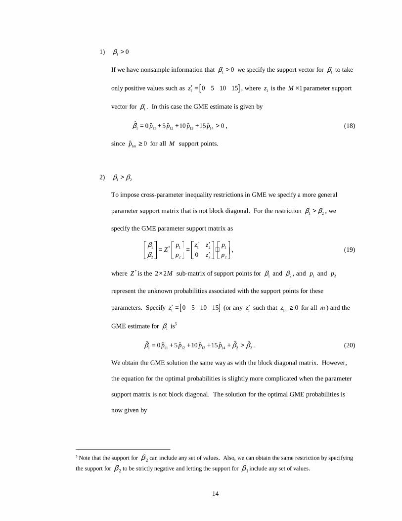
1) 1 0β >

If we have nonsample information that 1 0β > we specify the support vector for 1β to take

only positive values such as [ ]1 0 5 10 15z′ = , where 1z is the 1M × parameter support

vector for 1β . In this case the GME estimate is given by

1 11 12 13 14ˆ ˆ ˆ ˆ ˆ0 5 10 15 0p p p pβ = + + + > , (18)

since 1ˆ 0mp ≥ for all M support points.

2) 1 2β β>

To impose cross-parameter inequality restrictions in GME we specify a more general

parameter support matrix that is not block diagonal. For the restriction 1 2β β> , we

specify the GME parameter support matrix as

1 1 1 2 1*

2 2 2 20

p z z pZ

p z p

ββ

′ ′ = = ⋅ ′

, (19)

where *Z is the 2 2M× sub-matrix of support points for 1β and 2β , and 1p and 2p

represent the unknown probabilities associated with the support points for these

parameters. Specify [ ]1 0 5 10 15z′ = (or any 1z′ such that 1 0mz ≥ for all m ) and the

GME estimate for 1β is5

1 11 12 13 14 2 2ˆ ˆ ˆˆ ˆ ˆ ˆ0 5 10 15p p p pβ β β= + + + + > . (20)

We obtain the GME solution the same way as with the block diagonal matrix. However,

the equation for the optimal probabilities is slightly more complicated when the parameter

support matrix is not block diagonal. The solution for the optimal GME probabilities is

now given by

5 Note that the support for β 2 can include any set of values. Also, we can obtain the same restriction by specifying

the support for β 2 to be strictly negative and letting the support for β1 include any set of values.

15

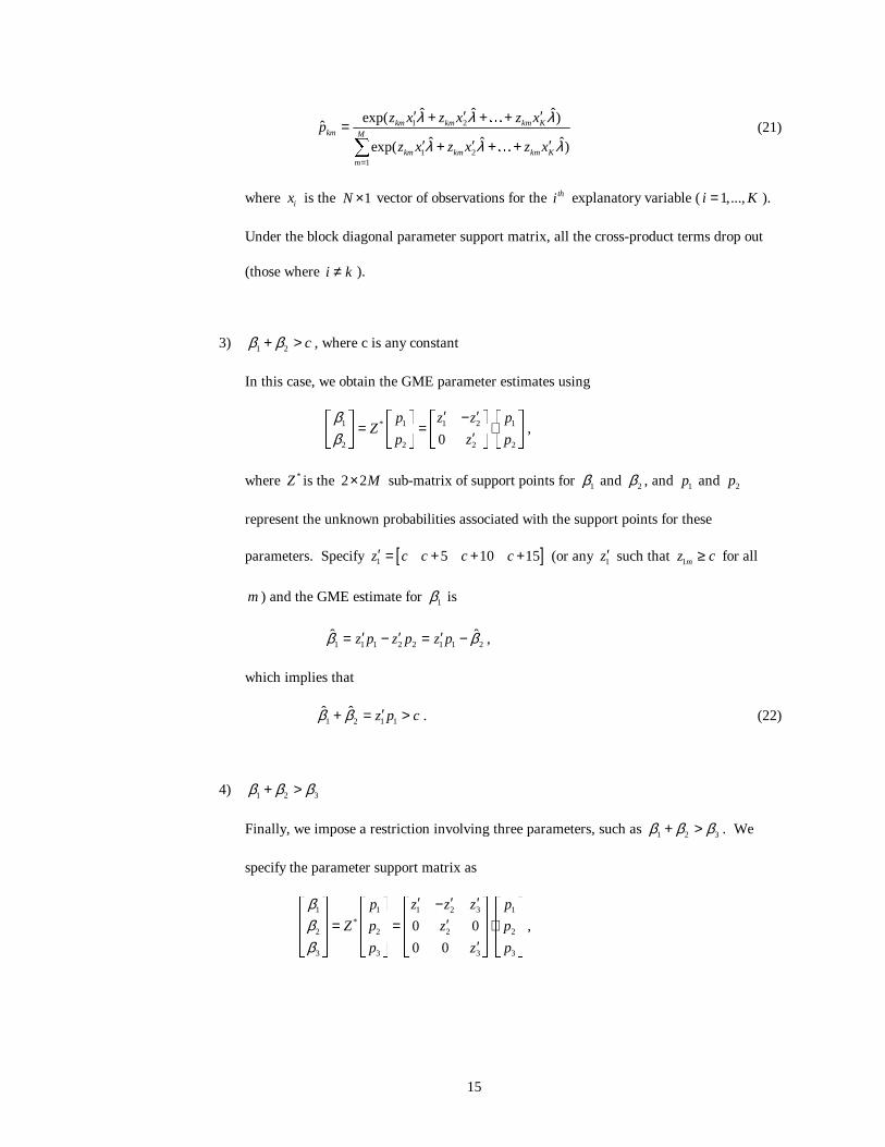
1 2

1 21

ˆ ˆ ˆexp( )ˆ

ˆ ˆ ˆexp( )

km km km Kkm M

km km km Km

z x z x z xp

z x z x z x

λ λ λ

λ λ λ=

′ ′ ′+ + +=′ ′ ′+ + +∑

…

…

(21)

where ix is the 1N × vector of observations for the thi explanatory variable ( 1,...,i K= ).

Under the block diagonal parameter support matrix, all the cross-product terms drop out

(those where i k≠ ).

3) 1 2 cβ β+ > , where c is any constant

In this case, we obtain the GME parameter estimates using

1 1 1 2 1*

2 2 2 20

p z z pZ

p z p

ββ

′ ′− = = ⋅ ′

,

where *Z is the 2 2M× sub-matrix of support points for 1β and 2β , and 1p and 2p

represent the unknown probabilities associated with the support points for these

parameters. Specify [ ]1 5 10 15z c c c c′ = + + + (or any 1z′ such that 1mz c≥ for all

m ) and the GME estimate for 1β is

1 1 1 2 2 1 1 2ˆ ˆz p z p z pβ β′ ′ ′= − = − ,

which implies that

1 2 1 1ˆ ˆ z p cβ β ′+ = > . (22)

4) 1 2 3β β β+ >

Finally, we impose a restriction involving three parameters, such as 1 2 3β β β+ > . We

specify the parameter support matrix as

1 1 1 2 3 1

*2 2 2 2

3 3 3 3

0 0

0 0

p z z z p

Z p z p

p z p

βββ

′ ′ ′− ′= = ⋅ ′

,

16

where *Z is the 3 3M× sub-matrix of support points for 1β , 2β , and 3β ; 1p , 2p , and 3p

represent the unknown probabilities associated with the support points for these

parameters. We specify 1z′ such that all its elements are positive and obtain

1 1 1 2 2 3 3 1 1 2 3ˆ ˆ ˆz p z p z p z pβ β β′ ′ ′ ′= − + = − + ,

which implies that

1 2 1 1 3 3ˆ ˆ ˆ ˆz pβ β β β′+ = + > . (23)

4.2 Imposing non-binding inequality information

GJM (1996, pp. 140-142) consider the cost of imposing incorrect sign information about a

parameter, but do not impose binding restrictions. They estimate a linear regression model using

the generalized cross-entropy (GCE) estimator, which is used to specify discrete prior distributions

that are not uniform. GJM specify parameter sign information by placing more prior weight on

either the positive or negative parameter support points. They specify a parameter support given by

[ ]10, 10kZ = − with prior weights of [ ].375 .625 and [ ].625 .375 and prior means equal to 2.5

and –2.5, respectively. These sign restrictions are not binding however since the parameter

estimate is free to take any value between –10 and 10. We imposed this type of non-binding prior

information on our GME3 estimator in section 3. For example, we specified a prior mean of –1 for

coefficient on COLL, but the parameter estimate still came out positive.

In several sampling experiments, GJM find that risk is only slightly lower when the prior

means are specified to take the correct signs compared to when they are specified to take incorrect

signs. This is consistent with our results, which showed the parameter estimates did not change

much in response to non-binding parameter restrictions.

4.3 GME estimation of an economic model with binding inequality restrictions

We now estimate the poverty rate model with binding inequality restrictions. This type of

binding restriction has been applied by Fraser (2000) who imposes the restriction that own-price

17

elasticities must be negative in a meat demand model and by Shen and Perloff (2001) who impose

the restriction that the speed of adjustment parameter in a cobweb model be positive and less than

one. In our model, the only coefficient that took an unexpected sign was the positive coefficient on

COLL since we expect the percentage of college-educated adults to have a negative impact on

poverty rates. For our first set of restricted estimates, we constrain the coefficient on COLL to be

negative.

Suppose we wanted to impose the stronger restriction that the percentage of college-educated

adults to has a larger negative impact on the poverty rate than percentage of high school educated

adults. To illustrate the use of our non-block diagonal parameter support matrix we obtain a second

set of restricted estimates in which we constrain 5 4 0β β< < .

For both sets of restricted estimates, we compare the IRLS estimates to the restricted GME

(RGME) estimates. We consider the relatively wide bounds (representing little prior information)

of GME1 and the narrower bounds of GME2. We do not re-estimate the GME3 model since it is

just GME2 with non-binding restrictions. In each model, we constrain the coefficients for HHSZ

and UNEMP to be positive and the coefficients for HS, COLL, and MEDINC to be negative. We

specify the parameter supports for RGME1 and RGME2 as follows:

• RGME1 – The support for RGME1 maintains the wide bounds, representing little

information about the magnitude of the parameters, as in GME1. Note that imposing sign

restrictions changes the prior mean of the variables. For example, the support for

MEDINC has the same lower bound as in GME1, but by removing the positive values we

have changed the prior mean from 0 to -10. This can have a potentially large impact on

our parameter estimates since they are shrunk towards the prior mean. Table 6 gives the

parameter support for RGME1.

18

Table 6. Parameter Support for RGME1 (sign restrictions only)

Parameter Parameter Support Prior Mean

1β (constant) { }1 50 25 0 25 50z′ = − − 0

2β (hhsz) { }2 0 5 10 15 20z′ = 10

3β (unemp) { }3 0 5 10 15 20z′ = 10

4β (hs) { }4 20 15 10 5 0z′ = − − − − -10

5β (coll) { }5 20 15 10 5 0z′ = − − − − -10

6β (medinc) { }6 20 15 10 5 0z′ = − − − − -10

7β (d90) { }7 20 10 0 10 20z′ = − − 0

• RGME2 – Here we specify narrower bounds representing better nonsample information.

The prior means of the parameters are smaller for RMGE2 than for RGME1. Table 7

gives the parameter support for RGME2.

Table 7. Parameter Support for RGME2 (sign restrictions only)

Parameter Parameter Support Prior Mean

1β (constant) { }1 50 25 0 25 50z′ = − − 0

2β (hhsz) { }2 0 2.5 5 7.5 10z′ = 5

3β (unemp) { }3 0 0.5 1 1.5 2z′ = 1

4β (hs) { }4 2 1.5 1 0.5 0z′ = − − − − -1

5β (coll) { }5 2 1.5 1 0.5 0z′ = − − − − -1

6β (medinc) { }6 10 7.5 5 2.5 0z′ = − − − − -5

7β (d90) { }7 20 10 0 10 20z′ = − − 0

We again specify error supports using bounds of 3σ± and 4σ± . The restricted GME

estimators are labeled RGME1S3, RGME2S3, RGME1S4, and RGME2S4, where S3 and S4 refer

to the use of a 3σ and 4σ rule, respectively. Table 8 gives point estimates for the poverty data

using IRLS and our four different RGME estimators.

19

Table 8. IRLS and RGME Estimates for Poverty Data with Sign Restrictions

S3 S4Variable OLS IRLS RGME1 RGME2 RGME1 RGME2POV 1β 21.659 23.139 12.765 16.223 9.289 15.103

HHSZ 2β 1.804 1.518 3.672 2.862 4.471 3.190

UNEMP 3β 0.076 0.072 0.113 0.184 0.110 0.214

HS 4β -0.201 -0.210 -0.160 -0.193 -0.144 -0.199

COLL 5β 0.021 0 0 -0.032 0 -0.066

MEDINC 6β -0.416 -0.400 -0.363 -0.324 -0.366 -0.293

D90 7β 8.504 8.189 8.171 7.295 8.647 7.105

The results show that signs of the parameter estimates are the same for IRLS and RGME. The

RGME estimates are larger in magnitude than the GME estimates reported in Table 5. Recall that

in our unrestricted GME1 and GME2 specification all of the parameter estimates had a prior mean

of zero. Imposing binding sign restrictions in GME not only restricts the values the parameter

estimates can take, but also effects the prior mean and therefore the magnitude of the parameter

estimates. The change in the prior means can have a fairly large impact on the GME parameter

estimates.

In the original model, the only coefficient that took a sign opposite our expectations was the

coefficient on COLL. With IRLS, restricted coefficients that take the wrong sign in OLS will be

equal to zero. Our results show that our RGME1 estimates, based on wide parameter bounds

representing little prior information, are also equal to zero. However, the RGME2 estimates for the

coefficient on COLL are negative. This is appealing since a coefficient estimate of zero is not

consistent with the restriction that it be negative. The IRLS estimator and our RGME1 estimator

simply eliminate from the model any variables whose coefficient estimates take incorrect signs. The

RGME2 estimates are consistent with our belief that the percent of college-educated individuals has

a negative effect on poverty rates.

We now estimate the poverty rate model with the sign restrictions plus the additional restriction

that 5 4β β< . We include this restriction to illustrate the use of a non-block diagonal parameter

support matrix. We specify the GME support matrix using

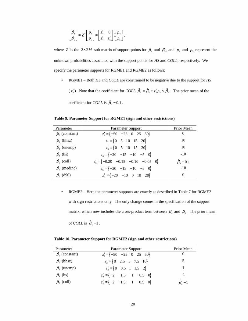
20

4 4 4 4*

5 5 4 5 5

0p z pZ

p z z p

ββ

′ = = ⋅ ′ ′

,

where *Z is the 2 2M× sub-matrix of support points for 4β and 5β , and 4p and 5p represent the

unknown probabilities associated with the support points for HS and COLL, respectively. We

specify the parameter supports for RGME1 and RGME2 as follows:

• RGME1 – Both HS and COLL are constrained to be negative due to the support for HS

( 4z′ ). Note that the coefficient for COLL, 5 4 5 5 4ˆ ˆ ˆz pβ β β′= + ≤ . The prior mean of the

coefficient for COLL is 4ˆ 0.1β − .

Table 9. Parameter Support for RGME1 (sign and other restrictions)

Parameter Parameter Support Prior Mean

1β (constant) { }1 50 25 0 25 50z′ = − − 0

2β (hhsz) { }2 0 5 10 15 20z′ = 10

3β (unemp) { }3 0 5 10 15 20z′ = 10

4β (hs) { }4 20 15 10 5 0z′ = − − − − -10

5β (coll) { }5 0.20 0.15 0.10 0.05 0z′ = − − − −4

ˆ 0.1β −

6β (medinc) { }6 20 15 10 5 0z′ = − − − − -10

7β (d90) { }7 20 10 0 10 20z′ = − − 0

• RGME2 – Here the parameter supports are exactly as described in Table 7 for RGME2

with sign restrictions only. The only change comes in the specification of the support

matrix, which now includes the cross-product term between 4β and 5β . The prior mean

of COLL is 4ˆ 1β − .

Table 10. Parameter Support for RGME2 (sign and other restrictions)

Parameter Parameter Support Prior Mean

1β (constant) { }1 50 25 0 25 50z′ = − − 0

2β (hhsz) { }2 0 2.5 5 7.5 10z′ = 5

3β (unemp) { }3 0 0.5 1 1.5 2z′ = 1

4β (hs) { }4 2 1.5 1 0.5 0z′ = − − − − -1

5β (coll) { }5 2 1.5 1 0.5 0z′ = − − − −4

ˆ 1β −

21

6β (medinc) { }6 10 7.5 5 2.5 0z′ = − − − − -5

7β (d90) { }7 20 10 0 10 20z′ = − − 0

We again specify error supports using bounds of 3σ± and 4σ± . The restricted GME

estimators are labeled RGME1S3, RGME2S3, RGME1S4, and RGME2S4, where S3 and S4 refer

to the use of a 3σ and 4σ rule, respectively. Table 11 summarizes the different GME estimators

we use in the paper with references to the tables they are used for. Table 12 gives point estimates

for the poverty data using IRLS and our four different RGME estimators.

Table 11. Summary of GME estimators used

Estimator Parameter Support Error Bounds LocationGME1S3 Wide parameter bounds [ 3 ,3 ]σ σ− Tables 2, 5GME2S3 Narrow parameter bounds [ 3 ,3 ]σ σ− Tables 3, 5GME3S3 Narrow parameter bounds with non-

binding restrictions[ 3 ,3 ]σ σ− Tables 4, 5

GME1S4 Wide parameter bounds [ 4 , 4 ]σ σ− Tables 2, 5GME2S4 Narrow parameter bounds [ 4 , 4 ]σ σ− Tables 3, 5GME3S4 Narrow parameter bounds with non-

binding restrictions[ 4 , 4 ]σ σ− Tables 4, 5

RGME1S3 Wide parameter bounds withbinding restrictions

[ 3 ,3 ]σ σ− Tables 6, 8, 9, 12

RGME2S3 Narrow parameter bounds withbinding restrictions

[ 3 ,3 ]σ σ− Tables 7, 8, 10, 12

RGME1S4 Wide parameter bounds withbinding restrictions

[ 4 , 4 ]σ σ− Tables 6, 8, 9, 12

RGME2S4 Narrow parameter bounds withbinding restrictions

[ 4 , 4 ]σ σ− Tables 7, 8, 10, 12

Table 12. IRLS and RGME Estimates for Poverty Data with Sign and Other Restrictions

S3 S4Variable OLS IRLS R1GME1 R1GME2 R1GME1 R1GME2POV 1β 21.659 16.509 2.712 8.004 1.247 7.543

HHSZ 2β 1.804 2.096 4.489 3.419 5.006 3.603

UNEMP 3β 0.076 0.045 0.115 0.189 0.092 0.215

HS 4β -0.201 -0.123 -0.034 -0.085 -0.031 -0.093

COLL 5β 0.021 -0.123 -0.087 -0.088 -0.102 -0.115

MEDINC 6β -0.416 -0.285 -0.262 -0.253 -0.266 -0.234

D90 7β 8.504 6.742 6.802 6.303 7.340 6.287

22

With the additional restrictions, RGME and IRLS parameter estimates again take the same

signs. IRLS has a corner solution to the restriction with 5 4ˆ ˆβ β= while the alternative RGME

estimators all have 5 4ˆ ˆβ β< as specified by the restriction. All of our GME programs were written

using the GAUSS constrained optimization module. The programs are available on our websites at

http://www.bus.lsu.edu/academics/economics/faculty/chill/main.html or

http://www.bus.lsu.edu/academics/economics/faculty/rcampbell/main.html.

5. GME Interval Estimates

In this section, we use a bootstrap to obtain interval estimates for the GME estimator. In

several sampling experiments, GJM find that the GME estimator has a smaller variance than the

OLS estimator. Thus, although the GME estimator is biased, GME has lower empirical risk than

OLS due to the small variability of the GME estimator.

The bootstrap is a method for estimating standard errors by resampling the original data.

Freedman and Peters (1984a) and Freedman and Peters (1984b) describe the use of the bootstrap in

regression models. Horowitz (1997) presents a bootstrap method for computing confidence

intervals where t-statistics are obtained from the resampled data and interval estimates are

computed as *ˆ ˆ( )ct seβ β± , where *ct is the bootstrap t-statistic and ˆ( )se β is the asymptotic standard

error of the estimator. Since we do not know the asymptotic distribution of the GME estimator, we

use the percentile method described by Mooney and Duval (1993) to obtain confidence intervals and

examine the precision of the GME estimator.

We construct our confidence intervals for GME and IRLS by resampling from our original data

and estimating the model 400T = times. We then order the resulting estimates and find the values

corresponding to the 2.5% or 10th value and the 97.5% or 390th value. For OLS we computed

confidence intervals as ( )k c kb t se b± . Table 13 gives interval estimates for the poverty data with no

restrictions on the parameter estimates. The interval estimates show a few interesting things about

the GME estimator. First, GME interval estimates are generally narrower than the OLS interval

23

estimates, indicating a higher degree of precision. The distribution of the GME estimator is roughly

symmetric about the mean as shown in Charts 1 and 2, which give the empirical distributions of 2β

and 4β for the GME1S4 estimator. GME estimates for the other parameters follow similar

distributions.

Table 13. OLS and GME Interval Estimates for Poverty Data (N =116 Observations)

S3Variable OLS GME1 GME2 GME3POV 1β [10.698, 32.619] [9.054, 22.147] [12.357, 23.057] [8.157, 19.711]

HHSZ 2β [-0.498, 4.107] [1.248, 3.929] [1.051, 3.123] [1.955, 4.189]

UNEMP 3β [-0.041, 0.193] [0, 0.275] [0.006, 0.274] [0.012, 0.272]

HS 4β [-0.279, -0.124] [-0.218, -0.113] [-0.221, -0.124] [-0.211, -0.113]

COLL 5β [-0.069, 0.112] [-0.047, 0.182] [-0.055, 0.165] [-0.044, 0.178]

MEDINC 6β [-0.508, -0.323] [-0.515, -0.301] [-0.503, -0.298] [-0.509, -0.299]

D90 7β [6.437, 10.572] [5.666, 10.412] [5.573, 9.965] [6.004, 10.447]

S4Variable GME1 GME2 GME3POV 1β [9.591, 19.636] [13.367, 21.147] [8.385, 17.051]

HHSZ 2β [1.567, 3.684] [1.242, 2.759] [2.385, 4.061]

UNEMP 3β [0.014, 0.269] [0.027, 0.262] [0.037, 0.272]

HS 4β [-0.200, -0.107] [-0.204, -0.122] [-0.196, -0.109]

COLL 5β [-0.050, 0.158] [-0.059, 0.139] [-0.053, 0.144]

MEDINC 6β [-0.495, -0.290] [-0.481, -0.286] [-0.485, -0.285]

D90 7β [5.918, 10.067] [5.632, 9.539] [6.100, 10.054]

0

20

40

60

80

100

1.2 1.8 2.4 3 3.6 4.2 4.8

Freq

uenc

y

24

Chart 1. Empirical Distribution of GME1S4 Estimator for 2β (T = 400 Observations)

25

Chart 2. Empirical Distribution of GME1S4 Estimator for 4β (T = 400 Observations)

Comparing GME1, GME2, and GME3 for a given set of error bounds we observe little

difference in the width of the confidence interval. The intervals shift due to differences in the prior

mean and the width of the parameter support, but the width of the interval remains fairly constant.

However, the intervals become narrower as we increase the error bounds from 3σ± to 4σ± .

Increasing the error bounds shrinks the estimates towards their prior mean and reduces the

variability of the parameter estimates. For our problem, it appears that using bounds of 4σ± leads

to better estimates than bounds of 3σ± . However, this may vary from problem to problem. Also,

this does not imply that using even wider bounds such as 5σ± would provide even better estimates.

As we make the error bounds infinitely wide the variability goes to zero and the parameter estimates

are equal to the prior mean. Table 14 gives interval estimates for the poverty data with sign

restrictions placed on the parameters.

0

20

40

60

80

100

-0.21 -0.19 -0.17 -0.15 -0.13 -0.11 -0.09 -0.07

Fre

quen

cy

26

Table 14. OLS and GME Interval Estimates for Poverty Data with Sign Restrictions

S3Variable IRLS RGME1 RGME2POV 1β [16.277, 30.641] [6.953, 16.890] [12.415, 19.131]

HHSZ 2β [0, 3.281] [2.855, 4.905] [2.369, 3.500]

UNEMP 3β [0, 0.180] [0.005, 0.229] [0.101, 0.279]

HS 4β [-0.264, -0.163] [-0.201, -0.112] [-0.235, -0.155]

COLL 5β [-0.063, 0] [-0.022, 0] [-0.096, -0.005]

MEDINC 6β [-0.472, -0.317] [-0.448, -0.285] [-0.403, -0.247]

D90 7β [6.119, 9.724] [6.247, 10.259] [5.479, 9.110]

S4Variable RGME1 RGME2POV 1β [3.985, 13.111] [11.952, 17.696]

HHSZ 2β [3.755, 5.461] [2.807, 3.674]

UNEMP 3β [0.022, 0.222] [0.143, 0.304]

HS 4β [-0.184, -0.095] [-0.242, -0.161]

COLL 5β [-0.028, 0] [-0.126, -0.030]

MEDINC 6β [-0.437, -0.295] [-0.374, -0.215]

D90 7β [6.819, 10.203] [5.428, 8.697]

The results are consistent with the results for the unrestricted estimates. The restrictions cause

all of the confidence intervals to become narrower and the distributions for some of the parameter

estimates to be truncated. We again observe smaller intervals as we increase the error bounds. In

the restricted case we also observe a large shift in the interval when we increase the error bounds

since the parameter estimates are moving towards their prior mean, which is not equal to zero for

most of the parameters.

6. Conclusions

This paper applies maximum entropy estimation in an economic model of poverty rates. We

discuss how to specify the parameter and error support matrices for the GME estimator. In our

model, the GME estimates take the same signs and are roughly the same magnitude as OLS

estimates. We find that varying the width of the parameter support does not affect the GME

estimates very much. Therefore, a researcher with little prior information could specify a wide

parameter support that is symmetric about zero and obtain estimates that are reasonably close to

27

OLS estimates. Varying the width of the error bounds has a larger impact on the estimates. For the

poverty rate example, we conclude that error bounds of ˆ4σ± are preferred over error bounds of

ˆ3σ± , where σ is the sample standard deviation of y .

We use a bootstrap to develop confidence intervals for GME. We find that the GME estimator

has a narrower confidence interval than the OLS estimator does, which is consistent with GJM.

The confidence intervals for the GME estimator become smaller, indicating greater precision in the

estimates, as we increase the error bounds. However, the wider the error bounds are set the more

important it is that we obtain good nonsample information for specifying the parameter support.

The GME estimator is a shrinkage estimator where the parameter estimates are shrunk towards the

prior mean, which is based on nonsample information. As we increase the degree of shrinkage

towards the prior mean we need to make sure that the prior mean is based on good nonsample

information.

Finally, we develop a more general parameter support matrix that allows us to impose a broader

set of parameter restrictions than are possible under the traditional support matrix for GME

estimation. We demonstrate how to impose restrictions on the GME estimator using a simple

example of sign restrictions and another more complicated example using our new parameter

support matrix. In both cases, the restrictions are relatively simple to impose and the restricted

GME estimator works very well in our model. One important feature of RGME estimation is that it

does not restrict us to corner solutions as the IRLS estimator does. For example, when we impose

that restriction that 2 0β < the IRLS estimate will be equal to OLS if the OLS estimate is negative

and to zero otherwise. We find that the RGME estimate is often negative even when OLS and

GME estimates are positive. Because GME estimation relies on prior information, our new support

matrix is an important contribution since it allows us a simple way to impose prior information that

is often encountered in empirical research.

28

References

Fraser, I., 2000. An application of maximum entropy estimation: the demand for meat in the UnitedKingdom. Applied Economics 32, 45-59.

Freedman, D.A, Peters, S.C., 1984a. Bootstrapping a regression equation: some empirical results.Journal of the American Statistical Association, 79, 97-106.

Freedman, D.A., Peters, S.C., 1984b. Bootstrapping an econometric model: some empirical results.Journal of Business and Economic Statistics, 2, 150-158.

Golan, A., Judge, G., Miller, D., 1996. Maximum entropy econometrics: robust estimation withlimited data (John Wiley and Sons, New York).

Golan, A., Judge, G., Perloff, J.M., 1997. Recovering information from censored and orderedmultinomial response data. Journal of Econometrics, 79, 23-51.

Golan, A., Perloff, J.M., Shen, E.Z., 2001. Estimating a demand system with nonnegativityconstraints: Mexican meat demand. The Review of Economics and Statistics, 83, 541-550.

Griffiths, W.E., Hill, R.C., Judge, G.G., 1993. Learning and practicing econometrics (John Wileyand Sons, New York).

Horowitz, J.L., 1997. Bootstrap methods in econometrics: theory and numerical performance. In:Krpes, D.M., Wallis, K.F. (Eds.), Advances in economics and econometrics: theory andapplications, Seventh World Congress, Volume III. University Press, Cambridge, pp. 188-222.

Jaynes, E.T., 1957a. Information theory and statistical mechanics. Physical Review 106, 620-630.

Jaynes, E.T., 1957b. Information theory and statistical mechanics II. Physical Review 108, 171-190.

Judge, G.G., Hill, R.C., Bock, M.E., 1990. An adaptive empirical bayes estimator of themultivariate

normal mean under quadratic loss. Journal of Econometrics 44, 189-213.

Judge, G.G., Hill, R.C., Griffiths, W.E., Lütkepohl, H., Lee, T., 1988. Introduction to the theory andpractice of econometrics 2nd ed. (John Wiley and Sons, New York).

Miller, D.J., Plantinga, A.J., 1999. Modeling land use decisions with aggregate data. AmericanJournal of Agricultural Economics, 81, 180-194.

Mooney, C.Z., Duval, R.D., 1993. Bootstrapping: a nonparametric approach to statistical inference.Sage University Paper series on Quantitative Applications in the Social Sciences, 07-095.Newbury Park, CA: Sage.

Preckel, P.V., 2001. Least squares and entropy: a penalty function perspective. American Journal ofAgricultural Economics, 83, 366-377.

Pukelsheim. F., 1994. The three sigma rule. American Statistician 48, 88-91.

Shen, E.Z., Perloff, J.M., 2001. Maximum entropy and Bayesian approaches to the ratio problem.Journal of Econometrics, 104, 289-313.

Ramanathan, R., 2002. Introductory econometrics with applications (Harcourt College Publishers,

29

Fort Worth).