entropy

Article

On the Entropy of Events under Eventually GlobalInflated or Deflated Probability Constraints.Application to the Supervision of Epidemic Modelsunder Vaccination Controls

Manuel De la Sen 1,* , Asier Ibeas 2 and Raul Nistal 1

1 Institute of Research and Development of Processes IIDP, University of the Basque Country, Campus ofLeioa, 48940 Leioa, Spain; raul.nistal@gmail.com

2 Department of Telecommunications and Systems Engineering, Universitat Autònoma de Barcelona (UAB),08193 Barcelona, Spain; Asier.Ibeas@uab.cat

* Correspondence: manuel.delasen@ehu.eus

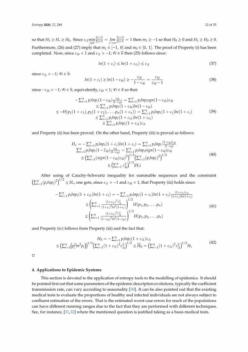
Received: 27 January 2020; Accepted: 27 February 2020; Published: 29 February 2020�����������������

Abstract: This paper extends the formulation of the Shannon entropy under probabilistic uncertaintieswhich are basically established in terms or relative errors related to the theoretical nominal set ofevents. Those uncertainties can eventually translate into globally inflated or deflated probabilisticconstraints. In the first case, the global probability of all the events exceeds unity while in the secondone lies below unity. A simple interpretation is that the whole set of events losses completenessand that some events of negative probability might be incorporated to keep the completeness of anextended set of events. The proposed formalism is flexible enough to evaluate the need to introducecompensatory probability events or not depending on each particular application. In particular, sucha design flexibility is emphasized through an application which is given related to epidemic modelsunder vaccination and treatment controls. Switching rules are proposed to choose through timethe active model, among a predefined set of models organized in a parallel structure, which betterdescribes the registered epidemic evolution data. The supervisory monitoring is performed in thesense that the tested accumulated entropy of the absolute error of the model versus the observed datais minimized at each supervision time-interval occurring in-between each two consecutive switchingtime instants. The active model generates the (vaccination/treatment) controls to be injected to themonitored population. In this application, it is not proposed to introduce a compensatory event tocomplete the global probability to unity but instead, the estimated probabilities are re-adjusted todesign the control gains.

Keywords: Shannon entropy; complete/incomplete systems of events; probabilistic uncertainty;probabilistic inflated/deflated probability constraints; epidemic model; vaccination controls;treatment controls

1. Introduction

Classical entropy is a state function in Thermodynamics. The originator of the concept of entropywas the celebrated Rudolf Clausius in the mid-nineteenth century. The property that reversibleprocesses have a zero variation of entropy among equilibrium states while irreversible processes havean increase of entropy is well-known. Reversible processes only occur under ideal theoretical modellingof isolated processes without energy losses such as, for instance, the Carnot cycle. Real processes areirreversible because the above ideal conditions are impossible to fulfil. In classical Thermodynamics,the Clausius equality establishes that the entropy variation in reversible cycle processes is zero. That is,

Entropy 2020, 22, 284; doi:10.3390/e22030284 www.mdpi.com/journal/entropy

Entropy 2020, 22, 284 2 of 35

the entropy variation is path-independent since it is a state function which takes an identical valueat a final state being coincident with an initial one state. However, in irreversible ones the entropyvariation is positive. This is the motivating reason which associates a positive variation of entropy toa “disorder increase”. It has to be pointed out that, in order to interpret correctly the non-negativevariations of entropy, the system under consideration has to be an isolated one. In other words, someof the mutually interacting subsystems of an isolated system can exhibit negative variations of entropy.Later on Boltzmann, Gibbs and Maxwell have defined entropy under a statistical framework. On theother hand, Shannon entropy (named after Claude E. Shannon, 1916–2001, “the father of informationtheory”) is a very important tool to measure the amount of uncertainty in processes characterized in theprobabilistic framework by sets of events, [1–5]. In some extended studies in the frameworks of physics,economy or fractional calculus, it is admitted the existence of events with negative probabilities, [4–6].Entropy may be interpreted as information loss [1–3,7–9] and is useful, in particular, to characterizedynamic systems from this point of view [8]. On the other hand, entropy tools have also being usedeither to model or for complementary modelling support to evaluate certain epidemic models, [10–17].In some of the studies, the investigation of epidemic models, which are ruled by a differential systemof coupled equations involving the various subpopulations, has been proposed in the frameworkof a patchy environment [13]. The model uncertainty amount is evaluated in such a way that thetime-derivative of the entropy is shown to be non-negative at a set of testing sampling instants. In [9],a technique to develop a formal Shannon entropy in the complex framework is proposed. In this way,the components of the overall entropy are calculated so as to determine the real and the imaginaryparts of the state complex Shannon entropy as a natural quantum-amplitude generalization of theclassical Shannon entropy.

Epidemic evolution has been typically studied through models based either on differentialequations, difference equations or mixed hybrid models. Such models, because of their structure,become very appropriate to study the equilibrium points, the oscillatory behaviors, the illnesspermanence and the vaccination and treatment controls. See, for instance, [18–24] and some of thereferences therein. More recently, entropy-based models have been proposed for epidemic models.See, for instance, [14–16,25] and some of the references therein. In particular, entropy tools for analysisare mixed with differential-type models in [16,25,26]. Also, the control techniques are appropriate forstudies of alternative biological problems, [27–29] and, in particular, for implementation of decentralizedcontrol techniques in patchy environments where several nodes are interlaced, [27,29]. Under thatgeneric framework, it can be described, for instance, the situation of several towns with different ownhealth centers, where the controls are implemented, and whose susceptible and infectious populationsinteract through in-coming and out-coming population fluxes. This paper proposes a supervisorydesign tool to decrease the uncertainty between the observed data related to infectious disease, orthose given by a complex model related to a disease, via the use of a set of dynamic integrated simplestmodels together with a higher-level supervisory switching algorithm. Such a hierarchical structureselects on line the most appropriate model as the one which has a smaller error uncertainty according toan entropy description (the so-called “active model”). Such an active model is re-updated through timein the sense that another active model can enter into operation. In that way, the active model is used togenerate the correcting sanitary actions to control the epidemics such as, for instance, the gains of thevaccination and antiviral or antibiotic treatment controls and the corresponding control interventions.

The paper is organized as follows: Section 2 recalls some basic concepts of Shannon entropy. Also,those concepts are extended to the case of eventual presence of relative probabilistic uncertainties inthe defined set of events compared to the nominal set of probabilities. Section 3 states and provesmathematical results for the Shannon entropy for the case when a nominal complete finite and discreteset of events is eventually subject to relative errors of their associate probabilities in some of all of theirvarious integrating events. The error-free nominal system of events is assumed to be complete. Thecurrent system of events under probabilistic errors may be either deflated or inflated in the sense thatthe total probability for the whole sets might be either below or beyond unity, respectively, so that it

Entropy 2020, 22, 284 3 of 35

might be non-complete. In the case of globally inflated of deflated probability of the whole set of events,new compensatory events can be used to accomplish with a unity global probability. The entropy of thecurrent system is compared via quantified worst-case results to that of the nominal system. Section 4applies partially the results of the former sections to epidemics control in the case that either the diseasetransmission coefficient rate is not well-known or it varies through time due, for instance, to seasonality.The controls are typically of vaccination or treatment type or appropriate mixed combinations of bothof them. A finite predefined set of running models described by a system of coupled differentialequations is set. Such a whole discrete set covers a range of variation of such a coefficient transmissionrate within known lower-bound and upper-bound limits. Each model is driven by a constant diseasetransmission rate and the whole set of models covers the whole range of foreseen variation of sucha parameter in the real system. Since the set of models is finite, the various values of the diseasetransmission rate are integrated in a discrete set within the whole range of admissible variation of thetrue coefficient rate. A supervisory technique of control monitoring is proposed which chooses theso-called active model which minimizes the accumulated entropy of the absolute error data/modelwithin each supervision interval. A switching rule allows to choose another active model as soon as itis detected that the current active model becomes more uncertain than other(s) related to the observeddata. The active model supplies the (vaccination and/or treatment) controls to be injected to the realepidemic process. Due to the particular nature of the problem, compensatory events are not introducedfor equalizing the global probability to unity. Instead, a re-adjustment of the error probabilities relatedto the true available data is performed to calculate the control gains provided by the active model.It can be pointed out that some parameters of the epidemic description evolutions, typically thecoefficient transmission rate, can vary according to seasonality [30]. This justifies the use of simpleractive invariant models to describe the epidemics evolution along time subject to appropriate modelswitching. On the other hand, the existing medical tests which evaluate the proportions of healthyand infected individuals within the total population are not always subject to confluent worst-caseestimation errors. See, for instance [31,32]. In the case that the estimated global probability of thevarious subpopulations is not unity, the estimated worst-case probabilities need to be appropriatelyamended before an intervention. This design work is performed and discussed in Section 5 throughnumerical simulations in confluence with the above mentioned supervision monitoring technique.Finally, conclusions end the paper.

2. Basic Entropy Preliminaries

Assume a finite system of events A ={Ai : i ∈ n

}of respective probabilities pi for Ai; i ∈ n =

{1, 2, · · · , n}with{pi : i ∈ n

}⊂ [0, 1], with

∑ni=1 pi = 1 which is complete, that is, only one event occurs

at each trial (e.g., the appearance of 1 to 6 points in rolling a die). The Shannon entropy is definedas follows:

H(p1, p2, . . . ..pn) = −n∑

i=1

pi ln pi (1)

which serves as a suitable measure of the uncertainty of the above finite scheme. The name “entropy”pursues a physical analogy with parallel problems, for instance, in Thermodynamics or StatisticsPhysics which does not have a similar sense here so that there is no need to go into in the currentcontext. The above entropy has been defined with neperian logarithms but any logarithm with a fixedbase could be used instead with no loss in generality.

Note that H(p1, p2, . . . ..pn) ≥ 0 with H(p1, p2, . . . ..pn) = 0 if and only if p j = 1 for some arbitraryj ∈ n and pi = 0; ∀i(, j) ∈ n and

Hmax = H(p, p, . . . ., p) = H(1/n, 1/n, . . . ., 1/n) = maxpi∈[0, 1],

∑ni=1 pi=1

= −nplnp = −ln(1/n) = lnn ≥ 0

Hmax = H(p, p, . . . ., p) = H(1/n, 1/n, . . . ., 1/n) = maxpi∈[0, 1],

∑ni=1 pi=1

= −nplnp = −ln(1/n) = lnn ≥ 0

Entropy 2020, 22, 284 4 of 35

with Hmax = 0 if and only if n = p = 1. Assume that the probabilities are uncertain, given by pi(1 + εi);∀i ∈ n, subject to the constraints pi(1− εi0) ≤ pi(1 + εi) ≤ pi(1 + εi1); ∀i ∈ n, where εi0 and εi1 areknown so that the current entropy (or the entropy of the current system) is uncertain and given byHε = H(p1(1 + ε1), p2(1 + ε2), . . . ..pn(1 + εn)); ∀i ∈ n. The reference entropy H∗ = H(p1, p2, . . . ..pn)

for the case when the probabilities of all the events are precisely known being equal to pi; ∀i ∈ n issaid to be the nominal entropy (or the entropy of the nominal system). Some constraints have to befulfilled in order for the formulation to be coherent related to the entropy bounds under probabilisticconstraints in the set of involved events. The following related result follows:

Lemma 1. Assume a nonempty finite complete nominal system of events A∗ ={Ai∗ : i ∈ n

}of respective nominal

probabilities pi ∈ [0, 1] for Ai∗; ∀i ∈ n = {1, 2, · · · , n} and a current (or uncertain) version of the system ofevents A =

{Ai : i ∈ n

}of uncertain probabilities pi(1 + εi) ∈ [0, 1]; ∀i ∈ n, where εi ∈ R are relative probability

errors due to probabilistic uncertainties. Define the following disjoint subsets of A:A+ = {Ai ∈ A : εi > 0}, A− = {Ai ∈ A : εi < 0}, A0 = {Ai ∈ A : εi = 0}.Then, the following constraints hold:

(i) A is complete if and only if∑n

i=1 εipi = 0 (global probabilistic uncertainty mutual compensation)(ii) max (cardA+, cardA−) < n, and min (cardA+, cardA−) > 0 or cardA0 = n (and then A+ = A− = ∅)

Proof: The proof of Property (i) follows since A∗ being complete implies that A is complete if and onlyif

∑ni=1 pi(1 + εi) = 1.∑n

i=1 pi(1 + εi) = 1 =∑n

i=1 pi +∑n

i=1 piεi = 1 +∑n

i=1 piεi ⇔∑n

i=1 piεi = 0and A is complete since

∑ni=1 pi(1 + εi) = 1. Property (i) has been proved, The proof of

Property (ii) follows from Property (i). To prove the first constraint, assume, on the contrary,that max (cardA+, cardA−) = n. Then, either cardA+ = n and A− = A0 = ∅ or cardA− = n andA+ = A0 = ∅. Assume that cardA+ = n and A− = A0 = ∅. Then,

∑ni=1 εipi > 0 which contradicts

Property (i). Similarly, if cardA− = n and A+ = A0 = ∅ then∑n

i=1 εipi < 0 which again contradictsProperty (i). Thus, max (cardA+, cardA−) < n and the first constraint of Property (i) has been proved.Now, assume that min (cardA+, cardA−) = 0 and 0 ≤ cardA0 < n. First, assume that cardA− = 0 andcardA+ = cardA− cardA0 = max (cardA+, cardA−) ≤ n (from the already proved above first constraintof this property). If cardA+ > 0 then,

∑ni=1 εipi > 0 which contradicts Property (i). If cardA+ = 0

then A = A0 and cardA0 = n. So, if cardA− = 0 then cardA+ = 0 and cardA0 = n (then A = A0). Inthe same way, interchanging the roles of A+ and A−, it follows that, if cardA+ = 0 then cardA− = 0and cardA0 = n. One concludes that either min (cardA+, cardA−) > 0 or cardA0 = n and Property (ii)is proved.

Note that, in Lemma 1, A0 ⊂ A is the subset of probabilistically certain events of A (in the sentthat is elements have a known probability) and A+ ∪A− ⊂ A is the subset of probabilistically uncertainevents of A. For A being nonempty, any of the sets A0, A+ and A− or pair combinations may be empty.Note also that the probabilistic uncertainties have been considered with fixed values εi ∈ [0, 1]; ∀i ∈ n.�

3. Entropy Versus Global Inflated and Deflated Probability Constraints in Incomplete Systems ofEvents under Probabilistic Uncertainties

An important issue to be addressed is how to deal with the case when, due to incompleteknowledge of the probabilistic uncertainties, the sum of probabilities of the current complete system ofevents, i.e., that related to the uncertain values of individual probability values exceeds unity, thatis

∑ni=1 pi(1 + εi) > 1, a constraint referred to as “global inflated probability”. If both the nominal

individual and nominal global probability constraints, pi ≥ 0; ∀i ∈ n and∑n

i=1 pi = 1 hold then thereis a global inflated probability if and only if the probabilistic disturbances fulfill

∑ni=1 piεi > 0. It is

Entropy 2020, 22, 284 5 of 35

always possible to include the case of “global deflated probability” if∑n

i=1 pi(1 + εi) < 1 implying that∑ni=1 piεi < 0 provided that

∑ni=1 pi = 1.

Three possible solutions to cope with this drawback, associate to an exceeding amount of modeledprobabilistic uncertainty leading to global inflated probability, are:

(a) To incorporate a new (non empty) event An+1 with negative probability which reduces theprobabilistic uncertainty so that the global probability constraint of the extended complete system ofevents Ae = A∪An+1 holds. Obviously, A losses is characteristic property of being a complete systemof events and Ae is said to be partially complete since it fulfills the global probability constraint but ithas one negative probability.

(b) To modify all or some of the probabilistic uncertainty relative amounts εi; i ∈ n so that theglobal probability constraint of the complete system of events holds for the new amended fixed set{εi : i ∈ n

}.

(c) To consider uncertain normalized probabilities pi =pi(1+εi)∑n

i=1 pi(1+εi); i ∈ n. In this case, there

is no need to modify the individual uncertainties of the events but the initial uncertainties arekept. Furthermore, the events would keep its ordination according to uncertainties, namely, ifpi(1 + εi) ≤ p j

(1 + ε j

)for i, j(, i) ∈ n then pi ≤ p j, the modified set of events is complete and keeps the

same number of events as the initial one.Two parallel solutions to cope with global deflated probability are:(d) To incorporate a new (non empty) event An+1 with positive probability which decreases the

probabilistic uncertainty so that the global probability constraint of the extended complete system ofevents Ae = A∪An+1 holds. As before, the current system of events A losses is completeness and Ae

is complete.(e) To modify all or some of the probabilistic uncertainty relative amounts εi; i ∈ n so that new

amended fixed set{εi : i ∈ n

}agrees with the global probability constraint.

Firstly, we note that the introduction of negative probabilities invoked in the first proposedsolution has a sense in certain problems. In this context, Dirac commented in a speech in 1942 thatnegative probabilities can have a sense in certain problems as negative money has in some financialsituations. Later on, Feynman has used also this concept to describe some problems of physics [4] andalso said that negative trees have nonsense but negative probability can have sense as negative moneyhas in some financial situations. More recently, Tenreiro-Machado has used this concept in the contextof fractional calculus [6].

It is now proved in the next result that the incorporation of a new event of negative probability todefine from the system of events A an extended partial complete system of events Ae does not alteratethe property of the non-negativity of the Shannon entropy in the sense that that of the extended systemof events is still non-negative. At the same time, it is proved that

(1) If 1 <∑n

i=1 pi(1 + εi) ≤ 2 then the real part of the entropy of Ae (which is complex because of thenegative probability of the added event for completeness) is smaller that that of A. The interpretationis that the excessive disorder in A, due to its global inflated probability, is reduced (equivalently, “theorder amount” Ae is increased in with respect to A) when building its extended version Ae by thecontribution of the added event of negative probability. Also, both A and Ae are not complete while Ae

is partially complete since it fulfills the global probability constraint although not the partial ones in allthe events due to the incorporated one of negative probability.

(2) If∑n

i=1 pi(1 + εi) > 2 then the above qualitative considerations on increase/ decrease of “order”or” disorder” are reversed with respect to Case a.

Theorem 1. Assume a nonempty finite complete nominal system of events A∗ ={Ai∗ : i ∈ n

}of respective nominal

probabilities pi ∈ [0, 1] for Ai∗; ∀i ∈ n = {1, 2, · · · , n} and a current (or uncertain) version of the system of eventsA =

{Ai : i ∈ n

}of uncertain probabilities pi(1 + εi) ∈ [0, 1]; ∀i ∈ n. Assume that 2 ≥

∑ni=1 pi(1 + εi) > 1

(that is, there is a global inflated probability of the current system of events). Define the extended system of eventsAe = A∪An+1 such that An+1 has a probability pn+1 = pn+1(ε1, ε2, · · · , εn) = 1−

∑ni=1 pi(1 + εi). Then,

Entropy 2020, 22, 284 6 of 35

(i) If 2 ≥∑n

i=1 pi(1 + εi) > 1 then ReHε1 ≤ Hε with 0 ≤ ReHε1 = Hε if and only if∑n

i=1 pi(1 + εi) = 2.(ii) If

∑ni=1 pi(1 + εi) > 2 then Hε1 > Hε ≥ 0,

where:

Hε = H(p1(1 + ε1), p2(1 + ε2), . . . .., pn(1 + εn)) =n∑

i=1

pi(1 + εi)(lnpi + ln(1 + εi)) (2)

Hε1 = H(p1(1 + ε1), p2(1 + ε2), . . . .., pn(1 + εn), pn)

= H(p1(1 + ε1), p2(1 + ε2), . . . .., pn(1 + εn), 1−

∑ni=1 pi(1 + εi)

) (3)

are the respective entropies of A and Ae, the second one being complex.

Proof: Since∑n

i=1 pi(1 + εi) > 1 then A ={Ai1 : i ∈ n

}is not complete. Since the nominal system of

events is complete then∑n

i=1 pi = 1 with pi ≥ 0; ∀i ∈ n and pn+1 = 1−∑n

i=1 pi(1 + εi) < 0. The entropyof A is

and that of the extended system of events Ae is Hε1. Consider two cases:Case (a) 0 <

∑ni=1 pi(1 + εi) − 1 ≤ 1

Since the neperian logarithm of a negative real number exists in the complex field and it is real suchthat its real part is the neperian logarithm of its modulus and the imaginary part is iπ (i =

√−1 being

the imaginary unit), so that it becomes a negative real number, one gets the following set of relations:

−Hε1 =∑n

i=1 pi(1 + εi)ln(pi(1 + εi)) +(1−

∑ni=1 pi(1 + εi)

)ln

(1−

∑ni=1 pi(1 + εi)

)= −Hε +

(1−

∑ni=1 pi(1 + εi)

)ln

(1−

∑ni=1 pi(1 + εi)

)= −Hε −

(∑ni=1 pi(1 + εi) − 1

)ln

(1−

∑ni=1 pi(1 + εi)

)= −Hε −

(∑ni=1 pi(1 + εi) − 1

) (ln

∣∣∣1−∑ni=1 pi(1 + εi)

∣∣∣+ iπ)

= −Hε +∣∣∣∑n

i=1 pi(1 + εi) − 1∣∣∣ (∣∣∣ln ∣∣∣1−∑n

i=1 pi(1 + εi)∣∣∣∣∣∣+ iπ

)(4)

Then:

Re (−Hε1)= −Hε +

∣∣∣∣∣∣∣ n∑

i=1

pi(1 + εi) − 1

ln

∣∣∣∣∣∣∣n∑

i=1

pi(1 + εi) − 1

∣∣∣∣∣∣∣∣∣∣∣∣∣∣ (5)

since 0 <∑n

i=1 pi(1 + εi) − 1 ≤ 1 leads to

ln

∣∣∣∣∣∣∣n∑

i=1

pi(1 + εi) − 1

∣∣∣∣∣∣∣ ≤ 0, ln

1−n∑

i=1

pi(1 + εi)

= −ln

∣∣∣∣∣∣∣1−n∑

i=1

pi(1 + εi)

∣∣∣∣∣∣∣ > 0 (6)

One concludes that that ReHε1 ≤ Hε with 0 ≤ ReHε1 = Hε if and only if∑n

i=1 pi(1 + εi) = 2.It has to be proved now that ReHε1 ≥ 0. Assume, on the contrary, that ReHε1 < 0. Since ReHε1 < Hε,

this happens if and only if the following contradiction holds∑ni=1 pi(1 + εi)(lnpi + ln(1 + εi)) =

∑ni=1 ln

[(pi(1 + εi))

pi(1+εi)]= ln

[∏ni=1(pi(1 + εi))

pi(1+εi)]

= Hε <(∑n

i=1 pi(1 + εi1) − 1)∣∣∣ln ∣∣∣∑n

i=1 pi(1 + εi1) − 1∣∣∣∣∣∣ = (∑n

i=1 piεi1)ln

∣∣∣∑ni=1 piεi1

∣∣∣=

(∑ni=1 piεi1

)(ln

∑ni=1 piεi1

)= ln

[(∑ni=1 piεi1

)∑ni=1 piεi1

] (7)

since∑n

i=1 pi(1 + εi) > 1 in the assumption of global inflated probability. Then, 0 ≤ ReHε1 ≤ Hε.Case (b) 1 <

∑ni=1 pi(1 + εi) − 1 ≤ z for some z(> 1) ∈ R+. Then ln

∣∣∣∑ni=1 pi(1 + εi) − 1

∣∣∣ > 0 andthen the last above identity changes the second term right-hand-side term resulting in:

Entropy 2020, 22, 284 7 of 35

−Hε1 = Re (−Hε1) = −Hε −∣∣∣∑n

i=1 pi(1 + εi) − 1∣∣∣ ∣∣∣∣ln(∑n

i=1 pi(1 + εi) − 1)∣∣∣∣

ReHε1 = Hε +

∣∣∣∣∣∣∣ n∑

i=1

pi(1 + εi) − 1

ln

∣∣∣∣∣∣∣n∑

i=1

pi(1 + εi) − 1

∣∣∣∣∣∣∣∣∣∣∣∣∣∣ > Hε ≥ 0 (8)

�

It is now proved in the next result for the case of deflated probability that the introduction ofan additional event of positive probability to define from the system of events A an extended partialcomplete system of events Ae does not modify the property of the non-negativity of the Shannonentropy in the sense that that of the extended system of events is still non-negative. At the same time,it is proved that the entropy of Ae is larger that that of A. The interpretation is that the excessivelylow disorder in A, due to its global deflated probability, is increased (equivalently, “the order amount”is decreased) when building its extended version Ae by the contribution of the added event An+1 ofpositive probability. Also, A is not complete while Ae is complete.

Theorem 2. Assume a nonempty finite complete nominal system of events A∗ ={Ai∗ : i ∈ n

}of respective

nominal probabilities pi ∈ [0, 1] for Ai∗; ∀i ∈ n = {1, 2, · · · , n} and a current (or uncertain) version of the systemof events A =

{Ai : i ∈ n

}of uncertain probabilities pi(1 + εi) ∈ [0, 1]; ∀i ∈ n. Assume that

∑ni=1 pi(1 + εi) < 1

(that is, there is a global deflated probability of the current system of events). Define the extended system of eventsAe0 = A∪An+1 such that An+1 has a probability pn+1 = pn+1(ε1, ε2, · · · , εn) = 1−

∑ni=1 pi(1 + εi). Then,

Hε0 > Hε ≥ 0, where:

Hε = H(p1(1 + ε1), p2(1 + ε2), . . . .., pn(1 + εn)) =n∑

i=1

pi(1 + εi)(lnpi + ln(1 + εi)) (9)

Hε0 = H(p1(1 + ε1), p2(1 + ε2), . . . .., pn(1 + εn), pn+1)

= H(p1(1 + ε1), p2(1 + ε2), . . . .., pn(1 + εn),

∑ni=1 pi(1 + εi) − 1

) (10)

are the respective entropies of A and Ae0.

Proof: Since∑n

i=1 pi(1 + εi) < 1 then A ={Ai : i ∈ n

}is not complete. Since the nominal system of

events is complete then∑n

i=1 pi = 1 with pi ≥ 0; ∀i ∈ n and pn+1 = 1−∑n

i=1 pi(1 + εi) > 0. The entropyof A is Hε and that of Ae0 is:

Hε0 = H(p1(1 + ε1), p2(1 + ε2), . . . .., pn(1 + εn), pn+1)

= H(p1(1 + ε1), p2(1 + ε2), . . . .., pn(1 + εn),

∑ni=1 pi(1 + εi) − 1

) (11)

Since 0 < 1−∑n

i=1 pi(1 + εi) < 1, one gets the following set of relations:

−Hε0 =∑n

i=1 pi(1 + εi)ln(pi(1 + εi)) +(1−

∑ni=1 pi(1 + εi)

)ln

(1−

∑ni=1 pi(1 + εi)

)= −Hε +

(1−

∑ni=1 pi(1 + εi)

)ln

(1−

∑ni=1 pi(1 + εi)

)= −Hε −

(1−

∑ni=1 pi(1 + εi)

)∣∣∣∣ln(1−∑ni=1 pi(1 + εi)

)∣∣∣∣ < −Hε

(12)

One concludes that that Hε0 > Hε ≥ 0.Note that since we entropy is defined with a sum of weighted logarithms of nonnegative real

numbers bounded by unity in the usual cases (which exclude negative probabilities) then the Shannonentropy of the worst case of the probability uncertainty is not necessarily larger than or equal to thenominal one. �

Entropy 2020, 22, 284 8 of 35

Example 1. Assume that the nominal system of two events is A ={A1(p1), A2(p2)

}with p1 = p2 = 0.5,

then H∗ = −2× 0.5× ln0.5 = −ln0.5 = 0.6931. Assume that it probabilistic uncertainty is given by ε = 0.1,p1(1 + ε) = 0.5 = 0.55, p2(1− ε) = 0.45 = 0.55. Then, the entropy under the uncertain probability ofAε =

{A1(p1(1 + ε)), A2(p2(1− ε))

}is Hε = −0.55ln(0.55) − 0.45ln(0.45) = 0.68814 < H∗.

Example 2. Consider the complete system of events A ={Ai : i ∈ n

}such that pi = λip; ∀i ∈ n, for some p > 0,

is the probability of Ai, ∀i ∈ n and constants λi ∈ R0+ = R+ ∪ {0}; ∀i ∈ n satisfying that∑n

i=1 λi = 1/p. Notethat

∑ni=1 pi = 1 so that there is no negative probability and neither global inflated or global deflated probabilities.

The Shannon entropy is the everywhere continuous real concave function:

Ha = Ha(p) = H(λ1p,λ2p, . . . .,λnp) = −n∑

i=1

λipln(λip) (13)

whose maximum value is reached at a real constant p∗ if dH/dp]p=p∗ = 0. Direct calculation yields, since∑ni=1 λi = 1/p,

dHa(p)dp = −

∑ni=1(λiln(λip) + λi) =

∑ni=1 λi(1 + lnp + lnλi)

= −∑n

i=1

(λi(1 + lnp) + ln

(λiλi))= −

1+lnpp −

∑ni=1

(ln

(λiλi))= 0

(14)

Such a p∗ is unique for the given set{λi : i ∈ n

}, since the function Ha(p) is concave in its whole definition

domain, and admissible provided that p∗ ∈ [0, 1]. The unique solution for each given set{λi : i ∈ n

}is

p∗ = p∗(λ1, λ2, . . . ,λn) satisfying the constraint:

f (p∗) =1 + lnp∗

p∗= Kλ = −

n∑i=1

(ln

(λiλi))< 0 (15)

Since f : [0 , 1]→ R is continuous and bounded from above with f (0) = −∞ and f (1) = 1, and K < 0such that a real p∗ exists in (0, 1] and it is unique, since there is a unique p∗ such that f (p∗) = Kλ, for eachgiven set

{λi : i ∈ n

}and the maximum entropy becomes

Hmax = Ha(p∗) = H(λ1p∗,λ2p∗, . . . .,λnp∗) = −n∑

i=1

λip ∗ ln(λip∗) (16)

In particular, if n = 2 with p1 = λ1p and p2 = λ2p = 1− λ1p thenHa(p) = −λ1pln(λ1p) − (1− λ1p)ln(1− λ1p)and:

dHa(p)dp = −λ1ln(λ1p) − λ1p λ1

λ1p + λ1ln(1− λ1p) − (1− λ1p) −λ11−λ1p

= −λ1(ln(λ1p) − ln(1− λ1p)) = 0(17)

leading to λ2p = 1− λ1p = 1/2 so that λ1p = λ2p = 1/2 and p∗ = 1/2λ1. Note that this is equivalent toln λ1p∗

1−λ1p∗ = 0, that is λ1p∗1−λ1p∗ = 1. In particular, if λ1 = λ2 = 1 then p∗ = 1/2. Assume now that one uses any

basis b of logarithms to define the entropy so that:

Hab(p) = −λ1plogb

(λ1p

)− (1− λ1p)logb(1− λ1p) (18)

leading to:dHab(p)

dp= λ1

(logb(λ1p) − logb(1− λ1p)

)= 0 (19)

which is satisfied for the same conditions as above, that is, if λ1p∗ = 1− λ1p∗ = 1/2 so that p∗ = 1/2λ1 again.However, Hab(p∗) , Ha(p∗) if b , e (e being the basis of the neperian algorithms).

Entropy 2020, 22, 284 9 of 35

Example 3. Consider the particular case of Example 2 for n = 2 with global deflated probability, that is,p1 = λ1p and p2 = λ2p < 1− λ1p. The system of two events {A1, A2} is not complete and we extend it witha new event A3 of positive probability p3 = 1− (λ1 + λ2)p so that the extended system of events is complete.Now, one has for such an extended system:

Ha(p) = −λ1pln(λ1p) − λ2pln(λ2p) − (1− (λ1 + λ2)p)ln(1− (λ1 + λ2)p) (20)

dHa(p)dp = −λ1ln(λ1p) − λ1p λ1

λ1p − λ2ln(λ2p) − λ2p λ2λ1p

+(λ1 + λ2)ln(1− (λ1 + λ2)p) − (1− (λ1 + λ2)p)−(λ1+λ2)

1−(λ1+λ2)p= −λ1ln(λ1p) − λ1 − λ2ln(λ2p) − λ2 + (λ1 + λ2)ln(1− (λ1 + λ2)p) + λ1 + λ2

= −λ1ln(λ1p) − λ2ln(λ2p) + (λ1 + λ2)ln(1− (λ1 + λ2)p)

= ln (1−(λ1+λ2)p)λ1+λ2

(λ1p)λ1p(λ2p)λ2p = 0

(21)

which is satisfied for p = p∗ such that (1−(λ1+λ2)p∗)λ1+λ2

(λ1p∗)λ1p∗(λ2p∗)λ2p∗ = 1. Note that Ha(p) > Ha(p) with Ha(p) being

obtained in Example 2 for the non-deflated probability case, as expected from Theorem 2. Note also that the valueof p∗ giving the maximum entropy is less than the one producing the maximum entropy in the non-deflated caseof Example 2 since that one p∗ = 1/(λ1 + λ2) with give the contradiction 0=1 in the above formula for p = p∗and p∗ < 1/(λ1 + λ2) would give the contradiction 1 < 0 in such a mentioned formula.

The next result relies on the case where the probabilities are uncertain but each nominal probabilityis assumed to be eventually subject to the whole set of probabilistic uncertainties so as to cover awider class of potential probabilistic uncertainties. It is also assumed (contrarily to the assumptions ofTheorem 1 and Theorem 2) that the probability disturbances never increase each particular probabilityof the nominal system of event since they are all constrained to the real interval [0, 1]. As a result, thecardinalities of the extended current and nominal systems of events are, in general, distinct. It is foundthat the entropy of the current system of events is non-smaller than the nominal entropy.

Theorem 3. Let Hεδ = H(p1δ1, p1δ2, . . . .., p1δm, . . . ., pnδ1, pnδ2, . . . .., pnδm) and H∗ = H(p1, p2, . . . .., pn)

the extended perturbed and current entropies of the sets of nonempty events Aα ={Ai j : (i, j) ∈ n×m

}and A∗ ={

Ai : i ∈ n}, respectively, of respective cardinalities n×m and n, with pi, δi ∈ [0, 1] and

∑ni=1 pi =

∑mi=1 δi = 1.

Then, the following properties hold:

(i) Hεδ = H∗+ Hδ ≥ H∗, where Hδ = H(δ1, δ2, . . . .., δm) is the incremental entropy due to the uncertaintiesand Hεδ = H∗ if and only if δ j = 1 and δi = 0; ∀i(, j) ∈ m and some arbitrary j ∈ m. If m = n andδi = 1 + εi with εi ∈ [0, 1]; ∀i ∈ n and

∑ni=1 εi = 1− n then the above relations hold with Hεδ = H∗ if

and only if ε j = 0 and εi = −1; ∀i(, j) ∈ n and some arbitrary j ∈ n.(ii) Assume that m = n and δi = 1− εi with εi ∈ [−1, 0]; ∀i ∈ n and

∑ni=1 εi = n− 1. Then,

H1−ε = H(n− k +

∑n−ki=1 εi, 1 + εk+1, . . . ., 1 + εn

)+∑n−k

j=1

(∑ ji=1 εi + j

)H(∑n−k−1

i=1 εi+n−2∑n−ki=1 εi+n−1

, εn−k+1∑n−ki=1 εi+n−1

)(22)

for any given integer n ≥ 3 and any k ∈ n− 2 such that 0 < n− k +∑n−1

i=1 εi < 1.(iii) The following identity holds under the constraints of Property (ii):

∑n−kj=1

(∑ ji=1 εi + j

)H(∑n−k−1

i=1 εi+n−2∑n−ki=1 εi+n−1

, εn−k+1∑n−ki=1 εi+n−1

)= Hδ −H

(n− k +

∑n−ki=1 εi, 1 + εk+1, . . . ., 1 + εn

)≥ 0

(23)

for any given integer n ≥ 3 and any k ∈ n− 2 such that 0 < n− k +∑n−1

i=1 εi < 1.

Entropy 2020, 22, 284 10 of 35

Proof: Note from the additive property of the entropy that Hεδ = H∗ + Hδ and pi, δ j ∈ [0, 1]; ∀i ∈ n,∀ j ∈ m,

∑mi=1 δi = 1, equivalently, εi(= δi − 1) ∈ [−1, 0] and

∑ni=1 εi = n− 1 if m = n. Then, Property

(i) follows from the non-negativity property of the entropy and the fact that Hδ = 0 if and onlyif δ j = 1 and δi = 0; ∀i(, j) ∈ m and some arbitrary j ∈ m what implies that H(δ1, δ2, . . . .., δm) =

H(0, 0, . . . , δ j (= 1), 0, . . . .., 0

)= 0. The property for m = n and εi = δi − 1; ∀i ∈ n is a particular case of

the above one. Property (i) has been proved.On the other hand, one gets from the recursive property of the entropy if m = n and εi = δi − 1;

∀i ∈ n with pi ∈ [0, 1], εi ∈ [−1, 0]; ∀i ∈ n,∑n

i=1 pi = 1 and∑n

i=1 εi = 1− n that:

H1−ε = H(2 + ε1 + ε2, 1 + ε3, . . . ., 1 + εn) + (2 + ε1 + ε2)H( 1+ε1

2+ε1+ε2, 1+ε2

2+ε1+ε2

)= H(3 + ε1 + ε2 + ε3, 1 + ε4, . . . ., 1 + εn)

+(3 + ε1 + ε2 + ε3)H( 2+ε1+ε2

3+ε1+ε2+ε3, 1+ε3

3+ε1+ε2+ε3

)+(2 + ε1 + ε2)H

( 1+ε12+ε1+ε2

, 1+ε22+ε1+ε2

)= H(3 + ε1 + ε2 + ε3, 1 + ε4, . . . ., 1 + εn) +

∑3j=1

(∑ ji=1 εi + 3

)H(∑2

i=1 εi+2∑3i=1 εi+3

, ε3+1∑3i=1 εi+3

)= H(3 + ε1 + ε2 + ε3, 1 + ε4, . . . ., 1 + εn) +

∑3j=1

(∑ ji=1 εi + 3

)H(∑2

i=1 εi+2∑3i=1 εi+3

, ε3+1∑3i=1 εi+3

)= H

(n− k +

∑n−ki=1 εi, 1 + εk+1, . . . ., 1 + εn

)+∑n−k

j=1

(∑ ji=1 εi + j

)H(∑n−k−1

i=1 εi+n−2∑n−ki=1 εi+n−1

, εn−k+1∑n−ki=1 εi+n−1

)= H

(n− 1 +

∑n−1i=1 εi, 1 + εn

)+

∑n−1j=1

(∑ ji=1 εi + j

)H(∑n−2

i=1 εi+n−2∑n−1i=1 εi+n−1

, εn−1+1∑n−1i=1 εi+n−1

)

(24)

for any given integer n ≥ 3 each equality for a right-hand-side H(n− k + (. . .), . . . ., , 1 + εn) is valid foreach k ∈ n− 2 such that pi ∈ [0, 1], εi ∈

[−1, 1−pi

pi

]; ∀i ∈ n, 0 < n− k +

∑n−1i=1 εi < 1 implying that the sum

of the two first argument of the entropy is positive, that is, ε1 + ε2 > −2. Property (ii) has been proved.Property (iii) is a consequence of Property (ii). �

The next result relies on the case where the probabilities are uncertain but belonging to a knownadmissibility real interval, rather than fixed as it has been assumed in Lemma 1. Contrarily to Theorem3, it is not assumed that the probabilistic disturbances are within [0, 1] so that they can increase thecorresponding nominal probabilities.

Theorem 4. Assume a finite complete system of events{Ai : i ∈ n

}such that the nominal and current

probabilities of the event Ai are pi and pi(1 + εi), respectively, with εi ∈ [−εi0, εi1], such that εi1 + εi0 ≥ 0(so that the constraint 1 + εi1 ≥ 1 − εi0 holds, εi0 ∈ [(pi − 1)/pi, 1] and −1 ≤ εi1 ≤ (1− pi)/pi; ∀i ∈ n and∑n

i=1 pi(1 + εi) = 1. Then, the following properties hold:

(i) Hε ≥ max [(1 + ε0)H∗ − (1 + ε1), 0] with ε1 = max1≤i≤n

|εi| and ε0 = min1≤i≤n

|εi| where Hε =

H(p1(1 + ε1), p2(1 + ε2), . . . .., pn(1 + εn)) and H∗ = H(p1, p2, . . . .., pn)

(ii)(1−m0)H∗≥ Hε ≥ (1 + m1)H∗ (25)

where:

m0 = 1−n∑

i=1

pilnpi

∞∑j=0

(1

2 j + 1+

εi0

2( j + 1)

)(−εi0)

2 j+1(1 + εi1)

(26)

m1 =∞∑

j=0

(1

2 j + 1−

εi1

2( j + 1)

)ε

2 j+1i1 (1 + εi1) − 1 (27)

Entropy 2020, 22, 284 11 of 35

(iii) If εi0 ∈ [(pi − 1)/pi, 1) and εi1 ∈ (−1, (1− pi)/pi] then:

n∑i=1

pilnpi(1− εi0)εi0|1− εi0|

≥ Hε ≥ −

n∑i=1

pilnpi(1 + εi1)εi1 (28)

(iv) If εi0 ∈ [(pi − 1)/pi, 1) and εi1 ∈ (−1, (1− pi)/pi] then:

−

n∑i=1

pilnpi(1 + εi1)εi1 = H0 ≤ Hε ≤ H1 =

n∑i=1

ε2i0

1/2

H(p1, p2, . . . ..pn) (29)

such that an upper-bound of the lower-bound H0 of Hε is:

H0 = H∗

n∑i=1

(1 + εi1)2ε2

i1

1/2

(30)

Proof: Note that, since εi > −1; ∀i ∈ n then ln(1 + εi) ≤ εi; ∀i ∈ n so that:

−Hε =∑n

i=1 pi(1 + εi)(lnpi + ln(1 + εi))

≤∑n

i=1 pi(1 + εi1)(εi1 + lnpi)

≤ −H∗ +∑n

i=1 pilnpiεi +∑n

i=1 pi(1 + εi)εi≤ −H∗ − ε0H∗ + (1 + ε1)

∑ni=1 piεi

= −H∗ − ε0H∗ + (1 + ε1)

= −(1 + ε0)H∗ + (1 + ε1)

(31)

and Property (i) follows directly. On the other hand, note that:∑ni=1 pi(1− εi0)(lnpi + ln(1− εi0))

≤ −H∗ ≤∑n

i=1 pi(1 + εi)(lnpi + ln(1 + εi))(32)

Note that, since max(εi0, εi1) ≤ 1; ∀i ∈ n, we can use Taylor’s expansion series around 1 for theabove neperian logarithms to get:

ln(1 + εi1) =∑∞

j=0(−1)nε

j+1i1

j+1 =∑∞

j=0ε

2 j+1i1

2 j+1 −∑∞

j=0ε

2( j+1)i1

2( j+1)

=∑∞

j=0

(ε

2 j+1i1

2 j+1 −ε

2( j+1)i1

2( j+1)

)=

∑∞

j=0

(1

2 j+1 −εi1

2( j+1)

)ε

2 j+1i1

(33)

ln(1− εi0) =∞∑

j=0

(−1) j(−εi0)j+1

j + 1=∞∑

j=0

(1

2 j + 1+

εi0

2( j + 1)

)(−εi0)

2 j+1 (34)

so that: ∑ni=1 pilnpi(1−m0) = −(1−m0)H∗ = −H1

≤ −Hε

≤ −H0 = −(1 + m1)H∗ =∑n

i=1 pilnpi(1 + m1)

(35)

ln(1 + εi1) =∞∑

j=0

(−1)nεj+1i1

j + 1=∞∑

j=0

ε2 j+1i1

2 j + 1−

∞∑j=0

ε2( j+1)i1

2( j + 1)(36)

Entropy 2020, 22, 284 12 of 35

so that H1 ≥ H∗ ≥ H0. Since εi1minj≥0

2 j+22 j+1 = lim

j→∞

2 j+22 j+1 = 1 then m1 ≥ −1 so that H0 ≥ 0 and H1 ≥ H0 ≥ 0.

Furthermore, (26) and (27) imply that m1 ∈ [−1, 0] and m0 ∈ [0, 1]. The proof of Property (i) has beencompleted. Now, since εi0 < 1 and εi1 > −1; ∀i ∈ n then (25) follows since:

ln(1 + εi) ≤ ln(1 + εi1) ≤ εi1 (37)

since εi1 > −1; ∀i ∈ n:ln(1 + εi) ≥ ln(1− εi0) ≥ −

εi01− εi0

=εi0

εi0 − 1(38)

since −εi0 > −1; ∀i ∈ n, equivalently, εi0 < 1; ∀i ∈ n so that:

−∑n

i=1 pilnpi(1− εi0)εi0|1−εi0 |

=∑n

i=1 pilnpisgn(1− εi0)εi0

≤∑n

i=1 pilnpi(1− εi0)ln(1− εi0)

≤ −H(p1(1 + ε1), p2(1 + ε2), . . . ..pn(1 + εn)) =∑n

i=1 pilnpi(1 + εi)ln(1 + εi)

≤∑n

i=1 pilnpi(1 + εi1)ln(1 + εi1)

≤∑n

i=1 pilnpi(1 + εi1)εi1

(39)

and Property (ii) has been proved. On the other hand, Property (iii) is proved as follows:

Hε = −∑n

i=1 pilnpi(1 + εi)ln(1 + εi) =∑n

i=1 pilnpi(1−εi0)εi0|1−εi0 |∑n

i=1 pilnpi(1− εi0)εi0|1−εi0 |

=∑n

i=1 pilnpisign(1− εi0)εi0

≤

(∑ni=1(sign(1− εi0)εi0)

2)1/2(∑n

i=1(pilnpi)2)1/2

≤

(∑ni=1 ε

2i0

)1/2|H∗|

(40)

After using of Cauchy-Schwartz inequality for summable sequences and the constraint(∑ni=1(pilnpi)

2)1/2≤ H∗, one gets, since εi1 > −1 and εi0 < 1, that Property (iii) holds since:

−∑n

i=1 pilnpi(1 + εi1)ln(1 + εi) = −∑n

i=1 pilnpi(1 + εi)ln(1 + εi)(1+εi1)εi1

(1+εi)ln(1+εi)

≤

(∑ni=1

(1+εi1)2ε2

i1

(1+εi)2ln2(1+εi)

)1/2

H(p1, p2, . . . ..pn)

≤

(∑ni=1

(1+εi1)2ε2

i1

(1−εi0)2ln2(1−εi0)

)1/2

H(p1, p2, . . . ..pn)

(41)

and Property (iv) follows from Property (iii) and the fact that:

H0 = −∑n

i=1 pilnpi(1 + εi1)εi1

≤

(∑ni=1

(p2

i ln2pi))1/2(∑n

i=1(1 + εi1)2ε2

i1

)1/2≤ H0 =

(∑ni=1(1 + εi1)

2ε2i1

)1/2H∗

(42)

�

4. Applications to Epidemic Systems

This section is devoted to the application of entropy tools to the modelling of epidemics. It shouldbe pointed first out that some parameters of the epidemic description evolutions, typically the coefficienttransmission rate, can vary according to seasonality [30]. It can be also pointed out that the existingmedical tests to evaluate the proportions of healthy and infected individuals are not always subject toconfluent estimation of the errors. That is the estimated worst-case errors for reach of the populationscan have different running ranges due to the fact that they are performed with different techniques.See, for instance, [31,32] where the mentioned question is justified taking as a basis medical tests.

Entropy 2020, 22, 284 13 of 35

-To solve the first problem, one considers the usefulness of designing a parallel scheme ofalternative time-invariant models, being ran by a supervisory switching law, to choose the mostappropriate active time-invariant model through time. The whole set of models covers the whole rangeof expected variations of the model parameters through time. The objective of the parallel structure isto select the one which describes the registered data more tightly along a certain period of time.

-On the other hand, the fact that the existing tests of errors on the subpopulation integrating themodel not always give similar worst-case allowed estimated errors for all the subpopulations, justifiesand adjustment of the probabilities in the case when the sum of all of them does not equalize unity. Twopotential actions to overcome this drawback are: (a) the introduction of events of positive (respectively,negative) probabilities in the case of deflated (respectively, inflated) global probability; (b) to readjustall the individuals estimated probabilities via normalization by the current sum which is distinct ofunity. In the first case, the re-adjustment is made by an algebraic sum manipulation. In the second one,be readjusting via normalization all the individual probabilities. In both cases, it is achieved that theamended global probability is unity.

Assume an epidemic disease with unknown time-varying bounded coefficient transmission rateβ(t) ∈

[β0, β1

], where β0 and β1 are known, which is defined by the following differential system of n

first-order differential equations:

.x(t) = Ψ(x(t), β(t) , p)x(t) + Γu(t); x(0) = x0 (43)

where x(t) ∈ Rn is the state-vector and p is the vector of parameters containing all other parametersthat the coefficient transmission rate, like recovery rate mortality rate, average survival rate, averageexpectation of life irrespective of the illness etc. In practice, Equation (43) can be replaced by anon-parameterized description, based on the state measurements through time, where x(t) is given byprovided experimental on-line data on the subpopulation which in this case, should be discretizedwith a small sampling period. In this way, (43) can be either a more sophisticated mathematical model,than those simplified ones provided later on, which provides data x(t) on the illness close to the realmeasurements or the listed real data themselves got from the disease evolution. The state vectorcontains the subpopulations integrated in the model which depend on the type of model itself such assusceptible (E), infectious (I) and recovered (or immune) (R) in the so-called SIR models to which it isadded, in the so-called SEIR models the exposed subpopulation (E) which are those in the first infectionstages with no external symptoms. The models can also contain a vaccinated subpopulation (V) andcan have also several nodes or patches, describing, for instance, different environments, in generalcoupled, each having their own set of coupled subpopulations which interact with the remaining onesthough population fluxes. The vector u(t) ∈ Rm is the control vector. There are typically either onecontrol, namely, vaccination on the susceptible, or two controls, namely, vaccination on the susceptibleand (either antiviral or antibiotic) treatment on the infectious in the case when there is only one node.Those controls might be applied to each subsystem associated to one patch if there are several patchesintegrated in the model. The matrix function of dynamics Ψ(x(t), β(t) , p) is a real n× n-matrix for eacht ∈ R0+. The control matrix Γ has as many columns as controls are applied and it typically consistsof entries being “o” (i.e., no control applied on the corresponding state component associated to onesubpopulation), “−1” if the control leads to a decrease of the rate of growing of a subpopulation, forinstance, vaccination effort on the susceptible) and “+1” if it leads to a compensatory increase rateof a subpopulation due to a corresponding decrease of another one, for instance, the increase in therecovered in the vaccination case (when the susceptible are decreased via vaccination) or again therecovered in the treatment case (when the infectious are decreased via treatment). For simplicity, it isassumed that p is constant and there are no delays in the dynamics.

The control architecture which is proposed consists of a scheme of approximated models located in a paralleldisposal, one of them being chosen by a higher- level supervisory switching scheme as the active model to selectthe controller gains along each current time interval.

Entropy 2020, 22, 284 14 of 35

In particular, it is proposed to run a set of Q + 1 approximated models of the same dimension asEquation (43) with a constant coefficient transmission rate βi; ∀i ∈ Q + 1 being chosen as:

.xi(t) = Ψi

(xi(t), βi , pi

)x(t) + Γui(t); xi(0) = x0, ∀i ∈ Q + 1 (44)

with xi(t) ∈ Rn,where:

βi+1 = βi +β1− β0

Q; ∀i(> 1) ∈ Q, β1 = β0 (45)

in such way that β1 = β0 and βQ+1 = β1. Note that the approximated models (44) and (45) areparameterized by a constant coefficient transmission rate contrarily to the real model (43) whosecoefficient transmission rate is time-varying. The remaining parameters are constant and eventuallytime- varying, respectively. Note also that the models (44) are initialized to the initial conditions.We consider a set of (Q + 1) event errors E =

{Ei : i ∈ Q + 1

}of the states of the models (44) and (45)

with respect to (43), that is, ei(t) = xi(t)− x(t); ∀i ∈ Q + 1. Each event Ei is integrated by a set of eventsEi j which are the errors of each of its integrating subpopulations with respect to the real system, that is,Ei =

{Ei j : j ∈ n

}; ∀i ∈ Q + 1.

Define the instantaneous error entropies of each error event by summing up all the component-wisecontributions, that is, H(Ei, t) = −

∑nj=1 pi j(t)lnpi j(t); ∀i ∈ Q + 1, while the corresponding accumulated

continuous-time and discrete-time entropies on the time interval [t, t + T) are defined in a natural wayfrom the instantaneous ones, respectively, as follows:

Hca(Ei, [t, t + T]) = −∫ t+T

tH(Ei, t + jτ)dτ = −

∫ t+T

t

n∑j=1

pi j(σ)lnpi j(σ)dσ (46)

and:

Hda(Ei, [t, t + T]) = −α∑

j=0

H(Ei, t + jτ) = −α∑

k=0

n∑j=1

pi j(t + kτ)lnpi j(t + kτ) (47)

provided that T = ατ so that α = T/τ is the set of sampling intervals on T of period τ which is asubmultiple of T with T and τ being design parameters satisfying these constraints.

The control effort is calculated by applying on a time interval [t, ti+1) the control which has madethe accumulated entropy of the error on an error event to be smallest one among all the error events on atested previous time interval [t− ti, t) which defines the so-called active model on [t, ti+1). To simplifythe exposition, and with no loss in generality, the accumulated discrete - time entropy is the particularone used for testing in the sequel. Then, the following switching Algorithm 1 is proposed:

Entropy 2020, 22, 284 15 of 35

Algorithm 1 (all the subpopulations are ran by the same active model within each inter-switching interval)

Step 0- Auxiliary design parameters:Define the prefixed minimum inter-sample period threshold Tmin > 0 and σ being an auxiliary time interval,0 < σ << Tmin, to measure the possible degradation of the current active model in operation what foresees anew coming switching.

Step 1-Initial control:u(t) = ui(t) for t = t0, with t0 = 0, for some arbitrary model i ∈ Q + 1 and make k(∈ Z0+) = 0, the initialactive control being a(0) = i ∈ Q + 1 an the initial running integer for switching time instants is k = 0.

Step 2- Eventually switched control:

u(t) ={

ui(t) : Hda(Ei, [tk, t)) = min1≤ j≤Q+1

Hda(E j, [tk, t)

)}; ∀t ∈ [tk, tk + Tk)

∧

(Hda(Ei, [tk, tk + τ)) > min

1≤ j(,i)≤Q+1Hda

(E j, [tk, tk + τ)

))} (48)

such that:-current active model: a(t) = i ∈ Q + 1; ∀t ∈ [tk, tk+1) is the active model in the set of (Q + 1) models whichgenerates the control on [tk, tk+1),- next active model: a(t) = j(, i) ∈ Q + 1,such that Hda

(E j, [tk+1, tk+1 − σ]

)< min

1≤`≤Q+1Hda(E`, [tk+1, tk+1 − σ]) is the next active model to be in operation

at the next switching time instant t = tk+1.- The switching time instants tk+1 = tk+1(tk) = tk + Tk and the inter-switching time periods Tk = Tk(tk) ≥ Tminfor j ∈ Z0+ depend on the set of preceding sampling instants

{t0 = 0, t1(t0), t2(t1), · · · , tk(tk−1), . . .

}.

- The control law (48) is calculated by computing the accumulated discrete- time entropies (47) with thefollowing probabilistic rule:

pi j(t + kτ) = 1−ki j(t)

∣∣∣ei j(t + kτ)∣∣∣∑n

j=1

∣∣∣ei j(t + kτ)∣∣∣ ; ∀i ∈ Q + 1, ∀ j ∈ n, ∀k ∈ T/τ∪ {0}, ∀t ∈ R0+ (49)

with ki j(t) ∈(0, ki j(t)

); ∀i ∈ Q + 1, ∀ j ∈ n, and

ei j(t) = xi j(t) − x j(t); ∀i ∈ Q + 1, ∀ j ∈ n, ∀t ∈ R0+

Step 3-Updating the activation of the next active control and inter-switching time interval:Do k← k + 1 with tk+1 ← tk + Tk being the next controller switching time instant to the next active modela(tk+1) ∈ Q + 1, re-initialize all the models to the measured data, that is, xi(tk+1) = x(tk+1); ∀i ∈ Q + 1 and Goto Step 2.

Remarks: (1) Note that the initial control run on a time interval lasting at least the designed time intervallength Tmin. In the case of availability of some “a priori” knowledge about the adequacy of the various models tothe epidemic process in the initial stage of the disease, this knowledge can be used to overcome the arbitrariness inthe selection of the initial controller.

(2) Note also that if ki j ≤

∑nj=1

∣∣∣ei j(t+ jτ)∣∣∣∣∣∣ei j(t+ jτ)

∣∣∣ ; i ∈ Q + 1, ∀ j ∈ n, ∀t ∈ R0+ then the global probability of the

error event Ei cannot be inflated but it can be deflated. If ki j(t) = n − 1; i ∈ Q + 1, ∀ j ∈ n, ∀t ∈ R0+ thensuch a global probability is neither inflated nor deflated for all time.∑n

j=1 pi j(t + jτ) =∑n

j=1

(1− (n− 1)

∣∣∣ei j(t+ jτ)∣∣∣(∑n

j=1

∣∣∣ei j(t+ jτ)∣∣∣))= n − (n− 1) = 1; ∀i ∈ Q + 1, ∀t ∈ R0+. Note

also that the fact that ki j(t) can be time-varying so that the probabilities have a margin for experimental designadjustment relies with the problem statement of probabilities subject to possible errors in the theoretical statementsof the above sections.

(3) Note that in the above algorithm there are zero-probability (although non impossible) events of leading aunique solution like, for instance, the first accumulated entropy equality in (48) of the strict inequality leadingthe next active controller. If the event a lack of uniqueness be detected one can fix any valid solution (from the set

Entropy 2020, 22, 284 16 of 35

of valid ones) to run or simply to give an uniqueness rule, as for instance, to get as active the nearest indexedmodel to the last active one active among the set of valid ones.

(4) Note also that the events Ei j for j ∈ n and each given i ∈ Q + 1 are not mutually independent sincethey consist of the solutions of all the subpopulations, each given by a single-order differential equation, betweenthe n-th differential equation of the i-th model. The reason is that first-order equations of the differential systemare coupled.

(5) It can be observed that the switching time instants are also resetting times of initial conditions with thereal (or more tightly) data provided by the real model (43).

(6) The use of Equation (49) to calculate the probabilities together with their companion saturation rules forthe control gains, is sufficient to evaluate the entropies of Equation (48) in order to implement the algorithm. So, itis no need of introduction of a compensatory event of negative probability to equalize to unity the global probability.

An alternative to the above switching algorithm consists of defining the error events, one- persubpopulation of the epidemic description (44) versus their real one counterparts in (43). For instance,we can think of choosing the “susceptible event error” with the Q + 1 first error components of allthe solutions of (44) compared to the first component of (43) and one proceeds so on for the variousremaining subpopulations. So, we can chose online the best simplified model (that is, the closest one tothe true complex model) for each subpopulation. Note that this can be reasonable since the approximatedmodels are designed by choosing parameterization of the coefficient transmission rate which sweep a region wherethe true one is point-wise allocated through time. In parallel, each whole set of error events, associated to eachof the subpopulations, consists of mutually independent events since, in this case, the data of all the set ofmodels, including those of the active one, are generated by different differential equations on nonzeromeasure intervals. In this case, the set of events is {E1, E2, · · · , En}, such that E j =

{Ei j : i ∈ Q + 1

};

∀ j ∈ n is associated to the j-th subpopulation, instead of{E1, E2, · · · , EQ+1

}with Ei =

{Ei j : j ∈ n

};

∀i ∈ Q + 1 as associated to one model as it was sated in the former design. Then, we have the followingAlgorithm 2.

Algorithm 2 (each subpopulation can be ran by a different active model within each inter-switching interval)

Step 0- Auxiliary design parameters: it is similar to that of Algorithm 1.Step 1-Initial control: it is similar to that of Algorithm 1.Step 2- Eventually switched control:

u j(t) ={

u ji(t) : Hda(E j, [tk, t)

)= min

1≤i≤nHda(Ei, [tk, t))

}; ∀t ∈ [tk, tk + Tk)

∧

(Hda

(E j, [tk, tk + τ)

)> min

1≤i(, j)≤nHda

(E j, [tk, tk + τ)

))} (50)

such that u j(t) is the j-th controller component, and one can distinguish:- the current active model for thej-th subpopulation: a(t) = i ∈ n; ∀t ∈ [tk, tk+1) is the active model in the set of nmodels which generates the control on [tk, tk+1),- the next active model for the j-th subpopulation: a(t) = j(, i) ∈ n,such that Hda

(E j, [tk+1, tk+1 − σ]

)< min

1≤`≤nHda(E`, [tk+1, tk+1 − σ]) is the next active model to be in operation at

the next switching time instant t = tk+1.- The switching time instants are obtained in a similar way as in Algorithm 1.- The control law (33) is calculated by computing the accumulated discrete- time entropies (47) with a similarprobabilistic rule as that of Algorithm1 with errors ei j(t) = xi j(t) − x j(t); ∀i ∈ Q + 1, ∀ j ∈ n, , ∀t ∈ R0+

Step 3- Updating the activation of the next active control and inter-switching time interval: it is similar tothat of Algorithm 1.

Remark 6. Related to (50) in Algorithm 2 versus (48) in Algorithm 1, note that u j(t) is the j-thcontroller component. Assume that the epidemic model is a SEIR one such that x = (x1, x2, x3, x4)

T =

Entropy 2020, 22, 284 17 of 35

(S−susceptible, E−exposed, I−in f ectious, R−immune

)T. The precise meaning of the sentence is that the active vaccination

control is got, for instance, from the active controller 1 ∈ n if feedback vaccination control is used as beingproportional to the susceptible subpopulation. And the active treatment control is got, for instance, from theactive controller 3 ∈ n if feedback treatment control is used being proportional to the infectious subpopulation.If there are no more controllers the remaining controllers would be zeroed for all time. The models for theother components could be omitted from the whole scheme or simply used for information of the estimation ofsubpopulations since no controls are got from them to be injected to the real population.

5. Simulation Examples

This section contains some simulation examples illustrating the application of the proposedEntropy paradigm to the multi-model epidemic system discussed in Section 4. Thus, the behavior ofAlgorithms 1 and 2 will be shown in this section through numerical examples in open and closed-loop.The accurate model considered as the one generating the actual or true data is the SEIR one describedin [27] with vaccination:

dSdt = µ− β(t)S(t)I(t) − µS(t) + δR(t) −V(t)

dEdt = β(t)S(t)I(t) − (µ+ ε)E(t)

dIdt = εE(t) − (µ+ γ)I(t)

dRdt = γI(t) − (µ+ δ)R(t) + V(t)

(51)

where µ = 2.0 years−1 is the growth and death rate of the population, ε = 1.0 years−1, δ = 0.1days−1, γ = 0.02 days−1 are the instantaneous per capita rates of leaving the exposed, infected andrecovered stages, respectively, and V(t) denotes the vaccination. This model fits in the structuregiven by (26) where u(t) = V(t) acts as the control command. The initial conditions are given byS(0) = E(0) = I(0) = R(0) = 0.1. All the parameters are assumed to be constant except β(t), thedisease transmission coefficient, which describes the seasonality in the infection rate and is given by thewidely accepted Dietz’s model, [30], β(t) = β0(1 + bcos(2πt)) with β0 = 6.2 and b = 0.6. The functionβ(t) describes annual seasonality in this example. Figure 1 shows the behavior of this system in theabsence of any external action (i.e., in open loop). As it can be observed in Figure 1, the disease ispersistent since the infectious do not converge to a zero steady-state value asymptotically. This situationwill be tackled in Section 5.2 by means of the vaccination function in order to generate a closed-loopsystem whose infectious tend to zero.

Entropy 2020, 22, 284 19 of 38

5. Simulation Examples

This section contains some simulation examples illustrating the application of the proposed Entropy paradigm to the multi-model epidemic system discussed in Section 4. Thus, the behavior of Algorithms 1 and 2 will be shown in this section through numerical examples in open and closed-loop. The accurate model considered as the one generating the actual or true data is the SEIR one described in [27] with vaccination:

)t(V)t(R)()t(IdtdR

)t(I)()t(EdtdI

)t(E)()t(I)t(S)t(dtdE

)t(V)t(R)t(S)t(I)t(S)t(dtdS

++−=

+−=

+−=

−+−−=

δμγ

γμε

εμβ

δμβμ

(51)

where 02 .=μ years −1 is the growth and death rate of the population, 01.=ε years −1 , 10.=δ days −1 , 020.=γ days −1 are the instantaneous per capita rates of leaving the exposed, infected and

recovered stages, respectively, and )t(V denotes the vaccination. This model fits in the structure

given by (26) where )t(V)t(u = acts as the control command. The initial conditions are given by

100000 .)(R)(I)(E)(S ==== . All the parameters are assumed to be constant except )t(β , the disease transmission coefficient, which describes the seasonality in the infection rate and is given by the widely accepted Dietz’s model, [30], ( ))tcos(b)t( πββ 210 += with 260 .=β and 60.b = . The

function β (t ) describes annual seasonality in this example. Figure 1 shows the behavior of this system in the absence of any external action (i.e., in open loop). As it can be observed in Figure 1, the disease is persistent since the infectious do not converge to a zero steady-state value asymptotically. This situation will be tackled in Subsection 5.2 by means of the vaccination function in order to generate a closed-loop system whose infectious tend to zero.

Figure 1. Dynamics of the accurate seasonal epidemic model.

This accurate time-varying model is described by a number of simplified time-invariant models running in parallel with the same constant parameter values and fixed values of β obtained according to (44). In this example 9=Q , so that 10 models will be running in parallel. The Figures 2–5 show the trajectory followed by these fixed models for the different considered constant values of β .

0 50 100 150 200 250 300 350 400 450time (days)

0

0.1

0.2

0.3

0.4

0.5

0.6

0.7

Popu

latio

n

SEIR

Figure 1. Dynamics of the accurate seasonal epidemic model.

This accurate time-varying model is described by a number of simplified time-invariant modelsrunning in parallel with the same constant parameter values and fixed values of β obtained according

Entropy 2020, 22, 284 18 of 35

to (44). In this example Q = 9, so that 10 models will be running in parallel. The Figures 2–5 show thetrajectory followed by these fixed models for the different considered constant values of β.

Entropy 2020, 22, 284 20 of 38

Figure 2. Dynamics of susceptible (S) for different values of constant β .

Figure 3. Dynamics of exposed (E) for different values of constant β .

Figure 4. Dynamics of infectious (I) for different values of constant β .

Figure 2. Dynamics of susceptible (S) for different values of constant β.

Entropy 2020, 22, 284 20 of 38

Figure 2. Dynamics of susceptible (S) for different values of constant β .

Figure 3. Dynamics of exposed (E) for different values of constant β .

Figure 4. Dynamics of infectious (I) for different values of constant β .

Figure 3. Dynamics of exposed (E) for different values of constant β.

Entropy 2020, 22, 284 20 of 38

Figure 2. Dynamics of susceptible (S) for different values of constant β .

Figure 3. Dynamics of exposed (E) for different values of constant β .

Figure 4. Dynamics of infectious (I) for different values of constant β . Figure 4. Dynamics of infectious (I) for different values of constant β.

It is worth to mention that none of the models whose trajectory is depicted in Figures 2–5 cansolely describe the dynamics of the whole accurate model, since none of them is able to reproducethe complex behavior generated by the time-varying seasonal incidence rate, β(t). In this way, theswitching mechanisms given by Algorithms 1 and 2 inspired in the entropy paradigm are employed togenerate a switched piecewise constant model able to describe the time-varying system by means oftime-invariant ones. Section 5.1 shows the capabilities of the switched model to reproduce the behaviorof the accurate model in open loop, i.e., in the absence of any external action.

Entropy 2020, 22, 284 19 of 35Entropy 2020, 22, 284 21 of 38

Figure 5. Dynamics of immune (R) for different values of constant β .

It is worth to mention that none of the models whose trajectory is depicted in Figures 2–5 can solely describe the dynamics of the whole accurate model, since none of them is able to reproduce the complex behavior generated by the time-varying seasonal incidence rate, )t(β . In this way, the switching mechanisms given by Algorithms 1 and 2 inspired in the entropy paradigm are employed to generate a switched piecewise constant model able to describe the time-varying system by means of time-invariant ones. Subsection 5.1 shows the capabilities of the switched model to reproduce the behavior of the accurate model in open loop, i.e., in the absence of any external action.

5.1. Open-Loop Switched Model

In this subsection the vaccination function is set to zero so that all the models are running in open loop. The simulations are completed for different values of the switching time T (in days) and the probability gains ijk of (49) in order to observe their influence on the open-loop trajectories. The

values of the probability gains include the case of inflation as well. Thus, the Figures 6–10 display the trajectories of the switched system for Algorithm 1, different values of the switching time T and a constant gain of 815.kij = while Figures 11–15 depict the trajectories for different values of the

probability gains ijk and a constant value of 5=T days. In all the subsequent figures, the blue line

denotes the output of the time-varying system while the output of the switched system is displayed in red; legends have been then omitted from figures for the sake of clarity. On the other hand, Figures 16–24 display the trajectories under the same conditions but for Algorithm 2.

Figure 5. Dynamics of immune (R) for different values of constant β.

5.1. Open-Loop Switched Model

In this subsection the vaccination function is set to zero so that all the models are running inopen loop. The simulations are completed for different values of the switching time T (in days)and the probability gains ki j of (49) in order to observe their influence on the open-loop trajectories.The values of the probability gains include the case of inflation as well. Thus, the Figures 6–10display the trajectories of the switched system for Algorithm 1, different values of the switching timeT and a constant gain of ki j = 15.8 while Figures 11–15 depict the trajectories for different valuesof the probability gains ki j and a constant value of T = 5 days. In all the subsequent figures, theblue line denotes the output of the time-varying system while the output of the switched system isdisplayed in red; legends have been then omitted from figures for the sake of clarity. On the otherhand, Figures 16–24 display the trajectories under the same conditions but for Algorithm 2.Entropy 2020, 22, 284 22 of 38

Figure 6. Trajectory of the susceptible for the switched system (Algorithm 1) and different values of T .

Figure 7. Trajectory of the exposed for the switched system (Algorithm 1) and different values of T .

0 100 200 300 400 500time (days)

0.1

0.2

0.3

0.4

0.5

0.6

Popu

latio

n S

T=3

0 100 200 300 400 500time (days)

0.1

0.2

0.3

0.4

0.5

0.6

Popu

latio

n S

T=5

0 100 200 300 400 500time (days)

0.1

0.2

0.3

0.4

0.5

0.6

Popu

latio

n S

T=7

0 100 200 300 400 500time (days)

0.1

0.2

0.3

0.4

0.5

0.6

Popu

latio

n S

T=10

Figure 6. Trajectory of the susceptible for the switched system (Algorithm 1) and different values of T.

Entropy 2020, 22, 284 20 of 35

Entropy 2020, 22, 284 22 of 38

Figure 6. Trajectory of the susceptible for the switched system (Algorithm 1) and different values of T .

Figure 7. Trajectory of the exposed for the switched system (Algorithm 1) and different values of T .

0 100 200 300 400 500time (days)

0.1

0.2

0.3

0.4

0.5

0.6

Popu

latio

n S

T=3

0 100 200 300 400 500time (days)

0.1

0.2

0.3

0.4

0.5

0.6

Popu

latio

n S

T=5

0 100 200 300 400 500time (days)

0.1

0.2

0.3

0.4

0.5

0.6

Popu

latio

n S

T=7

0 100 200 300 400 500time (days)

0.1

0.2

0.3

0.4

0.5

0.6

Popu

latio

n S

T=10

Figure 7. Trajectory of the exposed for the switched system (Algorithm 1) and different values of T.

Entropy 2020, 22, 284 23 of 38

Figure 8. Trajectory of the infectious for the switched system (Algorithm 1) and different values of T .

Figure 9. Trajectory of the immune for the switched system (Algorithm 1) and different values of T.

0 100 200 300 400 500time (days)

0.02

0.04

0.06

0.08

0.1

Popu

latio

n I

T = 3

0 100 200 300 400 500time (days)

0.02

0.04

0.06

0.08

0.1

Popu

latio

n I

T = 5

0 100 200 300 400 500time (days)

0.02

0.04

0.06

0.08

0.1

Popu

latio

n I

T = 7

0 100 200 300 400 500time (days)

0.02

0.04

0.06

0.08

0.1

Popu

latio

n I

T = 10

0 100 200 300 400 500time (days)

0

0.02

0.04

0.06

0.08

0.1

Popu

latio

n I

T = 10

0 100 200 300 400 500time (days)

0

0.02

0.04

0.06

0.08

0.1

Popu

latio

n I

T = 7

0 100 200 300 400 500time (days)

0

0.02

0.04

0.06

0.08

0.1

Popu

latio

n I

T = 5

0 100 200 300 400 500time (days)

0

0.02

0.04

0.06

0.08

0.1

Popu

latio

n I

T = 3

Figure 8. Trajectory of the infectious for the switched system (Algorithm 1) and different values of T.

Entropy 2020, 22, 284 21 of 35

Entropy 2020, 22, 284 23 of 38

Figure 8. Trajectory of the infectious for the switched system (Algorithm 1) and different values of T .

Figure 9. Trajectory of the immune for the switched system (Algorithm 1) and different values of T.

0 100 200 300 400 500time (days)

0.02

0.04

0.06

0.08

0.1

Popu

latio

n I

T = 3

0 100 200 300 400 500time (days)

0.02

0.04

0.06

0.08

0.1

Popu

latio

n I

T = 5

0 100 200 300 400 500time (days)

0.02

0.04

0.06

0.08

0.1

Popu

latio

n I

T = 7

0 100 200 300 400 500time (days)

0.02

0.04

0.06

0.08

0.1

Popu

latio

n I

T = 10

0 100 200 300 400 500time (days)

0

0.02

0.04

0.06

0.08

0.1

Popu

latio

n I

T = 10

0 100 200 300 400 500time (days)

0

0.02

0.04

0.06

0.08

0.1

Popu

latio

n I

T = 7

0 100 200 300 400 500time (days)

0

0.02

0.04

0.06

0.08

0.1

Popu

latio

n I

T = 5

0 100 200 300 400 500time (days)

0

0.02

0.04

0.06

0.08

0.1

Popu

latio

n I

T = 3

Figure 9. Trajectory of the immune for the switched system (Algorithm 1) and different values of T.

Entropy 2020, 22, 284 24 of 38

Figure 10. Active model within time intervals for the different values of T (Algorithm 1).

Figure 11. Trajectory of the susceptible for the switched system (Algorithm 1) and different values of

ijk .

0 100 200 300 400 500time (days)

0

2

4

6

8

10

Popu

latio

n I

T = 3

0 100 200 300 400 500time (days)

0

2

4

6

8

10

Popu

latio

n I

T = 5

0 100 200 300 400 500time (days)

0

2

4

6

8

10

Popu

latio

n I

T = 7

0 100 200 300 400 500time (days)

0

2

4

6

8

10

Popu

latio

n I

T = 10

0 100 200 300 400 500time (days)

0.1

0.2

0.3

0.4

0.5

0.6

Popu

latio

n S

kij = 0.8

0 100 200 300 400 500time (days)

0.1

0.2

0.3

0.4

0.5

0.6

Popu

latio

n S

kij = 5.8

0 100 200 300 400 500time (days)

0.1

0.2

0.3

0.4

0.5

0.6

Popu

latio

n S

kij = 15.8

0 100 200 300 400 500time (days)

0.1

0.2

0.3

0.4

0.5

0.6

Popu

latio

n S

kij = 150.8

Figure 10. Active model within time intervals for the different values of T (Algorithm 1).

Entropy 2020, 22, 284 22 of 35

Entropy 2020, 22, 284 24 of 38

Figure 10. Active model within time intervals for the different values of T (Algorithm 1).

Figure 11. Trajectory of the susceptible for the switched system (Algorithm 1) and different values of

ijk .

0 100 200 300 400 500time (days)

0

2

4

6

8

10

Popu

latio

n I

T = 3

0 100 200 300 400 500time (days)

0

2

4

6

8

10

Popu

latio

n I

T = 5

0 100 200 300 400 500time (days)

0

2

4

6

8

10

Popu

latio

n I

T = 7

0 100 200 300 400 500time (days)

0

2

4

6

8

10

Popu

latio

n I

T = 10

0 100 200 300 400 500time (days)

0.1

0.2

0.3

0.4

0.5

0.6

Popu

latio

n S

kij = 0.8

0 100 200 300 400 500time (days)

0.1

0.2

0.3

0.4

0.5

0.6

Popu

latio

n S

kij = 5.8

0 100 200 300 400 500time (days)

0.1

0.2

0.3

0.4

0.5

0.6

Popu

latio

n S

kij = 15.8

0 100 200 300 400 500time (days)

0.1

0.2

0.3

0.4

0.5

0.6

Popu

latio

n S

kij = 150.8

Figure 11. Trajectory of the susceptible for the switched system (Algorithm 1) and different valuesof ki j.

Entropy 2020, 22, 284 25 of 38

Figure 12. Trajectory of the exposed for the switched system (Algorithm 1) and different values of ijk.

Figure 13. Trajectory of the infectious for the switched system (Algorithm 1) and different values of kij .

0 100 200 300 400 500time (days)

0.1

0.2

0.3

0.4

0.5

0.6

0.7

Popu

latio

n E

kij = 150.8

0 100 200 300 400 500time (days)

0.1

0.2

0.3

0.4

0.5

0.6

0.7

Popu

latio

n E

kij = 15.8

0 100 200 300 400 500time (days)

0.1

0.2

0.3

0.4

0.5

0.6

0.7

Popu

latio

n E

kij = 5.8

0 100 200 300 400 500time (days)

0.1

0.2

0.3

0.4

0.5

0.6

0.7

Popu

latio

n E

kij = 0.8

0 100 200 300 400 500time (days)

0.02

0.04

0.06

0.08

0.1

Popu

latio

n I

kij = 0.8

0 100 200 300 400 500time (days)

0.02

0.04

0.06

0.08

0.1

Popu

latio

n I

kij = 5.8

0 100 200 300 400 500time (days)

0.02

0.04

0.06

0.08

0.1

Popu

latio

n I

kij = 15.8

0 100 200 300 400 500time (days)

0.02

0.04

0.06

0.08

0.1

Popu

latio

n I

kij = 150.8

Figure 12. Trajectory of the exposed for the switched system (Algorithm 1) and different values of ki j.

Entropy 2020, 22, 284 23 of 35

Entropy 2020, 22, 284 25 of 38

Figure 12. Trajectory of the exposed for the switched system (Algorithm 1) and different values of ijk.

Figure 13. Trajectory of the infectious for the switched system (Algorithm 1) and different values of kij .

0 100 200 300 400 500time (days)

0.1

0.2

0.3

0.4

0.5

0.6

0.7

Popu

latio

n E

kij = 150.8

0 100 200 300 400 500time (days)

0.1

0.2

0.3

0.4

0.5

0.6

0.7

Popu

latio

n E

kij = 15.8

0 100 200 300 400 500time (days)

0.1

0.2

0.3

0.4

0.5

0.6

0.7

Popu

latio

n E

kij = 5.8

0 100 200 300 400 500time (days)

0.1

0.2

0.3

0.4

0.5

0.6

0.7

Popu

latio

n E

kij = 0.8

0 100 200 300 400 500time (days)

0.02

0.04

0.06

0.08

0.1

Popu

latio

n I

kij = 0.8

0 100 200 300 400 500time (days)

0.02

0.04

0.06

0.08

0.1

Popu

latio

n I

kij = 5.8

0 100 200 300 400 500time (days)

0.02

0.04

0.06

0.08

0.1

Popu

latio

n I

kij = 15.8

0 100 200 300 400 500time (days)

0.02

0.04

0.06

0.08

0.1

Popu

latio

n I

kij = 150.8

Figure 13. Trajectory of the infectious for the switched system (Algorithm 1) and different values of ki j.

Entropy 2020, 22, 284 26 of 38

Figure 14. Trajectory of the immune for the switched system (Algorithm 1) and different values of kij .

Figure 15. Active model within each time interval for different values of ijk (Algorithm 1).

0 100 200 300 400 500time (days)

0

0.02

0.04

0.06

0.08

0.1

Popu

latio

n R

kij = 150.8

0 100 200 300 400 500time (days)

0

0.02

0.04

0.06

0.08

0.1

Popu

latio

n R

kij = 15.8

0 100 200 300 400 500time (days)

0

0.02

0.04

0.06

0.08

0.1

Popu

latio

n R

kij = 5.8

0 100 200 300 400 500time (days)

0

0.02

0.04

0.06

0.08

0.1

Popu

latio

n R

kij = 0.8

0 100 200 300 400 500time (days)

0

2

4

6

8

10

Popu

latio

n R

kij = 0.8

0 100 200 300 400 500time (days)

0

2

4

6

8

10

Popu

latio

n R

kij = 5.8

0 100 200 300 400 500time (days)

0

2

4

6

8

10

Popu

latio

n R

kij = 15.8

0 100 200 300 400 500time (days)

0

2

4

6

8

10

Popu

latio

n R

kij = 150.8

Figure 14. Trajectory of the immune for the switched system (Algorithm 1) and different values of ki j.

Entropy 2020, 22, 284 24 of 35

Entropy 2020, 22, 284 26 of 38

Figure 14. Trajectory of the immune for the switched system (Algorithm 1) and different values of kij .

Figure 15. Active model within each time interval for different values of ijk (Algorithm 1).

0 100 200 300 400 500time (days)

0

0.02

0.04

0.06

0.08

0.1

Popu

latio

n R

kij = 150.8

0 100 200 300 400 500time (days)

0

0.02

0.04

0.06

0.08

0.1

Popu

latio

n R

kij = 15.8

0 100 200 300 400 500time (days)

0

0.02

0.04

0.06

0.08

0.1

Popu

latio

n R

kij = 5.8

0 100 200 300 400 500time (days)

0

0.02

0.04

0.06

0.08

0.1

Popu

latio

n R

kij = 0.8

0 100 200 300 400 500time (days)

0

2

4

6

8

10

Popu

latio

n R

kij = 0.8

0 100 200 300 400 500time (days)

0

2

4

6

8

10

Popu

latio

n R

kij = 5.8

0 100 200 300 400 500time (days)

0

2

4

6

8

10

Popu

latio

n R

kij = 15.8

0 100 200 300 400 500time (days)

0

2

4

6

8

10

Popu

latio

n R

kij = 150.8

Figure 15. Active model within each time interval for different values of ki j (Algorithm 1).

Entropy 2020, 22, 284 27 of 38

Figure 16. Trajectory of the susceptible for the switched system (Algorithm 2) and different values of T .

Figure 17. Trajectory of the exposed for the switched system (Algorithm 2) and different values of T.

0 100 200 300 400time (days)

0.1

0.2

0.3

0.4

0.5

0.6

Popu

latio

n S

T = 3

0 100 200 300 400time (days)

0.1

0.2

0.3

0.4

0.5

0.6

Popu

latio

n S

T = 5

0 100 200 300 400time (days)

0.1

0.2

0.3

0.4

0.5

0.6

Popu

latio

n S

T = 7

0 100 200 300 400time (days)

0.1

0.2

0.3

0.4

0.5

0.6

Popu

latio

n S

T = 10

0 100 200 300 400time (days)

0.1

0.2

0.3

0.4

0.5

0.6

Popu

latio

n E

T = 10

0 100 200 300 400time (days)

0.1

0.2

0.3

0.4

0.5

0.6

Popu

latio

n E

T = 7

0 100 200 300 400time (days)

0.1

0.2

0.3

0.4

0.5

0.6

Popu

latio

n E

T = 5

0 100 200 300 400time (days)

0.1

0.2

0.3

0.4

0.5

0.6

Popu

latio

n E

T = 3

Figure 16. Trajectory of the susceptible for the switched system (Algorithm 2) and different values of T.

Entropy 2020, 22, 284 25 of 35

Entropy 2020, 22, 284 27 of 38

Figure 16. Trajectory of the susceptible for the switched system (Algorithm 2) and different values of T .

Figure 17. Trajectory of the exposed for the switched system (Algorithm 2) and different values of T.

0 100 200 300 400time (days)

0.1

0.2

0.3

0.4

0.5

0.6

Popu

latio

n S

T = 3

0 100 200 300 400time (days)

0.1

0.2

0.3

0.4

0.5

0.6

Popu

latio

n S

T = 5

0 100 200 300 400time (days)

0.1

0.2

0.3

0.4

0.5

0.6

Popu

latio

n S

T = 7

0 100 200 300 400time (days)

0.1

0.2

0.3

0.4

0.5

0.6

Popu

latio

n S

T = 10

0 100 200 300 400time (days)

0.1

0.2

0.3

0.4

0.5

0.6

Popu

latio

n E

T = 10

0 100 200 300 400time (days)

0.1

0.2

0.3

0.4

0.5

0.6

Popu

latio

n E

T = 7

0 100 200 300 400time (days)

0.1

0.2

0.3

0.4

0.5

0.6

Popu

latio

n E

T = 5

0 100 200 300 400time (days)

0.1

0.2

0.3

0.4

0.5

0.6

Popu

latio

n E

T = 3

Figure 17. Trajectory of the exposed for the switched system (Algorithm 2) and different values of T.

Entropy 2020, 22, 284 28 of 38

Figure 18. Trajectory of the infectious for the switched system (Algorithm 2) and different values of T .

Figure 19. Trajectory of the immune for the switched system (Algorithm 2) and different values of T .

0 100 200 300 400time (days)

0.02

0.04

0.06

0.08

0.1

Popu

latio

n I

T = 3

0 100 200 300 400time (days)

0.02

0.04

0.06

0.08

0.1

Popu

latio

n I

T = 5

0 100 200 300 400time (days)

0.02

0.04

0.06

0.08

0.1

Popu

latio

n I

T = 7

0 100 200 300 400time (days)

0.02

0.04

0.06

0.08

0.1

Popu

latio

n I

T = 10

0 100 200 300 400time (days)

0

0.02

0.04

0.06

0.08

0.1

Popu

latio

n R

T = 10

0 100 200 300 400time (days)

0

0.02

0.04

0.06

0.08

0.1

Popu

latio

n R

T = 7

0 100 200 300 400time (days)

0

0.02

0.04

0.06

0.08

0.1

Popu

latio

n R

T = 5

0 100 200 300 400time (days)

0

0.02

0.04

0.06

0.08

0.1

Popu

latio

n R

T = 3

Figure 18. Trajectory of the infectious for the switched system (Algorithm 2) and different values of T.

Entropy 2020, 22, 284 26 of 35

Entropy 2020, 22, 284 28 of 38

Figure 18. Trajectory of the infectious for the switched system (Algorithm 2) and different values of T .

Figure 19. Trajectory of the immune for the switched system (Algorithm 2) and different values of T .

0 100 200 300 400time (days)

0.02

0.04

0.06

0.08

0.1

Popu

latio

n I

T = 3

0 100 200 300 400time (days)

0.02

0.04

0.06

0.08

0.1

Popu

latio

n I

T = 5

0 100 200 300 400time (days)

0.02

0.04

0.06

0.08

0.1

Popu

latio

n I

T = 7

0 100 200 300 400time (days)

0.02

0.04

0.06

0.08

0.1

Popu

latio

n I

T = 10

0 100 200 300 400time (days)

0

0.02

0.04

0.06

0.08

0.1

Popu

latio

n R

T = 10

0 100 200 300 400time (days)

0

0.02

0.04

0.06

0.08

0.1

Popu

latio

n R

T = 7

0 100 200 300 400time (days)

0

0.02

0.04

0.06

0.08

0.1

Popu

latio

n R

T = 5

0 100 200 300 400time (days)

0

0.02

0.04

0.06

0.08

0.1

Popu

latio

n R

T = 3

Figure 19. Trajectory of the immune for the switched system (Algorithm 2) and different values of T.

Entropy 2020, 22, 284 29 of 38

Figure 20. Active model within each time interval for Algorithm 2 and values 5=T days and 815.kij = .

Figure 21. Trajectory of the susceptible for the switched system (Algorithm 2) and different values of

ijk .

0 100 200 300 400time (days)

0

2

4

6

8

10

Activ

e m

odel

0 100 200 300 400time (days)

0

2

4

6

8

10

Activ

e m

odel

0 100 200 300 400time (days)

0

2

4

6

8

10

Activ

e m

odel

0 100 200 300 400time (days)

0

2

4

6

8

10

Activ

e m

odel

0 100 200 300 400time (days)

0.1

0.2

0.3

0.4

0.5

0.6

Popu

latio

n S

kij = 0.8

0 100 200 300 400time (days)

0.1

0.2

0.3

0.4

0.5

0.6

Popu

latio

n S

kij = 5.8

0 100 200 300 400time (days)

0.1

0.2

0.3

0.4

0.5

0.6

Popu

latio

n S

kij = 15.8

0 100 200 300 400time (days)

0.1

0.2

0.3

0.4

0.5

0.6

Popu

latio

n S

kij = 150.8

Figure 20. Active model within each time interval for Algorithm 2 and values T = 5 days and ki j = 15.8.

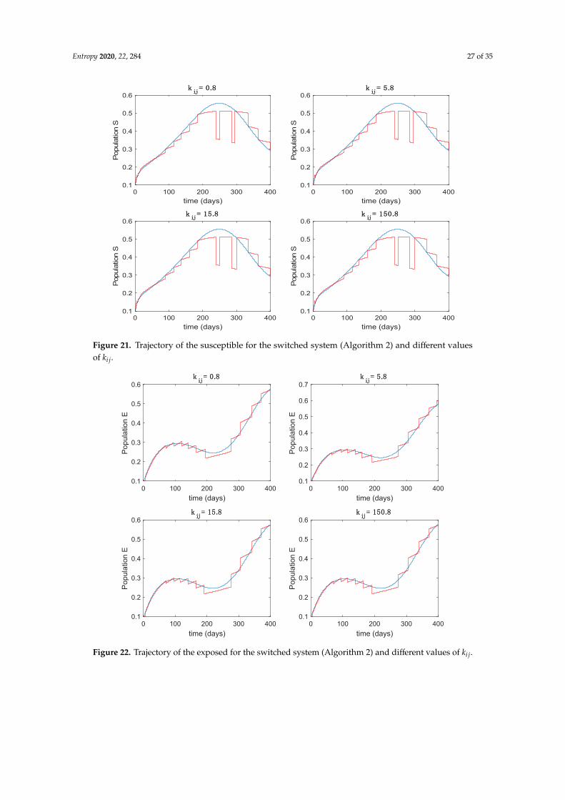
Entropy 2020, 22, 284 27 of 35

Entropy 2020, 22, 284 29 of 38

Figure 20. Active model within each time interval for Algorithm 2 and values 5=T days and 815.kij = .

Figure 21. Trajectory of the susceptible for the switched system (Algorithm 2) and different values of

ijk .

0 100 200 300 400time (days)

0

2

4

6

8

10

Activ

e m

odel

0 100 200 300 400time (days)

0

2

4

6

8

10

Activ

e m

odel

0 100 200 300 400time (days)

0

2

4

6

8

10

Activ

e m

odel

0 100 200 300 400time (days)

0

2

4

6

8

10

Activ

e m

odel

0 100 200 300 400time (days)

0.1

0.2

0.3

0.4

0.5

0.6

Popu

latio

n S

kij = 0.8

0 100 200 300 400time (days)

0.1

0.2

0.3

0.4

0.5

0.6

Popu

latio

n S

kij = 5.8

0 100 200 300 400time (days)

0.1

0.2

0.3

0.4

0.5

0.6

Popu

latio

n S

kij = 15.8

0 100 200 300 400time (days)

0.1

0.2

0.3

0.4

0.5

0.6

Popu

latio

n S

kij = 150.8

Figure 21. Trajectory of the susceptible for the switched system (Algorithm 2) and different valuesof ki j.

Entropy 2020, 22, 284 30 of 38

Figure 22. Trajectory of the exposed for the switched system (Algorithm 2) and different values of ijk.

Figure 23. Trajectory of the infectious for the switched system (Algorithm 2) and different values of kij .

0 100 200 300 400time (days)

0.1

0.2

0.3

0.4

0.5

0.6

Popu

latio

n E

kij = 150.8

0 100 200 300 400time (days)

0.1

0.2

0.3

0.4

0.5

0.6

Popu

latio

n E

kij = 15.8

0 100 200 300 400time (days)

0.1

0.2

0.3

0.4

0.5

0.6

0.7

Popu

latio

n E

kij = 5.8

0 100 200 300 400time (days)

0.1

0.2

0.3

0.4

0.5

0.6

Popu

latio

n E

kij = 0.8

0 100 200 300 400time (days)

0.02

0.04

0.06

0.08

0.1

Popu

latio

n I

kij = 0.8

0 100 200 300 400time (days)

0.02

0.04

0.06

0.08

0.1

Popu

latio

n I

kij = 5.8

0 100 200 300 400time (days)

0.02

0.04

0.06

0.08

0.1

Popu

latio

n I

kij = 15.8

0 100 200 300 400time (days)

0.02

0.04

0.06

0.08

0.1

Popu

latio

n I

kij = 150.8

Figure 22. Trajectory of the exposed for the switched system (Algorithm 2) and different values of ki j.

Entropy 2020, 22, 284 28 of 35

Entropy 2020, 22, 284 30 of 38

Figure 22. Trajectory of the exposed for the switched system (Algorithm 2) and different values of ijk.

Figure 23. Trajectory of the infectious for the switched system (Algorithm 2) and different values of kij .

0 100 200 300 400time (days)

0.1

0.2

0.3

0.4

0.5

0.6

Popu

latio

n E

kij = 150.8

0 100 200 300 400time (days)

0.1

0.2

0.3

0.4

0.5

0.6

Popu

latio

n E

kij = 15.8

0 100 200 300 400time (days)

0.1

0.2

0.3

0.4

0.5

0.6

0.7

Popu

latio

n E

kij = 5.8

0 100 200 300 400time (days)

0.1

0.2

0.3

0.4

0.5

0.6

Popu

latio

n E

kij = 0.8

0 100 200 300 400time (days)

0.02

0.04

0.06

0.08

0.1

Popu

latio

n I

kij = 0.8

0 100 200 300 400time (days)

0.02

0.04

0.06

0.08

0.1

Popu

latio

n I

kij = 5.8

0 100 200 300 400time (days)

0.02

0.04

0.06

0.08

0.1

Popu

latio

n I

kij = 15.8

0 100 200 300 400time (days)

0.02

0.04

0.06

0.08

0.1

Popu

latio

n I

kij = 150.8

Figure 23. Trajectory of the infectious for the switched system (Algorithm 2) and different values of ki j.

Entropy 2020, 22, 284 31 of 38

Figure 24. Trajectory of the immune for the switched system (Algorithm 2) and different values of

ijk .

From the above Figures we can conclude that the switched system, either with Algorithm 1 or with Algorithm 2, is able to reproduce the shape of the trajectories of the accurate-time-varying system. Consequently, the presented approach is useful to describe the overall dynamics of a complex set of data, coming either from real measurements or from a complex model, by means of a simpler piece-wise time-invariant model. The switching rules based on the entropy of the errors between each model and the data have revealed to be an adequate frame for such a task. Figures 10 and 15 show the active model selected within each time interval by Algorithm 1 to parameterize the switched system. Moreover, Figure 20 shows the active model when Algorithm 2 is employed. It is seen in Figure 20 how the algorithm selects a different model for each one of the state components of the system, which is the particularity of the algorithm. From the simulation results we can also observe that the probability value has a slight influence on the approximation performance and the selection of an appropriate value is not that critical. However, the switching time plays a more important role in the obtained performance as it can be deduced from the above examples. Moreover, there are no specific criteria for the selection of the switching time while a trial-error work can be performed in order to obtain an appropriate value for it. Finally, it can also be observed that Algorithm 1 is able to attain closer curves to the actual system than Algorithm 2, especially when it comes to the Susceptible population. The above figures show that the disease is persistent in the sense that the infectious do not vanish with time. Therefore, in the next Subsection 5.2 vaccination is used as external control to make the infectious converge to zero asymptotically.

5.2. Closed-Loop Control

In this subsection, vaccination is employed to avoid the persistency of the disease. To this end, the following state-feedback type vaccination law is used [29]:

)t(IK)t(SK)t(V activeIactiveS +=

0 100 200 300 400time (days)

0

0.02

0.04

0.06

0.08

0.1

Popu

latio

n R

kij = 150.8

0 100 200 300 400time (days)

0

0.02

0.04

0.06

0.08

0.1

Popu

latio

n R

kij = 15.8

0 100 200 300 400time (days)

0

0.02

0.04

0.06

0.08

0.1

Popu

latio

n R

kij = 5.8

0 100 200 300 400time (days)

0

0.02

0.04

0.06

0.08

0.1

Popu

latio

n R

kij = 0.8

Figure 24. Trajectory of the immune for the switched system (Algorithm 2) and different values of ki j.

From the above Figures we can conclude that the switched system, either with Algorithm 1 orwith Algorithm 2, is able to reproduce the shape of the trajectories of the accurate-time-varying system.Consequently, the presented approach is useful to describe the overall dynamics of a complex setof data, coming either from real measurements or from a complex model, by means of a simplerpiece-wise time-invariant model. The switching rules based on the entropy of the errors between each

Entropy 2020, 22, 284 29 of 35

model and the data have revealed to be an adequate frame for such a task. Figures 10 and 15 show theactive model selected within each time interval by Algorithm 1 to parameterize the switched system.Moreover, Figure 20 shows the active model when Algorithm 2 is employed. It is seen in Figure 20 howthe algorithm selects a different model for each one of the state components of the system, which is theparticularity of the algorithm. From the simulation results we can also observe that the probabilityvalue has a slight influence on the approximation performance and the selection of an appropriatevalue is not that critical. However, the switching time plays a more important role in the obtainedperformance as it can be deduced from the above examples. Moreover, there are no specific criteriafor the selection of the switching time while a trial-error work can be performed in order to obtainan appropriate value for it. Finally, it can also be observed that Algorithm 1 is able to attain closercurves to the actual system than Algorithm 2, especially when it comes to the Susceptible population.The above figures show that the disease is persistent in the sense that the infectious do not vanish withtime. Therefore, in the next Section 5.2 vaccination is used as external control to make the infectiousconverge to zero asymptotically.

5.2. Closed-Loop Control

In this subsection, vaccination is employed to avoid the persistency of the disease. To this end, thefollowing state-feedback type vaccination law is used [29]:

V(t) = KSSactive(t) + KIIactive(t)

with KS = 0.1 and KI = 0.01 being the state-feedback gains and Sactive(t), Iactive(t) the state componentsof the corresponding active model according to Algorithms 1 and 2. Along this section, T = 5 days andki j = 15.8. Figure 25 displays the evolution of the closed-loop system when Algorithm 1 is employedwhile Figure 26 shows the corresponding active model selected to parameterize the control commandwithin each time interval. Figure 27 shows the trajectories for Algorithm 2 and Figure 28 shows thecorresponding active model selected to parameterize the control command within each time interval.From Figures 25 and 27 we can conclude that the output of the real system and the output of theactive model are practically the same when a feedback control action is included in the system. Thus,the approximation errors appearing in open loop vanish in closed-loop because of the control action.Moreover, there are no differences in the closed-loop trajectories generated by Algorithms 1 and 2.It can also be observed in Figures 25 and 27 that the infectious tend to zero eradicating the disease fromthe population, as desired. Therefore, the control objective is achieved. Figures 29 and 30 display thevaccination function calculated by using both algorithms. It can be seen that both control commandsare very similar with only some peaks associated with the switching process making the differencebetween one and another. Overall, the proposed approach has been showed to be a powerful tool tomodel the complex time-varying system.

Entropy 2020, 22, 284 30 of 35

Entropy 2020, 22, 284 32 of 38

with 10.KS = and 010.KI = being the state-feedback gains and )t(Sactive , )t(Iactive the state components of the corresponding active model according to Algorithms 1 and 2. Along this section,

5=T days and 815.kij = . Figure 25 displays the evolution of the closed-loop system when

Algorithm 1 is employed while Figure 26 shows the corresponding active model selected to parameterize the control command within each time interval. Figure 27 shows the trajectories for Algorithm 2 and Figure 28 shows the corresponding active model selected to parameterize the control command within each time interval. From Figures 25 and 27 we can conclude that the output of the real system and the output of the active model are practically the same when a feedback control action is included in the system. Thus, the approximation errors appearing in open loop vanish in closed-loop because of the control action. Moreover, there are no differences in the closed-loop trajectories generated by Algorithms 1 and 2. It can also be observed in Figures 25 and 27 that the infectious tend to zero eradicating the disease from the population, as desired. Therefore, the control objective is achieved. Figures 29 and 30 display the vaccination function calculated by using both algorithms. It can be seen that both control commands are very similar with only some peaks associated with the switching process making the difference between one and another. Overall, the proposed approach has been showed to be a powerful tool to model the complex time-varying system.

Figure 25. Evolution of the closed-loop system when vaccination is applied and Algorithm 1 is used.

0 100 200 300 400 500time (days)

0

0.02

0.04

0.06

0.08

0.1

Popu

latio

n S

0 100 200 300 400 500time (days)

0

0.02

0.04

0.06

0.08

0.1

0.12

Popu

latio

n E

0 100 200 300 400 500time (days)

0

0.02

0.04

0.06

0.08

0.1

Popu

latio

n I

0 100 200 300 400 500time (days)

0

0.2

0.4

0.6

0.8

1

Popu

latio

n R

Figure 25. Evolution of the closed-loop system when vaccination is applied and Algorithm 1 is used.Entropy 2020, 22, 284 33 of 38

Figure 26. Active model when Algorithm 1 is employed.

Figure 27. Evolution of the closed-loop system when vaccination is applied and Algorithm 2 is used.

0 50 100 150 200 250 300 350 400 450time (days)

1

2

3

4

5

6

7

8

9

Activ

e m

odel

0 100 200 300 400 500time (days)

0

0.02

0.04

0.06

0.08

0.1

Popu

latio

n S

0 100 200 300 400 500time (days)

0

0.02

0.04

0.06

0.08

0.1

0.12

Popu

latio

n E

0 100 200 300 400 500time (days)

0

0.02

0.04

0.06

0.08

0.1

Popu

latio

n I

0 100 200 300 400 500time (days)

0

0.2

0.4

0.6

0.8

1

Popu

latio

n R

Figure 26. Active model when Algorithm 1 is employed.

Entropy 2020, 22, 284 31 of 35

Entropy 2020, 22, 284 33 of 38

Figure 26. Active model when Algorithm 1 is employed.

Figure 27. Evolution of the closed-loop system when vaccination is applied and Algorithm 2 is used.

0 50 100 150 200 250 300 350 400 450time (days)

1

2

3

4

5

6

7

8

9

Activ

e m

odel

0 100 200 300 400 500time (days)

0

0.02

0.04

0.06

0.08

0.1

Popu

latio

n S

0 100 200 300 400 500time (days)

0

0.02

0.04

0.06

0.08

0.1

0.12

Popu

latio

n E

0 100 200 300 400 500time (days)

0

0.02

0.04

0.06

0.08

0.1

Popu

latio

n I

0 100 200 300 400 500time (days)

0

0.2

0.4

0.6

0.8

1

Popu

latio

n R

Figure 27. Evolution of the closed-loop system when vaccination is applied and Algorithm 2 is used.

Entropy 2020, 22, 284 34 of 38

Figure 28. Active model when Algorithm 2 is employed.

Figure 29. Vaccination function for Algorithms 1 and 2.

Figure 30. Zoom on the vaccination function for Algorithms 1 and 2.

0 100 200 300 400 500time (days)

0

2

4

6

8

10

Activ

e m

odel

(S)

0 100 200 300 400 500time (days)

0

2

4

6

8

10

Activ

e m

odel

(E)

0 100 200 300 400 500time (days)

0

2

4

6

8

10

Activ

e m

odel

(I)

0 100 200 300 400 500time (days)

0

2

4

6

8

10

Activ

e m

odel

(R)

0 50 100 150 200 250 300 350 400 450time (days)

0

0.002

0.004

0.006

0.008

0.01

0.012

V(t)

120 140 160 180 200 220 240time (days)

2.8

2.9

3

3.1

3.2

3.3

3.4

3.5

3.6

10-3

Figure 28. Active model when Algorithm 2 is employed.

Entropy 2020, 22, 284 32 of 35

Entropy 2020, 22, 284 34 of 38

Figure 28. Active model when Algorithm 2 is employed.

Figure 29. Vaccination function for Algorithms 1 and 2.

Figure 30. Zoom on the vaccination function for Algorithms 1 and 2.

0 100 200 300 400 500time (days)

0

2

4

6

8

10

Activ

e m

odel

(S)

0 100 200 300 400 500time (days)

0

2

4

6

8

10

Activ

e m

odel

(E)

0 100 200 300 400 500time (days)

0

2

4

6

8

10

Activ

e m

odel

(I)

0 100 200 300 400 500time (days)

0

2

4

6

8

10

Activ

e m

odel

(R)

0 50 100 150 200 250 300 350 400 450time (days)

0

0.002

0.004

0.006

0.008

0.01

0.012

V(t)

120 140 160 180 200 220 240time (days)

2.8

2.9

3

3.1

3.2

3.3

3.4

3.5

3.6

10-3

Figure 29. Vaccination function for Algorithms 1 and 2.

Entropy 2020, 22, 284 34 of 38

Figure 28. Active model when Algorithm 2 is employed.

Figure 29. Vaccination function for Algorithms 1 and 2.

Figure 30. Zoom on the vaccination function for Algorithms 1 and 2.

0 100 200 300 400 500time (days)

0

2

4

6

8

10

Activ

e m

odel

(S)

0 100 200 300 400 500time (days)

0

2

4

6

8

10

Activ

e m

odel

(E)

0 100 200 300 400 500time (days)

0

2

4

6

8

10

Activ

e m

odel

(I)

0 100 200 300 400 500time (days)

0

2

4

6

8

10

Activ

e m

odel

(R)

0 50 100 150 200 250 300 350 400 450time (days)

0

0.002

0.004

0.006

0.008

0.01

0.012

V(t)

120 140 160 180 200 220 240time (days)

2.8

2.9

3

3.1

3.2

3.3

3.4

3.5

3.6

10-3

Figure 30. Zoom on the vaccination function for Algorithms 1 and 2.

5.3. Example with Actual Data

In this subsection the proposed entropy approach is applied to the real case of measles in the city ofNew York. In this way, it was stated in [33] that measles outbreaks in NYC during the period 1930–1970can be appropriately described by a SIR model with a time-varying contact rate. Moreover, [33]estimates a monthly contact rate for the model while [34] proposes a Dietz-type contact rate for thisproblem. Thus, this real situation fits in with the formulation treated in the application problem.The authors of [34] gathered the weekly amount of reported measles cases for 93 years correspondingto the period 1891–1984 and made them publicly available as a supplementary material of [34]. In thissimulation, the Algorithm 2 from Section 4 will be used to generate a switched model describing thedata set of the year 1960. The SIR model describing the problem is given by:

dSdt = ν− β(t)SI − µS

dIdt = β(t)SI − (γ+ µ)I

dRdt = γI − µR

(52)

The parameters of the model are estimated in [34] to be γ−1 = 13 days, µ = 0.02yr−1,βmin = 1.79 · 10−10, βmax = 5.3831 · 10−10 and the yearly number of new born is approximately 105.The initial values of the populations are S(0) = 7782000, the population of New York in 1960, I(0) = 225and R(0) = 0 while T = 20 days. There are 40 time-invariant models linearly spaced between βmin andβmax. Actual data for the infectious are used in (49) in order to calculate the error corresponding toeach one of models running in parallel. The Figure 31 shows the number infectious predicted by theswitched model compared to the actual data during 1960. The x axis of the figure represents the 52weeks of the year.

Entropy 2020, 22, 284 33 of 35

Entropy 2020, 22, 284 35 of 38

5.3. Example with Actual Data

In this subsection the proposed entropy approach is applied to the real case of measles in the city of New York. In this way, it was stated in [33] that measles outbreaks in NYC during the period 1930-1970 can be appropriately described by a SIR model with a time-varying contact rate. Moreover, [33] estimates a monthly contact rate for the model while [34] proposes a Dietz-type contact rate for this problem. Thus, this real situation fits in with the formulation treated in the application problem. The authors of [34] gathered the weekly amount of reported measles cases for 93 years corresponding to the period 1891–1984 and made them publicly available as a supplementary material of [34]. In this simulation, the Algorithm 2 from Section 4 will be used to generate a switched model describing the data set of the year 1960. The SIR model describing the problem is given by:

dSdt

= ν − β (t )SI − μS

dIdt

= β (t )SI − (γ + μ)I

dRdt

= γ I − μR

(52)

The parameters of the model are estimated in [34] to be γ −1 = 13 days, μ = 0.02 yr −1 ,

βmin = 1.79 ⋅10−10 , βmax = 5.3831⋅10−10 and the yearly number of new born is approximately 105 . The initial values of the populations are S (0) = 7782000, the population of New York in 1960, I (0) = 225

and R (0) = 0 while T = 20 days. There are 40 time-invariant models linearly spaced between βmin

and βmax . Actual data for the infectious are used in (49) in order to calculate the error corresponding to each one of models running in parallel. The Figure 31 shows the number infectious predicted by the switched model compared to the actual data during 1960. The x axis of the figure represents the 52 weeks of the year.

Figure 31. Comparison of the output of the switched model with the actual data set for 1960.

As it can be observed from Figure 31 the proposed approach succeeds at reproducing the trend contained in the data and predicting the time when the outbreak reaches the peak. Finally, the Figure 32 shows the active model at each time for the infectious population. Since the data are only available for the infectious, only this population has been displayed in the figures.

0 10 20 30 40 50 60time (weeks)

0

500

1000

1500

2000

2500

3000

3500

Popu

latio

n I

IswitchedActual data

Figure 31. Comparison of the output of the switched model with the actual data set for 1960.

As it can be observed from Figure 31 the proposed approach succeeds at reproducing the trendcontained in the data and predicting the time when the outbreak reaches the peak. Finally, the Figure 32shows the active model at each time for the infectious population. Since the data are only available forthe infectious, only this population has been displayed in the figures.Entropy 2020, 22, 284 36 of 38

Figure 32. Active model selected at each time interval for the infectious population.

6. Conclusions

This paper has presented results for the Shannon entropy when a complete the events of a complete finite and discrete set are eventually subject to relative errors of their associate probabilities. As a result, the current system of events, eventually under probabilistic errors, can lose its completeness since it may be either deflated or inflated in the sense that the total probability for the whole sets might be either below or beyond unity. Later on the previous technical results have been applied to control of epidemics evolution in the case that either the disease transmission coefficient rate is not well-known or it varies through time due, for instance, to seasonality. For such a purpose, a finite predefined set of running models, described by coupled differential equations, is chosen which covers a range of variation of such a coefficient transmission rate within known lower-bound and upper-bound limits. Each one of such models is driven by a constant disease transmission rate and the whole set of models covers the whole range of foreseen variation of such a parameter in the real system. In a general context, different uncertain parameters, or groups of parameters, other that the coefficient transmission rate could be checked by the proposed minimum-error entropy supervisory scheme. Two monitoring algorithms have been proposed to select the active one which minimizes the accumulated entropy of the absolute error data/model within each supervision time interval. A switching rule allows to choose another active model as soon as it is detected that the current active model becomes more uncertain than other (s) related to the observed data. Some numerical results have been also performed and discussed including a discussion on a real registered case. The active model, which is currently in operation, generates the vaccination and/or treatment controls to be injected to the real epidemic process.

Author Contributions Data curation, A.I.; Formal analysis, M.D.l.S.; Funding acquisition, M.D.l.S.; Investigation, M.D.l.S.; Methodology, M.D.l.S.; Project administration, M.D.l.S.; Resources, M.D.l.S. and A.I.; Software, A.I.; Supervision, M.D.l.S.; Validation, A.I. and R.N.; Visualization, A.I.; Writing–review and editing, R.N. All authors have read and agreed to the published version of the manuscript.

Funding: The authors are grateful to the Spanish Government for Grant RTI2018-094336-B-I00 (MCIU/AEI/FEDER, UE) and to the Basque Government for Grant IT1207-19.

Conflicts of Interest: The authors declare no conflict of interest.

References.

1. Khinchin, A.I. Mathematical Foundations of Information Theory; Dover Publications Inc.: New York, NY, USA, 1957.

2. Aczel, J.D.; Daroczy, Z. On Measures of Information and Their Generalizations; Academic Press: New York, NY, USA, 1975.

0 10 20 30 40 50 60time (weeks)

22

24

26

28

30

32

34

36

38

40

Activ

e m

odel

for t

he In

fect

ious

Figure 32. Active model selected at each time interval for the infectious population.

6. Conclusions

This paper has presented results for the Shannon entropy when a complete the events of a completefinite and discrete set are eventually subject to relative errors of their associate probabilities. As a result,the current system of events, eventually under probabilistic errors, can lose its completeness since itmay be either deflated or inflated in the sense that the total probability for the whole sets might beeither below or beyond unity. Later on the previous technical results have been applied to control ofepidemics evolution in the case that either the disease transmission coefficient rate is not well-knownor it varies through time due, for instance, to seasonality. For such a purpose, a finite predefined setof running models, described by coupled differential equations, is chosen which covers a range ofvariation of such a coefficient transmission rate within known lower-bound and upper-bound limits.Each one of such models is driven by a constant disease transmission rate and the whole set of modelscovers the whole range of foreseen variation of such a parameter in the real system. In a generalcontext, different uncertain parameters, or groups of parameters, other that the coefficient transmissionrate could be checked by the proposed minimum-error entropy supervisory scheme. Two monitoringalgorithms have been proposed to select the active one which minimizes the accumulated entropy of

Entropy 2020, 22, 284 34 of 35

the absolute error data/model within each supervision time interval. A switching rule allows to chooseanother active model as soon as it is detected that the current active model becomes more uncertain thanother (s) related to the observed data. Some numerical results have been also performed and discussedincluding a discussion on a real registered case. The active model, which is currently in operation,generates the vaccination and/or treatment controls to be injected to the real epidemic process.

Author Contributions: Data curation, A.I.; Formal analysis, M.D.l.S.; Funding acquisition, M.D.l.S.; Investigation,M.D.l.S.; Methodology, M.D.l.S.; Project administration, M.D.l.S.; Resources, M.D.l.S. and A.I.; Software, A.I.;Supervision, M.D.l.S.; Validation, A.I. and R.N.; Visualization, A.I.; Writing—review and editing, R.N. All authorshave read and agreed to the published version of the manuscript.

Funding: The authors are grateful to the Spanish Government for Grant RTI2018-094336-B-I00 (MCIU/AEI/FEDER,UE) and to the Basque Government for Grant IT1207-19.

Conflicts of Interest: The authors declare no conflict of interest.

References

1. Khinchin, A.I. Mathematical Foundations of Information Theory; Dover Publications Inc.: New York, NY, USA,1957.

2. Aczel, J.D.; Daroczy, Z. On Measures of Information and Their Generalizations; Academic Press: New York, NY,USA, 1975.

3. Ash, R.B. Information Theory; Interscience Publishers: New York, NY, USA; John Wiley and Sons: Hoboken,NJ, USA, 1965.

4. Feynman, R.P. Simulating Physics and Computers. Int. J. Theor. Phys. 1982, 21, 467–488. [CrossRef]5. Burgin, M.; Meissner, G. Larger than one probabilities in mathematical and practical finance. Rev. Econ.

Financ. 2012, 2, 1–13.6. Tenreiro-Machado, J. Fractional derivatives and negative probabilities. Commun. Nonlinear Sci. Numer. Simul.

2019, 79, 104913. [CrossRef]7. Baez, J.C.; Fritz, T.; Leinster, T. A characterization of entropy in terms of information loss. Entropy 2011, 2011,

1945–1957. [CrossRef]8. Delyon, F.; Foulon, P. Complex entropy for dynamic systems. Ann. Inst. Henry Poincarè Phys. Théor. 1991, 55,

891–902.9. Nalewajski, R.F. Complex entropy, resultant information measures. J. Math. Chem. 2016, 54, 1777–2782.

[CrossRef]10. Goh, S.; Choi, J.; Choi, M.Y.; Yoon, B.G. Time evolution of entropy in a growth model: Dependence of the

description. J. Korean Phys. Soc. 2017, 70, 12–21. [CrossRef]11. Wang, W.B.; Wu, Z.N.; Wang, C.F.; Hu, R.F. Modelling the spreading rate of controlled communicable

epidemics through and entropy-based thermodynamic model. Sci. China Phys. Mech. Astron. 2013, 56,2143–2150. [CrossRef]

12. Tiwary, S. The evolution of entropy in various scenarios. Eur. J. Phys. 2019, 41, 1–11. [CrossRef]13. Koivu-Jolma, M.; Annila, A. Epidemic as a natural process. Math. Biosci. 2018, 299, 97–102. [CrossRef]14. Artalejo, J.R.; Lopez-Herrero, M.J. The SIR and SIS epidemic models. A maximum entropy approach.

Theor. Popul. Biol. 2011, 80, 256–264. [CrossRef] [PubMed]15. Erten, E.Y.; Lizier, J.T.; Piraveenan, M.; Prokopenko, M. Criticality and information dynamics in

epidemiological models. Entropy 2017, 19, 194. [CrossRef]16. De la Sen, M. On the approximated reachability of a class of time-varying systems based on their linearized

behaviour about the equilibria: Applications to epidemic models. Entropy 2019, 2019, 1–31.17. Meyers, L. Contact network epidemiology: Bond percolation applied to infectious disease prediction and

control. Bull. Am. Math. Soc. 2007, 44, 63–86. [CrossRef]18. Cui, Q.; Qiu, Z.; Liu, W.; Hu, Z. Complex dynamics of an SIR epidemic model with nonlinear saturated

incidence and recovery rate. Entropy 2017, 2017, 1–16.19. Nistal, R.; de la Sen, M.; Alonso-Quesada, S.; Ibeas, A. Supervising the vaccinations and treatment control

gains in a discrete SEIADR epidemic model. Int. J. Innov. Comput. Inf. Control 2019, 15, 2053–2067.

Entropy 2020, 22, 284 35 of 35

20. Verma, R.; Sehgal, V.K.; Nitin, V. Computational stochastic modelling to handle the crisis occurred duringcommunity epidemic. Ann. Data Sci. 2016, 3, 119–133. [CrossRef]

21. Iggidr, A.; Souza, M.O. State estimators for some epidemiological systems. Math. Biol. 2019, 78, 225–256.[CrossRef]

22. Yang, H.M.; Ribas-Freitas, A.R. Biological view of vaccination described by mathematical modellings: Fromrubella to dengue vaccines. Math. Biosci. Eng. 2018, 16, 3185–3214.

23. De la Sen, M. On the design of hyperstable feedback controllers for a class of parameterized nonlinearities.Two application examples for controlling epidemic models. Int. J. Environ. Res. Public Health 2019, 16, 2689.[CrossRef]

24. De la Sen, M. Parametrical non-complex tests to evaluate partial decentralized linear-output feedback controlstabilization conditions for their centralized stabilization counterparts. Appl. Sci. 2019, 9, 1739. [CrossRef]

25. Abdullahi, A.; Shohaimi, S.; Kilicman, A.; Ibrahim, M.H.; Salari, N. Stochastic SIS modelling: Coinfection oftwo pathogens in two-host communities. Entropy 2019, 22, 54. [CrossRef]

26. Li, Y.; Cai, W.; Li, Y.; Du, X. Key node ranking in complex networks: A novel entropy and mutualinformation-based approach. Entropy 2019, 22, 52. [CrossRef]

27. Nakata, Y.; Kuniya, T. Global dynamics of a class of SEIRS epidemic models in a periodic environment.J. Math. Anal. Appl. 2010, 363, 230–237. [CrossRef]

28. De la Sen, M.; Alonso-Quesada, S. Control issues for the Beverton-Holt equation in ecology by locallymonitoring the environment carrying capacity: Non-adaptive and adaptive cases. Appl. Math. Comput. 2009,215, 2616–2633. [CrossRef]

29. De la Sen, M.; Ibeas, A.; Alonso-Quesada, S.; Nistal, R. On a SIR model in a patchy environment underconstant and feedback decentralized controls with asymmetric parameterizations. Symmetry 2019, 11, 430.[CrossRef]

30. Buonomo, B.; Chitnis, N.; d’Onofrio, A. Seasonality in epidemic models: A literature review. Ric. Mat. 2018,67, 7–25. [CrossRef]

31. Pewsner, D.; Battaglia, M.; Minder, C.; Markx, A.; Bucher, H.C. Ruling a diagnosis in or with “SpPin” and“SnOut”: A note of caution. Br. Med. J. 2004, 329, 209–213. [CrossRef]

32. Facente, S.N.; Dowling, T.; Vittinghoff, E.; Sykes, D.L.; Colfax, G.N. False positive rate of rapid oral fluid VIHtest increases as kits near expiration date. PLoS ONE 2009, 4, e8217. [CrossRef]

33. London, W.P.; Yorke, J. Recurrent outbreaks of measles, chickenpox and mumps. I Seasonal variations incontact rates. Am. J. Epidemiol. 1973, 98, 453–468. [CrossRef]

34. Hempel, K.; Earn, D.J.D. A century of transitions in New York City’s measles dynamics. J. R. Soc. Interface2015, 12, 20150024. [CrossRef] [PubMed]

© 2020 by the authors. Licensee MDPI, Basel, Switzerland. This article is an open accessarticle distributed under the terms and conditions of the Creative Commons Attribution(CC BY) license (http://creativecommons.org/licenses/by/4.0/).