ESTIMATION OF LINEAR PANEL DATA MODELS USING GMM

Seung Chan AhnArizona State University, Tempe, AZ 85287, USA

Peter SchmidtMichigan State University, E. Lansing, MI 48824, USA

August 1997

Revised: October 1998

Abstract

In this chapter we study GMM estimation of linear panel data models. Several different typesof models are considered, including the linear regression model with strictly or weakly exogenousregressors, the simultaneous regression model, and a dynamic linear model containing a laggeddependent variable as a regressor. In each case, different assumptions about the exogeneity ofthe explanatory variables generate different sets of moment conditions that can be used inestimation. This chapter lists the relevant sets of moment conditions and gives some results onsimple ways in which they can be imposed. In particular, attention is paid to the question ofunder what circumstances the efficient GMM estimator takes the form of an instrumentalvariables estimator.

Chapter 8

ESTIMATION OF LINEAR PANEL DATA MODELS USINGGMM

Seung C. Ahn and Peter Schmidt

Use of panel data regression methods has become increasingly popular as the availability of

longitudinal data sets has grown. Panel data contain repeated time-series observations (T) for a

large number (N) of cross-sectional units (e.g., individuals, households, or firms). An important

advantage of using such data is that they allow researchers to control for unobservable

heterogeneity, that is, systematic differences across cross-sectional units. Regressions using

aggregated time-series and pure cross-section data are likely to be contaminated by these effects,

and statistical inferences obtained by ignoring these effects could be seriously biased. When

panel data are available, error-components models can be used to control for these individual

differences. Such a model typically assumes that the stochastic error term has two components:

a time-invariant individual effect which captures the unobservable individual heterogeneity and

the usual random noise term. Some explanatory variables (e.g., years of schooling in the earnings

equation) are likely to be correlated with the individual effects (e.g., unobservable talent or IQ).

A simple treatment to this problem is the within estimator which is equivalent to least squares

after transformation of the data to deviations from means.

Unfortunately, the within method has two serious defects. First, the within transformation of

a model wipes out time invariant regressors as well as the individual effect, so that it is not

possible to estimate the effects of time-invariant regressors on the dependent variable. Second,

consistency of the within estimator requires that all the regressors in a given model be strictly

1

exogenous with respect to the random noise. The within estimator could be inconsistent for

models in which regressors are only weakly exogenous, such as dynamic models including

lagged dependent variables as regressors. In response to these problems, a number of studies

have developed alternative GMM estimation methods.

In this chapter we provide a systematic account of GMM estimation of linear panel data

models. Several different types of models are considered, including the linear regression model

with strictly or weakly exogenous regressors, the simultaneous regression model, and a dynamic

linear model containing a lagged dependent variable as a regressor. In each case, different

assumptions about the exogeneity of the explanatory variables generate different sets of moment

conditions that can be used in estimation. This chapter lists the relevant sets of moment

conditions and gives some results on simple ways in which they can be imposed. In particular,

attention is paid to the question of under what circumstances the efficient GMM estimator takes

the form of an instrumental variables estimator.1

8.1 Preliminaries

In this section we introduce the general model of interest, some basic assumptions, and some

notation. Given linear moment conditions, we consider the efficient GMM estimator and other

related instrumental variables estimators. We also examine general conditions under which the

efficient GMM estimator is of an instrumental variables form.

8.1.1 General Model

The models we examine in this chapter are of the following common form:

1Here and throughout this chapter, "efficient" means "asymptotically efficient."

2

Here i = 1, ... , Nindexes the cross-sectional unit (individual) and t = 1, ... , Tindexes time.

(8-1)

The dependent variable is yit, while xit is a 1 × pvector of explanatory variables. The p × 1

parameter vectorβ is unknown. The composite error uit contains a time invariant individual

effect αi and random noiseεit. We assume that E(αi) = 0 and E(εit) = 0 for any i and t; thus,

E(uit) = 0. The time dimension T is held fixed, so that usual asymptotics apply as N gets large.

We also assume that the data (yi1,yi2,...,yiT,xi1,...,xiT)′ i = 1,...,N are independently and

identically distributed (iid) over different i and have finite population moments up to fourth

order. Under this assumption, any sample moment (up to fourth order) of the data converges to

its counterpart population moment in probability, e.g., plimN→∞N-1ΣNi =1xit′yit = E(xit′yit).

Some matrix notation is useful throughout this chapter. For any single variable cit or row

vector dit, we denote ci ≡ (ci1, ... , ciT)′ and Dit ≡ (di1′, ... , diT′)′. Accordingly, yi and Xi denote

the data matrices of T rows. In addition, for any T × 1 vector ci or T × k matrix Di, we denote

c ≡ (c1′, ... , cN′)′ and D = (D1′, ... , DN′)′. Accordingly, y and X denote the data matrices of NT

rows. With this notation, we can rewrite equation (8-1) for individual i as

where eT is a T × 1vector of ones, and all NT observations as y = Xβ + u.

(8-2)

We treat the individual effectsαi as random, so that we can defineΣ ≡ Cov(ui) = E(uiui′). A

standard and popular assumption aboutΣ is so-called the random effects structure

which arises if theεit are iid over time and independent ofαi. This covariance structure often

(8-3)

takes an important role in GMM estimation as we discuss below.

3

There are two well-known special cases of the model (8-2); the traditional random effects

and fixed effects models. Both of these models assume that the regressors Xi are strictly

exogenous with respect to the random noiseεi (i.e., E(xit′εis) = 0 for any t and s). The random

effects model (Balestra and Nerlove [1966]) treats the individual effects as random

unobservables which are uncorrelated with all of the regressors. Under this assumption, the

parameterβ can be consistently and efficiently estimated by generalized least squares (GLS):

βGLS = (X′Ω-1X)-1X′Ω-1y, whereΩ = IN⊗Σ.

In contrast, when we treat theαi as nuisance parameters, the model (8-2) reduces to the

traditional fixed effects model. A simple treatment of the fixed effects model is to remove the

effects by the (within) transformation of the model (8-2) to deviations from individual means:

where QT = IT - PT, PT = T-1eTeT′, and the last equality results from QTeT = 0. Least squares on

(8-4)

(8-4) yields the familiar within estimator:βW = (X′QVX)-1X′QVy, where QV = IN⊗QT.

Although the fixed effects model views the effectsαi as nuisance parameters rather than

random variables, the fixed effects treatment (within estimation) is not inconsistent with the

random effects assumption. Mundlak [1978] considers an alternative random effects model in

which the effectsαi are allowed to be correlated with all of the regressors xi1,...,xiT. For this

model, Mundlak shows that the within estimator is an efficient GLS estimator. This finding

implies that the core difference between the random and fixed effects models is not whether the

effects are literally random or nuisance parameters, but whether the effects are correlated or

uncorrelated with the regressors.

8.1.2 GMM and Instrumental Variables

4

In this subsection we examine GMM and other related instrumental variables estimators for the

model (8-2). Our main focus is a general treatment of given moment conditions, so we do not

make any specific exogeneity assumption regarding the regressors Xi. We simply begin by

assuming that there exists a set of T × k instruments Zi which satisfies the moment condition

and the usual identification condition, rank[E(Zi′Xi)] = p.

(8-5)

Under (8-5) and other usual regularity conditions, a consistent and efficient estimate ofβ can

be obtained by minimizing the GMM criterion function N(y-Xβ)′Z(VN)-1Z′(y-Xβ), where VN is

any consistent estimate of V≡ E(Zi′uiui′Zi). A simple choice of VN is

N-1ΣNi =1Zi′uiui′Zi ,

where ui = yi - Xiβ and β is an initial consistent estimator such as two-stage least squares

(2SLS). The solution to the minimization leads to the GMM estimator:

βGMM ≡ [X ′Z(VN)-1Z′X] -1X′Z(VN)-1Z′y .

An instrumental variables estimator, which is closely related with this GMM estimator, is

three stages least squares (3SLS):

β3SLS ≡ [X ′Z(Z′ΩZ)-1Z′X] -1X′Z(Z′ΩZ)-1Z′y ,

whereΩ = IN⊗Σ. For notational convenience, we assume thatΣ is known, although, in practice,

it should be replaced by a consistent estimate such asΣ = N-1ΣNi =1uiui′. In order to understand

the relationship between the GMM and 3SLS estimators, consider the following condition

Under this condition, the 3SLS estimator is asymptotically identical to the GMM estimator,

(8-6)

because plimN→∞N-1Z′ΩZ = plimN→∞N-1ΣNi =1Ziuiui′Zi = E(Zi′uiui′Zi) = V. We will refer to (8-6) as

5

the condition of no conditional heteroskedasticity (NCH). This is a slight misuse of

terminology, since (8-6) is weaker than the condition that E(uiui′ Zi) = Σ. However, (8-6) is

what is necessary for the 3SLS estimator to coincide with the GMM estimator. When (8-6) is

violated,βGMM is strictly more efficient thanβ3SLS.

An alternative to the 3SLS estimator, which is popularly used in the panel data literature, is

the 2SLS estimator obtained by premultiplying (8-2) byΣ-½ to filter ui, and then applying the

instruments Zi:

βFIV ≡ [X ′Ω-½Z(Z′Z)-1Z′Ω-½X] -1X′Ω-½Z(Z′Z)-1Z′Ω-½y .

We refer to this estimator as the filtered instrumental variables (FIV) estimator. This estimator

is slightly different from the generalized instrumental variables (GIV) estimator, which is

originally proposed by White [1984]. The GIV estimator is also 2SLS applied to the filtered

modelΣ-½yi = Σ-½Xiβ + Σ-½ui, but it uses the filtered instrumentsΣ-½Xi. Thus

βGIV ≡ [X ′Ω-1Z(Z′Ω-1Z)-1Z′Ω-1X] -1X′Ω-1Z(Z′Ω-1Z)-1Z′Ω-1y .

Despite this difference, the FIV and GIV estimators are often equivalent in the context of panel

data models, especially whenΣ is of the random effects structure (8-3). We may also note that

the FIV and GIV estimators would be of little interest without the NCH assumption.

A motivation for the FIV (or GIV) estimator is that filtering the error ui may improve the

efficiency of instrumental variables, as GLS improves upon ordinary least squares (OLS).2

However, neither of the 3SLS nor FIV estimators can be shown to generally dominate the other.

This is so because the FIV estimator is a GMM estimator based on the different moment

condition E(Zi′Σ-½ui) =0 and the different NCH assumption E(Zi′Σ-½uiui′Σ-½Zi) = E(Zi′Zi).

We now turn to conditions under which the 3SLS and FIV estimators are numerically

2White [1984] offers some strong conditions under which the GIV estimator dominatesthe 3SLS estimator in terms of efficiency.

6

equivalent, whenever the same estimate ofΣ is used.

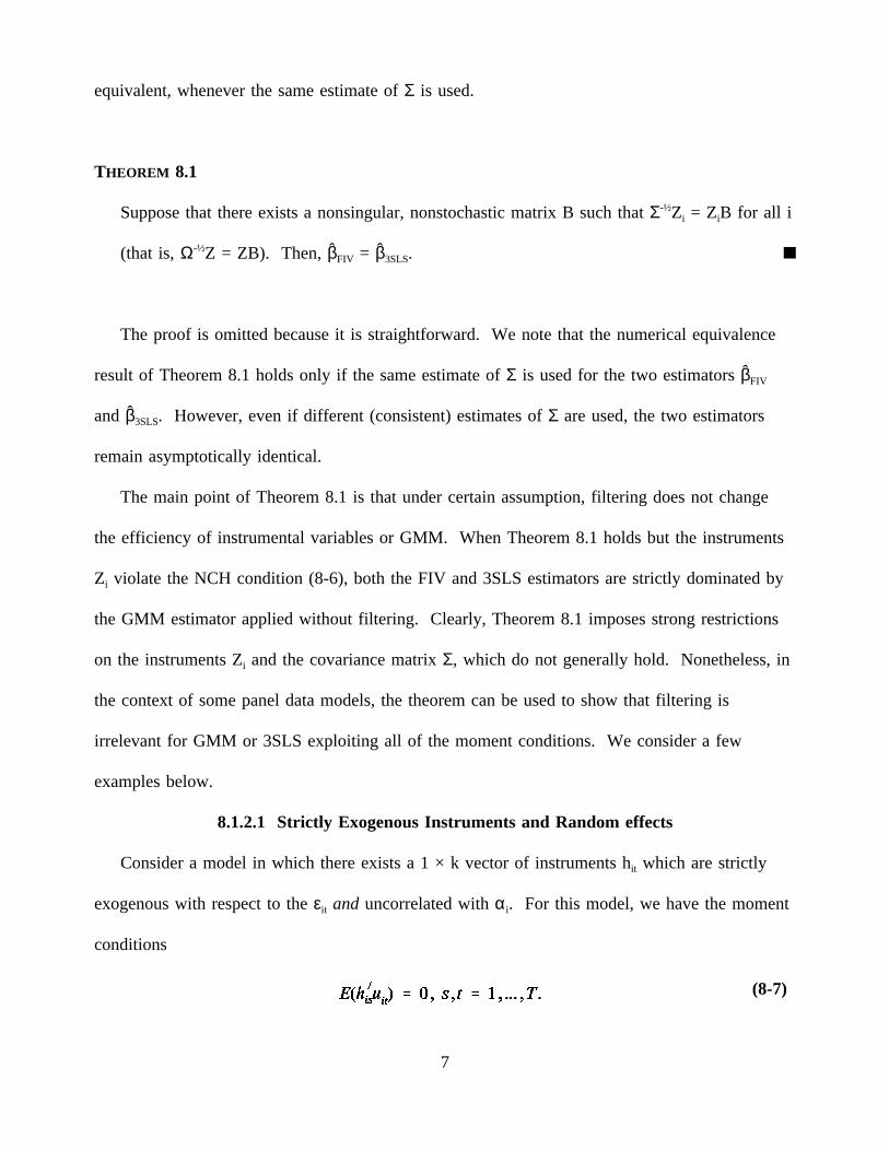
THEOREM 8.1

Suppose that there exists a nonsingular, nonstochastic matrix B such thatΣ-½Zi = ZiB for all i

(that is,Ω-½Z = ZB). Then,βFIV = β3SLS.

The proof is omitted because it is straightforward. We note that the numerical equivalence

result of Theorem 8.1 holds only if the same estimate ofΣ is used for the two estimatorsβFIV

and β3SLS. However, even if different (consistent) estimates ofΣ are used, the two estimators

remain asymptotically identical.

The main point of Theorem 8.1 is that under certain assumption, filtering does not change

the efficiency of instrumental variables or GMM. When Theorem 8.1 holds but the instruments

Zi violate the NCH condition (8-6), both the FIV and 3SLS estimators are strictly dominated by

the GMM estimator applied without filtering. Clearly, Theorem 8.1 imposes strong restrictions

on the instruments Zi and the covariance matrixΣ, which do not generally hold. Nonetheless, in

the context of some panel data models, the theorem can be used to show that filtering is

irrelevant for GMM or 3SLS exploiting all of the moment conditions. We consider a few

examples below.

8.1.2.1 Strictly Exogenous Instruments and Random effects

Consider a model in which there exists a 1 × kvector of instruments hit which are strictly

exogenous with respect to theεit and uncorrelated withαi. For this model, we have the moment

conditions

(8-7)

7

This is a set of kT2 moment conditions. Denote hoit ≡ (hi1,...,hit) for any t = 1,...,T, and set ZSE,i ≡

IT⊗hoiT, so that all of the moment conditions (8-7) can be expressed compactly as E(ZSE,i′ui) = 0.

We now show that filtering the error ui does not matter in GMM. Observe that for any T ×

T nonsingular matrix A,

AZSE,i = A(IN⊗hoiT) = A⊗ho

iT = (IN⊗hoiT)(A⊗IkT) = ZSE,iB ,

where B = A⊗IkT. If we replace A byΣ-½, Theorem 8.1 holds.

8.1.2.2 Strictly Exogenous Instruments and Fixed Effects

We now allow the instruments hit to be correlated withαi (fixed effects), while they are still

assumed to be strictly exogenous with respect to theεit. For this case, we may first-difference

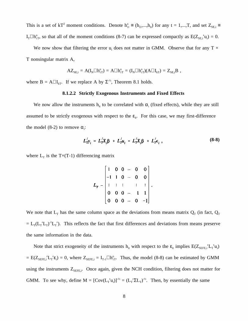
the model (8-2) to removeαi:

where LT is the T×(T-1) differencing matrix

(8-8)

We note that LT has the same column space as the deviations from means matrix QT (in fact, QT

= LT(LT′LT)-1LT′). This reflects the fact that first differences and deviations from means preserve

the same information in the data.

Note that strict exogeneity of the instruments hit with respect to theεit implies E(ZSEFE,i′LT′ui)

= E(ZSEFE,i′LT′εi) = 0, where ZSEFE,i = IT-1⊗hoiT. Thus, the model (8-8) can be estimated by GMM

using the instruments ZSEFE,i. Once again, given the NCH condition, filtering does not matter for

GMM. To see why, define M = [Cov(LT′ui)]-½ = (LT′ΣLT)

-½. Then, by essentially the same

8

algebra as in the previous subsection, we can show the FIV estimator applying the instruments

ZSEFE,i and the filter M to (8-8) equals the 3SLS estimator applying the same instruments to (8-

8).

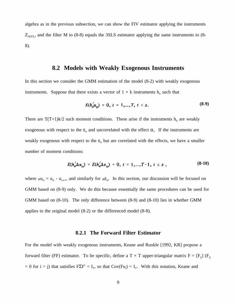
8.2 Models with Weakly Exogenous Instruments

In this section we consider the GMM estimation of the model (8-2) with weakly exogenous

instruments. Suppose that there exists a vector of 1 × k instruments hit such that

There are T(T+1)k/2 such moment conditions. These arise if the instruments hit are weakly

(8-9)

exogenous with respect to theεit and uncorrelated with the effectαi. If the instruments are

weakly exogenous with respect to theεit but are correlated with the effects, we have a smaller

number of moment conditions:

where uis = uis - ui,s-1, and similarly for εis. In this section, our discussion will be focused on

(8-10)

GMM based on (8-9) only. We do this because essentially the same procedures can be used for

GMM based on (8-10). The only difference between (8-9) and (8-10) lies in whether GMM

applies to the original model (8-2) or the differenced model (8-8).

8.2.1 The Forward Filter Estimator

For the model with weakly exogenous instruments, Keane and Runkle [1992, KR] propose a

forward filter (FF) estimator. To be specific, define a T × Tupper-triangular matrix F = [Fij] (Fij

= 0 for i > j) that satisfies FΣF′ = IT, so that Cov(Fui) = IT. With this notation, Keane and

9

Runkle propose a FIV-type estimator, which applies the instruments Hi ≡ (hi1′,,,.,hiT′)′ after

filtering the error ui by F:

βFF = [X ′F*′H(H′H)-1H′F*X] -1X′F*′H(H′H)-1H′F*y ,

where F* = IN⊗F.

The motivation of this FF estimator is that the FIV estimator using the instruments Hi and

the usual filterΣ-½ is inconsistent unless the instruments Hi are strictly exogenous with respect to

the εi. In contrast, the forward-filtering transformation F preserves the weak exogeneity of the

instruments hit. Hayashi and Sims [1983] provide some efficiency results for this forward

filtering in the context of time series data. However, in the context of panel data (with large N

and fixed T), the FF estimator does not necessarily dominate the GMM or 3SLS estimators using

the same instruments Hi.

One technical point is worth noting for the FF estimator. Forward filtering requires that the

serial correlations in the error ui do not depend on the values of current and lagged values of the

instruments hit. (See Hayashi and Sims (1983), pp. 788-789.) This is a slightly weakened

version of the usual condition of no conditional heteroskedasticity; it is weakened because

conditioning is only on current and lagged values of the instruments. If this condition does not

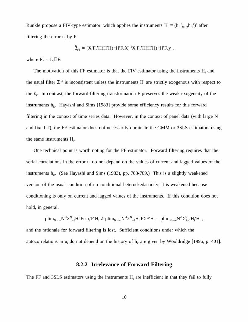
hold, in general,

plimN→∞N-1ΣNi =1Hi′Fuiui′F′Hi ≠ plimN→∞N-1ΣN

i =1Hi′FΣF′Hi = plimN→∞N-1ΣNi =1Hi′Hi ,

and the rationale for forward filtering is lost. Sufficient conditions under which the

autocorrelations in ui do not depend on the history of hit are given by Wooldridge [1996, p. 401].

8.2.2 Irrelevance of Forward Filtering

The FF and 3SLS estimators using the instruments Hi are inefficient in that they fail to fully

10

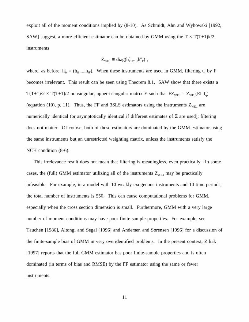
exploit all of the moment conditions implied by (8-10). As Schmidt, Ahn and Wyhowski [1992,

SAW] suggest, a more efficient estimator can be obtained by GMM using the T × T(T+1)k/2

instruments

ZWE,i ≡ diag(hoi1,...,h

oiT) ,

where, as before, hoi t = (hi1,...,hiT). When these instruments are used in GMM, filtering ui by F

becomes irrelevant. This result can be seen using Theorem 8.1. SAW show that there exists a

T(T+1)/2 × T(T+1)/2 nonsingular, upper-triangular matrix E such that FZWE,i = ZWE,i(E⊗Iq)

(equation (10), p. 11). Thus, the FF and 3SLS estimators using the instruments ZWE,i are

numerically identical (or asymptotically identical if different estimates ofΣ are used); filtering

does not matter. Of course, both of these estimators are dominated by the GMM estimator using

the same instruments but an unrestricted weighting matrix, unless the instruments satisfy the

NCH condition (8-6).

This irrelevance result does not mean that filtering is meaningless, even practically. In some

cases, the (full) GMM estimator utilizing all of the instruments ZWE,i may be practically

infeasible. For example, in a model with 10 weakly exogenous instruments and 10 time periods,

the total number of instruments is 550. This can cause computational problems for GMM,

especially when the cross section dimension is small. Furthermore, GMM with a very large

number of moment conditions may have poor finite-sample properties. For example, see

Tauchen [1986], Altongi and Segal [1996] and Andersen and Sørensen [1996] for a discussion of

the finite-sample bias of GMM in very overidentified problems. In the present context, Ziliak

[1997] reports that the full GMM estimator has poor finite-sample properties and is often

dominated (in terms of bias and RMSE) by the FF estimator using the same or fewer

instruments.

11

8.2.3 Semiparametric Efficiency Bound

In GMM, imposing more moment conditions never decreases efficiency. An interesting question

is whether there is an efficiency bound which GMM estimators cannot improve upon. Once this

bound is identified, we may be able to construct an efficient GMM estimator whose asymptotic

covariance matrix coincides with the bound. Chamberlain [1992] considers the semiparametric

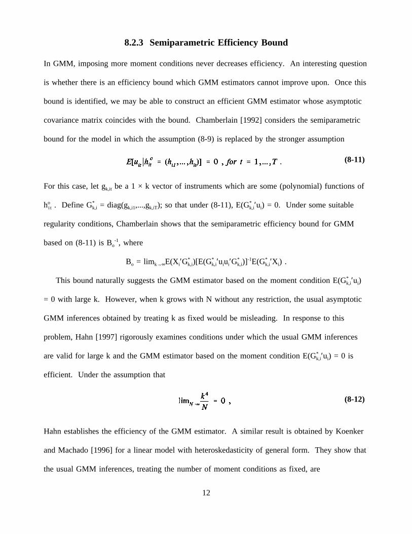
bound for the model in which the assumption (8-9) is replaced by the stronger assumption

For this case, let gk,it be a 1 × kvector of instruments which are some (polynomial) functions of

(8-11)

hoi t . Define G*

k,i = diag(gk,i1,...,gk,iT); so that under (8-11), E(G*k,i′ui) = 0. Under some suitable

regularity conditions, Chamberlain shows that the semiparametric efficiency bound for GMM

based on (8-11) is Bo-1, where

Bo = limk→∞E(Xi′G*k,i)[E(G*

k,i′uiui′G*k,i)]

-1E(G*k,i′Xi) .

This bound naturally suggests the GMM estimator based on the moment condition E(G*k,i′ui)

= 0 with large k. However, when k grows with N without any restriction, the usual asymptotic

GMM inferences obtained by treating k as fixed would be misleading. In response to this

problem, Hahn [1997] rigorously examines conditions under which the usual GMM inferences

are valid for large k and the GMM estimator based on the moment condition E(G*k,i′ui) = 0 is

efficient. Under the assumption that

Hahn establishes the efficiency of the GMM estimator. A similar result is obtained by Koenker

(8-12)

and Machado [1996] for a linear model with heteroskedasticity of general form. They show that

the usual GMM inferences, treating the number of moment conditions as fixed, are

12

asymptotically valid if the number of moment conditions grows more slowly than N . These

results do not directly indicate how to choose the number of moment conditions to use, for a

given finite value of N, but they do provide grounds for suspicion about the desirability of

GMM using numbers of moment conditions that are very large.

8.3 Models with Strictly Exogenous Regressors

This section considers efficient GMM estimation of linear panel data models with strictly

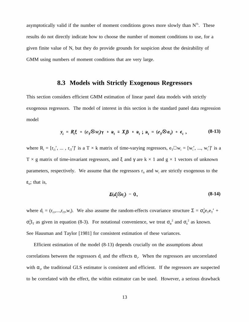
exogenous regressors. The model of interest in this section is the standard panel data regression

model

where Ri = [ri1′, ... , riT′]′ is a T × k matrix of time-varying regressors, eT⊗wi = [wi′, ..., wi′]′ is a

(8-13)

T × g matrix of time-invariant regressors, andξ andγ are k × 1 and g × 1vectors of unknown

parameters, respectively. We assume that the regressors rit and wi are strictly exogenous to the

εit; that is,

where di = (ri1,...,riT,wi). We also assume the random-effects covariance structureΣ = σ2αeTeT′ +

(8-14)

σ2εIT as given in equation (8-3). For notational convenience, we treatσα

2 andσε2 as known.

See Hausman and Taylor [1981] for consistent estimation of these variances.

Efficient estimation of the model (8-13) depends crucially on the assumptions about

correlations between the regressors di and the effectsαi. When the regressors are uncorrelated

with αi, the traditional GLS estimator is consistent and efficient. If the regressors are suspected

to be correlated with the effect, the within estimator can be used. However, a serious drawback

13

of the within estimator is that it cannot identifyγ because the within transformation wipes out

the time-invariant regressors wi as well as the individual effectsαi.

In response to this problem. Hausman and Taylor [1981, HT] considered the alternative

assumption that some but possibly not all of the explanatory variables are uncorrelated with the

effect αi. This offers a middle ground between the traditional random effects and fixed effects

approaches. Extending their study, Amemiya and MaCurdy [1986, AM] and Breusch, Mizon

and Schmidt [1989, BMS] considered stronger assumptions and derived alternative instrumental

variables estimators that are more efficient than the HT estimator. A systematic treatment of

these estimators can be found in Mátyás and Sevestre [1996, Chapter 6]. In what follows, we

will study these estimators and the conditions under which they are efficient GMM estimators.

8.3.1 The HT, AM and BMS Estimators

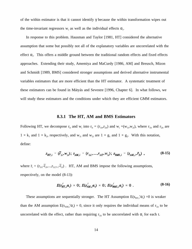
Following HT, we decompose rit and wi into rit = (r1it,r2it) and wi =(w1i,w2i), where r1it and r2it are

1 × k1 and 1 × k2, respectively, and w1i and w2i are 1 × g1 and 1 × g2. With this notation,

define:

whereri = (r2i1-r2i,...,r2i,T-1-r2i) . HT, AM and BMS impose the following assumptions,

(8-15)

respectively, on the model (8-13):

These assumptions are sequentially stronger. The HT Assumption E(sHT,i′αi) =0 is weaker

(8-16)

than the AM assumption E(sAM,i ′αi) = 0, since it only requires the individual means of r1it to be

uncorrelated with the effect, rather than requiring r1it to be uncorrelated withαi for each t.

14

(However, as AM argue, it is hard to think of cases in which each of the variables r1it is

correlated withαi while their individual means are not.) Imposing the AM assumption instead

of the HT assumption in GMM would generally lead to a more efficient estimator. The BMS

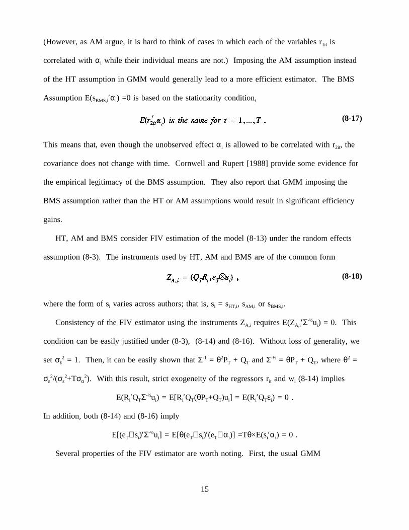
Assumption E(sBMS,i′αi) =0 is based on the stationarity condition,

This means that, even though the unobserved effectαi is allowed to be correlated with r2it, the

(8-17)

covariance does not change with time. Cornwell and Rupert [1988] provide some evidence for

the empirical legitimacy of the BMS assumption. They also report that GMM imposing the

BMS assumption rather than the HT or AM assumptions would result in significant efficiency

gains.

HT, AM and BMS consider FIV estimation of the model (8-13) under the random effects

assumption (8-3). The instruments used by HT, AM and BMS are of the common form

where the form of si varies across authors; that is, si = sHT,i, sAM,i or sBMS,i.

(8-18)

Consistency of the FIV estimator using the instruments ZA,i requires E(ZA,i′Σ-½ui) = 0. This

condition can be easily justified under (8-3), (8-14) and (8-16). Without loss of generality, we

setσε2 = 1. Then, it can be easily shown thatΣ-1 = θ2PT + QT andΣ-½ = θPT + QT, whereθ2 =

σε2/(σε

2+Tσα2). With this result, strict exogeneity of the regressors rit and wi (8-14) implies

E(Ri′QTΣ-½ui) = E[Ri′QT(θPT+QT)ui] = E(Ri′QTεi) = 0 .

In addition, both (8-14) and (8-16) imply

E[(eT⊗si)′Σ-½ui] = E[θ(eT⊗si)′(eT⊗αi)] =Tθ×E(si′αi) = 0 .

Several properties of the FIV estimator are worth noting. First, the usual GMM

15

identification condition requires that the number of columns in ZA,i should not be smaller than

the number of parameters inβ = (ξ′,γ′)′. This condition is satisfied if the number of variables

in si is not less than the number of time-invariant regressors (e.g., k1 ≥ g2 for the HT case).

Second, the FIV estimator is an intermediate case between the traditional GLS and within

estimators. It can be shown that the FIV estimator ofξ equals the within estimator if the model

is exactly identified (e.g, k1 = g2 for HT), while it is strictly more efficient if the model is

overidentified (e.g., k1 > g2 for HT). The FIV estimator ofβ is equivalent to the GLS estimator

if k 2 = g2 = 0 (that is, no regressor is correlated withαi). For more details, see HT. Finally,

the FIV estimator is numerically equivalent to the 3SLS estimator applying the instruments ZA,i;

thus, filtering does not matter. To see this, observe that

Σ-½ZA,i = (θPT+QT)(QTRi,eT⊗si)

= (QTRi,θeT⊗si) = (QTRi,eT⊗si) diag(I(1),θI(2)) = ZA,idiag(I(1),θI(2)) ,

where I(1) and I(2) are conformable identity matrices. Since the matrix diag(I(1),θI(2)) is

nonsingular, Theorem 8.1 applies:βFIV = β3SLS. This result also implies that the FIV estimator is

equally efficient as the GMM estimator using the instruments ZA,i, if the instruments satisfy the

NCH condition (8-6). When this NCH condition is violated, the GMM estimator using the

instruments ZA,i and an unrestricted weighting matrix is strictly more efficient than the FIV

estimator.

8.3.2 Efficient GMM Estimation

We now consider alternative GMM estimators which are potentially more efficient than the HT,

AM or BMS estimators. To begin with, observe that strict exogeneity of the regressors rit and wi

(8-14) implies many more moment conditions than the HT, AM or BMS estimators utilize. The

16

strict exogeneity condition (8-14) implies

E[(LT⊗di)′ui] = E(LT′ui⊗di) = E[LT′(eTαi+εi)⊗di) = E(LT′εi⊗di) = 0 ,

where LT⊗di is T × (T-1)(kT+g). Based on this observation, Arellano and Bover [1995] (and

Ahn and Schmidt [1995]) propose the GMM estimator using the instruments

which include (T-1)(Tk+g) - k more instruments than ZA,i. The covariance matrixΣ need not be

(8-19)

restricted. Clearly, the instruments ZB,i subsume ZA,i ≡ (QTRi,eT⊗si) which are essentially the

HT, AM or BMS instruments. Thus, the GMM estimator utilizing all of the instruments ZB,i

cannot be less efficient than the GMM estimator using the smaller set of instruments ZA,i. In

terms of achieving asymptotic efficiency, there is no reason to prefer to use the fewer

instruments ZB,i.

However, using all of the instruments ZA,i may not be practically feasible, even when T is

only moderately large. For example, consider the case in which k = g = 5 and T = 10. Forthis

case, the number of the instruments in ZA,i exceed the number of moment conditions in ZB,i by

490 (= 495-5). For such cases, the GMM estimator using the HT, AM or BMS instruments

would be of more practical use.

In addition, the GMM (or FIV) estimator using the instruments ZA,i can be shown to be

asymptotically as efficient as the GMM estimator using all of the instruments ZB,i, under specific

assumptions that are consistent with the motivation for the HT, AM or BMS estimators.

Arellano and Bover [1995] provide the foundation for this result.

THEOREM 8.2

Suppose thatΣ has the random effect structure (8-3). Then, the 3SLS estimator using the

17

instruments ZB,i is numerically identical to the 3SLS estimator using the smaller set of

instruments ZA,i, if the same estimate ofΣ is used.3

Although Arellano and Bover [1995] provide a detailed proof of the theorem, we provide a

shorter alternative proof. In what follows, we use the usual projection notation: For any matrix

B of full column rank, we define the projection matrix P(B) = B(B′B)-1B′. The following lemma

is useful for the proof of Theorem 8.2.

LEMMA 8.1

Let L* = IN⊗LT and D = [(IT-1⊗d1)′,...(IT-1⊗dN)′]′. Define V = IN⊗eT and W = (w1′,,,,wN′)′, so

that X = (R,VW). Then, P(L*D)X = P(QVR)X.

PROOF OFLEMMA 8.1

Since QV = P(L*) = L*(L*′L*)-1L*′, QVR = L*[(L *′L*)

-1L*′R]. In addition, since D spans all of

the columns in (L*′L*)-1L*′X, L*D must span QVR = L*[(L *′L*)

-1L*′R]. Finally, since QVL* =

L* and QVV = 0,

P(L*D)X = P(L*D)QVX = (P(L*D)QVR,0) = (QVR,0) = P(QVR)X .

We are now ready to prove Theorem 8.2.

PROOF OFTHEOREM 8.2

Note that ZA = [QVR,VW] and ZB = [L*D,VS], where S = (s1′,...,sN′)′. Since L* and QV are in

3Even if different estimates ofΣ are used, the two 3SLS estimators are asymptoticallyidentical.

18

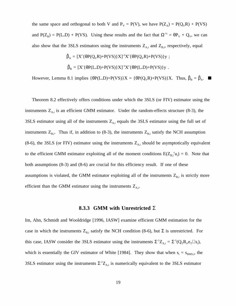
the same space and orthogonal to both V and PV = P(V), we have P(ZA) = P(QVR) + P(VS)

and P(ZB) = P(L*D) + P(VS). Using these results and the fact thatΩ-½ = θPV + QV, we can

also show that the 3SLS estimators using the instruments ZA,i and ZB,i, respectively, equal

βA = [X ′ θP(QVR)+P(VS)X]-1X′ θP(QVR)+P(VS)y ;

βB = [X ′ θP(L*D)+P(VS)X]-1X′ θP(L*D)+P(VS)y .

However, Lemma 8.1 implies θP(L*D)+P(VS)X = θP(QVR)+P(VS)X. Thus,βB = βA.

Theorem 8.2 effectively offers conditions under which the 3SLS (or FIV) estimator using the

instruments ZA,i is an efficient GMM estimator. Under the random-effects structure (8-3), the

3SLS estimator using all of the instruments ZA,i equals the 3SLS estimator using the full set of

instruments ZB,i. Thus if, in addition to (8-3), the instruments ZB,i satisfy the NCH assumption

(8-6), the 3SLS (or FIV) estimator using the instruments ZA,i should be asymptotically equivalent

to the efficient GMM estimator exploiting all of the moment conditions E(ZB,i′ui) = 0. Note that

both assumptions (8-3) and (8-6) are crucial for this efficiency result. If one of these

assumptions is violated, the GMM estimator exploiting all of the instruments ZB,i is strictly more

efficient than the GMM estimator using the instruments ZA,i.

8.3.3 GMM with Unrestricted Σ

Im, Ahn, Schmidt and Wooldridge [1996, IASW] examine efficient GMM estimation for the

case in which the instruments ZB,i satisfy the NCH condition (8-6), butΣ is unrestricted. For

this case, IASW consider the 3SLS estimator using the instrumentsΣ-1ZA,i = Σ-1(QTRi,eT⊗si),

which is essentially the GIV estimator of White [1984]. They show that when si = sBMS,i, the

3SLS estimator using the instrumentsΣ-1ZA,i is numerically equivalent to the 3SLS estimator

19

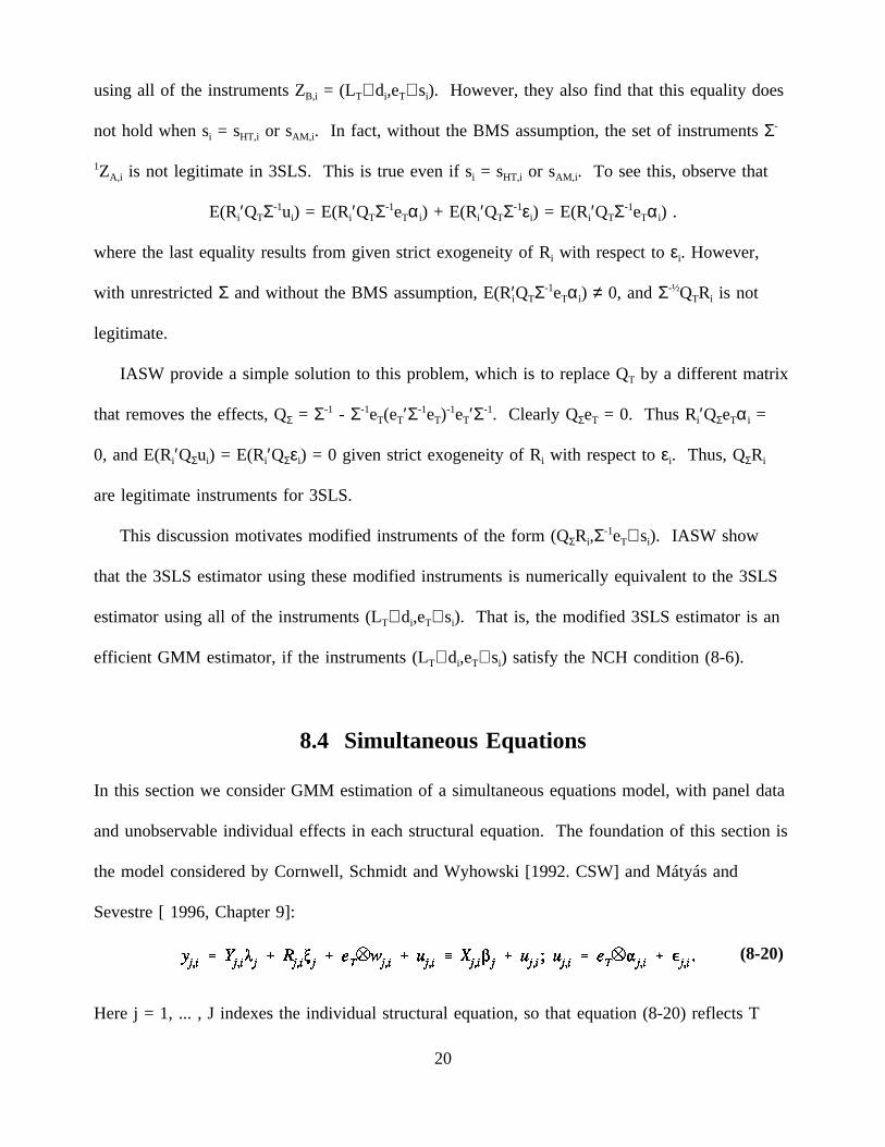
using all of the instruments ZB,i = (LT⊗di,eT⊗si). However, they also find that this equality does

not hold when si = sHT,i or sAM,i . In fact, without the BMS assumption, the set of instrumentsΣ-

1ZA,i is not legitimate in 3SLS. This is true even if si = sHT,i or sAM,i . To see this, observe that

E(Ri′QTΣ-1ui) = E(Ri′QTΣ-1eTαi) + E(Ri′QTΣ-1εi) = E(Ri′QTΣ-1eTαi) .

where the last equality results from given strict exogeneity of Ri with respect toεi. However,

with unrestrictedΣ and without the BMS assumption, E(Ri′QTΣ-1eTαi) ≠ 0, andΣ-½QTRi is not

legitimate.

IASW provide a simple solution to this problem, which is to replace QT by a different matrix

that removes the effects, QΣ = Σ-1 - Σ-1eT(eT′Σ-1eT)-1eT′Σ-1. Clearly QΣeT = 0. Thus Ri′QΣeTαi =

0, and E(Ri′QΣui) = E(Ri′QΣεi) = 0 given strict exogeneity of Ri with respect toεi. Thus, QΣRi

are legitimate instruments for 3SLS.

This discussion motivates modified instruments of the form (QΣRi,Σ-1eT⊗si). IASW show

that the 3SLS estimator using these modified instruments is numerically equivalent to the 3SLS

estimator using all of the instruments (LT⊗di,eT⊗si). That is, the modified 3SLS estimator is an

efficient GMM estimator, if the instruments (LT⊗di,eT⊗si) satisfy the NCH condition (8-6).

8.4 Simultaneous Equations

In this section we consider GMM estimation of a simultaneous equations model, with panel data

and unobservable individual effects in each structural equation. The foundation of this section is

the model considered by Cornwell, Schmidt and Wyhowski [1992. CSW] and Mátyás and

Sevestre [ 1996, Chapter 9]:

Here j = 1, ... , Jindexes the individual structural equation, so that equation (8-20) reflects T

(8-20)

20

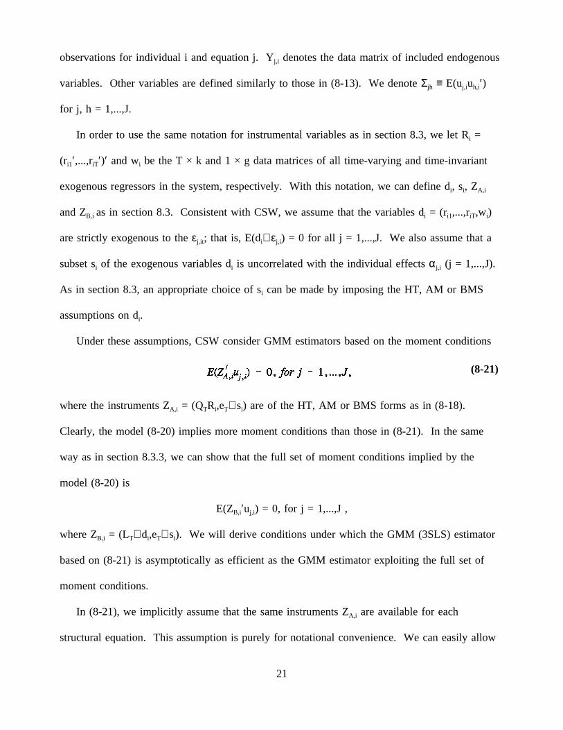
observations for individual i and equation j. Yj,i denotes the data matrix of included endogenous

variables. Other variables are defined similarly to those in (8-13). We denoteΣjh ≡ E(uj,iuh,i′)

for j, h = 1,...,J.

In order to use the same notation for instrumental variables as in section 8.3, we let Ri =

(ri1′,...,riT′)′ and wi be the T × k and 1 × gdata matrices of all time-varying and time-invariant

exogenous regressors in the system, respectively. With this notation, we can define di, si, ZA,i

and ZB,i as in section 8.3. Consistent with CSW, we assume that the variables di = (ri1,...,riT,wi)

are strictly exogenous to theεj,it; that is, E(di⊗εj,i) = 0 for all j = 1,...,J. We also assume that a

subset si of the exogenous variables di is uncorrelated with the individual effectsαj,i (j = 1,...,J).

As in section 8.3, an appropriate choice of si can be made by imposing the HT, AM or BMS

assumptions on di.

Under these assumptions, CSW consider GMM estimators based on the moment conditions

where the instruments ZA,i = (QTRi,eT⊗si) are of the HT, AM or BMS forms as in (8-18).

(8-21)

Clearly, the model (8-20) implies more moment conditions than those in (8-21). In the same

way as in section 8.3.3, we can show that the full set of moment conditions implied by the

model (8-20) is

E(ZB,i′uj,i) = 0, for j = 1,...,J ,

where ZB,i = (LT⊗di,eT⊗si). We will derive conditions under which the GMM (3SLS) estimator

based on (8-21) is asymptotically as efficient as the GMM estimator exploiting the full set of

moment conditions.

In (8-21), we implicitly assume that the same instruments ZA,i are available for each

structural equation. This assumption is purely for notational convenience. We can easily allow

21

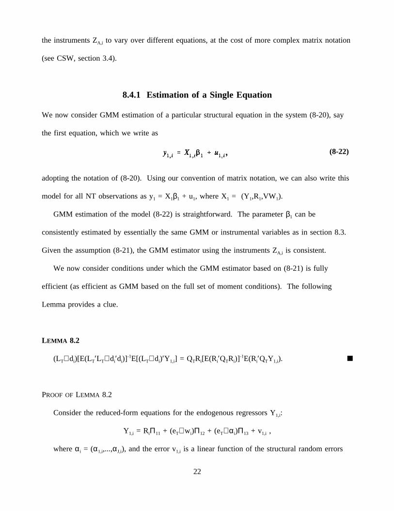
the instruments ZA,i to vary over different equations, at the cost of more complex matrix notation

(see CSW, section 3.4).

8.4.1 Estimation of a Single Equation

We now consider GMM estimation of a particular structural equation in the system (8-20), say

the first equation, which we write as

adopting the notation of (8-20). Using our convention of matrix notation, we can also write this

(8-22)

model for all NT observations as y1 = X1β1 + u1, where X1 = (Y1,R1,VW1).

GMM estimation of the model (8-22) is straightforward. The parameterβ1 can be

consistently estimated by essentially the same GMM or instrumental variables as in section 8.3.

Given the assumption (8-21), the GMM estimator using the instruments ZA,i is consistent.

We now consider conditions under which the GMM estimator based on (8-21) is fully

efficient (as efficient as GMM based on the full set of moment conditions). The following

Lemma provides a clue.

LEMMA 8.2

(LT⊗di)[E(LT′LT⊗di′di)]-1E[(LT⊗di)′Y1,i] = QTRi[E(Ri′QTRi)]

-1E(Ri′QTY1,i).

PROOF OFLEMMA 8.2

Consider the reduced-form equations for the endogenous regressors Y1,i:

Y1,i = RiΠ11 + (eT⊗wi)Π12 + (eT⊗αi)Π13 + v1,i ,

whereαi = (α1,i,...,αJ,i), and the error v1,i is a linear function of the structural random errors

22

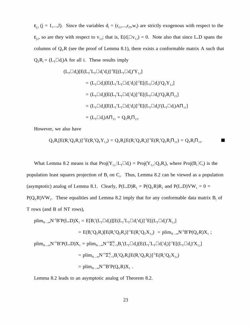
εj,i (j = 1,...,J). Since the variables di = (ri1,...,riT,wi) are strictly exogenous with respect to the

εj,i, so are they with respect to v1,i; that is, E(di⊗v1,i) = 0. Note also that since L*D spans the

columns of QVR (see the proof of Lemma 8.1), there exists a conformable matrix A such that

QTRi = (LT⊗di)A for all i. These results imply

(LT⊗di)[E(LT′LT⊗di′di)]-1E[(LT⊗di)′Y1,i]

= (LT⊗di)[E(LT′LT⊗di′di)]-1E[(LT⊗di)′QTY1,i]

= (LT⊗di)[E(LT′LT⊗di′di)]-1E[(LT⊗di)′QTRiΠ11]

= (LT⊗di)[E(LT′LT⊗di′di)]-1E[(LT⊗di)′(LT⊗di)AΠ11]

= (LT⊗di)AΠ11 = QTRiΠ11.

However, we also have

QTRi[E(Ri′QTRi)]-1E(Ri′QTY1,i) = QTRi[E(Ri′QTRi)]

-1E(Ri′QTRiΠ11) = QTRiΠ11.

What Lemma 8.2 means is that Proj(Y1,i LT⊗di) = Proj(Y1,i QTRi), where Proj(Bi Ci) is the

population least squares projection of Bi on Ci. Thus, Lemma 8.2 can be viewed as a population

(asymptotic) analog of Lemma 8.1. Clearly, P(L*D)R1 = P(QVR)R1 and P(L*D)VW1 = 0 =

P(QVR)VW1. These equalities and Lemma 8.2 imply that for any conformable data matrix Bi of

T rows (and B of NT rows),

plimN→∞N-1B′P(L*D)X1 = E[Bi′(LT⊗di)][E(LT′LT⊗di′di)]-1E[(LT⊗di)′X1,i]

= E(Bi′QTRi)[E(Ri′QTRi)]-1E(Ri′QTX1,i) = plimN→∞N-1B′P(QVR)X1 ;

plimN→∞N-½B′P(L*D)X1 = plimN→∞N-½ΣNi =1Bi′(LT⊗di)[E(LT′LT⊗di′di)]

-1E[(LT⊗di)′X1,i]

= plimN→∞N-½ΣNi =1Bi′QTRi[E(Ri′QTRi)]

-1E(Ri′QTX1,i)

= plimN→∞N-½B′P(QVR)X1 .

Lemma 8.2 leads to an asymptotic analog of Theorem 8.2.

23

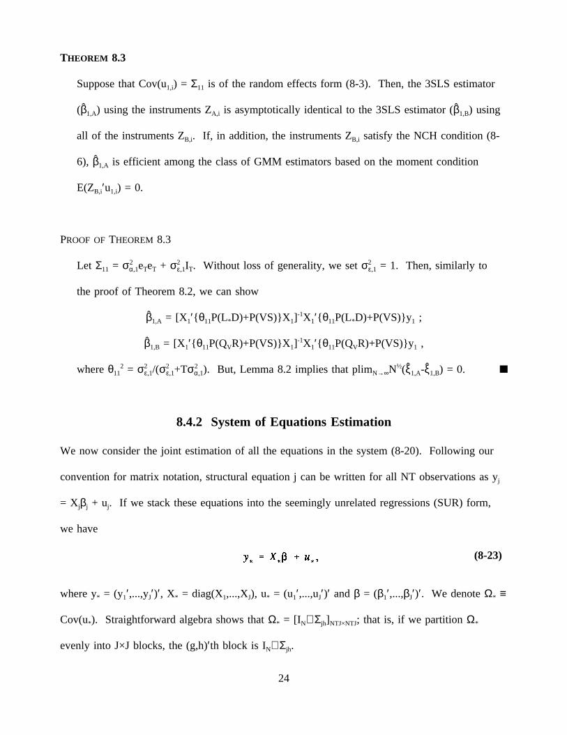
THEOREM 8.3

Suppose that Cov(u1,i) = Σ11 is of the random effects form (8-3). Then, the 3SLS estimator

(β1,A) using the instruments ZA,i is asymptotically identical to the 3SLS estimator (β1,B) using

all of the instruments ZB,i. If, in addition, the instruments ZB,i satisfy the NCH condition (8-

6), β1,A is efficient among the class of GMM estimators based on the moment condition

E(ZB,i′u1,i) = 0.

PROOF OFTHEOREM 8.3

Let Σ11 = σ2α,1eTeT + σ2

ε,1IT. Without loss of generality, we setσ2ε,1 = 1. Then, similarly to

the proof of Theorem 8.2, we can show

β1,A = [X1′ θ11P(L*D)+P(VS)X1]-1X1′ θ11P(L*D)+P(VS)y1 ;

β1,B = [X1′ θ11P(QVR)+P(VS)X1]-1X1′ θ11P(QVR)+P(VS)y1 ,

whereθ112 = σ2

ε,1/(σ2ε,1+Tσ2

α,1). But, Lemma 8.2 implies that plimN→∞N½(ξ1,A-ξ1,B) = 0.

8.4.2 System of Equations Estimation

We now consider the joint estimation of all the equations in the system (8-20). Following our

convention for matrix notation, structural equation j can be written for all NT observations as yj

= Xjβj + uj. If we stack these equations into the seemingly unrelated regressions (SUR) form,

we have

where y* = (y1′,...,yJ′)′, X* = diag(X1,...,XJ), u* = (u1′,...,uJ′)′ andβ = (β1′,...,βJ′)′. We denoteΩ* ≡

(8-23)

Cov(u*). Straightforward algebra shows thatΩ* = [IN⊗Σjh]NTJ×NTJ; that is, if we partitionΩ*

evenly into J×J blocks, the (g,h)′th block is IN⊗Σjh.

24

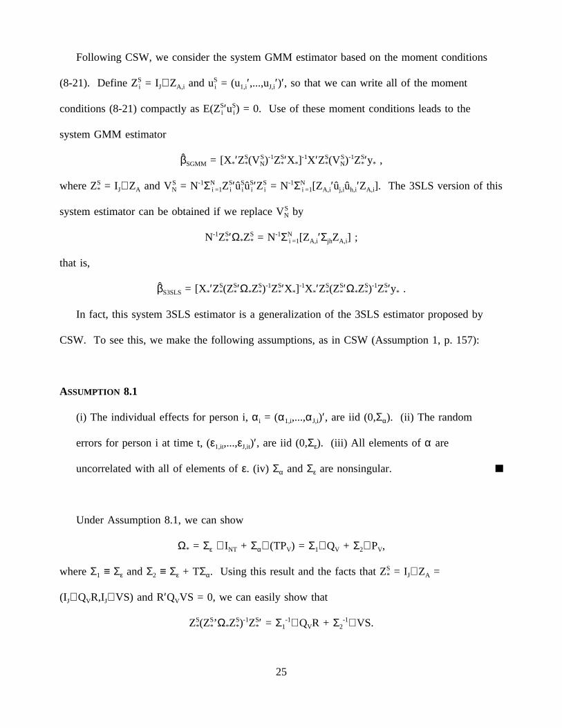
Following CSW, we consider the system GMM estimator based on the moment conditions

(8-21). Define ZSi = IJ⊗ZA,i and uSi = (u1,i′,...,uJ,i′)′, so that we can write all of the moment

conditions (8-21) compactly as E(ZSi ′uS

i ) = 0. Use of these moment conditions leads to the

system GMM estimator

βSGMM = [X*′ZS*(V

SN)-1ZS

* ′X*]-1X′ZS

*(VSN)-1ZS

* ′y* ,

where ZS* = IJ⊗ZA and VS

N = N-1ΣNi =1Z

Si ′uS

i uSi ′ZS

i = N-1ΣNi =1[ZA,i′uj,iuh,i′ZA,i]. The 3SLS version of this

system estimator can be obtained if we replace VSN by

N-1ZS* ′Ω*Z

S* = N-1ΣN

i =1[ZA,i′ΣjhZA,i] ;

that is,

βS3SLS = [X*′ZS*(Z

S* ′Ω*Z

S*)

-1ZS* ′X*]

-1X*′ZS*(Z

S* ′Ω*Z

S*)

-1ZS* ′y* .

In fact, this system 3SLS estimator is a generalization of the 3SLS estimator proposed by

CSW. To see this, we make the following assumptions, as in CSW (Assumption 1, p. 157):

ASSUMPTION 8.1

(i) The individual effects for person i,αi = (α1,i,...,αJ,i)′, are iid (0,Σα). (ii) The random

errors for person i at time t, (ε1,it,...,εJ,it)′, are iid (0,Σε). (iii) All elements of α are

uncorrelated with all of elements ofε. (iv) Σα andΣε are nonsingular.

Under Assumption 8.1, we can show

Ω* = Σε ⊗INT + Σα⊗(TPV) = Σ1⊗QV + Σ2⊗PV,

whereΣ1 ≡ Σε andΣ2 ≡ Σε + TΣα. Using this result and the facts that ZS* = IJ⊗ZA =

(IJ⊗QVR,IJ⊗VS) and R′QVVS = 0, we can easily show that

ZS*(Z

S*’Ω*Z

S*)

-1ZS* ′ = Σ1

-1⊗QVR + Σ2-1⊗VS.

25

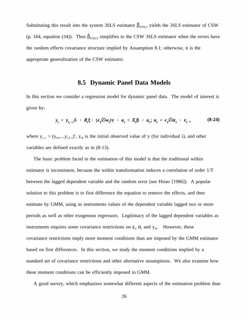
Substituting this result into the system 3SLS estimatorβS3SLS yields the 3SLS estimator of CSW

(p. 164, equation (34)). ThusβS3SLS simplifies to the CSW 3SLS estimator when the errors have

the random effects covariance structure implied by Assumption 8.1; otherwise, it is the

appropriate generalization of the CSW estimator.

8.5 Dynamic Panel Data Models

In this section we consider a regression model for dynamic panel data. The model of interest is

given by:

where yi,-1 = (yi0,...,yi,T-1)′, yi0 is the initial observed value of y (for individual i), and other

(8-24)

variables are defined exactly as in (8-13).

The basic problem faced in the estimation of this model is that the traditional within

estimator is inconsistent, because the within transformation induces a correlation of order 1/T

between the lagged dependent variable and the random error (see Hsiao [1986]). A popular

solution to this problem is to first difference the equation to remove the effects, and then

estimate by GMM, using as instruments values of the dependent variable lagged two or more

periods as well as other exogenous regressors. Legitimacy of the lagged dependent variables as

instruments requires some covariance restrictions onεi, αi and yi0. However, these

covariance restrictions imply more moment conditions than are imposed by the GMM estimator

based on first differences. In this section, we study the moment conditions implied by a

standard set of covariance restrictions and other alternative assumptions. We also examine how

these moment conditions can be efficiently imposed in GMM.

A good survey, which emphasizes somewhat different aspects of the estimation problem than

26

we do, is given by Mátyás and Sevestre [1996, Chapter 7].

8.5.1 Moment Conditions under Standard Assumptions

In this subsection we count and express the moment conditions implied by a standard set of

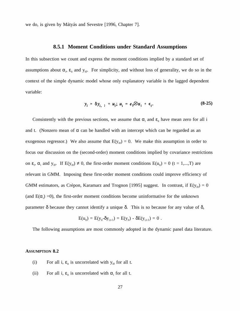
assumptions aboutαi, εit and yi0. For simplicity, and without loss of generality, we do so in the

context of the simple dynamic model whose only explanatory variable is the lagged dependent

variable:

Consistently with the previous sections, we assume thatαi andεit have mean zero for all i

(8-25)

and t. (Nonzero mean ofα can be handled with an intercept which can be regarded as an

exogenous regressor.) We also assume that E(yi0) = 0. We make this assumption in order to

focus our discussion on the (second-order) moment conditions implied by covariance restrictions

on εi, αi and yi0. If E(yi0) ≠ 0, the first-order moment conditions E(uit) = 0 (t = 1,...,T) are

relevant in GMM. Imposing these first-order moment conditions could improve efficiency of

GMM estimators, as Crépon, Karamarz and Trognon [1995] suggest. In contrast, if E(yi0) = 0

(and E(αi) =0), the first-order moment conditions become uninformative for the unknown

parameterδ because they cannot identify a uniqueδ. This is so because for any value ofδ,

E(uit) = E(yit-δyi,t-1) = E(yit) - δE(yi,t-1) = 0 .

The following assumptions are most commonly adopted in the dynamic panel data literature.

ASSUMPTION 8.2

(i) For all i, εit is uncorrelated with yi0 for all t.

(ii) For all i, εit is uncorrelated withαi for all t.

27

(iii) For all i, the εit are mutually uncorrelated.

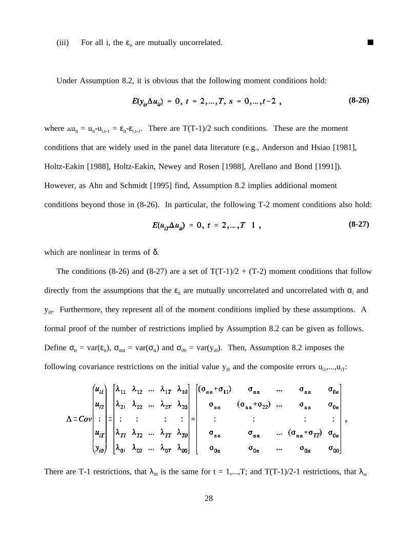
Under Assumption 8.2, it is obvious that the following moment conditions hold:

where uit = uit-ui,t-1 = εit-εi,t-1. There are T(T-1)/2 such conditions. These are the moment

(8-26)

conditions that are widely used in the panel data literature (e.g., Anderson and Hsiao [1981],

Holtz-Eakin [1988], Holtz-Eakin, Newey and Rosen [1988], Arellano and Bond [1991]).

However, as Ahn and Schmidt [1995] find, Assumption 8.2 implies additional moment

conditions beyond those in (8-26). In particular, the following T-2 moment conditions also hold:

which are nonlinear in terms ofδ.

(8-27)

The conditions (8-26) and (8-27) are a set of T(T-1)/2 + (T-2) moment conditions that follow

directly from the assumptions that theεit are mutually uncorrelated and uncorrelated withαi and

yi0. Furthermore, they represent all of the moment conditions implied by these assumptions. A

formal proof of the number of restrictions implied by Assumption 8.2 can be given as follows.

Define σtt = var(εit), σαα = var(σα) andσ00 = var(yi0). Then, Assumption 8.2 imposes the

following covariance restrictions on the initial value yi0 and the composite errors ui1,...,uiT:

There are T-1 restrictions, thatλ0t is the same for t = 1,...,T; and T(T-1)/2-1 restrictions, thatλts

28

is the same for t,s = 1,...,T, t≠ s. Adding the number of restrictions, we get T(T-1)/2 + (T-2).

Since the moment conditions (8-27) are nonlinear, GMM imposing these conditions requires

an iterative procedure. Thus, an important practical question is whether this computational

burden is worthwhile. Ahn and Schmidt [1995] provide a partial answer. They compare the

asymptotic variances of the GMM estimator based on (8-26) only and the GMM estimator based

on both of (8-26) and (8-27). Their computation results show that use of the extra moment

condition (8-27) can result in a large efficiency gain, especially whenδ is close to one or the

varianceσαα is large.

8.5.2 Some Alternative Assumptions

We now briefly consider some alternative sets of assumptions. The first case we consider is the

one in which Assumption 8.2 is augmented by the additional assumption that theεit are

homoskedastic. That is, suppose that we add the assumption:

ASSUMPTION 8.3

For all i, var(εit) is the same for all t.

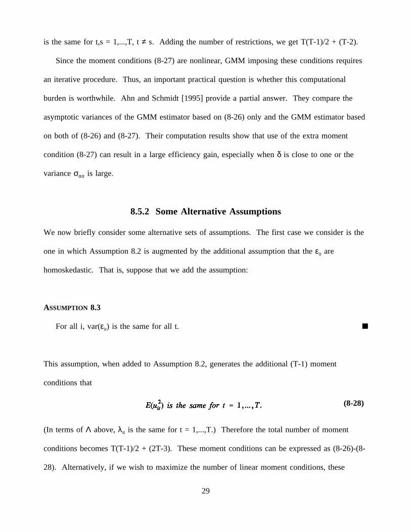
This assumption, when added to Assumption 8.2, generates the additional (T-1) moment

conditions that

(In terms ofΛ above,λtt is the same for t = 1,...,T.) Therefore the total number of moment

(8-28)

conditions becomes T(T-1)/2 + (2T-3). These moment conditions can be expressed as (8-26)-(8-

28). Alternatively, if we wish to maximize the number of linear moment conditions, these

29

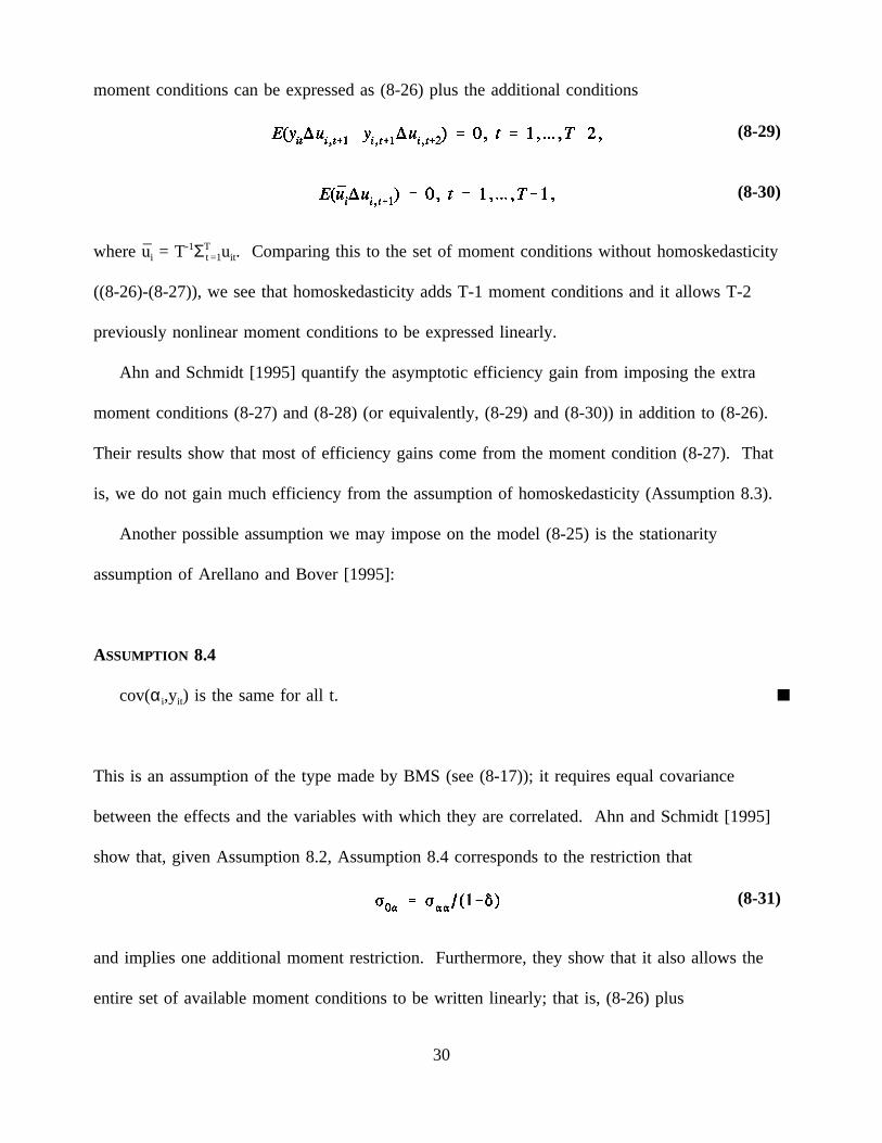
moment conditions can be expressed as (8-26) plus the additional conditions

where ui = T-1ΣTt =1uit. Comparing this to the set of moment conditions without homoskedasticity

(8-29)

(8-30)

((8-26)-(8-27)), we see that homoskedasticity adds T-1 moment conditions and it allows T-2

previously nonlinear moment conditions to be expressed linearly.

Ahn and Schmidt [1995] quantify the asymptotic efficiency gain from imposing the extra

moment conditions (8-27) and (8-28) (or equivalently, (8-29) and (8-30)) in addition to (8-26).

Their results show that most of efficiency gains come from the moment condition (8-27). That

is, we do not gain much efficiency from the assumption of homoskedasticity (Assumption 8.3).

Another possible assumption we may impose on the model (8-25) is the stationarity

assumption of Arellano and Bover [1995]:

ASSUMPTION 8.4

cov(αi,yit) is the same for all t.

This is an assumption of the type made by BMS (see (8-17)); it requires equal covariance

between the effects and the variables with which they are correlated. Ahn and Schmidt [1995]

show that, given Assumption 8.2, Assumption 8.4 corresponds to the restriction that

and implies one additional moment restriction. Furthermore, they show that it also allows the

(8-31)

entire set of available moment conditions to be written linearly; that is, (8-26) plus

30

E(uiT yit) = 0 , t = 1,...,T-1 ;

E(uityit - ui,t-1yi,t-1) = 0 , t = 2,...,T .

This is a set of T(T-1)/2 + (2T-2) moment conditions, all of which are linear inδ. Blundell and

Bond [1997] show that the GMM estimator exploiting all of these linear moment conditions has

much better asymptotic and finite sample properties than the GMM estimator based on (8-26)

only. Thus the stationarity assumption 8.4 may be quite useful.

Finally, we consider an alternative stationarity assumption, which is examined by Ahn and

Schmidt [1997]:

ASSUMPTION 8.5

In addition to Assumptions 8.2 and 3, the series yi0, ..., yiT is covariance stationary.

To see the connection between the two stationarity assumptions, Assumptions 8.4 and 5, we

use the solution

yit = δtyi0 + αi(1-δt)/(1-δ) + Σtj-=

10δjεi,t-j

to calculate

var(yit) = σ00δ2t + σ0α2δt(1-δt)/(1-δ)

+ σαα[(1-δt)/(1-δ)]2 + σεε(1-δ2t)/(1-δ2) ,

where the calculation assumes Assumptions 8.2 and 3. Assumption 8.5 implies that var(yit) =

σ00 for all t, which occurs if and only ifσαα = (1-δ)σ0α and also

Thus Assumption 8.5 impliesσαα = (1-δ)σ0α, which in turn implies Assumption 8.4. However,

(8-32)

it also implies the restriction (8-32) on the variance of the initial observation yi0. Imposing (8-

31

32) as well as Assumptions 8.2-4 yields one additional, nonlinear moment condition:

E[yi02 + yi1 ui2/(1-δ2) - ui2ui1/(1-δ)2] = 0.

An interesting question that we do not address here is how many moment conditions we

would have if the assumptions discussed above are relaxed. Ahn and Schmidt [1997] give a

partial answer by counting the moment conditions implied by many possible combinations of the

above assumptions. See that paper for more detail.

8.5.3 Estimation

In this subsection we discuss some theoretical details concerning GMM estimation of the

dynamic model. We also discuss the relationship between GMM based on the linear moment

conditions and 3SLS estimation. Our discussion will proceed under Assumptions 8.2-3, but can

easily be modified to accommodate the other cases.

8.5.3.1 Notation and General Results

We now return to the model (8-24) which includes exogenous regressors rit and wi.

Exogeneity assumptions on rit and wi generate linear moment conditions of the form

E(Ci′ui) = 0 ,

where Ci = ZA,i or ZB,i as defined in section 8.3. In addition, the moment conditions given by (8-

26), (8-29) and (8-30) above are valid. The moment conditions in (8-26) above are

linear in ξ and can be written as E(Ai′ui) = 0, where Ai is the T × T(T-1)/2 matrix

Similarly, the moment conditions in (8-29) above are also linear inβ and can be written as

E(Bi′ui) = 0, where Bi is the T × (T-2) matrix defined by

However, the moment conditions in (8-30) above are quadratic inβ.

We will discuss GMM estimation based on all of the available moment conditions and GMM

32

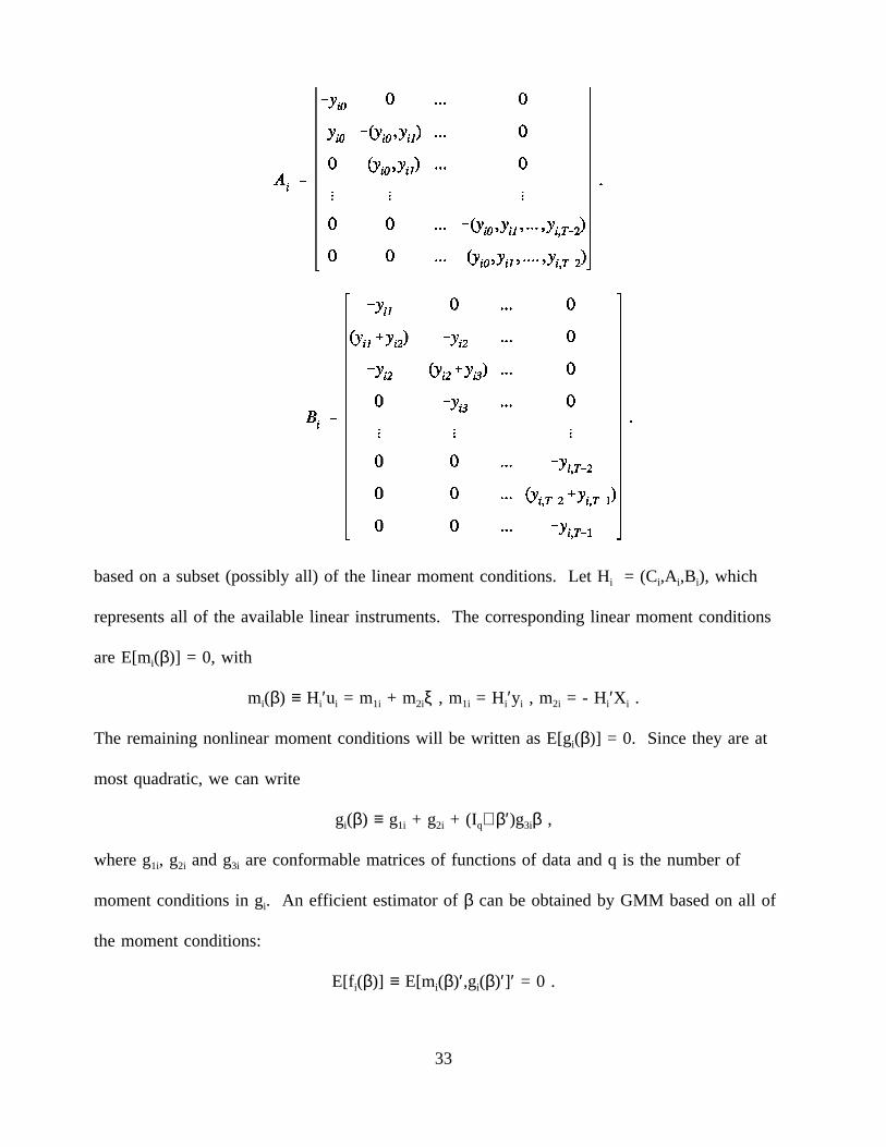
based on a subset (possibly all) of the linear moment conditions. Let Hi = (Ci,Ai,Bi), which

represents all of the available linear instruments. The corresponding linear moment conditions

are E[mi(β)] = 0, with

mi(β) ≡ Hi′ui = m1i + m2iξ , m1i = Hi′yi , m2i = - Hi′Xi .

The remaining nonlinear moment conditions will be written as E[gi(β)] = 0. Since they are at

most quadratic, we can write

gi(β) ≡ g1i + g2i + (Iq⊗β′)g3iβ ,

where g1i, g2i and g3i are conformable matrices of functions of data and q is the number of

moment conditions in gi. An efficient estimator ofβ can be obtained by GMM based on all of

the moment conditions:

E[fi(β)] ≡ E[mi(β)′,gi(β)′]′ = 0 .

33

Define fN = N-1Σif i(β), with mN, m1N, m2N, gN, g1N, g2N and g3N defined similarly; and define

FN = ∂fN/∂β′ = [∂mN′/∂β,∂gN′/∂β]′ = [MN′,GN′]′, where GN(β) = g2N + 2(I β′)g3N and MN = m2N.

Let F = plim FN, with M and G defined similarly. Define the optimal weighting matrix:

Let VN be a consistent estimate of V of the form

VN = N-1ΣNi =1fi(β)fi(β)′,

whereβ is an initial consistent estimate ofβ (perhaps based on the linear moment conditions mi,

as discussed below); partition it similarly to V.

In this notation, the efficient GMM estimatorβEGMM minimizes NfN(β)′(VN)-1fN(β). Using

standard results, the asymptotic covariance matrix of N½(βEGMM-β) is [F′V-1F]-1.

8.5.3.2 Linear Moment Conditions and Instrumental Variables

Some interesting questions arise when we consider GMM based on the linear moment

conditions mi(ξ) only. The optimal GMM estimator based on these conditions is

βm = -[m2N′(VN,mm)-1m2N]-1m2N′(VN,mm)-1m1N = [X ′H(VN,mm)-1H′X] -1X′H(VN,mm)-1X′y .

This GMM estimator can be compared to the 3SLS estimator which is obtained by replacing

VN,mm by N-1H′ΩH = N-1ΣNi =1Hi′ΣHi.

4 As discussed in section 8.1, they are asymptotically

equivalent in the case that Vmm ≡ E(Hi′uiui′Hi) = E(Hi′ΣHi). For the case that Hi consists only of

columns of Ci, so that only the moment conditions E(Ci′ui) =0 based on exogeneity of Ri and wi

are imposed, this equivalence may hold. Arellano and Bond [1991] considered the moment

conditions (8-26), so that Hi also contains Ai, and noted that asymptotic equivalence between the

3SLS and GMM estimates fails if we relax the homoskedasticity assumption, Assumption 8.3,

4Note that Assumptions 8.2 and 3 implies the random effects structure (8-3).

34

even though the moment conditions (8-26) are still valid under only Assumption 8.2. In fact,

even the full set of Assumptions 8.2-3 is not sufficient to imply the asymptotic equivalence of

the 3SLS and GMM estimates when the moment conditions (8-26) are used. Assumptions 8.2-3

deal only with second moments, whereas asymptotic equivalence of 3SLS and GMM involves

restrictions on fourth moments (e.g., cov(yi02,εit

2) = 0). Ahn [1990] proved the asymptotic

equivalence of the 3SLS and GMM estimators based on the moment conditions (8-26) for the

case that Assumption 8.3 is maintained and Assumption 8.2 is strengthened by replacing

uncorrelatedness with independence. Wooldridge [1996] provides a more general treatment of

cases in which 3SLS and GMM are asymptotically equivalent. In the present case, his results

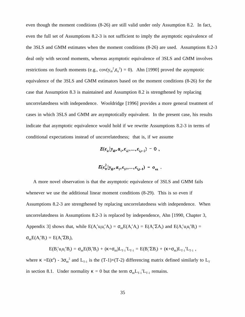
indicate that asymptotic equivalence would hold if we rewrite Assumptions 8.2-3 in terms of

conditional expectations instead of uncorrelatedness; that is, if we assume

A more novel observation is that the asymptotic equivalence of 3SLS and GMM fails

whenever we use the additional linear moment conditions (8-29). This is so even if

Assumptions 8.2-3 are strengthened by replacing uncorrelatedness with independence. When

uncorrelatedness in Assumptions 8.2-3 is replaced by independence, Ahn [1990, Chapter 3,

Appendix 3] shows that, while E(Ai′uiui′Ai) = σεεE(Ai′Ai) = E(Ai′ΣAi) and E(Ai′uiui′Bi) =

σεεE(Ai′Bi) = E(Ai′ΣBi),

E(Bi′uiui′Bi) = σεεE(Bi′Bi) + (κ+σεε)LT-1′LT-1 = E(Bi′ΣBi) + (κ+σεε)LT-1′LT-1 ,

whereκ =E(ε4) - 3σεε2 and LT-1 is the (T-1)×(T-2) differencing matrix defined similarly to LT

in section 8.1. Under normalityκ = 0 but the termσεεLT-1′LT-1 remains.

35

8.5.3.3 Linearized GMM

We now consider a linearized GMM estimator. Suppose thatβ is any consistent estimator of

β; for example,βm. Following Newey (1985, p. 238), the linearized GMM estimator is of the

form

βLGMM = β - [FN(β)′(VN)-1FN(β)]-1FN(β)′(VN)-1fN(β) .

This estimator is consistent and has the same asymptotic distribution asβEGMM.

When the LGMM estimator is based on the initial estimatorβm, some further simplification

is possible. Using the fact that m2N′(VN,mm)-1mN(βm) = 0 and applying the usual matrix inversion

rule to VN, we can write the LGMM estimator as follows:

βLGMM = βm - [ΓN + BN′(VN,bb)-1BN]-1BN′(VN,bb)

-1bN ,

where ΓN=m2N′(VN,ff)-1m2N, VN,bb=VN,gg-VN,gm(VN,mm)-1VN,mg, bN=gN(βm)-VN,gm(VN,mm)-1mN(βm), and

BN=GN(βm) - VN,gm(VN,mm)-1m2N. For more detail, see Ahn and Schmidt [1997].

8.6 Conclusions

In this chapter we have considered the GMM estimation of linear panel data models. We have

discussed standard models, including the fixed and random effects linear model, a dynamic

model, and the simultaneous equation model. For these models the typical treatment in the

literature is some sort of instrumental variables procedure; least squares and generalized least

squares are included in the class of such instrumental variables procedures.

It is well known that for linear models the GMM estimator often takes the form of an IV

estimator if a no conditional heteroskedasticity condition holds. Therefore we have focused on

three related points. First, for each model we seek to identify the complete set of moment

conditions (instruments) implied by the assumptions underlying the model. Next, one can

36

observe that the usual exogeneity assumptions lead to many more moment conditions than

standard estimators use, and ask whether some or all of the moment conditions are redundant, in

the sense that they are unnecessary to obtain an efficient estimator. Under the no conditional

heteroskedasticity assumption, the efficiency of standard estimators can often be established.

This implies that the moment conditions which are not utilized by standard estimators are

redundant. Finally, we ask whether anything intrinsic to the model makes the assumption of no

conditional heteroskedasticity untenable. In some models, such as the dynamic model, this

assumption necessarily fails if the full set of moment conditions is used, and correspondingly the

efficient GMM estimator is not an instrumental variables estimator.

The set of non-redundant moment conditions can sometimes be very large. For example, this

is true in the dynamic model, and also in simpler static models if the assumption of no

conditional heteroskedasticity fails. In such cases the finite sample properties of the GMM

estimator using the full set of moment conditions may be poor. An important avenue of research

is to find estimators which are efficient, or nearly so, and yet have better finite sample properties

than the full GMM estimator.

37

REFERENCES

Ahn, S.C., 1990, Three essays on share contracts, labor supply, and the estimation of models fordynamic panel data, Unpublished Ph.D. dissertation, Michigan State University.

Ahn, S. C. and P. Schmidt, 1995, Efficient estimation of models for dynamic panel data, Journalof Econometrics 68, 5-27.

Ahn, S. C. and P. Schmidt, 1997, Efficient estimation of dynamic panel data models: alternativeassumptions and simplified assumptions, Journal of Econometrics 76, 309-321.

Altonji, J. G. and L. M. Segal, 1996, Small-sample bias in GMM estimation of covariancestructure, Journal of Business & Economic Statistics 14, 353-366.

Amemiya, T. and T. E. MaCurdy, 1986, Instrumental-variables estimation of an error-components model, Econometrica 54, 869-880.

Andersen, T. G. and R. E. Sørensen, 1996, GMM estimation of a stochastic volatility model: AMonte Carlo Study, Journal of Business & Economic Statistics 14, 328-352.

Anderson, T.W. and C. Hsiao, 1981, Estimation of dynamic models with error components,Journal of the American Statistical Association, 76, 598-606.

Arellano, M. and S. Bond, 1991, Tests of specification for panel data: Monte Carlo evidence andan application to employment equations, Review of Economic Studies 58, 277-297.

Arellano, M. and O. Bover, 1995, Another look at the instrumental variables estimation of error-component models, Journal of Econometrics 68, 29-51.

Balestra, P. and M. Nerlove, 1966, Pooling cross-section and time-series data in the estimationof a dynamic model: The demand for natural gas, Econometrica 34, 585- 612.

Blundell, R. and S. Bond, 1997, Initial conditions and moment restrictions in dynamic panel datamodels, Unpublished manuscript, University College London

Breusch, T. S., G. E. Mizon and P. Schmidt, 1989, Efficient estimation using panel data,Econometrica 57, 695-700.

Chamberlain, G., 1992, Comment: sequential moment restrictions in panel data, Journal ofBusiness & Economic Statistics 10, 20-26.

Cornwell, C., P. Schmidt and D. Wyhowski, 1992, Simultaneous equations and panel data,Journal of Econometrics 51, 151-182.

Crépon, B., F. Kramarz and A. Trognon, 1995, Parameter of interest, nuisance parameter andorthogonality conditions, unpublished manuscript, INSEE.

Hahn, J, 1997, Efficient estimation of panel data models with sequential moment restrictions,

Journal of Econometrics 79, 1-21

Hausman, J. A. and W. E. Taylor, 1981, Panel data and unobservable individual effects,Econometrica 49, 1377-1398.

Hayashi, F. and C. Sims, 1983, Nearly efficient estimation of time series models withpredetermined but not exogenous instruments, Econometrica 51, 783-792.

Holtz-Eakin, D., 1988, Testing for individual effects in autoregressive models, Journal ofEconometrics 39, 297-308.

Holtz-Eakin, D., W. Newey and H.S. Rosen, 1988, Estimating vector autoregressions with paneldata, Econometrica 56, 1371-1396.

Hsiao, C., 1986, Analysis of Panel Data, New York: Cambridge University Press.

Im, K. S., S. C. Ahn, P. Schmidt and J. M. Wooldridge, 1996, Efficient estimation of panel datamodels with strictly exogenous explanatory variables, Econometrics and Economic TheoryWorking Paper 9600, Michigan State University.

Keane, M. P. and D. E. Runkle, 1992, On the estimation of panel data models with serialcorrelation when instruments are not strictly exogenous, Journal of Business & EconomicStatistics 10, 1-10.

Koenker, R. and A. F. Machado, 1997, GMM inferences when the number of moment conditionsis large, Unpublished manuscript, University of Illinois at Champaign.

Mátyás, L. and P. Sevestre, 1996, The econometrics of Panel Data, Dordrecht: Kluwer AcademicPublishers.

Mundlak, Y., 1978, On the pooling of time series and cross section data, Econometrica 46, 69-85.

Schmidt, P., S. C. Ahn and D. Wyhowski, 1992, Comment, Journal of Business & EconomicStatistics 10, 10-14.

Tauchen, G., 1986, Statistical properties of generalized method-of-moments estimators ofstructural parameters obtained from financial market data, Journal of Business & EconomicStatistics 4, 397-416.

White, H., 1984, Asymptotic theory for econometricians (Academic Press, San Diego, CA).

Wooldridge, J. M., 1996, Estimating system of equations with different instruments for differentequations, Journal of Econometrics 74, 387-405.

Ziliak, J. P., 1997, Efficient estimation with panel data when instruments are predetermined: anempirical comparison of moment-condition estimators, Journal of Business & EconomicStatistics, forthcoming.