Semiparametric Efficient Distribution Free Estimation of Panel Models

12345678910111213141516171819202122232425262728293031323334353637383940414243444546474849

Communications in Statistics—Theory and Methods, 36: 1–18, 2007Copyright © Taylor & Francis Group, LLCISSN: 0361-0926 print/1532-415X onlineDOI: 10.1080/03610920701215563

Survival Analysis

Semi-Parametric Efficient Distribution FreeEstimation of Panel Models

ROBERT M. ADAMS1 AND ROBIN C. SICKLES2

1Board of Governors of the Federal Reserve System,Washington, D.C. USA2Department of Economics, Rice University, Houston, Texas, USA

This article generalizes results from Park et al. (1998) and Adams et al. (1999)on semiparametric efficient estimation of panel models. The form of semiparametricefficient estimators depends on the statistical assumptions imposed. Normalityassumptions on the transitory error are sometimes inappropriate. We relaxthe normality assumption used in the articles above to derive more generalsemiparametric efficient estimators. These estimators are illustrated in a MonteCarlo simulation and an analysis of banking productivity.

Keywords Banking efficiency; Efficient estimation; Information bound; Panelmodels; Semiparametric estimation.

Mathematics Subject Classification C14; C23; G21.

1. Introduction

This study focuses on the semiparametric efficient estimation of panel modelsin which the effects and regressors are correlated (Hausman and Taylor, 1981).One motivation is the need to estimate a stochastic frontier distance function, isolatethe fixed effects estimates, and interpret transformations of them as firm-specificrelative efficiencies (Schmidt and Sickles, 1984). It is well known that instrumentalvariables methods can consistently estimate the parameters of interest, but theyare typically inefficient. Efficient estimation is of particular interest because itallows researchers to more accurately (with less variance) identify the parametersof interest. In the banking industry, this aspect of efficient estimation becomesimportant to determine the robustness of prior results and to aid in the resolutionof productivity issues. In contrast, maximum likelihood estimation methods can

Received August 12, 2005; Accepted December 15, 2006Address correspondence to Robin C. Sickles, Department of Economics, Rice

University, Houston, TX 77005, USA; E-mail: [email protected]

1

https://www.researchgate.net/publication/4855421_Panel_Data_and_Unobservable_Individual_Effect?el=1_x_8&enrichId=rgreq-e64d25a0-66d9-41f0-aaad-38673bcb231c&enrichSource=Y292ZXJQYWdlOzIzMzE0NDE4NTtBUzoxOTAwMDE3NzgyNzQzMDlAMTQyMjMxMTM2MjY3Mg==

50515253545556575859606162636465666768697071727374757677787980818283848586878889909192939495969798

2 Adams and Sickles

efficiently estimate the parameters of interest only if the distributional assumptionsare correct. This article introduces two semiparametric efficient estimators thatmake minimal assumptions on the distribution of the random errors, effects, andthe regressors and that provide semiparametric efficient estimates of the slopeparameters and of the effects. Our estimators extend the previous work of Park andSimar (1995), Park et al. (1998), and Adams et al. (1999).

Semiparametric efficient estimation has been discussed extensively in thestatistics and econometrics literature. Newey (1990), Bickel et al. (1993), as wellas others have developed semiparametric efficient methods and examples. In theirarticle on semiparametric efficient estimation, Park and Simar (1995) introducea semiparametric efficient estimator for the specific problem of a panel datamodel, where the distribution of the firm specific heterogeneity is unknown. In thederivation of their estimator, they assume normality of the transitory error aswell as independence of the regressors and effects. Park et al. (1998) extendedtheir model in that they allowed a regressor to be correlated with the effects andexplore the impacts of various correlation patterns among effects and regressorson the form of the semiparametric efficient estimator. The statistical assumptions,in particular normality of the transitory error and independence of the effects andregressors, have a direct bearing on the form of the efficient score and informationbound (the center pieces of the estimator) and allow the authors to concentrateon the unknown distribution of the effects and also draw similarities to otherestimators, such as the within estimator.1 A change in these assumptions resultsin a change in the loglikelihood function and nuisance parameter space and,hence, in the semiparametric efficient estimator. Adams et al. (1999) developedsemiparametric efficient estimators using higher dimensioned product kernels forthe (log) linear model as well for the semilinear model of Robinson. Othershave considered efficient estimation with different assumptions. Chamberlain (1987,1992) and Arrelano and Bover (1995) discussed efficient estimation with strictexogeneity assumptions. Chamberlain (1992) showed that the strictly exogenousregressors assumption is equivalent to the assumption that both regressors andeffects are strictly exogenous. Hahn (1997), Park and Simar (1995), and Park et al.(1998) assumed the residuals are normally distributed. This article generalizes thesemiparametric efficient estimator derived by Park and Simar (1995) and by Parket al. (1998) by allowing for the distribution of the transitory error as well as the AQ2

effects to be nonparametric.In Sec. 2, we outline our general panel model. In Sec. 3, we derive two

semiparametric efficient estimators, which make minimal distributional assumptionson both the transitory errors and the effects. The first semiparametric efficientestimator is a within type, where all the regressors are correlated with the effects,while the second assumes only a subgroup of regressors are correlated with theeffects. Section 4 considers Monte Carlo results. Section 5 describes the data andoutlines the modeling scenario on which our empirical illustration, estimating theefficiency of the U.S. banking industry during its regulatory transition of the 1980’s,is based. Section 6 describes the results from our application in analyzing bankingproductivity. Section 7 concludes.

1Park et al. (1998) show that within is efficient when all regressors are correlated withthe effects.

99100101102103104105106107108109110111112113114115116117118119120121122123124125126127128129130131132133134135136137138139140141142143144145146147

Semi-Parametric Efficient Distribution 3

2. Model and Statistical Assumptions

2.1. Model 1

We consider the following model which assumes N independent observations�Xi� Yi�:

Yit = Xit�+ �i + �it (1)

where Xi = �X′i1� � � � � X

′iT �

′ and Yi = �Yi1� � � � � YiT �′. Each Xit is a d-dimensional

random vector, Xi are iid dT-dimensional random vectors with unknown densityfunction g, and � is a d-dimensional unknown vector. The �it are iid froman unknown density. This is a key difference between our estimator and thoseconsidered in Park and Simar (1995) and Park et al. (1998) since they assume �itis normally distributed.2 We assume Xit and �i are independent of the transitoryerror, �it, and assume a joint distribution, h, between Xit and �i. The �i are iid froman unknown density. To place our estimator into a particular modeling scenariowe also assume that the support of the �i bounded above (below). This is the well-known stochastic panel frontier model (Schmidt and Sickles, 1984) motivated fromthe problem of measuring production inefficiency. Given these assumptions, thedensity of ��it� �i� X� can be described in the following manner:

f��it� �i� X� = fw��it�h��i� X�� (2)

3. Efficient Estimation of Slope parameters

The notion of efficient estimation in semiparametric models is discussed in detail inBickel (1982), Begun et al. (1983), Newey (1990), Bickel et al. (1993), and Pagan and AQ1

AQ2Ullah (1999). We refer the reader to these articles for a more detailed description.The first step in deriving the semiparametric efficient estimator is the derivation

of the efficient score. Let L�X� Y� �� be the loglikelihood function ��X� Y� = L�

and �j �X� Y� = L�j

the scores with respect to the slope parameters, �, and thenuisance parameters, �j , i.e., the unspecified parameters in the model. The efficientscore is defined by

∗� = � −�(� � ��

)(3)

∗� is called the efficient score with respect to �� is the linear span generated bythe �j s and �

(� � ��

)is the projection of � onto the linear span. The next step

in semiparametric efficient estimation is the construction of the information bound.The information bound for � is given by:

I�� = E∗�∗�′�X� Y�� (4)

2Horowitz and Markatou (1996) have considered alternative deconvolution methodsfor the random effects error components models and Horrace (1997) has modified theirapproach to consider stochastic frontier estimators for single cross-sections.

https://www.researchgate.net/publication/5068395_Stochastic_Frontiers_A_Semiparametric_Approach?el=1_x_8&enrichId=rgreq-e64d25a0-66d9-41f0-aaad-38673bcb231c&enrichSource=Y292ZXJQYWdlOzIzMzE0NDE4NTtBUzoxOTAwMDE3NzgyNzQzMDlAMTQyMjMxMTM2MjY3Mg==

https://www.researchgate.net/publication/38358971_Information_and_Asymptotic_Efficiency_in_Parametric-nonparametric_Models_The_Annals_of_Statistics_11_432-452?el=1_x_8&enrichId=rgreq-e64d25a0-66d9-41f0-aaad-38673bcb231c&enrichSource=Y292ZXJQYWdlOzIzMzE0NDE4NTtBUzoxOTAwMDE3NzgyNzQzMDlAMTQyMjMxMTM2MjY3Mg==

https://www.researchgate.net/publication/4815292_Efficiency_Bounds_for_Semiparametric_Regression?el=1_x_8&enrichId=rgreq-e64d25a0-66d9-41f0-aaad-38673bcb231c&enrichSource=Y292ZXJQYWdlOzIzMzE0NDE4NTtBUzoxOTAwMDE3NzgyNzQzMDlAMTQyMjMxMTM2MjY3Mg==

148149150151152153154155156157158159160161162163164165166167168169170171172173174175176177178179180181182183184185186187188189190191192193194195196

4 Adams and Sickles

An estimator �N is called efficient if as N → �,

√N��N − �� → N�0� I−1��

To show the efficient score and information bound for the model, letY = �Y1� � � � � YT �

′ and X = �X′1� � � � � X

′T �

′ for the generic observations �X� Y�.Let St��= Yt − X′

t� and Ut�� = St��− S��, where S�� = T−1 ∑Tt=1 St��. Let

��s� X� =∫

fb�s − u�h�u�X�du

be the density of S�� and X, where fb is the density of the between error. Define

�T = E

[T−1

T∑t=1

[[Xt − X

]− E[X − X

]][[Xt − X

]− E[X − X

]]′]where X = T−1 ∑T

t=1 Xt. It is assumed that �T exists and is non singular.Under the assumption of regularity conditions as described in Park and Simar

(1995) and Park et al. (1998),3 we prove the following theorem for the efficient scoreand information bound, where the argument � in Ut�� and St�� is dropped fornotational convenience.

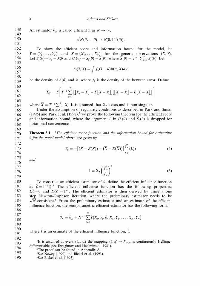
Theorem 3.1. 4The efficient score function and the information bound for estimating� for the panel model above are given by

∗� = −[�X − E�X��− (

X − E(X))]f ′

w

fw�Ut� (5)

and

I = �T

(f ′w

fw

)2

(6)

To construct an efficient estimator of �, define the efficient influence functionas = I−1∗�.

5 The efficient influence function has the following properties:E= 0 and E′ = I−1. The efficient estimator is then derived by using a onestep Newton–Raphson iteration, where the preliminary estimator needs to be√N -consistent.6 From the preliminary estimator and an estimate of the efficient

influence function, the semiparametric efficient estimator has the following form:

�N = �N + N−1N∑i=1

(Xi� Yi� �� X1� Y1� � � � � XN � YN

)where ˆ is an estimate of the efficient influence function, .

3It is assumed at every ��0� �0� the mapping �� → P�� is continuously Hellingerdifferentiable (see Ibragimov and Has’minskii, 1981).

4The proof can be found in Appendix A.5See Newey (1990) and Bickel et al. (1993).6See Bickel et al. (1993).

197198199200201202203204205206207208209210211212213214215216217218219220221222223224225226227228229230231232233234235236237238239240241242243244245


As a preliminary estimator, Park and Simar (1995) suggest the within estimatorobtained from using OLS on a transformed model of mean deviations or

�N = (NT�W

)−1N∑i=1

T∑t=1

(Xit − Xi

)(Yit − Y i

)where �W = �NT�−1 ∑N

i=1

∑Tt=1�Xit − Xi��Xit − Xi�

′ and is an estimate of �W . It iseasy to show that the within estimator is

√N -consistent. It is important to note that

other√N -consistent estimators can be used. For example, Park et al. (1998) use the

Hausman–Taylor estimator on a generalized form of this estimator that allows asubgroup of regressors to be correlated with the effects.

Define the estimate of �T as:

�T = E

[T−1

T∑t=1

[(X − X

)− (X − X

)][(X − X

)− (X − X

)]′]

where X = ∑Ni=1

∑Tt=1

Xit

�NT�. Given the efficient score and information bound from

Theorem 2.1, the efficient estimator is now defined by:

�N = �N + N−1I−1

N∑i=1

[[(X − X

)− (X − X

)] f ′w

fw�Ut�

](7)

where

I = �T

(f ′w

fw

)2

�

The f ′wfw

is estimated using a kernel estimator as described in Park and Simar (1995).These kernel estimates are then inserted into the estimator above.7 The convergenceof the semiparametric estimator now depends on the convergence rates of bothkernel estimates. Newey and McFadden (1994) discuss the asymptotics of kernelestimators in two-step semiparametric estimators. In keeping with their arguments,we use higher-order kernels to maintain

√n consistency of our adaptive estimator.

Park et al. (1998) show that within is efficient, when all of the regressors arecorrelated with the effects. We drop the normality assumption and we find within isno longer efficient.

3.1. Model 2

We next consider a new model, where a subgroup of the regressors is correlatedwith the effects. This model can be motivated using an output distance function for

AQ27Adams et al. (1999) analyzed the impact of kernel functions and of variance of optimalbandwidth selection criteria on the semiparametric efficient estimator. We use a normalkernel and higher-order normal kernel as opposed to the logistic kernel used by Park et al.(1998).

246247248249250251252253254255256257258259260261262263264265266267268269270271272273274275276277278279280281282283284285286287288289290291292293294

6 Adams and Sickles

a multiple output firm, where a second group of regressors representing normalizedright-hand side outputs, Z, are included in the model. The model can be written as:8

Yit = Xit� + Zit�+ �i + �it (8)

where Xit are independent of the transitory error and conditionally independent ofthe effects. Z and �i are independent of the transitory error term, but their jointdistribution with the effects is unknown. As a starting point, we assume that effectsare correlated in long run movements of Zit, i.e., only with Z. Thus, the density of�it� �i� X� Z is:

f��it� �� X� Z� = fw��it�h(�� Z

)g�X �Z�� (9)

Given the new model and assumptions, we get mutis mutandis, the followingtheorem.

Theorem 3.2. 9The efficient score function and the information bound for estimating �and � for the panel model above are given by

∗� = −[X − E�X�− (

X − E(X))]′ f ′

w

fw�Ut�−

[X − E

[X �Z]]w′

w

(S� Z

)(10)

∗� = −[[Zt − Z

]− E[Z − Z

]]f ′w

fw�Ut� (11)

and

I =�T

( f ′wfw

)2 + �B

(w′w

)2�XZ

( f ′wfw

)2�′

XZ

( f ′wfw

)2�TZ

( f ′wfw

)2

where

�T = E

[T−1

T∑t=1

[[Xt − X

]− E[X − X

]][[Xt − X

]− E[�X�− X

]]′]�

�B = E

[T−1

T∑t=1

[Xt − E�X

][Xt − E�X

]′]�

�TZ = E

[T−1

T∑t=1

[(Z − E�Z�

)− (Z − E

(Z))][(

Z − E�Z��− (Z − E

(Z))]′]

�

and

AQ2

�XZ = E

[T−1

T∑t=1

[�Z − E�Z��− (

Z − E(Z))][

�X − E�X��− (X − E

(X))]′]

�

8For a discussion of the output distance function with multiple outputs, see Adams et al.(1999).

9The proof can be found in Appendix A.

295296297298299300301302303304305306307308309310311312313314315316317318319320321322323324325326327328329330331332333334335336337338339340341342343


Defining estimates of the efficient influence function as before, thesemiparametric efficient estimator is now defined as

�N = �N + N−1I−1

∑Ni=1

[(X − X

)− (X − E

(X))] f ′w

fw�Ut�−

[X − E

[X]]

w′w

(S� Z

)∑N

i=1

[[Zt − Z

]− E[Z − Z

]] f ′wfw�Ut�

(12)

where

I =�T

( f ′wfw

)2 + �B

(w′w

)2�XZ

( f ′wfw

)2�′

XZ

( f ′wfw

)2�TZ

( f ′wfw

)2 �

4. Monte Carlo Simulations

In order to better understand the finite sample behavior of our estimators, weconducted a series of Monte Carlo experiments. We focus attention on our model 2,since we use this in our empirical study below.

In the Monte Carlo simulations, we develop samples with regressors andcorrelation structures similar to those in our empirical illustration using bankingdata. We then proceed by changing the correlation structure between the regressorsand by changing the distributional assumptions of the random error. We considercases where none or some of the regressors are correlated with the effects andthen introduce different random error distributions such as uniform and normal.We assume the effects are absolute normal distribution in all samples.

We draw 1,000 samples of 5 normally distributed regressors and set parametersto equal (0�5 0�5 0�5 −0�5 −0�5). These samples were estimated using thewithin, Hausman–Taylor, and semiparametric efficient estimator. Binwidth selectionmethods are discussed below. We use the within estimator as the preliminaryestimator for the semiparametric efficient estimator. In these experiments, we varyN from 10–20 and T from 10–100 and utilize higher-order bias reducing kernels.

Tables 1–4 show the results from some of these Monte Carlo simulations. T1-

T4These tables display the root mean squared error (RMSE) for all samples for

Table 1Monte Carlo RMSE of the estimator of � with effects

correlated with some regressors. Uniform error

N T �W �HT �spe

10 10 10�01 10�20 11�3110 20 7�11 7�11 7�3410 100 3�01 3�01 2�9320 10 7�28 8�53 9�6420 20 5�11 5�14 5�3220 100 2�12 2�12 2�07

344345346347348349350351352353354355356357358359360361362363364365366367368369370371372373374375376377378379380381382383384385386387388389390391392

8 Adams and Sickles


correlated with no regressors. Uniform error

n t �W �HT �spe

10 10 10�64 10�63 11�3610 20 7�30 7�30 7�4510 100 3�10 3�10 3�0220 10 7�06 7�07 8�0320 20 4�88 4�88 5�0020 100 2�17 2�17 2�11


correlated with some regressors. Normal error


10 10 34�80 36�65 38�6010 20 24�83 25�77 26�5410 100 10�64 10�74 10�7920 10 25�23 26�78 27�6720 20 17�62 17�72 18�0520 100 7�53 7�54 7�56


correlated with no regressors. Normal error


10 10 35�99 35�74 35�7410 20 24�23 24�18 24�9010 100 10�51 10�51 10�6220 10 24�85 24�73 25�5120 20 16�95 16�95 17�1720 100 7�32 7�32 7�34

393394395396397398399400401402403404405406407408409410411412413414415416417418419420421422423424425426427428429430431432433434435436437438439440441


each estimator.10 A closer look at the results indicates RMSE, and fall for allestimators as both N and T increase. When the random error is non normal(i.e., uniform), the semiparametric efficient estimator has higher RMSE than bothHausman–Taylor and within. However, the RMSE for the semiparametric efficientestimator is lower than the Hausman–Taylor and within, when T = 100. This seemsto be true for all cases where regressors are or are not correlated with the effects.In Monte Carlo simulations using normal distribution for the random error, boththe Hausman–Taylor and within estimators outperform the semiparametric efficientestimator.11

5. Data and Modeling Issues

Productivity and efficiency in the U.S. banking industry has become a topic ofparticular interest in the last decade. The 1980’s represent period of substantialchange for the industry. Regulations concerning capital requirements and depositinterest were changed at the beginning of the 1980’s. Ceilings on deposit interestrates were lifted and capital requirements were adjusted to allow for morecompetition and security in the industry. Also, the nature of banking changed asbanks moved away from traditional banking markets and the number of banksthrough mergers and failures decreased dramatically at the end of the 1980’s.12

These observations and the availability of a wealth of public data have promotedstudies of banking productivity and efficiency. The topic of productivity andefficiency in the industry are extremely relevant for future policy decisions inregulation and antitrust.

Studies of banking productivity and efficiency rely on three basic methods ofproductivity and efficiency measurement: linear programming, maximum likelihoodestimation (MLE), and instrumental variables (IV) least squares estimation.A general description of these methods can be found in Berger and Humphrey’ssurvey (1997). This study focuses on IV estimation of panel models motivatedby productivity estimation discussed in articles such as Hausman and Taylor(1981) and Schmidt and Sickles (1984). It is well known that IV methods canconsistently estimate the parameters of interest, but they are typically inefficientin that parameter estimates do not obtain the lower bound in variance. Efficientestimation is of particular interest because it allows researchers to more accurately(with less variance) identify the parameters of interest. In the banking industry,this aspect of efficient estimation becomes important to determine the robustness ofprior results and to aid in the resolution of productivity issues. In contrast, MLEmethods can efficiently estimate the parameters of interest only if the distributionalassumptions are correct. Our estimators extend the previous work of Park andSimar (1995) and Park et al. (1998).

The data set consists of about 2,550 banks from the first quarter of 1984 tothe fourth quarter of 1994. It is divided into three subsamples based on differentregulatory environments: statewide branching (State), limited branching (Limit),and no branching (Unit). These samples contain 750, 1,100, and 700 banks each.The data are taken from the Report of Condition and Income (Call Report) and

10In all tables, RMSE has been multiplied by 100. Binwidth has been set to 0.5.11This result is expected. See Park et al. (1998).12See Berger et al. (1995).

442443444445446447448449450451452453454455456457458459460461462463464465466467468469470471472473474475476477478479480481482483484485486487488489490

10 Adams and Sickles

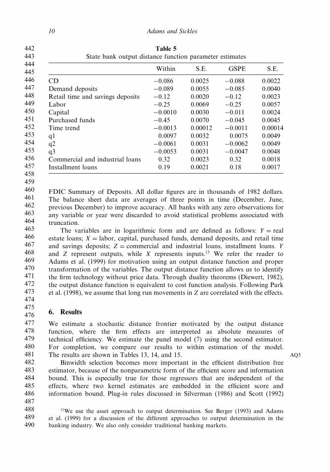
Table 5State bank output distance function parameter estimates

Within S.E. GSPE S.E.

CD −0�086 0�0025 −0�088 0�0022Demand deposits −0�089 0�0055 −0�085 0�0040Retail time and savings deposits −0�12 0�0020 −0�12 0�0023Labor −0�25 0�0069 −0�25 0�0057Capital −0�0010 0�0030 −0�011 0�0024Purchased funds −0�45 0�0070 −0�045 0�0045Time trend −0�0013 0�00012 −0�0011 0�00014q1 0�0097 0�0032 0�0075 0�0049q2 −0�0061 0�0031 −0�0062 0�0049q3 −0�0053 0�0031 −0�0047 0�0048Commercial and industrial loans 0�32 0�0023 0�32 0�0018Installment loans 0�19 0�0021 0�18 0�0017

FDIC Summary of Deposits. All dollar figures are in thousands of 1982 dollars.The balance sheet data are averages of three points in time (December, June,previous December) to improve accuracy. All banks with any zero observations forany variable or year were discarded to avoid statistical problems associated withtruncation.

The variables are in logarithmic form and are defined as follows: Y = realestate loans; X = labor, capital, purchased funds, demand deposits, and retail timeand savings deposits; Z = commercial and industrial loans, installment loans. Yand Z represent outputs, while X represents inputs.13 We refer the reader toAdams et al. (1999) for motivation using an output distance function and propertransformation of the variables. The output distance function allows us to identifythe firm technology without price data. Through duality theorems (Diewert, 1982),the output distance function is equivalent to cost function analysis. Following Parket al. (1998), we assume that long run movements in Z are correlated with the effects.

6. Results

We estimate a stochastic distance frontier motivated by the output distancefunction, where the firm effects are interpreted as absolute measures oftechnical efficiency. We estimate the panel model (7) using the second estimator.For completion, we compare our results to within estimation of the model.The results are shown in Tables 13, 14, and 15. AQ3

Binwidth selection becomes more important in the efficient distribution freeestimator, because of the nonparametric form of the efficient score and informationbound. This is especially true for those regressors that are independent of theeffects, where two kernel estimates are embedded in the efficient score andinformation bound. Plug-in rules discussed in Silverman (1986) and Scott (1992)

13We use the asset approach to output determination. See Berger (1993) and Adamset al. (1999) for a discussion of the different approaches to output determination in thebanking industry. We also only consider traditional banking markets.

491492493494495496497498499500501502503504505506507508509510511512513514515516517518519520521522523524525526527528529530531532533534535536537538539


Table 6Unit bank output distance function parameter estimates



are somewhat successful.14 We use a mixture of methods to determine optimalbinwidth. The binwidth for the multivariate kernel of the density of (S� Z�,w, is selected by the plug-in method in Adams et al. (1999).15 According tothis plug in method, the optimal binwidth is chosen by the following rule:hopt =

(4

2d+p

) 1d+2p n

1d+2p . The bin width for the density of Ut, f , is chosen by the

method suggested in Park and Simar (1995) and Park et al. (1998). In other words,the optimal h is found by bootstrapping the following: h∗ = argh minC�h� whereC�h� = (

1M

)∑Mm=1

[�∗�m�N�T �h�− �∗N�T �h�

]′[�∗�m�N�T �h�− �∗N�T �h�

]and �

∗�m�N�T �h� denotes the

mth pseudo sample bootstrap version of �∗N�T �h� using binwidth h. Our estimates arebased on M = 1� 000 and consisted of a grid search in the interval �0�1� 2�0 . Theoptimal bin width for h∗ was 0.16 for unit banks, 0.15 for state banks, and 0.15 forlimit banks. We then reestimated the � using the optimal bin width on the originaldata.

In a closer analysis of our results, we can see that the semiparametric efficientestimator improves on the IV estimator, within, in estimation efficiency. Variancein the semiparametric efficient estimates falls dramatically in comparison to thewithin estimates. Also, the parameter estimates do not change dramatically, butthe semiparametric efficient estimator does give a more precise estimate. In allthree banking environments, the standard deviations are smaller for the semipara-metric efficient estimator than those for within. Furthermore, we compare themeasurements of scale economies based on the semiparametric efficient parameterestimates to the measurements based on the within parameter estimates. We find inall cases slight economies of scale (a result that prevails in the extant literature).

We also calculated relative and absolute technical efficiencies for banks ineach data set. Figures 2 and 3 show the probability distributions of relative AQ4

and absolute technical efficiencies. Relative technical efficiencies are defined as

14This is especially true for parameter variance estimates, which can be sensitive tobinning.

15This is a simplification and other methods could be applied.

540541542543544545546547548549550551552553554555556557558559560561562563564565566567568569570571572573574575576577578579580581582583584585586587588


Table 7Limit bank output distance function parameter estimates



��j −max1��N ��j��, where efficiency scores are normalized by the most efficientfirm. Average relative technical efficiency ranges from 63% to 67%,16 where Unitand State banks are on average more efficient than Limit banks. Within andsemiparametric efficient estimates of average relative technical efficiency are veryclose. However, differences between the two estimators arise in average absolutetechnical efficiency. In Unit and Limit banks, average absolute technical efficiencydiffer substantially (limit banks differ by 0.27 and Unit banks by 0.20), while Statebank average absolute efficiencies are quite similar (only 0.0005). The more flexiblespecification of the semiparametric efficient estimator is apparently measuring ashift in the mean of the absolute efficiency densities relative to the within absoluteefficiency densities. Relative efficiencies do not change dramatically because thehigher moments of these densities are rather stable across estimators.

7. Conclusion

In this article, we introduce two efficient distribution free estimators for panelmodels. Our estimators extend the work of Park and Simar (1995), and Park et al.(1998) in that they do not specify the distribution of the transitory error term andthat the efficient estimator changes when we do not specify the distribution of thetransitory error. We find that the efficient estimator changes when we do not specifythe distribution of the transitory error. Monte Carlo simulations indicate that thesemiparametric efficient estimator improves over within and Hausman–Taylor atrelatively small sample sizes. Hence, our estimator can be used in cases with arelatively small panel (either small N or T ).

Our illustration in the banking industry displays this change in the efficiency ofthe within estimator. We observed an increase in efficiency of parameter estimatesnoted by a decrease in the variance. This study shows how these estimators can beused to determine the robustness of the productivity results in prior work.

16These averages are trimmed at the 0.1 level in keeping with Berger (1993).

589590591592593594595596597598599600601602603604605606607608609610611612613614615616617618619620621622623624625626627628629630631632633634635636637


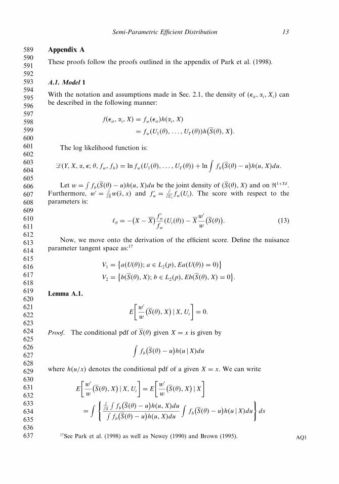
Appendix A

These proofs follow the proofs outlined in the appendix of Park et al. (1998).

A.1. Model 1

With the notation and assumptions made in Sec. 2.1, the density of ��it� �i� Xi� canbe described in the following manner:

f��it� �i� X� = fw��it�h��i� X�

= fw�U1�� UT ��h(S�� X

)�

The log likelihood function is:

��Y� X� �� fw� fb� = ln fw�U1�� UT ��+ ln∫

fb(S��− u

)h�u�X�du�

Let w = ∫fb�S��− u�h�u�X�du be the joint density of �S�� X� and on �1+Td.

Furthermore, w′ = Sw�s� x� and f ′

w = Ut

fw�Ut�. The score with respect to theparameters is:

� = −(X − X

)f ′w

fw�Ut��− X

w′

w

(S��

)� (13)

Now, we move onto the derivation of the efficient score. Define the nuisanceparameter tangent space as:17

V1 ={a�U�� a ∈ L2�p�� Ea�U�� = 0�

}V2 =

{b�S�� X�� b ∈ L2�p�� Eb�S�� X� = 0

}�

Lemma A.1.

E

[w′

w

(S�� X

) �X�Ut

]= 0�

Proof. The conditional pdf of S�� given X = x is given by∫fb(S��− u

)h�u �X�du

where h�u/x� denotes the conditional pdf of a given X = x. We can write

AQ1

E

[w′

w

(S�� X

) �X�Ut

]= E

[w′

w

(S�� X

) �X]

=∫ {

S

∫fb(S��− u

)h�u�X�du∫

fb(S��− u

)h�u�X�du

∫fb(S��− u

)h�u �X�du

}ds

17See Park et al. (1998) as well as Newey (1990) and Brown (1995).

638639640641642643644645646647648649650651652653654655656657658659660661662663664665666667668669670671672673674675676677678679680681682683684685686


=∫

S

{ ∫fb(S��− u

)h�u �X�du

}ds

=

S

[ ∫ { ∫fb(S��− u

)h�u �X�du

}ds

]=

S�1

= 0�

Lemma A.2.

E

(f ′w

fw� S�� X

)= 0�

Proof. By assumption, Ut is independent of S�� and X. Hence,

E

(f ′w

fw�Ut� S�� X

)= E

(f ′w

fw

)= 0

This follows from Lemma A.1. Now from Lemmas A.1 and A.2, we getE��= 0.

∗� = � −�(� �V1

)−�(� −�� V1� �W

)Now,

�� V1� = −E(X − X

)f ′w

fw�Ut��

where

W = V⊥1 ∩ �V1 + V2�

= {b(S�� X

)− E�b(S�� X�

)� b ∈ L2�p�� Eb

(S�� X

) = 0}�

Hence, ∗� = � −�� W�

�� W� = E�� −�� V1� � S�� X�− E��

= −Xw′

w

(S�� X

)�

The efficient score is:

∗� = −[X − E�X�− (

X − E�X�)]′ f ′

w

fw�Ut��

The information bound is

I�� = E∗�∗′�

I�� = �T

(f ′w

fw

)2

687688689690691692693694695696697698699700701702703704705706707708709710711712713714715716717718719720721722723724725726727728729730731732733734735


where

�T = E

[T−1

T∑t=1

[[Xt − X

]− E[X − X

]][[Xt − X

]− E[�X�− X

]]′]�

A.2. Model 2

Let � = �� . The setup is basically the same except now the loglikelihood of�X� Z� Y� is

��X� Z� Y� �� = ln g�X �Z�+ ln fw�Ut��+ ln∫fb�S��− ��h�� Z�d�� (14)

Let w = ∫fb�S��− ��h�� Z�d� be the density of S�� and Z and fw is defined

as before. The scores are as follows:

� = −(Xt − X

)f ′w

fw�Ut��− X

w′

w

(S�� Z

)� = −(

Zt − Z)f ′

w

fw�Ut��− Z

w′

w

(S�� Z

)�

In this model, the nuisance parameter space can be defined as follows:

V1 ={a�X�Z�� a ∈ L2�p�� E�a�X�Z� �Z� = 0

}V2 =

{b(S�� Z

)� b ∈ L2�p�� E�b�S�� Z�� = 0

}V3 =

{c�U�� c ∈ L2�p�� E�c�U�� = 0

}�

Lemma A.3.

E

[w′

w�S�� Z� �X�Z�Ut

]= 0�

Proof. Since X and � are independent conditionally on Z and �, X, and Z areindependent of Ut

E

[w′

w

(S�� Z

) �X�Z�Ut

]= E

[w′

w

(S�� Z

) �Z]�The proof follows as in Lemma A.1.

Lemma A.4.

E

(f ′w

fw� S�� X� Z

)= 0�

Proof. This proof is the same as Lemma A.2.Note

∗� = � −�(� �V1 + V2 + V3

)(15)

= � −�(� �V1 + V3

)−�(� −�� V1 + V3� �W1

)(16)

736737738739740741742743744745746747748749750751752753754755756757758759760761762763764765766767768769770771772773774775776777778779780781782783784


where

W2 = V⊥1 ∩ (

V1 + V2 + V3

) = {b�S�� Z�− E�b�S�� Z� �Z�� b ∈ L2�p�

}�

By Lemmas A.3 and A.4, � ⊥ V1 hence

�(� �V1

) = 0� (17)

Then by (A.1) and (A.2),

∗� = � −�(� −�� V3� �W1

)� (18)

From Lemma A.4,

−(Xt − X

)f ′w

fw�Ut�� ⊥ W1�

Thus,

�(� −��V3��W1

) = �

(−(

Xt − X)f ′

w

fw�Ut��− X

w′

w

(S�� Z

) �W1

)= E

(−X

w′

w

(S�� Z

) � S�� Z)− E

(−X

w′

w

(S�� Z

) �Z)�By Lemma A.3, E

(−Xw′w�S�� Z� �Z) = 0. Since X and � are independent

conditionally on Z,

E

(−X

w′

w

(S�� Z

) � S�� Z) = −E(X �Z)w′

w

(S�� Z

)�

Both imply that

�� W1� = E(X �Z)w′

w

(S�� Z

)�

Moreover, we find that

�� V3� = E(X − X

)f ′w

fw�Ut��

The efficient score and information bound are:18

∗� = −[X − E�X�− (

X − E(X))]f ′

w

fw�Ut��−

[X − E

[X �Z]]w′

w

(S�� Z

)∗� = −[

Z − E�Z�− (Z − E

(Z))]f ′

w

fw�Ut��

18The efficient score, ∗� , can be calculated in a similar fashion.

785786787788789790791792793794795796797798799800801802803804805806807808809810811812813814815816817818819820821822823824825826827828829830831832833


and

I =�T

( f ′wfw

)2 + �B

(w′w

)2�XZ

( f ′wfw

)2�′

XZ

( f ′wfw

)2�TZ

( f ′wfw

)2

where

�T = E

[T−1

T∑t=1

[[Xt − X

]− E[X − X

]][[Xt − X

]− E[�X�− X

]]′]�

�B = E

[T−1

T∑t=1

[Xt − E�X

][Xt − E�X

]′]�

�TZ = E

[T−1

T∑t=1

[�Z − E�Z��− �Z − E�Z��

][�Z − E�Z��− �Z − E�Z��

]′]and

�XZ = E

[T−1

T∑t=1

[�Z − E�Z��− �Z − E�Z��

][�X − E�X��− �X − E�X��

]′]�

Acknowledgments

This paper reflects the views of the authors and not those of the Federal ReserveBoard or the Federal Reserve System. We wish to thank Jinyong Hahn andparticipants of the Winter Econometric Society Meetings (1998) for their comments.Ying Fang provided needed editorial assistance.

References

Adams, R. M., Berger, A. N., Sickles, R. C. (1997). Computation and inference insemiparametric efficient estimation. In: Amman, H., Rustem, B., Whinston, A., eds.Adv. Computat. Econ. Boston: Kluwer Academic, pp. 57–70. AQ6

Adams, R. M., Berger, A. N., Sickles, R. C. (1999). Semiparametric approaches to stochasticpanel frontiers with applications in applications in the banking industry. J. Bus. Econ.Statist. 17:349–358.

Arrelano, M., Bover, D. (1995). Another look at the instrumental variable estimation oferror-components models. J. Econometrics 68:29–51.

Begun, J. M., Hall, W. J., Huang, W. M., Wellner, J. A. (1983). Information and asymptoticefficiency in parametric-nonparametric models. Ann. Statist. 11:432–452.

Berger, A. N. (1993). Distribution-free estimates of efficiency in U.S. banking industry andtests of the standard distributional assumptions. J. Productivity Anal. 4:261–292.

Berger, A. N., Humphrey, D. B. (1997). Efficiency of financial institutions: internationalsurvey and directions for future research. Eur. J. Operat. Res. 98:175–212.

Berger, A. N., Kashyap, A. K., Scalise, J. M. (1995). The transformation of the US bankingindustry: what a long strange tips it’s been. Brookings Pap. Econ. Activity 2:55–218.

Bickel, P. J., Klaassen, C. A. J., Ritov, Y., Wellner, J. A. (1993). Efficient and AdaptiveEstimation in Non- and Semi-Parametric Models. Baltimore, MD: Johns HopkinsUniversity Press.

Chamberlain, G. (1987). Asymptotic efficiency in estimation with conditional momentsrestrictions. J. Econometrics 34:305–334.

834835836837838839840841842843844845846847848849850851852853854855856857858859860861862863864865866867868869870871872873874875876877878879880881882


Chamberlain, G. (1992). Efficiency bounds for semiparametric regressions. Econometrica60:567–596.

Diewert, W. E. (1982). Duality approaches to microeconomic theory. In: Arrow K. J.,Intrilligator, M. D., eds. Handbook of Mathematical Economics, Volume II. Amsterdam:North Holland.

Hahn, J. (1997). Efficient estimation of panel data models with sequential momentrestrictions. J. Econometrics. AQ5

Hausman, J. A., Taylor, E. E. (1981). Panel data and unobservable individual effects.Econometrica 49:1377–1398.

Horowitz, J. L., Markatou, M. (1996). Semiparametric estimation of regression models forpanel data. Rev. Econ. Stud. 63:145–168.

Horrace, W. (1997). A semiparametric error component density estimation technique forstochastic frontier models. Mimeo, University of Arizona.

Ibragimov, I. A., Has’minskii, R. Z. (1981). Statistical Esimtation: Asymptotic Theory.New York: Springer.

Newey, W. K. (1990). Semiparametric efficiency bounds. J. App. Econometrics 5:99–136.Newey, W. K., McFadden, D. L. (1994). Large sample estimation and hypothesis testing. In:

Engle. R. F., Mcfadden, D. L., eds. Handbook of Econometrics, Volume IV. Amsterdam:Elsevier.

Pagan, P., Ullah, A. (1999). Non-Parametric Econometrics. New York: Cambridge UniversityPress.

Park, B. U., Simar, L. (1995). Efficient semiparametric estimation in stochastic frontiermodels. J. Amer. Statist. Assoc. 89:929–936.

Park, B. U., Sickles, R. C., Simar, L. (1998). Stochastic frontiers: a semiparametric approach.J. Econometrics 84:273–301.

Robinson, P. (1988). Root-N-consistent semiparametric regression. Econometrica 56:931–954. AQ6Schmidt, P., Sickles, R. C. (1984). Production frontiers and panel data. J. Bus. Econ. Statist.

2:367–374.Scott, D. W. (1992). Multivariate Density Estimation: Theory, Practice, and Visualization.

New York: John Wiley & Sons.Silverman, B. W. (1986). Density Estimation for Statistics and Data Analysis. London:

Chapman and Hall.

Semiparametric Efficient Distribution Free Estimation of Panel Models

Documents

Transcript of Semiparametric Efficient Distribution Free Estimation of Panel Models