This article was downloaded by: [University of Lethbridge]On: 24 July 2014, At: 11:35Publisher: Taylor & FrancisInforma Ltd Registered in England and Wales Registered Number: 1072954 Registered office: Mortimer House,37-41 Mortimer Street, London W1T 3JH, UK

Econometric ReviewsPublication details, including instructions for authors and subscription information:http://www.tandfonline.com/loi/lecr20

Local GMM Estimation of Semiparametric Panel Datawith Smooth Coefficient ModelsKien C. Tran a & Efthymios G. Tsionas ba Department of Economics , University of Lethbridge , Lethbridge, Alberta, Canadab Department of Economics , Athens University of Economics and Business , Athens, GreecePublished online: 10 Nov 2009.

To cite this article: Kien C. Tran & Efthymios G. Tsionas (2009) Local GMM Estimation of Semiparametric Panel Data withSmooth Coefficient Models, Econometric Reviews, 29:1, 39-61, DOI: 10.1080/07474930903327856

To link to this article: http://dx.doi.org/10.1080/07474930903327856

PLEASE SCROLL DOWN FOR ARTICLE

Taylor & Francis makes every effort to ensure the accuracy of all the information (the “Content”) containedin the publications on our platform. However, Taylor & Francis, our agents, and our licensors make norepresentations or warranties whatsoever as to the accuracy, completeness, or suitability for any purpose of theContent. Any opinions and views expressed in this publication are the opinions and views of the authors, andare not the views of or endorsed by Taylor & Francis. The accuracy of the Content should not be relied upon andshould be independently verified with primary sources of information. Taylor and Francis shall not be liable forany losses, actions, claims, proceedings, demands, costs, expenses, damages, and other liabilities whatsoeveror howsoever caused arising directly or indirectly in connection with, in relation to or arising out of the use ofthe Content.

This article may be used for research, teaching, and private study purposes. Any substantial or systematicreproduction, redistribution, reselling, loan, sub-licensing, systematic supply, or distribution in anyform to anyone is expressly forbidden. Terms & Conditions of access and use can be found at http://www.tandfonline.com/page/terms-and-conditions

Econometric Reviews, 29(1):39–61, 2010Copyright © Taylor & Francis Group, LLCISSN: 0747-4938 print/1532-4168 onlineDOI: 10.1080/07474930903327856

LOCAL GMM ESTIMATION OF SEMIPARAMETRIC PANELDATA WITH SMOOTH COEFFICIENT MODELS

Kien C. Tran1 and Efthymios G. Tsionas2

1Department of Economics, University of Lethbridge,Lethbridge, Alberta, Canada2Department of Economics, Athens University of Economics and Business,Athens, Greece

� In this article, we consider the estimation of semiparametric panel data smooth coefficientmodels. We propose a class of local generalized method of moments (LGMM) estimators thatare simple and easy to implement in practice. We show that the proposed LGMM estimatorsare consistent and asymptotically normal. Monte Carlo simulations suggest that our proposedestimator performs quite well in finite samples. An empirical application using a large panelof U.K. firms is also presented.

Keywords Local Generalized Method of Moments; Monte Carlo simulation; Semiparametricpanel data model; Smooth coefficient.

JEL Classification C13; C14; C33.

1. INTRODUCTION

The choice of a regression functional form is very importantfor economic analysis. Economic theory rarely provides a specificfunctional form for the regression relationship. Thus, unless thefunctional form is correctly specified, the performance of a modelwill generally be poor. Accordingly, it seems more desirable to workwith the nonparametric/semiparametric regression models to avoid themisspecification of the regression functional form. One of the advantagesof the nonparametric/semiparametric method is that little prior restrictionis imposed on the model’s structure, and it may provide useful guidancefor the construction of parametric models.

Address correspondence to Kien C. Tran, Department of Economics, University of Lethbridge,4401 University Drive, Lethbridge, Alberta T1K 3M4, Canada; E-mail: kien.tran@uleth.ca

Dow

nloa

ded

by [

Uni

vers

ity o

f L

ethb

ridg

e] a

t 11:

35 2

4 Ju

ly 2

014

40 K. C. Tran and E. G. Tsionas

In the context of panel data models, there has been a recent focuson semiparametric panel data models or “partial linear” panel datamodels. For example, Horowitz and Markatou (1996), Ullah and Roy(1998), Li and Hsiao (1998), Ullah and Mundra (1999), Knieser andLi (2002) considered semiparametric panel data models with exgoneousregressors, while Li and Stengos (1996), Li and Ullah (1998), Papalia(1999), Baltagi and Li (2002) considered semiparametric panel datamodels with endogenous regressors. However, all the above-mentionedworks assumed that the regression coefficients on the parametric partare constant over time and across individuals. In practice, it is possiblethat, in one set of data, this assumption produces more reasonableempirical results, but in another data set, allowing for the coefficientsto vary across individuals, or over time, or both on the parametricpart, may lead to more plausible empirical results. Thus, an importantextension to the semiparametric panel data models is to allow for theregression coefficients on the parametric part to vary according to thesmooth coefficient model. The smooth coefficient model lets the marginaleffect of a given variable be an unknown function of an observablecovariate, and hence, introduces heterogeneity into the marginal effect.This specification also nests the traditional linear model as a specialcase when the marginal effect is found to be constant over the supportof the observable covariate. Smooth coefficient models have receiveda lot of attention in the statistics/econometrics literature recently andhave been used in various applications; see for example, Hastie andTibshirani (1993), Carroll et al. (1998), Gozalo and Linton (2000), Fanand Zhang (1999), Cai et al. (2000), Das (2005), Cai et al. (2006), justto name a few. However, most of the works are focused on models withexogenous regressors, and very little attention has been paid to the case ofsemiparametric panel data with endogenous regressors.1

The purpose of this article is to extend the semiparametric paneldata models with endogenous regressors to allow for the slope coefficientheterogeneity in the parametric part of the model by allowing it tohave a smooth coefficient form. We propose a consistent two-steplocal generalized method of moments estimator to estimate the smoothcoefficients, and establish its asymptotic properties. After the initialrevised and resubmission of our article, an associate editor and a refereedirected our attention to the recent work of Cai and Li (2008). In that

1Das (2005) and Cai et al. (2006) considered cross-section varying–coefficient models withendogenous regressors whereas Carroll et al. (1998) and Gozalo and Linton (2000) consideredmodels with exogenous regressors. Also, it is worth to point out that Carroll et al. (1998)method for estimating varying coefficient is based on M -estimation procedure using the local first-order conditions; while Gozalo and Linton (2000) method is initially parameterizing an unknownregression function g (x), and then using local polynomial fitting to recover the g (x) and itsderivatives.

Dow

nloa

ded

by [

Uni

vers

ity o

f L

ethb

ridg

e] a

t 11:

35 2

4 Ju

ly 2

014

Local GMM Estimation 41

article, they suggest a nonparametric generalized method of moments(NPGMM) approach to estimate a varying coefficient panel data modelwith endogenous regressors. Their approach is based on a local linearfitting, and they consider the case where both N ,T → ∞. Although theirapproach has some overlap with our proposed method, there are someimportant differences. First, they only consider a one-step NPGMM witha weighting matrix that is the identity matrix, while we allow for moregeneral weighting matrix and consider a two-step (and/or iterative two-step) estimation approach. Consequently, the advantage of our methodover Cai and Li’s (2008) approach is a potential asymptotic efficiency gainfrom the use of such two-step estimator. Second, their article containsneither simulations nor an empirical application, while we provide someMonte Carlo simulations to examine the finite sample performance,and an empirical application to illustrate the usefulness of the proposedmethod.

The article is organized as follows. Section 2 introduces thesemiparametric panel model with smooth coefficients. Section 3 derivesthe local generalized method of moments (GMM) estimators andestablishes the asymptotic properties of the proposed estimators. MonteCarlo simulations are presented in Section 4. Section 5 provides anempirical illustration. Section 6 briefly discusses the fixed effects model.Concluding remarks are given in Section 7. Proof of the theorem is givenin the Appendix.

2. THE MODEL

We consider the following semiparametric panel data with varying–coefficient model:

yit = x ′it�(zit) + uit , (i = 1, � � � ,N ; t = 1, � � � ,T ), (1)

where the prime denotes the transpose of a matrix or vector, xit isof dimension (p × 1) with its first element xit ,1 = 1, zit is of dimension(q × 1) which does not contain a constant, �(zit) is a (p × 1) vector ofunknown and unspecified smooth functions, and uit is the usual randomdisturbance. We allow some or all components of xit to be correlated withthe error uit . We assume the data are independent across the i index butthere is no restriction on the time index t , and E(uit | zit) = 0. We considerthe common empirical case of N large and small T .

We also allow the possibility that the error term uit is seriallycorrelated. For example, when uit follows a one-way error componentspecification, uit = �i + �it , where �i a random individual specific effectwith �i ∼ i�i�d �(0, �2

�) and �it ∼ i�i�d �(0, �2�), which render the errors serially

correlated.

Dow

nloa

ded

by [

Uni

vers

ity o

f L

ethb

ridg

e] a

t 11:

35 2

4 Ju

ly 2

014

42 K. C. Tran and E. G. Tsionas

There are several interesting features of model (1) worth mentioning.First, (1) is an extension and generalization of the cross-section modelconsidered by Li et al. (2002). Second, when x1,it = 1 and �j(zit)= �0,j = 2, � � � , p, model (1) reduces to the semiparametric panel model ofBaltagi and Li (2002) and Li and Stengos (1996). Third, model (1)covers semiparametric IV models considered by Das (2005) for discreteendogenous regressors and Cai et al. (2006) for both discrete andcontinuous endogenous regressors. Finally, if there are no endogenousvariables and the coefficients �j(·), j = 2, � � � , p are threshold functionssuch as

�j(z) = �j1I (z ≤ �j) + �j2I (z > �j),

then model (1) may describe a threshold nondynamic panel regressionmodel of Hansen (1999). Thus, model (1) includes some interestingspecial cases that arise commonly in empirical research.

3. LOCAL GENERALIZED METHOD OF MOMENTS ESTIMATION

By stacking all T observations for the ith individual, (1) can bewritten as

yi = Xi�(Zi) + ui , i = 1, � � � ,N , (2)

where yi = (yi1, � � � , yiT )′ is a (T × 1) vector, Xi is a (T × p) matrix havingrows x ′

it , t = 1, � � � ,T , �(Zi) = (�(zi1), � � � , �(ziT ))′, Zi is a (T × q) matrixhaving rows z ′

it , t = 1, � � � ,T , and ui = (ui1, � � � ,uiT )′ is a (T × 1) vector.

Assume that there exists a (T × l) (where l ≥ p) matrix of instruments Wi

having rows w ′it (where the first component of wit ,wit ,1 = 1), t = 1, � � � ,T ,

such that (Xi ,Zi ,Wi ,ui) are iid over i = 1, � � � ,N and

E(wituit | zit) = 0, t = 1, � � � ,T ,

which implies, for a given zit = z

E(W ′i ui |Zi = �T z ′) =

T∑t=1

E(wituit | zit = z) = 0, (3)

where �T = (1, � � � , 1)′ is a (T × 1) vector of ones. Thus, Eq. (3) providesthe moment conditions that form the basis for identification and ourestimation below. In the cross-section context, Cai et al. (2006) providedthe conditions for which �(·) is identified (up to an additive constant)and proposed a two-stage estimation method. However, their identificationconditions are not directly applicable in our case since our estimation

Dow

nloa

ded

by [

Uni

vers

ity o

f L

ethb

ridg

e] a

t 11:

35 2

4 Ju

ly 2

014

Local GMM Estimation 43

method will be based on the conditional moment restrictions in (3).Furthermore, their proposed estimation method will require a two-stepnonparametric estimation procedure which will complicate the asymptoticanalysis of the resulting estimator. To avoid these shortcomings, we suggesta simple estimation which will require only one nonparametric estimationprocedure.

To obtain identification conditions for our case, note that from (3)fixing Zi = �T z ′ and for any �1(z), we have2

E[W ′

i (Yi − Xi�1(z)) |Zi = �T z ′] = E(W ′i ui |Zi = �T z ′)

+ E[W ′

i Xi(�(z) − �1(z)) |Zi = �T z ′]= E(W ′

i Xi |Zi = �T z ′)(�(z) − �1(z))�

Thus, the necessary and sufficient condition for identify �(z) is thatE(W ′

i Xi |Zi = �T z ′) has full column rank since E(W ′i Xi |Zi = �T z ′)(�(z) −

�1(z)) = 0 if and only if �(z) = �1(z).For the remaining part of the article, we assume that the vector

�(·) is identified and twice continuously differentiable. Then for a givenpoint z ∈�q and for �zit in the neighborhood of z, Eq. (3) provides theconditional moment restrictions that can be used to construct an estimatorsimilar to the GMM of Hansen (1982) for parametric models. Thus thelocal-GMM (LGMM) criterion function is

JN (�) =[1N(Y − X �(z))′KW

]R−1

N

[1NW ′K (Y − X �(z))

], (4)

where Y = (Y ′1, � � � ,Y

′N )

′ is a (NT × 1) vector, W = (W ′1 , � � � ,W

′N )

′ is a(NT × l) matrix of instruments, X = (X ′

1, � � � ,X′N )

′ is a (NT × p) matrixof regressors, RN is some (l × l) positive definite weighting matrix, andK is an (NT × NT ) matrix of kernel weights with K = diag�KT

1 , � � � ,KTN ,

KTi = diag(KH (zit − z)), t = 1, � � � ,T , is a (T × T ) matrix, and KH () =∏qj=1 h

−1j k(j/hj), in which k(�) ≥ 0, is a bounded univariate symmetric

function with∫k(�)d� = 1,

∫�2k(�)d� = � > 0,

∫k2(�)d� = > 0, so

that K () = ∏qj=1 k(j), and H = diag�h1, � � � , hq is a (q × q) matrix of

bandwidths with |H | = ∏qj=1 hj , and hj > 0.

For a given zit = z, minimizing (5) with respect to �, we obtain

�(z) = [X ′KWR−1

N W ′KX]−1

X ′KWR−1N W ′KY � (5)

The estimator given in (5) is termed a LGMM estimator. It is consistentbecause E(wituit | zit = z) = 0. However, to implement (5) one needs to

2We owe this observation to an anonymous referee.

Dow

nloa

ded

by [

Uni

vers

ity o

f L

ethb

ridg

e] a

t 11:

35 2

4 Ju

ly 2

014

44 K. C. Tran and E. G. Tsionas

specify the weighting matrix RN . Different full-rank weighting matrices RN

lead to different local GMM estimators, except in the just-identified casewhere l = p. The two leading choices are given below.

(1) One-Step LGMM Estimator:Under i�i�d � assumption, the one-step LGMM estimator uses weighting

matrix.3

R1N = R(z) ≡ E(W ′

1KT1 W1

) = f (z)E(W ′1W1 |Z1 = �T z ′) = O(1),

leading to

�OS(z) = [X ′KW (W ′KW )−1W ′KX

]−1X ′KW (W ′KW )−1W ′KY , (6)

where in (6) we have replaced R1N by its consistent estimator, R1N =N −1

∑Ni=1 W

′i K

Ti Wi . The motivation for this estimator is that it can be

shown to be the optimal LGMM estimator based on the conditionalmoment restrictions (3) if ui | zi is iid(0, �2IT ). Also, it is interesting tonote that the one-step local GMM estimator given in (6) is numericallyequivalent to the two-stage smooth coefficient least squares estimator(Li et al., 2002) where in the first stage, a smooth coefficient least squaresregression of X on W , yielding prediction X , and in the second stage,a smooth coefficient least squares regression of Y on X using the samekernel K and bandwidth H .

(2) Two-Step Local GMM Estimator:Under i�i�d � assumption over i and stationarity assumption over t ,

the two-step LGMM estimator uses the weighting matrix (see Appendix forderivation)

R2N = S(z) ≡ limN→∞

var{√

N |H |(W ′1K

T1 u1

)}= f (z)

∫K 2(z)dz ′E

(W ′

1V1W1 |Z1 = �T z ′)

= f (z)∫

K 2(z)dz ′E( T∑

t=1

u21tw1tw ′

1t | z1t = z)

= �0(z)f (z)∫

K 2(z)dz ′,

where V1 =diag(u211, � � � ,u

21T

)and �0 =E

(W ′

1V1W1 |Z1 = �T z ′) =E( ∑T

t=1

u21tw1tw ′

1t | z1t = z). Let A∗

i = (KT

i

)1/2Ai and A∗ = (

A∗1, � � � ,A

∗N

)′, where

3We use the subscript 1 to signify “typical i .”

Dow

nloa

ded

by [

Uni

vers

ity o

f L

ethb

ridg

e] a

t 11:

35 2

4 Ju

ly 2

014

Local GMM Estimation 45

(KT

i

)1/2 = diag(√

KH (zit − z)), t = 1, � � � ,T , and Ai = Xi ,Wi , or Yi , then

by standard arguments of kernel smoothing, S(z) can be consistentlyestimated by

SN (z) = f (z)∫

K 2(z)dz ′N∑i=1

T∑t=1

u21tw1tw ′

1tKH (zit − z)

= f (z)∫

K 2(z)dz ′{N −1

N∑i=1

W ∗′i ViW ∗

i

},

where uit = yit − x ′it �OS(z).

Thus, by replacing RN in (5) with SN (z), we obtain the following two-step LGMM estimator

�TS(z) = [X ∗′

W ∗(W ∗′V W ∗)−1

W ∗′X ∗]−1

X ∗′W ∗(W ∗′

V W ∗)−1W ∗′

Y ∗, (7)

where V = diag(V1, � � � , VN

)and Vi = diag

(u2i1, � � � , u

2iT

)is a consistent

estimator of Vi . We call this a two-step LGMM estimator because a first-stepconsistent estimator of �(z) such as �OS(z) is needed to form the residualsu used to compute V .

The two-step LGMM estimator may be iterated by recomputing theresiduals after computing (7) and then reentering the computation. Theasymptotic properties of the iterated estimator are the same as those oftwo-step estimator which will be discussed next.

Asymptotic Properties

First, we introduce some additional notation. Let �2 = ∫�2K (�)d�,

z0 = �T z ′, �j(z) = ��(z)/�zj , and �jj(z) = �2�(z)/�z2j be (q × 1) vectors. Inaddition, ��

� denote the class of functions such that if f ∈ ��� , then f is �

times continuously differentiable, and its derivatives up to order � are allbounded by some function that has �th order finite moments. We makethe following assumptions:

(A.1): (i) For each fixed t , �(yit , xit ,wit , zit ,uit) are iid in the isubscript and strictly stationary over t for each fixed i . Let f (z) bethe marginal density function of zit , and let A(z) = f (z)E(W ′

i Xi |Zi = z0).f (z)∈�∞

�−1, �(z) ∈ �4+�� , and A(z) ∈ �4+�

�−1 , for some � > 0 and some positiveinteger � ≥ 2. �(z), f (z), A(z), and f (z)�0(z), all satisfy some Lipschitz-typeof conditions in z.

(ii) For each t ≥ 1, let �r (z1, z2) = E(u1tw1tu1t−r w1t−r | z1t = z1, z1t−r = z2

)and gr (z1, z2), the joint density of (z1t , z1t−r ) is continuous at

(z1t = z1,

Dow

nloa

ded

by [

Uni

vers

ity o

f L

ethb

ridg

e] a

t 11:

35 2

4 Ju

ly 2

014

46 K. C. Tran and E. G. Tsionas

z1t−r = z2). In addition, supt≥1

∣∣�r (z1, z2)g (z1, z2)∣∣ ≤ C(z) < ∞ for some

function C(z).

(A.2): There exists a (T × l) (where l ≥ p) matrix of instrumentsWi having rows w ′

it , t = 1, � � � ,T such that E(W ′i ui |Zi = z0) = 0 and

E [W ′i Xi |Zi = z0] is of full column rank for all z.

(A.3): E |ui |2 < ∞, E‖W ′i Xi‖2 < ∞ and E‖W ′

i Wi‖2 < ∞.

(A.4): k(·) ≥ 0 is a bounded symmetric function with∫k(�)d� = 1,∫

�2k(�)d� = � > 0,∫k2(�)d� = > 0, and

∫K ()d′ = 1. As N → ∞,√

N |H | → ∞ and hj → 0.

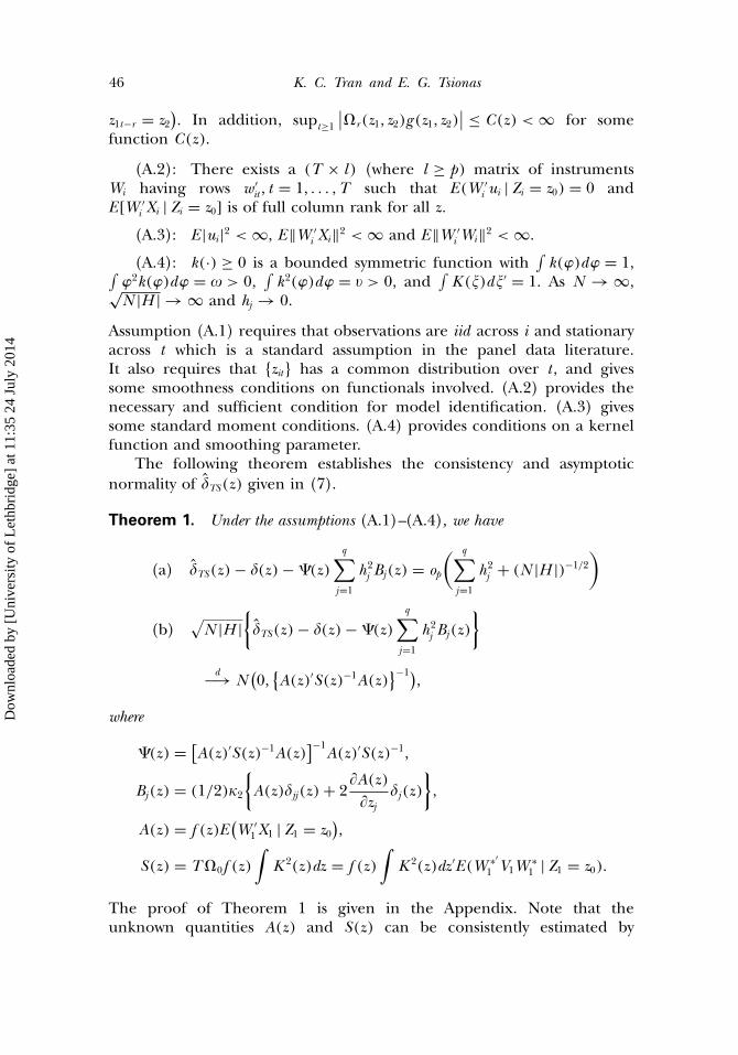
Assumption (A.1) requires that observations are iid across i and stationaryacross t which is a standard assumption in the panel data literature.It also requires that �zit has a common distribution over t , and givessome smoothness conditions on functionals involved. (A.2) provides thenecessary and sufficient condition for model identification. (A.3) givessome standard moment conditions. (A.4) provides conditions on a kernelfunction and smoothing parameter.

The following theorem establishes the consistency and asymptoticnormality of �TS(z) given in (7).

Theorem 1. Under the assumptions (A.1)–(A.4), we have

(a) �TS(z) − �(z) − �(z)q∑

j=1

h2j Bj(z) = op

( q∑j=1

h2j + (N |H |)−1/2

)

(b)√N |H |

{�TS(z) − �(z) − �(z)

q∑j=1

h2j Bj(z)

}

d−→ N(0,

{A(z)′S(z)−1A(z)

}−1),

where

�(z) = [A(z)′S(z)−1A(z)

]−1A(z)′S(z)−1,

Bj(z) = (1/2)�2

{A(z)�jj(z) + 2

�A(z)�zj

�j(z)},

A(z) = f (z)E(W ′

1X1 |Z1 = z0),

S(z) = T�0f (z)∫

K 2(z)dz = f (z)∫

K 2(z)dz ′E(W ∗′1 V1W ∗

1 |Z1 = z0)�

The proof of Theorem 1 is given in the Appendix. Note that theunknown quantities A(z) and S(z) can be consistently estimated by

Dow

nloa

ded

by [

Uni

vers

ity o

f L

ethb

ridg

e] a

t 11:

35 2

4 Ju

ly 2

014

Local GMM Estimation 47

AN (z)=N −1∑N

i=1 W′i XiK T

i (z) and SN (z) = N −1∫K 2(z)dz ′{∑N

i=1 W∗′i ViW ∗

i

},

respectively, where Vi = diag(u2i1, � � � , u

2iT

), and ui = Yi − Xi �TS(z) is a

(T × 1) estimated residual vector from the two-step LGMM estimatorin (7).

Remark 1. It is interesting to note that the results of Theorem 1also covers the results in the cross-sectional data case (e.g., T = 1).Furthermore, when there is no endogenous variable in the model(e.g., wit = xit), it also covers the results in Li et al. (2002).

Remark 2. To implement the estimator in (6) or (7), one needs tospecify the choice of the kernel function, the smoothing parameters,and the set of instrument variables. In practice, the most commonlyused kernel function is a Gaussian kernel, although any other functionthat satisfies the conditions in assumption (A.4) could be used. However,it is known that the choice of the kernel function is of less importancecompared to the choice of the smoothing parameters. In practice,one could use hj = sd(zj)N −1/(q+4), where sd(zj) is the sample standarddeviation of zj , j = 1, 2, � � � , q . Alternatively, one may use some data-drivenmethod such as cross-validation to select hj . As for the choice of instrumentvariables, by the exogenous assumption, we know that E

(uit | zit

) = 0,so that zit is uncorrelated with uit , and hence zit or any function of zit can beused as part of the set of instruments.4 On the other hand, Newey (1990)and Baltagi and Li (2002) offer discussion on how to choose optimalinstruments in the context of semiparametric panel data models, and ifwe restrict our attention to the case where the instruments are functionsof zit , we can use the results of Newey (1990) or Baltagi and Li (2002)to construct the optimal instruments. The readers are referred to thesearticles for more detailed.

4. MONTE CARLO SIMULATION

In this section, we report some simulation results to examine the finitesample performance of our proposed two-step LGMM estimator, and alsocompare it with the NPGMM estimator suggested by Cai and Li (2008).We consider the following data generating process (DGP):5

yit = �(zit)yi ,t−1 + xit�(zit) + �i + vit ,

4Note that when xit contains lagged of dependent variable, zit is assumed to be weaklyexogenous in the sense that E

(uit | zis

) = 0 for s ≤ t .5Part of the DGP are taken from Baltagi and Li (2002).

Dow

nloa

ded

by [

Uni

vers

ity o

f L

ethb

ridg

e] a

t 11:

35 2

4 Ju

ly 2

014

48 K. C. Tran and E. G. Tsionas

where

�(zit) = exp[−(0�5zit − 1�5)2] and �(zit) = zit + sin(zit)�

The error term vit is i�i�d � N (0, �2v), �i is i�i�d � N (0, �2

�), zit is generatedas by the i�i�d � uniform[2,6] distribution, and xit = �1it + �2it , where �jit ,j = 1, 2, are i�i�d � uniform[0,2]. We fixed the total error variance �2 = �2

� +�2v = 1�0, and define � = �2

�/�2 = �0�2, 0�5, 0�8. The sample sizes are

N = �100, 200 and T = 5, and the number of replications is 500 for allcases.

Note that the above DPG is a special case, where the model is adynamic one-way error component model with an exogenous regressor.The main reason why we chose this model for our simulation study isbecause it seems to be the most common case encountered in practice.

In our simulation, a Gaussian kernel function is used and thesmoothing parameter is chosen as h = �sd(z)N −1/5, where � = 0�8, 1�0 and1.2. However, our results do not seem to be sensitive to the choice of �,and consequently, we set � = 1�0 in all of our experiments. We comparethe estimated mean average square error (MASE) of �j(·) = (

�j(·), �j(·))′

defined by

MASE(�(·)) = 11000

1000∑j=1

{1NT

N∑i=1

T∑t=1

(�j(zit) − �j(zit)

)}2

,

where �j(·) is the estimate of �j(·) = (�j(·), �j(·)

)′from the j th replication

based on one of the two methods: the two-step LGMM method or theNPGMM method.

We use two sets of instruments for each method. The first setof instruments consists of the w(1)

it = {yi ,t−2, zit−1, xit , xit−1

}, and in the

second set, we use the optimal instruments given by w(o)it = {

E(yit−1 | zit−1),E(yit−1 | zit−2,E(yit−1 | zit−1, zit−2), xit

}(see Baltagi and Li, 2002). Note that

some of the optimal instruments in w(o)it are not feasible because

the conditional expectations involved are unknown. However, theseconditional expectations can be consistently estimated using somenonparametric approach such as kernel method, series method, etc.In this article, we suggest using the density-weighted kernel smoothingapproach (see Powell et al., 1989) to estimate these unknown conditionalexpectations.

The simulation results are presented in Table 1, where the instrumentset w(1)

it is used in the estimation. From Table 1, we first see that bothNPGMM and the two-step LGMM methods perform quite well in the finitesample. Second, by comparing the two methods, we observed that thereare substantial efficiency gains from using the two-step LGMM method as

Dow

nloa

ded

by [

Uni

vers

ity o

f L

ethb

ridg

e] a

t 11:

35 2

4 Ju

ly 2

014

Local GMM Estimation 49

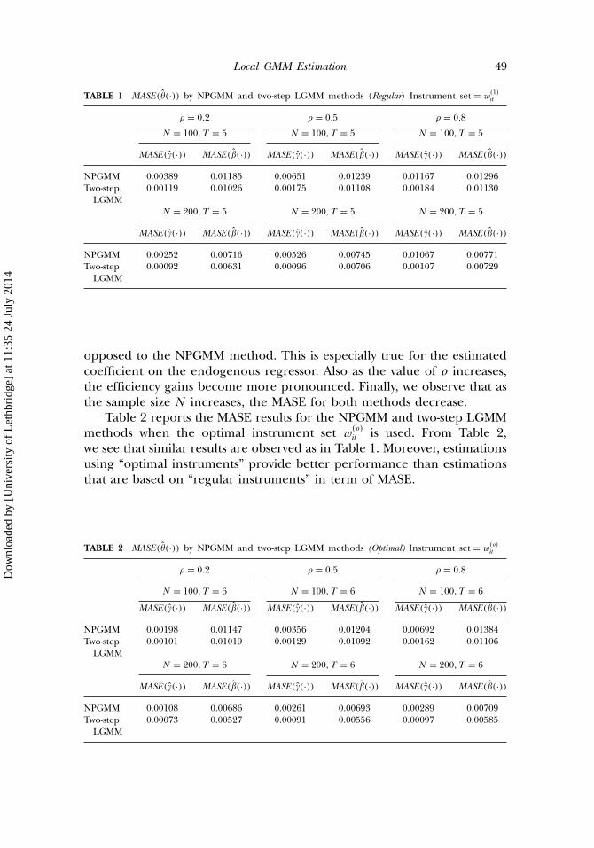
TABLE 1 MASE(�(·)) by NPGMM and two-step LGMM methods (Regular) Instrument set = w(1)it

� = 0�2 � = 0�5 � = 0�8

N = 100,T = 5 N = 100,T = 5 N = 100,T = 5

MASE(�(·)) MASE(�(·)) MASE(�(·)) MASE(�(·)) MASE(�(·)) MASE(�(·))NPGMM 0.00389 0.01185 0.00651 0.01239 0.01167 0.01296Two-step 0.00119 0.01026 0.00175 0.01108 0.00184 0.01130

LGMMN = 200,T = 5 N = 200,T = 5 N = 200,T = 5

MASE(�(·)) MASE(�(·)) MASE(�(·)) MASE(�(·)) MASE(�(·)) MASE(�(·))NPGMM 0.00252 0.00716 0.00526 0.00745 0.01067 0.00771Two-step 0.00092 0.00631 0.00096 0.00706 0.00107 0.00729

LGMM

opposed to the NPGMM method. This is especially true for the estimatedcoefficient on the endogenous regressor. Also as the value of � increases,the efficiency gains become more pronounced. Finally, we observe that asthe sample size N increases, the MASE for both methods decrease.

Table 2 reports the MASE results for the NPGMM and two-step LGMMmethods when the optimal instrument set w(o)

it is used. From Table 2,we see that similar results are observed as in Table 1. Moreover, estimationsusing “optimal instruments” provide better performance than estimationsthat are based on “regular instruments” in term of MASE.

TABLE 2 MASE(�(·)) by NPGMM and two-step LGMM methods (Optimal) Instrument set = w(o)it

� = 0�2 � = 0�5 � = 0�8

N = 100,T = 6 N = 100,T = 6 N = 100,T = 6

MASE(�(·)) MASE(�(·)) MASE(�(·)) MASE(�(·)) MASE(�(·)) MASE(�(·))NPGMM 0.00198 0.01147 0.00356 0.01204 0.00692 0.01384Two-step 0.00101 0.01019 0.00129 0.01092 0.00162 0.01106

LGMMN = 200,T = 6 N = 200,T = 6 N = 200,T = 6

MASE(�(·)) MASE(�(·)) MASE(�(·)) MASE(�(·)) MASE(�(·)) MASE(�(·))NPGMM 0.00108 0.00686 0.00261 0.00693 0.00289 0.00709Two-step 0.00073 0.00527 0.00091 0.00556 0.00097 0.00585

LGMM

Dow

nloa

ded

by [

Uni

vers

ity o

f L

ethb

ridg

e] a

t 11:

35 2

4 Ju

ly 2

014

50 K. C. Tran and E. G. Tsionas

5. EMPIRICAL APPLICATION

In this section, we apply the new techniques to data on a substantialnumber of U.K. manufacturing companies from 1982 to 1994 as used byNickell (1996) and Nickell et al. (1997). These authors have investigatedthe role of competition in productivity and productivity growth since“[the] general belief in the efficacy of competition exists despite the factthat it is not supported either by any strong theoretical foundation or by alarge corpus of hard empirical evidence in its favor” (Nickell, 1996, p. 725).The evidence provided in Nickell (1996) and Nickell et al. (1997) restsupon strong parametric assumptions, the assumption of constant returnsto scale in a Cobb–Douglas production technology,6 and the assumptionthat competition measures do not have a firm-specific or time-specificeffect on productivity. All these assumptions are troublesome and could beresponsible for biased results.

The basic model in Nickell (1996) is

yit = �yi�t−1 + (1 − �)�init + (1 − �)(1 − �i)kit + �hit + fit + uit ,

where yit is log of output, nit is log employment, kit is capital stock,hit is a business cycle component, fit reflects all factors influencing thelevel of productivity, uit is an error term, and we have omitted time-specific and firm-specific fixed effects. Nickell (1996) has estimated themodel in first-differenced form using the Arellano and Bond (1991) GMMtechnique. The variables used in fit that affect productivity or productivitygrowth are the following: market share, rents normalized on value-added,concentration ratio, and import penetration (imports divided by homesales). For detailed construction of these variables, see Nickell (1996) andNickell et al. (1997).

In this article, we use an extended unbalanced panel data set of 582companies taken from Nickell et al. (1997). We estimate the followingdynamic panel data with smooth coefficients model

yit = �(zit)yit−1 + (1 − �(zit))�1(zit)nit + (1 − �(zit))(1 − �1(zit))kit

+ �(zit)hit + �′(zit)fit + �i + uit ,

where the covariate zit is taken to be logarithm of debt. Thus our empiricalmodel suggests that the dynamic adjustment, labor, capital, and other inputscoefficients may vary directly with the firm’s debt values. As a result, thereturns to scale may also be a function of debt. Note that Nickell (1996)

6Nickell (1996) tried to deal with both assumptions in a parametric way. For example, headded a CES component to check whether the Cobb–Douglas assumption is responsible for seriousdifferences in the results.

Dow

nloa

ded

by [

Uni

vers

ity o

f L

ethb

ridg

e] a

t 11:

35 2

4 Ju

ly 2

014

Local GMM Estimation 51

treats kit and nit as endogenous in the model, so we follow the samepractice here.

We estimate the above model using the LGMM procedure givenin (7). We use a standard normal kernel for k(·) and since zit isa scalar, univariate crossvalidation bandwidth selection procedure isused to determine the optimal bandwidth. For the selection of theinstruments, we use the optimal instrument discussed in Baltagi andLi (2002). Specifically, we use the density-weighted kernel estimates of�E(yit−1 | zit−1),E(yit−2 | zit−2),E(kit | zit),E(kit−1 | zit−1),E(nit | zit),E(nit−1 | zit−1)as instrument set for �yit−1, kit ,nit.

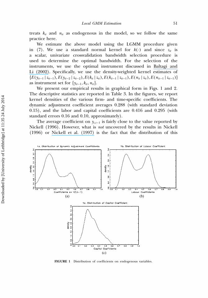
We present our empirical results in graphical form in Figs. 1 and 2.The descriptive statistics are reported in Table 3. In the figures, we reportkernel densities of the various firm- and time-specific coefficients. Thedynamic adjustment coefficient averages 0.288 (with standard deviation0.15), and the labor and capital coefficients are 0.416 and 0.295 (withstandard errors 0.16 and 0.10, approximately).

The average coefficient on yi ,t−1 is fairly close to the value reported byNickell (1996). However, what is not uncovered by the results in Nickell(1996) or Nickell et al. (1997) is the fact that the distribution of this

FIGURE 1 Distribution of coefficients on endogenous variables.

Dow

nloa

ded

by [

Uni

vers

ity o

f L

ethb

ridg

e] a

t 11:

35 2

4 Ju

ly 2

014

52 K. C. Tran and E. G. Tsionas

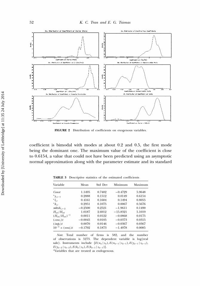
FIGURE 2 Distribution of coefficients on exogenous variables.

coefficient is bimodal with modes at about 0.2 and 0.5, the first modebeing the dominant one. The maximum value of the coefficient is closeto 0.6154, a value that could not have been predicted using an asymptoticnormal approximation along with the parameter estimate and its standard

TABLE 3 Descriptive statistics of the estimated coefficients

Variable Mean Std Dev Minimum Maximum

Const 1�1495 0.7402 −0�4729 5.9648∗yi ,t−1 0�2888 0.1512 0�0149 0.6154∗li ,t 0�4161 0.1604 0�1494 0.8055∗ki ,t 0�2951 0.1075 0�0067 0.5676mktshi ,t−2 −0�2500 0.2521 −1�9611 0.1490Hoit/Hnit 1�0187 2.6912 −15�8321 5.1019(Hoit/Hnit )

−1 0�0011 0.0122 −0�0868 0.0175(conci)t −0�0045 0.0105 −0�0373 0.0315(impi)t 0�0070 0.0146 −0�0367 0.036710−3 × (renti)t −0�1792 0.1873 −1�4978 0.0085

Note: Total number of firms is 582, and the numberof observations is 5273. The dependent variable is log(realsale). Instruments include �E(nit | zit ),E(nit−1 | zit−1),E(yit−1 | zit−1),E(yit−2 | zit−2),E(kit | zit ),E(kit−1 | zit−1).∗Variables that are treated as endogenous.

Dow

nloa

ded

by [

Uni

vers

ity o

f L

ethb

ridg

e] a

t 11:

35 2

4 Ju

ly 2

014

Local GMM Estimation 53

error from Nickell (1996) or Nickell et al. (1997). Our average coefficientsof labor and capital are also in agreement with Nickell (1996), althoughestimates in Nickell et al. (1997) tend to be somewhat higher.7 Again, thedistribution of the labor coefficients is bimodal (the modes are close to0.2 and 0.6) whereas the distribution of the capital coefficient is skewed tothe right. These results indicate that there is considerable heterogeneityin the sample that cannot be ignored and this heterogeneity is ofcomplex form.

Market share and rents (see Figs. 2(a) and 2(f)) provide a clearconclusion: The effect of these variables on productivity is unambiguouslynegative suggesting that competition has a positive effect on productivity.The distributions are clearly non-normal, and the distribution of the effectof rents is even trimodal with modes at 0, −0�4, and −0�8, suggesting thatthe effect of competition on productivity may vary by industry and also byfirm. The effect of concentration ratio appears to be close to zero on theaverage (−0�0045 with standard deviation 0.0105), but from Fig. 2(d) wesee that the mode near −0�02 suggests a positive effect of competition onproductivity growth for a non-negligible portion of the sample. Thus, onceagain we observe that competition improves performance, although notso clearly as in the case of rents and market share. For some firms andindustries, this effect does not exist (in fact, for a large but not dominatingpart). For others, the effect of competition on productivity growth is clearlypositive.

The effect of import penetration (Fig. 2(e)) ranges from −0�04–0.04,suggesting either that the effect is too heterogeneous or that the effectis really zero (this is, in fact the conclusion from the estimates reportedin Nickell, 1996 and Nickell et al., 1997). Finally, the effects of overtimeand its inverse (Figs. 2(b) and 2(c)) is as expected from the results inNickell (1996) and Nickell et al. (1997) although t -statistics reported bythese authors seem to severely understate the sampling variability, possiblydue to their parametric assumption and the highly asymmetric and non-normal pattern of the heterogeneity in coefficients.

Such results strongly suggest that competition is good for productivityand productivity growth, but the pattern is complicated, and the effectsare highly heterogeneous and cannot be described adequately by normal,symmetric, or unimodal distributions. In a sense, our results help toinvigorate the sometimes weak results reported by in Nickell (1996) andNickell et al. (1997). To summarize, our analysis suggests an unambiguouspositive effect of market share and rents on the level of productivity andan ambiguous positive effect of concentration of productivity growth. The

7Our measure of “long run” returns to scale is close to 0.88. Focusing on averages it doesnot appear that constant returns to scale is at odds with this data set. Given the shapes of thedistributions in Figs. 1(a)–(c), however, this would be a gross simplification of reality.

Dow

nloa

ded

by [

Uni

vers

ity o

f L

ethb

ridg

e] a

t 11:

35 2

4 Ju

ly 2

014

54 K. C. Tran and E. G. Tsionas

meaning of “ambiguous” here is that the effect exists for certain industriesand firms, but not for all firms and all industries in the sample—so thisis not in fact a weak result. Thus we feel that the techniques presentedhere can shed additional light on key debates of the industrial organizationliterature and can enrich our understanding of firm-level and industry-wide heterogeneity.

6. POSSIBLE EXTENSION

In this section, we will briefly discuss how to estimate the varyingcoefficient �(·) in a fixed effects model. The model is same as in (1) exceptthat uit = �i + �it with �i being individual fixed effects. Taking the firstdifferences to eliminate the fixed effects, we obtain

y∗it = x ′

it�(zit) − x ′i ,t−1�(zi ,t−1) + �∗

it , (8)

where y∗it , x

∗it , �

∗it are first differences variables. Note that equation (8) has

an additive form, and �∗it has at least an MA(1) structure. In principle,

the method discussed above can be modified coupled with integratingmethod to estimate �(zit) and �(zi ,t−1). However, one drawback with thisapproach is that it does not impose the restriction that the two additivefunctions in (8) have the same functional form �(·). To overcome thisshortcoming, an alternative approach is to use the series methods toestimate (8). Series methods can easily impose the restriction that twoadditive functions have the same functional form, see for example byLi (2000), Ahmad et al. (2005). We leave the estimation problem of (8)using series methods as a future research topic.

7. CONCLUSIONS

In this article, we propose semiparametric smooth coefficientmodels for panel data. The proposed models are useful and flexiblespecification for examining the varying coefficients in the generalregression relationship. We suggest a local generalized method ofmoments with kernel weights to estimate the smooth coefficient functions.The consistency and asymptotic normality of the proposed estimator areestablished. Limited Monte Carlo simulations suggest that our estimatorperforms quite well in finite sample. We apply the proposed method todata on the U.K. manufacturing companies from 1982–1994 to examinethe effects of competition and corporate performance on productivitygrowth. We found that the analysis not only reinforce the findings inNickell (1996) but also uncovered some of the heterogeneous effect thatare not captured in the parametric specification of the model.

Dow

nloa

ded

by [

Uni

vers

ity o

f L

ethb

ridg

e] a

t 11:

35 2

4 Ju

ly 2

014

Local GMM Estimation 55

We did not consider the hypothesis testing problems in this article.It would be interesting and useful to test (i) whether or not a homogenouseffect exists and (ii) whether or not serial correlation exists. Li et al. (2002),Fan et al. (2001), and Li and Hsiao (1998) provide testing frameworks inthe cross-sectional/time series context, and their methods can be extendedto the semiparametric panel data case. We leave these topics for futureresearch.

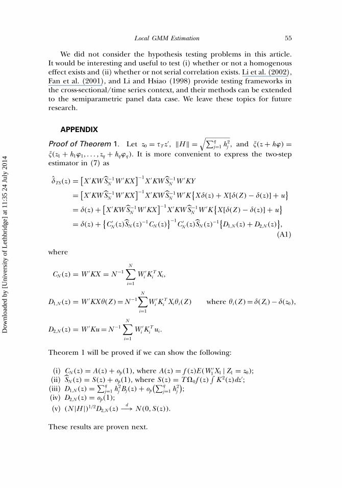
APPENDIX

Proof of Theorem 1. Let z0 = �T z ′, ‖H ‖ =√∑q

j=1 h2j , and (z + h�) =

(z1 + h1�1, � � � , zq + hq�q). It is more convenient to express the two-stepestimator in (7) as

�TS(z) = [X ′KW S−1

N W ′KX]−1

X ′KW S−1N W ′KY

= [X ′KW S−1

N W ′KX]−1

X ′KW S−1N W ′K

{X �(z) + X [�(Z ) − �(z)] + u

}= �(z) + [

X ′KW S−1N W ′KX

]−1X ′KW S−1

N W ′K{X [�(Z ) − �(z)] + u

}= �(z) + {

C ′N (z )SN (z)

−1CN (z)}−1

C ′N (z )SN (z)

−1{D1,N (z) + D2,N (z)

},

(A1)

where

CN (z) = W ′KX = N −1N∑i=1

W ′i K

Ti Xi ,

D1,N (z) = W ′KX �(Z )=N −1N∑i=1

W ′i K

Ti Xi�i(Z ) where �i(Z )= �(Zi)− �(z0),

D2,N (z) = W ′Ku =N −1N∑i=1

W ′i K

Ti ui �

Theorem 1 will be proved if we can show the following:

(i) CN (z) = A(z) + op(1), where A(z) = f (z)E(W ′1X1 |Z1 = z0);

(ii) SN (z) = S(z) + op(1), where S(z) = T�0f (z)∫K 2(z)dz ′;

(iii) D1,N (z) = ∑qj=1 h

2j Bj(z) + op

(∑qj=1 h

2j

);

(iv) D2,N (z) = op(1);

(v) (N |H |)1/2D2,N (z)d−→ N (0, S(z)).

These results are proven next.

Dow

nloa

ded

by [

Uni

vers

ity o

f L

ethb

ridg

e] a

t 11:

35 2

4 Ju

ly 2

014

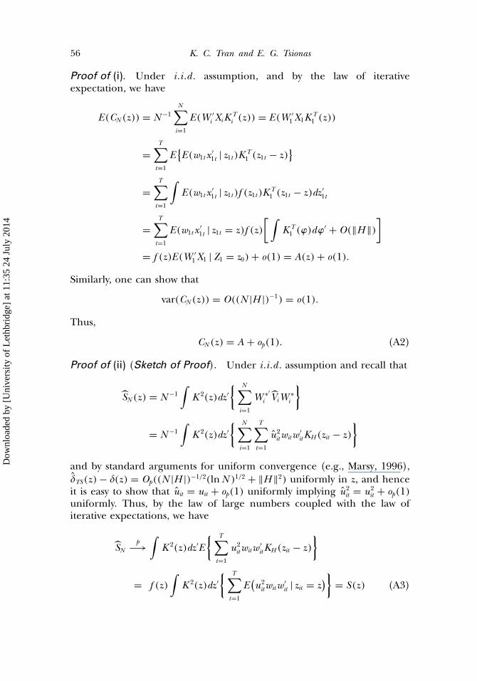
56 K. C. Tran and E. G. Tsionas

Proof of (i). Under i�i�d � assumption, and by the law of iterativeexpectation, we have

E(CN (z)) = N −1N∑i=1

E(W ′i XiK T

i (z)) = E(W ′1X1KT

1 (z))

=T∑t=1

E{E(w1t x ′

1t | z1t)KT1 (z1t − z)

}

=T∑t=1

∫E(w1t x ′

1t | z1t)f (z1t)KT1 (z1t − z)dz ′

1t

=T∑t=1

E(w1t x ′1t | z1t = z)f (z)

[ ∫KT

1 (�)d�′ + O(‖H ‖)]

= f (z)E(W ′1X1 |Z1 = z0) + o(1) = A(z) + o(1)�

Similarly, one can show that

var(CN (z)) = O((N |H |)−1) = o(1)�

Thus,

CN (z) = A + op(1)� (A2)

Proof of (ii) (Sketch of Proof). Under i�i�d � assumption and recall that

SN (z) = N −1

∫K 2(z)dz ′

{ N∑i=1

W ∗′i ViW ∗

i

}

= N −1

∫K 2(z)dz ′

{ N∑i=1

T∑t=1

u2itwitw ′

itKH (zit − z)}

and by standard arguments for uniform convergence (e.g., Marsy, 1996),�TS(z) − �(z) = Op((N |H |)−1/2(lnN )1/2 + ‖H ‖2) uniformly in z, and henceit is easy to show that uit = uit + op(1) uniformly implying u2

it = u2it + op(1)

uniformly. Thus, by the law of large numbers coupled with the law ofiterative expectations, we have

SNp−→

∫K 2(z)dz ′E

{ T∑t=1

u2itwitw ′

itKH (zit − z)}

= f (z)∫

K 2(z)dz ′{ T∑

t=1

E(u2itwitw ′

it | zit = z)} = S(z) (A3)

Dow

nloa

ded

by [

Uni

vers

ity o

f L

ethb

ridg

e] a

t 11:

35 2

4 Ju

ly 2

014

Local GMM Estimation 57

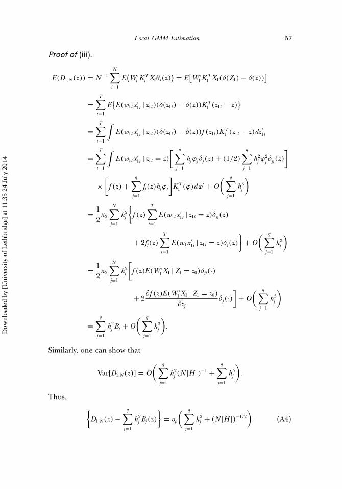
Proof of (iii).

E(D1,N (z)) = N −1N∑i=1

E(W ′

i KTi Xi�i(z)

) = E[W ′

1KT1 X1(�(Z1) − �(z))

]

=T∑t=1

E{E(w1t x ′

1t | z1t)(�(z1t) − �(z))KT1 (z1t − z)

}

=T∑t=1

∫E(w1t x ′

1t | z1t)(�(z1t) − �(z))f (z1t)KT1 (z1t − z)dz ′

1t

=T∑t=1

∫E(w1t x ′

1t | z1t = z)[ q∑

j=1

hj�j�j(z) + (1/2)q∑

j=1

h2j �

2j �jj(z)

]

×[f (z) +

q∑j=1

fj(z)hj�j

]KT

1 (�)d�′ + O( q∑

j=1

h3j

)

= 12�2

N∑j=1

h2j

{f (z)

T∑t=1

E(w1t x ′1t | z1t = z)�jj(z)

+ 2fj(z)T∑t=1

E(w1x ′1t | z1t = z)�j(z)

}+ O

( q∑j=1

h3j

)

= 12�2

N∑j=1

h2j

[f (z)E(W ′

1X1 |Z1 = z0)�jj(·)

+ 2�f (z)E(W ′

1X1 |Z1 = z0)�zj

�j(·)]

+ O( q∑

j=1

h3j

)

=q∑

j=1

h2j Bj + O

( q∑j=1

h3j

)�

Similarly, one can show that

Var[D1,N (z)] = O( q∑

j=1

h2j (N |H |)−1 +

q∑j=1

h5j

)�

Thus,

{D1,N (z) −

q∑j=1

h2j Bj(z)

}= op

( q∑j=1

h2j + (N |H |)−1/2

)� (A4)

Dow

nloa

ded

by [

Uni

vers

ity o

f L

ethb

ridg

e] a

t 11:

35 2

4 Ju

ly 2

014

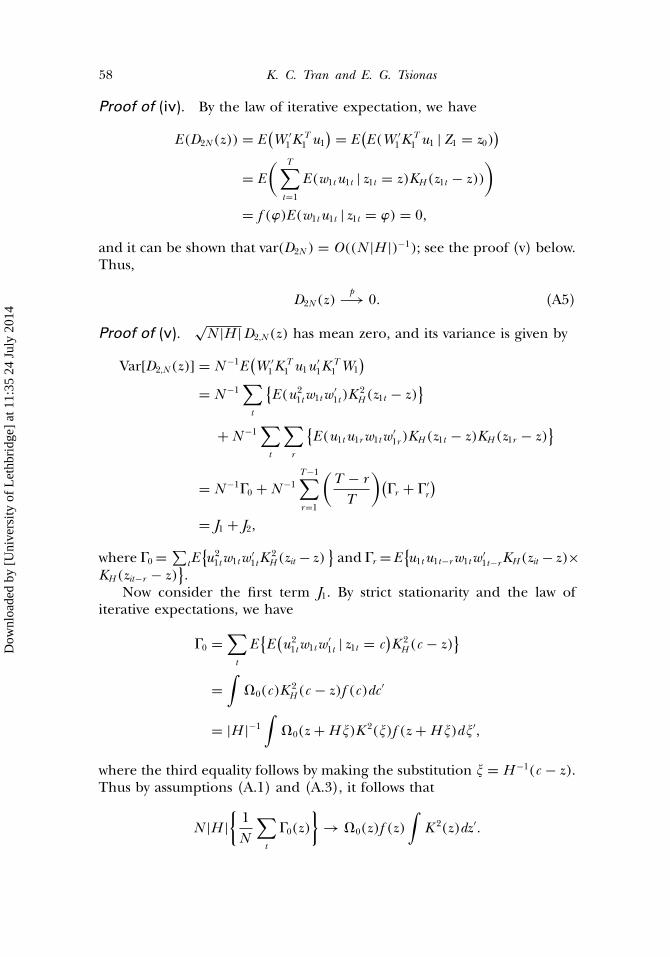
58 K. C. Tran and E. G. Tsionas

Proof of (iv). By the law of iterative expectation, we have

E(D2N (z)) = E(W ′

1KT1 u1

) = E(E(W ′

1KT1 u1 |Z1 = z0)

)= E

( T∑t=1

E(w1tu1t | z1t = z)KH (z1t − z)))

= f (�)E(w1tu1t | z1t = �) = 0,

and it can be shown that var(D2N ) = O((N |H |)−1); see the proof (v) below.Thus,

D2N (z)p−→ 0� (A5)

Proof of (v).√N |H |D2,N (z) has mean zero, and its variance is given by

Var[D2,N (z)] = N −1E(W ′

1KT1 u1u ′

1KT1 W1

)= N −1

∑t

{E(u2

1tw1tw ′1t)K

2H (z1t − z)

}+ N −1

∑t

∑r

{E(u1tu1r w1tw ′

1r )KH (z1t − z)KH (z1r − z)}

= N −1�0 + N −1T−1∑r=1

(T − rT

)(�r + � ′

r

)= J1 + J2,

where �0 = ∑tE

{u21tw1tw ′

1tK2H (zit − z)

}and �r =E

{u1tu1t−r w1tw ′

1t−r KH (zit − z)×KH (zit−r − z)

}.

Now consider the first term J1. By strict stationarity and the law ofiterative expectations, we have

�0 =∑t

E{E

(u21tw1tw ′

1t | z1t = c)K 2

H (c − z)}

=∫

�0(c)K 2H (c − z)f (c)dc ′

= |H |−1

∫�0(z + H )K 2()f (z + H )d′,

where the third equality follows by making the substitution = H −1(c − z).Thus by assumptions (A.1) and (A.3), it follows that

N |H |{1N

∑t

�0(z)}

→ �0(z)f (z)∫

K 2(z)dz ′�

Dow

nloa

ded

by [

Uni

vers

ity o

f L

ethb

ridg

e] a

t 11:

35 2

4 Ju

ly 2

014

Local GMM Estimation 59

Next we show that the second term J2 above is of order O(N −1). By thelaw of iterative expectations, and making substitutions s1 = H −1(c1 − z) ands2 = H −1(c2 − z), we obtain

�r = E{E

(u1tu1t−r w1tw ′

1t−r | z1t = c1, z1t−r = c2)KH (zit − z)KH (zit−r − z)

}=

∫�r (c1, c2)KH (c1 − z)KH (c2 − z)gr (c1, c2)dc ′

1dc′2

=∫

�r (z + Hs1, z + Hs2)K (s1)K (s2)gr (z + Hs1, z + Hs2)ds ′1ds

′2�

By assumptions (A.1) and (A.4), it follows that �r → �r (z, z)gr (z, z),implying J2 = O(N −1). Thus,

limN→∞

Var[√

N |H |D2,N (z)]

= �0(z)f (z)∫

K 2(z)dz ′ = S(z)�

It is straightforward to check that the conditions of Lyapounov’s centrallimit theorem hold. Thus,√

N |H |D2,N (z)d−→ N (0, S(z))� (A6)

Combining (A2)–(A6), we have shown that,

(a) ��TS(z0) − �(z0) = �CN (z)′S(z)−1CN (z)−1CN (z)′S(z)−1

× [D1,N (z) + D2,N (z)

]= �(z)

q∑j=1

h2j Bj(z) + op

( q∑j=1

h2j + (N |H |−1/2

)

Hence, �TS(z) − �(z) − �(z)∑q

j=1 h2j Bj(z) = op

(∑qj=1 h

2j + (N |H |)−1/2

);

(b)√N |H |��TS(z0) − �(z0)

= �CN (z)′S(z)−1CN (z)−1CN (z)′S(z)−1√N |H |[D1,N (z) + D2,N (z)

]= {

A(z)′S(z)−1A(z)}−1

A(z)′S(z)−1

×[√

N |H |q∑

j=1

h2j Bj + √

N |H |D2,N (z) + op(1)]

d−→ N(�(z)

q∑j=1

h2j Bj ,

{A(z)′S(z)−1A(z)

}−1)

√N |H |{�TS(z0)− �(z0)−�(z)

∑qj=1 h

2j Bj

} d−→N(0, �A(z)′S(z)−1A(z)−1

). �

Dow

nloa

ded

by [

Uni

vers

ity o

f L

ethb

ridg

e] a

t 11:

35 2

4 Ju

ly 2

014

60 K. C. Tran and E. G. Tsionas

ACKNOWLEDGMENTS

We would like to thank an associate editor and two anonymous refereesfor detailed insightful comments and suggestions that led to a substantialimprovement of the article. We would also like to thank the participantsof the Hellenic Workshop on Efficiency and Productivity Measurement(Patras, Greece, 2006) and especially Robin Sickles and Dawit Zerom formany useful comments on an earlier version of this article.

REFERENCES

Ahmad, I., Leelahanon, S., Li, Q. (2005). Efficient estimation of a semiparametric partially linearvarying coefficient model. The Annals of Statistics 33:258–283.

Arellano, M., Bond, S. (1991). Some tests of specification for panel data: Monte Carlo evidenceand an application to employment equations. Review of Economic Studies 58:277–297.

Baltagi, B. H., Li, Q. (2002). On instrumental variable estimation of semiparametric dynamic paneldata models. Economics Letters 76:1–9.

Cai, Z., Li, Q. (2008). Nonparametric estimation of varying coefficient dynamic panel data models.Econometric Theory 24:1321–1342.

Cai, Z., Fan, J., Zhao, Q. (2000). Functional coefficient regression models for nonlinear time series.Journal of the American Statistical Association 95:941–956.

Cai, Z., Das, M., Xiong, H., Wu, X. (2006). Functional coefficient instrumental variables models.Journal of Econometrics 133:207–241.

Carroll, R., Ruppert, J., Welsh, A. (1998). Local estimating equations. Journal of the American StatisticalAssociation 93:214–227.

Das, M. (2005). Instrumental variables estimators for nonparametric models with discreteendogenous regressors. Journal of Econometrics 124:335–361.

Gozalo, P., Linton, O. (2000). Local nonlinear least squares: using parametric information in non-parametric regression. Journal of Econometrics 99:63–106.

Fan, J., Zhang, W. (1999). Statistical estimation in varying coefficient models. The Annals of Statistics27:1491–1518.

Fan, J., Zhang, C., Zhang, J. (2001). Generalized likelihood ratio statistics and Wilks phenomenon.The Annals of Statistics 29:153–193.

Hansen, B. E. (1999). Threshold effects in non-dynamic panels: estimation, testing and inference.Journal of Econometrics 93:345–368.

Hansen, L. P. (1982). Large sample properties of generalized method of moments estimators.Econometrica 50:1029–1054.

Hastie, T., Tibshirani, R. (1993). Varying-coefficient models. Journal of the Royal Statistical Society B55:757–796.

Horowitz, J. L., Markatou, M. (1996). Semiparametric estimation of regression models for paneldata. The Review of Economic Studies 63:145–168.

Knieser, T. J., Li, Q. (2002). Nonlinearity in dynamic adjustment: semiparametric estimation ofpanel labor supply. Empirical Economics 27:131–148.

Li, Q. (2000). Efficient estimation of additive partially linear models. International Economic Review41:1073–1092.

Li, Q., Stengos, T. (1996). Semiparametric estimation of partially linear panel data models. Journalof Econometrics 71:389–397.

Li, Q., Hsiao, C. (1998). Testing for serial correlation in semiparametric panel data models. Journalof Econometrics 87:207–237.

Li, Q., Ullah, A. (1998). Estimating partially linear models with one-way error components.Econometric Reviews 17:145–166.

Li, Q., Huang, C., Li, D., Fu, T.-T. (2002). Semiparametric smooth coefficient models. Journal ofBusiness and Economic Statistics 20:412–422.

Dow

nloa

ded

by [

Uni

vers

ity o

f L

ethb

ridg

e] a

t 11:

35 2

4 Ju

ly 2

014

Local GMM Estimation 61

Marsy, E. (1996). Multivariate local polynomial regression for time series: uniform strong consistencyrates. Journal of Time Series Analysis 17:571–599.

Newey, W. (1990). Efficient instrumental variable estimation of nonlinear models. Econometrica58:809–837.

Nickell, S. J. (1996). Competition and corporate performance. Journal of Political Economy104:724–746.

Nickell, S. J., Nicolitsas, D., Dryden, N. (1997). What makes firms perform well? European EconomicReview 41:783–796.

Papalia, R. (1999). Local generalized method of moments estimation based on kernel weights: Anapplication to panel data. Journal of Applied Statistics 26(8):1005–1015.

Powell, J. L., Stock, J. H., Stoker, T. M. (1989). Semiparametric estimation of index coefficients.Econometrica 57:1043–1430.

Ullah, A., Roy, N. (1998). Nonparametric and semiparametric econometrics of panel data. In:Ullah, A., Giles, D. E. A., eds. Handbook of Applied Economic Statistics. Monticello, New York:Marcel Dekker, Chapter 17, pp. 579–604.

Ullah, A., Mundra, K. (1999). Semiparametric panel data estimation: An application to immigrateshomelink effect on US producer trade flows. Department of Economics, University ofCalifornia at Riverside, Working Paper 15.

Dow

nloa

ded

by [

Uni

vers

ity o

f L

ethb

ridg

e] a

t 11:

35 2

4 Ju

ly 2

014