Bayesian Semiparametric Inference for

Multivariate Doubly-Interval-Censored Data

ALEJANDRO JARA1∗, EMMANUEL LESAFFRE2, MARIA DE IORIO3, AND

FERNANDO A. QUINTANA 4

1 Department of Statistics, Facultad de Ciencias Fısicas y Matematicas, Universidad de Concepcion

2 Biostatistical Centre, Catholic University of Leuven, Kapucijnenvoer 35, B-3000 Leuven, Belgium.

3 Department of Epidemiology and Public Health, Imperial College London, UK

4 Departamento de Estadıstica, Pontificia Universidad Catolica de Chile, Santiago, Chile

January 18, 2010

Abstract

Based on a data set obtained in a dental longitudinal study, conducted in Flanders (Bel-

gium), the joint time to caries distribution of permanent first molars was modeled as a func-

tion of covariates. This involves an analysis of multivariate continuous doubly-interval-

censored data since: i) the emergence time of a tooth and the time it experiences caries

were recorded yearly, and ii) events on teeth of the same child are dependent. To model the

∗Author for correspondence: Alejandro Jara, Department of Statistics, Facultad de Ciencias Fısicas y

Matematicas, Universidad de Concepcion, Avenida Esteban Iturra S/N, Barrio Universitario, Concepcion, Chile

(E-mail :ajarav@udec.cl)

1

joint distribution of the emergence times and the times to caries, we propose a dependent

Bayesian semiparametric model. A major feature of the proposed approach is that survival

curves can be estimated without imposing assumptions such as proportional hazards, addi-

tive hazards, proportional odds, or accelerated failure time.

Keywords:Multivariate doubly-interval-censored data, Bayesian nonparametric, Linear de-

pendent Poisson-Dirichlet prior, Linear dependent Dirichlet process prior.

1 Introduction

The past three decades have witnessed a dramatic decline in the prevalence of dental caries in

children in countries of the Western World (De Vos & Vanobbergen, 2006). However, the dis-

ease has now become concentrated in a small group of children, with the majority unaffected;

about 10 to 15% of the children now experience 50% of all caries lesions and 25 to 30% suffer

75% of lesions (Marthaler et al., 1996; Petersson & Bratthall, 1996). The most likely expla-

nation for the difference in oral health seems to be socio-economic environmental factors and

it occurs early in childhood (Willems et al., 2005). Therefore, to improve dental health, early

identification of groups at a particular risk of developing caries becomes essential. In this paper

we present a Bayesian analysis of a longitudinal dataset, gathered in the Signal-Tandmobielr

study, to investigate the relationship between some potential exposure variables and the emer-

gence and development of caries in permanent teeth.

The Signal-Tandmobielr study is a 6-year longitudinal oral health study involving children

from Flanders (Belgium) and conducted between 1996 and 2001. Dental data were collected on

gingival condition, dental trauma, tooth decay, presence of restorations, missing teeth, stage of

tooth eruption, orthodontic treatment need, etc. Additionally, information on oral hygiene and

2

dietary behavior was collected from a questionnaire filled-in by the parents. The children were

examined annually during their primary school time by one ofsixteen trained and half yearly

calibrated dental examiners. More details on the Signal Tandmobielr study can be found in

Section 4.1 and in Vanobbergen et al. (2000). A primary objective of the investigation is to

assess the association of some covariates with the emergence and development of caries in per-

manent teeth. In particular, we are interested in studying the effect of the age at start brushing

(in years) and of deciduous second molars health status (sound/affected; teeth 55, 65, 75, 85, re-

spectively, see Figure 4(a)) on caries susceptibility of the adjacent permanent first molars (teeth

number 16, 26, 36, 46, see Figure 4(b)). Additionally, we considered the impact of gender

(girl/boy), presence of sealants in pits and fissures of the permanent first molar (none/present),

occlusal plaque accumulation on the permanent first molar (none/in pits and fissures/on total

surface), and reported oral brushing habits (not daily/daily). Note that pits and fissures seal-

ing is a preventive action which is expected to protect the tooth against caries development.

The information on occlusal plaque accumulation, presenceof sealants in pits and fissures, and

reported oral brushing habits was obtained at the examination where the presence of the perma-

nent first molar was first recorded.

The response of interest is the time to caries development onthe permanent dentition which

corresponds to the time from tooth emergence to onset of caries. Due to the setup of the study

(annual visits of dentists), the onset time and the failure time could only be recorded at reg-

ular intervals and observations on both events were, therefore, interval-censored. A graphical

illustration of a possible evolution of a tooth is shown in Figure 1. This type of data structure,

often referred to as doubly-interval-censored failure time data, is common in medical research,

especially in the context of the analysis of acquired immunodeficiency syndrome (AIDS) incu-

bation time; the time between the human immunodeficiency virus infection and the diagnosis

of AIDS.

3

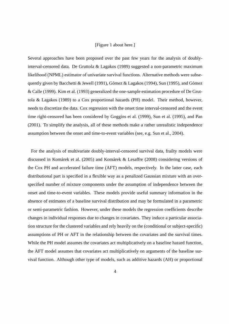
[Figure 1 about here.]

Several approaches have been proposed over the past few years for the analysis of doubly-

interval-censored data. De Gruttola & Lagakos (1989) suggested a non-parametric maximum

likelihood (NPML) estimator of univariate survival functions. Alternative methods were subse-

quently given by Bacchetti & Jewell (1991), Gomez & Lagakos(1994), Sun (1995), and Gomez

& Calle (1999). Kim et al. (1993) generalized the one-sampleestimation procedure of De Grut-

tola & Lagakos (1989) to a Cox proportional hazards (PH) model. Their method, however,

needs to discretize the data. Cox regression with the onset time interval-censored and the event

time right-censored has been considered by Goggins et al. (1999), Sun et al. (1995), and Pan

(2001). To simplify the analysis, all of these methods make arather unrealistic independence

assumption between the onset and time-to-event variables (see, e.g. Sun et al., 2004).

For the analysis of multivariate doubly-interval-censored survival data, frailty models were

discussed in Komarek et al. (2005) and Komarek & Lesaffre (2008) considering versions of

the Cox PH and accelerated failure time (AFT) models, respectively. In the latter case, each

distributional part is specified in a flexible way as a penalized Gaussian mixture with an over-

specified number of mixture components under the assumptionof independence between the

onset and time-to-event variables. These models provide useful summary information in the

absence of estimates of a baseline survival distribution and may be formulated in a parametric

or semi-parametric fashion. However, under these models the regression coefficients describe

changes in individual responses due to changes in covariates. They induce a particular associa-

tion structure for the clustered variables and rely heavilyon the (conditional or subject-specific)

assumptions of PH or AFT in the relationship between the covariates and the survival times.

While the PH model assumes the covariates act multiplicatively on a baseline hazard function,

the AFT model assumes that covariates act multiplicativelyon arguments of the baseline sur-

vival function. Although other type of models, such as additive hazards (AH) or proportional

4

odds (PO), could be considered in a frailty model context, all these assumptions may be consid-

ered too strong in many practical applications. For instance, under these models survival curves

from different covariate groups cannot cross which can be unrealistic in some applications (see,

De Iorio et al., 2009). This issue is particularly relevant for doubly-interval-censored data where

the degree of available information to perform diagnostic techniques is rather reduced due to

the censoring mechanism.

In this paper we discuss a Bayesian semiparametric approachfor the analysis of multivariate

doubly-interval-censored data where the dependence across sub-populations, defined by dif-

ferent combinations of the available covariates, is introduced without assuming independence

between the onset and time-to-event variables, without requiring data discretization, and any of

the commonly used assumptions for the inclusion of covariates in survival models. We extend

recent developments on the dependent nonparametric priors, initially proposed by MacEachern

(1999, 2000), to provide a framework for modeling multivariate doubly-interval-censored data

where the resulting survival curves have a marginal (or population level) interpretation and not

subject-specific. It must be pointed out that the dental datahas been analyzed before. How-

ever, the previous approaches were deficient in that either the doubly-interval-censored nature

was not taken into account (Leroy et al., 2005a) or restrictive in the sense that the focus was

on conditional interpretation of the effects of the covariates via frailty models and rely on the

AFT or PH assumption (Komarek et al., 2005; Komarek & Lesaffre, 2008). Overcoming these

problems largely motivates the developments presented in this paper.

The rest of the paper is organized as follows. In Section 2, weintroduce the proposed model,

which is based on the two parameter Poisson-Dirichlet process, and discuss its main properties.

Section 3 presents the analysis of simulated data which illustrate the main advantage of the

proposed model. Section 3 describes the analysis of the Signal Tandmobielr study. A final

5

discussion section concludes the article.

2 The model

2.1 Survival regression framework

Let TOij andTE

ij , i = 1, . . . , m, j = 1, . . . , n, be continuous random variables defined on[0,∞)

denoting the true chronological onset and event times for the jth measurement of theith ex-

perimental unit, respectively, and letT Tij = TE

ij − TOij be the true time-to-event. For example,

in our caseT Tij is the true time to caries for thejth tooth of theith child, with TO

ij denot-

ing the true emergence time andTEij the age of caries development. Assume that for each

of the m experimental units we record thep-dimensional andq-dimensional covariate vec-

tors xOij ∈ XO ⊂ R

p and xTij ∈ X T ⊂ R

q associated to the tooth onset timeTOij and to

the time-to-eventT Tij , respectively. LetT O

i =(

TOi1 , . . . , TO

in

)′

, T Ei =

(

TEi1 , . . . , TE

in

)′

, T Ti =

(

T Ti1 , . . . , T

Tin

)′

, T i =(

T O′

i , T T ′

i

)′

, XOi = diag

(

xO′

i1 , . . . , xO′

in

)

, XTi = diag

(

xT ′

i1 , . . . , xT ′

in

)

,

andX i = diag(

XOi , XT

in

)

, i = 1, . . . , m.

In order to model the joint distribution of the true chronological onset times and true time-to-

eventsT i as a function of covariates,T i | X iind∼ fXi

, we consider a mixture model. Specifi-

cally, we assumeT i | X iind∼ fXi

with

fXi(· | Σ, GXi

) =

∫

k2n (· | µ,Σ) dGXi(µ) , (1)

wherek2n (· | µ,Σ) denotes a2n-variate density onR2n+ with locationµ and unstructured scale

matrix Σ taking into account the association among variables of the same experimental unit,

respectively, and where the mixing distributionsGX : X ∈ X are dependent random proba-

bility measures. The degree of dependence among the random distributionsGX : X ∈ X is

governed by the level of the covariateX. If GXiwere indexed by a finite dimensional vector of

6

hyper-parameters, for example, normal moments, then the model would reduce to a traditional

parametric hierarchical model. In contrast, in a non-parametric Bayesian approachGXiis as-

sumed to be a random probability measure with an appropriateprior probability modelF for

the unknown distributions indexed by the set of covariates.In other words,F is a distribution

over related probability distributions

GX : X ∈ X | F ∼ F. (2)

Here we focus on the class of discrete random probability measures that can be represented as

GX(B) =∞∑

l=1

ωl δθ(X)l(B), (3)

whereB is a measurable set,ω1, ω2, . . . are random weights satisfying0 ≤ ωl ≤ 1 and

P (∑∞

l=1 ωl = 1) = 1, and whereδθ(Xi)l(·) denotes a Dirac measure at the random locations

θ(X i)1, θ(X i)2, . . ., which are assumed to be independent of theωll>1 collection. We dis-

cuss specific choices for the random probability measureF in (2) in the next sections. To better

explain our proposal, we start with a review of the construction of priors over related distribu-

tions.

2.2 Priors over related distributions

The problem of defining priors over related random probability distributions has received in-

creasing attention over the past few years. MacEachern (1999, 2000) proposes the dependent

Dirichlet Process (DDP) as an approach to define a prior modelfor an uncountable set of ran-

dom measures indexed by a single continuous covariate, sayx, Gx : x ∈ X ⊂ R. The

key idea behind the DDP is to create an uncountable set of Dirichlet Processes (DP) (Ferguson,

1973) and to introduce dependence by modifying the Sethuraman (1994)’s stick-breaking rep-

resentation of each element in the set. IfG follows a DP prior with precision parameterM and

7

base measureG0, denoted byG ∼ DP (MG0), then the stick-breaking representation ofG is,

G(B) =∞∑

l=1

ωlδθl(B), (4)

whereθl | G0iid∼ G0 andωl = Vl

∏

j<l(1−Vj), with Vl | Miid∼ Beta(1, M). MacEachern (1999,

2000) generalizes (4) by assuming the point massesθ(x)l, l = 1, . . ., to be dependent across

different levels ofx, but independent acrossl. This approach has been successfully applied

to ANOVA (De Iorio et al., 2004), survival (De Iorio et al., 2009), spatial modeling (Gelfand

et al., 2005), functional data (Dunson & Herring, 2006), time series (Caron et al., 2006), and

discriminant analysis (De la Cruz et al., 2007). Motivated by regression problems with con-

tinuous predictors, Griffin & Steel (2006) and Duan et al. (2007) developed models where the

dependence is introduced by making the weights dependent oncovariates.

Alternatives to these approaches include incorporating dependency by means of weighted

mixtures of independent random measures (Muller et al., 2004; Dunson & Park, 2008). This

approach was originally proposed by Muller et al. (2004), motivated for the problem of borrow-

ing strength across related sub-models. For regression problems with continuous predictors,

Dunson & Park (2008) proposed a countable mixture where the weights depend on the covari-

ates through the introduction of a bounded kernel function in the stick-breaking construction of

the weights. This approach requires the choice of a metric for the covariate values and, there-

fore, is not naturally extended to include factors and continuous predictors jointly in the model.

We build our proposal on the construction introduced in De Iorio et al. (2004) and De Iorio

et al. (2009) because it is a natural approach to introduce dependence on both factors and con-

tinuous covariates which are commonly of interest in survival models. We consider the class

of discrete Linear Dependent (LD) models defined as follows.For a given design matrixX,

in the notation of our motivating problem, the conditional distribution of the2n-dimensional

8

vectors of kernel locationsµ is given by the probability measure defined in expression (3),

GX(B) =∑∞

l=1 ωlδθ(X)l(B), where the2n-dimensional atoms follow a linear (in the parame-

ters) modelθ(X)l = Xβl where theβl’s representn(p+ q)-dimensional vectors of regression

coefficients. Therefore,P (µ = θ(X)l = Xβl) = ωl and the dependence is introduced through

the point mass locationsθ(X)l. For simplicity of explanation, consider the case ofn = 1 and

an ANCOVA type of design matrix

X =

1 V 0 0 0

0 0 1 V Z

,

whereV is an indicator variable andZ is continuous. For example,V could be the gender

indicator andZ the age at start brushing. In the LD model the dependence across the random

distributions is achieved by imposing a linear model on the point masses

θ(X)l = Xβl =

β1l + β2lV

β3l + β4lV + β5lZ

.

As in a standard linear model,β1l andβ3l can be interpreted as “overall means”, whileβ2l and

β4l are the main effects for gender, for the onset and time-to-event time, respectively, andβ5l

can be interpreted as a slope coefficient associated to the age at start brushing for time-to-caries.

Note that the linear specification is highly flexible and can include standard nonlinear transfor-

mations of the continuous predictors, e.g. additive modelsbased on B-splines (see, e.g. Lang &

Brezger, 2004), as well as linear forms in the continuous predictors themselves.

In this paper we extend the DDP framework to a construction that is based on the general class

of Poisson-Dirichlet (PD) processes (see e.g., Pitman, 1996; Pitman & Yor, 1997). The PD pro-

cesses belong to the class of species sampling models (see e.g., Pitman, 1996) and admits the

DP prior as an important special case. The PD process can alsobe defined as in expression (4),

where the random weightsωl are independent for theθl’s and theθl are i.i.d. from a continuous

9

distributionG0. The weights still admit a stick-breaking representationωl = Vl

∏

j<l(1 − Vj),

but in this caseVjind∼ Beta(1 − a, b + ja), where eithera = −κ < 0 andb = ςκ, for some

κ > 0 andς = 2, 3, . . ., or 0 ≤ a < 1 andb > −a. We restrict our attention to the parameter

spaceA = (a, b) ∈ R2 : 0 ≤ a < 1, b > −a because this is large enough to include two

important special cases. Whena = 0 andb = M , Ferguson’sDP (MG0) follows. Whena = γ,

0 < γ < 1, andb = 0, thePD(γ, 0) yields a measure whose random weights are based on a

stable law with indexγ. The DP and stable law are key processes because they represent the

canonical measures of the PD process (Pitman & Yor, 1997).

It is now straightforward to extend the Linear Dependent framework to the PD process assum-

ing a linear model for the atoms of the process. In this way we can define a model for related

probability distributions of the form

GX : X ∈ X | a, b, G0 ∼ LDPD(a, b, G0), (5)

whereLDPD(a, b, G0) refers to a Linear Dependent PD prior, with parametersa, b, andG0.

2.3 A PD mixture of AFT regression models

An appealing property of the LDPD survival model given by expressions (1) and (5) is that it

can be understood on the basis of an equivalent model reformulation as a mixture of multivari-

ate AFT regression models. Given a particular matrix of covariatesX, the vector of kernel

locationsµ in the mixture model (1) takes the valueXβ and where the mixture is defined

with respect to the regression coefficientsβ. In other words, the model can be alternatively

formulated by defining the mixture of multivariate regression models

fXi(· | Σ, G) =

∫

k2n (· | X iβ,Σ) dG (β) , (6)

10

and

G | a, b, G0 ∼ PD(a, b, G0). (7)

The discrete nature of the PD realizations leads to their well-known clustering properties. The

choice of parametersa andb in the PD process controls the clustering structure (Lijoi et al.,

2007b). Givenm observations, whena = 0 (i.e., a DP) the number of clustersn∗(m) is a sum

of independent indicator variables, which impliesn∗(m)/ log m → b almost surely andn∗(m)

is asymptotically normal (Korwar & Hollander, 1973). Underthe model with0 < a < 1 and

b > −a the sequencen∗(m) is an inhomogeneous Markov chain such thatn∗(m)/ma → S

almost surely, for a random variableS with a continuous density on(0,∞) depending on(a, b)

(Pitman & Yor, 1997). The asymptotic behavior of the distribution of the number of clusters

indicates that a general PD model increases asma which is much faster than the logarithmic

rate of the DP model. In general, values ofa close to 1 favour the generation of a larger number

of clusters.

Besides the clustering structure implied by the extraa parameter in the PD process, its role

can be also understood when the distribution of PD realizations is applied to a partition of the

space of interest. In particular, for measurable setsB, B1 andB2, with B1 ∩ B2 = ∅, it follows

that (Carlton, 1999)

V ar (G(B)) = G0(B) (1 − G0(B))

(

1 − a

b + 1

)

, (8)

and

Cov (G(B1), G(B2)) = −G0(B1)G0(B2)

(

1 − a

b + 1

)

. (9)

Therefore, the extraa parameter controls the variability and covariance of disjoint sets of the

PD realizations. Whena → 1, G is highly concentrated aroundG0 and the covariance between

disjoint sets is small. Whena = 0 we recover the corresponding expressions for the DP. Note

11

that the correlation betweenG(B1) andG(B2) does not depend on the parameter(a, b) and,

therefore, is the same than the one arising from the DP model.

To date, most practical implementations of PD processes have considered the parametersa

andb as fixed at user-specified values (see e.g., Ishwaran & James,2001), fixed at empirical

Bayes estimates (see e.g., Lijoi et al., 2007a), or exploredthe effect of different combinations

of fixed values for these parameters on the inferences (see e.g., Navarrete et al., 2008). Lijoi

et al. (2008) on the other hand proposed independent discrete uniform priors with support points

0.01, 0.02, . . . , 0.99 and0, 1, . . . , 2000 for a andb, respectively. Here we allowa andb to

be random having continuous random probability distributions supported on the restricted pa-

rameter space under consideration. Moreover, we allowa to be zero with positive probability

in order to test whether the data arose from LDDP versus a moregeneral LDPD process us-

ing a Bayes factor. This additional flexibility can be incorporated at essentially no additional

computational cost.

2.4 The hierarchical representation

So far, we have focused on modeling the joint distribution ofthe survival times of interest,

namely, the true chronological onset timesTOij and true times-to-eventT T

ij . However, in our set-

ting the observed data are given by the eventsTOij ∈ (uL

ij, uUij] : i = 1, . . . , m, j = 1, . . . , n,

and TEij ∈ (vL

ij , vUij ] : i = 1, . . . , m, j = 1, . . . , n, whereuL

ij and vLij , and uU

ij and vUij ,

represent the lower and upper limits of the intervals where the chronological onset,TOij , and

event time,TEij , for observationj from experimental uniti were observed, respectively. Un-

der the assumption of non-informative censoring, we define amodel for the eventsAOi =

TOij ∈ (uL

ij, uUij] : j = 1, . . . , n

andAEi =

TEij ∈ (vL

ij , vUij ] : j = 1, . . . , n

, by introducing

12

latent vectorsT Oi andT E

i . We assume

(

T Oi , T E

i

)

| hXi

ind∼ hXi

, (10)

with hXi

(

T Oi , T E

i | Σ, G)

= fXi

(

T Oi , T E

i − T Oi | Σ, G

)

and wherefXi(· | Σ, G) is defined

as in (6). Notice that a choice of the continuous kernelk defines the model. A multivariate log-

normal distribution is convenient for practical reasons. Letzi = (log TOi1 , . . . , log TO

in, log T Ti1 , . . . ,

log T Tin)

′

denote the logarithmic transformation of the true chronological onset times and true

times-to-event such that

fXi(T i | Σ, G) =

∫

(

N2n (zi | X iβ,Σ)

2n∏

j=1

T−1ij

)

dG (β) , (11)

whereN2n (· | µ,Σ) refers to a2n-dimensional normal distribution with meanµ and covari-

ance matrixΣ. The mixture modelfXican be equivalently written as a hierarchical model by

introducing latent variablesβ∗i such that

zi | β∗i ,Σ

ind∼ N2n (X iβ

∗i ,Σ) , (12)

β∗1, ..., β

∗m | G

iid∼ G, (13)

and

G | a, b, G0 ∼ PD(a, b, G0), (14)

where the baseline distributionG0 is assumed to ben(p + q)-dimensional normal distribution

G0 (β) = Nn(p+q) (m, S).

2.5 Some properties

An important property of the proposed model given by expressions (11) - (14), is that the com-

plete distribution of survival times is allowed to change with values of the predictors (including

13

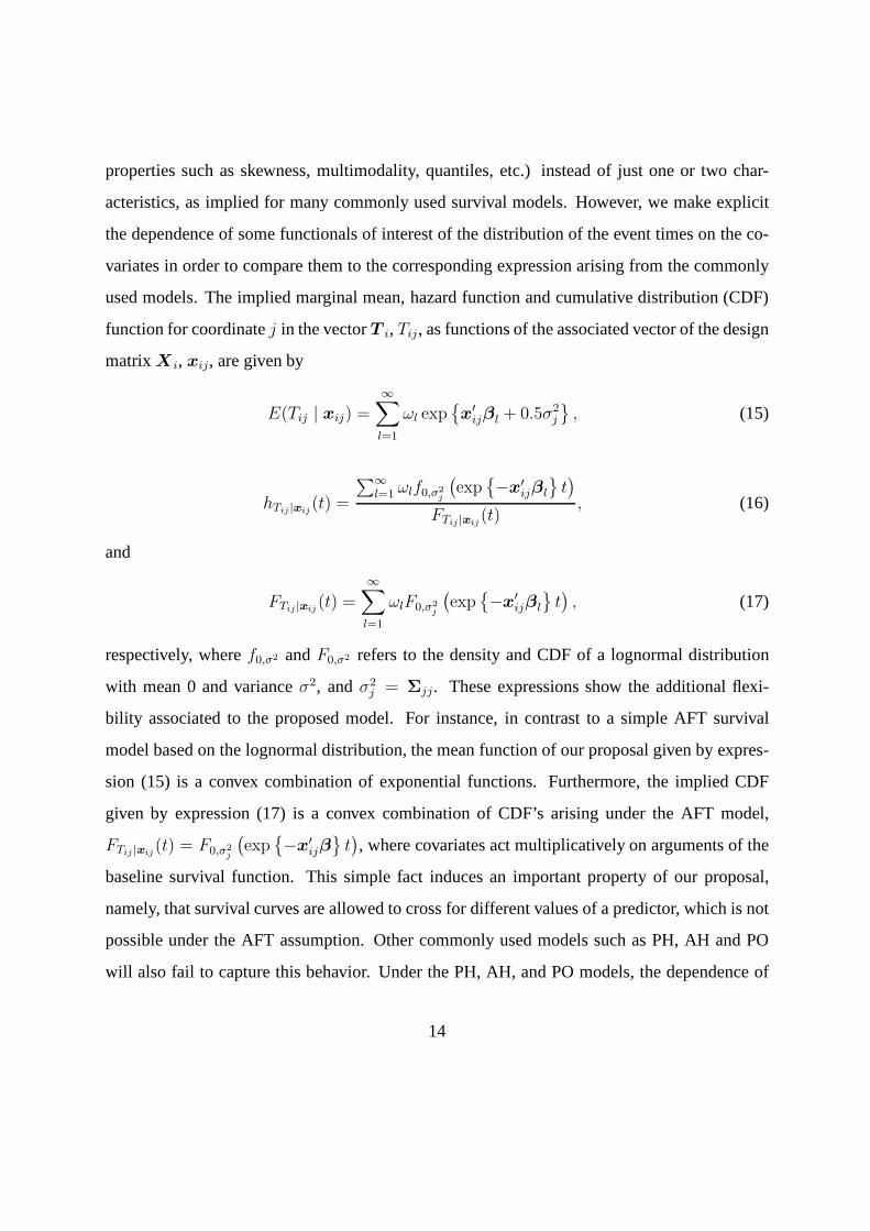
properties such as skewness, multimodality, quantiles, etc.) instead of just one or two char-

acteristics, as implied for many commonly used survival models. However, we make explicit

the dependence of some functionals of interest of the distribution of the event times on the co-

variates in order to compare them to the corresponding expression arising from the commonly

used models. The implied marginal mean, hazard function andcumulative distribution (CDF)

function for coordinatej in the vectorT i, Tij, as functions of the associated vector of the design

matrixX i, xij, are given by

E(Tij | xij) =∞∑

l=1

ωl exp

x′ijβl + 0.5σ2

j

, (15)

hTij |xij(t) =

∑∞l=1 ωlf0,σ2

j

(

exp

−x′ijβl

t)

FTij |xij(t)

, (16)

and

FTij |xij(t) =

∞∑

l=1

ωlF0,σ2

j

(

exp

−x′ijβl

t)

, (17)

respectively, wheref0,σ2 andF0,σ2 refers to the density and CDF of a lognormal distribution

with mean 0 and varianceσ2, andσ2j = Σjj. These expressions show the additional flexi-

bility associated to the proposed model. For instance, in contrast to a simple AFT survival

model based on the lognormal distribution, the mean function of our proposal given by expres-

sion (15) is a convex combination of exponential functions.Furthermore, the implied CDF

given by expression (17) is a convex combination of CDF’s arising under the AFT model,

FTij |xij(t) = F0,σ2

j

(

exp

−x′ijβ

t)

, where covariates act multiplicatively on arguments of the

baseline survival function. This simple fact induces an important property of our proposal,

namely, that survival curves are allowed to cross for different values of a predictor, which is not

possible under the AFT assumption. Other commonly used models such as PH, AH and PO

will also fail to capture this behavior. Under the PH, AH, andPO models, the dependence of

14

the CDF on predictors is given by

1 − FTij |xij(t) =

1 − F0,σ2

j(t)expx′

ijβ,

1 − FTij |xij(t) =

1 − F0,σ2

j(t)

exp

−x′ijβt

,

and1 − FTij |xij

(t)

FTij |xij(t)

=1 − F0,σ2

j(t)

F0,σ2

j(t)

exp x′β ,

respectively. Notice that this constraint associated to the commonly used models remains if

F0,σjis modeled in a nonparametric manner and/or if the linear form x′

ijβ is replace for a more

general functionm(xij). Although some fixes have been proposed in the context of PH models

for this unappealing property, e. g. the inclusion of interactions with time or stratification, our

modeling approach has proved to be a more flexible alternative. We refer to De Iorio et al.

(2009), for a thorough comparison in the context of univariate (not doubly censored) survival

data.

2.6 Prior distributions and MCMC implementation

Fora andb we consider joint prior distributions of the kindp(a, b) = p(a)p(b | a), wherep(a)

is a mixture of point mass at zero and a continuous distribution on the unit interval(0, 1) and

p(b | a) is a continuous distribution supported on(−a,∞). More, specifically we assume

a | λ, α0, α1 ∼ λδ0(·) + (1 − λ)Beta(· | α0, α1), (18)

and

b | a, µb, σb ∼ N(µb, σb)I(−a,∞), (19)

where0 ≤ λ ≤ 1, and Beta(· | α0, α1) refers to a beta distribution with parametersα0 and

α1. This modelling strategy allows us to explicitly compare a DP model versus an encompass-

ing PD alternative. Notice that this is an important component because the evaluation of any

15

other model comparison criteria would require the computation of a highly complex area under

the multivariate normal distribution which is difficult to be performed in practice. Finally, to

complete the model specification, we assume independent hyper-priorsm ∼ Nn(p+q) (η,Υ),

S ∼ IWn(p+q) (γ,Γ), andΣ ∼ IW2n (ν,Ω), whereIW2n (ν,Ω) denotes a2n-dimensional

inverted-Wishart distribution with degrees of freedomν and scale matrixΩ.

The hierarchical representation of the model allows straightforward posterior inference with

Markov Chain Monte Carlo (MCMC) simulation. As in the context of standard DP models,

two different kinds of MCMC strategies could be considered for computation in the LDPD

model: (I) to marginalize out the unknown infinite-dimensional distributions (see, e.g., Ish-

waran & James 2003; Navarrete et al. 2008) or (II) to employ a truncation to the stick-breaking

representation of the process (see, e.g., Ishwaran & James 2001). In the case (I), several alter-

native algorithms could be considered to sample the clusterconfigurations: (I.a) via a Gibbs

scheme through the coordinates (see, Navarrete et al. 2008 for a discussion in the PD context)

or (I.b) to adapt reversible-jump-like algorithms (see, e.g., Dahl 2005) to the PD context. Func-

tions implementing these approaches were written in a compiled language and incorporated

into the R library “DPpackage” (Jara, 2007). A supplementary document, including a com-

plete description of the full conditionals and algorithms is available from the following link:

http://www2.udec.cl/∼ajarav.

3 An illustration using simulated data

To validate our approach we conducted the analysis of simulated datasets which mimic to a

certain extent the Signal-Tandmobielr data. We consider one onset timeTOi and one time-to-

event timeT Ti for m = 500 subjects. We assume a binary predictor and 250 subjects in each

level (group A and B). Different distributions were assumedfor each level of the predictor such

16

that

log(TO1 , T T

1 ), . . . , log(TO250, T

T250) | fA

iid∼ fA,

and

log(TO251, T

T251), . . . , log(TO

500, TT500) | fB

iid∼ fB.

Two scenarios for the distributional parts of the model wereconsidered. In scenario I, a mixture

of two bivariate lognormal distributions was assumed for group A while a bivariate lognormal

distribution was assumed for group B. An important characteristic of scenario I is the bimodal

behavior of the distribution of the onset time and time-to-event in group A. In group B, a uni-

modal behavior for the distribution of both variables was assumed. In scenario II, mixtures of

bivariate lognormal distributions were assumed for both groups. However, the components of

the mixtures were specified in such a way that for group A, the onset times follow a bimodal dis-

tribution and the time-to-events follow a unimodal distribution. In group B, the reverse behavior

was assumed, namely, the onset times follow a unimodal distribution while the time-to-events a

bimodal distribution.

In both scenarios and variables of interest, the survival curves for both groups cross. The true

distributions in each scenario are given next.

• Scenario I: Mixture model for group A - Single model for group B.

fA ≡ 0.5 × N2

1.80

0.75

, 10−3

5.00 2.50

2.50 300

+

0.5 × N2

2.40

3.00

, 10−3

2.50 1.25

1.25 100

,

and

fB ≡ N2

2.1

2.2

, 10−2

3.24 8.10

8.10 64

17

• Scenario II: Mixture model for both group A and B.

fA ≡ 0.5 × N2

1.8

2.2

, 10−3

5.50 2.50

2.50 640

+

0.5 × N2

2.4

2.2

, 10−3

2.50 1.25

1.25 640

,

and

fB ≡ 0.5 × N2

2.10

0.75

, 10−2

3.24 8.10

8.10 30.00

+

0.5 × N2

2.10

0.75

, 10−3

32.4 1.25

1.25 100

.

The true onset and event times were interval-censored by simulating the visit times for each

subject in the data set. The first visit was drawn from anN(7, 0.22) distribution. Each of the

distances between the consecutive visits was drawn from anN(1, 0.052) distribution.

The LDPD model was fitted to both simulated datasets using thefollowing values for the

hyper-parameters:λ = 0.5, α0 = α1 = 1, µb = 10, σb = 200, ν = 4, Ω = I2, γ = 5,

Γ = I4, η = 04, andΥ = 100I4. In each analysis 4.02 million of samples of a Markov

chain cycle were completed. Because of storage limitationsand dependence, the full chain was

sub-sampled every 200 steps after a burn in period of 20,000 samples, to give a reduced chain

of length 20,000.

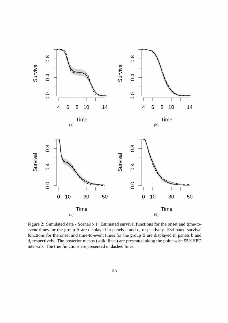
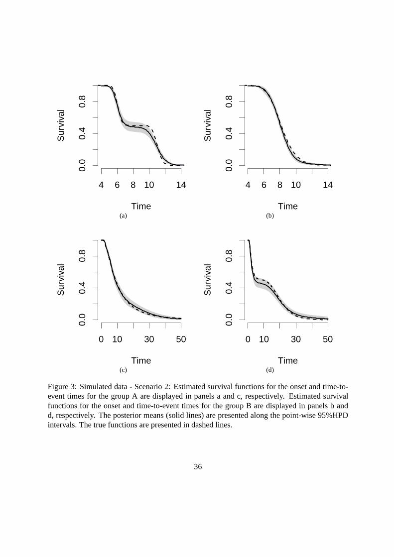
Figures 2 and 3 display the true and estimated survival curves for the onset and time-to-event

under scenario I and II, respectively. The predictive survival function closely approximated the

true survival functions, which were almost entirely enclosed in pointwise 95% highest posterior

18

density (HPD) intervals. We note that these results are for one random sample from two par-

ticular densities, and conclusions should be drawn with care. Nonetheless, these examples do

show that our proposal is highly flexible and is able to capture different behaviors of the onset

and time-to-event survival functions. The examples also show that when a parametric model is

appropriated, the proposed model does not overfit the data.

[Figure 2 about here.]

[Figure 3 about here.]

4 The Signal-Tandmobielr data

4.1 The Signal-Tandmobielr study and the research questions

For this project, 4,468 children were examined on a yearly basis during their primary school

time (between 7 and 12 years of age) by one of sixteen dental examiners. Sampling of the chil-

dren was done according to a cluster-stratified approach with 15 strata. A stratum consists of

a particular combination of one of the five provinces in Flanders with one of the three school

systems. Schools were selected such that all children had equal probability of being selected

and for each school all children of the first class were examined. Clinical data were collected

by the examiners based on visual and tactile observations (no X-rays were taken), and data on

oral hygiene and dietary habits were obtained through structured questionnaires completed by

the parents.

The primary interest of our analysis is to study the relationship between age at start brushing

(in years) and deciduous second molars health status (sound/affected) with caries susceptibility

of the adjacent permanent molars. Here, “affected molar” refers to a tooth that is decayed, filled

19

or missing due to caries. The deciduous second molars refer to teeth 55, 65, 75 and 85 and first

molars refer to teeth 16 and 26 on the maxilla (upper quadrants), and teeth 36 and 46 on the

mandible (lower quadrants). The numbering of the teeth follows the FDI (Federation Dentaire

Internationale) notation which indicates the position of the tooth in the mouth (see Figure 4).

Position 26, for instance, means that the tooth is in quadrant 2 (upper left quadrant) and position

6 where numbering starts from the mid-sagittal plane.

[Figure 4 about here.]

The level of decay was scored in four levels of lesion severity: d4 (dentine caries with pulpal

involvement),d3 (limited dentine caries),d2 (enamel cavity) andd1 (white or brown-spot initial

lesions without cavitation). Here we consider leveld3 of severity, which defines a progressive

disease.

Note that for about five years the deciduous second molars arein the mouth together with the

permanent first molars. It is thus possible that a caries process on the primary and permanent

molar occurs simultaneously. In this case it is difficult to know whether caries on the deciduous

molar caused caries on the permanent molar or vice versa. Forthis reason, the permanent first

molar was excluded from the analysis if caries were present when emergence was recorded.

Moreover, the permanent first molar had to be excluded from the analysis if the adjacent decid-

uous second molar has not been present in the mouth already atthe first examination. For 948

children none of the permanent first molars was included in the analysis due to the previously

mentioned reasons. In total, 3,520 children (12,485 permanent first molars) were included in

the analysis of which 187 contributed one tooth, 317 two teeth, 400 three teeth and 2,616 all

four teeth.

20

4.2 The analysis and the results

We consider gender (0 = boy, 1 = girl) and the status of the adjacent deciduous second molar

(sound = 0, affected = 1) as covariates for the emergence times TOij , namely, to define the de-

sign vectorsxOij. For the time-to-caries variables, we use a similar set of covariates as Leroy

et al. (2005a), namely, the covariate vectorsxTij for the caries part of the model include gender,

presence of sealants on the permanent first molar (0 = absent,1 = present), occlusal plaque ac-

cumulation for the permanent first molar (0 = none, 1 = in pits and fissures or on total surface),

reported oral brushing habits (0 = not daily, 1 = daily), and status of the adjacent deciduous

second molar. In contrast to Leroy et al. (2005a) we did not use the status of the adjacent decid-

uous first molar as covariate due to its large dependence on the status of the adjacent deciduous

second molar and included the age at start brushing in a linear fashion.

For the model, 4.02 million of samples of a Markov chain cyclewere completed. Because

of storage limitations and dependence, the full chain was sub-sampled every 200 steps after

a burn in period of 20,000 samples, to give a reduced chain of length 20,000. We consider

λ = 0.5 reflecting equal prior probabilities for the LDDP and LDPD models. The values of the

other hyper-parameters were taken asα0 = α1 = 1, µb = 10, σb = 200, ν = 10, Ω = I8,

γ = 31, Γ = I28, η = 028, andΥ = 100 × I28. We also performed the analysis with different

hyper-parameters values, obtaining very similar results.This suggests robustness to the prior

specification.

The posterior probability fora = 0 was 21.63%. Correspondingly, the Bayes factor for the

hypothesis of a LDPD against the DP version of the model was 3.62. This result suggests a

“substantial” support of the data to the PD version of the model according to the Jeffreys’ scale

(Jeffreys, 1961, page 432). As Bayes factors may be sensitive to the prior specification, we per-

formed a sensitivity analysis using different prior weights on the LDDP versus a more general

21

LDPD model. Specifically, we choseλ = 0.3 andλ = 0.7. The corresponding Bayes factors

for the LDPD against the DP version of the model were 2.72 and 2.21, respectively. The results,

therefore, indicate robustness of the model choice to the prior specification. More importantly,

in all cases the PD version of the model is to be preferred whencompared to the single precision

DP model.

The emergence and caries processes showed a non-significantassociation, evaluated by the

Pearson correlation coefficient on the log-scale induce byΣ, for most of the teeth, except for

tooth 46 where a small negative association was observed. The posterior mean (95% HPD

intervals) for the emergence and caries process for tooth 16, 26, 36, and 46, were -0.06 (-

0.18 ; 0.05), -0.06 (-0.18 ; 0.07), -0.05 (-0.13 ; 0.02), and -0.10 (-0.18 ; -0.02), respectively.

The association among emergence times and among time-to-caries was positive and significant.

Table 1 displays the posterior means and 95% HPD intervals for the Pearson correlation among

the teeth. The results indicate an exchangeable correlation matrix would suffice to explain

the caries process. However, this type of association structure does not hold for the caries

process. The Pearson correlation was bigger for the log time-to-caries for teeth in the same

jaw. Similar and lower associations were observed when considering diagonally or vertically

opponent teeth. Thus, the results suggest that the correlation structure induced for frailty models

is not appropriate for these data.

In contrast to NPML approaches, an important characteristic of the proposed model is the

ability to make inferences on any quantile of interest. Withrespect to the median, neither the

emergence nor the caries process exhibit a significant difference among the four permanent first

molars. For all combinations of covariates, molars of girlstend to emerge earlier than those

of boys. However, non-significant differences were found. Regarding caries experience, the

difference between boys and girls was not significant, however the frequency of brushing, pres-

22

ence of sealant, presence of plaque, age at start brushing and caries experience of neighboring

deciduous second molars have a significant effect on the caries process. Table 2 shows the pos-

terior mean and the 95% HPD interval for the median emergencetime and time-to-caries for

teeth 36 and 46 of boys with the “best”, “worst” and two intermediate combinations of discrete

covariates. The results are shown for 4 different values of age at start brushing.

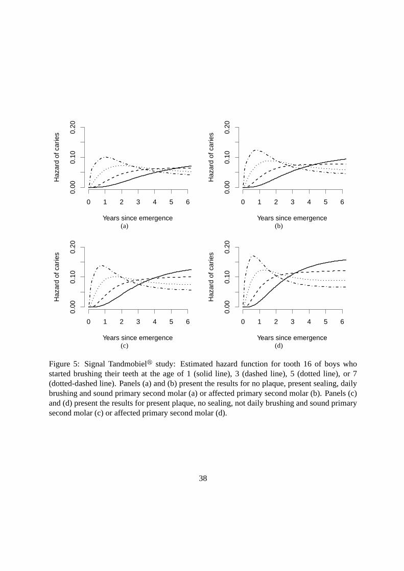
Figures 5 and 6 illustrate the estimated hazard and survivalfunctions for the time-to-caries

for tooth 16 in boys with the “best”, “worst” and two intermediate combinations of the discrete

covariates by age at start brushing. For children who started brushing their teeth after the age

of 5, a high peak in the hazard function of caries is observed already less than 1 year after

emergence. A smaller peak, shifted to the right and of much lower magnitude was observed

for children who brush their teeth before the age of 5. Furthermore, for a given combination

of the discrete predictors, the hazard function for caries crossed for different values of age at

start brushing, suggesting that a proportional hazards model is not an appropriate alternative

for modeling the time to caries. For a given age at start brushing, the presence of an affected

deciduous second molars significantly increases the pick inthe hazard function of caries in the

permanent first molar. When the teeth are daily brushed sincean early age, plaque-free and

sealed the hazard for caries starts to increase approximately 2 years after emergence, whereas,

when the teeth are not brushed daily and are exposed to other risk factors the hazard starts to

increase immediately after emergence. The peak in the hazard for caries after emergence can

be explained by the fact that teeth are most vulnerable for caries soon after emergence when the

enamel is not yet fully developed. The curves for girls were similar, and are therefore omitted.

[Figure 5 about here.]

[Figure 6 about here.]

23

Figure 6 also shows the way in which the age at start brushing is related to the caries process.

The smaller the age at start brushing the bigger the prevalence of caries. However, this increase

in the prevalence is only observed in the first years after emergence. After 5 years since emer-

gence, the prevalence of caries experience tend to be the same (and can be the same depending

on the exposure to other risk factors) regardless of the age at start brushing. This result suggests

that PH, AFT, AH or PO models are not appropriate for the analysis of caries experience since

their are constrained in such a way that survival curves are not allowed to cross for different

values of a predictor. Although the peak in the hazard for caries at approximately 1-2 years

after emergence was also observed in Leroy et al. (2005a) andKomarek & Lesaffre (2008), this

interesting finding was not detected due to the models considered by these authors.

5 Concluding remarks

We have introduced a probability model for dependent randomdistributions in the context of

multivariate doubly-interval-censored data. The main features of the proposed model are ease

of interpretation, allow for hypothesis testing of the independence assumption between onset

and time-to-event variables, efficient computation, and the fact that there is no need to assume

that the resulting survival curves satisfy assumptions such as proportional hazards, additive haz-

ards, proportional odds, or accelerated failure time.

The proposal is based on a LDPD model, which contains the LDDPmodel as an important

special case, and is specified in such a way that a simple hypothesis test for a LDDP versus a

more general LDPD alternative can be performed with no real additional computational effort

and independent fit of the models.

Several extensions of this work are possible. We are currently working on a version of the

24

model that takes into account potential misclassification of the caries process and its effect on

the corresponding inferences. Finally, the extension of the model allowing for weight dependent

covariates is also the subject of ongoing research.

Acknowledgements

The first author is supported by the Fondecyt grant 3095003. Part of this work was performed

when the first and the last two authors were visiting fellows at the Isaac Newton Institute for

Mathematical Sciences, Cambridge University. The second author has been supported by the

KUL-PUC bilateral (Belgium-Chile) grant BIL05/03. The last author has been partially sup-

ported by grants FONDECYT 1060729 and Laboratorio de Analisis Estocastico PBCT-ACT13.

The authors also acknowledge the partial support from the Interuniversity Attraction Poles Pro-

gram P5/24− Belgian State− Federal Office for Scientific, Technical and Cultural Affairs.

Data collection was supported by Unilever, Belgium. The Signal Tandmobielr study comprises

following partners: D. Declerck (Dental School, Catholic University Leuven), L. Martens (Den-

tal School, University Ghent), J. Vanobbergen (Oral HealthPromotion and Prevention, Flemish

Dental Association), P. Bottenberg (Dental School, University Brussels), E. Lesaffre (Biostatis-

tical Centre, Catholic University Leuven) and K. Hoppenbrouwers (Youth Health Department,

Catholic University Leuven; Flemish Association for YouthHealth Care).

References

BACCHETTI, P. & JEWELL, N. P. (1991). Nonparametric estimation of the incubation period

of AIDS based on a prevalent cohort with unknown infection times.Biometrics47 947–960.

BOGAERTS, K., LEROY, R., LESAFFRE, E. & DECLERCK, D. (2002). Modelling tooth emer-

gence data based on multivariate interval-censored data.Statistics in Medicine21 3775–3787.

25

CARLTON, M. A. (1999). Applications of the Two-Parameter Poisson-Dirichlet Distribution.

Unpublished doctoral thesis, University of California, Los Angeles.

CARON, F., DAVY, M., DOUCET, A., DUFLOS, E. & VANHEEGHE, P. (2006). Bayesian

inference for dynamic models with Dirichlet process mixtures. InInternational Conference

on Information Fusion. Florence, Italia, July 10-13.

CIFARELLI , D. & REGAZZINI , E. (1978). Problemi statistici non parametrici in condizioni di

scambialbilita parziale e impiego di medie associative. Tech. rep., Quaderni Istituto Matem-

atica Finanziaria, Torino.

DAHL , D. (2005). Sequentially-Allocated Merge-Split Sampler for Conjugate and Nonconju-

gate Dirichlet Process Mixture Models. Tech. rep., Texas A&M University, Department of

Statistics.

DE GRUTTOLA, V. & L AGAKOS, S. W. (1989). Analysis of doubly-censored survival data,

with application to AIDS.Biometrics45 1–11.

DE IORIO, M., JOHNSON, W. O., MUELLER, P. & L, R. G. (2009). Bayesian Nonparametric

NonProportional Hazards Survival Modelling.Biometrics65 762–771.

DE IORIO, M., MULLER, P., ROSNER, G. L. & M ACEACHERN, S. N. (2004). An ANOVA

model for dependent random measures.Journal of the American Statistical Association99

205–215.

DE LA CRUZ, R., QUINTANA , F. A. & M ULLER, P. (2007). Semiparametric Bayesian Classi-

fication with Longitudinal Markers.Applied Statistics56(2) 119–137.

DE VOS, E. & VANOBBERGEN, J. (2006). Caries prevalence in Belgian children: a review.

Arch Public Health64 217–229.

26

DUAN , J. A., GUINDANI , M. & GELFAND, A. E. (2007). Generalized Spatial Dirichlet Pro-

cess Models.Biometrika94 809–825.

DUNSON, B. D. & PARK , J. H. (2008). Kernel stick-breaking processes.Biometrika95 307–

323.

DUNSON, D. B. & HERRING, A. H. (2006). Semiparametric Bayesian latent trajectory models.

Tech. rep., ISDS Discussion Paper 16, Duke University, Durham, NC, USA.

FERGUSON, T. S. (1973). A Bayesian analysis of some nonparametric problems.The Annals

of Statistics1 209–230.

GELFAND, A. E. & KOTTAS, A. (2001). Nonparametric Bayesian Modeling for Stochastic

Order.Annals of the Institute of Statistical Mathematics53 865–876.

GELFAND, A. E., KOTTAS, A. & M ACEACHERN, S. N. (2005). Bayesian Nonparametric Spa-

tial Modeling With Dirichlet Process Mixing.Journal of the American Statistical Association

100 1021–1035.

GIUDICI , P., MEZZETTI, M. & M ULIERE, P. (2003). Mixtures of Dirichlet process priors

for variable selection in survival analysis.Journal of Statistical Planning and Inference111

101–115.

GOGGINS, W. B., FINKELSTEIN, D. M. & ZASLAVSKY, A. M. (1999). Applying the Cox

proportional hazards model for analysis of latency data with interval censoring.Statistics in

Medicine18 2737–2747.

GOMEZ, G. & CALLE , M. L. (1999). Non-parametric estimation with doubly censored data.

Journal of Applied Statistics26 45–58.

GOMEZ, G. & LAGAKOS, S. W. (1994). Estimation of the infection time and latency distribu-

tion of AIDS with doubly censored data.Biometrics50 204–212.

27

GRIFFIN, J. E. & STEEL, M. F. J. (2006). Order-based dependent Dirichlet processes. Journal

of the American Statistical Association101 179–194.

ISHWARAN, H. & JAMES, L. F. (2001). Gibbs Sampling Methods for Stick-Breaking Priors.

Journal of the American Statistical Association96 161–173.

ISHWARAN, H. & JAMES, L. F. (2003). Generalized weighted Chinese restaurant processes

for species sampling mixture models.Statistica Sinica13 1211–1235.

JAIN , S. & NEAL , R. M. (2004). A Split-Merge Markov Chain Monte Carlo Procedure for

the Dirichlet Process Mixture Model.Journal of Computational and Graphical Statistics13

158–182.

JARA , A. (2007). Applied Bayesian Non- and Semi-parametric Inference using DPpackage.

Rnews7 17–26.

JEFFREYS, H. (1961). The Theory of Probability (3rd. Ed.). Oxford, UK: Oxford University

Press.

K IM , M. Y., DE GRUTTOLA, V. G. & LAGAKOS, S. W. (1993). Analyzing doubly censored

data with covariates, with application to AIDS.Biometrics49 13–22.

KOMAREK, A. & L ESAFFRE (2008). Bayesian Accelerated Failure Time Model with Multi-

variate Doubly-Interval-Censored Data and Flexible Distributional Assumptions.Journal of

the American Statistical Association103 523–533.

KOMAREK, A., LESAFFRE, E., HARKANEN, T., DECLERCK, D. & V IRTANEN, J. I. (2005).

A Bayesian analysis of multivariate doubly-interval-censored dental data.Biostatistics6 (1)

145–155.

KORWAR, R. M. & HOLLANDER, M. (1973). Contributions to the theory of Dirichlet pro-

cesses.The Annals of Probability1 705–711.

28

LANG, S. & BREZGER, A. (2004). Bayesian P-splines.Journal of Computational and Graph-

ical Statistics13 183–212.

LEROY, R., BOGAERTS, K., LESAFFRE, E. & DECLERCK, D. (2005a). Effect of caries expe-

rience in primary molars on cavity formation in the adjacentpermanent first molar.Caries

Research39 342–349.

LEROY, R., BOGAERTS, K., LESAFFRE, E. & DECLERCK, D. (2005b). Multivariate survival

analysis for the identification of factors associated with cavity formation in permanent first

molars.European Journal of Oral Sciences113 145–152.

L IJOI, A., MENA, R. H. & PRUNSTER, I. (2007a). A Bayesian nonparametric method for

prediction in EST analysis.BMC Bioinformatics8 339–360.

L IJOI, A., MENA, R. H. & PRUNSTER, I. (2007b). Bayesian Nonparametric Estimation of the

Probability of Discovering New Species.Biometrika94 769–786.

L IJOI, A., MENA, R. H. & PRUNSTER, I. (2008). A Bayesian Nonparametric Approach for

Comparing Clustering Structures in EST Libraries.Journal of Computational BiologyTo

appear.

MACEACHERN, S. N. (1999). Dependent Nonparametric Processes. InASA Proceedings of the

Section on Bayesian Statistical Science, Alexandria, VA. American Statistical Association.

MACEACHERN, S. N. (2000). Dependent Dirichlet processes. Tech. rep., Department of

Statistics, The Ohio State University.

MARTHALER, T. M., O’MULLANE , D. M. & V RBIC, V. (1996). The prevalence of dental

caries in Europe 1990-1995.Caries Research30 237–255.

29

M IRA , A. & PETRONE, S. (1996). Bayesian hierarchical nonparametric inference for change-

point problems. In J. M. Bernardo, J. O. Berger, A. P. Dawid & A. F. M. Smith, eds.,Bayesian

Statistics 5. Oxford University Press.

MULIERE, P. & PETRONE, S. (1993). A Bayesian predictive approach to sequential search

for an optimal dose: parametric and nonparametric models.Journal of the Italian Statistical

Society2 349–364.

M ULLER, P., QUINTANA , F. A. & ROSNER, G. (2004). A method for combining inference

across related nonparametric Bayesian models.Journal of the Royal Statistical Society, Series

B 66 735–749.

NAVARRETE, C., QUINTANA , F. A. & M ULLER, P. (2008). Some Issues on Nonparametric

Bayesian Modeling Using Species Sampling Models.Statistical Modelling8 3–21.

PAN , W. (2001). A multiple imputation approach to regression analysis for doubly censored

data with application to AIDS studies.Biometrics57 1245–1250.

PETERSSON, G. H. & BRATTHALL , D. (1996). The caries decline: a review of reviews.

European Journal of Oral Sciences104 436–443.

PITMAN , J. (1995). Exchangeable and partially exchangeable random partitions.Probability

Theory and Related Fields102 145–158.

PITMAN , J. (1996). Some Developments of the Blackwell-MacQueen Urn Scheme. In T. S.

Ferguson, L. S. Shapeley & J. B. MacQueen, eds.,Statistics, Probability and Game Theory.

Papers in Honor of David Blackwell. IMS Lecture Notes - Monograph Series, Hayward,

California, 245–268.

PITMAN , J. & YOR, M. (1997). The Two-Parameter Poisson-Dirichlet Distribution Derived

from a Stable Subordinator.The Annals of Probability25 855–900.

30

SETHURAMAN , J. (1994). A constructive definition of Dirichlet process prior. Statistica Sinica

2 639–650.

SUN, J. (1995). Empirical estimation of a distribution function with truncated and doubly

interval-censored data and its application to AIDS studies. Biometrics51 1096–1104.

SUN, J., LIAO , Q. & PAGANO, M. (1995). Regression analysis of doubly censored failuretime

data with application to AIDS studies.Biometrics55 909–914.

SUN, J., LIM , H.-J. & ZHAO, X. (2004). An independence test for doubly censored failure

time data.Biometrical Journal46 503–511.

TIERNEY, L. (1994). Markov Chains for Exploring Posterior Distributions. The Annals of

Statistics22 1701–1762.

VANOBBERGEN, J., MARTENS, L., LESAFFRE, E. & DECLERCK, D. (2000). The Signal

Tandmobiel project, a longitudinal intervention health promotion study in Flanders (Bel-

gium): baseline and first year results.European Journal of Paediatric Dentistry2 87–96.

WILLEMS, S., VANOBBERGEN, J., MARTENS, L. & D E MAESENEER, J. (2005). The inde-

pendent impact of household and neighborhood-based socialdeterminants on early childhood

caries.Family & Community Health28 168–175.

31

Table 1: Signal Tandmobielr study: Posterior mean (95% HPD interval) for the Pearson correlation coefficient between

log emergence times (upper diagonal) and log time-to-caries (lower diagonal) for different teeth.

Tooth

Tooth 16 26 36 46

16 0.60 (0.56 ; 0.64) 0.60 (0.56 ; 0.64) 0.60 (0.56 ; 0.64)

26 0.88 (0.81 ; 0.94) 0.59 (0.55 ; 0.63) 0.59 (0.57 ; 0.63)

36 0.47 (0.35 ; 0.57) 0.43 (0.30 ; 0.55) 0.61(0.57 ; 0.65)

46 0.44 (0.28 ; 0.61) 0.39 (0.22 ; 0.58) 0.61 (0.54 ; 0.67)

32

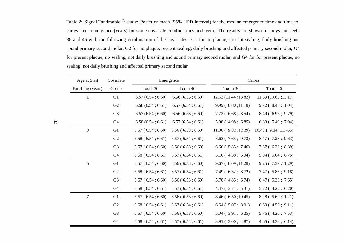
Table 2: Signal Tandmobielr study: Posterior mean (95% HPD interval) for the median emergence time and time-to-

caries since emergence (years) for some covariate combinations and teeth. The results are shown for boys and teeth

36 and 46 with the following combination of the covariates: G1 for no plaque, present sealing, daily brushing and

sound primary second molar, G2 for no plaque, present sealing, daily brushing and affected primary second molar, G4

for present plaque, no sealing, not daily brushing and soundprimary second molar, and G4 for for present plaque, no

sealing, not daily brushing and affected primary second molar.

Age at Start Covariate Emergence Caries

Brushing (years) Group Tooth 36 Tooth 46 Tooth 36 Tooth 46

1 G1 6.57 (6.54 ; 6.60) 6.56 (6.53 ; 6.60) 12.62 (11.44 ;13.82)11.89 (10.65 ;13.17)

G2 6.58 (6.54 ; 6.61) 6.57 (6.54 ; 6.61) 9.99 ( 8.80 ;11.18) 9.72 ( 8.45 ;11.04)

G3 6.57 (6.54 ; 6.60) 6.56 (6.53 ; 6.60) 7.72 ( 6.68 ; 8.54) 8.49( 6.95 ; 9.79)

G4 6.58 (6.54 ; 6.61) 6.57 (6.54 ; 6.61) 5.98 ( 4.98 ; 6.85) 6.83( 5.49 ; 7.94)

3 G1 6.57 ( 6.54 ; 6.60) 6.56 ( 6.53 ; 6.60) 11.08 ( 9.82 ;12.29) 10.48 ( 9.24 ;11.765)

G2 6.58 ( 6.54 ; 6.61) 6.57 ( 6.54 ; 6.61) 8.63 ( 7.65 ; 9.73) 8.47( 7.23 ; 9.63)

G3 6.57 ( 6.54 ; 6.60) 6.56 ( 6.53 ; 6.60) 6.66 ( 5.85 ; 7.46) 7.37( 6.32 ; 8.39)

G4 6.58 ( 6.54 ; 6.61) 6.57 ( 6.54 ; 6.61) 5.16 ( 4.38 ; 5.94) 5.94( 5.04 ; 6.75)

5 G1 6.57 ( 6.54 ; 6.60) 6.56 ( 6.53 ; 6.60) 9.67 ( 8.09 ;11.28) 9.25 ( 7.39 ;11.29)

G2 6.58 ( 6.54 ; 6.61) 6.57 ( 6.54 ; 6.61) 7.49 ( 6.32 ; 8.72) 7.47( 5.86 ; 9.18)

G3 6.57 ( 6.54 ; 6.60) 6.56 ( 6.53 ; 6.60) 5.78 ( 4.85 ; 6.74) 6.47( 5.33 ; 7.65)

G4 6.58 ( 6.54 ; 6.61) 6.57 ( 6.54 ; 6.61) 4.47 ( 3.71 ; 5.31) 5.22( 4.22 ; 6.20)

7 G1 6.57 ( 6.54 ; 6.60) 6.56 ( 6.53 ; 6.60) 8.46 ( 6.50 ;10.45) 8.28 ( 5.69 ;11.21)

G2 6.58 ( 6.54 ; 6.61) 6.57 ( 6.54 ; 6.61) 6.54 ( 5.07 ; 8.01) 6.69( 4.56 ; 9.11)

G3 6.57 ( 6.54 ; 6.60) 6.56 ( 6.53 ; 6.60) 5.04 ( 3.91 ; 6.25) 5.76( 4.26 ; 7.53)

G4 6.58 ( 6.54 ; 6.61) 6.57 ( 6.54 ; 6.61) 3.91 ( 3.00 ; 4.87) 4.65( 3.38 ; 6.14)

33

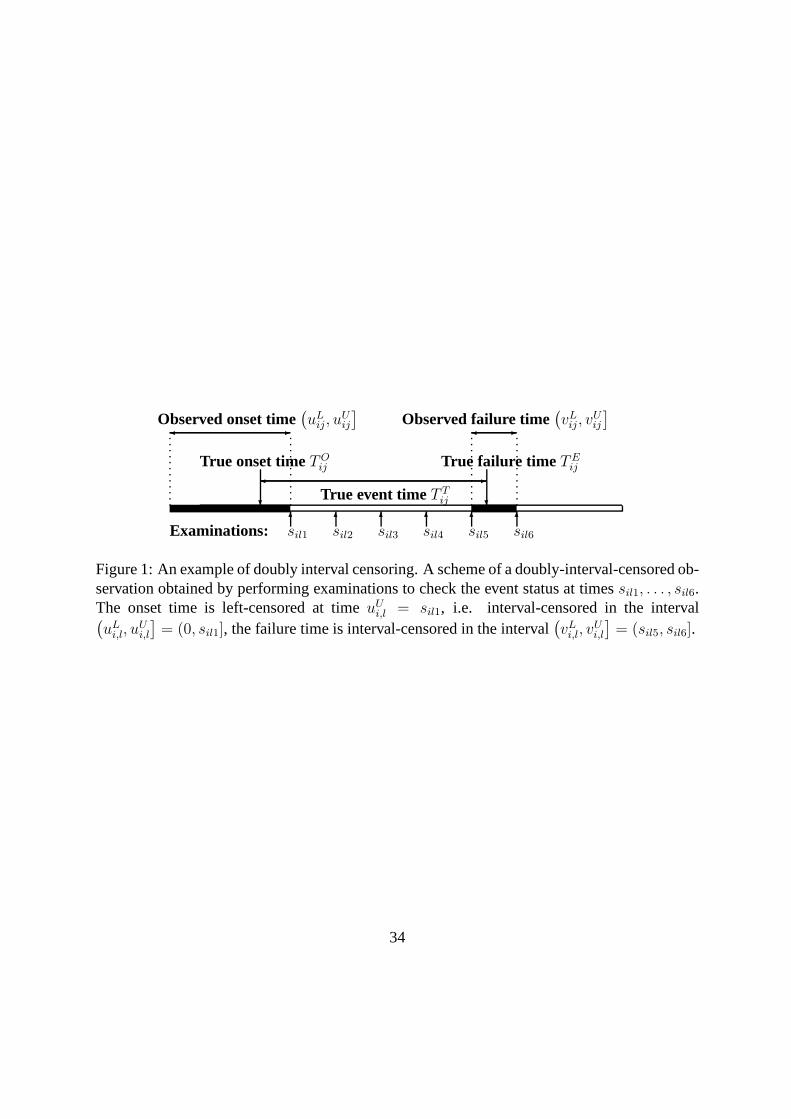
6 6 6 6 6 6Examinations: sil1 sil2 sil3 sil4 sil5 sil6

? ?

True onset time TOij True failure time TE

ij-

True event time T Tij

-Observed onset time

(

uLij, u

Uij

]

-Observed failure time

(

vLij, v

Uij

]

Figure 1: An example of doubly interval censoring. A scheme of a doubly-interval-censored ob-servation obtained by performing examinations to check theevent status at timessil1, . . . , sil6.The onset time is left-censored at timeuU

i,l = sil1, i.e. interval-censored in the interval(

uLi,l, u

Ui,l

]

= (0, sil1], the failure time is interval-censored in the interval(

vLi,l, v

Ui,l

]

= (sil5, sil6].

34

4 6 8 10 14

0.0

0.4

0.8

Time

Sur

viva

l

(a)

4 6 8 10 14

0.0

0.4

0.8

TimeS

urvi

val

(b)

0 10 30 50

0.0

0.4

0.8

Time

Sur

viva

l

(c)

0 10 30 50

0.0

0.4

0.8

Time

Sur

viva

l

(d)

Figure 2: Simulated data - Scenario 1: Estimated survival functions for the onset and time-to-event times for the group A are displayed in panels a and c, respectively. Estimated survivalfunctions for the onset and time-to-event times for the group B are displayed in panels b andd, respectively. The posterior means (solid lines) are presented along the point-wise 95%HPDintervals. The true functions are presented in dashed lines.

35

4 6 8 10 14

0.0

0.4

0.8

Time

Sur

viva

l

(a)

4 6 8 10 14

0.0

0.4

0.8

TimeS

urvi

val

(b)

0 10 30 50

0.0

0.4

0.8

Time

Sur

viva

l

(c)

0 10 30 50

0.0

0.4

0.8

Time

Sur

viva

l

(d)

Figure 3: Simulated data - Scenario 2: Estimated survival functions for the onset and time-to-event times for the group A are displayed in panels a and c, respectively. Estimated survivalfunctions for the onset and time-to-event times for the group B are displayed in panels b andd, respectively. The posterior means (solid lines) are presented along the point-wise 95%HPDintervals. The true functions are presented in dashed lines.

36

(a)

(b)

Figure 4: European notation for the position of (a) deciduous (primary); and (b) permanentteeth. Maxilla= upper jaw, mandible= lower jaw. In (a) the fifth and the eight quadrants are atthe right-hand side of the subject, and the sixth and the seventh quadrants are to the left. In (b)the first and the fourth quadrants are at the right-hand side of the subject, and the second andthe third quadrants are to the right.

37

0 1 2 3 4 5 6

0.00

0.10

0.20

Years since emergence

Haz

ard

of c

arie

s

(a)

0 1 2 3 4 5 6

0.00

0.10

0.20

Years since emergenceH

azar

d of

car

ies

(b)

0 1 2 3 4 5 6

0.00

0.10

0.20

Years since emergence

Haz

ard

of c

arie

s

(c)

0 1 2 3 4 5 6

0.00

0.10

0.20

Years since emergence

Haz

ard

of c

arie

s

(d)

Figure 5: Signal Tandmobielr study: Estimated hazard function for tooth 16 of boys whostarted brushing their teeth at the age of 1 (solid line), 3 (dashed line), 5 (dotted line), or 7(dotted-dashed line). Panels (a) and (b) present the results for no plaque, present sealing, dailybrushing and sound primary second molar (a) or affected primary second molar (b). Panels (c)and (d) present the results for present plaque, no sealing, not daily brushing and sound primarysecond molar (c) or affected primary second molar (d).

38

0 1 2 3 4 5 6

0.0

0.4

0.8

Years since emergence

Car

ies

free

(a)

0 1 2 3 4 5 6

0.0

0.4

0.8

Years since emergenceC

arie

s fr

ee

(b)

0 1 2 3 4 5 6

0.0

0.4

0.8

Years since emergence

Car

ies

free

(c)

0 1 2 3 4 5 6

0.0

0.4

0.8

Years since emergence

Car

ies

free

(d)

Figure 6: Signal Tandmobielr study: Estimated survival function for tooth 16 of boys whostarted brushing their teeth at the age of 1 (solid line), 3 (dashed line), 5 (dotted line), or 7(dotted-dashed line). Panels (a) and (b) present the results for no plaque, present sealing, dailybrushing and sound primary second molar (a) or affected primary second molar (b). Panels (c)and (d) present the results for present plaque, no sealing, not daily brushing and sound primarysecond molar (c) or affected primary second molar (d).

39