Sensitivity analysis of predictive modeling for responses from the three-parameter Weibull model...

This article appeared in a journal published by Elsevier. The attachedcopy is furnished to the author for internal non-commercial researchand education use, including for instruction at the authors institution

and sharing with colleagues.

Other uses, including reproduction and distribution, or selling orlicensing copies, or posting to personal, institutional or third party

websites are prohibited.

In most cases authors are permitted to post their version of thearticle (e.g. in Word or Tex form) to their personal website orinstitutional repository. Authors requiring further information

regarding Elsevier’s archiving and manuscript policies areencouraged to visit:

http://www.elsevier.com/copyright

http://www.elsevier.com/copyright

Author's personal copy

Computational Statistics and Data Analysis 55 (2011) 3093–3103

Contents lists available at ScienceDirect

Computational Statistics and Data Analysis

journal homepage: www.elsevier.com/locate/csda

Sensitivity analysis of predictive modeling for responses from thethree-parameter Weibull model with a follow-up doubly censoredsample of cancer patientsHafiz M.R. Khan a,∗, Ahmed Albatineh a, Saeed Alshahrani a, Nadine Jenkins b,Nasar U. Ahmed a

a Department of Epidemiology & Biostatistics, Robert Stempel College of Public Health and Social Work, Florida International University, Miami, FL 33199, USAb UMDNJ University Hospital, University of Medicine & Dentistry of New Jersey, 150 Bergen Street, Newark, NJ 07103, USA

a r t i c l e i n f o

Article history:Received 2 February 2011Received in revised form 23 May 2011Accepted 23 May 2011Available online 30 May 2011

Keywords:Censored sampleDoubly censored sampleThree-parameter Weibull modelBayesian approachPredictive inference

a b s t r a c t

The purpose of this paper is to derive the predictive densities for future responses from thethree-parameterWeibullmodel given a doubly censored sample. The predictive density fora single future response, bivariate future response, and a set of future responses has beenderived when the shape parameter α is unknown. A real data example representing 44patients who were diagnosed with laryngeal cancer (2000–2007) at a local hospital is usedto illustrate the predictive results for the four stages of cancer. The survival days of eight outof the 44 patients could not be calculated as the patients were lost to follow-up. They werethe first four and the last four patients’ survival days in order. Thus, the recorded data forthe survival days of 36 patients composed of 18male and 18 female patients with cancer ofthe larynx are used for the predictive analysis. Furthermore, a subgroup level of the maleand female patients follow-up data are considered to obtain the future survival days. Asensitivity study of themean, standard deviation, and 95% highest predictive density (HPD)interval of the future survival days with respect to stages and doses are performed whenthe shape parameter α is unknown.

© 2011 Elsevier B.V. All rights reserved.

1. Introduction

Predictive inference has been playing an important role in healthcare data analysis. Healthcare researchers rely on pastobservations to analyze and forecast treatment outcomes. Usually, observations recorded in the past can be incompletefor any reason such as lost to follow-up due to migration, early termination of the study, unrelated cause of death, limitedresources to conduct a study, or withdrawal from a study due to undesirable effect of a drug. When a data set is incomplete,the healthcare practitioners or researchers need to carefully deal with them, otherwise any underestimate or overestimateof some statistical measures may lead to misinterpretation of the data. There are three types of censored data such as left,right, and doubly censored. Recently several statistical research works have been accomplished based on censored data, forexamples, Ahmed and Saleh (1999) andBuhamra et al. (2004, 2007). Doubly censored data are commonly observed in clinicalstudies, where the first few observations and the last few observations are unavailable from a sequence of observations. Forexample, there are n patientswho are diagnosedwith a particular disease in a clinical study. These patients are given optimaldoses for a period of time. During the follow-up, the survival time of each patient is recorded in order with t1 ≤ · · · ≤ tn.In this case, the record of survival days of the first few observations and the last few observations may not be available.

∗ Corresponding author.E-mail address: [email protected] (H.M.R. Khan).

0167-9473/$ – see front matter© 2011 Elsevier B.V. All rights reserved.doi:10.1016/j.csda.2011.05.017


3094 H.M.R. Khan et al. / Computational Statistics and Data Analysis 55 (2011) 3093–3103

Therefore, they might be removed from the statistical analysis in order to make statistical inferences. This type of dataconstitutes a doubly censored sample. For more about doubly censored samples, the reader is referred to Sarhan (1955),Khan (2003), Khan et al. (2006), Kambo (1978), Raqab (1995) and Lalitha andMishra (1996), among others. Doubly censoreddata from clinical studies may be modeled by the three-parameter Weibull model. Based on a doubly censored sample, it isassumed in this paper that the three-parameter Weibull model specified by the following density is appropriate:

f (t|α, β, µ) =

α

β

t − µ

β

α−1

exp−

t − µ

β

α, for t ≥ µ; α, β > 0,

0 elsewhere,(1)

where µ is the location parameter, α is the shape parameter, and β is the scale parameter. This model is an extension of thetwo-parameter Weibull model. The additional parameter is the location parameter. For analytical convenience, on writingθ = βα , we have

f (t|α, θ, µ) =

α

θ(t − µ)α−1 exp

−

(t − µ)α

θ

, for t ≥ µ; α > 0, θ > 0,

0 elsewhere.(2)

Ahmed (1992) discussed an asymptotic estimation of reliability in a life-testingmodel. Sarhan (1955) obtained themean andstandard deviation of certain populations from singly and doubly censored samples. Kambo (1978) derived the maximumlikelihood estimators of the location and scale parameters by using a doubly censored sample. Khan et al. (2006) derived thepredictive distributions of future responses on the basis of a doubly censored sample from the two-parameter exponentiallife testingmodel. There are several studies on lifetimemodels related to censoring, for example, Ahmed et al. (2008), Ahmedand Saleh (1999) and Ahsanullah and Ahmed (2001).

The inference about the future responses given a set of observed data is known as predictive inference. In predictiveinference, the observed data can be considered as an informative experiment, and the unobserved future data form thefuture experiment. The goal of predictive inference is to obtain probability statements about the future experiment giventhe informative experiment. Predictive inference has been considered by many authors, for instance, Mahdi et al. (1998),Thabane (1998), Khan et al. (2006), Bernardo and Smith (1994), Gelman et al. (2004), and Martz and Waller (1982). Onemay consider the Bayesian approach to derive the predictive inference of future observations. Several authors have utilizedthe Bayesian approach for determining predictive inference. For example, in the past, Aitchison and Dunsmore (1975),Aitchison and Sculthorpe (1965), and Berger (1985) considered a general Bayesian predictive problem. Geisser (1993)discussed various Bayesian predictive problems for future responses. Moreover, Geisser (1971) discussed the inferentialuse of predictive distributions. Predictive distributions for linear models which make use of the Bayesian approach havebeen determined by Dunsmore (1974), and Zellner and Chetty (1965). Additional applications of the Bayesian approach topredictive inference have been considered for example by Khan (2003), Thabane and Haq (2000), Thabane (1998), Khan andProvost (2008), Khan et al. (2007), Gelman et al. (2004), Bernardo and Smith (1994), Sinha (1986), Evans andNigm (1980a,b),and Martz and Waller (1982).

The objective of this paper is to derive the predictive densities for future responses from the three-parameter Weibulldistribution given a doubly censored sample with unknown shape parameter (α). The results will be illustrated by makinguse of the Bayesian approach with application to larynx cancer patients.

The remainder of the paper is organized as follows: In the case of unknown shape parameter (α), Section 2 discussesthe derivation of the likelihood function, the prior density function, the posterior density function, the predictive densityfunction for a single future response, a bivariate future response, and a set of future responses. Section 3 discusses the highestpredictive density (HPD) interval. Section 4 describes the estimation of the hyperparameters of prior density. Section 5includes a real data example of larynx cancer patients to illustrate some of the results.

2. Posterior density

Let t1, . . . , tn be an ordered random sample of size n from model (2), where t1 ≤ · · · ≤ tg be the g smallest orderedobservations and tℓ+1 ≤ · · · ≤ tn be the (n − ℓ) largest ordered observations from the sample. Only the remaining orderedobservations t = (tg+1, . . . , tℓ) are used for statistical analysis. It is assumed that the sample data aremodeled by the three-parameter Weibull model. The likelihood function of θ , α, and µ for a given doubly censored sample t = (tg+1, . . . , tℓ) isgiven by

L(θ, α, µ|t) ∝

[F

(tg+1 − µ)α

θ

]g [1 − F

(tℓ − µ)α

θ

]n−ℓ

ℓ∏i=g+1

f

(ti − µ)α

θ

, for ti ≥ 0; θ ≥ 0,

where F{(tg+1−µ)α

θ} = 1 − exp{− (tg+1−µ)α

θ}.


H.M.R. Khan et al. / Computational Statistics and Data Analysis 55 (2011) 3093–3103 3095

Following Khan (2003), the simplified form of the likelihood function for a given doubly censored sample from themodelspecified by (2) is given by

L(θ, α, µ|t) ∝ α−(ℓ−g)θ−(ℓ−g)−g

ξ=0(−1)ξ

gξ

ℓ∏i=g+1

(ti − µ)α−1

× exp

−

∑ℓi=g+1(ti − µ)α + (n − ℓ)(tℓ − µ)α + ξ(tg+1 − µ)α

θ

.

Suppose the shape parameter α has a uniform prior over the interval (0, α). Furthermore, it is assumed that θ , α, and µ areindependently distributed. Then the joint prior density is

p(θ, α, µ|η, δ) ∝1

αθ δexp

−

η

θ

; µ > 0, θ > 0, α, η, δ > 0, (3)

where η and δ are hyperparameters. Thus, the posterior density of (θ, α, µ) is

p(θ, α, µ|t) ∝ L(θ, α, µ|t)p(θ, α, µ|η, δ)

= Ψ0(t) α−(ℓ−g+1) θ−(δ+ℓ−g)−g

ξ=0(−1)ξ

gξ

ℓ∏i=g+1

(ti − µ)α−1

× exp

−

η +∑ℓ

i=g+1(ti − µ)α + (n − ℓ)(tℓ − µ)α + ξ(tg+1 − µ)α

θ

,

where Ψ0(t) is a normalizing constant.

2.1. Predictive density for a single future response

The predictive density function for a single future response (v) is given by

p(v|t) =

Ψ1(t)

∫ min(tg+1, v)

µ=0

∫∞

α=0α−(ℓ−g)

−g

ξ=0(−1)ξ

gξ

ℓ∏i=g+1

(ti − µ)α

×(v − µ)α−1[Wξ (µ) + (v − µ)α]

−(δ+ℓ−g)dα dµ, for v ≥ 0,0 elsewhere,

(4)

whereWξ (µ) = η +∑ℓ

i=g+1(ti − µ)α + (n − ℓ)(tℓ − µ)α + ξ(tg+1 − µ)α and Ψ1(t) is a normalizing constant. There is noclosed form representation of this density function. For a given doubly censored data set, we can evaluate the above densityfunction by numerical integration methods after estimating the hyperparameters η and δ.

2.2. Predictive density for a bivariate and a set of future responses

Let v1 and v2 be two ordered future responses from the three-parameter Weibull model whose density function isspecified in Eq. (2), then the predictive density function for a bivariate future response is given by

p(v1, v2|t) =

Ψ2(t)∫ min(tg+1, v1)

µ=0

∫∞

α=0α−(ℓ−g−1)

−g

ξ=0(−1)ξ

gξ

ℓ∏i=g+1

(ti − µ)α−1

×

2∏

i=1

(vi − µ)α−1

Wξ (µ) +

−2

i=1(vi − µ)α

−(δ+ℓ−g+1)dα dµ, for vi ≥ 0,

0 elsewhere.

(5)

There is no closed form representation of the above bivariate predictive density function. However, for a given doublycensored sample, we can compute the values of this density function by numerical integration methods.

Similarly, let v1, . . . , vk be k ordered future responses from the three-parameter Weibull model whose density functionis specified in Eq. (2).



The predictive density function for a set of k future responses is given by

p(v1, . . . , vk|t) =

Ψk(t)∫ min(tg+1, v1)

µ=0

∫∞

α=0α−(ℓ−g−k+1)

−g

ξ=0(−1)ξ

gξ

ℓ∏i=g+1

(ti − µ)α−1

×

k∏

i=1

(vi − µ)α−1

Wξ (µ) +

−k

i=1(vi − µ)α

−(δ+ℓ−g+1)dα dµ, for vi ≥ 0,

0 elsewhere,

(6)

where Ψk(t) is a normalizing constant. For k = 1, the above predictive density reduces to the predictive density for a singlefuture response obtained inmodel (4); for k = 2, the above predictive density reduces to the predictive density for a bivariatefuture response obtained in model (5); and so on.

3. Highest predictive density (HPD) interval

An HPD interval is the interval which includes the most probable values of a given density at a given significance level,subject to the condition that the density function has the same value at the end points. An HPD interval U is of the formU = {v : p(v|t) ≥ uα}, where uα is the largest constant such that Pr(v ∈ U|t) = 1 − α, and α denotes the assumedsignificance level. The HPD interval [u1, u2] for v must simultaneously satisfy the following two conditions:

Pr(u1 ≤ v ≤ u2) = 1 − α and p(u1|t) = p(u2|t).

For more about HPD intervals, the reader is referred to Sinha (1986). It follows that Pr(u1 < v < tg+1) + Pr(tg+1 < v <u2) = 1 − α, where u1 and u2 are to be arbitrarily chosen so that p(u1|t) = p(u2|t). Thus, in light of the expression derivedfor p(v|t), in Eq. (4), a closed form solution for u1 and u2 may not be achievable. However, for a doubly censored sample, asolution can be obtained numerically.

4. Estimation of the hyperparameters of the prior density

The hyperparameters are usually unknown andmay be estimated from the data set by applying themaximum likelihoodmethod, see Geisser (1993) and Berger (1985). Then the likelihood function L(η, δ|t) can be written as follows

L(η, δ|t) =

∫ tg+1

µ=0

∫∞

α=0

∫∞

θ=0p(t|θ, α, µ) p(θ, α, µ|η, δ)dθ dα dµ

∝

−g

ξ=0(−1)ξ

gξ

∫ tg+1

µ=0

∫∞

α=0α−(ℓ−g)Γ (ℓ − g + δ − 1)

×

ℓ∏

i=g+1(ti − µ)α−1

η + (n − ℓ)(tℓ − µ)α +

∑ℓi=g+1(ti − µ)α + ξ(tg+1 − µ)

(ℓ−g+δ−1) dα dµ.

The maximum likelihood estimates of η and δ are the solutions of

∂

∂η

−g

ξ=0(−1)ξ

gξ

∫ tg+1

µ=0

∫∞

α=0α−(ℓ−g)Γ (ℓ − g + δ − 1)

×

ℓ∏

i=g+1(ti − µ)α−1

η + (n − ℓ)(tℓ − µ)α +

∑ℓi=g+1(ti − µ)α + ξ(tg+1 − µ)

(ℓ−g+δ−1) dαdµ

= 0

and

∂

∂δ

−g

ξ=0(−1)ξ

gξ

∫ tg+1

µ=0

∫∞

α=0α−(ℓ−g)Γ (ℓ − g + δ − 1)



×

ℓ∏

i=g+1(ti − µ)α−1

η + (n − ℓ)(tℓ − µ)α +

∑ℓi=g+1(ti − µ)α + ξ(tg+1 − µ)

(ℓ−g+δ−1) dαdµ

= 0.

Unfortunately, these equations do not yield closed form representations for η and δ, and the Newton–Raphson iterativealgorithm fails to achieve solutions for η and δ simultaneously. Thus, one can consider an advanced software package withsome arbitrary values of η̂ and δ̂, and these values may be substituted in Eq. (4) to determine the predictive density for asingle future response when the shape parameter is unknown.

5. A real data example

The larynx or voice box is located just below the throat and is made of cartilage and contains the vocal cords that vibrateto make sound when one talks, Mayo Clinic (2009). The larynx is a short passageway that also has a small piece of tissue,called the epiglottis, which moves to cover the larynx to prevent food from entering the air passages. The larynx is a criticaland significant organ that determines normal breathing, swallowing, and speaking. Any damage to the larynx or its tissuescan cause interference or inability with any or all of these functions, Johns Hopkins (2009). According to the National CancerInstitute, NCI (2009a), head and neck cancers represent approximately three to five percent of all cancers in the UnitedStates. These cancers are more common in men and in people over age 50.

There are several risk factors that may increase the chances of developing cancer. One of the main risk factorsassociated with the development of laryngeal cancer is tobacco use. Smoking cigarettes, pipes, cigars, and/or heavy alcoholconsumption further increase the risk of developing laryngeal cancer. According to the American Cancer Society, ACS (2009),it has been reported that individuals who both habitually drink and smoke have an increased risk of developing head andneck cancer by 100-fold. Some other factors that increase the risk of laryngeal cancer include unhealthy diet and vitamindeficiency, a compromised immune system, genetics, and prolonged and intense exposures to dust, fumes and chemicals.People over 65 years are at higher risk of developing laryngeal cancer than those who are of a younger age. African Americanand White adults are more commonly diagnosed with laryngeal cancer than that of Asian and Latino adults, ACS (2009).

Symptoms of laryngeal cancer include beginning sore throat, difficulty and painful swallowing, ear pain, and a changeor hoarseness in the voice, NCI (2009b). The American Cancer Society (2009) also notes symptoms that include a constantcough, difficulty breathing, weight loss, and a lump or mass in the neck. The hoarseness usually occurs only after the cancerhas reached a later stage or has spread to the vocal cords. This cancer is sometimes diagnosed when it spreads to the lymphnodes, and a growing mass is present in the neck, ACS (2009). The size and level of cancer spread is classified as the stage ofthe cancer.

The American Joint Committee on Cancer (2009), established a staging system to classify and describe the extent andmagnitude of cancers. Cancer cells can travel to other parts of the body and can damage or replace normal tissue or organs.This process of distant spread or travel of cancer cells is referred to as metastasis. Cancer cells metastasize when they getinto the bloodstream or lymph vessels and affect other parts of the body. Regardless of where cancer cells may travel to,the cancer is always identified by the originating organ (i.e. cancer of the larynx with spread to the lung is laryngeal cancer;cancer of the breast with spread to the brain is breast cancer, etc.). The distant site is always referred to as metastasis, ACS(2009). The extent or spread of the disease is determined by diagnostic testing.

The AJCC staging system assigns the extent of disease based on three major categories; T -tumor, N-lymph nodes, M-metastasis. The combination of each of the categories results in a stage group, which indicates the disease stage. All cancersites differ in the requirements for staging. For example, cancer of the larynx looks atwhether the primary tumor has invadednearby tissue/sites to assign the T -tumor code, while breast cancer looks at the size of the primary tumor. The lymph nodeclassification is fairly uniform acrossmost cancers and looks to signifywhether the tumor has invaded regional lymphnodes.TheM-metastasis coding is also similar across primary sites and notes whether the tumor has traveled away from the site oforigin and invaded distant organs or tissues, Greene et al. (2002). Once a diagnosis stage has been assigned to patient status,a treatment approach can be planned.

The twomajor approaches in treating cancer are curative and palliative. Curative treatment planning seeks to remove allof the known cancer from the body. Palliative treatment seeks to alleviate symptoms related to the cancer. The three mostcommon methods used to treat cancer are surgery (e.g. cordectomy, laryngectomy), radiation therapy (e.g. external beam,brachytherapy), and chemotherapy (e.g. conventional, targeted, chemoradiation). With laryngeal cancer, one of the maingoals is to preserve the larynx (voice box) so that individuals retain their ability to speak. Of course, the treatment methodselected is based on the stage of the disease, ACS (2009). The earlier the cancer is detected the more likely the result will bean early stage of disease. The prognosis and survival for laryngeal cancer are based on several factors that include the stageof the disease, the size and location of the tumor, and the patient’s age and general health. The Cleveland Clinic (2009) hassummarized the AJCC stage grouping for laryngeal cancer. Cancers found in stage 0 and stage 1 have a 75% to 95% cure rate,depending on where the cancer is located. Late stage cancers that have spread or metastasized to other areas of the bodyhave a very poor survival rate, Cleveland Clinic (2009).



Table 1Results of goodness of fit tests based on Kolmogorov–Smirnov, Ander-son–Darling, and Chi-Squared methods.

K–S test statistic = 0.10723Choice of α 0.10Critical value 0.1991Decision on Weibull dist. (3P) Accept

A–D test statistic = 0.31020Choice of α 0.10Critical Value 1.9180Decision on Weibull dist. (3P) Accept

Chi-Squared test statistic = 1.4701Choice of α 0.10Critical value 7.7794Decision on Weibull dist. (3P) Accept

Pdf

0.0001

0.0002

0.0003

2000 4000 6000 8000 10000 12000

Fig. 1. Predictive survival densities for a single future response v based on 36 patients, for certain values of the hyperparameters, η (stages) and δ (doses),namely, I: Long dashes (η = 1, δ = 1), II: Dotted line (η = 2, δ = 8), III: Short dashes (η = 3, δ = 12) & IV: Solid line (η = 4, δ = 16).

We consider a doubly censored sample of larynx cancer patients from a local hospital in Northern New Jersey. Whenobserving the rate of survival days for males and females, it was noted that 100% of the males were diagnosed duringthe years 2000 through 2002. Only 39% of the females were diagnosed during this time period and the remaining 61%were diagnosed in later years (2003–2007). Therefore, the lower survival days of the male subjects could be attributedto developing the laryngeal cancer three years before the female subjects.

A doubly censored data set (where the survival days of the first four and the last four patients were lost to follow-up)consisting of 36 subjects (18 male and 18 female) who were newly diagnosed (2000–07) with laryngeal cancer was usedto illustrate some of the predictive results. Based on the total sample size of 36, the summary of statistics for survival dayswere: minimum = 44 and maximum = 2553; the mean and the standard deviation were 1082.89 (± 836.06), respectively.

At the subgroup level, the summary of statistics of the observed survival days for the males were: minimum = 78 andmaximum = 2387; the mean and the standard deviation survival days for the males were 1085.17 (±865.88), respectively.Similarly, the observed survival days for the females were: minimum = 44 and maximum = 2553; the mean and thestandard deviation survival days for the females were 1080.61 (±830.28), respectively. We consider several statisticalprobability models to fit the data. Based on the descriptive statistics, statistical probability models, Kolmogorov–Smirnov,Anderson–Darling, and Chi-Squared goodness of fit tests, it is determined that the three-parameter Weibull model withestimated parameters, α̂ = 1.9703, β̂ = 19.6680, and µ̂ = 36.421 is appropriate for modeling the number of days apatient survives after the diagnosis of laryngeal cancer. It must be noted that all of the tests had low power with such asmall sample size. We used ‘EasyFit 5.4 Professional’ software from MathWave Technologies (2010) to run the goodness offit tests and their summary results are given in Table 1.

The data setwas used to estimate themeans, standard deviations, and 95%highest predictive density intervals for a futureresponse. Several 95% highest predictive density intervals for the future survival days were estimated by assigning certaindoses with respect to stages. By using Mathematica Software package 7.0, Wolfram Research (2008), the mean, standarddeviation, and 95% highest predictive density intervals of survival days were obtained for the combined group (male andfemale) and for their subgroup analysis. The values of normalizing constant were calculated at all stages based on a doublycensored sample in order to display the predictive survival densities. We also considered normalizing constant values forthe computation of mean, standard deviation, and highest predictive density intervals for each stage with respect to dose.We obtained the HPD intervals by setting p(u1|t) = p(u2|t) and aiming for Pr(u1 ≤ v ≤ u2) = 0.95, where p(.|t) is givenin Eq. (4).



Table 2Sensitivity of the predictive mean, standard deviation, and 95% highest predictive density(HPD) intervals based on 36 patients’ (both male and female) survival days by setting severalvalues of the hyperparameters for a single future response v.

Values of hyperparameters Mean(v) ± SD(v) 95% HPD intervalsη (stages) δ (doses)

1 1 2694.80 ± 1896.39 (222.98, 7000.01)1 2 2635.30 ± 1861.46 (210.68, 6700.23)1 3 2575.91 ± 1825.23 (199.45, 6500.14)1 4 2460.51 ± 1752.03 (189.16, 6380.10)2 5 2460.51 ± 1752.03 (179.71, 6210.19)2 6 2405.17 ± 1715.86 (170.99, 6055.20)2 7 2351.61 ± 1680.31 (162.93, 5910.09)2 8 2299.89 ± 1645.51 (155.48, 5765.04)3 9 2250.04 ± 1611.59 (148.57, 5625.30)3 10 2201.95 ± 1578.53 (142.15, 5495.21)3 11 2155.63 ± 1546.39 (136.17, 5370.27)3 12 2111.02 ± 1515.21 (130.60, 5245.18)4 13 2068.09 ± 1484.99 (125.41, 5130.12)4 14 2026.70 ± 1455.68 (120.54, 5020.23)4 15 1986.83 ± 1427.29 (115.99, 4910.40)4 16 1948.40 ± 1399.82 (111.72, 4810.29)

Table 3Sensitivity of the predictive mean, standard deviation, and 95% highest predictive density(HPD) intervals based on 18 male patients’ survival days by setting several values of thehyperparameters for a single future response v.

Values of hyperparameters Mean(v) ± SD(v) 95% HPD intervalsη (stages) δ (doses)

1 1 2672.31 ± 1914.46 (220.72, 6900.31)1 2 2559.81 ± 1846.96 (198.69, 6580.05)1 3 2449.33 ± 1776.47 (180.19, 6265.26)1 4 2343.98 ± 1706.37 (164.47, 5965.17)2 5 2244.91 ± 1638.35 (151.02, 5685.14)2 6 2152.18 ± 1573.12 (139.39, 5425.10)2 7 2065.73 ± 1511.12 (129.29, 5185.24)2 8 1985.2 ± 1452.48 (120.48, 4965.30)3 9 1910.26 ± 1397.27 (112.74, 4760.41)3 10 1840.35 ± 1345.29 (105.91, 4570.03)3 11 1775.12 ± 1296.44 (99.86, 4395.18)3 12 1714.19 ± 1250.56 (94.48, 4235.24)4 13 1657.25 ± 1207.52 (89.68, 4085.15)4 14 1603.84 ± 1167.03 (85.38, 3945.33)4 15 1553.72 ± 1128.97 (81.51, 3810.27)4 16 1506.60 ± 1093.14 (78.03, 3690.12)

Graphical representations of the predictive survival densities were given based on 36 patients’ survival days when theshape parameter α is unknown to compare the future survival days on the basis of stages and doses. Fig. 1 includes fourgraphs that are superimposed. The future survival in days is shownon the x-axis,whereas the y-axis represents the predictivedensities for a future response. The graph shows comparison between four different stages of larynx cancer considering aparticular dose for each stage. For instance, when patients are in stage 1 and are given one specific unit of dose, they have thehighest survival days (long-dashes line) compared to the patients in the other stages 2, 3, and 4 who are assigned to higherdoses. The survival days of patients who are in stage 2 and are given eight units of dose are represented by dotted line, whichhas the second highest survival days. By increasing the dose for the patients in stage 3 to 12 units of dose, the survival daysare continuing to decrease (short-dashes line). Finally, when patients are in stage 4 and are given 16 units of dose, they tendto have the least survival days among all patients (solid line). In general, it may be true in laryngeal patients with otherhealth-related illnesses that their survival days decrease whenever the stage of cancer and the given dose increase. It wasverified that each predictive density integrates to one based on the doubly censored sample for each stage with respect todose.

In Table 2, we considered the mean, standard deviation, and the highest predictive density interval of survival days of 36patients whowere diagnosedwith laryngeal cancer in four different stages. Every patient was assigned a certain unit of dosebased on their stage of cancer. For example, the patients in stage 1 were given a dose from one to four units, a unit increaseof dose on the basis of severity of laryngeal cancer disease; patients in stage 2 were given a dose from five to eight units;patients in stage 3 were given a dose from nine to twelve units; and patients in stage 4 were given a dose from 13 up to16 units. The mean, standard deviation, and the highest predictive density interval of survival days for each stage and each



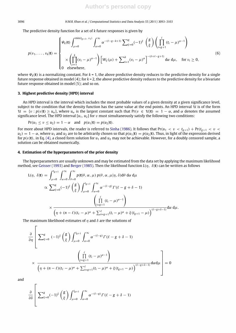
Fig. 2. Predictive survival densities for a single future response v based on 18 male patients, for certain values of the hyperparameters, η (stages) and δ

(doses).

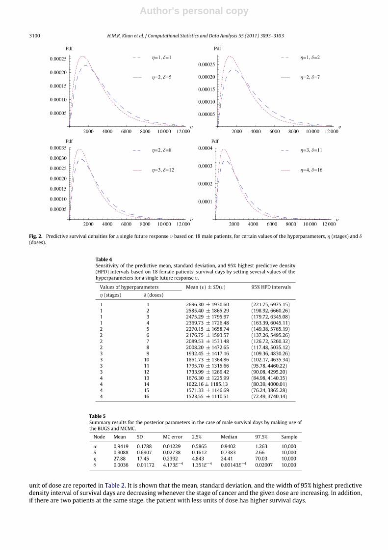
Table 4Sensitivity of the predictive mean, standard deviation, and 95% highest predictive density(HPD) intervals based on 18 female patients’ survival days by setting several values of thehyperparameters for a single future response v.

Values of hyperparameters Mean (v) ± SD(v) 95% HPD intervalsη (stages) δ (doses)

1 1 2696.30 ± 1930.60 (221.75, 6975.15)1 2 2585.40 ± 1865.29 (198.92, 6660.26)1 3 2475.29 ± 1795.97 (179.72, 6345.08)1 4 2369.73 ± 1726.48 (163.39, 6045.11)2 5 2270.15 ± 1658.74 (149.38, 5765.19)2 6 2176.75 ± 1593.57 (137.26, 5495.26)2 7 2089.53 ± 1531.48 (126.72, 5260.32)2 8 2008.20 ± 1472.65 (117.48, 5035.12)3 9 1932.45 ± 1417.16 (109.36, 4830.26)3 10 1861.73 ± 1364.86 (102.17, 4635.34)3 11 1795.70 ± 1315.66 (95.78, 4460.22)3 12 1733.99 ± 1269.42 (90.08, 4295.20)4 13 1676.30 ± 1225.99 (84.98, 4140.35)4 14 1622.16 ± 1185.13 (80.39, 4000.01)4 15 1571.33 ± 1146.69 (76.24, 3865.28)4 16 1523.55 ± 1110.51 (72.49, 3740.14)

Table 5Summary results for the posterior parameters in the case of male survival days by making use ofthe BUGS and MCMC.

Node Mean SD MC error 2.5% Median 97.5% Sample

α 0.9419 0.1788 0.01229 0.5865 0.9402 1.263 10,000δ 0.9088 0.6907 0.02738 0.1612 0.7383 2.66 10,000η 27.88 17.45 0.2392 4.843 24.41 70.03 10,000θ 0.0036 0.01172 4.173E−4 1.351E−4 0.00143E−4 0.02007 10,000

unit of dose are reported in Table 2. It is shown that the mean, standard deviation, and the width of 95% highest predictivedensity interval of survival days are decreasing whenever the stage of cancer and the given dose are increasing. In addition,if there are two patients at the same stage, the patient with less units of dose has higher survival days.



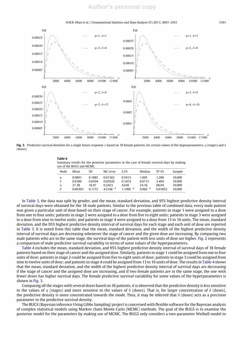
Fig. 3. Predictive survival densities for a single future response v based on 18 female patients, for certain values of the hyperparameters, η (stages) and δ

(doses).

Table 6Summary results for the posterior parameters in the case of female survival days by makinguse of the BUGS and MCMC.

Node Mean SD MC error 2.5% Median 97.5% Sample

α 0.9891 0.1885 0.01362 0.5913 1.005 1.288 10,000δ 0.8386 0.6594 0.02926 0.1474 0.6731 2.494 10,000η 27.38 16.97 0.2423 4.636 24.16 68.94 10,000θ 0.00303 0.1172 4.534E−4 1.149E−4 9.06E−4 0.01852 10,000

In Table 3, the data was split by gender, and the mean, standard deviation, and 95% highest predictive density intervalof survival days were obtained for the 18 male patients. Similar to the previous table of combined data, every male patientwas given a particular unit of dose based on their stage of cancer. For example, patients in stage 1 were assigned to a dosefrom one to four units; patients in stage 2 were assigned to a dose from five to eight units; patients in stage 3 were assignedto a dose from nine to twelve units; and patients in stage 4 were assigned to a dose from 13 to 16 units. The mean, standarddeviation, and the 95% highest predictive density interval of survival days for each stage and each unit of dose are reportedin Table 3. It is noted from this table that the mean, standard deviation, and the width of the highest predictive densityinterval of survival days are decreasing whenever the stage of cancer and the given dose are increasing. By comparing twomale patients who are in the same stage, the survival days of the patient with less units of dose are higher. Fig. 2 representsa comparison of male predictive survival variability in terms of some values of the hyperparameters.

Table 4 includes the mean, standard deviation, and 95% highest predictive density interval of survival days of 18 femalepatients based on their stage of cancer and the assigned dose. Similarly, patients in stage 1 could be assigned fromone to fourunits of dose; patients in stage 2 could be assigned from five to eight units of dose; patients in stage 3 could be assigned fromnine to twelve units of dose; and patients in stage 4 could be assigned from13 to 16 units of dose. The results in Table 4 showsthat the mean, standard deviation, and the width of the highest predictive density interval of survival days are decreasingif the stage of cancer and the assigned dose are increasing, and if two female patients are in the same stage, the one withfewer doses has higher survival days. The female predictive survival variability for some values of the hyperparameters isshown in Fig. 3.

Comparing all the stageswith several doses based on 36 patients, it is observed that the predictive density is less sensitiveto the values of η (stages) and more sensitive to the values of δ (doses). That is, for larger concentration of δ (doses),the predictive density is more concentrated towards the mode. Thus, it may be inferred that δ (doses) acts as a precisionparameter in the predictive survival density.

The BUGS (Bayesian inferenceUsing Gibbs Sampling) project is concernedwith flexible software for the Bayesian analysisof complex statistical models using Markov chain Monte Carlo (MCMC) methods. The goal of the BUGS is to examine theposterior model for the parameters by making use of MCMC. The BUGS only considers a two-parameter Weibull model to



Male:alpha sample: 10000

0. 0 0. 5 1. 0

0. 0

1. 0

2. 0

3. 0

Female:

alpha sample: 10000

0.0 0.5 1.0

0.0 0.5 1.0 1.5 2.0

eta sample: 10000

-50.0 0.0 50.0 150.0

eta sample: 10000

-50.0 0.0 50.0 150.0

theta sample: 10000

0.0 0.2 0.4 0.6

theta sample: 10000

0.0 0.2 0.4 0.6

0.0 100.0 200.0 300.0 400.0

delta sample: 10000

0.0 5.0 10.0

delta sample: 10000

0.0 5.0 10.0

0.0

0.5

1.0

0.0

0.01

0.02

0.03

0.0

100.0

200.0

300.0

0.0 0.25 0.5

0.75 1.0

0.0

0.01

0.02

0.03

Fig. 4. Posterior densities for the parameters of male and female by making use of the BUGS and MCMC.

achieve posterior summary results for the parameters but no indication is given about the three-parameter Weibull model.In this situation, we assumed that the location parameter µ is uniformly distributed over the interval (0, 1). Fig. 4 includesthe posterior densities for the parameters of male and female. The summary results of the posterior parameters for maleand female are given in Tables 5 and 6, respectively.

Acknowledgments

The authors are grateful to an Associate Editor and the reviewers for their valuable comments and suggestions whichgreatly improved the presentation of the manuscript.

References

Ahmed, S.E., 1992. Asymptotic estimation of reliability in a life-testing model. Journal of Industrial Mathematics Society 41, 7–18.Ahmed, S.E., Budsaba, K., Lisawadi, S., Volodin, A.I., 2008. Parametric estimation for the Birnbaum-Saunders lifetime distribution based on a new

parameterization. Thailand Statistician 6, 213–240.Ahmed, S.E., Saleh, E., 1999. Estimation of regression coefficients in an exponential regressionmodel with censored observations. Japan Journal of Statistics

29, 55–64.Ahsanullah, M., Ahmed, S.E., 2001. Bayes and empirical Bayes estimates of survival and hazard functions of a class of distributions. In: Ahmed, S.E., Reid, N.

(Eds.), Lecture Notes in Statistics, vol. 148. Springer-Verlag, New York, pp. 81–87.Aitchison, J., Dunsmore, I.R., 1975. Statistical Prediction Analysis. Cambridge University Press, New York.Aitchison, J., Sculthorpe, D., 1965. Some problems of statistical prediction. Biometrika 52, 469–483.American Cancer Society, 2009. Detailed guide: Laryngeal and hypopharyngeal cancer. Retrieved July 28, 2009 from web site http://www.cancer.org.American Joint Committee on Cancer, 2009. Retrieved July 28, 2009 from web site www.cancerstaging.org.Berger, J.O., 1985. Statistical Decision Theory and Bayesian Analysis. Springer-Verlag, New York.Bernardo, J.M., Smith, A.F.M., 1994. Bayesian Theory. Wiley, New York.Buhamra, S., Al-Kandarri, N., Ahmed, S.E., 2004. Inference concerning quantile for left truncated and right censored data. Computational Statistics and Data

Analysis 46, 819–831.Buhamra, S., Al-Kandarri, N., Ahmed, S.E., 2007. Nonparametric inference strategies for the quantile functions under left truncation and right censoring.

Journal of Nonparametric Statistics 19, 189–198.



Cleveland Clinic, 2009. The Stage of Laryngeal Cancer. Retrieved July 29, 2009 from web site http://my.clevelandclinic.org.Dunsmore, I.R., 1974. The Bayesian predictive distribution in life testing models. Technometrics 16, 455–460.Evans, I.G., Nigm, A.M., 1980a. Bayesian Prediction for two-parameter Weibull Lifetime models. Commu. Statist.–Theor. Meth. A9 (6), 649–658.Evans, I.G., Nigm, A.H.M., 1980b. Bayesian prediction for the left Truncated exponential distribution. Technometrics 22 (2), 201–204.Geisser, S., 1993. Predictive Inference: an Introduction. Chapman and Hall, New York.Geisser, S., 1971. The inferential use of predictive distributions. In: Godambe, V.P., Sprott, D.A. (Eds.), Foundation of Statistical Inference. Holt, Toronto,

pp. 456–469.Gelman, A., Carlin, J.B., Stern, H.S., Rubin, D.B., 2004. Bayesian Data Analysis. Chapman and Hall/CRC, New York.Greene, F.L., Page, D.L., Fleming, I.D., Fritz, A.G., Balch, C.M., Haller, D.G., et al., 2002. The AJCC Cancer Staging Handbook. From The AJCC Cancer Staging

Manual, 6th Ed.. Springer, New York.Johns Hopkins, 2009. The Larynx and Voice: Basic Anatomy and Physiology. Retrieved July 23, 2009 from web site

http://www.hopkinsmedicine.org/voice/anatomy.html.Kambo, N.S., 1978.Maximum likelihood estimators of the location and scale parameters of the scale and location parameters of the exponential distribution

from a censored sample. Comm. Statist. Theory Methods A 12, 1129–1132.Khan, H.M.R., 2003. Predictive Inference for Certain Life Testing Models. Ph.D. Thesis. The University of Western Ontario, Canada.Khan, H.M.R., Haq, M.S., Provost, S.B., 2006. Predictive inference for future responses given a doubly censored sample from a two parameter exponential

distribution. Journal of Statistical Planning and Inference 136 (9), 3156–3172.Khan, H.M.R., Provost, S.B., 2008. On predictive inference for future responses from the compound exponential model. Journal of Applied Probability and

Statistics 3 (2), 263–274.Khan, H.M.R., Provost, S.B., Hegele, R.A., 2007. Bayesian applications in cytogenetic studies. Journal of Applied Probability and Statistics 2 (2), 157–172.Lalitha, S., Mishra, A., 1996. Maximum likelihood estimation for Rayleigh distribution. Comm. Statist. Theory Methods 25 (2), 389–401.Mahdi, T.N., Ahmed, S.E., Ahsanullah, M., 1998. Improved prediction: pooling two identical regression lines. Journal of Applied Statistics 7, 63–86.Martz, H.F., Waller, R., 1982. Bayesian Reliability Analysis. Wiley, New York.MathWave Technologies, 2010. EasyFit 5.4 Professional, MathWave Technologies..Mayo Clinic, 2009. Throat cancer definition. Mayo Clinic Foundation for Medical Education and Research. Retrieved July 23, 2009 from web site

http://www.mayoclinic.com/health/oral-and-throat-cancer/DS00349.NCI, 2009a. Head and Neck Cancer. Retrieved July 28, 2009 from web site http://www.cancer.gov/cancertopics/types/head-and-neck.NCI, 2009b. Defining Cancer. National Cancer Institute. Retrieved July 22, 2009 from web site http://www.cancer.gov/cancertopics/what-is-cancer.Raqab, M.Z., 1995. On the maximum likelihood prediction of the exponential distribution based on double type II censored samples. Pakistan J. Statist. 11

(1), 1–10.Sarhan, A.E., 1955. Estimation of the mean and standard deviation by order statistics, part III. Annals of Mathematical Statistics 26, 576–592.Sinha, S.K., 1986. Reliability and Life Testing. John Wiley & Sons Inc., New York.Thabane, L., 1998. Contributions to Bayesian Statistical Inference. Ph.D. Thesis, The University of Western Ontario, Canada..Thabane, L., Haq, M.S., 2000. Bayesian prediction from a compound statistical model: an actuarial application.. Pakistan Journal of Statistics 16 (2), 110–125.Wolfram Research, 2008. The Mathematica Archive: Mathematica 7.0. Wolfram Research Inc., Illinois.Zellner, A., Chetty, V.K., 1965. Prediction and decision problems in regression models from the Bayesian point of view. Journal of the American Statistical

Association 60, 608–616.

Sensitivity analysis of predictive modeling for responses from the three-parameter Weibull model...

Documents

Transcript of Sensitivity analysis of predictive modeling for responses from the three-parameter Weibull model...