On the Hamiltonicity Gap andDoubly Stochastic Matrices∗

Vivek S. Borkar,† Vladimir Ejov and Jerzy A. Filar ‡

July 23, 2006

AbstractWe consider the Hamiltonian cycle problem embedded in singu-

larly perturbed (controlled) Markov chains. We also consider a func-tional on the space of stationary policies of the process that consistsof the (1,1)-entry of the fundamental matrices of the Markov chainsinduced by these policies. We focus on the subset of these policies thatinduce doubly stochastic probability transition matrices which we re-fer to as the “doubly stochastic policies”. We show that when theperturbation parameter, ε, is sufficiently small, the minimum of thisfunctional over the space of the doubly stochastic policies is attainedat a Hamiltonian cycle, provided that the graph is Hamiltonian. Wealso show that when the graph is non-Hamiltonian, the above mini-mum is strictly greater than that in a Hamiltonian case. We call thesize of this difference the “Hamiltonicity Gap” and derive a conserva-tive lower bound for this gap. Our results imply that the Hamiltoniancycle problem is equivalent to the problem of minimizing the vari-ance of the first hitting time of the home node, over doubly stochasticpolicies. Key words: Hamiltonian cycle, controlled Markov chains,optimal policy, singular perturbation.

∗This work is supported by ARC Grant DP0666632. We are indebted to Nelly Litvakand Giang Nguyen for their reading of the manuscript, comments and corrections.

†School of Technology and Computer Science, Tata Institute of Fundamental Research,Homi Bhabha Road, Mumbai 40005, India; e-mail: borkar@tifr.res.in. This author’s workwas supported in part by a grant from the Dept. of Science and Technology, Govt. ofIndia.

‡School of Mathematics, The University of South Australia, Mawson Lakes, SA 5095,Australia; e-mail: jerzy.filar@unisa.edu.au; e-mail: vladimir.ejov@unisa.edu.au

1

1 Introduction

We consider the following version of the Hamiltonian cycle problem: givena directed graph, find a simple cycle that contains all vertices of the graph(Hamiltonian cycle (HC)) or prove that HC does not exist . With respect tothis property - Hamiltonicity - graphs possessing HC are called Hamiltonian1.

This paper is a direct continuation of a recent contribution [3] by thepresent authors. It considerably strengthens the results reported in [3] andintroduces a new notion of “Hamiltonicity Gap” that differentiates betweenthe Hamiltonian and non-Hamiltonian graphs.

More generally, this contribution can be seen as belonging to a line ofresearch [8], [1], [10], [4], [7] which aims to exploit the tools of controlledMarkov decision chains (MDP’s)2 to study the properties of a famous problemof combinatorial optimization: the Hamiltonian Cycle Problem (HCP).

In particular, in [9] and Ejov et al [5] it was shown that Hamiltonian cyclesof a graph can be characterized as the minimizers of a functional based onthe fundamental matrices of Markov chains induced by deterministic policiesin a suitably perturbed MDP; provided that the value of the perturbationparameter, ε, is sufficiently small. Furthermore, it was conjectured that theminimum over the space of deterministic policies would also constitute theminimum over the space of all stationary policies. The above conjectureremains open under the perturbation studied in [5] and [9].

However, in the present paper we extend the results of Borkar et al [3] toprove that under another linear, but symmetric, singular perturbation, thesame element of the fundamental matrix - considered as a function on thethe space of all stationary policies that induce doubly stochastic probabilitytransition matrices - is minimized at a Hamiltonian cycle, provided that thegraph is Hamiltonian. Interestingly, the minimum value of this objectivefunction is a function of only the total number of nodes and the perturbationparameter and is strictly less than the corresponding minimum value of anynon-Hamiltonian graph with the same number of nodes. We name the dif-ference between the values of these global minima, the “Hamiltonicity gap”and claim that its presence has a theoretical - but, not necessarily, practical- importance.

We believe that the theoretical importance of the Hamiltonicity gap stems

1The name of the problem owes to the fact that Sir William Hamilton investigated theexistence of such cycles on the dodecahedron graph [14]

2The acronym MDP stems from the alternative name of Markov decision processes.

2

from the fact that it enables us to differentiate between Hamiltonian andnon-Hamiltonian graph on the basis of the minimum value of an objectivefunction of a mathematical program that lends itself to an appealing proba-bilistic/statistical interpretation; namely a constant plus the scaled varianceof the first return time of node 1. Hence, the Hamiltonian cycle problem isequivalent to the problem of minimizing the variance of the first hitting timeof the home node, over doubly stochastic policies.

Next, we shall briefly differentiate between our approaches and some ofthe best related lines of research. Many of the successful classical approachesof discrete optimization to the Hamiltonian cycle problem focus on solvinga linear programming “relaxation” followed by heuristics that prevent theformation of sub-cycles. In our approach, we embed a given graph in asingularly perturbed MDP in such a way that we can identify Hamiltoniancycles and sub-cycles with exhaustive and non-exhaustive ergodic classes ofinduced Markov chains, respectively. Indirectly, this allows us to exploit aformidable array of properties of Markov chains, including those of the cor-responding fundamental matrices. It should be mentioned that algorithmicapproaches to the HCP based on embeddings of the problem in Markov de-cision processes are also beginning to emerge (e.g., see Andramonov et al [1],Filar and Lasserre [10] and Ejov et al, [6]).

Note that this approach is essentially different from that adopted in thestudy of random graphs where an underlying random mechanism is used togenerate a graph (e.g., see Karp’s seminal paper [12]). In our approach, thegraph that is to be studied is given and fixed but a controller can choose arcsaccording to a probability distribution and with a small probability (due toa perturbation) an arc may take you to a node other than its “head”. Ofcourse, random graphs played an important role in the study of Hamiltonicity,a striking result to quote is that of Robinson and Wormald [13] who showedthat with high probability k-regular graphs are Hamiltonian for k ≥ 3.

2 Formulation and preliminaries

As in Borkar et al [3], our dynamic stochastic approach to the HCP considersa moving object tracing out a directed path on the graph Γ with its move-ment “controlled” by a function f mapping the set of nodes V = V(Γ) ={1, 2 . . . , s} of Γ into the set of arcs A = A(Γ) of Γ. We think of this set ofnodes as the state space of a controlled Markov chain Σ = Σ(Γ) where for

3

each state/node i, the action space A(i) := {a|(i, a) ∈ A} is in one-to-onecorrespondence with the set of arcs emanating from that node, or, equiva-lently, with the set of endpoints of those arcs.

Illustration: Consider the complete graph Γ5 on five nodes (with noself-loops) and think of the nodes as the states of an MDP, denoted by Σ,and of the arcs emanating from a given node as of actions available at thatstate. In a natural way the Hamiltonian cycle c1 : 1 → 2 → 3 → 4 → 5 → 1corresponds to the “deterministic control” f1 : {1, 2, 3, 4, 5} → {2, 3, 4, 5, 1},where f1(2) = 3 corresponds to the controller choosing arc (2,3) in state 2with probability 1. The Markov chain induced by f1 is given by the “zero-one” transition matrix P (f1) which, clearly, is irreducible. On the otherhand, the union of two sub-cycles: 1 → 2 → 3 → 1 and 4 → 5 → 4corresponds to the control f2 : {1, 2, 3, 4, 5} → {2, 3, 1, 5, 4} which identifiesthe Markov chain transition matrix P (f2) (see below) containing two distinctergodic classes. This leads to a natural embedding of the Hamiltonian cycleproblem in a Markov decision problem Σ. The latter MDP has a multi-chainergodic structure which considerably complicates the analysis. However, thismulti-chain structure can be “disguised” - but not completely lost - with thehelp of a “singular perturbation”. For instance, we could easily replace P (f2)with Pε(f2):

P (f2) =

0 1 0 0 00 0 1 0 01 0 0 0 00 0 0 0 10 0 0 1 0

and Pε(f2) =

ε 1− 4ε ε ε εε ε 1− 4ε ε ε

1− 4ε ε ε ε εε ε ε ε 1− 4εε ε ε 1− 4ε ε

.

The above perturbation is singular because it altered the ergodic structureof P (f2) by changing it to an irreducible (completely ergodic) Markov ChainPε(f2). Furthermore, it leads to a doubly stochastic matrix whose rows andcolumns both add to one. This has been achieved as follows: Each rowand column of the unperturbed s × s matrix (a permutation matrix) hasexactly one 1 and the rest zeros. We replace the 1’s by 1− (s− 1)ε for some0 < ε < 1/(s−1) and the zeros by ε to get the doubly stochastic perturbationof the matrix.

Next, we introduce the notion of a Markov chain induced by a stationaryrandomized policy (also called a randomized strategy or a randomized con-trol). The latter can be defined by an s× s stochastic matrix f with entries

4

representing probabilities f(i, a) of choosing a possible action a at a partic-ular state i whenever this state is visited. Of course, f(i, a) = 0, whenevera 6∈ A(i). Randomized policies compose the strategy space FS. The dis-crete nature of the HCP focuses our attention on special paths which ourmoving object can trace out in Γ. These paths correspond to the subspaceFD ⊂ FS of deterministic policies arising when the controller at every fixedstate chooses some particular action with probability 1 whenever this state isvisited (f1 and f2 are instances of the latter). To illustrate these definitionsconsider the simple case where fλ is obtained from the strictly deterministicpolicy f2 by the “controller” deciding to randomize at node 4 by choosingthe arcs (4, 5) and (4, 3) with probabilities f(4, 5) = 1 − λ and f(4, 3) = λ,respectively. The transition probability matrix of the resulting policy fλ isgiven by

Pε(fλ) =

ε 1− 4ε ε ε εε ε 1− 4ε ε ε

1− 4ε ε ε ε εε ε λ− 5ελ + ε ε 5ελ− λ− 4ε + 1ε ε ε 1− 4ε ε

.

As λ ranges from 0 to 1 the Markov chain ranges from the one inducedby f2 to one induced by another deterministic policy. An attractive featureof an irreducible Markov chain P is the simple structure of its Cesaro-limit(or, stationary distribution) matrix P ∗. It consists of an identical row-vectorπ representing the unique solution of the linear system of equations: πP =π, π1 = 1, where 1 is an s-dimensional column vector with unity in everyentry.

The fundamental matrix

We consider a Markov Chain {Xn} on a finite state space S = {1, 2, . . . , s},with a transition matrix P = [[p(i, j)]], assumed to be irreducible. Letπ = [π1, . . . , πs] denote its unique invariant probability vector and define

5

its stationary distribution matrix by

P ∗ = limN↑∞

1

N + 1

N∑n=0

P n =

π. . .π. . ....

. . .π

.

For the sake of completeness, we recall probabilistic expressions for the

elements of the fundamental matrix G = [[g(i, j)]]4= (I −P + P ∗)−1, I being

the s× s identity matrix.Let

r = [1, 0, . . . , 0]T ∈ Rs,1 = [1, 1, . . . , 1]T ∈ Rs,

and definew = G r, z = rT G.

These then satisfy the equations

(I − P + P ∗)w = r,

i.e.,

w − Pw + (∑

i

πiwi)1 = r, (1)

andz(I − P + P ∗) = rT ,

i.e.,

z − zP + (∑

i

zi)π = rT , (2)

respectively. Let τi = min{n > 0 : Xn = i}(= ∞ if the set on the right isempty). The following theorem is proved in [3]

Theorem 1 If P is irreducible, the elements of the fundamental matrix G =[[g(i, j)]] are given by:

g(i, i) =1

2

Ei[τi(τi + 1)]

(Ei[τi])2,

g(i, j) =1

2

Ei[τi(τi + 1)]

(Ei[τi])2− Ei[τj]

Ei[τi], i 6= j.

6

Doubly stochastic perturbations of graphs

A stochastic matrix P is called doubly stochastic if the transposed matrixP T is also stochastic (i.e., row sums of P and column sums of P add up toone). A doubly stochastic deterministic policy is one that induces a doublystochastic probability transition matrix where units are inserted in place ofarcs selected by that policy and zeroes in all other places. Hence a Markovchain induced by such a policy has a probability transition matrix that isa permutation matrix. The doubly stochastic perturbation of a policy (de-terministic or randomized) is achieved by passing to a singularly perturbedMDP that is obtained from the original MDP generated by the graph Γ byintroducing perturbed transition probabilities {pε(j|i, a)| i, a, j = 1, . . . , s}defined by the rule

pε(j|i, a) :=

{1− (s− 1)ε , if a = j and (i, a) is an arc of Γ,

ε , if a 6= j.

For any randomized policy f the corresponding s × s probability transitionmatrix Pε(f) has entries defined by the rule (for 0 < ε < 1

s−1)

Pε(f)(i, j) :=s∑

a=1

pε(j|i, a) · f(i, a).

Thus every stationary policy f induces not only a perturbed (irreducible)probability transition matrix Pε(f), but also the accompanying stationarydistribution matrix P ∗

ε (f) and the fundamental matrix Gε(f). The expressionfor the stationary distribution of a doubly stochastic policy f implies thatEf

i [τi] := Ei[τi] = π−1i = s for all i ∈ S, where πi(f) := πi is the ith element

of any row of P ∗ε (f).

Notational remark: Given the underlying graph, a selection of a particularpolicy f uniquely determines a Markov chain. Thus the various probabilisticquantities associated with that chain, in the sense prescribed above, aresynonymous with the selection of that policy. To simplify the notation, inmany parts of this manuscript the explicit dependence of these quantities onthe policy f will suppressed.

Denote by Dε the convex set of doubly stochastic matrices obtained bytaking the closed convex hull of the finite set Dε

e corresponding to the doublystochastic deterministic policies. We also write Dε

e as the disjoint union

7

Dεd ∪Dε

h where Dεh corresponds to the Hamiltonian cycles and Dε

d to disjointunions of short cycles that cover the graph. Double stochasticity eliminatesany other possibilities. Define the matrix norm ||A||∞ = maxi,j |a(i, j)| fora square matrix A = [[a(i, j)]]. Call P ∈ Dε a perturbation of Hamiltoniancycle if there exists a P̂ ∈ Dε

h such that ||P − P̂ ||∞ < ε0 for a prescribedε0 > 0. Let Dε

p denote the set of such P . The following are proved in [3].

Lemma 1 (a) For a policy f inducing a doubly stochastic probability tran-sition matrix we have (with wε

1 := wε1(f))

wε1 =

1

s2

∑i

Ei[τ1] (3)

=1

2

(s + 1)

s+

1

2s2E1[(τ1 − s)2].

Furthermore, for policies corresponding to Dεh, the above reduces to3

wε1 =

1

2

s + 1

s+ O(ε). (4)

(b) For P ε ∈ Dεd, wε

1 →∞ as ε ↓ 0.

(c) For Hamiltonian graphs and sufficiently small ε > 0, all minima of wε1

on Dεe are attained on Dε

p.

Theorem 2 For Hamiltonian graphs and sufficiently small ε > 0, all min-ima of wε

1 on Dε are attained on Dεp.

3 Hamiltonian cycles are global minimizers

Clearly, the preceding theorem would be considerably strengthened if it couldbe shown that the minima of wε

1 on Dε are attained at doubly stochasticmatrices induced by Hamiltonian cycles, not merely in their “sufficientlysmall” neighborhoods. This section is dedicated to the proof of this fact.

3Note that we the superscript in wε1 emphasizes the dependence on ε.

8

Directional derivatives

We shall now derive an expression for the directional derivative of ourobjective function wε

1. Let P0, P1 denote two doubly stochastic matrices inDε and for 0 ≤ λ ≤ 1, set P (λ) = λP1 + (1− λ)P0

4. Correspondingly defineVλ(i) := Ei[τ1], i ∈ S, Vλ = [Vλ(2), · · · , Vλ(s)]

T , 1 = [1, · · · , 1]T , where thedependence of the distribution of τ1 on the parameter λ is implicit. Also, letP̃0, P̃1, P̃ (λ) denote sub-matrices derived, respectively, from P0, P1, P (λ) bydeletion of their first row and column.

From Lemma 1.6, p. 46, of [2], we know that Vλ is the unique solution to

Vλ = 1 + P̃ (λ)Vλ. (5)

That is,Vλ = (I − P̃ (λ))−11. (6)

Let νλ(i) = E[∑τ1

m=1 I{Xm = i}] when the initial distribution is theuniform distribution. Then νλ := [νλ(2), · · · , νλ(s)] is the unique solution to

νλ =1

s1T + νλP̃ (λ), (7)

that is,

νλ =1

s1T (I − P̃ (λ))−1. (8)

Let J(λ) denote our objective as a function of λ, that is, wε1, evaluated along

the line segment {P (λ) : 0 ≤ λ ≤ 1}. From (3), we have

J(λ) =1

s2

∑i

Vλ(i).

Differentiating with respect to λ on both sides yields

J ′(λ) =1

s2

∑i

V ′λ(i) =

1

s2

∑

i 6=1

V ′λ(i),

because Vλ(1) = E1[τ1] = s ∀ λ ∈ [0, 1] ⇒ V ′λ(1) ≡ 0. From (5) and the

definition of P̃ (λ) we have

V ′λ = (P̃1 − P̃0)Vλ + P̃ (λ)V ′

λ.

4This is equivalent to a “line segment” fλ = λf1 + (1− λ)f0 in the strategy space.

9

ThereforeV ′

λ = (I − P̃ (λ))−1(P̃1 − P̃0)Vλ,

and with the help of (7)-(8) this leads to

J ′(λ) =1

s21T (I − P̃ (λ))−1(P̃1 − P̃0)Vλ

=1

sνλ(P̃1 − P̃0)Vλ (9)

=1

s21T (I − P̃ (λ))−1(P̃1 − P̃0)(I − P̃ (λ))−11. (10)

An alternative expression can be found as follows. Recall the fundamentalmatrix G(λ) = (I − P (λ) + P ∗)−1 from Theorem 1 of [3], where P ∗ is thematrix all of whose elements are equal to 1

s. Then G(λ) satisfies the identity

G(λ) = (P (λ)− P ∗)G(λ) + I.

Differentiating the above with respect to λ on both sides we obtain,

G′(λ) = (P1 − P0)G(λ) + (P (λ)− P ∗)G′(λ).

That is,

G′(λ) = (I − P (λ) + P ∗)−1(P1 − P0)G(λ) = G(λ)(P1 − P0)G(λ).

Since J(λ) = eT1 G(λ)e1 for e1

def= [1, 0, · · · , 0]T , we have

J ′(λ) = eT1 G(λ)(P1 − P0)G(λ)e1 (11)

= eT1 (I − P (λ) + P ∗)−1(P1 − P0)(I − P (λ) + P ∗)−1e1. (12)

It is not difficult to verify the equivalence of (9) and (11) directly.

Hamiltonian cycles are both local and global minima

The following, purely technical, lemma may already be known but weinclude its proof for the sake of completeness.

Lemma 3 If xm = m, 1 ≤ m ≤ s, and {ym} a permutation of {xj}, then∑i xiyi is maximized exactly when yi = xi ∀ i and minimized exactly when

yi = s + 1− xi ∀ i.

10

Proof The first claim is immediate from the Cauchy-Schwartz inequality.Thus for any permutation {yi} of {xj},

∑i xiyi ≤

∑i x

2i with equality if and

only if xi = yi ∀ i. In particular, for the permutation zi = s + 1− yi we have∑

i

xiyi =∑

i

xi(s + 1− zi)

= (s + 1)∑

i

xi −∑

i

xizi

≥ (s + 1)∑

i

xi −∑

i

x2i =

∑i

xi(s + 1− xi),

that is, ∑i

xiyi ≥∑

i

xi(s + 1− xi),

with equality if and only if yi = s + 1− xi ∀ i. The second claim follows. 2

We now consider J ′(0) in the situations where the doubly stochastic ma-trix P0 ∈ Dε

h is induced by a deterministic policy tracing out a Hamiltoniancycle. We shall first show that, on a straight line path from P0 towards anydoubly stochastic P1 induced by the graph, J ′(0) > 0. This shows that de-terministic policies inducing Hamiltonian cycles correspond to local minima.

Suppose then that P0 corresponds to a Hamiltonian cycle C0. Withoutloss of generality, we assume C0 is the simplest Hamiltonian cycle that corre-sponds to the permutation σ0 that maps {1, 2, · · · , s−1, s} onto {2, 3, · · · , s, 1}.

To start with, we consider P1 ∈ Dεh ∪ Dε

d, other than P0. That is, P1

is induced by any deterministic policy that traces out in the graph either aunion of disjoint cycles or a Hamiltonian cycle other than C0.

For each i ∈ S, other than 1, let m(i) denote the number of steps requiredto reach node 1 from i on C0, if ε = 0. It is clear that, with ε > 0,

V0(i) = Ei[τ1] = m(i) + O(ε) = (s− i + 1) + O(ε).

Also, if j is after i (or j = i) and before 1, then Ej[∑τ1

`=1 I{X` = i}] = O(ε).Further, if it is after 1 and before i, then Ej[

∑τ1`=1 I{X` = i}] = 1 + O(ε).

Hence, for i = 2, · · · , s

ν0(i) =1

s

∑1≤j≤i

Ej[

τ1∑

`=1

I{X` = i}] + O(ε)

=s−m(i)

s+ O(ε) =

i− 1

s+ O(ε).

11

Thus

ν0P̃0V0 =s−1∑i=2

ν0(i)V0(i + 1)

=1

s{1(s− 2) + 2(s− 3) + · · · (s− 2)1}+ O(ε)

=1

s{1[(s− 1)− 1] + 2[(s− 1)− 2] + · · · (s− 1)[(s− 1)− (s− 1)]}+ O(ε)

=1

s

((s− 1)

s−1∑r=1

r −s−1∑r=1

r2

)+ O(ε)

=(s− 1)2

2− 1

s

s−1∑r=1

r2 + O(ε).

A similar argument can be used to show that

ν0P̃1V0 =(s− 1)2

2− 1

s

s−1∑r=1

ryr + O(ε),

where yr ∈ {0, 1, 2, · · · , (s− 1)} and yr 6= yk whenever r 6= k. Note that if yr

were allowed to take values only in the set yr ∈ {1, 2, · · · , (s − 1)}, then byLemma 3 we would have that

s−1∑r=1

r2 >

s−1∑r=1

ryr,

whenever (y1, · · · , ys−1) 6= (1, · · · , s− 1). However, the inclusion of 0 as oneof the possible values for yr can only lower the right hand side of the aboveinequality.

Hence we have proved that

ν0P̃1V0 − ν0P̃0V0 > 0

whenever P̃1 ∈ Dεh ∪ Dε

d and P̃1 6= P̃0.

Now consider an arbitrary doubly stochastic P̃1 other than P̃0. By Birkhoff-von Neumann theorem we know that P̃1 =

∑Mi=1 γiP

∗i , where γi > 0 ∀ i,

∑i γi =

12

1, and P ∗i ∈ Dε

h ∪ Dεd correspond to permutation matrices. Note also that

for at least one i in the above summation P ∗i 6= P0. Then by the preceding

strict inequalities we have that

J ′(0) = ν0P̃1V0 − ν0P̃0V0 =∑

i

γi(ν0P∗i V0 − ν0P̃0V0) > 0.

The following main result now follows rather easily. 2

Theorem 4

(a) If P0 is induced by a Hamiltonian cycle, it is a strict local minimum forthe cost functional wε

1.

(b) If P0 is induced by a Hamiltonian cycle, it is also a global minimum forthe cost functional wε

1.

Proof The first part was proved above for P0 corresponding to the Hamilto-nian cycle C0: it is sufficient to observe that for a strict local minimum thequantity

ν0P̃1V0 − ν0P̃0V0

remains strictly bounded away from zero as ε ↓ 0 for all extremal P1 6= P0.The effect of considering another Hamiltonian cycle would be only to permuteorder of terms in various summations, without changing the conclusions.

To see the second part, first note that the above allows us to choose anε0 > 0 such that P0 is the strict local minimum of wε

1 in the ε0−neighborhoodof P0. As in the proof of Theorem 2 (see pp. 385-7 of [3]), choose ε > 0 smallenough so that the global minimum of wε

1 is attained on the ε0−neighborhoodof P0. (‘Small enough’ here is quantified by an upper bound that dependsonly on s and ε0, see ibid.) The claim follows. 2

4 Hamiltonicity Gap

Recall from Lemma 1 (see also Lemma 6 of [3]) that for a doubly stochasticpolicy f ∈ Dε, we had proved that the functional consisting of the top lefthand element of the fundamental matrix induced by f is given by

wε1 := wε

1(f) =1

2

s + 1

s+

1

2s2E1[(τ1 − s)2]. (13)

13

Note that dependence on f on the right is suppressed, but the expectationterm is a function of f , since the policy determines the distribution of τ1.

It should now be clear that a consequence of Lemma 1 and Theorem 4 isthat whenever the underlying graph Γ is Hamiltonian the minimum of theabove functional over f ∈ Dε is given by

wε1(fh) = min

f∈Dε[wε

1(f)] =1

2

s + 1

s+ O(ε), (14)

where fh ∈ Dεh is a policy defining any Hamiltonian cycle in the graph.

This section is devoted to the proof of the fact that, for ε > 0 andsufficiently small, there exists ∆(s) > 0 such that whenever the graph Γ isnon-Hamiltonian

minf∈Dε

[wε1(f)]− wε

1(fh) ≥ ∆(s)−O(ε).

We name the quantity ∆(s) the Hamiltonicity gap (of order s) because itdistinguishes all non-Hamiltonian graphs with s nodes from all Hamiltoniangraphs with the same number of nodes.

Before presenting the proof, we note that such a result is reasonablewhen we consider the possible variability of τ1 - as captured by its varianceE1[(τ1 − s)2] - for both Hamiltonian and non-Hamiltonian graphs. In theformer case, it is clear that this variance can be made nearly zero by fol-lowing a Hamiltonian cycle because the latter policy would yield a varianceactually equal to zero were it not for the (small) perturbation ε. However, ifthe graph is non-Hamiltonian, perhaps we can not avail ourselves of such avariance annihilating policy. This intuitive reasoning is made rigorous in theremainder of this section.

A lower bound for the non-Hamiltonian case

The key step in what follows is the derivation of a lower bound onPf ({τ1 = s}), for an arbitrary doubly stochastic, policy f in a non-Hamiltoniangraph.

Lemma 5 Suppose that the graph Γ is non-Hamiltonian, that is, Dεh = φ

and let f be an arbitrary doubly stochastic policy.

(a) If ε = 0, then

Pf ({τ1 = s}) ≤ 1

4

14

(b) If ε > 0 and small, then

Pf ({τ1 = s}) ≤ 1

4+ O(ε).

ProofFirst consider the case ε = 0. Let f be an arbitrary doubly stochastic

policy and let {Xt}∞0 be the Markov chain induced by f and the startingstate 1. Let γ1 = (X0, X1, . . . , Xs) be a path of s steps through the graphand let χ1 = {γ1|X0 = Xs = 1, Xk 6= s; k = 1, . . . s− 1}. That is, the eventthat the first return to 1 occurs after s steps is simply {τ1 = s} = {χ1} andhence

Pf ({τ1 = s}) =∑

γ1∈χ1

pγ1 ,

where pγ1 denotes the probability (under f) of observing the path γ1. How-ever, because the graph is assumed to be non-Hamiltonian, all the paths inχ1 that receive a positive probability have the structure

γ1 = γ′1 ⊕ γ̄1,

where γ′1 consists of a non-self-intersecting ‘reduced path’ from 1 to itself of

length m ≤ s−2 adjoined at some node(s) other than 1 by one or more loopsof total length s−m, that together constitute γ̄1. One can think of γ′1 and γ̄1

as the first and second parts of a figure comprising of basic loop with one ormore side-lobes attached to it, each of which is either a loop or a connectedunion of loops. The simplest instance of this is a figure of eight, with twoloops of length m and s−m respectively, attached at a node other than 1.

Let pγ1 denote the probability of the original path and p′γ1

that of the

reduced path. Let q := pγ1/p′γ1≤ 1, which is the contribution to p coming

from the loops comprising γ̄1. More generally, define

γ0 = γ′1, γ1 = γ

′1 ⊕ γ̄1, γ2 = γ

′1 ⊕ γ̄1 ⊕ γ̄1, γ2 = γ

′1 ⊕ γ̄1 ⊕ γ̄1, , . . . .

The paths γn (n 6= 2) from 1 to itself all begin with the same reduced pathγ′1 but may repeat exactly the same loop traversals γ̄1 path for n ≥ 2 times

all contribute to the event {τ1 6= s}, as does γ0 = γ′1.

The paths γn, n ≥ 2 have probabilities pγ1qn−1. The total probability

that these paths and γ0 = γ′1 (but excluding the original γ1) contribute to

15

{τ1 6= s} is as follows

pγ1

q+

∑n≥2

pγ1qn−1 = pγ1(

1

q+

q

1− q)

= pγ1(−1 +1

q(1− q))

≥ 3pγ1 .

From the above it follows that

Pf ({τ1 6= s}) ≥∑

γ1∈χ1

3pγ1 = 3Pf ({τ1 = s}).

Hence,

1 = Pf (τ1 < ∞)

= Pf (τ1 = s) + Pf (τ1 6= s)

≥ 4Pf (τ1 = s),

implying Pf (τ1 = s) ≤ 14, or, Pf (τ1 6= s) ≥ 3

4.

Returning to the case ε > 0 and small, we note that in the Markov chaininduced by f there are now two types of transitions: strong that correspondto f assigning a positive probability to arcs that are actually in the graphand weak that are strictly the result of our perturbation. The latter are oforder ε. Thus the only impact that the perturbation makes on the argumentpresented above is to introduce an adjustment of order ε. This completesthe proof. 2

Theorem 6 Suppose that the graph Γ is non-Hamiltonian, that is, Dεh = φ.

Let ∆(s) = 38s2 .

(a) For any policy f , we have that E1[(τ1 − s)2] ≥ 34−O(ε).

(b) We also have that

minf∈Dε

[wε1(f)]− wε

1(fh) ≥ ∆(s)−O(ε).

Proof Let f be an arbitrary doubly stochastic policy and E1[(τ1−s)2] be thecorresponding variance of the first hitting time of node 1 (starting from1).

16

Clearly,

E1[(τ1 − s)2] =∑

k≥1

(k − s)2Pf (τ1 = k)

≥∑

k≥1, k 6=s

Pf (τ1 = k) = Pf (τ1 6= s).

Hence by Lemma 4 (ii) we have obtained part (a), namely

E1[(τ1 − s)2] ≥ 3

4−O(ε). (15)

It now follows from (13) that

wε1 := wε

1(f) ≥ 1

2

s + 1

s+

1

2s2(3

4−O(ε)) =

s + 1

s+ ∆(s)−O(ε). (16)

Part (b) now follows immediately from (16) and (14). 2

5 Symmetric doubly stochastic policies

In view of the results of the preceding sections, it is clear that the Hamilto-nian cycle problem is equivalent to the following mathematical programmingproblem

min[wε1(f)] = min{[I − Pε(f) + P ∗

ε (f)]−11,1}

subject to:

(i)∑

a

f(i, a) = 1, i = 1, . . . , s, f(i, a) ≥ 0 ∀i, a,

(ii) 1T Pε(f) = 1T .

Of course, constraints (i) in the above ensure that f is a proper stationarypolicy, while constraints (ii) ensure that Pε(f) is a doubly stochastic prob-ability transition matrix. Furthermore, (14) ensures that this problem isequivalent to minimizing the variance of τ1, the first hitting time of the homenode 1. That is

arg minf∈Dε

[wε1(f)] = arg min

f∈Dε[V arf (τ1)] (17)

17

where for every doubly stochastic stationary policy the variance of the firstreturn time to 1 is denoted by V arf (τ1) := E1[(τ1 − s)2].

Since, in some contexts, variance minimization is a convex optimizationit is important to stress that this is not the case here. However, there is aninteresting convex subset of symmetric doubly stochastic policies such thatour objective function over that subset is strictly convex. At this stage, itis not clear whether the convex program consisting of minimization of wε

1(f)over that set is related to the original Hamiltonicity problem. Nonetheless,for the sake of completeness, the remainder of this section is devoted toestablishing these restricted convexity properties and to showing that theydo not extend to all of Dε.

Let P0, P1 be doubly stochastic matrices corresponding to a pair of policiesf0, f1 and let P̃0, P̃1 denote the corresponding matrices same with the firstrow and column removed. Also, P̃ (λ) = λP̃1 + (1− λ)P̃0 for λ ∈ (0, 1) and,as in Section 3, let

J(λ) =1

s2

∑i

Vλ(i), (18)

that is, J(λ) is the short-hand notation for the corresponding objective func-tion wε

1(fλ) = λwε1(f1) + (1 − λ)wε

1(f0). We now derive a useful expressionfor the m-th derivative of J(λ).

Lemma 7 For m ≥ 1,

J (m)(λ) =dmJ(λ)

dλm=

(m!

s2

)1T (I − P̃ (λ))−1

((P̃1 − P̃0)(I − P̃ (λ))−1

)m

1.

(19)

Proof In Section 3, the claim has already been proved for m = 1. We claim

that V(m)λ

def= dmVλ/dλm is uniquely specified by the linear system

V(m)λ = m(P̃1 − P̃0)V

m−1λ + P̃ (λ)V

(m)λ .

This follows by simple induction. The claim follows from this and (18). 2

In particular,

J (2)(λ) =2

s21(I − P̃ (λ))−1(P̃1 − P̃0)(I − P̃ (λ))−1(P̃1 − P̃0)(I − P̃ (λ))−11

=2

s2qT2 Aq1, (20)

18

where,

q1def= (I − P̃ (λ))−1(P̃1 − P̃0)(I − P̃ (λ))−11,

q2def= (I − P̃ (λ)T )−1(P̃ T

1 − P̃ T0 )(I − P̃ (λ)T )−11,

Adef= I − 1

2(P̃ (λ) + P̃ (λ)T ).

Lemma 8 A is positive definite.

Proof Since P (λ) is irreducible doubly stochastic, 12(P̃ (λ)+P̃ (λ)T ) is strictly

substochastic with spectral radius < 1. Thus A is symmetric with strictlypositive eigenvalues. The claim follows. 2

Lemma 9 If J (2)(λ) = 0, then J (m)(λ) = 0 ∀ m ≥ 2.

Proof By Lemma 8, J (2)(λ) = 0 would imply q = 0. The claim is nowimmediate from (19). 2

Define Dεsym

def= {Q ∈ Dε : Q = QT}. Note that for every P ∈ Dε,

P T ∈ Dε and hence 12(P + P T ) ∈ Dε

sym . Clearly Dεsym is a convex compact

polytope. Let Dεsym,e denote the set of its extreme points.

Lemma 10 P̄ ∈ Dεsym,e if and only if P̄ = 1

2(P + P T ) for some P ∈ Dε

e.

Proof If P̄ ∈ Dεe as well, the claim trivially holds. Suppose not. If the

claim is false, P̄ =∑m

i=1 aiP̂i for some m ≥ 2, ai > 0 ∀i with∑

i ai = 1, and

distinct P̂i ∈ De for 1 ≤ i ≤ m. Since P̄ = P̄ T , we also have P̄ =∑m

i=1 aiP̂Ti

and thus P̄ =∑m

i=1 aiP̄i for P̄idef= 1

2(P̂i + P̂ T

i ) ∀i. This contradicts the factP̄ ∈ Dε

sym,e, proving the claim. 2

From now on, consider P0, P1 ∈ Dεsym.

Lemma 11 J (2)(λ) > 0.

Proof Now q1 = q2. By Lemma 8 and (20), J (2)(λ) ≥ 0. If it were zero,so would be all the higher derivatives by Lemma 9 and the rational functionJ(λ) would have to be a constant, which it cannot be. 2

19

Corollary 12 The cost function wε1 restricted to Dε

sym is strictly convex and

hence attains its minimum at a unique point P̂ in Dεsym,e.

Lemma 13 The directional derivative of wε1 at P̂ above is nonnegative in all

directions.

Proof For P ∈ Dε, let P̄ = 12(P + P T ) ∈ Dε

sym. Then as P̂ is the minimizerof wε

1 on Dεsym,

V T0 (P̄ − P̂ )V0 =

1

2(V T

0 (P − P̂ )V0 + V T0 (P T − P̂ )V0) ≥ 0.

ButV T

0 (P − P̂ )V0 = V T0 (P T − P̂ )V0.

Hence V T0 (P − P̂ )V0 = V T

0 (P T − P̂ )V0 ≥ 0 ∀ P . The claim follows. 2

Our cost function is

1

s2

∑i

Ei[τ1] =1

s2

(∑

i6=1

Vi + s

)

=1

s21T (I − P̃ )−11 +

1

s.

Let P (λ) = λP T + (1− λ)P, λ ∈ [0, 1] and J(λ) the corresponding cost.

Lemma 14 J(λ) is symmetric about λ = 0.5.

Proof We have

1T (I − P̃ (λ))−11

= 1T (I − (λP̃ T + (1− λ)P̃ ))−11

= 1T (I − ((λ− 0.5)(P̃ T − P̃ ) + 0.5(P̃ + P̃ T )))−11 (21)

= 1T (I − P̃ (λ)T )−11

= 1T (I − ((λ− 0.5)(P̃ − P̃ T ) + 0.5(P̃ + P̃ T )))−11

= 1T (I − ((0.5− λ)(P̃ T − P̃ ) + 0.5(P̃ + P̃ T )))−11. (22)

Comparing (21) and (22), we get the result. 2

20

Lemma 15 The odd derivatives of J(λ) vanish at λ = 0.5 and the evenderivatives are negative.

This in particular implies that the minimum point among symmetric dou-bly stochastic matrices is in fact a saddle point over all doubly stochasticmatrices.

Proof The first claim is immediate from Lemma 8. Now for P̂ = 0.5(P+P T ),

J (2)(0.5) = 1T (I − P̂ )−1(P T − P )(I − P̂ )−1(P T − P )(I − P̂ )−11

= −1T (I − P̂ )−1(P − P T )(I − P̂ )−1(P T − P )(I − P̂ )−11

= −rT Ar

for A = I − P̂ and r = (I − P̂ )−1(P T − P )(I − P̂ )−11. A similar argumentworks for other even derivatives. The claim follows. 2

Remark We note that the above lemma does not necessarily imply that J(λ)is concave. Though the function J(λ) = 1T (

∑m P (λ)m)1, is real analytic

on [0, 1], the radius of convergence of its Taylor series around λ = 0.5, ingeneral, could be less than 0.5.

Example We consider Petersen graph with the adjacency matrix

0 1 0 0 1 1 0 0 0 0

1 0 1 0 0 0 1 0 0 0

0 1 0 1 0 0 0 1 0 0

0 0 1 0 1 0 0 0 1 0

1 0 0 1 0 0 0 0 0 1

1 0 0 0 0 0 0 1 1 0

0 1 0 0 0 0 0 0 1 1

0 0 1 0 0 1 0 0 0 1

0 0 0 1 0 1 1 0 0 0

0 0 0 0 1 0 1 1 0 0

. (23)

Next, we consider a deterministic policy f0 consisting of two sub-cycles oflength 5. In particular, f0 is equivalent to the map

{1, 2, 3, 4, 5, 6, 7, 8, 9, 10} → {2, 3, 4, 5, 1, 8, 9, 10, 6, 7}.

21

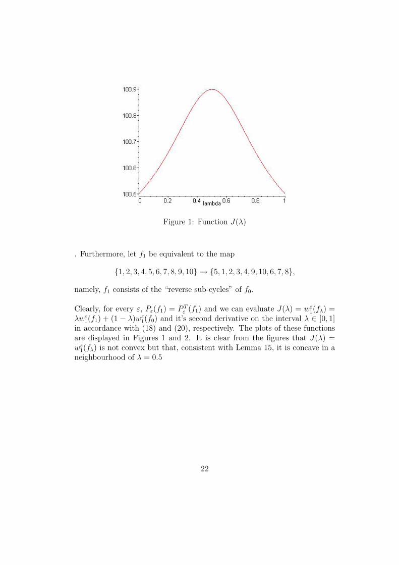
Figure 1: Function J(λ)

. Furthermore, let f1 be equivalent to the map

{1, 2, 3, 4, 5, 6, 7, 8, 9, 10} → {5, 1, 2, 3, 4, 9, 10, 6, 7, 8},

namely, f1 consists of the “reverse sub-cycles” of f0.

Clearly, for every ε, Pε(f1) = P Tε (f1) and we can evaluate J(λ) = wε

1(fλ) =λwε

1(f1) + (1 − λ)wε1(f0) and it’s second derivative on the interval λ ∈ [0, 1]

in accordance with (18) and (20), respectively. The plots of these functionsare displayed in Figures 1 and 2. It is clear from the figures that J(λ) =wε

1(fλ) is not convex but that, consistent with Lemma 15, it is concave in aneighbourhood of λ = 0.5

22

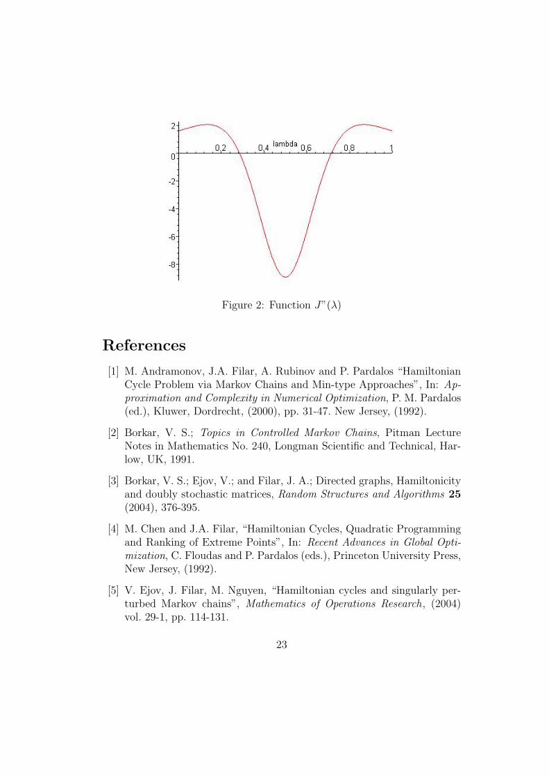
Figure 2: Function J”(λ)

References

[1] M. Andramonov, J.A. Filar, A. Rubinov and P. Pardalos “HamiltonianCycle Problem via Markov Chains and Min-type Approaches”, In: Ap-proximation and Complexity in Numerical Optimization, P. M. Pardalos(ed.), Kluwer, Dordrecht, (2000), pp. 31-47. New Jersey, (1992).

[2] Borkar, V. S.; Topics in Controlled Markov Chains, Pitman LectureNotes in Mathematics No. 240, Longman Scientific and Technical, Har-low, UK, 1991.

[3] Borkar, V. S.; Ejov, V.; and Filar, J. A.; Directed graphs, Hamiltonicityand doubly stochastic matrices, Random Structures and Algorithms 25(2004), 376-395.

[4] M. Chen and J.A. Filar, “Hamiltonian Cycles, Quadratic Programmingand Ranking of Extreme Points”, In: Recent Advances in Global Opti-mization, C. Floudas and P. Pardalos (eds.), Princeton University Press,New Jersey, (1992).

[5] V. Ejov, J. Filar, M. Nguyen, “Hamiltonian cycles and singularly per-turbed Markov chains”, Mathematics of Operations Research, (2004)vol. 29-1, pp. 114-131.

23

[6] V. Ejov, J. Filar, J. Gondzio, “An interior point heuristic algorithmfor the HCP”, Journal of Global Optimization, (2004) vol 29 (3), pp.315-334.

[7] E. Feinberg, “Constrained Discounted Markov Decision Process withHamiltonian cycles”, Mathematics of Operations Research, 25 (2000),pp. 130 -140.

[8] J.A. Filar and D. Krass, “Hamiltonian Cycles and Markov Chains”,Mathematics of Operations Research, 19 (1994), pp. 223-237.

[9] J.A. Filar and K. Liu, “Hamiltonian Cycle Problem and Singularly Per-turbed Markov Decision Process”, In: Statistics, Probability and GameTheory, Eds. T.S. Ferguson et al. IMS Lecture Notes - Monograph Series(1996).

[10] J.A. Filar and J-B Lasserre, “A Non-Standard Branch and BoundMethod for the Hamiltonian Cycle Problem”, ANZIAM J., 42 (E)(2000), pp. C556-C577.

[11] Filar, J. A.; and Vrieze, K.; Competitive Markov Decision Processes,Springer Verlag, New York, 1997.

[12] R. Karp, “Probabilistic Analysis of partitioning algorithms for thetravelling-salesman problem in the plane”, Mathematics of OperationsResearch, 2(3) (1977), 209–224.

[13] R. Robinson, N. Wormald, “Almost all regular graphs are Hamiltonian”,Random Structures and Algorithms , 5(2) (1994), 363–374.

[14] R. J. Wilson, “Introduction to graph theory”, Longman, (1996).

24