Nonlinear control of the doubly-fed induction generator in wind power systems
Upload
khangminh22Category
view
0download
0
Improved Winding Design of
a Doubly Fed Induction Generator (DFIG)
Wind Turbine using
Surrogate Optimisation Algorithm
Zheng Tan
School of Electrical and Electronic Engineering
Newcastle University
A thesis submitted for the degree of
Doctor of Philosophy
October, 2015


To my father, Yueting Tan
and my mother, Hong Zheng


Abstract
i
Abstract
The use of renewable sources of energy is becoming increasingly important role in electricity
generation. Wind energy is the fastest growing renewable energy source and is making a
significant contribution to meeting the energy demands while still reducing CO2 emissions. In
designing generators for installation in wind turbines, characteristics of high efficiency and low
cost are among the first to consider. As the number of installed wind turbines increases across
the world, questions of turbine component failure and repair are also receiving much attention.
This PhD starts with the investigation of modern wind turbine generator design with a focus on
electrical generator and its operation. The finite element analysis of an off-the-shelf 55 kW
doubly fed induction generator is used as a case study in order to investigate its design and
improve the machine performance.
The main work of this PhD is on a novel approach by surrogate-based analysis and the
optimisation of winding design and rewinding design based upon the doubly fed induction
generator for energy efficiency improvement. Surrogate models of the machine are constructed
using Latin Hypercube sampling and the Kriging modelling. Having validated the surrogate
models, the particle swarm optimisation algorithm is developed and applied to find the optimal
solution.
Assuming a winding failure occurs mid-life of the wind turbine, three optimisation plans have
been studied for the repair and re-design of the stator and rotor winding separately and in
combination.
To validate the optimisation results, an improved testing standard is developed to test doubly
fed induction generator. The original machine is then rewound following the optimised plan
and tested to determine the difference in performance. By comparing the two machines,
improved performance is achieved both in optimisation simulation and experiments.
Finally an annual wind speed profile at a specific location (Albemarle site) is analysed to
estimate wind power. The Weibull distribution of the wind speed data is combined with the
turbine topologies for estimating the annual wind energy production. The annual power
generation from the two machines is compared to validate the proposed technology.


Acknowledgements
ii
Acknowledgements
First and foremost, I would like to thank my supervisors, Prof. Wenping Cao, Prof. Bashar
Zahawi and Dr. Milutin Jovanovic, for their patience and confidence. Particular thanks go to
my supervisor Dr. Nick Baker, who imparted a lot of knowledge and critical thinking in the
field of electrical machine design.
The work would not have been possible without technical support and research idea from Prof.
Xueguan Song and Dr. Richard Martin. I would also like to thank Prof. Mingyao Ma, Dr. Bing
Ji, Dr. Wenjun Chen, and Dr Min Zhang, who gave me much help and advice.
I would like to acknowledge Dr. Chukwuma Junior Ifedi, Dr. Yasser Alamoudi, Haimeng Wu,
Zheng Liu, Sana Ullah, and Roziah Aziz for the times we spent together trying to solve
problems. Many friends and colleagues made my life in the UG-lab enjoyable and motivated,
these friends, to name but a few are Tahani Al-Mhana, Abdrrahman Al-Frhan, Maede Besharati,
Xu Deng, Congqi Yin, Chen Wang, Yamen Zbedi, Xiang Lu, Huaxia Zhan, Abdalbaset Mnider,
Musbahu Muhammad, Weichi Zhang, Chenming Zhang, and Jiankai Ma. My special thanks
goes to my girlfriend, Qian Liu for supporting and encouraging me all the time.
Finally, I could never have completed a doctorate without the ongoing support of my parents,
Yueting Tan and Hong Zheng, and most especially my mother who is the most understanding,
supportive and loving person in my life. Words are not profound enough to express my love
and respect to both of them; and they have encouraged me to become a responsible and strong
person.


Contents
iii
Contents
CHAPTER 1 INTRODUCTION .................................................................................................................... - 1 -
1.1 BACKGROUND........................................................................................................................................ - 1 - 1.2 MOTIVATIONS AND OBJECTIVES ............................................................................................................ - 3 - 1.3 METHODOLOGY ..................................................................................................................................... - 4 - 1.4 THESIS OVERVIEW ................................................................................................................................. - 4 - 1.5 CONTRIBUTION TO KNOWLEDGE ........................................................................................................... - 5 - 1.6 PUBLISHED WORK ................................................................................................................................. - 5 -
CHAPTER 2 LITERATURE REVIEW ........................................................................................................ - 7 -
2.1 WIND ENERGY ....................................................................................................................................... - 8 - 2.2 WIND TURBINES PAST AND PRESENT ..................................................................................................... - 9 - 2.3 OVERVIEW AND TOPOLOGIES OF WIND TURBINES ............................................................................... - 10 -
2.3.1 Rotor Axis Orientation .............................................................................................................. - 10 - 2.3.2 Rotor Power Control ................................................................................................................ - 11 - 2.3.3 Rotor Position ........................................................................................................................... - 12 - 2.3.4 Yaw Control .............................................................................................................................. - 13 - 2.3.5 Rotor Speed .............................................................................................................................. - 13 - 2.3.6 Number of Blades ..................................................................................................................... - 14 - 2.3.7 Generator Speed ....................................................................................................................... - 14 -
2.4 MODERN WIND TURBINE DESIGN ........................................................................................................ - 14 - 2.4.1 Rotor ......................................................................................................................................... - 15 - 2.4.2 Drive Train ............................................................................................................................... - 15 - 2.4.3 Nacelle ...................................................................................................................................... - 16 - 2.4.4 Yaw System ............................................................................................................................... - 17 - 2.4.5 Tower ........................................................................................................................................ - 17 -
2.5 SURVEY OF GENERATOR TYPES FOR WIND ENERGY ............................................................................ - 18 - 2.5.1 Direct Current Generator ......................................................................................................... - 18 - 2.5.2 Permanent Magnet Generator .................................................................................................. - 19 - 2.5.3 Switched Reluctance Generator ............................................................................................... - 21 - 2.5.4 Induction Generator ................................................................................................................. - 21 - 2.5.5 Manufactured Wind turbines .................................................................................................... - 27 -
2.6 MACHINE FAILURE TYPES ................................................................................................................... - 29 - 2.7 SUMMARY ............................................................................................................................................ - 31 -
CHAPTER 3 DOUBLY FED INDUCTION GENERATOR ANALYSIS ................................................ - 32 -
3.1 BACKGROUND...................................................................................................................................... - 33 - 3.2 MECHANICAL ASPECTS OF INDUCTION MACHINE ................................................................................ - 33 -
3.2.1 Stator Lamination ..................................................................................................................... - 34 - 3.2.2 Rotor Lamination ...................................................................................................................... - 35 - 3.2.3 Winding Design ........................................................................................................................ - 36 -
3.3 LOSS COMPONENTS ............................................................................................................................. - 43 - 3.3.1 Stator Conductor Loss .............................................................................................................. - 43 - 3.3.2 Rotor Conductor Loss ............................................................................................................... - 43 - 3.3.3 Core Loss .................................................................................................................................. - 44 - 3.3.4 Windage and Friction Losses ................................................................................................... - 45 - 3.3.5 Stray Load Loss ........................................................................................................................ - 47 -
3.4 FINITE ELEMENT ANALYSIS ................................................................................................................. - 50 - 3.4.1 Details of the Model ................................................................................................................. - 50 - 3.4.2 Equivalent Circuit of the DFIG ................................................................................................ - 52 - 3.4.3 Magnetic Field .......................................................................................................................... - 53 - 3.4.4 Core Loss .................................................................................................................................. - 55 - 3.4.5 Electrical Conductor Loss ........................................................................................................ - 56 -
3.5 SUMMARY ............................................................................................................................................ - 57 -
CHAPTER 4 SURROGATE-BASED ANALYSIS AND OPTIMISATION OF REWINDING
DESIGN………. .............................................................................................................................................. - 58 -

Contents
iv
4.1 INTRODUCTION..................................................................................................................................... - 59 - 4.2 OVERVIEW OF SURROGATE MODELLING .............................................................................................. - 60 - 4.3 DESIGN OF EXPERIMENT ...................................................................................................................... - 62 -
4.3.1 Orthogonal Array Design ......................................................................................................... - 63 - 4.3.2 Latin Hypercube Sampling (LHS) ............................................................................................. - 64 -
4.4 CONSTRUCTION OF SURROGATE MODEL .............................................................................................. - 65 - 4.4.1 Polynomial Regression Model .................................................................................................. - 65 - 4.4.2 Radial Basis Function ............................................................................................................... - 66 - 4.4.3 Kriging Model ........................................................................................................................... - 67 -
4.5 SURROGATE-BASED OPTIMISATION ...................................................................................................... - 68 - 4.5.1 Genetic Algorithm ..................................................................................................................... - 70 - 4.5.2 Particle Swarm Optimisation .................................................................................................... - 71 -
4.6 STATOR REWINDING DESIGN ............................................................................................................... - 73 - 4.6.1 Optimisation Problem Definition .............................................................................................. - 73 - 4.6.2 LHS for Stator Winding Optimisation ....................................................................................... - 74 - 4.6.3 Construction of Surrogate Model for Stator Winding ............................................................... - 76 - 4.6.4 Particle Swarm Optimisation .................................................................................................... - 82 - 4.6.5 Model Validation ...................................................................................................................... - 82 -
4.7 ROTOR REWINDING DESIGN ................................................................................................................. - 83 - 4.7.1 Optimisation Problem Definition .............................................................................................. - 83 - 4.7.2 LHS for Rotor Winding Optimisation ....................................................................................... - 83 - 4.7.3 Construction of Surrogate Model for Rotor Winding ............................................................... - 86 - 4.7.4 Particle Swam Optimisation ..................................................................................................... - 92 - 4.7.5 Model Validation ...................................................................................................................... - 92 -
4.8 REWINDING DESIGN FOR BOTH STATOR AND ROTOR ........................................................................... - 92 - 4.9 SUMMARY ............................................................................................................................................ - 94 -
CHAPTER 5 TESTING STANDARDS OF DOUBLY FED INDUCTION GENERATOR ................... - 95 -
5.1 INTRODUCTION..................................................................................................................................... - 96 - 5.2 TESTING STANDARDS ........................................................................................................................... - 97 -
5.2.1 Comparison of the Standards .................................................................................................... - 97 - 5.2.2 IEEE 112-B Standards .............................................................................................................. - 99 - 5.2.3 Improved Testing Method for DFIG ....................................................................................... - 103 -
5.3 DETERMINATION OF EFFICIENCY ....................................................................................................... - 107 - 5.3.1 Resistance Measurement ......................................................................................................... - 107 - 5.3.2 No-load test ............................................................................................................................. - 108 - 5.3.3 Load Test ................................................................................................................................ - 110 -
5.4 SUMMARY .......................................................................................................................................... - 114 -
CHAPTER 6 RESULTS AND ANALYSIS................................................................................................ - 115 -
6.1 INTRODUCTION................................................................................................................................... - 116 - 6.2 SIMULATED RESULTS ......................................................................................................................... - 116 -
6.2.1 Analysis of Losses and Efficiency ........................................................................................... - 116 - 6.2.2 Air-gap Flux Density Analysis ................................................................................................ - 118 -
6.3 EXPERIMENTAL TEST AND PERFORMANCE ......................................................................................... - 119 - 6.3.1 Test Bench ............................................................................................................................... - 119 - 6.3.2 No-load test ............................................................................................................................. - 120 - 6.3.3 Load Test ................................................................................................................................ - 129 -
6.4 SUMMARY .......................................................................................................................................... - 140 -
CHAPTER 7 WIND ENERGY PRODUCTION ....................................................................................... - 142 -
7.1 INTRODUCTION................................................................................................................................... - 143 - 7.2 ESTIMATION OF WIND RESOURCE ...................................................................................................... - 143 -
7.2.1 Available Wind Power ............................................................................................................ - 144 - 7.2.2 Mean Wind Speed ................................................................................................................... - 145 - 7.2.3 Power Law Profile .................................................................................................................. - 146 -
7.3 STATISTICAL ANALYSIS OF WIND SPEED DATA ................................................................................. - 148 - 7.3.1 Rayleigh Probability Distribution ........................................................................................... - 148 - 7.3.2 Weibull Probability Distribution ............................................................................................ - 149 -
7.4 WIND TURBINE ENERGY ESTIMATION ............................................................................................... - 153 - 7.4.1 Power Curve ........................................................................................................................... - 153 - 7.4.2 Betz Law .................................................................................................................................. - 154 -

Contents
v
7.4.3 Wind Turbine Annual Energy Production .............................................................................. - 155 - 7.4.4 Improved Annual Energy Production ..................................................................................... - 156 -
7.5 SUMMARY .......................................................................................................................................... - 159 -
CHAPTER 8 CONCLUSIONS ................................................................................................................... - 160 -
8.1 CONCLUSIONS .................................................................................................................................... - 160 - 8.2 FUTURE WORK ................................................................................................................................... - 163 -
References - 164 -
Appendix - 175 -

List of Figures
vi
List of Figures
FIGURE 1.1 GLOBAL CUMULATIVE INSTALLED WIND CAPACITY [4]. ............................................. - 2 - FIGURE 1.2 THE PREDICTION OF GLOBAL CUMULATIVE WIND POWER CAPACITY [4]. .............. - 2 - FIGURE 2.1 WIND TURBINE ROTOR POSITION. ..................................................................................... - 13 - FIGURE 2.2 CLASSIFICATIONS OF GEARBOX: (A) PARALLEL-SHAFT GEARBOX [18], (B)
PLANETARY GEARBOX [19]. ............................................................................................................ - 16 - FIGURE 2.3 A CUTAWAY OF TYPICAL YAW DRIVE WITH BRAKE [20]. ........................................... - 17 - FIGURE 2.4 TOWERS FOR WIND TURBINE: (A) TRUSS TOWER [21], (B) TUBULAR TOWER [22]. - 18 - FIGURE 2.5 RADIAL FLUX MACHINE TOPOLOGIES: (A) SURFACE PERMANENT MAGNET, (B) AND
(C) INTERIOR PERMANENT MAGNET [26]. .................................................................................... - 20 - FIGURE 2.6 A CUT-OUT SECTION OF A TRANSVERSAL FLUX MACHINE [28]. ............................... - 21 - FIGURE 2.7 SQUIRREL CAGE INDUCTION MACHINE [34]. .................................................................. - 23 - FIGURE 2.8 A SINGLE FED INDUCTION GENERATOR SCHEME. ........................................................ - 23 - FIGURE 2.9 AN ADVANCED SINGLE FED INDUCTION GENERATOR SCHEME. .............................. - 24 - FIGURE 2.10 SCHEMATIC OF A WOUND ROTOR INDUCTION GENERATOR ................................... - 25 - FIGURE 2.11 SCHEMATIC OF A DOUBLY FED INDUCTION GENERATOR WIND TURBINE SYSTEM..
................................................................................................................................................................. - 26 - FIGURE 2.12 CATASTROPHIC FAILURE OF A WIND TURBINE GENERATOR DUE TO ROTOR
WINDING FAULT [43]. ........................................................................................................................ - 29 - FIGURE 2.13 WINDING FAILURES IN THE ROTOR AND STATOR OF THE TURBINE GENERATORS.
............................................................................................................................................................. …- 30 - FIGURE 3.1 CUTAWAY OF A WOUND ROTOR INDUCTION GENERATOR [65]. ............................... - 34 - FIGURE 3.2 STRUCTURE OF STATOR AND STATOR SLOT. ................................................................. - 35 - FIGURE 3.3 STRUCTURE OF ROTOR AND ROTOR SLOT. ..................................................................... - 36 - FIGURE 3.4 THREE-PHASE 4-POLE 60 SLOTS DOUBLE LAYER WINDING CONFIGURATION WITH
TWO PARALLEL SETS (COIL PITCH 1-14). ..................................................................................... - 40 - FIGURE 3.5 THREE-PHASE 4-POLE 48 SLOTS DOUBLE LAYER WINDING CONFIGURATION WITH
TWO PARALLEL SETS (COIL PITCH 1-12). ..................................................................................... - 41 - FIGURE 3.6 THREE-PHASE WINDING CONNECTION IN STATOR. ...................................................... - 42 - FIGURE 3.7 THREE-PHASE WINDING CONNECTION IN ROTOR. ........................................................ - 42 - FIGURE 3.8 BH HYSTERESIS CURVE OF A FERROMAGNETIC MATERIAL AT 10 HZ (RED) AND 200
HZ (BLUE) [70]. ..................................................................................................................................... - 44 - FIGURE 3.9 EFFECT OF TEMPERATURE ON WINDAGE LOSS [77]...................................................... - 46 - FIGURE 3.10 COMPLETE EQUIVALENT CIRCUIT OF INDUCTION MOTOR [86]. .............................. - 48 - FIGURE 3.11 ASSIGNED ALLOWANCE FOR STRAY LOAD LOSS [82]. ............................................... - 49 - FIGURE 3.12 FEM MESH OF DFIG. ............................................................................................................. - 50 - FIGURE 3.13 CONTOUR FLUX PLOT OF DFIG. ........................................................................................ - 51 - FIGURE 3.14 EQUIVALENT CIRCUIT OF THE DFIG................................................................................ - 52 - FIGURE 3.15 B-H DATA FOR FEM. ............................................................................................................. - 54 - FIGURE 3.16 AIR-GAP FLUX DENSITY OF NORMAL AND TANGENTIAL COMPONENTS. ............ - 54 - FIGURE 3.17 MAGNETIC LOSS ESTIMATION FOR FEM. ....................................................................... - 55 - FIGURE 4.1 DIFFERENT SURROGATE MODELS MAY BE CONSTRUCTED WITH THE SAME DATA…
................................................................................................................................................................. - 60 - FIGURE 4.2 PREDICTED UNCERTAIN AREA USING PROBABILITY DENSITY FUNCTION Θ IN THE
PREDICTED FUNCTION 𝑬(𝒇𝒑) [108]. ............................................................................................... - 61 - FIGURE 4.3 THE FLOWCHART OF SURROGATE MODEL CONSTRUCTION. ..................................... - 62 - FIGURE 4.4 FACTORIAL DESIGNS FOR THREE DESIGN VARIABLES (N=3): (A) FULL FACTORIAL
DESIGN, (B) FRACTIONAL FACTORIAL DESIGN, (C) CENTRAL COMPOSITE DESIGN, (D)
STAR DESIGN, AND (E) BOX-BEHNKEN DESIGN [135]. .............................................................. - 63 - FIGURE 4.5 LATIN HYPERCUBE SAMPLING WITH P=8, N=2 FOR UNIFORM DISTRIBUTION. ..... - 64 - FIGURE 4.6 DIFFERENT PERFORMANCE OF LHS IN TERMS OF UNIFORMITY. .............................. - 65 - FIGURE 4.7 SURROGATE-BASED ANALYSIS AND OPTIMISATION. .................................................. - 69 - FIGURE 4.8 GENETIC ALGORITHM OPTIMISATION. ............................................................................. - 71 - FIGURE 4.9 PARTICLE SWARM OPTIMISATION ALGORITHM. ........................................................... - 72 -

List of Figures
vii
FIGURE 4.10 INITIAL LATIN HYPERCUBE SAMPLING PLAN FOR STATOR WINDING
OPTIMISATION. ................................................................................................................................... - 75 - FIGURE 4.11 DEFINITION OF THE CONSTRAINTS OF STATOR WINDING TURNS AND CROSS-
SECTIONAL AREA. ............................................................................................................................. - 75 - FIGURE 4.12 DEFINITION OF THE CONSTRAINT OF STATOR SLOT FILL FACTOR. ....................... - 76 - FIGURE 4.13 LATIN HYPERCUBE SAMPLING OF STATOR WINDING OPTIMISATION. ................. - 76 - FIGURE 4.14 INITIAL EFFICIENCY CONTOUR OF STATOR WINDING WITH TWO DESIGN
VARIABLES. ......................................................................................................................................... - 77 - FIGURE 4.15 INITIAL TORQUE CONTOUR OF STATOR WINDING WITH TWO DESIGN VARIABLES...
................................................................................................................................................................ - 78 - FIGURE 4.16 INITIAL THREE-DIMENSIONAL EFFICIENCY DISTRIBUTION OF STATOR WINDING
WITH TWO DESIGN VARIABLES. .................................................................................................... - 78 - FIGURE 4.17 INITIAL THREE-DIMENSIONAL TORQUE DISTRIBUTION OF STATOR WINDING WITH
TWO DESIGN VARIABLES. ............................................................................................................... - 79 - FIGURE 4.18 INFILL SAMPLING POINTS OF STATOR WINDING OPTIMISATION. .......................... - 79 - FIGURE 4.19 EFFICIENCY CONTOUR OF STATOR WINDING WITH TWO DESIGN VARIABLES. . - 80 - FIGURE 4.20 TORQUE CONTOUR OF STATOR WINDING WITH TWO DESIGN VARIABLES. ........ - 81 - FIGURE 4.21 THREE-DIMENSIONAL EFFICIENCY DISTRIBUTION OF STATOR WINDING WITH
TWO DESIGN VARIABLES. ............................................................................................................... - 81 - FIGURE 4.22 THREE-DIMENSIONAL TORQUE DISTRIBUTION OF STATOR WINDING WITH TWO
DESIGN VARIABLES. ......................................................................................................................... - 82 - FIGURE 4.23 INITIAL LATIN HYPERCUBE SAMPLING PLAN FOR ROTOR WINDING
OPTIMISATION. ................................................................................................................................... - 84 - FIGURE 4.24 DEFINITION OF THE CONSTRAINTS OF ROTOR WINDING TURNS AND CROSS-
SECTIONAL AREA. ............................................................................................................................. - 85 - FIGURE 4.25 DEFINITION OF THE CONSTRAINTS OF ROTOR SLOT FILL FACTOR........................ - 85 - FIGURE 4.26 LATIN HYPERCUBE SAMPLING OF ROTOR WINDING OPTIMISATION. ................... - 86 - FIGURE 4.27 INITIAL EFFICIENCY CONTOUR OF ROTOR WINDING WITH TWO DESIGN
VARIABLES. ......................................................................................................................................... - 87 - FIGURE 4.28 INITIAL TORQUE CONTOUR OF ROTOR WINDING WITH TWO DESIGN VARIABLES….
................................................................................................................................................................ - 87 - FIGURE 4.29 INITIAL THREE-DIMENSIONAL EFFICIENCY DISTRIBUTION OF ROTOR WINDING
WITH TWO DESIGN VARIABLES. .................................................................................................... - 88 - FIGURE 4.30 INITIAL THREE-DIMENSIONAL TORQUE DISTRIBUTION OF ROTOR WINDING WITH
TWO DESIGN VARIABLES. ............................................................................................................... - 88 - FIGURE 4.31 INFILL SAMPLING POINTS OF ROTOR WINDING OPTIMISATION. ............................ - 89 - FIGURE 4.32 EFFICIENCY CONTOUR OF ROTOR WINDING WITH TWO DESIGN VARIABLES. ... - 90 - FIGURE 4.33 TORQUE CONTOUR OF ROTOR WINDING WITH TWO DESIGN VARIABLES. .......... - 90 - FIGURE 4.34 THREE-DIMENSIONAL EFFICIENCY DISTRIBUTION OF ROTOR WINDING WITH TWO
DESIGN VARIABLES. ......................................................................................................................... - 91 - FIGURE 4.35 THREE-DIMENSIONAL EFFICIENCY DISTRIBUTION OF ROTOR WINDING WITH TWO
DESIGN VARIABLES. ......................................................................................................................... - 91 - FIGURE 5.1 COMPARISON OF DIFFERENT INTERNATIONAL TESTING STANDARDS................... - 98 - FIGURE 5.2 COMPARISON OF IEEE 112-B AND IEC 34-2 STANDARDS [190]. ................................... - 99 - FIGURE 5.3 MEASUREMENT LOCATIONS FOR DFIG TESTING. ....................................................... - 104 - FIGURE 5.4 POWER FLOW INSIDE DFIG IN SUB-SYNCHRONOUS MODE. ..................................... - 105 - FIGURE 5.5 POWER FLOW INSIDE THE DFIG IN SUPER-SYNCHRONOUS MODE. ........................ - 106 - FIGURE 5.6 DIAGRAM OF KELVIN DOUBLE BRIDGE. ........................................................................ - 107 - FIGURE 5.7 DETERMINATION OF WINDAGE AND FRICTION LOSS. ............................................... - 109 - FIGURE 5.8 DETERMINATION OF CORE LOSS. .................................................................................... - 110 - FIGURE 5.9. DIAGRAM OF DFIG IN SUB-SYNCHRONOUS MODE. .................................................... - 111 - FIGURE 5.10 DIAGRAM OF DFIG IN SUPER-SYNCHRONOUS MODE. .............................................. - 113 - FIGURE 6.1 COMPARISON OF SIMULATED LOSSES OF ORIGINAL AND OPTIMISED REWOUND
MACHINES AT 1457 RPM. ................................................................................................................ - 117 - FIGURE 6.2 COMPARISON OF EFFICIENCY OF ORIGINAL AND OPTIMISED REWOUND MACHINES.
.............................................................................................................................................................. - 118 - FIGURE 6.3 AIR-GAP FLUX DENSITY IN ORIGINAL MACHINE. ....................................................... - 119 - FIGURE 6.4 DFIG TEST RIG ....................................................................................................................... - 120 - FIGURE 6.5 STATOR WINDING RESISTANCE CORRECTION PER PHASE IN ORIGINAL MACHINE…..
.............................................................................................................................................................. - 124 - FIGURE 6.6 STATOR WINDING RESISTANCE CORRECTION PER PHASE IN OPTIMISED REWOUND
MACHINE. ........................................................................................................................................... - 124 -

List of Figures
viii
FIGURE 6.7 WINDING TEMPERATURE AT DIFFERENT VOLTAGE POINTS IN NO-LOAD TEST. - 125 - FIGURE 6.8 COMPARISON OF STATOR CONDUCTOR LOSS IN ORIGINAL MACHINE AND
OPTIMISED REWOUND MACHINE IN NO-LOAD TEST. ............................................................. - 126 - FIGURE 6.9 INPUT POWER AT DIFFERENT VOLTAGE POINT. .......................................................... - 126 - FIGURE 6.10 DETERMINATION OF THE CORE LOSS AND WINDAGE AND FRICTION LOSS OF THE
ORIGINAL MACHINE. ....................................................................................................................... - 127 - FIGURE 6.11 DETERMINATION OF THE CORE LOSS OF THE ORIGINAL MACHINE. ................... - 128 - FIGURE 6.12 DETERMINATION OF THE CORE LOSS AND WINDAGE AND FRICTION LOSS OF THE
OPTIMISED REWOUND MACHINE. ................................................................................................ - 128 - FIGURE 6.13 DETERMINATION OF THE CORE LOSS OF THE OPTIMISED REWOUND
MACHINE……………………………………………………………………………………………..- 129 - FIGURE 6.14 WINDING TEMPERATURE OF ORIGINAL MACHINE WITH DIFFERENT ROTATIONAL
SPEEDS. ............................................................................................................................................... - 130 - FIGURE 6.15 WINDING TEMPERATURE OF OPTIMISED REWOUND MACHINE WITH DIFFERENT
ROTATIONAL SPEEDS. ..................................................................................................................... - 131 - FIGURE 6.16 CONDUCTOR LOSSES AT 1457 RPM IN ORIGINAL MACHINE. .................................. - 132 - FIGURE 6.17 CONDUCTOR LOSSES AT 1457 RPM IN OPTIMISED REWOUND MACHINE. ........... - 132 - FIGURE 6.18 TOTAL CONDUCTOR LOSSES IN ORIGINAL MACHINE. ............................................. - 133 - FIGURE 6.19 TOTAL CONDUCTOR LOSSES IN OPTIMISED REWOUND MACHINE. ...................... - 133 - FIGURE 6.20 ANALYSIS OF STRAY LOAD LOSS IN SUB-SYNCHRONOUS ORIGINAL MACHINE….....
............................................................................................................................................................... - 134 - FIGURE 6.21 ANALYSIS OF STRAY LOAD LOSS IN SUPER-SYNCHRONOUS ORIGINAL MACHINE…
............................................................................................................................................................... - 135 - FIGURE 6.22 ANALYSIS OF STRAY LOAD LOSS IN SUB-SYNCHRONOUS REWOUND MACHINE……
............................................................................................................................................................... - 135 - FIGURE 6.23 ANALYSIS OF STRAY LOAD LOSS IN SUPER-SYNCHRONOUS REWOUND MACHINE...
............................................................................................................................................................... - 136 - FIGURE 6.24 COMPARISON OF ORIGINAL MACHINE AND OPTIMISED REWOUND MACHINE AT
1200 RPM. ............................................................................................................................................ - 137 - FIGURE 6.25 COMPARISON OF ORIGINAL MACHINE AND OPTIMISED REWOUND MACHINE AT
1300 RPM. ............................................................................................................................................ - 137 - FIGURE 6.26 COMPARISON OF ORIGINAL MACHINE AND OPTIMISED REWOUND MACHINE AT
1457 RPM. ............................................................................................................................................ - 138 - FIGURE 6.27 COMPARISON OF ORIGINAL MACHINE AND OPTIMISED REWOUND MACHINE AT
1600 RPM. ............................................................................................................................................ - 139 - FIGURE 6.28 COMPARISON OF ORIGINAL MACHINE AND OPTIMISED REWOUND MACHINE AT
1700 RPM. ............................................................................................................................................ - 139 - FIGURE 6.29 COMPARISON OF ORIGINAL MACHINE AND OPTIMISED REWOUND MACHINE AT
1800 RPM. ............................................................................................................................................ - 140 - FIGURE 7.1 ANNUAL WIND SPEED DATA AT ALBEMARLE. ............................................................. - 144 - FIGURE 7 2 AVAILABLE WIND POWER AT ALBEMARLE SITE........................................................ - 145 - FIGURE 7.3 ACTUAL WIND SPEED AT TURBINE HEIGHT. ................................................................. - 147 - FIGURE 7.4 AVAILABLE WIND POWER FOR WIND TURBINE. .......................................................... - 147 - FIGURE 7.5 RAYLEIGH DISTRIBUTION WITH DIFFERENT MEAN WIND SPEED [15]. .................. - 148 - FIGURE 7.6 EXAMPLE OF THE WEIBULL DISTRIBUTION WHEN MEAN WIND SPEED IS 6 M/S [15]...
............................................................................................................................................................... - 149 - FIGURE 7.7 WEIBULL DISTRIBUTION AT ALBEMARLE SITE. .......................................................... - 151 - FIGURE 7.8 WIND TURBINE POWER CURVE. ....................................................................................... - 153 - FIGURE 7.9 WIND POWER WASTAGE. .................................................................................................... - 154 - FIGURE 7.10 ESTIMATION OF ANNUAL ENERGY PRODUCTION. .................................................... - 155 - FIGURE 7.11 ANNUAL ENERGY PRODUCTION AT ALBEMARLE SITE. .......................................... - 156 - FIGURE 7.12 HIGH PROBABILITY AREA WITH TURBINE POWER CURVE. .................................... - 157 - FIGURE 7.13 IMPROVEMENT IN ANNUAL ENERGY PRODUCTION. ................................................ - 158 -

List of Tables
ix
List of Tables
TABLE 2.1 GENERATOR TECHNOLOGY USED IN MANUFACTURED WIND TURBINES. .............. - 28 - TABLE 3.1 STATOR WINDING CONFIGURATION .................................................................................. - 39 - TABLE 3.2 ROTOR WINDING CONFIGURATION .................................................................................... - 39 - TABLE 3.3 ASSIGNED RATIO OF STRAY LOAD LOSS TO RATED OUTPUT POWER IN IEEE 112-B......
................................................................................................................................................................ - 49 - TABLE 4.1 MODEL VALIDATION OF STATOR WINDING OPTIMISATION ........................................ - 83 - TABLE 4.2 MODEL VALIDATION OF ROTOR WINDING OPTIMISATION .......................................... - 92 - TABLE 4.3 OPTIMAL PLAN WITH 4 DESIGN VARIABLES COMPARED TO THE ORIGINAL DESIGN…
................................................................................................................................................................ - 94 - TABLE 5.1 OPERATIONAL SPEED MODES AND POWER SIGNS OF DFIG ....................................... - 111 - TABLE 6.1 STATOR WINDING RESISTANCE VALUES OF ORIGINAL MACHINE .......................... - 121 - TABLE 6.2 ROTOR WINDING RESISTANCE VALUES OF ORIGINAL MACHINE ............................ - 121 - TABLE 6.3 STATOR WINDING RESISTANCE VALUES OF OPTIMISED REWOUND MACHINE ... - 122 - TABLE 6.4 ROTOR WINDING RESISTANCE VALUES OF OPTIMISED REWOUND MACHINE ..... - 122 - TABLE 7.1 PROBABILITY OF WIND SPEED AT ALBEMARLE SITE .................................................. - 152 - TABLE 7.2 WIND SPEED OF AVERAGE DAYS IN A YEAR ................................................................. - 152 - TABLE 7.3 ANNUAL ENERGY PRODUCTION ........................................................................................ - 156 -

Acronyms and Symbols
x
Acronyms and Symbols
List of Symbols
A
As
B
CM
Cp,pmax
C1,2
c
Dbearing,r
F
f
H
Hs
H1,2
I
J
Ke
k
kp,d
kr
k1
kh,e
L
Lp
Lw,r
m
N
NPR
Nob
n
ns,r
P
cross-sectional area
swept area of rotor
magnetic field density
torque coefficient
power coefficient and maximum power coefficient
acceleration factor
scale factor
inner diameter of the bearing and the rotor diameter
bearing load
frequency
magnetic field intensity
significant wave height
turbine height
current
current density
energy pattern factor
shape factor
pitch and distribution factor
roughness coefficient
constant coefficient
hysteresis and eddy current coefficient
inductance
peak wave length for the wave spectrum
winding and rotor length
number of harmonic
number of winding turns
number of basis function
number of observations
number of coils per phase
synchronous speed and rotational speed
power
pjk personal best of particle j at the kth iteration

Acronyms and Symbols
xi
pgk
p
q
R
R-1
r
rc
global best of entire swarm at the kth iteration
number of magnetic pole pairs
unit vector
resistance
the inverse of the correlation matrix
correlation vector
basis function centre
s
T
t
V
Vw
Vjk
𝑤
w
Xjk
y
(𝑡)
Z
Z0
zj
z(t)
slip
torque
winding temperature
voltage
wind velocity
velocity of the jth at iteration k
mean wind speed
inertia weight
location of the jth at iteration k
observed data vector
approximation model
number of slots
aerodynamic roughness length
basis function
fundamental function
ϑ pitch angle
δ distribution angle
τw,p coil pitch and pole pitch
μf friction coefficient
ψ flux
𝜇0,𝑟 permeability of the air and material
α
β
frequency exponent
flux density exponent
𝜌𝑒,𝑎,𝑐 electrical resistivity and density of air and coolant
ε unobserved random error
𝜉2 variance
ωj coefficient of linear combinations

Acronyms and Symbols
xii
Φi(r) radial basis function
η efficiency
φ
ω
λ
σ2
η1,2
uniformly distributed random number
electrical angular speed
power law exponent
standard deviation
efficiency of drivetrain and generator

Acronyms and Symbols
xiii
List of Acronyms
AC
CFRP
C.S.A
CFD
DFIG
DC
DoE
Alternating current
Carbon fibre reinforced plastics
Cross-sectional area
Computational fluid dynamics
Doubly fed induction generator
Direct current
Design of experiment
FE
FEM
GA
GFRP
GSC
HAWT
LHS
OAD
PMG
PR
PSO
PMSG
RSC
RBF
SLL
SRG
SCIG
SFIG
Finite element
Finite element method
Genetic algorithm
Glass fibre reinforced plastics
Grid side converter
Horizontal axis wind turbine
Latin Hypercube sampling
Orthogonal array design
Permanent magnet generator
Polynomial regression model
Particle swarm optimisation
Permanent magnet synchronous generator
Rotor side converter
Radial basis function
Stray load loss
Switched reluctance generator
Squirrel cage induction generator
Single fed induction generator

Acronyms and Symbols
xiv
SBAO
VAWT
WRIG
2D
3D
Surrogate-based analysis and optimisation
Vertical axis wind turbine
Wound rotor induction generator
2-dimensional
3-dimensional

Chapter 1 Introduction
- 1 -
Chapter 1 Introduction
This doctoral thesis focuses on researching a novel approach to the winding design and
optimisation of a doubly fed induction generator to improve the machine’s efficiency. This
chapter gives an overview of the research background and objectives, and then discusses the
methodologies used to achieve each objective. The thesis structure is also described in detail.
1.1 Background
With increases in the population and economic development activities across the world, energy
demand is likely to soar in the coming years, especially in developing countries [1]. In the past
decade, the energy consumption of developed countries has grown by 1.5% per year, compared
to 3.2% per year in developing countries [2]. Assuming that this trend continues, global energy
demand will increase significantly in the future. Currently, there are many different types of
energy used to satisfy the world’s energy demand. Fossil fuel, which includes coal, petroleum,
and natural gas accounts for 80% of total demand; nuclear energy and bioenergy represent
approximately 7% and 13.7% respectively; and renewable energy, such as wind and solar
energy accounts for 2.2% of total energy demand [3]. It can easily be seen that the excessive
dependence on fossil fuel is quite serious today since it is non-renewable, and will therefore be
exhausted at some point. Therefore, renewable energy, including wind energy, has already
attracted increasing attention, and wind energy alone represents a huge potential source of
power.
Wind energy use is increasing significantly, since its development has been encouraged by the
policies of many governments throughout the world. Figure 1.1 shows the trend of increasing
global cumulative installed wind capacity from 1997 to 2014.

Chapter 1 Introduction
- 2 -
Figure 1.1 Global cumulative installed wind capacity [4].
Figure 1.2 then gives a prediction made by the GWE council of increasing trend of global
cumulative wind power capacity [4]. Their moderate scenario estimates the developing trend
of cumulative power capacity by considering the existing or planned policies supporting
renewable energy worldwide. The advanced scenario assumes that all of these policies to
support wind energy development can be achieved. From the chart, it can be seen that the
potential for future development is still vast.
Figure 1.2 The prediction of global cumulative wind power capacity [4].
0
50000
100000
150000
200000
250000
300000
350000
400000
Inst
alle
d W
ind
Cap
acit
y (
MW
)
0
500000
1000000
1500000
2000000
2500000
3000000
3500000
4000000
4500000
2013 2015 2020 2030 2040 2050
Glo
bal
Cu
mu
lati
ve
Win
d P
ow
er
Cap
acit
y (
MW
)
New Policies scenario Moderate scenario Advanced scenario

Chapter 1 Introduction
- 3 -
In the meantime, various different generator technologies have been developed for wind
turbines over the last three decades, including the Doubly Fed Induction Generator (DFIG),
Permanent Magnet Synchronous Generator (PMSG), and switched reluctance machines. In
particular, the PMSG was developed rapidly due to its high power density and high efficiency;
hence it attracted many people’s attention to develop the relevant technologies. However, an
inevitable problem with PMSG, is the materials used, because rare-earth metals are very
expensive and scarce, and also the environmental pollution from excavation sites is critical. In
addition, with their increased turbine power rates, the cost of the power electronics required
rises dramatically. Thus, for these reasons, the DFIG is coming into fashion again. Its
advantages, such as high reliability, low cost, lower cost of power electronic components, and
variable speed control at constant power, can definitely offset its drawback of giving lower
power density than the PMSG. Therefore, nowadays up to 70% of wind turbines installed
incorporate DFIGs [5], and they have already been widely used in onshore and offshore wind
farms. So the focus of this research is the wind turbine with a doubly fed induction generator.
1.2 Motivations and Objectives
This project focuses on the winding design and optimisation of the DFIG to obtain the
maximum power output from the wind turbine, and the objectives of the research are shown as
follows:
1. To achieve the rewinding optimisation of the DFIG machine in order to give higher
efficiency than the original;
2. To provide a detailed loss characterisation of all the different losses from the DFIG’s
components;
3. To develop a new method for the precise testing of the DFIG using input-output method
with loss segregation under two different operational mode;
4. To validate the results obtained using a laboratory test bench;
5. To estimate the likely improvement in annual wind energy production from a wind
turbine at a specific location.
To achieve these objectives, the efficiency of the DFIG for wind turbine applications should be
improved. For this purpose, the most suitable optimisation approach and algorithm is
determined and applied. The optimisation results are then applied to a wind turbine at a specific
site to estimate annual wind energy production.

Chapter 1 Introduction
- 4 -
1.3 Methodology
The work described in this thesis concerns the machine winding optimisation of a DFIG wind
turbine to acquire the maximum possible power output. In order to achieve the optimisation and
to validate the results, the following steps are introduced:
A design review and analysis of an initial DFIG machine. The software tool used is
Infolytica Magnet for Finite Element (FE) electromagnetic evaluation.
The performance of the initial DFIG machine is improved by applying a surrogate
optimisation algorithm with the evaluation of different winding parameters, with the
help of Matlab software based on Finite Element Method.
The original and optimised DFIG machines are constructed and tested of both to validate
the results, which involves exploring a method to test the performance of the DFIG
The wind speed profile at a specific location is estimated, and the annual wind energy
production of the original and optimised DFIG machines is compared.
1.4 Thesis Overview
This thesis presents the work conducted on the winding design and optimisation of a DFIG for
maximum power output. A total eight chapters are included in the thesis, and a brief description
of each is provided as follows:
Chapter 2 is a review chapter covering the history and development of wind turbines, wind
turbine topologies, modern wind turbine design, the selection of turbine generators, the
principles of the DFIG, and types of failure in turbine generators.
Chapter 3 describes a mechanical design review of a DFIG machine and the losses in different
components of DFIG are discussed. A finite element analysis of the original DFIG machine is
presented.
Chapter 4 proposes a novel method of constructing a surrogate model of the DFIG based on
finite element method, and also an optimisation algorithm is chosen to achieve optimisation.
Chapter 5 compares several of the main international test standards for induction machines.
Based on the IEEE standard 112-B, an improved method for testing the DFIG is carried out.
Chapter 6 validates the results of the simulation and practical work for the original designed
machine and the optimised rewound machine based on the proposed optimisation algorithm.

Chapter 1 Introduction
- 5 -
Chapter 7 investigates the statistical analysis of the wind speed profile for a specific site. The
annual wind energy production at this site is then estimated using the Weibull probability
density function.
Chapter 8 gives main conclusions of the study and recommendations for further work.
1.5 Contribution to Knowledge
This thesis contributes to knowledge in the following areas:
Development of surrogate modelling for use in the design of electromagnetic
applications.
Methodology for the winding optimisation of the DFIG.
Exploration of the selection of different winding parameters for both stator and rotor in
machine designing, instead of empirical formula.
Development of a testing method for the DFIG.
Segregation of all losses in different machine components, especially the addition loss
– stray load loss.
1.6 Published Work
The following peer-reviewed conference and journal papers have stemmed from this research:
a) Z. Tan, X. Song, W. Cao, Z. Liu, and Y. Tong, “DFIG Machine Design for Maximizing
Power Output Based on Surrogate Optimization Algorithm,” IEEE Transaction on Energy
Conversion, vol. 30, Issue 3, pp. 1154-1162, September 2015.
b) Z. Tan, X. Song, B. Ji, Z. Liu, J. Ma, and W. Cao, “3-D thermal analysis of a permanent
magnet motor with cooling fans,” Journal of Zhejiang University-Science A, ISSN 1673-
565X, August 2015.
c) Z. Tan, N. J. Baker, W. Cao, “Novel optimisation algorithm for electrical machines,” the
8th IET International Conference on Power Electronics, Machines and Drives (PEMD), UK,
2016.
d) Z. Tan, W. Cao, Z. Liu, X. Song, and B. Zahawi, “Optimization of doubly fed induction
generators (DFIGs) for Maximizing the Wind Power Yield,” the Ninth International
Symposium on Linear Drives for Industry Applications Conference (LDIA’13), 2013.
e) W. Cao, Z. Tan, Y. Xie, B. Zahawi, A. Smith, and M. Jovanovic. “Analysis of wind power
data for optimising DFIGs,” the 2nd International Symposium on Environment Friendly
Energies and Applications Conference (EFEA), pp. 452-457, June 2012.

Chapter 1 Introduction
- 6 -
f) W. Cao, Y. Xie, and Z. Tan, “Wind Turbine Generator Technologies,” Book Chapter in
Advances in Wind Power, INTECH, pp. 177-204, November 2012.
g) Z. Liu, W. Cao, Z. Tan, B. Ji, X. Song, and G. Tian, “Conditional monitoring of doubly-fed
induction generators in wind farms,” the Ninth International Symposium on Linear Drives
for Industry Applications (LDIA’13), 2013.
h) Z. Liu, W. Cao, Z. Tan, X. Song, B. Ji, and G. Tian, “Electromagnetic and temperature field
analyses of winding short-circuits in DFIGs,” the IEEE International Symposium on
Diagnostics for Electrical Machines, Power Electronics & Drives (SDEMPED), Spain,
August, 2013.
i) N. Yang, W. Cao, Z. Tan, X. Song, and T. Littler, “Novel asymmetrical rotor design based
on surrogate optimization algorithm,” the 8th IET International Conference on Power
Electronics, Machines and Drives (PEMD), UK, 2016.
j) N. Yang, W. Cao, Z. Liu, Z. Tan, Y. Zhang, S. Yu, and J. Morrow, “Novel asymmetrical
rotor design for easy assembly and repair of rotor windings in synchronous generators,” the
2015 IEEE International Magnetics Conference (INTERMAG), Beijing, China, May 2015.

Chapter 2 Literature Review
- 7 -
Chapter 2 Literature Review
In this chapter, the wind turbine history of development is introduced at the beginning. In
addition, an up-to-date survey of the current state of wind turbine technology is presented, the
benefits and the challenges associated with wind energy is discussed. As one of the most
important parts of turbine design, the generator design and its characteristics are considered.
The aim of this thesis is to present work done on the winding repair and re-design of doubly
fed induction generator to obtain the maximum power output for a specific wind turbine. So the
survey will focus more on introducing the turbine generator design and the modern wind turbine
topologies.

Chapter 2 Literature Review
- 8 -
2.1 Wind Energy
In recent years, major research in the electricity generation area has focused on the advancement
of wind energy as the main source of renewable energy. Wind energy has a lot of advantages
over conventional fossil fuel. First of all, wind energy does not emit harmful gases or hazardous
materials to pollute the air or water sources and while nuclear power plants; it does not produce
hazardous by products either, which are quite hard to deal with safety. Secondly, wind energy
as a clean fuel does not lead to CO2 or other atmospheric emissions, which cause acid rain or
greenhouse gases. Thirdly, wind power is one of the cheapest energy technologies available
today, depending on the wind resources available. Wind resources are inexhaustible, and so
wind energy as a clean and sustainable source of renewable energy could reduce dependence
on fossil fuels.
However, here are challenges too. Normally, sufficient wind resources exist in remote places,
far from the urban areas, so if the local power absorptive capacity is not strong enough, the
electricity will have to be delivered from wind farms to cities, but both the long building cycle
and coordination ability of power grid are very difficult to be solved. As a result, the wind
turbine has to be abandoned as the only one choice by power grid operator. Beside this, wind
energy does have an effect on the environment; it is well known that noise radiation from a
wind turbine is recognized as one of the key features controlling its public acceptability [6], and
for this reason, researchers have tried to reduce the mechanical and aerodynamic noise of wind
turbines [7, 8]. Furthermore, the aesthetic pollution and wildlife protection have been referred
to as well. Generally, before wind farms are built, the analysis of aesthetic sensitivity should be
combined with concern for the local environment, and there are a lot of ways to build aesthetic
sensitivity have been listed [9].
In addition, the death rates of birds are quite high when they fly into the rotors. Today, many
wind energy research groups are trying their best to solve this problem, even though birds
colliding with wind turbines do not always happen. For example, the Energy Technology
Support Unit (ETSU) started a series of activities to reduce the death rates of birds during a
wind energy project in the United Kingdom [10]. With all these factors in mind, it is imperative
for researchers to come up with improved methods to increase wind energy utilization and
reduce its effects on the environment.

Chapter 2 Literature Review
- 9 -
2.2 Wind Turbines Past and Present
The windmill was invented several centuries ago. As a source of power for grain milling and
water pumping, wind was first used for electricity generation over a hundred years ago, when
a windmill was built in Scotland in 1887 by James Blyth [11]. In 1891, the Danish scientist,
Poul la Cour constructed a wind turbine to generate electricity to light the Askov High School
[12]; after four years in 1895, he converted this into a prototype electrical power plant that was
used to light the village of Askov [12]. At the beginning of the 1930s, the wind turbine
technology with low power capacity was widely promoted and applied.
In 1941, Palmer Cosslett Putnam designed the world’s first megawatt-sized wind turbine, which
was connected to the local electrical distribution system on a mountain in the USA [13]. In
order to find cheaper energy sources, many countries in the world placed their hopes on wind
energy in the 1960s. In the meantime, some large-scale wind turbines were built by investing a
lot of manpower and material and financial resources. Research at this time proved that small-
scale wind turbines are relatively economical, but large-scale wind turbines are quite expensive
compared to the power generated from fossil fuels. In this period, the prevailing challenge faced
by the wind turbine development was cost, which caused research into wind energy to stagnate.
In 1973, the fuel crisis erupted across the whole world, and many countries encountered the
dilemma of energy shortages. Therefore, research into wind energy resumed again in developed
countries including the United States, United Kingdom, and Denmark. Medium-sized and large
wind turbines of low cost and high reliability were developed. In 1978, the Tvind wind turbine
was put into operation; at that time this was representative of the state of the art in wind energy.
In 1980, the Nortank 55kW wind power generator was unveiled in Denmark, and the price of
wind power had been reduced by about 50%. Wind energy technology was becoming more and
more mature.
The 21st century has seen a huge development in wind turbine manufacture, as improvements
in machine design and advancements in power electronics came to play a key role in the
development of wind energy. Wind turbine manufacturers have come up with many different
directions to improve current technologies. Some of these new wind turbines are already in
production and are distributed for consumer use, whilst other are still in concept form for the
future. A few prominent wind turbine companies currently present in the wind energy market
are mentioned below.

Chapter 2 Literature Review
- 10 -
Vestas, is a Danish wind turbine company which has the largest market share in the world.
Its production facilities have already been distributed in more than 12 countries, such as
China, Spain, and the United States. In the 1990s, Vestas produced a highly reliable,
advanced 55kW/11kW wind turbine, which has been called the beginning of modern wind
turbines.
GoldWind, is a Chinese wind turbine manufacturer which is engaged in developing and
producing large permanent magnet wind turbine generators. The major products of
GoldWind are 1.5MW and 2.5MW permanent magnet direct drive wind turbines.
Siemens, is a famous Germany company in the wind energy field. Both onshore and offshore
wind projects can be handled by Siemens, and its major aim is to reduce the costs of wind
turbines.
GE, wind turbines produce of with the highest annual energy yield in the world at 2MW and
3MW.
Nowadays, wind energy is the fastest growing renewable energy in the world; there were over
two hundred thousand wind turbines in operation, with a total nameplate capacity of 282482
MW, at the end of 2012 [14]. The marketing scale is expanding continuously, and so the cost
of wind energy is falling. In some places, the price of wind energy can compete with power
plants using fossil fuels. Although there is still a lot of work to be done on wind energy, the
sector is facing a promising future.
2.3 Overview and Topologies of Wind Turbines
There are a wide range of topologies established today for wind turbines, with different designs
of components and control methods explored to make the wind turbines more efficient, reliable
and safer. Most of these designs concentrate on the rotors of the wind turbines. The main
choices of wind turbine topology are introduced below.
2.3.1 Rotor Axis Orientation
The rotor axis orientation is the fundamental selection when designing a wind turbine. There
are two types of rotor axis orientation: the Horizontal Axis Wind Turbine (HAWT) and Vertical
Axis Wind Turbine (VAWT). The VAWT does not need a yaw system, and thus the wind power
can be captured from any direction. Moreover, its blades have a chord and no twist [15], which
could reduce complexity and costs. Although there are several promising advantages of the
VAWT, this kind of design has not been accepted widely, due to the likelihood of fatigue
damage to the blades, and especially since the connection points to the rotor are even weaker.

Chapter 2 Literature Review
- 11 -
On the other hand, another problem with the VAWT is control, such as variable pitch control.
In this case, stall control is the primary method in high winds, which causes a higher-rated wind
speed accordingly. Therefore, the space requirement of drive train components is large.
The HAWT is preferable in modern wind turbines, because rotor solidity is relatively low when
the design tip speed ratio is provided, so its cost is also lower. Another reason is that the average
height of the rotor swept area is higher above the ground [15], so the ability to capture wind
power could be better. At present here are no commercially available VAWT, at the multi-
megawatt scale, and so the focus of the work presented in this thesis is the horizontal axis wind
turbine.
2.3.2 Rotor Power Control
For maximum efficiency the wind turbine must operate within the designed speed and torque,
and so the rotation speed of the wind turbine has to be controlled properly for power generation.
Wind power increases as with wind speed cubed, and so in order to regulate power as wind
speed increases, the wind turbine design must take into consideration the maximum wind speed.
Actually, wind turbines produce power output under a range of wind speeds. If the wind speed
exceeds the survival speed of the wind turbine, it would suffer damage. Therefore, power has
to be limited when the wind speed exceeds the rated value of the design. To achieve this kind
of power control, stall control and pitch control are mainly selected.
In a stall-regulated wind turbine, power generation decreases when the wind speed is higher
than a certain value, which is due to the rotation speed or the aerodynamic torque decreases.
Therefore, the rotor of the wind turbine has to be controlled by reducing the rotation speed
during the period when wind speed exceeds the rated value. Generally, stall control is achieved
with an induction generator which is connected directly to the electrical grid. The blades in
stall-controlled wind turbines are designed aerodynamically to perform less efficiently when
wind speed is very high. The power decrease is due to the aerodynamic blade design of the
wind turbine in response to increasing wind speed. The advantage of this kind of wind turbine
is that, because of the simple structure by which the blade is connected to the rest of the hub,
the cost and maintenance of the stall-controlled wind turbine is lower. Beside this, a stall-
controlled wind turbine also has a braking system to make sure that the wind turbine can survive
in extreme wind speeds.
A pitch-controlled wind turbine can change the pitch angle of the wind turbine blades to reduce
the torque generated in a fixed speed wind turbine and to decrease the speed in a variable speed

Chapter 2 Literature Review
- 12 -
wind turbine when the wind speed is above the rated value. Generally, pitch control is selected
for high wind speed only. When the wind speed is very high, the blades will vary the pitch angle
to get less lift and more drag due to the increasing flow separation along the blade length [16].
In this way, either the rotation speed of the wind turbine and the torque produced can be reduced
appropriately to keep the power output more or less constant. There are four main regions in
the power curve of a pitch-regulated wind turbine. When the wind speed is very low, there is
not enough torque to support the rotation of the turbine blade, which is the first region. When
the wind speed then increases until the cut-in speed, the wind turbine will start to rotate and
deliver useful power; during this period, the power output increases rapidly. In the third region,
the wind speed reaches or even exceeds the rated output speed, and the output power will remain
constant as rated power output due to the limitation. In the final region the turbine braking
system causes the rotor to come to a standstill if the wind speed exceeds the survival speed of
the wind turbine, so that damage can be avoided. As in the stall-controlled wind turbine, brakes
are installed in the pitch control wind turbine to prevent damage under extreme wind conditions.
The difference between pitch control and stall control can be easily seen. The stall-regulated
wind turbine relies on the aerodynamic design of the turbine blades [16] to control the torque
produced and the rotation speed when the wind speed is very high, so the power output cannot
be kept constant. However, the pitch-regulated wind turbine has an active control system to
vary the pitch angle of turbine blades, so that constant power output will be generated above
the rated wind speed.
2.3.3 Rotor Position
In the design of a horizontal axis wind turbine, the rotor could be either upwind or downwind
of the nacelle, as shown in figure 2.1. Modern wind turbines adopt an upwind rotor design to
avoid the wake produced by the tower contributing to fatigue damage to the blades and ripples
in the electricity produced. Furthermore, noise is another drawback of downwind design when
the rotor blades pass through the wake. Although downwind rotors of wind turbines generally
have a free yaw system, which is simpler to implement than active yaw [15], free yaw is not in
fact really necessary due to the risk of sudden changes in wind direction with too fast a yaw
movement.

Chapter 2 Literature Review
- 13 -
Figure 2.1 Wind Turbine Rotor Position.
2.3.4 Yaw Control
As the wind direction changes constantly, horizontal axis wind turbines have to be able to adjust
their orientation. Usually a wind vane is installed on the back of the nacelle to detect wind
direction. As mentioned above, the downwind rotor allows the turbine to have free yaw.
Upwind wind turbines usually adopt active yaw control to maximise power output. In order to
keep the turbine stationary in yaw, the system must be robust, including a yaw motor, gears,
and a brake. Meanwhile, there is another method to control the power, where the rotor of the
wind turbine could be turned away from the wind when wind speed is relative high in order to
reduce the power.
2.3.5 Rotor Speed
In the 1990s, most turbine rotors were running at a constant speed, as determined by the
electrical generator and the gearbox, if they were not coupled with power converter and so
synchronous speed was fixed by grid frequency. More recently, due to advances in power
converters, generator speed can be decoupled from grid frequency, allowing rotors to run at
variable speeds. This allows rotor speed to match the maximum efficiency operation a point
which could capture the maximum power with an optimum tip speed ratio at low wind speeds
and to reduce the load in the drive train with a lower tip speed ratio under high wind speed
conditions. On the other hand, the conventional constant speed rotors of wind turbines could be
connected directly to the grid; however, complex and expensive power electronic equipment is
required for systems with variable speed rotors.

Chapter 2 Literature Review
- 14 -
2.3.6 Number of Blades
The selection of blade number is mainly determined by the stress in the blade root, where there
is a higher requirement for solidity made with an increasing number of blades. In modern wind
turbines, the three-blade structure is often chosen, but in some turbines two or even one blade
is adopted. Historically, a single-blade wind turbine was built, due to the low cost with only
one blade involved; also, the wind turbines can operate with a high tip speed ratio. Beside this,
wind turbines with more than three blades are rarely seen, because of the high cost of additional
blades. But now the three-bladed wind turbine is relatively popular due to its advantage that the
polar moment of inertia is constant with the yawing system, and it is independent of the
azimuthal position of the rotor [15].
2.3.7 Generator Speed
As discussed in section 2.5 below, different generator topologies operate at different operating
speeds, which are mainly classified as one synchronous speed, multiple synchronous speeds,
and variable speeds. For example, the squirrel cage induction generator and synchronous
generator have their own synchronous speed. Moreover, if a generator has two sets of winding
layouts with a different pole number, the generator can have two synchronous speeds,
depending on which winding configuration is used [15]. The wound rotor induction generator,
permanent magnet generator, and generator with fully rated output power conversion can
achieve variable speed operation.
In fact, the selection of generator speed is one of the most important design factors for wind
turbines, because it has significant effect on both the selection of power electronics and the
drive train design. When the rotor speed is the same as the generator speed, a gearbox is not
needed and the system is said to be direct drive. However, if a rotor speed and generator speed
differ, a torque converter needs to be installed in the drive train system.
2.4 Modern Wind Turbine Design
As mentioned in section 2.3.1, the performance and design requirements of horizontal axis wind
turbine depend on the topologies chosen. The electrical generator as the core component has an
immediate effect on the power delivered to the grid. The work presented in this thesis focuses
on the wind turbine application of the electrical generator as a Doubly Fed Induction Generator.

Chapter 2 Literature Review
- 15 -
2.4.1 Rotor
The blades and hub have a significant effect on turbine performance and total cost. The blade
converts the force of the wind into a shaft torque. The hub is used to connect the blades to the
main shafts and the rest of the drive train, so it has to handle all the load that is delivered from
the blades. Generally the hub is made of steel, either welded or cast [15].
The rotor of the modern wind turbine uses a three-blade structure with an upwind direction.
Historically, the material used for turbine blades was wood/epoxy laminates. Today glass and
carbon fibre reinforced plastics (GFRP and CFRP) can maximise power efficiency and exhibit
high fracture toughness, fatigue resistance and thermal stability [17].
2.4.2 Drive Train
The drive train system typically includes the rotor, a low-speed shaft, a high-speed shaft, a
gearbox, and generator. All of these components are introduced below. Other components in
the drive train system, such as the coupling, bearings, and brakes, are omitted as they are
unaffected by changes to the electrical machine topology.
2.4.2.1 Shafts
The main shaft transmits torque and must carry the weight of the rotor. So the shaft to be strong
is required and generally it is made of steel. The rotor, gearbox and generator are connected
together through the main high-speed shaft and low-speed shaft. In the design, the shaft may be
integrated into the gearbox or separated from it completely and connected by the couplings.
2.4.2.2 Gearbox
The gearbox appears in most wind turbine drive train systems. The function of the gearbox is
to increase the rotational speed and reduce the torque of the rotor from the low-speed shaft at
the rotor side to the high-speed shaft at the generator side. In fact, the gearbox is one of the
heaviest components in a wind turbine, especially in large turbines [15]. The weight of the
gearbox increases significantly with increasing power ratings of the turbine [15]. On the other
hand, gearbox is generally manufactured by a different company, and the gearbox is designed
based on a specific turbine model. So this means that the gearbox designer must understand
both gearboxes and wind turbine design. However, the cost of gearboxes is quite expensive,
and their maintenance is another problem because they are easily damaged and hard to replace.
Therefore, the concept of direct-drive wind turbine is mentioned, but in the same wind condition
the volume of direct-drive turbine generator is very large, so the weight of this kind of wind

Chapter 2 Literature Review
- 16 -
turbine is quite heavy; another problem is the cost of direct-drive system is more expensive than
the geared system.
There are two main types of gearbox which are selected in wind turbine applications, as shown
in figure 2.2. These are the parallel-shaft gearbox and planetary gearbox. In the single-stage
parallel-shaft gearbox, a low-speed shaft is connected to the rotor and a high-speed shaft is
connected to the generator. Beside this, gears of the two different sizes are assembled on each
shaft. Rotor rotation can thus speed up due to the ratio of rotational speed. On the other hand,
the planetary gearbox is notably different from the parallel-shaft gearbox. Firstly, its shafts are
coaxial, with a structure just like the planets. Moreover, the loads on each gear are lower due to
the multiple pairs of gear teeth meshing at any time [15]. In this case, the advantages of the
planetary gearbox are lighter weight and space savings.
(a)
(b)
Figure 2.2 Classifications of gearbox: (a) parallel-shaft gearbox [18], (b) planetary gearbox
[19].
2.4.3 Nacelle
The nacelle provides protection for the wind turbine components which may be damaged by
weather conditions, such as rain, snow or sunlight. Due to weight limitations, the nacelle
material normally selected is fibreglass. As mentioned above, the gearbox is the most
susceptible to damage component, so regular inspection and maintenance of the wind turbine
is necessary. In small and medium-sized wind turbines, the nacelle is connected to the main
frame, which can be opened directly. The larger wind turbines there are enough space to allow
maintenance staff to enter the nacelle, in order to achieve the purposes of inspection and
maintenance.

Chapter 2 Literature Review
- 17 -
2.4.4 Yaw System
The principle of the yaw system is to adjust the direction of the nacelle in order to keep the
wind turbine facing toward the wind so as to capture the maximum wind energy. Due to this
characteristic, the yaw system is sometimes selected as one of the methods to regulate power
output. The yaw systems generally installed on horizontal axis wind turbines may operate using
active yaw control or free yaw control.
The structure of the yaw system usually includes yaw bearings, a yaw drive, and a yaw brake,
as shown in figure 2.3. Among these, the yaw bearings are one of the most important
components in the yaw system. These are the rotational parts between the tower and the nacelle
of the wind turbine. So they have to have the ability to handle very high loads from the nacelle
and rotor. Furthermore, the yaw drive has an electrical motor, a speed reduction gear, and a
pinion gear [15]. Finally, the yaw brake is necessary to against yaw bearing rotation, and it
stabilizes the turbine nacelle.
Figure 2.3 A cutaway of typical yaw drive with brake [20].
2.4.5 Tower
Towers are used to support the main structure of the wind turbine at a very high position to
capture wind energy. Generally, tower height is higher than 24 metres, because lower wind
speed and more turbulence exist closer to the ground [15]. It is well known that three different
types of tower have been used for horizontal axis wind turbines: a tubular tower, truss tower,

Chapter 2 Literature Review
- 18 -
or guyed tower, as shown in figure 2.4. However, the guyed tower is not widely accepted, and
so is rarely seen in the market. In the past, the truss tower was commonly used in wind turbines.
However, the tubular tower is used more frequently today.
(a)
(b)
Figure 2.4 Towers for wind turbine: (a) truss tower [21], (b) tubular tower [22].
2.5 Survey of Generator Types for Wind Energy
The choice of generator type in wind turbines is based on cost, efficiency, and the ability to
power generate under conditions of varying wind speed. Each type of wind turbine has its own
power performance and their relative innovative researches on wind energy are not stopped
today; meanwhile, power output varies with wind speed. In order to produce a power curve for
a wind turbine it is necessary to predict the level of power generation.
Nowadays, induction and synchronous machines account for the biggest share of the market in
generator for wind energy applications, due to their inherent advantages and disadvantages of
characteristics and market background. Direct current generators were adopted when wind
energy technology started to be developed, but in recent years these are rarely seen due to their
own limitations. Beside this, switched reluctance machine is attempting to be applied in the
wind energy application.
2.5.1 Direct Current Generator
Direct current (DC) generators were a historically important type of electrical machine for wind
energy applications. In the past, they were commonly used in small-sized, battery charging

Chapter 2 Literature Review
- 19 -
wind turbines [15]. The conventional DC generator has the same basic elements as the
alternating current (AC) generator, so that when current pass through the field winding, an
electric field is generated. Beside this, a commutator is installed on the rotor to rectify the power
to DC. Meanwhile, brushes are needed to transmit the generated current. A characteristic of DC
generator is that the magnetic field, armature voltage, and electrical torque increase with speed.
However, DC generators are rarely used today, due to their high costs and maintenance
requirements. And they are to work in large power systems; the fire hazards of wiring must be
solved. Detailed information concerning DC generators is given by Johnson [23].
2.5.2 Permanent Magnet Generator
The Permanent Magnet Generator (PMG) is applied more frequently in both large and small
wind turbine applications today. This is because PMGs have higher efficiency compared with
other machine types when operating in the constant torque region, along with high torque
density due to their simple and lightweight rotor structure without windings. Therefore, its good
performance makes the PMG likely to be a great choice in the future with the development of
rare-earth magnets. Meanwhile, a special design needs to be used in wind energy, which is the
direct drive PMG. This is because the direct-drive wind energy system is not able to adopt the
conventional high-speed electrical machines. This kind of generator has a sufficient number of
poles to enable the generator rotor to turn at the same speed as the wind turbine rotor [15], and
so the gearbox is no longer needed. Normally, direct drive generators on wind turbines are used
with power electronic converters. Due to the large number of poles, the size of the generators
is relatively large, so it is quite important for machine designers to minimise their size and
weight with high torque density. Besides, Neodymium as the most important material in
permanent magnet machines, and therefore cost effectiveness is another important issue which
must be considered carefully.
2.5.2.1 Radial Flux Machine
The radial flux machine is the conventional type of PMSG. It has many different topologies due
to the flexibility of magnet location design in the rotor, where the magnets can either be on the
surface of the rotor, or inserted or buried in the rotor [24]. So the structure of radial flux
machines can be divided into three main topologies which are shown in figure 2.5, these are the
surface permanent magnet, inset permanent magnet, and interior permanent magnet.
Furthermore, the manufacturing technology of these machines is well established, which make
their production costs lower than for the axial flux machine [25].

Chapter 2 Literature Review
- 20 -
(a)
(b)
(c)
Figure 2.5 Radial flux machine topologies: (a) surface permanent magnet, (b) and (c) interior
permanent magnet [26].
2.5.2.2 Axial Flux Machine
In axial flux machines, the air-gap flux flows in the axial direction. In recent years, various
axial flux topologies have been developed. Generally, the length of an axial flux machine is
shorter than the radial flux machine, and another advantage is its high torque density. So it is
quite suitable for some applications where space is limited, especially in the axial direction.
However, the disadvantage is that any change in machine length will cause a change in air-gap
diameter. Hence, to increase the power rating a new design and a new geometry are needed
[27].
2.5.2.3 Transverse Flux Machine
In the transverse flux machine, the flux path is a 3-dimensional structure as is shown in figure
2.6 [28]. Figure 1 shows that the flux path of a transversal flux machine. The flux travelled from
the circumferentially magnetized magnets (1) to the “north” pole-piece (2) firstly, crossing the
air gap into the tooth (3) by changing the flow direction, then passing through the core back (4)
and returning via the opposing tooth (5), to arrive the “south” pole-piece (6) by crossing the air
gap once again to achieve the magnet circuit, finally enclosing the coil (7) [28]. The use of these
machines can be proposed in applications with low speed and high torque density requirements,
like wind systems, free piston generators for hybrid vehicles and for propulsion [29]. The
drawback of the transversal flux machine is its poor power factor due to the high leakage flux.
On the other hand, the complex structure of the machine causes weak mechanical construction
for rotation along with difficult manufacturing processes.

Chapter 2 Literature Review
- 21 -
Figure 2.6 A cut-out section of a transversal flux machine [28].
2.5.3 Switched Reluctance Generator
The switched reluctance generator (SRG) is proposed as an effective option for machines in the
future in wind energy applications [15]. No SRGs are currently installed in wind turbines, but
research in this direction is underway. Hansen has conducted a series of extensive research on
this type of generator for wind energy [30]. The SRG is suitable for any high-speed application
due to its simple robust iron rotor without any windings or magnets. Meanwhile, the cost of an
SRG is quite cheap, because there is only iron and copper in the structure; however, due to the
need to have a small air-gap the manufacturing tolerances can be tight [26, 31]. Because of its
simple construction, the SRG does not need much maintenance. At present, the development of
the SRG is matched with using of power electronic converters. However, the advantages of the
SRG are also drawbacks in certain respects. For example, the iron loss of its rotor can be
significantly higher than with other machine technologies at high speed [32], and moreover
these machine generate very loud acoustic noise and the torque ripple is very high due to its
operational mode. At present no turbine manufactures build SRGs, although advances in power
electronics and variations in permanent magnet costs may mean it attracts more interest in the
future.
2.5.4 Induction Generator
Among all of the main types of generator used for wind energy applications, the induction
generators are the most commonly used. They are asynchronous generators, and so they have
the ability to operate at variable speeds, which is good for wind power generation due to the
wide range of wind speeds involved. Furthermore, their simple rugged construction, relatively

Chapter 2 Literature Review
- 22 -
low cost, and ease of manufacture are also primary reasons for them to be adopted in industrial
applications in recent years. Generally, the induction machine is very efficient in the constant
power region, where a low magnetization current is required, and also the constant power region
can easily be extended to 4-5 times the base speed [26, 33]. However, the drawback of induction
machines is a lower torque density, and their efficiency is lower when operating at lower speeds.
Induction machines also require an external source of reactive power, along with an external
constant frequency source to control the speed of rotation [15]:
60 fn
p (2.1)
where f is the supply frequency in hertz and p is the number of magnetic pole pairs.
Slip is the percentage of the difference between the synchronous speed ns and the rotor speed
nr at the same frequency:
s r
s
n ns
n
(2.2)
For motor operation, the slip is positive; and for generator operation, the slip is negative.
Typical values of slip at rated conditions are in the order of 2% [15].
Currently, there are two main types of induction generator which are used in wind turbines.
These are the squirrel cage induction generator and the wound rotor induction generator
respectively.
2.5.4.1 Squirrel Cage Induction Generator
The squirrel cage induction generator (SCIG) has solid conducting bars embedded in the
grooves and both side ends are shorted through end rings, so that the bar structure makes the
rotor look like a squirrel cage, as shown in figure 2.7. The conducting bars are composed of
stacks of electrical steel laminations, which are made by either copper or aluminium. The stator
structure of this kind of generator is similar to that of a synchronous generator. The solid
conducting bars usually adopt a slightly skewed design which can eliminate torque ripple and
reduce noise.

Chapter 2 Literature Review
- 23 -
Figure 2.7 Squirrel cage induction machine [34].
In wind energy applications, the SCIG is coupled with the grid directly through a drive train
system, which enables stall-regulated machines to operate at constant speed. Generally, these
are defined as the singly fed induction generator (SFIG). The simple, rugged and cost effective
construction of the SFIG has the interest of attracted wind turbine manufacturer. But the
reactive power must be consumed in the SFIG because of its magnetizing reactance, and this is
undesirable especially in large wind turbines and weak grids. Therefore, a compensating
capacitor is generally adopted to compensate for the reactive power consumption, as shown in
figure 2.8. So the SFIG is usually used in low power installations (<1MW per turbine) [30].
Figure 2.8 A single fed induction generator scheme.
The drawback of the SFIG is that the speed of the machine is uncontrollable and variable only
in a very narrow range. Furthermore, generator operation is only available when the running

Chapter 2 Literature Review
- 24 -
speed is higher than the synchronous speed. It is well known that wind speed is variable and
irregular, so this type of wind turbine is not able to adjust to change speed, which causes low
efficiency. The difficulties of gearbox maintenance and acoustical noise are additional
problems with the SFIG.
An advanced version of the SCIG uses a back-to-back power converter to instead of the
capacitor bank. So a gearbox is still used and the generator is connected to the grid through a
back-to-back power converter, which is termed a fully rated converter SFIG as shown in figure
2.9. With this design, the ability to capture energy is better than with the conventional design,
but the cost of a full-scale back-to-back power converter should be considered carefully due to
its full power rating.
Figure 2.9 An advanced single fed induction generator scheme.
2.5.4.2 Wound Rotor Induction Generator
The Wound Rotor Induction Generator (WRIG) has the same stator structure as the squirrel
cage generator; but the rotor structure is quite different in that the insulated windings are placed
in the rotor slots, and the rotor is brought out via slip rings and brushes. The rotor component
is punched by stacked laminations and fitted directly onto the shaft. In wind turbine applications,
the WRIG adopts variable resistance and a compensating capacitor in the system. Its stator is
connected to the grid directly, while the rotor is connected to a variable resistance, as shown in
figure 2.10. In that case, variable speed operation can be achieved by controlling the energy
extracted from the WRIG rotor, but this power must be dissipated in the external resistor [35].

Chapter 2 Literature Review
- 25 -
Figure 2.10 Schematic of a wound rotor induction generator
2.5.4.3 Doubly Fed Induction Generator
The Doubly Fed Induction Generator (DFIG) is constructed from a WRIG with multiphase
windings which feed AC currents into both stator and rotor windings, where the former is
connected to the grid directly. In the rotor, the winding is connected to a multiphase slip ring
assembly with brushes which are used to transfer the power, in order to achieve the energy
conversion with the grid typically via a bi-directional back-to-back voltage source converter.
This part of the power in the rotor is the slip power, which could be either fed from the grid or
delivered to the grid. The back-to-back converter consists of three components: a rotor side
converter (RSC), DC link capacitor, and grid side converter (GSC). Inside the back-to-back
converter, the rotor side converter is used to control the speed or torque of the DFIG and the
machine power factor; the role of grid side converter is to minimise the DC link capacitor’s
voltage ripple [36]. Figure 2.11 presents the schematic of a DFIG wind turbine system. The
DFIG has become popular in recent years, and now is one of the most popular wind turbines
for industry applications, especially large-scale turbines.

Chapter 2 Literature Review
- 26 -
Figure 2.11 Schematic of a doubly fed induction generator wind turbine system
In variable speed wind turbines, as the name suggests, the rotation speed of the generators could
vary with wind speed. However, the three phase asynchronous generator cannot be used in
variable speed wind turbines, due to the fact that it is connected to the grid directly with a nearly
fixed rotation speed, which is similar to the synchronous generators. With wind speed
fluctuating naturally, both the torque and the power output of the wind turbines will change
together accordingly, and if a sudden wind gust occurs, the torque of the generator increases
significantly, as does the power output of the wind turbine. It is well known that significant
fluctuations in power output from wind turbines can cause the destabilization of the grid.
DFIGs are used since they can produce constant voltage and frequency outputs by adjusting the
amplitude and frequency of the AC current fed into the generator rotor winding [36] whatever
the variation of either generator rotation speed or wind speed. Hence, the primary feature of the
DFIG is that it is able to connect to the grid directly as an asynchronous generator, and to remain
synchronized with the AC power grid in the meantime. When the grid fault or an abrupt voltage
drop occurs, the ability of low voltage ride through could keep wind energy conversion system
remain connected to the grid and provide ancillary services [37]. Moreover, according to the
same method, regulation of the amount of reactive power exchanged between the generator and
the power grid could control the power factor of the system. So the DFIG is able to operate
close to a power factor of unity [36].
The DFIG’s rotor is connected to the grid via a power electronic converter, which means that
the rotor part actively participates in energy conversion with the power grid. So the converter
in the DFIG only needs to carry part of the power output, which is typically 30% of the rated
power output in industrial applications today. Accordingly, the size of the power electronic
converter used in DFIG is approximately only 30% of those used in synchronous generators for

Chapter 2 Literature Review
- 27 -
variable speed wind turbines. Consequently, the cost and losses of power electronic converters
in DFIG are reduced to achieve the same variable speed control compared with synchronous
generators.
To summarize, the doubly fed induction generator has the following advantages:
Operates under conditions in which both rotor and wind speeds are variable while the
amplitude and frequency of output voltage remain constant.
Ability to control the power factor.
The cost of the converter is lower than fully rated power converter, due to it carrying a
power rating of about 30% of the system power output.
Performs well with good efficiency.
However, the drawbacks of the DFIG with a gearbox are as follows [38]:
Maintenance of slip rings and gearbox required.
Limited capacity to supply reactive power.
High torque occurs during fault conditions, which require the ability of low voltage ride
through.
Start-up current shall be limited via the voltage source converters [39].
To eliminate the maintenance requirements of the slip rings, a brushless DFIG has been
developed. Here, a multiphase slip ring assembly is no longer needed, but there are still a lot of
problems with the efficiency, cost, and size of the brushless DFIG. Despite this, the DFIG is
still by far the main choice to be used in wind turbines to produce electricity.
2.5.5 Manufactured Wind turbines
Today, wind energy is extensively accepted, and wind turbine manufacturers are also investing
heavily in the development of wind energy technologies. Table 2.1 shows the generator
technologies in some manufactured wind turbines:

Chapter 2 Literature Review
- 28 -
Table 2.1 Generator technology used in manufactured wind turbines.
Model
Power
Rating
(MW)
Generator Type Wind Turbine Model
Vestas V110
(Denmark)
2MW DFIG
Goldwind
S48/750
(China)
750 kW PMSG
Enercon
E53-800
(Germany)
800 kW Annular generator
Siemens
SWT-2.3-
101
(Germany)
2.3 MW Asynchronous
generator
Nordex
N100
(Germany)
2.5 MW Doubly fed
asynchronous generator

Chapter 2 Literature Review
- 29 -
2.6 Machine Failure Types
As wind energy is occupying an increasingly important position in renewable energy, the faults
and failures of wind turbines attract considerable attention. In the literature, failures in all types
of wind turbine generator cause significant downtime and impact on the whole electrical system
[40, 41]. Undetected generator faults may have a catastrophic effect on the turbine drivetrain
resulting in costly and lengthy repairs [42]. These can be generally classified as:
Rotor winding faults
Stator winding faults
Bearing faults
Cooling system faults
Among these types of failure, there has been a considerable increase in rotor and stator winding
failures in wind turbine generators, especially when the installed capacity of the generator is
less than 1 MW [43]. As a result, winding faults in the rotors and stators of wind turbines are
major failures, and are extremely common in wind turbine systems [44]. They can be separated
into open circuits and short circuits faults. An open circuit happened in the windings, if it cannot
be detected in time, the machine will be damaged by overheating with continual unhealthy
shaking. Besides this, if a short circuit in the windings is not detected in time, this can cause the
catastrophic failure of the generator or even a breakdown of the entire wind turbine system, as
shown in figure 2.12 for a rotor-winding fault.
Figure 2.12 Catastrophic failure of a wind turbine generator due to rotor winding fault [43].

Chapter 2 Literature Review
- 30 -
Furthermore, winding faults in turbine generators may consist of turn-to-turn, coil-to-coil,
phase-to-phase, phase-to-ground, and winding-to-iron faults [45, 46], as shown in figure 2.13.
Figure 2.13 Winding failures in the rotor and stator of the turbine generators.
In fact, the turn-to-turn fault is often the initial problem [47-49], which leads to excessive heat
in the winding. With heat accumulation during generator operation, the temperature increases
considerably to create a hotspot inside the generator [50]. Finally, the overheating causes the
insulation to deteriorate and break down. Similarly, phase-to-phase or phase-to-ground faults
happen in the generator, which damage the entire wind turbine system and drop off the line [51].
More seriously, one damaged or shut down generator can cause a chain reaction, and lead to
the entire wind farm dropping out of the power grid [52]. Hence, the winding faults of wind
turbine generators are a serious problem which cannot be ignored.
In general, the conditional monitoring is used to detect the winding faults occurred in a wind
turbine [53], a choice is then faced to either repair the faulted machine or replace it with a new
one. In 1993, the number of new machines purchased and installed by the industry every year
is nearly the same as the number of motors repaired and reemployed [54]. This is because
machine repairs are thought to cause loss of efficiency loss and performance deterioration each
time [55]. In the literature, some rewinding studies have concluded that the losses involved are
less than 1% [56], or about 1% [57], 2% [58], or up to 6% [59] of efficiency. However, it has
to be pointed out that the common practice today in the machine repair industry is to return to
the original design as closely as possible. On the other hand, a lot of studies conclude not only
small or negligible losses occur [60-62] in efficiency or even an improvement may occur [63],

Chapter 2 Literature Review
- 31 -
so that the rewinding and repeated rewinding of an induction machine is another opportunity to
optimise machine efficiency or improve machine performance [64]. As a result, a novel method
is investigated in this thesis to design and re-design the windings of DFIGs for both stators and
rotors.
2.7 Summary
In this chapter, the topology of wind turbines and a survey of electrical generators have been
extensive reviewed. Although wind energy has been exploited for a long time, there is still
growing investment in research and development to improve system performance and tackle
the challenges facing the industry today. The designs of different components of modern wind
turbines are then introduced. Clearly, each machine technology has distinct advantages and
depending on considerations of cost, eco-friendliness, and utilization, the selected machine
technology can be optimised to best meet specifications. Electrical generators used in wind
turbines by different manufacturers are discussed and the power ratings of wind turbines
described. Different types of failure and relevant machine repair strategies are also reviewed.
This work focuses on the winding repair and re-design of an electrical generator in wind
turbines when winding failures occur, because winding selection and design can directly affect
machine performance. The generator selected for this work is the DFIG machine.

Chapter 3 Doubly Fed Induction Generator Analysis
- 32 -
Chapter 3 Doubly Fed Induction Generator Analysis
This chapter explains the mechanical aspects and winding configuration of an off-the-shelf
doubly fed induction generator for use as a wind turbine generator. The losses in different
generator components are separated into conventional and additional losses, and these are
investigated and discussed in detail. A numerical model of the equivalent circuit of the doubly
fed induction generator is then presented, and an analysis is carried out of the electromagnetic
losses according to the model and to validate its accuracy using a finite element package.

Chapter 3 Doubly Fed Induction Generator Analysis
- 33 -
3.1 Background
The use of electrical generators in wind turbines requires the development of a variable speed
generator while also achieving low cost and high efficiency. Among the several types of
electrical generator used in wind turbines, the induction machine plays an important role in
renewable energy systems. However, with the advances in wind turbine technology, stator and
rotor winding failures are becoming a major issue. When winding failures occur, this is also an
opportunity for machine winding re-design to take place. Hence, the purpose of this thesis is to
accomplish the repair and re-design of the winding of an off-the-shelf DFIG machine when
winding failure occurs.
During the process of rewinding, the damaged winding is first burned away, and then the new
winding is placed into the slots of either the stator or rotor lamination. Therefore, the
mechanical aspects of induction machines are presented firstly, and winding design is explained
in order to analyse the rewinding work needed. In any machine design, some part of the energy
during energy conversion will be dissipated as heat, reducing overall efficiency. It is important
to understand the different types and effects of losses in a DFIG in order to improve the
machine’s performance and efficiency.
Later in this chapter, the finite element method for the magnetic modelling of electric machines
is adopted in building a model of the DFIG based on the initial mechanical structural design,
and is used to estimate the various losses in different components, which will help in achieving
improvements in efficiency through winding design. The verification of the model’s accuracy
therefore must be rigorous; and a detail Finite Element Method (FEM) of this model is then
performed to validate its accuracy in terms of the original design of the DFIG. Meanwhile,
assessment of conductor and core loss is carried out using a FEM.
3.2 Mechanical Aspects of Induction Machine
As a key part of the power generating system, the DFIG is analysed and optimised in this thesis.
Figure 3.1 shows a cutaway of a doubly fed induction generator. In this thesis, a three-phase
four-pole 55 kW DFIG is used as the case study for the winding optimisation techniques
developed later in Chapter 4, and the machine structure and slot dimensions are described in
detail in this section before applying the optimisation routine.

Chapter 3 Doubly Fed Induction Generator Analysis
- 34 -
Figure 3.1 Cutaway of a wound rotor induction generator [65].
3.2.1 Stator Lamination
The stator is the stationary part of an induction machine which is used to carry the alternating
flux. Figure 3.2 presents the size of the stator structure and slot, where the stator core is made
of laminated steel to reduce eddy current. M600-50A silicon steel is selected for the
construction, and the properties of this laminated material will not change after winding
optimisation. These structures are made by stamping laminations 0.5 mm in thickness so as to
build a stator core, which is then housed in a stator frame. There are a total of 60 slots on the
periphery of the stator lamination where the three-phase stator windings will be placed.

Chapter 3 Doubly Fed Induction Generator Analysis
- 35 -
Figure 3.2 Structure of stator and stator slot.
The slot area and filling factor are very important to machine performance. The slot filling
factor is equal to the ratio of the conductor area over the total slot area, and thus if a slot filling
factor is 50% this signifies that half of the slot area is occupied by conductor material such as
pure copper or aluminium whereas the other 50% is accounted for by conductor isolation, slot
insulation, and the inevitable gaps between the conductors and the slot sides. Hence, selection
of the insulation around conductors has an effect on the slot filling factor. According to the
shape of the stator slot, its slot area is calculated at approximately 193 mm2. The detailed
winding design and slot filling factor are introduced later in section 3.2.3.
3.2.2 Rotor Lamination
The rotor is wound for the same number of poles as the stator, but it has fewer slots and less
turns per phase, with a larger Cross-Sectional Area (C.S.A) conductor, as shown in figure 3.3.
The lamination material is the same as for the stator lamination, which is M600-50A silicon
steel. The rotor consists of 48 slots and the three-phase rotor winding is placed inside these slots,

Chapter 3 Doubly Fed Induction Generator Analysis
- 36 -
whilst the three end terminals are connected together to form a star connection. Furthermore,
the rotor slot area is about 223 mm2.
Figure 3.3 Structure of rotor and rotor slot.
3.2.3 Winding Design
The winding configuration influences the machine’s weight, loss depletion, air-gap harmonic
distortion and current density. There are two basic types of winding for any electrical machine:
distributed and concentrated winding. Machines designed with distributed winding tend to
exhibit less harmonics or noise in the waveform and less armature reaction compare to a
concentrated winding. However the copper loss and weight of the machine are increased when
distributed winding is used [66, 67]. Due to the structure of the DFIG, its winding is composed
of stator and rotor winding. Three-phase winding can be further classified as single layer,
double layer, and mixed winding. In the single layer winding, each end of a single coil occupies
a full slot and there are four types of this kind of winding:

Chapter 3 Doubly Fed Induction Generator Analysis
- 37 -
concentrated winding
lap winding
chain winding
cross winding
When the ends of two coils occupy a slot equally, this is called a double layer construction,
which can be further separated into:
double layer lap winding
double layer wave winding
The double layer winding has a few advantages over a single layer winding. It has a neater
arrangement because all of the coils are of the same size, and it is more flexible since coil span
can be easily varied [68]. Although this design carries some inherent risk of isolation between
the coils inside a slot, this is offset by other advantages such as better performance and saving
in material. So the double layer winding is the most widely adopted class of windings, including
in this thesis. Meanwhile, lap winding can provide more parallel paths, and so it is more suitable
for low voltage and high current generators. For this reason, the double layer lap winding is
selected in electrical generator applications.
The span of the coil of a phase is defined as the coil pitch, and when the span angle is 180
electrical degrees, this is a fully pitched coil which is equal to pole pitch. If the electrical angle
between the starting and ending point of the coil is less than 180 degrees, the coil is short pitched.
Therefore, the configuration of double layer lap windings can either be fully pitched or short
pitched. Furthermore, the factor that describes the angle between two coils in one phase is
termed distribution factor [24]. So the winding factor can be calculated based on these two
factors as in equations 3.1-3.3; where kp is the pitch factor, kd is the distribution factor and kw is
the winding factor, m the harmonic number, ϑ the pitch angle, δ the distribution angle and n the
number of coils per phase [24]:
cos2
pm
mk
(3.1)
sin2
sin2
dm
mn
km
n
(3.2)

Chapter 3 Doubly Fed Induction Generator Analysis
- 38 -
wm pm dmk k k (3.3)
In this design, short-pitching coil is selected rather than full-pitching coil, due to a series of
advantages. For example, short pitched winding reduces the account of coil material requires
and the harmonic content of flux density in the air-gap, especially the high order harmonics. It
also produces a more sinusoidal current linkage distribution than a full-pitching coil. However,
whatever winding configuration is selected, some basic rules have to be obeyed for a three-
phase winding construction to generate a rotating magnetic field:
the slot number of winding per phase must be the same
the three-phase winding should be spaced at a 120° electrical angle to each other
the three-phase winding adopts a 60° phase spread, which is divided into 6 balanced
phase spreads in the magnetic field
In order to obtain better electrical performance, the coil pitch should be designed so to be as
close as possible to the pole pitch, as shown in equation 3.4.
2
w p
Z
p (3.4)
where τw is coil pitch, τp is pole pitch, Z is the number of slots, and p is the number of pole pairs.
Due to these reasons, the coil pitch of the stator and rotor were selected as 1-14 and 1-12 by the
machine manufacturer in the original DFIG design. The stator has 60 slots and the rotor has 48
slots with a four-pole design, so that the pole pitches are 15 and 12 respectively. Each coil has
16 turns with a C.S.A of the stranded conductor of 4.29 mm2 set for the stator winding, and 14
turns with a C.S.A of 6.95 mm2 for the rotor winding. Therefore, the filling factor of the stator
and rotor are about 35.52% and 37.35% respectively. The coil material is copper 100% IACS,
with a resistivity of 1.7843×10⁻⁸ Ωm at 20.
Because of the power rating of this DFIG, both the stator and rotor winding per phase are
connected with two parallel paths to draw high current flows into the winding, as shown in
figures 3.4 and 3.5. Figures 3.6 and 3.7 show details of the connection method with three-phase
winding for the stator and rotor. A delta connection for the stator winding and a star connection
for the rotor winding were selected. Table 3.1 and Table 3.2 present the winding configurations.

Chapter 3 Doubly Fed Induction Generator Analysis
- 39 -
Table 3.1 Stator winding configuration
Parameter Value
Winding 2 parallel sets of five adjacent coils per phase with
1-14 coil pitch, delta connection
Physical Type of Winding Double layer
Winding Material Copper 100% IACS
Number of Turns 16 per slot
Cross-sectional Area 4.29 mm2
Phase Resistance 0.1624 ohms
Fill Factor 35.52%
Table 3.2 Rotor winding configuration
Parameter Value
Winding 2 parallel sets of four adjacent coils per phase with
1-12 coil pitch, star connection
Physical Type of Winding Double layer
Winding Material Copper 100% IACS
Number of Turns 12 per slot
Cross-sectional Area 6.95 mm2
Phase Resistance 0.056 ohms
Fill Factor 37.35%

Chapter 3 Doubly Fed Induction Generator Analysis
- 40 -
Figure 3.4 Three-phase 4-pole 60 slots double layer winding configuration with two parallel sets (coil pitch 1-14).

Chapter 3 Doubly Fed Induction Generator Analysis
- 41 -
Figure 3.5 Three-phase 4-pole 48 slots double layer winding configuration with two parallel sets (coil pitch 1-12).

Chapter 3 Doubly Fed Induction Generator Analysis
- 42 -
Figure 3.6 Three-phase winding connection in stator.
Figure 3.7 Three-phase winding connection in rotor.

Chapter 3 Doubly Fed Induction Generator Analysis
- 43 -
3.3 Loss Components
Losses in induction machines occur in the windings and magnetic cores and include mechanical
friction and windage losses. These losses can be broken down into five components:
stator conductor loss
rotor conductor loss
core loss
windage and friction losses
stray load loss
Among these, only winding and core losses are electromagnetic losses. These are introduced
next.
3.3.1 Stator Conductor Loss
Stator conductor loss occurs in the conductors in the stator due to the current flowing through
it and the inherent resistance. This loss can be defined as stator copper loss, which is determined
by the conductor material, winding layout, operating temperature and current values.
For a three-phase induction machine, the stator conductor loss can be expressed as in equation
3.5:
𝑃𝑠 = 3𝐼2𝑅𝑝 (3.5)
where I is the measured current per phase in amperes (A), and Rp is the per-phase DC resistance
in Ohms.
3.3.2 Rotor Conductor Loss
The principle of rotor conductor loss is nearly the same as that in the stator in a wound rotor
induction machine in which the current flows through the rotor conductors. As such, it too is
affected by conductor material, winding layout, operating temperature, and current. In addition,
it is a non-linear function when frequency is applied to the rotor part of the induction machine.
So the harmonics of the power supply will affect the rotor conductor loss [69]. In a Squirrel-
Cage Induction Generator (SCIG), however, the rotor conductor loss is quite different due to
the different rotor structure where there are rotor bars, instead of rotor windings. These are
made either of copper or aluminium, but aluminium is generally selected to save the costs. The
present research focuses on a wound rotor induction machine, and so the SCIG is not considered
further.

Chapter 3 Doubly Fed Induction Generator Analysis
- 44 -
For a three-phase wound rotor induction machine, the rotor conductor loss Pr can be determined
by equations 3.6 and 3.7 as shown below:
Motor: r in s cP P P P s (3.6)
Generator: r out s cP P P P s (3.7)
where s is the slip per unit, Pc is the core loss, Pin is the measured input power, Ps is the stator
conductor loss, and Pout is measured power output.
3.3.3 Core Loss
Core loss occurs in magnetic steel components of both the stator and rotor, and so they can be
called iron loss or magnetic loss.
For conducting ferromagnetic materials, core loss is further divided into hysteresis loss and
eddy current loss. Stators are usually composed of stacked laminations, to give a lower relative
area, and so the total resistance increases. Eddy current loss can be minimised by laminating
the core back, because the current will flow in a loop in the plane of the laminations only, not
perpendicular to the plains. Hysteresis loss occurs due to reversals of the magnetic field. When
the magnetic material is magnetized initially with an increasing magnetic field H and then
demagnetized with an opposite magnetic field –H, the demagnetized path is different from the
magnetized path in the magnetization curve [70], as shown in figure 3.8.
Figure 3.8 BH hysteresis curve of a ferromagnetic material at 10 Hz (red) and 200 Hz (blue)
[70].

Chapter 3 Doubly Fed Induction Generator Analysis
- 45 -
Hysteresis loss is related to the area bound by these curves and is determined by the hysteresis
properties of the material. If high grade silicon steel is used, the hysteresis loss is low.
Consequently, any change in current or load conditions will cause the core loss to change.
The stator core loss is usually larger than the rotor core loss. This is because the stator frequency
is equal to the power supply frequency, but the frequency of the rotor equals the supply
frequency multiplied by the slip, and so is always less than stator frequency. The rotor core loss
is often neglected in running conditions.
It is not easy to predict or measure core loss accurately and directly. To estimate the iron loss,
“loss correction factors” or “build factors” are generally applied to FEM predictions. However,
these correction factors are empirical parameters, which are usually 1.6-2 or even higher, which
means that errors between simulations and corresponding measurements are often quite large
[71]. Alternatively, an indirect method using power measurement and loss separation can be
selected. But detailed information from the analytical model is required, such as concerning
geometry, saturation, and even the harmonics. Nowadays, the FEM is widely accepted to
provide the relevant calculations for the in-depth analysis of iron losses from electro-magnetic
simulations. For example, the software Infolytica Magnet is based on Epstein Frame loss
measurements, but uses the Steinmetz equation augmented by an eddy current term to separate
the total iron losses into two components: hysteresis with anomalous losses and eddy current
losses [72]. Unfortunately, error between the results of FE analysis and actual loss
measurements still exist, and these sometimes reach 20% [73].
3.3.4 Windage and Friction Losses
Windage and friction losses comprise losses due to bearing friction, windage, the cooling fan
load, and any other source of friction or air movement in the machine. Bearing friction loss
depends on the shaft speed, bear type, the properties of the lubricant and the load on the bearing
[74], as expressed by SKF [75] in equation 3.8:
, 0.5bearing f bearingP FD (3.8)
where ω is the angular velocity of the shaft supported by a bearing, μf is the friction coefficient
(typically 0.001-0.005), F is the bearing load and Dbearing is the inner diameter of the bearing.
Windage loss occurs in the air-gap due to the friction between the surfaces of the machine’s
rotating components and air. Extensive experimental investigations into windage loss in

Chapter 3 Doubly Fed Induction Generator Analysis
- 46 -
electrical machines were carried out by Vrancik in 1968 [76]. The windage loss is also affected
by the surface shape and material, as well as the air temperature as shown in figure 3.9.
Figure 3.9 Effect of temperature on windage loss [77].
Beside this, Saari [78] proposed a method to estimate the windage loss in 1995 using equation
3.9:
3 4
1
1
32w r M c r rP k LC D (3.9)
where kr is a roughness coefficient, CM is the torque coefficient, ρc is the density of the coolant,
ω is the angular velocity, Dr is the rotor diameter and Lr is the rotor length.
Also, the friction loss at the end surfaces of the rotor is expressed [78] as equation 3.10:
3 5 5
2
1
64w M c r riP C D D (3.10)
where Dr is the outer diameter of the rotor, and Dri is the shaft diameter. Therefore, the windage
losses are the sum of equations 3.9 and 3.10.
1 2w w wP P P (3.11)
The windage and friction losses are often appreciable in large and high speed motors with a
cooling fan. These losses vary with rotating speed whereas if the speed remains constant in a
three-phase induction motor, so the windage and friction losses remain almost constant. These
kinds of losses are generally determined either by using empirical formula or by Computational
Fluid Dynamics (CFD) simulations.

Chapter 3 Doubly Fed Induction Generator Analysis
- 47 -
3.3.5 Stray Load Loss
Conductor losses, core loss, windage and friction loss can be identified by experimental test of
induction machine, and are collectively called “conventional losses”. Meanwhile the Stray Load
Loss (SLL) is an additional loss caused by the non-ideal nature of a machine in practice [79],
and it is not a negligible component of the power and energetic balance in the induction machine
[80]. According to the relevant research for USA and European standards, this part of the losses
is a key part of the correct evaluation of an induction machine’s efficiency [81, 82]. The SLL
accounts for only a small fraction of the total power [79], but any error in the measurement or
calculation of other conventional losses will make the SLL quite difficult to calculate
analytically. Recognising the source of the SLL is important. It due to the pulsations of flux in
the teeth of the stator and rotor, and in air-gaps [83]. Beside this, a series of harmonics in the
conductors and magnetic materials are other causes of the SLL due to leakage flux, especially
in high frequency components in the rotor bars and teeth resulting from stator and rotor slotting
[84]. The currents in the stator windings produce a sinusoidal main field for the rotor windings
during operation, which is superimposed on a series of harmonics. These are generally
separated precisely as follows [85]:
MMF harmonics have a direct relationship with the style, connection, and geometry of the
stator winding. The frequency and order of the harmonics are determined by the number of
stator slots and the pitch of the winding.
Permeance harmonics are generated entirely due to the number of stator and rotor slots.
Saturation harmonics occur when the core laminations operate at levels of flux density that
are increasingly in the non-linear saturation zone.
So the harmonic losses can be analysed theoretically using the equivalent circuit method, and
superposition can be used to find the total harmonic load losses if saturation in the magnetic
circuit is neglected [69]. The individual harmonic losses can be separated from the total
harmonic losses, and the corresponding equivalent circuit is shown in figure 3.10, where R is
the resistance and X is the impedance.

Chapter 3 Doubly Fed Induction Generator Analysis
- 48 -
Figure 3.10 Complete equivalent circuit of induction motor [86].
The space harmonic is a result of non-sinusoidal distribution of the coils in the machine and
slotting, which has effects on torque, speed, and current; in the meanwhile, the rotor slot sweep
through the stator slot when the machine is running, the slot harmonic is generated by the flux
changing inside the slots. As a result, it can be clearly seen that winding layout, numbers of
slots in the stator and rotor, shape of the stator and rotor, and irregularities and mechanical
imperfections in the air-gap are the main factors which affect the SLL. Most of the SLL occurs
in the stator and rotor teeth at the air-gap surface [87].
Different testing standards have contrasting criteria for the accounting percentage of SLL in
induction machines. The IEC 34-2 [88] assumes that the SLL is 0.5% of the rated input power
to the motor. The NEMA MG1 [89] claims that SLL accounts for about 1.2% of the total losses
in induction machines when the rated power is less than 1.8 MW; if higher than this value the
rate will decrease to 0.9%. Furthermore, the IEC 61972 [82] gives a figure which illustrates the
percentage of SLL versus rated output power, as shown in figure 3.11. Finally, the IEEE 112
standard [81] gives details of the varying proportions of SLL with different motor ratings, as
shown in Table 3.3.

Chapter 3 Doubly Fed Induction Generator Analysis
- 49 -
Table 3.3 Assigned ratio of stray load loss to rated output power in IEEE 112-B
Motor ratings (kW) Stray load loss (%)
1-95 1.8
96-370 1.5
371-1799 1.2
≥1800 0.9
Figure 3.11 Assigned allowance for stray load loss [82].
Researchers have attempted to measure SLL accurately for many decades. For example, the
SLL was considered to calculate using equivalent circuit method [80]. The evaluation of SLL
can also be carried out using magnetic field analysis with the FEM [87, 90-92]. Beside this, an
alternative calorimetric technique has been developed to measure the SLL precisely [64, 93,
94]. Furthermore, direct SLL measurement is often adopted, which includes two independent
tests when the rotor is removed and in reverse rotation [95, 96]. Finally, the input-output method
with loss segregation by IEEE 112-B standard is used globally to remove the conventional
losses from total losses, and the measurement of SLL can thus be achieved by loss segregation.
In this case, the highly accurate measurement of conventional losses is conducted first.
Any mechanical imperfection, turbulence or interference from the power supply or load, or
other non-ideal situations, will cause errors in SLL measurement. Sometimes, similar induction

Chapter 3 Doubly Fed Induction Generator Analysis
- 50 -
machines may exhibit huge differences in the values of SLL. Even in the same induction
machine, the SLL could differ in varying experimental environments.
3.4 Finite Element Analysis
Now that the dimensions and previous descriptions of the DFIG have been introduced, a
detailed, high-fidelity model therefore requires a finite element analysis to provide an
estimation of machine losses and efficiency.
3.4.1 Details of the Model
The flux analysis of the DFIG is assumed to be two-dimensional, and modelling can hence be
undertaken using a two-dimensional FEM program. The commercial finite element software
used here is Infolytica Magnet. As described in section 3.2, a three-phase, four-pole DFIG was
simulated using this software, and due to the complex winding configuration of the machine a
full model is built. The 2D basic model with mesh is shown in Figure 3.12.
Figure 3.12 FEM mesh of DFIG.
The size of the mesh elements of the model varies, and mesh size is one of the most important
aspects of a finite element solution. Due to the unit of measurement of the air-gap and
conductors, the densest mesh sizes have to be used. In order to ensure the accuracy of simulation,

Chapter 3 Doubly Fed Induction Generator Analysis
- 51 -
the model boundary air was split into four parts: the air enclosures surrounding the stator and
rotor, and the static and rotating air-gaps that complete the two sections of the model’s air-gap.
The mesh of the static and rotating air-gap has a maximum element size of 3.5 mm to accurate
allow the description of the rate of change of the magnetic field in the air-gap. Beside this, the
smaller mesh size of 1.6 mm was chosen around the stator and rotor conductors. Meanwhile,
the model is surrounded by a background region of air in order to reduce the influence of
artificial boundary conditions. This is necessary in running the finite element analysis [97]. The
electromagnetic traveling field is generated by the stator currents which exist in the air-gap and
crosses the rotor teeth to embrace the rotor windings. Hence, the pattern of the electromagnetic
field is equivalent and symmetrical as shown in figure 3.13.
Figure 3.13 Contour flux plot of DFIG.
To achieve the purpose of the winding analysis, the prediction of machine behaviour using
finite element analysis requires the model to be run with various sizes of coil. All of the FE
model solutions applied to obtain the desired results were transient 2D with motion.

Chapter 3 Doubly Fed Induction Generator Analysis
- 52 -
3.4.2 Equivalent Circuit of the DFIG
To analyse the DFIG’s performance, the numerical model of the per-phase equivalent circuit is
used with the inclusion of the magnetizing losses, as shown in Fig. 3.14. The biggest difference
between the DFIG and conventional induction machines is in the rotor side circuit, where a
voltage source is added to inject voltage. Applying Kirchhoff’s voltage law to the circuit [98]
gives:
Figure 3.14 Equivalent circuit of the DFIG.
s s s ls s m s r mV R I j L I j L I I I (3.12)
r rr lr r m s r m
V RI j L I j L I I I
s s (3.13)
0 m m m s r mR I j L I I I (3.14)
where Vs is the stator voltage, Rs is stator resistance, Vr is rotor voltage, Rr is rotor resistance, Is
is stator current, Ir is rotor current, Rm is magnetizing resistance, Lls is stator leakage inductance,
Llr is rotor leakage inductance, Im is magnetizing resistance current, and Lm is the magnetizing
inductance.
The air-gap flux, stator flux and rotor flux are defined as in equations 3.15-3.17:
m m s r mL I I I (3.15)
s ls s m s r m ls s mL I L I I I L I (3.16)
r lr r m s r m lr r mL I L I I I L I (3.17)
/s

Chapter 3 Doubly Fed Induction Generator Analysis
- 53 -
Therefore, the equations describing the equivalent circuit can be reformulated as follows:
s s s sV R I j (3.18)
r rr r
V RI j
s s (3.19)
0 m m mR I j (3.20)
The resistive losses of the induction generator are
2 2 23loss s s r r m mP R I R I R I (3.21)
And it is then possible to express the electro-mechanical torque, Te as in equation 3.22 [98]:
* *3 3e m m r m r rT pI I pI I (3.22)
3.4.3 Magnetic Field
The software solves the FEM model based on electromagnetic field analysis; it therefore does
not take account of mechanical windage and friction loss or SLL. Electromechanical energy
process energy from mechanical to electrical energy and vice versa, within a magnetic field.
Magnetic fields created by current, equation 3.23 solved relate the magnetic field strength to
the current density in the conductor [97]:
𝐉 = ∇ (3.23)
where is the current density and is the magnetic field strength.
A magnetic field in a two dimensional problem is composed of tangential and normal
components, which can be expressed as in equation 3.24:
n n t tH a H a H (3.24)
In unsaturated material such as air, the relationship between flux density and field intensity can
be described as in equations 3.25 and 3.26. In order to facilitate highly precise modelling, the
non-linearity of the steel material M600-50A is provided, as shown in figure 3.15.
B H (3.25)
0 r (3.26)

Chapter 3 Doubly Fed Induction Generator Analysis
- 54 -
where μr is the relative permeability of the material and μ0 is the permeability of the air which
is equal to 4π × 10-7 [1/H]. Similar to field intensity, flux density contains normal and tangential
components, and hence it can be expressed as in equation 3.27.
n n t tB a B a B (3.27)
Figure 3.15 B-H data for FEM.
Figure 3.16 reveals that the FEM predicted that the peak value of Bnormal in the air-gap would
be at about 0.76T and the value of Btangential about 0.23T.
Figure 3.16 Air-gap flux density of normal and tangential components.
0
0.5
1
1.5
2
0 50000 100000 150000 200000
B (
T)
H (Amps/m)
-1
-0.8
-0.6
-0.4
-0.2
0
0.2
0.4
0.6
0.8
1
0 50 100 150 200 250 300 350B (
T)
Rotor Angle (°)
Bnormal Btangential

Chapter 3 Doubly Fed Induction Generator Analysis
- 55 -
3.4.4 Core Loss
As introduced in section 3.3, the hysteresis loss Ph is related to the hysteresis loop area and the
frequency of the magnetic field in sinusoidal systems [99], which can be described as in
equation 3.28.
2
h h mP k fB (3.28)
where kh is the hysteresis coefficient, 𝑓is the frequency, and Bm is the flux density.
The eddy current loss Pe occurs in magnetic material due to the induced electric current, which
can be shown as in equation 3.29.
2 2
e e mP k f B (3.29)
where ke is the eddy current coefficient.
Hence, analytical approximation is chosen to determine the core loss in the finite element
program, as shown in equation 3.30, and the relationship between the maximum magnetic field
intensity and the value of core loss for the magnetic material M600-50A at 50 Hz is presented
in figure 3.17.
2
h eP k f B k fB (3.30)
Figure 3.17 Magnetic loss estimation for FEM.
0
1
2
3
4
5
6
7
8
0 0.5 1 1.5 2
Lo
ss (
W/k
g)
Bpeak (T)

Chapter 3 Doubly Fed Induction Generator Analysis
- 56 -
For this DFIG model, finite element program calculates the solution of the core loss, which is
915.1W.
3.4.5 Electrical Conductor Loss
The material of the electrical conductor is selected as copper 100% IACS in the FEM, and the
electrical resistivity of the conductor is 1.7241×10⁻⁸ Ωm at 20 and the value varies with
temperature as referred to in section 5.2.4. Section 3.2.3 introduced the complex winding
layouts and design of this machine, where the stator coil pitch is 1-14 with two parallel delta
connections and the rotor coil pitch is 1-12 with two parallel star connections. Both stator and
rotor adopt a double layer connection. Beside this, a winding temperature of 20 is assumed.
The winding resistance of the original machine is then calculated as in the following equations.
The one-wire resistance of the stator winding is calculated as follows:
1
1 20
1
0.48676ρ 0.017241 0.00196
4.29
s
s
LR
A Ω (3.31)
Because of the two routes in the parallel connection layout of the stator winding, the single
route winding resistance of the stator winding is expressed as:
'
1 1
60 160.00196 0.3136
3 2
number of stator slots stator winding turnsinone slotR R
phasenumber routenumber of parallel conncetion
Ω
(3.32)
Hence, the phase resistance of the stator winding is calculated as:
' ' '
1 1 1
' '
1 1
0.15682
ps
R R RR
R R
Ω (3.33)
The one-wire resistance of the rotor winding is determined as follows:
1
2 20
1
0.45233ρ 0.017241 0.00112
6.95
r
r
LR
A Ω (3.34)
The rotor winding design uses a double layered structure too, so the single route winding
resistance of the rotor’s winding is as follows:

Chapter 3 Doubly Fed Induction Generator Analysis
- 57 -
'
2 2
48 120.00112 0.10752
3 2
number of rotor slots rotor winding turns inone slotR R
phasenumber routenumber of parallel conncetion
Ω
(3.35)
The phase resistance of the rotor winding is then calculated as in equation 3.36:
' ' '
2 2 2
' '
2 2
0.05382
pr
R R RR
R R
Ω (3.36)
It is now possible to investigate the accuracy of the model used to determine the three-phase
conductor losses of the stator and rotor and to predict machine efficiency. According to Joule’s
law, the three-phase stator conductor loss is 2163.8W and the rotor conductor loss is 1085.4W.
Therefore, the total losses are 3249.2W.
3.5 Summary
An off-the-shelf three-phase four-pole DFIG has been chosen and analysed for a wind turbine
application. The mechanical construction and materials of the DFIG having different numbers
of slots but similar types of slot shapes in the stator and rotor laminations have been described.
The winding design has been extensively investigated, and the three-phase winding
configurations for both stator and rotor presented with the initial setting s of the parameter of
the winding.
The characteristics and estimations of all the losses in DFIG have been described, which could
be split into two main parts: conventional losses and additional loss. Among the conventional
losses, conductor losses and core loss can be calculated using finite element electromagnetic
analysis. However, the windage and friction loss and additional loss (SLL) cannot be obtained
from the FEM.
A two-dimensional DFIG has then been extensively simulated to predict the conductor losses
and core loss using FEM, and also the FE model is validated using magnetic field analysis.

Chapter 4 Surrogate-based Analysis and Optimisation of Rewinding Design
- 58 -
Chapter 4 Surrogate-based Analysis and Optimisation of Rewinding
Design
The main aim of this PhD work is to apply a novel approach to the optimisation of winding
repair and re-design for a doubly fed induction generator, in order to improve the performance
of the machine. The number and locations of sampling points used for simulation is determined
according to the Latin Hypercube sampling. Then the method for the construction of the
surrogate model is investigated, and the Kriging model is chosen. The relationship between
machine performance and different winding parameters is investigated in great detail for the
stator and rotor separately, and combined. Three sets of optimisation results for the winding are
provided using the particle swarm optimisation algorithm, since winding faults may occur in
either the stator, the rotor, or both stator and rotor.

Chapter 4 Surrogate-based Analysis and Optimisation of Rewinding Design
- 59 -
4.1 Introduction
A major challenge in the successful full-scale development of electrical machines is to balance
competing objectives, such as improved performance, reduced costs, and a wide application
field. In this regard, accurate, high-fidelity models are typically obtained by using numerical
FEM [100], which takes into account the complex topology of the electrical machine as well as
its multi-physical characteristics, such as eddy currents and magneto thermal coupling [101].
However, FEM optimisation has the obvious disadvantages of being time consuming and
computationally expensive, due to the objective function needing to be evaluated for each set
of structural parameters. There is a way to solve this problem; however, using a simplified
objective function instead of the FEM estimation which requires less computing time since it
reduces the number of FEM simulation needed. A series of approximation methods have been
developed, such as polynomial regression [2], radial basis function [102], multi-quadratic basis
functions [103, 104], or diffuse element approximations [105]. Furthermore, the optimisation
of electrical machines involves a large amount of model parameters problems, which means
that the number of objective function estimations significantly increases. Therefore, the optimal
design process is difficult to identify when a multi-dimensional approximation of the objective
function is created. In order to solve this problem, statistical methods have been developed to
evaluate the relationships between the parameters of electrical machines and the relevant
numerical simulation results in order to reduce the number of significant parameters required
for efficiency optimal design [101]. A wide variety of statistical methods and analyses called
“design of experiment” has been developed [106, 107], initially in agricultural and industrial
applications [101].
The surrogate-based approach is an effective tool for the analysis and optimisation of
computationally expensive models, and is suitable for electrical machine optimisation. The
surrogate model is constructed by using the data obtained from high-fidelity models, and it
provides rapid approximations of objectives and constraints at new design points so that
optimisation studies are feasible [108]. Surrogate-Based Analysis and Optimisation (SBAO)
has been successfully applied in industrial applications, for example in rotor blade design and
optimisation [109], high-speed civil transport [110], aerofoil shape optimisation [111-113],
diffuser shape optimisation [114], supersonic turbines [115-117], and injectors [116-120].
However, no previous study has considered winding in electrical machines, and so this research
is the first to adopt SBAO for the winding design and optimisation of an induction machine.

Chapter 4 Surrogate-based Analysis and Optimisation of Rewinding Design
- 60 -
4.2 Overview of Surrogate Modelling
Before SBAO is carried out, surrogate modelling is the key part of the process. This can be
understood as a nonlinear inverse problem [121] to determine a continuous function (𝑓) of a
set of design variables from a limited amount of available data (f) [108]. These available data
(f) are used to evaluate the real function (𝑓), even though in general the available data could
not carry sufficient information to identify a real function (𝑓). This means that a variety of
estimated functions may be built based on the available data (f), as shown in figure 4.1, with an
assumed error of zero.
Figure 4.1 Different surrogate models may be constructed with the same data.
Therefore, in building a surrogate model two problems have to be faced: estimating the
surrogate model based on the available data, and evaluating the model by assessing its errors ε
[122, 123]. Hence, the predicted surrogate function based on simulation models can be
expressed as 𝑓𝑝(𝑥) = 𝑓(𝑥) + 𝜀(𝑥). In general, the variance of the predicted value is affected
by a probability density function θ, which means that the estimated uncertain area is a small
part of the area as shown in figure 4.2. So the challenge of surrogate modelling is to build a
surrogate model as accurately as possible, whilst using as few as possible simulation estimations.

Chapter 4 Surrogate-based Analysis and Optimisation of Rewinding Design
- 61 -
Figure 4.2 Predicted uncertain area using probability density function θ in the predicted function
𝑬(𝒇𝒑) [108].
The main advantage of a surrogate model is that it can be constructed without previous
knowledge of the physical system of interest, and it can be used for a wide variety of problems.
Importantly, evaluation of the model is often very cheap, but the selection of the amount of data
used should be considered carefully to ensure a reasonable general level of accuracy [124, 125].
Figure 4.3 shows the procedures used for surrogate model construction where the design of
experiment is for allocation of sampling points in the design space, and then the surrogate model
is constructed using predicted approximation approaches which have been proven to be
effective [126-129], such as polynomial regression, Gaussian radial basis function, neutral
network [130], and the Kriging model [131]. Model estimation and model appraisal in these
methods are discussed later. The next step is to check for convergence, and if the results have
not converged, the construction has to go back to the design of experiment to repeat the
procedures. Once results are converged and the model is validated, the surrogate model has
been built successfully.

Chapter 4 Surrogate-based Analysis and Optimisation of Rewinding Design
- 62 -
Figure 4.3 The flowchart of surrogate model construction.
4.3 Design of Experiment
The design of experiment (DoE) is the sampling plan to allocate sampling points in variable
design space [108, 132-134], which aims to maximise the amount of information acquired and
minimise the bias error. Sampling plans provide unique values of input variables at each point
in the input space. Meanwhile, a high-fidelity model will be simulated at these sampling
locations to acquire the training data set which will be used to construct the functional surrogate
model. However, due to the computational expense involved the number of sample points is
severely limited, and a balance between bias error and variance errors should be found during
the construction of the surrogate model. If a surrogate model has a lower bias error, so a larger
variance is needed, and vice versa. Both bias error and the variance could be decreased by
adding to the number of sampling points at the expense of computing costs. Therefore, there is
a clear trade-off between the number of points selected and the amount of information that can
be extracted from these points.
At present, several different DoE techniques have been adopted based on the different
characteristics and conditions of the design. Conventional DoE techniques are factorial designs
applied to discrete design variables to explore a large region of the search space [132]. Here, if
the design variables are continuous, they will be easily analysed once discretized. Factorial
designs can be categorized as full factorial, fractional factorial, central composite, star, and
Box-Behnken designs [135] as shown in figure 4.4.
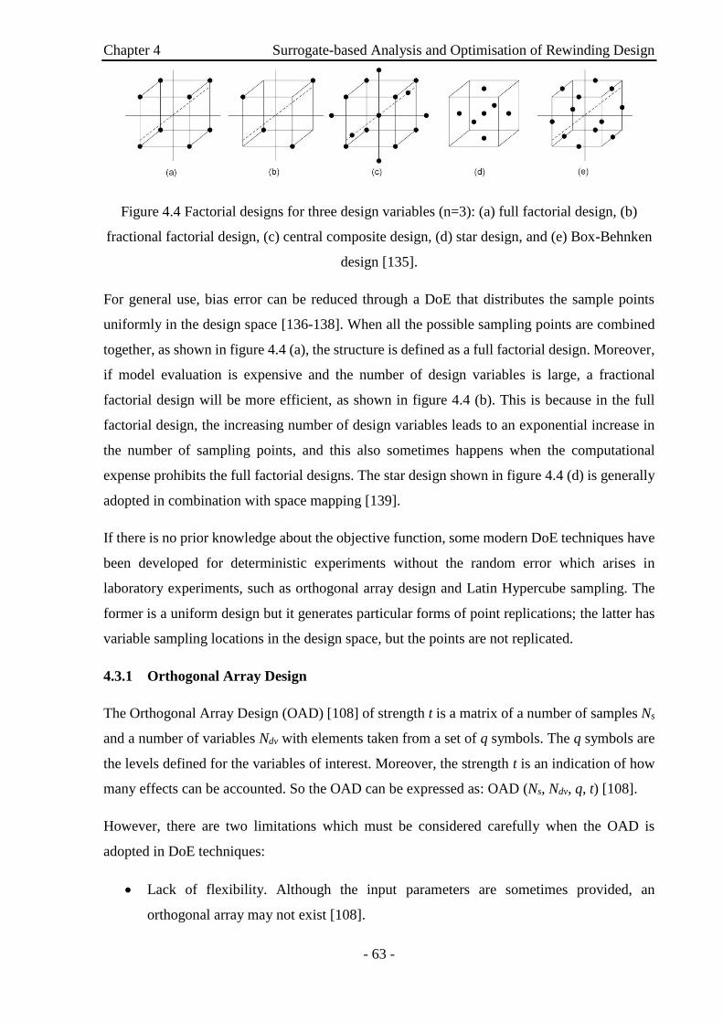
Chapter 4 Surrogate-based Analysis and Optimisation of Rewinding Design
- 63 -
Figure 4.4 Factorial designs for three design variables (n=3): (a) full factorial design, (b)
fractional factorial design, (c) central composite design, (d) star design, and (e) Box-Behnken
design [135].
For general use, bias error can be reduced through a DoE that distributes the sample points
uniformly in the design space [136-138]. When all the possible sampling points are combined
together, as shown in figure 4.4 (a), the structure is defined as a full factorial design. Moreover,
if model evaluation is expensive and the number of design variables is large, a fractional
factorial design will be more efficient, as shown in figure 4.4 (b). This is because in the full
factorial design, the increasing number of design variables leads to an exponential increase in
the number of sampling points, and this also sometimes happens when the computational
expense prohibits the full factorial designs. The star design shown in figure 4.4 (d) is generally
adopted in combination with space mapping [139].
If there is no prior knowledge about the objective function, some modern DoE techniques have
been developed for deterministic experiments without the random error which arises in
laboratory experiments, such as orthogonal array design and Latin Hypercube sampling. The
former is a uniform design but it generates particular forms of point replications; the latter has
variable sampling locations in the design space, but the points are not replicated.
4.3.1 Orthogonal Array Design
The Orthogonal Array Design (OAD) [108] of strength t is a matrix of a number of samples Ns
and a number of variables Ndv with elements taken from a set of q symbols. The q symbols are
the levels defined for the variables of interest. Moreover, the strength t is an indication of how
many effects can be accounted. So the OAD can be expressed as: OAD (Ns, Ndv, q, t) [108].
However, there are two limitations which must be considered carefully when the OAD is
adopted in DoE techniques:
Lack of flexibility. Although the input parameters are sometimes provided, an
orthogonal array may not exist [108].

Chapter 4 Surrogate-based Analysis and Optimisation of Rewinding Design
- 64 -
Point replication. OAD works on the subspace spanned by the effective factors, which
could generate replicated points. This may cause bias error, which has a deleterious
effect on the model estimation.
4.3.2 Latin Hypercube Sampling (LHS)
One of the most popular DoE techniques is Latin Hypercube sampling (LHS) [140], which is a
type of stratified sampling approach with the restriction that each of the input variables has all
portions of its distribution represented by input values [140]. In practice, the range of every
parameter for n design variables is separated as p bins, so that the total number of pn bins will
be generated in the design space. The samples are randomly selected in the design space, and
each will be located randomly in one of the whole bins, and a simple chart of LHS is shown in
figure 4.5. Moreover, there is exactly one sample in each bin for all one-dimensional projections
of the p samples and bins [135]. So the standard LHS is commonly not a uniform distribution.
Figure 4.5 Latin Hypercube Sampling with p=8, n=2 for uniform distribution.
While LHS represents an improvement over unrestricted stratified sampling [141], it can
provide sampling plans with very different performance in terms of uniformity, as shown in
figure 4.6. As a result, the LHS approach is adopted as the DoE technique in this work.

Chapter 4 Surrogate-based Analysis and Optimisation of Rewinding Design
- 65 -
Figure 4.6 Different performance of LHS in terms of uniformity.
4.4 Construction of Surrogate Model
Once the DoE technique has been selected and the data obtained from the high-fidelity model
simulation, a suitable approximation approach is chosen in the next step. Parametric approaches
such as polynomial regression model (PR) assume that the global functional form of the
relationship between the response variable and the design variables is known [108]. A non-
parametric approach such as the radial basis function (RBF) builds the overall model by using
different types of simple local models in different regions of the data. Furthermore, a semi-
parametric approach called the Kriging model has been developed which has the advantages of
both parametric and non-parametric methods. For example, it allows much more flexibility than
parametric models, since no specific model structure is used, and the non-parametric part is
considered as the realization of a random process [142]. In this section, brief introductions to
these approximation methods for the surrogate model are presented.
4.4.1 Polynomial Regression Model
PR analysis is a method to estimate the relationship between the prediction function 𝑓 and basis
function zj with the number of basis functions NPR [143], so the linear regression model is
expressed as in the equation below:
1
PRN
j j
j
f z z
(4.1)
2 V (4.2)

Chapter 4 Surrogate-based Analysis and Optimisation of Rewinding Design
- 66 -
where ε is the unobserved random error with an expected value equal to zero and a variance of
ξ2. For example, second order polynomial regression models with one variable and two
variables are shown in the following equation:
0 1 2f z z z (4.3)
2 2
0 1 1 2 2 11 1 22 2 12 1 2f z z z z z z z (4.4)
So a Ns × NPR matrix X of the set of equations above can be expressed with the number of
sampling points and the design variables, which is a general model for fitting any relationship
that is linear to the unknown parameter β as:
f X (4.5)
Hence, a solution for the estimated parameter using least square method can be calculated as
[144]:
1
fˆ T TX X X
(4.6)
However, there is an important limitation of polynomial regression models, which is the order
of the model. The order should be as low as possible and high order polynomials of more than
two should be avoided.
4.4.2 Radial Basis Function
The RBF belongs to the class of generalized linear models, which has been developed for the
interpolation of scattered multivariate data [108, 145]. The approximation method using linear
combinations of symmetrical functions ϕj with the number of radial basis functions NRBF is
shown in the next equation:
1
RBFNj
j j c
j
f r r r
(4.7)
where ωj is the coefficients of linear combinations and rc(j) is the different basis function centres.
Similar to the polynomial regression model, the radial basis function can be expressed as:
jf (4.8)
The coefficient of linear combinations ω can then be computed from:

Chapter 4 Surrogate-based Analysis and Optimisation of Rewinding Design
- 67 -
1
T T
j f
(4.9)
And the radial basis function Φ is a matrix with the number of sampling points and the number
of basis function Ns × NRBF given by:
1 1 1 2 1
2 1 2 2 2
1 2
RBF
RBF
s s s RBF
N
c c c
N
c c c
N N N N
c c c
r r r r r r
r r r r r r
r r r r r r
(4.10)
4.4.3 Kriging Model
The Kriging model is currently gaining in popularity as a technique to interpolate deterministic
noise-free data [146-149]. The basic formulation of the Kriging model is to estimate the value
of a function or response at some unknown location or area, which comprises of two
components: the polynomial model and a systematic departure representing either small scale
components with high frequency variation or large scale components with low frequency
variation [150].
The systematic departure component represents the fluctuations around the real function, with
the basic assumption being that these are correlated and the correlation depends only on the
distance between the locations under consideration [108]. More precisely, a zero mean, second-
order, stationary process is represented as described by a correlation model. Therefore, an
approximation expression of the Kriging model is given by:
y t z t (4.11)
where β is a constant, and the fundamental function z(t) is calculated by Gaussian distribution
with error, where the residual error is an independent, identically distributed error or normal
random variables whose mean and variance are 0 and ξ2 respectively. If (𝑡) is defined as the
approximation model, and the mean-squared error of y(t) and (𝒕) are minimum, satisfying the
unbiased condition, (𝑡) is estimated as
1ˆ ˆy y Tt r R q (4.12)
where R-1 is the inverse of the correlation matrix R, r is the correlation vector, y is the ns
observed data vector, and q is the unit vector. The correlation matrix and correlation vector are

Chapter 4 Surrogate-based Analysis and Optimisation of Rewinding Design
- 68 -
2
1
,n
j k j k
i i i
i
R Exp t t
t t (4.13)
1,2, , 1,2,j ns k ns (4.14)
1 2, , , , , ,
Tns
R R R
r t t t t t t t (4.15)
The parameters θ1, θ2, ……, θn are unknown, but they can be calculated using the following
equation.
𝑚𝑎𝑥𝑖𝑚𝑖𝑠𝑒 −
[𝑛𝑠 ln(𝜎2 + ln|𝑹|)]
2 (4.16)
where θi (i=1, 2, …, n) ˃ 0. θi can be solved using the optimisation algorithm.
With given the various approximation methods which have been developed, it is important to
select a relatively high precise method to construct a surrogate model. Various studies have
compared the precision of the estimated models using the RBF and Kriging methods, as the
Kriging model has been found to be more accurate [142, 151]. As a result, the Kriging model
is employed in this work as the approximation method used to construct the surrogate model.
4.5 Surrogate-based Optimisation
Surrogate model-based optimisation accomplishes optimisation rapidly by using a surrogate
model for the objective and constraint functions. The surrogate model is able to address
optimisation problems with non-smooth or noisy responses, and can even provide insights into
the nature of the design space [119, 120, 152, 153]. SBAO has also been found to be effective
in both multi-disciplinary and multi-objective optimisation [108]. The optimisation algorithms
of SBAO are discussed next.
The proposed surrogate-based analysis and optimisation algorithm is shown as a flowchart in
figure 4.7. The part of procedures have been introduced in the section 4.3 and 4.4, indicating
how to build the surrogate successfully. Before constructing the surrogate model, the problem
definition should make clear which parameters need to be varied or constrained, and what the
objective of the optimisation is. Furthermore, an optimisation algorithm is required to achieve
the SBAO.

Chapter 4 Surrogate-based Analysis and Optimisation of Rewinding Design
- 69 -
Figure 4.7 Surrogate-based analysis and optimisation.
Optimisation Problem Definition. Before any optimisation design is carried out, the
objectives and number of variables and constraints must be defined carefully.
Design of Experiment. The design of experiment method is adopted to determine the
locations of sampling points in the specific design space. In this step, the number of
sampling points is severely limited, because of the computing expense for each sample
point.
Numerical Simulation of Each Point. A computationally expensive model with all the
variables is simulated, and the variables are determined using the DOE method.
Construction of Surrogate Models. The selection of methods used for building the
surrogate model and model identification must be carefully considered.
Infill Sampling Points. This step makes the estimated function more accurate by adding
more sampling points at specific locations. If the results converge, then the model
estimation is stopped.
Converge. The convergence of the surrogate model can be judged according to the
linking of infill sampling points. If there is no convergence, the ‘best’ point has to be
added into the DoE again to obtain the next best point. Upon convergence, the surrogate
model has been built successfully.
Heuristic Search Method. When the surrogate model has been built, the exact optimal
point is found using the optimisation method.
Model Validation. The purpose of this step is to evaluate the precision of the predicted
surrogate model to the actual objective function.

Chapter 4 Surrogate-based Analysis and Optimisation of Rewinding Design
- 70 -
The optimisation of electrical machines is a multi-variable and multi-modal problem [154-160].
In such cases, a wide range of optimisation algorithms have been developed. In the past, these
optimisation algorithms were mostly used in combination with analytical models [161, 162];
however, there has been a trend in recent years to combine them with FEM [163, 164]. Hence,
the time and computing costs are important in judging which algorithm is more suitable. At
present, two main types of evolutionary optimisation algorithms are commonly adopted:
genetic algorithm and particle swarm optimisations.
4.5.1 Genetic Algorithm
The genetic algorithm (GA) was developed using the principles of evolution, natural selection
and genetics from natural biological systems [165, 166]. During GA computing, a population
of artificial individuals is modified repeatedly based on biological evolution rules that converge
towards a better solution of the problem to be solved. At each step, individuals are selected
randomly from the current population to be parents. These individuals are used to produce
children for the next generation. Based on biological principles, the fittest individuals survive
and the least fit die.
Generally, a GA consists of three main procedures: selection, crossover, and mutation. It starts
with an initial population containing a number of chromosomes each of which represents a
solution to the problem. However, some chromosomes are not fit, and these will be ignored
while only the fittest chromosomes will be designated for reproduction. In order to keep the
size of the initial population stable, some fit chromosomes will be used more than once, so this
subset is call the ‘matting pool’. The purpose of this selection operation is to obtain a mating
pool with the fittest individuals according to a probabilistic rule that allows the fittest
individuals to be mated into the new population. After the selection stage, a genetic crossover
operation is then applied between parent pairs from the mating pool. Each pair will produce
two children to maintain the size of the population. The crossover operation forces the new
chromosomes to have the properties and characteristics of both parents. Mutation is the final
operation which takes place after crossover and introduces a change into the offspring bit string
to produce new chromosomes. Beside this, it may represent a solution to the problem whilst
avoiding the population falling to a local optimal point. The mutation operation is performed
with a probability of mutation which is usually low. This preserves good chromosomes and
mimics real life where mutations rarely happen. The new individuals created by these three
basic operations may be fitter than their parents. This algorithm is repeated for many
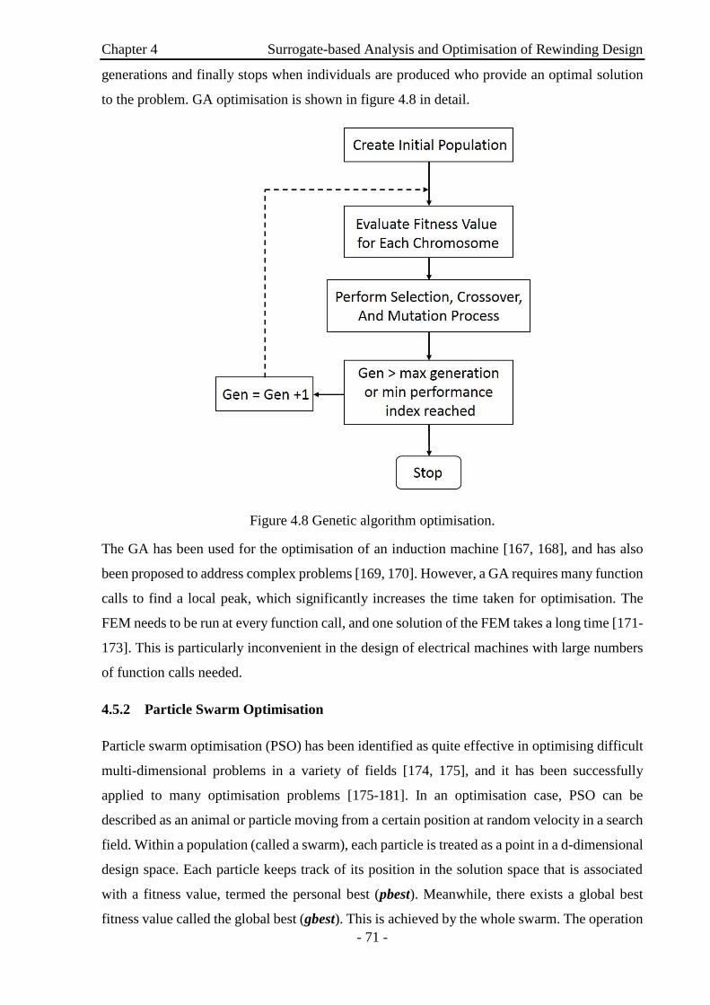
Chapter 4 Surrogate-based Analysis and Optimisation of Rewinding Design
- 71 -
generations and finally stops when individuals are produced who provide an optimal solution
to the problem. GA optimisation is shown in figure 4.8 in detail.
Figure 4.8 Genetic algorithm optimisation.
The GA has been used for the optimisation of an induction machine [167, 168], and has also
been proposed to address complex problems [169, 170]. However, a GA requires many function
calls to find a local peak, which significantly increases the time taken for optimisation. The
FEM needs to be run at every function call, and one solution of the FEM takes a long time [171-
173]. This is particularly inconvenient in the design of electrical machines with large numbers
of function calls needed.
4.5.2 Particle Swarm Optimisation
Particle swarm optimisation (PSO) has been identified as quite effective in optimising difficult
multi-dimensional problems in a variety of fields [174, 175], and it has been successfully
applied to many optimisation problems [175-181]. In an optimisation case, PSO can be
described as an animal or particle moving from a certain position at random velocity in a search
field. Within a population (called a swarm), each particle is treated as a point in a d-dimensional
design space. Each particle keeps track of its position in the solution space that is associated
with a fitness value, termed the personal best (pbest). Meanwhile, there exists a global best
fitness value called the global best (gbest). This is achieved by the whole swarm. The operation

Chapter 4 Surrogate-based Analysis and Optimisation of Rewinding Design
- 72 -
of PSO gradually changes the velocity of each particle toward its pbest and gbest positions each
time. The new velocity and position follow
𝑉𝑗𝑘+1 = 𝑤𝑉𝑗
𝑘 + 𝐶1𝜑1(𝑝𝑗𝑘 − 𝑋𝑗
𝑘) + 𝐶2𝜑2(𝑝𝑔𝑘 − 𝑋𝑗
𝑘)
𝑋𝑗𝑘+1 = 𝑋𝑗
𝑘 + 𝑉𝑗𝑘+1
(4.17)
(4.18)
where 𝑉𝑗𝑘 and 𝑋𝑗
𝑘 are the velocity and location of the jth particle at iteration k; 𝑝𝑗𝑘 is the pbest
of particle j at the kth iteration; 𝑝𝑔𝑘 is the gbest of the entire swarm at the kth iteration; C1 and
C2 are acceleration factors; 𝜑1 and 𝜑2 are the uniformly distributed random numbers between
0 and 1; and w is the inertia weight that controls the influence of the previous velocity on the
new velocity. Each particle will try to change its position according to four variables: the current
position, the current velocity, the distance between the current position and pbest, and the
distance between the current position and the gbest. The PSO algorithm is illustrated in figure
4.9.
Figure 4.9 Particle swarm optimisation algorithm.

Chapter 4 Surrogate-based Analysis and Optimisation of Rewinding Design
- 73 -
There is a large body of work comparing the GA and PSO to show which is more effective and
accurate [161, 182, 183]. From the results, the PSO performs better in terms of optima found
and time required to find these optima [184]. It is also suggested that PSO performs better in
terms of simple implementation and high computational efficiency with few control parameters
[174, 185]. For these reasons, the PSO is chosen as the optimisation algorithm in this work.
4.6 Stator Rewinding Design
As mentioned in the literature review, if winding failure happens only in the stator winding and
the rotor winding is without damage, only the stator winding could be replaced and the rotor
winding left intact. This presents a good opportunity to re-design and re-wind the induction
machine to make it more efficient. Unlike the original rewinding that follows the original design
as closely as possible, this thesis investigates a novel method to optimise machine efficiency
during the machine re-winding procedure. In the meantime, the relationship of efficiency to the
winding turns and the C.S.A is plotted using the surrogate modelling method, which provides
theoretical data for the machine winding design rather than conventional empirical information.
Also the relationship between the torque and winding turns and C.S.A are provided. The
detailed re-design and re-winding procedures are introduced in the following sections.
4.6.1 Optimisation Problem Definition
The objective of this work is to change the winding parameters to maximise machine efficiency
by taking into account a combination of variables and constraints. The dominant two-
dimensional parameters for optimisation are the number of stator winding turns Nstator and stator
winding C.S.A Astator, which can directly affect machine efficiency. Furthermore, some
constraints are imposed by the limitations of manufacturing processes, which limit the
maximum fill factor of stator slot with a thermocouple ffstator on 40% or 44% without the
thermocouple, torque T to maintain the machine power rating, and optimising range of winding
turns and C.S.A. In order to build the model, the FEM-based commercial software Infolytica
Magnet is used to analyse the performance of the induction machine with different winding
parameter designs.
It should be noted that, in order to gain precise testing results, a thermocouple is inserted into
the stator slot to test the winding temperature. This accounts for about 4% of the stator slot area,
and here two optimisation plans are presented: one space for the thermocouple, the other
without it. Therefore, the following general expression focuses on the optimisation problem
definition for stator winding with a thermocouple.
Chapter 4 Surrogate-based Analysis and Optimisation of Rewinding Design
- 74 -
Objective Maximise efficiency η
Subject to 20% ≤ ffstator ≤ 40%
360 ≤ T ≤ 363 Nm
1.61 ≤ Astator ≤ 8.5 mm2
10 ≤ Nstator ≤ 24
Similarly the optimisation problem definition for a stator slot without a thermocouple is:
Objective Maximise efficiency η
Subject to 20% ≤ ffstator ≤ 44%
360 ≤ T ≤ 363 Nm
1.61 ≤ Astator ≤ 8.5 mm2
10 ≤ Nstator ≤ 24
After determining the problem definition for the stator winding optimisation, the next step is to
generate the sampling plan using the LHS method.
4.6.2 LHS for Stator Winding Optimisation
The initial sampling plan is generated using the LHS realization of 50 samples, which is
achieved via Matlab software and plotted as in figure 4.10. Now, the relative constraints for
stator windings optimisation are plotted in the LHS plan. First of all, the two design variables
(ndvs = 2) of stator winding turns and C.S.A are defined as x-axial and y-axial separately as
shown in figure 4.11. The next constraint of the stator slot fill factor between 20% and 44% is
displayed in figure 4.12, which is due to the maximum fill factor of the stator slot being 44%.
The final sampling plan could then be obtained. However, there are some points which do not
satisfy the design constraints, to add the constraints of fill factor to reduce the non-meaningful
points. Figure 4.13 presents the available locations of sampling points, and information from
these sampling points is fed into the finite element model to acquire simulated results for the
construction of the surrogate model.

Chapter 4 Surrogate-based Analysis and Optimisation of Rewinding Design
- 75 -
Figure 4.10 Initial Latin hypercube sampling plan for stator winding optimisation.
Figure 4.11 Definition of the constraints of stator winding turns and cross-sectional area.

Chapter 4 Surrogate-based Analysis and Optimisation of Rewinding Design
- 76 -
Figure 4.12 Definition of the constraint of stator slot fill factor.
Figure 4.13 Latin hypercube sampling of stator winding optimisation.
4.6.3 Construction of Surrogate Model for Stator Winding
According to the Latin hypercube sampling plan for stator winding optimisation with two
design variables (stator winding turns and C.S.A), a total of 21 available sampling points have
been generated, and then each sampling point is run in the FEM to obtain the results used to

Chapter 4 Surrogate-based Analysis and Optimisation of Rewinding Design
- 77 -
construct the initial surrogate model. Once the simulation results have been calculated, the
relationship between efficiency and the two design variables can be plotted precisely, as well
as the relationship between the torque and two design variables. The initial efficiency and
torque contour of the stator winding optimisation function with two-dimensional variables are
displayed in figures 4.14 and 4.15. Hence, the point of the highest efficiency in the initial
surrogate model appears in top left corner, the winding parameter is 10 turns with 8.2 mm2
cross-sectional area.
Figure 4.14 Initial efficiency contour of stator winding with two design variables.

Chapter 4 Surrogate-based Analysis and Optimisation of Rewinding Design
- 78 -
Figure 4.15 Initial torque contour of stator winding with two design variables.
Meanwhile, for a better comprehension of the relationship between efficiency and torque versus
the two design variables, the initial three-dimensional distributions presented in figures 4.16
and 4.17.
Figure 4.16 Initial three-dimensional efficiency distribution of stator winding with two design
variables.

Chapter 4 Surrogate-based Analysis and Optimisation of Rewinding Design
- 79 -
Figure 4.17 Initial three-dimensional torque distribution of stator winding with two design
variables.
However, the initial sampling plan is often not very accurate, and at this time the procedure of
infilling sampling points is needed. The principle is generally to constrain the boundary of the
surrogate model and to try to make the locations of sampling points well-proportioned, which
means that infilled sampling points shall be put in obvious blank areas. Based on this principle,
another extra 13 sampling points are inserted into the LHS plan for stator winding optimisation,
as shown in figure 4.18.
Figure 4.18 Infill sampling points of stator winding optimisation.

Chapter 4 Surrogate-based Analysis and Optimisation of Rewinding Design
- 80 -
Then a new efficiency and torque contour with high precision are built accordingly, as displayed
in figures 4.19 and 4.20. Compared to the initial contour, it can easily be seen that the torque
contour has scarcely changed; but the efficiency contour appears the wave fluctuation. Now,
the surrogate model of stator winding with two variables has already been constructed, which
can be searched for the local best point using the PSO method. If the optimal point is not
converged when the optimal model is checked for validation, this means that the surrogate
model is still not accurate enough, and the ‘best’ point so far will be added into the link of the
DoE, in order to repeat the procedures of surrogate model construction until the results are
converged, and the local best point has been successfully found.
Figure 4.19 Efficiency contour of stator winding with two design variables.

Chapter 4 Surrogate-based Analysis and Optimisation of Rewinding Design
- 81 -
Figure 4.20 Torque contour of stator winding with two design variables.
As in the previous work, the efficiency and torque distribution of stator winding optimisation
with two design variables are better shown on 3-dimensional plot, as shown in figures 4.21 and
4.22.
Figure 4.21 Three-dimensional efficiency distribution of stator winding with two design
variables.

Chapter 4 Surrogate-based Analysis and Optimisation of Rewinding Design
- 82 -
Figure 4.22 Three-dimensional torque distribution of stator winding with two design
variables.
4.6.4 Particle Swarm Optimisation
In the previous section on optimisation problem definition, two different constraints are applied
due to the installation of a thermocouple. In the PSO, the constraint of maximum fill factor is
set to 40% in the thermocouple installed case, which is due to the limitation of the
manufacturing process; if the thermocouple is not installed in the stator slot, the upper limit of
stator slot fill factor increases to 44%, and other objectives and constraints do not change. The
next step is to use PSO to find the best point in this surrogate model of stator winding
optimisation with two design variables. In the meanwhile, it has to be mentioned that the
optimised winding layout and configuration are kept the same as the original design; they are
not changed during the rewinding process.
Therefore, the final best point for stator winding turns and C.S.A with a thermocouple installed
is 16 turns and 4.82 mm2. On the other hand, without a thermocouple installed in the stator slot,
the best point for stator winding turns and C.S.A is 16 turns and 5 mm2 respectively.
4.6.5 Model Validation
From PSO, the two optimisation results are provided with and without a thermocouple installed.
In order to verify the precision of the surrogate-based optimised results, finite element software
is used to check the machine efficiency with the two optimised design variables. The validation
results are illustrated in Table 4.1.

Chapter 4 Surrogate-based Analysis and Optimisation of Rewinding Design
- 83 -
Table 4.1 Model validation of stator winding optimisation
Stator winding parameter Fill factor Validated result
Original design 16 turns 4.29 mm2 35.52% 92.9%
Stator rewinding design
with thermocouple 16 turns 4.82 mm2 39.9% 93.3%
Stator rewinding design
without thermocouple 16 turns 5 mm2 41.4% 93.5%
Therefore, the optimised model has achieved validation. The SBAO has successfully achieved
the optimisation of the stator rewinding.
4.7 Rotor Rewinding Design
As with stator rewinding design, the principles and method are nearly the same for the stator
rewinding design. The relevant procedures and results are shown in this section.
4.7.1 Optimisation Problem Definition
The objective here is the same as in stator winding optimisation, apart from some of the
constraints being different, due to the different slot area in the rotor. It is impossible to install a
thermocouple in the rotor, so the expression for rotor winding optimisation problem definition
is listed below.
Objective Maximise efficiency η
Subject to 20% ≤ ffrotor ≤ 39%
360 ≤ T ≤ 363 Nm
1.86 ≤ Arotor ≤ 8.93 mm2
10 ≤ Nrotor ≤ 24
4.7.2 LHS for Rotor Winding Optimisation
Using the same method for stator winding optimisation, the LHS for rotor winding optimisation
generates 50 sampling points for two rotor winding design variables: rotor winding turns and
C.S.A, as shown in figure 4.23. In figures 4.24 and 4.25, a series of constraints such as the range
of two design variables and the rotor slot fill factor are defined. However, the maximum fill

Chapter 4 Surrogate-based Analysis and Optimisation of Rewinding Design
- 84 -
factor of the rotor slot is 39%. Here, the rotor slot fill factor constraint is still set between 20%
and 40% during the construction of the surrogate model. Finally, figure 4.26 gives the sampling
points available for rotor winding optimisation which will be used to construct the surrogate
model of rotor winding optimisation.
Figure 4.23 Initial Latin hypercube sampling plan for rotor winding optimisation.

Chapter 4 Surrogate-based Analysis and Optimisation of Rewinding Design
- 85 -
Figure 4.24 Definition of the constraints of rotor winding turns and cross-sectional area.
Figure 4.25 Definition of the constraints of rotor slot fill factor.

Chapter 4 Surrogate-based Analysis and Optimisation of Rewinding Design
- 86 -
Figure 4.26 Latin hypercube sampling of rotor winding optimisation.
4.7.3 Construction of Surrogate Model for Rotor Winding
From the LHS for rotor winding optimisation, 21 available sampling points were found to be
used for the initial surrogate model. Figures 4.27-4.30 present initial surrogate model for rotor
winding optimisation, showing the initial efficiency contour function, initial torque contour
function, three-dimensional efficiency distribution, and three-dimensional torque distribution
with two design variables.

Chapter 4 Surrogate-based Analysis and Optimisation of Rewinding Design
- 87 -
Figure 4.27 Initial efficiency contour of rotor winding with two design variables.
Figure 4.28 Initial torque contour of rotor winding with two design variables.

Chapter 4 Surrogate-based Analysis and Optimisation of Rewinding Design
- 88 -
Figure 4.29 Initial three-dimensional efficiency distribution of rotor winding with two design
variables.
Figure 4.30 Initial three-dimensional torque distribution of rotor winding with two design
variables.
In order to make the surrogate model for rotor winding optimisation more accurate, 4 boundary
sampling points and 11 extra sampling points are inserted in the LHS of the rotor winding

Chapter 4 Surrogate-based Analysis and Optimisation of Rewinding Design
- 89 -
optimisation via the procedure of infilling sampling points, as shown in figure 4.31. These 15
infill sampling points are run in the finite element software to get further information to estimate
precisely the new surrogate model.
Figure 4.31 Infill sampling points of rotor winding optimisation.
From the infill sampling points, the new surrogate models for rotor winding optimisation, as
shown in figures 4.32-4.35 are ready to be validated using the PSO algorithm, and the local
peak point can also be found.

Chapter 4 Surrogate-based Analysis and Optimisation of Rewinding Design
- 90 -
Figure 4.32 Efficiency contour of rotor winding with two design variables.
Figure 4.33 Torque contour of rotor winding with two design variables.

Chapter 4 Surrogate-based Analysis and Optimisation of Rewinding Design
- 91 -
Figure 4.34 three-dimensional efficiency distribution of rotor winding with two design
variables.
Figure 4.35 three-dimensional efficiency distribution of rotor winding with two design
variables.

Chapter 4 Surrogate-based Analysis and Optimisation of Rewinding Design
- 92 -
4.7.4 Particle Swam Optimisation
Before optimisation, the upper constraint of the rotor slot fill factor is altered from 40% down
to the actual available value of 39%, because there is no rule in the finite element software to
estimate situations which cannot be achieved in the real world. The local peak point for rotor
winding optimisation is then provided, where the number of turns is 16 and the C.S.A is 5.19
mm2 under the condition of unchanged winding layout and configuration.
4.7.5 Model Validation
The final step of rotor winding optimisation is model validation, by feeding the two optimised
design variables for rotor winding into finite element software. The validation results are
presented in Table 4.2.
Table 4.2 Model validation of rotor winding optimisation
Rotor winding parameter Fill factor Validated result
Original design 12 turns 6.95 mm2 37.35% 92.9%
Rotor rewinding design 16 turns 5.19 mm2 37.19% 93%
From the stator rewinding and rotor rewinding designs, the feasibility and precision of SBAO
has been proven for the electrical machine’s winding design. Evidence is also provided about
the winding design or redesign, rather than an empirical selection.
4.8 Rewinding Design for Both Stator and Rotor
It has been shown the SBAO is an effective method for the winding design of electrical
machines. So, in this section, optimisation is carried out based on the original induction machine
with four design variables for both stator and rotor winding. The optimisation procedures are
nearly the same as that for two design variables. The first step is to define the optimisation
problem. The optimisation of four variables for both stator and rotor winding will then be
proven by practical work, and so the upper constraint of the stator slot fill factor has to be
limited at 40%, due to the thermocouple being required to ensure the testing precision. The
objective of the problem is to maximise efficiency, subject to 9 constraints:
Objective: Maximise efficiency η
Subject to: 20% ≤ ffstator ≤ 40%
20% ≤ ffrotor ≤ 39%

Chapter 4 Surrogate-based Analysis and Optimisation of Rewinding Design
- 93 -
358 ≤ T ≤ 363 Nm
2.98 ≤ Astator ≤ 7.07 mm2
2.98 ≤ Arotor ≤ 7.07 mm2
8 ≤ Nstator ≤ 24
8 ≤ Nrotor ≤ 24
6 ≤ Jstator ≤ 10 A/mm2
6 ≤ Jrotor ≤ 10 A/mm2
where Jstator and Jrotor are the current density of the stator and rotor respectively. The first two
constraints are to make sure that the windings can be placed in the slot properly. The third
constraint ensures that the machine power rate does not change. The purpose of the last two
constraints is to prevent the machine from overheating. The optimisation process determines
the following:
stator and rotor lamination
air-gap length (0.9 mm)
slot structure of stator and rotor
The following parameters were variables:
number of stator winding turns
stator winding cross-sectional area
number of rotor winding turns
rotor winding cross-sectional area
Therefore, this optimisation is a multi-modal and multi-variable problem with four design
variables, which means that the LHS and surrogate model is constructed invisible and cannot
be expressed in charts. A total of 110 sampling points and an extra 50 infill sampling points are
provided by LHS to be used for finding the peak point. Therefore, according to the swarming
calculation, the best point is provided as in Table 4.3:

Chapter 4 Surrogate-based Analysis and Optimisation of Rewinding Design
- 94 -
Table 4.3 Optimal plan with 4 design variables compared to the original design
Turns C.S.A (mm2)
Original machine Stator 16 4.29
Rotor 12 6.95
Optimised rewound machine Stator 14 5.21
Rotor 10 5.94
As a result, this optimised plan with four design variables (for numbers of turns and cross-
sectional areas for both stator and rotor) were adopted to rewind a new machine, and efficiency
measurement was conducted on a DFIG test rig. Details are shown in Chapter 6.
4.9 Summary
In Chapter 4 the model of the existing DFIG was presented, keeping the size of the machine
structure fixed, and surrogate-based analysis and optimisation were applied to the machine
winding re-design and optimisation.
The process of optimisation has been investigated in detail here, and three steps were used in
the final optimisation procedure. Design of experiment techniques were presented, whilst one
of these – the Latin Hypercube sampling plan was selected to randomly allocate the sampling
points, which is not uniform distribution. In the second part, methods of construction of the
surrogate model were investigated and compared; the Kriging model was then chosen to
construct the surrogate model due to its higher precision. Based on the surrogate model built,
an optimisation algorithm was used to find the best location, and in this thesis the particle swam
optimisation algorithm was adopted.
For this novel approach to surrogate optimisation, the optimisation of two variables for either
stator winding or rotor winding was investigated, assuming that only part of the winding needs
to be repaired or replaced when winding failure occurs in either winding. In addition, the four
variable problem has then been extensively optimised for both stator and rotor windings,
assuming that all of the generator’s windings need to be replaced.

Chapter 5 Testing Standards of Doubly Fed Induction Generator
- 95 -
Chapter 5 Testing Standards of Doubly Fed Induction Generator
Several international testing standards of the polyphase induction machine are compared in this
chapter. The American standard IEEE 112-B is carried out in this work due to the higher
accuracy compared to the other standards. An improved testing method based on the IEEE 112-
B standard is presented to achieve the purpose of doubly fed induction generator testing. The
efficiency is determined by the input-output method with loss segregation for sub-synchronous
and super-synchronous operational mode; in the meanwhile, the measurement of different
losses in machine is separated in detail.

Chapter 5 Testing Standards of Doubly Fed Induction Generator
- 96 -
5.1 Introduction
Machine losses can usually be either predicted by analytical methods or measured by
experiments. The former is usually achieved using FEM to build accurate models and perform
electromagnetic analysis. The experimental methods involve three different ways to measure
the losses:
direct measurement of the loss
direct measurement of the effect of the loss (e.g. calorimetry)
loss segregation of the input-output method
The induction machine is a mature technology and its performance is now a concern for
manufactures, customers, and researchers. There is still no uniform test standard for evaluating
machine efficiency, and different standards adopted throughout the world lead to different test
results with the same machine. Therefore one is developed here.
Different countries hold their own opinions on the appropriate efficiency test for polyphase
induction machines and so several different standards exist. Nearly all the standards fall into
the three kinds of test, namely:
Institution of Electrical and Electronic Engineers (IEEE) 112-B [81]
International Electrotechnical Commission (IEC) 34-2 [88]
Japanese Electrotechnical Commission (JEC) 37
Other existing national standards typically resemble these three standards; although in different
areas, different standards are adopted. For example, the US National Electrical Manufacturers
Association (NEMA) MG-1-1993 standard [89] and Canadian C390-93 [186] are similar to the
IEEE standard 112-B in North America. Meanwhile, the European Committee of
Manufacturers of Electrical Machines and Power Electronics (CEMEP) and British BS EN
60034-2 standards are analogous to the IEC 34-2.
The primary differences between these standards lie in the accuracy the measurements of loss
and efficiency. In order to calculate motor efficiency within 0.5% error, the electrical industry
has spent an enormous amount of money working to improve the accuracy of instrumentation
[187]. However, it is impossible to acquire an exact value of efficiency with the current
standards. At this time, to recognize which standard is more accurate is becoming more
important. The major judgment adopted here is to consider the accuracy of loss and efficiency
among these test standards.

Chapter 5 Testing Standards of Doubly Fed Induction Generator
- 97 -
Efficiency is a measure of the mechanical power which is converted to electrical power by the
generator or vice versa by a motor. It is expressed as:
out out in loss
in out loss in
P P P P
P P P P
(5.1)
where η is efficiency, Ploss is the total loss in the machine, Pout is output power, and Pin is input
power.
This chapter presents an introduction to each individual type of loss in the induction machine.
Meanwhile, a brief comparison is presented of the different test standards for induction
generators. Also the testing standards used to measure the efficiency of induction generators
are described in this chapter. Finally, due to the requirements of the present work, some
modifications and supplements are applied to the DFIG test rig, which is based on the current
standards for a wound rotor induction generator.
5.2 Testing Standards
As introduced in the preceding section, all of the testing standards can be divided into two main
forms: the European area and the North American area. In Europe, the British standard BS EN
60034-2 is nearly the same as the European standard IEC 34-2; however, the latter has
undergone some modifications in loss determination, and the revised version is called the IEC
61982. In North America, the Canadian C390-1993 national standard corresponds to the
American IEEE 112-B, but has a slightly different measurement of windage and friction losses.
In the Canadian national standard, windage and friction losses are captured at between 50% and
approximately 20% of rated voltage during the no-load test. Furthermore, as the Japanese JEC
37 national standard does not have an English version, so it is not described in this thesis,
although the stray load loss (SLL) is completely ignored, and it does not consider the effect of
winding temperature on loss calculation. In the following section, the mainstream standards are
compared to check their respective precision.
5.2.1 Comparison of the Standards
In order to determine which standard has the higher accuracy, many relevant studies have been
conducted to verify their reliability. First of all, in comparing the most important worldwide
standards, the IEEE 112-B, IEC 34-2, and JEC 37, Renier used the efficiency testing of the
75kW 6 pole induction motor to estimate precision [188]. Figure 5.1 shows that the JEC 37
standard gives the highest value of efficiency, which is about 2% error to the real efficiency

Chapter 5 Testing Standards of Doubly Fed Induction Generator
- 98 -
due to neglecting the SLL completely. The measured efficiency of the IEEE 112-B standard is
quite close to the theoretical value, so this means the SLL measurement in this standard is more
accurate. Although the IEC 34-2 standard considers SLL, it is underestimated and this causes a
relatively higher efficiency to be given which is less accurate than the IEEE 112-B standard.
Similar work was done by Boglietti in 2003 [189], and the same results for the determination
of SLL and efficiency were given when four 10 Hp four pole induction motors were tested
using these standards. Because the Japanese JEC 37 standard does not include SLL
measurement, so the test results of machine efficiency and losses is not accurate, which means
that it is not recommended for practical evaluations of machine efficiency. As a result, the JEC
37 standard is the most inaccurate standard to use in evaluating the efficiency and should be
ignored.
Figure 5.1 Comparison of different international testing standards.
For this reason, more attention is paid to the IEEE 112-B and IEC 34-2 standards. In work
comparing these two standards, Roy [190] tested three kinds of induction motors with different
power rating, which were 11 kW (7 motors), 55 kW (6 motors), and 75 kW (5 motors).
According to the results shown in figure 5.2, the efficiency of the IEC 34-2 standard on the left
side was consistently higher than the efficiency values given by the IEEE 112-B standard on
the right side by about 1%, due to the error in SLL measurement, except for one 55 kW
induction motor. Similar work also in [191-193], has also declared that the IEC 34-2 standard
is discredited and inadequate. Therefore, the IEEE 112-B standard is obviously more accurate
84
85
86
87
88
89
90
91
92
93
94
95
0% 20% 40% 60% 80% 100% 120%
Eff
icie
ncy
(%
)
Load (%)
Motor Efficiency IEEE 112-B IEC 34-2 JEC 37

Chapter 5 Testing Standards of Doubly Fed Induction Generator
- 99 -
than both the IEC 34-2 standard and the JEC 37 standard on the evaluation of efficiency and
loss. So, in this work, the IEEE standard 112-B is adopted in the testing method.
Figure 5.2 Comparison of IEEE 112-B and IEC 34-2 standards [190].
5.2.2 IEEE 112-B Standards
The IEEE 112-B Standard was developed by the IEEE Power Engineering Society, which is an
American national standard to provide applicable and acceptable tests of polyphase induction
motors and generators between 1 and 250 Hp. Currently, almost all tests of medium AC motors
are conducted with reference to the IEEE 112-B in the US [187]. In this standard, the main
method used to determine efficiency is the input-output measurement with loss segregation.
The input power of induction generators is measured according to rotational speed and a torque
transducer and output power is captured by a high accuracy wattmeter. So the total loss could
be calculated by input power minus output power, which includes conventional losses and SLL.
As the conventional losses are segregated, the residual SLL could be determined against torque
squared, and linear regression is adopted to reduce the error. Meanwhile, the temperature of the
stator and rotor conductors should be corrected based on ambient temperature to precisely
calculate total loss and efficiency. The detailed tests are illustrated as follows.
5.2.2.1 Preliminary Test
Commonly, the first step test is to measure the winding resistance. At ambient temperature, the
terminal-to-terminal winding resistance is measured for using in the following efficiency test,
and meanwhile the structure of winding connection (winding circuits) is taken into
consideration. If the thermal detector (PT100 thermistor or thermocouples) is embedded in the
machine, the winding temperature could be monitored during the machine’s operation, or even

Chapter 5 Testing Standards of Doubly Fed Induction Generator
- 100 -
during the machine test. Beside this, the recorded temperature can be used to determine the
winding resistance correction under different temperature conditions (where the ambient
temperature is measured using the procedure of the IEEE Standard 119-1974). For the detection
of winding temperature, three thermal detectors are normally selected to be installed along the
coil sides in the stator slot, but in different positions. Two of them are located at the two sides
of winding, another is in the middle of the winding. And thus, the average temperature reading
of the winding can be calculated by measuring the three different temperatures. Also, the
winding resistance at a known temperature can be determined by comparison with the winding
resistance at known ambient temperature.
5.2.2.2 No-load test
In this test, the induction machine is operated as a motor under the rated voltage and frequency
condition without any mechanical load being connected. The purpose of the no-load test is to
determine the core loss, windage and friction losses. By adjusting the variac (adjustable voltage
source) at rated frequency, the input value of voltage is changed from 125% of the rated voltage
down to a lowest point, which will raise the current with further voltage reduction. The test
must be run until the bearing loss and winding temperature become stable, in order to read the
value of input power, voltage, current, and winding temperature. Total losses in the motor
running without load are equal to the measured input power. So, according to this data, the no-
load losses can be segregated as stator conductor loss, core loss, windage and friction losses.
To determine the windage and friction losses, first of all, based on the value of input power,
minus the stator conductor copper loss (I2R) at all the different voltage points to acquire the
summation of core loss, windage and friction losses. Secondly, the curve of power versus
voltage squared (Pin-Pstator copper vs. U2) can be plotted, then select more than three lower points
are selected to draw the curve to zero voltage using linear regression analysis. Finally, the
windage and friction losses can be deduced as the area where the curve of power versus voltage
squared crosses the voltage axis at the zero voltage point.
The core loss is determined by the same principle as in the calculation of windage and friction
losses. Subtracting the stator conductor copper loss (I2R) and the value of windage and friction
losses from the input power leaves the core loss. Then, the curve of core loss versus voltage is
plotted, so that the value of core loss can be expressed at any voltage.

Chapter 5 Testing Standards of Doubly Fed Induction Generator
- 101 -
5.2.2.3 Load Test
The load test is often used to determine machine efficiency. In this test, the machine is
connected to a mechanical load, and supplied at the rated voltage and rated frequency.
Meanwhile, the machine is operated with four different load points, which are equally spaced
from no less than 25% load to including 100% load (25%, 50%, 75%, 100%); and also two
overload points are measured as well, but their loading range is no more than 150% load, so
that 120% load and 140% load are usually selected as test points. The test is run until a thermal
balance is reached, and then records the data of voltage, current, power, and winding
temperature are recorded at each load point, and data of speed and torque are also collected by
accurate sensors.
5.2.2.4 Data Correction
In order to obtain the highest accuracy of the test in this standard, some data analysis is required
to apply a correction based on different temperatures.
Reference ambient temperature
The ambient temperature is defined as 25. If the temperature during the tests differs from the
ambient temperature, so the measured performance is corrected based on the ambient
temperature.
Winding resistance correction
The stator winding resistance value at any other temperature is corrected as in the equation 5.2
shown below:
0 1
0 1
c
c
R t kR
t k
(5.2)
where to is the winding temperature, in, as the reference value.
Ro is the winding resistance, in ohms, at temperature to.
tc is the winding temperature, in, for the corrected value of temperature.
Rc is the winding resistance, in ohms, to be corrected at temperature tc.
k1 is a constant coefficient, which is 234.5 for 100% IACS conductivity copper or
225 for aluminium.
Stator winding copper loss correction
When the winding resistance value is corrected at different temperatures, the winding copper

Chapter 5 Testing Standards of Doubly Fed Induction Generator
- 102 -
loss (I2R) at the specific temperature could be determined again.
Slip correction
As mentioned in section 3.3.2 above, the slip has a direct relationship with rotor resistance. As
long as the temperature changes, the slip can be corrected with rotor resistance changing.
0 1
0 1
c
c
s t ks
t k
(5.3)
where to is the winding temperature, in, as the reference value.
so is the slip, measured at stator winding temperature to.
tc is the winding temperature, corrected to the value of temperature, in.
sc is the slip, corrected at the stator winding temperature tc.
sc is the winding resistance, in ohms, to be corrected at temperature tc.
k1 is a constant coefficient, which is 234.5 for 100% IACS conductivity copper or
225 for aluminium.
Rotor winding copper loss correction
Because the stator winding copper loss correction and slip correction are measured based on
the specific temperature, the rotor winding copper loss is determined by equations 3.6 and 3.7.
Stray load loss correction
Determination of SLL is a function of the residual loss versus torque squared. In order to smooth
the curve to linearity, linear regression is used to precisely measure the SLL. The SLL is
expressed in equation 5.4.
2
SLP AT B (5.4)
where A is the slope.
T is the torque, in Nm.
B is the error, which is the intercept with the zero torque line.
To check the reliability of the SLL function, if the slope is negative or the correlation factor is
less than 0.9, the worst point is deleted and the linear regression procedure is repeated. If the
value is still negative, the test has to be repeated again. On the other hand, the SLL will be
corrected by moving the curve to cross the original point, which means to neglect the error. So
the SLL is shown in equation 5.5.
2
SLLP AT (5.5)

Chapter 5 Testing Standards of Doubly Fed Induction Generator
- 103 -
5.2.3 Improved Testing Method for DFIG
As referred to in the previous section, there are differences in the existing standards in the
accuracy of induction generator efficiency. Among these standards, the IEEE 112-B provides
relatively more precise measurements of generator efficiency, and it is commonly selected as
the global testing standard. However, this standard is generally used for testing conventional
polyphase wound rotor induction generators only. However, this thesis focuses on DFIG testing
and there is no relevant standard to measure the losses and the efficiency of the DFIG either.
So this means that the existing standards cannot satisfy the requirements of this work. Therefore,
an approach for testing the DFIG is presented and revised based on the IEEE 112-B standard
for this purpose.
The DFIG has two different operational modes: the super-synchronous and sub-synchronous
modes. In the super-synchronous mode, the rotor power is fed out from the induction generator
to the grid; on the other hand, the rotor power is fed into the induction generator when the DFIG
operates in the sub-synchronous mode. The two modes have to be measured and analysed
separately, whilst the improved testing method is quite complex and differs from the testing
standard for the conventional wound rotor induction generator.
Some parts of the test procedure in the improved testing method are the same as in the IEEE
112-B standard, which involve the preliminary test and the no-load test. In the meantime, the
induction machine test is performed by running a motor without any load connection.
According to the preliminary test, both stator and rotor winding resistance could be measured
to calculate the stator and rotor conductor losses later. And then, the core loss and windage and
friction loss are measured separately using the no-load test, and these are used for the
determination of efficiency. Furthermore, the input power is measured using rotational speed
and torque in both methods.
However, the differences between the improved testing method and the IEEE 112-B standard
mainly concern the load test. In the conventional wound rotor induction generator tests based
on the IEEE 112-B standard, the total power output is the stator output power, and the rotor
conductor loss is estimated by using an indirect method, which is calculated using slip. Both
the machine structure and testing procedure are relatively simpler than most for the DFIG, and
so some important modifications have to be highlighted during the DFIG testing.
First of all, extra experimental data need to be collected, which is different from the IEEE 112-
B standard test on the conventional WRIG. In total five experimental data need to be measured

Chapter 5 Testing Standards of Doubly Fed Induction Generator
- 104 -
in detail, as shown in figure 5.3, which is important in precisely determining the DFIG
efficiency.
Figure 5.3 Measurement locations for DFIG testing.
Stator power output:
The power output is generated from the stator of the induction generator, which is used to
determine the amount of power output delivered to the grid during operation.
Grid power output:
Grid power output is the amount of power output delivered to the grid, which is either
larger or smaller than the stator power output due to the different operational modes.
Rotor conductor current
Rotor conductor loss is difficult to determine directly in the WRIG based on IEEE 112-B
standard, as the exact value of rotor current cannot be easily obtained. So it has to be
determined by an indirect method using slip. But it is quite different in the DFIG, because
its rotor is connected to the grid through a DC link to achieve power transmission. So a
part of the power will flow through the rotor whether fed in or fed out. The rotor current
could be obtained using an accurate current clamp, which means that the rotor conductor
loss could be calculated directly. However, the current clamp should be selected carefully,
because if the rotational speed of the induction generator is very close to the synchronous
speed, the frequency will nearly be the same as the synchronous frequency. Accordingly,
in this case, the AC current clamp would not be able to measure the rotor current, where
as a DC current clamp could achieve the test’s purpose.
Grid side rotor power
The sum of grid side rotor power and stator power output is the grid side power output. As
mentioned above, the stator power output could be measured directly, so the grid side rotor
power is simple to calculate.

Chapter 5 Testing Standards of Doubly Fed Induction Generator
- 105 -
Machine side rotor power
This part of the power is located between the DC link and the induction generator.
Unfortunately, the measuring equipment cannot obtain its value and so it has to be
measured by an indirect method. Therefore, the stator power output, grid power output,
and efficiency of the DC link is used to calculate the machine side rotor power.
Furthermore, the DFIG test with two different operational modes must be tested separately, due
to the requirements of the data analysis. If the DFIG is running in different operational modes,
the method of calculating efficiency and power conversion in the induction generator are quite
different. The detailed principles of the DFIG for both operational modes are introduced below.
Sub-synchronous operational mode:
When the rotation speed of the induction generator is lower than the rated synchronous
speed, the DFIG will operate in sub-synchronous mode, where the rotor power is fed into
the induction generator through the DC link. At this time, the stator power output is larger
than the grid power output, and is equal to the grid power output plus the grid side rotor
power. Therefore, the machine side rotor power can be calculated based on the efficiency
of the DC link. A brief summary of power conversion in the DFIG under sub-synchronous
operation is illustrated in figure 5.4, showing that the input power and rotor power fed in
equals the stator power output and all of the losses in the induction generator.
Figure 5.4 Power flow inside DFIG in sub-synchronous mode.

Chapter 5 Testing Standards of Doubly Fed Induction Generator
- 106 -
Super-synchronous operational mode:
Super-synchronous mode starts when the rotation speed of the induction generator is higher
than the rated synchronous speed, and the rotor power is fed out from the induction
generator to the grid. The amount of grid power output equals the amount of stator power
output plus the grid side rotor power, because both stator and rotor deliver power to the grid
together. The determination of the machine side rotor power is similar to the situation in
sub-synchronous operation. So power conversion in the DFIG is slightly different from that
in the sub-synchronous operational mode, and is shown in figure 5.5. The input power is
now the amount of stator power output, machine side rotor power, and all the losses in
induction generator; or it is the amount of grid power output plus all of the losses in the
induction generator.
Figure 5.5 Power flow inside the DFIG in super-synchronous mode.
As a result, some measurements and modifications for DFIG testing have been presented based
on the IEEE 112-B standard. There is no change to the no-load test, the main work is focused
on the section of load test. So in DFIG testing, a lot of extra experimental data needs to be
measured, which are not required in conventional WRIG testing. Furthermore as the efficiency
of the DFIG is determined based on which operational mode is active, due to the differences in
power conversion in the induction generator.

Chapter 5 Testing Standards of Doubly Fed Induction Generator
- 107 -
5.3 Determination of Efficiency
The determination of efficiency combines the IEEE 112-B standard and the improved test
method to achieve an accurate measurement. All experimental data was collected with the
induction machine operating either as a motor or as a generator. The input-output method was
selected with loss segregation to distinguish all the losses in the induction generator into their
individual components such as stator and rotor conductor loss, core loss, windage and friction
losses, and SLL. The sum of these losses is the total loss and output power is found by
subtracting the total loss from the input power. A curve of SLL is plotted versus torque squared.
In order to reduce the error in the measurements and obtain the accurate curve of SLL, linear
regression is adopted. Importantly, the temperature must be recorded in any test of this work,
which is going to be used on data correction to make sure the experiment with high precise.
The following section describes the detailed procedure for efficiency determination.
5.3.1 Resistance Measurement
The winding resistances of both the stator and rotor in the induction machine are too small to
be measured precisely, so to achieve more accurate measurements, a Kelvin Bridge was adopted
to measure winding resistance. The Kelvin Double Bridge is generally used to measure
resistance below 1 Ohm. The principle of the Kelvin Double Bridge is quite similar to that of
the Wheatstone bridge, and its circuit diagram is shown in figure 5.6.
Figure 5.6 Diagram of Kelvin Double Bridge.

Chapter 5 Testing Standards of Doubly Fed Induction Generator
- 108 -
In the circuit, two additional resistors R1 and R2 are connected to the four different terminals RS
and RX, where RX is the unknown resistor and the target to be tested, and RS is the standard
resistor whose value is known. Usually, the Wheatstone bridge is comprised of R1, R2, RS, and
RX. But a parasitic resistance between RS and RX is included in the relevant measurement of the
circuit, which can affect the testing accuracy. To overcome this problem, the concept of second
arms of the bridge is presented by using a second pair of resistors R’1 and R’
2, which are
connected to the inner terminals of RS and RX. Furthermore, the galvanometer is located between
the junctions of R1R2 and R’1R
’2. When the galvanometer reads zero, the ratio of the resistors
has reached a balance condition, which is expressed in the following equation:
2
1
X
S
R R
R R (5.6)
So the unknown resistance is calculated from the balance equation as:
2
1
X S
RR R
R (5.7)
Therefore, if the ratio is the same, this means that the error is quite small, and the test results
are very precise. So in practice, the aim is to make the error as small as possible, and then to
take the resistance reading as the winding resistance.
As mentioned above, when the induction machine is standstill at ambient temperature, the
winding resistances are measured and recorded using the Kelvin Double Bridge as well as the
ambient temperature.
5.3.2 No-load test
The purpose of the no-load test is to determine the core loss, windage and friction losses. In the
no-load test, the induction machine operates as a motor at the rated voltage and frequency
without any load connected to the rotor. Decreasing the voltage from 125% of the rated level
to the point where the rotational speed shows a significant change, which is approximately 30%
of rated voltage in general. In the meantime, the information of temperature, voltage, current,
and power input at rated frequency must be recorded.
5.3.2.1 Windage and Friction Loss Determination
During the no-load test, the input power of the induction motor is mainly consumed by stator
conductor loss, core loss, and windage and friction losses. Due to the very small rotor current,

Chapter 5 Testing Standards of Doubly Fed Induction Generator
- 109 -
rotor conductor loss can be neglected. So the input power in the motor in the no-load condition
equals the total losses, which consist of stator conductor loss, core loss, and windage and
friction losses.
23in phase s core WFP I R P P (5.8)
To determine the windage and friction loss, firstly the stator conductor loss is subtracted from
the input power, so the rest of losses are the core loss and windage and friction loss, due to the
stator conductor loss could be measured directly, which can be shown in the following equation.
23in phase s core WFP I R P P (5.9)
So the power curve versus voltage squared is plotted in figure 5.7, to determine the windage
and friction loss. Linear regression analysis is then used by three or more lower points to extend
the curve to zero voltage. The intercept distance with the zero voltage axis is then the windage
and friction losses.
Figure 5.7 Determination of windage and friction Loss.
5.3.2.2 Core Loss Determination
Windage and friction losses are determined by a linear regression analysis, as detailed in section
3.3.3. So the core loss is equal to the input power minus the stator conductor loss and windage
and friction losses, as shown in the following equation.

Chapter 5 Testing Standards of Doubly Fed Induction Generator
- 110 -
23in phase s WF coreP I R P P (5.10)
The power curve of core loss versus voltage is plotted, as shown in figure 5.8, and thus the
value of core loss at any voltage can be obtained directly.
Figure 5.8 Determination of core loss.
5.3.3 Load Test
To determine the generator efficiency and SLL, a load test is required. Load points are selected
between approximately 25% and 100% of full load, and it is recommended in the IEEE 112-B
standard to select four equally spaced load points in this range, because it is necessary to
measure efficiency precisely to cover the entire load range of the induction generator. Even
more load points can be selected if desired. The test starts at the highest load and proceeds down
to the lowest load. Furthermore, it is most important in the load test to record the temperature,
due to the correction is needed to ensure the precision of the test. Finally, speed, torque, power
output, current, voltage, and temperature must be measured at each load point.
However, the principle of the operation of the DFIG is more complex than that of the
conventional WRIG, and in order to obtain accurate efficiency assessments, the two different
operational modes of the DFIG have to be analysed separately in determining efficiency and
SLL.
The operational modes and power signs of the DFIG are shown in Table 5.1.

Chapter 5 Testing Standards of Doubly Fed Induction Generator
- 111 -
Table 5.1 Operational speed modes and power signs of DFIG
Slip Operational Mode Pin Pstator Protor
0 < s < 1 Sub-synchronous < 0 ˃ 0 < 0
s < 0 Super-synchronous < 0 ˃ 0 ˃ 0
5.3.3.1 Sub-synchronous Operational Mode
Figure 5.9 shows that when the DFIG operates under in the sub-synchronous operational mode,
the rotor power is fed into the induction generator.
Figure 5.9. Diagram of DFIG in sub-synchronous mode.
The total input power Pin in the system is produced by torque T and rotational speed ω, as
defined in the equation:
inP T (5.11)
The power delivered to the grid Pgrid is less than the stator power output Pstator, because part of
the power is fed back into the induction generator. This is called the grid side rotor power Pgr.
However, the grid side rotor power cannot be fully fed back to the induction generator, because
the DC link causes slight losses too. In this project, the efficiency of rotor converter in the DC
link is approximately 95%, which is provided by the manufacturer. So the machine side rotor
power Pmr is 95% of the grid side rotor power. Therefore, the power balanced equation in the
induction generator can be calculated as in the following equation.
in loss stator mrP P P P (5.12)
The total losses in the sub-synchronous mode can be expressed as follows:

Chapter 5 Testing Standards of Doubly Fed Induction Generator
- 112 -
0.95loss mr stator gr statorP T P P T P P (5.13)
0.95loss stator grid statorP T P P P (5.14)
So the efficiency of the DFIG under the sub-synchronous operation using the input-output
method with loss segregation can be expressed as the following:
0.95
grid grid
grid loss grid stator grid stator
P P
P P P T P P P
(5.15)
The total losses Ploss consist of the stator and rotor conductor losses, core loss, windage and
friction losses, and SLL. So the SLL is calculated separately at each load point by subtracting
the stator and rotor conductor losses, core loss, and windage and friction losses, as shown below:
2 23 3SLL loss s s r r core WFP P I R I R P P (5.16)
2 20.95 3 3SLL stator grid stator s s r r core WFP T P P P I R I R P P (5.17)
where Is and Ir are the stator and rotor current respectively, and Rs and Rr are the stator and rotor
winding resistance. Now the value of SLL at different load points is acquired, and the curve of
smoothed SLL versus torque squared is plotted using linear regression analysis. The function
of SLL is expressed as:
2
SLP AT B (5.18)
where T is the torque in Nm, A is the slope, and B is the error at the intersect with the zero
torque line. The final step is to validate the function of SLL. If the slope is negative, so the
worst point shall be deleted and the procedure of linear regression is repeated. If the value is
still negative, the test is unsatisfactory. On the other hand, the SLL can be corrected by moving
the curve to cross the original point, which means to neglect the error. So the corrected function
of SLL goes through the original point, and the corrected equation 5.19 is used to determine the
corrected value of SLL PSLL for each load point.
2
SLLP AT (5.19)

Chapter 5 Testing Standards of Doubly Fed Induction Generator
- 113 -
5.3.3.2 Super-synchronous Operational mode
With increasing rotational speed, the operational mode of the DFIG changes from sub-
synchronous to super-synchronous. Now the rotor power is no longer fed into the induction
generator, but on the contrary is fed out from the induction generator to the grid through the
DC link. Figure 5.10 illustrates the super-synchronous operational mode of the DFIG.
Figure 5.10 Diagram of DFIG in super-synchronous mode.
Because the rotor power is delivered to the grid, so the grid power Pgrid is the amount of stator
power output Pstator plus the grid side rotor power Pgr. The grid side rotor power is 95% of the
machine side rotor power, due to the DC link loss. So the power balance in the DFIG in the
super-synchronous operational mode is shown as follows:
𝑃𝑖𝑛 = 𝑃𝑙𝑜𝑠𝑠 + 𝑃𝑠𝑡𝑎𝑡𝑜𝑟 + 𝑃𝑚𝑟 (5.20)
Therefore, the total loss in the induction generator operating in super-synchronous mode can be
expressed as:
𝑃𝑙𝑜𝑠𝑠 = 𝜔𝑇 − 𝑃𝑠𝑡𝑎𝑡𝑜𝑟 − 𝑃𝑚𝑟 = 𝜔𝑇 − 𝑃𝑠𝑡𝑎𝑡𝑜𝑟 −𝑃𝑔𝑟
0.95 (5.21)
𝑃𝑙𝑜𝑠𝑠 = 𝜔𝑇 − 𝑃𝑠𝑡𝑎𝑡𝑜𝑟 −(𝑃𝑔𝑟𝑖𝑑 − 𝑃𝑠𝑡𝑎𝑡𝑜𝑟)
0.95 (5.22)
The efficiency of the DFIG in sub-synchronous operation using the input-output method with
loss segregation can then be expressed as follows:
𝜂 =𝑃𝑔𝑟𝑖𝑑
𝑃𝑔𝑟𝑖𝑑 + 𝑃𝑙𝑜𝑠𝑠=
𝑃𝑔𝑟𝑖𝑑
𝑃𝑔𝑟𝑖𝑑 + 𝜔𝑇 − 𝑃𝑠𝑡𝑎𝑡𝑜𝑟 −(𝑃𝑔𝑟𝑖𝑑 − 𝑃𝑠𝑡𝑎𝑡𝑜𝑟)
0.95
(5.23)

Chapter 5 Testing Standards of Doubly Fed Induction Generator
- 114 -
The composition of the total losses does not change, but the estimation of SLL is not the same
as in the sub-synchronous mode because the power conversion is in the induction generator
differs as shown in the following equation:
𝑃𝑆𝐿𝐿 = 𝜔𝑇 − 𝑃𝑠𝑡𝑎𝑡𝑜𝑟 −(𝑃𝑔𝑟𝑖𝑑 − 𝑃𝑠𝑡𝑎𝑡𝑜𝑟)
0.95− 3𝐼𝑠
2𝑅𝑠 − 3𝐼𝑠2𝑅𝑟 − 𝑃𝑐𝑜𝑟𝑒 − 𝑃𝑊𝐹 (5.24)
The smoothing of the function of SLL is the same as in the sub-synchronous operational mode.
Hence, the precise value of SLL at any load point can be obtained accordingly.
5.4 Summary
This chapter is concerned with the characteristics of various machine testing standards, and
especially on the three major standards IEEE 112-B, IEC 34-2, and JEC 37. Through analysis
and a comparison of these major standards, the IEEE 112-B is chosen as the most accurate
standard in this thesis. Also loss determination and efficiency measurement using the input-
output method with loss segregation have been introduced in detail. However, the current
version of IEEE 112-B applies to conventional induction machine testing, and does not fully
cover the testing of DFIG machines. Also no specific testing standard for the DFIG could be
found in the literature. Therefore, an improved testing standard for the DFIG was purposed and
carried out based on the IEEE 112-B standard, which separates the DFIG test into two main
tests of the sub-synchronous and super-synchronous modes. In the improved standard, by
conducting no-load and load tests of the DFIG, all of the different losses can be segregated and
efficiency determined while the machine operates in the sub-synchronous and super
synchronous modes.

Chapter 6 Results and Analysis
- 115 -
Chapter 6 Results and Analysis
This chapter compares simulated and experimental results of the original and optimised
rewinding design for the 4-pole 55 kW DFIG presented in Chapter 3 and re-designed in Chapter
4. The various tests are carried out for both the original and the optimised machines; the results
are also compared to that of a machine built with optimised design plan. All tests are performed
on a test rig, both the original machine and optimised machine were driven by a DC motor
through a torque transducer and the following tests are carried out:
No-load tests to determine the winding resistance, core loss, windage and friction loss.
Load test to determine the efficiency of DFIG and stray load loss.

Chapter 6 Results and Analysis
- 116 -
6.1 Introduction
The simulation and testing results of the original DFIG winding design and optimised rewound
DFIG are presented in this chapter. Firstly, the FE calculated results of losses, efficiency, and
air-gap flux density are carried out to validate the model. Then, the final built DFIG with an
optimal number of wind turns and cross-sectional area (C.S.A) combinations was extensively
tested and the results are presented later in this chapter. These results are used for comparison
with the initial designed DFIG, with the aim of achieving high efficiency for a wind turbine
generator. Finally, the improvement in the annual maximum power output of the wind turbine
is calculated in detail.
6.2 Simulated Results
In chapter 4, the optimal results were provided using a surrogate-based optimisation algorithm.
This section presents the validation of the model by conducting FE predictions of machine
losses, efficiency, and air-gap flux density in the original and optimised rewound machines at
rated speed of 1457 rpm.
6.2.1 Analysis of Losses and Efficiency
The various losses are caused due to the varying air-gap field and conductor losses, where the
latter consist of the stator conductor loss, rotor conductor loss, and core loss. A transient 2D
with motion model was solved to determine the contribution of the various losses, and a
balanced three-phase voltage source was applied to the phases of the machine. Among these
losses, the conductor losses (I2R) are hugely important and are determined using the winding
resistance below:
. .
e wL NR
C S A
(6.1)
where L is the axial length of the conductor, N is the number of winding turns, and ρe is the
resistivity of the conductor. Figure 6.1 shows the FE analysed results for the differences in
losses in the two machines at a rated frequency of 50 Hz.

Chapter 6 Results and Analysis
- 117 -
Figure 6.1 Comparison of simulated losses of original and optimised rewound machines at
1457 rpm.
According to the comparison of the FEM results, the core loss of the optimised rewound
machine is still close to that of the original, showing an increase from 915W to 958W. But
conductor losses have changed markedly. The stator conductor loss has decreased from 2164W
in the original machine to 1357W, because the optimised design plan reduces the stator winding
resistance by about 0.05Ω per phase. Beside this, although the optimised resistance value of the
rotor winding is still quite close to the original, the reductions of winding turns and C.S.A in
the optimised design plan causes the higher current in rotor winding, so the rotor conductor loss
in optimised rewound machine is higher by about 316W than in the original machine. Hence,
the total losses in the optimised rewound machine are reduced by about 448W than compared
to the original machine. However, the electromagnetic analysis of the FEM is not able to
calculate the SLL, and it also would be unlikely to be affected by a change in windage and
friction losses.
The output power in the original and the optimised design plan are 55223W and 54932W
respectively, and so the efficiency can be calculated. The optimised design plan improves the
efficiency of the original design by approximately 0.6% at the rated conditions from 93% to
93.6%. Therefore, the efficiency comparison of the original and optimised rewound DFIGs
could then be shown in figure 6.2.
0
500
1000
1500
2000
2500
Original Machine Optimised Rewound Machine
Po
wer
Lo
ss (
W)
Core Loss Stator Conductor Loss Rotor Conductor Loss

Chapter 6 Results and Analysis
- 118 -
Figure 6.2 Comparison of efficiency of original and optimised rewound machines.
6.2.2 Air-gap Flux Density Analysis
In this test, the original and optimal design plans were simulated to check their individual air-
gap flux densities. Flux affects the electrical and magnetic loading of the machine, since the
electrical loading depends on the available slot area and the flux per pole depends on the amount
of flux that links a tooth from the magnet pole. If the number of winding turns is doubled in
motor mode, the air-gap flux density is halved, and the torque output is reduced accordingly.
So, in this design, to guarantee the air-gap flux density is also quite important.
Therefore, a simple comparison has been carried out between the original and the optimised
rewound machines. Figure 6.3 shows the air-gap flux density with the two different winding
design plans in the original and optimised machines. It is clear that the values of air-gap flux
density are quite close to each other, where the peak air-gap flux density in the original machine
is 0.75T, and that in the optimised rewound machine is 0.73T. Including the errors, the
fluctuation range is about 2%, which is acceptable.
92.6
92.8
93
93.2
93.4
93.6
93.8
900 1000 1100 1200 1300 1400 1500
Eff
icie
ncy
(%
)
Speed (rpm)
Original machine Optimised Rewound Machine

Chapter 6 Results and Analysis
- 119 -
Figure 6.3 Air-gap flux density in original machine.
6.3 Experimental Test and Performance
6.3.1 Test Bench
A DFIG laboratory test bench was set up as shown in figure 6.4 to validate FEM results, and
more details are given in Appendix. The DFIG was driven by a DC machine through a torque
transducer at various speeds and loads. The stator power output of the induction generator
achieved the energy conversion with rotor power, whilst the rotor was connected to the grid via
a DC link. A three phase power analyser was used to measure the output voltage, current, and
the power of the stator and grid using two-wattmeter method. Beside this, a DC current clamp
is used to measure the rotor current between the generator and the DC link. Beside this, the test
rig adopts the vector control techniques, which control the rotor currents to control the torque
and speed of the DFIG, to achieve the output power control. And also, vector control enables
the decoupled control of stator flux and electromagnetic torque.
-1
-0.8
-0.6
-0.4
-0.2
0
0.2
0.4
0.6
0.8
1
0 50 100 150 200 250 300 350 400B (
T)
Rotor Angle (°)
Air-gap flux density of the optimised rewound machine
Air-gap flux density of the original machine

Chapter 6 Results and Analysis
- 120 -
Figure 6.4 DFIG test rig
Both the original and the optimised rewound machine were built to compare the performance
of the machine designs, which have the same structure of stator and rotor and are mounted on
same jackets too; however, the winding designs of both the stator and rotor are different. Hence,
in order to compare the results for the two designs, the readings of electrical output power,
current, voltage, torque, speed, and winding temperature were recorded precisely at each load
point. Furthermore, the rotational speed of DFIG used in wind turbine is commonly between
1200 rpm and 1800 rpm, so in this work the selection of experimental rotation speeds selected
were 1200, 1300, 1457, 1600, 1700, and 1800 rpm.
6.3.2 No-load test
The no-load test is one of the most important parts of machine testing, and should be conducted
first. Generally, no-load tests can be divided into two tests: static and running no-load test. The
purpose of the static no-load test is to measure the winding resistance of both the stator and
rotor, while the running no-load test is used to evaluate the core loss and windage and friction
losses in the machine.
DC Motor
DFIG
Back-to-Back Converter
Torque Transducer

Chapter 6 Results and Analysis
- 121 -
6.3.2.1 Static no-load test
The measurement of resistance was performed first on the original and newly built rewound
machines during the no-load test, using the Kelvin Double Bridge since the resistance was lower
than 1 Ohm. These measurements are taken on the fully assembled machine, which means that
the windings have been inserted into the tooth slots of both stator and rotor, so that any short-
circuit or open-circuit of the coil or phase connections in the machine can be identified.
Tables 6.1 and 6.2 compare the values of calculated and measured resistances. The phase values
were measured with the machine delta connection in the stator and the star connection in the
rotor.
Table 6.1 Stator Winding Resistance Values of Original Machine
Single Phase Resistance Line Resistance
(Delta Connection)
Calculated
resistance
(Ω) at 21
0.1624 0.1083
Measured
resistance
(Ω) at 21
Phase A Phase B Phase C Phase
A&B
Phase
B&C
Phase
A&C
0.1591 0.1588 0.1588 0.111 0.1191 0.1089
Average 0.1589 Average 0.113
Error 2% 4%
Table 6.2 Rotor Winding Resistance Values of Original Machine
Single Phase Resistance Line Resistance
(Star Connection)
Calculated
resistance
(Ω) at 21
0.0560 0.1119
Measured
resistance
(Ω) at 21
Phase
A&B
Phase
B&C
Phase
A&C
0.1057 0.1059 0.1058
Average 0.1058
Error N/A 5%

Chapter 6 Results and Analysis
- 122 -
However, the single phase of the rotor winding cannot be measured directly because the
machine is fully assembled and there is no rotor winding terminal which could be used for
testing, so it has to be calculated using the experimental data of rotor winding phase resistance
with the star connection. So, the measured single phase resistance of the rotor winding is
approximately 0.0529Ω.
Furthermore, the calculated and measured winding resistance of the optimised machine is tested
using the same principles and procedures, and the comparison of the calculated and measured
resistances of the optimised machine is shown in Tables 6.3 and 6.4.
Table 6.3 Stator winding resistance values of optimised rewound machine
Single Phase Resistance Line Resistance
(Delta Connection)
Calculated
resistance
(Ω) at 21
0.1172 0.0781
Measured
resistance
(Ω) at 21
Phase A Phase B Phase C Phase
A&B
Phase
B&C
Phase
A&C
0.1119 0.1117 0.1118 0.07513 0.07484 0.07511
Average 0.1118 Average 0.075
Error 4% 3%
Table 6.4 Rotor winding resistance values of optimised rewound machine
Single Phase Resistance Line Resistance
(Star Connection)
Calculated
resistance
(Ω) at 21
0.0546 0.1091
Measured
resistance
(Ω) at 21
Phase
A&B
Phase
B&C
Phase
A&C
0.1014 0.1015 0.1015
Average 0.1015
Error N/A 6%
Determining the resistance of the single phase in the optimised machine is similar to the
measurement in the original machine, which is performed using experimental data based on the

Chapter 6 Results and Analysis
- 123 -
new winding parameters. So the measured single coil resistance of the rotor winding is
approximately 0.0507Ω.
According to the no-load test, core loss and windage and friction losses could be segregated
from the total loss in the DFIG. The calculated resistance values of the stator and rotor for both
machines were estimated using theoretical equations, and so the errors between the measured
and calculated values may be caused by the estimation of the actual total length of the wire,
temperature effects, and the accuracy of the testing equipment.
6.3.2.2 Running No-Load Test
The running no-load test was performed when the induction machine was fully assembled and
mounted on the test rig and the machine was operated as an induction motor at the rated
frequency and voltage without any load carried. The purpose of the running no-load test is to
measure the core loss, and windage and friction losses.
When the machine is running in a no-load condition, the losses are generated in its different
components, and include the core loss, windage loss, frictional loss, and stator conductor loss.
During this test, the test machine was configured as a motor, while the variable voltage power
supply was connected to the stator, which provides the rated frequency and voltage.
Furthermore, the rotor shaft is not connected to any load, whilst the three-phase rotor is short-
circuited. So, with the input of the rated frequency and voltage, the rotor will rotate at a fixed
speed which depends on the frequency. Generally the rotation speed is 1500 rpm with 50 Hz
and 1800 rpm with 60 Hz.
Then, the input voltage is varied from 100% of rated voltage down to the point where the speed
shows a significant decrease, which is approximately 30% of the rated voltage in this work.
Voltage, input power and current were measured using a high-precision power analyser. Also,
because a change in temperature could affect the value of winding resistance, it has to be
measured and recorded in order to ensure experimental accuracy. Figures 6.5 and 6.6 compare
the values of uncorrected winding resistance and corrected winding resistance at different
temperatures for the original and optimised rewound machines respectively, and the correction
method of winding resistance is expressed in equation 5.2.

Chapter 6 Results and Analysis
- 124 -
Figure 6.5 Stator winding resistance correction per phase in original machine.
Figure 6.6 Stator winding resistance correction per phase in optimised rewound machine.
Furthermore, for the different winding parameter designs, the balanced temperature at different
voltage points is compared in the original and optimised machines under the no-load condition,
as shown in figure 6.7. In the no-load test, the temperature data is recorded rapidly when the
wind temperature is stable by running machine for a while at different voltage points.
0.158
0.16
0.162
0.164
0.166
0.168
0.17
24 26 28 30 32 34 36
Res
ista
nce
(Ω
)
Winding Temperature ()
Uncorrected Winding Resistance Corrected Winding Resistance
0.111
0.112
0.113
0.114
0.115
0.116
0.117
0.118
0.119
0.12
23 25 27 29 31 33 35 37 39
Res
ista
nce
(Ω
)
Winding Temperature ()
Uncorrected Winding Resistance Corrected Winding Resistance

Chapter 6 Results and Analysis
- 125 -
Figure 6.7 Winding temperature at different voltage points in no-load test.
The balanced temperature is known during the no-load test, and therefore the winding resistance
is corrected to determine the conductor loss. In this test, the rotor current is very small due to
no load being carried, and so the rotor conductor loss can be neglected. Hence, the stator
conductor loss is the main conductor loss, which can be measured using the stator phase current
and corrected winding resistance. Therefore, the stator conductor loss can be obtained at any
voltage point. Figure 6.8 illustrates the stator conductor loss in the range of voltages.
20
25
30
35
40
45
50
90 140 190 240 290 340 390
Win
din
g T
emp
erat
ure
(
)
Voltage (V)
Optimised Rewound Machine Original Machine

Chapter 6 Results and Analysis
- 126 -
Figure 6.8 Comparison of stator conductor loss in original machine and optimised rewound
machine in no-load test.
During a no-load test, it is well known that the input power is consumed entirely in the form of
losses from the different components of a machine. Hence, according to the practical work, the
input power as shown in figure 6.9 shown could be measured directly. With the same voltage
supply, the input power of the optimised rewound machine is higher than the original.
Figure 6.9 Input power at different voltage point.
0
50
100
150
200
250
300
350
70 120 170 220 270 320 370 420
Sta
tor
Co
nd
uct
or
Lo
ss (
W)
Voltage (V)
Optimised Rewound Machine Original Machine
0
500
1000
1500
2000
2500
60 110 160 210 260 310 360 410
Input
Pow
er (
W)
Voltage (V)
Optimised Rewound Machine Original Machine

Chapter 6 Results and Analysis
- 127 -
So, after subtracting the stator conductor loss from the input power at each of the test voltage
points, the remaining losses are the core loss, and windage and friction loss. Meanwhile, the
power curve of core loss and windage and friction loss versus voltage squared are plotted
accordingly, and then linear regression analysis is used to extend the curve to zero voltage, so
that the point of intersection with the Y axis is the value of windage and friction losses. From
figure 6.10, the windage and friction losses of original machine is about 501.95 W.
Figure 6.10 Determination of the core loss and windage and friction loss of the original
machine.
During the machine in operation, the windage and friction loss is a constant value at any desired
voltage, if it is subtracted along with the stator conductor loss from the input power, so the
resulting power value represents the core loss. Figure 6.11, the core loss in the original machine
can be measured directly at any desired voltage. Assuming the voltage is 380 V, and then the
core loss in the original machine is 1136.44 W.
0
200
400
600
800
1000
1200
1400
1600
1800
0 20000 40000 60000 80000 100000 120000 140000 160000
Core
Loss
, W
indag
e an
d F
rict
ion
Lo
ss (
W)
Voltage Squared (V2)
Linear Regression Analysis
y=0.0077x + 501.95

Chapter 6 Results and Analysis
- 128 -
Figure 6.11 Determination of the core loss of the original machine.
The same calculation and measurement of core loss and windage and friction loss is then
adopted for the optimised rewound machine. Therefore, the windage and friction loss is about
521.47 W, and the core loss is approximately 1280.61 W when the voltage is 380 V. The
relevant results are displayed below in figures 6.12 and 6.13.
Figure 6.12 Determination of the core loss and windage and friction loss of the optimised
rewound machine.
y = 0.0083x2 - 0.2692x + 29.913
0
200
400
600
800
1000
1200
70 120 170 220 270 320 370 420
Co
re L
oss
(W
)
Input Voltage (V)
0
200
400
600
800
1000
1200
1400
1600
1800
2000
0 20000 40000 60000 80000 100000 120000 140000 160000
Co
re L
oss
, W
ind
age
and
Fri
ctio
n L
oss
(W
)
Voltage Squared (V2)
Linear Regression Analysis
y=0.0088x+521.47

Chapter 6 Results and Analysis
- 129 -
Figure 6.13 Determination of the core loss of the optimised rewound machine.
According to the comparison of the original and optimised rewound DFIG in no-load test, the
core loss and windage and friction loss of the optimised rewound DFIG has a slight increasing
of 170 W than the original when the supply voltage is 380 V.
6.3.3 Load Test
The load test is performed with the induction generator at a range of speeds with varying loads.
In this section, the efficiency of the DFIG and determination of stray load loss are presented,
which will provide a general idea of the machine’s performance over its operating range and
loss segregation in the DFIG.
6.3.3.1 Test Limitations
For a number of reasons the scope of the load test was limited:
The operational speed of the induction generator is limited to between 1200 rpm and
1800 rpm.
For safety reasons it was decided to limit the rotor RMS current to less than 100 A. This
was to prevent the overcurrent causing the breakdown of the IGBT in the back-to-back
converter, where the rotor is connected to the grid through a back-to-back converter.
y = 0.0077x2 + 0.5485x - 60.862
0
200
400
600
800
1000
1200
1400
70 120 170 220 270 320 370 420
Co
re L
oss
(W
)
Input Voltage (V)

Chapter 6 Results and Analysis
- 130 -
6.3.3.2 Temperature Measurement
The temperature measurement is used to correct the winding resistance so as to ensure the
precision of stator and rotor conduction loss measurements when the generator is in operation,
which has a significant direct effect on the determination of efficiency. So in this work, PT 100
thermocouples were embedded between the coil sides within a stator slot to monitor the stator
winding temperature during the testing of both the original and the optimised rewound
machines. Furthermore, the machines were run for a while during the test, until the coil
temperature achieved the balance, in order to measure the temperature as quickly as possible so
as to minimise any temperature change in the DFIG during the load test. This means that the
experimental data will be more accurate.
Balanced coil temperatures were recorded at different load points at a variety of speeds, as
shown in figures 6.14 and 6.15. The coil temperature of the original machine is relatively higher
than in the optimised rewound machine at the different load points, which is due to the winding
parameter design. Beside this, when machine speed increases, the winding temperature shows
a slight decrease at the same load points.
Figure 6.14 Winding temperature of original machine with different rotational speeds.
30
40
50
60
70
80
90
100
20% 30% 40% 50% 60% 70% 80% 90% 100% 110%
Tem
per
ature
(
)
Load
1200 rpm 1300 rpm 1457 rpm
1600 rpm 1700 rpm 1800 rpm

Chapter 6 Results and Analysis
- 131 -
Figure 6.15 Winding temperature of optimised rewound machine with different rotational
speeds.
6.3.3.3 Conductor Losses Measurement
As described in the previous section, some parts of the conventional loss have been obtained in
the no-load test, such as core loss and windage and friction loss. Conductor losses are one of
the most important conventional losses in the DFIG and consist of stator conductor loss and
rotor conductor loss. These can only be measured accurately in load test. During the test,
conductor losses vary with the load carried due to the changes in current and temperature.
Figures 6.16 and 6.17 compare the stator conductor loss and rotor conductor loss of the original
and optimised rewound machines at the rated speed of 1457 rpm at different load points.
40
50
60
70
80
90
100
20% 40% 60% 80% 100%
Tem
per
atu
re (
)
Load
1200 rpm 1300 rpm 1457 rpm
1600 rpm 1700 rpm 1800 rpm

Chapter 6 Results and Analysis
- 132 -
Figure 6.16 Conductor losses at 1457 rpm in original machine.
Figure 6.17 Conductor losses at 1457 rpm in optimised rewound machine.
According to the comparison, the total conductor losses of the original machine are higher than
in the rewound design, by approximately 500 W, and the rotor conductor loss in the optimised
rewound machine shows a significant increase compared to the original machine due to the
higher current density. Furthermore, the variation in total conductor losses in the original
machine is presented in figure 6.18, while figure 6.19 shows the total conductor losses in the
rewound machine operating at various speeds and different load points.
0
500
1000
1500
2000
2500
3000
3500
30% 40% 50% 60% 70% 80% 90% 100%
Co
nd
uct
or
Lo
ss (
W)
Load
Rotor Conductor Loss Stator Conductor Loss
0
500
1000
1500
2000
2500
3000
3500
30% 41% 49% 60% 68% 80% 90% 100%
Conduct
or
Loss
(W
)
Load
Rotor Conductor Loss Stator Conductor Loss

Chapter 6 Results and Analysis
- 133 -
Figure 6.18 Total conductor losses in original machine.
Figure 6.19 Total conductor losses in optimised rewound machine.
6.3.3.4 Stray Load Loss
Stray load loss (SLL) is the most elusive part of the losses in the DFIG, and it is hard to directly
and precisely measure using the experimental method. Loss segregation is a good way to
evaluate the SLL from the total losses based on the IEEE 112-B method. So before that, the
0
500
1000
1500
2000
2500
3000
3500
20% 40% 60% 80% 100%
To
tal
con
du
cto
r L
oss
es (
W)
Load
1200 rpm 1300 rpm 1457 rpm
1600 rpm 1700 rpm 1800 rpm
0
500
1000
1500
2000
2500
3000
20% 40% 60% 80% 100%
Tota
l co
nduct
or
Loss
es (
W)
Load
1200 rpm 1300 rpm 1457 rpm
1600 rpm 1700 rpm 1800 rpm

Chapter 6 Results and Analysis
- 134 -
various conventional losses must be clearly measured. Referring to chapter 6, the estimation of
SLL is proportional to torque squared and its slope has a significant effect on the value of SLL.
After neglecting the errors at various speeds, the corrected function of stray load loss goes
through the original point as presented in figures 6.20 to 6.23. The slope increases from 0.006
at 1200 rpm to 0.0243 at 1800 rpm in the original machine, and from 0.0097 at 1200 rpm to
0.0171 at 1800 rpm. There is an obvious trend for the slope of SLL to increase with rotational
speed at the same load point. Therefore, the SLL could be obtained by using the corrected SLL
function at any load point at various speeds.
Figure 6.20 Analysis of stray load loss in sub-synchronous original machine.
y = 0.006x
y = 0.0116x
y = 0.0143x
0
500
1000
1500
2000
2500
3000
0 50000 100000 150000
Str
ay L
oad
Lo
ss (
W)
Torque Squared (Nm2)
1200 rpm 1300 rpm 1457 rpm

Chapter 6 Results and Analysis
- 135 -
Figure 6.21 Analysis of stray load loss in super-synchronous original machine.
Figure 6.22 Analysis of stray load loss in sub-synchronous rewound machine.
y = 0.0153x
y = 0.0202xy = 0.0243x
0
500
1000
1500
2000
2500
3000
0 20000 40000 60000 80000 100000 120000 140000
Str
ay L
oad
Lo
ss (
W)
Torque Squared (Nm2)
1600 rpm 1700 rpm 1800 rpm
y = 0.0097x
y = 0.0113x
y = 0.0118x
0
500
1000
1500
2000
2500
0 50000 100000 150000
Str
ay L
oad
Loss
(W
)
Torque Squared (Nm2)
1200 rpm 1300 rpm 1457 rpm

Chapter 6 Results and Analysis
- 136 -
Figure 6.23 Analysis of stray load loss in super-synchronous rewound machine.
6.3.3.5 Efficiency Determination
This section determines the efficiency of the original and optimised rewound machine based on
the improved testing method. Following the method introduced in Chapter 5, efficiency can be
calculated after all parts of the losses have been segregated and measured precisely. It is worth
noting that the determination of efficiency is quite different in the two operational modes, and
so it has to be measured and calculated separately. Hence, in this section the efficiency of the
two machines is compared and presented in two different parts.
Efficiency in sub-synchronous mode
This section compares the efficiency of the original machine and the optimised rewound
machine during sub-synchronous operation. Figures 6.24 to 6.26 show the measured efficiency
with varying load when the rotational speed is selected as 1200 rpm, 1300 rpm, and the rated
1457 rpm to support the running of the sub-synchronous mode.
y = 0.0125x
y = 0.0129x
y = 0.0171x
0
500
1000
1500
2000
0 20000 40000 60000 80000 100000 120000
Str
ay L
oad
Lo
ss (
W)
Torque Squared (Nm2)
1600 rpm 1700 rpm 1800 rpm

Chapter 6 Results and Analysis
- 137 -
Figure 6.24 Comparison of original machine and optimised rewound machine at 1200 rpm.
Figure 6.25 Comparison of original machine and optimised rewound machine at 1300 rpm.
85%
86%
87%
88%
89%
90%
20% 30% 40% 50% 60% 70% 80%
Eff
icie
ncy
Load
1200 rpm
Optimised Rewound Machine Original Machine
87%
88%
89%
90%
91%
20% 30% 40% 50% 60% 70% 80%
Eff
icie
ncy
Load
1300 rpm
Optimised Rewound Machine Original Machine

Chapter 6 Results and Analysis
- 138 -
Figure 6.26 Comparison of original machine and optimised rewound machine at 1457 rpm.
According to the results in sub-synchronous mode, the optimised rewound machine has a higher
efficiency than the original machine. From the figures above, the improvement in efficiency is
about 0.9% from 88.4% to 89.3% when the rotational speed is 1200 rpm and approximately
0.4% from 89.8% to 90.2% at 1300 rpm when fully loaded. Beside this, when the rotational
speed increases to the rated 1457 rpm, the efficiency of the original machine is higher than the
rewound machine with a lower load carried, but with increasing load until nearly 50% load, the
value of efficiency are close to each other. Then the rewound machine has better efficiency than
the original at high loads representing an improvement of approximately 0.6% from 89.1% to
89.7%.
Efficiency in super-synchronous mode
Similarly, in the super-synchronous mode, the rotational speeds are set as 1600 rpm, 1700 rpm,
and 1800 rpm to carry varying loads. Figures 6.27 to 6.30 present the efficiency comparison of
the original and optimal rewound machine. The biggest improvement in efficiency is at 1800
rpm, with an approximately 1.3% efficiency increase compared to the original machine when
fully loaded. Beside this, there is about a 1% efficiency improvement at both 1600 rpm and
1700 rpm. During super-synchronous mode, the DFIG is more efficient at lower speed.
84%
85%
86%
87%
88%
89%
90%
91%
20% 40% 60% 80% 100%
Eff
icie
ncy
Load
1457 rpm
Optimised Rewound Machine Original Machine
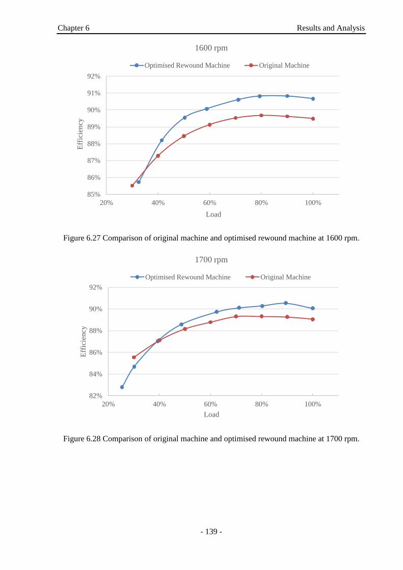
Chapter 6 Results and Analysis
- 139 -
Figure 6.27 Comparison of original machine and optimised rewound machine at 1600 rpm.
Figure 6.28 Comparison of original machine and optimised rewound machine at 1700 rpm.
85%
86%
87%
88%
89%
90%
91%
92%
20% 40% 60% 80% 100%
Eff
icie
ncy
Load
1600 rpm
Optimised Rewound Machine Original Machine
82%
84%
86%
88%
90%
92%
20% 40% 60% 80% 100%
Eff
icie
ncy
Load
1700 rpm
Optimised Rewound Machine Original Machine

Chapter 6 Results and Analysis
- 140 -
Figure 6.29 Comparison of original machine and optimised rewound machine at 1800 rpm.
Although the numerical and experimental results show similar trends in the two machine
designs, the numerical results do not precisely coincide with the experimental results. The
difference between the FEM and experimental results may be caused by several factors. Firstly,
the stator power loss is dependent on the winding temperature, and there is no guarantee that
the numerical and experimental tests were conducted at exactly the same winding temperature.
Secondly, there is no sensor to measure the rotor temperature, and so the rotor copper loss is
determined using IEEE standard methods. Thirdly, windage and friction and stray load losses
are also not measured in the numerical studies, and are a function of operational speed and load.
6.4 Summary
The results from simulation and practical work with both the original machine and the optimised
rewound machine have been presented in this chapter. The experimental results were used to
verify the FE predictions.
The no-load test compared the value of core loss and windage and friction losses in the original
and optimised rewound machines. It was found that the core loss and windage and friction
losses of the optimised rewound machine slightly increase. The load test was used to achieve
the segregation of losses such as conductor losses and stray load loss, whilst measuring machine
efficiency. The comparison of load test results was carried out on both machines under the same
experimental condition and with the same methods. This has shown that the stator conductor
83%
84%
85%
86%
87%
88%
89%
90%
91%
20% 40% 60% 80% 100%
Eff
icie
ncy
Load
1800 rpm
Optimised Rewound Machine Original Machine

Chapter 6 Results and Analysis
- 141 -
loss in the optimised rewound machine is much lower than in the original machine, but the rotor
conductor loss in the optimised rewound machine has slightly increases due to the higher
current density in the rotor winding. Beside this, the analysis of stray load loss was carried out
using the total losses in the DFIG. It was found that the efficiency of the optimised rewound
machine was about 0.6% better than that of the original machine in the sub-synchronous mode,
and about 1% better in the super-synchronous mode.

Chapter 7 Wind Energy Production
- 142 -
Chapter 7 Wind Energy Production
An estimation of the annual wind energy production of a wind turbine at a specific location is
presented in this chapter. The wind resource and its characteristics are investigated to estimate
the actual wind power in the air using the wind speed profile from a testing point. Annual wind
speed data is analysed using a statistical estimation method to determine the probability density
function of wind speed at a specific site. The annual power output of a wind turbine at the
Albemarle site is determined, along with studies of the Betz Law, Power Law, and turbine
power curve. A comparison of the annual wind energy production using the original and the
optimised rewound turbine generator is then presented. Meanwhile, improvements
demonstrated in the 55 kW wind turbine as a case study are now used to look at potential and
improvement in a real wind turbine.

Chapter 7 Wind Energy Production
- 143 -
7.1 Introduction
The United Kingdom is one of the most windy countries in Europe; the estimated mean wind
speed at a height of 45 metres is between 6 m/s and 7 m/s for England, and between 7 m/s and
8 m/s for Scotland [194-196]. Therefore, developing the wind technologies for the utilisation
of renewable wind resources in UK is an important task.
Before any wind turbine is installed, extensive knowledge of the wind characteristics at a
specific site has to be gained in the following areas [15]:
System design – the selection of an appropriate size of wind turbine for a particular site.
Hence, information about this site is required such as the wind speed profile and
variation, and the status of extreme wind.
Data analysis – initial wind speed data requires correction for turbine height and an
estimation of mean wind speed, as well as the statistics for wind speed variation.
Performance evaluation – prediction of annual energy production and cost effectiveness
based on the wind speed profile at the specific location.
Operation – a series of data analyse will be used for load and operation management
and system maintenance.
In this chapter, the wind speed profile at a specific location – Albemarle site (Latitude = 55:02
N, Longitude = 01:88 W), is analysed once the wind speed correction for the height difference
between the testing point and the wind turbine is completed. Also, the mean wind speed and
available wind power are estimated. Furthermore, in order to precisely predict the annual energy
production of a wind turbine at this specific site, one of the most important parts is that the
measurement of the Weibull distribution must be carried out to analyse the probability of wind
speed variation.
7.2 Estimation of Wind Resource
Actual annual wind speed data from a U.K. wind farm at Albemarle as shown in figure 7.1 was
analysed using statistical methods. The height of the test point is 144 metres.

Chapter 7 Wind Energy Production
- 144 -
Figure 7.1 Annual wind speed data at Albemarle.
7.2.1 Available Wind Power
Assuming that the rotor diameter is 19m, which is one of the largest rotor diameters per rated
kW in its class, when the wind is blowing to the turbine, the mass flow of air, 𝑑𝑚
𝑑𝑡, through the
swept area of turbine blade As, with air density ρa, and wind velocity Vw, is given by:
a s w
dmAV
dt (7.1)
The air density is 1.225 kg/m3 in standard condition (sea-level, 15). So the wind power is
shown in equation 7.2, which is proportional to the swept area of the rotor blade and the wind
velocity cubed.
31
2a s wP AV (7.2)
0
2
4
6
8
10
12
14
16
18
20
0 50 100 150 200 250 300 350
Win
d S
pee
d (
m/s
)
Day

Chapter 7 Wind Energy Production
- 145 -
Figure 7 2 Available wind power at Albemarle site.
Figure 7.2 gives the estimation of wind power at the Albemarle site. However, this is an ideal
situation. In reality the fluid mechanics of air flow through the turbine blades, their
aerodynamics, and the efficiency of the rotor/generator combination have a huge effect on
actual power production, which is approximately 45% at most values of available wind power
in the best horizontal axis wind turbines [15].
7.2.2 Mean Wind Speed
Compared to the direct method of mean value measurement, a more useful calculation of annual
mean wind speed 𝑤 over Nob observations is given by equation 7.3:
1
33
1
obN
wiw
ob
VV
N
(7.3)
Therefore, the mean wind speed at Albemarle site is about 6.32 m/s.
The estimation of power density is used to evaluate whether or not the wind resource is
generally sufficient, but it needs more accurate estimation if hourly wind speed data is available,
and so the observed points are for 8760 hours in a year. Then, the average wind power density
is determined from hourly mean wind speed Vh and energy pattern factor Ke as in equations 7.4
and 7.5.
0
200
400
600
800
1000
0 50 100 150 200 250 300 350
Win
d P
ow
er (
kW
)
Day

Chapter 7 Wind Energy Production
- 146 -
31
2a e w
s
PK V
A (7.4)
3
31
1 obN
e h
iob w
K VN V
(7.5)
A wind power density of less than 100 W/m2 is defined here as a low wind source, which means
that this place is not suitable to site a wind turbine; whereas at around 400 W/m2 it is a good
site; A very good wind resource has a power density of more than 700 W/m2 [15].
7.2.3 Power Law Profile
The power law is used to describe velocity with height due to surface roughness and boundary
effects, as in the equation shown below:
2
2 1
1
VH
VH
(7.6)
where V1 is the wind speed at a reference height H1, H2 is the projected height, and λ is the
power law exponent.
The power-law component, λ, depends upon the roughness of the surface. For open land, λ is
usually chosen as 1/7. From the previous studies [197, 198], the power law exponent is
determined as follows:
0
1
lnZ
Z
(7.7)
where Z0 is the aerodynamic roughness length, which depends on wave characteristics. It can
also be computed as shown in equation 7.8 [198, 199]:
4.5
0 1200 s
s p
Z H
H L
(7.8)
where Hs and Lp are the significant wave height and peak wave length respectively for the wave
spectrum.

Chapter 7 Wind Energy Production
- 147 -
The height of the test point at the Albemarle site is 144 metres and the turbine’s tower height is
36 metres, so figure 7.3 compares the available wind power captured with two different heights
at Albemarle after using power law correction.
Figure 7.3 Actual wind speed at turbine height.
Therefore, the wind turbine with 19 metres rotor diameter and 36 metres tower height is able to
harvest the available wind power at a height lower than the test point, as shown in figure 7.4.
Figure 7.4 Available wind power for wind turbine.
0
2
4
6
8
10
12
14
16
18
20
0 50 100 150 200 250 300 350
Win
d S
pee
d (
m/s
)
Day
wind speed at test point height wind speed at turbine height
0
100
200
300
400
500
600
0 50 100 150 200 250 300 350
Win
d P
ow
er (
kW
)
Day

Chapter 7 Wind Energy Production
- 148 -
7.3 Statistical Analysis of Wind Speed Data
It is very important to describe the variations in wind speed at a specific site and to estimate the
annual energy production from a wind turbine located there. To compute a random variable
such as wind speed, a probability density function is used to describe the likelihood of wind
speeds occurring. Two main types of probability density function are used to fit the distribution
of wind speed frequencies: the Rayleigh distribution and the Weibull distribution.
7.3.1 Rayleigh Probability Distribution
The Rayleigh distribution is simpler than the Weibull distribution in representing wind
resources, because only one parameter is used: mean wind speed. The Rayleigh probability
density function and the cumulative distribution function are expressed as the following
equations [15]:
2
22 4
w w
w w
V Vf V exp
V V
(7.9)
2
14
w
w
VF expv
V
(7.10)
Therefore, mean wind speed has a direct effect on the pattern of the Rayleigh probability density
function, as shown in figure 7.5. When the mean wind speed increases, a larger value of
probability density function is given.
Figure 7.5 Rayleigh distribution with different mean wind speed [15].

Chapter 7 Wind Energy Production
- 149 -
7.3.2 Weibull Probability Distribution
Unlike the Rayleigh distribution, the Weibull probability distribution adopts two parameters, a
shape factor k and a scale factor c, in wind speed analysis. This has been shown to give a better
and more accurate fit to measured wind speed data [200], and hence it is most commonly
recommended. However, situations of extreme wind speeds are not included in the analytic
procedure.
The Weibull probability density function is expressed as in equation 7.11.
1
kwVk
cww
Vkf V e
c c
(7.11)
The probability function can also be interpreted as a relative fractional probability function,
since wind speed exceeds zero in reality. The Weibull cumulative distribution function is given
by:
0
1
kwV
c
w wF v f V dV e
(7.12)
Therefore, the most important parameters in the Weibull distribution are the shape and scale
factors. The brief description in figure 7.6 shows that with an increasing shape factor increasing,
the peak of the curve becomes sharper when the mean wind speed is at a constant value.
Figure 7.6 Example of the Weibull distribution when mean wind speed is 6 m/s [15].

Chapter 7 Wind Energy Production
- 150 -
Several methods have already been used for the estimation of the Weibull distribution
parameters, such as statistical estimation, maximum likelihood and graphic methods. Among
these, the statistical estimation method uses average wind velocity and standard deviation to
estimate the Weibull probability density function based on statistical data of the wind speed.
The biggest advantages of this method is simple, convenient, and high precise. Therefore, it
was widely used and applied in wind data analysis.
It is worth noting that the shape and scale factors are related to mean wind speed and standard
deviation σ in the Weibull distribution. The mean wind speed describes the main tendency
change of in the data and the standard deviation of a sample represents the extent of deviation
from the mean wind speed [201]. The standard deviation of wind speed and mean wind speed
can be expressed as in equations 7.13 and 7.14.
22
1
1 obN
i w
iob
V VN
(7.13)
1
33
1
obN
iiw
ob
VV
N
(7.14)
Hence, the standard deviation of the wind speed at Albemarle is 2.94 when the mean wind speed
is 6.32 m/s. Therefore, the shape factor can be determined by a good approximation as shown
in equation 7.15, but there is a limitation in this approximation, which is that 1 ≤ k <10.
1.086
w
kV
(7.15)
So, the shape factor is calculated as 2.29 for Albemarle. The scale factor can also be solved
using the gamma function as in equation 7.16.
1
1
wVc
k
(7.16)
An approximation for the determination of the scale factor, which is shown in equation 7.17:
1
1 0.4341 0.568
k
k k
(7.17)

Chapter 7 Wind Energy Production
- 151 -
After calculating the gamma function, the scale factor is about 7.133 at Albemarle. Then, the
Weibull probability density functions and cumulative distribution functions at different wind
speeds can be obtained. It should be noted that in the Weibull distribution there is a special case
that when the shape factor k=2, when it equals the Rayleigh distribution. The Weibull
distribution at the Albemarle site is presented in figure 7.7. It can be seen that the highest
frequencies of wind speeds occurring are concentrated in the range between 4 m/s to 8 m/s. The
Weibull probability density function is hence expressed as in equation 7.18.
2.291.29
7.1330.3217.133
wV
ww
Vf V e
(7.18)
Figure 7.7 Weibull distribution at Albemarle site.
Tables 7.1 and 7.2 present the frequency and average days of various wind speeds in a year at
the Albemarle site, which are calculated based on the Weibull distribution. This will then be
used to estimate the annual wind turbine energy production.
0
0.02
0.04
0.06
0.08
0.1
0.12
0.14
1 2 3 4 5 6 7 8 9 10 11 12 13 14 15
Pro
bab
ilit
y
Wind Speed (m/s)

Chapter 7 Wind Energy Production
- 152 -
Table 7.1 Probability of wind speed at Albemarle site
Wind Speed
(m/s) Frequency
Wind Speed
(m/s) Frequency
1 3.18 % 9 7.95 %
2 6.17 % 10 5.39 %
3 8.87 % 11 3.88 %
4 11.24 % 12 2.47 %
5 12.83 % 13 1.43 %
6 12.92 % 14 0.56 %
7 11.92 % 15 0.42 %
8 10.76 %
Table 7.2 Wind speed of average days in a year
Wind Speed
(m/s) Days in a year
Wind Speed
(m/s) Days in a year
1 11.6 9 29.0
2 22.5 10 19.7
3 32.4 11 14.2
4 41.0 12 9.0
5 46.8 13 5.2
6 47.2 14 2.0
7 43.5 15 1.6
8 39.3 Total 365
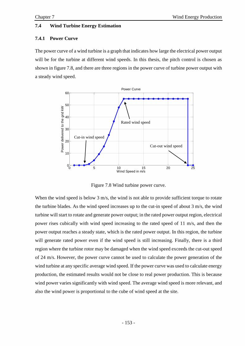
Chapter 7 Wind Energy Production
- 153 -
7.4 Wind Turbine Energy Estimation
7.4.1 Power Curve
The power curve of a wind turbine is a graph that indicates how large the electrical power output
will be for the turbine at different wind speeds. In this thesis, the pitch control is chosen as
shown in figure 7.8, and there are three regions in the power curve of turbine power output with
a steady wind speed.
Figure 7.8 Wind turbine power curve.
When the wind speed is below 3 m/s, the wind is not able to provide sufficient torque to rotate
the turbine blades. As the wind speed increases up to the cut-in speed of about 3 m/s, the wind
turbine will start to rotate and generate power output; in the rated power output region, electrical
power rises cubically with wind speed increasing to the rated speed of 11 m/s, and then the
power output reaches a steady state, which is the rated power output. In this region, the turbine
will generate rated power even if the wind speed is still increasing. Finally, there is a third
region where the turbine rotor may be damaged when the wind speed exceeds the cut-out speed
of 24 m/s. However, the power curve cannot be used to calculate the power generation of the
wind turbine at any specific average wind speed. If the power curve was used to calculate energy
production, the estimated results would not be close to real power production. This is because
wind power varies significantly with wind speed. The average wind speed is more relevant, and
also the wind power is proportional to the cube of wind speed at the site.
0 5 10 15 20 250
10
20
30
40
50
60
Wind Speed in m/s
Po
wer
de
live
red
to
th
e g
rid k
W
Power Curve
Cut-in wind speed
Rated wind speed
Cut-out wind speed

Chapter 7 Wind Energy Production
- 154 -
7.4.2 Betz Law
A German physicist, Albert Betz, concluded that a wind turbine is not able to convert more than
16/27 of the kinetic energy of wind into mechanical energy [202]. This is known as the Betz
Law. The power coefficient of wind turbine can be expressed in equation 7.19.
3
1
2
rotorp
a s w
P Rotor PowerC
Wind PowerA V
(7.19)
In theory, the maximum power coefficient Cpmax for any wind turbine design is 16/27, which is
defined as in equation 7.20:
16
0.592627
pmaxC (7.20)
However, only an ideal wind turbine can operate with the maximum power coefficient. In
reality, the real power coefficient is between 0.35 to 0.45 after taking into account various
inevitable losses, such as bearing, gearbox, and generator losses [203], so that only
approximately 10-30% of the wind power can be converted into usable electricity. In this work,
the conventional efficiency of 30% is assumed. Figure 7.9 gives a clear comparison of the wind
power wastage at the Albemarle site.
Figure 7.9 Wind power wastage.
0
2
4
6
8
10
12
1 2 3 4 5 6 7 8 9 10 11 12 13 14 15
Pow
er (
kW
)
Wind Speed (m/s)
Actual Wind Power Usable Wind Power (Betz Law) Turbine Power Output

Chapter 7 Wind Energy Production
- 155 -
7.4.3 Wind Turbine Annual Energy Production
The basic information about the wind turbine can be used to determine its annual power output.
Combined with the Weibull probability density function p(Vw), the average wind turbine energy
production can be expressed as in equation 7.21.
0
w w w w wP P V p V dV
(7.21)
Therefore, taking into consideration the drive train efficiency (generator power/rotor power) η1
and generator efficiency η2, another equation for the average power output of a turbine
generator is given by equation 7.22:
3
1 2
0
1
2w a s p w w wP A C V p V dV
(7.22)
In figure 7.10, the energy production with different wind speed and the Weibull distribution are
presented, and hence can be used to estimate actual annual energy production.
Figure 7.10 Estimation of annual energy production.
Assuming that drive train efficiency has a constant value, the annual energy production based
on the wind speed profile at the given site can be found to be approximately 192.3 MWh.
Detailed information about annual energy production is shown in Table 7.3 and Figure 7.11.
0
200000
400000
600000
800000
1000000
1200000
1400000
1600000
1800000
0
0.02
0.04
0.06
0.08
0.1
0.12
0.14
1 2 3 4 5 6 7 8 9 10 11 12 13 14 15
Ener
gy O
utp
ut (k
Wh)
Pro
bab
ilit
y
Wind Speed (m/s)

Chapter 7 Wind Energy Production
- 156 -
Table 7.3 Annual Energy Production
Wind Speed (m/s) Energy
Production (kWh) Wind Speed (m/s)
Energy
Production (kWh)
1 0 9 26724.83
2 0 10 24868.69
3 1105.608 11 23852.63
4 3318.09 12 19692.09
5 7401.433 13 14492.85
6 12879.1 14 7078.476
7 18870.98 15 6613.235
8 25411.29 Total 192309.3
Figure 7.11 Annual energy production at Albemarle site.
7.4.4 Improved Annual Energy Production
As referred to in section 7.3, no power is generated from the wind turbine in the first region,
and so the wind speed data in this area is not relevant to the performance of a turbine generator.
Then, with increasing wind speed, the turbine power output increases rapidly until the rated
wind speed is reached. This is the power increase area. The turbine generator then begins to
produce electrical power in sub-synchronous operational mode since the wind speed is between
3 to 11 m/s, and the rotational speed range of the turbine generator is from 1200 rpm to a value
less than 1500 rpm. From figure 7.12, it can be found that the higher probabilities of wind speed
0
5000
10000
15000
20000
25000
30000
3 5 7 9 11 13 15
Ener
gy P
roduct
ion (
kW
h)
Wind Speed (m/s)

Chapter 7 Wind Energy Production
- 157 -
always appear between 3 to 9 m/s, and so efficiency improvement is focused on sub-
synchronous operational mode. The final region is the constant power output area when the
wind speed exceeds the rated wind speed of 11 m/s. The DFIG is then running in the super-
synchronous operational mode since the generator speed is above 1500 to 1800 rpm.
Figure 7.12 High probability area with turbine power curve.
Because the wind turbine adopts the pitch control, the power generation is kept constant of 55
kW once the rated power level is achieved. Therefore, the improved efficiency of the optimised
rewound machine is only affect power increase area. In the power increase area, as referred to
in Chapter 6, the efficiency of the optimised rewound DFIG is improved by about 0.9%, 0.4%,
and 0.6% at 1200, 1300, 1457 rpm respectively, as shown in figure 7.13. So, based on equation
7.22, the improvement of the annual energy production is about 106.43, 228.65, and 452.68
kWh at these three generator rotational speed levels. Hence, the total improvement in annual
energy production is 787.76 kWh.
0
10
20
30
40
50
60
0
0.02
0.04
0.06
0.08
0.1
0.12
0.14
1 2 3 4 5 6 7 8 9 10 11 12 13 14 15
Pow
er O
utp
ut
(kW
)
Pro
bab
ilit
y
Wind Speed (m/s)
Power Increasing Area Constant Power Output No Power

Chapter 7 Wind Energy Production
- 158 -
Figure 7.13 Improvement in annual energy production.
As a result, in this case study of a 55 kW wind turbine, if the price for 1 kWh of electricity is
£0.145, then after winding repair and re-design, the extra saving per year is about £114.225. It
can be imagined that the repair and re-design of a mega-watts wind turbine generator could
save much more, so £114.225 on a 55 kW wind turbine could be scaled up to £4153.636 on a 2
MW wind turbine per year, if applied to 50 2-MW DFIG wind turbines over 5 year lifetime, the
total of 1 million pounds are saved.
The greatest interest of this work is to improve the machine efficiency to obtain the maximum
power generation; in the meanwhile, an alternative way of illustrating wind turbine performance
is to check the capacity factor, CF, for the turbine in a specific location. The capacity factor is
the energy actually produced by the turbine divided by the theoretical rated power output PR,
which is expressed as in equation 7.23.
w
R
PCF
P (7.23)
Therefore, the capacity factors of the original wind turbine and optimised wind turbine are 39.91%
and 40.19% respectively. Due to the efficiency of the optimised rewound DFIG is higher than
the original DFIG, so the average power output of a wind turbine is improved accordingly,
which means that the optimised wind turbine gives better performance than the original.
0
100000
200000
300000
400000
500000
600000
0
0.02
0.04
0.06
0.08
0.1
0.12
0.14
3 4 5 6 7 8 9 10 11
Win
d E
ner
gy O
utp
ut
(kW
h)
Pro
bab
ilit
y
Wind Speed (m/s)
0.9 %
0.4 %
0.6 %

Chapter 7 Wind Energy Production
- 159 -
7.5 Summary
The status of the wind resource and its characteristics has been introduced in this chapter,
presenting the different types of wind speed variation and the effects of wind speed at different
locations. The available wind power and mean wind speed have been estimated from the wind
speed profile of a specific location at Albemarle site. The power law is used to correct the actual
wind speed for turbine height, since the wind speed data is obtained from a specific test point
higher than the turbine height. The Weibull distribution has been chosen to analyse the
probability density of wind speed variations at the Albemarle site in this thesis, since research
into the most important factors in the Weibull distribution, the shape and scale factors, was
carried out using the statistical estimation method. Betz Law states that only part of available
wind power can be harvested by a wind turbine, and a series of mechanical losses also reduces
the utilization of wind power. The process of determining the annual energy production of a
wind turbine at the given site has been demonstrated, which is combined with the Weibull
probability density function, turbine power curve, and wind speed data. In this work, according
to the winding re-design and optimisation, the stator copper loss of the DFIG machine is
reduced to improve efficiency. So a comparison has been conducted of annual energy
production in the original and the optimised rewound DFIG wind turbines and the capacity
factors for both wind turbines have been determined.

Chapter 8 Conclusions
- 160 -
Chapter 8 Conclusions
The key points and important outcomes of the thesis are summarised in this chapter. The
winding repair and re-design of a doubly fed induction generator to obtain the maximum wind
energy production has been studied. This chapter also includes suggestions for future work.
8.1 Conclusions
The work of this thesis has been carried out in a number of steps.
First of all, the relevant literature has been reviewed in Chapter 2, and this has shown that the
doubly fed induction generator (DFIG) has huge potentials to be developed for wind energy
applications due to the overall considerations of cost, eco-friendliness, and machine
performance. The estimation of wind energy production is significantly related to the turbine
topology used, and much work has been undertaken on the design and topologies of modern
wind turbine generators. Nowadays, the specific sized DFIGs from different wind turbine
manufacturers are mass-produced, which have their fixed generator structure and winding
configurations. They are designed and operated for a large range of wind speed, so the problem
of modern DFIGs is that they are not running at the best operation point generally. When the
failure occurs in the turbine generator, it needs to be repaired and re-designed for safety reasons.
A study of turbine failures has highlighted winding faults in either the stator or the rotor. Current
opinions on repairing or replacing the generator with faulty winding were described, whilst
winding repair generally are attempted to return to the original design. However, in this thesis
a new viewpoint on winding repair is proposed, because it is a good opportunity to re-design
and optimise the winding configuration while the machine is being repaired in order to achieve
better performance than before.
The mechanical aspects of an existing doubly fed induction generator such as winding
configuration and laminations of the stator and rotor, have been studied in Chapter 3. In order
to improve machine efficiency, a study of the major power losses in DFIGs is presented and
analysed. This shows the characteristics and determination of conventional losses and
additional loss. An off-the-shelf 55kW, 4-pole, three-phase DFIG was modelled with an
electromagnetic finite element tool in order to validate the optimisation process, and the model
was solved by a 2-D transient with a motion optimiser. Its inclusion is important to validate the
Chapter 8 Conclusions
- 161 -
model’s accuracy via electromagnetic field and loss analysis in different components in the
machine. However, some limitations in the finite element analysis were also identified; these
are that the stray load loss cannot be estimated and nor can windage and friction losses be
included. A novel method of combining finite element analysis with an evolutionary
optimisation algorithm had been chosen to optimise the DFIG’s windings.
The novel approach to the winding re-design and optimisation of the DFIG was then focused
in Chapter 4. Based on the original design (stator: 16 turns with 4.29 mm2 cross-sectional area,
rotor: 12 turns with 6.95 mm2 cross-sectional area), a process of finite element-based surrogate
optimisation algorithm has been deployed to explore which combination of winding turn and
cross-sectional area of the stator and rotor has the highest efficiency. In this procedure, the
design of experiment is used to allocate the sampling points in the design space, in order to
minimise the time consumed and maximise the information acquired from a trade-off between
the number of selected points and the amount of information. The Latin Hypercube sampling
technique is the DoE technique selected to generate the random and uniform sampling
distributions. This has led to the maximising the amount of information acquired with the
minimum bias error, since a totally 34 and 36 sampling points were selected to build the
surrogate model of the stator winding and rotor winding. These sampling points have been used
in the finite element programme to obtain the numerical results of the electromagnetic analysis.
The results have then been further used to build the surrogate model of the DFIG and the
Kriging model takes the finite element outputs to estimate the value or response of a function
in the unknown area. The errors in the estimation fluctuate around the real function. With more
sampling points selected, the estimated function will become closer to the real function. The
optimisation algorithm is then developed to find the optimal location, once the surrogate model
is created. In addition, the particle swarm optimisation algorithm has already been proven to be
an efficient method, and has been adopted to find the best solution of the DFIG windings. The
optimised winding parameters for the stator and rotor windings are 14 turns with 5.21 mm2
cross-sectional area and 10 turns with 5.94 mm2 cross-sectional area, respectively. The
optimisation results have been successfully validated using the finite element analysis.
The optimised plan of the DFIG has been implemented, with the design of the machine winding
parameters learned along the way. The American IEEE standard 112-B for polyphase induction
machine testing has then been selected after comparison with other international testing
standards, due to its relatively higher precision. The IEEE standard 112-B is used for
conventional induction machine testing, but is found to be difficult to satisfy the requirements
of this work. An improved testing method based on IEEE standard 112-B has been developed

Chapter 8 Conclusions
- 162 -
to measure generator efficiency using an input-output method with loss segregation as described
in Chapter 5. In this method, the determination of the machine efficiency at sub-synchronous
and super-synchronous operational modes should be conducted separately. Meanwhile, the
converter efficiency of 95% has already been considered with grid-side rotor power. The
original and optimised rewound DFIGs have been tested based on this improved testing method
and presented in Chapter 6. The two machines are compared using the same method and
conditions. The no-load tests on the machines were used to determine the core loss and windage
and friction loss, the core loss of 521.47W and windage and friction loss of 1280.61W in the
optimised rewound DFIG has a slight increasing than that of 501.95W and 1136.44W in the
original DFIG. The load tests were used to determine conductor losses, stray load loss, and
machine efficiency. The tests show that the stator conductor loss in the optimised rewound
machine reduces significantly than the original machine, but the rotor conductor loss only
increases slightly. Overall, the optimised rewound DFIG has 0.9%, 0.4%, and 0.6% efficiency
improvement than the original machine at 1200, 1300, and 1457 rpm during the sub-
synchronous mode, respectively. In the super-synchronous operational mode, the machine
efficiency of the optimised rewound DFIG has improved by 1%, 1%, and 1.3% than the original
DFIG at 1600, 1700, and 1800 rpm, respectively.
Finally Chapter 7 has focused on the estimation of the annual wind energy production at a
specific site in the UK. The wind speed and direction vary randomly, and are also dramatically
affected by the surrounding environment. The wind speed profile of the Albemarle site was
analysed by combing the processed wind speed results with the turbine topology and tower
height following the Power Law and Betz Law. In addition, the Weibull distribution had been
employed to calculate the probability of the annual wind speed for annual power production.
Two 55 kW DFIGs were used on the wind turbine as a case study, and the annual wind energy
production had been further calculated by considering all of the factors involved. The efficiency
improvement of turbine generator lead to the increased annual energy production of 787.76
kWh, and the economic saving is £114.225 per year for one 55 kW wind turbine after winding
re-design. If it is then scaled up to 50 2 MW DFIG wind turbines for 5-year operation, the total
amount of 1 million pounds could be saved.
From this work, it is evident that the machine efficiency of turbine generators can be improved
during machine repair and rewinding procedures by incorporating the site-specific wind profile
and machine operational characteristics. This is more significant for the wind turbines operating
towards the end of their service life. A key message from this work is that the industrial mind-
set needs to be changed. That is, the machine rewinding holds a unique opportunity to resign

Chapter 8 Conclusions
- 163 -
the machine, instead of faithfully following the original design, which is presently the common
practice in industry. By doing so, the wind power industry will benefit from this work by the
increased productivity. The society will benefit from the growing penetration of renewable
energy in the power network. In the long run, everyone on the planet will benefit by the
significant reduction off greenhouse gas emissions to the atmosphere.
8.2 Future work
With the work is presented in this thesis, a few key areas are open for further investigation and
exploration:
Further investigation might apply the surrogate optimisation algorithm to the structural
optimisation of different parts of electrical machines, such as slot shape and the size of
internal components, since it has been proven to give good performance for the
electromagnetic design.
For specific industrial applications, the optimisation objectives and constraints can be
defined more flexible, such as high torque density and low torque ripple. Therefore, the
surrogate optimisation can be used in a wide range of applications.
Further investigation of multi-objective and multi-variable optimisation can be explored to
solve more complex problems, such as the efficiency improvement and cost reduction.
The environment surrounding a wind turbine in a specific location is not always flat, and it
has been shown that the terrain with obstacles has a significant effect on wind speed and
characteristics. Considering all the factors influencing wind turbine operation, more
accurate short-termed wind speed data are needed for statistical analysis.

Reference
- 164 -
References
[1] I. E. A. Staff, Energy Balances of Non-OECD Countries 2000-2001, 2003 Edition:
OECD, 2003.
[2] J. Goldemberg, T. B. Johansson, D. Anderson, P. United Nations Development, E.
United Nations. Dept. of, A. Social, et al., World Energy Assessment: Overview : 2004
Update: United Nations Development Programme, Bureau for Development Policy,
2004.
[3] W. E. Council, "World Energy Assessment: Energy and the Challenge of
Sustainability," December 2000.
[4] G. W. E. Council. (2014). Global Wind Report Annual Market 2014. Available:
http://www.gwec.net/global-figures/graphs/
[5] W. Wei, M. Kiani, and B. Fahimi, "Optimal Design of Doubly Fed Induction Generators
Using Field Reconstruction Method," Magnetics, IEEE Transactions on, vol. 46, pp.
3453-3456, 2010.
[6] M. V. Lowson, "A new prediction model for wind turbine noise," in Renewable Energy
- Clean Power 2001, 1993., International Conference on, 1993, pp. 177-182.
[7] A. L. Rogers and J. F. Manwell, "Wind Trubine Noise Issues - A white paper,"
Renewable Energy Research Laboratory, Center for Energy Efficiency and Renewable
Energy, Department of Mechanical and Industrial Engineering, University of
Massachusetts at Amherst, Amherst, MA 01003 June 2002.
[8] S. Wagner, R. Bareiss, and G. Guidati, Wind turbine noise: Springer, 1996.
[9] M. Associates, "Landscape assessment for wind farm planning and design-character and
sensitivity," Final Report2000.
[10] S. M. Lowther and S. Tyler, "A review of impacts of wind turbines on birds in the UK,"
Report No. W/13/00426/REP3, Energy Technology Support Unit (ETSU)1996.
[11] T. J. Price, "James Blyth – Britain’s First Modern Wind Power Engineer," Wind
Engineering, vol. 29, pp. 191-200, 2005.
[12] K. Warnes, "Poul la Cour Pioneered Wind Mill Power in Denmark," History, 2013.
[13] N. E. Power. (2010). The return of windpower to Grandpa's Knob and Rubland country.
[14] GWEC, "Global wind report annual market update 2013," Global Wind Energy
Council,2013.
[15] J. F. Manwell, J. G. McGowan, and A. L. Rogers, Wind energy explained: theory, design
and application: John Wiley & Sons, 2010.
[16] B. Chen. (2013). Pitch-regulated and Stall-regulated Wind Turbine. Available:
http://www.bindichen.co.uk/post/Fundamentals/Pitch-regulated-and-Stall-regulated-
Wind-Turbine.html
[17] M. Bassyouni and S. A. Gutub, "Materials selection strategy and surface treatment of
polymer composites for wind turbine blades fabrication," Polymers & Polymer
Composites, vol. 21, pp. 463-471, 2013.
[18] RENK-MAAG. (2015). Parallel Shaft Gearbox. Available: http://www.renk-
maag.ch/en/gearboxes/turbo-helical-gearboxes/
[19] B. S.L. Planetary Gearbox. Available: http://www.brotomatic.es/stober-producto.php
[20] L. E. Van Bibber and J. L. Kelly, "Westinghouse 600 kW wind turbine design,"
Proceedings of Windpower, American Wind Energy Association, 1985.
[21] "Truss tower," 2011.
[22] E. d. Vries. (2013). XEMC Darwind Refocuses on Onshore Wind with 4.5- and 5-MW
Direct Drive Turbines. Available:
http://www.renewableenergyworld.com/articles/2013/11/xemc-darwind-refocuses-on-
onshore-wind-with-4-5-and-5-mw-direct-drive-turbine.html

Reference
- 165 -
[23] G. L. Johnson, Wind energy systems: Gary L. Johnson, 2006.
[24] C. J. Ifedi, "A high torque density, direct drive in-wheel motor for electric vehicles,"
Ph.D., School of Electrical and Electronic Engineering, Newcastle University, 2013.
[25] F. Magnussen, "On design and analysis of synchronous permanent magnet machines for
field weakening operation in hybrid electric vehicles," Ph.D., Department of Electrical
Engineering, Royal Institute of Technology, Sweden, 2004.
[26] Z. Q. Zhu and D. Howe, "Electrical Machines and Drives for Electric, Hybrid, and Fuel
Cell Vehicles," Proceedings of the IEEE, vol. 95, pp. 746-765, 2007.
[27] A. Grauers, "Design of direct driven permanent magnet generators for wind turbines,"
PhD, Chalmers University of Technology, 1996.
[28] J. G. Washington, G. J. Atkinson, N. J. Baker, A. G. Jack, B. C. Mecrow, B. B. Jensen,
et al., "Three-Phase Modulated Pole Machine Topologies Utilizing Mutual Flux Paths,"
Energy Conversion, IEEE Transactions on, vol. 27, pp. 507-515, 2012.
[29] D. Svechkarenko, "On design and analysis of a novel transverse flux generator for direct
driven wind application," Ph.D., The Department of Electrical Machines and Power
Electronics, Royal Institute of Technology, Sweden, 2010.
[30] H. L. H., H. L., B. F., R. E., M.-N. S., B. H., et al., "Conceptual survey of Generators
and Power Electronics for Wind Turbines," Risø National Laboratory, Roskilde,
DK2001.
[31] P. C. Desai, M. Krishnamurthy, N. Schofield, and A. Emadi, "Novel Switched
Reluctance Machine Configuration With Higher Number of Rotor Poles Than Stator
Poles: Concept to Implementation," Industrial Electronics, IEEE Transactions on, vol.
57, pp. 649-659, 2010.
[32] D. G. Dorrell, A. M. Knight, M. Popescu, L. Evans, and D. A. Staton, "Comparison of
different motor design drives for hybrid electric vehicles," in Energy Conversion
Congress and Exposition (ECCE), 2010 IEEE, 2010, pp. 3352-3359.
[33] J. Herbst, J. Hahne, H. Jordan, H. Liu, A. Gattozzi, and W. Ben, "Challenges in the
design of a 100 kw induction motor for a PHEV application," in Vehicle Power and
Propulsion Conference, 2009. VPPC '09. IEEE, 2009, pp. 408-413.
[34] Zureks, "Stator and rotor," vol. 847 KB, ed. Wikimedia Commons, 2008, pp. Stator and
rotor of a three-phase induction motor: 0.75 kW, 1420 rpm, 50 Hz, 230-400 V AC, 3.4-
2.0 A.
[35] S. Tripathy, "A Case Study of Different Generator Topologies used in Wind Turbine
Applications," National Institute of Technology Rourkela2014.
[36] N. Madani, "Design of a permanent magnet synchronous generator for a vertical axis
wind turbine," Msc, Royal Institute of Technology, Sweden, 2011.
[37] H. Geng, C. Liu, and G. Yang, "LVRT Capability of DFIG-Based WECS Under
Asymmetrical Grid Fault Condition," IEEE Transactions on Industrial Electronics, vol.
60, pp. 2495-2509, 2013.
[38] E. Hau and H. Von Renouard, Wind turbines: fundamentals, technologies, application,
economics: Springer Science & Business Media, 2013.
[39] L. Wenjin, K. Yong, T. Guangfu, and K. Ming, "Start-up and integration of DFIG-based
wind farm using modular multilevel VSC-HVDC transmission system," in Applied
Power Electronics Conference and Exposition (APEC), 2014 Twenty-Ninth Annual
IEEE, 2014, pp. 358-365.
[40] Y. Wenxian, P. J. Tavner, C. J. Crabtree, and M. Wilkinson, "Cost-Effective Condition
Monitoring for Wind Turbines," Industrial Electronics, IEEE Transactions on, vol. 57,
pp. 263-271, 2010.
[41] M. N. Zaggout, P. J. Tavner, and L. Ran, "Wind turbine condition monitoring using
generator control loop signals," in Power Electronics, Machines and Drives (PEMD
2012), 6th IET International Conference on, 2012, pp. 1-6.

Reference
- 166 -
[42] S. Djurovic, C. J. Crabtree, P. J. Tavner, and A. C. Smith, "Condition monitoring of
wind turbine induction generators with rotor electrical asymmetry," IET Renewable
Power Generation, vol. 6, pp. 207-216, 2012.
[43] K. Alewine and W. Chen, "A review of electrical winding failures in wind turbine
generators," in Electrical Insulation Conference (EIC), 2011, 2011, pp. 392-397.
[44] Z. Liu, W. Cao, Z. Tan, B. Ji, X. Song, and G. Tian, "Condition Monitoring of Doubly-
Fed Induction Generators in Wind Farms," presented at the 2013 Ninth International
Symposium on Linear Drives for Industry Applications, 2013.
[45] D. Shah, S. Nandi, and P. Neti, "Stator-interturn-fault detection of doubly fed induction
generators using rotor-current and search-coil-voltage signature analysis," Industry
Applications, IEEE Transactions on, vol. 45, pp. 1831-1842, 2009.
[46] S. Djurovic, S. Williamson, and A. Renfrew, "Dynamic model for doubly-fed induction
generators with unbalanced excitation, both with and without winding faults," Electric
Power Applications, IET, vol. 3, pp. 171-177, 2009.
[47] P. S. Barendse, B. Herndler, M. A. Khan, and P. Pillay, "The application of wavelets
for the detection of inter-turn faults in induction machines," in Electric Machines and
Drives Conference, 2009. IEMDC '09. IEEE International, 2009, pp. 1401-1407.
[48] H. Douglas, P. Pillay, and P. Barendse, "The detection of interturn stator faults in
doubly-fed induction generators," in Industry Applications Conference, 2005. Fourtieth
IAS Annual Meeting. Conference Record of the 2005, 2005, pp. 1097-1102 Vol. 2.
[49] J.-q. Li, L. Ma, and D.-y. Wang, "Influence of stator turn-to-turn short-circuit on
magnetic field of DFIG," in Electrical Machines and Systems (ICEMS), 2011
International Conference on, 2011, pp. 1-5.
[50] A. H. Bonnett, "Analysis of winding failures in three-phase squirrel cage induction
motors," IEEE transactions on industry applications, vol. 3, pp. 223-226, 1978.
[51] J. Martinez, P. C. Kjar, P. Rodriguez, and R. Teodorescu, "Short circuit signatures from
different wind turbine generator types," in Power Systems Conference and Exposition
(PSCE), 2011 IEEE/PES, 2011, pp. 1-7.
[52] K. A. Folly and S. Sheetekela, "Impact of fixed and variable speed wind generators on
the transient stability of a power system network," in Power Systems Conference and
Exposition, 2009. PSCE '09. IEEE/PES, 2009, pp. 1-7.
[53] S. Djurovic, S. Williamson, P. J. Tavner, and W. Yang, "Condition monitoring artefacts
for detecting winding faults in wind turbine DFIGs," Proceedings of EWEC 2009,
Scientific Track-Wind Turbine Electrical System & Component, 2009.
[54] W. P. Brithinee, "Electric motor repair industry update," Electrical Insulation Magazine,
IEEE, vol. 9, pp. 23-24, 1993.
[55] C. Wenping and K. J. Bradley, "Assessing the impacts of rewind and repeated rewinds
on induction motors: is an opportunity for Re-designing the machine being wasted?,"
Industry Applications, IEEE Transactions on, vol. 42, pp. 958-964, 2006.
[56] EASA. Maintaining Efficiency During Electric Motor Repair [Online]. Available:
http://www.elongo.com/pdfs/MaintainEfficiency990514.pdf
[57] E Source Technology Atlas Series: Drivepower [Online]. Available:
http://www.esource.com/system/files/files/2009-07/Drivepower.pdf
[58] H. W. Penrose and B. Bauer, "Time savings and energy efficiency through alternate
electric motor rewind methods," in Electrical Electronics Insulation Conference, 1995,
and Electrical Manufacturing & Coil Winding Conference. Proceedings, 1995, pp. 457-
460.
[59] J. C. Hirzel, "Impact of rewinding on motor efficiency," in Pulp and Paper Industry
Technical Conference, 1994., Conference Record of 1994 Annual, 1994, pp. 104-107.
[60] R. S. Colby and D. L. Flora, "Measured efficiency of high efficiency and standard
induction motors," in Industry Applications Society Annual Meeting, 1990., Conference
Record of the 1990 IEEE, 1990, pp. 18-23 vol.1.

Reference
- 167 -
[61] A. Bonnett and B. Gibbon, "White Paper: The Results are in : Motor Repair's Impact on
Efficiency," EASA Tech, 2002.
[62] H. W. Penrose, "Repair Specification for Low Voltage Polyphase Induction Motors
Intended for PWM Inverter Application," Aurora, IL: Kennedy-Western University,
1997.
[63] EASA. Guidelines for Maintaining Motor Efficiency during Rebuilding [Online].
Available:
http://www.easa.com/sites/files/resource_library_public/MaintainingMotorEfficiency_
1107.pdf
[64] W. Cao, K. J. Bradley, and J. Allen, "Evaluation of additional loss in induction motors
consequent on repair and rewinding," Electric Power Applications, IEE Proceedings -,
vol. 153, pp. 1-6, 2006.
[65] M. Ruviaro, F. Runcos, N. Sadowski, and I. M. Borges, "Analysis and Test Results of
a Brushless Doubly Fed Induction Machine With Rotary Transformer," Industrial
Electronics, IEEE Transactions on, vol. 59, pp. 2670-2677, 2012.
[66] S. Wu, L. Tian, and S. Cui, "A comparative study of the interior permanent magnet
electrical machine’s rotor configurations for a single shaft hybrid electric bus," in
Vehicle Power and Propulsion Conference, 2008. VPPC'08. IEEE, 2008, pp. 1-4.
[67] Y.-Y. Choe, S.-Y. Oh, S.-H. Ham, I.-S. Jang, S.-Y. Cho, J. Lee, et al., "Comparison of
Concentrated and Distributed Winding in an IPMSM for Vehicle Traction," Energy
Procedia, vol. 14, pp. 1368-1373, // 2012.
[68] D. P. Kothari, Electric Machines (Sigma): McGraw-Hill Education (India) Pvt Limited,
2006.
[69] W. Cao, "Accurate Measurement and Evaluation Losses and Efficiency of New and
Rewound Induction Motors," Ph.D., Nottingham University, 2004.
[70] A. Krings, "Iron Losses in Electrical Machines - Influence of Material Properties,
Manufacturing Processes, and Inverter Operation," Ph.D., Electrical Engineering, Royal
Institute of Technology, 2014.
[71] A. Krings, S. Nategh, A. Stening, H. Grop, O. Wallmark, and J. Soulard, "Measurement
and modeling of iron losses in electrical machines," in 5th International Conference
Magnetism and Metallurgy WMM'12, June 20th to 22nd, 2012, Ghent, Belgium, 2012,
pp. 101-119.
[72] I. Magnet. Iron Loss Calculations in Laminated Structures. Available:
www.infolytica.com/en/applications/ex0166/
[73] G. Bertotti, A. Boglietti, M. Chiampi, D. Chiarabaglio, F. Fiorillo, and M. Lazzari, "An
improved estimation of iron losses in rotating electrical machines," Magnetics, IEEE
Transactions on, vol. 27, pp. 5007-5009, 1991.
[74] J. Pyrhonen, T. Jokinen, and V. Hrabovcova, Design of Rotating Electrical Machines:
Wiley, 2009.
[75] SKF, "General catalogue from SKF," Catalogue 4000/IV E, 1994.
[76] J. E. Vrancik, "Prediction of windage power loss in alternators," 1968.
[77] H. Auinger, "Determination and designation of the efficiency of electrical machines,"
Power Engineering Journal, vol. 13, pp. 15-23, 1999.
[78] J. Saari, Thermal Modelling of High-speed Induction Machines: Finnish Academy of
Technical Sciences, 1995.
[79] A. Nagornyy, A. K. Wallace, and A. V. Jouanne, "Stray load loss efficiency
connections," Industry Applications Magazine, IEEE, vol. 10, pp. 62-69, 2004.
[80] A. Boglietti, A. Cavagnino, L. Ferraris, and M. Lazzari, "Induction motor equivalent
circuit including the stray load losses in the machine power balance," Energy
Conversion, IEEE Transactions on, vol. 23, pp. 796-803, 2008.
[81] "IEEE Standard Test Procedure for Polyphase Induction Motors and Generators," in
IEEE Std 112-2004, ed, 2004, pp. 1-79.

Reference
- 168 -
[82] "Method for Determining Losses and Efficiency of Three-Phase Cage Induction
Motors," in IEC 61972 Standard, ed, 2002.
[83] H. Köfler, "Stray load losses in induction machines. A review of experimental
measuring methods and a critical performance evaluation," in International Conference
on Renewable Energy and Power Quality (ICREPQ), 2003.
[84] A. B. Plunkett, G. B. Kliman, and M. J. Boyle, "Digital techniques in the evaluation of
high-efficiency induction motors for inverter drives," Industry Applications, IEEE
Transactions on, pp. 456-463, 1985.
[85] C. N. Glew, "Stray load losses in induction motors: a challenge to academia," Power
Engineering Journal, vol. 12, pp. 27-32, 1998.
[86] N. Christofides, "Origins of load losses in induction motors with cast aluminium rotors,"
Electrical Engineers, Proceedings of the Institution of, vol. 112, pp. 2317-2332, 1965.
[87] K. Yamazaki and Y. Haruishi, "Stray load loss analysis of induction motor-comparison
of measurement due to IEEE standard 112 and direct calculation by finite-element
method," Industry Applications, IEEE Transactions on, vol. 40, pp. 543-549, 2004.
[88] "General requirements for rotating electrical machines - Part 102: Methods for
determining losses and efficiency from tests (excluding machines for traction
vehicles)," in IEC 34-2, ed, 1972.
[89] N. E. M. A. (NEMA) and W. DC, in NEMA standards Publication Number MG1, ed,
1993.
[90] Y. Gao, T. Sanmaru, G. Urabe, H. Dozono, K. Muramatsu, K. Nagaki, et al.,
"Evaluation of stray load losses in cores and secondary conductors of induction motor
using magnetic field analysis," Magnetics, IEEE Transactions on, vol. 49, pp. 1965-
1968, 2013.
[91] K. Yamazaki, A. Suzuki, M. Ohto, T. Takakura, and S. Nakagawa, "Equivalent circuit
modeling of induction motors considering stray load loss and harmonic torques using
finite element method," Magnetics, IEEE Transactions on, vol. 47, pp. 986-989, 2011.
[92] K. Yamazaki, "Stray load loss analysis of induction motors due to harmonic
electromagnetic fields of stator and rotor," European transactions on electrical power,
vol. 15, pp. 299-310, 2005.
[93] K. J. Bradley, W. Cao, and J. Arellano-Padilla, "Evaluation of stray load loss in
induction motors with a comparison of input-output and calorimetric methods," Energy
Conversion, IEEE Transactions on, vol. 21, pp. 682-689, 2006.
[94] C. Wenping, K. J. Bradley, J. C. Clare, and P. W. Wheeler, "Comparison of Stray Load
and Inverter-Induced Harmonic Losses in Induction Motors Using Calorimetric and
Harmonic Injection Methods," Industry Applications, IEEE Transactions on, vol. 46,
pp. 249-255, 2010.
[95] E. B. Agamloh, "An evaluation of induction machine stray load loss from collated test
results," Industry Applications, IEEE Transactions on, vol. 46, pp. 2311-2318, 2010.
[96] T. H. Morgan and P. M. Narbutovskih, "Stray Load Loss Test on Induction Machines,"
American Institute of Electrical Engineers, Transactions of the, vol. 53, pp. 286-290,
1934.
[97] N. J. Baker, "Linear generators for direct drive marine renewable energy converters,"
Durham University, 2003.
[98] R. Richter, Elektrische Maschinen, 1954.
[99] I. Boldea and S. A. Nasar, The Induction Machines Design Handbook, Second Edition:
Taylor & Francis, 2009.
[100] S. Koziel and L. Leifsson, "Surrogate-based modeling and optimization," Applications
in Engineering, 2013.
[101] S. Giurgea, H. S. Zire, and A. Miraoui, "Two-Stage Surrogate Model for Finite-
Element-Based Optimization of Permanent-Magnet Synchronous Motor," Magnetics,
IEEE Transactions on, vol. 43, pp. 3607-3613, 2007.

Reference
- 169 -
[102] S.-I. Kim, J.-P. Hong, Y.-K. Kim, H. Nam, and H.-I. Cho, "Optimal design of slotless-
type PMLSM considering multiple responses by response surface methodology,"
Magnetics, IEEE Transactions on, vol. 42, pp. 1219-1222, 2006.
[103] S. L. Ho, S. Y. Yang, G. Z. Ni, and H. C. Wong, "A response surface methodology
based on improved compactly supported radial basis function and its application to rapid
optimizations of electromagnetic devices," Magnetics, IEEE Transactions on, vol. 41,
pp. 2111-2117, 2005.
[104] T. Krishnamurthy, "Response surface approximation with augmented and compactly
supported radial basis functions."
[105] M. C. Costa, J. L. Coulomb, Y. Marechal, and S. L. Nabeta, "An adaptive method
applied to the diffuse element approximation in optimization process," Magnetics, IEEE
Transactions on, vol. 37, pp. 3418-3422, 2001.
[106] G. E. P. Box and N. R. Draper, Empirical model-building and response surfaces: Wiley,
1987.
[107] G. E. P. Box, W. G. Hunter, and J. S. Hunter, Statistics for experimenters: an
introduction to design, data analysis, and model building: Wiley, 1978.
[108] N. V. Queipo, R. T. Haftka, W. Shyy, T. Goel, R. Vaidyanathan, and P. Kevin Tucker,
"Surrogate-based analysis and optimization," Progress in Aerospace Sciences, vol. 41,
pp. 1-28, 1// 2005.
[109] A. J. Booker, J. E. Dennis Jr, P. D. Frank, D. B. Serafini, and V. Torczon, "Optimization
using surrogate objectives on a helicopter test example," in Computational Methods for
Optimal Design and Control, ed: Springer, 1998, pp. 49-58.
[110] D. L. Knill, A. A. Giunta, C. A. Baker, B. Grossman, W. H. Mason, R. T. Haftka, et al.,
"Response surface models combining linear and Euler aerodynamics for supersonic
transport design," Journal of Aircraft, vol. 36, pp. 75-86, 1999.
[111] M. M. Rai and N. K. Madavan, "Aerodynamic design using neural networks," AIAA
journal, vol. 38, pp. 173-182, 2000.
[112] M. M. Rai, N. K. Madavan, and F. W. Huber, "Improving the unsteady aerodynamic
performance of transonic turbines using neural networks," 2000.
[113] N. K. Madavan, M. M. Rai, and F. W. Huber, Neural net-based redesign of transonic
turbines for improved unsteady aerodynamic performance: National Aeronautics and
Space Administration, Ames Research Center, 1998.
[114] J. I. Madsen, W. Shyy, and R. T. Haftka, "Response surface techniques for diffuser
shape optimization," AIAA journal, vol. 38, pp. 1512-1518, 2000.
[115] N. Papila, W. Shyy, L. Griffin, and D. J. Dorney, "Shape optimization of supersonic
turbines using global approximation methods," Journal of Propulsion and Power, vol.
18, pp. 509-518, 2002.
[116] W. Shyy, N. Papila, P. K. Tucker, R. Vaidynanthan, and L. Griffin, "Global
Optimization for Fluid Machinery Applications," in Proceedings of the second
international symposium on fluid machinery and fluid engineering (ISFMFE), Beijing,
China, 2000.
[117] W. Shyy, N. Papila, R. Vaidyanathan, and K. Tucker, "Global design optimization for
aerodynamics and rocket propulsion components," Progress in Aerospace Sciences, vol.
37, pp. 59-118, 2001.
[118] R. Vaidyanathan, P. K. Tucker, N. Papila, and W. Shyy, "Computational-fluid-
dynamics-based design optimization for single-element rocket injector," Journal of
propulsion and power, vol. 20, pp. 705-717, 2004.
[119] R. Vaidyanathan, T. Goel, W. Shyy, R. T. Haftka, N. V. Queipo, and P. K. Tucker,
"Global sensitivity and trade-off analyses for multi-objective liquid rocket injector
design," in Proceedings of the 40th AIAA/ASME/SAE/ASEE joint propulsion conference
and exhibit, Fort Lauderdale, FL, 2004.

Reference
- 170 -
[120] T. Goel, R. Vaidyanathan, R. T. Haftka, W. Shyy, N. V. Queipo, and K. Tucker,
"Response surface approximation of Pareto optimal front in multi-objective
optimization," Computer methods in applied mechanics and engineering, vol. 196, pp.
879-893, 2007.
[121] L. Tenorio, "Statistical regularization of inverse problems," SIAM review, vol. 43, pp.
347-366, 2001.
[122] V. N. Vapnik and V. Vapnik, Statistical learning theory vol. 1: Wiley New York, 1998.
[123] F. Girosi, "An equivalence between sparse approximation and support vector
machines," Neural computation, vol. 10, pp. 1455-1480, 1998.
[124] A. I. J. Forrester and A. J. Keane, "Recent advances in surrogate-based optimization,"
Progress in Aerospace Sciences, vol. 45, pp. 50-79, 2009.
[125] J. Søndergaard, K. Madsen, and H. B. Nielsen, "Optimization using surrogate models-
by the Space Mapping technique," Technical University of DenmarkDanmarks
Tekniske Universitet, AdministrationAdministration, Office for Study Programmes and
Student AffairsAfdelingen for Uddannelse og Studerende, 2003.
[126] T. W. Simpson, T. M. Mauery, J. J. Korte, and F. Mistree, "Kriging models for global
approximation in simulation-based multidisciplinary design optimization," AIAA
journal, vol. 39, pp. 2233-2241, 2001.
[127] D. B. McDonald, W. J. Grantham, W. L. Tabor, and M. Murphy, "Response surface
model development for global/local optimization using radial basis functions," in
Proceedings of the eighth AIAA/USAF/NASA/ISSMO symposium on multidisciplinary
analysis and optimization, Long Beach, CA, 2000.
[128] H.-S. Chung and J. J. Alonso, "Comparison of approximation models with merit
functions for design optimization," AIAA 2000-4754, vol. 200, 2000.
[129] R. Jin, W. Chen, and T. W. Simpson, "Comparative studies of metamodelling
techniques under multiple modelling criteria," Structural and Multidisciplinary
Optimization, vol. 23, pp. 1-13, 2001.
[130] J. E. Rayas-Sánchez, "EM-based optimization of microwave circuits using artificial
neural networks: The state-of-the-art," Microwave Theory and Techniques, IEEE
Transactions on, vol. 52, pp. 420-435, 2004.
[131] J. Sacks, W. J. Welch, T. J. Mitchell, and H. P. Wynn, "Design and analysis of computer
experiments," Statistical science, pp. 409-423, 1989.
[132] A. A. Giunta, S. F. Wojtkiewicz, and M. S. Eldred, "Overview of modern design of
experiments methods for computational simulations," in Proceedings of the 41st AIAA
aerospace sciences meeting and exhibit, AIAA-2003-0649, 2003.
[133] T. J. Santner, B. J. Williams, and W. I. Notz, The design and analysis of computer
experiments: Springer Science & Business Media, 2013.
[134] J. R. Koehler and A. B. Owen, "9 Computer experiments," Handbook of statistics, vol.
13, pp. 261-308, 1996.
[135] S. Koziel and X.-S. Yang, Computational optimization, methods and algorithms vol.
356: Springer Science & Business Media, 2011.
[136] G. E. P. Box and N. R. Draper, "A basis for the selection of a response surface design,"
Journal of the American Statistical Association, vol. 54, pp. 622-654, 1959.
[137] J. Sacks and D. Ylvisaker, "Some model robust designs in regression," The Annals of
Statistics, pp. 1324-1348, 1984.
[138] B. Tang, "Orthogonal array-based Latin hypercubes," Journal of the American
statistical association, vol. 88, pp. 1392-1397, 1993.
[139] Q. S. Cheng, S. Koziel, and J. W. Bandler, "Simplified space‐mapping approach to
enhancement of microwave device models," International Journal of RF and
Microwave Computer‐Aided Engineering, vol. 16, pp. 518-535, 2006.

Reference
- 171 -
[140] M. D. McKay, R. J. Beckman, and W. J. Conover, "A comparison of three methods for
selecting values of input variables in the analysis of output from a computer code,"
Technometrics, vol. 42, pp. 55-61, 2000.
[141] M. Stein, "Large sample properties of simulations using Latin hypercube sampling,"
Technometrics, vol. 29, pp. 143-151, 1987.
[142] J. P. Costa, L. Pronzato, and E. Thierry, "A comparison between Kriging and radial
basis function networks for nonlinear prediction," in NSIP, 1999, pp. 726-730.
[143] N. R. Draper, H. Smith, and E. Pownell, Applied regression analysis vol. 3: Wiley New
York, 1966.
[144] G. H. Golub and C. F. Van Loan, Matrix computations vol. 3: JHU Press, 2012.
[145] S. M. Wild, R. G. Regis, and C. A. Shoemaker, "ORBIT: Optimization by radial basis
function interpolation in trust-regions," SIAM Journal on Scientific Computing, vol. 30,
pp. 3197-3219, 2008.
[146] T. W. Simpson, J. D. Poplinski, P. N. Koch, and J. K. Allen, "Metamodels for computer-
based engineering design: survey and recommendations," Engineering with computers,
vol. 17, pp. 129-150, 2001.
[147] J. P. C. Kleijnen, "Kriging metamodeling in simulation: A review," European Journal
of Operational Research, vol. 192, pp. 707-716, 2009.
[148] A. G. Journel and C. J. Huijbregts, Mining Geostatistics: Blackburn Press, 2003.
[149] A. O'Hagan and J. F. C. Kingman, "Curve fitting and optimal design for prediction,"
Journal of the Royal Statistical Society. Series B (Methodological), pp. 1-42, 1978.
[150] M. J. Sasena, "Flexibility and efficiency enhancements for constrained global design
optimization with kriging approximations," General Motors, 2002.
[151] P. Chandrashekarappa and R. Duvigneau, "Radial basis functions and kriging
metamodels for aerodynamic optimization," 2007.
[152] Y. Mack, T. Goel, W. Shyy, R. T. Haftka, and N. V. Queipo, "Multiple surrogates for
the shape optimization of bluff body-facilitated mixing," in Proceedings of the 43rd
AIAA aerospace sciences meeting and exhibit, Reno, NV, 2005, pp. 2005-0333.
[153] T. Goel, Y. Mack, R. T. Haftka, W. Shyy, and N. V. Queipo, "Interaction between grid
and design space refinement for bluff body-facilitated mixing," in Proceedings of the
43rd AIAA aerospace sciences meeting and exhibit, Reno, NV, 2005, pp. 2005-0125.
[154] Z. Bayraktar, J. Bossard, X. Wang, and D. H. Werner, "A real-valued parallel clonal
selection algorithm and its application to the design optimization of multi-layered
frequency selective surfaces," Antennas and Propagation, IEEE Transactions on, vol.
60, pp. 1831-1843, 2012.
[155] J. Yao, N. Kharma, and P. Grogono, "Bi-objective multipopulation genetic algorithm
for multimodal function optimization," Evolutionary Computation, IEEE Transactions
on, vol. 14, pp. 80-102, 2010.
[156] X. Li and X. Yao, "Cooperatively coevolving particle swarms for large scale
optimization," Evolutionary Computation, IEEE Transactions on, vol. 16, pp. 210-224,
2012.
[157] B.-Y. Qu, P. N. Suganthan, and J.-J. Liang, "Differential evolution with neighborhood
mutation for multimodal optimization," Evolutionary Computation, IEEE Transactions
on, vol. 16, pp. 601-614, 2012.
[158] C. Stoean, M. Preuss, R. Stoean, and D. Dumitrescu, "Multimodal optimization by
means of a topological species conservation algorithm," Evolutionary Computation,
IEEE Transactions on, vol. 14, pp. 842-864, 2010.
[159] X. Li, "Niching without niching parameters: particle swarm optimization using a ring
topology," Evolutionary Computation, IEEE Transactions on, vol. 14, pp. 150-169,
2010.

Reference
- 172 -
[160] J. Vrugt, B. Robinson, and J. M. Hyman, "Self-adaptive multimethod search for global
optimization in real-parameter spaces," Evolutionary Computation, IEEE Transactions
on, vol. 13, pp. 243-259, 2009.
[161] N. Bianchi and S. Bolognani, "Design optimisation of electric motors by genetic
algorithms," IEE Proceedings-Electric Power Applications, vol. 145, pp. 475-483, 1998.
[162] Y. Duan, R. G. Harley, and T. G. Habetler, "A useful multi-objective optimization
design method for PM motors considering nonlinear material properties," in Energy
Conversion Congress and Exposition, 2009. ECCE 2009. IEEE, 2009, pp. 187-193.
[163] G. Pellegrino and F. Cupertino, "FEA-based multi-objective optimization of IPM motor
design including rotor losses," in Energy Conversion Congress and Exposition (ECCE),
2010 IEEE, 2010, pp. 3659-3666.
[164] R. Wrobel and P. H. Mellor, "Particle swarm optimisation for the design of brushless
permanent magnet machines," in Industry Applications Conference, 2006. 41st IAS
Annual Meeting. Conference Record of the 2006 IEEE, 2006, pp. 1891-1897.
[165] M. J. Navardi, B. Babaghorbani, and A. Ketabi, "Efficiency improvement and torque
ripple minimization of Switched Reluctance Motor using FEM and Seeker Optimization
Algorithm," Energy Conversion and Management, vol. 78, pp. 237-244, 2014.
[166] M. S. Ismail, M. Moghavvemi, and T. M. I. Mahlia, "Characterization of PV panel and
global optimization of its model parameters using genetic algorithm," Energy
Conversion and Management, vol. 73, pp. 10-25, 2013.
[167] S. Palko and T. Jokinen, "Optimisation of squirrel cage induction motors using finite
element method and genetic algorithms," 1997.
[168] J. Lahteenmaki, "Optimisation of high-speed motors using a genetic algorithm," 1997.
[169] E. Dilettoso and N. Salerno, "A self-adaptive niching genetic algorithm for multimodal
optimization of electromagnetic devices," Magnetics, IEEE Transactions on, vol. 42,
pp. 1203-1206, 2006.
[170] D.-H. Cho, H.-K. Jung, T.-K. Chung, and C.-G. Lee, "Design of a short-time rating
interior permanent magnet synchronous motor using a niching genetic algorithm,"
Magnetics, IEEE Transactions on, vol. 36, pp. 1936-1940, 2000.
[171] D.-K. Lim, D.-K. Woo, I.-W. Kim, J.-S. Ro, and H.-K. Jung, "Cogging torque
minimization of a dual-type axial-flux permanent magnet motor using a novel
optimization algorithm," Magnetics, IEEE Transactions on, vol. 49, pp. 5106-5111,
2013.
[172] J. P. Lim, J. S. Rho, K. P. Yi, J. M. Seo, and H. K. Jung, "Characteristic analysis of a
traveling wave ultrasonic motor using an ellipsoidal static contact model," Smart
Materials and Structures, vol. 18, p. 115024, 2009.
[173] D.-K. Woo, J.-H. Choi, M. Ali, and H.-K. Jung, "A novel multimodal optimization
algorithm applied to electromagnetic optimization," Magnetics, IEEE Transactions on,
vol. 47, pp. 1667-1673, 2011.
[174] J. Kennedy, "Particle swarm optimization," in Encyclopedia of Machine Learning, ed:
Springer, 2010, pp. 760-766.
[175] J.-H. Seo, C.-H. Im, C.-G. Heo, J.-K. Kim, H.-K. Jung, and C.-G. Lee, "Multimodal
function optimization based on particle swarm optimization," Magnetics, IEEE
Transactions on, vol. 42, pp. 1095-1098, 2006.
[176] K. E. Parsopoulos and M. N. Vrahatis, "On the computation of all global minimizers
through particle swarm optimization," Evolutionary Computation, IEEE Transactions
on, vol. 8, pp. 211-224, 2004.
[177] J. Robinson and Y. Rahmat-Samii, "Particle swarm optimization in electromagnetics,"
Antennas and Propagation, IEEE Transactions on, vol. 52, pp. 397-407, 2004.
[178] S. Naka, T. Genji, T. Yura, and Y. Fukuyama, "A hybrid particle swarm optimization
for distribution state estimation," Power Systems, IEEE Transactions on, vol. 18, pp.
60-68, 2003.

Reference
- 173 -
[179] G. Ciuprina, D. Ioan, and I. Munteanu, "Use of intelligent-particle swarm optimization
in electromagnetics," Magnetics, IEEE Transactions on, vol. 38, pp. 1037-1040, 2002.
[180] B. Brandstätter and U. Baumgartner, "Particle swarm optimization-mass-spring system
analogon," Magnetics, IEEE Transactions on, vol. 38, pp. 997-1000, 2002.
[181] S. L. Ho, S. Yang, G. Ni, E. W. C. Lo, and H.-c. C. Wong, "A particle swarm
optimization-based method for multiobjective design optimizations," Magnetics, IEEE
Transactions on, vol. 41, pp. 1756-1759, 2005.
[182] S.-Y. Lee, J.-H. Seo, S.-Y. Kwak, C.-G. Lee, S.-Y. Jung, and H.-K. Jung, "Optimal
design of outer rotor permanent magnet machine using improved particle swarm
optimization," in Proceedings of the 11~(th) International Conference on Electrical
Machines and Systems Volume 6, 2008.
[183] C. A. C. Coello, G. T. Pulido, and M. S. Lechuga, "Handling multiple objectives with
particle swarm optimization," Evolutionary Computation, IEEE Transactions on, vol. 8,
pp. 256-279, 2004.
[184] M. Van der Geest, H. Polinder, J. A. Ferreira, and D. Zeilstra, "Optimization and
comparison of electrical machines using particle swarm optimization," in Electrical
Machines (ICEM), 2012 XXth International Conference on, 2012, pp. 1380-1386.
[185] Y. Duan and R. G. Harley, "A novel method for multiobjective design and optimization
of three phase induction machines," Industry Applications, IEEE Transactions on, vol.
47, pp. 1707-1715, 2011.
[186] "Energy Efficiency Test Methods for Three-Phase Induction Motors," in CSA Standard
C390-93, ed, 1993.
[187] G. G. Gray and W. J. Martiny, "Efficiency testing of medium induction motors-a
comment on IEEE Std 112-1991," Energy Conversion, IEEE Transactions on, vol. 11,
pp. 495-499, 1996.
[188] B. Renier, K. Hameyer, and R. Belmans, "Comparison of standards for determining
efficiency of three phase induction motors," Energy Conversion, IEEE Transactions on,
vol. 14, pp. 512-517, 1999.
[189] A. Boglietli, A. Cavagnino, M. Lazzari, and M. Pastorelli, "Induction motor efficiency
measurements in accordance to IEEE 112-B, IEC 34-2 and JEC 37 international
standards," in Electric Machines and Drives Conference, 2003. IEMDC'03. IEEE
International, 2003, pp. 1599-1605.
[190] P. Van Roy, B. Slaets, and R. Belmans, "Induction Motor Efficiency: a number with
many meanings."
[191] C. N. Glew, "Efficiency Measurement Testing Standards Stray Loss, the Key to
Efficiency Determination," in Energy Efficiency Improvements in Electric Motors and
Drives, A. de Almeida, P. Bertoldi, and W. Leonhard, Eds., ed: Springer Berlin
Heidelberg, 1997, pp. 249-265.
[192] A. Bousbaine, W. F. Low, and M. McCormick, "Novel approach to the measurement of
iron and stray load losses in induction motors," IEE Proceedings-Electric Power
Applications, vol. 143, pp. 78-86, 1996.
[193] D. Sarkar, P. K. Mukherjee, and S. K. Sen, "Use of 3-dimensional finite elements for
computation of temperature distribution in the stator of an induction motor," in IEE
Proceedings B (Electric Power Applications), 1991, pp. 75-86.
[194] S. F. Burch, Computer modelling of the UK wind energy resource: final overview report:
Great Britain, Department of Trade and Industry, 1992.
[195] I. Troen and E. L. Petersen, European wind atlas: Risø National Laboratory, 1989.
[196] "The UK wind resource," 2001.
[197] H. A. Panofsky and J. A. Dutton, Atmospheric turbulence: models and methods for
engineering applications: Wiley, 1984.

Reference
- 174 -
[198] S. A. Hsu, "Estimating overwater friction velocity and exponent of power-law wind
profile from gust factor during storms," Journal of waterway, port, coastal, and ocean
engineering, vol. 129, pp. 174-177, 2003.
[199] P. K. Taylor and M. J. Yelland, "The dependence of sea surface roughness on the height
and steepness of the waves," Journal of physical oceanography, vol. 31, pp. 572-590,
2001.
[200] C. G. Justus, W. R. Hargraves, and A. Yalcin, "Nationwide assessment of potential
output from wind-powered generators," Journal of applied meteorology, vol. 15, pp.
673-678, 1976.
[201] D. Wei, C. Jichuan, and F. Hengchang, "Comparative research on methods of
calculating Weibull distribution parameters of wind speed," in Power and Energy
Engineering Conference (APPEEC), 2011 Asia-Pacific, 2011, pp. 1-4.
[202] A. Betz, Introduction to the theory of flow machines: Pergamon Press, 1966.
[203] R. n. renewables, "Wind Turbine Power Calculations."

Appendix
- 175 -
Appendix
A. Thermocouple
The winding temperature is very important to accurately measure the conductor losses in the
DFIG machine. According to the PT 100 thermocouple, to determine the winding temperature
by measuring its resistance, Figure A.1 and Table A.1 show the detailed resistance of PT 100
with temperature varying.
Figure A.1 Determination of winding temperature using PT 100 thermocouple.
90
100
110
120
130
140
150
0 20 40 60 80 100 120
Res
ista
nce
(Ω
)
Temperature ()

Appendix
- 176 -
Table A.1 Characteristic of PT 100 thermocouple.

Appendix
- 177 -
B. Mechanical Structure of the DFIG
Table B.1 Stator parameter for the DFIG
Stator outer diameter 445 mm
Stator inner diameter 300 mm
Stator slot depth 27.6 mm
Pole 4
Stator slot area 193.24 mm2
Number of stator slots 60
Stator winding layer Double layer
Stator coil pitch 1-14
Stator winding material Copper 100% IACS
Stator winding connection 2 delta
Table B.2 Rotor parameter for the DFIG
Rotor outer diameter 298.2 mm
Rotor inner diameter 100 mm
Rotor slot depth 36.5 mm
Pole 4
Rotor slot area 223.29 mm2
Number of rotor slots 48
Rotor winding layer Double layer
Rotor coil pitch 1-12
Rotor winding material Copper 100% IACS
Rotor winding connection 2 star

Appendix
- 178 -

Appendix
- 179 -

Appendix
- 180 -
C. Measurement of Winding Resistance
Figure C.1 Stator winding resistance measurement.
Figure C.2 Rotor winding resistance measurement.

Appendix
- 181 -
D. No-Load Test
Copyright © 2022 FDOKUMEN