
Study of Stability Analysis of a Grid-Connected Doubly Fed ...
115
Western University Western University Scholarship@Western Scholarship@Western Electronic Thesis and Dissertation Repository 7-31-2013 12:00 AM Study of Stability Analysis of a Grid-Connected Doubly Fed Study of Stability Analysis of a Grid-Connected Doubly Fed Induction Generator (DFIG)-based small Wind Farm Induction Generator (DFIG)-based small Wind Farm Baishakhi Dhar, The University of Western Ontario Supervisor: Dr. Tarlochan S Sidhu, The University of Western Ontario Joint Supervisor: Dr.Amirnaser Yazdani, The University of Western Ontario A thesis submitted in partial fulfillment of the requirements for the Master of Engineering Science degree in Electrical and Computer Engineering © Baishakhi Dhar 2013 Follow this and additional works at: https://ir.lib.uwo.ca/etd Part of the Controls and Control Theory Commons, and the Power and Energy Commons Recommended Citation Recommended Citation Dhar, Baishakhi, "Study of Stability Analysis of a Grid-Connected Doubly Fed Induction Generator (DFIG)- based small Wind Farm" (2013). Electronic Thesis and Dissertation Repository. 1398. https://ir.lib.uwo.ca/etd/1398 This Dissertation/Thesis is brought to you for free and open access by Scholarship@Western. It has been accepted for inclusion in Electronic Thesis and Dissertation Repository by an authorized administrator of Scholarship@Western. For more information, please contact [email protected].
-
Upload
khangminh22 -
Category
Documents
-
view
4 -
download
0
Transcript of Study of Stability Analysis of a Grid-Connected Doubly Fed ...

Western University Western University
Scholarship@Western Scholarship@Western
Electronic Thesis and Dissertation Repository
7-31-2013 12:00 AM
Study of Stability Analysis of a Grid-Connected Doubly Fed Study of Stability Analysis of a Grid-Connected Doubly Fed
Induction Generator (DFIG)-based small Wind Farm Induction Generator (DFIG)-based small Wind Farm
Baishakhi Dhar, The University of Western Ontario
Supervisor: Dr. Tarlochan S Sidhu, The University of Western Ontario
Joint Supervisor: Dr.Amirnaser Yazdani, The University of Western Ontario
A thesis submitted in partial fulfillment of the requirements for the Master of Engineering
Science degree in Electrical and Computer Engineering
© Baishakhi Dhar 2013
Follow this and additional works at: https://ir.lib.uwo.ca/etd
Part of the Controls and Control Theory Commons, and the Power and Energy Commons
Recommended Citation Recommended Citation Dhar, Baishakhi, "Study of Stability Analysis of a Grid-Connected Doubly Fed Induction Generator (DFIG)-based small Wind Farm" (2013). Electronic Thesis and Dissertation Repository. 1398. https://ir.lib.uwo.ca/etd/1398
This Dissertation/Thesis is brought to you for free and open access by Scholarship@Western. It has been accepted for inclusion in Electronic Thesis and Dissertation Repository by an authorized administrator of Scholarship@Western. For more information, please contact [email protected].
i
Study of Stability Analysis of a Grid-Connected Doubly Fed Induction Generator
(DFIG)-based small Wind Farm
(Thesis format: Monograph)
by
Baishakhi Dhar
Graduate Program
In
Engineering Science
Department of Electrical and Computer Engineering
A thesis is submitted in partial fulfillment
of the requirements for the degree of
Master of Engineering Science
The School of Graduate and Postdoctoral Studies
University Of Western Ontario
London, Ontario, Canada
© Baishakhi Dhar 2013

ii
Abstract
Wind is the most reliable, clean and fast-developing renewable energy source. The DFIG-
based variable speed wind turbine system is now the most popular in wind power
industry. With power being so in-demanding, a large wind farm needs to be developed to
produce more power from a stable system. But before such a large wind farm is installed,
better understanding is needed of the system’s intrinsic dynamic behavior, range of
stability region and parametric effects on system stability. Hence, a small wind farm with
two identical DFIG-based wind turbines connected to a grid network has been considered
for this study.
A detailed non-linear mathematical model of grid-connected single DFIG-based wind
turbine system as well as a grid-connected multi DFIG-based wind turbine system in a
dq-frame has been developed. Linearization of these non-linear mathematical models for
both the systems has been performed from the set of developed non-linear equations.
These two linearized dynamic models provide an analytical platform for determining the
robustness and stability of the two systems. The linearized models are then verified with
the simulation results of non-linear systems designed in a PSCAD/EMTDC environment.
This step is needed to check the performance accuracy of the linearized models. The
small-signal stability, the system’s parametric effects on stability and the modal analysis
of two developed linearized models have been studied. Participation factor analysis has
been employed to determine system parametric effects on each eigenmode. The intrinsic
dynamic behavior of a single wind turbine connected to a grid and multi wind turbines
connected to a grid (a small wind farm) are observed to be identical in nature at the same
operating conditions and system parameters.

iii
Acknowledgements
The author remembers with gratitude the constant guidance, suggestions and
encouragement forwarded by several respected persons and knows well that is not
possible to express indebtedness for all those valuable assistances by writing some lines.
She therefore, acknowledges in this page, the assistance rendered by all the concerned
persons, as a token her of gratitude.
The author likes to express her sincere gratitude and thanks to her supervisors Dr.
Tarlochan Singh Sidhu and Dr. Amirnaser Yazdani for their financial support, invaluable
supervision, kind and persistent valuable suggestion, advice, guidance, help and
encouragement from without which this thesis would not have been a reality.
The author is also thankful for financial support from Faculty of Engineering of the
Western University.
Finally, the author wishes to express her profound gratitude to her beloved husband for
providing the necessary atmosphere of understanding and support during most crucial
and disheartening moments.

iv
Table of Contents
Abstract ii
Acknowledgements iii
Table of Contents iv
List of Tables vii
List of Figures viii
Nomenclature xiii
Abbreviations xvi
Chapter 1: Introduction 1
1.1 Historical Background of Wind Power 1
1.2 Growth of Electricity Demand 2
1.3 Electricity Generation from Wind Power System 7
1.3.1 Inside of a Wind Turbine 7
1.3.2 Physics of Generating Electricity from Wind Energy 11
1.3.3 Different Types of Wind Turbine 15
1.4 Survey of Existing Work 20
1.5 Scope of the Thesis 22
1.6 Thesis Objectives 22
1.7 Methodology 23
1.8 Thesis Layout 23

v
Chapter 2: Mathematical Modeling and Control of Grid-Connected
DFIG- based Wind Energy Conversion System 25
2.1 Grid-Connected Single DFIG-based Wind Power System 26
2.1.1 Stator Flux Observer 28
2.1.2 Torque/ Flux Controller 30
2.1.3 Phased Locked Loop (PLL) 33
2.1.4 Back-to-back Converter & DC Bus Voltage Controller 34
2.1.5 Distribution Network 38
2.2 Grid-Connected Two Identical DFIG-based Wind Power Systems 39
2.3 Model Linearization 41
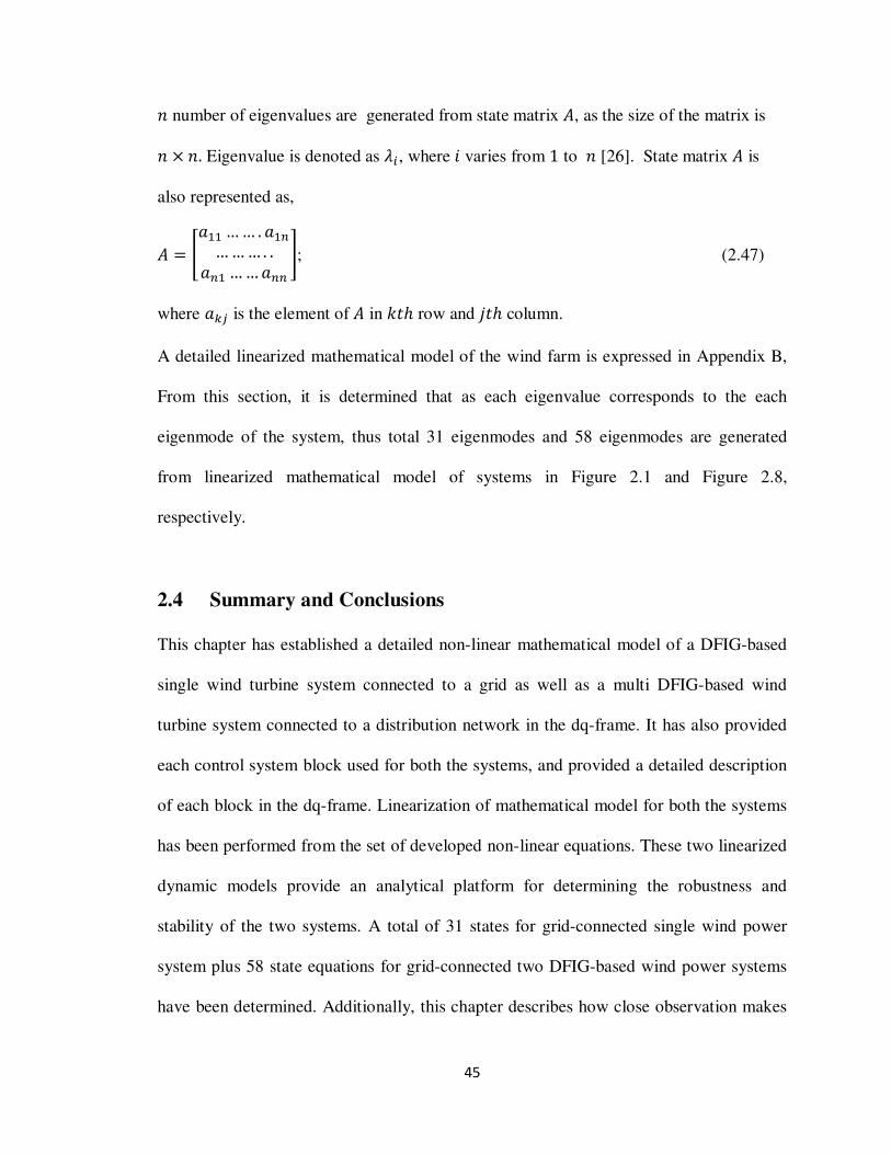
2.4 Summary and Conclusions 45
Chapter 3: Model Validation and Simulation Result 47
3.1 Case Study 1 48
3.2 Case Study 2 57
3.3 Summary and Conclusion 66
Chapter 4: Modal Analysis- System Parametric Effects 67
4.1 Brief Description of Stability & Modal Analysis 67
4.2 Sensitivity Analysis At Very Low Linking Inductances 69
4.2.1 Participation Factor Analysis 69

vi
4.2.2 Eigenvalue, Frequency of Oscillation and Damping Factor 74
4.3 Sensitivity Analysis at Very High Linking Inductances 82
4.4 Summary and Conclusion 84
Chapter 5: Summary, Conclusions and Future Works 86
5.1 Summary and Conclusions 86
5.2 Future Work 88
References 89
Appendices 93
Appendix A 93
Appendix B 95
Vita 98
vii
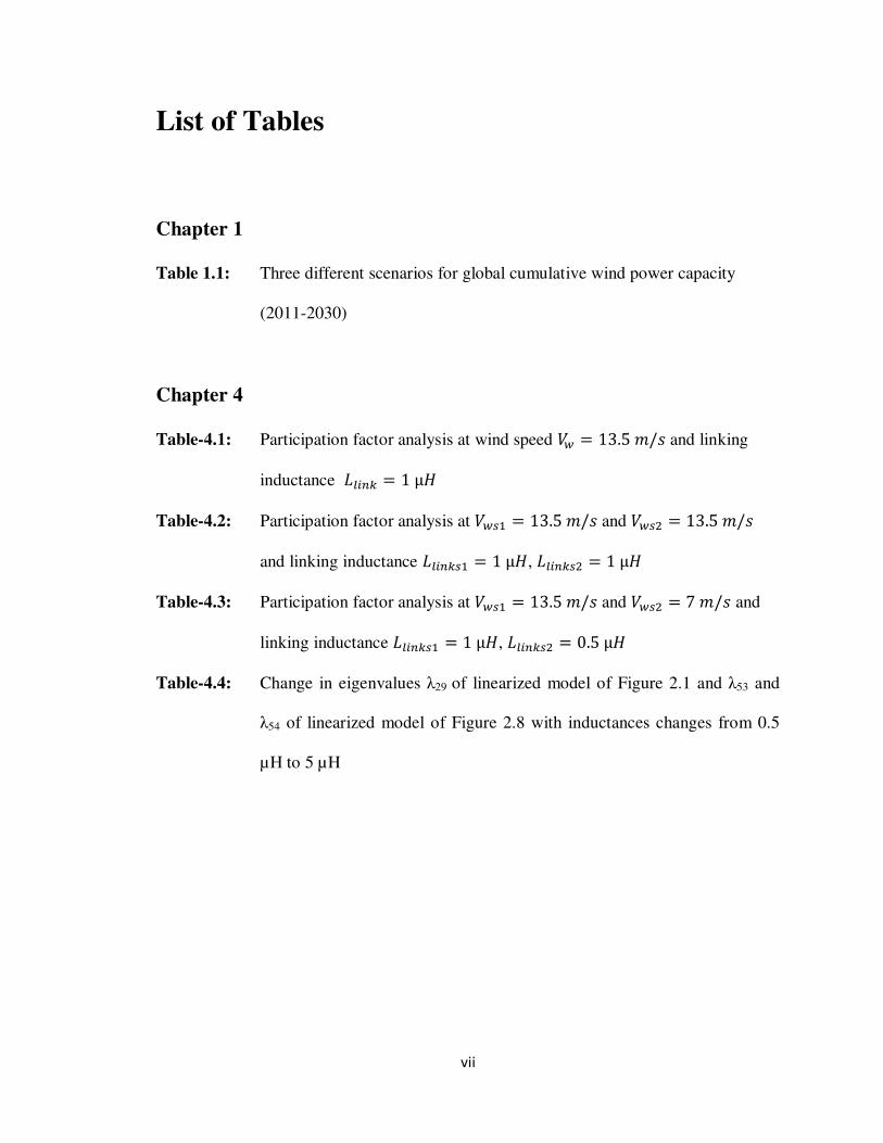
List of Tables
Chapter 1
Table 1.1: Three different scenarios for global cumulative wind power capacity
(2011-2030)
Chapter 4
Table-4.1: Participation factor analysis at wind speed = 13.5/ and linking
inductance = 1μ
Table-4.2: Participation factor analysis at = 13.5/ and = 13.5/
and linking inductance = 1μ, = 1μ
Table-4.3: Participation factor analysis at = 13.5/ and = 7/ and
linking inductance = 1μ, = 0.5μ
Table-4.4: Change in eigenvalues λ29 of linearized model of Figure 2.1 and λ53 and
λ54 of linearized model of Figure 2.8 with inductances changes from 0.5
µH to 5 µH
viii
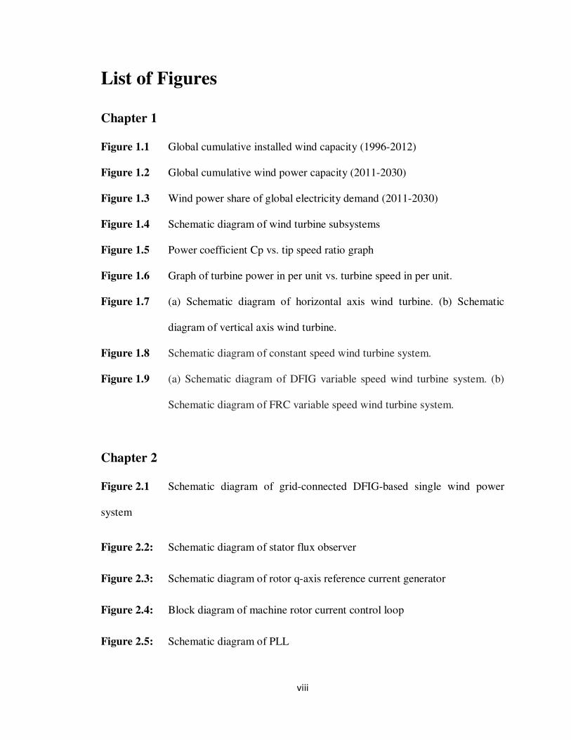
List of Figures
Chapter 1
Figure 1.1 Global cumulative installed wind capacity (1996-2012)
Figure 1.2 Global cumulative wind power capacity (2011-2030)
Figure 1.3 Wind power share of global electricity demand (2011-2030)
Figure 1.4 Schematic diagram of wind turbine subsystems
Figure 1.5 Power coefficient Cp vs. tip speed ratio graph
Figure 1.6 Graph of turbine power in per unit vs. turbine speed in per unit.
Figure 1.7 (a) Schematic diagram of horizontal axis wind turbine. (b) Schematic
diagram of vertical axis wind turbine.
Figure 1.8 Schematic diagram of constant speed wind turbine system.
Figure 1.9 (a) Schematic diagram of DFIG variable speed wind turbine system. (b)
Schematic diagram of FRC variable speed wind turbine system.
Chapter 2
Figure 2.1 Schematic diagram of grid-connected DFIG-based single wind power
system
Figure 2.2: Schematic diagram of stator flux observer
Figure 2.3: Schematic diagram of rotor q-axis reference current generator
Figure 2.4: Block diagram of machine rotor current control loop
Figure 2.5: Schematic diagram of PLL
ix
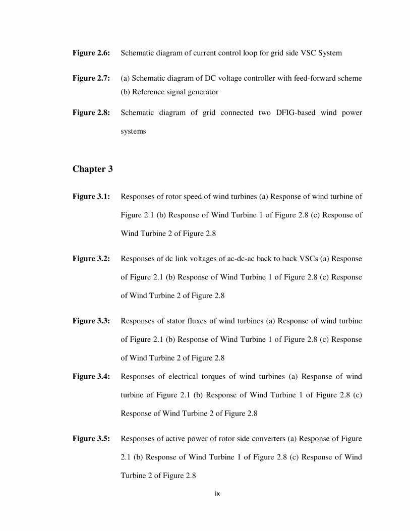
Figure 2.6: Schematic diagram of current control loop for grid side VSC System
Figure 2.7: (a) Schematic diagram of DC voltage controller with feed-forward scheme
(b) Reference signal generator
Figure 2.8: Schematic diagram of grid connected two DFIG-based wind power
systems
Chapter 3
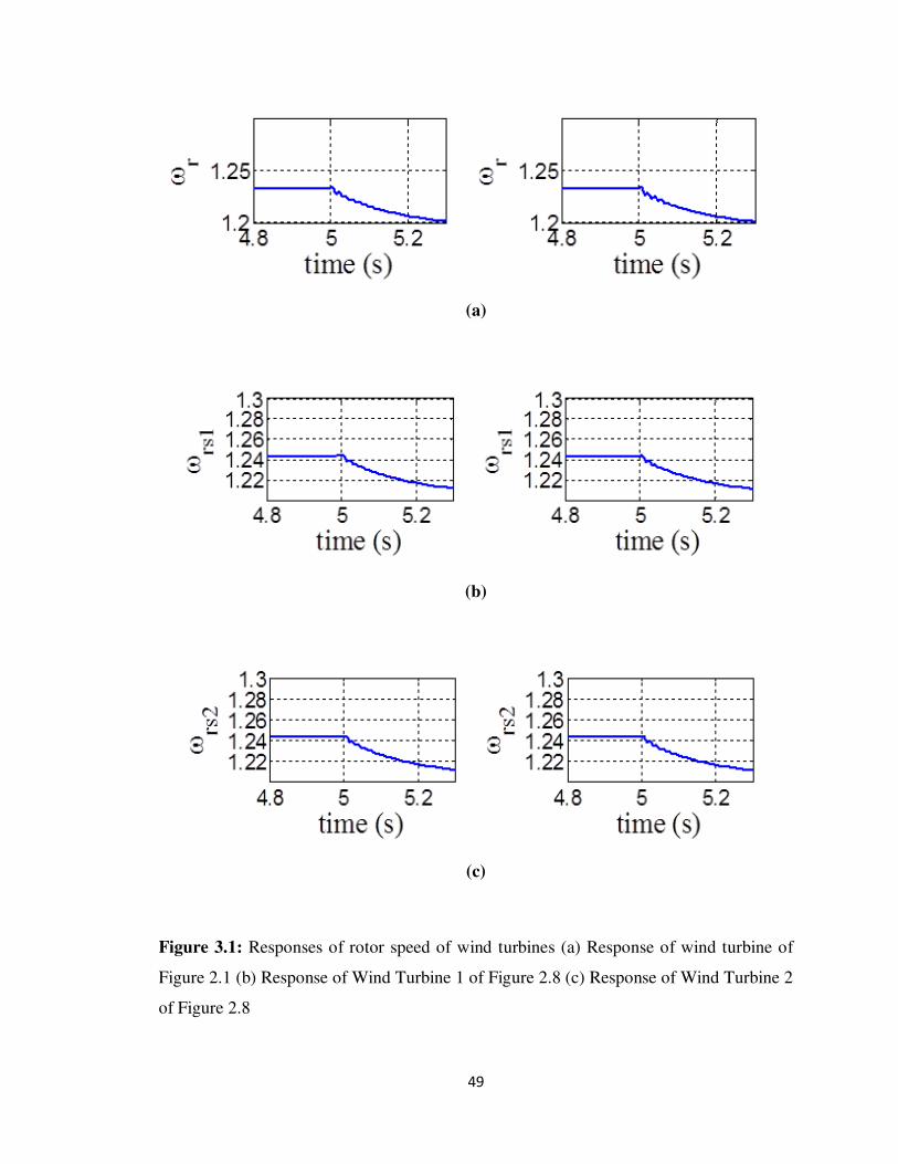
Figure 3.1: Responses of rotor speed of wind turbines (a) Response of wind turbine of
Figure 2.1 (b) Response of Wind Turbine 1 of Figure 2.8 (c) Response of
Wind Turbine 2 of Figure 2.8
Figure 3.2: Responses of dc link voltages of ac-dc-ac back to back VSCs (a) Response
of Figure 2.1 (b) Response of Wind Turbine 1 of Figure 2.8 (c) Response
of Wind Turbine 2 of Figure 2.8
Figure 3.3: Responses of stator fluxes of wind turbines (a) Response of wind turbine
of Figure 2.1 (b) Response of Wind Turbine 1 of Figure 2.8 (c) Response
of Wind Turbine 2 of Figure 2.8
Figure 3.4: Responses of electrical torques of wind turbines (a) Response of wind
turbine of Figure 2.1 (b) Response of Wind Turbine 1 of Figure 2.8 (c)
Response of Wind Turbine 2 of Figure 2.8
Figure 3.5: Responses of active power of rotor side converters (a) Response of Figure
2.1 (b) Response of Wind Turbine 1 of Figure 2.8 (c) Response of Wind
Turbine 2 of Figure 2.8

x
Figure 3.6: Responses of active power of grid side converters (a) Response of Figure
2.1 (b) Response of Wind Turbine 1 of Figure 2.8. (c) Response of Wind
Turbine 2 of Figure 2.8.
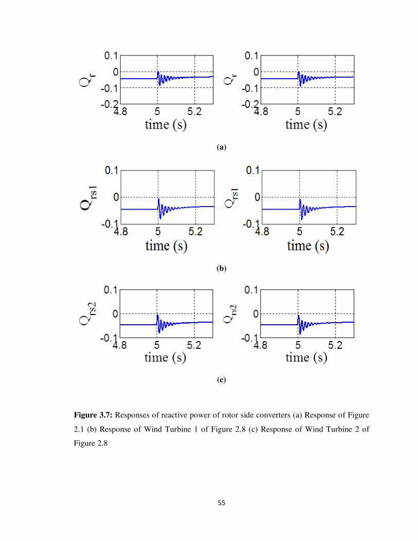
Figure 3.7: Responses of reactive power of rotor side converters (a) Response of
Figure 2.1 (b) Response of Wind Turbine 1 of Figure 2.8 (c) Response of
Wind Turbine 2 of Figure 2.8
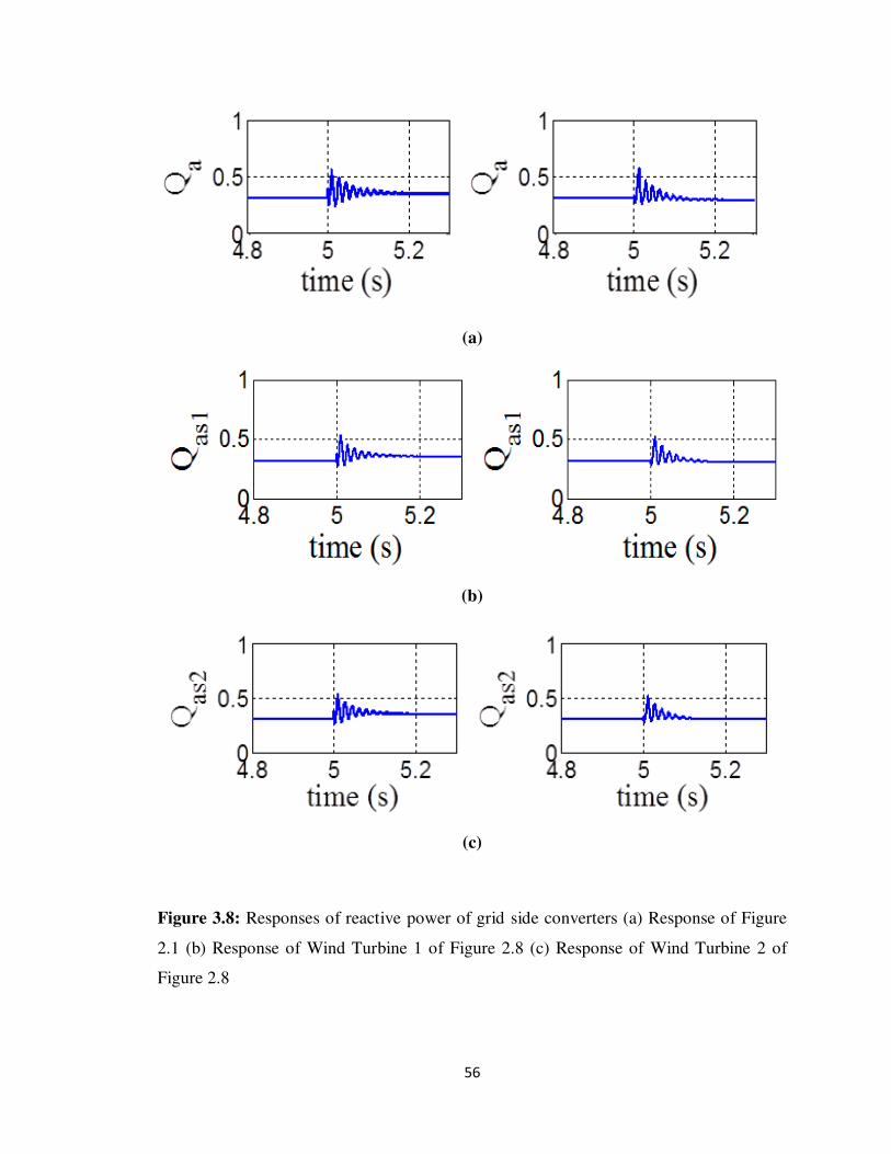
Figure 3.8: Responses of reactive power of grid side converters (a) Response of
Figure 2.1 (b) Response of Wind Turbine 1 of Figure 2.8 (c) Response of
Wind Turbine 2 of Figure 2.8
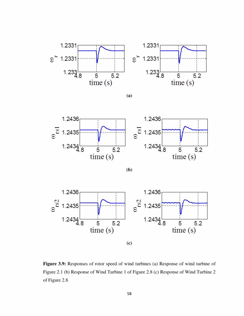
Figure 3.9: Responses of rotor speed of wind turbines (a) Response of wind turbine of
Figure 2.1 (b) Response of Wind Turbine 1 of Figure 2.8 (c) Response of
Wind Turbine 2 of Figure 2.8
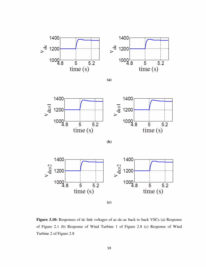
Figure 3.10: Responses of dc link voltages of ac-dc-ac back to back VSCs (a) Response
of Figure 2.1 (b) Response of Wind Turbine 1 of Figure 2.8. (c) Response
of Wind Turbine 2 of Figure 2.8.
Figure 3.11: Responses of stator fluxes of wind turbines (a) Response of wind turbine
of Figure 2.1 (b) Response of Wind Turbine 1 of Figure 2.8. (c) Response
of Wind Turbine 2 of Figure 2.8.
Figure 3.12: Responses of electrical torques of wind turbines (a) Response of wind
turbine of Figure 2.1 (b) Response of Wind Turbine 1 of Figure 2.8 (c)
Response of Wind Turbine 2 of Figure 2.8
xi
Figure 3.13: Responses of active power of rotor side converters (a) Response of Figure
2.1 (b) Response of Wind Turbine 1 of Figure 2.8 (c) Response of Wind
Turbine 2 of Figure 2.8
Figure 3.14: Responses of active power of grid side converters (a) Response of Figure
2.1 (b) Response of Wind Turbine 1 of Figure 2.8 (c) Response of Wind
Turbine 2 of Figure 2.8
Figure 3.15: Responses of reactive power of rotor side converters (a) Response of
Figure 2.1 (b) Response of Wind Turbine 1 of Figure 2.8 (c) Response of
Wind Turbine 2 of Figure 2.8
Figure 3.16: Responses of reactive power of grid side converters (a) Response of
Figure 2.1 (b) Response of Wind Turbine 1 of Figure 2.8 (c) Response of
Wind Turbine 2 of Figure 2.8
Chapter 4
Figure 4.1: Eigenvalue loci for change in linking inductances (a) λ1,2 and λ3,4 for
single- turbine connected with grid (b) λ1,2 and λ3,4 for two-turbine system
connected with grid. (c) λ5,6 and λ7,8 for two-turbine system connected to
a grid
Figure 4.2: Frequency of oscillation (fosc) and damping Factor (ζ) of eigenvalues of
Figure 4.1 (a) Frequency of oscillation (fosc) (b) Frequency of oscillation
(fosc) (c) damping Factor (ζ) (d) damping Factor (ζ)

xii
Figure 4.3: Graph for change in linking inductances with real part of dominant
eigenvalue (σ) of linearized model grid-connected single-turbine system
and grid- connected two-turbine systems, with change in linking
inductances
Figure 4.4: Eigenvalue loci for change in wind speed (a) λ29 for single-turbine
connected to a grid. (b) λ53 for two-turbine system connected to a grid (c)
λ54 for two-turbine system connected to a grid
Figure 4.5: Graph for change in wind speed with real part of dominant eigenvalue for
(a) Linearized model of Figure 2.1 and (b) Linearized model of Figure
2.8.
Figure 4.6: Graph for change in system parameters with real part of dominant
eigenvalue (a) Change in linking inductances (b) Change in wind speed
Figure 4.7: Dominant eigenvalue loci from 6 m/s to 14 m/s at linking inductance
0.00032 H (a) Linearized model of grid-connected single-turbine and (b)
Linearized model of grid-connected small wind farm

xiii
Nomenclature
Stator voltage
Stator current
Rotor current
Rotor voltage
Grid-side converter ac-side terminal voltage
Grid-side converter ac-side terminal current
Rotor active power
Rotor reactive power
Stator active power
Stator reactive power
Ac-side terminal active power of grid-side converter
Ac-side terminal reactive power of grid-side converter
Magnetizing inductance
Stator inductance
Rotor inductance
Rotor resistance
Stator resistance
Stator flux
xiv
s1 Subscript used for DFIG-based wind turbine 1
s2 Subscript used for DFIG-based wind turbine 2
Subscript used for direct axis component of a variable
! Subscript used for quadrature axis component of a variable
Voltage at PCC
"# Grid steady state angular frequency
" Rotor angular speed
$ Moment of inertia
% Stator time constant
% Rotor time constant
&'( Turbine torque
&) Electrical torqur
Linking inductance between machine and PCC
*'+ Turn ratio of transformer &
*', Turn ratio of transformer &,
, Resistance at Transmission line
Grid-side converter ac-side terminal resistance
Grid-side converter ac-side terminal inductance
, Grid Voltage
-. Shunt capacitor at PCC
xv
-/+ DC side capacitor of two VSC
/+ Voltage across -/+
- Shunt capacitor at machine and linking inductance meet point
+ Current across capacitor -
Current across
, Inductance at Transmission line
" Angular frequency of PLL reference frame
0 Reference frame angel of PLL
1 Stator flux phase-angle
" Angular frequency of stator flux
2 Damping factor
fosc Frequency of Oscillation

xvi
Abbreviations
DFIG Doubly Fed Induction Generator
VSC Voltage Source Converter
USSR Union of Soviet Socialist Republics
GWEO Global Wind Energy Outlook
HAWT Horizontal Axis Wind Turbine
VAWT Vertical Axis Wind Turbine
FRC Fully Rated Converter
IGBT Insulated Gate Bipolar Transistor
PWM Pulse Width Modulation
PCC Point of Common Coupling
PLL Phase Locked Loop

1
Chapter 1
Introduction
In recent years, nations have sought alternative renewable energy resources to meet their
rapidly growing demands of power, mainly due to the rapid increase of fuel costs and
rising pollution levels. Continuously trimming down traditional energy resources as well
as preservation of non-renewable energy resources are the two main causes of increased
fuel costs. Pollution levels keep increasing, mainly due to long-term use of fossil fuels
and increase in population. Different types of renewable energy sources are Biomass
Energy, Hydro-Power Energy, Solar Energy, and Wind Energy. Among all these
renewable energy sources, wind energy is most in-demand, as wind is a clean source of
energy, with no waste products created during wind power generation. Wind power
generation does not need any fuel and is able to supply considerable level of energy to
meet world demand.
1.1 Historical Background of Wind Power
Wind power has been used from many years, since humans first started of use of sailboats
and sailing ships. Ackermann [1] stated that at least from the 7th century BC, vertical axis
windmills were used in the Afghan highlands to grind grain. It has been found that
horizontal axis windmills were used in about 1000 AD by Persian, Chinese and Tibetan
people. The use of horizontal axis windmills reached the Mediterranean countries and

2
Central Europe from Persia and the Middle East. In around 1150 AD, this type of
windmill reached England; in 1180 AD it reached France, in 1222 AD Germany, and in
around 1259 AD, Denmark. Between the 12th to 19th centuries, windmill performance
was constantly enhanced, and by the end of the 19th century, typical European windmills
were developed, with a rotor of 25 m in diameter, and stocks reaching up to 30 m [1]. In
the mid-1700’s, Dutch settlers established windmills in America [2]. By 1800, 90% of
power used in industry in the Netherlands was from wind power [1]. In the United States
of America (USA), between 1880 and 1930, around 6.5 million units of windmills were
installed by different companies to provide water for farm animals [2].
1.2 Growth of Electricity Demand
Burton et al. [3] stated, 12 kW DC windmill generator was developed to produce
electricity in the late 19th century by Brush in USA and this research was carried out by
LaCour in Denmark. In 1931, Union of Soviet Socialist Republics (USSR) constructed
100 kW- 30 m diameter Balaclava wind turbine, which was the first utility scale wind
turbine in the world. In 1941, in USA, 1250 kW Smith-Putnam wind turbine was
developed that had a steel rotor with diameter of 53m, full-span pitch control and
flapping blades to reduce loads. This wind turbine was operated for 1100 hours before a
blade spar failed in 1945. This wind turbine remained the largest wind turbine for around
40 years.
A hollow blade, open at tip with 24 m diameter pneumatic wind turbine was constructed
in early 1950s in UK to draw air through the tower. In 1956 and in 1963, 200 kW with 24
m diameter Gedser wind turbine and 1.1 MW -35 m diameter wind turbine were

3
constructed in Denmark and in France, respectively. In between 1950s and 1960s a
number of modern, lightweight turbines were developed by U. Hutter in Germany. In
spite of this technological progress, it was seen that for much of the 20th century, world
had little interest to use wind energy other than in remote residences for battery charging
[3].
After a sudden price hike of oil occurred in 1973 because of inadequate fossil-fuel
resources, countries like USA, UK, Germany, Sweden took serious steps with a large
number of Government-funded programs of research, development and manifestation to
investigate cost effective sources of energy. As a result of fact, in between 1975 and
1987, a series of prototype wind turbines starting with 38 m diameter 100 kW Mod-0 and
97.5 m diameter 2.5 MW Mod-5B, respectively, were constructed in USA [3]. Nearly at
the same time a 4 MW vertical-axis Darrieus wind turbine and a 34 m diameter Sandia
vertical-axis wind turbine were constructed, in Canada and in USA, respectively. Another
vertical-axis wind turbine with straight blades using ‘H’ type rotor was designed by Peter
Musgrove and this model was constructed in UK that had a capacity to generate 500 kW
power. An entire structure of 3 MW horizontal axis wind turbine was designed and tested
in USA, in 1981 that used hydraulic transmission, an alternative to yaw drive [3]. In mid-
1980s, a large number of small wind turbines with capacity less than 100 kW were
installed in a wind farm with a maximum total capacity of 1.5 MW in California [4]. But
for some time, the selection of the number of blades remained undecided and the turbines
were constructed with a maximum of three blades. Installed wind turbine capacity was
increased from 2.5 GW in 1995 to 12 GW by 2001 [3]. Figure 1.1 shows a statistical
review of global cumulative installed wind capacity from 1996 till 2012; a promising

4
growth of wind energy has been noticed [5]. From 1996 to 2012, an exponential increase
of the growth of global cumulative installed wind capacity is observed in Figure 1.1.
Figure 1.1: Global cumulative installed wind capacity (1996-2012) [5]
As per the 2012 report on global wind energy outlook (GWEO), the growth of global
cumulative wind power capacity with three different scenarios in MW unit and wind
power share of global electricity demand in percentage, have been plotted for the time
period 2011 to 2030, in Figure 1.2 and in Figure 1.3, respectively; while Table 1.1 also
lays out the power generation for the three different scenarios [6]. On the basis of current
directions and intentions from both national and international energy and climate policy,
the “New Policies” scenario is analyzed. The factors related to “Moderate Policies”
scenario are mostly similar to “New Policies” scenario; but it also comprises of all policy
measures, which are either already implemented in the planning stages or are based on
5
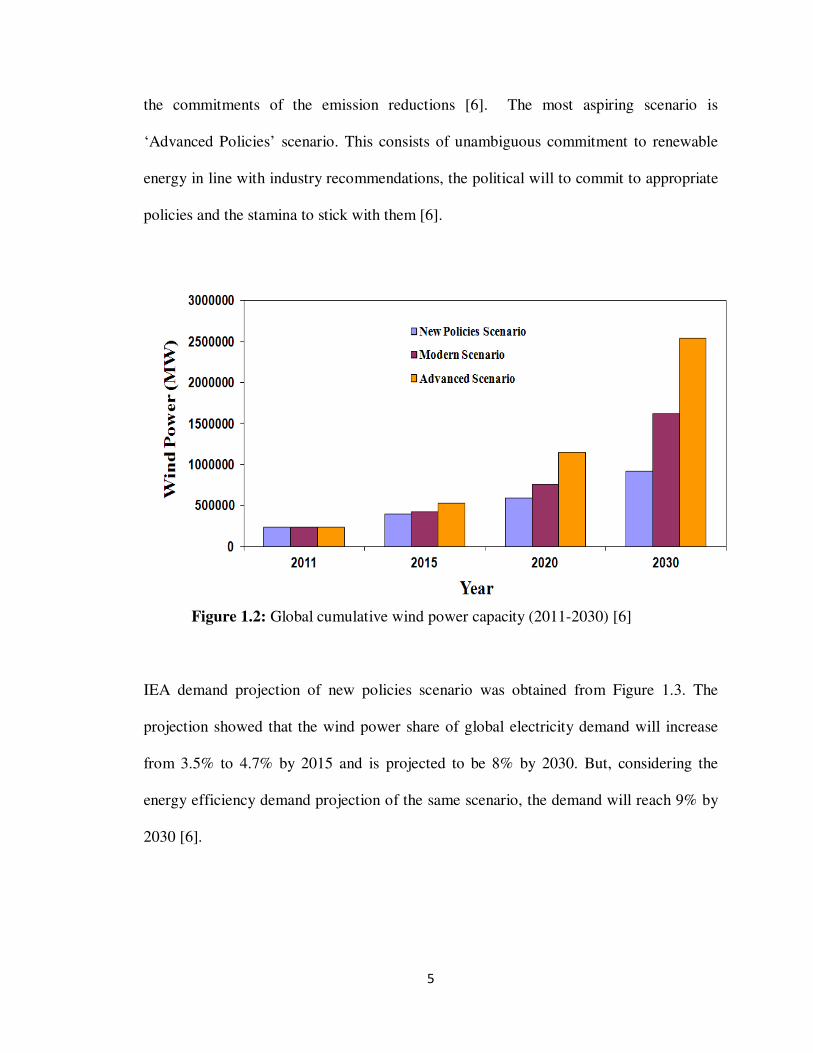
the commitments of the emission reductions [6]. The most aspiring scenario is
‘Advanced Policies’ scenario. This consists of unambiguous commitment to renewable
energy in line with industry recommendations, the political will to commit to appropriate
policies and the stamina to stick with them [6].
Figure 1.2: Global cumulative wind power capacity (2011-2030) [6]
IEA demand projection of new policies scenario was obtained from Figure 1.3. The
projection showed that the wind power share of global electricity demand will increase
from 3.5% to 4.7% by 2015 and is projected to be 8% by 2030. But, considering the
energy efficiency demand projection of the same scenario, the demand will reach 9% by
2030 [6].

6
Table 1.1: Three different scenarios for global cumulative wind power capacity (2011-
2030) [6]
Different Scenarios 2011 2015 2020 2030
New Policies Scenario
[MW]
237,699 397,859 586,729 917,798
Moderate Scenario [MW] 237,699 425,155 759,349 1,617,444
Advanced Scenario [MW] 237,699 530,945 1,149,919 2,541,135
Figure 1.3: Wind power share of global electricity demand (2011-2030) [6]

7
1.3 Electricity Generation from Wind Power System
Wind turbine generates electricity from wind power to drive electrical machine. If a
machine converts kinetic energy of the wind to mechanical energy, and then, this
mechanical energy is used to generate electrical energy, that machine is defined as the
wind power plant or wind turbine. A detailed description of some fundamental facts of
wind turbine such as basic parts, principle of operation and etc. are discussed to get an
idea of modern wind turbine system.
1.3.1 Inside of a Wind Turbine
Wind turbine mechanism is exactly the reverse of a fan. Fans use electricity to generate
wind, whereas wind turbines use wind to generate electric power. The rotor of wind
power system is connected to the main shaft, which spins a generator to produce
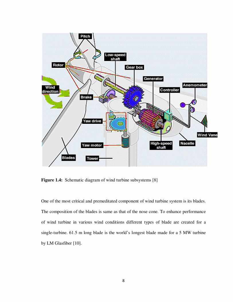
electricity [7]. Figure 1.4, illustrates a detailed view of the inside of a wind turbine
system and its components. Major components of a typical wind turbine system are as
follows:
Rotor: The most important part, from both performance and overall cost stand point, of a
wind turbine is its rotor; that consists the hub, the high tech blades and a spinner [9,10].
Heaviest components of wind turbine are the hub as it is made of ductile cast iron. For a 2
MW modern wind turbine the weight of the hub is normally in between 8 to 10 tons. The
hub can absorb a high level of vibration. The nose cone helps to cover the hub and also to
protect it slightly the hub from the environment. Nose cone is made from balsa wood,
carbon fiber, and fiberglass [10].
8
Figure 1.4: Schematic diagram of wind turbine subsystems [8]
One of the most critical and premeditated component of wind turbine system is its blades.
The composition of the blades is same as that of the nose cone. To enhance performance
of wind turbine in various wind conditions different types of blade are created for a
single-turbine. 61.5 m long blade is the world’s longest blade made for a 5 MW turbine
by LM Glasfiber [10].
9
Drive Train: This part consists of a low speed shaft, a high speed shaft, a gear box, one
or more couplings, support bearings, a brake and a rotating part of generator. The low
speed shaft is made on rotor side while the high speed shaft is on the generator side [9].
This drive train is electricity generating system of a wind power system. Gearbox steps
up the rate of rotation of the rotor from a low value to a high value suitable for electric
generator. As a gear box handles the frequent changes in torque due to changes in wind
speed, it must be robust. A lubrication system is used to minimize the wear needed for the
gear box system. Mainly parallel shaft and planetary, these two types of gear box are
used in wind turbine system. Planetary type gear box is used normally in large wind
turbine over 500 kW. Mainly induction generator based wind turbines need gearbox. To
stay away from mechanical problem related to gear box, some wind turbines use a direct
drive system which connects the rotor directly to a permanent magnet generator [9,10].
Nacelle: A box-like component at the top of tower is connected to the rotor, is called the
nacelle. This contains around 8000 components of wind power system like generator,
main frame, etc. Nacelle saves the internal components of turbine from weather and is
made of fiberglass. The nacelle cover is fixed firmly to the main frame, which also
supports all the other components inside the nacelle. The main frames provide proper
alignment of drive train components and are also able to withstand large fatigue loads
[10].
10
Yaw System: To keep the rotor shaft properly aligned with the wind a yaw system is
needed. A large bearing that connects the main frame to the tower is the main component
of yaw drive system. The yaw drive system uses either an electric or hydraulic motor
which drives a pinion gear on a vertical shaft through a reducing gearbox. Typically a
yaw drive system is used with an upwind wind turbine system, whereas downwind wind
power systems are often free from yaw systems. [9]. A brake is also used in a yaw drive
system to stop a turbine from turning and stabilizing it during normal operation [10].
Generator: To get constant rotational speed, mainly induction or synchronous generators
are used with all wind turbines. Power electronic converters are used with the generators
to run wind turbines at variable speed. Squirrel cage induction generators (SQIG) can be
used with many grid-connected wind turbines, due to it being rugged by nature, low cost,
and driven in a narrow range of speeds, slightly higher than its synchronous speed.
Nowadays, doubly fed induction generators (DFIG) have gained popularity in variable
speed applications. Main advantages of DFIG are simple configuration, over a wide range
of wind speed; wind turbines work efficiently [9].
Tower and Foundation: For use of maximum wind nacelle and generator are situated on
the top of the tower [10]. In recent times, lattice towers, concrete towers and free standing
steel tube towers are most popular. Depending on the site character, tower is selected.
Normally height of a tower varies from 1 to 1.5 times of the rotor diameter. Stiffness of
tower plays an important role in wind turbine system dynamics as vibration occurs
between rotor and tower. Tower shadow of turbines with downwind rotor must be
11
considered to have significant effect on power fluctuations, turbine dynamics and noise
generation [9].
Controls: To get proper functioning from wind turbine, few instruments like sensors,
controllers, power amplifiers, actuators and some intelligent devices like microprocessors
and computers are used as control system. Sensors are used to sense and give feedback of
wind speed, direction, flow, current, voltage, rotor speed, temperature, vibration levels
etc. Electrical circuits and mechanical systems act as controllers to control all the
parameters. Different types of switches, hydraulic pumps, electrical amplifiers etc. are the
parts of power amplifiers. Motors, magnets, solenoids etc. act as actuators. Few
intelligent devices like computers and microprocessors are used to process the inputs of
turbine to get proper function from turbine and also at an emergency situation, which
help to override the controller to safe overall system [9, 10].
The most fundamental and major components of a typical wind turbine connected to a
grid is discussed above. Other than these components, some other components like
transformers, power electronic converters and pitch motors etc. are used depending on the
complexity of the system to get proper functionality.
1.3.2 Physics of Generating Electricity from Wind Energy
Wind energy is one form of solar energy generated because of temperature and as well as
pressure differences in the atmosphere, the rotary motion of the earth, and the
irregularities of the earth's surface. Sun heats up the air, forcing the air to rise; this causes
a movement of air from high pressure zone to low pressure zone where temperature falls
12
to balance the differences. Wind turbine first catches wind’s kinetic energy which helps
to drive generator to produce electricity [11]. The kinetic energy in air with mass
moving with velocity is given by [12]:
34 = (1.1)
The power in wind is the Kinetic energy per unit time and as is expressed as:
= 5 , (1.2)
where 5 = //' = 6789:;6<= The mass flow rate
//' is:
//' = 1> , (1.3)
where 1 and > are defined as air density and the rotor effective area, respectively.
Finally, the wind power equation is:
= 1>? (1.4)
Power extracted from wind by the turbine blades is the difference between upstream and
downstream wind powers and is given by:
'( = 6789:;6<=( − B) , (1.5)
where is the actual wind speed or upstream wind velocity at the entrance of the rotor
blades and B is the downstream wind velocity at the exit of rotor. The mass flow rate of
the air through rotating blades is then expressed as:
6789:;6<= = 1> :+92 (1.6)
So the turbine power becomes:
13
'( = F1> (GHIGJ) K ( − B) (1.7)
Equation (1.7) is modified to be:
'( = 1>? LIMJMHNOPLMJMHNQR , (1.8)
where -S = LIMJMHNOPLMJMHNQR (1.9)
is the power coefficient of the rotor. -S, is the fraction of upstream wind power.
Finally the turbine power '( from equation (1.8) is rewritten to be:
'( = 1>?-S (1.10)
The power coefficient, -S, is thus a dimensionless parameter and is the ratio of turbine
power '( to that of wind power .
-S = STUVSH (1.11)
The maximum value of -S is defined by Betz limit and is 0.59, as Betz limit states that a
turbine can never extract more than 59.3% of wind power. Practically -S varies from
25% to 40% [13] for the wind turbine. -S, is a function of the blade pitch angle, WX'+Y
and the tip speed ratio, Z /) . Z /) , is defined as the ratio of upstream wind speed
and downstream wind speed B.
Z /) = GHGJ (1.12)
This, Z /) can also be expressed in terms of turbine angular speed, "'( , turbine radius,
;, and wind speed, , and is given as :
Z /) = [TUV×GH (1.13)
14
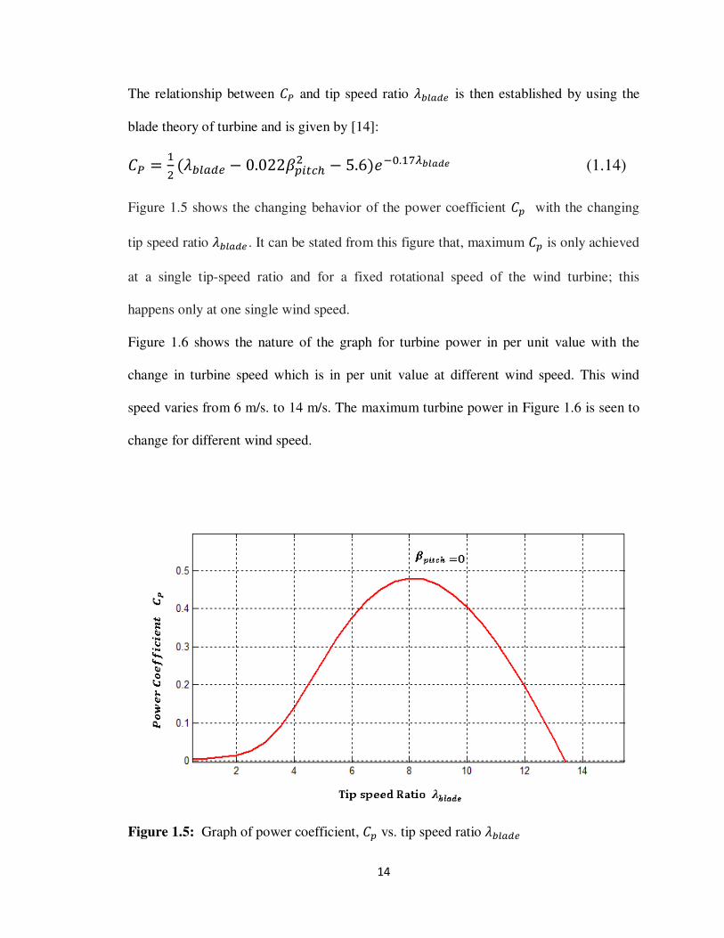
The relationship between -S and tip speed ratio Z /) is then established by using the
blade theory of turbine and is given by [14]:
-S = (Z /) − 0.022WX'+Y − 5.6)=P#.^_`abcd (1.14)
Figure 1.5 shows the changing behavior of the power coefficient -X with the changing
tip speed ratio Z /) . It can be stated from this figure that, maximum -X is only achieved
at a single tip-speed ratio and for a fixed rotational speed of the wind turbine; this
happens only at one single wind speed.
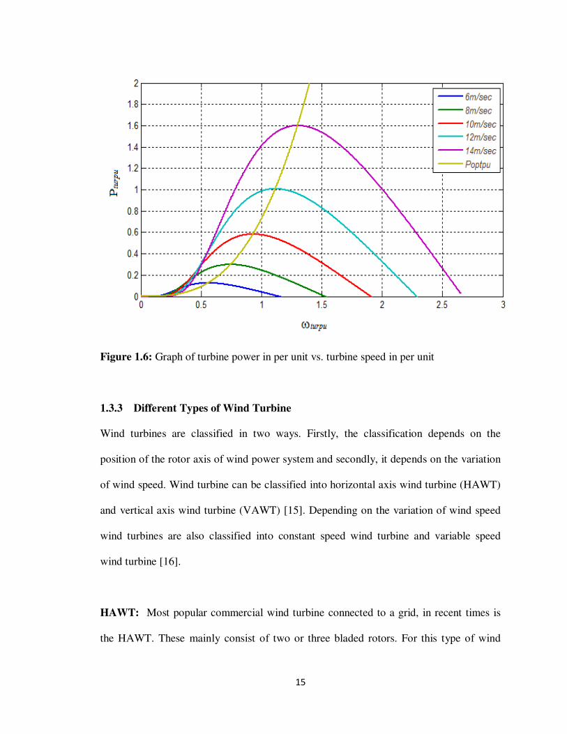
Figure 1.6 shows the nature of the graph for turbine power in per unit value with the
change in turbine speed which is in per unit value at different wind speed. This wind
speed varies from 6 m/s. to 14 m/s. The maximum turbine power in Figure 1.6 is seen to
change for different wind speed.
Figure 1.5: Graph of power coefficient, -X vs. tip speed ratio Z /)
15
Figure 1.6: Graph of turbine power in per unit vs. turbine speed in per unit
1.3.3 Different Types of Wind Turbine
Wind turbines are classified in two ways. Firstly, the classification depends on the
position of the rotor axis of wind power system and secondly, it depends on the variation
of wind speed. Wind turbine can be classified into horizontal axis wind turbine (HAWT)
and vertical axis wind turbine (VAWT) [15]. Depending on the variation of wind speed
wind turbines are also classified into constant speed wind turbine and variable speed
wind turbine [16].
HAWT: Most popular commercial wind turbine connected to a grid, in recent times is
the HAWT. These mainly consist of two or three bladed rotors. For this type of wind

16
turbine, the rotor shaft and electrical generator are placed at the top of the tower where
wind is less turbulent and wind has more power. Figure 1.7 (a) shows the schematic
diagram of HAWT [15].
Figure 1.7: (a) Schematic diagram of horizontal axis wind turbine. (b) Schematic
diagram of vertical axis wind turbine [15]
VAWT: The main rotor shaft in VAWT is placed vertically in the wind turbine system.
Figure 1.7 (b) shows Darrieus rotor type vertical axis wind turbine system which is the
most popular type VAWT [15]. The main advantages of this kind of wind turbines are
that, the generators and gearboxes are easy to repair and perform maintenance operation
of the components as they are placed close to ground, and also this turbine can catch the
wind from all direction without any yaw system. Though there are advantages, but this
type of wind turbine has many disadvantages like, low starting torque, sensible to design
conditions, tendency to stall under blustery wind conditions, used for low power

17
applications such as battery charging, as output power is very low; thus, minimizes the
popularity of VAWT comparing with HAWT [17].
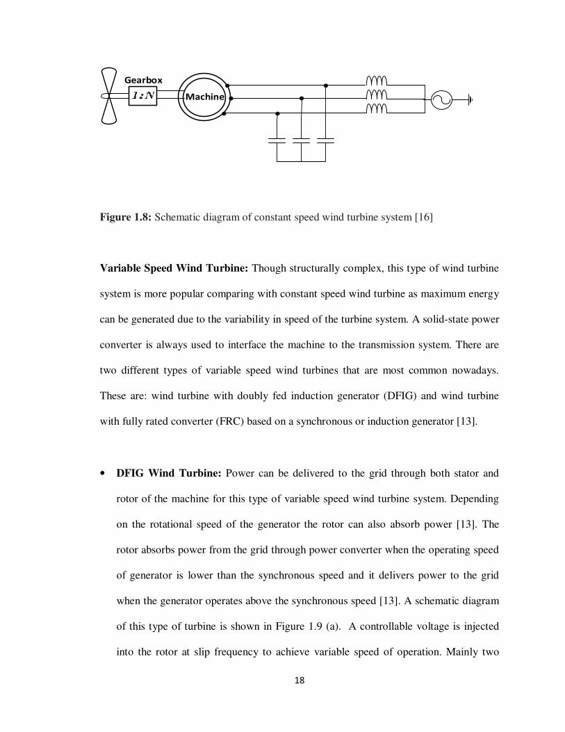
Constant Speed Wind Turbine: This type of turbine is simple in design and is
composed of a gearbox, a low speed shaft, a high speed shaft and an asynchronous
generator. Figure 1.8 presents the schematic diagram of a constant speed wind turbine
system. Mainly squirrel-cage induction generator is used to generate power from such
type of system [13]. For this turbine system, a power-electronic converter is not needed
since the system works at constant speed, and therefore it is structurally simple.
Synchronous frequency is imposed by the grid to the machine because the generator is
directly interfaced with the utility grid through a turbine transformer machine. The
rotational speed of the asynchronous generator is not exactly constant and varies within
±3% to ±8% of the synchronous speed which is very small, so this type of turbine is
considered to be a constant speed type wind turbine system. As asynchronous machines
consume reactive power, so power factor correction capacitors is used at each wind
turbine to maintain the voltage profile to get stable operation, mainly at non-stiff grid
conditions. Though simple in design, this type of turbine system is not able to extract
maximum power at different wind speed as it works at almost constant wind speed. The
stator of generator is directly connected to a utility grid, so, as a result of fact, any kind of
transmission line network will affect directly the wind based generating units of the
system [16].
18
Gearbox
Machine
Figure 1.8: Schematic diagram of constant speed wind turbine system [16]
Variable Speed Wind Turbine: Though structurally complex, this type of wind turbine
system is more popular comparing with constant speed wind turbine as maximum energy
can be generated due to the variability in speed of the turbine system. A solid-state power
converter is always used to interface the machine to the transmission system. There are
two different types of variable speed wind turbines that are most common nowadays.
These are: wind turbine with doubly fed induction generator (DFIG) and wind turbine
with fully rated converter (FRC) based on a synchronous or induction generator [13].
• DFIG Wind Turbine: Power can be delivered to the grid through both stator and
rotor of the machine for this type of variable speed wind turbine system. Depending
on the rotational speed of the generator the rotor can also absorb power [13]. The
rotor absorbs power from the grid through power converter when the operating speed
of generator is lower than the synchronous speed and it delivers power to the grid
when the generator operates above the synchronous speed [13]. A schematic diagram
of this type of turbine is shown in Figure 1.9 (a). A controllable voltage is injected
into the rotor at slip frequency to achieve variable speed of operation. Mainly two

19
AC/DC IGBT based voltage source converters (VSCs), linked by a DC bus is
interfaced in between the rotor winding and electrical network to decouple
transmission line electrical frequency from rotor mechanical frequency. Thus, the
variable speed operation of wind turbine is possible [13].
• FRC Wind Turbine: Figure 1.9 (b) shows a schematic diagram of FRC wind turbine
system. A wide range of electrical generators like wound rotor synchronous
generator, permanent magnet generator, induction generator etc. can be used for this
type of turbine system. Use of the gearbox is optional for FRC wind turbine system.
Variable speed operation can be performed as the dynamic operation of electrical
generator is effectively separated from the electrical network through power
converters [13]. A diode rectifier or a PWM VSC can be used as generator side
converter and only PWM VSC can be used as grid side converter. Each type of
converter can independently deliver or absorb reactive power independently. Mainly
DC bud voltage is controlled by the grid side converter whereas generator side
converter controls the torque applied to the generator. But reverse control strategy is
also applicable for these two types of converters [13].

20
Gearbox
Machine
AC/DC/AC Power
Electronic Converter
(a)
Gearbox
Machine AC/DC/AC Power
Electronic Converter
(b)
Figure 1.9: (a) Schematic diagram of DFIG variable speed wind turbine system [16] (b)
Schematic diagram of FRC variable speed wind turbine system [16]
1.4 Survey of Existing Work
As shown in section 1.2, the demand for wind power to meet global electricity demand
has been increasing. In Recent years, variable-speed DFIG-type wind-power systems
have become commercially very popular for generating wind power, but because of the
erratic nature of wind velocity, extensive research has been done to analyze system
stability and sensitivity for the changes of different system parameters to get efficient and
economic production of wind energy from a stable wind-power-generating system. A
brief review of previous research shows the relation between system modeling and
stability analysis of a DFIG wind turbine system. Different models of grid-connected
DFIG with one or two mass drive trains and with or without stator transients have been

21
formulated mathematically and compared with each other using eigenvalues and
participation factor analysis [18]. Rouco and Zamora [19] developed detailed non-linear
and corresponding linear mathematical models of DFIG systems for wind power
applications. They offered a reduced order model of the detailed models using
eigenvalues of the state matrix and corresponding participation factor analysis. A
comparative study has also been carried out on the detailed models and the proposed
reduced order models [19]. Modal analysis, with a 7th order grid-connected DFIG-based
system, has been performed for, better understanding of basic dynamics of the system,
model justification and control system design [20]. This study was carried out by
changing the modal properties for different operating points, grid strengths and system
parameters. [21] has designed damping controllers of DFIG for damping
electromechanical oscillation by eigenvalue sensitivity analysis with respect to some
parameters. A detailed mathematical model of DFIG has been developed, to analyze
eigenvalue sensitivity with respect to machine and control parameters, and to evaluate
their impacts on system stability; it has also been shown that without proper controller
tuning, a Hopf bifurcation can occur for various reasons [22]. [23] has presented a study
on participation factor analysis using eigenvalue of a mathematically developed DFIG-
based wind-power unit interfaced with the grid through a series compensated
transmission lines. The influence of the system parameters on stability of the system has
also been studied.
22
1.5 Scope of the Thesis
As the literature review makes clear, considerable research has been carried out to
analyze system stability and modal analysis in a single DFIG-based-turbine connected to
a grid. However, a very few research has been performed to clarify the intrinsic dynamic
behavior of a wind farm comprised of multi-turbine systems. As wind power is very
much in demand nowadays, being a non-conventional energy resource to generate
electric power, it is necessary to construct large wind farms that can produce maximum
power from a stable system. Hence, this thesis is motivated by the desire to contribute to
the better understanding of the intrinsic dynamic behavior, range of stability region and
system’s parametric effects on the system stability of a small wind farm. To achieve
these, a small wind farm with two identical DFIG-based wind turbines connected to a
grid network needs to be established.
1.6 Thesis Objectives
The objectives of the thesis are
• To develop a linearized mathematical model from a non-linear DFIG-based single
wind power system connected to a grid. Also on the basis of this model, to
establish a linearized model of a small DFIG-based wind farm connected to a
distribution network.
• To validate the established linearized mathematical models by comparing the
simulation results from both the linear and non-linear models.
• To study and analyze the system stability, eigenvalue sensitivity and modal
properties for the models of both systems.

23
1.7 Methodology
The following methodology is used in order to carry out the objectives:
• non-linear analytical models of a grid-connected DFIG-based single-turbine and
a grid-connected DFIG-based multi-turbine systems are established.
• to clarify the dynamic behavior of both the systems, linearized mathematical
models are developed from the non-linear models.
• to validate the linearized models for a single-turbine system and the wind farm,
the simulation results of the linear and non-linear models are compared
separately.
• to examine the system stability and fundamental dynamic behavior, participation
factor analysis and eigenvalue sensitivity analysis are performed for different
operating conditions and system parameters.
1.8 Thesis Layout
Thesis is organized in the following manner:
• Chapter 2 develops mathematical linearized models of a DFIG-based wind turbine
system connected to a grid and a small wind farm involving two identical DFIG-
based wind turbines connected to a grid around an equilibrium point, including all the
control system blocks, system and network equations, based on non-linear models.
• Chapter 3 deals with the validation of linearized system performance with non-linear
models developed in a PSCAD/EMTDC environment for a single-turbine connected
to a grid and as well as for a multi-turbine connected to a grid.

24
• Chapter 4 presents system stability analysis and modal analysis of the linearized
models developed in Chapter 2 to determine the intrinsic dynamics for model
justification and for useful control system block design in order to achieve wide range
system stability with maximum output power.
• Finally, Chapter 5, summarizes and concludes the thesis and presents the scope of
future work.

25
Chapter 2
Mathematical Modeling and Control of Grid-
Connected DFIG-based Wind Energy Conversion
System
This chapter develops a non-linear mathematical model of a DFIG-based wind power
system connected to a grid. A linearization is performed on the same system for small-
signal stability analysis. Two of these, identical DFIG-based wind power systems are
then considered to be connected in parallel with a distribution network through a Point of
Common Coupling (PCC). The resulting design is then referred to as a small wind farm
connected to a grid. A non-linear mathematical model of this wind farm is then
developed and linearization is performed.
The non-linear equations for both the models established on “dqo” frame are used, which
simplify the analysis of three phase circuits, transform AC quantities into DC quantities,
decouple DFIG torque and flux, and also avoid the time varying mutually coupled
inductances of the overall systems [16]. From each of the system equations, the o-axis
components are eliminated. The variables with the d- and q-axis components are denoted
by subscripts “d” and “q”; for instance as, , is represented as ,/ and ,e , respectively .
26
Each of the individual wind power systems consists of individual control system blocks,
back-to-back voltage source converters (VSCs), and a phase locked loop (PLL). An in-
depth description of each of these blocks for both in linear and non-linear mathematical
forms is presented here.
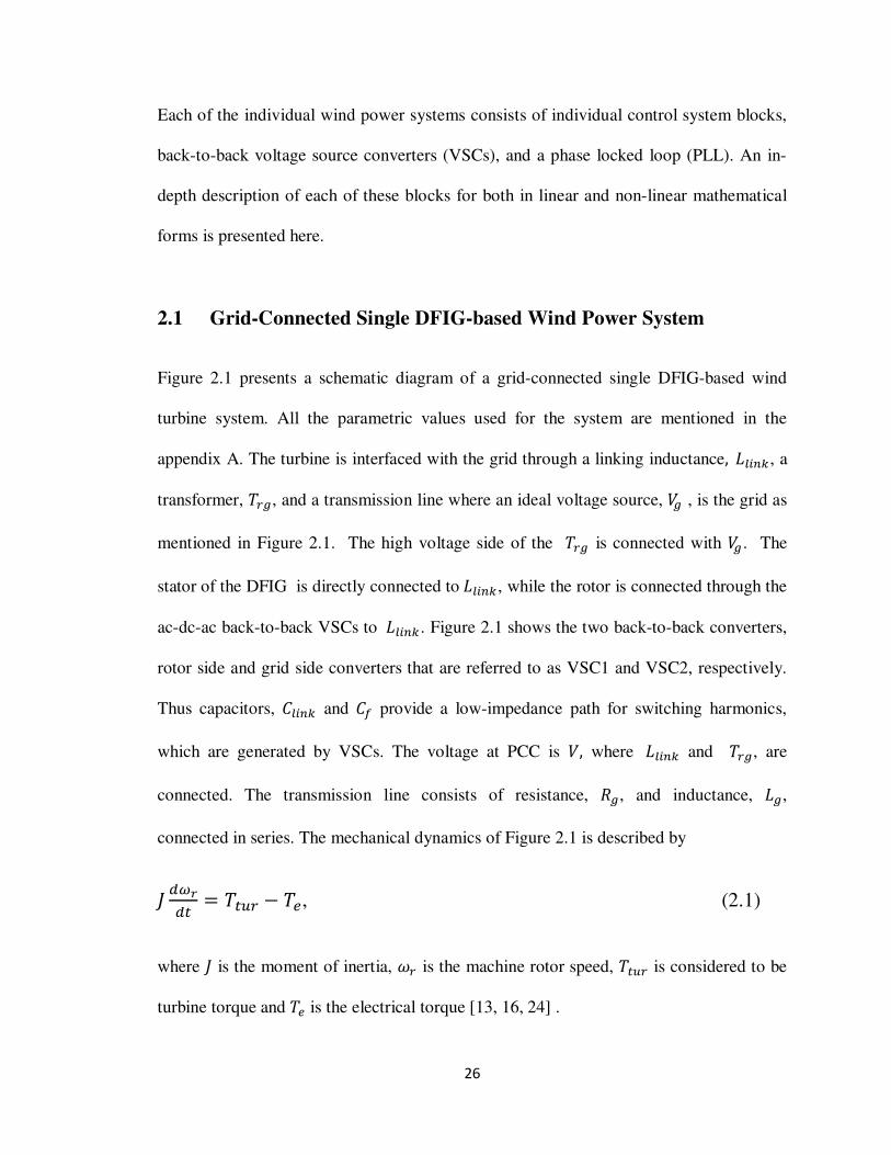
2.1 Grid-Connected Single DFIG-based Wind Power System
Figure 2.1 presents a schematic diagram of a grid-connected single DFIG-based wind
turbine system. All the parametric values used for the system are mentioned in the
appendix A. The turbine is interfaced with the grid through a linking inductance, , a
transformer, &,, and a transmission line where an ideal voltage source, , , is the grid as
mentioned in Figure 2.1. The high voltage side of the &, is connected with , . The
stator of the DFIG is directly connected to , while the rotor is connected through the
ac-dc-ac back-to-back VSCs to . Figure 2.1 shows the two back-to-back converters,
rotor side and grid side converters that are referred to as VSC1 and VSC2, respectively.
Thus capacitors, - and -. provide a low-impedance path for switching harmonics,
which are generated by VSCs. The voltage at PCC is , where and &,, are
connected. The transmission line consists of resistance, ,, and inductance, ,,
connected in series. The mechanical dynamics of Figure 2.1 is described by
$ /[V/' = &'( − &), (2.1)
where $ is the moment of inertia, " is the machine rotor speed, &'( is considered to be
turbine torque and &) is the electrical torque [13, 16, 24] .

27
TorqueControl
lerTorque
Controller
TorqueControl
lerTorque
Controller
GearboxGearbox GearboxGearbox
Averaged
Averaged
Averaged
Averaged
IdealVSC
IdealVSC
IdealVSC
IdealVSC
Averaged
Averaged
Averaged
Averaged
IdealVSC
IdealVSC
IdealVSC
IdealVSC
DCBusVoltage
Controller
DCBusVoltage
Controller
DCBusVoltage
Controller
DCBusVoltage
Controller
VSCVSC VSCVSC 11 11VSCVSC VSCVSC 22 22
DFIGDFIG DFIGDFIG
PLLPLL PLLPLLdqdq dqdqabcabc abcabc
V dcC dcV r
abcabc abcabc dqdq dqdq
P r Q r
P s P aQ si r
i sQ a V aR a
i aL a
m rd
V s
m rqm ad
m aq
T rsC linki mi clinki linkL link
C fi fT rgR gP gridi gV g
L gVYY YY :: :: YY YY
YY YY :: :: YY YY1:N
T erefV dcref
Q aref
Figure 2.1: Schematic diagram of grid-connected DFIG-based single wind power
system
28
Equation (2.1) is significant in analyzing the stability of the wind power system as it
helps to describe the effect of any mismatch between the electrical and the mechanical
torques generated by the turbine. A detailed description and a non-linear mathematical
model of each block of the overall system as shown in Figure 2.1 is synchronously
developed.
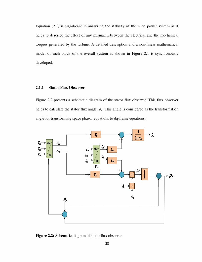
2.1.1 Stator Flux Observer
Figure 2.2 presents a schematic diagram of the stator flux observer. This flux observer
helps to calculate the stator flux angle, 1. This angle is considered as the transformation
angle for transforming space phasor equations to dq-frame equations.
abcabcabcabcdqdqdqdq
abcabcabcabcdqdqdqdqVVVVscscscsc
VVVVsbsbsbsbVVVVsasasasaiiiircrcrcrciiiirarararaiiiirbrbrbrb
iiiirdrdrdrdiiiirqrqrqrq
VVVVsdsdsdsdVVVVsqsqsqsqVVVVscscscsc
LLLLmmmmLLLLmmmm
ττττssss
ττττssss
ττττssss 11111111++++ττττssss
ρρρρssssωωωω
θθθθrrrrλλλλ
λλλλ
Figure 2.2: Schematic diagram of stator flux observer
29
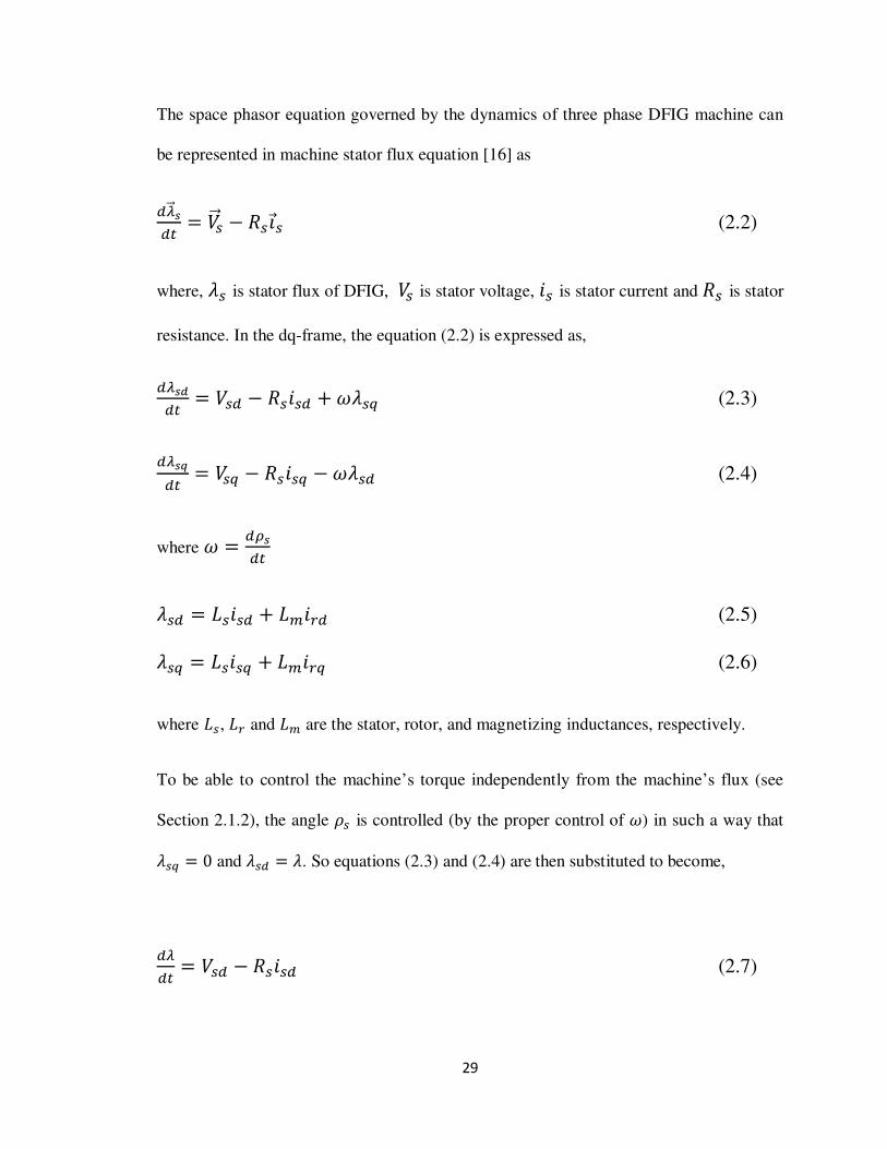
The space phasor equation governed by the dynamics of three phase DFIG machine can
be represented in machine stator flux equation [16] as
/_/' = − (2.2)
where, is stator flux of DFIG, is stator voltage, is stator current and is stator
resistance. In the dq-frame, the equation (2.2) is expressed as,
/_c/' = / − / +"e (2.3)
/_/' = e − e −"/ (2.4)
where " = //'
/ = / + / (2.5)
e = e + e (2.6)
where , and are the stator, rotor, and magnetizing inductances, respectively.
To be able to control the machine’s torque independently from the machine’s flux (see
Section 2.1.2), the angle 1 is controlled (by the proper control of ") in such a way that
e = 0 and / = . So equations (2.3) and (2.4) are then substituted to become,
/_/' = / − / (2.7)

30
//' = _ (e − e) (2.8)
The dq-frame currents, / and e are eliminated from equations (2.7) and (2.8) by
substituting equations (2.5) and (2.6). The two equations are then rewritten in terms of
/ and e.
/_/' = − _+/ + Vc (2.9)
//' = _ (e + V ) (2.10)
where / and e are the d- and q-axis components of rotor currents, respectively and
%= is called the stator time constant.
2.1.2 Torque/ Flux Controller
The machine torque equation is written as,
&) = ? e (2.11)
It is observed from (2.11) that machine’s electrical torque is controlled linearly by the
rotor q-axis current e.
Under steady-state condition, the stator flux and stator voltage of DFIG are sinusoidal
waveforms with amplitudes and , respectively. As e = 0, / = = , thenignoring from equation (2.7), at steady state condition, / = 0 and as

31
/ +e = is the peak value of the line to neutral voltage and is a constant, e ,
which becomes . Also, at steady state condition, " = "#, where "# is the machine’s
nominal frequency. Then ≈ G[. Considering all the assumptions, the machine torque
equation can be rewritten as
&) = ? G[ e (2.12)
&) can also be represented in terms of " , and the equation is given by [16],
&) = BX'" (2.13)
where BX' is a constant. The value of BX' depends on the wind-turbine’s design
specification and characteristics. A detail description for BX' is as given in Hilal et al.
[25]. To extract the maximum possible electrical power from a variable speed wind
power system, &) is expressed as &)). and is given by
&)). = BX'" (2.14)
From equations (2.12) and (2.14), the expression for e is obtained. This e is
represented as e).which controls the electrical torque. The expression of e). is
schematically shown in Figure 2.3.

32
×sm
os
VL
L
ˆ3
2 ω
Figure 2.3: Schematic diagram of rotor q-axis reference current generator
Figure 2.4 presents the schematic diagram of the d- and q- axis current controllers of the
rotor side converter VSC1 [16] , where = ( − Q ) and 3() is a PI controller; the
values of which are given in appendix A.
- -
-
iiiirdrefrdrefrdrefrdref
iiiirqrefrqrefrqrefrqref
iiiirdrdrdrdiiiirqrqrqrq
KKKKrrrr((((ssss))))
KKKKrrrr((((ssss)))) RRRRrrrr
RRRRrrrrηηηηωωωω0000––––ωωωωrrrr
((((ωωωω0000––––ωωωωrrrr))))
mmmmrdrdrdrd
mmmmrqrqrqrq
VVVVdcdcdcdc________________2222eeeerrrr2222
eeeerrrr1111
λλλλ
LLLLmmmm________________LLLLssss
ηηηη
Figure 2.4: Block diagram of machine rotor current control loop

33
The rotor d- and q- axis currents / and e are controlled through their corresponding
reference current control commands /). and e)., respectively; / and e are the
modulating signals and stand as the output of the controller, as described in Figure 2.4.
Modulating signals / and e are transformed into their “abc” frame, and the signal is
presented as Z+ . Switching sequences in the rotor side converters are controlled by
the modulating signals Z+.
2.1.3 Phase Locked Loop (PLL)
The schematic diagram of PLL for synchronizing the utility voltages with controlled
voltages is shown in Figure 2.5.
abc
dq
VVVVsasasasaVVVVsbsbsbsbVVVVscscscscVVVVsdlsdlsdlsdlVVVVsqlsqlsqlsql HHHHssss((((ssss)))) θθθθllll
Figure 2.5: Schematic diagram of PLL
From the above schematic diagram, the following equation is derived;
/£a/' = ()e (2.15)
34
where () is a compensator. The transfer function of () is given in the appendix A.
As the PLL frame and the stator flux frame angles are different so, the PLL voltages,
/ and e , are expressed in terms of stator flux voltages.
/ = / cos(1 − 0 ) − e sin(1 − 0 ) (2.16)
e = / sin(1 − 0 ) + e cos(1 − 0 ) (2.17)
() changes 0 in a way so that e = 0 and / = . A detailed design and
operation of PLL are mentioned in [16].
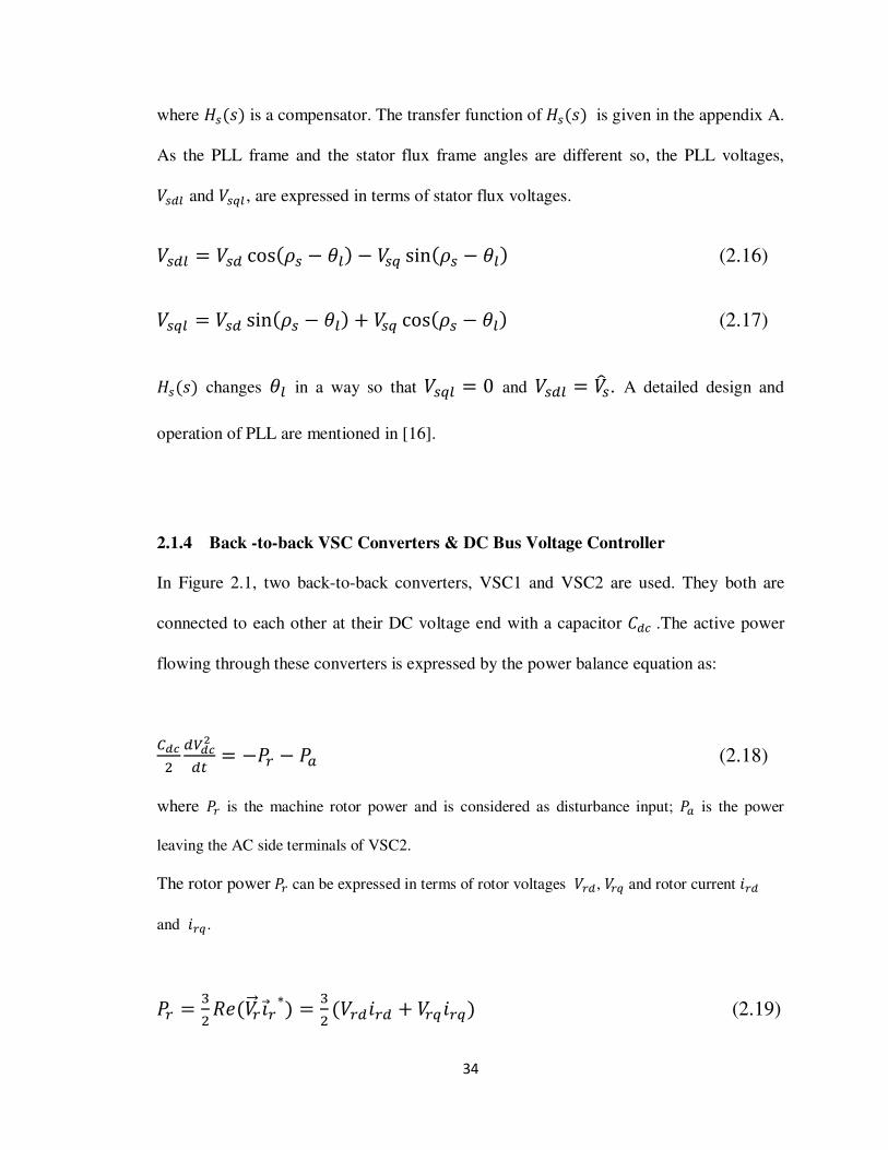
2.1.4 Back -to-back VSC Converters & DC Bus Voltage Controller
In Figure 2.1, two back-to-back converters, VSC1 and VSC2 are used. They both are
connected to each other at their DC voltage end with a capacitor -/+ .The active power
flowing through these converters is expressed by the power balance equation as:
¤c¥ /Gc¥Q/' = − − (2.18)
where is the machine rotor power and is considered as disturbance input; is the power
leaving the AC side terminals of VSC2.
The rotor power can be expressed in terms of rotor voltages /, e and rotor current /
and e.
= ?=(∗) = ? (// + ee) (2.19)
35
Also can be represented as:
= ?=§∗¨
As, / = ?Gca©T¥ ; and e = ?Ga©T¥ ;
= ?©T¥ (/ / + e e) (2.20)
where *'+ is turn ratio of the transformer, &. / , e and /, eare d-and q-axis
components of voltage and current, respectively, of the ac-side terminal of VSC2 in
Figure 2.1.
Based on equation (2.18) and equation (2.20), is the dc voltage /+ is controlled by /
only, because in the previous section, e = 0 . Figure 2.6 illustrates the current control
loop for DC bus voltage regulation. The ac side d- and q- axis current components /
and e of VSC2 are controlled through their corresponding reference current control
commands /). and e)., respectively; / and e are the modulating signals, and
stand as the output of the controller, as described in Figure 2.6. Modulating signals /
and e are transformed into their “abc” frame, and the signal is presented as Z+ .
Switching sequences in the grid side converters are controlled by the modulating signals
Z+.

36
- -
-
iiiiadrefadrefadrefadref
iiiiaqrefaqrefaqrefaqref mmmmaqaqaqaq
mmmmadadadad
iiiiaqaqaqaqiiiiadadadad LLLLaaaa
ωωωωllllLLLLaaaa
KKKKaaaa((((ssss))))
KKKKaaaa((((ssss))))GGGGffff((((ssss))))
GGGGffff((((ssss))))VVVVsqlsqlsqlsql________________________________NNNNtctctctc
VVVVsdlsdlsdlsdl________________________________NNNNtctctctc
VVVVdcdcdcdc____________________________2222
Figure 2.6: Schematic diagram of current control loop for grid side VSC System
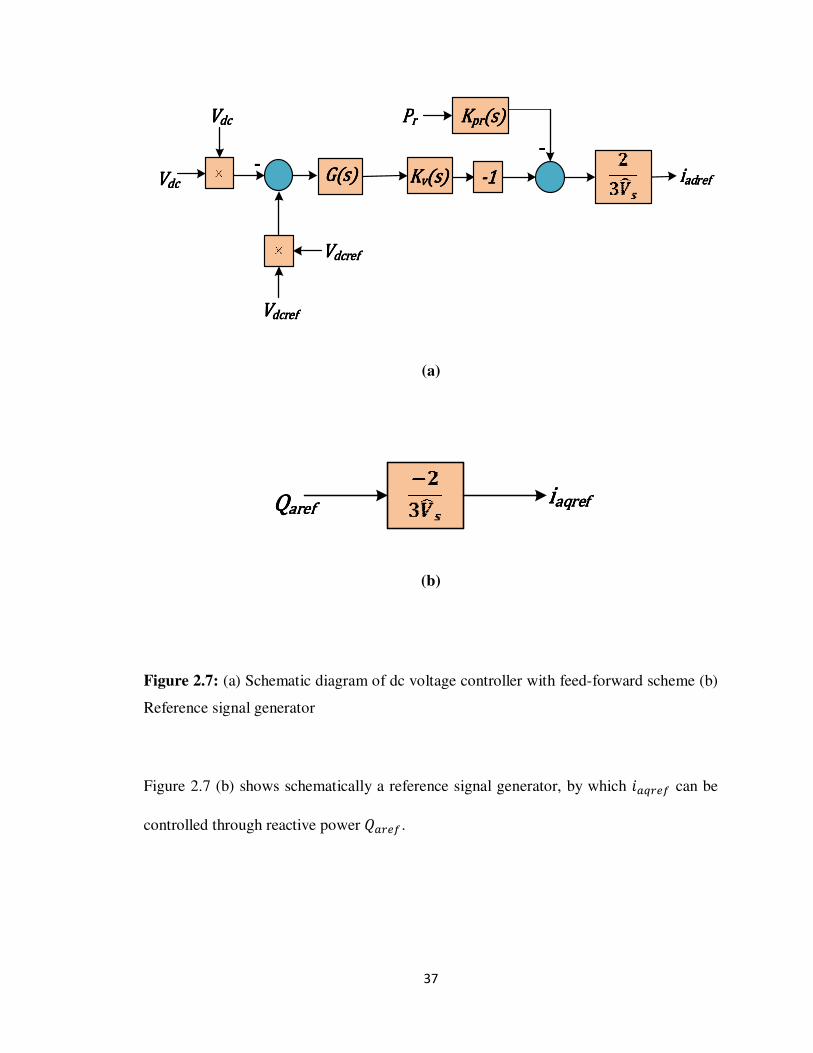
Figure 2.7 (a) shows the schematic diagram of DC-bus voltage controller with feed-
forward scheme. This figure shows that the effect of on /+ can be ignored by using a
feedforward term, which measures through filter 3X. Transfer function of 3X is given
in the Appendix A.
37
VVVVdcdcdcdcVVVVdcdcdcdc
VVVVdcrefdcrefdcrefdcrefVVVVdcrefdcrefdcrefdcref
KKKKvvvv((((ssss)))) iiiiadrefadrefadrefadrefPPPPrrrr KKKKprprprpr((((ssss))))
----1111GGGG((((ssss))))
(a)
QQQQarefarefarefaref iiiiaqrefaqrefaqrefaqref
(b)
Figure 2.7: (a) Schematic diagram of dc voltage controller with feed-forward scheme (b)
Reference signal generator
Figure 2.7 (b) shows schematically a reference signal generator, by which e). can be
controlled through reactive power ). .
38
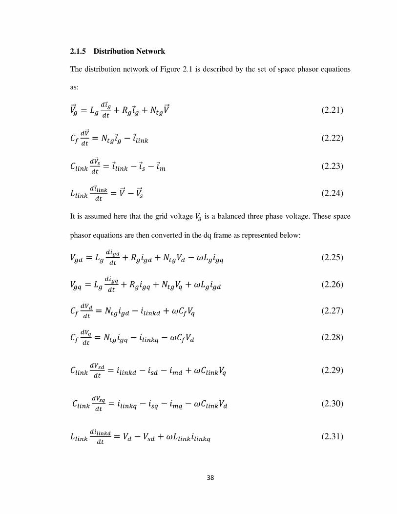
2.1.5 Distribution Network
The distribution network of Figure 2.1 is described by the set of space phasor equations
as:, = , /¬/' + ,, +*', (2.21)
-. /G/' = *',, − (2.22)
- /G/' = − − (2.23)
/¬a®¯°/' = − (2.24)
It is assumed here that the grid voltage , is a balanced three phase voltage. These space
phasor equations are then converted in the dq frame as represented below:
,/ = , /c/' + ,,/ +*',/ − ",,e (2.25)
,e = , //' + ,,e + *',e + ",,/ (2.26)
-. /Gc/' = *',,/ − / + "-.e (2.27)
-. /G/' = *',,e − e − "-./ (2.28)
- /Gc/' = / − / − / +"- e (2.29)
- /G/' = e − e − e − "- / (2.30)
/a®¯°c/' = / − / +" e (2.31)
39
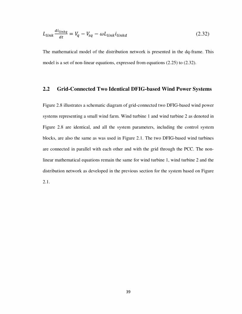
/a®¯°/' = e − e − " / (2.32)
The mathematical model of the distribution network is presented in the dq-frame. This
model is a set of non-linear equations, expressed from equations (2.25) to (2.32).
2.2 Grid-Connected Two Identical DFIG-based Wind Power Systems
Figure 2.8 illustrates a schematic diagram of grid-connected two DFIG-based wind power
systems representing a small wind farm. Wind turbine 1 and wind turbine 2 as denoted in
Figure 2.8 are identical, and all the system parameters, including the control system
blocks, are also the same as was used in Figure 2.1. The two DFIG-based wind turbines
are connected in parallel with each other and with the grid through the PCC. The non-
linear mathematical equations remain the same for wind turbine 1, wind turbine 2 and the
distribution network as developed in the previous section for the system based on Figure
2.1.

40
DFIGBased
DFIGBased
DFIGBased
DFIGBased
WindTurbine
WindT
urbine
WindTurbine
WindT
urbine 11 11
DFIGDFIG DFIGDFIG -- -- BasedBased
Based
Based
WindT
urbine
WindTurbine
WindT
urbine
WindTurbine
22 22
CC CC linkslinks linkslinks 22 22iiiiclinksclinksclinksclinks2222
LL LL linkslinks linkslinks 22 22iiiiffff CC CC ff ff
CC CC linkslinks linkslinks 11 11iiiiclinksclinksclinksclinks1111
PCCPCC PCCPCCTT TT rgrg rgrg
VV VVYY YY:: :: YY YY
RR RR gg ggLL LL gg gg
ii ii gg ggVV VV gg gg
PP PP gridgrid gridgrid
Figure 2.8: Schematic diagram of grid-connected two DFIG-based wind power systems.
41
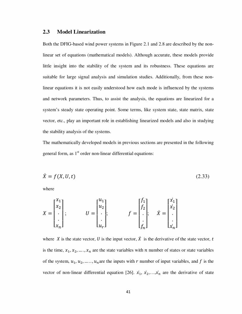
2.3 Model Linearization
Both the DFIG-based wind power systems in Figure 2.1 and 2.8 are described by the non-
linear set of equations (mathematical models). Although accurate, these models provide
little insight into the stability of the system and its robustness. These equations are
suitable for large signal analysis and simulation studies. Additionally, from these non-
linear equations it is not easily understood how each mode is influenced by the systems
and network parameters. Thus, to assist the analysis, the equations are linearized for a
system’s steady state operating point. Some terms, like system state, state matrix, state
vector, etc., play an important role in establishing linearized models and also in studying
the stability analysis of the systems.
The mathematically developed models in previous sections are presented in the following
general form, as 1st order non-linear differential equations:
²5 = 7(², ³, <) (2.33)
where
² = µµµ¶··..· ¹¹
¹º ; ³ = µµµ
¶»»..» ¹¹¹º; 7 = µµµ
¶77..7 ¹¹¹º; ²5 = µµµ
¶·5·5..·5 ¹¹¹º
where ² is the state vector, ³ is the input vector, ²5 is the derivative of the state vector, < is the time, ·, ·, … . , · are the state variables with ½ number of states or state variables
of the system, », », … . . , »are the inputs with ; number of input variables, and 7 is the
vector of non-linear differential equation [26]. ·5 , ·5 ,…,·5 are the derivative of state
42
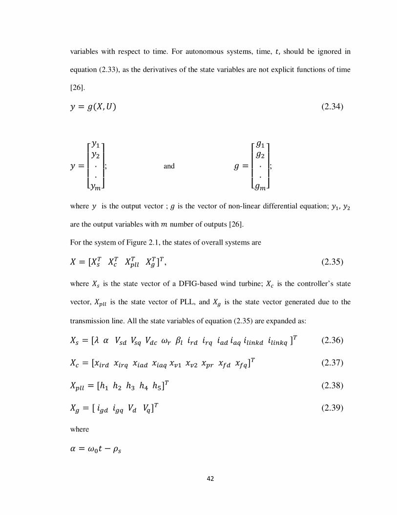
variables with respect to time. For autonomous systems, time, <, should be ignored in
equation (2.33), as the derivatives of the state variables are not explicit functions of time
[26].
¾ = ¿(²,³) (2.34)
¾ = µµµ¶¾¾..¾ ¹¹
¹º; and ¿ = µµµ
¶ ¿¿..¿ ¹¹¹º;
where ¾ is the output vector ; ¿ is the vector of non-linear differential equation; ¾, ¾ are the output variables with number of outputs [26].
For the system of Figure 2.1, the states of overall systems are
² = [²Á ²+Á ²X Á ²,Á]Á, (2.35)
where ² is the state vector of a DFIG-based wind turbine; ²+ is the controller’s state
vector, ²X is the state vector of PLL, and ², is the state vector generated due to the
transmission line. All the state variables of equation (2.35) are expanded as:
² = [Ã/e/+"W /e /e / e]Á (2.36)
²+ = [·/ ·e·/·e·Ä·Ä·X ·./·.e]Á (2.37)
²X = [ℎℎℎ?ℎÆℎÇ]Á (2.38)
², = [,/,e/e]Á (2.39)
where
à = "#< − 1

43
W = "#< − 0 ·/, and ·e are generated due to controller 3(), used in Figure 2.4.
·/, ·e, and ·./ , ·.e are created due to compensators 3(), and È.(), respectively,
in Figure 2.6.
·Ä, ·Ä, and ·X are generated due to controllers È(), 3Ä() and 3X(), respectively,
in Figure 2.7(a).
²X is generated due to one 5th order compensator used in the PLL block, () in Figure
2.5.
The input vector ³ for the system of Figure 2.1 is given by:
³ = [³Á³,Á]Á (2.40)
where ³ and ³, are expanded as
³ = ['(/). ).).]Á (2.41)
³, = [,]Á (2.42)
³ is the input vector applied to the DFIG-based wind turbine, where '( is the turbine
power; and ³,is the input vector generated due to grid voltage , , where , is the peak
value of the grid line to neutral voltage. For the mathematical model developed for Figure
2.1, 31 state equations are generated.
Figure 2.8 has two identical DFIG-based wind turbines, so for this case, ², ²+ , ²X , and
³ are generated twice. A few states generated due to the distribution network from the
model based in Figure 2.1 remain common for the overall system in Figure 2.8. Thus, as
a result, 58 state equations are mathematically created. A liniearization method

44
considering initial state vector, ²#, and initial input vector ³#, around the state vector, ²,
and input vector, ³, are needed to linearize the non-linear differential equations in (2.33)
and (2.34). 1st order differential equation of ²# is expressed as:
²5# = 7(²#³#) = 0 (2.43)
The final linearized differential equations mathematically modeled from the developed
non-linear models are then written as:
∆²5 = >∆² + Ê∆³ (2.44)
∆¾ = -∆² + Ë∆³ (2.45)
In equations (2.44) and (2.45), ∆² is the state vector with dimension½; > is the system
state matrix with size ½ × ½ ; ∆³ is the input vector with dimension;; Ê is the system
input matrix with size ½ × ;; ∆¾ is the output vector with dimension ; - is the output
matrix with size × ½, and Ë is the feedforward matrix with size × ;.
where
> = ÍÎ.ÏÎÐÏ…… . Î.ÏÎЯ……… . .Î.ÎÐÏ…… Î.ÎÐ¯Ñ ; Ê = ÍÎ.ÏÎ(Ï…… . Î.ÏÎ(V……… . .Î.Î(Ï…… Î.Î(V
Ñ (2.46)
- = ÍÎ,ÏÎÐÏ…… . Î,ÏÎЯ……… . .Î,ÎÐÏ …… Î,ÎÐ¯Ñ ; Ë = ÍÎ,ÏÎ(Ï…… . Î,ÏÎ(V……… . .Î,Î(Ï …… Î,Î(V
Ñ
45
½ number of eigenvalues are generated from state matrix >, as the size of the matrix is
½ × ½. Eigenvalue is denoted as , where varies from 1 to ½ [26]. State matrix > is
also represented as,
> = Ò6…… . 6……… . .6……6 Ó; (2.47)
where 6Ô is the element of > in <ℎ row and Õ<ℎ column.
A detailed linearized mathematical model of the wind farm is expressed in Appendix B,
From this section, it is determined that as each eigenvalue corresponds to the each
eigenmode of the system, thus total 31 eigenmodes and 58 eigenmodes are generated
from linearized mathematical model of systems in Figure 2.1 and Figure 2.8,
respectively.
2.4 Summary and Conclusions
This chapter has established a detailed non-linear mathematical model of a DFIG-based
single wind turbine system connected to a grid as well as a multi DFIG-based wind
turbine system connected to a distribution network in the dq-frame. It has also provided
each control system block used for both the systems, and provided a detailed description
of each block in the dq-frame. Linearization of mathematical model for both the systems
has been performed from the set of developed non-linear equations. These two linearized
dynamic models provide an analytical platform for determining the robustness and
stability of the two systems. A total of 31 states for grid-connected single wind power
system plus 58 state equations for grid-connected two DFIG-based wind power systems
have been determined. Additionally, this chapter describes how close observation makes

46
decoupling of the d-and q-axis current components of rotor side and grid side converters
possible with the proper selection of angular speed of dq-frame.
47
Chapter 3
Model Validation and Simulation Result
In this chapter, simulation studies are carried out on a detailed switched model of a grid-
connected DFIG-based single wind turbine, as well as on the switched model of a grid-
connected small wind farm. The simulations are conducted in PSCAD/EMTDC
environment and performed to ensure the algebraic accuracy of the linearized models of
Chapter 2. The linearized models are simulated in the MATLAB/SIMULINK software
environment, and their responses are compared with those obtained from the switched
models of the PSCAD/EMTDC environment. Hence, the switched models are considered
in this thesis as the equivalents of experimental set-ups. Since the linearized models
approximate the small-signal behaviors of their corresponding non-linear switched
counterparts, the levels of test disturbances have been kept to about or less than 10% of
their corresponding nominal values. Two different case studies are conducted on each
switched model and their corresponding linearized model at a 13.5 m/s wind speed. In
case study 1, a 10% step change of grid signal at t=5.0 s is imposed. In case study 2, a
step change in dc link voltage of VSCs is applied from 1200V to 1350V at t=5.0 s.

48
3.1 Case Study 1
In this case study, 10% step change in grid voltage is imposed at 13.5m/s wind speed and
1 µH linking inductances to the models of both the systems developed in the
PSCAD/EMTDC and MATLAB/SIMULINK environment for validation. The results,
achieved from linear and non-linear models are then compared. The simulation results for
case study 1 are presented from Figure 3.1 to Figure 3.8. Figure 3.1 presents simulation
results of rotor speed ", ", and " of each turbine. Figure 3.2 describes dc link
voltages /+ , /+,/+ of ac-dc-ac back to back VSCs of both the systems. Figure 3.3
and Figure 3.4 presents simulation results of stator fluxes, , and electrical
torques &), &), &), respectively, of each of the turbines. Figure 3.5 and Figure 3.6
compares the simulation results ofactive power components of rotor side (, ,)
and grid side converters ( , , ) , respectively. Figure 3.7 and Figure 3.8 present
simulation results of reactive power components of rotor side (, ,) and grid
side converters (, ,), respectively.
In these figures, left columns represent the simulation results, achieved from linearized
models whereas right columns represents the simulation results of non-linear models. It is
noticed that the graphs of linearized models closely agree with the results from
PSCAD/EMTDC environment [27].
49
(a)
(b)
(c)
Figure 3.1: Responses of rotor speed of wind turbines (a) Response of wind turbine of
Figure 2.1 (b) Response of Wind Turbine 1 of Figure 2.8 (c) Response of Wind Turbine 2
of Figure 2.8

50
(a)
(b)
(c)
Figure 3.2: Responses of dc link voltages of ac-dc-ac back to back VSCs (a) Response of
Figure 2.1 (b) Response of Wind Turbine 1 of Figure 2.8 (c) Response of Wind Turbine 2
of Figure 2.8

51
(a)
(b)
(c)
Figure 3.3: Responses of stator fluxes of wind turbines (a) Response of wind turbine of
Figure 2.1 (b) Response of Wind Turbine 1 of Figure 2.8 (c) Response of Wind Turbine 2
of Figure 2.8

52
(a)
(b)
(c)
Figure 3.4: Responses of electrical torques of wind turbines (a) Response of wind turbine
of Figure 2.1 (b) Response of Wind Turbine 1 of Figure 2.8 (c) Response of Wind
Turbine 2 of Figure 2.8

53
(a)
(b)
(c)
Figure 3.5: Responses of active power of rotor side converters (a) Response of Figure
2.1 (b) Response of Wind Turbine 1 of Figure 2.8 (c) Response of Wind Turbine 2 of
Figure 2.8

54
(a)
(b)
(c)
Figure 3.6: Responses of active power of grid side converters (a) Response of Figure 2.1
(b) Response of Wind Turbine 1 of Figure 2.8 (c) Response of Wind Turbine 2 of Figure
2.8
55
(a)
(b)
(c)
Figure 3.7: Responses of reactive power of rotor side converters (a) Response of Figure
2.1 (b) Response of Wind Turbine 1 of Figure 2.8 (c) Response of Wind Turbine 2 of
Figure 2.8
56
(a)
(b)
(c)
Figure 3.8: Responses of reactive power of grid side converters (a) Response of Figure
2.1 (b) Response of Wind Turbine 1 of Figure 2.8 (c) Response of Wind Turbine 2 of
Figure 2.8
57
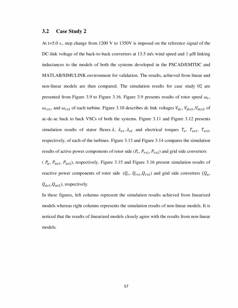
3.2 Case Study 2
At t=5.0 s., step change from 1200 V to 1350V is imposed on the reference signal of the
DC-link voltage of the back-to-back converters at 13.5 m/s wind speed and 1 µH linking
inductances to the models of both the systems developed in the PSCAD/EMTDC and
MATLAB/SIMULINK environment for validation. The results, achieved from linear and
non-linear models are then compared. The simulation results for case study 02 are
presented from Figure 3.9 to Figure 3.16. Figure 3.9 presents results of rotor speed ",
", and " of each turbine. Figure 3.10 describes dc link voltages /+ , /+,/+ of
ac-dc-ac back to back VSCs of both the systems. Figure 3.11 and Figure 3.12 presents
simulation results of stator fluxes, , and electrical torques &), &), &),
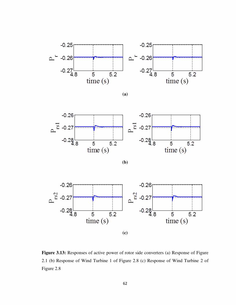
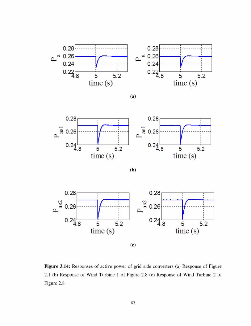
respectively, of each of the turbines. Figure 3.13 and Figure 3.14 compares the simulation
results ofactive power components of rotor side (, ,) and grid side converters
( , , ), respectively. Figure 3.15 and Figure 3.16 present simulation results of
reactive power components of rotor side (, ,) and grid side converters (,
,), respectively.
In these figures, left columns represent the simulation results achieved from linearized
models whereas right columns represents the simulation results of non-linear models. It is
noticed that the results of linearized models closely agree with the results from non-linear
models.
58
(a)
(b)
(c)
Figure 3.9: Responses of rotor speed of wind turbines (a) Response of wind turbine of
Figure 2.1 (b) Response of Wind Turbine 1 of Figure 2.8 (c) Response of Wind Turbine 2
of Figure 2.8
59
(a)
(b)
(c)
Figure 3.10: Responses of dc link voltages of ac-dc-ac back to back VSCs (a) Response
of Figure 2.1 (b) Response of Wind Turbine 1 of Figure 2.8 (c) Response of Wind
Turbine 2 of Figure 2.8

60
(a)
(b)
(c)
Figure 3.11: Responses of stator fluxes of wind turbines (a) Response of wind turbine of
Figure 2.1 (b) Response of Wind Turbine 1 of Figure 2.8 (c) Response of Wind Turbine 2
of Figure 2.8

61
(a)
(b)
(c)
Figure 3.12: Responses of electrical torques of wind turbines (a) Response of wind
turbine of Figure 2.1 (b) Response of Wind Turbine 1 of Figure 2.8 (c) Response of Wind
Turbine 2 of Figure 2.8
62
(a)
(b)
(c)
Figure 3.13: Responses of active power of rotor side converters (a) Response of Figure
2.1 (b) Response of Wind Turbine 1 of Figure 2.8 (c) Response of Wind Turbine 2 of
Figure 2.8
63
(a)
(b)
(c)
Figure 3.14: Responses of active power of grid side converters (a) Response of Figure
2.1 (b) Response of Wind Turbine 1 of Figure 2.8 (c) Response of Wind Turbine 2 of
Figure 2.8

64
(a)
(b)
(c)
Figure 3.15: Responses of reactive power of rotor side converters (a) Response of Figure
2.1 (b) Response of Wind Turbine 1 of Figure 2.8 (c) Response of Wind Turbine 2 of
Figure 2.8
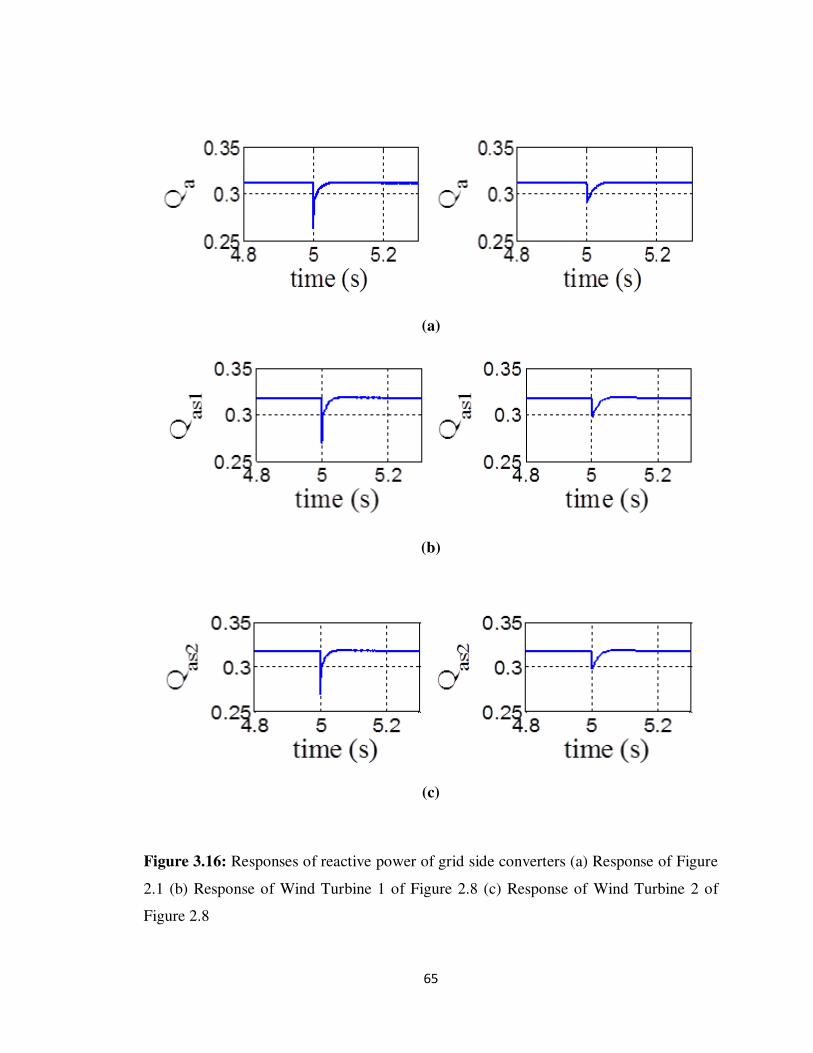
65
(a)
(b)
(c)
Figure 3.16: Responses of reactive power of grid side converters (a) Response of Figure
2.1 (b) Response of Wind Turbine 1 of Figure 2.8 (c) Response of Wind Turbine 2 of
Figure 2.8

66
3.3 Summary and Conclusion
The linearized models developed in Chapter 2 have been verified with the simulation
results of non-linear systems designed in the PSCAD/EMTDC environment. Model
validation was carried out for two different conditions. Firstly, a 10% step change in grid
voltage at t=5 s. was applied to both the linear and non-linear systems, and secondly, a
step change from 1200V to 1350V of the dc link voltage of VSCs was applied. All the
simulation results of both the linear and non-linear models of both the systems were
compared and found to be identical.

67
Chapter 4
Modal Analysis- System Parametric Effects
The modal analysis of the two linearized systems, a single-turbine and a small wind farm
both individually connected to a grid, developed in Chapter 2, are performed separately
by changing different system parameters and operating conditions of the systems. For
better understanding of intrinsic dynamic behavior and enhancement of system stability,
this analysis is of utmost importance. Modal analysis also allows in figuring out the
change in modal properties that occurs due to the change of system parameters and
operating conditions. A brief detail of the terms participation factor, system stability,
frequency of oscillations, and damping ratio are presented in this chapter, before modal
analysis of the systems is performed. Eigenvalue sensitivity is then determined from the
modal analysis by changing the linking inductances and wind speed.
4.1 Brief Description of Stability & Modal Analysis
Stability: The stability of the linearized models of grid-connected single wind power
system and the grid-connected small wind farm is achieved by means of eigenvalue
analysis.

68
Participation Factor: Effects of system parameters, on each eigenmode for linearized
system, is determined by participation factor analysis. The element Ö is denoted as
participation factor and is given by:
Ö = Î_®Î°° (4.1)
where Î_®Î°° = ×Ø , (4.2)
where is the eigenvalue of the linearized system and 6 is the diagonal element of
state matrix > [26, 28, 29]; already discussed in Chapter 2. × is the k th entry of the
right eigenvector × of state matrix >; Ø is the k th entry of the left eigenvector Ø of
state matrix > [26,28].
Frequency of Oscillations and Damping Factor: Oscillatory mode of a system occurs
for a complex eigenvalue. These eigenvalues always occur in conjugate pairs and is
expressed as [26]:
= Ù ± ÕW , (4.3)
where Ù is the real part of the eigenvalue and W is the complex part. Frequency of
oscillation (fÛÜÝ) in Hz is then expressed as:
fÛÜÝ = Þß (4.4)
The damping of the system depends on the real part of the eigenvalue. The damping
factor (ζ) is written as:
ζ= PàáàQIÞQ (4.5)
The rate of decay of amplitude of system oscillation is determined by ζ.

69
4.2 Sensitivity Analysis at very low Linking Inductances
In this section, relative participation factor analysis for dominant eigenvalue is studied.
The dominant eigenmode are compared on the basis of participation of different states,
for, linearized models; grid-connected DFIG-based single wind turbine and grid-
connected DFIG-based small wind farm, developed in Chapter 2. Participation of states
that are generated due to linking inductances, and wind speed, in eigenmodes are also
observed. Then, eigenvalue loci are drawn to compare the intrinsic dynamic behavior of
both the linearized systems. The behavior of frequency of oscillation and damping factor
of linearized systems are analyzed. All these analysis are performed under low linking
inductances.
4.2.1 Participation Factor Analysis
Participation factor, Ö , analysis is carried out for both the linearized systems,
developed in Chapter 2. However, the relative participation, âÖâ , of a state variable in
an eigenmode for both the systems is of prime interest, therefore, âÖâ is determined and
presented in Table 4.1, Table 4.2 and Table 4.3. Additionally, relative participation
factors which are less than 0.01 are considered zero in the tables.
Table 4.1 presents, the participation factor analysis for linearized DFIG-based single
wind turbine system connected to a grid at a wind speed, = 13.5m/s. and linking
inductance, = 1 µH. Table 4.2 analyzes the participation factors of linearized model
of two DFIG-based wind turbine systems connected to a grid (small wind farm) by
applying wind speed = =13.5 m/s. and linking inductances = = 1
µH.

70
Table-4.1: Participation factor analysis at wind speed = 13.5/ and linking
inductance = 1μ
System State ãä,å
−å.æç ± èåéçéæéæ.äê
ãë,é
−å.æì ± èåééìçæ.äí
ãåí
−ç. îìéìæéîëçî
/ 0.17 0.17 ≈ 0
e 0.17 0.17 ≈ 0
/ 0.08 0.08 ≈ 0
e 0.08 0.08 ≈ 0
/ 0.25 0.25 ≈ 0
e 0.25 0.25 ≈ 0
" ≈ 0 ≈ 0 1.002
e ≈ 0 ≈ 0 0.01
·e ≈ 0 ≈ 0 0.01
All other state ≈ 0 ≈ 0 ≈ 0
Participation of state variables in each dominant eigenmode is viewed in Table-4.1 and
Table-4.2. /, e, /, e , / , e, /, e , / , e of Table
4.2 and/, e,/, e , / , eof Table 4.1, are directly related to the system’s
linking inductances, present significant participation in eigenmode ,, ?,Æ, Ç,ï, ^,ð of
linearized model of two-turbine system and in eigenmode ,, ?,Æ of linearized model
of single-turbine system, respectively. Participation of the state variables, " and "
of Table 4.2 and the state variable " of Table 4.1, are significant in eigenmode Ç?, ÇÆ
and in eigenmode ñ, respectively.
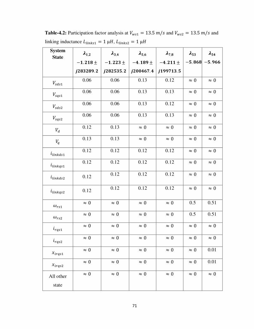
71
Table-4.2: Participation factor analysis at = 13.5/ and = 13.5/ and
linking inductance = 1μ, = 1μ
System
State ãä,å −ä.åäê ± èåêëåêí.å
ãë,é −ä.ååë ± èåêåçëç.å
ãç,ì −é.äêí ± èåææéìî.é ãî,ê −é.åää ± èäííîäë.ç
ãçë −ç. êìê
ãçé −ç. íìì /
0.06 0.06 0.13 0.12 ≈ 0 ≈ 0
e 0.06 0.06 0.13 0.13 ≈ 0 ≈ 0
/ 0.06 0.06 0.13 0.12 ≈ 0 ≈ 0
e 0.06 0.06 0.13 0.13 ≈ 0 ≈ 0
/ 0.12 0.13 ≈ 0 ≈ 0 ≈ 0 ≈ 0
e 0.13 0.13 ≈ 0 ≈ 0 ≈ 0 ≈ 0
/ 0.12 0.12 0.12 0.12 ≈ 0 ≈ 0
e 0.12 0.12 0.12 0.12 ≈ 0 ≈ 0
/ 0.12 0.12 0.12 0.12 ≈ 0 ≈ 0
e 0.12 0.12 0.12 0.12 ≈ 0 ≈ 0
" ≈ 0 ≈ 0 ≈ 0 ≈ 0 0.5 0.51
" ≈ 0 ≈ 0 ≈ 0 ≈ 0 0.5 0.51
e ≈ 0 ≈ 0 ≈ 0 ≈ 0 ≈ 0 ≈ 0
e ≈ 0 ≈ 0 ≈ 0 ≈ 0 ≈ 0 ≈ 0
·e ≈ 0 ≈ 0 ≈ 0 ≈ 0 ≈ 0 0.01
·e ≈ 0 ≈ 0 ≈ 0 ≈ 0 ≈ 0 0.01
All other
state
≈ 0 ≈ 0 ≈ 0 ≈ 0 ≈ 0 ≈ 0
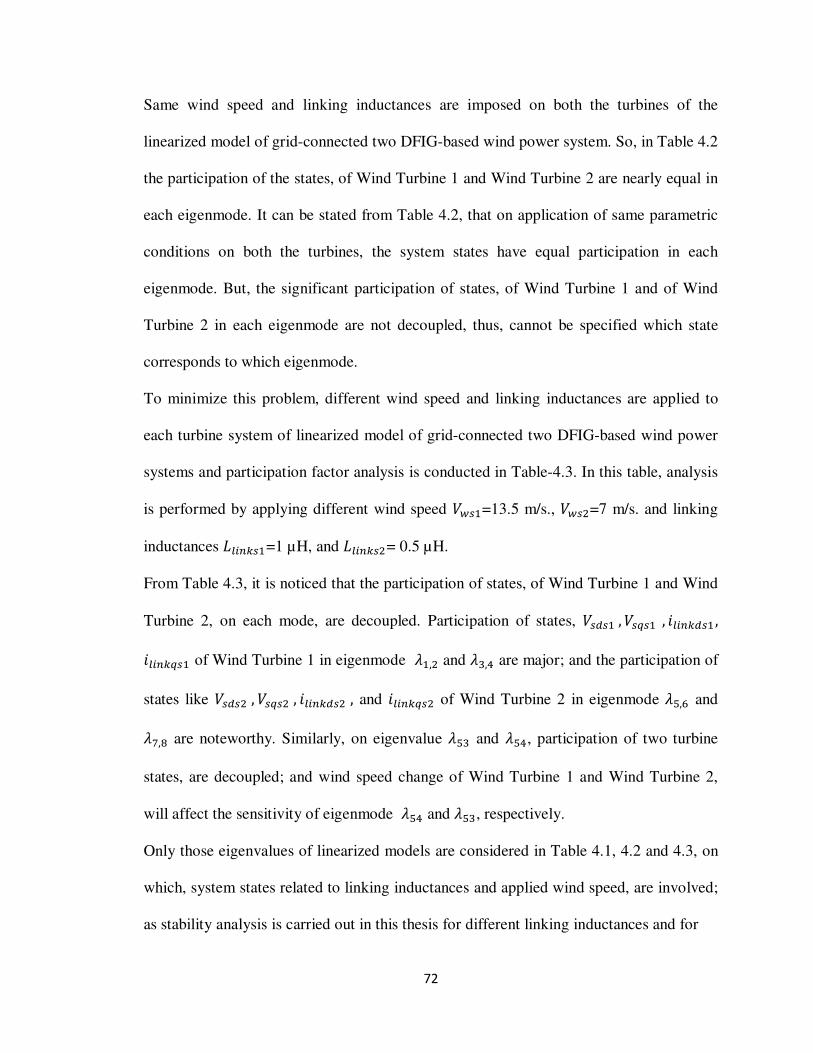
72
Same wind speed and linking inductances are imposed on both the turbines of the
linearized model of grid-connected two DFIG-based wind power system. So, in Table 4.2
the participation of the states, of Wind Turbine 1 and Wind Turbine 2 are nearly equal in
each eigenmode. It can be stated from Table 4.2, that on application of same parametric
conditions on both the turbines, the system states have equal participation in each
eigenmode. But, the significant participation of states, of Wind Turbine 1 and of Wind
Turbine 2 in each eigenmode are not decoupled, thus, cannot be specified which state
corresponds to which eigenmode.
To minimize this problem, different wind speed and linking inductances are applied to
each turbine system of linearized model of grid-connected two DFIG-based wind power
systems and participation factor analysis is conducted in Table-4.3. In this table, analysis
is performed by applying different wind speed =13.5 m/s., =7 m/s. and linking
inductances =1 µH, and = 0.5 µH.
From Table 4.3, it is noticed that the participation of states, of Wind Turbine 1 and Wind
Turbine 2, on each mode, are decoupled. Participation of states, /, e, / , e of Wind Turbine 1 in eigenmode , and ?,Æ are major; and the participation of
states like /, e, / , and e of Wind Turbine 2 in eigenmode Ç,ï and
^,ð are noteworthy. Similarly, on eigenvalue Ç? and ÇÆ, participation of two turbine
states, are decoupled; and wind speed change of Wind Turbine 1 and Wind Turbine 2,
will affect the sensitivity of eigenmode ÇÆ and Ç?, respectively.
Only those eigenvalues of linearized models are considered in Table 4.1, 4.2 and 4.3, on
which, system states related to linking inductances and applied wind speed, are involved;
as stability analysis is carried out in this thesis for different linking inductances and for

73
Table-4.3: Participation factor analysis at = 13.5/ and = 7/ and
linking inductance = 1μ, = 0.5μ
System
State ãä,å −ä.íæî ± èåéêìîë.å
ãë,é −ä. íäì± èåéîíäí
ãçë −å. íäêî ãçé −ç. íåéì ãç,ì −î.íê ± èäæåéîå. é
ãî,ê −ê. æåì± èä. æäî /
0.16 0.16 ≈ 0 ≈ 0 0.03 0.03
e 0.16 0.16 ≈ 0 ≈ 0 0.03 0.03
/ ≈ 0 ≈ 0 ≈ 0 ≈ 0 0.19 0.19
e ≈ 0 ≈ 0 ≈ 0 ≈ 0 0.19 1.19
/ 0.09 0.09 ≈ 0 ≈ 0 0.03 0.03
e 0.09 0.09 ≈ 0 ≈ 0 0.03 0.03
/ 0.24 0.24 ≈ 0 ≈ 0 0.01 0.01
e 0.24 0.24 ≈ 0 ≈ 0 0.01 0.01
/ ≈ 0 ≈ 0 ≈ 0 ≈ 0 0.24 0.24
e ≈ 0 ≈ 0 ≈ 0 ≈ 0 0.24 0.24
" ≈ 0 ≈ 0 ≈ 0 1 ≈ 0 ≈ 0
" ≈ 0 ≈ 0 1.005 ≈ 0 ≈ 0 ≈ 0
e ≈ 0 ≈ 0 ≈ 0 0.01 ≈ 0 ≈ 0
e ≈ 0 ≈ 0 ≈ 0 ≈ 0 ≈ 0 ≈ 0
·e ≈ 0 ≈ 0 ≈ 0 0.01 ≈ 0 ≈ 0
·e ≈ 0 ≈ 0 0.01 ≈ 0 ≈ 0 ≈ 0
All other
state
≈ 0 ≈ 0 ≈ 0 ≈ 0 ≈ 0 ≈ 0
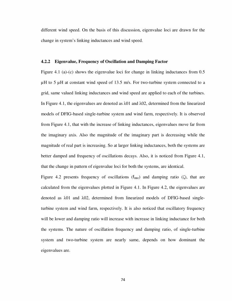
74
different wind speed. On the basis of this discussion, eigenvalue loci are drawn for the
change in system’s linking inductances and wind speed.
4.2.2 Eigenvalue, Frequency of Oscillation and Damping Factor
Figure 4.1 (a)-(c) shows the eigenvalue loci for change in linking inductances from 0.5
µH to 5 µH at constant wind speed of 13.5 m/s. For two-turbine system connected to a
grid, same valued linking inductances and wind speed are applied to each of the turbines.
In Figure 4.1, the eigenvalues are denoted as λ01 and λ02, determined from the linearized
models of DFIG-based single-turbine system and wind farm, respectively. It is observed
from Figure 4.1, that with the increase of linking inductances, eigenvalues move far from
the imaginary axis. Also the magnitude of the imaginary part is decreasing while the
magnitude of real part is increasing. So at larger linking inductances, both the systems are
better damped and frequency of oscillations decays. Also, it is noticed from Figure 4.1,
that the change in pattern of eigenvalue loci for both the systems, are identical.
Figure 4.2 presents frequency of oscillations (fosc) and damping ratio (ζ), that are
calculated from the eigenvalues plotted in Figure 4.1. In Figure 4.2, the eigenvalues are
denoted as λ01 and λ02, determined from linearized models of DFIG-based single-
turbine system and wind farm, respectively. It is also noticed that oscillatory frequency
will be lower and damping ratio will increase with increase in linking inductance for both
the systems. The nature of oscillation frequency and damping ratio, of single-turbine
system and two-turbine system are nearly same, depends on how dominant the
eigenvalues are.

75
(a)
(b) (c)
Figure 4.1: Eigenvalue loci for change in linking inductances (a) λ1,2 and λ3,4 for single-
turbine connected to a grid (b) λ1,2 and λ3,4 for two-turbine system connected to a grid
(c) λ5,6 and λ7,8 for two-turbine system connected to a grid
-6 -5 -4 -3 -2 -11
1.5
2
2.5
3
3.5x 10
5
Real
Imag
inar
y
λ011,2
λ013,4
-4 -3 -2 -11
1.5
2
2.5
3
3.5
4
4.5x 10
5
Real
Imag
inar
y
λ021,2
λ023,4
-12 -10 -8 -6 -4 -20.5
1
1.5
2
2.5
3x 10
5
Real
Imag
inar
y
λ025,6
λ027,8
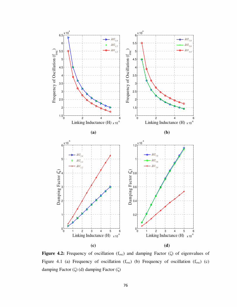
76
(a) (b)
(c) (d)
Figure 4.2: Frequency of oscillation (fosc) and damping Factor (ζ) of eigenvalues of
Figure 4.1 (a) Frequency of oscillation (fosc) (b) Frequency of oscillation (fosc) (c)
damping Factor (ζ) (d) damping Factor (ζ)
0 2 4 6
x 10-6
1.5
2
2.5
3
3.5
4
4.5
5
5.5
6
6.5x 10
4
Linking Inductance (H)
Fre
qu
ency
of
Osc
illa
tio
n (
f osc
)
λ023,4
λ021,2
λ011,2
0 2 4 6
x 10-6
1
1.5
2
2.5
3
3.5
4
4.5
5
5.5
6x 10
4
Linking Inductance (H)F
req
uen
cy o
f O
scil
lati
on
(f o
sc)
λ027,8
λ025,6
λ013,4
0 1 2 3 4 5 6
x 10-6
0
1
2
3
4
5
6x 10
-5
Linking Inductance (H)
Dam
pin
g F
acto
r (ζ
)
λ023,4
λ021,2
λ011,2
0 1 2 3 4 5 6
x 10-6
0
0.2
0.4
0.6
0.8
1
1.2x 10
-4
Linking Inductance (H)
Dam
pin
g F
acto
r (ζ
)
λ027,8
λ025,6
λ013,4

77
Figure 4.3 describes and compares the change in real part of dominant eigenvalues (σ) of
two different linearized models, with change in linking inductances varying from 0.5 µH
to 5 µH at a constant wind speed of 13.5 m/s. It is also observed that with rise in linking
inductances, the magnitudes of real part of dominant eigenvalues increase for both the
systems.
From Figure 4.1 to Figure 4.3, it is observed that with change in linking inductances,
eigenvalues, λ1,2 and λ3,4 for single wind power system connected to a grid and
eigenvalues, λ1,2, λ3,4, λ5,6 and λ7,8 for two wind power system connected to a grid, vary
Figure 4.3: Graph for change in linking inductances with real part of dominant
eigenvalue (σ) of linearized model grid-connected single-turbine system and grid-
connected two-turbine systems, with change in linking inductances
0.5 1 1.5 2 2.5 3 3.5 4 4.5 5-6
-5
-4
-3
-2
-1
0
Linking Inductance (µH)
σ
grid-connected single-turbine system
grid-connected two-turbine system
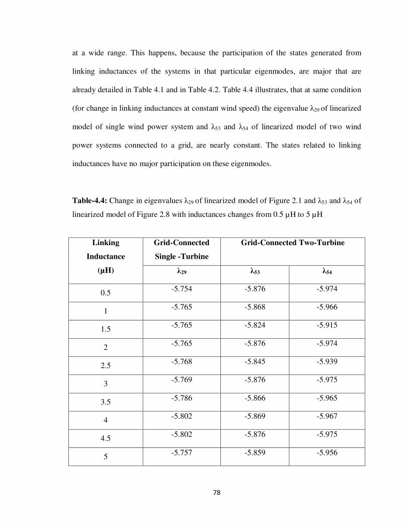
78
at a wide range. This happens, because the participation of the states generated from
linking inductances of the systems in that particular eigenmodes, are major that are
already detailed in Table 4.1 and in Table 4.2. Table 4.4 illustrates, that at same condition
(for change in linking inductances at constant wind speed) the eigenvalue λ29 of linearized
model of single wind power system and λ53 and λ54 of linearized model of two wind
power systems connected to a grid, are nearly constant. The states related to linking
inductances have no major participation on these eigenmodes.
Table-4.4: Change in eigenvalues λ29 of linearized model of Figure 2.1 and λ53 and λ54 of
linearized model of Figure 2.8 with inductances changes from 0.5 µH to 5 µH
Linking
Inductance
(µH)
Grid-Connected
Single -Turbine
Grid-Connected Two-Turbine
λ29 λ53 λ54
0.5 -5.754 -5.876 -5.974
1 -5.765 -5.868 -5.966
1.5 -5.765 -5.824 -5.915
2 -5.765 -5.876 -5.974
2.5 -5.768 -5.845 -5.939
3 -5.769 -5.876 -5.975
3.5 -5.786 -5.866 -5.965
4 -5.802 -5.869 -5.967
4.5 -5.802 -5.876 -5.975
5 -5.757 -5.859 -5.956

79
Figure 4.4 (a)-(c) shows the eigenvalue loci for change in wind speed from 6 m/s to 14
m/s at constant linking inductances of 1 µH. For two-turbine system connected to a grid,
the linking inductances and wind speed applied to each of the turbines are same. It is
observed in Figure 4.4 that with the rise in wind speed, eigenvalues λ29 of linearized
model of grid-connected single DFIG-based wind power system and λ53 and λ54 of
linearized model of grid-connected small wind farm, move far from imaginary axis.
Figure 4.4 illustrates that, these eigenmodes are non-oscillatory by nature.
Figure 4.5 shows that with change in wind speed, there is not much change on dominant
eigenvalues of both the systems. As was discussed previously, that the participation of
system states related to linking inductances are significant on dominant eigenvalues,
whereas the participation of the states related to wind speed on dominant eigenvalue are
insignificant.

80
(a)
(b)
(c)
Figure 4.4: Eigenvalue loci for change in wind speed (a) λ29 for single-turbine connected
to a grid. (b) λ53 for two-turbine system connected to a grid (c) λ54 for two-turbine system
connected to a grid
-6.5 -6 -5.5 -5 -4.5 -4 -3.5 -3 -2.5-1
-0.5
0
0.5
1
Real
Imag
inar
y
-6.5 -6 -5.5 -5 -4.5 -4 -3.5 -3 -2.5-1
-0.5
0
0.5
1
Real
Imag
inar
y
-6.5 -6 -5.5 -5 -4.5 -4 -3.5 -3 -2.5-1
-0.5
0
0.5
1
Real
Imag
inar
y

81
(a)
(b)
Figure 4.5: Graph for change in wind speed with real part of dominant eigenvalue for (a)
Linearized model of Figure 2.1 and (b) Linearized model of Figure 2.8
6 7 8 9 10 11 12 13 14-2.0525
-2.052
-2.0515
-2.051
-2.0505
-2.05
-2.0495
-2.049
-2.0485
-2.048
-2.0475
Wind Speed (m/s)
σ
grid-connected single-turbine system
6 7 8 9 10 11 12 13 14-1.218
-1.2175
-1.217
-1.2165
-1.216
-1.2155
-1.215
Wind speed (m/s)
σ
grid-connected two-turbine system
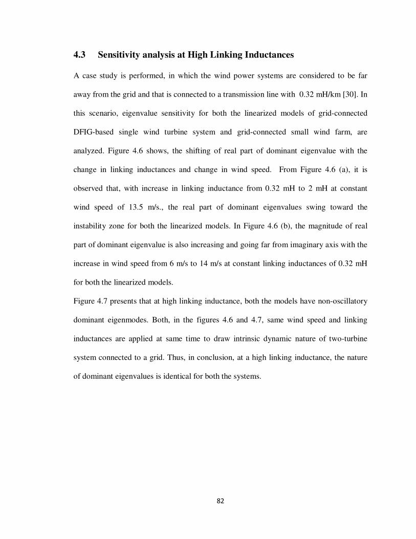
82
4.3 Sensitivity analysis at High Linking Inductances
A case study is performed, in which the wind power systems are considered to be far
away from the grid and that is connected to a transmission line with 0.32 mH/km [30]. In
this scenario, eigenvalue sensitivity for both the linearized models of grid-connected
DFIG-based single wind turbine system and grid-connected small wind farm, are
analyzed. Figure 4.6 shows, the shifting of real part of dominant eigenvalue with the
change in linking inductances and change in wind speed. From Figure 4.6 (a), it is
observed that, with increase in linking inductance from 0.32 mH to 2 mH at constant
wind speed of 13.5 m/s., the real part of dominant eigenvalues swing toward the
instability zone for both the linearized models. In Figure 4.6 (b), the magnitude of real
part of dominant eigenvalue is also increasing and going far from imaginary axis with the
increase in wind speed from 6 m/s to 14 m/s at constant linking inductances of 0.32 mH
for both the linearized models.
Figure 4.7 presents that at high linking inductance, both the models have non-oscillatory
dominant eigenmodes. Both, in the figures 4.6 and 4.7, same wind speed and linking
inductances are applied at same time to draw intrinsic dynamic nature of two-turbine
system connected to a grid. Thus, in conclusion, at a high linking inductance, the nature
of dominant eigenvalues is identical for both the systems.
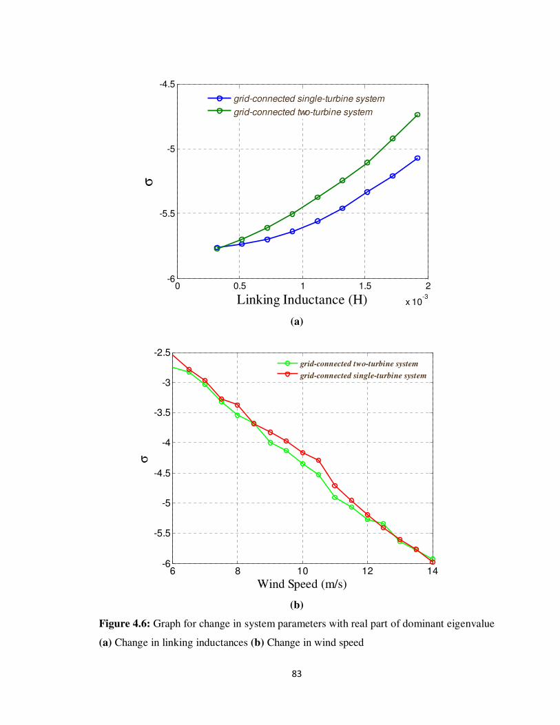
83
(a)
(b)
Figure 4.6: Graph for change in system parameters with real part of dominant eigenvalue
(a) Change in linking inductances (b) Change in wind speed
0 0.5 1 1.5 2
x 10-3
-6
-5.5
-5
-4.5
Linking Inductance (H)
σ
grid-connected single-turbine system
grid-connected two-turbine system
6 8 10 12 14-6
-5.5
-5
-4.5
-4
-3.5
-3
-2.5
Wind Speed (m/s)
σ
grid-connected two-turbine system
grid-connected single-turbine system

84
(a)
(b)
Figure 4.7: Dominant eigenvalue loci draw for change in wind speed from 6 m/s to 14
m/s at linking inductance 0.00032 H (a) Linearized model of grid-connected single-
turbine and (b) Linearized model of grid-connected small wind farm
4.4 Summary and Conclusion
This chapter has studied the small-signal stability, the system’s parametric effects on
stability and modal analysis of the two linearized models developed in Chapter 2. The
system’s parametric effects were analyzed using a participation factor. Modal analysis
was carried out by determining participation factor, damping factor and frequency of
oscillation of dominant eigenvalues of the systems. This study was conducted in the
MATLAB/SIMULINK environment. In conclusion, under the same operating conditions
and system parameters, the dynamic behavior of a multi-unit wind power system (farm)
-6 -5.5 -5 -4.5 -4 -3.5 -3 -2.5-1
-0.5
0
0.5
1
Real
Imag
inar
y
-6 -5.5 -5 -4.5 -4 -3.5 -3 -2.5-1
-0.5
0
0.5
1
Real
Imag
inar
y

85
is very similar to that of a single-unit wind power system connected to a grid; also, the
system parameters exhibit nearly the same effects on the stability of both aforementioned
systems.
86
Chapter 5
Summary, Conclusions and Future Works
5.1 Summary and Conclusions
Summary and conclusions of the thesis are stated below:
• Detailed non-linear mathematical models as well as linearization of a grid-
connected single DFIG-based turbine and a two DFIG-based wind turbine system
connected to a grid have been presented;
• Two ac-dc-ac back-to-back VSCs, PLL, rotor current controller block, dc bus
voltage current controller block, reference signal generator, stator flux observer,
current control loop for a grid side VSC system, DC voltage controller with feed-
forward block are introduced with each wind turbine system. Also, the role of
each controller block is explained in detail, and non-linear equations as well as
linearization are generated for each individual block;
• The system’s mathematical model is introduced in a dq-frame to avoid the
complexity of three phase circuits;
• Participation factor analysis is carried out to determine the system parametric
effects on each eigenmode for systems;
• The intrinsic dynamic behaviors of grid-connected single-turbine system and a
grid-connected two-turbine system are analyzed individually by observing the

87
pattern of eigenvalue loci, frequency of oscillation, and damping ratio. This study
is performed by changing system’s parameters and operating conditions such as
by linking inductance and wind speed;
• A comparative study of eigenvalue sensitivity, system parametric effects and
system stability is presented for a grid-connected single wind-power system to
that of a grid-connected two wind power system;
• Finally, to assess the stability, dynamic behavior, and effects of different system
parameters in a wind farm constituted entirely with identical wind power systems,
it is sufficient to only study one of the constituting wind power systems, as a good
approximation.

88
5.2 Future Work
The scope of future work is discussed as follows:
• It is necessary to lump the two turbines into one single-turbine and compare the
output result of the lumped system with that of two-turbine system.
• Extended research can be performed on disturbances generated by mechanical
parts of the wind turbine and affecting the electrical system.
• Interaction between a wind farm with an HVDC system and FACTS controllers
can be studied.

89
References
[1] T. Ackermann, Wind Power in Power Systems. Chichester, UK: Wiley, 2005.
[2] G. L. Johnson, Wind Energy Systems. USA: Pentrice Hall, 1985.
[3] T. Burton, N. Jenkins, D. Sharpe, E. Bossanyi, Wind Energy Handbook, 2nd Ed.,
Chichester, UK: Wiley, 2011.
[4] S. Heier, Grid Integration of Wind Energy Conversion Systems, 2nd Ed.,
Chichester, UK: Wiley, 2006.
[5] Global Wind Energy Council (GWEC), “http://www.gwec.net/wp-
content/uploads/2013/02/GWEC-PRstats-2012_english.pdf”, Belgium, Feb. 2013.
[6] Global Wind Energy Outlook (GWEO), “http://www.gwec.net/wp-
content/uploads/2012/11/GWEO_2012_lowRes.pdf”, Belgium, Nov. 2012.
[7] Energy Efficiency & Renewable Energy (EERE),
“http://www2.eere.energy.gov/wind/inside_a_wind_turbine.html”, USA, Jan.
2013.
[8] Union of Concerned Scientists (UCS), “http://www.ucsusa.org/clean_energy/our-
energy-choices/renewable-energy/how-wind-energy-works.html”, USA, Dec.
2009.
[9] J.F. Manwell, J. G. Magowan, A.L. Rogers, Wind Energy Explained: Theory,
Design and Application. Chichester, UK: Wiley, 2009.
[10] American Wind Energy Association (AWEA),
“http://www.awea.org/issues/supply_chain/Anatomy-of-a-Wind-Turbine.cfm”,
USA, 2013.
90
[11] Green Rhino Energy, “http://www.greenrhinoenergy.com/renewable/wind/”,
2013.
[12] M. R. Patel, Wind and Solar Power Systems. Florida, USA: CRC Press, 1999.
[13] O. A. Lara, N. Jenkins, J. Ekanayake, P. Cartwright, M. Hughes, Wind Energy
Generation: Modelling and Control. Chichester, UK: Wiley, 2009.
[14] A. W. Manyonge, R. M. Ochieng, F. N. Onyango , J. M. Shichikha,
“Mathematical Modelling of Wind Turbine in a Wind Energy Conversion System:
Power Coefficient Analysis”, Applied Mathematical Sciences, Vol. 6, no. 91, pp.
4527 – 4536, Apr. 2012.
[15] F. D. Bianchi, H. D. Battista, R. J. Mantz, Wind Turbine Control Systems:
Principles, Modeling and Gain Scheduling Design. London, UK: Springer, 2007.
[16] A. Yazdani, R. Iravani, Voltage-Sourced Converters in Power Systems: Modeling,
Control, and Applications. Hoboken, New Jersey: IEEE/Wile, 2010.
[17] A. R. Jha, Wind Turbine Technology. Florida: USA, C.R.C Press, 2011.
[18] F. Mei, B. C. Pal, “Modelling and Small-Signal Analysis of a Grid Connected
Doubly- Fed Induction Generator”, IEEE Power Engineering Society General
Meeting, Vol. 3, pp. 2101-2108, Jun. 2005.
[19] L. Rouco, and J. L. Zamora, “ Dynamic Patterns and Model Order Reduction in
Small-signal Models of Doubly Fed Induction Generators for Wind Power
Applications”, IEEE Power Eng. Soc. Gen. Meeting, pp.1-8, 2006.
[20] F. Mei, and B. Pal, “Modal Analysis of Grid-Connected Doubly Fed Induction
Generators”, IEEE Trans. Of Energy Conv., Vol. 22, no. 3, pp. 728-736, Sep.
2007.

91
[21] L. Sigrist, and L. Rouco, “Design of Damping Controllers for Doubly Fed
Induction Generators Using Eigenvalue Sensitivities”, IEEE Power Sys. Conf. &
Expo. PSCE’09, Seattle, WA, USA, pp.1-7, Mar. 2009.
[22] L. Yang, Z. Xu, J. Østergaard, Z. Y. Don, K. P. Wong, and X. Ma, “Oscillatory
Stability and Eigenvalue Sensitivity Analysis of A DFIG Wind Turbine System”,
IEEE Trans. of Energy Conv., Vol. 26, no. 1, pp. 328-329, Mar. 2011
[23] A. Ostadi, A. Yazdani, and R. K. Varma, “Modeling and Stability Analysis of a
DFIG-Based Wind-Power Generator Interfaced With a Series-Compensated
Line”, IEEE Trans. on Power Delivery, Vol. 24, no. 3, pp. 1504-1514, July 2009.
[24] W. Leonhard, Control of Electrical Drives. New York, USA: Springer, 3rd ed.,
2001.
[25] Md. Hilal, Md. Maaroufi, and Md. Ouassaid, “Doubly Fed Induction Generator
Wind Turbine Control for a maximum Power Extraction”, Int. Conf. on
Multimedia Comp. and Sys. (ICMCS), IEEE, Apr. 2011, pp.1-7.
[26] P. Kundar, Power system stability and control, New York, USA: McGraw-Hill,
1994.
[27] PSCAD/EMTDC, Manitoba HVDC Research Centre, V. 4.2 Winnipeg, MB,
Canada.
[28] P. W. Sauer, M. A. Pai, “Power system dynamics and stability”, Prentice Hall,
Upper Saddle River, New Jersey, USA, 1998.
[29] B. Porter & R. Crossley, Modal Control: Theory and Applications. London, UK:
Taylor & Francis, 1972.

92
[30] W. Kling, P. Bresesti, I. Valadè, D. Canever, R. Hendriks, “Transmission
systems for offshore wind farms in the Netherlands”, In s.n. (Ed.), Copenhagen
Offshore Wind Conference Proceedings , Copenhagen , Oct. 2005, pp. 1-7.
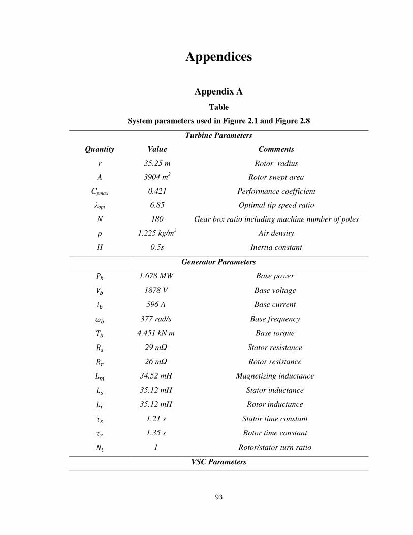
93
Appendices
Appendix A
Table
System parameters used in Figure 2.1 and Figure 2.8
Turbine Parameters
Quantity Value Comments
r 35.25 m Rotor radius
A 3904 m2 Rotor swept area
Cpmax 0.421 Performance coefficient
λopt 6.85 Optimal tip speed ratio
N 180 Gear box ratio including machine number of poles 1 1.225 kg/m3 Air density
H 0.5s Inertia constant
Generator Parameters Z 1.678 MW Base power Z 1878 V Base voltage Z 596 A Base current "Z 377 rad/s Base frequency &Z 4.451 kN m Base torque 29 mΩ Stator resistance 26 mΩ Rotor resistance 34.52 mH Magnetizing inductance 35.12 mH Stator inductance 35.12 mH Rotor inductance % 1.21 s Stator time constant % 1.35 s Rotor time constant *' 1 Rotor/stator turn ratio
VSC Parameters
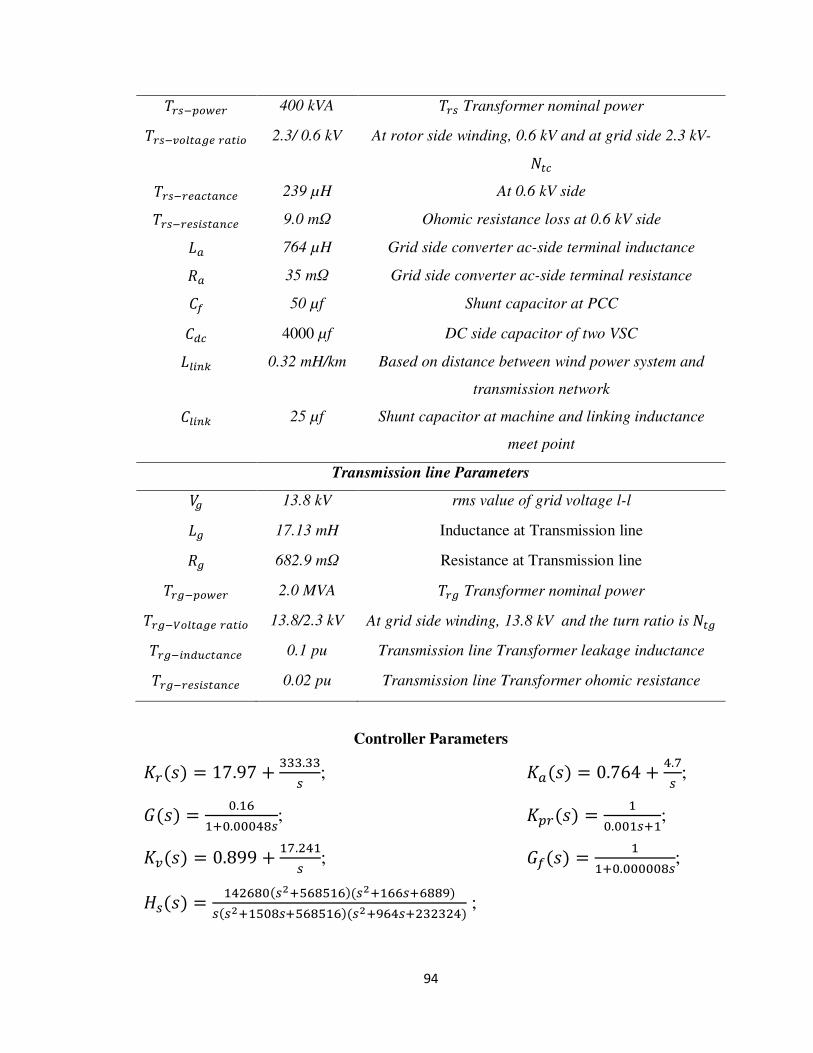
94
&PXB) 400 kVA & Transformer nominal power &PÄB ',)'B 2.3/ 0.6 kV At rotor side winding, 0.6 kV and at grid side 2.3 kV-*'+ &P)+'+) 239 µH At 0.6 kV side &P)'+) 9.0 mΩ Ohomic resistance loss at 0.6 kV side 764 µH Grid side converter ac-side terminal inductance 35 mΩ Grid side converter ac-side terminal resistance -. 50 µf Shunt capacitor at PCC -/+ 4000 µf DC side capacitor of two VSC 0.32 mH/km Based on distance between wind power system and
transmission network - 25 µf Shunt capacitor at machine and linking inductance
meet point
Transmission line Parameters , 13.8 kV rms value of grid voltage l-l , 17.13 mH Inductance at Transmission line , 682.9 mΩ Resistance at Transmission line &,PXB) 2.0 MVA &, Transformer nominal power &,PGB ',)'B 13.8/2.3 kV At grid side winding, 13.8 kV and the turn ratio is *', &,P/(+'+) 0.1 pu Transmission line Transformer leakage inductance &,P)'+) 0.02 pu Transmission line Transformer ohomic resistance
Controller Parameters 3() = 17.97 + ???.?? ; 3() = 0.764 + Æ. ;
È() = #.ïI#.###Æð; 3X() = #.##I; 3Ä() = 0.899 + ^.Æ ; È.() = I#.#####ð; () = Æïð#(QIÇïðÇï)(QIïïIïððñ)(QIÇ#ðIÇïðÇï)(QIñïÆI??Æ) ;
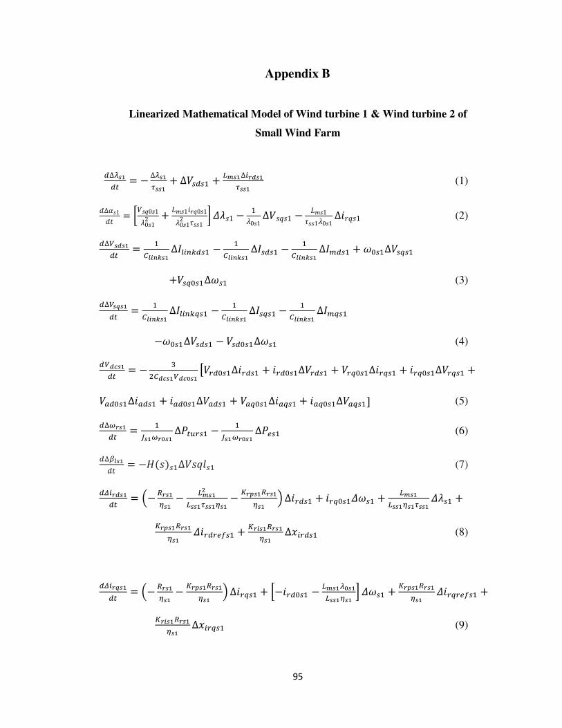
95
Appendix B
Linearized Mathematical Model of Wind turbine 1 & Wind turbine 2 of
Small Wind Farm
/∆_Ï/' = − ∆_ÏÏ + ∆/ + Ï∆VcÏÏ (1)
/∆Ã1/' = O!01012 + 1;!01012 %1 Rõ1 − 101 ∆!1 − 1%101 ∆;!1 (2)
/∆GcÏ/' = ¤a®¯°Ï ∆ö / − ¤a®¯°Ï ∆ö/ − ¤a®¯°Ï ∆ö/ + "#∆e
+e#∆" (3)
/∆GÏ/' = ¤a®¯°Ï ∆ö e − ¤a®¯°Ï ∆öe − ¤a®¯°Ï ∆öe
−"#∆/ − /#∆" (4)
/Gc¥Ï/' = − ?¤c¥ÏGc¥Ï ÷/#∆/ + /#∆/ + e#∆e + e#∆e +/#∆/ + /#∆/ + e#∆e + e#∆e] (5)
/∆[VÏ/' = øÏ[VÏ ∆'( − øÏ[VÏ ∆) (6)
/∆ÞaÏ/' = −()∆!8 (7)
/ùVcÏ/' = L− VÏúÏ − ÏQÏÏúÏ − ûVüÏVÏúÏ N ∆/ + e#õ" + ÏÏúÏÏ õ +ûVüÏVÏúÏ õ/). + ûV®ÏVÏúÏ ∆·/ (8)
/ùVÏ/' = L− VÏúÏ − ûVüÏVÏúÏ N ∆e + F−/# − Ï_ÏÏúÏ K õ" + ûVüÏVÏúÏ õe). +ûV®ÏVÏúÏ ∆·e (9)

96
∆/ < = 3X ∆/). − ý3X + þ ∆/ − 1*'+ ∆/
+È. ∆GcaÏ©T¥ÏbÏ (10)
/∆a®¯°cÏ/' = ∆Gca®¯°Ï − ∆GcÏa®¯°Ï +"#∆ e + e#∆" (12)
/∆a®¯°Ï/' = ∆Ga®¯°Ï − ∆GÏa®¯°Ï −"#∆ / − /#∆" (13)
/∆ЮVcÏ/' = ∆/). − ∆/ (14)
/∆ЮVÏ/' = ∆e). − ∆e (15)
/∆ЮbcÏ/' = ∆/). − ∆/ (16)
/∆ЮbÏ/' = ∆e). − ∆e (17)
/∆ÐÏÏ/' = ∆·Ä (18)
/∆ÐQÏ/' = Gc¥VdÏ∆Gc¥VdÏÁÏ − Gc¥Ï∆Gc¥ÏÁÏ − ∆ÐQÏÁÏ (19)
/∆üVÏ/' =? ÷GVcÏ∆VcÏIVcÏ∆GVcÏIGVÏ∆VÏIVÏ∆GVÏÁÏ +? ÷GbcÏ∆bcÏIbcÏ∆GbcÏIGbÏ∆bÏIbÏ∆GbÏÁÏ − ∆üVÏÁÏ (20)
/∆cÏ/' = ∆GcaÏ©T¥ÏÁÏ − ∆cÏÁÏ (21)
/∆Ï/' = ∆GaÏ©T¥ÏÁÏ − ∆ÏÁÏ (22)
/∆YÏÏ/' = ∆ℎ (23)
/∆YQÏ/' = ∆ℎ? (24)
/∆YÏ/' = ∆ℎÆ (25)
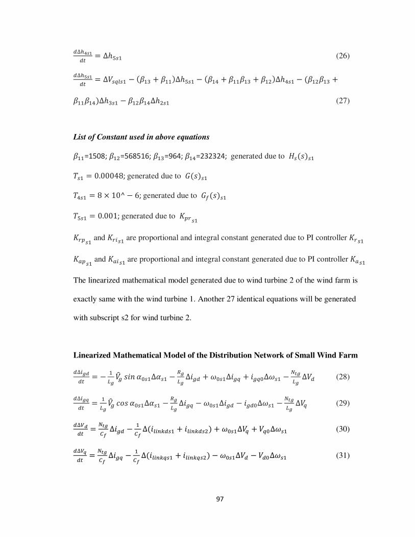
97
/∆YÏ/' = ∆ℎÇ (26)
/∆YÏ/' = ∆e − (W? + W)∆ℎÇ − (WÆ + WW? + W)∆ℎÆ − (WW? +WWÆ)∆ℎ? − WWÆ∆ℎ (27)
List of Constant used in above equations
W=1508; W=568516; W?=964; WÆ=232324; generated due to ()
& = 0.00048; generated due to È()
&Æ = 8 × 10^− 6; generated due to È.()
&Ç = 0.001; generated due to 3X
3X and 3 are proportional and integral constant generated due to PI controller 3
3X and 3 are proportional and integral constant generated due to PI controller 3
The linearized mathematical model generated due to wind turbine 2 of the wind farm is
exactly same with the wind turbine 1. Another 27 identical equations will be generated
with subscript s2 for wind turbine 2.
Linearized Mathematical Model of the Distribution Network of Small Wind Farm
/∆c/' = − , ½ Ã#∆à − ∆,/ + "#∆,e + ,e#∆" − ©T ∆/ (28)
/∆/' = , 9 Ã#∆à − ∆,e − "#∆,/ − ,/#∆" − ©T ∆e (29)
/∆Gc/' = ©T¤ ∆,/ − ¤ ∆( / + /) + "#∆e + e#∆" (30)
/∆G/' = ©T¤ ∆,e − ¤ ∆( e + e) − "#∆/ − /#∆" (31)
98
Vita
NAME: Baishakhi Dhar POST-SECONDARY Western University EDUCATION: London, Ontario
2011-2013 M.E.Sc.
Jadavpur University Kolkata, India 2006-2008 M.E
AWARDS: Western Engineering Scholarship
(WES) since May 2011 RELATED WORK Research Assistant
Western University 2011-2013 Teaching Assistant Western University 2011-2013