A Unified Integral Equation Scheme for Doubly Periodic ...

A Unified Integral Equation Scheme for Doubly PeriodicLaplace and Stokes Boundary Value Problems

in Two Dimensions

ALEX H. BARNETTDartmouth College

Center for Computational Biology, Flatiron Institute

GARY R. MARPLEUniversity of Michigan

SHRAVAN VEERAPANENIUniversity of Michigan

AND

LIN ZHAOINTECH Investment Management

Abstract

We present a spectrally accurate scheme to turn a boundary integral formulationfor an elliptic PDE on a single unit cell geometry into one for the fully peri-odic problem. The basic idea is to use a small least squares solve to enforceperiodic boundary conditions without ever handling periodic Green’s functions.We describe fast solvers for the two-dimensional (2D) doubly periodic conduc-tion problem and Stokes nonslip fluid flow problem, where the unit cell containsmany inclusions with smooth boundaries. Applications include computing theeffective bulk properties of composite media (homogenization) and microfluidicchip design.

We split the infinite sum over the lattice of images into a directly summed“near” part plus a small number of auxiliary sources that represent the (smooth)remaining “far” contribution. Applying physical boundary conditions on the unitcell walls gives an expanded linear system, which, after a rank-1 or rank-3 cor-rection and a Schur complement, leaves a well-conditioned square system thatcan be solved iteratively using fast multipole acceleration plus a low-rank term.We are rather explicit about the consistency and nullspaces of both the contin-uous and discretized problems. The scheme is simple (no lattice sums, Ewaldmethods, or particle meshes are required), allows adaptivity, and is essentiallydimension- and PDE-independent, so it generalizes without fuss to 3D and toother elliptic problems. In order to handle close-to-touching geometries accu-rately we incorporate recently developed spectral quadratures. We include eightnumerical examples and a software implementation. We validate against high-accuracy results for the square array of discs in Laplace and Stokes cases (im-proving upon the latter), and show linear scaling for up to 104 randomly locatedinclusions per unit cell. © 2018 Wiley Periodicals, Inc.

Communications on Pure and Applied Mathematics, Vol. LXXI, 2334–2380 (2018)© 2018 Wiley Periodicals, Inc.

DOUBLY PERIODIC LAPLACE AND STOKES 2335

1 IntroductionPeriodic boundary value problems (BVPs) arise frequently in engineering and

the sciences, either when modeling the behavior of solid or fluid media with trueperiodic geometry, or when applying artificial periodic boundary conditions to sim-ulate a representative domain of a random medium or particulate flow (often calleda supercell or representative volume element simulation). The macroscopic re-sponse of a given microscopic periodic composite medium can often be summa-rized by an effective material property (e.g., a conductivity or permeability ten-sor), a fact placed on a rigorous footing by the field of homogenization (for a re-view see [14]). However, with the exception of layered media that vary in onlyone dimension, finding this tensor requires the numerical solution of “cell prob-lems” [62, 66], namely BVPs in which the solution is periodic up to some additiveconstant expressing the macroscopic driving. Application areas span all of the ma-jor elliptic PDEs, including the Laplace equation (thermal/electrical conductivity,electrostatics and magnetostatics of composites [12, 27, 35, 38]); the Stokes equa-tions (porous flow in periodic solids [18, 26, 50, 75], sedimentation [1], mobility[69], transport by cilia carpets [16], vesicle dynamics in microfluidic flows [58]);elastostatics (microstructured periodic or random composites [29, 36, 61, 64]); andthe Helmholtz and Maxwell equations (phononic and photonic crystals, bandgapmaterials [42, 65]). In this work we focus on the first two (nonoscillatory) PDEsabove, noting that the methods that we present also apply with minor changes tothe oscillatory Helmholtz and Maxwell cases, at least up to moderate frequen-cies [5, 13, 56].

The accurate solution of periodic BVPs has remained a challenging problem atthe forefront of analytical and computational progress for well over a century [9].Modern simulations may demand large numbers of objects per unit cell, with ar-bitrary geometries, that at high-volume fractions may approach arbitrarily closeto each other [72]. In such regimes asymptotic methods based upon expansion inthe inclusion size do not apply [18, 26]. Polydisperse suspensions or nonsmoothgeometries may require spatially adaptive discretizations. In microfluidics, highaspect ratio and/or skew unit cells are needed, for instance in the optimal designof particle sorters. Furthermore, to obtain accurate average material properties forrandom media or suspensions via the Monte Carlo method, thousands of simula-tion runs may be needed [38]. A variety of numerical methods are used (see [62,sec. 2.8]), including particular solutions (starting in 1892 with Rayleigh’s methodfor cylinders and spheres [70], and, more recently, in Stokes flow [71]), eigen-function expansions [75], lattice Boltzmann and finite differencing [48], and finiteelement methods [29, 61]. However, for general geometries, it becomes very hardto achieve high-order accuracy with any of the above apart from finite elements,and the cost of meshing renders the latter unattractive when moving geometries areinvolved. Integral equation methods [45, 49, 55, 67] are natural, since the PDE haspiecewise constant coefficients, and are very popular [1, 12, 26, 27, 36, 50, 64, 69].

2336 A. H. BARNETT ET AL.

By using potential theory to represent the solution field in terms of the convolutionof a free-space Green’s function with an unknown “density” function living onlyon material boundaries, one vastly reduces the number of discretized unknowns.The linear system resulting from applying boundary conditions takes the form

(1.1) A D f;

where the N N matrix A is the discretization of an integral operator. The latteris often of Fredholm second-kind; hence A remains well-conditioned, independentof N , so that iterative methods converge rapidly. Further advantages include theirhigh-order or spectral accuracy (e.g., via Nyström quadratures), the ease of adap-tivity on the boundary, and the existence of fast algorithms to apply A with optimalO.N / cost, such as the fast multipole method (FMM) [28].

The traditional integral equation approach to periodic problems replaces thefree-space Green’s function by a periodic Green’s function, so that the densityis solved on only the geometry lying in a single unit cell [12, 26, 27, 36, 64]. Thereis an extensive literature on the evaluation of such periodic Green’s functions (e.g.,in the Stokes case see [68,74]); yet any such pointwise evaluation for each source-target pair leads to O.N 2/ complexity, which is unacceptable for large problems.There are two popular approaches to addressing this in a way compatible with fastalgorithms:

Lattice sums. Noticing that the difference between the periodic and free-space Green’s function is a smooth PDE solution in the unit cell, one ex-pands this in a particular solution basis (a cylindrical or spherical expan-sion); the resulting coefficients, which need to be computed only once fora given unit cell, are called lattice sums [7, 26, 27, 35]. They originate inthe work of Rayleigh [70] and in the study of ionic crystals (both reviewedin [9, chaps. 2–3]). The FMM may then be periodized by combining thetop-level multipole expansion coefficients with the lattice sums to give acorrection to the local expansion coefficients (in 2D this is a discrete con-volution) that may be applied fast [28, sec. 4.1] [64]. This method has beenused for the doubly periodic Laplace BVP by Greengard–Moura [27], andStokes BVP by Greengard–Kropinski [26]. Particle-mesh Ewald (PME) methods. These methods exploit Ewald’s re-

alization [20] that, although both the spatial and the spectral (Fourier) sumsfor the periodic Green’s function in general converge slowly, there is ananalytic splitting into spatial and spectral parts such that both terms con-verge superalgebraically. Numerically, the spatial part is now local, whilethe spectral part may be applied by “smearing” onto a uniform grid, us-ing a pair of FFTs, and (as in the nonuniform FFT [19]) correcting for thesmearing. The result is a O.N logN/ fast algorithm; for a review see [15].Recently this has been improved by Lindbo–Tornberg to achieve overallspectral accuracy in the Laplace [53] and Stokes [51] settings, with appli-cations to 3D fluid suspensions [1].


FIGURE 1.1. Solution of the Laplace equation in a doubly periodic do-main with Neumann boundary conditions on each of K D 104 inclu-sions, driven by a specified potential drop p D .1; 0/ (Example 2). Asingle unit cell is shown, with the solution u indicated by a color scaleand contours. The inset shows detail. Each inclusion has Nk D 700

discretization nodes on its boundary, resulting in 7 million degrees offreedom. The solution took about 10 hours on a 12-core 3.4 GHz IntelXeon desktop. The flux is J1 D 0:1963795463 with estimated absoluteerror of 1 1010.


FIGURE 1.2. Periodic Stokes flow using in doubly periodic domain withno-slip boundary conditions on each of K D 103 inclusions (Example7). Flow is driven by a specified pressure difference between left andright sides. A single unit cell is shown. Color here indicates fluid speed(red is high and blue is low). Each inclusion boundary has Nk D 350

discretization points, resulting in 700 000 degrees of freedom (not ac-counting for copies). The estimated absolute error in the computed fluxis 9 109.


The scheme that we present is based purely on free-space Green’s functions, andhas distinct advantages over the above two periodization approaches.

(1) Only physically meaningful boundary conditions and compatibility con-ditions are used. Aside from conceptual and algebraic simplification, this alsoremoves the need for (often mysterious and subtle [9]) choices of the values ofvarious conditionally or even nonconvergent lattice sums based on physical argu-ments [18, 27, 28, 36] (e.g., six such choices are needed in [26]). When it comesto skewed unit cells combined with applied pressure driving, such hand-pickedchoices in lattice sum methods become far from obvious.

(2) Free-space FMM codes may be inserted without modification, and fast di-rect solvers (based on hierarchical compression of matrix inverses) [23,31] requireonly slight modification [22, 58].

(3) When multiscale spatial features are present in the problem—commonlyobserved in practical applications such as polydisperse suspensions and complexmicrofluidic chip geometries—PME codes become inefficient because of their needfor uniform grids. In contrast, our algorithm retains the fast nature of the adaptiveFMM in such cases.

(4) In contrast to lattice sums and Ewald methods, which intrinsically rely onradially symmetric expansions and kernels, our scheme can handle reasonably highaspect ratio unit cells with little penalty.

(5) Since our Stokes formulation does not rely on complex variables (e.g.,Sherman–Lauricella [26]), the whole scheme generalizes to 3D with no conceptualchanges [57]. A disadvantage of our scheme is that the prefactor may be slightlyworse than Ewald methods due to the direct summation of neighboring images.

The basic idea is simple and applies to integral representations for a variety ofelliptic PDEs. Let B be a (generally parallelogram) unit cell “box,” and let @ bethe material boundary that is to be periodized (@ may even intersect the wallsof B). Applying periodic boundary conditions is equivalent to summing the free-space representation on @ over the infinite lattice, as in Figure 1.3(a). Our schemesums this potential representation over only the 3 3 nearest-neighbor images of@ (see Figure 1.3(b)) but adds a small auxiliary basis of smooth PDE solutionsin B, with coefficient vector , that efficiently represents the (distant) contributionof the rest of the infinite image lattice. For this auxiliary basis we use point sources(Figure 1.3(c)); around 102 are needed, a small number which, crucially, is inde-pendent of N and the boundary complexity. We apply the usual (homogeneous)boundary condition on @, which forms the first block row of a linear system. Weimpose the desired physical periodicity as auxiliary conditions on the Cauchy datadifferences between wall pairs R–L and U –D (see Figure 1.3(a)), giving a secondblock row. The result is a 2 2 block “extended linear system” (ELS),

(1.2)A B

C Q

D

0

g

:


(a) periodic problem and unit cell (c) auxiliary sources (far interaction)

RLC

B

Q

A

3x3 block (central copy and neighbors)

(b) direct sum over near image interactions

U

D

B

pR

Ω

FIGURE 1.3. 2D periodic problem in the case of a single inclusion with boundary @. (a) Periodic BVP in R2, showing a possible unit cell“box” B and its four walls L, R, D, U , and senses of wall normals. (b)Directly-summed “near” copies of @. (c) Circle of auxiliary sources(red dots) which represent the field in B due to the infinite puncturedlattice of “far” copies (dashed curves). In (b)–(c) blue arrows indicatethe action (source to target) of the four matrix blocks A, B , C , Q.

Here g accounts for the applied macroscopic thermal or pressure gradient in theform of prescribed jumps across one unit cell. Figure 1.3(b)–(c) sketches the in-teractions described by the four operators A, B , C , and Q. This linear system isgenerally rectangular and highly ill conditioned, but when solved in a backward-stable least-squares sense can result in accuracies close to machine precision.

Three main routes to a solution of (1.2) are clear. (a) The simplest is to use adense direct least-squares solve (e.g., via QR), but the O.N 3/ cost becomes im-practical for large problems with N > 104. Instead, to create fast algorithms oneexploits the fact that the numbers of auxiliary rows and columns in (1.2) are bothsmall, as follows. (b) One may attempt to eliminate to get the Schur complementsquare linear system involving Aper, the periodized version of A, of the form

(1.3) Aper WD .A BQCC/ D BQCg;

where QC is a pseudoinverse of Q (see Section 2.4). As we will see, (1.3)can be well-conditioned when (1.1) is and can be solved iteratively by using theFMM to apply A while applying the second term in its low-rank factored formB..QCC//. (c) One may instead eliminate by forming, then applying, a com-pressed representation of A1 via a fast direct solver; this has proven useful for thecase of fixed periodic geometry with multiple boundary data vectors [22,58]. Bothmethods (b) and (c) can achieve O.N / complexity.

This paper explores route (b). A key contribution is overcoming the stumblingblock that, for many standard PDEs and integral representations, Aper as writtenin (1.3) does not in fact exist. Intuitively, this is due to divergence in the sum ofthe Green’s function over the lattice. For instance, the sum of log.1=r/ clearlydiverges, and thus the single-layer representation for Laplace’s equation, which we


use in Section 2, cannot be periodized unless the integral of density (total charge)vanishes. This manifests itself in the second block row of (1.2): the range of Ccontains vectors that are not in the range of Q; thus QCC numerically blows up.After studying in Sections 2.1 and 4.1 the consistency conditions for the linearsystem involving Q (the “empty unit cell” problem), we will propose rank-1 (forLaplace) and rank-3 (for no-slip Stokes) corrections to the ELS that allow the Schurcomplement to be taken, and, moreover, that remove the nullspace associated withthe physical BVP. We justify these schemes rigorously and test them numerically.Examples of our large-scale tests include Figures 1.1 and 1.2.

Although the idea of imposing periodicity via extra linear conditions has aidedcertain electromagnetics solvers for some decades [32, 78], we believe that thisidea was first combined with integral equations by the first author and Green-gard in [5], where controlled a Helmholtz local expansion. Since then it hasbecome popular for a variety of PDEs [5, 12, 13, 22, 30, 56, 58]. From [5] wealso inherit the split into near and far images, and cancellations in C that allowa rapidly convergent scheme even when @ intersects unit cell walls. The use ofpoint sources as a particular solution basis that is efficient for smooth solutions isknown as the “method of fundamental solutions” (MFS) [8, 21], “method of auxil-iary sources” [46], “charge simulation method” [44], or, in fast solvers, “equivalentsource” [11] or “proxy” [59] representations. This is also used in the recent 3D pe-riodization schemes of Gumerov–Duraiswami [30] and Yan–Shelley [76]. Finally,the low-rank perturbations that enlarge the range ofQ are inspired by the low-rankperturbation methods for singular square systems of Sifuentes et al. [73].

Here is a guide to the rest of this paper. In Section 2 we present the periodicNeumann Laplace BVP, possibly the simplest application of the scheme. This firstrequires understanding and numerically solving the “empty unit cell” subproblem,which we do in Section 2.1. The integral formulation, discretization, and directnumerical solution of the ELS (1.2) follows in Section 2.2. A general scheme tostably take the Schur complement is given in Section 2.4, along with a scheme toremove the physical nullspace specific to our representation. The latter is testednumerically. Section 2.5 shows how the FMM and close-evaluation quadraturesare incorporated and applies them to large problems with thousands of inclusions.Section 2.6 defines the effective conductivity tensor and shows how to evaluateit efficiently using a pair of BVP solutions. In Section 3 we show that this sameperiodizing scheme solves the benchmark periodic disc array conduction problemto high accuracy. In Section 4 we move to periodic Dirichlet (no-slip) Stokes flowand show how its periodizing scheme closely parallels the Laplace version. Infact, the only differences are new consistency conditions for the empty subproblem(Section 4.1), the use of a combined-field formulation (Section 4.2), and the needfor a rank-three perturbation for a stable Schur complement (Section 4.3). Experi-ments on the drag of a square array of discs, and on large-scale flow problems, areperformed in Section 4.4. We discuss generalizations and conclude in Section 5.


Our aim is to illustrate, with two example BVPs, a unified route to a well-conditioned periodization compatible with fast algorithms. We take care to state theconsistency conditions and nullspaces of the full and empty problems, this beingthe main area of problem-specific variation. We believe that the approach adaptssimply to other boundary conditions and PDEs, once the corresponding consis-tency conditions and nullspaces are laid out. Although general aspect ratios andskew unit cells are amongst our motivations, for clarity we stick to the unit square;the generalization is straightforward.

Remark 1.1 (Software). We maintain self-contained MATLAB® codes for the meth-ods and figures in this paper at http://github.com/ahbarnett/DPLS-demos.

2 The Neumann Laplace CaseWe now present the heat/electrical conduction problem in the exterior of a pe-

riodic lattice of insulating inclusions (corresponding to d D 0 in [27]). For sim-plicity we first assume a single inclusion per unit cell. Let e1 and e2 be vectorsdefining the lattice in R2; we work with the unit square so that e1 D .0; 1/ ande2 D .1; 0/. Letƒ WD fx 2 R2 W xCm1e1Cm2e2 2 for some m1; m2 2 Zgrepresent the infinite lattice of inclusions. The scalar u, representing electric po-tential or temperature, solves the BVP

u D 0 in R2 nƒ;(2.1)

un D 0 on @ƒ;(2.2)

u.xC e1/ u.x/ D p1 for all x 2 R2 nƒ;(2.3)

u.xC e2/ u.x/ D p2 for all x 2 R2 nƒI(2.4)

i.e., u is harmonic, has zero flux on inclusion boundaries, and is periodic up toa given pair of constants p D .p1; p2/ that encode the external (macroscopic)driving. We use the abbreviation un D @u

@nD n ru, where n is the unit normal on

the relevant evaluation curve.

PROPOSITION 2.1. For each .p1; p2/ the solution to (2.1)–(2.4) is unique up to anadditive constant.

PROOF. As usual, one considers the homogeneous BVP arising when u is thedifference of two solutions. Let B be any unit cell (tiling domain) containing ;then using Green’s first identity, we have

0 D

ZBn

uu D

ZBnjruj2 C

Z@Buun

Z@

uun:

The first boundary term cancels by periodicity, and the second by (2.2); henceru 0.

http://github.com/ahbarnett/DPLS-demos


To solve the periodic BVP we first re-express it as a BVP on a single unit cell Bwith coupled boundary values on the four walls comprising its boundary @B WD L[R[D[U ; see Figure 1.3(a). For simplicity we assume for now that the square Bcan be chosen such that does not intersect any of the walls; this restriction willlater be lifted (see Remark 2.7). We use the notation uL to mean the restriction of uto the wall L, and unL for its normal derivative using the normal on L (note thatthis points to the right, as shown in the figure.) Consider the following reformulatedBVP:

u D 0 in B n x;(2.5)

un D 0 on @;(2.6)uR uL D p1;(2.7)

unR unL D 0;(2.8)uU uD D p2;(2.9)

unU unD D 0:(2.10)

Clearly any solution to (2.1)–(2.4) also satisfies (2.5)–(2.10). Because of the uniquecontinuation of Cauchy data .u; un/ as a solution to the second-order PDE, theconverse holds; thus the two BVPs are equivalent. We define the discrepancy [5]of a solution u as the stack of the four functions on the left-hand side of (2.7)–(2.10).

2.1 The Empty Unit Cell Discrepancy BVP and Its Numerical SolutionWe first analyze, then solve numerically, an important subproblem that we call

the “empty unit cell BVP.” We seek a harmonic function v matching a given dis-crepancy g D Œg1Ig2Ig3Ig4 (i.e., a stack of four functions defined on the wallsL, L, D, D, respectively). That is,

v D 0 in B;(2.11)vR vL D g1;(2.12)

vnR vnL D g2;(2.13)vU vD D g3;(2.14)

vnU vnD D g4:(2.15)

We now give the consistency condition and nullspace for this BVP, which showsthat it behaves essentially like a square linear system with nullity 1.

PROPOSITION 2.2. A solution v to (2.11)–(2.15) exists if and only ifRL g2 ds CR

D g4 ds D 0 and is then unique up to a constant.

PROOF. The zero-flux conditionR@B vn D 0 holds for harmonic functions.

Writing @B as the union of the four walls, with their normal senses, gives the sumof the integrals of (2.13) and (2.15). Uniqueness follows from the method of proofof Proposition 2.1.


We now describe a numerical solution method for this BVP that is accurate for acertain class of data g, namely those for which the solutions v may be continued asregular solutions to Laplace’s equation into a large neighborhood of B, and henceeach of g1; : : : ; g4 is analytic. It will turn out that this class is sufficient for ourperiodic scheme (essentially because v will only have to represent distant imagecontributions, as shown in Figure 1.3(c)).

Let B be centered at the origin. Recalling the fundamental solution to Laplace’sequation,

(2.16) G.x; y/ D1

2log

1

r; r WD kx yk;

we approximate the solution in B by a linear combination of such solutions withsource points yj lying uniformly on a circle of radiusRp > rB, where rB WD 1=

p2

is the maximum radius of the unit cell. That is, for x 2 B,

(2.17) v.x/

MXjD1

jj .x/; j .x/ WD G.x; yj /;

yj WD .Rp cos 2j=M;Rp sin 2j=M/;

with unknown coefficient vector WD fj gMjD1. As discussed in the introduction,this is known as the MFS. Each basis function j is a particular solution to (2.11)in B; hence only the boundary conditions need enforcing (as in Rayleigh’s originalmethod [70]).

This MFS representation is complete for harmonic functions. More precisely,for v in a suitable class, it is capable of exponential accuracy uniformly in B. Inparticular, since B is contained within the ball kxk rB, we may apply knownconvergence results to get the following.

THEOREM 2.3. Let v extend as a regular harmonic function throughout the closedball kxk of radius > rB. Let the fixed proxy radius Rp ¤ 1 satisfy

prB <

Rp < . For each M 1 let f.M/j gMjD1 be a proxy basis set as in (2.17). Then

there are a sequence of coefficient vectors .M/, one vector for each M , and aconstant C dependent only on v such that v MX

jD1

.M/j

.M/j

L1.B/

C

rB

M=2; M D 1; 2; : : : :

In addition, the vectors may be chosen so that the sequence k.M/k2, M D

1; 2; : : : , is bounded.

This exponential convergence—with rate controlled by the distance to the near-est singularity in v—was derived by Katsurada [43, remark 2.2] in the context ofcollocation (point matching) for a Dirichlet BVP on the boundary of the disc ofradius rB, which is enough to guarantee the existence of such a coefficient vectorsequence. The boundedness of the coefficient norms has been known in the context


of Helmholtz scattering in the Russian literature for some time (see [47, sec. 3.4]and references within, and [17, thm. 2.4]). We do not know of a reference statingthis for the Laplace case, but note that the proof is identical to that in [4, thm. 6],by using equation (13) from that paper. The restriction Rp < is crucial for highaccuracy, since when Rp > , although convergence occurs, k.M/k2 blows up,causing accuracy loss due to catastrophic cancellation [4, thm. 7].

Remark 2.4. Intuitively, the restriction Rp ¤ 1 arises because the proxy basismay be viewed as a periodic trapezoid rule quadrature approximation to a single-layer potential on the circle kxk D Rp, a representation that is incomplete whenRp D 1: it cannot represent the constant function [77, remark 1].

To enforce boundary conditions, let xiL 2 L, xiD 2 D, i D 1; : : : ; m, betwo sets of m collocation points, on the left and bottom wall, respectively; we useGauss–Legendre nodes. Enforcing (2.12) between collocation points on the leftand right walls then gives

(2.18)MXjD1

Œj .xiL C e1/ j .xiL/j D g1.xiL/ for all i D 1; : : : ; m:

Continuing in this way, the full set of discrepancy conditions (2.12)–(2.15) givesthe linear system

(2.19) Q D g;

where g 2 R4m stacks the four vectors of discrepancies sampled at the collocation

points, while the matrix Q D ŒQ1IQ2IQ3IQ4 consists of four block rows, each

of size m M . By reading from (2.18), one sees that Q1 has elements .Q1/ij D

j .xiL C e1/ j .xiL/. Analogously, .Q2/ij D@j

@n.xiL C e1/

@j

@n.xiL/,

.Q3/ij D j .xiD C e2/ j .xiD/, and finally .Q4/ij D@j

@n.xiD C e2/

@j

@n.xiD/.

We solve the (generally rectangular) system (2.19) in the least squares sense,which corresponds to minimizing a weighted L2-norm of the discrepancy error(we find in practice that there is no advantage to incorporating the square-rootof the weights associated with the collocation nodes). As is well-known in theMFS community [21, 43], Q becomes exponentially ill-conditioned as M grows;intuitively this follows from the exponential decay of the singular values of thesingle-layer operator from the proxy radiusRp to the circle radius rB containing B.Thus, a least squares solver is needed that can handle rank deficiency stably, i.e.,return a small-norm solution when one exists. In this case the ill-conditioningcauses no loss of accuracy, and, even though there is instability in the vector , forthe evaluation of v errors close to machine precision ("mach) are achieved [4].

Remark 2.5. For this and subsequent direct solves we use MATLAB®’s linsolve(with the option RECT=true to prevent the less accurate LU from being used in the


5 10 15 20

m

10 -15

10 -10

10 -5

10 0

ma

x a

bs e

rro

r in

v

(a)

20 40 60 80 100 120

M

10 -15

10 -10

10 -5

10 0

10 5 (b)

20 40 60 80 100 120

M

10 -15

10 -10

10 -5

10 0

(c)

FIGURE 2.1. Convergence of the proxy point numerical scheme for theempty discrepancy BVP, for the case of known solution with singularityx0 D 1:5.cos 0:7; sin 0:7/ is a distance 1:5 from the center of the squareunit cell of side 1. The proxy radius is Rp D 1:4. (a)–(b) are for theLaplace case with g deriving from the known solution v.x/ D logkx x0k; (c) is for the Stokes case with known v coming from a stokesletat x0 with force f0 D Œ0:3I 0:6. (a) Shows convergence in maximumabsolute error in v at 100 target points interior to B, versus the numbermof wall quadrature nodes, with fixed M D 100 proxy points. (b) Showsconvergence in M with fixed m D 22 (C signs) and its prediction viaTheorem 2.3 (dotted line), the lowest five singular values of Q (graylines), and the solution vector norm kk2 (circles). (c) is the same as (b)but for Stokes. Note that in the Laplace case (b) there is one singularvalue smaller than the others, whereas for Stokes (c) there are three suchsingular values.

square case), which uses column-pivoted QR to find the so-called “basic” solution[63, sec. 5.7] having at most r nonzero entries, where r is the numerical rank; thisis close to having minimum norm [25, sec. 5.5].

We illustrate this with a simple numerical test, in which g is the discrepancyof a known harmonic function v of typical magnitude O.1/ and with sufficientlydistant singularity. Once Q is filled and (2.19) solved, the numerical solution isevaluated via (2.17), and the maximum error at 100 random target points in B istaken (after removing an overall constant error, expected from Proposition 2.2).Figure 2.1(a) shows exponential convergence in this error versus the number ofwall nodes m. Figure 2.1(b) shows exponential convergence with respect to M ,the number of proxy points, with a rate slightly exceeding the predicted rate. It isclear that wheneverm 20 andM 70 the norm kk2 remains O.1/, and around15 digits of accuracy result.

The decaying lowest few singular values of Q are also shown in panel (b): inparticular there is one singular value decaying faster than all others. It is easy to


verify that this corresponds to the nullspace of the BVP (Proposition 2.2); indeed,we have tested that its right singular vector is approximately constant and generatesvia (2.17) the constant function in B to within O."mach/ relative error. Likewise, You are also using O as

well as O. Is there adistinction that you aremaking, or should theyall be made the same?

the consistency condition in Proposition 2.2 manifests itself in NulQT: let w bethe vector that applies the discretization of this consistency condition to a vector g,namely,

(2.20) w WD Œ0mIwLI 0mIwD 2 R4m;

where semicolons indicate vertical stacking, wL;wD 2 Rm are the vectors ofweights corresponding to the collocation nodes on L, D, and 0m 2 Rm is thezero vector. Then we expect that

(2.21) wTQ 0TM ;

and indeed observe numerically that kwTQk2 D O."mach/ once m 20. Insummary, although the matrix Q is generally rectangular and ill-conditioned, italso inherits both aspects of the unit nullity of the empty BVP that it discretizes.

Remark 2.6. A different scheme is possible in whichQwould be square, and (mod-ulo a nullity of one, as above) well-conditioned, based on a “tic-tac-toe” set of layerpotentials (see [5, sec. 4.2] in the Helmholtz case). However, we recommend theabove proxy point version, since (i) the matrix Q is so small that handling its ill-conditioning is very cheap, (ii) the tic-tac-toe scheme demands close-evaluationquadratures for its layer potentials, and (iii) the tic-tac-toe scheme is more compli-cated.

2.2 Extended Linear System for the Conduction ProblemWe now treat the above empty BVP solution scheme as a component in a scheme

for the periodic BVP (2.5)–(2.10). Simply put, we take standard potential theoryfor the Laplace equation [45, chap. 6], and augment this by enforcing periodicboundary conditions. Given a density function on the inclusion boundary @,recall that the single-layer potential, evaluated at a target point x, is defined by

v D .S@/.x/ WDZ@

G.x; y/.y/dsy

D1

2

Z@

log1

kx yk.y/dsy ; x 2 R2:

(2.22)

Using nx to indicate the outward normal at x, this potential obeys the jump relation[45, thm. 6.18]

(2.23) v˙n WD limh!0C

nx r.S@/.x˙ hnx/ D

1

2CDT

@;@

.x/;


where DT 0; denotes the usual transposed double-layer operator from a general

source curve to a target curve 0, defined by

DT 0;

.x/ D

Z

@G.x; y/

@nx.y/dsy

D1

2

Z

.x y/ nx

kx yk2.y/dsy ; x 2 0:

(2.24)

The integral implied by the self-interaction operator DT@;@

is to be interpreted inthe principal value sense.

Our representation for the solution sums the standard single-layer potential overthe 3 3 copies closest to the origin and adds an auxiliary basis as in (2.17),

(2.25)

u D Snear@ C

MXjD1

jj where

.Snear@ /.x/ WD

Xm1;m22f1;0;1g

Z@

G.x; y Cm1e1 Cm2e2/.y/dsy :

Our unknowns are the (physical charge) density and the auxiliary vector . Sub-stituting (2.25) into the Neumann boundary condition (2.6), and using the exteriorjump relation on the central copy (m1 D m2 D 0) only, gives our first block row,

(2.26)1

2CD

near;T@;@

C

MXjD1

j@j

@n

ˇ@

D 0;

where, as before, the “near” superscript denotes summation over source images asin (2.25).

The second block row arises as follows. Consider the substitution of (2.25) intothe first discrepancy equation (2.7): there are nine source copies, each of whichinteracts with the L and R walls, giving 18 terms. However, the effect of the right-most six sources on R is cancelled by the effect of the leftmost six sources on L,leaving only six terms, as in [5, fig. 4(a)–(b)]. All of these surviving terms involvedistant interactions (the distances exceed one period if is contained in B). Simi-lar cancellations occur in the remaining three equations (2.8)–(2.10). The resultingfour subblocks are X

m22f1;0;1g

.SR;@e1Cm2e2 SL;@Ce1Cm2e2

/(2.27)

C

MXjD1

.j jR j jL/j D p1;

DOUBLY PERIODIC LAPLACE AND STOKES 2349Xm22f1;0;1g

DTR;@e1Cm2e2

DTL;@Ce1Cm2e2

(2.28)

C

MXjD1

@j

@n

ˇR

@j

@n

ˇL

j D 0;

Xm12f1;0;1g

.SU;@Cm1e1e2 SD;@Cm1e1Ce2

/(2.29)

C

MXjD1

.j jU j jD/j D p2;

Xm12f1;0;1g

DTU;@Cm1e1e2

DTD;@Cm1e1Ce2

(2.30)

C

MXjD1

@j

@n

ˇU

@j

@n

ˇD

j D 0:

Remark 2.7 (Wall intersection). The cancellation of all near interactions in (2.27)–(2.30) is due to the 3 3 neighbor summation in the representation (2.25). Fur-thermore, this cancellation allows an accurate solution even when intersects @B,without the need for specialized quadratures, as long as the 3 3 copies of ac-count for all of the images inside and near to B (see Figure 2.2(a)). Informally,the unit cell walls are “invisible” to the inclusions. If is elongated such that thelast condition cannot hold, one would need to include all of the (pieces of) imagesof that fell within and near to B, needing different bookkeeping in the aboveformulae; we leave this case for future work.

(2.26)–(2.30) form a set of coupled integral-algebraic equations, where the onlydiscrete aspect is that of the O.1/ proxy points.1 It is natural to ask how the unitnullity of the BVP manifests itself in the solution space for the pair .; /. Arethere pairs .; / with no effect on u, enlarging the nullspace? It turns out thatthe answer is no, and that the one-dimensional nullspace (constant functions) isspanned purely by , as a little potential theory now shows.

LEMMA 2.8. In the solution to (2.26)–(2.30), is unique.

PROOF. Let .; / be the difference between any two solutions to (2.26)–(2.30).Let v be the representation (2.25) using this .; /, both in B n but also inside. Then by construction v is a solution to the homogeneous BVP (2.5)–(2.10),i.e., with p1 D p2 D 0; thus by Proposition 2.1, v is constant in B n. Thus bythe continuity of the single-layer potential [45, thm. 6.18], the interior limit of v

1 It would also be possible to write a purely continuous version by replacing the proxy circle by asingle-layer potential; however, sometimes an intrinsically discrete basis fj g is useful [5, 13].


on @ is constant. However, v is harmonic in , so v is constant in . By (2.23),vCn v

n D , but we have just shown that both vCn and vn vanish, so 0.

Discretization of the ELSWe discretize (2.26), the first row of the system, using a set of quadrature nodes

fxigNiD1 on @ and weights fwigNiD1 such thatZ

@

f .y/dsy

NXiD1

wif .xi /

holds to high accuracy for smooth functions f . In practice, when @ is parame-trized by a 2-periodic function x.t/, 0 t < 2 , then using the periodic trape-zoid rule in t gives xi D x.2i=N / and wi D .2=N/kx0.2i=N /k. Since DT

has a smooth kernel, we apply Nyström discretization [45, sec. 12.2] to the integralequation (2.26) using these nodes, to get our first block row

(2.31) A C B D 0;

where D figNiD1 is a vector of density values at the nodes, and A 2 RNN has

entries

(2.32) Aij D 1

2ıij C

Xm1;m22f1;0;1g

@G.xi ;xj Cm1e1 Cm2e2/

@nxiwj ;

where ıij is the Kronecker delta. Here, for entries i D j the standard diagonal limitof the kernel @G.xi ;xi /=@nxi D .xi /=4 is needed, where .x/ is the signedcurvature at x 2 @. The matrix B 2 RNM has entries Bij D @j .xi /=@nxi .

For the second block row (2.27)–(2.30) we use the above quadrature for thesource locations of the operators and enforce the four equations on the wall collo-cation nodes xiL, xiL C e1, xiD , xiD C e2, i D 1; : : : ; m, to get

(2.33) C CQ D g;

with the macroscopic driving .p1; p2/ encoded by the right-hand side vector

(2.34) g D Œp11mI 0mIp21mI 0m 2 R4m;

where 1m 2 Rm is the vector of ones. The matrix Q is precisely as in (2.19).Rather than list formulae for all four blocks in C D ŒC1IC2IC3IC4, we have

.C1/ij DX

m22f1;0;1g

G.xiL C e1;xj e1 Cm2e2/

G.xiL;xj C e1 Cm2e2/wj ;

with the others filled analogously. Stacking the two block rows (2.31) and (2.33)gives the .N C4m/ .N CM/ extended linear system (1.2), which we emphasizeis just a standard discretization of the BVP conditions (2.6)–(2.10).

For small problems (N less than a few thousand), the ELS is most simply solvedby standard dense direct methods; for larger problems a Schur complement must


be taken in order to solve iteratively, as presented in Section 2.4. First we performa numerical test of the direct method.

2.3 Numerical Tests Using Direct Solution of the ELSExample 1. We define a smooth “worm”-shaped inclusion that crosses the unit cellwalls L and R by x.t/ D .0:7 cos t; 0:15 sin t C 0:3 sin.1:4 cos t //. The solutionof the periodic Neumann Laplace BVP with external driving p D .1; 0/ is shownin Figure 2.2(a). Here u is evaluated via (2.25) (using the standard far-field Nys-tröm quadrature), both inside B (where it is accurate) and, to show the nature ofthe representation, out to the proxy circle (where it is certainly inaccurate). Recallthat the proxy sources must represent the layer potentials due to the infinite latticeof copies that excludes the 3 3 central block. Note that two tips of copies in thisset slightly penetrate the proxy circle, violating the condition in Theorem 2.3 thatthe function the proxy sources represent be analytic in the closed ball of radius Rp.We find in practice that such slight geometric violations do not lead to problem-atic growth in kk, but that larger violations can induce a large kk, which limitsachievable accuracy. Panel (c) shows the convergence of errors in u (at the pair ofpoints shown) to their numerically converged value, fixing converged values forMand m. Convergence to around 13 digits (for N D 140, M D 70) is apparent, andthe solution time is 0.03 second.

As an independent verification of the method, we construct a known solutionto a slightly generalized version of (2.5)–(2.10), where (2.6) is replaced by inho-mogeneous data un D f and a general discrepancy g is allowed. We choose theknown solution

uex.x/ DX

m1;m22f2;1;:::;2g

n0 rG.x; y0 Cm1e1 Cm2e2/;

where the central dipole has direction n0 and location y0 chosen inside andfar from its boundary (so that the induced data f is smooth). The grid size of55 (some of which is shown by symbols in Figure 2.2(a)) is chosen so that g issufficiently smooth (which requires at least 33), and so that the periodizing part is nontrivial. From uex the right-hand side functions f and g are then evaluatedat nodes, the ELS solved directly, the numerical solution (2.25) evaluated, andthe difference at two points compared to its known exact value. The resulting N -convergence to 13 digits is shown in Figure 2.2(c). The convergence rate is slowerthan before, due to the unavoidable closeness of the dipole source to @.

Finally, the gray lines in panel (e) show that, as with Q, there is one singularvalue of E that is much smaller than the others, reflecting the unit nullity of theunderlying BVP (Proposition 2.1). Also apparent is the fact that, despite the expo-nential ill-conditioning, the solution norm remains bounded once M -convergencehas occurred.


L R

D

U

Ω

(a) (b)

50 100 150 200

N

10 -15

10 -10

10 -5

(c) u conv ELS

J1

conv ELS

u conv Schur

J1

conv Schur

u err vs known

100 200 300 40010

−15

10−10

10−5

Nk

(d)

M = 70, m = 22

u conv SchurJ

1 conv Schur

20 40 60 80 100

M

10 -15

10 -10

10 -5

10 0

(e)

J1

conv, Ex.1

J1

conv, Ex.2

soln norm, Ex.1

sing vals, Ex.1

FIGURE 2.2. Periodic Laplace Neumann tests driven by external driv-ing p D .1; 0/. (a) Solution potential u contours for “worm” inclusion(Example 1), with N D 140, M D 70, and Rp D 1:4. The m D 22

nodes per wall and nodes on @ are also shown (with normals), proxypoints (red dots), test points (two black dots), and some of the 5 5 gridof dipoles generating a known solution (* symbols). The representationfor u is only accurate inside the unit cell. (b) Solution with K D 100

inclusions (Example 2), withNk D 400 unknowns per inclusion, by iter-ative solution of (2.38). A single unit cell is shown. (c) N -convergenceof error in difference of u at the two test points, and of flux J1 computedvia (2.43), relative to their values at N D 230 (M D 70 is fixed), forExample 1. Squares show error convergence in u (difference at the testpoints) in the case of known uex due to the dipole grid. Solid lines arefor direct solution of the ELS, and dashed lines for the iterative solu-tion of (2.38). (d) Convergence with Nk for Example 2, for pointwise u(+ symbols) and flux J1 (circles). (e) M -convergence of flux J1 error,for Example 1 (C signs) and Example 2 (squares), with other parame-ters converged. For K D 1 the lowest six singular values of E are alsoshown (gray lines), and the solution norm kŒI k2 (dots).


2.4 Schur Complement System and Its Iterative SolutionWhen N is large, solving the ill-conditioned rectangular ELS (1.2) is imprac-

tical. We would like to use a Schur complement in the style of (1.3) to create anequivalent N N system, which we do in Section 2.4. Furthermore, in order touse Krylov subspace iterative methods with known convergence rates, we wouldlike to remove the nullspace to make this well-conditioned, which we do in Sec-tion 2.4. We will do both these tasks via low-rank perturbation of certain blocks of(1.3) before applying the Schur complement.

In what follows,QC is the pseudoinverse [25, sec. 5.5] ofQ, i.e., the linear mapthat recovers a small-norm solution (if one exists) to Q D g via D QCg. Theobstacle to using (1.3) as written is thatQ inherits a consistency condition from theempty BVP so that Q has one smooth vector in its left nullspace (w ; see (2.21)).However, the range of C does not respect this condition; thus QCC has a huge2-norm (which we find numerically is at least 1016). We first need to show thatthe range of a rank-deficient matrix Q may be enlarged by a rank-k perturbation,a rectangular version of results about singular square matrices in [73].

LEMMA 2.9. Let Q 2 Rmn have a k-dimensional nullspace. Let R 2 Rnk

have full-rank projection onto NulQ, i.e., if N has columns forming a basis forNulQ, then RTN 2 Rkk is invertible. Let V 2 Rmk be arbitrary. ThenRan.QC VRT/ RanQ˚ RanV ; i.e., the range now includes that of V .

PROOF. We need to check that .Q C VRT/x D Qx0 C V˛0 has a solutionx for all given pairs x0 2 Rn, ˛0 2 Rk . Recalling that RTN is invertible, bysubstitution one may check that x D x0 C N.R

TN/1.˛0 RTx0/ is an explicit

such solution.

Remark 2.10. With additional conditions m n and the fact that V has full-rank projection onto a part of NulQT (i.e., if W has columns forming a basisfor a k-dimensional subspace of NulQT, then W TV 2 Rkk is invertible), weget incidentally thatQCVRT has trivial nullspace (generalizing [73, sec. 3]). Theproof is as follows. Let x 2 Rn solve the homogeneous equation .QCVRT/x D 0.Then 0 D W TQx D .W TV /RTx, but W TV is invertible, so RTx D 0. Thus thehomogeneous equation becomes Qx D 0, which means there is an ˛ 2 Rk suchthat x D N˛. Thus RTN˛ D 0, but RTN is invertible, so that ˛ D 0, so x D 0.

We also need the fact that a block-column operation allowsQ to be perturbed asabove while changing the ELS solution space in a known way. The proof is simpleto check.

PROPOSITION 2.11. Let A, B , C , and Q be matrices, and let P be a matrix withas many rows as A has columns and as many columns as B has rows. Then thepair .z; / solves the block system

(2.35)A B C AP

C QC CP

z

D

0g


if and only if the pair .; /, with D z C P, solves the original ELS (1.2).

An Equivalent Square System Preserving the NullspaceArmed with the above, a method to “fold” the Neumann Laplace ELS into an

equivalent square system is as follows:(1) Set the proxy coefficient vector R D .1=M/1M and the discrete density

vector H D 1N . Create low-rank perturbed matrix blocks zB WD B C

AHRT and zQ WD QC CHRT.(2) Solve for the vector z in the N N Schur complement linear system

(2.36) .A zB zQCC/z D zB zQCg:

More precisely, since (due to the numerical ill-conditioning in zQ) multi-plying by zQC would lose accuracy due to rounding error, instead solve thesmall systems zQX D C for X and zQy D g for y , heeding Remark 2.5.From them, build A zBX and zBy , which are, respectively, the systemmatrix and right-hand side for (2.36). This large square system may thenbe solved iteratively (see Section 2.5).

(3) Recover the proxy coefficients via D y Xz.(4) Recover the density via D z CHRT.

Note that in Step 1 the prefactor 1=M leads to correct quadrature scaling, so thatHRT has similar 2-norm to the other matrices (also recommended in [73]).

THEOREM 2.12. Let g encode the driving as in (2.34). Then for all sufficientlylarge N , M , and m, any pair .; / produced by the above procedure performedin exact arithmetic solves the original ELS (1.2).

PROOF. By rotational invariance, a constant single-layer density on a circle gen-erates a constant potential inside, and inserting R into (2.17) gives the periodictrapezoid quadrature approximation to such a potential, thus generating discrep-ancy near zero (in fact, exponentially small in M ). Thus for all sufficiently largeM , R is not orthogonal to NulQ. Applying Lemma 2.9 with k D 1 gives thatthe range of zQ includes the discrepancy vector V D CH produced by the con-stant density H . Thus, to show that the range of zQ includes all smooth vectors,i.e., that it does not have the consistency condition (2.21), one needs to check thatwTV D wTCH ¤ 0, which is done in Lemma 2.13 below. Thus the systemszQX D C and zQy D g are consistent for any C and g, so that the Schur comple-

ment is well-defined. Finally, Proposition 2.11, using the rank-1 matrix P D HRT,insures that Step 4 recovers a solution to (1.2).

For the missing technical lemma, we first need a form of Gauss’s law, statingthat for any density on a curve @ the single-layer potential v D S@ generatesflux equal to minus the total charge, i.e.,

(2.37)Z@Kvn D

Z@

ds


where @K is the boundary of some open domain K containing @. This may beproved by combining the jump relation vCn v

n D (from (2.23)) with the fact

that, since v is a Laplace solution in R2 n @,Rvn D 0 taken over the boundaries

of and of K n.

LEMMA 2.13. Let the matrix C be defined as in Section 2.2 and w be as in (2.20).Then, for all N and m sufficiently large, wTC1N ¤ 0.

PROOF. Let d D Œd1I d2I d3I d4 be the discrepancy of the potential v D Snear@

for density 1. As used in the proof of Proposition 2.2, the flux (left-hand sideof (2.37)) out of the unit cell B equals

RL d2 ds C

RD d4 ds, which by (2.37) (and

noting that only one of the nine source terms in Snear@

lies within B) equals minusthe perimeter

R@ 1 ds D j@j < 0. What we seek is the discretization of this

statement about the PDE. If d is the discrepancy of v sampled at the wall nodes,then its quadrature approximation is d C1N , and so (as discussed above (2.20))the quadrature approximation to

RL d2 ds C

RD d4 ds is wTd wTC1N . Thus,

as N and m tend to infinity, the latter converges to j@j.

Theorem 2.12 justifies rigorously one procedure to create a square system equiv-alent to the ELS (1.2). However, by the equivalence in Proposition 2.11, the sys-tem matrix A zBX at the heart of the procedure is singular, as it inherits the unitnullity of the ELS, which itself derives from the unit nullity of the Laplace Neu-mann BVP. Since the convergence of iterative solvers for singular matrices is asubtle matter [10], this motivates the following improved variant, which removesthe nullspace.

A Well-Conditioned Square SystemThe following simpler variant creates a nonsingular square system from the

ELS; its proof is more subtle. It is what we recommend for the iterative solution ofthe periodic Neumann Laplace problem and test numerically:

(1) Set the constant proxy coefficient vector R D .1=M/1M , the constantdiscrete density vector H D 1N , and zQ WD QC CHRT.

(2) Solve for the vector in the N N Schur complement linear system

(2.38) zAper WD .A B zQCC/ D B zQCg;

where, as before, one solves the small systems zQX D C and zQy D g, tobuild the large system matrix zAper D A BX and right-hand side Byfor (2.38), which may then be solved iteratively (see Section 2.5).

(3) Recover the proxy coefficients via D y X.

THEOREM 2.14. Let g encode the driving as in (2.34). Then for all N , M , andm sufficiently large, the pair .; / produced by the above procedure is unique andsolves the ELS (1.2) with residual of order the quadrature error on boundaries.


PROOF. First note that (2.38) is the Schur complement of the perturbed ELS

(2.39)A B

C QC CHRT

D

0

g

:

In particular, one may check that if solves (2.38), then .; /, with as in Step 3,solves (2.39). Given such a solution .; /, define the potential generated by theusual representation

v.x/ WDX

m1;m22f1;0;1g

NXiD1

wiG.x;xi Cm1e1 Cm2e2/i C

MXjD1

jj .x/;

i.e., the quadrature approximation to (2.25). Note that C C Q then approx-imates the discrepancy of v at the nodes on the unit cell walls. The first rowof (2.39) states that vn D 0 on @, and since v is harmonic in B n , the netflux of v through @B is zero. This means that the discrepancy of v obeys thesame consistency condition as in Proposition 2.2, which when discretized on thewalls gives wT.C C Q/ D 0, where w is defined by (2.20). Subtracting thisfrom the second row of (2.39) left-multiplied by wT leaves only the expression.wTCH/RT D wTg. By Lemma 2.13, wTCH ¤ 0, and computation, wTg D 0.Thus RT D 0, so the pair also solves the original ELS (1.2). Thus Lemma 2.8(strictly, its quadrature approximation) holds, so is unique.

In contrast to the previous section, the system (2.38) to be solved is well-condi-tioned if the nonperiodic BIE matrixA is; the unit nullity of (1.2) has been removedby imposing one extra condition RT D 0.

We now test the above procedure for the Laplace Neumann periodic BVP ofExample 1 (Figure 2.2(a)). We solve (2.38) iteratively via GMRES with a relativestopping residual tolerance of 1014. In Step 2 we use linsolve as in Remark 2.5and verify that the resulting norm kXk2 9 is not large. Figure 2.2(c) includes (asdashed lines) the resulting self-convergence of u and of the flux J1 (computed asin Section 2.6), with other parameters converged as before. The converged valuesagree to around 1013. Above 1013, the errors are identical to those of the fullELS. The condition number of zAper is 8.3, and the number of GMRES iterationsrequired was 12, both independent of N and M .

2.5 Multi-inclusion Examples and Close-to-Touching GeometriesGeneralizing the above to K > 1 disjoint inclusions fkgKkD1 in the unit cell is

largely a matter of bookkeeping. The representation (2.25) becomes a 3 3 imagesum over single-layer potentials on each inclusion boundary,

(2.40) u D

KXkD1

Snear@k

k C

MXjD1

jj with WD fkg:

In particular, the proxy representation is unchanged. Upon discretization usingNk nodes on the kth inclusion boundary, with a total number of unknowns N WD

DOUBLY PERIODIC LAPLACE AND STOKES 2357PKkD1Nk , the A matrix now has a K K block structure where the 1

2identity

only appears in the diagonal blocks. For large N , to solve the resulting linearsystem (2.38) iteratively via GMRES, one needs to apply zAper D A BX to anygiven vector . We can perform this matrix-vector multiplication in O.N / time,as follows. We apply the off-diagonal of A using the FMM with source chargesjwj and the diagonal of A as discussed below (2.32). Then, having prestored Band X , which needs O.MN/ memory, we compute the correction B.X/ usingtwo standard BLAS2 matrix-vector multiplications.

When curves come close (in practice, closer than 5h, where h is the local nodespacing [3, remark 6]), high accuracy demands replacing the native Nyström quad-rature (2.32) with special quadrature formulae. Note that this does not add extraunknowns. For this we use a variant of recently developed close-evaluation quadra-tures for the periodic trapezoid rule with the Laplace single-layer potential [6]. Inparticular, for barycentric evaluation of Cauchy integrals we use Helsing’s exteriorformula, and interpolation of the derivative, following remarks 2 and 3 in [6]; therelevant code is Cau_closeglobal.m (see Remark 1.1). Exterior close evalua-tions build upon this; the single-layer case needs an additional choice of an interiorpoint far from the source curve @k , for which we use its centroid. For each of thesource curves for which a given target is within 5h, we subtract off the native con-tribution from the above FMM evaluation and add in the special close evaluationfor that curve.

Remark 2.15 (Geometry generation). In all our remaining numerical examples ex-cept Examples 4 and 6, we create random geometries with a large number K ofinclusions as follows. We generate polar curves of the form

r./ D s.1C a cos.w C //;

with random, a uniformly random in Œ0; 0:5, w randomly chosen from the setf2; 3; 4; 5g, and s varying over a size ratio of 4. Starting with the largest s, weadd in such curves (translated to uniformly random locations in the unit cell), thendiscard any that intersect. This is repeated in a sequence of decreasing s-valuesuntil a total of K inclusions are generated. Finally, the s (size) of all inclusionswere multiplied by 0.97. This has the effect of making a random geometry with aminimum relative closeness of around 3% of the radius (this is only approximatesince it depends on local slope r 0./). Helsing–Ojala [40] defines for circles acloseness parameter fclup as the upper bound on the the circumference of the largercircle divided by the minimum distance between the curves. If in their definitionone replaces circumference by 2 times the largest radius of a noncircular curve,then in our geometry fclup 200.

Example 2. With K D 100 inclusions generated as just described, and an externaldriving p D .1; 0/, we use the well-conditioned iterative method from Section 2.4and the Laplace FMM of Gimbutas–Greengard [24]. Figure 2.2(b) shows the so-lution potential, and Figure 2.2(d) the self-convergence of the potential at a point


0 5000 100000

100

200

300

400

500

K (number of inclusions)

tim

e p

er

itera

tion (

sec)

(a) Laplace

0 500 10000

5

10

15

20


GM

RE

S ite

rations

(b) Laplace

0 500 10000

20

40

60


tim

e p

er

itera

tion (

sec)

(c) Stokes

0 500 10000

50

100

150

200


GM

RE

S ite

rations (d) Stokes

FIGURE 2.3. Scaling of computation time per iteration, and iterationcounts, with K, the number of inclusions. In all four plots, we setNk D 256. (a) CPU time per iteration for the Laplace problem withrandom star-shaped obstacles as in Figures 1.1 and (2.2)(b). (b) Numberof GMRES iterations to reach a relative residual of D 1014 for circleswith fclup D 10. (c) and (d) are the same as (a) and (b), but for the Stokesproblem.

and of the flux with respect to Nk . Both achieve at least 13 digits of absolute accu-racy (the flux is of size around 0.2, so the relative accuracy is similar). At a fullyconverged Nk D 400, the solution time was 445 seconds. Figure 2.2(e) shows theconvergence with respect toM , the number of proxy points: this confirms that thisconvergence rate is at least as good as it is for K D 1. In other words, at least for asquare unit cell, the M required for close-to-machine accuracy is around 70, and,as expected, is independent of the complexity of the geometry.

For this example, we verify linear complexity of the scheme in Figure 2.3(a) forup to K D 104 inclusions (N D 2:56 106 total unknowns). In Figure 1.1, weplot the solution for K D 104 inclusions and Nk D 700 (i.e., N D 7 106 totalunknowns). The solution requires 69 GMRES iterations and around 10 CPU hours.The absolute flux error of 1010 is estimated by convergence and comparison tothe solution with Nk D 1000. (The flux is again around 0.2, so relative erroris similar.) The code is found in the directory multiinclusion_Laplace (seeRemark 1.1).

Example 3. A natural question is how the complexity of the geometry affects thenumber of GMRES iterations. To address this, we generate simpler random geome-tries using K circles, again with random sizes of ratio up to 4, but with fclup D 10,which means that curves are not very close to each other. Figure 2.3(b) shows thatthe number of iterations grows very weakly, if at all, withK. The interesting ques-tion of the impact of fclup on iteration count we leave as an open question. We notethat this has been studied in the nonperiodic case [40]; we would expect similarresults.

2.6 Computing the Effective Conductivity TensorAn important task is to compute the effective conductivity 2 R22, which

expresses how the mean flux depends on the driving. Let J WD .J1; J2/ be the


mean flux, with components

(2.41) J1 WD

ZL

un ds and J2 WD

ZD

un ds;

and, recalling the pressure vector p D .p1; p2/, the conductivity tensor is definedby Darcy’s law

(2.42) J D p:

As is well-known [27,62], to extract the four elements of , it is sufficient to solvetwo BVPs (“cell problems”), one with p1 D 1; p2 D 0 (from which one mayread off 11 D J1 and 21 D J2), and the other with p1 D 0; p2 D 1 (and readoff 12 D J1 and 22 D J2). Note that is symmetric [14, cor. 6.10]; hencej12 21j provides an independent gauge of numerical accuracy. Also note thatin the trivial case of no inclusions (i.e., uniform medium), the tensor takes the valueof the background conductivity D I .

For large-scale problems, approximating the integrals (2.41) directly by quadra-ture on the walls L and D is inconvenient, because, when inclusions intersect thewalls, this forces the integral to be broken into intervals and forces close-evaluationquadratures to be used. One could deform the integration paths to avoid inclusions,but finding such a smooth path is complicated and needs many quadrature nodes,due to having to pass near inclusions. Instead, we propose the following method,which pushes all interactions to the far field and thus requires only a fixed m 20target nodes per wall and no special quadratures.

PROPOSITION 2.16. Let u be represented by (2.25) and solve the BVP (2.5)–(2.10)in B. Define v D S@ . Then the horizontal flux in (2.41) can be written

J1 DX

m12f1;0;1g

.m1 C 2/

ZUCm1e1Ce2

vn ds

ZDCm1e1e2

vn ds

C 3X

m22f1;0;1g

ZRCe1Cm2e2

vn ds C

ZL

MXjD1

@j

@nj ds:

(2.43)

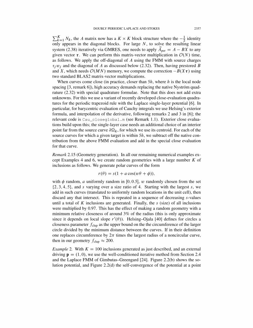
The flux integrals involving v are on the distant walls of the 3 3 “super-cell,” with locations and weights shown in Figure 2.4(c). The final term involvesa smooth integrand on the original wall L. A similar far-field formula for J2is achieved by reflection through the line x1 D x2, with weights shown in Fig-ure 2.4(d).

PROOF. Substituting (2.25) into J1 in (2.41) involves a 3 3 sum over densitysources (Figure 2.4(a)), which by translational invariance we reinterpret as a sumover displaced target copies as in panel (b). These nine copies of L form threecontinuous vertical walls. Since v is harmonic in R2 n, then

R vn D 0 for any

closed curve that does not enclose or touch @. However, since un D 0 on@ and u v is harmonic in a neighborhood of , this also holds if encloses


J1

−1 −2 −3

3

3

3

1 2 33

2

1

J1 J2(c) far field wall weights for

33−3

−2

−1

3

(d) far field wall weights for

L

(b) rewrite as sum over target walls (a) layer potential flux integral in

FIGURE 2.4. Efficient evaluation of fluxes .J1; J2/ using far-field in-terations alone. (a) Nine terms in L wall integral in J1 from the 3 3layer potential image sum in (2.25). (b) Re-interpretation as a sum overtargets (nine copies of L) for the potential v. The red dotted line showsthe closure of the boundary where flux conservation is applied. (c) Re-sulting weights of the flux integrals of v on nine wall segments; note allare distant from @. (d) The wall weights for J2.

@. Thus the flux through each length-3 vertical wall is equal to the flux throughits closure to the right along the dotted contour shown in panel (b). Summingthese three contour closures, with appropriate normal senses, gives the weights inpanel (c), i.e., (2.43). One may check that the result is unaffected by intersectionsof @ with the original unit cell walls.

We have tested that this formula matches the naive quadrature of (2.41) when@ is far from L. For Example 1, Figure 2.2(c) and (d) include convergence plotsfor the flux J1 as computed by (2.43), showing that it converges at least as fastas do pointwise potential values. For the parameters of panel (a) we find thatj12 21j D 6 10

14, indicating high accuracy of the computed tensor.

3 The Case of Conducting InclusionsThe above section generalizes easily to the case where the inclusions have nonzero

conductivity ; as before, without loss of generality, the background medium is as-signed unit conductivity. This replaces the pair (2.5)–(2.6) by

u D 0 in B n @;(3.1)


c N iters. time calc H94 H17 rel. diff.

100 100 200 56 0.8 s 35.95764629703 35.957646297 35.95764629705 3 1013

100 1000 200 93 0.8 s 164.1473079002 164.14730790 164.1473079006 2 1012

1000 100 200 81 0.8 s 36.67257761067 36.672577611 36.67257761078 3 1012

1000 1000 300 187 2.6 s 243.00597811 243.005978 243.0059781329 8 1011

TABLE 3.1. Validation of the effective conductivity of an infinite unitsquare array of discs with radius r D 1

2

p1 c2 and conductiv-

ity within a background conductivity of 1 (Example 4). The well-conditioned Schur system of (2.38) was used, with the matrix A givenby (2.32) with the factor 1=2 replaced by 1=. GMRES with a rela-tive tolerance of 1014 was used, although stagnation at up to 4 digitsworse than this occurred. calc shows the results. H94 shows publishedresults in [35, table 2]; H17 shows results using a slight variant of thecode demo14b.m due to Helsing [37, sec. 21.2]. The last column showsthe relative differences jcalc H17j=H17.

uC u D 0 on @;(3.2)

uCn un D 0 on @;(3.3)

where the superscriptsC and denote exterior and interior limits, respectively, asin (2.23). Following [27] we keep the standard single-layer representation (2.25);however, this representation now acquires physical meaning both inside and out-side the inclusion. This, plus the continuity of the single-layer potential across@ [45, chap. 6], means that (3.1)–(3.2) are already satisfied, leaving (3.3) as theonly remaining equation. Inserting into this the jump relation (2.23) and simplify-ing gives

(3.4)1

2CD

near;T@;@

C

MXjD1

j@j

@n

ˇ@

D 0;

where WD . 1/=. C 1/ is a contrast parameter. This equation differs from(2.26) only in the prefactor of the identity term, and becomes identical in the in-sulating case D 0. Thus, in the discretized matrix A of (2.32) the factor 1=2becomes 1=, but no other aspect of the scheme of Section 2 changes.

Example 4. The effective conductivity of an infinite square array of conductingdiscs of radius r is a standard test case. Only a single driving p D .1; 0/ need beapplied, because is a multiple of the identity. The more challenging cases arewhen the gap 1 2r is very small and is large [60]. In Table 3.1 we validateagainst four such results published by Helsing [35, table 2], also against recompu-tation with Helsing’s recent RCIP method [37]. Both of these methods use latticesums to periodize. Radius is controlled by a parameter c D .1 4r2/1=2; forc D 1000 the gap is 5 107 (i.e., fclup 107). We are still able to efficientlyexploit the periodic trapezoid rule by combining the close-evaluation quadratures


discussed in Section 2.5 with a geometrically graded parametrization of the circle,

(3.5) x.t/ D .r cos .t/; r sin .t// where 0.t/ D ˛ cosh.ˇ sin 2t/;

which bunches quadrature points by a factor of order eˇ around the four close-to-touching regions. We fix ˇ D 1

2log.1 2r/, based on theory [60] implying that

is smooth on scales as large as .1 2r/1=2. The constant ˛ in (3.5) is evalu-ated numerically by enforcing

R 20 0.t/dt D 2 . This simple reparametrization

achieves a similar effect as adaptively refined panel quadratures (which would bepreferable in more general geometries). As evident in the table, a very small Nmay thus be used, while still matching all published digits of the lattice-sum basedresults in [35, table 2], and matching to 10–12 digits values found with the moreinvolved panel-based RCIP method.

Since the main point of Example 4 is to validate the periodizing scheme, wedo not push to more extreme closeness (higher c). Nor do we use integral for-mulations such as [39, eq. (9)] or [37, eq. (90)] better suited to large ; perhapsdoing so would reduce our iteration count to near the 10 or 11 needed by Helsing’sRCIP method. CPU times are quoted for a laptop with an i7-7700HQ processorat 2.8 GHz, running the code tbl_discarray_effcond.m (see Remark 1.1).They are dominated by a rather crude O.N 3/MATLAB® implementation of close-evaluation quadratures for filling A; they could be much reduced.

4 The No-Slip Stokes Flow CaseWe move to our second BVP, that of viscous flow through a periodic lattice

of inclusions with no-slip boundary conditions. We follow the normalization andsome of the notation of [41, sec. 2.2, 2.3]. Let the constant > 0 be the fluid vis-cosity. The periodic BVP is to solve for a velocity field u and pressure p functionsatisfying

uCrp D 0 in R2 nƒ;(4.1)

r u D 0 in R2 nƒ;(4.2)

u D 0 on @ƒ;(4.3)

u.xC e1/ D u.xC e2/ D u.x/ for all x 2 R2 nƒ;(4.4)

p.xC e1/ p.x/ D p1 for all x 2 R2 nƒ;(4.5)

p.xC e2/ p.x/ D p2 for all x 2 R2 nƒ:(4.6)

The first two are Stokes equations, expressing local force balance and incompress-ibility, respectively. The third is the no-slip condition, and the remainder expressthat the flow is periodic and the pressure periodic up to the given macroscopicpressure driving .p1; p2/.


We recall some basic definitions. Given a pair .u; p/ the Cauchy stress tensorfield has entries

(4.7) ij .u; p/ WD ıijp C .@iuj C @jui /; i; j D 1; 2:

The hydrodynamic traction T (force vector per unit length that a boundary surfacewith outwards unit normal n applies to the fluid), also known as the Neumann data,has components

(4.8) Ti .u; p/ WD ij .u; p/nj D pni C .@iuj C @jui /nj ;

where here and below the Einstein convention of summation over repeated indicesis used. We first show that the BVP has a one-dimensional nullspace.

PROPOSITION 4.1. For each .p1; p2/ the solution .u; p/ to (4.1)–(4.6) is uniqueup to an additive constant in p.

PROOF. The proof parallels that of Proposition 2.1. Given any function pairs.u; p/ and .v ; q/, Green’s first identity on a domain K is [49, p. 53]

(4.9)ZK.ui@ip/vi D

2

ZK.@iujC@jui /.@ivjC@j vi /C

Z@KTi .u; p/vi :

Now let .u; p/ be the difference between two BVP solutions, and set v D u andK D B n in (4.9). The left-hand side vanishes due to (4.1), the @ boundaryterm vanishes due to (4.3), and the unit cell wall terms vanish by u periodicity,leaving only

RBn

P2i;jD1.@iuj C @jui /

2 D 0. Thus u has zero stress, i.e., is arigid motion, so, by (4.3), u 0. Thus, by (4.1), and because p has no pressuredrop, p is constant.

Since, for Stokes, the Cauchy data is .u;T / [41, sec. 2.3], the BVP (4.1)–(4.6)is equivalent to the BVP on a single unit cell,

uCrp D 0 in B n;(4.10)

r u D 0 in B n;(4.11)

u D 0 on @;(4.12)uR uL D 0(4.13)

T .u; p/R T .u; p/L D p1n(4.14)uU uD D 0(4.15)

T .u; p/U T .u; p/D D p2n;(4.16)

where the normal n has the direction and sense for the appropriate wall as in Fig-ure 1.3(a). Discrepancy will refer to the stack of the four vector functions on theleft-hand side of (4.13)–(4.16).


4.1 The Stokes Empty Unit Cell Discrepancy BVPProceeding as with Laplace, one must first understand the empty unit cell BVP

with given discrepancy data g WD Œg1Ig2Ig3Ig4, which is to find a pair .v ; q/solving

v Crq D 0 in B;(4.17)r v D 0 in B;(4.18)

vR vL D g1;(4.19)

T .v ; q/R T .v ; q/L D g2;(4.20)vU vD D g3;(4.21)

T .v ; q/U T .v ; q/D D g4;(4.22)

This BVP has three consistency conditions and three nullspace dimensions, as fol-lows:2

PROPOSITION 4.2. A solution .v ; q/ to (4.17)–(4.22) exists if and only ifZL

g2 ds C

ZD

g4 ds D 0 (zero net force) and(4.23) ZL

n g1 ds C

ZD

n g3 ds D 0 (volume conservation),(4.24)

and then is unique up to translational flow and additive pressure constants; i.e., thesolution space is .v C c; q C c/ for .c; c/ 2 R3.

PROOF. Noting that (4.9), with .u; p/ and .v ; q/ swapped, holds for all constantflows u shows that

R@K T .v ; q/ D 0; setting K D B gives (4.23). (4.24) follows

from the divergence theorem and (4.18). The proof of Proposition 4.1 shows thatthe nullspace is no larger than constant p and rigid motions for v , but it is easy tocheck that rotation is excluded due to its effect on g1 and g3.

We solve this Stokes empty BVP in an entirely analogous fashion to Laplace,namely via an MFS representation with sources yj as in (2.17), but now withvector-valued coefficients. For x 2 B,

v.x/

MXjD1

j .x/j ; j .x/ WD G.x; yj /;(4.25)

q.x/

MXjD1

pj .x/ j ;

pj .x/ WD G

p.x; yj /;(4.26)

2 Note that, although three is also the nullity of the 2D Stokes interior Neumann BVP [41, table2.3.3], both nullspace and consistency conditions differ from that case.


where the velocity fundamental solution (stokeslet or single-layer kernel) is thetensor G.x; y/ with components

(4.27)Gij .x; y/ D

1

4

ıij log

1

rCrirj

r2

;

i; j D 1; 2; r WD x y ; r WD krk:

and the single-layer pressure kernel is the vector Gp with components

(4.28) Gpj .x; y/ D

1

2

rj

r2; j D 1; 2:

We will also need the single-layer traction kernel Gt with components (applying(4.8) to the above),

Gtik.x; y/ D ij .G;k. ; y/; G

pk. ; y//.x/nx

j

D 1

rirk

r2r nx

r2; i; k D 1; 2;

(4.29)

where the target x is assumed to be on a surface with normal nx.The generalization of the linear system from (scalar) Laplace to (vector) Stokes

is routine bookkeeping, which we now outline. The MFS coefficient vector WDfj g

MjD1 has 2M unknowns, which we order with the M 1-components followed

by the M 2-components. Discretizing (4.19)–(4.22) on m collocation nodes perwall, as in Section 2.1, gives Q D g as in (2.19), with discrepancy vector g 2R8m. We choose to order each of the four blocks in g with all m 1-componentsfollowed by m 2-components. As before, Q D ŒQ1IQ2IQ3IQ4 with each Qksplit into 22 sub-blocks based on the 1- and 2-components. For instance, writingklj , k; l D 1; 2, for the four components of the basis function j in (4.25), thenthe R-L velocity block is

Q1 D

"Q111 Q211

Q121 Q221

#;

with each sub-block having entries .Qkl1 /ij D klj .xiLC e1/

klj .xiL/. The R-

L traction blockQ2 has sub-blocks .Qkl2 /ij D Gtkl.xiLCe1; yj /G

tkl.xiL; yj /,

where it is implied that the target normal is on L. The other two blocks are similar.In Figure 2.1(c) we show the convergence of the solution error produced by

numerical solution of the Stokes version of (2.19) (again, see Remark 2.5). Theresults are almost identical to the Laplace case in Figure 2.1(b), converging to 15-digit accuracy with a similar exponential rate; keep in mind that now there are2M unknowns rather than M . Note that we do not know of a Stokes version ofTheorem 2.3. Figure 2.1(c) also shows that three singular values decay faster thanthe others, as expected from Proposition 4.1.


Finally, the discretization of the consistency conditions in Proposition 4.1 is thestatement that

(4.30) W TQ 032M ;

where 0mn is the m n zero matrix, and the weight matrix W (the analogue of(2.20)) is

(4.31) W D

24 0 0 wTL 0 0 0 wT

D 0

0 0 0 wTL 0 0 0 wT

LwTL 0 0 0 0 wT

D 0 0

35T

2 R8m3:

4.2 Integral Representation and the Stokes ELSIn contrast to the Laplace problem, we are now solving a Dirichlet BVP, which

suggests a pure double-layer representation on inclusion boundaries. However,this would lead to a 3D nullspace for each inclusion, associated with its comple-mentary interior Neumann BVP [41, table 2.3.3]. We remove this nullspace via a“compound” or mixed double-layer formulation, namely an admixture of double-and single-layers [34, thm. 2.1] [67, p. 128]; this avoids the use of extra interiorstokeslet degrees of freedom that can add O.K3/ work for K inclusions [26].

For convenience we define the 2D Stokes layer potentials. Given a vector-valueddensity D .1; 2/ on @, the Stokes single-layer potential generates (via (4.27)and (4.28)) velocity and pressure:

u.x/ D .S/.x/ WD

Z

G.x; y/.y/dsy ;

p.x/ D .Sp/.x/ WD

Z

Gp.x; y/.y/dsy :

(4.32)

Using ny to denote the source normal, the Stokes double-layer velocity potential is

(4.33)u.x/ D .D/.x/ WD

Z

D.x; y/.y/dsy ;

Dij .x; y/ D1

rirj

r2r ny

r2; i; j D 1; 2;

a kernel that is the negative transpose of (4.29), and the associated pressure

(4.34)

p.x/ DDp.x/ WD

Z

Dp.x; y/.y/dsy ;

Dpj .x; y/ D

n

yj

r2C 2r ny rj

r4

:

The Stokes analogue of the boundary integral operator (2.24) is the single-layertraction

(4.35)DT 0;

.x/ WD

Z

Gt.x; y/.y/dsy ; x 2 0;


Ω

(a) (b)

50 100 150 200

N

10 -15

10 -10

10 -5

(c) u conv ELS

J1

conv ELS

u conv Schur

J1

conv Schur

u err vs known

50 100 150 200 250 30010

−15

10−10

10−5

Nk

(d)

M = 70, m = 22

u conv SchurJ

1 conv Schur

FIGURE 4.1. Periodic Stokes flow tests with applied pressure drop p D.1; 0/. (a) Solution velocity u (arrows) and pressure p (contours) forExample 5 (same geometry as Figure 2.2(a)), with N D 150, M D 70,and Rp D 1:4. A single unit cell is shown, and the m D 22 nodes perwall are shown as dots. (b) Flow speed juj for K D 100 inclusionsper unit cell, using iterative solution of (4.44) (Example 7; geometryidentical to Figure 2.2(b)). (c) N -convergence of u error (with M D 70fixed) at the same test points as in Figure 2.2(a), and of flux J1 (see theend of Section 4.2), relative to their values at N D 230 (Example 5).Squares show error convergence in u in the case of known uex due to astokeslet grid. Solid lines are for direct solution of the ELS, and dashedlines for the iterative solution of (4.44). (d) Convergence with Nk forK D 100 inclusions per unit cell (Example 7). Errors in velocity (+signs) and flux J1 (circles) are shown, estimated relative to their valuesat Nk D 400.


which uses (4.29). Finally, the hypersingular double-layer traction operator isneeded,

(4.36) .T 0;/.x/ WD

Z

Dt.x; y/.y/dsy ; x 2 0;

whose kernel is computed by inserting (4.33) and (4.34) into (4.8) and simplifyingto get (e.g., [55, (5.27)]),

Dtik D

ny nx

r2 8dxdy

rirk

r2

C dxdyıik Cnxi n

yk

r2C dx

rknyi

r2C dy

rinxk

r2

(4.37)

where for conciseness we defined the target and source “dipole functions,” respec-tively,

dx D dx.x; y/ WD .r nx/=r2; dy D dy.x; y/ WD .r n

y/=r2:

The Stokes jump relations [49, sec. 3.2] are identical to the usual Laplace ones(2.23) with the potential taken to be velocity potential, and the normal derivativereplaced by the traction. In short, the single-layer velocity and double-layer trac-tions are continuous, whereas the single-layer traction jump is minus the density,and the double-layer velocity jump is the density itself.

Armed with the above, our representation for the solution .u; p/ in B n is themixed formulation,

(4.38) u DDnear@ CSnear

@

C

MXjD1

j j ; p DDp,near@CSp,near

@

C

MXjD1

pj j ;

where “near” denotes 3 3 image sums as in (2.25). With this choice made, thecontinuous form of the ELS is similar to (2.26)–(2.30). The first block is, applyingthe exterior jump relation to (4.12),

(4.39)1

2CDnear

@;@ C Snear@;@

C

MXjD1

j j@j D 0:

Rather than list all second subblocks, we note that they are simply (2.27)–(2.30)with S replaced by D C S , DT replaced by T C DT, and @j .x/=@n replacedby the basis traction, which has kernel Gt

lk.x; yj /. Finally, the pressure driving

.p1; p2/ is encoded by the discrete right-hand side

(4.40) g D Œ0I 0Ip11mI 0I 0I 0I 0Ip21m 2 R8m;

so that the ELS has, as for Laplace, the form (1.2).This mixed formulation allows an analogue of Lemma 2.8: the Stokes ELS

nullspace is spanned by .

LEMMA 4.3. In the solution to the Stokes ELS (i.e., (4.39) plus the Stokes versionof (2.27)–(2.30) described above), is unique.


PROOF. The proof parallels that of Lemma 2.8, but adapts the 2D version of theproof of [34, thm. 2.1] for the interior uniqueness step. Let vC and v denote theexterior and interior limits, respectively, of v on @, and TC and T be the samelimits of T .v ; q/. If .; / is the difference between any two ELS solutions, let.v ; q/ be given by the representation (4.38) both in B n and inside . Thus, byProposition 4.1, v 0, and q D c, some constant, and TC D cn. The jumprelations for D C S then give v D and T D cn . Thus in , .v ; q/ isa Stokes solution with Robin (impedance) data, v C T D cn. Applying (4.9)with u D v and K D gives 0 D .=2/

R.@ivj C @j vi /

2 C cR@ n v

R@ kv

k2. However by incompressibilityR@ n v

D 0, and the two remainingnonpositive terms have the same sign, so must both vanish. Hence v 0 in . Bythe double-layer jump relation, D vC v, both of which have been shown tovanish, thus 0.

The filling of the discrete .2NC8m/.2NC2M/ ELS is now routine, being asin Section 2.2, apart from vector bookkeeping, and the following two details.

(i) For the discretization of D@;@ with kernel (4.33), the diagonal limitat node xk is Dij .xk;xk/ D ..xk/=2/ti .xk/tj .xk/ where .t1; t2/ are thecomponents of the unit tangent vector on @.

(ii) The kernel of S@;@ has a logarithmic singularity on the diagonal, sothe plain Nyström rule cannot be used. However, there exist several high-orderdiscretizations for such a kernel [2,33,45]; when theN per inclusion is not large weprefer the spectral product quadrature due to Martensen, Kussmaul, and Kress [45,chap. 12.3] [33, sec. 6.2].

We provide an implementation of the above kernel quadratures in StoSLP.mand StoDLP.m, and of filling the ELS in fig_stoconvK1.m; see Remark 1.1.

Example 5. We illustrate the above with results obtained via a simple dense directsolve of the ELS, for the periodic “worm” geometry from Example 1, with no-slipboundary conditions, pressure driving p D .1; 0/, and D 0:7. Figure 4.1(a)shows the resulting flow u and pressure p. Here we evaluated u using the close-evaluation quadratures from [6], and p using similar formulae, to provide spectralaccuracy even up to the curve. As expected from Proposition 4.1, the ELS exhibitsunit numerical nullity: the Stokes version of Figure 2.2(e) is very similar, and we donot show it. Figure 4.1(c) shows the pointwise convergence in u and is consistentwith exponential convergence down to 13-digit accuracy. For a known solutionproduced by stokeslets on the same grid as in Section 2.3, convergence stops ataround 12 digits.

Rapid convergence of the flux J1 is also shown in Figure 4.1(c), reaching 13-digit accuracy at only N D 100. Here, flux is evaluated using the Stokes versionof (2.43), which replaces the representation S by D C S and replaces @=@n by n,and in the proof replaces the zero-flux condition by incompressibility.


4.3 Schur Complement Systems for StokesHaving filled the Stokes version of the ELS (1.2), we would like to eliminate the

periodizing unknowns j to leave a 2N 2N system that can be solved iteratively.

An Equivalent Square System Preserving the NullspaceIt is possible to build such a system that preserves the rank-3 nullity using ex-

actly the recipe in Section 2.4. For this we need only two ingredients: (i) H mustbe a stack of three densities so that CH enlarges the range of zQ to include allsmooth vectors, and (ii) R must be a stack of three proxy coefficient vectors withfull-rank projection onto NulQ.

We first need the Stokes version of the technical lemma. For Stokes there are twotypes of Gauss’s law. Let v D S@ CD@ be a velocity potential with arbitrarydensities and on a curve @, with associated pressure q D Sp

@ C Dp

@.

Then,

(4.41)

Z@K

T .v ; q/ D

Z@

ds (net force);Z@K

v n D

Z@

n ds (net flux);

where @K is the boundary of some open domain K containing @. The proofs ofboth are similar to that of (2.37), summing over the boundaries of and of K nto get the left-side integral. For the first law one uses the single-layer traction jumprelation, and, for the second, the double-layer velocity jump relation [49, pp. 57–58].

Remark 4.4. The second law of (4.41) implies that the net fluid flux through theboundary of K is generally nonzero, i.e., that the Stokes double-layer velocity po-tential on the enclosed curve does not generally conserve fluid volume. This sur-prising fact we did not find stated in standard literature.

Now, for H we can choose densities that, when used with our D C S represen-tation, generate net force in the 1-direction, in the 2-direction, and break volumeconservation, respectively:

(4.42) H Dh.1/ h.2/ h.3/

D

1N 0N fn

xi

1 gNiD1

0N 1N fnxi

2 gNiD1

;

where in the columns of the matrix we use “nodes fast, components slow” ordering,and recall that the normals live on the nodes of @. Next we show that CH hasfull-rank projection onto RanW .

LEMMA 4.5. GivenH in (4.42),W in (4.31), and C the Stokes discrepancy matrixfilled as in Section 4.2, then the 3 3 matrix W TCH is diagonal, and, for all Nand m sufficiently large, invertible.

PROOF. The proof parallels that of Lemma 2.13. For instance, setting v D

.Snear@C Dnear

@/h.1/ and using (4.41) we see the discrepancy has net force j@j in


the 1-direction only, and sinceR@ n D 0 the discrepancy is volume conserving.

Discretizing shows that the first column of W TCH converges (in m and N ) toŒj@j 0 0T. Similar steps apply to the other two columns, showing that thematrix in fact converges, up to signs, to j@j times the 3 3 identity.

For R we choose the three analogous scaled coefficient vectors on the proxycircle:

(4.43) R Dr.1/ r.2/ r.3/

D

1

M

"1M 0M fcos 2j=M gMjD10M 1M fsin 2j=M gMjD1

#:

Reasoning as in the start of the proof of Theorem 2.12, the three (linearly inde-pendent) columns of R are exponentially close to generating constant flow in the1-direction, the 2-direction, and constant pressure, respectively, which, accordingto Proposition 4.2, fall into NulQ.

Given the above statements about H and R, Theorem 2.12 holds for the Stokesversion of the procedure of Section 2.4; in its proof one need only change w to theW of (4.31). Because of the unit nullity of the Stokes ELS, this would result in arank-1 deficient square system matrix.

A Well-Conditioned Square Stokes SystemTo remove this nullspace, it is tempting to take the obvious Stokes generaliza-

tion of Section 2.4, leaving the B block unperturbed as in (2.39). However, thisfails (the solution having constant, but incorrect, pressure drops) because W Tg DŒp1Ip2I 0 ¤ 03. However, since only one nullspace dimension needs to be re-moved, and this nullspace is common to the empty unit cell BVP, this suggests ahybrid where the perturbation of B involves only the remaining two dimensions.This indeed leads to a well-conditioned square system:

(1) Set H as in (4.42) and R as in (4.43), then set zQ WD Q C CHRT andyB WD B C AP12, where P12 WD Œh.1/ h.2/Œr.1/ r.2/T involves the two

force (but not the one pressure) perturbations.(2) Solve for the vector y in the 2N 2N Schur complement linear system

(4.44) yApery WD .A yB zQCC/y D yB zQCg;

where, as before, one solves the small systems zQX D C and zQy D g tobuild the large system matrix yAper D A yBX and right-hand side yByfor (4.44), which may then be solved iteratively.

(3) Recover the proxy coefficients via D y Xy.(4) Recover the density via D y C P12.

THEOREM 4.6. Let g encode the pressure driving as in (4.40). Then for all N ,M ,andm sufficiently large, the pair .; / produced by the above procedure is uniqueand solves the Stokes version of the ELS (1.2) with residual of order the quadratureerror on boundaries.

This is a Stokes analogue of Theorem 2.14, and its proof structure is similar.


PROOF. (4.44) is the Schur complement of the perturbed ELS

(4.45)A B C AP12C QC CHRT

y

D

0

g

;

so that if y solves (4.44) then .y; /, with as in Step 3, solves (4.45). ApplyingStep 4, one may check that the pair .; / then solves a rank-1 perturbed systemsimilar to (2.39),

(4.46)

"A B

C QC Ch.3/r.3/T

#

D

0

g

:

From this pair, define v as the resulting quadrature approximation to the velocitypotential (4.38), namely,

v.x/ WDX

m1;m22f1;0;1g

NXiD1

wiD.x;xi Cm1e1 Cm2e2/

CG.x;xi Cm1e1 Cm2e2/i

C

MXjD1

j .x/j :

Since it matches that of the ELS, the first row of (4.46) implies that v j@ D 0.Thus

R@ v n D 0 and, by volume conservation in B n, the discrepancy of

.v ; q/ obeys (4.24), whose discretization is w.3/T.C C Q/ D 0, where w.3/

is the third column of (4.31). Subtracting this from the second row of (4.46) left-multiplied by w.3/T leaves .w.3/TCh.3//r.3/

T D w.3/Tg. Lemma 4.5 implies

that w.3/TCh.3/ ¤ 0, and by computation w.3/Tg D 0. Thus r.3/T D 0, so the

pair also solves the ELS. Thus Lemma 4.3 holds, so is unique.

We expect (4.44) to be well-conditioned if A is, since the unit nullity has beenremoved by enforcing one extra condition r.3/

T D 0. In contrast to Laplace, here

the rank-3 nullity of the empty BVP demands a hybrid scheme which “segregates”the other two conditions.

We test this scheme returning to Example 5 (Figure 4.1). Panel (c) includes (asdotted lines) the convergence using the above recipe, using GMRES with tolerance1014. The convergence is almost identical to that of the direct ELS solution, andthe converged values differ by around 2 1014. The condition number of yAperis 82.7, independent of N and M , and the number of GMRES iterations variedbetween 25 and 30.

4.4 More Challenging Numerical Tests for StokesWe now validate the above periodic Stokes scheme against a known test case,

and in geometries with large numbers of inclusions.


c (vol. frac.) N iters. time est. rel. err. Dcalc DGK

0.05 60 5 0.02 s 8 1015 15.5578223189024 15.55780.1 60 7 0.03 s 3 1014 24.831675248849 24.83170.2 60 8 0.02 s 3 1014 51.526948961799 51.52690.3 100 10 0.02 s 1 1013 102.88130367005 102.8810.4 150 10 0.03 s 1 1013 217.89431472214 217.8940.5 150 12 0.03 s 9 1013 5:325481184633 102 5:32548 102

0.6 300 13 0.08 s 1 1012 1:763573112520 103 1:76357 103

0.7 400 20 0.14 s 7 1011 1:35191501298 104 1:35193 104

0.75 500 28 0.22 s 2 1010 1:2753159105 105 1:27543 105

0.76 600 32 0.31 s 1 109 2:948165200 105 2:94878 105

0.77 700 44 0.42 s 7 109 1:03826971 106 1:03903 106

0.78 1300 64 1.5 s 6 108 1:4379206 107 —

TABLE 4.1. Computation of the 2D viscous Stokes drag of an infinitesquare array of no-slip discs of various volume fractions c (Example 6).The well-conditioned Schur system of (4.44) was used. Dcalc shows thedimensionless drag results. Relative errors were estimated by conver-gence (comparing each against three N values larger than shown, andincreasing M ). The last column DGK shows for comparison the numeri-cal findings of [26, table 1, column 5].

Example 6. The effective permeability of the no-slip flow around an infinite squarelattice of discs is a standard test case. Only one pressure drop p D .1; 0/ needbe solved, since the permeability tensor is a multiple of the identity. The dimen-sionless drag is then related to the permeability 11 by D D 1=.11/. We com-puted this for a list of volume fractions c D r2 including those of Greengard–Kropinski [26] (note that to match the literature, the definition of c has changedfrom Example 4). We used the graded circle parametrization (3.5) with N chosenby convergence studies. As c approaches =4, the discs come closer, the solutiondensity becomes more peaked, and the required N grows. At the most extremecase of c D 0:78, the gap is 3 103 (i.e., fclup 1800). Since the gap is muchlarger than in Example 4, we were able to use the plain far-field Nyström rule forfilling A. (We found that, in this setting, close-evaluation quadratures [6] wereslower, and around one digit less accurate.) At large c theN values needed are stillsmaller than in [26, table 1]. We used GMRES with D 1014 and dense matrix-vector multiplication, and find similar numbers of iterations as in [26]. CPU timesare quoted for a laptop with an i7-7700HQ processor at 2.8 GHz, running the codetbl_discarray_drag.m (see Remark 1.1).

Our results are given in Table 4.1. For validation we include in the last columnthe numerical findings from [26, table 1], which were quoted to 6 digits, and inturn validated against prior less accurate results [71]. For c 0:6, our resultsmatch the 6 digits quoted in [26, table 1], but above this the match deteriorates,reaching only 3 digits at their most challenging case c D 0:77 (we believe thattheir nonmatching digits are incorrect). ForN values larger than shown, our results


fluctuate only at the estimated error levels shown; thus we are confident that ourscheme reaches around 14 digits of accuracy for the smaller c values, dropping to 7digits at c D 0:78. This loss of accuracy cannot be explained by condition numberalone, since the latter reaches only 104 at c D 0:78. Further work is needed toascertain whether this loss is controlled by an underlying condition number of theBVP (and hence impossible to improve upon in double-precision arithmetic), or ifa different representation or quadrature, analogous to [37], could reduce the error.

Example 7. We solve the geometry of Example 2, with K D 100 inclusions, butwith Stokes no-slip conditions, and the well-conditioned iterative scheme of Sec-tion 4.3. We apply Stokes potentials using a few calls to the Laplace FMM, aspresented in [6, sec. 2.1]. Close-evaluation quadratures for S and D are used, asin Example 5. One period of the resulting solution flow speed is plotted in Fig-ure 4.1(b). Convergence is shown by Figure 4.1(d); 11–12 digits of accuracy influx is achieved, which is around 2 digits less than for Laplace. At the convergedvalue Nk D 200, the solution takes 1720 seconds.

Linear complexity as a function ofK is demonstrated by Figure 2.3(c). The timeper iteration is similar to that for Laplace; this is because we prestore the close-evaluation matrix blocks, whereas for Laplace we evaluated them on the fly. Weshow the solution forK D 103 in Figure 1.2, using Nk D 350. This required 1289GMRES iterations and took 21 hours using the same machine as in Figure 1.1. Bycomparison to the solution at Nk D 450, we estimate that the absolute flux erroris 9 109. However, due to the narrow channels in this porous medium, the sizeof the flux is only around 105, meaning that relative accuracy is only 3 digits.Further study is needed to determine if it is an underlying condition number of theflux problem that prevents more digits from being achieved. The code is found inthe directory multiinclusion_Stokes (see Remark 1.1).

Example 8. In the previous example large numbers of GMRES iterations wereneeded, in contrast to the Laplace case (cf. Example 2). This motivates studyingthe growth of iteration count with geometric complexity. We use exactly the samecircular geometries as in Example 3. Figure 2.3(d) shows that the numbers ofiterations are around 10 times those for Laplace, and that they grow with K in amore aggressive manner possibly consistent with K1=2.

5 ConclusionsWe have presented a unified framework for the second-kind integral equation

solution of large-scale periodic Laplace and Stokes BVPs, which we believe willbe useful in related settings such as multiphase composites, photonic crystals, andparticulate flows. The philosophy is quite simple, and we encourage readers to tryimplementing it in their applications:

Use a free-space potential theory representation for the near-neighbor im-ages, plus O.1/ auxiliary “proxy” degrees of freedom to represent the restof the infinite lattice.


Augment the linear system by applying physical boundary conditions on aunit cell. Use a low-rank perturbation of the empty BVP system to remove the con-

sistency condition, allowing elimination of the auxiliary unknowns to givea well-conditioned system compatible with fast algorithms.

This cures two ills in one fell swoop: it removes zero eigenvalue(s) that arise in thephysical BVP, and circumvents the issue of nonexistence of the periodic Green’sfunction for general densities.

In Section 2.4 we provided a simple unified procedure for periodizing Laplaceand Stokes integral representations when the physical BVP nullspace is numeri-cally tolerable—we believe that this would be a useful starting point for relatedelliptic BVPs. However, when a well-conditioned system is desired, we have pre-sented and analyzed procedures for Laplace (Section 2.4) and Stokes (Section 4.3)systems, where the latter exploits the fact that the physical BVP consistency con-ditions form a subset of those of the empty BVP. The relevant theorems (2.12, 2.14and 4.6) generalize simply to the case of any consistent right-hand side. We show-cased the scheme with high-accuracy computations of the effective conductivityand the viscous drag of a square lattice of discs and of random composites with alarge number of inclusions needing several million unknowns.

Remark 5.1 (Randomization). In this work we have been explicit about choosinglow-rank matrices R and H proven to have the required full-rank projections, inboth Laplace and Stokes cases (Lemmata 2.9, 2.13, and 4.5). For other BVPs,this may not be easy or convenient. However, in practice, there is much flexibil-ity in their choice. Following [73], one may even pick random matrices for bothR and H , exploiting the fact that with probability 1 they have the required full-rank projections. In our experiments, the only penalty is a small loss of GMRESconvergence rate, and a larger, fluctuating condition number.

We finish with directions for future work. We believe that an elastostatic version[12, 36] would be very similar to what we present for Stokes. While we restrictedour attention to static geometry BVPs, the scheme can handle moving geometryproblems, such as the flow of bubbles, vesicles, or bacteria, in a straightforwardmanner (e.g., see [58]). The scheme generalizes easily to 3D (requiring M 103

auxiliary unknowns) [57]. Note that in (2.25) one need not sum all 3 3 copies ofsource quadrature nodes when applyingA, but just the ones falling inside the proxycircle (or sphere) [30]. Exploiting this can lower the overall constant, especially in3D, but requires extra bookkeeping in the C matrix block.

By further augmenting the linear system to include decay/radiation conditions,the scheme has already proven useful for cases when the periodicity is less thanthe space dimension, such as singly periodic in 2D [13, 22, 58] or doubly periodicin 3D [56]. The latter case has applications in electrostatics [54] and Stokes flow[16,52]. The case of singly periodic in 3D, and of nonperiodic solutions in periodic


geometries, await development. The generalization to arbitrary skew and/or high-aspect unit cells has applications in shearing suspensions and in microfluidics. Thisis easy in principle, with the proxy circle becoming an oval in order to “shield” thefar images, as in Figure 1.3(c). However, sinceM must grow with the aspect ratio,this will require new ideas beyond an aspect ratio of, say, 103 in 2D.

More theoretical work is required, since our analysis does not attempt precisebounds on how quadrature errors propagate to solution errors for the scheme. Workis also needed to understand if observed limitations in Stokes relative flux accuracy(such as 7 digits at the end of Table 4.1 and 3 relative digits in Figure 1.2) are in-trinsic (unavoidable in double precision due to ill-conditioning of the BVP), or areinstead due to lack of optimality in the scheme. Finally, to reduce the large GM-RES iteration counts for Stokes flows in complicated close-to-touching geometries,adaptive schemes such as that of Helsing [37], or the use of fast direct solvers orlocal preconditioners, will be important.

Acknowledgments. We are grateful for useful discussions with Bob Kohn,Leslie Greengard, Jun Lai, Mark Tygert, Manas Rachh, and the anonymous ref-erees. The work of AB and LZ was supported in part by National Science Founda-tion Grant DMS-1216656. The work of LZ was largely done while at DartmouthCollege. The work of GM and SV was supported in part by National ScienceFoundation grants DMS-1418964 and DMS-1454010. The Flatiron Institute is adivision of the Simons Foundation.

Bibliography[1] af Klinteberg, L.; Tornberg, A.-K. Fast Ewald summation for Stokesian particle suspensions.

Internat. J. Numer. Methods Fluids 76 (2014), no. 10, 669–698. doi:10.1002/fld.3953[2] Alpert, B. K. Hybrid Gauss-trapezoidal quadrature rules. SIAM J. Sci. Comput. 20 (1999), no. 5,

1551–1584. doi:10.1137/S1064827597325141[3] Barnett, A. H. Evaluation of layer potentials close to the boundary for Laplace and Helmholtz

problems on analytic planar domains. SIAM J. Sci. Comput. 36 (2014), no. 2, A427–A451.doi:10.1137/120900253

[4] Barnett, A. H.; Betcke, T. Stability and convergence of the method of fundamental solutionsfor Helmholtz problems on analytic domains. J. Comput. Phys. 227 (2008), no. 14, 7003–7026.doi:10.1016/j.jcp.2008.04.008

[5] Barnett, A.; Greengard, L. A new integral representation for quasi-periodic fields and Its ap-plication to two-dimensional band structure calculations. J. Comput. Phys. 229 (2010), no. 19,6898–6914. doi:10.1016/j.jcp.2010.05.029

[6] Barnett, A.; Wu, B.; Veerapaneni, S. Spectrally accurate quadratures for evaluation of layerpotentials close to the boundary for the 2D Stokes and Laplace equations. SIAM J. Sci. Comput.37 (2015), no. 4, B519–B542. doi:10.1137/140990826

[7] Berman, C. L.; Greengard, L. A renormalization method for the evaluation of lattice sums.J. Math. Phys. 35 (1994), no. 11, 6036–6048. doi:10.1063/1.530726

[8] Bogomolny, A. Fundamental solutions method for elliptic boundary value problems. SIAMJ. Numer. Anal. 22 (1985), no. 4, 644–669. doi:10.1137/0722040

[9] Borwein, J. M.; Glasser, M. L.; McPhedran, R. C.; Wan, J. G.; Zucker, I. J. Lattice sums thenand now. Encyclopedia of Mathematics and Its Applications, 150. Cambridge University Press,Cambridge, 2013. doi:10.1017/CBO9781139626804

http://dx.doi.org/doi:10.1002/fld.3953

http://dx.doi.org/doi:10.1137/S1064827597325141

http://dx.doi.org/doi:10.1137/120900253

http://dx.doi.org/doi:10.1016/j.jcp.2008.04.008



http://dx.doi.org/doi:10.1063/1.530726


http://dx.doi.org/doi:10.1017/CBO9781139626804


[10] Brown, P. N.; Walker, H. F. GMRES on (nearly) singular systems. SIAM J. Matrix Anal. Appl.18 (1997), no. 1, 37–51. doi:10.1137/S0895479894262339

[11] Bruno, O. P.; Kunyansky, L. A. Surface scattering in three dimensions: an accelerated high-order solver. R. Soc. Lond. Proc. Ser. A Math. Phys. Eng. Sci. 457 (2001), no. 2016, 2921–2934.doi:10.1098/rspa.2001.0882

[12] Cazeaux, P.; Zahm, O. A fast boundary element method for the solution of periodic many-inclusion problems via hierarchical matrix techniques. CEMRACS 2013—modelling and sim-ulation of complex systems: stochastic and deterministic approaches, 156–168. ESAIM: Pro-ceedings and Surveys, 48. EDP Sciences, Les Ulis, 2015. doi:10.1051/proc/201448006

[13] Cho, M. H.; Barnett, A. H. Robust fast direct integral equation solver for quasi-periodic scat-tering problems with a large number of layers. Opt. Express 23 (2015), no. 2, 1775–1799.doi:10.1364/OE.23.001775

[14] Cioranescu, D.; Donato, P. An introduction to homogenization. Oxford Lecture Series in Math-ematics and Its Applications, 17. The Clarendon Press, Oxford University Press, New York,1999.

[15] Deserno, M.; Holm, C. How to mesh up Ewald sums. I. A theoretical and numerical com-parison of various particle mesh routines. J. Chem. Phys. 109 (1998), no. 18, 7678–7693.doi:10.1063/1.477414

[16] Ding, Y.; Nawroth, J. C.; McFall-Ngai, M. J.; Kanso, E. Mixing and transport by ciliary carpets:a numerical study. J. Fluid Mech. 743 (2014), 124–140. doi:10.1017/jfm.2014.36

[17] Doicu, A.; Eremin, Y. A.; Wriedt, T. Acoustic and electromagnetic scattering analysis usingdiscrete sources. Academic Press, San Diego, 2000.

[18] Drummond, J. E.; Tahir, M. I. Laminar viscous flow through regular arrays of parallel solidcylinders. Int. J. Multiphase Flow 10 (1984), 515–540. doi:10.1016/0301-9322(84)90079-X

[19] Dutt, A.; Rokhlin, V. Fast Fourier transforms for nonequispaced data. SIAM J. Sci. Comput. 14(1993), no. 6, 1368–1393. doi:10.1137/0914081

[20] Ewald, P. P. Die Berechnung optischer und elektrostatischer Gitterpotentiale. Ann. Phys. 64(1921), 253–287. doi:10.1002/andp.19213690304

[21] Fairweather, G.; Karageorghis, A. The method of fundamental solutions for elliptic boundaryvalue problems. Numerical treatment of boundary integral equations. Adv. Comput. Math. 9(1998), no. 1-2, 69–95. doi:10.1023/A:1018981221740

[22] Gillman, A.; Barnett, A. A fast direct solver for quasi-periodic scattering problems. J. Comput.Phys. 248 (2013), 309–322. doi:10.1016/j.jcp.2013.04.015

[23] Gillman, A.; Young, P. M.; Martinsson, P.-G. A direct solver with O.N/ complexity for in-tegral equations on one-dimensional domains. Front. Math. China 7 (2012), no. 2, 217–247.doi:10.1007/s11464-012-0188-3

[24] Gimbutas, Z.; Greengard, L. FMMLIB2D, Fortran libraries for fast multipole methods in twodimensions. Available at: https://github.com/zgimbutas/fmmlib2d.

[25] Golub, G. H.; Van Loan, C. F. Matrix computations. Third edition. Johns Hopkins Studies inthe Mathematical Sciences. Johns Hopkins University Press, Baltimore, 1996.

[26] Greengard, L.; Kropinski, M. C. Integral equation methods for Stokes flowin doubly-periodic domains. J. Engrg. Math. 48 (2004), no. 2, 157–170.doi:10.1023/B:ENGI.0000011923.59797.92

[27] Greengard, L.; Moura, M. On the numerical evaluation of electrostatic fields in composite mate-rials. Acta numerica, 1994, 379–410. Acta Numerica, Cambridge University Press, Cambridge,1994.

[28] Greengard, L.; Rokhlin, V. A fast algorithm for particle simulations. J. Comput. Phys. 73(1987), no. 2, 325–348. doi:10.1016/0021-9991(87)90140-9

[29] Guedes, J. M.; Kikuchi, N. Preprocessing and postprocessing for materials based on the homog-enization method with adaptive finite element methods. Comput. Methods Appl. Mech. Engrg.83 (1990), no. 2, 143–198. doi:10.1016/0045-7825(90)90148-F


http://dx.doi.org/doi:10.1098/rspa.2001.0882

http://dx.doi.org/doi:10.1051/proc/201448006

http://dx.doi.org/doi:10.1364/OE.23.001775


http://dx.doi.org/doi:10.1017/jfm.2014.36

http://dx.doi.org/doi:10.1016/0301-9322(84)90079-X


http://dx.doi.org/doi:10.1002/andp.19213690304

http://dx.doi.org/doi:10.1023/A:1018981221740


http://dx.doi.org/doi:10.1007/s11464-012-0188-3

https://github.com/zgimbutas/fmmlib2d

http://dx.doi.org/doi:10.1023/B:ENGI.0000011923.59797.92

http://dx.doi.org/doi:10.1016/0021-9991(87)90140-9

http://dx.doi.org/doi:10.1016/0045-7825(90)90148-F


[30] Gumerov, N. A.; Duraiswami, R. A method to compute periodic sums. J. Comput. Phys. 272(2014), 307–326. doi:10.1016/j.jcp.2014.04.039

[31] Hackbusch, W. A sparse matrix arithmetic based on H -matrices. I. Introduction to H -matrices. Computing 62 (1999), no. 2, 89–108. doi:10.1007/s006070050015

[32] Hafner, C. The generalized multipole technique for computational electromagnetics. ArtechHouse Books, Boston, 1990.

[33] Hao, S.; Barnett, A. H.; Martinsson, P. G.; Young, P. High-order accurate methods for Nys-tröm discretization of integral equations on smooth curves in the plane. Adv. Comput. Math. 40(2014), no. 1, 245–272. doi:10.1007/s10444-013-9306-3

[34] Hebeker, F.-K. Efficient boundary element methods for three-dimensional exterior vis-cous flows. Numer. Methods Partial Differential Equations 2 (1986), no. 4, 273–297.doi:10.1002/num.1690020404

[35] Helsing, J. Fast and accurate calculations of structural parameters for suspensions. Proc. R. Soc.Lond. A 445 (1994), no. 1923, 127–140. doi:10.1098/rspa.1994.0052

[36] Helsing, J. An integral equation method for elastostatics of periodic composites. J. Mech. Phys.Solids 43 (1995), no. 6, 815–828. doi:10.1016/0022-5096(95)00018-E

[37] Helsing, J. Solving integral equations on piecewise smooth boundaries using the RCIP method:a tutorial. Preprint, 2017. arXiv:1207.6737v7 [physics.comp-ph]

[38] Helsing, J.; Greengard, L. A numerical study of the 2 parameter for random suspensions ofdisks. J. Appl. Phys. 77 (1995), no. 5, 2015–2019. doi:10.1063/1.358838

[39] Helsing, J.; Ojala, R. Corner singularities for elliptic problems: integral equations, gradedmeshes, quadrature, and compressed inverse preconditioning. J. Comput. Phys. 227 (2008),no. 20, 8820–8840. doi:10.1016/j.jcp.2008.06.022

[40] Helsing, J.; Ojala, R. On the evaluation of layer potentials close to their sources. J. Comput.Phys. 227 (2008), no. 5, 2899–2921. doi:10.1016/j.jcp.2007.11.024

[41] Hsiao, G. C.; Wendland, W. L. Boundary integral equations. Applied Mathematical Sciences,164. Springer, Berlin, 2008. doi:10.1007/978-3-540-68545-6

[42] Joannopoulos, J. D.; Johnson, S. G.; Meade, R. D.; Winn, J. N. Photonic crystals: molding theflow of light. Second edition. Princeton University Press, Princeton, N.J., 2008.

[43] Katsurada, M. A mathematical study of the charge simulation method. II. J. Fac. Sci. Univ.Tokyo Sect. IA Math. 36 (1989), no. 1, 135–162.

[44] Katsurada, M.; Okamoto, H. A mathematical study of the charge simulation method. I. J. Fac.Sci. Univ. Tokyo Sect. IA Math. 35 (1988), no. 3, 507–518.

[45] Kress, R. Linear integral equations. Third edition. Applied Mathematical Sciences, 82.Springer, New York, 2014. doi:10.1007/978-1-4614-9593-2

[46] Kupradze, V. D. On the approximate solution of problems in mathematical physics. UspekhiMat. Nauk 22 (1967), no. 2, 58–108. doi:10.1070/RM1967v022n02ABEH001210

[47] Kyurkchan, A. G.; Sternin, B. Y.; Shatalov, V. E. Singularities of continuation of wave fields.Physics-Uspekhi 12 (1996), 1221–1242. doi:10.1070/PU1996v039n12ABEH000184

[48] Ladd, A. J. C. Numerical simulations of particulate suspensions via a discretizedBoltzmann equation. II. Numerical results. J. Fluid Mech. 271 (1994), 311–339.doi:10.1017/S0022112094001783

[49] Ladyzhenskaya, O. A. The mathematical theory of viscous incompressible flow. Second Englishedition, revised and enlarged. Mathematics and Its Applications, 2. Gordon and Breach, SciencePublishers, New York–London-Paris, 1969.

[50] Larson, R. E.; Higdon, J. J. L. Microscopic flow near the surface of two-dimensionalporous media. Part 2. Transverse flow. J. Fluid Mech. 178 (1987), 119–136.doi:10.1017/S0022112087001149

[51] Lindbo, D.; Tornberg, A.-K. Spectrally accurate fast summation for periodic Stokes potentials.J. Comput. Phys. 229 (2010), no. 23, 8994–9010. doi:10.1016/j.jcp.2010.08.026


http://dx.doi.org/doi:10.1007/s006070050015


http://dx.doi.org/doi:10.1002/num.1690020404


http://dx.doi.org/doi:10.1016/0022-5096(95)00018-E

http://arxiv.org/abs/1207.6737v7




http://dx.doi.org/doi:10.1007/978-3-540-68545-6

http://dx.doi.org/doi:10.1007/978-1-4614-9593-2

http://dx.doi.org/doi:10.1070/RM1967v022n02ABEH001210

http://dx.doi.org/doi:10.1070/PU1996v039n12ABEH000184





[52] Lindbo, D.; Tornberg, A.-K. Fast and spectrally accurate summation of 2-periodic Stokes po-tentials. Preprint, 2011. arXiv:1111.1815 [physics.flu-dyn]

[53] Lindbo, D.; Tornberg, A.-K. Spectral accuracy in fast Ewald-based methods for particle simu-lations. J. Comput. Phys. 230 (2011), no. 24, 8744–8761. doi:10.1016/j.jcp.2011.08.022

[54] Lindbo, D.; Tornberg, A.-K. Fast and spectrally accurate Ewald summation for 2-periodic elec-trostatic systems. J. Chem. Phys. 136 (2012), no. 16, 164111. doi:10.1063/1.4704177

[55] Liu, Y. Fast multipole boundary element method: theory and applications in engineering. Cam-bridge University Press, Cambridge, 2009.

[56] Liu, Y.; Barnett, A. H. Efficient numerical solution of acoustic scattering from doubly-periodic arrays of axisymmetric objects. J. Comput. Phys. 324 (2016), 226–245.doi:10.1016/j.jcp.2016.08.011

[57] Marple, G. R. Fast, high-order algorithms for simulating vesicle flows through periodic geome-tries. Ph.D thesis, University of Michigan, 2016.

[58] Marple, G. R.; Barnett, A.; Gillman, A.; Veerapaneni, S. A fast algorithm for simulating mul-tiphase flows through periodic geometries of arbitrary shape. SIAM J. Sci. Comput. 38 (2016),no. 5, B740–B772. doi:10.1137/15M1043066

[59] Martinsson, P. G.; Rokhlin, V. A fast direct solver for scattering problems involving elongatedstructures. J. Comput. Phys. 221 (2007), no. 1, 288–302. doi:10.1016/j.jcp.2006.06.037

[60] McPhedran, R. C.; Poladian, L.; Milton, G. W. Asymptotic studies of closely spaces,highly conducting cylinders. Proc. R. Soc. Lond. A 415 (1988), no. 1848, 185–196.doi:10.1098/rspa.1988.0009

[61] Miehe, C.; Koch, A. Computational micro-to-macro transitions of discretized microstructuresundergoing small strains. Arch. Appl. Mech. 72 (2002), no. 4-5, 300–317. doi:10.1007/s00419-002-0212-2

[62] Milton, G. W. The theory of composites. Cambridge University Press, Cambridge, 2002.[63] Moler, C. B. Numerical computing with MATLAB. Society for Industrial and Applied Mathe-

matics, Philadelphia, 2008.[64] Otani, Y.; Nishimura, N. A fast multipole boundary integral equation method for

periodic boundary value problems in three-dimensional elastostatics and Its applica-tion to homogenization. Int. J. Multiscale Comput. Eng. 4 (2006), no. 4, 487–500.doi:10.1615/IntJMultCompEng.v4.i4.60

[65] Otani, Y.; Nishimura, N. A periodic FMM for Maxwell’s equations in 3D and Its applica-tions to problems related to photonic crystals. J. Comput. Phys. 227 (2008), no. 9, 4630–4652.doi:10.1016/j.jcp.2008.01.029

[66] Pavliotis, G. A.; Stuart, A. M. Multiscale methods. Averaging and homogenization. Texts inApplied Mathematics, 53. Springer, New York, 2008.

[67] Pozrikidis, C. Boundary integral and singularity methods for linearized viscous flow. Cam-bridge Texts in Applied Mathematics. Cambridge University Press, Cambridge, 1992.doi:10.1017/CBO9780511624124

[68] Pozrikidis, C. Computation of periodic Green’s functions of Stokes flow. J. Engrg. Math. 30(1996), no. 1-2, 79–96. doi:10.1007/BF00118824

[69] Rachh, M.; Greengard, L. Integral equation methods for elastance and mobility problems in twodimensions. SIAM J. Numer. Anal. 54 (2016), no. 5, 2889–2909. doi:10.1137/15M103251X

[70] Rayleigh, J. W. On the influence of obstacles arranged in rectangular order on the properties ofthe medium. Philos. Mag. 43 (1892), 481–502. doi:10.1080/14786449208620364

[71] Sangani, A. S.; Acrivos, A. Slow flow past periodic arrays of cylinders with application to heattransfer. Int. J. Multiphase Flow 8 (1982), no. 3, 193–206. doi:10.1016/0301-9322(82)90029-5

[72] Sangani, A. S.; Mo, G. Inclusion of lubrication forces in dynamic simulations. Phys. Fluids 6(1994), no. 5, 1653–1662. doi:10.1063/1.868228

[73] Sifuentes, J.; Gimbutas, Z.; Greengard, L. Randomized methods for rank-deficient linear sys-tems. Electron. Trans. Numer. Anal. 44 (2015), 177–188.

http://arxiv.org/abs/1111.1815




http://dx.doi.org/doi:10.1137/15M1043066





http://dx.doi.org/doi:10.1615/IntJMultCompEng.v4.i4.60


http://dx.doi.org/doi:10.1017/CBO9780511624124

http://dx.doi.org/doi:10.1007/BF00118824

http://dx.doi.org/doi:10.1137/15M103251X





[74] van de Vorst, G. A. L. Integral formulation to simulate the viscous sintering of a two-dimensional lattice of periodic unit cells. J. Engrg. Math. 30 (1996), no. 1-2, 97–118.doi:10.1007/BF00118825

[75] Wang, C. Y. Stokes flow through an array of rectangular fibers. Int. J. Multiphase Flow 22(1996), no. 1, 185–194. doi:10.1016/0301-9322(95)00063-1

[76] Yan, W.; Shelley, M. Flexibly imposing periodicity in kernel independent FMM: a multipole-to-local operator approach. J. Comput. Phys. 355 (2018), 214–232. doi:10.1016/j.jcp.2017.11.012

[77] Yan, Y.; Sloan, I. H. On integral equations of the first kind with logarithmic kernels. J. IntegralEquations Appl. 1 (1988), no. 4, 549–579. doi:10.1216/JIE-1988-1-4-549

[78] Yuan, J.; Lu, Y. Y.; Antoine, X. Modeling photonic crystals by boundary integral equa-tions and Dirichlet-to-Neumann maps. J. Comput. Phys. 227 (2008), no. 9, 4617–4629.doi:10.1016/j.jcp.2008.01.014

ALEX H. BARNETTCenter for Computational BiologyFlatiron Institute162 Fifth Ave.New York, NY 10010-7037USAE-mail: abarnett@

flatironinstitute.org

SHRAVAN VEERAPANENIDepartment of MathematicsUniversity of Michigan530 Church StreetAnn Arbor, MI 48109USAE-mail: [email protected]

GARY MARPLEDepartment of MathematicsUniversity of Michigan530 Church StreetAnn Arbor, MI 48109USAE-mail: [email protected]

LIN ZHAOINTECHOne Palmer SquareSuite 441Princeton, NJ 08542USAE-mail: [email protected]

Received December 2016.Revised December 2017.

http://dx.doi.org/doi:10.1007/BF00118825



http://dx.doi.org/doi:10.1216/JIE-1988-1-4-549


mailto:abarnett@\ flatironinstitute.org

mailto:[email protected]



A Unified Integral Equation Scheme for Doubly Periodic ...

Documents

Transcript of A Unified Integral Equation Scheme for Doubly Periodic ...