arX

iv:1

410.

5170

v2 [

mat

h.ST

] 2

4 D

ec 2

014

Robust and Efficient Parameter Estimation based on

Censored Data with Stochastic Covariates

Abhik Ghosh and Ayanendranath BasuIndian Statistical Institute

abhianik@gmail.com, ayanbasu@isical.ac.in

December 25, 2014

Abstract

Analysis of random censored life-time data along with some related stochastic covariablesis very important in several applied sciences like medical research, population studies andplanning etc. The parametric estimation technique commonly used under this set-up isbased on the efficient but non-robust likelihood approach. In this paper, we propose a robustparametric estimator for the censored data with stochastic covariates based on the minimumdensity power divergence approach. The resulting estimator also have competitive efficiencywith respect to the maximum likelihood estimator under the pure data. High robustnessproperty of the proposed estimator with respect to the presence of outliers is examinedthrough an appropriate simulation study in the context of censored regression with stochasticcovariates. Further, the theoretical asymptotic properties of the proposed estimator are alsoderived in terms of a general class of M-estimators based on the estimating equation.

Keywords: Censored Data; Robust Methods; Linear Regression; Density power divergence;M-Estimator; Exponential Regression Model, Accelerated Failure Time Model.

1 Introduction

It is essential to analyze the life-time data in many applied sciences including medical sciences,population studies, planning etc. For these survival analyses, researchers often cannot observethe full data because some of the respondents may leave the study in between or some may bestill alive after the study period. Statistical modelling of such data involves the idea of censoreddistribution and random censoring variables. Mathematically, let Y1, . . . , Yn be n independentand identically distributed (i.i.d.) observations from the population with unknown life-timedistribution GY . We assume that the observations are censored by a censoring distribution GCindependent of GY and C1, . . . , Cn denote n i.i.d. sample observations from GC . We only observethe portion of Yis (right) censored by Cis, i.e., we observed

Zi = min (Yi, Ci) and δi = I(Yi ≤ Ci), i = 1, . . . , n,

where I(A) denote the indicator function of the event A. Based on these data (Zi, δi), our aimis to get inference about the lifetime distribution GY . Suppose Z(i,n) denotes the i-th orderstatistics in {Z1, · · · , Zn} and δ[i,n] is the value of corresponding δ (i-th concomitant). The

1

famous product-limit (non-parametric) estimator of GY under this set-up had been derived byKaplan and Meier (1958), which is given by

GY (y) = 1−n∏

i=1

[1−

δ[i,n]

n− i+ 1

]I(Z(i,n)≤y)

.

It can be seen that, under suitable assumptions, the above product-limit estimator is in fact themaximum likelihood estimator of the distribution function in presence of censoring and enjoysseveral optimum properties. Many researchers have proved such properties and also extendedit for different complicated inference problems with censored data; for example, see Petersen(1977), Chen et al. (1982), Campbell and Foldes (1982), Wang et al. (1986), Tsi et al. (1987),Dabrowska (1988), Lo et al. (1989), Zhou (1991), Cai (1998), Sattern and Datta (2001) amongmany others.

In this present paper we further assume the availability of a set of uncensored covariablesX ∈ R

p that are associated with our target response Y ; i.e., for each respondent i we haveobserved the values Xi along with (Zi, δi). These covariables are generally the demographicconditions of the subject or some measurable indicator of the response variable (e.g., medicaldiagnostic measures like blood pressure, Hemoglobin contents etc. for clinical trial responses).Let us assume that the distribution function of these i.i.d. covariates is GX and their jointdistribution function with Y is G so that

GY (y) =

∫G(x, y)dx =

∫GY |X=x(y)GX(x)dx,

where GY |X=x is the conditional distribution function of Y given X = x. Instead of inferringabout the response Y alone, here we are more interested in obtaining the association betweenresponse and covariables through the conditional distribution GY |X ; the distribution GX ofcovariates are often important to study but sometime it may act as nuisance component too.Let us denote the i-th concomitant of X associated with Z(i,n) by X[i,n]. Under this set-up,

Stute (1993) has extended the Kaplan-Meier product limit (KMPL) estimator GY (y) to obtaina non-parametric estimate of the joint multivariate distribution function G given by

G(x, y) =

n∑

i=1

WinI(X[i,n] ≤ x,Z(i,n) ≤ y)

where the weights are calculated as

Win =δ[i,n]

n− i+ 1

i−1∏

j=1

[n− j

n− j + 1

]δ[j,n]

.

Note that when there is no censoring at all, i.e., δi = 1 for all i, then Win = 1n for each i so

that GY (y) and G(x, y) coincide with respective empirical distribution functions. Further, aboveestimator is also self-adjusted in presence of any ties in the data. These give the framework fornon-parametric inference based on the censored data with covariates. Stute (1993, 1996) provedseveral asymptotic properties like strong consistency, asymptotic distribution of G(x, y) andrelated statistical functionals. Several non-parametric and semi-parametric inference proceduresusing G(x, y) are widely used in real life applications.

2

However, for many applications in medical sciences, one may know the parametric form ofthe distribution of the survival time (censored responses) possibly through previous experienceon similar context (similar drugs or similar diseases may have studied in the past). In such cases,the use of a fully parametric model is much more appropriate over the semi-parametric or non-parametric models. Many advantages of a fully parametric model for the regression with censoredresponses had been illustrated in Chapter 8 of Hosmer et al. (2008) which include – (a) greaterefficiency due to the use of full likelihood, (b) more meaningful estimates of clinical effects withsimple interpretation, (c) prediction of the response variable from the fitted model etc. The mostcommon parametric models used for the analysis of survival data are the exponential, Weibullor log-logistic distributions. Many researchers had used such parametric models to analyze thesurvival data more efficiently; see for example, Cox and Oakes (1984), Crowder et al. (1991),Collett (2003), Lawless (2003), Klein and Moeschberger (2003) among others.

The robustness issue with the survival data, on the other hand, has got prominent atten-tion very recently. Clearly there are growing size and availabilities of survival data in recentbiomedical and other industries which often may contain few erroneous observations or outliersand it is very difficult to sort out those observations in presence of the complicated censoringschemes. Some recent attempts have been made to obtain robust parametric estimators basedon survival data without any covariates. For example, Wang (1999) has derived the properties ofM-estimators for univariate life-time distributions and Basu et al. (2006) have developed a moreefficient robust parametric estimator by minimizing the density power divergence measure (Basuet al., 1998). These estimators, along with the automatic control for the effect of outlying ob-servations, provide a compromise between the most efficient classical parametric estimators likemaximum likelihood or method of moment and the inefficient non-parametric or semi-parametricapproaches provided there is no significant loss of efficiency under the pure data. Present paperextends this idea to develop such robust estimators for the model parameters under the cen-sored response with covariates. It does not follow directly from existing literature as we need tochange the laws of large number and central limit theorem for censored data suitably in presenceof covariates.

It is to be noted that, in this paper we consider a fully parametric model for survival datawith covariates, which is not the same as the usual semi-parametric or nonparametric regres-sion models like the Cox proportional hazard model (Cox, 1972) or the Buckley-James linearregression (Buckley and James, 1979; Ritov, 1990). The later methods are generally more ro-bust with respect to model misspecification but less efficient compared to a fully parametricmodels. Further, many recent attempts have been made to develop inference under such semi-parametric models that are robust also with respect to the outliers in data; e.g., Zhou (1992),Bednarski (1993), Kosorok et al. (2004), Bednarski and Borowicz (2006), Salibian-Barrera andYohai (2008), Farcomeni and Viviani (2011) etc. However, no such work has been done to de-velop robust inference under fully parametric regression models with survival response. The onlyclosest work is by Locatelli et al. (2011) who have proposed a robust solution for a particularcase of accelerated failure time regression model with parametric location-scale error but with-out any parametric assumptions on the stochastic covariates. The present paper fill this gap inthe literature of survival analysis by proposing a simple yet general robust estimation criterionwith more efficiency under any general parametric model for both the censored response and thestochastic covariates.

The rest of the paper is organized as follows: We start with a brief review of backgroundconcepts and results about the non-parametric estimator G(x, y) and the minimum density powerdivergence estimators in Section 2. Next we consider a general parametric set-up for the censored

3

lifetime data with covariates as described above and propose the modified minimum densitypower divergence estimator for the present set-up in Section 3; its applications in the contextof simple linear and exponential regression model with censored response and for the generalparametric accelerated failure time model are also described in this section. The performancesof the proposed minimum density power divergence estimator in terms of both efficiency androbustness have been illustrated through some appropriate simulation studies in Section 4. InSection 5, we derive theoretical asymptotic properties for a general class of estimators containingthe proposed minimum density power divergence estimator under the present set-up; this generalclass of estimators is indeed a suitable extension of the M-estimators. Some remarks on the choiceof the tuning parameter in the proposed estimator are presented in Section 6, while the paperends with a short concluding remark in Section 7.

2 Preliminary Concepts and Results

2.1 Asymptotic Properties of G(x, y)

One of the main barriers to derive any asymptotic results based on survival data was the un-availability of limit theorems, like law of iterated logarithm, law of large number, central limittheorem etc., under censorship. This problem has been solved recently mainly through theworks of Stute and Wang; see Stute and Wang (1993), Stute (1995) for such limit theorems forthe censored data without covariates and Stute (1993, 1996) for similar results in presence ofcovariables. In this section, we briefly describe some results from the later works with covariatesthat will be needed in this paper.

Assume the set-up of life-time variable Y censored by an independent censoring variable Cas discussed in Section 1. Denote Z = min(Y,C); the distribution function of Z is given byGZ = 1 − (1 − GY )(1 − GC). In order to have the limiting results for this set-up, we need toassume the following basic assumptions:

(A1) The life-time variable Y and the censoring variable C are independent and their respectivedistribution functions GY and GC have no jump in common.

(A2) The random variable δ = I(Y ≤ C) and X are conditionally independent given Y, i.e.whenever actual life-time is known the covariates provide no further information on cen-soring. More precisely, P (Y ≤ C|X,Y ) = P (Y ≤ C|Y ).

Now, consider a real valued measurable function φ from Rp+1 to R

k and define

Sn =

n∑

i=1

Winφ(X[i,n], Z(i,n)) =

∫φ(x, y)G(dx, dy). (1)

This functional Sn forms the basis of several estimators under this set-up. The results presentedbelow describe its strong consistency and distributional convergence; see Stute (1993, 1996) fortheir proofs and details.

Proposition 2.1 [Strong Consistency (Stute, 1993)]Suppose that φ(X,Y ) is integrable and Assumptions (A1) and (A2) hold for the above mentionedset-up. Then we have, with probability one and in the mean,

limn→∞

Sn =

∫

Y <τGZ

φ(X,Y )dP + I(τGZ∈ A)

∫

Y=τGZ

φ(X, τGZ)dP, (2)

4

where τGZdenote the least upper bound for the support of GZ given by

τGz = inf{z : GZ(z) = 1},

and A denote the set of atoms (jumps) of GZ .

Above convergence can be written in a simpler form, by defining

G(x, y) =

{G(x, y) if y < τGZ

G(x, τGZ−) + I(τGZ

∈ A)G(x, {τGZ}) if y ≥ τGZ

.

Then, the convergence in (2) yields

limn→∞

∫φ(x, y)G(dx, dy) =

∫φ(x, y)G(dx, dy) = S, say.

Further, note that the independence of Y and C gives τGZ= min(τGY

, τGC), where τGY

and τGC

are the least upper bound of the supports of GY and GC respectively. So, whenever τGY< τGC

or

τGC= ∞, the modified distribution function G coincides with G and the estimator Sn becomes

a strongly consistent estimator of its population counterpart S =∫φ(x, y)G(dx, dy). Further,

it follows that the Glivenko-Cantelli type strong uniform convergence of G to G holds underassumptions (A1) and (A2); see Corollary 1.5 of Stute (1993).

Proposition 2.2 [Cntral Limit Theorem (Stute, 1996, Theorem 1.2)]Consider the above mentioned set-up with Assumption (A2) and suppose that the measurablefunction φ(X,Y ) satisfies

(A3)∫[φ(X,Z)γ0(Z)δ]

2 dP <∞,

(A4)∫|φ(X,Z)|C1/2(w)G(dx, dw) <∞,

where

γ0(z) = exp

{∫ z−

0

G0Z(dz

′)

1−GZ(z′)

}, with G0

Z(z) = P (Z ≤ z, δ = 0),

and C(w) =

∫ w−

0

GC(dz′)

[1−GC(z′)][1 −GZ(z′)].

Then we have, as n→ ∞,

√n(Sn − S)

D→N(0,Σφ), (3)

where

Σφ = Cov [φ(X,Z)γ0(Z)δ + γ1(Z)(1− δ)− γ2(Z)] , (4)

where γ1 and γ2 are vectors of the same length as φ and are defined as

γ1(z) =1

1−GZ(z)

∫I(z < w)φ(x,w)γ0(w)G

11(dx, dw),

and γ2(z) =

∫∫I(v < z, v < w)φ(x,w)γ0(w)

[1−GZ(v)]2G0Z(dv)G

11(dx, dw),

with G11(x, z) = P (X ≤ x,Z ≤ z, δ = 1).

5

Note that a consistent estimator of the above asymptotic variance can be obtained by usingthe corresponding sample covariance and by replacing the distribution functions in the definitionsof γ0, γ1 and γ2 by their respective empirical estimators.

In this context, we should note that the assumptions (A2) is strictly stronger than the usualassumptions in regression analysis for censored life-time data (Begun et al., 1983). This can beseen by writing the Stute’s estimate G as a particular case of the inverse of the probability ofcensoring weighted (IPCW) statistic, where the censoring weights are estimated by the marginalKaplan-Meier estimator for the censoring time. This may lead to some biased inference whenthe censoring distribution depends on the covariates, but in such cases we cannot have robustresults unless moving to the semi-parametric models like cox regressions. Further, Robins andRotnitzky (1992) also assumed this stronger condition (A2) to develop a more efficient IPCWstatistic under the semi-parametric set-up (see also Van der Laan and Robins, 2003). So, whileconsidering the fully parametric set-up throughout this paper, we continue with the assumption(A2) for deriving any asymptotic result; clearly it does not restrict the practical use of theproposed method in finite samples.

2.2 The Density Power Divergence and Corresponding Estimators

The density power divergence based statistical inferences have become quite popular now-a-daysdue to their strong robustness properties and high asymptotic efficiency without using any non-parametric smoothing. The density power divergence measure between any two densities g andf (with respect to some common dominating measure) is defined in terms of a tuning parameterα ≥ 0 as (Basu et al., 1998),

dα(g, f) =

∫ [f1+α −

(1 +

1

α

)fαg +

1

αg1+α

], for α > 0,

∫g log(g/f), for α = 0.

(5)

When we have n i.i.d. samples Y1, . . . , Yn from a population with true density function g, modeledby the parametric family of densities F = {fθ : θ ∈ Θ ⊂ R

p}, the minimum density powerdivergence estimator (MDPDE) of the parameter θ is to be obtained by minimizing the densitypower divergence between the data and the model family; or equivalently by minimizing

∫f1+αθ (y)dy − 1 + α

α

∫fαθ (y)dGn(y) =

∫f1+αθ (y)dy − 1 + α

α

1

n

n∑

i=1

fαθ (Yi), (6)

with respect to θ; here Gn is the empirical distribution function based on the sample. See Basuet al. (1998, 2011) for more details and other properties of the MDPDEs. It is worthwhile tonote that the MDPDE corresponding to α = 0 coincides with the maximum likelihood estimator(MLE); the MDPDEs become more robust but less efficient as α increases, although the extent ofloss is not significant in most cases with small positive α. Thus the parameter α gives a trade-offbetween robustness and efficiency. Hong and Kim (2001) and Warwick and Jones (2005) havepresented some data-driven choices for the selection of optimal tuning parameter α.

The MDPDE is then applied to several statistical problems and has been extended suitablyfor different types of data. For example, Kim and Lee (2001) have extended it for the robustestimation of extreme value index, Lee and Song (2006, 2013) have provided extensions inthe context of GARCH model and diffusion processes respectively and Ghosh and Basu (2013,

6

2014) have generalized it to the case of non-identically distributed data with applications tothe linear regression and the generalized linear model. In the context of survival analysis, Basuet al. (2006) have extended the concept of MDPDE for censored data without any covariatesto obtain a robust and efficient estimator. Based on n i.i.d. right censored sample Y1, . . . , Ynas above, Basu et al. (2006) have proposed to use the Kaplan-Meier product limit estimator

GY in place of the empirical distribution function Gn in (6) and derived the properties of thecorresponding MDPDEs. In the next section, we will further generalize this idea to obtain robustestimators for a joint parametric model based on censored data with covariates.

3 The Minimum Density Power Divergence Estimation (MD-PDE) under Random Censoring with Covariates

3.1 General Parametric Models and Estimating Equations

Let us consider the set-up of Section 1. We are interested in getting some inference aboutthe distribution of the lifetime variable Y and its relation with the covariates (through thedistribution GY |X) based on the survival data with covariates (Zi, δi,Xi). Sometimes one mayalso be interested in the distribution GX of the covariates. As noted earlier, this paper focuseson the parametric approach of inference; so we assume two model family of distributions forGY |X and GX given by FX = {Fθ(y|X) : θ ∈ Θ ⊆ R

q} and F′ = {FX,γ(x) : γ ∈ Γ ⊆ Rr}

respectively. Then the target parameters of interest are θ and γ which we will estimate jointlybased on (Zi, δi,Xi). The case of known γ can be easily derived from this general case or fromthe work of Basu et al. (2006).

The most common and popular method of estimation is the maximum likelihood estimator(MLE) that is obtained by maximizing the probability of the observed data (Zi, δi,Xi) withrespect to the parameters (θ, γ). However, in spite of several optimal properties, the MLEhas well-known drawback of the lack of robustness. As noted in previous section, the minimumdensity power divergence estimator can be used as a robust alternative to the MLE with nosignificant loss in efficiency under pure data for several common problems. Motivating fromthese, specially from the work of Basu et al. (2006), here we consider the minimum densitypower divergence estimator (MDPDE) of (θ, γ) obtained by minimizing the objective function(6) for the joint density of the variables (Y, X) and a suitable estimator of this joint distribution.Let us denote the density of Fθ(y|X) by fθ(y|X) and so on. Then the joint model density of(X, Y ) is fθ(y|x)fX,θ(x). As an estimator of their true joint distribution G we use the KMPL

G(x, y), because of its optimality properties as described in Section 2.1. Thus, for any α > 0,the objective function to be minimized with respect to (θ, γ) is given by

Hn,α(θ, γ) =

∫∫fθ(y|x)1+αfX,γ(x)1+αdxdy −

1 + α

α

∫∫fθ(y|x)αfX,γ(x)αdG(x, y)

=

∫∫fθ(y|x)1+αfX,γ(x)1+αdxdy −

1 + α

α

n∑

i=1

Winfθ(Z(i,n)|X[i,n])αfX,γ(X[i,n])

α. (7)

For the case α = 0, the MDPDE of (θ, γ) is to be obtained by minimizing the objective function[limα↓0

Hn,α(θ, γ)

], or equivalently

Hn,0(θ, γ) = −n∑

i=1

Win log[fθ(Z(i,n)|X[i,n])fX,γ(X[i,n])

]. (8)

7

The estimator obtained by minimizing (8) is nothing but the maximum likelihood estimator of(θ, γ) under the present set-up. Therefore, the proposed MDPDE is indeed a generalization ofthe MLE.

The estimating equation of the MDPDE of (θ, γ) are then given by

∂Hn,α(θ, γ)

∂θ= 0,

∂Hn,α(θ, γ)

∂γ= 0. α ≥ 0.

For α > 0, routine differentiation simplifies the estimating equations to yield

ζθ −n∑

i=1

Winuθ(Z(i,n),X[i,n])fθ(Z(i,n)|X[i,n])αfX,γ(X[i,n])

α = 0, (9)

ζγ −n∑

i=1

Winuγ(X[i,n])fθ(Z(i,n)|X[i,n])αfX,γ(X[i,n])

α = 0, (10)

where

ζθ =

∫∫uθ(y, x)fθ(y|x)1+αfX,γ(x)1+αdxdy,

ζγ =

∫∫uγ(x)fθ(y|x)1+αfX,γ(x)1+αdxdy,

with uθ(y, x) =∂ ln fθ(y|x)

∂θ and uγ(x) =∂ ln fγ(x)

∂γ being the score functions corresponding to θ andγ respectively. For α = 0, the corresponding estimating equation obtained by differentiatingHn,0 has the simpler form given by

n∑

i=1

Winuθ(Z(i,n),X[i,n]) = 0,

n∑

i=1

Winuγ(X[i,n]) = 0,

which can also be obtained from Equations (9) and (10) by substituting α = 0; note that, atα = 0, ζθ = 0 and ζγ = 0. Therefore, Equations (9) and (10) represent the estimating equationsfor all MDPDEs with α ≥ 0.

Definition 3.1 Consider the above mentioned set-up. The minimum density power divergenceestimator of (θ, γ) based on the observed data (Zi, δi,Xi), i = 1, . . . , n is defined by the simul-taneous root of the equations (9) and (10). If there are multiple roots of these equations, theMDPDE will be given by the root which minimizes the objective function (7) for α > 0, or (8)for α = 0.

Clearly, the MDPDE is Fisher consistent by its definition and the estimating equations (9)and (10) are unbiased at the model. Further, there will not be any problem of root selection incase of multiple root, which is a general issue in the inferences based on estimating equation.This is because we have a proper objective function in the case of MDPDE.

Note that the MDPDE estimating equations (9) and (10) can also be written as

∫∫ψ(y, x; θ, γ)dG(x, y) =

n∑

i=1

Winψ(Z(i,n),X[i,n]; θ, γ) = 0, (11)

8

where ψ(y, x; θ, γ) = (ψ1,α(y, x; θ, γ), ψ2,α(y, x; θ, γ))T with

ψ1,α(Y,X; θ, γ) = ζθ − uθ(Y,X)fθ(Y |X)αfX,γ(X)α,ψ2,α(Y,X; θ, γ) = ζγ − uγ(X)fθ(Y |X)αfX,γ(X)α.

}(12)

This particular estimating equation (11) is similar to that of the M-estimator for i.i.d. non-censored data with covariates (they in fact become the same if G is the empirical distributionfunction). So, extending the concept of Wang (1999), we can define the general M-estimator ofθ and γ based on any general function

ψ(y, x; θ, γ) : R× Rp × R

q × Rr 7→ R

q ×Rr, (13)

as the solution of the estimating equation (11). However, to make it an unbiased estimatingequation, we consider only the ψ-functions for which

∫∫ψ(y, x; θ, γ)dG(x, y) = 0. (14)

Definition 3.2 Consider the above mentioned parametric set-up for censored data with stochas-tic covariates. Also, consider a general ψ-function (13) satisfying the condition (14). AnM-estimator of (θ, γ) corresponding to this general ψ-function based on the observed data(Zi, δi,Xi), i = 1, . . . , n, is defined as the root of the estimating equation (11).

Note that any general M-estimator is also Fisher consistent and is based on an unbiasedestimating equation, by definition. But, in general, they may suffer from the problem of multipleroots and need a proper numerical techniques (like bootstrapping) to get a well-defined M-estimator. So, in this paper, we restrict our attention mainly to examine the performances ofthe robust MDPDE corresponding to the particular ψ-function defined in (12). However, wederive theoretical asymptotic properties of the general M-estimators in Section 5 and deduce theproperties of MDPDEs from those general results in Section 5.2.

3.2 Application (I): Linear Regression model (LRM)

We first consider the simplest problem of linear regression with censored responses and stochasticcovariables. Precisely, we assume the linear regression model

Yi = XTi θ + ǫi, i = 1, . . . , n, (15)

where Yi is the censored response (generally the lifetime), Xi is a p-variate stochastic auxiliaryvariable associated with the response, θ is the vector of unknown regression coefficients andǫi is the error in specified linear model. We assume that the errors ǫis are independent andidentically distributed with distribution function Fe andXis are independent of the errors havingdistribution function FX,γ . Generally we can assume both the symmetric error distributions likenormal as well as the asymmetric errors like exponential distributions; however the second groupis used in most reliability applications. Then, the conditional distribution of the response variableYi given Xi is Fθ(y|Xi) = Fe(y−XT

i θ). Now, we consider the incomplete censored observations(Zi, δi) as defined in Section 1 and use them to estimate (θ, γ) robustly and efficiently.

This inference problem clearly belongs to the general set-up considered in the previous sub-section and frequently arises in reliability studies and other applied researches. We can obtaina robust solution to this problem through the proposed MDPDEs, obtained by just solving the

9

estimating equations (9) and (10). Here we present the detail working for one particular exampleof model families FX and F′. The case of other model families can also be tackled similarly.

Suppose the response variable is exponentially distributed with mean depending on thecovariates as E[Y |X] = XT θ; then FX =

{Exp(XT θ) : θ ∈ R

p}. Also, for simplicity, let us

assume that the auxiliary variables are independent to each other and normally distributed sothat F′ = {Np(γ, Ip) : γ ∈ R

p}. In this case, the objective function Hn,α(θ, γ) of the MDPDEhas a simpler form given by

Hn,α(θ, γ) =(1 + α)−3/2

(2π)α/2ψ(0)(θ, γ)− 1 + α

(2π)α/2α

n∑

i=1

Wine−αψi(θ,γ)

(XT[i,n]θ)

αα > 0, (16)

and Hn,0(θ, γ) =

n∑

i=1

Win

[ψi(θ, γ) + log(XT

[i,n]θ) +1

2log(2π)

], (17)

where ψ(0)(θ, γ) =∫(xT θ)−αNp(x, γ,

11+αIp)dx and ψi(θ, γ) =

Z(i,n)

XT[i,n]

θ+ 1

2 (X[i,n]− γ)T (X[i,n] − γ).

Note that the integral ψ(0)(θ, γ) is just the expectation of a simple function of multivariatenormal random variable; so it can be computed quite easily using standard numerical integrationtechniques. Therefore, we can simply minimize the above objective functions by any numericalalgorithm to obtain the MDPDE at any α ≥ 0.

Alternatively, we can obtain the MDPDE by solving the estimating equations (9) and (10),which can also be simplified in this particular situation as

α

(1 + α)5/2ψ(0)(θ, γ) =

n∑

i=1

Wine−αψi(θ,γ)

(1

(XT[i,n]θ)

(1+α)−

Z(i,n)

(XT[i,n]θ)

2

)X[i,n],

α

(1 + α)5/2

[ψ(0)(θ, γ)− γψ(0)(θ, γ)

]=

n∑

i=1

Wine−αψi(θ,γ)

(X[i,n] − γ)

(XT[i,n]θ)

α,

where ψ(0)(θ, γ) =∫(xT θ)−αxNp(x, γ,

11+αIp)dx. The case of α = 0 (MLE) can be simplified

further where the estimator of γ becomes independent of the parameter θ. To see this, wesimplify the above estimating equations at α = 0 as

n∑

i=1

Win

(Z(i,n) −XT

[i,n]θ)

(XT[i,n]θ)

2X[i,n] = 0,

n∑

i=1

Win

(X[i,n] − γ

)= 0.

Solving the second equation, we get that γ =∑n

i=1WinX[i,n]∑ni=1Win

, which clearly does not depend on θ.

3.3 Application (II): Exponential Regression model for Medical Sciences

The simple linear regression model considered in the previous subsection is the most popularinference problem under the set-up considered in this paper. However, although it is simple andpotentially applied in several real life problems, for the purpose of serving the typical applicationsin the medical science this simple linear model is rarely used. The reason is that in almost allmedical applications the support of the distribution of the censoring times is shorter than thesupport of the lifetimes (we cannot follow the patients until they die). For this reason the linearmodel is usually not identifiable and in order to become applicable the setup of the proposedmethod needs to introduce a truncation time, say τ , such that the probability to be uncensored

10

by time τ is strictly greater than zero for all x. We can suitably extend the proposed MDPDE tocover these assumptions through some more routine calculations, which we leave for the readers.

In this section we present an alternative multiplicative model with exponential error for theapplications in medical sciences. This particular model, known as the exponential regressionmodel, is widely used and most popular in the medical sciences and related applications. Moreprecisely, let us assume the multiplicative regression model for the survival times (responses) Yi,i = 1, . . . , n as

Yi = eXTi θ × ǫi, i = 1, . . . , n, (18)

where Xi is a p-variate stochastic auxiliary variable associated with the response, θ is the vectorof unknown regression coefficients and ǫi is the error in the specified linear model. Such amultiplicative model ensures the positivity of the the response variables, which are generally life-time in most applications. In the exponential regression model, we assume that the error variableǫ is exponentially distributed with mean 1. Then the conditional distribution of the responsevariable Y given the covariate X is also exponential with mean E[Y |X] = eX

T θ; so considering

the notations of Section 1, FX ={Exp(eX

T θ) : θ ∈ Rp}. Also, let Xis are independent of

the errors having distribution function FX,γ . Our objective is to estimate (θ, γ) robustly andefficiently based on the incomplete (censored) observations (Zi, δi,Xi) as defined in Section 1.

Again this inference problem belongs to the general set-up of Section 3.1 so that the proposedMDPDEs provide a robust solution to it. In the case of independent and normally distributedcovariates with F′ = {Np(γ, Ip) : γ ∈ R

p}, we can simplify the objective function Hn,α(θ, γ), tobe minimized in order to obtain the MDPDE, as

Hn,α(θ, γ) =eα(γT θ)+ α2

2(1+α)(θT θ)

(1 + α)3/2(2π)α/2− (1 + α)

(2π)α/2α

n∑

i=1

Wine−αΓi(θ,γ) α > 0, (19)

and Hn,0(θ, γ) =

n∑

i=1

Win

[Γi(θ, γ) +

1

2log(2π)

], (20)

where Γi(θ, γ) = Z(i,n)eXT

[i,n]θ+ (XT

[i,n]θ) +12(X[i,n] − γ)T (X[i,n] − γ). This objective function can

be easily minimized using any standard numerical techniques for any α ≥ 0.The estimating equations (9) and (10) can also be simplified for this particular case of ERM

with normal covariates. For α > 0, they have the form

n∑

i=1

Wine−αΓi(θ,γ)

(Z(i,n)e

(XT[i,n]

θ)+ 1)X[i,n] =

α

(1 + α)5/2

[γ +

αθ

(1 + α)

]eα(γT θ)+ α2

2(1+α)(θT θ)

,

n∑

i=1

Wine−αΓi(θ,γ)

(X[i,n] − γ

)=

α2θ

(1 + α)5/2eα(γT θ)+ α2

2(1+α)(θT θ)

.

At α = 0 (MLE), these estimating equations further simplifies to

n∑

i=1

Win

(Z(i,n)e

(XT[i,n]

θ)+ 1)X[i,n] = 0,

n∑

i=1

Win

(X[i,n] − γ

)= 0,

which again produce the estimator of γ to be exactly as in the case of the LRM and independentof the parameter θ.

11

3.4 Application (III): Parametric Accelerated Failure Time (AFT) Models

The exponential regression model considered in the previous section can be linearized by takingnatural logarithm of the response time:

log(Yi) = XTi θ + ǫ∗i , (21)

where ǫ∗i = log(ǫ) follows the standard extreme value distribution. This model can be generalizedby considering some alternative distribution for ǫ∗i , but with mean 0. When ǫ∗i follows an extremevalue distribution with mean 0 and scale parameter σ, then Yi follows a Weibull distribution andthe resulting regression model is known as the Weibull regression model (WRM). Other commondistributions for ǫ∗i are logistic (survival time has log-logistic distribution), normal (survival timesare log-normal) etc. In such models, the covariate has a multiplicative effect of the responselife-time and hence they are generally known as the accelerated failure time (AFT) model.

Consider a general location scale model family {fµ,σ(x) = f((x− µ)/σ)} for some knownfunction f and let ǫ∗i has density f0,σ. Then, given the covariate X, Yi has density

1

yf

(log(y)− (XT θ)

σ

).

This is the general form of the parametric AFT regression model; taking f as standard extremevalue distribution it simplifies to the Weibull regression model and so on. Suppose the distribu-tion of the covariates Xi is modeled by the family FX,γ as in the earlier cases so that our targetbecomes the estimation of (θ, σ, µ) based on the censored observations (Zi, δi,Xi) as defined inSection 1.

Now we can again minimize the objective function (7) with respect to the parameters toobtain their robust MDPDE. The exact form of this objective function can be obtained easilyfor any particular choice of f and any standard numerical algorithm provide us with the solutionof this optimization problem.

Further, as we will see through the numerical illustrations in the next section, the proposedMDPDE provides highly robust solution in presence of outliers in data with a little loss inefficiency at small positive α. In the case of the accelerated failure time models, the robustnessof the MDPDE is directly comparable with the alternative proposal of Locatelli et al. (2011). Asthe advantages over the Locatelli et al. (2011) approach, our proposed estimator can estimatethe parameter (γ) in the distribution of covariates simultaneously with the regression parameterθ and σ, is computationally much simpler and is generally applicable for any kind of parametricmodel with censored survival data with stochastic covariates.

4 Numerical Illustrations

Consider the exponential regression model with randomly censored data and normal covariablesas discussed in the previous subsection. For simulation exercise, we consider only one covariableso that X is a univariate normal random variable with mean γ (scalar) and variance 1. Thena covariate sample of size n is generated from N(γ, 1) distribution and given the value x of thecovariate we simulate the (lifetime) response variable from an exponential distribution with meanθx under a random censoring scheme; the true values of the parameters are taken to be θ = 1and γ = 5. Here we consider the simple exponential censoring distribution, but the censoringrate is determined to keep the expected proportion of censoring at 10 or 20% under the true

12

distribution. Under the exponential censoring distribution with mean τ , i.e., C ∼ Exp(τ), theexpected proportion of censoring under the true distribution Exp(θx) can be seen to be

P (Y > C) =θx

τ + θx.

So to make this proportion equal to 10% or 20%, we need to take τ = 9θx and τ = 4θxrespectively (with θ = 1 for our simulation study).

Then we compute the MDPDE of (θ, γ) numerically and repeat the process 1000 times toobtain the empirical estimates for the total absolute bias (sum of the absolute biases of θ andγ) and the total MSE (sum of the MSEs of θ and γ) of the MDPDE with respect to the targetvalue (1, 5). One can measure the performance of the proposed MDPDE with respect to severalchoice of tuning parameter α and with the maximum likelihood estimator (MLE) at α = 0 bycomparing these empirical bias and MSEs.

At first we consider only the pure sample without any contamination and compare theefficiencies of the MDPDEs for different α with the MLE (at α = 0). The empirical estimatesof efficiency are computed from the total MSEs and are reported in Table 1 along with thetotal absolute bias for different α and different censoring proportions. It is clear from the tablethat the efficiency of the MDPDE decreases as α increases but the loss in efficiency is not sosignificant at smaller positive values of α. Further, for any fixed α both the total absolute biasand MSE increase as the censoring proposing increases.

Table 1: Empirical Summary measures for the MDPDEs under no contaminationα

Cens. Prop. 0.00 0.01 0.10 0.30 0.50 0.70 1.00

Total Abs. 10% 0.3848 0.3695 0.4067 0.4659 0.5145 0.5474 0.5801Bias 20% 0.4260 0.4192 0.4616 0.5472 0.6122 0.6518 0.6890

Total 10% 0.1363 0.1490 0.1577 0.1873 0.2198 0.2458 0.2773MSE 20% 0.1860 0.1954 0.2078 0.2656 0.3097 0.3424 0.3782

Relative 10% 100% 91% 86% 73% 62% 55% 49%Efficiency 20% 100% 95% 90% 70% 60% 54% 49%

Next, to examine the robustness of the proposed MDPDEs over the MLE, we repeat the abovesimulation study but with 5, 10, 15 or 20% contamination in the response variable and covariates.For contamination in response variable, we generate them from an Exp(5x) distribution (θ = 5)under the same censoring scheme as before; for contamination in the covariates, we simulateobservations from another normal distribution with mean 10 and variance 1. The empiricalbias and MSE of the estimators are reported in Tables 2 and 3 respectively. Clearly, note thatthe total absolute bias as well as the total MSE increases for any fixed α as the contaminationproportion increases. However, these changes are rather drastic at smaller values of α andstabilize as α increases. In other words, the MDPDE with larger α ≥ 0.3 can successfully ignorethe outliers to generate robust inference.

5 Asymptotic Properties

Consider the models and set-up described in Section 3.1. First, we derive the asymptotic proper-ties of the general M-estimator (θn, γn) of (θ, γ) as defined in Definition 3.2 based on a (random)

13

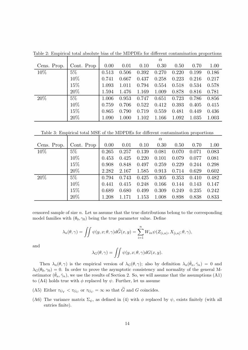
Table 2: Empirical total absolute bias of the MDPDEs for different contamination proportions

αCens. Prop. Cont. Prop 0.00 0.01 0.10 0.30 0.50 0.70 1.00

10% 5% 0.513 0.506 0.392 0.270 0.220 0.199 0.18610% 0.741 0.667 0.437 0.258 0.223 0.216 0.21715% 1.093 1.011 0.794 0.554 0.518 0.534 0.57820% 1.594 1.476 1.169 1.009 0.878 0.816 0.781

20% 5% 1.006 0.953 0.747 0.651 0.723 0.786 0.85610% 0.759 0.706 0.522 0.412 0.393 0.405 0.41515% 0.865 0.790 0.719 0.559 0.481 0.449 0.43620% 1.090 1.000 1.102 1.166 1.092 1.035 1.003

Table 3: Empirical total MSE of the MDPDEs for different contamination proportions

αCens. Prop. Cont. Prop 0.00 0.01 0.10 0.30 0.50 0.70 1.00

10% 5% 0.265 0.257 0.139 0.081 0.070 0.071 0.08310% 0.453 0.425 0.220 0.101 0.079 0.077 0.08115% 0.908 0.848 0.497 0.259 0.229 0.244 0.29820% 2.282 2.167 1.585 0.913 0.714 0.629 0.602

20% 5% 0.794 0.743 0.425 0.305 0.353 0.410 0.48210% 0.441 0.415 0.248 0.166 0.144 0.143 0.14715% 0.689 0.680 0.499 0.309 0.249 0.235 0.24220% 1.208 1.171 1.153 1.008 0.898 0.838 0.833

censored sample of size n. Let us assume that the true distributions belong to the correspondingmodel families with (θ0, γ0) being the true parameter value. Define

λn(θ, γ) =

∫∫ψ(y, x; θ, γ)dG(x, y) =

n∑

i=1

Winψ(Z(i,n),X[i,n]; θ, γ),

and

λG(θ, γ) =

∫∫ψ(y, x; θ, γ)dG(x, y).

Then λn(θ, γ) is the empirical version of λG(θ, γ); also by definition λn(θn, γn) = 0 andλG(θ0, γ0) = 0. In order to prove the asymptotic consistency and normality of the general M-estimator (θn, γn), we use the results of Section 2. So, we will assume that the assumptions (A1)to (A4) holds true with φ replaced by ψ. Further, let us assume

(A5) Either τGY< τGC

or τGC= ∞ so that G and G coincides.

(A6) The variance matrix Σψ, as defined in (4) with φ replaced by ψ, exists finitely (with allentries finite).

14

Then Proposition 2.1 and Proposition 2.2 give the strong consistency and asymptotic normalityof λn(θ, γ), which are summarized in the following lemma.

Lemma 5.1 Consider the above set-up with an integrable function ψ and let (θ0, γ0) be the trueparameter value. Then,

(i) Under Assumptions (A1), (A2) and (A5) we have, with probability one,

limn→∞

λn(θ0, γ0) = λG(θ0, γ0)

(ii) Under Assumptions (A2) to (A6), the asymptotic distribution of

√n [λn(θ, γ)− λG(θ, γ)] =

√n

∫∫ψ(y, x; θ, γ)d[G −G](x, y)

is normal with mean 0 and variance matrix Σψ.

5.1 Strong Consistency and Asymptotic Normality of General M-estimators

Wang (1999) has proved the strong consistency and asymptotic normality results for the M-estimators based on only censored variable with no covariables. This section extend the theoryto the case where covariables are present along with the censored response. The extensionsare in the line of the corresponding results with no censoring (see Huber, 1981; Serfling, 1980).Further note that whenever γ is known the asymptotic properties of θn follows from just a routineapplication of the results derived in Wang (1999); so here we assume γ to be known and derivethe joint distribution of M-estimator of θ and γ. These results provide a general (asymptotic)theoretical framework to study the properties of a wide class of estimators of (θ, γ) dependingon the estimating equations.

Denote the j-th component of the function ψ by ψj for j = 1, . . . , q + r. Also, considerfollowing (stronger) conditions on the nature of the function ψ.

(A7) ψ(y, x; θ, γ) is continuous in (θ, γ) and also bounded.

(A8) The population estimating equation λG(θ, γ) = 0 has an unique root given by (θ0, γ0).

(A9) There exists a compact set C in Rq × R

r satisfying

inf(θ,γ)/∈C

∣∣∣∣∫∫

ψj(y, x; θ, γ)dG(x, y)

∣∣∣∣ > 0, j = 1, . . . , q + r.

Now let us start with the strong consistency of the M-estimator (θn, γn) by an extension ofTheorem 3 of Wang (1999, page 307) under above conditions. The proof follows in the same lineof Wang (1999) by replacing the corresponding SLLN, given in Proposition 1 of Wang (1999), bythe part (i) of Lemma 5.1 in the present context; hence it is omitted for simplicity of presentation.

Theorem 5.2 Consider the above set-up with Assumptions (A1), (A2), (A5), (A7) and (A8).Then we have the following results.

(i) There exists a sequence of M-estimators {(θn, γn)} satisfying the empirical estimating equa-tion λn(θ, γ) = 0 that converges with probability one to (θ0, γ0).

15

(ii) Further if (A9) also holds true, then any sequence of M-estimators {(θn, γn)} satisfyingλn(θ, γ) = 0 converges with probability one to (θ0, γ0).

Note that the first part (i) of Theorem 5.2 is just a multivariate extension of Lemma B ofSerfling (1980, page 249) from the complete data case to the present case of censored data withcovariates. Further, the additional condition (A9) in the part (ii) makes any sequence of M-estimators satisfying the estimating equation (11) to eventually fall in a compact neighborhoodof (θ0, γ0). This result, even with the stronger conditions, becomes really helpful when theempirical estimating equation λn(θ, γ) = 0 has multiple roots and one suspect to obtain differentM-estimator sequences by applying different numerical equation solving techniques. Part (ii) ofTheorem 5.2 ensures that all theses sequences of M-estimators will be strongly consistent for theunique root (θ0, γ0) of the equation λG(θ, γ) = 0.

Next we turn our attention to the asymptotic normality of the M-estimators. In this regard,we will first present a useful lemma in terms of any real valued function g(y, x, θ0, γ0). This isagain a suitable extension of Lemma 1 of Wang (1999, page 307) to the present set-up and theproof follows similarly by replacing the corresponding SLLN (Proposition 1 of Wang) by Part(i) of Lemma 5.1. Assume the following condition about the function g(y, x, θ0, γ0).

(A10) For a real valued function g(y, x, θ0, γ0), at least one of the following holds:

(i) g(y, x, θ, γ) is continuous at (θ0, γ0) uniformly in (y, x).

(ii) As δ → 0,∫∫

sup{(θ,γ):||(θ,γ)−(θ0,γ0)||≤δ}

|g(y, x, θ, γ) − g(y, x, θ0, γ0)| dG(x, y) = hδ → 0.

(Here || · || denotes the euclidean norm).

(iii) g is continuous in (y, x) for (θ, γ) in a neighborhood of (θ0, γ0), and

lim(θ,γ)→(θ0,γ0)

||g(y, x, θ, γ) − g(y, x, θ0, γ0)||v = 0.

(Here || · ||v denotes the total variation norm).

(iv)∫∫

g(y, x, θ, γ)dG(x, y) is continuous at (θ, γ) = (θ0, γ0), and g is continuous in (y, x)for (θ, γ) in a neighborhood of (θ0, γ0), and

lim(θ,γ)→(θ0,γ0)

||g(y, x, θ, γ)− g(y, x, θ0, γ0)||v <∞.

(v)∫∫

g(y, x, θ, γ)dG(x, y) is continuous at (θ, γ) = (θ0, γ0), and∫∫

g(y, x, θ, γ)dG(x, y)P→∫∫

g(y, x, θ, γ)dG(x, y) <∞,

uniformly for (θ, γ) in a neighborhood of (θ0, γ0).

Lemma 5.3 Suppose g(y, x, θ0, γ0) is a real valued function with∫∫

g(y, x, θ0, γ0)dG(x, y) <∞. Assume that the conditions (A1), (A2) and (A10) hold for g. Then, for any sequences

(θn, γn)P→(θ0, γ0), we have

∫∫g(y, x, θn, γn)dG(x, y)

P→∫∫

g(y, x, θ0, γ0)dG(x, y).

16

Theorem 5.4 Consider the above set-up and assume that ψ is differentiable with respect to(θ, γ) in a neighborhood of (θ0, γ0) and the matrix

ΛG(θ0, γ0) =

∫∫∂

∂(θ, γ)ψ(y, x, θ, γ)

∣∣∣∣(θ,γ)=(θ0,γ0)

dG(x, y), (22)

exists finitely and is non-singular. Further assume that the assumptions of Lemma 5.3 holdfor g(y, x, θ, γ) = ΛijG(θ0, γ0), the (i, j)-th element of ΛG(θ0, γ0), with i, j = 1, . . . , q + r. Then,

under Assumptions (A2) to (A6) we have, for any sequence of M-estimators {(θn, γn)} satisfyingλn(θ, γ) = 0 that converges in probability to (θ0, γ0),

√n[(θn, γn)− (θ0, γ0)

]D→N

(0,ΛG(θ0, γ0)

−1Σψ(G)ΛG(θ0, γ0)−1

).

Proof: Since ψ is differentiable in (θ, γ) , so is the function λn(θ, γ). So an application ofmultivariate mean value theorem yields

λn(θn, γn)− λn(θ0, γ0) = ΛG(ζ1n, ζ2n)[(θn, γn)− (θ0, γ0)

],

with ||(ζ1n, ζ2n) − (θ0, γ0)|| < ||(θn, γn) − (θ0, γ0)||. Further, by definition, λn(θn, γn) = 0 andλG(θ0, γ0) = 0. Hence we get,

(θn, γn)− (θ0, γ0) = −[ΛG(ζ1n, ζ2n)

]−1[∫∫

ψ(y, x; θ, γ)d[G −G](x, y)

].

However, it follows from Lemma 5.3 that each term of ΛG(ζ1n, ζ2n) convergence in probabilityto the corresponding term of ΛG(θ0, γ0). Then, an application of Slutsky’s theorem and Part(ii) of Lemma 5.1 completes the proof of the theorem. �

It is to be noted that the asymptotic normality of the M-estimators require more conditionsthan that required for its strong consistency in terms of differentiability properties of the ψfunction, but it avoid the strong assumptions (A7) – (A9) used in Theorem 5.2. In fact, toobtain the asymptotic distributional convergence of any sequence of M-estimators in this case,it is just enough to ensure their convergence to the true parameter value in probability. All therelated conditions used here are in the same spirit with that used in Wang (1999) have been nocovariables are present and were discussed extensively in that paper.

Finally, note that the estimating equation of any general M-estimator can be solved throughan appropriate numerical technique but the complexity in terms of the iterative procedure in-creases extensively for a complicated non-linear ψ-function. However, one can show that, forthe Newton-Raphson algorithm, if we start the iterations with some

√n-consistent estimator of

(θ, γ) then the estimator obtained by just one iteration, known as the one-step M-estimator, willhave the same asymptotic distribution as the fully iterated M-estimator even in case of censoreddata with covariables as considered here. This is a well-known property of the M-estimatorin case of complete data. The following theorem present this precisely for our case; the prooffollows by an argument similar to that of Theorem 6 of Wang (1999) replacing Proposition 1and 2 of that paper by Part (i) and Part (ii) of Lemma 5.1 respectively.

17

Theorem 5.5 Suppose the conditions of Theorem 5.4 hold true and let (θn, γn) is any√n-

consistent estimate of the true parameter value (θ0, γ0). Then, the one-step M-estimator (θ(1)n , γ

(1)n ),

defined as

(θ(1)n , γ(1)n ) = (θn, γn)−[ΛG(θn, γn)

]−1λn(θn, γn), (23)

has the same distribution as that of the M-estimator (θn, γn) derived in Theorem 5.4.

5.2 Properties of the MDPDE

Note that, the MDPDE is a particular M-estimator with the ψ-function given by (12) and soall the results derived in the previous subsection for general M-estimators also hold true for theMDPDEs. In particular MDPDEs are strongly consistent and asymptotically normal under theassumptions considered in Theorems 5.2 and 5.4. However, in this particular case of MDPDEs,we can closely investigate the required assumptions for the particular form of the ψ-function.

Note that assumptions (A1), (A2) and (A5) are related to the censoring scheme under consid-eration and others are about the special structure of the ψ-function. Further, in this particularcase of MDPDE, the ψ-function depends on the model density and its score function. So, con-ditions (A3), (A4) and (A6) can easily be shown to hold for most statistical models by usingthe existence of finite and continuous second order moments of the score functions with respectto the true distribution G. Similar differentiability conditions on the model and score functionsfurther ensure the assumptions of Lemma 5.3. So, the asymptotic normality of the MDPDEsfollows from Theorem 5.4 for most models provided we can prove its consistency. However,assumptions (A6)–(A9), required to prove the strong consistency in Theorem 5.2, are ratherdifficult one and may not always hold for the assumed model.

Noting that, the asymptotic normality of MDPDEs, as obtained in Theorem 5.4, does notrequire its strong consistency (only convergence in probability is enough), now we present analternative approach to prove the (weak) consistency for the particular case of MDPDEs undersome simpler conditions. This approach has been used by Basu et al. (1998) to prove the asymp-totic properties of the MDPDEs under i.i.d. complete data and extended by many researcherslater in the context of different inference problems. Here, we extend their approach further forthe present case of censored data with covariates. Let us also relax the assumption that the truedistribution G belongs to the model family in the sense of assumption (D1) below. Define

V (Y,X; θ, γ) =

∫∫fθ(y|x)1+αfX,γ(x)1+αdxdy −

1 + α

αfθ(Y |X)αfX,γ(X)α,

so that the MDPDE of (θ, γ) is to be obtained by minimizing

Hn(θ, γ) =

∫∫V (y, x; θ, γ)dG(x, y),

with respect to the parameters. Further, the ψ-function for the MDPDEs as given by Equation(12) satisfies

ψ1(Y,X; θ, γ) =∂V (Y,X; θ, γ)

∂θ, ψ2(Y,X; θ, γ) =

∂V (Y,X; θ, γ)

∂γ. (24)

Now, let us assume the following conditions:

18

(D1) The supports of the distributions Fθ and FX,γ for any value of X are independent of theparameters θ and γ respectively. The true distribution G(x, y) is also supported on the setA = {(x, y) : fθ(y|x)fX,γ(x) > 0}, on which the true density g is positive.

(D2) There exists an open subset ω of the parameter space that contains the best fitting pa-rameter (θ0, γ0) and for all (θ, γ) ∈ ω and for almost all (x, y) ∈ A, the densities fθ andfX,γ are thrice continuously differentiable with respect to θ and γ respectively.

(D3) The integrals∫∫

fθ(y|x)1+αfX,γ(x)1+αdxdy and∫∫

fθ(y|x)αfX,γ(x)αdG(x, y) can be dif-ferentiated three times and the derivatives can be taken under the integral sign. Furtherthe ψ-function under consideration is finite.

(D4) The matrix

ΛG(θ0, γ0) =

∫∫∂

∂(θ, γ)ψ(y, x, θ, γ)

∣∣∣∣(θ,γ)=(θ0,γ0)

dG(x, y)

=

∫∫∂2

∂(θ, γ)2V (y, x, θ, γ)

∣∣∣∣(θ,γ)=(θ0,γ0)

dG(x, y),

exists finitely and is non-singular.

(D5) For all (θ, γ) ∈ ω, each of the third derivatives of V (y, x, θ, γ) with respect to (θ, γ) isbounded by a function of (x, y), independent of (θ, γ), that has finite expectation withrespect to the true distribution G.

Theorem 5.6 Under Assumptions (A1), (A2), (A5) and (D1)–(D5), there exists a sequence ofsolutions {(θn, γn)} of the minimum density power divergence estimating equations (9) and (10)with probability tending to one, that is consistent for the best fitting parameter (θ0, γ0).(Then, the asymptotic normality of this sequence {(θn, γn)} follows from Theorem 5.4 under theassumptions of that theorem.)

Proof: We follow a similar argument to that in the proof of Theorem 6.4.1(i) of Lehman(1983). Consider the behavior of Hn(θ, γ), as a function of (θ, γ), on a sphere Qa having center(θ0, γ0) and radius a. Then, to prove the existence part, it is enough to show that, for sufficientlysmall a,

Hn(θ, γ) > Hn(θ0, γ0), (25)

with probability tending to one, for any point (θ, γ) on the surface of Qa. Hence, for any a > 0,Hn(θ, γ) has a local minimum in the interior of Qa and the estimating equations of the MDPDEhave a solution {(θn(a), γn(a)} within Qa, with probability tending to one.

Now a Taylor series expansion of Hn(θ, γ) around (θ0, γ0) yields

Hn(θ0, γ0)−Hn(θ, γ) = −q+r∑

i=1

(ζi − ζ0i )∂Hn(θ, γ)

∂ζi

∣∣∣∣(θ,γ)=(θ0,γ0)

−1

2

q+r∑

i,j=1

(ζi − ζ0i )(ζj − ζ0j )∂2Hn(θ, γ)

∂ζiζj

∣∣∣∣(θ,γ)=(θ0,γ0)

+1

6

q+r∑

i,j,k=1

(ζi − ζ0i )(ζj − ζ0j )(ζk − ζ0k)∂3Hn(θ, γ)

∂ζiζjζk

∣∣∣∣(θ,γ)=(θ∗,γ∗)

= S1 + S2 + S3, (say), (26)

19

where ζi and ζ0i are the i-the component of the parameter vectors (θ, γ) and (θ0, γ0) respectively

for all i = 1, . . . , q+r, and (θ∗, γ∗) lies in between (θ, γ) and (θ0, γ0) with respect to the euclideannorm. A direct extension of the arguments presented in the proof of Theorem 3.1 of Basu etal. (2006), we get, with probability tending to one, on Qa,

|S1| < (q + r)a3, for all a > 0;

S2 < −ca2, for all a < a0 with some c, a0 > 0;

and |S3| < ba3, for all a > 0 with some b > 0,

using the assumptions (D1)–(D5) and Lemma 5.1 whenever necessary. Combining these, we get

max(S1 + S2 + S3) < −ca2 + (b+ q + r)a3,

which is less that zero whenever a < cb+q+r proving (25) holds.

Finally, to show that one can choose a root of the estimating equations of MDPDEs inde-pendent of the radius a, consider the sequence of roots closest to the best fitting parameter(θ0, γ0), which exists by continuity of Hn(θ, γ) as a function of (θ, γ). This sequence will also beconsistent completing the proof of the theorem. �

Note that Assumptions (D1)–(D5) are easier to check compared to (stronger) Assumptions(A6)–(A9) and are the routine extensions of the corresponding assumptions [(A1)–(A5)] of Basuet al. (2006).

5.3 Other M-estimators with Different ψ-Functions

Although our main focus in this paper is to study one particular M-estimator, namely theminimum density power divergence estimator (MDPDE), it opens the scope of many differentM-estimators through the general results derived in Section 5.1. This general framework ofparameter estimation based on some suitable estimating equation is well studied in case ofcomplete data and several optimum robustness properties of these M-estimators has been provedfor different classes of weights function; for example, see Huber (1981) and Hampel et al. (1986).In fact, there exists different class of ψ-function generating optimum solution in case of differentproblems. For example, in case of estimating the location parameter in a symmetric distribution,the ψ functions, that are odd in the targeted parameter, lead to such optimum M-estimation.

However, as pointed out in Wang (1999), an optimum ψ-function for the complete data mightnot enjoy similar optimality for the censored data, even if there is no covariable presence. Themain reason is that the lifetime variables are are not usually symmetric and neither belongsto a location-scale family; rather it is usually asymmetric. The case of censored data withcovariates, as considered here, is much more complicated and we can not directly pick a ψ-function from the theory of complete data. Wang (1999) presented some example of ψ-functionin the context of censored data with no covariates that can be extended in the present case withseveral covariables. However, their usefulness and optimality both in terms of efficiency androbustness need to be verified for the censored data cases with or without covariates. Thereneed a lot of research in this area to suggest an optimum ψ-function under any suitable criteriaof robustness or efficiency based on censored data.

However, we believe that the minimum density power divergence estimator proposed hereis quite sufficient for most practical situations since it produces highly robust estimators withonly a slight loss in efficiency compared to the maximum likelihood estimator (as described in

20

Section 4). Further, the estimating equation of MDPDEs can be solved by any simple numericaltechnique quite comfortably and has a simple interpretation in terms of the density powerdivergence. Thus, although some future research work may provide suitable ψ-function satisfyingsome optimality criteria with complicated form or estimation procedure, the MDPDE will stillhave its importance in many practical scenarios due to its simplicity.

6 On the Choice of Tunning Parameter α in MDPDE

A crucial issue for applying the proposed MDPDE in any real-life problem is the choice of tun-ing parameter α. As we have seen that the robustness and efficiency of the MDPDEs dependcrucially on the tuning parameter α, it needs to be chosen carefully in practice where we haveno idea regarding the contamination and censoring proportions. The simulation study presentedin Section 4 gives some indication in this direction. We have seen that the MDPDEs with largerα ≥ 0.3 are robust enough to successfully address the problem of outliers; the robustness in-creases as α increases. On the other hand, the efficiency of the MDPDEs under pure data isseen to decreases as α increases, but there is no significant loss in efficiency at smaller positivevalues of α near 0.3. So, we recommend to use a value of the tuning parameter α near 0.3 to geta fair compromise between efficiency and robustness whenever the amount of contamination isnot known in practice. This is in-line with the empirical suggestions given by Basu et al. (2006)in the context of MDPDE based on censored data with no covariables. However, these empiri-cal suggestions need further justification based on more elaborative simulation and theoreticalaspects. In case of complete data, some such justifications of the data driven choice of α isgiven by Hong and Kim (2001) and Warwick and Jones (2005). Their work might have beengeneralized to the case of censored data, although it is not very easy, in order to solve this issueof selecting α. We hope to pursue this in our future research.

7 Conclusion

The present paper proposes the minimum density power divergence estimator under the para-metric set-up for censored data with covariables to generate highly efficient and robust inference.The applicability of the proposed technique is illustrated through appropriate theoretical resultsand simulation exercise in the context of censored regression with stochastic covariates. Further,the paper provide the asymptotic theory for a general class of estimators based on the estimatingequation which opens the scope of studying many such estimators in the context of censoreddata in presence of some stochastic covariates.

References

[1] Basu, S., Basu, A., and Jones, M. C. (2006). Robust and efficient parametric estimation forcensored survival data. Annals of the Institute of Statistical Mathematics, 58(2), 341–355.

[2] Basu, A., Harris, I. R., Hjort, N. L., and Jones, M. C. (1998). Robust and efficient estimationby minimising a density power divergence. Biometrika, 85(3), 549–559.

[3] Bednarski, T. (1993) Robust estimation in the Cox regression model. Scand. J. Statist., 20,213–225.

21

[4] Bednarski, T. and Borowicz, F. (2006). coxrobust: Robust Estimation in Cox Model. Rpackage version 1.0.

[5] Begun, J. M., Hall, W. J., Huang, W. M., Wellner, J. A. (1983). Information and AsymptoticEfficiency in Parametric-Nonparametric Models. Annals of Statistics, 11, 432–452.

[6] Buckley, J., and James, I., (1979). Linear regression with censored data. Biometrika, 66,429–436.

[7] Cai, Z. (1998). Asymptotic properties of Kaplan-Meier estimator for censored dependentdata. Statistics and probability letters, 37(4), 381–389.

[8] Campbell, G., and Foldes, A. (1982). Large sample properties of nonparametric bivariateestimators with censored data. Nonparametric statistical inference, 1, 103-121.

[9] Chen, Y. Y., Hollander, M., and Langberg, N. A. (1982). Small-sample results for the Kaplan-Meier estimator. Journal of the American Statistical Association, 77, 141-144.

[10] Collett, D. (2003). Modelling Survival Data in Medical Research. Chapman Hall, London,U.K.

[11] Cox, D.R. (1972). Regression models and life tables (with discussion). Journal of RoyalStatistical Society, Series B. 34, 187–220.

[12] Cox, D. R., and Oakes, D. (1984). Analysis of Survival Data. Chapman Hall, London, U.K.

[13] Crowder, M. J., Kimber, A. C., Smith, R. L., and Sweeting, T. J. (1991). Statistical Analysisof Reliability Data. Chapman Hall, London, U.K.

[14] Dabrowska, D. M. (1988). Kaplan-Meier estimate on the plane. The Annals of Statistics,16(4), 1475–1489.

[15] Farcomeni, A. and Viviani, S. (2011) Robust estimation for the Cox regression model basedon trimming. Biometrical Journal, 53(6), 956–973.

[16] Ghosh, A., and Basu, A. (2013). Robust estimation for independent non-homogeneous ob-servations using density power divergence with applications to linear regression. ElectronicJournal of statistics, 7, 2420-2456.

[17] Ghosh, A., and Basu, A. (2014). Robust Estimation in Generalized Linear Models : TheDensity Power Divergence Approach. ArXiv pre-print, arXiv:1403.6606.

[18] Hampel, F. R., E. Ronchetti, P. J. Rousseeuw, and W. Stahel (1986). Robust Statistics:The Approach Based on Influence Functions. New York, USA: John Wiley & Sons.

[19] Hong, C. and Kim, Y. (2001), Automatic selection of the tuning parameter in the minimumdensity power divergence estimation. Journal of the Korean Statistical Society, 30, 453–465.

[20] Hosmer, D. W., Lemeshow, S. and May, S. (2008). Applied Survival Analysis: RegressionModeling of Time-to-Event Data. John Wiley & Sons.

[21] Huber, P. J. (1981). Robust Statistics. John Wiley & Sons.

22

[22] Kaplan, E. L., and Meier, P. (1958). Nonparametric estimation from incomplete observa-tions. Journal of the American statistical association, 53 (282), 457–481.

[23] Kim, M., and Lee, S. (2008). Estimation of a tail index based on minimum density powerdivergence. Journal of Multivariate Analysis, 99(10), 2453–2471.

[24] Klein, J.P. and Moeschberger, M.L. (2003). Survival Analysis Techniques for Censored andTruncated Data, Second Edition. Springer-Verlag, New York.

[25] Kosorok, M.R., Lee, B.L. and Fine, J.P. (2004). Robust inference for univariate proportionalhazards frailty regression models. Annals of Statistics, 32, 1448–1491.

[26] Lawless, J.F. (2003). Statistical Models and Methods for Lifetime Data, Second Edition.John Wiley & Sons, Inc. New York.

[27] Lee, S., and Song, J. (2009). Minimum density power divergence estimator for GARCHmodels. Test, 18(2), 316–341.

[28] Lee, S., and Song, J. (2013). Minimum density power divergence estimator for diffusionprocesses. Annals of the Institute of Statistical Mathematics, 65(2), 213-236.

[29] Lehmann, E. L. (1983). Theory of Point Estimation. John Wiley & Sons.

[30] Lo, S. H., Mack, Y. P., and Wang, J. L. (1989). Density and hazard rate estimation forcensored data via strong representation of the Kaplan-Meier estimator. Probability theory andrelated fields, 80(3), 461-473.

[31] Locatelli, I., Marazzi, A., Yohai, V. J. (2011). Robust accelerated failure time regression.Computational Statistics and Data Analysis. 55, 874–887.

[32] Peterson Jr, A. V. (1977). Expressing the Kaplan-Meier estimator as a function of empiricalsubsurvival functions. Journal of the American Statistical Association, 72 (360a), 854–858.

[33] Ritov, Y. (1986). Estimation in a Linear Regression Model with Censored Data. The Annalsof Statistics, 18(1), 303–328.

[34] Robins, J. M., and Rotnitzky, A. (1992). Recovery of information and adjustment for depen-dent censoring using surrogate markers. In AIDS Epidemiology, 297–331. Birkh’auser Boston.

[35] Satten, G. A., and Datta, S. (2001). The KaplanMeier estimator as an inverse-probability-of-censoring weighted average. The American Statistician, 55(3), 207–210.

[36] Salibian-Barrera, M., and Yohai, V. J. (2008). High breakdown point robust regression withcensored data. The Annals of Statistics, 36(1), 118–146.

[37] Serfling, R. J. (1980). Approximation Theorems of Mathematical Statistics. New York, USA:John Wiley & Sons.

[38] Stute, W. (1993). Consistent estimation under random censorship when covariables arepresent. Journal of Multivariate Analysis, 45(1), 89–103.

[39] Stute, W. (1995). The central limit theorem under random censorship. The Annals of Statis-tics, 23(2), 422–439.

23

[40] Stute, W. (1996). Distributional convergence under random censorship when covariablesare present. Scandinavian Journal of Statistics, 23(4), 461–471.

[41] Stute, W., and Wang, J. L. (1993). The strong law under random censorship. The Annalsof Statistics, 21(3), 1591–1607.

[42] Tsai, W. Y., Jewell, N. P., and Wang, M. C. (1987). A note on the product-limit estimatorunder right censoring and left truncation. Biometrika, 74(4), 883–886.

[43] Van der Laan, M. J., and Robins, J. M. (2003). Unified methods for censored longitudinaldata and causality. Springer.

[44] Wang, J. L. (1999). Asymptotic Properties of M-Estimators Based on Estimating Equationsand Censored Data. Scandinavian journal of statistics, 26(2), 297–318.

[45] Wang, M. C., Jewell, N. P., and Tsai, W. Y. (1986). Asymptotic properties of the productlimit estimate under random truncation. The Annals of Statistics, 14(4), 1597–1605.

[46] Warwick, J., and Jones, M. C. (2005). Choosing a robustness tuning parameter. Journal ofStatistical Computation and Simulation, 75(7), 581–588.

[47] Zhou, M. (1991). Some properties of the Kaplan-Meier estimator for independent noniden-tically distributed random variables. The Annals of Statistics, 19(4), 2266–2274.

[48] Zhou, M. (1992). M-estimation in censored linear models. Biometrika, 79(4), 837-841.

Address of Corresponding Author:Abhik GhoshIndian Statistical Institute,203, B. T. Road, Kolkata 700108, India.E-mail: abhianik@gmail.com

24