Estimating the E�ects of Covariateson Health ExpendituresDonna B. GilleskieandThomas A. MrozUniversity of North Carolina at Chapel HillSeptember 2000AbstractThis paper addresses estimation of an outcome characterized by mass at zero, signi�cantskewness, and heteroscedasticity. Unlike other approaches suggested recently that requireretransformations or arbitrary assumptions about error distributions, our estimation strat-egy uses sequences of conditional probability functions, similar to those used in discrete timehazard rate analyses, to construct a discrete approximation to the density function of theoutcome of interest conditional on exogenous explanatory variables. Once the conditionaldensity function has been constructed, we can examine expectations of arbitrary functions ofthe outcome of interest and evaluate how these expectations vary with observed exogenouscovariates. This removes a reseacher's reliance on strong and often untested maintainedassumptions. We demonstrate the features and precision of the conditional density estima-tion method through Monte Carlo experiments and an application to health expendituresusing the RAND Health Insurance Experiment data. Overall, we �nd that the approximateconditional density estimator that we propose provides accurate and precise estimates ofderivatives of expected outcomes for a wide range of types of explanatory variables. We �ndthat two-part smearing models often used by health economists do not perform well. Ourresults, both in Monte Carlo experiments and in our real application, also indicate that sim-ple one-part OLS models of level health expenditures can provide more accurate estimatesthan commonly used two-part models with smearing, provided one uses enough expansionterms in the one-part model to �t the data well.The authors thank Lara Bryant, Jae-Young Lim, and Bill Lu for valuable research assistanceon this project. We are grateful to Will Manning and John Mullahy for providing data and programsused in our preliminary research. We also appreciate comments from participants at the TriangleEconometrics Conference and the Murrary S. Johnson Memorial Conference at the University ofTexas - Austin. Please send comments to donna gilleskie@unc.edu or tom mroz@unc.edu.

Health economists and other empirical researchers often debate the advantages and disad-vantages of various functional forms used in regression analyses. Researchers frequently use, forexample, logarithmic transformations of the dependent variable when the variable exhibits signif-icant skewness. Often it is the level of the dependent variable that is of interest in the analysisand retransformation of the estimated predictions is necessary. Many health outcomes are alsocharacterized by a signi�cant point mass at zero. It has become common among health economiststo use a two-part model even though the outcome of interest is typically the unconditional outcomethat includes the zero values. Examples of health outcomes exhibiting skewness and point massat zero include health care expenditures, number of doctor visits, and duration of hospital stay.Several recent papers have addressed these modeling issues from a variety of points of view (e.g.,Mullahy, 1998; Manning, 1998; Angrist, 2000; Manning and Mullahy, 2000).Retransformation and two-part modeling require that the researcher make distributional as-sumptions. For example, in order to obtain predicted values of the unconditional level outcomesfrom a logarithmic transformed dependent variable, a researcher must retransform the predictedlogged dependent variable. This retransformation requires assumptions about the dependence ofthe error term distribution on observable covariates. One also must specify assumptions about therelationship between the errors of the marginal and conditional outcomes represented in two-partmodels. To our knowledge there is no general empirical approach that simultaneously \makes irrel-evant" the decision to transform or not and the choice of two-part versus one-part modeling whilealso allowing for possibly complex interactions of explanatory variables on the outcome of interest.Our goal in this paper is to provide such an approach.In this paper we describe a relatively simple estimation approach that \solves" the transfor-mation problem while incorporating explicitly the potential confounding e�ects of two-part models.Our estimation strategy uses sequences of conditional probability functions, similar to those used indiscrete time hazard rate analyses, to construct a discrete approximation to the density function ofthe outcome of interest conditional on exogenous explanatory variables. Once we have constructedthe conditional density function, it is straightforward to examine expectations of arbitrary functionsof the outcome of interest and to evaluate how these expectations vary with observed exogenouscovariates. Our implementations of the approach use exible functional forms when de�ning the1

sequences of conditional probabilities. This means that we have exible representations of the con-ditional density functions, and consequently exible representations for regression functions suchas the expected value of the outcome conditional on exogenous covariates.In our formulation we construct the sequences of conditional probabilities using standardbinary outcome models. In our Monte Carlo experiments and health economics application weuse a logit probability model because of its simplicity, but any binary outcome model could beused. We allow the arguments of these conditional probability functions to be loosely-speci�edpolynomial functions of covariates. These models can then be estimated using standard computerpackages such as SAS and Stata. In fact, we used Stata for all of the Monte Carlo experimentsand real application estimates reported in this paper. It is simple for researchers to implement thisapproach in practice.The approach we use naturally admits variations in covariate e�ects over particular rangesof the variables. It might be the case, for example, that particular variables have no impacts onan outcome of interest until the outcome exceeds some pre-speci�ed cuto� level. Characteristicsof one's health insurance contract (e.g., the deductible, the coinsurance rate after exceeding thedeductible, and the maximum out-of-pocket expenditure) are obvious examples in the health insur-ance literature where the economic impacts of these covariates vary over the range of the dependentvariable. One could, in principal, model directly how such features e�ect the budget constraint andthen solve for the correct demand function to use in a least squares estimation. The resultingfunctional form for the regression model would almost always be quite nonlinear, and it woulddepend crucially upon arbitrary distributional and functional form assumptions. The approach weexamine here incorporates such e�ects with almost no modi�cation.While the presence of unobserved individual heterogeneity could limit a researcher's abilityto translate such economic restrictions directly to restrictions in a statistical model, these typesof functional restrictions can provide key information to help identify nonparametrically both thebehavioral relationship and the heterogeneity distribution (Mroz and Weir, 1990; Hahn, Todd,and Van der Klaauw, 2000); this is a clear case where a well-speci�ed economic theory can help2

provide identi�cation without the imposition of arbitrary functional forms.1 The discrete condi-tional density estimation approach we use can be applied directly to a wide range of situationswhere researchers have relied upon restrictive functional forms and distributional assumptions. Itis straightforward to apply the approaches we describe to: discrete time hazard rate models (Alli-son, 1984); ordered data models, where researchers almost always assume either an ordered logit oran ordered probit model with covariate-invariant cuto� points (Maddala, 1983); count data mod-els, where most researchers use a Poisson model or simple, parametrically restrictive modi�cationsof the Poisson such as the negative binomial model or the zero-in ated Poisson model (Cameronand Trivedi, 1998); and multinomial models with mutually exclusive outcomes, where researchershave relied almost exclusively on multivariate probit or logit models (Maddala, 1983). In additionto this wide application of the conditional density estimation technique, the use of a maximumlikelihood framework provides the foundation for more complex modeling of selection, endogeneity,and unobserved heterogeneity.Using Monte Carlo experiments and our health economics application, we examine the per-formance of these discrete, conditional density approximations when the outcome of interest is apositively-skewed continuous variable with mass at zero. We �nd that the discrete approxima-tion works quite well with these outcomes. This suggests that the approach may be useful whena researcher is interested in estimating the expected impact of exogenous covariates on particu-lar functions of the outcome variable, regardless of whether the outcomes of interest are discrete,continuous, or mixed.1The approach we use yields estimates of how the entire distribution of health expenditures would changein response to variations in exogenous characteristics. Conceptually it is straightforward to add unobservedheterogeneity to the speci�cations we use along the lines suggested by Heckman and Singer (1984),Mroz(1999), and Mroz and Guilkey (1992). This would, in principal, allow one to examine how covariate e�ectsvary within ranges of the outcome variable. For example, one might be interested in how increasing coin-surance rates would e�ect health care expenses for those spending more than $500 per year. To do this well,however, the researcher would need to hold constant the distribution of the \heterogeneity" applicable forthis range of the outcome and must specify precisely how the heterogeneity distribution would be identi�ed.This would require strong assumptions or additional information. In general one would need multiple ob-servations per agent in order to identify the heterogeneity distribution separately from the distribution ofthe outcome conditional on exogenous covariates and the heterogeneity (Heckman and Honore, 1990). Suchextensions are beyond the scope of this paper. Hence, the approach we detail in this paper does not addressthe question of how one can obtain interesting and consistent estimates of how covariates in uence outcomesover intervals of the support of the dependent variable conditional on the random variable falling within theinterval. 3

1 Description of Estimation ProcedureWe begin by describing in detail the estimation technique. The approach requires determination ofintervals within the support of the dependent variable, approximation of the conditional expectedvalue, and implementation of the empirical approximation in practice. We conclude this section byexplaining how to calculate statistical derivations of interest.The conditional density estimation approach we propose in this paper closely resembles theapproaches used by Efron (1988) and Donald, Green, and Paarsch (2000). The Efron model, likethat proposed here, approximates the distribution of a continuous outcome by a discrete distributionfunction. He proposes that one estimate the statistical approximation to the distribution functionby a sequence of logit hazard rates, which is precisely the modeling approach we adopt. Themain di�erence between our approach and Efron's is that we examine distributions conditional onobserved covariates, while Efron models only the unconditional distribution. An important resultfrom Efron's analysis concerns the fact that the e�ciency loss due to discretization can be quitesmall. For a true underlying continous Poisson process, for example, he �nds that information lossquickly goes to zero as the number of discrete intervals gets large.Donald, Green, and Paarsch (2000) propose an estimator quite similar to the one we describebelow. The primary di�erence between their estimator and ours is that they use a continuousdistribution with discrete structural shifts to approximate the underlying distribution, as in Meyer's(1990) approach to estimating hazard models. To allow for e�ects of covariates that vary overthe support of the outcome, they rely on separate, discontinous \proportional hazard" e�ects forvarious ranges of the the outcome variable. Our approach, on the other hand, allows the impacts ofcovariates to vary smoothly over the entire range of the support of the outcome of interest, exceptpossibly at particular points or regions where the researcher has an a priori notion that behaviormight be discontinuous. The complexity of the estimated distribution and its dependence uponcovariates is pre-speci�ed in the Donald, Green, and Paarsch approach, while the estimator wepropose allows the data to determine the number of terms and breakpoints used to approximatethe conditional distribution function. Eastwood and Gallant (1991), for example, �nd that datadependent rules for choosing the number of terms in an expansion often yields less bias than using�xed rules. A �nal advantage of our approach is that estimating the smoothed conditional density4

function only requires one to use simple logit models. Donald, Green, and Paarsch's estimator canbe di�cult to use because it requires that the reseacher provide reasonable starting values for theparameter estimates. All of the di�erences we mention are quite minor, and the choice of which ofthese two apporaches would be better depends upon whether one believes that the distribution ofthe outcome of interest has many interesting and important, discontinuous segments.1.1 Discretizing the Support of the Dependent VariableFigure 1 displays an arbitrary distribution function for a random variable Y conditional on a setof covariates x with density f(yjx).2 Suppose we break the range of the dependent variable into Kintervals, where the kth interval is de�ned by [yk�1; yk); for yk�1 � yk; y0 = �1 and yK =1.6

-0

f(yjx)

Yyk�1 yk

������ p [yk�1 � Y < ykjx]@@@@@@@@@@@@@@@@@@@@@@@@@@@@@@@@@@@@@@@@@Figure 1: Arbitrary Distribution of YThe probability that the random variable Y falls in the �rst interval is given by:p [y0 � Y < y1jx; Y � y0] = Z y1y0 f(yjx)dy = �(1; x) (1)2If the random variable Y is discrete, then each partition may include one or more points in the supportof Y. For most of the following discussion, we use notation for a continuous distribution for the outcome,but little would need to be changed to accommodate discrete or mixed outcomes.5

where �(1; x) is that function of x that gives this probability. Note that �(1; x) is implicitly afunction of the choice of partition for the support of Y , but this dependence on the partition iscaptured entirely though the values y0 and y1. The probability that the random variable Y falls inthe kth interval is given by p [yk�1 � Y < ykjx] = Z ykyk�1 f(yjx)dy (2)and the conditional probability that the random variable falls in the kth interval given that it didnot fall in one of the �rst (k � 1) intervals is�(k; x) = p [yk�1 � Y < ykjx; Y � yk�1]= R ykyk�1 f(yjx)dy1� R yk�1y0 f(yjx)dy (3)The functions �(�; �) de�ne the \discrete time hazard" function representation for the chosenpartition of the support of Y . By the properties of hazard functions, the probability that therandom variable Y falls in the kth interval is given byp [yk�1 � Y < ykjx] = �(k; x) k�1Yj=1 [1� �(j; x)] : (4)The hazard rate decomposition implies, by de�nition, a conditional independence between theevents fyk�1 � Y < ykjx; Y � yk�1g and fyj�1 � Y < yjjx; Y � yj�1g 8j 6= k. If a researcherimposes a functional form for f(yjx) or �(k; x), however, the potential for unobserved heterogeneityexists and the conditional independence can break down (Heckman and Singer, 1984). This happensbecause the same unobservable, say �, in uences all of the events represented in Equation (4).This, however, is only an issue for the hazard function that is constructed by conditioning on theunobserved heterogeneity. Suppose �g(k; xj�) is the discrete hazard rate under density g(yjx; �)that is conditional on the unobserved heterogeneity and that Q(�) is the cumulative distribution ofthe unobserved heterogeneity. Conditional on the heterogeneity the independence properties hold.The conditional distribution function is given byp [yk�1 � Y < ykjx; �] = �g(k; xj�) k�1Yj=1 [1� �g(j; xj�)] (5)and the unconditional distribution function isp [yk�1 � Y < ykjx] = Z �g(k; xj�) k�1Yj=1 [1� �g(j; xj�)] dQ(�) : (6)6

This distribution in Equation (6) must, by de�nition, have an \independent" hazard rate decom-position like that described above in Equation (4).The primary implication of unobserved individual heterogeneity is that one cannot interpretthe distribution function f(yjx) and the \hazard" function �(k; x) as holding the heterogeneity�xed, as would be the case if one were able to estimate the \hazard" functions �g(k; xj�). Thus onecannot give a clear structural interpretation to e�ects of variations in x on the outcome y in sub-intervals of its support; to do this would require knowledge of the distribution of the heterogeneityconditional on being in the speci�ed sub-intervals. The point here is similar to the interpretationof estimates of \duration dependence" of the hazard rate in waiting time models with unobservedheterogeneity. Unless one holds constant the unobserved heterogeneity in a waiting time model,the time shape of the hazard function does not have a structural interpretation; the time shapedepends upon changes in the distribution of the unobserved heterogeneity over the support of thedependent variable. The decomposition we use, however, does permit one to make precise structuralstatements about the impact of the covariates x on the expectation of any function of y that doesnot condition on particular ranges for the random variable. It is straightforward, for example, tocalculate how the mean and the variance of the random variable Y , or the mean and variance offunctions of the random variable Y , vary with changes in the exogeneous covariates x.1.2 Approximating Moments of the DistributionIn this discussion we focus on �rst conditional moments, but the discussion could easily be modi�edfor any conditional moments. The true expecation of a function h(�) of a random variable Y , givenx, is E(h(Y )jx) = Z 1�1 h(y)f(yjx)dy (7)where h(�) is any smooth and continuous function of Y . For a partition of the support of Y withK intervals, we approximate the expectation of a function h(Y ) conditional on covariates x by~E(h(Y )jx) = KXk=1h�(kjK)�(k; x) k�1Yj=1 [1� �(j; x)] (8)where each h�(kjK) is an approximation to h(y) in the kth interval (corresponding to interval[yk�1; yk)). The approximation we use treats the h�(kjK)'s as �xed for all values of x within the7

kth interval. For smooth and continuous functions h(Y ), this approximation to the expectation willconverge to the true expectation as the widths of the intervals shrink towards zero. The empiricalquestion, then, is how well this approximation can work in practice.1.3 Implementing the Approximation EmpiricallyBefore one can apply this approximation in practice, several decisions need to be made regardingimplementation. The �ve decisions at the discretion of the researcher are to:1. choose the number of intervals to use (K),2. specify boundaries of the intervals (i.e., the values of y1; y2; : : : ; yK�1 ),3. pick a set of constants h�(1jK); h�(2jK); : : : ; h�(KjK) to use in the approximation to theintegral,4. decide how to approximate the conditional density functions, and5. calculate derivatives of the expectation of the function of the outcome of interest.For each of the �ve decisions we use empirical analogues to guide our choices.Choosing Widths of the IntervalsFirst, consider the choice of the boundaries of the intervals. Suppose that one has already chosento have K intervals. For the most part, in our Monte Carlo experiments and empirical examplewe choose as boundary points values that place an equal number of observations in each interval(i.e., 1=Kth of the sample of Y falls within each interval). If we chose 10 intervals, for example,then y1 is the tenth percentile of the observed outcome Y , y2 is the twentieth percentile of theobserved outcome Y , and yK�1 is the ninetieth percentile of Y . Boundaries chosen in this fashionare equivalent for monotonic transformations of the random variable Y . In those instances wherethere are signi�cant point masses in the observed distribution of Y , one can allow each mass pointto de�ne a single interval. In the work we report here we examine annual health care expenses. Weallow zero expenditures to be a single interval and choose boundary points such that there are anequal number of observed positive expenditures in each of the remaining intervals.33When there are minor point masses, say heaping at $100 in health expenditures for example, we typicallydo not allow for additional intervals that contain only one point of the distribution unless the number of8

Selecting the Number of IntervalsNext, consider the question of how many intervals to use for the discrete distribution. In practice weaddress this question empirically. We choose as the number of points of support that number whichmaximizes the goodness of �t of the model given the four additional decisions being discussed. To dothis, consider having already chosen K 0 intervals with each interval containing N=K 0 observations.Estimate the discrete distribution function and construct the value of the log likelihood of thischoice of K 0 intervals asL(Y jK 0) = NXi=1 ln264 K0Yk=18<:�(k; x(i)) k�1Yj=1 [1� �(j; x(i))]9=;1fy(i)2[yk�1;yk)g375 (9)Next, consider taking each of the K 0 intervals (each with an equal number of observed Y 'sper interval) and breaking each one into R sub-intervals with an equal number of observed valuesof Y in each interval. Each of the new intervals contains N=(K 0R) observations. Let the estimatedprobability of an observation being in the kth of the original K 0 intervals be �(k; x(i);K 0). Now,allocate this probability equally among each of the R sub-intervals that comprise this kth inter-val. Under this allocation rule for distributing the estimated probability, the probability that anobservation falls in one of these R sub-intervals is given by��(r;K 0; x(i); R �K 0) = �(k; x(i);K 0)R (10)This is the adjusted probability that an observation falls in the rth sub-interval of the original kthinterval. All we have done is distributed these probabilities equally over the �ner partition.Since (1=R) of the observations that originally fell in the kth interval fall in each of these Rnew, smaller intervals, it is straightforward to calculate the sample log likelihood when one usesthese equal allocation probabilities. This adjusted log likelihood is given byL�(Y jK 0; R�K 0) = L(Y jK 0)�N ln(R) (11)where N is the number of observations not at places of signi�cant point mass. For each observation,the log-likelihood value is reduced by ln(R). This re ects the fact that it is \harder" to predictobservations at that one value is large relative to the number of intervals. These heaped values, however,can make it impossible to distribute the mass equally among the remaining intervals. Do note that if suchminor mass points are substantively interesting and important, for example at 26 weeks duration in anunemployment spell or 2000 hours in an annual hours worked distribution, one can and should allow thesemass points to be separate intervals. 9

which interval an observation falls into when one allows for more intervals. This adjusted likelihoodfunction value re ects changes in the log likelihood value associated with expanding the number ofintervals and not re-estimating the model.Now, consider estimating a model containing R � K 0 intervals. A reasonable criterion touse to decide whether one should use the estimates from the model with K 0 intervals or thosefrom the model with R�K 0 intervals in whether or not the the new log likelihood function value,L(Y jR � K 0), exceeds the original log likelihood function value for K 0 intervals adjusted for the�ner partition, L�(Y jK 0; R�K 0). If by choosing a �ner partition we �t the data worse than we didby using a model with fewer intervals (and an equal allocation of probability within each interval),then we would choose the model with a fewer number of intervals. The usefulness of this criterioncomes from the fact that our estimators of �(k; x) are smooth over regions of the support of y. Ifone were more nonparametric and allowed for completely separate functions �(k; x) across intervals,then following this criterion would always select the model with the most partitions.To implement this in practice, consider comparing each choice of R to a model with only onepartition.4 The adjusted log likelihood function value with one partition isL��(Y jR; 1) = L(Y jR) +N ln(R) (12)This tells us how much better a model with R intervals �ts the data than a model with only oneinterval and an equal allocation of probabilities across the R intervals. We choose as the numberof intervals, K, that value of R which maximizes the above adjusted log likelihood function value.In our Monte Carlo experiments and real example, we examine sample sizes from 1,000 to 5,000.We found that one did not need to examine more than 50 partitions; typically 10 to 20 intervalswere su�cient.Evaluating Expectations of the OutcomeNext, consider how one should choose the evaluation point within each interval for the desiredfunction of the outcome variable (i.e., the h�(kjK)'s). For most applications, each interval will4One partition, from �1 to +1, broken into R sub-intervals with equal probability is just a simplemultinomial density with all intervals having the same probability. So, the approach we use chooses thenumber of intervals with the maximum gain in the likelihood function resulting from including covariatesas determinants of the interval probabilities (after adjusting the likelihood function value for the number ofintervals). 10

contain many observed values of the outcomes. In the Monte Carlo experiments and examplereported here, we evaluate the function h(�) at each observed value within the interval and take asimple arithmetic average: h�(kjK) = Py2[yk�1;yk) h(y)Py2[yk�1;yk) 1 (13)It is important to note that this might be an extremely important assumption in small samplesfor the approach that we use. In particular, consider the derivative of the expected value of thefunction h(Y ) @ ~E(h(Y )jx)@x = KXk=1h�(kjK)@f�(k; x)Qk�1j=1 [1� �(j; x)]g@x (14)given our assumption that h�(kjK) does not vary with x.A better approximation might be to recognize that the average of the function h(Y ) within thekth interval would vary with changes in the covariates; this would happen because the distributionof y within the interval would vary with changes in x. The actual derivative of the conditionalexpected value would be@E(h(Y )jx)@x = KXk=1h��(kjK;x)@f�(k; x)Qk�1j=1 [1� �(j; x)]g@x+ KXk=1 @h��(kjK;x)@x �(k; x) k�1Yj=1 [1� �(j; x)] (15)where h��(kjK;x) is the average value of Y in the kth interval as a function of the explanatoryvariables.A comparison of Equations (14) and (15) reveals that the approach we use ignores the secondterm in the formulation of the derivative. Note that one could run a regression of the outcomesin each interval on the covariates and use that regression to calculate the average of the derivativewithin each interval. For smooth and continuous functions h(�) with �nite expected value, thesecond term in the above derivative expression could be asymptotically negligible compared to the�rst term in the sum (i.e., as the number of partitions grows large, the limit of the ratio of the �rstterm in the sum to the total sum is one), but we have not yet shown this for general cases. Thisis clearly a topic that deserves additional attention. But note that the Monte Carlo experimentspresented here do indicate that ignoring the second term in this sum appears to introduce littlebias in the estimated derivatives. 11

Estimating the Conditional Multinomial ProbabilitiesOur �nal speci�cation of the approximation to the expected conditional value concerns the approx-imation to the density function p[yk�1 � Y < ykjx]. We approximate this density using the hazardrate decomposition discussed above. In particular, we specify a logit function for the probability ofan outcome falling in the kth interval given that it was not in one of the lower (k� 1) intervals. Inpractice, one could estimate a separate logit model for each \hazard" of falling within each interval.5This, however, would introduce a large number of parameters in most realistic-sized problems. In-stead, we estimate one logit probability using polynomials in functions of the covariates and theinterval number.Suppose one chooses to use K partitions. By using partitions containing an equal numberof observations, the unconditional probability (not conditional on the x's) of an observation beingin the kth interval given that it was not in one of the lower (k � 1) intervals is 1K�(k�1) . Let�k = �ln(K � k) for k < K. Then,logit(�k) = e�k1 + e�k = 1K � (k � 1) : (16)If one estimated a single logit function for all of the (K � 1) hazard rates with �k as the onlycovariate in the logit function, then the �t of the unconditional discrete distribution function wouldbe \perfect;" the predicted probabilities of the outcome falling in each of the intervals is identical towhat one would obtain by estimating a logit hazard model with dummy variables for each interval,or a separate logit model for each event of an observation falling into each of the intervals. Byusing �k as the only covariate in a logit formulation of the hazard function, we are guaranteed to�t exactly the discretized marginal distribution of y given the choice of K intervals.In our estimation of the \hazard" functions that condition on covariates we follow a similarstrategy and estimate a single logit model for all hazard rates. We include polynomials in �k inaddition to polynomials in the observed covariates as linear arguments to the logit function. Wealso include interactions among the covariate polynomials and the �k's. This provides a exible5The fact that each outcome can contribute an \observation" to more than one \logit" and that outcomesvary in the number of \observations" they contribute is a non-issue. One can always apply a \hazard"decomposition to any conditional or unconditional distribution function and end up with exactly this type offormulation. Every maximum likelihood estimation problem with continuous outcomes, then, can be thoughtof as one where each observed outcome can contribute an \observation" to more than one interval.12

way to smooth the hazard rate decomposition of the conditional density function. When we havean outcome with substantively and quantitatively interesting point masses, as we do at zero expen-ditures in our analysis of health care expenses, we estimate a separate logit model with polynomialsin the covariates and without the �k polynomials.6We use downwards testing to guide the selection of the degree of the polynomial to use in thelogit model of the hazard functions. In particular, the most complex model we consider includes afourth degree polynomial in �k and all fourth order terms in the covariates, their interactions, andthe covariate polynomials (including their interactions) interacted with the �k polynomial. We thenreduce the order by one for the covariate polynomials, their interactions, and their interactions withthe shape parameter �k, but retain fourth order polynomials in �k. We test whether the additionalcoe�cients as a group are signi�cant with a Wald test at the �ve percent level.7 If the higher orderterms are signi�cant, then we keep the unrestricted speci�cation. If not signi�cant, we reducethe polynomials and interactions by an additional order. We then use another Wald test at the�ve percent level to test whether the more detailed speci�cation provides a better �t than therestricted model. If we do not �nd a signi�cant improvement with the higher order terms, wereduce the speci�cation further by eliminating all third order polynomials, third order interactionsof the covariates with themselves and with �k, and fourth order polynomials in �k. Again, we testat the �ve percent level whether the additional terms improve the goodness of �t. The simplestmodel we consider includes �k, the square of �k, and �rst order terms in the covariates. In ourMonte Carlo work we �nd that this procedure almost always selected the most complex set ofinteractions in the logit hazard function.86We found that polynomials in the logarithms of the covariates seemed to provide somewhat more stableestimates than polynomials in the levels of the variables. Except for the dummy variables we use as explana-tory variables, we add a constant to each covariate to ensure that the minimum value is positive and thenconstruct polynomials in the logarithms of the normalized covariates.7While the hazard formulation implies theoretically that there is independence between the events de�nedby the hazard rates, we recognize that the approximation we use may not be perfect. We use standard errorestimators (Eicher-Huber-White) that allow for correlation among the conditional events for each observedoutcome in the Wald tests.8Our estimation programs automatically drop linearly dependent variables and we take this into accountwhen testing. See Appendix Tables A3, A4, and A8 for a precise description of the polynomial terms weinclude in the conditional density estimation for the Monte Carlo experiments and the Rand Health InsuranceExperiment data.13

1.4 Calculating DerivativesWhen calculating derivatives of the expectation of the function of the outcome of interest, wehold constant the approximation to the function within each interval (the h�(kjK)'s) as mentionedabove, di�erentiate the approximating density function for each interval with respect to a set ofcovariates, and then sum the products of the h�(kjK)'s and the derivatives of the density function,as described in Equation (14). To do this in practice we evaluate the conditional expected valueat various values of the explanatory variables and calculate the \arc" derivatives. Suppose we areinterested in calculating the derivatives of the expectation of health care expenses with respectto the level of deductible in the health insurance plan, which we report in Table 1. One way ofcalculating the average derivative (Average in the tables), is �rst to calculate the expected valueof expenditures using the estimated distribution function for all observations. Next, deviate eachobservation's deductible level and recalculate the expected values for all observations. Given thepolynomial approximations we use, it is advisable to ensure that the deductible levels are set tovalues that are actually observed in the data; each observation could have a di�erent deviation.Then, take the di�erence between these two expectations observation by observation and dividethe di�erence by the �nite di�erence chosen for the covariate for each observation to obtain the\derivative" for each observation. The population derivative is the average of these derivativesacross observations. This most closely corresponds to the average impact in the population of aone unit change in a covariate9 In other instances, we evaluate the expected value of the function ofthe outcome of interest for each observation with one particular covariate set to the same value forall observations. We then deviate the covariate for each observation, recalculate the expectation,take di�erences, divide through by the change in the covariate, and average across observations.This corresponds to the average derivative at a particular value of the chosen covariate, when allof the other characteristics of individuals follow the joint (marginal) distribution observed in thedata. We also experimented with aggregating these values to construct di�erent measures of theoverall \average" derivative of a covariate. These are reported as Min Variance, Equal Weights,Weight 1, and Weight 2 in Table 1; these are de�ned in detail in Appendix Table A2. Clearly, one9In our Monte Carlo experiments we randomly draw sets of explanatory variables from sets of covariatesfor 1219 observations observed in the NMES data set. Rather than calculating derivatives for the estimationsample, we calculate the derivatives for these 1219 sets of explanatory variables.14

could chose a wide variety of ways to calculate derivatives of the expected value with respect toparticular covariates and how these derivatives vary with values of the other covariates.1.5 Summary of the Estimation ProcedureFirst, split the sample intoK intervals. Estimate the approximation to the conditional density func-tion using all of the possible polynomial speci�cations, and test downwards from the most complexmodel to simpler models. Select that model that �rst indicates that the additional coe�cientsare statistically signi�cant. Repeat this procedure for a wide range of K values for the numberof intervals. Next select the value of K that maximizes the likelihood function value adjusted tore ect the di�erences in the number of intervals. This procedure yields the estimator of the densityfunction. We then calculate the derivatives using the �nite di�erence procedure described above.When we examine the data from the Rand Health Insurance Experiment, we bootstrap this entireprocedure to obtain estimators of the standard errors. This means that the standard errors wereport control for all of the pre-testing we do with respect to the degree of the polynomial and theselection of the number of intervals.2 Speci�cation of the Monte Carlo ExperimentsIn the Monte Carlo experiments we focus on �ve speci�cations of the data generating process. Foreach model we use data from the National Medical Expenditure Survey (NMES) from 1987 to setcoe�cients and to de�ne the joint distribution of the explanatory variables. For the most part,we ran simple regressions of health care expenditures on age, household income, coinsurance rate,deductible amount, and demographic controls to de�ne the parameters determining the continuousoutcome in each data generating process (DGP). We used probit models, in which the dependentvariable is whether an individual had any medical expenditures in the NMES data, to calibratethose DGPs that use a \two-part" approach. We used the same explanatory variables in theprobit equation as in the conditional expenditures equation along with an indicator of whetheran individual had a regular health care provider. For each replication within each DGP we drawsamples of the explanatory variables, with replacement, from a set of 1219 individuals in the NMES15

data set. We examined sample sizes of 1000, 3000, and 5000, but we focus on sample size 5000 inour discussion.The �rst DGP we examine is a single equation OLS model where the outcome is a simplelinear function of the covariates. This model has normal disturbances, and OLS is the best unbiasedestimator (e�cient). We use this DGP to examine whether the complex estimation model we usecan replicate well a simple process and to uncover how much e�ciency might be lost because weallow for extremely exible functional forms and distributions.The second DGP we examine is a two-part model. In the �rst part a probit model withnormal errors, calibrated with the NMES data, determines whether or not an individual has positiveexpenditures. If the outcome generated by the DGP indicates that the individual had positiveexpenditures, then a simple linear regression function with an independent normal error determinesthe natural logarithm of the expenditure for the individual. With this DGP and the following threeDGPs, we use a \two-part" version of the conditional density estimation approach where we specifya simple, separate logit for the �rst stage (any expenditures) and a sequence of related logits tode�ne the conditional density function for positive expenditures.The third DGP is quite similar to the second DGP. It only di�ers by allowing the error vari-ance in the second part to be proportional to the expected value of the logarithm of the dependentvariable. The fourth DGP adds additional heterogeneity and heteroscedasticity. In particular, itspeci�es a random parameter model in the second stage regression function for the logarithmicexpenditures. The �nal DGP we consider is a mixture model. Here, there is a distribution ofindividuals, and each type has a di�erent propensity to have positive expenditures and a di�erentexpected level of logged expenditures given that they have some positive expenditures. The errorterms in the two parts are related, so a standard two-part model would su�er from selection bias.We compare the conditional density approximation estimators (CDE) of the derivatives ofexpected expenditures to a variety of OLS estimators. Each OLS estimator regresses observedexpenditures (including the zero values) on a set of covariates; we do not use two-part models.10Because we use level expenditures as the dependent variable in the OLS regressions, we need not10Since E(Y jx) = p(Y = 0jx) � 0+ p(Y > 0jx) �E(Y jY > 0; x) = R(x), E(Y jx) is a function of x only. Theone-part models that we estimate are approximations to the expected value function R(x).16

consider issues related to how one can translate from regressions of the outcome estimated inlogarithms to levels.11The OLS estimators we consider are: 1) a simple OLS model with only linear covariates[labeled OLS (levels, 1st order) in the tables];12 2) an OLS model that uses (up to) fourth orderpolynomials in the levels of the explanatory variables where the forms of the polynomial interactionsare the same as those used in the conditional density estimation procedure except there is no need tospecify the �k's as this linear form is the conditional expectation [labeled OLS (levels, 4th order)];13and 3) an OLS estimator identical to the second one, except that it uses polynomials in the logsof the transformed explanatory variables rather than polynomials in the levels of the explanatoryvariables [labeled OLS (logs, 4th order)]. A list of the full set of expansion terms used in estimationare provided in Appendix Table A3. The frequency of selection of order of the polynomial expansionis provided for each model for each data generating process in Appendix Table A4.In Tables 1a through 1e we report the derivative of expected expenditures with respect tothe insurance deductible amount from several estimation models for each DGP in the Monte Carloexperiments. The deductible is that amount of health expenditure dollars that a consumer paysbefore the insurance company begins sharing the costs. Table 1a contains Monte Carlo evidencewhen the DGP is a simple OLS model, and the DGPs for Tables 1b through 1e are describedin the table titles. We calculate the derivative by numerically di�erentiating with respect to theexplanatory variable. When calculating this derivative, we hold constant the values of the errorterms for each observation and rely upon the averaging across observations to integrate out theheterogeneity. Note that the simplest OLS model is the e�cient estimator for the �rst DGP. Forall other DGPs, all the empirical models are approximations to the true conditional expectations11We considered two-part models with logged expenditures conditional on any expenditures and the smear-ing retransformation in our comparisons of di�erent models. We found that these models, when estimatedwith higher levels of polynomials whose coe�cients could not be deemed insigni�cant, produced unreliableestimates and extremely large standard errors. Given this �nding, we did not explore modi�cations of thesmearing/retransformation approach in our Monte Carlo experiments. Examples of this type of result arefound in our application to real data in the next section.12For the �rst DGP this OLS estimator is the e�cient estimator. In all others, the true DGP is considerablymore complex than a simple linear model.13We select the degree of the polynomial by a downwards testing approach using a similar Wald test atthe �ve percent level for each Monte Carlo replication. We also calculate the derivatives of the expectedvalues in a fashion similar to that used with the conditional density estimator. We take �nite di�erences ofexpectations by deviating one explanatory variable from the value it took on in the data set exactly as wedo for the conditional density estimator. 17

function. The tables report the numerical derivative at each chosen evaluation point and the averagederivative calculated by numerically di�erentiating at every observed value in the data. The tablesreport the \true" derivative, where we similarly numerically di�erentiate the known DGP withrespect to each explanatory variable, and the derivatives from the OLS and CDE models. Webegin by demonstrating the ability of our quite non-linear conditional density estimation (CDE)technique to uncover the true derivative according to the Monte Carlo experiment.In Table 1a, using OLS to estimate derivatives provides the most e�cient estimator. Werecover the true mean of -0.399 almost exactly and fairly accurately with a standard deviation is0.057. Higher orders of level X's and OLS also reproduce the true e�ects becasue the �rst ordermodel is always chosen by the Wald tests. However, higher orders of logged X's do a relatively poorjob of �tting the truth. The mean value of the average derivative is almost two (OLS 1st order)standard derviations from the truth. The CDE technique with polynomials and interactions in thelogged X's produces estimates with little bias (from the truth) but with somewhat larger standarddeviations. This larger variance is expected since OLS is e�cient. However, the CDE proceduredoes very well when the data are generated from a simple model. It has the ability, generally, tocapture the true constant derivative at di�erent evaluation points.The di�erent DGPs examined in Tables 1b through 1e are intended to generate increasinglymore heterogeneity in the data generating process. Immediately we see that the simple �rst orderOLS model does not do a good job of �tting the data as the DGP becomes more complicated.Allowing for higher order level polynomials in the OLS model provides a better �t, but at aloss of e�ciency. The best OLS model is one with polynomials and interactions in the loggedvalues of the transformed explanatory variables. The CDE technique produces little bias and hasstandard deviations that are close to those provided by the one-part OLS models with fourth orderinteractions of all the explanatory variables.We also examined the impacts of age, income, and coinsurance rate in these Monte Carloexperiments. The assessments of the various estimators for these alternative e�ects are similarto those for the deductible level examined in Table 1. The simple OLS model yields derivativeestimates that are quite far from the true average derivatives in models with any complexity. TheOLS estimators with fourth order terms and the CDE estimators all perform quite well in recoveringthe average derivative as well as the non-constant derivative at speci�c evaluation points. They18

Table 1a: Average Deductible DerivativesDGP: Yi = �0Xi + �i, iid normal errors, OLSOLS OLS OLSDerivative Truth Levels Levels Logs CDEEvaluation point 1st order 4th order 4th order0 -0.399 -0.396 -0.396 -0.014 -0.190( 0.000) ( 0.057) ( 0.057) ( 0.883) ( 1.050)50 -0.399 -0.396 -0.396 -0.807 -0.488( 0.000) ( 0.057) ( 0.057) ( 0.261) ( 0.567)100 -0.399 -0.396 -0.396 -0.591 -0.404( 0.000) ( 0.057) ( 0.057) ( 0.200) ( 0.183)150 -0.399 -0.396 -0.396 -0.473 -0.396( 0.000) ( 0.057) ( 0.057) ( 0.165) ( 0.123)200 -0.399 -0.396 -0.396 -0.398 -0.398( 0.000) ( 0.057) ( 0.057) ( 0.142) ( 0.106)250 -0.399 -0.396 -0.396 -0.346 -0.400( 0.000) ( 0.057) ( 0.057) ( 0.126) ( 0.097)300 -0.399 -0.396 -0.396 -0.267 -0.397( 0.000) ( 0.057) ( 0.057) ( 0.101) ( 0.095)Average� -0.399 -0.396 -0.396 -0.493 -0.409( 0.000) ( 0.057) ( 0.057) ( 0.113) ( 0.172)Min Variance� -0.372( 0.061)Equal Weights� -0.382( 0.130)Weight 1� -0.382( 0.121)Weight 2� -0.391( 0.110)Standard deviations from the Monte Carlo experiments are in parentheses.See Appendix Table A2 for measures of the average derivatives.19

Table 1b: Average Deductible DerivativesDGP: ln(Yi) = �0Xi + �i, iid normal errors, 2-partOLS OLS OLSDerivative Truth Levels Levels Logs CDEEvaluation point 1st order 4th order 4th order0 -2.632 -0.279 -1.173 -2.752 -2.543( 0.000) ( 0.064) ( 0.532) ( 0.947) ( 1.288)50 -0.412 -0.279 -0.823 -0.435 -0.368( 0.000) ( 0.064) ( 0.290) ( 0.296) ( 0.584)100 -0.219 -0.279 -0.536 -0.262 -0.227( 0.000) ( 0.064) ( 0.164) ( 0.146) ( 0.243)150 -0.166 -0.279 -0.307 -0.188 -0.152( 0.000) ( 0.064) ( 0.158) ( 0.112) ( 0.180)200 -0.131 -0.279 -0.133 -0.146 -0.112( 0.000) ( 0.064) ( 0.193) ( 0.098) ( 0.144)250 -0.094 -0.279 -0.008 -0.119 -0.088( 0.000) ( 0.064) ( 0.223) ( 0.090) ( 0.123)300 -0.070 -0.279 0.102 -0.081 -0.060( 0.000) ( 0.064) ( 0.311) ( 0.076) ( 0.118)Average� -0.513 -0.279 -0.518 -0.531 -0.533( 0.000) ( 0.064) ( 0.141) ( 0.117) ( 0.184)Min Variance� -0.472( 0.128)Equal Weights� -0.507( 0.163)Weight 1� -0.429( 0.164)Weight 2� -0.394( 0.145)Standard deviations from the Monte Carlo experiments are in parentheses.See Appendix Table A2 for measures of the average derivatives.20

Table 1c: Average Deductible DerivativesDGP: ln(Yi) = �0Xi + �i; var(�) � E[ln(Y )], 2-partOLS OLS OLSDerivative Truth Levels Levels Logs CDEEvaluation point 1st order 4th order 4th order0 -2.577 -0.292 -1.257 -3.033 -2.965( 0.000) ( 0.077) ( 0.695) ( 1.394) ( 1.490)50 -0.491 -0.292 -0.863 -0.360 -0.396( 0.000) ( 0.077) ( 0.360) ( 0.411) ( 0.725)100 -0.241 -0.292 -0.547 -0.237 -0.229( 0.000) ( 0.077) ( 0.207) ( 0.188) ( 0.274)150 -0.193 -0.292 -0.304 -0.183 -0.147( 0.000) ( 0.077) ( 0.212) ( 0.118) ( 0.181)200 -0.121 -0.292 -0.126 -0.152 -0.106( 0.000) ( 0.077) ( 0.239) ( 0.096) ( 0.148)250 -0.098 -0.292 -0.005 -0.130 -0.082( 0.000) ( 0.077) ( 0.250) ( 0.089) ( 0.130)300 -0.082 -0.292 0.073 -0.100 -0.055( 0.000) ( 0.077) ( 0.393) ( 0.089) ( 0.120)Average� -0.583 -0.292 -0.537 -0.531 -0.527( 0.000) ( 0.077) ( 0.170) ( 0.134) ( 0.219)Min Variance� -0.522( 0.141)Equal Weights� -0.568( 0.169)Weight 1� -0.473( 0.152)Weight 2� -0.432( 0.145)Standard deviations from the Monte Carlo experiments are in parentheses.See Appendix Table A2 for measures of the average derivatives.21

Table 1d: Average Deductible DerivativesDGP: ln(Yi) = �0iXi + �i = ��Xi + (�i � ��)Xi + �i; random coe�cients modelOLS OLS OLSDerivative Truth Levels Levels Logs CDEEvaluation point 1st order 4th order 4th order0 -2.477 -0.267 -1.004 -2.670 -2.695( 0.000) ( 0.100) ( 0.959) ( 1.591) ( 1.836)50 -0.415 -0.267 -0.701 -0.458 -0.288( 0.000) ( 0.100) ( 0.503) ( 0.397) ( 0.842)100 -0.211 -0.267 -0.466 -0.259 -0.193( 0.000) ( 0.100) ( 0.258) ( 0.228) ( 0.281)150 -0.158 -0.267 -0.292 -0.184 -0.147( 0.000) ( 0.100) ( 0.263) ( 0.171) ( 0.236)200 -0.125 -0.267 -0.172 -0.145 -0.124( 0.000) ( 0.100) ( 0.327) ( 0.140) ( 0.203)250 -0.121 -0.267 -0.100 -0.121 -0.112( 0.000) ( 0.100) ( 0.348) ( 0.119) ( 0.171)300 -0.060 -0.267 -0.098 -0.091 -0.101( 0.000) ( 0.100) ( 0.384) ( 0.090) ( 0.134)Average� -0.481 -0.267 -0.464 -0.531 -0.509( 0.000) ( 0.100) ( 0.235) ( 0.184) ( 0.213)Min Variance� -0.458( 0.173)Equal Weights� -0.523( 0.256)Weight 1� -0.433( 0.256)Weight 2� -0.394( 0.214)Standard deviations from the Monte Carlo experiments are in parentheses.See Appendix Table A2 for measures of the average derivatives.22

Table 1e: Average Deductible DerivativesDGP: Mixture model where type depends on unobserved health state, 2-partOLS OLS OLSDerivative Truth Levels Levels Logs CDEEvaluation point 1st order 4th order 4th order0 -5.814 -0.551 -2.982 -5.487 -4.149( 0.000) ( 0.090) ( 1.058) ( 1.865) ( 1.581)50 -1.117 -0.551 -1.805 -0.908 -1.272( 0.000) ( 0.090) ( 0.518) ( 0.809) ( 0.845)100 -0.714 -0.551 -0.977 -0.604 -0.618( 0.000) ( 0.090) ( 0.260) ( 0.264) ( 0.275)150 -0.407 -0.551 -0.454 -0.461 -0.398( 0.000) ( 0.090) ( 0.260) ( 0.142) ( 0.201)200 -0.538 -0.551 -0.188 -0.374 -0.304( 0.000) ( 0.090) ( 0.274) ( 0.112) ( 0.167)250 -0.388 -0.551 -0.135 -0.315 -0.251( 0.000) ( 0.090) ( 0.239) ( 0.109) ( 0.153)300 -0.221 -0.551 -0.665 -0.230 -0.176( 0.000) ( 0.090) ( 0.483) ( 0.125) ( 0.167)Average� -1.155 -0.551 -1.016 -0.848 -0.990( 0.000) ( 0.090) ( 0.233) ( 0.233) ( 0.236)Min Variance� -0.985( 0.182)Equal Weights� -1.024( 0.220)Weight 1� -0.884( 0.219)Weight 2� -0.851( 0.192)Standard deviations from the Monte Carlo experiments are in parentheses.See Appendix Table A2 for measures of the average derivatives.23

exhibit little bias and have roughly comparable standard errors. Comparisons of these estimatede�ects across the various estimation approaches for the other variables are provided in AppendixTables A5 through A7.3 An Application: Annual Medical ExpensesTo demonstrate the exibility and comparative advantages of the conditional density estimationprocedure we use data from the Rand Health Insurance Experiment (RHIE) to explain annualmedical expenses. The RHIE randomly assigned health insurance to participating individuals withthe hope of overcoming adverse selection issues associated with the purchase of health insurancewhen examining the impacts of health insurance on medical care expenditures. While the data werecollected some time ago (between 1974 and 1981), this data set is useful for our purposes because1) these data have recently become available for public use, 2) results from the Experiment arewidely known among health economists, and 3) the data exhibit features that presumably requirespecial econometric treatment in estimation or prediction.Individuals from six sites in di�erent regions of the country participated in the RHIE whichrandomly assigned households to one of 19 di�erent health insurance plans. Because dental andmental health expenses were compensated di�erently by many plans we restrict our attention tophysician and hospital expenses. Similarly, we analyze expenses of individuals randomized toplans with free care or a coinsurance rate and a maximum deductible amount only. We do notconsider Health Maintenance Organization (HMO) plans or plans with a deductible. We restrictour attention to individuals between the ages of 14 and 62. We drop individuals in Dayton, Ohiobecause it was a site that was atypical with regard to the Experiment. We consider the expensesof each individual in every full year of participation (for a total of 1 to 5 years) unless attrition wasthe result of death. In this case, we retain the part year observation because expenditures prior todeath are likely to be in uenced by health insurance. In order to keep the sample size as large aspossible we impute values of missing variables such as income, general health index, and numberof diseases using data on individuals with complete records. All dollar values are in 1999 dollars.24

Table 2 lists summary statistics and de�nitions for variables used in our analysis.14 A list of thefull set of expansion terms used in estimation are provided in Appendix Table A8.Table 2: Summary Statistics from Rand HIE | All person years (8039)Continuous Variables Mean Std.Dev. Min MaxAnnual medical expenses ($1999) 947.25 3052.48 0 79455.11Annual family income in thousands ($1999) 31.75 13.13 0 98.93Annual participation incentive ($1999) 994.04 866.28 0 2955.65Index of general health at enrollment 70.34 14.15 5.7 100.00Number of disease conditions at enrollment 10.33 8.04 0 58.60Maximum deductible amount ($1999) 876.02 943.09 0 2437.95Coinsurance rate (%) 30.14 37.13 0 95Age in years 32.76 13.13 14 61Annual family size 3.53 1.85 1 14Dummy Variables PercentSeattle (omitted category) 27.37Fitchburg 16.15Franklin County 18.97Charleston 16.73Georgetown County 20.79Female 53.14Non-white 18.36Distribution of person-year observations by year Percent1976 5.221977 20.321978 20.351979 24.541980 15.661981 13.89The conditional density estimation procedure, as the Monte Carlo experiments demonstrate,produces reliable estimates of the e�ects of covariates regardless of the functional form of thedependent variable or the true, underlying regression framework. Thus, there is no need to concernoneself with appropriate treatment of the error term when retransforming the predictions to levels.14A considerable amount of work went into preparation of the data set used in estimation in order to obtainconsistent observations on each eligible person-year within a family and to produce a set of explanatoryvariables that most closely resembles that used in the published literature (Manning et al., 1987). SAS codeto replicate our research data �le is available upon request.25

Additionally, the procedure explores high order polynomials and interactions of the explanatoryvariables and chooses the speci�cation with the best �t. Finally, the estimation technique allowsfor variation in covariate e�ects over particular ranges of the dependent variable. For example, thee�ect of a one thousand dollar increase in income might have very di�erent e�ects on expendituresat low income levels than at high income levels. These di�erential e�ects are not simply a trivialimplication of a dependent variable transformation.Table 3 reveals the varying derivatives for di�erent values of selected explanatory variables.We begin by discussing the derivative of expenditures with respect to income. Standard errorsfor all estimation procedures come from the standard deviation of 50 bootstrap replications. Allderivatives are calculated by taking �nite di�erences as discussed above. For all estimation models,upwards testing for the appropriate level of expansion overwhelmingly selected the fourth orderwith these real data. In general, the CDE procedure reveals that $23 of an additional $1000 dollarsat low income levels ($10,000) will be spent on medical care. As income initially rises, individualsspend more on medical care, but at a decreasing rate. As income continues to rise to higher levels,there is little signi�cant change in the amount spent on medical care. The second column of Table 3reports results using the traditional two-part estimation technique and smearing to account for thepredicted errors in retransformation of the predicted log expenditures to produce level outcomes.Here we use fourth order polynomials in the explanatory variables as we rejected the restrictionsimplied by a third order polynomial model at the 5% level. The two-part model with smearingyields qualitatively similar point estimates for the income e�ects, but the bootstrapped standarderrors for this commonly used procedure are two to forty times larger than those of the CDEmodel.15The last two columns of Table 3 contain estimates from one-part models where those in-dividuals with zero expenditures are included in the same OLS regression as those with positiveexpenditures. Expenditures are measured in level real dollars, so there is no need to make ad hoc15Much of the original Rand work analyzing the HIE data attempted to account for potential heteroscedas-ticity by using plan-speci�c smearing retransformations, while we have used a single retransformationcorrection using all observations with positive outcomes. Neither approach, however, can account for the fullrange of variation in the x's that might be the source of heteroscedasticity. When we tried to estimate morecomplex forms of heteroscedasticity, the excessively large standard errors often became even more absurd.26

Table 3: Selected Covariate Derivatives Using Alternative ModelsCDE Two-part, ln(Y ), One-part, OLS Y , One-part, OLS Y ,log X's, 4th order Smearing, 4th order log X's, 4th order level X's, 4th orderEvaluation Point Mean Std.Error Mean Std.Error Mean Std.Error Mean Std.ErrorHousehold Income (1000s 1999$, mean: 32.7, sd: 16.9)10 22.923 (13.866) 13.727 (57.120) 21.932 (17.631) 18.039 (15.390)15 5.687 (6.942) 0.055 (14.448) 6.199 (10.004) 9.568 (9.254)20 -1.861 (5.062) -4.491 (13.771) -0.925 (7.243) 3.407 (7.581)25 -4.458 (4.323) -4.978 (20.910) -4.009 (5.546) -0.859 (7.134)30 -4.671 (3.616) -3.825 (33.364) -5.102 (4.283) -3.645 (6.186)35 -3.770 (3.024) -2.064 (52.397) -5.170 (3.584) -5.367 (5.138)40 -2.380 (2.771) -0.115 (80.257) -4.703 (3.629) -6.439 (5.387)45 -0.811 (2.943) 1.869 (120.163) -3.958 (4.259) -7.275 (7.128)50 0.790 (3.430) 3.846 (176.511) -3.079 (5.158) -8.291 (9.128)avg -0.008 (0.008) -0.010 (0.013) -0.005 (0.010) 0.003 (0.004)Coinsurance Rate0 -10.076 (3.450) 111.435 (7.65 �107) -6.347 (5.320) -10.783 (5.254)25 4.021 (6.845) -114.300 (7.09 �107) -0.428 (9.452) 2.950 (10.251)50 -4.698 (4.058) -7.038 (3.23 �1012) -4.846 (5.004) -4.709 (4.900)avg -6.202 (2.085) 83.067 (5.55 �107) -4.918 (2.267) -7.445 (2.296)

27

Table 3: Selected Covariate Derivatives Using Alternative Models | continuedCDE Two-part, ln(Y ), One-part, OLS Y , One-part, OLS Y ,log X's, 4th order Smearing, 4th order log X's, 4th order level X's, 4th orderEvaluation Point Mean Std.Error Mean Std.Error Mean Std.Error Mean Std.ErrorGeneral Health Index (higher is better health, mean: 70.3, sd: 14.2)30 -12.847 (30.583) -58.472 (83.355) -18.766 (41.129) -36.987 (30.129)40 -20.213 (12.935) -39.185 (16.188) -27.653 (16.839) -35.839 (16.387)50 -19.080 (5.325) -25.090 (6.226) -26.683 (8.988) -26.234 (9.793)60 -14.504 (3.800) -15.186 (3.700) -20.540 (7.531) -14.337 (6.572)70 -9.333 (3.180) -8.245 (2.319) -12.008 (4.319) -6.309 (6.619)80 -4.623 (4.629) -3.084 (4.028) -2.574 (5.937) -8.316 (6.531)avg -11.354 (2.445) -17.366 (30.022) -14.244 (3.361) -15.537 (3.286)Female Indicator 388.258 (63.397) 435.579 (63.504) 361.629 (93.917) 337.893 (89.007)Non-white Indicator -193.209 (123.959) -273.867 (2753.129) -307.955 (157.995) -288.725 (159.226)

28

assumptions to transform the estimated e�ects to level expenditures. The third column uses poly-nomials in the levels of the explanatory variables, while the last column uses polynomials in thelogarithms of the adjusted explantory variables. As in the Monte Carlo experiments, these one-partmodels perform almost as well as the CDE model. They yield point estimates quite similar to thoseof the CDE model, but their bootstrapped standard errors are almost always larger than those fromthe CDE approach.Similar comparisons are found when we examine derivatives with respect to other variables.Consider the e�ects of the coinsurance rate, or the percent paid out-of-pocket by the individual,on health expenditures. In the RHIE data this variable is not continuous, as it takes on only thevalues 0, 25, 50, and 95%. The free plan (0% coinsurance rate) also has associated with it a $0maximum deductible amount (MDE); the MDE is that level of out-of-pocket expenditures afterwhich additional medical care is free. In calculation of the impact on expenditures of changes inthe coinsurance rate, we have to move individuals from the free plan to a plan with some out-of-pocket responsibility. Such a move requires that we assign an MDE at the evaluation of a non-zerocoinsurance rate. We set the new MDE to 10% of family income or $2200 (1999 dollars), whicheveris less.16 This reassignment of originally free plans to paying plans is considerably di�erent fromsimply increasing the percentage paid by the individual who faced some out-of-pocket responsibilityoriginally. The CDE technique signi�cantly predicts that movement from a free plan to a 25% planresults in a $10 reduction in total health care expenditures per coinsurance percentage point increase(i.e., a $250 decrease in expenditures with movement from a free plan to the 25% plan). Changesin behavior associated with movement from a 25% plan to a 50% plan are less precise (across allmodels) because few individuals in the RHIE were randomized to the 50% plan (about 5% of oursample). On average, across all coinsurance rates, a one percentage point increase in out-of-pocketresponsibility results in a $6 decrease in expenditures.The estimates of the coinsurance e�ects from the two-part smearing model are disturbing. Inseveral of the bootstrap replications, a small fraction of the sample had absurdly large predictedmedical expenditures. This appears to happen because, for some combinations of the explanatoryvariables, changing the coinsurance rate to evaluate the e�ect yields a set of explanatory variables16The RHIE assigned MDE's as 5, 10 and 15% of income or $1000 (current year dollars), whichever wasless. Note that this way of setting the MDE in the RHIE is inconsistent with the true experimental design.29

that is not well represented in the estimation sample. While the predictions of log expendituresin these instances are not too extreme, once one antilogs the predicted level expenditures becomehuge. This sensitivity to slightly out of sample predictions only seems to a�ect substantially thetwo-part smearing model. Both of the one-part level outcome models, also with fourth degreepolynomials in the explanatory variables, yield estimates of the coinsurance e�ects close to thosefrom the CDE model. As for the income e�ects discussed above, these two OLS models do havelarger bootstrapped standard errors than the CDE approach.The e�ect on health expenditures, as measured by the derivative with respect to the generalhealth index, reveals that better health leads to lower medical expenditures. In terms of thishealth index, a one unit increase in health has a larger reduction in expenditures at low levels ofhealth than at levels at or above the mean level of the health index. Again, the two-part smearingmodel provides imprecise estimates. The two OLS models predict somewhat larger responses thanthe CDE model, and, as above, they uniformly have larger bootstrapped standard errors. Thedi�erences in mean expenditures between men and women and between whites and non-whites arequite similar across estimation procedures. As above, the CDE model has the smallest bootstrappedstandard errors of all procedures.We next explore how some of the average e�ects described in Table 3 vary across subsets ofindividuals. To do this, we take each person-year in the RHIE dataset, change two or three char-acteristics of the explanatory variables at a time, and examine how predicted health expendituresvary for each characteristic. The changes correspond directly to some of those in Table 3, exceptthat the impacts can vary by health and demographic characteristics. Because all the evidence fromthe Monte Carlo experiments and from Table 3 indicate that the CDE model provides accruateestimates, we only present these multidimensional derivatives as calculated from the CDE model.Bootstrapped standard errors are after the derivatives at each point and are in parentheses.The �rst panel in Table 4 displays how age e�ects vary by gender. At age 20, for example,men appear to increase health expenditures by $4.37 for each year they age. By age 30, healthexpenditures of men increase by $12.06 for every year they get older, and at age 45 and later ex-penditures are increasing, on average, by more than $16.00 per year. Expenditures of women followa much di�erent pattern. During their teens and twenties, young womens' health expenditures, onaverage, rise rapidly. This is due to pregnany and childbirth costs. Linear interpolation of the age30

Table 4: Derivative E�ects by Group Using the Conditional Density Estimation TechniqueEvaluation Point Mean Std.Error Mean Std.Error Mean Std.Error Mean Std.ErrorBy Gender Male FemaleAge = 15 0.579 (21.791) 71.456 (20.878)Age = 20 4.368 (10.076) 40.661 (15.009)Age = 25 8.667 (7.906) 14.646 (12.091)Age = 30 12.057 (7.570) -1.499 (10.133)Age = 35 14.485 (7.201) -10.803 (8.560)Age = 40 15.979 (6.585) -15.706 (7.584)Age = 45 16.563 (7.518) -17.689 (9.029)Age = 50 16.312 (11.087) -17.778 (11.684)Average 12.388 (4.401) 15.055 (4.967)By Gender and Race White Male Non-white Male White Female Non-white FemaleIncome = 10K 18.300 (14.953) 11.447 (10.523) 29.914 (17.294) 18.372 (14.230)Income = 15K 1.674 (8.316) 6.084 (5.593) 8.006 (9.229) 10.970 (7.912)Income = 20K -5.246 (6.859) 3.795 (5.594) -1.724 (6.706) 7.704 (7.665)Income = 25K -7.296 (6.033) 3.237 (6.304) -5.296 (5.560) 6.880 (8.408)Income = 30K -7.107 (5.038) 3.588 (6.867) -5.891 (4.581) 7.372 (9.052)Income = 35K -5.962 (4.074) 4.423 (7.386) -5.070 (3.800) 8.575 (9.625)Income = 40K -4.475 (3.361) 5.527 (7.958) -3.609 (3.412) 10.169 (10.233)Income = 45K -2.928 (3.026) 6.789 (8.626) -1.897 (3.482) 11.981 (10.926)Income = 50K -1.440 (3.074) 8.150 (9.405) -0.128 (3.903) 13.909 (11.720)Average -0.006 (0.007) 0.006 (0.008) -0.005 (0.010) 0.007 (0.009)Coinsurance = 0% -4.618 (4.248) -1.490 (7.157) -15.850 (5.154) -10.769 (10.641)Coinsurance = 25% -2.485 (7.720) -12.127 (5.734) 12.402 (8.702) -8.189 (8.408)Coinsurance = 50% -5.171 (4.284) 8.436 (4.219) -9.436 (5.848) 12.868 (6.082)Average -4.425 (2.392) -0.840 (3.639) -9.836 (2.831) -4.198 (5.996)

31

Table 4: Derivative E�ects by Group Using the Conditional Density Estimation Technique | continuedEvaluation Point Mean Std.Error Mean Std.Error Mean Std.ErrorBy Income Income = 10K Income = 20K Income = 30KCoinsurance = 0% -4.455 (9.675) -14.294 (6.087) -13.515 (4.651)Coinsurance = 25% -6.546 (10.483) -1.423 (8.174) 3.986 (7.369)Coinsurance = 50% -3.625 (5.053) -2.973 (3.985) -4.132 (4.178)Average -2.792 (5.093) -9.695 (3.326) -8.770 (2.806)GHI = 30 -25.290 (33.713) -25.001 (34.047) -17.386 (32.687)GHI = 40 -27.572 (15.113) -30.776 (14.959) -25.116 (13.846)GHI = 50 -22.704 (7.108) -26.732 (7.133) -23.042 (6.154)GHI = 60 -16.007 (6.176) -19.660 (5.443) -17.420 (4.490)GHI = 70 -9.806 (6.435) -12.745 (4.848) -11.460 (3.706)GHI = 80 -4.649 (7.591) -6.938 (5.821) -6.248 (4.825)Average -13.382 (5.070) -16.078 (4.331) -13.876 (3.249)By General Health Index GHI = 50 GHI = 60 GHI = 70Coinsurance = 0% -10.992 (6.045) -9.083 (4.647) -8.981 (3.929)Coinsurance = 25% 11.726 (10.938) 7.193 (8.084) 3.408 (6.733)Coinsurance = 50% -8.182 (7.198) -5.879 (5.199) -4.142 (3.919)Average -6.484 (3.189) -5.440 (2.546) -5.544 (2.187)By Race White Non-whiteFemale Indicator 393.183 (73.822) 384.401 (173.283)

32

e�ects implies that womens' average health expenditures do not return to their average age 20 leveluntil they are 45 years old.The second panel of Table 4 explores how the income e�ects vary by race and gender. Foreach of the four groups, additional income has the largest impact on health expenditures at thelowest income levels. At income level $10,000, for example, an additional thousand dollars in in-come increases health expenditures by $11.45 for non-white males and by $29.91 for white females.For non-whites, the point estimates indicate that additional income always increases health ex-penditures at higher income levels. But these point estimates for both whites and non-whites arerelatively small and not signi�cantly di�erent from zero.The second panel in Table 4 also contains how the e�ects of changing the coinsurance ratevary by race and gender. Except for non-white males, the largest reduction in health expendituresoccurs when the coinsurance rate is raised from zero. Presumably, even a small copayment canreduce substantively average health expenditures.The third panel of Table 4 examines the coinsurance and health e�ects on expenditures as afunction on income level. Somewhat surprisingly, a rise in the coinsurance rate from zero reduceshealth expenditures more for those with average incomes ($30K) than for those with quite lowincomes ($10K). Given the low levels of expenditures at very low incomes, this might simply re ectthe fact that the poor have very little in the way of \discretionary" health expenditures.The �nal three sets of results indicate that the CDE models can easily estimate constante�ects across levels of characteristics. The bottom of the third panel in Table 4 indicates thatthe impact of health status, as measured by the general health index, does not vary by incomelevel. Likewise, the fourth panel in Table 4 indicates that the e�ect of the coinsurance rate onexpenditures does not vary across health levels. The �nal panel of this table shows that there isalmost no di�erence by race in the male-female expenditure di�erential.4 ConclusionThis paper explores the performance of a new approach for estimating how expected derivativesof an outcome vary with covariate values when the distribution of the outcome is characterizedby a point mass at zero and large positive skews. Such types of outcomes are often encountered33

in health economics, where a signi�cant fraction of people have no health expenditures and a fewhave extremely high expenditures. In Monte Carlo work we calibrated our experimental designto National Medical Expenditure Survey data and compared the performance of the approximateconditional density estimator to a simple ordinary least squares model and to more complex ordinaryleast squares models that use as explanatory variables polynomials in the explanatory variables usedin the simple OLS models. Overall, we found that the approximate conditional density estimatorthat we propose provided accurate and precise estimates of derivatives of expected outcomes fora wide range of types of explanatory variables. The simple OLS models performed quite poorly,while the OLSmodels including the higher order polynomials in the explanatory variables performednearly as well as the conditional density estimation approach.Using the CDE model we reexamine the Rand Health Insurance Experiment data and uncoverseveral new empirical results. We �nd that the largest increases in health expenditures due toincreases in income happen at the lowest levels of the income distribution. We also �nd thatincreases in the coinsurance rate from free health care to low levels of copayment reduce healthcare expenditures more for those with average incomes than for those with well-below averageincomes. It might be the case that those with very low incomes have few discretionary healthexpenditures. The third most important result from our examination of the Rand Health InsuranceExperiment data is that increases in health expenditures due to declines in health do not vary byincome level. On average, the poor increase their health expenditures by the same amount as thosewith average incomes when their health, as measured by Rand's general health index, declines. Wealso recon�rm other researchers' results that the largest impacts of increases in coinsurace rates onhealth expenditures take place when one raises the coinsurance rate from zero (Newhouse, 1993).It is important to note that these e�ects are based on estimates from the Rand Health InsuranceExperiment where even the poorest individuals in the analysis sample do have health insurance.We also examined brie y the performance of the commonly used two-part model, where oneestimates whether or not there are positive outcomes with a logit model in the �rst part and asimple OLS model relating the logarithm of the positive outcomes to explanatory variables in asecond part of the statistical model. In order to calculate how the expected outcome changes withcovariates in this framework, it is necessary to exponentiate the predicted log-outcome and adjustmultiplicatively for the expectation of the antilog of the disturbance term. In our preliminaryMonte34

Carlo work we found that this approach yielded imprecise and often absurd estimates. The worstperformances happened in those models where the true data generating process di�ered from theexact statistical speci�cation used to de�ne the two-part model with logarithmic outcomes. Whenwe tested for whether one could use a simple speci�cation of the explanatory variables in the linear-in-logarithm part of the model instead of including higher order polynomial terms, we often rejectedthe simpler model because it did not �t the data well. Once higher order terms were introduced intothis continuous, logarithmic part of the model, the estimation and approximation errors interactedwith the exponentiation of the expected outcome to yield quite inaccurate predictions of the leveloutcomes. The corrections for the expectation of the antilog of the disturbance did not introduceanywhere near as much noise into the estimates, unless we attempted to model and estimate theheteroscedasticy of the error terms when applying a \smearing" type correction. We ended up notusing the two-part models with predicted logarithmic expenditures in our Monte Carlo experiments,as the preliminary evidence suggested that this approach was dominated by the other estimatorswe examined. Such extreme inaccuracies were not important for the conditional density estimatorsor for the OLS models with level dependent variables and polynomials in the explanatory variables.Our examination of the Rand Health Insurance Experiment data does provide an illustration ofthe poor performance of the two-part model approach used with logarithmic positive expendituresand smearing.The implications from our analysis, however, are quite encouraging. They indicate thatresearchers who wish to estimate the impact of exogenous changes in covariates such as income,coinsurance rate, insurance deductible, and health status on expected health expenditures needonly estimate standard ordinary least squares models that combine zero expenditures along withthe level of positive expenditures. The Monte Carlo work also indicates that it is imperative to usegenerously speci�ed functions of and interactions among the explanatory variables in these OLSmodels. The simplest OLS models we explore in the Monte Carlo experiments, i.e., those with leveloutcomes and regressors and no higher order terms or interactions, almost always fail to measureanything resembling a population average derivative in even moderately complex models.The only drawback to using the OLS and CDE models with polynomials and interactions ofthe explanatory variables is the seemingly low precision of the estimates. The standard deviationfor the CDE estimator of the deductible derivative in Table 1a, for example, is three times larger35

than the standard deviation of the OLS estimator (0.172 vs. 0.057); these standard deviationsindicate the magnitude of the standard errors of the estimates from these estimators. By usingthe exible CDE model with the simple linear model DGP in Table 1a (and also Tables A5a, A6a,and A7a, all of which have the same DGP), calculated t-statistics will be about three times smallerfor the CDE than for the simple OLS estimator. This \lack of precision," however, is due to thefact that the CDE model allows for the possibility that the e�ect of insurance deductible can varywith the level of the deductible and with the levels of the other covariates. The OLS model imposesthe true restriction, for this DGP, that the deductible e�ect is constant across all dimensions.To put the CDE model onto a more level playing �eld with the OLS estimator for this DGP,consider imposing the restriction that the CDE estimated deductible derivatives are estimating thesame quantity at each level of the deductible that we examined in Table 1a. We do not imposethe restriction that these derivative levels are also constant across all values of all of the othercovariates, as is imposed by the simple OLS estimator. We impose these restrictions ex post bycalculating the covariance matrix for the CDE estimators of the derivative at the seven deductiblelevels displayed in this table and solving for that weighted average of the seven point derivativesthat yields the smallest variance. This result is the evaluation point labeled \Min Variance" inTable 1a and the other tables of Monte Carlo results. We �nd that by imposing this restrictionex post, the standard error of the CDE estimator of the deductible e�ect is only 7% higher thanthat of the OLS estimator. If one is willing to impose this additional information on the empiricalmodel, the CDE approach can do nearly as well as the e�cient OLS estimator.Looking across the tables for all of the other DGPs, i.e., those where the classical regressionmodel is not a true representation of the DGP (Tables 1b-1e, A5b-A5e, A6b-A6e, A7b-A7e), it isclear that in almost all cases that the simple OLS estimator has the largest bias of all of the fourapproaches we examine. It rarely has an average e�ect that is closer to the true e�ect than any ofthe other approaches, and often the bias exceeds 50% of the true average derivative. Simple OLSstill retains the feature that it has the smallest standard deviation of all of the estimators, but forthese DGPs this \precision gain" is more than o�set by the misleading information conveyed bythe OLS point estimate of the derivative. This result highlights the fact that relying upon simpleregression speci�cations can lead to quite misleading implications. These Monte Carlo experimentsdemonstrate that is not the case that a mis-speci�ed model is correct on average. Simple and36

mis-speci�ed models can exhibit signi�cant biases, and tests based upon estimates from theseapproaches will provide misleading information. The exible approaches that we use in the MonteCarlo experiments and in the examination of the RHIE data do not have this drawback. They doexhibit larger standard errors than the simple OLS models, but these larger standard errors merelyre ect the fact that the researcher is, truthfully, often unsure about the precise form of the trueregression speci�cation. The apparent precision for the simple OLS estimator is �ctional and onlycomes from the fact that one estimates many fewer parameters than are needed to �t the data well.These CDE models allow one to model more directly the impact of covariates on outcomes.One could, for example, model exactly how the budget constraint and structure of coinsurancerates and deductible levels impact health expenditures at various points in the health expendituredistribution. To do this well would require that one address issues of unobserved endogeneity, andthe CDE approach allows one to use the economic structure of the budget constraint to provideimportant restrictions to help achieve identi�cation. A �nal advantage of the CDE approach is thatin most real world situations researchers will not have experimental data with random assignmentof the features of the health insurance programs that individuals face. Examination of such datarequires that one model endogeneity and address sample selection issues. Accurate estimation willoften entail the use of maximum likelihood models that �t the data well, and that is precisely whatthe conditional density estimation models can do.

37

ReferencesAllison, P. (1984). Event History Analysis : Regression for Longitudinal Event Data. Beverly Hills,Calif. : Sage Publications.Angrist, J. (2000). \Estimation of Limited-Dependent Variable Models with Binary EndogenousRegressors: Simple Strategies for Empirical Practice," Journal of Business and Economic Statistics,forthcoming.Cameron, A. and P. Trivedi (1998). Regression Analysis of Count Data, Cambridge: CambridgeUniversity Press.Donald, S., D. Green, and H. Paarsch (2000). \Di�erences in Wage Distributions between Canadaand the United States: An Application of a Flexible Estimator of Distribution Functions in thePresence of Covariates," Review of Economic Studies, forthcoming.Eastwood, B. and R. Gallant (1991). \Adaptive Rules for Seminonparametric Estimators thatAchieve Asymptotic Normality," Econometric Theory 3, 307-340.Efron, B. (1988). \Logistic Regression, Survival Analysis, and the Kaplan-Meier Curve," Journalof the American Statistical Association 83, 414-425.Hahn, J., P. Todd, and W. Van der Klaauw (2000). \Identi�cation and Estimation of TreatmentE�ects with a Regression-Discontinuity Design," Econometrica, forthcoming.Heckman, J. and B. Honore (1990). \The Empirical Content of the Roy Model," Econometrica 58,1121-49.Heckman, J. and B. Singer (1984). \A Method for Minimizing the Impact of Distributional As-sumptions in Econometric Models for Duration Data," Econometrica 52, 271-320.Manning, W. (1998). \The Logged Dependent Variable, Heteroscedasticity, and the Retransforma-tion Problem," Journal of Health Economics 17, 283-295.Manning, W. and J. Mullahy. (2000). \Estimating Log Models: To Transform or Not to Trans-form," working paper. 38

Manning, W., J. Newhouse, N. Duan, E. Keeler, A. Leibowitz, and M. Marquis (1987). \HealthInsurance and the Demand for Medical Care: Evidence from a Randomized Experiment," AmericanEconomic Review 77, 251-277.Maddala, G. (1983). \A Survey of the literature on Selectivity Bias as it Pertains to Health CareMarkets," in Sche�er, R. and L. Rossiter (eds.) Advances in Health Economics and Health ServicesResearch 6, London: JAI Press.Meyer, B. (1990). \Unemployment Insurance and Unemployment Spells," Econometrica 58, 757-782.Mullahy, J. (1998). \Much Ado About Two: Reconsidering the Retransformation and the Two-partModel in Health Economics," Journal of Health Economics 17, 247-281.Mroz, T. (1999). \Discrete Factor Approximation in Simultaneous Equation Models: Estimatingthe Impact of a Dummy Endogenous Variable on a Continuous Outcome," Journal of Econometrics92, 233-274.Mroz, T. and D. Guilkey (1992). \Discrete Factor Approximations for Use in Simultaneous Equa-tion Models with Both Continuous and Discrete Endogenous Variables," manuscript, University ofNorth Carolina at Chapel Hill.Mroz, T. and D. Weir (1990). \Structural Change in Life Cycle Fertitly during the FertilityTransition: France before and after the Revolution of 1789," Population Studies 44, 61-87.Newhouse, J. (1993). Free for All? Lessons from the RAND Health Insurance Experiment, Cam-bridge: Harvard University Press.

39

Table A1: Summary Statistics from Rand HIE | First year of each person (2479)Continuous Variables Mean Std.Dev. Min MaxAnnual medical expenses ($1999) 783.52 2592.95 0 79455.11Annual family income in thousands ($1999) 31.79 13.56 0 98.93Annual participation incentive ($1999) 995.46 864.89 0 2955.65Index of general health at enrollment 70.34 13.93 5.7 100.00Number of disease conditions at enrollment 10.31 7.97 0 58.60Maximum deductible amount ($1999) 876.84 937.53 0 2437.95Coinsurance rate (%) 30.87 37.50 0 95Age in years 31.10 13.56 14 61Annual family size 3.71 1.91 1 13Dummy Variables PercentSeattle (omitted category) 27.43Fitchburg 15.69Franklin County 19.00Charleston 16.54Georgetown County 21.34Female 52.84Non-white 18.96Distribution of First Year Observed Percent1976 16.941977 49.701978 1.981979 27.711980 2.381981 1.29

40

Table A2: Average Derivative De�nitionsDerivative De�nitionLet the evaluation points for calculation of the numerical derivative with respect to variable kbe denoted ejk; j = 1; : : : ; J(k). We approximate the derivative by �nite di�erences.Let the sample size at each evaluation point for variable k be denoted njk and the cuto� pointsbe denoted ckj where njk is the number of observations observed to have the value ofvariable k fall in the interval [cjk ; cj+1;k).Average For each observed value of Xk, evaluate the function at Xk � �2where � is either the exact distance between adjacent evaluation points(i.e., � = ej+1;k � ejk) or the average of the distances between theevaluation points (i.e., � = (Pj ejk)=J(k)). The choice of � depends on thenature of the observed data (continuous or discrete). Calculate the di�erencebetween values of the function at each deviated point.Min Variance In the calculations of the derivatives for variable k, �nd the covariance matrixof the J(k) derivatives. Find the weighted sum that minimizes the sum of thesquared errors.Equal Weights Calculate a simple average of the J(k) derivatives at each evaluation point.This measure accounts for neither the sample size at di�erent evaluation pointsnor the variances or covariances of the J(k) derivatives.Weight 1 Calculate the weighted average of the derivatives where the weight is de�nedas the sample size about the evaluation point (njk). This measure accounts forthe sample size at di�erent evaluation points but not the variances or covariancesof the J(k) derivatives.Weight 2 Calculate the weighted average of the derivatives where the weight is de�ned aswjk = 1=((1=njk) + (1=nj+1;k)) for each derivative evaluated at a speci�c evaluationpoint. This measure accounts for sample size at di�erent evaluation points.In part, it accounts for the variances because it accounts for the sample sizesabout the points at where the derivatives are calculated.41

Table A3: List of Explanatory Variables used in Monte Carlo ExperimentsOrder ofPolynomial List of VariablesExpansionFirst ded � insurance deductible levelOrder age � ageinc � incomecoi � coinsurance rate (%)fem � female indicatornwh � non-white indicatorhsg � good health status indicatorhsf � fair/poor health status indicator�k � function of cell indicator used only in CDE model�2k � squared � used only in CDE modelSecond ded*ded ded*coi ded*inc ded*age ded*fem ded*nwh ded*hsg ded*hsfOrder coi*coi coi*inc coi*age coi*fem coi*nwh coi*hsg coi*hsfinc*inc inc*age inc*fem inc*nwh inc*hsg inc*hsfage*age age*fem age*nwh age*hsg age*hsffem*nwh fem*hsg fem*hsfnwh*hsg nwh*hsf�k*(all 1st order variables)�3kThird ded2*ded ded2*coi ded2*inc ded2*age ded2*fem ded2*nwh ded2*hsg ded2*hsfOrder coi2*ded coi2*coi coi2*inc coi2*age coi2*fem coi2*nwh coi2*hsg coi2*hsfinc2*ded inc2*coi inc2*inc inc2*age inc2*fem inc2*nwh inc2*hsg inc2*hsfage2*ded age2*coi age2*inc age2*age age2*fem age2*nwh age2*hsg age2*hsf�k*(all 2nd order variables)�2k*(all 1st order variables)�4kFourth ded3*ded ded3*coi ded3*inc ded3*age ded3*fem ded3*nwh ded3*hsg ded3*hsfOrder coi3*ded coi3*coi coi3*inc coi3*age coi3*fem coi3*nwh coi3*hsg coi3*hsfage3*ded age3*coi age3*inc age3*age age3*fem age3*nwh age3*hsg age3*hsfinc3*ded inc3*coi inc3*inc inc3*age inc3*fem inc3*nwh inc3*hsg inc3*hsfded2*coi2 ded2*inc2 ded2*age2 coi2*inc2 coi2*age2 inc2*age2�k*(all 3rd order variables)�3k*(all 1st order variables)The �rst part of all two-part speci�cations allows for di�erent e�ects of the explantory variablesand does not include the shape parameters or its interactions in the CDE model.42

Table A4: Frequency of Selection of Order of Polynomial Expansionfor each Data Generating ProcessModel Order of Polynomial ExpansionFirst Second Third Fourth TotalDGP: Yi = �0Xi + �i, iid normal errors, OLSOLS levels 50 0 0 0 50OLS logs 7 42 1 0 50CDE 0 0 0 50 50DGP: ln(Yi) = �0Xi + �i, iid normal errors, 2-partOLS levels 0 8 31 11 50OLS logs 0 44 4 2 50CDE 0 0 0 50 50DGP: ln(Yi) = �0Xi + �i; var(�) � E[ln(Y )], 2-partOLS levels 0 11 31 8 50OLS logs 0 41 8 1 50CDE 0 0 0 50 50DGP : ln(Yi) = �0iXi + �i = ��Xi + (�i � ��)Xi + �i;random coe�cients modelOLS levels 0 30 10 10 50OLS logs 0 41 7 2 50CDE 0 0 0 50 50DGP : Mixture model where type depends onunobserved health state, 2-partOLS levels 0 0 4 46 50OLS logs 0 10 23 17 50CDE 0 0 0 50 5043

Table A5a: Average Age DerivativesDGP: Yi = �0Xi + �i, iid normal errors, OLSOLS OLS OLSDerivative Truth Levels Levels Logs CDEEvaluation point 1st order 4th order 4th order30 7.504 7.356 7.356 7.841 7.369( 0.000) ( 0.597) ( 0.597) ( 1.733) ( 2.272)35 7.504 7.356 7.356 7.549 7.149( 0.000) ( 0.597) ( 0.597) ( 0.748) ( 1.720)40 7.504 7.356 7.356 7.253 7.230( 0.000) ( 0.597) ( 0.597) ( 0.752) ( 1.733)45 7.504 7.356 7.356 6.967 7.323( 0.000) ( 0.597) ( 0.597) ( 1.172) ( 1.613)50 7.504 7.356 7.356 6.697 7.375( 0.000) ( 0.597) ( 0.597) ( 1.539) ( 1.763)55 7.504 7.356 7.356 6.446 7.423( 0.000) ( 0.597) ( 0.597) ( 1.822) ( 2.904)Average� 7.504 7.356 7.356 7.400 7.586( 0.000) ( 0.597) ( 0.597) ( 0.949) ( 1.481)Min Variance� 7.371( 0.672)Equal Weights� 7.311( 0.780)Weight 1� 7.314( 0.899)Weight 2� 7.313( 0.749)Standard deviations from the Monte Carlo experiments are in parentheses.See Appendix Table A2 for measures of the average derivatives.44

Table A5b: Average Age DerivativesDGP: ln(Yi) = �0Xi + �i, iid normal errors, 2-partOLS OLS OLSDerivative Truth Levels Levels Logs CDEEvaluation point 1st order 4th order 4th order30 11.274 15.324 13.010 12.809 11.472( 0.000) ( 1.031) ( 2.152) ( 1.742) ( 2.267)35 11.650 15.324 13.537 14.528 12.265( 0.000) ( 1.031) ( 2.209) ( 1.411) ( 2.067)40 13.939 15.324 14.148 15.496 13.588( 0.000) ( 1.031) ( 2.354) ( 1.408) ( 2.356)45 13.594 15.324 15.144 16.051 15.006( 0.000) ( 1.031) ( 2.489) ( 1.603) ( 2.301)50 15.749 15.324 16.821 16.364 16.179( 0.000) ( 1.031) ( 2.859) ( 1.917) ( 2.522)55 15.782 15.324 19.480 16.534 16.654( 0.000) ( 1.031) ( 5.542) ( 2.350) ( 4.044)Average� 12.759 15.324 15.042 13.504 13.477( 0.000) ( 1.031) ( 1.908) ( 1.165) ( 1.713)Min Variance� 13.871( 1.047)Equal Weights� 14.194( 1.195)Weight 1� 13.160( 1.024)Weight 2� 13.591( 0.998)Standard deviations from the Monte Carlo experiments are in parentheses.See Appendix Table A2 for measures of the average derivatives.45

Table A5c: Average Age DerivativesDGP: ln(Yi) = �0Xi + �i; var(�) � E[ln(Y )], 2-partOLS OLS OLSDerivative Truth Levels Levels Logs CDEEvaluation point 1st order 4th order 4th order30 13.339 16.165 14.457 14.165 12.912( 0.000) ( 0.956) ( 2.595) ( 2.238) ( 2.634)35 12.580 16.165 13.978 15.070 13.333( 0.000) ( 0.956) ( 2.641) ( 1.817) ( 2.502)40 13.872 16.165 14.449 15.833 14.000( 0.000) ( 0.956) ( 2.443) ( 1.785) ( 2.383)45 15.288 16.165 15.686 16.372 14.904( 0.000) ( 0.956) ( 2.756) ( 1.860) ( 2.164)50 16.130 16.165 17.504 16.696 15.738( 0.000) ( 0.956) ( 3.063) ( 2.087) ( 2.565)55 16.573 16.165 19.717 16.837 15.986( 0.000) ( 0.956) ( 5.237) ( 2.733) ( 4.537)Average� 14.389 16.165 16.182 14.732 13.823( 0.000) ( 0.956) ( 1.815) ( 1.466) ( 1.819)Min Variance� 14.354( 1.056)Equal Weights� 14.479( 1.190)Weight 1� 13.876( 1.239)Weight 2� 14.128( 1.107)Standard deviations from the Monte Carlo experiments are in parentheses.See Appendix Table A2 for measures of the average derivatives.46

Table A5d: Average Age DerivativesDGP: ln(Yi) = �0iXi + �i = ��Xi + (�i � ��)Xi + �i; random coe�cients modelOLS OLS OLSDerivative Truth Levels Levels Logs CDEEvaluation point 1st order 4th order 4th order30 12.963 18.157 13.669 13.881 14.528( 0.000) ( 1.646) ( 3.171) ( 2.519) ( 2.537)35 13.464 18.157 14.794 16.352 16.231( 0.000) ( 1.646) ( 2.871) ( 2.446) ( 2.389)40 16.153 18.157 16.733 17.996 17.347( 0.000) ( 1.646) ( 2.832) ( 2.542) ( 2.860)45 18.340 18.157 19.103 19.217 17.795( 0.000) ( 1.646) ( 3.947) ( 2.589) ( 2.947)50 20.627 18.157 21.526 20.199 17.318( 0.000) ( 1.646) ( 4.730) ( 3.540) ( 3.932)55 22.756 18.157 23.618 21.036 15.277( 0.000) ( 1.646) ( 8.008) ( 5.866) ( 7.665)Average� 16.067 18.157 17.162 15.524 14.422( 0.000) ( 1.646) ( 2.031) ( 1.730) ( 1.905)Min Variance� 16.196( 1.547)Equal Weights� 16.416( 2.081)Weight 1� 15.837( 1.602)Weight 2� 16.042( 1.739)Standard deviations from the Monte Carlo experiments are in parentheses.See Appendix Table A2 for measures of the average derivatives.47

Table A5e: Average Age DerivativesDGP: Mixture model where type depends on unobserved health state, 2-partOLS OLS OLSDerivative Truth Levels Levels Logs CDEEvaluation point 1st order 4th order 4th order30 12.291 16.489 15.396 14.635 13.706( 0.000) ( 1.257) ( 3.626) ( 3.469) ( 3.367)35 13.134 16.489 15.691 15.140 14.108( 0.000) ( 1.257) ( 3.797) ( 2.836) ( 2.539)40 13.041 16.489 14.968 15.570 14.933( 0.000) ( 1.257) ( 2.566) ( 2.409) ( 2.759)45 15.615 16.489 14.868 16.229 15.790( 0.000) ( 1.257) ( 3.314) ( 2.430) ( 2.423)50 16.841 16.489 17.035 17.149 16.585( 0.000) ( 1.257) ( 3.786) ( 2.724) ( 2.406)55 17.258 16.489 23.110 18.295 17.389( 0.000) ( 1.257) ( 5.742) ( 5.061) ( 4.410)Average� 14.135 16.489 15.801 14.644 14.169( 0.000) ( 1.257) ( 2.249) ( 2.145) ( 2.332)Min Variance� 15.357( 1.249)Equal Weights� 15.419( 1.281)Weight 1� 14.757( 1.532)Weight 2� 15.040( 1.323)Standard deviations from the Monte Carlo experiments are in parentheses.See Appendix Table A2 for measures of the average derivatives.48

Table A6a: Average Income DerivativesDGP: Yi = �0Xi + �i, iid normal errors, OLSOLS OLS OLSDerivative Truth Levels Levels Logs CDEEvaluation point 1st order 4th order 4th order5 4.391 4.408 4.408 5.400 4.964( 0.000) ( 0.453) ( 0.453) ( 2.908) ( 3.562)10 4.391 4.408 4.408 5.596 4.356( 0.000) ( 0.453) ( 0.453) ( 0.915) ( 1.539)15 4.391 4.408 4.408 5.156 4.292( 0.000) ( 0.453) ( 0.453) ( 0.649) ( 1.239)20 4.391 4.408 4.408 4.701 4.286( 0.000) ( 0.453) ( 0.453) ( 0.714) ( 1.079)25 4.391 4.408 4.408 4.305 4.266( 0.000) ( 0.453) ( 0.453) ( 0.770) ( 0.931)30 4.391 4.408 4.408 3.969 4.226( 0.000) ( 0.453) ( 0.453) ( 0.798) ( 0.887)35 4.391 4.408 4.408 3.684 4.169( 0.000) ( 0.453) ( 0.453) ( 0.806) ( 0.974)40 4.391 4.408 4.408 3.441 4.099( 0.000) ( 0.453) ( 0.453) ( 0.804) ( 1.143)45 4.391 4.408 4.408 3.230 4.018( 0.000) ( 0.453) ( 0.453) ( 0.795) ( 1.341)Average� 4.391 4.408 4.408 4.310 4.411( 0.000) ( 0.453) ( 0.453) ( 1.592) ( 1.849)Min Variance� 4.217( 0.623)Equal Weights� 4.297( 0.708)Weight 1� 4.388( 0.877)Weight 2� 4.420( 0.984)Standard deviations from the Monte Carlo experiments are in parentheses.See Appendix Table A2 for measures of the average derivatives.49

Table A6b: Average Income DerivativesDGP: ln(Yi) = �0Xi + �i, iid normal errors, 2-partOLS OLS OLSDerivative Truth Levels Levels Logs CDEEvaluation point 1st order 4th order 4th order5 32.353 13.406 32.388 36.985 33.601( 0.000) ( 0.857) ( 5.360) ( 3.233) ( 4.648)10 22.130 13.406 26.066 23.892 23.326( 0.000) ( 0.857) ( 2.241) ( 1.485) ( 1.881)15 16.872 13.406 20.709 17.770 17.802( 0.000) ( 0.857) ( 1.717) ( 1.252) ( 2.023)20 14.227 13.406 16.229 14.205 14.252( 0.000) ( 0.857) ( 2.580) ( 1.288) ( 2.078)25 11.406 13.406 12.537 11.868 11.710( 0.000) ( 0.857) ( 3.087) ( 1.319) ( 1.938)30 11.673 13.406 9.545 10.215 9.763( 0.000) ( 0.857) ( 3.271) ( 1.326) ( 1.825)35 8.512 13.406 7.166 8.984 8.210( 0.000) ( 0.857) ( 3.497) ( 1.322) ( 1.867)40 8.840 13.406 5.310 8.030 6.933( 0.000) ( 0.857) ( 4.118) ( 1.312) ( 2.084)45 7.353 13.406 3.889 7.270 5.854( 0.000) ( 0.857) ( 5.198) ( 1.302) ( 2.426)Average� 20.164 13.406 22.683 25.220 22.529( 0.000) ( 0.857) ( 1.609) ( 1.322) ( 1.811)Min Variance� 14.653( 0.785)Equal Weights� 14.606( 0.904)Weight 1� 18.861( 0.871)Weight 2� 20.004( 0.892)Standard deviations from the Monte Carlo experiments are in parentheses.See Appendix Table A2 for measures of the average derivatives.50

Table A6c: Average Income DerivativesDGP: ln(Yi) = �0Xi + �i; var(�) � E[ln(Y )], 2-partOLS OLS OLSDerivative Truth Levels Levels Logs CDEEvaluation point 1st order 4th order 4th order5 30.522 13.862 31.142 36.797 34.075( 0.000) ( 0.912) ( 4.823) ( 2.315) ( 3.872)10 24.562 13.862 25.751 24.294 23.400( 0.000) ( 0.912) ( 2.258) ( 1.294) ( 2.046)15 17.096 13.862 21.095 18.359 17.883( 0.000) ( 0.912) ( 1.635) ( 1.213) ( 1.889)20 14.553 13.862 17.121 14.860 14.445( 0.000) ( 0.912) ( 2.189) ( 1.184) ( 1.696)25 12.383 13.862 13.774 12.540 12.059( 0.000) ( 0.912) ( 2.577) ( 1.190) ( 1.459)30 10.243 13.862 11.002 10.885 10.290( 0.000) ( 0.912) ( 2.773) ( 1.230) ( 1.472)35 10.686 13.862 8.750 9.642 8.921( 0.000) ( 0.912) ( 3.164) ( 1.293) ( 1.811)40 8.625 13.862 6.965 8.672 7.827( 0.000) ( 0.912) ( 4.121) ( 1.367) ( 2.318)45 7.520 13.862 5.592 7.894 6.929( 0.000) ( 0.912) ( 5.688) ( 1.444) ( 2.868)Average� 23.489 13.862 22.700 25.628 22.871( 0.000) ( 0.912) ( 1.833) ( 1.536) ( 2.205)Min Variance� 15.102( 0.990)Equal Weights� 15.092( 1.209)Weight 1� 19.135( 1.177)Weight 2� 20.283( 1.244)Standard deviations from the Monte Carlo experiments are in parentheses.See Appendix Table A2 for measures of the average derivatives.51

Table A6d: Average Income DerivativesDGP: ln(Yi) = �0iXi + �i = ��Xi + (�i � ��)Xi + �i; random coe�cients modelOLS OLS OLSDerivative Truth Levels Levels Logs CDEEvaluation point 1st order 4th order 4th order5 28.395 11.573 22.747 28.427 27.908( 0.000) ( 1.236) ( 5.416) ( 3.934) ( 4.824)10 19.444 11.573 19.666 19.763 18.553( 0.000) ( 1.236) ( 2.767) ( 1.494) ( 2.142)15 14.883 11.573 17.002 15.392 14.285( 0.000) ( 1.236) ( 1.693) ( 1.424) ( 1.888)20 12.681 11.573 14.725 12.729 11.942( 0.000) ( 1.236) ( 2.045) ( 1.558) ( 2.003)25 11.092 11.573 12.803 10.925 10.456( 0.000) ( 1.236) ( 2.539) ( 1.760) ( 1.898)30 10.219 11.573 11.208 9.616 9.382( 0.000) ( 1.236) ( 2.893) ( 2.026) ( 1.783)35 8.816 11.573 9.908 8.619 8.518( 0.000) ( 1.236) ( 3.329) ( 2.324) ( 1.845)40 9.702 11.573 8.873 7.833 7.765( 0.000) ( 1.236) ( 4.144) ( 2.621) ( 2.122)45 7.666 11.573 8.074 7.196 7.076( 0.000) ( 1.236) ( 5.477) ( 2.904) ( 2.538)Average� 21.139 11.573 17.709 20.200 18.865( 0.000) ( 1.236) ( 2.211) ( 1.881) ( 2.244)Min Variance� 12.914( 1.171)Equal Weights� 12.876( 1.254)Weight 1� 15.703( 1.323)Weight 2� 16.605( 1.423)Standard deviations from the Monte Carlo experiments are in parentheses.See Appendix Table A2 for measures of the average derivatives.52

Table A6e: Average Income DerivativesDGP: Mixture model where type depends on unobserved health state, 2-partOLS OLS OLSDerivative Truth Levels Levels Logs CDEEvaluation point 1st order 4th order 4th order5 37.375 15.628 39.450 39.784 40.267( 0.000) ( 0.984) ( 4.452) ( 4.527) ( 4.931)10 27.317 15.628 30.468 27.726 28.573( 0.000) ( 0.984) ( 1.975) ( 2.024) ( 2.656)15 21.204 15.628 23.459 22.122 22.068( 0.000) ( 0.984) ( 2.082) ( 1.624) ( 1.832)20 19.742 15.628 18.292 18.894 17.901( 0.000) ( 0.984) ( 2.755) ( 2.004) ( 1.903)25 16.285 15.628 14.834 16.784 15.048( 0.000) ( 0.984) ( 2.967) ( 2.491) ( 2.214)30 13.597 15.628 12.954 15.289 13.000( 0.000) ( 0.984) ( 3.225) ( 2.960) ( 2.530)35 12.681 15.628 12.521 14.166 11.474( 0.000) ( 0.984) ( 4.598) ( 3.388) ( 2.843)40 12.177 15.628 13.401 13.286 10.310( 0.000) ( 0.984) ( 7.461) ( 3.771) ( 3.155)45 10.595 15.628 15.465 12.572 9.409( 0.000) ( 0.984) ( 11.597) ( 4.111) ( 3.491)Average� 29.559 15.628 28.424 29.753 27.355( 0.000) ( 0.984) ( 2.083) ( 2.292) ( 2.595)Min Variance� 18.736( 1.180)Equal Weights� 18.672( 1.477)Weight 1� 23.371( 1.313)Weight 2� 24.694( 1.450)Standard deviations from the Monte Carlo experiments are in parentheses.See Appendix Table A2 for measures of the average derivatives.53

Table A7a: Average Coinsurance DerivativesDGP: Yi = �0Xi + �i, iid normal errors, OLSOLS OLS OLSDerivative Truth Levels Levels Logs CDEEvaluation point 1st order 4th order 4th order0 -5.000 -4.985 -4.985 -4.801 -4.644( 0.000) ( 0.955) ( 0.955) ( 4.017) ( 5.101)10 -5.000 -4.985 -4.985 -4.585 -4.621( 0.000) ( 0.955) ( 0.955) ( 2.881) ( 3.247)20 -5.000 -4.985 -4.985 -3.590 -4.695( 0.000) ( 0.955) ( 0.955) ( 2.350) ( 6.294)Average� -5.000 -4.985 -4.985 -4.184 -4.621( 0.000) ( 0.955) ( 0.955) ( 1.871) ( 3.054)Min Variance� -4.633( 1.484)Equal Weights� -4.653( 2.390)Weight 1� -4.683( 5.119)Weight 2� -4.634( 1.500)Standard deviations from the Monte Carlo experiments are in parentheses.See Appendix Table A2 for measures of the average derivatives.54

Table A7b: Average Coinsurance DerivativesDGP: ln(Yi) = �0Xi + �i, iid normal errors, 2-partOLS OLS OLSDerivative Truth Levels Levels Logs CDEEvaluation point 1st order 4th order 4th order0 -5.565 -9.393 -5.977 -4.528 -5.206( 0.000) ( 1.530) ( 4.899) ( 4.566) ( 5.429)10 -7.270 -9.393 -7.810 -8.155 -7.082( 0.000) ( 1.530) ( 3.228) ( 3.316) ( 3.386)20 -6.637 -9.393 -8.103 -7.027 -8.057( 0.000) ( 1.530) ( 10.263) ( 4.088) ( 9.418)Average� -6.212 -9.393 -7.668 -7.235 -7.395( 0.000) ( 1.530) ( 4.501) ( 2.338) ( 4.043)Min Variance� -6.626( 2.120)Equal Weights� -6.781( 3.663)Weight 1� -7.708( 7.696)Weight 2� -6.558( 2.136)Standard deviations from the Monte Carlo experiments are in parentheses.See Appendix Table A2 for measures of the average derivatives.55

Table A7c: Average Coinsurance DerivativesDGP: ln(Yi) = �0Xi + �i; var(�) � E[ln(Y )], 2-partOLS OLS OLSDerivative Truth Levels Levels Logs CDEEvaluation point 1st order 4th order 4th order0 -7.450 -9.791 -6.754 -4.172 -5.698( 0.000) ( 1.592) ( 6.809) ( 6.586) ( 6.733)10 -7.468 -9.791 -8.145 -8.984 -7.472( 0.000) ( 1.592) ( 3.789) ( 3.500) ( 3.826)20 -7.101 -9.791 -8.547 -7.496 -8.243( 0.000) ( 1.592) ( 8.204) ( 3.792) ( 7.828)Average� -7.122 -9.791 -8.198 -7.755 -7.645( 0.000) ( 1.592) ( 3.756) ( 2.473) ( 3.349)Min Variance� -7.064( 1.892)Equal Weights� -7.138( 2.912)Weight 1� -7.942( 6.298)Weight 2� -6.965( 1.934)Standard deviations from the Monte Carlo experiments are in parentheses.See Appendix Table A2 for measures of the average derivatives.56

Table A7d: Average Coinsurance DerivativesDGP: ln(Yi) = �0iXi + �i = ��Xi + (�i � ��)Xi + �i; random coe�cients modelOLS OLS OLSDerivative Truth Levels Levels Logs CDEEvaluation point 1st order 4th order 4th order0 -5.791 -9.430 -8.905 -3.995 -3.988( 0.000) ( 1.961) ( 5.742) ( 8.117) ( 7.898)10 -7.656 -9.430 -7.420 -9.230 -8.573( 0.000) ( 1.961) ( 4.146) ( 4.465) ( 4.046)20 -8.829 -9.430 -8.459 -7.374 -9.017( 0.000) ( 1.961) ( 12.778) ( 5.252) ( 11.922)Average� -8.092 -9.430 -8.012 -7.771 -8.048( 0.000) ( 1.961) ( 5.527) ( 3.423) ( 5.444)Min Variance� -7.186( 2.088)Equal Weights� -7.192( 4.190)Weight 1� -8.527( 9.641)Weight 2� -7.140( 2.157)Standard deviations from the Monte Carlo experiments are in parentheses.See Appendix Table A2 for measures of the average derivatives.57

Table A7e: Average Coinsurance DerivativesDGP: Mixture model where type depends on unobserved health state, 2-partOLS OLS OLSDerivative Truth Levels Levels Logs CDEEvaluation point 1st order 4th order 4th order0 -16.186 -16.352 -13.445 -12.729 -10.509( 0.000) ( 1.904) ( 8.236) ( 7.427) ( 8.116)10 -12.461 -16.352 -12.808 -11.821 -16.380( 0.000) ( 1.904) ( 5.133) ( 4.542) ( 4.764)20 -8.644 -16.352 -12.567 -12.757 -14.362( 0.000) ( 1.904) ( 21.886) ( 8.804) ( 9.012)Average� -11.443 -16.352 -13.514 -13.011 -15.211( 0.000) ( 1.904) ( 8.118) ( 4.436) ( 4.403)Min Variance� -14.250( 2.704)Equal Weights� -13.750( 3.701)Weight 1� -14.217( 7.336)Weight 2� -14.341( 2.695)Standard deviations from the Monte Carlo experiments are in parentheses.See Appendix Table A2 for measures of the average derivatives.58

Table A8: List of Explanatory Variables used in HIE ApplicationOrder ofPolynomial List of VariablesExpansionFirst mde � maximum deductible amount �t � Fitchburg-Leominster, MAOrder coi � coinsurance rate fra � Franklin Co., MAinc � income cha � Charleston, SCage � age geo � Georgetown Co., SCghi � general health index yr2 � 1977 indicatordis � number of diseases yr3 � 1978 indicatorfam � family size yr4 � 1979 indicatorfem � female indicator yr5 � 1980 indicatornwh � non-white indicator yr6 � 1981 indicator�k � function of cell indicator used only in CDE model�2k � squared � used only in CDE modelSecond mde*mde mde*coi mde*inc mde*age mde*ghi mde*dis mde*fam mde*fem mde*nwhOrder coi*coi coi*inc coi*age coi*ghi coi*dis coi*fam coi*fem coi*nwhinc*inc inc*age inc*ghi inc*dis inc*fam inc*fem inc*nwhage*age age*ghi age*dis age*fam age*fem age*nwhghi*ghi ghi*dis ghi*fam ghi*fem ghi*nwhdis*dis dis*fam dis*fem dis*nwhfam*fam fam*fem fam*nwhfem*nwh�k*(all 1st order variables)�3k

59

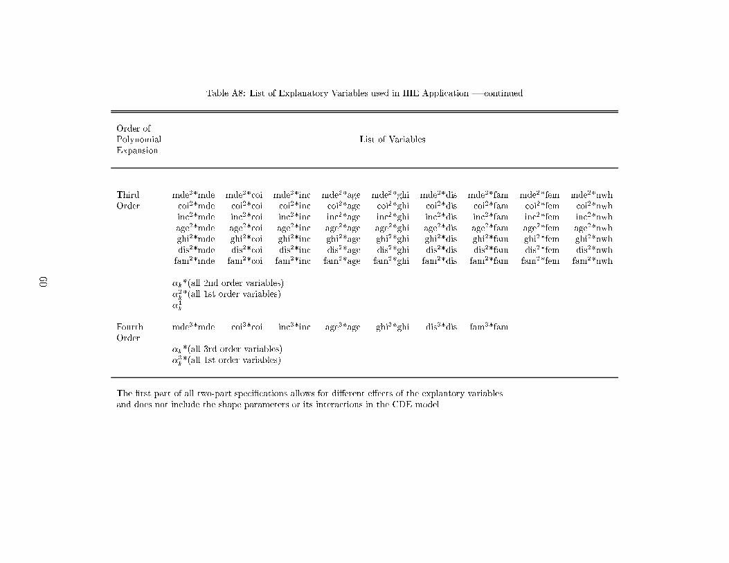
Table A8: List of Explanatory Variables used in HIE Application | continuedOrder ofPolynomial List of VariablesExpansionThird mde2*mde mde2*coi mde2*inc mde2*age mde2*ghi mde2*dis mde2*fam mde2*fem mde2*nwhOrder coi2*mde coi2*coi coi2*inc coi2*age coi2*ghi coi2*dis coi2*fam coi2*fem coi2*nwhinc2*mde inc2*coi inc2*inc inc2*age inc2*ghi inc2*dis inc2*fam inc2*fem inc2*nwhage2*mde age2*coi age2*inc age2*age age2*ghi age2*dis age2*fam age2*fem age2*nwhghi2*mde ghi2*coi ghi2*inc ghi2*age ghi2*ghi ghi2*dis ghi2*fam ghi2*fem ghi2*nwhdis2*mde dis2*coi dis2*inc dis2*age dis2*ghi dis2*dis dis2*fam dis2*fem dis2*nwhfam2*mde fam2*coi fam2*inc fam2*age fam2*ghi fam2*dis fam2*fam fam2*fem fam2*nwh�k*(all 2nd order variables)�2k*(all 1st order variables)�4kFourth mde3*mde coi3*coi inc3*inc age3*age ghi3*ghi dis3*dis fam3*famOrder �k*(all 3rd order variables)�3k*(all 1st order variables)The �rst part of all two-part speci�cations allows for di�erent e�ects of the explantory variablesand does not include the shape parameters or its interactions in the CDE model.

60