Dynamic censored regression and the Open Market

Desk reaction function

Robert de Jong∗ Ana Marıa Herrera†

March 9, 2009

Abstract

The censored regression model and the Tobit model are standard tools in economet-rics. This paper provides a formal asymptotic theory for dynamic time series censoredregression when lags of the dependent variable have been included among the regres-sors. The central analytical challenge is to prove that the dynamic censored regressionmodel satisfies stationarity and weak dependence properties if a condition on the lagpolynomial holds. We show the formal asymptotic correctness of conditional maximumlikelihood estimation of the dynamic Tobit model, and the correctness of Powell’s leastabsolute deviations procedure for the estimation of the dynamic censored regressionmodel. The paper is concluded with an application of the dynamic censored regressionmethodology to temporary purchases of the Open Market Desk.

1 Introduction

The censored regression model and the Tobit model are standard tools in econometrics. Ina time series framework, censored variables arise when the dynamic optimization behavior

∗Department of Economics, Ohio State University, 429 Arps Hall, Columbus, OH 43210, emaildejong@econ.ohio-state.edu

†Department of Economics, Michigan State University, 215 Marshall Hall, East Lansing, MI 48824, emailherrer20@mail.msu.edu. We thank Selva Demiralp and Oscar Jorda for making their data available, andBruce Hansen for the use of his code for kernel density estimation.

1

of a firm or individual leads to a corner response for a significant proportion of time. Inaddition, right-censoring may rise due to truncation choices made by the analysts in theprocess of collecting the data (i.e., top coding). Censored regression models apply to vari-ables that are left-censored at zero, such as the level of open market operations or foreignexchange intervention carried out by a central bank, and in the presence of an intercept inthe specification they also apply to time series that are censored at a non-zero point, suchas the clearing price in commodity markets where the government imposes price floors, thequantity of imports and exports of goods subject to quotas, and numerous other series.

The asymptotic theory for the Tobit model in cross-section situations has long beenunderstood; see for example the treatment in Amemiya (1973). In recent years, asymp-totic theory for the dynamic Tobit model in a panel data setting has been established usinglarge-N asymptotics; see Arellano and Honore (1998) and Honore and Hu (2004). However,there is no result in the literature that shows stationarity properties of the dynamic cen-sored regression model, leaving the application of cross-section techniques for estimating thedynamic censored regression model in a time series setting formally unjustified. This paperseeks to fill this gap. After all, a justication of standard inference in dynamic nonlinearmodels requires laws of large numbers and a central limit theorem to hold. Such resultsrequire weak dependence and stationarity properties.

While in the case of linear AR models it is well-known that we need the roots of thelag polynomial to lie outside the unit circle in order to have stationarity, no such resultis known for nonlinear dynamic models in general and the dynamic regression model inparticular. The primary analytical issue addressed in this paper is to show that under someconditions, the dynamic censored regression model as defined below satisfies stationarity andweak dependence properties. This proof is therefore an analogue to well-known proofs ofstationarity of ARMA models under conditions on the roots of the AR lag polynomial. Thedynamic censored regression model under consideration is

yt = max(0,

p∑

i=1

ρiyt−i + γ′xt + εt), (1)

where xt denotes the regressor, εt is a regression error, we assume that γ ∈ Rq, and we

define σ2 = Eε2t . One feature of the treatment of the censored regression model in this

paper is that εt is itself allowed to be a linear process (i.e., an MA(∞) process driven byan i.i.d. vector of disturbances), which means it displays weak dependence and is possiblycorrelated. While stationarity results for general nonlinear models have been derived in e.g.Meyn and Tweedie (1994), there appear to be no results for the case where innovations arenot i.i.d. (i.e. weakly dependent or heterogeneously distributed). The reason for this is thatthe derivation of results such as those of Meyn and Tweedie (1994) depends on a Markov

2

chain argument, and this line of reasoning appears to break down when the i.i.d. assumptionis dropped. This means that in the current setting, Markov chain techniques cannot be usedfor the derivation of stationarity properties, which complicates our analysis substantially,but also puts our analysis on a similar level of generality as can be achieved for the linearmodel.

A second feature is that no assumption is made on the lag polynomial other than thatρmax(z) = 1 −

∑pi=1 max(0, ρi)z

i has its roots outside the unit circle. Therefore, in termsof the conditions on ρmax(z) and the dependence allowed for εt, the aim of this paper is toanalyze the dynamic Tobit model on a level of generality that is comparable to the level ofgenerality under which results for the linear model AR(p) model can be derived. Note thatintuitively, negative values for ρj can never be problematic when considering the stationarityproperties of yt, since they “pull yt back to zero”. This intuition is formalized by the factthat only max(0, ρj) shows up in our stationarity requirement.

An alternative formulation for the dynamic censored regression model could be

yt = y∗t I(y∗t > 0) where ρ(B)y∗t = γ′xt + εt, (2)

where B denotes the backward operator. This model will not be considered in this paper,and its fading memory properties are straightforward to derive. The formulation consideredin this paper appears the appropriate one if the 0 values in the dynamic Tobit are notcaused by a measurement issue, but have a genuine interpretation. In the case of a model forthe difference between the price of an agricultural commodity and its government-institutedprice floor, we may expect economic agents to react to the actually observed price in theprevious period rather than the latent market clearing price, and the model considered in thispaper appears more appropriate. However, if our aim is to predict tomorrow’s temperaturefrom today’s temperature as measured by a lemonade-filled thermometer that freezes at zerodegrees Celsius, we should expect that the alternative formulation of the dynamic censoredregression model of Equation (2) is more appropriate.

The literature on the dynamic Tobit model appears to mainly consist of (i) theoreticalresults and applications in panel data settings, and (ii) applications of the dynamic Tobitmodel in a time series setting without providing a formal asymptotic theory. Three notewor-thy contributions to the literature on dynamic Tobit models are Honore and Hu (2004), Lee(1999), and Wei (1999). Honore and Hu (2004) considers dynamic Tobit models and dealswith the problem of the endogeneity of lagged values of the dependent variable in panel datasetting, where the errors are i.i.d., T is fixed and large-N asymptotics are considered. In fact,the asymptotic justification for panel data Tobit models is always through a large-N typeargument, which distinguishes this work from the treatment of this paper. For a treatmentof the dynamic Tobit model in a panel setting, the reader is referred to Arellano and Honore(1998, section 8.2).

3

Lee (1999) and Wei (1999) deal with dynamic Tobit models where lags of the latentvariable are included as regressors. Lee (1999) considers likelihood simulation for dynamicTobit models with ARCH disturbances in a time series setting. The central issue in this paperis the simulation of the log likelihood in the case where lags of the latent variable (in contrastto the observed lags of the dependent variable) have been included. Wei (1999) considersdynamic Tobit models in a Bayesian framework. The main contribution of this paper is thedevelopment of a sampling scheme for the conditional posterior distributions of the censoreddata, so as to enable estimation using the Gibbs sampler with a data augmentation algorithm.

In related work, de Jong and Woutersen (2003) consider the dynamic time series binarychoice model and derive the weak dependence properties of this model. This paper also con-siders a formal large-T asymptotic theory when lags of the dependent variable are included asregressors. Both this paper and de Jong and Woutersen (2003) allow the error distribution tobe weakly dependent. The proof in de Jong and Woutersen (2003) establishes a contractionmapping type result for the dynamic binary choice model; however, the proof in this paperis completely different, since other analytical issues arise in the censored regression context.

As we mentioned above, a significant body of literature on the dynamic Tobit model con-sists of applications in a time series setting without providing a formal asymptotic theory.Inference in these papers is either conducted in a classical framework, by assuming the max-imum likelihood estimates are asymptotically normal, or by employing Bayesian inference.Papers that estimate censored regression models in time series cover diverse topics. In the fi-nancial literature, prices subject to price limits imposed in stock markets, commodity futureexchanges, and foreign exchange futures markets have been treated as censored variables.Kodres (1988, 1993) uses a censored regression model to test the unbiasedness hypothesisin the foreign exchange futures markets. Wei (2002) proposes a censored-GARCH modelto study the return process of assets with price limits, and applies the proposed Bayesianestimation technique to Treasury bill futures.

Censored data are also common in commodity markets where the government has histor-ically intervened to support prices or to impose quotas. An example is provided by Chavasand Kim (2006) who use a dynamic Tobit model to analyze the determinants of U.S. butterprices with particular attention to the effects of market liberalization via reductions in floorprices. Zangari and Tsurumi (1996), and Wei (1999) use a Bayesian approach to analyze thedemand for Japanese exports of passenger cars to the U.S., which were subject to quotasnegotiated between the U.S. and Japan after the oil crisis of the 1970’s.

Applications in time series macroeconomics comprise open market operations and foreignexchange intervention. Dynamic Tobit models have been used by Demiralp and Jorda (2002)to study the determinants of the daily transactions conducted by the Open Market Desk,and Kim and Sheen (2002) and Frenkel, Pierdzioch and Stadtmann (2003) to estimate theintervention reaction function for the Reserve Bank of Australia and the Bank of Japan,

4

respectively.The structure of this paper is as follows. Section 2 present our weak dependence results

for (yt, xt) in the censored regression model. In Section 3, we show the asymptotic validity ofthe dynamic Tobit procedure. Powell’s LAD estimation procedure for the censored regres-sion model, which does not assume normality of errors, is considered in Section 4. Section5 studies the determinants of temporary purchases of the Open Market Desk. Section 6concludes. The Appendix contains all proofs of our results.

2 Main results

We will prove that yt as defined by the dynamic censored regression model satisfies a weakdependence concept called Lr-near epoch dependence. Near epoch dependence of randomvariables yt on a base process of random variables ηt is defined as follows:

Definition 1 Random variables yt are called Lr-near epoch dependent on ηt if

supt∈Z

E|yt − E(yt|ηt−M , ηt−M+1, . . . , ηt+M)|r = ν(M)r → 0 as M → ∞. (3)

The base process ηt needs to satisfy a condition such as strong or uniform mixing orindependence in order for the near epoch dependence concept to be useful. For the definitionsof strong (α-) and uniform (φ-) mixing see e.g. Gallant and White (1988, p. 23) or Potscherand Prucha (1997, p. 46). The near epoch dependence condition then functions as a devicethat allows approximation of yt by a function of finitely many mixing or independent randomvariables ηt.

For studying the weak dependence properties of the dynamic censored regression model,assume that yt is generated as

yt = max(0,

p∑

i=1

ρiyt−i + ηt). (4)

Later, we will set ηt = γ′xt + εt in order to obtain weak dependence results for the generaldynamic censored regression model that contains regressors.

When postulating the above model, we need to resolve the question as to whether thereexists a strictly stationary solution to it and whether that solution is unique in some sense.See for example Bougerol and Picard (1992) for such an analysis in a linear multivariate set-ting. In the linear model yt = ρyt−1+ηt, these issues correspond to showing that

∑∞j=0 ρ

jηt−j

is a strictly stationary solution to the model that is unique in the sense that no other functionof (ηt, ηt−1, . . .) will form a strictly stationary solution to the model.

5

An alternative way of proceeding to justify inference could be by considering arbitraryinitial values (y1, . . . , yp) for the process instead of starting values drawn from the stationarydistribution, but such an approach will be substantially more complicated.

The idea of the strict stationarity proof of this paper is to show that by writing thedynamic censored regression model as a function of the lagged yt that are sufficiently remotein the past, we obtain an arbitrarily accurate approximation of yt. Let B denote the backwardoperator, and define the lag polynomial ρmax(B) = 1−

∑pi=1 max(0, ρi)B

i. The central resultof this paper, the formal result showing the existence of a unique backward looking strictlystationary solution that satisfies a weak dependence property for the dynamic censoredregression model is now the following:

Theorem 1 If the linear process ηt satisfies ηt =∑∞

i=0 aiut−i, where a0 > 0, ut is a sequenceof i.i.d. random variables with density fu(.), E|ut|

r <∞ for some r ≥ 2,∫ ∞

−∞

|fu(y + a) − fu(y)|dy ≤M |a|

for some constant M whenever |a| ≤ δ for some δ > 0,∑∞

t=0G1/(1+r)t < ∞ where Gt =

(∑∞

j=t a2j)

r/2, ρmax(z) has all its roots outside the unit circle, and for all x ∈ R,

P (ut ≤ x) ≥ F (x) > 0 (5)

for some function F (.), then (i) there exists a solution yt to the model of Equation (4) suchthat (yt, ηt) is strictly stationary; (ii) if zt = f(ηt, ηt−1, . . .) is a solution to the model, thenyt = zt a.s.; and (iii) yt is L2-near epoch dependent on ηt. If in addition, ai ≤ c1 exp(−c2i)for positive constants c1 and c2, then the near epoch dependence sequence ν(M) satisfiesν(M) ≤ c1 exp(−c2M

1/3) for positive constants c1 and c2.

Our proof is based on the probability of yt reaching 0 given the last p values of ηt alwaysbeing positive. This property is the key towards our proof and is established using the linearprocess assumption in combination with the condition of Equation (5). Note that by theresults of Davidson (1994, p. 219), our assumption on ηt implies that ηt is also strong mixing

with α(m) = O(∑∞

t=m+1 G1/(1+r)t ). Also note that for the dynamic Tobit model where errors

are i.i.d. normal and regressors are absent, the condition of the above theorem simplifies tothe assumption that ρmax(z) has all its roots outside the unit circle.

One interesting aspect of the condition on ρmax(z) is that negative ρi are not affectingthe strict stationarity of the model. The intuition is that because yt ≥ 0 a.s., negative ρi

can only “pull yt back to zero” and because the model has the trivial lower bound of 0 foryt, unlike the linear model, this model does not have the potential for yt to tend to minusinfinity.

6

3 The dynamic Tobit model

Define β = (ρ′, γ′, σ)′, where ρ = (ρ1, . . . , ρp), and define b = (r′, c′, s)′ where r is a (p × 1)vector and c is a (q × 1) vector. The scaled Tobit loglikelihood function conditional ony1, ..., yp under the assumption of normality of the errors equals

LT (b) = LT (c, r, s) = (T − p)−1T∑

t=p+1

lt(b), (6)

where

lt(b) = I(yt > 0) log(s−1φ((yt −

p∑

i=1

riyt−i − c′xt)/s))

+I(yt = 0) log(Φ((−

p∑

i=1

riyt−i − c′xt)/s)). (7)

In order for the loglikelihood function to be maximized at the true parameter β, it ap-pears hard to achieve more generality than to assume that εt is distributed normally givenyt−1, . . . , yt−p, xt. This assumption is close to assuming that εt given xt and all lagged yt

is normally distributed, which would then imply that εt is i.i.d. and normally distributed.Therefore in the analysis of the dynamic Tobit model below, we will not attempt to considera situation that is more general than the case of i.i.d. normal errors. Alternatively to theresult below, we could also find conditions under which βT converges to a pseudo-true valueβ∗. Such a result can be established under general linear process assumptions on (x′t, εt), bythe use of Theorem 1. It should be noted that even under the assumption of i.i.d. errors, noresults regarding stationarity of the dynamic Tobit model have been derived in the literaturethus far.

Let βT denote a maximizer of LT (b) over b ∈ B. Define wt = (yt−1, . . . , yt−p, x′t, 1)′. The

“1” at the end of the definition of wt allows us to write “b′wt”. For showing consistency, weneed the following two assumptions. Below, let |.| denote the usual matrix norm defined as|M | = (tr(M ′M))1/2, and let ‖ X ‖r= (E|X|r)1/r.

Assumption 1 The linear process zt = (x′t, εt)′ satisfies zt =

∑∞j=0 Πjvt−j, where the vt are

i.i.d. (k × 1) vectors, ‖ vt ‖r< ∞ for some r ≥ 1, the coefficient matrices Πj satisfy and∑∞t=0 G

1/(1+r)t <∞ where Gt = (

∑∞j=t |Πj |

2)r/2, xt ∈ Rq, and

yt = max(0,

p∑

i=1

ρiyt−i + γ′xt + εt). (8)

7

Assumption 2

1. The linear process zt = (x′t, εt)′ satisfies zt =

∑∞j=0 Πjvt−j, where the vt are i.i.d.,

‖ vt ‖r< ∞, and the coefficient matrices Πj satisfy∑∞

t=0G1/(1+r)t < ∞ where Gt =

(∑∞

j=t |Πj |2)r/2.

2. Conditional on (x1, . . . , xT ), εt is independently normally distributed with mean zeroand variance σ2 > 0.

3. β ∈ B, where B is a compact subset of Rp+q+1, and B = Γ × R× Σ where inf Σ > 0.

4. Ewtw′tI(

∑pi=1 ρiyt−i + γ′xt > δ) is positive definite for some positive δ.

Theorem 2 Under Assumption 1 and 2, βTp

−→ β.

For asymptotic normality, we need the following additional assumption.

Assumption 3

1. β is in the interior of B.

2. I = E(∂/∂b)lt(β)(∂/∂b′)lt(β) = −E(∂/∂b)(∂/∂b′)lt(β) is invertible.

Theorem 3 Under Assumptions 1, 2, and 3, T 1/2(βT − β)d

−→ N(0, I−1).

4 Powell’s LAD for dynamic censored regression

For this section, define β = (ρ′, γ′)′, where ρ = (ρ1, . . . , ρp), define b = (r′, c′)′ where r isa (p × 1) vector and c is a (q × 1) vector, and wt = (yt−1, . . . , yt−p, x

′t)

′. This redefines theb and β vectors such as to not include s and σ respectively; this is because Powell’s LADestimator does not provide a first-round estimate for σ2. Powell’s LAD estimator βT of thedynamic censored regression model is defined as a minimizer of

ST (b) = ST (c, r, s) = (T − p)−1T∑

t=p+1

s(yt−1, . . . , yt−p, xt, εt, b)

= (T − p)−1

T∑

t=p+1

|yt − max(0,

p∑

i=1

riyt−i + c′xt)| (9)

over a compact set subset B of Rp+q. We can prove consistency of Powell’s LAD estimator

of the dynamic time series censored regression model under the following assumption.

8

Assumption 4

1. β ∈ B, where B is a compact subset of Rp+q.

2. The conditional distribution F (εt|wt) satisfies F (0|wt) = 1/2, and f(ε|wt) = (∂/∂ε)F (ε|w)is continuous in ε on a neighborhood of 0 and satisfies c2 ≥ f(0|wt) ≥ c1 > 0 for con-stants c1, c2 > 0.

3. E|xt|3 <∞, and Ewtw

′tI(

∑pi=1 ρiyt−i + γ′xt > δ) is nonsingular for some positive δ.

Theorem 4 Under Assumptions 1 and 4, βTp

−→ β.

For asymptotic normality, we need the following additional assumption. Below, let

ψ(wt, εt, b) = I(b′wt > 0)(1/2 − I(εt + (β − b)′wt > 0))wt. (10)

ψ(., ., .) can be viewed as a “heuristic derivative” of s(., .) with respect to b.

Assumption 5

1. β is in the interior of B.

2. Defining G(z, b, r) = EI(|w′tb| ≤ |wt|z)|wt|

r, we have for z near 0, for r = 0, 1, 2,

sup|b−β|<ζ0

|G(z, b, r)| ≤ K1z. (11)

3. The matrix

Ω = limT→∞

E(T−1/2T∑

t=1

ψ(wt, εt, β))(T−1/2T∑

t=1

ψ(wt, εt, β))′ (12)

is well-defined, and N = Ef(0|wt)I(w′tβ > 0)wtw

′t is invertible.

4. For some r ≥ 2, E|xt|2r < ∞, E|εt|

2r < ∞, and |Πj| ≤ c1 exp(−c2j) for positiveconstants c1 and c2.

5. The conditional density f(ε|wt) satisfies, for a nonrandom Lipschitz constant L0,

|f(ε|wt) − f(ε|wt)| ≤ L0|ε− ε|. (13)

9

Theorem 5 Under Assumptions 1, 4 and 5, T 1/2(βT − β)d

−→ N(0, N−1ΩN−1).

Assumption 5.1 is identical to Powell’s Assumption P.2, and Assumption 5.2 is the sameas Powell’s Assumption R.2. Theorem 5 imposes moment conditions of order 4 or higher. Theconditions imposed by Theorem 5 are moment restrictions that involve the dimensionalityp+ q of the parameter space. These conditions originate from the stochastic equicontinuityproof of Hansen (1996), which is used in the proof. One would expect that some progressin establishing stochastic equicontinuity results for dependent variables could aid in relaxingcondition 4 imposed in Theorem 5.

5 Simulations

In this section, we evaluate the consistency of the Tobit and CLAD estimators of the dynamiccensored regression model. We consider the data generating process

yt = max(0, γ1 + γ2xt +

p∑

i=1

ρiyt−i + εt)

where

xt = α1 + α2xt−1 + vt,

εt ∼ N(0, σ2ε ), and vt ∼ N(0, σ2

v). For our simulations, we consider the cases p = 1 and p = 2.Many configurations for α1, α2, γ1, γ2, σ

2v , and σ2

ε were considered. To conserve space, weonly report results for γ1 = 1, γ2 = 1, α1 = α2 = 0.5, σ2

ε = σ2v = 1.

For p = 1, simulations were conducted for ρ ∈ 0, 0.3, 0.6, 0.9, whereas for p = 2 weconducted simulations for (ρ1, ρ2) ∈(0.2, 0.1) , (0.5, 0.1) , (0.8, 0.1) , (0,−0.3) , (0.3,−0.3) ,(0.6,−0.3) , (0.9,−0.3). Note that, in contrast with Honore and Hu (2004), in our simu-lations the values of ρi are not restricted to be non-negative. For both the case p = 1 andthe case p = 2 the number of replications used to compute the bias reported in the tables is10,000.

Tables 4 reports simulation results for the dynamic Tobit model where estimates ofβ = (ρ′, γ′, σε) , with ρ′ = ρ if p = 1, ρ′ = (ρ1, ρ2) if p = 2, and γ′ = (γ1, γ2) are obtained viamaximum likelihood. Results for Powell’s LAD estimates of the dynamic censored regressionmodel are reported in Table 5 where β = (ρ′, γ′) , with ρ′ = ρ if p = 1, ρ′ = (ρ1, ρ2) if p = 2,and γ′ = (γ1, γ2) . As we mentioned in section 4, because Powell’s LAD estimator does notprovide a first-round estimator of σε we redefine β as to not include σε. Estimates in this

10

case are obtained using the BRCENS algorithm proposed by Fitzenberger (1997a,b). Wereport results for T = 100, 300, 600, 1000, 2000.

The simulations reveal that the maximum likelihood estimator for the dynamic Tobitmodel and Powell’s LAD estimator of the dynamic censored regression model perform wellfor T ≥ 300 (see Tables 4 and 5). As expected, the bias decreases as the sample size increases.For the same number of observations, the bias does not seem to vary much over the differentvalues for ρ and (ρ1,ρ2) that were considered.

6 Empirical Application

In a time series framework, censored variables can arise when the dynamic optimizationbehavior of a firm, individual or policy maker leads to a corner response for a significantproportion of time. Thus, is not surprising that dynamic Tobit models have been estimatedto study a number of variables such as open market operations (Demiralp and Jorda, 2002)and central bank intervention in foreign exchange markets (Kim and Sheen, 2002). What issurprising is that inference is conducted using the t-statistic critical values, without havingconsidered formal issues of stationarity. As we have noted before, strict stationarity andergodicity of the dynamic censored regression model is required to show asymptotic normalityand consistency of the maximum likelihood estimator of the dynamic Tobit model and ofPowell’s LAD estimator of the dynamic censored regression.

In what follows we discuss an application of the dynamic censored regression modelto the Open Market Desk reaction function. Although there are a significant number ofpapers that model and estimate the Federal Open Market Committee’s reaction function(e.g. Feinman, 1993, Demiralp and Farley, 2005), we are only aware of a recent studywhere lags of the dependent variable (i.e. open market operations) are included among theregressors. Without having considered formal issues of stationarity, Demiralp and Jorda(2002) estimated a dynamic Tobit model to analyze whether the February 4, 1994, Feddecision to publicly announce changes in the federal funds rate target affected the mannerin which the Open Market Desk conducts operations. In the following section we re-evaluatetheir findings.

6.1 Data and Summary of Previous Results

The data used by Demiralp and Jorda (2002) to study the announcement effect on theOpen Market Desk reaction function are daily and span the period between April 25, 1984and August 14, 2000. They divide the sample in three subsamples. The first subsamplecorresponds to the period preceding the Fed decision to publicly announce changes in the

11

federal fund rate target on February 4, 1994. The second period spans the days betweenFebruary 4, 1994 and the decision to shift from contemporaneous reserve accounting (CRA)to lagged reserves accounting (LRA) system in August 17, 1998. The last subsample coversthe period following the shift to the CRA system.

Demiralp and Jorda (2002) classify open market operations in six groups according towhether they inject or drain liquidity and to the permanence of the operation. Operationsthat add liquidity can be grouped into overnight reversible repurchase agreements (OB), termrepurchase agreements (TB), and permanent purchases (PB), which include T-bill purchasesand coupon purchases. Operations that drain liquidity can be grouped into overnight sales(OS), term matched-sale purchases (TS), and permanent sales (PS), which comprise T-billsales and coupon sales.

Because the computation of reserves is based on a 14-day maintenance period that startson Thursday and finishes on the ”Settlement Wednesday” two weeks later, the maintenance-period average is the object of attention of the Open Market Desk. Thus, all operationsare adjusted according to the number of days spanned by the transaction, and standardizedby the aggregate level of reserves held by depository institutions in the maintenance periodprevious to the execution of the transaction.

Demiralp and Jorda (2002) separate deviations of the federal funds rate from the targetinto three components:

NEEDt = ft −[f ∗

m(t)−1 + wtEm(t)−1

(∆f ∗

m(t)

)](14)

EXPECTt = Em(t)−1

(∆f ∗

m(t)

)(15)

SURPRISEt = ∆f ∗t − Em(t)−1

(∆f ∗

m(t)

)(16)

where the maintenance period to which observation in day t belongs is denoted by m(t),ft denotes the federal funds rate in day t; f ∗

m(t)−1 denotes the value of the target in the

maintenance period previous to the one to which observation t belongs; Em(t)−1(∆f∗m(t))

denotes the expectation of a target change in day t, conditional on the information availableat the beginning of the 14-day maintenance period; and wt denotes the probability of a targetchange on date t. Both the expected change in the target, Em(t)−1(∆f

∗m(t)), and the weights

wt are calculated by Demiralp and Jorda (2002) using the ACH model of Hamilton and Jorda(2002). This decomposition is intended to reflect three different motives for open marketpurchases: (1) to add or drain liquidity in order to accommodate shocks to the demand forreserves; (2) to accommodate expectations of future changes in the target; and (3) to adjustto a new target level. Thus, NEEDt represents a proxy for the projected reserve need, andchanges in the federal funds rate are separated into an expected component, EXPECTt,and a surprise component, SURPRISEt. The latter takes a non-zero value for the 115 daysin the sample when there was a change in the target, and zero otherwise.

12

Because the Desk engages in open market operations only on 60% of the days in thesample, and even the most common operation only takes place on 35% of the days (i.e., thedata is censored at zero during a large number of days), Demiralp and Jorda (2002) use aTobit model to analyze the reaction function of the Open Market Desk. Furthermore, toallow for a different response of sales and purchases –with varying degrees of permanence–to changes in the explanatory variables they estimate separate regressions for each of thesix types of operation and each of the periods of interest. Because very few term andpermanent sales were carried out during the 1998-2000 and 1984-1994 periods, no regressionsare estimated for this type of operation in these subsamples. Hence, a total of sixteenregression are estimated. Demiralp and Jorda (2002) use the following dynamic Tobit modelto describe open market operations carried out by the Open Market Desk:

yt = max(0,10∑

m=1

γαmDAYtm +

3∑

j=1

ρjyt−j +3∑

j=1

υ′

jzt−j +10∑

m=1

γNmNEEDt−m ×DAYtm

+10∑

m=1

γEmEXPECTt−m ×DAYtm +

3∑

j=0

γSj SURPRISEt−j + εt) (17)

where yt denotes one of the open market operation of interest, that is, yt equals eitherovernight purchases (OBt), term purchases (TBt), permanent purchases (PBt), overnightsales (OSt), term sales (TSt), or permanent sales (PSt). zt denotes a vector containing theremaining five types of operations. For instance, if yt = OBt (overnight purchases), thenzt = [TBt, PBt, OSt, TSt, PSt] . DAYtm denotes a vector of maintenance-day dummies, andεt is a stochastic disturbance.

We thus start our empirical analysis by re-estimating Demiralp and Jorda’s (2002) spec-ifications under the assumption of normality. That is, we follow their lead in assuming thedynamic Tobit model is correctly specified. We report the coefficient estimates for the lags ofthe dependent variable in Table 1. See Tables A.1 and A.2 in the Appendix for the completeset of parameter estimates. Because we are interested in whether the roots of the polyno-mial ρmax(z) = 1 −

∑3i=1 max(0, ρi)z

i are outside the unit circle we report the smallest ofthe moduli of the roots of this lag polynomial.

Note that 10 out of the 16 regressions estimated by Demiralp and Jorda (2002) appearto have at least one root that falls on or inside the unit circle. One may wonder whether thisresult stems from nonstationarity issues or from misspecification in the error distribution. Toinvestigate this issue, we test for normality of the Tobit residuals and report the Jarque-Berastatistics in Table 1; these results lead us to reject the null that the underlying disturbancesare normally distributed. Thus, we proceed in the following section to estimate the OpenDesk’s reaction function using Powell’s LAD estimator, which is robust to unknown error

13

distributions. If the problem is one of nonstationarity, one would then expect the roots ofthe ρmax(.) polynomial to be on or inside the unit circle. However, in what follows we willsee that CLAD estimates for temporary Open Market purchases indicate that the roots ofthe ρmax(.) polynomial are outside the unit circle. That finding suggests that the resultsof Demiralp and Jorda (2002) suffer from misspecification in the error distribution, but notfrom nonstationarity issues.

6.2 Model and estimation procedure

From here on we will restrict our attention to the Desk’s reaction function for temporaryopen market purchases over the whole 1984-2000 sample. We focus on temporary purchasesbecause overnight and term RPs are the most common operations carried out by the OpenMarket Desk; thus, they are informative regarding the Desk’s reaction function. In fact,daily values of temporary purchases plotted in Figure 1 reveal that the Open Market Deskengaged in temporary purchases on 37% of the days between April 25, 1984 and August 14,2000. In contrast, permanent purchases, temporary sales, and permanent sales were carriedout, respectively, on 24%, 7%, and 2% of the days in the sample.

Thus, in contrast with Demiralp and Jorda (2002) we re-classify open market operationsin four groups: (a) temporary purchases, which comprise overnight reversible repurchaseagreements (RP) and term RP, OTBt = OBt+TBt; (b) permanent purchases, which includeT-bill purchases and coupon purchases, PBt; (c) temporary sales, which include overnightand term matched sale-purchases, OTSt = OSt + TSt; and (d) permanent sales, whichcomprise T-bill sales and coupon sales, PSt. In brief, we group overnight and term operationsand restrict our analysis to the change in the maintenance-period-average level of reservesbrought about by temporary purchases of the Open Market Desk, OTBt.

We employ the following dynamic censored regression model to describe temporary pur-chases by the Open Market Desk:

OTBt = max(0, γ +

4∑

m=1

γαmDtm +

3∑

j=1

ρjOTBt−j +

3∑

j=1

γTSj OTSt−j +

3∑

j=1

γPBj PBt−j

+

3∑

j=1

γPSj PSt−j +

10∑

m=1

γNmNEEDt−m ×DAYtm +

10∑

m=1

γEmEXPECTt−m ×DAYtm

+

3∑

j=0

γSj SURPRISEt−j + εt) (18)

14

where OTBt denotes temporary purchases, OTSt denotes temporary sales, PBt denotespermanent purchases, PSt denotes permanent sales, DAYtm denotes a vector of maintenance-day dummies, Dtm is such that Dt1 = DAYt1 (First Thursday), Dt2 = DAYt2 (First Friday),Dt3 = DAYt7 (Second Friday), and Dt4 = DAYt,10 (Settlement Wednesday), and εt is astochastic disturbance.

This model is a restricted version of (17) in that it does not include dummies for all daysin the maintenance period. Instead, to control for differences in the reserve levels that theFederal Reserve might want to leave in the system at the end of the day, we include onlydummies for certain days of the maintenance period where the target level of reserves isexpected to be different from the average (see Demiralp and Farley, 2005). However, we doallow the response of temporary purchases to reserve needs and expected changes in the fedfunds rate to vary across all days of the maintenance period.

Regarding the estimation procedure, Tobit estimates b are obtained in the usual mannervia maximum likelihood estimation, whereas the CLAD estimates b are obtained by using theBRCENS algorithm proposed by Fitzenberger (1997a,b). Extensive Monte Carlo simulationsby Fitzenberger (1997a) suggest that this algorithm, which is an adaptation of the Barrodale-Roberts algorithm for the censored quantile regression, performs better than the iterativelinear programming algorithm (ILPA) of Buchinsky (1994) and the modified ILPA algorithm(MILPA) of Fitzenberger (1994), in terms of the percentage of times it detects the globalminimum of a censored quantile regression. In fact, for our application, a grid search over1000 points in the neighborhood of the estimates b indicates both the ILPA and MILPAalgorithms converge to a local minimum. In contrast, the BRCENS algorithm is stable andappears to converge to a global minimum.

Because the CLAD does not provide a first-round estimate for the variance, N−1ΩN−1,we compute it in the following manner. Ω is calculated as the long-run variance of ψ(wt, b) =

I (b′wt > 0)[12− I(yt < b′wt)]wt, following the suggestions of Andrews (1991) to select the

bandwidth for the Bartlett kernel. To compute N , we estimate f(0|wt) using a higher-orderGaussian kernel with the order and bandwidth selected according to Hansen (2003, 2004).

6.3 Estimation Results

Maximum likelihood estimates of the dynamic Tobit model for the entire sample, andcorresponding standard errors are presented in the first two columns of Table 2.1 Be-fore we comment on the estimation results, it is important to inspect whether the rootsof the lag polynomial ρmax(z) lie outside the unit circle. The three roots of ρmax(z) =1 − 0.2639z − 0.2916z2 − 0.3054z3 lie all outside the unit circle, and the smallest modulus

1The reported standard errors for the Tobit estimates are the quasi-maximum likelihood standard errors.

15

of these roots equals 1.075. Because this root is near the unit circle and because we do nothave the tools to test if it is statistically greater than one, we should proceed with caution.

Of interest is the presence of statistically significant coefficients on the lags of the depen-dent variable, TBt−j . This persistence suggests that in order to attain the desired target,the Open Market Desk had to exercise pressure on the fed funds market in a gradual man-ner, on consecutive days. The negative and statistically significant coefficients on laggedtemporary sales, TSt−j , imply that temporary sales constituted substitutes for temporarypurchases. In other words, in the face of a reserve shortage the Open Market Desk couldreact by conducting temporary purchases and/or delaying temporary sales. The positive andstatistically significant coefficients on the NEEDt−1×DAYtm variables is consistent with anaccommodating behavior of the Fed to deviations of the federal funds rate from its target.The Tobit estimates suggest that expectations of target changes were accommodated in thefirst days of the maintenance period, and did not significantly affect temporary purchaseson most of the remaining days. As for the effect of surprise changes in the target, the es-timated coefficients are statistically insignificant. According to Demiralp and Jorda (2002),statistically insignificant coefficients on SURPRISEt−j can be interpreted as evidence ofthe announcement effect.2 This suggests that the Fed did not require temporary purchasesto signal the change in the target, once it had been announced (or inferred by the markets).

However, it is well known that the Tobit estimates are inconsistent if the underlyingdisturbances are heteroskedastic or non-normal (Greene, 2000). Thus, to assess whether theTobit specification of the reaction function is appropriate, we conduct tests for homoskedas-ticity and normality. A Lagrange multiplier test of heteroskedasticity obtained by assumingV ar(εt|wt) = σ2 exp(δ′zt), where zt is a vector that contains all elements in wt but the con-stant, rejects the null H0 : δ = 0 at the 1% level. In addition, the Jarque-Bera statistic leadsus to reject the null that the residuals are normally distributed at a 1% level. This is clearlyillustrated in Figure 2, which plots the histogram for the Tobit residuals.

Summing up, the finding of a root that is close to the unit circle in conjunction withthe rejection of the normality and homoskedasticity assumptions suggest that the Tobitestimates could be biased. Hence, our finding of a root near the unit circle may stem ei-ther from misspecification of the error term or from non-stationarity of the dynamic Tobitmodel. To further investigate this issue, we consider the CLAD estimator, which is robust toheteroskedasticity and nonnormality and is consistent in the presence of weakly dependenterrors (see Section 4). Finding a root close to unity for the CLAD estimates would be indica-

2Even though the federal funds target has only been announced since the February 3-4 FOMC meeting,Demiralp and Jorda (2004) provide evidence that, since late 1989, financial markets were able to decodechanges in the target from the pattern of open market operations. Furthermore, research by Cook and Hahn(1988) suggests that even in earlier periods, market participants were able to read signals of a target changein the Fed’s behavior.

16

tive of nonstationarity in the dynamic censored regression model driving the test results. Incontrast, finding roots that are outside the unit circle would point towards misspecificationof the error distribution being the cause of the bias in the Tobit estimates.

CLAD estimates and corresponding standard errors are reported in the third and fourthcolumn of Table 2, respectively3. Notice that, in this case, the smallest root of the lagpolynomial ρmax(z) = 1 − 0.068z − 0.093z2 − 0.073z3 appears to be clearly outside theunit circle. Here the smallest modulus of the roots equals 1.928. Given that the roots arefar from the unit circle, standard inference techniques seem to be asymptotically justified.Furthermore, this suggest that our finding of roots that are near the unit circle for the Tobitmodel is a consequence of misspecification in the error term as normal and homoskedastic.

Comparing the CLAD and the Tobit estimates reveals some differences regarding theDesk’s reaction function. First, the CLAD estimates imply a considerably smaller degree ofpersistence in temporary purchases. The magnitude of the ρj , j = 1, 2, 3, parameter estimatesis at most 1/3 of the Tobit estimates. Consequently, the roots of the lag polynomial ρmax(z)implied by the CLAD estimates are larger, giving us confidence regarding stationarity of thecensored regression model.

Second, although both estimates imply a similar reaction of the Fed to reserve needs,there are some differences in the magnitude and statistical significance of the parameters.In particular, the CLAD estimates suggest a pattern in which the Fed is increasingly lessreluctant to intervene during the first three days of the maintenance period; then, no sig-nificant response is apparent for the following four days (with the exception of Day5, thefirst Wednesday); and finally, the response to reserve needs becomes positive and significantfor the last three days of the period. Furthermore, on Mondays (Day3 and Day8), the Deskappears to be more willing to accommodate shocks in the demand for reserves in order tomaintain the federal funds rate aligned with the target.

The expectation of a change in the target seldom triggers temporary open market pur-chases. The coefficient on EXPECT is statistically significant on the first and eight dayof the maintenance period, and marginally significant on the second and sixth day. Thissuggest the Fed in only seldom willing to accommodate (or profit) from anticipated changesin the target. Moreover, even though both estimation methods point towards a larger effecton the first day, the CLAD estimate (40.5) suggest an impact that is about 67% smallerthan the Tobit estimate (121.5).

The majority of the coefficients on the contemporaneous and lagged SURPRISE havea negative sign, which is consistent with the liquidity effect. That is, in order to steer the

3Our estimate for Ω was calculated with an HAC estimator using the Bartlett kernel, and the bandwidthwas selected using the data-driven method suggested by Andrews (1991). The density function f(0|wt) wasestimated using a higher-order Gaussian kernel with the order and bandwidth selected according to Hansen(2003, 2004).

17

federal funds rate towards a new lower target level the Desk would add liquidity by usingtemporary purchases. Yet, the fact that none of the coefficients are statistically significantsuggests that once the target was announced (or inferred by the financial markets) littleadditional pressure was needed to enforce the new target.

Finally, to further explore the “announcement effect” we redo the estimation using onlythe observations after the Fed started announcing the new target level in February 4, 1994(see Table 3)4. There appears to be a somewhat smaller but still significant degree ofpersistence in temporary open market purchases after the decision to announce the targetlevel. This suggest the Fed still had to exert some pressure on the market to drive the fedfunds rate towards the new target level.5 In brief, we find the coefficients on the current andlagged values of SURPRISE to be statistically insignificant whether we include or not theobservations that predate the Fed decision to announce the target level.

7 Conclusions

This paper shows stationarity properties of the dynamic censored regression model in a timeseries framework. It then provides a formal justification for maximum likelihood estimation ofthe dynamic Tobit model and for Powell’s LAD estimation of the dynamic censored regressionmodel, showing consistency and asymptotic normality of both estimators. Two importantfeatures of the treatment of the censored regression model in this paper is that no assumptionis made on the lag polynomial other than that ρmax(z) = 1−

∑pi=1 max(0, ρi)z

i has its rootsoutside the unit circle and that the error term, εt, is itself allowed to be potentially correlated.Hence, in terms of the conditions on ρmax(z) and the dependence allowed for εt, this paperanalyzes the dynamic censored regression model on a level of generality that is comparable tothe level of generality under which results for the linear model AR(p) model can be derived.

The censored regression model is then applied to study the Open Market Desk’s re-action function. Robust estimates for temporary purchases using Powell’s CLAD suggestthat maximum likelihood estimates of the dynamic Tobit model may lead to overestimatingthe persistence of temporary purchases, as well as the effect of demand for reserves andexpectations of future changes in the federal funds target on temporary purchases. More-over, a comparison of the Tobit and CLAD estimates suggests that temporary purchases arestationary, but that the error normality assumed in the Tobit specification does not hold.

4Due to the stationarity issues discussed in the previous section, we do not use the same subsamples asDemiralp and Jorda (2002).

5Similar conclusions are drawn if we use the futures federal funds rate (Kuttner, 2001) to decomposeanticipated and unanticipated changes in policy.

18

References

Amemiya, T. (1973), Regression analysis when the dependent variable is truncated normal,Econometrica 41, 997-1016.

Amemiya, T. (1985) Advanced Econometrics. Oxford: Basil Blackwell.

Andrews, D.W.K. (1987), Consistency in nonlinear econometric models: a generic uniformlaw of large numbers, Econometrica 55, 1465-1471.

Andrews, D.W.K. (1988), Laws of large numbers for dependent non-identically distributedrandom variables, Econometric Theory 4, 458-467.

Andrews, D.W.K. (1991), Heteroskedasticity and Autocorrelation Consistent CovarianceMatrix Estimation, Econometrica 59, 817-858.

Arellano, M. and B. Honore (1998), Panel data models: some recent developments, Chapter53 in Handbook of Econometrics, Vol. 5, ed. by James J. Heckman and Edward Leamer.Amsterdam: North-Holland.

Azuma, K. (1967), Weighted sums of certain dependent variables, Tokohu MathematicalJournal 19, 357-367.

Bierens, H. J. (2004) Introduction to the mathematical and statistical foundations of Econo-metrics. Cambridge University Press, forthcoming, available athttp://econ.la.psu.edu/~hbierens/CHAPTER7.PDF .

Bougerol, P. and N. Picard (1992), Strict stationarity of generalized autoregressive processes,Annals of Probability 20, 1714-1730.

Buchinsky, M. (1994), Changes in the U.S. wage structure 1963-1987: application of quantileregression, Econometrica 62, 405-458.

Chavas, J-P. and Kim (2006), An econometric analysis of the effects of market liberalizationon price dynamics and price volatility, Empirical Economics 31, 65-82.

Cook, T. and T. Hahn (1988), The information content of discount rate announcements andtheir effect on market interest rates, Journal of Money, Credit, and Banking 20, 167-180.

Chernozhukov, V. and H. Hong (2002), Three-step censored quantile regression and extra-marital affairs, Journal of the American Statistical Association 97 (459), 872-882.

Davidson, J. (1994) Stochastic Limit Theory. Oxford: Oxford University Press.

de Jong, R.M. (1997), Central limit theorems for dependent heterogeneous random variables,

19

Econometric Theory 13, 353-367.

de Jong, R.M. and T. Woutersen, Dynamic time series binary choice, forthcoming, Econo-metric Theory.

Demiralp, S. and D. Farley (2005), Declining required reserves, funds rate volatility, andopen market operations, Journal of Banking and Finance 29, 1131-1152.

Demiralp, S. and O. Jorda (2002), The announcement effect: evidence from open marketdesk data, Economic Policy Review, 29-48.

Demiralp, S. and O. Jorda (2004), The response of term rates to Fed announcements, Jour-nal of Money, Credit, and Banking 36, 387-406.

Feinman, J. (1993), Estimating the Open Market Desk’s daily reaction function, Journal ofMoney, Credit, and Banking 25, 231-247.

Frenkel, M., Pierdzioch, C. and G. Stadtmann (2003), Modeling coordinated foreign ex-change market interventions: The case of the Japanese and U.S. interventions in the 1990s,Review of World Economics, 139, 709-729.

Fitzenberger, B. (1994), A note on estimating censored quantile regressions, Discussion Pa-per 14, University of Konstanz.

Fitzenberger, B. (1997a), “Computational Aspects of Censored Quantile Regression,” inProceedings of the 3rd International Conference on Statistical Data Analysis Based on theL1-Norm and Related Methods, ed. Y. Dodge, Hayward, CA: IMS, 171–186.

Fitzenberger, B. (1997b), “A Guide to Censored Quantile Regressions,” in Handbook ofStatistics, Vol. 14, Robust Inference, Amsterdam: North-Holland, pp. 405–437.

Gallant, A.R. and H. White (1988) A unified theory of estimation and inference for nonlineardynamic models. New York: Basil Blackwell.

Greene, W. (2000) Econometric Analysis, 5th Edition. New Jersey: Prentice-Hall.

Hamilton, J.D. and O. Jorda (2002), A Model for the Federal Funds Rate Target, Journalof Political Economy, 110, 1135-1167.

Hansen, B. E. (1996), Stochastic equicontinuity for unbounded dependent heterogeneous ar-rays, Econometric Theory, 12, 347-359.

Hansen, B.E. (2003), Exact mean integrated square error of higher-order kernel estimators,Working Paper, University of Wisconsin.

Hansen, B.E. (2004), Bandwidth selection for nonparametric kernel estimation, Working Pa-

20

per, University of Wisconsin.

Kim, S. and J. Sheen (2002), The determinants of foreign exchange intervention by centralbanks: evidence from Australia, Journal of International Money and Finance, 21, 619-649.

Kodres, L. E. (1988), Test of unbiasedness in the foreign exchange futures markets: Theeffects of price limits, Review of Futures Markets 7, 139-166.

Kodres, L.E. (1993), Test of unbiasedness in the foreign exchange futures makets: An Exam-ination of Price Limits and Conditional Heteroscedasticity, Journal of Business 66, 463-490.

Kuttner, Kenneth (2001), Monetary policy surprises and interest rates: evidence from theFed funds futures market, Journal of Monetary Economics 47, 523-544.

McLeish, D. L. (1974), Dependent central limit theorems and invariance principles, Annalsof Probability 2, 620-628.

Meyn, S.P. and R.L. Tweedie (1994) Markov Chains and Stochastic Stability. Berlin: Springer-Verlag, second edition.

Newey, W. K., and D. McFadden (1994), Large sample estimation and hypothesis testing,in Handbook of Econometrics, Vol. 4, ed. by R. F. Engle and D. MacFadden. Amsterdam:North-Holland.

Persitiani, S. (1994), An empirical investigation of the determinants of discount window bor-rowing: a disaggregate analysis, Journal of Banking and Finance 18, 183-197.

Phillips, P. and V. Solo (1992), Asymptotics for linear processes, Annals of Statistics, Vol.20, No. 2, p. 971-1001.

Potscher, B.M. and I.R. Prucha (1986), A class of partially adaptive one-step M-estimatorsfor the nonlinear regression model with dependent observations, Journal of Econometrics32, 219-251.

Potscher, B.M. and I.R. Prucha (1997) Dynamic nonlinear econometric models. Berlin:Springer-Verlag.

Powell, J.L. (1984), Least absolute deviations estimation for the censored regression model,Journal of Econometrics 25, 303-325.

Wei, S.X. (1999), A Bayesian approach to dynamic Tobit models, Econometric Reviews 18,417-439.

Wei, S.X. (2002), A censored-GARCH model of asset returns with price limits, Journal ofEmpirical Finance 9, 197-223.

Wooldridge, J. (1994), Estimation and inference for dependent processes, in Handbook of

21

Econometrics, volume 4, ed. by R. F. Engle and D. MacFadden. Amsterdam: North-Holland.

Zangari, P.J. and Tsurumi, H. (1996), A Bayesian analysis of censored autocorrelated data onexports of Japanese passenger cars to the United States, Advances in Econometrics, Volume11, Part A, 111-143.

22

23

1984

-199

419

94-1

998

1998

-200

019

84-1

994

1994

-199

819

98-2

000

1984

-199

419

94-1

998

1998

-200

0

Lag

10.

628

0.51

30.

063

0.26

50.

129

-0.0

240.

145

0.21

7-0

.068

(0

.141

)(0

.093

)(0

.078

)(0

.146

)(0

.105

)(0

.120

)(0

.044

)(0

.174

)(0

.282

)La

g 2

0.26

80.

300

-0.0

170.

594

0.08

0-0

.039

0.10

80.

329

0.73

7(0

.146

)(0

.091

)(0

.070

)(0

.099

)(0

.095

)(0

.114

)(0

.046

)(0

.164

)(0

.213

)La

g 3

0.02

50.

236

0.08

70.

404

0.15

40.

113

0.10

10.

281

0.42

1(0

.148

)(0

.087

)(0

.065

)(0

.104

)(0

.098

)(0

.120

)(0

.045

)(0

.168

)(0

.227

)

Sm

alle

st ro

ot1.

063

0.97

22.

154

0.89

41.

574

2.06

91.

661

1.09

50.

940

1984

-199

419

94-1

998

1998

-200

019

84-1

994

1994

-199

819

98-2

000

1984

-199

419

94-1

998

1998

-200

0

Lag

10.

938

1.89

71.

104

0.75

92.

623

--

-98.

549

-31.

074

(0.2

40)

(0.4

06)

(0.6

85)

(0.2

69)

(2.8

71)

(126

5867

7)(1

9394

016)

Lag

2-0

.064

-0.0

25-0

.185

1.26

90.

487

--7

7.08

21.

515

(0.2

13)

(0.3

57)

(0.7

03)

(0.2

61)

(0.5

02)

-(1

1727

925)

(0.8

40)

Lag

3 0.

197

0.52

20.

084

1.06

90.

322

--7

7.95

8-6

2.09

8(0

.178

)(0

.336

)(0

.702

)(0

.239

)(0

.591

)-

(110

2178

4)(2

8391

370)

Sm

alle

st ro

ot0.

908

0.49

40.

858

0.55

70.

353

1.00

00.

812

Not

e: S

tand

ard

erro

rs re

porte

d in

par

enth

esis

. "S

mal

lest

root

" den

otes

the

smal

lest

mod

ulus

of t

he ro

ots

of th

e ρ

max

(B)

lag

poly

nom

ial.

24

Tabl

e 1

Dem

iralp

and

Jor

dà (2

002)

Tob

it re

gres

sion

for O

pen

Mar

ket O

pera

tions

OB

TBPB

OS

TSPS

Coe

ffici

ent E

stim

ates

for L

ags

of th

e D

epen

dent

Var

iabl

e

Variable Estimate Std. Err. Estimate Std. Err.

Constant -18.742 *** 1.753 -1.252 *** 0.341First Thursday 16.962 *** 2.833 1.814 *** 0.502First Friday -17.046 *** 2.917 -3.595 *** 1.393Second Friday -12.051 *** 2.683 -3.466 *** 1.262Settlement Wednesday 4.456 *** 1.553 2.811 *** 0.464OTB(-1) 0.264 *** 0.035 0.068 *** 0.008OTB(-2) 0.292 *** 0.042 0.093 *** 0.007OTB(-3) 0.305 *** 0.049 0.073 *** 0.007OTS(-1) -1.726 *** 0.611 -3.941 3.666OTS(-2) -0.865 * 0.447 -1.025 1.554OTS(-3) -1.895 *** 0.408 -0.558 * 0.359PB(-1) -0.018 0.085 -0.164 *** 0.065PB(-2) -0.065 0.074 -0.045 0.038PB(-3) -0.073 0.072 -0.022 0.031PS(-1) 0.146 0.253 -0.033 0.116PS(-2) -0.151 0.245 -0.067 0.092PS(-3) -0.198 0.223 0.065 * 0.045SURPRISE -14.046 15.387 -0.659 4.441SURPRISE(-1) 11.516 13.044 -0.268 3.898SURPRISE(-2) -14.619 17.648 0.735 3.849SURPRISE(-3) -7.259 14.832 -1.755 4.08NEED(-1)*Day1 -0.501 2.974 1.742 *** 0.526NEED(-1)*Day2 11.645 ** 4.691 3.433 *** 0.794NEED(-1)*Day3 24.030 *** 8.595 9.163 *** 2.108NEED(-1)*Day4 -7.489 7.775 -1.868 1.822NEED(-1)*Day5 21.671 *** 7.612 5.884 *** 2.012NEED(-1)*Day6 5.312 10.941 -0.593 2.478NEED(-1)*Day7 33.429 *** 10.471 1.367 2.362NEED(-1)*Day8 6.842 7.789 9.616 *** 2.213NEED(-1)*Day9 13.402 *** 4.953 5.206 *** 1.248NEED(-1)*Day10 3.972 * 2.083 1.144 ** 0.52EXPECT*Day1 121.451 ** 53.231 40.461 *** 5.499EXPECT*Day2 48.599 34.018 13.107 * 8.277EXPECT*Day3 -14.656 38.828 1.884 6.077EXPECT*Day4 -25.528 29.346 3.586 5.711EXPECT*Day5 -54.997 * 29.859 -1.924 7.271EXPECT*Day6 51.573 * 30.636 8.856 * 5.449EXPECT*Day7 -37.603 36.721 1.632 12.704EXPECT*Day8 39.313 * 20.515 12.535 ** 5.454EXPECT*Day9 -48.249 * 24.666 -11.71 9.445EXPECT*Day10 16.269 16.363 7.958 * 5.168SCALE 1094.099 *** 104.478

Smallest root 1. 0750 2. 0315

Note: ***, ** and * denote significance at the 1, 5 and 10% level, respectively. "Smallest root"denotes the smallest modulus of the roots of the ρmax (B) lag polynomial.

25

Table 2

Tobit CLAD

1986-2000Tobit and CLAD Estimates for Open Market Temporary Purchases

Variable Estimate Std. err. Estimate Std. Err.

Constant -3.856 ** 1.904 3.318 *** 0.379First Thursday 24.899 *** 4.520 10.248 *** 0.766First Friday -13.723 *** 4.013 -4.162 *** 1.145Second Friday -9.781 *** 3.389 -3.006 *** 0.885Settlement Wednesday 1.914 1.771 2.443 *** 0.750OTB(-1) 0.146 *** 0.040 0.015 * 0.010OTB(-2) 0.142 *** 0.043 0.037 *** 0.009OTB(-3) 0.219 *** 0.053 0.023 *** 0.009OTS(-1) -0.904 0.563 -3.435 * 2.091OTS(-2) -0.561 0.440 -1.144 ** 0.570OTS(-3) -2.068 *** 0.710 -3.851 *** 1.233PB(-1) -0.109 0.117 -0.028 0.042PB(-2) 0.030 0.108 0.008 0.027PB(-3) -0.082 0.103 -0.049 * 0.036PS(-1) 0.135 0.255 0.335 *** 0.092PS(-2) 0.398 0.244 0.586 *** 0.085PS(-3) -0.212 0.270 -0.008 0.081SURPRISE 19.230 * 10.688 1.898 5.521SURPRISE(-1) -18.989 15.698 -1.063 5.790SURPRISE(-2) -42.791 34.819 -0.654 8.035SURPRISE(-3) -42.019 * 23.901 -12.702 12.600NEED(-1)*Day1 -1.260 11.661 7.145 *** 1.624NEED(-1)*Day2 24.978 15.438 11.032 *** 4.263NEED(-1)*Day3 22.241 ** 10.014 26.737 *** 5.221NEED(-1)*Day4 -11.121 10.667 2.232 3.159NEED(-1)*Day5 42.804 *** 12.427 17.637 *** 4.020NEED(-1)*Day6 -14.788 19.240 -28.351 *** 6.376NEED(-1)*Day7 20.849 19.487 10.726 *** 3.831NEED(-1)*Day8 8.298 14.080 11.127 *** 4.187NEED(-1)*Day9 0.540 7.724 2.384 2.055NEED(-1)*Day10 10.502 * 5.679 0.945 2.493EXPECT*Day1 93.199 68.418 33.119 *** 7.166EXPECT*Day2 27.979 38.112 0.933 10.344EXPECT*Day3 -12.791 38.854 -3.585 7.963EXPECT*Day4 -43.710 31.953 -13.921 ** 7.604EXPECT*Day5 -77.641 ** 33.233 -18.657 ** 9.407EXPECT*Day6 7.185 30.834 9.525 * 6.507EXPECT*Day7 -51.883 37.008 -8.995 17.458EXPECT*Day8 -9.313 21.748 6.363 6.739EXPECT*Day9 -98.467 *** 29.943 -18.863 ** 11.178EXPECT*Day10 -15.402 16.353 0.078 7.091SCALE 983.513 *** 132.711

Smallest root 1.353 3.001

Note: ***, ** and * denote significance at the 1, 5 and 10% level, respectively. "Smallest root"denotes the smallest modulus of the roots of the ρ max (B) lag polynomial.

26

Table 3

1994-2000

Tobit CLAD

Tobit and CLAD Estimates for Open Market Temporary Purchases

T=100 T=300 T=600 T=1000 T=2000

γ 1 1 0.0157 0.0046 0.0030 0.0017 0.0011 γ 2 1 0.0076 0.0027 0.0007 0.0007 0.0005 ρ 0 -0.0098 -0.0031 -0.0013 -0.0009 -0.0007 σ 2 1 -0.0307 -0.0099 -0.0049 -0.0035 -0.0016

γ 1 1 0.0285 0.0074 0.0042 0.0023 0.0012 γ 2 1 0.0099 0.0037 0.0019 0.0013 0.0007 ρ 0.3 -0.0105 -0.0033 -0.0019 -0.0011 -0.0007 σ 2 1 -0.0294 -0.0105 -0.0038 -0.0035 -0.0014

γ 1 1 0.0428 0.0111 0.0072 0.0051 0.0019 γ 2 1 0.0131 0.0040 0.0025 0.0009 0.0003 ρ 0.6 -0.0086 -0.0025 -0.0015 -0.0008 -0.0005 σ 2 1 -0.0302 -0.0095 -0.0058 -0.0030 -0.0015

γ 1 1 0.1091 0.0324 0.0156 0.0091 0.0101 γ 2 1 0.0077 0.0018 0.0018 0.0006 0.0004 ρ 0.9 -0.0036 -0.0010 -0.0006 -0.0003 -0.0005 σ 2 1 -0.0295 -0.0095 -0.0050 -0.0031 -0.0017

Model: yt = max(0, γ 1 + γ 2 *xt + ρ *yt-1+ ε t)xt = 0.5 + 0.5xt-1 +vt

Table 4Bias: Tobit model with p=1

Observations

T=100 T=300 T=600 T=1000 T=2000

γ 1 1 0.0394 0.0125 0.0071 0.0044 0.0018 γ 2 1 0.0070 0.0027 0.0004 0.0007 0.0000 ρ 1 0.2 -0.0062 -0.0018 -0.0008 -0.0006 -0.0002 ρ 2 0.1 -0.0099 -0.0034 -0.0018 -0.0012 -0.0004 σ 2 1 -0.0408 -0.0129 -0.0067 -0.0044 -0.0020

γ 1 1 0.0613 0.0169 0.0095 0.0053 0.0028 γ 2 1 0.0058 0.0022 0.0012 0.0009 0.0004 ρ 1 0.5 -0.0072 -0.0023 -0.0011 -0.0009 -0.0004 ρ 2 0.1 -0.0062 -0.0015 -0.0011 -0.0004 -0.0003 σ 2 1 -0.0394 -0.0138 -0.0054 -0.0044 -0.0018

γ 1 1 0.2140 0.0647 0.0330 0.0230 0.0087 γ 2 1 0.0076 0.0022 0.0016 0.0002 0.0005 ρ 1 0.8 -0.0091 -0.0024 -0.0016 -0.0005 -0.0005 ρ 2 0.1 -0.0020 -0.0010 -0.0001 -0.0006 0.0001 σ 2 1 -0.0411 -0.0131 -0.0076 -0.0041 -0.0020

γ 1 1 0.0161 0.0054 0.0023 0.0025 0.0014 γ 2 1 0.0058 -0.0001 0.0015 -0.0001 0.0001 ρ 1 0 -0.0068 -0.0006 -0.0011 -0.0002 -0.0007 ρ 2 -0.3 -0.0069 -0.0026 -0.0016 -0.0010 -0.0002 σ 2 1 -0.0380 -0.0121 -0.0067 -0.0043 -0.0022

γ 1 1 0.0167 0.0066 0.0017 0.0024 0.0012 γ 2 1 0.0061 0.0022 0.0006 0.0007 0.0003 ρ 1 0.3 -0.0064 -0.0029 -0.0012 -0.0009 -0.0004 ρ 2 -0.3 -0.0055 -0.0016 -0.0004 -0.0007 -0.0002 σ 2 1 -0.0369 -0.0139 -0.0061 -0.0040 -0.0017

γ 1 1 0.0220 0.0060 0.0035 0.0016 0.0010 γ 2 1 0.0075 0.0016 0.0008 0.0010 0.0003 ρ 1 0.6 -0.0072 -0.0020 -0.0008 -0.0007 -0.0005 ρ 2 -0.3 -0.0030 -0.0007 -0.0007 -0.0004 0.0001 σ 2 1 -0.0399 -0.0124 -0.0059 -0.0044 -0.0020

γ 1 1 0.0332 0.0128 0.0055 0.0030 0.0011 γ 2 1 0.0074 0.0026 0.0014 0.0003 0.0005 ρ 1 0.9 -0.0081 -0.0031 -0.0015 -0.0007 -0.0003 ρ 2 -0.3 -0.0001 -0.0001 0.0002 0.0000 0.0000 σ 2 1 -0.0391 -0.0130 -0.0056 -0.0042 -0.0023

Model: yt = max(0, γ 1 + γ 2 *xt + ρ 1 *yt-1 +ρ 2 *yt-2 +ε t)xt = 0.5 + 0.5xt-1 +vt

Observations

Table 5Bias: Tobit model with p=2

T=100 T=300 T=600 T=1000 T=2000

γ 1 1 -0.0027 0.0008 0.0004 0.0005 0.0008 γ 2 1 0.0112 0.0043 0.0026 0.0009 0.0001 ρ 0 -0.0071 -0.0032 -0.0021 -0.0011 -0.0007

γ 1 1 0.0130 0.0072 0.0024 0.0020 0.0020 γ 2 1 -0.0012 0.0034 0.0015 0.0003 0.0005 ρ 0.3 -0.0090 -0.0039 -0.0012 -0.0010 -0.0007

γ 1 1 0.0414 0.0168 0.0063 0.0045 0.0030 γ 2 1 0.0077 0.0033 0.0005 0.0005 0.0006 ρ 0.6 -0.0100 -0.0040 -0.0014 -0.0011 -0.0008

γ 1 1 0.1939 0.0592 0.0248 0.0189 0.0086 γ 2 1 0.0063 0.0029 0.0002 0.0007 0.0004 ρ 0.9 -0.0100 -0.0031 -0.0013 -0.0010 -0.0004

Model: yt = max(0, γ 1 + γ 2 *xt + ρ *yt-1+ ε t)xt = 0.5 + 0.5xt-1 +vt

Table 6Bias: CLAD with p=1

Observations

T=100 T=300 T=600 T=1000 T=2000

γ 1 1 0.0309 0.0101 0.0036 0.0031 0.0020 γ 2 1 0.0078 0.0037 0.0009 0.0008 -0.0003 ρ 1 0.2 -0.0050 -0.0018 -0.0005 -0.0007 -0.0002 ρ 2 0.1 -0.0091 -0.0031 -0.0014 -0.0007 -0.0004

γ 1 1 0.0588 0.0170 0.0101 0.0045 0.0029 γ 2 1 0.0075 0.0027 0.0002 0.0006 -0.0002 ρ 1 0.5 -0.0091 -0.0015 -0.0011 -0.0007 -0.0003 ρ 2 0.1 -0.0041 -0.0024 -0.0010 -0.0003 -0.0003

γ 1 1 0.2206 0.0657 0.0323 0.0181 0.0094 γ 2 1 0.0065 0.0029 0.0003 0.0007 -0.0002 ρ 1 0.8 -0.0107 -0.0025 -0.0015 -0.0010 -0.0003 ρ 2 0.1 -0.0007 -0.0009 -0.0001 0.0000 -0.0002

γ 1 1 -0.0035 0.0008 0.0008 0.0009 0.0002 γ 2 1 0.0195 0.0055 0.0017 0.0013 0.0008 ρ 1 0 -0.0063 -0.0015 -0.0009 -0.0008 -0.0001 ρ 2 -0.3 -0.0115 -0.0039 -0.0018 -0.0011 -0.0005

γ 1 1 0.0066 0.0029 0.0022 0.0010 0.0008 γ 2 1 0.0126 0.0044 0.0011 0.0009 -0.0002 ρ 1 0.3 -0.0078 -0.0012 -0.0008 -0.0007 -0.0001 ρ 2 -0.3 -0.0041 -0.0027 -0.0014 -0.0004 -0.0003

γ 1 1 0.0142 0.0054 0.0027 0.0015 0.0013 γ 2 1 0.0093 0.0036 0.0016 0.0008 -0.0002 ρ 1 0.6 -0.0078 -0.0014 -0.0010 -0.0008 -0.0003 ρ 2 -0.3 -0.0012 -0.0019 -0.0007 -0.0001 -0.0001

γ 1 1 0.0321 0.0117 0.0039 0.0030 0.0018 γ 2 1 0.0072 0.0031 0.0010 0.0007 -0.0003 ρ 1 0.9 -0.0077 -0.0023 -0.0017 -0.0009 -0.0003 ρ 2 -0.3 -0.0003 -0.0006 0.0005 0.0001 0.0000

Model: yt = max(0, γ 1 + γ 2 *xt + ρ 1 *yt-1 +ρ 2 *yt-2 +ε t)xt = 0.5 + 0.5xt-1 +vt

Table 7Bias: CLAD with p=2

Observations

Appendix

Define ymt = 0 for m ≤ 0 and ym

t = max(0, ηt +∑p

i=1 ρiym−it−i ). Therefore, ym

t is the approx-imation for yt that presumes yt−m, . . . , yt−m−p = 0. We can obtain an almost surely finiteupper bound for yt and ym

t :

Lemma 1 If the lag polynomial (1−max(0, ρ1)B−. . .−max(0, ρp)Bp) has all its roots outside

the unit circle and supt∈ZEmax(0, ηt) <∞, then for an almost surely finite random variable

ft = f(ηt, ηt−1, . . .) =∑∞

j=0Lj1 max(0, ηt−j), and Lj

1 that are such that Lj1 ≤ c1 exp(−c2j) for

positive constants c1 and c2,

ymt ≤ ft.

Proof of Lemma 1:

Note that, by successive substitution of the definition of ymt for the ym

t that has the largestvalue for t,

ymt ≤ max(0, ηt) +

p∑

i=1

max(0, ρi)ym−it−i

= max(0, ηt) +

p∑

i=1

L1i y

m−it−i

≤ max(0, ηt) +

p∑

i=2

max(0, ρi)ym−it−i + max(0, ρ1)(max(0, ηt−1) +

p∑

i=1

max(0, ρi)ym−i−1t−i−1 )

= max(0, ηt) + L11 max(0, ηt−1) +

p∑

i=1

L2i y

m−i−1t−i−1

≤ max(0, ηt) + L11 max(0, ηt−1) + L2

1 max(0, ηt−2) +

p∑

i=1

L3i y

m−i−2t−i−2

≤

∞∑

j=0

Lj1 max(0, ηt−j).

31

The Lji satisfy, for j ≥ 2,

Lj1 = Lj−1

2 + max(0, ρ1)Lj−11 ,

Lj2 = Lj−1

3 + max(0, ρ2)Lj−11 ,

...

Ljp−1 = Lj−1

p + max(0, ρp−1)Lj−11 ,

Ljp = max(0, ρp)L

j−11 .

From these equations it follows that we can write, for the backward operator B that is suchthat B(Lj

i ) = Lj−1i ,

(1 −

p∑

j=1

max(0, ρj)Bj)Lj

1 = 0.

From the fact that the above lag polynomial has all its roots outside the unit circle byassumption, it follows that Lj

1 ≤ c1 exp(−c2j) for positive constants c1 and c2. Also, ifsupt∈Z

Emax(0, ηt) <∞, then∑∞

j=0Lj1 max(0, ηt−j) is an a.s. finite random variable.

We will first proceed by deriving a moment bound for yt. The following theorem providessuch a result:

Lemma 2 If ηt is strictly stationary, ρmax(B) has all its roots outside the unit circle, and‖ max(0, ηt) ‖r<∞ for some r ≥ 1, then supt∈Z

‖ ft ‖r<∞.

Proof of Lemma 2:

The result Lemma 2 follows by noting that, by Lemma 1,

‖ ft ‖r≤

∞∑

j=0

Lj1 ‖ max(0, ηt−j) ‖r<∞.

We will also need an exponential inequality:

32

Lemma 3 If xt is L1-near epoch dependent on vt, where vt is α-mixing and α(m)+ ν(m) ≤C1 exp(−C2m) for positive constants C1 and C2, and |xt| ≤ 1, then for all δ > 0,

P (|m−1m∑

t=1

xt| > δ) ≤ c1 exp(−c2δ2m1/3)

for positive constants c1 and c2 possibly depending on δ.

Proof of Lemma 3:

Observe that for all k > 0,

xt =k−1∑

j=−k

(E(xt|vt−j , . . .) −E(xt|vt−j−1, . . .)) + E(xt|vt−k, . . .) + (xt − E(xt|vt+k, . . .)),

and therefore for all k > 0,

P (|m−1

m∑

t=1

xt| > δ)

≤ δ−1 ‖ E(xt|vt−k−1, . . .) ‖1 +δ−1 ‖ xt −E(xt|vt+k, . . .) ‖1

+k∑

j=−k

P (m−1m∑

t=1

(E(xt|vt−j , . . .) − E(xt|vt−j−1, . . .)) > δ/(2k + 1)).

By the L1-near epoch dependence condition, boundedness and the L1-mixingale property ofxt (see Andrews (1988) ),

δ−1 ‖ E(xt|vt−k−1, . . .) ‖1 +δ−1 ‖ xt −E(xt|vt+k, . . .) ‖1≤ δ−1C1 exp(−C2k),

and by Azuma’s inequality (see Azuma (1967)),

P (m−1m∑

t=1

(E(xt|vt−j , . . .) − E(xt|vt−j−1, . . .)) > δ/(2k))

≤ 2 exp(−δ2m/8k2).

By choosing k = [m1/3] and collecting terms, the result now follows.

33

The following lemma is needed for the stationarity proof of Theorem 1. For ζ > 0, let

Hζ(x) = −ζ−1xI(−ζ ≤ x ≤ 0) + I(x ≤ −ζ).

Itl =

p−1∏

j=0

I(ηt−l−j ≤ −

p∑

i=1

ρjft−l−j−i)

and

Iζtl =

p−1∏

j=0

Hζ(ηt−l−j +

p∑

i=1

ρjft−l−j−i).

Lemma 4 Assume that ηt is strictly stationary and strong mixing and satisfies ‖ max(0, ηt) ‖2<∞. Then for all t ∈ Z and δ > 0, as m→ ∞,

(m− p)−1

m−p∑

l=1

(Iζtl log(δ) + log(1 + δ)(1 − Iζ

tl))p

−→ E(Iζtl log(δ) + log(1 + δ)(1 − Iζ

tl)).

Proof of Lemma 4:

Note that we can write

(m− p)−1

m−p∑

l=1

(Iζtl log(δ) + log(1 + δ)(1 − Iζ

tl))

= (m− p)−1

m−p∑

l=1

(Iζt,m−p+1−l log(δ) + log(1 + δ)(1 − Iζ

t,m−p+1−l)).

Note that

Iζt,m−p+1−l =

p−1∏

j=0

Hζ(ηt−(m−p+1−l)−j +

p∑

i=1

ρift−(m−p+1−l)−j−i),

and for all t and j,

ηt−(m−p+1−l)−j +

p∑

i=1

ρift−(m−p+1−l)−j−i

34

= ηt−(m−p+1−l)−j +

p∑

i=1

∞∑

k=0

ρiLk1 max(0, ηt−(m−p+1−l)−j−i−k)

= ηt−(m−p+1−l)−j +∞∑

k=0

max(0, ηt−(m−p+1−l)−j−i−k)

p∑

i=1

ρiLk−i1 I(i ≤ k) = wt−(m−p+1−l)−j

is strictly stationary (as a function of l) and L2-near epoch dependent on ηt−(m−p+1−l)−j , andthat ν(M) decays exponentially. This is because for M ≥ 1,

‖ wt−(m−p+1−l)−j −E(wt−(m−p+1−l)−j |ηt−(m−p+1−l)−j−M , . . . , ηt−(m−p+1−l)−j) ‖2

≤‖ max(0, ηt) ‖2

∞∑

k=M+1

p∑

i=1

ρiLk−i1 I(i ≤ k),

and the last expression converges to 0 as M → ∞ at exponential rate because Lk1 converges

to zero at an exponential rate. Therefore, because Hζ(·) is Lipschitz-continuous,

Hζ(ηt−(m−p+1−l)−j +

p∑

i=1

ρift−(m−p+1−l)−j−i)

is also L2-near epoch dependent on ηt with an exponentially decreasing ν(·) sequence, andso is

p−1∏

j=0

Hζ(ηt−(m−p+1−l)−j +

p∑

i=1

ρift−(m−p+1−l)−j−i).

See Potscher and Prucha (1997) for more information about these manipulations with nearepoch dependent processes. The result of this lemma then follows from the weak law of largenumbers for L2-near epoch dependent processes of Andrews (1988).

Lemma 5 Under the assumptions of Theorem 1, for all ζ > 0,

E

p∏

j=1

I(ηt−j +

p∑

i=1

ρift−i−j ≤ −ζ) > 0.

35

Proof of Lemma 5:

Note that, under our assumptions, for some c > 0 and a ∈ (0, 1),

ηt +

p∑

i=1

ρift−i ≤ ut + c

∞∑

j=0

|a|j|ut−j|.

Noting that

E

p∏

j=1

I(ηt−j +

p∑

i=1

ρift−i−j ≤ −ζ) > 0

= E(P (ηt−1 +

p∑

i=1

ρift−1−j ≤ −ζ)

p∏

j=2

I(ηt−j +

p∑

i=1

ρift−i−j ≤ −ζ))

≥ E(P (ut−1 + c

∞∑

j=1

|a|j|ut−1−j| ≤ −ζ)

p∏

j=2

I(ηt−j +

p∑

i=1

ρift−i−j ≤ −ζ))

= E(F (−c∞∑

j=0

|a|j|ut−j| − ζ)

p∏

j=2

I(ηt−j +

p∑

i=1

ρift−i−j ≤ −ζ))

where F (.) is as defined in Equation (5), and observing that for random variables X suchthat X ≥ 0, we can have EX = 0 only if P (X = 0) = 1, it can be seen that it suffices toshow that

F (−c∞∑

j=0

|a|j|ut−j| − ζ)

p∏

j=2

I(ηt−j +

p∑

i=1

ρift−i−j ≤ −ζ)

exceeds zero with probability 1. Because of positivity of F (.), this means it suffices that

E

p∏

j=2

I(ηt−j +

p∑

i=1

ρift−i−j ≤ −ζ) > 0

(that is, the product is over j = 2 instead of j = 1 now.) By repeating this reasoning p timesand because of the finiteness of random variables such as

∑∞j=0 |a|

j|wt−j|, it now follows thatfor all ζ > 0,

E

p∏

j=1

I(ηt−j +

p∑

i=1

ρift−i−j ≤ −ζ) > 0.

36

Lemma 6 For some almost surely finite random variable yt such that (yt, ηt) is strictlystationary,

ymt

as−→ yt as m→ ∞.

Proof of Lemma 6:

We will use the Cauchy criterion to show that ymt converges almost surely, and we will define

yt to be this limit. By the Cauchy criterion, ymt converges a.s. if maxk≥m |yk

t − ymt | converges

to zero in probability as m→ ∞. Now, note that for all m ≥ k,

ykt = ym

t = 0 if ηt ≤ −

p∑

i=1

ρiyt−i and ηt ≤ −

p∑

i=1

ρiyk−it−i ,

so certainly,

ykt = ym

t = 0 if ηt ≤ −

p∑

i=1

ρift−i,

and therefore maxk≥m |ykt − y

mt | = 0 for all m > p if there can be found p consecutive “small”

ηt−l that are negative and large in absolute value in the range l = 1, . . . , m− 1; i.e. if

ηt−l ≤ −

p∑

i=1

ρift−l−i

for all l ∈ a, a+1, . . . , a+p−1 for some a ∈ 1, . . . , m−p. Therefore, for all 1/2 > δ > 0,ζ > 0, and c > 0,

P [maxk≥m

|ykt − ym

t | > 0]

≤ P [there are no p consecutive “small” ηt]

≤ E

m−p∏

l=1

(1 − I(there are p consecutive “small” ηt starting at t− l))

37

≤ E

m−p∏

l=1

(1 −

p−1∏

j=0

I(ηt−l−j ≤ −

p∑

i=1

ρjft−l−j−i))

= E exp[(m− p)(m− p)−1

m−p∑

l=1

log(1 −

p−1∏

j=0

I(ηt−l−j ≤ −

p∑

i=1

ρift−l−j−i))]

≤ exp(−(m− p)c)) + P [(m− p)−1

m−p∑

l=1

log(1 −

p−1∏

j=0

I(ηt−l−j ≤ −

p∑

i=1

ρift−l−j−i)) > −c]

≤ exp(−(m− p)c)) + P [(m− p)−1

m−p∑

l=1

(Itl log(δ) + log(1 + δ)(1 − Itl)) > −c]

≤ exp(−(m− p)c)) + P [(m− p)−1

m−p∑

l=1

(Iζtl log(δ) + log(1 + δ)(1 − Iζ

tl)) > −c], (19)

where

Itl =

p−1∏

j=0

I(ηt−l−j ≤ −

p∑

i=1

ρjft−l−j−i)

and

Iζtl =

p−1∏

j=0

Hζ(ηt−l−j +

p∑

i=1

ρjft−l−j−i)

for

Hζ(x) = −ζ−1xI(−ζ ≤ x ≤ 0) + I(x ≤ −ζ).

Note that Itl ≥ Iζtl because I(x ≤ 0) ≥ Hζ(x). Both terms in Equation (19) now converge

to zero as m→ ∞ for a suitable choice of ζ , c and δ if

E(m− p)−1

m−p∑

l=1

(Iζtl log(δ) + log(1 + δ)(1 − Iζ

tl))

= E(Iζtl log(δ) + log(1 + δ)(1 − Iζ

tl)) < 0 (20)

38

and

(m− p)−1

m−p∑

l=1

(Iζtl log(δ) + log(1 + δ)(1 − Iζ

tl))

satisfies a weak law of large numbers as m→ ∞. This weak law of large numbers is provenin Lemma 4. Now if EIζ

tl > 0, we can pick δ > 0 small enough to satisfy the requirement ofEquation (20). Now,

EIζtl = E

p∏

j=1

Hζ(ηt−l−j −

p∑

i=1

ρjft−l−j−i)

≥ E

p∏

j=1

I(ηt−l−j +

p∑

i=1

ρjft−l−j−i ≤ −ζ),

and the last term is positive by Lemma 5.Since ym

t = fm(ηt, . . . , ηt−m) is strictly stationary because it depends on a finite numbers ofηt, limm→∞(ym

t , ηt) = (yt, ηt) is also strictly stationary.

Proof of Theorem 1:

Noting that yt as constructed in Lemma 6 is a solution to the dynamic censored regressionmodel, part (i) of Theorem 1 follows. Also, by the reasoning of Lemma 6 it follows thatany zt = f(ηt, ηt−1, . . .) that is a solution to the model also satisfies maxk≥m |yk

t − zt| = 0,implying that zt = yt a.s., thereby showing part (ii) of Theorem 1. To show part (iii), notethat, by strict stationarity of (yt, ηt) and by noting that the conditional expectation is thebest L2-approximation,

supt∈Z

E|yt − E(yt|ηt−m, ηt−m+1, . . . , ηt)|2

= E|yt − E(yt|ηt−m, ηt−m+1, . . . , ηt)|2

≤ E|yt − ymt |2,

and because |yt| + |ymt | ≤ 2ft, it now follows by the dominated convergence theorem that yt

is L2-near epoch dependent because E|ft|2 <∞ by assumption and by Lemma 1.

In order to obtain the explicit bound for ν(M) of the last part of Theorem 1, note that

ν(m) = E(yt − E(yt|ηt−m, . . . , ηt))2 ≤ E(yt − ym

t )2I(|ymt − yt| > 0)

39

≤ (E|2ft|2p)1/p(P (|ym

t − yt| > 0))1/q

for p ≥ 1 and q ≥ 1 such that p−1 + q−1 = 1. Now by choosing p small enough, E|ft|2p <∞

by assumption and by Lemma 1. Therefore, it suffices to show that P (|ymt − yt| > 0) decays

as c1 exp(−c2m1/3) with m. By the earlier reasoning,

P [maxk≥m

|ykt − yt| > 0]

≤ exp(−(m− p)c)) + P [(m− p)−1

m−p∑

l=1

(Iζtl log(δ) + log(1 + δ)(1 − Iζ

tl)) > −c],

and the last probability will decay as c1 exp(−c2m1/3) by Lemma 2. This is because earlier,

it was established that the summands are near epoch dependent with an exponentially de-creasing ν(·) sequence. The observations that L2-near epoch dependent processes are alsoL1-near epoch dependent and that α(M) decays exponentially by assumption now completethe proof.

The consistency proofs for this paper rest upon the following lemma.

Lemma 7 Assume that zt is strictly stationary and L2-near epoch dependent on a strictlystationary strong mixing process ηt, and assume that q(z, b) is continuous on R

a ×B, whereB is a compact subset of R

c. Then if E supb∈B |q(zt, b)| <∞,

supb∈B

|T−1T∑

t=1

(q(zt, b) − Eq(zt, b))|p

−→ 0.

Proof of Lemma 7:

See Lemma A.2 of Potscher and Prucha (1986).

Proof of Theorem 2:

For convergence in probability, we check the conditions of Theorem 2.7 of Newey and Mc-Fadden (1994). As is well-known (see e.g. Greene (2000)), the objective function is concave

40

in (b/s, r/s, 1/s). The assumptions of Theorem 1 are met, and the conclusion of the theoremimplies ergodicity; see White (2001, theorem 3.34). This and the moment conditions ofAssumption 2 imply the pointwise convergence of the objective function. Assumption 2.4 andthe condition that inf Σ > 0 imply that the limit objective function is uniquely maximized.Therefore, all conditions of Theorem 2.7 of Newey and McFadden (1994) are satisfied, andconsistency follows.

Lemma 8 Under the conditions of Theorem 3,

(T − p)1/2(∂LT (b)/∂b)|b=βd

−→ N(0, I).

Proof of Lemma 8:

Note that by assumption, E((∂lt(b)/∂b)|b=β |yt−1, . . . , xt) = 0 so that E(∂lt(b)/∂b)|b=β = 0,implying that (∂lt(b)/∂b)|b=β is a martingale difference sequence. In particular, by notingthat (yt, xt) has a “strong mixing base” in Bierens’ (2004) terminology, asymptotic normalitynow follows from the version of Bierens (2004, Theorem 7.11) of a central limit theorem ofMcLeish (1974). Applying the information matrix equality yields the result.

Proof of Theorem 3:

We prove Theorem 3 by checking the conditions of Newey and McFadden (1994, Theorem3.1). Consistency was shown in Theorem 2. Condition (i) was assumed. Condition (ii),twice differentiability of the loglikelihood, follows from the Tobit specification. Condition(iii) was shown in Lemma 8. Note that stationarity and the strong mixing base implyergodicity. Condition (iv) follows from the result of Lemma 7, the Tobit specification, andthe assumption of finite second moments for |xt| and εt. Condition (v) is assumed.

Proof of Theorem 4:

Under Assumption 4, it follows from the discussion in Powell (1984, p. 318) that ST (b) isuniquely minimized at β = (ρ′, γ′)′. From Assumption 4 it follows thatE supb∈B |s(yt−1, . . . , yt−p, xt, εt, b)| <

41

∞, and therefore the uniform law of large numbers of Lemma 7 applies. Therefore, all con-ditions of the consistency result of Theorem A1 of Wooldridge (1994) are satisfied.

For the asymptotic normality result, we use the following lemma, which provides a suitableanalogue to Powell’s lemma A3. For strictly stationary (wt, εt), let

λ(b) = Eψ(wt, εt, b).

Lemma 9 Assume that (wt, εt) is strictly stationary and that |βT − β| = op(1). In additionassume that

T−1/2

T∑

t=1

ψ(wt, εt, βT ) = op(1),

and assume that

T−1/2

T∑

t=1

(ψ(wt, εt, b) − Eψ(wt, εt, b))

is stochastically equicontinuous on B. Then

T 1/2λ(b)|b=βT= −T−1/2

T∑

t=1

ψ(wt, εt, β) + op(1).

Proof of Lemma 9:

This follows by writing

op(1) = T−1/2

T∑

t=1

ψ(wt, εt, βT )

= T−1/2

T∑

t=1

(ψ(wt, εt, βT ) −Eψ(wt, εt, βT ) − ψ(wt, εt, β) + Eψ(wt, εt, β))

+T−1/2T∑

t=1

ψ(wt, εt, β) + T 1/2λ(βT ),

42

and noting that by the stochastic equicontinuity assumption, the first term in the last ex-pression is op(1) if |βT − β| = op(1).

Remember that wt = (yt−1, . . . , yt−p, x′t)

′ and b = (c′, r′, s)′. To show the stochastic equicon-

tinuity of T−1/2∑T

t=1(ψ(wt, εt, b)−Eψ(wt, εt, b)) and thereby obtain our analogue of Powell’sLemma A3, we first need the following results.

Lemma 10 Assume u1t ∈ and u2t ∈ Rq, and assume that (u1t, u

′2t)

′ is strictly stationary andLr-near epoch dependent, r ≥ 2, on ηt with a ν(·) sequence satisfying ν(m) ≤ c1 exp(−c2m

1/3)for c1, c2 > 0. Then if |u1t| ≤ 1 and ‖ u2t ‖r+δ<∞ for δ < r/(r− 1), u1tu2t is Lr-near epochdependent on ηt with a ν(·) sequence that satisfies ν(m) ≤ c1 exp(−c2m

1/3) for constantsc1, c2 > 0 (that are not necessarily identical to the earlier c1 and c2).

Proof of Lemma 10:

This follows by noting that

‖ u1tu2t − E(u1tu2t|ηt−M , . . . , ηt) ‖r

≤‖ u1tu2t −E(u1t|ηt−M , . . . , ηt)E(u2t|ηt−M , . . . , ηt) ‖r

≤‖ u1t(u2t −E(u2t|ηt−M , . . . , ηt)) ‖r + ‖ E(u2t|ηt, . . . , ηt−m)(u1t −E(u1t|ηt−M , . . . , ηt)) ‖r

≤‖ u2t − E(u2t|ηt−M , . . . , ηt) ‖r

+ ‖ E(u2t|ηt−M , . . . , ηt) ‖r+δ‖ u1t − E(u1t|ηt−M , . . . , ηt) ‖r(1+r/δ)

≤‖ u2t − E(u2t|ηt−M , . . . , ηt) ‖r

+ ‖ E(u2t|ηt−M , . . . , ηt) ‖r+δ‖ u1t − E(u1t|ηt−M , . . . , ηt) ‖r/(1+r/δ)r ,

and all terms in the last expression decay with m as specified.

We also need the following result.

Lemma 11 Under Assumption 5 and the conditions of Theorem 1, for all η > 0, I(b′wt >0), I(b′wt > −η|wt|), I(b

′wt ≤ η|wt|), and I(εt+(β−b)′wt > 0)), I(εt+(β−b)′wt > −η|wt|),I(εt + (β − b)′wt ≤ η|wt|) are Lr-near epoch dependent on ηt with a ν(·) sequence satisfyingν(m) ≤ c1 exp(−c2m

1/3) for c1, c2 > 0.

43

Proof of Lemma 11:

We will show this for one case; the other cases are analogous. Note that wt is near epochdependent on ηt = γ′xt +εt with ν(·) sequence satisfying ν(m) ≤ c1 exp(−c2m

1/3) for c1, c2 >0 by Theorem 1. In addition, for any δ > 0, let Tδ(·) be a continuously differentiable functionsuch that Tδ(x) = I(x > 0) for |x| > δ and sup|x|≤δ |(∂/∂x)T (x)| = K/δ <∞. Then

‖ I(b′wt + η|wt| > 0) − E(I(b′wt + η|wt| > 0)|ηt−M , . . . , ηt) ‖r

≤ 2 ‖ I(b′wt + η|wt| > 0) − Tδ(b′wt + η|wt|) ‖r

+ ‖ Tδ(b′wt + η|wt| > 0) − E(Tδ(b

′wt + η|wt| > 0)|ηt−M , . . . , ηt) ‖r

≤ 2 ‖ I(|b′wt + η|wt|| ≤ δ) ‖q +C2δ−1 ‖ b′wt −E(b′wt|ηt−M , . . . , ηt) ‖r

+C2δ−1 ‖ wt − E(wt|ηt−M , . . . , ηt) ‖r

≤ C1δ + C3ν(M)δ−1

because b′wt + η|wt| has a uniformly bounded density, which follows from the assumptionthat the density of εt|wt is uniformly bounded. Therefore by setting δ = ν(M)1/2, it followsthat I(b′wt + η|wt| > 0) is near epoch dependent on ηt with a ν(·) sequence satisfyingν(m) ≤ c1 exp(−c2m

1/3) for c1, c2 > 0 as well.

Lemma 12 Under Assumption 5, T−1/2∑T

t=1(ψ(wt, εt, b) − Eψ(wt, εt, b)) is stochasticallyequicontinuous on B.

Proof of Lemma 12:

Note that for ψ(wt, εt, b) we have that

µt(b, δ) = supb:|b−b|<δ

|ψ(wt, εt, b) − ψ(wt, εt, b)|

satisfies

Eµt(b, δ) ≤ Cδ

for some C > 0 under Assumption 5.2; see Equation (A.22) of Powell (1984) for this result.Therefore, we can cover B by O(δp+q) balls with center bj and radius η and we can definethe bracketing functions as

fLj (wt) = I(b′jwt > 0)(1/2 − I(εt + (β − bj)

′wt > 0))wt

44

−I(b′jwt > −δ|wt|)|1/2 − I(εt + (β − bj)′wt > −δ|wt|)||wt|

and

fUj (wt) = I(b′jwt > 0)(1/2 − I(εt + (β − bj)

′wt > 0))wt

+I(b′jwt > −δ|wt|)|1/2 − I(εt + (β − bj)′wt > −δ|wt|)||wt|.

By the result of Lemma 11, the bracketing functions fLj (·) and fU

j (·) as well as the ψ(wt, εt, β)are Lr-near epoch dependent on ηt with an exponentially decreasing ν(·) sequence. ByEquation (2) of Andrews (1988), Lr-near epoch dependent processes are also Lr-mixingaleswith mixingale numbers ν(M) + α(M)1/r−1/(2r) and uniformly bounded mixingale numbers.We will now apply Theorem 3 of Hansen (1996); note that while Hansen’s smoothnesscondition with respect to the parameter on the function class under consideration does nothold in our situation, his argument will still go through, because his cover number andweak dependence conditions hold in exactly the same way as for his proof. For Hansen’sproof to work, we set Hansen’s constants γ, q and s equal to 1/2, r and 2r respectively,and we note that the bracketing functions fL

j (·) and fUj (·) as well as ψ(wt, εt, β) are also

Lr-mixingales with mixingale numbers ν(M)1/2 + α(M)1/(2r)−1/(4r) and mixingale numbers

ct =‖ fLj (wt) ‖

1/22r , ct =‖ fL

j (wt) ‖1/22r , or ct =‖ fL

j (wt) ‖1/22r respectively. The condition

∞∑

M=0

(ν(M)1/2 + α(M)1/(4r)) <∞

now corresponds to Hansen’s (1996) condition 2 of his Assumption 1, and Hansen’s conditionq > a/(λγ) now corresponds to, in our notation, r > (p+ q)/(1/2) = 2(p+ q).

Proof of Theorem 5:

We follow the asymptotic normality proof of Powell (1984). The strategy of our proof is toreplace Powell’s Lemma A3 by the result of Lemma 9, and we note that under the conditionsof Theorem 5, the stochastic equicontinuity condition of Lemma 9 follows from the result ofLemma 12. The remainder argument of Powell’s proof can be cast into the current frameworkin the following manner. It follows from the argument in Powell (1984, p.320) that, underAssumption 4 and 5 (because Powell’s E.1, R.1, and R.2 are met),

T−1/2T∑

t=1

ψ(wt, εt, βT ) = op(1).

45

By Lemma 9 and Lemma 12, for λ(b) = Eψ(wt, εt, b),

T 1/2λ(b)|b=βT= −T−1/2

T∑

t=1

ψ(wt, εt, β) + op(1).

It now follows from Lemma 10 and Lemma 11 that ψ(wt, εt, b) is L2-near epoch dependenton ηt with an exponentially decreasing ν(·) sequence. Therefore by the central limit theoremof Theorem 2 of de Jong (1997), it follows that

T−1/2T∑

t=1

ψ(wt, εt, β)d

−→ N(0,Ω).

Since λ(β) = 0 by assumption, for some mean value β∗T ,

T 1/2λ(b)|b=βT= op(1) + (∂/∂b)λ(b)|b=β∗

TT 1/2(βT − β),

and identically to the discussion in Powell (1984, p. 320-321, equations A.16-A.19), it nowfollows that, under Assumptions 4.3, 5.2, and 5.5, (i.e. the analogues of Powell’s E.2, R.1,and R.2),

(∂/∂b)λ(b)|b=β∗

T= op(1) +N.

Therefore, it now follows that

T 1/2(βT − β)d

−→ N(0, N−1ΩN−1),

as asserted by the theorem.

46

Est

imat

eS

td. E

rr.

Est

imat

eS

td. E

rr.

Est

imat

eS

td. E

rr.

Est

imat

eS

td. E

rr.

Est

imat

eS

td. E

rr.

Est

imat

eS

td. E

rr.

Est

imat

eS

td. E

rr.

Est

imat

eS

td. E

rr.

Est

imat

eS

td. E

rr.

Day

1-2

4.80

2.55

-10.

751.

654.

141.

56-3

9.09

5.05

-9.5

46.

0523

.12

10.6

23.

271.

43-1

1.34

5.64

-1.5

24.

67D

ay2

-24.

512.

70-1

0.92

1.91

3.91

1.89

-132

.62

20.0

9-6

4.39

10.3

8-4

2.82

15.2

9-9

.38

1.77

-39.

248.

06-1

6.05

6.81

Day

3-3

8.84

4.89

-9.8

21.

651.

131.

96-4

0.99

5.35

-17.

506.

544.

9014

.36

-14.

561.

74-3

6.29

7.56

-13.

607.

24D

ay4

-32.

173.

60-1

2.73

1.77

1.69

1.97

-67.

947.

59-3

4.28

7.59

-31.

7915

.16

-12.

541.

79-3

6.23

7.21

-6.7

96.

34D

ay5

-28.

103.

08-7

.11

1.43

0.69

1.78

-89.

189.

25-5

2.72

8.10

-36.

5614

.11

-11.

431.

57-4

3.89

7.30

-24.

818.

26D

ay6

-26.

922.

77-9

.47

1.52

1.50

1.62

-34.

284.

57-1

1.69

5.41

-12.

2411

.52

-8.6

11.

44-3

4.34

6.01

-10.

495.

14D

ay7

-24.

862.

74-7

.04

1.50

-1.1

62.

01-8

1.43

8.16

-54.

508.

42-2

5.28

13.2

8-1

3.03

1.55

-48.

308.

43-1

5.46

5.76

Day

8-2

7.56

2.91

-8.5

71.

502.

861.

73-3

3.64

4.69

-12.

125.

39-7

.12

11.8

2-1

3.12

1.59

-44.

007.

48-1

4.08

5.55

Day

9-2

9.02

2.97

-10.

591.

59-1

.09

1.93

-40.

715.

07-4

0.23

6.83

-52.

1315

.12

-13.

491.

65-3

7.91

6.85

-20.

756.

68D

ay10

-8.1

51.

632.

151.

085.

561.

62-1

11.8

413

.23

-89.

9013

.74

-101

.96

23.8

7-1

3.73

1.58

-44.

247.

08-1

9.65

6.02

OB

(-1)

0.63

0.14

0.51

0.09

0.06

0.08

1.45

0.34

0.98

0.41

0.79

0.58

0.09

0.12

-0.5

70.

51-0

.25

0.31

OB

(-2)

0.27

0.15

0.30

0.09

-0.0

20.

07-1

.03

0.47

0.28

0.46

-0.7

30.

56-0

.14

0.13

0.08

0.43

-0.4

70.

31O

B(-

3)0.

020.

150.

240.

090.

090.

070.

240.

430.

300.

48-1

.26

0.71

-0.0

40.

12-0

.95

0.56

-0.2

80.

31TB

(-1)

0.14

0.04

-0.0

10.

020.

000.

020.

270.

150.

130.

10-0

.02

0.12

0.06

0.04

-0.1

90.

13-0

.07

0.07

TB(-

2)-0

.01

0.06

0.04

0.02

0.02

0.02

0.59

0.10

0.08

0.09

-0.0

40.

110.

070.

040.

180.

09-0

.08

0.06

TB(-

3)0.

080.

040.

100.

020.

010.

020.

400.

100.

150.

100.

110.

120.

020.

040.

020.

09-0

.05

0.06

PB

(-1)

-0.0

40.

07-0

.09

0.06

-0.1

50.

080.

570.

210.

080.

260.

050.

550.

140.

040.

220.

17-0

.07

0.28

PB

(-2)

-0.1

50.

160.

030.

05-0

.13

0.08

-0.1

70.

16-0

.20

0.22

0.10

0.53

0.11

0.05

0.33

0.16

0.74

0.21

PB

(-3)

-0.0

30.

090.

020.

05-0

.17

0.09

0.20

0.15

-0.1

20.

250.

830.

560.

100.

050.

280.

170.

420.

23O

S(-

1)-1

.94

1.18

-2.6

11.

22-0

.72

0.42

-3.2

61.

62-2

.47

1.37

-0.8

12.

37-0

.67

0.38

-115

.60

1.81

E+0

7-1

.85

1.34

OS

(-2)

-0.9

90.

790.

220.

37-0

.69

0.44

0.31

1.32

-1.0

61.

453.

162.

72-0

.95

0.45

-83.

071.

52E

+07

-1.3

91.

34O

S(-

3)-0

.27

0.44

0.00

0.26

-0.5

60.

40-1

.37

1.54

0.77

1.41

-10.

616.

01-1

.10

0.43

-4.4

45.

12-1

.64

1.82

TS(-

1)-2

5.91

9.10

E+0

6-2

2.26

1.55

E+0

6-0

.18

0.44

-62.

741.

50E

+07

-91.

143.

84E

+06

-8.3

05.

44E

+05

-1.5

10.

55-6

4.65

1.11

E+0

7-1

.48

2.22

E+0

6TS

(-2)

-1.7

31.

24-0

.35

0.34

0.51

0.40

-73.

661.

67E

+07

-110

.88

4.20

E+0

6-4

1.52

1.27

E+0

6-1

.16

0.38

-71.

411.

22E

+07

-15.

325.

23E

+06

TS(-

3)-0

.81

0.71

-0.1

40.

27-6

.60

2.75

E+0

5-4

.12

2.82

-83.

724.

15E

+06

-36.

261.

10E

+06

-0.7

80.

34-2

3.91

8.70

E+0

6-1

3.54

4.66

E+0

6P

S(-

1)0.

100.

200.

180.

320.

390.

120.

250.

63-3

.28

3.41

-7.1

16.

93-0

.04

0.15

-2.7

02.

95-1

.13

1.37

PS

(-2)

-0.0

10.

320.

000.

33-0

.09

0.12

-10.

066.

06-0

.22

1.44

0.36

0.75

0.07

0.15

-3.7

73.

590.

280.

32P

S(-

3)0.

330.

18-1

.62

1.09

0.02

0.12

-5.9

33.

311.

251.

190.

081.

14-0

.35

0.26

-219

.99

3.44

E+0

70.

600.

34N

EE

D(-

1)*D

ay1

3.25

1.67

1.71

3.08

10.4

66.

50-1

.97

4.97

24.3

110

.56

-27.

5739

.86

-2.4

01.

72-1

6.67

11.6

81.

3118

.21

NE

ED

(-1)

*Day

28.

442.

0023

.61

5.74

-33.

188.

1013

.26

8.63

5.51

40.7

994

.03

60.8

7-8

.99

5.18

14.5

125

.40

16.1

042

.54

NE

ED

(-1)

*Day

324

.33

13.3

9-6

.22

8.76

-1.2

26.

6614

.95

19.7

2-6

.78

31.0

513

0.04

69.3

2-3

.29

7.17

-15.

4443

.78

16.6

739

.30

NE

ED

(-1)

*Day

423

.09

9.07

8.10

4.80

5.50

9.32

25.7

723

.59

-105

.39

51.5

0-1

16.4

273

.14

-6.0

46.

353.

9823

.19

-45.

5530

.47

NE

ED

(-1)

*Day

512

.48

9.81

13.4

16.

1710

.26

9.79

99.7

225

.48

46.2

831

.34

-1.8

990

.02

-2.1

96.

14-2

1.80

32.0

3-4

3.33

58.0

1N

EE

D(-

1)*D

ay6

22.9

08.

4310

.44

10.1

27.

359.

703.

8318

.34

-62.

1038

.79

-49.

7868

.10

-1.5

26.

5820

.08

33.3

9-2

7.42

30.1

4N

EE

D(-

1)*D

ay7

22.4

26.

975.

405.

5841

.15

10.5

715

.11

20.9

1-2

3.26

56.3

22.

0966

.43

-7.3

75.

9710

.24

27.1

5-0

.01

28.5

1N

EE

D(-

1)*D

ay8

15.5

68.

149.

847.

4116

.32

8.71

-12.

8416

.46

21.9

126

.66

-47.

1354

.76

-1.6

35.

7727

.33

30.2

9-0

.68

28.5

4N

EE

D(-

1)*D

ay9

21.9

05.

195.

083.

1414

.42

8.05

-1.1

412

.84

-8.3

618

.57

-71.

6873

.45

2.25

4.20

-8.4

819

.65

-19.

4332

.72

NE

ED

(-1)

*Day

102.

691.

430.

673.

447.

617.

010.

189.

1525

.60

29.7

2-8

5.46

69.6

90.

951.

49-4

.68

21.4

646

.04

42.0

5E

XP

EC

T(-1

)*D

ay1

-17.

3039

.44

-45.

5021

.78

19.9

021

.60

52.4

583

.47

94.4

645

.08

576.

8813

3.90

4.25

25.7

6-4

0.08

42.0

5-2

1.21

63.8

6E

XP

EC

T(-1

)*D

ay2

-25.

5042

.35

4.40

13.2

051

.33

24.8

146

9.49

204.

2723

.87

72.4

838

7.22

167.

29-2

1.30

29.6

737

.91

46.2

6-7

28.7

498

6.54

EX

PE

CT(

-1)*

Day

323

.02

73.1

9-2

2.05

16.3

5-4

6.00

29.0

7-1

09.3

996

.81

20.2

948

.58

123.

8115

3.54

-5.9

731

.00

-11.

6753

.56

-28.

0610

8.68

EX

PE

CT(

-1)*

Day

4-3

7.16

51.0

28.

3012

.94

12.7

623

.10

25.9

510

5.05

10.2

556

.67

73.4

916

9.67

-29.

9830

.96

76.4

841

.56

12.9

473

.23

EX

PE

CT(

-1)*

Day

50.

1942

.93

-40.

3618

.38

-2.6

822

.06

-152

.51

124.

2227

.25

63.9

710

2.51

160.

34-2

3.80

29.5

752

.71

50.9

8-1

826.

9897

8.21

EX

PE

CT(

-1)*

Day

6-2

5.11

38.9

9-3

5.96

20.2

5-3

3.79

24.6

862

.84

80.3

023

.22

47.7

4-6

3.79

153.

04-1

0.98

27.5

376

.30

40.6

5-5

9.91

89.1

7E

XP

EC

T(-1

)*D

ay7

-11.

3741

.68

-7.7

713

.29

-16.

0427

.81

-283

.58

163.

53-2

37.3

219

1.75

168.

4814

6.45

-12.

7929

.48

58.9

754

.58

-455

.14

551.

67E

XP

EC

T(-1

)*D

ay8

44.2

342

.16

-22.

2116

.31

-150

.37

84.9

1-3

7.89

87.4

09.

6448

.39

-49.

0115

3.97

-25.

0730

.39

-16.

1666

.40

-360

.66

473.

80E

XP

EC

T(-1

)*D

ay9

-17.

5240

.94

-10.

0115

.47

-33.

8830

.55

14.9

989

.55

-56.

4370

.62

160.

6715

6.52

2.63

29.8

2-7

.58

54.7

6-2

38.0

442

2.71

EX

PE

CT(

-1)*

Day

101.

9429

.18

-4.9

810

.04

0.47

21.2

515

9.85

217.

3746

.46

99.3

117

7.40

268.

139.

7430

.14

70.7

745

.16

-119

.49

180.

78S

UR

PR

ISE

-28.

5811

.43

15.2

48.

751.

9411

.51

-53.

6629

.53

21.1

568

.18

-2.8

611

6.51

-14.

409.

2630

.69

33.9

87.

7347

.59

SU

RP

RIS

E(-

1)-2

.80

14.7

0-2

1.42

11.6

6-8

.03

11.8

872

.78

38.4

227

.17

50.7

4-1

26.6

713

1.85

15.2

010

.83

66.7

839

.02

-19.

0654

.39

SU

RP

RIS

E(-

2)-4

2.29

14.5

6-1

8.47

17.6

4-7

.51

13.3

95.

2835

.11

-56.

7159

.00

-93.

7279

.92

2.13

11.0

242

.45

38.6

14.

1138

.59

SU

RP

RIS

E(-

3)-1

9.09

12.9

6-2

4.12

18.6

1-8

.50

13.4

4-1

2.63

40.4

5-2

9.72

87.7

5-1

67.1

511

4.22

-6.0

010

.37

49.7

638

.08

0.20

53.9

9S

CA

LE16

.92

0.90

9.04

0.42

9.02

0.40

43.5

92.

0040

.56

1.90

55.9

63.

4117

.17

0.45

29.4

52.

0920

.16

1.83

47

1998

-200

019

94-1

998

1984

-199

419

84-1

994

1994

-199

819

98-2

000

1998

-200

019

84-1

994

1994

-199

8

Tabl

e A

.1D

emira

lp a

nd J

ordà

(200

2) T

obit

regr

essi

on fo

r Ope

n M

arke

t Pur

chas

es

OB

TBPB

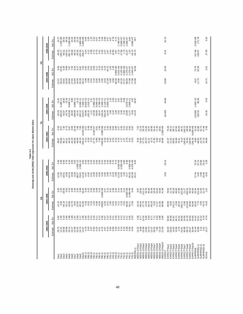
Est

imat

eS

td. E

rr.

Est

imat

eS

td. E

rr.

Est

imat

eS

td. E

rr.

Est

imat

eS

td. E

rr.

Est

imat

eS

td. E

rr.

Est

imat

eS

td. E

rr.

Est

imat

eS

td. E

rr.

Day

1-2

9.75

5.92

-14.

103.

39-1

2.55

4.26

-38.

876.

33-2

5.53

11.9

1-2

1.57

6.66

-40.

2514

.37

Day

2-1

2.31

1.90

-3.0

62.

29-2

.20

3.58

-50.

868.

57-4

00.0

35.

18E

+11

-48.

2320

.82

-259

.17

1.20

E+0

8D

ay3

-26.

064.

18-6

4.18

28.0

0-1

9.01

6.85

-46.

177.

30-5

3.87

18.8

2-1

9.81

6.39

-56.

3128

.02

Day

4-1

9.96

2.84

-16.

114.

03-5

.06

3.78

-42.

416.

73-4

3.76

15.2

6-3

3.59

9.89

-130

.10

48.1

8D

ay5

-16.

141.

98-1

6.56

4.15

-10.

134.

16-4

4.33

6.87

-313

.68

8.94

E+1

1-2

8.50

7.87

-281

.73

1.23

E+0

8D

ay6

-15.

271.

89-1

2.78

3.09

-8.5

93.

55-4

4.19

6.55

-26.

939.

80-2

7.81

7.40

-35.

6615

.03

Day

7-1

3.48

1.87

-8.6

42.

46-8

.28

3.55

-65.

8310

.19

-339

.69

4.89

E+1

1-3

3.84

9.26

-66.

7024

.69

Day

8-2

0.42

2.69

-22.

005.

35-8

8.57

1.50

E+1

0-4

9.49

7.66

-42.

4114

.19

-34.

049.

47-6

2.92

23.1

9D

ay9

-15.

742.

17-2

0.31

5.58

-78.

611.

53E

+10

-46.

197.

65-3

02.1

26.

03E

+11

-25.

266.

82-4

15.3

41.

48E

+08

Day

10-1

4.37

1.96

-51.

0618

.44

-12.

263.

84-2

54.2

46.

67E

+08

-319

.07

7.25

E+1

1-2

9.12

7.63

-256

.47

1.08

E+0

8O

B(-

1)-0

.79

0.54

0.18

0.28

-0.5

70.

330.

130.

57-6

4.66

8.61

E+1

00.

080.

500.

240.

83O

B(-

2)0.

030.

18-0

.02

0.22

-0.4

00.

29-0

.28

0.49

-100

.15

1.01

E+1

1-3

.56

2.04

-3.1

22.

05O

B(-

3)0.

070.

120.

150.

26-0

.01

0.15

0.23

0.45

-1.2

12.

21-0

.54

0.62

0.38

1.23

TB(-

1)-0

.55

0.18

-1.0

40.

49-0

.08

0.04

-27.

753.

21E

+07

-22.

562.

38E

+10

0.10

0.09

-2.7

43.

22TB

(-2)

-0.2

00.

11-0

.08

0.09

-0.0

40.

05-0

.90

0.61

-40.

833.

04E

+10

-0.0

50.

11-0

.75

0.57

TB(-

3)-0

.21

0.12

-0.2

50.

13-0

.09

0.05

-1.5

81.

00-2

8.47

2.78

E+1

00.

000.

100.

410.

18P

B(-

1)-0

.75

0.36

-230

205.

80E

+09

0.05

0.12

-734

0.65

2.95

E+0

8-1

39.1

91.

04E

+11

0.55

0.25

0.25

1.06

PB

(-2)

0.07

0.07

-0.3

00.

470.

050.

16-0

.18

0.31

-633

.28

2.11

E+1

1-0

.03

0.19

0.47

0.90

PB

(-3)

-0.1

00.

10-0

.01

0.13

0.08

0.16

-0.3

00.

35-1

0.44

5.66

E+1

0-2

7.09

44.7

00.

670.

57O

S(-

1)0.

940.

241.

900.

411.

100.

690.

420.

601.

661.

15-0

.90

1.50

-3.4

44.

67O

S(-

2)-0

.06

0.21

-0.0

30.

36-0

.18

0.70

0.25

0.63

0.44

1.63

0.58

1.39

10.9

54.

78O

S(-

3)0.

200.

180.

520.

340.

080.

700.

160.

852.

953.

27-8

2.06

6.90

E+0

60.

875.

74TS

(-1)

0.22

0.10

0.11

0.14

-11.

033.

01E

+09

0.76

0.27

2.62

2.87

-8.9

82.

61E

+06

-2.1

51.

74E

+07

TS(-

2)0.

140.

120.

230.

44-6

.05

2.25

E+0

91.

270.

260.

490.

50-3

2.33

4.12

E+0

6-1

7.66

3.04

E+0

7TS

(-3)

0.10

0.12

0.25

0.15

1.50

0.85

1.07

0.24

0.32

0.59

-27.

074.

06E

+06

1.73

1.76

E+0

7P

S(-

1)0.

380.

11-6

6.56

4.66

E+0

9-0

.17

0.38

0.79

0.51

10.8

92.

07E

+11

-98.

551.

27E

+07

-31.

071.

94E

+07

PS

(-2)

-0.5

60.

36-5

3.11

4.78

E+0

9-4

5.20

3.92

E+0

90.

010.

5611

.27

2.00

E+1

1-7

7.08

1.17

E+0

71.

520.

84P

S(-

3)-0

.04

0.23

0.26

0.44

-62.

484.

37E

+09

-0.2

30.

62-0

.05

2.87

-77.

961.

10E

+07

-62.

102.

84E

+07

NE

ED

N(-

1)-2

0.21

6.05

-14.

2326

.87

-15.

9910

.59

-54.

7429

.7N

EE

D(-

1)*D

ay1

-12.

254.

38-1

0.16

8.97

-9.3

47.

02N

EE

D(-

1)*D

ay2

-8.6

86.

77-6

6.44

28.5

0-1

0.83

22.1

3N

EE

D(-

1)*D

ay3

-23.

5813

.32

-27.

7521

2.12

-27.

7529

.78

NE

ED

(-1)

*Day

4-1

3.90

8.46

12.4

516

.76

-33.

7021

.82

NE

ED

(-1)

*Day

5-1

0.70

5.93

-54.

7430

.29

-11.

2119

.37

NE

ED

(-1)

*Day

6-1

3.37

8.71

-40.

2920

.39

-6.7

326

.08

NE

ED

(-1)

*Day

7-3

9.20

7.11

-5.5

018

.18

27.9

526

.41

NE

ED

(-1)

*Day

8-7

.85

6.33

-17.

2724

.44

-5.6

017

.30

NE

ED

(-1)

*Day

9-1

3.19

4.98

-21.

6515

.66

-4.6

118

.61

NE

ED

(-1)

*Day

10-1

1.50

3.06

-95.

8841

.38

28.8

61.

55E

+09

EX

PE

CT

4.63

19.1

464

.409

44.6

6-1

9.69

19.4

5-6

.31

81.1

0E

XP

EC

T*D

ay1

64.2

050

.84

-69.

5678

.53

-22.

3775

.26

EX

PE

CT*

Day

2-2

8.50

26.5

8-8

.94

21.7

6-1

1.02

95.1

2E

XP

EC

T*D

ay3

14.6

351

.87

142.

2193

.29

-59.

8198

.71

EX

PE

CT*

Day

410

.56

40.7

4-2

.94

45.8

353

.46

87.9

2E

XP

EC

T*D

ay5

-2.7

631

.82

-25.

2637

.96

51.5

185

.03

EX

PE

CT*

Day

6-2

3.51

30.9

0-2

55.1

131

0.30

8.10

84.3

1E

XP

EC

T*D

ay7

60.9

924

.95

-2.9

821

.27

-169

.45

148.

13E

XP

EC

T*D

ay8

-59.

7041

.29

-213

.83

450.

43-7

8.30

99.0

6E

XP

EC

T*D

ay9

-25.

4734

.46

30.9

026

.19

135.

9398

.16

EX

PE

CT*

Day

1055

.94

23.0

055

.96

45.6

5-1

56.1

89.

62E

+09

SU

RP

RIS

E31

.44

14.4

2-2

5.02

52.3

427

.44

75.3

3-9

.84

31.5

411

9.00

61.

02E

+13

-8.0

773

.76

517.

662.

51E

+08

SU

RP

RIS

E(-

1)10

.86

10.5

17.

7414

1.49

9.40

37.1

4-6

9.52

31.8

8-1

62.9

485

.35

-11.

7092

.35

-130

.07

171.

78S

UR

PR

ISE

(-2)

3.15

10.2

24.

0521

.55

0.89

25.8

6-1

0.79

32.7

4S

UR

PR

ISE

(-3)

0.31

9.79

-76.

7531

.70

25.4

615

.14

57.1

347

.46

SC

ALE

10.1

70.

748.

431.

018.

031.

3926

.66

2.58

24.3

55.

0314

.72

2.91

27.3

95.

92

1984

-199

419

94-1

998

48

1984

-199

419

94-1

998

Tabl

e A

.2D

emira

lp a

nd J

ordà

(200

2) T

obit

regr

essi

on fo

r Ope

n M

arke

t Sal

es

OS

TSPS

1994

-199

819

98-2

000

1998

-200

0