applied sciences

Article

A Frequency–Power Droop Coefficient DeterminationMethod of Mixed Line-Commutated andVoltage-Sourced Converter Multi-Infeed,High-Voltage, Direct Current Systems: An ActualCase Study in Korea

Gyusub Lee 1 , Seungil Moon 1 and Pyeongik Hwang 2,*1 Department of Electrical and Computer Engineering, Seoul National University, Seoul 08826, Korea;

lgs1106@snu.ac.kr (G.L.); moonsi@snu.ac.kr (S.M.)2 Department of Electrical Engineering, Chosun University, Gwangju 61452, Korea* Correspondence: hpi@chosun.ac.kr; Tel.: +82-62-230-7033

Received: 10 December 2018; Accepted: 9 February 2019; Published: 12 February 2019�����������������

Abstract: Among the grid service applications of high-voltage direct current (HVDC) systems,frequency–power droop control for islanded networks is one of the most widely used schemes. In thispaper, a new frequency-power droop coefficient determination method for a mixed line-commutatedconverter (LCC) and voltage-sourced converter (VSC)-based multi-infeed HVDC (MIDC) system isproposed. The proposed method is designed for the minimization of power loss. An interior-pointmethod is used as an optimization algorithm to implement the proposed scheduling method, and thedroop coefficients of the HVDCs are determined graphically using the Monte Carlo sampling method.Two test systems—the modified Institute of Electrical and Electronics Engineers (IEEE) 14-bussystem and an actual Jeju Island network in Korea—were utilized for MATLAB simulation casestudies, to demonstrate that the proposed method is effective for reducing power system loss duringfrequency control.

Keywords: grid service of HVDC; frequency droop control; multi-infeed HVDC system; LCC HVDC;VSC HVDC; loss minimization

1. Introduction

High-voltage direct current (HVDC) systems have played an important role in sub-marinepower transmission, due to economic advantages over their alternating current (AC) counterparts [1].Nowadays, due to the complexity of modern power systems, HVDC systems are adopted inpractice, not only for constant power delivery between massive networks, but also to providegrid services for island grids [2–8]. For example, in Korea, two line-commutated converter (LCC)HVDCs, the 180-kV/300-MW Haenam–Jeju HVDC [9] and ±250 kV/400 MW Jindo–Jeju HVDC [10],were constructed by the Korea Electric Power Corporation (KEPCO) for supporting Jeju Island andintegrating massive wind power plants. Furthermore, KEPCO is planning to construct one more±150 kV/200 MW voltage-sourced converter (VSC) HVDC between the main grid and Jeju Island [11].

With the technical development of both the LCC and VSC HVDC systems, there are numerousisland networks with multi-infeed HVDC (MIDC) systems, encompassing both types of HVDCs,similar to the Jeju Island case. According to trends, many studies have concentrated on the MIDCsystems [12–16]. Major research effort has been focused on the stable operation of the MIDC systemsby introducing novel indexes, such as the multi-infeed interaction factor (MIIF), multi-infeed effective

Appl. Sci. 2019, 9, 606; doi:10.3390/app9030606 www.mdpi.com/journal/applsci

Appl. Sci. 2019, 9, 606 2 of 14

short-circuit ratio (MIESCR) [12], apparent increase in short-circuit ratio (AISCR) [13], and improvedeffective short-circuit ratio (IESCR) [14]. In parallel with such research, some studies have concentratedon the economic operation of MIDC systems, which is represented by optimal power flow (OPF) [17–20].In two such studies [17,18], steady-state VSC–HVDC modeling methods and OPF formulations basedon the Newton–Raphson method are proposed. Although only a single HVDC system is considered inthese studies [17,18], the principle can be easily expanded to MIDC systems. In one study [19], a lossminimization method with an AC/DC hybrid grid incorporating only VSC HVDCs is proposed, basedon an interior-point method. In another study [20], a similar method adopting both LCC and VSCHVDC is proposed. However, the authors of the above studies only consider the steady-state values ofthe HVDC systems. Thus, if the load profiles were different from the forecasted value, the previousmethods were unable to find the optimal set-point, because the forecasting error was not considered.

A common method used to satisfy the power balance between generation and load caused by theforecasting error is frequency–power droop control [21]. Similar to conventional generators, HVDCsystems also adopt frequency–power droop controllers [22–24]. For economic operation of powersystems during frequency control, the calculation of droop coefficients is a significant issue, and thecoefficients are used to exploit multiple HVDC systems efficiently. It is practically important in thecase of an islanded network, because the islanded system has a small load level and high renewableenergy penetration, which cause high uncertainties in the power system. Due to those characteristics,off-nominal frequency situations occur more frequently, and the frequency deviation is more severethan the conventional large power network. In one study [25], an optimum calculation method ofvoltage–power droop coefficients for multi-terminal HVDC (MTDC) systems is proposed. However,the method could only be applied to the specific topology of the DC grid investigated in the paper.Another study proposes an optimization-based droop coefficient calculation method to maximizeconverter efficiencies for a low-voltage system [26]. A method to minimize DC transmission line lossusing voltage–current droop coefficients has also been proposed [27]. The above research suggests thatthe droop coefficients of converters can be calculated by optimization of the problem. However, to ourknowledge, optimization problems have rarely been suggested to calculate frequency–power droopcoefficients of MIDC systems.

This paper suggests a method to determine the frequency–power droop coefficients of multipleHVDCs in MIDC systems. First, we propose an optimization problem for MIDC systems, to determinethe operating points of HVDCs to minimize system loss. Using the results of the optimization problem,we propose a droop coefficient design method based on Monte Carlo sampling. The proposed methodis verified by MATLAB simulation utilizing IEEE test systems and the actual networks of Jeju Island inKorea. Using our method, a system operator can define the operating points and droop coefficients ofan MIDC system more efficiently.

2. Description of the Proposed Method

2.1. Optimazation Problem to Determine Operating Points

In this section, we formulate an optimization problem to determine the operating points ofmultiple HVDCs, including LCC and VSC HVDCs. This study is different from previous studiescovering various type of HVDCs [22–25,27], because HVDCs can be regarded as active and reactivepower sources in MIDC systems. Also, only the outputs of multiple HVDCs are considered in theoptimization problem. In other words, generator outputs are considered as a constant in the problem.

2.1.1. Model Description

To formulate the constraints used in the optimization problem, power balance equationsand converter models are required. In the case of the VSC, which can synthesize sine-wave ACvoltage regardless of the residual network, the active and reactive power output—PVSC and QVSC,

Appl. Sci. 2019, 9, 606 3 of 14

respectively—are regulated independently [28]. Therefore, a VSC can be considered similar to a PQload for the optimization, and the only consideration is the rated output power, as follows:√

P2VSC(n) + Q2

VSC(n) < SVSC.rate(n), (1)

where SVSC.rate(n) is the rated apparent power of the VSC HVDC connected to the n-th bus. Note thatconversion loss of a VSC HVDC is ignored, because the input variables of controller are active andreactive power output at the inverter side. However, for future work, the conversion loss of VSCshould be considered for solving overall optimization problems, including a DC system. The reactivepower output of the LCC, QLCC, is different from the VSC, and cannot be regulated independent ofthe active power, PLCC [29]. As conversion loss of LCC is less than 1% in general, the loss can beignored [30]. Thus, QLCC can be presented as:

QLCC(n) = PLCC(n) tan Φ(n) (2)

where Φ(n) is the power factor angle of LCC HVDC connected to the n-th bus. The power factor anglecan be expressed as follows [31]:

tan Φ(n) =2µ(n) + sin(2α(n))− sin(2α(n) + 2µ(n))

cos(2α(n))− cos(2α(n) + 2µ(n))(3)

where

α(n) = cos−1

[π

3√

2B(n)T(n)V(n)

(VDC.rate(n) +

3XC(n)PLCC(n)πVDC.rate(n)

)](4)

µ(n) = cos−1

[cos(α(n))−

√2XC(n)PLCC(n)

B(n)T(n)V(n)VDC.rate

]− α (5)

where V(n) represents voltage magnitude at n-th bus, and VDC.rate(n) is the rated DC voltage of the LCCHVDC connected to the n-th bus. The transformer turn ratio and the number of six-pulse bridges atthe n-th bus are represented by T(n) and B(n), respectively. The reactance of the converter transformerat the n-th bus is described by XC(n). An inequality constraint of an LCC HVDC can be represented as

PLCC(n) < PLCC.rate(n) (6)

where PLCC.rate(n) is the rated active power of the LCC HVDC connected to n-th bus. Note that theindex of the bus number (n) is utilized to express HVDC system connected to the n-th bus, which meansmultiple HVDCs can be considered in the proposed models, because each converter is connected toa different bus.

For every bus, the injected active (P) and reactive (Q) power, including generator output(PGEN and QGEN), VSC output (PVSC and QVSC), LCC output (PLCC and QLCC), and connected load(PLOAD and QLOAD) satisfy the following constraints [32]:

PGEN(n) + PVSC(n) + PLCC(n)− PLOAD(n)−N∑

k=1V(n)V(k){G(n, k) cos(θ(n)− θ(k)) + B(n, k) sin(θ(n)− θ(k))} = 0 (7)

QGEN(n) + QVSC(n) + QLCC(n)−QLOAD(n)−N∑

k=1V(n)V(k){G(n, k) sin(θ(n)− θ(k))− B(n, k) cos(θ(n)− θ(k))} = 0 (8)

where the phase angle of n-th bus is represented by θ(n). An injected active and reactive powerof the n-th bus can be represented by P(n) and Q(n), respectively. The real and imaginary partsof the admittance matrix between the n-th bus and k-th bus are represented as G(n,k) and B(n,k),respectively. If the generator, VSC, LCC, or load is not connected to bus n, the value of each symbolis zero. Note that PGEN and QGEN are pre-determined by the system operator, and PLOAD and QLOAD

Appl. Sci. 2019, 9, 606 4 of 14

are previously forecasted values, which are considered as constant in the optimization problem.The security constraint of the AC voltage magnitude for per unit (p.u.) system can be represented as:

0.95 p.u. < V(n) < 1.05 p.u. (9)

2.1.2. Optimization Formulation and Solving Method

The vectors of the phase angle and voltage magnitude are represented as θ and V, respectively.The output references of VSC and LCC HVDCs can be represented by vector form, as PVSC, QVSC,and PLCC. Note that the reactive power of LCC HVDC, QLCC, can be represented in terms of PLCC andV using Equations (2)–(5), so it is not necessary to include QLCC with the unknown vector. Therefore,the unknown vector, X, can be defined as:

X =[

PTVSC QT

VSC PTLCC θT VT

]T. (10)

The purpose of the proposed problem is to minimize the system loss. Since conversion loss is notincluded in MIDC systems, only the line loss of AC systems is considered in the objective function.The objective function of the optimization is represented as:

minimize f =N

∑j=n{PGEN(n) + PVSC(n) + PLCC(n)− PLOAD(n)} (11)

where N is the number of buses. Note that the difference between the active power injected tothe network, PGEN, PVSC, PLCC, and PLOAD is the same as the system loss. Only LCC and VSCHVDCs are considered as frequency-supporting resources in this paper, with the assumption thatconventional generators do not participate in frequency support. However, conventional generatorscan be considered in the optimization problem with a little modification, because the generators canbe represented as active and reactive power sources similar to the VSC HVDC system. Additionally,the security constraint of the conventional generators can be represented by simple inequality of activeand reactive power [33].

To solve the optimization problem, an interior-point method is used [34,35]. For the proposedoptimization problem, an interior-point method cannot guarantee global optimality. However, as thesolution found by the method is better than a trivial solution, the interior-point method can besuccessfully applied to the proposed optimization problem.

2.2. Frequency–Power Droop Coefficient Determination Method

In the optimization problem described in the previous section, the forecasted load profile is used tocalculate the optimal operating points. However, load characteristics are different from the forecastedvalues, because there are uncertainties in the load forecasting procedure. Furthermore, uncertaintyincreases with the integration of bulk renewable energies [36]. In this situation, the outputs of multipleHVDCs form new operating points following droop characteristics, the coefficient of which is generallyproportional to the capacities of the converters [37]. The conventional method for determining droopcoefficients is simple, but the coefficients cannot create a more efficient solution. Therefore, a droopcoefficient design method based on an optimization problem is required to operate MIDC systemsmore economically. We propose a statistical method to obtain optimal droop coefficients in this section.

2.2.1. Stochastic Optimization Based on the Monte Carlo Sampling Method

To determine the droop coefficient in the proposed method, the Monte Carlo sampling methodwas utilized [38]. In the Monte Carlo sampling method, a number of load profiles are generated and areutilized for solving the optimization problem. All cases are generated based on probabilistic function,such as normal distribution, to represent possible realizations in the presence of forecast errors. For each

Appl. Sci. 2019, 9, 606 5 of 14

load profile, the optimization problem of the previous section is solved, and operating points of HVDCsare calculated. The sampling number is represented by i, and the output of LCC and VSC HVDCsconnected to the n-th bus at the i-th sample is represented as PVSC(n,i) and PLCC(n,i), respectively.

Furthermore, frequency deviation for each load profile is also calculated in this stage. To derivefrequency deviation, the relationship between load profile and grid frequency should be established.Therefore, on the assumption that only HVDCs participate in frequency regulation, we use the swingequations of the power network, including frequency-supporting HVDCs and a load with dampingeffects, as follows [21]:

N

∑j=n{PGEN(n, i) + PVSC(n, i) + PLCC(n, i)− PLOAD(n, i)} = Meq

d∆ω(i)dt

+ D∆ω(i) (12)

where Meq is the moment of inertia and D is the load damping coefficient. The deviation of gridfrequency is represented by ∆ω. As the steady-state value (i.e., ∆ω = 0) of the left side of Equation (12)is equal to zero, and the active power of the HVDCs can be represented by the corresponding droopcoefficients, the frequency deviation can be described as

∆ω(i) =−

N∑

n=1∆PLOAD(n, i)

N∑

n=1

1RVSC(n)

+N∑

n=1

1RLCC(n)

+ D, (13)

where ∆PLOAD(n,i) is the change in the load profile of the n-th bus at the i-th sample, which is definedby the Monte Carlo sampling method. RVSC(n) and RLCC(n) represent the droop coefficient of the VSCand LCC HVDC connected to the n-th bus, respectively. The frequency deviation cannot be deriveddirectly from Equation (13), because the droop coefficients of the HVDCs, which are not determinedyet, are utilized to derive the frequency deviation. Therefore, we assume that the sum of coefficients isconstant, as follows:

N

∑n=1

1RVSC(n)

+N

∑n=1

1RLCC(n)

=1

Req(14)

where Req is an equivalent droop coefficient of the total system. Note that the active power of HVDCsduring grid frequency only depends on the ratio of the droop coefficient, so power sharing betweenmultiple HVDCs can be regulated properly while satisfying the constraint (14).

2.2.2. Graphical Analysis to Determine Droop Coefficients

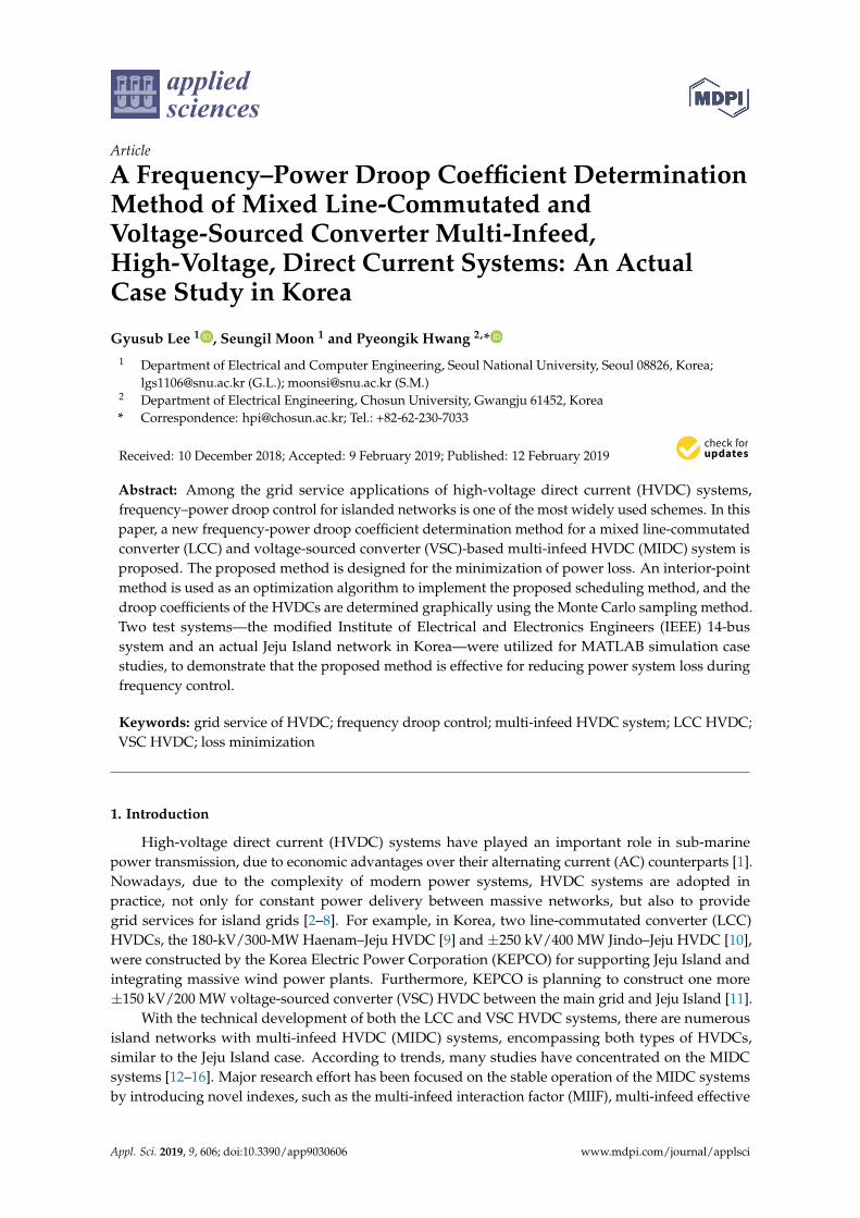
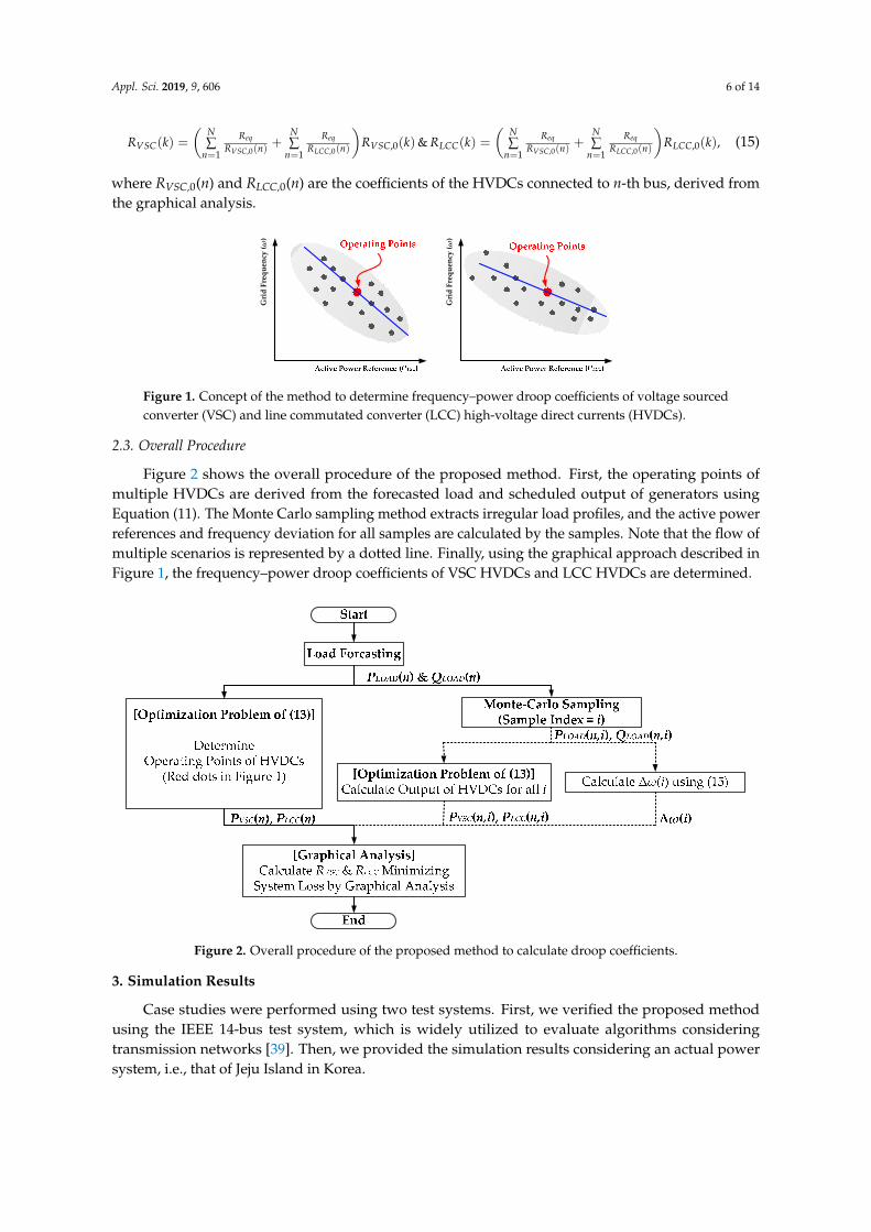
In this section, we derive the droop coefficients of LCC and VSC HVDCs by graphical analysis.Figure 1 shows a concept of the proposed method of droop coefficient determination. Red pointsare operating points of LCC and VSC HVDCs determined by the optimization problem. Grey dotsrepresent optimization results of the Monte Carlo samples. The points are categorized by active powerreference and grid frequency, so that the frequency–power droop can be represented by the slope ofthe blue line, to minimize the root mean square error between the points above the blue line and thegrey dots. The slopes of the blue lines are presented as −RVSC,0 for VSC HVDC and −RLCC,0 for theLCC HVDC. Note that the determination method is called the “graphic method”, in that curve-fittingis exploited for coefficient determination.

We can derive droop coefficients of LCC and VSC HVDCs from Figure 1, but the coefficientsmay not satisfy Equation (14), because the power loss of the system is not considered in (12). We candetermine final values of the coefficients by the additional correction method. As active power sharingratio of HVDCs depend on the ration of droop coefficients, final droop coefficients are corrected bymultiplying the same constant to RLCC,0 and RVSC,0. Thus final coefficients are determined as

Appl. Sci. 2019, 9, 606 6 of 14

RVSC(k) =(

N∑

n=1

ReqRVSC,0(n)

+N∑

n=1

ReqRLCC,0(n)

)RVSC,0(k)& RLCC(k) =

(N∑

n=1

ReqRVSC,0(n)

+N∑

n=1

ReqRLCC,0(n)

)RLCC,0(k), (15)

where RVSC,0(n) and RLCC,0(n) are the coefficients of the HVDCs connected to n-th bus, derived fromthe graphical analysis.

Appl. Sci. 2018, 8, x FOR PEER REVIEW 5 of 15

Furthermore, frequency deviation for each load profile is also calculated in this stage. To de-rive frequency deviation, the relationship between load profile and grid frequency should be estab-lished. Therefore, on the assumption that only HVDCs participate in frequency regulation, we use the swing equations of the power network, including frequency-supporting HVDCs and a load with damping effects, as follows [21]:

{ } ω ω=

Δ+ + − = + Δ ( )( , ) ( , ) ( , ) ( , ) ( )N

GEN VSC LCC LOAD eqj n

d iP n i P n i P n i P n i M D idt

(12)

where Meq is the moment of inertia and D is the load damping coefficient. The deviation of grid frequency is represented by Δω. As the steady-state value (i.e., Δω = 0) of the left side of Equation (12) is equal to zero, and the active power of the HVDCs can be represented by the corresponding droop coefficients, the frequency deviation can be described as

ω =

= =

− ΔΔ =

+ +

1

1 1

( , )( )

1 1( ) ( )

N

LOADn

N N

n nVSC LCC

P n ii

DR n R n

, (13)

where ΔPLOAD(n,i) is the change in the load profile of the n-th bus at the i-th sample, which is de-fined by the Monte Carlo sampling method. RVSC(n) and RLCC(n) represent the droop coefficient of the VSC and LCC HVDC connected to the n-th bus, respectively. The frequency deviation cannot be derived directly from Equation (13), because the droop coefficients of the HVDCs, which are not determined yet, are utilized to derive the frequency deviation. Therefore, we assume that the sum of coefficients is constant, as follows:

= =

+ = 1 1

1 1 1( ) ( )

N N

n nVSC LCC eqR n R n R (14)

where Req is an equivalent droop coefficient of the total system. Note that the active power of HVDCs during grid frequency only depends on the ratio of the droop coefficient, so power sharing between multiple HVDCs can be regulated properly while satisfying the constraint (14).

2.2.2. Graphical Analysis to Determine Droop Coefficients

In this section, we derive the droop coefficients of LCC and VSC HVDCs by graphical analysis. Figure 1 shows a concept of the proposed method of droop coefficient determination. Red points are operating points of LCC and VSC HVDCs determined by the optimization problem. Grey dots represent optimization results of the Monte Carlo samples. The points are categorized by active power reference and grid frequency, so that the frequency–power droop can be represented by the slope of the blue line, to minimize the root mean square error between the points above the blue line and the grey dots. The slopes of the blue lines are presented as −RVSC,0 for VSC HVDC and −RLCC,0 for the LCC HVDC. Note that the determination method is called the “graphic method”, in that curve-fitting is exploited for coefficient determination.

Gri

d Fr

eque

ncy

(ω)

Gri

d Fr

eque

ncy

(ω)

Figure 1. Concept of the method to determine frequency–power droop coefficients of voltage sourced converter (VSC) and line commutated converter (LCC) high-voltage direct currents (HVDCs).

Figure 1. Concept of the method to determine frequency–power droop coefficients of voltage sourcedconverter (VSC) and line commutated converter (LCC) high-voltage direct currents (HVDCs).

2.3. Overall Procedure

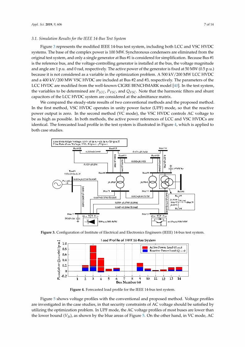
Figure 2 shows the overall procedure of the proposed method. First, the operating points ofmultiple HVDCs are derived from the forecasted load and scheduled output of generators usingEquation (11). The Monte Carlo sampling method extracts irregular load profiles, and the active powerreferences and frequency deviation for all samples are calculated by the samples. Note that the flow ofmultiple scenarios is represented by a dotted line. Finally, using the graphical approach described inFigure 1, the frequency–power droop coefficients of VSC HVDCs and LCC HVDCs are determined.

Appl. Sci. 2018, 8, x FOR PEER REVIEW 6 of 15

We can derive droop coefficients of LCC and VSC HVDCs from Figure 1, but the coefficients may not satisfy Equation (14), because the power loss of the system is not considered in (12). We can determine final values of the coefficients by the additional correction method. As active power sharing ratio of HVDCs depend on the ration of droop coefficients, final droop coefficients are cor-rected by multiplying the same constant to RLCC,0 and RVSC,0. Thus final coefficients are determined as

= = = =

= + = + ,0 ,0

1 1 1 1,0 ,0 ,0 ,0

( ) ( ) & ( ) ( )( ) ( ) ( ) ( )

N N N Neq eq eq eq

VSC VSC LCC LCCn n n nVSC LCC VSC LCC

R R R RR k R k R k R k

R n R n R n R n, (15)

where RVSC,0(n) and RLCC,0(n) are the coefficients of the HVDCs connected to n-th bus, derived from the graphical analysis.

2.3. Overall Procedure

Figure 2 shows the overall procedure of the proposed method. First, the operating points of multiple HVDCs are derived from the forecasted load and scheduled output of generators using Equation (11). The Monte Carlo sampling method extracts irregular load profiles, and the active power references and frequency deviation for all samples are calculated by the samples. Note that the flow of multiple scenarios is represented by a dotted line. Finally, using the graphical approach described in Figure 1, the frequency–power droop coefficients of VSC HVDCs and LCC HVDCs are determined.

Figure 2. Overall procedure of the proposed method to calculate droop coefficients.

3. Simulation Results

Case studies were performed using two test systems. First, we verified the proposed method using the IEEE 14-bus test system, which is widely utilized to evaluate algorithms considering transmission networks [39]. Then, we provided the simulation results considering an actual power system, i.e., that of Jeju Island in Korea.

3.1. Simulation Results for the IEEE 14-Bus Test System

Figure 3 represents the modified IEEE 14-bus test system, including both LCC and VSC HVDC systems. The base of the complex power is 100 MW. Synchronous condensers are eliminated from the original test system, and only a single generator at Bus #1 is considered for simplification. Be-cause Bus #1 is the reference bus, and the voltage-controlling generator is installed at the bus, the voltage magnitude and angle are 1 p.u. and 0 rad, respectively. The active power of the generator is

Figure 2. Overall procedure of the proposed method to calculate droop coefficients.

3. Simulation Results

Case studies were performed using two test systems. First, we verified the proposed methodusing the IEEE 14-bus test system, which is widely utilized to evaluate algorithms consideringtransmission networks [39]. Then, we provided the simulation results considering an actual powersystem, i.e., that of Jeju Island in Korea.

Appl. Sci. 2019, 9, 606 7 of 14

3.1. Simulation Results for the IEEE 14-Bus Test System

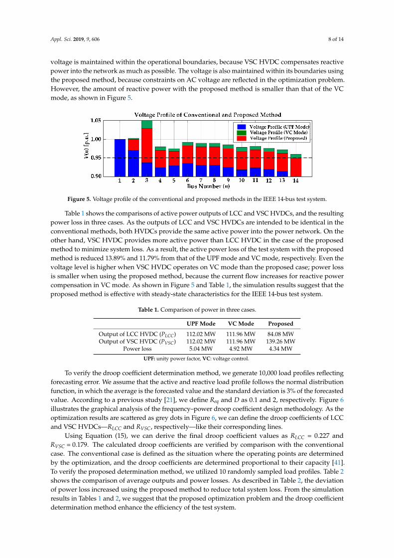
Figure 3 represents the modified IEEE 14-bus test system, including both LCC and VSC HVDCsystems. The base of the complex power is 100 MW. Synchronous condensers are eliminated from theoriginal test system, and only a single generator at Bus #1 is considered for simplification. Because Bus #1is the reference bus, and the voltage-controlling generator is installed at the bus, the voltage magnitudeand angle are 1 p.u. and 0 rad, respectively. The active power of the generator is fixed at 50 MW (0.5 p.u.)because it is not considered as a variable in the optimization problem. A 500 kV/200 MW LCC HVDCand a 400 kV/200 MW VSC HVDC are included at Bus #2 and #3, respectively. The parameters of theLCC HVDC are modified from the well-known CIGRE BENCHMARK model [40]. In the test system,the variables to be determined are PLCC, PVSC, and QVSC. Note that the harmonic filters and shuntcapacitors of the LCC HVDC system are considered at the admittance matrix.

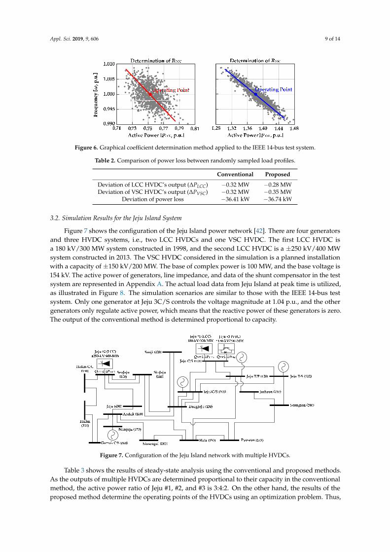
We compared the steady-state results of two conventional methods and the proposed method.In the first method, VSC HVDC operates in unity power factor (UPF) mode, so that the reactivepower output is zero. In the second method (VC mode), the VSC HVDC controls AC voltage tobe as high as possible. In both methods, the active power references of LCC and VSC HVDCs areidentical. The forecasted load profile in the test system is illustrated in Figure 4, which is applied toboth case studies.

Appl. Sci. 2018, 8, x FOR PEER REVIEW 7 of 15

fixed at 50 MW (0.5 p.u.) because it is not considered as a variable in the optimization problem. A 500 kV/200 MW LCC HVDC and a 400 kV/200 MW VSC HVDC are included at Bus #2 and #3, re-spectively. The parameters of the LCC HVDC are modified from the well-known CIGRE BENCH-MARK model [40]. In the test system, the variables to be determined are PLCC, PVSC, and QVSC. Note that the harmonic filters and shunt capacitors of the LCC HVDC system are considered at the ad-mittance matrix.

We compared the steady-state results of two conventional methods and the proposed method. In the first method, VSC HVDC operates in unity power factor (UPF) mode, so that the reactive power output is zero. In the second method (VC mode), the VSC HVDC controls AC voltage to be as high as possible. In both methods, the active power references of LCC and VSC HVDCs are iden-tical. The forecasted load profile in the test system is illustrated in Figure 4, which is applied to both case studies.

Figure 3. Configuration of Institute of Electrical and Electronics Engineers (IEEE) 14-bus test system.

Figure 4. Forecasted load profile for the IEEE 14-bus test system.

Figure 5 shows voltage profiles with the conventional and proposed method. Voltage profiles are investigated in the case studies, in that security constraints of AC voltage should be satisfied by utilizing the optimization problem. In UPF mode, the AC voltage profiles of most buses are lower than the lower bound (Vlb), as shown by the blue areas of Figure 5. On the other hand, in VC mode, AC voltage is maintained within the operational boundaries, because VSC HVDC compensates re-active power into the network as much as possible. The voltage is also maintained within its boundaries using the proposed method, because constraints on AC voltage are reflected in the op-timization problem. However, the amount of reactive power with the proposed method is smaller than that of the VC mode, as shown in Figure 5.

Figure 3. Configuration of Institute of Electrical and Electronics Engineers (IEEE) 14-bus test system.

Appl. Sci. 2018, 8, x FOR PEER REVIEW 7 of 15

fixed at 50 MW (0.5 p.u.) because it is not considered as a variable in the optimization problem. A 500 kV/200 MW LCC HVDC and a 400 kV/200 MW VSC HVDC are included at Bus #2 and #3, re-spectively. The parameters of the LCC HVDC are modified from the well-known CIGRE BENCH-MARK model [40]. In the test system, the variables to be determined are PLCC, PVSC, and QVSC. Note that the harmonic filters and shunt capacitors of the LCC HVDC system are considered at the ad-mittance matrix.

We compared the steady-state results of two conventional methods and the proposed method. In the first method, VSC HVDC operates in unity power factor (UPF) mode, so that the reactive power output is zero. In the second method (VC mode), the VSC HVDC controls AC voltage to be as high as possible. In both methods, the active power references of LCC and VSC HVDCs are iden-tical. The forecasted load profile in the test system is illustrated in Figure 4, which is applied to both case studies.

Figure 3. Configuration of Institute of Electrical and Electronics Engineers (IEEE) 14-bus test system.

Figure 4. Forecasted load profile for the IEEE 14-bus test system.

Figure 5 shows voltage profiles with the conventional and proposed method. Voltage profiles are investigated in the case studies, in that security constraints of AC voltage should be satisfied by utilizing the optimization problem. In UPF mode, the AC voltage profiles of most buses are lower than the lower bound (Vlb), as shown by the blue areas of Figure 5. On the other hand, in VC mode, AC voltage is maintained within the operational boundaries, because VSC HVDC compensates re-active power into the network as much as possible. The voltage is also maintained within its boundaries using the proposed method, because constraints on AC voltage are reflected in the op-timization problem. However, the amount of reactive power with the proposed method is smaller than that of the VC mode, as shown in Figure 5.

Figure 4. Forecasted load profile for the IEEE 14-bus test system.

Figure 5 shows voltage profiles with the conventional and proposed method. Voltage profilesare investigated in the case studies, in that security constraints of AC voltage should be satisfied byutilizing the optimization problem. In UPF mode, the AC voltage profiles of most buses are lower thanthe lower bound (Vlb), as shown by the blue areas of Figure 5. On the other hand, in VC mode, AC

Appl. Sci. 2019, 9, 606 8 of 14

voltage is maintained within the operational boundaries, because VSC HVDC compensates reactivepower into the network as much as possible. The voltage is also maintained within its boundaries usingthe proposed method, because constraints on AC voltage are reflected in the optimization problem.However, the amount of reactive power with the proposed method is smaller than that of the VCmode, as shown in Figure 5.Appl. Sci. 2018, 8, x FOR PEER REVIEW 8 of 15

Figure 5. Voltage profile of the conventional and proposed methods in the IEEE 14-bus test system.

Table 1 shows the comparisons of active power outputs of LCC and VSC HVDCs, and the re-sulting power loss in three cases. As the outputs of LCC and VSC HVDCs are intended to be iden-tical in the conventional methods, both HVDCs provide the same active power into the power net-work. On the other hand, VSC HVDC provides more active power than LCC HVDC in the case of the proposed method to minimize system loss. As a result, the active power loss of the test system with the proposed method is reduced 13.89% and 11.79% from that of the UPF mode and VC mode, respectively. Even the voltage level is higher when VSC HVDC operates on VC mode than the proposed case; power loss is smaller when using the proposed method, because the current flow increases for reactive power compensation in VC mode. As shown in Figure 5 and Table 1, the sim-ulation results suggest that the proposed method is effective with steady-state characteristics for the IEEE 14-bus test system.

Table 1. Comparison of power in three cases

UPF Mode VC Mode Proposed Output of LCC HVDC (PLCC) 112.02 MW 111.96 MW 84.08 MW Output of VSC HVDC (PVSC) 112.02 MW 111.96 MW 139.26 MW

Power loss 5.04 MW 4.92 MW 4.34 MW UPF: unity power factor, VC: voltage control

To verify the droop coefficient determination method, we generate 10,000 load profiles reflect-ing forecasting error. We assume that the active and reactive load profile follows the normal distri-bution function, in which the average is the forecasted value and the standard deviation is 3% of the forecasted value. According to a previous study [21], we define Req and D as 0.1 and 2, respectively. Figure 6 illustrates the graphical analysis of the frequency–power droop coefficient design method-ology. As the optimization results are scattered as grey dots in Figure 6, we can define the droop coefficients of LCC and VSC HVDCs—RLCC and RVSC, respectively—like their corresponding lines.

Figure 6. Graphical coefficient determination method applied to the IEEE 14-bus test system.

Using Equation (15), we can derive the final droop coefficient values as RLCC = 0.227 and RVSC = 0.179. The calculated droop coefficients are verified by comparison with the conventional case. The conventional case is defined as the situation where the operating points are determined by the op-

Figure 5. Voltage profile of the conventional and proposed methods in the IEEE 14-bus test system.

Table 1 shows the comparisons of active power outputs of LCC and VSC HVDCs, and the resultingpower loss in three cases. As the outputs of LCC and VSC HVDCs are intended to be identical in theconventional methods, both HVDCs provide the same active power into the power network. On theother hand, VSC HVDC provides more active power than LCC HVDC in the case of the proposedmethod to minimize system loss. As a result, the active power loss of the test system with the proposedmethod is reduced 13.89% and 11.79% from that of the UPF mode and VC mode, respectively. Even thevoltage level is higher when VSC HVDC operates on VC mode than the proposed case; power lossis smaller when using the proposed method, because the current flow increases for reactive powercompensation in VC mode. As shown in Figure 5 and Table 1, the simulation results suggest that theproposed method is effective with steady-state characteristics for the IEEE 14-bus test system.

Table 1. Comparison of power in three cases.

UPF Mode VC Mode Proposed

Output of LCC HVDC (PLCC) 112.02 MW 111.96 MW 84.08 MWOutput of VSC HVDC (PVSC) 112.02 MW 111.96 MW 139.26 MW

Power loss 5.04 MW 4.92 MW 4.34 MW

UPF: unity power factor, VC: voltage control.

To verify the droop coefficient determination method, we generate 10,000 load profiles reflectingforecasting error. We assume that the active and reactive load profile follows the normal distributionfunction, in which the average is the forecasted value and the standard deviation is 3% of the forecastedvalue. According to a previous study [21], we define Req and D as 0.1 and 2, respectively. Figure 6illustrates the graphical analysis of the frequency–power droop coefficient design methodology. As theoptimization results are scattered as grey dots in Figure 6, we can define the droop coefficients of LCCand VSC HVDCs—RLCC and RVSC, respectively—like their corresponding lines.

Using Equation (15), we can derive the final droop coefficient values as RLCC = 0.227 andRVSC = 0.179. The calculated droop coefficients are verified by comparison with the conventionalcase. The conventional case is defined as the situation where the operating points are determinedby the optimization, and the droop coefficients are determined proportional to their capacity [41].To verify the proposed determination method, we utilized 10 randomly sampled load profiles. Table 2shows the comparison of average outputs and power losses. As described in Table 2, the deviationof power loss increased using the proposed method to reduce total system loss. From the simulationresults in Tables 1 and 2, we suggest that the proposed optimization problem and the droop coefficientdetermination method enhance the efficiency of the test system.

Appl. Sci. 2019, 9, 606 9 of 14

Appl. Sci. 2018, 8, x FOR PEER REVIEW 8 of 15

Figure 5. Voltage profile of the conventional and proposed methods in the IEEE 14-bus test system.

Table 1 shows the comparisons of active power outputs of LCC and VSC HVDCs, and the re-sulting power loss in three cases. As the outputs of LCC and VSC HVDCs are intended to be iden-tical in the conventional methods, both HVDCs provide the same active power into the power net-work. On the other hand, VSC HVDC provides more active power than LCC HVDC in the case of the proposed method to minimize system loss. As a result, the active power loss of the test system with the proposed method is reduced 13.89% and 11.79% from that of the UPF mode and VC mode, respectively. Even the voltage level is higher when VSC HVDC operates on VC mode than the proposed case; power loss is smaller when using the proposed method, because the current flow increases for reactive power compensation in VC mode. As shown in Figure 5 and Table 1, the sim-ulation results suggest that the proposed method is effective with steady-state characteristics for the IEEE 14-bus test system.

Table 1. Comparison of power in three cases

UPF Mode VC Mode Proposed Output of LCC HVDC (PLCC) 112.02 MW 111.96 MW 84.08 MW Output of VSC HVDC (PVSC) 112.02 MW 111.96 MW 139.26 MW

Power loss 5.04 MW 4.92 MW 4.34 MW UPF: unity power factor, VC: voltage control

To verify the droop coefficient determination method, we generate 10,000 load profiles reflect-ing forecasting error. We assume that the active and reactive load profile follows the normal distri-bution function, in which the average is the forecasted value and the standard deviation is 3% of the forecasted value. According to a previous study [21], we define Req and D as 0.1 and 2, respectively. Figure 6 illustrates the graphical analysis of the frequency–power droop coefficient design method-ology. As the optimization results are scattered as grey dots in Figure 6, we can define the droop coefficients of LCC and VSC HVDCs—RLCC and RVSC, respectively—like their corresponding lines.

Figure 6. Graphical coefficient determination method applied to the IEEE 14-bus test system.

Using Equation (15), we can derive the final droop coefficient values as RLCC = 0.227 and RVSC = 0.179. The calculated droop coefficients are verified by comparison with the conventional case. The conventional case is defined as the situation where the operating points are determined by the op-

Figure 6. Graphical coefficient determination method applied to the IEEE 14-bus test system.

Table 2. Comparison of power loss between randomly sampled load profiles.

Conventional Proposed

Deviation of LCC HVDC’s output (∆PLCC) −0.32 MW −0.28 MWDeviation of VSC HVDC’s output (∆PVSC) −0.32 MW −0.35 MW

Deviation of power loss −36.41 kW −36.74 kW

3.2. Simulation Results for the Jeju Island System

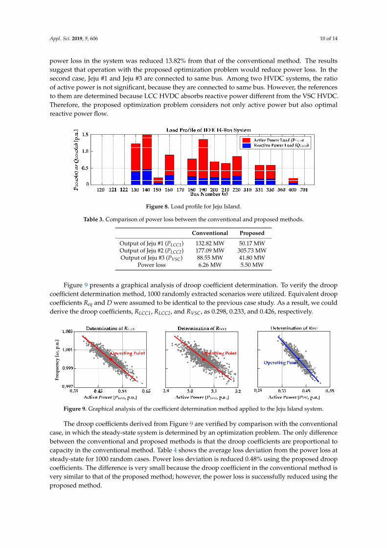
Figure 7 shows the configuration of the Jeju Island power network [42]. There are four generatorsand three HVDC systems, i.e., two LCC HVDCs and one VSC HVDC. The first LCC HVDC isa 180 kV/300 MW system constructed in 1998, and the second LCC HVDC is a ±250 kV/400 MWsystem constructed in 2013. The VSC HVDC considered in the simulation is a planned installationwith a capacity of ±150 kV/200 MW. The base of complex power is 100 MW, and the base voltage is154 kV. The active power of generators, line impedance, and data of the shunt compensator in the testsystem are represented in Appendix A. The actual load data from Jeju Island at peak time is utilized,as illustrated in Figure 8. The simulation scenarios are similar to those with the IEEE 14-bus testsystem. Only one generator at Jeju 3C/S controls the voltage magnitude at 1.04 p.u., and the othergenerators only regulate active power, which means that the reactive power of these generators is zero.The output of the conventional method is determined proportional to capacity.

Appl. Sci. 2018, 8, x FOR PEER REVIEW 9 of 15

timization, and the droop coefficients are determined proportional to their capacity [41]. To verify the proposed determination method, we utilized 10 randomly sampled load profiles. Table 2 shows the comparison of average outputs and power losses. As described in Table 2, the deviation of power loss increased using the proposed method to reduce total system loss. From the simulation results in Tables 1 and 2, we suggest that the proposed optimization problem and the droop coeffi-cient determination method enhance the efficiency of the test system.

Table 2. Comparison of power loss between randomly sampled load profiles.

Conventional Proposed Deviation of LCC HVDC’s output (ΔPLCC) −0.32 MW −0.28 MW Deviation of VSC HVDC’s output (ΔPVSC) −0.32 MW −0.35 MW

Deviation of power loss −36.41 kW −36.74 kW

3.2. Simulation Results for the Jeju Island System

Figure 7 shows the configuration of the Jeju Island power network [42]. There are four genera-tors and three HVDC systems, i.e., two LCC HVDCs and one VSC HVDC. The first LCC HVDC is a 180 kV/300 MW system constructed in 1998, and the second LCC HVDC is a ± 250 kV/400 MW sys-tem constructed in 2013. The VSC HVDC considered in the simulation is a planned installation with a capacity of ±150 kV/200 MW. The base of complex power is 100 MW, and the base voltage is 154 kV. The active power of generators, line impedance, and data of the shunt compensator in the test system are represented in Appendix A. The actual load data from Jeju Island at peak time is utilized, as illustrated in Figure 8. The simulation scenarios are similar to those with the IEEE 14-bus test system. Only one generator at Jeju 3C/S controls the voltage magnitude at 1.04 p.u., and the other generators only regulate active power, which means that the reactive power of these generators is zero. The output of the conventional method is determined proportional to capacity.

Figure 7. Configuration of the Jeju Island network with multiple HVDCs.

Figure 8. Load profile for Jeju Island.

Figure 7. Configuration of the Jeju Island network with multiple HVDCs.

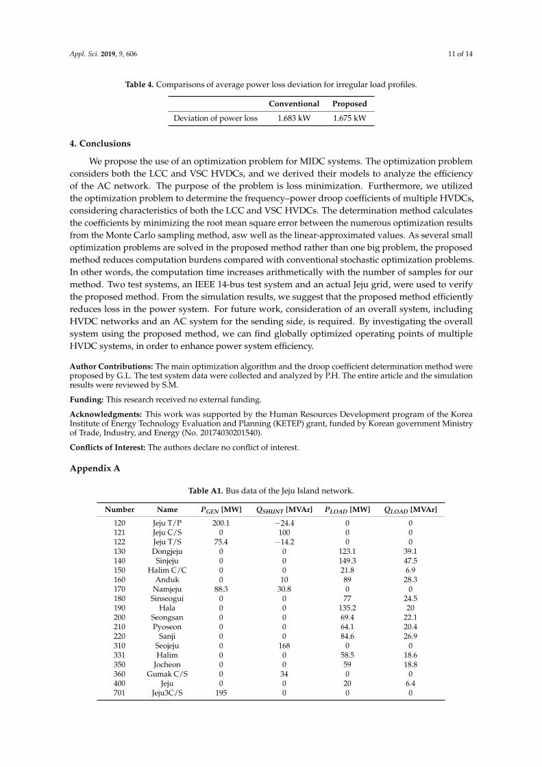
Table 3 shows the results of steady-state analysis using the conventional and proposed methods.As the outputs of multiple HVDCs are determined proportional to their capacity in the conventionalmethod, the active power ratio of Jeju #1, #2, and #3 is 3:4:2. On the other hand, the results of theproposed method determine the operating points of the HVDCs using an optimization problem. Thus,

Appl. Sci. 2019, 9, 606 10 of 14

power loss in the system was reduced 13.82% from that of the conventional method. The resultssuggest that operation with the proposed optimization problem would reduce power loss. In thesecond case, Jeju #1 and Jeju #3 are connected to same bus. Among two HVDC systems, the ratioof active power is not significant, because they are connected to same bus. However, the referencesto them are determined because LCC HVDC absorbs reactive power different from the VSC HVDC.Therefore, the proposed optimization problem considers not only active power but also optimalreactive power flow.

Appl. Sci. 2018, 8, x FOR PEER REVIEW 9 of 15

timization, and the droop coefficients are determined proportional to their capacity [41]. To verify the proposed determination method, we utilized 10 randomly sampled load profiles. Table 2 shows the comparison of average outputs and power losses. As described in Table 2, the deviation of power loss increased using the proposed method to reduce total system loss. From the simulation results in Tables 1 and 2, we suggest that the proposed optimization problem and the droop coeffi-cient determination method enhance the efficiency of the test system.

Table 2. Comparison of power loss between randomly sampled load profiles.

Conventional Proposed Deviation of LCC HVDC’s output (ΔPLCC) −0.32 MW −0.28 MW Deviation of VSC HVDC’s output (ΔPVSC) −0.32 MW −0.35 MW

Deviation of power loss −36.41 kW −36.74 kW

3.2. Simulation Results for the Jeju Island System

Figure 7 shows the configuration of the Jeju Island power network [42]. There are four genera-tors and three HVDC systems, i.e., two LCC HVDCs and one VSC HVDC. The first LCC HVDC is a 180 kV/300 MW system constructed in 1998, and the second LCC HVDC is a ± 250 kV/400 MW sys-tem constructed in 2013. The VSC HVDC considered in the simulation is a planned installation with a capacity of ±150 kV/200 MW. The base of complex power is 100 MW, and the base voltage is 154 kV. The active power of generators, line impedance, and data of the shunt compensator in the test system are represented in Appendix A. The actual load data from Jeju Island at peak time is utilized, as illustrated in Figure 8. The simulation scenarios are similar to those with the IEEE 14-bus test system. Only one generator at Jeju 3C/S controls the voltage magnitude at 1.04 p.u., and the other generators only regulate active power, which means that the reactive power of these generators is zero. The output of the conventional method is determined proportional to capacity.

Figure 7. Configuration of the Jeju Island network with multiple HVDCs.

Figure 8. Load profile for Jeju Island. Figure 8. Load profile for Jeju Island.

Table 3. Comparison of power loss between the conventional and proposed methods.

Conventional Proposed

Output of Jeju #1 (PLCC1) 132.82 MW 50.17 MWOutput of Jeju #2 (PLCC2) 177.09 MW 305.73 MWOutput of Jeju #3 (PVSC) 88.55 MW 41.80 MW

Power loss 6.26 MW 5.50 MW

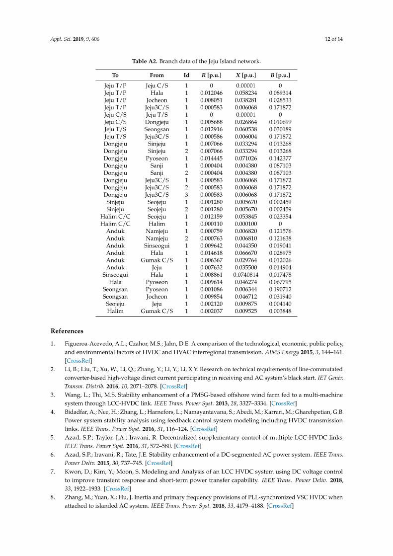
Figure 9 presents a graphical analysis of droop coefficient determination. To verify the droopcoefficient determination method, 1000 randomly extracted scenarios were utilized. Equivalent droopcoefficients Req and D were assumed to be identical to the previous case study. As a result, we couldderive the droop coefficients, RLCC1, RLCC2, and RVSC, as 0.298, 0.233, and 0.426, respectively.

Appl. Sci. 2018, 8, x FOR PEER REVIEW 10 of 15

Table 3 shows the results of steady-state analysis using the conventional and proposed meth-ods. As the outputs of multiple HVDCs are determined proportional to their capacity in the con-ventional method, the active power ratio of Jeju #1, #2, and #3 is 3:4:2. On the other hand, the results of the proposed method determine the operating points of the HVDCs using an optimization prob-lem. Thus, power loss in the system was reduced 13.82% from that of the conventional method. The results suggest that operation with the proposed optimization problem would reduce power loss. In the second case, Jeju #1 and Jeju #3 are connected to same bus. Among two HVDC systems, the ratio of active power is not significant, because they are connected to same bus. However, the references to them are determined because LCC HVDC absorbs reactive power different from the VSC HVDC. Therefore, the proposed optimization problem considers not only active power but also optimal reactive power flow.

Table 3. Comparison of power loss between the conventional and proposed methods.

Conventional Proposed Output of Jeju #1 (PLCC1) 132.82 MW 50.17 MW Output of Jeju #2 (PLCC2) 177.09 MW 305.73 MW Output of Jeju #3 (PVSC) 88.55 MW 41.80 MW

Power loss 6.26 MW 5.50 MW

Figure 9 presents a graphical analysis of droop coefficient determination. To verify the droop coefficient determination method, 1000 randomly extracted scenarios were utilized. Equivalent droop coefficients Req and D were assumed to be identical to the previous case study. As a result, we could derive the droop coefficients, RLCC1, RLCC2, and RVSC, as 0.298, 0.233, and 0.426, respectively.

Freq

uenc

y[ω

, p.u

.]

Figure 9. Graphical analysis of the coefficient determination method applied to the Jeju Island sys-tem.

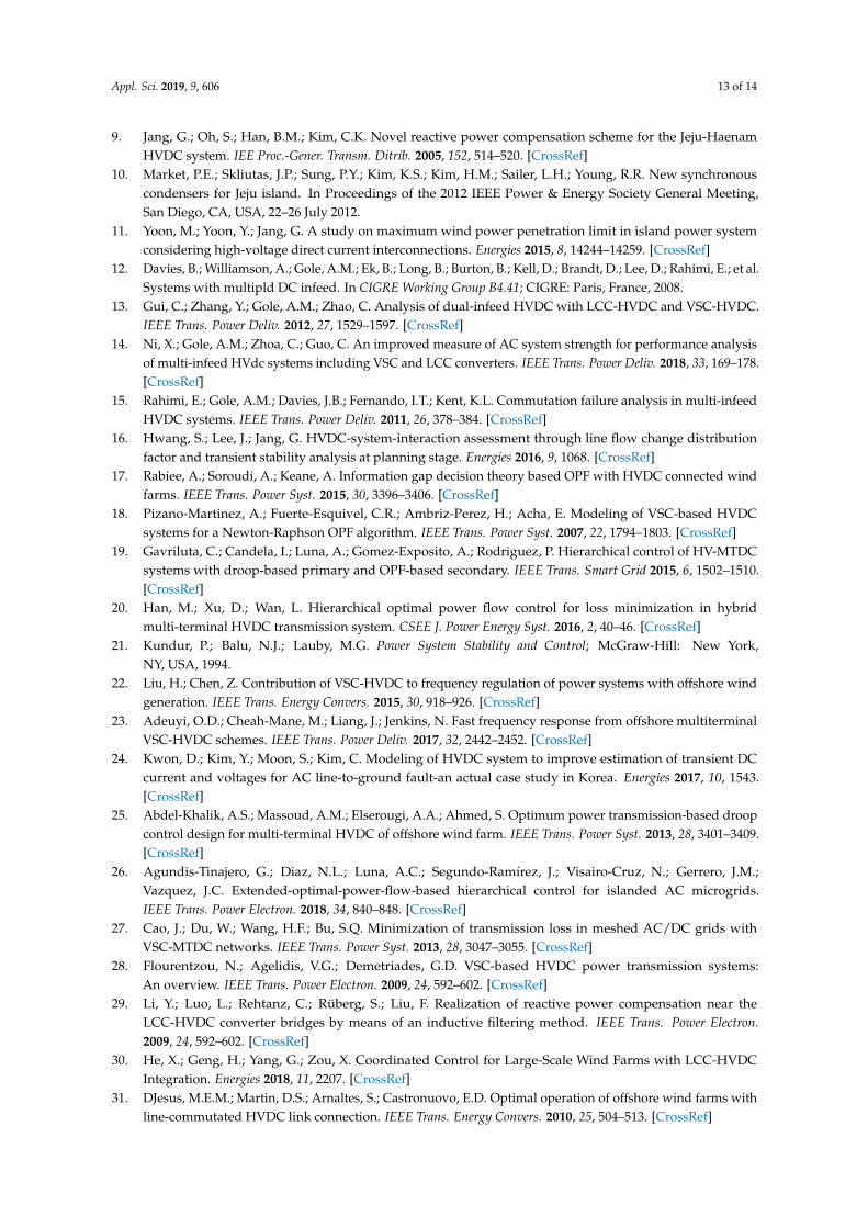
The droop coefficients derived from Figure 9 are verified by comparison with the conventional case, in which the steady-state system is determined by an optimization problem. The only differ-ence between the conventional and proposed methods is that the droop coefficients are proportion-al to capacity in the conventional method. Table 4 shows the average loss deviation from the power loss at steady-state for 1000 random cases. Power loss deviation is reduced 0.48% using the pro-posed droop coefficients. The difference is very small because the droop coefficient in the conven-tional method is very similar to that of the proposed method; however, the power loss is success-fully reduced using the proposed method.

Table 4. Comparisons of average power loss deviation for irregular load profiles.

Conventional Proposed Deviation of power loss 1.683 kW 1.675 kW

4. Conclusions

We propose the use of an optimization problem for MIDC systems. The optimization problem considers both the LCC and VSC HVDCs, and we derived their models to analyze the efficiency of

Figure 9. Graphical analysis of the coefficient determination method applied to the Jeju Island system.

The droop coefficients derived from Figure 9 are verified by comparison with the conventionalcase, in which the steady-state system is determined by an optimization problem. The only differencebetween the conventional and proposed methods is that the droop coefficients are proportional tocapacity in the conventional method. Table 4 shows the average loss deviation from the power loss atsteady-state for 1000 random cases. Power loss deviation is reduced 0.48% using the proposed droopcoefficients. The difference is very small because the droop coefficient in the conventional method isvery similar to that of the proposed method; however, the power loss is successfully reduced using theproposed method.

Appl. Sci. 2019, 9, 606 11 of 14

Table 4. Comparisons of average power loss deviation for irregular load profiles.

Conventional Proposed

Deviation of power loss 1.683 kW 1.675 kW

4. Conclusions

We propose the use of an optimization problem for MIDC systems. The optimization problemconsiders both the LCC and VSC HVDCs, and we derived their models to analyze the efficiencyof the AC network. The purpose of the problem is loss minimization. Furthermore, we utilizedthe optimization problem to determine the frequency–power droop coefficients of multiple HVDCs,considering characteristics of both the LCC and VSC HVDCs. The determination method calculatesthe coefficients by minimizing the root mean square error between the numerous optimization resultsfrom the Monte Carlo sampling method, asw well as the linear-approximated values. As several smalloptimization problems are solved in the proposed method rather than one big problem, the proposedmethod reduces computation burdens compared with conventional stochastic optimization problems.In other words, the computation time increases arithmetically with the number of samples for ourmethod. Two test systems, an IEEE 14-bus test system and an actual Jeju grid, were used to verifythe proposed method. From the simulation results, we suggest that the proposed method efficientlyreduces loss in the power system. For future work, consideration of an overall system, includingHVDC networks and an AC system for the sending side, is required. By investigating the overallsystem using the proposed method, we can find globally optimized operating points of multipleHVDC systems, in order to enhance power system efficiency.

Author Contributions: The main optimization algorithm and the droop coefficient determination method wereproposed by G.L. The test system data were collected and analyzed by P.H. The entire article and the simulationresults were reviewed by S.M.

Funding: This research received no external funding.

Acknowledgments: This work was supported by the Human Resources Development program of the KoreaInstitute of Energy Technology Evaluation and Planning (KETEP) grant, funded by Korean government Ministryof Trade, Industry, and Energy (No. 20174030201540).

Conflicts of Interest: The authors declare no conflict of interest.

Appendix A

Table A1. Bus data of the Jeju Island network.

Number Name PGEN [MW] QSHUNT [MVAr] PLOAD [MW] QLOAD [MVAr]

120 Jeju T/P 200.1 −24.4 0 0121 Jeju C/S 0 100 0 0122 Jeju T/S 75.4 −14.2 0 0130 Dongjeju 0 0 123.1 39.1140 Sinjeju 0 0 149.3 47.5150 Halim C/C 0 0 21.8 6.9160 Anduk 0 10 89 28.3170 Namjeju 88.3 30.8 0 0180 Sinseogui 0 0 77 24.5190 Hala 0 0 135.2 20200 Seongsan 0 0 69.4 22.1210 Pyoseon 0 0 64.1 20.4220 Sanji 0 0 84.6 26.9310 Seojeju 0 168 0 0331 Halim 0 0 58.5 18.6350 Jocheon 0 0 59 18.8360 Gumak C/S 0 34 0 0400 Jeju 0 0 20 6.4701 Jeju3C/S 195 0 0 0

Appl. Sci. 2019, 9, 606 12 of 14

Table A2. Branch data of the Jeju Island network.

To From Id R [p.u.] X [p.u.] B [p.u.]

Jeju T/P Jeju C/S 1 0 0.00001 0Jeju T/P Hala 1 0.012046 0.058234 0.089314Jeju T/P Jocheon 1 0.008051 0.038281 0.028533Jeju T/P Jeju3C/S 1 0.000583 0.006068 0.171872Jeju C/S Jeju T/S 1 0 0.00001 0Jeju C/S Dongjeju 1 0.005688 0.026864 0.010699Jeju T/S Seongsan 1 0.012916 0.060538 0.030189Jeju T/S Jeju3C/S 1 0.000586 0.006004 0.171872Dongjeju Sinjeju 1 0.007066 0.033294 0.013268Dongjeju Sinjeju 2 0.007066 0.033294 0.013268Dongjeju Pyoseon 1 0.014445 0.071026 0.142377Dongjeju Sanji 1 0.000404 0.004380 0.087103Dongjeju Sanji 2 0.000404 0.004380 0.087103Dongjeju Jeju3C/S 1 0.000583 0.006068 0.171872Dongjeju Jeju3C/S 2 0.000583 0.006068 0.171872Dongjeju Jeju3C/S 3 0.000583 0.006068 0.171872

Sinjeju Seojeju 1 0.001280 0.005670 0.002459Sinjeju Seojeju 2 0.001280 0.005670 0.002459

Halim C/C Seojeju 1 0.012159 0.053845 0.023354Halim C/C Halim 1 0.000110 0.000100 0

Anduk Namjeju 1 0.000759 0.006820 0.121576Anduk Namjeju 2 0.000763 0.006810 0.121638Anduk Sinseogui 1 0.009642 0.044350 0.019041Anduk Hala 1 0.014618 0.066670 0.028975Anduk Gumak C/S 1 0.006367 0.029764 0.012026Anduk Jeju 1 0.007632 0.035500 0.014904

Sinseogui Hala 1 0.008861 0.0740814 0.017478Hala Pyoseon 1 0.009614 0.046274 0.067795

Seongsan Pyoseon 1 0.001086 0.006344 0.190712Seongsan Jocheon 1 0.009854 0.046712 0.031940

Seojeju Jeju 1 0.002120 0.009875 0.004140Halim Gumak C/S 1 0.002037 0.009525 0.003848

References

1. Figueroa-Acevedo, A.L.; Czahor, M.S.; Jahn, D.E. A comparison of the technological, economic, public policy,and environmental factors of HVDC and HVAC interregional transmission. AIMS Energy 2015, 3, 144–161.[CrossRef]

2. Li, B.; Liu, T.; Xu, W.; Li, Q.; Zhang, Y.; Li, Y.; Li, X.Y. Research on technical requirements of line-commutatedconverter-based high-voltage direct current participating in receiving end AC system’s black start. IET Gener.Transm. Distrib. 2016, 10, 2071–2078. [CrossRef]

3. Wang, L.; Thi, M.S. Stability enhancement of a PMSG-based offshore wind farm fed to a multi-machinesystem through LCC-HVDC link. IEEE Trans. Power Syst. 2013, 28, 3327–3334. [CrossRef]

4. Bidadfar, A.; Nee, H.; Zhang, L.; Harnefors, L.; Namayantavana, S.; Abedi, M.; Karrari, M.; Gharehpetian, G.B.Power system stability analysis using feedback control system modeling including HVDC transmissionlinks. IEEE Trans. Power Syst. 2016, 31, 116–124. [CrossRef]

5. Azad, S.P.; Taylor, J.A.; Iravani, R. Decentralized supplementary control of multiple LCC-HVDC links.IEEE Trans. Power Syst. 2016, 31, 572–580. [CrossRef]

6. Azad, S.P.; Iravani, R.; Tate, J.E. Stability enhancement of a DC-segmented AC power system. IEEE Trans.Power Deliv. 2015, 30, 737–745. [CrossRef]

7. Kwon, D.; Kim, Y.; Moon, S. Modeling and Analysis of an LCC HVDC system using DC voltage controlto improve transient response and short-term power transfer capability. IEEE Trans. Power Deliv. 2018,33, 1922–1933. [CrossRef]

8. Zhang, M.; Yuan, X.; Hu, J. Inertia and primary frequency provisions of PLL-synchronized VSC HVDC whenattached to islanded AC system. IEEE Trans. Power Syst. 2018, 33, 4179–4188. [CrossRef]

Appl. Sci. 2019, 9, 606 13 of 14

9. Jang, G.; Oh, S.; Han, B.M.; Kim, C.K. Novel reactive power compensation scheme for the Jeju-HaenamHVDC system. IEE Proc.-Gener. Transm. Ditrib. 2005, 152, 514–520. [CrossRef]

10. Market, P.E.; Skliutas, J.P.; Sung, P.Y.; Kim, K.S.; Kim, H.M.; Sailer, L.H.; Young, R.R. New synchronouscondensers for Jeju island. In Proceedings of the 2012 IEEE Power & Energy Society General Meeting,San Diego, CA, USA, 22–26 July 2012.

11. Yoon, M.; Yoon, Y.; Jang, G. A study on maximum wind power penetration limit in island power systemconsidering high-voltage direct current interconnections. Energies 2015, 8, 14244–14259. [CrossRef]

12. Davies, B.; Williamson, A.; Gole, A.M.; Ek, B.; Long, B.; Burton, B.; Kell, D.; Brandt, D.; Lee, D.; Rahimi, E.; et al.Systems with multipld DC infeed. In CIGRE Working Group B4.41; CIGRE: Paris, France, 2008.

13. Gui, C.; Zhang, Y.; Gole, A.M.; Zhao, C. Analysis of dual-infeed HVDC with LCC-HVDC and VSC-HVDC.IEEE Trans. Power Deliv. 2012, 27, 1529–1597. [CrossRef]

14. Ni, X.; Gole, A.M.; Zhoa, C.; Guo, C. An improved measure of AC system strength for performance analysisof multi-infeed HVdc systems including VSC and LCC converters. IEEE Trans. Power Deliv. 2018, 33, 169–178.[CrossRef]

15. Rahimi, E.; Gole, A.M.; Davies, J.B.; Fernando, I.T.; Kent, K.L. Commutation failure analysis in multi-infeedHVDC systems. IEEE Trans. Power Deliv. 2011, 26, 378–384. [CrossRef]

16. Hwang, S.; Lee, J.; Jang, G. HVDC-system-interaction assessment through line flow change distributionfactor and transient stability analysis at planning stage. Energies 2016, 9, 1068. [CrossRef]

17. Rabiee, A.; Soroudi, A.; Keane, A. Information gap decision theory based OPF with HVDC connected windfarms. IEEE Trans. Power Syst. 2015, 30, 3396–3406. [CrossRef]

18. Pizano-Martinez, A.; Fuerte-Esquivel, C.R.; Ambriz-Perez, H.; Acha, E. Modeling of VSC-based HVDCsystems for a Newton-Raphson OPF algorithm. IEEE Trans. Power Syst. 2007, 22, 1794–1803. [CrossRef]

19. Gavriluta, C.; Candela, I.; Luna, A.; Gomez-Exposito, A.; Rodriguez, P. Hierarchical control of HV-MTDCsystems with droop-based primary and OPF-based secondary. IEEE Trans. Smart Grid 2015, 6, 1502–1510.[CrossRef]

20. Han, M.; Xu, D.; Wan, L. Hierarchical optimal power flow control for loss minimization in hybridmulti-terminal HVDC transmission system. CSEE J. Power Energy Syst. 2016, 2, 40–46. [CrossRef]

21. Kundur, P.; Balu, N.J.; Lauby, M.G. Power System Stability and Control; McGraw-Hill: New York,NY, USA, 1994.

22. Liu, H.; Chen, Z. Contribution of VSC-HVDC to frequency regulation of power systems with offshore windgeneration. IEEE Trans. Energy Convers. 2015, 30, 918–926. [CrossRef]

23. Adeuyi, O.D.; Cheah-Mane, M.; Liang, J.; Jenkins, N. Fast frequency response from offshore multiterminalVSC-HVDC schemes. IEEE Trans. Power Deliv. 2017, 32, 2442–2452. [CrossRef]

24. Kwon, D.; Kim, Y.; Moon, S.; Kim, C. Modeling of HVDC system to improve estimation of transient DCcurrent and voltages for AC line-to-ground fault-an actual case study in Korea. Energies 2017, 10, 1543.[CrossRef]

25. Abdel-Khalik, A.S.; Massoud, A.M.; Elserougi, A.A.; Ahmed, S. Optimum power transmission-based droopcontrol design for multi-terminal HVDC of offshore wind farm. IEEE Trans. Power Syst. 2013, 28, 3401–3409.[CrossRef]

26. Agundis-Tinajero, G.; Diaz, N.L.; Luna, A.C.; Segundo-Ramírez, J.; Visairo-Cruz, N.; Gerrero, J.M.;Vazquez, J.C. Extended-optimal-power-flow-based hierarchical control for islanded AC microgrids.IEEE Trans. Power Electron. 2018, 34, 840–848. [CrossRef]

27. Cao, J.; Du, W.; Wang, H.F.; Bu, S.Q. Minimization of transmission loss in meshed AC/DC grids withVSC-MTDC networks. IEEE Trans. Power Syst. 2013, 28, 3047–3055. [CrossRef]

28. Flourentzou, N.; Agelidis, V.G.; Demetriades, G.D. VSC-based HVDC power transmission systems:An overview. IEEE Trans. Power Electron. 2009, 24, 592–602. [CrossRef]

29. Li, Y.; Luo, L.; Rehtanz, C.; Rüberg, S.; Liu, F. Realization of reactive power compensation near theLCC-HVDC converter bridges by means of an inductive filtering method. IEEE Trans. Power Electron.2009, 24, 592–602. [CrossRef]

30. He, X.; Geng, H.; Yang, G.; Zou, X. Coordinated Control for Large-Scale Wind Farms with LCC-HVDCIntegration. Energies 2018, 11, 2207. [CrossRef]

31. DJesus, M.E.M.; Martin, D.S.; Arnaltes, S.; Castronuovo, E.D. Optimal operation of offshore wind farms withline-commutated HVDC link connection. IEEE Trans. Energy Convers. 2010, 25, 504–513. [CrossRef]

Appl. Sci. 2019, 9, 606 14 of 14

32. Bergen, A.R.; Vittal, V. Power Systems Analysis, 2nd ed.; Prentice-Hall: Upper Sandle River, NJ, USA, 1994.33. Sahli, Z.; Hamouda, A.; Bekrar, A.; Trentesaux, D. Reactive Power Dispatch Optimization with Voltage

Profile Improvement Using an Efficient Hybrid Algorithm†. Energies 2018, 11, 2134. [CrossRef]34. Jeong, M.G.; Kim, Y.J.; Moon, S.I.; Hwang, P.I. Optimal voltage control using an equivalent model of

a low-voltage network accommodating inverter-interfaced distributed generators. Energies 2017, 10, 1180.[CrossRef]

35. Huang, Y.; Yang, K.; Zhang, W.; Lee, K.Y. Hierarchical energy management for the multienergy carrierssystem with different interest bodies. Energies 2018, 11, 2834. [CrossRef]

36. Li, J.; Wang, B.; Ren, H.; Zhao, D.; Wang, F.; Shafie-khah, M.; Catalao, J.P.S. Two-tier reactive power andvoltage control strategy based on ARMA renewable power forecasting models. Energies 2017, 10, 1518.

37. Yuan, C.; Xie, P.; Yang, D.; Xiao, X. Transient stability analysis of islanded AC microgrids with a significantshare of virtual synchronous generators. Energies 2018, 11, 44. [CrossRef]

38. Sauhats, A.; Zemite, L.; Petrichenko, L.; Moshkin, I.; Jasevics, A. Estimating the economic impacts of netmetering schemes for residential PV systems with profiling of power demand, generation, and market prices.Energies 2018, 11, 3222. [CrossRef]

39. Modeling and Simulation of IEEE 14 Bus System with FACTS Controllers; Electrical and Computer EngineeringDepartment, University of Waterloo: Waterloo, ON, Canada, 2003. Available online: https://www.researchgate.net/profile/Mohamed_Mourad_Lafifi/post/Datasheet_for_5_machine_14_bus_ieee_system2/attachment/59d637fe79197b8077995408/AS%3A395594351824896%401471328451959/download/MODELING+AND+SIMULATION+OF+IEEE+14+BUS+SYSTEM+WITH+FACTS+CONTROLLERS+IEEEBenchmarkTFreport.pdf(accessed on 11 February 2019).

40. Faruque, M.O.; Zhang, Y.; Dinavahi, V. Detailed modeling of CIGRE HVDC benchmark system usingPSCAD/EMTDC and PSB/SIMULINK. IEEE Trans. Power Deliv. 2005, 21, 378–387. [CrossRef]

41. Mohamed, Y.A.-R.I.; El-Saadany, E.F. Adaptive decentralized droop controller to preserve power sharingstability of paralleled inverters in distributed generation microgrids. IEEE Trans. Power Electron. 2008,23, 2806–2816. [CrossRef]

42. An, K.; Song, K.B.; Hur, K. Incorporating charging/discharging strategy of electric vehicles intosecurity-constrained optimal power flow to support high renewable penetration. Energies 2017, 10, 729.[CrossRef]

© 2019 by the authors. Licensee MDPI, Basel, Switzerland. This article is an open accessarticle distributed under the terms and conditions of the Creative Commons Attribution(CC BY) license (http://creativecommons.org/licenses/by/4.0/).