Three-dimensional influence coefficient method for cohesive crack simulations

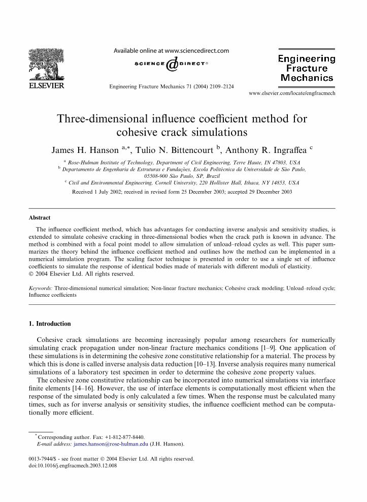
Engineering Fracture Mechanics 71 (2004) 2109–2124

www.elsevier.com/locate/engfracmech

Three-dimensional influence coefficient method forcohesive crack simulations

James H. Hanson a,*, Tulio N. Bittencourt b, Anthony R. Ingraffea c

a Rose-Hulman Institute of Technology, Department of Civil Engineering, Terre Haute, IN 47803, USAb Departamento de Engenharia de Estruturas e Fundac�~oes, Escola Polit�ecnica da Universidade de S~ao Paulo,

05508-900 S~ao Paulo, SP, Brazilc Civil and Environmental Engineering, Cornell University, 220 Hollister Hall, Ithaca, NY 14853, USA

Received 1 July 2002; received in revised form 25 December 2003; accepted 29 December 2003

Abstract

The influence coefficient method, which has advantages for conducting inverse analysis and sensitivity studies, is

extended to simulate cohesive cracking in three-dimensional bodies when the crack path is known in advance. The

method is combined with a focal point model to allow simulation of unload–reload cycles as well. This paper sum-

marizes the theory behind the influence coefficient method and outlines how the method can be implemented in a

numerical simulation program. The scaling factor technique is presented in order to use a single set of influence

coefficients to simulate the response of identical bodies made of materials with different moduli of elasticity.

� 2004 Elsevier Ltd. All rights reserved.

Keywords: Three-dimensional numerical simulation; Non-linear fracture mechanics; Cohesive crack modeling; Unload–reload cycle;

Influence coefficients

1. Introduction

Cohesive crack simulations are becoming increasingly popular among researchers for numerically

simulating crack propagation under non-linear fracture mechanics conditions [1–9]. One application of

these simulations is in determining the cohesive zone constitutive relationship for a material. The process by

which this is done is called inverse analysis data reduction [10–13]. Inverse analysis requires many numerical

simulations of a laboratory test specimen in order to determine the cohesive zone property values.The cohesive zone constitutive relationship can be incorporated into numerical simulations via interface

finite elements [14–16]. However, the use of interface elements is computationally most efficient when the

response of the simulated body is only calculated a few times. When the response must be calculated many

times, such as for inverse analysis or sensitivity studies, the influence coefficient method can be computa-

tionally more efficient.

* Corresponding author. Fax: +1-812-877-8440.

E-mail address: [email protected] (J.H. Hanson).

0013-7944/$ - see front matter � 2004 Elsevier Ltd. All rights reserved.

doi:10.1016/j.engfracmech.2003.12.008

mail to: [email protected]

2110 J.H. Hanson et al. / Engineering Fracture Mechanics 71 (2004) 2109–2124

This paper details how the influence coefficient method can be implemented for numerical simulation of

three-dimensional bodies with a cohesive crack. An advantage of implementing the method in three

dimensions is that the crack front is not constrained to be straight and the crack path need not be straight.

A limitation of the method is that the crack path must be known a priori. When the method is used with acohesive zone constitutive relationship for unloading, the method can also simulate the response of a

cracked body when unloaded. Issues of mesh dependence and computational effort are discussed.

To enhance the computational efficiency of the influence coefficient method, the scaling factor technique

has been developed. This technique allows the use of one set of influence coefficients, generated for a body

with a particular modulus of elasticity, to simulate the response of an identical body with a different

modulus of elasticity. Therefore, a single set of influence coefficients can be used repeatedly when applying

inverse analysis to results from the same test specimen size and geometry but different materials.

2. Cohesive crack simulations

2.1. Cohesive zone constitutive relationship

The defining characteristic of a cohesive crack simulation is that all of the crack region non-linear

behavior is represented by the constitutive relationship between crack opening displacement, COD, andcohesive traction, r, along the crack path. This model for non-linear crack propagation was first proposed

by Dugdale [17] and Barrenblatt [18]. Since then, researchers have used cohesive zone relationships of

different shapes to simulate crack propagation in materials such as metals, polymers, and concrete [1–9].

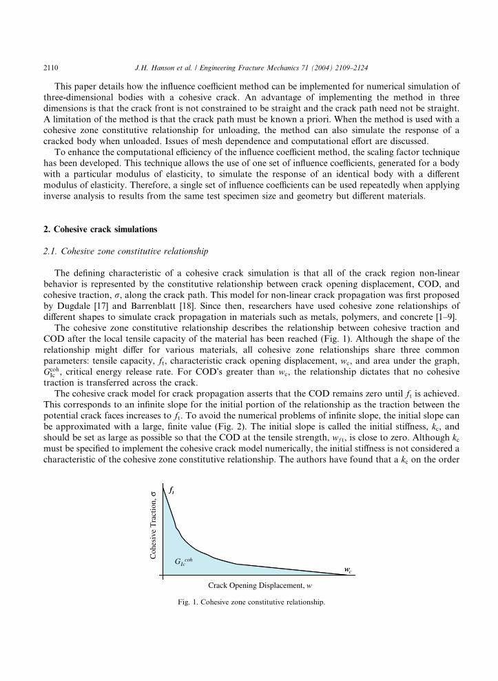
The cohesive zone constitutive relationship describes the relationship between cohesive traction and

COD after the local tensile capacity of the material has been reached (Fig. 1). Although the shape of the

relationship might differ for various materials, all cohesive zone relationships share three common

parameters: tensile capacity, ft, characteristic crack opening displacement, wc, and area under the graph,

GcohIc , critical energy release rate. For COD�s greater than wc, the relationship dictates that no cohesive

traction is transferred across the crack.

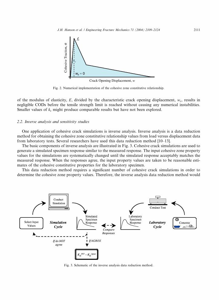
The cohesive crack model for crack propagation asserts that the COD remains zero until ft is achieved.This corresponds to an infinite slope for the initial portion of the relationship as the traction between the

potential crack faces increases to ft. To avoid the numerical problems of infinite slope, the initial slope can

be approximated with a large, finite value (Fig. 2). The initial slope is called the initial stiffness, kc, andshould be set as large as possible so that the COD at the tensile strength, wf t, is close to zero. Although kcmust be specified to implement the cohesive crack model numerically, the initial stiffness is not considered a

characteristic of the cohesive zone constitutive relationship. The authors have found that a kc on the order

ft

GIccoh

wc

ft

GIccoh

w

Coh

esiv

e T

ract

ion,

σ

Crack Opening Displacement, w

Fig. 1. Cohesive zone constitutive relationship.

ft

kc

wft 0Coh

esiv

e T

ract

ion,

σ


ft

kc

wft∼∼ 0

Fig. 2. Numerical implementation of the cohesive zone constitutive relationship.

J.H. Hanson et al. / Engineering Fracture Mechanics 71 (2004) 2109–2124 2111

of the modulus of elasticity, E, divided by the characteristic crack opening displacement, wc, results innegligible CODs before the tensile strength limit is reached without causing any numerical instabilities.

Smaller values of kc might produce comparable results but have not been explored.

2.2. Inverse analysis and sensitivity studies

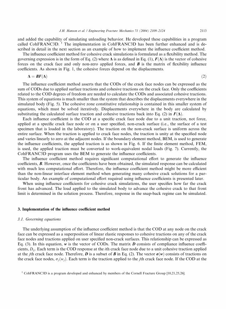
One application of cohesive crack simulations is inverse analysis. Inverse analysis is a data reduction

method for obtaining the cohesive zone constitutive relationship values from load versus displacement data

from laboratory tests. Several researchers have used this data reduction method [10–13].

The basic components of inverse analysis are illustrated in Fig. 3. Cohesive crack simulations are used to

generate a simulated specimen response similar to the measured response. The input cohesive zone property

values for the simulations are systematically changed until the simulated response acceptably matches themeasured response. When the responses agree, the input property values are taken to be reasonable esti-

mates of the cohesive constitutive properties for the laboratory specimen.

This data reduction method requires a significant number of cohesive crack simulations in order to

determine the cohesive zone property values. Therefore, the inverse analysis data reduction method would

Fig. 3. Schematic of the inverse analysis data reduction method.


benefit from a computationally efficient algorithm for solving many cohesive crack simulations for a specific

test specimen size and geometry.

For some structures, the behavior of the structure is very sensitive to the cohesive zone constitutive

relationship. For other structures, the behavior is relatively insensitive to the relationship. Studies are oftenperformed to determine the magnitude of this sensitivity. Such studies might require many analyses of the

same structure using different cohesive zone constitutive relationships. Therefore, sensitivity studies would

also benefit from a computationally efficient algorithm for solving many cohesive crack simulations for a

specific structure.

2.3. Interface elements

Interface elements are a commonly used tool for cohesive crack simulations [14–16]. The cohesive zone

constitutive relationship is included in the formulation of the interface element stiffness coefficients while

the other elements remain linear elastic. The numerical simulations are often performed based on the direct

stiffness method. The governing expression of the direct stiffness method is given in Eq. (1) where F is thevector of applied force at every unrestrained degree of freedom, DOF, D is the vector of resulting dis-

placement at each unrestrained DOF, and KðDÞ is the matrix of finite element stiffness coefficients. Because

of the constitutive relationship of the interface elements, some of the stiffness coefficients depend on the

displacements; therefore, Eq. (1) is a non-linear system of equations. To simulate the response of a body to

an applied load or displacement requires an iterative solution of Eq. (1), Fig. 4. Each point on a simulated

load versus displacement curve is one solution of Eq. (1). If many points must be calculated for a specific

body, the interface element approach can be computationally expensive.

F ¼ KðDÞD ð1Þ

2.4. Influence coefficients

Petersson [19] proposed a method for cohesive crack simulation that consists of superimposing the effectsof applied forces and the effects of cohesive tractions on a linear elastic body. Therefore, cohesive crack

simulation can be performed using a matrix of influence coefficients generated from linear elastic simula-

tions. The method was called the ‘‘influence method’’ [20] and was enhanced by several authors [20–22].

Bittencourt and coworkers [9,22–24] implemented the method for simulation of three-dimensional bodies

F

n x nK(∆)∆= F

n x 1 n x 1InterfaceElements

n = DOF in model

Iteratively solve n x nsystem for each point

Applied L

oad

Displacement

Fig. 4. Schematic of generating a simulated response graph from cohesive crack simulations using interface elements.


and added the capability of simulating unloading behavior. He developed these capabilities in a program

called CohFRANC3D. 1 The implementation in CohFRANC3D has been further enhanced and is de-

scribed in detail in the next section as an example of how to implement the influence coefficient method.

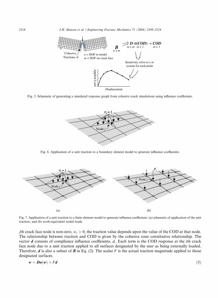
The influence coefficient method for cohesive crack simulations is formulated as a flexibility method. Thegoverning expression is in the form of Eq. (2) where D is as defined in Eq. (1), FðDÞ is the vector of cohesiveforces on the crack face and only non-zero applied forces, and B is the matrix of flexibility influence

coefficients. As shown in Fig. 1, the cohesive forces depend on the displacements.

1 Co

D ¼ BFðDÞ ð2Þ

The influence coefficient method asserts that the CODs of the crack face nodes can be expressed as the

sum of CODs due to applied surface tractions and cohesive tractions on the crack face. Only the coefficientsrelated to the COD degrees of freedom are needed to calculate the CODs and associated cohesive tractions.

This system of equations is much smaller than the system that describes the displacements everywhere in the

simulated body (Fig. 5). The cohesive zone constitutive relationship is contained in this smaller system of

equations, which must be solved iteratively. Displacements everywhere in the body are calculated by

substituting the calculated surface traction and cohesive tractions back into Eq. (2) in FðDÞ.Each influence coefficient is the COD at a specific crack face node due to a unit traction, not force,

applied at a specific crack face node or on a user specified, non-crack surface (i.e., the surface of a test

specimen that is loaded in the laboratory). The traction on the non-crack surface is uniform across theentire surface. When the traction is applied to crack face nodes, the traction is unity at the specified node

and varies linearly to zero at the adjacent nodes. If the boundary element method, BEM, is used to generate

the influence coefficients, the applied traction is as shown in Fig. 6. If the finite element method, FEM,

is used, the applied traction must be converted to work-equivalent nodal loads (Fig. 7). Currently, the

CohFRANC3D program uses the BEM to generate the influence coefficients.

The influence coefficient method requires significant computational effort to generate the influence

coefficients, B. However, once the coefficients have been obtained, the simulated response can be calculated

with much less computational effort. Therefore, the influence coefficient method might be more efficientthan the non-linear interface element method when generating many cohesive crack solutions for a par-

ticular body. An example of computational effort required using influence coefficients is presented later.

When using influence coefficients for cohesive crack simulations, the user specifies how far the crack

front has advanced. The load applied to the simulated body to advance the cohesive crack to that front

limit is determined in the solution process. Therefore, response in the snap-back regime can be simulated.

3. Implementation of the influence coefficient method

3.1. Governing equations

The underlying assumption of the influence coefficient method is that the COD at any node on the crack

face can be expressed as a superposition of linear elastic responses to cohesive tractions on any of the crackface nodes and tractions applied on user specified non-crack surfaces. This relationship can be expressed as

Eq. (3). In this equation, w is the vector of CODs. The matrix D consists of compliance influence coeffi-

cients, Dij. Each term is the COD response at the ith crack face node due to a unit cohesive traction applied

at the jth crack face node. Therefore, D is a subset of B in Eq. (2). The vector rðwÞ consists of tractions onthe crack face nodes, rjðwjÞ. Each term is the traction applied to the jth crack face node. If the COD at the

hFRANC3D is a program developed and enhanced by members of the Cornell Fracture Group [10,21,25,26].

j = 1

Node j

σj = 1

Node j

Fig. 6. Application of a unit traction to a boundary element model to generate influence coefficients.

j = 1

Node j

σj = 1

Node j

Node j

Fj

Node j

Fj

(a) (b)

Fig. 7. Application of a unit traction to a finite element model to generate influence coefficients: (a) schematic of application of the unit

traction, and (b) work-equivalent nodal loads.

n x mB m x m

D σ(COD) = CODm x 1 m x 1

CohesiveTractions, σ

n = DOF in model m = DOF on crack face

Iteratively solve m x msystem for each point

Applied

Load

Displacement

Fig. 5. Schematic of generating a simulated response graph from cohesive crack simulations using influence coefficients.


jth crack face node is non-zero, wj > 0, the traction value depends upon the value of the COD at that node.The relationship between traction and COD is given by the cohesive zone constitutive relationship. The

vector d consists of compliance influence coefficients, di. Each term is the COD response at the ith crack

face node due to a unit traction applied to all surfaces designated by the user as being externally loaded.

Therefore, d is also a subset of B in Eq. (2). The scalar F is the actual traction magnitude applied to those

designated surfaces.

w ¼ DrðwÞ þ F d ð3Þ

F

(w)

F

Zone 4: uncracked

Zone 3: peak stress,σ max = ft

Zone 2: cohesive zone,with stresses σ(w)

Zone 1: stress free crack

Loaded face, with appliedtraction F

σ(w)

Fictitious crack front limit

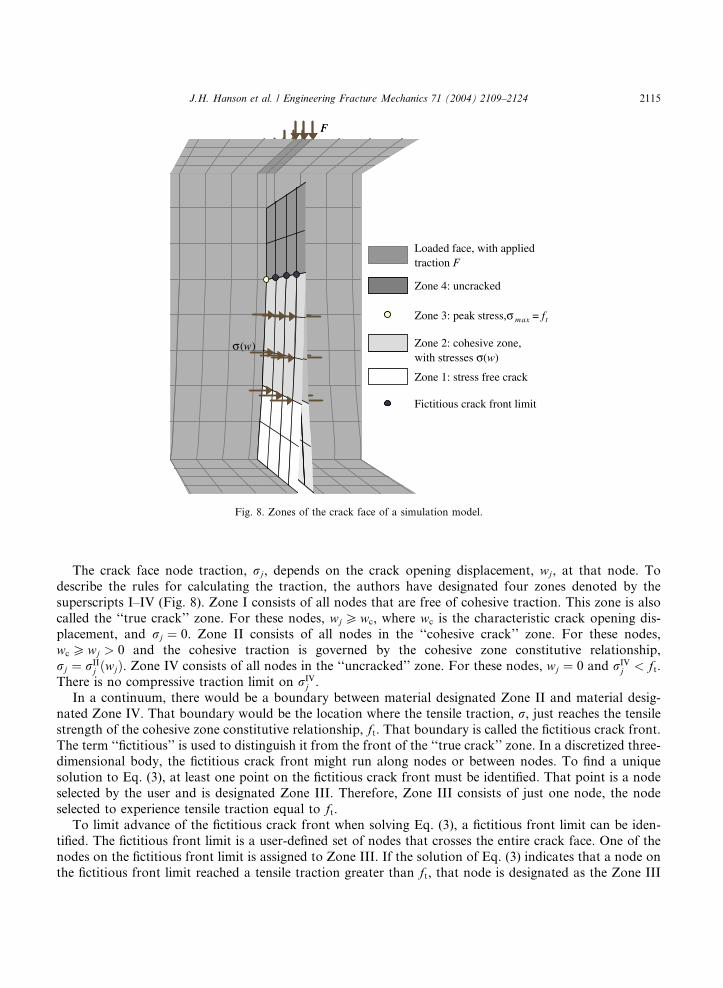
Fig. 8. Zones of the crack face of a simulation model.


The crack face node traction, rj, depends on the crack opening displacement, wj, at that node. To

describe the rules for calculating the traction, the authors have designated four zones denoted by the

superscripts I–IV (Fig. 8). Zone I consists of all nodes that are free of cohesive traction. This zone is also

called the ‘‘true crack’’ zone. For these nodes, wj Pwc, where wc is the characteristic crack opening dis-placement, and rj ¼ 0. Zone II consists of all nodes in the ‘‘cohesive crack’’ zone. For these nodes,

wc Pwj > 0 and the cohesive traction is governed by the cohesive zone constitutive relationship,

rj ¼ rIIj ðwjÞ. Zone IV consists of all nodes in the ‘‘uncracked’’ zone. For these nodes, wj ¼ 0 and rIV

j < ft.There is no compressive traction limit on rIV

j .

In a continuum, there would be a boundary between material designated Zone II and material desig-

nated Zone IV. That boundary would be the location where the tensile traction, r, just reaches the tensilestrength of the cohesive zone constitutive relationship, ft. That boundary is called the fictitious crack front.

The term ‘‘fictitious’’ is used to distinguish it from the front of the ‘‘true crack’’ zone. In a discretized three-dimensional body, the fictitious crack front might run along nodes or between nodes. To find a unique

solution to Eq. (3), at least one point on the fictitious crack front must be identified. That point is a node

selected by the user and is designated Zone III. Therefore, Zone III consists of just one node, the node

selected to experience tensile traction equal to ft.To limit advance of the fictitious crack front when solving Eq. (3), a fictitious front limit can be iden-

tified. The fictitious front limit is a user-defined set of nodes that crosses the entire crack face. One of the

nodes on the fictitious front limit is assigned to Zone III. If the solution of Eq. (3) indicates that a node on

the fictitious front limit reached a tensile traction greater than ft, that node is designated as the Zone III


node and Eq. (3) is evaluated again. Therefore, the fictitious front is ensured to not pass the fictitious front

limit.

Each time the user advances the fictitious front limit, Eq. (3) must be solved again, thus producing a new

simulated response. If the solution of Eq. (3) indicates that some Zone II nodes near the fictitious front limithave not reached the tensile strength, ft, those nodes enter Zone IV. Eq. (3) can be expanded to produce Eq.

(4) where the superscripts refer to the four zones.

wI

wII

wIII

wIV

8>><>>:

9>>=>>; ¼

DI;I DI;II DI;III DI;IV

DII;I DII;II DII;III DII;IV

DIII;I DIII;II DIII;III DIII;IV

DIV;I DIV;II DIV;III DIV;IV

2664

3775

rI

rII

rIII

rIV

8>><>>:

9>>=>>;þ F

dI

dII

dIII

dIV

8>><>>:

9>>=>>; ð4Þ

Each zone has a prescribed boundary condition. These boundary conditions are summarized in Eqs.(5a)–(5e).

rI ¼ 0 ð5aÞ

rII ¼ rIIðwIIÞ ð5bÞ

rIII ¼ ft ð5cÞ

wIII ¼ 0 ð5dÞ

wIV ¼ 0 ð5eÞ

Inserting the boundary conditions of Eq. (5) into Eq. (4) and rearranging terms leads to Eq. (6) where I is

the identity matrix.

I 0 �DI;IV �dI

0 I �DII;IV �dII

0 0 �DIII;IV �dIII

0 0 �DIV;IV �dIV

2664

3775

wI

wII

rIV

F

8>><>>:

9>>=>>; ¼

DI;IIrIIðwIIÞ þ ftDI;III

DII;IIrIIðwIIÞ þ ftDII;III

DIII;IIrIIðwIIÞ þ ftDIII;III

DIV;IIrIIðwIIÞ þ ftDIV;III

8>><>>:

9>>=>>; ð6Þ

Let C represent the matrix on the left side of Eq. (6), u represent the unknowns, and gðuÞ represent theright side of Eq. (6). This substitution results in the more compact equation (7). Eq. (7) is the governing

expression describing all cohesive crack solutions using influence coefficients. The vector g is a function of ubecause the magnitude of the cohesive traction at a node in Zone II, rII

j , depends upon the COD at that

node, wIIj .

Cu ¼ gðuÞ ð7Þ

3.2. Solving the governing equations

Because g in the governing expression depends upon the unknowns, u, Eq. (7) is a system of non-linear

equations. The algorithm described in Fig. 9 can be used to solve these equations. Numerical schemes such

as Newton–Raphson or Modified Newton–Raphson can be used to calculate the incremental change of the

solution.

Define eðuÞ as the vector of residuals as shown in Eq. (8). Then the nth increment toward the solution,

Dun, is calculated by Eq. (9) for the Newton–Raphson scheme or Eq. (10) for the Modified Newton–Raphson scheme. To quantify the residual error, eðuÞ, calculate the norm of the residual error vector. One

possibility is the Euclidean norm given by Eq. (11).

Compare Errorand Tolerance

SolutionComplete

SolveGoverningEquation

CalculateIncremental Change

in Solution, un

Error <Tolerance

InitialEstimate

of Solution, u1

Error >Tolerance

UpdateSolution

Estimate, un

Fig. 9. Solution algorithm used by CohFRANC3D to solve the governing equations.


eðuÞ ¼ Cu� gðuÞ ð8Þ

� C

"� ogðuÞ

ou

��un�1

#�1

eðun�1Þ ¼ Dun ð9Þ

�C�1eðun�1Þ ¼ Dun ð10Þ

keðuÞk2 ¼ffiffiffiffiffiffiffiffiffiffiffiffiffiffiffiffiffiffiffiffiffiXi

½eiðuÞ�2r

ð11Þ

Note that the term in brackets in Eq. (9) must be recalculated and inverted with each iteration. Because

the Modified Newton–Raphson scheme uses only the term C in the brackets, the inverted value of C in Eq.

(10) does not need to be recalculate with each iteration. However, the Modified Newton–Raphson scheme

will typically require more iterations to converge compared to the Newton–Raphson scheme.

Neither the Newton–Raphson nor theModified Newton–Raphson scheme is guaranteed to converge. For

cases where the solution to the system of equations does not converge, multiplying Dun in Eq. (9) or (10) by a

relaxation factor before updating the solution, un, can help the system converge. The relaxation factor is a

positive number less than one. The authors have successfully used relaxation factors from 0.8 to 0.003. Usinga smaller relaxation factor increases the likelihood of convergence but requires more iterations.


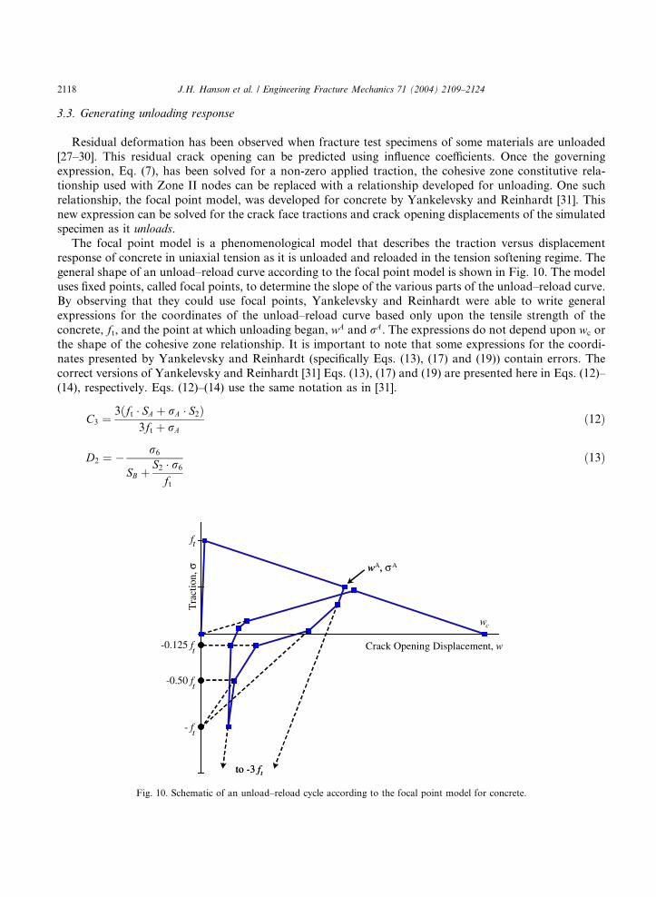
3.3. Generating unloading response

Residual deformation has been observed when fracture test specimens of some materials are unloaded

[27–30]. This residual crack opening can be predicted using influence coefficients. Once the governingexpression, Eq. (7), has been solved for a non-zero applied traction, the cohesive zone constitutive rela-

tionship used with Zone II nodes can be replaced with a relationship developed for unloading. One such

relationship, the focal point model, was developed for concrete by Yankelevsky and Reinhardt [31]. This

new expression can be solved for the crack face tractions and crack opening displacements of the simulated

specimen as it unloads.

The focal point model is a phenomenological model that describes the traction versus displacement

response of concrete in uniaxial tension as it is unloaded and reloaded in the tension softening regime. The

general shape of an unload–reload curve according to the focal point model is shown in Fig. 10. The modeluses fixed points, called focal points, to determine the slope of the various parts of the unload–reload curve.

By observing that they could use focal points, Yankelevsky and Reinhardt were able to write general

expressions for the coordinates of the unload–reload curve based only upon the tensile strength of the

concrete, ft, and the point at which unloading began, wA and rA. The expressions do not depend upon wc or

the shape of the cohesive zone relationship. It is important to note that some expressions for the coordi-

nates presented by Yankelevsky and Reinhardt (specifically Eqs. (13), (17) and (19)) contain errors. The

correct versions of Yankelevsky and Reinhardt [31] Eqs. (13), (17) and (19) are presented here in Eqs. (12)–

(14), respectively. Eqs. (12)–(14) use the same notation as in [31].

C3 ¼3ðft � SA þ rA � S2Þ

3ft þ rAð12Þ

D2 ¼ � r6

SB þS2 � r6

ft

ð13Þ

ft

- ft

-0.50 ft

-0.125 ft

to -3 ft

wA, A

wc

to -3 ft

Tra

ctio

n, σ


w , σ

Fig. 10. Schematic of an unload–reload cycle according to the focal point model for concrete.

0

500

1000

1500

2000

2500

0.0E+0 2.0E-2 4.0E-2 6.0E-2

Crack Mouth Opening Displacement (mm)

App

lied

Loa

d (N

)

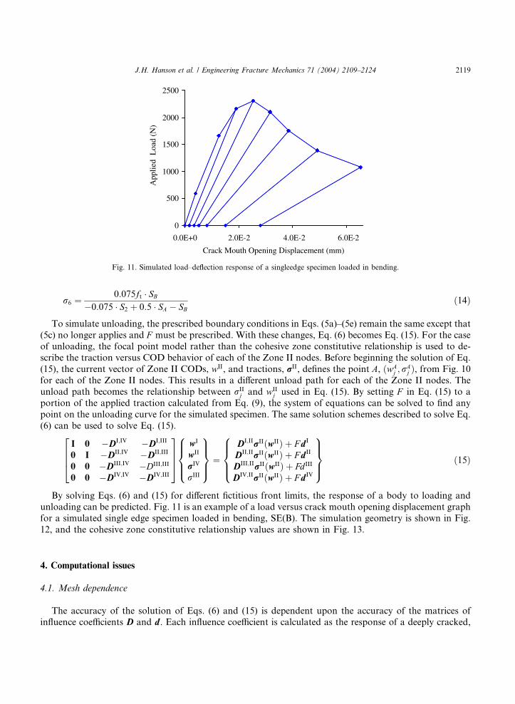
Fig. 11. Simulated load–deflection response of a singleedge specimen loaded in bending.


r6 ¼0:075ft � SB

�0:075 � S2 þ 0:5 � SA � SBð14Þ

To simulate unloading, the prescribed boundary conditions in Eqs. (5a)–(5e) remain the same except that

(5c) no longer applies and F must be prescribed. With these changes, Eq. (6) becomes Eq. (15). For the caseof unloading, the focal point model rather than the cohesive zone constitutive relationship is used to de-

scribe the traction versus COD behavior of each of the Zone II nodes. Before beginning the solution of Eq.

(15), the current vector of Zone II CODs, wII, and tractions, rII, defines the point A, ðwAj ; r

Aj Þ, from Fig. 10

for each of the Zone II nodes. This results in a different unload path for each of the Zone II nodes. The

unload path becomes the relationship between rIIj and wII

j used in Eq. (15). By setting F in Eq. (15) to a

portion of the applied traction calculated from Eq. (9), the system of equations can be solved to find any

point on the unloading curve for the simulated specimen. The same solution schemes described to solve Eq.

(6) can be used to solve Eq. (15).

I 0 �DI;IV �DI;III

0 I �DII;IV �DII;III

0 0 �DIII;IV �DIII;III

0 0 �DIV;IV �DIV;III

2664

3775

wI

wII

rIV

rIII

8>><>>:

9>>=>>; ¼

DI;IIrIIðwIIÞ þ F dI

DII;IIrIIðwIIÞ þ F dII

DIII;IIrIIðwIIÞ þ Fd III

DIV;IIrIIðwIIÞ þ F dIV

8>><>>:

9>>=>>; ð15Þ

By solving Eqs. (6) and (15) for different fictitious front limits, the response of a body to loading and

unloading can be predicted. Fig. 11 is an example of a load versus crack mouth opening displacement graph

for a simulated single edge specimen loaded in bending, SE(B). The simulation geometry is shown in Fig.

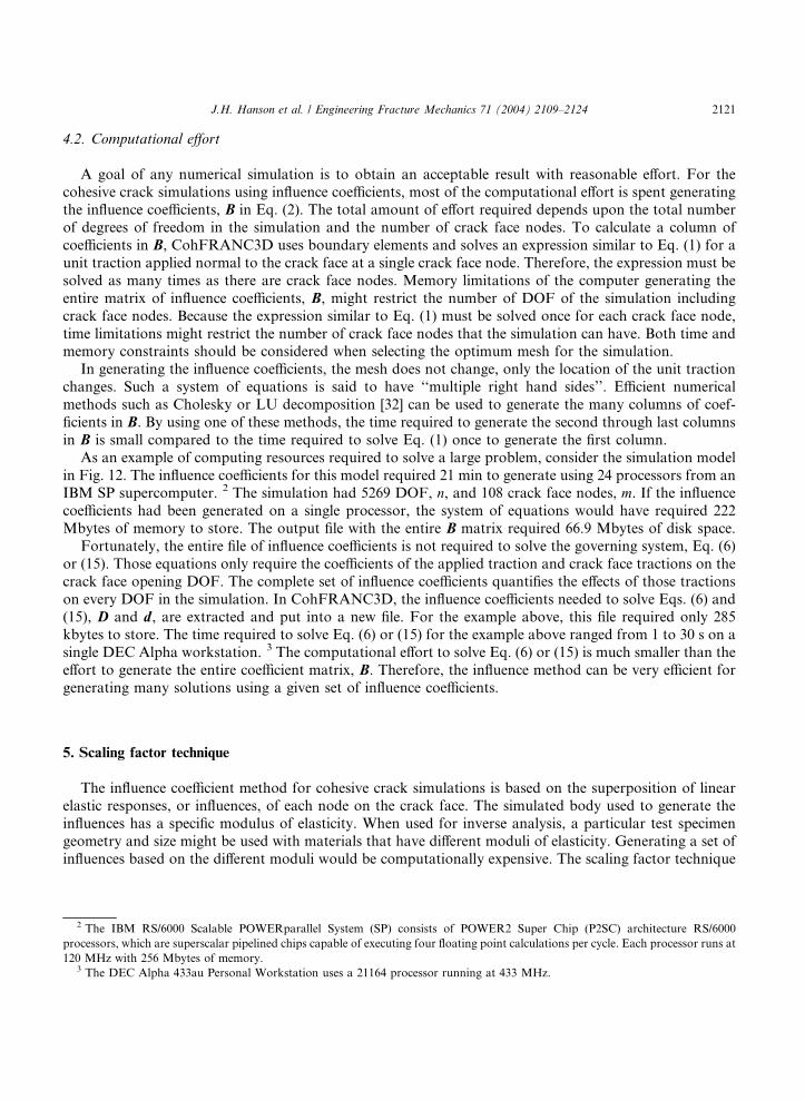
12, and the cohesive zone constitutive relationship values are shown in Fig. 13.

4. Computational issues

4.1. Mesh dependence

The accuracy of the solution of Eqs. (6) and (15) is dependent upon the accuracy of the matrices ofinfluence coefficients D and d. Each influence coefficient is calculated as the response of a deeply cracked,

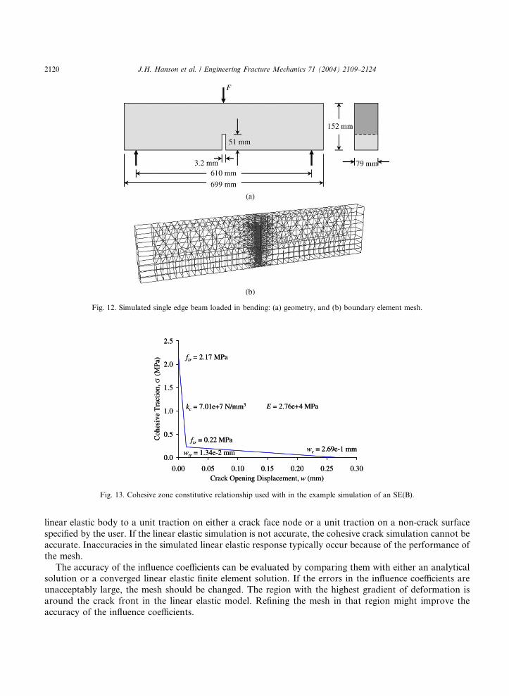
Fig. 12. Simulated single edge beam loaded in bending: (a) geometry, and (b) boundary element mesh.

0.0

0.5

1.0

1.5

2.0

2.5

0.00 0.05 0.10 0.15 0.20 0.25 0.30Crack Opening Displacement, w (mm)

Coh

esiv

e T

ract

ion,

(MPa

)

wc = 2.69e-1 mmwtr = 1.34e-2 mm

ftr = 0.22 MPa

ftr = 2.17 MPa

kc = 7.01e+7 N/mm3 E = 2.76e+4 MPa

0.0

0.5

1.0

1.5

2.0

2.5

0.00 0.05 0.10 0.15 0.20 0.25 0.30Crack Opening Displacement, w (mm)

Coh

esiv

e T

ract

ion,

(MPa

)

wc = 2.69e-1 mmwtr = 1.34e-2 mm

ftr = 0.22 MPa

ftr = 2.17 MPa

kc = 7.01e+7 N/mm3 E = 2.76e+4 MPa

σ

Fig. 13. Cohesive zone constitutive relationship used with in the example simulation of an SE(B).


linear elastic body to a unit traction on either a crack face node or a unit traction on a non-crack surface

specified by the user. If the linear elastic simulation is not accurate, the cohesive crack simulation cannot be

accurate. Inaccuracies in the simulated linear elastic response typically occur because of the performance of

the mesh.

The accuracy of the influence coefficients can be evaluated by comparing them with either an analyticalsolution or a converged linear elastic finite element solution. If the errors in the influence coefficients are

unacceptably large, the mesh should be changed. The region with the highest gradient of deformation is

around the crack front in the linear elastic model. Refining the mesh in that region might improve the

accuracy of the influence coefficients.


4.2. Computational effort

A goal of any numerical simulation is to obtain an acceptable result with reasonable effort. For the

cohesive crack simulations using influence coefficients, most of the computational effort is spent generatingthe influence coefficients, B in Eq. (2). The total amount of effort required depends upon the total number

of degrees of freedom in the simulation and the number of crack face nodes. To calculate a column of

coefficients in B, CohFRANC3D uses boundary elements and solves an expression similar to Eq. (1) for a

unit traction applied normal to the crack face at a single crack face node. Therefore, the expression must be

solved as many times as there are crack face nodes. Memory limitations of the computer generating the

entire matrix of influence coefficients, B, might restrict the number of DOF of the simulation including

crack face nodes. Because the expression similar to Eq. (1) must be solved once for each crack face node,

time limitations might restrict the number of crack face nodes that the simulation can have. Both time andmemory constraints should be considered when selecting the optimum mesh for the simulation.

In generating the influence coefficients, the mesh does not change, only the location of the unit traction

changes. Such a system of equations is said to have ‘‘multiple right hand sides’’. Efficient numerical

methods such as Cholesky or LU decomposition [32] can be used to generate the many columns of coef-

ficients in B. By using one of these methods, the time required to generate the second through last columns

in B is small compared to the time required to solve Eq. (1) once to generate the first column.

As an example of computing resources required to solve a large problem, consider the simulation model

in Fig. 12. The influence coefficients for this model required 21 min to generate using 24 processors from anIBM SP supercomputer. 2 The simulation had 5269 DOF, n, and 108 crack face nodes, m. If the influencecoefficients had been generated on a single processor, the system of equations would have required 222

Mbytes of memory to store. The output file with the entire B matrix required 66.9 Mbytes of disk space.

Fortunately, the entire file of influence coefficients is not required to solve the governing system, Eq. (6)

or (15). Those equations only require the coefficients of the applied traction and crack face tractions on the

crack face opening DOF. The complete set of influence coefficients quantifies the effects of those tractions

on every DOF in the simulation. In CohFRANC3D, the influence coefficients needed to solve Eqs. (6) and

(15), D and d, are extracted and put into a new file. For the example above, this file required only 285kbytes to store. The time required to solve Eq. (6) or (15) for the example above ranged from 1 to 30 s on a

single DEC Alpha workstation. 3 The computational effort to solve Eq. (6) or (15) is much smaller than the

effort to generate the entire coefficient matrix, B. Therefore, the influence method can be very efficient for

generating many solutions using a given set of influence coefficients.

5. Scaling factor technique

The influence coefficient method for cohesive crack simulations is based on the superposition of linear

elastic responses, or influences, of each node on the crack face. The simulated body used to generate the

influences has a specific modulus of elasticity. When used for inverse analysis, a particular test specimen

geometry and size might be used with materials that have different moduli of elasticity. Generating a set of

influences based on the different moduli would be computationally expensive. The scaling factor technique

2 The IBM RS/6000 Scalable POWERparallel System (SP) consists of POWER2 Super Chip (P2SC) architecture RS/6000

processors, which are superscalar pipelined chips capable of executing four floating point calculations per cycle. Each processor runs at

120 MHz with 256 Mbytes of memory.3 The DEC Alpha 433au Personal Workstation uses a 21164 processor running at 433 MHz.


allows one to use a single set of influence coefficients to simulate the response of laboratory specimens with

the same geometry and size but different moduli of elasticity.

5.1. How to apply the scaling factor technique

The scaling factor technique asserts that the deformation response of a simulated body with a cohesive

crack and modulus of elasticity, E1 can be scaled by E1=E2 to match the response of an identical body with a

modulus E2. This assertion leads to the requirement that the cohesive zone constitutive relationship for the

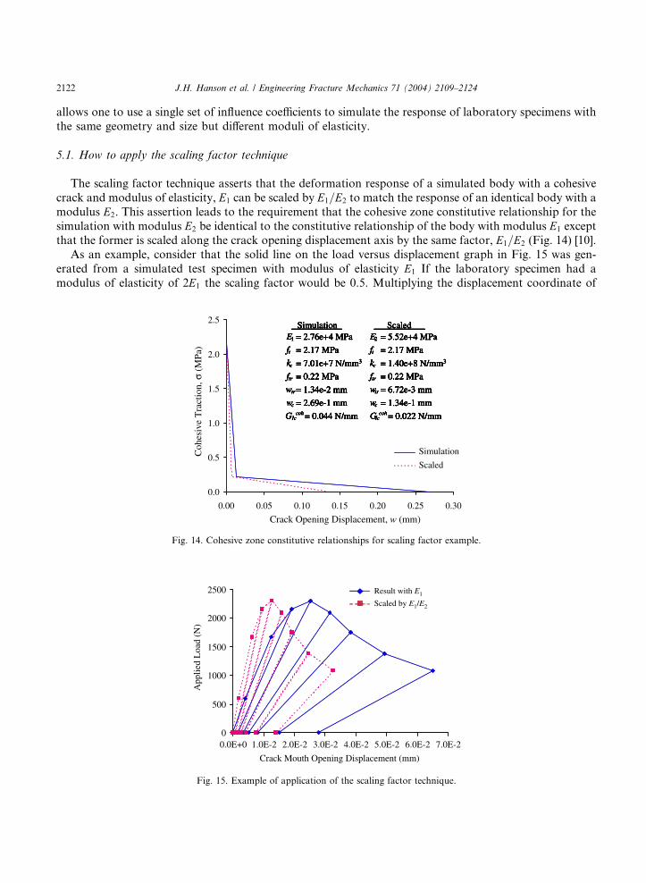
simulation with modulus E2 be identical to the constitutive relationship of the body with modulus E1 exceptthat the former is scaled along the crack opening displacement axis by the same factor, E1=E2 (Fig. 14) [10].

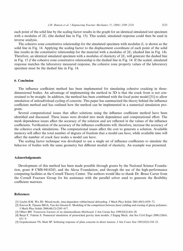
As an example, consider that the solid line on the load versus displacement graph in Fig. 15 was gen-

erated from a simulated test specimen with modulus of elasticity E1 If the laboratory specimen had a

modulus of elasticity of 2E1 the scaling factor would be 0.5. Multiplying the displacement coordinate of

E1

ftkc

ftrwtr

wc

GIccoh

= 2.76e+4 MPa

= 2.17 MPa

= 7.01e+7 N/mm3

= 0.22 MPa

= 1.34e-2 mm

= 2.69e-1 mm

= 0.044 N/mm

SimulationE2

ftkc

ftrwtr

wc

GIccoh

= 5.52e+4 MPa

= 2.17 MPa

= 1.40e+8 N/mm3

= 0.22 MPa

= 6.72e-3 mm

= 1.34e-1 mm

= 0.022 N/mm

ScaledE1

ftkc

ftrwtr

wc

GIccoh

= 2.76e+4 MPa

= 2.17 MPa

= 7.01e+7 N/mm3

= 0.22 MPa

= 1.34e-2 mm

= 2.69e-1 mm

= 0.044 N/mm

SimulationE1

ftkc

ftrwtr

wc

GIccoh

= 2.76e+4 MPa

= 2.17 MPa

= 7.01e+7 N/mm3

= 0.22 MPa

= 1.34e-2 mm

= 2.69e-1 mm

= 0.044 N/mm

SimulationE2

ftkc

ftrwtr

wc

GIccoh

= 5.52e+4 MPa

= 2.17 MPa

= 1.40e+8 N/mm3

= 0.22 MPa

= 6.72e-3 mm

= 1.34e-1 mm

= 0.022 N/mm

ScaledE2

ftkc

ftrwtr

wc

GIccoh

= 5.52e+4 MPa

= 2.17 MPa

= 1.40e+8 N/mm3

= 0.22 MPa

= 6.72e-3 mm

= 1.34e-1 mm

= 0.022 N/mm

Scaled

0.0

0.5

1.0

1.5

2.0

2.5

0.00 0.05 0.10 0.15 0.20 0.25 0.30

Simulation

Scaled

E1

ftkc

ftrwtr

wc

GIccoh

= 2.76e+4 MPa

= 2.17 MPa

= 7.01e+7 N/mm3

= 0.22 MPa

= 1.34e-2 mm

= 2.69e-1 mm

= 0.044 N/mm

SimulationE2

ftkc

ftrwtr

wc

GIccoh

= 5.52e+4 MPa

= 2.17 MPa

= 1.40e+8 N/mm3

= 0.22 MPa

= 6.72e-3 mm

= 1.34e-1 mm

= 0.022 N/mm

ScaledE1

ftkc

ftrwtr

wc

GIccoh

= 2.76e+4 MPa

= 2.17 MPa

= 7.01e+7 N/mm3

= 0.22 MPa

= 1.34e-2 mm

= 2.69e-1 mm

= 0.044 N/mm

SimulationE1

ftkc

ftrwtr

wc

GIccoh

= 2.76e+4 MPa

= 2.17 MPa

= 7.01e+7 N/mm3

= 0.22 MPa

= 1.34e-2 mm

= 2.69e-1 mm

= 0.044 N/mm

SimulationE2

ftkc

ftrwtr

wc

GIccoh

= 5.52e+4 MPa

= 2.17 MPa

= 1.40e+8 N/mm3

= 0.22 MPa

= 6.72e-3 mm

= 1.34e-1 mm

= 0.022 N/mm

ScaledE2

ftkc

ftrwtr

wc

GIccoh

= 5.52e+4 MPa

= 2.17 MPa

= 1.40e+8 N/mm3

= 0.22 MPa

= 6.72e-3 mm

= 1.34e-1 mm

= 0.022 N/mm

Scaled

Crack Opening Displacement, w (mm)

Coh

esiv

e T

ract

ion,

σ (M

Pa)

Fig. 14. Cohesive zone constitutive relationships for scaling factor example.

0

500

1000

1500

2000

2500

0.0E+0 1.0E-2 2.0E-2 3.0E-2 4.0E-2 5.0E-2 6.0E-2 7.0E-2

Crack Mouth Opening Displacement (mm)

App

lied

Loa

d (N

)

Result with E1

Scaled by E1/E2

Fig. 15. Example of application of the scaling factor technique.


each point of the solid line by the scaling factor results in the graph for an identical simulated test specimen

with a modulus of 2E1 (the dashed line in Fig. 15). This scaled, simulated response could then be used in

inverse analysis.

The cohesive zone constitutive relationship for the simulated specimen with modulus E1 is shown as thesolid line in Fig. 14. Applying the scaling factor to the displacement coordinate of each point of the solid

line results in the constitutive relationship for the material with a modulus of 2E1 (dashed line in Fig. 14).

Therefore, an identical simulated specimen with a modulus of elasticity of 2E1 will generate the dashed line

in Fig. 15 if the cohesive zone constitutive relationship is the dashed line in Fig. 14. If the scaled, simulated

response matches the laboratory measured response, the cohesive zone property values of the laboratory

specimen must be the dashed line in Fig. 14.

6. Conclusion

The influence coefficient method has been implemented for simulating cohesive cracking in three-

dimensional bodies. An advantage of implementing the method in 3D is that the crack front is not con-

strained to be straight. In addition, the method has been combined with the focal point model [31] to allow

simulation of unload/reload cycling of concrete. This paper has summarized the theory behind the influencecoefficient method and has outlined how the method can be implemented in a numerical simulation pro-

gram.

Several computational issues that affect solutions using the influence coefficient method have been

identified and discussed. These issues were divided into mesh dependence and computational effort. The

mesh dependence issues affect the accuracy of the solution and are reflected in the values of the influence

coefficients. Verification of the accuracy of the influence coefficients will, therefore, increase the accuracy of

the cohesive crack simulations. The computational issues affect the cost to generate a solution. Available

memory will affect the total number of degrees of freedom that a model can have, while available time willaffect the number of crack face nodes a model can have.

The scaling factor technique was developed to use a single set of influence coefficients to simulate the

behavior of bodies with the same geometry but different moduli of elasticity. An example was presented.

Acknowledgements

Development of this method has been made possible through grants by the National Science Founda-

tion, grant # CMS-9414243, and the Alcoa Foundation, and through the use of the high-performance

computing facilities at the Cornell Theory Center. The authors would like to thank Dr. Bruce Carter from

the Cornell Fracture Group for his assistance with the parallel solver used to generate the flexibility

coefficient matrices.

References

[1] Liechti KM, Wu JD. Mixed-mode, time-dependent rubber/metal debonding. J Mech Phys Solids 2001;49(5):1039–72.

[2] Estevez R, Tijssens MGA, Van der Giessen E. Modeling of the competition between shear yielding and crazing of glassy polymers.

J Mech Phys Solids 2000;48(12):2585–617.

[3] Olbert BH. Transverse fracture of an aluminosilicate fiberboard. J Am Ceram Soc 1999;82(2):414–20.

[4] Barpi F, Valente S. Numerical simulation of prenotched gravity dam models. J Engng Mech, Am Soc Civil Engrs 2000;126(6):

611–9.

[5] Gopalaratnam VS, Shah SP. Softening response of plain concrete in direct tension. J Am Concr Inst 1985;82(3):310–23.


[6] Hawkins NM, Yin X, Du J, Kobayashi AS. Fracture testing of CLWL-DCB specimens. In: Mihashi H, Takahashi H, Wittmann

FH, editors. Fracture toughness and fracture energy: test methods for concrete and rock. Brookfield, VT: Balkema; 1989. p. 205–

20.

[7] Hillerborg A, Modeer M, Petersson PE. Analysis of crack formation and crack growth in concrete by means of fracture mechanics

and finite elements. Cement Concr Res 1976;6:773–82.

[8] Rokugo K, Iwasa M, Seko S, Koyanagi W. Tension softening diagrams of steel fiber reinforced concrete. In: Shah SP, Swartz SE,

Barr B, editors. Fracture of concrete and rock: recent developments. Essex, England: Elsevier Applied Science; 1989. p. 513–22.

[9] Bittencourt TN, Ingraffea AR. Three-dimensional cohesive crack analysis of short-rod specimens. In: Fatigue and Fracture

Mechanics: 25th Volume, ASTM STP 1220. 1995. p. 46–60.

[10] Hanson JH. An experimental–computational evaluation of the accuracy of fracture toughness tests on concrete. PhD Dissertation.

Ithaca, NY: School of Civil and Environmental Engineering, Cornell University; 2000.

[11] Kitsutaka Y. Fracture parameters by polylinear tension-softening analysis. J Engng Mech, Am Soc Civil Engrs 1997;123(5):444–

50.

[12] Roelfstra PE, Wittmann FH. Numerical method to link strain softening with failure of concrete. In: Wittmann FH, editor.

Fracture toughness and fracture energy of concrete. Proceedings of the International Conference on Fracture Mechanics of

Concrete, Lausanne, Switzerland. The Netherlands: Elsevier, Amsterdam; 1986. p. 163–75.

[13] Uchida Y, Kurihara N, Rokugo K, Koyanagi W. Determination of tension softening diagrams of various kinds of concrete by

means of numerical analysis. In: Proceedings, 2nd International Conference on Fracture Mechanics of Concrete and Concrete

Structures, International Association of Fracture Mechanics for Concrete and Concrete Structures (IAFraMCoS), Zurich,

Switzerland, vol. 1, 1995. p. 17–30.

[14] Ortiz M, Pandolfi A. Finite deformation irreversible cohesive elements for three-dimensional crack-propagation analysis. Int J

Numer Meth Engng 1999;44(9):1267–82.

[15] G�alvez JC, Tork B, Cend�on DA, Planas J. Concrete splitting and bond in prestressed concrete beams with indented wires. In:

Proceedings, 4th International Conference on Fracture Mechanics of Concrete and Concrete Structures, International Association

of Fracture Mechanics for Concrete and Concrete Structures (IAFraMCoS), Paris, France, vol. 1, 2001. p. 557–63.

[16] Tvergaard V, Hutchinson JW. The relation between crack growth resistance and fracture process parameters in elastic–plastic

solids. J Mech Phys Solids 1992;40(6):1377–98.

[17] Dugdale DS. Yielding in steel sheets containing slits. J Mech Phys Solids 1960;8(2):100–4.

[18] Barenblatt GI. In: Dryden HL, von K�arm�an Th, editors. The mathematical theory of equilibrium cracks in brittle fracture.

Advances in applied mechanics, vol. 7. New York, NY: Academic Press; 1962. p. 55–129.

[19] Petersson P-E. Crack growth and development of fracture zones in plain concrete and similar materials. Report TVBM-1006/1-

174. Lund, Sweden: Division of Building Materials, Lund Institute of Technology; 1981.

[20] Planas J, Elices M. Nonlinear fracture of cohesive materials. Int J Fract 1991;51(2):139–57.

[21] Gopalaratnam VS, Ye BS. Numerical characterization of the nonlinear fracture process in concrete. Engng Fract Mech

1991;40(6):991–1006.

[22] Bittencourt TN. Computer simulation of linear and nonlinear crack propagation in cementitious materials. PhD Dissertation.

Ithaca, NY: Department of Civil and Environmental Engineering, Cornell University; 1993.

[23] Bittencourt TN, Ingraffea AR. Um M�etodo Num�erico para o Modelamento de Fraturamento Coesivo em 3D. Revista

Internacional de M�etodos Num�ericos para C�alculo y Dise~no en Ingenieria 1995;11(4):555–64 [in Portuguese].

[24] Bittencourt TN. Discrete approaches to cohesive-crack modeling through the finite element method. Escola Politecnica da

Universidade de Sao Paulo, Boletim Tecnico BT/PEF-9711, 1997.

[25] Martha LF. Topological and geometrical modeling approach to numerical discretization and arbitrary fracture simulation in three

dimensions. PhD dissertation. Ithaca, NY: Department of Civil and Environmental Engineering, Cornell University; 1989.

[26] Lutz EF. Numerical methods for hypersingular and near-singular boundary integrals in fracture mechanics. PhD dissertation.

Ithaca, NY: Department of Civil and Environmental Engineering, Cornell University; 1991.

[27] Barker LM. Residual stress effects on fracture toughness measurements. In: Proceedings, 5th International Conference on

Fracture, ICF, Cannes, France, vol. 5, 1981. p. 2563–70.

[28] Labuz JF, Shah SP, Dowding CH. The fracture process zone in granite: evidence and effect. Int J Rock Mech Mining Sci Geomech

Abstr 1987;24(4):235–46.

[29] Tosal Mart�ınez L, Rodriguez Gonz�alez C, Belzunce Varela FJ, Beteg�on Biempica C. The influence of specimen size on the fracture

behavior of a structural steel at different temperatures. J Testing Eval, JTEVA 2000;28(4):276–81.

[30] Wang Y-L, Anandakumar U, Singh RN. Effect of fiber bridging stress on the fracture resistance of silicon-carbide-fiber/zircon

composites. J Am Ceram Soc 2000;83(5):1207–14.

[31] Yankelevsky DZ, Reinhardt HW. Uniaxial behavior of concrete in cyclic tension. J Struct Engng, Am Soc Civil Engrs

1989;115(1):166–82.

[32] Press WH, Teukolsky SA, Vetterling WT, Flannery BP. Numerical recipes in C: the art of scientific computing. 2nd ed.

Cambridge, England: Cambridge University Press; 1993. 994 pp.

Three-dimensional influence coefficient method for cohesive crack simulations

Documents

Transcript of Three-dimensional influence coefficient method for cohesive crack simulations